kaushik i. andrew j. morton

Journal of Financial Economics 35 (1994) 141- 180. North-Holland

Kaushik I. University of Michigan, Ann Arbor, MI 48109, USA

Andrew J. Morton University of Illirlois at Chicago, Chicago, IL 60680, USA

Received May 1993, final version received November 1993

We test six term structure models in the Heath, Jarrow, and Morton (1992) class using Eurodollar futures and options data from 1987-1992. We study the time series of implied interest rate volatilities from these models. Using one-day lagged implied volatilities, our one- and two-parameter models simultaneously price zn average of 18.5 options each day with an average absolute error of one-and-a-half to two basis points. Although the models fit well, we document systematic strike- price and time-to-maturity biases for all models. We also implement simple trading strategies to test whether the models identify genuine biases.

Key words: Arbitrage-free models; Eurodollar tutures options; Implied volatility; Interest rate options; Term structure JEL class$cation: G12; G13

1. Introduction

Much recent academic research has focused on modeling the evolution of the term structure of interest rates with a view to valuing interest rate claims. In particular, the models of Ho and Lee (1986) and Heath, Jarrow, and (1991,1992), hereafter HJM, have received considerable attention in the literature.

Correspondence to: Kaushik I. Amin, 7210 Business Administration, University of Michigan, Ann Arbor, MI 48109-1234, USA.

* We thank David Heath for permission to use computer software developed jointly with one of the authors, as we!! as Peter Bossaerts, Jennifer Dragon, Bob Jarrow, John Long (the editor), Francis Longstaff, Victor Ng, Ehud Ronn, Paul Seguin, Aamir Sheikh, an anonymous referee, and the participants of the Derivative Securities Symposium at Queen’s University for ilelpfu! comments. We also thank Chris Mitchell for supplying Treasury bill data and Blair Wellensiek and the Chicago Mercantile Exchange for supplying the Eurodollar futures and futures options data. This work was completed while the second stithor was visiting the University of ichigan.

03G+405X/94/$07.00 (0 1994-Elsevier Science B.V. A!! rights reserved

142 1y.A Amin and A.J. Morton, Implied volatility in term structure models

In this paper, we test six specific models in the HJM class using transaction prices of Eurodollar futures and futures options from the Chicago Mercantile Exchange. For each model, we determine a daily time series of forward rate volatilities most consistent with Eurodollar futures options prices and analyze its time series properties. Using these volatility estimates, we test the ability of the models to predict the next day’s option prices. We document systematic discrepancies between the various model and market prices, as a function of option type, maturity, strike, etc. Finally, we test whether the mispricings found by each model are genuine by testing if these mispricings can be captured by simple trading strategies. Based on these tests, we provide some recommenda- tions regarding the type of models that should be used in research and in practice.

The HJM approach offers several advantages over the traditional term structure models of Cox, Ingersoll, and Ross (1983, Vasicek (1977), Brennan and Schwartz (1979), and others. First, HJM models match the current term structure of interest rates by construction. Second, like the Black-Scholes model, these models require no assumptions about investor preferences. As a result, claim prices are completely determined by a description of the variance structure of interest rate changes. In particular, estimates of drifts or expected rate changes are not needed. The wide popularity of the Black-Scholes equity model can be attributed in large part to similar features.

Despite the advantages of the HJM approach, very little empirical work has been done to test and apply these models to the prices of traded options. The only studies of which we are aware are Flesaker (1992) and Cohen (1991).’ For computational tractability, Flesaker tests only the path-independent Ho and Lee (1986) model using the Generalized Method of Moments. Under the Ho and Lee model, the volatility of each forward interest rate is constant and independent of maturity and interest rate levels. Since Flesaker tests only the constant volatility form of the HJM model, it is worth investigating whether other functional forms better describe the data. Cohen (1991) applies HJM models to assess the efficiency of the Treasury bond futures and options market. His study uses weekly data and historically estimated volatility functions.

The lack of empirical work examining general HJM models stems from the difficulty of efficiently implementing them. Only in special cases are closed-form solutions available for European options. All of these special cases entail Gaussian interest rates and have been criticized because they permit interest rates to become negative with positive probability. Therefore, there is a need for testing alternative specifications.

In general, however, I-IJM models are path-dependent. In a diffusion framework, this implies that the forward rates of all maturities cannot be represented

‘Bliss and Ronn (1992) have studied the valuation of Treasury bond futures options using an extension of the Ho and Lee (1986) modei proposed in Bliss and Ronn (1989). The model used in these studies is also an arbitrage-free n,odel. However, this model is not m the HJM class of models.

K.I. Amin and A.J. Morton, Implkd volatility in ter.m structure models 143

as functions of a small number of sItate variables whose evolution is governed by a Markov diffusion process. In particular, it is not possible to construct discrete- time approximations in which an ‘up’ move followed by a ‘down’ move yields the same term structure as a ‘down’ move followed by aAl ‘up’ move.2 Therefore, the level of computational eflori grows exponentially with the number of steps. In some cases, Monte Carlo simulation methods can be used [e.g., Cortazar and Schwartz (1992)-j, but they are slow and applicable only to European options. However, advances in comporting technology and numerical techniques allow us to value both American and European options using these models [Amin and Bodurtha (1994) and Heath, Jarrow, Morton, and Spindel(1992)]. These numerical procedures are briefly described in the appendix. This study is the first systematic empirical study which implements and tests a broad class of path- dependent HJM models.

We analyze prices of Eurodollar futures and futures options traded on the Chicago Mercantile Exchange. Besides being extremely liquid, the Eurodollar series allows us to infer a complete initial term structure of forward interest rates’ that is contemporaneous with option prices (which, for example, the Treasury bond futures and options would not). Given the term structure, under HJM models, only a volatility function is needed to price and hedge options. We infer this function from market option prices by parameterizing the functicn and then estimating parameter values which cause model prices to best match market prices. Based on these estimates, we test for model fit and parameter stationarity and set up simple trading strategies designed to exploit mispriced options.

The paper proceeds as follows. In section 2, we provide a brief description of the HJM model. In section 3, we describe the data. We develop the concept of implied volatility in HJM models in section 4. In sections 5 and 6, we fit the models to the data, and document the systematic biases we find between market and model prices. In section 7, we test whether simple trading s’rategies can capture the mispricings detected by each of the modsls. Section 8 concludes the paper, and the appendix provides some details about numerical implementation of the models.

JM approach

In the traditional models of Cox, Ingersoll, and Ross (1985), Brennan and Schwartz (1979), Vasicek (19 / I), Dothan (1978), and others, the evolution of the

2This property holds in almost all the discrete-time models used for computing option prices [for example, Cox, Ross, and Rubinstein (1979), Amin (1991) or Boyle, Evnine, and Gibbs (1989)].

3Forward interest rates carTot be computed directly from futures prices in our framework. Therefore, this step is not imr ediate, as we discuss in section 4.1.

144 K.1. Amin and A.J. Mor*ton, Implied volatility in term structure models

entire term structure is inferred from the evolution of the spot interest rate and possibly another long-term interest rate. In these models, the stochastic process for the spot interest rate [and the long-term interest rate in the Brennan and Schwartz (1979) model] is either specified exogenously or determined endoge- nously from assumptions on investor preferences and technologies. These models are very useful for studying the relationship between bond prices of different maturities and how investors deteilnine these prices.

However, the application of these models to the pricing of interest rate options has been disappointing. Since the models determine the term structure endoge- nously, they have difficulty matching an obser arket term structure. Hull and White (1990) have modified some of these 1s to match the initial term structure, at the price of introducing several rying parameters. Moreover, the models contain several parameters that difficult to estimate. See, for example, the differing parameter estimates for Cox, Ingersoll, and Ross (1985) model reported by Gibbons and Ramaswamy 6) and Pearson and Sun (1989).

Ho and Lee (1986) began a new approach term structure modeling. These authors take as given the prices of discount nd prices of all maturities and model the subsequent evolution of this price vector to preclude arbitrage opportunities. ‘diewing their bond price movements as term structure movements reveals that under the model the forward interest rate curve moves up or down in a nearly parallel manner each oeriod. The size of this shift is independent of the level of rates. Heath, Jarrow, and Morton (1992) extend the work of Ho and Lee (1986) to a continuous-time framework and permit the form of forward rate changes to be specified almost arbitrarily. In particular, many of the processes specified for the evolution of spot interest rates in the literature can be treated as special cases of HJM models by appropriately specifying the volatility of forward interest rates. For example, by Lpecifying the volatility function to be an exponential function of time to maturity, we obtain the spot rate process assumed by Vasicek (1977).

A> 2 prelude to our analysis, we provide a brief description of the HJM class of rn% Idels. We first remark that we only need to describe the evolution of rates undei the risk-neutral or martingale measure arrison and Pliska (198 1) and

1. Under complete markets, only the ev ion of asset prices under this measure is relevant for claims pricing.

Letf(t, T) be the forward interest rate at da t for instantaneous and riskless borrowing or lending at date T. At each ding date t, HJM specify the evolution of forward interest rates of every maturity T simultaneously according to the stochastic differential equation:

df 0, T) = dt, T, l ) di + g(t: T, f (t, T))d W’(t), (1)

where W(t) is a one-dimensional standard o(t, T, f (t, T)) are the drift and dispersion

nian motion and a(t, T, 9) and cients for the forward interest

K.I. Amin and A.J. Morton, Implied volatility in term siructure models 145

rate of maturity ‘1”. In general, the drift coefficient for each maturity T depends on the forward rates of all other maturities s such that t 6 s < T. This depen- dence is represented by 9 as t re third argument of a(t7 Ty 0).

The notable feature in (1) is that the evolution of forward interest rates of all maturities is simultaneously and exogenously specified. In the spot interest rate models of Cox, Ingersoll, arG oss (1985) or Vasicek (1977), only the evolution of the spot interest rate is directly modeled. The evolution of other rates is inferred from that of the spot interest rate.

The function a(t, T,f(t, T)) represents the instantaneous standard deviation (volatility) of the forward interest rate of maturity Tat date t, and can be chosen rather arbitrarily. In fact, the choice of a( 0) completely determines all claim prices, since for each such choice, the drifts a(t, T, 0) are uniquely determined under the risk-neutral measure by the no-arbitrage condition:

T

a(t, K l ) = dt, T,f 0, 7’)) dt, u,f(t, u))du 1

l (2)

In this paper, we focus on single-factor HJM models, i.e., models in which all interest rate changes are driven by a single source of uncertainty. Since we study only Eurodollar futures and their options, which generally mature in less than one year, there is insufficient variation in the term structure across different maturities to require the use of a multi-factor HJM model. Although Eurodollar futures options of longer maturities have been trading since early 1992, the trading volume in these options is quite small, and their prices are accordingly less reliable. As Dybvig (1990) shows, almost all of the variation in forward rates with maturities less than five years can be explained by a dominant single factor. Further, from an estimation perspective, it is not possible to reliably disentangle the effects of two factors in the HJM class of models with only short-term futures and futures options data.

Consider the valuation of interest rate claims under HJM models. Under the risk-neutral measure, the instantaneous expected rate of return on every traded security equals the spot interest rate. Therefore, the futures price for a continuously-marked-to-market futures contract follows a martingale, since opening a futures position requires no investment. If the futures price at date t for

a contract that matures at date T is &(t), then

h(t) = WFT(T)l 9 (3)

where FTCT) is the futures price at maturity, which equals the spot price at date T, and E, denotes the expectation with respect to the risk-neutra’a measure conditioral on the information set at date t.

146 K.I. Amin and A.J. Morton, Implied volatility in term structure models

If the price of an European option at date t is represented by C(t), and this option matures at date T, then

C(t) = E, (4)

where r(u) =f(u, u) is the spot interest rate at date u. Given the option value at the maturity date as a function of the state variables, we can compute its value at any prior date from the above equation. American options can similarly be valued by the equation:

C(t) = sup E,[GB(*bxP(- ~wq]~ (5) OES [t, T]

where Ge(e ) is the payoff to the option when it is exercised at date 8 and F[t, T] is the class of all early exercise strategies (stopping times) in [t, T]. Further, G& ) can be any function of current and past realizations of the term &tructure.

In practice, we need to discretize (1) under the risk-neutral measure by building a path-dependent, binomial-type model (some details on effective numerical procedures are provided in the appendix). Using the discrete approximation, we can accurately value Eurodollar futures and futures options by backward induction.

urodollar futures and futures o

Eurodollar futures began trading in December 1981 on the Chicago Mercan- tile Exchange (CME). Identical futures contracts are now also traded on t1.Z London International Futures Exchange (since 1982) and the Singapore Inter- national Monetary Exchange (since 1984). Eurodollar fu.tures options have been traded on the CME since March 20, 1985. The trading hours for both Euro- dollar futures and options are 7: 20 am CST to 2: 00 pm CST on the CME.

Table 1 reports the annual trading volume in Eurodollar futures and Euro- dollar futures options over the last decade. These volumes are approaching those of Treasury bond (T-bond) futures and futures options contracts, which are the most heavily traded interest rate futures and futures options contracts, respectively. In fact, the open interest in Eurodollar futures and options is now much higher than that for T-bond futures and options.

esides being extremely liquid, the Eurodollar contract is well suited for our study for two reasons, First, we can use Eurodollar futures prices to generate a complete initial term structure as required by the HJ approach. This is not possible with T-bond futures. Since the underlying instrument for the T-bond contract ca 5 years to maturity, while the futures

ICI. Amin and A.J. Morton, A Implied volatility in term structure models

Table 1

Annual trading volume for Eurodollar futures and futures options.*

147

This table reports the annual trading volume in thousands of contracts for Eurodollar futures and futures options traded on the Chicago Mercantile Exchange during 1983-1992. For comparison, the trading volume (in thousands of contracts) for Treasury bond futures and futures options traded on

the Chicago Board of Trade are also reported.

Volume in thousands of contracts --___-.-- --_ _

Fu!ures options Futures

Eurodollar Treasury bond Treasury

Year Eurodollar bond Calls Puts Calls + puts -

1983 891 f 9,550 b - _b 1,664 1984 4,193 29,963 b - _b 6,636 1985 8,901 40,448 366 377 11,901 1986 10,825 52,598 1,007 750 17,314 1987 20,416 66,84 1 1,045 1,525 21,720 1988 21,705 70,307 1,219 1,380 19,509 1989 40,818 70,303 3,190 2,811 20,784 1990 34,696 75,499 3,878 2,982 27,315 1991 37,244 6 ‘,887 4,310 3,565 21,926 1992 60,488 70,003 7,408 6,297 20,259

aSource: CBOT and CME. bContract was not traded in that year.

contracts mature in less than a year, a complete initial term structure cannot be computed using only futures prices. To compute the entire term structure would require simultaneous prices of all Treasury bills, notes, and bonds of all maturities on a frequent basis. Further, using transactions prices is clearly infeasible. Second, the cash-settled Eurodollar contract does not involve any complicated delivery and timing options which are inherent in the T-bond futures contract [see Gay and Manaster (1986) for a description of these implicit options].

Eurodollar futures trade with up to five years to maturity and with almost the entire trading volume in contracts that expire in March, June, September, and December. The last trading day for each contract is the second London bank business day before the third Wednesday of the contract month. At maturity date T, the quoted futures cash settlement price is

F,QT) = lOO[l - y(T)]. (6)

where y(T) is the three-month annualized add-on yield on Eurodollar time deposits’ (three-month LIBQR). The minimum change in the quoted futures

4Tht: add-on yield is defined so that the actual interest payment on a three-month deposit based on the add-on yield is y( 7) x number ~~~Q~~~~Q~ damps for inrestmenf/360.

14s K.I. Amin and A.J. Morton, Impiied volatility in term structure models

price is 0.01 and corresponds to a basis point or tick. Each futures contract has a $1 million notional amount. Each basis point change thus represents a price change of $l,OOO,OOOx~xO.Ol”/, = $25.

The options on this contract are American with the same maturity date as the futures. Upon exercise, the owner of a call option essentially receives the cash difference between the current futures price and the exercise price.’ The owner of a put option receives the cash difference between the exercise price and the current futures price. One option covers one futures contract, and like the futures contract has a minimum quoted price change of 0.01 (one basis point or tick), equal to $25. The dollar value of an option is equal to the quoted option price times $2,500. The trading volume is concentrated in options with maturities of less than a year. Since January 1992, options with up to two years in maturity have also been traded. However, the trading volume in these long-term options is quite small.

3.1. Dtita

We use the Chicago Mercantile Exchange’s (CME) time and sales database containing transactions prices of Eurodollar futures and Eurodollar futures options from January 1, 1987 to November IO, 1992. For each type of contract, the database consists of a record for each transaction that occurred at a different price from the previous price. The data also contains bid and ask quote prices if the bid price exceeds or the ask price is smaller than the last transaction price.

For our analysis, we need to select contemporaneous options and futures prices on each date. Unfortunately, the CME does not record every transaction in the database, but only transactions which took place at a different price from the previous transaction. Therefore, it is not possible to determine at any instant the time of the last transaction, even though the price of the last transaction is known. To mitigate this problem, we select the last traded price as of 8 : 30.am CST for each of the futures and futures options contracts. Since trading com- mences at 7 : 20 am CST, this yields approximately a one-hour window from

_-

determined as follows. The CME conducts two surveys of 12 London banks which are randomly selected from a list of no less than 20 banks. The first survey is conducred sometime during the hour-and-a-halfjust before the close of trading in the expiring contract; the second takes place right at the close. The banks are polled on their ‘perception of the rate at which three-month Eurodollar time deposit funds are currently offered by the market to prime banks’. The two highest and two lowest rates are eliminated in each :;urvey and the remaining rates are averaged and then rounded to the nearest basis point to arrive at the current LIBOR rate used for settlement.

‘The caIB owner actually obtains a long position in the futures contract with a futures price equal to the exercise price. The call writer receives a short futures position. On marking-to-market, the owner obtains the cash difference between the marked-to- arket futures price and the exercise price. For the purpose of valuation, we a>sume that I e owner rea;eives the difference between the futures price a

Amin and A.J. Morton,

which the prices are determined. r usi we can fit an implied volatility function based on these prices, an trading strategies which can prices later in the s day. This approach ensures t is no data-snoopin us to trade based on up-to-date information.

Table 2 summarizes the ata selected above maturities. On average, we have 9.3 calls an 9.2 puts every futures for which there were no options of that matu 4 futures contracts per day. The last colum trading vol.ume per day in each category duri years of our sample period. These volume numbers were obtained from a sepa- rate dataset supplied by the CME, containing settlement prices and the trading volume. The CME supplies a limited amount of data free of charge; we ob?ained the Stats database only for the middle two years of our sample period. The trading volume in each category indicates the liquidity of the options as strike price and maturity vary.

4. Implied volatility

As in the Black-Scholes equity model, the HJM approach to interest rate modeling ensures that claim prices are determined through ‘volatility’ parameters (dispersion coefficients in stochastic differential equations), not through drifts or risk premia. However, in the Black-Scholes model a single scalar carries all volatility information, whereas in HJM models the volatility function must describe the stochastic evolution of the entire term structure curve. We focus on models possessing the ‘time invariance’ property that a(t, T,f(t, T)) depends on t and Tonly through T - t. In other words, given a term structure at time t, the form of its subsequent evolution through time depends only on the term structure, not on the specific calendar date t.

Even with the time invariance assumption, a rich class of volatility structure remains. Since our numerical procedures price under arbitrary volatility functions, we have no a priori restrictions on the class of volatility functions. We have chosen the following six forms:

(1) Absolute [continuous-time o-Lee (1986)]: c7(+ = tro ,

(2) Square Root: a(*) = aoS(t, T)‘12 ,

(3) Proportional:‘j a(*) = aof(t, T) )

%JM require that their volatility functions be bounded. Therefore, we ca at crO_f*. For su ciently largef” t C%S.


Table 2

Summary statistics on number of futures and futures options, average price, and standard deviations of prices classified by maturity and moneyness.

All prices are reported in basis points (multiples of $25). Number of trading days = 1,483. Total number of observations (options only) = 27,368. Average number of futures per day = 4.001. Average number of calls per day = 9.3. Average number of puts per day = 9.2. Futures for which there were no traded options of the corresponding ?&u&y were eliminated from the sample. The

sample period is January 1, 1987 to November 10, 1992.

Maturity” Moneynessb NC Average

price

Standard Average deviation daily volume of price per contractd

Futures

Short 1,478 9,283.9 180.8 61,455 Medium 1,456 9,274.2 175.2 65,227 Long 3,004 9,247.s 162.4 8,561

Calls

Shot out 843 8.00 4.37 2,102 Short At 2,396 17.59 9 36 2,374 Short In 1,887 76.24 46.46 442

Medium out 2,474 12.45 7.60 912 Medium At 2,363 29.13 10.84 1,477 Medium In 1,438 83.20 43.06 415

Long out 2,224 18.19 10.32 242 Long At 1,948 40.95 13.22 253 Long In 1,046 101.85 48.69 234

Puts

Short out 1,024 8.38 4.77 1,638 Short At 2,319 17.45 9.18 1,858 Short In 1,259 64.54 35.9 1 370

Medium out 2,923 12.55 7.53 664 Medium At 2,378 29.70 11.09 1,121 Medium In 1,009 72.28 33.53 348

Long out 2,830 18.97 10.87 185 Long At 1,916 41.41 13.14 243 Long In 659 88.03 37.80 135

- aShort: maturity < 90 days, medium: 90 < maturity d 180 days, long: maturity > 180 days. bOut (out-of-the-money options): at least 25 basis points out-of-the-money, at (at-the-money

options): 1Strike price - Futures price] < 25 basis points, in (in-the-money options): at least 25 basis points in-the-monev.

‘N = total number of observations in data sample for that classification. dAvernge number of contracts traded per day per contract during 1989 and 1990.

K.I. Amin and AJ. Morton, Implied volatibty in term structure models 151

(4) Linear Absolute: C(O) = I30 + GO- O] 9

(5) Exponential [Vasicek (1977)]:’ c(e) = ooexp[ - d(T- t)] , and

(6) Linear Proportional: 06) = Cao + al(T- OlS(t, T).

The first three functions contain one parameter, the others contain two. All these volatility functions are nested by the function:

d4 qf(t, T)) = [Q + ~1 (T - t)] exp[ - A( T - t)] f(t, T)Y ,

which contains four parameters: co, cl, A, and y. Since we infer these parameters from the prices of options which expire in under two years, we are unable to isolate the individual effect of four parameters directly.* Consequently, we impose specific functional forms on the volatility function and test these specifications separately. Although futures contracts with maturities of up to five years trade, the effect of volatility on futures prices is nearly model-independent, and so information about volatility structure cannot be extracted from futures prices.

4.1. Estimation of implied volatility functions

Since HJM model the evolution of forward interest rates, as opposed to futures rates or yields,g we first need to estimate the forward interest rates. If the forward prices of three-month discount bonds for each of the futures maturities were available, we could compute three-monr:h forwa1.d interest rates easily. By assuming that the instantaneous forward interest rate curve is flat between

‘This function yields an CIrnstein-Uhlenbeck process for the spot interest rate as assumed by Vasicek (1977). See Brenner (1989) for a proof.

*For example, we attempted to estimate the volatility function given by

00, T,S(t, T)) = ao_IIt, W,

by trying to imply out both o. and y. The parameter estimates were highly unstable. The standard errors as measured by the inverse of the Hessian were typically of a higher order than the parameter value. Also, the parameter estimates were highly dependent on the initial starting point in the iterative procedure.

Another possibility is to restrict the values of ‘J in a finite set (for example IO,& 11) and each date iterate over only these values of 1~. However, this implies that each day we will use qualitatively different models. For example, on date 1 we might use an absolute model, on date 2 we might use a proportional model, and on date 3 we might use a square root model. This kind of model switching seems unsatisfactory.

‘!t is not poss ible to simply reparameterize the model in terms of the evoPution of futures yields (rates) obtained by inverting (6). For example, w date t for maturity date ;6as ydt) = I - FT(t)/

reparameterization poses difficulties in valuing many types of claims. For example, this futures term structure is not sufficient to value even a pure discount bond.


available maturities, we could then obtain a good approximation of the entire term structure.

However, such forward bond prices cannot be readily L .~!.ited from futures prices due to two complicating factors. First, futures prick * ~~:8) are not equal to forward prices (rates) when interest rates are sto&;n&. L<c;nd, even if we abstract from the daily marking-to-market feature of F ?_.xts ,.~~“racts, an unam- biguous forward price does not exist which corresponds to $..l\e 5zrodollar futures price. This follows since the terminal futures price is based on a three-month yield and is not a linear function of the price of a traded spot asset (such as a bond). Therefore, the usual arbitrage arguments cannot be used to define forward bond prices and corresponding forward interest rates.” Thus, we compute the term structure of forward interest rates in an iterative fashion as described below.

We assume that each model correctly prices all futures contracts. We estimate forward interest rates for each futures maturity date and linearly interpolate between these dates to obtain the forward interest rates for other maturities. The forward interest rate curve up to the first available futures maturity is assumed to be flat.

Each day we carry out our estimation in two stages. In the first stage, we use futures prices and the previous day’s volatility function to determine a piecewise flat forward interest rate term structure. In the second stage, given the term structure determined from the first stage, we use futures option prices to estimate the volatility parameters. We now describe the details of this procedure.

Let 0 = (O,, . . . , 8,) be a vector of m parameters determining the volatility function. At each date t, let @, = (f(t, T&Jo, T2), . . . ,f(t, Tk)) be a k-dimensional vector of forward rates for maturity dates T1, &, . . . , Tk which are thle maturity dates of the futures contracts available on date t. The maturity dates of the forward rates in @, are approximately thi.ee months apart since futures contracts mature approximately every three months. Our term structure at date: t is completely defined by the vector @, since we assume that the forward rates of all intermediate maturity dates are obtained by assuming that the rates are flat between maturity dates in @,.

In stage one, we estimate the term structure of forward interest rates (@J by fixing the imphed volatility function (0) from the previous day and using the Levenberg--Marquardt procedure’ ’ to compute forward interest rates such that the sum of the squares between model futures prices [from eq. (3)] and market futures prices is minimized. Since we estimate as many points on the term structure as there are futures contracts, the model futures prices exactly match market futures prices. This first step is carried out without using option prices.

“We are grateful to John Long for pointing out this second reason why futures prices do not equal forward prices.

“See Press et al. (1988) for a description. The Levenberg-Marquardt procedure is simply an efficient numerical procedure for minimizing a weighted sum of squares.

K.I. Amin and A.J. Morton, Implied volatiiity in term structure models 153

In the second stage, we again use Levenberg- arquardt, but we fix the input

forward rates (9,) determined from stage one, and vary (0). ore specifi&y, we

minimize the sum of squared errors

where Vj(0) is the model price of the ith option, & is the corresponding market price, and n is the number of options in that day’s sample.

Other methods of implied volatility estimation are certainly possible. For example, a weighted sum of squares might be appropriate if information on the precision of a price (such as the bid-ask spread) were available. Or one could argue that we should weight deep-in-the-money options less, since otherwise their large prices will unduly affect our sum of squares. However, only a small part of the large price of an in-the-money option is sensitive to volatility, and only this pact will affect the estimation. Finally, note that our minimization implicitly weights options by their sensitivity to volatility: setting the derivative with respect to 6 of (7) to zero gives

After the above two steps, we could reestimate the term structure using the new volatility function and futures prices and then, using this new term structure, recompute (0) minimizing (7). In practice, we found this iterative procedure unnecessary. Although the gap between futures rates (see footnote 9 for a defini- tion of futures rates) and forward rates is nontrivial, the size of this gap does not depend on whether the previous day’s volatility function or the current day’s volatility function is used.

Using this procedure, we compute a time series of implied volatility parameters on each day during our sample period.

5. Estimated implied volatility functions

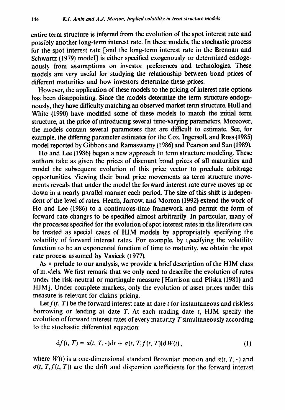
We compute a daily time series of the implied volatility parameters for the six different models described earlier. Fig. 1 shows the imputed single parameter of the proportional and absolute models on every fifth day (because of the large sample size). The parameter of the absolute model is scaled by ten to make the numbers similar in magnitude.

Parameter estimates across models are not directly comparable since the volatility functions differ in form. To compare across models, one must compute the volatility of forward rates as implied by the insta

154 K.I. Amin and A..!. Morton, Imp&d volatility in term structure moc’&

Proportional and Absolute Implied Volatility Parameters (1987-92)

- Proportional Volatility

The absolute implied volatility parameter is scaled by ten.

Absolute Spot Rate Volatility( 1987.92) Absolute and Proportional Models

- 1

p-q - Absolute Model - Proportlonal Model

The negative of the ahsolute volalility is plotted for the proportional mtdcl.

Fig. 1. Implied volatility parameters and absolute implied volatility for absolute and proportional models.

This figure plots the daily time series of estimated implied volatility parameters (6,-J on an annualized basis and the absolute implied volatility of the spot interest rate for the absolute volatility [o(t, T,f(t, T)) = oo] and the proportional volatility [o(t, T,f(t, 7)) = aof(t, T)] models. For the absolute volatility graph, the negative of the absolute volatility is plotted for the proportional model to distinguish it from the absolute volatility from the absolute model. The data period

is January 1, 1987 to November 10, 1992.

deviation of changes in forward interest rates, a@, 7’..f(t, T)), for each of the models. For example, consider the proportional model. The volatility function is

a(t, KS (t, T)) = oaf (t, T). Therefore, the absolute volatility of the spot rate equals o&t, t) and that of the one-year forward rate equals ctO f (t, t F 1). Fig. 1 also shows a plot of the implied absolute volatility of the spot interest rate obtained from the absolute and proportional models.

strates that im ied volatilities vary nificantly over the six- lied volatili’v may

K.I. Amin and A.J. Morton, Implied volatility in term structure models 155

be viewed as representi;lg the market’s conditional expectation of future volatility, and realized volatility of rates does fluctuate significantly [Engle, Rothschild (1991)]. In the equity market, we know that the series variation in realized volatility [Schwert (19$9)], and (1992) document similar variation in the volatility implied Poors 100 index option prices.

Of course, our six models posit that volatility parameters (measured different- ly in each) are constant. For this reason, a formal test of model fit would probably reject any of our models [Flesaker (1992) rejects the Ho-Lee (1986) model largely for this reason]. One possibility is that a second driving factor is influencing the evolution of rates, and manifests itself in the form of time-varying parameter estimates. However, it is unlikely that this second factor (if it exists) appears as an additive factor in (1). As we argued earlier, with options on short-maturity instruments, we cannot distinguish between multiple additive factors. After an analysis of historical forward rates with maturities of up to five years, Dybvig (1990) states that ‘the second factor (if any) in a term structure model should be related to the variance or other distributional features of interest rates, not additive in levels of interest rates as is usually assumed’.

Therefore, we may want to attempt to model the random evolution of the volatility itself, via the so-called stochastic volatility approach. Some problems can arise, however. First, prices in stochastic volatility models are not determined solely by arbitrage; one must specify the risk premium associated with the stochastic volatility. Moreover, such models would necessarily require more parameters, and would therefore exacerbate the problems of stable estimation that arise even in our two-parameter models. Finally, for options not too far from the money, prices in stochastic volatility models [Hull and White (198711 are of similar form to those in a constant volatility model, with volatility terms in the latter replaced by their conditional expected levels in the stochastic volatility environment. Thus, using a constant volatility model with market- implied volatility parameters achieves nearly the same effect.

Although our implied volatility parameters vary over time, they do not appear to be unstable. A qualitative difference in the behavior of the absolute and proportional models appears in the second half of 1992, when short-term rates were very low. Implied proportional volatility increased dramatically, while implied absolute volatility did not. A similar phenomenon occurs with equity options in that (proportional) volatility rises as equity prices decline and vice versa (the so-called leverage effect).

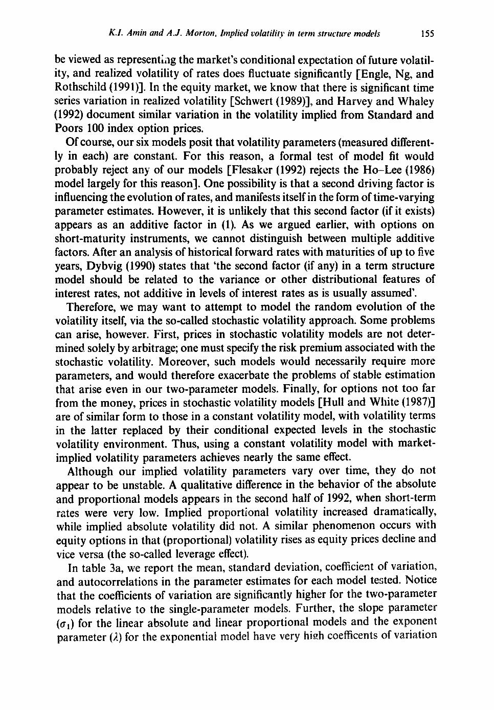
In table 3a, we report the mean, standard deviation, coefficient of variation, and autocorrelations in the parameter estimates for each model tested Notice that the coefficients of variation are significantly higher for the two-parameter models relative to the single-parameter models. (cl) for the linear absolute and line

arameter (A) for the ex

Tab

le

3a

L

37

Vol

atili

ty

para

met

er

estim

ates

fr

om s

ix d

iffe

rent

mod

els,

1,

483

obse

rvat

ions

.

is t

able

re

port

s th

e m

ean,

sta

ndar

d de

viat

ion,

co

effi

cien

t of

var

iatio

n,

the

auto

corr

elat

ions

, an

d m

odif

ied

Dic

key-

Fulle

r un

it ro

ot

stat

istic

s fo

r th

e -a

am

eter

s (o

n an

a.n

nual

bas

is)

and

thei

r fi

rst

diff

eren

ces

for

six

diff

eren

t vo

latil

ity f

unct

ions

est

imat

ed

usin

g an

im

plie

d vo

latil

ity p

roce

dure

fo

r th

e pe

riod

Ja

nuar

y 1,

198

7 to

Nov

embe

r 10

, 199

2. T

he m

odel

def

inin

g th

e pa

ram

eter

s w

hich

nes

ts a

ll th

e si

x vo

latil

ity

func

tions

es

timat

ed

is

z s

4t,

T,f(

f, T

)) =

[a0

+ q

x(

T-

tj]ex

p[

- ilx

(T-

t)lf

(t,

T)Y

,

The

cha

ract

eris

tics

of e

ach

mod

el i

n re

latio

n to

the

abo

ve e

quat

ion

are

desc

ribe

d in

par

enth

eses

be

low

eac

h m

odel

. T

he l

ast

colu

mn

repo

rts

mod

ifie

d D

icke

y-Fu

ller

unit

root

te

st s

tatis

tics

as t

he t

-sta

tistic

of

the

/?

coef

fici

ent

in t

he r

egre

ssio

n

i=l

3 -*

here

8 r

epye

sent

s ea

ch p

aram

eter

an

d A

rep

rese

nts

a fi

rst

diff

eren

ce.

The

uni

t ro

ot

is r

ejec

ted

with

a p

roba

bilit

y of

at

leas

t 0.

99 i

n ea

ch c

ase.

h

A A

bef

ore

a pa

ram

eter

in

dica

tes

the

firs

t di

ffer

ence

of

the

daily

par

amet

er

estim

ates

. 3 E

-

2 A

utoc

orre

latio

ns

Stan

dard

U

nit

2 ro

ot

test

od

e1

Nle

an

devi

atio

n C

.V.”

P

l P

2 P

3 P

lO

Pso

stat

istic

B

--

- z?

Abs

olut

e (C

T1 =

1. =

y =

0)

:io

0.0

1305

0.

0033

0.

26

0.98

0.

96

0.95

0.

87

0.62

-

4.58

0.

22 x

lo-

5

0.75

x 1

o-3

- 0.

26

- 0.

01

0.04

0.

04

- 0.

05

Squa

re

root

0.

0485

0.

0107

0.

22

0.97

0.

96

0.94

0.

84

0.56

-

5.21

@

l =

A =

0;

y =

0.5

) :,

0.15

x 1

o-4

0.00

24

- 0.

19

0.01

0.

05

0.06

-

0.04

K.I. Amin and A.J. Morton, Implied vuktility in term structure models

z 2 vi \d

I I

mu*- 000~0 dddd

I I

z 2 d d

I

I I

z VI d 0;

I

157

Tab

le

3b

Spot

and

one

-yea

r es

timat

ed

abso

lute

vo

latil

ities

fr

om s

ix d

iffe

rent

mod

els,

1,

483

obse

rvat

ions

.

Thi

s ta

ble

repo

rts

the

mea

n, s

tand

ard

devi

atio

n,

coef

fici

ent

of v

aria

tion,

th

e au

toco

rrel

atio

ns,

and

mod

ifie

d D

icke

y-Fu

ller

unit

root

sta

tistic

s fo

r th

e sp

ot

and

one-

year

ab

solu

te

vola

tiliti

es (

mea

sure

d on

an

annu

al

basi

s) a

nd t

heir

fir

st d

iffe

renc

es f

or s

ix d

iffe

rent

vol

atili

ty

func

tions

es

timat

ed

usin

g an

im

plie

d vo

latil

ity

proc

edur

e fo

r th

e pe

riod

Jan

uary

1,

198

7 to

Nov

embe

r 10

, 199

2. T

he m

ode1

def

inin

g th

e pa

ram

eter

s w

hich

nes

ts a

ll th

e si

x vo

latil

ity

func

tions

es

timat

ed

is

d4 T

,fk

T))

= [

co +

o1 x

(T -

t)

] ex

p[

- d

x (T

-

t)]f

(t,

ny .

a(0)

= a

@, t

,f(t

, t)

) is

the

abso

lute

vo

latil

ity o

f th

e sp

ot i

nter

est

rate

, o(

1) =

a(?

, t +

l,f

(t,

t +

1)

) is

the

abso

lute

vo

latil

ity

of th

e on

e-ye

ar

forw

ard

inte

rest

ra

te.

The

cha

ract

eris

tics

of e

ach

mod

el i

n re

latio

n to

the

abo

ve e

quat

ion

are

desc

ribe

d in

par

enth

eses

be

low

eac

h m

odel

. T

he l

ast

colu

mn

repo

rts

mod

ifie

d D

icke

y-Fu

ller

unit

root

tes

t st

atis

tics

as t

he t

-sta

tistic

of

the

/I

coef

fici

ent

in t

he r

egre

ssio

n

whe

re 0

rep

rese

nts

the

vola

tility

in

eac

h ca

se a

nd d

rep

rese

nts

a fi

rst

difl

eren

ce.

The

tin

it r’

oot i

s re

ject

ed w

ith a

pro

babi

lity

of a

t le

ast

0.99

in

each

cas

e.

A d

ind

icat

es

the

firs

t di

ffer

ence

of

the

daily

abs

olut

e vo

latil

ity

estim

ates

. -_

_ -.

~.- _-

--

~

Aut

ocor

rela

tions

U

nit

Stan

dard

-.

_ _^

.__”

ro

ot

test

od

e1

Mea

n de

viat

ion

C.Y

.”

Pr

P2

P3

PlO

P

so

stat

istic

-.

- -

-I

_.

Abs

olut

e a(

O)

0.01

31

0.00

33

0.25

0.

97

C.9

6 9.

95

0.87

0.

62

- 4.

58

(01

=n=

y=O

) A

u(O

) 0.

22 x

lo+

0.

75 x

IO

--”

- 0.

26

- 0.

01

o.u4

0.

04

-0.0

5 a(

l)

0.01

31

0.01

333

0.25

0.

97

0.96

0.

95

0.87

0.

62

- 4.

58

do(l

) 0.

22 x

lo+

0.

75 x

1o-

3 -

0.26

-

0.01

0.

04

0.04

-

0.05

Squa

re

root

a(

O)

0.01

29

0.00

34

0.26

0.

98

0.97

0.

96

0.83

0.

64

- 4.

45

(a,

= E

. = 0

; y

= 0

.5)

da(O

) 0.

15 x

1o-

s 0.

67 x

1O

”3

- 0.

21

- Q

.00

0.04

0.

04

- 0.

04

a(l)

0.

0135

0.

0034

0.

25

0.98

0.

97

0.95

0.

87

0.59

-

4.69

W

I)

0.27

x l

Ws

0.71

x 1

o-3

- 0.

20

0.01

0.

04

0.W

-

0.05

Prop

ortio

nal

a(O

) 0.

0127

0.

0034

0.

27

0.98

0.

97

0.96

0.

90

0.67

-

4.26

(a

1 =

A=

o;y=

l)

da(O

) 0.

077

x lo

+

0.63

x 1

0’ 3

-

0.18

-

0.01

-

0.03

0.

02

- 0.

03

a(l)

0.

0138

0.

0035

0.

26

0.98

0.

97

0.95

0.

86

0.57

-

4.72

M

l)

0.31

x l

o+

0.7

x 10

-j

- 0.

15

0.02

0.

04

0.03

-

0.04

Lin

ear

abso

lute

o(

O)

0.01

06

0.00

54

0.51

0.

92

0.89

0.

86

0.71

0.

36

- 4.

65

(A =

y =

0)

MO

) 0.

014

x lo

+

0.00

22

- 0.

31

- 0.

02

- 0.

03

0.00

-

0.01

a(

l)

0.01

39

0.01

6 1.

2 0.

86

0.81

0.

76

0‘54

0.

08

- 5.

45

Ml)

0.

57 x

1o-

5 0.

0084

-

0.29

-

0.05

-

0.05

-

0.02

0.

02

Exp

onen

tial

(171

= y

= 0

) a(

O)

0.01

08

MO

) 0.

047

x lo

- 5

o(l)

0.

020

Ml)

0.

37 x

lo+

Lin

ear

prop

ortio

nal

(A =

0;

3’ =

1)

a(O

) M

O)

dl)

Ml)

0.00

39

0.36

0.

90

0.86

0.

83

0.68

0.

37

- 5.

34

0.00

17

- 0.

32

0.00

-

0.06

-

0.02

0.

01

0.01

1 0.

58

0.58

0.

56

0.58

0.

47

0.27

-

5.44

0.

010

- 0.

47

- 0.

06

0.06

-

0.02

-

0.00

0.01

08

0.00

39

0.25

x 1

O-5

0.

0019

0.

0118

0.

0072

-

0.36

x l

o-’

0.00

59

0.36

0.

88

0.84

0.

81

0.64

0.

31

- 5.

38

- 0.

35

- 0.

00

- 0.

04

- 0.

05

0.01

0.

61

0.66

0.

58

0.55

0.

44

0.23

-

5.97

-

0.38

-

0.08

-

0.03

-

0.07

0.

02

“Coe

ffic

ient

of

vari

atio

n.


and these parameter estimates are not very reliable. Finally, the standard errors in estimating these parameters are much higher (results are not reported) than those for the other parameters even on a day-by-day basis.

The autocorrelations and the results of the Dickey-Fuller tests demonstrate that in each case the time series of volatility parameter estimates is stationary and mean-reverting. The first order correlation, pl, of the first difference in the time series of daily parameter estimates is - 0.12 for the proportional model, - 0.19 for the square root model, and - 0.26 for the absolute model.

The autocorrelation values are similar to those found for Standard and Poor”s 100 (OEX) options. Using a dividend-adjusted Black-Scholes model, Harvey and Whaley (1992) compute the first- and second-order autocorrelations in the implied volatility series as - 0.18 and - 0.11 for QEX call implied volatilities and - 0.15 and - 0.12 for OEX put implied volatilities. All the options prices used to compute their implied volatilities are sampled from a ten-minute window using transaction prices. Therefore, it is quite unlikely that their volatility estimates are significantly affected by asynchronous prices. Since our numbers are similar to those of Harvey and Whaley (1992), it is unlikely that the asynchronous trading problem is very serious. Recall that our options and futures prices are all obtained during the first hour of trading and the Eurodollar futures and options market is extremely liquid.

For the two-parameter models, the first-order autocorrelations, pl, for the daily change in the parameter values are also negative, and larger in magnitude. For the exponential model, p1 is - 0.32 and - 0.46 for changes in cio and a, respectively. However, for all models, the autocorrelations beyond the second lag are insignificant. The larger magnitudes of pl (and the coefficents of variation) are consistent with the hypothesis that the two-parameter models are, in part, fitting to noise and bid-ask bounce. Later we shall see other evidence off this phenomenon.

Under the absolute model, the slope of the estimated volatility function, gl, is positive on average. Under the exponential model, ;1 is negative on average. Thus, the estimated volatility of the one-year forward rate is higher than that of the spot rate. However, we have made some ‘market snapshot’ studies of longer-maturity caps and swaptions prices. Implied volatility functions for these instruments exhibit a hump in the volatility structure; in the Eurodollar data we see one side of the hump. Finally, notice that the average slope of the volatility function under the linear proportional model is negative. Therefore, the proportional volatility of the one-year forward rate is lower than the proportional volatility of the spot interest rate. This seems to be due to the fact that the term structure is upward sloping throughout most of our sample period.

In table 3b, we report similar statistics as in table 3a, but with absolute volatilities of the spot rate, S(t, t), and the one-year forward interest rate, f(t,t + 1). he ab so u 1 t e volatilities are very similar across models. The one-year

K.I. Arrin and A.J. Morton, Implied volatility in term structure models 161

forward rate volatility is now higher on average than the spot rate volatility in all models except the absolute (where equality of absolute volatilities across maturity is ensured by construction). owever, the absolute volatility of the one-year forward rate is much higher for the exponential model than for the other models. Suppose that the absolute volatility is truly I creasing with

maturity. When fitting the exponential model to option prices, the fitting procedure will choose ;1 to match the majority of options which are short-term options. The value of R necessary to generate the increases in volatility at the short end of the term structure will force high volatility at the one-year maturity because of the exponential function. This interpretation seems to argue against a good fit to the data with the exponential model.

The autocorrelations are similar to those reported for the actual parameter estimates in table 3a. In conjunction with the results of the modi Dickey-Fuller tests, they indicate that the absolute strongly mean-reverting and stationary irrespective of compute the volatility.

volatility time series is which model is used to

6. Pricing options using lagged implied volatility

For our predictive tests, we compute each day the term structure of forward rates by using the previous day’s implied volatility function and the current futures prices. Using this estimated term structure and the previous day’s implied volatility function, we then compute the model value for each option. This value is the simple model forecast. The forecast error is equal to rhe difference between the true market price observed on that day anti i&e forecasted value.

We first present some simple summary statistics. In table 4a, we summarize the model errors for each of the volatility functions. The average forecast error is close to zero, even in the out-of-sample fit.

In the third column of the table, we report the average ab!G>!e error in basis points (ticks) for each of the volatility functions for the e~~%~i~ pooled dataset. Recall that a basis point represents the minimum t>rice change of $25. Notice that the avertige absolute error for the absolute &dei is significantly higher than that for any of the other models. The averag?: ~+b~ol.:t~ error is of the order of one-and-a-half basis points for the linear ~~oport:+r~~:~ model and approximately one-and-a-half to two basis points for the other models. Since the bid-ask spread in this market is roughly one basis point (both for the futures and for the futures options), the fit of the models is good. Recall that these models use one or two parameters (estimated out of sample) to simultaneously generate an average of 18.5 option prices each day.

In the fourth column of table 4a, we report the corresponding average

absolute fractional errors. The fractional error is computed as the error divided by the market price. The average absolute fractional error is fairly high (15.2%


Table 4a

Summary error measures with six different volatility functions.

This table reports measures of model forecast error (measured in basis points) for six different volatility functions. The previous day’s implied volatility function is used to obtain out-of-sampls model forecast prices for the next day. The in-sample model prices (errors) are based on fitting an implied volatility function to the current day’s option prices. The implied volatility function is computed based on minimizing the sum of squares of errors between market prices and model prices. The sample period is January I,1987 to Novemeber 10, 1992 and there are 13,743 calls and

13,625 puts in the data sample. -~

Out-of-sample forecasta In-sample’

Av. abs. err. av. abs. err. Av. abs. Av. frac.

Volatility function Av. err. err. abs. err. Calls Puts All options

Absolute - 0.13 2.23 0.211 2.13 2.32 1.95 Square root - 0.12 1.94 0.188 1.88 2.01 1.71 Proportional - 0.06 1.76 0.173 1.76 1.77 1.55 Linear absolute 0.01 1.76 0.171 1.63 1.90 1.36 Exponential - 0.11 1.85 0.176 1.73 1.98 1.36 Linear proportionalb - 0.06 1.57 0.152 1.56 1.59 1.17

‘Forecast error = [Market price - Model forecast price] in basis points (or multiples of $25). Av. err. = average forecast error in basis points. Av. abs. err. = average absolute forecast error in basis points. Av. abs. frac. err. = average of (Forecast error/Market price).

bBased on the ‘g sr ns test, we can reject the hypothesis with probability at !east 0.99 in each case that any of the other models has a lower absolute error than the linear proportional model.

TaF!e 4b

Correlations between forecast errors across six volatility functions.

This table reports the correlations between the out-of-sample forecast errors in option prices with six different volatility functions for the period January 1, 1987 to November 10, 1992.

---~~- ______ -___ ~~___

Square Linear Linear Volatility function Absolute root Proportional absolute Exponential proportional

Absolute 1.0 Square root 0.97 1.0 Proportional 0.86 0.95 1.0 Linear absolute 0.49 0.51 0.50 1.0 Exponential 0.33 0.35 0.35 0.87 5.9 Linear proportional 0.38 0.46 0.53 0.87 0.86 1.0 ___ ._.___~. -- - -. --___

for the linear proportional model). However, these numbers are driven by the large fractional errors for options that are well out-of-the-money. The small prices of these options magnify even small pricing errors into large fractional errors. However, since these options also have very low volume, the average absolute fractional errors are less meaningful than the average absolute errors.

ecause the two-parameter models nest the single-parameter models, thq will always provide better in-sample fits. But, they may not perform as well

K.1. Amin and A.J. Morton, hplied volati 1:” f6.3

out-of-sample, due to the possibility of overfitting to noise. ur case, however, the linear absolute and exponential models fit better t solute model which they nest, and the linear proportional model fits than the proportional model. This is true with one-day-ahead forecasts. ion 7, we will also compare the ability of the models to explain option pri and compare models based on their ability to detect which can be exploited using trading strategies. A given to uncover genuine pricing errors that persist over t incorporated into misestimated parameter values. Our in section 7 will distinguish the models based on this yardstick.

Table 4b demonstrates the importance of the num of parameters in determining the behavior of a model. In both the on nd two-parameter groups, the lowest correlation between models is 0.86. Al gh the errors in all six models contain a common component due to n * in prices, bid-ask bounce, presence of a possible second interest rate factor, ge correlation within the one-parameter and two-parameter classes ies that the choice of the number of parameters has as great an impact ar options prices as the form of the model.

In figs. 2 and 3 we plot the average forecast error nction of time to maturity and option moneyness, where moneyness is defi as the futures price less the strike price for calls and strike price less the rice for puts= For puts and calls separately, the options are grouped into e categories containing an equal number of options, with the average value the maturity/moneyness for each group shown on the X-axis. Fig. 2 shows at all models tend to overprice short-dated options of both types. The e-parameter models compensate by underpricing the longer-dated opti , particularly puts. The two-parameter models overprice medium-term o ns, and in fact end up underpricing the long-term options, particularly c However, the two- parameter models are a better fit for long-dated puts. This is one reason why the two-parameter models produce lower fitting errors than the one-parameter models.

Fig. 3 exhibits the pattern of mispricing as a function of moneyness. The linear absolute and exponential models overprice almost all calls, except far-in-the- money ones. The other models underprice out-of-the-money calls and overprice nearer-to-the-money calls. For puts, the pattern is stronger and similar across models. All models seem to overprice in-the-money puts and underprice out- of-the-money puts. However, notice that the average error for at-the-money calls (puts) is smaller than that for other calls (puts). In seems to be a ‘smile effect’ for both calls and puts.

To study possible systematic biases in more detail, cross-sectional regression separately for calls and puts:

trader parlance, there

we run the following


Calls

23 52 76 101 126 155 204 344 MabityinDays

-BAbS -x sq. Root 43 Prop

WLinAbs c3Expixlmw tinProp

32 $1

EO

f -1

g-2

-3

t -- y I

I t 1 1 I 1 t I I I 1 1 1 I I I

24 54 78 101 126 153 196 295 Maturity in Days

V-AbS -x sq.Rlmt +Pfop -eLinAbs QExpculential tinProp

- --

Fig. 2. Forecast error as a function of maturity.

This figure plots the forecast error as a function of the option maturity separately for calls and puts. All the options are sorted by maturity and grouped into eight categories containing an equal number of options. The average maturity for each of the eight groups is plotted on the X-axis. The units for all prices are basis points (multiples of $25). The sample period is January 1, 1987 to November 10,

1992.

where is the market price, 6 is the mo el price, and E is the error. The results are summarized in table 5. The average prediction error is quite small, except for

1 and linear absolute models. The high R-square is not t is also evident i tests of equity options

torl==4a

L


3

-2 -121 -63 -40 -24 -10 4 20 70

Futures Price - Strike Price

-BAbs -X Sq. Root Prop -W LinAbs i3 Exponenlial tin Prop

Average Forecast Error with Puts

Strike Price - Futures Price

1 - .-

=+ Abs -X Sq. Root 4+ Prop

Q tin Abs -0 Exponenlial tin Prop _ __ _ ~_ _ ~_ - ~- --- -- --

Fig. 3. Forecast error as a function of moneyness.

This figure plots the forecast error for calls and puts separately as a function of moneyness (futures price less strike price for calls and strike price less futures price for puts). All the options are sorted by moneyness and grouped into eight categories containing an equal number of observations. The average moneyness for each of the eight groups is plotted on the X-axis. The units for all prices are

basis points (multiples of $25). The sample period is January 1, 1987 to November 10, 1992.

overwhelmingly rejected for all models. The lar size of the data sa

that even small mispricings are evident from e regression. [See

Turnbull (1990) for a similar observation in the context of foreign currency

owever, if we take the view that ‘it takes a model to beat a model’, then we are only concerned about relative objective is to study which model is the most


Table 5

Overview of model performance.

Regression results for

Market price of option = a0 + a1 Model forecast price + E ,

for six different volatility functions. The T-statistics [adjusted for heteroskedasticity using White (1985)] for a0 = 0 and al = 1, respectively, are reported in parentheses below each coefficient. The previous day’s implied volatility function is used to forecast the current day’s prices using the current forward interest rates. The model and market prices are expressed in basis points. The sample period

is January 1, 1987 to Yovember 10, 1992.

Volatility Function 010 R2 F-stat.a

Call options (13,743 observatiorrs)

Absolute

Square root

Proportional

Linear absolute

Exponential

Linear proportional

- 0.908 1.015 0.9885 401.4 ( - 27.2) ( - 13.2)

- 0.586 1.0087 0.9907 225.3 ( - 19.6) ( - 8.0)

- 0.174 1.0010 0.99 16 30.6 ( - 6.1) ( - 0.9)

- 0.425 0.99994 0.9892 257.0 ( - 12.8) (0.04)

- 0.192 0.9860 0.9765 228.1 ( - 1.1) (1.8)

0.204 0.9857 0.9897 34.0 (5.7) (7.9)

Absolute

Square root

Proportional

Linear absolute

Exponential

Linear proportional

Put options (13,625 observations)

0.505 0.9890 (14.6) (8.1)

0.232 0.9950 (7.6) (4 ‘,)

0.0706 0.9985 (2.5) (1.2) 1.342 0.9596

(30.4) (16.9)

1.50 0.948 (17.1) (11.0)

0.706 0.9708 (16.9) (12.7)

0.9793 108.1

0.9848 30.1

0.9877 3.5

0.9844 730.8

0.9774 427.8

0.9867 167.3

aF-statistic for joint test of a0 = 0 and a1 = 1.

For calls, the & coefficient in table 5 is always greater than one for the single- parameter models, and always less than one for the two-parameter models. Thus, the single-parameter models tend to underprice high-priced calls and overprice low-priced calls, while the opposite holds for t*.lo-parameter models. On the other hand, a similar examination of the &r coefficient for puts demonstrates that all six models overprice high-priced puts and underprice low-priced


puts. The last result is exactly the opposite of that found bv Whaley (1982) for D

equity options. Note that 010 is negative for calls (except in the case of the linear proportional

model) and positive for puts. A similar result obtains if we restrict al to be unity (for conciseness, these results are not reported in the table). Thus, the models tend to overprice call options and underprice puts. Put another way, the implied volatility of calls is lower than that of puts, on average. A similar phenomenon has been observed in Standard and Poor’s 500 futures options [Whaley (1986)] and in Standard and Poor’s 100 index options [Harvey and Whaley (193211.

We next regressed the prediction error on the amount by which the option was in-the-money, the maturity of the option, the forward yield implicit in the underlying futures contract on which the option is based, and the TED spread defined as the spread between three-month Treasury bill (T-bill) and three- month Eurodollar yields. The three-month Eurodollar yield is computed from the term structure estimated in section 4.1. We obtained daily bid and ask prices on T-bills from Data Resources (DRI), and computed the three-month Treasury yield by linearly interpolating between the average of bid and ask yields of available T-bills. The reason for including the TED spread is that our model assumes that the forward interest rates are default-free. However, the Eurodollar rates contain some element of default risk. If the difference between Eurodollar rates and Treasury rates follows systematic time series patterns, then it is possible that this variation itself may be responsible for some of the pricing errors that we find. The regression equation is:

Market - Model = PO + /I1 [Futures - Strike] + /&Maturity

+ &&D + B4TED + E,

where ED is the three-month forward yield for maturity equal to the option maturity and TED is the TED spread defined earlier. The results are summarized in table 6.

Table 6 shows that, when significant, the estimate of p1 is negative for calls and positive for puts. Thus, out-of-the-money options are underpriced by the models. Since these options have low prices and low sensitivity to the volatility, our fitting procedures give them less weight. Therefore, their errors will tend to be larger in general. It is also possible that market-makers and speculators demand a premium to supply these options to investors to compensate for low trading volume (see table 2).

The pZ estimate is significantly positive for puts and calls for all single- parameter models and significantly negative for puts and calls for all two- parameter models. Therefore, the single-parameter models underprice long-maturity options and overprice short-maturity options. These facts are also apparent from fig. 2. From table 3a, we know that, in our data, the volatility


Table 6

Systematic biases in each model for call and put options.

Regression results for

Market price - Model price = PO + PI [F;crtures price - Strike price] + f12Matu.-ity + &ED + f14TE5 -t_ E ,

where ED is the three-month forward yield corresponding to option maturity, and TED is the spread between the three-month Treasury yield and the three-month Eurodollar yield. All prices are in basis points, all the yields are continuously-compounded yields expressed as fraction per year, and the option maturity is in days. The T-statistics of the regression coefficients, adjusted for heteroskedasticity using White (1985), are reported in

pzentheses below each coefficient value. The sample period is January 1, 1987 to November 10, 1992.

Volatility function Bl B3 84 R2 F-stat?

Absolute

Square root

Proportional

Linear absolute

Exponential

Linear proportional

- 3.8 ( - 33.77)

- 2.77 ( - 27.9)

- 1.54 ( - 16.7)

0.73 (464) 1.23

(3.92)

1.2 (7.2)

Call options (13,743 observations)

0.003 (5.70)

- 0.0014 ( - 2.87)

- 0.0057 ( - 11.3)

0.0012 (2.03)

Q.0011 (1.46)

- 0.0092 ( - 15.5)

0.015 (43.07)

0.011 (37.7)

0.0076 (26.4)

- 0.0045 ( - 7.91)

- 0.0073 ( - 6.05)

- 0.0048 ( - 7.8)

17.96 (12.4)

11.44 (8.8) 2.63

(2.13)

- 7.0 ( - 4.05)

- 9.66 ( - 3.1)

- 12.54 ( - 7.0)

11.71 0.21 718 (1.8)

8.65 0.17 557 (1.37)

7.11 0.13 342 (1.13)

- 2.38 0.03 92 ( - 0.34)

- 9.96 0.03 92 ( - 1.02)

- 1.41 0.04 51 ( - 0.21)

Absolute

Square root

Proportional

Linear absolute

Exponential

Linear proportional

- 4.51 ( - 39.5)

- 3.47 ( - 35.06)

- 2.15 ( - 23.4)

0.474 (3.11)

0.86 (4.17)

0.845 (5.56)

Put options (13,625 observations)

0.016 (32.1)

0.013 (30.3)

0.009 (23.4)

0.018 (34.8)

0.019 (31.0)

0.011 (25.6)

0.019 (43.3)

0.014 (39.0)

0.0094 (26.1)

- 0.0015 (-2.17)

- 0.004 ( - 3.96)

- 0.0057 ( - 8.4)

18.15 (13.51)

13.8 (11.5)

6.58 (5.54)

- ‘,.66 (-6.43)

- 11.65 ( - 5.9)

- 6.06 ( - 3.98)

62.4 0.37 665 (11.39)

44.77 0.29 569 (8.6) 26.65 0.17 298 (5.11)

36.52 0.13 522 (5.67)

27.9 0.10 442 j4.02)

3.71 0.08 192 (0.66)

aF-statistic for the joint test of fli = 0 for i = 0, 1,2,3,4.

of longer-term forward rates is higher than that of short-term rates. Since the single-parameter models cannot capture this feature, the volatility of longer- term futures prices is too low in these models. Since option values are increasing functions of volatility, longer-term options are underpriced.

The sign of the biases induced by the variable ED is identical to those due to maturity for ever model and for both calls and puts. Recall that ED is the

K.I. Amin and A..!. Morton, Implied volatility in term structure models 169

three-month Eurodollar forward yield corresponding to the option maturity. Since the term structure is usually upward-sloping in our data, the variable ED and the option maturity are positively correlated, so the pricing biases for both variables are similar.

Finally, the coefficient for the TED spread is insignificant for call options. For puts, it is significant and positive for all models except the linear proportional, possibly explaining why the put valuation errors are larger than for calls. Calls are not affected by variations in the TED spread, whereas puts are. It may be worthwhile to model the systematic variation in the TED spread when valuing puts. However, the problems of parameter estimation in any model involving both Treasury and Eurodollar rates are likely to be severe.

7. Trading strategies based on mispriced o

In this section, we compare model performance based on whether simple trading strategies can exploit the deviations between model and market prices. Roughly speaking, our trading strategies will be of the following form: each day fit to the market as well as possible, then buy underpriced options and sell overpriced options, and finally hedge these options using their underlying futures contract. In an efficient market, no such strategy should earn abnormal returns, after accounting for transaction costs and risk.

Since we are studying models that posit particular forms of term structure evolution, we can develop a hedging method that is consistent with the pricing model. To that end, for a given choice of model and its parameters, define an instrument’s delta as the change in its model price induced by an instantaneous shift in the term structure, of the form implied by the model, and with magnitude ecgual to one day’s standard deviation. This delta is clearly a linear operator, and a portfolio is delta-neutral if and only if its delta is zero. Such a portfolio is immunized against term structure movements of the form dictated by the model.

Notice that the form of term structure movements hedged by delta can vary significantly from model to model. For example, under the absolute model, delta hedging amounts to hedging against Rat parallel shifts in forward rates. How- ever, under a linear absolute model with nonzero slope Q, delta hedging means hedging against a term structure twist.

Finally, note that we do not hedge against changes in the environment which are ‘outside the model’ (such as changes in the level of volatility, changes in parameter values, etc.).

The focus of the remainder of our study will be the relationship between the original mispricing of an option and the eventual profit realize a position in that option. e use the term allocated prc$t to refe profit for that option. In calculating allocated profits, we charge or earn the short-term interest rate each day dependin on whether ca generated by the position.


Each day and for each model, we fit (as described in section 3) a term structure and a volatility Amt. -iron to those futures and options prices observed by 8:30 am

. We randomly decide (independently, with probability 0.2) to take a position in each mispriced ?>ption not already in the portfolio. We do not initially impose any filter rules. The price charged (or earned) for every option traded is its first recorded price after 8:45 ‘m, thus guaranteeing a minimum lag of 15 minutes from fitting to trading time. Since our database contains only a record of trades at new prices, the price we record for an option might not be its first traded price after 8:45. If the option’s price does not appear that day after 8:45, its order is canceled.

We randomly choose option positions to trade because if we traded every option not already found in the portfolio, we would necessarily trade every option on the first day it appears, perhaps inducing a bias. Selecting options randomly reduces this bias, and yet leaves us with many trading opportunities.

We also impose a position limit of one on each option. This rather severe constraint helps give some independence between different trades (although complete independence between two positions held at the same time cannot be assured). It will be evident from table 7 and our later discussion that the model pricing errors persist over many days. Therefore, in the absence of a position limit, we would purchase the same underpriced option (sell an overpriced option) again and again on many consecutive days. Consequently, our sample of trades would contain highly-correlated observations. Our position limit constraint prevents us from accruing profits from large positions in a single option and alleviates this problem.

Each day that an option position is maintained, we delta hedge it with its underlying futures contract. That is, we determine the delta of the option and of its underlying futures contract, and take a position in the futures contract so that the combined delta is zero. We close out the position when any of the following conditions occur:

the mispricing disappears (e.g., an option which was originally underpriced becomes overpriced, or vice versa), the option expires, or the option goes in or out of the money by 150 basis points.

The reasons for conditions 1 and 2 are obvious. Condition 3 is imposed since

1.

2. 3.

options this far out of the money or in the money trade extremely infrequently. It is possible that conditions 2 or 3 could occur without observing a price for

the option on the final day the position is held. In this case, we mark the contract at its model price plus its ‘gap’, where the gap is the most recently observed difference between the market and model price. The reason for this choice is that when an option in our portfolio does not trade, it is usually because a market movement has caused the option to no longer be near the money. Thus, marking it at an earlier price could be quite misleading. n the other hand, marking at

K.1. Amin and A.J. A4orton, Implied volatility in term structure models 171

Table 7

Trading strategies based on m&priced options: Summary results.

This table reports the results of a trading strategy of buying (selling) underpriced . .a __ __ _ (overpriced)

options and hedging them with the underlying futures contract until the mispricing disappears for each of the six models for the sample period January 1,1987 to November 10,1992. The numbers in parentheses denote T-statistics, adjusted for heteroskedasticity using White (1985). The profit is

measured in basis points. The average investment per trade does not vary significantly by option type (calls or puts) or

according to the model used. It is approximately 28 to 30 basis points.

Model Option

type N”

Average days held

Average profit in

basis points

Gap coefficientb

a

Market coefficient ’

B

Absolute

Square root

Proportional

Linear absolute

Exponential

Linear proportional

All Calls Puts

All Calls Puts

All Calls Puts

All Calls Puts

All Calls Puts

All Calls Puts

3,131 23.1 1,648 20.9 1,483 25.7

3,154 22.7 1,633 21.3 1,521 24.2

3,433 20.6 1,767 19.9 1,666 21.2

3,564 19.5 1,932 17.6 1,632 21.7

3,568 19.2 1,873 18.1 1,695 20.5

3,850 17.9 2,039 16.8 1,811 19.1

1.74(6.41) 0.7 l(3.66) 1.53 (3.95) 0.57(1.91) 1.96(5.22) 0.82 (3.23)

1.30 (4.67) 0.65 (2.26) 0.41(0.98) O.lO(O.22) 2.26 (6.28) 1.15 (4.23)

1.15(4.41) 0.45 (1.48) 0.43(1.10) - 0.34( - 0.83) 1.92 (5.56) 1.29 (4.43)

0.37 (1.58) 0.49 (2.20) 0.18 (0.53) - 0.06( - 0.20) 0.59 (1.93) 0.88 (3.05)

0.45 (2.06) 0.41(1.72) 0.29 (0.89) 0.16(6.58) 0.64(2.16) 0.62(1.71)

0.45 (1.99) 0.10 (0.37) - 0.07( 0.22) - - 0.28( 0.73) -

1.03(3.53) 0.51(1.40)

- 0.131 - 0.86) - 0.75 ( - 3.48)

0.38 ( 1.94)

0.02(0.16) - 0.46( - 1.99)

0.43 (2.37)

0.04 (0.27) - 0.44( - 1.97)

O&(2.15)

- 0.25( - 1.32) - 0.24( - 0.59) - 0.26( - 1.74)

- 0.35( - 2.68) - 0.55( - 2.52) - 0.20( - 1.27)

- 0.20( - 1.26) - 0.26( - 0.94) - 0.15( - 0.84)

‘Number of individual futures options purchased or sold. bCoefficient of the initial gap ( = 1 Market price - Model price 1) when regressed against the

realized allocated profit from the regression: Realized allocated profit = Constant + a(Initia1 gap) + error.

“Coefficient of the market return (return on the value-weighted returns of all firms on the NASDAQ, NYSE, and AMEX measured as a fraction per year) when regressed against the allocated profit (in basis points) to the hedged trade from the regression: Allocated profit = Constant + /3(Market return) -t error.

the model price can be too optimistic, given that we are trading on discrepancies between the model and the market. Our procedure seems to be a reasonable compromise. Finally, we note that the estimated parameters and model prices are determined only from prior data. Therefore, our results are not subject to data-snooping biases.

The results of these trading strategies are summarized in table 7. The most basic result is that, with no transaction costs, all rnc .!els produce significant abnormal profits.

172 K.I. Amin and A.J. Morton, Implied volatili’ty in term structure models

As a group, the one-parameter models substantially outperform the two- parameter models, producing profits that are roughly one basis point higher per position taken. This finding is consistent with the t meter models overfitting to spurious noise in the data. If the pricing rsist over even a few days, it is plausible that systematic pricing errors er time will simply be incorporated into misestimated parameter values think of an extreme case in which there might exist a large number of ispriced with respect to the ‘true model’, but by fitting a large number of parameters, we exactly fit all the option prices on a given day. If the pricing errors persist over time, the model with these parameters will not be able to detect the mispriced options on the subsequent day.

Notice that the average holding period for the hedged position varies between 17 and 25 days. If the pricing error for a given option was random from one day to the next, we would expect very short holding periods. Therefore, the pricing errors are persistent over time. We also note that the average holding period is larger for single-parameter models relative to two- parameter models. Therefore, the pricing errors are more persistent for the single-parameter models and provide some evidence of overfitting in the case of the two-parameter models.

We now study the allocated profits as a function of the initial mispricing. If the models can detect true mispricing, then one would expect a positive relationship between anticipated profit (as measured by the initial mispricing or gap) and the realized profit of the hedged trade. Fig. 4 and table 8 display the realized profits as a function Jf initial mispricing, broken down by option type and direction of position taken. Several facts emerge. The largest profits are obtained by selling options, and this profit is generally a monotonic function of the initial gap. Buying mispriced puts is also profitable, although the levels of profits are not as large. Again, the initial gap provides a strong signal about the profit expected. Finally, buying mispriced calls seems to generate losses in many cases.

Recall from fig. 2 th;;t the major qualitative difference between the behavior of the one- and two-parameter models is the latter’s ability to better fit market prices of long-dated puts. However, the trading results shown in fig. 4 indicate that, in fact, the one-parameter models are correctly pricing the puts. These models are able to extract from the market, by trading, nearly the entire amount of the apparent mispricing.

To make these observations more precise, we regressed realized profit against the initial gap for all the trades irrespective of the initial gap. The results are also reported in table 7. As expected, the gap coeficient is positive in all models, and statistically significant at the 95% level in the absolute, linear absolute, and square root models. In the absolute model, for example, the average realized profit is 82% and 57% of the initial gap for calls and puts,

he initial gap is a strong predictor of the final realized profit.

K.I. Amin and A.J. Morton,

Allocated Profit versus lnitial Gap Sold Calls

Implied volatility in term structure nood~h

jr- --

173

Allocated Profit versus Initial Gap

-, - ’ * ’ 1 to 2 Bans Points 2 to 3 Bask Points B 3 Bask Point; Initial Gap

Allocated Profit versus Initial Gap Sold Puts

. ’ . 1 10 2 Bass Poms 2 lo 3 Basis Pmts s 3 Basrs Pmnts Inmal Gap

Allocated Profit versus Initial Gap Bought Puts

lnitiil Gap > 3 Basis Pods 1 to 2 Basis Points 2 to 3 Base Poms

Initial Gap

Fig. 4. Profits from trading strategies to exploit mispriced options.

This figure plots the average allocated profit from a trading strategy of buying (selling) underpriced (overpriced) options and hedging them with the underlying futures contract until the mispricing reverses. Trades are classified by the initial gap ( = 1 Market price - Model price I), and we plot the average realized profit per trade separately for puts and calls and separately for positions in which the options are bought and sold. The profit per trade and the initial gap are in basis points (multiples of $25). The sample period is January 1,1987 to November 10, 1992. The six bars in each group in the figures are, from left to right: absolute, square root, proportional, linear absolute, exponential,

and linear proportional models.

I indication that the model is picking up and exploiting This seems to be an genuine mispricings.

As fig. 4 and table differ markedly. The

8 demonstrate, the profit opportunities in puts and calls gap coefficients seem to support the hypothesis that all

models, but particularly the one-parameter ones, can detect and exploit mispriced puts. Moreover, the size of the original mispricing is very significant in predicting the eventual profits. For calls, the story is mixed - the models perfor well in detecting opportunities to sell calls, t their signals to buy calls are not

Tab

le

8

Ave

rage

pro

fits

to

trad

ing

stra

tegi

es

by i

nitia

l op

tion

m

ispr

icin

g fo

r si

x m

odel

s.

Thi

s ta

ble

repo

rts

the

prof

its

obta

ined

by

em

ploy

ing

a tr

adin

g st

rate

gy o

f bu

ying

(se

lling

) un

derp

rice

d (o

verp

rice

d) o

ptio

ns a

nd h

edgi

ng t

hem

with

the

und

erly

ing

futu

res

cont

ract

un

til t

he m

ispr

icin

g di

sapp

ears

fo

r ea

ch o

f th

e si

x m

odel

s. E

ach

obse

rvat

ion

corr

epon

ds

to t

he p

urch

ase

or s

ale

of a

sin

gle

opti

on,

and

a po

sitio

n lim

it of

one

con

trac

t is

im

pose

d on

eac

h op

tion

. T

he t

rade

s ar

e cl

assi

fied

by

the

initi

al m

ispr

icin

g (g

ap)

and

whe

ther

th

e op

tion

is

bou

ght

or s

old.

The

pro

fit

per

trad

e an

d th

e in

itial

gap

are

rep

orte

d in

bas

is p

oint

s (m

ultip

les

of $

25).

T-s

tatis

tics,

adj

uste

d fo

r he

tero

sked

astic

ity

usin

g W

hite

(19

85),

are

rep

orte

d in

par

enth

eses

. T

he s

ampl

e pe

riod

is

Jan

uary

1,

1987

to

Nov

embe

r 10

, 19

92.

Initi

al

gap:

” 1

to 2

bas

is p

oint

s In

itial

ga

p: 2

to

3 ba

sis

poin

ts

Initi

al

gap:

Mor

e th

an

3 ba

sis

poin

ts

Sol

db

Bou

ght”

So

ld

Bou

ght

Sold

B

ough

t

Nd

Av.

Pro

f.”

N

Av.

Pro

f.

N

AX

Pro

f.

N

Av.

Pro

f.

N

Av.

Pro

f.

N

Av.

Pro

f.

Abs

olut

e

All

419

1.61

(2.4

9)

422

0.33

(0.

45)

182

2.05

(2.

28)

215

2.29

(3.

77)

299

6.46

(4.

30)

210

3.26

(2.

67)

Cal

ls

198

1.15

(2.3

8)

240

- 0.

18 (

-

0.16

) 73

1.

46 (1

.78)

12

1 2.

52 (

3.53

) 12

6 7.

03 (

2.73

) 11

7 1.

13 (0

.76)

Puts

22

1 2.

02 (1

.76)

18

2 0.

99 (

1.24

) 10

9 2.

44 (

1.75

) 94

1.

99 (1

.92)

17

3 6.

05 (

3.36

) 93

5.

96 (

2.97

) --

Squa

re

root

All

448

1.03

(2.7

3)

440

0.81

(1.

28)

209

4.06

(2.

82)

177

0.39

(0.

19)

261

6.36

(3.

74)

161

2.10

(1.

40)

Cal

ls

209

1.12

(2.7

5)

221

- 0.

14 (

-

0.13

) 83

1.

42 (1

.49)

10

3 -

0.98

( -

0.

39)

120

6.01

(2.

22)

83

-- 1

.48

( 0.

71)

-

Puts

23

9 0.

95 (

1.56

) 21

9 1.

76 (2

.42)

12

6 5.

80 (

2.53

) 74

2.

08 (

2.12

) 14

1 6.

65 (

3.11

) 78

5.

91 (

2.85

)

-

A!!

C

alls

Pu

ts

Prop

ortio

nal

497

1.41

(4.4

4)

430

0.21

(0.

25)

217

3.67

(2.

16)

176

- 0.

78 (

-

0.50

) 22

5 6.

60 (

3.73

) 11

72

244

1.78

(4.5

5)

213

- 1.

90 (

- 1.

18)

105

1.74

(1.4

8)

99

- 2.

92 (

-

1.1)

10

7 5.

35 (

1.88

) 89

25

3 1.

06 (2

.13)

21

7 2.

28 (

4.03

) 11

2 5.

49 (

1.77

) 77

1.

97 (1

.97)

11

8 7.

72 (

3.58

) 83

Lin

ear

abso

lute

All

480

1.04

(3.0

0)

516

- 0.

21 (

-

0.32

) 17

1 1.

49 (2

.58)

24

4 -

0.35

( -

0.

37)

199

2.95

(2.

61)

155

- 1.

99 (

- 0.

73)

Cal

ls

224

1.70

(2.8

9)

304

0.67

(0.

92)

65

1.18

(1.3

5)

135

- 0.

76 (

-

0.49

) 67

1.

97 (0

.77)

92

-

4.89

( -

1.

46)

Puts

25

6 0.

46 (

1.18

) 21

2 -

1.45

( -

1.27

) 10

6 1.

68 (2

.21)

10

9 0.

15 (

0.15

) 13

2 3.

45 (

3.10

) 63

2.

26 (

0.49

)

1.30

(0.9

3)

- 2.

03 (

-

1.07

) 4.

86 (

2.41

2)

--

Exp

onen

tial

All

487

0.95

(2.

67)

514

0.27

(0.

49)

189

1.16

(1.7

7)

238

- 1.

40(

-0.9

4)

196

2.79

(2.

69)

145

0.73

(0.

31)

Cal

ls

219

2.0

(3.2

5)

294

0.54

(0.

7Q)

72

0.99

(1.

28)

144

- 2.

31 (

-

0.96

) 66

3.

03 (

1.31

) 83

-

0.63

( -

0.35

) P

uts

268

0.10

(0.

24)

220

- 0.

09 (

-

0.94

) 11

7 1.

27 (1

.34)

94

0.

0 (0

.0)

130

2.59

(2.

63)

62

2.56

(0.

51)

Lin

ear

prop

ortio

nal

Ah

565

1.14

(4.3

5)

534

- 0.

42 (

-

0.51

) 20

8 1.

39 (1

.62)

17

9 0.

47 (

0.40

) 13

3 3.

02 (

2.13

) 13

5 -

3.56

( --

1.

15)

Cal

ls

306

0.80

(2.

62)

294

- 1.

36 (

- 0.

96)

90

1.19

(1.6

6)

93

- 1.

30 (

- 0.

66)

68

2.73

(1.

18)

75

- 6.

59 (

--

1.78

) Pu

ts

259

1.54

(3

.50)

24

0 0.

74 (

1.32

) 11

8 1.

59 (1

.09)

86

2.

38 (

2.14

) 65

3.

31 (

2.08

) 60

0.

35 (

0.06

)

“Ini

tial

opti

on

mis

pric

ing

(in

basi

s po

ints

) w

hen

the

trad

e is

fir

st e

stab

lishe

d.

ptio

ns

in w

hich

a s

hort

po

sitio

n is

tak

en.

‘Opt

ions

in

whi

ch a

lon

g po

sitio

n is

tak

en.

dNum

ber

of i

n di

vidu

al

optio

ns

boug

ht

or s

old.

ve

rage

pro

fit

per

opti

on

trad

e in

bas

is p

oint

s.


reliable. Even though fig. 4 and table 8 document large losses for purchased calls, the losses are not statistically significant for any of the models or filter rule as there is a wide dispersion in the allocated profits. However, the profits generated from selling both puts and calls with each of the individual filter rules are individually significant for all the models.

The fact that the gap coefficients are less than one indicates that large pricing errors are perhaps not as reliable. Recall t&t both the futures price and the option price are subject to the bid-ask spre:.J, which is typically one basis point. Perhaps the larger pricing errors that we detect reflect a larger component due to these bid-ask effects.

Since our trading strategies are not riskless, the abnormal profits that they generate could be due to ‘systematic risk’. Even though it is difficult to measure systematic risk in our context, regressing the realized profits against a market return can provide some rough guidelines. To test if systematic risk is the cause of the excess returns, we regress the realized profit on each position against the value-weighted returns of all firms on the NASDAQ, NYSE, and AMEX, over the period that the position is held. The market coefficients are predominantly negative, except in the case of put trades under one-factor models. Since these types of trades are quite profitable, systematic risk is the cause of some of the profits. However, the average profit seems too large and over too short an interval to be due to systematic risk alone. Still, in the absence of an equilibrium model, it is difficult to quantify the excess profit.

In sum, the trading results indicate that the market systematically contains mispricings, particularly in long-dated puts, which appear overpriced. The one-parameter models are able to detect and exploit this mispricing. Moreover, the initial gap predicts the realized profits well.

Whether our results are evidence of market inefficiency depends on the transaction costs involved in implementing our strategy. The bid-ask spread in the Eurodollar futures options market is of the order of one basis point and there is a brokerage fee as well. However, market makers on the floor of the exchange are subject to only a small clearing fee and by timing the trade, they can avoid paying the bid-ask sprtsd as liquidity providers. Therefore, the transaction costs of setting up the initial trade are probably significantly smaller than one basis point. However, one must also incur the costs associated with daily hedging (a position is typically held for about 20 days). Clearly, if a cost of one basis point must be paid each day to hedge, then the profits we see for puts (two basis points on average, higher if a ‘silter rule’ is used to select trades based on initial gap) are insignificant. bn the other hand, our strategy was deliberately simple. Perhaps hedging every day is not required, or perhaps one can hedge with other mispriced options +I- So generate even higher profits. We do not pursue these issues here. Our primary objective is to compare the ability of the models to value and hedge options correctly and not to formally test for market efficiency.

K.I. Amin and A..!. Mortora, haplied ~o~~ti~it~ in term structure” models

8. Conclusions

We implement and test six HJM interest rate models u an implied volatility technique. We apply our models, which contain ei one or two parameters, to Eurodollar futures and options rices between 11987 aged 1992. Each day, we fit the parameter(s) to all traded options, after using the futures prices to determine the term structure.

We characterize the implied volatility of interest rates from each of the models. The implied volatility series is stationary and mean-reverting irrespective of the model used. The mean absolute volatility estimates are similar across models, although the single-parameter models produce significantly more stable estimates of implied volatility. On average, the absolute volatility of the one- year forward rate is larger than the absolute volatility of the spot interest rate. However, since forward interest rates are typically increasing with maturity, the proportional volatility of the one-year forward interest rate is lower than the proportional volatility of the spot rate on average.

We compare the models based on three criteria: (1) stability of parameter values, (2) fit between model and market prices, and (3) ability of the model to earn profits when it trades on perceived mispricings. We find that the number of parameters used in the modeI has a strong effect on the behavior of the model - in fact stronger than the form of the model used (proportional, absolute, etc.). Two-parameter models tend to fit prices better (even one day out of the sample), but their parameter estimates are less stabie and thev earn less from their perceivlei: mispricings. Although the one-parameter models fit slightly less well, their implied parameter values are more stable over time and they are able to earn significantly larger and more consistent abnormal profits from the mispricings they detect.

As with equity options, put options are overpriced relative to call options and there are significant biases as a function of strike price and maturity for all the models. All models, particularly the one-parameter models, suggest that long- dated puts are overpriced in the Eurodollar market. The poor fit of the single- parameter models is attributable in large part to the mispricing of these puts. Together with the observation that the one-parameter models earn larger and more consistent profits, there are strong reasons to conc’lude that one-parameter models are preferable for valuing options with maturities of less than a year. Among the one-paramete; models, the absolute model seems to be preferable since its parameter estimates are the most stable and it earns the largest profits.

A ix

For completeness, we outline a nu.merical irllplementation of single-factor models as described in

orton, and Spindel (1992).

178 K.I. Amin and A..!. Morton, Implied volatility in term structure models

At date 0, we wish to value an option maturing at T. Discretize the interval [0, T] into M subintervals of width h,, for m = 1,. . . , M, such that c,“=,hm = T. The choice of subintervals will have some effect on the rate of convergence of the discrete approximations. One satisfactory scheme is to choose linearly increasing (or decreasing) subinterval lengths so that the largest is twice the size of the smallest [Amin and Rodurtha (1994)]. Under the HJM approach, with the entire term structure as a state variable, we need to track the evolution of rates only up to time T to value such an option. We construct a binary (non-recombihg) tree under which the mth step induces volatility corresponding to the passage of h, time units. In general, one cannot use the recombining lattice approach [Cox, Ross, and Rubinstein (1979) or Amin (1991)] to approximate path-dependent HJM models.

Let t be the date at the beginning of the ith time interval, that is t = ct& h,. We track k forward ratesf(t, t + tj) with times to maturity tj for j = 1,. . . , k at each of the 2’- ’ nodes in the binary tree representing the term structure at date t. It is suficient to choose forward rates approximately one month apart. Other forward rates can be obtained as needed by linear interpolation.

Assume that all the forward rates at a given node at date t have already been computed, and that we have Ito generate rates at time t + hi. The stochastic differential equation (1) can be discretized by the equation:

f(t + hi, t + tj) -f(t, t -t tj)

= a(& t + tj, . )hi + a(t, t + tj,_/‘(t, t + ti,)J& with probability 3,

= Ct(t, t + tj, .)hi - a(t, t + tj,f(t, t + tj))Jhi with probability 4,

forj= 1,. . . , k. The increment to the forward rate of maturity t + tj over the interval (t, t + hi) has mean O(t, t + tj,f(t, t + tjj)J&*

v(t, t + tjv . )hi and standard deviation

Initially, suppose that the drift a(a) is computed using eq. (2). Let

P(ZT)=exp[ -[f(t,u)du] (10)

be the price at time t of a pure discount bond paying one dollar at T. The martingale condition, applied to the discrete time framework, requires that

t[P(t + hi, T)P(t, t + hi)] = P(t, T). (11)

In our discrete-time will be satis

erforma~ce is 0

if’ we use the drifts from eq. (2), this e limit as i etter numerical

that the martIngale condition olds exactly

K.I. Amin and A.J. Mor!on, Implied volatility in term structure models 179

under the discrete time framework. From (9) the martingale cundition (10) holds only when

‘~(t, U, e)du + fi s

T dt, u9f (4 @Mu

t >3 T Ct(tv U, l )du - Jhi

s

T o(t, u,f (t, u))du >3 = 1 . (12) t

Given the volatility function, the drift coefficients can be computed from the above equation. They differ from those in (2) by terms of order o(h) .

We found that very few time steps (ten or less) were required to achieve accurate option prices. This number appears small at first, but observe that a ten-step binary (non-recombining) tree contains 1,024 final nodes and thus should sample the true continuous distribution well. In contrast, a NO-step Cox, Ross, and Rubinstein (1979) binomial tree contains 101 final nodes. Moreover, the options in our sample have maturities of less than one year, making their valuation relatively easy. The absolute model yields closed-form solutions for European Eurodollar options. It is also amenable to a path-independent discretization (with a recombining lattice) which can be used to compute accurate American option values with 200 time steps. We tested our discretization using these solutions. For detailed benchmarking results, see Amin and Bodurtha (1994) and Heath, Jarrow, Morton, and Spindel (1992).

References

Amin, Kaushik I., 1991, On the computation of continuous-time option prices using discrete approximations, Journal of Financial and Quantitative Analysis 26,477-495.

Amin, Kaushik I. and James N. Bodurtha, Jr., 1994, Discrete-time valuaticn of American options with stochastic interest rates, Review of Financial Studies, forthcoming.

Bliss, Robert and Ehud Ronn, 1989, Arbitrage-based estimation of non-stationary shifts in the term structure of interest rates, Journal of Finance 44, 591-610.

Bliss, Robert and Ehud Ronn, 1992, A non-stationary trinomial model for the valuation of options on Treasury bond futures options, Technical report (University of Texas, Austin, TX).

Boyle, Phelim, Jeremy Evnine, and Stephen Gibbs, 1989, Numerical evaluation of multivariate contingent claims, Review of Financial Studies 2, 241-251.

Brennan, Michael J. and Eduardo S. Schwartz, 1979, A continuou time approach to the pricing of bonds, Journal of Banking and Finance 3, 133-155.

Brenner, Robin, 1989, The Vasicek model and the Ornstein-Uhlenbeck process: A new perspective, Technical report (Cornell University, Ithaca, NY).

Cohen, Hugh I., 1991, Testing pricing models for the Treasury bond futures contract, (School of Operations Research, Cornell University, Ithaca, NY).

Cortazar, Gonzalo and Eduar Schwartz, 199 aluation of commodity contingent cla Technical report (Aderson aduzte Schoo t, University of California, Angeles, CA).


@ox, John C., Jonathan E. Ingersoll, and Stephen A. Ross, 1985, A theory of the term structure of interest rates, Econometrica 53, 385407.

Cox, John C., Stephen A. Ross, and Mark Rubinstein, 1979, Option pricing: A simplified approach. Journal of Financial Economics 7, 229-263.

Dothan, L. Uri, 1978, On the term structure of interest rates, Journal of Financial Economics 6, 59-69.

Dybvig, Philip H., 1990, Bond and bond option pricing based on the current term structure, Technical report (Washington University in St. Louis, St. Louis, MO).

Engle, Robert, Victor Ng, and Michael Rothschild, 1991, Asset pricing with a factor ARCH structure: Empirical estimates for T-bills, Journal of Econometrics 45, 213-237.

Flesaker, Bjorn, 1992, Testing and estimation of the constant volatility HJM term structure model, Technical report (University of Illinois, Champaign, IL).

Gay, Gerald and Stephen Manaster, 19867, Implicit delivery options and optimal exercise strategies for financial futures contracts, Journal of Financial Economics 16,41-72.

Gibbons, Michael R. and Krishna Ramaswaimy, 1986, The term structure of interest rates: Empirical evidence, Technical report (The Wharttii: School, University of Pennsylvania, Philadelphia, PA).

Harrison, J. Michael and Stanley R. Pliska, 11981, Martingales and stochastic integrals in the theory of continuous trading, Stochastic Processes and their Applications 11, 215-260.

Harvey, Campbell and Robert Whaley, 1992, Market volatility prediction and the efficiency of the S&P 100 index option market, Journal of Financial Economics 31,43-74.

Heath, David, Robert Jarrow, and Andrew Morton, 1991, Contingent claims valuation with a random evolution of interest rates, Journal of Futures Markets 10, 55-78.

Heath, David, Robert Jarrow, and Andrew Morton, 1992, Bond pricing and the term structure of interest rates: A new methodology, Econometrica 60, 77-105.

Heath, David, Robert Jarrow, Andrew Morton, and Mark Spindel, 1992, Easier done than said, Risk 5(9), 77-80.

Ho, Thomas S.Y. and Sang-Bin Lee, 1986, Term structure movements and pricing interest rate contingent claims, Journal of Finance 41, 101 l-1029.

Hull, John and Alan White, 1987, The pricing of options on assets with stochastic volatilities, Journal of Finance 42,281-300.

Hull, John and Alan White, 1990, Pricing interest-rate derivative securities, Review of Financial Studies 3, 573-592.

Melino, Angelo and Stuart M. Turnbull, 1990, Pricing foreign currency options with stochastic volatility. !ournal of Econometrics 45, 239-265.

Pearson, Neal D. and Tong-Sheng Sun, 1989, A test of the Cox, Ingersoll and Ross model of the term structure of interest rates using the method of maximum likelihood, Technical report (MIT, Cambridge, MA).

Press, William H., Saul Teukolsky, Brian P. Flannery, and Wiliiam T. Veeterling, 1988, Numerical recipes in C (Cambridge University Press, New York, NY).

Schwert, G. William, 1989, Why does stock market volatility change over time?, Journal of Finance 44,1115-1154.

Vasicek, O., 1977, An equilibrium characterization of the term structure, Journal of Financial Economics 5, 177- 188.

Whaley, Robert E., 1982, Valuation of American call options on dividend paying stocks, Journal of Financial Economics 10, 29-58.

Whaley, Robert E., 1986, Valuation of America1 futures options: Theory and empirical tests, Journal of Finance 41, 127-150.

White, Halbert, 1985, A heteroskedasticity consistent convariance matrix estimator and a direct test of heteroskedasticity, Econometrica 48, 8 17-838.

kaushik i. andrew j. morton

Documents