karel de grote-hogeschool antwerpen vzw - · pdf fileassociation university and university...
TRANSCRIPT

Association University and University Colleges Antwerp. RGBd, ToF ! Final Report IWT 2012.
Industrial VisionLab: [email protected] and [email protected] 1
Karel de Grote-Hogeschool Antwerpen vzw Departement Industriële Wetenschappen en Technologie Campus Hoboken, Salesianenlaan 30.
Technologie Transfer Project 100191: RGBd, ToF ! (2010-2012).
Logic brings you from A to B …
creativity brings you anywhere … but this takes its ‘time of flight’ … ToF.
(inspired by … ) A. Einstein.
Industrial

Association University and University Colleges Antwerp. RGBd, ToF ! Final Report IWT 2012.
Industrial VisionLab: [email protected] and [email protected] 2
Tetra: RGBd, TOF! Nr. 100191 . www.innovatienetwerk.be/projects/1583
Organisation-company
Contact person Tel: 00 32 Project input
Industrieel VisieLab http://project.iwt-kdg.be
[email protected] 03 354 50 39 [email protected] [email protected] [email protected] [email protected]
03 613 17 62
Project leader. Mathematician. Project cooperator. Team Leader. PR Support .
IWT (Vlaanderen) www.iwt.be/tetra
Jef Celen [email protected]
02 432 42 95 Project advisor.
Active Perception Lab www.ua.ac.be/apl
03 265 46 70
Project support Publication.
VisionLab UA www.visielab.ua.ac.be
03 265 24 64
Vision & Robotics 2011.
Interfacedienst Universiteit Antwerpen
[email protected] [email protected]
03 265 30 36 03 213 92 63
Valorisation Innovation center.
Centrum voor Zorgtechnologie (CZT). www.czt.ua.ac.be
[email protected] [email protected]
03 265 23 12 0495 38 80 86
Representative from ‘Healthcare’
Artesis Hogeschool [email protected] [email protected]
03 213 79 52
Cooperation KdG + Artesis .
Ingenieurskamer VIK www.vik.be
[email protected] Karel [email protected]
03 259 11 11 03 259 11 05
Education Vision VIK-Vorming. ie-net.
Phaer + ViiV. www.phaer.be Acro Diepenbeek www.acro.be EAVISE www.eavise.be
[email protected] Koenraad Van de Veere [email protected] Tor-Björn Johansson [email protected] Toon Goedemé: (De Nayer) Lessius Hogeschool.
09 265 02 10 0474 57 81 57 011 27 88 20 015 31 69 44
ViiV: Vlaams Innovatieplatform voor industriële visie. Embedded technology
Egemin www.egemin.be
[email protected] [email protected] [email protected]
0498/581507 03 641 12 10 03 641 18 58
Case Studies AGV.
Hero Technologies www.hero-technologies.be
[email protected] Tim Godden / Michel Vleminckx.
03 827 43 93 0473 445 239
Case Studis Robotics
HMC-International NV www.hmc-products.com
Deinze (Aalter) Hans Fraeyman [email protected]
09 381 09 52 Case Study Wheelchair Navigation
Data Vision (MESA) www.datvision.be MESA Imaging
[email protected] (Johan de Vits) [email protected]
03 780 17 62 00 41445081824
Company projects. MESA
Ifm electronics n.v. www.ifm.be
[email protected] Marc Everaert [email protected]
02 481 02 20 Industrial ToF cameras. Studiedag.
Iris-Vision www.iris-vision.nl
Dietmar Serbée ([email protected] ) René Stevens ( [email protected] )
+31 (0)575 - 495 159
Fotonic ToF camera’s Indoor & Outdoor.
www.optrima.com Optrima NV Brussels Softkinetic.
[email protected] [email protected] (Ilse ravyse) www.softkinetic-optrima.com
02 888 42 60 02 888 42 91
iisu. Local alternative for ‘Project Natal en Kinect van XBox 360’ , Microsoft.
DEVISA bvba www.sdvision.be
Stefan de Vilder [email protected]
0486 84 18 29 Clients SDVision. Multiple view.
Vision & Robotics 2012 Microcentrum NL
www.vision-robotics.nl Els Van De Ven. Seminar Manager [email protected]
+31402969922
Vision Trade, the Netherlands.
Vision & Robotics (PR) Liam Van Koert (Hoofdredacteur) [email protected]
31 6 17588265
Vision++ , Heverlee www.visionplusplus.com
[email protected] Geert Caenen & Kurt Cornelis
016 40 53 07 Knowhow sharing.
Bedelec Cases AGV
Melexis Case Automotive
Voxdale Case Sewerage
UA + Genicap Case Peppers
VIM Case Mobility
UA + VisieLab Case Mice Observations
Underwater Navigation Caeleste
Case Robot Navigation Case Distanza camera

Association University and University Colleges Antwerp. RGBd, ToF ! Final Report IWT 2012.
Industrial VisionLab: [email protected] and [email protected] 3
Introduction This report gives an overview of many experiments carried out during the tetra project ‘RGBd,
ToF!’. It is written in order to convince companies that the so called Time of Flight
measurements can help them in a lot of applications. As far as we can imagine thousands of
new applications will arise in the next decade. Companies who like it to be helped can contact us.
Some programs aren’t given in full version since they belong to the IP of the lab. Of
course we can negociate about the valorization of this programs. Beside this program a
lot of other programs are available from other contract research and the paper we work
out around the practical calibration of time of flight cameras in real live circumstances.
In part 1 we present a lot of aspects on a step by step basis. Programs are more or less
independant from each other. Part 2 is more application based: this means that hardware and
software aspects are present at a higher level and integrated in a total construction. In this
document some powerpoint slides are incorporated, but it is useful to give attention to the full
collection of slides we made.
The document is a collection of Matlab and Halcon programs. It can inspire programmers in
finding good practices when using ToF cameras in industrial applications. We wish all Time of
flight users success during the creation of their own 3D-Vision-applications.
Often used variable names (alfabetic). Alfa, beta, gamma: angular values.
bw,BW black/white image.
BWc Black/white image complement.
co abbreviation for a cosine value: e.g. coA, coB ….
d,D distance values.
Dd,dD Distance to distance ratio: world positions relative to camera pixel positions.
f focale length measured in pixel.
ff, FF set of coordinates resulting from a FIND command.
G Gaussian filter to reduce noise.
H historgam for a certain population.
i row counter.
ii extension for the row counter i . e.g. ii = i*i .
I Total number of rows in an image. Look e.g. [I J] = size(D).
I2 extension on value I; e.g. I2 = round(I/2) , or I2 = I+2 , or I2 = 2*I …
im,IM local name for an image.
j column couter.
jj extension for counter j. e.g. jj = j*j .
J Total number of columns in an image. Look e.g. [I J] = size(D).
J2 extension on value I; e.g. J2 = round(J/2) , or J2 = J+2 , or J2 = 2*J …
l,L intensity image, Luminance values.
LSf, LSb, MSf, MSb, HSf, HSb: low/medium/high speed, forward/backward.
mm minimum value in a sequence of values.
MM maximum value in a sequence of values.
phi angular coordinate of a World Point projected on a reference plane.
Angular value used for navigation.
O2,O3… matrix of order n, filled up with ‘ones’: Matlab ones(2), ones(3),… ones(n) .
R cylinder coordinate of a World Point projected on a reference plane.
Rio,RIO Range, related to a Region Of Interest.
som sum over a sequence of values.
si abbreviation for a sine value: e.g. siA, siB, …
t counter in a for-loop.
u Image coordintes relative to the optical center. u = j-J2 (Column counter).
v Image coordintes relative to the optical center. v = i-I2 (Row counter).
x,y,z cartesian coordinates seen from the camera Point of view.
X,Y,Z relatieve coordinates seen from the AGV Point of view.

Association University and University Colleges Antwerp. RGBd, ToF ! Final Report IWT 2012.
Industrial VisionLab: [email protected] and [email protected] 4
Karel de Grote-Hogeschool Antwerpen vzw. Department Industrial Science and Technology
(University College, campus Hoboken, Belgium)
Part 1 (pages 1 -> 99) 1. General introduction about the ‘time of flight cameras’.
Red Green Blue cameras (RGB) have a long history yet and a lot of industrial applications work at
a high accuracy level. Based on photogrammetry random image shots of the 3D-world can be
combined to become high resolution and more or less real time 3D information from the scène.
Industrial vision packages (like Halcon, OpenCV, Matlab…) became mature to deal with this kind
of image information.
A second group of cameras uses the principle of ‘Time of Flight’. Their resolution is growing
fast and nowadays a grid of 200 by 200 measurement points can be refreshed in each image
shot, with an accuracy of about 5.10-3 m/m. In the recent past both camera types are combined
in one concept and this is very powerful since a lot of precise calibration activities become
overruled. This new type of RGBd-camera makes it possible to carry out efficient image
segmentations in order to become a correct perception of the different objects in the world.
Colour aspects alone are not robust enough to distinguish the objects. Neither ToF nor RGB
cameras are able to make correct interpretations. Combining both camera types deliver
synergetic possibilities which must be analysed carefully and used in practical circumstances.
Software must be worked out and proofs of concepts (demonstrators) must be delivered. At that
moment companies will feel the power of the new approach and will be smart enough to realize
that thousands of applications can be worked out on this combined principle.
With the recent international Trade Fair for Machine Vision and Identification Technologies
Stuttgart 2010-2011 as important reference for the state of the art of robotic vision technology
we mean that 3D-Vision Technology has many more opportunities than currently present and
used in the average European SME’s. We think about applications in rather weak structured
production environments in which automatic guided vehicles must operate; in which robots are in
full action, in which computer interactions are useful (e.g. Human Machine Interfacing, gaming)
or in which intelligent supervision has to be done on moving objects (e.g. Healthcare: fall
detection..).
Therefor our intentions are to design and work out some 3D-proofs of concepts in order to
convince companies about the new possibilities that arise from this technology. Based on
expected accuracy levels the best practices should be explored and expressed in terms of
price/quality ratios. Advices must be given on how the newest 3D-Vision principals could be
successfully incorporated in practice. .
The core of the project should be a confrontation of the classic stereo or multiple view vision
applications with the abilities of Time of Flight (ToF) cameras and the mentioned RGBd cameras.
The dissemination of the 3D-vision results will be done in the courses and labs for Master
students as well as in many courses and seminars given to industry and SME’s. Also some
international cooperation is looked for. One of the opportunities was in cooperation with the
University College of Boudapest (Hongaria).
The fact that 3D-vision didn’t reach its full speed conditions in industrial practice has to do with
the overall complexity of real time 3D-vision intelligence, caused by the correspondence

Association University and University Colleges Antwerp. RGBd, ToF ! Final Report IWT 2012.
Industrial VisionLab: [email protected] and [email protected] 5
problem known for stereo vision. Problems arise from the tasks we like to solve: what’s the
object of interest, what view direction delivers optimal perception conditions, what is the better
zooming factor for an optimal contrast between the object and its background, how to deal with
unexpected reflections or shadow zones, what integration times must be advised for typical
lighting conditions, what are the world coordinates of the objects to be handled? This are
just a few questions for which the answers seem evident for us, ‘biological robots’. We don’t feel
any problem while doing our ‘robotic’ tasks at a high accuracy level and real time balanced. For
robots, seen as ‘artificial humans’, this is totally different. Beside the lack of a clear visual
perception system robots neither have ears or sophisticated tactile abilities (touch, thermal…)
which could help them to make dynamic decisions in the real world. In the active perception lab
of prof. Peremans (University Antwerp, Belgium) investigations are carried out on sonar principals
to offer robots auditive navigation capabilities. In the lab of prof. Claes (University Antwerp) one
uses the Lidar principal to give cars for invalid people the ability to register the distance to
surrounding objects and to find out if a car (wheelchair) keeps in track with a chosen trajectory.
In the biomedical lab of prof. Dirckx accurate laser measurement techniques are used to get
accurate 3D information of objects in the world (3D-position, 3D-deformation and/or 3D-speed
evaluation). This was once again proven during the recent ‘OptiMess’ conference, held in March
2012.
Despite of all these capabilities one has to realize that robots and automatic guided vehicles
remain very helpless with respect to visual, tactile en audio perceptions. Especially the real
time aspects and the correct interpretations of the relative position of the objects in
the scene form basic ‘bottlenecks’.
Nevertheless a new ‘breakthrough’ arises at the horizon. The innovative possibilities come
from the fact that so called RGBd-cameras introduce themselves on the market. With such
cameras the visual information in RGB and the depth information of the scène are captured by
one single camera. This fact must be seen as a revolution in the world of 3D perception
since this means that the old fashion way of stereo vision is deliberated from its hard calibration
requirements and deliberated from the time consuming correspondence evaluations. In contrast
with the well known ToF cameras and/or the Lidar laser measurement principles the common
visual contact with the world remains intact for RGBd cameras. Another benefit for the newest
types of cameras originates from the fact that the image information for colour and for distance is
controlled by the manufacturers hard- and software. This enlarges the compatibility of both
information streams and avoids unlikely calibration steps concerning the focal distances or the
damaging lens distortions. The disadvantage of pose calibrations for stereo vision setups are also
avoided by this RGBd type of cameras. In combination with the recent progress on the level of
hard- and software it is clear that SME’s should be informed and introduced in the new evolutions
especially in industrial 3D-vision possibilities. Such activity must narrow the gap between the
latest technological possibilities and the common used know how in industry. Efficient industrial
vision packages in combination with high speed hardware (like GPU’s, embedded software) form
a new basis for high speed evaluation in combination with high quality performance. And this is
what it is all about.
The project will communicate about the state of the art of RGBd driven Real Time 3D-
Supervisor possibilities in an industrial environment. From this the overall trust in 3D-vision
must grow to a level that ‘indoor and outdoor, nearby and real time 3D-vision’ grew out to a
higher level which is worthfull to realize in practice. Insight in the possibilities will strengthen the
European SME’s in their concurrence position. It will lead to specialized high tech jobs and
improved production speed. All these things give expression to the degree of valorisation that
might be expected with this new 3D-vision capabilities.
Antwerp, Belgium 15 September 2012 . dr. ir. Luc Mertens & ing. Wim Abbeloos.

Association University and University Colleges Antwerp. RGBd, ToF ! Final Report IWT 2012.
Industrial VisionLab: [email protected] and [email protected] 6
2. Application categories for ToF cameras
2.1. Appliaction domains for ‘Time of Flight cameras’.
Building technology
safety surveillance for automatic doors, gates and windows
Room, building and lift surveillance
present or not-present control
Industrial automation
Robot control
Machine safety and object security Recognizing and measuring objects on conveyor belts
Transport technology
Track detection at stopping points
Pedestrian detection and protection
Calculating trafic volume
Railway platfrom monitoring
Military
Driverless vehicles
Recognizing and assured detection of incoming flying objects
Battle simulation Land-up support for helicopter and airplanes
Logistics
Control and monitoring during package sorting
Volume measurements, eg. pallets and packages Avoiding collisions between mobile systems.
Automotive
Avoidung collisions
Pre-Crash detection
Interior-room monitoring
Monitoring "dead angles" Distance measurements
2.2. Overview of applications worked out during our tetra project.
1. DepthSense 311 camera.
2. ToF guided material handling (ifm-electronic O3D2xx). (Robotic application).
3D-character recognition, paprika handling program, beer vessels manipluation.
3. ToF guided AGV and Wheelchair navigation. Sewer inspections. ( MESA SR 4000 )
4. RGBd, ToF calibration: depth to colour, colour to depth information, ToF stitching.
Internal and external camera calibration. ( MESA SR 4000 ) + ( uEye )
Collinearity, Coplanarity and Cross Ratios.
5. Fall Detection for ederly people. ( MESA SR 4000 )
6. Outdoor applications for ToF cameras. ( Fotonic Z70 )
7. Euro Palet handling: a comparison of 4 ToF camera types.

Association University and University Colleges Antwerp. RGBd, ToF ! Final Report IWT 2012.
Industrial VisionLab: [email protected] and [email protected] 7
3. Image Acquisition for ifm-electronic/ Mesa/ DepthSense/ Fotonic
3.1. DepthSense 311
Download ‘OptriView and OptriImageRegistrationDemo’. The programs can be reached via URL: www.softkinetic.com/PublicDownload.aspx
A. Hardware aspects (120x160 pixel ToF; 480x640 RGB): 1. Camera connection: RED = power , BLACK = camera !
2. PC connection: BLACK USB.
3. Extra Power Supply: RED USB.
B. Start the program ‘OptriView’ ( = DepthSense Viewer ).
The program opens a Graphic User Interface (GUI) which acts as a Limited Software
Development Kit (SDK). You are able to do things like:
framerate handling: default = 30 f/s.
Confidence Threshold settings: the ratio between Luminace and distance.
If Confidence Threshold = 0 all measurements are accepted.
At a positive value a minimum Luminance needed before accepting the measurement.
NIR-light intensity setting between 0 and 100% . Experiment with it in relation
to the maximum depth you like to measure.
Activation of the RGB and/or ToF camera ( enable / disable ).
Finding the 3D-objects borders or acquire common ToF images (phasemap).
Reducing the image noise (denoising: yes/no ).
via item VIEW: - show the ‘Confidence Map’.
- show the common RGB-image.
- show Colour on Depth (ColourOnDepth).
C. Start the program ‘OptriImageRegistrationDemo’: RGBd .
The program shows ‘Coloured Point Clouds’. This are small and flat segments who have a position
description (x, y and z) and also a local colour definition. This colour is taken from the
corresponding RGB-image. Non defined fragments remain black.
With the combination: Shift 2 you can lower the ‘Confidence Level’ (less rejection).
Shift 8 the Confidence Threshold can be up scaled (more rejection).
With the functions (F1, F2 en F3) you can change on the presentation level:
Fnct 1 : brings colour to the ToF-image (ColorOnDepth).
Fnct 2 : the colour image becomes 3D-fragmented (DepthOnColor).
Fnct 3: depth is converted in to gray value (0-255). (DepthOnly).
With the ‘keyboard arrows up/down’ ‘, ’ you are able to change the relative camera position.
The point cloud will rotate on a corresponding way.
With the ‘ r ’ button you can reset the image in its original position. (Reset).

Association University and University Colleges Antwerp. RGBd, ToF ! Final Report IWT 2012.
Industrial VisionLab: [email protected] and [email protected] 8
3.2. TOF_LiveView from ifm-electronic O3D2xx camera
3.2.1: Acquire O3D2xx images based on its dll-files. % 1. Install the MESA software and the Mesa Command Library.
% 2. Change the IP-address based on next procedure:
% Start -> Control Panel -> Network and Sharing Centre.
% Right Click on your Local Area Network and select ‘Properties'.
% Select Internet Protocol Version 4 (TCP/IPv4) and Click ‘Properties'
% Select the radio button which give entrance to 'free IP addressing'.
% Set IP Address, (e.g. 192.168.1.xx where xx is any other than 42).
% Click on Subnet mask, to apply default of 255.255.255.0
% 3. Connect computer and camera by means of the Ethernet-Network cable.
% 4. Connect the camera with the power supply: 12V DC .
% 5. Run this program and get ‘Distance’ and ‘Luminance’ data (174x144 pixel).
% Tetra project 100191: RGBd, TOF ! September 2012.
% Wim Abbeloos & Luc Mertens: Industrial VisionLab.
%
% Program: ' AcquireIFM.m '.
function [D L]= AcquireIFM(inttime)
dllname = 'O3D2xxCamera'; headername = 'O3D2xxCameraMatlab.h';
IP = '192.168.0.69'; XMLPort = uint32( 8080 );
hwnd = libpointer( 'uint32Ptr', 0 ); FWversion = libpointer( 'stringPtr', 'xxxxxx' );
SensorType = libpointer( 'stringPtr', 'xxxxxxxxxx' );
if ~libisloaded( dllname ) loadlibrary( dllname, headername ); end;
for c = 1:3 % Try to connect camera.
[ answer, hwnd, IP, FWversion, SensorType ] = calllib( dllname,...
'O3D2XXConnect', hwnd, IP, XMLPort, FWversion, SensorType );
if answer == 0 disp( 'Camera Connected' );
calllib( dllname, 'O3D2XXPerformHeartBeat' ); break;
else calllib( dllname, 'O3D2XXDisconnect', 1 );
disp( strcat( 'Failed to connect, attempt no', num2str(c) ) );
if ( c == 3 ) error( 'Failed to connect' ); end; end; end;
calllib( dllname, 'O3D2XXSetTrigger', 4 ); % 4 = Software trigger.
head = libpointer('int32Ptr', zeros(1,21*4)); SIZE = uint32(64*50*4);
dat = libpointer('uint8Ptr', zeros(1,SIZE)); TCPport = int32(50002);
cam = struct( 'dllname', dllname, 'dat', dat, 'SIZE', SIZE,...
'head', head, 'TCPport', TCPport);
setfrontend = libpointer( 'int32Ptr', [1, 0, 3, inttime, inttime, 0] );
calllib( dllname, 'O3D2XXSetFrontendData', setfrontend );
% Front end parameters: [1, 0, 3, inttime, inttime, 0]
% 1. ModulationFrequency [0,1,2,3] default = 0; Range = 6.51m 7.38m 7.40m 45m.
% 2. Single or double sampling normal/high dynamic
% 3. Illumode: 0 = off, 1 = 'a' on, 2 = 'b' off, 3 = Illumination 'a and b' on.
% 4. First integration time [µs] (single sampling mode), 1-5000, default 2000.
% 5. Second integration time [µs] (double sampling mode), 1-5000.
% 6. Delay time [ms] default = 141 ms.
% Get frame:
calllib(cam.dllname, 'O3D2XXTriggerImage' ); datmode = int8( 'd' );
[answer,data,header] = calllib(cam.dllname, 'O3D2XXGetImageData',...
datmode, cam.dat, cam.SIZE, cam.head, cam.TCPport );
frame.D = double(typecast(data,'single')); frame.D = reshape(frame.D,64,50);
datmode = int8( 'i' ); [answer,data,header] = calllib(cam.dllname,...
'O3D2XXGetImageData',datmode,cam.dat,cam.SIZE,cam.head,cam.TCPport);

Association University and University Colleges Antwerp. RGBd, ToF ! Final Report IWT 2012.
Industrial VisionLab: [email protected] and [email protected] 9
frame.L = double(typecast(data,'single')); frame.L = reshape(frame.L,64,50);
Head = double(typecast(header(1:21),'single')); frame.time = Head(12:13);
D = frame.D; L = frame.L;
% Stop camera
dllname = 'O3D2xxCamera';
for c = 1:3 answer = calllib( dllname, 'O3D2XXDisconnect', 1 );
if answer == 0 disp( 'Camera disconnected' ); break;
else disp( strcat('Failed to disconnect, attempt no', num2str(c)));
pause(0.5); end; end;
if libisloaded( dllname ) unloadlibrary( dllname ); end;
figure(100); % In order to test the setup: plot results.
subplot(131); imshow(D,[0.4 4]); title('Distance image: [0.4 4]');
subplot(132); imshow(L./D,[0.4 4]); title('Confidence image L./D .)');
subplot(133); imshow(L,[0.4 4]); title('Luminance image.');
3.2.2 Live O3D2xx View for O3D2xx-cameras,
based on its dll-files.
% Tetra project 100191: RGBd, TOF ! September 2012.
% Wim Abbeloos & Luc Mertens: Industrial VisionLab.
%
% Program: AcquirePMD_live.m .
% Time of Flight Image Acquisition (PMDTechnolgies)
% This program is the smallest version to get live contact
% with the Time of Flight camera of PMDVision.
function LiveView()
min = 0.8; max = 4; % Load library, connect camera...
[cam, height, width] = connectcamera('192.168.0.1', 6000);
distance = zeros(width, height, 'double');
distancePtr = libpointer('voidPtrPtr', distance);
for i = 1:30
acquireframe(cam,distancePtr); % Read camera data.
distance = distancePtr.value;
imshow(distance,[min max],'InitialMagnification',800);
pause(0.01); end;
endsession(cam);
function [hnd,height,width] = connectcamera(IP,inttime)
if ~libisloaded('pmd')
warning('off'); loadlibrary pmdaccess pmdmsdk.h alias pmd;
warning('on'); end;
hnd = libpointer('voidPtrPtr',0);
calllib('pmd','pmdConnectTCPIP',hnd,IP);
widthPtr = libpointer('uint32Ptr',0);
calllib('pmd','pmdGetWidth',hnd,widthPtr);
width = widthPtr.value;
heightPtr = libpointer('uint32Ptr',0) ;
calllib('pmd','pmdGetHeight',hnd,heightPtr);
height = heightPtr.value;
calllib('pmd','pmdSetIntegrationTime',hnd,inttime);
function acquireframe( hnd, distancePtr )
calllib('pmd','pmdUpdate',hnd);
calllib('pmd','pmdGetDistances',hnd,distancePtr);
function endsession(hnd)
calllib('pmd','pmdDisconnect',hnd);
192.168.0.1
Association University and University Colleges Antwerp. RGBd, ToF ! Final Report IWT 2012.
Industrial VisionLab: [email protected] and [email protected] 10
3.3. Camera activations: uEye + IFM cameras . % Tetra project 100191: RGBd, TOF ! July 2012.
% Wim Abbeloos & Luc Mertens: Industrial Vision Lab.
% Stephanie Buyse (Master student) & Rudi Penne.
%
% Program: Acquire_RGB_ToF_ifm.m
clear all; close all; home; delete(imaqfind); debug = true;
nimgs = 1; filename = 'img'; filefmt = '.mat'; % #images and format.
% uEye camera configuration: create camera object
if exist( 'ueye' ) stop( ueye ); flushdata( ueye ); clear( 'ueye' ); end;
ueye = videoinput('winvideo', 1, 'RGB24_1280x1024' );
prop = get( ueye, 'Source' ); % Display camera properties.
if debug warning( 'on' );
disp( 'Hardware Properties:' ); imaqhwinfo( 'winvideo', 1 )
disp( 'Camera Properties:' ); get( ueye )
disp( 'Exposure Properties:' ); propinfo( prop )
else warning( 'off' ); end;
triggerconfig( ueye, 'manual' ); % Set camera properties.
set( ueye, 'FramesPerTrigger', 1 ); set( ueye, 'TriggerRepeat', nimgs-1 );
set( prop, 'VerticalFlip', 'on' );
set( prop, 'ExposureMode', 'manual', 'Exposure', -3 ); % range: [-16 -3].
set( prop, 'GainMode', 'manual', 'Gain', 0 );
set( prop, 'ContrastMode', 'manual', 'Contrast', 0 );
start( ueye ); % Start camera.
% ifm camera configuration.
alg = algorithms(); % Load algorithms WIM.
inttime = 300; % Integration time.
navg = 10; % Number of images to average.
frame_array = zeros( 64, 50, navg, 2 ); % Initialize frame stack.
ifm = alg.startcamera( inttime );
for c1 = 1:nimgs trigger( ueye ); % uEye acquisition.
for c2 = 1:navg % ifm acquisition.
frame = alg.getframe( ifm );
frame_array( :, :, c2, 1) = frame.L; frame_array( :, :, c2, 2) = frame.D; end;
L = mean( frame_array(:,:,:,1), 3 ); D = mean( frame_array(:,:,:,2), 3 );
rgbimg = getdata( ueye, 1 );
figure(1);
subplot(131); imshow( rgbimg ); title( strcat( 'RGB Image nr', num2str(c1) ) );
subplot(132); imshow( L, [] ); title( 'Intensity image' );
subplot(133); imshow( D, [0.55 0.8] ); title( 'Distance image' );
filename2 = strcat( filename, num2str(c1), filefmt );
save( filename2, 'D', 'L', 'rgbimg' );
%pause();
end;
% Close cameras
stop( ueye ); clear( 'ueye' );
alg.stopcamera();

Association University and University Colleges Antwerp. RGBd, ToF ! Final Report IWT 2012.
Industrial VisionLab: [email protected] and [email protected] 11
4. Geometrical considerations about ToF data. 4.1. Normal vector components derived from ToF-images. The components nx, ny and nz of the ‘normal vector’ at a point of a surface in the world can be found from the vector product of two
vectors present in or tangent to a curved surface. The vectors can be estimated from row and column wise ToF-camera information. Here,
the distances D1 and D2 are column wise related while D3 and D4 are row wise bounded. All the vectors have corresponding x, y and z-
coordinates but these components need not to be calculated. In formulas we get:
nx x1 - x2 x3 – x4 D1.u1/d1 - D2.u2/d2 D3.u3/d3 - D4.u4/d4
ny = y1 - y2 x y3 – y4 = D1.v1/d1 - D2.v2/d2 x D3.v3/d3 - D4.v4/d4 nz z1 - z2 z3 – z4 D1.f/d1 - D2.f/d2 D3.f/d3 - D4.f/d4 .
If we use the abbreviations: δ13 = D1D3/d1d3 ; δ14 = D1D4/d1d4 ; δ23 = D2D3/d2d3 ; δ24 = D2D4/d2d4 , then the vector product can be expressed as:
nx δ13.(v1-v3).f - δ14.(v1-v4).f - δ23.(v2-v3).f + δ24.(v2-v4).f ny = - [δ13.(u1-u3).f - δ14.(u1-u4).f - δ23.(u2-u3).f + δ24.(u2-u4).f ] nz δ13.(u1v3 – u3v1) - δ14.(u1v4 – u4v1) - δ23.(u2v3 – u3v2) + δ24.(u2v4 – u4v2)
Under the special circumstances that: u1 = u2 = u, u3 = u-1, u4 = u+1, v1 = v-1, v2 = v+1 en v3 = v4 = v, we get:
nx ( δ14 + δ24 - δ13 - δ23 ).f 1 D1 ny = ( δ23 + δ24 - δ13 - δ14 ).f 3 (v,u) 4
nz δ13.(u+v-1) - δ14.(u-v+1) - δ23.(-u+v+1) + δ24.(-u-v-1) (v-1,u) D3 n D4
d1 (v,u+1) 2 nx (D1/d1+ D2/d2).(D4/d4 - D3/d3).f D2 d2 (v+1,u) ny = (D2/d2 - D1/d1).(D3/d3 + D4/d4).f
nz u.(D1/d1+ D2/d2)(D3/d3 - D4/d4) + v.(D1/d1- D2/d2)(D3/d3 + D4/d4) - (D1/d1+ D2/d2)(D3/d3 + D4/d4)
nx = f.(D1/d1+ D2/d2).(D4/d4 - D3/d3) Nx ~ (D4/d4 - D3/d3)/(D4/d4 + D3/d3).f
a division by
ny = f.(D2/d2 - D1/d1).(D3/d3 + D4/d4) Ny ~ (D2/d2 - D1/d1)/ (D2/d2 + D1/d1).f
(D1/d1+ D2/d2)(D3/d3 + D4/d4) nz = - [ u.nx + v.ny + (D1/d1+ D2/d2)(D3/d3 + D4/d4) ] Nz ~ - ( u.Nx + v.Ny + 1 ) ▪

Association University and University Colleges Antwerp. RGBd, ToF ! Final Report IWT 2012.
Industrieel VisieLab: [email protected] and [email protected] 12
4.2. Collinearity and coplanarity (straightness and flatness analysis). Collinearity
1 z
2
D1 3
D2 D3
d1 f d2
d3 u
C
x
Coplanarity
2 z
1
D1
y 3
4
d1
v
C u
X
4.2.1. Colinearity is present if the next sequence of determinant equals zero. x1 x2 x3 D1.u1/d1 D2.u2/d2 D3.u3/d3 D1/d1 u1 u2 u3 z1 z2 z3 = f.D1/d1 f.D2/d2 f.D3/d3 = D2/d2 f f f = 0.
1 1 1 1 1 1 D3/d3 d1/D1 d2/D2 d3/D3
The determinant calculation can use an expansion over the last row while dividing by the factor f:
(d1/D1).(u2-u3) – (d2/D2).(u1-u3) + (d3/D3).(u1-u2) = 0 . (Collineratity Constraint)
For equidistant points the constraint becomes:
(d1/D1) – 2.(d2/D2) + (d3/D3) = 0 . (Equidistant Collineratity Constraint)
The continuation of this constraint delivers:
d/D = f(u) and ∂²(d/D)/∂u² = 0 . ( Local Collinearity, row wise ).
Column wise it holds that: d/D = f(v) and ∂²(d/D)/∂v² = 0 .
Notice that ∂²(d/D)/∂u² + ∂²(d/D)/∂v² can be zero without local flatness while
flatness itself means that the local Laplacian is zero.
4.2.2. Coplanarity delivers another constraint. The next determinant should equal zero.
D1.u1/d1 D2.u2/d2 D3.u3/d3 D4.u4/d4 D1/d1 u1 u2 u3 u4
0 D1.v1/d1 D2.v2/d2 D3.v3/d3 D4.v4/d4 D2/d2 v1 v2 v3 v4
f.D1/d1 f.D2/d2 f.D3/d3 f.D4/d4 = D3/d4 f f f f = 0. 0
1 1 1 1 D4/d4 d1/D1 d2/D2 d3/D3 d/D4
det A . det B
Since det(A.B) = det(A).det(B) = 0 , de non zero value ‘det(A)’ can be ommitted. Expand the
determinant calculation of the matrix B over the last row and divide the result by the constant

Association University and University Colleges Antwerp. RGBd, ToF ! Final Report IWT 2012.
Industrieel VisieLab: [email protected] and [email protected] 13
value f. The sub determinants that arise are formed by the components of the vectors di , i = 1:4.
(d1/D1).det([d2 d3 d4]) - (d2/D2).det([d1 d3 d4]) +
(d3/D3).det([d1 d2 d4]) - (d4/D4).det([d1 d2 d3]) = 0
or,
(d1/D1).[(u2v3 – u3v2) + (u3v4 – u4v3) + (u4v2 – u2v4)] -
(d2/D2).[(u1v3 – u3v1) + (u3v4 – u4v3) + (u4v1 – u1v4)] + (Coplanarity
(d3/D3).[(u1v2 – u2v1) + (u2v4 – u4v2) + (u4v1 – u1v4)] - Constraint).
(d4/D4).[(u1v2 – u2v1) + (u2v3 – u3v2) + (u3v1 – u1v3)] = 0
For regular chosen vectors d1, d2, d3 and d4 (grid based) it can be proven that all determinants
are equal. In such case the ‘Coplanarity Constraint’ reduces it selves to:
d1/D1 - d2/D2 + d3/D3 - d4/D4 = 0 (Coplanarity Constraint for regular grids).
Remark: the coplanarity constraint can directly be found from the row wise and column
wise ToF collinearity constraints:
(d1/D1) – 2.(dM/DM) + (d2/D2) = 0 . (Column wise equidistant collineratity).
(d3/D3) – 2.(dM/DM) + (d4/D4) = 0 . (Row wise equidistant collineratity).
The difference gives: (d1/D1) + (d2/D2) - (d3/D3) – (d4/D4) = 0 .
The sum gives: ∆²(d/D) = 0; (Laplacian at point M).
% Tetra project 100191: RGBd, TOF ! June 2012.
% Luc Mertens & Rudi Penne & Wim Abbeloos: Industrial VisionLab.
% Kenny Hemgenbergs (Masterstudent).
%
% Function: Indoor_Flatness_dD.m .
close all; clear all; home; ThresFloor = -0.500; E = 0.6; % Floor at 0.6 m.
I = 144; J = 176; I2 = I/2; J2 = J/2; f = 150; ff = f*f; ku = 1.0; kv = 1.0;
a0 = pi/30; co = cos(a0); si = sin(a0); % a0 = camera inclination.
E = 0.60; % Floor corresponding to E = 600 mm.
u = ku*((1:J) - (J2+0.5)); uuff = u .* u + ff;
v = kv*((1:I) - (I2+0.5)); vv = v .* v;
U = repmat( u , [I 1]); UUff = repmat( uuff, [I 1]);
V = repmat( v', [1 J]); VV = repmat( vv',[1 J]);
d = sqrt( VV + UUff ); Ed = E*d; fsi = f*sin(a0); % Camera inclination.
vco = kron(ones(1,J),v')*cos(a0); factor = fsi + vco;
name = 'T1TMv.mat'; % T1TLv.mat; T1TMv.mat; T1TRv.mat; T2TLv.mat;
% T2TMv.mat; T2TRv.mat; T3TMv.mat;
% T4TMv.mat; T5TLa.mat ; T5TLv.mat;
t0 = cputime;
load(name); [I J] = size(D); J2 = round(J/2); LD = double(L)./D;
D = medfilt2(D,[3 3]); ff = find(D< -0.1); D(ff) = 5*(1+rand); dD = d./D;
Balance = Ed - D.*factor; bwFloor = Balance < ThresFloor;
filter = [0 0 1 0 0;0 0 0 0 0;-1 0 0 0 -1;0 0 0 0 0;0 0 1 0 0];
Flat = conv2(dD,filter,'same'); bwFlat = abs(Flat) < 0.7 & ~bwFloor;
%bwFlat = imerode(bwFlat,ones(2)); % Erode after segmentation !
t0 = cputime - t0;

Association University and University Colleges Antwerp. RGBd, ToF ! Final Report IWT 2012.
Industrieel VisieLab: [email protected] and [email protected] 14
figure(1);
subplot(221); imshow(D,[0.5 3]); title('Distances from [ 0.5 3 ].');
ylabel(name);
subplot(222); imshow(LD,[]); title('Confidence Image.');
subplot(223); imshow(bwFloor); title('Free Floor.');
subplot(224); imshow(bwFlat); title('Flat Parts.');
xlabel(cat(2,'CPUtime = ',num2str(t0)));
ylabel('Coplanarity Check');
figure(2);
imshow(bwFlat); title('dD(i-2,j) - dD(i,j-2) + dD(i,j+2) - dD(i+2,j).');
xlabel(cat(2,'CPUtime = ',num2str(t0)));
ylabel('Coplanarity Check dD = d./D . ');
Further ‘Erosion’ is advised after segmentation and after selection of a
‘segment of interest SOI’.

Association University and University Colleges Antwerp. RGBd, ToF ! Final Report IWT 2012.
Industrieel VisieLab: [email protected] and [email protected] 15
4.3. Cross Ratios (straightness and flatness analysis).
D1² + D3² - 2.D1.D3.cos(D1,D3) D1/D3 + D3/D1 – 2.cos(D1,D3)
D1² + D4² - 2.D1.D4.cos(D1,D4) D1/D4 + D4/D1 – 2.cos(D1,D4)
=
D2² + D3² - 2.D2.D3.cos(D2,D3) D3/D2 + D2/D3 – 2.cos(D2,D3)
D2² + D4² - 2.D2.D4.cos(D2,D4) D2/D4 + D4/D2 – 2.cos(D4,D2)
ρ² =
12
34
2.cos(D1,D3) = [ d1² + d3² - (j3-j1)² ] / d1d3 = 2.cos(d1,d3)
2.cos(D1,D4) = [ d1² + d4² - (j4-j1)² ] / d1d4 = 2.cos(d1,d4)
2.cos(D2,D3) = [ d2² + d3² - (j3-j2)² ] / d2d3 = 2.cos(d2,d3)
2.cos(D2,D4) = [ d2² + d4² - (j4-j2)² ] / d2d4 = 2.cos(d2,d4)
Cross Ratios in practice.
D1
D2
D3
D4
d4
d2d3
d1
j1j2
j3 j4
{ [D1//D3 + D3/D1 – 2.cos(d1,d3) ].[D2//D4 + D4/D2 – 2.cos(d2,d4) ] }
{ [D1//D4 + D4/D1 – 2.cos(d1,d4) ].[D2//D3 + D3/D2 – 2.cos(d2,d3) ] }
ρ² =
sensor
Optical centre
ρ² =(j3 – j1)²/(j4 – j1)²
(j3 – j2)²/(j4 – j2)²= (9/16)/(4/9) = 81/64
ρ = 9/8For equidistant pixels:
Fast Flatness Analysis
2/5
The cosine values can be calculated in advance !
% Tetra project 100191: RGBd, TOF ! September 2012.
% Luc Mertens & Wim Abbeloos: Industrial VisionLab.
% Kenny Hemgenberghs (Master Student).
%
% Program: FreeFloorFlatnessCrossRatio.m

Association University and University Colleges Antwerp. RGBd, ToF ! Final Report IWT 2012.
Industrieel VisieLab: [email protected] and [email protected] 16
%
% The 'real world flatness' is in strongly related with 'horizontal' and 'vertical'.
% Therefore flatness analysis forms a strong basis of plane segmentation.
% For navigation purposes its also important to evaluate the free floor area.
%
% This aspects are present in the following program.
close all; clear all; home; f = 150; ff = f*f;
ThresFloor = 1; ThresVFlat = 3*10^-3; ThresHor = 1*10^-3;
I = 144; J = 176; I2 = round(I/2); J2 = round(J/2); % Image dimensions.
u = [0.5:J-0.5]-J2; uuff = u.*u + ff; v = [0.5:I-0.5]-I2; vv = v.*v;
UUff = kron(uuff,ones(length(v),1)); VV = kron(vv',ones(1,J));
d = sqrt(UUff+VV); % Distances from the optical centre to the pixels.
E = 0.600; Ed = E*d; % Floor at a distance E = 600 mm.
a0 = pi/30; fsi = f*sin(a0); % Camera inclination.
vco = kron(ones(1,J),v')*cos(a0); factor = fsi + vco;
% Prepare the Vertical Flatness Analyser.
d1 = d(:,1:end-4); d2 = d(:,2:end-3); d3 = d(:,4:end-1); d4 = d(:,5:end);
d13 = d1.*d3; d24 = d2.*d4; d14 = d1.*d4; d23 = d2.*d3;
cos13c = d1./d3 + d3./d1 - 9./d13; % Column wise values.
cos24c = d2./d4 + d4./d2 - 9./d24; % Column wise values.
cos14c = d1./d4 + d4./d1 - 16./d14; % Column wise values.
cos23c = d2./d3 + d3./d2 - 4./d23; % Column wise values.
% Images are: T1TLv, T1TMv, T1TRv, T2TRv, T2TMv, T2TLv...
name = 'T1TLv.mat'; load(name); t0 = cputime;
% 1. Fast Floor Analyser (FFA).
Dev = Ed - D.*factor; bwFloor = Dev < ThresFloor; % One sided Thresh.!
% 2. Connected Vertical Flatness Analyser.
D1 = D(:,1:end-4); D2 = D(:,2:end-3); D3 = D(:,4:end-1); D4 = D(:,5:end);
t1 = D1./D3 + D3./D1 - cos13c; t2 = D2./D4 + D4./D2 - cos24c;
n1 = D1./D4 + D4./D1 - cos14c; n2 = D2./D3 + D3./D2 - cos23c;
VFlat = abs(9*(t1.*t2) - 16*(n1.*n2)); % Column wise.
bwVFlat = abs(VFlat) < ThresVFlat;
bwVFlat = bwVFlat & ~bwFloor(:,3:end-2);
diffV = abs(diff(D)); bwV = diffV < 0.03;
diffH = abs(diff(D')); bwH = diffH' < 0.03;
bwVH = bwV(:,1:end-1) & bwH(1:end-1,:); % Vert & Hor edges !
bwPlanes = bwVFlat(2:I-1,:) & bwVH(1:I-2,3:end-1);
[planes count] = bwlabel(bwPlanes,4); CC = []; % 4-connected labeling.
for c = 1:count, FF = find(planes == c); % Remove small areas.
if length(FF) < 50 planes(FF) = 0; else CC = cat(2,CC,c); end; end;
LenCC = length(CC);
for c = 1:LenCC, FF = find(planes == CC(c)); planes(FF) = c; end;
t0 = cputime-t0;
figure(1);
subplot(221); imshow(bwFloor); title(' White = floor.');
xlabel('Deviation = E.d - D.*factor');
subplot(222); imshow(L./D,[]); title('Confidence image.'); xlabel(name);
subplot(223); imshow(bwPlanes); title('Connected Vertical Flat & ~Floor.');
xlabel(cat(2,'Connected if abs(diff) < 0.03 m.'));
subplot(224); imshow(planes,[-1 LenCC-1]); title('Labeled planes.');
xlabel(cat(2,'CPUtime = ',num2str(t0)));
ylabel(cat(2,'# Planes = ', num2str(length(CC))));

Association University and University Colleges Antwerp. RGBd, ToF ! Final Report IWT 2012.
Industrieel VisieLab: [email protected] and [email protected] 17

Association University and University Colleges Antwerp. RGBd, ToF ! Final Report IWT 2012.
Industrieel VisieLab: [email protected] and [email protected] 18

Association University and University Colleges Antwerp. RGBd, ToF ! Final Report IWT 2012.
Industrieel VisieLab: [email protected] and [email protected] 19
Further ‘Erosion’ is adviced after segmentation and after selection of a
‘segment of interest SOI’.

Association University and University Colleges Antwerp. RGBd, ToF ! Final Report IWT 2012.
Industrieel VisieLab: [email protected] and [email protected] 20
4.4. Free floor detection for fixed cameras.
The free floor area can be found from the measurement Di
and the location of its associated pixel (at the distance di ):
di/Di = e/E = [ f.sin(a0) + vi.cos(a0) ] / E .
The points on the floor fulfil the relation: E = (Di/di)[ f.sin(a0) + vi.cos(a0) ] .
a0
vi
f
Edie
Di
Camera bounded
parallel to the floor.
Floor.
camera
zi
Camera
inclination = a0 .
% Tetra project 100191: RGBd, TOF ! September 2012.
% Luc Mertens & Wim Abbeloos: Industrial VisionLab.
%
%% Program
%
% For navigation purposes its important to evaluate the free floor area.
% The dimensions of this free floor determine the entrance possibilities
% for the AGV (wheelchair..).
close all; clear all; home; f = 150; ff = f*f; Thres = -0.500;
I = 144; J = 176; I2 = round(I/2); J2 = round(J/2); % Image dimensions.
u = [0.5:J-0.5]-J2; uuff = u.*u + ff; v = [0.5:I-0.5]-I2; vv = v.*v;
UUff = kron(uuff,ones(length(v),1)); VV = kron(vv',ones(1,J));
d = sqrt(UUff+VV); % Distances from the optical centre to the pixels.
E = 0.600; Ed = E*d; % Floor corresponding to E = 600 mm.
a0 = pi/30; fsi = f*sin(a0); % Camera inclination.
vco = kron(ones(1,J),v')*cos(a0); factor = fsi + vco;
load('T1TLv.mat'); t0 = cputime; Balance = Ed - D.*factor;
bwFloor = Balance < Thres; t0 = cputime-t0;
figure(1);
subplot(131); imshow(Balance,[]); title('E.d - D.[ f.sin(a0) + v.cos(a0) ]');
xlabel('Grey values');
subplot(132); imshow(L./D,[]); title('Confidence image.');
subplot(133); imshow(bwFloor); title(' White = floor.');
xlabel(cat(2,'CPUtime = ',num2str(t0)));

Association University and University Colleges Antwerp. RGBd, ToF ! Final Report IWT 2012.
Industrieel VisieLab: [email protected] and [email protected] 21
4.5. RGBd, ToF: images correspondence
4.5.1. The correspondence between parallel aligned cameras. ToF tx RGB x
Consider the sine rule:
f 90°-b F
vt vc sin(90-b) sin(a+b) --------------- = ---------------- [ 1 ]
D tx
a b
tx = D.sin(a+b)/cos(b) [2]
D
During a calibration step one can present
points P with a known position. The focal
distances f and F can be derived. From there
the basis tx can be calculated.
During camera usage the angle b can be
found as a function of D. From b and F the
calculation of the pixel position vc is
z
From [2] it follows that: tx = DP.[ sin(a).cos(b) + cos(a).sin(b) ] / cos(b)
tx /D = sin(a) + cos(a).tg(b)
tg(b) = [tx/D - sin(a) ] / cos(a) = vc/F ;
________
vc,P/F = tx/√(zP² + yP²) – tg(aP) ; Take care for the sign: tg(a) = - kv.vt,P/f .
_______ vc,P/F = tx/√(z²P + y²P) + kv.vt,P/f .
__________
vc,P/F – kv.vt/f = tx/√(z²P + y²P) . [3]
The left hand side of [3] may be seen as an extended ‘disparity’.
Ponits on the optical axis of the colour camera fullfill the relation:
tx = Dc.sin(ac) . (best fit over more points Pc)
___________
tx = Dc.kv.vt,Pc / √f²+(kv.vt,Pc)² . [4]
Remark: the value tx is undependent from the F-value changings (e.g. focal steps).
Based on logarithmic differentiantion the relative accuracy of the value tx can be
expressed as a function of the errors dD and daPc . iet te klein mag zijn:
dtx/tx = dD/D + d[sin(aPc)]/sin(aPc)
dtx /tx = dD/D + cotg(aPc).daPc ( relatieve error on tx in % ). [5]
De punten Pt op de optische as van de ToF-camera kunnen benut worden om F te ijken:
vt = 0 en xPt = yPt = 0 F = vc,Q1.zPt/tx . [6]
Voor de rijcoördinaten ut en uc van goed uitgelijnde camera’s, kan men het vlak beschouwen
dat door de basis en door het ruimtelijke punt P gaat. Er geldt dan:
uc/F = ku.ut/f ( de relatieve rijcoördinaten zijn gelijk ) . [7]

Association University and University Colleges Antwerp. RGBd, ToF ! Final Report IWT 2012.
Industrieel VisieLab: [email protected] and [email protected] 22
4.5.2. De correspondentie tussen een RGB en een hellende ToF-camera
We veronderstellen beide camera-horizonten in hetzelfde platte vlak.
Of, ty = 0 + relatieve camerarotatie = 0 + gelijk georiënteerde y-assen. !
De loodrechte stand van een RGB-camera ten opzichte van het werkvlak kan men eenvoudig
realiseren met behulp van een spiegel. De beeldkrommings-constanten kt en kc voor beide
camera’s kunnen vooraf door ijking worden vastgelegd. (Remember: straight lines should be
straight!). De distorsiecorrectie kan onafhankelijk uitgevoerd worden op beide beelden en leidt
dan tot de zogenaamde ‘pin hole views’, verbonden door de translatie-vector t(tx,tz). (Nota: ty
= 0 !) . Bij het zoeken naar de translatie t beschouwen we de
ToF tz x
tx
f F
vt,Q vc,P
b b
Ht Hc
DT
aP
δ
R
ε T
DP DQ
π
xP P δ Q
punten P, Q en R :
P ligt op de optische as van de ToF-camera.
Q ligt op de optische as van de RGB-camera. P en Q liggen in het vlak π op een meetbare
afstand δ. ( P en Q spelen een sleutelrol, zoals
de epipolen dat doen bij stereovisie ) .
Het ‘ToF optische centrum’ ligt op een hoogte Ht
Het ‘RGB optische centrum’ ligt op een hoogte Hc
Het hoogteverschil tz := Ht - Hc (hier negatief !)
Na de calibratie van de ToF-camera tegenover het werkvlak π , bekomt men zeer betrouwbare
waarden voor f , ku , kv, DP , aP en δ (zie
vroeger). Verder geldt opeenvolgend:
[1] Ht = cos(aP).DP ( best fit value )
[2] xP = sin(aP).DP ( best fit value )
[3] tx = xP + δ . ( best fit value )
Verder geldt voor de punten P en R ook:
vc,P/δ = F/Hc en vc,R/δ = F/(Hc–ε) ,
vc,P.Hc = F.δ = vc,R.(Hc–ε) ,
Hc.(vc,R - vc,P) = vc,R . ε .
[4] Hc = ε/(1 - vc,P/vc,R) ; tz = HP – Hc ;
[5] F = vc,P.Hc/δ = (ε/δ)/(v-1c,P – v-1
c,R)
Daarmee is de calibratie rond. Ze leidde tot de
parameters: kt, kc, tx, tz, f, ku, kv, DP,aP, δ en F
Voor elk willekeurig punt T geldt nu de volgende
beeldcorrespondentie. Vertrek bij de ToF-camera
1. aT = atan2(kv.vt,T , f) ( hier negatief !); HT = DT.cos(aP - aT) ; XT = DT.sin(aP - aT) ;
waaruit volgt: tg(b) = vc,T / F = ( tx - XT )/( HT -tz) ; waaruit volgt:
vc,T / F = [ tx/DT - sin(aP-aT)]/[cos(aP-aT) - tz/DT] . [6]
Indien aP = 0: vc,T / F = [ tx/DT + sin(aT)]/ [cos(aT) - tz/DT] . [6’]
2. Op vergelijkbare wijze:
bT = atan2(ku.ut,T , f) ; (let op: de hoek bT ligt in een loodvlak op de tekening) .
YT = DT.sin(bT) => tg(bT) = uc,T/ F = YT/(HT -tz) ; waaruit volgt:
uc,T/ F = sin(bT)/[cos(aP-aT) - tz/DT] [7]
Indien aP = 0: uc,T/ F = sin(bT)/[cos(aT) - tz/DT] [7’]

Association University and University Colleges Antwerp. RGBd, ToF ! Final Report IWT 2012.
Industrieel VisieLab: [email protected] and [email protected] 23
4.5.3. Matlab program: image correspondence
% Tetra project 100191: RGBd, TOF ! July 2012.
% Luc Mertens & Wim Abbeloos: Industrial Vision Lab.
% Stephanie Buyse (Master student) & Rudi Penne.
%
% Program: ToF versus RGB Correspondency
%
% The correspondence between a ToF and an RGB image must be found.
% As a proof of concept we take images of a disk and show that the boarder
% is associated well.
% size(RGB) = 1280 x 1024 x 3
% size(ToF) = 64 x 50
% The values B and b0 should be calibrated in advance.
close all; clear all; format short; home; rep = 'replicate';
% 1. From previous calibrations we found:
B = 110; z0 = 672; f = 81; F = 2900;
corrI = -35; corrJ = -100; % Corrections in order to outline ToF and RGB.
% 2. Load and initialize images.
load('RGBd2_disk.mat'); D = 1000*rot90(D,-1); % General data in mm.
Time = cputime;
f4 = 4*f; G = fspecial('gaussian',9,1.5);
O2 = ones(2); O3 = ones(3); O4 = ones(4);
[It Jt] = size(D); It2 = It/2; Jt2 = Jt/2;
RGB = rgbimg; Gray = rgb2gray(RGB); [Ig Jg] = size(Gray);
Ig2 = round(Ig/2); Jg2 = round(Jg/2);
ff = f*f;
ut = [0.5:Jt-0.5]-Jt2; uut = ut.*ut; % column pixel values ut = -Jt/2:Jt/2 .
vt = [0.5:It-0.5]-It2; vvt = vt.*vt; % row pixel values vt = -It/2:It/2 .
Ut = kron(ut,ones(It,1)); % Row wise extension (Kronecker product).
UUt = kron(uut,ones(It,1));
Vt = kron(vt',ones(1,Jt)); % Column wise extension (Kronecker product).
VVt = kron(vvt',ones(1,Jt));
VVfft = VVt+ff;
d = sqrt(UUt+VVt+ff); % Pythagoras. Internal camera distances --> LUT.
Dd = D./d; % Distance ratios for world points.
x = Ut.*Dd; % Camera x-coordinates.
y = Vt.*Dd; % Camera y-coordinates. Downwards oriented !!
z = f*Dd; % Camera z-coordinates.
x = kron(x,O4); y = kron(y,O4); z = kron(z,O4);
It = 4*It; Jt = 4*Jt; It2 = It/2; Jt2 = Jt/2;
x = round(imfilter(x,G,rep)); y = round(imfilter(y,G,rep));
z = round(imfilter(z,G,rep)); Df = sqrt(x.*x + y.*y + z.*z);
bwCircle = z < z0-5; % Disk on a flat plane at a distance 672 mm.
bwCircle = imerode(bwCircle,O4);
bwCircle = imdilate(bwCircle,O4); % Denoise.
border = imdilate(bwCircle,O3) & ~imerode(bwCircle,O2);
FF = find(border == true); z(FF) = 1000;
c0 = z(It2,Jt2)/Df(It2,Jt2); s0 = sqrt(1-c0*c0) ; t0 = s0/c0; % c0 = cos(a0).
for it = 1:It, ut = it-It2;
for jt = 1:Jt, vt = jt-Jt2;
if border(it,jt) == true
xt = x(it,jt); yt = y(it,jt); zt = z(it,jt);
jc = Jg2-round(F*( B/zt - (f4*t0 + vt)/(f4- t0*vt) )) + corrJ;

Association University and University Colleges Antwerp. RGBd, ToF ! Final Report IWT 2012.
Industrieel VisieLab: [email protected] and [email protected] 24
ic = Ig2+round(ut*F/(f4*c0 - vt*s0)) + corrI; % Take care the borders might be crossed.
Gray(ic-1:ic+1,jc-1:jc+1) = 255; end; end; end;
Time = cputime - Time;
figure(1);
subplot(221); imshow(Df,[]); title('Filtered distance data.');
subplot(222); imshow(z,[]); title('z-values');
subplot(223); imshow(RGB); title('RGB-image Ueye');
subplot(224); imshow(bwCircle); title('bwCircle: raw filtering');
figure(2);
subplot(121); imshow(Df,[]); title('Range Image');
subplot(122); imshow(Gray); title('From colour to Gray');
xlabel('Correspondency indicated: white spots.');
figure(3);
subplot(131); imshow(z,[]); title('ToF image: z-values.');
xlabel('Disk border positions');
subplot(132); imshow(Gray); title('Gray image.');
xlabel('Corresponding Gray positions.');
subplot(133); imshow(bwCircle); title('bwCircle.');
figure(4); imshow(Gray); title('Correspondence.');
xlabel(cat(2,'f = ',num2str(f),' F = ',num2str(F), ' B = ',num2str(B), ' a0 = ',...
num2str(asin(s0)) ));
ylabel(cat(2,'CPUtime = ',num2str(Time)));
From ‘ToF disk border’ positions to corresponding ‘Gray image positions’.

Association University and University Colleges Antwerp. RGBd, ToF ! Final Report IWT 2012.
Industrieel VisieLab: [email protected] and [email protected] 25
4.5.6. Matlab program.
% Tetra project 100191: RGBd, TOF ! January 2012.
% Wim Abbeloos & Luc Mertens: Industrial Vision Lab.
% Stephanie Buyse (Master student) & Rudi Penne.
%
% Program: RGBd_Calib2012.m
%
% The correspondence between a ToF and an RGB image must be found.
% As a proof of concept we take images of a chekerboard and show the colour
% to distance image (colour2distance).
clear all; close all; home;
load XYZ % XYZ = 3x80x24 Cartesian coord. of the 80 corners in 24 images.
load RGBd_tof_corners % Corners = 2x80x25 image coordinates (25 images).
% Corners_D = 80x25 distances (25 images).
X = XYZ(1,:,:); X = X(:); % X-coordinates of 80x24 = 1920 points.
Y = XYZ(2,:,:); Y = Y(:); % Y-coordinates of 80x24 = 1920 points.
Z = XYZ(3,:,:); Z = Z(:); % Z-coordinates of 80x24 = 1920 points.
D = corners_D(:,2:25); D = 1000*D(:); % Distances of 80x24 = 1920 points.
% 1. Find translation vector: minimalize the cost function
t0 = [80 0 0]
minfunc = @(t) sum((( X+t(1)).^2 + (Y+t(2)).^2 + (Z+t(3)).^2 - D.^2) .^2) ;
[ t t_cost ] = fminsearch( minfunc , t0 )
t = t % t is the best fit translation after one iteration.
% 2. Find improved intrinsic parameters of TOF camera
u = corners(1,:,2:25); u = u(:)/10; % u/10-coordinates of 80x24 points.
v = corners(2,:,2:25); v = v(:)/10; % v/10-coordinates of 80x24 points.
x = cat(2, u, v, ones(size(u)) ); % Table = [ u v 1] ; 1920 rows 3 columns.
for qq = 1:10 % Iterate to refine the translation and the TOF internal parameters.
A = []; b = [];
for q = 1:size(X(:)) % For 80x24 points.
A = cat(1,A,[(X(q)+t(1))/(Z(q)+t(3)) 0 1 0; 0 (Y(q)+t(2))/(Z(q)+t(3)) 0 1 ]);
b = cat( 1, b, [ u(q); v(q) ]); end;
P = A \ b % Focal length u, focale length v, central point u0, central point v0.
temp = inv([P(1) 0 P(3); 0 P(2) P(4); 0 0 1]) * x';
n = sqrt( temp(1,:).^2 + temp(2,:).^2 + 1);
n = repmat( n, [3 1]); d = repmat( D', [3 1]); xyz = d .* temp ./ n;
t = [ mean(xyz(1,:)-X') mean(xyz(2,:)-Y') mean(xyz(3,:)-Z') ]
end
% 3. Transform distance to XYZ
load('RGBd12');
error_points = D < 0; D(error_points) = 5;
ups = 0; % Interpolation factor related with 2^ups.
D = interp2(D,ups); % Linear interpolated distances.
L = interp2(L,ups); % Linear interpolated luminaces.
[I J] = size(D); ut = repmat( 0:J-1, [I 1] ); vt = repmat( (0:I-1)', [1 J] );
ut = ut(:); vt = vt(:); Dt = D(:);
xt = cat(2, ut, vt, ones(size(ut)) );
temp = inv([2^(ups)*P(1) 0 2^(ups)*P(3); 0 2^(ups)*P(2) 2^(ups)*P(4); 0 0 1])*xt';
n = sqrt( temp(1,:).^2 + temp(2,:).^2 + temp(3,:).^2 );
n = repmat(n, [3 1]); d = repmat(Dt', [3 1]); xyz = d.*temp./n;
x = xyz(1,:)*1000 - t(1); % From ToF coordinates to RGB(x) coordinates.
y = xyz(2,:)*1000 - t(2); % From ToF coordinates to RGB(y) coordinates.
z = xyz(3,:)*1000 - t(3); % From ToF coordinates to RGB(z) coordinates.
% From a previous calibration of the RGB-camera we found:
f = [ 1153.99786 1154.35200 ]; % Focal Lengths.
c = [ 485.32366 582.87738 ]; % Central point (u,v) .
k = [ -0.18174 0.15183 -0.00045 0.00201 0.00000 ]; % Distortion param.

Association University and University Colleges Antwerp. RGBd, ToF ! Final Report IWT 2012.
Industrieel VisieLab: [email protected] and [email protected] 26
a = x./z; b = y./z; % Project 3D coordinates onto color image.
r = sqrt(a.^2 + b.^2);
xx = a .* (1 + k(1)*r.^2 + k(2).*r.^4) + 2*k(3)*a.*b + k(4)*(r.^2 + 2*a.^2);
yy = b .* (1 + k(1)*r.^2 + k(2).*r.^4) + k(3)*(r.^2 + 2*b.^2) + 2*k(4)*a.*b;
xxp = f(1)*xx + c(1); % If negative, take 1; if to big take border.
xxp = max(xxp,1); xxp = min(xxp, size(rgb,2)); % Keep points inside the image.
yyp = f(2)*yy + c(2); yyp = max(yyp, 1); yyp = min(yyp, size(rgb,1));
C = zeros( size(xxp(:)),3 ); % Assign colour to 64*50 ToF pixels.
for q = 1:size(xxp(:)) C(q,:) = rgb( round(yyp(q)), round(xxp(q)), : ); end;
figure(1);
subplot(131); imshow(D,[0.5 1]); title('Raw distance data.');
subplot(132); imshow(L,[]); title('Raw lunimance data.');
subplot(133); imshow(rgb); title('Raw RGB data.');
figure(2);
xr = reshape(xyz(1,:),I,J); yr = reshape(xyz(2,:),I,J), zr = reshape(xyz(3,:),I,J);
surf(xr,yr,zr, L, 'LineStyle', 'None');
xlim( [-0.3 0.3] ); ylim( [-0.3 0.3] ); zlim( [0 1.2] );
xlabel( 'X' ); ylabel( 'Y' ); zlabel( 'Z' );
daspect( [1 1 1] ); colormap( 'gray' );
cameratoolbar( 'Show' ); cameratoolbar( 'SetMode', 'Orbit' );
title( 'ToF camera coordinates presented in 3D.' );
figure(3);
imshow( rgb ); hold on; plot( xxp, yyp, 'r.','Linewidth',0.1);
title('ToF points projected onto the colour image');
xlabel('64 rows, 50 columns')
figure(4);
surf(xr,yr,zr,reshape(C/255,I,J,3), 'LineStyle', 'None' );
xlim( [-0.3 0.3] ); ylim( [-0.3 0.3] ); zlim( [0 1.2] );
xlabel( 'X' ); ylabel( 'Y' ); zlabel( 'Z' );
daspect( [1 1 1] );
cameratoolbar( 'Show' ); cameratoolbar( 'SetMode', 'Orbit' );
title( '3D + colour reconstruction' );

Association University and University Colleges Antwerp. RGBd, ToF ! Final Report IWT 2012.
Industrieel VisieLab: [email protected] and [email protected] 27
Colour to Depth Depth to Colour

Association University and University Colleges Antwerp. RGBd, ToF ! Final Report IWT 2012.
Industrieel VisieLab: [email protected] and [email protected] 28
5. The calibration of ToF-cameras.
Definition: the distances from the pinhole center to the different sensor points (pixels)
are named the Internal Radial Distances (IRD). Calibration can be developed
in terms of IRD’s. The calibration of a camera can be seen as the activity during which one is
able to find the final most accurate IRD-values.[Luc Mertens, Rudi Penne & Wim Abbeloos 2012].
We will proof that a ToF-camera can be calibrated based on the perception of flat objects. Since
‘Straigthness and Flatness’ are primitive geometrical properties, they are independent of the
camera position or orientation. Therefor the internal calibration parameters should have such
values that the perception of the camera about straightness and flatness is guaranteed from
ervery point of view.
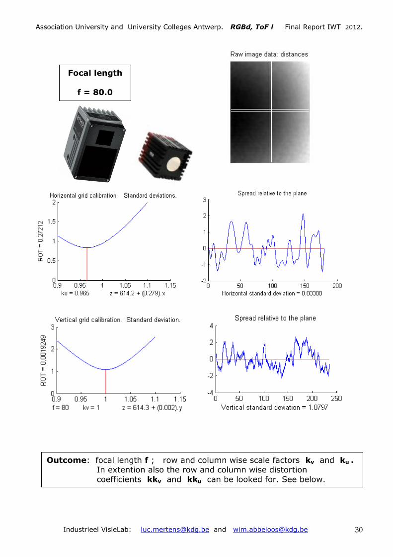
5.1. First calibration step: Focal length + row and column wise scale factors.
f = 80.0
f = 140.0
Een zeer eenvoudige calibratiestap leidt tot de intrinsieke ToF-camera
parameters: ku, kv, f, ( + distorsie parameters ).
Introduction Program used for calibration
% Tetra project 100191: RGBd, TOF ! September 2012.
% Luc Mertens & Wim Abbeloos: Industrial VisionLab.
%
% Program: 'CalibrationRowColumn.m'.
%
% During the calibration step a flat plane is presented to the camera.
% Row wise median filtering is used as a horizontal noise suppressor.
% Just the horizon and its perpendicular direction are inspected.
% Combined with a good guess for the focal value f , the values ku and kv
% are derived. They represent the asymmetry between the row wise and the
% column wise pixel locations of the optical sensor.
% Meanwhile the inclination of the world lines are found and expressed as best fit
% calculation: z = a + b.x (row wise) and z = a' + c.y (column wise) .
close all; clear all; home;

Association University and University Colleges Antwerp. RGBd, ToF ! Final Report IWT 2012.
Industrieel VisieLab: [email protected] and [email protected] 29
load('ifm_PLANE.mat'); f = 80; f4 = 4*f; ff = f4*f4;
D = rot90(D,2); G = fspecial('gaussian',11,2.2);
D = kron(D,ones(4)); D = imfilter(D,G,'replicate');
figure(10); imshow(D,[]); title('Raw image data: distances'). [I J] = size(D); ID2 = I/2; JD2 = J/2;
DD = 1000*sum( D(ID2:ID2+1,11:end-10) )/2;
J = length(DD); J2 = round(J/2); STD = []; Z = []; range = 0.90:0.001:1.1;
for ku = range % ku is a grid factor in the u-direction (row wise).
u = ku*([0.5:J-0.5]-J2); uu = u.*u; % column pixel values u = -J/2:J/2 .
d = sqrt(uu + ff); DDd = DD./d; % Distance ratios for world points.
x = u.*DDd; z = f4*DDd; % Camera x,z-coordinates.
data = cat(2,ones(J,1),x(:)); a = data\z(:); % Best Fit over the camera horizon.
ROT = atan2(a(2),1); % Rotation around the y-axis.
co = cos(ROT); si = sin(ROT); zz = co*z - si*x; stdz = std(zz); Z = cat(1,Z,zz);
STD = cat(2,STD,stdz); end;
disp(cat(2,'Grondvlak z = ',num2str(a(1)),' + (',num2str(abs(a(2))),').x '));
a(1) = round(10*a(1))/10; a(2) = round(1000*a(2))/1000;
[mmSTD r] = min(STD); ku = range(r);
figure(1); hold on; plot(range, STD); plot([ku ku],[0 mmSTD],'r');
title('Horizontal grid calibration. Standard deviations.');
xlabel(cat(2,'ku = ', num2str(ku), ...
' z = ', num2str(a(1)), ' + (', num2str(a(2)),').x')) ;
ylabel(cat(2, 'ROT = ',num2str(ROT)));
figure(2); Zr = Z(r,:); Zr = Zr - mean(Zr); hold on; plot(Zr);
plot([1 length(Zr)],[0 0],'r'); title('Spread relative to the plane');
xlabel(cat(2,'Horizontal standard deviation = ',num2str(mmSTD)));
DD = 1000*sum( D(11:end-10,JD2:JD2+1),2)/2; corr = -0.5 ;
I = length(DD); I2 = round(I/2); for i = 1:2:I, DD(i) = DD(i)+corr; end;
STD = []; Z = [];
for kv = range % kv is a grid factor in the v-direction (column wise).
v = kv*([0.5:I-0.5]-I2); vv = v.*v; % row pixel values v = -I/2:I/2 .
d = sqrt(vv + ff); DDd = DD'./d; % Distance ratios for world points.
y = v.*DDd; z = f4*DDd; % Camera y,z-coordinates.
data = cat(2,ones(I,1),y(:)); a = data\z(:); ROT = atan2(a(2),1);
co = cos(ROT); si = sin(ROT); zz = co*z - si*y; Z = cat(1,Z,zz);
STD = cat(2,STD,std(zz)); end;
disp(cat(2,'Grondvlak z = ',num2str(a(1)),' - ',num2str(abs(a(2))),'.y '));
a(1) = round(10*a(1))/10; a(2) = round(1000*a(2))/1000;
[mmSTD r] = min(STD); kv = range(r);
figure(3); hold on; plot(range, STD); plot([kv kv],[0 mmSTD],'r');
title('Vertical grid calibration. Standard deviation.');
xlabel(cat(2,'f = ', num2str(f), ' kv = ', num2str(kv), ...
' z = ', num2str(a(1)), ' + (', num2str(a(2)),').y')) ;
ylabel(cat(2, 'ROT = ',num2str(ROT)));
figure(4); Zr = Z(r,:); Zr = Zr - mean(Zr); hold on; plot(Zr);
plot([1 length(Zr)],[0 0],'r'); title('Spread relative to the plane');
xlabel(cat(2,'Vertical standard deviation = ',num2str(mmSTD)));
Association University and University Colleges Antwerp. RGBd, ToF ! Final Report IWT 2012.
Industrieel VisieLab: [email protected] and [email protected] 30
Focal length
f = 80.0
Outcome: focal length f ; row and column wise scale factors kv and ku . In extention also the row and column wise distortion coefficients kkv and kku can be looked for. See below.

Association University and University Colleges Antwerp. RGBd, ToF ! Final Report IWT 2012.
Industrieel VisieLab: [email protected] and [email protected] 31
4.2. Second calibration step: calibration of the work plane.
Calibration: based on the
perception of a flat plane:
• Select a rough substrate.
• Evaluate the row and column wise
standard deviations as a function of
the integration time.
• Eliminate (if present) the systematic
odd-even-errors.
• Make use of an adequate filter:
Gaussian, Mean, Median, …
• Calculate the best fit reference
plane: z = a + b.x + c.y .
• Find the camera rotation angles:
ROTx and ROTy .
• Find the central distance z0.
Calibration = shoot some images,
calculate the parameters…
At that moment the camera is
ready for use: … ToF !
f , ku , kvz
j
i
I
11
J
u.ku
v.kv
d
rD
x
y
z
(0,0,f)
f
R
phi
u = j – J/2 ; xu = ku*uv = i – I/2 ; yv = kv*v
tg φ = xu/f
r = √(xu²+f²)
d = √(xu²+yv²+f²)
D/d = x/xu = y/yv = z/f
J/2
I/2
ToFToF VISION: world to image, image to world VISION: world to image, image to world –– conversion.conversion.
horizon
N
Aan elk wereldpunt en aan zijn locale omgeving kunnen
12 belangrijke coördinaten verbonden worden:
x, y, z, Nx, Ny, Nz, N, kr, kc, R, G, B .
kr,kc
A
Association University and University Colleges Antwerp. RGBd, ToF ! Final Report IWT 2012.
Industrieel VisieLab: [email protected] and [email protected] 32
% Tetra project 100191: RGBd, TOF ! September 2011.
% Luc Mertens & Wim Abbeloos: Industrial VisionLab.
%
% Program: 'CalibrationPlane.m'.
%
% During the calibration step a flat plane is presented to the camera.
% Row wise median filtering is used as a horizontal noise suppressor.
% Mean filtering is used as a column wise noise suppressor.
% The inclination of the plane is found from a best fit calculation z = a.x + b.y + c.
close all; clear all; home; f = 80; ku = 0.965 ; kv =1.000; f2 = 2*f; corr = 0.005;
load('ifm_PLANE.mat');
[I J] = size(D); I2 = I/2; J2 = J/2; for i = 1:2:I, D(i) = D(i)-corr; end;
ROIi = 15:I-14; ROIj =15:J-14;
D = kron(D(ROIi,ROIj),ones(2)); % Resized image D-coordinates.
[I J] = size(D); I2 = I/2; J2 = J/2;
[x y z] = Dist2Cam(D,f2,ku,kv); % From camera distances to z-values.
data = cat(2,ones(I*J,1),x(:),y(:)); a = data\z(:); % Best Fit in reserved area.
disp('Grondvlak z = a(1) + a(2).x + a(3).y');
disp(cat(2,'Grondvlak z = ',num2str(a(1)),' - ',num2str(abs(a(2))),'.x - ',...
num2str(abs(a(3))),'.y '));
ROTy = atan2(a(2),1); ROTx = atan2(a(3),1); % Inclination.
cox = cos(ROTx); six = sin(ROTx); coy = cos(ROTy); siy = sin(ROTy);
z = cox*z - six*y ; z = coy*z - siy*x; % Transformation: camera to world coord.
MEDz = medfilt2(z,[1 5],'symmetric'); % Horizontal median filter.
Z = (MEDz(1:end-3,:) + MEDz(2:end-2,:) + ... % Vertical mean filter.
MEDz(3:end-1,:) + MEDz(4:end,:))/4;
correction = z(2:end-2,:) - Z; sigma = std2(correction);
std2z = std2(z); std2Z = std2(Z);
figure; hold on; axis([-0.15 0.15 -0.22 0.22 0.58 0.6]); view(75,30);
plot3(x,y,z,'.'); grid on; xlabel(cat(2,'ROTx = ' ,num2str(ROTx)));
title('Raw data'); ylabel(cat(2,'ROTy = ',num2str(ROTy)));
zlabel(cat(2,'"Interlace" correction = ',num2str(corr)));
Z = cat(1,Z(1:2,:),Z,Z(end,:));
figure(1); hold on; axis([-0.15 0.15 -0.22 0.22 0.58 0.6]); view(75,30);
plot3(x,y,Z,'.'); grid on; xlabel(cat(2,'ROTx = ' ,num2str(ROTx)));
title('Raw data'); ylabel(cat(2,'ROTy = ',num2str(ROTy)));
zlabel(cat(2,'"Interlace" correction = ',num2str(corr)));
figure(2); hold on; grid on; plot(std(z),'r'); plot(std(Z),'r');
ylabel(cat(2,'I = ', num2str(I), ' J = ', num2str(J)));
plot(std(z'),'k'); plot(std((Z(1:end-1,:))'),'k');
xlabel('red = std(z) ... blue = std(Z) ');
figure(3);
D(3,3:end-2) = 1; D(end-2,3:end-2) = 1;
D(3:end-2,3) = 1; D(3:end-2,end-2) = 1;
subplot(221); imshow(D,[]); title('Distance image 2x(64x50).');
ylabel('Raw Data');
subplot(222); imshow(z,[]); title('z-image 2x(64x50).');
xlabel(cat(2,'std2(z) = ',num2str(std2z))); ylabel('Raw Data');
subplot(223); imshow(Z,[]);
title('Best Fit Z = (MEDz(1:end-3,:)+..+ MEDz(4:end,:))/4;');
xlabel(cat(2,'std2(Z) = ',num2str(std2Z))); ylabel('Filtered Data');
subplot(224); imshow(correction,[]); ylabel('correction = z-Z');
xlabel(cat(2,'std2(z-Z) = ',num2str(sigma)));

Association University and University Colleges Antwerp. RGBd, ToF ! Final Report IWT 2012.
Industrieel VisieLab: [email protected] and [email protected] 33

Association University and University Colleges Antwerp. RGBd, ToF ! Final Report IWT 2012.
Industrieel VisieLab: [email protected] and [email protected] 34
% Tetra project 100191: RGBd, TOF ! September 2012.
% Luc Mertens & Wim Abbeloos: Industrial VisionLab.
%
% Program: 'FlatnessBasedCalibration.m'.
%
% During the calibration step a flat plane is presented to the camera.
% Based on colpanarity checks the local flatness is calulated in every point.
% The border is excluded. The standard deviation of the flatness is a
% function of f, corr, kv and ku. A multidimensional least mean square
% calcultion can give the optimal parameter values.
close all; clear all; home; load('ifm_1.mat');
f = 79; corr = -0.0003; ku = 1.0; kv = 1.0; ff = f*f;
[I J] = size(D); I2 = I/2; J2 = J/2;
u = ku*((1:J) - (J2+0.5)); uuff = u .* u + ff;
v = kv*((1:I) - (I2+0.5)); vv = v .* v;
U = repmat( u , [I 1]); UUff = repmat( uuff, [I 1]);
V = repmat( v', [1 J]); VV = repmat( vv',[1 J]); d = sqrt( VV + UUff );
t0 = cputime; for i = 1:2:I, D(i,:) = D(i,:)+corr; end;
dD = d./D; Dd = 1./dD; % Ratios.
dD12 = imfilter(dD,[1 0 1],'same'); dD34 = imfilter(dD,[1; 0; 1],'same');
Flatness = dD12 - dD34;
Flat = Flatness(5:end-4,5:end-4); stdFlat = std2(Flat);
Dd12m = imfilter(Dd,[-1; 0; 1],'same'); Dd34m = imfilter(Dd,[-1 0 1],'same');
Dd12p = imfilter(Dd,[1; 0; 1],'same'); Dd34p = imfilter(Dd,[1 0 1],'same');
Nx = Dd34m./Dd34p; Ny = Dd12m./Dd12p; Nz = - (U.*Nx + V.*Ny +1)/f;
N = sqrt(Nx.*Nx + Ny.*Ny + Nz.*Nz); Nx = Nx./N; Ny = Ny./N; Nz = Nz./N;
t0 = cputime - t0;
figure(1); subplot(131); imshow(D,[]); title('Raw distances.');
ylabel('Coplanarity test');
subplot(132); imshow(Flat,[-1 1]);
title(cat(2,'StdFlat = ',num2str(stdFlat)));
xlabel('Flatness = d1/D1-d2/D2+d3/d3-d4/D4');
ylabel(cat(2,'Focal length = ',num2str(f),' corr = ',num2str(corr)));
subplot(133); hist(Flat(:)); xlabel(cat(2,'CPUtime = ', num2str(t0)));
title('Histogram of Flatness');
ylabel(cat(2,'kv = ',num2str(kv),' ku = ',num2str(ku)));
figure(2); subplot(131); imshow(Nx,[-0.5 0.5]); title('Nx ~ (D4/d4 - D3/d3)/(D4/d4 + D3/d3)');
subplot(132); imshow(Ny,[-0.5 0.5]); title('Ny ~ (D2/d2 - D1/d1)/(D2/d2 + D1/d1)');
subplot(133); imshow(Nz,[-1 0]); xlabel(cat(2,'CPUtime = ', num2str(t0)));
title('Nz ~ - (U.*Nx + V.*Ny +1)/f');

Association University and University Colleges Antwerp. RGBd, ToF ! Final Report IWT 2012.
Industrieel VisieLab: [email protected] and [email protected] 35
4.3. Calibration based on the straightness of 5 consecutive points on a flat wall.
As we will show a calibration based on the straightness of 5 consecutive pixels will not give a stable calibration method. Nevertheless it
gives some insights in the calibration problem and therefor we think it is worthfull to investigate on the method. In 6.2. a stable method
will be explained. It is based on coplanarity of a 5 points-star.
Let’s think diagonal, column or row wise while looking to a wall from which we (persons) now it is perfectly flat in every direction. The
camera has to believe this ‘flatness’ and can try to find the relation between his unique optical sensor construction (exact 3D-pixel
positions) and the perception of a flat wall. Five consecutive pixels will deliver 5 measured distances (D1, D2, D3, D4 and D5 ). Their
internal radial distances d1, d2, d3, d4 and d5 are unknowns during the calibration step. As we showed before the following equations are
valid:
1
2
3
4
5
d1/D1 – 2.d2/D2 + d3/D3 = 0 Collineariteit (1) d5/D5 – 2.d4/D4 + d3/D3 = 0
d2/D2 - 2.d3/D3 + d4/D4 = 0 in de World (2) d4/D4 - 2.d3/D3 + d2/D2 = 0
d1² - 2.d2² + d3² = 2.r² Equidistant (3) d5² - 2.d4² + d3² = 2.r²
pixels.
d2² - 2.d3² + d4² = 2.r² (4) d4² - 2.d3² + d2² = 2.r²
From (1) and (3) , respectively (2) and (4) we get:
(2.d2/D2 – d3/D3)² = 2d2²/D1² - d3²/D1² + 2r²/D1² (a) (2.d4/D4 – d3/D3)² = 2d4²/D5² - d3²/D5² + 2r²/D5²
(2.d3/D3 – d2/D2)² = 2d2²/D4² - d3²/D4² + 2r²/D4² (b) (2.d3/D3 – d4/D4)² = 2d4²/D2² - d3²/D2² + 2r²/D2²

Association University and University Colleges Antwerp. RGBd, ToF ! Final Report IWT 2012.
Industrieel VisieLab: [email protected] and [email protected] 36
Working out the squares and subtracting (b) from (a) delivers:
(3/D2² – 2/D1² - 1/D4²).d2² = (3/D3² – 2/D4² - 1/D1²).d3² + 2r²(1/D1² - 1/D4²) . (Ia)
(3/D4² – 2/D5² - 1/D2²).d4² = (3/D3² – 2/D2² - 1/D5²).d3² + 2r²(1/D5² - 1/D2²) . (Ib)
Because of equation (4) the form (Ib) can further be worked out:
(3/D4² – 2/D5² - 1/D2²).(2r² + 2d3² - d2²) = (3/D3² – 2/D2² - 1/D5²).d3² + 2r²(1/D5² - 1/D2²) .
(3/D4²–2/D5²-1/D2²).d2² = 2.(3/D4²–2/D5²-1/D2²).d3²-(3/D3²–2/D2²-1/D5²).d3² + 2r².(3/D4²–2/D5²-1/D2²) - 2r²(1/D5²-1/D2²)
(3/D4²–2/D5²-1/D2²).d2² = (6/D4² – 3/D5² - 3/D3²).d3² + 2r².(3/D4² – 2/D5²) (IIb)
From (Ia) and (IIb) the value d2² can be eliminated in order to find d3² as a function of the measuring values D1,..,D5 .
This gives us the final result:
(3/D4² – 2/D5² - 1/D2²).(3/D3² – 2/D4² - 1/D1²).d3² + 2r²(1/D1² - 1/D4²).(3/D4² – 2/D5² - 1/D2²) =
(3/D2² – 2/D1² - 1/D4²).(6/D4² – 3/D5² - 3/D3²).d3² + 2r².(3/D2² – 2/D1² - 1/D4²)(3/D4² – 2/D5²) (IIb’)
[ (3/D4² – 2/D5² - 1/D2²).(3/D3² – 2/D4² - 1/D1²) - (3/D2² – 2/D1² - 1/D4²).(6/D4² – 3/D5² - 3/D3²) ].d3² =
2r².{(3/D2² – 2/D1² - 1/D4²)(3/D4² – 2/D5²) - (1/D1² - 1/D4²).(3/D4² – 2/D5² - 1/D2²)}
[ (3/D4² – 2/D5² - 1/D2²).(3/D3² – 2/D4² - 1/D1²) - (3/D2² – 2/D1² - 1/D4²).(6/D4² – 3/D5² - 3/D3²) ].d3² =
2r².{16/(D1²D5²) + 16/(D2²D4²) + 2/(D1²D2²) + 2/(D4²D5²) - 18/(D2²D5²) - 18/(D1²D4²) }
[ (3/D4² – 2/D5² - 1/D2²).(3/D3² – 2/D4² - 1/D1²) - (3/D2 – 2/D1² - 1/D4²).(6/D4² – 3/D5² - 3/D3²) ].d3² =
2r².{ 8/(D1²D5²) + 8/(D2²D4²) + 1/(D1²D2²) + 1/(D4²D5²) - 9/(D2²D5²) - 9/(D1²D4²) }
{ D32².(D31²+6+9D35²-8D34²) + D34².(9D31²+6+D35²-8D32²) - 6.(D35²+D31²) - 4.D31²D35² } d3² = (IIb’’)
2r².{ 8.(D31²-D32²)(D35²-D34²) - (D31²-D35²)(D34²-D32²) }

Association University and University Colleges Antwerp. RGBd, ToF ! Final Report IWT 2012.
Industrieel VisieLab: [email protected] and [email protected] 37
Unfortunately, while the formula is theoretical correct it has one important disadventage: the
numerical stability is very week. Small changes in de measured values, as must be expected for
ToF camera’s, make that the coefficient of d3² and the right side of the equation can change from
–ε till +ε . Therefor the nominator and the denominator are that close to zero that every result
can be found in practice.
5.4. Calibration based on the straightness of 3 consecutive points on a flat wall.
Imagine a camera with just 3 pixels. Such camera can be seen as a primitive part of a common
ToF-camera. The pixel triplet ‘is looking to’ a flat plane which is hit at the measured world
distances D1, DM and D2 . These values are temporal mean values. Apart from a systematic error
they have a repeatable value. We will proof that the internal camera distances d1 and d2 of the
anti-symmetric pixels 1 and 2 are bounded to the central distance dM . A full sensor can be
viewed as a collection of separate antisymmetric pixels relative to the principal point of the
sensor.
D1
1 d1
r1=r
O
DM M dM
r2=r d2
D2 2
For every sensor triplet the next constraints hold:
Antisymmetry: r1 = r2 = r [1]
Collinerarity: d1/D1 – 2.dM/DM + d2/D2 = 0 [2]
From the cosine rule it can be derived that: d1² – 2.dM² + d2² = 2r² [3]
The substitution of d1 from [2] into equation [3] gives an expression for d2 as a function of dM:
d2² = 2.dM² - d1² + 2r² = 2.dM² - { 2.dM.D1/DM - d2.D1/D2 }² + 2r²
or, in short: d2² = 2.dM² - {2dM.D1M - d2.D12 }² + 2r² ; D1M := D1/DM .
d2² = 2.dM² - 4dM²D1M² +4 dMD1MD12.d2 - d2².D12² + 2r²
(1 + D12²).d2²- 4dMD1MD12.d2 + [4dM²D1M² – 2(r² + dM²)] = 0 .
2dMD1MD12 + sqrt{4dM²D1M²D12² - (1 + D12²)[4dM²D1M² – 2(r²+dM²)]}
d2 = ----------------------------------------------------------------------------------
(1 + D12²)
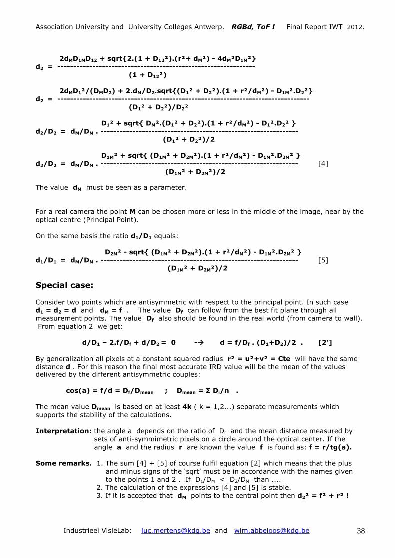
Association University and University Colleges Antwerp. RGBd, ToF ! Final Report IWT 2012.
Industrieel VisieLab: [email protected] and [email protected] 38
2dMD1MD12 + sqrt{2.(1 + D12²).(r²+ dM²) - 4dM²D1M²}
d2 = --------------------------------------------------------------
(1 + D12²)
2dMD1²/(DMD2) + 2.dM/D2.sqrt{(D1² + D2²).(1 + r²/dM²) - D1M².D2²}
d2 = -------------------------------------------------------------------------------
(D1² + D2²)/D2²
D1² + sqrt{ DM².(D1² + D2²).(1 + r²/dM²) - D1².D2² }
d2/D2 = dM/DM . --------------------------------------------------------------
(D1² + D2²)/2
D1M² + sqrt{ (D1M² + D2M²).(1 + r²/dM²) - D1M².D2M² }
d2/D2 = dM/DM . -------------------------------------------------------------- [4]
(D1M² + D2M²)/2
The value dM must be seen as a parameter.
For a real camera the point M can be chosen more or less in the middle of the image, near by the
optical centre (Principal Point).
On the same basis the ratio d1/D1 equals:
D2M² - sqrt{ (D1M² + D2M²).(1 + r²/dM²) - D1M².D2M² }
d1/D1 = dM/DM . -------------------------------------------------------------- [5]
(D1M² + D2M²)/2
Special case:
Consider two points which are antisymmetric with respect to the principal point. In such case
d1 = d2 = d and dM = f . The value Df can follow from the best fit plane through all
measurement points. The value Df also should be found in the real world (from camera to wall).
From equation 2 we get:
d/D1 – 2.f/Df + d/D2 = 0 - d = f/Df . (D1+D2)/2 . [2’]
By generalization all pixels at a constant squared radius r² = u²+v² = Cte will have the same
distance d . For this reason the final most accurate IRD value will be the mean of the values
delivered by the different antisymmetric couples:
cos(a) = f/d = Df/Dmean ; Dmean = Σ Di/n .
The mean value Dmean is based on at least 4k ( k = 1,2...) separate measurements which
supports the stability of the calculations.
Interpretation: the angle a depends on the ratio of Df and the mean distance measured by
sets of anti-symmimetric pixels on a circle around the optical center. If the
angle a and the radius r are known the value f is found as: f = r/tg(a).
Some remarks. 1. The sum [4] + [5] of course fulfil equation [2] which means that the plus
and minus signs of the ‘sqrt’ must be in accordance with the names given
to the points 1 and 2 . If D1/DM < D2/DM than ....
2. The calculation of the expressions [4] and [5] is stable.
3. If it is accepted that dM points to the central point then d2² = f² + r² !
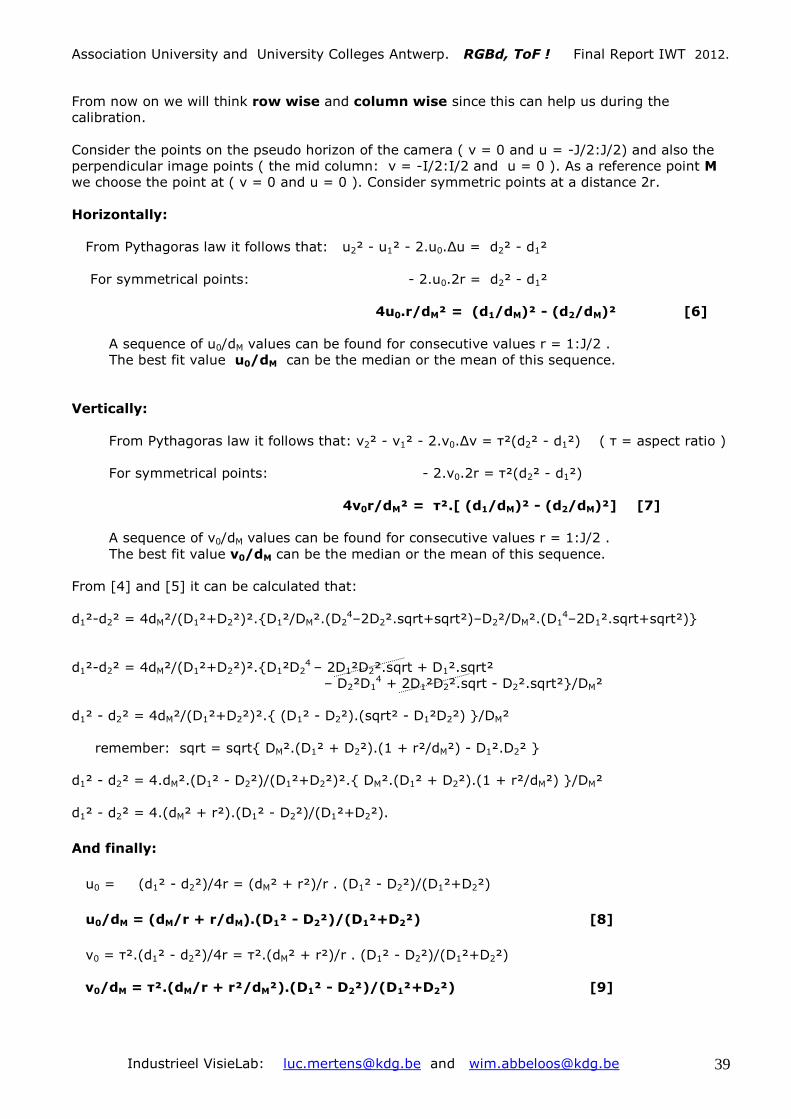
Association University and University Colleges Antwerp. RGBd, ToF ! Final Report IWT 2012.
Industrieel VisieLab: [email protected] and [email protected] 39
From now on we will think row wise and column wise since this can help us during the
calibration.
Consider the points on the pseudo horizon of the camera ( v = 0 and u = -J/2:J/2) and also the
perpendicular image points ( the mid column: v = -I/2:I/2 and u = 0 ). As a reference point M
we choose the point at ( v = 0 and u = 0 ). Consider symmetric points at a distance 2r.
Horizontally:
From Pythagoras law it follows that: u2² - u1² - 2.u0.Δu = d2² - d1²
For symmetrical points: - 2.u0.2r = d2² - d1²
4u0.r/dM² = (d1/dM)² - (d2/dM)² [6]
A sequence of u0/dM values can be found for consecutive values r = 1:J/2 .
The best fit value u0/dM can be the median or the mean of this sequence.
Vertically:
From Pythagoras law it follows that: v2² - v1² - 2.v0.Δv = τ²(d2² - d1²) ( τ = aspect ratio )
For symmetrical points: - 2.v0.2r = τ²(d2² - d1²)
4v0r/dM² = τ².[ (d1/dM)² - (d2/dM)²] [7]
A sequence of v0/dM values can be found for consecutive values r = 1:J/2 .
The best fit value v0/dM can be the median or the mean of this sequence.
From [4] and [5] it can be calculated that:
d1²-d2² = 4dM²/(D1²+D2²)².{D1²/DM².(D24–2D2².sqrt+sqrt²)–D2²/DM².(D1
4–2D1².sqrt+sqrt²)}
d1²-d2² = 4dM²/(D1²+D2²)².{D1²D24 – 2D1²D2².sqrt + D1².sqrt²
– D2²D14 + 2D1²D2².sqrt - D2².sqrt²}/DM²
d1² - d2² = 4dM²/(D1²+D2²)².{ (D1² - D2²).(sqrt² - D1²D2²) }/DM²
remember: sqrt = sqrt{ DM².(D1² + D2²).(1 + r²/dM²) - D1².D2² }
d1² - d2² = 4.dM².(D1² - D2²)/(D1²+D2²)².{ DM².(D1² + D2²).(1 + r²/dM²) }/DM²
d1² - d2² = 4.(dM² + r²).(D1² - D2²)/(D1²+D2²).
And finally:
u0 = (d1² - d2²)/4r = (dM² + r²)/r . (D1² - D2²)/(D1²+D2²)
u0/dM = (dM/r + r/dM).(D1² - D2²)/(D1²+D2²) [8]
v0 = τ².(d1² - d2²)/4r = τ².(dM² + r²)/r . (D1² - D2²)/(D1²+D2²)
v0/dM = τ².(dM/r + r²/dM²).(D1² - D2²)/(D1²+D2²) [9]

Association University and University Colleges Antwerp. RGBd, ToF ! Final Report IWT 2012.
Industrieel VisieLab: [email protected] and [email protected] 40
5.5. ToF camera calibration
The calibration of the suggested primitive ToF cell corresponds to the problem of finding the final
most accurate values d1 and d2 in correspondence with the distance dM of ‘the central pixel’.
The calculation is straightforward for all the triplets of anti-symmetric pixels in the ToF image
relative to the reference pixel of the optical pinhole centre to the sensor.
The points at the pseudo horizon and its perpendicular direction (row wise and column wise) can
further be used for finding a consistent set of classic calibration parameters. These parameters
define the difference between the theoretical pinhole coordinates δuv(f,u,v) of a perfect
(u,v)-grid relative to the real pixel positions duv. We have:
- the theoretical distances δuv² = f² + (u-u0)² + (v-v0)² ,
- the distances after distortion: duv² = f² + (u-u0)²[au+bu.(u-u0)²] + (v-v0)²[av+bv.(v-v0)²]. [8]
dM² = d00² = f² + u0²(au+bu.u0²) + v0²(av+bv.v0²)
The parameters au and bu can be estimated e.g. from the points corresponding with v = 0 ;
Su = ∑ { [au + bu.(u-u0)²] – (du0²-f²-avv0²-bvv04)/(u-u0)² }² = minimum; v = 0 , u = -J/2:J/2 .
∂Su/∂au = 0 ∑ { (au + bu.(u-u0)²) – (du0²-f²-avv0²-bvv04)/(u-u0)² } = 0 ;
∂Su/∂bu = 0 ∑ { (au + bu.(u-u0)²) – (du0²-f²-avv0²-bvv04)/(u-u0)² }.(u-u0)² = 0 .
J.au + bu . ∑(u-u0)² = ∑ (du0²-f²-avv0²-bvv04)/(u-u0)² [10a]
au . ∑(u-u0)²+ bu.∑(u-u0)4 = ∑ du0² - J.(f²-avv0²-bvv0
4) . [10b]
Similar calculations for the points corresponding with u = 0 and v = -I/2:I/2, deliver av and bv :
Sv = ∑ { [av + bv.(v-v0)²] – (d0v²-f²-auu0²-buu04)/(v-v0)² }² = minimum ; v = -I/2:I/2 .
J.av + bv . ∑(u-u0)² = ∑ (du0²-f²-auu0²-buu04)/(v-v0)² [11a]
av . ∑(v-v0)²+ bv.∑(v-v0)4 = ∑ du0² - J.(f²-auu0²-buu0
4) . [11b]
The equation sets [9a,b] and [10a,b] are dependent from each other. This means that the sets
need to be solved iteratively.
Once the coefficients au, bu, av and bv are known the analytically best fit d-values (IRD’s) for the
ToF-camera follow equation [8], distortion included.
If the ToF-image is assumed to be distortion free the parameters bu and bv equal zero and the
formulas reduce to the equation sets:
Su = ∑ { au – (du0²-f²-avv0²)/(u-u0)² }² = minimum; v = 0 , u = -J/2:J/2 .
Sv = ∑ { av – (d0v²-f²-auu0²)/(v-v0)² }² = minimum; u = 0 , v = -I/2:I/2 .
J.au = ∑ (du0²-f²-avv0²)/(u-u0)² ; v = 0 , u = -J/2:J/2 . [10c]
J.av = ∑ (du0²-f²-auu0²)/(v-v0)² ; u = 0 , v = -I/2:I/2 . [11c]

Association University and University Colleges Antwerp. RGBd, ToF ! Final Report IWT 2012.
Industrieel VisieLab: [email protected] and [email protected] 41
6. AGV and Wheelchair navigation.
6.1. AGV-translation: finding the displacement between two images. In order to avoid ‘backfolding’ (periodicity) it’s better to give the camera’s a small inclination
ortiented to the floor. The angle ‘a’ can be calibrated by a simple measurement (e.g. a free wall).
δ
RMS error. d1 = sqrt(u1² + v1² + f²)
x1 = u1* D1/d1; y1 = v1* D1/d1; z1 = f* D1/d1
D22 = D1² + δ² - 2.δ.D1.cos(A)
D22 = D1² + δ² - 2.δ.z1
u2/f = x1/(z1 - δ); ( x2 = x1 ! )
v2/f = y1/(z1 - δ) .
Measurement at (v2,u2) DP .
v1,u1
δ
v2,u2
y1D1 D2 = DP ?
P
Every single point P can be used in order to estimate the translation δ .
More points make a statistic approach possible.
ff
A
Random world
For every δ there is a D2 .
For one specific δ the
error | D2 – DP | is minimal.
Floor.
d1
1/6
Distance estimation during pure translations,
horizontal camera.
Procedure:
Select a random point (u1,v1) in the prvious image. The values x1, y1, z1 and d1 can be found.
Don’t select in the center or at the border of the image. For a chosen value δ the corresponding
distance and position (u2,v2) can be calculated. These distance values must be confronted with
the measured distances at th same senor pixel. The difference ε(d) between measurement and
calculated distances will be minimum at the correct distance δ .
The calcultion can be extended to a collection of random start points. The sum of square errors
must be minimised. A set of 20 points seem to be enough. The calculation can be done in less
than 125 msec (in Matlab).

Association University and University Colleges Antwerp. RGBd, ToF ! Final Report IWT 2012.
Industrieel VisieLab: [email protected] and [email protected] 42
% Tetra project 100191: RGBd, TOF ! July 2012.
% Luc Mertens & Wim Abbeloos: Industrial Vision Lab.
% Kenny Hemgenberghs (master student).
%
% Program: Translation_VR2012.m .
%
% During navigation it's important to evaluate the forward translation relative
% to a random scene in front. At a rate of 10 images a second this progress
% can be evaluated. If necessary the measurement can be reset and the
% measurement starts over again.
%
% Note: the method needs some texture in the scene.
% This gives opportunities to find the better correspondences.
close all; clear all; home; rep = 'replicate'; f = 158; ff = f*f;
ROTx = 0.01; cox = cos(ROTx); six = sin(ROTx); % Values from calibration.
load('mesa_trans_data.mat'); % Previous and next image: D1 and D2.
%%%%%
% Acquire ToF image if live camera --> Distance D1 matrix .
% Acquire ToF image if live camera --> Distance D2 matrix .
%%%%%
[I J] = size(D(:,:,1)); I2 = I/2; J2 = J/2;
I2p = I2+1; J2p = J2+1; I2m= I2-1; J2m = J2-1;
MSQE = []; T = 21; % T is the number of random points chosen.
D1 =1000*D(:,:,1); D2 =1000*D(:,:,5);
t0 = cputime; U1 = []; U2 = U1; V1 = U1; V2 = U1; U2 = zeros(1,T); V2 = U2;
x1 = zeros(1,T); y1 = x1, z1 = x1; d12 = x1;
for t = 1:T
r1 = 0; while abs(r1) < 0.3 r1 = 1.2*rand -0.5; end;
r2 = 0; while abs(r2) < 0.1 r2 = 1.2*rand -0.5; end;
v1 = round(I2*r1); V1 = cat(2,V1,v1+I2);
u1 = round(J2*r2); U1 = cat(2,U1,u1+J2);
h = D1(v1+I2m : v1+I2p , u1+J2m : u1+J2p); d1 = median(h(:));
d12(t) = d1*d1;
Dd = d1/sqrt(u1*u1 + v1*v1 + ff);
x1(t) = u1*Dd; y1(t) = v1*Dd; z1(t) = f*Dd; end;
x1f = x1*f; term = 2*(y1*six - z1*cox);
for delta = 0:100 % Displacement between 0 tot 100 mm/(image pair).
SQE = []; dsix = delta*six; dcox = delta*cox;
for t = 1:T % 15 random image points.
d2delta = sqrt(d12(t) + delta*(delta + term(t)));
u2 = round(x1f(t)./(z1(t) - dcox)); U2(t) = u2+J2;
v2 = round((y1(t)+ dsix)*f./(z1(t) - dcox)); V2(t) = v2+I2;
h = D2(v2+I2m:v2+I2p,u2+J2m:u2+J2p); d2 = median(h(:));
SQE = cat(2,SQE,(d2 - d2delta)*(d2 - d2delta)); % Deviations.
end;
MSQE = cat(2, MSQE, mean(SQE));
end;
t0 = cputime - t0;
RMS = sqrt(MSQE); [mmRMS jj] = min(RMS); JJ = jj-1;
figure(1); mm = min(D1(:));
subplot(121); imshow(D1, [mm mm+400]); title('Previous image.');
subplot(122); imshow(D2 ,[mm mm+400]); title('Next image.');
figure(2); hold on; axis([1 J 1 I]); plot(U1,V1,'k.'); plot(U2,V2,'ro');
plot(J2,I2,'b+'); title('Imagine: STAR TREK');
xlabel('Black = previous position. Red = next position.');

Association University and University Colleges Antwerp. RGBd, ToF ! Final Report IWT 2012.
Industrieel VisieLab: [email protected] and [email protected] 43
figure(3); hold on; plot([JJ JJ],[0 mmRMS],'r'); grid on;
plot([0:100],RMS); plot([0 JJ],[ mmRMS mmRMS],'r');
title('Root Mean Square Error as a function of delta. Delta = 0:100 mm. ')
xlabel(cat(2,'Calculation time = ', num2str(t0),'. Minimum at delta = ',num2str(jj-1)));
ylabel(cat(2,num2str(T),' random points used.', ' Minimum at RMS = ',
num2str(mmRMS)));
Distance Images: previous and next.

Association University and University Colleges Antwerp. RGBd, ToF ! Final Report IWT 2012.
Industrieel VisieLab: [email protected] and [email protected] 44
6.2. AGV-rotation: angle between two images.
In order to avoid ‘backfolding’ (periodicity) it’ better to give the cameras a small inclination
ortiented to the floor. The angle ‘a’ can be calibrated by a simple measurement (e.g. a free wall).
δ
RMS error. d1 = sqrt(u1² + v1² + f²)
x1 = u1* D1/d1; y1 = v1* D1/d1; z1 = f* D1/d1
D22 = D1² + δ² - 2.δ.[D1.cos(A)]
D22 = D1² + δ.(δ - 2.[z1.cos(a) - y1.sin(a)])
u2/f = x1/(z1 - δ*cos(a)); ( x2 = x1 ! )
v2/f = (y1+ δ*sin(a))/(z1 - δ*cos(a)) .
Measurement at (v2,u2) DP .
v1,u1
δ
v2,u2a = camera inclination.
y1
D1 D2 = DP ?
P
ff
A
Random world
For every δ there is a D2 .
For one specific δ the
error | D2 – DP | is minimal.
Floor.
Horizontal movement !
Distance estimation during pure translations,
camera inclination ‘a’.
2/6
d1
Every single point P can be used in order to estimate the translation δ .
More points make a statistic approach possible.
δ
RMS error. x1 = u1.D1/d1; y1 = v1.D1/d1 ; z1 = f D1/d1; α = atan(x1,z1);
D22 = D1² + δ² - 2.δ.D1.cos(A) ; cosine rule.
A = π/2 – β/2 – α ; B = π/2 – β/2 – γ ; A - B = γ - α ;
Every distance D1 and associated choises of δ D2 .
From sin(B) = sin(A).D1/D2 B γ β .
x2 = D2.sin(γ) ; y2 = y1 : z2 = D2.cos(γ) ;
u2 = f.x2/z2 ; v2 = f.y2/z2 ; Measurement DP at (v2,u2) Error = D2 – DP ;
β
f
r0
z1
z2
x1
x2
Camera
previous position
Camera
next position
δA
B
α
γ
P
D2 = DP ?
D1
Distance correspondence during a pure rotation + horizontal camera.
3/6
Every single point P
can be used in order to
estimate the angle β.
More points make a
statistic approach
possible.
Top View !
For every δ there is a D2 .
For one single δ the
error D2 – DP is minimal.

Association University and University Colleges Antwerp. RGBd, ToF ! Final Report IWT 2012.
Industrieel VisieLab: [email protected] and [email protected] 45
δ
RMS error.
β
f
r0
z1
z2
x1
x2
Camera
previous position
Camera
next position
δA
B
α
γ
P
D2 = DP ?
D1
Distance correspondence during a pure rotation + camera inclination ‘a’.
4/6
Every single point P
can be used in order to
estimate the angel β.
More points make a
statistic approach
possible.
Top View !
x1
= u1.D
1/d
1; y
1= v
1.D
1/d
1; z
1= f D
1/d
1; α = atan(X1,Z1);
Z1
= z1.cos(a) + y
1.sin(a) ; Y
1= y
1.cos(a) - z
1.sin(a) ; (Projection)
δ1² = x1² + Z1² ; (Projected distance δ1)
δ22 = δ1² + δ² - 2.δ.δ1.cos(A) ; (Cosine rule).
A = π/2 – β/2 – α ; B = π/2 – β/2 – γ ; A - B = γ - α ;
For every projected distance δ1 and associated choises of δ, a corresponding projected distance δ2 is found.From sin(B) = sin(A). δ1/δ2 B γ β .X2 = δ2.sin(γ); Y2 = y1 ; Z2 = δ2.cos(γ) ; x2 = X2 ; y
2= Y
2.cos(a)+Z
2.sin(a); z
2= Z
2.cos(a)-Y2.sin(a); (Back projection).
D2 = sqrt( x2² + y2² + z2² ) ;
u2 = f.x2/z2 ; v2 = f.y2/z2 ; Measurement DP at (v2,u2) Error = D2 – DP ;
For every δ there is a D2 .
For one single δ the
error D2 – DP is minimal.
β
RMS error. x
1= u
1.D
1/d
1; y
1= v
1.D
1/d
1; z
1= f D
1/d
1; α = atan(x1,z1);
Z1
= z1.cos(a) + y
1.sin(a) ; Y
1= y
1.cos(a) - z
1.sin(a) ; (Projection)
δ1² = x1² + Z1² ; (Projected distance δ1)
δ22 = δ1² + δ² - 2.δ.δ1.cos(A) ; (Cosine rule).
A = α – β/2 ; B = π - β/2 – γ ;
For every projected distance δ1 and associated choises of δ,
a corresponding projected distance δ2 is found.From sin(B) = sin(A). δ1/δ2 B γ β .X2 = δ2.sin(γ) ; Y2 = y1 : Z2 = δ2.cos(γ) ;y
2= Y
2.cos(a) + Z
2.sin(a); z
2= Z
2.cos(a) - Y2.sin(a); (Reprojection)
D2 = sqrt( x2² + y2² + z2² );
u2 = f.x2/z2 ; v2 = f.y2/z2 ; Error = D2 – DP ;
Camera
previous position
Distance correspondence during a general rotation + camera inclination ‘a’.
6/6
Every single point P
can be used in order to
estimate the angle β.
More points make a
statistic approach
possible.
R
Z1
Z2
X1
X2
δ
BA
α
P
d1
D2 = DP ?
δ1
Next camera
position
v1,u1 v2,u2
βD1
δ2
γ
For every δ there is a D2 .
For one single δ the
error D2 – DP is minimal.

Association University and University Colleges Antwerp. RGBd, ToF ! Final Report IWT 2012.
Industrieel VisieLab: [email protected] and [email protected] 46
% Tetra project 100191: RGBd, TOF ! July 2012.
% Luc Mertens & Wim Abbeloos: Industrial Vision Lab.
% Kenny Hemgenberghs (master student).
%
% Program: Rotation_VR2012.m .
%
% During navigation it's important to evaluate the actual rotation relative
% to a random scene in front. At a rate of 10 images a second this progress
% can be evaluated. If necessary the measurement can be reset and the
% measurement can be started over again.
%
% Note: the method needs some texture in the scene.
close all; clear all; home; rep = 'replicate'; f = 158; ff = f*f; MSQE = []; T = 5;
ROTx = 0.01; co = cos(ROTx); si = sin(ROTx); % Values from calibration.
load('rotatietest.mat'); % Previous and next image: D1 and D2.
% Take care for the vertical 'world-offset' between both images.
t0 = cputime; D1 = 1000*D1; D2 = 1000*D2;
%%%%%
% Acquire ToF image if live camera --> Distance D1 matrix .
% Acquire ToF image if live camera --> Distance D2 matrix .
%%%%%
[I J] = size(D1); I2 = I/2; J2 = J/2;
I2p = I2+1; J2p = J2+1; I2m= I2-1; J2m = J2-1;
U1 = []; U2 = U1; V1 = U1; V2 = U1; U2 = zeros(1,T); V2 = U2;
L = zeros(1,T); L2 = L; x1 = L; y1 = L; z1 = L; Y1 = L; Z1 = L; r0 = 0;
for t = 1:T
r1=0; while abs(r1<0.2) r1=rand -0.5; end; r2=(rand-0.5)/2; % Mid right region !
u1 = round(J2*r1); U1 = cat(2,U1,u1+J2);
v1 = round(I2*r2); V1 = cat(2,V1,v1+I2);
h = D1(v1+I2m : v1+I2p , u1+J2m : u1+J2p); d1 = median(h(:));
D1(v1+I2m : v1+I2p , u1+J2m : u1+J2p) = 5000;
Dd = d1/sqrt(u1*u1 + v1*v1 + ff);
x1(t) = u1*Dd; y1(t) = -v1*Dd; z1(t) = f*Dd;
Y1(t) = y1(t)*co -z1(t)*si; Z1(t) = z1(t)*co + y1(t)*si;
L2(t) = x1(t)*x1(t) + (Z1(t)+r0)*(Z1(t)+r0); end;
L = sqrt(L2); Z2 = L; x2 = L; y2 = L; z2 = L; d2 = L; Dd = L; u2 = L; v2 = L;
range = [1:1:20]*pi/180; Len = length(range); MSQE = []; b = 0
mmMSQE = 10000000;
for beta = range, b = b+1; % Angles between 0 tot 45 degrees.
SSQE = 0; TT = 0; U2 = []; V2 = []; sib = sin(beta); cob = cos(beta);
for t = 1:T % 15 random image points.
Y1t = Y1(t); Z2t = L(t)*cob - r0; x2t = -L(t)*sib; % Negative x-values !
D2t = sqrt(x2t*x2t + Y1t*Y1t + Z2t*Z2t);
y2t = Y1t*co + Z2t*si; z2t = Z2t*co - Y1t*si; Dd = z2t/f;
u2 = round(x2t/Dd); v2 = round(-y2t/Dd);
U2 = cat(2,U2,u2+J2); V2 = cat(2,V2,v2+I2);
if abs(u2)<J2-1 && abs(v2)<I2-1
TT = TT+1;
h = D2(v2+I2m:v2+I2p,u2+J2m:u2+J2p); dp = median(h(:));
SQE = (D2t - dp)*(D2t - dp); SSQE = SSQE + SQE; end;
end;
if TT > 0.9*T MSQE = cat(2,MSQE,SSQE/TT);
if length(MSQE) > 0 % Keep the best set of points.
if MSQE(b) < mmMSQE mmMSQE = MSQE(b); UU2 = U2; VV2 = V2; end; end; end;
end;
for tt = 1:length(VV2), D2(VV2(tt),UU2(tt)) = 5000; end;
t0 = cputime - t0;

Association University and University Colleges Antwerp. RGBd, ToF ! Final Report IWT 2012.
Industrieel VisieLab: [email protected] and [email protected] 47
RMS = sqrt(MSQE); [mmRMS jj] = min(RMS); JJ = jj;
figure(1);
subplot(121); imshow(D1, [700 3500]); title('Previous image.');
subplot(122); imshow(D2 ,[700 3500]); title('Next image.');
figure(2); hold on; axis([1 J 1 I]); plot(U1,V1,'k.'); plot(UU2,VV2,'r.');
plot(J2,I2,'b+'); title('Imagine: STAR TREK');
xlabel('Black = previous position. Red = next position.');
figure(3); hold on;
plot([1:length(RMS)],RMS); plot([0 JJ],[ mmRMS mmRMS],'r');
plot([JJ JJ],[0 mmRMS],'r'); grid on;
title('Root Mean Square Error as a function of alfa. Alfa = 0 : 45° .')
xlabel(cat(2,'Calculation time = ', num2str(t0),'. Minimum at beta = ',num2str(jj)));
ylabel(cat(2,num2str(T),' random points used.', ' Minimum at RMS = ',
num2str(mmRMS)));
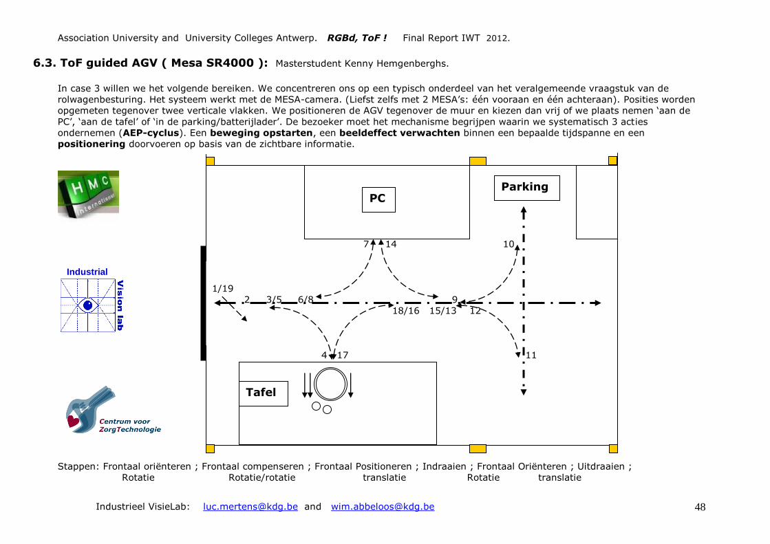
Association University and University Colleges Antwerp. RGBd, ToF ! Final Report IWT 2012.
Industrieel VisieLab: [email protected] and [email protected] 48
6.3. ToF guided AGV ( Mesa SR4000 ): Masterstudent Kenny Hemgenberghs. In case 3 willen we het volgende bereiken. We concentreren ons op een typisch onderdeel van het veralgemeende vraagstuk van de
rolwagenbesturing. Het systeem werkt met de MESA-camera. (Liefst zelfs met 2 MESA’s: één vooraan en één achteraan). Posities worden
opgemeten tegenover twee verticale vlakken. We positioneren de AGV tegenover de muur en kiezen dan vrij of we plaats nemen ‘aan de
PC’, ‘aan de tafel’ of ‘in de parking/batterijlader’. De bezoeker moet het mechanisme begrijpen waarin we systematisch 3 acties
ondernemen (AEP-cyclus). Een beweging opstarten, een beeldeffect verwachten binnen een bepaalde tijdspanne en een
positionering doorvoeren op basis van de zichtbare informatie.
7 14 10
1/19
2 3/5 6/8 9
18/16 15/13 12
4 17 11
Stappen: Frontaal oriënteren ; Frontaal compenseren ; Frontaal Positioneren ; Indraaien ; Frontaal Oriënteren ; Uitdraaien ;
Rotatie Rotatie/rotatie translatie Rotatie translatie
PC
Tafel
Parking
Industrial

Association University and University Colleges Antwerp. RGBd, ToF ! Final Report IWT 2012.
Industrieel VisieLab: [email protected] and [email protected] 49
Basic tasks of ToF cameras in order to support Healthcare Applications:
• Guide an autonomous wheelchair along the wall of a corridor.
• Avoid collisions between an AGV and unexpected objects.
• Give warnings about obstacles (‘mind the step’…, ‘kids’, stairs…)
• Take position in front of at a table, a desk or a TV monitor.
• Drive over a ramp at a front door or the door leading to the garden.
• Drive backwards based on a ToF camera (find the free floor).
• Park a wheelchair or an AGV autonomous.
• Command a wheelchair to reach a given position.
• Guide a patient in a semi automatic bad room.
• Support the supervision on elderly people.
• Fall detection of (elderly) people.
Healthcare Center (UA).Bart Geraets & Victor Claes.
ToF driven navigation of AGVs and Wheelchairs (indoor and outdoor).
% Tetra project 100191: RGBd, TOF ! July 2012.
% Wim Abbeloos & Luc Mertens & Rudi Penne: Industrial VisionLab.
% Kenny Hemgenbergs (Masterstudent).
%
% Program: wchair_DS_door.m .
%
% Our intention is to organize a closed loop wheelchair parcours .
% In an open area the camera is looking for a door opening in a wall.
% It uses the right door edge to calculate the radius of a circle that
% will bring the wheelchair to the other domain part. There it turns
% around and will come back through the door.
function wchair_DS_door() % Created for the DepthSense ToF camera.
clear all; close all; clc;
global intens D L x y z nx ny nz f c1;
f = 150; c1 = 1; intens = 30; first = 0; t = 0; start_DS(); startmotor();
while 1 == 1
update_data(); % function starts at line 121.
switch c1 % Start driving: speed = 30 % ; Angular Velocity = 50 % .
case 1 % Rotate right untill R ~= 0 .
motorcmd(30,50); R = analyze_img(); if R ~= 0 c1 = c1+1; end;
case 2 % R ~=0 , so rotate over a fixed time.
motorcmd(33, round(130/R)); pause(8.5); c1 = c1+1; end;
case 3 % Drive straight forward but compensate for deviations.
motorcmd(40,4); pause(9); c1 = 1; end;
otherwise
motorcmd(0,0); break; end; end; stopmotor(); stop_DS();
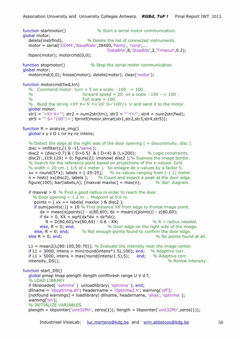
Association University and University Colleges Antwerp. RGBd, ToF ! Final Report IWT 2012.
Industrieel VisieLab: [email protected] and [email protected] 50
function startmotor() % Start a serial motor communication.
global motor;
delete(instrfind); % Delete the list of connected instruments.
motor = serial('COM4','BaudRate',38400,'Parity', 'none',...
'DataBits',8,'StopBits',2,'Timeout',0.2);
fopen(motor); motorcmd(0,0);
function stopmotor() % Stop the serial motor communication.
global motor;
motorcmd(0,0); fclose(motor); delete(motor); clear('motor');
function motorcmd(fwd,trn)
% Command motor: turn = 5 on a scale -100 -> 100 .
% forward speed = 20 on a scale -100 --> 100 .
% Full scale = 100.
% Build the string <XY X='5' Y='20' S='100'/> \r and send it to the motor.
global motor;
str1 = '<XY X='''; str2 = num2str(trn); str3 = ''' Y='''; str4 = num2str(fwd);
str5 = ''' S=''100''/>'; fprintf(motor,strcat(str1,str2,str3,str4,str5));
function R = analyze_img()
global x y z D L nx ny nz intens;
% Detect the edge at the right side of the door opening ( = discontinuity, disc ).
disc = imfilter(z,[1 0 -1],'same');
disc2 = (disc>0.7) & ( D>0.5) & ( D<4) & (L>200); % Logic constraints.
disc2(:,119:120) = 0; figure(2); imshow( disc2 );% Supress the image border.
% Search for the reference point based on projections of the x-values. Grid
% width = 20 cm. ( 1/5 of 1 meter ). So enlagre de x-values by a factor 5.
xx = round(5*x); labels = [-25:25]; % xx-values ranging from [-1 1] meter.
n = histc( xx(disc2), labels ); % Count and expect a peak at the door edge.
figure(100); bar(labels,n); [maxval maxloc] = max(n); % 'Bar' diagram.
if maxval > 0 % Find a good radius in order to reach the door.
% Door opening = 1.2 m . Midpoint at 0.6 m.
points = ( xx == labels( maxloc ) & disc2 );
if sum(points(:)) > 10 % Find distance XX from edge to frontal image point.
dx = mean(x(points)) - x(80,60); dz = mean(z(points)) - z(80,60);
if dx > 0, XX = sqrt(dx*dx + dz*dz);
R = D(80,60)/nx(80,60) - 0.6 - XX; % R = radius needed.
else, R = 0; end; % Door edge on the right side of the image.
else, R = 0; end; % Not enough points found to confirm the door edge.
else R = 0; end; % No points found at all.
L1 = mean2(L(80:100,50:70)); % Evaluate the intensity near the image center.
if L1 < 3000, intens = min(round(intens*1.5),100); end; % Adaptive corr.
if L1 > 5000, intens = max(round(intens/1.5),5); end; % Adaptive corr.
intensity_DS(); % Renew intensity .
function start_DS()
global pmap lmap plength llength confthresh range U V d f;
% LOAD LIBRARY
if libisloaded( 'optrima' ) unloadlibrary( 'optrima' ); end;
dllname = 'liboptrima.dll'; headername = 'Optrima2.h'; warning('off');
[notfound warnings] = loadlibrary( dllname, headername, 'alias', 'optrima' );
warning('on');
% INITIALIZE VARIABLES
plength = libpointer('uint32Ptr', zeros(1)); llength = libpointer('uint32Ptr',zeros(1));

Association University and University Colleges Antwerp. RGBd, ToF ! Final Report IWT 2012.
Industrieel VisieLab: [email protected] and [email protected] 51
rangeval = libpointer('singlePtr', zeros(1));
pmap = libpointer('int16Ptr', zeros(160,120,'int16'));
lmap = libpointer( 'uint16Ptr', zeros160,120,'uint16')); confthresh = single(5);
% START CAMERA AND SET PROPERTIES
calllib( 'optrima', 'optrima_init'); pause(3);
errmsgx1 = calllib(‘optrima','optrima_set_property','ENABLE_RGB_EVENT_HANDLERS', 0 );
errmsgx2 = calllib('optrima', 'optrima_set_property', 'ENABLE_DENOISING', 0 );
errmsgx3 = calllib('optrima', 'optrima_set_property', 'ENABLE_LEAKAGE_ALGORITHM', 0 );
errmsgx4 = calllib('optrima', 'optrima_set_property', 'ENABLE_DENOISING', 0 );
errmsgx5 = calllib('optrima', 'optrima_set_property', 'OC310_ENABLE_SATURATION', 1 );
errmsgx6 = calllib('optrima', 'optrima_set_property', 'OC310_FRAMERATE', 25 );
% RESTART CAMERA
calllib( 'optrima', 'optrima_exit'); pause(1);
calllib( 'optrima', 'optrima_init'); pause(3);
errmsg1 = calllib( 'optrima', 'optrima_enable_camera' );
errmsg2 = calllib( 'optrima', 'optrima_enable_camera_rgb' ); pause(3);
% GET RANGE
[errmsg4 range] = calllib( 'optrima', 'optrima_get_range', rangeval );
I = 160; J = 120; I2 = I/2; J2 = J/2; ff = f * f;
u = (1:J) - (J2+0.5); uu = u .* u; v = (1:I) - (I2+0.5); vv = v .* v;
U = repmat( u , [I 1]); UU = repmat( uu, [I 1]);
V = repmat( v', [1 J]); VV = repmat( vv',[1 J]); d = sqrt( UU + VV + ff );
intensity_DS() % Start up intensity setting.
function stop_DS() % Shut down camera.
errmsg7 = calllib( 'optrima', 'optrima_disable_camera' );
errmsg8 = calllib( 'optrima', 'optrima_disable_camera_rgb' );
calllib( 'optrima', 'optrima_exit');
function update_data()
global pmap plength confthresh range D lmap llength L d x y z U V f nx ny nz;
% Get camera data: phase map, luminance map, confidence threshold.
[errmsg5 P q] = calllib('optrima','optrima_get_phasemap',pmap,plength,confthresh);
[errmsg7 L q] = calllib('optrima', 'optrima_get_confidencemap',lmap,llength );
% Calculate distance from phase data.
D = double(fliplr(P))*(range/2^15); L = fliplr(L);
Dd = D ./ d; x = U.* Dd; y = -V.* Dd; z = f*Dd;
f1 = zeros(1, 9); f1(1) = 1; f1(end) = -1; f2 = f1';
z1 = conv2( z, f1, 'same' ); z2 = conv2( z, f2, 'same' ); % Local diferrences.
x1 = conv2( x, f1, 'same' ); x2 = conv2( x, f2, 'same' );
y1 = conv2( y, f1, 'same' ); y2 = conv2( y, f2, 'same' );
nx = y1.*z2-z1.*y2; ny = z1.*x2-x1.*z2; nz = x1.*y2-y1.*x2; % Normal vector.
n = sqrt(nx.^2 + ny.^2 + nz.^2 ); nx = nx./n; ny = ny./n; nz = nz./n;
function intensity_DS()
global intens;
calllib( 'optrima', 'optrima_set_light_intensity', uint8(intens));

Association University and University Colleges Antwerp. RGBd, ToF ! Final Report IWT 2012.
Industrieel VisieLab: [email protected] and [email protected] 52
6.4. An introduction on Kalman Filters in order to use it in navigation programs.
x 1 dt x dt²/2 Anoise.randn.dt²/2
d/dt = + . u(t) +
v 0 1 v dt Anoise.randn.dt
x
y = C. + Mnoise
v
State space models as a start to explain the Kalman
Filter Technique. SLAM: simultanous Localisation and Mapping .
a = input = u(t) = 0.01
v
x
KalmanKalman FiltersFilters
Process to be estimated:Process to be estimated:xk = A.xk-1 + B.uk + wk-1
yk = C.xk + vk
Process Noise (w) with covariance Q
Measurement Noise (v) with covariance R
KalmanKalman FilterFilterPredicted: ^xk is estimate based on measurements at previous time-steps
^xk = ^x-k + K.( yk – C.^x-
k )
Corrected: ŷk has additional information – the measurement at time k
, with K := P-kC
T(CP-kC
T + R)-1
^x-k = A.xk-1 + B.uk Time update.
P-k = APk-1A
T + Q Prediction Error Covariance
Pk = (I - KC)P-k
Measurement update.
Final Error Covariance
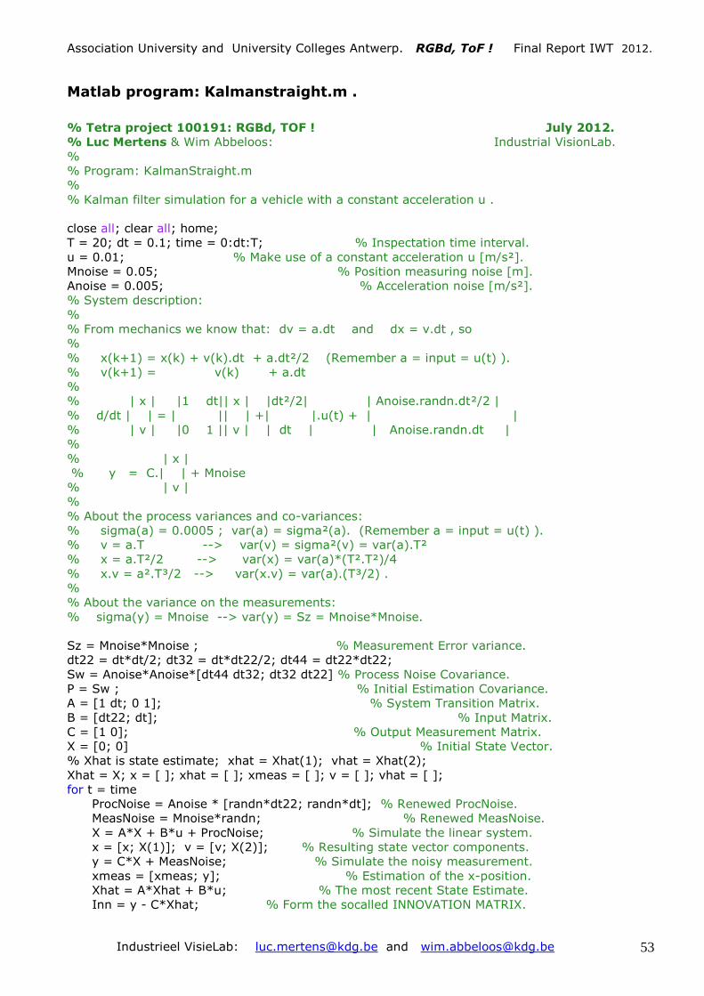
Association University and University Colleges Antwerp. RGBd, ToF ! Final Report IWT 2012.
Industrieel VisieLab: [email protected] and [email protected] 53
Matlab program: Kalmanstraight.m .
% Tetra project 100191: RGBd, TOF ! July 2012.
% Luc Mertens & Wim Abbeloos: Industrial VisionLab.
%
% Program: KalmanStraight.m
%
% Kalman filter simulation for a vehicle with a constant acceleration u .
close all; clear all; home;
T = 20; dt = 0.1; time = 0:dt:T; % Inspectation time interval.
u = 0.01; % Make use of a constant acceleration u [m/s²].
Mnoise = 0.05; % Position measuring noise [m].
Anoise = 0.005; % Acceleration noise [m/s²].
% System description:
%
% From mechanics we know that: dv = a.dt and dx = v.dt , so
%
% x(k+1) = x(k) + v(k).dt + a.dt²/2 (Remember a = input = u(t) ).
% v(k+1) = v(k) + a.dt
%
% | x | |1 dt|| x | |dt²/2| | Anoise.randn.dt²/2 |
% d/dt | | = | || | +| |.u(t) + | |
% | v | |0 1 || v | | dt | | Anoise.randn.dt |
%
% | x |
% y = C.| | + Mnoise
% | v |
%
% About the process variances and co-variances:
% sigma(a) = 0.0005 ; var(a) = sigma²(a). (Remember a = input = u(t) ).
% v = a.T --> var(v) = sigma²(v) = var(a).T²
% x = a.T²/2 --> var(x) = var(a)*(T².T²)/4
% x.v = a².T³/2 --> var(x.v) = var(a).(T³/2) .
%
% About the variance on the measurements:
% sigma(y) = Mnoise --> var(y) = Sz = Mnoise*Mnoise.
Sz = Mnoise*Mnoise ; % Measurement Error variance.
dt22 = dt*dt/2; dt32 = dt*dt22/2; dt44 = dt22*dt22;
Sw = Anoise*Anoise*[dt44 dt32; dt32 dt22] % Process Noise Covariance.
P = Sw ; % Initial Estimation Covariance.
A = [1 dt; 0 1]; % System Transition Matrix.
B = [dt22; dt]; % Input Matrix.
C = [1 0]; % Output Measurement Matrix.
X = [0; 0] % Initial State Vector.
% Xhat is state estimate; xhat = Xhat(1); vhat = Xhat(2);
Xhat = X; x = [ ]; xhat = [ ]; xmeas = [ ]; v = [ ]; vhat = [ ];
for t = time
ProcNoise = Anoise * [randn*dt22; randn*dt]; % Renewed ProcNoise.
MeasNoise = Mnoise*randn; % Renewed MeasNoise.
X = A*X + B*u + ProcNoise; % Simulate the linear system.
x = [x; X(1)]; v = [v; X(2)]; % Resulting state vector components.
y = C*X + MeasNoise; % Simulate the noisy measurement.
xmeas = [xmeas; y]; % Estimation of the x-position.
Xhat = A*Xhat + B*u; % The most recent State Estimate.
Inn = y - C*Xhat; % Form the socalled INNOVATION MATRIX.

Association University and University Colleges Antwerp. RGBd, ToF ! Final Report IWT 2012.
Industrieel VisieLab: [email protected] and [email protected] 54
s = C*P*C' + Sz; % % Compute the covariance of the Innovation.
K = A*P*C'*inv(s); % % Form the Kalman Gain Matrix.
Xhat = Xhat + K*Inn; % % Update the State Estimate.
P = (A*P - K*C*P)*A' + Sw; % % Covariance of the Estimated Error.
xhat = [xhat; Xhat(1)];
vhat = [vhat; Xhat(2)];
end;
figure; grid on; plot(time,x, time,xmeas, time,xhat);
legend('True Position','Measured Position','Estimated Position');
xlabel('Time (sec)'); ylabel('Position [m]');
title('Vehicle Position ( True, Measured & Estimated)');
figure; grid on; plot(time,x-xmeas, time, x-xhat);
legend('True Position - Measured Position','True Position - Estimated Position');
xlabel('Time (sec)'); ylabel('Position Error [m]');
title('Position Measurement Error & Position Estimation Error [m].');
figure; grid on; plot(time,v, time,vhat);
legend('Velocity','vhat');
xlabel('Time (sec)'); ylabel('Velocity [m/s]');
title('Velocity (True and Estimated [m/s]).');
figure; grid on; plot(time,v-vhat);
legend('Velocity - Estimated Velocity');
xlabel('Time (sec)'); ylabel('Velocity Error [m/s]');
title('Velocity Estimation Error [m/s].');
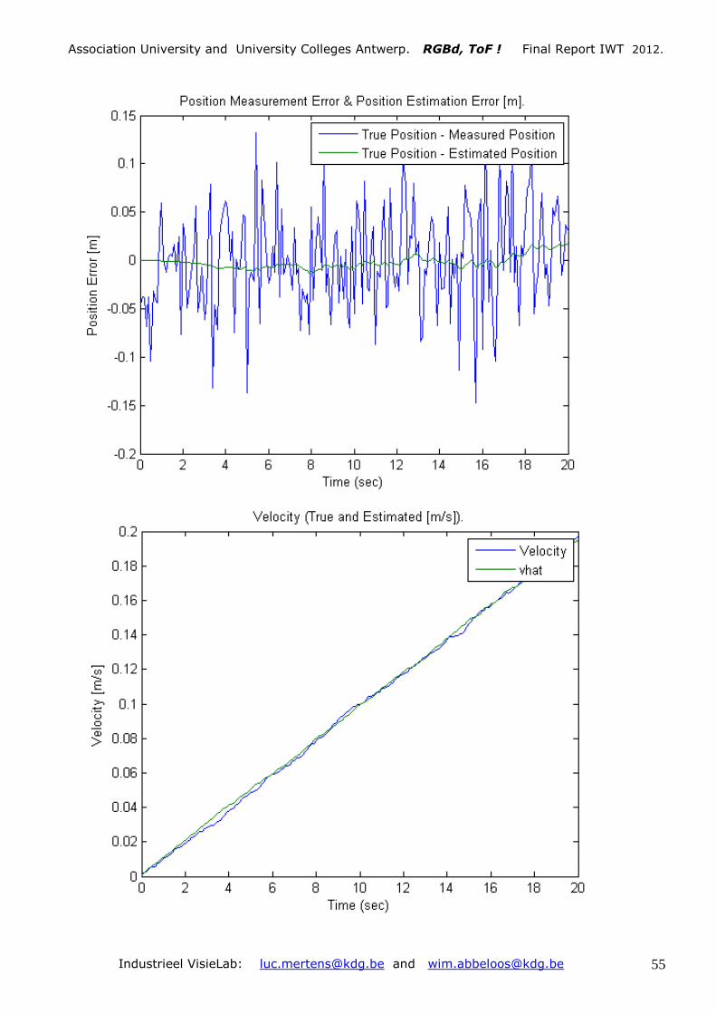
Association University and University Colleges Antwerp. RGBd, ToF ! Final Report IWT 2012.
Industrieel VisieLab: [email protected] and [email protected] 55

Association University and University Colleges Antwerp. RGBd, ToF ! Final Report IWT 2012.
Industrieel VisieLab: [email protected] and [email protected] 56
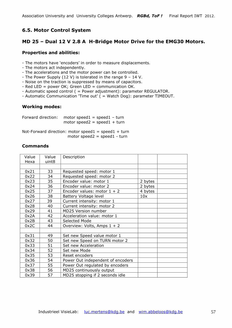
Association University and University Colleges Antwerp. RGBd, ToF ! Final Report IWT 2012.
Industrieel VisieLab: [email protected] and [email protected] 57
6.5. Motor Control System
MD 25 – Dual 12 V 2.8 A H-Bridge Motor Drive for the EMG30 Motors. Properties and abilities: - The motors have ‘encoders’ in order to measure displacements.
- The motors act independently.
- The accelerations and the motor power can be controlled.
- The Power Supply (12 V) is tolerated in the range 9 – 14 V.
- Noise on the traction is suppressed by means of capacitors.
- Red LED = power OK; Green LED = communication OK.
- Automatic speed control ( = Power adjustment): parameter REGULATOR.
- Automatic Communication ‘Time out’ ( = Watch Dog): parameter TIMEOUT.
Working modes:
Forward direction: motor speed1 = speed1 – turn
motor speed2 = speed1 + turn
Not-Forward direction: motor speed1 = speed1 + turn
motor speed2 = speed1 - turn
Commands
Value
Hexa
Value
uint8
Description
0x21 33 Requested speed: motor 1
0x22 34 Requested speed: motor 2
0x23 35 Encoder value: motor 1 2 bytes
0x24 36 Encoder value: motor 2 2 bytes
0x25 37 Encoder values: motor 1 + 2 4 bytes
0x26 38 Battery Voltage level 10x
0x27 39 Current intensity: motor 1
0x28 40 Current intensity: motor 2
0x29 41 MD25 Version number
0x2A 42 Acceleration value: motor 1
0x2B 43 Selected Mode
0x2C 44 Overview: Volts, Amps 1 + 2
0x31 49 Set new Speed value motor 1
0x32 50 Set new Speed on TURN motor 2
0x33 51 Set new Acceleration
0x34 52 Set new Mode
0x35 53 Reset encoders
0x36 54 Power Out independent of encoders
0x37 55 Power Out regulated by encoders
0x38 56 MD25 continuously output
0x39 57 MD25 stopping if 2 seconds idle

Association University and University Colleges Antwerp. RGBd, ToF ! Final Report IWT 2012.
Industrieel VisieLab: [email protected] and [email protected] 58
6.6. Matlabprogram: Wheelchair Navigation. % Tetra project 100191: RGBd, TOF ! July 2012.
% Wim Abbeloos & Luc Mertens: Industrial VisionLab.
%
% Wheelchair navigation.
%
% Function: 'wchair5.m'.
function wchair5() % Wheelchair5.
clear all; close all; clc;
global cam speed first d2 a2 f2 D L x y z nx ny nz f ku kv c1;
addpath( strcat(cd,'/MESA/') );
if exist('cam','var') sr_close(cam); end;
f = 138; ku = 1.0; kv = 1.0; % Values from the calibration step.
speed = 20; c1 = 1; first = true; % c1 = case 1; % first --- delay.
process_init(144,176); % Calculate the distances d = sqrt(u²+v²+f²).
cam = sr_open; res = sr_setautoexposure(cam,0,255,0,50);
startmotor(4); % USB poort 4 !
while 1 == 1
update_data();
[d2 a2 f2] = analyze_img(); % Wall distance, Wall Orientation, Wall Flatness.
switch c1
case 1 move_rot(1); % Rotate in order to find ‘Main Wall 1’ .
case 2 move_trans(2.73); % Move forward to ‘distance 2.73 meter’.
case 3 move_arc(1,1); % Rotate in order to find ‘the Table Wall’.
case 4 move_trans(0.25) % Move forward to ‘distance 0.25 meter’.
case 5 move_trans(-0.7); % Move backward to ‘distance 0.7 meter’.
case 6 move_arc(-1,-1); % Rotate in order to find ‘Main Wall 1’ .
case 7 move_trans(1.7); % Move forward to ‘distance 1.7 meter’.
case 8 move_arc(1,-1); % Rotate in order to find ‘the Park Wall’ .
case 9 move_trans(0.25); % Move forward to ‘distance 0.25 meter’.
case 10 move_trans(-1.8); % Move backward to ‘distance 1.8 meter’.
case 11 move_arc(1,-1); % Rotate in order to find ‘Main Wall 2’ .
case 12 move_trans(1.65); % Move forward to ‘distance 1.65 meter’.
case 13 move_arc(1,1); % Rotate in order to find ‘PC Wall’.
case 14 move_trans(0.25); % Move forward to ‘distance 0.25 meter’.
case 15 move_trans(-0.7); % Position at a distance 0.7 meter.
case 16 move_arc(-1,-1); % Rotate in order to find ‘Main Wall 2’ .
case 17 move_trans(0.6); % Position at a distance 0.6 meter.
otherwise motorcmd('setspeed1',0); motorcmd('setspeed2',0); break;
end; end;
stopmotor();
sr_close( cam );
function process_init(I,J) % process_init.
global U V d f ku kv;
I2 = I/2; J2 = J/2; ff = f * f;
u = ku*((1:J) - (J2+0.5)); uu = u .* u;
v = kv*((1:I) - (I2+0.5)); vv = v .* v;
U = repmat( u , [I 1]); UU = repmat( uu, [I 1]);
V = repmat( v', [1 J]); VV = repmat( vv',[1 J]);
UUff = UU + ff; d = sqrt( VV + UUff );
function startmotor(portnr) % startmotor.
global motor;
delete( instrfind );

Association University and University Colleges Antwerp. RGBd, ToF ! Final Report IWT 2012.
Industrieel VisieLab: [email protected] and [email protected] 59
port = strcat('COM',num2str(portnr)); % Start serial communication.
motor = serial(port,'BaudRate',9600,'Parity','none','DataBits',8,'StopBits',2,'Timeout',0.2);
fopen(motor); motorcmd('disabletimeout'); motorcmd('enablereg');
% ‘disabletimeout’ means: output will stop after 2 seconds without communication
% ‘enablereg’ means: power output is changed by encoder feedback !
motorcmd('resetenc'); motorcmd('setmode',3);
motorcmd(‘setspeed1',0); motorcmd('setspeed2',0); motorcmd('setaccel',10);
% ‘setaccel’ expresses the acceleration the controller takes to change voltages.
function update_data() % update_data.
global cam U V d D L x y z nx ny nz f;
sr_acquire( cam ); D = sr_getimage(cam,1); L = sr_getimage(cam,2);
D = double( D' ) / (double(intmax( 'uint16' ))/5); L = L';
Dd = D ./ d; x = U .* Dd; y = -V .* Dd; z = f * Dd;
f1 = zeros(1, 9); f1(1) = 1; f1(end) = -1; f2 = f1'; % Gradient-filters.
x1 = conv2( x, f1, 'same' ); x2 = conv2( x, f2, 'same' ); % Grad(x).
y1 = conv2( y, f1, 'same' ); y2 = conv2( y, f2, 'same' ); % Grad(y).
z1 = conv2( z, f1, 'same' ); z2 = conv2( z, f2, 'same' ); % Grad(z).
% Create ‘vectors normal to the world objects’.
nx = (y1.*z2)-(z1.*y2); ny = (z1.*x2)-(x1.*z2); nz = (x1.*y2)-(y1.*x2);
n = sqrt( nx.^2 + ny.^2 + nz.^2 ); % Normalized normal = n/|n|.
nx = nx ./ n; ny = ny ./ n; nz = nz ./ n;
function [d1 a1 f1] = analyze_img() % analyze_img.
global nx z;
Z1 = z(72:92,78:98); d1 = mean(Z1(:)); % Distance to wall.
A1 = nx(72:92,78:98); a1 = abs(mean(A1(:))); % Abs(orientation) of wall.
f1 = mean(Z1); f1 = sum(abs(diff(f1)))/d1; % Relative Flatness.
function move_trans( dz ) % move_trans.
global c1 d2 a2 speed first; % case, angle, distance, speed and first(Y/N).
if first==true motorcmd( 'setspeed1', sign(dz)*speed );
motorcmd( 'setspeed2', round(-speed/2*a2) ); end; % a2 -> 0.
if (sign(dz)*d2) < dz c1 = c1+1; first = true; end;
function move_rot(cw) % move_rot.
global c1 d2 a2 f2 speed first;
if first == true motorcmd( 'setspeed1', 0 );
motorcmd( 'setspeed2', sign(cw)*round(speed/3) );
for c2 = 1:10 update_data(); pause(0.1); end;
[d2 a2 f2] = analyze_img(); first = false; end; % dist., angle and flatness.
if a2 < 0.1 && f2 < 0.025 c1 = c1+1; first = false; end;
function move_arc( fwd, cw ) % move_arc.
global c1 d2 a2 f2 speed first;
if first == true motorcmd( 'setspeed1', sign(fwd)*speed );
motorcmd( 'setspeed2', sign(cw*fwd)*round(speed/2) );
for c2 = 1:10 update_data(); pause(0.1); end; % Adaptive Exposure.
[d2 a2 f2] = analyze_img(); first = false; end;
if abs(a2) < 0.1 && f2 < 0.025 c1 = c1+1; first = true; end;
function stopmotor() % stopmotor.
global motor;
motorcmd('setmode',3); motorcmd('enabletimeout');
motorcmd('setspeed1',0); motorcmd('setspeed2',0);
fclose(motor); delete(motor); clear('motor'); % Stop serial communication.
function varargout = motorcmd(cmd,varargin) % motorcmd.

Association University and University Colleges Antwerp. RGBd, ToF ! Final Report IWT 2012.
Industrieel VisieLab: [email protected] and [email protected] 60
global motor;
if ~ischar( cmd ) error( 'Second argument must be a command string' ); end;
switch cmd
case 'getspeed1'
fwrite(motor,[0 33],'int8'); % returns the requested speed of motor 1.
varargout(1) = { -fread(motor,1,'uint8') };
case 'getspeed2'
fwrite(motor,[0 34],'int8'); % returns the requested speed of motor 2.
varargout(1) = { -fread(motor,1,'uint8') };
case 'getenc1' % motor 1: encoder count.
fwrite(motor,[0 35],'uint8'); % 4 bytes returned, high byte first (signed).
val = fread(motor,4,'uint8');
val2 = uint32(bitcmp(uint8(val))); % Reorder data !
val3=bitshift(val2(1),24)+bitshift(val2(1),16)+bitshift(val2(3),8)+val2(4);
varargout(1) = { double(val3) };
case 'getenc2' % motor 2, encoder count,
fwrite(motor,[0 36],'uint8'); % 4 bytes returned, high byte first (signed).
val = fread(motor,4,'uint8');
val2 = uint32(bitcmp(uint8(val)));
val3=bitshift(val2(1),24)+bitshift(val2(1),16)+bitshift(val2(3),8)+val2(4);
varargout(1) = { double(val3) };
case 'getencs'
fwrite(motor,[0 37],'uint8' ); % returns 8 bytes: encoder1/2 count.
varargout(1) = { fread(motor,8,'uint8') };
case 'getvolts'
fwrite(motor,[0 38],'uint8'); % returns the input battery voltage level.
varargout(1) = { fread(motor,1,'uint8') };
case 'getcurrent1'
fwrite(motor,[0 39],'uint8'); % returns the current drawn by motor 1.
varargout(1) = { fread( motor, 1, 'uint8' ) };
case 'getcurrent2'
fwrite(motor,[0 40],'uint8'); % returns the current drawn by motor 2.
varargout(1) = { fread( motor, 1, 'uint8' ) };
case 'getversion'
fwrite(motor,[0 41],'uint8'); % returns the software version.
varargout(1) = { fread( motor, 1, 'uint8' ) };
case 'getaccel'
fwrite(motor,[0 42],'uint8'); % returns the current acceleration level.
varargout(1) = { fread( motor, 1, 'uint8' ) };
case 'getmode'
fwrite(motor,[0 43],'uint8'); % returns the currently selected mode.
varargout(1) = { fread( motor, 1, 'uint8' ) };
case 'getVI'
fwrite(motor,[0 44],'uint8'); % returns ‘Volts’, motor 1/2 current.
varargout(1) = { fread(motor,1,'uint8') }; % Battery voltage.
varargout(2) = { fread(motor,1,'uint8') }; % Current motor 1.
varargout(3) = { fread(motor,1,'uint8') }; % Current motor 2.
case 'setspeed1'
if nargin ~= 2 error( 'Incorrect number of input arguments' ); end;
speed = cell2mat(varargin(1));
fwrite(motor,[0 49 -speed],'int8'); % set new speed1.
case 'setspeed2'
if nargin ~= 2 error( 'Incorrect number of input arguments' ); end;
speed = cell2mat(varargin(1));
fwrite(motor,[0 50 -speed],'int8'); % set new speed2.
case 'setaccel'
if nargin ~= 2 error( 'Incorrect number of input arguments' ); end;
accel = cell2mat(varargin(1));

Association University and University Colleges Antwerp. RGBd, ToF ! Final Report IWT 2012.
Industrieel VisieLab: [email protected] and [email protected] 61
fwrite(motor,[0 51 accel],'uint8'); % set new acceleration.
case 'setmode'
if nargin ~= 2 error( 'Incorrect number of input arguments' ); end;
mode = cell2mat(varargin(1));
fwrite(motor,[0 52 mode],'uint8'); % set the motor mode.
case 'resetenc' fwrite(motor,[0 53],'uint8'); % zero both encoder counts.
case 'disablereg'
fwrite(motor,[0 54],'uint8'); % power not changed by encoder feedback.
case 'enablereg'
fwrite(motor,[0 55],'uint8'); % power regulated by encoder feedback.
case 'disabletimeout'
fwrite(motor,[0 56],'uint8'); % Continuously out if no regular commands.
case 'enabletimeout'
fwrite(motor,[0 57],'uint8'); % Watch dog: 2 seconds.
otherwise error( 'Incorrect command' ); % Incorrect command string.
end;
Reach position relative to target (i+1)Reach position relative to target (i+1)
Expect marker or target (i+1) Expect marker or target (i+1)
Start action (i+1). Start action (i+1).
Reach poReach position relative to target i .sition relative to target i .
Expect marker or target i . Expect marker or target i .
Start action i . Start action i .
GrafcetGrafcet DrivenDrivenMake use of posMake use of position tolerance if possible !ition tolerance if possible !
Example: the sequence from Example: the sequence from ‘‘PC PC ––> TV> TV’’ can be expressed in 3 AEP cyclescan be expressed in 3 AEP cycles
Cb(50) M2(Cb(50) M2(--250)250) Cf(Cf(--200) T4(200)200) T4(200) R(60) T3R(60) T3 . .
AEP cycles: Action / Expect target / Positioning
PC
TV

Association University and University Colleges Antwerp. RGBd, ToF ! Final Report IWT 2012.
Industrieel VisieLab: [email protected] and [email protected] 62
6.7. Navigation Practice
6.7.1. Forming a virtual descending path leading from the start to the end point.
% Tetra project 100191: RGBd, TOF ! June 2012.
% Luc Mertens & Luc Mertens: Industrial VisionLab.
%
% Program: WaveFrontTest2.m .
clear all; close all; clc; V = 120; U = 250; O3 = ones(3); O10 = ones(10);
map = false(V,U); % Generate new map: 240 * 500 cm .
start = [100 10]; target = [25 225]; % Define start point and target point.
map(1,:) = 1; map(end,:) = 1; map(:,1) = 1; map(:,end) = 1; % Walls.
map(1:30,50) = 1; map(1:30,100) = 1; map(1:30,200) = 1; % Obstacles.
map(30,170:200) = 1; map(end-90:end,140) = 1; map(end-30:end,190) = 1;
map(70:90,70:90) = 1; D = bwdist(map); % Eucledian distances to nearest 1.
map = imdilate(map,O10); % Dilated map.
map2 = zeros(V,U); map2(target(1),target(2)) = 2; % End point.
cn = 3; old = double(map2 ~= 0); % cn = current #.
tic; while map2(start(1),start(2)) == 0, % While 'start' not reached...
new = conv2(old,O3,'same'); % Number of neighbours.
change = ~old & new & ~map; old(change) = 1;
map2(change) = cn; cn = cn + 1; end; toc;
verDiff = diff(map2,1,1); horDiff = diff(map2,1,2);
S = cat( 1, -verDiff, zeros(1,U) ); N = cat( 1, zeros(1,U), verDiff );
E = cat( 2, -horDiff, zeros(V,1) ); W = cat( 2, zeros(V,1), horDiff );
NESW = cat( 3, N, E, S, W ); NESW(find( abs(NESW) > 1)) = -1;
tic; cp = start; track = uint8(map); [m1 m2] = max(NESW,[],3); % m2 = layer !
while map2(cp(1),cp(2)) ~= 2, nn = m2(cp(1),cp(2));
if nn == 1 cp(1) = cp(1) - 1; elseif nn == 2; cp(2) = cp(2) + 1;
elseif nn == 3 cp(1) = cp(1) + 1; else cp(2) = cp(2) - 1; end;
track(cp(1),cp(2)) = 2; end; toc;
figure(1); subplot(211); imshow(map); title( 'Map' );
subplot(212); imshow(track,[]); title( 'Simple Track.' );
figure(2); imshow(map2,[]); title( 'Wavefront' ); colormap('jet');
xlabel('Bleu = Low potential; Red = High potential.');
% Wavefront vectors.
[gR gC] = gradient(single(map2));
temp = imdilate(map2 < 1, O3); gR(temp) = 0; gR = -gR; gC(temp) = 0;
tn = imfilter(double(~temp), O10,'same'); % Count # OK points.
ggR = imfilter(gR,O10,'same'); ggR = ggR./tn; % Vector component 1.
ggC = imfilter(gC,O10,'same'); ggC = ggC./tn; % Vector component 2.
U = 250; V = 120;
P = kron([1:U],ones(V,1)); P4 = kron([1:4:U],ones(round(V/4),1));
Q = kron([V:-1:1]',ones(1,U)); Q4 = kron([V:-4:1]',ones(1,round(U/4)));
figure(10); axis equal; title('Wavefront vector field');
quiver( P4, Q4, ggR(1:4:V,1:4:U), ggC(1:4:V,1:4:U));
xlabel('Walls and obstacles.');
figure(20); imshow(D, [0 35] ); title( 'Distance Transform.' ); colormap( 'jet' );
[gDr gDc] = gradient(single(D)); gDc = -gDc; % Distance vector components.
figure(30); axis equal; title('Distance vector field.'); quiver(P,Q,gDr,gDc);
figure(40); axis equal; title('Combined vector field: wave front & distance.');
hold on; quiver(P,Q,ggR+ 0.5*gDr,ggC+0.5*gDc); % Weighted combination of...
angles = atan2((ggC+0.5*gDc),(ggR + 0.5*gDr)); % wavefront and distances.
figure(50); imshow(angles, [-pi pi]); title('Angles');

Association University and University Colleges Antwerp. RGBd, ToF ! Final Report IWT 2012.
Industrieel VisieLab: [email protected] and [email protected] 63

Association University and University Colleges Antwerp. RGBd, ToF ! Final Report IWT 2012.
Industrieel VisieLab: [email protected] and [email protected] 64

Association University and University Colleges Antwerp. RGBd, ToF ! Final Report IWT 2012.
Industrieel VisieLab: [email protected] and [email protected] 65
6.7.2. Potential based flow
% Tetra project 100191: RGBd, TOF ! July 2012. % Wim Abbeloos & Luc Mertens: Industrial VisionLab.
% % Program: Navigation3DviewWim.m .
clear all; close all; clc; pi2 = pi/2; wb = 0.365; % Vehicle weelbase.
O10 = ones(10); dt = 0.1; wf = 0.3; % Time step & weigth factor.
hh = 10; O3 = ones( 3, 'single' ); % Wall and object height.
oc = [.5 .5 .5]; fc = [.7 .7 .7]; vc = [.4 .7 1]; % Color settings.
map = false(120,250); % Map dimensions: 240 * 500 cm.
wd = [ 1 1 1 250; 120 120 1 250; 1 120 1 1 ; 1 120 250 250];
od = [ 1 30 50 50; 1 30 100 100; 1 30 200 200;
30 30 170 200; 30 120 140 140; 90 120 190 190;
70 90 70 70; 70 90 90 90; 70 70 70 90;
90 90 70 90]; % Wall and obstacle definition.
vd = [ -5 -5 10; -5 5 0; 1 1 1]; % Vehicle definition.
h = figure(2); % Add walls and objects to map and figure.
axis equal; hold on; view(70,30); camzoom(3.5);
cameratoolbar('Show'); cameratoolbar('SetMode','Orbit');
set( h, 'Renderer', 'OpenGL' ); %maxfig_7a(h,1);
patch([120 120 1 1], [1 250 250 1], [0 0 0 0], fc);
for c1 = 1:size(wd,1)
map(wd(c1,1):wd(c1,2),wd(c1,3):wd(c1,4)) = 1;
patch([wd(c1,1) wd(c1,2) wd(c1,2) wd(c1,1)],...
[wd(c1,3) wd(c1,4) wd(c1,4) wd(c1,3)], [0 0 hh hh], oc); end;
for c1 = 1:size(od,1)
map(od(c1,1):od(c1,2),od(c1,3):od(c1,4)) = 1;
patch([od(c1,1) od(c1,2) od(c1,2) od(c1,1)],...
[od(c1,3) od(c1,4) od(c1,4) od(c1,3)], [0 0 hh hh], oc); end;
map = imdilate( map, ones(10) );
ifh = figure(1);
title( 'Map' ); xlabel( 'Select start and endpoint' );
imshow( map ); %maxfig_7a(ifh,1);
[ spx spy ] = ginput(2); % Select start position and start direction.
line( spx, spy, 'Color', [0 1 1], 'LineWidth', 2 ); % Use quiver
[ epx epy ] = ginput(1); close(ifh); % Select target position (end point).
sp = round([spx(1) spy(1)]); ep = round([epx(1) epy(1)]);
S = [sp(1) sp(2) atan2(spy(1)-spy(2),spx(2)-spx(1))];
lmap = bwlabel(~map); % Region to handle.
ptodo = (lmap == lmap(ep(2), ep(1))); % Points to handle.
ntodo = sum(ptodo(:)); % Number of points to handle.
Wave = zeros( size(map), 'uint32' ); % Create empty 'Wave map'.
Wave( ep(2), ep(1) ) = 2; cn = 3; % Mark endpoint / current number.
old = single( Wave ~= 0 );
while sum(old(:)) < ntodo
new = conv2(old,O3,'same');
xtra = ~old & new & ptodo; % Extract pixels to set to handle.
old(xtra) = 1; Wave(xtra) = cn; cn = cn + 1; end;
[gr gc] = gradient(single(Wave)); temp = imdilate(Wave < 1,O3);
gr(temp) = 0; gr = -gr; gc(temp) = 0;
tn = imfilter(double(~temp),O10,'same'); % Filter wavefront vectors.
ggr = imfilter(gr,O10, 'same' ); ggr = ggr./tn;
ggc = imfilter(gc,O10, 'same' ); ggc = ggc./tn;
D = bwdist( map ); % Distance to nearest object border.
[gdr gdc] = gradient( single(D) ); gdc = -gdc;

Association University and University Colleges Antwerp. RGBd, ToF ! Final Report IWT 2012.
Industrieel VisieLab: [email protected] and [email protected] 66
% Angles of combined vector fields
angles = atan2( (ggc + wf*gdc), (ggr + wf*gdr) );
temp = angles < 0; angles(temp) = angles(temp) + pi2;
ed = Wave( S(2), S(1)); tc = 0; % Distance to endpoint and time counter.
figure(2); Kp = 150; Ki = 5; aev = []; % Start simulation.
while ed > 5, tc = tc + 1; S3 = S(3);
ca = S3 - pi2*sign(S3)*floor(abs(S3/pi2)); % Current angle.
ba = angles(S(2),S(1)); ae = ba - ca; % Best angle and angle error.
if abs(ba - ca) > pi ae = ae - pi2; end;
if size(aev,1) < 5, aev = cat(1,aev,ae);
else aev(1:end-1) = aev(2:end); aev(end) = ae; end;
speed = 20; dv = (Kp*ae + Ki*sum(aev))/pi; vl = speed - dv; vr = speed + dv;
co = cos(S3); si = sin(S3); sf = 0.00588; % m/s per motor speed unit
vl = vl*sf; vr = vr*sf;
if vl == vr, da = 0; l = vl*dt; dx = l*co; dy = l*si;
else v = (vr + vl)/2; r = (vr*wb)/(vr - vl) - wb/2;
da = v/r*dt; dx1 = r*sin(da); dy1 = r - r*cos(da);
dx = 100*(co*dx1 - si*dy1); dy = 100*(si*dx1 + co*dy1); end;
S = S + [ round(dx) round(dy) da ];
ed = Wave(S(2),S(1));
% Transform vehicle to current position and orientation.
T = [co si S(1); -si co S(2); 0 0 1]; veh = T*vd;
if exist( 'm', 'var' ), delete(m); delete(n); end; % Remove old vehicle.
quiver3( S(2), S(1), 5, -10*si, 10*co, 0, 'g' );
m = patch( veh(2,:), veh(1,:), [5 5 5], vc );
n = text( 130, 125, 0, ['time: ' num2str(tc*0.1) 's'] ); drawnow; end;

Association University and University Colleges Antwerp. RGBd, ToF ! Final Report IWT 2012.
Industrieel VisieLab: [email protected] and [email protected] 67
6.8. Fotonic Z40 camera:
6.8.1. Indoor application at Vision & Robotics.
% Tetra project 100191: RGBd, ToF ! July 2012.
% Luc Mertens & Wim Abbeloos & Rudi Penne: Industrial VisionLab. %
% Program: Indoor_WheelchairNavigation_VR2012. FOTONIC CAMERA .
% % Our intention is to develop a wheelchair navigation system that is able
% to find its path from a given position and direction to a free selected % end point and end direction. First we calculate a potential field. This
% may not have local minima and must keep the AGV away from the world % objects. The gradient of the field shows the way to follow. If the actual
% direction differs from the desired one a PI-control system slightly
% changes it. The method isn't finished yet but from now different strategies % can be evaluated and tested out.
function fot_app4() % Fotonic application.
clear all; close all; clc;
global D L x y z nx ny nz L1 L2 wall ftime cd cnx cnz mo;
wb = 0.3625; v = 5; wf = 0.5; Kp = 0.5; Ki = 0; w = 350; h = 120; pi2 = 2*pi;
L1 = [ 350 350 -350 -350 60 -60 60 -270 -270 % Wall definition.
-350 -314 -314 -230 105 105 135;
-120 120 120 -120 120 80 80 120 84
-4 -4 -84 -84 -120 -76 -76];
L2 = [ 350 -350 -350 350 60 -60 -60 -270 -350 % Wall definition.
-314 -314 -230 -230 105 135 135;
120 120 -120 -120 80 120 80 84 84
-4 -84 -84 -120 -76 -76 -120];
fh = figure(); hold on; title( 'World' ); axis equal; h1 = gca; maxfig(fh,1);
xlim( [min(L1(1,:))-0.1 max(L1(1,:))+0.1]./100 );
ylim( [min(L1(2,:)-0.1) max(L1(2,:))+0.1]./100 );
map = false(240,700);
M1 = L1; M1(1,:) = M1(1,:) + 350; M1(2,:) = 120-M1(2,:);
M2 = L2; M2(1,:) = M2(1,:) + 350; M2(2,:) = 120-M2(2,:);
bw = (M1 == 0); M1(bw) = 1; bw = (M2 == 0); M2(bw) = 1;
for c1 = 1:size(L1,2)
map( min(M1(2,c1),M2(2,c1)):max(M1(2,c1),M2(2,c1)), ...
min(M1(1,c1),M2(1,c1)):max(M1(1,c1),M2(1,c1)) ) = 1;
plot( h1, [L1(1,c1) L2(1,c1)]./100, [L1(2,c1) L2(2,c1)]./100, 'k' ); end;
map((45:120)+120,(210:320)+350) = 1; % Table
L1 = L1/100; L2 = L2/100;
L1 = cat( 1, L1, ones(1,size(L1,2)) ); L2 = cat( 1, L2, ones(1,size(L2,2)) );
map = imdilate( map, ones(10) ); % Enlarge the map.
ifh = figure(2); title( 'Map' ); imshow(map); maxfig(ifh,1); hold on;
xlabel( 'Select the endpoint' );
[epx epy] = ginput(1); ep = round([epx(1) epy(1)]); close( ifh ); % End point.
T = [-2.5 0 pi]; E = T; lmap = bwlabel( ~map ); % Labeled empty space.
ptodo = (lmap == lmap( ep(2), ep(1) )); ntodo = sum( ptodo(:) );
map2 = zeros( size(map), 'uint32' ); % Create empty map.
map2( ep(2), ep(1) ) = 2; cn = 3; % Mark endpoint.
old = single(map2 ~= 0); O3 = ones( 3, 'single' );
while sum(old(:)) < ntodo
new = conv2( old, O3, 'same' ); ff = (~old & new & ptodo);
old(ff) = 1; map2(ff) = cn; cn = cn + 1; end; % Create potential field.
% figure(100); imshow(map2,[]); colormap('jet');

Association University and University Colleges Antwerp. RGBd, ToF ! Final Report IWT 2012.
Industrieel VisieLab: [email protected] and [email protected] 68
[t1 t2] = gradient(single(map2)); bw = imdilate( map2 < 1, ones(3) );
t1(bw) = 0; t1 = -t1; t2(bw) = 0; % Wavefront vectors.
tn = imfilter(double(~bw), ones(10), 'same'); % Filter wavefront vectors.
tt1 = imfilter(t1, ones(10), 'same'); tt1 = tt1 ./ tn;
tt2 = imfilter(t2, ones(10), 'same'); tt2 = tt2 ./ tn;
D = bwdist(map); % Distance to nearest object.
[d1 d2] = gradient(single(D)); d2 = -d2;
angles = atan2((tt2 + wf.*d2), (tt1 + wf.*d1)); % Angles of weighted fields.
bw = (angles < 0); angles(bw) = angles(bw) + pi2;
E1 = E(1); E2 = E(2); E3 = E(3); cosE = 0.1*cos(E3); sinE = 0.1*sin(E3);
T1 = T(1); T2 = T(2); T3 = T(3); cosT = 0.1*cos(T3); sinT = 0.1*sin(T3);
ed = map2(round(h-E2*100), round(E1*100+w)); % Distance to endpoint.
quiver(h1,E1,E2,cosE,sinE,'r'); quiver(h1,T1,T2,cosT,sinT,'g');
% figure(1000); w2 2*w; h2 = h*2; axis equal; title('Wavefront vector field');
% quiver(repmat((1:1:w2),[h2 1]),repmat((h2:-1:1)',[1 w2]),tt1,tt2);
% figure(3000); axis equal; title('Distance vector field');
% quiver(repmat((1:1:w2),[h2 1]),repmat((h2:-1:1)',[1 w2]),d1,d2);
% figure(5000); axis equal; title('Combined vector field'); hold on;
% quiver( repmat((1:1:w2),[h2 1]), repmat((h2:-1:1)', [1 w2]), tt1+d1/2, tt2+d2/2);
startmotor(6); fot_start(); fot_getframe(); st=ftime;% Start: motor/camera/timer.
while ed > 15 % While distance to end point > 15 pixel.
ltime = ftime; fot_getframe();
if E3 > 2*pi E3 = E3 - pi2; end; if E3 < 0 E3 = E3 + pi2; end;
ca = E3; ba = angles(round(h-E2*100), round(E1*100+w)); % Best angle.
[vl vr] = speeds(v,ca,ba,Kp,Ki); % Speed controller.
motorcmd('setspeed1', vr); motorcmd('setspeed2', vl); % Set speeds.
dt = ftime - ltime; ct = ftime - st; Eold = E;
[dx dy da db dd dc] = move1(E3,dt,wb,vl,vr); % Update position.
[dx2 dy2 da2 db2 dd2 dc2] = move1(T3,dt,wb,vl,vr);
E = double(E + [dx dy da] );
T = double(T + [dx2 dy2 da2] );
if E3 > pi2 E3 = E3 - pi2; end; if E3 < 0 E3 = E3 + pi2; end
cosE = cos(E3); sinE = sin(E3);
quiver(h1, E1, E2, 0.1*cosE3, 0.1*sinE3, 'b');
ET = [cosE -sinE E1; sinE cosE E2; 0 0 1]; % New transformation matrix.
LT1 = ET\L1; LT2 = ET \ L2; % Transform worldmap to camera.
leq = cross( LT1, LT2 ); leq1 = leq(1,:); leq2 = leq(2,:); leq3 = leq(3,:);
% World wall parameters in camera framework
wd = abs(leq3) ./sqrt(leq1.*leq1 + leq2.*leq2);
wnx = -sin(atan2(leq2,leq1)); wnz = cos(atan2(leq2,leq1));
walls(); % Get camera wall parameters.
wall = zeros( size(cd) ); % Associate camera walls to transformed world walls.
TC = 0; for c3 = 1:size(wall,1) de = abs((wd-cd(c3)) ./(0.01*wd));
xe = abs((wnx-cnx(c3))/0.05); ze = abs((wnz-cnz(c3))/0.05);
C = de + xe + ze; [mval mind] = min(C); % Search minimum cost.
wall(c3) = mind; TC = TC + mval; end; % Total Cost.
m = [db dd dc]; [E cst] = fminsearch(@(t) cost(t,Eold,m), E); % Optimization.
if cst > TC disp('cost to high');
quiver( h1, E(1), E(2), 0.1*cos(E(3)), 0.1*sin(E(3)), 'k' );
E = double( Eold + [dx dy da] ); end;
E1 = E(1); E2 = E(2); E3 = E(3); sinE = 0.1*sin(E3); cosE = 0.1*cos(E3);
T1 = T(1); T2 = T(2); T3 = T(3); sinT = 0.1*sin(T3); cosT = 0.1*cos(T3);
ed = map2( round(h-E2*100), round(E1*100+w) ); % Distance to target.
quiver(h1,E1,E2,cosE,sinE,'r'); quiver(h1,T1,T2,cosT,sinT, 'g' ); drawnow; pause(0.1); end;
stopmotor(); fot_stop(); save('debug.mat');
% figure(200); subplot(121); imshow(D,[0.5 3]); title( 'Distance' );
% subplot(122); imshow(L, []); title( 'Luminance' );
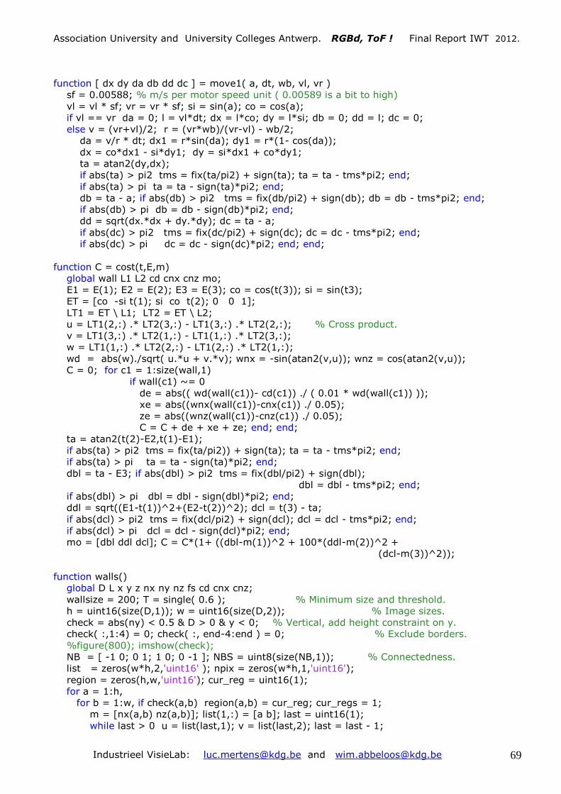
Association University and University Colleges Antwerp. RGBd, ToF ! Final Report IWT 2012.
Industrieel VisieLab: [email protected] and [email protected] 69
function [ dx dy da db dd dc ] = move1( a, dt, wb, vl, vr )
sf = 0.00588; % m/s per motor speed unit ( 0.00589 is a bit to high)
vl = vl * sf; vr = vr * sf; si = sin(a); co = cos(a);
if vl == vr da = 0; l = vl*dt; dx = l*co; dy = l*si; db = 0; dd = l; dc = 0;
else v = (vr+vl)/2; r = (vr*wb)/(vr-vl) - wb/2;
da = v/r * dt; dx1 = r*sin(da); dy1 = r*(1- cos(da));
dx = co*dx1 - si*dy1; dy = si*dx1 + co*dy1;
ta = atan2(dy,dx);
if abs(ta) > pi2 tms = fix(ta/pi2) + sign(ta); ta = ta - tms*pi2; end;
if abs(ta) > pi ta = ta - sign(ta)*pi2; end;
db = ta - a; if abs(db) > pi2 tms = fix(db/pi2) + sign(db); db = db - tms*pi2; end;
if abs(db) > pi db = db - sign(db)*pi2; end;
dd = sqrt(dx.*dx + dy.*dy); dc = ta - a;
if abs(dc) > pi2 tms = fix(dc/pi2) + sign(dc); dc = dc - tms*pi2; end;
if abs(dc) > pi dc = dc - sign(dc)*pi2; end; end;
function C = cost(t,E,m)
global wall L1 L2 cd cnx cnz mo;
E1 = E(1); E2 = E(2); E3 = E(3); co = cos(t(3)); si = sin(t3);
ET = [co -si t(1); si co t(2); 0 0 1];
LT1 = ET \ L1; LT2 = ET \ L2;
u = LT1(2,:) .* LT2(3,:) - LT1(3,:) .* LT2(2,:); % Cross product.
v = LT1(3,:) .* LT2(1,:) - LT1(1,:) .* LT2(3,:);
w = LT1(1,:) .* LT2(2,:) - LT1(2,:) .* LT2(1,:);
wd = abs(w)./sqrt( u.*u + v.*v); wnx = -sin(atan2(v,u)); wnz = cos(atan2(v,u));
C = 0; for c1 = 1:size(wall,1)
if wall(c1) ~= 0
de = abs(( wd(wall(c1))- cd(c1)) ./ ( 0.01 * wd(wall(c1)) ));
xe = abs((wnx(wall(c1))-cnx(c1)) ./ 0.05);
ze = abs((wnz(wall(c1))-cnz(c1)) ./ 0.05);
C = C + de + xe + ze; end; end;
ta = atan2(t(2)-E2,t(1)-E1);
if abs(ta) > pi2 tms = fix(ta/pi2)) + sign(ta); ta = ta - tms*pi2; end;
if abs(ta) > pi ta = ta - sign(ta)*pi2; end;
dbl = ta - E3; if abs(dbl) > pi2 tms = fix(dbl/pi2) + sign(dbl);
dbl = dbl - tms*pi2; end;
if abs(dbl) > pi dbl = dbl - sign(dbl)*pi2; end;
ddl = sqrt((E1-t(1))^2+(E2-t(2))^2); dcl = t(3) - ta;
if abs(dcl) > pi2 tms = fix(dcl/pi2) + sign(dcl); dcl = dcl - tms*pi2; end;
if abs(dcl) > pi dcl = dcl - sign(dcl)*pi2; end;
mo = [dbl ddl dcl]; C = C*(1+ ((dbl-m(1))^2 + 100*(ddl-m(2))^2 +
(dcl-m(3))^2));
function walls()
global D L x y z nx ny nz fs cd cnx cnz;
wallsize = 200; T = single( 0.6 ); % Minimum size and threshold.
h = uint16(size(D,1)); w = uint16(size(D,2)); % Image sizes.
check = abs(ny) < 0.5 & D > 0 & y < 0; % Vertical, add height constraint on y.
check( :,1:4) = 0; check( :, end-4:end ) = 0; % Exclude borders.
%figure(800); imshow(check);
NB = [ -1 0; 0 1; 1 0; 0 -1 ]; NBS = uint8(size(NB,1)); % Connectedness.
list = zeros(w*h,2,'uint16' ); npix = zeros(w*h,1,'uint16');
region = zeros(h,w,'uint16'); cur_reg = uint16(1);
for a = 1:h,
for b = 1:w, if check(a,b) region(a,b) = cur_reg; cur_regs = 1;
m = [nx(a,b) nz(a,b)]; list(1,:) = [a b]; last = uint16(1);
while last > 0 u = list(last,1); v = list(last,2); last = last - 1;

Association University and University Colleges Antwerp. RGBd, ToF ! Final Report IWT 2012.
Industrieel VisieLab: [email protected] and [email protected] 70
if check(u,v)
for c1 = 1:NBS iu = u + NB(c1,1); iv = v + NB(c1,2); % Inside?
if iu > 0 && iu <= h && iv > 0 && iv <= w && check( iu, iv )
d = sqrt((m(1) - nx(iu,iv)).^2 + (m(2) - nz(iu, iv)).^2 );
if d <= T last = last + 1; region(iu,iv) = cur_reg;
m = m + [nx(iu,iv)-m(1) nz(iu,iv)-m(2)]./cur_regs;
cur_regs = cur_regs + 1; list(last,1) = iu; list(last,2) = iv;
end; end; end;
check( u, v ) = false; end; end;
npix( cur_reg ) = cur_regs; cur_reg = cur_reg + 1; end; end; end;
goodwalls = find( npix > wallsize );
cd=[]; cnx = []; cnz = []; % Wall parameters: perpencidular distance, nx and nz.
for c1 = 1:size(goodwalls,1)
cur_wall = (region == goodwalls(c1)); p = polyfit(x(cur_wall),z(cur_wall),1);
cd = cat(1,cd,abs(p(2))./sqrt(p(1).*p(1)+1)); % Current perp. distance.
cnx = cat(1,cnx,mean(nx(cur_wall))); % Current normal-x.
cnz = cat(1,cnz,mean(nz(cur_wall))); end; % Current normal-x.
for c1 = 1:h, for c2 = 1:w % Remove region if not good.
if region(c1,c2) ~= 0 & npix(region(c1,c2)) < wallsize region(c1,c2) = 0;
end; end; end;
% figure(100); subplot(121); imshow(D,[]); title( 'Distance' );
% subplot(122); imshow(region,[0 1]); title( 'Vertical planes' );
function [vl vr] = speeds(v,ca,ba,Kp,Ki)
% current angle, best angle, Proportional factor, Integral factor, add speed error.
global aev % 'Angle error vector', used for integration.
if abs(ba - ca) < pi ae = ba - ca; else ae = ba - ca - sign(ba-ca)*pi2; end;
if size(aev,1) < 5 aev = cat(1,aev,ae);
else aev(1:end-1) = aev(2:end); aev(end) = ae; end; % Update aev.
dv = (Kp*ae + Ki*sum(aev))*2/pi; % Set speeds.
vl = v*(1-dv); vr = v*(1+dv);
function fot_start()
addpath('CameraCtrl\'); Closeldu; global cont;
cont.first = 1;
OpenCamera(); StartSensor(); % Open camera and start comm. interface.
% SetMode('MSSTcont'); % Set mode to Multishutter.
% SetMSlimit(1000); % Value proportional to Active brightness.
% SetMSShutter(220,25); % Value in 0.1 ms.
SetMode('MultiSpatioTemporal'); % Set mode to Multishutter.
SetShutter(300); % Value in 0.1 ms.
SetFrameRate(20); % Set frame rate to 20 fps.
SetLightSwitchState(1); % Turn on LED's.
for i=1:100, [xt, yt, zt, Lt] = GrabImage(); end; % Dummy images.
function fot_getframe()
global x y z D L nx ny nz ftime;
[yt, xt, zt, Lt, fc, head] = GrabImage();
x = double(rot90(xt))./1000; y = -double(rot90(yt))./1000;
z = double(rot90(zt))./1000; L = rot90(Lt); D = sqrt(x.*x + y.*y + z.*z);
ftime = double(head.reserved(1)) + double(head.reserved(2))/1000; % Time.
fs = 9; f1 = zeros(1, fs); f1(1) = 1; f1(end) = -1; f2 = f1'; % Filter preparation.
z1 = conv2( z, f1, 'same' ); z2 = conv2( z, f2, 'same' );
x1 = conv2( x, f1, 'same' ); x2 = conv2( x, f2, 'same' );
y1 = conv2( y, f1, 'same' ); y2 = conv2( y, f2, 'same' );
nx = y1.*z2-z1.*y2; ny = z1.*x2-x1.*z2; nz = x1.*y2-y1.*x2; % Normal.
n = sqrt( nx.^2 + ny.^2 + nz.^2 ); nx = nx ./ n; ny = ny ./ n; nz = nz ./ n;

Association University and University Colleges Antwerp. RGBd, ToF ! Final Report IWT 2012.
Industrieel VisieLab: [email protected] and [email protected] 71
function fot_stop()
StopSensor(); CloseCamera(); Closeldu;
function startmotor( portnr )
global motor; delete( instrfind );
port = strcat('COM', num2str(portnr)); % Start serial communication
motor = serial( port, 'BaudRate', 9600, 'Parity', 'none', 'DataBits', 8, …
'StopBits', 2, 'Timeout', 0.2 );
fopen( motor );
motorcmd( 'disabletimeout' ); motorcmd( 'enablereg' ); motorcmd( 'resetenc' );
motorcmd('setmode',1); motorcmd('setspeed1',0); motorcmd('setspeed2',0);
motorcmd( 'setaccel', 1 ); %motorcmd( 'setaccel', 10 );
function stopmotor() % Stop serial communication.
global motor;
motorcmd('setmode',1); motorcmd('setspeed1',0); motorcmd('setspeed2',0);
motorcmd( 'enabletimeout' );
fclose( motor ); delete( motor ); clear( 'motor' );
function varargout = motorcmd( cmd, varargin ) % MOTOR COMMANDS.
global motor;
if ~ischar( cmd ) error( 'Second argument must be a command string' ); end;
switch cmd
case 'getspeed1'
fwrite(motor,[0 33],'int8'); % returns the current requested speed of motor 1
varargout(1) = { -fread( motor, 1, 'uint8' ) };
case 'getspeed2'
fwrite(motor,[0 34],'int8'); % returns the current requested speed of motor 2
varargout(1) = { fread( motor, 1, 'uint8' ) };
case 'getenc1' % Motor 1.
fwrite(motor,[0 35],'uint8'); % 4 bytes returned high byte first (signed).
val = fread( motor, 4, 'uint8' );
val2 = uint32( bitcmp( uint8(val) ) );
val3 = bitshift(val2(1),24)+bitshift(val2(1),16)+bitshift(val2(3),8)+val2(4);
varargout(1) = { val3 };
case 'getenc2' % Motor 2.
fwrite(motor,[0 36],'uint8'); % 4 bytes returned high byte first (signed).
val = fread( motor, 4, 'uint8' );
val2 = uint32( bitcmp( uint8(val) ) );
val3 = bitshift(val2(1),24)+bitshift(val2(1),16)+bitshift(val2(3),8)+val2(4);
varargout(1) = { double(val3) };
case 'getencs'
fwrite(motor,[0 37],'uint8'); % Returns 8 bytes. Encoder1/encoder2 count.
varargout(1) = { fread( motor, 8, 'uint8' ) };
case 'getvolts'
fwrite( motor, [0 38], 'uint8' ); % Returns the input battery voltage level.
varargout(1) = { fread( motor, 1, 'uint8' ) };
case 'getcurrent1'
fwrite( motor, [0 39], 'uint8' ); % Returns the current drawn by motor 1.
varargout(1) = { fread( motor, 1, 'uint8' ) };
case 'getcurrent2'
fwrite( motor, [0 40], 'uint8' ); % returns the current drawn by motor 2.
varargout(1) = { fread( motor, 1, 'uint8' ) };
case 'getversion'
fwrite( motor, [0 41], 'uint8' ); % Returns the software version.
varargout(1) = { fread( motor, 1, 'uint8' ) };
case 'getaccel'
fwrite( motor, [0 42], 'uint8' ); % Returns the current acceleration level.

Association University and University Colleges Antwerp. RGBd, ToF ! Final Report IWT 2012.
Industrieel VisieLab: [email protected] and [email protected] 72
varargout(1) = { fread( motor, 1, 'uint8' ) };
case 'getmode'
fwrite( motor, [0 43], 'uint8' ); % Returns the currently selected mode.
varargout(1) = { fread( motor, 1, 'uint8' ) };
case 'getVI'
fwrite( motor, [0 44], 'uint8' ); % Returns Volts, current1 and current2.
varargout(1) = { fread( motor, 1, 'uint8' ) }; % Battery voltage
varargout(2) = { fread( motor, 1, 'uint8' ) }; % Current motor 1
varargout(3) = { fread( motor, 1, 'uint8' ) }; % Current motor 2
case 'setspeed1'
if nargin ~= 2 error( 'Incorrect number of input arguments' ); end;
speed = cell2mat(varargin(1));
fwrite( motor, [0 49 -speed], 'int8' ); % set new speed1
case 'setspeed2'
if nargin ~= 2 error( 'Incorrect number of input arguments' ); end;
speed = cell2mat(varargin(1));
fwrite( motor, [0 50 -speed], 'int8' ); % set new speed2
case 'setaccel'
if nargin ~= 2 error( 'Incorrect number of input arguments' ); end;
accel = cell2mat(varargin(1));
fwrite( motor, [0 51 accel], 'uint8' ); % set new acceleration
case 'setmode'
if nargin ~= 2 error( 'Incorrect number of input arguments' ); end;
mode = cell2mat(varargin(1));
fwrite( motor, [0 52 mode], 'uint8' ); % Set the mode.
case 'resetenc'
fwrite( motor, [0 53], 'uint8' ); % Zero both of the encoder counts.
case 'disablereg'
fwrite(motor,[0 54],'uint8'); % Power output not changed by encoder feedback.
case 'enablereg'
fwrite(motor,[0 55],'uint8'); % Power output regulated by encoder feedback.
case 'disabletimeout'
fwrite( motor, [0 56], 'uint8' ); % Continuous output if no-regular commands.
case 'enabletimeout'
fwrite( motor, [0 57], 'uint8' ); % Watch dog, 2 seconds.
otherwise
error( 'Incorrect command' );
end;

Association University and University Colleges Antwerp. RGBd, ToF ! Final Report IWT 2012.
Industrieel VisieLab: [email protected] and [email protected] 73
8.6.2. Outdoor application at Vision & Robotics.
% Tetra project 100191: RGBd, ToF ! June 2012.
% Wim Abbeloos & Luc Mertens: Industrial VisionLab.
%
% Program: Outdoor_WheelchairNavigation_VR2012. FOTONIC CAMERA .
%
% Our intention is to organize a closed loop wheelchair parcours .
% In an open area the camera is looking for a door opening in a wall.
% It uses the right door edge to calculate the radius of a circle that
% will bring the wheelchair to the other domain part. There it turns
% around and will come back through the door.
function outdoorv2() % Created for the Fotonic ToF camera.
clear all; close all; clc;
global x y z D L nx ny nz d;
fot_start(); startmotor(); loop = 0; step = 1; first = 0;
while loop == 0
fot_getframe(); % function starts at line 77.
switch step % Start driving: speed = 30 % ; Angular Velocity = 50 % .
case 1 % Rotate right untill R = 0 .
motorcmd(30,60); R = analyze_img1(); if R ~= 0 c1 = c1+1; end;
case 2 % R ~=0 , so rotate over a fixed time.
beep; motorcmd(33, -round(245/R)); P = analyse_img2();
if P ~= 0 beep; step = 3; end; % Search for the small plate.
case 3 % Drive straight forward but compensate for deviations.
motorcmd(40,4); pause(9); c1 = 1; end;
if first == 0 first = 1; t = tic; end;
if toc(t) > 20 motorcmd( 0, 0 ); loop = 1; first = 0; end;
otherwise
motorcmd(0,0); break; end; end; stopmotor(); fot_stop();
function fot_start()
addpath('CameraCtrl\'); Closeldu; global cont; cont.first = 1;
OpenCamera(); % Open sensor communication interface.
StartSensor();
SetMode('MultiSpatioTemporal'); % Set mode to Multishutter.
SetShutter(800); % Value in 0.1 ms.
SetFrameRate(20); % Set frame rate to 20 fps.
SetLightSwitchState(1); % Turn on LED's.
for i=1:100 [xt, yt, zt, Lt] = GrabImage(); end; % Dummy information.
function startmotor() % Start a serial motor communication.
global motor;
delete(instrfind); % Delete the list of connected instruments.
motor = serial('COM4','BaudRate',38400,'Parity', 'none',...
'DataBits',8,'StopBits',2,'Timeout',0.2);
fopen(motor); motorcmd(0,0);
function stopmotor() % Stop the serial motor communication.
global motor;
motorcmd(0,0); fclose(motor); delete(motor); clear('motor');
function motorcmd(fwd,trn)
% Command motor: turn = 5 on a scale -100 -> 100 .
% forward speed = 20 on a scale -100 --> 100 .
% Full scale = 100.
% Build the string <XY X='5' Y='20' S='100'/> \r and send it to the motor.

Association University and University Colleges Antwerp. RGBd, ToF ! Final Report IWT 2012.
Industrieel VisieLab: [email protected] and [email protected] 74
global motor;
str1 = '<XY X='''; str2 = num2str(trn); str3 = ''' Y='''; str4 = num2str(fwd);
str5 = ''' S=''100''/>'; fprintf(motor,strcat(str1,str2,str3,str4,str5));
function R = analyze_img1() % Find largest wall part.
global x y z nx ny nz D L; R = 0; % In case no wall is found, R = 0 .
bwW = abs(ny) < 0.6 & L > 0 & nx > 0 & y > -0.50 & y < 0.2 & del2(z) < 0.2;
bwW = imerode(bwW, ones(2)); [Seg, count] = bwlabel(bwW); % Segmentation.
MSeg = 0; MArea = 0; % Largest wall area
for c1 = 1:count cS = (Seg == c1); cSA = sum(cS(:)); % Current segment area.
if cSA > MArea MSeg = c1; MArea = cSA; end; end;
if MArea > 500 Wall = (Seg == MSeg); % Wall segment large enough.
WallSum = sum(Wall); Corner = min(find(WallSum > 5)) + 1; % Find corner.
if Corner < 50 && Corner > 20 % If corner 'frontal'.
ff = find(Wall(:,Corner) == true); % Find x and z values for corner.
xcorner = mean(x(ff,Corner)); zcorner = mean(z(ff,Corner));
ff = find(Wall(:,60)==true); % Find x and z values in the middle.
xmid = mean(x(ff,60)); zmid = mean(z(ff,60)); dmid = mean(D(ff,60));
alfa = acos( mean2(nx(Wall) )) * 180 / pi; % Find radius.
XX = sqrt( (xcorner-xmid).^2 + (zcorner-zmid).^2 );
R = dmid/cosd(alfa) - 0.75 - XX; save('debug_R.mat');
% figure(1); subplot(121); imshow( L, []); subplot(122); imshow( z, [0 5]);
% figure(2); imshow(Wall); xlabel(num2str(sum(Wall(:))));
% figure(3); plot( x(Wall), z(Wall), 'r*' ); xlim( [-3 3] ); ylim( [0 5] );
end; end;
function P = analyze_img2()
global x y z nx ny nz D L; P = 0; % In case no plate is found, P = 0.
bwP = abs(ny) < 0.6 & D > 4; L > 0 & abs(nx) < 0.5 &...
y > -0.50 & y < 0.2 & del2(z) < 0.2;
bwP = imerode(bwP, ones(2)); [Seg, count] = bwlabel(bwP); % Segmentation.
MSeg = 0; MArea = 0; % Largest wall area
for c1 = 1:count cS = (Seg == c1); cSA = sum(cS(:)); % Current segment area.
if cSA > MArea MSeg = c1; MArea = cSA; end; end;
if MArea > 100 Plate = (Seg == MSeg); % Plate found ?
if mean(abs(nx(Plate))) < 0.3 P = 1; save('debug_P.mat'); end; end;
function fot_getframe()
global x y z D L nx ny nz ftime;
[yt, xt, zt, Lt, fc, head] = GrabImage(); L = rot90(Lt);
x = double(rot90(xt))./1000; y = -double(rot90(yt))./1000;
z = double(rot90(zt))./1000; D = sqrt(x.*x + y.*y + z.*z);
ftime = double(head.reserved(1)) + double(head.reserved(2))/1000; % Time.
fs = 9; f1 = zeros(1, fs); f1(1) = 1; f1(end) = -1; f2 = f1'; % Filter preparation.
x1 = conv2( x, f1, 'same' ); x2 = conv2( x, f2, 'same' );
y1 = conv2( y, f1, 'same' ); y2 = conv2( y, f2, 'same' );
z1 = conv2( z, f1, 'same' ); z2 = conv2( z, f2, 'same' );
nx = y1.*z2-z1.*y2; ny = z1.*x2-x1.*z2; nz = x1.*y2-y1.*x2; % Normal vectors.
n = sqrt(nx.*nx + ny.*ny + nz.*nz); nx = nx./n; ny = ny./n; nz = nz./n;
function fot_stop()
StopSensor(); CloseCamera(); Closeldu; % ?? ldu = ?

Association University and University Colleges Antwerp. RGBd, ToF ! Final Report IWT 2012.
Industrieel VisieLab: [email protected] and [email protected] 75
7. Material handling
7.1. Hero-Technologies: material handling combined with free OCR. 7.1.1. Procedure in advance:
1. Bring the camera in an orientation so that it can view a marble at a central
position. After this the camera may not move anymore !.
2. Define a robot reference coordinate system.
3. Take an image of ‘the flat work plane’ and find: f , corr, ku , kv , ROTx and ROTy.
4. Bring the constants into the Hero_PickUp program.
ROTx = -ROTx en ROTy = -ROTy since the program needs to transform back.
5. Take 3 images of the separate characters H E R and derive their histograms.
6. Find the histograms of other characters X Y Z …
Make use of characters with enough ‘histogram contrast’ relative to H E R .
7. Take random stacked combinations of characters and verify if the program
works well.
8. Verify that the axis found are perpendicular to one other : R*R’ = I3 .
9. If the previous works well, the program is OK.
Success ... ToF !.
ifm electronic: O3D2xx ToF camera You Tube: ‘KdGiVL’.
Time of flight
3D – OCR
Bin Picking
Proof of concept (1) Tim Godden, Wim Abbeloos en Luc Mertens.
FANUC M – 10iA

Association University and University Colleges Antwerp. RGBd, ToF ! Final Report IWT 2012.
Industrieel VisieLab: [email protected] and [email protected] 76
7.1.2. Matlab program
% Tetra project 100191: RGBd, TOF ! June 2012.
% Luc Mertens & Wim Abbeloos: Industrial VisionLab.
% Mesut Usul, Zoltán Nyiro ; Kornel Koksic;
% Program: Robo_OCR.m .
%
% This program can deal with a stack of 3D-characters. Each character is member
% of a specific font (Height = 150 mm, Width = 120 mm, Thickness = 25 mm).
% A character can be found by edge-considerations in the 'range image (ToF)'.
% The 'distance gradients' can be used during the segmentation of th image.
% The edges could be found easely. Image resizing seems to be an other
% interesting approach.
close all; clear all; home; rep = 'replicate'; O2 = ones(2); O3 = ones(3); O4 = ones(4);
disp('From calibration: f = 85, z0 = 673.4 ; ROT = -0.342');
z0 = 673; ROT = 0.342 ; co = cos(ROT); si = sin(ROT);% sign opposite to turn back!
G = fspecial('gaussian',7,1.2); ku = 1.016 ; kv = 1.001; f = 85; f2 = 2*f; ff = f2*f2;
load('ifm_RH1.mat'); % HE, HE1, HER, RE, RH, RH1.
% [D L] = AcquireIFM(400); % With some intergration time, acquire D and L image.
t0 = cputime; [I J] = size(D); LD = L./D; % ToF Confidence matrix.
ROId = 1000*D(4:end-3,4:end-3);
ROId = kron(ROId,O2); ROId = imfilter(ROId,G,rep);
[I J] = size(ROId); I2 = I/2; J2 = J/2; IJ = I*J; x = zeros(I,J); y = x; z = x;
% Edge detection based on row and column wise differences ...
dDr = abs(diff(ROId)); dDr = cat(1, dDr(1,:),dDr);
dDc = abs(diff(ROId,1,2)); dDc = cat(2, dDc(:,1),dDc);
dD = max(dDr,dDc); BW = dD < 5 ; BW = imerode(BW,O2);
figure; imshow(BW);
[label count] = bwlabel(BW,4); % Label the connected regions.
C = [];
for c=1:count, % Objects may not touch the image border.
bw = (label==c); rs = sum(bw,2); cs = sum(bw); Area = sum(cs);
if Area > 250 && Area < 5000 && rs(1)*cs(1)*rs(end)*cs(end) == 0
C = [C c]; end; end;
if length(C) > 0
mm = min(min(ROId(I2-45:I2+45,J2-35:J2+35)));
MM = label(find(ROId == mm)); MMlabel = MM(1);
object = (label==MMlabel); rs = sum(object,2); cs = sum(object);
Area = sum(rs); BlobThin = bwmorph(object,'thin',inf); % Intensive calcul!
for i = 1:I, for j = 1:J,
if BlobThin(i,j) == true; v = kv*(i-I2+0.5); u = ku*(j-J2+0.5);
d = sqrt(ff+u*u+v*v); Dd = ROId(i,j)/d;
y(i,j) = v*Dd; x(i,j) = u*Dd; z(i,j) = f2*Dd; end; end; end;
FF = find(BlobThin == true); Len = length(FF);
XYZ = [mean(x(FF)); mean(y(FF)); mean(z(FF))]; % Pick up nearby XYZ.
X = x(FF) - XYZ(1); Y = y(FF) - XYZ(2); Z = z(FF) - XYZ(3);
data = cat(2,ones(Len,1),X,Y);
a = data\Z; a1 = 0; a2 = a(2); a3 = a(3); % Linear best fit: Z = a2.X + a3.Y .
N = [a2; a3; -1.0]; N = N/norm(N);
ZZ = a2*X + a3*Y; % Noisy points are projected to the best fit plane.
Char = false(201); R2 = 10000; % Character in millimeter size.
for tt = 1:Len % Looking for the pick up point.
Xtt = X(tt); Ytt = Y(tt); ZZtt = ZZ(tt); XXr = round(Xtt); YYr = round(Ytt);
r2 = Xtt*Xtt + Ytt*Ytt +ZZtt*ZZtt; if r2 < R2 R2 = r2 ; TT = tt; end;
Char(XXr+99:XXr+100,YYr+99:YYr+100) = true; end;
XXR = round(X(TT)); YYR = round(Y(TT));

Association University and University Colleges Antwerp. RGBd, ToF ! Final Report IWT 2012.
Industrieel VisieLab: [email protected] and [email protected] 77
vecX = [90; 90; a2*90+a3*90]; vecX = vecX/norm(vecX);
vecY = cross(N,vecX); vecY = vecY/norm(vecY);
xyz = XYZ + [X(TT); Y(TT); ZZ(TT)];
PUy = - xyz(2)*co + xyz(3)*si - z0*si; % Remember y is downwards.
PUz = - xyz(2)*si - xyz(3)*co + z0*co;
PU = round (10*[xyz(1) PUy PUz ])/10; % World pick up positions: x, y, z.
R = [vecX vecY N]'; RR = R*R';
aa = 180*atan2(R(3,2),R(3,3))/pi; % Rotation around x.
bb = 180*atan2(-R(3,1),sqrt(R(3,2)^2 + R(3,3)^2))/pi; % around y.
cc = 180*atan2(R(2,1),R(1,1))/pi; % Rotation around z.
% OCR part
Radii = zeros(201); Cloud = []; % Collecting square radii of CharSE.
SE = strel('octagon',6); CharSE = imdilate(Char,SE); % Octagonal element.
for i = 1:201, for j = 1:201,
if CharSE(i,j) == true; ii = (i-100)*(i-100); jj = (j-100)*(j-100);
Radii(i,j) = sqrt(ii + jj); end; end; end;
Cloud = Radii(find(Radii>0)); % B/W-cloud as a basis for the histogram.
% Remember the expected histogram from a learning step:
% H = hist(Cloud, [7.5:15:90]); H = H/sum(H);
HH = [0.0938 0.1173 0.3375 0.2912 0.1588 0.0014];
HO = [ 0 0.0283 0.3974 0.3472 0.2271 0 ];
HR = [0.0626 0.1571 0.2537 0.3810 0.1352 0.0103];
HE = [0.0858 0.1340 0.1853 0.3063 0.2659 0.0227];
HV = [0.0668 0.4316 0.2308 0.2210 0.0499 0];
HX = [0.1268 0.2048 0.2615 0.2592 0.1370 0.0108];
H = hist(Cloud, [7.5:15:90]); H = H/sum(H); % Measured histogram.
SSQ = zeros(1,4); % Evaluate histogram, relative to H E R O .
SSQ(1) = (HH-H)*(HH-H)'; SSQ(2) = (HE-H)*(HE-H)';
SSQ(3) = (HR-H)*(HR-H)'; SSQ(4) = (HO-H)*(HO-H)';
[ssq pos] = min(SSQ); hero = ['H'; 'E'; 'R'; 'O'];
if ssq < 0.1 Character = hero(pos); text = cat(2,'Character = ', Character);
else text = cat(2,'Character differs from H, E, R, O'); end;
t0 = cputime - t0
disp('R = [vecX" vecY" N"]');
R = R
RR = R*R'
aa = 180*atan2(R(3,2),R(3,3))/pi
bb = 180*atan2(-R(3,1),sqrt(R(3,2)^2 + R(3,3)^2))/pi
cc = 180*atan2(R(2,1),R(1,1))/pi
figure(1);
subplot(221); imshow(ROId,[]); title('Raw Distance values.');
subplot(222); imshow(label*round(255/(count-1)),[0 255]);
title('Labeled image segments');
subplot(223); imshow(dD,[]); title('dD = max(abs(dDr),abs(dDc))');
subplot(224); imshow(object); title('Highest free object');
figure(2);
subplot(221); imshow(ROId,[]); title('Raw Distance values.');
subplot(222); imshow(LD,[]); title('ToF confidence image.');
subplot(223); imshow(z ,[]); title('Corresponding z-values.');
subplot(224); imshow(label*round(255/(count-1)),[0 255]);
title('Labeled image segments');
figure(3);
Char(XXR+97:XXR+103,YYR+97:YYR+103) = true;
object(I2,:) = true; object(:,J2) = true;
subplot(231); imshow(Char); title('Relative to the robot.');
xlabel('Pick Up Point = big square.');

Association University and University Colleges Antwerp. RGBd, ToF ! Final Report IWT 2012.
Industrieel VisieLab: [email protected] and [email protected] 78
subplot(232); hold on; axis([-80 80 -80 80 -80 80]); view(20,45);
plot3( X,Y,Z,'.'); xlabel('x-as'); ylabel('y-as'); zlabel('z-as'); grid on;
subplot(233); hold on; axis([-80 80 -80 80 -80 80]); view(20,45);
plot3(X,Y,ZZ,'.'); xlabel('x-as'); ylabel('y-as'); zlabel('z-as'); grid on;
plot3(vecX(1),vecX(2),vecX(3),'r.'); plot3(0,0,0,'r.');
plot3([0 100*vecX(1)],[0 100*vecX(2)],[0 100*vecX(3)],'r');
plot3([0 100*vecY(1)],[0 100*vecY(2)],[0 100*vecY(3)],'g');
plot3([0 50*N(1)],[0 50*N(2)],[0 50*N(3)],'b');
title(cat(2,'CPUtime = ',num2str(t0)));
subplot(234); imshow(z,[]); title('z-values');
xlabel(cat(2,'Gravity xyz = [ ',num2str(xyz'),' ]'));
ylabel('Segments marked');
subplot(235); imshow(BW); title('Flat object --> white !');
xlabel(cat(2,'N = [ ',num2str(N'),' ]'));
ylabel(cat(2,'Area = ',num2str(Area)));
subplot(236); imshow(object);
title(cat(2,'Pick Up position: PU = ',num2str(PU)));
xlabel(cat(2,'z = ',num2str(round(XYZ(3))),' + (', num2str(round...
(-1000*a(2))/1000),').x + (', num2str(round(-1000*a(3))/1000),').y '));
ylabel('Camera x // robot x, camera y // robot y.')
figure(4);
for alfa = 0:360, co = cos(alfa); si = sin(alfa);
for Radius = 15:15:95
CharSE(100+round(co*Radius),100+round(si*Radius)) = true; end; end;
subplot(121); imshow(CharSE); title(text);
xlabel(cat(2,'CPUtime = ',num2str(t0)));
subplot(122); hist(Cloud,[10:15:99]); title('Histogram of the cloud point radii');
else disp('No objects found'); end;

Association University and University Colleges Antwerp. RGBd, ToF ! Final Report IWT 2012.
Industrieel VisieLab: [email protected] and [email protected] 79

Association University and University Colleges Antwerp. RGBd, ToF ! Final Report IWT 2012.
Industrieel VisieLab: [email protected] and [email protected] 80
7.2. University College Limburg, Flanders (KHLim): peppers handling. % Tetra project 100191: RGBd, TOF ! June 2012.
% Luc Mertens & Wim Abbeloos: Industrial VisionLab.
% Mesut Usul (Master student).
%
% Program: 'PepperD_short.m'.
%
% This program analyses the difference between an empty and a loaded pepper
% scene. The peppers are isolated and their orientation are found one by one.
% Paprika0 is the empty image giving the characteristics of the work plane.
% This plane can be used to calibrate the ToF camera in order to find the
% focal length, the distortion parameters ku en kv, the angles of the work plane
% relative to the camera...
%
% Image names are: paprika11 ->15 ; 21-> 25; ... ; 51 -> 55.
close all; clear all; home; Thres = 0.005; O4 = ones(4);
G = fspecial('gaussian',5,2); rep = 'replicate'; se3 = [0 1 0 ; 1 1 1 ; 0 1 0];
load Paprika D0; load('paprika54.mat'); L = ones(size(D));
t0 = cputime;
D = 1500*kron(D, O4); D = imfilter(D,G,rep); % To millimeter + magnif.
% D0 = D; save Paprika D0; imshow(D0,[]); pause; % Reference plane.
ff = find( D > (D0-0.005)); D(ff) = D0(ff); % Remove below the work plane.
[I J] = size(D); I2 = round(I/2); J2 = round(J/2); Dw = D0 - D; L = kron(L, O4);
[gX gY] = gradient(Dw,7); % Gradient distance = 3,5,7... .
[Firstlabel, count] = bwlabel(Dw,4); % Label the connected regions.
for cc = 1:count, ff = find(Firstlabel == cc);
if length(ff) < 500 Dw(ff) = 0; end; end; % Remove small objects.
gg = gX.*gX + gY.*gY; bwG = gg > 0.5; % Find pepper border.
bwDw = Dw > 0.01; bw = bwDw & ~bwG; % Shrink the blobs.
bw = imdilate(bw,ones(3)); bw = imerode(bw,strel('disk',10));
[label, count] = bwlabel(bw,4); CC = [];
for c = 1:count, FF = find(label==c); % Remove small objects.
if length(FF) < 50 bw(FF) = false; else CC = cat(2,CC,c); end; end;
LenCC = length(CC); T = 0; Segment = zeros(I,J); paprika = false(I,J,LenCC);
if LenCC >0
for c = 1:LenCC, object = false(I,J); FF = find(label==CC(c));
object(FF)= true; papri = imdilate(object,strel('disk',12)) & bwDw;
T = T+1; paprika(:,:,c) = papri; FF = find(papri==true); Segment(FF) = T;
papri(:,J2) = true; papri(I2,:) = true;
s = regionprops(Segment, 'area','orientation','centroid');
Area = cat(2,s.Area); Orient = cat(2,s.Orientation);
Centroids = cat(1, s.Centroid);
Centroids(:,1) = Centroids(:,1) - J2; Centroids(:,2) = Centroids(:,2) - I2;
figure(c); imshow(papri); title(cat(2,'Pepper #',num2str(c)));
xlabel(cat(2,'A = ',num2str(Area(c)),' Orient = ',...
num2str(round(Orient(c)))));
ylabel(cat(2,'Center = ',num2str(round(Centroids(c,:)))));
end; end;
t0 = cputime-t0;
figure(10); subplot(221); imshow(Dw,[]); title('Approx. Thickness');
subplot(222); imshow(bwDw,[]); title('bwDw = (D0-D) > 0.01 . ');
subplot(223); imshow(gg,[0 1]); title('gg = (gradX² + gradY²) .');
subplot(224); imshow(Segment,[]); title('Segmented Peppers.');
xlabel(cat(2,'Time to find regionprops = ',num2str(t0)));

Association University and University Colleges Antwerp. RGBd, ToF ! Final Report IWT 2012.
Industrieel VisieLab: [email protected] and [email protected] 81

Association University and University Colleges Antwerp. RGBd, ToF ! Final Report IWT 2012.
Industrieel VisieLab: [email protected] and [email protected] 82
% Function regionprops: --> Region Properties.
% 'Image' Sub image per 'area', met afmetingen van de Bounding Box.
% 'Perimeter' Omtreklengte, geteld in aantal pixel.
% 'Area' Oppervlakte, geteld in aantal pixel.
% 'Centroid' Zwaartepunt van de pixelcollectie.
% 'BoundingBox' Omsloten rechthoek volgens de rij en kolomrichting.
% 'Extent' Vullingsgraad van de 'BoundingBox'
% 'EquivDiameter' Traagsheidsstraal: 4*area/pi .
% 'MajorAxisLength' Lengte van de hoofd-as, gemeten in pixel.
% 'MinorAxisLength' Lengte van de neven-as, gemeten in pixel.
% 'Eccentricity' Verhouding: Minor/Major axis.
% 'Orientation' Oriëntatie van de hoofdas tegenover de rijrichting.
% 'FilledImage' Opgevuld oppervlak.
% 'FilledArea' Oppervlak na opvulling van de holten.
% 'ConvexHull' Kleinste, omsloten vierhoek. (Omhullende vierhoek).
% 'ConvexImage' Black/White image van de convex hull. (Mask).
% 'ConvexArea' Aantal 'true'-pixels in de 'ConvexImage'.
% 'Solidity' Vullingsgraad van de 'convex hull'.
% 'Extrema' Rij- en kolomcoördinaten van de 8 uiterst-gelegen punten.
% 'EulerNumber' Aantal objecten, verminderd met het aantal gaten.
% *******************************
% Function 'bwmorph' --> Morphological Operations:
% 'bridge' Bridge previously unconnected pixels.
% 'clean' Remove isolated pixels (1's surrounded by 0's).
% 'fill' Fill isolated interior pixels (0's surrounded by 1's).
% 'open' Perform binary opening (erosion followed by dilation).
% 'close' Perform binary closure (dilation followed by erosion).
% 'bothat' Subtract the input image from its closing.
% 'tophat' Subtract the opening from the input image.
% 'diag' Diagonal fill to eliminate 8-connectivity of background.
% 'dilate' Perform dilation using the structuring element ones(3).
% 'erode' Perform erosion using the structuring element ones(3).
% 'hbreak' Remove H-connected pixels.
% 'majority' Set a pixel to 1 if five or more pixels in its 3-by-3 neighbors are 1's.
% 'remove' Set a pixel to 0 if its 4-connected neighbors are all 1's,
% thus leaving only boundary pixels.
% 'shrink' With N = Inf, shrink objects to points;
% shrink objects with holes to connected rings
% 'skel' With N = Inf, 'remove' pixels on the boundaries of objects without
% allowing objects to break apart.
% 'spur' Remove end points of lines without removing small objects.
% 'thicken' With N = Inf, thicken objects by adding pixels to the exterior of
% objects without connecting previously unconnected objects.
% 'thin' With N = Inf, remove pixels so that an object without holes shrinks to
% a minimally connected stroke, and an object with holes shrinks
% to a ring halfway between the hole and outer boundary.

Association University and University Colleges Antwerp. RGBd, ToF ! Final Report IWT 2012.
Industrieel VisieLab: [email protected] and [email protected] 83
7.3. KdG: palet handling
DepthSense 311
1. Find the z –discontinuity
2. Look for vertical parts with
forward oriented normals
3. Inspect collineraity
4. Use geometrical laws
in order to find
x, y, z and b.
RGBd
Ingewikkeld !
Mesa SwissRanger 4000
1. Remove bright pixels
2. Find the z –discontinuity
3. Look for vertical parts with
forward oriented normals
4. Inspect collineraity
5. Use geometrical laws
in order to find
x, y, z and b.
ToFIngewikkeld !

Association University and University Colleges Antwerp. RGBd, ToF ! Final Report IWT 2012.
Industrieel VisieLab: [email protected] and [email protected] 84
ToF
IFM O3D2xx.
1. Remove weak defined
pixels.
2. Find the z –discontinuity
3. Look for vertical parts with
forward oriented normals
4. Inspect collineraity
5. Use geometrical laws
in order to find
x, y, z and b.
Ingewikkeld !
7.3.1. Connect camera: O3D2xx.dll and O3D2xx.h should be present .
% Camera connect, ToF ! July 2012.
% Wim Abbeloos & Luc Mertens: Industrial VisionLab.
if exist(cam) == 0 % If 'open camera' then 'close camera'.
for c = 1:3 % Disconnect the camera.
answer = calllib('O3D2xxCamera','O3D2XXDisconnect',1);
if answer == 0 disp('Camera disconnected'); break;
else disp(strcat('Failed to disconnect, attempt no',num2str(c)));pause(0.5);
end; end; end;
% Start live camera:
dllname = 'O3D2xxCamera'; inttime = 500; % Driver & camera integration time.
headername = 'O3D2xxCameraMatlab.h'; IP = '192.168.0.69'; XMLPort = uint32(8080);
hwnd = libpointer('uint32Ptr',0); FWversion = libpointer('stringPtr','xxxxxx'); SensorType =
libpointer( 'stringPtr', 'xxxxxxxxxx' );
if ~libisloaded(dllname) loadlibrary(dllname,headername); end; % Load library.
for c = 1:3 % Connect the camera.
[answer,hwnd,IP,FWversion,SensorType] = ...
calllib(dllname,'O3D2XXConnect',hwnd,IP,XMLPort,FWversion,SensorType);
if answer == 0 disp('Camera Connected');
calllib(dllname,'O3D2XXPerformHeartBeat'); break;
else calllib(dllname,'O3D2XXDisconnect',1);
disp(strcat('Failed to connect, attempt no', num2str(c)));
if c == 3 error('Failed to connect'); end; end; end;
% Software trigger type:
% 1 = positive edge, 2 = negative edge, 3 = free running, 4 = software based.
calllib(dllname,'O3D2XXSetTrigger',4);
head = libpointer('int32Ptr',zeros(1,21*4)); % Init variables.

Association University and University Colleges Antwerp. RGBd, ToF ! Final Report IWT 2012.
Industrieel VisieLab: [email protected] and [email protected] 85
SIZE = uint32(64*50*4); dat = libpointer('uint8Ptr',zeros(1,SIZE));
TCPport = int32(50002);
cam = struct('dllname',dllname,'dat',dat,'SIZE',SIZE,'head',head,'TCPport',TCPport);
% Set front end data
% 1. Modulation Frequency and wave length code [0,1,2,3]; default = 0;
% 2. Single or double sampling corresponding with normal/high dynamic.
% 3. Illumination mode: 0 = off, 1 = A on, 2 = B on, 3 = A and B on.
% 4. First integration time [µs] (single sampling mode), 1-5000; default=2000.
% 5. Second integration time [µs] (double sampling mode), 1-5000.
% 6. Delay time [ms] default = 141.
setfrontend = libpointer('int32Ptr',[0,0,3,1,inttime,0]);
calllib(dllname,'O3D2XXSetFrontendData',setfrontend);
%%% END camera start up .
calllib(cam.dllname,'O3D2XXTriggerImage'); % Get new frame.
[answer,data,header] = calllib(cam.dllname,'O3D2XXGetImageData',...
int8('d'),cam.dat,cam.SIZE,cam.head,cam.TCPport);
7.3.2. Image analysis and measuring results
% Proof of concept, ToF ! July 2012.
% Luc Mertens & Wim Abbeloos: Industrial VisionLab.
% Usul Mesut (student).
%
% Program: ifm_palette_GP.m
%
% Find the palettes visible in a ToF image. Palettes are near the floor (0-140 mm).
% Palettes have 2 predescribed holes. The following data are looked for:
% 1. Find the centre of gravity (xz, yz = Floor - 90 mm. , zz) relative to the AGV.
% 2. Find the orientation -90° < alfa < 90 relative to the AGV.
% Since the palettes must be placed on exact positions (+/- 1.5 cm) they must
% be picked up as correct as possible.
close all; clear all; home; rep = 'replicate'; ku = 0.965; kv = 1.0;
G = fspecial('gaussian',11,2.2); O2 = ones(2); O3 = ones(3); O4 = ones(4);
T = 20; D_left = 0; D_right = 0; % T is the maximum # blobs.
Co = ones(3); xz = 0; zz = 0; alfa = 0; % Co is a collinearity check matrix.
f = 80; f4 = 4*f; H1 = 50; % Focal length + Rows of interest.
ThresCollin = 0.05; % Threshold on the collinearity calculation.
ThresDist = 0.05; % Threshold on the square distance between the frontal blobs.
MatchFound = false; % Result of the analysis.
load('ifm6.mat');
% [D L] = AcquireIFM(200); % With some intergration time, acquire D and L image.
t0 = cputime;
% D = D(end:-1:1,:); L = L(end:-1:1,:);
D = rot90(D,1); L = rot90(L,1); % Rotation if necessary.
D = D(2:end-1,2:end-1); L = L(2:end-1,2:end-1); % Never trust border pixels.
bwOUT = L < 0; NN = sum(bwOUT(:)); %%% Some points are out of control...
if NN > 0 for t = 1:5
bwE = imerode(bwOUT,O2); bwD = imdilate(bwOUT,O3);
OUTER = bwD & ~bwOUT; FF = find(OUTER==true);
INNER = bwOUT & ~bwE; ff = find(INNER==true);
for g = 1:length(ff) FFg = abs(FF-ff(g)); [mm gg] = min(FFg);
D(ff(g)) = D(FF(gg)); end;
figure(20); imshow(kron(bwOUT,O2)); title('Out of control');
xlabel(cat(2,'# OUT of control = ', num2str(length(ff)))); pause(0.5);

Association University and University Colleges Antwerp. RGBd, ToF ! Final Report IWT 2012.
Industrieel VisieLab: [email protected] and [email protected] 86
bwOUT = bwE; end; end;
D(find(D > 3.5 | D < 0.4)) = 3.5; D = kron(D,O4); L = kron(L,O4);
D = imfilter(D,G,rep); LD = L./D; % Confidence image.
[I J] = size(D); I2 = I/2; J2 = J/2; ff4 = f4*f4; % f4 is the adapted focal length.
u = ku*([0.5:J-0.5]-J2); uu = u.*u; % column pixel values u = -J/2:J/2 .
v = kv*([0.5:I-0.5]-I2); vv = v.*v; % row pixel values v = -I/2:I/2 .
U = kron(u,ones(I,1)); UU = kron(uu,ones(I,1));
V = kron(v',ones(1,J)); VV = kron(vv',ones(1,J));
d = sqrt(VV+UU + ff4); % Pythagoras. Internal camera distances --> LUT.
Dd = D./d; % Distance ratios for world points.
x = U.*Dd; % Camera x-coordinates.
y = V.*Dd; % Camera y-coordinates. Downwards oriented !!
z = f4*Dd; % Camera z-coordinates.
x = imfilter(x,G,rep); y = imfilter(y,G,rep); z = imfilter(z,G,rep);
xL = x(H1:end,:); yL = y(H1:end,:); zL = z(H1:end,:); IL = I-H1+1;
DL =sqrt(xL.*xL + yL.*yL + zL.*zL); % Improved distance image.
[gXr gXc] = gradient(xL); [gYr gYc] = gradient(yL); [gZr gZc] = gradient(zL);
v1 = cat(3,gXr,gYr,gZr); v2 = cat(3,gXc,gYc,gZc); v = cross(v1,v2);
normV = sqrt(sum(v.*v, 3)); normV = repmat(normV,[ 1 1 3 ]);
normal = v./normV; % Vectors are normalized as v = v/|v| .
nXL = normal(:,:,1); nYL = normal(:,:,2); nZL = normal(:,:,3);
% Find the floor: take care for the reflections of the plastic foil --> use medians.
i = I2/2; while median(y(i,J2-15:J2+15))<0 i=i+1; end; H = i; % Camera horizon.
i = H+50; while median(z(i,J2-15:J2+15)) < median(z(i+3,J2-15:J2+15)) + 0.10; i = i-1; end;
i = i-52; while median(nYL(i,J2-15:J2+15)) > 0.95 i = i-1; end; i = i+50;
Floor=median(y(i,J2-15:J2+15)); yz = Floor - 0.07; JJ =[]; SP=[]; mX=[]; mZ=[];
bwLP = ( yL < Floor ) & ( yL > Floor - 0.150 ); % Region near the floor.
bwROI = bwLP & nYL<0.5 & nYL>-0.1 & nZL>cos(pi/4); % Horizontal oriented.
bwROI = imdilate(bwROI,ones(1,5)); bwROI = imerode(bwROI,ones(1,5));
BWroi = bwROI; % A copy of ROI.
sumBW = sum(bwROI); FF = find(sumBW>0); LenFF = length(FF);
if LenFF > 5 for j = FF, if sumBW(j) < 10 bwROI(:,j) = false; end; end; end;
sumBW = sum(bwROI); FF = find(sumBW>0); LenFF = length(FF);
if LenFF > 5 for j = FF % Dealing with perception errors.
bwj = bwROI(:,j); zj = z(:,j); ff = find(bwj) == true; mm = min(zj(ff));
bwj( zj(ff) > mm+0.03) = false; bwROI(:,j) = bwj; end; end;
FF = find(bwROI == true); DL(FF) = 0.5; nYL(FF) = 1; % Proof the correct ROI.
[Labeled, count]=bwlabel(bwROI,4); % Label the connected regions.
LABEL = Labeled; % A copy of 'Labeled'.
for t = 1:count
FF = find(LABEL == t); if length(FF) < 20 bwROI(FF) = false; end; end;
[Labeled, count]=bwlabel(bwROI,4); % Label the connected regions.
if count > 2 & count < 30 % At least 3 and no more than 10 blobs allowed !
for i=1:count, % sp indicate: 'sub pixel level'.
bw = (Labeled==i); FF = find(sum(bw) > 0); % Bounded box.
sp = mean(FF); jj = round(sp); JJ = cat(1,JJ,jj); SP = cat(1,SP,sp);
nZL(end-10:end,jj) = 1; ii = find(bw(:,jj) == true);
mX = cat(1, mX, mean(xL(ii,jj))); mZ = cat(1, mZ, mean(zL(ii,jj))); end;
DET = 100000;
for t = 1:count-2
Co = cat(2,mX(t:t+2),mZ(t:t+2),ones(3,1));
Det = abs(det(Co));
if Det < DET DET = Det; T = t; end;
end; end;
if T > 1 for t = 1:T-1, Labeled(find(Labeled==t)) = 0; end; end;
if count > T+2 for t = T+3:count, Labeled(find(Labeled==t)) = 0; end; end;

Association University and University Colleges Antwerp. RGBd, ToF ! Final Report IWT 2012.
Industrieel VisieLab: [email protected] and [email protected] 87
Co = cat(2,mX(T:T+2),mZ(T:T+2),ones(3,1)); Det = det(Co)
dX = Co(3,1)-Co(1,1); dZ = Co(3,2)-Co(1,2); btan13 = 180*atan2(dX,dZ)/pi
if Det < ThresCollin % Collinearity will make the determinant = 0.
xz = Co(2,1); zz = Co(2,2); yz = yz;
dX12 = xz - Co(1,1); dZ12 = zz - Co(1,2); dX23 = Co(3,1) - xz; dZ23 = Co(3,2) - zz;
btan12 = 180*atan2(dX12,dZ12)/pi
btan23 = 180*atan2(dX23,dZ23)/pi
D_left = sqrt(dX12*dX12 + dZ12*dZ12); D_right = sqrt(dX23*dX23 + dZ23*dZ23);
if abs(btan12 - btan23)<5 & abs(btan13 - btan23)<5 & abs(btan13 - btan12)<5
alfa = sum(btan12 + btan23 + btan13)/3;
else alfa = btan13;
disp('Angle deviations from support to support bigger than 5 degrees'); end;
if abs(D_left-D_right) < ThresDist MatchFound = true; end;
else disp('Distances left and right are NOT EQUAL.'); end;
t0 = cputime-t0
Labeled(:,J2) = count+2;
Co = Co
D_left = D_left
D_right = D_right
xz = xz
yz = yz
zz = zz
alfa = alfa
Floor = Floor
MatchFound = MatchFound
T = T
SP = SP
figure(1);
subplot(231); imshow(D,[1.400 2.100]); title('Distances.');
xlabel('imshow(D,[1.400 2.100])');
subplot(232); imshow(L,[]); title('Luminances');
xlabel('Out of control points removed!');
subplot(233); imshow(LD,[]); title('Confidence values.');
subplot(234); imshow(x,[]); title('x-values');
subplot(235); imshow(y,[]); title('y-values');
subplot(236); imshow(z,[]); title('z-values');
xlabel(cat(2,'CPUtime = ',num2str(t0)));
figure(2);
subplot(221); imshow(DL,[1.300 2.200]); title('Improved distances.');
xlabel('imshow(DL,[1300 2200])');
subplot(222); imshow(LD,[ ]); title('Confidence image.');
subplot(223); imshow(nYL,[ ]); title('nYL-values');
xlabel('imshow(nYL,[ ])');
subplot(224); imshow(nZL,[]); title('nZL-values');
xlabel('imshow(nZL,[])');
figure(3);
subplot(221); imshow(D,[1.000 2.500]); title('Original ToF image.')
xlabel('White spots indicate the ROI.')
subplot(222); imshow(L,[]); title('Intensity image.');
subplot(223); imshow(BWroi); title('From Floor+10 -> Floor + 130 mm.');
xlabel('Initial blobs encountered.');
subplot(224); imshow(bwROI); xlabel('Filtered blobs.');
title(cat(2,'MatchFound = ',num2str(MatchFound)));
figure(4); imshow(Labeled,[0 count]); title('Filtered labels');
xlabel(cat(2,'x = ',num2str(xz),' y = ',num2str(yz),' z = ',num2str(zz),...

Association University and University Colleges Antwerp. RGBd, ToF ! Final Report IWT 2012.
Industrieel VisieLab: [email protected] and [email protected] 88
' b = ',num2str(alfa),'°'));
figure(5); plot3(xL,zL,-yL,'k.','MarkerSize',1); grid on;
xlabel('Lower x part'); ylabel('Lower z part'); zlabel('Lower y part');

Association University and University Colleges Antwerp. RGBd, ToF ! Final Report IWT 2012.
Industrieel VisieLab: [email protected] and [email protected] 89

Association University and University Colleges Antwerp. RGBd, ToF ! Final Report IWT 2012.
Industrieel VisieLab: [email protected] and [email protected] 90
7.4. Hero-technologies: barrel inspection Object Handling (Robotics)
MESA camera: wide angle of view ; 144x174 pixels.
Suppose: a random set of empty beer barrels collected on a palette.
How to handle the barrels without ToF cameras: stereo vision ?
With ToF-information
this becomes an easy
task.
Look for the circular
edges of the barrels
(del2).
Convolute the inner
areas with ‘a little-bit-
to-small-disk’
Find the centres of
gravity.
Project the results to
the RGB image and
segment it.
uEye
% Tetra project 100191: RGBd, TOF ! July 2012.
% Luc Mertens & Wim Abbeloos: Industrial Vision Lab.
% Stephanie Buyse & Rudi Penne.
%
% Program: barrel inspection
%
% The correspondence between a ToF and an RGB image must be used in
% order to find the exact position (x, y, z) of the barrels on a palette.
% The detailed RGB-image can also be used to evaluate the visible quality of
% the separated barrels. The segmentation is based on the ToF image.
% size(RGB) = 1280 x 1024 x 3
% size(ToF) = 64 x 50
% To do:
% 1. A 3D segmentation based on the Laplacian of the ToF image.
% 2. The correspondence ToF and RGB (one scale factor, two offset values.
% 3. Subplots(5,5,p): for every barrel one RGB region.
close all; clear all; format short; home; rep = 'replicate';
O2 = ones(2); O4 = ones(4); O6 = ones(6);
f= 79.5; f4 = 4*f; G1 = fspecial('gaussian',7,1.2);
Thres = 0.7; % Threshold related to the convolution calculation.
Ro = 18; R1 = Ro+1; CR = false(Ro+R1,Ro+R1); Cr = CR; %'Circular matching'.
for i=-Ro+0.5:Ro-0.5, ii = i*i;

Association University and University Colleges Antwerp. RGBd, ToF ! Final Report IWT 2012.
Industrieel VisieLab: [email protected] and [email protected] 91
for j=-Ro+0.5:Ro-0.5, r2 = ii+j*j; r = sqrt(r2);
if r <= Ro CR(round(i+R1),round(j+R1)) = true;
if r >= Ro-1 Cr(round(i+R1),round(j+R1)) = true; end; end; end; end;
% figure(11); subplot(121); imshow(CR); title('Inspection Disk');
% subplot(122); imshow(Cr); title('Border of the Inspection Disk');pause(0.2);
load('RGBd_Hero_Vat21.mat'); % Vat1, Vat21, Vat31,... Vat91, Vat101.
% [D L] = AcquireIFM(200); % With some intergration time, acquire D and L image.
%%%%%
% Acquire RGB image if live camera --> 'rgbimg' matrix .
%%%%%
t0 = cputime; im = rgbimg(230:951,240:985,:); LD = L./D; % ToF confidence.
Gray = rgb2gray(im); [Ig Jg] = size(Gray); Ig2 = round(Ig/2); Jg2 = round(Jg/2);
D = rot90(D,1); L = rot90(L,1); D = D(:,7:59); L = L(:,7:59); LD = L./D;
bwOUT = D < 0; % OUT = find(bwOUT == true);
for t = 1:5
bwE = imerode(bwOUT,O2); bwD = imdilate(bwOUT,O2);
OUTER = bwD & ~bwOUT; FF = find(OUTER==true); medianOUT = median(D(FF));
INNER = bwOUT & ~bwE; ff = find(INNER==true); D(ff) = medianOUT;
% figure(20); imshow(bwOUT); title('Out of control');
% xlabel(cat(2,'# OUT of control = ', num2str(length(ff)))); pause(0.5);
% ylabel(cat(2,'Interpolated value = ', num2str(medianOUT))); pause(2)
bwOUT = bwE; end;
D = kron(D,O4); L = kron(L,O4); [It Jt] = size(D); It2 = It/2; Jt2 = Jt/2;
D = round(1000*D); FF = find(D < 1500); D(FF) = 1500 + 100*rand;
%figure(12); hist(D(:)); title('Histogram of distances D.');
D = imfilter(D,G1,rep);
ff = f4*f4; u = [0.5:Jt-0.5]-Jt2; uu = u.*u; v = [0.5:It-0.5]-It2; vv = v.*v;
U = kron(u,ones(It,1)); UU = kron(uu,ones(It,1));
V = kron(v',ones(1,Jt)); VV = kron(vv',ones(1,Jt)); d = sqrt(UU+VV+ff);
Dd = D./d; z = f4*Dd; % Camera z-coordinates.
del2Z = del2(z); bwROI = del2Z > -1 & z < 1900 ;
se = strel('disk',4); bwROI = imdilate(bwROI,se);
se = strel('disk',10); bwROI = imerode(bwROI,se); bwROI = imerode(bwROI,se);
[labeled count] = bwlabel(bwROI,4);
bwC = false(size(bwROI)); bwC1 = bwC;
for cc = 1:count
bw = (labeled == cc); FF = find(bw == true); Len = length(FF);
FFi = find(sum(bw') > 0); iF = round(mean(FFi));
FFj = find(sum(bw) > 0); jF = round(mean(FFj));
bwC(iF:iF,jF:jF) = true; end;
p = 0; Locations = []
for i = R1:It-Ro, for j = R1:Jt-Ro,
if bwC(i,j) == true
bwC1(i-Ro:i+Ro,j-Ro:j+Ro) = Cr;
bwROI(i-10:i+10,j) = true; bwROI(i,j-10:j+10) = true;
Locations = cat(1,Locations, [i j])
end; end; end;
%figure(13);
%subplot(121); imshow(del2Z>-0.5); title('del2>-0.5');
%subplot(122); imshow(bwROI); title('Expected centres of gravity')
scale = (Jg+50)/Jt; Positions = [];
for i = 1:It, for j = 1:Jt
if bwC(i,j)==true u = i-0.5-It2; v = j-0.5-It2;
d = sqrt(u*u+v*v+ff); Dd = D(i,j)/d;
Positions = cat(1,Positions, [ v*Dd u*Dd 2370 - f4*Dd]);
ii = round(scale*i-20); jj = round(scale*j-30) ;
Gray(ii-1:ii+1,jj-1:jj+1) = 255; end; end; end;
Positions = round(Positions);

Association University and University Colleges Antwerp. RGBd, ToF ! Final Report IWT 2012.
Industrieel VisieLab: [email protected] and [email protected] 92
t0 = cputime - t0;
figure(1);
subplot(221); imshow(D,[1700 1900]); title('Distances: filtered data');
subplot(222); imshow(LD,[]); title('ToF Confidence L./D .');
subplot(223); imshow(im,[]); title('RGB image');
subplot(224); imshow(Gray,[]); title('Gray image');
xlabel(cat(2,'CPUtime = ',num2str(t0)));
figure(2);
subplot(221); imshow(D,[1700 1900]); title('D, [1700 1900]');
subplot(222); imshow(Gray,[]); title('Gray image');
subplot(223); imshow(z,[1700 2100]); title('z-values, [1700 2100]');
subplot(224); imshow(del2Z,[-1 5]); title('Laplacian(z),[-1 5]');
xlabel(cat(2,'CPUtime = ',num2str(t0)));
figure(3);
subplot(121); imshow(Gray,[]); title('Gray image.');
subplot(122); imshow(im,[]); title('RGB image.');
Len = length(Locations); im1 = im; im1(:,Jg2-1:Jg2+1,1) = 255;
im1 = im; im1(:,Jg2-1:Jg2+1,1) = 255; im1(Ig2-1:Ig2+1,:,3) = 255;
if Len < 17 q = round(23*scale)
for t = 1:Len, i=round(Locations(t,1)*scale-20); j=round(Locations(t,2)*scale-30);
Object = im(i-q:i+q, j-q:j+q,:); figure(100+t);
subplot(121); imshow(Object); pause(0.2);
xlabel(num2str(Positions(t,:)));
ylabel(cat(2,'Object # ',num2str(t)));
subplot(122); imshow(im1); xlabel('Palette'); pause(0.5); end;
figure(116); imshow(im); xlabel('Palette');
else disp('To much objects') ; end;
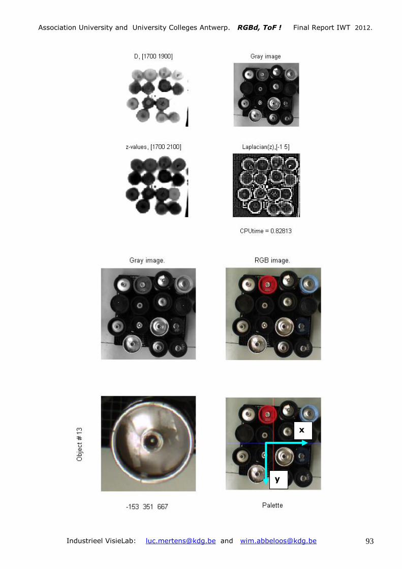
Association University and University Colleges Antwerp. RGBd, ToF ! Final Report IWT 2012.
Industrieel VisieLab: [email protected] and [email protected] 93
x
y

Association University and University Colleges Antwerp. RGBd, ToF ! Final Report IWT 2012.
Industrieel VisieLab: [email protected] and [email protected] 94
8. Gesture based interfacing (DepthSense 311)
SoftKinetic
Confidence Map L/D Depth Map (ToF) Colour Map160 x 120 pix. 160 x 120 pix. 640 x 480 pix.
Anno 2011
RGBd,
ToF
DepthSense 311
The future has begun

Association University and University Colleges Antwerp. RGBd, ToF ! Final Report IWT 2012.
Industrieel VisieLab: [email protected] and [email protected] 95
Algorithms useful for Time of Flight cameras: Wim Abbeloos.
The next set of algorithms were developed during the project. We keep them as a collection since
they can inspire programmers at a given moment. To keep a good overview most of these
functions are directly present in the main program.
Nevertheless in combination with toolboxes for the SwissRanger cameras, toolboxes for the Fotonic
cameras, the ToF-functionalities in Halcon, Matlab, C++ and OpenCV they give a practical
solution for typical problems of Material Handling (Robotics) and Navigation (AGVs and
Wheelchairs).
function alg = algorithms()
alg.startcamera = @ startcamera;
alg.getframe = @ getframe;
alg.stopcamera = @ stopcamera; % Start / acquire image / stop .
alg.calcnormal = @ calcnormal; % Calculate normal vector.
alg.calcavgnormal = @ calcavgnormal; % Calculate average normal vector.
alg.displaynormal = @ displaynormal; % Display normal.
alg.D2cam = @ D2cam; % From distances to camera x, y, z.
alg.z2cam = @ z2cam; % From camera z to camera x, y,D.
alg.cam2vehicle = @ cam2vehicle; % From camera to AGV-world.
alg.view2D = @ view2D; % Common 2D-plot.
alg.view3D = @ view3D; % Common 3D-plot.
alg.startmotor = @ startmotor; % Start/ command / stop motor.
alg.stopmotor = @ stopmotor;
alg.motorcmd = @ motorcmd;
function cam = startcamera( inttime )
dllname = 'O3D2xxCamera'; headername = 'O3D2xxCameraMatlab.h';
IP = '192.168.0.69'; XMLPort = uint32( 8080 );
hwnd = libpointer( 'uint32Ptr', 0 );
FWversion = libpointer( 'stringPtr', 'xxxxxx' );
SensorType = libpointer( 'stringPtr', 'xxxxxxxxxx' );
if ~libisloaded( dllname ) loadlibrary( dllname, headername ); end;
for c = 1:3 % Try to connect camera.
[ answer, hwnd, IP, FWversion, SensorType ] = calllib( dllname,…
'O3D2XXConnect', hwnd, IP, XMLPort, FWversion, SensorType );
if answer == 0 disp( 'Camera Connected' );
calllib( dllname, 'O3D2XXPerformHeartBeat' ); break;
else calllib( dllname, 'O3D2XXDisconnect', 1 );
disp( strcat( 'Failed to connect, attempt no', num2str(c) ) );
if ( c == 3 ) error( 'Failed to connect' ); end; end; end;
% Software trigger
% Trigger type: 1 for pos. edge, 2 for neg. edge, 3 for free running and 4
% for software trigger
calllib( dllname, 'O3D2XXSetTrigger', 4 );
head = libpointer( 'int32Ptr', zeros( 1, 21 * 4 ) );
SIZE = uint32( 64 * 50 * 4 );
dat = libpointer( 'uint8Ptr', zeros( 1, SIZE ) ); TCPport = int32( 50002 );
cam = struct( 'dllname', dllname, 'dat', dat, 'SIZE', SIZE, 'head', head,…
'TCPport', TCPport);
% Set frontend data
% 3 -> 6.5m, 1 -> 7.4, 0 -> 6.5
% 1. ModulationFrequency [0,1,2,3] default = 0
% 6.51m 7.38m 7.40m 45m
% Modulation Frequency 0 (23MHz) 1 (20.4MHz) 2 (20.6MHz)
% 2. Single or double sampling normal/high dynamic

Association University and University Colleges Antwerp. RGBd, ToF ! Final Report IWT 2012.
Industrieel VisieLab: [email protected] and [email protected] 96
% 3. Illumode: 0 = turn all Illuminations off, 1 = Illumination a on,
2 = Illumination b off, 3 = a and b on.
% 4. First integration time [us] (single sampling mode), 1-5000, default 2000
% 5. Second integration time [us] (double sampling mode), 1-5000
% 6. Delay time [ms] default = 141
setfrontend = libpointer( 'int32Ptr', [1, 0, 3, inttime, inttime, 0] );
calllib( dllname, 'O3D2XXSetFrontendData', setfrontend );
function frame = getframe( cam )
calllib( cam.dllname, 'O3D2XXTriggerImage' );
datmode = int8( 'd' );
[ answer, data, header ] = calllib( cam.dllname, 'O3D2XXGetImageData',…
datmode, cam.dat, cam.SIZE, cam.head, cam.TCPport );
frame.D = double( typecast( data, 'single' ) );
frame.D = reshape( frame.D, 64, 50 );
datmode = int8( 'i' );
[ answer, data, header ] = calllib( cam.dllname, 'O3D2XXGetImageData', ...
datmode, cam.dat, cam.SIZE, cam.head, cam.TCPport );
frame.L = double( typecast( data, 'single' ) );
frame.L = reshape( frame.L, 64, 50 );
Head = double(typecast(header(1:21),'single'));
frame.time = Head(12:13);
function stopcamera()
dllname = 'O3D2xxCamera';
for c = 1:3
answer = calllib( dllname, 'O3D2XXDisconnect', 1 );
if answer == 0 disp( 'Camera disconnected' ); break;
else
disp( strcat( 'Failed to disconnect, attempt no', num2str(c) ) );
pause(0.5); end; end;
if libisloaded( dllname ) unloadlibrary( dllname ); end;
function normal = calcnormal( x, y, z, filtersize, fdir )
% fdir: filter direction
% Define filters
if fdir == 1 f1 = zeros( filtersize ); f1(1) = 1; f1(end) = -1;
f2 = fliplr( f1 );
else f1 = zeros( 1, filtersize ); f1(1) = 1; f1(end) = -1; f2 = f1'; end;
x1 = imfilter( x, f1 ); x2 = imfilter( x, f2 ); % Filter image.
y1 = imfilter( y, f1 ); y2 = imfilter( y, f2 );
z1 = imfilter( z, f1 ); z2 = imfilter( z, f2 );
v1 = cat( 3, x1, y1, z1 ); % Create vector1, vector2 and Normal vector.
v2 = cat( 3, x2, y2, z2 ); v = cross( v1, v2 );
SumV = sqrt( sum( v.*v, 3 ) ); % Normalize.
SumV = repmat( SumV, [ 1 1 3 ] ); normal = v ./ SumV;
function normal = calcavgnormal( x, y, z, filtersize )
normal1 = calcnormal( x, y, z, filtersize, 0 );
normal2 = calcnormal( x, y, z, filtersize, 1 );
mnorm = ( normal1 + normal2 ) / 2;
SumV = sqrt( sum( mnorm.*mnorm, 3 ) ); % Normalize.
SumV = repmat( SumV, [ 1 1 3 ] ); normal = mnorm ./ SumV;
function N = displaynormal( normal )
N = normal / 2 + 0.5; N(:,:,3) = 1 - N( :, :, 3 );
function [x y z R phi] = D2cam( D, f )

Association University and University Colleges Antwerp. RGBd, ToF ! Final Report IWT 2012.
Industrieel VisieLab: [email protected] and [email protected] 97
[I J] = size( D ); I2 = I/2; J2 = J/2;
ff = f * f; u = (1:J) - (J2+0.5); uu = u .* u;
v = (1:I) - (I2+0.5); vv = v .* v;
U = repmat( u , [I 1]); UU = repmat( uu, [I 1]);
V = repmat( v', [1 J]); VV = repmat( vv',[1 J]);
UUff = UU + ff; r = sqrt( UUff ); d = sqrt( VV + UUff );
Dd = D ./ d; R = r .* Dd; phi = atan2( U, f );
x = U .* Dd; y = -V .* Dd; z = f * Dd;
function [x y z D] = z2cam( z, f )
[J I] = size( z ); I2 = I/2; J2 =J/2; % Calculate pixel coordinates
x = repmat( ( (1:I) - (I2+0.5) ), J, 1 ) .* (z / f);
y = repmat( ( (J2+0.5) - (1:J)' ), 1, I ) .* (z / f);
D = sqrt( x .^ 2 + y .^ 2 + z .^ 2 );
function [x y z] = cam2vehicle( x, y, z, ca )
% ca: Camera Angle to horizon, negative for looking down
zt = z .* cosd(ca) - y.* sind(ca); yt = z .* sind(ca) + y.* cosd(ca);
z = zt; y = yt;
function view2D( x, z )
plot( x, z, 'ko', 'MarkerSize', 2 ); set( gca, 'DataAspectRatio', [1 1 1]); axis off;
function view3D( x, y, z )
plot3(x,y,z,'ko','MarkerSize',2); set(gca,'DataAspectRatio',[1 1 1]); axis off;
function startmotor()
global motor;
delete( instrfind ); % Start serial communication
motor = serial( 'COM7', 'BaudRate', 9600, 'Parity', 'none', 'DataBits', 8, …
'StopBits', 2, 'Timeout', 0.2 );
fopen( motor );
motorcmd( 'disabletimeout' ); motorcmd( 'enablereg' ); motorcmd( 'resetenc' );
motorcmd('setmode',3); motorcmd('setspeed1',0); motorcmd('setspeed2',0);
motorcmd( 'setaccel', 10 );
function stopmotor() % Stop serial communication.
global motor;
motorcmd('setmode',3); motorcmd('setspeed1',0); motorcmd('setspeed2',0);
motorcmd( 'enabletimeout' );
fclose( motor ); delete( motor ); clear( 'motor' );
function varargout = motorcmd( cmd, varargin ) % MOTOR COMMANDS.
global motor;
if ~ischar( cmd ) error( 'Second argument must be a command string' ); end;
switch cmd
case 'getspeed1'
fwrite(motor,[0 33],'int8'); % returns the current requested speed of motor 1
varargout(1) = { fread( motor, 1, 'uint8' ) };
case 'getspeed2'
fwrite(motor,[0 34],'int8'); % returns the current requested speed of motor 2
varargout(1) = { fread( motor, 1, 'uint8' ) };
case 'getenc1' % Motor 1.
fwrite(motor,[0 35],'uint8'); % 4 bytes returned high byte first (signed).
val = fread( motor, 4, 'uint8' );
val2 = uint32( bitcmp( uint8(val) ) );
val3 = bitshift(val2(1),24)+bitshift(val2(1),16)+bitshift(val2(3),8)+val2(4);
varargout(1) = { val3 };
case 'getenc2' % Motor 2.
fwrite(motor,[0 36],'uint8'); % 4 bytes returned high byte first (signed).
val = fread( motor, 4, 'uint8' );

Association University and University Colleges Antwerp. RGBd, ToF ! Final Report IWT 2012.
Industrieel VisieLab: [email protected] and [email protected] 98
val2 = uint32( bitcmp( uint8(val) ) );
val3 = bitshift(val2(1),24)+bitshift(val2(1),16)+bitshift(val2(3),8)+val2(4);
varargout(1) = { val3 };
case 'getencs'
fwrite(motor,[0 37],'uint8'); % Returns 8 bytes. Encoder1/encoder2 count.
varargout(1) = { fread( motor, 8, 'uint8' ) };
case 'getvolts'
fwrite( motor, [0 38], 'uint8' ); % Returns the input battery voltage level.
varargout(1) = { fread( motor, 1, 'uint8' ) };
case 'getcurrent1'
fwrite( motor, [0 39], 'uint8' ); % Returns the current drawn by motor 1.
varargout(1) = { fread( motor, 1, 'uint8' ) };
case 'getcurrent2'
fwrite( motor, [0 40], 'uint8' ); % returns the current drawn by motor 2.
varargout(1) = { fread( motor, 1, 'uint8' ) };
case 'getversion'
fwrite( motor, [0 41], 'uint8' ); % Returns the software version.
varargout(1) = { fread( motor, 1, 'uint8' ) };
case 'getaccel'
fwrite( motor, [0 42], 'uint8' ); % Returns the current acceleration level.
varargout(1) = { fread( motor, 1, 'uint8' ) };
case 'getmode'
fwrite( motor, [0 43], 'uint8' ); % Returns the currently selected mode.
varargout(1) = { fread( motor, 1, 'uint8' ) };
case 'getVI'
fwrite( motor, [0 44], 'uint8' ); % Returns Volts, current1 and current2.
varargout(1) = { fread( motor, 1, 'uint8' ) }; % Battery voltage
varargout(2) = { fread( motor, 1, 'uint8' ) }; % Current motor 1
varargout(3) = { fread( motor, 1, 'uint8' ) }; % Current motor 2
case 'setspeed1'
if nargin ~= 2 error( 'Incorrect number of input arguments' ); end;
speed = cell2mat(varargin(1));
fwrite( motor, [0 49 speed], 'int8' ); % set new speed1
case 'setspeed2'
if nargin ~= 2 error( 'Incorrect number of input arguments' ); end;
speed = cell2mat(varargin(1));
fwrite( motor, [0 50 speed], 'int8' ); % set new speed2
case 'setaccel'
if nargin ~= 2 error( 'Incorrect number of input arguments' ); end;
accel = cell2mat(varargin(1));
fwrite( motor, [0 51 accel], 'uint8' ); % set new acceleration
case 'setmode'
if nargin ~= 2 error( 'Incorrect number of input arguments' ); end;
mode = cell2mat(varargin(1));
fwrite( motor, [0 52 mode], 'uint8' ); % Set the mode.
case 'resetenc'
fwrite( motor, [0 53], 'uint8' ); % Zero both of the encoder counts.
case 'disablereg'
fwrite(motor,[0 54],'uint8'); Power output not changed by encoder feedback
case 'enablereg'
fwrite(motor,[0 55],'uint8'); Power output is regulated by encoder feedback
case 'disabletimeout'
fwrite( motor, [0 56], 'uint8' ); % Continuous output if no-regular ommands.
case 'enabletimeout'
fwrite( motor, [0 57], 'uint8' ); % Watch dog, 2 seconds.
otherwise
error( 'Incorrect command' );
end;
Association University and University Colleges Antwerp. RGBd, ToF ! Final Report IWT 2012.
Industrieel VisieLab: [email protected] and [email protected] 99
Part 2 (pages 99 -> 170)
Deel 2 van het verslag handelt vooral in op de wijze waarop allerlei ToF-camera’s in Matlab en in Halcon aangesproken kunnen worden. Een aantal programma’s werden meer als een totale applicatie benaderd, zodat software en hardware aspecten meer inpliciet aan bod zullen komen.
Inhoud van deel 2. 1. IFM O3D2xx cameras ( www.ifm-electronic.com )................................................................................ 100
1.1. Camera connectie met behulp van de bijgeleverde files. ................................................................. 100
1.2. Camera connection based on Java TCP IP ......................................................................................... 105
2. MESA Swiss Ranger SR4000 ( www.mesa.com ) ................................................................................... 108
3. Fotonic Z-70 ( www.fotonic.com ) ...................................................................................................... 110
4. DepthSense 311 ( www.Softkinetic.com ) ............................................................................................. 112
5. uEye RGB camera ( www.IDS-imaging.com ) ......................................................................................... 114
6. De motoren van de AGV. ....................................................................................................................... 115
7. Wheelchair navigation (Rolstoel Permobil). .......................................................................................... 121
8. Wall segmentation in the outdoor application of Vision & Robotics. ................................................... 122
9. Path planning for the indoor application at Vision & Robotics. ............................................................ 125
Free navigation in a world with a known map. ............................................................................................. 125
9.1. The Brushfire algorithm ( Principles of Robot Motion: Howie Choset,… ) ........................................ 125
9.2. The Wave Front Algorithm ................................................................................................................ 126
9.3. Combined Algorithm: ( Wave Front and Distance Repulsion ). ......................................................... 127
10. Localisation ........................................................................................................................................ 128
10.1. Punten ........................................................................................................................................... 128
10.2. Muren ......................................................................................... Fout! Bladwijzer niet gedefinieerd.
11. AGV sturing ........................................................................................................................................ 136
12. Camera calibrations: Color and TOF camera. .................................................................................. 137
13. Halcon ( Industrial Vision Package of MVTec (www.mvtec.com )..................................................... 142
13.1. Halcon in combination with IFM O3D201 (ifm-electronic) ........................................................... 142
13.2. Halcon in combination with Mesa SR4000 ( www.mesa.com ) .................................................... 147
13.3. Halcon used on an AGV in combination with a MESA SR4000. .................................................... 149
14. Vision & Robotics 2012 demo. Fotonic camera. ............................................................................... 150

Association University and University Colleges Antwerp. RGBd, ToF ! Final Report IWT 2012.
Industrieel VisieLab: [email protected] and [email protected] 100
1. IFM O3D2xx cameras ( www.ifm-electronic.com )
1.1. Camera connectie met behulp van de bijgeleverde files. We maken gebruik van de bijgeleverde functiebibliotheek voor alle communicatie tussen camera en
computer. Er is enkel een 32 bit dll bestand, dit is dus enkel mogelijk voor 32 bit applicaties (niet
mogelijk in 64-bit matlab!). De bijgevoegde header bestanden (met .h extensie ) dienen ook in
dezelfde directory aanwezig te zijn.
Er werden enkele wijzigingen in de header bestanden aangebracht om de compatibiliteit met de oudere
MATLAB versies te verzekeren.
Installeer de bijgevoegde software.
Voor computers onder toezicht dient een nieuwe regel aan de firewall settings te worden toegevoegd om
de applicaties toe te laten me de camera te communiceren.
Gebruik de bijgevoegde software om de netwerkparameters van de camera te achterhalen.
( Het IP-adres is standaard 192.168.0.69, maar kan gewijzigd zijn). (De netwerkparameters zijn ook
rechtstreeks op de camera op te vragen). Na wijziging dient de camera opnieuw te worden opgestart.
Gebruik de bijgevoegde software om de camera terug om te schakelen naar fabrieksinstellingen voor
verder gebruik.
Beschrijving van de ‘frontend-data’: Setting front-end data
1. Modulation Frequency Parameter
Value Frequency (MHz)
Max. Range (m)
Remarks
0 23 6.5172 Default Points outside of range will be
measured at distance with equivalent phase angle in range. (eg. 7.51m as 1m)
1 20.4 7.3862 Points outside of range will be measured at distance with equivalent phase angle in range. (eg. 8.39m as 1m)
2 20.6 7.4059 Only works when in double sampling mode. In single sampling mode returns -2 ( bug? )
Points outside of range will be measured at distance with equivalent phase angle in range. (eg. 8.41m as 1m)
3 Multiple 6.51 Points outside of range will be set to -2
4 Multiple 45 Only works when in double sampling mode. In single sampling mode returns -2 ( bug? )
2. Sampling mode
Parameter Value Description
0 Single Sampling ( Use 1 integration time ) 1 Double Sampling ( Use 2 integration times )
3. Illumination mode
Parameter Value Description
0 Turn all illumination off

Association University and University Colleges Antwerp. RGBd, ToF ! Final Report IWT 2012.
Industrieel VisieLab: [email protected] and [email protected] 101
1 Illumination a on 2 Illumination b off 3 Illumination a and b on ( recommended )
4. First integration time:
Minimum: 0 µs Maximum: 5000 µs Default: 125 µs.
5. Second integration time: Minimum: 0 µs Maximum: 5000 µs Default: 200 µs.
6. Delay time (ms): Default: 141 ms
Remark:
Underexposed pixels are set to -2, overexposed pixels are set to -1. Out-of-range pixels are set to -2 (only) when using Modulation Frequency 3.
function IFM_dll_all3()
% Prepare new session
clear all; close all; clc;
% Declare global variables
global D L xc yc zc e f g frame;
% Camera communication parameters
cam.ip = '192.168.0.71';
cam.xmlPort = 8080;
cam.tcpPort = 50002;
% Camera settings
cam.trigger = 4;
cam.averageDetermination = 1;
cam.meanFilter = 0;
cam.medianFilter = 0;
% Camera front-end data
cam.modulationFrequency = 1;
cam.samplingMode = 0;
cam.illuminationMode = 3;
cam.shortIntegrationTime = 300;
cam.longIntegrationTime = 300;
cam.delayTime = 141;
% Start camera
ifm_start( cam );
% Get a frame
ifm_getframe();
% Stop camera
ifm_stop();
% Convert D to x y z from distance and camera vectors
xt = D .* e;
yt = D .* f;
zt = D .* g;
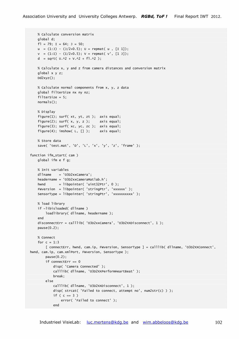
Association University and University Colleges Antwerp. RGBd, ToF ! Final Report IWT 2012.
Industrieel VisieLab: [email protected] and [email protected] 102
% Calculate conversion matrix
global d;
fl = 79; I = 64; J = 50;
u = (1:J) - (J/2+0.5); U = repmat( u , [I 1]);
v = (1:I) - (I/2+0.5); V = repmat( v', [1 J]);
d = sqrt( U.^2 + V.^2 + fl.^2 );
% Calculate x, y and z from camera distances and conversion matrix
global x y z;
Dd2xyz();
% Calculate normal components from x, y, z data
global filterSize nx ny nz;
filterSize = 5;
normals();
% Display
figure(1); surf( xt, yt, zt ); axis equal;
figure(2); surf( x, y, z ); axis equal;
figure(3); surf( xc, yc, zc ); axis equal;
figure(4); imshow( L, [] ); axis equal;
% Store data
save( 'test.mat', 'D', 'L', 'x', 'y', 'z', 'frame' );
function ifm_start( cam )
global ifm e f g;
% Init variables
dllname = 'O3D2xxCamera';
headername = 'O3D2xxCameraMatlab.h';
hwnd = libpointer( 'uint32Ptr', 0 );
FWversion = libpointer( 'stringPtr', 'xxxxxx' );
SensorType = libpointer( 'stringPtr', 'xxxxxxxxxx' );
% load library
if ~libisloaded( dllname )
loadlibrary( dllname, headername );
end
disconnectErr = calllib( 'O3D2xxCamera', 'O3D2XXDisconnect', 1 );
pause(0.2);
% Connect
for c = 1:3
[ connectErr, hwnd, cam.ip, FWversion, SensorType ] = calllib( dllname, 'O3D2XXConnect',
hwnd, cam.ip, cam.xmlPort, FWversion, SensorType );
pause(0.2);
if connectErr == 0
disp( 'Camera Connected' );
calllib( dllname, 'O3D2XXPerformHeartBeat' );
break;
else
calllib( dllname, 'O3D2XXDisconnect', 1 );
disp( strcat( 'Failed to connect, attempt no', num2str(c) ) );
if ( c == 3 )
error( 'Failed to connect' );
end

Association University and University Colleges Antwerp. RGBd, ToF ! Final Report IWT 2012.
Industrieel VisieLab: [email protected] and [email protected] 103
end
end
% Set parameters
setTriggerErr = calllib( dllname, 'O3D2XXSetTrigger', cam.trigger );
setAverageDeterminationErr = calllib( dllname, 'O3D2XXSetAverageDetermination',
cam.averageDetermination );
setMeanFilterErr = calllib( dllname, 'O3D2XXSetMeanFilterStatus', cam.meanFilter );
setMedianFilterErr = calllib( dllname, 'O3D2XXSetMedianFilterStatus', cam.medianFilter );
% Check filters
O3D2XXFilterStatus = struct( 'MedianFilter', 2, 'MeanFilter', 2 );
[getFilterStatusErr O3D2XXFilterStatus] = calllib( dllname, 'O3D2XXGetFilterStatus',
O3D2XXFilterStatus );
% Reset front-end data
resetFrontendErr = calllib( dllname, 'O3D2XXResetFrontend' );
% Set front-end data
head = libpointer( 'int32Ptr', zeros( 1, 21 * 4 ) );
SIZE = uint32( 64 * 50 * 4 );
dat = libpointer( 'uint8Ptr', zeros( 1, SIZE ) );
ifm = struct( 'dllname', dllname, 'dat', dat, 'SIZE', SIZE, 'head', head, 'TCPport',
int32(cam.tcpPort) );
frontend = libpointer( 'int32Ptr', [ cam.modulationFrequency, cam.samplingMode,
cam.illuminationMode,cam.shortIntegrationTime,cam.longIntegrationTime,min( cam.delayTime,141)]);
setFrontendErr = calllib( dllname, 'O3D2XXSetFrontendData', frontend );
pause(0.2);
% Trigger image
triggerErr = calllib( 'O3D2xxCamera', 'O3D2XXTriggerImage' );
% Get pixel vectors
datmode = 'efg';
for c1 = 1:length(datmode)
[ getImageDataErr, data, header ] = calllib( 'O3D2xxCamera', 'O3D2XXGetImageData',
int8(datmode(c1)), ifm.dat, ifm.SIZE, ifm.head, ifm.TCPport );
eval([datmode(c1) '= reshape( double( typecast( data, ''single'' ) ), 64, 50 );']);
end
% Get first frame
ifm_getframe();
function ifm_getframe()
global ifm D L xc yc zc header;
% Trigger next image
triggerErr = calllib( 'O3D2xxCamera', 'O3D2XXTriggerImage' );
% Read data
datmode = 'Dixyz';
varname = { 'D' 'L' 'xc' 'yc' 'zc' };
for c1 = 1:length(datmode)
[ getImageDataErr, data, theader ] = calllib( 'O3D2xxCamera', 'O3D2XXGetImageData',
int8(datmode(c1)), ifm.dat, ifm.SIZE, ifm.head, ifm.TCPport );
eval([cell2mat(varname(c1)) '= reshape(double(typecast(data,''single'')),64,50);']);
header = double( typecast( theader, 'single') );
headerinfo();
end

Association University and University Colleges Antwerp. RGBd, ToF ! Final Report IWT 2012.
Industrieel VisieLab: [email protected] and [email protected] 104
function ifm_stop()
for c = 1:3
disconnectErr = calllib( 'O3D2xxCamera', 'O3D2XXDisconnect', 1 );
if disconnectErr == 0
disp( 'Camera disconnected' );
break;
else
disp( strcat( 'Failed to disconnect, attempt no', num2str(c) ) );
pause(0.5);
end
end
if libisloaded( 'O3D2xxCamera' )
unloadlibrary( 'O3D2xxCamera' );
end
function headerinfo()
global header frame;
imageTypes = {'INVALID_IMAGE', 'DISTANCE_IMAGE', 'INTERNAL_DATA_A', 'AMPLITUDE_IMAGE',
'INTERNAL_DATA_B', 'NORMAL_X_IMAGE', 'NORMAL_Y_IMAGE', ...
'NORMAL_Z_IMAGE', 'KARTESIAN_X_IMAGE', 'KARTESIAN_Y_IMAGE',
'KARTESIAN_Z_IMAGE', 'INTERNAL_DATA_C', 'SEGMENTATION_IMAGE' };
frame.dataSize = header(1); % Size of data (bytes)
frame.headerSize = header(2); % Size of header (bytes)
frame.imageType = imageTypes{header(3)+1};
frame.version = header(4);
frame.samplingMode = header(5);
frame.illuMode = header(6);
frame.frequencyMode = header(7);
frame.unambRange = header(8); % Unambiguous range in meters
frame.evalTime = header(9); % Evaluation time (in ms)
frame.intTime1 = header(10); % First intergration time (in single sampling mode)
frame.intTime2 = header(11); % Second intergration time (in double sampling mode)
frame.time = header(12) + header(13)*10.^(-6); % Timestamp (number of seconds since
camera startup)
frame.medianav = header(14);
frame.meanav = header(15);
frame.average = header(16);
frame.valid = header(17);
frame.errorCode = header(18);
frame.temperature = header(19);
frame.trigger = header(20);
frame.ifmTime = header(21);
function normals()
global x y z nx ny nz filterSize;
% Calculate normal
f1 = zeros(1, filterSize); f1(1) = 1; f1(end) = -1; f2 = f1';
z1 = conv2( z, f1, 'same' ); z2 = conv2( z, f2, 'same' );
x1 = conv2( x, f1, 'same' ); x2 = conv2( x, f2, 'same' );
y1 = conv2( y, f1, 'same' ); y2 = conv2( y, f2, 'same' );
% Calculate normal components
nx = y1.*z2-z1.*y2; ny = z1.*x2-x1.*z2; nz = x1.*y2-y1.*x2;

Association University and University Colleges Antwerp. RGBd, ToF ! Final Report IWT 2012.
Industrieel VisieLab: [email protected] and [email protected] 105
% Normalize
n = sqrt( nx.^2 + ny.^2 + nz.^2 );
nx = nx ./ n; ny = ny ./ n; nz = nz ./ n;
function Dd2xyz()
global D d x y z;
% Convert D to x, y, z using conversion matrix
Dd = D ./ d;
x = U .* Dd;
y = -V .* Dd;
z = fl * Dd;
1.2. Camera connection based on Java TCP IP Er wordt gebruik gemaakt van de functie jtcp (java TCP-IP communicatie) die terug te vinden is op de
mathworks File-Exchange website. De communicatie verloopt volgens de XML-RPC standaard.
De namen van de functies en hun respectievelijke parameters zijn terug te vinden in de IFM O3D201
programmeerhandleiding.
Voor elke instelling dient een bericht opgebouwd te worden uit verschillende delen dat vervolgens
wordt samengevoegd en doorgestuurd met een ‘write’ commando. Vervolgens kan het antwoord van de
camera uitgelezen worden met een ‘read’ commando.
function ifm_xml()
% Prepare new session
clear all; close all; clc;
% Declare global variables
global cam1 D L x y z;
% Define camera parameters
cam1.HOST = '192.168.0.69';
cam1.DATAPORT = 50002;
cam1.XMLPORT = int16(8080);
cam1.TrigType = 4;
cam1.ModFreq = 0;
cam1.SampMode = 0;
cam1.IntTimeBig = 1000;
cam1.IntTimeSmall = 1000;
cam1.ifmTime = 141; % Must be atleast 141 in triggermode 4 to prevent camera damage
cam1.averaging = 1;
cam1.median = 0;
cam1.mean = 0;
ifmstart();
% Open new figure
figure(1); colormap( 'gray' );
h11 = subplot(121); h1 = imagesc(L); title( 'Intensity' ); axis image; axis off;
set( h11, 'CLim', [0 20] );
h22 = subplot(122); h2 = imagesc(D); title( 'Distance' ); axis image; axis off;
set( h22, 'CLim', [0 5] );

Association University and University Colleges Antwerp. RGBd, ToF ! Final Report IWT 2012.
Industrieel VisieLab: [email protected] and [email protected] 106
% Acquisition loop
nloop = 100;
for c1 = 1:nloop
% Get next frame
ifmgetframe();
%Display data
set( h1, 'CData', L );
set( h2, 'CData', D );
drawnow;
end
ifmstop();
% Write data
save( 'test.mat', 'D', 'L', 'x', 'y', 'z' );
function ifmstart()
global cam1;
% Request connection configuration port
cam1.jTcpObjXML = jtcp('REQUEST',cam1.HOST,cam1.XMLPORT,'TIMEOUT',2000);
% Request connection data port
cam1.jTcpObj = jtcp('REQUEST',cam1.HOST,cam1.DATAPORT,'TIMEOUT',200);
cam1.jTcpObj.socket.setReceiveBufferSize(400000);
disp( 'Connected' );
% Disconnect camera
disconnect_data = sendXML( 'MDAXMLDisconnect', num2str(cam1.HOST) );
% Connect camera
connect_data = sendXML( 'MDAXMConnect', num2str(cam1.HOST), 1 );
% Reset camera
averaging_data = sendXML( 'MDAXMLSetProgram', 0, 0, 7 );
% Change trigger type
settrigger_data = sendXML( 'MDAXMLSetTrigger', 0, 0, cam1.TrigType );
% Set frontend data
setfrontend_data = sendXML( 'MDAXMLSetFrontendData', 0, cam1.ModFreq, cam1.SampMode, 0,
cam1.IntTimeSmall, cam1.IntTimeBig, 20, cam1.ifmTime );
% Set averaging
averaging_data = sendXML( 'MDAXMLSetAverageDetermination', 0, 0, cam1.averaging );
% Set median filter
median_data = sendXML( 'MDAXMLSetMedianFilterStatus', 0 );
% Set mean filter
mean_data = sendXML( 'MDAXMLSetMeanFilterStatus', 0 );
% Trigger
trigger_data = sendXML( 'MDAXMLTriggerImage' );

Association University and University Colleges Antwerp. RGBd, ToF ! Final Report IWT 2012.
Industrieel VisieLab: [email protected] and [email protected] 107
% Get first frame
ifmgetframe();
function ifmgetframe()
global D L x y z cam1;
HEADERSIZE = 94;
OVERALLIMAGESIZE = (64*50 + HEADERSIZE) * 4;
% Trigger
trigger_data = sendXML( 'MDAXMLTriggerImage' );
% Request and read data
msg = int8('Dixyz');
jtcp('WRITE',cam1.jTcpObj,msg);
h = tic;
while (cam1.jTcpObj.dataInputStream.available < (OVERALLIMAGESIZE * length(msg)))
if toc(h) > 2
disconnect_data = sendXML( 'MDAXMLDisconnect', num2str(cam1.HOST) );
ifmstop();
error( 'Timeout: no response during image acquisition' );
end
end
data = jtcp('read',cam1.jTcpObj,'MAXNUMBYTES',OVERALLIMAGESIZE);
RealData=swapbytes(typecast(data, 'single'));
D = reshape(RealData(HEADERSIZE+1:end), 64, 50);
data = jtcp('read',cam1.jTcpObj,'MAXNUMBYTES',OVERALLIMAGESIZE);
RealData=swapbytes(typecast(data, 'single'));
L = reshape(RealData(HEADERSIZE+1:end), 64, 50);
data = jtcp('read',cam1.jTcpObj,'MAXNUMBYTES',OVERALLIMAGESIZE);
RealData=swapbytes(typecast(data, 'single'));
x = reshape(RealData(HEADERSIZE+1:end), 64, 50);
data = jtcp('read',cam1.jTcpObj,'MAXNUMBYTES',OVERALLIMAGESIZE);
RealData=swapbytes(typecast(data, 'single'));
y = reshape(RealData(HEADERSIZE+1:end), 64, 50);
data = jtcp('read',cam1.jTcpObj,'MAXNUMBYTES',OVERALLIMAGESIZE);
RealData=swapbytes(typecast(data, 'single'));
z = reshape(RealData(HEADERSIZE+1:end), 64, 50);
function ifmstop()
global cam1;
disconnect_data = sendXML( 'MDAXMLDisconnect', num2str(cam1.HOST) );
jtcp('close',cam1.jTcpObjXML);
msg = int8('q');
jtcp('WRITE',cam1.jTcpObj,msg);
jtcp('close',cam1.jTcpObj);
function answer = sendXML( func_name, varargin )
global cam1;

Association University and University Colleges Antwerp. RGBd, ToF ! Final Report IWT 2012.
Industrieel VisieLab: [email protected] and [email protected] 108
% Create body
body = ['<?xml version="1.0" encoding="UTF-8"?>' 13 10 '<methodCall><methodName>' func_name
'</methodName>' 13 10 '<params>'];
% Add arguments
for c1 = 1:nargin-1
if ischar(varargin{c1})
body = [body '<param><value>' varargin{c1} '</value></param>'];
else
body = [body '<param><value><i4>' num2str(varargin{c1}) '</i4></value></param>'];
end
end
body = [body '</params></methodCall>' 13 10];
% Create header
header = ['POST /RPC2 HTTP/1.1' 13 10 'User-Agent: XMLRPC++ 0.7' 13 10 'Host: ' cam1.HOST
':' num2str(cam1.XMLPORT) 13 10 'Content-Type: text/xml' 13 10 'Content-length: '
num2str(length(body(:))) 13 10 13 10];
% Send message
jtcp('WRITE',cam1.jTcpObjXML,int8( [header body] ) );
% Wait for answer and receive data
h = tic;
while (cam1.jTcpObjXML.dataInputStream.available == 0)
if toc(h) > 2
disconnect_data = sendXML( 'MDAXMLDisconnect', num2str(cam1.HOST) );
ifmstop();
error( ['Timeout: no answer was received for following function: ' func_name] );
end
end
answer = jtcp('read',cam1.jTcpObjXML);
2. MESA Swiss Ranger SR4000 ( www.mesa.com ) Installeer de bijgeleverde MESA-software
Sluit de netwerk kabel en vervolgens de spanning (12V) aan ( Let op juiste polariteit ).
Stel het computer IP-adres in op 192.168.1.x
Voor computers onder toezicht is het noodzakelijk de gebruikte applicaties toe te voegen aan de firewall
regels om communicatie mogelijk te maken.
Gebruik ‘ping 192.168.1.y’ om te kijken of u het juiste adres van de camera kent.
Volg anders volgende instructies:
In order to set the static IP address of the camera, it is necessary to use a fall back address:
Apply power to the unit without connecting the Ethernet cable.
Wait 20 seconds before plugging in the network cable.
The camera now has a fixed IP address of 192.168.1.42. The camera cannot function normally using
this address: the only purpose is to set another static IP address.
In the following, the tool Telnet wil be used. This is not enabled by default on Windows platforms.
Here are the instructions to do this: 1. Start/Control Panel/Programs and Features

Association University and University Colleges Antwerp. RGBd, ToF ! Final Report IWT 2012.
Industrieel VisieLab: [email protected] and [email protected] 109
2. On left side, select \Turn Windows features on or off
3. Check Telnet, wait until it has been installed
Start now a command prompt or equivalent console. 1. Telnet to the camera: telnet 192.168.1.42 2. set the static address, e.g. fw_setenv staticip 192.168.1.33
Exit telnet and repower the camera with the network cable connected. The camera will always use the static address on power-on when attached to a host PC or network.
De camera is nu klaar voor gebruik.
% Start new session
clear all; close all; clc;
% Add camera control functions
addpath( strcat(cd,'/swissranger/') );
% Open camera connection
cam = sr_open;
% Set exposure
%res = sr_setautoexposure( cam, 0, 255, 100, 150 ); % Automatic exposure
res = sr_setintegrationtime( cam, 15 ); % Manual exposure
% Create figure
ha = axes( 'YDir', 'reverse', 'CLim', [0.5 1] );
hf = gcf;
set( hf, 'Colormap', colormap( 'gray' ) );
hi = image( 'cdata', zeros(144,176), 'CDataMapping', 'scaled', 'Parent', ha );
axis image;
for c1 = 1:50
% Trigger next image
sr_acquire( cam );
% Readout pointcloud
[ res, x, y, z ] = sr_coordtrf( cam );
% Readout raw data
D = sr_getimage( cam, 1 ); % Distance
L = sr_getimage( cam, 2 ); % Intensity
D = double( D )./ double( intmax( 'uint16' ) ) .* 5; % Convert phase to meters
% Rotate data
x = x'; x2(:,:,c1) = x;
y = y'; y2(:,:,c1) = y;
z = z'; z2(:,:,c1) = z;
D = D'; D2(:,:,c1) = D;
L = L'; L2(:,:,c1) = L;
% Draw to screen
set( hi, 'cdata', z );
drawnow;
end
% Close camera connection
sr_close( cam );

Association University and University Colleges Antwerp. RGBd, ToF ! Final Report IWT 2012.
Industrieel VisieLab: [email protected] and [email protected] 110
% Convert all data to doubles
x = double(x2);
y = double(y2);
z = double(z2);
D = double(D2);
L = double(L2);
% Store data
%save( 'test.mat', 'x', 'y', 'z', 'L', 'D' );
%save( 'test.mat', 'x', 'y', 'z', 'L', 'D' );
figure(100); surf(mean(x,3),mean(y,3),mean(z,3), 'LineStyle', 'none' ); axis equal;
cameratoolbar('Show'); cameratoolbar('SetMode','Orbit');
3. Fotonic Z-70 ( www.fotonic.com ) Installeer de bijgeleverde installatiebestanden.
Verbind alle connectoren (eerst netwerk, dan spanning aansluiten).
Verander het computer IP-adres naar 192.168.1.x
Voor computers onder toezicht moeten de firewall regels ingesteld worden die de programma’s toelaten
met de camera te communiceren!
Indien de spanning van de camera verbroken en terug aangesloten wordt en indien er geen netwerkkabel
is aangesloten, dan wordt het IP-adres na 50 seconden veranderd naar 192.168.1.10
Voer het EthConfig programma uit (\Fotonic\FZ-API\bin\x64\) om de camera IP in te stellen.
Type ‘ping 192.168.1.y’ in een commando venster om te controleren of de camera correct is
aangesloten.
Met behulp van ‘SetMode()’ kunnen verschillende modi geselecteerd worden (in matlab):
'Temporal'
'SpatioTemporal' 'MultiSpatioTemporal' 'zfine' 'zfast' 'MSSTcont' 'burstzfine'
'bursttemporal' There are different measurement modes in the camera. Each mode uses frames captured by sensor in different ways and most modes use several captures to calculate one frame. The characteristics of a measurement, e.g. motion blur, noise and accuracy will be different for the different modes. Generally the motion blur that is seen on the image and also accuracy will increase with the number of captures used to generate each frame. Temporal mode In temporal mode, the depth at each pixel is computed from the last four phase captures. This mode provides highest depth resolution per pixel. Spatio-Temporal mode In Spatio-Temporal mode, two captures are used to compute one frame. Bias cancellation is done temporally on the same pixel, whereas the arctangent function is computed on two adjacent pixels of the same row.

Association University and University Colleges Antwerp. RGBd, ToF ! Final Report IWT 2012.
Industrieel VisieLab: [email protected] and [email protected] 111
Multi-frequency Spatio-Temporal mode In Multi-frequency Spatio-Temporal mode, four captures are used to calculate one frame. The four captures are used to disambiguate the distance of the objects beyond the sensor nominal unambiguous range. Z-fast In zfast mode, the depth is calculated from a single capture, were the depth is calculated from two adjacent pixels. Z-fast do not utilize bias cancellation. This mode has the least motion artifacts. The resolution is lower and the noise levels are higher than in other modes. Z-fine In Z-fine mode, the depth of each pixel is calculated using two consecutive captures on each pixel. Z-fine does not utilize bias cancellation. This means highest resolution, small motion artifacts but slightly more noise than in e.g. temporal. Multishutter Spatio-Temporal Multi-shutter Spatio-Temporal is basically a High Dynamic version of Spatio-Temporal. Instead of using two captures, four captures is used. The first two frames are with the higher shutter time whilst capture three and four are using a lower shutter time. The parameter Saturation is used to determine the limit when a pixel is improper to use.If a pixel has to high signal(A-B > Saturation) it will be replaced with the one using the lower shutter. Burst Modes All modes except Z-fast are possible to run in Burst mode. The modes has the same characteristics as non burst but it uses a different image capture sequence. In non burst the camera sensor is set to capture a new image every x ms. This will make the camera produce a new frame every x:s ms since each frame needs for captures but each capture is used up 2-4 times. In Burst mode however, the camera sensor is set to capture 2-4 images as fast as possible. These captures are than used to produce one new frame. This continues so each capture is only used once for each frame. The big benefit of this is that the time between each capture can be kept short so there will be very little motion blur. The drawback is that the camera will not be able to send as many frames per second as with non burst modes.
clear all; close all; clc; format long;
addpath('CameraCtrl\')
Closeldu;
global cont;
cont.first = 1;
OpenCamera(); % Open sensor communication interface
StartSensor();
SetMode('Temporal');
it = 40; % Integration time
SetShutter(it); % Value in 0.1 ms
SetFrameRate(40); % Set frame rate to 20 fps
SetLightSwitchState(1); % Turn on LED's
for i=1:3
[x, y, z, L] = GrabImage();
end
tic;
for c1 = 1:50
[x, y, z, L] = GrabImage;

Association University and University Colleges Antwerp. RGBd, ToF ! Final Report IWT 2012.
Industrieel VisieLab: [email protected] and [email protected] 112
x2(:,:,c1) = x;
y2(:,:,c1) = y;
z2(:,:,c1) = z;
L2(:,:,c1) = L;
pause(0.02);
end
toc;
StopSensor();
CloseCamera();
Closeldu;
% Convert all data to doubles
x = double(x2);
y = double(y2);
z = double(z2);
L = double(L2);
% Store data
%save( 'B0_fot_exp40_d1920_o330.mat', 'x', 'y', 'z', 'L' );
ih1 = imshow( z(:,:,50), [0 500] );
% figure(100); surf(mean(x,3),mean(y,3),mean(z,3), 'LineStyle', 'none' ); axis equal;
% cameratoolbar('Show'); cameratoolbar('SetMode','Orbit');
4. DepthSense 311 ( www.Softkinetic.com ) Er wordt gebruik gemaakt van een meegeleverde 32-bit .dll functiebibliotheek voor alle
cameracommunicatie.
De nieuwste drivers ( na de versie 2.3.10.0) zijn NIET compatibel met Matlab.
De optrima.h header-file werd aangepast om compatibiliteit met oudere Matlab versies te verzekeren.
function depthsense()
clear all; close all; clc;
global intens D L x y z nx ny nz f;
f = 150; intens = 20;
start_DS();
update_data();
stop_DS();
figure(1); imshow(D, [0 3]); title('Distance');
figure(2); imshow(L, []); title('Intensity');
figure(3); imshow(z, [0 3]); title('z');
function start_DS()
global pmap lmap plength llength confthresh range U V d f intens;
% LOAD LIBRARY
if libisloaded( 'optrima' )
unloadlibrary( 'optrima' );
end
dllname = 'liboptrima.dll';
headername = 'Optrima2.h';
warning('off');
[notfound warnings] = loadlibrary( dllname, headername, 'alias', 'optrima' );

Association University and University Colleges Antwerp. RGBd, ToF ! Final Report IWT 2012.
Industrieel VisieLab: [email protected] and [email protected] 113
warning('on');
% INITIALIZE VARIABLES
plength = libpointer( 'uint32Ptr', zeros( 1 ) );
llength = libpointer( 'uint32Ptr', zeros( 1 ) );
rangeval = libpointer( 'singlePtr', zeros( 1 ) );
pmap = libpointer( 'int16Ptr', zeros( 160,120,'int16' ) );
lmap = libpointer( 'uint16Ptr', zeros( 160,120,'uint16' ) );
confthresh = single(5);
% START CAMERA AND SET PROPERTIES
calllib( 'optrima', 'optrima_init');
pause(3);
errmsgx1 = calllib( 'optrima', 'optrima_set_property', 'ENABLE_RGB_EVENT_HANDLERS', 0 );
errmsgx2 = calllib( 'optrima', 'optrima_set_property', 'ENABLE_DENOISING', 0 );
errmsgx3 = calllib( 'optrima', 'optrima_set_property', 'ENABLE_LEAKAGE_ALGORITHM', 0 );
errmsgx4 = calllib( 'optrima', 'optrima_set_property', 'ENABLE_DENOISING', 0 );
errmsgx5 = calllib( 'optrima', 'optrima_set_property', 'OC310_ENABLE_SATURATION', 1 );
errmsgx6 = calllib( 'optrima', 'optrima_set_property', 'OC310_FRAMERATE', 25 );
% RESTART CAMERA
calllib( 'optrima', 'optrima_exit');
pause(1);
calllib( 'optrima', 'optrima_init');
pause(3);
errmsg1 = calllib( 'optrima', 'optrima_enable_camera' );
errmsg2 = calllib( 'optrima', 'optrima_enable_camera_rgb' );
pause(3);
% Get range
[errmsg4 range] = calllib( 'optrima', 'optrima_get_range', rangeval );
% Set intensity
calllib( 'optrima', 'optrima_set_light_intensity', uint8(intens));
I = 120; J = 160;
I2 = I/2; J2 = J/2;
ff = f * f;
u = (1:J) - (J2+0.5); uu = u .* u;
v = (1:I) - (I2+0.5); vv = v .* v;
U = repmat( u , [I 1]);
UU = repmat( uu, [I 1]);
V = repmat( v', [1 J]);
VV = repmat( vv',[1 J]);
UUff = UU + ff;
d = sqrt( VV + UUff );
function stop_DS()
% Shut down camera
errmsg7 = calllib( 'optrima', 'optrima_disable_camera' );
errmsg8 = calllib( 'optrima', 'optrima_disable_camera_rgb' );
calllib( 'optrima', 'optrima_exit');
function update_data()
global pmap plength confthresh range D lmap llength L d x y z U V f nx ny nz;
% Get camera data
[errmsg5 P q] = calllib( 'optrima', 'optrima_get_phasemap', pmap, plength, confthresh);
[errmsg7 L q] = calllib( 'optrima', 'optrima_get_confidencemap', lmap, llength );

Association University and University Colleges Antwerp. RGBd, ToF ! Final Report IWT 2012.
Industrieel VisieLab: [email protected] and [email protected] 114
%pause(0.05);
% Calculate distance from phase data
D = double(P') * (range / 2^15);
L = L';
Dd = D ./ d;
x = U .* Dd; y = -V .* Dd; z = f * Dd;
f1 = zeros(1, 9); f1(1) = 1; f1(end) = -1; f2 = f1';
% Filter image
z1 = conv2( z, f1, 'same' ); z2 = conv2( z, f2, 'same' );
x1 = conv2( x, f1, 'same' ); x2 = conv2( x, f2, 'same' );
y1 = conv2( y, f1, 'same' ); y2 = conv2( y, f2, 'same' );
% Create X vector, Y vector and Normal
nx = y1.*z2-z1.*y2; ny = z1.*x2-x1.*z2; nz = x1.*y2-y1.*x2;
% Normalize
n = sqrt( nx.^2 + ny.^2 + nz.^2 );
nx = nx ./ n; ny = ny ./ n; nz = nz ./ n;
5. uEye RGB camera ( www.IDS-imaging.com ) Installeer de drivers en de software (http://www.ids-imaging.com)
Verbind de camera met een USB kabel aan de computer, de LED op de achterzijde verandert van rood
naar groen.
% KdG Industrieel Visielab 2011
% Luc Mertens, Rudi Penne, Stephanie Buyse, Wim Abbeloos
% uEye camera image acquisition
% Prepare new session
clear all; close all; clc;
delete(imaqfind);
% Display debugging information?
debug = 1;
% Create camera object
if exist( 'cam' )
stop( cam );
flushdata( cam );
clear( 'cam' );
end
cam = videoinput('winvideo', 1, 'RGB24_1280x1024' );
% Display camera properties
prop = get( cam, 'Source' );
if debug
warning( 'on' );
disp( 'Hardware Properties:' ); imaqhwinfo( 'winvideo', 1 )
disp( 'Camera Properties:' ); get( cam )
disp( 'Exposure Properties:' ); propinfo( prop )
else warning( 'off' );

Association University and University Colleges Antwerp. RGBd, ToF ! Final Report IWT 2012.
Industrieel VisieLab: [email protected] and [email protected] 115
end
% Set Properties
triggerconfig( cam, 'manual' );
set( cam, 'FramesPerTrigger', 1 );
set( prop, 'VerticalFlip', 'on' );
set( prop, 'ExposureMode', 'manual', 'Exposure', -3 ); % range: [-16 -3]
set( prop, 'GainMode', 'manual', 'Gain', 0 );
set( prop, 'ContrastMode', 'manual', 'Contrast', 0 );
% Start camera
start( cam );
% Trigger acquisition
trigger( cam );
wait( cam );
% Get image
img = getdata( cam, 1 ); imshow( img ); title( 'Image' );
% Write image
imwrite( img , 'testimg.png' );
% Close camera
stop( cam ); clear( 'cam' );
6. De motoren van de AGV.

Association University and University Colleges Antwerp. RGBd, ToF ! Final Report IWT 2012.
Industrieel VisieLab: [email protected] and [email protected] 116
Het aandrijfsysteem
Er wordt gebruik gemaakt van een aandraafsysteem RD03 - 24v Robot drive (http://www.robot-
electronics.co.uk/acatalog/Drive_Systems.html).
Dit bestaat uit:
2 x 24V DC motoren
2 x Wielen
2 x motorsteunen
1 x sturingsmodule
De motoren en hun encoders dienen verbonden te worden met de sturingsmodule. De sturingsmodule
dient voorzien te worden van 24V DC.

Association University and University Colleges Antwerp. RGBd, ToF ! Final Report IWT 2012.
Industrieel VisieLab: [email protected] and [email protected] 117
De communicatie
De sturingsmodule kan aangestuurd worden met behulp van seriële communicatie.
We gebruiken een USB->serieel adapter om communicatie over USB mogelijk te maken. Hiervoor
gebruiken we de S27 USB to Serial module (http://www.robot-
electronics.co.uk/acatalog/Serial_Interface.html). De drivers voor de virtuele COM poort zijn te
vinden op http://www.ftdichip.com/Drivers/VCP.htm .
De Baudrate voor de communicatie kan ingesteld worden met jumpers (beide contacten open voor
9600bps).
De batterijen
3 x 14.8V ( 14V -> 16.8V ) 5 Ah lithium polymeer. Deze batterijen bestaan uit 4 serieel geschakelde
cellen van 3.7V per stuk. OPGELET: DE SPANNING VAN DE BATTERIJEN MAG NOOIT
ONDER DE 14V ZAKKEN.
De batterijlader
Sluit de oplader aan op de netspanning
Selecteer LiPo Batt ( druk enkele malen op stop, druk vervolgens start om te bevestigen)
Selecteer LiPo Balance (gebruik pijltjes, druk op start)
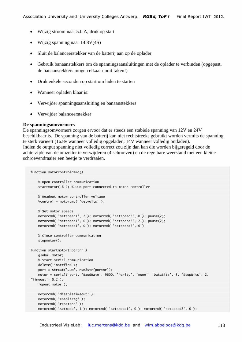
Association University and University Colleges Antwerp. RGBd, ToF ! Final Report IWT 2012.
Industrieel VisieLab: [email protected] and [email protected] 118
Wijzig stroom naar 5.0 A, druk op start
Wijzig spanning naar 14.8V(4S)
Sluit de balanceerstekker van de batterij aan op de oplader
Gebruik banaanstekkers om de spanningsaansluitingen met de oplader te verbinden (opgepast,
de banaanstekkers mogen elkaar nooit raken!)
Druk enkele seconden op start om laden te starten
Wanneer opladen klaar is:
Verwijder spanningsaansluiting en banaanstekkers
Verwijder balanceerstekker
De spanningsomvormers
De spanningsomvormers zorgen ervoor dat er steeds een stabiele spanning van 12V en 24V
beschikbaar is. De spanning van de batterij kan niet rechtstreeks gebruikt worden vermits de spanning
te sterk varieert (16.8v wanneer volledig opgeladen, 14V wanneer volledig ontladen).
Indien de output spanning niet volledig correct zou zijn dan kan die worden bijgeregeld door de
achterzijde van de omzetter te verwijderen (4 schroeven) en de regelbare weerstand met een kleine
schroevendraaier een beetje te verdraaien.
function motorcontroldemo()
% Open controller communication
startmotor( 6 ); % COM port connected to motor controller
% Readout motor controller voltage
Vcontrol = motorcmd( 'getvolts' );
% Set motor speeds
motorcmd( 'setspeed1', 2 ); motorcmd( 'setspeed2', 0 ); pause(2);
motorcmd( 'setspeed1', 0 ); motorcmd( 'setspeed2', 2 ); pause(2);
motorcmd( 'setspeed1', 0 ); motorcmd( 'setspeed2', 0 );
% Close controller communication
stopmotor();
function startmotor( portnr )
global motor;
% Start serial communication
delete( instrfind );
port = strcat('COM', num2str(portnr));
motor = serial( port, 'BaudRate', 9600, 'Parity', 'none', 'DataBits', 8, 'StopBits', 2,
'Timeout', 0.2 );
fopen( motor );
motorcmd( 'disabletimeout' );
motorcmd( 'enablereg' );
motorcmd( 'resetenc' );
motorcmd( 'setmode', 1 ); motorcmd( 'setspeed1', 0 ); motorcmd( 'setspeed2', 0 );

Association University and University Colleges Antwerp. RGBd, ToF ! Final Report IWT 2012.
Industrieel VisieLab: [email protected] and [email protected] 119
motorcmd( 'setaccel', 1 ); %motorcmd( 'setaccel', 10 );
function stopmotor()
global motor;
% Stop serial communication
motorcmd( 'setmode', 1 ); motorcmd( 'setspeed1', 0 ); motorcmd( 'setspeed2', 0 );
motorcmd( 'enabletimeout' );
fclose( motor ); delete( motor ); clear( 'motor' );
function varargout = motorcmd( cmd, varargin )
global motor;
if ~ischar( cmd )
error( 'Second argument must be a command string' );
end
switch cmd
case 'getspeed1'
fwrite( motor, [0 33], 'int8' ); % returns the current requested speed of motor 1
varargout(1) = { -fread( motor, 1, 'uint8' ) };
case 'getspeed2'
fwrite( motor, [0 34], 'int8' ); % returns the current requested speed of motor 2
varargout(1) = { -fread( motor, 1, 'uint8' ) };
case 'getenc1'
fwrite( motor, [0 35], 'uint8' ); % motor 1 encoder count, 4 bytes returned high
byte first (signed)
val = fread( motor, 4, 'uint8' );
val2 = uint32( bitcmp( uint8(val) ) );
val3 = bitshift( val2(1), 24 ) + bitshift( val2(1), 16 ) + bitshift( val2(3), 8 ) +
val2(4);
varargout(1) = { double(val3) };
case 'getenc2'
fwrite( motor, [0 36], 'uint8' ); % motor 2 encoder count, 4 bytes returned high
byte first (signed)
val = fread( motor, 4, 'uint8' );
val2 = uint32( bitcmp( uint8(val) ) );
val3 = bitshift( val2(1), 24 ) + bitshift( val2(1), 16 ) + bitshift( val2(3), 8 ) +
val2(4);
varargout(1) = { double(val3) };
case 'getencs'
fwrite( motor, [0 37], 'uint8' ); % returns 8 bytes - encoder1 count, encoder2
count
varargout(1) = { fread( motor, 8, 'uint8' ) };
case 'getvolts'
fwrite( motor, [0 38], 'uint8' ); % returns the input battery voltage level
varargout(1) = { fread( motor, 1, 'uint8' ) };
case 'getcurrent1'
fwrite( motor, [0 39], 'uint8' ); % returns the current drawn by motor 1
varargout(1) = { fread( motor, 1, 'uint8' ) };
case 'getcurrent2'
fwrite( motor, [0 40], 'uint8' ); % returns the current drawn by motor 2
varargout(1) = { fread( motor, 1, 'uint8' ) };
case 'getversion'
fwrite( motor, [0 41], 'uint8' ); % returns the software version
varargout(1) = { fread( motor, 1, 'uint8' ) };
case 'getaccel'
fwrite( motor, [0 42], 'uint8' ); % returns the current acceleration level
varargout(1) = { fread( motor, 1, 'uint8' ) };
case 'getmode'

Association University and University Colleges Antwerp. RGBd, ToF ! Final Report IWT 2012.
Industrieel VisieLab: [email protected] and [email protected] 120
fwrite( motor, [0 43], 'uint8' ); % returns the currently selected mode
varargout(1) = { fread( motor, 1, 'uint8' ) };
case 'getVI'
fwrite( motor, [0 44], 'uint8' ); % returns battery volts, motor1 current and
then motor2 current
varargout(1) = { fread( motor, 1, 'uint8' ) }; % Battery voltage
varargout(2) = { fread( motor, 1, 'uint8' ) }; % Current motor 1
varargout(3) = { fread( motor, 1, 'uint8' ) }; % Current motor 2
case 'setspeed1'
if nargin ~= 2
error( 'Incorrect number of input arguments' );
end
speed = cell2mat(varargin(1));
fwrite( motor, [0 49 -speed], 'int8' ); % set new speed1
case 'setspeed2'
if nargin ~= 2
error( 'Incorrect number of input arguments' );
end
speed = cell2mat(varargin(1));
fwrite( motor, [0 50 -speed], 'int8' ); % set new speed2
case 'setaccel'
if nargin ~= 2
error( 'Incorrect number of input arguments' );
end
accel = cell2mat(varargin(1));
fwrite( motor, [0 51 accel], 'uint8' ); % set new acceleration
case 'setmode'
if nargin ~= 2
error( 'Incorrect number of input arguments' );
end
mode = cell2mat(varargin(1));
fwrite( motor, [0 52 mode], 'uint8' ); % set the mode
case 'resetenc'
fwrite( motor, [0 53], 'uint8' ); % zero both of the encoder counts
case 'disablereg'
fwrite( motor, [0 54], 'uint8' ); % power output not changed by encoder feedback
case 'enablereg'
fwrite( motor, [0 55], 'uint8' ); % power output is regulated by encoder feedback
case 'disabletimeout'
fwrite( motor, [0 56], 'uint8' ); % Continuously output with no regular commands
case 'enabletimeout'
fwrite( motor, [0 57], 'uint8' ); % Output will stop after 2 seconds without
communication
otherwise
error( 'Incorrect command' ); % Incorrect command string
end
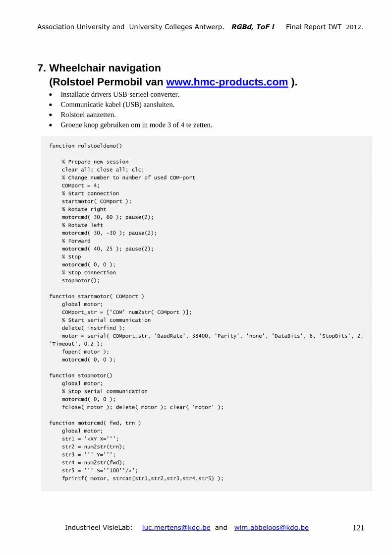
Association University and University Colleges Antwerp. RGBd, ToF ! Final Report IWT 2012.
Industrieel VisieLab: [email protected] and [email protected] 121
7. Wheelchair navigation
(Rolstoel Permobil van www.hmc-products.com ). Installatie drivers USB-serieel converter.
Communicatie kabel (USB) aansluiten.
Rolstoel aanzetten.
Groene knop gebruiken om in mode 3 of 4 te zetten.
function rolstoeldemo()
% Prepare new session
clear all; close all; clc;
% Change number to number of used COM-port
COMport = 4;
% Start connection
startmotor( COMport );
% Rotate right
motorcmd( 30, 60 ); pause(2);
% Rotate left
motorcmd( 30, -30 ); pause(2);
% Forward
motorcmd( 40, 25 ); pause(2);
% Stop
motorcmd( 0, 0 );
% Stop connection
stopmotor();
function startmotor( COMport )
global motor;
COMport_str = ['COM' num2str( COMport )];
% Start serial communication
delete( instrfind );
motor = serial( COMport_str, 'BaudRate', 38400, 'Parity', 'none', 'DataBits', 8, 'StopBits', 2,
'Timeout', 0.2 );
fopen( motor );
motorcmd( 0, 0 );
function stopmotor()
global motor;
% Stop serial communication
motorcmd( 0, 0 );
fclose( motor ); delete( motor ); clear( 'motor' );
function motorcmd( fwd, trn )
global motor;
str1 = '<XY X=''';
str2 = num2str(trn);
str3 = ''' Y=''';
str4 = num2str(fwd);
str5 = ''' S=''100''/>';
fprintf( motor, strcat(str1,str2,str3,str4,str5) );

Association University and University Colleges Antwerp. RGBd, ToF ! Final Report IWT 2012.
Industrieel VisieLab: [email protected] and [email protected] 122
8. Wall segmentation in the outdoor application of Vision &
Robotics.
% Start new session
clear all; close all; clc;
load walltest;
% Parameters
wallsize = 200; % Minimum size of wall in pixels
T = single( 0.4 ); % Threshold
L = rot90(L,3);
D = rot90(D,3);
% Calculate xyz
f = 78; ff = f * f;
I = 50; J = 64;
I2 = I/2; J2 = J/2;
u = (1:J) - (J2+0.5); uu = u .* u;
v = (1:I) - (I2+0.5); vv = v .* v;
U = repmat( u , [I 1]);
V = repmat( v', [1 J]);
UU = repmat( uu, [I 1]);
VV = repmat( vv',[1 J]);
d = sqrt( VV + UU + ff );
Dd = D ./ d;
x = U .* Dd;
y = -V .* Dd;
z = f * Dd;
% Filter image
fs = 5;
f1 = zeros(1, fs); f1(1) = 1; f1(end) = -1; f2 = f1';
z1 = conv2( z, f1, 'same' ); z2 = conv2( z, f2, 'same' );
x1 = conv2( x, f1, 'same' ); x2 = conv2( x, f2, 'same' );
y1 = conv2( y, f1, 'same' ); y2 = conv2( y, f2, 'same' );
% Create X vector, Y vector and Normal
nx = y1.*z2-z1.*y2; ny = z1.*x2-x1.*z2; nz = x1.*y2-y1.*x2;
% Normalize
n = sqrt( nx.^2 + ny.^2 + nz.^2 );
nx = nx ./ n; ny = ny ./ n; nz = nz ./ n;
% Enter normals into 3D matrix
img = single(cat( 3, nx, ny, nz ));
% Image size
h = uint16( size( img, 1)); w = uint16( size( img, 2));
% Pixels to check
check = abs(ny) < 0.2; % Vertical, add height constraint on y
check(:,1:uint8(fs)/2) = 0; % Exclude borders
check(:,end-uint8(fs)/2:end) = 0;
% Region

Association University and University Colleges Antwerp. RGBd, ToF ! Final Report IWT 2012.
Industrieel VisieLab: [email protected] and [email protected] 123
region = zeros( size( img, 1 ), size( img, 2 ), 'uint16' );
cur_reg = uint16(1);
% Neighbours, connectedness
NB = [ -1 0; 0 1; 1 0; 0 -1 ];
NBS = uint8( size(NB,1) );
% Initialize arrays
list = zeros( w*h, 2, 'uint16' );
num_el = zeros( w*h, 1, 'uint16' );
color = zeros( w*h, 2);
tic;
for a = 1:h
for b = 1:w
if check( a, b )
region( a, b ) = cur_reg;
cur_regs = 1;
m = [ img( a, b, 1 ) img( a, b, 3 )];
list( 1, : ) = [a b];
last = uint16(1);
while last > 0
u = list( last, 1 ); v = list( last, 2 );
last = last - 1;
if check( u, v )
for c1 = 1:NBS
iu = u + NB( c1, 1 ); iv = v + NB( c1, 2 );
% Inside?
if iu > 0 && iu <= h && iv > 0 && iv <= w && check( iu, iv )
% Add to region?
d = sqrt(( m(1)-img(iu,iv,1)).^2 + (m(2)-img(iu,iv,3)).^2);
if d <= T
last = last + 1;
region(iu,iv) = cur_reg;
m = m + [img(iu, iv, 1)-m(1) img(iu, iv, 3)-m(2)] ./ cur_regs;
cur_regs = cur_regs + 1;
list( last, 1 ) = iu; list( last, 2 ) = iv;
end
end
end
check( u, v ) = false;
end
end
num_el( cur_reg ) = cur_regs;
color( cur_reg, : ) = m;
cur_reg = cur_reg + 1;
end
end
end
toc;
goodwalls = find( num_el > wallsize );

Association University and University Colleges Antwerp. RGBd, ToF ! Final Report IWT 2012.
Industrieel VisieLab: [email protected] and [email protected] 124
% Find parameters for good walls (perpencidular distance, normal-x, normal-z)
tic;
for c1 = 1:size(goodwalls,1)
cur_wall = region == goodwalls(c1);
p = polyfit(x(cur_wall),z(cur_wall),1);
goodwalls(c1)
wd = abs(p(2)) ./ sqrt(p(1).^2+1)
wnx = mean(nx(cur_wall))
wnz = mean(nz(cur_wall))
end
toc;
% Display walls
for c1 = 1:h
for c2 = 1:w
if region(c1,c2) ~= 0
if num_el(region(c1,c2)) < wallsize
region(c1,c2) = 0; % remove if not good
end
end
end
end
figure(1);
subplot(121); imshow( D, [] ); title( 'Distance' );
subplot(122); imshow( region, [0 max(goodwalls)] ); title( 'Vertical planes' );

Association University and University Colleges Antwerp. RGBd, ToF ! Final Report IWT 2012.
Industrieel VisieLab: [email protected] and [email protected] 125
9. Path planning for the indoor application at Vision & Robotics.
Free navigation in a world with a known map.
9.1. The Brushfire algorithm (Principles of Robot Motion)
Because of its IP value the program is not given free.
% Prepare new session
clear all; close all; clc;
% Generate new map
map = false(120,250); % 240 * 500 cm
% Define startpoint and endpoint
ep = [25 225];
sp = [100 20];
% Prefer straight line
line = 0;
% Walls
map(1,:) = 1;
map(end,:) = 1;
map(:,1) = 1;
map(:,end) = 1;
% Objects
map(1:30,50) = 1;
map(1:30,100) = 1;
map(1:30,200) = 1;
map(30,170:200) = 1;
map(end-90:end,140) = 1;
map(end-30:end,190) = 1;
map(70:90,70:90) = 1;
ent' ); colormap( 'jet' );

Association University and University Colleges Antwerp. RGBd, ToF ! Final Report IWT 2012.
Industrieel VisieLab: [email protected] and [email protected] 126
As can be seen the path is not OK. The algorithm encounters a boogie trap. Another algorithm should
be found.
9.2. The Wave Front Algorithm
% Prepare new session
clear all; close all; clc;
% Generate new map
map = false(120,250); % 240 * 500 cm
% Define startpoint and endpoint
ep = [25 225];
sp = [100 10];
% Walls
map(1,:) = 1;
map(end,:) = 1;
map(:,1) = 1;
map(:,end) = 1;
% Objects
map(1:30,50) = 1;
map(1:30,100) = 1;
map(1:30,200) = 1;
map(30,170:200) = 1;
map(end-90:end,140) = 1;
map(end-30:end,190) = 1;
map(70:90,70:90) = 1;

Association University and University Colleges Antwerp. RGBd, ToF ! Final Report IWT 2012.
Industrieel VisieLab: [email protected] and [email protected] 127
9.3. Combined Algorithm: ( Wave Front and Distance Repulsion ).
% Prepare new session
clear all; close all; clc;
% Generate new map
map = false(120,250); % 240 * 500 cm
% Define startpoint and endpoint
ep = [25 225];
sp = [100 10];
% Walls
map(1,:) = 1;
map(end,:) = 1;
map(:,1) = 1;
map(:,end) = 1;
% Objects
map(1:30,50) = 1;
map(1:30,100) = 1;
map(1:30,200) = 1;
map(30,170:200) = 1;
map(end-90:end,140) = 1;
map(end-30:end,190) = 1;
map(70:90,70:90) = 1;
% Dilate map
map = imdilate(map,ones(10));

Association University and University Colleges Antwerp. RGBd, ToF ! Final Report IWT 2012.
Industrieel VisieLab: [email protected] and [email protected] 128
Remark: take into account that the final theoretical path depends on the weights used to balance
the Wave Front and the Repulsion Force relative to each other.
10. Localization
10.1. Localization based on known landmarks
function pointnav()
% Navigate using points
% Prepare new session
clear all; close all; clc;
lm = 1; % Random landmarks or square
pp = 1; % Display planned path or not
% Landmarks
if lm == 1
P = 100 * randn(2,200);
P = cat( 1, P, ones( 1, size(P,2) ));
else
P0 = -50:10:50;
P1 = cat(1,P0,-50 * ones(1,size(P0,2)) );
P2 = cat(1,P0, 50 * ones(1,size(P0,2)) );
P3 = cat(1,-50 * ones(1,size(P0,2)), P0 );
P4 = cat(1, 50 * ones(1,size(P0,2)), P0 );
P = cat(2, P1, P2, P3, P4);
P = cat(1, P, ones(1,size(P,2)));
end
Repulsio
n

Association University and University Colleges Antwerp. RGBd, ToF ! Final Report IWT 2012.
Industrieel VisieLab: [email protected] and [email protected] 129
% Parameters
T = [0 0 0]; R = T; E = T; % Start position
p = [1 20 18; % Path definition
2 20 20; % Time | Left speed | Right speed
2 10 9;
2 30 30];
dt = 0.1; % Simulation time step
wb = 0.5; % Vehicle wheel base
fov = pi/3; % Camera field of view
dm = 100; % Max. distance
me = 0.02; % Measurement error
se = 0.5; % Speed error
% Triangulation
if ~exist('DelaunayTri')
TRI = delaunay(P(1,:)',P(2,:)');
else
TRI = DelaunayTri(P(1,:)',P(2,:)');
end
figure(1);
plot(P(1,:), P(2,:), 'k*'); title( 'Points and Positions' );
xlim([-50 50]); ylim([-50 50]); daspect([1 1 1]); hold on;
RelPos = zeros(3,1);
% Start simulation
for c1 = 1:size(p,1)
% number of sub-steps
n = p(c1,1) / dt;
vl = p(c1,2);
vr = p(c1,3);
for c2 = 1:n
% Update position
vl2 = vl - 1/3*RelPos(2) + se * randn(1); % Noise on speed
vr2 = vr + 1/3*RelPos(2) + se * randn(1);
[dx dy da] = move( T(3), dt, wb, vl, vr ); % Theoretical path
[dx2 dy2 da2] = move( R(3), dt, wb, vl2, vr2 ); % Real
[dx3 dy3 da3] = move( E(3), dt, wb, vl, vr ); % Estimate
T = T + [dx dy da]; % Theoretical position
R = R + [dx2 dy2 da2]; % Real
E = E + [dx3 dy3 da3]; % Estimate
% Calculate visible points
RT = [cos(R(3)) -sin(R(3)) R(1); % Current position
sin(R(3)) cos(R(3)) R(2);
0 0 1];
Pc = RT \ P; % Points in camera coordinate system
d = sqrt( Pc(1,:).^2 + Pc(2,:).^2 ); % Distance from camera
m = d .* ( me * randn(size(d)) + 1); % Distance with measurement noise
r = m < dm; % Range, max. distance
a = atan2( Pc(1,:), Pc(2,:) );
a1 = a > pi()/2 - fov/2; % Field of view
a2 = a < pi()/2 + fov/2;
v = r & a1 & a2; % Visible points

Association University and University Colleges Antwerp. RGBd, ToF ! Final Report IWT 2012.
Industrieel VisieLab: [email protected] and [email protected] 130
% Measurements
Pmc = [ m .* sin(a); m .* cos(a); ones(size(m)) ];
Pm = RT * Pmc;
% Find better estimate by minimizing distance of measurements to points
if ~exist('DelaunayTri')
PI = dsearch( P(1,:)', P(2,:)', TRI, Pm(1,v)', Pm(2,v)' );
else
PI = nearestNeighbor( TRI, Pm(1,v)', Pm(2,v)' );
end
E = fminsearch( @(t) cost( PI, P, Pmc, t), E );
ET = [cos(E(3)) -sin(E(3)) E(1);
sin(E(3)) cos(E(3)) E(2);
0 0 1];
Pe = ET * Pmc;
% Correct speeds
RelPos = ET \ [E(1); E(2); 1];
figure(1);
if pp
quiver(T(1),T(2),10*cos(T(3)),10*sin(T(3)), 'g'); % Theoretical path
end
quiver(R(1),R(2),10*cos(R(3)),10*sin(R(3)), 'b'); % Real
quiver(E(1),E(2),10*cos(E(3)),10*sin(E(3)), 'c'); % Estimated
plot(Pm(1,v), Pm(2,v), 'b*'); % Measurements
plot(Pe(1,v), Pe(2,v), 'r*'); % Corrected measurements
%pause();
end
end
function C = cost( PI, P, Pmc, t)
ET = [cos(t(3)) -sin(t(3)) t(1);
sin(t(3)) cos(t(3)) t(2);
0 0 1];
Pe = ET * Pmc;
D = ( Pe(1,PI) - P(1,PI) ).^2 + ( Pe(2,PI) - P(2,PI) ).^2;
C = sum( D );
function [ dx dy da ] = move( a, dt, wb, vl, vr )
if vl == vr
da = 0;
l = vl * dt;
dx = l * cos(a);
dy = l * sin(a);
else
v = ( vr + vl ) / 2;
r = ( vr * wb ) / ( vr - vl ) - wb/2;
da = v / r * dt;
dx1 = r * sin(da);
dy1 = r - r * cos(da);
dx = cos(a) * dx1 - sin(a) * dy1;
dy = sin(a) * dx1 + cos(a) * dy1;
end

Association University and University Colleges Antwerp. RGBd, ToF ! Final Report IWT 2012.
Industrieel VisieLab: [email protected] and [email protected] 131
10.2. Localization based on known Walls
(seen as specific landmarks).
function wallnav_test5()
% Navigate using walls
% Green is 'predicted path'
% Blue is 'true path'
% Cyan is 'current estimated location after optimalisation'
% Black is 'next estimated location'
clear all; close all; clc;
global wall L1 L2 D2 nx2 nz2 mo;
% Define walls
L1 = [ 250 250 -250 -250;
-120 120 120 -120]; L1 = L1/2;
L2 = [ 250 -250 -250 250;
120 120 -120 -120]; L2 = L2/2;
L1 = cat( 1, L1, ones(1,size(L1,2)) );
L2 = cat( 1, L2, ones(1,size(L2,2)) );
% Define path and specify vehicle parameters
p = [1 20 18;
2 20 20;
2 9 10;
2 30 30];
dt = 0.1; % Simulation time step
wb = 0.5; % Wheel base (m)
fov = pi/3; % Camera field of view

Association University and University Colleges Antwerp. RGBd, ToF ! Final Report IWT 2012.
Industrieel VisieLab: [email protected] and [email protected] 132
% Transforms
T = [0 0 0]; R = T; E = T;
% Create figure to display path
figure(1); hold on; title( 'World' ); axis equal;
xlim( [min(L1(1,:))-10 max(L1(1,:))+10] ); ylim( [min(L1(2,:)-10) max(L1(2,:))+10] );
% Display current position
quiver( T(1), T(2), 10*cos(T(3)), 10*sin(T(3)), 'g' );
quiver( R(1), R(2), 10*cos(R(3)), 10*sin(R(3)), 'b' );
quiver( E(1), E(2), 10*cos(E(3)), 10*sin(E(3)), 'c' );
drawnow;
for c1 = 1:size(p,1)
% number of sub-steps
n = p(c1,1) / dt;
vl = p(c1,2);
vr = p(c1,3);
for c2 = 1:n
% Update position
if E(3) > 2*pi
E(3) = E(3) - 2*pi;
end
if E(3) < 0
E(3) = E(3) + 2*pi;
end
Eold = E;
vl2 = vl + 0.5 * randn(1);
vr2 = vr + 0.5 * randn(1);
[dx dy da db1 dd1 dc1 ] = move1( T(3), dt, wb, vl, vr );
[dx2 dy2 da2 db2 dd2 dc2 ] = move1( R(3), dt, wb, vl2, vr2 );
[dx3 dy3 da3 db3 dd3 dc3 ] = move1( E(3), dt, wb, vl, vr );
T = T + [dx dy da]; % Theoretical
R = R + [dx2 dy2 da2]; % Real
E = E + [dx3 dy3 da3]; % Estimate
if E(3) > 2*pi
E(3) = E(3) - 2*pi;
end
if E(3) < 0
E(3) = E(3) + 2*pi;
end
quiver( E(1), E(2), 10*cos(E(3)), 10*sin(E(3)), 'k' );
% New transformation matrix
RT = [cos(R(3)) -sin(R(3)) R(1);
sin(R(3)) cos(R(3)) R(2);
0 0 1];
% Transform lines
LT1 = RT \ L1;
LT2 = RT \ L2;
la1 = atan2(LT1(2,:),LT1(1,:));
la2 = atan2(LT2(2,:),LT2(1,:));
leq = cross(LT1,LT2);
% Find visible planes

Association University and University Colleges Antwerp. RGBd, ToF ! Final Report IWT 2012.
Industrieel VisieLab: [email protected] and [email protected] 133
alc1 = la1 < -fov/2 & la2 < -fov/2;
alc2 = la1 > fov/2 & la2 > fov/2;
vec = cross( [0 0 1], [1 0 1] );
temp = cross( leq, repmat( vec', [1 size(leq,2)] ) );
temp = temp ./ repmat( temp(3,:), [3 1] );
alc3 = temp(1,:) > 0;
ac = ~( alc1 | alc2 ) & alc3;
% Plane parameters
D = abs( leq(3,:) ) ./ sqrt( leq(1,:).^2 + leq(2,:).^2 );
nx = -sin( atan2( leq(2,:), leq(1,:) ) );
nz = -cos( atan2( leq(2,:), leq(1,:) ) );
% Measurement noise
D2 = D + 0.01 .* randn(size( D)) .* D;
nx2 = nx + 0.05 .* randn(size(nx));
nz2 = nz + 0.05 .* randn(size(nz));
nx2(nx2(:)> 1) = 1; nx2(nx2(:)<-1) = -1;
nz2(nz2(:)> 1) = 1; nz2(nz2(:)<-1) = -1;
% Find association
wall = zeros(size(ac));
for c4 = 1:size(wall,2)
if ac(c4) == 1
de = abs( (D-D2(c4)) ./ ( 0.01 * D ));
xe = abs((nx-nx2(c4)) ./ 0.05);
ze = abs((nz-nz2(c4)) ./ 0.05);
C = de + xe + ze;
[mval mind] = min(C);
wall(c4) = mind;
end
end
% Optimization
m = [db3 dd3 dc3]
[E mval] = fminsearch( @(t) cost(t,Eold,m), E );
mo
% Display visible walls
for c3 = 1:size(L1,2)
plot( [L1(1,c3) L2(1,c3)], [L1(2,c3) L2(2,c3)], 'b' );
if ac(c3)
plot( [L1(1,c3) L2(1,c3)], [L1(2,c3) L2(2,c3)], 'r' );
end
end
% Display current position
quiver( T(1), T(2), 10*cos(T(3)), 10*sin(T(3)), 'g' );
quiver( R(1), R(2), 10*cos(R(3)), 10*sin(R(3)), 'b' );
quiver( E(1), E(2), 10*cos(E(3)), 10*sin(E(3)), 'c' );
drawnow;
end
end
function [ dx dy da db dd dc ] = move1( a, dt, wb, vl, vr )
% sf = 0.00588; % m/s per motor speed unit ( 0.00589 a bit to high)
% vl = vl * sf;
% vr = vr * sf;
if vl == vr
da = 0;

Association University and University Colleges Antwerp. RGBd, ToF ! Final Report IWT 2012.
Industrieel VisieLab: [email protected] and [email protected] 134
l = vl * dt;
dx = l * cos(a);
dy = l * sin(a);
db = 0;
dd = l;
dc = 0;
else
v = ( vr + vl ) / 2;
r = ( vr * wb ) / ( vr - vl ) - wb/2;
da = v / r * dt;
dx1 = r * sin(da);
dy1 = r - r * cos(da);
dx = cos(a) * dx1 - sin(a) * dy1;
dy = sin(a) * dx1 + cos(a) * dy1;
ta = atan2(dy,dx);
if abs(ta) > 2*pi
tms = fix(ta/(2*pi)) + sign(ta);
ta = ta - tms*2*pi;
end
if abs(ta) > pi
ta = ta - sign(ta)*2*pi;
end
db = ta - a;
if abs(db) > 2*pi
tms = fix(db/(2*pi)) + sign(db);
db = db - tms*2*pi;
end
if abs(db) > pi
db = db - sign(db)*2*pi;
end
dd = sqrt((dx)^2+(dy)^2);
dc = ta - a;
if abs(dc) > 2*pi
tms = fix(dc/(2*pi)) + sign(dc);
dc = dc - tms*2*pi;
end
if abs(dc) > pi
dc = dc - sign(dc)*2*pi;
end
end
function C = cost( t, E, m )
global wall L1 L2 D2 nx2 nz2 mo;
ET = [cos(t(3)) -sin(t(3)) t(1);
sin(t(3)) cos(t(3)) t(2);
0 0 1];
LT1 = ET \ L1;
LT2 = ET \ L2;
% Cross product
u = LT1(2,:) .* LT2(3,:) - LT1(3,:) .* LT2(2,:);
v = LT1(3,:) .* LT2(1,:) - LT1(1,:) .* LT2(3,:);
w = LT1(1,:) .* LT2(2,:) - LT1(2,:) .* LT2(1,:);
D = abs( w ) ./ sqrt( u.^2 + v.^2 );
nx = -sin( atan2( v, u ) );
nz = -cos( atan2( v, u ) );
C = 0;

Association University and University Colleges Antwerp. RGBd, ToF ! Final Report IWT 2012.
Industrieel VisieLab: [email protected] and [email protected] 135
for c4 = 1:size(wall,2)
if wall(c4) ~= 0
de = abs(( D(wall(c4))- D2(c4)) ./ ( 0.01 * D(wall(c4)) ));
xe = abs((nx(wall(c4))-nx2(c4)) ./ 0.05);
ze = abs((nz(wall(c4))-nz2(c4)) ./ 0.05);
C = C + de + xe + ze;
end
end
ta = atan2(t(2)-E(2),t(1)-E(1));
if abs(ta) > 2*pi
tms = fix(ta/(2*pi)) + sign(ta);
ta = ta - tms*2*pi;
end
if abs(ta) > pi
ta = ta - sign(ta)*2*pi;
end
dbl = ta - E(3);
if abs(dbl) > 2*pi
tms = fix(dbl/(2*pi)) + sign(dbl);
dbl = dbl - tms*2*pi;
end
if abs(dbl) > pi
dbl = dbl - sign(dbl)*2*pi;
end
ddl = sqrt((E(1)-t(1))^2+(E(2)-t(2))^2);
dcl = t(3) - ta;
if abs(dcl) > 2*pi
tms = fix(dcl/(2*pi)) + sign(dcl);
dcl = dcl - tms*2*pi;
end
if abs(dcl) > pi
dcl = dcl - sign(dcl)*2*pi;
end
mo = [dbl ddl dcl];
C = C * ( 1 + ( (dbl-m(1))^2 + 100*(ddl-m(2))^2 + (dcl-m(3))^2 ) );

Association University and University Colleges Antwerp. RGBd, ToF ! Final Report IWT 2012.
Industrieel VisieLab: [email protected] and [email protected] 136
11. AGV sturing We gebruiken het eerder besproken ‘wave front’ algoritme om van een gekende locatie ‘A’ naar
een willekeurige locatie ‘B’ te rijden. Er wordt gebruik gemaakt van een eenvoudige sturing die
‘bijstuurt’ aan de hand van de hoekfout ten opzichte van de ideale rijrichting. De sturing bevat
een proportionele en een integrerende term.
function AGVsturing()
% Prepare new session
clear all; close all; clc;
% Parameters
wb = 36.5; % Vehicle wheelbase (cm)
v = 20; % Vehicle speed (units in motor controller)
dt = 0.1; % Simulation time step (s)
wf = 0.5; % Weigth factor of distance vectorfield
vf = 1; % Turn vector field display on or off
v_err = 0; % Speed error
l_err = 0; % Localization error
% Display parameters
hh = 10; % Wall and object height
oc = [0.5 0.5 0.5]; % Object color
fc = [0.7 0.7 0.7]; % Floor color
vc = [0.4 0.7 1.0]; % Vehicle color
% Generate new map
map = false(120,250); % 240 * 500 cm
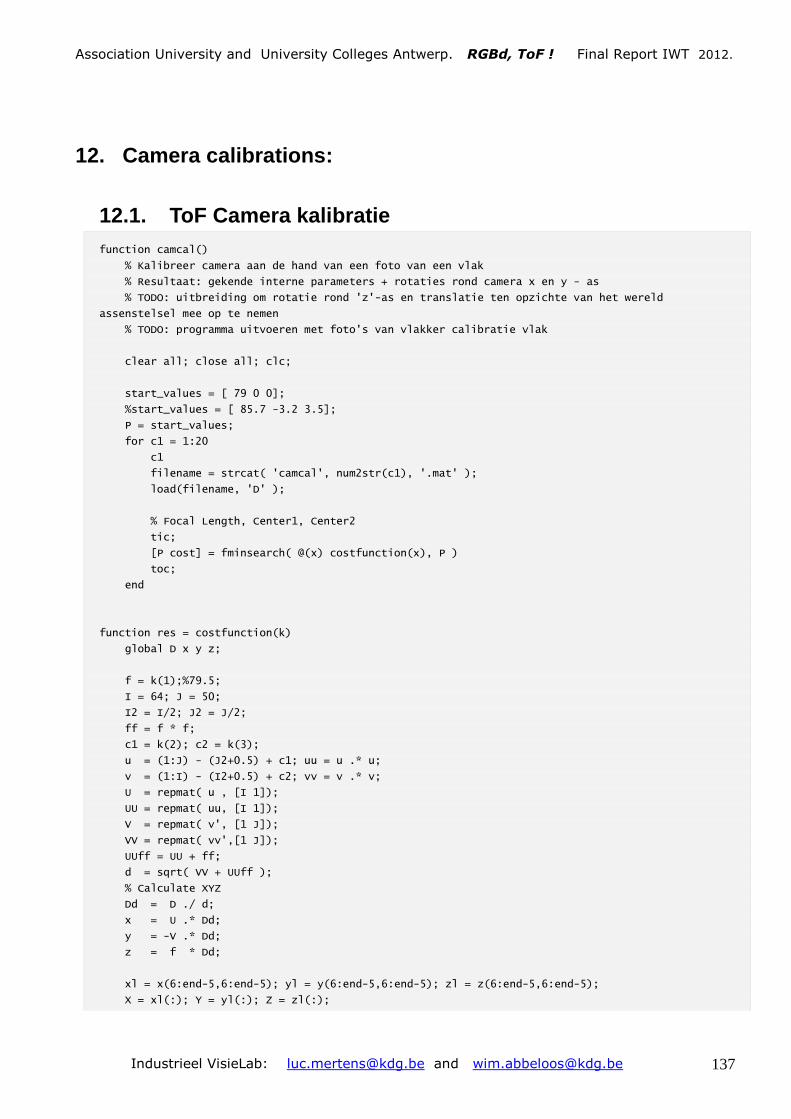
Association University and University Colleges Antwerp. RGBd, ToF ! Final Report IWT 2012.
Industrieel VisieLab: [email protected] and [email protected] 137
12. Camera calibrations:
12.1. ToF Camera kalibratie
function camcal()
% Kalibreer camera aan de hand van een foto van een vlak
% Resultaat: gekende interne parameters + rotaties rond camera x en y - as
% TODO: uitbreiding om rotatie rond 'z'-as en translatie ten opzichte van het wereld
assenstelsel mee op te nemen
% TODO: programma uitvoeren met foto's van vlakker calibratie vlak
clear all; close all; clc;
start_values = [ 79 0 0];
%start_values = [ 85.7 -3.2 3.5];
P = start_values;
for c1 = 1:20
c1
filename = strcat( 'camcal', num2str(c1), '.mat' );
load(filename, 'D' );
% Focal Length, Center1, Center2
tic;
[P cost] = fminsearch( @(x) costfunction(x), P )
toc;
end
function res = costfunction(k)
global D x y z;
f = k(1);%79.5;
I = 64; J = 50;
I2 = I/2; J2 = J/2;
ff = f * f;
c1 = k(2); c2 = k(3);
u = (1:J) - (J2+0.5) + c1; uu = u .* u;
v = (1:I) - (I2+0.5) + c2; vv = v .* v;
U = repmat( u , [I 1]);
UU = repmat( uu, [I 1]);
V = repmat( v', [1 J]);
VV = repmat( vv',[1 J]);
UUff = UU + ff;
d = sqrt( VV + UUff );
% Calculate XYZ
Dd = D ./ d;
x = U .* Dd;
y = -V .* Dd;
z = f * Dd;
xl = x(6:end-5,6:end-5); yl = y(6:end-5,6:end-5); zl = z(6:end-5,6:end-5);
X = xl(:); Y = yl(:); Z = zl(:);

Association University and University Colleges Antwerp. RGBd, ToF ! Final Report IWT 2012.
Industrieel VisieLab: [email protected] and [email protected] 138
% Vlak door punten schatten
XYZ = cat(1,X',Y',Z');
P2 = plane(XYZ);
P2 = P2 ./ P2(4);
% Normaal van vlak
nt = sqrt(P2(1)^2+P2(2)^2+P2(3)^2);
n = P2(1:3)./nt;
% Rotatiematrix om vlak horizontaal te leggen
R = [ 1-n(1)^2 0 n(1);
0 1-n(2)^2 n(2);
n(1) n(2) n(3) ];
XYZr = R * XYZ;
% Rotatie en translatie in één stap uitvoeren
P = cat(2, R, [0; 0; -mean(XYZr(3,:))] );
XYZ2 = cat(1, XYZ, ones(1,size(XYZ,2)));
XYZtest = P * XYZ2;
% Std van Z waarden als maat van vlakheid
res = std(XYZtest(3,:));
function B = plane(XYZ)
[rows,npts] = size(XYZ);
if rows ~=3
error('data is not 3D');
end
if npts < 3
error('too few points to fit plane');
end
% Set up constraint equations of the form AB = 0,
% where B is a column vector of the plane coefficients
% in the form b(1)*X + b(2)*Y +b(3)*Z + b(4) = 0.
A = [XYZ' ones(npts,1)]; % Build constraint matrix
if npts == 3 % Pad A with zeros
A = [A; zeros(1,4)];
end
[u d v] = svd(A); % Singular value decomposition.
B = v(:,4); % Solution is last column of v.

Association University and University Colleges Antwerp. RGBd, ToF ! Final Report IWT 2012.
Industrieel VisieLab: [email protected] and [email protected] 139
12.2. Calibration: Color relative to TOF camera.
% Prepare new session
clear all; close all; clc;
% Load data
load XYZ
load RGBd_tof_corners
X = XYZ(1,:,:); X = X(:);
Y = XYZ(2,:,:); Y = Y(:);
Z = XYZ(3,:,:); Z = Z(:);
D = corners_D(:,2:25); D = 1000 * D(:);
% Select data-subset
% a1 = 1; a2 = 20;
% p1 = a1*80+1; p2 = a2*80;
% X = X(p1:p2); Y = Y(p1:p2); Z = Z(p1:p2); D = D(p1:p2);
% Find translation vector: Minimalize cost function
startpoint = [80 0 0];
minfunc = @(t) sum((( X + t(1) ).^2 + ( Y + t(2) ).^2 + ( Z + t(3) ).^2 - D.^2) .^2) ;
[t2 t_cost] = fminsearch( minfunc , startpoint )
% Find intrinsic parameters of TOF camera
u = corners(1,:,2:25); u = u(:) / 10;
v = corners(2,:,2:25); v = v(:) / 10;
x = cat(2, u, v, ones(size(u)) );
% Iterate to refine translation and TOF internal parameters
for c2 = 1:10
A = []; b = [];
for c1 = 1 : size(X(:))
A = cat(1,A,[ (X(c1)+t2(1))/(Z(c1)+t2(3)) 0 1 0; 0 (Y(c1)+t2(2))/(Z(c1)+t2(3)) 0 1 ]);
b = cat( 1, b, [ u(c1); v(c1) ]);
end
P = A \ b
temp = inv([P(1) 0 P(3); 0 P(2) P(4); 0 0 1]) * x';
n = sqrt( temp(1,:).^2 + temp(2,:).^2 + temp(3,:).^2 );
n = repmat( n, [3 1]);
d = repmat( D', [3 1]);
xyz = d .* temp ./ n;
t2 = [ mean(xyz(1,:)-X') mean(xyz(2,:)-Y') mean(xyz(3,:)-Z') ]
end
% Nearest Neighbours (later: using voronoi diagram)
% Trasform distance to XYZ
load('RGBd'); D = D(:,:,12); L = L(:,:,12); rgb = rgb(:,:,:,12);
errorp = D < 0; D(errorp) = 5;

Association University and University Colleges Antwerp. RGBd, ToF ! Final Report IWT 2012.
Industrieel VisieLab: [email protected] and [email protected] 140
ups = 1; % Upscale to achieve higher color resolution (use 2, 3, ...)
D = interp2(D,ups);
L = interp2(L,ups);
[I J] = size(D);
u = repmat( 0:J-1, [I 1] );
v = repmat( (0:I-1)', [1 J] );
u = u(:); v = v(:); D = D(:);
x = cat(2, u, v, ones(size(u)) );
temp = inv([2^(ups)*P(1) 0 2^(ups)*P(3); 0 2^(ups)*P(2) 2^(ups)*P(4); 0 0 1]) * x';
n = sqrt( temp(1,:).^2 + temp(2,:).^2 + temp(3,:).^2 );
n = repmat( n, [3 1] );
d = repmat( D', [3 1] );
xyz = d .* temp ./ n;
figure(100);
surf(reshape(xyz(1,:),I,J),reshape(xyz(2,:),I,J),reshape(xyz(3,:),I,J),L,'LineStyle', 'None');
xlim( [-0.3 0.3] ); ylim( [-0.3 0.3] ); zlim( [0.4 1] );
xlabel( 'X' ); ylabel( 'Y' ); zlabel( 'Z' );
daspect( [1 1 1] ); colormap( 'gray' );
cameratoolbar( 'Show' ); cameratoolbar( 'SetMode', 'Orbit' );
title( '3D reconstruction in TOF camera coordinates' );
set(gca,'ZDir','reverse'); view(180,45);
% Transform from TOF coordinate system to RGB coordinate system
x = xyz(1,:)*1000 - t2(1);
y = xyz(2,:)*1000 - t2(2);
z = xyz(3,:)*1000 - t2(3);
% Focal Length:
f = [ 1153.99786 1154.35200 ];
% Principal point:
c = [ 485.32366 582.87738 ];
% Distortion:
kc = [ -0.18174 0.15183 -0.00045 0.00201 0.00000 ];
% Project 3D coordinates onto color image
a = x./z; b = y./z;
r = sqrt(a.^2 + b.^2);
xx = a .* (1 + kc(1)*r.^2 + kc(2).*r.^4) + 2*kc(3)*a.*b + kc(4)*(r.^2 + 2*a.^2);
yy = b .* (1 + kc(1)*r.^2 + kc(2).*r.^4) + kc(3)*(r.^2 + 2*b.^2) + 2*kc(4)*a.*b;
xxp = f(1)*xx + c(1); xxp = max(xxp, 1); xxp = min(xxp, size(rgb,2));
yyp = f(2)*yy + c(2); yyp = max(yyp, 1); yyp = min(yyp, size(rgb,1));
figure(1);
imshow( rgb ); hold on;
plot( xxp, yyp, 'r+' ); title('TOF 3D points projected onto color image');
% Assign color to TOF pixels
C = zeros( size(xxp(:)),3 );
for c1=1:size(xxp(:))
C(c1,:) = rgb( round(yyp(c1)), round(xxp(c1)), : );
end

Association University and University Colleges Antwerp. RGBd, ToF ! Final Report IWT 2012.
Industrieel VisieLab: [email protected] and [email protected] 141
figure(2);
surf( reshape(xyz(1,:),I,J), reshape(xyz(2,:),I,J), reshape(xyz(3,:),I,J),
reshape(C/255,I,J,3), 'LineStyle', 'None' );
xlim( [-0.3 0.3] ); ylim( [-0.3 0.3] ); zlim( [0.4 1] );
xlabel( 'X' ); ylabel( 'Y' ); zlabel( 'Z' );
daspect( [1 1 1] );
cameratoolbar( 'Show' ); cameratoolbar( 'SetMode', 'Orbit' );
title( '3D + color reconstruction' );
set(gca,'ZDir','reverse'); view(180,45);
% dt = DelaunayTri(xxp(:),yyp(:));
% NN = zeros(size(rgb,1),size(rgb,2));
% rgbu = repmat( [0:size(rgb,2)-1], [size(rgb,1) 1]);
% rgbv = repmat( [0:size(rgb,1)-1]', [1 size(rgb,2)]);
%
% NN = dt.nearestNeighbor([rgbu(:) rgbv(:)]);
% X = xyz(1,NN)';
% Y = xyz(2,NN)';
% Z = xyz(3,NN)';
% C = reshape(double(rgb), [size(rgb,1)*size(rgb,2) 3]) / 255;
% figure(3);
% scatter3( X(1:100:end), Y(1:100:end), Z(1:100:end), 10, C(1:100:end,:) );
Color to Depth Depth to Color

Association University and University Colleges Antwerp. RGBd, ToF ! Final Report IWT 2012.
Industrieel VisieLab: [email protected] and [email protected] 142
13. Halcon ( Industrial Vision Package of MVTec (www.mvtec.com )).
13.1. Halcon in combination with IFM O3D201 (ifm-electronic)
* IWT TETRA RGBd, ToF! * IFM O3D201 data acquisition demo * Wim Abbeloos & Luc Mertens * Turn update off dev_update_off () * Camera connection parameters CamIP := '192.168.0.69' XMLPort := 8080 DataPort := 50002 * Camera settings ModFreq := 0 SampMode := 0 IlluMode := 3 IntTime1 := 500 IntTime2 := 500 Delay := 141 * Camera control settings Trigger := 3 * Image processing settings MeanFilt := 0 MedianFilt := 0 Averaging := 1 * Convert parameter values to strings tuple_string (ModFreq, 'd', ModFreqStr) tuple_string (SampMode, 'd', SampModeStr) tuple_string (IlluMode, 'd', IlluModeStr) tuple_string (IntTime1, 'd', IntTime1Str) tuple_string (IntTime2, 'd', IntTime2Str) tuple_string (Delay, 'd', DelayStr) tuple_string (XMLPort, 'd', XMLPortStr) tuple_string (Trigger, 'd', TriggerStr) tuple_string (MeanFilt, 'd', MeanFiltStr) tuple_string (MedianFilt, 'd', MedianFiltStr) tuple_string (Averaging, 'd', AveragingStr) * Close windows dev_close_window () dev_close_window () * Open new graphics windows dev_open_window (0, 0, 50*6, 64*6, 'black', WindowHandle1) dev_open_window (0, 500, 50*6, 64*6, 'black', WindowHandle2) * Create blank images gen_image_const (Dimg, 'real', 50, 64) gen_image_const (Limg, 'real', 50, 64) gen_image_const (ximg, 'real', 50, 64) gen_image_const (yimg, 'real', 50, 64) gen_image_const (zimg, 'real', 50, 64)

Association University and University Colleges Antwerp. RGBd, ToF ! Final Report IWT 2012.
Industrieel VisieLab: [email protected] and [email protected] 143
* Create indexing tuples dev_update_off () s := [] l := [] for sindex := 0 to 49 by 1 for lindex := 0 to 63 by 1 s := [s, sindex] l := [l, lindex] endfor endfor * Open XML and data sockets open_socket_connect (CamIP, XMLPort, ['protocol','timeout'], ['TCP',0.2], XMLSocket) open_socket_connect (CamIP, DataPort, ['protocol','timeout'], ['TCP',0.2], DataSocket) wait_seconds(0.1) * Disconnect camera body := '<?xml version="1.0" encoding="UTF-8"?>\r\n<methodCall><methodName>MDAXMLDisconnectCP</methodName>\r\n<params><param><value>'+CamIP+'</value></param><param><value><i4>1</i4></value></param></params></methodCall>\r\n' * Get message length tuple_strlen (body, Length) * Create header header := 'POST /RPC2 HTTP/1.1\r\nUser-Agent: XMLRPC++ 0.7\r\nHost: ' + CamIP + ':' + XMLPortStr + '\r\nContent-Type: text/xml\r\nContent-length: ' + Length + '\r\n\r\n' * Send and receive disconnect data send_data (XMLSocket, 'z', header+body, [CamIP,XMLPort]) wait_seconds(0.1) receive_data (XMLSocket, 'z', DisconnectData, From10) * Connect to camera body := '<?xml version="1.0" encoding="UTF-8"?>\r\n<methodCall><methodName>MDAXMLConnectCP</methodName>\r\n<params><param><value>'+CamIP+'</value></param><param><value><i4>1</i4></value></param></params></methodCall>\r\n' * Get message length tuple_strlen (body, Length) * Create header header := 'POST /RPC2 HTTP/1.1\r\nUser-Agent: XMLRPC++ 0.7\r\nHost: ' + CamIP + ':' + XMLPortStr + '\r\nContent-Type: text/xml\r\nContent-length: ' + Length + '\r\n\r\n' * Send and receive connect data send_data (XMLSocket, 'z', header+body, [CamIP,XMLPort]) wait_seconds(0.1) receive_data (XMLSocket, 'z', ConnectData, From1) * Set program body := '<?xml version="1.0" encoding="UTF-8"?>\r\n<methodCall><methodName>MDAXMLSetProgram</methodName>\r\n<params><param><value><i4>0</i4></value></param><param><value><i4>0</i4></value></param><param><value><i4>7</i4></value></param></params></methodCall>\r\n' * Get message length tuple_strlen (body, Length) * Create header header := 'POST /RPC2 HTTP/1.1\r\nUser-Agent: XMLRPC++ 0.7\r\nHost: ' + CamIP + ':' + XMLPortStr + '\r\nContent-Type: text/xml\r\nContent-length: ' + Length + '\r\n\r\n' * Send and receive connect data send_data (XMLSocket, 'z', header+body, [CamIP,XMLPort]) wait_seconds(0.1)

Association University and University Colleges Antwerp. RGBd, ToF ! Final Report IWT 2012.
Industrieel VisieLab: [email protected] and [email protected] 144
receive_data (XMLSocket, 'z', SetProgram, FromSP) * Set triggering body := 'POST /RPC2 HTTP/1.1\r\nUser-Agent: XMLRPC++ 0.7\r\nHost: '+CamIP+':'+XMLPortStr+'\r\nContent-Type: text/xml\r\nContent-length: 247\r\n\r\n<?xml version="1.0" encoding="UTF-8"?>\r\n<methodCall><methodName>MDAXMLSetTrigger</methodName>\r\n<params><param>\r\n\t<value><i4>0</i4></value></param><param>\r\n\t<value><i4>0</i4></value></param><param>\r\n\t<value><i4>'+TriggerStr+'</i4></value></param></params></methodCall>\r\n' * Get message length tuple_strlen (body, Length) * Create header header := 'POST /RPC2 HTTP/1.1\r\nUser-Agent: XMLRPC++ 0.7\r\nHost: ' + CamIP + ':' + XMLPortStr + '\r\nContent-Type: text/xml\r\nContent-length: ' + Length + '\r\n\r\n' * Send and receive connect data send_data (XMLSocket, 'z', header+body, [CamIP,XMLPort]) wait_seconds(0.1) receive_data (XMLSocket, 'z', SetCtTriggerData, From2) * Set averaging body := '<?xml version="1.0" encoding="UTF-8"?>\r\n<methodCall><methodName>MDAXMLSetAverageDetermination</methodName>\r\n<params><param><value><i4>0</i4></value></param><param><value><i4>0</i4></value></param><param><value><i4>'+AveragingStr+'</i4></value></param></params></methodCall>\r\n' * Get message length tuple_strlen (body, Length) * Create header header := 'POST /RPC2 HTTP/1.1\r\nUser-Agent: XMLRPC++ 0.7\r\nHost: ' + CamIP + ':' + XMLPortStr + '\r\nContent-Type: text/xml\r\nContent-length: ' + Length + '\r\n\r\n' * Send and receive connect data send_data (XMLSocket, 'z', header+body, [CamIP,XMLPort]) wait_seconds(0.1) receive_data (XMLSocket, 'z', SetAverage, FromAv) * Set median body := '<?xml version="1.0" encoding="UTF-8"?>\r\n<methodCall><methodName>MDAXMLSetMedianFilterStatus</methodName>\r\n<params><param><value><i4>'+MedianFiltStr+'</i4></value></param></params></methodCall>\r\n' * Get message length tuple_strlen (body, Length) * Create header header := 'POST /RPC2 HTTP/1.1\r\nUser-Agent: XMLRPC++ 0.7\r\nHost: ' + CamIP + ':' + XMLPortStr + '\r\nContent-Type: text/xml\r\nContent-length: ' + Length + '\r\n\r\n' * Send and receive connect data send_data (XMLSocket, 'z', header+body, [CamIP,XMLPort]) wait_seconds(0.1) receive_data (XMLSocket, 'z', SetMedian, FromMedian) * Set mean body := '<?xml version="1.0" encoding="UTF-8"?>\r\n<methodCall><methodName>MDAXMLSetMeanFilterStatus</methodName>\r\n<params><param><value><i4>'+MeanFiltStr+'</i4></value></param></params></methodCall>\r\n' * Get message length tuple_strlen (body, Length) * Create header

Association University and University Colleges Antwerp. RGBd, ToF ! Final Report IWT 2012.
Industrieel VisieLab: [email protected] and [email protected] 145
header := 'POST /RPC2 HTTP/1.1\r\nUser-Agent: XMLRPC++ 0.7\r\nHost: ' + CamIP + ':' + XMLPortStr + '\r\nContent-Type: text/xml\r\nContent-length: ' + Length + '\r\n\r\n' * Send and receive connect data send_data (XMLSocket, 'z', header+body, [CamIP,XMLPort]) wait_seconds(0.1) receive_data (XMLSocket, 'z', SetMean, FromMean) * Set camera frontend data body := '<?xml version="1.0" encoding="UTF-8"?>\r\n<methodCall><methodName>MDAXMLSetFrontendData</methodName>\r\n<params><param><value><i4>0</i4></value></param><param><value><i4>'+ModFreqStr+'</i4></value></param><param><value><i4>'+SampModeStr+'</i4></value></param><param><value><i4>0</i4></value></param><param><value><i4>'+IntTime1Str+'</i4></value></param><param><value><i4>'+IntTime2Str+'</i4></value></param><param><value><i4>20</i4></value></param><param><value><i4>'+DelayStr+'</i4></value></param></params></methodCall>\r\n' * Get message length tuple_strlen (body, Length) * Create header header := 'POST /RPC2 HTTP/1.1\r\nUser-Agent: XMLRPC++ 0.7\r\nHost: ' + CamIP + ':' + XMLPortStr + '\r\nContent-Type: text/xml\r\nContent-length: ' + Length + '\r\n\r\n' * Send and receive frontend data send_data (XMLSocket, 'z', header+body, [CamIP,XMLPort]) wait_seconds(0.1) receive_data (XMLSocket, 'z', SetFrontEndData, Fromx) * Data acquisition loop for index := 1 to 100 by 1 * Perform HeartBeat send_data (XMLSocket, 'z', 'POST /RPC2 HTTP/1.1\r\nUser-Agent: XMLRPC++ 0.7\r\nHost: '+CamIP+':'+XMLPortStr+'\r\nContent-Type: text/xml\r\nContent-length: 109\r\n\r\n<?xml version="1.0" encoding="UTF-8"?>\r\n<methodCall><methodName>MDAXMLHeartbeat</methodName>\r\n</methodCall>\r\n', [CamIP,XMLPort]) wait_seconds(0.1) receive_data (XMLSocket, 'z', HeartBeatData, FromH) * Request and receive Distance and Intensity data send_data (DataSocket, 'z', 'D', [CamIP,DataPort]) receive_data (DataSocket, 'f94', Dheader, From5) receive_data (DataSocket, 'f3200', D, From6) send_data (DataSocket, 'z', 'i', [CamIP,DataPort]) receive_data (DataSocket, 'f94', Lheader, From7) receive_data (DataSocket, 'f3200', L, From8) send_data (DataSocket, 'z', 'x', [CamIP,DataPort]) receive_data (DataSocket, 'f94', xheader, From7) receive_data (DataSocket, 'f3200', x, From8) send_data (DataSocket, 'z', 'y', [CamIP,DataPort]) receive_data (DataSocket, 'f94', yheader, From7) receive_data (DataSocket, 'f3200', y, From8) send_data (DataSocket, 'z', 'z', [CamIP,DataPort]) receive_data (DataSocket, 'f94', zheader, From7) receive_data (DataSocket, 'f3200', z, From8) * Add new data to images and display set_grayval (Dimg, l, s, D) set_grayval (Limg, l, s, L) set_grayval (ximg, l, s, x) set_grayval (yimg, l, s, y) set_grayval (zimg, l, s, z) dev_set_window(WindowHandle1)

Association University and University Colleges Antwerp. RGBd, ToF ! Final Report IWT 2012.
Industrieel VisieLab: [email protected] and [email protected] 146
dev_display(Dimg) dev_set_window(WindowHandle2) dev_display(Limg) endfor * Disconnect camera and close XML and Data sockets body := '<?xml version="1.0" encoding="UTF-8"?>\r\n<methodCall><methodName>MDAXMLDisconnectCP</methodName>\r\n<params><param><value>'+CamIP+'</value></param><param><value><i4>1</i4></value></param></params></methodCall>\r\n' * Get message length tuple_strlen (body, Length) * Create header header := 'POST /RPC2 HTTP/1.1\r\nUser-Agent: XMLRPC++ 0.7\r\nHost: ' + CamIP + ':' + XMLPortStr + '\r\nContent-Type: text/xml\r\nContent-length: ' + Length + '\r\n\r\n' * Send and receive disconnect data send_data (XMLSocket, 'z', header+body, [CamIP,XMLPort]) wait_seconds(0.1) receive_data (XMLSocket, 'z', DisconnectData, From10) send_data (DataSocket, 'z', 'q', [CamIP,DataPort]) close_socket (DataSocket) close_socket (XMLSocket) * Convert last x/y/z image to object model and store for further processing xyz_to_object_model_3d (ximg, yimg, zimg, ObjectModel3DID) write_object_model_3d (ObjectModel3DID, 'om3', 'ObjectModel1', [], []) * Save all images write_image (Dimg, 'tiff', 0, 'Dimg') write_image (Limg, 'tiff', 0, 'Limg') write_image (ximg, 'tiff', 0, 'ximg') write_image (yimg, 'tiff', 0, 'yimg') write_image (zimg, 'tiff', 0, 'zimg')

Association University and University Colleges Antwerp. RGBd, ToF ! Final Report IWT 2012.
Industrieel VisieLab: [email protected] and [email protected] 147
13.2. Halcon in combination with Mesa SR4000
( www.mesa.com ) * Example for the usage of the SwissRanger interface close_all_framegrabbers () * check interface revision info_framegrabber ('SwissRanger', 'revision', RevInfo, RevInfoValues) * check actual configuration info_framegrabber ('SwissRanger', 'info_boards', BoardInfo, BoardInfoValues) * select camera type ('usb' or 'eth') CamType := 'eth' * camera ip CamIP := '192.168.1.33' * Set camera integration time IntegrationTime := 45 * open camera open_framegrabber ('SwissRanger', 1, 1, 0, 0, 0, 0, 'default', -1, 'default', -1, 'false', CamType, CamIP, 0, -1, AcqHandle) * open some graphics windows get_framegrabber_param (AcqHandle, 'image_width', Width) get_framegrabber_param (AcqHandle, 'image_height', Height) dev_close_window () dev_close_window () dev_close_window () dev_close_window () dev_close_window () dev_close_window () dev_close_window () dev_open_window (0, 0, Width*2, Height*2, 'black', WindowID1) dev_open_window (0, Width*2+20, Width*2, Height*2, 'black', WindowID2) dev_open_window (0, Width*4+40, Width*2, Height*2, 'black', WindowID3) dev_open_window (Height*2+60, 0, Width*2, Height*2, 'black', WindowID4) dev_open_window (Height*2+60, Width*2+20, Width*2, Height*2, 'black', WindowID5) dev_open_window (Height*2+60, Width*4+40, Width*2, Height*2, 'black', WindowID6) dev_update_off() * query available parameter names get_framegrabber_param (AcqHandle, 'available_param_names', ParameterNames) * query current integration time *get_framegrabber_param (AcqHandle, 'integration_time', IntegrationTime) * Set integration time set_framegrabber_param (AcqHandle, 'integration_time', IntegrationTime) * use grab_data[_async] to acquire all images (as float / UINT2 images)

Association University and University Colleges Antwerp. RGBd, ToF ! Final Report IWT 2012.
Industrieel VisieLab: [email protected] and [email protected] 148
* query current acquire mode get_framegrabber_param (AcqHandle, 'acquire_mode', AcquireMode) * turn on confidence image tuple_bor (AcquireMode, 256, AcquireModeWithConf) set_framegrabber_param (AcqHandle, 'acquire_mode', AcquireModeWithConf) for i := 1 to 20 by 1 grab_data (ImageData, Region, Contours, AcqHandle, Data) count_obj (ImageData, NumImageData) * select_obj (ImageData, ImageX, 1) dev_set_window (WindowID1) dev_display (ImageX) disp_message (WindowID1, 'grab_data: calibrated x image (float)', 'window', 10, 10, 'black', 'true') * select_obj (ImageData, ImageY, 2) dev_set_window (WindowID2) dev_display (ImageY) disp_message (WindowID2, 'grab_data: calibrated y image (float)', 'window', 10, 10, 'black', 'true') * select_obj (ImageData, ImageZ, 3) dev_set_window (WindowID3) dev_display (ImageZ) disp_message (WindowID3, 'grab_data: calibrated z image (float)', 'window', 10, 10, 'black', 'true') * select_obj (ImageData, DistanceImage, 4) dev_set_window (WindowID4) dev_display (DistanceImage) disp_message (WindowID4, 'grab_data: distance image (uint2)', 'window', 10, 10, 'black', 'true') * select_obj (ImageData, AmplitudeImage, 5) dev_set_window (WindowID5) dev_display (AmplitudeImage) disp_message (WindowID5, 'grab_data: amplitude image (uint2)', 'window', 10, 10, 'black', 'true') * if (NumImageData > 5) select_obj (ImageData, ConfidenceImage, 6) dev_set_window (WindowID6) dev_display (ConfidenceImage) disp_message (WindowID6, 'grab_data: confidence image (uint2)', 'window', 10, 10, 'black', 'true') endif endfor close_framegrabber (AcqHandle) * convert last x/y/z image to object model and store for further processing xyz_to_object_model_3d (ImageX, ImageY, ImageZ, ObjectModel3DID) write_object_model_3d (ObjectModel3DID, 'om3', 'ObjectModel1', [], [])

Association University and University Colleges Antwerp. RGBd, ToF ! Final Report IWT 2012.
Industrieel VisieLab: [email protected] and [email protected] 149
13.3. Halcon used on an AGV in combination with a MESA SR4000. dev_close_window () * * Parameters speedl0 := [0,49,0] speedr0 := [0,50,0] speedl1 := [0,49,-10] disabletimeout := [0,56] setmode := [0,52,3] * close_all_framegrabbers () * * Open camera connection open_framegrabber ('SwissRanger', 1, 1, 0, 0, 0, 0, 'default', -1, 'default', -1, 'false', 'eth', '192.168.1.33', 0, -1, AcqHandle) * * Set integration time to 100 set_framegrabber_param (AcqHandle, 'integration_time', 10) * * Get z image grab_image_async (Image, AcqHandle, -1) * * Get Distance get_grayval (Image, 72, 88, Distance) * * DistanceOK tuple_greater (Distance, 1000, DistanceOK) * * Open connection open_serial ('COM6', SerialHandle) set_serial_param (SerialHandle,9600, 8, 'none', 'none', 2, 1000, 1000) * * Disable time-out write_serial (SerialHandle, disabletimeout) * Set mode write_serial (SerialHandle, setmode) * * Stop write_serial (SerialHandle, speedl0) write_serial (SerialHandle, speedr0) * while (DistanceOK) * Get z grab_image_async (Image, AcqHandle, -1) * Get Distance get_grayval (Image, 72, 88, Distance) * DistanceOK tuple_greater (Distance, 1000, DistanceOK) * Drive write_serial (SerialHandle, speedl1) wait_seconds (0.01) endwhile * Stop write_serial (SerialHandle, speedl0) * Close connection close_serial (SerialHandle) * Close camera connection close_framegrabber (AcqHandle) * Display last frame dev_open_window (0, 0, 176*3, 144*3, 'black', WindowID1) dev_display (Image)

Association University and University Colleges Antwerp. RGBd, ToF ! Final Report IWT 2012.
Industrieel VisieLab: [email protected] and [email protected] 150
14. Vision & Robotics 2012 demo. Fotonic camera. Indoor application: free navigation in a known world (map).
function fot_app_VR2()
clear all; close all; clc;
global D L x y z nx ny nz L1 L2 wall ftime cd cnx cnz mo;
% Parameters
wb = 0.3625; % Wheel base
v = 17; % Vehicle speed
wf = 0.5; % Weight factor of distance vector (to wavefront)
Kp = 1;
Ki = 0;
% Define walls
L1 = [ 510 510 0 0 390 390 294 294 215 ...%80
80 0 36 36 ...%140
220;
0 366 366 0 0 230 366 326 326 ...%366
330 125 125 36 ...%0
0];
L2 = [ 510 0 0 510 390 390 294 215 215 ...%80
0 36 36 115 ...%140
220;
366 366 0 0 110 366 326 326 366 ...%330
330 125 36 36 ...%72
72];