kahler-einstein metrics and k-stability - purdue …li2285/thesis1.pdfconjecture which reduce the...
TRANSCRIPT

Kahler-Einstein metrics and K-stability
Chi Li
A Dissertation
Presented to the Faculty
of Princeton University
in Candidacy for the Degree
of Doctor of Philosophy
Recommended for Acceptance
by the Department of
Mathematics
Adviser: Professor Gang Tian
June 2012

c© Copyright by Chi Li, 2012.
All Rights Reserved

Abstract
In this thesis, we study several problems related to the existence problem of Kahler-Einstein
metric on Fano manifold. After introduction in the first chapter, in the second chapter, we
review the basic theory both from PDE and variational point of view. Tian’s program using finite
dimensional approximation is then explained. Futaki invariant is discussed in detail for both its
definition and calculation. K-stability is introduced following Tian and Donaldson. In the third
chapter, we extend the basic theory to the twisted setting. As an important case, the analytic
and algebraic theory are both extended to the conic setting. In the third chapter, we study the
continuity method on toric Fano manifolds. We calculate the maximal value of parameter for
solvability and study the limit behavior of the solution metrics. As a corollary, we prove Tian’s
partial C0-estimate on toric Fano manifolds. The log-Futaki invariant is calculated on toric
Fano manifolds too. In the fourth chapter, we discuss the recent joint work with Dr. Chenyang
Xu. We use Minimal Model Program (MMP) to simplify the degeneration and prove Tian’s
conjecture which reduce the test for K-stability to special degenerations. In the final chapter, we
construct examples of rotationally symmetric solitons. These solitons are local models of special
singularities of Kahler-Ricci flow.
iii

Acknowledgements
It’s hard to imagine I could finish my Ph.D. work without the help of the following people.
I would like to thank my advisor Professor Gang Tian for his guidance, constant encourage-
ment, enlightening discussions and great support through the years. He lead me from the start
to the central issues of Kahler-Einstein problem. He taught me different view points toward the
problem and made a lot of suggestions which enable me to progress in my research. He helped
me enormously in every respect and in different stage of my career from my master study in
Peking University.
I would like to thank Dr. Chenyang Xu for proposing the joint work on applying Minimal
Model Program to simplifying test configurations and teaching me various MMP techniques.
I would like to thank Dr. Yanir Rubinstein for a lot of discussions and encouragement through
the years, and for proposing that we jointly write the appendix to his paper with Jeffres and
Mazzeo.
I would like to thank Professor Jian Song for his interest in my work and for encouraging me
to write down the calculation of rotationally symmetric solitons. He also pointed out and helped
me correct some mistake in my paper.
I am grateful to Professor Simon Donaldson for supporting me to visit Imperial College and
kindly agreeing to be the second reader of my thesis.
I am grateful to Professor Xiuxiong Chen for his interest in my work and great support in
my post-doc search.
I would like to thank Professor Sean Paul for sending me various versions of his beautiful
paper on the formula of K-energy using hyperdiscriminant.
I would like to thank other people with whom I have discussed about my work: Professor Pro-
fessor Christina Sormani, Professor Steve Zelditch, Professor Xiaohua Zhu, Professor Xiaodong
Cao, Dr. Song Sun, Dr. Yuan Yuan, Dr. Zhou Zhang.
I would like to thank Professor Shouwu Zhang and Professor Robert C. Gunning for kindly
agreeing to join my defense committee.
I would like to thank people who like to share their interest in math with me: Dr. Hans-
Joachim Hein, Dr. Zheng Huang, Dr. Ye Li, Dr. Yalong Shi, Dr. Jinxing Xu, Dr. Xin Zhou.
I would like to thank a lot of my other friends. I can not list all of their names here, but
every moment of talking to, working or playing with them not only helps me to make progress
in my career but also enriches my life outside mathematics.
iv

I would like to thank the faculties who taught me much knowledge and the secretary Jill
JeClair who helped me a lot at Department of Mathematics at Princeton University. When
coming to my non-proficiency of teaching at the beginning, I would like to thank Professor
Skinner for kindly talking to me and judging me fairly.
I would like to thank Beijing International Center for Mathematics Research (BICMR) for
providing good research environment in the Spring 2009 where I made progress in my research.
In particular, I would like to thank its former secretary Ms. Xianghui Yu for a lot of help.
I would like to thank Mathematics Institute at Oberwolfach where my joint work with Dr.
Chenyang Xu started, and Simons Center at Stony Brook University for inviting me to visit
there.
My old lasting thanks also goes to a couple Mr. Fuping Zhang and Ms. Ping Qu who were
my Math teacher and English teacher in middle school. Mr. Zhang inspired my interest in math
and gave me greatest support of my choice during that time. Both of them set up the early
foundation that my current work rely on.
Finally and most importantly, I would like to thank my family (my parents and my wife) for
their love and constant support of my work.
v

Contents
Abstract . . . . . . . . . . . . . . . . . . . . . . . . . . . . . . . . . . . . . . . . . . . . iii
Acknowledgements . . . . . . . . . . . . . . . . . . . . . . . . . . . . . . . . . . . . . . iv
1 Introduction 1
1.1 Main Theme: Kahler-Einstein metric as canonical metric . . . . . . . . . . . . . 1
1.2 Content of the thesis . . . . . . . . . . . . . . . . . . . . . . . . . . . . . . . . . . 3
2 Preliminaries 8
2.1 Basic Kahler geometry . . . . . . . . . . . . . . . . . . . . . . . . . . . . . . . . . 8
2.2 Kahler-Einstein problem and complex Monge-Ampere equation . . . . . . . . . . 10
2.3 C2-estimate and complex Krylov-Evans estimate . . . . . . . . . . . . . . . . . . 12
2.3.1 C2-estimate . . . . . . . . . . . . . . . . . . . . . . . . . . . . . . . . . . . 12
2.3.2 Complex Krylov-Evans estimate . . . . . . . . . . . . . . . . . . . . . . . 15
2.4 Energy functionals and Variational point of view . . . . . . . . . . . . . . . . . . 16
2.5 Finite dimensional approximation . . . . . . . . . . . . . . . . . . . . . . . . . . . 18
2.5.1 Tian-Catlin-Zelditch-Lu expansion . . . . . . . . . . . . . . . . . . . . . . 18
2.5.2 F 0ω functional and Chow norm . . . . . . . . . . . . . . . . . . . . . . . . 20
2.5.3 Application: CSCK as minimizer of K-energy . . . . . . . . . . . . . . . . 21
2.6 Tian’s Conjecture and Partial C0-estimate . . . . . . . . . . . . . . . . . . . . . . 27
2.7 Futaki invariant and K-stability . . . . . . . . . . . . . . . . . . . . . . . . . . . . 34
2.7.1 Analytic and algebraic definition of Futaki Invariant . . . . . . . . . . . . 34
2.7.2 Donaldson-Futaki invariant and asymptotic slope of K-energy along one
parameter subgroup . . . . . . . . . . . . . . . . . . . . . . . . . . . . . . 36
2.7.3 Test configuration and K-stability . . . . . . . . . . . . . . . . . . . . . . 40
2.7.4 Calculation of Futaki invariant . . . . . . . . . . . . . . . . . . . . . . . . 41
vi

3 Some Extension of general theories 49
3.1 Twisted Kahler-Einstein equation and Invariant Rη(X) . . . . . . . . . . . . . . 49
3.2 Existence of conic Kahler-Einstein metric on Fano manifold . . . . . . . . . . . . 55
3.2.1 A calculation of bisectional curvature of a conic metric . . . . . . . . . . . 59
3.3 Log-Futaki invariant and log-K-stability . . . . . . . . . . . . . . . . . . . . . . . 65
3.3.1 Log-Futaki invariant . . . . . . . . . . . . . . . . . . . . . . . . . . . . . . 65
3.3.2 Integrating log-Futaki-invariant . . . . . . . . . . . . . . . . . . . . . . . . 68
3.3.3 log-K-stability . . . . . . . . . . . . . . . . . . . . . . . . . . . . . . . . . 69
4 Continuity method in Kahler-Einstein problem on toric Fano manifold 74
4.1 Introduction to results . . . . . . . . . . . . . . . . . . . . . . . . . . . . . . . . . 74
4.2 Consequence of Wang-Zhu’s theory . . . . . . . . . . . . . . . . . . . . . . . . . . 77
4.3 Calculate R(X) on any toric Fano manifold . . . . . . . . . . . . . . . . . . . . . 83
4.4 On behaviors of the limit metric . . . . . . . . . . . . . . . . . . . . . . . . . . . 86
4.4.1 Equation for the limit metric . . . . . . . . . . . . . . . . . . . . . . . . . 86
4.4.2 Change to Complex Monge-Ampere equation . . . . . . . . . . . . . . . . 88
4.4.3 Discussion on the conic behavior of limit metric . . . . . . . . . . . . . . . 90
4.4.4 Proof of Theorem 20 . . . . . . . . . . . . . . . . . . . . . . . . . . . . . . 91
4.5 Partial C0-estimate and Multiplier ideal sheaf . . . . . . . . . . . . . . . . . . . . 99
4.6 Example . . . . . . . . . . . . . . . . . . . . . . . . . . . . . . . . . . . . . . . . . 101
4.7 Log-Futaki invariant for 1psg on toric Fano variety . . . . . . . . . . . . . . . . . 104
4.7.1 Example . . . . . . . . . . . . . . . . . . . . . . . . . . . . . . . . . . . . . 107
5 Intersection formula of Donaldson-Futaki invariant and applications 108
5.1 Introduction . . . . . . . . . . . . . . . . . . . . . . . . . . . . . . . . . . . . . . . 108
5.2 Intersection formula for the Donaldson-Futaki invariant . . . . . . . . . . . . . . 109
5.2.1 Song-Weinkove’s condition from intersection formula . . . . . . . . . . . . 113
5.3 Special degeneration and K-stability of Fano manifold . . . . . . . . . . . . . . . 116
5.3.1 Preliminaries from algebraic geometry . . . . . . . . . . . . . . . . . . . . 116
5.3.2 Step 0: Normalization . . . . . . . . . . . . . . . . . . . . . . . . . . . . . 117
5.3.3 Step 1: Equivariant semi-stable reduction . . . . . . . . . . . . . . . . . . 118
5.3.4 Step 2: Log canonical modification . . . . . . . . . . . . . . . . . . . . . . 119
5.3.5 Step 3: Running MMP with scaling . . . . . . . . . . . . . . . . . . . . . 120
5.3.6 Decreasing of DF-intersection number . . . . . . . . . . . . . . . . . . . . 121
vii

5.3.7 Step 4: Q-Fano extension . . . . . . . . . . . . . . . . . . . . . . . . . . . 124
5.3.8 Completion of Proof of Theorem 23 . . . . . . . . . . . . . . . . . . . . . 126
5.3.9 Simplification in the unstable case and Discussions . . . . . . . . . . . . . 127
6 Rotationally symmetric Kahler-Ricci solitons on flips 129
6.1 Introduction and motivation . . . . . . . . . . . . . . . . . . . . . . . . . . . . . . 129
6.2 General setup and the result . . . . . . . . . . . . . . . . . . . . . . . . . . . . . . 132
6.3 Reduction to ODE . . . . . . . . . . . . . . . . . . . . . . . . . . . . . . . . . . . 133
6.3.1 Rotationally Symmetric Model of Tian-Yau metrics . . . . . . . . . . . . 136
6.4 Boundary condition at zero section . . . . . . . . . . . . . . . . . . . . . . . . . . 136
6.5 Complete noncompact case . . . . . . . . . . . . . . . . . . . . . . . . . . . . . . 138
6.5.1 Condition at infinity . . . . . . . . . . . . . . . . . . . . . . . . . . . . . . 138
6.5.2 Existence and asymptotics . . . . . . . . . . . . . . . . . . . . . . . . . . . 139
6.6 Compact shrinking soliton . . . . . . . . . . . . . . . . . . . . . . . . . . . . . . . 142
viii

Chapter 1
Introduction
1.1 Main Theme: Kahler-Einstein metric as canonical met-
ric
Complex geometry aims to study complex manifolds, which are manifolds with complex struc-
tures. Kahler manifolds form a large class of complex manifolds. A Kahler manifold is a complex
manifold with a Riemannian metric compatible with the complex structure. One basic problem
in Kahler geometry is to find the canonical metric on a given Kahler manifold. Canonical means
that the metric depends on the complex structure and is unique up to biholomorphic automor-
phisms. This problem is similar to Thurston’s Geometrization Conjecture for real 3-manifolds.
They all intend to classify manifolds by extending the Uniformization Theorem for Riemann
Surfaces to higher dimensions.
One class of canonical metric is Kahler-Einstein (KE) metric. In order for a Kahler manifold
X to have a Kahler-Einstein metric, its first Chern class has to be definite, that is either −c1(X)
is a Kahler class, or c1(X) = 0, or c1(X) is a Kahler class. For the first case, Aubin [Aub]
and Yau [Yau1] independently proved the existence of Kahler-Einstein metric in −c1(X). For
the second case, the existence of Kahler-Einstein metric in any Kahler class follows from Yau’s
solution of Calabi conjecture [Yau1]. These Kahler-Einstein metrics with zero Ricci curvature
are known as Calabi-Yau metrics and play a major role in the String Theory.
The remaining case is the Fano case, i.e. when the anti-canonical line bundle −KX is ample.
In general, there are obstructions to the existence of Kahler-Einstein metric on X. For example,
a theorem of Matsushima [Mat] says that, any Kahler-Einstein Fano manifold has a reductive
1

automorphism group, which is the complexification of the isometry group of the Kahler-Einstein
metric. The goal now is to find all obstructions and characterize all Fano manifolds with Kahler-
Einstein metric. Now this is a big subject of intensive research.
On the one hand, finding Kahler-Einstein metric reduces to solving a fully non-linear complex
Monge-Ampere equation. The standard tool from PDE is to use continuity method or flow
method.
Since the equation in general can not be solved, in both of these methods, the difficulty
lies in studying the singularities formed at certain threshold of the parameter and hopefully the
information of the singularities will give us obstructions to the existence. These are tied with
the compactness result from Riemannian geometry. More specifically, along continuity method,
the metrics have a uniform lower Ricci bound. By Cheeger-Colding’s theory, they converge in
Gromov-Hausdorff sense to some metric space. But it’s a weak limit and one does not know
much things about the singularities. For the Kahler-Ricci flow case, there is the well-known
Hamilton-Tian’s conjecture, which predicts the limit to be Kahler-Ricci soliton on some normal
Fano variety. In general there may be a jump to a different complex structure and even jump to
a singular variety.
On the other hand, Kahler-Einstein problem is a variational problem. Futaki [Fut] found
an important invariant as the obstruction to this problem. Then Mabuchi [Mab1] defined the
K-energy functional by integrating this invariant. The minimizer of the K-energy is the Kahler-
Einstein metric. Tian [Tia9] proved that there is a Kahler-Einstein metric if and only if the
K-energy is proper on the space of all Kahler metrics in c1(X). So the problem is how to test
the properness of the K-energy.
Tian developed a program to reduce this infinitely dimensional problem to finitely dimensional
problems. More precisely, he proved in [Tia9] that the space of Kahler metrics in a fixed Kahler
class can be approximated by a sequence of spaces consisting of Bergman metrics. The latter
spaces are finitely dimensional symmetric spaces. Tian ([Tia9]) then introduced the K-stability
condition using the generalized Futaki invariant ([DiTi]) for testing the properness of K-energy
on these finitely dimensional spaces. Later Donaldson [Don4] reformulated it using algebraically
defined Futaki invariant (see (2.27)), which is now called the Donaldson-Futaki invariant. The
following folklore conjecture is the guiding question in this area.
Conjecture 1 (Yau-Tian-Donaldson conjecture). Let (X,L) be a polarized manifold. Then there
is a constant scalar curvature Kahler metric in c1(L) if and only if (X,L) is K-polystable.
2

1.2 Content of the thesis
Chapter 2 In 2.1, we will recall some standard notation in Kahler geometry. In 2.2, we will reduce the
Kahler-Einstein problem to solving a complex Monge-Ampere equation. Then we introduce
the continuity method and reduce the solvability to establishing a priori estimates. In 2.3,
we explain how the C2-estimate and higher order estimate follow from the C0-estimate.
This means the non-existence of KE is due to the failure of uniform C0-estimate. In
2.4, we will view Kahler-Einstein metric as critical points of two functionals: K-energy
and F-functional. We will also define various other energy functional which we will use
frequently later. We will state Tian’s important result which gives a analytic criterion of
existence of Kahler-Einstein metric using properness of K-energy or F-functional. This
raise the problem of how to test the properness of K-energy functional. In 2.5, we will
explain the important results and idea of finite dimensional approximation. This is the
link to the algebraic geometry side of the problem. As an application of finite dimensional
approximation, we prove:
Theorem 1. Constant scalar curvature Kahler (CSCK) metric obtains the minimum of
K-energy.
In 2.6, we will explain Tian’s conjecture which reduces properness of K-energy on the
infinite dimensional space of Kahler metrics to the properness of K-energy on finite dimen-
sional spaces. We explain how Tian’s another conjecture called partial C0-estimate would
complete the program if established. In 2.7, we will explain the important Futaki invariant,
which is roughly the asymptotic slope of K-energy along a one parameter subgroup of pro-
jective transformations. This invariant is used to test the properness in finite dimensional
spaces.
Chapter 3 In this chapter, we generalize some of the standard theory associated to classical Kahler-
Einstein problem. In 3.1, we consider the twisted Kahler-Einstein equation. We define the
corresponding twisted version of K-energy and F-functional. We define the invariant Rη
which measures the extent to which we can untwist such equation. Continuity method is
a special case of twisted Kahler-Einstein. The other important case is the conic Kahle-
Einstein metric. In 3.2, we explain the recent work of Jeffres-Mazzeo-Rubinstein-Li which
proved existence of conic Kahler-Einstein metric on Fano manifold along a smooth anti-
canonical divisor under the assumption that the log-K-energy is proper. The main strategy
3

is the same as in the smooth case. But there are many technical difficulties to overcome.
One technical point is
Proposition 1. There exists a reference conic Kahler metric whose holomorphic bisectional
curvature is bounded from above but not from below.
In 3.3, we extend the algebraic part of story to the conic setting. In particular, we explain
the log-Futaki invariant and log-K-stability, and extend conjectural K-stability picture to
conic case.
Chapter 4 This chapter forms first main part of this thesis. Here we carry out a detailed study of
continuity method in Kahler-Einstein problem on toric Fano manifolds. As explained in
4.2, this study is partly based on Wang-Zhu’s [WaZh] a priori estimates of the convex
solutions to real Monge-Ampere equations which are reductions of the complex Monge-
Ampere equations by toric symmetry. In 4.3, we calculate the greatest lower bound of Ricci
curvature in the first Chern class of toric Fano manifold. This invariant (called R(X)) is
also the maximal parameter for which one can solve the equations in the continuity method.
It is entirely determined by the geometry of the momentum polytope. Such a polytope 4
contains the origin O ∈ Rn. We denote the barycenter of 4 by Pc. If Pc 6= O, the ray
Pc + R≥0 ·−−→PcO intersects the boundary ∂4 at point Q.
Theorem 2. If Pc 6= O,
R(X4) =
∣∣OQ∣∣∣∣PcQ∣∣Here
∣∣OQ∣∣, ∣∣PcQ∣∣ are lengths of line segments OQ and PcQ. In other words,
Q = − R(X4)1 −R(X4)
Pc ∈ ∂4
If Pc = O, then there is Kahler-Einstein metric on X4 and R(X4) = 1.
In 4.4, we study the limit behavior of the sequence of solutions to continuity family when
the parameter approach the maximal value. We prove the convergence upon holomorphic
transformation.
Theorem 3. After some biholomorphic transformation σt : X4 → X4, there is a subse-
quence ti → R(X), such that σ∗tiωti converge to a Kahler current ω∞ = ω +
√−1∂∂ψ∞,
with ψ∞ ∈ L∞(X4)∩C∞(X4\Bs(LF )), which satisfies a complex Monge-Ampere equation
4

of the form
(ω +√−1∂∂ψ∞)n = e−R(X)ψ∞
(∑α
′bα|sα|2)−(1−R(X))
Ω. (1.1)
Here Ω = ehωωn is a smooth volume form. For each vertex lattice point pFα of F , bα is a
constant satisfying 0 < bα ≤ 1. ‖ · ‖ = ‖ · ‖FS is (up to multiplication of a constant) the
Fubini-Study metric on K−1X4
. In particular
Ric(ωψ∞) = R(X)ωψ∞ + (1 −R(X))√−1∂∂ log(
∑α
′bα|sα|2). (1.2)
This convergence should be compared to the Cheeger-Gromov convergence of manifolds
with lower Ricci bounds. In particular, the limit we get has conic type singularities whose
information can be read out from the geometry of the moment polytope. As a corollary of
the convergence result, in 4.5, we prove
Corollary 1. Tian’s partial C0-estimate holds along the continuity method on toric Fano
manifolds.
For special toric Fano manfolds, we can describe the multipler ideal sheaf very explicitly.
We give examples in 4.6. In 4.7, we do some calculation for the log-Futaki invariant on
toric Fano manifolds.
Theorem 4. Let X4 be a toric Fano variety with a (C∗)n action. Let Y be a general
hyperplane section of X4. When β < R(X4), (X4, βY ) is log-K-stable along any 1 pa-
rameter subgroup in (C∗)n. When β = R(X4), (X4, βY ) is semi-log-K-stable along any
1 parameter subgroup in (C∗)n and there is a 1 parameter subgroup in (C∗)n which has
vanishing log-Futaki invariant. When β > R(X4), (X4, βY ) is not log-K-stable.
Chapter 5 This chapter grow out of the joint work with Dr. Chenyang Xu. In 5.2, we derive the
intersection formula for Donaldson-Futaki invariant.
Theorem 5. [LiXu] Assume X is normal, then
a1b0 − a0b1a20
= DF(X ,L) =1
(n+ 1)!a0
(a1
a0Ln+1 +
n+ 12
KX/P1 · Ln). (1.3)
In 5.3, we modify the test configuration using Minimal Model Program (MMP) step by
step and calculate the derivative of the Donaldson-Futaki invariant. We prove that any
5
test configuration can be modified to a special test configuration which means the central
fibre is a Q-Fano variety. Moreover, the Donaldson-Futaki invariant is decreasing along the
process.
Theorem 6. [LiXu]Let X be a Q-Fano variety. Assume (X ,L) → A1 is a test configuration
of (X,−rKX). We can construct a special test configuration (X s,−rKX s) and a positive
integer m, such that (X s,−rKX s) is a and
mDF(X ,L) ≥ DF(X s,−rKX s).
Furthermore, if we assume X is normal, then the equality holds only when (X ,X0) itself is
a special test configuration.
These important facts allows us to confirm one of Tian’s conjecture: to test K-stability,
one only needs to test on special test configurations.
Theorem 7 (Tian’s conjecture). ([LiXu])Assume X is a Q-Fano variety. If X is destablized
by a test configuration, then X is indeed destablized by a special test configuration. More
precisely, the following two statements are true.
1. (K-semistability) If (X,−rKX) is not K-semi-stable, then there exists a special test
configuration (X s,−rKX s) with a negative Futaki invariant DF(X s,−rKX s) < 0.
2. (K-polystability) Let X be a K-semistable variety. If (X,−rKX) is not K-polystable,
then there exists a special test configuration (X st,−rKX s) with Donaldson-Futaki in-
variant 0 such that X s is not isomorphic to X × A1.
Chapter 6 In the last chapter, we construct examples of Kahler-Ricci solitons on direct sum of KE
line bundles on KE manifolds. The construction is straightforward using the rotational
symmetry to reduce the equation to an ODE.
Theorem 8. Assume (L, h) → (M,ωKE) is a line bundle with Hermitian metric h over
a Kahler-Einstein manifold, such that −√−1∂∂ log h = −εωKE and Ric(ωKE) = τωKE.
Then on the total space of L⊕n, there exist complete rotationally symmetric solitons of types
depending on the sign of λ = τ −nε. If λ > 0, there exists a unique rotationally symmetric
shrinking soliton. If λ = 0, there exists a family of rotationally symmetric steady solitons.
If λ < 0, there exists a family of rotationally symmetric expanding solitons.
6

When n = 1, this construction recovers the previous constructions by Cao [Cao], Koiso
[Koi], Feldman-Ilmane-Knopf [FIK]. The singularities of Kahler-Ricci flow correspond to
extremal contractions in MMP. While their examples can serve as the local model in the
case of divisorial contraction, the example in the above theorem should correspond to the
Kahler-Ricci soliton appeared when a special flipping contraction happens, because the
contracting base is of high codimension.
In the compactified Fano manifold, there also exists shrinking Kahler-Ricci soliton.
Theorem 9. [Li3] Using the notation as in Theorem 8, assume λ = τ − nε > 0, then
on the space P(C ⊕ L⊕n) = P(L−1 ⊕ C⊕n), there exists a unique rotationally symmetric
shrinking Kahler-Ricci soliton.
Remark: Ideas in different chapters are inter-related. For example,
• The theory to the twisted KE problem, in particular for the conic KE, are essentially the
same as in the smooth case except for several technical difficulties.
• The idea of using symmetry to simplify the problem is manifest in both Chapter 4 (toric
symmetry) and Chapter 6 (rotational symmetry).
• Since the Kahler-Ricci flow is just the metric counter part of Minimal Model Program
(MMP) with scaling. The solitons in Chapter 6 should be the scaling limit of the special
extremal contractions in MMP with scaling. Actually, this is true if the singularity of
Kahler-Ricci flow is of type I.
• The study of singularities are important for the existence problem. These are tied with
the compactness result from Riemannian geometry. Chapter 4 and Chapter 6 can be seen
as examples of the singularities developed along continuity method and Kahler-Ricci flow
respectively.
7

Chapter 2
Preliminaries
2.1 Basic Kahler geometry
Let (X,J) be a complex manifold. g is a Riemannian metric on X. Assume g is compatible with
respect to J , i.e.
g(JV, JW ) = g(V,W ), for any V,W ∈ TRX
Define the form ωg(X,Y ) = g(JX, Y ). Then g(X,Y ) = ωg(X, JY ). Then
Lemma 1. The following are equivalent: 1. ∇LCJ = 0, 2. dωg = 0.
The Kahler condition is characterized by either of the condition. ωg is called the Kahler form
of the Kahler metric g.
In local complex coordinate, any Kahler metric can be represented by its Kahler form
ωg =√−1∑i,j
gijdzi ∧ dzj , satisfying g = (gij) > 0 and dωg = 0
Since dωg = 0 and ωng 6= 0, ω represents a nonzero cohomology class in H1,1(M,R). Since ωg
comes from a Kahler metric which is positive definite, we write [ωg] > 0. The Kahler cone on
any Kahler manifold is characterized by Demailly-Paun [DePau]. If [ω] ∈ H2(X,Z) then [ω] is
the first Chern class of an ample line bundle L: [ω] = c1(L).
The curvature tensor of a Kahler metric is easier to compute using the complex coordinates.
• ∇∂zi∂zj = Γkij∂zk , with Γkij = gkl∂zjgil. Similarly, Γk
ij= glk∂ziglj
• ∇∂zi∂zj = 0 = ∇∂zi
∂zj
8

So the curvature is (use ∂i = ∂zi and ∂j = ∂zj )
R(∂zi , ∂zj )∂zk = Rlijk∂zl , with Rlijk = −∂zjΓlik = gls(∂jgrs)grq(∂igkq) − glq∂i∂jgkq
So we get:
Rijkl = − ∂2gkl∂zi∂zj
+ grq∂gkq∂zi
∂grl∂zj
The Ricci curvature
Rij = Rji = Rkkji = −∂j(gkl∂igkl
)= −∂j∂i log det(gkl)
So we get the simple expression for the Ricci curvature of the
Ric(ω) = −√−1∂∂ logωn = −
√−1∑i,j
∂2
∂zi∂zjlog det(gkl)dz
i ∧ dzj
We can give the Chern-Weil explanation of this formula. Any volume form Ω induces an Hermi-
tian metric on K−1X by
|∂z1 ∧ · · · ∂zn |2Ω =
2nΩ√−1
ndz1 ∧ dz1 ∧ · · · ∧ dzn ∧ dzn
By abuse of notation, we denote the Chern curvature of the (K−1X , | · |Ω) to be Ric(Ω) then we
see that Ric(ω) = Ric(ωn). So we see that the Ricci form is a closed (1,1) form representing the
class 2πc1(X).
S(ωφ) = gijφ Ric(ωφ)ij , S =〈n(2πc1(X))[ω]n−1, [X]〉
〈[ω]n, [X]〉
are the scalar curvature of ωφ and average of scalar curvature. Note that S is a topological
constant.
Lemma 2 (∂∂-Lemma). If [ω1] = [ω2], then there exists φ ∈ C∞(M) such that ω2 − ω1 =√−1∂∂φ.
This Lemma is very useful because it reduces equations on Kahler metriccs to equations
involving Kahler potentials.
Definition 1. Fix a reference metric ω and define the space of smooth Kahler potentials as
H := Hω = φ ∈ C∞(M)|ωφ := ω +√−1∂∂φ > 0 (2.1)
9

Remark 1. The set H depends on reference Kahler metric ω. However in the following, we will
omit writing down this dependence, because it’s clear that H is also the set of Hermitian metrics
h on L whose curvature form
ωh := −√−1∂∂ log h
is a positive (1,1) form on X. Since ωφ determines φ up to the addition of a constant, H/C is
the space of smooth Kahler metric in the Kahler class [ω]. By abuse of language, sometimes we
will not distinguish H and H/C.
2.2 Kahler-Einstein problem and complex Monge-Ampere
equation
We are interested in Kahler-Einstein metrics on Kahler manifolds, that is the Kahler metric
ωKE ∈ [ω] satisfying
Ric(ωKE) = λωKE
There are three cases.
c1(X, J) < 0: X is canonically polarized. Let [ω] = −c1(X,J) and λ = −1. There exists a unique
Kahler-Einstein metric ωKE in −c1(X, J) such that Ric(ωKE) = −ωKE . This was proved
independently by Aubin [Aub] and Yau [Yau1].
c1(X, J) = 0: X is Calabi-Yau. Let [ω] be any Kahler class and λ = 0. There exists a unique Kahler
metric in [ω] which is Ricci flat Ric(ω) = 0. This is a consequence of Yau’s solution of
Calabi’s conjecture in [Yau1].
c1(X, J) > 0: X is Fano, i.e. anti-canonically polarized. Let [ω] = c1(X) and λ = 1. In contrast with
the previous 2 cases, in general there are obstructions to the existence of KE metric. Mat-
sushima [Mat] proved Kahler-Einstein Fano manifold must have reductive automorphism
group which is just the complexification of the isometric group Isom(X, gKE). Futaki [Fut]
found an important invariant which is now called Futaki invariant as the obstruction to the
existence. The Yau-Tian-Donaldson conjecture aims to characterize all the Fano manifolds
which have Kahler-Einstein metrics.
10

From PDE point of view, the Kahler-Einstein equation is equivalent to the complex Monge-
Ampere equation
(ω +√−1∂∂φ)n = ehω−λφωn
where hω is the function measuring the deviation of ω from ωKE which is determined by the
following Lemma.
Lemma 3. There exists hω ∈ C∞(X) such that
Ric(ω) − λω =√−1∂∂hω,
∫X
ehωωn/n! = V
Through out the paper, we will use the notation hω for this meaning and call it the Ricci potential
of the smooth metric ω.
One classical method to solve the complex Monge-Ampere equation is continuity method.
The main reason that we can solve the case when λ = −1, 0 is that along the continuity method
we can get a priori C0-estimate from which the C2 and higher order estimate follows (as we will
discuss in the next section). But for the λ = 1 case, the C0-estimate in general does not hold.
More precisely, for the Fano case, we fix a reference metric ω and consider a family of equations
with parameter t:
Ric(ωφ) = tωφ + (1 − t)ω ⇐⇒ (ω +√−1∂∂φ)n = ehω−tφωn (∗)t
Define S = t ∈ [0, 1]; ((∗)t) is solvable . Then by [Yau1], 0 ∈ S. By implicit function theorem,
S is open. To show the closed-ness of S one needs to show uniform a priori estimate for φt. But
when there is no Kahler-Einstein metric on X, then ‖φt‖C0 will blow up when t approaches some
critical value. We will study this continuity method in detail on toric Fano manifolds in Chapter
4.
The other method to get a Kahler-Einstein metric is to use the Kahler-Ricci flow. Actually
one can run Kahler-Ricci flow on any projective variety with mild singularties [SoTi]. This can
be seen as the metric counterpart of Minimal Model Program in birational algebraic geometry.
See Chapter 6 for more details.
11
2.3 C2-estimate and complex Krylov-Evans estimate
2.3.1 C2-estimate
Lemma 4. [Yau1, Yau2]
1. Assume ωφ satisfies ωnφ = eFωn. Let Λ = log(n+ ∆φ) − λφ = log trωωφ − λφ, then
∆′Λ ≥(
infi 6=j
Siijj + λ
)∑i
11 + φii
+(
∆F − n2 infi 6=j
Siijj
)1
n+ ∆φ− λn (2.2)
2. Define Ξ = log trωφω − λφ, then
∆′Ξ ≥ (inf R′ii − λn) + (λ− supSiijj)trωφω (2.3)
Proof. We will give a proof of Item 2. Let f = trωφω and ∆′ be the complex Laplacian associated
with Kahler metric ωφ. As in [Yau2], we have the Chern-Lu’s identity:
∆′f = g′ilg′kjR′klgij + g′ijg′klTαi,kT
β
j,lgαβ − g′ijg′klSijkl.
Here the tensor Tαi,j = Γαij − Γαij is the difference of Levi-Civita connections Γ and Γ associated
with gω and g′ = gωφ respectively. R′kj
is the Ricci curvature of ωφ and Sijkl is the curvature of
reference metric ω. Let ∇′ be the gradient operator associated with gωφ , then
∆′ log f =∆′f
f−
|∇′f |2ωψf2
=g′ilg′kjR′
klgij
f−g′ijg′klSijkl
f+g′ijg′klTαi,kT
β
j,lgαβ
f−g′pqg′ijg′klTαipT
β
lqgαjgkβ
f2
=∑i µ
−2i R′
ii∑i µ
−1i
−∑i,j µ
−1i µ−1
j Siijj∑i µ
−1i
+
∑i,k,α µ
−1i µ−1
k |Tαik|2∑i µ
−1i
−∑p µ
−1p |∑i µ
−1i T iip|2
(∑i µ
−1i )2
≥ infiRii − (sup
i,jSiijj)
∑i
µ−1i = inf
iRii − (sup
i,jSiijj)f (2.4)
In the 3rd equality in (2.4), for any fixed point P ∈ X, we chose a coordinate near P such that
gij = δij , ∂kgij = 0. We can assume g′ = gωφ is also diagonalized so that
g′ij = µiδij , with µi = 1 + ψii.
12

For the last inequality in (2.4), we the following inequality:
∑p
µ−1p |∑i
µ−1i T iip|2 =
∑p
µ−1p
∣∣∣∣∣∑i
µ−1/2i T iipµ
−1/2i
∣∣∣∣∣2
≤ (∑p,i
µ−1p µ−1
i |T iip|2)(∑i
µ−1i )
≤ (∑p,i,α
µ−1p µ−1
i |Tαip|2)(∑i
µ−1i ).
Proposition 2. 1. There exists λ = λ(n, inf ∆F, infi 6=j Siijj) and C = C(n, inf ∆F, supF, infi 6=j Siijj)
such that
trωωφ ≤ Ceλ(Osc(φ))
2. There exists a constant λ = λ(n, supSiijj) and C = C(inf Ric(ωφ), supSiijj) such that
trωφω ≤ Ceλ(Osc(φ)) (2.5)
Remark 2. This proposition implies that, under appropriate assumptions, the C2 estimate is
valid if there is a C0 estimate for the potential. Yau [Yau2] used Chern-Lu’s formula to deduce
the Schwartz Lemma which generalize the classical Schwartz Lemma by Ahlfors.
Proof. 1. Let C1 = −min(0, inf ∆F − n2 infi 6=j Siijj) ≥ 0. Since 11+φii
≥ 1n+∆φ , we get
∆′Λ ≥ (λ+ infi 6=j
Siijj − C1)∑i
11 + φii
− λn = C2
∑i
11 + φii
− C3
≥ C2(n+ ∆φ)1/(n−1)e−Fn−1 − C3
with C2 = (λ+ infi 6=j Siijj −C1) > 0 by choosing λ sufficiently large and C3 = λn. For the
2nd inequality, we used the following trick
∑i
11 + φii
≥
(∑i(1 + φii)∏j(1 + φjj)
)1/(n−1)
= ((n+ ∆φ)ωn/ωnφ)1/(n−1).
So at the maximal point P of Λ, we have
0 ≥ ∆′Λ ≥ C2(trωωφ)(P )1
n−1 e−F (P )n−1 − C3,
13

which implies trω(ωφ)(P ) ≤ (C3C2
)n−1eF (P ) ≤ C4esupF = C5. So at general point x ∈ X,
we get the C2-estimate:
n+ ∆φ(x) ≤ (trωωφ)(x) ≤ trωωφ(P )eλ(φ(x)−φ(P )) ≤ C5eλOsc(φ)
2. Assume Ric(ωφ) ≥ −δωφ. Let f = trωφω, then by (2.3),
∆′(log f − λφ) ≥ −(δ + λn) + (λ− supSiijj)f =: C1f − C2
for some constants C1 > 0, C2 > 0, if we choose λ to be sufficiently large. So at the
maximum point P of the function log f − λφ, we have
0 ≥ ∆′(log f − λφ)(P ) = C1f(P ) − C2.
with C1 = −(δ + λn) and C2 = λ− supSiijj . So
f(P ) = trωφ(ω)(P ) ≤ C3.
So for any point x ∈ X, we have
trωφω(x) ≤ C3eλ(φ(x)−φ(P )) ≤ C3e
λ(Osc(φ)).
To apply the Chern-Lu’s inequality method, we sometimes need to use the following observa-
tion [Yau2]:
Lemma 5. Let (X,J, g) be a complex Kahler manifold. If Y ⊂ X is a complex submanifold.
Then the holomorphic bisectional curvature RYiijj
of Y is bounded from above by the holomorphic
bisectional curvature RXiijj
of X.
Proof. By Gauss’ formula:
RX(∂i, ∂i, ∂j , ∂j) = RY (∂i, ∂i, ∂j , ∂j) + |II(∂i, ∂j)|2 − |II(∂i, ∂j)|2
14

For any V,W ∈ TY and N ∈ (TY )⊥, because ∇J = 0 by Lemma 1, we have
〈II(JV, JW ), N〉 = 〈∇JV (JW ), N〉 = 〈J∇JVW,N〉 = −〈∇JVW,JN〉
= −〈∇W (JV ), JN〉 = −〈J∇WV, JN〉
= −〈∇WV,N〉 = −〈II(V,W ), N〉
So II(JV, JW ) = −II(V,W ) which implies II(∂i, ∂j) = 0.
In particular, if X ⊂ PN is a projective manifold and ω = ωFS |X . Then where R is the
curvature of Fubini-Study metric of ambient PN . R satisfies: Rijkl = gijgkl + gilgkj , So the holo-
morphic bisectional curvature of the restriction of Fubini-Study metric satisfies Riijj ≤ Riijj = 2.
For any σ ∈ PSL(N,C), let ωσ = σ∗ωFS |X = ωFS +√−1∂∂φσ. Then
φσ = log|σ · Z|2
|Z|2
By the above discussion and by (2.5), we have the C2-estimate of φσ in terms of oscillation of φσ
Corollary 2.
ωσ ≤ Ceλ osc(φσ)ω
In particular, since Osc(φσ) has log polynomial growth,
logωnσωn
≤ n logC + nλ Osc(φσ)
has log polynomial growth.
2.3.2 Complex Krylov-Evans estimate
In the proof of Calabi conjecture in [Yau1], Yau proved 3rd order estimate. Define S =∑g′irg′jsg′ktφijkφrst. By complicated computation, Yau showed that
∆′(S + C1∆φ) ≥ C2S − C3
We have now a systematic way of getting higher order estimate thanks to the work of Krylov-
Evans-(Safonov). This estimate is purely local in contrast with Yau’s proof which is global and
uses maximal principle. We record a version here from [B lo] (See also [Tia3]:
15

Theorem 10 ([B lo]). Let u be a C4 plurisubharmonic function in an open Ω ⊂ Cn such that
f := det(uij) > 0. Then for any Ω′ b Ω there exist α ∈ (0, 1) depending only on n and on
upper bounds for ‖u‖C0,1(Ω), supΩ ∆u, ‖f‖C0,1(Ω), 1/ infΩ f and C > 0 depending in addition on
a lower bound for dist(Ω′, ∂Ω) such that
‖u‖C2,α ≤ C
2.4 Energy functionals and Variational point of view
The Kahler-Einstein problem is variational. Futaki [Fut] found an important invariant (now
known as Futaki invariant) as the obstruction to its existence. Then Mabuchi [Mab1] defined
K-energy functional by integrating this invariant:
νω(ωφ) = −∫ 1
0
dt
∫X
(S(ωφt) − S)φtωnφ/n!
where φt is any path connecting 0 and φ in the space of Kahler potentials H. This is well-defined,
i.e. it is independent of the path connecting ω and ωφ. This follows from Stokes’ Theorem because
the one form defined by the variation:
δνω(ωφ) · δφ = −∫X
S(ωφ) − S)δφωnφ/n! (2.6)
is a closed one form one H and H is contractible.
It’s easy to see that the constant scalar curvature Kahler (CSCK) metric is the critical point
of K-energy. Actually, CSCK metric obtains the absolute minimum of K-energy. (See section
2.5.3).
In the Fano case, it’s easy to see that for ω ∈ 2πc1(X),
ω is CSCK ⇐⇒ hω = 0 ⇐⇒ ω is KE
Define the functional:
Iω(ωφ) =∫X
φ(ωn − ωnφ)/n!, Jω(ωφ) =∫ 1
0
I(xφ)x
dx, F 0ω(φ) = Jω(φ) −
∫X
φωn/n!
16

We have the well known formula for K-energy [Tia10]:
νω(ωφ) =∫X
logωnφ
ehωωnωnφn!
− (Iω − Jω)(φ) +∫X
hωωn/n!
=∫X
logωnφ
ehω−φωnωnφn!
+ F 0ω(φ) +
∫X
hωωn/n!
It’s easy to verify that
(Iω − Jω)(φ) = −(∫
X
φωnφ/n! + F 0ω(φ)
)There is another energy functional associated with Monge-Ampere equation:
Fω(φ) = F 0ω(φ) − V log
(1V
∫X
ehω−φωn/n!)
Lemma 6. We have the following relations between these functionals:
1.
Fω(ωφ) = νω(ωφ) −∫X
hωωn
n!+∫X
hωφωnφn!
≤ νω(ωφ) −∫X
hωωn
n!.
2.
Jω(φ) =n−1∑i=0
n− i
n+ 1
∫X
∂φ ∧ ∂φ ∧ ωkφ ∧ ωn−1−k/n!
3.n+ 1n
Jω(φ) ≤ Iω(φ) ≤ (n+ 1)Jω(φ),
4.
F 0ω(φ) = − 1
n+ 1
n∑i=0
∫X
φωiφ ∧ ωn−i/n!
5.
F 0ω(φ2) ≥ F 0
ω(φ1) −∫X
(φ2 − φ1)ωnφ1/n!
6.d
dtJω(φt) =
∫X
φ(ωn − ωnφ)/n!,d
dtF 0ω(φt) = −
∫X
φωnφ/n!
7. [Ding]
Jω(tφ) ≤ t1+1/nJω(φ), for 0 < t < 1.
17

Definition 2. A functional F : H → R is called proper if there is an inequality of the type
F (ωφ) ≥ f ((I − J)ω(ωφ)) , for any ωφ ∈ H
where f(t) : R+ → R is some monotone increasing function satisfying limt→+∞ f(t) = +∞.
Theorem 11. [Tia9] If Aut(X, J) is discrete. There exists a Kahler-Einstein metric on X if
and only if either Fω(ωφ) or νω(ωφ) is proper.
So, at least when there is no holomorphic vector field, the problem is how to test the properness
of K-energy. The basic idea due to Tian ([Tia4], [Tia5]) is to use finite dimensional approximation.
2.5 Finite dimensional approximation
2.5.1 Tian-Catlin-Zelditch-Lu expansion
Let (X,L) be a fixed polarized manifold. h is any fixed Hermitian metric on L with positive
Chern curvature ωh = −√−1∂∂ log h. Let Nk = dim H0(X,Lk), V =
∫Xωnh/n!.
Definition 3. 1. Bk :=
1k log
∑Nkα=1 |sα|2; sα is a basis of H0(X,Lk)
⊂ H
2. Hk = ( the space of inner products on the vector space H0(X,L⊗k)) ∼= GL(Nk,C)/U(Nk, C)
3. Define two maps between Hk and H.
Hilbk : H −→ Hk
h 7→ 〈s1, s2〉Hilbk(h)=∫X
(s1, s2)h⊗kωnh/n!, ∀s1, s2 ∈ H0(X,Lk)
FSk : Hk −→ Bk ⊂ H
Hk 7→ |s|2FSk(Hk)=
|s|2(∑Nkα=1
∣∣∣s(k)α
∣∣∣2)1/k, ∀s ∈ L.
In the above definition, s(k)α ; 1 ≤ α ≤ Nk is an orthonormal basis of the Hermitian
complex vector space (H0(X,Lk),Hk).
For any Hermitian metric h on L such that ωh > 0, the kth Bergman metric of h is
hk = FSk(Hilbk(h)) ∈ H.
18

Let s(k)α , 1 ≤ α ≤ Nk be an orthonormal basis of Hilbk(h). Define the kth (suitably
normalized) Bergman kernel of ω
ρk(ω) =Nk∑α=1
|s(k)α |2h⊗k .
Note that although h is determined by ωh up to a multiplication by a positive constant, ρk(ωh)
doesn’t depend on the choice of h.
The following proposition is now well known.
Proposition 3. ([Tia4],[Cat],[Zel],[Ruan],[Lu2])
(i) For fixed ω, there is an asymptotic expansion as k → +∞
ρk(ω) = A0(ω)kn +A1(ω)kn−1 + . . .
where Ai(ω) are smooth functions on X defined locally by ω.
(ii) In particular
A0(ω) = 1, A1(ω) =12S(ω).
(iii) The expansion holds in C∞ in that for any r,N ≥ 0
∥∥∥∥∥ρk(ω) −N∑i=0
Ai(ω)kn−i∥∥∥∥∥Cr(X)
≤ Kr,N,ωkn−N−1
for some constants Kr,N,ω. Moreover the expansion is uniform in that for any r,N , there
is an integer s such that if ω runs over a set of metrics, which are bounded in Cs, and with
ω bounded below, the constants Kr,N,ω are bounded by some Kr,N independent of ω.
The following approximation result is a corollary of Proposition 3.(i)–(ii).
Corollary 3 ([Tia4]). Using the notation at the beginning of this subsection, we have, as
k → +∞, hk → h, and ωk → ω, the convergence in C∞ sense. More precisely, for any r > 0,
there exists a constant Cn,r,ω such that
∥∥∥∥loghkh
∥∥∥∥Cr
≤ Cn,r,ωlog kk
, ‖ωk − ω‖Cr ≤ Cn,r,ωk−2. (2.7)
19

Proof. It’s easy to see that
hk = h ·
(∑α
|s(k)α |2h⊗k
)− 1k
=: he−ψk .
Note that by the expansion in Proposition 3.(i)–(ii), we have
∑α
|s(k)α |2h⊗k = kn(
1 +12S(ω)k−1 +O(k−2)
)= kn(1 +O(k−1)).
So
ψk =1k
log
(∑α
|s(k)α |2h⊗k
)= n
log kk
+O(k−2).
The error term is in C∞ sense. So the first inequality in (2.7) holds. The second inequality in
(2.7) follows because
ωk − ω =√−1∂∂ψk.
2.5.2 F 0ω functional and Chow norm
Under the orthonormal basis τ (k)α , 1 ≤ α ≤ Nk of H∗
k , H0(X,Lk) ∼= CNk and P(H0(X,Lk)∗) ∼=
CPNk−1.
For any Hk ∈ Hk, take an orthonormal basis sα, 1 ≤ α ≤ Nk of Hk. Let detHk
denote the determinant of matrix (Hk)αβ = (H∗k(sα, sβ)). sα determines a projective
embedding into CPNk−1. (Note that the fixed isomorphism P(H0(X,Lk)∗) ∼= CPNk−1 is
determined by the basis τ (k)α .) The image of this embedding is denoted by Xk(Hk) ⊂ CPNk−1
and has degree dk = V n!kn. Xk(Hk) has a Chow point ([Zha], [Paul]):
Xk(Hk) ∈ Wk := H0(Gr(Nk − n− 2,PNk−1),O(dk))
such that the corresponding divisor
Zero(Xk(Hk)) = L ∈ Gr(Nk − n− 2,PNk−1);L ∩Xk(Hk) 6= ∅.
Proposition 4 ([Zha], [Paul]). Wk has a Chow norm ‖ · ‖CH(H∗k), such that for all Hk ∈ Hk we
20

have1Nk
log detHk −k
VF 0ω(FS(Hk)) =
1V kn
log ‖Xk(Hk)‖2CH(H∗
k)
SL(Nk,C) acts on Hk and Wk. Note that Xk(σ ·H∗k) = σ ·Xk(H∗
k). Define
fk(σ) = log(‖Xk(σ ·H∗
k)‖2CH(H∗
k)
)∀σ ∈ SL(Nk,C)
It’s easy to see that fk(σ ·σ1) = fk(σ) for any σ1 ∈ SU(Nk), so fk is a function on the symmetric
space SL(Nk,C)/SU(Nk). We have
Proposition 5. ([KeNe], [Zha], [Don2], [PhSt1]) fk(σ) is convex on SL(Nk,C)/SU(Nk).
To relate H and Hk, following Donaldson [Don2], we change FS(Hk) in the above formula
into general hφ ∈ H and define:
Definition 4. For all hφ ∈ H and Hk ∈ Hk,
Pk(hφ,Hk) =1Nk
log detHk −k
VF 0ω(φ).
Note that, for any c ∈ R,
Pk(echφ, eckHk) = Pk(hφ,Hk). (2.8)
Remark 3. This definition differs from Donaldson’s definition by omitting two extra terms, since
we find no use for these terms in the following argument.
2.5.3 Application: CSCK as minimizer of K-energy
The finite dimensional symmetric space Hk∼= GL(Nk)/U(Nk) in Definition section 5.3 can be
identified as the space of Hermitian inner products on H0(X,Lk). There are natural convex
functional on Hk:
1Nk
log detHk −k
VF 0ω(FS(Hk)) =:
1V kn
log ‖Xk(Hk)‖2CH(H∗
k)
where Ik is called Aubin-Yau functional defined as integration of some Bott-Chern class. For
any Hk ∈ Hk, we can choose an orthonormal base of Hk and get a Kodaira’s embedding into
Xk(Hk) ⊂ P(H0(X,Lk)∗) ∼= PNk−1. Xk(Hk) denotes the Chow form of Xk(Hk). The functional
21

defines some norm ‖ ·‖CH(H∗k) for any Chow form. These Chow-norm functionals approximate K-
energy as Hk approximate H by the Tian-Catlin-Zelditch-Lu expansion. If there exists a constant
scalar curvature Kahler (CSCK) metric ω∞, then its Bergman metrics ω(k)∞ is the approximate
minimum of the k-th Chow-norm. Using this, we can prove
Theorem 12. [Li2] Assume there is CSCK metric ω∞ on the polarized manifold (X,L), then it
obtains the global minimum of K-energy.
Remark 4. In the Fano case, this was proved by Bando-Mabuchi [BaMa] using the continuity
method. Donaldson [Don2] proved the above result assuming the automorphism group is discrete.
Chen-Tian [ChTi] proved the same result for general Kahler class (not necessarily rational) using
the convexity of K-energy along geodesics in H.
To prepare for the proof of the above theorem, assume we have a Kahler metric of constant
scalar curvature ω∞ in the Kahler class c1(L). Take a h∞ ∈ K1 such that ω∞ = ωh∞ . We will
make extensive use of the kth Bergman metric of h∞ and its associated objects, so for the rest
of this note, we denote
H∗k = Hilbk(h∞), h∗k = FSk(H∗
k) = FSk(Hilbk(h∞)), ω∗k = ωh∗
k=
1k
√−1∂∂ log
(Nk∑α=1
|τ (k)α |2
).
(∗)
Hereafter, we fix an orthonormal basis τ (k)α , 1 ≤ α ≤ Nk of H∗
k = Hilbk(h∞).
The following is the direct corollary of Proposition 3.
Proposition 6. For any r > 0, there exists some constant Cn,r,ω∞ such that
∥∥∥∥∥Nk∑α=1
|τ (k)α |2
h⊗k∞
− NkV
∥∥∥∥∥Cr
≤ Cn,r,ω∞kn−2 (2.9)
So in particular,1k
√−1∂∂ log
(Nk∑α=1
|τ (k)α |2
)− ω∞ = O(k−3) (2.10)
Lemma 7. For any hφ1 , hφ2 ∈ Kk, we have
−∫X
(φ2 − φ1)ωnφ1
n!≤ F 0
ω(φ2) − F 0ω(φ1) ≤ −
∫X
(φ2 − φ1)ωnφ2
n!.
This is the same as Lemma 6-5
Proof. This lemma just says F 0ω is a convex function on H, regarded as an open subset of C∞(X).
22

We only need to calculate its second derivative along the path φt = tφ:
d2
dt2F 0ω(tφ) = −
∫X
φ∆tφωntn!
=∫X
|∇tφ|2ωntn!
≥ 0
∆t and ∇t are the Laplace and gradient operators of Kahler metric c1(Lk, hk(t)).
From now on, fix a H such that ωφ = ωhφ ∈ c1(L).
Lemma 8.
Pk(hφ,Hilb(hφ)) ≥ Pk(FS(Hilb(hφ)),Hilb(hφ)) − logNkV.
This is a corollary of [Don2, Lemma 4]. Since the definition of P is a little different from that
in [Don2], we give a direct proof here.
Proof. Let he−φk = FSk(Hilbk(hφ)). Then
Pk(hφ,Hilb(hφ)) − Pk(FS(Hilb(hφ)),Hilb(hφ)) =k
V(F 0ω(φk) − F 0
ω(φ)).
Let s(k)α , 1 ≤ α ≤ Nk be an orthonormal basis of Hilbk(hφ). Then φ−φk = φ− 1k log
(∑Nkα=1 |s
(k)α |2h⊗k
)=
− 1k log ρk(ωφ). By Lemma 7 and concavity of the function log,
k
V
(F 0ω(φk) − F 0
ω(φ))
≥ − 1V
∫X
log ρk(ωφ)ωnφn!
≥ − log
(1V
∫X
∑α
|s(k)α |2hkωnφn!
)
= − logNkV
Lemma 9. There exists a constant C > 0, depending only on hφ and h∞, such that
Pk(FSk(Hilbk(hφ)),Hilbk(hφ)) − Pk(FSk(H∗k),H∗
k) ≥ −Ck−1.
Proof. Recall that H∗k = Hilbk(h∞) and τ (k)
α ; 1 ≤ α ≤ Nk is an orthonormal basis of H∗k (see
(∗)). Let Hk = Hilbk(hφ) and s(k)α ; 1 ≤ α ≤ Nk be an orthonormal basis of Hk. Transforming
by a matrix in SU(Nk), we can assume
s(k)α = eλ(k)α τ (k)
α
23

Evaluating the norm Hilbk(hφ) on both sides, we see that
e−2λ(k)α =
∫X
|τ (k)α |2
h⊗kφ
ωnφn!. (2.11)
There exists a constant C1 > 0, C2 > 0, depending only on hφ and h∞, such that C−11 ≤
hφh∞
≤ C1, C−12 ω∞ ≤ ωφ ≤ C2ω∞, so we see from (2.11) that |λ(k)
α | ≤ Ck.
Let λ = (1/Nk)∑Nkβ=1 λ
(k)β , H ′
k = e2λHk, λ(k)α = λ
(k)α − λ. Then s(k)α = eλ
(k)α τ
(k)α is an
orthonormal basis of H ′k. Note that λ(k)
α satisfies the same estimate as λ(k)α :
|λ(k)α | ≤ Ck. (2.12)
(eΛ)αβ = eλ(k)α δαβ is a diagonal matrix in SL(Nk,C). By scaling invariance of Pk (2.8) and
Proposition 4, we have
Pk(FS(Hk),Hk) = Pk(FS(H ′k),H ′
k) = − k
VF 0ω(FSk(H ′
k))
=1
V knlog ‖Xk(H ′
k)‖2CH(H∗
k) = − 1V kn
F 0kω((FSk(H ′
k))⊗k) (2.13)
Pk(FS(H∗k),H∗
k) = − k
VF 0ω(FSk(H∗
k))
=1
V knlog ‖Xk(H∗
k)‖2CH(H∗
k) = − 1V kn
F 0kω((FSk(H∗
k))⊗k) (2.14)
As in Section 2.5.2, let
Xk(s) = esΛ ·Xk(H∗k)
fk(s) = log ‖Xk(s)‖2CH(H∗
k) = −F 0kω((FSk(esΛ ·H∗
k))⊗k).
Then Xk(0) = Xk(H∗k) and Xk(1) = Xk(H ′
k) = Xk(Hk). By Proposition 5, fk(s) is a convex
function of s, so
fk(1) − fk(0) ≥ f ′k(0).
24

We can estimate f ′k(0) by the estimates in Proposition 6:
f ′k(0) =∫X
∑α λ
(k)α |τ (k)
α |2h⊗k∞∑
α |τ(k)α |2
h⊗k∞
(√−1∂∂ log
Nk∑α=1
|τ (k)α |2
)n
=∫X
∑α λ
(k)α |τ (k)
α |2h⊗k∞
Nk/V +O(kn−2)(1 +O(k−3))
(kω∞)n
n!
=∫X
O(k−2)(Nk∑α=1
λ(k)α |τ (k)
α |2h⊗k∞
)ωn∞n!
where the last equality is because of
∫X
Nk∑α=1
λ(k)α |τ (k)
α |2h⊗k∞
ωn∞n!
=Nk∑α=1
λ(k)α = 0
By the estimate for λ(k)α (2.12), we get
|f ′k(0)| ≤ Ck−2kNk ≤ Ckn−1.
So fk(1) − fk(0) ≥ f ′k(0) ≥ −Ckn−1, and
1V kn
(log ‖Xk(H ′k)‖2
CH−1
V knlog ‖Xk(H∗
k)‖2CH) =
1V kn
(fk(1)−fk(0)) ≥ −C 1V kn
kn−1 ≥ −Ck−1.
So the lemma follows from identities (2.13) and (2.14).
Remark 5. The proof of this lemma is similar to the argument in the beginning part of [Mab6,
Section 5] where Mabuchi proved K-semistability of varieties with constant scalar curvature met-
rics. Roughly speaking, here we consider geodesic segment connecting H∗k and Hk in Hk, while
Mabuchi [Mab6, Section 5] considered geodesic ray in Hk defined by a test configuration. The es-
timates in Proposition 6 show that, to prove the K-semistability as in Mabuchi’s argument [Mab6,
Section 5], we only need Bergman metrics of h∞ instead of Mabuchi’s T-balanced metrics.
Remark 6. Some similar argument also appears in the proof of Theorem 2 in [PhSt2].
Remark 7. In [Don2, Corollary 2], H∗k is taken to be balance metric, that is, H∗
k is a fixed point
of the mapping Hilb(FS(·)). Then the difference in Lemma 9 is nonnegative, instead of bounded
below by error term −Ck−1.
25

Lemma 10. There exists a constant C > 0, which only depends on h∞, such that
∣∣∣∣Pk(FSk(H∗k),H∗
k) − Pk(h∞,Hilbk(h∞)) + logNkV
∣∣∣∣ ≤ Ck−2
Proof. Recall from (∗) that: Hilbk(h∞) = H∗k , h∗k = FSk(H∗
k) = FSk(Hilbk(h∞)). Let h∞ =
he−φ∞ , h∗k = he−φ∗k . Since F 0
ω(φ + c) = F 0ω(φ) − cV . So defining φ∗k = φ∗k − 1
k log(Nk/V ), it’s
easy to see that,
Pk(FSk(H∗k),H∗
k) − Pk(h∞,Hilbk(h∞)) =k
V(F 0ω(φ∞) − F 0
ω(φ∗k))
=k
V
(F 0ω(φ∞) − F 0
ω(φ∗k))
+ log(Nk/V )
For any section s of L, |s|2h∗k
=|s|2h∞
„
P
α |τ(k)α |2
h⊗k∞
«1/k . So by proposition 6.
∣∣∣φ∗k − φ∞
∣∣∣ =∣∣∣∣log
h∞h∗k
− 1k
logNkV
∣∣∣∣ =
∣∣∣∣∣1k log
(V
Nk
∑α
|τ (k)α |2
h⊗k∞
)∣∣∣∣∣ = O(k−3).
So by Lemma 7, we get ∣∣∣∣ kV (F 0ω(φ∞) − F 0
ω(φ∗k))∣∣∣∣ ≤ Ck−2
Definition 5. For any hφ = he−φ ∈ H and its corresponding Kahler form ωφ ∈ [ω]. Define
Lk(ωφ) = Pk(hφ,Hilbk(hφ))
Lemma 11 ([Don2]). There exist constants µk, such that
Lk(ωφ) + µk =12νω(ωφ) +O(k−1).
Here O(k−1) depends on ω and ωφ.
Proof. Let ψ(t) = tφ ∈ H connecting 0 and φ, htφ = he−tφ, ωt = ω + t√−1∂∂φ, ∆t be the
Laplace operator of metric ωt. Plugging in expansions for Bergman kernels ρk in Proposition 3,
26
we get
ddtPk(htφ,Hilbk(htφ)) =
1Nk
∫X
∑α
|s(k)α |2h⊗ke−kφ(−kφ+ 4tφ)
ωntn!
+k
V
∫X
φωntn!
=1V
1kn + 1
2S kn−1 + · · ·
∫X
(−kρk(ωt) + 4tρk(ωt))φωnt +k
V
∫X
φωnt
= − 12V
∫X
(S(ωt) − S)φωnt +O(k−1)
ωt, 0 ≤ t ≤ 1 have uniformly bounded geometry, so by Proposition 3.(3), the expansions above
are uniform. So the lemma follows after integrating the above equation.
Proof of Theorem 12. By Lemma 8, Lemma 9, Lemma 10
Pk(hφ,Hilbk(hφ)) ≥ Pk(FSk(Hilbk(hφ)),Hilb(hφ)) − logNkV
≥ Pk(FS(H∗k),H∗
k) − logNkV
+O(k−1)
= Pk(h∞,Hilbk(h∞)) +O(k−1)
So by Lemma 11
νω(ωφ) = 2Lk(ωφ) + 2µk +O(k−1) = 2Pk(hφ,Hilbk(hφ)) + 2µk +O(k−1)
≥ 2Pk(h∞,Hilbk(h∞)) + 2µk +O(k−1) = 2Lk(ω∞) + 2µk +O(k−1)
= νω(ω∞) +O(k−1)
The Theorem 12 follows by letting k → +∞.
2.6 Tian’s Conjecture and Partial C0-estimate
The following conjecture of Tian is the analytic version of Yau-Tian-Donaldson conjecture spe-
cialized to the Fano case.
Conjecture 2 (Tian). There is a Kahler-Einstein metric on X if and only if for sufficiently
large k, νω is proper on Bk.
Lemma 12. [PaTi2] For fixed k, there exists a constant Ck > 0 such that for any
C−1k · (I − J)ω(ωφ) ≤ Osc(φ) ≤ Ck · (I − J)ω(ωφ)
27

Remark 8. So the properness in the sense of Definition 2 is the same as saying that there exists
some monotone increasing function fk as in Definition 2 such that:
νω(ωφ) ≥ fk(Osc(φ))
holds for any φ ∈ Bk. In particular, Osc(φ) → +∞ would imply νω(ωφ) → +∞.
Definition 6 (Partial C0-estimate). Assume ωφt ⊂ c1(L) is a family of Kahler metrics
parametrized by t, we say the partial C0-estimate holds for ωφt if there exists an integer k
and positive constants Ck, both independent of t, such that C−1k ≤ ρk(ωφt) ≤ Ck. Equivalently,
if s(k)α (t)Nkα=1 are orthonormal basis of Hilbk(hφ) then
∣∣∣∣∣φt − 1k
log∑α
|s(k)α (t)|2h⊗k
∣∣∣∣∣ ≤ logCkk
To get the upper bound for Bergman kernel, we use the standard Moser iteration. We need
to the estimate on L2-Sobolev constant.
Definition 7 (L2-Sobolev constant). For any fixed Kahler metric ωg, there exists a positive
constant CSob > 0 such that for any F ∈ C∞(X) we have
CSob
(∫X
|F |2nn−1 dVω
)n−1n
≤∫X
(|∇F |2 + F 2)dVω (2.15)
Remark 9. If Ric(ωg) ≥ δωg with δ > 0, then Csob ≥ C(δ, n) > 0. The L2-Sobolev constants is
also uniformly bounded away from 0 along the normalized Kahler-Ricci flow [Zhu].
Lemma 13. Suppose φ = φ(t) is a sequence of Kahler potentials. k ≥ 1 is fixed integer. Then
1. If the Sobolev constant of ωφt is uniformly bounded, then ρk(ωφt) ≤ C(Csob, k) or equiva-
lently, if s(k)α is an orthonormal basis of Hilbk(hφ) then
φ− 1k
log
(∑α
|s(k)α |2h⊗k
)≥ − logC(Csob, k)
k
2. Assume the Sobolev constant of ωφt is uniformly bounded. If exists a constant C2 indepen-
dent of t, such that for every t there exists a base s(k)α (t) of H0(X,−kKX) such that the
inequality ∣∣∣∣∣φ− 1k
log
(Nk∑α=1
|s(k)α (t)|2h⊗k
)∣∣∣∣∣ ≤ C2
28

holds, then the the partial C0-estimate holds.
3. Assume ωt converge to ω∞ = ω +√−1∂∂ψ∞ with ψ∞ ∈ L∞(X) and the relative density
function ωn∞ωn is integrable. Assume there is a closed subset S ⊂ X with zero Hausdorff
measure, such that for any compact set K ⊂⊂ X\S, φt converge to ψ∞ uniformly on K.
Then the partial C0-estimate holds.
Proof. 1.
∆ωφ |s|2h⊗kφ
= |∇s|2hφ − nk|s|2h⊗kφ
Let ω′ = ωφ, ∆′ = ∆ωφ and f = |s|h⊗kφ
. We get −∆′f2 ≤ nkf2 which implies
−∆′f ≤ kn
2f
We want to use Moser iteration method, so we multiply both sides by fp for p ≥ 1 and
integrate by parts with respect volume form dVω′ = ω′n/n! to get
4p(p+ 1)2
∫X
|∇f (p+1)/2|2ω′dVω′ ≤ nk
2
∫X
fp+1dVω′
Using this and rearranging the terms we get
(∫X
f (p+1) nn−1 dVω′
)n−1n
≤ 1C(Csob, n)
((p+ 1)2
4pnk
2+ 1)∫
X
fp+1dVω′
Taking (p+ 1)-th root on both sides, we get
‖f‖(p+1) nn−1
≤ (C(Csob, n)k(p+ 1))1p+1 ‖f‖p+1
Define pi + 1 = (pi−1 + 1) nn−1 for i ≥ 1 and p0 = 1. We get pi + 1 = 2( n
n−1 )i. So
‖f‖∞ = limi→+∞
‖f‖pi+1 ≤ C(k, n, Csob)‖f‖2
29

where
C(k, n, Csob) =∞∏i=0
(Ck(pi + 1))1
pi+1
= exp
[log(Ck)
2
∑i
(n− 1n
)i+
12
∑i
(n− 1n
)i(log 2 + i log
(n
n− 1
))]= Ckn/2
If we assume ‖s‖Hilb(h⊗kφ ) =
∥∥∥|s|h⊗kφ
∥∥∥2
= 1 then |s|2h⊗kφ
≤ Ckn which implies
ρk = sup|s|2h⊗kφ
; ‖s‖2Hilbk(hφ) = 1 ≤ Ckn
2. By a unitary transformation, we can assume s(k)α =√dα(t)s(k)α (t).
‖√cαsα‖2
Hilbk=
∫X
cα|sα|2h⊗ke−kφω
nφ
n!
≤ ekC2
∫X
cα|sα|2∑β cβ |sβ |2
ωnφn!
≤ ekC2V
where we used(−φ+ 1
k log∑α cα|sα|2h⊗k < C2
). So cα ≤ ekC2V dα, and
ρk(ωt) =∑α
dα|sα|2h⊗kφt
≥ e−kC2V −1∑α
cα|sα|2h⊗kφt
≥ e−2kC2V −1 > 0
The upper bound follows from part (1).
3. This follows from ρk(ωt) → ρk(ω∞) ≥ inf ρk(ω∞) > 0.
Remark 10. In Section 4.5, we will show that the partial C0-estimate holds along the classical
continuity method on toric Fano manifolds. More precisely, on toric Fano manifolds, we will
prove, along the continuity method, the condition (2) holds, and also (3) holds upon transforma-
tion by holomorphic automorphisms.
But in general, one can not expect such strong convergence in the fixed complex manifold
and one expects the jump of complex structure. This is where the notion of Gromov-Hausdorff
convergence comes in. The partial C0-estimate should comes from the understanding of Gromov-
Hausdorff limit, in particular the structure of the singular set.
One such successful example is in Tian’s solution of Kahler-Einstein problem on del Pezzo
surfaces [Tia4] where the partial C0-estimate for a sequence of Kahler-Einstein complex del Pezzo
30

surfaces played an important role. Tian proved the partial C0-estimate by proving the Gromov-
Hausdorff limit of a sequence of Kahler-Einstein del Pezzo surfaces is an complex orbifold.
Partial C0-estimate and Tian’s Conjecture
The importance of partial C0-estimate lies in its implication of Tian’s conjecture 2. We will
explain this now. For more discussion, see [Tia10].
Along the continuity method (∗)t, it’s easy to see that the K-energy is decreasing. So in
particular it’s uniformly bounded from above: νω(ωt) ≤ C.
Lemma 14. If the partial C0-estimate holds, then νω(ωk(t)) ≤ C ′, where ωk(t) is the k-th
Bergman metric of ωφt .
Proof. By the co-cycle property of ν-energy. νω(ωk(t)) = νω(ωt) + νωt(ωk(t)). So we only need
to bound νωt(ωk(t)). By the explicit formula of ν-energy:
νωt(ωk(t)) =∫X
logωk(t)n
ωnt
ωk(t)n
n!− (I − J)ωt(ωk(t)) ≤
∫X
logωk(t)n
ωnt
ωk(t)n
n!
where ψt = 1k log ρk(ωt) = 1
k log∑α |s
(k)α (t)|2h − φ is the relative potential between ωt and ωk(t):
√−1∂∂ψt = ωk(t) − ωt. By Corollary 2, we have the C2-estimate: log ωk(t)
n
ωnt≤ C · Osc(ψ) So
νωt(ωk(t)) ≤ CV · Osc(ψ). The bound Osc(ψ) follows from partial C0-estimate.
Now we can prove Tian’s Conjecture 2 assuming partial C0-estimate as follows. If νω is proper
on Bk, then by Remark 8 Osc(φk(t)) must be bounded. But since |φk(t) − φt| = |ψt| ≤ C by
partial C0-estimate, Osc(φt) is uniformly bounded. By Harnack inequality, ‖φ‖C0 is uniformly
bounded. So there exists Kahler-Einstein metric.
Partial C0-estimate and effective finite generation
Following the idea of Siu [Siu], we explain how partial C0-estimate implies some effective finite
generation of the rings∞⊕m=1
H0(X, kL)
Let’s first recall the following generation theorem of Skoda.
Theorem 13. ([Sko]) Let Ω be a domain spread over Cn which is Stein. Let ψ be a plurisubhar-
monic function on Ω, g1, . . . , gp be holomorphic functions on Ω, α > 1, q = min(n, p− 1), and f
31

be a holomorphic function on Ω. Assume that
∫Ω
|f |2e−ψ
(∑pj=1 |gj |2)αq+1
< +∞
Then there exist holomorphic functions h1, · · · , hp on Ω with f =∑pj=1 hjgf on Ω such that
∫Ω
|hk|2e−ψ
(∑pj=1 |gj |2)αq
≤ α
α− 1
∫Ω
|f |2e−ψ
(∑pj=1 |gj |2)αq+1
for 1 ≤ k ≤ p.
We also have the global version due to [Siu]. Note that we can choose α = n+ln and q = n.
Theorem 14. ([Siu, 2.4]) Let X be a compact complex algebraic manifold of complex dimension
n, G be a holomorphic line bundle over X, and E be a holomorphic line bunlde on X with
e−ψ such that ψ is plurisubharmonic. Let l ≥ 1 be an integer, g1, . . . , gp ∈ H0(X,G), and
|g|2 =∑pj=1 |gj |2. If f ∈ H0(X, (n+ l + 1)G+ E +KX) satisfies
∫X
|f |2e−ψ
|g|2(n+l+1)< C
Then f =∑pj=1 hjgj with hj ∈ H0(X, ((n+ l)G+ E +KX)) satisfying
∫X
|hj |2e−ψ
|g|2(n+l)≤ n+ l
l
∫X
|f |2e−ψ
|g|2(n+l+1)
Write mL = (n+ l+ 1)(kL) + ((m− (n+ l+ 1)k)L−KX) +KX =: (n+ l+ 1)G+E +KX .
Define the ψ = (m− (n+ l + 1)k)φ− log ωnφn! . Then
√−1∂∂ψ = (m− (n+ l + 1)k)ωφ +Ric(ωφ) ≥ (m− (n+ l + 1)k + δ)ωφ
Now assume the partial C0-estimate in the definition 6 holds for some integer k. Let s1, . . . , sNk
be the orthonormal basis of (H0(X, kL),Hilbk(hφ)). We want to prove
Proposition 7.+∞⊕m=1
H0(X,mL)
is finite generated by(n+2)k⊕i=0
H0(X, iL)
32

with effective estimates.
Proof. • Fix m ≥ (n+ 2)k, assume m = (n+ l + 1)k + r with 0 ≤ r < k.
• For any u(0) := u ∈ H0(mL), there exists u(1)α ∈ H0(X, (n+ l)G+E +KX) = H0(X, (m−
k)L) with u(0) =∑Nkα=1 u
(1)α sα such that
∫X
|u(1)α |2e−ψ
|s|2(n+l)≤ n+ l
l
∫X
|u(0)|2e−ψ
|s|2(n+l+1)(2.16)
The left hand side
∫X
|u(1)α |2e−ψ
|s|2(n+l)=
∫X
|u(1)α |2e−(m−k)φ e
−(n+l)kφ
|s|2(n+l)
ωnφn!
=∫X
|u(1)α |2e−(m−k)φρ
−(n+l)k
ωnφn!
Similarly
∫X
|u(0)|2e−ψ
|s|2(n+l+1)=∫X
|u(0)|2e−mφ e−(n+l+1)kφ
|s|2(n+l+1)
ωnφn!
=∫X
|u(0)|2e−mφρ−(n+l+1)k
ωnφn!
So (2.16) is equivalent to
∫X
|u(1)α |2e−(m−k)φρ
−(n+l)k
ωnφn!
≤ n+ l
l
∫X
|u(0)|2e−mφρ−(n+l+1)k
ωnφn!
(2.17)
• Repeat the above process for each u(1)α ∈ H0(X, (m − k)L). We get u(2)
α1,α2 ∈ H0(X, (m −
2k)L) with u(1)α1 =
∑Nkα2=1 u
(2)α1,α2sα, such that
∫X
|u(2)α1,α2
|2e−(m−2k)φρ−(n+l−1)k
ωnφn!
≤ n+ l − 1l − 1
∫X
|u(1)α |2e−(m−k)φρ
−(n+l)k
ωnφn!
• By induction, we get u(j+1)α1,...,αj+1 ∈ H0(X, (m− (j + 1)k)L) with
u(j)α1,...,αj =
Nk∑αj+1=1
u(j+1)α1,...,αj+1
sαj+1
such that
∫X
|u(j+1)α1,...,αj+1
|2e−(m−(j+1)k)φρ−(n+l−j)k
ωnφn!
≤ n+ l − j
l − j
∫X
|u(j)α1,...,αj |
2e−(m−jk)φρ−(n+l−j+1)k
ωnφn!
33

• When j + 1 = l, we get u(l)α1,...,αl ∈ H0(X, (m− lk)L) = H0(X, ((n+ 1)k + r)L) with
u(l−1)α1,...,αl−1
=Nk∑αl=1
u(l)α1,...,αl
sαl
such that
∫X
|u(l)α1,...,αl
|2e−(m−lk)φρ−(n+1)k
ωnφn!
≤ (n+ 1)∫X
|u(l−1)α1,...,αl−1
|2e−(m−(l−1)k)φρ−(n+2)k
ωnφn!
• So for any u ∈ H0(X,mL) with m ≥ (n+ 2)k, if we let l = bmk c − n− 1, then
u =Nk∑
α1,...,αl=1
u(l)α1,...,αl
sα1 . . . sαl
with u(l)α1,...,αl ∈ H0(X, (m− lk)L) and
‖u(l)α1,...,αl
‖2Hilbm−lk
≤ (n+ l)!l!n!
(sup ρk)n+1
(inf ρk)n+l+1‖u‖2
Hilbm
2.7 Futaki invariant and K-stability
2.7.1 Analytic and algebraic definition of Futaki Invariant
Let X be an n dimensional normal variety. Assume it’s Fano, i.e. its anticanonical line bundle
K−1X is ample. If X is smooth, then for any Kahler form ω in c1(X), by ∂∂-lemma, we have
a smooth function hω, such that Ric(ω) − ω =√−1∂∂hω. We call hω := − log ωnh
ηhthe Ricci
potential of ω. Let v be a holomorphic vector field on X, i.e. v is of type (1,0) and ∂v = 0. Then
the Futaki invariant is defined to be
Fc1(X)(v) =∫X
v(hω)ωn (2.18)
It’s a holomorphic invariant, as a character on the Lie algebra of holomorphic vector field, and
independent of the choice of the Kahler form in c1(X). See [Fut]. The necessary condition of
existence of Kahler-Einstein metric on X is that the Futaki invariant vanishes.
In [DiTi], the Futaki invariant is generalized to the singular case. When X is possibly singular
34

normal, first use |kK−1X | to embed X into projective spaces, φk = φ|kK−1
X | : X → CPNk . hFS
is the Fubini-Study metric determined by an inner product on H0(X, kK−1X ). h = (φ∗khFS)1/k
is an Hermitian metric on K−1X . Note that on the smooth part of X, Hermitian metrics on
K−1X one-to-one corresponds to volume forms. If zi is a local holomorphic coordinate, denote
dz1 ∧ · · · ∧ dzn by dz, and dz1 ∧ · · · dzn by dz, the correspondence is given by
h 7→√−1
n dz1 ∧ · · · dzn ∧ dz1 ∧ · · · ∧ dzn|dz1 ∧ · · · ∧ dzn|2h−1
=√−1
n dz ∧ dz|dz|2h−1
=: ηh
|dz|−2h−1 = |∂z1 ∧ · · · ∧ ∂zn |2h is the induced Hermitian metric on KX by the metric dual. On the
smooth part of X,
ωh :=√−1∂∂ log h = −
√−1∂∂ log
ηh√−1
ndz ∧ dz
=: −√−1∂∂ log ηh
is a Kahler form, its Ricci curvature is: Ric(ωh) = −√−1∂∂ log detωnh .
Ric(ωh) − ωh = −√−1∂∂ log
ωnhηh
So the Ricci potential is hωh = − log ωnhηh
.
−∫Xsm
v(logωnhηh
)ωnh = −∫Xsm
v(ωnhηh
)ηh = −∫Xsm
(Lvωnh − Lvηhηh
ωnh)
=∫Xsm
divηh(v)ωnh =1
n+ 1
∫Xsm
(divηh(v) + ωh)n+1
In [DiTi], it’s proved this is still a well defined holomorphic invariant. Note that in local holo-
morphic coordinate, Lvdzi = 0, so
Lv(ηh)ηh
=Lv(dz)dz
+ v(log |dz|−2h−1)
Note that the first term on the right is holomorphic , so
∂divηh(v) = −iv∂∂ log |dz|−2h−1 = − 2π√
−1ivωh (2.19)
We can transform the expression of Futaki invariant (2.18) into another form:
Fc1(X)(v) = −∫X
(S(ω) − ω)θvωn (2.20)
35

where S(ω) is the scalar curvature of ω, and θv is the potential function of the vector field v
satisfying
ivω =√−1∂θv
In this way, the Futaki invariant generalizes to any Kahler class. The vanishing of Futaki invariant
is necessary for the existence of constant scalar Kahler metric in the fixed Kahler class.
Assume there is a C∗ action on (X,L), there are induced actions on H0(X,Lk). Let wk be
the k − th (Hilbert) weight of these actions. For k sufficiently large,
dk = dimH0(X,Lk) = a0kn
n!+ a1
kn−1
2n!+O(kn−2) , a0 =
∫X
ωn, a1 =∫X
S(ω)ωn
wk = b0kn+1
n!+ b1
kn
2n!+O(kn−1) (2.21)
At least in the smooth (or normal) case, one can show that (See [Don4])
b0 =∫X
θvωn, b1 =
∫X
S(ω)θvωn (2.22)
By this, Donaldson [Don4] gives an algebro-geometric definition of Futaki invariant:
Fc1(L)(v) =a1b0 − a0b1
a0(2.23)
Remark 11. Assume we can embed X into P(H0(X,L)∗) using the complete linear system |L|
such that the C∗ action is induced by a one parameter subgroup in SL(d1,C). Then we see that,
at least in the smooth case, if we normalize θv, the (normalized) leading coefficient ((n + 1)b0)
in the expansion (2.21) is the Chow weight of this C∗ action.
2.7.2 Donaldson-Futaki invariant and asymptotic slope of K-energy
along one parameter subgroup
Sean Paul’s work
Assume X ⊂ PN is embedded into the projective space and ωFS is the standard Fubini-Study
metric on PN . For any σ ∈ SL(N + 1,C), denote ωσ = σ∗ωFS |X .
Theorem 15. [Paul] Let Xn → PN be a smooth, linearly normal, complex algebraic variety of
degree ≥ 2. Let RX denote the X-resultant (the Cayley-Chow form of X). Let 4X×Pn−1 denote
36
the X-hyperdiscriminant of f format (n-1) (the defining polynomial for the dual of X × Pn−1
in the Segre embedding). Then there are norms such that the Mabuchi-energy restricted to the
Bergman metrics is given as follows:
νω(ωσ) = deg(RX) log‖σ · 4X×Pn−1‖2
‖4X×Pn−1‖2− deg(4X×Pn−1) log
‖σ ·RX‖2
‖RX‖2
Lemma 15 (Tian).
log‖σ ·RX‖2
‖RX‖2= (n+ 1)
∫ 1
0
∫X
φσωnσ
log‖σ · 4X×Pn−1‖2
‖4X×Pn−1‖2= (N + n− 1)
∫ 1
0
dt
∫(X×Pn−1)∨
ΦσωN+n−1FS(PN+n−1∨)
Lemma 16.
deg(4X×Pn−1) = deg((X × Pn−1)∨) =∫X×Pn−1
c2n−1(J(O(1, 1))) = (n(n+ 1) − nµ)V
where J(O(1, 1)) is the jet bundle of O(1, 1) = π∗1OPN (1) ⊗ π∗
2OPn−1(1) while
deg(RX) = (n+ 1)d
The most important ingredient is the following identity
Theorem 16 (Hyper-discriminant part in the K-energy).
(N+n−1)∫ 1
0
dt
∫(X×PN+n−1)∨
ΦσωN+n−1FS(P∨) =
∫ 1
0
dt
∫X
φσ(n(n+1)ωnσ−nRic(ωσ)∧ωn−1σ ) (2.24)
To get the above identity, the idea is to consider both sides as function of G := SL(N + 1,C).
Then one takes ∂∂ of both sides and pair with any smooth test (m − 1,m − 1)-form η on G
to conclude the above identity after taking ∂∂. To remove the transgression operator ∂∂ one
uses the following trick by Tian. First compactify G to be G such that G\G has an irreducible
divisor. Then one verify the log polynomial growth of both sides. The following is an immediate
corollary of Corollary 2 in Section 2.3.1.
Proposition 8. The functional
−∫ 1
0
dt
∫X
nφσ(Ric(ωσ) −Ric(ω0)) ∧ ωn−1σ =
∫X
logωnσωn0
ωnσ
37

has log polynomial growth as function on SL(N + 1,C). In particular, the K-energy ν(ωσ) has
log polynomial growth as a function of σ ∈ SL(N + 1,C).
Futaki invariant as asymptotic slope
By Tian’s Conjecture 2, we need to test if the K-energy functional is proper on Bk. Following the
Hilbert-Mumford Criterion for GIT stability, we consider any one parameter subgroup λ(t) =
tA ∈ SL(N + 1,C). Although the K-energy is not convex along λ(t), the above theorem 15 by
Sean Paul says that it is the difference of two convex functionals. As a corollary, we have the
existence of asymptotic slope as the difference of Chow weight and the hyperdiscriminant weight.
Define ωλ(t) = λ(t)∗ωFS |X , and X0 to be the limit limt→0 λ(t) ·X in the Hilbert scheme (which
is the central fibre of the induced test configuration introduced in the next subsection). Then
combined with [PaTi2], we also have the following expansion
Proposition 9. [Tia9, PaTi2]
νω(ωλ(t)) = (F1(λ) + a) log1t
+O(1) (2.25)
where F1 is the Donaldson-Futaki invariant. a ∈ Q is negative if and only if the central fibre X0
has generically non-reduced fibre.
Remark 12. In fact, if X0 is irreducible, then by ([Tia9], [PaTi2]) one can calculate that
−a = c · (mult(X0) − 1) for c > 0 ∈ Q.
Without loss of generality, we assume each homogeneous coordinate Zi are the eigenvector
of λ(t) on H0(X,O(1)) with eigenvalues λ0 = · · · = λK < λK+1 ≤ · · · ≤ λN . Let ωλ(t) =
ωFS +√−1∂∂φt. Then
φt = log∑i tλi |Zi|2∑i |Zi|2
(2.26)
There are three possibilities for X0. Compare [Sto1].
1. (non-degenerate case)
limt→0 Osc(φt) → +∞. By (2.26), this is equivalent to ∩Ki=0Zi = 0∩X 6= ∅.
2. (degenerate case) Osc(φt) ≤ C for C independent of t. This is equivalent to ∩Ki=0Zi =
0∩X = ∅. In this case, X0 is the image of X under the projection PN → PK given by
[Z0, . . . , ZN ] 7→ [Z0, . . . , ZK , 0, . . . , 0] and there is a morphism from Φ : X = Xt6=0 → X0
which is the restriction of the projection. There are two possibilities.
38

(a) deg(Φ) > 1. In this case, X0 is generically non-reduced. So a < 0 in (2.25).
Example: X = Z30+Z3
1+Z32+Z3
3 = 0. λ(t) : (Z0, Z1, Z2, Z3) 7→ (t−1Z0, t−1Z1, t
−1Z2, Z3).
X0 = 3Z3 = 0.
More generally, assume Xn ⊂ PN is in general position. Then the generical linear
subspace L ∼= PN−n−1 satisfies L ∩X = ∅. Let M ∼= Pn be a complement of L ⊂ PN .
Then the projection of Φ : PN\L → M gives a projection Φ : X → Φ(X) with degree
equal to the degree of X.
(b) deg(Φ) = 1. In this case, X0 is generically reduced. We have the following fact
Lemma 17. If Φ(X) is normal, then X ∼= Φ(X).
Proof. Note that Φ is generically one to one, Φ is a birational morphism. Assume
y ∈ Φ(X), such that Φ−1(y) contains a positive dimensional subvariety C. The sub-
linear system L of |O(1)| defining Φ has a basis Z0, . . . , ZK has no base point, so
the form defined by
ω =√−1∂∂ log
K∑i=1
|Zi|2
is a smooth form representing c1(O(1)). By assumption ω|C = 0. So
degC =∫C
ωdimC = 0
This contradicts the ampleness of O(1). So the inverse image of Φ contains only finite
many points. Since Φ(X) is normal, by Zariski’s main theorem [Hart, 11.4], the fibre
of Φ is connected, so Φ must be isomorphism.
Example: Assume Xn ⊂ PN is in general position. Assume K ≥ n+ 1, then N −K−
1 ≤ N −n− 2. So the generical linear subspace L ∼= PN−K−1 satisfies L∩X = ∅. Let
M ∼= PK be a complement of L ⊂ PN . Then the projection of Φ : PN\L → M gives a
projection Φ : X → Φ(X) with degree 1.
Now assume νω(ωφ) is proper on Bk in the sense of Definition 2. Then by Lemma 12 and Remark
8 (See [PaTi2]), in case 1 or 2(a), F1 > 0. However, in case 2(b), F1 = 0. So there always exists
non-product test configuration with vanishing Donaldson-Futaki invariant. This case was missing
in most of previous works as pointed out in [LiXu] (See also [Sto2] and [Odak4]).
39

2.7.3 Test configuration and K-stability
Following [LiXu], we will state the definition for any Q-Fano variety X which by definition is a
normal, klt variety with −KX ample.
Definition 8. 1. Let X be a Q-Fano variety. Assume −rKX is Cartier. A test configuration
of (X,−rKX) consists of
• a variety X with a Gm-action,
• a Gm-equivariant ample line bundle L → X ,
• a flat Gm-equivariant map π : (X ,L) → A1, where Gm acts on A1 by multiplication in the
standard way (t, a) → ta,
such that for any t 6= 0, (Xt = π−1(t),L|Xt) is isomorphic to (X,−rKX).
2. If L is only a Q-Cartier divisor on X such that for an integer m ≥ 1, (X ,mL) yields a test
configuration of (X,−mrKX). We call (X ,L) a Q-test configuration of (X,−rKX).
Remark 13. With this definition, in fact any test configuration comes from a Q-test configura-
tion of (X,−KX) by taking power of a Q-polarization. In the following, by the abuse of notation,
if we do not want to specify the exponent r, we will just call (X ,L) a test configuration for both
cases in the above definition.
Similarly, we have the following definition.
Definition 9. A Q-test configuration (X ,L) of (X,−rKX) is called a special test configuration
if L = −rKX and X0 is a Q-Fano variety.
For any test configuration, we can define the Donaldson-Futaki invariant. First by the
Riemann-Roch theorem,
dk = dimH0(X,OX(−rkKX)) = a0kn + a1k
n−1 +O(kn−2)
for some rational numbers a0 and a1. Let (X0,L0) be the restriction of (X ,L) over 0. Since Gm
acts on (X0,L⊗k0 ), Gm also acts on H0(X0,L⊗k
0 ). We denote its total Gm-weight by wk. By the
equivariant Riemann-Roch Theorem,
wk = b0kn+1 + b1k
n +O(kn−1).
40

So we can expandwkkdk
= F0 + F1k−1 +O(k−2).
Definition 10 ([Don4]). The (normalized) Donaldson-Futaki invariant (DF-invariant) of the
test configuration (X ,L) is defined to be
DF(X ,L) = −F1
a0=a1b0 − a0b1
a20
(2.27)
With the normalization in (2.27), we can define the Donaldson-Futaki invariant for any Q-test
configuration by DF(X ,L) := DF(X ,mL). It is easy to see that this definition does not depend
on the choice of m because of the normalization in the definition (2.27).
Definition 11. Let X be a Q-Fano variety.
1. X is called K-semistable if for any Q-test configuration (X ,L) of (X,−rKX) with r > 0,
we have DF(X ,L) ≥ 0.
2. X is called K-stable (resp. K-polystable) if for any normal Q-test configuration (X ,L) of
(X,−rKX) with r > 0, we have DF(X ,L) ≥ 0, and the equality holds only if (X ,L) is
trivial (resp. X ∼= X × A1).
Remark 14. The original definition of K-polystability and K-stability need to be amended as
pointed out in [LiXu] or at the end of Subsection 2.7.2. Here for the triviality of the test con-
figuration with Donaldson-Futaki invariant 0, we require the test configuration to be normal.
See the case 2-(b) at the end of Section 2.7.2 and Remark 41 in Section 5.3.2. On the other
hand, for K-semistability, it follows from [RoTh1, 5.2] that we only need to consider normal test
configurations, too. See Subsection 5.3.2.
2.7.4 Calculation of Futaki invariant
by Log Resolution
Assume X is an equivariant log resolution of singularity of X such that
K−1
X= π∗K−1
X −∑i
aiEi
Ei are exceptional divisors with normal crossings. v lifts to be a smooth holomorphic vector
field v on X, which is tangential to each exceptional divisor Ei. Let Si be the defining section of
41

[Ei], so Ei = Si = 0. Let hi be an Hermitian metric on [Ei] and Rhi =√−1∂∂ log hi be the
corresponding curvature form. By ∂∂ lemma (or Hodge theory), there is an Hermitian metric h
on K−1
Xsuch that its curvature form Rh =
√−1∂∂ log h = −
√−1∂∂ log ηh satisfies
Rh = π∗ωh −∑i
aiRhi
So
π∗(Ric(ωh) − ωh) = −√−1∂∂ log
π∗ωnhηh
+√−1∑i
ai∂∂ log |Si|2hi
π∗hωh = − logπ∗ωnhηh
+∑i
ai log |Si|2hi + C
∫Xsm
v(hωh)ωnh =∫X\∪iEi
π∗(v(hωh))π∗ωnh =∫X\∪iEi
−v(π∗ωnhηh
)ηh +∑i
aiv(log |Si|2hi)π∗ωnh
v(π∗ωnhηh
) is a smooth function on X.
Lemma 18. θi = v(log |Si|2hi) extends to a smooth function on X such that
√−1∂θi = −ivRhi
Proof. It’s clearly true away from exceptional divisors. Let p ∈ Ei, in a neighborhood U of p,
choose a local frame ei of [Ei], Si = fiei, and Ei = fi = 0. We assume Ei is smooth at p, so
we can take fi to be a coordinate function, say z1. Since v is tangent to Ei, v is of the form
v(z) = z1b1(z)∂z1 +∑i>1
ci(z)∂zi
b1(z), ci(z) are holomorphic functions near p. Now
θi = v(log |z1|2) + v(log |ei|2hi)
the second term is smooth near p, and
v(log |z1|2) =v(z1)z1
= b1(z)
42

is holomorphic near p. Also
∂θi = ∂(v(log |ei|2hi)) = −iv∂∂ log |ei|2hi = − 2π√−1
ivRhi (2.28)
So the Futaki invariant can be written as
Fc1(X)(v) =∫X
(Lvηhηh
+∑i
aiθi)(Rh +∑i
aiRhi)n
=1
n+ 1
∫X
(divη(v) +∑i
aiθi +Rh +∑i
aiRhi)n+1
Now by (2.19) and (2.28), (divη(v) +∑i aiθi + Rh +
∑i aiRhi) is an equivariantly closed form,
so we can apply localization formula to this integral. See [BGV], [Tia10] for localization formula.
Remark 15. Note that at any zero point p of v, the divergence divη(v) is well defined independent
of volume forms. Also by the proof of previous lemma, if p ∈ Ei, θi(p) = b1(p) is the weight
on the normal bundle of Ei at p, otherwise θi(p) = 0. In any case, if q = π(p) ∈ X, then
div(v)(p) +∑i aiθi(p) is the weight on K−1
X |q.
An example of calculation
We calculate an example from [DiTi] using log resolution.
X is the hypersurface given by F = Z0Z21+Z1Z
23+Z3
2 . v is given by λ(t) = diag(1, e6t, e4t, e3t).
The zero points of v are [1, 0, 0, 0], [0, 1, 0, 0], [0, 0, 0, 1].
[1, 0, 0, 0] is an A-D-E singular point of type E6. Locally, it’s C2/Γ, Γ is the lifting to SU(2)
of the symmetric group of Tetrahedron in SO(3). |Γ| = 24. After a (nonlinear) change of
coordinate, we change it to the standard form z21 + z3
2 + z43 . The vector field is given by v =
6z1∂z1 + 4z2∂z2 + 3z3∂z3 . By viewing the surface as a two-fold covering of C2, branched along a
singular curve, we can equivariantly resolve the singularity by blowup and normalization (at the
origin of each step). See [BPV].
1. z21 + z3
2 + z43 = 0. z1 7→ e6tz1, z2 7→ e4tz2, z3 7→ e3tz3.
2. s21 + z3(z3 + t31) = 0. t1 = z2z3
7→ ett1, s1 = z1z3
7→ e3ts1.
3. s22 + t2(t2 + t21) = 0. t2 = z3t1
7→ e2tt2, s2 = s1t1
7→ e2ts2.
4. s23 + t3(t3 + t1) = 0. t3 = t2t1
7→ ett3, s3 = s2t1
7→ ets3.
43
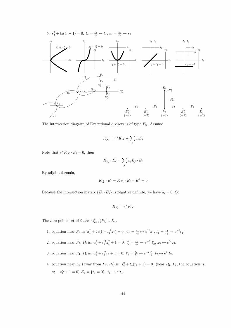
5. s24 + t4(t4 + 1) = 0. t4 = t3t1
7→ t4, s4 = s3t1
7→ s4.
z2
z3
z32 + z4
3 = 0
z3
t1
z2z3 + t31 = 0
t2
t1
z2z3
t2 + t21 = 0
t3
t1
t1 + t3 = 0
z2t2
z3 t4
t1
z2t3
t2
z3
t4 = −1
P6
P7
P4
P5
E4
E13
P2
E12
E23
P3
E22
P9
P8E1P1
E12
(−2)E1
3
(−2)E4
(−2)E2
3
(−2)E2
2
(−2)
E1(−2)
P4 P6 P7 P5
P8
The intersection diagram of Exceptional divisors is of type E6. Assume
KX = π∗KX +∑i
aiEi
Note that π∗KX · Ei = 0, then
KX · Ei =∑j
ajEj · Ei
By adjoint formula,
KX · Ei = KEi · Ei − E2i = 0
Because the intersection matrix Ei · Ej is negative definite, we have ai = 0. So
KX = π∗KX
The zero points set of v are: ∪5i=1Pi ∪ E4.
1. equation near P1 is: u21 + z2(1 + t′41 z2) = 0. u1 = z1
z27→ e2tu1, t′1 = z3
z27→ e−tt′1.
2. equation near P2, P3 is: u22 + t′32 z
23 + 1 = 0. t′2 = t1
z37→ e−2tt′2, z3 7→ e3tz3.
3. equation near P4, P5 is: u23 + t′23 t2 + 1 = 0. t′3 = t1
t27→ e−tt′3, t2 7→ e2tt2.
4. equation near E4 (away from P6, P7) is: s24 + t4(t4 + 1) = 0. (near P6, P7, the equation is
u24 + t′24 + 1 = 0) E4 = t1 = 0. t1 7→ ett1.
44
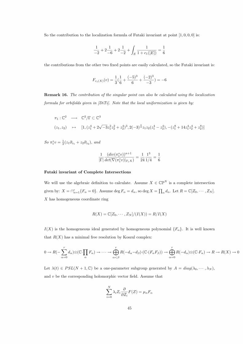
So the contribution to the localization formula of Futaki invariant at point [1, 0, 0, 0] is:
1−2
+ 21−6
+ 21−2
+∫E
11 + c1([E])
=16
the contributions from the other two fixed points are easily calculated, so the Futaki invariant is:
Fc1(X)(v) =13
(16
+(−5)3
6+
(−2)3
−3) = −6
Remark 16. The contribution of the singular point can also be calculated using the localization
formula for orbifolds given in [DiTi]. Note that the local uniformization is given by:
π1 : C2 −→ C2/Γ ⊂ C3
(z1, z2) 7→ [1, (z41 + 2
√−3z2
1z22 + z4
2)3, 2(−3)34 z1z2(z4
1 − z42),−(z8
1 + 14z41z
42 + z8
2)]
So π∗1v = 1
2 (z1∂z1 + z2∂z2), and
1|Γ|
(div(π∗1v))n+1
det(∇(π∗1v)|TzX)
=124
13
1/4=
16
Futaki invariant of Complete Intersections
We will use the algebraic definition to calculate. Assume X ∈ CPN is a complete intersection
given by: X = ∩rα=1Fα = 0. Assume degFα = dα, so degX =∏α dα. Let R = C[Z0, · · · , ZN ].
X has homogeneous coordinate ring
R(X) = C[Z0, · · · , ZN ]/(I(X)) = R/I(X)
I(X) is the homogeneous ideal generated by homogeneous polynomial Fα. It is well known
that R(X) has a minimal free resolution by Koszul complex:
0 → R(−r∑
α=0
dα)⊗(C·∏α
Fα) → · · · →r⊕
α<β
R(−dα−dβ)·(C·(FαFβ)) →r⊕
α=0
R(−dα)⊗(C·Fα) → R→ R(X) → 0
Let λ(t) ∈ PSL(N + 1,C) be a one-parameter subgroup generated by A = diag(λ0, · · · , λN ),
and v be the corresponding holomorphic vector field. Assume that
N∑i=0
λiZi∂
∂ZiF (Z) = µαFα
45

(C∗)2 acts on S(X). Let ak,l = dimS(X)k,l be the dimensions of weight spaces, then this action
has character:
Ch(S(X)) =∑
(k,l)∈N×Z
ak,ltk1tl2 =
∏rα=1(1 − tdα1 tµα2 )∏Ni=0(1 − t1t
λi2 )
= f(t1, t2)
The k − th Hilbert weight is (note it’s a finite sum) wk =∑l∈Z ak,l × l and
∑k∈N
wktk1 =
∂f
∂t2
∣∣∣∣t2=1
= −∑α(µαtdα1
∏β 6=α(1 − t
dβ1 ))
(1 − t1)N+1+ (∑i
λi)t1
∏rα=1(1 − tdα1 )
(1 − t1)N+2
= −∑α(µαtdα1
∏β 6=α(1 + · · · + t
dβ−11 ))
(1 − t1)N+2−r + λt1
∏rα=1(1 + · · · + tdα−1
1 )(1 − t1)N+2−r (2.29)
Lemma 19. Let
f(t) =g(t)
(1 − t)n+1=∑ri=0 ait
i
(1 − t)n+1=
+∞∑k=0
bktk
then
bk =kn
n!g(1) +
kn−1
2(n− 1)!((n+ 1)g(1) − 2g′(1)) +O(kn−2)
Proof.
f(t) = (r∑i=0
aiti) ·
∞∑j=0
(n+ j
n
)tj
So when k 1,
bk =r∑i=0
ai
(n+ k − i
n
)=
r∑i=0
ai(n+ k − i) · · · (k − i+ 1)
n!
=kn
n!
r∑i=0
ai +kn−1
2(n− 1)!
r∑i=0
ai(n+ 1 − 2i) +O(kn−2)
=kn
n!g(1) +
kn−1
2(n− 1)!((n+ 1)g(1) − 2g′(1)) +O(kn−2)
Let g(t) = −∑α(µαtdα1
∏β 6=α(1 + · · · + t
dβ−11 )) + λt1
∏rα=1(1 + · · · + tdα−1
1 ), n = N + 1 − r,
let µα = µα − λN+1dα, then µ is invariant when λ(t) differs by a diagonal matrix. by the lemma,
we can get
g(1) = −∑α
µα∏β 6=α
dβ+λ∏α
dα = −∏α
dα(∑β
µβdβ
−λ) = −∏α
dα
∑β
µβdβ
− λ
N + 1(N + 1 − r)
(2.30)
46
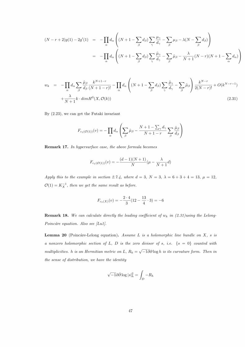
(N − r + 2)g(1) − 2g′(1) = −∏α
dα
(N + 1 −∑β
dβ)∑γ
µγdγ
−∑β
µβ − λ(N −∑β
dβ)
= −
∏α
dα
(N + 1 −∑β
dβ)∑γ
µγdγ
−∑β
µβ − λ
N + 1(N − r)(N + 1 −
∑α
dα)
wk = −∏α
dα∑β
µβdβ
kN+1−r
(N + 1 − r)!−∏α
dα
(N + 1 −∑β
dβ)∑γ
µγdγ
−∑β
µβ
kN−r
2(N − r)!+O(kN−r−1)
+λ
N + 1k · dimH0(X,O(k)) (2.31)
By (2.23), we can get the Futaki invariant
Fc1(O(1))(v) = −∏α
dα
∑β
µβ −N + 1 −
∑γ dγ
N + 1 − r
∑β
µβdβ
Remark 17. In hypersurface case, the above formula becomes
Fc1(O(1))(v) = − (d− 1)(N + 1)N
(µ− λ
N + 1d)
Apply this to the example in section 2.7.4, where d = 3, N = 3, λ = 6 + 3 + 4 = 13, µ = 12,
O(1) = K−1X , then we get the same result as before.
Fc1(X)(v) = −2 · 43
(12 − 134
· 3) = −6
Remark 18. We can calculate directly the leading coefficient of wk in (2.31)using the Lelong-
Poincare equation. Also see [Lu1].
Lemma 20 (Poincare-Lelong equation). Assume L is a holomorphic line bundle on X, s is
a nonzero holomorphic section of L, D is the zero divisor of s, i.e. s = 0 counted with
multiplicities. h is an Hermitian metric on L, Rh =√−1∂∂ log h is its curvature form. Then in
the sense of distribution, we have the identity
√−1∂∂ log |s|2h =
∫D
−Rh
47

i.e., for any smooth (2n− 2) form η on X, we have
√−1∫X
(log |s|2h)∂∂η =∫D
η −∫X
Rh ∧ η
Let X0 = CPN , Xa+1 = Xa ∩ Fa = 0, then X0 ⊃ X1 · · · ⊃ Xr = X. θv =P
i λi|Zi|2
P
i |Zi|2, then
ivωFS =√−1∂θv. On Xa−1, by the lemma, we have
√−1∂∂ log
|Fa|2
(∑i |Zi|2)da
∣∣∣∣Xa−1
=∫Xa
−da · ωFS |Xa−1
So
∫Xa
θvωN−aFS = da
∫Xa−1
θvωN−a+1FS +
√−1∫Xa−1
θv∂∂ log|Fa|2
(∑i |Zi|2)d
∧ ωN−aFS
Using integration by parts, the second integral on the right equals
√−1∫Xa−1
∂θv ∧ ∂ log|Fa|2
(∑i |Zi|2)d
∧ ωN−aFS =
∫Xa−1
ivωFS ∧ ∂ log|Fa|2
(∑i |Zi|2)da
∧ ωN−aFS
= − 1N − a+ 1
∫Xa−1
v(log|Fa|2
(∑i |Zi|2)da
)ωN−a+1FS
= − 1N − a+ 1
∫Xa−1
(µa − da
∑i λi|Zi|2∑i |Zi|2
)ωN−a+1FS
= − 1N − a+ 1
µa deg(Xa−1) + da1
N − a+ 1
∫Xa−1
θvωN−a+1FS
So
(N − a+ 1)∫Xa
θvωN−aFS = −µa deg(Xa−1) + da(N − a+ 2)
∫Xa−1
θvωN−a+1FS
While
(N + 1)∫X0
θvωNFS = (N + 1)
∫CPN
∑i λi|Zi|2∑i |Zi|2
ωNFS =∑i
λi = λ
By induction, we get
(N − r + 1)∫Xr
θvωN−rFS = −
∏α
dα∑β
µβdβ
+ λ∏α
dα =∏α
dα
−∑β
µβdβ
+ (N + 1 − r)λ
N + 1
This is the same as g(1), (2.30).
48

Chapter 3
Some Extension of general
theories
3.1 Twisted Kahler-Einstein equation and Invariant Rη(X)
In the following, we will always use the notation: β ∈ [0, 1] and α = 1 − β.
Let’s consider the twisted Kahler-Einstein equation
Ric(ωφ) = βωφ + αη (3.1)
for some current η ∈ 2πc1(X) which is allowed to be non-positive and singular. This is equivalent
to the following Monge-Ampere equation:
(ω +√−1∂∂φ)n = eHω,αη−βφωn
where Hω,αη satisfies:
√−1∂∂Hω,αη = Ric(ω) − βω − αη,
∫X
eHω,αηωn/n! = V
One can define the associated K-energy and F -energy:
•
Fω,αη(ωφ) = F 0ω(φ) − V
βlog(
1V
∫X
eHω,αη−βφωn/n!)
49
•
νω,αη(ωφ) = βF 0ω(φ) +
∫X
logωnφ
eHω,αη−βφωnωnφn!
+∫X
Hω,αηωn/n!
It’s easy to verify that these two functional are dual to each other under Legendre transform
([Berm]). Berman called νω,αη the free energy associated with (3.24). The name comes from
his statistical mechanical derivation of Kahler-Einstein equations. Note that in this notation,
νω(ωφ) = νω,0(ωφ).
Proposition 10. We have the following formulas:
1.
νω,αη(ωφ) = −∫ 1
0
dt
∫X
φt · n(Ric(ωt) − βωt − αη) ∧ ωn−1t
2.
νω,αη(ωφ) = βFω,αη(ωφ) +∫X
Hω,αηωn/n! −
∫X
Hωφ,αηωnφ/n!
≥ βFω,αη +∫X
Hω,αηωn/n!
3. Let ωψ solve the equation ωnψ = eHω,αη−βφωn. In other words, Ric(ωψ) = βωφ + αη. then
βFω,αη(ωφ) +∫X
Hω,αηωn
n!≥ νω,αη(ωψ)
4.
νω,αη(ωφ) =∫X
logωnφ
eHω,αηωnωnφn!
− β(Iω − Jω)(ωφ) +∫X
Hω,αηωn/n!
5. Assume ω1 = ω +√−1∂∂φ1, ω2 = ω +
√−1∂∂φ2 = ω +
√−1∂∂(φ1 + φ2). Then
νω,αη(ω1) + νω1,αη(ω2) = νω,αη(ω2), Fω,αη(ω1) + Fω1,αη(ω2) = Fω,αη(ω2)
In other words, νω,αη and Fω,αη satisfy the cocycle condition.
Proof. (2),(3) and (5) follows from the formula relating twisted potentials of two Kahler metrics.
Hωφ,αη = Hω,αη + logωn
ωnφ− βφ− log
(1V
∫X
eHω,αη−βφωn/n!)
= −(
logωnφ
eHω,αη−βφωn+ log
(1V
∫X
eHω,αη−βφωn/n!))
50

The inequality in (3.2) follows from concavity of log:
1V
∫X
Hωφ,αη
ωnφn!
≤ log(
1V
∫X
eHωφ,αηωnφn!
)= 0
For (3), since we have normalized φ so that∫XeHω,αη−βφωn/n! = V ,
Fω,αη(φ) = F 0ω(φ)
νω,αη(ωψ) = βF 0ω(ψ) + β
∫X
(φ− ψ)ωnψn!
+∫X
Hω,αηωn
n!
So (3) follows from
F 0ω(φ) ≥ F 0
ω(ψ) −∫X
(φ− ψ)ωnψn!
Corollary 4. Fω,αη is bounded from below if and only if νω,αη is bounded from below. In this
case, ∫X
Hω,αηωn
n!+ β inf Fω,αη = inf νω,αη
Proposition 11. ([Bern],[BaMa],[Ban]) If η is a positive current, and ωβ := ωφβ solves the
equation (3.1), then ωβ obtains the minimum of Fω,αη(ωφ) and νω,αη(ωφ).
Proof. If ωβ to the equation (3.1) is the critical point of Fω,αη(ωφ). Berndtsson [Bern] proved
Fω,αη(ωφ) is convex on H. So ωβ obtains the minimum of Fω,αη(ωφ). The inequality (3.2) implies
νω,αη also obtains the minimum at ωβ .
There are 2 cases we would like to consider in this Chapter.
• η is any smooth Kahler metric in 2πc1(X).
It was first showed by Tian [Tia6] that we may not be able to solve (∗)t on certain Fano
manifold for t sufficiently close to 1. Equivalently, for such a Fano manifold, there is some
t0 < 1, such that there is no Kahler metric ω in c1(X) which can have Ric(ω) ≥ t0ω. It is
now made more precise. Define
R(X) = supt : (∗)t is solvable
Szekelyhidi proved
51

Proposition 12 ([Sze]).
R(X) = supt : Ric(ω) > tω, ∀ smooth Kahler metric ω ∈ c1(X)
In particular, R(X) is independent of η ∈ c1(X).
• η = D = 0 is the integration along a smooth anti-canonical divisor. One can extend the
theory in smooth case to the conic case. We can define the logarithmic Futaki invariant
after Donaldson (See Section 3.3, [Don6]) and integrate the log-Futaki invariant to get log-
K-energy (See Section 3.3.2). If we assume the log-K-energy is proper, then there exists
conic Kahler-Einstein metric. (Cf. [JMRL]). Note that, we need to relax the C∞ condition
for Kahler potentials to include the potential of Kahler metric with conic singularities. This
conic type Holer space is studied by Donaldson [Don6] (also called wedge Holder space in
[JMRL]). See section 3.2 for sketched proof.
The two cases can be related as follows. Take ηε = ω +√−1∂∂ log(|s|2 + ε), then it’s easy to
verify that limε→0 ηε = αs = 0 =: D, and
limε→0
νω,αηε(φ) = νω,D(φ)
limε→0
Fω,αηε(φ) = Fω,D(φ)
Proposition 13. ([Tia1],[Tia10],[Berm]) For the above two cases, when 0 < β 1, νω,αη is
proper.
Proof. When η is smooth, this was proved by Tian ([Tia1], [Tia10]). The modification to the
conic case was proved by [Berm]. First define the log-alpha-invariant.
α(K−1X , (1−β)D) = max
u > 0;∃0 < Cu < +∞ such that
1V
∫X
e−u(φ−supφ) ehωωn
|sD|2(1−β)n!≤ Cu
Now for any u < α(K−1X , (1 − β)D),
logCu ≥ log(
1V
∫X
e−u(φ−supφ) ehωωn
n!|sD|2(1−β)
)= log
(1V
∫X
e−u(φ−supφ)−log|sD|2(1−β)ωnφ
ehωωnωnφn!
)
≥ − 1V
∫X
log
(|sD|2(1−β)ωnφ
ehωωn
)ωnφn!
+ u
(supφ− 1
V
∫X
φωnφn!
)
≥ 1V
(−∫X
log|sD|2(1−β)ωnφ
ehωωnωnφn!
+ uIω(ωφ)
)
52

νω,(1−β)D(ωφ) ≥ uIω(ωφ) − β(I − J)ω(ωφ) − C(β)
≥(u− β
n
n+ 1
)Iω(ωφ) − C
So if
β <n+ 1n
α(K−1X , (1 − β)D),
then log-K-energy is proper for smooth reference metric. Berman estimated the log-alpha-
invariant:
Proposition 14. [Berm]
α(K−1X , (1 − β)D) = α(LD, (1 − β)D) ≥ minβ, α(LD|D), α(LD) > 0 (3.2)
So when
0 < β <n+ 1n
minα(LD|D), α(LD), (3.3)
the log-K-energy is proper. In particular, when 0 < β 1, the log-K-energy is proper.
Remark 19. Let D be a smooth divisor such that D ∼Q −λKX for some 0 < λ ∈ Q. If we let
η = λ−1D ∈ c1(X), then as we will show in [LiSu], the conclusion in Lemma 13 in general is
false if λ < 1.
Proposition 15. ([Berm], [Rub]) νω,αη is proper if and only if Fω,αη is proper.
We give a proof due to Berman [Berm, Cor.3.5].
Proof. If Fω,αη is proper, then νω,αη is proper by inequality in (3.2).
Now assume νω,αη is proper. Then νω,αη − δ(I − J)ω is proper for δ small. Let η′ = (αη −
δω)/(α− δ). Note that α− δ = 1− (β+ δ). Then it’s easy to verify that Hω,(α−δ)η′ = Hω,αη and
νω,αη − δ(I − J)ω = νω,(α−δ)η′
Because it’s bounded from below, by Corollary 4, Fω,(α−δ)η′ is bounded from below (even when
53

η′ is not a positive current). So
Fω,αη(φ) = F 0ω(φ) − β + δ
β
V
β + δlog(
1V
∫X
eHω,αη−(β+δ) βφβ+δωn/n!
)≥ F 0
ω(φ) − β + δ
βF 0ω
(β
β + δφ
)+β + δ
βFω,(α−δ)η′(βφ/(β + δ))
≥ F 0ω(φ) − β + δ
βF 0ω
(β
β + δφ
)− C
= Jω(φ) − β + δ
βJω
(β
β + δφ
)− C
≥ (1 − (β/(β + δ))1/n)Jω(φ) − C
Now by Lemma 13,
Corollary 5. In the two cases (smooth or conic), when β 1, Fω,(1−β)η is proper.
The following lemma is observed together with Dr. Song Sun.
Lemma 21. If Fω,(1−β)η is proper (resp. bounded) when β = β0 and it’s bounded (resp. proper)
when β = β1, then it’s proper when β = (1− t)β0 + tβ1 for 0 < t < 1. The same conclusion holds
for νω,(1−β)η.
Proof. Let βt = (1− t)β0 + tβ1. First note that Hω,(1−βt)η = (1− t)Hω,(1−β0)η + tHω,(1−β1)η. So
by Holder inequality we get
∫X
eHω,(1−βt)η−βtφωn
n!=
∫X
(eHω,α0η−β0φ
)1−t (eHω,α1η−β1φ
)t ωnn!
≤(∫
X
eHω,(1−β0)η−β0φωn
n!
)1−t(∫X
eHω,(1−β1)η−β1φωn
n!
)t
So the statement follows. The last statement follows by noting νω,(1−β)η is linear in β.
Proposition 16. In the above two cases (smooth or conic), if (3.1) is solvable for β = β1 ≤ 1,
then it’s solvable for any 0 < β < β1.
Proof. Let ωβ1 be a solution of the equation (3.1). Because η is positive, ωβ1 obtains the minimum
of νω,α1η(ωφ) by Proposition 11. In particular it’s bounded from below . By Proposition 13, νω,α0η
is proper for any 0 < β0 1. So by Lemma 21, νω,(1−β)η is proper for any 0 < β < β1. By
Proposition 15, Fω,(1−β)η is proper for 0 < β < β1. Now the solvability in the smooth case is
well known ([Tia9],[Tia10]). The conic case is solved in [JMRL]. See section 3.2 for sketched
proof.
54

For the above two cases (smooth or conic), we can define
Rη(X) = sups : (3.1) is solvable for β ∈ (0, s]
Corollary 6. The following are equivalent:
1. Rη(X) ≥ t0, i.e. (3.1) is solvable for 0 < β < t0;
2. The function νω,αη(ωφ) is proper for any 0 < β < t0;
3. Fω,αη(ωφ) is proper for any 0 < β < t0.
Proof. (1)⇒(2). Take any β1 < t0. The solution ωβ1 obtains the minimum of νω,(1−β1)η by
Proposition 11. By Proposition 13, νω,(1−β0)η is proper for any 0 < β0 1. So by Lemma 21,
νω,(1−β)η is proper for β0 < β < β1. (2)⇒(3) follows from Proposition 15. (3)⇒(1): This is well
known in the smooth case (See e.g. [BaMa], [Tia10]). In the conic case, see Section 3.2.
3.2 Existence of conic Kahler-Einstein metric on Fano man-
ifold
There is another continuity method, which is via Kahler-Einstein metrics with conic singularities.
This is equivalent to solving the following family of equations with parameter β:
Ric(ωψ) = βωψ + (1 − β)D ⇐⇒ (ω +√−1∂∂ψ)n = ehω−βψ
ωn
|s|2(1−β)(∗)β
where D ∈ | −KX | is a smooth divisor, s is the defining section of [D] ∼= −KX , and | · |2 is a
Hermitian metric on −KX such that its curvature form −√−1∂∂ log | · |2 = ω.
Remark 20. The weak solution was obtained by Berman [Berm] using pluripotential theory. For
the geometric conic solution, in the early version of [JMRL], the authors need to assume the cone
angle is in (0, π] or the bisectional curvature of some reference conic metric has upper bound.
Joint with Yanir Rubinstein, by carefully choosing adapted local coordinates, we showed in the
appendix that the bisectional curvature of a natural reference conic metric is indeed bounded from
above. So this allows any cone angle in (0, 2π].
We will use the log-K-energy associated with a reference conic metric. Let ω = ω+√−1∂∂|s|2β .
55

So for any ω ∈ [ω] with at most conic singularities, we can define the log-K-energy and
log-F-energy to be
νbω(ψ) := ν
bω,D =∫X
logωnψ
ebhbω−βψωn
ωnψn!
+ βF 0bω(ψ) +
∫X
hbωω
n/n!.
Fbω(ψ) = F 0
bω(ψ) − V
βlog(
1V
∫X
ebh
bω−βψωn/n!).
where hbω satisfies
√−1∂∂h
bω = Ric(ω) − βω − αs = 0, and∫X
ebh
bωωn = V (3.4)
Theorem 17. [JMRL] Assume Fbω is proper or ν
bω is proper, then there exists a conic metric
along the divisor D of conic angle 2πβ.
Sketch of the proof. The idea is using continuity method as in the proof in the smooth case. So
we consider a family of equations:
(ω +√−1∂∂ψ)n = e
bhbω−tψωn (3.5)
This is equivalent to the equation
Ric(ωψ) = tωψ + (β − t)ω + αs = 0. (3.6)
• Step 0: Set up good function space. This is essentially carried out by Donaldson in [Don6].
We first write the metric and differential operator in the conic coordinate. Let z = reiθ be
the ordinary complex coordinate. Define ρ = rβ . The model case tells us the right thing
to do.
ω =dz1 ∧ dz1|z1|2α
+∑j>1
dzj ∧ dzj =(dr + irdθ) ∧ (dr − irdθ)
r2β+∑j>1
dzj ∧ dzj
= (dρ+ iβρdθ) ∧ (dρ− iβρdθ) +∑j>1
dzj ∧ dzj
Let ε = eiβθ(dρ+iβρdθ) = dζ, where ζ = zβ = ρeiβθ is defined by choosing a branch locally
away from 0. Then the general (1,1) form, in particular the Kaler form for a conic metric,
56

also has cross terms:
ω =√−1(fε ∧ ε+ fjε ∧ dzj + fjdzj ∧ ε+ fijdzi ∧ dzj
)(3.7)
If ω =√−1∂∂φ,
f =∂2φ
∂ζ∂ζ=
14
(e−iβθ(
∂
∂ρ− i
βρ
∂
∂θ))(
eiβθ(∂
∂ρ+
i
βρ
∂
∂θ))φ
=14
∆C2,βφ =14
1βρ
(∂
∂ρ(βρ
∂
∂ρ) +
1β2ρ2
∂
∂θ(βρ
∂
∂θ))φ
=14
(∂2
∂ρ2+
1ρ
∂
∂ρ+
1β2ρ2
∂2
∂θ2
)φ
where ∆C2,β is the Laplacian associated with the standard conic metric on C2: gβ =
dρ2 + β2ρ2dθ2.
fj =∂2φ
∂ζ∂zj=
12e−iβθ
(∂
∂ρ− i
βρ
∂
∂θ
)∂
∂zjφ
Following Donaldson, we define
Definition 12. 1. f is in C ,γ,β if f is Holer continuous in the coordinate
(ζ = ρeiθ = rβeiθ = z|z|β−1, zj)
2. A (1,0)-form α = f1ε+∑j>1 fjdzj is in C,γ,β if fi ∈ C,γ,β for 1 ≤ i ≤ n, and f1 → 0
as z1 → 0.
3. A (1,1)-form ω is in C,γ,β if f, fj , fj , fij ∈ C,γ,β, and fj , fj → 0 as z1 → 0.
4. A function f is in C2,γ,β if f, ∂f, ∂∂f are all C ,γ,β.
Remark 21. The point is the derivatives involve only the following wedge differentials:
∂
∂ρ,
1ρ
∂
∂θ,∂
∂zj,∂2
∂ζ∂ζ,
∂2
∂ρ∂zj,
1ρ
∂2
∂θ∂zj,
∂2
∂zi∂zj
The linear theory is set up by Donaldson:
Proposition 17. [Don6] If γ < µ = β−1 − 1, the inclusion C2,α,β → C ,γ,β is compact.
If ω is a C ,γ,β Kahler metric on (X,D) then the Laplacian of ω defines a Fredholm map
∆bω : C2,γ,β → C,γ,β.
57

• Step 1: Start the continuity method. Let
S = t ∈ (−∞, β); (3.5) is solvable.
Then S is non-empty. This is achieved by solving the equation (3.5) when t 0 using
Newton-Moser iteration method.
• Step 2: Openness of solution set. This follows from implicit function theorem thanks to
the Fredholm linear theory set up in Step 0. See [JMRL] for details.
• Step 3: C0-estimate. This is the same as in the smooth case. By taking derivative with
respect to t on both sides of (3.5)
∆bωψt = −tψ − ψ
By calculation, one can prove that
F 0bω(ψt) = −1
t
∫ t
0
(I − J)bωt(ψt)ω
nt /n! ≤ 0
So
Fbω(ψt) ≤ −V
βlog(
1V
∫X
ebh
bω−βψωn/n!)
= −Vβ
log(
1V
∫X
e−(β−t)ψωnt /n!)
≤ β − t
β
∫X
ψtωnt /n! ≤ β − t
β2V log
(1V
∫X
eβψt ωnt /n!)
=β − t
β2V log
(1V
∫X
ebh
bω ωn/n!)
= 0
So if Fbω(ψ) is proper, then I
bω(ωψt) ≤ C. Now the C0-estimate follows from the following
Proposition.
Proposition 18. 1. Osc(ψt) ≤ Ibω(ψt).
2. (Harnack estimate) − infX ψt ≤ n supX ψt.
• Step 3: C2-estimate. To get the C2-estimate, we can use the Chern-Lu’s inequality and
maximal principle as in Proposition 2. By the equation (3.6), Ric(ωψt) ≥ tωψt . The
upper bound of bisectional curvature of ω is crucial, which will be shown in the following
subsection.
58
Let Ξ = log trbωψ ω − λψ as in (2.3). To use the maximal principle in the conic setting, one
can use Jeffres’s trick as in [Jef]. We add the barrier function ε‖s‖2γ′for 0 < γ′ < γ so
that Ξ + ε‖s‖2γ′obtains the maximum x′0 6∈ D. We then apply the maximal principle to
Ξ + ε‖s‖2γ′and let ε→ 0.
• Step 4: C ,2,γ,β-estimate. There is a Krylov-Evans’ estimate in the conic setting as developed
in [JMRL]. The proof is similar to the smooth case in Subsection 2.3.2 but adapted to the
conic(wedge) Holder space.
3.2.1 A calculation of bisectional curvature of a conic metric
We consider reference metric of the form
ω = ω′ +√−1∂∂‖S‖2β
ω′ is a smooth Kahler form. Let D = S = 0. Assume we choose a local coordinate zi, such
that D = zn = 0. Denote ∇zn = dzn + zna−1∂a.
∂‖S‖2β = β‖S‖2(β−1)azn∇zn
∂∂‖S‖2β = −β‖S‖2βω + β2‖S‖2β−2a∇zn ∧∇zn
where ω = c1([D], ‖ · ‖) = −∂∂ log a. So
ω = ω′ − β‖S‖2βω + β2‖S‖2β−2a∇zn ∧∇zn (3.8)
By scaling the Hermitian metric ‖ · ‖, we can assume this is positive definite.
To simplify the calculation of curvature of ω, we need lemma.
Lemma 22. For any point p ∈ X\D, there exists ε > 0, such that if distg′(p,D) ≤ ε, then we
can choose local holomorphic frame e of LD and local coordinates zini=1 such that S = zne, and
a = ‖e‖2 satisfies a(p) = 1, da(p) = 0, ∂2a∂zi∂zj
a(p) = 0.
Proof. Fix any point q ∈ D, we can choose local holomorphic frame e′ and complex coordinates
wi in Bg′(q, ε(q)) for ε(q) 1. Let S = f ′e′ with f ′ a holomorphic function and ‖e′‖2 = c. Let
e = he′ for some holomorphic function h to be chosen. Then a = ‖he′‖2 = |h|2c. Now fix any
59

point p ∈ Bg′(q, ε(q)). In order for a to satisfy the vanishing property with respect to variables
wi at point p, we can just choose h such that h(p) = c(p)−1/2, ∂ih(p) = −c(p)−1h(p)∂ic(p) =
−c(p)−3/2∂ic(p) and
∂i∂jh(p) = −c(p)−1(h(p)∂i∂jc(p) + ∂jc(p)∂ih(p) + ∂ic(p)∂jh(p))
= −c(p)−3/2∂i∂jc(p) + 2c(p)−5/2∂ic(p)∂jc(p)
Here we used ∂i to mean partial derivatives with respect to variable wi. Then we get S = fe =
f ′e′ with f = f ′h−1 a holomorphic function. Since D = S = 0 is a smooth divisor, we can
assume ∂f∂wn
(q) 6= 0. Choose ε(q) sufficiently small, we can assume ∂f∂wn
6= 0 in Bg′(q, ε(q)). So by
inverse function theorem, z1 = w1, · · · , zn−1 = wn−1, zn = f(w1, · · · , wn) are complex coordinate
in Bg′(q, ε(q)/2) and now S = ef(w) = zne. By chain rule, it’s easy to verify that a satisfy the
condition. a(p) = 1, ∂ia(p) = ∂i∂ja(p) = 0.
We can cover D by Bg′(q, ε(q)/2) for any q ∈ D. By compactness of D, the conclusion
follows.
Remark 22. By the above proof, we can choose zn = f = f ′h−1 = f ′c1/2 for any point p in
Bg′(q, ε(q)). So zn is uniformly equivalent to f ′, i.e. C−1|f ′|(p) ≤ |zn|(p) ≤ C|f ′|(p) for any
p ∈ Bg′(q, ε(q)/2).
Proposition 19. The holomorphic bisectional curvatures of ω are bounded from above.
Proof. Using the above lemma, for any point q ∈ D, fix any point p ∈ Bg′(q, ε) and choose the
adapted local holomorphic frame e and complex coordinate zi provided by the last lemma.
Assume in the representation (3.8), ω′ =∑i,j g
′ijdzi ∧ dzj , ω =
∑i,j hijdzi ∧ dzj and ω =∑
i,j gijdzi∧dzj . We do some calculation. The calculation is straightforward although laborious.
In particular, note that the formula we get has the right symmetry for the subindex.
gij = g′ij − βaβ |zn|2βhij + β2aβ |zn|2β(
(dzn + a−1∂azn) ∧ (dzn + a−1∂azn)|zn|2
)ij
= g′ij − βaβhij |zn|2β + β2aβ−2∂ia∂ja|zn|2β + β2aβ−1∂ia|zn|2(β−1)znδjn
+β2aβ−1∂ja|zn|2(β−1)znδin + β2aβ |zn|2(β−1)δinδjn
Using the vanishing property of a we get
gij(p) = g′ij − βhij |zn|2β + β2|zn|2(β−1)δinδjn (3.9)
60

∂gij∂zk
=∂g′
ij
∂zk− β∂k(aβhij)|zn|2β + β2∂k(aβ−2∂ia∂ja)|zn|2β + β2∂k(aβ−1∂ia)|zn|2(β−1)znδjn
+β2∂k(aβ−1∂ja)|zn|2(β−1)znδin + β2∂k(aβ)|zn|2(β−1)δinδjn
−β2aβhij |zn|2(β−1)znδnk + β3aβ−2∂ia∂ja|zn|2(β−1)znδnk + β3aβ−1∂ia|zn|2(β−1)δnkδnj
β2(β − 1)aβ−1∂ja|zn|2(β−2)z2nδnkδin + β2(β − 1)aβ |zn|2(β−2)znδnkδinδnj
Now we use the vanishing property of a and ∂i∂ja(p) = ∂i∂j log a(p) = −hij to get
∂kgij(p) = ∂kg′ij − β∂khij |zn|2β − β2hkj |zn|2(β−1)znδin − β2hij |zn|2(β−1)znδnk
+β2(β − 1)|zn|2(β−2)znδnkδniδnj
= ∂kg′ij − β∂khij |zn|2β − β2(hkjδin + hijδnk)|zn|2(β−1)zn
+β2(β − 1)|zn|2(β−2)znδnkδniδnj
The last ingredient appearing in holomorphic bisectional curvature can also be calculated.
∂l∂kgij(p) = ∂l∂kg′ij − β(−βhklhij + ∂l∂khij)|zn|2β + β2hilhkj |zn|2β − β2∂khil|zn|2(β−1)znδjn
−β2∂lhkj |zn|2(β−1)znδin − β3hkl|zn|2(β−1)δinδjn − β2∂lhij |zn|2(β−1)znδnk
−β3hil|zn|2(β−1)δnkδnj
−β2(∂khij)|zn|2(β−1)znδnl − β3hkj |zn|2(β−1)δnlδin − β3hij |zn|2(β−1)δnlδnk
+β2(β − 1)2|zn|2(β−2)δnlδnkδniδnj
= ∂l∂kg′ij + β2(hklhij + hilhkj)|zn|2β − β(∂l∂khij)|zn|2β
−β2(∂khilδjn + ∂khijδnl)|zn|2(β−1)zn − β2(∂lhijδin + ∂lhijδnk)|zn|2(β−1)zn
−β3(hklδinδjn + hkjδnlδin + hijδnlδnk + hilδnkδnj)|zn|2(β−1)
+β2(β − 1)2|zn|2(β−2)δnlδnkδniδnj (3.10)
Now we can estimate the holomorphic bisectional curvature. Let ξini=1, ηini=1 be two unit
vectors with respect to gij(p): gij(p)ξiξj = gij(p)ηiηj = 1. Using the formula for gij(p) in (3.9).
This implies in particular
|ξi| ≤ C, |ηi| ≤ C, 1 ≤ i ≤ n− 1
|ξn| ≤ C|zn|1−β , |ηn| ≤ C|zn|1−β (3.11)
61

We want to estimate
Rijkl(p)ξiξjηkηl =(−∂2gij∂zk∂zl
+∂giq∂zk
gpq∂gpj∂zl
)ξiξjηkηl
There are several types of singular terms. In order to estimate them, we first estimate the inverse
of (gij). Let fij = g′ij− βhij |zn|2β , It’s easy to get from (3.9) that
det(gij) =β2
|zn|2(1−β)det(fij)1≤i,j≤n−1 + det(fij) =:
β2
|zn|2(1−β)(a+ b|zn|2(1−β))
with a = det(fij)1≤i,j≤n−1 and b = det(fij)/(β2) and
gpq = O(1) p, q < n
gpn, gnq = O(|zn|2(1−β)) p, q < n
gnn = β−2|zn|2−2β aa+b|zn|2(1−β)
(3.12)
Remark 23. Since when |zn| is small, fij is uniformly positive definite, a and b are uniformly
positive when |zn| is small.
1. Possible singular terms in − ∂2gij∂zk∂zl
ξiξjηkηl
(a) ∣∣O(1)δjn|zn|2β−2znξj∣∣ =
∣∣|zn|2β−1ξn∣∣ ≤ C|zn|β
(b) ∣∣O(1)δinδjn|zn|2β−2ξiξj∣∣ =
∣∣|zn|2β−2|ξn|2∣∣ ≤ C
∣∣O(1)δinδkn|zn|2β−2ξiηk∣∣ =
∣∣|zn|2β−2ξnηn∣∣ ≤ C
(c) So here the singular term is the only last one
−β2(β − 1)2|zn|2β−4|ξn|2|ηn|2 (3.13)
2. Possible singular terms in ∂giq∂zk
gpq∂gpj∂zl
ξiξjηkηl.
We first define the bilinear form for local tensor A = (Aikq) satisfying Aikq = Akiq as
follows:
A ∗B = AikqgpqBjlpξiξjηkηl (3.14)
62

where Bjlp = Bjlp.
By diagonalization, it’s easy to see that ∗ is a semipositive bilinear form.
Now we can write
gpq∂giq∂zk
∂gpj∂zl
ξiξjηkηl = (A+B + C +D) ∗ (A+B + C +D)
where
Aikq = ∂kg′iq, Bikq = −β∂khiq|zn|2β
Cikq = −β2(hkqδin + hiqδnk)|zn|2(β−1)zn, Dikq = β2(β − 1)|zn|2(β−2)znδnkδniδnq
Using (3.12) and (3.11), let’s check all the possible singular terms:
(a) Terms in C ∗ C:
∣∣hkqδin|zn|2β−2zngpqhplδjn|zn|2β−2znξiξjηkηl
∣∣ =∣∣O(1)|zn|4β−2|ξn|2
∣∣ ≤ C|zn|2β
∣∣hiqδkn|zn|2β−2zngpqhplδjn|zn|2β−2znξiξjηkηl
∣∣ =∣∣O(1)|zn|4β−2ξnηn
∣∣ ≤ C|zn|2β
(b) Terms in A ∗ C:
∣∣(∂kg′iq)gpqhplδjn|zn|2β−2znξiξjηkηl∣∣ =
∣∣O(1)|zn|2β−1ξn∣∣ ≤ C|zn|β
This also implies the terms in B ∗ C are bounded.
(c) Terms in B ∗D:
∣∣(∂khiq)|zn|2βgpq|zn|2β−4znδnpδnjδnlξiξjηkηl∣∣ =
∣∣O(1)|zn|4β−3gnq ξnηn∣∣ ≤ C|zn|
(d) Terms in C ∗D:
∣∣hkqδin|zn|2β−2zngpq|zn|2β−4znδnpδnjδnlξiξjηkηl
∣∣ =∣∣gnq|zn|4β−4|ξn|2ηn
∣∣ ≤ C|zn|1−β
(e) So the only singular terms are contained in (A+D) ∗ (A+D).
Now to deal with this bad term, we first note the Cauchy-Schwartz inequality
(A+D) ∗ (A+D) = |A|2 + |D|2 +A ∗D +D ∗A ≤ (1 + 1/ε)A ∗A+ (1 + ε)D ∗D
63

where ε is to determined. Indeed, this follows from ( 1√εA−
√εD) ∗ ( 1√
εA−
√εD) ≥ 0.
To find ε, replacing gnn by it’s explicit expression in (3.12) we get:
D ∗D = β4(β − 1)2|zn|4β−6gnn|ξn|2|ηn|2 = β2(β − 1)2|zn|2β−4|ξn|2|ηn|2a
a+ b|zn|2−2β
(3.15)
We can add (3.13) and (1 + ε)D ∗D to get
β2(β − 1)2|zn|2β−4|ξn|2|ηn|2(−1 + (1 + ε)
a
a+ b|zn|2−2β
)
So if we choose ε:
1 = (1 + ε)a
a+ b|zn|2−2β=⇒ ε =
b
a|zn|2−2β
The only singular term left is
E := (1 + 1/ε)A ∗A =a+ b|zn|2−2β
b|zn|2−2βgpq(∂kg′iq) (∂lg
′pj)ξiξjηkηl (3.16)
To bound this term, we first note that there were some ambiguity in choosing first
n − 1 coordinates z1, · · · , zn−1 in Lemma 22. Now we can choose these coordinates
more carefully.
Lemma 23. At a fixed point P , We can modify the first (n− 1) coordinates zin−1i=1
and leave zn unchanged such that ∂kg′iq(P ) = 0, for 1 ≤ q ≤ n− 1. Also under these
coordinate, the condition for a is preserved: a(p) = 1, ∂ia(p) = 0, ∂i∂ja(p) = 0.
Proof. Denote zi = zi − zi(P ) for 1 ≤ i ≤ n, we can write ω′ as
ω′ = (cij + aijkzk + ajikzk)dzi ∧ dzj +O(2) (3.17)
We want to do coordinate change:
zi = wi +12bilmwmwl (3.18)
with bilm = biml, and bnlm = 0 since we want zn to stay unchanged.
64

When we substitute (3.18) into (3.17), we get
ω′ =(cij + (aijk + crjbrki)wk + (ajik + cisbskj)wk
)dwi ∧ dwj +O(2)
For any fixed 1 ≤ i, k ≤ n, we want to solve (n-1) unknown brkin−1r=1 from (n-1)
equations:
aij +n−1∑r=1
crjbrki = 0, 1 ≤ j ≤ n− 1
Note that the 1 ≤ r ≤ n− 1 since bnki = 0.
If we denote the truncated square matrix (crj = crj)n−1r,j=1, then crj is positive definite.
Denote by crj its inverse matrix. Then we can choose
brki = −n−1∑r=1
crjaijk for 1 ≤ r, j ≤ n− 1, and bnki = 0
to get∂
∂wkg′(
∂
∂wi,∂
∂wj
)(P ) = aijk + crjbrki = 0 for 1 ≤ j ≤ n− 1
The last statement follows from chain rule.
Using this lemma and gnn in (3.12), we see the last singular term in (3.16) becomes
E =a+ b|zn|2−2β
b|zn|2−2βgnn(∂kg′in)(∂lg
′nj)ξiξjηkηl = β−2 a
bO(1) = O(1)
3.3 Log-Futaki invariant and log-K-stability
3.3.1 Log-Futaki invariant
In this section, we recall Donaldson’s definition of log-Futaki invariant (3.22). Let (X,L) be a
polarized projective variety and D be a normal crossing divisor:
D =r∑i=1
αiDi
with αi ∈ (0, 1).
From now on, we fix a Hermitian metric | · |i = hi and defining section si of the line bundle
65

[Di]. Assume ω ∈ c1(L) is a smooth Kahler form. We define
P(ω) =ωφ := ω +
√−1∂∂φ; φ ∈ L∞(X) ∩ C∞(X\D) such that ω +
√−1∂∂φ ≥ 0
Around any point p ∈ X, we can find local coordinate zi; i = 1, · · · , n, such that D is defined
by
D = ∪rpi=1αizi = 0
where rp = ]i; p ∈ Di.
Definition 13. We say that ω ∈ P(ω) is a conic Kahler metric on (X,D), if around p, ω is
quasi-isometric to the metric
rp∑i=1
dzi ∧ dzi|zi|2αi
+n∑
j=rp+1
dzj ∧ dzj
We will simply say that ω is a conic metric if it’s clear what D is.
Geometrically, this means the Riemannian metric determined by ω has conic singularity along
each Di of conic angle 2π(1 − αi).
Remark 24. Construction of Kahler-Einstein metrics with conic singularites was proposed long
time ago by Tian, see [Tia8] in which he used such metrics to prove inequalities of Chern numbers
in algebraic geometry.
One consequence of this definition is that globally the volume form has the form
ωn =Ω∏r
i=1 |si|2αii
where Ω is a smooth volume form. For any volume form Ω, let Ric(Ω) denote the curvature of
the Hermitian metric on K−1X determined by Ω. Then, by abuse of notation,
Ric(ω) = Ric(ωn) = Ric(Ω) +√−1
r∑i=1
αi∂∂ log |si|2hi = Ric(Ω) −r∑i=1
αic1([Di], hi) +r∑i=1
αiDi
= Ric(Ω) − c1([D], h) + D (3.19)
where h = ⊗ri=1hαii and s = ⊗ri=1s
αii are Hermitian metric and defining section of the R-line
bundle [D] = ⊗ri=1[Di]αi .
66

Here we used the Poincare-Lelong identity:
√−1∂∂ log |si|2hi = −c1([Di], hi) + Di
where Di is the current of integration along the divisor Di.
The scalar curvature of ω on its smooth locus X\D is
S(ω) = gijRij =nRic(ω) ∧ ωn−1
ωn=n(Ric(Ω) − c1([D], h)) ∧ ωn−1
ωn
So if S(ω) is constant, then the constant only depends on cohomological classes by the identity:
nµ1 :=n(c1(X) − c1([D])) ∧ [c1(L)]n−1
c1(L)n=
−n(KX +D) · Ln−1
Ln= nµ− V ol(D)
V ol(X)(3.20)
Here
nµ =n c1(X) · c1(L)n−1
c1(L)n=
−nKX · Ln−1
Ln
is the average scalar curvature for smooth Kahler form in c1(L). And
V ol(D) =∫D
c1(L)n−1
(n− 1)!=D · Ln−1
(n− 1)!, V ol(X) =
∫X
c1(L)n
n!=Ln
n!
Now assume C∗ acts on (X,L) and v is the generating holomorphic vector field. Recall that the
ordinary Futaki-Calabi invariant ([Fut], [Cal3]) is defined by
F (c1(L))(v) = −∫X
θv(S(ω) − nµ)ωn
n!
where θv satisfies
ιvω = ∂θv
Now assume ω∞ ∈ P(ω) is a conic metric and satisfies
S(ω∞) = nµ1 (3.21)
Assume D is preserved by the C∗ action. Let’s calculate the ordinary Futaki invariant using the
conic metric ω∞. Let θv = θ(ω∞, v). Then near p ∈ D, v ∼∑rpi=1 cizi∂zi+ v with v = o(z1 · · · zrp)
holomorphic. θv ∼∑rpi=1 |zi|2(1−αi).
67

We then make use of the distributional identity (3.19) to get
F (c1(L))(v) = −∫X
θv(nRic(ω∞) − nµω∞) ∧ ωn−1∞n!
= −∫X
θv [(nRic(Ω) − nc1([D], h) − nµ1ω∞) + nD − (nµ− nµ1)ω∞] ∧ ωn−1∞n!
= −∫X
θv(S(ω∞) − nµ1)ωn∞n!
−∫X
Dθvωn−1∞
(n− 1)!+ (nµ− nµ1)
∫X
θvωn∞n!
= −(∫
D
θvωn−1∞
(n− 1)!− V ol(D)V ol(X)
∫X
θvωn∞n!
)
So we get
0 = F (c1(L))(v) +(∫
D
θvωn−1∞
(n− 1)!− V ol(D)V ol(X)
∫X
θvωn∞n!
)Since the two integrals in the above formula is integration of (singular) equivariant forms, they are
independent of the chosen Kahler metric in P(ω) with at worst conic singularities. In particular,
we can choose the smooth Kahler metric ω, then we just discover the log-Futaki invariant defined
by Donaldson:
Definition 14. [Don6]
F (c1(L), D)(v) = F (c1(L))(v) +(∫
D
θvωn−1
(n− 1)!− V ol(D)V ol(X)
∫X
θvωn
n!
)(3.22)
Remark 25. This differs from the formula in [Don6] by a sign. And we think of D as a cycle
with real coefficients, so if we replace D by (1−β)4, we have the same formua as that in [Don6].
3.3.2 Integrating log-Futaki-invariant
We can integrate the log-Futaki-invariant to get log-K-energy
νω,D(φ) = −∫ 1
0
dt
∫X
(S(ωt) − S)φωntn!
+∫ 1
0
dt
∫D
φωn−1t
(n− 1)!− V ol(D)V ol(X)
∫ 1
0
dt
∫X
φωntn!
= νω(φ) +∫ 1
0
∫X
(i∂∂ log |sD|2 + 2πc1([D], h)
)φωn−1t
(n− 1)!+V ol(D)V ol(X)
F 0ω(φ)
= νω(φ) +V ol(D)V ol(X)
F 0ω(φ) + J χD
ω (φ) +∫X
log |sD|2(ωnφ − ωn)/n! (3.23)
where χD = c1([D], h) is the Chern curvature form. The J χω (φ) is defined by:
J χω (φ) =
∫ 1
0
dt
∫X
φχ ∧ωn−1φt
(n− 1)!
68

Let’s now focus on the Fano case as in the beginning of this paper. ((∗)β) is equivalent to the
following singular complex Monge-Ampere equation:
(ω +√−1∂∂φ)n = e−βφ
Ω1
|s|2(1−β)(3.24)
with Ω1 = ehωωn and s is a defining section of [Y ]. Note that the line bundle [Y ] = K−1X has the
Hermitian metric ‖ · ‖ such that the curvature is ω.
We have D = (1 − β)Y . Since [Y ] = K−1X , we can assume χD = (1 − β)ω, V ol((1 − β)D) =
n(1 − β)V ol(X). Then (3.23) becomes
νω,D(ωφ) = νω(ωφ) + (1 − β)(nF 0
ω(φ) + J ωω (φ)
)+ (1 − β)
∫X
log |s|2ωnφn!
= νω(ωφ) + (1 − β)(Iω − Jω)(ωφ) + (1 − β)∫X
log |s|2ωnφn!
=∫X
logωnφ
ehωωnωnφn!
− β(Iω − Jω)(ωφ) + (1 − β)∫X
log |s|2ωnφn!
+∫X
hωωn/n!
=∫X
logωnφ
ehωωn/|s|2(1−β)
ωnφn!
+ β
(∫X
φωnφ/n! + F 0ω(φ)
)+∫X
hωωn/n!
=∫X
logωnφ
ehω−α log |s|2−βφωnωnφn!
+ βF 0ω(φ) +
∫X
hωωn/n!
=∫X
logωnφ
ebhω−βφωn
ωnφn!
+ βF 0ω(φ) +
∫X
hωωn/n!
where hω = hω − α log |s|2 satisfies
√−1∂∂hω = Ric(ω) − βω − αs = 0, and
∫X
ebhωωn = V (3.25)
3.3.3 log-K-stability
We imitate the definition of K-stability to define log-K-stability. First we recall the definition of
test configuration [Don4] or special degeneration [Tia9] of a polarized projective variety (X,L).
Definition 15. A test configuration of (X,L), consists of
1. a scheme X with a C∗-action;
2. a C∗-equivariant line bundle L → X
3. a flat C∗-equivariant map π : X → C, where C∗ acts on C by multiplication in the standard
way;
69

such that any fibre Xt = π−1(t) for t 6= 0 is isomorphic to X and (X,L) is isomorphic to
(Xt,L|Xt).
Any test configuration can be equivariantly embedded into PN × C∗ where the C∗ action on
PN is given by a 1 parameter subgroup of SL(N + 1,C). If Y is any subvariety of X, the test
configuration of (X,L) also induces a test configuration (Y,L|Y) of (Y,L|Y ) .
Let dk, dk be the dimensions of H0(X,Lk), H0(Y, L| kY ), and wk, wk be the weights of C∗
action on H0(X0,L| kX0), H0(Y0,L| kY0
), respectively. Then we have expansions:
wk = a0kn+1 + a1k
n +O(kn−1), dk = b0kn + b1k
n−1 +O(kn−2)
wk = a0kn +O(kn−1), dk = b0k
n−1 +O(kn−2)
If the central fibre X0 is smooth, we can use equivariant differential forms to calculate the
coefficients by [Don4]. Let ω be a smooth Kahler form in c1(L), and θv = Lv −∇v, then
a0 = −∫X
θvωn
n!; a1 = −1
2
∫X
θvS(ω)ωn
n!(3.26)
b0 =∫X
ωn
n!= V ol(X); b1 =
12
∫X
S(ω)ωn
n!(3.27)
a0 = −∫Y0
θvωn−1
(n− 1)!; b0 =
∫Y0
ωn−1
(n− 1)!= V ol(Y0) (3.28)
Remark 26. To see the signs of coefficients and give an example, we consider the case where
X = P1, L = OP1(k). C∗ acts on P1 by multiplication: t · z = tz. A general D ∈ |L| consists of k
points. As t→ 0, t ·D → k0. D is the zero set of a general degree k homogeneous polynomial
Pk(z0, z1) and k0 is the zero set of zk1 . C∗ acts on H0(P1,O(k)) by t · zi0zj1 = t−jzi0z
j1 so
that limt→0[t · Pk(z0, z1)] = [zk1 ], where [Pk] ∈ P(H0(P1,O(k))). Take the Fubini-Study metric
ωFS =√−1∂∂ log(1 + |z|2) =
√−1 dz∧dz
(1+|z|2)2 , then θv = ∂ log(1+|z|2)∂ log |z|2 = |z|2
1+|z|2 . So
−a0 =∫
P1θvωFS =
∫ +∞
0
r2
(1 + r2)32rdr =
12
−a1 =12
∫P1S(ωFS)θvωFS =
∫P1θvωFS =
12
While
wk = −(1 + · · · + k) = −12k2 − 1
2k
70

which gives exactly a0 = a1 = − 12 .
Comparing (3.22), (3.26)-(3.28), we can define the algebraic log-Futaki invariant of the given
test configuration to be
F (X ,Y,L) =2(a1b0 − a0b1)
b0+ (−a0 +
b0b0a0)
=(2a1 − a0)b0 − a0(2b1 − b0)
b0(3.29)
Definition 16. (X,Y, L) is log-K-stable along the test configuration (X ,L) if F (X ,Y,L) ≤ 0,
and equality holds if and only if (X ,Y,L) is a product configuration.
(X,Y, L) is semi-log-K-stable along (X ,L) if F (X ,Y,L) ≤ 0. Otherwise, it’s unstable.
(X,Y, L) is log-K-stable (semi-log-K-stable) if, for any integer r > 0, (X,Y, Lr) is log-K-stable
(semi-log-K-stable) along any test configuration of (X,Y, Lr).
Remark 27. When Y is empty, then definition of log-K-stability becomes the definition of K-
stability. ([Tia9], [Don4])
Remark 28. In applications, we sometimes meet the following situation. Let λ(t) : C∗ →
SL(N+1,C) be a 1 parameter subgroup. As t→ ∞, λ(t) will move X,Y ⊂ PN to the limit scheme
X0, Y0. Then stability condition is equivalent to the other opposite sign condition F (X0, Y0, v) ≥
0. This is of course related to the above definition by transformation t→ t−1.
Example 1 (Orbifold). Assume X is smooth. Y =∑ri=1(1− 1
ni)Di is a normal crossing divisor,
where ni > 0 are integers. The conic Kahler metric on (X,Y ) is just the orbifold Kahler metric
on the orbifold (X,Y ). Orbifold behaves similarly as smooth variety, but in the calculation, we
need to use orbifold canonical bundle Korb = KX + Y . For example, think L as an orbifold line
bundle on X, then the orbifold Riemann-Roch says that
dimH0orb((X,Y ), L) =
Ln
n!kn +
12−(KX + Y ) · Ln
(n− 1)!kn−1 +O(kn−2)
= b0kn +
12
(2b1 − b0)kn−1 +O(kn−2)
For the C∗-weight of H0orb((X,Y ), L), we have expansion:
worbk = aorb0 kn+1 + aorb1 kn +O(kn−1)
71

By orbifold equivariant Riemann-Roch, we have the formula:
aorb0 =∫X
θvωn
n!=∫X
θvωn
n!= a0
aorb1 =∫X
θvS(ω)ωn
n!
To calculate the second coefficient aorb1 , we choose an orbifold metric ω, then by (3.26):
a1 = −12
∫X
θvn Ric(ω) ∧ ωn−1
n!
= −12
∫X
θvn(Ric(Ω) − c1([D], h) + D) ∧ ωn−1
n!
= −12
∫X
θvS(ω)ωn
n!− 1
2
∫D
θvωn−1
(n− 1)!
= aorb1 − 12
∫D
θvωn−1
(n− 1!= aorb1 +
12a0
So
aorb1 =12
(2a1 − a0) (3.30)
Comparing (3.29), we see that the log-Futaki invariant recovers the orbifold Futaki invariant,
and similarly log-K-stability recovers orbifold K-stability. Orbifold Futaki and orbifold K-stability
were studied by Ross-Thomas [RoTh2].
Example 2. X = P1, L = K−1P1 = OP1(2), Y =
∑ri=1 αipi. For any i ∈ 1, · · · , r, we choose
the coordinate z on P1, such that z(pi) = 0. Then consider the holomorphic vector field v = z∂z.
v generates the 1 parameter subgroup λ(t) : λ(t) · z = t · z. As t → ∞, λ(t) degenerate (X,Y )
into the pair (P1, αi0 +∑j 6=i αj∞). We take θv = −|z|−2+|z|2
|z|−2+1+|z|2 . Then it’s easy to get the
log-Futaki invariant of the degeneration determined by λ:
F (P1,
r∑i=1
αipi,OP1(2))(λ) =∑j 6=i
αj − αi
If (P1,∑ri=1 αipi) is log-K-stable, by Remark 28, we have
∑j 6=i
αj − αi > 0 (3.31)
Equivalently, if we let t→ 0, we get αi −∑j 6=i αj < 0 from log-K-stability.
Let’s consider the problem of constructing singular Riemannian metric g of constant scalar
72

curvature on P1 which has conic angle 2π(1−αi) at pi and is smooth elsewhere. Assume pi 6= ∞
for any i = 1, . . . , r. Under conformal coordinate z of C ⊂ P1, g = e2u|dz|2. u is a smooth
function in the punctured complex plane C−p1, . . . , pr so that near each pi, u(z) = −2αi log |z−
pi|+a continuous function, where αi ∈ (0, 1) and u = −2 log |z|+ a continuous function near
infinity. We call such function is of conic type. The condition of constant scalar curvature
corresponds to the following Liouville equations.
1. ∆u = −e2u
2. ∆u = 0
3. ∆u = e2u
which correspond to scalar curvature=1, 0, -1 case respectively.
For such equations, we have the following nice theorem due to Troyanov, McOwen, Thurston,
Luo-Tian.
Theorem 18 (See [LuTi] and the reference there). 1. For equation 1, it has a solution of
conic type if and only if
(a)∑ri=1 αi < 2, and
(b)∑j 6=i αj − αi > 0, for all i = 1, . . . , n.
2. For equation 2, it has a solution of conic type if and only if (a):∑ri=1 αi = 2.
In this case, (a) implies the condition: (b)∑j 6=i αj − αi > 0, for all i = 1, . . . , r.
3. For equation 3, it has a solution of conic type if and only if (a):∑ri=1 αi > 2.
Again in this case, (a) implies the condition: (b)∑j 6=i αj − αi > 0, for all i = 1, . . . , r.
Moreover, the above solutions are all unique.
Note that deg(−(KP1 +∑ri=1 αipi)) = 2 −
∑ri=1 αi, so by (3.20), conditions (a) in above
theorem correspond to the cohomological conditions for the scalar curvature to be positive, zero,
negative respectively. While the condition (b) is the same as (3.31). So by the above theorem,
if (P1,∑ri=1 αipi) is log-K-stable, then there is a conic metric on (P1,
∑ri=1 αipi) with constant
curvature whose sign is the same as that of 2 −∑i αi.
This example clearly suggests
Conjecture 3 (Logarithmic version of Tian-Yau-Donaldson conjecture). There is a constant
scalar curvature conic Kahler metric on (X,Y ) if and only if (X,Y ) is log-K-stable.
73

Chapter 4
Continuity method in
Kahler-Einstein problem on toric
Fano manifold
4.1 Introduction to results
Recall that the continuity method on Fano manifold in (∗)t is defined as the following family of
equations parameterized by t
(ω +√−1∂∂φt)n = ehω−tφtωn
where hω is defined by
Ric(ω) − ω =√−1∂∂hω,
∫X
ehωωn/n! = V (4.1)
We get much information about the continuity method for toric Fano manifolds. A toric Fano
manifold X4 is determined by a reflexive lattice polytope 4. For example, BlpP2 i.e. P2 blown
up one point is represented by
@@
@
@@
@@
@@
@@@
qqqQ
O Pc
74

Such a polytope 4 contains the origin O ∈ Rn. We denote the barycenter of 4 by Pc. If Pc 6= O,
the ray Pc + R≥0 ·−−→PcO intersects the boundary ∂4 at point Q.
Theorem 19. ([Li1]) If Pc 6= O,
R(X4) =
∣∣OQ∣∣∣∣PcQ∣∣Here
∣∣OQ∣∣, ∣∣PcQ∣∣ are lengths of line segments OQ and PcQ. In other words,
Q = − R(X4)1 −R(X4)
Pc ∈ ∂4
If Pc = O, then there is Kahler-Einstein metric on X4 and R(X4) = 1.
Remark 29. The last statement was already proved by Wang-Zhu [WaZh].
Remark 30. Szekelyhidi [Sze] proved that R(BlpP2) = 67 and R(Blp,qP2) ≤ 21
25 . My result gives
the sharp value for R(X4) of any toric Fano manifold.
The next natural problem is how the limit metric looks like as t → R(X). For the special
example X = BlpP2, which is also the projective compactification of the total space of line bundle
O(−1) → P2. Szekelyhidi [Sze] constructed a sequence of Kahler metric ωt, with Ric(ωt) ≥ tωt
and ωt converge to a metric with conic singularty along the divisor D∞ of conic angle 2π × 5/7,
where D∞ is divisor at infinity added in projective compactification. Shi-Zhu [ShZh] proved that
rotationally symmetric solutions to the continuity equations (∗)t converge to a metric with conic
singularity of conic angle 2π× 5/7 in Gromov-Hausdorff sense, which seems to be the first strict
result on the limit behavior of solutions to (∗)t. Note that by the theory of Cheeger-Colding-
Tian [CCT], the limit metric in Gromov-Hausdorff sense should have complex codimension 1
conic type singularities since we only have the positive lower Ricci bound.
For the more general toric case, if we use a special toric metric, which is just the Fubini-Study
metric in the projective embedding given by the vertices of the polytope, then, after transforming
by some biholomorphic automorphism, we prove that there is a sequence of Kahler metrics which
solve the equation (∗)t, and converge to a limit metric satisfying a singular complex Monge-
Ampere equation (Also see equivalent real version in Theorem 21). This generalizes the result of
[ShZh] for the special reference Fubini-Study metric. Precisely, let pα;α = 1, . . . , N be all the
vertex lattice points of 4 and sα;α = 1, . . . , N be the corresponding holomorphic sections of
75

K−1X4
. Then we take the reference metric to be
ω = ωFS :=√−1∂∂ log
N∑α=1
|sα|2,
which is the pull-back of the Fubini-Study metric of CPN−1 under Kodaira embedding induced
by sα. Now using the above notation, let F be the minimal face of 4 containing Q. Let pFk
be the vertex lattice points of F , then they correspond to a sub-linear system LF of | −KX4 |.
We let Bs(LF ) denote the base locus of this sub-linear system. Also let∑α
′ denote the sum∑pFk
, then we have
Theorem 20. ([Li4]) After some biholomorphic transformation σt : X4 → X4, there is a
subsequence ti → R(X), such that σ∗tiωti converge to a Kahler current ω∞ = ω +
√−1∂∂ψ∞,
with ψ∞ ∈ L∞(X4) ∩ C∞(X4\Bs(LF )), which satisfies a complex Monge-Ampere equation of
the form
(ω +√−1∂∂ψ∞)n = e−R(X)ψ∞
(∑α
′bα|sα|2)−(1−R(X))
Ω. (4.2)
Here Ω = ehωωn is a smooth volume form. For each vertex lattice point pFα of F , bα is a constant
satisfying 0 < bα ≤ 1. ‖ · ‖ = ‖ · ‖FS is (up to multiplication of a constant) the Fubini-Study
metric on K−1X4
. In particular
Ric(ωψ∞) = R(X)ωψ∞ + (1 −R(X))√−1∂∂ log(
∑α
′bα|sα|2). (4.3)
The above equation shows the conic type singularities for the limit metric. We can read out
the place of conic singularities and conic angles from the geometry of the polytope. See Section
4.4.3 for the method and discussions. In particular, this can give a toric explanation of the special
case BlpP2 just mentioned (See example 3).
Note that, although we can prove the limit metric is smooth outside the singular locus, to
prove geometrically it’s a conic metric along codimension one strata of singular set, we need to
prove more delicate estimate that we wish to discuss in future. There are also difficulties for
studying the behavior of limit metric around higher codimensional strata (See Remark 34 and
Example 2).
Finally, we remark that, in view of the special case BlpP2 in [ShZh] and results in [LaSo], we
expect the following statement is true: the Gromov-Hausdorff limit of (X4, ωti) is the metric
completion of (X4\Bs(LF ), ω∞).
76

4.2 Consequence of Wang-Zhu’s theory
For a reflexive lattice polytope 4 in Rn = Zn ⊗Z R, we have a Fano toric manifold X4 ⊃ (C∗)n
with a (C∗)n action. In the following, we will sometimes just write X for X4 for simplicity.
Let (S1)n ⊂ (C∗)n be the standard real maximal torus. Let zi be the standard coordinates
of the dense orbit (C∗)n, and xi = log |zi|2. We have a standard lemma about toric Kahler
metric, which we omit the proof. See for example [WaZh].
Lemma 24. Any (S1)n invariant Kahler metric ω on X has a potential u = u(x) on (C∗)n, i.e.
ω =√−1∂∂u. u is a proper convex function on Rn, and satisfies the momentum map condition:
Du(Rn) = 4.
Also,(√−1∂∂u)n/n!
dz1z1
∧ dz1z1
· · · ∧ dznzn
∧ dznzn
= det(
∂2u
∂xi∂xj
)=: det(uij). (4.4)
Let pα; α = 1, · · · , N be all the vertex lattice points of 4. Each pα corresponds to a
holomorphic section sα ∈ H0(X4,K−1X4
). We can embed X4 into PN using sα. Let us first
find the appropriate potential on (C∗)n for the pull back of Fubini-Study metric. (Cf. [WaZh])
Recall that, for any section s of K−1X , the Fubini-Study metric as a Hermitian metric on K−1
X
is defined up to the multiplication by a positive constant:
|s|2FS = e−C|s|2∑β |sβ |2
. (4.5)
The righthand side is well defined by using local trivializations. C is some normalizing constant
which we choose now to simplify the computation later.
First, let s0 be the section corresponding to the origin 0 ∈ 4. On the open dense orbit (C∗)n,
by standard toric geometry, we can assume
sαs0
=n∏i=1
zpα,ii . (4.6)
So the Fubini-Study norm of s0 is
‖s0‖2FS = e−C
|s0|2∑Nα=1 |sα|2
= e−C
(N∑α=1
n∏i=1
|zi|2pα,i)−1
= e−C
(N∑α=1
e<pα,x>
)−1
=: e−u0 .
77

In other words, we define
u0 = log
(N∑α=1
e<pα,x>
)+ C. (4.7)
Now we can choose C by the normalization condition:
∫Rne−u0dx = V ol(4) =
c1(X4)n
n!=
1(2π)n
∫X4
ωn
n!. (4.8)
On the other hand, Ric(ω) is the curvature form of Hermitian line bundle K−1M with Hermitian
metric determined by the volume form ωn. Note that we can take s0 = z1∂∂z1
∧· · ·∧zn ∂∂zn
. Since
∂∂ log zi
= 12 ( ∂∂ log |zi| −
√−1 ∂
∂θi) = ∂
∂ log |zi|2 = ∂∂xi
when acting on any (S1)n invariant function on
(C∗)n, we have
‖s0‖2ωn =
∥∥∥∥z1 ∂
∂z1∧ · · · ∧ zn
∂
∂zn
∥∥∥∥2
ωn= det
(∂2u0
∂ log zi ∂ log zj
)= det
(∂2u0
∂ log |zi|2 ∂ log |zj |2
)= det(u0,ij).
It’s easy to see from definition of hω in (4.1) and normalization condition (4.8) that
ehωωn/n!dz1z1
∧ dz1z1
· · · ∧ dznzn
∧ dznzn
= ehω‖s0‖2ωn = ‖s0‖2
FS = e−u0 . (4.9)
Remark 31. We only use vertex lattice points because, roughly speaking, later in Lemma 23,
vertex lattice points alone helps us to determine which sections become degenerate when doing
biholomorphic transformation and taking limit. See remark 33. We expect results similar to
Theorem 20 hold for general toric reference Kahler metric.
So divide both sides of (∗)t by meromorphic volume form n!(dz1z1 ∧ dz1z1
· · · ∧ dznzn
∧ dznzn
), We
can rewrite the equations (∗)t as a family of real Monge-Ampere equations on Rn:
det(uij) = e−(1−t)u0−tu (∗∗)t
where u is the potential for ω +√−1∂∂φ on (C∗)n, and is related to φ in (∗)t by
φ = u− u0.
Every strictly convex function f appearing in (∗∗)t (f = u0, u, wt = (1− t)u0 + tut) must satisfy
Df(Rn) = 4 (4 means the interior of 4). Since 0 is (the unique lattice point) contained in
78

4 = Df(Rn), the strictly convex function f is properly. For simplicity, let
wt(x) = tu(x) + (1 − t)u0.
Then wt is also a proper convex function on Rn satisfying Dwt(Rn) = 4. So it has a unique
absolute minimum at point xt ∈ Rn. Let
mt = infwt(x) : x ∈ Rn = wt(xt).
Wang-Zhu’s [WaZh] method for solving (∗∗)t consists of two steps. The first step is to show
some uniform a priori estimates for wt. For t < R(X4), the proper convex function wt obtains
its minimum value at a unique point xt ∈ Rn. Let
mt = infwt(x) : x ∈ Rn = wt(xt)
Proposition 20 ([WaZh],See also [Don3]). [1.]
1. there exists a constant C, independent of t < R(X4), such that
|mt| < C
2. There exists κ > 0 and a constant C, both independent of t < R(X4), such that
wt ≥ κ|x− xt| − C (4.10)
For the reader’s convenience, we record the proof here.
Proof. Let A = x ∈ Rn;mt ≤ w(x) ≤ mt+1. A is a convex set. By a well known lemma due to
Fritz John, there is a unique ellipsoid E of minimum volume among all the ellipsoids containing
A, and a constant αn depending only on dimension, such that
αnE ⊂ A ⊂ E
αnE means the αn-dilation of E with respect to its center. Let T be an affine transformation
with det(T ) = 1, which leaves x′=the center of E invariant, such that T (E) = B(x′, R), where
79

B(x′, R) is the Euclidean ball of radius R. Then
B(x′, αnR) ⊂ T (A) ⊂ B(x′, R)
We first need to bound R in terms of mt. Since D2w = tD2u+ (1 − t)D2u0 ≥ tD2u, by ((∗∗)t),
we see that
det(wij) ≥ tne−w
Restrict to the subset A, it’s easy to get
det(wij) ≥ C1e−mt
Let w(x) = w(T−1x), since det(T ) = 1, w satisfies the same inequality
det(wij) ≥ C1e−mt
in T (A).
Construct an auxiliary function
v(x) = C1n1 e
−mtn
12(|x− x′|2 − (αnR)2
)+mt + 1
Then in B(x′, αnR),
det(vij) = C1e−mt ≤ det(wij)
On the boundary ∂B(x′, αnR), v(x) = mt + 1 ≥ w. By the Comparison Principle for Monge-
Amere operator, we have
w(x) ≤ v(x) in B(x′, αnR)
In particular
mt ≤ w(x′) ≤ v(x′) = C1n1 e
−mtn
12
(−R2
n2) +mt + 1
So we get the bound for R:
R ≤ C2emt2n
So we get the upper bound for the volume of A:
V ol(A) = V ol(T (A)) ≤ CRn ≤ Cemt2
80

By the convexity of w, it’s easy to see that x;w(x) ≤ mt + s ⊂ s · x;w(x) ≤ mt + 1 = s ·A,
where s ·A is the s-dilation of A with respect to point xt. So
V ol(x;w(x) ≤ mt + s) ≤ snV ol(A) ≤ Csnemt2 (4.11)
The lower bound for volume of sublevel sets is easier to get. Indeed, since |Dw(x)| ≤ L, where
L = maxy∈4 |y|, we have B(xt, s · L−1) ⊂ x;w(x) ≤ mt + s. So
V ol(x;w(x) ≤ mt + s) ≥ Csn (4.12)
Now we can derive the estimate for mt. First note the identity:
∫Rne−wdx =
∫Rn
det(uij)dx =∫4dσ = V ol(4) (4.13)
Second, we use the coarea formula
∫Rne−wdx =
∫Rn
∫ +∞
w
e−sdsdx =∫ +∞
−∞e−sds
∫Rn
1w≤sdx
=∫ +∞
mt
e−sV ol(w ≤ s)ds
= e−mt∫ +∞
0
e−sV ol(w ≤ mt + s)ds (4.14)
Using the bound for the volume of sublevel sets (4.11) and (4.12) in (4.14), and compare with
(4.13), it’s easy to get the bound for |mt|.
Now we prove the estimate (4.10) following the argument of [Don3]. We have seenB(xt, L−1) ⊂
w ≤ mt + 1, and V ol(w ≤ mt + 1) ≤ C by (4.11) and uniform bound for mt. Then we must
have w ≤ mt + 1 ⊂ B(xt, R(C,L)) for some uniformly bounded radius R(C,L). Otherwise,
the convex set w ≤ mt + 1 would contain a convex subset of arbitrarily large volume. By the
convexity of w, we have w(x) ≥ 1R(C,L) |x − xt| + mt − 1 Since mt is uniformly bounded, the
estimate (4.10) follows.
The second step is trying to bound |xt|. In Wang-Zhu’s [WaZh] paper, they proved the exis-
tence of Kahler-Ricci soliton on toric Fano manifold by solving the real Monge-Ampere equation
corresponding to Kahler-Ricci solition equation. But now we only consider the Kahler-Einstein
equation, which in general can’t be solved because there is the obstruction of Futaki invariant.
81
Proposition 21 ([WaZh]). the uniform bound of |xt| for any 0 ≤ t ≤ t0, is equivalent to that
we can solve (∗∗)t, or equivalently solve (∗)t, for t up to t0. More precisely, (by the discussion
in introduction,) this condition is equivalent to the uniform C0-estimates for the solution φt in
(∗)t for t ∈ [0, t0].
Again we sketch the proof here.
Proof. If we can solve (∗∗)t (or equivalently (∗)t) for 0 ≤ t ≤ t0. Then w(t) = (1− t)u0 + tu; 0 ≤
t ≤ t0 is a smooth family of proper convex functions on Rn. By implicit function theorem, the
minimal point xt depends smoothly on t. So xt are uniformly bounded in a compact set.
Conversely, assume |xt| is bounded. First note that φt = u− u0 = 1t (wt(x) − u0).
As in Wang-Zhu [WaZh], we consider the enveloping function:
v(x) = maxpα∈Λ∩4
〈pα, x〉
Then 0 ≤ u0(x) − v(x) ≤ C, and Dw(ξ) · x ≤ v(x) for all ξ, x ∈ Rn. We can assume t ≥ δ > 0.
Then using uniform boundedness of |xt|
φt(x) =1t(wt(x) − u0) =
1t[(wt(x) − wt(xt)) − v(x) + (v(x) − u0(x)) + wt(xt)]
≤ δ−1(Dwt(ξ) · x− v(x) −Dwt(ξ) · xt) + C ≤ C ′
Thus we get the estimate for supt φt. Then one can get the bound for inft φt using the Harnack
inequality in the theory of Monge-Ampere equations. For details see ([WaZh], Lemma 3.5) (see
also [Tia1]).
By the above proposition, we have
Lemma 25. If R(X4) < 1, then there exists a subsequence xti of xt, such that
limti→R(X4)
|xti | = +∞
The observation now is that
Lemma 26. If R(X4) < 1, then there exists a subsequence of xti which we still denote by
xti, and y∞ ∈ ∂4, such that
limti→R(X4)
Du0(xti) = y∞ (4.15)
82

This follows easily from the properness of u0 and compactness of 4.
We now use the key relation (See [WaZh] Lemma 3.3, and also [Don3] page 29)
0 =∫
RnDw(x)e−wdx =
∫Rn
((1 − t)Du0 + tDu)e−wdx
Since ∫RnDue−wdx =
∫RnDu det(uij)dx =
∫4ydσ = V ol(4)Pc
where Pc is the barycenter of 4, so
1V ol(4)
∫RnDu0e
−wdx = − t
1 − tPc. (4.16)
Remark 32. This identity is a toric form of a general formula for solutions of equations (∗)t:
− 1V
∫X
divΩ(v)ωnt =t
1 − tF2πc1(X)(v).
Here Ω = ehωωn. v is any holomorphic vector field, and divΩ(v) = LvΩΩ is the divergence of v
with respect to Ω.
F2πc1(X)(v) =1V
∫X
v(hω)ωn
is the Futaki invariant in class 2πc1(X) [Fut].
We will show this vector tend to a point on ∂4 when t goes to R(X4). To prove this we use
the defining function of 4. Similar argument was given in the survey [Don3], page 30.
4.3 Calculate R(X) on any toric Fano manifold
We now assume the reflexive polytope 4 is defined by inequalities:
λr(y) ≥ −1, r = 1, · · · ,K (4.17)
λr(y) = 〈vr, y〉 are fixed linear functions. We also identify the minimal face of 4 where y∞ lies:
λr(y∞) = −1, r = 1, · · · ,K0 (4.18)
λr(y∞) > −1, r = K0 + 1, · · · ,K
83

Clearly, Theorem 19 follows from
Proposition 22. If Pc 6= O,
− R(X4)1 −R(X4)
Pc ∈ ∂4
Precisely,
λr
(− R(X4)
1 −R(X4)Pc
)≥ −1 (4.19)
Equality holds if and only if r = 1, · · · ,K0. So − R(X4)1−R(X4)Pc and y∞ lie on the same faces (4.18).
Proof. By (4.16) and defining function of 4, we have
λr
(− t
1 − tPc
)+1 =
1V ol(4)
∫Rnλr(Du0)e−wdx+1 =
1V ol(4)
∫Rn
(λr(Du0)+1)e−wdx (4.20)
The inequality (4.19) follows from (4.20) by letting t→ R(X4). To prove the second statement,
by (4.20) we need to show
limti→R(X4)
1V ol(4)
∫Rnλr(Du0)e−wtidx+ 1
= 0 : r = 1, · · · ,K0
> 0 : r = K0 + 1, · · · , N(4.21)
By the uniform estimate (4.10) and fixed volume (4.13), and since Du0(Rn) = 4 is a bounded
set, there exists Rε, independent of t ∈ [0, R(X4)), such that
1V ol(4)
∫Rn\BRε (xt)
λr(Du0)e−wtdx < ε, and1
V ol(4)
∫Rn\BRε (xt)
e−wtdx < ε (4.22)
Now (4.21) follows from the following claim.
Claim 1. Let R > 0, there exists a constant C > 0, which only depends on the polytope 4, such
that for all δx ∈ BR(0) ⊂ Rn,
e−CR(λr(Du0(xti)) + 1) ≤ λr(Du0(xti + δx)) + 1 ≤ eCR(λr(Du0(xti)) + 1) (4.23)
Assuming the claim, we can prove two cases of (4.21). First by (4.15) and (4.18), we have
limti→R(X4)
λr(Du0(xti)) + 1 = λr(y∞) + 1 =
0 : r = 1, · · · ,K0
ar > 0 : r = K0 + 1, · · · , N(4.24)
1. r = 1, · · · ,K0. ∀ε > 0, first choose Rε as in (4.22). By (4.23) and (4.24), there exists
84

ρε > 0, such that if |ti −R(X4)| < ρε, then for all δx ∈ BRε(0) ⊂ Rn,
0 ≤ λr(Du0(xti + δx)) + 1 < eCRε(λr(Du0)(xti) + 1) < ε
in other words, λr(Du0(xti + δx)) + 1 → 0 uniformly for δx ∈ BRε(0), as ti → R(X4). So
when |ti −R(X4)| < ρε,
1V ol(4)
∫Rnλr(Du0)e−wdx+ 1 =
1V ol(4)
∫Rn\BRε (xti )
λr(Du0)e−wdx
+1
V ol(4)
∫Rn\BRε (xti )
e−wdx+1
V ol(4)
∫BRε (xti )
(λr(Du0) + 1)e−wdx
≤ 2ε+ ε1
V ol(4)
∫BRε (xti )
e−wdx ≤ 3ε
The first case in (4.21) follows by letting ε→ 0.
2. r = K0 + 1, · · · , N . We fix ε = 12 and R 1
2in (4.22). By (4.23) and (4.24), there exists
ρ > 0, such that if |ti −R(X4)| < ρ, then for all δx ∈ BR 12
(0) ⊂ Rn,
λr(Du0(xti + δx)) + 1 > e−CR 1
2 (λr(Du0(xti)) + 1) > e−CR 1
2ar2> 0
1V ol(4)
∫Rnλr(Du0)e−wdx+ 1 ≥ 1
V ol(4)
∫BR 1
2(xti )
(λr(Du0) + 1)e−wdx
≥ e−CR 1
2ar2
1V ol(4)
∫BR 1
2(xti )
e−wdx
≥ e−CR 1
2ar2
12> 0
Now we prove the claim. We can rewrite (4.23) using the special form of u0 (4.53).
Du0(x) =∑α
e<pα,x>∑β e
<pβ ,x>pα =
∑α
cα(x)pα
Here the coefficients
0 ≤ cα(x) =e<pα,x>∑β e
<pβ ,x>,
N∑α=1
cα(x) = 1
85
So
λr(Du0(x)) + 1 =∑α
cα(x)(λr(pα) + 1) =∑
α:λr(pα)+1>0
cα(x)(λr(pα) + 1)
Since λr(pα) + 1 ≥ 0 is a fixed value, to prove the claim, we only need to show the same estimate
for cα(x).
But now
cα(xti + δx) =e<pα,xti>e<pα,δx>∑β e
<pβ ,xti>e<pβ ,δx>≤ e|pα|R · emaxβ |pβ |·R e<pα,xti>∑
β e<pβ ,xti>
≤ eCRe<pα,xti>∑β e
<pβ ,xti>= eCRcα(xti)
And similarly
cα(xti + δx) ≥ e−CRcα(xti)
So the claim holds and the proof is completed.
4.4 On behaviors of the limit metric
4.4.1 Equation for the limit metric
We first fix the reference metric to be the Fubini-Study metric.
ω =√−1∂∂u0 =
√−1∂∂ log(
∑α
|sα|2)
We want to see what’s the limit of ωt as t→ R(X) under suitable transformation, where
ωt = ω +√−1∂∂φt
is solution of continuity equation (∗)t. We now use notations from previous section. So in toric
coordinates,
ωt =∂2u
∂ log zi∂ log zjd log zi ∧ d log zj = −
√−1uijdxidθj ,
where u = ut is the solution of real Monge-Ampere equation (∗∗)t.
Let σ = σt be the holomorphic transformation given by
σt(x) = x+ xt.
86

Assume xt = (x1t , · · · , xnt ), then under complex coordinate, we have
σt(zi) = exit/2zi.
By the analysis of previous section, we do the following transformation.
U(x) = σ∗t u(x) − u(xt) = u(x+ xt) − u(xt), Ut(x) = σ∗
t u0(x) − u0(xt) = u0(x+ xt) − u0(xt).
(4.25)
Note that wt(x) = tu+(1−t)u0. Then U = Ut(x) satisfies the following Monge-Ampere equation
det(Uij) = e−tU−(1−t)U−w(xt) (∗∗)′t
By Proposition 22, we know that Q = − R(X4)1−R(X4)Pc lies on the boundary of 4. Let F be the
minimal face of 4 which contains Q. Now the observation is
Proposition 23. There is a subsequence ti → R(X), Uti converge locally uniformly to a convex
function of the form:
U∞ := log
∑pα∈F
bαe〈pα,x〉
, (4.26)
where 0 < bα ≤ 1 are some constants. For simplicity, we will use∑α
′ =∑pα∈F to denote the
sum over all the vertex lattice points contained in F .
Proof. By (4.53) and (4.25), we have
U(x) = log(∑α
e〈pα,x+xt〉) − log(∑α
e〈pα,xt) = log(∑
b(pα, t)e〈pα,x〉), (4.27)
where
b(pα, t) =e〈pα,xt〉∑β e
〈pβ ,xt〉.
Since 0 < b(pα, t) < 1, we can assume there is a subsequence ti → R(X), such that for any vertex
lattice point pα,
limt→R(X)
b(pα, t) = bα. (4.28)
We need to prove bα 6= 0 if and only if pα ∈ F . To prove this, we first note that
Du0(xt) =∑α pαe
〈pα,xt〉∑β e
〈pβ ,xt〉=∑α
b(pα, t)pα. (4.29)
87

By Lemma 25, Du0(xt) → y∞ ∈ ∂4. So by letting t→ R(X) in (4.29) and using (4.28), we get
y∞ =∑α
bαpα.
By Proposition 22, y∞ ∈ ∂4 lies on the same faces as Q does, i.e. F is also the minimal face
containing y∞, so we must have bα = 0 if pα /∈ F . We only need to show if pα ∈ F , then bα 6= 0.
If dim F=k, then there exists k+1 vertex lattice points p1, · · · , pk+1 of F , such that the
corresponding coefficient bi 6= 0, i = 1, · · · , k + 1, i.e. limt→R(X) b(pi, t) = bi > 0.
Remark 33. Here is why we need to assume pα are all vertex lattice points.
Let p be any vertex point of F , then
p =k+1∑i=1
cipi, wherek+1∑i=1
ci = 1.
Then
b(p, t) =e〈
Pk+1i=1 cipi,xt〉∑β e
〈pβ ,xt〉=k+1∏i=1
(e〈pi,xt〉∑β e
〈pβ ,xt〉
)ci=k+1∏i=1
b(pi, t)cit→R(X)−−−→
k+1∏i=1
bcii > 0.
We can now state a real version of Theorem 20
Theorem 21. There is a subsequence ti → R(X), Uti(x) converge to a smooth entire solution
of the following equation on Rn
det(Uij) = e−R(X)U(x)−(1−R(X))U∞(x)−c (∗∗)′∞
c = limti→R(X) w(xti) is some constant.
4.4.2 Change to Complex Monge-Ampere equation
The proof of Theorem 21 might be done by the theory of real Monge-Ampere equation. But
here, we will change our view and rewrite (∗∗)′t as a family of complex Monge-Ampere equations.
This will alow us to apply some standard estimates in the theory of complex Monge-Ampere
equations.
88

We rewrite the formula for U(x) in (4.27) as
eU =∑α b(pα, t)e
〈pα,x〉∑β e
〈pβ ,x〉
∑β
e〈pβ ,x〉 =∑α b(pα, t)|sα|2∑
β |sβ |2e−C+u0 = (
∑α
b(pα, t)|sα|2)eu0 . (4.30)
sα is the holomorphic section of K−1X corresponding to lattice point pα. Here and in the following
‖ · ‖ := ‖ · ‖FS is the Fubini-Study metric on K−1X . Recall that, by (4.5), for any section s,
|s|2FS = e−C|s|2∑β |sβ |2
.
The second equality in (4.30) holds because e〈pα,x〉 =∣∣∣ sαs0 ∣∣∣2 by (4.6). We also used the definition
of u0 in (4.53).
(∗∗)′t can then be rewritten as
det(Uij) = e−tψe−u0
(∑α
b(pα, t)|sα|2)−(1−t)
e−w(xt).
where
ψ = ψt = U − u0. (4.31)
By (4.4) and (4.54), (∗∗)′t can finally be written as the complex Monge-Ampere equation
(ω +√−1∂∂ψ)n = e−tψ
(∑α
b(pα, t)|sα|2)−(1−t)
ehω−w(xt)ωn (∗ ∗ ∗)t
Similarly for U∞ in (4.26), we write
eU∞ =∑α
′bαe〈pα,x〉∑
β e〈pβ ,x〉
∑β
e〈pβ ,x〉 = (∑α
′bα|sα|2)eu0 .
And the limit equation (∗∗)′∞ becomes:
(ω +√−1∂∂ψ)n = e−R(X)ψ
(∑α
′bα|sα|2)−(1−R(X))
ehω−cωn (∗ ∗ ∗)∞
So we reformulate Theorem 21 as the main Theorem 20 in the introduction.
89

4.4.3 Discussion on the conic behavior of limit metric
For any lattice point pα ∈ 4, let Dpα = sα = 0 be the zero divisor of the corresponding
holomorphic section sα. By toric geometry , we have
Dpα = sα = 0 =K∑i=1
(〈pα, vi〉 + 1)Di.
Here vi is the primitive inward normal vector to the i-th codimension one face, and Di is the
toric divisor corresponding to this face.
Recall that F is the minimal face containing Q. Let pFk be all the vertex lattice points of
F . They correspond to a sublinear system LF of |K−1X |. The base locus of LF is given by the
schematic intersection
Bs(LF ) =∩k
DpFk
The fixed components in Bs(LF ) are
DF =r∑i=1
aiDi, (4.32)
where
N 3 ai = 1 + mink
〈pFk , vi〉 > 0, i = 1, . . . , r.
For i = 1, . . . ,K, we always have ai = 1 + mink〈pFk , vi〉 ≥ 0. In (4.32), the coefficients ai are
those with ai 6= 0.
Pick any generic point p on DF . p lies on only one component of DF . Without loss of
generality, assume p ∈ D1, and in a neighborhood Up of p, choose local coordinate zi such that
D1 is defined by z1 = 0, then the singular Monge-Ampere equation (4.2) locally becomes:
(ω +√−1∂∂ψ)n = |z1|−2a1(1−R(X))Ω (4.33)
with Ω a nonvanishing smooth volume form in Up.
So locally around generic point on p, we have
Ric(ωψ) = 2π(1 −R(X))a1(z1 = 0) +Ric(Ω) (4.34)
where z1 = 0 is the current of integration along divisor z1 = 0.
90

Note that we have the following singular conic metric in Up
η =dz1 ∧ dz1|z1|2α
+n∑i=2
dzi ∧ dzi.
η has conic singularity along z1 = 0 with conic angle 2π(1 − α), and satisfies
ηn =dz1 ∧ dz1 ∧ · · · ∧ dzn ∧ dzn
|z1|2α, and Ric(η) = 2πα(z1 = 0).
Comparing this with (4.33) and (4.34), we expect that the limit Kahler metric around p has
conic singularity along D1 with conic angle equal to 2π(1− (1−R(X))a1) and the same hold for
generic points on Di, i.e. the limit metric should have conic singularity along Di of conic angle
equal to 2π(1 − (1 −R(X))ai).
Remark 34. At present, it seems difficult to speculate the behavior of limit metric around higher
codimensional strata of DF . See the discussion in example 2. We hope to return to this issue in
future.
4.4.4 Proof of Theorem 20
We are now in the general setting of complex Monge-Ampere equations. (∗ ∗ ∗)∞ is a complex
Monge-Ampere equation with poles at righthand side. (∗ ∗ ∗)t can be seen as regularizations of
(∗ ∗ ∗)∞. We ask if the solutions of (∗ ∗ ∗)t converge to a solution of (∗ ∗ ∗)∞. Starting from
Yau’s work [Yau1], similar problems have been considered by many people. Due to the large
progress made by Ko lodziej[Kolo], complex Monge-Ampere equation can be solved with very
general, usually singular, righthand side. Ko lodziej’s result was also proved by first regularizing
the singular Monge-Ampere equation, and then taking limit back to get solution of original
equation.
We will derive several apriori estimate to prove Theorem 20. For the C0-estimate, the upper
bound follows from how we transform the potential function in (4.25). The lower bound follows
from a Harnack estimate for the transformed potential function which we will prove using Tian’s
argument in [Tia3]. For the proof of partial C2-estimate, higher order estimates and convergence
of solutions, we use some argument similar to that used by Ruan-Zhang [RuZh], and Demailly-
Pali [DePai].
91

C0-estimate
We first derive the C0-estimate for ψ = U − u0. Let v = v(x) be a piecewise linear function
defined to be
v(x) = maxpα
〈pα, x〉.
Then u0 is asymptotic to v and it’s easy to see that |v − u0| ≤ C. So we only need to show that
|U(x) − v(x)| ≤ C. Here and in the following, C is some constant independent of t ∈ [0, R(X)).
One side is easy. Since DU(Rn) = 4 and U(0) = 0, we have for any x ∈ Rn, U(x) =
U(x) − U(0) = DU(ξ) · x ≤ v(x). ξ is some point between 0 and x. So
ψ = (U − v) + (v − u0) ≤ C.
To prove the lower bound for ψ, we only need to prove a Harnack inequality
Proposition 24.
supX
(−ψ) ≤ n supXψ + C(n)t−1. (4.35)
For this we use the same idea of proof in [Tia3]. First we rewrite the (∗ ∗ ∗)t as
(ω +√−1∂∂ψ)n = e−tψ+F−Btωn, (4.36)
where
Bt = (1 − t) log
(∑α
b(pα, t)|sα|2), F = hω − w(xt).
Now consider a new continuous family of equations
(ω +√−1∂∂θs)n = e−sθs+F−Btωn. (4.36)s
Define S = s′ ∈ [0, t]|(4.36)s is solvable for s ∈ [s′, t]. We want to prove S = [0, t]. Since (4.36)
has a solution ψ, t ∈ S and S is nonempty. It is sufficient to show that S is both open and closed.
For openness, we first estimate the first eigenvalue of the metric gθ associated with the Kahler
92

form ωθ = ω +√−1∂∂θ for the solution θ of (4.36)s.
Ric(ωθ) = s√−1∂∂θ −
√−1∂∂F +
√−1∂∂Bt +Ric(ω)
= s√−1∂∂θ + ω + (1 − t)(σ∗ω − ω) = s(
√−1∂∂θ + ω) + (t− s)ω + (1 − t)σ∗ω
= sωθ + (t− s)ω + (1 − t)σ∗ω. (4.37)
In particular, Ric(ωθ) > sωθ. So by Bochner’s formula, the first nonzero eigenvalue λ1(gθs) > s.
This gives the invertibility of linearization operator (−∆s)−s of equation (4.36)s, so the openness
of solution set S follows.
Recall the functional Iω, Jω defined in Section 2.4.
Lemma 27 ([BaMa],[Tia3]). (i) n+1n Jω(θs) ≤ Iω(θs) ≤ (n+ 1)Jω(θs),
(ii) dds (I(θs) − J(θs)) = −
∫Xθs(∆sθs)ωnθs .
Using λ1(gθs) > s, Lemma 27.(ii) gives
Lemma 28 ([BaMa],[Tia3]). I(θs) − J(θs) is monotonically increasing.
Let’s recall Bando-Mabuchi’s estimate for Green function.
Proposition 25 ([BaMa]). For every m-dimensional compact Riemannian manifold (X,g) with
diam(X, g)2Ric(g) ≥ −(m− 1)α2, there exists a positive constant γ = γ(m,α) such that
Gg(x, y) ≥ −γ(m,α)diam(X, g)2/Vg. (4.38)
Here the Green function Gg(x, y) is normalized to satisfy
∫M
Gg(x, y)dVg(x) = 0.
Bando-Mabuchi used this estimate to prove the key estimate:
Proposition 26 ([BaMa]). Let
Hs = θ ∈ C∞(X);ωθ = ω +√−1∂∂θ > 0, Ric(ωθ) ≥ sωθ,
then for any θ ∈ Hs, we have
93

(1)
supX
(−θ) ≤ 1V
∫X
(−θ)ωnθ + C(n)s−1, (4.39)
(2)
Osc(θ) ≤ I(θ) + C(n)s−1. (4.40)
Proposition 27. (4.36)s is solvable for 0 ≤ s ≤ t.
Proof. From (4.36)s, there exists xs ∈ X such that −sθs(xs) +F (xs)−Bt(xs) = 0, so |θs(xs)| =
1s |F −Bt|(xs) ≤ Cts
−1. By (4.40) and I ≤ (n+ 1)(I − J) (by Lemma 27-(i)), we get
supXθs ≤ Osc(θ) + θ(xs) ≤ (n+ 1)(I − J)(θ) + C(n)s−1 + Cts
−1.
By Lemma 28, for any δ > 0, we get uniform estimate for supX θs and hence also infX θs for
s ∈ [δ, t]. So ‖θs‖C0 ≤ Cδ−1. We can use Yau’s estimate to get C2 and higher order estimate.
So we can solve (4.36)s for s ∈ [δ, t], for any δ > 0.
On the otherhand, by Yau’s theorem, we can solve (4.36)s for s = 0. And by implicit function
theorem, we can solve (4.36)s for s ∈ [0, τ) for τ sufficiently small. We can pick δ such that δ < τ ,
so we get solution of (4.36)s for s ∈ [δ, τ) in two ways. They must coincide by the recent work of
Berndtsson [Bern] on the uniqueness of solutions for the twisted Kahler-Einstein equation (4.37).
So we complete the proof.
Then one can use the same argument as in [Tia3] to prove
Proposition 28 ([Tia3]).
− 1V
∫X
θωnθ ≤ n
V
∫X
θωn ≤ n supXθ. (4.41)
Proof. First by taking derivatives to equation (4.36)s, we get
∆sθ = −θ − sθ.
So
d
ds(I − J)(θs) = −
∫X
θd
dsωnθ = − d
ds
(∫X
θωnθ
)+∫X
θωnθ
= − d
ds
(∫X
θωnθ
)− 1s
∫X
θωnθ = −1s
d
ds
(s
∫X
θωnθ
).
94

Sod
ds(s(I − J)(θs)) − (I − J)(θs) = − d
ds
(s
∫X
θωnθ
). (4.42)
By Proposition 27, θs can be solved for s ∈ [0, t], and θt = ψ = ψt, we can integrate to get
t(I − J)(ψ) −∫ t
0
(I − J)(θs)ds = −t∫X
ψωnψ.
Divide both sides by t to get
(I − J)(ψ) − 1t
∫ t
0
(I − J)(θs)ds = −∫X
ψωnψ.
By Lemma 27.(i), we can get
n
n+ 1
∫X
ψ(ωn − ωnψ) =n
n+ 1I(ψ) ≥ −
∫X
ψωnψ.
(4.41) follows from this inequality imediately.
Combine (4.41) with Bando-Mabuchi’s estimate (4.39) when s = t, we then prove the Harnack
estimate (4.35). So we can derive the lower bound of ψ from the upper bound of ψ and C0-
estimate is obtained.
Remark 35. Professor Jian Song showed me that by modifying the above argument one can
prove Harnack inequality using the weaker statement instead of that in Proposition 27: (4.36)s
can be solved for s ∈ (0, t]. In this way, one can avoid using Berndtsson’s uniqueness result. Here
we give his nice argument from [Son] for comparison. First by the concavity of log function and
using (4.36)s, we have
1V
(−s∫X
θsωn +
∫X
(F −Bt)ωn)
≤ log(
1V
∫X
e−sθs+F−Btωn)
= log(
1V
∫X
ωnθS
)= 0.
So
−s∫X
θsωn ≤
∫X
(Bt − F )ωn ≤ C. (4.43)
C is a constant independent of both s and t. Now we integrate (4.42) from any s to t, then
t(I − J)(ψ) − s(I − J)(θs) −∫ t
s
(I − J)(θs)ds = −t∫X
ψωnψ + s
∫X
θs(ωnθs − ωn) + s
∫X
θsωn.
95

Using positivity of I − J , (4.43), Lemma 27 and Lemma 28, we get
t(I − J)(ψ) ≥ −t∫X
ψωnψ − sI(θs) − C
≥ −t∫X
ψωnψ − s(n+ 1)(I − J)(θs) − C
≥ −t∫X
ψωnψ − s(n+ 1)(I − J)(ψ) − C.
Now letting s→ 0, we get
(I − J)(ψ) ≥ −∫X
ψωnψ − C
t.
Now we can argue as before to get Harnack.
Partial C2-estimate
(∗)t is equivalent to
Ric(ωφ) = tωφ + (1 − t)ω.
From our transformation (4.25), we get
Ric(ωψ) = tωψ + (1 − t)σ∗ω. (4.44)
In particular, Ric(ωψ) > tωψ.
By C0-estimate of ψ and Proposition 2, we get the estimate trωψω ≤ C4. So ωψ ≥ C4ω. If
we choose local coordinate such that ω(∂i, ∂j) = δij and ωψ(∂i, ∂j) = µiδij , then µi ≥ C4.
Now by (4.36), ∏j
µj =ωnψωn
= e−tψ+F−B
with F = h− w(xt) and B = (1 − t) log(∑
α b(pα, t)|sα|2). So by the C0-estimate of ψ, we get
µi =
∏j µj∏j 6=i µj
≤ e−tψ+F−B
Cn−14
≤ C5e−B .
In conclusion, we get the partial C2-estimate
C4ω ≤ ωψ ≤ C5e−Bω. (4.45)
Remark 36. The partial C2-upper bound ωψ ≤ C5e−Bω can also be proved by maximal principle.
96

In fact, let
Λ = log(n+ ∆ψ) − λψ +B, (4.46)
where ∆ = ∆ω is the complex Laplacian with respect to reference metric ω. Then by standard
calculation as in Yau [Yau1], we have
∆′Λ ≥(
infi 6=j
Siijj + λ
)∑i
11 + ψii
+(
∆F − ∆B − t∆ψ − n2 infi 6=j
Siijj
)1
n+ ∆ψ− λn+ ∆′B
=(
infi 6=j
Siijj + λ
)∑i
11 + ψii
+(
∆F + nt− n2 infi 6=j
Siijj
)1
n+ ∆ψ+
+∑i
Bii
(1
1 + ψii− 1n+ ∆ψ
)− (λn+ t). (4.47)
Since for each i, 1n+∆ψ ≤ 1
1+ψii, so 1
n+∆ψ ≤ 1n
∑i
11+ψii
. So the second term on the right of
(4.47) is bounded below by −C0
∑i
11+ψii
for some positive constant C0 > 0
For the 3rd term, we observe from (4.25) and (4.30) that
√−1∂∂B = (1 − t)(σ∗ω − ω) ≥ −(1 − t)ω.
So, since again 1n+∆ψ ≤ 1
1+ψii, we have
Bii
(1
1 + ψii− 1n+ ∆ψ
)≥ −(1 − t)
(1
1 + ψii− 1n+ ∆ψ
)≥ −(1 − t)
11 + ψii
.
By the above discussion, at the maximal point Pt of Λ, we have
0 ≥ ∆′Λ ≥ (λ+ infi 6=j
Siijj − C0 − (1 − t))∑i
11 + ψii
− (λn+ t) = C2
∑i
11 + ψii
− C3 (4.48)
for some constants C2 > 0, C3 > 0, by choosing λ sufficiently large.
Now we use the following inequality from [Yau1]
∑i
11 + ψii
≥
(∑i(1 + ψii)∏j(1 + ψjj)
)1/(n−1)
= (n+ ∆ψ)1/(n−1)eB−F+tψn−1
= eΛn−1 e
−F+(t+λ)ψn−1 . (4.49)
By (4.48) and (4.49), we get the bound
eΛ(Pt) ≤ C4e−(t+λ)ψ(Pt).
97

So we get estimate that for any x ∈ X = X4,
(n+ ∆ψ)e−λψeB ≤ eΛ(Pt) ≤ C4e−(t+λ)ψ(Pt).
Since we have C0-estimate for ψ, we get partial C2-upper estimate:
(n+ ∆ψ)(x) ≤ C4e−(t+λ)ψ(Pt)eλψ(x)e−B ≤ C5
(∑α
b(pα, t)|sα|2)−(1−t)
. (4.50)
In particular,
1 + ψii ≤ C5e−B ,
which is same as ωψ ≤ C5e−B.
Higher order estimate and completion of the proof of Theorem 20
For any compact set K ⊂ X\D, we first get the gradient estimate by interpolation inequality:
maxK
|∇ψ| ≤ CK(maxK
∆ψ + maxK
|ψ|). (4.51)
Next, by the complex version of Evans-Krylov theory (Section 2.3.2, [Tia2], [B lo]), we have a
uniform C2,K > 0, such that ‖ψ‖C2,α(K) ≤ C2,K sor some α ∈ (0, 1). Now take derivative to the
equation:
log det(gij + ψij) = log det(gij) − tψ + F −B
to get
g′ijψij,k = −tψk + Fk −Bk + gijgij,k − g′ijgij,k. (4.52)
By (4.45), (4.51) and ‖ψ‖C2,α(K) ≤ C2,K , (4.52) is a linear elliptic equation with Cα coefficients.
By Schauder’s estimate, we get ‖ψk‖C2,α ≤ C, i.e. ‖ψ‖C3,α ≤ C. Then we can iterate in (4.52)
to get ‖ψ‖Cr,α ≤ C for any r ∈ N. So we see that (ψ = ψ(t))t<R(X) ⊂ C∞(X\D) is precompact
in the smooth topology.
Now we can finish the proof of Theorem 20 using argument from [DePai]
Proof of Theorem 20. The uniform estimate ‖ψ‖L∞ implies the existence of a L1-convergent
sequence (ψj = ψtj )j , tj ↑ R(X) with limit ψ∞ ∈ PSH(ω) ∩ L∞(X). We can assume that
a.e.-convergence holds too. The precompactness of the family (ψj) ⊂ C∞(X\D) in the smooth
98

topology implies the convergence of the limits over X\D:
(ω +√−1∂∂ψ∞)n = lim
tj→R(X)(ω +
√−1∂∂ψj)n
= limtj→R(X)
e−tjψtj
(∑α
b(pα, tj)|sα|2)−(1−tj)
ehω−w(xtj )ωn
= e−R(X)ψ∞
(∑α
′bα|sα|2)−(1−R(X))
ehω−cωn.
The fact that ψ∞ is a bounded potential implies that the global complex Monge-Ampere mea-
sure (ω +√−1∂∂ψ∞)n does not carry any mass on complex analytic sets. This follows from
pluripotential theory ([Klim]) because complex analytic sets are pluripolar. We conclude that
ψ∞ is a global bounded solution of the complex Monge-Ampere equation (∗ ∗ ∗)∞ which belongs
to the class PSH(ω) ∩ L∞(X) ∩ C∞(X\D).
4.5 Partial C0-estimate and Multiplier ideal sheaf
Proposition 29. The partial C0-estimate holds along the continuity method (∗∗)t, i.e. the k-th
Bergman kernel of√−1∂∂ut is uniformly bounded away from zero for any k ≥ 1.
This follows from immediately from Lemma 13-(3). Alternatively, define
c(pα, t) =e−〈pα,xt〉∑β e
−〈pβ ,xt〉.
Note that∑α c(pα, t)pα = Du(−xt). By Lemma 13, the above Proposition follows from the
following Lemma-(2).
Lemma 29. There exists a constant C independent of t such that
∣∣∣∣∣φ− supφ− log∑α
c(pα, t)|sα|2h
∣∣∣∣∣ ≤ C
Proof. Let ξt = φt − supφt, then
√−1∂∂ξt = ωt − ω = (σ−1
t )∗(σ∗t ωt − ω) + ((σ−1
t )∗ω − ω).
99

For the first bracket on the right
(σ−1t )∗(σ∗
t ωt − ω) =√−1∂∂((σ−1
t )∗ψt)
For the second bracket on the right, we can take the potential of (σ−1t )∗ω to be
(σ−1t )∗u− u(−xt) = log
∑α
e〈pα,x−xt〉 − log∑α
e〈pα,−xt〉 = log∑α
c(pα, t)e〈pα,x〉
So
(σ−1t )∗ω − ω =
√−1∂∂ log
∑α
c(pα, t)|sα|2
ξt = (σ−1t )∗ψt + log
∑α
c(pα, t)|sα|2 + C(t)
For the first term on the right ‖(σ−1t )∗ψt‖C0 = ‖ψt‖C0 ≤ C1 with C1 independent of t.
So it’s easy to see that
∣∣∣∣∣sup ξt − sup log∑α
c(pα, t)|sα|2 − C(t)
∣∣∣∣∣ ≤ C1
To estimate C(t), note that sup ξt = 0, and
sup log∑α
c(pα, t)|sα|2 ≥ log(
1N + 1
minα
sup |sα|2)
= C ′2
sup log∑α
c(pα, t)|sα|2 ≤ log∑α
|sα|2 = C ′′2
So |C(t)| ≤ C1 + max(|C ′2|, |C ′′
2 |).
By the similar argument as in [DeKo], the space of closed positive currents contained in a
given class is compact for the weak topology. So there exists a subsequence ωφti converging
weakly to a limit ω∞ = ωφ∞ . The potential φ∞ can be recovered from trωω∞ by means of the
Green kernel, and φti converges to φ∞ in L1(X). We define the multiplier ideal sheaf of φ∞ with
exponent γ to be
I(γφ∞)(U) = f ∈ OX(U);∫U
|f |2e−γφ∞dV < +∞
where U ⊂ X is any open set and dV is any smooth volume form on U . Define
AutZn(4) = g ∈ GL(n,Z); g(4) = 4
100

Corollary 7. Assume the toric Fano manifold has very large symmetry in the sense that the fixed
points of the action of AutZn(4) on Rn is a one dimensional space generated by the barycenter
Pc ∈ Rn. Assume the metric ω is AutZn(4) invariant. Let Q be the intersection of the ray−−−−−→O(−Pc) with ∂4. Let F be the minimal face of 4 containing Q. Then the multiplier ideal sheaf
I(γφ∞) is the same as the multiplier ideal sheaf I(γφ) where
φ = log∑pα∈F
|sα|2.
Proof. By symmetry, it’s easy to see that ct = Du(−xt) converge to the intersection of−−−−−→O(−Pc)
and ∂4.
Remark 37. The Kahler-Ricci flow version of the above corollary was obtained by Sano [Sano].
His argument depends on the convergence results obtained in [Zhu]. Here in the continuity method,
our convergence result Theorem 20 plays the role of Zhu’s convergence result in Kahler-Ricci flow
setting.
4.6 Example
Example 3. X4 = BlpPn. The polytope 4 is defined by
xi ≥ −1, i = 1, · · · , n;∑i
xi ≥ −1; and −∑i
xi ≥ −1.
Using the symmetry of the polytope, we can calculate that
V ol(4) =1n!
((n+ 1)n − (n− 1)n),
Pc =(xi =
2(n− 1)n
(n+ 1)((n+ 1)n − (n− 1)n)
), and Q =
(xi = − 1
n
).
So
R(X4) =|OQ||PcQ|
=(
1 +|OPc||OQ|
)−1
=(n+ 1)((n+ 1)n − (n− 1)n)(n+ 1)(n+1) + (n− 1)(n+1)
.
F is the (n-1)-dimensional simplex with vertices
Pi = (−1, · · · ,i−th placen− 2 , · · · ,−1) i = 1, · · · , n.
101

Let ej be the j-th coordinate unit vector, then 〈Pi, ej〉 = −1 for i 6= j. 〈Pi, ei〉 = n − 2.
〈Pi,±(1, · · · , 1)〉 = ∓1. So Pi corresponds to a holomorphic section si with si = 0 = (n −
1)Di + 2D∞, where Di is the toric divisor corresponding to the codimension one face with in-
ward normal ei, and D∞ is the toric divisor corresponding to the simplex face with vertices
Qi = (−1, · · · , n, · · · ,−1).
It’s easy to see that Bs(LF ) = 2D∞. If we view X4 as the projective compactification of
O(−1) → Pn−1, then D∞ is just the divisor added at infinity. So the limit metric should have
conic singularity along D∞ with conic angle
θ = 2π × (1 − (1 −R(X)) × 2) = 2π(n+ 1)n+1 − (3n+ 1)(n− 1)n
(n+ 1)n+1 + (n− 1)n+1.
In particular, if n = 2, i.e. X4 = BlpP2 which is the case of the figure in the Introduction, then
R(X4) =67, θ = 2π × 5
7.
This agrees with the results of [Sze] and [ShZh]. In fact, the results in [Sze] and [ShZh] can be
easily generalized to BlpPn which give the same results as here.
For the multiplier ideal sheaf, by symmetry, we see that F is the facet corresponding to D∞.
F has vertex given by
Pi = (−1, · · · ,i−th place
n , · · · ,−1) i = 1, · · · , n.
Let si be the holomorphic section corresponding to Pi. Then it’s easy to see that
si = 0 = 2E + (n+ 1)Di
where E is the exceptional divisor corresponding to the facet F above. So
I(γφ∞) = I(2γE)
So when γ < 1/2, the multiplier ideal scheme is empty. When γ ≥ 1/2, the support of multiplier
ideal scheme is the exceptional divisor E.
Example 4. X4 = Blp,qP2, Pc = 27 (− 1
3 ,−13 ), −21
4 Pc ∈ ∂4, so R(X4) = 2125 .
F = Q1Q2. Q1 corresponds to holomorphic section s1 with s1 = 0 = 2D1 + D2 + D5. Q2
102
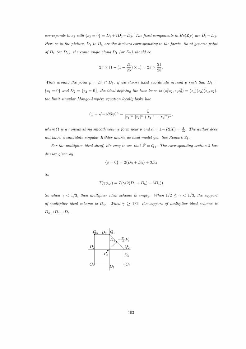
corresponds to s2 with s2 = 0 = D1 +2D2 +D3. The fixed components in Bs(LF ) are D1 +D2.
Here as in the picture, D1 to D5 are the divisors corresponding to the facets. So at generic point
of D1 (or D2), the conic angle along D1 (or D2) should be
2π × (1 − (1 − 2125
) × 1) = 2π × 2125.
While around the point p = D1 ∩ D2, if we choose local coordinate around p such that D1 =
z1 = 0 and D2 = z2 = 0, the ideal defining the base locus is (z21z2, z1z
22) = (z1)(z2)(z1, z2).
the limit singular Monge-Ampere equation locally looks like
(ω +√−1∂∂ψ)n =
Ω|z1|2α|z2|2α(|z1|2 + |z2|2)α
,
where Ω is a nonvanishing smooth volume form near p and α = 1−R(X) = 425 . The author does
not know a candidate singular Kahler metric as local model yet. See Remark 34.
For the multiplier ideal sheaf, it’s easy to see that F = Q4. The corresponding section s has
divisor given by
s = 0 = 2(D3 +D5) + 3D4
So
I(γφ∞) = I(γ(2(D3 +D5) + 3D4))
So when γ < 1/3, then multiplier ideal scheme is empty. When 1/2 ≤ γ < 1/3, the support
of multiplier ideal scheme is D4. When γ ≥ 1/2, the support of multiplier ideal scheme is
D3 ∪D4 ∪D5.
@@
@@r
rPc
−214 Pc
q
q q
Q5 D3
D1
D5
Q4
D2
D4
Q3
Q1
Q2
103

4.7 Log-Futaki invariant for 1psg on toric Fano variety
Donaldson made a conjecture relating the two continuity methods.
Conjecture 1. [Don6] There is a cone-singularity solution ωβ to (∗)β for any parameter β ∈
(0, R(X)). If R(X) < 1, there is no solution for parameter β ∈ (R(X), 1).
The case of conic Riemann surface was known by the work of Troyanov, McOwen, Thurston,
Luo-Tian, etc. we can provide more evidence on toric Fano manifolds:
Theorem 22. [Li5] Let X4 be a toric Fano variety with a (C∗)n action. Let Y be a general
hyperplane section of X4. When β < R(X4), (X4, βY ) is log-K-stable along any 1 parameter
subgroup in (C∗)n. When β = R(X4), (X4, βY ) is semi-log-K-stable along any 1 parameter
subgroup in (C∗)n and there is a 1 parameter subgroup in (C∗)n which has vanishing log-Futaki
invariant. When β > R(X4), (X4, βY ) is not log-K-stable.
Let pα; α = 1, · · · , N be all the lattice points of 4. Each pα corresponds to a holomorphic
section sα ∈ H0(X4,K−1X4
). We can embed X4 into PN using sα. Define u to be the potential
on (C∗)n for the pull back of Fubini-Study metric (i.e.√−1∂∂u = ωFS):
u = log
(N∑α=1
e<pα,x>
)+ C (4.53)
C is some constant determined by normalization condition:
∫Rne−udx = V ol(4) =
1n!
∫X4
ωn =c1(X4)n
n!
By the above normalization of u, it’s easy to see that
ehω =| · |2FS| · |2ωn
=e−u
ωn/(dz1z1 ∧ dz1z1
· · · ∧ dznzn
∧ dzn)zn
So
hω = − log det(uij) − u (4.54)
Now let’s calculate the log-Futaki invariant for any 1-parameter subgroup in (C∗)n. Each 1-
parameter subgroup in (C∗)n is determined by some λ ∈ Rn such that the generating holomorphic
vector field is
vλ =n∑i=1
λizi∂
∂zi
104

A general Calabi-Yau hypersurface Y ∈ | −KX | is a hyperplane section given by the equation:
s :=N∑α=1
b(pα)zpα = 0
By abuse of notation, we denote λ(t) to be the 1 parameter subgroup generated by vλ, then
λ(t) · s =N∑α=1
b(pα)t−〈pα,λ〉zpα (4.55)
Let
W (λ) = maxp∈4〈p, λ〉
Then Hλ = p ∈ Rn, 〈p, λ〉 = W (λ) is a supporting plane of 4, and
Fλ := p ∈ 4; 〈p, λ〉 = W (λ) = Hλ ∩4
is a face of 4.
We have limt→0[s] =[s0 :=
∑pα∈Fλ b(pα)zpα
], and by (4.55), the C∗-weight of s0 is −W (λ).
Proposition 30. Let F (K−1X , βY )(λ) denote the Futaki invariant of the test configuration asso-
ciated with the 1 parameter subgroup generated by vλ. We have
F (K−1X , βY )(λ) = − (β〈Pc, λ〉 + (1 − β)W (λ))V ol(4) (4.56)
Proof. We will use the algebraic definition of log-Futaki invariant (3.29) to do the calculation.
Note that (X,Y,K−1X ) degenerates to (X,Y0,K
−1X ) under λ.
Y0 is a hyperplane section of X, and s0 ∈ H0(X,K−1X ) is the defining section, i.e. Y0 = s0 =
0. Then
H0(Y0,K−1X | kY0
) ∼= H0(X,K−kX )/(s0 ⊗H0(X,K−(k−1)
X ))
So
wk = wk − (wk−1 −W (λ)dk−1)
Plugging the expansions, we get
a0 = (n+ 1)a0 +W (λ)b0
105

Note that b0 = nb0 = nV ol(4), we have
−a0 +b0b0a0 = −a0 −W (λ)b0
where
−a0 =∫X
θvωn
n!=∫
Rn
∑i
λiui det(uij)dx =∫4
∑i
λiyidy = V ol(4)〈Pc, λ〉
By (4.54), the ordinary Futaki invariant is given by
F (c1(X))(vλ) =∫X
v(hω)ωn
n!= −
∫Rn
n∑i=1
λi∂u
∂xidet(uij)dx
= −∫4
∑i
λiyidy = −V ol(4)〈Pc, λ〉
Substituting these into (3.29), we get
F (K−1X , βY )(λ) = −V ol(4)〈Pc, λ〉 + (1 − β)(V ol(4)〈Pc, λ〉 −W (λ)V ol(4))
= −(β〈Pc, λ〉 + (1 − β)W (λ))V ol(4)
Proof of Theorem 22. Note that for any Pλ ∈ Fλ ⊂ ∂4, W (λ) = 〈Pλ, λ〉. By Theorem 19, we
have
F (K−1X , βY )(λ) =
(β
1 − β
1 −R(X)R(X)
〈Q,λ〉 −W (λ))
(1 − β)V ol(4)
= 〈Qβ − Pλ, λ〉
where Qβ = β1−β
1−R(X)R(X) Q.
Note that λ is a outward normal vector of Hλ. By convexity of 4, it’s easy to see that (see
the picture after Example 2)
• β < R(X): Qβ ∈ 4. For any λ ∈ Rn, 〈Qβ − Pλ, λ〉 < 0.
• β = R(X): Qβ = Q ∈ ∂4. For any λ ∈ Rn, 〈Qβ − Pλ, λ〉 ≤ 0. Equality holds if and only
if 〈Q,λ〉 = W (λ), i.e. Hλ is a supporting plane of 4 at point Q.
• β > R(X): Qβ /∈ 4. There exists λ ∈ Rn such that 〈Qβ − Pλ, λ〉 > 0
106

4.7.1 Example
1. X4 = BlpP2. See the picture in Introduction. Pc = 14 ( 1
3 ,13 ), Q = −6Pc ∈ ∂4, so
R(X) = 67 .
If we take λ = 〈−1,−1〉, then W (λ) = 1. So by (4.56)
F (K−1X , βY )(λ) =
23β − 4(1 − β)
So F (K−1X , βY )(λ) ≤ 0 if and only if β ≤ 6
7 , and equality holds exactly when β = 67 .
2. X4 = Blp,qP2, Pc = 27 (−1
3 ,−13 ), Q = − 21
4 Pc ∈ ∂4, so R(X4) = 2125 .
If we take λ1 = 〈1, 1〉, then W (λ1) = 1. By (4.56),
F (K−1X , βY )(λ1) =
23β − 7
2(1 − β)
F (K−1X , βY )(λ1) ≤ 0 if and only if β ≤ 21
25 .
This is essentially the same as Donaldson’s calculation in [Don6].
If we take λ3 = 〈−1, 2〉, then W (λ3) = 〈−1, 2〉 · 〈−1, 1〉 = 3. By (4.56)
F (K−1X , βY )(λ3) =
13β − 21
2(1 − β)
So F (K−1X , βY )(λ3) ≤ 0 if and only if β ≤ 63
65 which means that (X,βY ) is log-K-stable
along λ3 when β ≤ 2125 <
6365 .
@@
@@@
ss
Pc
Q 2125
H3P3A
AAKλ3
?λ2
P2r
rλ1
P1rQ< 2125
rQ> 2125
r
q q
qqqq
107

Chapter 5
Intersection formula of
Donaldson-Futaki invariant and
applications
5.1 Introduction
K-stability is defined via the notion of test configurations. They are just C∗-equivariant degen-
erations of the polarized manifold (X,L), usually denoted by (X ,L). When the central fibre
X0 is normal, Ding-Tian [DiTi] defined generalized Futaki invariant by extending the differential
geometric defining formula from smooth case to normal case. Later Donaldson [Don4] defined
Futaki invariant algebraically so that one can define it for any test configuration as scheme which
may be very singular. However, motivated by compactness result for Kahler-Einstein metrics (cf.
[CCT]), Tian conjectured that
Conjecture 2 (Tian’s conjecture). When X is Fano, one only needs to consider those test
configurations with normal Q-Fano central fibers.
As in [Tia9], we will call such a test configuration to be a Special Test Configuration.
Recall that, in birational geometry, a Q-Fano variety is a Kawamata Log Terminal (klt) Fano
variety.
In this Chapter, we prove Theorem 24 which verify Tian’s conjecture. This will be an imme-
diate consequence of the following theorem proved jointly with Dr. Chenyang Xu.
108
Theorem 23. [LiXu] Let X be a Q-Fano variety. Assume (X ,L) → A1 is a test configuration
of (X,−rKX). We can construct a special test configuration (X s,−rKX s) and a positive integer
m, such that (X s,−rKX s) is a and
mDF(X ,L) ≥ DF(X s,−rKX s).
Furthermore, if we assume X is normal, then the equality holds only when (X ,X0) itself is a
special test configuration.
As a immediate corollary, we can verify Tian’s conjecture:
Theorem 24 (Tian’s conjecture). ([LiXu]) Assume X is a Q-Fano variety. If X is destablized by
a test configuration, then X is indeed destablized by a special test configuration. More precisely,
the following two statements are true.
1. (unstable case) If (X,−rKX) is not K-semi-stable, then there exists a special test configu-
ration (X s,−rKX s) with a negative Futaki invariant DF(X s,−rKX s) < 0.
2. (semistable\ polystable case) Let X be a K-semistable variety. If (X,−rKX) is not K-
polystable, then there exists a special test configuration (X st,−rKX s) with Donaldson-Futaki
invariant 0 such that X s is not isomorphic to X × A1.
To prove the above result, we first derive an intersection formula for Donaldson-Futaki invari-
ant. Then we use various birational transformations in MMP to modify the test configuration
and prove the Donaldson-Futaki invariant is decreasing along the process. The end product will
be X s.
5.2 Intersection formula for the Donaldson-Futaki invari-
ant
Given any test configuration (X ,L), we first compactify it. So we want to glue (X ,L) with (X×
A1, p∗1L). In this section, we will compute the Donaldson-Futaki invariants by the intersection
formula on this compactified space. The same formula appeared before (see [Wang] and [Odak2]).
We include a proof here using Donaldson’s argument.
Example 5. Gm acts on (X,L−1) = (P1,OP1(−1)) by
t ([Z0, Z1], λ(Z0, Z1)) = ([Z0, tZ1], λ(Z0, tZ1)).
109

In particular, the Gm-weights on
OP1(−1)|0,OP1(1)|0,OP1(−1)|∞ and OP1(1)|∞
are 0,0,1 and -1. Let τ0 = Z1, τ∞ = Z0 be the holomorphic sections of OP1(1). Then the
Gm-weights of τ0 and τ∞ are −1 and 0.
Take X = P(OP1(1) ⊕ OP1) and L = OX (1) = OD∞ , where D∞ is the divisor at infinity.
We see that (X := X \ P1∞,L := L|X ) yields a test configuration of (X,L). Then H0(P1, L⊗k)
is of dimension dk = k + 1 and by the calculation in the first paragraph the total Gm-weight of
H0(P1, L⊗k) is wk = −12 (k2 + k). We know D2
∞ = −1 and K−1X ·D∞ = 1. So
wk =D2
∞2k2 +
(K−1
X ·D∞
2− 1
)k and DF(X ,L) =
D2∞2
−
(K−1
X ·D∞
2− 1
)(= 0).
This example can be generalized to more general cases (see (5.2), (5.3)) by using Donaldson’s
argument in the following way. Also see the proof of Proposition 4.2.1 in [Don4].
First note that, after identifying the fiber X1 over 1 and X, we have an equivariant isomor-
phism:
(X\X0,L) ∼= (X × (A1 \ 0), p∗1L)
by (p, a, s) → (a−1 p, a, a−1 s). Therefore, Gm acts on the right hand side by
t (p × a, s) = (p × ta, s)
for any p ∈ X, a ∈ A1 and s ∈ Lp. The gluing map is given by
(X ,L) (X × P1 \ 0, p∗1L)∪ ∪(X\X0,L) −→ (X × (A1 \ 0), p∗1L)
(p, a, s) 7−→ (a−1 p × a, a−1 s),
where Gm only acts by multiplication on the factor P1 \ 0 of (X × P1 \ 0, p∗1L).
Using the above gluing map, we get a compact complex manifold projective over P1: π :
(X ,L) → P1. In the following, we will denote (X ,L) by (X , L) for simplicity. Note that there
exists an integer N , such that M = L ⊗ π∗(OP1(N · ∞)) is ample on X (cf. [KoMo, 1.45]).
110

We need the following weak form of the Riemann-Roch formula whose proof is well known.
Lemma 30. Let X be a normal projective variety and L an ample divisor on X then
dimH0(X,L⊗k) =Ln
n!kn +
12K−1X · Ln−1
(n− 1)!kn−1 +O(kn−2).
We define
dk = dimH0(X,L⊗k) =: a0kn + a1k
n−1 +O(kn−2)
Theorem 25. Assume X is normal, then
a1b0 − a0b1a20
= DF(X ,L) =1
(n+ 1)!a0
(a1
a0Ln+1 +
n+ 12
KX/P1 · Ln). (5.1)
Proof. For k 0, by Kodaira Vanishing Theorem, we have two exact sequences:
A B C
‖ ‖ ‖
0 −→ H0(X ,M⊗k(−X0)) ⊗σ0−→ H0(X ,M⊗k) −→ H0(X0,M⊗k|X0) −→ 0
0 −→ H0(X ,M⊗k(−X∞)) ⊗σ∞−→ H0(X ,M⊗k) −→ H0(X∞,M⊗k|X∞) −→ 0,
‖ ‖ ‖
A B D
where σ0, σ∞ are sections of π∗OP1(1) which are pull back of the divisors 0, ∞ on P1.
We can assume the Gm-weights of σ0 and σ∞ are -1 and 0. Note the first terms in the
two exact sequences are the same as A := H0(X ,M⊗k ⊗ π∗OP1(−1)). We have the equation:
wB = wA − dA + wC = wA + wD, where we denote dA and wA to be the dimension and the
Gm-weight of the vector space A and similarly for dB etc. Since the Gm-weight of OP1(1)|∞ is
-1 and Gm acts on L|X∞ trivially, we have wD = −kNdimH0(X∞, Lk|X∞). So we get
wC = dA + wD = dB − dC − kNdD = dB − (kN + 1)dC ,
In other words, we get the Gm-weight on H0(X0,M⊗k|X0) = H0(X0, L⊗k|X0):
wk = dimH0(X ,M⊗k) − (kN + 1) dimH0(X0, L⊗k|X0).
111

Expanding wk, we get:
wk = b0kn+1 + b1k
n +O(kn−1)
with
b0 =Mn+1
(n+ 1)!−Na0 =
Ln+1
(n+ 1)!, and (5.2)
b1 =12K−1
X · Mn
n!−Na1 − a0 =
12K−1
X · Ln
n!− a0. (5.3)
We get (5.1) by substituting the coefficients into (2.27).
Remark 38. This intersection formula is related to the interpretation of Donaldson-Futaki in-
variant as the CM-weight as in [PaTi2]. It was extensively used in [ALV], [Odak1], [RoTh1],
etc.
The intersection formula gives us a way to define the Donaldson-Futaki invariants when L is
a π-big and semiample R-divisor.
Definition 17. (Donaldson-Futaki invariant for a semi-test configuation) Let π : (X ,L) → A1
be a Gm-equivariant flat family with L being π-big and π-semiample, such that for t ∈ A1\0,
(Xt,L|Xt) ∼= (X,−rKX). We call (X ,L) a semi-test configuration and L a semi-polarization.
Assume X is normal. We define the Donaldson-Futaki invariant by the intersection formula:
DF(X ,L) =1
(n+ 1)!a0
(a1
a0Ln+1 +
n+ 12
KX/P1 · Ln)
(5.4)
A frequent example is as follows: Suppose there is a Gm-equivariant birational morphism
between normal varieties ρ : X ′tc → X over A1 and L′ = ρ∗(L) where (X ,L) is a test configura-
tion. If ρ is an isomorphism over the preimage images of A1 \ 0, then L′ is big and semi-ample
but not ample in general. So (X ′,L′) is a semi-test configuration of (X,−rKX). The projection
formula and (5.1) imply that
DF(X ′,L′) = DF(X ,L).
Remark 39. For any relative big and semi-ample line bundle, this definition of Futaki invariant
coincides with the definition via computing the Gm-weights of cohomological groups as in [ALV].
For more details, see [RoTh1] and [ALV].
Remark 40. Using the above argument, we can also get the intersection formula in the log
case. Any test configuration can be equivariantly embedded into PN ×C∗ where the C∗ action on
112

PN is given by a 1 parameter subgroup of SL(N + 1,C). If Y is any subvariety of X, the test
configuration of (X,L) also induces a test configuration (Y,L|Y) of (Y, L|Y ). Let dk, dk be the
dimensions of H0(X,Lk), H0(Y, L| kY ), and wk, wk be the weights of C∗ action on H0(X0,L| kX0),
H0(Y0,L| kY0), respectively. Then we have expansions:
dk = a0kn + a1k
n−1 +O(kn−2), a0 =Ln
n!, a1 = −KX · Ln−1
2(n− 1)!
wk = b0kn+1 + b1k
n +O(kn−1), b0 =Ln+1
(n+ 1)!, b1 = −KX · Ln
2n!− a0
dk = a0kn−1 +O(kn−2), a0 =
Ln−1 · Y(n− 1)!
wk = b0kn +O(kn−1), b0 =
Ln · Yn!
alog1 = a1 −
12a0, blog1 = b1 −
12b0
K log
X = KX + Y + X0
So we can calculate the intersection formula for the log-Futaki invariant:
DF(X ,Y,L) =2(a1b0 − a1b0) + (a0b0 − a0b0)
a20
=(2a1 − a0)b0 − a0(2b1 − b0)
a20
=1
a0(n+ 1)![c1Ln+1 + (n+ 1)(KX + Y) · Ln
]+ 2
=1
a0(n+ 1)!
[2alog
1
a0Ln+1 + (n+ 1)K log
(X ,Y)/P1 · Ln]
c1 =alog1
a0=
2a1 − a0
a0=n(KX + Y ) · Ln−1
Ln
5.2.1 Song-Weinkove’s condition from intersection formula
As a preliminary formal application of the intersection formula, we derive an inequality condition
discovered by Song-Weinkove [SoWe]. When c1(X) < 0 and c1(L) satisfies this condition (5.6),
then the K-stability of (X,L) may follow from purely algebraic calculations. We haven’t been
able to prove this entirely though.
113

Following [Odak1], we only need to consider the blow up of X × P1 along a flag ideal
J = J0 + tJ1 + · · · + tkJk
Let X := BlJ (X × P1) → X × P1 be the blow up of along J . Let Lt = π∗L − tE we need to
show that
DF(X ,Lt) ≥ 0, for 0 < t < Seshadri constant of J with respect to L
Following [Odak1], we first rewrite the intersection formula for Donaldson-Futaki invariant
DF(X ,Lt) =2a1
a0(L(−tE))n+1 + (n+ 1)KX(L(−tE))n + (n+ 1)KX/(X×P1)(L(−tE))n
= I(t) + II(t)
Since X×P1 is smooth, so KX/(X×P1) is effective so we have II(t) > 0 for t > 0. Let nµ = 2a1/a0,
thend
dtI(t) = −(n+ 1)nLn−1
t · (µLt +KX) · E
If L = KX , then µ = −1, and ddt I(t) = −t(n + 1)nLn−1
t · E2. By Hodge index theorem, this is
positive if t > 0. So we get result that (X,KX) is K-stable which was shown by Odaka using
combinatoric formulas.
For more general classes, note that ddt I(0) = 0. We can differentiate again:
d2
dt2I(t) = n(n+ 1)
(nµLn−1
t + (n− 1)KX · Ln−2t
)· E2
= −n(n+ 1)(−nc1(X) · [L]n−1
[L]nLt − (n− 1)KX
)· Ln−2
t · E2 (5.5)
One should compare this intersection product with [Theorem 1.2 in [SoWe]]
Theorem 26 (Song-Weinkove). Suppose that X satisfies c1(X) < 0. Let V be the cone of all
Kahler class [χ0] with the property that there exist metrics ω in −c1(X) and χ′ in [χ0] with
(−nc1(X) · [χ0]n−1
[χ0]nχ′ − (n− 1)ω
)∧ χ′n−2 > 0 (5.6)
Then the Mabuchi energy is proper on every class [χ0] in V .
Recently, in [FLSW] the condition (5.6) is weakened to allow equality. So by discussion in
114

section 2.7.2, when (5.6) and its equality case holds, (X,L) is K-stable. This should follow from
the positivity of (5.5) for 0 < t < Seshadri constant of J with respect to L. This is indeed true
when 0 < t 1. This follows from the following Lemma.
Lemma 31. Let s = dim Supp(O/J ). If (5.6) holds, then
1. For k < n+ 1 − s, dk
dtkI(0) = 0.
2. For k = n+ 1 − s, dk
dtkI(0) ≥ 0.
Proof. We first calculate
dk
dtkI(t) = (n+ 1)n
(n− 1)!(n− k + 1)!
(nµLn−k+1 + (n− k + 1)Ln−k ·KX
)· (−E)k (5.7)
So in particular,
dk
dtkI(0) =
(n+ 1)!(n− k + 1)!
(−nµLn−k+1 − (n− k + 1)Ln−k ·KX) · (−E)k−1 · E
By projection formula, this is zero when n− k+ 1 > s. This shows Item 1. When k = n+ 1− s,
dn+1−s
dtn+1−s I(0) =(n+ 1)!
s!(cLs − sLs−1 ·KX) · (−E)n−s · E (5.8)
where we let c = −nµ > 0. By (5.6) and its equality case, there exist Kahler metrics χ ∈ c1(L)
and ω ∈ −c1(X), such that
cχn−1 − (n− 1)χn−2 ∧ ω ≥ 0, (5.9)
Now choose local coordinate chart zi such that χij = δij and ωij = λiδij with λi > 0.
Then (5.9) is equivalent to that, for any 1 ≤ i ≤ n,∑j 6=i λj ≤ c. As a consequence, for any
I = i1, i2, . . . , in−k+1 ⊂ 1, 2, . . . , n with 1 ≤ i1 < · · · < in−k+1 ≤ n,∑j∈I λj ≤ c. It’s easy
to see that this is equivalent to
cχn−k+1 − (n− k + 1)χn−k ∧ ω ≥ 0.
In particular, this holds when n− k + 1 = s. Now we can see that dn+1−s
dtn+1−s I(0) ≥ 0 in (5.8).
115

5.3 Special degeneration and K-stability of Fano manifold
In this section, we will prove Theorem 23 by simplifying the test configuration through various
birational transformations from MMP.
5.3.1 Preliminaries from algebraic geometry
Definition and Theorem 1 (Relative MMP with scaling). ([BCHM], [KoMo])
Let (X0,∆0) := (X,∆) be a klt pair, projective over a smooth curve C. Let H be an ample
line bundle such that ∆ +H is nef. Assume KX + ∆ is not pseudo-effective. Let
µ = mint;KX + ∆ + tH pseudo-effective .
We can define a sequence rational numbers 1 = λ0 ≥ λ1 ≥ · · · ≥ λK > λK+1 = µ and a sequence
of models over C related by birational transformations:
(X0,∆0) 99K (Xi,∆i) 99K (XK ,∆K)
by the following inductive process. Assume (Xi,∆i) is defined. Let Hi be the birational transform
of H on Xi. Define
λi+1 = mint ∈ [µ, 1];KXi + ∆i + tHi is nef .
So there exists an extremal ray R ∈ NE(Xi/C) such that (KXi + ∆i) · R = −Hi · R < 0. We
can contract R by a contraction map πR : Xi → Y . There are two possibilities:
1. πR is divisorial contraction. Let Xi+1 = Y and ∆i+1 = (πR)∗∆i.
2. πR is a flipping contraction. Let f : Xi 99K Xi+ be the (KXi+∆i)-flip. Define Xi+1 = Xi+
and ∆i+1 = f∗∆i.
On the end product (X k,∆k) we have KXk + ∆k + µHk ∼Q,C 0.
The following two theorem are very important in the theory of MMP. We will frequently use
in the following argument too.
Theorem 27 (Relative base point free theorem). Let (X,4) be a klt pair, 4 effective, and
f : X → Y a proper morphism of projective varieties over C. Let D be an f-nef Cartier divisor
such that aD −KX −4 is f-nef and f-big for some a > 0. Then bD is f-free for all b 0.
116

Lemma 32 (Negativity Lemma). ([KoMo, 3.39]) Let h : Z → Y be a proper birational morphism
between normal varieties. Let −B is an h-nef Q-Cartier Q-divisor on Z. Then
1. B is effective iff h∗B is.
2. Assume B is effective. Then for every y ∈ Y , either h−1(y) ⊂ SuppB or h−1(y)∩SuppB =
∅.
We also need the higher dimensional version of the Zariski Lemma in the following calculation
of Donaldson-Futaki invariant. See [LiXu].
Lemma 33 (Zariski’s Lemma). Let X → C be a projective dominant morphism from a n-
dimensional normal variety to a proper smooth curve. Let E be a Q-divisor which supports on
some fiber X0. Let L1, ..,Ln−2 be n− 2 nef divisors on X . Then
E2 · L1 · · · Ln−2 ≤ 0.
If all Li’s are ample, then the equality holds if and only if E = tX0 for some t ∈ Q.
5.3.2 Step 0: Normalization
Assume (X ,L) → A1 is a test configuration. Let πν : X ν → X be the normalization of X . By
[RoTh1, Proposition 5.1] and [ALV, Corollary 3.9],
DF (X ν , (πν)∗L) ≤ DF (X ,L)
with equality holds if and only if Xnon−normal (i.e. the set of non-normal points of X has
codimension at least two.
Remark 41. Any test configuration can be equivariantly embedded into PN ×A1. So it’s induced
by a one parameter subgroup λ(t) of SL(N + 1,C). As we have seen in the end of Section 2.7.2,
there are three cases for X0. For the 3rd case, in general, the test configuration X is non-normal
(hence non-product), isomorphic to X × A1 in codimension 1, with Donaldson-Futaki invariant
0. This case was missing in most of precious work, e.g. [Sto1], as pointed out in [LiXu]. See
[Sto2], [Odak4] for related issues and corrections.
From now on, we will assume the test configuration X is normal. Since we can naturally
compactify any test configuration as in Section 5.2, we will consider more generally a polarized
family over a proper smooth curve whose total space is normal.
117

Definition 18. A polarized generically Q-Fano family is a projective morphism π : (X ,L) → C
from a normal polarized variety X to a smooth curve, whose generic fibre (Xη,Lη) ∼= (Xη,−rKXη )
is a Q-Fano variety for some r ∈ Q. If each fibre is a Q-Fano variety, then (X ,−rKX/C) called
a Q-Fano family.
Definition 19. Assume (X ,L) → C is a polarized generically Q-Fano family over a proper
smooth curve. Assume for generic fibre L|Xt ∼Q −rKXt . We can define the Donaldson-Futaki
intersection number as
DF(X/C,L) =1
2(n+ 1)rn(−KXt)n(nrLn+1 + (n+ 1)KX/C · Ln
),
If C = P1 and (X , L) → P1 is the compactification of a Q-test configuration (X ,L) → A1 as
in Section 5.2 by simply adding a ‘trivial fiber’ over the point ∞ ∈ P1, then we have the equality
DF(X/P1, L) = DF(X ,L).
Remark 42. In the following, without loss of generality, we assume there is only one degenerate
fibre over 0 ∈ C, or 0′ ∈ C ′. We also note that although the following step of modification
was originally obtained without group action, they all can be carried out equivariantly. For
explanations, see [LiXu, Section 2.3], [And], [KoMo].
5.3.3 Step 1: Equivariant semi-stable reduction
Theorem 28. [LiXu] There exists a finite morphism φ : C ′ → C such that, if we denote X to
be the main component of the normalization of X ×C C ′, then
1. X0 is reduced.
2. DF(X , φ∗X/XL) ≤ deg(φ)DF(X ,L), where φX/X : X → X is the natural finite morphism.
The identity holds if and only if X0 is reduced.
3. then there exists a birational morphism f : Y → X such that Y is smooth and the degenerate
fibre Y0 is simple normal crossing.
Proof. The existence of semi-stable reduction (1. and 3.) was obtained in ([KKMS] and [KoMo]).
We have the following commutative diagram:
118

Y
φY/X
##
????
???
?
X
// X
C ′ // C
such that
• Y is smooth
• Y0 =∑N1i=1 Y0,i is simple normal crossing.
Because KX + X0 = φ∗X (KX + red(X0)) and KC′ + 0′ = φ∗(KC + 0), we see that
KX/C′ = φ∗X (KX/C + red(X0) −X0)
So 2. follows from projection formula. Equality holds if and only if X0 = red(X0) is reduced.
5.3.4 Step 2: Log canonical modification
Theorem 29. [LiXu] Let (X , L) → C be the polarized generic Q-Fano family such that X0 is
reduced and there exists a birational morphism Y → X0 such that Y is smooth and Y0 is simple
normal crossing. Then there exists a log canonical modification πlc : X lc → X and polarization
Llc on X lc such that
(1) (X lc,X lc0 ) is log canonical
(2) KX lc is relatively ample over X .
(3) DF(X lc,Llc) ≤ DF(X , L). The equality holds if and only if (X , X0) is log canonical.
Proof. X lc is obtained by running (KY + Y0)-minimal model program on Y over X . So X lc =
Proj R(Y/X ,KY + Y0). For details, see ([LiXu],[OdXu]). Let
Lt =r
r − t
(πlc∗L + tKX lc
)Since KX lc is relatively ample over X , Lt is relatively ample over C if t is sufficiently small. Then
1rLt + KX lc = r
r−t(
1rπ
lc∗L +KX lc
)and L′
t = r2
(r−t)2(
1rπ
∗L +KX lc
). Let E = 1
rπlc∗L + KX lc ,
119

then E is supported on X lc0 .
d
dtDF(X lc,Lt) =
1(n+ 1)rn(−KXt)n
n(n+ 1)Ln−1t
(1rLt +KX lc
)· L′
t
=nr3
rn(r − t)3(−KXt)n· Ln−1
t ·(
1rπlc∗L +KX lc
)2
≤ 0
for t sufficiently small. So we choose Llc = Lε for sufficiently small rational number ε. Then
DF(X lc,Llc) ≤ DF(X , L). The equality holds only if E ∼Q,C X lc0 , but then KX lc ∼Q,X 0, so X lc
is isomorphic to X .
5.3.5 Step 3: Running MMP with scaling
Now we let X 0 = X lc, L0 = Llc. Given an exceptional divisor E, if its center dominates C
then a(E,X 0) > −1 because X ∗ is klt; if its center is vertical over C, then a(E,X 0) ≥ 0, since
(X 0,X 0t ) is log canonical for any t in C. In particular, X 0 is klt.
Since L0 is ample, we can choose λ0 sufficiently large such that KX + λ0L is ample. To
simplify the family, we run a sequence of KX 0 -MMP over C with scaling of L0 as in Subsection
5.3.1. (This is equivalent to running (KX 0 + L0)-MMP with scaling L0. Compare with Section
5.3.9). So we obtain a sequence of models
X 0 99K X 1 99K · · · 99K X k.
Recall that, as in 5.3.1, we have a sequence of critical value of scaling factors
λi+1 = minλ | KX i + λLi is nef over C
with 1 = λ0 ≥ λ1 ≥ ... ≥ λk > λk+1 = 1r . Note that 1
r is the pseudo-effective threshold of KX 0
with respect to L0 over C, since it is the pseudo-effective threshold for the generic fiber. Any
X i appearing in this sequence of KX 0 -MMP with scaling of L0 is a relative weak log canonical
model of (X 0, tL0) for any t ∈ [λi, λi+1] (see [BCHM, 3.6.7] for the definition of weak log canonical
model).
For λ ∈ [λi+1, λi], we denote by
Liλ =r
λr − 1(KX i + λLi). (5.10)
120
where Li is the push forward of L0 to X i. As is clear from the context, this should not be
confused with the i-th power or intersection product of Lλ.
Lemma 34. −rKXk ∼Q,C Lk is big and semi-ample over C.
Proof. Since λk+1 = 1r , the line bundle KXk + 1
rLk is relatively nef over C and its restriction to
the generic fiber is trivial, so it is Q-linearly equivalent to a linear sum of components of X k0 . By
its nefness, we can apply Lemma 33 to get
KXk +1rLk ∼Q,C 0.
Now for any λ ∈ [1/r, λk+1], λkλ ∼ Lk is nef. Lk is big because λk > 1r , and from the relative
base-point free theorem (cf. Theorem 3.3 in [KoMo]), it is semi-ample over C.
By the above Lemma, we can define
X an = ProjR(X k/C,Lk) = ProjR(X k/C,−rKXk/C).
Since (X 0,X 00 ) is log canonical and and X 0
0 = (f πlc)∗(0), this is a also a sequence of
(KX 0 + X 00 )-MMP and thus (X k,X k
0 ) is log canonical which implies that (X an,X an0 ) is log
canonical as well.
5.3.6 Decreasing of DF-intersection number
For any λ > 1r , the restriction of KX 0 + λL0 over C∗ is ample. So the MMP with scaling does
not change X 0 ×C C∗, i.e., X 0 ×C C∗ ∼= X i ×C C∗ for any i ≤ k. Let’s calculate the variation of
DF-intersection number.
Proposition 31. ([LiXu]) With the notation above, we have
DF(X 0/C,L0) ≥ DF(X k/C,Lk) = DF(X k/C,−rKXk/C) = DF(X an/C,−rKXan/C)
The firt equality holds if and only if h : X 0 99K X k is an isomorphism.
121

Decreasing of DF on a fixed model
Assume X i0 =
∑αE
iα, where Eiα’s are the prime divisors. Since (X 0,L0)×C C∗ is isomorphic to
(X 0 ×C C∗,−rKX 0×CC∗), there exist aiα ∈ R such that
KX i +1rLi ∼R,C
∑α∈I
aiαEα.
Let Zλ be the relative log canonical model of (X 0, λL0) over C. Then there is a morphism
πλ : X i → Zλ and an relatively ample Q-divisor Mλ on Zλ whose pull back is Liλ.
Lemma 35. If λi ≥ a > b ≥ λi+1 and b > 1r , then DF(X i,Lia) ≥ DF(X i,Lib). The inequality
is strict if there is a rational number λ ∈ [a, b], such that the push forward of∑α a
iαEα to Zλ is
not a multiple of the pull back of 0 ∈ C on Zλ.
Proof. Note that
(Liλ)′ =d
dλLiλ = − r2
(λr − 1)2(KX i +
1rLi), KX i +
1rLiλ =
λr
λr − 1(KX i +
1rLi)
Now we compute the derivative of the Donaldson-Futaki invariants:
d
dλDF(X i/C,Liλ) = C0
((Liλ)n−1 · (Liλ)′ · (
1rLiλ +KX i)
)= −C ′
0(Liλ)n−1 ·(KX i +
1rLi)2
= −C ′0(Mi
λ)n−1 ·
∑β
aiβEβ
2
,
where C0, C′0 are positive constants. Then the lemma follows from Lemma 33.
Lemma 36.
limλ→+∞
DF(X 0,L0λ) = DF(X 0,L0)
Proof. This follows from limλ→+∞ L0λ = L0 and the intersection formula.
The following corollary is a consequence of above two Lemmas.
Corollary 8.
DF(X 0,L0) ≥ DF(X 0,L0λ0
)
122

Invariance of DF at contraction or flip points
If λi+1 >1r , then by the definition of MMP with scaling, we pick up a KX i-negative extremal
ray [R] in NE(X i/C) such that R · (KX i + λi+1Li) = 0. we perform a birational transformation:
X ifi //
AAA
AAAA
A Yi
~~
P1,
which contracts all curves R′ whose classes [R′] are in the ray R>0[R]. There are two cases:
1. (Divisorial Contraction) If f i is a divisorial contraction. Then X i+1 = Yi. Since f i is a
(KX i + λi+1Li)-trivial morphism by the definition of the MMP with scaling, we have
KX i + λi+1Li = (f i)∗(KYi + λi+1Li+1),
which implies
Liλi+1= (f i)∗Li+1
λi+1.
Then it follows from projection formula that
DF(X i/C,Liλi+1) = DF(X i+1/C,Li+1
λi+1).
2. (Flipping Contraction) If f i is a flipping contraction, let φi : X i 99K X i+1 be the flip.
X iφi //_______
−KXi is fi-amplefi
AAA
AAAA
A X i+1
KXi+1 is fi+-amplefi+
||zzzz
zzzz
Yi
As f i is a (KX i + λi+1Li)-trivial morphism, (KX i + λi+1Li) = (f i)∗DYi for some divi-
sor DYi . Since f i, f i+, φi are isomorphisms in codimension one, we also have KX i+1 +
λi+1Li+1 = (f i+)∗DLi . Therefore, using the intersection formula, we see that
DF(X i/C,KX i + λi+1Li) = DF(Yi/C,DYi) = DF(X i+1/C,KX i+1 + λi+1Li+1).
Now we can finish the proof of Proposition 31:
123

Proof.
DF(X 0/C,L0) ≥ DF(X 0/C,L0λ0
) ≥ DF(X 0/C,L0λ1
)
= DF(X 1/C,L1λ1
) ≥ DF(X 1/C,L1λ2
)
· · · · · · · · ·
= DF(X i/C,Liλi) ≥ DF(X i/C,Liλi+1)
= DF(X i+1/C,Li+1λi+1
) ≥ DF(X i+1/C,Li+1λi+2
)
· · · · · · · · ·
= DF(X k/C,Lkλk) = DF(X k/C,−rKXk).
Now we characterize the equality case. Since −KXk ∼Q,C1rL
k is relatively nef over C, we
conclude that fk−1 : X k−1 → X k is a divisorial contraction contracting a divisor E. So if we let
aE = KXk−1 +1rLk−1λk
− (fk−1)∗(KXk +1rLk)
then because fk−1 is (KXk−1 + λkLk−1)- trivial, for any curve C ∈ E,
aE · C =(
1r− λk
)Lk−1 · C < 0
because λk > 1r . Since E·C < 0, we have a > 0. BecauseKXk+ 1
rLk ∼Q,C 0, KXk−1+ 1
rLk−1λk
∼Q,C
aE whose support E is a proper subset of X k−10 . So the equality condition of Lemma 35 can not
hold on X k−1. Thus
DF(X lc/C,Llc) ≥ DF(X 0/C,L0λ0
) ≥ DF(X k−1/C,Lk−1λk−1
)
> DF(X k/C,Lkλk) = DF(X k/C,Lk)
= DF(X an/C,−rKXan).
5.3.7 Step 4: Q-Fano extension
From last section, we get some family X k and its anti-canonical model X an. Now we need to use
results from MMP to carry on. We collect the result we need in the following theorem.
124

Theorem 30. [LiXu]
1. There exists a finite morphism φ : C ′ → C and a birational morphism π : X ′ → X :=
X an ×C C ′ such that, if X ′0 =
∑iEi, then
• We can find some polarization L′ such that
L′ +KX ′/C′ =∑
Ei 6=EsaiEi
with ai > 0.
• π is a divisorial contraction contracting divisor Es with a(Es, X ) = 0.
2. We can run (KX ′ +L′)-MMP over C ′ and get a klt model X s such that X s0 is an irreducible
Q-Fano variety which is the strict transform of Es.
Theorem 31. [LiXu]
DF(X/C ′,−KX/C′) ≥ DF(X s/C ′,−KX s)
with equality holds if and only if X ∼= X s.
Proof. The Donaldson-Futaki intersection number becomes very simple for relative anti-canonical
polarization:
DF(X/C ′,−KX/C′) = − 12(n+ 1)(−KXt)n
(−KX/C′)n+1
= − 12(n+ 1)(−KXt)n
(−KX ′/C′)n+1
The second equality comes from π∗KX = KX ′ because of a(Es, X ) = 0. Similarly,
DF(X s/C ′,−KX s/C′) = − 12(n+ 1)(−KXt)n
(−KX s/C′)n+1
Let p : X → X ′ and q : X → X s be common resolution. Define E = p∗KX ′ − q∗KX s so that
q∗(−KX s/C′) = p∗(−KX ′/C′) + E
Then −E is q-nef and E is supported on X0.
Let p = πp : X → X . We can write KX = p∗KX +B = p∗KX ′ +B with B being exceptional
over X ′. Because X ′ 99K X s is a birational contraction, B is also exceptional over X s. Similarly,
125

KX = q∗KX s + F with F exceptional over X s. So E = −B + F is exceptional over X s. By the
Negativity Lemma 32, E ≥ 0.
If E = 0 or, X ′ and X s are not isomorphic in codimension 1, then
X = ProjR(X ′,−KX ′/C′) = ProjR(X s,−KX s/C′) = X s
So we can assume E > 0 and X ′ is not isomorphic to X s in codimension 1. Then E > 0 contains
some divisor E1 which is the strict transform of E1 ⊂ X0 and is contracted via the birational
map X ′ 99K X s.
Let Lt = p∗(−KX ′/C′) + tE = (1 − t)p∗(−KX ′/C′) + tq∗(−KX s/C′). Then Lt is nef for
0 ≤ t ≤ 1. We can differentiate again:
d
dt
(Ln+1t
n+ 1
)= Lnt · E
≥ (1 − t)np∗(−KX ′/C′)n · E1
= (1 − t)n(−KX ′/C′)n · p∗E1
= (1 − t)n(−KX/C′)n · E1 > 0
5.3.8 Completion of Proof of Theorem 23
Proof. For any test configuration X , we modify it by the above steps.
X/C X ν/C ( Step 0: normalization )
X/C ′ ( Step 1: base change and normalization)
X lc/C ′ ( Step 2: log canonical modification )
X an/C ′ ( Step 3: Run MMP with scaling )
X ′/C ′′ ( Step 4a: Base change and crepant blow up)
X s/C ′′ ( Step 4b: Contracting extra components)
For each step, the Donaldson-Futaki invariant decreases up to a factor due to base change
deg(C ′/C) and deg(C ′′/C). So
DF(X/C,L) ≤ deg(C ′′/C ′)DF(X s,−rKX s)
126

The equality holds if and only if Xnon−normal has codimension at least two and X ν ×C C ′′ = X s
is a special test configuration. So if X is normal, then the equality holds if and only if X is itself
a special test configuration.
5.3.9 Simplification in the unstable case and Discussions
If we want to prove the following weaker statement of the theorem.
Theorem 32. Given any test configuration (X ,L) → C1, for any ε 1, we can construct a
special test configuration (X s,−rKX s) and a positive integer m, such that
m(ε+ DF(X ,L)) ≥ DF(X s,−rKX s)
Then we can simplify the argument. Note that the weaker statement implies Tian’s conjecture
in the un-stable case.
Proof. 1. Step 1: Equivariant semistable reduction. Y → X → X .
2. Step 2: perturb the pull back polarization.
LY = εA+ φ∗Y/X (L)
by an ample divisor A (ε 1) such that
• LY is still ample
• For some a ∈ Q
LY +KY + aY0 =N∑i=2
aαY0,α
with aα > 0 for any α ≥ 2.
3. step 3: Run (KX + LY)-MMP with scaling LY over C. Define
Mλ =(KX + L) + λL
λ, M1 = L.
so that M+∞ = L. As λ decreases from +∞ to 0, we get a sequence of critical points of λ
and a sequence of models:
+∞ ≥ λ1 ≥ . . . ≥ λk > λk+1 = 0
X 0 99K X 1 99K . . . 99K X k → C
127

The X k in the above sequence has very good properties:
• Ek is linearly trivial. Lk ∼C −KXk is semiample.
• Assume X0 =∑Nα=1 aαX0,α = E ≥ 0, then X 99K X 0 contracts precisely Supp(E).
This can easily seen as follows. Using hyperplane section, we can assume dim(X ) = 2.
If the strict transform of E denoted by Ek still contains X k0,β for some β ≥ 2. Then
Ek · X k0,1 > 0. This contradicts the Ek ∼C 0.
By property 1 above, we can define: X s = X an = Proj(X k,−KXk/C) so that −KX s is
ample and X s0 is Q-Fano.
Again, Donaldson-Futaki invariant decreases along Mλ. Note that
KX + Mλ =λ+ 1λ
(KX + L),d
dλMλ = − 1
λ2(KX + L).
As before, we can calculate
d
dλDF(X ,Mλ) = −C(n, λ, r)Mn−1
λ · (L +KX/P1)2 ≥ 0
by the Hodge index theorem, because L +KX/P1 =∑i aiX0,i only supports on X0. This means
that DF invariant decreases as λ decreases.
Remark 43. Let’s explain the formal similarity between MMP and (normalized) Kahler Ricci
flow. Assume L|Xt ∼C −KX . In MMP, we vary the polarization in the direction of KX :
Ms :=L + sKX
1 − s, Ms|Xt ∼ −KX .
The derivative of Ms is
d
dsMs =
1(1 − s)2
(L +KX )s=1/(1−s)⇐==⇒ d
dsMs = KX + L
This variation corresponds to the normalized Kahler-Ricci flow.
∂ω
∂s= −Ric(ωs) + ωs
Remark 44. The idea of running semi-stable MMP ([KoMo, Chapter 7]) to simplify degenera-
tion is well known to experts in MMP. For example, the procedure was used by Hacking [Hac].
128
Chapter 6
Rotationally symmetric
Kahler-Ricci solitons on flips
6.1 Introduction and motivation
Song-Tian [SoTi] used Kahler-Ricci flow to study general algebraic varieties. The goal is to con-
struct canonical metrics on algebraic varieties obtained after surgeries and this can be seen as the
metric counterpart of Minimal Model Program(MMP). Tian-Zhang [TiZha] proved singularity-
occurring time is the same as nef threshold. It is proved in the theory of Ricci flow that, the
type-I singularity will produce Ricci soliton after rescaling. In general, we don’t know whether the
singularity is type-I or not. In Fano case, this is related to the famous Hamilton-Tian conjecture
on the limit behavior of Kahler-Ricci flow on any Fano manifold. If we assume the singularity is
type-I, it’s interesting to see examples of Kahler-Ricci solitons.
In [FIK], the authors constructed some examples of gradient Kahler-Ricci soliton. Among
them is the shrinking soliton on the Bl0Cm. They also glue this to an expanding soliton on Cm
to extend the Ricci flow across singular time.
Recently, La Nave and Tian [LaTi] studied the formation of singularity along Kahler-Ricci
flow by symplectic quotient. The idea is explained by the following example.
Let C∗ act on Cm+n by
t · (x1, · · · , xm, y1, · · · , yn) = (t x1, · · · , t xm, t−1 y1, · · · , t−1 yn)
129
S1 ⊂ C∗ preserves the standard Kahler structure on Cm+n:
ω =√−1(
m∑i=1
dxi ∧ dxi +n∑α=1
dyα ∧ dyα)
Let z = (x, y) = (x1, · · · , xm, y1, · · · , yn). The momentum map of this Hamiltonian action is
m(z) =m∑i=1
|xi|2 −n∑α=1
|yα|2 = |x|2 − |y|2
The topology of symplectic quotient Xa = m−1(a)/S1 changes as a across 0.
Let OPN (−1) be the tautological line bundle on the complex projective space PN . We will
use YN,R to represent the total space of holomorphic vector bundle (OPN (−1)⊕R → PN ).
1. (a>0) ∀z = (x, y) ∈ Xa, m(z) = |x|2 − |y|2 = a > 0, so x 6= 0.
Xa ' Ym−1,n ' Cm+n − x = 0/C∗. The isomorphism is given by
(x1, · · · , xm, y1, · · · , yn) 7→ ([x1, · · · , xm], y1 · x, · · · , yn · x)
There is an induced Kahler metric on Xa. Choose a coordinate chart u1 = x2x1, · · · , um−1 =
xmx1, ξ1 = x1y1, · · · , ξn = x1yn. The C∗ action is then trivialized to: (x1, u, ξ) 7→ (tx1, u, ξ).
The Kahler potential can be obtained by some Legendre transformation (see [BuGu]).
Specifically, the potential for the standard flat Kahler metric on Cm+n − x = 0 is
φ = |x|2 + |y|2 = |x1|2(1 + |u|2) +|ξ|2
|x1|2= er1(1 + |u|2) + e−r1 |ξ|2
where r1 = log |x1|2. φ is a convex function of r1. a = ∂φ∂r1
is the momentum map of the S1
action. In the induced coordinate chart (u, ξ), the Kahler potential of the induced metric
on the symplectic quotient is the Legendre transform of φ with respect to r1:
Φa = a log(1 + |u|2) +√a2 + 4(1 + |u|2)|ξ|2 − a log(a+
√a2 + 4(1 + |u|2|)|ξ|2) + (log 2) a
(6.1)
2. (a<0) By symmetry, Xa ' Yn−1,m ' Cm+n − y = 0/C∗. Choose a coordinate chart
v1 = y2y1, · · · , vn−1 = yn
y1, η1 = y1x1, · · · , ηm = y1xm. The Kahler potential has the same
expression as (6.1) but replacing a by −a, u by v, and ξ by η.
130

3. (a=0) Xa∼= affine cone over the Segre embedding of Pm−1 × Pn−1 → Pmn−1:
(x1, · · · , xm, y1, · · · , yn) 7→ xiyα
Away from the vertex of the affine cone, choose a coordinate chart: u1 = x2x1, · · · , um−1 =
xmx1, v1 = y2
y1, · · · , vn−1 = yn
y1, ζ = x1y1. The Kahler potential is given by
Φ0 = 2√
(1 + |u|2)(1 + |v|2)|ζ|2
Note that Φ0 is obtained from Φa by coordinate change ξ1 = ζ, ξ2 = v1ζ, · · · , ξn = vn−1ζ,
and let a tend to 0.
This is a simple example of flip when m 6= n, or flop when m = n, in the setting of symplectic
geometry. X<0 is obtained from X>0 by first blowing up the zero section Pm−1, and then blowing
down the exceptional divisor E ∼= Pm−1 × Pn−1 to Pn−1. Note that when n = 1, this process is
just blow-down of exceptional divisor in Bl0Cm.
One hopes to have a Kahler metric on a larger manifold M such that induced Kahler metrics
on symplectic quotient would satisfy the Kahler-Ricci flow equation as the image of momentum
varies. See [LaTi] for details.
Our goal to construct a Kahler-Ricci soliton on Y = Ym−1,n and its projective compactifica-
tion, and this generalizes constructions of [Koi], [Cao] [FIK]. See also [DaWa]. The construction
follows these previous constructions closely, but we need to modify them to fit our setting. The
higher dimensional analogs have the new phenomenon of contracting higher codimension subva-
riety to highly singular point. To continue the flow, surgery are needed. The surgeries in these
cases should be the naturally appearing flips.
The organization of this note is as follows. In section 2, we put the construction in a more
general setting where the base manifold is Kahler-Einstein, and state the main results: Theorem
33 and Theorem 34. In section 3, by the rotational symmetry, we reduce the Kahler-Ricci soliton
equation to an ODE. In section 4, we analyze the condition in order for the general solution of
the ODE to give a smooth Kahler metric near zero section. In section 5.1, we get the condition
for the metric to be complete near infinity. In section 5.2, we prove theorem 33, i.e. construct
Kahler-Ricci solitons in the noncompact complete Kahler manifold and study its behavior as
time approaches the singular time. Finally in section 6, we prove theorem 34 by constructing the
compact shrinking soliton on projective compactification.
131

6.2 General setup and the result
Let M be a Kahler manifold of dimension d. Kahler-Ricci soliton on M is a Kahler metric ω
satisfying the equation
Ric(ω) = λω + LV ω (6.2)
where V is a holomorphic vector field. The Kahler-Ricci soliton is called gradient if V = ∇f for
some potential function f . If σ(t) is the 1-parameter family of automorphisms generated by V ,
then
ω(t) = (1 − λt)σ(− 1λ
log(1 − λt))∗
ω (6.3)
is a solution of Kahler-Ricci flow equation:
∂ω(t)∂t
= −Ric(ω(t))
We will construct gradient Kahler-Ricci solitons on the total space of special vector bundle
L⊕n → M and its projective compactification P(C ⊕ L⊕n) = P(L−1 ⊕ C⊕n). Here M is a
Kahler-Einstein manifold:
Ric(ωM ) = τωM
L has an Hermitian metric h, such that
c1(L, h) = −√−1∂∂ log h = −εωM
In the following, we always consider the case ε ≥ 0.
We consider the Kahler metric of the form considered by Calabi [Cal1]:
ω = π∗ωM + ∂∂P (s) (6.4)
Here s is the norm square of vectors in L. Under local trivialization of holomorphic local section
eL,
s(ξeL) = a(z)|ξ|2, ξ = (ξ1, · · · , ξn)
P is a smooth function of s we are seeking for.
Using the form (6.4), we can determine λ immediately. Let M be the zero section. By adjoint
132

formula,
−KY |M = −KM + ∧nNM |M = −KM + nL
Note that ω|M = ωM , so by restricting both sides of (6.2) to M , and then taking cohomology,
we see that
τ [ωM ] − nε[ωM ] = c1(Y )|M = λ[ωM ] (6.5)
So λ = τ − nε.
Remark 45. If we rescale the Kahler-Einstein metric: ωM → κωM , then τ → τ/κ, ε → ε/κ,
λ→ λ/κ.
The main theorem is
Theorem 33. On the total space of L⊕n, there exist rotationally symmetric solitons of types
depending on the sign of λ = τ − nε. If λ > 0, there exists a unique shrinking soliton. If λ = 0,
there exists a family of steady solitons. If λ < 0, there exists a family of expanding solitons. (The
solitons are rotationally symmetric in the sense that it’s of the form of (6.4))
Remark 46. If we take M = Pm−1, L = O(−1), ωM = ωFS, then τ = m, ε = 1. Then we get
to the situation in section 1. So depending on the sign of λ = m− n, there exist either a unique
rotationally symmetric shrinking KR soliton when m > n, or a family of rotationally symmetric
steady KR solitons when m=n, or a family of rotationally symmetric expanding KR solitons when
m < n.
We also have the compact shrinking soliton:
Theorem 34. Using the above notation, assume λ = τ−nε > 0, then on the space P(C⊕L⊕n) =
P(L−1 ⊕ C⊕n), there exists a unique shrinking Kahler-Ricci soliton.
6.3 Reduction to ODE
The construction of solitons is straightforward by reducing the soliton equation to an ODE.
First, in local coordinates, (6.4) is expressed as
ω = (1 + εPss)ωM + a(Psδαβ + Pssaξαξβ)∇ξα ∧∇ξβ (6.6)
Here
∇ξα = dξα + a−1∂a ξα
133

Note that dzi,∇ξα are dual to the basis consisting of horizontal and vertical vectors:
∇zi =∂
∂zi− a−1 ∂a
∂zi
∑α
ξα∂
∂ξα,
∂
∂ξα
ω is positive if and only if
1 + εPss > 0, Ps > 0, and Ps + Psss > 0 (6.7)
ωd+n = (1 + εPss)dωdManPn−1
s (Ps + Psss)n∏α=1
dξα ∧ dξα
Since we assume Ric(ωM ) = τωM = (λ+ nε)ωM ,
∂∂ log detωd+n+λ(ωM+∂∂P ) = ∂∂ [d · log(1 + εPss) + (n− 1) logPs + log((Pss)s) + (τ − nε)P ]
Let r = log s, then ∂r = s∂s. Define
Q := d · log(1 + εPss) + (n− 1) logPs + log((Pss)s) + (τ − nε)P
= d · log(1 + εPr) + (n− 1) logPr + logPrr − nr + (τ − nε)P (6.8)
To construct a gradient Kahler-Ricci soliton (6.2), it is sufficient to require that Q(t) is a potential
function for the holomorphic vector field −V . Notice that, for the radial holomorphic vector field:
Vrad =n∑α=1
ξα∂
∂ξα(6.9)
iVradω = (Ps + Psss)a∑β
ξβ∇ξβ = (Pss)s∂s
Now
−iV ω = ∂Q(s) = Qs∂s =Qs
(Pss)siVradω
which means −V = Qs(Pss)s
Vrad, so Qs(Pss)s
is a holomorphic function. Since s = a(z)|ξ|2 is not
holomorphic, Qs(Pss)s
has to be a constant µ. We assume µ 6= 0, since V 6= 0. So we get the
equation: Qs = µ(Pss)s. Multiplying by s on both sides, this is equivalent to
Qr = µPrr (6.10)
134

Remark 47. Note that, if µ = 0, then we go back to Calabi’s construction of Kahler-Einstein
metrics in [Cal1].
Define φ(r) = Pr(r) and substitute (6.8) into (6.10), then we get
dεφr
1 + εφ+ (n− 1)
φrφ
+φrrφr
+ (τ − nε)φ− n = µφr (6.11)
Since φr = Prr = (Pss)ss = (Ps+Psss)s > 0 by (6.7), we can solve r as a function of φ: r = r(φ).
Define F (φ) = φr(r(φ)), then F ′(φ) = φrrr′(φ) = φrr
φr. So the above equation change into an
ODE
F ′(φ) + dεF (φ)1 + εφ
+ (n− 1)F (φ)φ
− µF (φ) = n− (τ − nε)φ = n(1 + εφ) − τφ (∗)
Remark 48. We will explain how this equation is related to the ODE in [FIK],(25). with our
notation, in [FIK], M = Pd, L = OPd(−k), n = 1. For the shrinking soliton case, d+ 1− k > 0,
ωM = (d + 1 − k)ωFS, τ = d+1d+1−k , ε = k
d+1−k , λ = τ − ε = 1. Let r = kr, P (r) = P (r) −
(d + 1 − k)r = P ( rk ) − d+1−kk r, φ(r) = Pr(r) = Pr(r) 1
k − d+1−kk = 1
k (φ(r) − (d + 1 − k)),
F (φ) = φr(r(φ)) = 1k2 φr(r(φ)) = 1
k2 F (φ), F ′φ(φ) = 1
k F′φ(φ). Substitute these expressions into
(∗), then we get the ODE
F ′φ
+(d
φ− µ
k
)F − ((d+ 1) − φ) = 0
So we see this is exactly the ODE in [FIK], (25). The expanding soliton case is the similar.
We can solve (∗) by multiplying the integral factor: (1 + εφ)dφn−1e−µφ:
φr = F (φ) = ν(1 + εφ)−dφ1−neµφ − (1 + εφ)−dφ1−neµφ∫h(φ)e−µφdφ (6.12)
where
h(φ) = τ(1 + εφ)dφn − n(1 + εφ)d+1φn−1 (6.13)
is a polynomial of φ with degree d+ n. Note the identity:
∫h(φ)e−µφdφ = −
+∞∑k=0
1µk+1
h(k)(φ)e−µφ
135

Since h(φ) is a polynomial of degree d+n, the above sum is a finite sum. So
F (φ) = (1 + εφ)−dφ1−n
(νeµφ +
d+n∑k=0
1µk+1
h(k)(φ)
)(6.14)
6.3.1 Rotationally Symmetric Model of Tian-Yau metrics
Using similar calculation, we can also give an interpretation of the leading term in Tian-Yau’s
[TiYa1, TiYa2] construction of complete Ricci flat Kahler metrics on X\D where X is a Fano
manifold and D is a smooth divisor such that −KX ∼Q βD. By adjunction formula, K−1D =
K−1X |D −D ∼ (β − 1)D. Let M = D, L = ND, n = 1, ε = −1, d = dimD , F (r) = −r + P in
the above. Then
ωd+1 = (−Fr)dFrrωdD ∧ d log ξ ∧ dlog ξ
So Ric(ω) = −√−1∂∂ log((−Fr)dFrr) + τωD = −
√−1∂∂
(log((−Fr)dFrr
)+ τr
). In order for
Ric(ω) = 0, it suffices for
log((−Fr)dFrr
)+ τr = constant (6.15)
1. (β = 1) τ = 0. We can solve F = C · (−r)(d+2)/(d+1)which is same as F = C ·
(− log ‖s‖2)(n+1)/n using Tian-Yau’s notation in [TiYa1, equation 4.1].
2. (β > 1) τ = β− 1. We can solve F = C · e−τr/(d+1) which is C · ‖s‖−2(β−1)/n in Tian-Yau’s
notation in [TiYa2, equation 2.2].
6.4 Boundary condition at zero section
Since limr→−∞ φ(r) = lims→0 Pss = 0, we have the boundary condition
limφ→0
F (φ) = limr→−∞
φr = lims→0
(Pss)ss = 0 (6.16)
So φn−1(1 + εφ)dF (φ) = O(φn). Now the l-th term of Taylor expansion of φn−1(1 + εφ)dF (φ) at
φ = 0 is
(φn−1(1 + εφ)dF (φ))(l)∣∣∣φ=0
= νµl ++∞∑k=0
1µk+1
h(k+l)(0) = µl
(ν +
d+n∑k=l
1µk+1
h(k)(0)
)(6.17)
136

Note that by (6.13) h(k)(φ) = 0 for k > d + n, and h(k)(0) = 0 for k < n − 1. The vanishing of
the 0-th(constant) term in expansion gives the equation:
ν +d+n∑k=n−1
1µk+1
h(k)(0) = 0 (6.18)
Using relation (6.18) we see that, when l < n, (φn−1(1 + εφ)dF (φ))(l)∣∣φ=0
= 0, and
(φn−1(1 + εφ)dF (φ))(n)∣∣∣φ=0
= µn
(ν +
d+n∑k=n
1µk+1
h(k)(0)
)= −h(n−1)(0) = n! > 0
So we see that (6.16) and (6.18) are equivalent, and if they are satisfied,
φn−1(1 + εφ)dF (φ) = φn +O(φn+1), or F (φ) = φ+O(φ2)
So F (φ) > 0 for φ near 0.
We can rewrite the relation (6.18) more explicitly:
ν =+∞∑k=0
1µk+1
[n((1 + εφ)d+1φn−1)(k) − τ((1 + εφ)dφn)(k)
]∣∣∣∣∣φ=0
=d+n∑k=n−1
1µk+1
(n
(k
n− 1
)(n− 1)!
(d+ 1)!(d+ n− k)!
εk−n+1 − τ
(k
n
)n!
d!(d+ n− k)!
εk−n)
=d+n∑k=n−1
Ck1
µk+1εk−n (6.19)
Here
Ck =k!d!
(k − n+ 1)!(d+ n− k)!(nε(d+ 1) − τ(k − n+ 1)) (6.20)
Cn−1 = n!ε, Cd+n = −(d+ n)!(τ − nε)
So, when k starts from n − 1 to d + n, Ck change signs from positive to negative if and only if
λ = τ − nε > 0. We need the following simple lemma later.
Lemma 37. Let P (x) =∑li=0 aix
i −∑Nj=l+1 ajx
j be a polynomial function. Assume ai > 0 for
0 ≤ ai ≤ N . Then there exists a unique root for P (x) on [0,∞).
Proof. First P (0) = a0 > 0. Since aN < 0, when x is large enough P (x) < 0. So there exists at
least one root on [0,∞). Assume there are more than one root, than it’s easy to see that P ′(x)
has at least two roots on [0,∞). Note that P ′(x) has the same form as P (x), so P ′′(x) has at
137

least two roots on [0,∞). By induction, P (l)(x) has at least two roots on [0,∞), but P (l)(x) has
only negative coefficients, so it has no root at all. This contradiction proves the lemma.
6.5 Complete noncompact case
We prove theorem 33 in this section.
6.5.1 Condition at infinity
As φ→ +∞,
F (φ) = ν(1 + εφ)−dφ1−neµφ +τ − nε
µφ+O(1) (6.21)
Let φ = b1 > 0 be the first positive root for F (φ) = 0, then F ′(b1) ≤ 0. By (∗), F ′(b1) =
n − (τ − nε)b1. So if λ = τ − nε ≤ 0, there exits no such b1. If λ = τ − nε > 0, we integrate
(6.12) to get
r = r(φ) =∫ φ
φ0
1F (u)
du+ r(φ0) (6.22)
then the metric is defined for −∞ < r < r(b1). We require that
rmax = r(b1) = +∞ (6.23)
We can also calculate the length of radial curve extending to infinity. In a fixed fibre, the
radial vector∂
∂r=
12|ξ| ∂∂|ξ|
=12
n∑α=1
ξα∂
∂ξα=
12Vrad
∣∣∣∣ ∂∂r∣∣∣∣2 =
14gω(Vrad, Vrad) = C(Pss+ Psss
2) = Cφr
The completeness implies that the length of the radial curve extending to infinity is infinity:
∫ r(b1)
−∞
√φrdr =
∫ b1
0
√φrφ
−1r dφ =
∫ b1
0
φ− 1
2r dφ =
∫ b1
0
F (φ)−12 dφ = +∞ (6.24)
If 0 < b1 < +∞,(6.24) means F (φ) = c(φ− b1)2 +O((φ− b1)3), i.e. F ′(b1) = F (b1) = 0.
But this can’t happen: b1 = nτ−nε , and c = −(τ − nε). First we have b1 > 0. Second, c ≥ 0
since F (φ) > 0 when φ < b1. But they contradict with each other.
In conclusion, there can’t be any finite value positive root for F (φ).
138

6.5.2 Existence and asymptotics
1. (λ = τ − nε > 0) The solution is a shrinking Kahler-Ricci soliton. If µ < 0, then when φ
becomes large, the dominant term in F (φ)(6.21) is λµφ < 0, so there exists 0 < b < +∞
such that F (b) = 0. But this is excluded by former discusions. So we must have µ > 0.
If ν < 0 the dominant term is νφ1−n(1 + εφ)−meµφ < 0, so there is 0 < b < +∞, such that
F (b) = 0. Again, this is impossible. If ν > 0, when φ becomes large, the dominant term is
νφ1−d−neµφ, ∫ +∞
φ0
1F (s)
ds ≤ C
∫ +∞
φ0
1νφd+n−1e−µφdφ < +∞
This contradicts (6.23). So we must have ν = 0. This gives us an equation for µ via (6.19).
Since when λ = τ − nε > 0, Ck change signs exactly once, by lemma 37, there exists a
unique µ such that ν(µ) = 0 in (6.19). We now verify this µ guarantees the positivity of
φr. Since the dominant term in (6.21) is λµφ > 0, F (φ)
φ→+∞−→ +∞. We have also F (φ) > 0
for φ near 0. If φ = b1 > 0 is the first root and φ = b2 > 0 is the last root of F (φ), then
b1 ≤ b2, and
F ′(b1) = −λb1 + n ≤ 0, F (b2) = −λb2 + n ≥ 0
So b1 ≥ nλ ≥ b2, this implies b1 = b2 and F ′(b1) = 0. We have ruled out this possibility
before. In conclusion, F (φ) > 0 for all φ > 0, or equivalently φr > 0 for all r.
So we already get the soliton. In the following, we study the limit of flow as time approaches
singularity time.
Define p = λµ = τ−nε
µ ,
r(φ) − r(φ0) =∫ φ
φ0
du
F (u)=∫ φ
φ0
du
pu+∫ φ
φ0
pu− F (u)puF (u)
ds =1p
(log φ− log φ0) +G(φ0, φ)
φ(r) = φ0e−pr(φ0)e−G(φ0,φ)epr = φ0e
−pr(φ0)e−G(φ0,φ(r))sp (6.25)
The holomorphic vector field −V2 = µ
2
∑α ξ
α ∂∂ξα generates the 1-parameter family of au-
tomorphisms: σ(t) · (u, ξ) = (u, etµ2 ξ). Let
t(t) = − 1λ
log(1 − λt) (6.26)
139

limt→ 1
λ
(1 − λt)σ(t)∗φ = φ0e−pr(φ0)e− limφ→+∞ G(φ0,φ) lim
t→ 1λ
(1 − λt)((1 − λt)−µλ s)p
= φ0e−pr(φ0)e−G(φ0,+∞)sp = D0s
p
So
limt→ 1
λ
(1 − λt)σ(t)∗φr = limt→ 1
λ
(1 − λt)σ(t)∗F (φ) = pD0sp
(6.6) can be rewritten as
ω = (1 + εφ)π∗ωFS + (φ|ξ|−2δαβ + (φr − φ)|ξ|−4ξαξβ)∇ξα ∧∇ξβ (6.27)
limt→ 1
λ
(1 − λt)σ(t)∗ω = D0
[spεωM + sp(|ξ|−2δαβ + (p− 1)|ξ|−4ξαξβ)∇ξα ∧∇ξβ
]= D0∂∂
(1psp)
Remark 49. One sees that as t→ 1λ , the flow shrinks the base (zero section of the vector
bundle). In the model case, M = Pm−1, L = O(−1), the flow contracts the manifold to the
affine cone of the Segre embedding Pm−1 × Pn−1 → Pmn−1. This is the same phenomenon
as that appears for the symplectic quotients at the beginning of this note.
2. (λ = τ − nε = 0) the solution is a steady Kahler-Ricci soliton.
F (φ) = ν(1 + εφ)−dφ1−neµφ − n(1 + εφ)−dφ1−nd+n−1∑k=0
1µk+1
((1 + εφ)dφn−1
)(k)If µ > 0, then v(µ) > 0 by (6.19). So the dominant term in (6.21) is ν(1 + εφ)−dφ1−neµφ,
so rmax < +∞.
So µ < 0 and the dominant term in (6.14) is the constant term −nµ > 0. As φ→ +∞,
F (φ) = −nµ− n(d+ n− 1)
µ2
1φ
+O
(1φ2
)= c1 − c2
1φ
+O
(1φ2
)∫
du
c1 − c2u
=1c1u+
c2c21
log(c1u− c2) = R(u)
r(φ) − r(φ0) =∫ φ
φ0
du
F (u)=∫ φ
φ0
du
c1 − c2u
+∫ φ
φ0
(1
F (u)− 1c1 − c2
u
)du
= R(φ) −R(φ0) +G(φ0, φ)
140

Since c1 > 0 and c2 > 0 (µ < 0, d > 0, n ≥ 1), R(u) is an increasing function for u 0,
and has an inverse function denoted by R−1. Let G(r) = −G(φ0, φ(r)) + R(φ0) − r(φ0),
then G is a bounded smooth function of r. We have
φ(r) = R−1(r + G(r))
The condition (6.24) is always satisfied. There is a family of steady Kahler-Ricci solitons.
Remark 50. If we let d = 0, then we get expanding solitons on Cn. 6.18 becomes νµn = n!.
The equation becomes
(|µ|φ)r = (−1)nn!(|µ|φ)1−ne−|µ|φ + n!n−1∑k=0
(−1)k
(n− 1 − k)!(|µ|φ)k
In particular, if n = 1, the equation becomes
φr = F (φ) = νeµφ − 1µ
φ(r) = − 1µ
log(µν + Cer) = − 1µ
log(1 + C|z|2), φr = − C|z|2
µ(1 + C|z|2)
ω =φr|z|2
dz ∧ dz = − Cdz ∧ dzµ(1 + C|z|2)
w=√Cz=
1−µ
dw ∧ dw1 + |w|2
This is cigar steady soliton.
3. (λ = τ − nε < 0) the solution is an expanding Kahler-Ricci soliton. By similar argument,
we see that µ < 0. The situation is similar to the shrinking soliton case. Now t → 1λ < 0,
or equivalently t→ −∞ (6.26),
φ(r) = φ0e−pr(φ0)e−G(φ0,φ(r))sp
limt→ 1
λ
(1 − λt)σ(t)∗φr = limt→ 1
λ
(1 − λt)σ(t)∗F (φ) = pD0sp
limt→ 1
λ
(1 − λt)σ(t)∗ω = D0∂∂
(1psp)
The condition (6.24) is always satisfied. So there is a family of expanding Kahler-Ricci
solitons.
Remark 51. One could apply the same argument in [FIK] to get the Gromov-Hausdorff conver-
141

gence and continuation of flow through singularity time.
6.6 Compact shrinking soliton
We prove theorem 34 in this section. First we show the considered manifold is Fano. For some
results on Fano manifolds with a structure of projective space bundle, see [SzWi].
Lemma 38. If λ = τ − nε > 0, then P(C ⊕ L⊕n) is Fano.
Proof. Let E = C ⊕ L⊕n and X = P(E). We have the formula for anti-canonical bundle:
K−1X = (n+ 1)O(1) + π∗(K−1
M + L⊗n)
O(1) is the relative hyperplane bundle. Since c1(L−1) = ε[ωM ] ≥ 0, one can prove O(1) is nef
on X [Laz]. c1(K−1M + L⊗n) = (τ − nε)[ωM ] > 0, so K−1
M + L⊗n is an ample line bundle on M .
So O(1) and π∗(K−1M + L⊗n) are different rays of the cone of numerically effective divisors in
Pic(P(E)) = ZPic(M) + ZO(1). So K−1X is ample, i.e. X is Fano.
The construction of shrinking soliton was developed for the n=1 case, see [Cal2], [Koi], [Cao],
[FIK]. We will give a simple direct argument under our setting. Note here we will use Tian-Zhu’s
theory [TiZhu] to get the uniqueness of Kahler-Ricci soliton.
First we need to know the expression for the metric near infinity. By change of coordinate
[1, ξ1, ξ2, · · · , ξn] = [η, 1, u2, · · · , un]
So the coordinate change is given by
ξ1 =1η, ξ2 =
u2
η, · · · , ξn =
unη
⇐⇒ η =1ξ1, u2 =
ξ2ξ1, · · · , un =
ξnξ1
Since
ξ1∂
∂ξ1= −η ∂
∂η−
n∑i=2
uα∂
∂uα, ξα
∂
∂ξα= uα
∂
∂uα
So the radial vector∑ni=α ξα
∂∂ξα
= −η ∂∂η is a holomorphic vector field on P(C⊕L⊕n). The dual
1-forms transform into
∇ξ1 = − 1η2
(dη − ηa−1∂a) = − 1η2ω0, ∇ξα =
duαη
− uαη2
(dη − ηa−1∂a) =duαη
− uαη2ω0
142

Note that the dual basis for the basis dzi, ω0, duα is
∇zi =∂
∂zi+ a−1 ∂a
∂ziη∂
∂η,
∂
∂η,
∂
∂uα
So making coordinate change,
ω = (1 + Pss)ωM +n∑α=2
n∑β=2
a
(Psδαβ + Pssa
uαuβ|η|2
)(1ηduα − uα
η2ω0
)∧(
1ηduβ − uβ
η2ω0
)
−n∑β=2
Pssa2 uβ|η|2
ω0
η2∧(
1ηduβ − uβ
η2ω0
)−
n∑α=2
Pssa2 uα|η|2
(1ηduα − uα
η2ω0
)∧ ω0
η2
+a(Ps + Pssa1
|η|2)ω0 ∧ ω0
|η|4
= (1 + Pss)ωM +n∑α=2
n∑β=2
(Psδαβ + Psssuαuβ
1 + |u|2)
s
1 + |u|2duα ∧ duβ
−n∑α=2
uαη
a(1 + |u|2)2(Ps + Psss)s2duα ∧ ω0 −
n∑β=2
uβ η
a(1 + |u|2)2(Ps + Psss)s2ω0 ∧ duβ(6.28)
+1
a(1 + |u|2)(Ps + Psss)s2ω0 ∧ ω0
In the above calculation, we used many times the relation s = a|ξ|2 = a(1+|u|2)|η|2 .
Lemma 39. The closing condition for compact shrinking soliton is: there exists a b1 > 0, such
that
F (b1) = 0, F ′(b1) = −1 (6.29)
Proof. Define s = s−1 = |η|2a(1+|u|2) . Under the condition (6.29), then near b1, φr = F (φ) =
−(φ − b1) + O((φ − b1)2. So up to the main term, φ − b1 ∼ −C0e−r = −C0
1s = −C0s for some
C0 > 0, (Pss)ss2 = φss2 ∼ C0, Psss2 = (Pss)ss − Pss = φss − φ ∼ −b1 + 2C0
s = −b1 + 2C0s,
. So we first see that the coefficients in (6.28) are smooth near infinity divisor defined by η = 0
(or equivalently s = 0). We only need to show ω is positive definite everywhere. In fact, we only
need to check when s = 0. When s = 0, we have
ω = (1 + b1)ωM +n∑α=2
n∑β=2
(b1δαβ − b1uαuβ
1 + |u|2)
11 + |u|2
duα ∧ duβ +C0
a(1 + |u|2)ω0 ∧ ω0
So ω is positive definite. So it defines a smooth Kahler metric on the projective compactification.
143

By (∗), this condition determines
b1 =n+ 1τ − nε
=n+ 1λ
Since F (0) = 0, this condition is equivalent to
0 = F (b1) − F (0) =∫ b1
0
h(φ)e−µφdφ = T (µ) (6.30)
T (0) =∫ b1
0
h(φ)dφ =∫ b1
0
(1 + εφ)dφn−1((τ − ε)φ− 1)
=∫ b1
0
d∑k=0
(d
k
)εk(λφk+n − φk+n−1)dφ
=d∑k=0
(d
k
)εkbk+n1
(λb1
k + n+ 1− n
k + n
)
=d∑k=0
(d
k
)εkbk+n1
k
(k + n+ 1)(k + n)> 0
On the other hand,
T (µ) =1
µd+n+1
d+n∑k=0
µd+n−k(h(k)(0) − h(k)(b1)e−µb1)
Since h(0)(0) < 0 (6.20), and limµ→+∞ e−µb1 = 0. It’s easy to see that T (µ) < 0 for µ sufficiently
large. So there is a zero point for T (µ) on (0,∞). The uniqueness is difficult to see directly, but
because different solutions of (6.30) would give proportional vector fields and hence proportional
potential functions, by using Tian-Zhu’s invariant [TiZhu], we indeed have the uniqueness.
144

Bibliography
[And] Marco Andreatta: Actions of linear algebraic groups on projective manifolds and minimal
model program. Osaka J. Math. 38 (2001), no. 1, 151–166.
[ALV] Claudio Arezzo, Alberto Della Vedova, and Gabriele La Nave: Singularities and K-
semistability. Int Math Res Notices (2011) doi: 10.1093/imrn/rnr044.
[Aub] Thierry Aubin: Equations du type Monge-Ampere sur les varietes compactes, C.R.Acad.
Sc. Paris, 283, 1976, pp. 119-121.
[BCHM] Caucher Birkar, Paolo Cascini, Christopher D. Hacon, and James McKernan: Existence
of minimal models for varieities of log general type. Journal of the Ameriman Mathematical
Society, vol 23, No. 2, 2010, 405-468.
[Berm] Robert J. Berman: A thermodynamic formalism for Monge-Ampere equations, Moser-
Trudinger inequalities and Kahler-Einstein metrics. arXiv:1011.3976
[Bern] Bo Berndtsson: A Brunn-Minkowski type inequality for Fano manifolds and the Bando-
Mabuchi uniqueness theorem,
[BaMa] Shigetoshi Bando, Toshiki Mabuchi: Uniqueness of Einstein Kahler metrics modulo
connected group actions, Algebraic geometry, Sendai 1985, Advanced Studies in Pure Math-
ematics 10, 1987: 11-40
[Ban] Shigetoshi Bando: The K-energy map, almost Einstein Kahler metrics and an inequality
of the Miyaoka-Yau type. Tohuku Mathematical Journal 39 (1987): 231-235.
[BGV] Nicole Berline, Ezra Getzler, Michele Vergne: Heat kernels and Dirac operators, Springer-
Verlag Berlin-Heidelberg-New York, 1992
[B lo] Zbigniew B locki: The Calabi-Yau Theorem. Course given at the Winter School in Complex
Analysis, Toulouse, 2005
145

[BPV] Wolf P. Barth, Klaus Hulek, Chris A.M. Peters, Antonius Van de Ven: Compact complex
surfaces. Berlin-Heidelberg-New York: Springer 1984
[BuGu] Daniel Burns, Victor Guillemin: Potential functions and actions of tori on Kahler man-
ifolds, arXiv:0302350
[Cal1] Eugenio Calabi: Metriques Kahleriennes et fibres holomorphes, Annales scientifiques de
l’E.N.S. 4e serie, tome 12, n 2(1979), p. 269-294.
[Cal2] Eugenio Calabi: Extremal Kahler metrics, Seminar on differential geometry, Princeton
University Press, 1982, 259-290.
[Cal3] Eugenio Calabi: Extremal Kahler metrics II, in ”Differential geometry and complex anal-
ysis”, Springer-Verlag, Berlin, Heidelberg, New York, 1985, pp. 95-114.
[Cao] Huaidong Cao: Existence of gradient Kahler-Ricci solitons, Elliptic and parabolic methods
in geometry, 1996, 1-16.
[Cat] David Catlin: The Bergman kernel and a theorem of Tian. In Analysis and geometry in
several complex variables (Katata, 1997) 1-23 Birkhauser, Boston 1999
[CCT] Jeff Cheeger, Tobias H. Colding and Gang Tian: On the singularities of spaces with
bounded Ricci curvature, Geom. Funct. Anal. Vol.12 (2002) 873-914.
[ChSu] Xiuxiong Chen, and Song Sun: Space of Kahler metrics (V)-Kahler quantization.
arxiv:0902.4149
[ChTi] Xiuxiong Chen, and Gang Tian: Geometry of Kahler metrics and holomorphic foliation
by discs.:Publications Mathematiques de l’IHES 107 (2008): 1-107.
[DaWa] Andrew S. Dancer, Mckenzie Y. Wang: On Ricci solitons of cohomogeneity one, Ann.
Global Anal. Geom. 39 (2011), no. 3, 259-292.
[DeKo] Jean-Pierre Demailly, Janos Kollar: Semi-continuity of complex singularity exponents
and Kahler-Einstein metrics on Fano orbifolds. Ann. Scient. Ec. Norm. Sup., 4e serie, t. 34,
2001, p. 525 a 556.
[DePai] Jean-Pierre Demailly, Nefton Pali: Degenerate complex Monge-Ampere equations over
compact Kahler manifolds, Internat. J. Math. Vol.21, 3(2010) 357-405
146

[DePau] Jean-Pierre Demailly, Mihai Paun: Numerical characterization of the Kahler cone of a
compact Kahler manifold. Annals of Mathematics, Vol. 159 (2004) 1247-1274.
[Ding] Wei-Yue Ding: Remarks on the existence problem of positive Kahler-Einstein metrics.
Math. Ann. 282, 463-471 (1988)
[DiTi] Weiyue Ding, Gang Tian: Kahler-Einstein metrics and the generalized Futaki invariant.
Invent. Math. 110 (1992), no. 2, 315-335
[Don1] S.K. Donaldson: Scalar curvature and projective embeddings I. Journal of Differential
Geometry 59 (2001): 479-522
[Don4] S.K. Donaldson: Scalar curvature and stability of toric varieties, Jour. Differential Ge-
ometry 62 289-349 (2002)
[Don2] S.K. Donaldson: Scalar curvature and projective embeddings, II. Quarterly Journal of
Mathematics 56 (2005): 345-356
[Don3] S.K. Donaldson: Kahler geometry on toric manifolds, and some other manifolds with large
symmetry, in Handbook of Geometric Analysis, No. 1, 29-75, Adv. Lect. Math. (ALM), 7 ,
Int. Press, Somerville, MA, 2008.
[Don6] S.K. Donaldson: Kahler metrics with cone singularities along a divisor. arXiv:1102.1196
[FLSW] Hao Fang, Mijia Lai, Jian Song and Ben Weinkove: The J-flow on Kahler surfaces: a
boundary case. arXiv:1204.4068.
[FIK] Mikhail Feldman, Tom Ilmanen, Dan Knopf: Rotationally symmetric shrinking and ex-
panding gradient Kahler-Ricci solitons. J. Differential Geometry 65 (2003) 169-209
[Fut] Akito Futaki: An obstruction to the existence of Einstein Kahler metrics, Inventiones
Mathematicae, 73,437-443 3(1983).
[Hac] Paul Hacking: Compact moduli of plane curves. Duke Mathematical Journal, Vol. 124.
No.2. 2004.
[Jef] Thalia D. Jeffres: Uniqueness of Kahler-Einstein cone metrics, Publ. Math. 44(2000), 437-
448.
[JMRL] Thalia D. Jeffres, Rafe Mazzeo, Yanir A. Rubinstein: Kahler-Einstein metrics with edge
singularities, with an appendix by Chi Li and Yanir A. Rubinstein. arXiv:1105.5216.
147

[Hart] Robin Hartshorne: Algebraic Geometry. Graduate Texts in Mathematics, No. 52.
Springer-Verlag, New York-Heidelberg, 1977.
[KKMS] G. Kempf, F. Knudsen, D. Mumford, B. Saint-Donat: Toroidal Embeddings I, Springer,
LNM 339, 1973.
[Klim] Maciej Klimek: Pluripotential theory, Clarendon Press, 1991.
[Koi] N. Koiso: On rotationally symmetric Hamilton’s equation for Kahler-Einstein metrics,
Recent Topics in Differential and Analytic Geometry, Advanced Studies in Pure Math.,
18(1), 1990, 327-337.
[KoMo] Janos Kollar, Shigefumi Mori: Birational geometry of algebraic varieties. Cambridge
Tracts in Mathematics, 134. Cambridge University Press, 1998.
[Kolo] S lawomir Ko lodziej: The complex Monge-Ampere equation, Acta Math. 180 (1998), no.
1, 69-117
[KeNe] G. Kempf, L. Ness: The length of vectors in representation spaces. In Algebraic Geometry
Lecture Notes in Mathematics Springer 732 (1979): 233-243.
[LaSo] Sajjad Lakzian, Christina Sormani: Smooth convergence away from singular sets,
arXiv:1202.0875.
[LaTi] Gabriele La Nave, Gang Tian: Soliton-type metrics and Kahler-Ricci flow on symplectic
quotients, arXiv:0903.2413
[Laz] Robert Lazarsfeld: Positivity in algebraic geometry, Ergebnisse der Mathematik und ihrer
Grenzgebiete, 3. Folge, Vol. 49, Springer-Verlag, Berlin, 2004
[Li1] Chi Li: Greatest lower bounds on the Ricci curvature of toric Fano manifolds, Advances in
Mathematics 226 (2011) 4921-2932
[Li2] Chi Li: Constant scalar curvature Kahler metric obtains the minimum of K-energy. Inter-
national Mathematics Research Notices, Vol. 2011, No.9, 2161-2175.
[Li3] Chi Li: On rotationally symmetric Kahler-Ricci solitons. arXiv:1004.4049.
[Li4] Chi Li: On the limit behavior of metrics in continuity method to Kahler-Einstein problem
in toric Fano case. Accepted by Compositio Mathematica. arXiv:1012.5229
148

[Li5] Chi Li: Remarks on logarithmic K-stability. arXiv:1104.0428
[LiSu] Chi Li, Song Sun: Conic Kahler-Einstein metric revisted, in preparation.
[LiXu] Chi Li, Chenyang Xu: Special test configurations and K-stability of Fano varieties.
arXiv:1111.5398
[Lu1] Zhiqin Lu: On the Futaki invariants of complete intersections, Duke Math. J., Volume 100,
Number 2 (1999), 359-372
[Lu2] Zhiqin Lu: On the lower order terms of the asymptotic expansion of Tian-Yau-Zelditch.
American Journal of Mathematics 122, no. 2 (2000): 235-273
[LuTi] Feng Luo, Gang Tian: Liouville equation and spherical convex polytopes, Proceedings of
the American Mathematical Society, Vol 116, No. 4 (1992) 1119-1129
[Mab1] Toshiki Mabuchi: K-energy maps integrating Futaki invariants. Tohoku Math. J. (2) Vol
38, No. 4 (1986), 575-593.
[Mab3] Toshiki Mabuchi: An obstruction to asymptotic semistability and approximate critical
metrics. Osaka Journal of Mathematics 41 (2004): 463-472
[Mab4] Toshiki Mabuchi: Stability of extremal Kahler manifolds. Osaka Journal of Mathematics
41 (2004): 563-582
[Mab5] Toshiki Mabuchi: An energy-theoretic approach to the Hitchin-Kobayashi correspon-
dence for manifolds I. Inventiones Mathematicae 159 (2005): 225-243
[Mab6] Toshiki Mabuchi: K-stability of constant scalar curvature polarization. arxiv:0812.4093
[Mab7] Toshiki Mabuchi: An energy-theoretic approach to the Hitchin-Kobayashi correspon-
dence for manifolds II. Osaka Journal of Mathematics 46 (2009): 115-139
[Mat] Y. Matsushima: Sur la structure du group d’homeomorphismes analytiques d’une certaine
varietie Kaehleriennes. Nagoya Math. J., 11, 145-150 (1957)
[Oda] Tadao Oda: Convex bodies and algebraic geometry-an introduction to the theory of toric
varieties, Springer-Vergla, 1988
[Odak1] Yuji Odaka: The GIT stability of Polarized Varieties via Discrepancy. arXiv:0807.1716.
149

[Odak2] Yuji Odaka: A generalization of Ross-Thomas’ slope theory. arXiv:0910.1794. to appear
in Osaka J. Math..
[Odak3] Yuji Odaka: The Calabi conjecture and K-stablity. Int. Math. Res. Notices no. 13
(2011).
[Odak4] Yuji Odaka: On parametrization, optimization and triviality of test configurations.
arXiv:1201.0692.
[OdXu] Yuji Odaka, Chenyang Xu: Log-canonical modification of singular pairs and its applica-
tions. arXiv:1108.1996. To appear in Math. Res. Lett..
[PhSt1] D.H. Phong, Jacob Sturm: Stability, energy functionals, and Kahler-Einstein metrcs
arxiv:0203254
[PhSt2] D.H. Phong, Jacob Sturm: The Monge-Ampere operator and geodesics in the space of
Kahler potentials. Inventiones Mathematicae 166 (2006): 125-149
[Paul] Sean T. Paul: Geometric analysis of Chow Mumford stability. Advances in Mathematics
182 (2004): 333-356.
[Paul] Sean T. Paul: Hyperdiscriminant polytopes, Chow polytopes, and Mabuchi energy asymp-
totics, Annals of Mathematics, 175(2012), 255-296.
[PaTi1] Sean T. Paul, Gang Tian: CM stability and the generalized Futaki invariant I. arXiv:
0605278.
[PaTi2] Sean T. Paul, Gang Tian: CM stability and the generalized Futaki invariant II.
Asterisque No. 328, 339-354.
[RoTh1] Julius Ross, Richard Thomas: A study of the Hilbert-Mumford criterion for the stability
of projective varieties. J. Algebraic Geom. 16 (2007), 201-255.
[RoTh2] Julius Ross, and Richard Thomas: Weighted projective embeddings, stability of orb-
ifolds and constant scalar curvature Kahler metrics, arXiv:0907.5214.
[Ruan] Weidong Ruan: Canonical coordinates and Bergman metrics. Communications in Anal-
ysis and Geometry 6, no. 3 (1998): 589-631.
[Rub] Yanir A. Rubinstein: On energy functionals, Kahler-Einstein metrics, and the Moser-
Trudinger-Onofri neighbordhood, J. Funct. Anal. 255, special issue dedicated to Paul Malli-
avin (2008), 2641-2660.
150

[RuZh] Weidong Ruan, Yuguang Zhang: Convergence of Calabi-Yau manifolds, arXiv:0905.3424
[Sano] Yuji Sano: Multiplier ideal sheaves and the Kahler-Ricci flow on toric Fano manifolds
with large symmetry.arXiv:0811.1455.
[ShZh] Yalong Shi, Xiaohua Zhu: An example of a singular metric arising from the blow-up limit
in the continuity approach to Kahler-Einstein metrics, Pacific J. Math. 250 (2011), no. 1,
191-203
[Siu] Yum-Tong Siu: Techniques for the analytic proof of the finite generation of the canonical
ring, arXiv:0811.1211.
[Sko] Henri Skoda: Application des techniques L2 a la theorie des ideaux d’une algere de fonctions
holomorphes avec poids. Ann. Sci. ecole Norm. Sup. 5 (1972), 545-579.
[Son] Jian Song: Private communication, 2011
[SoTi] Jian Song, Gang Tian: The Kahler-Ricci flow through singularities. arXiv:0909.4898
[SoWe] Jian Song, Weinkove, B.: On the convergence and singularities of the J-flow with appli-
cations to the Mabuchi energy. Volume 61, Issue 2, 210-229, 2008.
[Sto1] Jacopo Stoppa: K-stability of constant scalar curvature Kahler manifolds, Advances in
Mathematics 221 (2009) 1397-1408.
[Sto2] Jacopo Stoppa: A note on the definition of K-stability, arXiv:1111.5826
[Sze] Gabor Szekelyhidi: Greatest lower bounds on the Ricci curvature of Fano manifolds, Com-
positio Math. 147 (2011), 319-331
[SzWi] M. Szurek, J. A. Wisniewski: On Fano manifolds which are Pk bundles over P2. Nagoya
Math. J. 120, 89-101.
[Tia1] Gang Tian: On Kahler-Einstein metrics on certain Kahler manifolds with c1(M) > 0,
Invent. Math., 89 (1987) 225-246
[Tia2] Gang Tian: On the existence of solutions of a class of Monge-Ampere equations, (A
Chinese summary appears in Acta Math. Sinica 32 (1989), no.4, 576) Acta Math. Sinica
(N.S.) 4 (1988), no 3, 250-265
[Tia3] Gang Tian: A Harnack type inequality for certain complex Monge-Ampere equations, J.
Differential Geom. 29 (1989), no. 3, 481-488
151

[Tia4] Gang Tian: On a set of polarized Kahler metrics on algebraic manifolds. Journal of
Differential Geometry 32 (1990): 99-130.
[Tia5] Gang Tian: On Calabi’s conjecture for complex surfaces with positive first Chern class.
Invent. math. 101, 101-172 (1990)
[Tia6] Gang Tian: On stability of the tangent bundles of Fano varieties, Internat. J. Math. 3,
3(1992), 401-413
[Tia7] Gang Tian: The K-energy on hypersurfaces and stability. Communications in Analysis
and Geometry 2, no. 2 (1994): 239-265.
[Tia8] Gang Tian: Kahler-Einstein metrics on algebraic manifolds. Lecture notes in Mathematics,
1996, Volume 1646/1996, 143-185.
[Tia9] Gang Tian: Kahler-Einstein metrics with positive scalar curvature. Invent. math. 137,
1-37 (1997)
[Tia10] Gang Tian: Canonical Metrics on Kahler Manifolds, Birkhauser, 1999
[Tia10] Gang Tian: Existence of Einstein metrics on Fano manifolds. Preprint 2010.
[TiYa1] Gang Tian, Shing-Tung Yau: Complete Kahler manifolds with zero Ricci curvature I.
Journal of the American Mathematical Society, Vol.3, No.3. (Jul., 1990), pp. 579-609
[TiYa2] Gang Tian, Shing-Tung Yau: Complete Kahler manifolds with zero Ricci curvature II.
Invent. math. 106, 27-60(1991)
[TiZha] Gang Tian, Zhou Zhang: On the Kahler-Ricci flow on projective manifolds of general
type, Chinese Ann. Math. Ser. B 27 (2006). no.2, 179-192
[TiZhu] Gang Tian, Xiaohua Zhu: A new holomorphic invariant and uniqueness of Kahler-Ricci
solitons, Comment. Math. Helv. 77 (2002) 297-325.
[Wang] Xiaowei Wang: Height and GIT weight. Preprint 2011.
[WaZh] Xujia Wang, Xiaohua Zhu: Kahler-Ricci solitons on toric manifolds with positive first
Chern class. Advances in Math. 188 (2004) 87-103
[Yau1] Shing-Tung Yau: On the Ricci curvature of a compact Kahler manifold and the complex
Monge-Ampere equation, I, Comm. Pure Appl. Math. 31 (1978) 339-441.
152

[Yau2] Shing-Tung Yau: A general Schwarz lemma for Kahler manifolds, American Journal of
Mathematics, Vol. 100, No.1 (1978) 197-203.
[Zel] Steve Zelditch: Szego kernel and a theorem of Tian. International mathematics Research
Notices 6, (1998) 317-331.
[ZhaQ] Qi S. Zhang: A uniform Sobolev inequality under Ricci flow, IMRN 2007, ibidi Erratum
Addendum.
[Zha] Shouwu Zhang: Heights and reductions of Semi-stable varieties. Compositio Mathematica
104 (1996): 77-105.
[Zhu] Xiaohua Zhu: Kahler-Ricci flow on a toric manifold with positive first Chern class.
arXiv:0703486
153