k purdue university - dtic.mil < k' in section 4 we will consider the partial order-ing...

K PURDUE UNIVERSITY7))

DEPARTMENT OF STATISTICS

DIVISION OF MATHEMATICAL SCIENCES

"82 01 05 011

S~--.'~ - ~

ISOTONIC PROCEDURES FOR SELECTING POPULATIONS

li. BETTER THAN A CONTROL UNDER ORDERING PRIOR*

Shanti S. Gupta. ,Purdue University• --..

and

Hwa-Mi ng Yang•The University of Toledo

S~Mimeograph Series -481-24J

46

k'

Department of Statistics

Division of Mathematical SciencesMimeograph Series #81-24

July 1981

(Revised November 1981)

*This research was supported by the Office of Naval Research contractN00014-75-C-0455 at Purdue University. Reproduction in whole or in partis permitted for any purpose of the United States Government.

. .

r~777

Isotonic Procedures for Selecting Populations

Better Than a Control under Ordering Prior**

by

Shanti S. Gupta and itwa-Ming Yang

Purdue University University of Toled,,W. Lafayette, Toledo, Ohio, U.S.,,%.Indiana, U.S.A.

7 Abstract*

The problem of selecting a subset containing all populations

better than a control under an ordering prior is considered. Three

new selection procedures which satisfy a desirable basic requirement

on the probability of a correct selection are proposed and studied.

Two of the three procedures use the isotonic regression over the

sample means of the k-treatments with respect to the given ordering

prior. Tables of constants which are necessary to carry out the

selection procedures with isotonic approach for the selection of

unknown means of norn~al populations are given. The results including

Monte Carlo studies indicate that, in general, the stepwise procedure

6 based on isotonic estimators is the best.

*This paper will be presented by Professor Shanti S. Gupta at. theGolden Jubilee Conference of the Indian Statistical Institute,Calcutta, December 15-20, 1981.

"**Research supported by the Office of Naval Research ContractN00014-75-C-0455 at Purdue University.

*t ---.---. ~~

Acasgsion F-or

NTIS pA&I

Isotonic Procedures for Selecting Populations flTI TAB

Better Than a Control under Ordering Prior* ,

byShanti S. Gupta ' DittrlbJ"!

Purdue University i A Jand !., .. ",.,•

Hwa-Minq Yang 1 , 1The University of Toledo

1. IrLroduction

"In this paper, three new selection procedures are given for the

problem of selecting a subset which contains all populations better

than a standard or control under simple or partial ordering prior.

Here by simple or partial ordering prior we mean that there exist

known simple or partial order relationships (defined more specifically

later in Section 2) among unknown parameters. The procedures described

do meet the usual requirement that the probability of a correct

selection is greater than or equal to a predetermined number P*, the

so-called P*-condition.

Many authors have considered the problem of comparing popt:lations

with a control under different types of formulations (see Gupta and

Pav-hapakesan (1979)). Dunnett (1955) considered the problem of sepa-

rating those treatments which are better than the control from those

that are worse. Gupta and Sobel (1958), Gupta (1965), Naik (1975),

• ~Brostr()m (1977) studied the problem of selecting a subset containing

all populations better than the control. Lehmann (1961) discussed

similar problems with emphasis on the derivation of a restricted minimax

procedure. Gupta and Kim (1980), Gupta and Hsiao (1980) studied the problem of*rhis research was supported by the Office of Naval Research contract

N00014-75-C-0455 at Purdue University. Reproduction in whole or in partis permitted for any purpose of the United States Government.

2

selecting populations close to a control. In all these papers it is

L assumed that all populations are independent and that there is no in-

formation about the ordering of unknown parameters. However, in many sit-

uations, we may know something about the unknown parameters. What we

know is always not the prior distributions but some partial or incom-

plete prior information, such as the simple or partial order relation-

ship among the unknown parameters. This type of information about the

ordering prior may come from the past experiences; or it may arise in

the experiments where, for example, higher dose level of a drug

always has larger effect on the patients.

F, In Section 2 definitions and notations used in this paper are

introduced. In Section 3 we consider the problem for location param-

eters. We propose three types of selection procedures for the cases

when the control parameter is known or not known (the scale parameter

may or may not be assumed known). Some equivalent forms of the pro-

cedures are given, and their properties are discussed. In Section 3

simple ordering priors are assumed and some theorems in the theory

of random walks are used. A selection procedure for the problem of

selecting all populations better than the control under partial ordering

prior is given in Section 4. Section 5 deals with the use of Monte Carlo

techniques to make comparisons among the selection procedures proposed

in Section 3 and those in Section 4, respectively.

3

2. Notations and Definitions

Suppose we have k + 1 populations w0' ii"" k" The population

treatment wO is called the control or standard population. Assume

that the random variable Xijit associated with F(.;Bi) and Xil,... ,Xini,

i = l,...,k, are independent samples from 7l,...,"k. Assume that we have an

ordering prior of 0l,...,'k First we assume that the ordering prior

is the simple order, so that without loss of generality, we may assume

that, 01... < k' In Section 4 we will consider the partial order-

ing prior case. Note that the values of ei's are unknown.

Suppose our goal is to select a non-trivial (small) subset which con-

tains all populations with parameterslarger (smaller) than the control

e0 (known or unknown) with probability not less than a given value P*.

The action space G is the class of all subsets of the set {1 2,... k}.

An action A is the selection of some subset of the k populations. i EA

means that wi is included in the selected subset.

Let a (0l,.., k). Then the parameter space is denoted by 0,(os. kk+l~where a= {eERki 0l<62<• . <k; - ®< 00 <w} is a subset of

k + 1 dimensional Euclidean space kl

The sampleý space is denoted by X where

z= R x•nl " 11 *1 • l . . ln , ... kl,' "X* kn k)(Here 00 is assumed to be known).

Definition 2.1. A (non-randomized) selection procedure (rule) 6(x)

is a mapping from X to Q.

!I

LM~ -j

4

A population lTi (I = 1,...,k) Is called a good population if

S3I _. 00. A correct selection (CS) is the selection of a subset which

contains all good populations. A selection procedure a satisfies the

P*-condition if

inf PY(CSI6) > P*. (2.1)

Let b= {61inf P (CSIS) > P*} be the collection of all selection

procedures satisfying the P*-condition.

In the sequel we will use th. isotonic estimators (see Barlow,

Bartholomew, Bremner and Brunk (1972)). Hence we give the following def-

initions and theorems.

Definition 2.2. Let the set .7 be a finite set. A binary relation

"<" on .7 is called a simple order if it is

(1) reflexive: x < x for xE.7

(2) transitive: x, y, zE.7 and x < y, y < z imply x < z

(3) antisymmetric: x, y E.7 and x < y, y x imply x = y

(4) every two elements are comparable: x, y E.7 imply either

x < y or y <x.

Definition 2.3. A partial order on.7 is a binary relation '1"" on .T, such that

it is (1) reflexive, (2) transitive, and (3) antisynmnetric. Thus every

simple order is a partial order. We use poset (.7,<) to denote the set

.7 that has a partial order binary relation "<" on it.

I'01/. , .

5

Definition 2.4. A real-valued function f is called isotonic on poset

(,V,<) if and only if (1) f is defined on:., (2) if x, yE., x< y imply

f(x) < f(y).

Definition 2.5. Let g be a real-valued function on .7 and let W be a

given positive function on .7. A function g* on .7 is called an isotonic

regression of g with weights W if and only if:

(1) g* is an isotonic function on poset (..,<)

*(f2W) 2(2) • [g(x) - g*(x)]2W(x) min I [g(x) - f(x)] W(x),

xE .T fE4 xE.7

where .3 is the class of all isotonic functions on poset (.7,<).

From Barlow, et. al. (1972), (see their Fh-,nrems 1.3, 1.6 and the

corollary there), we have the following theorems.

Theorem 2.1. There exists one and only one isotonic regression g*

of g with weight W on poset (.7,<).

There are some known algorithms, such as the "pool-adjacent-violators"

algorithm (see page 13 of Barlow, et. al. (1972)) or Aver, Brunk, Ewing,

Reid and Silverman (1955) or the "up-and-down blocks" algorithm, Kruskal

(1964), which show how to calculate the isotonic regression under simple

order.

The following max-min formulas were given by Ayer et. al. (1955).

Theorem 2.2. (max-min formulas)Assume that we have poset (.7,<) where J= {ol,...k}, e .. Ok

and that function g: 7* -* R , then the isotonic regression g* of g with

weight W has the followinq formulas:

-- --- -

6

g*(oj) max mtn Av(s,t)s<_ t>1

- max min Av(s,t)Ss

k_

Smin max Av(s-t)t>i si s<t

where

tSg(er)Mer

Av(s,t) =r~stSW(er)

r= s

Corollary 2.1. (g + c)*= g* + c, (ag)* - ag*, if a > 0, c E IR.

Corollary 2.2. [p(g*)g + Yp(g*)]* = p(g*) + y(g*), where p is a

nonnegative function and yp is an arbitrary function.

3. Proposed Selection Procedures for the Normal Means Problem

We are interested in the (subset) selection problem of the unknown

means of k normal populations in comparison with a standard or control

normal with its mean known or unknown. Thus observations are taken on

Xi, which are independently distributed normal random variables

2N(iyti2), j l,...,ni; i = l,...,k. The values of 11la•2 1"..."I•k are

unknown, but their ordering, say, Il 1 u2 <- k is ki:own. Note that

in this case we replace 0 in the parameter space & by k, all other

quantities remaining the same.

1-V

!

7

Let us define the subspace Q = a(PEllI k-i " 00 < k-i+l} for

1 - 1,...,k-I , the subspace n k - {V E DI "0 < Pl}, and the subspace

k1 {-EoI Uk < 0; then we have n - oU n. Note that the control

10 could be known or unknown. If v0 is unknown, we assume that the

distribution of population no is N(Po, a 2) and we take independent

observations Xol,...)Xonofrom •0 and the sample space X becomes

no+..+nk

{XE R 0 k (Xol,.,X 0 n* XllI, ,ln, .. Xkl. .Xknk)} Using

the partition {QO""..kOk} of parameter space o, we have

inf P (CSIS) = inf {inf P (CSJ5)},

for any selection procedure 6 Eb. Hence the P*-condition is equivalent

to

inf P (CSIS) > P*, for i 1,...,k.

Note that inf P (CSI6) = 1 for any selection procedure 6 since thereuE0-

exists no good population in this case.

Let Xi = xi be the observed sample mean from population ni,

i = 1,...,k. Let . denote the set Ul, U2""... lkl where P1 P "" -k'

and let W(vi) = nia-2 = wi, g(ji) = xi, i 1 1,...,k. Then by the max-

min formulas, the isotonic regression of g is g*, where

t

g*(vi) max min Js , i 1 ,...,k.l<_s<_i s<_t<k It

The isotonic estimator of Pi is denoted by Xi:ki = l,...,k where

-*-_-

t 8

J X.w.- ma mlnJ~s J JX *max Mi 'nS: <_s<i s!.tlk Iw

JUs J

* max X (3.1)

where

____+__ X W +.. .+X, w1Xs~ min{Xs .ssX~~~ I.s"'X~ i i

s k Ws s+Ws+1 , Ws+...+wk

It is known that the isotonic estimators 1i:k' i = l,...,k are also the

maximum likelihood estimators of pi, - ... ,k.=3.1. Proposed Selection Procedure 61

2Case I. p0 knnwn, common variance a known, and common sample size n.

[ Definition 3.1. We define the procedure 6, as follows:

Step 1. Select ni, i l,...,k and stop, if

( X:k "0~ 1 :k

otherwise reject vl and go to Step 2.

Step 2. Select i i 2,...,k and stop, if

X2 :k >0_ - d2:k •"

otherwise reject n2 and go to Step 3.ili

Step k-i. Select i, i =k-l, k and stop, if

k- - _ 0 k- .I :k /n-1

otherwise reject rk-l and go to Step k.

"-tep K. Select •k and stop, if

Xk:k IP ' k0 dkk r

otherwise reject uk'

Here dllk's are the smallest values such that 61 E D, that is 6 sat-

isfies the p*-condition.

9

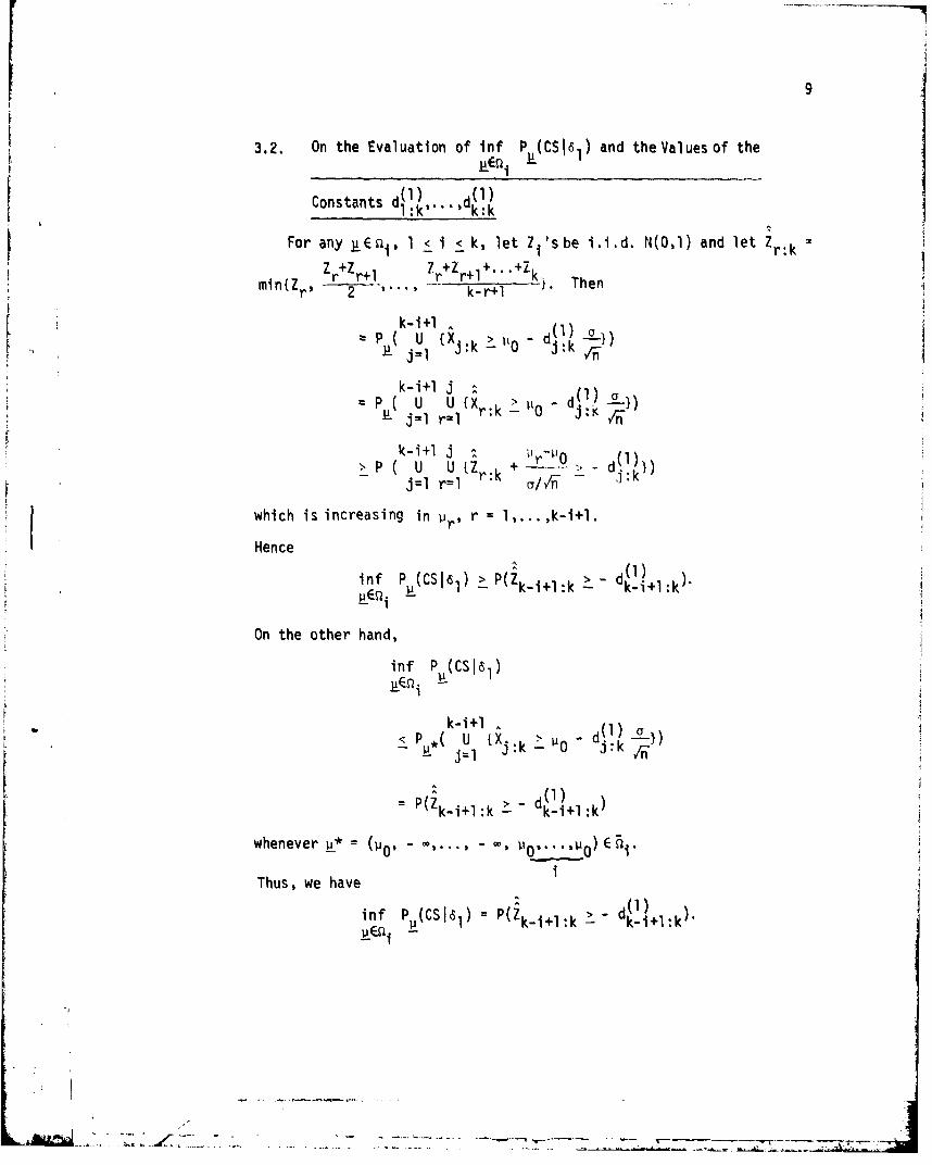
3.2. On the Evaluation of inf P (CS161.) and the Values of the

Constants d~l) d~ll:k'"' k:k

LFor any p E~1 1l 0 -k n

j 1r IC~ J

k-~l - dP1 --P

- P(Zk+ -k + -P- - d) ))

inf P P'Z1 _-

_E '1 1 (k-i+l:k L k-i+l:k

in P(CS6 1)

- -L----

S-~~ - ----- k- -i--+-

10

AAO

Since Z��i+l:k has the same distributions as Z

letting

Vi Z (3.3)

we haveSinf P (CSI16I d= P(V >(-.4)

i 1 -I j-i+l:k)9 i = l,..,,k. (3,4)

It is clear from the above that dt1l) d~l) for allS jk-i+l:k 1:1

i 1, 2,...,k, and d(l" is increasing in i.

Theorem 3.1. In case I, (U0 known, common known and common sample

Ssize n), kif d[l) k is the solution of equation•L •P(Vi >_-X) =P* (3.5)

where

i•j1 rV. j= r Z. and Zi are i.i.d. N(0,l),l<r - d,-i~+,l:k) = P*.

so 61 satisfies the P*-condition.

Therefore, the problem of finding the dl:k s reduces to finding thedistributions 'of VI,...,Vk. This is achieved by using some results

in the theory of random walk.

-'TI

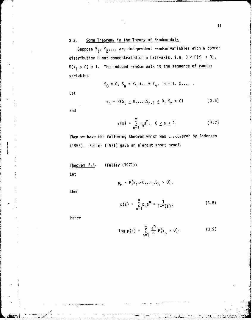
3.3. Some Theoremh in the Theory of Random Walk

Suppose Y1, Y2 "'" art- independent random variables with a coni',on

distribution H not concentrated on a half-axis, i.e. 0 < P(YI < 0),

P(Y > 0) < 1. The induced random walk is the sequence of random

variables

S 0, Sn = Y1 +''' Yn n = 1, 2,...

Let

n P(S1 -<- 0""'Sn Sn 0 O ( 3.6)

and

T(S) = tnsn 0 < s < 1. (3.7)n=l

Then we have the following theorem which was u,,uvered by Andersen

(1953). Feller (1971) gave an elegant short proof.

Theorem 3.2. (Feller (1971))

Let

n= P(S 1 O.' n > 0),

then

p(s) Psn (3.8)p~~s) I -T-- S- 'n=l

henceCO Sn

log p(s) - - P(S > 0). (3.9)n~l

'n'l- " n

12

By symmetry, the probabilities

q P(Sl < 0,...,S < fl) (3.10)

have the generating function q given by

n

log q(s) = Z - P(S < 0). (3.11)nl 1nl

Note: The above theorem remains valid if the signs > and < are

replaced by > and <, respectively.

Theorem 3.3. The generating function p(s) of p(Vj.> x), j = 1,2,...

is•b sn P(Sn> ) 31)

Z sj P(V. > x) = exp {nn(j=ln

where

n

Sn = (Zi - x), n 1, 2.1n1

Proof. Since the distribution of random variable Y. : Zi - x is not

concentrated on a half-axis, and Yi's are i.i.d. let Sr (zi "x),i=l

r 1,...,k. Then

IV. > x'} { min _ S > 01 = {S >O,.,.,S. >01.-<r<j r - 1 0-

By Fellerps Theorem 3.2 , we complete the proof.

II

13

Now let _

A (X) A~ P(S. > ) (xvrj7) j 12,...

sna(s) n "n

n1 *

then we have

pCs j s P(V. x) =exp (a(s)).j=1

Lema 31. (n+l)( 5) = I~ (ý) ~('~' (f+l1j)(s), for all n > 1

Proof. Since p'(s) P(s) al(s), the resul a epoe yidc

tion on n.

Theorem 3.4. Under the assumptionl of Theorem 3.3

= n+l

P (V~ > x) Tl) 50 dsn

n 1 P(V > X)A n 0, 1,2..(3.13)

n+l -= n-j+l

where

P(V0 > x) 1, for all x.

Proof. By Lemma 3.1, we have

li (f+l)(5sP(Vn+ _ýX S4+

S 1 flI p ~(0) ) [(n-l)' An 3

j=0 T p2+ (0) J n

-n+1 j.-:O PV

14

Let G (x) p(V x) and l-G.(x) denote the limiting distributionnn

function as n +-~ of V .Suppose the distribution of r',Rndorn variable

V1 Z x is not concentrated on a half axis, then we have from

Andersen-Feller Theorem

G.(x) exp r-~ P(Sr 0)1

Now, let

Now we can use the recurrence formiula of Theorem 3.4 to

solve the equations P(V1 d~~l :) P* i 19,.. .,k.

Remark .3. 1. From Section 3.2 we know that dl) 1,..,k)

The values of d~l) for k =1 (1) 6, 10, and P* .99, .975, .95,

II.925, .90 are t, ulated in Table 1.I1

Definition 3.2. We define a selectioti procedure 61,by replacing

teinequality in the ith step of procedure A by the ine~uality

K ~~XIkP - d!~r-- i = I,..

where d! . ,t.~d;k are the smallest values such that 6satisfies

the P*-.condition.

Then it can easily be shown that the selection procedure a1 and6

are identical and P) = d!.k' i - ,2,...,k.

3.4. Somie Other Proposed Selection Procedures 62' 63' 64I, In Case 1?, we propose some other selection procedures:

15

Definition 3.3. We define a selection procedure 62 by

62: Select Ti if and only if Xi:k > "0 d i i = 1,...,k

where d is the smallest value such that 62 satisfies the P*-condition.

Note that under assumptions of Case I, and selection procedure

2•2 if we select population lri' then we will select populations n

for al! l _* i, since Xi~k _ Xj:k"

Evaluation of the d-Values of S2

For any i, I <_ i < k, we have from a similar argument as for 61 that

inf P(CS16 2 ) inf P(Xk-i+l:k > 0 d•_Ei- 1_~ - -V

: P(V. - d).

We need the constant d such that P(V > - d) > P* holds for all i,

1 < i < k. By Theorem 3.1we have d = d1Ik It also follows that- - 1:k"

if S and S2 are the selected subsets associated with selection proce-

dures 61 and 62, respectively, then1 S2. Thus e is better than 6 .

Definition 3.4. The procedure 63 is defined as follows: Let Xjýmax(X 1 %X

Step 1. Select Ti' i -1 and stop, if

X1 > I0 " d1 ,1 - PO,

otherwise reject n and go to Step 2.

Step 2. Select ni, i > 2 and stop, if

7 7

!-"d 16

otherwise reject W and go to Step 3.

Step k-i. Select i > k -1 and stop, if

k-l > •0 - dk- 1 0n

otherwise reject 7k- and go to Step k

Step k. Select and stop, if

Xk > - dk

otherwise reject "

Here di's are the smallest values such that 63 satisfies the P*-condition.

Evaluation of di's

For any i, 1 1<i <k,

k-i+l

inf P (Cs51 3 ) = inf P ( U (Xj - d. -Sn1)E - _Ea " j

k-i+l -

Pu, U IX -dj

=P(Zki+1 - dki+l)

whenever E = ,..., . ) E

Since Zi is N(O,1), it implies dk-i+l - d for all i, and

Hd = v t(po)r

Hence, we have the following theorem:

17

Theorem 3.5. Selection procedure 63 satisfies the P*-condition with

di d, i = 1,...,k, which do not depend on i. Hence the procedure is

not changed if the statistics Xi are replaced by Xi, the sample mean of

population wi for i = 1,...,k.

The following procedure 64 was given by Gupta and Sobel (1958),

without assuming any ordering prior:

Definition 3.5. The selection procedure 64 is defined as follows:

Select i if and only if Xi " d -s- i =

where d is the smallest constant such that 6 satisfies the P*-condition.

It was shown that the value d is determined by the equation

1 1

t(- d) = 1 - p* i.e. d = I•-(p*k).

3.5. Some Proposed Selection Procedures 1,2) i 1 2, 3, 4

When 110 is Unknown

Case II. vO unknown, convion 2 known, common sample size n.

Definition 3.6. We define a selection procedure 6(2) by replacing

the inequalities

X > - 1:k '

in procedure 61 (Definition 3.1) with

Xi:k XO i i = 1,.... k, respectively.0- 1 :k /n-

n '2'Here X Xi/n, d:k i = 1,...,k are the smallest :onstants such

that the selection procedure 6 (2) satisfies the P*-condition.

Similar to the Case I, we have the following theorem:

18

Theorem 3.6. For any i, 1 t - d 2 i+l:k)dO(t) P*. (3.15)

It is easy to see that d(2) - d(2) and it is increasing in i The fol-k-i+l :k 1 :1

lowing theorem gives us an identical form of the selection procedure 6,

Theorem 3.7. The selection procedure a(2) is not changed if

the statistics Xi:k' i = l,...,k, are replaced by Xi:k, i = ... ,k,

respectively.

Proof. The proof is straightforward and hence it is omitted.

The values d(2) i = 1,... ,k are tabulated in Table II forl:i' "

k 1 (1) 6, 8, 10, - and P* = .99, .975, .95, .925, .90.

Similar to the Case I, we propose a selection procedure 6(2) as2follows:

Definition 3.7. We define a selection procedure 6(2) by2-y

2:Select 7ri if and only if ii:k .1 XO d-- i 1,.,

where d is the smallest value such that 652) satisfies the P*-condition.r 2

Then, similar to procedure a2 we have d = d( 2 )S1l:k'

Next, we define a selection orocedure 6(2) which is similar to 3

13 V

19

Definition 3.8. The selection procedure 62) is defined by replacing

- 0 " d -S!-_in 83 (Definition 3.4) by _>X0 - d' l-

where di,...,dk are the smallest values such that 6(2) satisfies the

P*-condition.

Similar to Theorem 3.5 we have:

Theorem 3.8. The selection procedure 6 2) satisfies the P*-condition

with d' = d, i = 1,...,k where d is determined by the equation

f 4(d-t)do(t) = P*. (3.16)

And 6 2)is not changed if the statistics X is replaced by Xis

the sample mean of population 7i for i = 1,...,k.The following selection procedure 62) was proposed by Gupta and

Sobel (1958):

D-.-flnition 3.9. The selection procedure 6(2) is defined by

(?): Select and only if X > - dX-s i = l,...,k

where d is determined by the followirg equation.

TI + d)]o(u)du P*. (3.17)- 0n

20

ror the special case n1 2 n (1 0, 1,... ,k)

f k(t+d)o,(t)dt - P*. (3.18)

Under the normal distribution N(0,1), the tables of d-values sat-

isfying the Equation (3.18) for several values of P* are given in

Bechhofer (1954) for k = 1 (1) 10 and in Gupta (1956) for k = 1 (1) 50.

S3.6. Some Proposed Selection Procedures 6 1 t 1, 2, 3 4 for the Normal

Means Problem When Common Variance oa is Unknown

Case III. v0 known, common variance a unknown, ni = n > 1.

_______(3) b elcnDefinition 3.10. We define the selection procedure 61 by replacing

the inequalities

X ~k > O d() i I....k-k i :k k

in procedure 61 (Definition 3.1) by

Xi-k d iO d S I = l,...,k, respectively,

where d (3)'s are the smallest values such that •3) satisfies the

P*-condition; S denotes the pooled estimator of a2 based on

v k(n-1), that is

k nk 2 (X, X 1i2/v. (3.19)12=1iX j~l J ~

• -_,_____- -•

21

Note that .S has the chi-square distribution 2 with v degrees ofav

freedom. The following theorem then follows:

Theorem 3. 9. The equation which determines the constant dk3)k-i+l :k

is

P(Vi > (ki+ll:k ) =p (3.20)

or

0 k-il• l:k y)qv(y)dy P* 3.21)

where q (y) is the density of S_

va

We can rewrite Formula (3.21) as

SP(Vi k--- - Vt(3) 1// X 2() Pf (1 _- djlk/i)dx•(t) -p

0

or

*"tle'tf P(V1 > d(3)) dt (3 ,22)Sk-i+1 :k F() t 3.20 r(v)

22

(3) 1..kdpdon •kn1;lsRemark 3.2. The values of di+l:k I ,. k depend on v k(n- also

By using Rabinowitz and Weiss table (1959) (with N-24 and n of their table(3) , - , , ,

equal to 0) we have evaluated and tabulated the values of d k-+l:k' 1.1,.. %k9

in Table III, for k - 2 (1) 6, P*- .99, .975, .95, .925, .90,

with common sample size n = 3, 5, 9, and 21.

For k > 6 and n > 21 , i.e. v > 120 we can reasonably well approximate

P() by d(l)k-i+l:k 1:i"

Definition 3. 11. We define the selection procedure 8(3) b2 by

63): Select n if and only if XP:k -L" d3S = l,...,k

where S is defined as in procedure 3 and d( 3 ) is the smallest

constant such that 63 satisfies the P*-condition.

As before, it can be shown that d = d(3k• 1:k'

(3)Remark 3.3. In Case III the selection procedure 61 will not be

changed if we replace the isotonic statistics Xi:k respectively.

But this is not necessarily true for selection procedure 62(3)

Definition 3.12. The selection procedure 5(3) is defined to have the3

same form as procedure 6(2) except that the inequality defined in the3

ith step of procedure a2) is replaced by

X 1 0 " d S for i =1,.k.-rn

23

The proof of the following theorem, uses the same arguments

as that in Case I, hence it is omitted.

Theorem 3.10. The equation which determines the constant d of

selection procedure 6(3) is3

f *(yd)q (y)dy P*. (3.23)

0

Gupta and Sobel (1958) gave a selection procedure 6 in this

case. It is as follows:

6(3): Select ni if and only if Xi> - = 1,...,-1

and the equation which determines D is

*k(yD)q (y)dy = P*k (3.24)

kwhere v = i (ni-l).

3.7. Some Proposed Selection Procedures 614), i = 1, 2, 3, 4 for the Normal

2Means Problem When Both Control V0 and Common Variance a. are Unknown

Case IV. 0 unknown, common variance o2 unknown and common sample

size n.

Here we replace l0 in each selection procedure 63) by X0, 1 < j <4,and procedures (4), 1 < j < 4, respectively. The constants d(4)

get k-i+l:k'i = 1,...,k, of procedure 61 are determined by

II

- § _- -!~ .

24

P(f ._( u dk(4) )d:(u)dx 2(t) (P* 3. 25)[0 -CO [ i k - -i + 1 kA.

The constant d of procedure 6(4) is Id = d4

1 :k*

"The constants d of procedures s64 ) and 4)are determined by3 4 ardeemndb

i/r(u+)-d)do(u)dx2(t) = P.(3.26)

with r = 1 and k, respectively, and their values for selected values

of P*, k and v are given in Gupta and Sobel (1957) and Dunnett (1955).

3.8. Properties of the Selection Procedures

Under simple ordering prior, it is natural to require that an ideal

selection procedure is. isotonic as defined below:

Definition 3.13. A selection procedure 6 is isotonic i-i it

selects wi with parameter vi, and if pi < pj, then it also selects Trj.

Procedure 6 is weak isotonic or monotone if

P(wi is selected16)< P(nr is selected j) whenever Pi < Pj.

It is easy to see that any isotonic selection procedure

is weak isotonic, but the converse is not true.

Now, let 6.1) = i i = 1, 2, 3, 4.

Theorem 3.11. The selection procedures 0), 6' ) and 6(i) are

isotonic and procedure 6(') is, monotone, for i 1, 2, 3, 4.

K! I

i7|r

25

Proof. The proof follows immediately from the definitions of the pro-

cedures.

Given observations X = x = (xo,...,xk) where xi is the sample mean

of population 1Ti i = 1,...,k, and x0 -- O if p0 is known, otherwise

x0 is the sample mean of population n 0' Let

pi(x, 6) = P(•i included in the selected subsetix = x, j)

Sfor i 1 ,..,k.

Definition 3.14. A selection procedure 6 is called translation-

invariant if for any x E , c E R

,i(Xo + c, x + c,...,xk + c; •) ,(Xo .... x ; 6), i = ,...,k.

Theorem 3.12. The selection procedures 6(i), (i) 6(i) and 6(i)

are translation-invariant for i = 1, 2, 3, 4. 2 ,

Proof. Proof is straightforward and hence omitted.

Expected Number (Size)of Bad Populations in the Selected Subset

Suppose the control p0 is known and we have common sample size n

2and common known variance a ; without loss of generality, we assume

that p0 = 0 and a/vn = 1. Let E(S'16) denote the expected number of

bad populations in the selected subset in using the selection procedure

7 -- ~ . i L-----------

26

3, then for any j, 0 < j < k,

sup E (S'[I6)Eak-j -

r '

sup P( U {X > dl})-j r = l Z- = 1 k -•k

=:P( U {Z > - d ('3.27)r=1 t=I z:J - Z: k

On the other hand, for procedure 62

2(

sup E(S'162 ) P( U {Z* >-'dl)) (3.28).

. eqa l (.kj 7)r=l ,

From (3.28) we see that the supemum for :2 is' increasing inlj andis greater than or equal to the supremum for 6, given in (3.27), since

Z:k = :k-t~ I -- k"

Therefore, we have the following theorem (see also the remark just beforeDef. 3.4).

Theorem 3.13.- For any i, 0 < i < k

sup E(S'182 sup -(S'i61 ),

sup E(S'1) sup E(S'6 2 ).

Theorem 3.14. In Section 3.1, Case I, for any J, 0 < j •_k

sup E(S'b53 ) q(l-qJ)/P* (3.29)

where q 1- P*.

, 22 I 1.Z .L S tk2l~ l . i 4 S 7~~

27

Proof.

sup E(S' Is3)U•k .j

= sup P (select 7i 163)pEsikj i=l

=sup P( max X >-d)k. 1 t<r<_ r-

'• " = (I - • (-d)) ,,

S= j q(l-qJ)/P*

,, . w h e r e q = ( 1- P * ) .

Theorem 3.15. sup E(S' ) is increasing in j, hence

sup E(S' 53)- sup E(S' 13) = k - q-( k/P*. (3.30)

V-- k-j •0

Proof. Since

0+l) q (j- qi) = l-q+l > 0.

In Case I , Gupta (1965) showed that

sup E(S'I 4 ) kP*k. (3.31)

v EQ~

28

Letusdefnethe event A > (1)} .. ;teLet us aerinei:k >- l:k' =l,.k;te

we have

Lemma 3.2. P( U A1 n A.j1) P( Lu Ai)* for all j, 1 < j < k-i,k > 2.

Proof: P( U~ A1 fl A+

( -{d(1)) n A +)PijUl{Z:j i~ d1 k ijl

P(U {Z >-d(l)})1 Ajl

P( U= : ~ Ai P(Aj+1)jl

P( U A.) P*

The above inequality is a result of the fact

A. c Z. . i-d. for all i = 1,... ,j;j 1,. kl

Theorem 3.16. For all k > 2, sup E(S'j1s 1) 2, P,( u Ad) < 1 - 0l-P*)J for all j and strictly inequality

holds for some j, 1 < j < k.

Istr: holds for j = 1, .since P(Al) =P*. Suppose P( U A) 1< lp)

itrefor some j, 1 < j < k-1, then

29J~•Jt lj jP( U Ai) = P( u A1) + P* - P( u A n Aj+l

i-l i=l i=lSj j

< P( U A.) + P* - P( U Ai)P*l=l i=l

SP* + (I-p*)(I-{I-P*)j)

- 1 (l-.P*)J~l. jHonce by induction principle, the proof is finished.

This theorem tells us that procedure 61 is better than 63 in

the sense that in i0 it tends to select smaller number of bad populations,

however, procedure 61 is not uniformly better than 63. In some cases

(see Section 5), 63 is slightly better than o

When the ordering prior among the unknown parameters is unknown,

we can use the selection procedure of Gupta and Sobel (1958) or use

the ordering of the sample means as the ordering of unknown parameters

and apply the selection procedure which is originally used underordering prior.

In the normal case with the latter approach, the substitution implies that the

isotonic regression of the sample means turns to the usual ordered

sample means, and that the selection procedures 6i), i = 1, 2, 3, 4,

are of the same type as 6(l) (i = 1,2,3,4), respectively, and the selection

procedures 6i) = 1,3, i = 1,2,3,4 are of the same form as J , i=1,2,3,4,35

respectively, which are equivalent to the procedures proposed by Naik

(1975) and Brostrim (1977), independently (see also Holm (1979)).

4. Selection Rules for the Location Parameter Under Partial

Ordering Prior Assumption

Assume that we have only a partial ordering prior of k unknown

location parameters, that is the parameter space

I.I30

1016E and there is a partial order relation "<" among el's)

Our approach is to partition the set {01,,..,Ok}ifnto several sub-

sets, say BO,...,B so that BI n B -, if I J J, U B {e

and for each Bj (j = l,...,U) there is a simple order on It and there

is no order relation among the elements of subset B0.

Let b= Bil, the number of elements contained in Bi, i = ... ,9,

so we have

b = k.

If we denote the new induced partial order by "<" then we have

a parameter space ýi" = ,. We use an example to illustrate how to find

an induced partial order.

Example. Suppose k = 8, and we have a partial ordering prior e01 < 5,01 < 8, 01 < 2 < 3 04, and 02 <6 07. We use a "tree" to

rep,'esent this partial ordering as in Figure 1.

04

03 07

02

e1

Figure 1. Original partial ordering

LI

31

Then we have an Induced partial ordering e8 <82 ' 83 ' 041 '6 '7

as in Figure 2.

83 7[ 05* 08.

f

e3 e5

F Figure 2. Induced partial ordering.

And

B0 = (o5, 081

B1 = fell 02' 031 841

B2 6{o6 071.

It is clear that the induced partial order is not unique, for

example, we can partition fol,...,9 8 into three other subsets

B6, Bit Bi where

B6= {O5, 8

B•= (81) 82, e6, 071SBi {Olt, e4}

B2k 603 07}

For the location parameter case, a selection procedure 6P can be

defined as follows:Definition 4 .1. We define a selection procedure t5p as follows:

Suppose BO,...,Bk are induced subsets and that for each subset

B., j = 1,... , there is a simple order on it. We choose a proper

32

selection procedure 6 for each subset Bi, such that the corresponding

probability of a correct selection is not less than P P* . For

subset B0 we may use selection procedure 54 or 65 with P* = P*-E-.

Theorem 4.1. The selection procedure 6P satisfies the P*-condition.

Proof.

inf P (CS16P)

> inf P (CS16p)- OEI -

II inf P(CSI6p)

where Q' is the parameter space associated with the subset Bi.Bij

5. Comparisons of the Performance of Basic Rules for the Normal Means Problem

In this section we describe results of a Monte Carlo study to compare

the performance of selection procedures 5,, 62 6 39 and 64" Suppose we2

have k iindependent populations, each population with distribution N(.i,L 2with common known variance u2 and common sample size n. Assume that

the mean P of the control is known; without loss of generality we

assume that u0 = 0 and o//r = 1.

k..J ,•JA / -- ....... .... .. .. I

33

In the simulation study, we used Rubin and Hinkle's RVP-Random Variable

Package, Purdue University Computing Center, to generate random

numbers. For each k, we generated one random number (variable) for

each population, then applied each selection procedure separately

and repeated it ten thousand times; we used the relative frequenciesI)as an approximation of the exact values of the associated performance

characteristics for each procedure. In Table IV we use the following

notations:

~ =(�"" k 1 is the parameter of population i

PS = P(CS)

PI = P(correctly rejecting aHl bad populations)

PC = P(correct classification of all popufluL,un)

I where the correct classification means that we select all good

populations and reject all bad populations.

El = Expected number (size) of bad populations contained in

the selected subset.

EJ = ( 0) P (ni is selected)

SES Expected size of the selected subset.

Table IV.l consists of four parts, namely, the four values of

k 2,3,4,5, for each value of k we assume that we have two bad populations.

In this case based on the performance characteristics PI, PC, El or EJ, we

found the performance ordering as follows:

where 61 > 62 means that 6, is better than 62.

[ "I

34

In Table IV.2 we assume that we have three bad populations for k = 3,

and that both populations are bad for k - 2, this table indicates the same

trend as Table IMl, i.e. 6 1 ý 2 . 64. If k is increased by adding

strictly good (parameter strictly larger than control) populations, then

EI(6i), i = 1,2 does not increase. This is because Xi:k > Xi:k+l a.s.

1< i< k.

In Table IV.3 we assume that for each k, k = 2,3,4,5 that every population

is bad. Based on the quantities PI, PC, El and EJ, we find that the perfor-

mance is as follows:

1l 62 63 64"

This is the same result as before.

Table IV.4 has the same structure as before, but for each value of k,

k = 2,3,4,5, we assume that the first population is the one and only one

bad population with parameter -1 which is less than the control PO = 0.

A glance at the table indicates that the performance, based on the charac-

teristics PI, PC, El and ES, can roughly be ordered as follows:

63 . ['2, 'l '4•

i.e. procedure 63 is the best and is slightly better than 62 and 61, 62

and 61 are very close and both are better than 64. As the number of

populations k increases from two to five and the three additional poptulations

are good populations with parameter 1, 2, and 3, respectively, we find

that EI(6i, k = 5) - EI(6i, k = 2), i = 1,2,3,4, is 0.0124, 0.0124, 0.0031,

0.121, respectively. This means that when k increases and the additional

populations are good, then procedure 64 is the most sensitive procedure with

k and thus not good in terms of El. 63 seems to perform better in terms of

El while 6 1 and 62 are about the same.

S--.-~.-..- ,.I

35

In Table IV.5 we assume that the ordering prior of unknown parameter

is incorrect; i.e. the true configuration (-2, -1.0,1,2) is replaced by

(-1,-2,1,0,2). The simulation results indicate that, based on PI, PC,

EI and EJ we have performance 61 > 62 > [63,64). Thus here again 61 is

the best. If we compare Table IV.5 with Table IV.l, we see that 64 does

not change (the small differences are because of random fluctuations),

EI(6 3 ) and EJ(6 3 ) increase quite appreciably.

From these five tables, it appears that, in general, the overall

performance of these procedures is 61 " 62> 63> 641 if the ordering

prior is correct. If there is no information regarding the prior ordering,

then 64 or 65 seem to be an appropriate procedure to use,

b

4 5

.f f .........

36

TABLE I

fTable of d~) values (satisfying (3.5) and (3.14)) necessary to

carry out the procedure 6 for the normal means problem under the simple

ordering prior.

1 :kk __ _ _ ___ _ _ _

k .99 .975 .95 .925 .90

1 2.3264 1.9600 1.6449 1.4395 1.2816

2 2.3337 1.9775 1.6780 1.4872 1.3430

3 2.3339 1.9787 1.6817 1.4942 1.35384

4 2.3339 1.9787 1.6823 1.495-6 1.3563

5 2.3339 1.9787 1.6824 1.4960 1.3571I .39 198 .62 .90 13762.3339 1.9787 1.6824 1.4960 1.3574

TABLE 11

Tabl of (2) vTabe o d1:k vlues (satisfying (3.15)) necessary to carry out the

procedure 6 (2 for the normal means problem under simple ordering prior.

k .99 .975 .95 .925 1 .0

1 3.2886 2.7711 2.3258 2.0355 1.8122

2 3.3449 2.8494 2.4267 2.1530 1.9434

3 3.3605 2.8730 2.4589 2.,917 1.9874

f4 3,3673 2.8840 2.4723 2.2105 2.0091

5 3.3711 2.8901 2.4832 2.2215 2.0219

6 3.3734 2.8941 2,4890 2.2286 2.0303

8 3.3761 2.8988 2.4960 2.2375 2.0406

10 3.3776 2.9014 2,5000 2.2426 2.0440

3.3787 2.9032 2.5021 2.2448 2.0487

-~~ ------ -----

37

Lg~~Li 4wa o~-r-~ inl frf0.1 0n C1. Lnm . t- ~ I D0 0 -

1.-0.1 (1

0 tm

S , ... . Nl ~tý L n r'0-, n q. C . C~i cor-\itM O t ko L( mlf mU I-,

0) C\J Ln. W~ %0 C', %t t "- n r- - r- Q M .nL n n 0

V CLl

0 0 r- Lf0 eJ-rwt r~- LnLn0 ~r- r %0 3 C 0 M

S r-. n" 0m 1 D0 cyl mc Rro Je.r--c en k tDkD n oCL ON m 04 .oL M c 14c )cýC ýIlr

Ln 10 M cc. ý C)V~ cooc'-. 00rt )C)O OL o C)00c )q~Vt1 Iý 00 Ic m c. .c na 4CJýr-0 )0 Y A

Nl 00 I 0 t % D n nm U~l (_:I~ CDp0~ LfC:) Q

Nr- u~~40O.LL

o to

(a I ON 00r lC 0-) r-) k co co CI to C 0C-0C c ONt o. a 0t coD t~tou 0 'LnLnL I~ cc qt.rm

Ln Lo m m-c c~l CY e enY) C C c cli ci C, ~

0 tLC 0m ý r- 00l CNO 04*C1 00O) cccrr-r- o LO C) n

ccoi- (-u' 5 ooooa coco cci--

-l oa n( mk jmma

(A E- 6 ; Lfo i-- 1-1) Illr) fll,0 ko%0kokoDIf

LO. M0 L00 00p00I- - 0 00I t00 -It0M00

IRE

i~ Ar (1)

7.-- 38

1.0 qu mcOI'%k L( 00~ mmmwu- W toW w -

o) 0

S- C7 w N lO O C'J 00r-00co I'll %o %atoZo -- c nto r-..oc -it .o~C *l iný Co. c C,- I.:o~e '.r:~. r.: -:

LO S

C- 0 I 00 C0. S.. ejý Cl ~ coi~ - 0ra -,I nV o t

CLLU~fL Cýcl lCVl ý ý ~Y ý l

4-)

0O o C\JL) 0sCý 0a Lt0CY 'J C , o %D koe m )C C %Co I' 'cv)C t,- )C to.. t.C0 t ' CA I'llJ CD CD C (1 oi

m. m~ 0)j --- .-j .- j f. . . .~ .~ -l N -I -" - -

4* amM Oa r-r v mO 0) M~ P-. r-,- f"~ inin, C

I-- (A I

0 0 0 , 00 I,0ti 0\CO-. iCJ -Lfl L1dO Ch-L.C\

CD 0eJý CItolto-. C,- C 471 i~~ C% 'j00 Je'04.--.-r-.0 m. mo cn m--,- COCCO

u l 3 i 1 ýC rý 1 l ý Ll1E 0 CI-O. si-.~r- cmi

C14 -,J C71 00 C>J OD 00 ' C )J. r- CJ, oclJ' CI~J " N " C\m l oc oc t Dk D I , nU)I 4

Ei uggl iggC ý-ý ligg Ilrlýg m igmiggtgmtu"u-

w 0 11 ~~~~~~~~~~~Im ),r-r-'C W M M Ir-rIrtu. 0 0 0 0 00 0 0 0 0 0 0

-D"D-O-- , m - 0 - O )CLr.)iQ ~ :....... tA \ - 0r omm )0 : ~ tqrciC

39

TABLE IMl

Simulation results 'or the comparative performance of various selectionprocedures for the normal means problem (notation explained in Section5) under simple ordering prior.

P = .900

k = 2, P= (-2,-I)61 62 ] 3 64

PS 1.0000 1.0000 1.0000 1.0000PI .3420 .3252 .3001 .1719PC .3420 .3252 .3001 .1719FT .8673 .8841 .9389 1.0950EJ 1.4952 1.5120 1.6559 2.1831ES .8673 .8841 .9389 1.0950

k = 3, i (-2,-I,0)

1 - -. 2 - a3 a4

PS .9535 .9573 .9696 .9632PI .3437 .3407 .3'j, .1233PC .2972 .2980 .2703 .1175El .8585 .8615 .9350 1.2126EJ 1.4651 1.4681 1.6421 2.4996ES 1.8120 1.8188 1.9046 2.1758

k 4, (-2,-l,0,1)61 62 63 64

PS .9596 .9606 .9715 .9747PI .3269 .3254 .2936 .0874PC .2865 .2860 .2651 .0851El .8802 .8817 .9431 1.3062EJ 1.5015 1.5030 1.6532 2.7378ES 2.8387 2.8412 2.9142 3.2808

k = 5, • = (-2,-l,0,1,2)

6 1 6 2 63 64

PS .9562 .9564 .9690 .9765PI .3333 .3331 .2984 .0746PC .2895 .2895 .2674 .0725El .8835 .8837 .9480 1.3712EJ 1.5339 1.5341 1.6872 2.9450ES 3.8386 3.8390 3.9167 4.3477

AW:r

40

TABLE IV.2

Simulation results for the comparative performance of various selectionprocedures for the normal means problem (notation explained in Section

5) under simple ordering prior.

P = .900

k = 2, • = (-3,-2)-1 02 03 04

PS 1.0000 1.0000 1.0000 1.0000PI .7551 .7380 .7342 .5912PC .7551 .7380 .7342 .5912El .2632 .2803 .3035 ,4395EJ 1.1443 1.2127 1.4025 2.1590ES .2632 .2803 .3035 .4395

k = 3, = (-3,-2,-1)1 62 a3 64

PS 1.0000 1.0000 1.0000 1.0000PI .3362 .3156 .2837 .1090PC .3362 .3156 .2837 .1090El .8937 .9166 1.0275 1.3290EJ 1.6654 1.6952 2.1746 3.5318ES .8937 .9166 1.0275 1.3290

k 4, u = (-3,-2,-1,0)

______ 1 62 63 64

PS .9579 .9616 .9737 .9731PI .3257 .3225 .2801 .0759PC .2836 .2841 .2538 .0736El .9118 .9160 1.0419 1.4675EJ 1.7093 1.7165 2.2324 4.1380ES 1.8697 1.0776 2.0156 2.4406

k ="5, ( .... _

1I 62 63 64PS .9582 .9590 .9714 .9796Pi .3292 .3281 .2877 .0602PC .2874 .2871 .2591 .0582EI .8962 .8976 1.0172 1.5283EJ 1.6554 1.6577 2.1429 4.3912ES 2.8536 2.8559 2.9884 3.5078

41

TABLE IV.3

Simuilation results for the comparative performance of various selection

procedures for the normal means problem (notation explained in Section5) under simple ordering prior.

p 900

k 2, =p

S1 62 3 64

PS 1.0000 1.0000 1.0000 1.0000PI .9613 .9560 .9585 .9130PC .9613 .9560 .9585 .9130r-LI .0392 .04&45 .0448 .0876EJ .3563 .4040 .4263 .8493

F ES .0392 .0445 .0448 .0876

k = 3, _ = (-4,-3,-2)61 6 2 63 6 4

PS 1.0000 1.0000 1. Oq'.' 1.0000PI .7587 .7359 .7300 .4997PC .7587 .7359 .7300 .4997El .2599 .2835 .3201 .5574EJ 1.1340 1.2324 1.5547 2.9908ES .2599 .2835 .3201 .5574

k =4, (-4,-3,-2,- l)

S1 62 3 64

PS 1.0000 1.0000 1.0000 1.0000PI .3348 .3114 .2814 .0747PC .3348 .3114 .2814 .0747El .9003 .9282 1.0440 1.4745EJ 1.7013 1.7437 2.2947 4.3666ES .9003 .9282 1.0440 1.4745

k = 5, E = (-4,-3,-2,-1,-0.5)61 62 1 3 6 4

PS 1.0000 1.0000 1.0000 1.0000Pl .1117 .1045 .0615 .0036PC .1117 .1045 .0615 .0036El 1.7460 1.7600 1.9734 2.4985EJ 1.8147 1.8275 2.4965 5.0978ES 1.7460 1.7600 1.9734 2.4985

42

TABLE IV.4

Simulation results for the comparative performance of various selectionprocedures for the normal means problem (notation explained in Section

5) under simple ordering prior.

P = 900

k = 2, v (-1,0)S1 62 3 a4

PS .9453 .9490 .9579 .9470iPI .3854 .3854 .3937 .2676

PC .3307 .3344 .3516 .2530El .6146 .6146 .6063 .7324EJ .6146 .6146 .6063 .7324ES 1.5599 1.5636 1.5642 1.6794

k = 3, = (-1,0,2)61 62 a3 64

PS .9531 .9535 .9638 .9616PI .3741 .3741 .3826 .2044PC .3272 .3276 .3464 .1970El .6259 .6259 .6174 .7956EJ .6259 .6259 .6174 .7956ES 2.5779 2.5777 2.5803 2.7574

k 4 5, •: (-1,0,1,2)1 62 63 64

PS .9580 .9582 .9640 .9765PI .3664 .3664 .3834 .1683PC .3244 .3246 .3474 .1640El .6336 .6336 .6166 .8317EJ .6336 .6336 .6166 .8317ES 3.5902 3.5904 3.5801 3.8081

,• k = 5, = (-1,0,1,2,3)

6I

------ �-- U=

i,'1 62 3 64!"PS .9554 .9554 .9623 .9794•'PI .3730 .3730 .3906 .1465itPC .3284 .3284 .3529 .1431SEl .6270 .6270 .6094 .8535SEJ .6270 .6270 .6094 .8535

ES 4.5812 4.5812 4.5714 4.8329

JUVJ

43TABLE IV.5

Simulation results for the comparative performance of various selectionprocedures for the normal means problem (notation explained in Section5) under simple ordering prior.

P = .900

k = 2, (-l,-2)

2 3 4

PS 1.0000 1.0000 1.6000 1.0000PI .5405 .5349 .2W37 .1722Pr. .5405 .5349 .2937 .1722LI .8331 .8387 1.3151 1.0904EJ 2.2116 2.2340 3.4232 2.1578ES .8331 .8387 1.3151 1.0904

k = 3, i = (-l,-2,1)61 I 62 63 64

PS .9932 .9943 .Q•::' .9976PI .5365 .5349 .2987 .1190PC .5297 .5292 .2944 .1189El .8347 .8363 1.3116 1.2154EJ 2.2252 2.2316 3.4155 2.4919ES 1.8279 1.8306 2.3073 2.2130

k 4, = (-l,-2,1,O)_l1 2 63 64

PS .9921 .9923 .9973 .9746PI .5271 .5269 .2894 .0873PC .5192 .5192 .2867 .0849El .8498 .8500 1.3235 1.3077EJ 2.2685 2.2693 3.4553 2.7474ES 2.8390 2.8395 3.3207 3.2822

k = 5, • (-l,-2,1,0,2)61 62 a3 64

PS .9906 .9906 .9958 .9795

PI .5317 .5316 .2937 ,0711PC .5223 .5222 .2895 .0693El .8461 .8462 1.3217 1.3593EJ 2.2510 2.2514 3.4406 2.8830ES 3.8341 3.8342 4.3173 4.3388

i

---

44

BIBLIOGRAPHY

Andersen, E. S. (1953). On the fluctuation of sums of randomvariables. Math. Scand., 1, 263-285.

Ayer, M., Brunk, H. D., Ewing, G. M., Reid, W. T. and Silverman, E.(1955). An empirical distribution function for sampling withincomplete information. Ann. Math. Statist., 26, 641-647.

Barlow, R. E., Bartholomew, D. J., Bremner, J. N. and Brunk, H. D.(1972). Statistical Inference under Order Restrictions.John Wiley & Sons, New York. j

Bechhofer, R. E. (1954). A single-sample multiple decision procedure forranking means of normal populations with known variances. Ann. Math.Statist., 25, 16-39.

Bechhofer, R. E., Kiefer, J. and Sobel, M. (1968). SequentialIdentification and Ranking Procedures. Univ. of ChTcago Press,Chicago.

-Brostr6m, G. (1977). An improved procedure for selecting all popu-lations better than a standard. Tech. Report 1977-3, Inst. ofMath. and Statist., Univ. of Umel, Sweden.

Dunnett, C. W. (1955). A multiple comparison procedure for comparingseveral treatments with a control. J. Amer. Statist. Assoc.,50, 1090-1121.

Feller, W. (1971). An Introduction to Probability Theory and ItsApplications, Vol. II, 2nd Edition. John Wiley & Sons, New York.

Gupta, S. S. (1956). On a decision rule for a problem in ranking means.Ph.D. Thesis (Mimeo. Ser. No. 150). Inst. of Statist., Univ. ofNorth Carolina, Chapel Hill.

Gupta, S. S. (1965). On some multiple decision (selection and ranking)rules. Technometrics, 7, 225-245.

Gupta, S. S. (1967). On selection and ranking procedures. Trans.Amer. Soc. Qual. Control., pp. '151-155.

Gupta, S. S. and Hsiao, P. (1980). On r-minimax, minimax and Bayesprocedures for selecting populations close to a control. (submitted).

Gupta, S. S., and Kim, W. C. (1980). r-minimax and minimax decision rulesfor comparison of treatments with a control. Recent Developmntsin Statistical Inference and Data Analysis. North-Holland PublishingCompany, 55-71.

Gupta, S. S. and Panchapakesan, S. (1972). On a class of subset selection

procedures. Ann. Math. Statist., 43, 814-822.

Gupta, S. S. and Panchapakesan, S. (1979). Multiple Decision Procedures:Theory and Methodolozv of Selection and Ranking Populations. JohnWiley & Sons, New York.

45

Gupta, S. S. and Sobel, M. (1957). On a statistic arises in selection andranking problems. Ann. Math. Statist. 28,957-67.

Gupta, S. S. and Sobel, M. (1958). On selecting a subset which containsall populations better than a standard. Ann3 Math. Statist., 29,

Holin, S. (1979). A simple sequentially rejective multiple test procedure.Scand. J. Statist., 6, 65-70.

Kruskal, J. B. (1964). Nonnietric multidimensional scaling: a numericalmethod. Psychometrika,29, 115-129.

Lehmann, E. L. (1961). Some Model I problems of selection. Ann. Math.

Statist., 32, 990-1012.

Marcus, R. (1976). The power of some tests of the equality of normalmeans against an ordered alternative. Biometrika, 63, 1, 177-183.

Naik, U. D. (1975). Some selection rules for comparing p processes witha standard. Comm. Statist., 4, 519-535.

Paulson, E. (1962). A sequential procedure for comparing several experi-mental categories with a standard or control. Ann. Math. Statist.,33, 438-443.

Rabinowitz, P. and Weiss, G. (1959). Tables of abscissas and weights

for numerical evaluation of integrals of the form eXxnf(x)dx.

Ath. Tables and Other Aids to Comput., Vol. XIII, 68, 285-294.

Williams, D. A. (VY). A test for differences between treatment meanswhen several dose levels are compared with a zero dose control.Biometrics, 27, 103-117.

Williams, D. A. (1977). Inference procedures for monotonically orderednormal means. Biometrika, 64, 9-14.

FII. I

UNCLASSIFIED *

StCURIITY CLASSIPICATION OR THIS WAGE (fWhen Does Entered)REPORT ~ ~ ~ ~ ~ R DOUEDTO PAGNS JT"sR~UCTIONSREPORT DOCUMENTATION PAGE _ BEFORE COMPLETING FORM

1, REPORT NUMBER GOVT ACCESSION NO. 1. RECIPIENT'S CATALOG NUMBER

Mimeograph Series #81-24 AC

4. TITLE (and Subtitle) S. TYPE OF REPORT & PERIOO COVERED

Ih Isotonic Procedures for Selecting PopulationsBetter Than a Control under Ordering Prior Technical

i A. PERFORMING DAG. REPORT NUMBER

Mimeo. Series #81-247. AUTNOR(*) s, CONTRACT CR GRANT NUMBER(#)

Shanti S. Gupta and Hwa-Ming Yang ONR N00014-75-C-0455

'. PERFORMING ORGANIZATION NAME AND AODRESS 10. PROGRAM ELEMENT. PROJECT. TASKARVA & WORK UNIT NUMBERS

Purdue UniversityDepartment of StatisticsWest Lafayette, IN 47907

II. CONTROLLING OFFICE NAME AND ADDRESS 12, REPORT DATE

Office of Naval Research July 1981Washington, DC 13. NUMBER OF PAGESS~45

14 MONITORING AGENCY NAME S AOORE(.S(If different from Controlling Oltice) I$. SECURITY CLASS. (*I this tepor?)

UnclassifiedI~a, DECLASSIFICATION, DOWNGRADING

SCHEDULI!

16. OISTRIBJTION STATEMENT (of thie Report)

Approved for public release, distribution unlimited.

17. DISTRIBUTION ST. 4ENT (of V a4betrct entered In Block 20, It difectont (rom Report)

IS. SUPPLEMENTARY tES

19. KEY WORDS (Continue on ?*verse side It necesuary and Idenftl.y by block number)

Selection procedure, Subset selection, P*-condition, Stepwise procedure,Ordering prior, Isotonic regression, Isotonic estimators, Random walk,Isotonic procedure, Monte Carlo comparisons.

20. ABSTRACT (Canltinue on teveree aid* It naceoeery and Idonertl,, by block number)

The problem of selecting a subset containing all populations better than acontrol under an ordering prior is considered. Three new selection procedureswhich satisfy a desirable basic requirement on the probability of a correctselection are proposed and studied. lwo of the three procedures -use the isotonicregression over the sample means of the k-treatments with respect to the givenordering prior. Tables of constants which are necessary to carry out the selec-tion procedures with isotonic approach for the selection of unknown means ofnormal populations are given. The results including Monte Carlo studies indicate

DD tI AN"o, 1473 UNCLASSIFIEDSECURITY CLASSIFICATION OF THIS PAGE (When Daot Entered)

"SECURITY CLASSIFICATION uIF Tb1iS PAGOC(• on Data Intoeod)

that, in general, the stepwise procedure 61, using isotonic estimators, is

the best.

UNCLASSIFIEDSECURITY CLASSIFICATION OF THIS PAGE(When Data Intated)

-F

k purdue university - dtic.mil < k' in section 4 we will consider the partial order-ing...

Documents