jun-bao wu and chuan-jie zhu-mhv vertices and scattering amplitudes in gauge theory

8/3/2019 Jun-Bao Wu and Chuan-Jie Zhu-MHV Vertices and Scattering Amplitudes in Gauge Theory

http://slidepdf.com/reader/full/jun-bao-wu-and-chuan-jie-zhu-mhv-vertices-and-scattering-amplitudes-in-gauge 1/39

a r X i v : h

e p - t h / 0 4 0 6 0 8 5 v 3

8 J u l 2 0 0 4

MHV Vertices and ScatteringAmplitudes in Gauge Theory

Jun-Bao WuSchool of Physics, Peking University

Beijing 100871, P. R. China

Chuan-Jie Zhu∗

Institute of Theoretical Physics, Chinese Academy of SciencesP. O. Box 2735, Beijing 100080, P. R. China

February 1, 2008

Abstract

The generic googly amplitudes in gauge theory are computed by us-ing the Cachazo-Svrcek-Witten approach to perturbative calculationin gauge theory and the results are in agreement with the previouslywell-known ones. Within this approach we also discuss the paritytransformation, charge conjugation and the dual Ward identity. Wealso extend this calculation to include fermions and the googly ampli-tudes with a single quark-anti-quark pair are obtained correctly fromfermionic MHV vertices. At the end we briefly discuss the possibleextension of this approach to gravity.

1 Introduction

Recently Witten [1] found a deep connection between the perturbative gaugetheory and string theory in twistor space [2]. Based on this work, Cachazo,

∗Supported in part by fund from the National Natural Science Foundation of Chinawith grant Number 90103004.

1

http://arxiv.org/abs/hep-th/0406085v3

































Svrcek and Witten reformulated the perturbative calculation of the scattering

amplitudes in Yang-Mills theory by using the off shell MHV vertices [3]. TheMHV vertices they used are the usual tree level MHV scattering amplitudesin gauge theory [4, 5], continued off shell in a particular fashion as given in [3].(For references on perturbative calculations, see for example [6, 7, 8, 9, 10].The 2 dimensional origin of the MHV amplitudes in gauge theory was firstgiven in [11].) Some sample calculations were done in [3], sometimes withthe help of symbolic manipulation. The correctness of the rules was partiallyverified by reproducing the known results for small number of gluons [6].

In a previous work [12] (for recent works, see [13, 14, 15, 16, 17, 18, 19, 20,21, 22, 23, 24, 25, 26, 27, 28, 29]), by following the new approach of [3], oneof the authors computed the exceptionally simple amplitudes with two posi-

tive helicity gluons and an arbitrary number of negative helicity ones, calledgoogly amplitudes in [3]. These amplitudes were calculated from the stringtheory in [13]. In the special case when the two positive helicity particlesare adjacent, the result was shown to be in agreement with the well-knownresult [4]. In this paper we will calculate the generic googly amplitudes. Byreproducing the previously well known results, our calculation gives a quitestrong support to the Cachazo-Svrcek-Witten (CSW for short) proposal.

Although these calculations gave strong support to the CSW approach tothe perturbative calculation in gauge theory, a direct proof for the equivalenceto the usual Feynman rules seems hopeless. On the other hand, the twistor

string theory approach [1] gives a different but rather compact expressionfor the tree level amplitude of gluons [13, 14]. It was proved [14] that thisexpression satisfies most of the requirements for the tree amplitude of gluons.In [22] it was argued that the string representation (a connected instanton) of the tree amplitude can indeed be decomposed into a summation of differentMHV amplitudes (a set of disconnected instantons), giving precisely the CSWrules of perturbative calculations. Encouraged by the success of the googlyamplitude calculation we will present some general discussions on the MHVdiagrams in gauge theory. We note that in the calculation of the googlyamplitudes by using the CSW rules, we only need the MHV vertices with3 lines and the MHV vertices with 4 lines. So in a parity conserved theory

the higher point (5 or more) MHV amplitudes can be obtained by paritytransformation from the googly amplitudes and so the higher point MHVvertices can’t be chosen arbitrarily. We also prove that the CSW rules satisfythe dual ward identity and the charge conjugation identity [6].

The CSW proposal [3] can also be extended to gauge theory with fermions

2



(see also [21]). Although the MHV (and googly) fermionic amplitudes can

be easily obtained by supersymmetric Ward identities [30, 31, 6] we think itis still worthy to compute these amplitudes directly because the general non-MHV (googly) ammplitudes cannot be determined in terms of amplitudesonly and should be computed separately1. We will compute the googly am-plitudes with fermions by extending the CSW rules with MHV vertices. Forillustration we consider only the simplest case of a single quark-anti-quarkpair. The general cases, including the supersymmetric case with gluinos, willbe discussed in a separate publication [33]. Some generic non-MHV fermionicamplitudes were also computed in [21, 32].

Another interesting question is whether the CSW approach can be ex-tended to theories with gravity. A naive extension of the the CSW rules to

graviton doesn’t seem to work [24]. Nevertheless we believe that some sim-ilar rules for graviton must exist, given the simplicity of the MHV gravitonamplitude [34] and the KLT relations between gauge theory and gravity [35].In [26], Berkovits and Witten put forward a similar connection between thesuperconformal supergravity and closed string theory in twistor space. Thismay also suggest an extension of the CSW rules. In the last section we willpresent our partial successful and un-successful attempts to this problem. Inparticular we give a simple rule for the calculation of the off-shell amplitudewith a single positive helicity graviton. This amplitude is proportional to thesquare of the (only) off-shell momentum and it is vanishing on shell.

This paper is organized as follows. In section 2, we present the com-putation of the generic googly amplitudes. In section 3, we give some gen-eral discussions on the MHV diagrams. We define precisely how the paritytransformation operates in the CSW approach. We also prove the chargeconjugation identity and the dual Ward identity in this section. In section4, we extend the CSW rules to include fermions and compute the googlyamplitude with a single quark and anti-quark pair. In the last section wemake some investigations on the graviton MHV diagrams. Some technicalproofs are relegated to two Appendices.

1In an early version of this paper we don’t say this explicitly although we suspect thisis the case. See the footnote of the recent paper [32]. We thank the referee to point out

this to us.

3



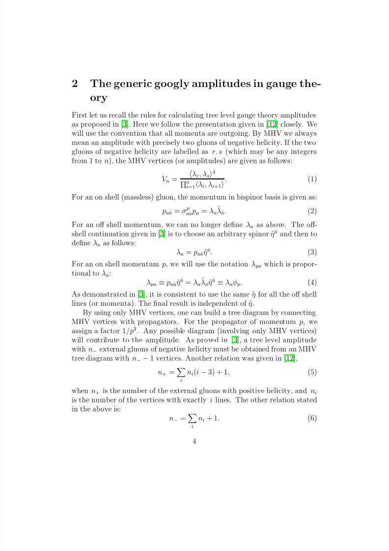
2 The generic googly amplitudes in gauge the-

oryFirst let us recall the rules for calculating tree level gauge theory amplitudesas proposed in [3]. Here we follow the presentation given in [12] closely. Wewill use the convention that all momenta are outgoing. By MHV we alwaysmean an amplitude with precisely two gluons of negative helicity. If the twogluons of negative helicity are labelled as r, s (which may be any integersfrom 1 to n), the MHV vertices (or amplitudes) are given as follows:

V n =λr, λs

4

ni=1λi, λi+1

. (1)

For an on shell (massless) gluon, the momentum in bispinor basis is given as:

paa = σµaa pµ = λaλa. (2)

For an off shell momentum, we can no longer define λa as above. The off-shell continuation given in [3] is to choose an arbitrary spinor ηa and then todefine λa as follows:

λa = paaηa. (3)

For an on shell momentum p, we will use the notation λ pa which is propor-tional to λa:

λ pa ≡ paaηa = λaλaη

a ≡ λaφ p. (4)

As demonstrated in [3], it is consistent to use the same η for all the off shelllines (or momenta). The final result is independent of η.

By using only MHV vertices, one can build a tree diagram by connectingMHV vertices with propagators. For the propagator of momentum p, weassign a factor 1/p2. Any possible diagram (involving only MHV vertices)will contribute to the amplitude. As proved in [3], a tree level amplitudewith n− external gluons of negative helicity must be obtained from an MHVtree diagram with n− − 1 vertices. Another relation was given in [12],

n+ =

ini(i − 3) + 1, (5)

when n+ is the number of the external gluons with positive helicity, and niis the number of the vertices with exactly i lines. The other relation statedin the above is:

n− =i

ni + 1. (6)

4



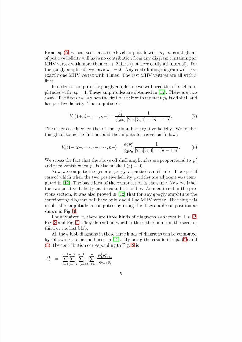
From eq. (5) we can see that a tree level amplitude with n+ external gluons

of positive helicity will have no contribution from any diagram containing anMHV vertex with more than n+ + 2 lines (not necessarily all internal). Forthe googly amplitude we have n+ = 2. Any contributing diagram will haveexactly one MHV vertex with 4 lines. The rest MHV vertices are all with 3lines.

In order to compute the googly amplitude we will need the off shell am-plitudes with n+ = 1. These amplitudes are obtained in [12]. There are twocases. The first case is when the first particle with moment p1 is off shell andhas positive helicity. The amplitude is

V n(1+, 2−, · · · , n−) =p21

φ2φn

1

[2, 3][3, 4] · · · [n − 1, n]. (7)

The other case is when the off shell gluon has negative helicity. We relabelthis gluon to be the first one and the amplitude is given as follows:

V n(1−, 2−, · · · , r+, · · · , n−) =φ4r p

21

φ2φn

1

[2, 3][3, 4] · · · [n − 1, n]. (8)

We stress the fact that the above off shell amplitudes are proportional to p21and they vanish when p1 is also on shell ( p21 = 0).

Now we compute the generic googly n-particle amplitude. The special

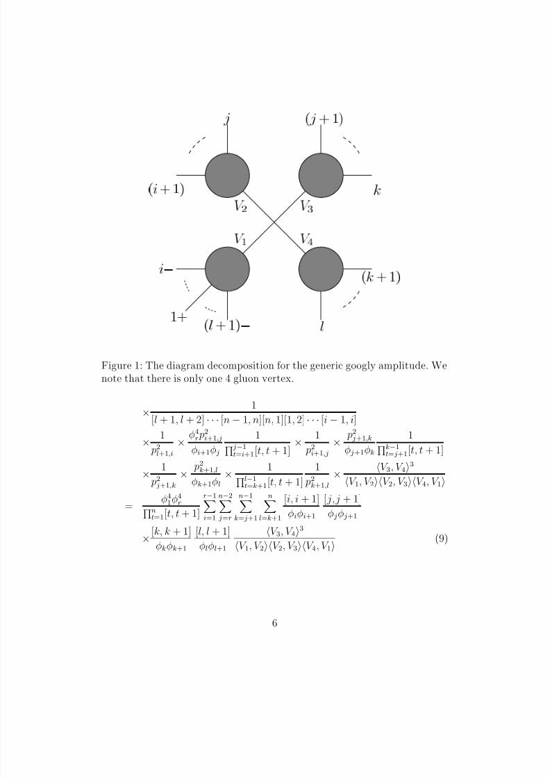
case of which when the two positive helicity particles are adjacent was com-puted in [12]. The basic idea of the computation is the same. Now we labelthe two positive helicity particles to be 1 and r. As mentioned in the pre-vious section, it was also proved in [12] that for any googly amplitude thecontributing diagram will have only one 4 line MHV vertex. By using thisresult, the amplitude is computed by using the diagram decomposition asshown in Fig. 1.

For any given r, there are three kinds of diagrams as shown in Fig. 2,Fig. 3 and Fig. 4. They depend on whether the r-th gluon is in the second,third or the last blob.

All the 4 blob diagrams in these three kinds of diagrams can be computed

by following the method used in [12]. By using the results in eqs. (7) and(8), the contribution corresponding to Fig. 2 is

A1n =

r−1i=1

n−2 j=r

n−1k= j+1

nl=k+1

φ41 p

2l+1,i

φl+1φi

5



Ð

½ ·

· ½ µ

Ð · ½ µ

· ½ µ

· ½ µ

Î

½

Î

¾

Î

¿

Î

Figure 1: The diagram decomposition for the generic googly amplitude. Wenote that there is only one 4 gluon vertex.

× 1[l + 1, l + 2] · · · [n − 1, n][n, 1][1, 2] · · · [i − 1, i]

×1

p2l+1,i×

φ4r p

2i+1,j

φi+1φ j

1 j−1t=i+1[t, t + 1]

×1

p2i+1,j×

p2 j+1,kφ j+1φk

1k−1t= j+1[t, t + 1]

×1

p2 j+1,k×

p2k+1,lφk+1φl

×1l−1

t=k+1[t, t + 1]

1

p2k+1,l×

V 3, V 43

V 1, V 2V 2, V 3V 4, V 1

=φ41φ4rn

t=1[t, t + 1]

r−1i=1

n−2 j=r

n−1k= j+1

nl=k+1

[i, i + 1]

φiφi+1

[ j,j + 1]

φ jφ j+1

×[k, k + 1]

φkφk+1

[l, l + 1]

φlφl+1

V 3, V 43

V 1, V 2V 2, V 3V 4, V 1(9)

6



· ½ µ

· ½ µ

Ð

· ½ µ

Ö ·

·

½ ·

Ð · ½ µ

·

Figure 2: The diagram decomposition for the generic googly amplitude when(i + 1) ≤ r ≤ j.

where2

V 1 =n+is=l+1

λsφs, V 2 = js=i+1

λsφs, (10)

V 3 =ks= j+1

λsφs, V 4 =ls=k+1

λsφs, (11)

and when i ≤ j, we define pi,j as pi,j = jt=i pt as in [3], when i > j, we

define pi,j as pi,j =nt=i pt +

jt=1 pt.

The contribution corresponding to Fig. 3 and Fig. 4 is similar. The resultare

A2n =

φ41φ4rn

t=1[t, t + 1]

r−2i=1

r−1 j=i+1

n−1k=r

nl=k+1

[i, i + 1]

φiφi+1

[ j,j + 1]

φ jφ j+1

2Here and below the summation liken+i

s=l+1 is understood asn

s=l+1 +i

s=1.

7



· ½ µ

·

Ö ·

· ½ µ

Ð

· ½ µ

½ ·

Ð · ½ µ

·

Figure 3: The diagram decomposition for the generic googly amplitude when( j + 1) ≤ r ≤ k.

×

[k, k + 1]

φkφk+1

[l, l + 1]

φlφl+1

V 2, V 44

V 1, V 2V 2, V 3V 3, V 4V 4, V 1 (12)

and

A3n =

φ41φ4rn

t=1[t, t + 1]

r−3i=1

r−2 j=i+1

r−1k= j+1

nl=r

[i, i + 1]

φiφi+1

[ j,j + 1]

φ jφ j+1

×[k, k + 1]

φkφk+1

[l, l + 1]

φlφl+1

V 2, V 33

V 1, V 2V 3, V 4V 4, V 1(13)

respectively.The sum of Ain, i = 1, 2, 3 can be written as

An =φ41φ4rn

t=1[t, t + 1]

r−1i=1

nl=max{i+3,r}

l−2 j=i+1

l−1k= j+1

[i, i + 1]

φiφi+1

[ j,j + 1]

φ jφ j+1

×[k, k + 1]

φkφk+1

[l, l + 1]

φlφl+1

V p, V q4

V 1, V 2V 2, V 3V 3, V 4V 4, V 1, (14)

8



· ½ µ

· ½ µ

Ð

Ö ·

·

· ½ µ

½ ·

Ð · ½ µ

·

Figure 4: The diagram decomposition for the generic googly amplitude when(k + 1) ≤ r ≤ l.

where p and q in eq. (14) are the two indexes ( p = 2, 3, q = 3, 4, p = q) which

satisfy that neither V p nor V q includes λrφr as defined in eqs. (10) and (11).As in [12], we can prove that the 4-fold summation in eq. (14) gives exactly

the required result, i.e.

r−1i=1

nl=max{i+3,r}

l−2 j=i+1

l−1k= j+1

[i, i + 1]

φiφi+1

[ j,j + 1]

φ jφ j+1

[k, k + 1]

φkφk+1

[l, l + 1]

φlφl+1

×V p, V q

4

V 1, V 2V 2, V 3V 3, V 4V 4, V 1=

[1, r]4

φ41φ4r

. (15)

The proof of this identity, eq. (15), will be given in Appendix A. As in [12],it is proved by analyzing its pole terms and finding that all the pole termsare vanishing.

By using eq. (15) in eq. (14), we have

An(1+, 2−, · · · , r+, · · · , n−) =[1, r]4ni=1[i, i + 1]

. (16)

9



This is the known result for the googly amplitude [4, 5]. It is the complex

conjugate of the MHV amplitude, eq. (1), for Minkowski signature.

3 Some general discussions on the MHV di-agrams in gauge theory

3.1 Parity transformation and the googly amplitude

As shown in the previous section, in our calculation of the googly amplitudes,we use the 3-line and 4-line MHV vertices only. The vertices with more than4 lines don’t appear in the contributing diagrams. A parity transformation

will exchange the googly amplitudes with the MHV amplitudes. So in aparity invariant theory, once the off-shell continuation of 3 point and 4 pointMHV amplitudes are given, the on-shell n point MHV amplitudes (n > 4)can be obtained from the googly amplitudes by parity transformation. Thehigher MHV amplitudes (and vertices) can’t be chosen arbitrarily.

The parity invariance of the tree level amplitude is discussed in [14, 18]using string theory in twistor space [1]. Other related works are [16, 15, 17,19].

We can make the parity transformation more precise. Denoting the paritytransformation in Minkowski space by P , we can choose its action on themomentum as follows:

λ1(P p) = −λ2( p), λ2(P p) = λ1( p). (17)

This transformation satisfies our basic requirement of changing a quantity toits complex conjugate:

λ(P p1), λ(P p2) = [λ( p1), λ( p2)]. (18)

For the polarization vectors, we have

ǫ+aa =µaλa

µ, λ

, ǫ−aa =λaµa

[˜λ, µ]

. (19)

If we choose µ1(P p) = −µ2( p) and µ2(P p) = µ1( p), then we have ǫµ(P p,h) =P µν ǫν ( p, −h) (h is the helicity). From this we get

A(P p1, h1; · · · ; P pn, hn) = A( p1, −h1; · · · ; pn, −hn). (20)

10



So we have

A( p1, +; · · · , pr, −; · · · ; ps, −; · · · ; pn, +)

= A(P p1, −; · · · ; P pr, +; · · · ; P ps, +, · · · , P pn, −)

=[λ(P pr), λ(P ps)]4ni=1[λ(P pi), λ(P pi+1)]

=λ( pr), λ( ps)4ni=1λ( pi), λ( pi+1)

. (21)

This shows that a parity transformation indeed exchange the googly ampli-tudes with the MHV amplitudes, as we expected.

3.2 The charge conjugation

Ò

½

· ¾

Ò

½

· Ò

¾

· ½

Õ

¾

Ò Ò

· ½

Ò

Õ

¾

Ò

½

· ½

Õ

½

½

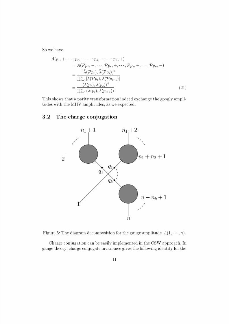
Figure 5: The diagram decomposition for the gauge amplitude A(1, · · · , n).

Charge conjugation can be easily implemented in the CSW approach. Ingauge theory, charge conjugate invariance gives the following identity for the

11



Ò

½

· Ò

¾

· ½

Ò

½

· ¾

Õ

¾

Ò

½

· ½

¾

Õ

½

Ò

Ò Ò

· ½

Õ

½

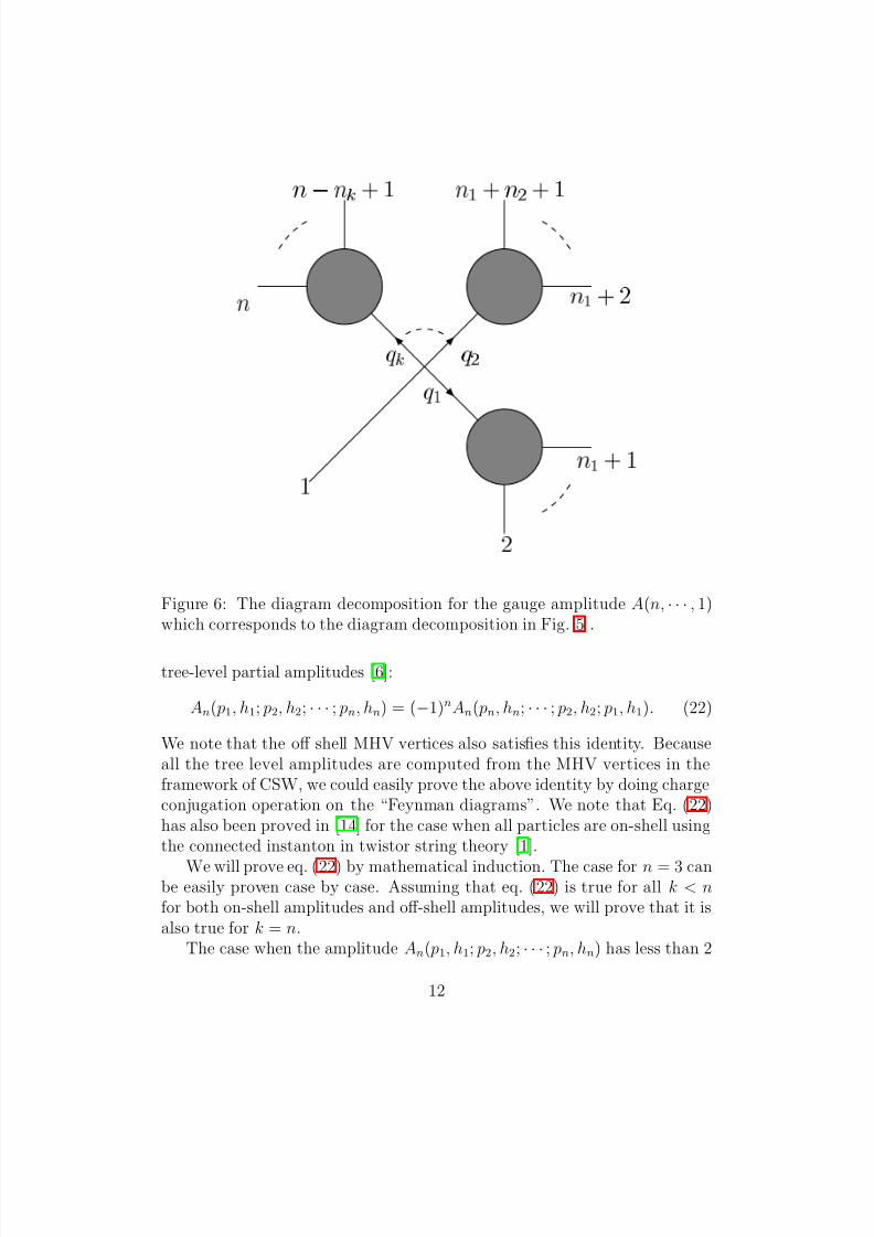
Figure 6: The diagram decomposition for the gauge amplitude A(n, · · · , 1)which corresponds to the diagram decomposition in Fig. 5 .

tree-level partial amplitudes [6]:

An( p1, h1; p2, h2; · · · ; pn, hn) = (−1)nAn( pn, hn; · · · ; p2, h2; p1, h1). (22)

We note that the off shell MHV vertices also satisfies this identity. Becauseall the tree level amplitudes are computed from the MHV vertices in theframework of CSW, we could easily prove the above identity by doing chargeconjugation operation on the “Feynman diagrams”. We note that Eq. (22)has also been proved in [14] for the case when all particles are on-shell usingthe connected instanton in twistor string theory [1].

We will prove eq. (22) by mathematical induction. The case for n = 3 canbe easily proven case by case. Assuming that eq. (22) is true for all k < nfor both on-shell amplitudes and off-shell amplitudes, we will prove that it isalso true for k = n.

The case when the amplitude An( p1, h1; p2, h2; · · · ; pn, hn) has less than 2

12



gluons with negative helicity are trivial. Since

An( p1, h1; p2, h2; · · · ; pn, hn) = 0 = (−1)nAn( pn, hn; · · · ; p2, h2; p1, h1). (23)

When the amplitude An( p1, h1; p2, h2; · · · ; pn, hn) is an MHV amplitude, theamplitude An( pn, hn; · · · ; p2, h2; p1, h1) is an MHV amplitude, too. In thiscase we can easily prove eq. (22) by using eq. (1).

If the amplitude An( p1, h1; p2, h2; · · · ; pn, hn) has more than 2 gluons withnegative helicity, then the MHV diagrams has more than 1 MHV vertices[3]. We can use the diagram decomposition as in Fig. 5 to calculate thisamplitude.3 The helicities hq1, · · · , hqk of the momenta q1, · · · , qk must sat-isfy the constraint that the vertex V k+1( p1, h1; q1, hq1; · · · ; qk, hqk) is an MHV

vertex. For every diagram in this diagram decomposition, there is a uniquecorresponding diagram in the diagram decomposition used for calculatingAn( pn, hn; · · · ; p2, h2; p1, h1) as in Fig. 6 with the same hq1, · · · , hqk . In factthis is a one-to-one correspondence between the diagrams in these two dia-gram decompositions.

By using the above diagram composition we have

An( p1, h1; p2, h2; · · · ; pn, hn)

=

V k+1( p1, h1; q1, hq1; · · · ; qk, hqk) ×1

q21× · · · ×

1

q2k×An1+1( p2, h2; · · · ; pn1+1, hn1+1; −q1, −hq1)

× · · · × Ank+1( pn−nk+1, hn−nk+1; · · · ; pn, hn; −qk, −hqk), (24)

where

qi =n1+n2+···+ni

j=n1+n2+···+ni−1+1

p j , (25)

for 1 ≤ i ≤ k and the summation in eq. (24) is over n1, · · · , nk subject tothe constrains n1 + · · · + nk = n − 1, ni > 0. There is also a summationover all possible helicity hq1, · · · , hqk subject to the constraint that the vertexV k+1( p1, h1; q1, hq1; · · · ; qk, hqk) is an MHV vertex. In the above, the momen-tum p1 can be off shell.

From the assumed result for all less multi-gluon amplitudes, we have

An( p1, h1; p2, h2; · · · ; pn, hn) =

(−1)k+1V k+1( p1, h1; qk, hqk ; · · · ; q1, hq1)

3We note that when n+ = 0, there are no contributing diagrams and the amplitudevanishes. Then it is trivial to find that eq. (22) is valid in this case.

13



×1

q21

× · · · ×1

q2k

(−1)n1+1An1+1( pn1+1, hn1+1; · · · ; p2, h2; −q1, −hq1)

× · · · × (−1)nk+1Ank+1( pn, hn; · · · ; pn−nk+1, hn−nk+1; −qk, −hqk)

=

V k+1( p1, h1; qk, hqk ; · · · , q1, hq1)1

q21× · · ·

×1

q2kAn1+1( pn1+1, hn1+1; · · · ; p2, h2; −q1, −hq1) × · · ·

×Ank+1( pn, hn; · · · ; pn−nk+1, hn−nk+1; −qk, −hqk)

×(−1)k+1+n1+n2+···+nk+k

= (−1)nAn( pn, hn; · · · ; p2, h2; p1, h1). (26)

The degenerate case when some ni’s equal to 1 is also correctly included inthe previous equation. This completes our proof of eq. (22).

3.3 The dual Ward identity

The dual Ward identity is [5]

σ∈Z n−1

A(σ(1), · · · , σ(n − 1), n) = 0. (27)

where the summation σ is over all of the cyclic permutation of 1, · · · , n − 1and the position of n is held fixed to be the last one by using the cyclicsymmetry of the amplitude. This identity reflect the decoupling of the U (1)degree of freedom and links the factorization of the partial amplitudes to thefactorization of the full amplitudes [6]. This has been discussed in [14]. It isalso proved in [36] that the dual Ward identity is valid for (on-shell) MHVamplitudes. We will show that the above dual Ward identity is valid for alltree-level amplitudes in the framework of CSW.

Firstly, we prove that the dual Ward identity is true for the off shell MHVvertices. By assuming that the two gluons with negative helicity are g p andgq, we must prove the following:

σ∈Z n−1 V (σ(1), · · · , σ(n − 1), n)

= p,q4σ∈Z n−1

1

σ(1), σ(2) · · · σ(n − 1), n n, σ(1)= 0. (28)

14



In order to prove this last equality, we note first the following relation:

i, j = λi1λ j2 − λi2λ j1 =

λi1λi2

− λ j1λ j2

λi2λ j2 . (29)

Setting ψi = λi1/λi2, we have

σ∈Z n−1

1

σ(1), σ(2) · · · σ(n − 1), n n, σ(1)=

1

(ni=1 λi2)2

×σ∈Z n−1

1

(ψσ(1) − ψσ(2)) · · · (ψσ(n−1) − ψn)(ψn − ψσ(1)). (30)

So what we need to prove is the following identity:

σ∈Z n−1

1(ψσ(1) − ψσ(2)) · · · (ψσ(n−1) − ψn)(ψn − ψσ(1))

= 0, (31)

for arbitrary ψi’s.We will prove eq. (31) by mathematical induction. The case for n = 3

can be easily checked to be valid. Assuming that it is valid for k = n − 1, wewill show that it is valid for k = n.

We will first prove that the l.h.s. is a constant by showing that all thepole terms are vanishing. When ψi → ∞ (1 ≤ i ≤ n + 1), it is evident thatthe pole terms are vanishing. So we only need to consider the finite poleterms. The possible finite pole terms appear when ψ j = ψn, 1 ≤ j ≤ n − 1,

or ψi = ψi+1, 1 ≤ i ≤ n − 2, or ψn−1 = ψ1.When ψ j = ψn, 1 ≤ j ≤ n − 1, the pole terms in eq. (31) are from the

following two cyclic permutations:

σ j−1(1, · · · , n − 1) = ( j,j + 1, · · · , n − 1, 1, 2, · · · , j − 2, j − 1), (32)

and

σ j(1, · · · , n − 1) = ( j + 1, j + 2, · · · , n − 1, 1, 2, · · · , j − 1, j). (33)

These give 2 pole terms:

1

ψ j − ψ j+1

1

ψ j+1 − ψ j+2

· · ·1

ψ j−1 − ψn

1

ψn − ψ j

+

1

ψn − ψ j+1

1

ψ j+1 − ψ j+2· · ·

1

ψ j−1 − ψ j

1

ψ j − ψn

=1

ψn − ψ j

1

ψ j − ψ j+1

1

ψ j+1 − ψ j+2· · ·

1

ψ j−1 − ψn− (ψn ↔ ψ j)

. (34)

15



The residues in the bracket vanish by taking ψ j = ψn.

For ψi = ψi+1, 1 ≤ i ≤ n − 2, the only cyclic permutation which doesn’tgive a pole term is:

σi(1, 2, · · · , n − 1) = (i + 1, i + 2, · · · , n − 1, 1, 2, · · · , i − 1, i). (35)

The residues are

σ=σi

1

ψσ(1) − ψσ(2)

1

ψσ(2) − ψσ(3)

× · · ·1

ψi−1 − ψi+1

1

ψi+1 − ψi+2· · ·

1

ψσ(n−1) − ψn

1

ψn − ψσ(1). (36)

One easily convinces oneself that the above summation is actually the l.h.sof eq. (31) with the deletion of ψi and so it sums to zero by the assumptionof our mathematical induction. This proves that the residues for ψi = ψi+1vanish. The case for ψn−1 = ψ1 can be proved by the same method.

So we proved that all the finite pole terms are vanishing and we concludethat the l.h.s. must be a constant. This constant can only be zero becauseit is homogeneous (with negative degree) in ψi’s. This completes our proof of eq. (31).

By using the above result for dual Ward identity for the off-shell MHVvertices, one can easily prove the general dual Ward identity, eq. (27). The

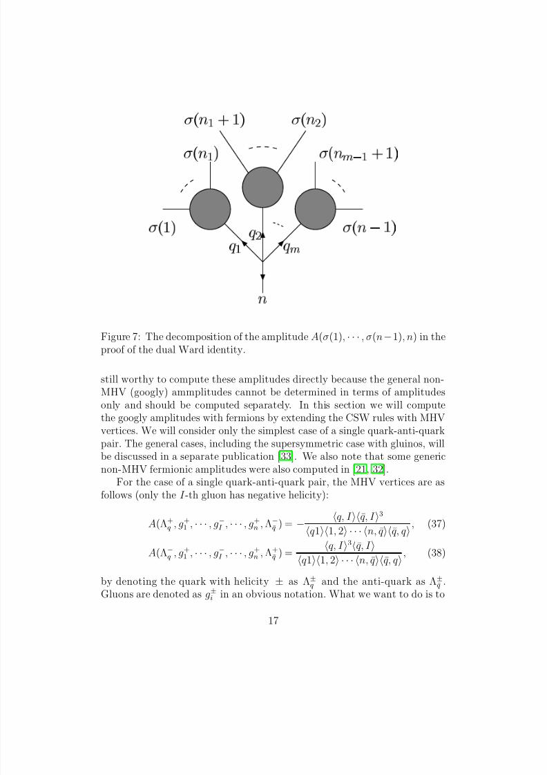
strategy is to write each amplitude A(σ(1), · · · , σ(n − 1), n) as a sum overall possible MHV vertices connected with the n-th gluon as shown in Fig. 7.For a fixed MHV vertex, the summation over all possible cyclic permutationsare decomposed as a sum over cyclic permutations of q1, q2, · · ·, qm.4 Eachsum over cyclic permutations of q1, q2, · · ·, qm is zero by using the dual Wardidentity for MHV vertex and the general dual Ward identity then follows.

4 The googly amplitudes with fermions

The proposal of [3] can also be extended to gauge theory with fermions (see

also [21]). Although the MHV (and googly) fermionic amplitudes can beeasily obtained by supersymmetric Ward identities [30, 31, 6] we think it is

4This statement should be proved rigorously. We will not try to spell out the full detailsof the proof here.

16



Ò

Õ

½

Õ

¾

Õ

Ñ

´ ½ µ

Ò

½

µ

Ò ½ µ

Ò

Ñ ½

· ½ µ

Ò

½

· ½ µ Ò

¾

µ

Figure 7: The decomposition of the amplitude A(σ(1), · · · , σ(n−1), n) in theproof of the dual Ward identity.

still worthy to compute these amplitudes directly because the general non-MHV (googly) ammplitudes cannot be determined in terms of amplitudes

only and should be computed separately. In this section we will computethe googly amplitudes with fermions by extending the CSW rules with MHVvertices. We will consider only the simplest case of a single quark-anti-quarkpair. The general cases, including the supersymmetric case with gluinos, willbe discussed in a separate publication [33]. We also note that some genericnon-MHV fermionic amplitudes were also computed in [21, 32].

For the case of a single quark-anti-quark pair, the MHV vertices are asfollows (only the I -th gluon has negative helicity):

A(Λ+q , g+1 , · · · , g−I , · · · , g+n , Λ−

q ) = −q, I q, I 3

q11, 2 · · · n, qq, q, (37)

A(Λ−q , g+1 , · · · , g−I , · · · , g+n , Λ+

q ) = q, I 3q, I q11, 2 · · · n, qq, q

, (38)

by denoting the quark with helicity ± as Λ±q and the anti-quark as Λ±

q .Gluons are denoted as g±i in an obvious notation. What we want to do is to

17



reproduce the following googly amplitudes (only the I -th gluon has positive

helicity):

A(Λ+q , g−1 , · · · , g+I , · · · , g−n , Λ−

q ) =[q, I ]3[q, I ]

[q1][1, 2] · · · [n, q][q, q], (39)

A(Λ−q , g−1 , · · · , g+I , · · · , g−n , Λ+

q ) = −[q, I ][q, I ]3

[q1][1, 2] · · · [n, q][q, q]. (40)

We use the same off shell continuation as given in [3] (see also section 2) foroff-shell momenta lines. The propagator for both gluon and gluino internallines is just 1/p2, as explained in [21].

We first calculate the amplitudes with a quark-anti-quark pair when all

gluons have negative helicity and only one particle is off-shell. By using thesame method as in [12], we find that all vertices in the contribution diagramsare 3-line MHV vertices. When all the 3 particles are off shell, the MHVamplitudes with a quark-anti-quark pair can be written as:

A(Λ+q , g−1 , Λ−

q ) =1, q2

q, q= q, 1 = 1, q = q, q, (41)

A(Λ−q , g−1 , Λ+

q ) = −1, q2

q, q= −q, 1 = −1, q = −q, q (42)

The amplitudes A(Λ±q , g−1 , · · · , g−n , Λ∓

q ) when Λ±q is off shell are given as

follows:

A(Λ+q , g−1 , · · · , g−n , Λ−

q ) =p2qφ1

1

[1, 2][2, 3] · · · [n − 1, n][n, q], (43)

A(Λ−q , g−1 , · · · , g−n , Λ+

q ) = − p2qφ1

1

[1, 2][2, 3] · · · [n − 1, n][n, q], (44)

and

A(Λ+q , g−1 , · · · , g−n , Λ−

q ) =p2qφ

2q

φn

1

[q, 1][1, 2][2, 3] · · · [n − 1, n], (45)

A(Λ−q , g−1 , · · · , g−n , Λ+

q ) = − p2qφ2q

φn1

[q, 1][1, 2][2, 3] · · · [n − 1, n], (46)

when the anti-quark Λ±q is off-shell. We will not give the proof of the above

formulas here.

18



When the off shell particle is gi, the result is

A(Λ+q , g−1 , · · · , g−n , Λ−

q ) = p2iφ3qφq

φi−1φi+1

×1

[q, 1][1, 2] · · · [i − 2, i − 1][i + 1, i + 2] · · · [n, q][q, q], (47)

A(Λ−q , g−1 , · · · , g−n , Λ+

q ) = −p2iφ

3qφq

φi−1φi+1

×1

[q, 1][1, 2] · · · [i − 2, i − 1][i + 1, i + 2] · · · [n, q][q, q]. (48)

Here and in the remaining part of this section the index 0 refers to Λ q and

the index n + 1 refers to Λq.

£

Õ

£

Õ

· ½

· ½

Á

· ½

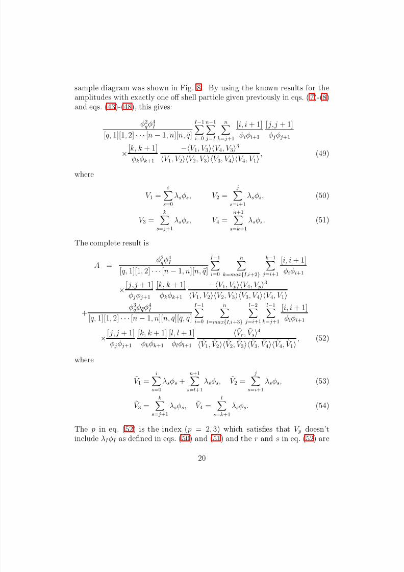
Figure 8: A sample diagram of 4-line MHV vertex with the quark-anti-quarkpair.

Now we begin to compute the googly amplitudes with one quark-anti-quark pair. Using the same method used in [12], one can find that in everycontributing diagram there is only one vertex with 4 lines, all other ver-tices are with 3 lines. For the amplitude A(Λ+

q , g−1 , · · · , g+I , · · · , g−n , Λ−q ), one

19



sample diagram was shown in Fig. 8. By using the known results for the

amplitudes with exactly one off shell particle given previously in eqs. (7)-(8)and eqs. (43)-(48), this gives:

φ2qφ

4I

[q, 1][1, 2] · · · [n − 1, n][n, q]

I −1i=0

n−1 j=I

nk= j+1

[i, i + 1]

φiφi+1

[ j,j + 1]

φ jφ j+1

×[k, k + 1]

φkφk+1

−V 1, V 3V 4, V 33

V 1, V 2V 2, V 3V 3, V 4V 4, V 1, (49)

where

V 1 =i

s=0

λsφs, V 2 = j

s=i+1

λsφs, (50)

V 3 =ks= j+1

λsφs, V 4 =n+1s=k+1

λsφs. (51)

The complete result is

A =φ2qφ

4I

[q, 1][1, 2] · · · [n − 1, n][n, q]

I −1i=0

nk=max{I,i+2}

k−1 j=i+1

[i, i + 1]

φiφi+1

×[ j,j + 1]

φ jφ j+1

[k, k + 1]

φkφk+1

−V 1, V pV 4, V p3

V 1, V 2V 2, V 3V 3, V 4V 4, V 1

+φ3qφqφ

4I

[q, 1][1, 2] · · · [n − 1, n][n, q][q, q]

I −1i=0

nl=max{I,i+3}

l−2 j=i+1

l−1k= j+1

[i, i + 1]

φiφi+1

×[ j,j + 1]

φ jφ j+1

[k, k + 1]

φkφk+1

[l, l + 1]

φlφl+1

V r, V s4

V 1, V 2V 2, V 3V 3, V 4V 4, V 1, (52)

where

V 1 =is=0

λsφs +n+1s=l+1

λsφs, V 2 = js=i+1

λsφs, (53)

V 3 =ks= j+1

λsφs, V 4 =ls=k+1

λsφs. (54)

The p in eq. (52) is the index ( p = 2, 3) which satisfies that V p doesn’tinclude λI φI as defined in eqs. (50) and (51) and the r and s in eq. (52) are

20



the two indices (r = 2, 3, s = 3, 4, r = s) which satisfy that neither V r nor V s

includes λI φI as defined in eqs. (53) and (54). The summations in eq. (52)can be done by using identities involving λi as in the gluon googly amplitude.After doing this summation we obtained the correct googly amplitude with asingle quark-anti-quark pair as given in eqs. (39) and (40). The details for therelevant identities and also the extension to multi-pairs of quark-anti-quarkpairs and gluinos will be given in a separate publication [33].

5 The MHV diagrams for gravity

Encouraged by the success of the CSW approach to gauge theory, it is natural

to ask if a similar approach to gravity exists. We expected so also becausethere exist some close relations between the gravity amplitudes and the gaugeamplitudes, the famous KLT relations [35].

We use the same off-shell continuation λa = paaηa as in [3]. The off shell

MHV vertex with 3 gravitons is [34]

V graviton3 (1+, 2−, 3−) =

2, 33

1, 23, 1

2

, (55)

and the propagator for the graviton with momentum p is still 1/p2.As in gauge theory, we first compute A(1+, 2−, · · · , n−) when only one

particle is off-shell. We will give a formula for A(1+, 2−, · · · , n−) when onlythe momentum pi is off-shell. This amplitude vanishes when all momentaare on shell. So we expect that it is proportional to p2i . This turns out to betrue for gravity. We note that the vanishing for the 4-particle and 5-particleon-shell amplitudes were also obtained in [24].

The diagrams which contribute to A(1+, 2−, · · · , n−) include the MHVvertices with 3 lines only. By using momentum conservation, one can showthat the MHV vertex V 3(1+, 2−, 3−) is actually polynomial in λ:

V 3(1+, 2−, 3−) = λ1, λ22 = λ2, λ32 = λ3, λ12. (56)

In order to present the rules for the computation of A(1+, 2−, · · · , n−), wewill need some basic concepts and notations from graph theory. By a graph Γ,we mean two set: the vertex set V and the edge set E ⊆ {eij|i, j ∈ V, i = j}.We will use the undirected graph only. This means that eij = e ji for alli, j ∈ V . We will denote the vertex set of graph Γ as V (Γ) and denote the

21



edge set of graph Γ as E (Γ). A connected graph not containing any cycles is

called a tree. Two vertex i, j are adjacent if there is a edge eij in E (Γ).We relabel the off-shell graviton to be the first one. The formula for theamplitudes is:

A( p1, h1; p2, h2; · · · ; pn, hn) = p21

Γ,V (Γ)=S (n)

P (Γ), (57)

where hi = ±2 is the helicity of the graviton whose momentum is pi and Γis undirected tree whose vertex set is V (Γ) = S (n) ≡ {2, 3, · · · , n} and P (Γ)can be obtained from the following rules:

• For every vertex i in V (Γ), there is a factor p(i) = φ2hii . It means that

if the graviton with momentum pi has positive helicity, the factor is φ4i ;otherwise the factor is φ−4i . We stress the fact that there is only one

positive helicity graviton.

• For every edge eij in E (Γ) there is a factor p(eij):

p(eij) = φ2i φ

2 j

i, j

[i, j]. (58)

P (Γ) is the product of above factors:

P (Γ) = i∈V (Γ)

p(i) eij∈E (Γ)

p(eij). (59)

By using the above rules we have

A( p1, h1, · · · , pn, hn) = p21

ni=2

φ2hii

Γ,V (Γ)=S (n)

eij∈E (Γ)

p(eij). (60)

The summation in eq. (60) is over all of the inequivalent undirected treeswith vertex set S n. The result can be proved by mathematical induction.The detail is relegated to Appendix B.

The on-shell 4-graviton MHV amplitude is [34]:

A4(1+, 2+, 3−, 4−) = 3, 48

1, 21, 31, 42, 32, 43, 4[3, 4]1, 2

. (61)

We note that a straightforward off-shell continuation λa = paaηa is not possi-

ble for A4 because of the existence of the “anti-holomorphic term” [3, 4]. By

22



using the on-shell condition, like p23 = p24 = 0, and momentum conservation,

one can write this term in various forms which are equivalent on shell andinclude the “holomorphic terms” and the momenta product only.For example, we can use 3, 4[3, 4] = 2 p3· p4 to write [3, 4] as 2 p3· p4/3, 4.

On the other hand, using the on-shell condition p2i = 0, i = 1, · · · , 4 and themomentum conservation, we have 2 p3 · p4 = p234 = 2 p1 · p2. We can use theserelations to give two more way of writing the “non-holomorphic” expression[3, 4].

We can also use 1, 2[2, 3] + 1, 4[4, 3] = 0 to write

[3, 4]

1, 2=

[2, 3]

1, 4=

p2232, 31, 4

, (62)

or use 1, 3[3, 4] + 1, 2[2, 4] = 0 to write

[3, 4]

1, 2=

[4, 2]

1, 3=

p2131, 34, 2

. (63)

One can try to write all the possible (on shell) equivalent forms for the 4-graviton MHV amplitude. There are about 9 different forms which satisfythe obvious symmetry. Nevertheless we have not been able to obtain thecorrect 5-graviton amplitude by using any one of these forms or one of theirlinear combination. It is safe to conclude that a naive extension of the CSWapproach to gravity failed (see also [24]). New ingredient must be introducedin order to develop a CSW like rules for gravity. The similar connectionbetween conformal supergravity and twistor string theory discussed in therecent paper [26] may offer some clues.

To extend the CSW approach further, we may change the 3-particle ver-tex. A possible “MHV vertex” for charged particle is

A(1+, 2−, 3−) =

2, 33

1, 23, 1

2s−1

= 1, 22s−1 = 2, 32s−1 = 3, 12s−1, (64)

where s is a positive integer. By using this vertex and the CSW rules, onecan also compute A(1+, 2−, 3−, 4−) and the result is

A(1+, 2−, 3−, 4−) = (φ2φ3φ4)−(2s−1) ×

2, 32s−2

[2, 3]λ23, λ p42s−1

+3, 42s−2

[3, 4]λ p2, λ342s−1

. (65)

23



By using the following equation:

λ23, λ p4

[2, 3]+

λ p2, λ34

[3, 4]= 0, (66)

we have

A(1+, 2−, 3−, 4−) =1

[2, 3]2s−1

( p2 · p3)2s−2 − ( p3 · p4)2s−2

×λ23, λ p42s−1(φ2φ3φ4)−(2s−1). (67)

So when s > 1 this amplitudes doesn’t vanish for generic λi, λi(1 ≤ i ≤4). This indicates that the CSW approach can’t be arbitrarily extended to

include higher derivative theories. It remains to discover the hidden principlebehind the success of the CSW approach to gauge theory and its coupling tofermions, at least for tree level calculations.

Acknowledgments

We would like to thank Zhe Chang, Bin Chen, Han-Ying Guo, Miao Li, Jian-Xin Lu, Jian-Ping Ma, Ke Wu and Yong-Shi Wu for discussions. Jun-Bao Wuwould like to thank Qiang Li for help on drawing the figures. Chuan-Jie Zhuwould like to thank Jian-Xin Lu and the hospitality at the Interdisciplinary

Center for Theoretical Study, University of Science and Technology of Chinawhere part of this work was done.

Appendix A: The proof of eq. (15)

In this appendix we will prove eq. (15). As in [12], we can use a SL(2, C)transformation and a rescaling of η to choose η1 = 0 and η2 = 1. Then wehave

φi = λi2 (68)

and [i, j]

φiφ j=

λi1λ j2 − λi2λ j1

λi2λ j2=

λi1

λi2−

λ j1

λ j2. (69)

24



If we do a rescaling of λi1 by λi2, i.e. by defining ϕi =λi1λi2

, and also do a

rescaling of λia by 1/λi2, then eq. (15) becomes:

F (ϕ) =r−1i=1

nl=max{i+3,r}

l−2 j=i+1

l−1k= j+1

(ϕi − ϕi+1)(ϕ j − ϕ j+1)

×(ϕk − ϕk+1)(ϕl − ϕl+1)V p, V q

4

V 1, V 2V 2, V 3V 3, V 4V 4, V 1

= (ϕ1 − ϕr)4. (70)

where

V 1 =n+i

s=l+1

λs, V 2 = j

s=i+1

λs, (71)

V 3 =ks= j+1

λs, V 4 =ls=k+1

λs. (72)

There are also two constraints:

V 1 + V 2 + V 3 + V 4 =nl=1

λl = 0, (73)

nl=1

λi ϕi = 0, (74)

from momentum conservation.From eq. (73) and eq. (74) we can solve λ1 and λr in terms of the rest

λi’s and all ϕ j ’s as:

λ1 = −

2≤ j≤n,j=r

ϕ j − ϕrϕ1 − ϕr

λ j, (75)

λr =

2≤ j≤n,j=r

ϕ j − ϕ1

ϕ1 − ϕrλ j. (76)

By using the above result, the left hand side of eq. (70) can be considered as

a function of λ j (2 ≤ j ≤ n, j = r) and all ϕ j. As a function of ϕ we willshow that it is independent of ϕ j for 2 ≤ j ≤ n and j = r.

First we show that there is no pole terms for ϕs → ∞, 2 ≤ s ≤ n − 1, s =r. We will show that every term in the l.h.s of eq. (70) will not tend toinfinity when ϕs → ∞. We denote (ϕi − ϕi+1)(ϕ j − ϕ j+1)(ϕk − ϕk+1)(ϕl −

25



ϕl+1) in eq. (70) as F (i ,j,k,l) and V p, V q4/(V 1, V 2V 2, V 3V 3, V 4V 4, V 1)

as A4(V 1, V 2, V 3, V 4).When ϕs → ∞, λ1 and λr will grow as ϕs and other λi’s does not dependon ϕs. V 1 and the V t which includes λr as defined in eqs. (71) and (72)will tend to infinity as fast as ϕs. V p and V q are independent of ϕs. So thenumerator of A4(V 1, V 2, V 3, V 4) is independent of ϕs.

Now we prove that V 1, V t grows as ϕs. From eq. (75) and eq. (76), we canwrite λ1 and λr as λ1 = a1sϕsλs + µ1s and λr = arsϕsλs + µrs respectively,where µ1s and µrs is independent on ϕs. Then V 1, V t = ϕsλs, a1sµrs −arsµ1s + O(ϕ0

s) will grow as ϕs for generic ϕi, λ j, 1 ≤ j ≤ n, j = r.The factor F (i ,j,k,l) grows as ϕ2

s at most. Also one can check case bycase and find the denominator of A4(V 1, V 2, V 3, V 4) grows as ϕ2

s at least5. By

combing all these results one sees that there is no pole terms for F (ϕ) asϕs → ∞.

The next step is to show that all the finite pole terms in F (ϕ) are vanish-ing. The possible terms appear if any factor of V 1, V 2V 2, V 3V 3, V 4V 4, V 1is vanishing.

Let us consider first the vanishing of V 1, V 2. We denote this set of V 1and V 2 as v1 and v2:

v1 =n+n1i=n3+1

λi, v2 =n2i=n1+1

λi. (77)

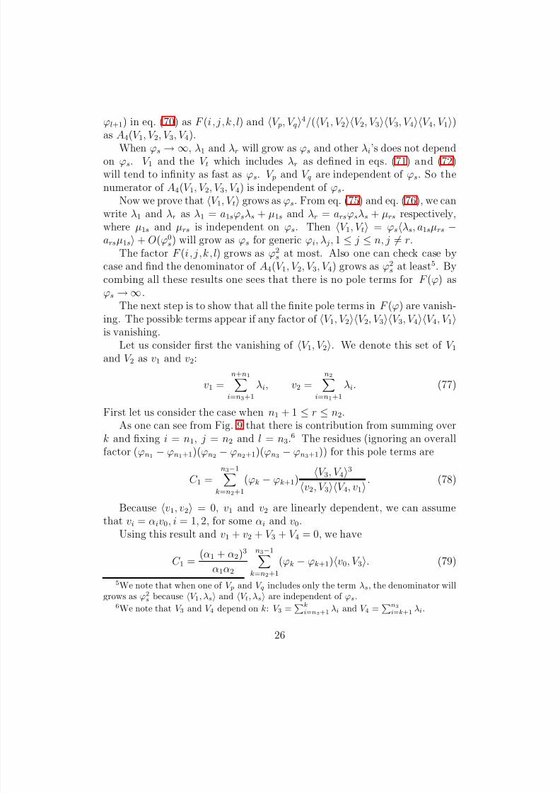
First let us consider the case when n1 + 1 ≤ r ≤ n2.As one can see from Fig. 9 that there is contribution from summing overk and fixing i = n1, j = n2 and l = n3.6 The residues (ignoring an overallfactor (ϕn1 − ϕn1+1)(ϕn2 − ϕn2+1)(ϕn3 − ϕn3+1)) for this pole terms are

C 1 =n3−1k=n2+1

(ϕk − ϕk+1)V 3, V 43

v2, V 3V 4, v1. (78)

Because v1, v2 = 0, v1 and v2 are linearly dependent, we can assumethat vi = αiv0, i = 1, 2, for some αi and v0.

Using this result and v1 + v2 + V 3 + V 4 = 0, we have

C 1 = (α1 + α2)3

α1α2

n3−1k=n2+1

(ϕk − ϕk+1)v0, V 3. (79)

5We note that when one of V p and V q includes only the term λs, the denominator willgrows as ϕ2s because V 1, λs and V t, λs are independent of ϕs.

6We note that V 3 and V 4 depend on k: V 3 =k

i=n2+1λi and V 4 =

n3i=k+1

λi.

26



Ò

¾

· ½ µ

· ½ µ

Ò

¿

·

·

Ú

½

Ú

¾

Figure 9: The pole terms v1, v2 from the factor V 1, V 2. There is a sum-mation over k.

By using a little algebra, we can write the summation in eq. (79) as following

C 1 =(α1 + α2)3

α1α2

n3−1

k=n2+1

ϕkv0, λk − ϕn3v0,n3−1

m=n2+1

λm

. (80)

Because v0,n3m=n2+1 λm = v0, V 2 = 0, we have v0,

n3−1m=n2+1 λm =

27



−v0, λn3. Then

C 1 =(α1 + α2)3

α1α2

v0,n3k=n2+1

ϕkλk. (81)

Ò

¿

· ½ µ

Ð

½ ·

Ò

½

Ð · ½ µ

·

Ú

½

Ú

¾

µ

Ú

¾

·

Figure 10: The pole terms v1, v2 from the factor V 2, V 3. There is a sum-mation over l.

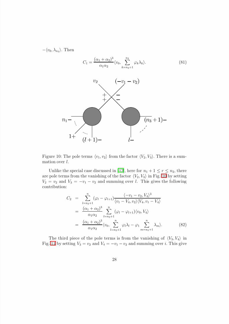
Unlike the special case discussed in [12], here for n1 + 1 ≤ r ≤ n2, thereare pole terms from the vanishing of the factor V 2, V 3 in Fig. 10 by settingV 2 = v2 and V 3 = −v1 − v2 and summing over l. This gives the followingcontribution:

C 2 =nl=n3+1

(ϕl − ϕl+1)−v1 − v2, V 43

v1 − V 4, v2V 4, v1 − V 4

=(α1 + α2)3

α1α2

nl=n3+1

(ϕl − ϕl+1)v0, V 4

=

(α1 + α2)3

α1α2 v0,

n

l=n3+1 ϕlλl − ϕ1

n

m=n3+1 λm. (82)

The third piece of the pole terms is from the vanishing of V 3, V 4 inFig. 11 by setting V 3 = v2 and V 4 = −v1 − v2 and summing over i. This give

28



½ ·

Ò

¿

· ½ µ

·

· ½ µ

Ò

¾

Ú

¾

Ú

½

Ú

¾

µ

·

Figure 11: The pole terms v1, v2 from the factor V 3, V 4. There is a sum-mation over i.

the following contribution:

C 3 =(α1 + α2)3

α1α2v0, ϕ1

n+1m=n3+1

λm +n1i=2

ϕiλi (83)

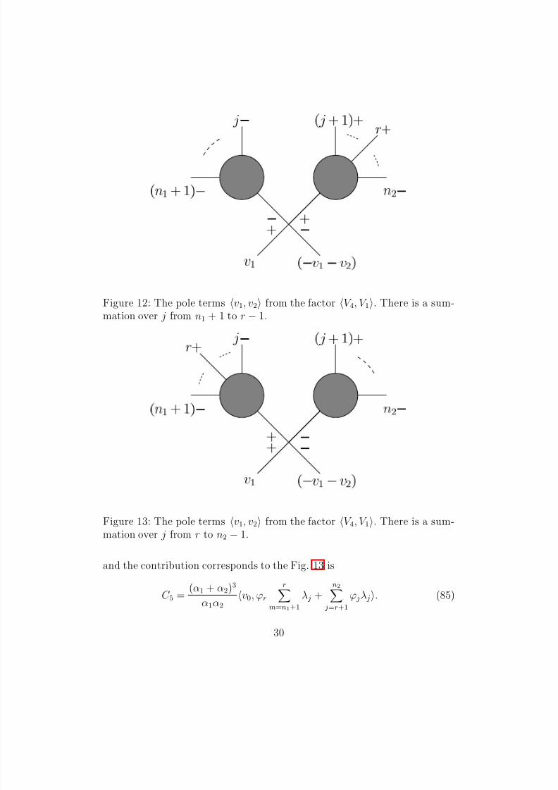
The last piece of the pole terms is from the vanishing of V 4, V 1 in Fig. 12and Fig. 13 by setting V 1 = v1 and V 4 = −v1 − v2 and summing over j. Thecontribution corresponds to the Fig. 12 is

C 4 =(α1 + α2)3

α1α2

v0,r−1 j=n1+1

ϕ jλ j − ϕrr−1m=n1+1

λm, (84)

29



Ò

½

· ½ µ

· ½ µ ·

Ò

¾

·

Ö ·

Ú

½

·

Ú

½

Ú

¾

µ

Figure 12: The pole terms v1, v2 from the factor V 4, V 1. There is a sum-mation over j from n1 + 1 to r − 1.

Ò

½

· ½ µ

·

Ö ·

· ½ µ ·

Ò

¾

Ú

½

·

Ú

½

Ú

¾

µ

Figure 13: The pole terms v1, v2 from the factor V 4, V 1. There is a sum-mation over j from r to n2 − 1.

and the contribution corresponds to the Fig. 13 is

C 5 =(α1 + α2)3

α1α2

v0, ϕrrm=n1+1

λ j +n2 j=r+1

ϕ jλ j. (85)

30



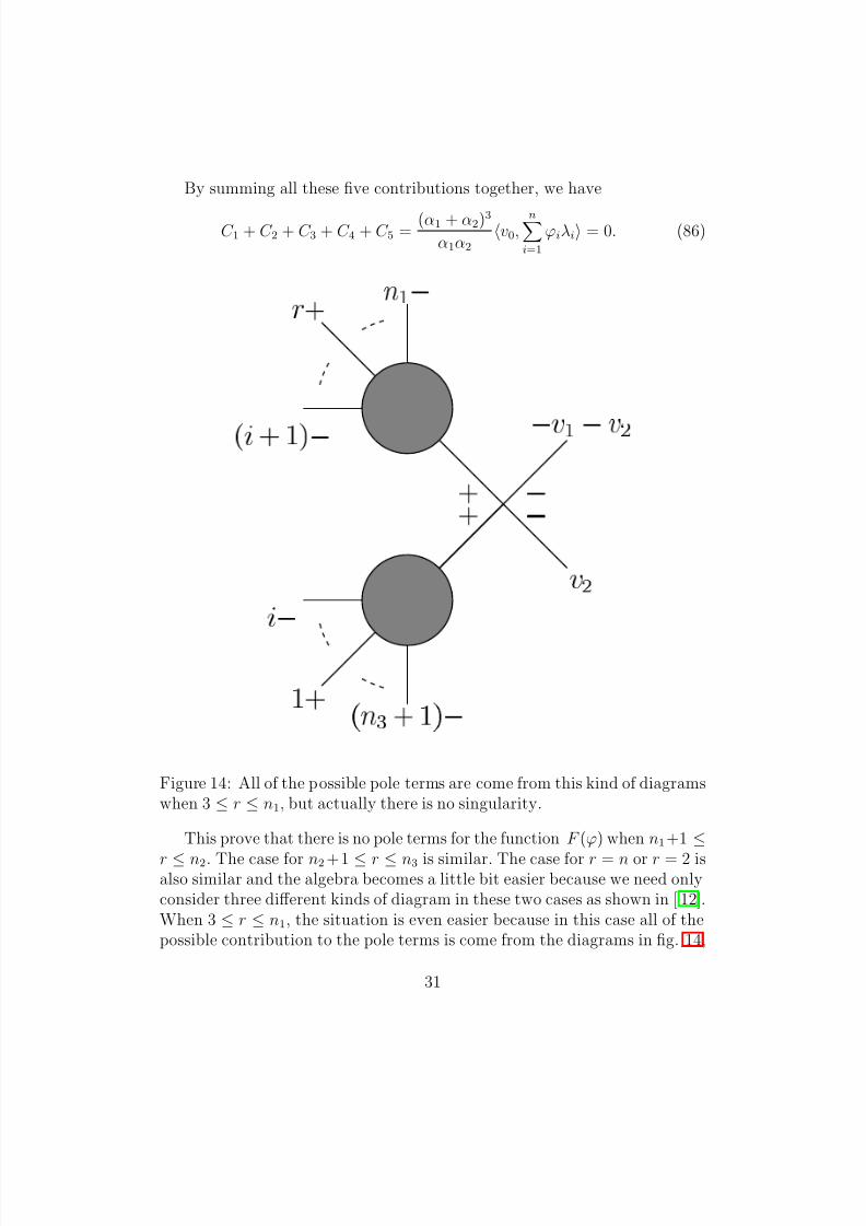
By summing all these five contributions together, we have

C 1 + C 2 + C 3 + C 4 + C 5 =(α1 + α2)3

α1α2v0,ni=1

ϕiλi = 0. (86)

Ú

¾

Ú

½

Ú

¾

· ½ µ

Ò

½

Ö ·

·

½ ·

Ò

¿

· ½ µ

·

Figure 14: All of the possible pole terms are come from this kind of diagramswhen 3 ≤ r ≤ n1, but actually there is no singularity.

This prove that there is no pole terms for the function F (ϕ) when n1+1 ≤

r ≤ n2. The case for n2+1 ≤ r ≤ n3 is similar. The case for r = n or r = 2 isalso similar and the algebra becomes a little bit easier because we need onlyconsider three different kinds of diagram in these two cases as shown in [ 12].When 3 ≤ r ≤ n1, the situation is even easier because in this case all of thepossible contribution to the pole terms is come from the diagrams in fig. 14,

31



but actually the numerator has a zero of order 4 while the denominator has a

zero of order 1. So there is no singularity in every individual term. Similarlythere is no pole terms when n3 + 1 ≤ r ≤ n − 1. In summary we proved thatall the finite pole terms in F (ϕ) are vanishing in all different cases.

So F (ϕ) is independent of ϕ j for 2 ≤ j ≤ n, j = r. Now we computeF (ϕ) explicitly by choosing a special set of ϕ j for 2 ≤ j ≤ n, j = r.7 Aconvenient choice is as follows:

ϕ2 = · · · = ϕr−1 = x, ϕr+1 = · · · = ϕn = y. (87)

By using eq. (75) and eq. (76), we have

λ1 =(x − ϕ

r)λ + (y − ϕ

r)µ

ϕr − ϕ1, λr = −

(x − ϕ1)λ + (y − ϕ

1)µ

ϕr − ϕ1, (88)

by settingr−1i=2 λi = λ and

n j=r+1 λ j = µ. In the following we will use the

new variables x′ and y′ which we define as

x′ =x − ϕr

ϕr − ϕ1, y′ =

y − ϕrϕr − ϕ1

, (89)

then we havex − ϕ1

ϕr − ϕ1= x′ + 1,

y − ϕ1

ϕr − ϕ1= y′ + 1. (90)

Now we show that for generic x and y (and generic λi which we don’t sayexplicitly) all the possible V 1, V 2, V 2, V 3, V 3, V 4 and V 4, V 1 for differentchoices of i, j, k and l are non-vanishing.

In order to do this, let’s define a matrix {tij}(1≤i≤n,1≤ j≤4). If λi is one of the terms in V j then we define tij = 1. Otherwise we set tij = 0. Then

V j =ni=1

tijλi =r−1i=2

λi[tij + t1 jx′ − trj(x′ + 1)]

+ni=r+1

λi[tij + t1 jy′ − trj(y′ + 1)]. (91)

So for generic x, y and λi, V i and V i+1 are linearly independent and soV i, V i+1 is non-vanishing.

7The case when r = n or r = 2 is a little bit different, and it is done in [12].

32



For our choice of ϕ, the possible non-vanishing factor for (ϕi− ϕi+1)(ϕ j−

ϕ j+1)(ϕk − ϕk+1) is from i = 1, j = r − 1 , k = r and l = n only. Then wehave

F (ϕ) = (ϕ1 − x)(x − ϕr)(ϕr − y)(y − ϕ1)

×λ, µ

λ1, λλ, λrλr, µµ, λ1. (92)

By using eq. (88), we have

λ1, λ = −y − ϕr

ϕr − ϕ1

λ, µ, (93)

λ, λr = −

y − ϕ1

ϕr − ϕ1 λ, µ, (94)

λr, µ = −x − ϕ1

ϕr − ϕ1

λ, µ, (95)

µ, λ1 = −x − ϕr

ϕr − ϕ1λ, µ, (96)

and so we haveF (ϕ) = (ϕr − ϕ1)4. (97)

This completes the proof of eq. (15).

Appendix B: The computation of P (Γ)

In this appendix, we will give the proof of eq. (57). We assume that theoff-shell graviton has positive helicity. The case when it has negative helicityis similar.

When n = 3, we have λ1 + λ2φ2 + λ3φ3 = 0, so 1, 2 = φ32, 3, 3, 1 =φ22, 3. Then

A3(1+, 2−, 3−) =1

φ22φ2

3

2, 32 =p21

φ22φ2

3

2, 3

[2, 3]. (98)

There is only one inequivalent undirected tree with vertex set {2, 3}. Thereis only one edge e23 in this tree. It is easy to see that

P (Γ) = p(2) p(3) p(e23) = φ−42 φ−43

φ22φ2

3

2, 3

[2, 3]

=

1

φ22φ2

3

2, 3

[2, 3]. (99)

33



½

Ò Ñ

Ñ

½

Õ

½

Õ

¾

½

Figure 15: The decomposition for the amplitude for gravitons using in thecomputation of P (Γ).

So M 3(1+, 2−, 3−) = p21P (Γ). This completes the proof for eq. (57) whenn = 3. Assuming that it is true for all k ≤ n, we will prove that it is alsotrue for k = n + 1.

We use the diagram decomposition in Fig. 15 to calculate An+1. So wehave

An+1 =

{i1,···,im}

Am+1(−q1, i1, · · · , im)1

q21

×An−m+1(−q2, j1, · · · , jn−m)1

q22V 3(1, q1, q2), (100)

where i1, · · · , im are any m (1 ≤ m ≤ n − 1) gravitons in {2, · · · , n + 1},

j1, · · · , jn−m are the remaining n − m ones. q1 and q2 are two internal lineswith momenta q1 =mk=1 pik and q1 =

n−mk=1 p jk respectively. We denote

{i1, · · · , im} as S 1 and { j1, · · · , jn−m} as S 2. It is easy to see that whenm = 1 (m = n − 1), if we understand A2(−q1, i1) (A2(−q2, j1)) as 1/φ4

i1

(1/φ4 j1

), then these two degenerate cases are included correctly.

34



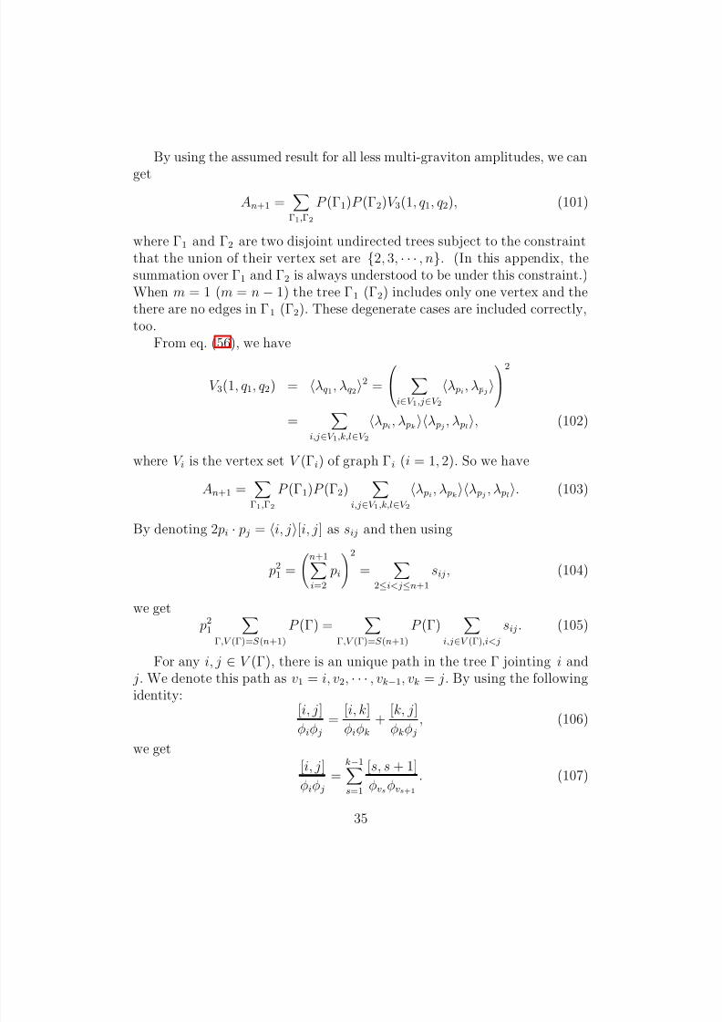
By using the assumed result for all less multi-graviton amplitudes, we can

getAn+1 =

Γ1,Γ2

P (Γ1)P (Γ2)V 3(1, q1, q2), (101)

where Γ1 and Γ2 are two disjoint undirected trees subject to the constraintthat the union of their vertex set are {2, 3, · · · , n}. (In this appendix, thesummation over Γ1 and Γ2 is always understood to be under this constraint.)When m = 1 (m = n − 1) the tree Γ1 (Γ2) includes only one vertex and thethere are no edges in Γ1 (Γ2). These degenerate cases are included correctly,too.

From eq. (56), we have

V 3(1, q1, q2) = λq1, λq22 =

i∈V 1,j∈V 2

λ pi, λ pj

2

=

i,j∈V 1,k,l∈V 2

λ pi , λ pkλ pj , λ pl, (102)

where V i is the vertex set V (Γi) of graph Γi (i = 1, 2). So we have

An+1 =Γ1,Γ2

P (Γ1)P (Γ2)

i,j∈V 1,k,l∈V 2

λ pi, λ pkλ pj , λ pl. (103)

By denoting 2 pi

· p j

= i, j[i, j] as sij

and then using

p21 =

n+1i=2

pi

2

=

2≤i<j≤n+1

sij, (104)

we get p21

Γ,V (Γ)=S (n+1)

P (Γ) =

Γ,V (Γ)=S (n+1)

P (Γ)

i,j∈V (Γ),i<j

sij. (105)

For any i, j ∈ V (Γ), there is an unique path in the tree Γ jointing i and j. We denote this path as v1 = i, v2, · · · , vk−1, vk = j. By using the followingidentity:

[i, j]φiφ j= [i, k]φiφk

+ [k, j]φkφ j, (106)

we get[i, j]

φiφ j=k−1s=1

[s, s + 1]

φvsφvs+1. (107)

35



So

P (Γ)sij = P (Γ)i, jφiφ j[i, j]φiφ j

=k−1s=1

P (Γ)i, jφiφ j[vs, vs+1]

φvsφvs+1. (108)

If we move away an edge from a tree, we can get two disjoint trees.Conversely, assuming that Γ1 and Γ2 are two disjoint trees, if we connect onevertex in Γ1 with another vertex in Γ2 by an edge, we get a bigger tree. Wedenote the two trees obtained by moving away the edge evsvs+1 as Γ1(vs) andΓ2(vs). Then we have

P (Γ)sij =k−1s=1

P (Γ1(vs))P (Γ2(vs))vs, vs+1

[vs, vs+1]φ2vs

φ2vs+1

i, jφiφ j[vs, vs+1]

φvsφvs+1

=k−1s=1

P (Γ1(vs))P (Γ2(vs))vs, vs+1φvsφvs+1i, jφiφ j . (109)

From this we can get

Γ,V (Γ)=S (n+1)

P (Γ) p21 =

Γ,V (Γ)=S (n+1)

P (Γ)

i,j∈V (Γ),i<j

sij

=Γ1,Γ2 P (Γ1)P (Γ2)

i,j∈V 1,k,l∈V 2λ pi, λ pkλ pj , λ pl

= An+1, (110)

as announced. This completes the proof of eq. (57) by mathematical induc-tion.

References

[1] E. Witten, “Perturbative Gauge Theory As A String Theory In TwistorSpace,” hep-th/0312171.

[2] R. Penrose, “Twistor Algebra,” J. Math. Phys. 8 (1967) 345; “TheCentral Programme of Twistor Theory,” Chaos, Solitons, and Fractal10 (1999) 581.

36

http://arxiv.org/abs/hep-th/0312171




[3] F. Cachazo, P. Svrcek and E. Witten, “MHV Vertices and Tree Am-

plitudes In Gauge Theory,” hep-th/0403047.[4] S. Parke and T. Taylor, “An Amplitude For N Gluon Scattering,”

Phys. Rev. Lett. 56 (1986) 2459.

[5] F. A. Behrends and W. T. Giele, “Recursive Calculations For ProcessesWith N Gluons,” Nucl. Phys. B306 (1988) 759.

[6] M. L. Mangano and S. Parke, “Multiparton Amplitudes in Guage The-ories,” Phys. Rept. 200 (1991) 30.

[7] Z. Bern, “String-Based Perturbative Methods for Gauge Theories,”

TASI Lectures, 1992, hep-ph/9304249.

[8] L. Dixon, “Calculating Scattering Amplitudes Efficiently,” TASI Lec-tures, 1995, hep-ph/9601359.

[9] Z. Bern, L. Dixon, and D. Kosower, “Progress In One-Loop QCD Cal-culations,” hep-ph/9602280, Ann. Rev. Nucl. Part. Sci. 36 (1996) 109.

[10] C. Anastasiou, Z. Bern, L. Dixon, and D. Kosower, “Planar AmplitudesIn Maximally Supersymmetric Yang-Mills Theory,” hep-th/0309040;Z. Bern, A. De Freitas, and L. Dixon, “Two Loop Helicity Ampli-tudes For Quark Gluon Scattering In QCD and Gluino Gluon Scat-tering In Supersymmetric Yang-Mills Theory,” JHEP 0306:028 (2003),hep-ph/0304168.

[11] V. P. Nair, “A Current Algebra for Some Gauge Theory Amplitudes,”Phsy. Lett. B214 (1988) 215–218.

[12] Chuan-Jie Zhu, “The Googly Amplitudes in Gauge theory,” J. HighEnergy Phys. 0404 (2004) 032, hep-th/0403115.

[13] R. Roiban, M. Spradlin, and A. Volovich, “A Googly Amplitude FromThe B Model In Twistor Space,” J. High Energy Phys. 0404 (2004) 012,

hep-th/0402016; R. Roiban and A. Volovich, “All Googly AmplitudesFrom The B Model In Twistor Space,” hep-th/0402121.

[14] R. Roiban, M. Spradlin, and A. Volovich, “ On the Tree-Level S-Matrixof Yang-Mills Theory ,” hep-th/0403190.

37


http://arxiv.org/abs/hep-ph/9304249





















[15] N. Berkovits, “An Alternative String Theory in Twistor Space for N =

4 Super-Yang-Mills,” hep-th/0402045.[16] N. Berkovits and L. Motl, “Cubic Twistorial String Field Theory,” J.

High Energy Phys. 0404 (2004) 056, hep-th/0403187.

[17] M. Aganagic and C. Vafa, “Mirror Symmetry and Supermanifolds,”hep-th/0403192.

[18] E. Witten, “Parity Invariance For Strings In Twistor Space,”hep-th/0403199.

[19] A. Neitzke and C. Vafa,“N = 2 Strings and the Twistorial Calabi-

Yau,” hep-th/0402128.

[20] N. Nekrasov, H. Ooguri and C. Vafa, “S-duality and TopologicalStrings,” hep-th/0403167.

[21] G. Georgiou and V. V. Khoze, “Tree Amplitudes in Gauge Theoryas Scalar MHV Diagrams,” J. High Energy Phys. 0405 (2004) 070,hep-th/0404072.

[22] Sergei Gukov, Lubos Motl and Andrew Neitzke, “Equivalence of twistor prescriptions for super Yang-Mills,” hep-th/0404085.

[23] Warren Siegel, “Untwisting the twistor superstring,” hep-th/0404255.

[24] S. Giombi, R. Ricci, D. Robles-Llana and D. Trancanelli, “A Note onTwistor Gravity Amplitudes,” hep-th/0405086.

[25] Alexander D. Popov and Christian Saemann, “On Supertwistors,the Penrose-Ward Transform and N = 4 super Yang-Mills Theory,”hep-th/0405123.

[26] Nathan Berkovits and Edward Witten, “Conformal Supergravity inTwistor-String Theory,” hep-th/0406051.

[27] I. Bena, Z. Bern and D. A. Kosower, “Twistor-Space Recursive For-mulation of Gauge-Theory Amplitudes,” hep-th/0406133.

[28] D. A. Kosower, “Next-to-Maximal Helicity Violating Amplitudes inGauge Theory,” hep-th/0406175.

38































[29] F. Cachazo, P. Svrcek and E. Witten, “Twistor Space Structure of

One-Loop Amplitudes in Gauge Theory,” hep-th/0406177.[30] M. T. Grisaru, H. N. Pendleton and P. van Nieuwenhuizen, “Super-

gravity and the S Matrix,” Phys. Rev. D15(1977) 996.

[31] M. T. Grisaru and H. N. Pendleton, “Some Properties of ScatteringAmplitudes in Supersymmetric Theories,” Nucl. Phys. B214(1977) 81.

[32] George Georgiou, E.W.N. Glover and Valentin V. Khoze, “Non-MHVTree Amplitudes in Gauge Theory,” hep-th/0407027.

[33] Jun-Bao Wu and Chuan-Jie Zhu, “ MHV Vertices and Fermionic

Scattering Amplitudes in Gauge Theory with Quarks and Gluinos,”hep-th/0406146.

[34] F. A. Berends, W. T. Giele and H. Kuijf, “On Relations between Multi-gluon and Multi-graviton Scattering,” Phys. Lett. B211(1988) 91.

[35] H. Kawai, D. C. Lewellen and S. H. Tye, “A Relation between TreeAmplitudes of Closed and Open Strings,” Nucl. Phys. B269(1986) 1.

[36] M. Magano, S. Parke and Z. Xu, “Duality and Multi-Gluon Scatter-ing,” Nucl. Phys. B298 (1988) 653.

39







jun-bao wu and chuan-jie zhu-mhv vertices and scattering amplitudes in gauge theory

Documents