July 2021

DEVELOPING A PRACTICAL AND ROBUST FEEDBACK CONTROL SYSTEM FOR OPEN WATER CHANNELS TO DELIVER THE CORRECT AMOUNT OF WATER TO THE INTENDED USER AT THE DESIRED TIME NM WRRI Technical Completion Report No. 393 Blair Stringam

New Mexico Water Resources Research Institute New Mexico State University MSC 3167, P.O. Box 30001 Las Cruces, New Mexico 88003-0001 (575) 646-4337 email: nmwrri@nmsu.edu

Part of the Elephant Butte Irrigation District main canal near the Leasburg Diversion. Photo courtesy of EBID.

DEVELOPING A PRACTICAL AND ROBUST FEEDBACK CONTROL SYSTEM FOR OPEN WATER CHANNELS TO DELIVER THE CORRECT AMOUNT OF

WATER TO THE INTENDED USER AT THE DESIRED TIME

By

Blair Stringam, College Professor Department of Plant and Environmental Sciences

New Mexico State University

TECHNICAL COMPLETION REPORT Account Number 131563

Technical Completion Report #393

July 2021

New Mexico Water Resources Research Institute in cooperation with the

Department of Plant and Environmental Sciences New Mexico State University

The research on which this report as based was financed in part by the U.S. Department of the Interior, Geological Survey and the New Mexico Legislature, through the New Mexico Water Resources Research Institute.

ii

iii

DISCLAIMER The purpose of the NM Water Resources Research Institute (NM WRRI) technical reports is to provide a timely outlet for research results obtained on projects supported in whole or in part by the institute. Through these reports the NM WRRI promotes the free exchange of information and ideas and hopes to stimulate thoughtful discussions and actions that may lead to resolution of water problems. The NM WRRI, through peer review of draft reports, attempts to substantiate the accuracy of information contained within its reports, but the views expressed are those of the authors and do not necessarily reflect those of the NM WRRI or its reviewers. Contents of this publication do not necessarily reflect the views and policies of the Department of the Interior, nor does the mention of trade names or commercial products constitute their endorsement by the United States government.

iv

TABLE OF CONTENTS DISCLAIMER ............................................................................................................................... iii LIST OF FIGURES .........................................................................................................................v LIST OF TABLES ...........................................................................................................................v ABSTRACT .....................................................................................................................................1 INTRODUCTION ...........................................................................................................................2 Objectives ....................................................................................................................................2 METHODS AND PROCEDURES..................................................................................................2 Ratio Control Design ..................................................................................................................5 Feedback Controller Design ........................................................................................................6 Proportional Integral Control Design (PI) ..................................................................................6 Soil Moisture Sensor ...................................................................................................................7 RESULTS ........................................................................................................................................8 Ratio Control Field Test ............................................................................................................11 Soil Moisture Sensor Testing ....................................................................................................12 CONCLUSION ..............................................................................................................................14 PROJECT DELIVERABLES ........................................................................................................15 REFERENCES ..............................................................................................................................16

v

LIST OF FIGURES Figure 1. Map of Leasburg Dam and Canal .....................................................................................3 Figure 2. Diagram of 2 canal reaches in series ................................................................................4 Figure 3. Soil moisture light sensor concept ....................................................................................5 Figure 4. Light emitter, a light sensor, a microprocessor, and support electronics .........................7 Figure 5. Plexiglas rod inserted in a soil column with an attached light emitter .............................8 Figure 6. EBID reaches 1 and 2 controller test response. Turnout flowrates are decreased

from 40 cfs to 30 cfs for each reach. Reach 1 has an initial flowrate of 270 cfs .............9 Figure 7. EBID reaches 1 and 2 controller test response. Turnout flowrates are increased

from 20 cfs to 30 cfs for each reach. Reach 1 has an initial flowrate of 270 cfs ...........10 Figure 8. EBID reaches 1 and 2 controller test response. Turnout flowrates are increased

from 20 cfs to 30 cfs for each reach. Reach 1 has an initial flowrate of 380 cfs ...........11 Figure 9. EBID Main Canal Ratio Control Field Test. The downstream water depth setpoint

was decreased from 8.4 feet to 8.0 feet ..........................................................................12 Figure 10. 650 nm soil moisture sensor graph indicating soil watering and gradual water

loss over time ................................................................................................................13 Figure 11. 1310 nm and 1550 nm soil moisture sensor graphs indicating soil watering and

gradual water loss over time. ........................................................................................14

LIST OF TABLES Table 1. Dimensions for the first two Elephant Butte Irrigation supply canal reaches ...................3

vi

1

ABSTRACT The majority of irrigation districts in the U.S. and throughout the world deliver water to their users using open channels. Supplying water in this manner presents a number of complications that usually results in the loss of water. Many of these complications occur because of sediment accumulation and vegetation growing in the channel. These complications impede accurate and timely water deliveries. To deliver the correct amount of water to the right place at the right time, water managers must determine when to start the water diversion and determine the travel time to deliver the water at the required time. The delay time makes this a difficult task because the delay time varies over the growing season due to the vegetative growth and sediment accumulation. It is very difficult to determine the time delay change and subsequently make an adjustment to delivery procedures. In recent years, a number of irrigation districts have installed automation equipment to provide water deliveries in a timely manner. This equipment consists of water-level sensors, gate-position sensors, gate actuators, onsite computer control units and data communication radios or phones. These automation systems are normally programmed with routines that provide remote monitoring, data collection and remote movement of the water delivery gates and structures. The majority of software is simple and provides limited operation of these sites and subsequently limited water savings ability. This project has taken further steps and developed software that will operate these remote water control sites and provide timely water deliveries. The program was implemented on an actual canal reach. A recently developed open channel flow control method that is reported by Stringam and Wahl (2014) was used to develop this program. This project also developed a prototype soil moisture sensor to help irrigators track crop water use and order accurate water deliveries in a timely manner. This prototype sensor has been programmed to communicate directly with the farmer’s cellphone to provide timely soil water information. The light-based sensor is proving to provide accurate measurements for the soils that we have tested thus far. Providing an accurate sensor to irrigation farmers will help them order water for irrigating more precisely. This will make the canal feedback control software more effective for district managers who work to deliver water to water users.

Keywords: irrigation, open channels, sediment accumulation, water delivery, automation systems, water diversion

2

INTRODUCTION This work has had two goals: the first was to develop a simple, robust, and adaptable computer control routine that can operate multiple open channels in an optimal manner. The control routine will use small site control computers, control program, sensors and gate motors with the present canal system to deliver water to intended locations at the desired time and in the desired quantity while limiting or eliminating water waste. Instead of focusing on a complex algorithm that has proven to be troublesome in past research, this project is focusing on a simple robust solution. The second goal was to develop a soil moisture sensor that can be used by irrigators to track crop water use so that they can better manage that use. This soil moisture sensor would use new laser light detection technology as well as cellphone communications to transmit timely field soil moisture values to the irrigators so that irrigation water can be ordered in the right amount and at the right time. This soil moisture device would help the irrigators take advantage of the canal computer control routine to deliver the correct amount of water and limit water waste. Objectives

1. Enhance open channel computer control routines to operate multi-reach time - varying open channels so that water is delivered in a timely manner with little waste.

2. Develop an inexpensive soil water content sensor that can be easily linked to a farmer’s cell phone to provide timely soil moisture readings.

3. Implement the open channel computer control routine on multiple reaches in the Elephant Butte Irrigation District in Las Cruces, NM.

METHODS AND PROCEDURES

Initially, the canal control programming work was conducted at New Mexico State University (NMSU), and then the work continued on the Elephant Butte Irrigation District (EBID) main canals. EBID has a number of canals that convey water to water users and it has been cooperating with us by providing access to their canal system as well as by installing automation equipment for this project. EBID’s cooperation has been invaluable because it would be impossible to get access to facilities that are close to NMSU. This research focuses on developing an optimal feedback control for the first two reaches of the EBID main canal that start at the Leasburg diversion (Figure 1). These two reaches were modelled using open channel software that solves the St. Venant hydraulic equations using numerical integration routines (Stringam and Merkley, 2013). A control routine was then designed and tested on the reach models. We first determined the EBID canal dimensions for the first two reaches on the main supply canal as indicated in Figure 1. The dimensions were needed to develop a model of the canal system to determine canal behavior characteristics. This helped to simulate canal hydraulic behavior, which was used to develop a feedback control algorithm. It is more time effective and

3

easier to develop a feedback control algorithm on a model because hours of simulation and subsequent controller development can be accomplished quickly and in a safe manner. If any mistakes are made, they are made on the model. The possibility of damaging the canal system due to design errors is significantly reduced. The process of determining the canal dimensions required site survey work to determine canal slopes, side slopes, bottom widths and roughness (Table 1). Canal lengths were obtained from Google Earth. Once the dimensions were determined, the task of programming and calibrating the canal models began. Slide gates modeled to simulate water off take discharges. These gates were modelled with a width of 3.5 feet and a discharge coefficient of 0.69. This modelling was conducted using Matlab/Simulink software. This software was used because it is developed specifically to test feedback control routines. This feature makes development and testing for feedback control routines much easier than trying to code the control routines into an open channel program such as HEC-RAS. Table 1. Dimensions for the first two Elephant Butte Irrigation supply canal reaches.

Length (feet)

Roughness Side slope Bottom width (ft) Slope

Reach 1 3356 0.025 1.5 25.0 0.0005 Reach 2 6400 0.025 1.5 35.0 0.00026

Once the canal model was developed and calibrated, simulations were run wherein discharge level response simulations were conducted and evaluated for appropriate response.

Figure 1. Map of Leasburg Dam and Canal.

4

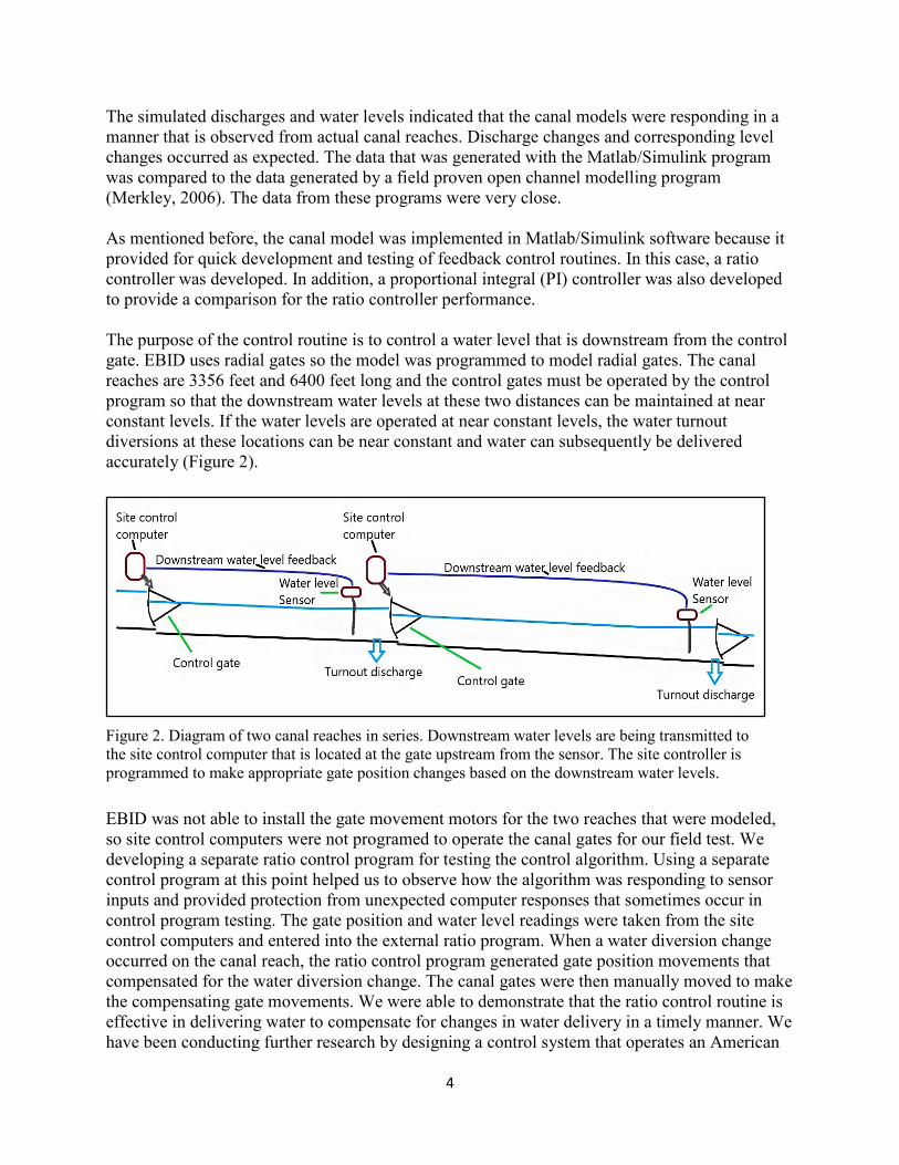
The simulated discharges and water levels indicated that the canal models were responding in a manner that is observed from actual canal reaches. Discharge changes and corresponding level changes occurred as expected. The data that was generated with the Matlab/Simulink program was compared to the data generated by a field proven open channel modelling program (Merkley, 2006). The data from these programs were very close. As mentioned before, the canal model was implemented in Matlab/Simulink software because it provided for quick development and testing of feedback control routines. In this case, a ratio controller was developed. In addition, a proportional integral (PI) controller was also developed to provide a comparison for the ratio controller performance. The purpose of the control routine is to control a water level that is downstream from the control gate. EBID uses radial gates so the model was programmed to model radial gates. The canal reaches are 3356 feet and 6400 feet long and the control gates must be operated by the control program so that the downstream water levels at these two distances can be maintained at near constant levels. If the water levels are operated at near constant levels, the water turnout diversions at these locations can be near constant and water can subsequently be delivered accurately (Figure 2).

EBID was not able to install the gate movement motors for the two reaches that were modeled, so site control computers were not programed to operate the canal gates for our field test. We developing a separate ratio control program for testing the control algorithm. Using a separate control program at this point helped us to observe how the algorithm was responding to sensor inputs and provided protection from unexpected computer responses that sometimes occur in control program testing. The gate position and water level readings were taken from the site control computers and entered into the external ratio program. When a water diversion change occurred on the canal reach, the ratio control program generated gate position movements that compensated for the water diversion change. The canal gates were then manually moved to make the compensating gate movements. We were able to demonstrate that the ratio control routine is effective in delivering water to compensate for changes in water delivery in a timely manner. We have been conducting further research by designing a control system that operates an American

Figure 2. Diagram of two canal reaches in series. Downstream water levels are being transmitted to the site control computer that is located at the gate upstream from the sensor. The site controller is programmed to make appropriate gate position changes based on the downstream water levels.

5

Society of Civil Engineers (ASCE) multi reach canal test case model (Clemmens et al. 1998). This ASCE model was developed to provide a standard that researchers use to test different control methods and compare their results. The results that we are observing are encouraging because the physics of this model make it extremely difficult to operate. In addition, we have been making steady progress in the development of the soil moisture sensor. We have developed a prototype sensor that uses a simple and effective design. Light frequencies that are specifically sensitive to water are fired down a plexiglass rod where the light escapes from the rod into the soil. Some of the light is absorbed by the water that exists within the soil profile, while some of the light is reflected by the soil particles back into the plexiglass rod. A detector sensor measures the returning light and sends the sensed value to a microprocessor. The microprocessor computes a corresponding soil moisture content from the sensor input. This value is determined from the difference between the exiting light from the plexiglass rod and the returning light. This moisture content is then transmitted to the irrigator’s cellphone (Figure 3).

Ratio Control Design Ratio Control simply uses the principle of ratios to determine a control output. This formula was developed considering the limitation of measurement instrumentation and the resistance of operations personnel to implement formulas beyond one or two math operations. The principal equation used in this work was modified from an equation that is reported by Stringam and Wahl (2014):

Figure 3. Soil moisture light sensor concept. Light is emitted from the plexiglass rod where some light is absorbed by soil water while some light is reflected by soil particles and returns to the plexiglass rod.

6

𝑛𝑛𝑛𝑛𝑛𝑛𝑤𝑤𝑤𝑤𝑤𝑤𝑛𝑛

= 𝑛𝑛𝑛𝑛𝑛𝑛𝑛𝑛𝑤𝑤𝑤𝑤

(1) where ngp = new gate position (opening); wlsp = water-level setpoint; pgp = present gate position (opening); and pwl = present water level. The gate position variables must indicate the size of the gate opening that is effective for allowing flow into the downstream canal. It should be noted that this formula reflects that undershot or slide gates are used to control water discharge. When Equation (1) is solved for ngp it takes the following form: 𝑛𝑛𝑛𝑛𝑛𝑛 = 𝑛𝑛𝑛𝑛𝑛𝑛

𝑛𝑛𝑤𝑤𝑤𝑤𝑤𝑤𝑤𝑤𝑤𝑤𝑛𝑛 (2)

In this form, the new gate position is equal to the water level setpoint multiplied by the ratio of the present gate position to the present water level. Considering computed gate positions at discrete points in time, the new gate position variable is a combination of the old gate position and the change in gate position as shown in the following equation: 𝑛𝑛𝑛𝑛𝑛𝑛 = ∆𝑛𝑛𝑛𝑛 + 𝑛𝑛𝑛𝑛𝑛𝑛 (3) where Δgp = change in gate position. When this relationship is substituted into Equation (2), it can be written in the following form: ∆𝑛𝑛𝑛𝑛 = 𝑛𝑛𝑛𝑛𝑛𝑛

𝑛𝑛𝑤𝑤𝑤𝑤(𝑤𝑤𝑤𝑤𝑤𝑤𝑛𝑛 − 𝑛𝑛𝑤𝑤𝑤𝑤) (4)

This equation indicates that the gain is variable and is determined by the ratio between the desired and present water levels. Feedback Controller Design The ratio controllers were designed by simply programing the ratio control equation into the simulation program. The ratio control equation would only stabilize the canal model and not return it back to the original downstream level setpoint. This is actually typical for simple control methods, so a weak integrator was also included with the ratio design. Initially the controller did not respond as quickly as desired, so a gain was added to Equation 4 to speed the system response. The result is the following equation:

∆𝑛𝑛𝑛𝑛 = 𝑘𝑘 �𝑛𝑛𝑛𝑛𝑛𝑛𝑛𝑛𝑤𝑤𝑤𝑤

(𝑒𝑒)�+ 𝑘𝑘𝑖𝑖 ∑ 𝑒𝑒 (5)

Where k = a control gain that speeds system response, ki = integrator gain and e = wlsp - pwl. Proportional Integral Control Design (PI) As mentioned earlier, a PI controller (Ziegler and Nichols, 1942) was designed and tested on the canal model to provide a comparison for the ratio controller. Numerous feedback control methods have been developed over the last 70 years. The most widely used is the proportional,

7

integral method. PI control has demonstrated a great degree of robustness in many industrial applications. This type of controller is designed/tuned to drive a system to a desired setpoint value. In this case, the measured value is a downstream water level of a canal reach. The control algorithm compares the measured value to the desired setpoint value and determines if there is an error that must be acted on. If there is an error, the controller multiplies it by a constant value called the proportional gain (kp). The controller uses this value to help drive the system back to setpoint. As the system is driven closer to setpoint, the error becomes smaller and eventually the multiple of the kp and error are not large enough to push the system all the way back to setpoint. However, the controller also sums the errors over a period of time and multiplies the summed error by an additional constant called the integral gain (ki). The controller uses the multiple of the summed errors and ki to continue to push the system all the way back to setpoint. The basic PI equation is listed below. ∆𝑛𝑛𝑛𝑛 = kp(𝑒𝑒) + 𝑘𝑘𝑖𝑖 ∑ 𝑒𝑒 (6) It should be noted that this equation is simpler than the ratio control equation, but the simplicity makes the tuned equation suitable for only one operation point. If canal physical parameters change such as flow rates or water levels, the PI equation will not work as efficiently. Soil Moisture Sensor The soil moisture sensor was developed using light emitters, a light sensor, a microprocessor, a plexiglass rod, a small mirror (Figures 3 and 4), radio transmitter, and support electronics. The sensor has been designed so that it can be inserted vertically into the soil profile. The light emitter is set up so the light shines down at a 45° angle into the plexiglass rod (Figure 5). This design will allow for the sensor to produce an average soil moisture content for the depth of the soil through which the rod extends. The light emitter wavelengths that are being used are 650 nm, 1310 nm, and 1550 nm. These wavelengths are sensitive to water absorption.

Figure 4. Light emitter, a light sensor, a microprocessor, and support electronics.

8

Initially, a prototype sensor was developed using the 650nm light wavelength. This initial wavelength was used because the cost of the light emitter and support electronics were much less than for the 1310 nm and 1550 nm light wavelengths. The 650 nm electronics helped to develop a prototype sensor that was then adapted to the 1310 nm and 1550 nm technology.

RESULTS Once the EBID canals were modelled, a series of simulation tests were conducted on the canal models. In an initial simulation test, Reach 1 discharge was set at 270 cfs with a turnout flowrate of 40 cfs. Reach 2 had an initial discharge of 230 cfs with a turnout flowrate of 40 cfs. The downstream water level setpoint for Reach 1 was set at 6.17 feet and the downstream water level setpoint for Reach 2 was set at 5.91 feet. At 20 minutes from the start of the simulation, the turnout flow for Reach 2 was reduced to 30 cfs. Then at 60 minutes from the start of the simulation the turnout flowrate from Reach 1 was reduced to 30 cfs. Changing the turnout flowrate in Reach 1 while Reach 2 is working on responding to the turnout change helps to see

Figure 5. Plexiglas rod inserted in a soil column with an attached light emitter.

9

how well the controllers interact with each other and also determines how quickly the controllers can bring the canals back to steady state operation. The response from the two control methods for both reaches are indicated in Figure 6. In this simulation there appears to be less interference or fighting between the ratio controllers. The ratio controllers respond to the change in the turnout flows and drive the canal back to steady state. The PI controllers seem to interfere more with each other. This is demonstrated by the oscillatory response from Reach 1.

In the second test the initial flowrate in Reach 1 was set at 270 cfs with a turnout flowrate of 20 cfs, and the Reach 2 flowrate was set at 250 cfs with a turnout flowrate of 20 cfs. The downstream water level setpoint for the Reach 1 was set at 6.17 feet and the downstream water level setpoint for Reach 2 was set at 5.60 feet. The turnout flowrate for Reach 2 was increased from 20 to 30 cfs at 20 minutes into the simulation, and 40 minutes later the turnout flowrate from Reach 1 was increased from 20 to 30 cfs (Figure 7). In this test, the PI controllers again demonstrated an oscillatory response while the ratio controllers simply pull the water level back to the setpoint. It should be pointed out that these two reaches are part of the main supply canal system, and these turnout flowrates are small in comparison to the main canal flows. For this reason, there was not a significant change in water level for any of the simulations.

Figure 6. EBID Reaches 1 and 2 controller test response. Turnout flowrates are decreased from 40 cfs to 30 cfs for each reach. Reach 1 has an initial flowrate of 270 cfs.

10

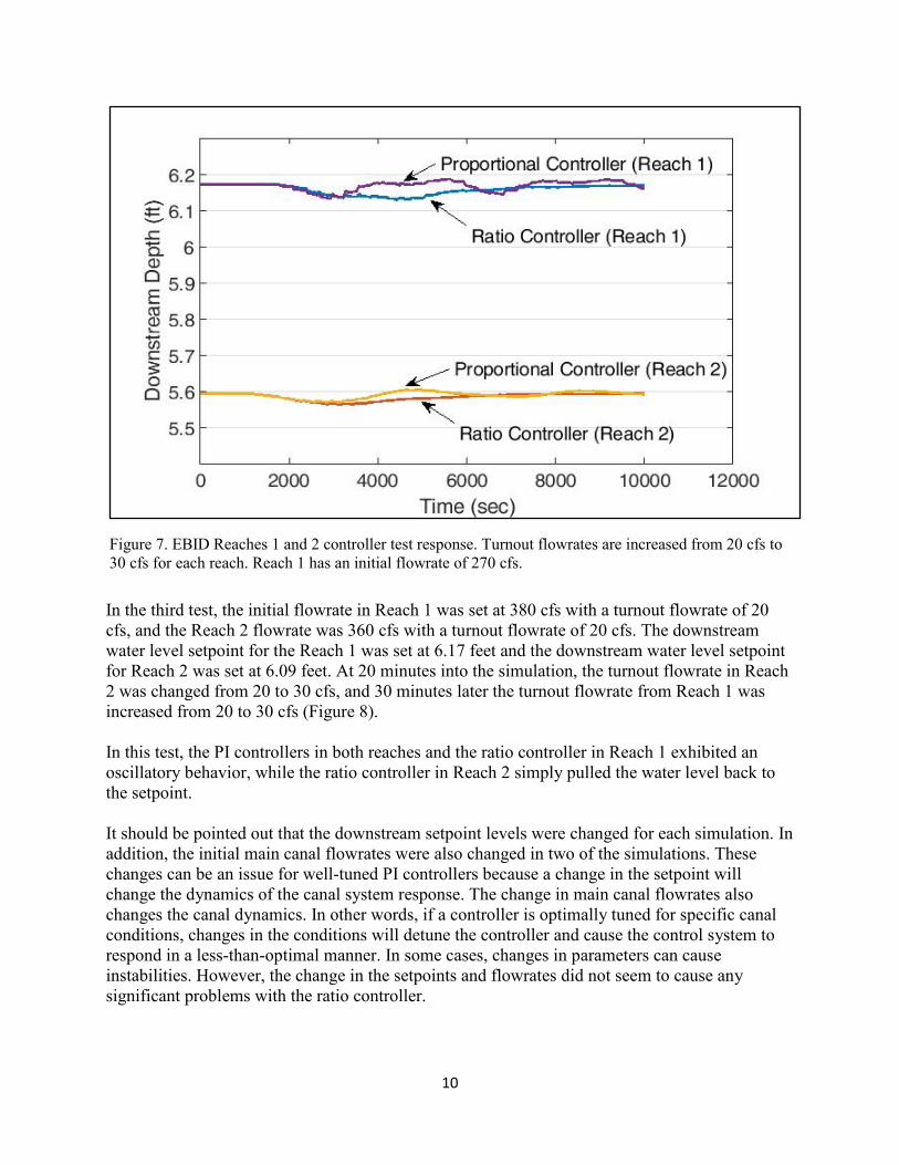
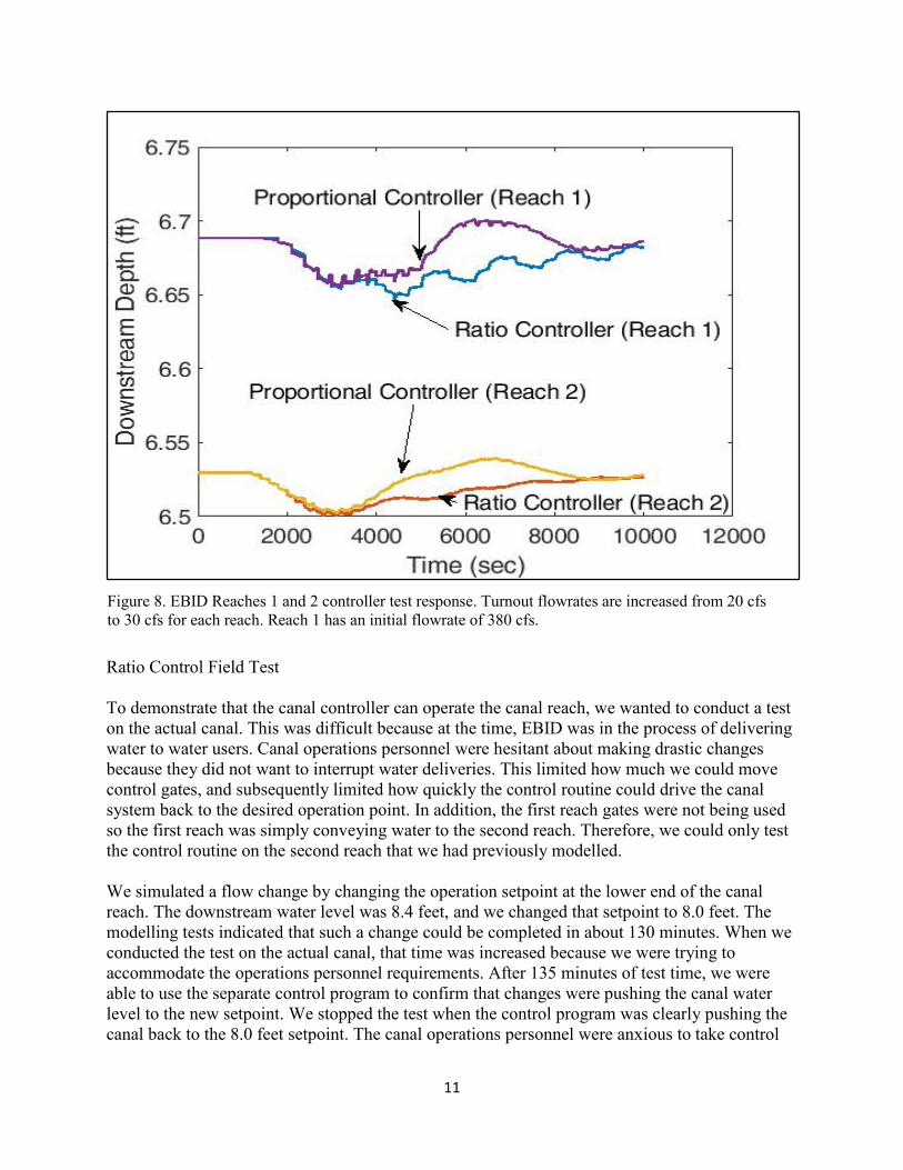
In the third test, the initial flowrate in Reach 1 was set at 380 cfs with a turnout flowrate of 20 cfs, and the Reach 2 flowrate was 360 cfs with a turnout flowrate of 20 cfs. The downstream water level setpoint for the Reach 1 was set at 6.17 feet and the downstream water level setpoint for Reach 2 was set at 6.09 feet. At 20 minutes into the simulation, the turnout flowrate in Reach 2 was changed from 20 to 30 cfs, and 30 minutes later the turnout flowrate from Reach 1 was increased from 20 to 30 cfs (Figure 8). In this test, the PI controllers in both reaches and the ratio controller in Reach 1 exhibited an oscillatory behavior, while the ratio controller in Reach 2 simply pulled the water level back to the setpoint. It should be pointed out that the downstream setpoint levels were changed for each simulation. In addition, the initial main canal flowrates were also changed in two of the simulations. These changes can be an issue for well-tuned PI controllers because a change in the setpoint will change the dynamics of the canal system response. The change in main canal flowrates also changes the canal dynamics. In other words, if a controller is optimally tuned for specific canal conditions, changes in the conditions will detune the controller and cause the control system to respond in a less-than-optimal manner. In some cases, changes in parameters can cause instabilities. However, the change in the setpoints and flowrates did not seem to cause any significant problems with the ratio controller.

Figure 7. EBID Reaches 1 and 2 controller test response. Turnout flowrates are increased from 20 cfs to 30 cfs for each reach. Reach 1 has an initial flowrate of 270 cfs.

11

Ratio Control Field Test To demonstrate that the canal controller can operate the canal reach, we wanted to conduct a test on the actual canal. This was difficult because at the time, EBID was in the process of delivering water to water users. Canal operations personnel were hesitant about making drastic changes because they did not want to interrupt water deliveries. This limited how much we could move control gates, and subsequently limited how quickly the control routine could drive the canal system back to the desired operation point. In addition, the first reach gates were not being used so the first reach was simply conveying water to the second reach. Therefore, we could only test the control routine on the second reach that we had previously modelled. We simulated a flow change by changing the operation setpoint at the lower end of the canal reach. The downstream water level was 8.4 feet, and we changed that setpoint to 8.0 feet. The modelling tests indicated that such a change could be completed in about 130 minutes. When we conducted the test on the actual canal, that time was increased because we were trying to accommodate the operations personnel requirements. After 135 minutes of test time, we were able to use the separate control program to confirm that changes were pushing the canal water level to the new setpoint. We stopped the test when the control program was clearly pushing the canal back to the 8.0 feet setpoint. The canal operations personnel were anxious to take control

Figure 8. EBID Reaches 1 and 2 controller test response. Turnout flowrates are increased from 20 cfs to 30 cfs for each reach. Reach 1 has an initial flowrate of 380 cfs.

12

of canal operations so the test was ended. Figure 9 shows how the downstream water level was approaching the level setpoint. This is a significant accomplishment considering that the field control algorithm was not tuned/adjusted in the field, size of the canal reaches, and the volumes of water that were involved.

Soil Moisture Sensor Testing A 650 nm prototype soil moisture sensor was inserted into a column of soil that was contained in a PVC (polyvinyl chloride) pipe (Figure 5). The column was then set on a weigh scale so that the weight of the column could be measured in order to determine water loss over time. As water was lost/evaporated from the column, there was a clear signal change indicating that the sensing system was tracking the water loss (Figure 10). This experiment was repeated several times with the same results. The curve is flatter for the 650 nm light, but the signal can be amplified to provide a greater change in measured signal. There is also an outliner in Figure 10 that is a bit of concern, but we have not been able to duplicate the outliner and believe it to be an erroneous measurement. We have concluded that this method of measuring soil moisture is valid and shows tremendous potential for helping irrigators manage their water.

77.27.47.67.8

88.28.48.6

0 10 20 30 40 50 60 70 80 90 100 110 120 130Dow

nstr

eam

Wat

er D

epth

(ft)

Time (min)

EBID Main Canal Ratio Control Test Data

Figure 9. EBID Main Canal Ratio Control Field Test. The downstream water depth setpoint was decreased from 8.4 feet to 8.0 feet.

13

The sensor output has been set up to transmit the results to a cellphone. However, this is a very basic communication routine and more work is required for improvement. Once the 650 nm sensor was developed and proven to work consistently, the 1310 nm and 1550 nm soil sensors were then constructed. At the 1310 nm and 1550 nm range, sensor development was more difficult because these wavelengths are out of the visible light spectrum. In addition, the light frequency circuitry is more sensitive. The initial 650 nm sensor development was extremely beneficial in helping us develop the higher light frequency sensors. Sensor development for these higher frequencies continued, and we were able to demonstrate that these higher frequencies were even more sensitive to the soil water content. Figure 11 indicates the response that was achieved when the 1310 and 1550 nm sensors were fabricated and tested on the soil column. The graph indicates that the sensor response is close to linear for the 1550 nm circuit. The response for the 1310 nm sensor has been similar, but at the lower soil water content, there is a departure from the linear behavior. After further testing, we concluded that the apparatus that we had constructed to hold the light emitter and sensor was subject to small amounts of movement which was influencing the sensor measurement. We began the development of a sensor housing unit that would be better suited for measurement at this light frequency. A sensor housing was designed and a 3D printer was used to construct a prototype sensor housing. As this study was coming to a close the housing unit was being shipped to us. This housing will allow for the consistent placement of light sensors that will allow for solid sensor positioning and we expect that there will be more of a linear response for lower soil moisture content. The housing will also help to provide better calibration performance for testing in different soil types.

Figure 10. 650 nm soil moisture sensor graph indicating soil watering and gradual water loss over time.

0.5

0.6

0.7

0.8

0.9

1

1.1

13.5 13.55 13.6 13.65 13.7 13.75 13.8 13.85

Volts

Kilograms

Water Session 1 A2 Volts vs. Kilograms

14

CONCLUSION

An open channel canal model was developed for the first two reaches on the EBID main supply canal so the canal control routines could be tested on the model before they were tested on the actual canals. The ratio control routine performed very well on the canal model so the routine was tested subsequently on a portion of the EBID canal system. The control routine demonstrated that it could operate the actual canal despite limitations that were placed on the gate movements. The limitations were placed on the gate movements because the canal operations personnel were not comfortable with the gate movements. They did not want to risk interrupting water delivery to their water users. While we proved that this control method works, further work needs to be done to demonstrate that this control method works on multiple reaches. In order to help irrigators track crop water use and provide a tool that can be used to measure water use accurately, a soil moisture sensor was developed. This low-cost sensor can help the irrigator determine the required amount of water that is needed for the field so that exact water orders could be placed that would allow the canal control system to respond appropriately. The initial sensor that was developed indicates that the device is repeatable and accurate but there were some problems with the 1310 nm light frequency. We believe that the problem can be corrected with a sensor housing. An additional basic communication feature was developed with this soil sensor, but it needs further development to be user friendly. While this soil moisture measurement method has been proven to work, additional work needs to be conducted to calibrate this sensor for multiple soil types.

175

180

185

190

195

200

205

17 17.5 18 18.5

mill

ivol

ts

Kilograms

1310 nm Sensor Performance millivolts vs. Kilograms

180

185

190

195

200

205

17 17.5 18 18.5 19

mill

ivol

ts

Kilograms

1550 nm Sensor Performance millivolts vs. Kilograms

Figure 11. 1310 nm and 1550 nm soil moisture sensor graphs indicating soil watering and gradual water loss over time.

15

PROJECT DELIVERABLES The results from the canal modelling and control simulation tests were reported in a conference paper given at the US Committee on Irrigation and Drainage (USCID) 12th International Conference on Irrigation and Drainage, Reno, Nevada in November 2019. This paper was well received and generated a number of questions. The USCID asked if this paper could be printed in the biyearly newsletter that circulates amongst USCID members. In an effort to prove the robust ability of the ratio control method, this control method was developed for the multi-reach model specified by the American Society of Civil (ASCE) Engineers. This multi-reach model has little storage capacity and is difficult to operate. However, initial testing indicates that the ratio control method is effective for operating this difficult model. A research paper will be written that reports the finding from the EBID field test and the ASCE model test (Clemmens et al. 1998).

16

REFERENCES Clemmens, A.J., T.F. Kacerek, B. Grawitz, and W. Schuurmans.1998. Test Cases for Canal

Control Algorithms. J. Irrig. Drain Eng. 124:23-30. Cooper, D.J. 2006. Practical Process Control. Control Station, Inc., One Technology

Drive, downloaded on September 2016 from: https://controlstation.com/education/textbooks/

Merkley, G.P. 2006. RootCanal: A hydraulic simulation model for unsteady flow in

branching canal networks. Dept. of Civil and Environmental Engineering, Utah State University, Logan, Utah.

Phillips, C.L., and R.D. Harbor. 2000. Feedback Control Systems. Prentice-Hall Inc., Upper Saddle River, N.J.

Stringam, B., and G. Merkley. 2013. Matlab/Simulink Nonlinear Hydraulic Models for

Testing Canal Gate Control Algorithms. The Agriculture/Urban Water Interface – Conflicts and Opportunities, US Committee on Irrigation and Drainage, Denver, Colorado.

Stringam, B., and T. Wahl. 2014. Ratio controller for regulation of turnout flow rate.

International Commission on Irrigation and Drainage Journal. 64:69-76. https://doi.org/10.1002/ird.1881

Ziegler, J.G., and N.B. Nichols. 1942. Optimum Settings for Automatic Controllers.

Transactions of the ASME. 64:759-768.