julien narboux, pascal schreck, ileana streinu .pdf · julien narboux pascal schreck ileana streinu...
TRANSCRIPT
HAL Id: hal-01334334https://hal.inria.fr/hal-01334334
Submitted on 20 Jun 2016
HAL is a multi-disciplinary open accessarchive for the deposit and dissemination of sci-entific research documents, whether they are pub-lished or not. The documents may come fromteaching and research institutions in France orabroad, or from public or private research centers.
L’archive ouverte pluridisciplinaire HAL, estdestinée au dépôt et à la diffusion de documentsscientifiques de niveau recherche, publiés ou non,émanant des établissements d’enseignement et derecherche français ou étrangers, des laboratoirespublics ou privés.
Proceedings of ADG 2016Julien Narboux, Pascal Schreck, Ileana Streinu
To cite this version:Julien Narboux, Pascal Schreck, Ileana Streinu. Proceedings of ADG 2016: Eleventh InternationalWorkshop on Automated Deduction in Geometry. Jun 2016, Strasbourg, France. pp.224, 2016. hal-01334334

Julien NarbouxPascal SchreckIleana Streinu (Eds.)
ADG2016Eleventh International Workshop on
Automated Deduction in Geometry
University of Strasbourg, France, June 27-29, 2016


Julien NarbouxPascal SchreckIleana Streinu (Eds.)
Automated Deduction
in Geometry
11th International Workshop, ADG 2016Strasbourg, France, June 27-29, 2016

Preface
This volume contains the 14 papers and 3 invited talkspresented at ADG 2016: Eleventh International Work-shop on Automated Deduction in Geometry held on June26-28, 2016 in Strasbourg, France.
ADG is a forum facilitating the exchange of ideas,presentation of new research results and demonstrationsof software tools lying at the intersection of geometryand automated deduction. The selected papers, reviewedby an international Program Committee, cover diversetopics ranging from polynomial algebra, invariant andcoordinate-free methods, synthetic and logic approaches,techniques for automated geometric reasoning from dis-crete mathematics, symbolic and numeric methods forgeometric computation, geometric algorithms, geometricconstraint solving, experimental studies with automatedtheorem provers, applications to mechanics, origami andgeometric modeling.
The previous ten workshops were held in Coimbra 2014,Edinburgh 2012, Munich 2010, Shanghaı 2008, Ponteve-dra 2006, Gainesville 2004, Linz 2002, Zurich 2000, Bei-jing 1998, and Toulouse 1996.
The conference was organized by the Computer Graph-ics and Geometry Group of ICube Laboratory (CNRS /Universite de Strasbourg).
We would like to thank the invited speakers and au-thors for their contributions. We are very grateful to theprogram committee members and referees for their exper-tise which ensures the high scientific standard of ADG.We also warmly thank all the local organizers for con-

tributing to the practical organisation so that the meet-ing can be held smoothly. We thank the IGG team andthe ICube laboratory for helping us by sponsoring thisconference. Support from EasyChair is also gratefully ac-knowledged.
June 13, 2016Strasbourg
Julien NarbouxPascal SchreckIleana Streinu

Program Committee
Michael Beeson San Jose State UniversityFrancisco Botana University of VigoJohn Bowers James Madison UniversityXiaoyu Chen Beihang UniversityXiao-Shan Gao Academia SinicaTetsuo Ida University of TsukubaFilip Maric University of BelgradePascal Mathis University of StrasbourgJulien Narboux University of StrasbourgPavel Pech University of South BohemiaPedro Quaresma University of CoimbraTomas Recio Universidad de CantabriaPascal Schreck University of StrasbourgMeera Sitharam University of FloridaIleana Streinu Smith CollegeDongming Wang Beihang University and CNRSBican Xia Peking University
Additional Reviewers
Fadoua Ghourabi Wenping WangMenghan Wang Jeremy Youngquist
Organizers
Pierre Boutry Pascal MathisDavid Braun Julien NarbouxGabriel Braun Pascal SchreckNicolas Magaud Dan Song

Table of Contents
Invited Speakers
Geometrisation of Geometry . . . . . . . . . . . . . . . . . . . 1
Predrag Janicic
Solving With Or Without Equations . . . . . . . . . . . . 15
Dominique Michelucci
Dependence of Axioms for Weak GeometriesProved Syntactically . . . . . . . . . . . . . . . . . . . . . . . . . . 21
Victor Pambuccian
Contributed Papers
Implementing Automatic Discovery in GeoGebra . 23
Miguel A. Abanades, Francisco Botana, ZoltanKovacs, Tomas Recio and Csilla Solyom-Gecse
Geodesic Star Unfolding . . . . . . . . . . . . . . . . . . . . . . 32
Md. Ashraful Alam and Ileana Streinu
Geometric Deformations of Sodalite Frameworks . 44
Ciprian Borcea and Ileana Streinu
Computing the Straight Skeleton of a SimplePolygon from its Motorcycle Graph inDeterministic O(n.logn) Time . . . . . . . . . . . . . . . . . 54
John C. Bowers
An Equivalence Proof Between Rank Theoryand Incidence Projective Geometry . . . . . . . . . . . . . 62
David Braun, Nicolas Magaud and Pascal Schreck

From Hilbert to Tarski . . . . . . . . . . . . . . . . . . . . . . . . 78
Gabriel Braun, Pierre Boutry and Julien Nar-boux
Massic points, Bezier Curves and Conics: a Survey 97
Lionel Garnier and Jean-Paul Becar
A New Formalization of Origami in GeometricAlgebra . . . . . . . . . . . . . . . . . . . . . . . . . . . . . . . . . . . . . 117
Tetsuo Ida, Jacques Fleuriot and Fadoua Ghourabi
Automatic Rewrites of Input Expressions inComplex Algebraic Geometry Provers . . . . . . . . . . . 137
Zoltan Kovacs, Tomas Recio and Csilla Solyom-Gecse
Two ways of using Rabinowitsch trick forimposing non-degeneracy conditions . . . . . . . . . . . . 144
Manuel Ladra, Pilar Paez-Guillan and TomasRecio
Portfolio Methods in Theorem Proving forElementary Geometry . . . . . . . . . . . . . . . . . . . . . . . . 152
Vesna Marinkovic, Mladen Nikolic, Zoltan Kovacsand Predrag Janicic
On a Certain Class of Cubic Surfaces Related tothe Simson–Wallace Theorem . . . . . . . . . . . . . . . . . . 162
Pavel Pech
Automated Generation of Keywords fromImages for Geometric Information Search . . . . . . . . 172
Dan Song and Xiaoyu Chen

Formalization of a Surface Subdivision Allowinga Region with Holes without Coordinates . . . . . . . . 190
Kazuko Takahashi, Sosuke Moriguchi and MizukiGoto

Geometrisation of Geometry?
Predrag Janicic1
Faculty of Mathematics, University of Belgrade, Serbia
Abstract. Coherent logic (CL) is a fragment of first-order logic suitablefor automation of proving process and also for formalization of variousmathematical theories, including geometry. This paper gives an overviewof several developments based on CL with geometry as the domain: au-tomated theorem provers for CL, CL-based formalizations of geometry,CL-based proof representation, links between CL and geometry construc-tion problems, links between CL and geometrical illustrations, etc.
1 Introduction
Automated deduction in geometry has been around for more than sixty years nowand it still attracts a lot of attention for several reasons: it requires paradigmaticreasoning that is very difficult to automate, progress in automated reasoning ingeometry often leads to ideas that influence other fields, there are practical appli-cations in areas such as robotics, ... and, of course, it is very beautiful. Over thedecades, there were several ingenious insights into geometrical reasoning and alsolinks to algebra that led to new methods capable of solving many hard geometryproblems [9,10,22]. Still, after all that years and methods, there are no computerprograms capable of routinely solving all geometry problems explored in high-school Euclidean geometry. Like in other related domains, there are importantissues and challenges concerning scope and efficiency, but in geometry it is alsoreadability of solutions that matters. While algebraic theorem provers for geom-etry proved that they can efficiently solve a wide scope of geometry problems,they cannot provide readable, understandable solutions in terms of syntheticgeometry. The same holds for resolution-based approaches. Some semi-syntheticapproaches (such as the area method or the full-angle method) provide proofsthat can be concise and intuitive, but not always (often their outputs involveenormously large expressions).
In this paper, coherent logic, denoted by CL, is discussed. A number oftheories and theorems can be formulated directly and simply in CL, for in-stance group theory, ring theory, category theory, the theory of fields, latticetheory, a range of geometries, etc. Several authors independently point to CLor similar fragments of first order logic as suitable for expressing (sometimes –also automating) portions of standard mathematics, for instance, Ganesalingamand Gowers in the context of automated generation of readable proofs [18],Tarski in the context of his geometry [37], Avigad et.al. in the context of a
? Partly supported by the grant 174021 of the Ministry of Science of Serbia.

2 Predrag Janicic
new diagram-based axiomatic foundations of geometry [1], etc. In contrast toresolution-based theorem proving, in CL the conjecture being proved is kept un-changed and proved without using refutation, Skolemization and clausal form.Thanks to this, CL can serve as a vehicle for producing, at least in some casesand to some extent, human-readable synthetic geometry proofs (in the style offorward reasoning) [4] with ”structure of ordinary mathematical arguments bet-ter retained“ [16]. Moreover, since it allows (limited) existential quantification,it allows building theorem provers with the scope that goes beyond universallyquantified fragment, typical for most available proving methods in geometry.CL proofs can also be easily translated into input language of different proofassistants and in a natural language form.
2 Coherent and Geometric Logic
A formula of first-order logic is said to be coherent if it has the following form:
A1(x) ∧ . . . ∧An(x)⇒ ∃y(B1(x,y) ∨ . . . ∨ Bm(x,y))
where universal closure is assumed, and where 0 ≤ n, 0 ≤ m, x denotes asequence of variables x1, x2, . . . , xk (0 ≤ k), Ai (for 1 ≤ i ≤ n) denotes anatomic formula (involving zero or more variables from x), y denotes a sequenceof variables y1, y2, . . . , yl (0 ≤ l), and Bj (for 1 ≤ j ≤ m) denotes a conjunctionof atomic formulae (involving zero or more of the variables from x and y). Ifn = 0, then the left hand side of the implication is assumed to be > and can beomitted. If m = 0, then the right hand side of the implication is assumed to be⊥ and can be omitted. There are no function symbols with arity greater thanzero. Coherent formulae do not involve negation. A coherent theory is a set ofsentences, closed under derivability, axiomatised by coherent formulae.1
An example of a coherent geometry axiom is (the intuitive meaning is obvi-ous): point(A) ∧ point(B)⇒ ∃p(line(p) ∧ incident(A, p) ∧ incident(B, p)).
Every first-order theory has a coherent conservative extension [16,30], i.e.,any first-order theory can be translated into coherent logic possibly with addi-tional predicate symbols. This translation process is called “coherentisation” or,sometimes, “geometrisation” [15]. There are several effective ways for translatingfrom FOL to CL (used for proving FOL formulae by coherent provers). Trans-lations typically work by introducing new predicates symbols for subformulaeof the input. In translations, one FOL formula may give several CL formulae.Translation of FOL formulae into CL involves elimination of negations: negations
1 A coherent formula is also known as a “coherent axiom”, “special coherent impli-cation”, “geometric axiom”, “geometric sentence”, “basic geometric sequent” [16].A coherent theory is sometimes called a “geometric theory” [23]. However, muchmore widely used notion of “geometric formula” allows infinitary disjuctions (butonly over finitely many variables) [38]. Coherent formulae involve only finitary dis-junctions, so coherent logic can be seen as a special case of geometric logic, or as afirst-order fragment of geometric logic.
Geometrisation of Geometry 3
can be kept in place and new predicates symbols for corresponding subformulahave to be introduced, or negations can be pushed down to atomic formulae [30].In the latter case, for every predicate symbol R (that appears in negated form),a new symbol R is introduced that stands for ¬R, and the following axioms areintroduced ∀x(R(x) ∧ R(x) ⇒ ⊥), ∀x(R(x) ∨ R(x)). In order to enable moreefficient proving, some advanced translation techniques are used. Elimination offunction symbols is also done by introducing additional predicate symbols.2
If a coherent formula can be classically proved from a set of coherent formulae,then it can be also intuitionistically proved from that set (this statement is knownas the first-order Barr’s Theorem [16]). However, translation from FOL to CL isnot neccessarily constructive.
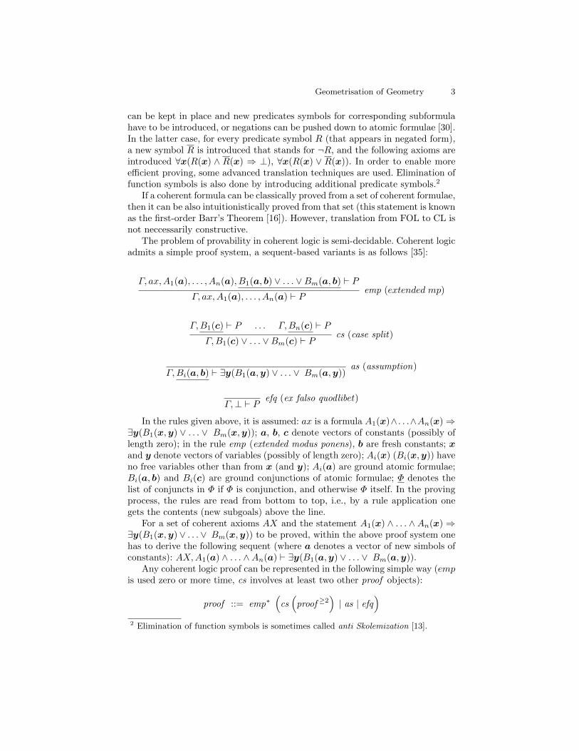
The problem of provability in coherent logic is semi-decidable. Coherent logicadmits a simple proof system, a sequent-based variants is as follows [35]:
Γ, ax,A1(a), . . . , An(a), B1(a, b) ∨ . . . ∨Bm(a, b) ` PΓ, ax,A1(a), . . . , An(a) ` P emp (extended mp)
Γ,B1(c) ` P . . . Γ,Bn(c) ` PΓ,B1(c) ∨ . . . ∨Bm(c) ` P cs (case split)
Γ,Bi(a, b) ` ∃y(B1(a,y) ∨ . . . ∨ Bm(a,y))as (assumption)
Γ,⊥ ` P efq (ex falso quodlibet)
In the rules given above, it is assumed: ax is a formula A1(x)∧ . . .∧An(x)⇒∃y(B1(x,y) ∨ . . . ∨ Bm(x,y)); a, b, c denote vectors of constants (possibly oflength zero); in the rule emp (extended modus ponens), b are fresh constants; xand y denote vectors of variables (possibly of length zero); Ai(x) (Bi(x,y)) haveno free variables other than from x (and y); Ai(a) are ground atomic formulae;Bi(a, b) and Bi(c) are ground conjunctions of atomic formulae; Φ denotes thelist of conjuncts in Φ if Φ is conjunction, and otherwise Φ itself. In the provingprocess, the rules are read from bottom to top, i.e., by a rule application onegets the contents (new subgoals) above the line.
For a set of coherent axioms AX and the statement A1(x) ∧ . . . ∧ An(x)⇒∃y(B1(x,y)∨ . . .∨ Bm(x,y)) to be proved, within the above proof system onehas to derive the following sequent (where a denotes a vector of new simbols ofconstants): AX,A1(a) ∧ . . . ∧An(a) ` ∃y(B1(a,y) ∨ . . . ∨ Bm(a,y)).
Any coherent logic proof can be represented in the following simple way (empis used zero or more time, cs involves at least two other proof objects):
proof ::= emp∗(cs(proof ≥2
)| as | efq
)
2 Elimination of function symbols is sometimes called anti Skolemization [13].
4 Predrag Janicic
3 Automated Theorem Proving for CL
There are several semi-decision proving procedures for coherent logic and thereare several implemented automated provers. To our knowledge, the first CLautomated theorem prover was developed in Prolog by Janicic and Kordic [21]and was used for one fixed axiomatization of Euclidean geometry – an axiomsystem closely related to Borsuk’s one [7]. This prover, based on forward chainingand iterative deepening, was later reimplemented in C++ to give a more efficientand generic theorem prover ArgoCLP [36] that produces both natural languageproofs (formatted in LATEX or in HTML) and object level proofs in the Isabelleform [29]. Bezem developed in Prolog a CL prover based on depth-first searchthat can generate proof objects in Coq [4]. This prover was used for provingHessenberg’s theorem of projective plane geometry (that states that Pappusaxiom implies Desargues axiom), by proving a number of lemmas [5]. Fisherdeveloped a prover GeologUI with graphical interface [17]. Berghofer developed(using shallow embedding) an internal prover for CL in ML to be used withinthe system Isabelle. None of these provers uses backjumps or lemma learning.De Nivelle implemented a theorem prover Geo for logic close to coherent logic,that uses a mechanism for learning lemmas of somewhat restricted form [13]. Allof these systems perform only ground reasoning. A prover Calypso [28] supportslemma learning and introduces non-ground reasoning in automated proving forCL. For lemma learning, the latter two systems use ideas from CDCL SATsolving [6].
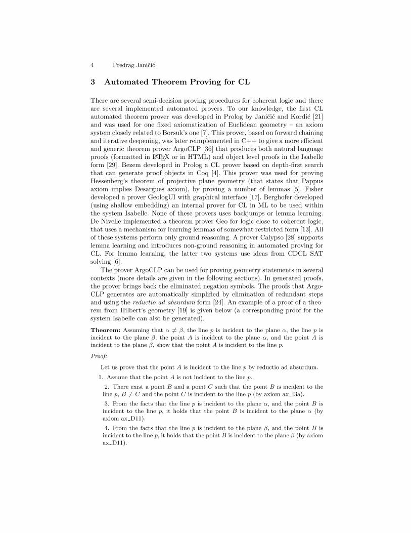
The prover ArgoCLP can be used for proving geometry statements in severalcontexts (more details are given in the following sections). In generated proofs,the prover brings back the eliminated negation symbols. The proofs that Argo-CLP generates are automatically simplified by elimination of redundant stepsand using the reductio ad absurdum form [24]. An example of a proof of a theo-rem from Hilbert’s geometry [19] is given below (a corresponding proof for thesystem Isabelle can also be generated).
Theorem: Assuming that α 6= β, the line p is incident to the plane α, the line p isincident to the plane β, the point A is incident to the plane α, and the point A isincident to the plane β, show that the point A is incident to the line p.
Proof:
Let us prove that the point A is incident to the line p by reductio ad absurdum.
1. Assume that the point A is not incident to the line p.
2. There exist a point B and a point C such that the point B is incident to theline p, B 6= C and the point C is incident to the line p (by axiom ax I3a).
3. From the facts that the line p is incident to the plane α, and the point B isincident to the line p, it holds that the point B is incident to the plane α (byaxiom ax D11).
4. From the facts that the line p is incident to the plane β, and the point B isincident to the line p, it holds that the point B is incident to the plane β (by axiomax D11).

Geometrisation of Geometry 5
5. From the facts that B 6= C, the point B is incident to the line p, the point Cis incident to the line p, and the point A is not incident to the line p, it holds thatthe points B, C and A are not collinear (by axiom ax D1a).
6. From the facts that the line p is incident to the plane α, and the point C isincident to the line p, it holds that the point C is incident to the plane α (by axiomax D11).
7. From the facts that the line p is incident to the plane β, and the point C isincident to the line p, it holds that the point C is incident to the plane β (by axiomax D11).
8. From the facts that the points B, C and A are not collinear, it holds that thepoints A, B and C are not collinear (by axiom ax ncol 231).
9. From the facts that the points A, B and C are not collinear, the point A isincident to the plane α, the point B is incident to the plane α, the point C isincident to the plane α, the point A is incident to the plane β, the point B isincident to the plane β, and the point C is incident to the plane β, it holds thatα = β (by axiom ax I5).
10. From the facts that α = β, and α 6= β we get a contradiction.
Contradiction.
Therefore, it holds that the point A is incident to the line p.
This proves the conjecture.
Theorem proved in 10 steps and in 4.56 s.
4 CL Vernacular
Automated provers for coherent logic such as ArgoCLP export proofs in somecustom format(s). However, it would be beneficial if there is an output formatsupported by various CL provers that can be further used for generating proofs indifferent target languages. Following this motivation, a new proof representationand a corresponding format for coherent logic were developed [35].
De Bruijn used a syntagm mathematical vernacular3 in 1980’s within hisformalism proposed for trying to “put a substantial part of the mathematicalvernacular into the formal system” [12]. Several authors later modified or ex-tended de Bruijn’s framework. Wiedijk follows de Bruijn’s motivation [41], buthe also notices: “It turns out that in a significant number of systems (proof assis-tants) one encounters languages that look almost the same. Apparently there isa canonical style of presenting mathematics that people discover independently:something like a natural mathematical vernacular. Because this language ap-parently is something that people arrive at independently, we might call it themathematical vernacular.” The language discussed by Wiedijk is actually closelyrelated to a proof language of coherent logic. CL can naturally express a numberof mathematical theories, including different geometries. A proof representation
3 Vernacular is the everyday, ordinary language (in contrast to the official, literarylanguage) of the people of some country or region.
6 Predrag Janicic
called “coherent logic vernacular” [35] can link different proof formats and pre-sentations. CL vernacular is simple, yet expressive proof representation with onlya few inference rules, shown in Section 2, supported.
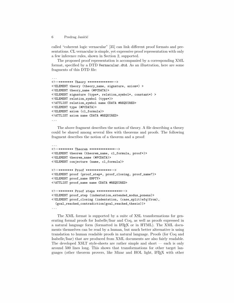
The proposed proof representation is accompanied by a corresponding XMLformat, specified by a DTD Vernacular.dtd. As an illustration, here are somefragments of this DTD file:
...
<!--******** Theory **************-->
<!ELEMENT theory (theory_name, signature, axiom*) >
<!ELEMENT theory_name (#PCDATA)>
<!ELEMENT signature (type*, relation_symbol*, constant*) >
<!ELEMENT relation_symbol (type*)>
<!ATTLIST relation_symbol name CDATA #REQUIRED>
<!ELEMENT type (#PCDATA)>
<!ELEMENT axiom (cl_formula)>
<!ATTLIST axiom name CDATA #REQUIRED>
...
The above fragment describes the notion of theory. A file describing a theorycould be shared among several files with theorems and proofs. The followingfragment describes the notion of a theorem and a proof:
...
<!--******** Theorem **************-->
<!ELEMENT theorem (theorem_name, cl_formula, proof+)>
<!ELEMENT theorem_name (#PCDATA)>
<!ELEMENT conjecture (name, cl_formula)>
<!--******** Proof **************-->
<!ELEMENT proof (proof_step*, proof_closing, proof_name?)>
<!ELEMENT proof_name EMPTY>
<!ATTLIST proof_name name CDATA #REQUIRED>
<!--******** Proof steps **************-->
<!ELEMENT proof_step (indentation,extended_modus_ponens)>
<!ELEMENT proof_closing (indentation, (case_split|efq|from),
(goal_reached_contradiction|goal_reached_thesis))>
...
The XML format is supported by a suite of XSL transformations for gen-erating formal proofs for Isabelle/Isar and Coq, as well as proofs expressed ina natural language form (formatted in LATEX or in HTML). The XML docu-ments themselves can be read by a human, but much better alternative is usingtranslation to human readable proofs in natural language. Proofs (for Coq andIsabelle/Isar) that are produced from XML documents are also fairly readable.The developed XSLT style-sheets are rather simple and short — each is onlyaround 500 lines long. This shows that transformations for other target lan-guages (other theorem provers, like Mizar and HOL light, LATEX with other
Geometrisation of Geometry 7
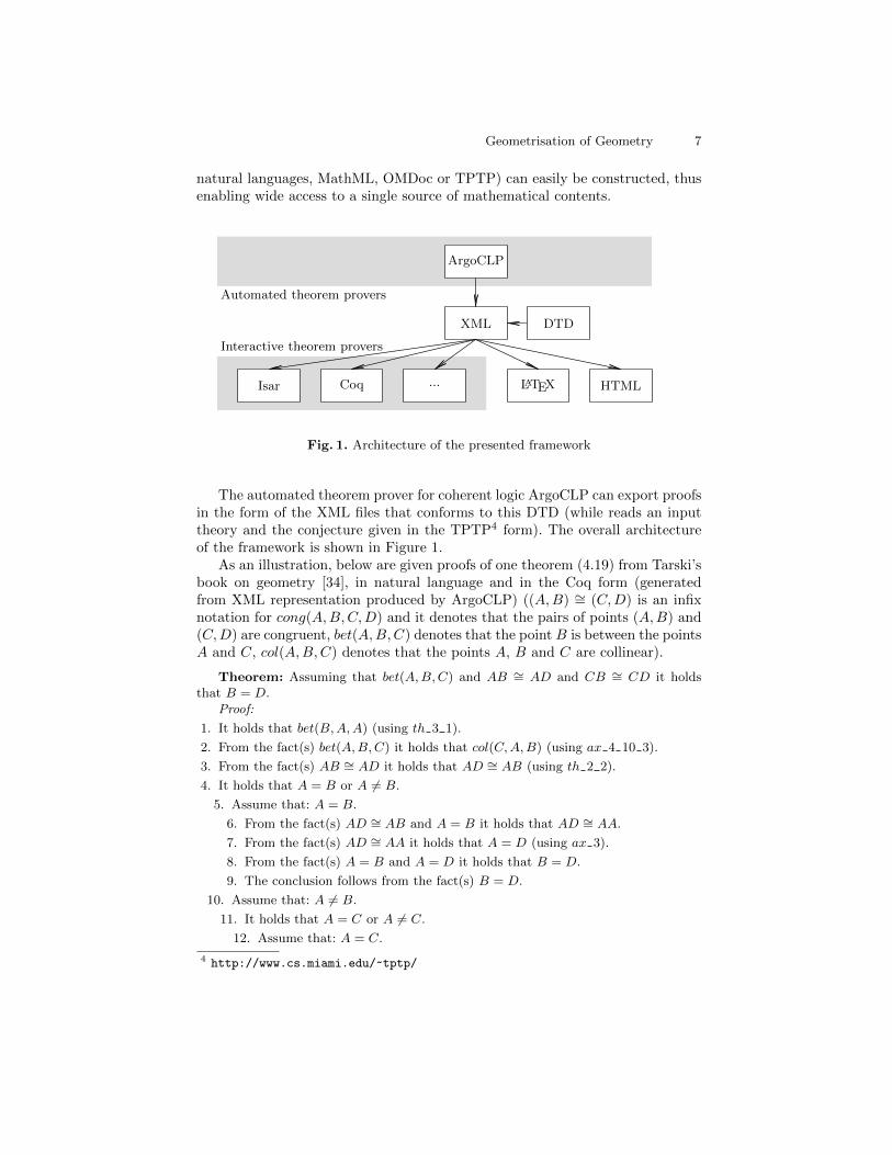
natural languages, MathML, OMDoc or TPTP) can easily be constructed, thusenabling wide access to a single source of mathematical contents.
Automated theorem provers
ArgoCLP
XML DTD
Interactive theorem provers
Isar Coq ... LATEX HTML
Fig. 1. Architecture of the presented framework
The automated theorem prover for coherent logic ArgoCLP can export proofsin the form of the XML files that conforms to this DTD (while reads an inputtheory and the conjecture given in the TPTP4 form). The overall architectureof the framework is shown in Figure 1.
As an illustration, below are given proofs of one theorem (4.19) from Tarski’sbook on geometry [34], in natural language and in the Coq form (generatedfrom XML representation produced by ArgoCLP) ((A,B) ∼= (C,D) is an infixnotation for cong(A,B,C,D) and it denotes that the pairs of points (A,B) and(C,D) are congruent, bet(A,B,C) denotes that the point B is between the pointsA and C, col(A,B,C) denotes that the points A, B and C are collinear).
Theorem: Assuming that bet(A,B,C) and AB ∼= AD and CB ∼= CD it holdsthat B = D.
Proof:
1. It holds that bet(B,A,A) (using th 3 1).
2. From the fact(s) bet(A,B,C) it holds that col(C,A,B) (using ax 4 10 3).
3. From the fact(s) AB ∼= AD it holds that AD ∼= AB (using th 2 2).
4. It holds that A = B or A 6= B.
5. Assume that: A = B.
6. From the fact(s) AD ∼= AB and A = B it holds that AD ∼= AA.
7. From the fact(s) AD ∼= AA it holds that A = D (using ax 3).
8. From the fact(s) A = B and A = D it holds that B = D.
9. The conclusion follows from the fact(s) B = D.
10. Assume that: A 6= B.
11. It holds that A = C or A 6= C.
12. Assume that: A = C.
4 http://www.cs.miami.edu/~tptp/

8 Predrag Janicic
13. From the fact(s) bet(A,B,C) and A = C it holds that bet(A,B,A).
14. From the fact(s) bet(A,B,A) and bet(B,A,A) it holds that A = B (usingth 3 4).
15. From the fact(s) A 6= B and A = B we get contradiction.
16. Assume that: A 6= C.
17. From the fact(s) A 6= C it holds that C 6= A.
18. From the fact(s) C 6= A and col(C,A,B) and CB ∼= CD and AB ∼= ADit holds that B = D (using th 4 18).
19. The conclusion follows from the fact(s) B = D.
20. The conclusion follows in all cases.
21. The conclusion follows in all cases.
QED
Theorem th 4 19 : ∀ (A:point) (B :point) (C :point) (D :point), (bet A B C ∧ congA B A D ∧ cong C B C D) → B = D.Proof.intros.assert (bet B A A) by applying (th 3 1 B A ) .assert (col C A B) by applying (ax 4 10 3 A B C ) .assert (cong A D A B) by applying (th 2 2 A B A D ) .assert (A = B ∨ A 6= B) by applying (ax g1 A B ) .by cases on (A = B ∨ A 6= B).- assert (cong A D A A) by (substitution).assert (A = D) by applying (ax 3 A D A ) .assert (B = D) by (substitution).conclude.
- assert (A = C ∨ A 6= C ) by applying (ax g1 A C ) .by cases on (A = C ∨ A 6= C ).- assert (bet A B A) by (substitution).assert (A = B) by applying (th 3 4 A B A ) .assert (False) by (substitution).contradict.
- assert (C 6= A) by (substitution).assert (B = D) by applying (th 4 18 C A B D ) .conclude.
Qed.

Geometrisation of Geometry 9
5 CL-based Formalizations of Geometry
Large portions of geometry can be expressed in coherent logic, or can be rela-tively easily transformed into coherent logic. This is supported by a study [14]of the book on foundations of geometry Metamathematische Methoden in derGeometrie, by Wolfram Schwabhauser, Wanda Szmielew, and Alfred Tarski [34].This book has been a subject of several automation and formalization projects,using automated theorem proving [2,3,31] or interactive theorem proving [8,27].Geometry in this book is expressed in terms of first-order logic with equality,without sorts (the only primitive objects are points) and with two primitivepredicate symbols written (in prefix form) as cong (for congruence) and bet (forbetweeness). There are only eleven axioms (it is assumed that all axioms areuniversally closed):
Axiom A1: cong(A,B,B,A)Axiom A2: cong(A,B, P,Q) ∧ cong(A,B,R, S) ⇒ cong(P,Q,R, S)Axiom A3: cong(A,B,C,C) ⇒ A = BAxiom A4: ∃X (bet(Q,A,X) ∧ cong(A,X,B,C))Axiom A5: A 6= B ∧ bet(A,B,C) ∧ bet(A′, B′, C ′) ∧ cong(A,B,A′, B′) ∧
cong(B,C,B′, C ′) ∧ cong(A,D,A′, D′) ∧cong(B,D,B′, D′) ⇒ cong(C,D,C ′, D′)
Axiom A6: bet(A,B,A) ⇒ A = BAxiom A7: bet(A,P,C) ∧ bet(B,Q,C) ⇒ ∃X (bet(P,X,B) ∧ bet(Q,X,A))Axiom A8: ∃A ∃B ∃C (¬bet(A,B,C) ∧ ¬bet(B,C,A) ∧ ¬bet(C,A,B))Axiom A9: P 6= Q ∧ cong(A,P,A,Q) ∧ cong(B,P,B,Q) ∧
cong(C,P,C,Q) ⇒ (bet(A,B,C) ∨ bet(B,C,A) ∨ bet(C,A,B))Axiom A10: bet(A,D, T ) ∧ bet(B,D,C) ∧ A 6= D ⇒∃X ∃Y (bet(A,B,X) ∧ bet(A,C, Y ) ∧ bet(X,T, Y ))
Axiom A11 (continuity): ∀Φ ∀Ψ ∃A ∀X ∀Y ((X ∈ Φ∧Y ∈ Ψ ⇒ bet(A,X, Y ))⇒ ∃B ∀X ∀Y (X ∈ Φ ∧ Y ∈ Ψ ⇒ bet(X,B, Y ))
One goal of the study was analysis of how many theorems from such book canbe proved by coherent logic prover ArgoCLP supported by resolution theoremprovers [14]. The process of coherentisation of the theorems was straightforward(and included eliminating sets that were used in the book only as a syntacticsugar, for the sake of clarity and conciseness). From the original 179 theorems,the process gave 238 coherent formulae (while 5 schematic theorems involvingn-tuples were considered only for n = 2).
Given all the axioms and the theorems from the book in coherent form andwritten in the TPTP format, the proving process went as follows.
– Given a theorem to be proved, all axioms and theorems that precede it (in thebook) are passed to resolution provers (Vampire [32], E [33], or SPASS [39]).
– If one or more resolution provers proves the conjecture, the smallest list ofused axioms/theorems (returned by the resolution prover) is used for provingthe conjecture again, in the same manner. This process is repeated until thelist of used axioms/theorems remains unchanged between two consecutiveiterations.
10 Predrag Janicic
– With the obtained list of axioms, ArgoCLP prover is invoked, and (if suc-cessful) the proof is exported in the CL vernacular XML format.
ArgoCLP supported by resolution provers proved (in the above way) 37%of the theorems from chapters 1 to 12 of the book completely automatically.This performance was reached in the scenario that mimics humans doing math-ematics: even if one cannot prove some theorem, he/she proceeds with furthertheorems and uses even those theorems that were unproven. In a more strictformalization scenario, in which only theorems that were already automaticallyproved could be used, the framework proved 17% of the theorems.
One of the outputs of the proving framework within the above study was adigital version of the book, with all axioms, definitions, theorems, and generatedproofs filled-in, all in the natural language form.
6 Coherent Logic and Construction Problems
Almost all automated theorem provers for geometry focus on universally quanti-fied statements. However, statements of the form ∀∃ naturally arise in geometry.One source of such statements are construction problems. Popular geometrytheorem provers (like those based on Wu’s method) can be used for showing cor-rectness of a solution for a construction problem, however, they cannot providea full answer: they can (at least for some constructions) prove statements suchas if some points meet some conditions, then it holds that.... However, it is notanswered whether such points exist, and if yes – under what conditions.
For a construction problem, roughly said, the task is to prove constructively atheorem of the following form (where x and y denote vectors of objects – points,lines, rays, etc):
∀x∃y Ψ(x;y)
The above subsumes two claims: that the problem is solvable (say, by rulerand compass) and that a particular construction (that witnesses ∃y Ψ(x;y)) iscorrect. There could be given some constraints imposed on the given objects x— some construction problems do not have solutions and some problems havesolutions only under some additional conditions, not known in advance. So, onetypically has to discover5 Φ(x) (for the given Ψ(x;y)) and to prove:
∀x(Φ(x)⇒ ∃y Ψ(x;y))
The above claims that solution exists under some conditions. But one may claimeven more:
∀x(Φ(x)⇒ ∃y Ψ(x;y) ∧ ¬Φ(x)⇒ ¬∃y Ψ(x;y))
5 In solving specific classes of construction problems, some goal conditions may beassumed. For instance, in solving triangle construction problems, an implicit goalcondition is that the constructed points A, B, and C are not collinear.

Geometrisation of Geometry 11
The above gives a complete characterization of solvability: it states that solutionexists under some conditions Φ(x) and solution does not exist otherwise.
Let us, for example, consider the contruction problem 4 from Wernick’s list[40]: Given points A, B, and G, construct a triangle ABC, such that G is thecentroid of ABC. A careful analysis leads to the theorem that gives a clearcharacterization of solvability:
∀A,B,G (¬collinear(A,B,G)⇔∃C.(¬collinear(A,B,C) ∧ centroid(G,A,B,C)))
which can be trivially transformed into two coherent formulae.The system ArgoTriCS [26] is able to automatically find constructions for
almost all solvable Wernick’s and Connelly’s [11] problems. It uses algebraicprovers for proving correctness of solutions (under assumption that the con-structed object do exist) and the prover ArgoCLP for showing statements thatgive characterizations of solvability [25]. The prover ArgoCLP is not powerfulenough to prove needed theorems and it uses facts used by ArgoTriCS in thegenerated solution for the construction problem.
7 Coherent Logic and Geometric Illustrations
In geometry and in the whole of mathematics, illustrations are often very valu-able, but almost always just an informal content, provided to support intuitionand understandability of proofs. Links between proofs and associated illustra-tion are typically very loose: proofs do not rely on illustrations, illustrations arenot derived from proofs. However, proofs in coherent logic can be used, in somecases, for automated generation of illustrations.6 The idea is not to instruct aCL prover to generate illustrations, but to use proofs themselves (represented,say, as discussed in Section 4) and generate illustrations from them directly.
In each substantial step of a CL proof, one formula (axiom or a lemma) ofthe following form is used:
A1(x) ∧ . . . ∧An(x)⇒ ∃y(B1(x,y) ∨ . . . ∨ Bm(x,y)).Each axiom (or potentially used lemma) with m > 0 (i.e., each axiom that
introduce news objects) need to have an associated illustration rule. For instan-tiated x interpreted in some model (e.g., Cartesian plane), there should be arule for determining y. In some cases, such y are determined uniquely, and insome cases there are degrees of freedom. These rules should be formulated in alanguage that can serve as a specification language for illustrations. One suchlanguage is geometry language GCLC [20]. For example, an axiom for any twopoints A and B, there is a point C such that bet(A,B,C) can be modelled inGCLC in the following way:
random r
expression r’ 1+r
towards C A B r’
6 This idea has not been implemented yet.

12 Predrag Janicic
where random choses a non-negative pseudorandom real number r, the secondline gives a number r’ such that r’ ≥ 1, and the third line determines C (aconcrete point in Cartesian plane) given two (concrete points) A and B. Whenthe case split rule is applied, only one case is illustrated (so, one proof has onlyone illustration). This process is straightforward and yields illustration for eachproof (with all axioms properly processed). However, there is still one initialchallenge. If the conjecture being proved has the form: ∀x(Φ(x)⇒ ∃y Ψ(x;y))in order to be illustrated, one must have initial objects x meeting conditionsΦ(x). So, the first step is to prove that Φ(x) is consistent (if it is not, thestatement is trivially valid), i.e., to prove ∃x Φ(x). A constructive proof of thisconjecture will give one model for Φ(x) and will serve as a basis for an illustrationfor the main proof. Note that this step may not be easy and it actually involvessolving a geometry construction problem.
8 Conclusions
Coherent logic has several applications in automated deduction in geometry:in producing human-readable proofs, in producing machine verifiable proofs, inproving statemens of the form ∀∃, in producing illustrations automatically fromproofs, etc. However, there are still potentials to be used. For instance, theoremprovers for coherent logic have been so far used for fully automated proving ofonly low-level conjectures (with proofs close to the axiomatic level). It would beinteresting to construct suitable sets of geometry lemmas that can be used inproving higher-level conjectures.
Acknowledgements The author is grateful to Marc Bezem, Vesna Marinkovic,Mladen Nikolic, and Sana Stojanovic Ðurevic for their feedback on earlier ver-sions of this paper.
References
1. Jeremy Avigad, Edward Dean, and John Mumma. A formal system for Euclid’sElements. The Review of Symbolic Logic, 2009.
2. Michael Beeson. Proof and computation in geometry. In Automated Deduction inGeometry - 9th International Workshop, volume 7993 of Lecture Notes in ComputerScience, pages 1–30. Springer, 2013.
3. Michael Beeson and Larry Wos. OTTER proofs in tarskian geometry. In Auto-mated Reasoning - 7th International Joint Conference, IJCAR 2014, Held as Partof the Vienna Summer of Logic, VSL 2014, Vienna, Austria, July 19-22, 2014.Proceedings, volume 8562 of Lecture Notes in Computer Science, pages 495–510.Springer, 2014.
4. Marc Bezem and Thierry Coquand. Automating coherent logic. In Geoff Sutcliffeand Andrei Voronkov, editors, 12th International Conference on Logic for Pro-gramming, Artificial Intelligence, and Reasoning — LPAR 2005, volume 3835 ofLecture Notes in Computer Science. Springer-Verlag, 2005.

Geometrisation of Geometry 13
5. Marc Bezem and Dimitri Hendriks. On the Mechanization of the Proof of Hes-senberg’s Theorem in Coherent Logic. Journal of Automated Reasoning, 40(1),2008.
6. Armin Biere, Marijn Heule, Hans van Maaren, and Toby Walsh, editors. Handbookof Satisfiability, volume 185 of Frontiers in Artificial Intelligence and Applications.IOS Press, 2009.
7. Karol Borsuk and Wanda Szmielew. Foundations of Geometry. Norht-HollandPublishing Company, Amsterdam, 1960.
8. Gabriel Braun and Julien Narboux. From Tarski to Hilbert. In Tetsuo Ida andJacques Fleuriot, editors, Automated Deduction in Geometry 2012, Edinburgh,United Kingdom, September 2012.
9. Shang-Ching Chou. Mechanical Geometry Theorem Proving. D.Reidel PublishingCompany, Dordrecht, 1988.
10. Shang-Ching Chou, Xiao-Shan Gao, and Jing-Zhong Zhang. Machine Proofs inGeometry. World Scientific, Singapore, 1994.
11. Harold Connelly. An Extension of Triangle Constructions from Located Points.Forum Geometricorum, 9:109–112, 2009.
12. Nicolaas Govert de Bruijn. The mathematical vernacular, a language for mathe-matics with typed sets. In Dybjer et al., editor, Proceedings of the Workshop onProgramming Languages, 1987.
13. Hans de Nivelle and Jia Meng. Geometric resolution: A proof procedure based onfinite model search. In Automated Reasoning, Third International Joint Confer-ence, IJCAR, volume 4130 of Lecture Notes in Computer Science, pages 303–317.Springer, 2006.
14. Sana Stojanovic Djurdjevic, Julien Narboux, and Predrag Janicic. Automated gen-eration of machine verifiable and readable proofs: A case study of tarski’s geometry.Annals of Mathematics and Artificial Intelligence, 74(3-4):249–269, 2015.
15. Roy Dyckhoff. Coherentisation of first-order logic. In Automated Reasoningwith Analytic Tableaux and Related Methods - 24th International Conference,TABLEAUX 2015, volume 9323 of Lecture Notes in Computer Science, pages 3–5.Springer, 2015.
16. Roy Dyckhoff and Sara Negri. Geometrization of first-order logic. The Bulletin ofSymbolic Logic, 21:123–163, 2015.
17. John Fisher and Marc Bezem. Skolem machines and geometric logic. In Cliff B.Jones, Zhiming Liu, and Jim Woodcock, editors, 4th International Colloquium onTheoretical Aspects of Computing — ICTAC 2007, volume 4711 of Lecture Notesin Computer Science. Springer-Verlag, 2007.
18. Mohan Ganesalingam and William Timothy Gowers. A fully automatic problemsolver with human-style output. CoRR, abs/1309.4501, 2013.
19. David Hilbert. Grundlagen der Geometrie. Leipzig, 1899.20. Predrag Janicic. Geometry Constructions Language. Journal of Automated Rea-
soning, 44(1-2):3–24, 2010.21. Predrag Janicic and Stevan Kordic. EUCLID — the geometry theorem prover.
FILOMAT, 9(3):723–732, 1995.22. Predrag Janicic, Julien Narboux, and Pedro Quaresma. The area method: a reca-
pitulation. Journal of Automated Reasoning, 48(4):489–532, 2012.23. Saunders MacLane and Ieke Moerdijk. Sheaves in geometry and logic: a first in-
troduction to topos theor. Springer-Verlag, 1992.24. Vesna Marinkovic. Proof simplification in the framework of coherent logic. Com-
puting and Informatics, 34(2):337–366, 2015.
14 Predrag Janicic
25. Vesna Marinkovic, Predrag Janicic, and Pascal Schreck. Computer theorem provingfor verifiable solving of geometric construction problems. In Automated Deductionin Geometry - 10th International Workshop, Revised Selected Papers, volume 9201,pages 72–93. Springer, 2015.
26. Vesna Marinkovic and Predrag Janicic. Towards Understanding Triangle Con-struction Problems. In J. Jeuring et al., editor, Intelligent Computer Mathematics- CICM 2012, volume 7362 of Lecture Notes in Computer Science. Springer, 2012.
27. Julien Narboux. Mechanical theorem proving in Tarski’s geometry. In Proceedingsof Automatic Deduction in Geometry 06, volume 4869 of Lecture Notes in ArtificialIntelligence, pages 139–156. Springer-Verlag, 2007.
28. Mladen Nikolic and Predrag Janicic. CDCL-based abstract state transition systemfor coherent logic. In J. et.al. Jeuring, editor, Intelligent Computer Mathematics -CICM 2012, volume 7362 of Lecture Notes in Computer Science. Springer, 2012.
29. Tobias Nipkow, Lawrence C. Paulson, and Markus Wenzel. IsabelleHOL: a Proof Assistant for Higher-Order Logic. Springer, 2005. url:http://www.cl.cam.ac.uk/research/hvg/Isabelle/dist/Isabelle/doc.
30. Andrew Polonsky. Proofs, Types and Lambda Calculus. PhD thesis, University ofBergen, 2011.
31. Art Quaife. Automated development of tarski’s geometry. Journal of AutomatedReasoning, 5(1):97–118, 1989.
32. Alexandre Riazanov and Andrei Voronkov. The design and implementation ofvampire. AI Communications, 15(2-3):91–110, 2002.
33. Stephan Schulz. E - a brainiac theorem prover. AI Communications, 15(2-3):111–126, 2002.
34. Wolfram Schwabhuser, Wanda Szmielew, and Alfred Tarski. MetamathematischeMethoden in der Geometrie. Springer-Verlag, Berlin, 1983.
35. Sana Stojanovic, Julien Narboux, Marc Bezem, and Predrag Janicic. A vernacularfor coherent logic. In Intelligent Computer Mathematics, volume 8543 of LectureNotes in Computer Science, pages 388–403. Springer, 2014.
36. Sana Stojanovic, Vesna Pavlovic, and Predrag Janicic. A coherent logic based ge-ometry theorem prover capable of producing formal and readable proofs. In PascalSchreck, Julien Narboux, and Jurgen Richter-Gebert, editors, Automated Deduc-tion in Geometry, volume 6877 of Lecture Notes in Computer Science. Springer,2011.
37. Alfred Tarski and Steven Givant. Tarski’s system of geometry. The Bulletin ofSymbolic Logic, 5(2), June 1999.
38. Steven Vickers. Geometric logic in computer science. In Theory and Formal Meth-ods, Workshops in Computing, pages 37–54. Springer, 1993.
39. Christoph Weidenbach, Dilyana Dimova, Arnaud Fietzke, Rohit Kumar, MartinSuda, and Patrick Wischnewski. Spass version 3.5. In Automated Deduction -CADE-22 Proceedings, volume 5663 of Lecture Notes in Computer Science, pages140–145. Springer, 2009.
40. William Wernick. Triangle constructions vith three located points. MathematicsMagazine, 55(4):227–230, 1982.
41. Freek Wiedijk. Mathematical Vernacular. Unpublished note. http://www.cs.ru.nl/~freek/notes/mv.pdf, 2000.
Solving With Or Without Equations
Dominique Michelucci
LE2I UMR6306, CNRS, Arts et Metiers,Bourgogne Franche-Comte University, Dijon, France
1 Equations versus algorithms, back and forth
The pentahedron problem (§2) shows the proximity between Geometric TheoremProving (GTP) and Geometric Constraint Solving (GCS). However, the twofields separate, due to specificities of GCS (§3), which prefers algorithms toequations. Yet GCS still benefits from symbolic tools, like DAG (§4), and dualnumbers (§5). Finally, §6 conjectures that algorithms can be converted to systemsof equations.
E
A
D
F
C
B
I
A C
I
FD
B
E
I
A C
B
F D
E EF
B
C
D
A
I
A
B
C
D
E
F
I
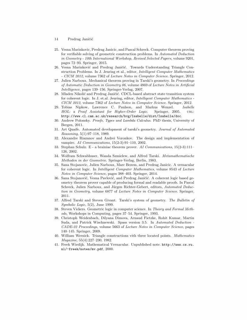
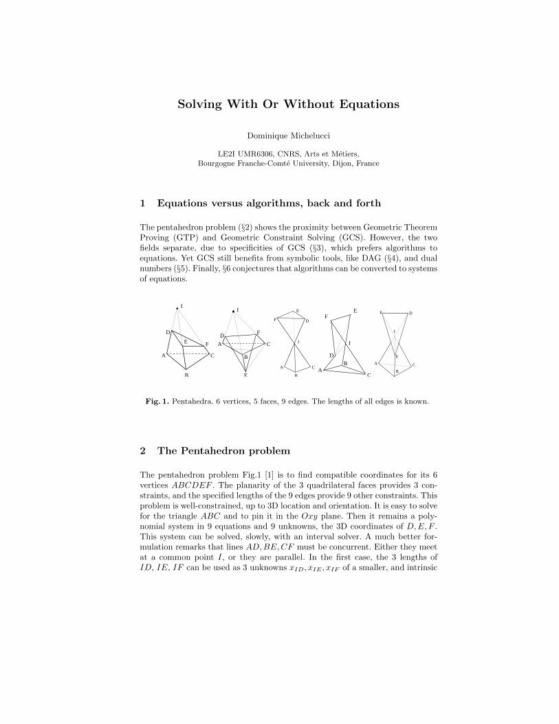
Fig. 1. Pentahedra. 6 vertices, 5 faces, 9 edges. The lengths of all edges is known.
2 The Pentahedron problem
The pentahedron problem Fig.1 [1] is to find compatible coordinates for its 6vertices ABCDEF . The planarity of the 3 quadrilateral faces provides 3 con-straints, and the specified lengths of the 9 edges provide 9 other constraints. Thisproblem is well-constrained, up to 3D location and orientation. It is easy to solvefor the triangle ABC and to pin it in the Oxy plane. Then it remains a poly-nomial system in 9 equations and 9 unknowns, the 3D coordinates of D,E, F .This system can be solved, slowly, with an interval solver. A much better for-mulation remarks that lines AD,BE,CF must be concurrent. Either they meetat a common point I, or they are parallel. In the first case, the 3 lengths ofID, IE, IF can be used as 3 unknowns xID, xIE , xIF of a smaller, and intrinsic

16 Dominique Michelucci
(coordinate-free) system of 3 equations and 3 unknowns: the law of cosines gives
the 3 equations, one per quadrilateral face; e.g., let α = DIE = AIB; then
cosα =x2ID + x2
IE − l2DE
2xIDxIE=
(xID + lAD)2 + (xIE + lBE)2 − l2AB
2(xID + lAD)(xIE + lBE)
gives the equation in xID, xIE for the quadrilateral face ABED. This systemis solved 42 times faster than the previous one. In the second case, the point Iis at infinity and a simple geometric construction shows that there are alwayspentahedra with parallel edges AD,BE,CF , except when some triangular ortetrahedric inequality is violated. Finally, there are 6 spurious roots, where thepentahedron is flat, so edges AD,BE,CF need not be concurrent.
This problem illustrates many common issues to GCS and GTP: what isthe dimension of the manifold solution? Are there points at infinity? What isthe best way to pose equations? Are there any degenerate solutions, and whatis the topological dimension of the degenerate manifold? Indeed, in GTP, nondegeneracy conditions (the triangle must not be flat, vertices must be distinct,etc) have to be specified in order to prove theorems. This example also showsthat GCS and GTP are close while all constraints are incidence, or distance,or angle constraints between flats: points, lines, planes. But the latter are notsufficient in CADCAM.
3 Specificities of GCS for CADCAM
The first specificity in GCS is the inaccuracy issue. The nullity of a number, theequality of two numbers are no more decidable. The computation of the rank ofa set of vectors, or of a Jacobian, is no more guaranteed. The distinction betweenx > 0 and x ≥ 0 becomes irrelevant. The equivalence x 6= 0 ⇔ ∃y |xy − 1 = 0used in Grobner bases becomes irrelevant as well.
Another specificity is the need for optimization and algorithms.For example, there are many orthogonal projections of a point on a non linear
curve or surface but for distance constraints, only one is relevant. First orderconditions, like KKT (Karush-Kuhn-Tucker), are necessary but not sufficient tofully characterize solutions. Solving KKT equations provides a superset of theroots, and spurious ones (saddle points, local optima) must be cancelled withsome algorithm.
When computing the orthogonal projection of a point p to a composite object(e.g., the union of a line and a conic), often used in CADCAM, the relevantsystem of equations depends on the location of p. Again, some optimizationproblem occurs. For the orthogonal projection on a part of an object, like asegment, optimization can be avoided, but an algorithm and some if-then-elseare more convenient than equations.
CADCAM systematically uses piecewise polynomials (box splines, bsplines,etc). They are not polynomials and standard tools of Computer Algebra (Grobnerbases, Wu-Ritt method, resultants, GCD, fundamental theorem of algebra, Sturm’stheorem, etc) no more apply. Idem for NURBS and piecewise rational functions.
Solving With Or Without Equations 17
Finally, Computer Graphics and CADCAM use algorithmic shapes, calledfeatures or parametric objects, like staircases, gears and sprockets, etc. Thenumber of steps in a staircase is an integer (thus diophantine equations occur)and depend on parameter values of length and height: the number of unknownsand equations depend on parameter values. In passing, there is some similaritywith Steiner’s porism, or Poncelet’s porism, in GTP.
Worse, subdivision curves and subdivision surface have invaded ComputerGraphics: designers interactively define a coarse mesh, and a procedure roundsvertices and edges. Most of the time, there is no equation for the limit surface.
Sometimes, equations are available but too huge to be symbolically expanded,e.g., det(M(X)) = 0. Of course, a numerical algorithm can still be used tocompute det(M(V )) for a given numerical vector V . Another example is givenby intersection curves between rational surfaces: they are not rational but allgeometric modelers approximate them with rational curves.
4 DAGs
Gouaty et al [2] solve such geometric constraints for CADCAM: equations arereplaced with algorithms. Constraints are represented with DAGs (DirectedAcyclic Graph). DAG is a popular data structure in Dynamic Geometry soft-wares (where they are called Straight Line Programs) and in Computer Alge-bra. In CADCAM, DAGs involve spline or NURBS functions, algorithms (forrounding, for orthogonal projection), subdivision surfaces and other algorithmicshapes. They are no more convertible into polynomials, and it is no more possi-ble to compute the DAG of the derivative of a given DAG. But these DAG keepsome interesting features: they still can be evaluated for given values of param-eters, thus it is still possible to solve; DAG can be interactively specified andmodified by users or designers who are not computer scientists, thus users canstill pose their problems; probabilistic tests for nullity or equality (up to sometolerance) are still possible; and finally, exact computations (up to floating pointprecision) of derivatives are still possible, after all, with dual numbers. This isinteresting because derivatives computed with finite differences are inaccurate,which hampers the convergence of numeric solvers close to the solution.
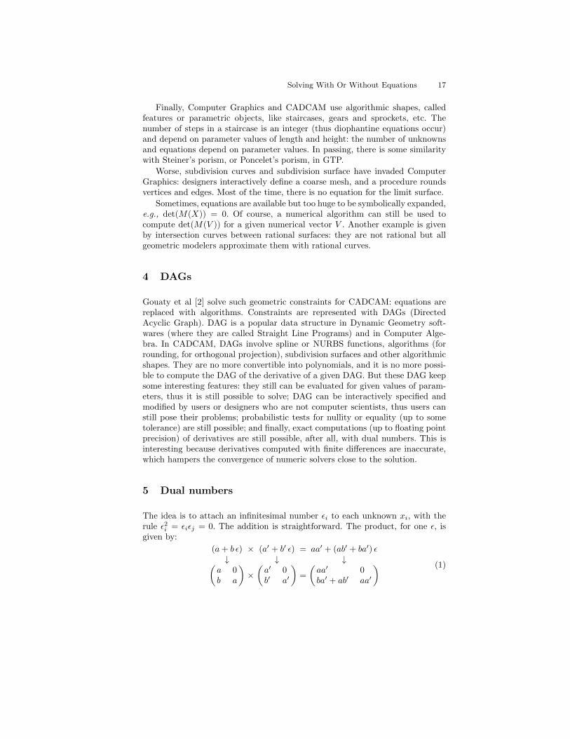
5 Dual numbers
The idea is to attach an infinitesimal number ǫi to each unknown xi, with therule ǫ2i = ǫiǫj = 0. The addition is straightforward. The product, for one ǫ, isgiven by:
(a+ b ǫ) × (a′ + b′ ǫ) = aa′ + (ab′ + ba′) ǫ↓ ↓ ↓(
a 0b a
)×
(a′ 0b′ a′
)=
(aa′ 0ba′ + ab′ aa′
) (1)

18 Dominique Michelucci
and it is generalizable to many ǫi. The bijection between dual numbers and ma-trices is an isomorphism: the matrice of the opposite (inverse) of a dual numberis the opposite (inverse) of the matrice of the dual number. Other rules are:
1
a+ b ǫ=
1
a− b
a2ǫ when a 6= 0 (2)
thus bǫ has no inverse (the associated matrice is not invertible). This rule is aspecial case of:
(a+ bǫ)k = ak + kak−1b ǫ (3)
If P is a polynomial, then P (xv + ǫ) where xv is a floating-point number,gives P (xv) and the derivative P ′(xv):
P (xv + ǫ) = a(xv + ǫ)3 + b(xv + ǫ)2 + c(xv + ǫ) + d= a(x3
v + 3x2v ǫ) + b(x2
v + 2xv ǫ) + c(xv + ǫ) + d= (ax3
v + bx2v + cxv + d) + (3ax2
v + 2bxv + c) ǫ= P (xv) + P ′(xv) ǫ
(4)
It extends to multivariate polynomials: either we have only one ǫ and two eval-uations are needed:
Q(xv + ǫ, yv) = Q(xv, yv) +Q′x(xv, yv)ǫ
Q(xv, yv + ǫ) = Q(xv, yv) +Q′y(xv, yv)ǫ
(5)
or each variable is attached its own ǫ and one evaluation suffices:
Q(xv + ǫx, yv + ǫy) = Q(xv, yv) +Q′x(xv, yv)ǫx +Q′
y(xv, yv)ǫy
Dual numbers extend to non polynomial functions:
exp(a+ b ǫ) = ea + bea ǫ
cos(a+ bǫ) = cos(a)− b sin(a) ǫ
sin(a+ bǫ) = sin(a) + b cos(a) ǫ
tan(a+ bǫ) = tan(a) + b(1 + tan2(a)) ǫ
|a+ bǫ| = |a|+ (sgn(a)b+ (1− sgn(a)2)|b|) ǫ
Dual numbers permit to compute the derivative of D(X) = det(M(X)), forsquare matrices M(X), even if entries of M are piecewise polynomials, or algo-rithms: just replace floating point numbers with dual numbers and then use anystandard numerical method (Gauss pivot, LUP). There are also formulas.
Lemma: det(I + ǫM) = 1 + Trace(M) ǫ, where M ∈ Rn,n. Proof:
det(I + ǫM) = (1 +M11ǫ)(1 +M22ǫ) . . . (1 +Mnnǫ) +R = 1 + Trace(M) ǫ+R
where R represents other perfect matchings in I + ǫM . But other matchings useat least two off-diagonal entries in I+ǫM , thus are multiples of ǫ2, thus are zero.

Solving With Or Without Equations 19
When A is inversible, det(M(x+ ǫ)) = det(A+ ǫB) is:
det(A+ ǫB) = det(A(I + ǫA−1B))= det(A) det(I + ǫA−1B)= det(A)(1 + Trace(A−1B) ǫ)
(6)
When A is not inversible, we use its SVD : A = UΣV t (with Σ diagonal andU, V unitary):
det(A+ ǫB) = det(UΣV t + ǫB)= det(U(ΣV t + ǫU tB))= det(U(Σ + ǫU tBV )V t)= det(Σ + ǫU tBV )
(7)
equals the product of diagonal entries of Σ + ǫU tBV . It is 0 when there are atleast two null singular values in Σ. Otherwise it is
(σ1 + k1ǫ) . . . (σn−1 + kn−1ǫ)(0 + knǫ) = 0 + σ1 . . . σn−1kn ǫ (8)
The extension to many ǫ is lengthy but easy.Dual numbers provide exact (up to floating point precision) derivatives even
when equations are not available and are replaced with algorithms. Thus theymake possible to use Newton method for solving, Euler method for following anhomotopy curve, BFGS method for optimizing.
It is possible to compute Taylor expansions beyond degree 1 (using ǫ4 = 0),which eases Runge Kutta method for homotopy. It has a cost, reducible withthe sparsity of ǫ expansions. ǫ expansions are sortable [3] with compatible ordersused in Grobner bases.
In passing, an algebraic construction φ starting from R gives the quaternions,which represent 3D rotations. If φ is applied to R + ǫR, it gives biquaternions,aka dual quaternions, which represent both 3D rotations and translations.
6 From algorithms to systems of equations
Algorithms are more convenient than equations to express constraints. Butmaybe algorithms can be automatically converted into systems of equations,and algorithms are just a convenience to pose equations?
Let a ∈ R, and s = sgn(a) be the sign of a: a = 0 ⇒ s = 0, a 6= 0 ⇒ s = |a|/a.Then the system of equations below is such that S(a, s) = 0 ⇔ s = sgn(a).
0 = s3 − s ⇔ s ∈ 0,−1, 10 = a− sy2 ⇔ y2 = |a| except when a = 00 = y2z − 1 ⇔ y2 6= 0 Remark that 0 = yz − 1 also works
The reader can check that when a > 0, there is only one real solution y2 =|a| = a, s = 1, z = 1/a. When a < 0, there is only one real solution y2 =|a| = −a, s = −1, z = −1/a. Finally, if a = 0, then s = 0 and y2 is free; foruniqueness, add the equation: (1 − s2)(y − 1) = 0. It changes nothing if a 6= 0.

20 Dominique Michelucci
Otherwise, if a = 0, the only real solution is s = 0, y = z = 1. Then it is easy tobuild systems S(a,R) for defining |a|, the positive (negative) part a+ (a−), etc:
R = |a| = saR = a+ = max(0, a) = (a+ |a|)/2 = (a+ sa)/2R = a− = min(0, a) = a−max(0, a) = (a− |a|)/2 = (a− sa)/2R = max(a, b) = (a+ b)/2 + |b− a|/2R = min(a, b) = (a+ b)/2− |b− a|/2
Then we can convert the if-then-else instruction: F = (if x > 0 then P elseif x < 0 then N else Z) into equations:
F = sgn(x+)P + sgn(x−)N + (1− (sgn(x+) + sgn(x−))Z
For translating the arithmetic constraint x ∈ Z into equations, we can usethe equation sin(πx) = 0, which indeed describes Z, but it is not algebraic. Analgebraic system is: x = x0+2x1+ . . . 2nxn and xi(1−xi) = 0 for all i ∈ [[0, n]].The system has logarithmic size in 2n, but it describes only integers in [[0, 2n−1]].The naive representation: x(x− 1) . . . (x− 2n − 1) = 0 is exponential size.
After functional programming, assignments and iterations are useless. It issufficient to consider fixpoints : F (F (...(X))), where F is some algorithm. As-sume the program Y = F (X) is represented with some system of equations:S(X,Y ) = 0. Then fixpoints of F are solutions of the system S(X,X) = 0. Thelatter clearly shows that the sizes of X and Y must be equal. It is untrue forsome algorithm F , e.g., for subdivision curves, the size of Y is twice the size ofX.
We only sketched this conversion: we did not treat the conversion of functioncalls, or of data structures like Lisp pairs. Assume this conversion is possible un-der mild assumption. Then Computer Algebra applies to resulting polynomialsystems, e.g., ideals and radicals concepts become relevant for piecewise polyno-mials after all. We can deduce equations from algorithms, e.g., for the distancebetween a point and a segment, or for canceling spurious roots. Thus algorithmsare just a convenient way to pose equations. Is it possible to find (Grobner basesof) polynomial preconditions for the algorithm to work, and to fail?
References
1. Barki, H., Cane, J.M., Garnier, L., Michelucci, D., Foufou, S.: Solving the pentahe-dron problem. Computer-Aided Design 58, 200–209 (2015)
2. Gouaty, G., Fang, L., Michelucci, D., Daniel, M., Pernot, J.P., Raffin, R., Lanquetin,S., Neveu, M.: Variational geometric modeling with black box constraints and dags.Computer-Aided Design 75, 1–12 (2016)
3. Michelucci, D.: An epsilon-arithmetic for removing degeneracies. In: 12th Sympo-sium on Computer Arithmetic. p. 230. IEEE (1995)
Dependence of Axioms for Weak GeometriesProved Syntactically
Victor Pambuccian
School of Mathematical and Natural Sciences (MC 2352)Arizona State University - West Campus
P. O. Box 37100Phoenix, AZ 85069-7100
U.S.A. [email protected]
Abstract. This talk will focus on two separate topics. The first oneconcerns the geometry of point-reflections, and the various axioms thatone can add to an axiom system for point-reflections valid in absolutegeometry to get a hierarchy of geometries that are intermediate betweenabsolute an affine geometry. The language in which the axioms are ex-pressed is a one-sorted one, with variable to be interpreted as ‘points’,with two binary operation symbols, σ — with σ(ab) standing for the re-flection of b in a — and µ — with µ(ab) standing for the midpoint of ab.All statements considered are universal. The dependencies and indepen-dencies involved were all established with the aid of Tipi, an aggregateof automatic theorem provers designed by Jesse Alama. The results werepublished in [1]. Several open problems remain.The second part is a walk through results known to be true, regardingstatements that are known to be equivalent to established axioms, butfor which we have only algebraic proofs, or even proofs using Tarski’sprinciple and other deep model-theoretical results. The challenge wouldbe to find syntactic proofs by means of automatic theorem provers. Ex-amples are: Szmielew’s [7] proof that the circle axiom implies the Paschaxiom in a certain axiom system for semi-ordered Euclidean geometry,the fact that the Erdos-Mordell theorem is equivalent to the statementthat the angle sum in a triangle is not larger than two right angles,proved in [4], the fact that the distances from a point to the verticesof an equilateral triangle satisfy the generalized triangle inequality isequivalent to the same statement that the angle sum in a triangle isnot larger than two right angles, proved in [2] and [6], the equivalenceof Lagrange’s axiom with Bachmann’s Lotschnittaxiom (stating that aquadrilateral with three right angles closes), proved in [5], or the equiva-lence of the Lotschnittaxiom with the universal statement “In an isoscelestriangle with base angles of 45, the altitude to the base is smaller thanthe base” (proved in [3]).
References
1. Alama, J., Pambuccian, V.: From absolute to affine geometry in terms of point-reflections, midpoints, and collinearity, Note di Matematica, 36: 11–24 (2016).

22 Victor Pambuccian
2. Barbilian, D. : Exkurs uber die Dreiecke, Bulletin Mathematique de la Societe desSciences Mathematiques de Roumanie 38: 3–62 (1936).
3. Pambuccian, V.: Zum Stufenaufbau des Parallelenaxioms, Journal of Geometry, 51:79-88 (1994).
4. Pambuccian, V.: The Erdos-Mordell inequality is equivalent to non-positive curva-ture Journal of Geometry, 88: 134 139 (2008).
5. Pambuccian, V.: On the equivalence of Lagrange’s axiom to the Lotschnittaxiom,Journal of Geometry, 95: 165–171 (2009).
6. Pambuccian, V.: On a paper of Dan Barbilian, Note di Matematica, 29: 29–31 (2009).7. Szmielew, W.: The Pasch axiom as a consequence of the circle axiom, Bulletin
de l’Academie Polonaise des Sciences. Serie des Sciences Mathematiques, As-tronomiques et Physiques, 18: 751–758 (1970).

Implementing Automatic Discovery in GeoGebraExtended Abstract
Miguel A. Abánades1, Francisco Botana2, Zoltán Kovács3,Tomás Recio4 and Csilla Sólyom-Gecse5
1 Depto. de Economía Financiera y Contabilidad e Idioma ModernoUniversidad Rey Juan Carlos, Madrid
[email protected] Depto. de Matemática Aplicada I, EE Forestal, Campus A Xunqueira
Universidade de Vigo, [email protected]
3 Private University College of Education of the Diocese of Linz, [email protected]
4 Depto. de Matemáticas, Estadística y ComputaciónUniversidad de Cantabria, Santander
[email protected] Babeş-Bolyai University, Cluj-Napoca, Romania
Abstract. A prototype for the automatic discovery and derivationof elementary geometry statements, based on the implementation ofcomputational algebraic geometry methods onto the dynamic geome-try program GeoGebra, is presented. The emphasis is placed on the di-verse mathematical and educational challenges posed by the—apparentlystraightforward—application of some well known algorithms onto the Ge-oGebra framework.
Keywords: Automatic Theorem Proving, Automatic Theorem Discovery, Au-tomatic Theorem Deduction, Computational Algebraic Geometry, ElementaryGeometry, Dynamic Geometry Software, GeoGebra
1 Automatic Discovery in GeoGebraIn this paper we address the automatic discovery and derivation of elementarygeometry statements onto the dynamic geometry program GeoGebra, by im-plementing the computational algebraic geometry methods described in [3]. Werefer the reader to such work for technical details about the main concepts andalgorithms. We remark that the considered methods are constrained to work un-der an algebraically closed field of coordinates, e.g. the field of complex numbers;the validity of the output on the real plane is subject to future development.
Since September 2014, with the launching of version 5.0, GeoGebra includesproving capabilities based on symbolic algebraic computations through the com-mand Prove[<Boolean Expression>]6, where a Boolean expression is a GeoGe-6 See https://www.geogebra.org/wiki/en/Prove_Command for documentation.
24 Abánades, Botana, Kovács, Recio and Sólyom-Gecse
bra statement with possible logical values true/false (e.g. AreCollinear(E,F,G)for points E, F, G in a diagram). Alternatively, in GeoGebra, one can checkwhether a Boolean expression is true or not simply by typing the said expres-sion in the command line. In this case, GeoGebra uses the numerical coordi-nates of all the basic elements in the construction to compute the value of thegiven Boolean expression. However, the Prove command assigns symbolic co-ordinates (i.e. variables x, y, u, v, . . .) to the free and semi-free points in theconstruction, and uses symbolic methods to determine whether the proposedstatement is true or false in general. This way Prove[<Boolean Expression>]returns whether the given Boolean expression is true or false for any numer-ical instance of the construction. For example, if we start with a triangleABC and the intersection point O of the altitudes from points A, B and typeProve[ArePerpendicular[Line(O,C),Line(A,B)]] we obtain true, meaningthat for any triangle, its three altitudes share one point (more details in [1]).
The new feature we are reporting here, that of automatic discovery in GeoGe-bra, requires that the user first constructs a geometric diagram with GeoGebra’sdrawing tools or drawing commands. Although theoretically all algebraic con-structions (i.e. those composed of elements that can be expressed by polynomialequations) can serve as initial data for GeoGebra’s discovery tool, technical rea-sons, mainly related to computational time limitations, restrict the applicabilityof the tool for complicated constructions. Moreover, it is important to note thatnon-algebraic elements, such as the graph of a sine function, fall out of the scopeof the method, algebraic in nature.
After constructing a geometric diagram the user needs to type the commandLocusEquation[<Boolean Expression>, <FreePoint> ]7 with two parameters:the sought thesis T (which must be a Boolean expression) and a free point P ‘sup-porting’ the discovery. Remark this is a drastically new functionality, availablein GeoGebra, version 5.0.213.0, since March 2016, of the preexisting commandLocusEquation. We have decided to extend the features of the command ratherthan adding a new name to the long list of GeoGebra commands.
The Boolean expression defining the discovery plays the part of the extracondition that we require our diagram to satisfy. The coordinates of the freepoint P , second parameter of the command LocusEquation, are those the soughtextra hypothesis will deal with. That is, the symbolic coordinates of P will be thevariables of the polynomials conforming the necessary conditions obtained as aresult of the discovery process. As a result, LocusEquation[T,P] will produce aset V (providing its implicit equation) such that “if T is true then P ∈ V ”. Noticethat this set can be empty (if the result of the algorithmic elimination yields thepolynomial equation 1 = 0, or it can be the whole plane, if the equation is 0 = 0.
7 See https://www.geogebra.org/manual/en/LocusEquation_Command.
Automatic Discovery in GeoGebra 25
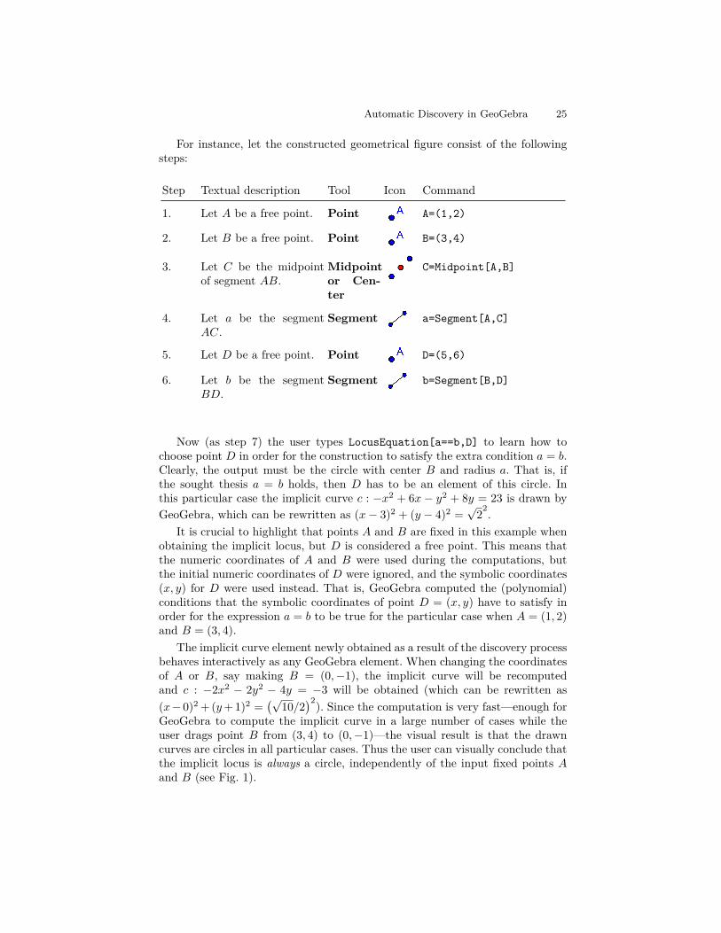
For instance, let the constructed geometrical figure consist of the followingsteps:
Step Textual description Tool Icon Command
1. Let A be a free point. Point A=(1,2)
2. Let B be a free point. Point B=(3,4)
3. Let C be the midpointof segment AB.
Midpointor Cen-ter
C=Midpoint[A,B]
4. Let a be the segmentAC.
Segment a=Segment[A,C]
5. Let D be a free point. Point D=(5,6)
6. Let b be the segmentBD.
Segment b=Segment[B,D]
Now (as step 7) the user types LocusEquation[a==b,D] to learn how tochoose point D in order for the construction to satisfy the extra condition a = b.Clearly, the output must be the circle with center B and radius a. That is, ifthe sought thesis a = b holds, then D has to be an element of this circle. Inthis particular case the implicit curve c : −x2 + 6x − y2 + 8y = 23 is drawn byGeoGebra, which can be rewritten as (x− 3)2 + (y − 4)2 =
√22.
It is crucial to highlight that points A and B are fixed in this example whenobtaining the implicit locus, but D is considered a free point. This means thatthe numeric coordinates of A and B were used during the computations, butthe initial numeric coordinates of D were ignored, and the symbolic coordinates(x, y) for D were used instead. That is, GeoGebra computed the (polynomial)conditions that the symbolic coordinates of point D = (x, y) have to satisfy inorder for the expression a = b to be true for the particular case when A = (1, 2)and B = (3, 4).
The implicit curve element newly obtained as a result of the discovery processbehaves interactively as any GeoGebra element. When changing the coordinatesof A or B, say making B = (0,−1), the implicit curve will be recomputedand c : −2x2 − 2y2 − 4y = −3 will be obtained (which can be rewritten as(x− 0)2 + (y + 1)2 =
(√10/2
)2). Since the computation is very fast—enough forGeoGebra to compute the implicit curve in a large number of cases while theuser drags point B from (3, 4) to (0,−1)—the visual result is that the drawncurves are circles in all particular cases. Thus the user can visually conclude thatthe implicit locus is always a circle, independently of the input fixed points Aand B (see Fig. 1).

26 Abánades, Botana, Kovács, Recio and Sólyom-Gecse
Fig. 1. Dragging point B from (3, 4) to (0, −1) and conjecturing that the implicit locusis always a circle. (Here tracing was enabled for the point B and also for the implicitlocus c.)
As mentioned above, the LocusEquation[T,P] command produces extra nec-essary conditions, say H ′, over P for T to be true for the initial construction.To formally check that the found necessary conditions are also sufficient, theuser needs to use the Prove command with T as thesis for the geometric dia-gram modified so that P satisfies H ′. For instance, in the example above, wehave obtained ‘H ′ = D is in the circle with center B and radius a’, so to provethe conjecture ‘a = b if H ′’ we would type Prove[a==b] for the constructionmodified so that D is defined to be in the circle with center B and radius a.
Technically speaking, the implementation of LocusEquation uses GeoGe-bra’s theorem proving subsystem to translate the geometric construction into acomplex algebraic geometry model and also to obtain an algebraic equation asa representation of the algebraic variety, hence all tools with proof capabilitiescan also be used to obtain an implicit locus [4].
1.1 Examples
https://www.geogebra.org/book/title/id/mbXQuvUV points to a GeoGebra-Book where we describe some examples of use of the LocusEquation commandin GeoGebra. They show how we can (re-)discover and generalize geometric re-sults while pointing out some precautions that one has to keep in mind whileusing this automated geometric discovery tool.

Automatic Discovery in GeoGebra 27
Example Discovering the Simson-Wallace theorem in the above GeoGe-braBook shows how LocusEquation can be used to discover highly non-trivial geometric results. In particular, the classical Wallace-Simson theoremis (re-)discovered.
In example A generalization of the right triangle altitude theorem, a naturalgeneralization of the known right triangle altitude theorem is obtained for non-right triangles.
The examples in Dependency of locus sets on the initial construction 1–2 em-phasize the key idea of the dual symbolic-numeric nature of the protocol behindLocusEquation. They show how the numeric nature of the protocol material-izes in a subtle dependence of the produced necessary conditions on the initial(numeric) coordinates of the basic elements in the construction; in such a waythat for some initial construction we might find that the sought locus is a line,while for other initial configuration it is a circle. An example is also provided inthis section that deals with the important special cases in which a property isnever/always true. It shows how the answer by GeoGebra in these cases takesthe form of a trivially false/true equation.
Being LocusEquation based on algebraic methods, it can sometimes pro-duce sensible conditions from an algebraic point of view that are geometricallymeaningless. That is the case of most of the instances associated to the locus setin example Degenerate cases and necessary not-sufficient conditions, producinggeometrically degenerate situations due to the coincidence of two points.
2 Further developments
We think that featuring automatic discovery tools, in the generalized sense wehave described in section 1, combined with automatic proving, in a widely acce-sible Dynamic Geometry programa such as GeoGebra, is an interesting feature,deserving some consideration in the realm of mathematics education, for in-stance, in the context of intelligent tutoring. The previous list of examples shows,on the one hand, the power of the implemented tool; and, on the other hand, thesubtleties and limitations that are, sometimes, involved in its use. What followsare some reflections on further developments we are currently working on.
2.1 Extending the number of discovery points
Firstly, while the proposed protocol for discovery is naturally aimed to search fornecessary conditions involving more than one point, the LocusEquation com-mand only accepts exactly one point, thus severely limiting the scope of discov-ery. If necessary conditions on a construction are to be discovered, and thereis exactly one point involved in the discovery, the result, if found, returns animplicit curve, which can be plotted, thus graphically suggesting the conjecture.Nevertheless, it is easy to pose questions where there are several (and not neces-sarily free) points a priori unknown on which the discovery is to be performed.Consider, for instance, a triangle ABC and the midpoints D and E of sides
28 Abánades, Botana, Kovács, Recio and Sólyom-Gecse
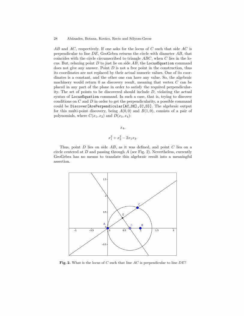
AB and AC, respectively. If one asks for the locus of C such that side AC isperpendicular to line DE, GeoGebra returns the circle with diameter AB, thatcoincides with the circle circumscribed to triangle ABC, when C lies in the lo-cus. But, relaxing point D to just lie on side AB, the LocusEquation commanddoes not give any answer. Point D is not a free point in the construction, thusits coordinates are not replaced by their actual numeric values. One of its coor-dinates is a constant, and the other one can have any value. So, the algebraicmachinery would return 0 as discovery result, meaning that vertex C can beplaced in any part of the plane in order to satisfy the required perpendicular-ity. The set of points to be discovered should include D, violating the actualsyntax of LocusEquation command. In such a case, that is, trying to discoverconditions on C and D in order to get the perpendicularity, a possible commandcould be Discover[ArePerpendicular[AC,DE],C,D]. The algebraic outputfor this multi-point discovery, being A(0, 0) and B(1, 0), consists of a pair ofpolynomials, where C(x1, x2) and D(x3, x4):
x4,
x21 + x2
2 − 2x1x3.
Thus, point D lies on side AB, as it was defined, and point C lies on acircle centered at D and passing through A (see Fig. 2). Nevertheless, currentlyGeoGebra has no means to translate this algebraic result into a meaningfulassertion.
Fig. 2. What is the locus of C such that line AC is perpendicular to line DE?
Automatic Discovery in GeoGebra 29
This example shows that, in some sense, what we are considering as an exten-sion of the LocusEquation command, is the possibility of pointing out severalcoordinates for discovery (such as one for the semi-free point D and two coordi-nates for C), not just the two of the single point P , whose locus we are searchingfor. Moreover, we should also include, in the extended discovery features, the pos-sibility to find the locus, not only of points, but also of some geometric objectssuch as lengths, distances, areas, etc. I.e. we could be asking for the polynomialequation that a length or a distance must satisfy if some thesis is to becometrue.
In particular this could be very useful for automatic derivation, since it canbe considered as a discovery in a context in which there is not a new thesis,but we would like to obtain conclusions from the construction in terms of somespecific variables. Say, to discover the relation between the lengths of the sidesof a triangle and its area, a sort of “locus” of the lengths and the area.
2.2 Handling directly entered algebraic inputs
The theorem proving subsystem is designed to work with geometric inputs likeparallel lines, perpendiculars, intersection of circles, and so on, but not to handlealgebraic descriptions like y = x2 to define a parabola. This means that a directlyentered input equation of a geometric curve cannot be handled at the moment.On the other hand, an algebraic equation is considered to be the natural way forits output, so that the result of the LocusEquation command is internally alwaysan algebraic equation (which is visualized by another subsystem in GeoGebra),independently from computing which type of locus (explicit or implicit).
As a result, unfortunately, the algebraic output cannot be used as anotherinput for the theorem proving subsystem at the moment. This means that, fromthe perspective of automated proving, the user cannot directly investigate theimplicit curve created by the LocusEquation command. It requires to make a newconstruction, including the conjectural locus, and then use the Prove command.To simplify this issue, the theorem proving subsystem has to be extended tomake it possible to handle direct algebraic inputs as well. See https://jira.geogebra.org/browse/TRAC-3596 for more on this.
2.3 3D loci
A further step is to generalize locus computations to work in 3 dimensions.There are no theoretical issues concerning this, but computationally we cannotexpect fast results for the moment. In general the number of coordinates are 50%more than for the 2D case, and this will increase the number of variables by 50%.Considering that the underlying computer algebra system uses Gröbner bases formanipulating the polynomials, and in worst case it is doubly exponential in thenumber of variables, we cannot be optimistic for the general case. Nevertheless,technically it is still possible to generalize the current 2D implementation to be3D ready to harness GeoGebra’s attracting features to visualize 3D objects.

30 Abánades, Botana, Kovács, Recio and Sólyom-Gecse
2.4 Enlarging Boolean expressions
A more promising possibility for further improvement is to enable us-ing disjunctions for Boolean expressions as the first parameter of theLocusEquation command. Clearly, for an arbitrary disjunction A orB, LocusEquation[A||B,...] should be the same as the union ofLocusEquation[A,...] and LocusEquation[B,...], and algebraically theproduct of the two locus equation polynomials will describe the polynomial ofthe union. On the other hand, a similar strategy for conjunctions may be tech-nically more difficult, because a symbolically reliable display of the intersectionof two algebraic curves is a more challenging task.
2.5 Unification parts of the source code
GeoGebra supports symbolic computation of explicit locus equations since ver-sion 4.2 (December 2012) by the result of the collaborative work of some ofthe authors and other researchers (see [2]). Independently from that research,another module of GeoGebra was started in 2011 by the joint work of the au-thors and other developers, namely the theorem proving subsystem includingthe Prove command. It was published in version 5.0 (September 2014) and isbeing improved continuously since then. The implicit locus equation command—presented in this paper—uses the same module.
The two subsystems were developed separately and have no common parts.Meanwhile the first module was not improved any longer, but recently it turnedout that unifying the codebases of the two projects is achievable. Such a unifi-cation would be fruitful to avoid double implementation of translating geometrystatements into algebraic equations, so that user experiments may be extendedalso for the explicit locus equations by harnessing many advanced features ofthe second module, including direct definition of conic sections or geometricinversion.
Fortunately, the GeoGebra Team decided to officially support this workfrom 2016 and the codebase has been started to be merged. See https://jira.geogebra.org/browse/GGB-641 for details. We expect fruitful resultsshortly.
Acknowledgement
First, second and fourth authors are partially supported by the Spanish Re-search Project ‘Construcciones algebro-geométricas: fundamentos, algoritmos yaplicaciones’ (MTM2014-54141-P).
References1. F. Botana, M. Hohenwarter, P. Janičić, Z. Kovács, I. Petrović, T. Recio, S.
Weitzhofer: Automated theorem proving in GeoGebra: Current achievements,Journal of Automated Reasoning 55: 39–59, 2015.

Automatic Discovery in GeoGebra 31
2. F. Botana, Z. Kovács: A Singular web service for geometric computations, Annalsof Mathematics and Artificial Intelligence 74(3-4): 359–370, 2015.
3. G. Dalzotto and T. Recio: On protocols for the automated discovery of theoremsin elementary geometry, Journal of Automated Reasoning 43(2): 203–236, 2009.
4. Z. Kovács, C. Sólyom-Gecse: GeoGebra Tools with Proof Capabilities. http://arxiv.org/abs/1603.01228. March, 2016.

Geodesic Star Unfolding
Md. Ashraful Alam1 and Ileana Streinu1,2
1 Computer Science Department, University of Massachusetts Amherst, Amherst,MA 01003, USA
2 Computer Science Department, Smith College, Northampton, MA 01063, USA
Abstract. If we draw a non-crossing tree on the surface of a convexpolyhedral surface in R3 such that it touches all the vertices of the poly-hedron, and then cut along the tree edges, the resulting surface can beunfolded onto the Euclidean plane, possibly with overlap. A well studiedcase, called star unfolding, cuts along the shortest paths from a sourcepoint to all vertices. This is one of the few instances that guaranteesa non-overlapping unfolding of the flat polygonal surface resulting fromthe cutting. In this paper, we introduce geodesic star unfolding, a gen-eralization that allows cuts along arbitrary geodesics from the sourcepoint to the polyhedral vertices, rather than just the shortest paths. Wediscuss a number of geometric properties that transfer from the shortest-path version, and others (such as non-overlapping) that do not. Some ofthese properties were identified via experimentation with an interactiveMathematica implementation.
1 Introduction
In this paper we introduce a new type of polyhedral unfolding, called geodesicstar unfolding, and initiate the study of its properties. We focus on the compar-ison to the well studied case when the geodesics are all shortest paths. Severaldistinguishing properties are presented via examples obtained by experimenta-tion with an interactive Mathematica implementation.
Fig. 1. A classical example of an edge un-folding obtained by cutting the tetrahedronalong a spanning tree of its 1-skeleton.
Unfolding. Let P be a convex poly-hedron in R3 on whose surface wedraw a collection of non-crossinggeodesic arcs forming a tree andtouching all the vertices of the poly-hedron (this is called a cut tree). If wecut the surface along the tree edges,we obtain an intrinsically flat surfacewith boundary which is topologicallya disk. An unfolding is obtained by
immersing the cut surface into the 2D plane such that it is locally non-overlapping. The boundary becomes a planar polygon which, in general, maynot be simple (i.e. may be self-intersecting) due to global self-overlaps of theimmersed unfolded surface.

Geodesic Star Unfolding 33
Non-overlapping unfoldings. Different types of unfoldings are distinguishedby the choice of the cut tree. The edge unfolding, illustrated in Fig. 1 for atetrahedron, uses a spanning tree of the 1-skeleton of the polyhedron. An edgeunfolding is often non-overlapping, as in Fig. 1, but this does not always happen;self-overlapping examples are presented in [7, 10]. A long standing open questionis whether every convex polyhedron has some edge unfolding to a simple, non-overlapping polygon. Experimental evidence points to a positive answer, yet aproof or counter-example remain elusive. However, there exist specific kinds ofunfoldings which are always non-overlapping: (shortest-path) star unfolding andsource unfolding [5]. In this paper we introduce a generalization of star unfolding;the ultimate goal is to identify critical properties that could help prove globalnon-self-overlap in general unfoldings.
Fig. 2. A tetrahedron with the shortestpaths from a source vertex, and the corre-sponding sp-star unfolding polygon. Sourceand polyhedral vertices are colored inwhite, resp. black.
Shortest-path star unfolding. Thistype of unfolding is obtained bychoosing a point s (the source vertex )on the surface of the polyhedron Pand cutting along the shortest paths(on the surface) from s to all verticesv1, v2, . . . , vn of P , as in Fig. 2. Sincethe cut tree is a star, this is known inthe literature as a star unfolding of P .To distinguish it from the generaliza-tion introduced in this paper, we willrefer to it as the shortest-path star un-
folding, shortly sp-star unfolding. It is also known as Alexandrov unfolding [8],and it was first mentioned in [4]. A detailed exposition can be found in [6].Thenon-overlapping property of the shortest path star unfolding was studied in [5]and a number of applications appear in [1]. Building on these results, we gave in[2] a complete characterization of those polygons which arise as sp-star unfold-ings.
Fig. 3. One of the shortest paths on thetetrahedron from Fig. 2 is replaced bya geodesic. The dotted line indicates thegeodesic which is not a shortest path.
Geodesic star unfolding. We gen-eralize the sp-star unfolding by cut-ting along a star-tree whose edges arenon-crossing geodesics (i.e. not neces-sarily the shortest geodesics) from thesource vertex. We refer to this moregeneral setting as a geodesic star un-folding (shortly, star unfolding in thispaper) and use the term geodesic starunfolding polygon to refer to its polyg-onal boundary.
Contributions. Since geodesic star unfoldings are relaxed versions of sp-starunfoldings, one might anticipate some properties similar to those of the sp-star unfolding, as well as differences. In particular, are they always non-self-
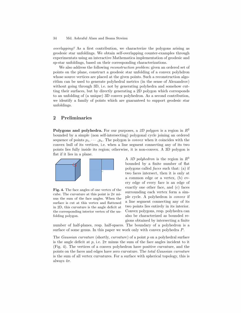
34 Md. Ashraful Alam and Ileana Streinu
overlapping? As a first contribution, we characterize the polygons arising asgeodesic star unfoldings. We obtain self-overlapping counter-examples throughexperimentats using an interactive Mathematica implementation of geodesic andsp-star unfoldings, based on their corresponding characterizations.
We also address the following reconstruction problem: given an ordered set ofpoints on the plane, construct a geodesic star unfolding of a convex polyhdronwhose source vertices are placed at the given points. Such a reconstruction algo-rithm can be used to generate polyhedral metrics (in the sense of Alexandrov)without going through 3D, i.e. not by generating polyhedra and somehow cut-ting their surfaces, but by directly generating a 2D polygon which correspondsto an unfolding of (a unique) 3D convex polyhedron. As a second contribution,we identify a family of points which are guaranteed to support geodesic starunfoldings.
2 Preliminaries
Polygons and polyhedra. For our purposes, a 2D polygon is a region in R2
bounded by a simple (non self-intersecting) polygonal cycle joining an orderedsequence of points p1, · · · , pn. The polygon is convex when it coincides with theconvex hull of its vertices, i.e. when a line segment connecting any of its twopoints lies fully inside its region; otherwise, it is non-convex. A 3D polygon isflat if it lies in a plane.
Fig. 4. The face angles of one vertex of thecube. The curvature at this point is 2π mi-nus the sum of the face angles. When thesurface is cut at this vertex and flattenedin 2D, this curvature is the angle deficit atthe corresponding interior vertex of the un-folding polygon.
A 3D polyhedron is the region in R3
bounded by a finite number of flatpolygons called faces such that: (a) iftwo faces intersect, then it is only ata common edge or a vertex, (b) ev-ery edge of every face is an edge ofexactly one other face, and (c) facessurrounding each vertex form a sim-ple cycle. A polyhedron is convex ifa line segment connecting any of itstwo points lies entirely in its interior.Convex polygons, resp. polyhedra canalso be characterized as bounded re-gions obtained by intersecting a finite
number of half-planes, resp. half-spaces. The boundary of a polyhedron is asurface of some genus. In this paper we work only with convex polyhedra P .
The Gaussian curvature (shortly, curvature) of a point p on a polyhedral surfaceis the angle deficit at p, i.e. 2π minus the sum of the face angles incident to it(Fig. 4). The vertices of a convex polyhedron have positive curvature, and thepoints on the faces and edges have zero curvature. The total Gaussian curvatureis the sum of all vertex curvatures. For a surface with spherical topology, this isalways 4π.

Geodesic Star Unfolding 35
Polyhedral metric and Alexandrov’s Theorem. A polyhedral metric is acollection of (one or more) planar polygonal pieces together with rules for glueingthem, along pieces of their boundaries, into an intrinsic surface with the topologyof a sphere. The glueing may result in a finite set of points of non-zero intrinsic(Gaussian) curvature, called the vertices of the surface. The metric is convex ifthe sum of the surface angles at each vertex is at most 2π, i.e. if the curvatureis positive. The following classical result provides the connection with convexpolyhedra.
Theorem 1. (A.D. Alexandrov’s theorem [3]) For every convex polyhedralmetric, there exists a unique convex polyhedron (up to translation and symmetry)realizing this metric.
As a side note, we remark that the edges of the polygonal pieces in the polyhedralmetric need not be related in any way to the edges of the realization as a convexpolyhedron, and that there exist infinitely many polyhedral metrics that giverise to the same convex polyhedron.
Shortest paths and geodesics. A shortest path between two points on aconvex polyhedral surface P is the shortest of all possible curves between thesetwo points, measured on the surface of P . Various properties of shortest pathson polyhedral surfaces have been identified in [11, 9].
A geodesic path between two points on the surface is a locally shortest path. Inthis paper we consider only non-self-intersecting (simple) geodesics and refer tothem, shortly, as geodesics. Given two points on the polyhedral surface, theremay be more than one (even an infinity of) geodesic paths between them. Theshortest paths, by definition, are geodesics. However, in this paper we need todistinguish those which are not shortest paths: in short, we refer to them simplyas geodesics. For a convex polyhedral surface, a geodesic segment may contain apoint of strictly positive curvature (i.e. a polyhedral vertex) only as an endpoint(but not strictly interior to the segment). In particular, a geodesic segment is astraight line segment on some unfolding of (possibly, a cover of) the surface.
Geodesic star unfolding. We consider only unfoldings which are obtained bycutting a polyhedral surface along a tree whose edges are disjoint (non-crossing,simple) geodesic segments. These tree edges may be shortest geodesics, as is thecase for all edge or sp-star unfoldings. The geodesic star unfolding (shortly, starunfolding) is obtained by cutting along geodesic edges connected as a star, butwhere some or all of these edges are not shortest paths. The common vertexs of all the edges is called the source vertex. The polygon obtained via a starunfolding (Fig. 2) has 2n vertices: n of them correspond to polyhedral verticesof P and n to copies of the source vertex (source images). These two typesof vertices appear alternately on the boundary of the unfolding, meaning eachsource image has one polyhedral vertex preceeding and one following it, in cyclicorder. The angle at each source image is a source angle. The sum of all sourceangles is 2π when the source vertex is on a polyhedral face or an edge and strictly

36 Md. Ashraful Alam and Ileana Streinu
less than 2π when it is placed on a polyhedral vertex (by an amount given bythe curvature of the polyhedral vertex). Given a polyhedron, a source vertex anda geodesic star, we can angularly sort the star edges around the source vertex.This induces a circular ordering of the polyhedral vertices. If we join by shortestpaths the polyhedral vertices, in this order, we obtain a geodesic polygon on thesurface of the polyhedron. In the case of an sp-star unfolding, this polygon isnon-self-intersecting and bounds a region called the core of the sp-star. In thecorresponding sp-star unfolding, the core unfolds as the inner polygonal regionobtained by joining the polyhedral vertices in the order in which they appear onthe boundary of the unfolding polygon.
Voronoi diagram. A set Pn of n points (called sites) in the Euclidean planeinduces a Voronoi diagram VD(Pn). This is a planar subdivision of n Voronoiregions (one for each site), Voronoi edges between them and Voronoi verticeswhere the Voronoi edges meet, defined as follows. An arbitrary point x ∈ R2 liesin the Voronoi region of site pi if the Euclidean distance from x to pi is smallerthan the distance to any other point pj ∈ Pn, j 6= i. There are two kinds ofVoronoi edges: segments, bounded at both ends by Voronoi vertices, and rays,having just one Voronoi vertex at one end (the closed end) but unbounded atthe other end (the open end).
Ridge tree. Given a source point s on the surface of a convex polyhedron P ,the ridge tree is the set of all the points r ∈ P for which there exist at least twodistinct shortest paths from r to s on the surface. It is known that its closureis a tree which touches all the vertices of the polyhedron. Another remarkableproperty (see [5]) relates the sp-star unfolding to the ridge tree (from the samesource vertex), as follows. Take the images of the source vertex in the sp-starunfolding and compute their Voronoi diagram. Then delete the part that liesoutside the sp-star unfolding polygon: what remains is a tree which, on the(folded) 3D polyhedron surface, is precisely the ridge tree for source s.
3 Characterization of geodesic star unfoldings
In this section we prove a very simple characterization of (geodesic) star un-foldings, and remind the reader of additional features of sp-star unfoldings. Thebasic properties of a geodesic star unfolding mentioned in the Introduction leadto the following definition:
Su-Polygon. An su-polygon (short for abstract star-unfolding polygon3) is adisk-like zero-curvature (intrinsically flat) surface, whose boundary satisfies thefollowing properties (known to hold by any geodesic star unfolding polygon): (a)it has 2n vertices, alternately labeled as si and vi and referred to as s-, resp.v-vertices. The angle (interior to the surface) at an s-vertex is refered to as ans-angle; (b) the sum of all the s-angles is 2π, and (c) the v-vertices are placed
3 The modifier “abstract” is used to emphasize that, a priori, such polygons are notguaranteed to arise from star unfoldings of 3D convex polyhedra.
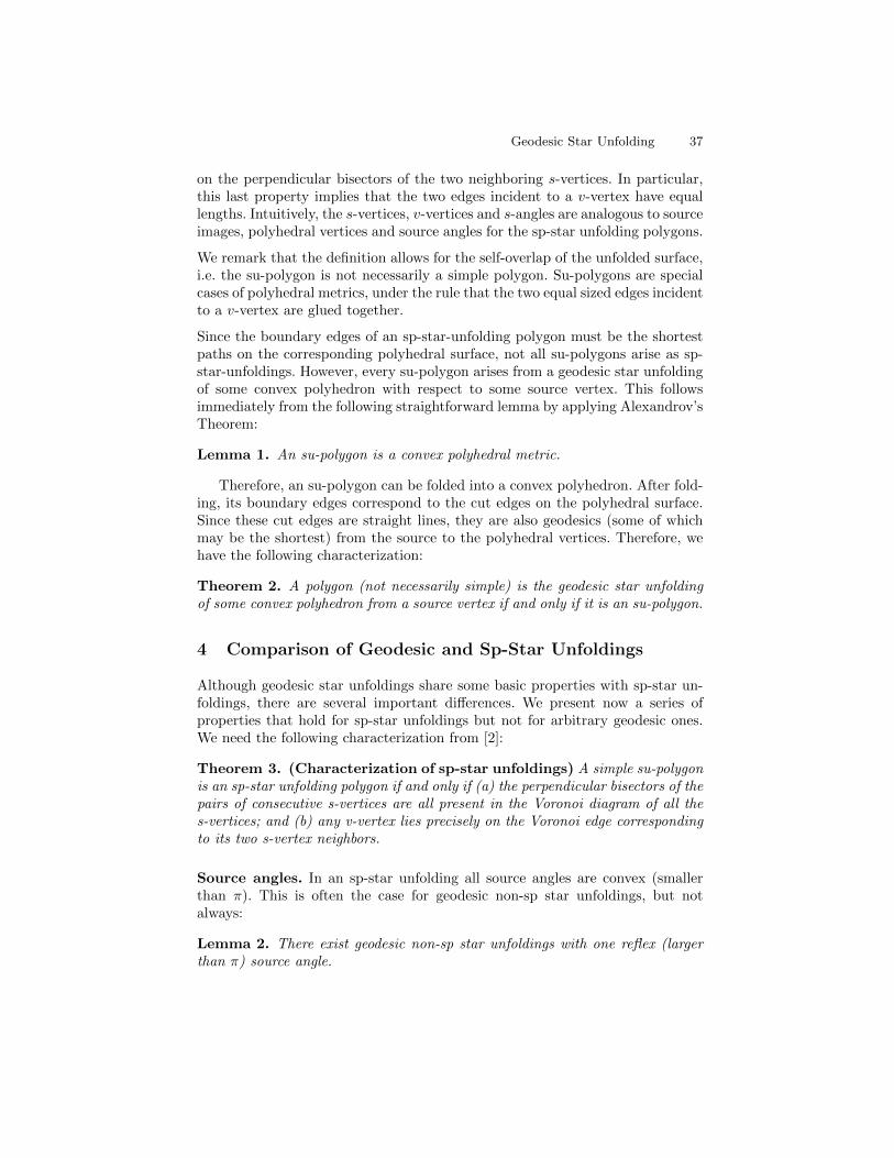
Geodesic Star Unfolding 37
on the perpendicular bisectors of the two neighboring s-vertices. In particular,this last property implies that the two edges incident to a v-vertex have equallengths. Intuitively, the s-vertices, v-vertices and s-angles are analogous to sourceimages, polyhedral vertices and source angles for the sp-star unfolding polygons.
We remark that the definition allows for the self-overlap of the unfolded surface,i.e. the su-polygon is not necessarily a simple polygon. Su-polygons are specialcases of polyhedral metrics, under the rule that the two equal sized edges incidentto a v-vertex are glued together.
Since the boundary edges of an sp-star-unfolding polygon must be the shortestpaths on the corresponding polyhedral surface, not all su-polygons arise as sp-star-unfoldings. However, every su-polygon arises from a geodesic star unfoldingof some convex polyhedron with respect to some source vertex. This followsimmediately from the following straightforward lemma by applying Alexandrov’sTheorem:
Lemma 1. An su-polygon is a convex polyhedral metric.
Therefore, an su-polygon can be folded into a convex polyhedron. After fold-ing, its boundary edges correspond to the cut edges on the polyhedral surface.Since these cut edges are straight lines, they are also geodesics (some of whichmay be the shortest) from the source to the polyhedral vertices. Therefore, wehave the following characterization:
Theorem 2. A polygon (not necessarily simple) is the geodesic star unfoldingof some convex polyhedron from a source vertex if and only if it is an su-polygon.
4 Comparison of Geodesic and Sp-Star Unfoldings
Although geodesic star unfoldings share some basic properties with sp-star un-foldings, there are several important differences. We present now a series ofproperties that hold for sp-star unfoldings but not for arbitrary geodesic ones.We need the following characterization from [2]:
Theorem 3. (Characterization of sp-star unfoldings) A simple su-polygonis an sp-star unfolding polygon if and only if (a) the perpendicular bisectors of thepairs of consecutive s-vertices are all present in the Voronoi diagram of all thes-vertices; and (b) any v-vertex lies precisely on the Voronoi edge correspondingto its two s-vertex neighbors.
Source angles. In an sp-star unfolding all source angles are convex (smallerthan π). This is often the case for geodesic non-sp star unfoldings, but notalways:
Lemma 2. There exist geodesic non-sp star unfoldings with one reflex (largerthan π) source angle.

38 Md. Ashraful Alam and Ileana Streinu
Proof. An example of a geodesic star unfolding polygon with one source anglelarger than π is shown in Fig. 3. Since the angle sum at the source vertex is atmost 2π, at most one source angle can be reflex.
Placement of polyhedral vertices. The characterization of sp-star unfoldingpolygons [2] states that if vi is the v-vertex between two s-vertices si and si+1,then the Voronoi diagram of the source vertices contains an edge between thesetwo sites, and, moreover, vi lies precisely on this Voronoi edge (segment or ray).This property depends on the “shortest path” assumption and does not extendto arbitrary geodesic star unfoldings.
Fig. 5. An example of a geodesic star unfolding with v-vertices that do not lie onVoronoi edges: the polyhedral vertex v2 is on the extension of a Voronoi segment andthe bisector on which v4 lies is not present in the Voronoi diagram.
Lemma 3. There exist geodesic star unfolding polygons where some perpendic-ular bisectors on which the polyhedral vertices lie are not part of the Voronoidiagram.
Lemma 4. There exist geodesic star unfolding polygons where some polyhedralvertex lies not on its corresponding Voronoi segments, but on an extension ofthe underlying bisector.
Proof. Both cases are illustrated in Fig. 5. ut
Ridge tree. In the case of an sp-star unfolding, we have seen that the ridge treeis part of the Voronoi diagram of the source images. The above counter-examplesindicate that this may not be the case for arbitrary geodesic star unfoldings.
Self-overlapping geodesic star unfolding. It is known that sp-star unfold-ings are non-self-overlapping. On the other side:
Lemma 5. There exist self-overlapping geodesic star unfolding polygons.
Proof. The example in Fig. 6 has been obtained by experimenting with an in-teractive implementation of su-polygons in Mathematica. ut

Geodesic Star Unfolding 39
Fig. 6. An example of a self-overlapping geodesic star unfolding polygon. Polyhedral,resp. source vertices are shown with colored circles, resp. white squares.
Fig. 7. An example of a geodesic star un-folding where the core polygon, shown inblue, is self-intersecting.
Self-intersecting core. The coreof an sp-star unfolding joins the v-vertices and is a simple polygon [6].Furthermore, in this case the core, asa polygonal region, contains the ridgetree inside. On the other hand:
Lemma 6. There exist convex poly-hedra, source vertices and non-crossinggeodesics from the source to the poly-hedral vertices such that the core ofthe resulting geodesic star unfoldingpolygon is self-intersecting.
Proof. An example, obtained by ex-perimentation with our interactive
Mathematica implementation of su-polygons, is shown in Fig. 7. ut
5 Reconstruction of geodesic star unfolding polygons
Based on the characterization given in Theorem 3, we presented in [2] a lin-ear time algorithm that constructs sp-star unfolding polygons with prescribedcombinatorics, as captured in the (topologically embedded) ridge tree. It turnsout that our algorithm always produces an sp-star unfolding polygon whose s-vertices lie in convex position. We also know that this property, of having thesource vertices in convex position, does not hold for all sp-star unfoldings poly-gons. On the other hand, if we are given an ordered point set in convex position,

40 Md. Ashraful Alam and Ileana Streinu
is it true that it supports some sp-star unfolding? This question was answered inthe negative in [2]. Here, we investigate the extent to which such reconstructionquestions can be answered for geodesic star unfoldings, where we encounter newchallenges.
Challenges. We have shown in [2] that not all ordered sets of s-vertices supportsp-star unfolding polygons, and in particular not all that are in convex position.For this purpose, we introduced the concept of a flap polygon, which satisfiesthe same properties as a sp-star unfolding polygon except that the source vertexangle sum may be arbitrary (in particular, larger than 2π). We defined theextreme flap polygon, whose v-vertices are placed at Voronoi vertices in a specificmanner that minimizes the source angle sum; when these vertices are moved awayfrom the Voronoi vertex on incident Voronoi edges, this angle sum increases. Forcertain source point sets, the angle sum of the extreme flap polygon exceeds 2π,hence they do not support any sp-star unfolding polygon.
However, this constraint is not prohibitive for arbitrary geodesic star unfold-ings: here, the polyhedral vertices are not constrained to lie on correspondingVoronoi segments. Hence if the sum of the s-angles of an extreme flap polygon islarger than 2π, we can push some v-vertices inwards until the s-angles sum up to2π. This causes some v-vertices to be placed on the line extension of their cor-responding Voronoi segments. Theorems 3 and 2 then ensure that the resultingpolygon is a geodesic star unfolding.
Fig. 8. An example of a extreme flap polygon whose s-angle sum is larger than 2π. Itis difficult to push the v-vertices inwards (on the line extensions of the correspondingVoronoi edges) to achieve a sum of the s-angles equal to 2π, while maintaining a validgeodesic star unfolding. Note that in this example, the s-vertices are in convex positionand hence all the consecutive bisectors are part of the Voronoi diagram.
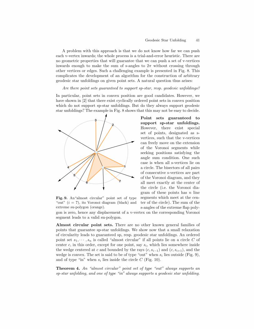
Geodesic Star Unfolding 41
A problem with this approach is that we do not know how far we can pusheach v-vertex inwards; the whole process is a trial-and-error heuristic. There areno geometric properties that will guarantee that we can push a set of v-verticesinwards enough to make the sum of s-angles to 2π without crossing throughother vertices or edges. Such a challenging example is presented in Fig. 8. Thiscomplicates the development of an algorithm for the construction of arbitrarygeodesic star unfoldings on given point sets. A natural question thus arises:
Are there point sets guaranteed to support sp-star, resp. geodesic unfoldings?
In particular, point sets in convex position are good candidates. However, wehave shown in [2] that there exist cyclically ordered point sets in convex positionwhich do not support sp-star unfoldings. But do they always support geodesicstar unfoldings? The example in Fig. 8 shows that this may not be easy to decide.
1
2
3
4
5
6 7
Fig. 9. An“almost circular” point set of type“out” (i = 7), its Voronoi diagram (black) andextreme su-polygon (orange).
Point sets guaranteed tosupport sp-star unfoldings.However, there exist specialset of points, designated as s-vertices, such that the v-verticescan freely move on the extensionof the Voronoi segments whileseeking positions satisfying theangle sum condition. One suchcase is when all s-vertices lie ona circle. The bisectors of all pairsof consecutive s-vertices are partof the Voronoi diagram, and theyall meet exactly at the center ofthe circle (i.e. the Voronoi dia-gram of these points has n linesegments which meet at the cen-ter of the circle). The sum of thes-angles of the extreme flap poly-
gon is zero, hence any displacement of a v-vertex on the corresponding Voronoisegment leads to a valid su-polygon.
Almost circular point sets. There are no other known general families ofpoints that guarantee sp-star unfoldings. We show now that a small relaxationof circularity leads to guaranteed sp, resp. geodesic star unfoldings. An orderedpoint set s1, · · · , sn is called “almost circular” if all points lie on a circle C ofcenter c, in this order, except for one point, say si, which lies somewhere insidethe wedge centered at c and bounded by the rays (c, si−1) and (c, si+1), and thewedge is convex. The set is said to be of type “out” when si lies outside (Fig. 9),and of type “in” when si lies inside the circle C (Fig. 10).
Theorem 4. An “almost circular” point set of type “out” always supports ansp-star unfolding, and one of type “in” always supports a geodesic star unfolding.

42 Md. Ashraful Alam and Ileana Streinu
1
2
34
5
6
7
(a)
1
2
34
5
67
(b)
Fig. 10. Two “almost circular” point sets (i = 7) of type “in”: (a) convex and (b)non-convex. The Voronoi diagram is shown in black. In orange is shown the adaptedgeodesic su-polygon, with all the source vertices at the center of the circles, except forthe two incident with the special source vertex (shown slightly apart from the extremeposition, for clarity).
Proof. (Sketch) Let c be the center of the circle and assume, without loss ofgenerality, that the points are labeled consecutively such that let s1, · · · , sn lieon the circle, except si (the “special” source vertex) which lies somewhere insidethe wedge (si−1, c, si+1). We place the v-vertices on the corresponding Voronoisegments and build the flap polygon by joining the s- and v-vertices alternately.Let us label the vertices of su-polygon as s1, v1, s2, v2, . . . , si, vi, . . . , sn, vn. Weanalyze three cases, illustrated in Figs. 9 and 10.
Case “Out”: si lies outside the circle C. Independent on whether the wholepoint set is convex or not, the extreme su-polygon has the same shape, illustratedin Fig. 9, with exactly two strictly positive source angles. Since the total curva-ture at the source vertex is positive, the point set supports an sp-star unfoldingpolygon.
Case “In”: si lies inside the circle C. The entire point set may be convex ornot, depending on whether the special point lies outside or inside the convex hullof the others. In the first case, the Voronoi diagram has only unbounded faces,otherwise the Voronoi region for the special source vertex is bounded (Fig. 10).
In both cases, we define an adapted extreme su-polygon, where all v-verticesare moved to the center of the circle except vi−1 and vi. The lines si−1c andsi+1c will intersect the Voronoi segments corresponding to vi−1 and vi respec-tively. We place vi−1 and vi, respectively, on those intersection points, as illus-trated in Fig. 10 (where these vertices are shown slightly apart from the extremeposition, for clarity). In this configuration, the s-angles at all s-vertices exceptsi are zero, and thus the total angle sum at the s-vertices is no more than 2π
Geodesic Star Unfolding 43
(positive curvature). All v-vertices except vi−1 and vi are on the extension oftheir corresponding Voronoi segments, while vi−1 and vi lie on the Voronoi seg-ments. Now we can now move the v-vertices that are placed on the center of thecircle, outwards (away from the center of the circle in the direction towards theVoronoi edge to which they are associated) and the s-angle sum increases. Thisallows us to obtain a geodesic su-polygon by moving a little so that all s-vertexangles are strictly positive.
This concludes the proof that almost circular point sets support geodesicstar-unfoldings. ut
Conclusion. We have examined some properties of geodesic star unfoldingsthat distinguish them from shortest-path star unfoldings. In particular, we haveshown that they may not always lead to simple (non-overlapping) unfoldings.We have also discussed specific challenges for reconstructing geodesic star un-foldings on given point sets and presented a method to construct the geodesicstar unfolding for “almost circular” points.
Acknowledgement. This research was supported by the NSF grant CCF-1319366 of the second author.
References
1. P. K. Agarwal, B. Aronov, J. O’Rourke, and C. A. Schevon. Star unfolding of apolytope with applications. SIAM J. Computing, 26:1689–1713, 1997.
2. M. A. Alam and I. Streinu. Star unfolding polygons. In F. Botana and P. Quaresma,editors, Lecture Notes in Artificial Intelligence 9201, Automated Deduction in Ge-ometry (ADG’14, Coimbra, Portugal, July 9-11, 2014), volume 9201 of LectureNotes in Artificial Intelligence, pages 1–20. Springer Verlag, 2015. ISBN 978-3-319-21362-0.
3. A. D. Alexandrov. Convex Polyhedra. Springer Monographs in Mathematics.Springer Verlag, Berlin Heidelberg, 2005. English Translation of Russian edition,Gosudarstv. Izdat.Tekhn.-Teor.Lit., Moscow-Leningrad, 1950.
4. A. D. Alexandrov. Intrinsic Geometry of Convex Surfaces. Chapman andHill/CRC, Taylor and Francis Group, Boca Raton, Florida, 2006. Selected WorksII, translated from Russian by S. S. Kutateladze.
5. B. Aronov and J. O’Rourke. Non-overlap of the star unfolding. Discrete andComputational Geometry, 8:219–250, 1992.
6. E. D. Demaine and J. O’Rourke. Geometric Folding Algorithms: Linkages,Origami, and Polyhedra. Cambridge University Press, 2007.
7. K. Fukuda. Strange unfoldings of convex polytopes. http://www.ifor.math.ethz.ch/~fukuda/unfold_home/unfold_open.html, 1997.
8. E. Miller and I. Pak. Metric combinatorics of convex polyhedra: Cut loci andnonoverlapping unfoldings. Discrete Comput. Geom., 39(1):339–388, 2008.
9. D. Mount. On finding shortest path on convex polyhedra. Technical Report 1495,University of Maryland, 1985.
10. W. Schlickenrieder. Nets of polyhedra. Technical report, Technische UniversitatBerlin, 1997.
11. M. Sharir and A. Schorr. On shortest path in polyhedral spaces. SIAM Journalon Computing, 15(1):193–215, February 1986.

Geometric Deformations of Sodalite Frameworks
Ciprian Borcea1 and Ileana Streinu2
1 Department of Mathematics, Rider University, Lawrenceville, NJ 08648, USA2 Computer Science Department, Smith College, Northampton, MA 01063, USA
Abstract. In mathematical crystallography and computational mate-rials science, it is important to infer flexibility properties of frameworkmaterials from their geometric representation. We study combinatorial,geometric and kinematic properties for frameworks modeled on sodalite.
Keywords: periodic framework, sodalite, geometric flexibility.
1 Introduction
In this paper we study the deformation space of a periodic framework modeledafter the ideal sodalite.
The sodalite framework is the prototype of numerous crystal structures. Infact, more than 900 crystals of this family have been identified [7]. This structureis remarkable not only for crystallography and materials science. It has directconnections with tiling and sphere packing problems and has natural generaliza-tions in arbitrary dimension [11].
A one-parameter geometric deformation of sodalite was first observed byPauling [12] in 1930, and used as a phase transition model [10, 13, 5].
We show that, besides this classical ‘Pauling tilt scenario’, the deformationspace of sodalite includes a six-dimensional component, which can be describedin fairly intuitive terms.
Our study relies on the mathematical foundations of a deformation theoryfor periodic frameworks introduced in [2]. In general, the deformation spaceis a semi-algebraic set made of real solutions of a finite system of polynomialequations. For applications, such as displacive phase transitions in crystallinematerials, it is highly desirable to obtain explicit and detailed descriptions ofthe deformation space [6, 3, 4].
We start with the presentation of the three-dimensional structure of the idealsodalite framework in a realization with congruent regular tetrahedra and max-imal crystallographic symmetry [10, 9, 4]. We express the periodic graph under-lying the framework via 6-rings of tetrahedra with marked periods. This formu-lation leads naturally into considerations of symmetry preservation in deforma-tions, with central symmetry at the forefront. The existence of a six-dimensionaldeformation component follows naturally from this formulation. We also inves-tigate dihedral symmetry and use it to explain the one-dimensional ‘classicalPauling tilt’.

Geometric Deformations of Sodalite Frameworks 45
2 A placement with maximal symmetry
We use Figure 1 to illustrate the essential aspects of the initial placement ofthe sodalite framework: a 6-ring of regular tetrahedra (a) is placed in a specificmanner relative to a cube of side length 2 centered at the origin (c). Three pairsof parallel vectors between specific vertices of the ring (b) yield the generatorsof the periodicity lattice.
(a) (b)
(c) (d)
Fig. 1. An ideal sodalite placement with cubical symmetry. A 6-ring of this frameworkis highlighted, with three pairs of generators of the periodicity lattice. In each pair thevectors must be equal. All tetrahedra are congruent and regular.

46 Ciprian Borcea and Ileana Streinu
Specifically, we consider the origin of the Cartesian system of coordinates at thecenter of the cube depicted in Fig.1 (c), with standard basis vectors e1, e2, e3reaching to the centers of the frontal, right side and top face respectively. Thus,the edge length for the cube is 2. The edge length for the regular tetrahedra ofthe framework is determined by the condition that each tetrahedron has a pairof opposite (and hence orthogonal) edges parallel to a pair of standard directionsei, ej . This requires an edge lengths of 2a, with a =
√2− 1.
The 4 × 6 = 24 tetrahedra around the cube. We give the coordinates forthe four vertices v0, ..., v3 of the tetrahedron touching the cube at v0 = e1 + e3.They are:
v0 = (1, 0, 1), v1 = (1, 0, 2√
2− 1), (1)
v2 = (√
2− 1,√
2− 1,√
2), v3 = (√
2− 1, 1−√
2,√
2)
The coordinates for the vertices of the other tetrahedra are obtained by sym-metry. The symmetries of the cube are represented by permutations and signchanges of the three coordinates and form a group of order 3! · 23 = 48. Thisgroup has a double-transitive action on the 24 framework tetrahedra around thecube.
Periodicity lattice. The translational symmetries of the whole framework aregenerated by the three (pairs of equal) vectors shown in Figure 1(b). In coordi-nates:
λ1 =√
2(1,−1,−1), λ2 =√
2(−1, 1,−1), λ3 =√
2(−1,−1, 1) (2)
with the natural labeling suggested by the order three rotational symmetryaround the diagonal direction e1 + e2 + e3. We note that the periods
λ2 + λ3 = −2√
2e1, λ3 + λ1 = −2√
2e2, λ1 + λ2 = −2√
2e3 (3)
are mutually orthogonal and generate a sublattice of index 2 in the full lattice ofperiods generated by (2).
The sodalite cage and the Kelvin polyhedron. The 24 framework tetra-hedra wrapped around a cube form a so-called sodalite cage. We note that thebarycenter of the tetrahedron in (1) has coordinates b = ( 1√
2, 0,√
2) and the
barycenters of the 6-ring of tetrahedra highlighted in Figure 1 form the verticesof a planar regular hexagon of edge one, centered at c = 1√
2(1, 1, 1).
Thus, the 24 barycenters of the sodalite cage tetrahedra give the vertices ofa centrally symmetric polyhedron with 8 hexagonal faces and 6 square faces.Under translation by the periodicity lattice Λ generated by (2), this polyhedrontiles the three dimensional space R3, as illustrated in Figure 2. Translationsidentifying opposite faces are periods and generate the periodicity lattice Λ. Thepolyhedron is the Voronoi cell at the origin for the lattice Λ. It may be seen as atruncated regular octahedron (with edge length 3 at our chosen scale). It is alsocalled the Kelvin polyhedron, due to a famous conjecture formulated by Kelvin

Geometric Deformations of Sodalite Frameworks 47
Fig. 2. Kelvin polyhedra tiling space.
[14] and disproved by a counter-example of Weaire and Phelan [15]. The namepermutohedra is also used for a family which includes this polyhedron.
Fig. 3. (Left) Periodicity identifications in the Kelvin polytope. Opposite faces areidentified by translation. (Right) The quotient graph of the Kelvin polytope skeleton.
Figure 3 illustrates the result of periodicity identifications in the vertex-and-edgeskeleton of a sodalite cage. The quotient graph pattern is also encoded in a 6-ring(with marked periods), as discussed below.
The 6-rings. A 6-ring of tetrahedra, as in Figure 1, contains all the informationneeded for generating the whole periodic framework. It contains vertex represen-tatives for all the vertex orbits and edge representatives for all the edge orbitsunder periodicity. The 6 pairs of vertices which have to be further identified byperiodicity provide the generators of the periodicity lattice Λ. It is important tonote that (up to sign) we have exactly three generators, since the 6 periods, as
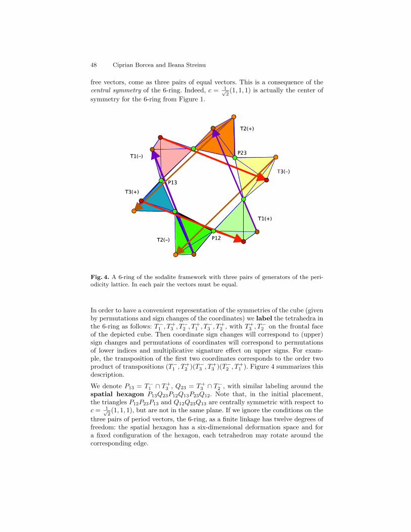
48 Ciprian Borcea and Ileana Streinu
free vectors, come as three pairs of equal vectors. This is a consequence of thecentral symmetry of the 6-ring. Indeed, c = 1√
2(1, 1, 1) is actually the center of
symmetry for the 6-ring from Figure 1.
Fig. 4. A 6-ring of the sodalite framework with three pairs of generators of the peri-odicity lattice. In each pair the vectors must be equal.
In order to have a convenient representation of the symmetries of the cube (givenby permutations and sign changes of the coordinates) we label the tetrahedra inthe 6-ring as follows: T−1 , T
+3 , T
−2 , T
+1 , T
−3 , T
+2 , with T+
3 , T−2 on the frontal face
of the depicted cube. Then coordinate sign changes will correspond to (upper)sign changes and permutations of coordinates will correspond to permutationsof lower indices and multiplicative signature effect on upper signs. For exam-ple, the transposition of the first two coordinates corresponds to the order twoproduct of transpositions (T−1 , T
+2 )(T−3 , T
+3 )(T−2 , T
+1 ). Figure 4 summarizes this
description.
We denote P13 = T−1 ∩ T+3 , Q23 = T+
3 ∩ T−2 , with similar labeling around thespatial hexagon P13Q23P12Q13P23Q12. Note that, in the initial placement,the triangles P12P23P13 and Q12Q23Q13 are centrally symmetric with respect toc = 1√
2(1, 1, 1), but are not in the same plane. If we ignore the conditions on the
three pairs of period vectors, the 6-ring, as a finite linkage has twelve degrees offreedom: the spatial hexagon has a six-dimensional deformation space and fora fixed configuration of the hexagon, each tetrahedron may rotate around thecorresponding edge.
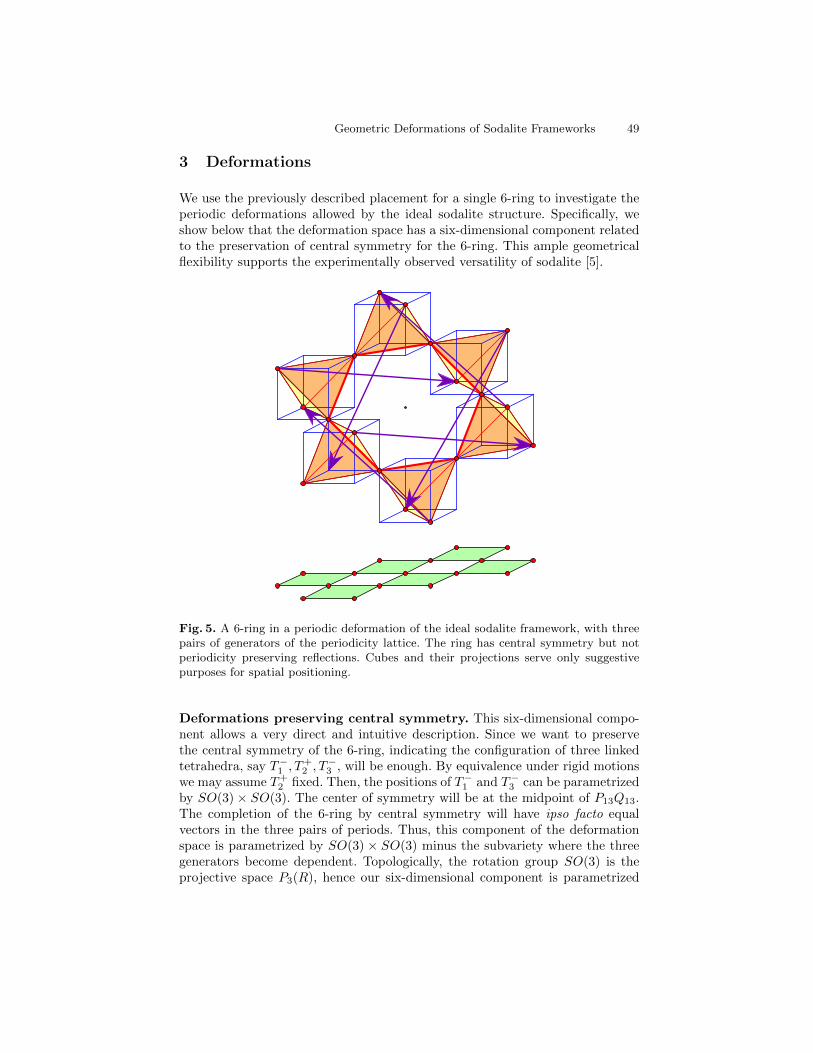
Geometric Deformations of Sodalite Frameworks 49
3 Deformations
We use the previously described placement for a single 6-ring to investigate theperiodic deformations allowed by the ideal sodalite structure. Specifically, weshow below that the deformation space has a six-dimensional component relatedto the preservation of central symmetry for the 6-ring. This ample geometricalflexibility supports the experimentally observed versatility of sodalite [5].
Fig. 5. A 6-ring in a periodic deformation of the ideal sodalite framework, with threepairs of generators of the periodicity lattice. The ring has central symmetry but notperiodicity preserving reflections. Cubes and their projections serve only suggestivepurposes for spatial positioning.
Deformations preserving central symmetry. This six-dimensional compo-nent allows a very direct and intuitive description. Since we want to preservethe central symmetry of the 6-ring, indicating the configuration of three linkedtetrahedra, say T−1 , T
+2 , T
−3 , will be enough. By equivalence under rigid motions
we may assume T+2 fixed. Then, the positions of T−1 and T−3 can be parametrized
by SO(3)× SO(3). The center of symmetry will be at the midpoint of P13Q13.The completion of the 6-ring by central symmetry will have ipso facto equalvectors in the three pairs of periods. Thus, this component of the deformationspace is parametrized by SO(3) × SO(3) minus the subvariety where the threegenerators become dependent. Topologically, the rotation group SO(3) is theprojective space P3(R), hence our six-dimensional component is parametrized

50 Ciprian Borcea and Ileana Streinu
by an open and dense subset of P3(R)× P3(R). One configuration is illustratedin Figure 5 and shows that reflection symmetries of the initial 6-ring are lost.
Deformations preserving dihedral symmetry D3. We now investigate de-formations which preserve the symmetries induced by permutations of coordi-nates in the initial placement. This group of order six may be conceived as adihedral group D3 generated by reflections in three planes with a common axisand forming dihedral angles of π/3 or 2π/3. When restricting our attention toour chosen 6-ring, the group is simply transitive on the six tetrahedra and theirbarycenters form the vertices of a planar regular hexagon.
Suppose we want to preserve the reflection symmetry given by the transpositionof the first two coordinates in the initial placement. The reflection plane goesthrough P12 andQ12 and the two marked periods from T−2 to T−1 and respectivelyT1+ to T+
2 are parallel to this plane and one is the reflection of the other.
Thus, in order to retain this feature when deforming the 6-ring, we look only atthe three linked tetrahedra T−1 , T
+3 , T
−2 and adopt as reflection plane the plane
through P12Q12 which runs parallel to the period from T−2 to T−1 . When wecomplete the 6-ring by reflection in this plane, we have to satisfy only one ofthe remaining periodicity constraints, since the other one will then be fulfilledas well by reflection.
Fig. 6. A tetrahedrite 6-ring resulting from a periodic deformation of the ideal sodaliteframework. The regular tetrahedra are pointing towards the viewer. The 6-ring has D3
dihedral symmetry but no central symmetry.
Similar considerations apply for the other two transpositions of coordinates. InFigure 6 we show a deformation which has preserved all three reflections, but

Geometric Deformations of Sodalite Frameworks 51
central symmetry for the 6-ring has been lost. The illustrated structure is that ofanother mineral called tetrahedrite. According to [1], this relationship betweensodalite and tetrahedrite was noticed only at a later stage in the mineralogyliterature, by A.S. Povarennykh. We now compare deformations which ‘break’the central symmetry of the 6-ring and those which maintain it.
Fig. 7. The regular hexagon of barycenters in a 6-ring with D3 dihedral symmetry.Circumscribed spheres for linked tetrahedra meet in circles on the reflection planes. Apossible edge position is shown.
Given the observed fact that barycenters must form a planar regular hexagon, wemay start with the configuration shown in Figure 7. The connecting vertices ofthe tetrahedra in the 6-ring must be in the reflection planes, indicated by theircommon axis and intersections with the plane of barycenters. More precisely,they belong to circles of intersection of circumscribed spheres of consecutivetetrahedra. Since one edge determines by symmetry the entire 6-ring, we seethat we have a one-parameter family of possible configurations for the 6-ringwith given hexagon of barycenters. When we ask for fulfillment of the period-icity conditions, the selection of the edge is subject to an additional conditionexpressing the parallelism of one of the periods to the corresponding reflectionplane.
These considerations show that deformations preserving a dihedral D3 sym-metry consist of curves. One type breaks the central symmetry of the 6-ring:this is the ‘Pauling tilt scenario’ [12, 13, 10, 8, 5]. As mentioned above, the tetra-hedrite structure can be reached via this classical tilt. What is distinctive in thisscenario is that sodalite cages maintain their shape, although decreasing in sizerelative to the initial case.
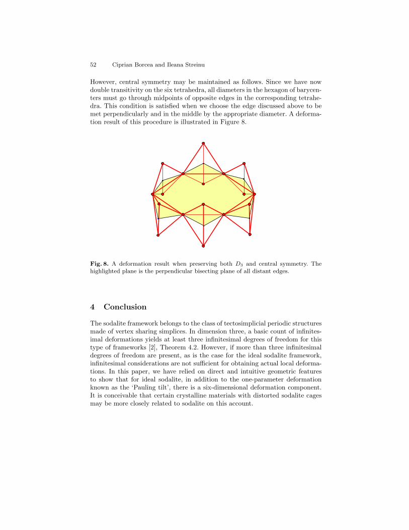
52 Ciprian Borcea and Ileana Streinu
However, central symmetry may be maintained as follows. Since we have nowdouble transitivity on the six tetrahedra, all diameters in the hexagon of barycen-ters must go through midpoints of opposite edges in the corresponding tetrahe-dra. This condition is satisfied when we choose the edge discussed above to bemet perpendicularly and in the middle by the appropriate diameter. A deforma-tion result of this procedure is illustrated in Figure 8.
Fig. 8. A deformation result when preserving both D3 and central symmetry. Thehighlighted plane is the perpendicular bisecting plane of all distant edges.
4 Conclusion
The sodalite framework belongs to the class of tectosimplicial periodic structuresmade of vertex sharing simplices. In dimension three, a basic count of infinites-imal deformations yields at least three infinitesimal degrees of freedom for thistype of frameworks [2], Theorem 4.2. However, if more than three infinitesimaldegrees of freedom are present, as is the case for the ideal sodalite framework,infinitesimal considerations are not sufficient for obtaining actual local deforma-tions. In this paper, we have relied on direct and intuitive geometric featuresto show that for ideal sodalite, in addition to the one-parameter deformationknown as the ‘Pauling tilt’, there is a six-dimensional deformation component.It is conceivable that certain crystalline materials with distorted sodalite cagesmay be more closely related to sodalite on this account.

Geometric Deformations of Sodalite Frameworks 53
Acknowledgements. The first author acknowledges partial support throughNSF award no. 1319389 and the second author acknowledges partial supportthrough NSF award no. 1319366. Both authors are partially supported throughNIH Grant 1R01GM109456. All statements, findings or conclusions contained inthis paper are those of the authors and do not necessarily reflect the position orpolicy of the US Government. No official endorsement should be inferred.
References
1. Baur, W.H. and Fischer, R.X.: A historical note on the sodalite framework: Thecontribution of Frans Maurits Jaeger, Microporous and Mesoporous Materials116 (2008), 1-3.
2. Borcea, C.S. and Streinu, I.: Periodic frameworks and flexibility, Proc. Roy. Soc.A 466 (2010), 2633-2649.
3. Borcea, C.S. and Streinu, I.: “Deformations of crystal frameworks”,arXiv:1110.4661 (2011).
4. Borcea, C.S. and Streinu,I.: “Frameworks with crystallographic symmetry”,Philosophical Transactions of the Royal Society A (2014) 372, 20120143.
5. Depmeier, W.: The sodalite family - a simple but versatile framework structure,Reviews in Mineralogy and Geochemistry 57 (2005), 203-240.
6. Dove, M.T.: Theory of displacive phase transitions in minerals, American Min-eralogist 82 (1997), 213-244.
7. Fischer, R.X. and Baur, W.H.: Symmetry relationships of sodalite (SOD)-typecrystal structures, Z. Kristallogr. 224 (2009), 185-197.
8. Hassan, I. and Grundy, H.D.: The crystal structures of sodalite-group minerals,Acta Crys. B40 (1984), 6-13.
9. Kotani, M. and Sunada, T.: Standard realizations of crystal lattices via harmonicmaps, Trans. Amer. Math.Soc. 353 (2000), 1-20.
10. Megaw, H.D.: Crystal Structures: A working Approach, W.B. Saunders Com-pany, Philadelphia, (1973).
11. O’Keeffe, M.: N-Dimensional Diamond, Sodalite and Rare Sphere Packings, ActaCryst. (1991), A47, 748-753.
12. Pauling, L.: The structure of sodalite and helvite, Z. Kristallogr. 74(1930), 213-225.
13. Taylor, D.: The thermal expansion behaviour of the framework silicates, Miner-alogical Mag. 38 (1972) , 593-604.
14. Thompson, William (Lord Kelvin): On the Division of Space withMinimum Partitional Area, Philosophical Magazine 24 (1887), 503,doi:10.1080/14786448708628135
15. Weaire, D.; Phelan, R.: A counter-example to Kelvin’s conjecture on minimalsurfaces, Phil. Mag. Lett. 69 (1994), 107110, doi:10.1080/09500839408241577

Computing the Straight Skeleton?
Extended Abstract
John C. Bowers
Department of Computer Science, James Madison University, Harrisonburg, VA,USA.
Abstract. The straight skeleton of a polygon is a certain tree structureon the polygon’s interior made up of straight line segments. It serves asa straight-line analog of the medial axis of a polygon. It is an example ofan angular bisector network because each of its line segments lies on anangle bisector of a pair of the polygon’s edges. It has many applications,including applications in origami design, computer aided design (CAD),and graphics.Though computing the medial axis of a polygon can be done in lineartime, fast algorithms for computing the straight skeleton have not yetbeen found. In this paper we identify several elementary combinatorialand geometry properties of the straight skeleton that allow us to computeit efficiently from a secondary structure called the motorcycle graph ofthe polygon.
1 Introduction
e
(b) (c) (d) (e)
e
(f)(a)
Tuesday, November 26, 13
Fig. 1. (a) A polygon, (b) its straight skeleton, (c) its induced motorcycle graph (d) thestraight skeleton roof, (e) a slab shown from above, (f) the slab shown in perspective.
An angular bisector network is a tree structure on the interior of a polygoncomprised of line segments each of which lie on an angle bisector of the linessupporting two of the polygon’s edges. (The edges need not be consecutive inthe polygon.) The straight skeleton is one particular angular bisector networkthat has found many applications. It is used, for instance, in computer aideddesign to construct polygonal roofs on which water does not pool [1]; in graphicsto generate mitered offset polygons; and more interestingly, in origami design.
? A version of this work with all details and proofs has been submitted to Computa-tional Geometry: Theory and Applications.
Computing the Straight Skeleton 55
In origami design, the straight skeleton is particularly interesting as a specialcase of Lang’s universal molecule algorithm [8]. In [3] it was shown that most ofthe origami patterns created by the universal molecule algorithm are not foldableas panel-and-hinge structures; however, in the special case that the universalmolecule is a straight skeleton, the pattern is always foldable [6].
The simplest way to define the straight skeleton is via a wavefront processin which the sides of the polygon are moved inwards in parallel, each at thesame speed. The vertices in this motion move along the angle bisectors of theiradjacent edges. If an edge collapses to zero-length it is contracted in the polygon,and if a vertex “hits” another side of the wavefront, the wavefront is split at thehit point into two polygons, and continues independently in each. The straightskeleton is defined as the trace of the vertices throughout this wavefront motion.Figure 1b depicts the straight skeleton of a polygon.
Computing the straight skeleton has proved challenging. This is particularlyintriguing because of its similarity to the medial axis, which can be computed inlinear time. Currently, the fastest algorithms for computing the straight skeletonrequire first computing a secondary structure called the motorcycle graph of thepolygon. The motorcycle graph is defined by placing a “motorcycle” at eachreflex vertex in the polygon. The motorcycle moves inwards along the vertex’sangle bisector at a speed equal to speed of the vertex in the wavefront. As itmoves it lays down a “track” behind it. When a motorcycle encounters eitheran edge of the polygon or another motorcycle’s track it crashes, but its trackpersists. The motorcycle graph is the set of tracks left over after all motorcycleshave crashed. A motorcycle graph is illustrated in fig. 1c. The fastest algorithmis that of [4], which requires that the motorcycle graph be provided as input.That algorithm takes O(n log r log n) time given the motorcycle graph (where nis the number of vertices and r is the number of reflex vertices in the polygon).Currently, the fastest algorithm for computing the motorcycle graph is that of [9],which takes O(r4/3+ε) time (in non-degenerate cases) leading to a full straightskeleton computation in O(n log r log n+ r4/3+ε) time.
A second way of defining the straight skeleton, which has proved useful forcomputation, is as the straight skeleton roof. This is depicted in fig. 1d. It isa lifting of the straight skeleton into R3, such that each vertex is lifted to thez-coordinate given by the time at which the vertex appeared in the wavefront.Each region of the straight skeleton becomes a face of the roof. It was shown in[9] that this roof is equivalent to the lower envelope of a set of partially infinitestrips in R3 called slabs (see fig. 1(e, f)). Note that the slabs are defined withrespect to the motorcycle graph.
Using the straight skeleton roof, a simple divide and conquer algorithm hasbeen described that computes the straight skeleton of a monotone polygon inO(n log n) time [2]. (Recall that a monotone polygon is one in which there is adirection such that all lines parallel to that direction intersect the polygon in atmost two points.) The algorithm makes use of several special properties of thestraight skeleton of a monotone chain to compute two terrains. Computing the in-tersection between the two terrains allows the computation of the straight skele-

56 John C. Bowers
ton roof. Generalizing this to non-monotone polygons is not straight-forward,because the straight skeleton of a non-monotone chain is not a terrain, anddealing with the resulting objects is more challenging.
In this paper we identify several elementary combinatorial and geometricproperties of the straight skeleton that allow us to generalize the straight skeletonroof to subchains of the polygon. We call our generalization a partial roof forthe subchain. One key property of our generalization is that two partial roofsfor adjacent subchains of the polygon can be merged in linear time by walkingalong their intersection in a manner similar to [2]. The second key property ofour partial roof is that there is a unique object that satisfies our definition ofa partial roof for the entire polygon, namely the straight skeleton roof itself.These two properties gives us a straightforward divide and conquer algorithmfor computing the straight skeleton of a polygon from its slab set in O(n log n)time. First divide the polygon into two, then recursively compute a partial rooffor each of the subchains, finally merge the two partial roofs to compute thepartial roof for the entire polygon, which is the straight skeleton roof. In theremainder of this paper, we will present an overview of the main properties thatmake our approach work, and sketch the algorithm for merging partial roofs.
2 Straight skeleton properties
Known properties The following are several known properties of the straightskeleton of a polygon:
1. The straight skeleton is a tree on the interior of the polygon and the leavesof the tree are the polygon vertices.
2. It divides the interior of the polygon into a set of faces, each of which isincident along one entire edge of the polygon. We call the polygon edgeincident to a face of the straight skeleton its base edge.
3. Each face is monotone with respect to its base edge, meaning that any lineorthogonal to the base edge intersects the face in at most two points.
4. Two faces of the straight skeleton are incident along at most one edge.
Critical edges Our goal is to generalize the straight skeleton roof to subchainsof the polygon and to provide a method of merging partial roofs for adjacentsubchains. Here we identify a relationship between straight skeleton edges andsubchains of a polygon. Suppose C is a subchain of a polygon and e is a straightskeleton edge. We say that e is critical for C if both of the faces incident alonge have their base edge on C. The reason for identifying these critical edges, isthat they play a key role in our generalization of the straight skeleton roof tothe subchain C.
Now suppose C is split into two subchains C1 and C2. Each critical edge efor C can be classified into one of three sets: those where the two base edges ofthe faces incident to e are in C1, those where the two base edges of the facesincident to e are in C2, and those where one of the base edges is in C1 and one isin C2. In the first case, the edge e is critical for C1. In the second, e is critical for

Computing the Straight Skeleton 57
C2. Interestingly, in the third case e is neither critical for C1 or C2, but becomescritical when C1 and C2 are combined to create C. The key property of thisthird set is summarized in the following lemma:
Lemma 1. Let E be the set of straight skeleton edges that are critical for C butnot for C1 or C2. E forms a path in the straight skeleton starting at the vertexv common to C1 and C2.
This lemma follows from the fact that the straight skeleton is a tree andeach of its faces are incident along an edge of the polygon P . It is relativelysimple, but is the main reason our merge operation works. The fact that thecritical edges form a path allows us to describe a simple walk procedure thatrecovers this path. We call the set of edges that become critical when C1 and C2
are combined to form C the critical path for C1 and C2. Figure 2 depicts thestraight skeleton of a polygon, two subchains C1 and C2, and the edges that arecritical for C1 (red), for C2 (blue), and the critical path (gray).
v
C1
C2
Fig. 2. A straight skeleton for a polygon and the edges that are critical for threesubchains: C1 (red), C2 (blue), and C1 and C2 combined at v (thick gray).
Slab set for a polygon Recall from the introduction that an alternative definitionof the straight skeleton is as a lower envelope of a set of partially infinite stripsin R3 called slabs. Following Huber and Held [7] we define a single infinite stripin R3 called a “slab” for each edge e of the polygon. The slab lies in the planeΠe through e that makes an angle of π/4 with the interior of P . If any of thevertices of e is reflex, then the vertex has an edge in the motorcycle graph, whichwe call its motorcycle arm. An edge e may have zero, one, or two motorcyclearms. We will orient the polygon P counter-clockwise so that each edge has awell defined left and right vertex, and call the motorcycle arms its left andright motorcycle arms. For each edge e lift its motorcycle arms upwards ontoΠe.
We establish a local coordinate system for Πe so that the positive x-directionpoints counter-clockwise along e in P and the y-direction points upward alongthe slope vector of Πe. The slab s for e is defined as the region of Πe above
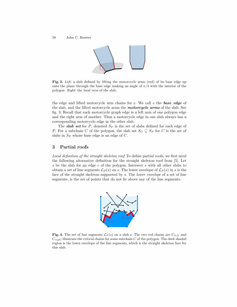
58 John C. Bowers
∞
Fig. 3. Left: a slab defined by lifting the motorcycle arms (red) of its base edge uponto the plane through the base edge making an angle of π/4 with the interior of thepolygon. Right: the local view of the slab.
the edge and lifted motorcycle arm chains for e. We call e the base edge ofthe slab, and the lifted motorcycle arms the motorcycle arms of the slab. Seefig. 3. Recall that each motorcycle graph edge is a left arm of one polygon edgeand the right arm of another. Thus a motorcycle edge in one slab always has acorresponding motorcycle edge in the other slab.
The slab set for P , denoted SP is the set of slabs defined for each edge ofP . For a subchain C of the polygon, the slab set SC ⊆ SP for C is the set ofslabs in SP whose base edge is an edge of C.
3 Partial roofs
Local definition of the straight skeleton roof To define partial roofs, we first needthe following alternative definition for the straight skeleton roof from [5]. Lets be the slab for an edge e of the polygon. Intersect s with all other slabs toobtain a set of line segments LP (s) on s. The lower envelope of LP (s) in s is theface of the straight skeleton supported by s. The lower envelope of a set of linesegments, is the set of points that do not lie above any of the line segments.
Cleft
Cright
Fig. 4. The set of line segments LP (s) on a slab s. The two red chains are Cleft andCright illustrate the critical chains for some subchain C of the polygon. The dark shadedregion is the lower envelope of the line segments, which is the straight skeleton face forthis slab.

Computing the Straight Skeleton 59
Cleft
Cright
Fig. 5. The restriction of the line segments from fig. 4 to only those in LC(s) for somesubchain C. Notice that the two critical chains Cleft and Cright are still supported bythe segments and lie on the lower envelope of LC(s).
Restricting the slab set to a subchain Our working definition of the straightskeleton roof uses the entire slab set for the polygon P . To generalize the roof toa subchain C of P , we restrict our attention to the slab set SC for C. Let LC(s)denote the set of line segments given by intersecting a slab s ∈ SC with all otherslabs in SC . Notice that since we are simply restricting which slabs we intersect,LC(s) ⊆ LP (s). Furthermore, notice that if e is a critical edge for the straightskeleton, then both of its faces (and hence both of its supporting slabs) havetheir base edge in SC . Thus e must be supported by one of the line segmentsin LC(s). One further property that can be derived is that the set of criticaledges on s form (at most) two polygonal chains on arrangement of line segmentsLC(s), and these two chains are incident to the left and right motorcycle armsof s. For this reason, we call these the critical chains Cleft and Cright of s.
Partial roof We defined the partial roof for a subchain C locally as we did withthe straight skeleton above. For each slab s in SC , we define a partial face for sis given by any two polygonal chains on the arrangement LC(s) that contain thecritical chains for s with respect to C. We call these the defining chains forthe face. The lower envelope of these two chains gives us the a (possibly partiallyinfinite) polygon on the surface of s. Suppose we now have a partial face for eachslab in SC . Every defining chain edge of a partial face for a slab s lies on theintersection of s with some other slab s′ in SC . If the partial face for s′ also hasan edge on the intersection of s and s′ and the two edges are equal in R3, wesay that the partial faces for s and s′ are compatible and we glue the two facestogether by identifying the two corresponding edges. A partial roof is given bythe following construction. Start with a set of partial faces, one for each slab inSC such that all pairs of partial faces are compatible. Glue every pair of partialfaces along their corresponding edges to form a single surface. If that surface istopologically a disk, we call it a partial roof for C. The main property of partialroofs is that the partial roof for the entire polygon is the straight skeleton roof.

60 John C. Bowers
4 Merging partial roofs
A key property of a partial face is that the partial face for any given slab s con-tains the corresponding straight skeleton roof face. Thus if two straight skeletonroof faces are incident along an edge, any two corresponding partial faces inter-sect along the edge. We now want to merge two partial roofs R1 and R2 for C1
and C2. Recall that the critical edges for C1 and C2 form a path in the straightskeleton. Since each partial roof face contains its straight skeleton face, this pathis on the intersection of R1 and R2. Walking along this intersection allows us tofind the critical path. Once we have the critical path, we cut the two roofs R1
and R2 along this path, discard the part of each partial face above the path, andmerge R1 and R2 by gluing them together along the path. We are glossing overthe details here, but the punchline is that our method can be executed in lineartime.
5 Conclusion
Given our merge operation, the following strategy computes a partial roof: dividethe polygon into two, recursively compute a partial roof for each, and thenmerge the two into a partial roof for the entire polygon. Since the unique partialroof for an entire polygon is the straight skeleton roof, this gives us a methodfor computing the straight skeleton of a polygon. The algorithm has the samerecurrence as merge sort, and thus requires O(n log n) time where n is the numberof vertices in the polygon (given the slab set as input). Since computing theslab set requires computing the motorcycle graph, this leads to an algorithmfor computing the straight skeleton in O(n log n + r4/3+ε) time where r is thenumber of reflex vertices in the polygon.
References
1. O. Aichholzer, D. Alberts, F. Aurenhammer, and B. Gartner. A novel type ofskeleton for polygons. Journal of Universal Computer Science, 1(12):752–761, 1995.
2. T. Biedl, M. Held, S. Huber, D. Kaaser, and P. Palfrader. Straight skeletons ofmonotone polygons. In 30th (EuroCG ’14), Dead Sea, Israel, Mar. 2014.
3. J. C. Bowers and I. Streinu. Rigidity of origami universal molecules. In T. Ida andJ. D. Fleuriot, editors, Automated Deduction in Geometry, volume 7993 of LectureNotes in Computer Science, pages 120–142. Springer, 2012.
4. S.-W. Cheng, L. Mencel, and A. Vigneron. A faster algorithm for computing straightskeletons. In Proc. 22nd Euro. Symp. on Algorithms (ESA 2014), Worclaw, Poland,Sept. 2014.
5. S. W. Cheng and A. Vigneron. Motorcycle graphs and straight skeletons. In Proc.13th Symp. on Discrete algorithms, SODA ’02, pages 156–165, Philadelphia, PA,USA, 2002. Society for Industrial and Applied Mathematics.
6. E. D. Demaine and M. L. Demaine. Computing extreme origami bases. TechnicalReport CS-97-22, Department of Computer Science, University of Waterloo, May1997.

Computing the Straight Skeleton 61
7. S. Huber and M. Held. Theoretical and practical results on straight skeletons ofplanar straight-line graphs. In Proc. 27th Symp. on Computational geometry, SoCG’11, pages 171–178, New York, NY, USA, 2011. ACM.
8. R. J. Lang. A computational algorithm for origami design. In Proceedings of the12th Annual ACM Symposium on Computational Geometry, pages 98–105, 1996.
9. A. Vigneron and L. Yan. A faster algorithm for computing motorcycle graphs. InProc. 29th Symp. on Computational geometry, SoCG ’13, pages 17–26, New York,NY, USA, 2013. ACM.

An Equivalence Proof Between Rank Theoryand Incidence Projective Geometry
David Braun, Nicolas Magaud, and Pascal Schreck
ICube, UMR 7357 CNRS, University of StrasbourgPole API, Bd Sebastien Brant, BP 10413, 67412 Illkirch, France
david.braun, magaud, [email protected]
Abstract. Incidence geometry is a well-established theory which cap-tures the very basic properties of all geometries in terms of belongingof points to lines, planes, etc. Moreover, considering incidence projectivegeometry leads to a very simple framework. This article considers two dif-ferent approaches to formalize this theory in Coq. The first one consistsin the usual geometric axiom system encountered in the literature. Thesecond one relies on combinatorial aspects through the notion of rankwhich is based on the matroid structure of incidence geometry. In thispaper, we prove in Coq the equivalence between these two approachesin both 2D and 3D. This result allows to study further automation ofmany proofs of projective geometry theorems. We already present someautomation techniques in the proof of equivalence.
Keywords: automation, Coq, formalization, incidence, matroid, projective ge-ometry, ranks
1 Introduction
In this article, we consider two axiom systems of incidence projective geome-try. The equivalence proof between these two formalizations through the proofassistant Coq is our main original contribution.
The most elementary geometry that can be studied is the incidence geometry.It basically analyzes the incidence relation between two types of objects: pointsand lines. This geometry is ubiquitous, collinearity issues are found in variouscontexts. For example, it appears in graph theory, subways maps and even chil-dren games such as dobble. Moreover, this simple geometry can be defined bya fairly simple set of axioms both in the plane and in an at least three dimen-sional setting (noted ≥3D) [3,6]. So it is conceivable to efficiently automate thereasoning.
We describe two geometrical axiomatizations. The first one is based on aclassical geometrical characterization. The second one relies on the combinatorialnotion of rank provided by the matroid structure of incidence geometry. Thelatter allows to represent homogeneously all incidences of this geometry (point-point, point-line, point-plan, line-line, line-plan, plan-plan) but also relations of

Equivalence Proof Between Rank and Projective Geometry 63
collinearity, coplanarity, etc. Thanks to the unique representation of all incidencerelations as ranks, we can thus consider a more systematic automation.
Our main motivation is the mechanization of demonstrations to ease thetask of mathematicians but also to more effortlessly study the degenerate cases.Formalization and proof of geometrical theorems are not an easy task. It needs tobe very rigorous to take into account all non degeneracy conditions that can occurin this context. These conditions often lead to long and tedious technical proofs.That is why, many papers have emphasized the importance of investigating theproblem of degenerate cases in formal geometry [7, 21,28].
In this paper, we work in the specific context of projective geometry in whichthe notion of parallel does not exist. This simple framework is powerful enoughto study the formalization and proof of complex problems as suggested in [23]. Inaddition, there is no loss of generality since it is possible to switch from projectivegeometry to affine geometry putting a chosen line at infinity. Moreover, it ispossible to consider finite geometries containing only finite sets of points and linesthat check the properties of projective framework. Examples of finite geometrysuch as Fano plane are often used to analyze the behavior of geometric theorems.
Some ideas behind this work have their origins in previous studies aboutcombinatoric aspects of proofs in incidence geometry as described in [18, 24],and particularly a proof of Desargues theorem using only ranks [19,20]. To carryout the latter, the authors have proven only one direction of the equivalencetheorem between the two theories: the one from a classical incidence projectivegeometry axiomatization to a rank-based axiom system in 3D and not the con-verse which was useless at the time. To our knowledge, mathematicians havenot studied extensively the details of the equivalence proof between these twoapproaches.
Related Work Geometry is a good candidate to be studied through the proofassistants like Coq. Many formalizations of plane geometry, Hilbert and Tarskiaxiomatization has already be done [8,11,21,28]. In the narrower context of pro-jective geometry, there is work in constructive projective geometry initiated byVon Plato [14,33]. Our formalization differs by considering a decidable incidencerelation. In the field of automatic methods in projective geometry, we can men-tion the algebraic formalization of Grassmann-Cayley algebra [9,17,30]. Finally,to our knowledge there is no work treating incidence geometry in a projectiveframework using the equivalence between a geometrical characterization and acombinatorial approach.
Outline of the paper The paper is organized as follows. In Section 2, wepresent the axioms for incidence projective geometry and we give an previewof our Coq formalization. In Section 3, we expose our axiomatizations based onthe concept of rank from matroid theory. Section 4 investigates in details theequivalence proof between these two formalizations. Finally, the conclusion andperspectives are discussed in Section 5.

64 David Braun, Nicolas Magaud, and Pascal Schreck
Notation We use the naming convention AXYN for our axioms. The letterstands A for axiom, X for the axiom number, Y may take two values (P =projective, R = rank) and N designs the dimension.
2 Axiom Systems of Projective Geometry
In a general setting, geometry such as Euclidean geometry is a complicatedsubject mixing objects like points, lines and planes with concepts of distance,angle, continuity, incidence etc. Among all these notions, we keep only two kindsof objects, points and lines, and the incidence relation between them to form theelementary incidence geometry.
2.1 Incidence Geometry
Incidence geometry is the study of a triple (Ω,∆,Φ) called incidence structure.Ω refers to the set of points, ∆ is the disjoint set composed of lines and Φ is thebinary relation that unite them. Elements which are mutually incident constitutea subset Φ ⊆ Ω × ∆. Intuitively, a point and a line are within this subset if andonly if the point is on the line. It is possible to describe this geometry informallywith three axioms.
– There is always a line passing through two points.– On any line, there are at least two points.– There exist three points that are not aligned.
This characterization is sufficient to prove many theorems [3]. In addition,the enrichment of incidence geometry by new concepts keeps many fundamentalresults. Projective geometry relies on the basics of incidence geometry. It isa general setting in the hierarchy of geometries which assumes that two linesin a plane always meet [6]. Planes can be defined within our theory but theyare not a primitive object. With the concepts of incidence geometry, we candescribe properly projective geometry in 2-dimensional space and in at least3-dimensional space.
2.2 Axioms System for Projective Plane Geometry
The axiom system for projective plane geometry consists of five axioms presentedin Coxeter’s book [6]. The first two axioms deal with construction of points andlines. We do not specify that the involved points (resp. lines) should be differentin axiom Line-Existence (resp. Point-Existence). Indeed if these points (resp.lines) are equal, the line (resp. point) still exists. In fact, there exists an infinityof lines (resp. points). This formalization choice follows this general principlein formal geometry: it is decisive to define statements in the most general waypossible. The next axiom (A3P2) concerns uniqueness of the two defined objects.Finally, axiom (A4P2) states that each line contains at least three points; and

Equivalence Proof Between Rank and Projective Geometry 65
axiom (A5P2) expresses that there always exists two distinct lines, which meansdimension is at least 2. Together with axiom Point-Existence which show that thedimension is at most 2. Therefore the dimension is exactly 2. The formalizationof this axiom system is straightforward, textbooks often use some variants ofthis system [6] but we choose the latter to ease mechanization of proofs.
(A1P2) Line-Existence : ∀ A B : Point, ∃ l : Line, A ∈ l ∧ B ∈ l
(A2P2) Point-Existence : ∀ l m : Line, ∃ A : Point, A ∈ l ∧ A ∈ m
(A3P2) Uniqueness : ∀ A B : Point, ∀ l m : Line, A ∈ l ∧ B ∈ l ∧ A ∈ m∧ B ∈ m ⇒ A = B ∨ l = m
(A4P2) Three-Points : ∀ l : Line, ∃ A B C : Point,A 6= B ∧ B 6= C ∧ A 6= C ∧ A ∈ l ∧ B ∈ l ∧ C ∈ l
(A5P2) Lower-Dimension : ∃ l m: Line, l 6= m
2.3 Axioms System for Projective Space Geometry
In the same way, we define an axiom system for projective space geometry.The system still contains five axioms with three of them remaining unchanged(A1P3, A3P3, A4P3). Pasch’s axiom substitutes (A5P2) assuming that twocoplanar lines always meet. Furthermore, we modify the axiom Lower-Dimensionto capture a projective geometry in at least 3-dimensional space. For this, weassume that there exist two lines which do not meet. This time, the second axiomdoes not allow to limit the higher dimension, that is why we consider a geometry≥3D.
(A1P3) Line-Existence : ∀ A B : Point, ∃ l : Line, A ∈ l ∧ B ∈ l
(A2P3) Pasch : ∀ A B C D : Point, ∀ lAB lCD lAC lBD : Line,A 6= B ∧ A 6= C ∧ A 6= D ∧ B 6= C ∧ B 6= D ∧ C 6= D ∧A ∈ lAB ∧ B ∈ lAB ∧ C ∈ lCD ∧ D ∈ lCD ∧A ∈ lAC ∧ C ∈ lAC ∧ B ∈ lBD ∧ D ∈ lBD ∧(∃ I : Point, I ∈ lAB ∧ I ∈ lCD) ⇒(∃ J : Point, J ∈ lAC ∧ J ∈ lBD)
(A3P3) Uniqueness : ∀ A B : Point, ∀ l m : Line,A ∈ l ∧ B ∈ l ∧ A ∈ m ∧ B ∈ m ⇒ A = B ∨ l = m
(A4P3) Three-Points : ∀ l : Line, ∃ A B C : Point,A 6= B ∧ B 6= C ∧ A 6= C ∧ A ∈ l ∧ B ∈ l ∧ C ∈ l
(A5P3) Lower-Dimension : ∃ l m : Line, ∀ p : Point, p /∈ l ∨ p /∈ m

66 David Braun, Nicolas Magaud, and Pascal Schreck
2.4 Formalization in Coq
Implementing these two systems of axioms is rather immediate in the Coq proofassistant; we present below our formalization of the projective space. The nota-tion ∈ denotes the predicate Incid. To enhance modularity, we take advantageof the type classes and functors of Coq. The most difficult notation to handle forthe reader probably is the curly-brackets notation for constructive existentialquantification over the sort Type. For example, the formula forall l:Line,
P:Point | ∼ Incid P l states that ∀ l:Line, ∃ P:Point, ¬ Incid P l.To observe equivalences between different variants of our axiomatizations,
we split our axioms in different classes considering the dimension. Moreover,this decomposition allows us to bring out the minimal axiom system requiredto demonstrate a set of properties. First, we build a type class with commonaxioms between the dimensions namely Line-Existence, Uniqueness and Three-Points. Then, we construct two classes, the first one captures the whole projectiveplane, and the second one describes the projective space. For the sake of clarity,we present here a simplified version of our implementation.
Class ProjectiveSpaceOrHigher ‘(PPS : PreProjectiveSpace) :=
(* Line-Existence *)
A1P3 : forall (A B : Point) , l : Line | Incid A l /\ Incid B l;
(* Pasch *)
A2P3: forall A B C D : Point, forall lAB lCD lAC lBD : Line,
~ A [==] B /\ ~ A [==] C /\ ~ A [==] D /\
~ B [==] C /\ ~ B [==] D /\ ~ C [==] D ->
Incid A lAB /\ Incid B lAB ->
Incid C lCD /\ Incid D lCD ->
Incid A lAC /\ Incid C lAC ->
Incid B lBD /\ Incid D lBD ->
(exists I : Point, (Incid I lAB /\ Incid I lCD)) ->
exists J : Point, (Incid J lAC /\ Incid J lBD);
(* Uniqueness *)
A3P3: forall (A B : Point)(l1 l2 : Line), Incid A l1 -> Incid B l1 ->
Incid A l2 -> Incid B l2 -> A [==] B \/ l1 = l2;
(* Three-Points *)
A4P3: forall l : Line, A : Point & B : Point & C : Point |
(~ A [==] B /\ ~ A [==] C /\ ~ B [==] C /\
Incid A l /\ Incid B l /\ Incid C l);
(* Lower-Dimension *)
A5P3: l1 : Line & l2 : Line | forall p : Point,
~(Incid p l1 /\ Incid p l2)
.

Equivalence Proof Between Rank and Projective Geometry 67
The main difference between our formalization and the axiom system shownabove comes from decidability issues and equality relations. The equality onpoints, denoted [==], is a parameter of our theory. This equality allows to maketransparent the way in which the point is built. As the underlying logic of theCoq system is intuitionist, we have to declare explicitly which predicates aredecidable. Assuming only the decidability of the predicate Incid, we prove thedecidability of all other predicates used in this theory (points, lines) [18]. Wechoose to not use a parametric equality for lines since it can be represented as aset of points in the other axiomatization. It is quite possible to use one, but ithas not been necessary.
3 A Rank-based Axiom System
In Section 2, we present a standard axiomatization for projective geometry asa reference. We propose here an alternative axiom system based on the notionof rank. This new approach takes homogeneously the flats into account and wehope that it will simplify the proof schemes in higher dimensions.
3.1 Matroid Properties
The concept of rank comes from matroid theory [29]. Matroids were introducedby Whitney in 1935 to capture abstractly the essence of dependence. Whitney’sdefinition embraces a surprising diversity of combinatorial structures. Matroidallows to capture and generalize the main set properties of linear dependence invector spaces. When combined with a finite set of points, it catches incidence(collinearity, coplanarity, ...) between these points. However matroids apply ina much larger object class. Other natural examples are obtained from graphtheory, fields, greedy algorithms. There are several cryptomorphic ways to definea matroid. In our context, we use the definition based on ranks. Using ranksallows to deal only with points which makes proofs easier because we do nothandle directly lines or planes. An integer function rk on E a finite set is therank function of a matroid if and only if the following conditions are satisfied:
(* nonnegative and subcardinal *)(A1R2-R3) : 0 ≤ rk(X) ≤
∣∣X∣∣, ∀ X ⊆ E
(* nondecreasing *)(A2R2-R3) : rk(X) ≤ rk(Y), ∀ X ⊆ Y
(* submodular *)(A3R2-R3) : rk(X ∪ Y) + rk(X ∩ Y) ≤ rk(X) + rk(Y), ∀ X, Y ⊆ E
3.2 Rank to Describe Incidence Projective Geometry
In the framework of projective geometry, we define a rank function on finitesets of points which checks the three conditions above. We specify the notion of

68 David Braun, Nicolas Magaud, and Pascal Schreck
flat which is a set of points closed by the collinearity/coplanarity relation. Therank of a flat is the cardinal of a smallest set generating A (see Fig. 1 for someexamples).
rkA,B = 1 A = BrkA,B = 2 A 6= BrkA,B,C = 2 A,B,C are collinear with at least two of them distinctrkA,B,C ≤ 2 A,B,C are collinearrkA,B,C = 3 A,B,C are not collinearrkA,B,C,D = 3 A,B,C,D are coplanar, not all collinearrkA,B,C,D = 4 A,B,C,D are not coplanar
Fig. 1. Some rank statements and their geometric interpretations
Using this definition, it can be shown that every projective space has a ma-troid structure, but the converse is not true. To capture all the projective geom-etry, we need to introduce some additional axioms to matroid’s one.
3.3 2D Rank-based Axioms System
We present a rank-based axiom system to describe projective plane. The firsttwo axioms establish the non degeneracy of the rank function. The others aremore or less direct translations of the axioms of projective geometry.
(A4R2) Rk-Singleton : ∀ P : Point, rkP ≥ 1
(A5R2) Rk-Couple : ∀ P Q: Point, P 6= Q ⇒ rkP, Q ≥ 2
(A6R2) Rk-Inter : ∀ A B C D, ∃ J, rkA, B, J = rkC, D, J = 2
(A7R2) Rk-Three-Points : ∀ A B, ∃ C, rkA, B, C = rkB, C = rkA,C = 2
(A8R2) Rk-Lower-Dimension : ∃ A B C, rkA, B, C ≥ 3
3.4 ≥3D Rank-based Axioms System
In the same way, we define a rank-based axiom system to describe projectivespace. Again, we modify only the axioms of Pasch and Lower-Dimension.
(A4R3) Rk-Singleton : ∀ P : Point, rkP ≥ 1
(A5R3) Rk-Couple : ∀ P Q: Point, P 6= Q ⇒ rkP, Q ≥ 2
Equivalence Proof Between Rank and Projective Geometry 69
(A6R3) Rk-Pasch : ∀ A B C D, rkA, B, C, D ≤ 3 ⇒ ∃ J,rkA, B, J = rkC, D, J = 2
(A7R3) Rk-Three-Points : ∀ A B, ∃ C, rkA, B, C = rkB, C = rkA,C = 2
(A8R3) Rk-Lower-Dimension : ∃ A B C D, rkA, B, C, D ≥ 4
The Implementation in Coq follows the same process, we use type classes toincrease modularity of the code depending of the dimension.
Now that we have specified the axiomatization, we will focus on proof of theequivalence between these two axiom systems. In previous works [19, 20], onlythe implication of the ranks to ≥3D projective geometry has been proven. It issufficient to justify the case study on the formalization of Desargues theorem withthe ranks [19,20]. To allow bilateral translation and to increase the possibilitiesof automation, we have completed the proof of this equivalence.
4 Equivalence Proof
We prove the following statement:
Theorem 1. Axiomatization on incidence projective geometry and rank-basedaxioms system are equivalent respectively in 2D and ≥ 3D.
To achieve this proof, we split the demonstration of the equivalence depend-ing on the dimension and the direction.
4.1 From Ranks to Projective Geometry
We begin with the implication from ranks to projective geometry both 2D and≥ 3D. The conduct of the proofs remains the same no matter the dimension.
Preliminaries
First, we need to characterize the notion of line and incidence that does notexist in the axiom system based on ranks. We build, using an inductive definition,a line from two distinct points. A point P is incident to a line, if the rank of thetriple formed by the two points constituting the line and the point P remainsequal to 2.
Definition Point := Point.
Inductive LineInd : Type :=
|Cline : forall (A B : Point)(H : ~ A[==]B), LineInd.
Definition Line := LineInd.
70 David Braun, Nicolas Magaud, and Pascal Schreck
Definition Incid (P : point)(l : Line) := rk ((fstP l)(sndP l) P) = 2.
From there we can express the axioms of projective geometry and prove themusing rank axioms.
Submodularity
We detail proof techniques used to demonstrate the five axioms in projec-tive geometry both 2D and ≥3D. First, we usually prove equalities on ranks(rk(a) = rk(b)) in two steps : first that rk(a) ≤ rk(b), then rk(a) ≥ rk(b). Sec-ond, we work systematically with the axiom of submodularity (A3R2-R3). Theissue is that to determine the intersection of two finite set of points, we needto distinguish cases about the equalities of points. The resulting proofs becomesmore complex with these distinctions. Therefore, we define a particular lemmaderived from the axiom A3R2-R3 that does not consider the theoretical inter-section but a lower approximation of this intersection (noted u).
Definition 1. (Literal Intersection).Let L1 and L2 be two sets of points. By definition L1 u L2 is the intersection
of the two sets of points considered syntactically.
From this literal intersection, we can derive a more appropriate version ofthe axiom ignoring case distinctions:
Lemma 1. (A3R2-R3-lit),∀ X Y, rk(X ∪ Y) + rk(X u Y) ≤ rk(X) + rk(Y).
In Coq, it is not possible to define the literal intersection. To capture themeaning of the lemma, we define a practical version:
Lemma 2. (A3R2-R3-alt),∀ X Y I, I ⊆ X ∩ Y ⇒ rk(X ∪ Y) + rk(I) ≤ rk(X) + rk(Y).
This functional version of the submodularity will be extensively employed ineach proof. To illustrate the mechanism of proof of this subsection, we detail thedemonstration of the Uniqueness property.
Proof of the uniqueness property
Lemma 3. (A3P2)(A3P3) Uniqueness,∀ A B : Point, ∀ l m : Line, A ∈ l ∧ B ∈ l ∧ A ∈ m ∧ B ∈ m ⇒ A = B ∨
l = m
Proof (test). We begin this proof by performing a case distinction on the equalitybetween A and B. The first case A = B is immediately checked with the goal. IfA 6= B, by unfolding definitions of Line and Incid, it follows that :

Equivalence Proof Between Rank and Projective Geometry 71
We have A <> BLet P ∈ l, Q ∈ l and P <> QLet R ∈ m, S ∈ m and R <> SIncid A l ⇒ rkP, Q, A = 2Incid B l ⇒ rkP, Q, B = 2Incid A m ⇒ rkR, S, A = 2Incid B m ⇒ rkR, S, B = 2
Assumptions
l = m ⇒ rk(P Q R S) = 2Goal
To continue, we determine the rank of two new sets using A3R2-R3-alt:rkP, Q, A, B and rkR, S, A, B.
rk(P, Q, A ∪ P, Q, B) + rk(P, Q, A ∩ P, Q, B)≤ rkP, Q, A + rkP, Q, B⇒ rkP, Q, A, B + rkP, Q ≤ rkP, Q, A + rkP, Q, B⇒ rkP, Q, A, B ≤ 2
Analogously, we calculate rkR, S, A, B ≤ 2. Then we establish thatrkP, Q, R, S, A, B ≤ 2.
rk(P, Q, A, B ∪ R, S, A, B) + rk(P, Q, A, B ∩ R, S, A, B)≤ rkP, Q, A, B + rkR, S, A, B⇒ rkP, Q, R, S, A, B + rkA, B ≤ rkP, Q, A, B + rkR, S, A, B⇒ rkP, Q, R, S, A, B ≤ 2
Using A2R2-R3, we prove that:
P, Q, R, S ⊂ P, Q, R, S, A, B ⇒rkP, Q, R, S ≤ rkP, Q, R, S, A, B
So rkP, Q, R, S ≤ 2 and contains at least two distinct points, we concludethat rkP, Q, R, S=2.
Coq implementation
At the implementation level, to make the deduction on abstract sets, we usethe tactic fsetdecide provided by the library on Containers [16]. We also usesetoids to make substitutions when we have to indicate to the system that thesets are identical. Finally to address inequalities, we use omega [5]1 tactic. Weproved with similar techniques others lemmas of projective geometry.
1 Omega: a solver of quantifier-free problems in Presburger Arithmetic

72 David Braun, Nicolas Magaud, and Pascal Schreck
4.2 From Projective Geometry to Ranks
The opposite direction is more difficult to handle, we need to specify the con-cept of rank from projective geometry. This implication is much more difficultto prove.
Preliminaries
It is not possible to directly describe rank, we have to define intermediatedefinitions representing the different returned values of the rank function. Tocharacterize the rank, we are inspired by the concept of flat from the matroidtheory. The set of points is either empty or it represents a point, a line, a planeor a space. To represent abstract sets, we can manipulate AVLs or lists. Giventhat we are working on sets of small sizes, we choose to work with lists for theimplementation.
Definition rkl s := match s with
| nil => 0
| x :: nil => 1
| s => if contains_four_non_coplanar_points s then 4 else
if contains_three_non_collinear_points s then 3 else
if contains_two_distinct_points s then 2 else 1
end.
The three predicates contains four, contains three and contains two
put bounds on the dimension of the set. For instance the coplanarity, eitherthere is a quadruple of non coplanar points and the set represents a space, or itcontinue recursion analyzing collinearity. These predicates form what is called anintermediate layer. They help to make transition between the two axiom systemsand are often accompanied by dozens of lemmas. It is desirable to remain vigilantduring the development of such definitions to take into account all the degeneratecases (mainly coincident points).
Fixpoint contains_four_non_coplanar_points l :=
match l with
| nil => false
| a::r => if coplanar_with_all a (all_triples r)
then contains_four_non_coplanar_points r
else true
end.
Proof techniques
Similarly, we present the main technical aspects to perform demonstrationsof the eight axioms. We exploit mostly the induction mechanism. Manipulationof the three conditionals in the rank’s characterization and the management of

Equivalence Proof Between Rank and Projective Geometry 73
degenerate cases yield many goals which significantly increase the size of theproofs. Resulting proofs are often tedious, however it is possible to automatemany steps. For this, we use Ltac the tactical language provided by Coq. Weidentify specific patterns within hypothesis and goals that we simplify by a se-quence of tactics and lemmas. This tactic allows to unfold as much as possiblethe goal while introducing a maximum of assumptions. If the goal has becometrivial with a simple equality/inequality, the work is finished. Otherwise one hasto make explicit a contradiction in assumptions. This logic work is the core ofthe proof and must be done by hand. To raise contradictions in context, it makessense to write intermediate lemmas.
Ltac my_rank :=
repeat match goal with
|[H : _ |- _] => progress intros
|[H : _ |- _] => progress intro
|[H : _ |- _ <-> _] => split
|[H : _ |- _ /\ _] => split
|[H : _ /\ _ |- _] => destruct H
|[H : _ |- _] => solve[intuition]
|[H : _ |- _] => progress contradiction
|[H : ?X :: _ = nil |- _] => inversion H
|[H : false = true |- _] => inversion H
|[H : true = false |- _] => inversion H
|[H : ?X[==]?X -> False |- _] => apply False_ind;apply H;reflexivity
|[H : _ |- (if if ?X then _ else _
then _ else _) = _ \/ _] => case_eq X
|[H : _ |- (if ?X then _ else _) = _ \/ _] => case_eq X
...
end.
Proof of the nondecreasing property
We give an overview with the proof of the nondecreasing property of thematroid theory.
Lemma 4. (A2R2-R3),∀ X ⊆ Y, rk(X) ≤ rk(Y).
In our context, the rank function can take five possible values from 0 to 4,which leads us twenty five different cases to treat when we make a structuralinduction on X and Y. First case 0 ≤ 0, second case 0 ≤ 1, etc. With the tactic,we eliminate fifteen trivial goals immediately wherein X is included in Y. Toprove the remaining ones, we build a contradiction and we simplify with a tacticthat automatically handles the calculation of inclusion. For example, we clarifythat a plane can not be included in a line. It is therefore impossible to reach thecase 3 ≤ 2.

74 David Braun, Nicolas Magaud, and Pascal Schreck
Coq implementation
Lemma A3R2-R3 is the hardest lemma to prove with the management of theintersection and the union. It contains many nontrivial cases that we decomposeinto several lemmas as below.
Lemma matroid3_rk2_rk2_interrk2_to_unionrk2 :
forall l m,
rkl l = 2 ->
rkl m = 2 ->
rkl (inter l m) = 2 ->
rkl (union l m) = 2.
Another recurring issue is caused by our parametric equality on points. Wemust write a morphism for each definition that we cross when we perform arewrite. We prove that the equality is compatible and consistent with the defi-nition in which it is used. In this way, it is possible to substitute a set X similarto a set Y directly in the rank definition. The writing of such morphism in Coqis as below:
Instance rank_morph : Proper (@equivlistA Point eq => (@Logic.eq nat)) rkl.
Proof.
...
Qed.
This leads to the following lemma where the predicate equivlist indicatesthat the two lists are equal:
Lemma 5. rank morph,∀ x y : list Point, equivlist x y → rkl x = rkl y
4.3 Statistics
Finally, we give some data about our library, we also detail the impact of automa-tion that we have put in place throughout the process. Overall, our developmentconsists of more than 30 000 lines and 850 lemmas. We dedicate 14 000 lines todemonstrate the equivalence organized as shown in the Fig. 2 below. Using tac-tics and splitting the demonstration into lemmas has divided by three the sizeof the formalization.
5 Conclusion and Future Work
This paper explain how projective geometry can be formalized in Coq using twodifferent axioms systems in both 2D and 3D. We detail in particular the originalaxiomatization based on the notion of rank from the matroid theory. Then we
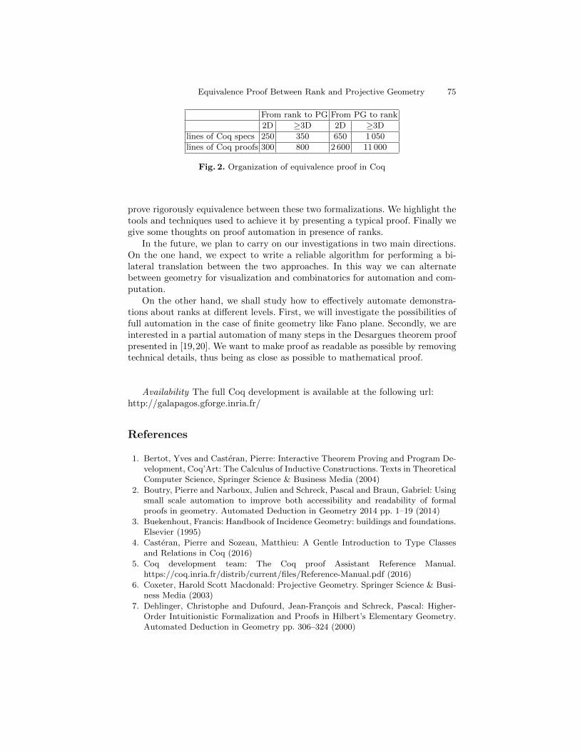
Equivalence Proof Between Rank and Projective Geometry 75
From rank to PG From PG to rank
2D ≥3D 2D ≥3D
lines of Coq specs 250 350 650 1 050
lines of Coq proofs 300 800 2 600 11 000
Fig. 2. Organization of equivalence proof in Coq
prove rigorously equivalence between these two formalizations. We highlight thetools and techniques used to achieve it by presenting a typical proof. Finally wegive some thoughts on proof automation in presence of ranks.
In the future, we plan to carry on our investigations in two main directions.On the one hand, we expect to write a reliable algorithm for performing a bi-lateral translation between the two approaches. In this way we can alternatebetween geometry for visualization and combinatorics for automation and com-putation.
On the other hand, we shall study how to effectively automate demonstra-tions about ranks at different levels. First, we will investigate the possibilities offull automation in the case of finite geometry like Fano plane. Secondly, we areinterested in a partial automation of many steps in the Desargues theorem proofpresented in [19,20]. We want to make proof as readable as possible by removingtechnical details, thus being as close as possible to mathematical proof.
Availability The full Coq development is available at the following url:http://galapagos.gforge.inria.fr/
References
1. Bertot, Yves and Casteran, Pierre: Interactive Theorem Proving and Program De-velopment, Coq’Art: The Calculus of Inductive Constructions. Texts in TheoreticalComputer Science, Springer Science & Business Media (2004)
2. Boutry, Pierre and Narboux, Julien and Schreck, Pascal and Braun, Gabriel: Usingsmall scale automation to improve both accessibility and readability of formalproofs in geometry. Automated Deduction in Geometry 2014 pp. 1–19 (2014)
3. Buekenhout, Francis: Handbook of Incidence Geometry: buildings and foundations.Elsevier (1995)
4. Casteran, Pierre and Sozeau, Matthieu: A Gentle Introduction to Type Classesand Relations in Coq (2016)
5. Coq development team: The Coq proof Assistant Reference Manual.https://coq.inria.fr/distrib/current/files/Reference-Manual.pdf (2016)
6. Coxeter, Harold Scott Macdonald: Projective Geometry. Springer Science & Busi-ness Media (2003)
7. Dehlinger, Christophe and Dufourd, Jean-Francois and Schreck, Pascal: Higher-Order Intuitionistic Formalization and Proofs in Hilbert’s Elementary Geometry.Automated Deduction in Geometry pp. 306–324 (2000)

76 David Braun, Nicolas Magaud, and Pascal Schreck
8. Duprat, Jean: Une axiomatique de la geometrie plane en Coq. Journees Franco-phones des Langages Applicatifs pp. 123–136 (2008)
9. Fuchs, Laurent and Thery, Laurent: A formalization of grassmann-cayley algebrain Coq and its application to theorem proving in projective geometry. AutomatedDeduction in Geometry 6877, 51–67 (2010)
10. Genevaux, Jean-David and Narboux, Julien and Schreck, Pascal: Formalization ofWu’s simple method in Coq. Certified Programs and Proofs 7086, 71–86 (2011)
11. Guilhot, Frederique: Formalisation en Coq et visualisation d’un cours de geometriepour le lycee. Journees Francophones des Langages Applicatifs 7, 15 (2004)
12. Janicic, Predrag and Narboux, Julien and Quaresma, Pedro: The Area Method :a Recapitulation. Journal of Automated Reasoning 48(4), 489–532 (2012)
13. Jermann, Christophe and Trombettoni, Gilles and Neveu, Bertrand and Mathis,Pascal: Decomposition of Geometric Constraint Systems: a survey. InternationalJournal of Computanional Geometry & Application 16(05n06), 379–414 (2006)
14. Kahn, Gilles: Constructive geometry according to Jan von Plato (1995)15. Kusak, Eugeniusz: Desargues theorem in projective 3-space. J. of Formalized Math-
ematics 2 (1990)16. Lescuyer, Stephane: First-Class Containers in Coq. Stud. Inform. Univ. 9(1), 87–
127 (2011)17. Li, Hongbo and Wu, Yihong: Automated short proof generation for projective geo-
metric theorems with Cayley and bracket algebras: I. Incidence geometry. Journalof Symbolic Computation 36(5), 717–762 (2003)
18. Magaud, Nicolas and Narboux, Julien and Schreck, Pascal: Formalizing ProjectivePlane Geometry in Coq. Automated Deduction in Geometry 6301, 141–162 (2008)
19. Magaud, Nicolas and Narboux, Julien and Schreck, Pascal: Formalizing Desarguestheorem in Coq using ranks. ACM pp. 1110–1115 (2009)
20. Magaud, Nicolas and Narboux, Julien and Schreck, Pascal: A Case Study in For-malizing Projective Geometry in Coq: Desargues Theorem. Computational Geom-etry : Theory and Applications 45(8), 406–424 (2012)
21. Meikle, Laura I and Fleuriot, Jacques D: Formalizing Hilbert’s Grundlagen inIsabelle/Isar. Theorem proving in higher logics 2758, 319–334 (2003)
22. Michelucci, D and Schreck, P: Detecting induced incidences in the projective plane.isiCAD Workshop. Citeseer (2004)
23. Michelucci, Dominique and Foufou, Sebti and Lamarque, Loic and Schreck, Pascal:Geometric constraints solving:some tracks. ACM pp. 185–196 (2006)
24. Michelucci, Dominique and Schreck, Pascal: Incidence constraints : a combinatorialapproach. International J. of Computational Geometry & Application 16(05n06),443–460 (2006)
25. Moulton, Forest Ray: A Simple Non-Desarguesian Plane Geometry. Transactionsof the American Mathematical Society 3(2), 192–195 (1902)
26. Narboux, Julien: A Decision Procedure for Geometry in Coq. Theorem Proving inHigher Order Logics 3223, 225–240 (2004)
27. Narboux, Julien: Formalisation et automatisation du raisonnement geometrique enCoq. Ph.D. thesis, Universite Paris Sud-Paris XI (2006)
28. Narboux, Julien: Mechanical Theorem Proving in Tarski’s Geometry. AutomatedDeduction in Geometry 4869, 139–156 (2006)
29. Oxley, James G: Matroid Theory, vol. 3. Oxford University Press, USA (2006)30. Richter-Gebert, Jurgen: Mechanical theorem proving in projective geometry. An-
nals of Mathematics and Artificial Intelligence 13, 139–172 (1995)31. Sozeau, Matthieu and Oury, Nicolas: First-class type classes. Theorem Proving in
Higher Order Logics 5170, 278–293 (2008)

Equivalence Proof Between Rank and Projective Geometry 77
32. Tarski, Alfred: What is Elementary Geometry ? (1983)33. von Plato, Jan: The axioms of constructive geometry. Annals of pure and applied
logic 76(2), 169–200 (1995)
From Hilbert to Tarski
Gabriel Braun, Pierre Boutry, and Julien Narboux
ICube, UMR 7357 CNRS, University of StrasbourgPole API, Bd Sebastien Brant, BP 10413, 67412 Illkirch, Francegabriel.braun, boutry, [email protected]
Abstract. In this paper, we describe the formal proof using the Coq proof as-sistant that Tarski’s axioms for plane neutral geometry (excluding continuity ax-ioms) can be derived from the corresponding Hilbert’s axioms. Previously, wemechanized the proof that Tarski’s version of the parallel postulate is equivalentto the Playfair’s postulate used by Hilbert [9] and that Hilbert’s axioms for planeneutral geometry (excluding continuity) can be derived from the correspondingTarski’s axioms [12]. Hence, this work allows us to complete the formal proof ofthe equivalence between the two axiom systems for neutral and plane Euclideangeometry. Formalizing Hilbert’s axioms is not completely straightforward, in thispaper we describe the corrections we had to make to our previous formalization.We mechanized the proof of Hilbert’s theorems that are required in our proofof Tarski’s axioms. But this connection from Hilbert’s axioms, allows to recoverthe many results we obtained previously in the context of Tarski’s geometry: thisincludes the theorems of Pappus[13], Desargues, Pythagoras and the arithmetiza-tion of geometry [8].
Keywords: formal proof, geometry, foundations, Tarski’s axioms, Hilbert’s axioms,Coq
1 Introduction
There are several ways to define the foundations of geometry. In the synthetic approach,the axiomatic system is based on some geometric objects and axioms about them. Thebest known modern axiomatic systems based on this approach are Hilbert’s [17] andTarski’s ones [32]. In the analytic approach, a field F is assumed (usually R) and thespace is defined as Fn. In the mixed analytic/synthetic approaches, one assumes boththe existence of a field and also some geometric axioms. For example, the axiomaticsystems for geometry used for education in North America are based on Birkhoff’saxiomatic system [7] in which the field serves to measure distances and angles. Thisis called the metric approach. A modern development of geometry based on this ap-proach can be found in the books of Millman [21] or Moise [22]. The textbook ofHartshorne [16] provides a development of geometry based on Hilbert’s axioms. A rig-orous development of geometry based on Tarski’s axioms appears in the first part of thebook by Tarski, Szmielew and Schwabhauser [27].
The GeoCoq library gathers results about the foundations of geometry formalized inCoq [23]. It includes a formalization of the first part of [27]. We formalized in Coq the

From Hilbert to Tarski 79
link between the synthetic geometry defined by Tarski’s axioms and analytic geome-try [8]. We also formalized the link from Tarski’s axioms to Hilbert’s axioms [12], Bee-son has later written a note [5] to demonstrate that the main results to obtain Hilbert“saxioms are contained in [27]. In this paper, we complete the picture, by proving for-mally that Tarski’s axioms can be derived from Hilbert’s axiom.
Dehlinger, Dufourd and Schreck have studied the formalization of Hilbert’s founda-tions of geometry in the intuitionist setting of Coq [14]. They have highlighted the factthat Hilbert’s proofs require the excluded middle axiom applied to the point equalityand the role of non degenerate conditions. They focus on the first two groups of ax-ioms and prove some betweenness properties. Meikle and Fleuriot have done a similarstudy within the Isabelle/HOL proof assistant [20]. They went up to twelfth1 theoremof Hilbert’s book. Scott has continued the formalization of Meikle using Isabelle/HOLand revised it [28]. He has corrected some ”subtle errors in the formalization of GroupIII by Meikle”. Scott was interested in trying to obtain readable proofs. Later, he de-veloped a system within the HOL-Light proof assistant to automatically fill some gapsin the incidence proofs [30]. In our work, even if we use some tactics to obtain someproofs more easily [11,10], we do not focus on obtaining readable proofs. Scott thenfocused on proving a theorem, which Hilbert’s states without proof: that a special caseof the Jordan Curve Theorem can be proved using the first two groups of Hilbert’s ax-ioms only [29]. Moreover Richter has formalized a substantial number of results basedon Hilbert’s axioms and a metric axiom system using HOL-Light [25]. Finally Beesonand Wos have used the OTTER automatic theorem prover to mechanize some proofsin Tarski’s geometry [3,4]. They manage to automatically prove many results from thefirst twelve chapter of [27], with the help of some human generated hints OTTER canprove all the lemmas necessary to derive Hilbert’s axioms.
The earlier errors in Meikle’s formalization found by Scott can frighten the reader.How can we be sure that there are no errors in the formalization presented in this paper?They are two kinds of potential errors:
1. the axioms are inconsistent2. the axioms do not capture the desired theory - some standard geometry theorems
may not be provable from the axioms
In our previous work [12], we have shown that Tarski’s axioms for plan Euclidean ge-ometry can serve as a model for the corresponding Hilbert’s axioms. In an unpublishedresult, Boutry has built a formal proof that the Cartesian plane over a Pythagorean or-dered field is a model of Tarski’s axioms (A1-A10, i.e. excluding the continuity axiom).This can convince the reader that Tarski’s axioms as they are formalized are consistentand hence our formalization of Hilbert’s axiom system as well. Makarios has also shownusing the Isabelle/HOL proof assistant that there are both euclidean and a non-euclideanmodels of Tarski’s axioms for plane neutral geometry [19]. However our axiom systemcould be weaker than necessary. As a matter of fact, the axiom system we proposed in2012 was not sufficient to prove Tarski’s axioms and we had to correct it. In this paper,we present a formal proof that the formalization of Hilbert’s axioms is not only correct
1 We use the numbering of theorems as of the tenth edition.
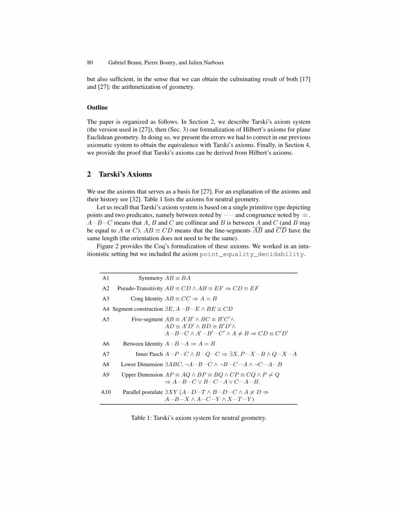
80 Gabriel Braun, Pierre Boutry, and Julien Narboux
but also sufficient, in the sense that we can obtain the culminating result of both [17]and [27]: the arithmetization of geometry.
Outline
The paper is organized as follows. In Section 2, we describe Tarski’s axiom system(the version used in [27]), then (Sec. 3) our formalization of Hilbert’s axioms for planeEuclidean geometry. In doing so, we present the errors we had to correct in our previousaxiomatic system to obtain the equivalence with Tarski’s axioms. Finally, in Section 4,we provide the proof that Tarski’s axioms can be derived from Hilbert’s axioms.
2 Tarski’s Axioms
We use the axioms that serves as a basis for [27]. For an explanation of the axioms andtheir history see [32]. Table 1 lists the axioms for neutral geometry.
Let us recall that Tarski’s axiom system is based on a single primitive type depictingpoints and two predicates, namely between noted by and congruence noted by ≡ .A B C means that A, B and C are collinear and B is between A and C (and B maybe equal to A or C). AB ≡ CD means that the line-segments AB and CD have thesame length (the orientation does not need to be the same).
Figure 2 provides the Coq’s formalization of these axioms. We worked in an intu-itionistic setting but we included the axiom point_equality_decidability.
A1 Symmetry AB ≡BA
A2 Pseudo-Transitivity AB ≡ CD ∧AB ≡ EF ⇒ CD ≡ EF
A3 Cong Identity AB ≡ CC ⇒ A = B
A4 Segment construction ∃E,A B E ∧BE ≡ CD
A5 Five-segment AB ≡A′B′ ∧BC ≡B′C′∧AD ≡A′D′ ∧BD ≡B′D′∧A B C ∧A′ B′ C′ ∧A 6= B ⇒ CD ≡ C′D′
A6 Between Identity A B A⇒ A = B
A7 Inner Pasch A P C ∧B Q C ⇒ ∃X,P X B ∧Q X A
A8 Lower Dimension ∃ABC,¬A B C ∧ ¬B C A ∧ ¬C A B
A9 Upper Dimension AP ≡AQ ∧BP ≡BQ ∧ CP ≡ CQ ∧ P 6= Q⇒ A B C ∨B C A ∨ C A B.
A10 Parallel postulate ∃XY (A D T ∧B D C ∧A 6= D ⇒A B X ∧A C Y ∧X T Y )
Table 1: Tarski’s axiom system for neutral geometry.
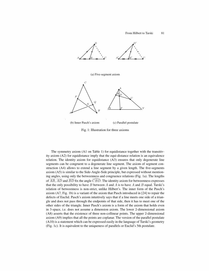
From Hilbert to Tarski 81
bA bCb B
bD
bA′
bC′
b B′
bD′
.
.
(a) Five-segment axiom
bA
bC
bB
bP
bQ
bcX
.
.
(b) Inner Pasch’s axiom
bA
bD
bC
b B
bTbc X bcY
.
.
(c) Parallel postulate
Fig. 1: Illustration for three axioms
The symmetry axiom (A1 on Table 1) for equidistance together with the transitiv-ity axiom (A2) for equidistance imply that the equi-distance relation is an equivalencerelation. The identity axiom for equidistance (A3) ensures that only degenerate linesegments can be congruent to a degenerate line segment. The axiom of segment con-struction (A4) allows to extend a line segment by a given length. The five-segmentsaxiom (A5) is similar to the Side-Angle-Side principle, but expressed without mention-ing angles, using only the betweenness and congruence relations (Fig. 1a). The lengthsofAB,AD andBD fix the angle CBD. The identity axiom for betweenness expressesthat the only possibility to have B between A and A is to have A and B equal. Tarski’srelation of betweenness is non-strict, unlike Hilbert’s. The inner form of the Pasch’saxiom (A7, Fig. 1b) is a variant of the axiom that Pasch introduced in [24] to repair thedefects of Euclid. Pasch’s axiom intuitively says that if a line meets one side of a trian-gle and does not pass through the endpoints of that side, then it has to meet one of theother sides of the triangle. Inner Pasch’s axiom is a form of the axiom that holds evenin 3-space, i.e. does not assume a dimension axiom. The lower 2-dimensional axiom(A8) asserts that the existence of three non-collinear points. The upper 2-dimensionalaxiom (A9) implies that all the points are coplanar. The version of the parallel postulate(A10) is a statement which can be expressed easily in the language of Tarski’s geometry(Fig. 1c). It is equivalent to the uniqueness of parallels or Euclid’s 5th postulate.
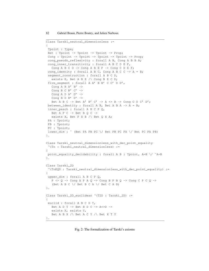
82 Gabriel Braun, Pierre Boutry, and Julien Narboux
Class Tarski_neutral_dimensionless :=Tpoint : Type;Bet : Tpoint -> Tpoint -> Tpoint -> Prop;Cong : Tpoint -> Tpoint -> Tpoint -> Tpoint -> Prop;cong_pseudo_reflexivity : forall A B, Cong A B B A;cong_inner_transitivity : forall A B C D E F,
Cong A B C D -> Cong A B E F -> Cong C D E F;cong_identity : forall A B C, Cong A B C C -> A = B;segment_construction : forall A B C D,
exists E, Bet A B E /\ Cong B E C D;five_segment : forall A A’ B B’ C C’ D D’,
Cong A B A’ B’ ->Cong B C B’ C’ ->Cong A D A’ D’ ->Cong B D B’ D’ ->Bet A B C -> Bet A’ B’ C’ -> A <> B -> Cong C D C’ D’;
between_identity : forall A B, Bet A B A -> A = B;inner_pasch : forall A B C P Q,
Bet A P C -> Bet B Q C ->exists X, Bet P X B /\ Bet Q X A;
PA : Tpoint;PB : Tpoint;PC : Tpoint;lower_dim : ˜ (Bet PA PB PC \/ Bet PB PC PA \/ Bet PC PA PB).
Class Tarski_neutral_dimensionless_with_dec_point_equality‘(Tn : Tarski_neutral_dimensionless) :=point_equality_decidability : forall A B : Tpoint, A=B \/ ˜A=B.
Class Tarski_2D‘(TnEQD : Tarski_neutral_dimensionless_with_dec_point_equality) :=upper_dim : forall A B C P Q,
P <> Q -> Cong A P A Q -> Cong B P B Q -> Cong C P C Q ->(Bet A B C \/ Bet B C A \/ Bet C A B)
.
Class Tarski_2D_euclidean ‘(T2D : Tarski_2D) :=euclid : forall A B C D T,
Bet A D T -> Bet B D C -> A<>D ->exists X, exists Y,Bet A B X /\ Bet A C Y /\ Bet X T Y
.
Fig. 2: The formalization of Tarski’s axioms

From Hilbert to Tarski 83
3 Hilbert’s Axioms
Our formalization of Hilbert’s axiom system is derived on the French translation of thetenth edition annotated by Rossier [18].
Hilbert’s axiom system is based on two abstract types: points and lines (as we limitourselves to 2-dimensional geometry we did not introduce ’planes’ and the related ax-ioms).
In our initial version of Hilbert’s axioms, we made several mistakes. None of theaxioms were incorrect (as they are formally proved from Tarski’s axioms), but someshould be strengthened and some others are useless because they can be derived. Foreach group of axioms, we detail the changes we made to our previous formalization, wedo not detail all the axioms that have already been described in [12]. But, we give thefull list of axioms as a reference.
3.1 Group I
Group I of axioms contains the incidence axioms.First, we had to change the lower dimensional axiom. Hilbert states that there ex-
ists three non collinear points and three points are said to be collinear if there existsa line going through these three points. This assumption is not enough, because in aworld without lines, assuming that there are three non collinear points does not implythat they are distinct. Indeed, there is a model of the first two groups of Hilbert’s ax-ioms with only one point and no lines (interpreting congruence by the empty relation).We can construct a line only if we have two distinct points. Scott’s formalization doesnot need this modification because in Isabelle/HOL all types are inhabited, hence hisformalization includes implicitly the fact that there is at least one line. Meikle’s andRichter’s formalizations enforce that the three points are distinct.
Hence, for the lower dimension axiom, we state that there is a line and point not onthis line:
l0 : Line;P0 : Point;plan : ˜ Incid P0 l0;
As there is an axiom stating there are always at least two points on a line, the formeraxiom stating that there are three non collinear points can be derived.
Second, we had to introduce the property that line equality is an equivalence relationand that incidence is a morphism for line equality:
EqL_Equiv : Equivalence EqL;Incid_morphism :forall P l m, Incid P l -> EqL l m -> Incid P m;
Finally, as we are working in an intuitionist setting we had to introduce some de-cidability properties which allow to perform case distinctions. It would be interesting toformalize a constructive version of Hilbert’s axioms, following Beeson’s work [1], weleave this for future work.

84 Gabriel Braun, Pierre Boutry, and Julien Narboux
Incid_dec : forall P l, Incid P l \/ ˜Incid P l;eq_dec_pointsH : forall A B : Point, A=B \/ ˜ A=B;
The complete list of axioms for group I is given in Fig. 3.
Point : Type;Line : Type;EqL : Line -> Line -> Prop;EqL_Equiv : Equivalence EqL;Incid : Point -> Line -> Prop;Incid_morphism :forall P l m, Incid P l -> EqL l m -> Incid P m;
Incid_dec : forall P l, Incid P l \/ ˜ Incid P l;eq_dec_pointsH : forall A B : Point, A=B \/ ˜ A=B;line_existence :forall A B, A <> B -> exists l, Incid A l /\ Incid B l;
line_uniqueness :forall A B l m,
A <> B ->Incid A l -> Incid B l -> Incid A m -> Incid B m ->
EqL l m;two_points_on_line :forall l,
A : Point & B | Incid B l /\ Incid A l /\ A <> B;ColH :=fun A B C => exists l, Incid A l /\ Incid B l /\ Incid C l;
l0 : Line;P0 : Point;plan : ˜ Incid P0 l0;
Fig. 3: Formalization of Group I
3.2 Group II
Group II of axioms contains the betweenness axioms. We denote byA B C Hilbert’sbetweenness predicate, which is strict. It expresses the fact that B is on the line ACbetween A and C and different from A and C. We could not derive the fact that ifA B C then A 6= C from our former axioms so we added this property as an axiom.The fact that A 6= B and B 6= C (which is assumed by Greenberg, Hartshorne andRichter) is not necessary as it can be derived from the other axioms. The fact that Ashould be different from C is not explicit in Hilbert’s book.
between_diff : forall A B C, BetH A B C -> A <> C;

From Hilbert to Tarski 85
The property between_one states that given three collinear points distinct pointsat least one of them is between the other two:
between_one :forall A B C,
A <> B -> A <> C -> B <> C -> ColH A B C ->BetH A B C \/ BetH B C A \/ BetH B A C.
In our earlier formalization as well as earlier editions of Hilbert’s book, this prop-erty was taken as an axiom. Following the proof by Wald published by Hilbert in latereditions, we derived it from the other axioms. Richter assumes this property. Moreover,in the axiom between_only_one, we removed one of the conjuncts as it can bederived. We now have:
between_only_one : forall A B C, BetH A B C -> ˜ BetH B C A;
instead of:
between_only_one :forall A B C, BetH A B C -> ˜ BetH B C A /\ ˜ BetH B A C;
The other axioms could be kept unmodified. The axioms for the second group aregiven in Fig. 4.
BetH : Point -> Point -> Point -> Prop;between_col : forall A B C, BetH A B C -> ColH A B C;between_diff : forall A B C, BetH A B C -> A <> C;between_comm : forall A B C, BetH A B C -> BetH C B A;between_out : forall A B, A <> B -> exists C, BetH A B C;between_only_one : forall A B C, BetH A B C -> ˜ BetH B C A;cut :=fun l A B => ˜ Incid A l /\ ˜ Incid B l /\
exists I, Incid I l /\ BetH A I B;pasch :forall A B C l,
˜ ColH A B C -> ˜ Incid C l -> cut l A B ->cut l A C \/ cut l B C;
Fig. 4: Formalization of Group II

86 Gabriel Braun, Pierre Boutry, and Julien Narboux
3.3 Group III
Group III of axioms contain those about congruence of segments and angles.
Congruence of segments Hilbert defines congruence as a relation about segments,where segments are defined as unordered pairs of points. In our formalization, we choseto avoid defining the concept of segment. We denote by ≡H the Hilbert segment con-gruence relation. Hence, we have an axiom which says that segments can be permutedon the right. Other permutations can be derived.
cong_permr : forall A B C D, CongH A B C D -> CongH A B D C;
The uniqueness of segment construction can be derived if one assume the reflexivityof congruence of angles, therefore we dropped this axiom. Richter assumes uniquenessof segment construction. The other axioms were not changed, the full list is given onFig. 5. Our formalization of the segment addition axiom follows Hilbert’s prose. It isbased on the definition of the concept of disjoint segments. Note that in the segmentaddition axiom, the concept of disjoint segments could be replaced by a betweennessassumption stating that B is between A and C and B′ is between A′ and C ′, we provedit as lemma:
Lemma addition_betH : forall A B C A’ B’ C’,BetH A B C -> BetH A’ B’ C’ ->CongH A B A’ B’ -> CongH B C B’ C’ ->CongH A C A’ C’.
Congruence of angles In early editions of the Foundations of Geometry, Hilbert hadtaken pseudo-transitivity of congruence of angles as an axiom. Later Rosenthal hasshown that this axiom can be derived from the others [26]. We used the later version ofHilbert’s axioms. Note that, as we need transitivity of congruence in our proofs, we hadto formalize Rosenthal’s proofs. These proofs are rather technical, not very interestingin a pedagogical context, that is why Hartshorne chose to take the simpler, not mini-mal, axiom system of the earlier editions [16]. Richter also assumes the transitivity ofcongruence of angles. In our previous formalization, we defined the concept of anglesABC as three points A, B and C, with a proof that A 6= B and B 6= C. We did notwant to open the Pandora box of the dependent types [6] (types that depend on a proof),so we dropped the proofs from the angle type, and even made implicit the angle type. Tobe faithful to Hilbert, some non degeneracy conditions are added to ensure that anglesare neither flat nor null. This makes the proof of the Tarski’s five-segment axiom (A5)more involved.
We used a predicate of arity six for the congruence of angles:
CongaH :Point -> Point -> Point -> Point -> Point -> Point -> Prop;
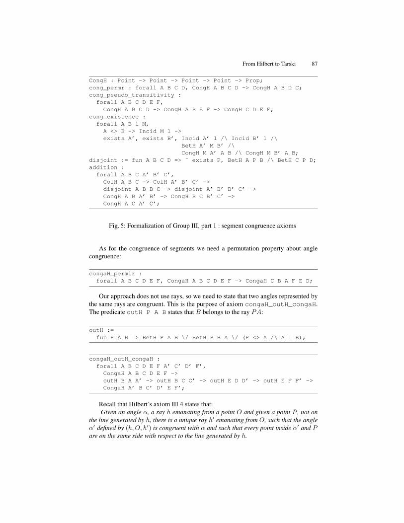
From Hilbert to Tarski 87
CongH : Point -> Point -> Point -> Point -> Prop;cong_permr : forall A B C D, CongH A B C D -> CongH A B D C;cong_pseudo_transitivity :forall A B C D E F,
CongH A B C D -> CongH A B E F -> CongH C D E F;cong_existence :forall A B l M,
A <> B -> Incid M l ->exists A’, exists B’, Incid A’ l /\ Incid B’ l /\
BetH A’ M B’ /\CongH M A’ A B /\ CongH M B’ A B;
disjoint := fun A B C D => ˜ exists P, BetH A P B /\ BetH C P D;addition :forall A B C A’ B’ C’,
ColH A B C -> ColH A’ B’ C’ ->disjoint A B B C -> disjoint A’ B’ B’ C’ ->CongH A B A’ B’ -> CongH B C B’ C’ ->CongH A C A’ C’;
Fig. 5: Formalization of Group III, part 1 : segment congruence axioms
As for the congruence of segments we need a permutation property about anglecongruence:
congaH_permlr :forall A B C D E F, CongaH A B C D E F -> CongaH C B A F E D;
Our approach does not use rays, so we need to state that two angles represented bythe same rays are congruent. This is the purpose of axiom congaH_outH_congaH.The predicate outH P A B states that B belongs to the ray PA:
outH :=fun P A B => BetH P A B \/ BetH P B A \/ (P <> A /\ A = B);
congaH_outH_congaH :forall A B C D E F A’ C’ D’ F’,
CongaH A B C D E F ->outH B A A’ -> outH B C C’ -> outH E D D’ -> outH E F F’ ->CongaH A’ B C’ D’ E F’;
Recall that Hilbert’s axiom III 4 states that:Given an angle α, a ray h emanating from a point O and given a point P , not on
the line generated by h, there is a unique ray h′ emanating from O, such that the angleα′ defined by (h,O, h′) is congruent with α and such that every point inside α′ and Pare on the same side with respect to the line generated by h.
88 Gabriel Braun, Pierre Boutry, and Julien Narboux
We simplified the formalization of Hilbert’s axiom III 4, instead of consideringevery point inside the angle, our proof shows that it is sufficient to state that the pointthat defines the angle is on the same side as P . Hence, we can save the burden ofdefining what it means for a point to be inside an angle. Our version is also simpler thanScoot’s one, which follows Hilbert’s definition.
We say that two points are on the same side of a line, if there is a point P such thatthey are both on opposite sides wrt. P . The fact that two points are on opposite sides ofa line is defined by the cut predicate of Group II.
hcong_4_existence :forall A B C O X P,
˜ ColH P O X -> ˜ ColH A B C ->exists Y, CongaH A B C X O Y /\ same_side’ P Y O X;
hcong_4_uniqueness :forall A B C O P X Y Y’,
˜ ColH P O X -> ˜ ColH A B C ->CongaH A B C X O Y -> CongaH A B C X O Y’ ->same_side’ P Y O X -> same_side’ P Y’ O X ->outH O Y Y’
The full list of axioms is given in Fig. 6.
3.4 Group IV
In 2012, we had an axiom saying that given a line and a point there exists a parallelline through this point. Only the uniqueness of the parallel should be assumed as theexistence can be derived from other axioms. The uniqueness axiom is depicted on Fig. 7.
4 Proving Tarski’s Axioms
To prove Tarski’s axioms we use a trick: we worked on both sides. We derived somelemmas in the context of Hilbert’s axioms and we also proved Tarski’s axioms in thecontext of a variant of these axioms. We introduced this variant of Tarski’s axiom systeminspired by the one adopted by Beeson in [2]. We added the following two properties asaxioms: symmetry of betweenness and inner transitivity and we number them as in [32].We modified Pasch’s axiom to have a version which excludes the degenerate case whenthe triangle ABC is flat. This non degeneracy condition is crucial because obtainingthe general case from Hilbert’s version is not trivial.
Formally, we consider the following axioms:
A14 := ∀ABC, A B C ⇒ C B AA15 := ∀ABCD, A B D ∧B C D ⇒ A B CA′
7 := ∀ABCPQ, A P C ∧B Q C∧A 6= P ∧ P 6= C ∧B 6= Q ∧Q 6= C ∧ ¬Col(ABC)⇒∃X,P X B ∧Q X A

From Hilbert to Tarski 89
CongaH :Point -> Point -> Point -> Point -> Point -> Point -> Prop;
conga_refl : forall A B C, ˜ ColH A B C -> CongaH A B C A B C;conga_comm : forall A B C, ˜ ColH A B C -> CongaH A B C C B A;congaH_permlr :forall A B C D E F, CongaH A B C D E F -> CongaH C B A F E D;
cong_5 :forall A B C A’ B’ C’,
˜ ColH A B C -> ˜ ColH A’ B’ C’ ->CongH A B A’ B’ -> CongH A C A’ C’ ->CongaH B A C B’ A’ C’ ->CongaH A B C A’ B’ C’;
same_side := fun A B l => exists P, cut l A P /\ cut l B P;same_side’ :=fun A B X Y =>
X <> Y /\forall l, Incid X l -> Incid Y l -> same_side A B l;
outH :=fun P A B => BetH P A B \/ BetH P B A \/ (P <> A /\ A = B);
congaH_outH_congaH :forall A B C D E F A’ C’ D’ F’,
CongaH A B C D E F ->outH B A A’ -> outH B C C’ -> outH E D D’ -> outH E F F’ ->CongaH A’ B C’ D’ E F’;
hcong_4_existence :forall A B C O X P,
˜ ColH P O X -> ˜ ColH A B C ->exists Y, CongaH A B C X O Y /\ same_side’ P Y O X;
hcong_4_uniqueness :forall A B C O P X Y Y’,
˜ ColH P O X -> ˜ ColH A B C ->CongaH A B C X O Y -> CongaH A B C X O Y’ ->same_side’ P Y O X -> same_side’ P Y’ O X ->outH O Y Y’
Fig. 6: Formalization of Group III, part 2: angle congruence axioms
Para := fun l m => ˜ exists X, Incid X l /\ Incid X m;euclid_uniqueness :forall l P m1 m2,
˜ Incid P l ->Para l m1 -> Incid P m1-> Para l m2 -> Incid P m2 ->EqL m1 m2
Fig. 7: Formalization of Group IV

90 Gabriel Braun, Pierre Boutry, and Julien Narboux
We denote by V the following set of axioms:
A1, A2, A3, A4, A5, A′7, A8, A9, A14, A15.
Figure 8 provides an overview of the structure of the proof.
A1
A2
A3
A4
A5
A6
A7
A8
A9
A1
A2
A3
A4
A5
A′7
A8
A9
A14
A15
Group IGroup IIGroup III
Tarski’sNeutral 2D
Hilbert’sPlane
V
A10Group IV
Tarski’sEuclidean
2D
Hilbert’sEuclidean
2D
CartesianPlane over apythagoreanordered field
Fig. 8: Overview of the proofs
4.1 Hilbert Plane is equivalent to Tarski A1-A9
The proof is divided into two parts.First, we proved that the variant of Tarski V implies Tarski’s axioms. The fact that
the axiom A6 can be derived from V is Theorem 2.17 of Gupta’s Ph.D. Thesis [15].Second, we proved that V follows from Hilbert’s axioms. Hilbert’s betweenness re-
lation is strict, whereas Tarski’s one is not. Obviously, we defined Tarski’s betweennessrelation (Bet) from Hilbert’s one (BetH) as:
Definition Bet A B C := BetH A B C \/ A = B \/ B = C.
Hilbert’s congruence relation is defined only for non degenerate segments, whereasTarski’s one include the case of the null segment:
Definition Cong A B C D :=(CongH A B C D /\ A <> B /\ C <> D) \/ (A = B /\ C = D).

From Hilbert to Tarski 91
Axioms A1, A2, A3, A4, A8 and A14 are already axioms in Hilbert or easy conse-quences of the axioms. A15 is a theorem in Hilbert which can be proved easily. Tarski’sversion of Pasch’s axiom is stronger than Hilbert’s one, because it provides informationabout the relative position of the points. We could recover the non degenerate case ofTarski’s version of Pasch (A′
7) using some betweenness properties and repeated appli-cations of Hilbert’s version of Pasch. The five-segment axiom requires a longer proof.The non degenerate case is a trivial consequence of the Side-Side-Side theorems andthe fact that if two angles are congruent their supplements are congruent as well. Thosetheorems are proved by Hilbert as theorems 18 and 14. To prove these two theoremswe had to formalize the proof of Hilbert’s theorems 12, 15, 16 and 17 as well. Hilbert’sproofs can be formalized without serious problem; we only had to introduce some lem-mas about the relative position of two points and a line. For example, we had to provethat the same-side relation is transitive: if A and B are of the same side of l, and Band C are on the same side of l then A and C are also on the same side of l. As al-ready noticed by Meikle and Scott, these lemmas, which are as difficult to prove asHilbert’s other theorems are completely implicit in Hilbert’s prose. The non-obviouspart of the proof has been the degenerate case of the five-segment axiom and the upper2-dimensional axiom (A9).
To prove the degenerate case of the five-segment axiom (when the point D belongsto the line AB), we had to prove that then D′ also belongs to line A′B′. We alsohad to prove many degenerate cases which reduce to segment addition and subtraction.Segment subtraction can be deduced from uniqueness of segment construction and fromaddition. We give here only the proof of the key lemma (Lemma 2 below), assumingthe following lemma:
Lemma 1.
A B C ∧A′ B′ C ′ ∧AC ≡H A′C ′ ∧AB ≡H A′B′ ⇒ A′ B′ C ′
Lemma 2.
A B C ∧AB ≡H A′B′ ∧BC ≡H B′C ′ ∧AC ≡H A′C ′ ⇒ Col A′B′ C ′
Proof. We will prove this lemma by contradiction so let us assume that B′ does notbelong to line A′C ′. Let B′′ be a point on A′C ′ such that A′B′′ ≡H AB. Let C ′′ apoint such that B′C ′′ ≡H BC and A′ B′ C ′′ (Fig. 9). So the triangle B′C ′′C ′ isisosceles in B′. Then Hilbert’s theorem 12 lets us prove that B′C ′C ′′ = B′C ′′C ′.By Lemma 1, we have that A′ B′′ C ′. We can derive B′′C ′ ≡H BC by subtractionand then A′C ′ ≡H A′C ′′ by addition. Therefore triangle C ′A′C ′′ is isosceles in A′,hence Hilbert’s theorem 12 implies that A′C ′′C ′ = A′C ′C ′′. By transitivity of anglecongruence (Hilbert’s theorem 19), we know that B′C ′C ′′ = A′C ′C ′′. Finally weobtain a contradiction as the uniqueness of angle construction and the fact that B′ andC ′′ are on the same side of C ′C ′′ let us prove that C ′B′ is the same ray as C ′A′.
The last axiom we need to prove is the upper 2-dimensional axiom. The proof isnot completely straightforward because we do not assume decidability of intersectionof lines: we can not distinguish cases to know if two lines intersect or not.
Let us first prove two useful lemmas.

92 Gabriel Braun, Pierre Boutry, and Julien Narboux
A′B′′ C′
B′
C′′
Fig. 9: Proof of Lemma 2
Lemma 3. If two points A and B are not collinear with two points X and Y , theneither they are one the same side of the line XY or they are on opposite sides of thisline.
Proof. First, one can construct a point C, such that points A and C are on the oppositeside of the line XY . Therefore, there exists a point I collinear with X and Y . If A, Band I are collinear, then either A B I , B A I or A = B and then A and B are onthe same side of line XY or A I B and then A and B are on opposite sides of lineXY , as, neither A nor B can be equal to I since they would then be collinear with Xand Y . Finally, if A, B and C are not collinear, then Pasch’s axiom lets us conclude theproof.
In order to prove Lemma 5 we first prove a particular case which will be usedrepeatedly throughout this proof.
Lemma 4. If three distinct points A, B and C are equidistant from two different pointsP and Q, then, assuming that A is collinear with P and Q, these points are collinear.
Proof. We know that neither B or C are collinear with P and Q because if they werethen they would be equal to A, thus obtaining a contradiction. Therefore, using theprevious lemma, either B and C are on opposite sides or on the same side of line PQ.
– If they are on opposite sides of line PQ, then we name I the point of intersectionbetween this line and the segment BC. If we can prove that A is equal to point Iwe will be done. To do this we just have to prove that I is equidistant from P andQ. Using Hilbert’s theorem 18, we know that the angles PAB and QAB are equal.Then Hilbert’s theorem 12 lets us prove that I is equidistant from P and Q.
– If they are on the same side of line PQ, the previous lemma states that either P andQ are on opposite sides or on the same side of line BC.• If they are on the same side, the uniqueness axioms let us prove that they are
equal, therefore obtaining a contradiction.

From Hilbert to Tarski 93
• If they are on opposite side, then we name I the point of intersection betweenthis line and the line PQ. Without loss of generality, let us consider that B isbetween C and I (if they are equal then A, B and C are trivially collinear).Using Hilbert’s theorems 14 and 18, we know that the angles PBI and QBIare equal. Then Hilbert’s theorem 12 let us prove that I is equidistant from Pand Q. Therefore A is equal to I and we are done.
Lemma 5. If three distinct points A, B and C are equidistant from two different pointsP and Q, then these points are collinear.
Proof. We just have to consider the case where neither A, B or C are collinear withP and Q since otherwise the previous lemma lets us conclude. We know that either atleast two of these points are on opposite sides of the line PQ or all the points are onethe same side of this line.
– If they are on opposite sides of line PQ, then we name I the point of intersectionbetween this line and the segment formed by the points which are on opposite sidesof this line. As in the previous lemma we can prove that I is equidistant from Pand Q. Then apply the previous lemma twice we know that A, B and I as well asA, C and I are collinear and the transitivity of collinearity allows us conclude.
– If they are on the same side of line PQ, either P and Q are on opposite sides or onthe same side of line AB.• If they are on the same side, the uniqueness axioms let us prove that they are
equal, therefore obtaining a contradiction.• If they are on opposite side, then we name I the point of intersection between
this line and the line PQ. As in the previous lemma we can prove that I isequidistant from P and Q. Then apply the previous lemma twice we know thatA,B and I as well asA,C and I are collinear and the transitivity of collinearityallows us conclude.
4.2 Euclidean Hilbert Plane is equivalent to Tarski A1-A10
The fact that Playfair’s postulate can be derived from Tarski’s version of the postulateappears in Chapter 12 of [27], that we have formalized previously. The reverse implica-tion and many other equivalence results have been described in [9]. For this implication,we have to assume the decidability of intersection of line: given two lines either theyintersect or they do not.
5 Conclusion
We have obtained a formal proof that Hilbert’s geometric axioms implies Tarski’s ones.It is interesting to note, that to prove this result we had to correct the axioms we hadgiven in [12], both removing unnecessary axioms and adding some properties. Theconnection between Hilbert’s axioms and Tarski’s ones allows us to obtain all the resultswe had proven in the context of Tarski’s axiom system, in particular the culminatingresult which is the arithmetization of geometry.
94 Gabriel Braun, Pierre Boutry, and Julien Narboux
In our experience, manipulating Hilbert’s axioms is more tedious than Tarski’s ones.As the axioms involve both points and lines (and planes in 3D), a single result can bestated in many different ways, and it requires formally a lot of administrative work toconvert assumptions about lines into assumptions about points and vice-versa. Even ifthis administrative work can be partially automated, using for example the techniquesproposed by Scott and Fleuriot [31], we have the impression that the mechanization ofgeometry based on a single primitive type as in Tarski’s axiom system is more con-venient. Moreover, Hilbert chose to exclude some degenerate cases from its axioms:angles are never null nor full, segments are never degenerate, this makes the proofsmore tedious than in Tarski’s setting. Still, Hilbert’s axiom system has the advantagethat axioms are grouped and each group can serve to develop a significant part of ge-ometry, whereas in a development of geometry based on Tarski’s axioms, one has to useboth the betweenness and congruence axioms very early. Our formalization of Hilbert’saxiom system avoids the concept of sets of points, segments, rays and angles. Our cur-rent formalization can hence be considered less faithful to the original than the one wepresented in 2012, but this new formalization produces axioms which are both clearerand simpler to use.
Perspectives
This work completes the formalization of a non trivial part of Hilbert’s book. But, theformalization could be completed. Among the chapters which have not been formalized,we can cite the one about meta-mathematical results, and the one about arithmetizationof hyperbolic geometry. It would also be useful to extend the formalization to 3D.
It would be also interesting to generate readable proofs from our Coq formalizationto obtain a mechanized book about foundations of geometry.
We leave to future work the proof that our version of Hilbert’s axiom is equivalentto a version in which angles are defined as a pair of rays.
Availability
The full Coq development is available here (release 2.1.0):http://geocoq.github.io/GeoCoq/
References
1. Michael Beeson. Constructive geometry. In Proceedings of the Tenth Asian Logic Collo-quium. World Scientific, 2010.
2. Michael Beeson. A constructive version of Tarski’s geometry. Annals of Pure and AppliedLogic, 166(11):1199–1273, 2015.
3. Michael Beeson and Larry Wos. OTTER proofs of theorems in Tarskian geometry. InStephane Demri, Deepak Kapur, and Christoph Weidenbach, editors, 7th International JointConference, IJCAR 2014, Held as Part of the Vienna Summer of Logic, Vienna, Austria,July 19-22, 2014, Proceedings, volume 8562 of Lecture Notes in Computer Science, pages495–510. Springer, 2014.

From Hilbert to Tarski 95
4. Michael Beeson and Larry Wos. Finding Proofs in Tarskian Geometry. Journal of AutomatedReasoning, submitted, 2015.
5. Michel Beeson. Proving Hilbert’s axioms in Tarski geometry.http://www.michaelbeeson.com/research/papers/TarskiProvesHilbert.pdf, 2014.
6. Yves Bertot and Pierre Casteran. Interactive Theorem Proving and Program Development,Coq’Art: The Calculus of Inductive Constructions. Texts in Theoretical Computer Science.An EATCS Series. Springer, 2004.
7. George D Birkhoff. A set of postulates for plane geometry, based on scale and protractor.Annals of Mathematics, 33:329–345, 1932.
8. Pierre Boutry, Gabriel Braun, and Julien Narboux. From Tarski to Descartes: Formalizationof the Arithmetization of Euclidean Geometry. In The 7th International Symposium on Sym-bolic Computation in Software (SCSS 2016), EasyChair Proceedings in Computing, page 15,Tokyo, Japan, March 2016.
9. Pierre Boutry, Julien Narboux, and Pascal Schreck. Parallel postulates and decidability ofintersection of lines: a mechanized study within Tarski’s system of geometry. submitted, July2015.
10. Pierre Boutry, Julien Narboux, and Pascal Schreck. A reflexive tactic for automated genera-tion of proofs of incidence to an affine variety. October 2015.
11. Pierre Boutry, Julien Narboux, Pascal Schreck, and Gabriel Braun. Using small scale au-tomation to improve both accessibility and readability of formal proofs in geometry. InFrancisco Botana and Pedro Quaresma, editors, Preliminary Proceedings of the 10th In-ternational Workshop on Automated Deduction in Geometry (ADG 2014), 9-11 July 2014,University of Coimbra, Portugal, pages 1–19, Coimbra, Portugal, July 2014.
12. Gabriel Braun and Julien Narboux. From Tarski to Hilbert. In Tetsuo Ida and JacquesFleuriot, editors, Post-proceedings of Automated Deduction in Geometry 2012, volume 7993of LNCS, pages 89–109, Edinburgh, United Kingdom, September 2012. Springer.
13. Gabriel Braun and Julien Narboux. A synthetic proof of Pappus’ theorem in Tarski’s geom-etry. Journal of Automated Reasoning, 2015. accepted, revision pending.
14. Christophe Dehlinger, Jean-Francois Dufourd, and Pascal Schreck. Higher-Order Intuition-istic Formalization and Proofs in Hilbert’s Elementary Geometry. In Automated Deductionin Geometry, volume 2061 of Lecture Notes in Computer Science, pages 306–324. Springer,2001.
15. Haragauri Narayan Gupta. Contributions to the axiomatic foundations of geometry. PhDthesis, University of California, Berkley, 1965.
16. Robin Hartshorne. Geometry : Euclid and beyond. Undergraduate texts in mathematics.Springer, 2000.
17. David Hilbert. Foundations of Geometry (Grundlagen der Geometrie). Open Court, LaSalle, Illinois, 1960. Second English edition, translated from the tenth German edition byLeo Unger. Original publication date, 1899.
18. David Hilbert. Les fondements de la geometrie. Dunod, Paris, jacques gabay edition, 1971.Edition critique avec introduction et complements preparee par Paul Rossier.
19. Timothy James McKenzie Makarios. A Mechanical Verification of the Independence ofTarski’s Euclidean Axiom. PhD thesis, Victoria University of Wellington, 2012. MasterThesis.
20. Laura Meikle and Jacques Fleuriot. Formalizing Hilbert’s Grundlagen in Isabelle/Isar. InTheorem Proving in Higher Order Logics, volume 2758 of Lecture Notes in Computer Sci-ence, pages 319–334. Springer, 2003.
21. Richard S Millman and George D Parker. Geometry, A Metric Approach with Models.Springer Science & Business Media, 1991.
22. E.E. Moise. Elementary Geometry from an Advanced Standpoint. Addison-Wesley, 1990.

96 Gabriel Braun, Pierre Boutry, and Julien Narboux
23. Julien Narboux. Mechanical Theorem Proving in Tarski’s Geometry. In Francisco BotanaEugenio Roanes Lozano, editor, Post-proceedings of Automated Deduction in Geometry2006, volume 4869 of Lecture Notes in Computer Science, pages 139–156, Pontevedra,Spain, 2008. Springer.
24. Moritz Pasch. Vorlesungen uber neuere Geometrie. Springer, 1976.25. William Richter. Formalizing Rigorous Hilbert Axiomatic Geometry Proofs in the Proof
Assistant Hol Light.26. Artur Rosenthal. Vereinfachungen des Hilbertschen Systems der Kongruenzaxiome. Math-
ematische Annalen, 71(2):257–274, June 1911.27. Wolfram Schwabhauser, Wanda Szmielew, and Alfred Tarski. Metamathematische Methoden
in der Geometrie. Springer-Verlag, Berlin, 1983.28. Phil Scott. Mechanising Hilbert’s Foundations of Geometry in Isabelle. Master thesis, Ed-
inburgh, 2008.29. Phil Scott and Jacques Fleuriot. Compass-free Navigation of Mazes. In James H. Daven-
port and Fadoua Ghourabi, editors, SCSS 2016. 7th International Symposium on SymbolicComputation in Software Science, volume 39 of EPiC Series in Computing, pages 143–155.EasyChair, 2016.
30. Phil Scott and Jacques D. Fleuriot. An Investigation of Hilbert’s Implicit Reasoning throughProof Discovery in Idle-Time. In Automated Deduction in Geometry - 8th InternationalWorkshop, ADG 2010, Munich, Germany, July 22-24, 2010, Revised Selected Papers, pages182–200, 2010.
31. Phil Scott and Jacques D. Fleuriot. A Combinator Language for Theorem Discovery. In Intel-ligent Computer Mathematics - 11th International Conference, AISC 2012, 19th Symposium,Calculemus 2012, 5th International Workshop, DML 2012, 11th International Conference,MKM 2012, Systems and Projects, Held as Part of CICM 2012, Bremen, Germany, July 8-13,2012. Proceedings, pages 371–385, 2012.
32. Alfred Tarski and Steven Givant. Tarski’s System of Geometry. The bulletin of SymbolicLogic, 5(2):175–214, June 1999.

Mass points, Bezier Curves and Conics: a Survey
Lionel Garnier1 and Jean-Paul Becar2
1 LE2I, UMR CNRS 6306, University of Burgundy, 21000 Dijon, France2 LAMAV-CGAO, CNRS 2956, Le Mont-Houy, 59313 Valenciennes cedex 9
Abstract. It is well known that rational quadratic Bezier curves defineconics. The use of massic points permits one to define a semi-conic inthe Euclidean plane. Moreover, from a given quadratic Bezier curve, wedetermine the properties of the underlying conic using only one theoremwhich leads to a very simple program.
Keywords: Massic points; rational quadratic Bezier curves; invarients of conics
1 Introduction
In the computer aided domain, the use of rational Bezier curves play an impor-tant role for geometric modelling. Among these curves, the second order curvesdefine a conic arc (see [1–4]). Such a curve is considered as the set of barycentresof weighted points. However, some problems occur for the representation of nonbounded parabolic or hyperbolic arcs. One answer is the use of weighted pointsand vectors in the same space (see [5]). In that space, vectors get a null weight.Thus Bezier curves can be generalised. In the second order rational curves, bythe use of some homographic parameter changes, all features of conics such asfocus and directrix can be determined (see [4]).
Our method offers a new approach of others method developed by G. Albrecht(see [6]), R. Goldman and W. Wang (see [7]), E. Lee (see [8]), J. Sanchez-Reyes(see [9]). Using one of these methods, the construction of a Bezier curve is notpossible in a non-Euclidean space. Some other examples of these models, in thespace of spheres, can be found in [10–12].
Moreover, some researchers use homogeneous coordinates to model a semi-circle (see [13–15]), but A. Piegl noticed (see [14]) that: ”A point in projec-tive space is what mathematicians call an equivalence class. This means that−→Pj (xj , yj , zj , 0) and
−→Pj
∗ (αxj , αyj , αzj , 0) are two representations of the same
point in projective space. However, substituting−→Pj and
−→Pj
∗ into Eq (7.34)(see [14]) clearly results in two different curves.” We can choose a vector us-ing perpendicular conditions and pseudo-metric conditions to determine a Beziercurve which models a given conic seen as a circle (for an adequate non-degenerateindefinite quadratic form) (see [11]). Some applications of the representations,on the space of spheres, of Dupin cyclides using rational quadratic Bezier curveswith mass points can be found in (see [16–19]). In this space, the use of thehomogeneous coordinates are not possible.

98 Lionel Garnier and Jean-Paul Becar
This paper is organised as follows: Section 2 presents the mass points andrational quadratic Bezier curves where their control points are mass points. Insection 3, we determine the elements of a conic defined by a rational quadraticBezier curve in the Euclidean plane. The last section draws some conclusions.
In this paper, (O;−→ı0 ;−→0 ) designates the initial direct reference frame in the
usual Euclidean affine plane P. Let−→P be the set of the vector plane.
2 About mass points
Let I be a finite subset of N. Consider a family (Ai;ωi)i∈I of weighted points inthe affine plane satisfy ∑
i∈I
ωi 6= 0
The centre of mass (or barycentre) G of the weighted points (Ai;ωi)i∈I isthe unique point in P defined by
∑
i∈I
ωi−−→GAi =
−→0 (1)
A mass point is a couple (M,m) such that: if m is equal to 0,−→M is a vector
belonging to the vector plane−→P otherwise M is a point belonging to the affine
plane P. So, a mass point is a weighted point or a vector. J.C. Fiorot (see [5, 20,21]) defined the set of mass points as
P = (P × R∗) ∪(−→P ×
−→0)
What is the barycentre of weighted points when the sum of the weights
vanishes? It is well known that this sum is a vector in the vector plane−→P and
for example:
(A;B) ∈ P ⇒ bar (A;−1) ; (B; 1) is:−−→AB ∈ −→P
where bar (M ;ω) ; (N ;µ) designates the barycentre of the weighted points(M ;ω) and (N ;µ). Moreover, if (Ai, ωi)i∈I is a family of weighted points with∑
i∈I ωi = 0, then we cannot define the barycentre of this family, but we obtainthe vector −→u =
∑
i∈I
ωi−−−→MAi
for any point M in P (the vector −→u does not depend on the point M).
To construct a vector space, we have to define some operations in P usinganalytical geometric methods and then the addition, noted⊕, is defined as follow:
• ω 6= 0 =⇒ (M ;ω)⊕ (N ;−ω) =(ω−−→NM ; 0
);

Mass points, Bezier Curves and Conics: a Survey 99
• if we have ωµ (ω + µ) 6= 0, then
(M ;ω)⊕ (N ;µ) =
(bar
(M ;ω) ; (N ;µ)
;ω + µ
)
• (−→u ; 0)⊕ (−→v ; 0) = (−→u +−→v ; 0);
• ω 6= 0 =⇒ (M ;ω)⊕ (−→u ; 0) =(T 1
ω−→u (M) ;ω
)where T−→w is the translation of
P of vector −→w .
In the same way, on the space P, we define the multiplication by a scalar,noted ⊙, as follow:
• α 6= 0 =⇒ α⊙ (M ;ω) = (M ;αω)
• ω 6= 0 =⇒ 0⊙ (M ;ω) =(−→0 ; 0
)
• α⊙ (−→u ; 0) = (α−→u ; 0)
Let G2 be the midpoint of the segment [MN ]. We have
(M ; 1)⊕ (N ; 1) = (M ; 2)⊕ (M ;−1)⊕ (N ; 1)
= (M ; 2)⊕(−−→MN ; 0
)
=(T 1
2
−−→MN
(M) ; 2)= (G2; 2)
and we generalise the associativity of the barycentre to the set of vectors.Notice that we do not use homogeneous coordinates, we do not use quotient
space and we can define any metric or pseudo-metric on−→P (see [16, 19]). The
notion of barycentre is lost using homogeneous coordinates. For more details onthis space, the reader can refer to books of Fiorot and Jeannin (see [5, 20]).
2.1 Rational quadratic Bezier curves in PLet us recall the definition of the quadratic Bernstein polynomials
B0 (t) = (1− t)2, B1 (t) = 2t (1− t) , B2 (t) = t2 , t ∈ [0, 1] (2)
Now, we can define a rational quadratic Bezier curve having three controlmass points (P0;ω0), (P1;ω1) and (P2;ω2), Definition 1.
Definition 1 : Rational quadratic Bezier curve (BR curve) in PLet ω0, ω1 and ω2 be three real numbers. Let (P0;ω0), (P1;ω1) and (P2;ω2)
be three mass points in P, these points are not colinear.Define two sets I = i|ωi 6= 0 and J = i|ωi = 0Define the function ωf from [0; 1] to R as follows
ωf (t) =∑
i∈I
ωi ×Bi (t) (3)
A mass point (M ;ω) or (−→u ; 0) belongs to the quadratic Bezier curve definedby the three control mass points (P0;ω0), (P1;ω1) and (P2;ω2), if there is a realt0 in [0; 1] such that:
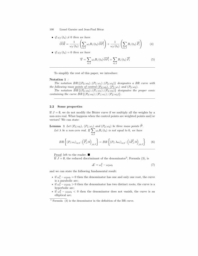
100 Lionel Garnier and Jean-Paul Becar
• if ωf (t0) 6= 0 then we have
−−→OM =
1
ωf (t0)
(∑
i∈I
ωiBi (t0)−−→OPi
)+
1
ωf (t0)
(∑
i∈J
Bi (t0)−→Pi
)(4)
• if ωf (t0) = 0 then we have
−→u =∑
i∈I
ωiBi (t0)−−→OPi +
∑
i∈J
Bi (t0)−→Pi (5)
To simplify the rest of this paper, we introduce:
Notation 1 :The notation BR (P0;ω0) ; (P1;ω1) ; (P2;ω2) designates a BR curve with
the following mass points of control (P0;ω0), (P1;ω1) and (P2;ω2).The notation BR (P0;ω0) ; (P1;ω1) ; (P2;ω2) designates the proper conic
containing the curve BR (P0;ω0) ; (P1;ω1) ; (P2;ω2).
2.2 Some properties
If J = ∅, we do not modify the Bezier curve if we multiply all the weights by anon-zero real. What happens when the control points are weighted points and/orvectors? We can state:
Lemma 1 Let (P0;ω0), (P1;ω1) and (P2;ω2) be three mass points P.
Let λ be a non-zero real. If∑
i∈I
ωiBi (t0) is not equal to 0, we have
BR
(Pi;ωi)i∈I ;
(−→Pj ; 0
)j∈J
= BR
(Pi;λωi)i∈I ;
(λ−→Pj ; 0
)j∈J
(6)
Proof: left to the reader. If J = ∅, the reduced discriminant of the denominator3, Formula (3), is
∆′ = ω21 − ω2ω0 (7)
and we can state the following fundamental result:
⋆ if ω21 −ω2ω0 = 0 then the denominator has one and only one root, the curve
is a parabolic arc;⋆ if ω2
1 −ω2ω0 > 0 then the denominator has two distinct roots, the curve is ahyperbolic arc;
⋆ if ω21 − ω2ω0 < 0 then the denominator does not vanish, the curve is an
elliptical arc.
3 Formula (3) is the denominator in the definition of the BR curve.
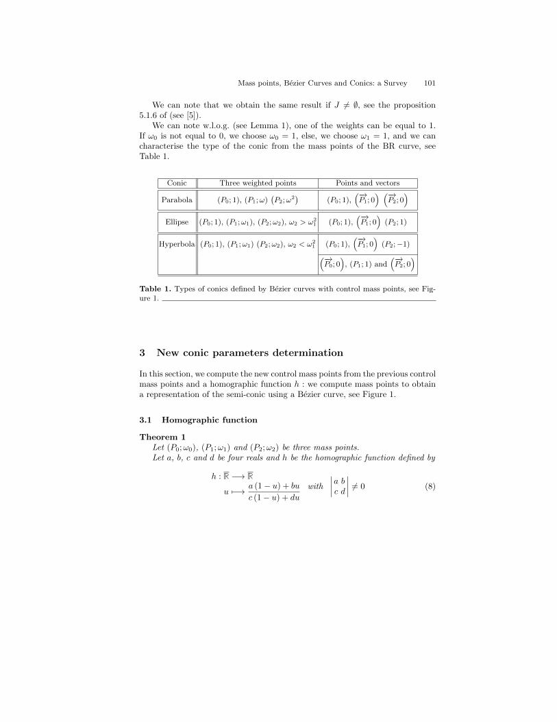
Mass points, Bezier Curves and Conics: a Survey 101
We can note that we obtain the same result if J 6= ∅, see the proposition5.1.6 of (see [5]).
We can note w.l.o.g. (see Lemma 1), one of the weights can be equal to 1.If ω0 is not equal to 0, we choose ω0 = 1, else, we choose ω1 = 1, and we cancharacterise the type of the conic from the mass points of the BR curve, seeTable 1.
Conic Three weighted points Points and vectors
Parabola (P0; 1), (P1;ω)(P2;ω
2)
(P0; 1),(−→P1; 0
) (−→P2; 0
)
Ellipse (P0; 1), (P1;ω1), (P2;ω2), ω2 > ω21 (P0; 1),
(−→P1; 0
)(P2; 1)
Hyperbola (P0; 1), (P1;ω1) (P2;ω2), ω2 < ω21 (P0; 1),
(−→P1; 0
)(P2;−1)
(−→P0; 0
), (P1; 1) and
(−→P2; 0
)
Table 1. Types of conics defined by Bezier curves with control mass points, see Fig-ure 1.
3 New conic parameters determination
In this section, we compute the new control mass points from the previous controlmass points and a homographic function h : we compute mass points to obtaina representation of the semi-conic using a Bezier curve, see Figure 1.
3.1 Homographic function
Theorem 1Let (P0;ω0), (P1;ω1) and (P2;ω2) be three mass points.Let a, b, c and d be four reals and h be the homographic function defined by
h : R −→ R
u 7−→ a (1− u) + bu
c (1− u) + du
with
∣∣∣∣a bc d
∣∣∣∣ 6= 0 (8)

102 Lionel Garnier and Jean-Paul Becar
Fig. 1. Standard representation of a semi-conic using a BR curve with three controlmass points.
Let (Q0;0), (Q1;1) and (Q2;2) be the mass points defined as follow
(Q0;0) = (c− a)2 ⊙ (P0;ω0)⊕ 2a (c− a)⊙ (P1;ω1)
⊕ a2 ⊙ (P2;ω2)
(Q1;1) = (c− a) (d− b)⊙ (P0;ω0)
⊕ (bc− 2ab+ ad)⊙ (P1;ω1)
⊕ ab⊙ (P2;ω2)
(Q2;2) = (d− b)2 ⊙ (P0;ω0)⊕ 2b (d− b)⊙ (P1;ω1)
⊕ b2 ⊙ (P2;ω2)
(9)
Let γP be the map of BR (P0;ω0) ; (P1;ω1) ; (P2;ω2). Let γQ be the map ofBR (Q0;0) ; (Q1;1) ; (Q2;2). Then γQ = γP h and
BR (P0;ω0) ; (P1;ω1) ; (P2;ω2) = BR (Q0;0) ; (Q1;1) ; (Q2;2) (10)
Proof: see [4]. In the rest of this paper, we will just write the result using Formula (9) but
the reader keeps in mind that γQ = γP h and that Formula (10) is always true.

Mass points, Bezier Curves and Conics: a Survey 103
We note, using Theorem 10 with a = 0, c =1√ω0
and d = b =1√ω2
, that
only the weights of P0 and P2 change. Moreover, if ω0 and ω2 are two positivereal numbers, if ω1 6= 0, we have
BR (P0;ω0) ; (P1;ω1) ; (P2;ω2) = BR
(P0; 1) ;
(P1;
ω1√ω0ω2
); (P2; 1)
(11)
else, (if ω1 = 0), we have
BR(P0;ω0) ;
(−→P1; 0
); (P2;ω2)
= BR
(P0; 1) ;
(1√ω0ω2
−→P1; 0
); (P2; 1)
(12)
Thus we generalise to vectors the formulae given by Farin (see [22]). In the restof this paper, if the first control point is a weighted point, we take ω0 = 1.
3.2 The parabola case
From Formula (7), the BR (P0; 1) ; (P1;ω1) ; (P2;ω2) is a parabola iff we have
ω2 = ω21
Theorem 2Let (P0; 1), (P1;ω) and
(P2;ω
2)be three control weighted points of a BR
curve. We distinguish two cases.
1. If ω = 1. Let h be defined by h (u) =u
1− u.
Then, the point (P0; 1) is unchanged and we obtain
(−→U1; 0
)=
(−−−→P0P1; 0
)
(−→U2; 0
)=(−−−→P1P0 +
−−−→P1P2; 0
) (13)
2. If ω /∈ 0; 1. Let h be defined by h (u) =u
1− ω.
Then, the point (P0; 1) is unchanged and we obtain
(−→U1; 0
)=
(ω
1− ω
−−−→P0P1; 0
)
(−→U2; 0
)=
((ω
1− ω
)2 (−−−→P1P0 +
−−−→P1P2
); 0
) (14)
Proof: This proof is obtained using Theorem 10 with a = 0, b = 1, c = 1 andd = 0 for the first case and a = 0, b = 1
1−ω , c = 1 and d = 1 for the second case.

104 Lionel Garnier and Jean-Paul Becar
In Theorem 2, if t0 belongs to [0, 1[, the mass point of the BR curve is aweighted point (M,B0 (t0)) defined by
−−→OM =
1
B0 (t0)
(B0 (t0)
−−→OP0 +B1 (t0)
−→U1 +B2 (t0)
−→U2
)(15)
whereas, for t0 = 1, the mass point of the BR curve is the vector(−→U2; 0
).
Figures 2 show the effect of Theorem 2 with (P0; 1) = ((0.; 6) ; 1), (P1;ω) =((−13.; 0) ; 1) and
(P2;ω
2)= ((−1;−1) ; 1).
(a) (b)
Fig. 2. Illustration of Theorem 2 with ω = 1. (a): the initial BR curve with threecontrol weighted points. (b): the new BR curve with three control mass points (oneweighted point and two vectors).
The second step of this work is done using the following theorem.
Theorem 3 Let (P0; 1),(−→U1; 0
)and
(−→U2; 0
)be three control mass points of a
BR curve such that −→U1 •
−→U2 6= 0
Let h be defined by
h (u) =ru
(1− u) + ruwith r =
1∥∥∥−→U2
∥∥∥2
−→U1 •
−→U2 (16)
Then, the point (P0; 1) is unchanged and we obtain
(−→V1; 0
)=(r−→U1; 0
)
(−→V2; 0
)=(r2−→U2; 0
) (17)
Proof: This proof is obtained using Theorem 10 with a = 0, d = b = r andc = 1.
Figure 3 shows an application of Theorem 3 with (P0; 1) = ((0.; 6) ; 1),(P1; 1) = ((−13.; 0) ; 1) and (P2; 1) = ((−1;−1) ; 1).
Now we can state:

Mass points, Bezier Curves and Conics: a Survey 105
Fig. 3. Illustration of Theorem 3 with ω = 1.
Theorem 4 Let (P0; 1),(−→V1; 0
)and
(−→V2; 0
)be three control mass points of a
BR curve such that −→V1 •
−→V2 6= 0
Let h be defined by h (u) =− (1− u) + u
u.
Then, the point (P0; 1) is unchanged and we obtain
(Q0; 1) =(T−→V2−2
−→V1
(P0) ; 1)
(−→W1; 0
)=
(−→V1 −
−→V2; 0
) (18)
Proof: This proof is obtained using Theorem 1 with a = −1, b = d = 1 andc = 0.
Figure 4 gives an illustration of Theorem 4 with (P0; 1) = ((0.; 6) ; 1), (P1; 1) =((−13.; 0) ; 1) and (P2; 1) = ((−1;−1) ; 1).
Fig. 4. Illustration of Theorem 4 with ω = 1.
We can state a fundamental remark. The vectors defined in Formula (18)verify −→
W1 •−→V2 = 0 (19)
Now we can determine the parabola invariants.

106 Lionel Garnier and Jean-Paul Becar
Theorem 5 :Let ω ∈ R∗. Let (P0; 1), (P1;ω) and
(P2;ω
2)be three control mass points of a
BR curve. Let BR(Q0; 1) ;
(−→W1; 0
);(−→V2; 0
), be the BR curve obtained using
Theorems 2, 3 and 4.Then, BR (P0; 1) ; (P1;ω) ; (P2;ω2) is a parabola P, its vertex is Q0, its
equation is
Y =
∥∥∥−→V2
∥∥∥2
4∥∥∥−→W1
∥∥∥X2
in the orthonormal reference frame
Q0;
1∥∥∥−→W1
∥∥∥−→W1;
1∥∥∥−→V2
∥∥∥−→V2
.
Proof: see [4]. The vector
−→W1 is tangent to the parabola at Q0 whereas the focal axis is
defined by Q0 and−→V2.
Figure 5 shows two arcs of the same parabola: BR(P0; 1) , (P1; 1) , (P2; 1)on one hand and BR(Q0; 1) ,
(−→W1; 0
),(−→V2; 0
) on the other hand. This curve
offers the computation of the elements of the parabola using Theorem 5.
1
2
3
4
5
6
−1−1−2−3−4−5−6−7−8−9−10−11−12−13−14b
b
b
rrQ0
P2
P1
P0
F
−→V2
−→W1
Fig. 5. Two arcs of the same parabola defined with two BR curves with control mass
points (P0; 1), (P1; 1) and (P2; 1) (in orange) on one hand (Q0; 1),(−→W1; 0
)and
(−→V2; 0
)
(in black) on the other hand. The first mass point is the weighted point (Q0; 1) whereas
the last mass point is the vector(−→V2; 0
).

Mass points, Bezier Curves and Conics: a Survey 107
3.3 The ellipse case
In this section, the weights satisfy the condition ω21 − ω2ω0 < 0 and w.l.o.g.,
we can suppose ω0 = 1 and ω2 > 0. Moreover, using Theorem 10 with a = 0,b = d = −1 and c = 1, we can suppose ω1 ≥ 0. In fact, using the multiplicationof a mass point by a scalar, we transform the mass point (P1;ω1) into the mass
point −1⊙ (P1;ω1). So a weighted point (P1;ω1) (resp. vector(−→P1; 0
)) becomes
(P1;−ω1) (resp. vector(−−→P1; 0
)). Now we can begin the change of the control
mass points and we can state:
Theorem 6 Let (P0; 1), (P1;ω1), ω2 > ω21 6= 0, and (P2;ω2) be three control
weighted points of a BR curve. Let h be defined by
h (u) =ru
(1− u) + (1 + r)uwith r = − 1
ω1(20)
Then, the point (P0; 1) is unchanged and we obtain
(−→U1; 0
)=(−−−→P1P0; 0
)
(P3;3) =
(bar
(P0; 1) ; (P1;−2)
(P2;
ω2
ω21
);−1 +
ω2
ω21
)(21)
Proof: This proof is obtained using Theorem 1 with a = 0, b = r, c = 1 andd = 1 + r.
We note that the last weight is positive and the midpoint O0 of [P0P3] is thecentre of the ellipse.
Figure 6 shows the effect of Theorem 6 with (P0; 1) = ((0.; 6) ; 1), (P1; 1) =((−13.; 0) ; 1
2
)and (P2; 1) = ((−1;−1) ; 1) (the curve is in green). The inter-
mediate weighted point is transformed into a vector, the last weighted point ismodified into another weighted point. The obtained curve is in red.
Fig. 6. Illustration of Theorem 6.
The next theorem offers the weights of the weighted points to be equal to 1.

108 Lionel Garnier and Jean-Paul Becar
Theorem 7 :Consider BR
(P0; 1) ;
(−→U1; 0
); (P3;3)
obtained using Theorem 6.
Let h be defined by h (u) =u√
ω3 (1− u) + u.
Then, the point (P0; 1) is unchanged, the weight of P3 becomes 1 and weobtain −→
V1 =1√ω3
−→U1 (22)
Proof We use Theorem 10 with a = 0, d = b = 1 and c =√ω3, and then we
use Formula (6) with λ = 1ω3
.Figure 7 shows the effect of Theorem 7 with (P0; 1) = ((0.; 6) ; 1), (P1; 1) =(
(−13.; 0) ; 12
)and (P3; 1) = ((−1;−1) ; 1).
Fig. 7. Illustration of Theorem 7.
Let k1 and k2 be the reals defined by
k1 =−−−→P0P3 •
−→V1
k2 =−→V1
2 − 1
4P0P
23
(23)
If k1 = 0 and k2 = 0 then the BR(P0; 1) ;
(−→V1; 0
); (P3; 1)
is a circular arc,
see [4]. In the rest of this section, we do not consider this case. The followingtheorem permits us to model a semi-ellipse.
Theorem 8 Let (P0; 1),(−→V1; 0
)and (P3; 1) be the control mass points of a
Bezier curve, obtained using Theorem 7.
If k2 = 0, we take θ = π8 , else we take θ =
1
4arctan
(k1k2
).
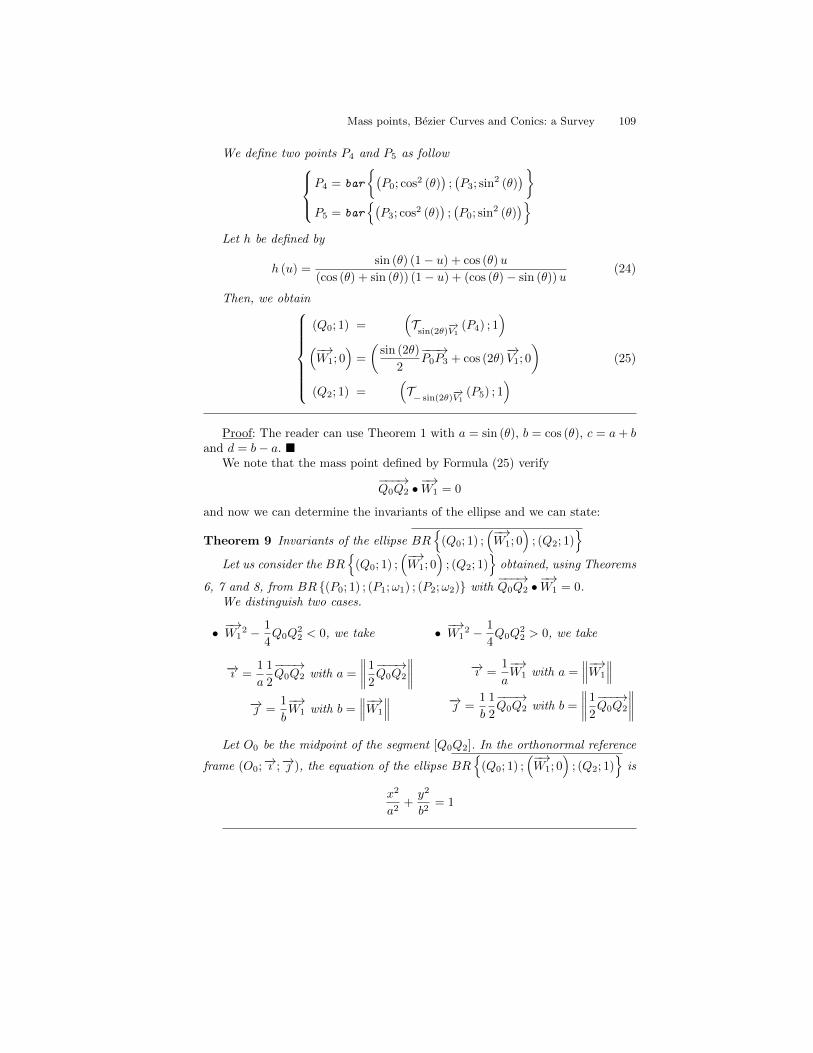
Mass points, Bezier Curves and Conics: a Survey 109
We define two points P4 and P5 as follow
P4 = bar
(P0; cos
2 (θ));(P3; sin
2 (θ))
P5 = bar(
P3; cos2 (θ)
);(P0; sin
2 (θ))
Let h be defined by
h (u) =sin (θ) (1− u) + cos (θ)u
(cos (θ) + sin (θ)) (1− u) + (cos (θ)− sin (θ))u(24)
Then, we obtain
(Q0; 1) =(Tsin(2θ)
−→V1
(P4) ; 1)
(−→W1; 0
)=
(sin (2θ)
2
−−−→P0P3 + cos (2θ)
−→V1; 0
)
(Q2; 1) =(T− sin(2θ)
−→V1
(P5) ; 1)
(25)
Proof: The reader can use Theorem 1 with a = sin (θ), b = cos (θ), c = a+ band d = b− a.
We note that the mass point defined by Formula (25) verify
−−−→Q0Q2 •
−→W1 = 0
and now we can determine the invariants of the ellipse and we can state:
Theorem 9 Invariants of the ellipse BR(Q0; 1) ;
(−→W1; 0
); (Q2; 1)
Let us consider the BR(Q0; 1) ;
(−→W1; 0
); (Q2; 1)
obtained, using Theorems
6, 7 and 8, from BR (P0; 1) ; (P1;ω1) ; (P2;ω2) with−−−→Q0Q2 •
−→W1 = 0.
We distinguish two cases.
• −→W1
2 − 1
4Q0Q
22 < 0, we take
−→ı =1
a
1
2
−−−→Q0Q2 with a =
∥∥∥∥1
2
−−−→Q0Q2
∥∥∥∥
−→ =1
b
−→W1 with b =
∥∥∥−→W1
∥∥∥
• −→W1
2 − 1
4Q0Q
22 > 0, we take
−→ı =1
a
−→W1 with a =
∥∥∥−→W1
∥∥∥
−→ =1
b
1
2
−−−→Q0Q2 with b =
∥∥∥∥1
2
−−−→Q0Q2
∥∥∥∥
Let O0 be the midpoint of the segment [Q0Q2]. In the orthonormal reference
frame (O0;−→ı ;−→ ), the equation of the ellipse BR
(Q0; 1) ;
(−→W1; 0
); (Q2; 1)
is
x2
a2+
y2
b2= 1
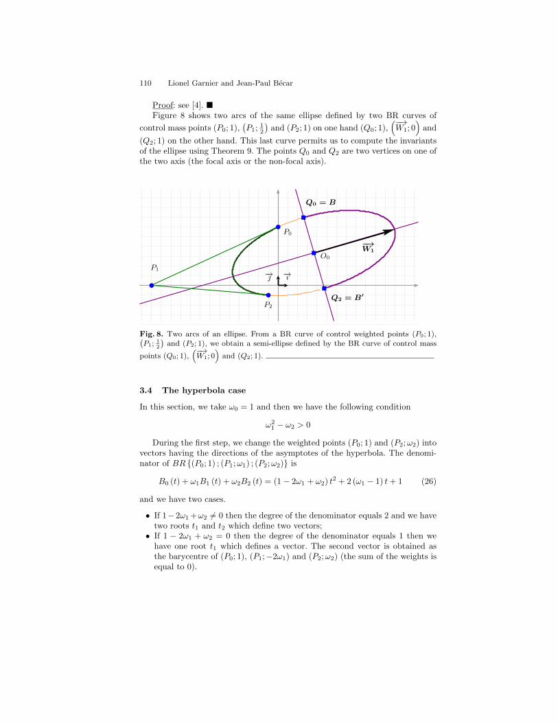
110 Lionel Garnier and Jean-Paul Becar
Proof: see [4]. Figure 8 shows two arcs of the same ellipse defined by two BR curves of
control mass points (P0; 1),(P1;
12
)and (P2; 1) on one hand (Q0; 1),
(−→W1; 0
)and
(Q2; 1) on the other hand. This last curve permits us to compute the invariantsof the ellipse using Theorem 9. The points Q0 and Q2 are two vertices on one ofthe two axis (the focal axis or the non-focal axis).
r
r
rb
b
b
O0
−→ı−→
−→W1
P2
P1
P0
Q0 = B
Q2 = B′
Fig. 8. Two arcs of an ellipse. From a BR curve of control weighted points (P0; 1),(P1;
12
)and (P2; 1), we obtain a semi-ellipse defined by the BR curve of control mass
points (Q0; 1),(−→W1; 0
)and (Q2; 1).
3.4 The hyperbola case
In this section, we take ω0 = 1 and then we have the following condition
ω21 − ω2 > 0
During the first step, we change the weighted points (P0; 1) and (P2;ω2) intovectors having the directions of the asymptotes of the hyperbola. The denomi-nator of BR (P0; 1) ; (P1;ω1) ; (P2;ω2) is
B0 (t) + ω1B1 (t) + ω2B2 (t) = (1− 2ω1 + ω2) t2 + 2 (ω1 − 1) t+ 1 (26)
and we have two cases.
• If 1−2ω1+ω2 6= 0 then the degree of the denominator equals 2 and we havetwo roots t1 and t2 which define two vectors;
• If 1 − 2ω1 + ω2 = 0 then the degree of the denominator equals 1 then wehave one root t1 which defines a vector. The second vector is obtained asthe barycentre of (P0; 1), (P1;−2ω1) and (P2;ω2) (the sum of the weights isequal to 0).

Mass points, Bezier Curves and Conics: a Survey 111
Theorem 10 Let (P0; 1), (P1;ω1) and (P2;ω2) be three control weighted pointsof a BR curve. We have two cases.
• If 1− 2ω1+ω2 6= 0, the equation given in Formula (26) has two roots t1 andt2 defined by
t1 =1− ω1 +
√ω21 − ω2
1− 2ω1 + ω2, t2 =
1− ω1 −√ω21 − ω2
1− 2ω1 + ω2
Let h be defined by h (u) = t1 (1− u) + t2u. Then
−→U0 = B0 (t1)
−−→ΩP0 + ω1B1 (t1)
−−→ΩP1 + ω2B2 (t1)
−−→ΩP2
(Q1;1) =
(bar (P0;α0) ; (P1;α1) ; (P2;α2) ;
2(ω2 − ω2
1
)
(1− 2ω1 + ω2)
)
−→U2 = B0 (t2)
−−→ΩP0 + ω1B1 (t2)
−−→ΩP1 + ω2B2 (t2)
−−→ΩP2
(27)
with
(α0, α1, α2) = ((1− t1) (1− t2) , ω1 (t2 − 2t1t2 + t1) , t1t2ω2)
• If 1− 2ω1 + ω2 = 0, the root of the equation given in Formula (26) is
t0 =1
2 (1− ω1)
Let h be defined by h (u) =t0 (1− u) + u
(1− u). Then
−→U0 = B0 (t0)
−−→ΩP0 + ω1B1 (t0)
−−→ΩP1 + ω2B2 (t0)
−−→ΩP2
(Q1;1) = (bar (P0;α0) ; (P1;α1) ; (P2;α2) ;ω1 − 1)
−→U2 =
−−→ΩP0 − 2ω1
−−→ΩP1 + ω2
−−→ΩP2
(28)
with(α0, α1, α2) = t0 − 1, ω1 (1− 2t0) , t0ω2
Proof: This proof is obtained using Theorem 10 with a = t1, b = t2, c = 1and d = 1 for the first case and a = t0, b = c = 1 and d = 0 for the second case.
Figure 9 shows the effect of the first case of Theorem 10 with (P0; 1) =((√2; 1); 1), (P1;ω1) and (P2; 1) =
((2;−
√3); 1)with
(P1;ω1) =
((√2
2−
√3
3; 1 +
(1 +
√3)(
1−√2))
;
√2√3 + 4
√2 + 2
2
)

112 Lionel Garnier and Jean-Paul Becar
Fig. 9. Illustration of the first case of Theorem 10.
Let us define−→V0 = 1
1
−→U0 and
−→V2 = 1
1
−→U2. The new control mass points of
the Bezier curve are(−→V0; 0
), (Q1; 1) and
(−→V2; 0
). The centre of the hyperbola is
Q1, its weight is equal to 1. In the next theorem, we obtain two vectors havingthe same norm.
Theorem 11 Let(−→V0; 0
), (Q1; 1) and
(−→V2; 0
)be the control mass points of a
BR curve obtained using previous theorems. Let h be defined by
h (u) =ru
1
r(1− u) + ru
with r =4
√√√√√
∥∥∥−→V0
∥∥∥∥∥∥−→V2
∥∥∥(29)
Then
(Q0;0) =(−→W0; 0
)=(r4
−→V0; 0
)
(Q2;0) =(−→W2; 0
)=(r4
−→V2; 0
) (30)
with the fundamental relation
∥∥∥−→W0
∥∥∥ =∥∥∥−→W2
∥∥∥ (31)
Proof : From Theorem 10 with a = 0, d = b = r and c = 1r .
Figure 10 shows the effect of Theorem 11 from the example given in Figure 9.
The last step consists in computing the hyperbola invariants.

Mass points, Bezier Curves and Conics: a Survey 113
Fig. 10. Illustration of Theorem 11 from Figure 9.
Theorem 12 Invariants of a hyperbola
The curve BR(−→
W0; 0); (Q1; 1) ;
(−→W2; 0
)is obtained using Theorems 10 and 11.
Define
−→ı =1
a
1
2
(−→W0 +
−→W2
)with a =
∥∥∥−→W0 +−→W2
∥∥∥2
(32)
and
−→ =1
b
1
2
(−→W0 −
−→W2
)with b =
∥∥∥−→W0 −−→W2
∥∥∥2
(33)
Then BR(−→
W0; 0); (Q1; 1) ;
(−→W2; 0
)is the hyperbola of centre Q1, of equa-
tion
x× y =
∥∥∥−→W0
∥∥∥2
4
in the orthonormal reference frame
(Q1;
1∥∥∥−→W0
∥∥∥−→W0;
1∥∥∥−→W2
∥∥∥−→W2
), of equation
x2
a2− y2
b2= 1
in the orthonormal reference frame (Q1;−→ı ;−→ ).
Proof: see [4]. We remark that the vertices A and A′ of the hyperbola satisfy
−−→Q1A =
1
2
(−→W0 +
−→W2
)= −
−−−→Q1A
′ (34)

114 Lionel Garnier and Jean-Paul Becar
Figure 11 shows two arcs of the same hyperbola. The first arc is modelled
by a BR curve, its control weighted points are (P0; 1),
(P1;
√2√3+4
√2+2
2
)and
(P2; 1), Figure 9. The second arc is a branch of the hyperbola, the control mass
points of the BR curve are(−→W0; 0
), (Q1; 1) and
(−→W2; 0
). From this curve, using
Theorem 12, we can determine the elements of this hyperbola.
1
2
−1
−2
1 2−1b
b
r
b
∆ ′
P1Q1
−→W0
−→W2
−→ı
P0
P2
−→
∆
Fig. 11. A connected arc of hyperbola mode led by a BR curve of control mass points
(P0; 1),
(P1;
√2√3+4
√2+2
2
)and (P2; 1), a BR curve of control mass points
(−→W0; 0
),
(Q1; 1) and(−→W2; 0
)which models a branch of the Hyperbola.
Mass points, Bezier Curves and Conics: a Survey 115
4 Conclusion
We have presented a survey of mass points: in the same space, we aggregate theaffine points and the vectors. Moreover, we can generalise the notion of barycen-tre and its associativity to the vectors. We have modelled non-degenerate conicsusing rational quadratic Bezier curves. In the Euclidean plane, starting withthese kinds of curves, we have computed the elements of these conics (parabola,ellipse and hyperbola).
To complete this discussion, the reader may consult (see [23]) which gives amodern application of conics in the context of curve approximations and (see [16,24]) where the authors compute the characteristic circles of a Dupin cyclidemodelled in the space of spheres.
Acknowledgements
The authors warmly thank Prof R. Goldman from Rice University in Houstonfor his review and his helpful comments.
References
1. Bezier, P.: Courbe et surface. 2eme edn. Volume 4. Hermes, Paris (1986)2. Casteljau, P.D.: Mathematiques et CAO. Volume 2 : formes a poles. Hermes (1985)3. Garnier, L.: Mathematiques pour la modelisation geometrique, la representation
3D et la synthese d’images. Ellipses (2007) ISBN : 978-2-7298-3412-8.4. Becar, J.P.: Forme (BR) des coniques et de leurs faisceaux. PhD thesis, Universite
de Valenciennes et de Hainaut-Cambresis, LIMAV (1997)5. Fiorot, J.C., Jeannin, P.: Courbes et surfaces rationnelles. Volume RMA 12. Mas-
son (1989)6. Albrecht, G.: Mathematical methods for curves and surfaces. Vanderbilt Univer-
sity, Nashville, TN, USA (2001) 15–247. Goldman, R.N., Wang, W.: Using invariants to extract geometric characteristics
of conic sections from rational quadratic parameterizations. Int. J. Comput. Ge-ometry Appl. 14 (2004) 161–187
8. Lee, E.: The rational Bezier representation for conics. In (ed.), G.F., ed.: InGeometric Modeling, Algorithms and New Trends. SIAM, Philadelphia (1985) 3–19
9. Sanchez-Reyes, J.: Characteristics of conic segments in Bezier form. In: Interna-tional Conference on Innovative Methods in Product Design, Venise, Italy (2011)231–234
10. Garnier, L., Druoton, L., Langevin, R.: Subdivisions iteratives d’arcs d’ellipseset d’hyperboles et application a la visualisation de cyclides de Dupin. RevueElectronique Francophone d’Informatique Graphique 6 (2012) 1–36
11. AFIG, ed.: Inversions de coniques a centres vues comme des cercles, Universite deLimoges (2013)
12. Garnier, L., Druoton, L., Becar, J.P.: Points massiques, espace des spheres et”hyperbole”. In: G.T.M.G. 2015, Poitiers (2015) http://gtmg2015.conference.univ-poitiers.fr/programme details.

116 Lionel Garnier and Jean-Paul Becar
13. Versprille, K.J.: Computer-aided Design Applications of the Rational B-splineApproximation Form. PhD thesis, Syracuse, NY, USA (1975) AAI7607690.
14. Piegl, L., Tiller, W.: The NURBS book. Monographs in visual communication.Springer (1995)
15. Farin, G.: From conics to nurbs: A tutorial and survey. IEEE Comput. Graph.Appl. 12 (1992) 78–86
16. Druoton, L., Garnier, L., Langevin, R.: Iterative construction of Dupin cy-clide characteristic circles using non-stationary Iterated Function Systems (IFS).Computer-Aided Design 45 (2013) 568–573 Solid and Physical Modeling 2012,Dijon.
17. Garnier, L., Becar, J.P., Druoton, L.: Subdivisions de courbes deBezier quadratiques, Lyon, France, Universite de Lyon, LIRIS (2015)http://liris.cnrs.fr/afig2015/?page id=939#sthash.IbJxJhLu.dpuf.
18. Garnier, L., Becar, J.P., Morin, G., Fuchs, L.: Une application de l’espace dessphres : determination des spheres de Dandelin, Lyon, France, Universite de Lyon,LIRIS (2015) http://liris.cnrs.fr/afig2015/?page id=939#sthash.IbJxJhLu.dpuf.
19. Garnier, L., Becar, J.P., Druoton, L.: Surfaces canal et courbes de bezier ra-tionnelles quadratiques, Dijon, France, Universite de Bourgogne, Le2i (2016)
20. Fiorot, J.C., Jeannin, P.: Courbes splines rationnelles, applications a la CAO.Volume RMA 24. Masson (1992)
21. Goldman, R.: On the algebraic and geometric foundations of computer graphics.ACM Trans. Graph. 21 (2002) 52–86
22. Farin, G.: NURBS from Projective Geometry to Pratical Use. 2 edn. A K Peters,Ltd (1999) ISBN 1-56881-084-9.
23. Albrecht, G., Becar, J.P., Farin, G.E., Hansford, D.: On the approximation orderof tangent estimators. Computer Aided Geometric Design 25 (2008) 80–95
24. Garnier, L., Druoton, L.: Constructions, dans l’espace des spheres, de car-reaux de cyclides de Dupin a bords circulaires. Revue Electronique Francophoned’Informatique Graphique 7 (2013) 17–40

A New Formalization of Origami in GeometricAlgebra
Tetsuo Ida1, Jacques Fleuriot2, and Fadoua Ghourabi3
1 University of Tsukuba, Tsukuba, [email protected]
2 University of Edinburgh, Edinburgh, [email protected]
3 Ochanomizu University, Tokyo, [email protected]
Abstract. We present a new formalization of origami modeling and the-orem proving using a geometric algebra. We formalize in Isabelle/HOLa geometric algebra G3) to treat origamis in both 2D and 3D physicalspace. We define G3 as a type class of Isabelle/HOL. The objects in G3
are multivectors. We prove that the co-datatype of a multivector is anelement instance of the type class G3. We prove by Isabelle/HOL a largenumber of identities and equations that hold in G3. With G3 we thenreformulate Huzita’s elementary origami folds in equations of multivec-tors. They are translated to the equations of the polynomial ring. Bysolving the equations, we can construct origamis computationally, andfurthermore prove geometric properties of the constructed origami. Weshow an example of trisecting an arbitrary angle by origami using G3.
1 Introduction
We show an application of a geometric algebra to computational origami. Thereare several definitions of geometric algebra. We take the one expounded byHestenes [1]. We call for geometric algebra, as we are investigating the extensionof the computational origami system Eos [2] to deal with modeling and verifying3D origamis more systematically. There are two main reasons for this.
Firstly, a uniform treatment of 3D and 2D models within the same systemis important to us since many origamis can be made in a single flat 2D plane,whereas folding papers apparently involve the notion of superpositions of flatplanes. This mere fact shows the need for the concept of 3D. In other words,modeling origami entirely in 3D destroys the simplicity of origami geometricproblems, whereas to model origamis entirely in 2D is too restrictive, as we aremostly interested in the 3D shapes of origami as the result of construction.
Secondly, the algebraic and geometric structures used for computational pur-poses are often boiled down to the collection of simple symbolic forms by thetranslations via the Cartesian coordinate system. Whether the resulting onesare polynomials or matrices, for example, the geometric meanings that origi-nally pertain to geometric objects are often lost in the translation. Here, we
118 Tetsuo Ida, Jacques Fleuriot, and Fadoua Ghourabi
need adequate abstraction layers between the geometric language of our dailyuse and the language for the computational purposes.
We organize the rest of the paper as follows. In Section 2, we present thegeometric algebra (to be abbreviated to GA, hereafter), but only as much asis needed for the computational origami construction and verification, with theuse of new notations that facilitate the reading of identities involved. As we aretreating formulas of the GA in two computer languages, some deviation fromthe usual mathematical notations, and complication in expressing the formulasare inevitable. To simplify our explanation, we remove type information fromthe GA formulas of this paper. From the outset of Section 2, we introduce thenotion of a multivector, i.e. the element of GA, together with its operations.Then, we formalize the multivector and the operations on it using Isabelle/HOL.In Section 3, we briefly introduce Huzita’s elementary fold operations since weuse them in origami geometry. In Section 4, we describe Huzita’s fold in GA.In Section 5, we show a simple example to illustrate our method of geometrictheorem proving using GA. We give an example of trisecting an arbitrary angleby origami. Although it is a typical 2D origami problem, indeed had been one ofthe famous impossibility problems in classical Euclidean geometry, it can serveas a non-trivial illustration of GA. In Section 6, we briefly discuss research worksin the past two decades whose methodology and goal we share, i.e. geometrictheorem proving. In Section 7, we summarize our results and point out thedirections for further research.
2 Geometric algebra
2.1 Objects and operations
We are going to define a geometric algebra G, following Hestenes’ definition[1]with the application to origami in mind. In particular, we would like to describeG3 as a formal system to reason about the geometric objects and their operationson them in 2D and 3D physical spaces.
Elements of G3 are called multivectors. A multivector consists of the followingcomponents: a real number (we also call it a scalar, to be consistent with theusage in the linear algebra), a vector, a bivector, and a trivector. They aresometimes written as 0-vector, 1-vector, 2-vector, and 3-vector, respectively. Thevectors and bivectors are three dimensional. A vector is a triplet of scalars,generally written as (x1, x2, x3). We fix the basis of the 3D vector space to bethe set of the orthonormal vectors σ1, σ2, and σ3. By convention, they form aright-handed set. In traditional 3D geometry, they correspond to the unit vectorsalong x-axis, y-axis, and z-axis, respectively. The basis of the 3D bivector (linear)space is the set of the orthonormal bivectors i1, i2, and i3. They are related toσ1, σ2, and σ3 as i1 = σ2 ∗ σ3, i2 = σ3 ∗ σ1, and i3 = σ1 ∗ σ2. The multiplicationoperator * is one of the operators of the geometric algebra and will be explainedin Sub-section 2.2 in conjunction with type mvec of multivectors. It is worthmentioning, however, that unlike usual arithmetics, * is non-commutative. The3D trivector space is a one-dimensional space. The basis of the 3D trivector

A New Formalization of Origami in Geometric Algebra 119
(linear) space is the set ι . The trivector ι is a unit trivector and is equal toσ1∗σ2∗σ3. In summary, we will write a multivector x as a quadruple (λ, v, b, t),where λ, v, b, and t are a scalar, a vector, a bivector and a trivector, respectively.An i-vector of a multivector is said to be at grade i of the multivector. The i-vector of x is denoted by 〈x〉i, or xi if the context guarantees the unambiguity.We call a multivector x homogeneous if 〈x〉i = x for a single i such that 0 ≤ i ≤ 3.Moreover, we call i-vector xi of such a homogeneous multivector x i-blade.
We can show that, by appropriately defining * and + on multivectors, theset of multivectors together with addition operator + (with neutral element 0)and multiplication operator * (with neutral element 1) form an algebra (unit)ring, where the unit is the multiplicative neutral element 1. Furthermore, realnumbers and i-vectors (i = 1,2, 3) form a real linear spaces. We can see that thequadratic form of the multivectors can be defined, and it provides the squaredmagnitude of the multivectors. All these properties qualify our algebra G3 as acommonly agreed geometric algebra.
For geometric reasoning, we define · and ∧, the operators for constructinginner and outer products, respectively, as follows. For any r-blade ar and s-bladebs, we define each inner and outer products as follows:
ar · bs = 〈ar ∗ bs〉|r−s|
ar ∧ bs =
〈ar ∗ bs〉r+s r + s ≤ 3
0 otherwise
Inner and outer products of G3 agree with the notions of inner and outerproducts in the usual vector algebra and via the former, algebraic expressionsin G3 often lead to easier geometric interpretations. For instance, orthogonalityand parallelism of 1-vectors a and b are expressed as a · b = 0 and a ∧ b = 0,respectively.
2.2 Formalization in Isabelle/HOL
We first define concrete data structures. We define a type mvec of a multivectoras a codatatype in Isabelle. We could have used a datatype but by defining thisnotion coalgebraically, we can formalize the various multivector operations moreelegantly by considering their grades separately.
codatatype mvec =
Mvec (Scalar: real) (Vec: "real^3") (Bivec: "real^3") (Trivec: real)
We can then start to take advantage of Isabelle type classes [3] to show thatour concrete type mvec is an instance of various algebraic structures. We do soby providing in each case suitable definitions for the class operations and proofsof their properties as specified by the class. For instance, to start with, we easilyshow that our multivectors form an abelian group under addition.

120 Tetsuo Ida, Jacques Fleuriot, and Fadoua Ghourabi
instantiation mvec :: ab_group_add
beginprimcorec zero_mvec where"Scalar 0 = 0"
| "Vec 0 = 0"
| "Bivec 0 = 0"
| "Trivec 0 = 0"
primcorec plus_mvec where"Scalar (x + y) = Scalar x + Scalar y"
| "Vec (x + y) = Vec x + Vec y"
| "Bivec (x + y) = Bivec x + Bivec y"
| "Trivec (x + y) = Trivec x + Trivec y"
primcorec uminus_mvec where"Scalar (-x) = - Scalar x"
| "Vec (-x) = - Vec x"
| "Bivec (-x) = - Bivec x"
| "Trivec (-x) = - Trivec x"
primcorec minus_mvec where"Scalar (x - y) = Scalar x - Scalar y"
| "Vec (x - y) = Vec x - Vec y"
| "Bivec (x - y) = Bivec x - Bivec y"
| "Trivec (x - y) = Trivec x - Trivec y"
instanceby intro_classes (simp_all add: mvec_eq_iff)
end
The use of a codatatype mvec enables us to use corecursion to define addition,for instance, and nicely separate the results for its scalar, vector, bivector andtrivector parts.
We also define the geometric product and then show that multivectors forma monoid. We only give below a brief extract of the formalization due to spaceconsiderations. The proof scripts of the formalization of G3 are available athttp://www.i-eos.org:8080/ieos/OpenXchive.
instantiation mvec :: monoid_mult
begin
primcorec times_mvec where"Scalar (x * y) = Scalar x * Scalar y + (Vec x · Vec y) -
(Bivec x · Bivec y) - Trivec x * Trivec y"
| "Vec (x * y) = ..."
| "Bivec (x * y) = ..."
| "Trivec (x * y) = ..."
end

A New Formalization of Origami in Geometric Algebra 121
The full definition of the geometric product for mvec is derived by using thedefinitions of i1, i2, and i3, and the property that σ1, σ2, and σ3 are pairwiseanti-commute.
With multiplication defined, we show mvec is a multiplicative monoid.To obtain an algebra, we define a scalar product (denoted by ∗R in Isabelle)
and show that it has the expected property by proving that mvec is an instanceof Isabelle’s algebra type class:
instantiation mvec :: real_algebra
begin
primcorec scaleR_mvec where"Scalar (r *R x) = r * Scalar x"
| "Vec (r *R x) = r *R (Vec x)"
| "Bivec (r *R x) = r *R (Bivec x)"
| "Trivec (r *R x) = r * Trivec x"
instanceproof
fix a b :: real and x y :: mvec
show "a *R (x + y) = a *R x + a *R y"
by (simp add: mvec_eq_iff distrib_left scaleR_add_right)
show...
qedend
We consider G3 now. Let us first recapitulate what we have done so far. Weassume that type scalar is synonymous to type real, and define datatypes vec,bivec,trivec and mvec, which represent types 1-vector, bivector and multivec-tor. In Isabelle/HOL syntax these are written as
type synonym scalar = real
type synonym vec = scalar^3
type synonym bivec = scalar^3
codatatypemvec = Mvec (Scalar: scalar) (Vec: vec) (Bivec: bivec) (Trivec: trivec)
The symbols Mvec, Scalar, Vec, Bivec, and Trivec play a similar role of theconstructor symbols. For example, Mvec 0 (Vec 1 0 0) (Bivec 0 1 0) 1) isan Isabelle object of type mvec. This object is translated to the term Mvec[0,
Vec[1, 0, 0], Bivec[0, 1, 0], Trivec[1]] of Mathematica.Next we define G3 as a type class.
class g3= ring+ real_algebra + one+
fixes quad_form:: "’a ⇒ bool"
After defining functions that operate on the terms of the defined (co)datatypesand lemmas that will be necessary for proving mvec is a type in G3, we completethe instantiation proof by issuing
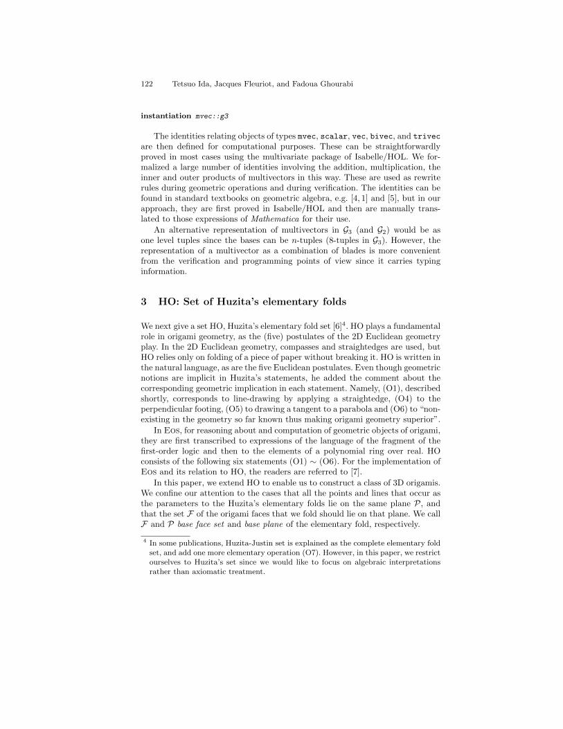
122 Tetsuo Ida, Jacques Fleuriot, and Fadoua Ghourabi
instantiation mvec::g3
The identities relating objects of types mvec, scalar, vec, bivec, and trivec
are then defined for computational purposes. These can be straightforwardlyproved in most cases using the multivariate package of Isabelle/HOL. We for-malized a large number of identities involving the addition, multiplication, theinner and outer products of multivectors in this way. These are used as rewriterules during geometric operations and during verification. The identities can befound in standard textbooks on geometric algebra, e.g. [4, 1] and [5], but in ourapproach, they are first proved in Isabelle/HOL and then are manually trans-lated to those expressions of Mathematica for their use.
An alternative representation of multivectors in G3 (and G2) would be asone level tuples since the bases can be n-tuples (8-tuples in G3). However, therepresentation of a multivector as a combination of blades is more convenientfrom the verification and programming points of view since it carries typinginformation.
3 HO: Set of Huzita’s elementary folds
We next give a set HO, Huzita’s elementary fold set [6]4. HO plays a fundamentalrole in origami geometry, as the (five) postulates of the 2D Euclidean geometryplay. In the 2D Euclidean geometry, compasses and straightedges are used, butHO relies only on folding of a piece of paper without breaking it. HO is written inthe natural language, as are the five Euclidean postulates. Even though geometricnotions are implicit in Huzita’s statements, he added the comment about thecorresponding geometric implication in each statement. Namely, (O1), describedshortly, corresponds to line-drawing by applying a straightedge, (O4) to theperpendicular footing, (O5) to drawing a tangent to a parabola and (O6) to “non-existing in the geometry so far known thus making origami geometry superior”.
In Eos, for reasoning about and computation of geometric objects of origami,they are first transcribed to expressions of the language of the fragment of thefirst-order logic and then to the elements of a polynomial ring over real. HOconsists of the following six statements (O1) ∼ (O6). For the implementation ofEos and its relation to HO, the readers are referred to [7].
In this paper, we extend HO to enable us to construct a class of 3D origamis.We confine our attention to the cases that all the points and lines that occur asthe parameters to the Huzita’s elementary folds lie on the same plane P, andthat the set F of the origami faces that we fold should lie on that plane. We callF and P base face set and base plane of the elementary fold, respectively.
4 In some publications, Huzita-Justin set is explained as the complete elementary foldset, and add one more elementary operation (O7). However, in this paper, we restrictourselves to Huzita’s set since we would like to focus on algebraic interpretationsrather than axiomatic treatment.

A New Formalization of Origami in Geometric Algebra 123
Let O denote an origami structure on the base plane P, whose details areleft unspecified in this paper. We fold an origami O along a fold line determinedby the parameters of each elementary operation. The parameters are lines de-termined by a pair of distinct points on the faces, and points on the faces.
(O1) Given two distinct points P and Q, both on F , fold O along the line on Pthat passes through P and Q.
(O2) Given two distinct points P and Q, both on F , fold O along the line on Pto superpose P and Q.
(O3) Given two distinct lines m and n, both on F , fold O along a line on P tosuperpose m and n.
(O4) Given a line m and a point P , both on F , fold O along the line on Ppassing through P to superpose m onto itself.
(O5) Given a line m, a point P not on m and a point Q, where m, P and Q are onF , fold O along a line on P passing through Q to superpose P and m.
(O6) Given lines m and n, a point P not on m and a point Q not on n, wherem and n are distinct or P and Q are distinct, and furthermore m, n, P and Q
are on F , fold O along a line on P to superpose P and m, and Q and n.
Subsequently, we often denote a line by a sequence of two points, like P Q , whichis the line passing through points P and Q.
Clearly, those statements, if interpreted as those of the decision problems,the answers are all positive. We have algorithms, using algebraic methods, tofind fold lines, if any, along which we fold origami O in each case. We will showhow we translate (O1) ∼ (O6) into expressions of G3 involving multivector xwhich represents a fold line.
(a) Points P and Q (b) Folded along fold lineP Q
Fig. 1: Fold (O1)
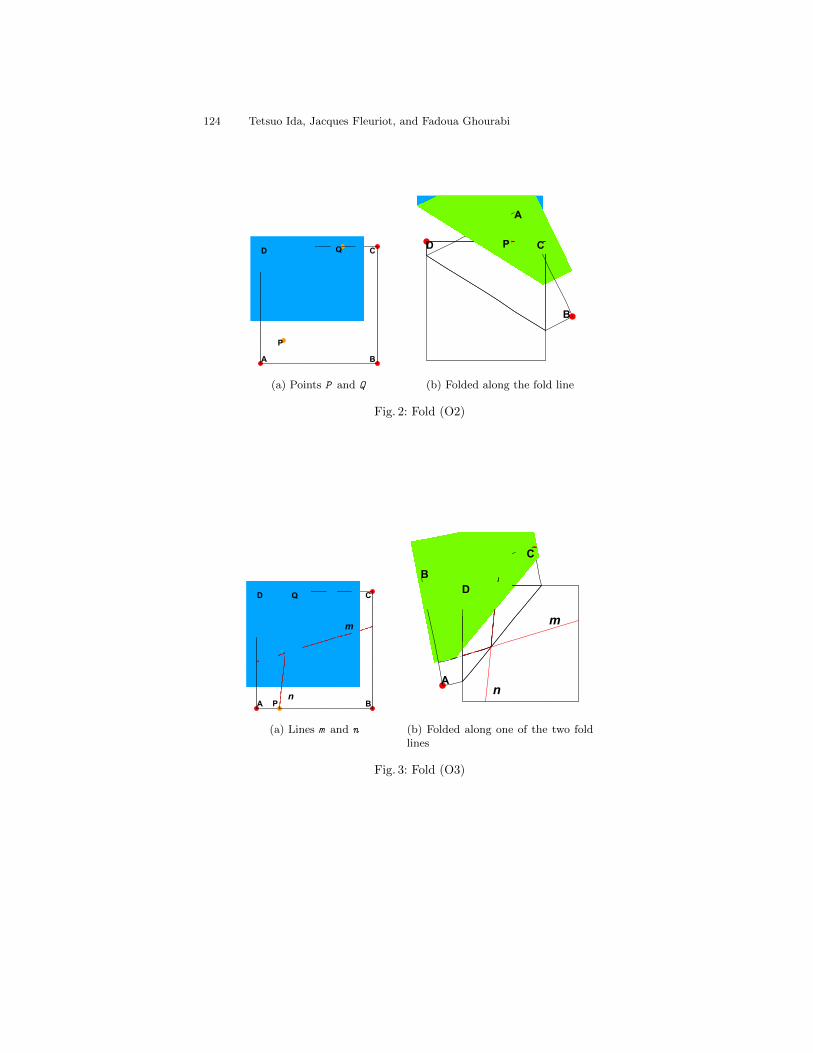
124 Tetsuo Ida, Jacques Fleuriot, and Fadoua Ghourabi
(a) Points P and Q (b) Folded along the fold line
Fig. 2: Fold (O2)
(a) Lines m and n (b) Folded along one of the two foldlines
Fig. 3: Fold (O3)
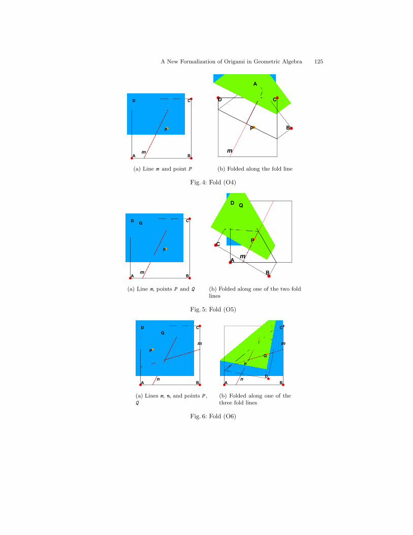
A New Formalization of Origami in Geometric Algebra 125
(a) Line m and point P (b) Folded along the fold line
Fig. 4: Fold (O4)
(a) Line m, points P and Q (b) Folded along one of the two foldlines
Fig. 5: Fold (O5)
(a) Lines m, n, and points P ,Q
(b) Folded along one of thethree fold lines
Fig. 6: Fold (O6)

126 Tetsuo Ida, Jacques Fleuriot, and Fadoua Ghourabi
4 HO in the geometric algebra
4.1 O1 in GA
In G3, points, lines, planes, etc. are treated uniformly as multivectors. Therefore,points P, Q etc. are multivectors p and q etc., respectively. We denote anypoints on the fold line by x. The line passing through distinct points P and Q isexpressed in G3 as follows.
(x− p) ∧ (q− p) = 0. (1)
Since q - p can be written as λ u for any scalar λ 6= 0 and a unit vector uwhose direction is the same as q - p, we have
(x− p) ∧ u = 0. (2)
as the standard representation of a line whose direction is u and passes throughpoint p.
To obtain the traditional form of line equations, let us recall that we representx by (x1, x2, x3). Thus term (Vec x1 x2 x3) in Isabelle/HOL (and Vec[x1, x2, x3]inMathematica) is the representation of vector x = x1∗σ1+x2∗σ2+x3∗σ3. Givenp =(p1, p2, p3) and q =(q1, q2, q3), a straightforward symbolic computation onEq. (1) yields the following three equations in the polynomial ring.
p3q2 + q3x2 + p2x3 = p2q3 + p3x2 + q2x3
p3q1 + q3x1 + p1x3 = p1q3 + p3x1 + q1x3
p2q1 + q2x1 + p1x2 = p1q2 + p2x1 + q1x2
Noting the conditions that P and Q are distinct, we solve the above equationsfor x1, x2 and x3 and obtain
x2 → −x1(q2 − p2)
p1 − q1− p2q1 − p1q2
p1 − q1, x3 → −x1(q3 − p3)
p1 − q1− p3q1 − p1q3
p1 − q1(3)
when p1 6= q1. Equation (3) is a yet another algebraic representation of thedesired line in 3D. By virtue of our choice of the basis σ1, σ2 and σ3, they arethe expressions of the line in Cartesian coordinate system. The other cases ofthe combinations of unequality and equality of p1 and q1, of p2 and q2 and of p3and q3 are dealt with similarly and gives the corresponding line representation.
In practice, we can take the base plane to be x3 = 0. Then we obtain thefollowing line equation.
(−p2 + q2)(−p1 + x1)− (−p1 + q1)(−p2 + x2) = 0
from Eq. (1).

A New Formalization of Origami in Geometric Algebra 127
4.2 O2 in G3
The statement (O2) is translated to the set of G3 equations as follows.
1. We stipulate that the plane defined by p ∧ q is a base plane.2. We have a non-degeneracy condition that P 6= Q.3. We define the midpoint m of P and Q, i.e. m = (p+ q)/2.4. The line x passes through m and is orthogonal to line PQ.
(x−m) · (p− q) = 0 (4)
5. Line x is on the base plane: x ∧ p ∧ q = 0.
Note that without Condition 5, we would have obtained an infinite number oflines. We are only interested in the line that is on the base face. The line x isthen the set of points (x1, x2, x3) that satisfies
(p1 6= q1∨
p2 6= q2∨
p3 6= q3)∧
p1q3x2 + p2q1x3 + p3q2x1 = p1q2x3 + p2q3x1 + p3q1x2
∧(5)
p12 + p2
2 + p32 + 2q1x1 + 2q2x2 + 2q3x3 = 2p1x1 + 2p2x2 + 2p3x3+
q12 + q2
2 + q32
The above set of the equations can be solved numerically at the time oforigami construction. To fold the origami, we need to know the fold line, whichthe solutions of Eq. (5) can fully specify. The symbolic form of Eq. (5) is savedand later used for proving purpose.
The following lemma is useful as the situation it specifies frequently appearswhen we define a line m that is orthogonal to line n.
Lemma 1 Let p, q and r be vectors denoting pairwise distinct points P, Q andR, respectively. Furthermore, we assume that P, Q and R are on the base planewhose direction is the same as that of i3 and that P and Q are on line n. Thefollowing equation represents the line that passes through R and is orthogonal tothe line n.
(x− r) ∧ 〈(p− q) ∗ i3〉1 = 0 (6)
The proof is done by a straightforward algebraic manipulation on multivectors.For the geometric interpretation of Eq. (6), see Fig. 7. The line (to the right,colored in blue) is the solution of x of Eq. (6).
Using Lemma 1, we immediately obtain the fold line of (O2):
(x− 1
2(p+ q)) ∧ 〈(p− q) ∗ i3〉1 = 0
4.3 O3 in G3
It is natural to view (O3) as a special case of (O6). It is a degenerate case where(i) the two lines m and n are the same, (ii) points P and Q in (O6) define anotherline, say l, and (iii) l and m superpose (cf. Fig. 8).
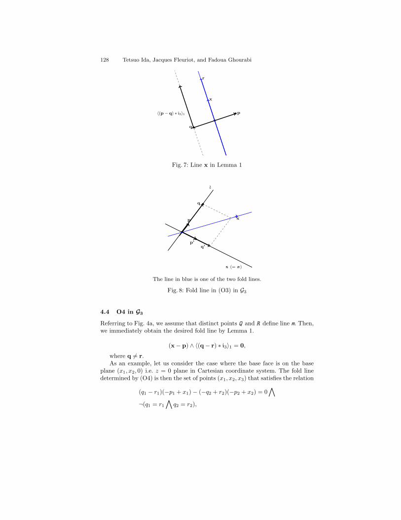
128 Tetsuo Ida, Jacques Fleuriot, and Fadoua Ghourabi
q
p
r
x
〈(p− q) ∗ i3〉1
Fig. 7: Line x in Lemma 1
l
n (= m )
p
p’
q
q’
x
The line in blue is one of the two fold lines.
Fig. 8: Fold line in (O3) in G3
4.4 O4 in G3
Referring to Fig. 4a, we assume that distinct points Q and R define line m. Then,we immediately obtain the desired fold line by Lemma 1.
(x− p) ∧ 〈(q− r) ∗ i3〉1 = 0,
where q 6= r.As an example, let us consider the case where the base face is on the base
plane (x1, x2, 0) i.e. z = 0 plane in Cartesian coordinate system. The fold linedetermined by (O4) is then the set of points (x1, x2, x3) that satisfies the relation
(q1 − r1)(−p1 + x1)− (−q2 + r2)(−p2 + x2) = 0∧
¬(q1 = r1∧
q2 = r2),

A New Formalization of Origami in Geometric Algebra 129
m
r
q
p
x
〈(q− r) ∗ i3〉1
Fig. 9: Geometric configuration in (O4) in G3
where r = (r1, r2, 0).
4.5 O5 in G3
We can view the operations (O5) and (O6) as a fold to bring a point onto a lineor vice versa, as seen from Figs 13 and 14. The fold reflects the point across thefold line determined by the parameters of (O5) or (O6).
Let w and z be vectors, and v be a unit vector. We then define a reflectionoperator Rv(z,w), as follows.
Rv(z,w) = v ∗ (z−w) ∗ v+w.
Rv(z,w) reflects z across v at pivot w (cf. Fig. 10).
z
Rv(z,w)
w
u
v
P
The base plane P (colored in light grey) is specified by vector u, which is orthogonalto P. Vectors z, z’ and v are on the base plane and v is unit vector.
Fig. 10: Reflection
Referring to Fig. 5a, we assume assume that distinct points S and T defineline m. Since the fold line passes through point Q and its direction is determined

130 Tetsuo Ida, Jacques Fleuriot, and Fadoua Ghourabi
by a unit vector u, we have the following equation for x.
(x− q) ∧ u = 0,
satisfying the following conditions.
non-degeneracy : s 6= t
reflected point on m : 〈Ru(p,q)− s〉1 ∧ (t− s) = 0
unit vector : u ∗ u = 1
u on the base plane : u ∧ i3 = 0
Figure 11 shows the geometric configuration of (O5) before the fold. Thiscorresponds to the origami of Fig. 5a.
m
p
q
s tRu(p,q)
u
Fig. 11: Geometric configuration of (O5) in G3
4.6 O6 in G3
Finally, we derive the following equations from the statement (O6). We assumethat the pairs of distinct points A and B, and of distinct points C and D determinelines m and n, respectively. Recall that we stipulate all the points A, B, C, D, Pand Q of the arguments of (O6) are on the base face.
The desired fold line satisfies
(x−w) ∧ u = 0,
where g and u satisfy the following conditions.
non-degeneracy : a 6= b
reflected point on m : 〈Ru(p,w)− a〉1 ∧ (b− a) = 0
non-degeneracy : c 6= d
reflected point on n : 〈Ru(q,w)− c〉1 ∧ (d− c) = 0
unit vector : u ∗ u = 1
u on the base plane : u ∧ i3 = 0
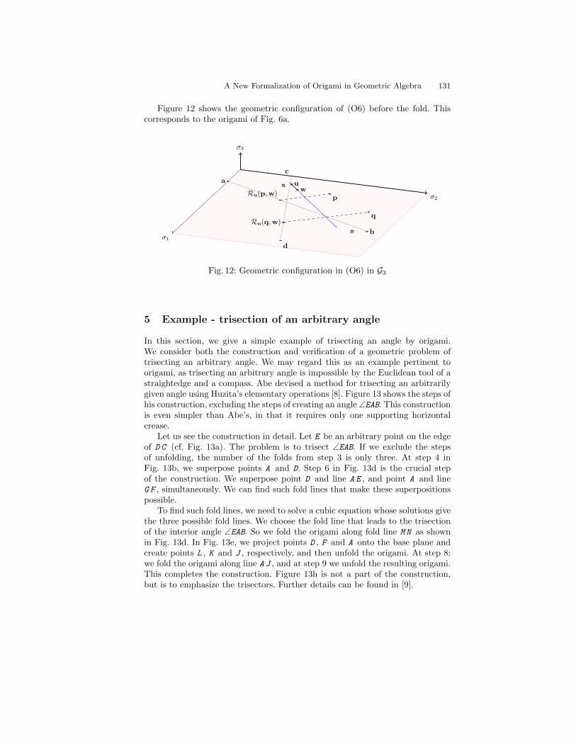
A New Formalization of Origami in Geometric Algebra 131
Figure 12 shows the geometric configuration of (O6) before the fold. Thiscorresponds to the origami of Fig. 6a.
σ1
a
b
c
d
p
q
Ru(p,w)
Ru(q,w)
wun
m
σ2
σ3
Fig. 12: Geometric configuration in (O6) in G3
5 Example - trisection of an arbitrary angle
In this section, we give a simple example of trisecting an angle by origami.We consider both the construction and verification of a geometric problem oftrisecting an arbitrary angle. We may regard this as an example pertinent toorigami, as trisecting an arbitrary angle is impossible by the Euclidean tool of astraightedge and a compass. Abe devised a method for trisecting an arbitrarilygiven angle using Huzita’s elementary operations [8]. Figure 13 shows the steps ofhis construction, excluding the steps of creating an angle ∠EAB. This constructionis even simpler than Abe’s, in that it requires only one supporting horizontalcrease.
Let us see the construction in detail. Let E be an arbitrary point on the edgeof D C (cf. Fig. 13a). The problem is to trisect ∠EAB. If we exclude the stepsof unfolding, the number of the folds from step 3 is only three. At step 4 inFig. 13b, we superpose points A and D. Step 6 in Fig. 13d is the crucial stepof the construction. We superpose point D and line A E , and point A and lineG F , simultaneously. We can find such fold lines that make these superpositionspossible.
To find such fold lines, we need to solve a cubic equation whose solutions givethe three possible fold lines. We choose the fold line that leads to the trisectionof the interior angle ∠EAB. So we fold the origami along fold line M N as shownin Fig. 13d. In Fig. 13e, we project points D , F and A onto the base plane andcreate points L , K and J , respectively, and then unfold the origami. At step 8;we fold the origami along line A J , and at step 9 we unfold the resulting origami.This completes the construction. Figure 13h is not a part of the construction,but is to emphasize the trisectors. Further details can be found in [9].

132 Tetsuo Ida, Jacques Fleuriot, and Fadoua Ghourabi
(a) Step 3: Angle ∠EAB (b) Step 4: (O2) (c) Step 5: Unfold
(d) Step 6: (O6) (e) Step 7: Unfold (f) Step 8:(O1)
(g) Step 9: Unfold (h) Two trisectors of ∠EAB
Fig. 13: Abe’s method for trisecting angle ∠EAB

A New Formalization of Origami in Geometric Algebra 133
From these operations, we obtain the trisector A J , which is the solution ofxof the equation
(x−w) ∧ u = 0,
with the following relations:
〈Ru(d,w)− a〉1 ∧ (e− a) = 0 (7)
〈Ru(a,w)− g〉1 ∧ (f− g) = 0 (8)
w =1
2〈a+Ru(a,w))〉1 (9)
j = 〈Ru(a,w)〉1 (10)
l = 〈Ru(d,w)〉1 (11)
k = 〈Ru(f,w)〉1 (12)
u ∗ u = 1 (13)
Point W is the pivot of the reflection in the above equations, and is the intersectionof the fold line M N and line A J as shown in Figs. 13f and 13h.
Next, we prove that lines AK and AJ are the trisectors of ∠EAB. To that end,we show that vectors j, k and l are obtained by rotating vectors b, j and k witha as the pivot, by an angle θ, respectively. We therefore have the following threegoals of the proof. If the goals are proven to be correct, then we have θ = 1
3∠EAB.
〈(b− a) ∗ ei3θ〉1 ∧ (j− a) = 0 (14)
〈(j− a) ∗ ei3θ〉1 ∧ (k− a) = 0 (15)
〈(k− a) ∗ ei3θ〉1 ∧ (l− a) = 0 (16)
We negate each equations (14) ∼ (16). Let us denote them by (14’), (15’), and(16’). We translate equations (7) ∼ (13), and (14’) to the set of polynomialequations. The Grobner basis computation of the polynomials thus obtainedyields the reduced Grobner base 1. The same computing procedures for theother two goals also yield 1. Thus, the proof is successful. Note that ei3θ
is an expression of G3, and should be interpreted in the following way. Themultiplications with ei3θ in Eqs. (14) ∼ (16) generate sinusoidal functions. Thesehave to be transformed to polynomials using the identity sin2 θ + cos2 θ = 1 forarbitrary θ before they are processed by Grobner basis computations.
6 Related works
We have two sources to recall in relating our present work to previous works,i.e., origami and geometric algebra. As for the former, we see the significantdifficulties and challenges ahead in constructing 3D origamis. To circumventthe difficulties, Lang introduced search heuristics to find fold patterns in 3D[10] and Streinu et al. analyzed Lang’s algorithm and made it more reliable

134 Tetsuo Ida, Jacques Fleuriot, and Fadoua Ghourabi
in more cases [11]. While our approach is axiomatic, at some stage of furtherdevelopment, we will explore the possibility of incorporating heuristics for findingnew folds. Especially, to place appropriate constraints on the use of parametersto a fold operation is necessary for feasible 3D origami construction.
As for the latter, geometric algebra, now commonly coined as such, is afamily of algebras and has the fascinating history. There exist many kinds ofliterature including textbooks at the undergraduate and graduate levels andresearch monographs on it. We will point out the publications in the contextof automated geometric theorem proving, and limit ourselves to those relatingdirectly to our present study of origami. The main motivation of the use of GA isto explore computational methods of geometric theorem proving, that are freedfrom the dimensions and the coordinates. The work of Wang et al [12][13], amongothers, is one of the pioneering ones with this motivation. They tried to applythe equations of GA systematically and successfully proves classical geometricaltheorems of Euclidean geometry. Yhey went on to construct a rewrite systemwith nice computational properties such as strong normalization and confluence.To define a rewrite system from a large number of employable equations, a properchoice of rules and/or Knuth-Bendix completion procedure seem a formidabletask.
Our approach in the context of the origami research is a hybrid approach inwhich we use GA in formalizing geometrical properties and use polynomial ringsthat we can obtain by compiling GA expressions, for computationally intensivetasks. The work was initiated to formalize 2D origami geometry in 2014. Weintroduced a variant of G2 [14]. In the similar vein, our axiomatic study ofalgebraic treatment of origami may benefit from a variant of geometric algebra,conformal geometric algebra, proposed by Mizoguchi et al. [15].
Another work that has similar motivation, but differs from our approach isthat of Fuchs’ and Thery’s [16, 17]. They formalized GA in Coq using the datastructure of a binary tree. Their goal is not only to formalize GA but also toderive a set of efficient functions that we can use for non-trivial computations.
As for the implementation of GA in general, depending on the applications,a wide range of software libraries and systems are available. Among them, wenote the work of Aragon-Camerasa et al. on the Mathematica package imple-mentation of GA [18]. As our GA is designed and implemented to be a partof Eos system (also implemented in Mathematica), the analysis of the packagewould be of benefit to our further system development. However, the direct useof the package by us is unlikely as it would involve much efforts of transformingthe data structures, among others.
7 Concluding remarks
We have shown a rigorous approach to the use of the geometric algebra in com-putational origami. We proved in Isabelle/HOL most of the useful identitiesthat hold among algebraic expressions of G3. Thus, we can state the elementaryorigami operations in geometric algebra and further correctly apply the equations

A New Formalization of Origami in Geometric Algebra 135
to compute the transformations of the objects under study both symbolically andnumerically. Furthermore, we can now use G3 to geometric theorem proving. Theexample we have given in Section 5 is simple enough to show how we can use ourmethodology to automated theorem proving in geometry. However, it is scalableto other more sophisticated geometric problems.
We can observe the importance of the geometric algebra as the layer of ab-straction between the language for the origami geometry and the algebraic ex-pressions. We also see that the distinctions between points, lines and vectorsdisappear and that the derived expressions do not depend on the dimensionalityof the coordinate system.
Since we want to integrate the functionality of G3 into the computational sys-tem tightly, we start with the formalization of G3 in Isabelle/HOL with the helpof Mathematica, and then for most computational, i.e. simplification, purposes,we use Mathematica. In this paper, we focussed on the transformation from HOto G3. Further work is in progress to incorporate the obtained results to extendEos to 3D visualization and the verification of 3D origami.
Acknowledgments
This work was supported by JSPS KAKENHI Grants Numbers 25330007 and16K00008.
References
1. D. Hestenes: New Foundations for Classical Mechanics (Second Edition). KluwerAcademic Publishers (1986)
2. Ida, T., Takahashi, H., Marin, M., Ghourabi, F., Kasem, A.: Computational Con-struction of a Maximal Equilateral Triangle Inscribed in an Origami. In: Mathe-matical Software - ICMS 2006. Volume 4151 of Lecture Notes in Computer Science.,Springer (2006) 361–372
3. Haftmann, F.: Haskell-style Type Classes with Isabelle/Isar.http://isabelle.in.tum.de/doc/classes.pdf (2014)
4. C. Doran and A. Lasenby: Geometric Algebra for Physicists. Cambridge UniversityPress (2003)
5. L. Dorst and D. Fontijne and S. Mann: Geometric Algebra for Computer Science.Elsevier Inc. (2007)
6. Huzita, H.: Axiomatic Development of Origami Geometry. In Huzita, H., ed.:Proceedings of the First International Meeting of Origami Science and Technology.(1989) 143–158
7. Ida, T., Ghourabi, F., Takahashi, K.: Formalizing Polygonal Knot Origami. Journalof Symbolic Computation (2014)
8. Abe, H.: Trisecting an Angle by Origami. Sugaku Seminar (1980) cover pagehttp://www.phoenix-c.or.jp/ tokioka/n!/suu(underscore)semi.html.
9. Ida, T., Kasem, A., Ghourabi, F., Takahashi, H.: Morley’s Theorem Revisited:Origami Construction and Automated Proof. Journal of Symbolic Computation46 (2011) 571 – 583
136 Tetsuo Ida, Jacques Fleuriot, and Fadoua Ghourabi
10. Lang, R.J.: A computational algorithm for origami design. In: The 12th annualACM symposium on computational geometry. (1996) 98–105
11. Bowers, J.C., Streinu, I.: Rigidity of Origami Universal Molecules. In Ida, T.,Fleuriot, J., eds.: Automated Deduction in Geometry. Volume 7993 of LNAI.,Springer Heidelberg New York Dordrecht London (2013) 120–142
12. Wang, D. In: Clifford algebraic calculus for geometric reasoning. Springer BerlinHeidelberg, Berlin, Heidelberg (1997) 115–140
13. Fevre, S., Wang, D. In: Combining algebraic computing and term-rewriting forgeometry theorem proving. Springer Berlin Heidelberg, Berlin, Heidelberg (1998)145–156
14. Ida, T.: Huzita’s basic origami fold in geometric algebra. In: Post-Proceedings ofthe 16th International Symposium on Symbolic and Numeric Algorithms for Scien-tific Computing (SYNASC 2014), IEEE Computer Society Conference PublishingServices (CPS) (2015) 11 – 13
15. Kondo, M., Matsuo, T., Mizoguchi, Y., Ochiai, H.: A mathematica module forconformal geometric algebra and origami folding. In Davenport, J.H., Ghourabi,F., eds.: SCSS 2016: 7th International Symposium on Symbolic Computation inSoftware Science. Volume 39 of EPiC Series in Computing., EasyChair (2016) 68–80
16. Fuchs, L., Thery, L. In: A Formalization of Grassmann-Cayley Algebra in COQand Its Application to Theorem Proving in Projective Geometry. Springer BerlinHeidelberg, Berlin, Heidelberg (2011) 51–67
17. Fuchs, L., Thery, L.: Implementing geometric algebra products with binary trees.Advances in Applied Clifford Algebras 24 (2014) 589–611
18. Arag/’on-Camarasa, G., Arag/’on-Gonz/’alez, G., Arag/’on, J.J.,Rogr/’iguez-Andrade, M.A.: Clifford Algebra with Mathematica.http://arxiv.org/dbs/0810.2412 (2008)
Automatic Rewrites of Input Expressions inComplex Algebraic Geometry Provers
Extended Abstract
Zoltan Kovacs1, Tomas Recio2 and Csilla Solyom-Gecse3
1 Private University College of Educationof the Diocese of Linz, Austria
[email protected] Depto. de Matematicas, Estadıstica y Computacion
Universidad de Cantabria, [email protected]
3 Babes-Bolyai University, Cluj-Napoca, [email protected]
Abstract. We present an algorithm to help converting expressions hav-ing non-negative quantities (like distances) in Euclidean geometry theo-rems to be usable in a complex algebraic geometry prover. The algorithmhelps in refining the output of an existing prover, therefore it supportsimmediate deployment in high level prover systems.
Keywords: Automatic Theorem Proving, Automatic Theorem Deduction,Complex Algebraic Geometry, Elementary Geometry, Dynamic Geometry Soft-ware, GeoGebra
1 Introduction
Many dynamic geometry systems support covering textbook problems by offer-ing an intuitive interface to construct geometry diagrams. When combined withautomated theorem proving tools, the first steps are the graphical constructionof the hypotheses and the final step is the definition of the thesis. In many text-book theorems in elementary geometry the thesis is a relation between somegeometry objects in the diagram, but sometimes the thesis is an equation con-taining variables representing lengths, angles, areas or volumes. Such an exampleis the Pythagorean theorem, among many others, including Ptolemy’s theoremor Heron’s formula.
The most adequate way for entering such expressions is not yet completelydiscussed. Some software tools like JGEX [13] or OpenGeoProver [11] have theirown user interface and rewrite mechanism to reformulate the input equation(e.g. a = 2b, here a and b are distances) to a more suitable form (e.g. a2−4b2 = 0).The problem with the equation a = 2b is that complex algebraic geometry(CAG) solvers cannot assume that the quantities a and b are non-negative since
138 Zoltan Kovacs, Tomas Recio and Csilla Solyom-Gecse
the variables are always chosen from the set of complex numbers. By using themore suitable form a2 − 4b2 = 0 we can implicitly ignore the difference betweenpositive and negative values for the quantities.
The first references about the need to reformulate the thesis expression are inChou’s book [4], by specifying different rewrites for the various input expressionsto be more suitable for the CAG method.
In this work we propose a general way to handle a large number of possiblealgebraic input expressions defined in the thesis equation. We use computeralgebra to determine the more suitable expression instead of using the inputequation, namely by elimination of certain variables. We claim that the numberof terms of the more suitable expression is double exponential in the number ofodd powers in the term form of the input—the suggested way for the computationis still achievable for the usual classroom situations.
We also suggest a modification of the typical workflow for a CAG proof of anelementary geometry theorem by factorizing the more suitable expression. Thenotion of “essential conditions” of a statement will be introduced, which may playan important role similarly to non-degeneracy conditions. As an illustration werecall Viviani’s theorem and its one-dimensional specific case by demonstratingour algorithm implemented in GeoGebra.
2 The problem
Chou’s book [4] presents a list of cases when translating statements into un-ordered geometry requires further considerations. In its Part II, section 2 (p. 97)Chou mentions
– the length of a segment (which should be substituted by its square),– the equality of length of two segments (for a = b ⇐⇒ a − b = 0 the
polynomial a2 − b2 is used),– the equality of product of two segments (for a · b = c · d ⇐⇒ ab − cd = 0
the polynomial a2b2 − c2d2 will be utilized),– a ratio of length of two segments (for 3a = 7b the expression 9a2 − 49b2 is
used),– the sum of length of two segments is a third length (for a + b = c the
polynomial (a− b− c) · (a− b + c) · (a + b− c) · (a + b + c) is used).
Here the last case is the most difficult one. Let us illustrate it by a simplestatement:
Example 1. Let a be the length of the segment joining the free points A and B.Define point C as an arbitrary point of this segment and and let the length ofsegment AC be b and that of BC be c. Now a = b + c.
Let us try to prove this easy theorem with the usual CAG approach. Apossible translation of the geometric diagram into algebraic equations is to usevariables v1, v2, v3, v4, v5, v6 to describe the Cartesian coordinates of points A,

Automatic Rewrites of Input Expressions in CAG Provers 139
B and C: A = (v1, v2), B = (v3, v4), C = (v5, v6). Now we can state thatv1v4 + v3v6 + v5v2 − v1v6 − v3v2 − v5v4 = 0, and we can also claim that a2 =(v1−v3)2 +(v2−v4)2, b2 = (v1−v5)2 +(v2−v6)2, c2 = (v3−v5)2 +(v4−v6)2 byusing the Pythagorean theorem for distances of the vertices. Here 4 equationsdescribe the hypotheses. By following [8] and the Grobner bases method, let ususe the negated form of a = b+ c as z(a− b− c) = 1 to describe the thesis. Nowwe use the prover algorithm from [5] (chapter 6, §4), implemented in Singular4.0.2 [6], and enter the following program code:
ring r=(0,v1,v2,v3,v4,v5),(v6,a,b,c,z),dp;
ideal i=v1*v4+v3*v6+v5*v2-v1*v6-v3*v2-v5*v4,
a^2-(v1-v3)^2-(v2-v4)^2,
b^2-(v1-v5)^2-(v2-v6)^2,
c^2-(v3-v5)^2-(v4-v6)^2,
z*(a-b-c)-1;
groebner(i);
We recall that (in the standard framework for automatic theorem provingas in [4]) the output is 〈1〉 if and only if the statement is true interpreted in analgebraic closed field. But our statement is not true in the complex numbers: infact, the output is an ideal (a reduced Grobner basis) with several elements. Onthe other hand, in the complex numbers the following can be proved:
(a− b− c) · (a− b + c) · (a + b− c) · (a + b + c) = 0
as one can check by changing in the above list, the thesis polynomial to
z*((a-b-c)*(a-b+c)*(a+b-c)*(a+b+c))-1
In this case we have the expected result, the reduced minimal Grobner basis is〈1〉.
One important note must be remarked: the proven statement is actually thefollowing:
Theorem 1. Let us denote by a the length of the segment AB by joining the freepoints A and B. Define point C as an arbitrary point of the line going throughA,B, and let length(AC) = b and length(BC) = c. Now a = b + c, unlessb = a + c or c = a + b.
It is easy to see that the last condition a + b + c(= 0) in our modified inputhas no essential geometrical meaning, it is a degenerate case, therefore it canbe omitted from the precise statement. On the other hand, the other excludedconditions do have geometrical meanings:
1. b = a + c, in this case C is not on the segment, but on a line which joins Aand B; C is on the red dotted ray in Fig. 1. Here we must admit that ourproblem setting is not even compatible with CAG since we cannot distinguisha segment from a line. That is, in the geometric approach we need to clarifyif we allow points outside the segment (but still on the line) or not. It isquite straightforward that in the CAG approach the only possible approachis to extend the meaning of a segment to be a line.

140 Zoltan Kovacs, Tomas Recio and Csilla Solyom-Gecse
2. c = a + b, this is a similar case, but C is on the blue dotted ray.
Fig. 1. Example 1
We call these two extra assumptions essential conditions to highlight theirgeometrical importance and distinguish them from the degeneracy conditionswhich are geometrically a “much smaller” set.
3 A detailed example
Given the input polynomial equation p = 0 where p is squarefree, we performthe following computation by using a computer algebra system (here Giac [7]will be used). In our example, let p = a− b− c.
>> factor(eliminate([a-b-c,a^2=A^2,b^2=B^2,c^2=C^2],[a,b,c]))
that is, we eliminate all terms from p which are not of even powers of a, b, c andthe obtained output is:
[(A-B-C)*(A-B+C)*(A+B-C)*(A+B+C)]
This technique works in general, and as special cases it covers all instancesreported by Chou. We tested this idea for several elementary geometry theo-rems and successfully proved them without any manual computations or furtherchallenges. Our tests include the Pythagorean theorem, the cathetus, the geo-metric mean, the angle bisector, the intercept, Ceva’s, Menelaus’ and Ptolemy’stheorems, and Heron’s formula. A detailed list of our tests can be found athttp://tinyurl.com/adg16-formula-rewrite which is generated on a dailybasis automatically from the latest source code of the open dynamic geometrysystem GeoGebra.
As an illustration, we recall Viviani’s theorem (see [12]). It is a generalizationof our example in two dimensions. On the other hand, here 7 of the appearing 8factors are essential, while one is degenerate.
Example 2. Let ABC be a regular triangle and D an internal point of it. Let i,j and k be the distance of D from the sides of the triangle, respectively. Theni + j + k is a constant (it is actually the height m of the triangle, see Fig. 2).
Similarly to Example 1 here we cannot restrict D to be an internal point ofthe triangle. We can divide the plane to 7 different areas and enumerate themfrom 1 to 7. In area 1 the equation i+ j +k−m = 0 holds, in 2–4 the equations

Automatic Rewrites of Input Expressions in CAG Provers 141
Fig. 2. Example 2: Viviani’s theorem
i− j − k + m = −(−i + j + k −m) = 0, i− j + k −m = 0, i + j − k −m = 0,respectively, and in 5–7 the equations i− j − k −m = −(−i + j + k + m) = 0,i− j + k + m = 0, i + j − k + m = 0, respectively.
When using our method with input as the left hand side of any of these 7equations, the output expression is a product of the 7 ones and an extra one,i+ j +k+m. It is clear that this last 8th one cannot be zero, only if the trianglecollapses to a point, that is, A = B = C(= D), which is obviously a degeneratecase.
Our method finally modifies Viviani’s theorem in the following form:
Theorem 2. Let ABC be a regular triangle and D another point on the plane.Let i, j and k be the distance of D from the sides of the triangle, respectively.Let m be the height of the triangle. Then, provided that none of the conditions
– i + m = j + k,– i + k = j + m,– i + j = k + m,– i = j + k + m,– j = i + k + m,– k = i + j + m
hold, i + j + k = m follows.
This process is purely automatic, since both the rewrite and also adding theessential conditions can be done without any human intervention. The essentialconditions will be those factors of the output which are not appearing in theinput p, except the only factor which is a sum of the quantities.
Viviani’s theorem can also be generalized for 3 dimensions, see [1].

142 Zoltan Kovacs, Tomas Recio and Csilla Solyom-Gecse
4 Other uses, future work
The same idea can be applied when putting equations containing quantitiesamong the hypotheses. An important question in the CAG approach how to dis-tinguish between an ellipse and a hyperbola, since their definition—by using thefoci A, B and a circumpoint C—cannot be separated. Actually, some theoremscan be even generalized by using this fact (see [9] for an example). On the otherhand, a better understanding can be obtained with the help of the factorizedelimination.
For instance, given a hyperbola with foci A and B and point C, another pointP is an element of the hyperbola if and only if |AC − CB| = |AP − PB|, thatis, (AC − CB)2 = (AP − PB)2. Now let ph = (AC − CB)2 − (AP − PB)2 =(AC−CB−AP +PB)·(AC−CB+AP−PB). Similarly, for an ellipse describedwith the same points, the equation AC + CB = AP + PB can be assumed, sowe set pe = AC + CB −AP − PB. By using our method for the inputs ph andpe we get the same output ph · pe · (AC + CB −AP − PB) · (AC + CB + AP −PB) · (AC +CB +AP +PB) · (AC−CB−AP −PB) · (AC−CB +AP +PB).Here the last 5 factors are geometrically degenerate cases, that is, the hyperbolaand the ellipse are undistinguishable, but there are no other geometrical curveswhich can be mixed with them in the CAG approach.
This example also supports the fact that given an input polynomial p with lterms which are not of even power, (independently of the number of even powersin p) the output polynomial will consist of 2l (or eventually 2l−1) factors. In otherwords, the expansion of the output polynomial will consist of doubly exponentialnumber of terms of the number of not even powers. For example, for l = 6 thecomputation will not finish in a feasable time in Giac:
factor(eliminate([x1+x2+x3+x4+x5+x6,x1^2=X1^2,x2^2=X2^2,x3^2=X3^2,
x4^2=X4^2,x5^2=X5^2,x6^2=X6^2],[x1,x2,x3,x4,x5,x6]))
The opportunity to type arbitrary expressions (involving distances, lengths,volumes, etc.) is, in our opinion, a desirable feature of theorem provers in adynamic geometry system, allowing the user to access new horizons in studying,discovering and enjoying Euclidean geometry.
Acknowledgments
Computing the output formula by elimination was suggested by Bernard Parisse,inventor of Giac.
We are thankful to Predrag Janicic, Julien Narboux and Francisco Botanafor their suggestions to improve the text of this paper.
Second author is partially supported by the Spanish Research Project‘Construcciones Algebra-geometricas: fundamentos, algoritmos y aplicaciones’(MTM2014-54141-P).
Automatic Rewrites of Input Expressions in CAG Provers 143
References
1. A. Bogomolny. Viviani’s 3D Analogue from Interactive Mathematics Miscel-lany and Puzzles. Downloaded from http://www.cut-the-knot.org/triangle/
VivianiTetrahedron.shtml, accessed in April 2016.2. F. Botana, M. Hohenwarter, P. Janicic, Z. Kovacs, I. Petrovic, T. Recio and S.
Weitzhofer. Automated Theorem Proving in GeoGebra: Current Achievements. JAutom Reasoning, 55(1):39–59, March 2015.
3. K. Brown. Polynomials For Sums of Square Roots. Downloaded from http://
www.mathpages.com/home/kmath111/kmath111.htm, accessed in February 2016.4. S.-C. Chou. Mechanical Geometry Theorem Proving. Springer Science + Business
Media, 1987.5. D. Cox, J. Little and D. O’Shea. Ideals Varieties and Algorithms. Springer New
York, 2007.6. W. Decker, G.-M. Greuel, G. Pfister and H. Schonemann. Singular 4-0-2 —
A computer algebra system for polynomial computations. 2015. http://www.
singular.uni-kl.de.7. Z. Kovacs and B. Parisse. Giac and GeoGebra – Improved Grobner basis com-
putations. Computer Algebra and Polynomials, Volume 8942 of the series LectureNotes in Computer Science, 126–138. Springer, 2015.
8. D. Kapur. Using Grobner bases to reason about geometry problems. Journal ofSymbolic Computation, 2(4):399–408, December 1986.
9. Z. Kovacs, C. Solyom-Gecse. GeoGebra Tools with Proof Capabilities, 2016. http://arxiv.org/abs/1603.01228.
10. B. Kutzler and S. Stifter. On the application of Buchberger’s algorithm to auto-mated geometry theorem proving. Journal of Symbolic Computation, 2(4):389–397,December 1986.
11. I. Petrovic and P. Janicic. Integration of OpenGeoProver with Ge-oGebra, 2012. http://argo.matf.bg.ac.rs/events/2012/fatpa2012/slides/
IvanPetrovic.pdf.12. T. J. Recio Muniz. Calculo simbolico y geometrico. Editorial Sıntesis. Madrid,
1998.13. Z. Ye, S.-C. Chou and X.-S. Gao. An Introduction to Java Geometry Expert. In
Automated Deduction in Geometry, pages 189–195. Springer Science + BusinessMedia, 2011.
Two Ways of Using Rabinowitsch Trick forImposing Non-degeneracy Conditions
Manuel Ladra1, Pilar Páez-Guillán1, and Tomás Recio2
1 Universidad de Santiago, Santiago de Compsotela, [email protected],
[email protected] Depto. de Matemáticas, Estadística y Computación, Universidad de Cantabria,
Santander, [email protected]
Abstract. In the algebraic-geometry-based theory of automated prov-ing and discovery, it is usually required that the user includes, as com-plementary hypotheses, some intuitively obvious non-degeneracy condi-tions. There are two main procedures to introduce such conditions intothe hypotheses set, and both of them rely on the well known Rabinow-itsch trick. But it happens that each of these very close methods canlead to very different situations (truth/false statements). The aim of thisextended abstract is to present and to discuss in detail this usually for-gotten dilemma,highlighting the need to do some further work on thisissue.We present one example, in the context of automatic discovery, where itwill be checked that, after imposing the thesis to be true and eliminatingthe non-independent variables, different additional hypotheses appear,depending on the chosen approach when including the non-degeneracyconditions; this fact is directly related to the change in the way we pro-ceed eliminating variables and introducing hypotheses. All the calcula-tions have been carried out using the software Singular in the FinisTerrae2 supercomputer.
Keywords: Automated discovery, non-degeneracy conditions, Rabinowitschtrick, saturation
1 Introducing non-degeneracy conditions as hypotheses
The framework of this paper is the automated theorem proving theory initiated,forty years ago, by Wu on his seminal paper ‘On the decision problem andthe mechanization of theorem-proving in elementary geometry’ [8]. Its goal is toprovide computer algebra algorithms to automatically decide if a given geometricstatement is generally true or not, i.e. true except for some exceptional cases,usually not explicitly declared, such as the collinearity of the three vertices of ageneric triangle or dealing with circle of radius zero.

Rabinowitsch Trick 145
Roughly speaking, this method proceeds by assigning coordinates and equa-tions to the elements (points, lines, circles, etc.) and conditions (perpendicularity,incidence, etc.) of the involved geometric hypotheses H and theses T , creating,in this way, two systems of polynomial equations H, T . Then it declares the va-lidity of the geometric statement H =⇒ T over an algebraically closed field K byconsidering the inclusion V (H) ⊆ V (T ) between the solution set of the systemof equations H and that of the corresponding system T . Finally, this inclusionis tested by some computational algebraic geometry methods (triangularization,Gröbner basis, etc.).
Now, it is often the case that in many elementary geometric statements thealgebraic variety defined by the hypotheses is not totally contained in the onedefined by the thesis. In fact, in most cases the output of an automatic provingalgorithm is that the tested statement is false unless the hypotheses variety isfurther restricted by adding some complementary constraints such as: these twopoints must be different, this triangle should not collapse to a line, etc. Theseadditional hypotheses are known as non-degeneracy conditions and statementsthat are true except in theses cases are called generally true. See [2, Chapter 6,Section 4] or [7] for further details on this issue.
As shown long time ago by the quantity and quality of the examples in [1],it is clear that this computer algebra approach to mechanical theorem provingis quite successful. Yet, it is also well known the high complexity of the involvedpolynomial Gröbner basis algorithms [2]. For this reason it is often the casethat the user attempts to prevent the failure of the computation by manuallyintroducing, before starting to run the proving algorithm, some easy-to-guessnon-degeneracy conditions.
The main problem here is that the methods we are describing are, basically,designed only to deal with equalities, not with inequations. Thus we have got tofind a way to introduce non-degeneracy conditions that both reflects (as closelyas possible) the geometric meaning of the condition (i.e. to avoid some degeneratecases) and expresses it by means of equations.
2 Different ways. . .
Traditionally (at least since [5]) the refutation of a given property f = 0, i.e.three points not aligned, two points not coincident, etc., is handled as an equationby adding some auxiliary variable t and considering the equation f · t− 1 = 0 asrepresenting ¬f = 0, emulating Rabinowitsch trick3.
3 Originally, this “trick” was designed to deduce the general Hilbert Nullstellensatz(about the vanishing of a polynomial f on the solution set of some system of poly-nomial equations) from the Weak Nullstellensatz (about the existence of solution fora systems of equations), by introducing some extra variable and considering f · t − 1.Thus, if f vanishes on some solution set, f · t − 1 can not have a solution on this set.Thus, the Weak Nullstellensatz implies that 1 is a combination of the polynomialsin the set of equations and of f · t − 1. Next, replace t by 1/f in this expression of

146 Manuel Ladra, Pilar Páez-Guillán, and Tomás Recio
For instance, if we want to declare that points A(x1, x2), B(x3, x4), C(x5, x6)should not lie on a line, we can proceed as follows. First notice that (x1x4−x1x6−x2x3 + x2x5 + x3x6 − x4x5) = 0 is the condition for the alignment of the threepoints A, B, C. Then notice that every solution to the equation (x1x4 − x1x6 −x2x3 + x2x5 + x3x6−x4x5) · t−1 = 0 has to verify (x1x4−x1x6−x2x3 + x2x5 +x3x6 − x4x5) 6= 0, i.e. that A, B, C are not aligned. And conversely, for everychoice of coordinates for A, B, C such that A, B, C are not aligned, we will have(x1x4−x1x6−x2x3 +x2x5 +x3x6−x4x5) 6= 0, and, then, there will be a value oft = 1/(x1x4−x1x6−x2x3+x2x5+x3x6−x4x5) such that (x1, x2, x3, x4, x5, x6, t)is a solution to (x1x4 − x1x6 − x2x3 + x2x5 + x3x6 − x4x5) · t− 1 = 0.
Speaking in general, if f(x1, . . . , xn) · t − 1 = 0, then the inequalityf(x1, . . . , xn) 6= 0 holds, and conversely, if f(x1, . . . , xn) 6= 0, then we can taket = 1/f(x1, . . . , xn) and so f(x1, . . . , xn) · t− 1 = 0. Therefore, if we are dealingwith an ideal of hypotheses H, and we want to add the condition ¬f = 0 toit, we must consider the ideal H + (f · t− 1).
It is easy to generalize this procedure for the case of having to negate theconjunction or the disjunction of several conditions. Clearly, the assertion ¬f1 =0 ∧ . . .∧ fr = 0 translates into ¬f1 = 0 ∨ . . .∨ ¬fr = 0. So, we will have todeal with the ideal H +(f1 · t1−1) · · · (fr · tr−1) (although we could also employthe same slack variable t for all the conditions). Regarding ¬f1 = 0 ∨ . . .∨ fr =0, it can be expressed as ¬f1 = 0 ∧ . . . ∧ ¬fr = 0. Therefore, the idealwhich we must consider is H + (f1 · t1 − 1, . . . , fr · tr − 1). In this case, wecannot use a single auxiliary variable t. However, in practice we can express¬f1 = 0 ∧ . . . ∧ ¬fr = 0 as (f1 · · · fr · t− 1).
But imposing, as part of the hypotheses, the avoidance of some conditionf = 0, i.e. requiring that our hypothesis solution set V (H) verifies f 6= 0, can bedone in a different, although quite similar, way. Say, by considering the Zariskiclosure of the difference V (H) \ V (f), i.e. by considering as new hypotheses thepolynomial equations expressing the smallest set that verifies the given hypothe-ses and not the condition f = 0. As it is well known ( [2]) this smallest algebraicset is defined, when H is radical, by means of the zeroes of the quotient ideal(H) : (f). On the other hand let us remark that, geometrically, it is the same toconsider V (f) or V (fn), for whatever n-th power of f ; thus, we can deal simul-taneously with the collection of ideals (H) : (f)n. And this is, precisely, the ideaof saturation of the ideal H by the ideal (f). More generally, let I, J be ideals ofa polynomial ring K[X]. Recall that I : J = x | xJ ⊂ I. Then, the saturationof I by J is defined as Saturate(I, J) = I : J∞ = ∪n(I : Jn) (see [2, 3]), andit satisfies V (Saturate(I, J)) = V (I) \ V (J). In summary, the other option weare considering here to include non-degeneracy conditions ¬f = 0 is to satu-rate the ideal of hypotheses by the condition f . Again, it is straightforward thegeneralization of this idea of saturation to the case of several conditions (see [3]).
This second option, by means of saturation, could seem, at first glance, moresophisticated than the first option, the one relying on the implementation of
1 and clear denominators to obtain some power of f as a combination of the givenpolynomials (see [6]).

Rabinowitsch Trick 147
Rabinowitsch trick. But there is not a big difference. In fact, [3, Proposition 6and Corollary 2 of Appendix] as well as in [2, Theorem 14 of Chapter 4, Section4] show that the saturation of ideal I by polynomial f is equal to the result ofeliminating the variable t in the ideal I + (f · t− 1).
Thus, the actual dilemma is: do we want to add non degeneracy conditions asin Rabinowitsch trick, by carrying around an extra, alien, variable, which shouldbe eliminated at the end of the theorem proving or discovery process; or shouldwe deal, from the beginning, with the non degeneracy condition expressed interms of the “real” variables of our statement, by saturation? Warning: elimina-tion implies, in geometric terms, taking the Zariski closure of the projection [2];while, as reported above, saturation involves taking the closure of the differenceof two sets by eliminating the variable t in the ideal I + (f · t− 1).
Thus, we can summarize the characteristic feature of both approaches as fol-lows: do we want to deal with inequations by doing an early closure or eliminationstep or is it better to postpone it until the end of the proving method?
3 . . . different consequences
We think the analysis of the different ways of introducing non-degeneracy condi-tions is an important issue, seemingly forgotten by the automated proving anddiscovery community. Important because the decision about which one of thetwo described approaches is more suitable (i.e more efficient to prove or moresuccessful to discover interesting theorems) could have relevant consequences.
Thus, in [3] it is presented one specific example of how both methods differin a common context, yielding, if non-degeneracy is introduced by means of Ra-binowitsch trick, an interesting theorem discovering the conditions for the orthictriangle of a given triangle with non-collinear vertices, to be equilateral. On theother hand, if the non-collinearity of the vertices is introduced by saturation,there is no discovery at all. It is remarkable that the approaches to discoveryin [3] and the one we employ here are slightly different.
Generally speaking, we have the following relation between both approaches:
Proposition 1. Let H be the ideal of hypotheses of a given statement, andlet f = 0 be a new degenerate condition. Let I1 = H + (f · t − 1) and letI2 = Saturate(H, f) be the new ideals of hypotheses corresponding to the twopossibilities of introducing the non-degeneracy conditions. Then I2 ⊆ I1.
Proof. In fact, as mentioned above, Saturate(H, f) ⊂ H + (f · t− 1), since thesaturation is equal to the elimination of the variable t in the ideal at the rightside, and, thus, it is contained in it.
Example 1. The following trivial example H = (0), f = x shows that, in gen-eral, the inclusion Saturate(H, f) ⊂ H + (f · t − 1) is strict, since in this caseSaturate(H, f) = (0) and H + (f · t− 1) = (x · t− 1).

148 Manuel Ladra, Pilar Páez-Guillán, and Tomás Recio
Now let us recall (c.f. [7]) that a statement H =⇒ T is called generally trueif it is not zero the elimination of all variables, except the independent onesruling our statement (say x1, . . . , xs) , in the ideal H + (T · t − 1); and it iscalled generally false if it is not zero the elimination of all variables, except theindependent ones ruling our statement, in the ideal H + T . Obviously, if twoideals J, I verify J ⊆ I, the result of adding to each one the same new idealand intersecting the sum with K[x1, . . . , xs] will preserve the inclusion. So, ifthe result of some elimination yields zero for an ideal, the same happens for allsmaller ideals contained in it. Thus:
Corollary 1. Notation as above. If the statement I1 =⇒ T is not generallytrue, then, the same happens to the statement I2 =⇒ T ; and if I1 =⇒ T is notgenerally false, then, the same happens to the statement I2 =⇒ T . That is,
I2 =⇒ T generally false =⇒ I1 =⇒ T generally false (GF)I2 =⇒ T generally true =⇒ I1 =⇒ T generally true. (GT)
We can informally say that I2 can be a more “exigent” hypotheses set for astatement to be true than I1, for proving (see statement (GT)) and for discovery(see (GF)).
It is also interesting to remark that, in the theory of automated discovery,the polynomials in (H + T ) ∩K[x1, . . . , xs] are seen as necessary conditions forthe thesis to be true (see [7]), and must be added to the set of hypotheses. Aswe stated before,
(I2 + T ) ∩K[x1, . . . , xs] ⊆ (I1 + T ) ∩K[x1, . . . , xs]. (1)So, the Rabinowitsch trick is able to provide more additional conditions for
discovery than the saturation, increasing the differences between the two sets ofhypotheses.
Example 2. Again, we present a simple example to illustrate that the inclu-sion in (1) is, in general, strict. Consider the ideal H = (x + y), and let x bean independent variable, while y is non-independent. Consider also the non-degeneracy condition x 6= 0, and the thesis x · y = 0. With the above notation,I1 = (x + y, x · t− 1) and I2 = (x + y). If we add T to our ideals and eliminatevariables y, t, we obtain, respectively, (x2) and (1).
Situations as the previous one can happen, as already remarked, because thesaturation method involves the early consideration of the closure. For instance,considering Example 1, the saturation of (0) by (x) is (0), and its zero set –thewhole line– surely includes a point where x = 0, although we wanted to avoidsuch instances!
4 An example
Finally, we would like to present a particular example in order to show in somedetail the described situation. Our example is based on the already cited theorem

Rabinowitsch Trick 149
about the orthic triangle, but with a different approach to the one presentedin [3]–the conclusions will be different too. We wish to show that the orthictriangle associated to an equilateral triangle is also equilateral (see Fig. 1). Sincewe want to address the theorem from the point of view of discovery, we decideto ignore the hypothesis about the original triangle being equilateral and take acompletely arbitrary one, with the purpose of obtaining the condition for it tobe equilateral as necessary.
So, we take A = (0, 0), B = (u1, 0) and C = (u2, u3) as the vertices of themain triangle, and set D = (u2, 0), E = (x1, x2) and F = (x3, x4) the vertices ofthe orthic one. We force the segments AE and BC to be perpendicular, as well asE to be collinear with B and C; analogously, BF and AC must be perpendicular,and F must be aligned with A and C. By construction, it is obvious that thepoint D is collinear with A and B, and that CD is perpendicular to AC. Asfor our desired conclusion, we state it using two polynomials, each one forcingtwo sides of the orthic triangle to have the same length. We deal with themseparately.
A B
C
D
E
F
Fig. 1. Orthic triangle
Besides the main hypotheses, we choose as non-degeneracy conditions thosewhich force the triangle ABC not to collapse to a line, i.e., u1 6= 0 and u3 6= 0.These two conditions can be summarised in just one: u1u3 6= 0. We introducethis new hypothesis in the two ways described above: by adding to the primitivehypotheses the polynomial u1u3 · t − 1 or by saturating the hypotheses by theideal (u1u3). It can be shown that the resulting ideals are different in the senseof Proposition 1. Moreover, with the choice of saturation it is easy to see thatthe assertion stating that the orthic triangle is equilateral is generally false.Thus, by Corollary 1, it is also generally false with the choice of Rabinowitschtrick. After that, we continue to find new hypotheses by imposing the thesis –theorthic triangle to be equilateral– to be true and eliminating the non-independentvariables.
As we expected, we obtain necessary conditions for the thesis to verify related,in both cases, with the main triangle to be equilateral. What is interesting isthat we find here another example of the inclusion 1 being strict. On the one

150 Manuel Ladra, Pilar Páez-Guillán, and Tomás Recio
hand, using saturation we obtain as generators the polynomials
− u1(u1 − 2u2)(u1u2 − u22 + u2
3)(−u1u2 + u22 + u2
3) (2)
andu2(−u2
1 + u22 + u2
3)(−u21u2 + 2u1u2
2 + 2u1u23 − u3
2 − u2u23), (3)
corresponding to the two polynomials in the thesis ideal. On the other hand,using the traditional approach, we find a very similar output: two polynomials,the first of them having the same factors as (2), except u1, and the second oneequal to (3). As a consequence of the choice of the non-degeneracy condition,the factor u1 does not give any new information. Is is easy to check that if thetriangle ABC is equilateral, the polynomials vanish. Nevertheless, there are morepossible configurations of that triangle which make them vanish, and should becarefully studied.
The next step consists on including the “discovered” polynomials in the setof hypotheses, and check if the theorem holds under these new conditions. Usingthe approach of saturation, the calculations present no difficulties, and we easilycheck that the theorem is generally true–more non-degeneracy conditions areneeded. Regarding the traditional approach, one of the polynomials in the thesisideal follows directly from the augmented set of hypotheses, without needingmore non-degeneracy conditions. As for the other one, no calculations are needed:in particular, with the approach of saturation, it holds when taking as hypothesesjust the primitive ones and (3). Therefore, and since polynomial (3) appearsagain with this focus, Corollary 1 assures that the statement is also generallytrue employing Rabinowitsch trick.
Thus, we have discovered two “different” (in a formal sense) theorems con-cerning the posed problem, although their geometrical meanings are the same.
The calculations have been carried out using the software Singular [4] in theFinisTerrae 2 supercomputer.
Acknowledgement
The first author was supported by Ministerio de Economía y Competitividad(Spain), grant MTM2013-43687-P (European FEDER support included) and byXunta de Galicia, grant GRC2013-045 (European FEDER support included).The third author was partially supported by the Spanish Research Project ‘Con-strucciones Algebra-geométricas: fundamentos, algoritmos y aplicaciones’, grantMTM2014-54141-P (European FEDER support included). We also gratefullythank CESGA (Centro de Supercomputación de Galicia, Santiago de Com-postela, Spain) for providing access to the FinisTerrae 2 supercomputer.
References1. Chou, S.C.: Mechanical geometry theorem proving, Mathematics and its Applica-
tions, vol. 41. D. Reidel Publishing Co., Dordrecht (1988), with a foreword by LarryWos

Rabinowitsch Trick 151
2. Cox, D.A., Little, J., O’Shea, D.: Ideals, varieties, and algorithms. An introduc-tion to computational algebraic geometry and commutative algebra. 4th revised ed.Undergraduate Texts in Mathematics, Springer, Cham (2015)
3. Dalzotto, G., Recio, T.: On protocols for the automated discovery of theorems inelementary geometry. J. Automat. Reason. 43(2), 203–236 (2009)
4. Decker, W., Greuel, G.M., Pfister, G., Schönemann, H.: Singular 4-0-2 — A com-puter algebra system for polynomial computations. http://www.singular.uni-kl.de (2015)
5. Kapur, D.: A refutational approach to geometry theorem proving. Artificial Intelli-gence 37(1-3), 61–93 (1988)
6. Rabinowitsch trick. Bronawell, W. D. (originator), Encyclopedia of Math-ematics, http://www.encyclopediaofmath.org/index.php?title=Rabinowitsch_trick&oldid=12019
7. Recio, T., Vélez, M.P.: Automatic discovery of theorems in elementary geometry. J.Automat. Reason. 23(1), 63–82 (1999)
8. Wu, W.T.: On the decision problem and the mechanization of theorem-proving inelementary geometry. Sci. Sinica 21(2), 159–172 (1978), Reprinted in: Automatedtheorem proving: After 25 years (Bledsoe, W. W., Loveland, D. W., eds.), Contem-porary Mathematics, 29. AMS, Providence, RI, pp. 213–234, 1984

Portfolio Methods in Theorem Proving forElementary Geometry?
Extended Abstract
Vesna Marinkovic1, Mladen Nikolic1, Zoltan Kovacs2, and Predrag Janicic1
1 Faculty of Mathematics, University of Belgrade, Serbia2 The Private University College of Education of the Diocese of Linz, Austria
Abstract. Portfolio problem solving is an approach in which for anindividual instance of a specific problem, one particular solver or oneparticular solving technique is selected among several available ones andused. This approach has given many successes in recent years, in manyareas, including automated theorem proving, especially in SAT solving.We report on our first attempts at using the portfolio approach in prov-ing geometry theorems. There are several challenges in this, including:domains of the popular geometry provers are not the same (some proverssupport some constructs and some not), there is no standard format forstoring geometry theorems, available geometry provers are implementedin different programming languages, etc. However, the biggest challengeis defining a set of relevant features that characterize a specific theoremand that should serve for choosing an appropriate prover. Our first pre-liminary experiments are promising and we believe there is a big roomfor further progress in this direction.
1 Introduction
Theorems in geometry are often given in terms of a construction and a goal [1,2].Hence, conjectures of this form can also be seen as correctness statements aboutspecific constructions (i.e., statements that the constructions meet the givenconstraints). For proving such theorems, one can use a number of automatedtheorem provers developed so far.
Portfolio problem solving is an approach in which for an individual instanceof a specific problem, one particular solver or one particular solving technique isselected among several available ones (based on some specifics of the input in-stance) and used. An expected gain is that for a number of future input instancesthe percentage of solved problems will be higher than for any individual solverand/or that overall solving time will be lower than for any individual solver.In that, it is assumed that choosing of the appropriate solvers takes negligi-ble computing time (compared to solving time). This approach has given manysuccesses in recent years, in many areas, including automated theorem proving
? The first, the second, and the fourth authors have been partly supported by thegrant 174021 of the Ministry of Science of Serbia.

Portfolio Methods in Geometry Theorem Proving 153
and related problems, and especially in SAT solving [3,4]. One of the most im-portant challenges in building successful portfolio system is identifying suitablefeatures—properties of input instances that influence performance of individualsolvers.
The portfolio approach in proving geometry theorems has not been used sofar. However, there are already systems that need and actually can support port-folio theorem proving in geometry. For instance, tools GeoGebra [5] and GCLC[6] have several theorem provers built-in and should be able to automaticallychoose an appropriate one given a goal to be proved. Using the portfolio ap-proach in geometry seems like a promising idea, but there are several challengeswith integrating several automated geometry provers within one portfolio sys-tem (challenges not present in some other domains, such as SAT). One problemis that their domains are not the same—some provers support some constructsand some not (say, intersections of two circles). The second problem is thatthere is no standard format for storing geometry theorems. The third problemis that available geometry provers are implemented in different programminglanguages. However, probably the hardest challenge is identifying a set of appro-priate features, harder than in problems such as SAT. In this paper we presentour first experiences and experiments with portfolio proving in geometry. Thesteps of portfolio development we will follow consist of choosing: the corpus ofinstances, the set of provers, the set of instance features, and the prover selectionmechanism.
2 Corpora of Theorems
The corpus of theorems that we consider are theorems obtained as correctnesstheorems for solutions of 560 triangle construction problems from Wernick’slist [7]. The solutions (i.e. the constructions) and the corresponding correctnesstheorems were generated automatically by a system ArgoTriCS [8,9,10].
In order to prove that the generated construction is correct, one has to provethat the points given by the problem setting (for each three) are indeed thecorresponding points of the constructed triangle ABC. One example of such(automatically generated) conjecture follows. It states that for a given construc-tion of the triangle ABC given its vertex A, circumcenter O and midpoint Ma
of the side BC, the point Ma is indeed a midpoint of the side BC of the con-structed triangle ABC (this conjecture follows from problem 28:A,O,Ma fromWernick’s corpus). The list of primitive constructions supported in ArgoTriCSis given in the Appendix.
Example 1. Given a point A, a point O and a point Ma, construct the triangleABC.
Construction:
1. Using the point A and the point Ma, construct a point G (rule W01);2. Using the point O and the point G, construct a point H (rule W01);3. Using the point A and the point H, construct a line ha (rule W02);

154 Vesna Marinkovic, Mladen Nikolic, Zoltan Kovacs, and Predrag Janicic
4. Using the point A and the point O, construct a circle k(O,C) (rule W06);5. Using the point Ma and the line ha, construct a line a (rule W10);6. Using the circle k(O,C) and the line a, construct a point C and a point B
(rule W04);7. Using the point B and the point C, construct a point Ma (rule W01);8. Using the point A and the point C construct the line b (rule W02);9. Using the point C and the point A, construct a point Mb (rule W01);
10. Using the point B and the point C construct the line a (rule W02);11. Using the point Ma and the line a construct the line ma (rule W10);12. Using the point Mb and the line b construct the line mb (rule W10);13. Using the line ma and the line mb construct the point O (rule W03);
Statement: Prove that the point Ma is identical to the point Ma.
The illustration of the generated construction is given in Figure 1.
A
O
Ma
G
H
CB
Fig. 1. Illustration of the construction
We tried to prove all conjectures generated this way using four theoremprovers: three provers integrated in GCLC [6] (there is support for three methods:the area method, simple Wu’s method, and the Grobner bases method) andOpenGeoProver [11] (it currently provides support only for simple Wu’s method)with a timeout set to 5 minutes. However, some conjectures are beyond thescope of specific provers (for instance, conjectures which include intersectionsof circles in the area method), for some of them the prover concludes that it

Portfolio Methods in Geometry Theorem Proving 155
can neither prove nor disprove, while for some the timeout is reached withoutgetting any answer. Here we focus only on solvable construction problems thatArgoTriCS succeeded to solve and for each of these problems 3 conjectures aregenerated.3 There were 828 conjectures altogether, 537 theorems were proved byat least one prover, Wu’s method implemented within OpenGeoProver proved486 conjectures, the same method in GCLC proved 295, area method 350, whilethe Grobner bases method proved 264 conjectures. So, the prover that showedthe best performance is Wu-OpenGeoProver, but the total number of conjecturesproved is 537 which shows that there is a room for the portfolio approach.
3 Set of Features and Portfolio Design
A construction will be represented by a vectors of some numbers—values ofselected features. The basic features should reflect complexity of the constructionand of the construction steps used. The additional statistics over these basicfeatures will be inspired by similar statistics used in SAT portfolios. For mostof them there is no corresponding geometrical meaning—still, we consider themmimicking the SAT portfolios and hoping that we might capture some relevantproperty not covered by the basic features.
We define a construction graph as a directed labeled graph consisting of aset of labeled nodes and a set of edges. Each node corresponds to one step ofthe construction and is labeled by a rule applied and an object constructed inthat step. Edges are pairs of nodes such that first node corresponds to the stepin which an object is derived which is used in the step corresponding to thesecond node. The construction graph of the construction given in Example 1 isillustrated in Figure 2.
We consider the following features over the construction graph:
– the number of nodes in the graph,– the number of nodes whose in-degree is zero,– the number of edges in the graph,– the ratio of number of nodes and edges and its reciprocal,– the ratio of longest path length and number of nodes and its reciprocal,– the ratio of longest path length and number of edges and its reciprocal,– the node degree statistics,– the node in-degree statistics,– the node out-degree statistics,– the number of nodes whose in-degree is zero and that are not labeled by A,B, or C,
– the rule application frequencies (normalized) and their statistics,– the object type frequencies (normalized) and their statistics,– statistics of normalized frequencies of referencing each specific object,– the statement size.
3 Some of these conjectures are trivial—in cases when one of the points given by theproblem setting is one of the vertices A,B,C.

156 Vesna Marinkovic, Mladen Nikolic, Zoltan Kovacs, and Predrag Janicic
A O Ma
G,W01 k(O,C),W06
H,W01ha,W02
a,W10
B,W04 C,W04
Ma,W01 b,W02 Mb,W01 a,W02
ma,W10 mb,W10
O,W03
Fig. 2. Example construction graph
We consider the following statistics over the set of basic features: the mean,variation coefficient, minimum, maximum, and entropy of the distributions ofthose statistics.
Alltogether, currently there are 67 features. For instance, the constructiongraph illustrated in Figure 2 has 17 nodes, 28 edges, the mean of in-degrees ofits nodes is 1.647, while their variation is 0.581.
The first portfolio system for the prover selection that we formulate is basedon the k nearest neighbors technique [12] and is similar to existing portfoliosystems for SAT [3,4]. The method assumes that the training set is availablethat consists of feature vectors and proving times for each prover. If the proverdid not finish in some fixed predetermined cutoff time (5 minutes in our case),then for that instance ten times the cutoff time is recorded. For a given instanceto be proven, its feature vector is computed and k instances from the trainingset, with feature vectors closest to the input one, are found. The prover with thebest performance on these k instances is invoked for the input instance.
The second portfolio system is based on multinomial logistic regression (MLR)[13] as a second natural approach to multiclass classification, where each proveris treated as a separate class and MLR models the probability over provers foreach instance. In the training phase, instead of using clear-cut assignment ofprovers to instances, as is usual in classification, MLR allows assigning relativedesirability of different provers based on the amount of time provers saved withrespect to the cutoff time. In the exploitation phase, the feature vector is com-puted for the input instance, and the prover with highest probability predictedby the MLR model is invoked.

Portfolio Methods in Geometry Theorem Proving 157
4 Results and Portfolio Performance
We evaluate the above two portfolios on our set of conjectures. Both the provingand the exploitation cutoff are set to be 300 seconds. Evaluation is performed by5-fold nested crossvalidation [14]. This procedure is generally used for evaluationof machine learning models with metaparameters (e.g. k in k nearest neighbors).One of its qualities is that the whole data set is used for evaluation and yettraining and test instances are always separated. Since the crossvalidation splitsthe training set randomly into subsets (each of which will at one point serve asthe testing set, while the others will serve the training set), there might be somevariation in the results due to particular split. In order to avoid that, we averagethe results over 100 such splits, having performed crossvalidation for each ofthem. As the reference prover, we used the best prover among component proversof portfolios and the virtual best prover which represents the best performanceone could hope for with the given provers. The results are given in Table 1.The proposed portfolios perform very well—they cover around 80% of the gapbetween reference solvers both in terms of number of solved instances and interms of proving time. Two portfolio approaches perform roughly the same. TheCPU time needed by the portfolios to select a prover for an input instance isless than 0.001 second, so it is virtually negligible. The CPU time needed forcomputing feature values for input instance is also negligible (less than 0.01s).
Prover # proved σ % increase Time (s) σ % decrease
Best prover 486.0 0 0 15831 0 0MLR portfolio 525.4 2.44 77 4250 724 77k-nn portfolio 526.5 2.47 79 3776 731 80.1Virtual best prover 537.0 0 100 776 0 100
Table 1. Results of evaluation of two portfolios compared to two reference provers (bestsingle prover and, idealized, virtual best prover). For each portfolio we provide averagenumber of instances proved and its standard deviation over 100 runs, percentage ofgap between two reference provers which is covered, average time per one run on wholecorpus and its standard deviation over 100 runs, and percentage of gap between tworeference solvers which is covered.
Aside of selecting an appropriate prover, in practical contexts, it is importantto provide some information to the user regarding the time required for the proverto finish. The simplest requirement would be to estimate whether the proverwill finish in the given cutoff time. We model this problem as a classificationproblem. One class consists of conjectures for which the prover finishes in 300seconds and the other class consists of all other instances. For classification weuse regularized logistic regression and evaluate it using nested crossvalidation.We enriched the feature set by adding products of features to the base featureset. That way we model feature interactions—presence of product xixj allowsthe change in feature xi to contribute to the model value proportionally to xj .
158 Vesna Marinkovic, Mladen Nikolic, Zoltan Kovacs, and Predrag Janicic
The classification accuracy obtained ranges from 94% to 98%, depending on theprover, which is very high (especially considering that the classes are relativelywell balanced), meaning that for future conjectures we can predict if they willbe proven in the given time with very high probability.
We also deal with prediction of prover runtime and its logarithm. Consideringthat provable formulae are easily identified by classification, we evaluate runtimeprediction only on the subset of conjectures which are proven within cutoff time.For prediction we use ridge regression and for evaluation we again use nestedcrossvalidation. The root mean square error [13] for runtime prediction rangesfrom 0.07 to 3.07s, depending on the prover, which is good, except for one proverfor which it is 13.16s. The root mean square error for prediction of logarithmof runtime ranges from 0.04 to 0.39s which we consider to be a good result. Inalmost all cases, r2 (coefficient of determination [15]) testifies that the varianceof prediction by the model is reduced more then 80% compared to the varianceof prediction using the test set mean as a predictive model, meaning that thelearning process was successful. We conclude that for future conjectures we ex-pect to be able to predict proving time roughly with error of several seconds,and to predict the order magnitude of the proving time rather accurately.
5 Current and Future Work
As we hoped, the portfolio approach in theorem proving in geometry gives goodperformance, at least in the domain of theorems obtained from constructionproblems. There are gains, even without any geometrical considerations, apartfrom considerations within designing the set of features.
The experiments performed do not exhaust opportunities in this domain. TheGeoGebra system currently has at its disposal several geometry provers [16,17]and could, therefore, benefit from our portfolio approach (a response will be morequickly given to the user). Currently, we are constructing a similar portfolioover those provers. Preliminary evaluation on a corpus of classroom orientedgeometry statements yields encouraging results. We also plan to consider othercorpora of problems, such as those obtained on the basis of Connelly’s corpus ofconstruction problems [18].
Portfolio systems are built expecting gains in proving performance. However,one may be interested in explaining a deeper relationship between feature valuesand the provers which were selected. Considering the high dimension of featurevectors and statistical nature of the models, such relationships are very hard toestablish, but we will look at this problem it in future. In this context, we intendto explore performance of portfolios using subsets of currently used 67 features.Feature selection techniques used in machine learning may be useful in findingmost relevant ones.
It would be also interesting to explore if some features can be used for settingparameters of the provers (in order to make it more efficient for that particularinstance). However, most of provers used in geometry do not have adjustableparameters. Instead of setting parameters, one can use the portfolio in the phase

Portfolio Methods in Geometry Theorem Proving 159
of constructing a theorem (for choosing a most promising formulation), but suchapproach is yet to be considered.
References
1. Chou, S., Gao, X., Zhang, J.: Machine Proofs in Geometry. World Scientific,Singapore (1994)
2. Chou, S.C.: Mechanical geometry theorem proving. Kluwer Academic PublishersNorwell, MA, USA (1987)
3. Malitsky, Y., Sabharwal, A., Samulowitz, H., Sellmann, M.: Non-model-basedalgorithm portfolios for SAT. In: Theory and Applications of Satisfiability Testing(SAT). (2011)
4. Nikolic, M., Maric, F., Janicic, P.: Simple algorithm portfolio for sat. ArtificialIntelligence Review (2012) 1–9
5. Hohenwarter, M.: GeoGebra: Ein Softwaresystem fur dynamische Geometrie undAlgebra der Ebene. Master’s thesis, Paris Lodron University, Salzburg, Austria(2002)
6. Janicic, P.: GCLC – A Tool for Constructive Euclidean Geometry and More thanThat. In Takayama, N., Iglesias, A., Gutierrez, J., eds.: Proceedings of InternationalCongress of Mathematical Software (ICMS 2006). Volume 4151 of Lecture Notesin Computer Science., Springer-Verlag (2006) 58–73
7. Wernick, W.: Triangle constructions vith three located points. Mathematics Mag-azine 55 (1982) 227–230
8. Marinkovic, V.: ArgoTriCS – Automated Triangle Construction Solver. Journal ofExperimental & Theoretical Artificial Intelligence (2016)
9. Marinkovic, V., Janicic, P.: Towards Understanding Triangle Construction Prob-lems. In Jeuring et al., J., ed.: Intelligent Computer Mathematics - CICM 2012.Volume 7362 of Lecture Notes in Computer Science., Springer (2012)
10. Marinkovic, V., Janicic, P., Schreck, P.: Computer Theorem Proving for VerifiableSolving of Geometric Construction Problems. In: 10th International Workshop onAutomated Deduction in Geometry (ADG 2014). Volume 9201 of Lecture Notesin Computer Science., Springer (2015) 72–93
11. Maric, F., Petrovic, I., Petrovic, D., Janicic, P.: Formalization and implementationof algebraic methods in geometry. In Quaresma, P., Back, R.J., eds.: ProceedingsFirst Workshop on CTP Components for Educational Software, Wroc law, Poland,31th July 2011. Volume 79 of Electronic Proceedings in Theoretical ComputerScience., Open Publishing Association (2012) 63–81
12. Hastie, T., Tibshirani, R., Friedman, J.: The Elements of Statistical Learning.Springer New York Inc. (2001)
13. Murphy, K.P.: Machine Learning: A Probabilistic Perspective. The MIT Press(2012)
14. Krstajic, D., Buturovic, L.J., Leahy, D.E., Thomas, S.: Cross-validation pitfallswhen selecting and assessing regression and classification models. Journal of Chem-informatics 6 (2014) 1–15
15. Rao, C.R.: Linear Statistical Inference and its Applications. Wiley (1973)16. Botana, F., Hohenwarter, M., Janicic, P., Kovacs, Z., Petrovic, I., Recio, T.,
Weitzhofer, S.: Automated theorem proving in GeoGebra: Current achievements.Journal of Automated Reasoning 55 (2015) 39–59 http://dx.doi.org/10.1007/
s10817-015-9326-4.
160 Vesna Marinkovic, Mladen Nikolic, Zoltan Kovacs, and Predrag Janicic
17. Kovacs, Z.: The portfolio prover in GeoGebra 5. In Botana, F., Quaresma, P.,eds.: Proceedings of the 10th International Workshop on Automated Deduction inGeometry (ADG 2014), 9-11 July 2014. University of Coimbra, Portugal (2014)191–205
18. Connelly, H.: An Extension of Triangle Constructions from Located Points. ForumGeometricorum 9 (2009) 109–112
A List of primitive constructions used by ArgoTriCS
1. Given points X, Z, and W , and a rational number r one can construct a
point Y for which holds:−−→XY /
−−→ZW = r; NDG condition is that the points Z
and W are distinct4.2. Given points X and Y one can construct a line XY ; DET condition is that
the points X and Y are distinct5.3. Given two lines, it is possible to construct their intersection point; NDG
condition is that lines are not parallel, while DET condition is that lines arenot equal.
4. Given a line and a circle, it is possible to construct their intersection points;NDG condition is that they do intersect.
5. Given a line, a circle, and one intersection point, it is possible to constructtheir second intersection point; NDG condition is that the line and the circleintersect.
6. Given two distinct points X and Y it is possible to construct a circle k(X,Y )centered at point X which passes through the point Y ; NDG condition isthat the points X and Y are distinct.
7. Given two circles, one can construct their intersection points; NDG condi-tion is that the circles intersect, while DET condition is that the circles aredistinct.
8. Given two circles and one intersection point, one can construct their secondintersection point; NDG condition is that the circles intersect, while DETcondition is that the circles are distinct.
9. Given points X and Y one can construct a circle with diameter XY ; NDGcondition is that points are distinct.
10. Given a point X and a line p one can construct a line q which passes throughthe point X and which is perpendicular to the line p.
11. Given a line p and a point X which does not belong to the line p one canconstruct a circle k centered at point X which touches the line p; NDGcondition is that the point X does not belong to the line p.
12. Given a circle k and a point X outside the circle k, one can construct twotangents from the point X to the circle k; NDG condition is that the pointX is outside the circle k.
4 NDG conditions denote non-degeneracy conditions which guarantee that the con-structed objects indeed exist.
5 DET conditions denote determination conditions which enable that the constructedobjects are uniquely determined.
Portfolio Methods in Geometry Theorem Proving 161
13. Given a circle k, a point X outside the circle k, and one tangent from thepoint X to the circle k, one can construct the second tangent from the pointX to the circle k; NDG condition is that the point X is outside the circle k.
14. Given points X and Y one can construct bisector of the segment XY ; NDGcondition is that points X and Y are distinct.
15. Given a point X, a line p and a rational number r, one can construct a linewhich is an image of the line p in homothety with center at the point X withcoefficient r.
16. Given a point X and a line p one can construct a line which passes throughthe point X and which is parallel to the line p.
17. Given points X and Y and an angle α one can construct the line q such thatthat ∠(XY , q) = A · α/2B + C · π/2D holds.6
18. Given points X and Y and an angle α one can construct a line q such that∠(q,XY ) = A · α/2B + C · π/2D holds.
19. Given points X, Y , and Z one can construct a point W which is harmonicconjugate of Z with respect to X and Y ; NDG conditions are that pointsX and Y are distinct, points Y and Z are distinct and point Y is not amidpoint of the segment XZ.
20. Given points X and Y and an angle α one can construct a locus of pointssuch that the segment XY can be seen at angle A · α/2B + C · π/2D.
21. Given a point X and a line p one can construct a foot of the perpendicularfrom the point X to the line p.
22. Given a point X and a circle k1 one can construct a circle k2 centered atpoint X which internally touches the circle k1; NDG conditions are that thepoint X is inside the circle k1 and that the point X is not the center of thecircle k1.
23. Given a point A, a circle C, and a rational number r one can constructan image of the circle C in homothety with a center at the point A withcoefficient r.
6 Here we use the fact that if an angle α is constructible, then the angle K1 ·α/2K2 +K3 · π/2K4 is constructible as well, where K1,K2,K3, and K4 are natural numbers.

On a Certain Class of Cubic Surfaces Related tothe Simson–Wallace Theorem
Extended Abstract
Pavel Pech
Faculty of Education, University of South Bohemia,Ceske Budejovice, Czech Republic
Abstract. Properties of a cubic surface which is related to the Simson–Wallace theorem are studied. Given a skew quadrilateral in the real Eu-clidean 3D-space E3, then the locus of a point whose orthogonal projec-tions onto the sides of the quadrilateral are coplanar is a cubic surface.Properties of this locus such as decomposability, structure of lines on thesurface and existence of singular points are investigated using computeraided analytical method.
Keywords: Simson–Wallace locus. Skew quadrilaterals. Cubic surfaces.
1 Introduction
The well-known Simson–Wallace theorem reads [5]:
Feet of perpendiculars from a point P onto the lines AB,BC and CA of a triangleABC are collinear iff P lies on the circumcircle of ABC.
There are several generalizations of the Simson–Wallace theorem, see [2], [3], [5],[9], [10]. The following is a generalization on skew quadrilaterals [6–8]:
Theorem 1. Let K,L,M,N be orthogonal projections of a point P onto thesides AB, BC, CD, AD of a skew quadrilateral ABCD respectively. Let A =(0, 0, 0), B = (a, 0, 0), C = (b, c, 0) and D = (d, e, f). Then the locus of P =(p, q, r) such that the tetrahedron KLMN has a constant volume s is a cubicsurface F in (2).
Outline of the proof [8]: Suppose that acf 6= 0 since otherwise the quadrilateralis planar. Denote K = (k1, 0, 0), L = (l1, l2, 0), M = (m1,m2,m3), N =(n1, n2, n3) and P = (p, q, r). Then
PK ⊥ AB ⇔ h1 := a(p− k1) = 0,
L ∈ BC ⇔ h2 := l2(b− a)− c(l1 − a) = 0,
PL ⊥ BC ⇔ h3 := (p− l1)(b− a) + c(q − l2) = 0,
On Cubic Surfaces Related to the Simson–Wallace Theorem 163
M ∈ CD ⇔ h4 := (d− b)(m2 − c)− (e− c)(m1 − b) = 0,
h5 := (e− c)m3 − (m2 − c)f = 0, h6 := (m1 − b)f −m3(d− b) = 0,
PM ⊥ CD ⇔ h7 := (p−m1)(d− b) + (q −m2)(e− c) + (r −m3)f = 0,
N ∈ DA ⇔ h8 := dn2 − en1 = 0, h9 := dn3 − fn1 = 0,
h10 := fn2 − en3 = 0,
PN ⊥ DA ⇔ h11 := (p− n1)d+ (q − n2)e+ (r − n3)f = 0,
Volume of KLMN = s ⇔
h12 :=
∣∣∣∣∣∣∣∣
k1, 0, 0, 1l1, l2, 0 1m1, m2, m3, 1n1, n2, n3, 1
∣∣∣∣∣∣∣∣− 6s = 0. (1)
Elimination of k1, . . . , n3 in the system h1 = 0, h2 = 0, . . . , h12 = 0 yields theformula1
F := cfH + sR = 0, (2)
where
H = p3(c2d(d− a)− (be2 + bf2 − 2cde)(a− b))− p2qc(ae(c− e) + f2(a− 2b))−p2rcf(ac−2cd−2e(a−b))+pq2(c2(d2+f2−ad)+e(2cd−be)(a−b))+2pqrf(cd−be)(a−b)−pr2f2(ab−b2−c2)−q3ace(c−e)−q2racf(c−2e)+qr2acf2+p2(cd(a2(c−2e) + e(ab + b2 + c2)) + (e2 + f2)(ab + b2 + c2)(a − b) − c(e2 + f2 + d2)(cd +ae− be)) + pq(cd(d− a)(ab− b2 − c2 − ad+ bd)− de(a− b)(b2 + c2) + a2ce(c−e)− cf2(ab+ b2 + c2 − a2) + (a− b)((e2 + f2)(be− cd) + bd2e))− prf((ab− b2 −c2)(bd+ ce− d2 − e2 − f2)− ac(2be+ ac− 2cd− 2ae)) + q2ae(c(bd+ ce− d2 −e2 − f2)− (c− e)(ab− b2 − c2))+ qra(cf(bd+ ce− d2 − e2 − f2)− f(c− 2e)(ab−b2 − c2))+ r2af2(ab− b2 − c2)− pa(cd(c(ad− d2 + ce)− (be+ de)(a− b))+ (e2 +f2)((b2+ c2− ce)(a− b)− c2d))+ (qe+ rf)a(bd+ ce− d2 − e2− f2)(ab− b2− c2)
and
R = 6(d2 + e2 + f2)((b− d)2 + (c− e)2 + f2)((a− b)2 + c2).
Hence P ∈ F is the necessary condition for the feet K,L,M,N to be coplanar.Similarly, with the use of program Epsilon [12, 13], we prove that P ∈ F is thesufficient condition as well [8]. We see that F = 0 describes a cubic surface.
We can also proceed in another way to find F. Expressing k1, . . . , n3 from thesystem above we get:
k1 = p,
1 We use software CoCoA which is freely distributed athttp://cocoa.dima.unige.it and Epsilon library which is freely distributedat http://www-calfor.lip6.fr/∼wang/epsilon/

164 Pavel Pech
l1 = (p(a− b)2 + qc(b− a) + ac2)/((a− b)2 + c2),
l2 = (pc(b− a) + c2q + ac(a− b))/((a− b)2 + c2),
m1 = (p(b− d)2+ q(b− d)(c− e)+ rf(d− b)+ c(cd− be− de)+ b(e2 + f2))/((b−d)2 + (c− e)2 + f2),
m2 = (p(b− d)(c− e) + q(c− e)2 + fr(e− c)− bcd+ cd2 + b2e− bde+ cf2)/
((b− d)2 + (c− e)2 + f2),
m3 = (pf(d− b) + qf(e− c) + f2r + f(b2 + c2 − bd− ce))/
((b− d)2 + (c− e)2 + f2),
n1 = (d2p+ deq + dfr)/(d2 + e2 + f2),
n2 = (dep+ e2q + efr)/(d2 + e2 + f2),
n3 = (dfp+ efq + f2r)/(d2 + e2 + f2).
Substitution for k1, l1, l2, . . . , n3 into (1) gives F in the form (2), where
H = c(dp + eq + fr)(p(d − b) + (e − c)q + fr − (d − b)d − (e − c)e − f2)(cp +q(a− b)− ac) + (p(b− a) + cq + a(a− b))((−p(e2 + f2) + qde+ rdf)(p(d− b) +q(e− c) + rf + b2 + c2 − bd− ce) + (dp+ eq+ fr)(p((c− e)2 + f2)− q(b− d)(c−e)− rf(d− b)− c(cd− be− de)− b(e2 + f2))),
i.e., H = K1K2K3 +K4(K5K6 +K1K7), where K1,K2,K3,K4,K5,K6 and K7
are linear factors in p, q, r.
Later we will express F even in the more concise form.
2 Properties of the locus
In the following suppose that s = 0 in (2). Then F = H, since cf 6= 0. Inthis section some properties of the cubic H which is associated with a skewquadrilateral ABCD are investigated.
Particularly the following properties of H are studied:
a) decomposability,
b) structure of lines on the cubic,
c) singular points.
2.1 Decomposability
The next theorem is on decomposability of the locus H:
Theorem 2. The cubic surface which is associate with a skew quadrilateralABCD is decomposable iff two pairs of sides — either adjacent or opposite
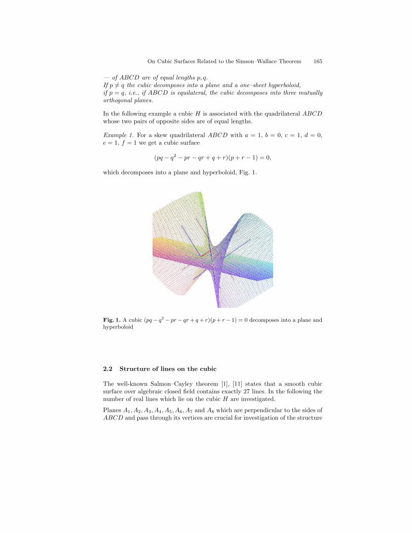
On Cubic Surfaces Related to the Simson–Wallace Theorem 165
— of ABCD are of equal lengths p, q.If p 6= q the cubic decomposes into a plane and a one–sheet hyperboloid,if p = q, i.e., if ABCD is equilateral, the cubic decomposes into three mutuallyorthogonal planes.
In the following example a cubic H is associated with the quadrilateral ABCDwhose two pairs of opposite sides are of equal lengths.
Example 1. For a skew quadrilateral ABCD with a = 1, b = 0, c = 1, d = 0,e = 1, f = 1 we get a cubic surface
(pq − q2 − pr − qr + q + r)(p+ r − 1) = 0,
which decomposes into a plane and hyperboloid, Fig. 1.
Fig. 1. A cubic (pq− q2 − pr− qr+ q+ r)(p+ r− 1) = 0 decomposes into a plane andhyperboloid
2.2 Structure of lines on the cubic
The well-known Salmon–Cayley theorem [1], [11] states that a smooth cubicsurface over algebraic closed field contains exactly 27 lines. In the following thenumber of real lines which lie on the cubic H are investigated.
Planes A1, A2, A3, A4, A5, A6, A7 and A8 which are perpendicular to the sides ofABCD and pass through its vertices are crucial for investigation of the structure
166 Pavel Pech
of lines on the cubic:
A1 : A1 ⊥ DA, D ∈ A1, A5 : A5 ⊥ BC, B ∈ A5,
A2 : A2 ⊥ DA, A ∈ A2, A6 : A6 ⊥ BC, C ∈ A6,
A3 : A3 ⊥ CD, C ∈ A3, A7 : A7 ⊥ AB, A ∈ A7,
A4 : A4 ⊥ CD, D ∈ A4, A8 : A8 ⊥ AB, B ∈ A8.
We will see later that they belong to the system of tritangent planes whichintersect the cubic H in three lines.
We can easily verify that it holds
H = A1A3A5A7 −A2A4A6A8, (3)
or
H = (dp + eq + fr − d2 − e2 − f2)((d − b)p + (e − c)q + fr − (d − b)b − (e −c)c)((b− a)p+ cq − (b− a)a)p− (dp+ eq + fr)((d− b)p+ (e− c)q + fr − (d−b)d− (e− c)e− f2)((b− a)p+ cq − (b− a)b− c2)(p− a).
Note that this is one of the most concise forms of H.
The importance of (3) appears by searching for lines lying on the cubic. Namelyfrom H = 0 and (3) we get that the line Ai ∩ Aj , i = 1, 3, 5, 7, j = 2, 4, 6, 8belongs to H.From (3) we obtain the following 12 lines which belong to the cubic surface:
a = A2 ∩A7, b = A8 ∩A5, c = A6 ∩A3, d = A4 ∩A1,
e = A2 ∩A5, f = A8 ∩A3, g = A6 ∩A1, h = A4 ∩A7,
i = A7 ∩A6, j = A2 ∩A3, k = A8 ∩A1, l = A5 ∩A4.
Another 6 tritangent planes given by pairs of parallel lines:
A9 = a ∪ k, A10 = b ∪ i, A11 = c ∪ l,
A12 = d ∪ j, A13 = e ∪ g, A14 = f ∪ h.
Denote:
C1 = ab− bd− ce,
C2 = b2 + c2 − ab− bd− ce, (4)
C3 = d2 + e2 + f2 − a2 + ab− bd− ce.
It holds:
Proposition 1.
a) The lines m,n coincide ⇔ C1 = 0 and C2 6= 0, C3 6= 0.
b) The lines m, o coincide ⇔ C2 = 0 and C1 6= 0, C3 6= 0.
c) The lines n, o coincide ⇔ C3 = 0 and C1 6= 0, C2 6= 0.
(5)
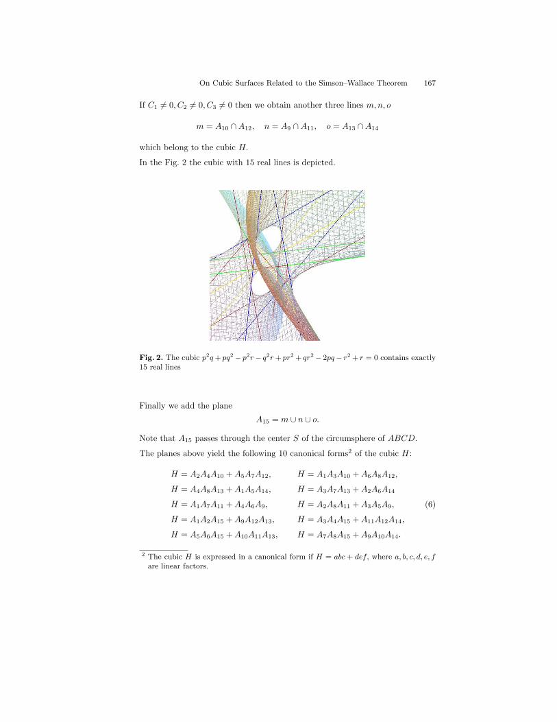
On Cubic Surfaces Related to the Simson–Wallace Theorem 167
If C1 6= 0, C2 6= 0, C3 6= 0 then we obtain another three lines m,n, o
m = A10 ∩A12, n = A9 ∩A11, o = A13 ∩A14
which belong to the cubic H.
In the Fig. 2 the cubic with 15 real lines is depicted.
Fig. 2. The cubic p2q+ pq2 − p2r− q2r+ pr2 + qr2 − 2pq− r2 + r = 0 contains exactly15 real lines
Finally we add the plane
A15 = m ∪ n ∪ o.
Note that A15 passes through the center S of the circumsphere of ABCD.
The planes above yield the following 10 canonical forms2 of the cubic H:
H = A2A4A10 +A5A7A12, H = A1A3A10 +A6A8A12,
H = A4A8A13 +A1A5A14, H = A3A7A13 +A2A6A14
H = A1A7A11 +A4A6A9, H = A2A8A11 +A3A5A9,
H = A1A2A15 +A9A12A13, H = A3A4A15 +A11A12A14,
H = A5A6A15 +A10A11A13, H = A7A8A15 +A9A10A14.
(6)
2 The cubic H is expressed in a canonical form if H = abc + def, where a, b, c, d, e, fare linear factors.

168 Pavel Pech
2.3 27 lines on the cubic
So far we have investigated cubics H which contain 15 lines. Is there a case whena cubic H contains 27 real lines? The answer gives the following theorem:
Theorem 3. Let C1 6= 0, C2 6= 0, C3 6= 0. Then a cubic H contains exactly 27distinct real lines iff
(C1C2 − C2C3 + C3C1)2 − 4a2C1C2C3 > 0 . (7)
Example 2. For a skew quadrilateral a = 1, b = −2, c = 1, d = 2, e = −1, f = 1we get the cubic
2p3 − 3p2q− 3pq2 +2q3 − 3p2r− 3q2r+7pr2 + qr2 +24p2 +24pq− 3q2 − 74pr+10qr − 7r2 − 26p− 77q + 77r = 0.
It holds C1 = 3, C2 = 12, C3 = 8 and
(C1C2 − C2C3 + C3C1)2 − 4a2C1C2C3 = 144 > 0 .
Then by the Theorem 3 there exist 27 real lines on the cubic, Fig. 3. The com-
Fig. 3. The cubic 2p3 − 3p2q − 3pq2 + 2q3 − 3p2r− 3q2r+ 7pr2 + qr2 + 24p2 + 24pq −3q2 − 74pr + 10qr − 7r2 − 26p− 77q + 77r = 0 contains 27 real lines
putation of all 27 lines was done in Maple.

On Cubic Surfaces Related to the Simson–Wallace Theorem 169
2.4 Singular points
The following theorem holds:
Theorem 4. If C1 = 0, C2 6= 0, C3 6= 0 or C2 = 0, C1 6= 0, C3 6= 0 or C3 = 0,C1 6= 0, C2 6= 0 then H possesses 2 nodes.
Proof. First assume that C1 = 0, C2 6= 0, C3 6= 0. By (1) the lines m and ncoincide. As m = A10 ∩A12 and n = A9 ∩A11 then the planes A9, A10, A11 andA12 have a common line. Further since A9 = a ∪ k, A10 = b ∪ i, A11 = c ∪ l andA12 = d ∪ j, then the lines a, k, b, i, c, l, d, j intersect the common line m = n. Itis easy to verify that the lines a, c, i, j,m meet at
S1 =[0,
b2 + c2 − ab
c,e(ab− b2 − c2)
cf
],
and the lines b, d, k, l,m at
S2 =[a, 0,
d2 + e2 + f2 − ad
f
].
Since neither a, c, i, j,m nor b, d, k, l,m are coplanar, the points S1 and S2 areconical singular points — nodes.
Similarly we proceed if C2 = 0 or C3 = 0. Remark 1. Note that the singular points S1 and S2 are intersections of oppositenormals a, c and b, d, and also of the lines i, j and k, l. This is guaranteed by thecondition C1 = 0 which means that the diagonals AC and BD are orthogonal.
Example 3. For a = 1, b = 0, c = 1, d = 0, e = 0, f = 2 we get the cubic
2p2q − 2pq2 + p2r + q2r − 2pr2 − 2qr2 − 2p2 + 3pr + 3qr + 2r2 + 2p− 4r = 0.
Since C1 = 0, C2 = 1, C3 = 3 then the cubic has two nodes at the points (0, 1, 0)and (1, 0, 2), Fig. 4.
Remark 2. How to find singular points of H in general? Solving the systemH = 0, ∂H
∂p = 0, ∂H∂q = 0, ∂H
∂r = 0 together with the condition Ci = 0 fori = 1, 2, 3 does not give any result at the moment.
3 Concluding remarks
In the text some properties of the cubic surface which is associated with a skewquadrilateral in E3 were investigated. A few remarks and questions:
Some properties of H are still explored (e.g. Eckhards points, the set of all sin-gular points, etc.).
We used 6 parameters a, b, c, d, e, f to describe a cubic H. Is it possible to de-crease the number of parameters, for instance by C1, C2, C3 and ”an unknown

170 Pavel Pech
Fig. 4. The cubic 2p2q−2pq2+p2r+q2r−2pr2−2qr2−2p2+3pr+3qr+2r2+2p−4r = 0with two nodes.
expression”?
So far we explored the case when orthogonal projections of a locus point ontothe sides of a skew quadrilateral were coplanar (the case s = 0 in (2)). Similarlywe can explore the case when orthogonal projections of a locus point onto thesides of a skew quadrilateral form a tetrahedron of a constant non-zero volumes. What are the properties of the locus (the case s 6= 0 in (2))?
What is the locus if we take 4 an arbitrary lines in 3D real Euclidean spaceinstead of 4 lines which form a skew quadrilateral?
The cubic H could serve as a model for demonstration of some types of cubicsurfaces.
References
1. Dolgachev, I. V.: Classical Algebraic Geometry: A Modern View. Cambridge Univ.Press, Cambridge (2012)
2. Giering, O.: Affine and Projective Generalization of Wallace Lines. J. Geometryand Graphics 1, 119–133 (1997)
3. Guzman, M.: An Extension of the Wallace–Simson Theorem: Projecting in Arbi-trary Directions. Amer. Math. Monthly 106, 574–580 (1999)
4. Holzer, S., Labs, O.: Illustrating the Classification of Real Cubic Surfaces. In:Elkadi, Mourrain, M. B., Piene R. (eds.) Algebraic Geometry and Geometric Mod-eling, pp. 119–134 (2006)

On Cubic Surfaces Related to the Simson–Wallace Theorem 171
5. Johnson, R.: Advanced Euclidean Geometry. Dover, New York (1960)6. Pech, P.: On Simson–Wallace Theorem and Its Generalizations. J. Geometry and
Graphics 9, 141–153 (2005)7. Pech, P.: On a 3D Extension of the Simson–Wallace Theorem. J. Geometry and
Graphics 18, 205–215 (2014)8. Pech, P.: Extension of Simson–Wallace Theorem on Skew Quadrilaterals and Fur-
ther Properties. LNAI, vol. 9201, pp. 108–118. Springer, Heidelberg (2015)9. Riesinger, R.: On Wallace Loci from the Projective Point of View. J. Geometry
and Graphics 8, 201–213 (2004)10. Roanes–Lozano, E. M., Roanes–Lozano, M.: Automatic Determination of Geomet-
ric Loci. 3D-Extension of Simson–Steiner Theorem. LNAI, vol. 1930, pp. 157–173.Springer, Heidelberg (2000)
11. Schlafli, L.: On the Distribution of Surfaces of the Third Order into Species, inReference to the Presence or Absence of Singular Points, and the Reality of theirLines. Philos. Trans. Royal Soc. 153, 193–241 (1863)
12. Wang, D.: Elimination Methods. Springer, Wien New York (2001)13. Wang, D.: Elimination Practice. Software Tools and Applications. Imperial College
Press, London (2004)
Automated Generation of Keywords fromImages for Geometric Information Search
Dan Song and Xiaoyu Chen?
SKLSDE–LMIB–School of Mathematics and Systems Science,Beihang University, Beijing 100191, China
Abstract. We outline an approach for automated generation ofkeywords in a domain of interest from an image to characterize thedomain information and knowledge that the image may imply. Wetake geometry of Euclidean plane as our domain of study and showhow keywords with geometric meanings may be generated and be usedto search for geometric information on the web with image query.The approach is based on our previous work on automated retrievalof geometric information from images of diagrams. It works by firstretrieving basic geometric entities and relations from the query imageby means of pattern recognition and numerical verification respectivelyand then generating advanced geometric information introduced alongthe hierarchical definitions of derived geometric concepts. Finally, thekeywords of different levels are weighted for their influences on thecharacterization of the image and are combined to generate severalgroups of keywords ordered according to their weights. Experiments witha preliminary implementation of the approach illustrate the feasibility ofautomated generation of keywords for searching the web for geometricinformation, in particular geometric theorems, which query images mayimply.
Keywords: geometric feature, pattern matching, image search, geometricknowledge management
1 Introduction
To search for information or knowledge in a domain of interest from web resourcesvia popular search engines such as Google and Bing, one usually needs tocharacterize queries in a group of keywords in the domain [5]. However, thechoice of keywords may heavily influence the quality of searching results. Forexample, it is not easy to efficiently find appropriate keywords to search forgeometric theorems on the web. Images are widely used to represent informationin a domain. An interesting question is how to search for domain information onthe web with image query. Answers to this question may lead to more friendlyand robust interface for general search engines.
? Corresponding author.

Automated Generation of Keywords from Images 173
A lot of work has been dedicated to domain information retrieval with imagequery. For example, to retrieve mathematical expressions, an expression-levelTF-IDF (term frequency-inverse document frequency) approach was proposedusing keyword search, where queries and indexed expressions are represented bykeywords taken from LaTeX strings in [7]. For general image retrieval, an efficientapproach was proposed in [4] by combining color information and keywordinformation. Content-based image retrieval approaches have been studied tosearch for images and perform automatic annotation [3].
In this paper, we will take geometry of Euclidean plane as our domain of studyand show how keywords with geometric meanings may be generated and be usedto search for deep geometric information on the web by taking images of diagramsas queries. The approach is based on our previous work on automated retrievalof basic geometric information from images of diagrams [2, 6], and then generateadvanced geometric information introduced along the hierarchical definitions ofderived geometric concepts. Finally, the keywords of different levels are weightedfor their influences on the characterization of the image and are combined togenerate several groups of keywords ordered according to their weights. In thisway, one is able to take an image of diagram as query and obtain geometricinformation relevant to the query on the web.
The rest of the paper is organized as follows. In Section 2, a generalapproach is outlined for automated generation of keywords in a domain ofinterest from an image. The domain E of geometry of Euclidean plane isbriefly specified in Section 3. Then particular strategies and rules developedfor deriving advanced geometric entities and relations from the retrieved basicinformation are presented in Section 4 followed by methods of generating groupsof keywords from the derived geometric information in Section 5. Discussionson implementation issues with experimental results are given in Section 6. Thepaper is concluded with some remarks in Section 7.
2 Generation of Keywords from Images: A GeneralApproach
In this section, we outline a general approach for automated generation ofkeywords in a domain of interest from an image to characterize the domaininformation and knowledge that the image may imply. The approach may leadto methods of searching for domain information on the web with image query.It consists of four main steps as shown in Fig. 1.
1. Specifying the domain of interest. Identify a set E of domain entities, aset Q of quantities, and a set R of domain relations and represent theentities, quantities, and their relations formally. Let an image I in the domaininvolving the elements of E, Q, and R be given.
2. Retrieving basic domain information. First use pattern recognition andmachine learning techniques to detect domain objects from I and then usenumerical computation to mine domain relations among the detected objectsto obtain basic domain information that the image may imply.

174 Dan Song and Xiaoyu Chen
3. Deriving advanced domain information. Along the hierarchical definitions ofderived domain concepts, advanced domain information may be introducedfrom the retrieved basic domain information.
4. Generating appropriate keywords. From the derived domain information,keywords of different levels are weighted for their influences on thecharacterization of the image and are combined to generate groups ofkeywords ordered according to their weights.
Fig. 1: Overview of a general approach for generating keywords from images
The general approach may be applied to any concrete domain byimplementing the tasks proposed in each step. In the following sections, wetake geometry of Euclidean plane as the domain of our study and show howkeywords with geometric meanings may be generated and be used to search fordeep geometric information on the web with image query.
3 Specification of Plane Euclidean Geometric Information
To retrieve geometrically meaningful information from image data, it is necessaryto identify in which domain the data should be interpreted and to specify thedomain with formal representation of geometric concepts, so that geometricinformation becomes meaningful and processable.
3.1 Representation of Basic Geometric information
Let the sets E0, Q0, and R0 of concepts of basic geometric entities, basicgeometric quantities, and basic geometric relations, respectively, in E be

Automated Generation of Keywords from Images 175
determined first. For example:
E0 = point(a::Number, b::Number), line(A::Point, B::Point),halfline(A::Point, B::Point), segment(A::Point, B::Point),circle(A::Point, B::Point, C::Point), circle(A::Point, B::Point),circle(A::Point, r::Distance);
Q0 = distance(A::Point, B::Point), angle(A::Point, B::Point, C::Point),size(α::Angle);
R0 = incident(A::Point, l::Line), pointOnC(A::Point, o::Circle),parallel(l::Line,m::Line), perpendicular(l::Line,m::Line),equal(a::Distance, b::Distance), equal(a::Size, b::Size).
Instances of the concepts in E0, Q0, andR0 are given with types, representations,explanations, and keywords as follows.1 Note that the keyword(s) of eachinstance is/are ordered in a list with respect to the frequency of each keywordappearing in geometric documents on the web, such as articles in Wikipediaand other web pages. The higher the frequency of one keyword is, the top thekeyword is arranged.
Basic geometric entities
1. Type: PointRepresentation: point(x, y)Meaning: a point with coordinates (x, y)Keywords: point
2. Type: LineRepresentation: line(A,B) or halfline(A,B) or segment(A,B)Meaning: a straight line or a halfline or a segment passing through twodifferent points A and BKeywords: line, halfline, segment
3. Type: CircleRepresentation: circle(A, r) or circle(A,B) or circle(A,B,C)Meaning: a circle with center A and radius r or a circle with center Aand passing through another point B or a circle passing through threedifferent points A, B, CKeywords: circle
Basic geometric quantities
1. Type: DistanceRepresentation: distance(A,B)Meaning: the distance between A and B where A and B are two pointsKeywords: distance
2. Type: AngleRepresentation: angle(A,B,C)Meaning: ∠ABC where A, B, and C are three different pointsKeywords: angle
1 Given an instance I, we use I.type, I.representation, I.meaning, and I.keywordsto represent the type, representation, meaning, and keywords of I, respectively.
176 Dan Song and Xiaoyu Chen
3. Type: SizeRepresentation: size(α)Meaning: the size of α where α is an angleKeywords: size
Basic geometric relations
1. Type: BooleanRepresentation: incident(A, l)Meaning: a point A lies on a line lKeywords: collinear, incident
2. Type: BooleanRepresentation: pointOnC(A, o)Meaning: a point A is on a circle oKeywords: incident
3. Type: BooleanRepresentation: parallel(l1, l2)Meaning: a line l1 is parallel to a line l2Keywords: parallel
4. Type: BooleanRepresentation: perpendicular(l1, l2)Meaning: a line l1 is perpendicular to a line l2Keywords: perpendicular
5. Type: BooleanRepresentation: equal(distance(A,B), distance(C,D))Meaning: the distance between two points A and B is equal to thedistance between two points C and DKeywords: equidistant
6. Type: BooleanRepresentation: equal(size(angle(A,B,C)), size(angle(D,E, F )))Meaning: the size of ∠ABC is equal to the size of ∠DEFKeywords: equal angle
The sets of basic geometric entities, quantities, and relations in E givenabove are not meant to be complete and they can be diminished or enlargedas necessary. For instance, the set of basic geometric quantities can be enlargedby adding the quantity Area.
3.2 Representation of Advanced Geometric information
Based on the concepts in E0,Q0, and R0, advanced geometric concepts may bederived with formal definitions. For example, the following advanced conceptscan be defined and represented in the formal Geometry Description Language(GDL [1]).
Advanced geometric entities
1. Advanced geometric entities with type Point

Automated Generation of Keywords from Images 177
(a) Name: MidpointRepresentation: M := midpoint(A,B)Definition: midpoint(A::Point, B::Point) , [M ::Point whereincident(M, line(A,B)) ∧ equal(distance(M, A), distance(M,B))]Keywords: midpoint, bisect
(b) Name: IntersectionRepresentation: P := intersection(l1, l2)Definition: intersection(l1::Line, l2::Line) , [P ::Point whereincident(P, l1) ∧ incident(P, l2)]Keywords: intersection, intersect
(c) Name: FootRepresentation: A := foot(l1, l2)Definition: foot(l1::Line, l2::Line) , [A::Point whereA := intersection(l1, l2) ∧ perpendicular(l1, l2)]Keywords: closest, foot
2. Advanced geometric entities with type Line
(a) Name: TriangleRepresentation: t := triangle(A,B,C)Definition: triangle(A::Point, B::Point, C::Point) , [segment(A,B),segment(B,C), segment(C,A), where ¬incident(A, segment(B,C))]Keywords: triangle
(b) Name: QuadrilateralRepresentation: q := quadrilateral(A,B,C,D)Definition: quadrilateral(A::Point, B::Point, C::Point, D::Point) ,[segment(A,B), segment(B,C), segment(C,D), segment(D,A), where¬incident(A, segment(B,C)) ∧ ¬incident(B, segment(C,D)) ∧¬incident(C, segment(D,A)) ∧ ¬incident(B, segment(D,A))]Keywords: quadrilateral
(c) Name: ParallelogramRepresentation: p := parallelogram(A,B,C,D)Definition: parallelogram(A::Point, B::Point, C::Point, D::Point) ,[quadrilateral(A::Point, B::Point, C::Point, D::Point, whereparallel(segment(A,B), segment(C,D))∧parallel(segment(B,C), segment(A,D))]Keywords: parallelogram
(d) Name: IsoscelestrapezoidRepresentation: i := trapezoid(A,B,C,D)Definition: trapezoid(A::Point, B::Point, C::Point, D::Point) ,[quadrilateral(A::Point, B::Point, C::Point, D::Point), whereparallel(segment(A,B), segment(C,D))∧¬parallel(segment(B,C), segment(A,D))∧equal(distance(A, B), distance(C, D))]Keywords: isosceles trapezoid

178 Dan Song and Xiaoyu Chen
(e) Name: n-Polygon (n ≥ 5)Representation: t := npolygon(P1, . . . , Pn)Definition: npolygon(P1::Point, . . . , Pn::Point) , [segment(Pi, Pi+1),i = 1, . . . , n−1, segment(Pn, P1), where ¬incident(Pi, segment(Pj , Pk)),i, j, k ∈ 1, . . . , n]Keywords: polygon
3. Advanced geometric entities with type Circle
(a) Name: CircumcircleRepresentation: c := circumcircle(t)Definition: circumcircle(t::Triangle) , [circle(A,B,C) whereA,B,C := vertex(t)]Keywords: circumcircle
(b) Name: IncircleRepresentation: c := incircle(t)Definition: incircle(t::Triangle), [c := circle(O::Point, r::Length) where t := triangle(A,B,C),tangent(segment(A,B), c) ∧ tangent(segment(A,C), c)∧tangent(segment(B,C), c)]Keywords: incircle
Advanced geometric relations
1. Name: TangentRepresentation: tangent(l, c)Definition: tangent(l::Line, c::Circle) , [pointOnC(foot(center(c), l), c)]Keywords: tangent
2. Name: BisectorRepresentation: bisect(A,B,C,D)Definition: bisect(A::Point, B::Point, C::Point, D::Point) ,[equal(size(angle(A,B,D)), size(angle(C,B,D)))]Keywords: angle bisector
3. Name: TrisectorRepresentation: trisect(A,B,C,D)Definition: trisect(A::Point, B::Point, C::Point, D::Point, E::Point) ,[equal(size(angle(A,B,D)), size(angle(D,B,E)))∧equal(size(angle(D,B,E)), size(angle(E,B,C)))])Keywords: trisector, trisect
4. Name: ConcurrentRepresentation: concurrent(l1, l2, l3)Definition: concurrent(l1::Line, l2::Line, l3::Line) ,[incident(intersection(l1, l2), l3)∨incident(intersection(l2, l3), l1)∨incident(intersection(l1, l3), l2)]Keywords: concurrent
Automated Generation of Keywords from Images 179
4 Derivation of Advanced Geometric Information
By using the approaches described in [2, 6], a set F of basic geometric entitiesand relations can be retrieved from a given image of diagram. In this section,we explain how to derive advanced geometric entities and relations from theobtained basic information.
4.1 Strategies for deriving geometric information
From a set of basic geometric entities and relations, different advancedentities and relations can be derived according to their definitions.For instance, from basic relations incident(P, l), incident(P, line(C,D)),and equal(distance(C,P ), distance(D,P )), two advanced entities P :=intersection(l, line(C,D)) and P := midpoint(C,D) can be obtained. Inorder to help efficiently derive necessary advanced geometric information inquiry,the following notations and strategies are introduced.
For each geometric instance O, we introduce a property level (denoted asO.level), which is an integer in [0,+∞), to characterize the priority of O in thederivation process.
1. If O is a basic geometric entity or a basic geometric relation, then O.level =0;
2. if O is an advanced geometric entity P(O1, . . . ,On) with definition in theform that P(O1, . . . ,On) , [O0 where S(R1, . . . ,Rm)], then O.level =n
maxi=1Oi.level + 1;
3. if O is an advanced geometric relation R(O1, . . . ,On) with definitionin the form that R(O1, . . . ,On) , [S(R1, . . . ,Rm)], then O.level =m
maxi=1Ri.level + 1.
With the property level of each geometric instance, advanced geometricentities and relations can be derived according to the following strategies:
1. derive advanced geometric entities and relations in order from lower level tohigher level;
2. for each geometric instance with the same level, first derive advancedgeometric entities, and then derive advanced geometric relations;
3. when deriving advanced geometric entities, first generate derived entitieswith type Point, then generate derived entities with type Line, and finallygenerate derived entities with type Circle;
4. given geometric relations R1, . . . ,Rm ∈ F, create a new label P , derive anadvanced geometric entity P := P(O1, . . . ,On) by definition in the form thatP(O1, . . . ,On) , [O0 where S(R1, . . . ,Rm)], and add P := P(O1, . . . ,On)into F; then remove R1, . . . ,Rm from F;
5. given geometric relations R1, . . . ,Rm ∈ F, derive an advanced geometricrelation R(O1, . . . ,On) by definition in the form that R(O1, . . . ,On) ,[S(R1, . . . ,Rm)], add add R(O1, . . . ,On) into F; then remove R1, . . . ,Rm
from F.
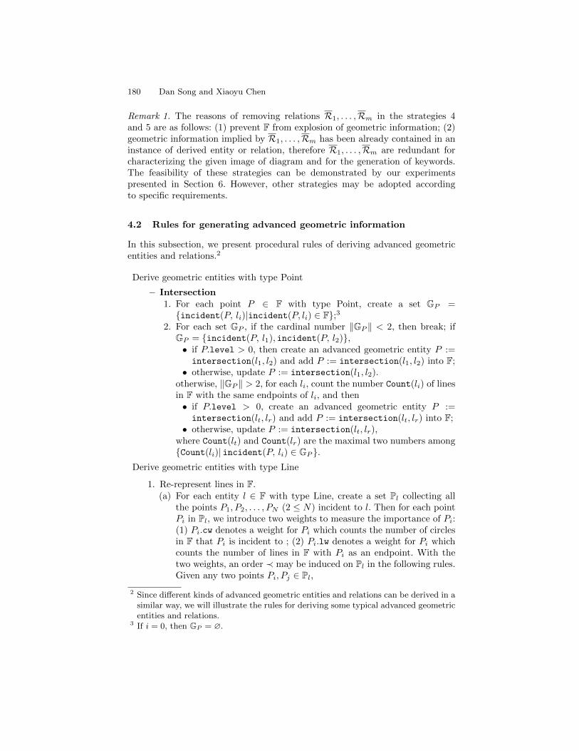
180 Dan Song and Xiaoyu Chen
Remark 1. The reasons of removing relations R1, . . . ,Rm in the strategies 4and 5 are as follows: (1) prevent F from explosion of geometric information; (2)geometric information implied by R1, . . . ,Rm has been already contained in aninstance of derived entity or relation, therefore R1, . . . ,Rm are redundant forcharacterizing the given image of diagram and for the generation of keywords.The feasibility of these strategies can be demonstrated by our experimentspresented in Section 6. However, other strategies may be adopted accordingto specific requirements.
4.2 Rules for generating advanced geometric information
In this subsection, we present procedural rules of deriving advanced geometricentities and relations.2
Derive geometric entities with type Point
– Intersection1. For each point P ∈ F with type Point, create a set GP =incident(P, li)|incident(P, li) ∈ F;3
2. For each set GP , if the cardinal number ‖GP ‖ < 2, then break; ifGP = incident(P, l1), incident(P, l2),• if P.level > 0, then create an advanced geometric entity P :=intersection(l1, l2) and add P := intersection(l1, l2) into F;
• otherwise, update P := intersection(l1, l2).otherwise, ‖GP ‖ > 2, for each li, count the number Count(li) of linesin F with the same endpoints of li, and then• if P.level > 0, create an advanced geometric entity P :=intersection(lt, lr) and add P := intersection(lt, lr) into F;
• otherwise, update P := intersection(lt, lr),where Count(lt) and Count(lr) are the maximal two numbers amongCount(li)| incident(P, li) ∈ GP .
Derive geometric entities with type Line
1. Re-represent lines in F.(a) For each entity l ∈ F with type Line, create a set Pl collecting all
the points P1, P2, . . . , PN (2 ≤ N) incident to l. Then for each pointPi in Pl, we introduce two weights to measure the importance of Pi:(1) Pi.cw denotes a weight for Pi which counts the number of circlesin F that Pi is incident to ; (2) Pi.lw denotes a weight for Pi whichcounts the number of lines in F with Pi as an endpoint. With thetwo weights, an order ≺ may be induced on Pl in the following rules.Given any two points Pi, Pj ∈ Pl,
2 Since different kinds of advanced geometric entities and relations can be derived in asimilar way, we will illustrate the rules for deriving some typical advanced geometricentities and relations.
3 If i = 0, then GP = ∅.

Automated Generation of Keywords from Images 181
i. if (Pi.cw = 1 and Pi.lw = 0) or (Pj .cw = 1 and Pj .lw = 0) or(Pi.cw = Pj .cw), then if Pi.cw + Pi.lw ≤ Pj .cw + Pj .lw, thenPi ≺ Pj ; else Pj ≺ Pi;
ii. else if Pi.cw < Pj .cw, then Pi ≺ Pj ;iii. else Pj ≺ Pi.
(b) All the points in Pl can be ordered with respect to ≺. Suppose P1 ≺P2 ≺ · · · ≺ PN , then re-represent l into l := Segment(PN−1, PN ).
2. If there exists a nonempty set S of lines in F such that all the endpointsof the lines in S are incident to a circle, then retrieve a set of n-polygons(n ≥ 3) S by Algorithm 1 and add all the obtained n-polygons into F;
3. Retrieve a set of n-polygons (n ≥ 3) from F−S by Algorithm 1 and addall the obtained n-polygons into F.
Derived geometric entities with type Circle
– CircumcircleAmong all the derived n-polygons (n ≥ 3), if there exist m polygonsp1, p2, . . . , pm which are inscribed to a circle c, then
1. if there exists pi (1 ≤ i ≤ m) such that the number of edges ofpi is greater than that of any pj (1 ≤ j ≤ m), then replace therepresentation of c with c := circumcircle(pi);
2. otherwise, select pj (1 ≤ j ≤ m) such that there exists no other pithe number of edges of which is greater than that of pj (1 ≤ j ≤ m),and replace the representation of c with c := circumcircle(pj).
5 Generation of Keywords for Web and Image Search
In this subsection, we outline our approach of generating keywords from retrievedgeometric information for a given image of diagram. Given a set F of geometricinformation and an positive integer N , the following procedure outputs a set K,whose element is a set of keywords with cardinal number N .
1. Select a geometric entity Ol with type Line from F such that Ol.level ≥O.level for all O ∈ F where O is with type Line. Then K′ := ∅. For eachKi ∈ K, Ki := Ki∪k | k ∈ Ol.keywords, K′ := K′∪Ki. Then K := K′and F := F− Ol.
2. Select a geometric entity Oc with type Circle from F such that Oc.level ≥O.level for all O ∈ F where O is with type Circle. Then K′ := ∅. For eachKi ∈ K, Ki := Ki∪k | k ∈ Oc.keywords, K′ := K′∪Ki. Then K := K′and F := F− Oc.
3. Select a geometric entity Op with type Point from F such that Op.level > 0and Op.level ≥ O.level for all O ∈ F where O is with type Point.Then K′ := ∅. For each Ki ∈ K, Ki := Ki ∪ k | k ∈ Op.keywords,K′ := K′ ∪Ki. Then K := K′ and F := F− Op.

182 Dan Song and Xiaoyu Chen
Algorithm 1 detectPolygon(Sg)
Require: A set Sg of segments.Ensure: P, a set of set of segments, each P ∈ P is a set of segments, which implies a
polygon P by just containing all the edges of P.1: P := ∅;2: Collect all the endpoints of segments in Sg to V, and set n := ‖V‖, visited[i] :=
False, i = 1, . . . , n, curV := 0, E := ∅ denotes the used edges from original startvertex to current one;
3: visited[curV] := True, ncount := 0, m := ‖Sg‖;4: for i = 1, . . . ,m do5: if curV is an endpoint of Sg[i] and all the segments in E lie on the
same side of Sg[i] then6: idx := the index of the other endpoint of Sg[i] in ‖V‖ except V[curV];7: if visited[idx] = True then8: Construct the set C ⊂ E which denote a loop from V[idx] to
V[idx], P := P ∪ C;9: Sg := Sg ∪ E− Sg[i];
10: go to line 3;11: else12: E := E ∪ Sg[i], Sg := Sg − Sg[i], curV := idx;13: go to line 3;14: end if15: else ncount := ncount + 1;16: end if17: end for18: if ncount = m then19: nE := E, visited[curV] := False, curV := the other endpoint of
E[nE] except V[curV], E := E− E[nE];20: go to line 3;21: end if22: Combine polygons in P if they share some common edges;23: return P;
4. Select a geometric relation R with type Boolean from F such that R.level ≥R′.level for all R′ ∈ F where R′ is with type Boolean. Then K′ := ∅. Foreach Ki ∈ K, Ki := Ki ∪ k | k ∈ R.keywords, K′ := K′ ∪Ki. ThenK := K′ and F := F− R.
5. In each of the above four steps, if for any K ∈ K, ‖K‖ ≥ N , then theprocedure stops; otherwise, repeat the four steps.
6 Implementation and Experiments
The techniques of keyword generation from an image of diagram described abovehave been implemented in C++ development environment. Diagram images usedfor our experiments were produced by using GeoGebra.
We have made some preliminary experiments with a number of selecteddiagram images, for which keyword generation was carried out on a PC with
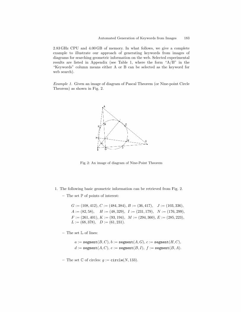
Automated Generation of Keywords from Images 183
2.83 GHz CPU and 4.00 GB of memory. In what follows, we give a completeexample to illustrate our approach of generating keywords from images ofdiagrams for searching geometric information on the web. Selected experimentalresults are listed in Appendix (see Table 1, where the form “A/B” in the“Keywords” column means either A or B can be selected as the keyword forweb search).
Example 1. Given an image of diagram of Pascal Theorem (or Nine-point CircleTheorem) as shown in Fig. 2.
Fig. 2: An image of diagram of Nine-Point Theorem
1. The following basic geometric information can be retrieved from Fig. 2.
– The set P of points of interest:
G := (108, 412), C := (484, 384), B := (36, 417), J := (103, 336),
A := (82, 58), H := (48, 329), I := (231, 179), N := (176, 299),
F := (261, 401), K := (93, 194), M := (294, 360), E := (285, 223),L := (68, 378), D := (61, 231).
– The set L of lines:
a := segment(B,C), b := segment(A,G), c := segment(H,C),
d := segment(A,C), e := segment(B, I), f := segment(B,A).
– The set C of circles: g := circle(N, 133).

184 Dan Song and Xiaoyu Chen
– The set R of geometric relations:
incident(G, a), incident(J, b), incident(J, c), incident(J, e),
incident(H, f), incident(I, d), incident(F, a), incident(K, b),
incident(M, c), incident(E, d), incident(L, e), incident(D, f),
pointOnC(G, g), pointOnC(H, g), pointOnC(I, g),
pointOnC(F, g), pointOnC(K, g), pointOnC(M, g),
pointOnC(E, g), pointOnC(L, g), pointOnC(D, g),
perpendicular(a, b), perpendicular(c, f), perpendicular(d, e),
equal(distance(C,F ), distance(B,F )),
equal(distance(J,K), distance(A,K)),
equal(distance(C,M), distance(J,M)),
equal(distance(C,E), distance(A,E)),
equal(distance(B,L), distance(J, L)),
equal(distance(B,D), distance(A,D)).
2. Advanced geometric information can be derived by using strategies and rulespresented in Section 4.
– The set E of advanced geometric entities:
C := (484, 384), B := (36, 417), A := (82, 58), N := (176, 299),
F := midpoint(C,B),K := midpoint(J,A),M := midpoint(C, J),E := midpoint(C,A), L := midpoint(B, J), D := midpoint(B,A),J := intersection(b, c), H := foot(c, segment(B,A)),I := foot(segment(A,C), e), G := foot(segment(B,C), b),b := halfline(A,G), c := segment(H,C), e := segment(B, I),
g := circle(N, 133), h := triangle(A,B,C).
– The set R of advanced geometric relations:
concurrent(b, c, e),
pointOnC(G, g), pointOnC(H, g), pointOnC(I, g),pointOnC(F, g), pointOnC(K, g), pointOnC(M, g),
pointOnC(E, g), pointOnC(L, g), pointOnC(D, g).
3. When set N to be 5, the following four groups of keywords can be generatedby using the procedure shown in Section 5.
(a) triangle, circle, closest, concurrent, midpoint;(b) triangle, circle, foot, concurrent, midpoint;(c) triangle, circle, closest, concurrent, bisect;(d) triangle, circle, foot, concurrent, bisect;

Automated Generation of Keywords from Images 185
4. By using the generated keywords, geometric information can be searchedfrom web via Google, as shown in Figs. 3 and 4. From the results, we foundthat the second (or the fourth) group of keywords lead to more relevantinformation than the first (or the third) group of keywords. The keywordfoot has more influences on the results than midpoint.
Fig. 3: Searching for web pagesvia Google by using the generatedkeywords
Fig. 4: Searching for images viaGoogle by using the generatedkeywords
7 Concluding Remarks
We have presented an approach for automated generation of keywordsin geometry of Euclidean plane from an image to characterize geometricinformation and knowledge that the image may imply. This approach can be usedto search the web for geometric information, in particular geometric theorems,which a query image may imply. The approach may be also generalized to thegeneration of keywords in any other domain of interest from an image in thedomain.
Acknowledgments. The authors wish to thank Professor Dongming Wang forhis insightful ideas on the problem and the referees for their helpful commentson improving the paper. This work has been supported by the Foundation ofthe State Key Laboratory of Software Development Environment under GrantNo. SKLSDE-2016ZX-18 and the Fundamental Research Funds for the CentralUniversities under Grant No. YWF-16-SXXY-01.

186 Dan Song and Xiaoyu Chen
References
1. X. Chen. Representation and automated transformation of geometric statements.Journal of Systems Science & Complexity 27(2):382–412, 2014
2. X. Chen, D. Song, and D. Wang. Automated generation of geometric theoremsfrom images of diagrams. Geometric Reasoning — Special issue of Annals ofMathematics and Articial Intelligence 74(3-4):333–358, 2015
3. R. Datta, J. Li, and J. Wang. Content-based image retrieval approaches and trendsof the new age. Multimedia Information Retrieval, 2005
4. Y. Jiang, Z. Zhou, and M.U. Chowdhury. Image retrieval based on the combinationof color and keyword. In: Proceedings of the International Conference onComputer Science, Software Engineering, Information Technology, e-Businessand Applications, pp. 450–453. International Society for Computers and TheirApplications (ISCA), 2003
5. S. Oyama, T. Kokubo, and T. Ishida. Domain-specific web search with keywordspices. IEEE Transactions on Knowledge and Data Engineering 16(1):17–27, 2004
6. D. Song, D. Wang, and X. Chen. Discovering geometric theorems from scannedand photographed images of diagrams. In: Automated Deduction in Geometry (F.Botana and P. Quaresma, eds.), Lecture Notes in Computer Science 9201, pp.149–165. Springer, Berlin Heidelberg, 2015
7. R. Zanibbi and B. Yuan. Keyword and image-based retrieval of mathematicalexpressions. In: Proceedings of SPIE 7874, Document Recognition and RetrievalXVIII, 78740I, 2011
Appendix.
Table 1: Selected experimental results
ID Diagram image Keywords
1 quadrilateral, circumcircle,
closest/foot, midpoint/bisect
2 segment, circle,
midpoint/bisect, equidistant
3 triangle, circumcircle,
midpoint/bisect, perpendicular

Automated Generation of Keywords from Images 187
Table 1: Selected experimental resultsID Diagram image Keywords
4 triangle, midpoint/bisect,
concurrent,
intersection/intersect
5 triangle, circle, closest/foot,
concurrent, midpoint/bisect
6 triangle, circumcircle,
concurrent, closest/foot,
midpoint/bisect
7 triangle, trisector,
equidistant
8 triangle, midpoint/bisect,
collinear/incident,
intersection/intersect
9 quadrilateral, incircle,
midpoint/bisect,
collinear/incident
10 quadrilateral,intersection/intersect,
collinear/incident

188 Dan Song and Xiaoyu Chen
Table 1: Selected experimental resultsID Diagram image Keywords
101 polygon, circumcircle,
intersection/intersect,
concurrent
11 polygon, incircle, concurrent
12 triangle, intersection, angle
bisector, equidistant
13 polygon, intersection,
collinear/incident, triangle
14 polygon, intersection,
perpendicular, equidistant
15 triangle, circumcircle,
midpoint, tangent
16 isosceles trapezoid,
midpoint/bisect, equidistant,
intersection/intersect

Automated Generation of Keywords from Images 189
Table 1: Selected experimental resultsID Diagram image Keywords
17 polygon, midpoint/bisect,
equidistant,
intersection/intersect
18 triangle, midpoint/bisect,
concurrent, closest/foot
19 quadrilateral,intersection/intersect, angle
bisector,collinear/incident
20 triangle, concurrent,angle
bisector

Formalization of a Surface Subdivision Allowinga Region with Holes without Coordinates
Kazuko Takahashi, Sosuke Moriguchi, and Mizuki Goto⋆
School of Science&Technology, Kwansei Gakuin University,2-1, Gakuen, Sanda, 669-1337, JAPAN
[email protected], [email protected], [email protected]
Abstract. This paper discusses how a surface subdivision is formalizedsymbolically. We formalize a subdivision of a finite two-dimensional planeallowing a region with holes. We use a data structure called PLCA. APLCA expression is defined using four constructors and represents a sur-face subdivision without coordinates. We show construction of a configu-ration for a subdivision and representation of a subdivision using PLCA.Formalization and proofs are performed within Coq proof assistant.
Keywords: surface subdivision, formalization, PLCA, planarity, Coq
1 Introduction
A number of studies have been undertaken previously on symbolic treatmentof geometric or topological properties. Some of these studies used proof assis-tants to give a computational model representing spatial data, and to certifyits formalization with a mechanical proof. They sometimes find drawbacks oroversights in pen-and-paper proofs.
Surface subdivision is a basic concept in computational geometry and topol-ogy. Intuitively, it is an embedding of a surface with a finite number of connectedregions. There are a number of geometric or topological topics related to sur-face subdivision, for example, graph embedding, four color theorem and Jordan’ssimple curve theorem [1]. Surface subdivision determines locations of regions fora given set of points, and it commonly uses a region without holes such as De-launay triangulation [1]. On the other hand, we consider a case in which a regionwith holes can be regarded as a subdivision. That is, we admit all configurationsshown in Figure 1 as a subdivision of a plane. Configuration here means thata representation of a figure showing its geometric or topological characteristics.In these figures, a red part shows a region with a hole and a green part showsa region as a hole. When we admit such cases, the border of each region is notalways a Jordan curve, that is, a simple closed curve without a self-loop [10] (e.g,Figure 1(c)(d)).
⋆ Currently, JFE Advantech Co., Ltd.

Formalization of a Surface Subdivision 191
(a) (b) (c) (d)
Fig. 1. Surface subdivision: (a) triangulation (no holes), (b) a region with holes, (c) aregion with holes which are connected with a point, and (d) a region with a hole whichis connected to itself with a point.
(a) (b)
Fig. 2. Different configurations with a disconnected component.
There are few symbolic expressions focusing on topological aspects withoutthe use of coordinates and, to the best of our knowledge, none gives a mechanicalproof of the algorithms for handling disconnected components.
Disconnected components can be regarded as regions that are embedded intothe holes of another region. Therefore, when we admit disconnected components,we have to explicitly represent the region with holes in which the componentis located, since no coordinate information is provided. For example, the twoconfigurations shown in Figure 2 should be considered as being different, whichmakes formalization difficult.
In this paper, we describe formalization with PLCA to represent a surfacesubdivision that allows disconnected components. PLCA is a data structure inwhich all incidence relations between objects are stored [14]. Topological andgeometric aspects can be distinguished in this structure. Previously, we havedescribed its inductive construction and proved that the obtained class is pla-nar [15]. We first gave a pen-and-paper proof and then a mechanical proof usinga proof assistant Coq [2]. As a rigorous specification is required in a symbolicformalization, it was necessary to solve subtle problems that can be ignored ina pen-and-paper proof [11].
In these studies, “planarity” means not only embedding a PLCA expressionin a two-dimensional plane, but also forming a subdivision of a plane. However,we did not refer to subdivision explicitly, nor did we explain in detail the mean-ing of the preconditions of each constructor; nevertheless, those are significantfactors in the symbolic treatment of geometric/topological data. In this paper,we describe construction of PLCA from the viewpoint of subdivision, and howconditions for surface subdivision are represented with PLCA.

192 Kazuko Takahashi, Sosuke Moriguchi, and Mizuki Goto
isolatedpoint
isolated line
bridge
Fig. 3. Disallowed configurations of a subdivision
We consider a surface subdivision as a configuration in which both side ofeach line always belong to distinct regions. It means that there are no isolatedpoints or isolated lines, and no bridges (Figure 3). In addition, a configurationcan include a region with holes as a piece of subdivision and regions connectedwith a point, which are shown in Figure 1. We represent these conditions inthe form of PLCA planarity. We give a more specific expression for a subdi-vision and show that a planar PLCA forms a subdivision. Our final goal is toimplement computational geometry algorithms related to surface subdivision inPLCA, based on the formalization described in this paper.
All the formalization is implemented in Coq. Although we will avoid describ-ing the messy Coq code here, the entire formalization and proofs have beenuploaded to [12].
The remainder of this paper is organized as follows. In Section 2, we describea data structure of PLCA. In Section 3 we show how a surface subdivision isconstructed with PLCA in Coq. In Section 4, we discuss how surface subdivisionis represented in our formalization. In Section 5 we compare our work withrelated work, and Section 6 concludes the paper.
2 PLCA
2.1 PLCA Expression
A PLCA data structure was originally designed to give a qualitative representa-tion of a spatial object. The term “qualitative” implies no use of numerical datasuch as coordinates, sizes or ratios etc.; instead, we perform reasoning focusingon certain characteristics of a spatial object. So far, several qualitative spatialrepresentations have been proposed [13, 4]. Among them, PLCA is designed todistinguish connection patterns of regions [14].
Definition 1 (PLCA expression). A PLCA expression is defined as a five-tuple, 〈P,L,C,A, o〉, where P is a set of points, L ⊆ P 2, C ⊆ Ln (n ≥ 3),A ⊆ Cm (m ≥ 1), o ∈ C.
In PLCA, there are four kinds of object: points, lines, circuits, and areas.
– Points are the most primitive objects. Points are distinguishable from eachother. We use p as a variable for points.
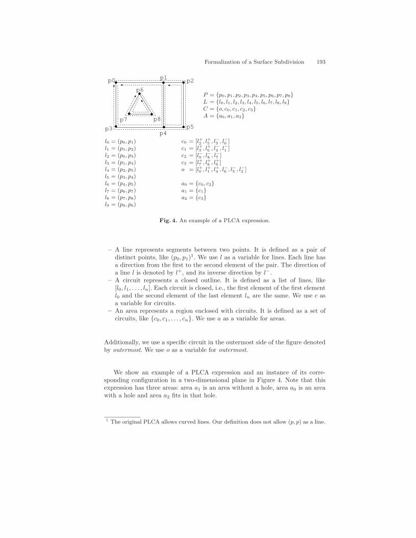
Formalization of a Surface Subdivision 193
p4
p0 p1 p2
p3 p5
p6
p7 p8
P = p0, p1, p2, p3, p4, p5, p6, p7, p8L = l0, l1, l2, l3, l4, l5, l6, l7, l8, l9C = o, c0, c1, c2, c3A = a0, a1, a2
l0 = (p0, p1)l1 = (p1, p2)l2 = (p0, p3)l3 = (p1, p4)l4 = (p2, p5)l5 = (p3, p4)l6 = (p4, p5)l7 = (p6, p7)l8 = (p7, p8)l9 = (p8, p6)
c0 = [l+2 , l+5 , l
−3 , l−0 ]
c1 = [l+3 , l+6 , l
−4 , l−1 ]
c2 = [l−9 , l−8 , l−7 ]c3 = [l+7 , l
+8 , l
+9 ]
o = [l+0 , l+1 , l
+4 , l
−6 , l−5 , l−2 ]
a0 = c0, c2a1 = c1a2 = c3
Fig. 4. An example of a PLCA expression.
– A line represents segments between two points. It is defined as a pair ofdistinct points, like (p0, p1)
1. We use l as a variable for lines. Each line hasa direction from the first to the second element of the pair. The direction ofa line l is denoted by l+, and its inverse direction by l−.
– A circuit represents a closed outline. It is defined as a list of lines, like[l0, l1, . . . , ln]. Each circuit is closed, i.e., the first element of the first elementl0 and the second element of the last element ln are the same. We use c asa variable for circuits.
– An area represents a region enclosed with circuits. It is defined as a set ofcircuits, like c0, c1, . . . , cn. We use a as a variable for areas.
Additionally, we use a specific circuit in the outermost side of the figure denotedby outermost. We use o as a variable for outermost.
We show an example of a PLCA expression and an instance of its corre-sponding configuration in a two-dimensional plane in Figure 4. Note that thisexpression has three areas: area a1 is an area without a hole, area a0 is an areawith a hole and area a2 fits in that hole.
1 The original PLCA allows curved lines. Our definition does not allow (p, p) as a line.

194 Kazuko Takahashi, Sosuke Moriguchi, and Mizuki Goto
(a) (b)
Fig. 5. Same subdivision, different data structures.
2.2 Equivalence on objects
We use a list as a data type to implement P,L,C,A, each line, circuit and area,as our first implementation in Coq. It causes us to define the equivalence relationon lists 2.
Hereafter, the symbol ‘+’ denotes an operation of list contcatenation. Forexample, when V = [v, w], [u] + V returns [u, v, w].
Two symbolic expressions that are not identical may stand for the sameconfiguration. For example, circuits [l1, l2, l3] and [l2, l3, l1] represent the samecircuit, and areas [c1, c2, c3] and [c3, c2, c1] represent the same area. This is dueto the cyclic structure of a circuit, and the data structure of a list for an area.In this case, we should regard them as equivalent.
On the other hand, we have to distinguish between two expressions when theystand for the same subdivision but have different configurations. For example, theexpressions for the two configurations shown in Figure 5 should be distinguished,since the number of points and lines are different.
Considering the above points, we define an equivalence relation over PLCAexpressions.
As P,L,C and A are defined as lists, they are equivalent to permutations ofthemselves. Each element of L is equivalent to its inverse, and each element ofC is equivalent to its rotation.
Definition 2 (PLCA-equivalence). Two expressions are PLCA-equivalentiff the pair of them is in the transitive closure of the following binary relationReq.
– 〈P, [l+] + L,C,A, o〉 Req 〈P, [l−] + L,C,A, o〉.– 〈P,L, [c] +C, [[c] + a] +A, o〉 Req 〈P,L, [c′] +C, [[c′] + a] +A, o〉, where c′ is
a rotated circuit of c.– 〈P,L,C,A, o〉 Req 〈P ′, L′, C ′, A′, o〉, where P ′, L′, C ′ and A′ are permuta-
tions of P , L, C and A, respectively.– 〈P,L,C, [a] +A, o〉 Req 〈P,L,C, [a′] +A, o〉, where a′ is a permutation of a.– 〈P,L, [o] + C,A, o〉 Req 〈P,L, [o′] + C,A, o′〉, where o′ is a rotated circuit of
o.
2 If we use data type from a Coq library, for example, MSet, then we may omit thesedefinitions.

Formalization of a Surface Subdivision 195
We call the above relation PLCA-equivalence.
Note thatReq is reflexive because of the third condition ofReq and the reflex-ivity of permutations. Therefore, PLCA-equivalence is reflexive and transitive.
2.3 PLCA consistency
A PLCA expression is too permissive to find a corresponding topological space.For example, if there exists more than one area that contain the same circuit,such an expression does not make sense. And we should also avoid duplicationin a list. Therefore, we put consistency on this data structure so that it makessense.
Definition 3 (consistent PLCA). Let 〈P,L,C,A, o〉 be a PLCA expression.The PLCA expression is said to be a consistent PLCA expression iff it satisfiesall of the following conditions.
– For each point p ∈ P , there exists l ∈ L such that p ∈ l.– For each line l ∈ L, all points in l are in P .– For each line l ∈ L, there exist circuits c, c′ ∈ C such that l+ ∈ c and
l− ∈ c′3.– For each circuit c ∈ C, each line in c or its inverse line is in L.– For each circuit c ∈ C except for o, there exists an area a ∈ A such that
c ∈ a.– For each area a ∈ A, all circuits in a are in C.– For any area a ∈ A, o 6∈ a.– Each point p ∈ P appears only once in P .– Each line l+ ∈ L appears only once in L and l− 6∈ L.– Each circuit c ∈ C appears only once in C and any rotated circuits other
than c do not appear in C.– Each area a ∈ A appears only once in A and any equivalent area other than
a does not appear in A.
3 Encoding PLCA
We show PLCA specification in Coq.
3.1 Construction of PLCA
We construct PLCA so that its configuration is a subdivision of a finite two-dimensional plane allowing a region with holes. We use four constructors, andexplain each constructor according to the meaning of their preconditions.
3 In the formalization in Coq, we define this condition as “for each line l such thatl+ ∈ L or l− ∈ L, there exists the circuit c such that l ∈ c.” These conditions arethe same.

196 Kazuko Takahashi, Sosuke Moriguchi, and Mizuki Goto
Initially, we make a finite area, then apply constructors sequentially. Wedivide an existing area into two areas and as a result, the number of areas isincremented by exactly one each time a constructor is applied. At this time,we either add a connected component or a disconnected component dependingon whether we cut an existing circuit or not. We introduce a new object pathto divide an area. As PLCA has no coordinate information, we have to specifythe area in which such a path is added. As a symbolic operation, we delete oneexisting area and add two new areas, and also reconfigure all related objects. Thedifficulty on re-composition of a circuit is that we have to find the beginning ofa list, since a circuit has a cyclic structure.
3.2 Objects
Objects in PLCA are defined as follows, where nat denotes a natural numberand prod denotes a product of the two specified arguments.
Definition Point := nat.
Definition Line := prod Point Point.
Definition Circuit := list Line.
Definition Area := list Circuit.
3.3 Basics
Here we provide some definitions of basic functions. Functions reverse andreverse linelist are prepared to make the reverse circuit (lists of lines), i.e.,reverse linelist([l+1 , l
+2 , ..., l
+n ]) = [l−n , ..., l
−2 , l
−1 ]). Proposition Rot is defined on a
pair of circuits to check whether one circuit is obtained by rotating the other,i.e., Rot([l+1 , l
+2 , ..., l
+n ], [l
+2 , l
+3 , ..., l
+n , l
+1 ]) is true, which is used to define PLCA-
equivalence. InL is a proposition that checks whether a line or its inverse is inL.
Definition reverse(l : Line) := (snd l, fst l).
Definition reverse_linelist(ll : list Line) := rev (map reverse ll).
Inductive Rot : list A -> list A -> Prop :=
| rotSame : forall (l : list A), Rot l l
| rotNext : forall (l l’ : list A) (a : A), Rot l (a :: l’)
-> Rot l (l’ ++ [a]).
Definition InL (l: Line)(L: set Line) : Prop :=
set_In l L \/ set_In (reverse_linelinst l) L.
PLCA-equivalence is defined as a proposition on a pair of lists of points, apair of lists of lines, a pair of lists of circuits, a pair of lists of areas, and apair of circuits. Each condition of Definition 2 is encoded. For example, the lastcondition, showing that the rotated outermost is equivalent to the original one,
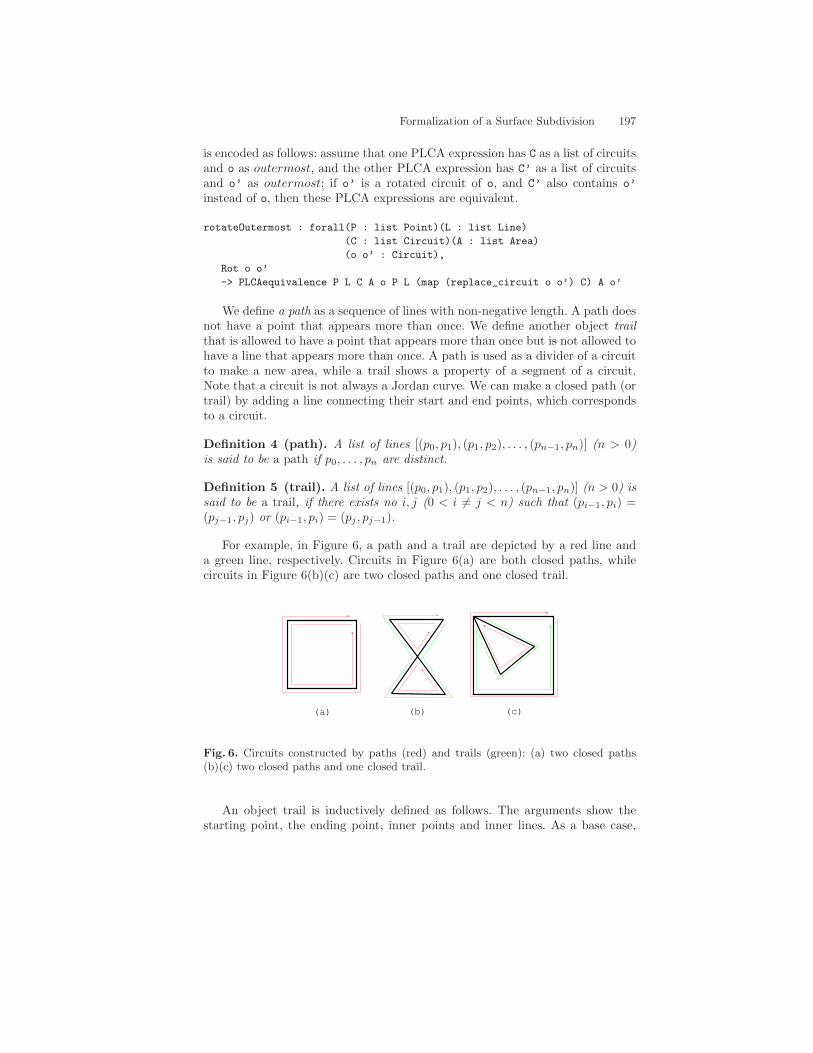
Formalization of a Surface Subdivision 197
is encoded as follows: assume that one PLCA expression has C as a list of circuitsand o as outermost, and the other PLCA expression has C’ as a list of circuitsand o’ as outermost; if o’ is a rotated circuit of o, and C’ also contains o’
instead of o, then these PLCA expressions are equivalent.
rotateOutermost : forall(P : list Point)(L : list Line)
(C : list Circuit)(A : list Area)
(o o’ : Circuit),
Rot o o’
-> PLCAequivalence P L C A o P L (map (replace_circuit o o’) C) A o’
We define a path as a sequence of lines with non-negative length. A path doesnot have a point that appears more than once. We define another object trailthat is allowed to have a point that appears more than once but is not allowed tohave a line that appears more than once. A path is used as a divider of a circuitto make a new area, while a trail shows a property of a segment of a circuit.Note that a circuit is not always a Jordan curve. We can make a closed path (ortrail) by adding a line connecting their start and end points, which correspondsto a circuit.
Definition 4 (path). A list of lines [(p0, p1), (p1, p2), . . . , (pn−1, pn)] (n > 0)is said to be a path if p0, . . . , pn are distinct.
Definition 5 (trail). A list of lines [(p0, p1), (p1, p2), . . . , (pn−1, pn)] (n > 0) issaid to be a trail, if there exists no i, j (0 < i 6= j < n) such that (pi−1, pi) =(pj−1, pj) or (pi−1, pi) = (pj , pj−1).
For example, in Figure 6, a path and a trail are depicted by a red line anda green line, respectively. Circuits in Figure 6(a) are both closed paths, whilecircuits in Figure 6(b)(c) are two closed paths and one closed trail.
(a) (b) (c)
Fig. 6. Circuits constructed by paths (red) and trails (green): (a) two closed paths(b)(c) two closed paths and one closed trail.
An object trail is inductively defined as follows. The arguments show thestarting point, the ending point, inner points and inner lines. As a base case,

198 Kazuko Takahashi, Sosuke Moriguchi, and Mizuki Goto
(a) (b)
rll(c)
C
c
rll(c)
x
y
z
s
e
x
y
z
(c) (d)
Fig. 7. Constructors: (a) single loop, (b) add loop, (c) add inpath, and (d) add inline.In these figures, ‘rll’ denotes reverse line list.
make a nil trail that consists of a single point without lines 4. Make a step trailby adding a point that is not included in the existing inner points, and a lineconnecting to the new point and the ending point of the existing path. Thefunction also checks that the new line is not included in the existing inner lines.
Inductive trail : Point -> Point -> list Point -> list Line -> Prop :=
| nil_trail : forall(p : Point), trail p (p::nil) nil
| step_trail : forall(p1 p2 p3 : Point)(pl : list Point)(ll : list Line),
trail p2 p1 pl ll
-> p3 <> p2
-> ~LIn (p3, p2) ll
-> trail p3 p1 (p3::pl) ((p3, p2)::ll).
3.4 Constructors
We show four constructors together with their preconditions: single loop,add loop, add inpath and add inline. A path is added in the inner side of theoutermost. In the previous work, we consider another constructor add outpaththat adds a path on the outer side of the outermost [11]. In that case, we allowa trail as an outermost. We can construct PLCA that admits such a configura-tion, but when focusing on subdivision, it is not suitable to consider such a case.Therefore, the definition is little different from the one shown in the previouswork.
single loop: Constructor single loop is an initialization that corresponds to adda Jordan curve to make outermost. It makes a simple path and adds a new linethat connects its start and end points (Figure 7(a)).
The preconditions are simple. (1) The length of a path is more than two tomake directions of its inner lines deterministic. (2) Points in the path should notbe existing ones.
4 A data structure [(p, p)] is taken as a base case in this implementation, which isnot allowed in the definition of a trail or path. And when trail or path is used in aconstructor in the implementation, condition on the length is added.

Formalization of a Surface Subdivision 199
add loop: Constructor add loop adds a Jordan curve to the specified area. Itmakes a simple path and adds a new line that connects its start and end points(Figure 7(b)).
The preconditions are the same as those of single loop. (1) The length ofa path is more than two to make directions of its inner lines deterministic. (2)Points in the path should not be existing ones.
A new configuration is obtained after putting the closed path onto the exist-ing area.
add inpath: Constructor add inpath is rather complicated. This constructor cor-responds to the division of an area by cutting two points of the same existingcircuit that belongs to that area (Figure 7(c)).
The preconditions are as follows. (1) The length of a path is more than zeroto make directions of its inner lines deterministic. (2) Points in the path shouldnot be existing ones. (3) Two points (that may be the same) connected to thestart and end points of the path should be in the same circuit to avoid a bridge.
A new configuration is obtained after making an area by re-composing anexisting circuit with a new path. In this case, at least two lines are added to L.
add inline: Constructor add inline is similar to add inpath but simpler, since nonew points are added. Intuitively, it makes a shortcut between the two existing,different points in the same circuit (Figure 7(d)).
The precondition is: (1) There is no line that connects two different pointsin the same circuit to guarantee planarity.
A new configuration is obtained after making an area by re-composing anexisting circuit with a new line. In this case, only one line is added to L.
3.5 Inductive PLCA
The four described constructors are formalized below. A PLCA expression con-structed in this way is called an inductive PLCA expression. In the following,‘rll’ denotes a function reverse linelist.
single loop: Let p1, p2, ..., pn (n ≥ 3) be distinct points, P = [p1, p2, ..., pn],L = [(pn, p1), (p1, p2), ..., (pn−1, pn)], c = [(pn, p1), (p1, p2), ..., (pn−1, pn)], C =[c, rll(c)] and A = [[c]]. Then, 〈P,L,C,A, rll(c)〉 is an inductive PLCA expression.
add loop: Let 〈P,L,C,A, o〉 be an inductive PLCA expression. If p1, p2, ..., pn(n ≥ 3) are distinct, pi for any i does not appear in P , c = [(pn, p1), (p1, p2), ...,(pn−1, pn)] and a ∈ A, then 〈P ′, L′, C ′, A′, o〉 is an inductive PLCA expression,where P ′, L′, C ′, A′ are as follows.
– P ′ = [p1, ..., pn] + P– L′ = [(pn, p1), (p1, p2), ..., (pn−1, pn)] + L– C ′ = [c, rll(c)] + C– A′ = [[c]] + [[rll(c)] + a] + (A− [a])
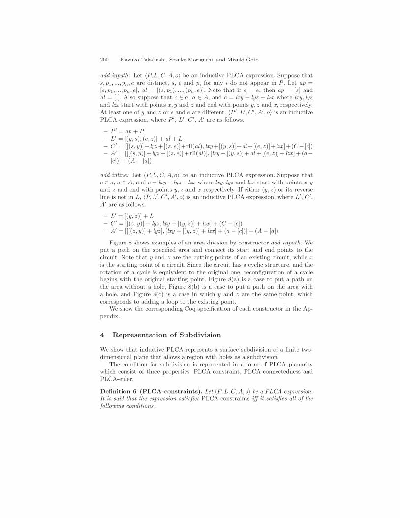
200 Kazuko Takahashi, Sosuke Moriguchi, and Mizuki Goto
add inpath: Let 〈P,L,C,A, o〉 be an inductive PLCA expression. Suppose thats, p1, ..., pn, e are distinct, s, e and pi for any i do not appear in P . Let ap =[s, p1, ..., pn, e], al = [(s, p1), ..., (pn, e)]. Note that if s = e, then ap = [s] andal = [ ]. Also suppose that c ∈ a, a ∈ A, and c = lxy + lyz + lzx where lxy , lyzand lzx start with points x, y and z and end with points y, z and x, respectively.At least one of y and z or s and e are different. 〈P ′, L′, C ′, A′, o〉 is an inductivePLCA expression, where P ′, L′, C ′, A′ are as follows.
– P ′ = ap + P– L′ = [(y, s), (e, z)] + al + L– C ′ = [[(s, y)]+ lyz+[(z, e)]+rll(al), lxy+[(y, s)]+al+[(e, z)]+ lzx ]+(C− [c])– A′ = [[[(s, y)]+ lyz +[(z, e)]+ rll(al)], [lxy +[(y, s)]+al +[(e, z)]+ lzx ]+ (a−
[c])] + (A− [a])
add inline: Let 〈P,L,C,A, o〉 be an inductive PLCA expression. Suppose thatc ∈ a, a ∈ A, and c = lxy + lyz + lzx where lxy , lyz and lzx start with points x, yand z and end with points y, z and x respectively. If either (y, z) or its reverseline is not in L, 〈P,L′, C ′, A′, o〉 is an inductive PLCA expression, where L′, C ′,A′ are as follows.
– L′ = [(y, z)] + L– C ′ = [[(z, y)] + lyz , lxy + [(y, z)] + lzx ] + (C − [c])– A′ = [[[(z, y)] + lyz ], [lxy + [(y, z)] + lzx ] + (a− [c])] + (A− [a])
Figure 8 shows examples of an area division by constructor add inpath. Weput a path on the specified area and connect its start and end points to thecircuit. Note that y and z are the cutting points of an existing circuit, while xis the starting point of a circuit. Since the circuit has a cyclic structure, and therotation of a cycle is equivalent to the original one, reconfiguration of a cyclebegins with the original starting point. Figure 8(a) is a case to put a path onthe area without a hole, Figure 8(b) is a case to put a path on the area witha hole, and Figure 8(c) is a case in which y and z are the same point, whichcorresponds to adding a loop to the existing point.
We show the corresponding Coq specification of each constructor in the Ap-pendix.
4 Representation of Subdivision
We show that inductive PLCA represents a surface subdivision of a finite two-dimensional plane that allows a region with holes as a subdivision.
The condition for subdivision is represented in a form of PLCA planaritywhich consist of three properties: PLCA-constraint, PLCA-connectedness andPLCA-euler.
Definition 6 (PLCA-constraints). Let 〈P,L,C,A, o〉 be a PLCA expression.It is said that the expression satisfies PLCA-constraints iff it satisfies all of thefollowing conditions.

Formalization of a Surface Subdivision 201
x
y
z
lxy
lyz
lzx
(a)
paths
e
x
y
z
(b)
xy
z
lxy
lyz
lzx
paths
e
xy
z
(c)
x
y z
lxy
lyz
lzx
path
s e
x
y z
Fig. 8. Examples of dividing an area by add inpath: (a) put a path on the area withouta hole, (b) put a path on the area with a hole, (c) two points in the circuit are thesame.
1. For each line (p, p′) ∈ L, p 6= p′.2. For each circuit c ∈ C, |c| ≥ 3 and c is a closed trail.3. For each area a ∈ A,
– if c, c′ ∈ a and c 6= c′, then c and c′ have no shared points or lines.– if c ∈ a, then c appears in a only once and no rotated circuit of c appear
in a.– |a| ≥ 1.
4. o is a closed path.
The first condition of PLCA-constraints guarantees that there is no iso-lated point, and the second condition guarantees that there is no bridge be-tween points. The third condition is for handling duplicated points in a sin-gle circuit. For example, in Figure 9, a circuit [(p0, p1), (p1, p2), (p2, p3), (p3, p1),(p1, p4), (p4, p5), (p5, p0)], that passes point p1 more than once, is included onlyin the green area. Note that it is not a combination of two circuits. The fourthcondition is to guarantee that our target plane to be divided is a finite planeencircled with a Jordan curve.
Definition PLCAconstraints(L : list Line)(C : list Circuit)
(A : list Area)(o : Circuit) : Prop :=
Lconstraint L /\ Cconstraint C /\ Aconstraint A
/\ Circuit_constraints o.
Each constraint is defined as a proposition. For example, the second conditionof Definition 6 is encoded as follows:
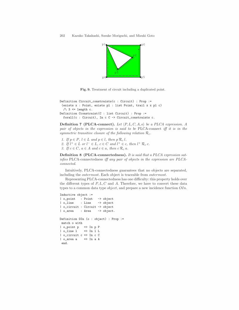
202 Kazuko Takahashi, Sosuke Moriguchi, and Mizuki Goto
p1
p2
p3
p5p4
p0
Fig. 9. Treatment of circuit including a duplicated point.
Definition Circuit_constraints(c : Circuit) : Prop :=
(exists x : Point, exists pl : list Point, trail x x pl c)
/\ 3 <= length c.
Definition Cconstraint(C : list Circuit) : Prop :=
forall(c : Circuit), In c C -> Circuit_constraints c.
Definition 7 (PLCA-connect). Let 〈P,L,C,A, o〉 be a PLCA expression. Apair of objects in the expression is said to be PLCA-connect iff it is in thesymmetric transitive closure of the following relation Rc.
1. If p ∈ P , l ∈ L and p ∈ l, then pRc l.2. If l+ ∈ L or l− ∈ L, c ∈ C and l+ ∈ c, then l+ Rc c.3. If c ∈ C, a ∈ A and c ∈ a, then cRc a.
Definition 8 (PLCA-connectedness). It is said that a PLCA expression sat-isfies PLCA-connectedness iff any pair of objects in the expression are PLCA-connected.
Intuitively, PLCA-connectedness guarantees that no objects are separated,including the outermost. Each object is traceable from outermost.
Representing PLCA-connectedness has one difficulty: this property holds overthe different types of P,L,C and A. Therefore, we have to convert these datatypes to a common data type object, and prepare a new incidence function OIn.
Inductive object :=
| o_point : Point -> object
| o_line : Line -> object
| o_circuit : Circuit -> object
| o_area : Area -> object.
Definition OIn (o : object) : Prop :=
match o with
| o_point p => In p P
| o_line l => In l L
| o_circuit c => In c C
| o_area a => In a A
end.

Formalization of a Surface Subdivision 203
Then, PLCA-connectedness is implemented as follows.
Inductive PLCAconnect : object -> object -> Prop :=
| PLcon : forall(p : Point)(l : Line),
In p P -> In l L -> InPL p l ->
PLCAconnect (o_point p) (o_line l)
| LCcon : forall(l : Line)(c : Circuit),
In l L -> In c C -> LIn l c ->
PLCAconnect (o_line l) (o_circuit c)
| CAcon : forall(c : Circuit)(a : Area),
In c C -> In a A -> In c a ->
PLCAconnect (o_circuit c) (o_area a)
| SYMME : forall(o1 o2 : object),
PLCAconnect o1 o2 -> PLCAconnect o2 o1
| TRANS : forall(o1 o2 o3 : object),
PLCAconnect o1 o2 -> PLCAconnect o2 o3 -> PLCAconnect o1 o3.
Definition PLCAconnected : Prop :=
forall(o1 o2 : object), OIn o1 -> OIn o2 -> PLCAconnect o1 o2.
Definition 9 (PLCA-euler). Let 〈P,L,C,A, o〉 be a PLCA expression. It issaid that the expression satisfies PLCA-euler iff |P | − |L| − |C|+ 2|A| = 0.
PLCA-euler guarantees that a PLCA expression can be embedded in a two-dimensional plane so that the orientation of each circuit can be correctly defined.
Coq implementation is straightforward.
Definition PLCAeuler : Prop :=
length P + 2 * length A = length L + length C.
Definition 10 (planar PLCA). If a consistent PLCA satisfies PLCA-constraints, PLCA-connectedness, and PLCA-euler, then it is said to be a planarPLCA.
The following theorem shows that inductive PLCA satisfies planarity.
Theorem 1. Inductive PLCA is a planar PLCA.
This is proved by proving the following three lemmas.
Lemma PLCA_consistency_and_constraints :
forall(P : list Point)(L : list Line)(C : list Circuit)(A : list Area)
(o : Circuit),
I P L C A o -> PLCAconsistency P L C A o /\ PLCAconstraints L C A o.
Lemma PLCAconnectedness :
forall(P : list Point)(L : list Line)(C : list Circuit)(A : list Area)
(o : Circuit),
I P L C A o ->
(forall(p : Point)(l : Line),

204 Kazuko Takahashi, Sosuke Moriguchi, and Mizuki Goto
In p P -> In l L -> PLCAconnect P L C A (o_point p) (o_line l))
/\ (forall(l : Line)(c : Circuit),
In l L -> In c C -> PLCAconnect P L C A (o_line l) (o_circuit c))
/\ (forall(c : Circuit)(a : Area),
In c C -> In a A -> PLCAconnect P L C A (o_circuit c) (o_area a)).
Lemma PLCAeuler :
forall(P : list Point)(L : list Line)(C : list Circuit)(A : list Area)
(o : Circuit),
I P L C A o -> PLCAeuler P L C A.
The PLCA-equivalence preserves PLCA planarity.
Theorem 2. Let e, e′ be equivalent PLCA expressions. If e is a planar PLCAthen e′ is also a planar PLCA.
We define that an expression of subdivision mentioned in Section 1 as follows.It is defined depending on the case whether a line is included in outermost ornot. Intuitively, this definition means that for each line, if it is not in outermost,then distinct two areas are connected by this line; otherwise, there exists onlyone area that is connected with the outside of the figure by this line.
Definition 11 (subdivision). Let e = 〈P,L,C,A, o〉 be a consistent PLCAexpression. For each l ∈ L, if the following condition is satisfied, then e is saidto be a subdivision: (i) there exist areas a, a′ ∈ A such that a 6= a′, l+ ∈ c ∈ a,and l− ∈ c′ ∈ a′, for l 6∈ outermost, and (ii) there exists an area a and a circuitc such that l ∈ c ∈ a, c 6= outermost, for l ∈ outermost.
Finally, we get the following theorem that means a planar PLCA forms asubdivision.
Theorem 3. A planar PLCA is a subdivision.
It is proved by the following theorems by case split depending on whether aline is included by the outermost.
Theorem PLCAsubdivision_area :
forall(P : list Point)(L : list Line)(C : list Circuit)(A : list Area)
(o : Circuit),
PLCA_planar P L C A o ->
forall (l : Line),
In l L
-> ~LIn l o
-> exists (c c’ : Circuit),
In c C
/\ In c’ C
/\ In l c
/\ In (reverse l) c’
/\ exists (a a’ : Area),
In a A

Formalization of a Surface Subdivision 205
/\ In a’ A
/\ In c a
/\ In c’ a’
/\ a <> a’.
Theorem PLCAsubdivision_outermost :
forall(P : list Point)(L : list Line)(C : list Circuit)(A : list Area)
(o : Circuit),
PLCA_planar P L C A o ->
forall (l : Line),
LIn l o
-> exists (c : Circuit),
In c C
/\ LIn l c
/\ o <> c
/\ exists (a : Area),
In a A
/\ In c a.
5 Related Works
Hypermap is a well-known data structure for handling topological aspects ofspatial data; it is an algebraic data structure that consists of a set of darts andtwo permutations. Hypermap uses a dart as a primitive, and an edge and avertex are defined as compositions of darts. Circuit and connected componentsare calculated by permutations. Hypermap is a useful data structure but it ishard to envisage, for example, a figure embedded in a two-dimensional plane,since vertices, edges and faces are not represented directly. On the other hand,PLCA provides a more straightforward expression of a figure.
There are several works that give a formalization based on hypermap anda proof of geographic/topological properties using proof assistants. Brun et al.showed a derivation of a program to compute a convex-hull for a given set ofpoints from their specification [3]. They specified the algorithm and proved itscorrectness using a structural induction. Gonthier showed the four color theorembased on surface subdivision [9]. However, they did not treat a disconnected com-ponent. Dufourd discusses that embedding polyhedra onto a plane is a sufficientcondition for planarity [6]. In that work, a hypermap was applied to formalizea discrete version of a Jordan curve and to prove its soundness [7]. Dufourd’smost relevant work is a formalization of an Delaunay triangulation [8]. Theyrepresented Delaunay triangulation in a form where all edges have two dartsand all faces have three vertices. A coordinate was used to represent a propertriangle, and disconnected components were not handled. Our formalization onsubdivision includes disconnected components.
Besides a hypermap, Yamamoto et al. studied a graph embedded on a planeusing HOL [16]. That model is simpler since it does not handle regions. There arefew studies on qualitative spatial representation from the viewpoint of theoremproving. Recently, an interesting work is done by Dapoigny et al. [5]. They

206 Kazuko Takahashi, Sosuke Moriguchi, and Mizuki Goto
formalized Tarski’s mereogeometry using Coq. The representation is based on apart-hole relationship between regions, which is completely different from thatof PLCA.
The doubly connected edge list is a popular data structure in computationalgeometry for representing a surface subdivision allowing disconnected compo-nents [1]. It contains records for each face, edge, vertex of the subdivision. Eachedge is regarded as two half-edges bounding different faces, and each half-edgehas a pointer to its connecting half-edges as well as its twin. Comparing itsdata structure with PLCA, an edge (or a line) is represented in relating to thetwo faces that share it in both data structures; however, incidence relations ofobjects are represented as pointers in the record in doubly connected edge list,whereas an object is explicitly defined using other existing objects in PLCA;the location of each object is determined uniquely by the coordinates in doublyconnected edge list, which is different from our work. Moreover, the main goalof computational geometry is to develop an algorithm that can reduce compu-tational complexity, whereas here, we investigate the soundness of an algorithm.The method proposed can handle geometric data on a more abstract level, andcan therefore be applied to prove the correctness of algorithms including doublyconnected edge lists.
6 Conclusion
We have shown a symbolic representation with PLCA for a surface subdivision ofa finite two-dimensional plane that allows holes in a region. All the formalizationand proofs are performed in Coq and consist of about 12,800 lines [12].
In future work, following issues are considered:
– To specify other intuitive definition of planarity and prove the equivalencewith PLCA-Euler.
– To implement high level computational geometry algorithms such as Delau-nay triangulation or graph embedding algorithms in PLCA and prove them.
– To extend the proposed approach to handle more general surfaces such aspolyhedra or torus with an arbitrary genus.
References
1. de Berg, M., van Kreveld, M., Overmars, M. and Schwarzkopf, O.: ComputationalGeometry, Springer-Verlag (1997).
2. Bertot, Y. and Casteran, P.: Interactive Theorem Proving and Program Development- Coq’Art: The Calculus of Inductive Constructions, Springer Verlag (1998).
3. Brun, C., Dufourd, J. -F. and Magaud, N,: Designing and Proving Correct a ConvexHull Algorithm with Hypermaps in Coq. Computational Geometry : Theory andApplications, 45(8):436-457 (2012).
4. Cohn, A. G. and Renz, J.: Qualitative Spatial Reasoning Handbook of KnowledgeRepresentation, F. Harmelen, V. Lifschitz and B. Porter(eds.), Chapt 13, pp.551-596, Elsevier (2007).

Formalization of a Surface Subdivision 207
5. Dapoigny, R. and Barlatier, P.: A Coq-Based Axiomatization of Tarski’s Mereoge-ometry, 12th Conference on Spatial Information Theory (COSIT2015), LNCS, vol.9368, pp. 108–129, Springer-Verlag (2015).
6. Dufourd, J. -F.: Polyhedra Genus Theorem and Euler Formula: A hypermap-formalized intuitionistic proof, Theoretical Computer Science, 403(2-3):133-159,Elsevier (2008).
7. Dufourd, J. -F.: An Intuitionistic Proof of a Discrete Form of the Jordan CurveTheorem Formalized in Coq with Combinatorial Hypermaps. Journal of AutomatedReasoning, 43(1):19-51 (2009).
8. Dufourd, J. -F. and Bertot, Y.: Formal Study of Plane Delaunay Triangulation. 1stInternational Conference on Interactive Theorem Proving (ITP2010), LNCS, vol.6172, pp. 211–226, Springer-Verlag (2010).
9. Gonthier, G.: Formal Proof - The Four Color Theorem. Notices of the AMS,55(11):1382-1393 (2008).
10. Kosniowski, C.: A First Course in Algebraic Topology, Cambridge University Press(1980).
11. Moriguchi, S., Goto, M., Takahashi, K.: Towards Verified Construction for PlanarClass of a Qualitative Spatial Representation. 7th International Symposium onSymbolic Computation in Software Science (SCSS2016), EPiC Series in Computing,vol.39, pp.117-129 (2016).
12. Moriguchi, S., Goto, M., Takahashi, K.: Formalization of IPLCA. http://ist.ksc.kwansei.ac.jp/~ktaka/IPLCA2016Apr
13. Stock, O. (Ed.): Spatial and Temporal Reasoning. Kluwer Academic Publishers(1997).
14. Takahashi, K., Sumitomo, T. and Takeuti, I.: On Embedding a Qualitative Rep-resentation in a Two-Dimensional Plane. Spatial Cognition and Computation, 8(1-2):4-26 (2008).
15. Takahashi, K., Goto, M. and Miwa, H.: Construction of a Planar PLCA Expression:A Qualitative Treatment of Spatial Data. Agents and Artificial Intelligence, LNCS,vol. 9494, pp. 298–315, Springer-Verlag (2015).
16. Yamamoto, M., Nishizaki, S., Hagiya, M. and Toda, Y.: Formalization of PlanarGraphs. Higher Order Logic Theorem Proving and Its Applications, LNCS, vol.971,pp. 369–384, Springer-Verlag (2005).
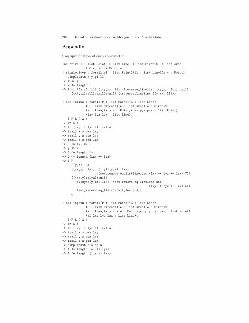
208 Kazuko Takahashi, Sosuke Moriguchi, and Mizuki Goto
Appendix
Coq specification of each constructor.
Inductive I : list Point -> list Line -> list Circuit -> list Area
-> Circuit -> Prop :=
| single_loop : forall(pl : list Point)(ll : list Line)(x y : Point),
simplepath x y pl ll
-> x <> y
-> 2 <= length ll
-> I pl ((y,x)::ll) (((y,x)::ll)::(reverse_linelist ((y,x)::ll))::nil)
((((y,x)::ll)::nil)::nil) ((reverse_linelist ((y,x)::ll)))
| add_inline : forall(P : list Point)(L : list Line)
(C : list Circuit)(A : list Area)(o : Circuit)
(a : Area)(x y z : Point)(pxy pyz pzx : list Point)
(lxy lyz lzx : list Line),
I P L C A o
-> In a A
-> In (lxy ++ lyz ++ lzx) a
-> trail x y pxy lxy
-> trail y z pyz lyz
-> trail z x pzx lzx
-> ~LIn (y, z) L
-> y <> z
-> 2 <= length lyz
-> 2 <= length (lxy ++ lzx)
-> I P
((y,z)::L)
(((z,y)::lyz)::(lxy++(y,z)::lzx)
::(set_remove eq_listline_dec (lxy ++ lyz ++ lzx) C))
((((z,y)::lyz)::nil)
::((lxy++(y,z)::lzx)::(set_remove eq_listline_dec
(lxy ++ lyz ++ lzx) a))
::(set_remove eq_listcircuit_dec a A))
o
| add_inpath : forall(P : list Point)(L : list Line)
(C : list Circuit)(A : list Area)(o : Circuit)
(a : Area)(x y z s e : Point)(ap pxy pyz pzx : list Point)
(al lxy lyz lzx : list Line),
I P L C A o
-> In a A
-> In (lxy ++ lyz ++ lzx) a
-> trail x y pxy lxy
-> trail y z pyz lyz
-> trail z x pzx lzx
-> simplepath s e ap al
-> 1 <= length (al ++ lyz)
-> 1 <= length (lxy ++ lzx)

Formalization of a Surface Subdivision 209
-> y <> z \/ s <> e
-> (forall(p : Point), In p ap -> ~In p P)
-> I (ap++P)
((y,s)::(e,z)::al++L)
((((s,y)::lyz)++((z,e)::(reverse_linelist al)))
::(lxy++((y,s)::al)++((e,z)::lzx))
::(set_remove eq_listline_dec (lxy ++ lyz ++ lzx) C))
(((((s,y)::lyz)++((z,e)::(reverse_linelist al)))::nil)
::((lxy++((y,s)::al)++((e,z)::lzx))
::(set_remove eq_listline_dec (lxy ++ lyz ++ lzx) a))
::(set_remove eq_listcircuit_dec a A))
o
| add_loop : forall(P : list Point)(L : list Line)
(C : list Circuit)(A : list Area)(o : Circuit)
(a : Area)(x y : Point)(ap : list Point)(al : list Line),
I P L C A o
-> In a A
-> simplepath x y ap al
-> x <> y
-> 2 <= length al
-> (forall(p : Point), In p ap -> ~In p P)
-> I (ap++P)
((y,x)::al++L)
(((y,x)::al)::(reverse_linelist ((y,x)::al))::C)
((((y,x)::al)::nil)
::((reverse_linelist ((y,x)::al))::a)
::(set_remove eq_listcircuit_dec a A))
o.

Author Index
AAbanades, Miguel A. 23Alam, Md. Ashraful 32BBorcea, Ciprian 44Botana, Francisco 23Boutry, Pierre 78Bowers, John C. 54Braun, David 62Braun, Gabriel 78Becar, Jean-Paul 97CChen, Xiaoyu 172FFleuriot, Jacques 117GGarnier, Lionel 97Ghourabi, Fadoua 117Goto, Mizuki 190IIda, Tetsuo 117JJanicic, Predrag 1, 152KKovacs, Zoltan 23, 137, 152LLadra, Manuel 144MMagaud, Nicolas 62Marinkovic, Vesna 152Michelucci, Dominique 15Moriguchi, Sosuke 190NNarboux, Julien 78Nikolic, Mladen 152PPambuccian, Victor 21Pech, Pavel 162Paez-Guillan, Pilar 144RRecio, Tomas 23, 137, 144
SSchreck, Pascal 62Song, Dan 172Streinu, Ileana 32, 44Solyom-Gecse, Csilla 23, 137TTakahashi, Kazuko 190


ADG 2016
This volume contains the 14 papers and 3 invited talks pre-sented at ADG 2016: Eleventh International Workshop onAutomated Deduction in Geometry held on June 26-28,2016 in Strasbourg, France.
ADG is a forum facilitating the exchange of ideas, pre-sentation of new research results and demonstrations ofsoftware tools lying at the intersection of geometry andautomated deduction. The selected papers, reviewed byan international Program Committee, cover diverse topicsranging from polynomial algebra, invariant and coordinate-free methods, synthetic and logic approaches, techniquesfor automated geometric reasoning from discrete mathe-matics, symbolic and numeric methods for geometric com-putation, geometric algorithms, geometric constraint solv-ing, experimental studies with automated theorem provers,applications to mechanics, origami and geometric model-ing.
The previous ten workshops were held in Coimbra 2014,Edinburgh 2012, Munich 2010, Shanghaı 2008, Ponteve-dra 2006, Gainesville 2004, Linz 2002, Zurich 2000, Bei-jing 1998, and Toulouse 1996.