juan carlos cuestas. the great (de)leveraging in the giips countries. foreign liabilities and...

The Great (De)leveraging in the GIIPS countries. Foreign liabilities

and private credit 1998-2013

Eesti Pank seminar, 30th June 2014

Juan Carlos Cuestas(Visiting researcher Eesti Pank, University of Sheffield)

Karsten Staehr(Eesti Pank, Tallinn Technical University)

All views expressed here are personal. Preliminary work, please do not quote

Little introduction, who am I?

• Name: Juan Carlos Cuestas Olivares

• Citizenship: Spanish/British

• Age: Unknown

• Weight: Even more unknown

• Height: 176 cm (-2cm Spanish average, -3cm Estonian average)

• Current position: Senior Lecturer (associate professor), University of Sheffield and last day as a visiting researcher, Eesti Pank

• PhD from Jaume I University (Spain) in 2005

• Keen on applied macroeconometrics and international finance

• Website: http://jccuestas.me.uk

2

Stylised facts

• Pre-crisis:

– Low interest rates in industrialised countries.

– Savings glut.

– International investors more willing to take higher risks.

– Money flowing to less developed economies, amongst them peripheral European countries.

– Boom-ing (or rather bombing) global economy, huge domestic credit expansion.

3

4

20

40

60

80

100

120

140

98 99 00 01 02 03 04 05 06 07 08 09 10 11 12 13

CR_GR

50

60

70

80

90

100

98 99 00 01 02 03 04 05 06 07 08 09 10 11 12 13

CR_IT

60

80

100

120

140

160

180

98 99 00 01 02 03 04 05 06 07 08 09 10 11 12 13

CR_PT

60

80

100

120

140

160

180

98 99 00 01 02 03 04 05 06 07 08 09 10 11 12 13

CR_ES

60

80

100

120

140

160

180

200

00 01 02 03 04 05 06 07 08 09 10 11 12 13

CR_IE

5

20

40

60

80

100

120

98 99 00 01 02 03 04 05 06 07 08 09 10 11 12 13

NFL_GR

4

8

12

16

20

24

28

32

98 99 00 01 02 03 04 05 06 07 08 09 10 11 12 13

NFL_IT

20

30

40

50

60

70

80

90

100

98 99 00 01 02 03 04 05 06 07 08 09 10 11 12 13

NFL_ES

20

40

60

80

100

120

140

98 99 00 01 02 03 04 05 06 07 08 09 10 11 12 13

NFL_PT

0

20

40

60

80

100

120

140

00 01 02 03 04 05 06 07 08 09 10 11 12 13

NFL_IE

Stylised facts (cont’d)

Big question:

What is relation between credit expansion and capital inflows?

• Global Financial Crisis ignition: BIG CRISIS!!!

• Need to understand:

– Linkages between finance and macroeconomic developments.

– Linkages between domestic and cross-border finance.

6

Structure of the presentation

• Introduction/motivation

• Brief literature review

• Data and graphs

• Method and results

• Mini conclusions

• Comments, discussion, complaints

7

Introduction

• We’ve observed less restrictions to international capital flows since the 80s. + introduction of the € which reduces international investment risks + the need to invest in more profitable/riskier sectors/investments.

• Have capital inflows been a “bad boy”?– Capital inflow / current account deficit interest rate ↓ / borrowing

possibility demand ↑ boom.

– On the other hand: excessive credit expansions, concentration of production on small number of sector and distortion of prices.

– Contractionary monetary policy (if any) may become ineffective.

• Sudden stops of capital inflows + Fisher’s debt deflation channel.

8

Introduction (cont’d)

• Exposed countries experience large CA deficits, increasing their exposure to international shocks.– increased risk perception of these countries.

– High leverage may increase the risk of mismatches between borrowing and investment (“hot money” invested in long run projects).

• Obstfeld (2012) says that CA deficits could be a potential indicator of internal macroeconomic weakness.

9


Capital inflows Credit expansion

10


• We are not concerned about the final sector of destination, but about the effect on the overall credit expansion in the receiving economy + the direction of causality.

• Push factors vs pull factors.

• Hypotheses: H1: Capital flows have a significant impact on the overall credit creation in the receiving country. H2: credit creation needs foreign capital to keep the booming economy.

11


• Is there a theoretical connection between capital inflow and credit creation?

• Yes, there is. Carvalho (2004) nails both stories nicely

M = C + D (liabilities side definition)

M = DCNBS + NFA + ODA – LFL (assets side definition)

12

Brief literature review

• Lane and Milesi-Ferretti (2008): analyse the level of foreign assets as a function of amongst others, GDP per capita and ca-openness.

• Lane and Milesi-Ferretti (2010): analyse whether the cross-country incidence and severity of the crisis is related to pre-crisis macro and finance factors.

• Reinhart and Reinhart (2008): sudden stops and its effects on the receiving economies.

• Avdijev et al. (2012): analyse the impact of financial openness, economic size and FX volatility on the change of credit/GDP. (Asia)

• Reinhart and Vesperoni (2012) look at the reaction of domestic credit/GDP as to capital inflows, XR regime, money growth etc.

13

Brief literature review (cont’d)

• Jordá et al. (2013): analyse the effect on real GDP per capita of excess credit pre recession. (cross-section)

• Taylor (2013) is concerned about the change in credit/GDP as a function of changes in ca/GDP.

• Carvalho (2014) cross section for different averages, looking at flows of capital on credit and money

• Veld et al. (2014): Analysis for Spain’s housing market

14

Brief literature review (cont’d)

• Issues:

– Δca and Δcr ~ I(0), miss long-run

– ca and cr ~ I(1), cointegration, but interpretation?

– Δnfl or ca and Δcr ~ I(0), miss long-run

– nfl and cr ~ I(1), THIS IS THE ONE!!

• Our specification: VAR/VECM (𝑐𝑟, 𝑛𝑓𝑙)

𝑐𝑜𝑖𝑛𝑡𝑒𝑔𝑟𝑎𝑡𝑖𝑜𝑛? ?

adjustment??

15

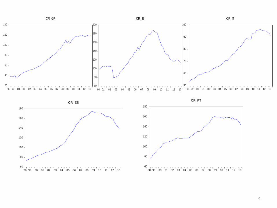
Data and graphs

• This analysis uses quarterly data for the GIIPS for credit from banks to private sector/GDP, (cr) and net foreign liabilities/GDP (nfl)

• Databases: Eurostat, BIS.

– Span of data 1998:4-2013:3

– Ireland 2000:4-2013:4

• L1NFL = log(1 + NFL)

• L1CR = log(1 + CR)

16

17

.2

.3

.4

.5

.6

.7

.8

.28 .32 .36 .40 .44 .48 .52 .56 .60 .64 .68 .72 .76 .80

L1CR_GR

L1

NF

L_

GR

2007:4

.0

.1

.2

.3

.4

.5

.6

.7

.8

0.55 0.60 0.65 0.70 0.75 0.80 0.85 0.90 0.95 1.00 1.05 1.10

L1CR_IE

L1

NF

L_

IE

2007:4

.04

.08

.12

.16

.20

.24

.28

.42 .44 .46 .48 .50 .52 .54 .56 .58 .60 .62 .64 .66 .68

L1CR_IT

L1

NF

L_

IT

2007:4

.1

.2

.3

.4

.5

.6

.7

.8

0.55 0.60 0.65 0.70 0.75 0.80 0.85 0.90 0.95 1.00

L1CR_PT

L1

NF

L_

PT

2007:4

.2

.3

.4

.5

.6

.7

0.50 0.55 0.60 0.65 0.70 0.75 0.80 0.85 0.90 0.95 1.00 1.05

L1CR_ES

L1

NF

L_

ES

2007:4

18

NFL = Net Foreign Liabilities = – Net International Investment Position

+ + + =

+

+

+

+

=

NFL (t – 1) Financial account (t)

1)

Valuation changes (t) NFL (t)

Capital account (t)

1)

Errors and omissions (t)

Current account balance (t)

0

Change in official reserves (t)

Method and results

19

tit

p

i

itt XXX

1

1

∆𝑙1𝑐𝑟𝑡 = 𝜇1 + 𝛼1 𝑙1𝑐𝑟𝑡−1 − 𝛽𝑙1𝑛𝑓𝑙𝑡−1 +

𝑖=1

𝑝

𝛾11(𝑖)∆𝑙1𝑐𝑟𝑡−𝑖 +

𝑖=1

𝑝

𝛾12(𝑖)∆𝑙1𝑛𝑓𝑙𝑡−𝑖 + 𝜀1𝑡

∆𝑙1𝑛𝑓𝑙𝑡 = 𝜇2 + 𝛼2 𝑙1𝑐𝑟𝑡−1 − 𝛽𝑙1𝑛𝑓𝑙𝑡−1 +

𝑖=1

𝑝

𝛾21(𝑖)∆𝑙1𝑐𝑟𝑡−𝑖 +

𝑖=1

𝑝

𝛾22(𝑖)∆𝑙1𝑛𝑓𝑙𝑡−𝑖 + 𝜀2𝑡

Method and results

Steps in the Johansen method:

• Test for unit roots, since at least two of the variables need to be I(1) processes

• Misspecification tests and lag length selection

• Rank test, for the number of cointegration vectors, max n-1 cointegrating vectors

• Estimation of the restricted model, i.e. identification of the cointegration space

• Stability20

tit

p

i

itt XXX

1

1

21

Augmented Dickey-Fuller test

L1NFL L1CR

Country-period t-Statistic p-value t-Statistic p-value

Greece-full -1.533847 0.5097 -2.017650 0.2786

Greece-pre’08 2.658311 0.9999 1.9447208 0.9998

Greece-post’08 -1.250382 0.6341 -2.366735 0.1614

Ireland-full -1.067586 0.7218 -1.457032 0.5472

Ireland-pre’08 -2.493829 0.1272 0.461843 0.9822

Ireland-post’08 -3.378249 0.0227a -0.253291 0.9179

Italy-full -1.363708 0.5932 -1.540276 0.5058

Italy-pre’08 1.106011 0.9967 1.975874 0.9998

Italy-post’08 -2.853174 0.0666 -2.316202 0.1755

Portugal-full -2.056691 0.2626 -1.383531 0.5836

Portugal-pre’08 -1.559765 0.4921 -3.145626 0.0320b

Portugal-post’08 -1.493430 0.5189 -0.874522 0.7777

Spain-full -0.357813 0.9091 -1.507840 0.5226

Spain-pre’08 1.839332 0.9997 1.087170 0.9966

Spain-post’08 -1.651234 0.4415 -0.037465 0.9454

Note: Rejection of the null hypothesis of a unit root at the 5% in bold. Lag length obtained by the modified Akaike Information

Criterion. a This result is confirmed by the Phillips-Perron test. Results available upon request.

b The Phillips-Perron test cannot reject the null of unit root. This result is confirmed by the KPSS test for stationarity. Results

available upon request. Hence we proceed under the assumption that the variable is an I(1) process.

22

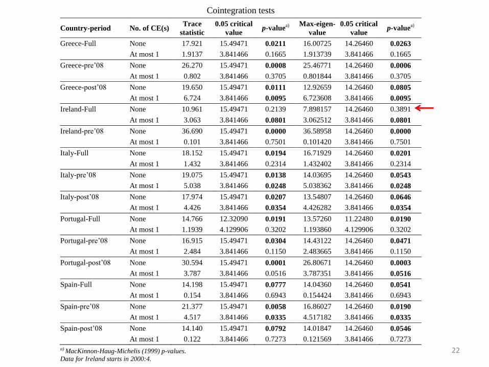
Cointegration tests

Country-period No. of CE(s) Trace

statistic

0.05 critical

value p-value

a)

Max-eigen-

value

0.05 critical

value p-value

a)

Greece-Full None 17.921 15.49471 0.0211 16.00725 14.26460 0.0263

At most 1 1.9137 3.841466 0.1665 1.913739 3.841466 0.1665

Greece-pre’08 None 26.270 15.49471 0.0008 25.46771 14.26460 0.0006

At most 1 0.802 3.841466 0.3705 0.801844 3.841466 0.3705

Greece-post’08 None 19.650 15.49471 0.0111 12.92659 14.26460 0.0805

At most 1 6.724 3.841466 0.0095 6.723608 3.841466 0.0095

Ireland-Full None 10.961 15.49471 0.2139 7.898157 14.26460 0.3891

At most 1 3.063 3.841466 0.0801 3.062512 3.841466 0.0801

Ireland-pre’08 None 36.690 15.49471 0.0000 36.58958 14.26460 0.0000

At most 1 0.101 3.841466 0.7501 0.101420 3.841466 0.7501

Italy-Full None 18.152 15.49471 0.0194 16.71929 14.26460 0.0201

At most 1 1.432 3.841466 0.2314 1.432402 3.841466 0.2314

Italy-pre’08 None 19.075 15.49471 0.0138 14.03695 14.26460 0.0543

At most 1 5.038 3.841466 0.0248 5.038362 3.841466 0.0248

Italy-post’08 None 17.974 15.49471 0.0207 13.54807 14.26460 0.0646

At most 1 4.426 3.841466 0.0354 4.426282 3.841466 0.0354

Portugal-Full None 14.766 12.32090 0.0191 13.57260 11.22480 0.0190

At most 1 1.1939 4.129906 0.3202 1.193860 4.129906 0.3202

Portugal-pre’08 None 16.915 15.49471 0.0304 14.43122 14.26460 0.0471

At most 1 2.484 3.841466 0.1150 2.483665 3.841466 0.1150

Portugal-post’08 None 30.594 15.49471 0.0001 26.80671 14.26460 0.0003

At most 1 3.787 3.841466 0.0516 3.787351 3.841466 0.0516

Spain-Full None 14.198 15.49471 0.0777 14.04360 14.26460 0.0541

At most 1 0.154 3.841466 0.6943 0.154424 3.841466 0.6943

Spain-pre’08 None 21.377 15.49471 0.0058 16.86027 14.26460 0.0190

At most 1 4.517 3.841466 0.0335 4.517182 3.841466 0.0335

Spain-post’08 None 14.140 15.49471 0.0792 14.01847 14.26460 0.0546

At most 1 0.122 3.841466 0.7273 0.121569 3.841466 0.7273

a) MacKinnon-Haug-Michelis (1999) p-values.

Data for Ireland starts in 2000:4.

23

Cointegration vector full sample

Cointegrating Eq: Greece Italy Portugal Spain

L1CR(-1) 1.000000 1.000000 1.000000 1.000000

L1NFL(-1) -1.158486 -1.055730 -0.884030 -0.889948

[-18.0053] [-13.4315] [-6.19853] [-10.5795]

C 0.063333 -0.382137 - -0.399525

Cointegration vector pre’08


L1CR(-1) 1.000000 1.000000 1.000000 1.000000

L1NFL(-1) -0.898460 -1.289770 -1.141753 -1.281070

[-36.7244] [-7.64582] [-5.13698] [-6.03797]

C -0.035412 -0.337444 -0.241992 -0.238181


L1CR(-1) 1.000000 1.000000 1.000000 1.000000

L1NFL(-1) -0.880867 -15.45274 -0.515191 -1.925565

[-2.77320] [-2.92785] [-9.83420] [-8.15636]

C -0.155192 2.935343 -0.569312 0.247744

Cointegration vector post’08

24

Adjustment parameters of Error Correction Term (ECT)

Greece Italy Portugal Spain

D(L1CR) D(L1NFL) D(L1CR) D(L1NFL) D(L1CR) D(L1NFL) D(L1CR) D(L1NFL)

Full -0.163 0.121 -0.120 -0.025 -0.005 0.033 -0.084 0.0356

[-3.765] [1.316] [-3.993] [-0.289] [-0.586] [ 2.872] [-3.167] [ 0.508]

Pre’08 -0.708 0.0436 -0.0807 -0.079 -0.146 -0.021 -0.387 0.206

[-5.156] [0.680] [-3.456] [-0.748] [-2.347] [-0.232] [-2.874] [ 0.491]

Post’08 -0.203 0.588 -0.0266 0.0769 -1.647 -2.660 -0.024 1.366

[-1.960] [2.562] [-1.619] [ 2.481] [-1.822] [-2.625] [-0.054] [ 1.352]

Note: t-statistics are given in square brackets. Significant cases at the 10% are given in bold.

Mini conclusions

• Set up the analysis of capital flows and credit expansion

• Theoretical reasons to analyse cr and nfl together

• Descriptive analysis suggest correlation

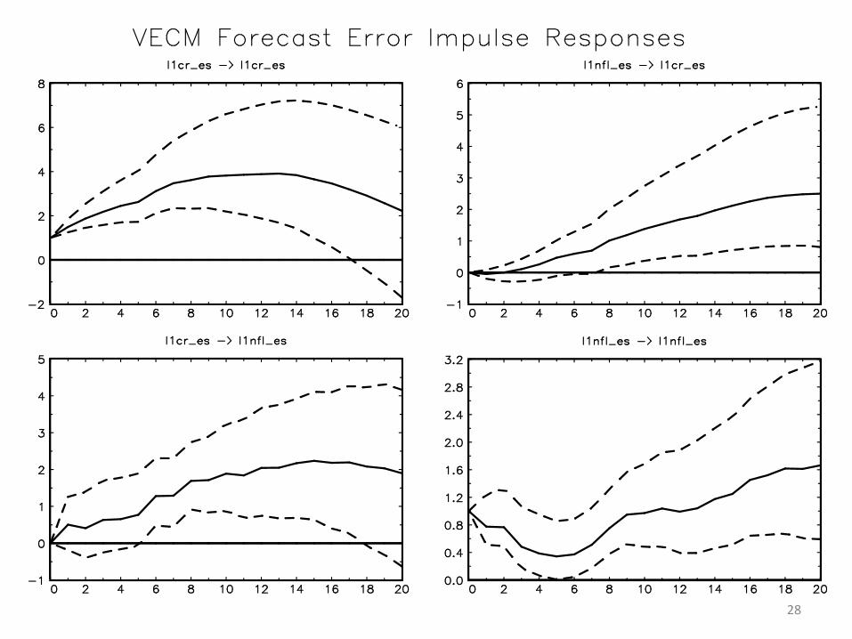
• Cointegration analysis shows clear causation, in most cases from capital inflows to credit expansion. Spain is different! (as usual )

• Clear changes in the behaviour of the relationship after 2008.

29

Comments??

Tänan väga

30