journal ol r biology - university of arizonamath.arizona.edu/~cushing... · j. math. biol. (1987)...

J. Math. Biol. (1987) 24:627-649

Journal ol r

Mathematical Biology

�9 Springer-Verlag 1987

Equilibria in systems of interacting structured populations

J. M. Cushing

Department of Mathematics, University of Arizona, Tucson, AZ 85721, USA

Abstract. The existence of a stable positive equilibrium density for a community of k interacting structured species is studied as a bifurcation problem. Under the assumption that a subcommunity of k - 1 species has a positive equilibrium and under only very mild restrictions on the density dependent vital growth rates, it is shown that a global continuum of equilibria for the full community bifurcates from the subcommunity equilibrium at a unique critical value of a certain inherent birth modulus for the kth species. Local stability is shown to depend upon the direction of bifurcation. The direction of bifurcation is studied in more detail for the case when vital per unity birth and death rates depend on population density through positive linear functionals of density and for the important case of two interacting species. Some examples involving competition, predation and epidemics are given.

Key words: Communities of structured populations - - Equilibria - - Stability - - Bifurcation - - Interacting species - - Competit ion - - Predator-prey interactions

1. Introduction

The equation

O~p+aa(Vp)+6 =0, t>O, a > O (1.1)

(0, = O/Ot etc.) governs the dynamics of the density p = p(t, a) >i 0 of a population consisting of individuals who have been categorized by a variable a >i 0 (age, size etc.) whose growth rate with respect to time t is ~. Here 6 is a population growth law which depends in general on time t, the variable a and the density p. Under the assumption that all newborns have characteristic a = 0 and that no member of the populat ion can have characteristic greater than A < +o0, Eq. (1.1) is accompanied by the conditions

vp[a=o =/3 (1.2)

p(t ,a)=-O f o r a l l a ~ A (1.3)

where /3 is a birth rate. In general /3 depends on t, a and p, as does v. It is assumed here that both vital rates /3 and 6 vanish when density drops to zero (/3 and 6 ~ 0 when p -= 0).

628 J.M. Cushing

Of fundamental importance in population dynamics are the asymptotic states of the population as t ~ +co. When 8,/3 and v do not depend explicitly on time t and when v does not depend on density p, the existence and stability of nontrivial equilibrium solutions p = p(a) of (1.1)-(1.3) were studied in [2] using bifurcation methods for very general 8 and/3. A birth modulus or a generalized inherent net reproductive rate defined by normalizing the linearization of the birth rate/3 at p---0 was used as a bifurcation parameter.

There are relatively few results which provide existence and stability of equilibria for systems of interacting structured populations in any amount of generality; see [15, 16, 19]. In this paper we offer one approach which not only yields general results, but which we feel provides a conceptionally simple point-of- view with regard to these questions. We will study the existence and stability of equilibria for multi-species communities of interacting structured populations whose dynamics are modelled by systems of coupled nonlinear equations of the form (1.1)-(1.3) by means of bifurcation theory methods, both global and local. The approach taken here will be centered around the idea of attempting to add a single species to a given community of interacting species. Thus, for example in the simplest case of two species, we begin with the assumption that one species has, in the absence of the other, a positive equilibrium state (the results in [2] are pertinent to this assumption) and we then ask for what values of a certain designated "birth modulus" or "inherent net reproductive rate" can the second species interact with the first and result in a nontrivial equilibrium state (i.e. one in which the second species has a positive equilibrium state). As will be seen bifurcation theory provides very powerful methods for obtaining answers to this question in a very general setting for communities of arbitrary size. Moreover these techniques offer a way, at least locally (but nonetheless still in a very general setting), to analyze the stability of the community equilibrium and to obtain lowest order approximations to equilibrium densities.

The paper is organized as follows. Preliminary matters, including the set up of notation and certain Banach spaces, are given in the following Sect. 2. In Sect. 3 a global existence result for nontrivial equilibria is given for a system of k t> 2 interacting structured populations in the form of a globally defined continuum of equilibria using a birth modulus of the kth species as a parameter (Theorem 1). The positivity and stability of the equilibria on this continuum are also considered (Theorems 2 and 3). Stability, at least linearized stability locally near bifurcation, is shown to depend upon the direction of bifurcation. In Sect. 4 the important special case when the vital rates ~ and/3 are given in terms of per unit rates D and F

fo = Dp, /3 = Fp da (1.4)

is considered. The case when D and F depend on density only through a linear functional of density (such as total population size ~A P da) is discussed and a method of deriving information about the continuum of equilibria by means of certain invariants that must hold along the continuum (as developed in [2] for k = 1 species) is given under certain restrictions. This procedure is discussed in more detail for the simplest case of k = 2 species in Sect. 5. In Sect. 6 the results

Equilibria in systems of interacting structured populations 629

of the paper are illustrated by several applications. A summary is given in Sect. 7. Finally, an appendix is included which gives the prerequisite linear theory (the systems considered here require an extension of the linear theory given in [2]).

2. Preliminaries

Let R = ( - ~ , +oo), R + = [0, +c~) and let k/> 2 be an integer. The notation ..... "~ k will be used to denote k - 1 vectors, e.g. A = (Ai)~_~l 1 for A~ ~ R. Then k vectors

will be written in the form (A, A), A e R. Let A t denote the transpose of A. Assume (,4, A) > 0, i.e. A > 0 and all A~ > 0. The Banach space of continuous

functions p :[0, A~]-> R under the usual sup-norm IPli = sUpto,A, jlP(a)I will be denoted by C(A~) and the product space C(A~) x . �9 �9 x C(Ak-a) under the norm IPl = "~IP,]~ will be denoted by C(.4).

The Banach space in which equilibrium solutions will be sought is defined as follows. Let A(A) denote the set ofaU pairs (/2, 13) for which 0 < ~e C(A) and / ~ k - 1 = (/x~)i=~ where/z~: [0, Ai )~ R is continuous and for which

M i ( A , - ) = +oo, Mi(a) = (tz,(s)/v~(s)) ds. (2.1)

Define

vi(o) H i ( a ) = v - - ~ e x p ( - M i ( a ) ) forO<~a<~AiandOfora>Ai . (2.2)

The space/J of those functions fi for which all p~ : R + --> R are continuous, p~ = 0 for a >i Ai and pi/Fli e C(Ai) is a Banach space under the norm IPl = Eilp~/FI~li �9 Note t h a t / I = (Hi) e/~.

I f /2 ~ is such that/~ - /2 ~ e C(A), then we write/2 o ~/2. If in this case we set M~ = So ~~ ds and replace M~ in (2.1) by M ~ and if (2.2) is used to define a function H ~ then/~o e B.

k - 1 For notational convenience we write 13 ̂ ~ for the vector (viw~)i=l and we denote 0aft= (0ap~)~l ~ and S~f ids=(S ~' p,~ds)~Z_ 1. For the case k = 2 t h e " ~ " notation will be dropped. Finally we let B + denote the set of positive fi ~ B(A), i.e. fi for which all p~ > 0 on the half open interval [0, A,). Note that H and H ~ e B +.

We are interested in systems of k ~> 2 coupled, nonlinear equations of the form (1.1)-(1.3) when ~ = ~(fi, p) and fl = fl(fi, p) depend in a general way on the densities (fi, p). The equilibrium equations

8a(~ ^/~) + g(/~, p) = 0 (2.3)

~(0) ^ ~(0) =/~(A p) Oa(vp)+~(~,p)=O

(2.4) v(0)p(0) =/~ (.a, p)

are to be solved for (fi, p) e/J(fi,) x B(A). The equations which we wish to consider can be written in the form

A A A A A ^

Oty+O~(~^ ~)+ l~~ ̂ ~+ L~(y)+ L2(y)+ h2=O

t3(0) ^ 33(t, 0) = r~,(33) + tfi2(y) +/~, (2.5)

630 J. M. Cushing

(2.6)

(2.7)

equilibrium

O,y + Oa( vy) + l~~ + h2=O

v(O) y( t, O) = nm( y) + ha

yi(t ,a)=O for a>~Ai and y( t ,a)=O for a>~A

for the k unknowns (~ , y )=( f ( t , a ) , y ( t , a ) ) . The associated equations for (fi, y) = ( f ( a ) , y(a)) are

ao(~^#)+#o^#+ ~ Lx(y) + s + #,~ = 6 (2.8)

,3(o) A # ( 0 ) = , ~ , ( ~ ) + , ~ ( y ) + ~,

0a(vy)+ Oy+h2=0 (2.9)

v(O)y(O) = nm( y) + hi.

In these equations the s are linear operators and the rhi, m are linear functionals * 0 - " 0 . * A

for each t and n is a real constant. Also /z ~/z, /x ~ /z with (/2, ~)~A(A), (/~, v) ~ a (A).

A

Equilibrium solutions of (2.5)-(2.7) will be sought in B(A) x B(A), in which case (2.7) is automatically fulfilled. By a solution of Eqs. (2.8)-(2.9) will be meant a k-tuple (~, y) e/~(fi~) x B(A) for which viyi and vy are differentiable on [0, Ai) and [0, A), respectively.

The prerequisite linear theory in which the /~ and hi do not depend on the densities fi, p is given in the Appendix. Our interest here is with the nonlinear case when the/~ and h~ are nonlinear expressions in (~, y). Systems of this form arise from systems of the model equations (1.1)-(1.3) under certain circumstances. For example, if we assume that the "reduced system" of equilibrium equations for the subcommunity of k - 1 species in which p is absent

0a(13 ~ ~ ^ A p)+ t~(p, 0) = 0 (2.10)

A A

~(0) ^ #(0) = #(p, 0) t , ~ A A 0

has a solution fl~ B(A) and if we set f i = p - p , y = p then the full system of k equilibrium equations for (y, y) given by (2.3)-(2.4) has the form (2.8)-(2.9) if the following assumptions are made about the vital death 8, 8 and birth fl, fl rates:

g ( # + # O , y ) = g ( # o , o ) + # o * ~ ~ ~ A y+ LI(y)+ L2(y)+ h2

6(~+ fi~ y)= lz~ h2 (2.11)

A ~ , ~ A A

fl ( y +/3 ~ y) =/3(#3 ~ O) + trt I (y) + rfi2(y) + hi # ( # + -o p ,y) = nm(y)+hl

where/~i and hi are higher order in (fi, y) near (0, 0). n is a real parameter about which more will be said later 2 Specific hypotheses on the linear terms L;, rhi and m and the nonlinear terms hi, h~ will be made below.

The major restriction on the density dependent vital rates made here is that they have expansions of the form (2.11) so that the linearizations at the "trivial" equilibrium (fi,/3) = (rio, 0) have the required forms in (2.8)-(2.9). An example is provided by the case when the vital rates are given in terms of per unit rates (as in (1.4))

= D(p, p), D D(~, p) and /~ =/~(fi, p), F = F(p, p). (2.12)

Equilibria in systems of interacting structured poptllations 631

Then the linear terms have the form

/20-~- O ( p , 0), Zl()~ ) = p ^ O f i D ( p , O ) ( y ) , L2(y) = ~o^ OoD(p* *0, 0)(y)

~r~p , O) = ^ y+O~F(p , O)(y) ^ r ds

(2.13)

IO ~ "" ^0 rfi2(y) = apF(p , 0)(y) ^ t~ ~ as

0 -~0 I0 A tx = D ( p ,0), n m ( y ) = F(~~

Here/2 = E3(6, 0) and ~ = D(0, 0) are taken as the inherent per unit death rates ("inherent" means at low species density in the absence of all other species). The terms 0~/) etc are Fr6chet derivatives. Thus in fact systems (2.3)-(2.4) with per unit vital rates as in (1.4) and (2.12) do have the required form (2.8)-(2.9) after the densities are centered on a "trivial" equilibrium (t~, P) = (t ;~ 0).

3. Bifurcating branches of positive equilibria

(a) Existence. The reduced system (2.10) represents the equilibrium equations for the community of k - 1 species ~ in the absence of the kth species p. Under the assumption that this reduced system possesses a positive equilibrium ~ = ~o > 0 we will look for positive solutions of the equilibrium equations (2.3)-(2.4) which bifurcate from the "trivial" equilibrium (/~, p) = (~o, 0) as a function of the real parameter n. This will be done by studying the equilibrium equations in the form (2.8)-(2.9) for (3~, y ) = ( ~ - ~ ~ p) under the assumption that the vital rates 6, 6 and/3,/3 satisfy (2.11). This approach can be viewed as an attempt to add a kth species to a community of k - 1 species which possesses at least one equilibrium in such a way as to obtain a community of k species which possesses at least one positive equilibrium. The stability of these equilibria will be studied in the next section.

As in [2] the bifurcation parameter n > 0 is chosen so as to have a certain biological interpretation. The linear term nm(p) is an inherent birth law for species p (i.e. the birth law at low densities in the absence of density effects or h I ~ 0 ) . It is assumed that

/ / O ( a ) = .~ v-~-~a~ exp~ - ~ ~ O ~ a < a m(l~~ ~ O, / " -

I0, a>~ A

or, by rescaling n if necessary, that

m ( n ~ = 1. (3.1)

Then m can be referred to as a normalized inherent birth rate and n can be called an inherent birth or fertility modulus. "Inherent" in this case refers to the situation when species p is at low (technically zero) density and the remaining species are near (technically at) the equilibrium ~o. In most applications m is a positive functional, i.e. re(p) > 0 if p ~> 0 ( r 0) so that this condition holds.

632 J.M. Cushing

In the case (1.4) of a per unit birth rate this normalization takes the form

F(p, p) = n f (~ , p) , f (~o , 0)1i o da = 1. (3.2)

H ~ is the (inherent) probability of survival to characteristic a and hence n = SAo F ( ~ ~ O)H ~ da is the inherent net reproductive rate, i.e. the expected number of offspring per lifetime.

An equilibrium pair is a pair (n, (p~, p)) c P = R x (/~ x B) for which (~, p) is a solution of the equilibrium equations (2.3)-(2.4) for the corresponding value of n. A positive equilibrium pair is a pair in P+ = R x (B+ x B +) and a nontrivial pair is one for which (~, P) ~ (~o, 0).

A

With regard to the Banach spaces B, B in which equilibria are sought, a natural choice given (2.11) would be to use t 2 = ~o =/xo. ~ , ~ For more flexibility

, ~ 0 ^ 0 ^ however we allow i.t - ~ , ~ - / . t where ~,/.t are specified functions in ~ A

ZI(A), zl (A). In doing this w e are motivated by applications in which ,per unit death rates have the form D =/2 + ~(p~, 0), D = ~ + r(~, 0) where ~(0, 0) = 0,

A

r(0, 0) = 0; i.e./2 and ~ are "inherent", density independent a-specific per unit death rates. In such cases, we have (see (2.13)) that t2~ ~,^o = r t p ,O), o _ ~ =

A 0 A A 0 A O r(f$ ~ 0) and that /.t - # , f t~ provided ri(p , 0) and r(p , 0) are continuous functions of a on [0, Ai] and [0, A]. (This means for these motivating models that regardless of density effects, as embodied in f and r, the death rate for a near its limit value Ai or A is dominated by the inherent, density independent terms /~ and /~ or, put another way, density effects do not alter the maximal characteristic limits.)

The needed hypotheses on the vital rates are summarized in H1-H3 below.

HI : (i ~, ~ ) ~ , ~ ( A ) , (it, v )~ A ( A ) and the reduced system (2.10) has a positive ^ 0 # ~ + solution p E ~ .

Thus (2.8)-(2.9) have a trivial solution (rio, 0)c /~ x B. With regard to the vital rates 8, S and/3, fl we want to assume that they satisfy (2.11) with the normalization (3.1). For added generality the higher order terms are allowed to depend on n.

A A

H2: The vital death rates ~, ~ and birth r a t~ 13, fl have the form (2.11) where A A ^ .,,

A 0 A 0 ._> ._> k - - I /x ~/ . t , /z ~ /x and (3.1) holds, where L~:B B, L2 :B B, rn1:B->R , m2 ^ : B ~ R k-l, m : B-> R are linear and bounded and where/~i = hi(n,p,p)," " hi = hi (n, p, p) satisfy h~ : P ~/~, hi : P ~ R and are continuous, take bounded sets to bounded sets and are of order o(1(~, P)I) near (0, 0) uniformly on bounded n ~ R sets.

Note that under these assumptions (n, (/So, 0)) is an equilibrium pair for all n ~ R. We will also have occasion to use

H3: In addition to satisfying H2, hi and hi are q 1> 2 times continuously Fr6chet ditterentiable near (1, (/~o, 0)).

We want to study the existence and stability of positive solutions of the equilibrium equations (2.8)-(2.9) as they depend on the "birth modulus" n. Our approach will be to use bifurcation techniques. Thus positive equilibrium "pairs" (n, (r p)) c P, (p, p) > O, are sought which bifurcate from the "trivial" equilibrium


pair (n, (t3 ~ 0)) for some critical value of n. This might be viewed as a search for those birth moduli n at which the species p can invade a community of k - 1 species at low density (although the global result below is not restricted to low density levels for species p).

In order to use bifurcation techniques it is necessary to have an adequate linear theory for the type of equations obtained from the linearization of systems like (2.8)-(2.9). Such a theory was developed in [2, 3] for the single species case. For the multi-species case k 1> 2 an extension of this linear theory is given in the Appendix. By means of this extended linear theory the multi-species equilibrium equations can be handled in a manner quite similar to the single species case in [2-4] under one further "nondegeneracy" type condition on the subcommunity equilibrium t~ ~

H4: t~ ~ is nondegenerate, i.e. the linearization of the reduced equations (2.10) at t3 ~ has no non-identically zero solution in/~.

A general principle of bifurcation theory is that bifurcation can occur at a "trivial" solution, in this case at (t3 ~ 0), only at values of the bifurcation parameter n at which the linearization at (t3 ~ 0) is degenerate. From (2.11) the linearization of (2.3)-(2.4) at (rio, 0) leads to (2.8)-(2.9) with /~i=0, h~ =0 and the only candidates for critical bifurcation points are given by those values of n for which this linear homogeneous system has a nontrivial (i.e. nonzero) solution (33, y ) = (330, yO)~/~ x B. Now y ~ implies, by the nondegeneracy condition H4, that 330= 6 and consequently any nontrivial solution (330, yO) must have yO~ 0. But the normalization (3.1) and the fact that 0 _ /z imply that (2.9) with hi = 0 (which is decoupled from (2.8) with h~ = 0) has a nontrivial solution in B if and only if n = 1, in which case all solutions are constant multiples of H ~ (see [2, 3]). Substituting

y~ = H~ A A A

into (2.8) (with h~ = 0, hi = 0) one can uniquely solve (2.8) for 33 ~ B by H4 and the linear theory in the Appendix. Denote this solution by 330.

Thus the linearized equations have a nontrivial solution in/~ x B if and only if n = 1, in which case all nontrivial solutions are constant multiples of ()3 ~ yO). This means that n = 1 is the only candidate for a critical bifurcation value corresponding to the "trivial" equilibrium (t3 ~ 0). That bifurcation in fact does occur at n = 1 follows from the theorem below. Let E denote the set of nontrivial equilibrium pairs (n, (/3, p)) c P, i.e. pairs for which (t~, P) ~ (t3 ~ 0) solves (2.8)- (2.9) with the corresponding value of n and let cl(E) denote the closure of this set. Let B ~ denote those p ~ B such that ~a p i i o da = O.

Theorem 1. Assume that H1, H2 and H4 hold. Then el(E) contains two unbounded continua C + and C - which contain (1, (13 ~ 0)) and for which (n, (~, p)) C • -{(1, (t3 ~ 0))} implies (~, p) ~ (~o, 0).

Assume further that H3 holds. Then in a neighborhood of (1, (r ~ 0)) in P the continua C + and C- have the form

/~ =/~(e) = t3~ e33~ e~(e), p = p ( e ) = e y ~ n = l + y ( e ) (3.3)

634 J.M. Cushing

for small e > 0 and e < 0 respectively (say l e I< e~ Here ( ff~, w) : ( - e ~ e ~ ~ B x B ~ and y: ( - e ~ e ~ ~ R are q times continuously differentiable and o f order O(lel) near e = O. Moreover 3'1 := O~y(O) is given by

7 , = � 8 9 1 7 6 I o O 2 h ~ 1 7 6 1 7 6 1 7 6 1 7 6 1 7 6 1 8 9 1 7 6 1 7 6 1 7 6 1 7 6 1 7 6 (3.4)

where 02h~ ., ) and 2 o �9 0 h 2 ( ' , ' ) are the second order (Frs derivatives o f h~ and h2 with respect to (~, p) at (n, (~, p)) = (1, (t3 ~ 0)).

The proof of this theorem is, given the extended linear theory in the Appendix, very analogous to that of Theorem 1 in [2] for the single species case. A brief sketch which gives those details pertinent to the case k~>2 appears in the Appendix.

Remarks. (1) Theorem 1 is a global existence result for equ~ibrium pairs in that the continua C • are unbounded. If in H2 the nonlinearities hi, hi are not globally defined, but instead are only defined on an open set S2 containing (1, (t3 ~ 0)) then both C • meet the boundary of I2 (see Remark 1 [2]).

(2) The number 3/1, when nonzero, determines the direction o f bifurcation as e increases through 0 in that y~>0 (resp. <0) implies n = n ( e ) is increasing (resp. decreasing) near e = 0. The case Yl > 0 will be referred to as supercritical bifurcation while the case y~ < 0 will be referred to as subcritical bifurcation. As will be seen below this direction of bifurcation is closely connected with the stability of the nontrivial equilibria on the bifurcating continuum.

(3) Theorem 1 does not exclude the possible existence of other nontrivial equilibrium pairs which do not lie on the continua C •

(4) If the vital rates are given as in (2.12) in terms of per unit rates which are at least twice continuously differentiable then H3 holds. In this case however one continuous derivative suffices for Theorem 1, as a careful reading of the proofs in [2] and the Appendix show. Furthermore, in this case the crucial quantity 71 is given by the formula

fo Yl --- yOfO OD~ ds da - yO ofo da (3.5) �9 t O JO

where fo =f(~o, O) and aD o = a~D(~ ~ O) ~o + apD(~O, O) yO

Of ~ = Or ~ O) rio + Ovf(fio, O) yO.

(5) If one or more Ai or A is +oe then a crucial compactness property is lost in the linear theory and with it the proof of the global, unbounded branches C • However the local existence of the bifurcating branches in the parametric form (3.3), which is obtained by means of the implicit function theorem can still be obtained with only a suitable modification of the corresponding Banach space B(Ai ) or B ( A ) , e.g. these spaces can be replaced by LI(0, +oe) or by a space of exponentially decaying functions when lim in f /x i (a )> 0 [4].

(b) Positivity. It follows from the definition of the Banach space B ( A ) and its norm that /7 lies in the interior int(B § of the cone B § Moreover / z ~


implies that /7 0 also lies in int(B+). Consequently p(e) in (3.3) of Theorem 1 lies in int(B § for e > 0 sufficiently small. A similar conclusion holds for t3(e) provided

H5: t~~ ~ int(/~+).

Under this assumption, about which more will be said in (d) below, the bifurcating branch C § consists of positive equilibrium pairs at least near the bifurcation point (1, (/3 ~ 0)).

Theorem 2. Assume HI, H3 and H4. I f H5 holds or if the death rate ~) is given by a per unit death rate (as in (1.4)-(2.12)), then the nontrivial equilibrium pairs on C + near the bifurcation point (1, (t3 ~ 0)) are positive.

The equilibria from C § do not in general remain positive globally, however. This is true even in the single species case; an example appears in [2].

H5 is not needed in the case when g is given in terms of a per unit death rate because in this case each component pi of any equilibrium t; must be of one sign on [0, A~). Consequently p ( e ) > 0 in (3.3) for e > 0 sufficiently small and the continuum C + in Theorem 1 is always locally positive. Even in this case however the continuum still need not remain positive globally. This can be seen by classical, non-age structured model systems (e.g. Volterra-Lotka predator-prey or competition equations) in which equilibria can move across the first (positive) quadrant, passing from the fourth to the second quadrant, as parameters vary (see Example 1 in Sect. 6 below). In this respect, systems of two or more interacting species are different from the single species case studied in [2] for which C § remains in the positive cone globally in the case of a per unit death rate.

(c) Stability. We are interested in the stability of two equilibria as it depends on the parameter n, namely the trivial equilibrium (t;, P) = (t 3~ 0) and the positive equilibria (t;(e), p(e)) given by Theorem 1 for small e > 0. A rigorous stability analysis will not be given here. Instead an informal linearized stability analysis will be carried out by linearizing the dynamical equations (2.5)-(2.6) at the equilibrium of interest and searching for nontrivial solutions of the form (33, y) exp(zt), (0, 0) # (33, y) ~/~ x B, z = complex. If no such solutions exist for Re z t> 0 then the equilibrium will be called stable while if at least one such solution exists for a z with Re z > 0 then it will be called unstable. The technical details of this procedure are quite similar to those for the case k = 1 in [2-4] and hence only a brief presentation of the important points is given here. We make no attempt to rigorously justify this standard procedure. A rigorous study of linearized stability for a closely related problem has been made by Webb [19]. Also see [15, 16].

This linearization procedure for the trivial solution (t; ~ 0) leads to the Eqs. (2.8)-(2.9) with /~2, h2 replaced by z33, zy respectively and with hi = 0, h i = 0.

These linear homogeneous equations, in which the equation (2.9) is decoupled from (2.8), is to be solved for (33, y) # (0, 0). If the assumption

H6: t; ~ is a stable solution of the reduced system

is made then such a solution (33, y) for which y = 0 corresponds to Re z < 0. Thus stability is determined by a study of the scalar equations for y r 0. The stability

636 J . M . Cushing

results of [2] apply directly to this problem. For this application we need the following hypotheses.

H7: m( I I ~ V:= ds

H8: 1~ cl{c(z)]Re z~>0, [ z [ ~ } for all 0 < ~ e R where c(z) := m ( I I ~ exp( -zV)) .

Under these assumptions the trivial equilibrium is stable for n < 1 (n -~ 1) and unstable for n > 1 (n ~ 1).

With regard to the equilibria (~(e), 0(e)) from C + for e > 0 small as given by (3.3) it is possible to give a straightforward extension of the Lemma in [2] and its implicit function theorem based proof for the case k I> 2 being considered here. Thus the linearization at these equilibria has an eigensolution of the form fi = rio+ ~(e), y = H~ u(e) corresponding to z = z(e) where t~(0) = 0, u(0) = 0, z(0) = 0 and

zl := dz(O)/ de = - y l / m( I I~ (3.6)

By H7 the sign of zl and hence of z(e) for small e > 0 is the opposite of that of Yl (whose sign determines the direction of bifurcation).

Theorem 3. Assume that H1, H3, H5 and H7 hold and that Yl ~ O. Then the trivial equilibrium (~o, O) is unstable for n > 1, n ~- 1, and the nontrivial equilibria from C + are unstable i f the bifurcation is subcritical and n ~- 1. I f H8 also holds then the trivial equilibrium (~o, O) is stable for n < 1, n ~- 1, and the nontrivial equilibria from C + are stable i f the bifurcation is supercritical and n ~- 1.

The hypothesis H6 means that the subcommunity of k - 1 species ~ to which the kth species p is being added has a stable equilibrium in the absence of p. If A0 p is unstable, then the nontrivial equilibria from C + are unstable regardless of the direction of bifurcation, i.e. the addition of a low density species p will not stabilize the community.

As pointed out in [2], H7 is a generalization of the requirement for age structured populations that the mean age of reproduction is positive and the technical requirement H8 is always fulfilled by a per unit fertility rate.

(d) The reduced system. The existence, positivity and stability results in Theorems 1-3 concerning equilibrium densities (t3, p) of k species utilize hypotheses H1, H4, H5 and H6 concerning the existence, positivity and stability of an equilibrium t3 ~ for the subcommunity of k - 1 species t3 in the absence of the kth species p. Theorems 1-3 can, however, be applied in turn to this reduced system (2.10) in order to establish these hypotheses. To do this the same hypotheses must hold for a reduced system for the dynamics of, say, the k - 2 species Pl , - �9 �9 , Pk-2 in the absence of species Pk-1 and Pk, using the inherent birth modulus of species Pk-I as a bifurcation parameter. In this way one can derive existence, positivity and stability results for equilibria of a community of k species by a repeated application of Theorems 1-3 and, in order to get the process started, an application of the results for a single species in [2]. (This


procedure of building a community of k species by adding one species at a time has been successfully used in other contexts as well [1, 7, 8].)

4. Per unit density vital rates

Many if not most models of population growth involve vital rates defined by per unit rates of the form (2.12). Moreover the dependence of the per unit vital rates on the densities ~, p is most often through a dependence on specific linear

A^ functionals of the densities, such as total population sizes ~o P da, ~A P da, or more generally on weighted integrals of the form (4.2) below.

In the case of a single species it was shown in [2] how a bifurcation diagram plotting (n, P) for (n, p) ~ C + could very easily be obtained by drawing the graph of the relation 1 = n ~ ( x ) where ~ ( x ) is a certain real valued function of a real variable x (namely the normalized net reproductive rate at population size x). Simple analytic geometric methods can then be used to plot the graph from which a great deal of information concerning the bifurcating branch C + can be deduced, for example the direction of bifurcation (hence local stability), the spectrum associated with C + (i.e. the set of values of n associated with positive equilibria from C§ boundedness or unboundedness of the set of equilibria derived from C § possible hysteresis phenomena, etc.

A similar method can be used to derive information about the branch C § of equilibrium pairs for systems of interacting species in certain restrictive cases. Suppose that the vital rates are given in terms of per unit rates (2.12) and that these per unit rates depend on population densities only through a dependency on specific linear functionals of density or "populat ion sizes" P = P ( ~ ) =

k - - 1 (P~(Pi))~I, P = P(P) as follows.

Di = I~i(a) + tpi(a, P(~) , P (p ) ) , 1 <~ i <~ k - 1

A A

F~ = ~b~(a, P (p ) , P (p ) ) , 1 <~ i <~ k - 1 A (4.1)

D = p . (a )+ ~(a, P(~) , P (p ) )

F = n(a(a,/5(~), p (p ) ) .

Here /3 :/~ -> R, P : B --> R are linear and bounded and satisfy P~(p,) >! O, P (p ) >~ 0 for p~ i> 0, p i> 0 (p~ ~ 0, p ~ 0). An important example is given by the weighted integrals

;o Io' A i

Pi = wi(a)p~(a) da, P = w ( a ) p ( a ) da (4.2)

which give total population sizes when w~ --- w --- 1. Here the 0~ = qJ~( ", ", "), 4~ = q~( . , . , �9 ), etc. are real valued functions of k + 1 real variables defined on [0, A~] x Rk- I x R.

Just as in the single species case (cf. [2]), if (~, p) solves the equilibrium equations and p~ is positive then

1 = ~ ( / 5 ( f i ) , p(p)) (4.3)

638 J.M. Cushing

where

fo' (;o / ) r x):.= r .~, x)IIi(a) exp - Oi(s, x. x) v,(s) as da. (4.4)

Similarly if p is positive then

1 = nr P(p ) ) (4 .5 )

where

r x):= f ) r O(s,~,x)/v(s)ds)da. (4.6)

These equations simply express the fact that at equilibrium the net reproductive rate of each species (with positive density) must be exactly one. It follows then that the continuum of population sizes r = {(n, (/3, P))[(n, (/;, p))~ C +} has a graph which lies on the graph of the relations

(a) 1 = r x), l<~i<~k-1 (4.7)

(b) 1 = n r

As in [2] it can be shown, when/2 > 0 and /z > 0, that F is unbounded if and only if C + is unbounded and that if (/;1, Pl) and (/;2, p2) are equilibria for which P(/;1) = P(/;2), P(PI) = P(p2) then (/;1, pl) = (/;2, p2). Thus from the relations (4.7) one can deduce properties of the set F and hence of the continuum C +.

As one example, consider the local direction of bifurcation. Supercritical bifurcation will occur if

a0 d r x) < 0 at (; , x) = (P , 0) (4.8) dx

where (~, x) is subject to the constraints (4.7a). Here/30=/3(/30). Note that

1 = r ~ 0 ) , 1 <~ i ~< k - 1.

Using the implicit function theorem we can solve (4.7a) for 5 = ~(x), ~(0) =/3o, under the assumption that the ( k - 1) x ( k - 1) matrix

j := ( o j r 1 7 6 0~r ~ := or ~ o)/oxj

is nonsingular. Then the supercritical bifurcation condition (4.8) becomes

-V r O)j-loxc~, (/30, 0) + 0xr176 0) < 0 (4.9)

" [0 t~ "~k--1 (0 (~]k--1 w h e r e a x r x iJi=l a n d V r i ji=l. This local existence and stability condition (4.9) for a positive equilibrium

guarantees that the species p can be added to the stable subcommunity of k - 1 species /;, at least when its inherent net reproductive rate is greater than 1, its density is low and the subcommunity is near equilibrium. It involves the partial derivatives a ~ , 0xr and hence depends on how the net reproductive rate of each species changes in response to changes in population sizes of all species. These partial derivatives can themselves be used to characterize the type of interactions between species or, as is more usual, can be related to the dependencies of the per unit death and birth rates/~,/) , etc. on population sizes through the defining relationships (4.1), (4.4) and (4.6). As an example the case of k = 2 species is considered in the next section.


5. Two species interactions

The simplest and most fundamental multi-species interactions in theoretical ecology are those between just two species. In this case k = 2. To use a more familiar notation, let ~ = xl , x = x2, ~b = ~1, qb = qb2, etc. In this case the supercritical stable bifurcation condition (4.9) reduces to

0 0 0 0 --01 (~2 02 (~ 1/01 (~1 "~ 02~2 ~ 0 (5.1)

under the assumption J = 01@~ # 0. In most models it is assumed that intraspecies effects of density are deleterious

to growth and reproduction, i.e. growth rates decrease with an increase in the population's own size. This could be modeled by assuming that ~b~ decreases and @~ increases with increases in x~ (see (4.1)). Or more simply one could assume

01t~)0 ( 0, 02 (~)0 ~"~ 0 (5.2)

i.e. that an increase in each species' population size results in a decrease in its own net reproductive rate. Then the supercritical bifurcation condition (5.1) is equivalent to the determinant-like condition

01~~ 02~0 0 o -- 01 ~)2 02 (~) 1 > 0. (5.3)

Suppose we characterize the interaction according to density effects on net reproductive rates as follows:

Prey-predator: 02(~~ < 0, 0 it/)0 > 0

Competition: 02 ~)0 < 0, 01 (~)0 < 0.

This categorization is non-age specific. A categorization based upon density effects on death and birth rates would in general be age-specific. Indeed for many interactions the type may well depend and even change with age, e.g. predation may only be between certain age classes of prey and predator. Nonetheless, it is only the net reproductive rates qbi which determine the local stability or instability of the bifurcation via the condition (5.3).

Inequality (5.3) always holds in the case of a prey-predator interaction. We conclude that the predator can always survive on the prey (at least at low density) provided that its inherent net reproductive rate when the prey is near its stable equilibrium density is large enough (namely greater than, but close to 1).

On the other hand, for a competitor at low density to successfully invade a stable species it is not enough that its inherent net reproductive rate exceed 1, but that the constraint (5.3) hold as well. Inequality (5.3) in this case is subject to the same interpretation as similar constraints in classical competition models, namely that intraspecific competition (but here measured by the product

0 0 01~ 1 02(~2) must be greater than interspecific competition (as measured by the

01 (/)2 ~2(Pl) �9 product 0 o

6. Examples

The results and techniques of the previous sections are illustrated in this section by several applications. In the two species competition and the prey-predator models below a is taken as chronological age. In the epidemics model a is class age. In all examples v-= 1.

640 J .M. Cushing

A two species competition model

Suppose two species compete in such a way that the effects of the competition manifest themselves through decreased fertility. It will be assumed first that the death rates are density independent and that the birth rates are functions of arbitrary weighted functionals of density PI(P), P2(P) as in Sect. 4. Specifically

D, = iz,(a) ~ A ( A , ) (6.1)

and Fi = nicbi(a, PI,/)2) where

~b, = b,(a)[1 - c,xl - c~xj]+, j = 3 - i, i = 1 and 2 (6.2)

b i~C(A~) , 0 < c ~ R, [x]§ = x f o r x > - O a n d O f o r x < O .

This Lotka-Volterra type per unit birth rate is suggested by the models in [12]. Consider first the species /91 in isolation from p2, i.e. consider the reduced

system for Pl. The equilibrium equations for Pl are

f? Oapl +/-LIP1 = 0, pl(0) = nl bl(a)[1 - c , ,P1p , ) ]§ da. (6.3)

I f b~ is normalized so that

Io" (fo ) 1 = H~ da, H ~ exp - /~1 da (6.4)

(/11 = H~ in this example) then nl is the inherent net reproductive rate of pl (in the absence of P2).

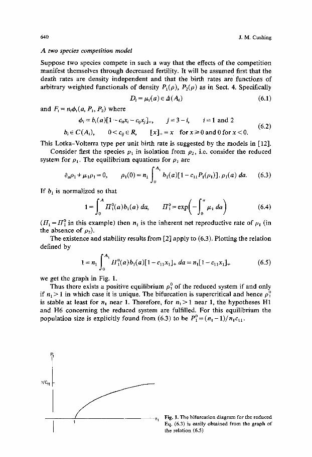
The existence and stability results from [2] apply to (6.3). Plotting the relation defined by

f? 1 = nl H~(a)b l (a)[1 - CnXl]§ da = nl[1 - CnXl]§ (6.5)

we get the graph in Fig. 1. Thus there exists a positive equilibrium pO of the reduced system if and only

if n] > 1 in which case it is unique. The bifurcation is supercritical and hence p ~ is stable at least for n~ near 1. Therefore, for ni > 1 near 1, the hypotheses H1 and H6 concerning the reduced system are fulfilled. For this equilibrium the population size is explicitly found from (6.3) to be p o= ( n l - 1)/nlc11.

1/Cll

1 nl Fig. 1. The bifurcation diagram for the reduced Eq. (6.3) is easily obtained from the graph of the relation (6.5)

The first case occurs if

Equilibria in systems of interacting structured populat ions 641

For the competit ion model (6.1)-(6.2) the functions @~ of Sect. 6 are

~ 1 = nl[1 -- C11X 1 -- C1222] +

I? ~2 = [1 - c21xl - c22x2]+ IIOb2 da,

where b2 is normalized so that (3.1) holds, i.e.

Io A2 II~ = 1/[1 - c21P~ da

Here nl is chosen sufficiently close to 1 so that pO< 1/c21, i.e.

1 Cll 1 - - - < - - . (6.6)

nl c21

The supercritical (stable) bifurcation condition (5.3) is equivalent to

A := C11C22- C12C21 > 0. (6.7)

Using the invariants (4.7) one can deduce that the continuum of population sizes (Pa, P2) obtained from the equilibrium pairs from the unbounded continuum C + in Theorem 1 either leaves the positive cone at a point (n2, (P1, P2))= (n ~ (0, pO)) where

pO = (n I - - 1)/n,c,2, n o = (1 - c2~P~ - c22P ~

or does not leave the positive cone for any n2>1 and (Pi, P2)->(P1, P~) as n2 ~ +co where

1 za

and the latter if

1 - 1 < c-021 2 (6.8) n 1 c22

1 c~2<~ 1___" C22 n 1

These cases are illustrated in Figs. 2 and 3.

(6.9)

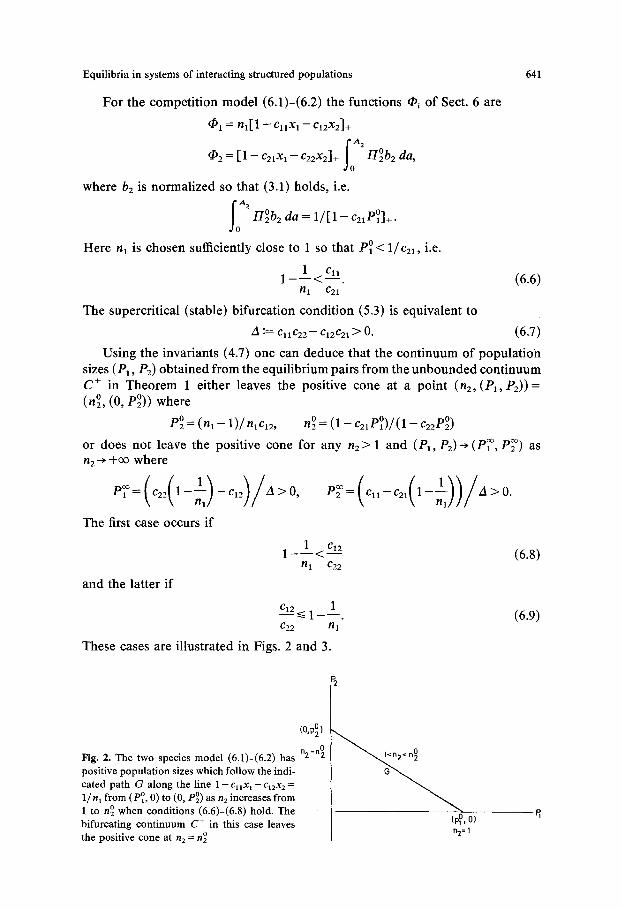
{O, pOl

Fig. 2. The two species model (6.1)-(6.2) has n2:nO

positive populat ion sizes which follow the indi- cated path G along the line 1-C~lX~-C12X2 =

1 / n l from (po, 0) to (0, pO) as n2 increases from 1 to n o when conditions (6.6)-(6.8) hold. The bifurcating cont inuum C + in this case leaves the positive cone at n2 = n o

(pO O) n2:1

642 J .M. Cushing

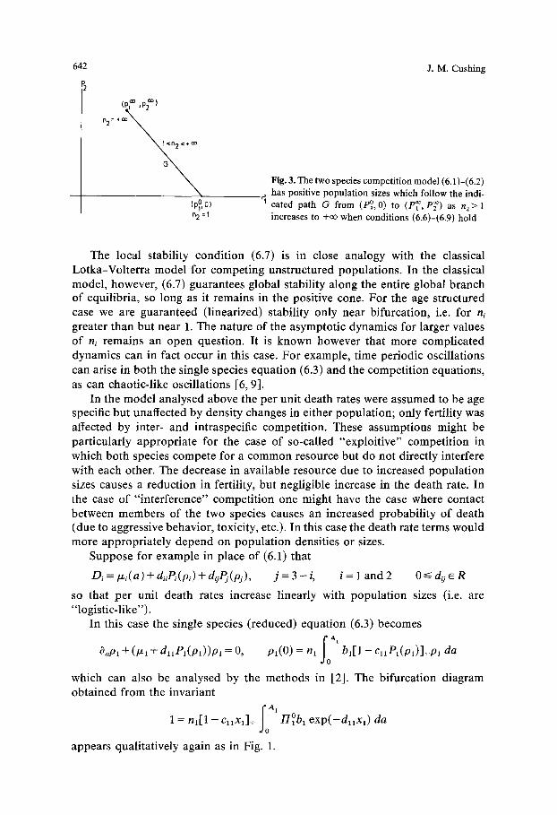
{p~ n 2 =I

Fig. 3. The two species competition model (6.1)-(6.2) has positive population sizes which follow the indi. cated path G from (P~ to (P~,P~) as n 2 > l increases to + ~ when conditions (6.6)-(6.9) hold

The local stability condition (6.7) is in close analogy with the classical Lotka-Volterra model for competing unstructured populations. In the classical model, however, (6.7) guarantees global stability along the entire global branch of equilibria, so long as it remains in the positive cone. For the age structured case we are guaranteed (linearized) stability only near bifurcation, i.e. for ni greater than but near 1. The nature of the asymptotic dynamics for larger values of ni remains an open question. It is known however that more complicated dynamics can in fact occur in this case. For example, time periodic oscillations can arise in both the single species equation (6.3) and the competition equations, as can chaotic-like oscillations [6, 9].

In the model analysed above the per unit death rates were assumed to be age specific but unaffected by density changes in either population; only fertility was affected by inter- and intraspecific competition. These assumptions might be particularly appropriate for the case of so-called "exploitive" competition in which both species compete for a common resource but do not directly interfere with each other. The decrease in available resource due to increased population sizes causes a reduction in fertility, but negligible increase in the death rate. In the case of "interference" competition one might have the case where contact between members of the two species causes an increased probability of death (due to aggressive behavior, toxicity, etc.). In this case the death rate terms would more appropriately depend on population densities or sizes.

Suppose for example in place of (6.1) that

D~=/x~(a)+d~iP~(p~)+d~Pj(&), j = 3 - i , i = l a n d 2 O<~ducR

so that per unit death rates increase linearly with population sizes (i.e. are "logistic-like").

In this case the single species (reduced) equation (6.3) becomes

io ,1 o ~ p l + ( m + a l l P l ( p l ) ) p l = o , ol(o) = nl b l [ l -C.Pl (OO]+p, da

which can also be analysed by the methods in [2]. The bifurcation diagram obtained from the invariant

1 n l [ 1 -- C l l X l ] + o = Hlbl e x p ( - d n x l ) da

appears qualitatively again as in Fig. 1.


The bifurcation analysis of the two species interaction can be carried out along the lines of the simpler case above. It is now based on the graph of the relations (4.7) where now

Io" 41 = n1[1-CllXl-C12X2]+ HOb1 exp(-(dHxl+da2x2)a) da

Io" 42 = [1 - c21xl - c22x2]+ II~ exp(-(d21xl + d22x2)a) da.

The added integral factors in these functions complicate the details of the analysis, but nonetheless the condition (5.1) guarantees supercritical bifurcation and stable coexistence. The partial derivatives are now more involved, e.g.

fo" o II~ exp(-dnP~ da 014 1 = --nlCll

Io" - n~dl,(1 - C, lPO) FIOb~ exp(-dHPOa)a da.

Clearly all 0i4 ~ < 0 so that this is a competitive interaction by the definition in Sect. 5. Also the inequalities (5.2) clearly hold, but to relate the condition (5.3) directly to the coefficients % dij in a simple way (such as (6.7) in the simpler case above) is not straightforward. This argues in favor of using the (normalized) density dependent net reproductive rates 4~ to interpret this stability condition.

One can easily see, however, that

014100242__ 0 1 4 2 0 00240 = (ell _~_ d11)(c22 q_ d22) - ( c ,2 + d12)(c21 + d21)

for pO = 0, i.e. for n~ - 1, so that once again an analog to the classical coexistence condition (6.7), obtained by requiring that the RHS be positive, is obtained.

A prey-predator model

As a second example we consider the interaction between a prey species ~ = Pl and a predator species p = p2 in which the predation rate is (possibly) different for different prey age classes and for different predator age classes. In the absence of predation the prey's dynamics are assumed governed by (6.3) with P1 = S A1 pl da taken as total population size and the per unit birth r a t e b 1 ~ constant> 0. (By the normalization (6.4), ba = 1/~ A~ 1I ~ da.) Predation is modelled by adding a term to the prey's per unit death rate which is (age specifically) proportional to the total population size of the predator, i.e.

D1 = Ixl(a) + WoW(a)P2

Io % >O, w(a) )O, fo%W(a) da=l . P2-~ P2 da, Wo

The distribution and magnitude of the age specific predation rate are determined by w(a) and Wo, respectively. The benefit of predation for the predator species is manifested through an increased per unit, age specific birth rate F2 = n2q~2 where

I? 42 = b2(a) W(pl), b2(a) >i 0, W(pa) = w(a)p~(a) da.

644

Consequently the model equations are

OPl + (~1 + WPz)Pl = 0

pl(0) = n,bl[1 - enP1]+P1

0192 "-I-/~2P2 = 0

p2(O) = n2 [ % b2(a) W(p l )P2(a) da .Io with the normalizations (6.4) and

fa % bz(a) W(p~176 = 1, da =0

Here Cll = constant > 0.

.o oxp( fo

J. M. Cushing

(6.10)

The reduced equation (6.3) has a unique positive equilibrium

o / fo~H~ da (6.11) p l -= ( n l - 1)rl~ nlc,1

for each nl > 1 which is stable at least for nl = 1. We assume in any case that

1 < n 1 < 2 . (6.12)

Theorems 1 and 2 can be straightforwardly applied to obtain a continuum of positive equilibria for the predator-prey equations (6.10) which bifurcates from (po, 0) at n2 = 1. Of interest is the direction of bifurcation which, by Theorem 3, determines the (local) stability of these equilibria. The constant Yl whose positivity implies a supercritical stable bifurcation and an exchange of stability from the trivial equilibrium (po, 0) to the positive equilibria on the continuum as n2 is increased through 1 turns out for this example to be

Yl = - W(Y~ W(P~ �9 (6.13)

Recall that the pair (yO, yO) is an "eigensolution", i.e. it solves the equations linearized at (pO, 0) with n2= 1. A straightforward solution of these linear equations yields o o Y2 = H2 and

Io 2 H ~ da 1 12 {7l

o n1-1 [ 2-n~lfa ~ H~ wdceda+fo wda]. Yl = f n ~ bl n1--1 nlc, A, 1i ~ da

#o

Clearly (6.12) and the assumptions on w imply that

y~ <0 , O<--a<A. (6.14)

This leads to the not unexpected conclusion that (at least) near bifurcation the prey equilibrium density is decreased by predation for every age class. This is true even if only selected age classes are preyed upon as determined by the distribution w( a ).

Moreover, (6.14) implies that Yl as given by (6.13) is positive and that supercritical bifurcation occurs. Thus we find in this model that the predator can survive, at low density, in stable coexistence with the prey if its inherent net reproductive rate at the prey equilibrium state pl ~ exceeds one.


As a simple illustration of how the bifurcation techniques developed here can be further used to analyse multi-species interactions consider the question of how the stability of the positive branch equilibria near bifurcation is affected by changes in certain system parameters. Specifically, we study how the stability of a branch equilibrium for a fixed n2 > 1, as measured by the "stability determining" eigenvalue (i.e. by the linearized eigenvalue of smallest magnitude), depends on the age class most preferred by predators.

Note that 'Yl ~ 0 implies that locally the parameter e which parameterizes the bifurcating continuum of equilibrium pairs in Theorem 1 can be eliminated and the positive equilibria written in terms of the inherent net reproductive rate n 2. Similarly the linearized eigenvalue z = z(e), z(0) = 0, can be written as a function of n2: z = z(n2), z(1) = 0. Then by Theorem 1 and (3.6)

dz/ dn2ln2=l_ dz/ de dn2/de ~=o=-l/ f ; 2bz(a)11~ W(p~ (6.15)

Any change in the system parameters which produces an increased magnitude of this expression will result in a new model which is "more stable" in the sense that for a fixed value of n2 sufficiently close to 1 this new system will have a (negative) stability determining eigenvalue of increased magnitude.

The expression in the denominator of (6.15) is called the "inherent mean age of reproduction" of the predator [19] ("inherent" means at low predator density /92-- 0 when pl = pO and n2 = 1). It depends on virtually every parameter in the model (see (6.11)). According to (6.15) a change in system parameters which decreases this mean age will result in a more stable system in the sense above.

For example, suppose that all parameters are held fixed (including n2---1) and only the distribution w(a) defining the functional W is changed in order to compare two predator-prey interactions with different predator age-specific prey consumption preferences. Since pO is a monotonically decreasing function of a, the distribution w which places more weight on the younger ages of prey will result in a larger value of W(p ~ and hence decreased stability. This is in agreement with the conclusion reached in [ 10] that predation on young prey is a destabilizing agent. It is the opposite of the conclusion reached by some earlier researchers [14, 17] using other models. The reconciliation of these antithetical conclusions seems to lie in the fact that such conclusions are very model dependent and, as A. Hasting puts it "age dependent predation is not a simple process" [11], a wide diversity of dynamical behavior being possible as various age-specific assumptions on fertility and death rates are made.

An epidemic model Deterministic models of epidemics typically involve a threshold property according to which a disease will spread through a population if a critical parameter (measuring the "virulence" of the disease) exceeds a critical value. This is very suggestive of the occurrence of a bifurcation phenomenon and in fact bifurcation theory methods can often be used to analyze such models. We give one brief illustration involving an epidemic in a population structured according to "class

646 J .M. Cushing

age", i.e. the time spent in certain defined epidemological subclasses of the population.

A so-called SIR model entails a categorization of the (living) individuals in a population according to three classes: susceptible, infectives and recovered. Let p~, P2 and P3 represent the densities of these classes as functions of time and class age a. Assume that the exposure rate due to contacts with infectives is expressed by

f? --pl(t, a) r(a, a)p2(t, a) da

where r(a, a) measures the effect of class age a infectives on class a susceptibles. The equations

Oapl+(tza+IA2r(a,a)p2(a)da)pl=O

[ ~'f,(P,, P2)P, da p~(0) = nl ~ O

(6.16) O ap 2 "q- /z2p 2 = 0

I0'I? p2(O) = r(a, a)pl(a) da p2(a) da

are the equilibrium equations for susceptibles p~ and infectives P2 under the assumption that only susceptibles reproduce (with a per unit birth rate n l f l ( P l , Pc)) and that all newborns fall into the susceptibles class. The equations for the density P3 of the removed class are decoupled from those above and are solvable for P3 as soon as p~ and P2 are found. For further details concerning models of this kind see [12, 13, 18].

Suppose that the reduced system

OaPl"b l.ZlPl = 0

p(O) = Jf f (Pl ,0)P, da

has a positive, stable solution Pl = pO. I f f is normalized so that

fo 4'f(O, 0)1I 0 = 1 da

then the bifurcation results in [2] apply to the question of the existence of such a pO. This assumption means that the population in the absence of the disease has a positive stable equilibrium state. In order to apply the results of Sects. 3-5 to (6.16) the kernel r is written r(a, or) = n2r*(a, a) where r* has the normalization (3.1), namely

f f2 f f~ r*(a, a)p~ da11~ da= l.

Then n2 measures the virulence of the disease in that it is the expected number of replacements for each infective lost to the recovered class (at low infective class densities when pl is at the equilibrium pO).


The bifurcation and exchange of stability results of Sect. 3 imply that if supercritical bifurcation occurs then for n2 < 1 the disease dies out asymptotically and pl reverts to pl ~ while for n2> 1 then the disease will persist in that the density of infectives will possess a positive equilibrium state.

For example, if f l is as in (6.3) with PI=~ al Pl da and r = WoW(a) then the epidemic model (6.16) is equivalent to the prey-predator model (6.10) and as seen above supercritical bifurcation does occur.

7. Concluding remarks

In this paper we have studied the existence and stability of positive equilibrium densities for systems of k/> 2 interacting structured populations. This was done by applying bifurcation theory methods using a normalized birth modulus n of the kth species as a bifurcation parameter. This approach results in the existence of a global continuum of nontrivial equilibria for the community of k species which bifurcates from any given equilibrium state for the community of k - 1 species (with the kth species absent) at a unique critical value of the parameter n (Theorem 1). This branch is locally positive (Theorem 2) and is locally stable with an exchange of stability occurring from the equilibrium for the subcommunity of k - 1 species to the equilibrium for the community of k species if the bifurcation is supercritical (Theorem 3).

The direction of bifurcation is determined by the quantity 71 given by (3.4) which depends on the nonlinear responses of the kth species' vital rates to changes in the densities of all species (including its own). More specifically 3/1 is the difference between two terms which are kinds of "averaged" effects of the nonlinear density dependencies in the kth species' death and birth rates taken over all species and all type classes. If this "averaged" effect corresponding to the death rate exceeds that corresponding to the birth rate then the bifurcation is supercritical. In this event the kth species at low density can successfully be added to or " invade" the stable subcommunity of k - 1 species provided its birth modulus (or inherent net reproductive rate) exceeds unity.

The existence result in Theorem 1 is global in the sense that the continuum of nontrivial equilibria is unbounded (or connects to the boundary of the domain on which the hypotheses hold). This continuum however need not remain in the positive cone of positive equilibria, as the competition example in Sect. 6 shows. A point at which the continuum intersects the boundary of the positive cone corresponds to another equilibrium of a subcommunity with at least one species absent and indicates a circumstance under which these species may be threatened with extinction.

The stability of the nontrivial equilibria locally near the bifurcation point in the event of supercritical bifurcation may not persist globally along the branch. This can be seen for example by familiar models for the total population size of nonstructured prey and predators whose positive equilibria can lose stability and give rise to a Hopf bifurcation to a time periodic limit cycle. Hopf-type bifurcation to time periodic densities was studied for age structured models in [5]. Even more complicated, chaotic-like oscillations can occur due to age structure in simple models which otherwise exhibit equilibrium dynamics [6, 9]. The study

648 J . M . Cushing

of such complicated and global dynamics for structured population interactions via nonlinear models of the McKendrick type studied in this paper offers sig- nificant mathematical challenges for further research.

0 A --1 �9 0 k--1 ( / / ^ v) .= (1//7~ v~),~,,

which can be written as

Appendix

In this Appendix the linear theory for systems of the form (2.8)-(2.9) is developed and a brief sketch of the proof of the Theorem 1 is given.

Consider the k - 1 linear nonhomogeneous equations for )3 ~./~ = /7(A)

y(O) = /~/1(33) q- hi ( h l )

and its associated homogeneous system

O. ( f i ^ f i )+ f i~ p + / ~ i ( f i ) = 6 ( i 2 )

)~(0) =/~l(fi)-

Here f i o f i , fheB, f l i E R k - m and / ~ , : / ~ / 7 , rfi:B-->R k-~ are bounded and linear. Equation (A1) is equivalent to the equation

S; .~= O~ ^ (~,(~)+#7, - (s + #7~) ̂ (s~~ ̂ ~)- ' do~)

l I~ t t , ( a ) / v , (a ) dot) = v(~,, ~2) + r ; (A3)

where

V(/~,, ]~2) := ~t~ ̂ (/~l - / ; /~2 ̂ (/~t~ dot ) , K)3 := V(rhl(33),/~1 (fi)).

It is clear that V: R k-~ • .+ ~ is linear and compact. Thus K :/7 ~ /~ is linear and compact. It follows that 1 - K is Fredholm and consequently if k e r ( I - K ) = {0} then ( I - K ) -1 exists and is bounded. In this case (A3) has a unique solution fi = ( I - K) -1V(/~I,/~2). Setting S := ( I - K ) -1V we conclude that if the homogeneous system (A2) has no nontrivial solution in /~ then (A1) has, for each (/~t, h~) ~ R k-1 • B ~, a unique solution )~ e /7 and the solution operator S : R k-1 X J~ + /~ defined by (/~,/~2) ~)3 is linear and compact. Note that K33 and V(/~,/~2), and hence the solution f of (A3), are continuous differentiable functions of a.

Consider now the linear equations (2.8)-(2.9). The linear theory in [2] applies to the scalar equations (2.9). Since the normalization (3.1) holds, the homogeneous counterpart of (2.9) has a nontrivial solution if and only if n = 1.

Suppose (A2) has no nontrivial solutions in/7. I f n ~s 1 then (2.9) has a unique solution y = S(hl, h2) given by a l inear compact solution operator S: R x B ~ B [2]. (2.8) then has a unique solution 33 ~ B with this y substituted. Thus if n # 1, then (2.8)-(2.9) has a unique solution (~, y) = Y((/~I,/~2), (h~, h2)) given by the compact linear solution operator Y: ( R k-~ x B) x ( R x B) -> B x B defined by

Y= ( S( rn2( S( hl, h2) )+ /~ , s S( h~ , h2))+ ]~2), S( hl, h2)).

On the other hand if n = 1 then (2.9) has a solution if and only if (hi , h2) ~ (R x B) • i.e. if and only if the "orthogonali ty condi t ion"

holds [2]. In this event (2.9) has a unique solution y ~ S~ h2)~ B ~ i.e. satisfying ~A HOyd = 0, given by a compact linear solution operator S o : (R • B) l ~ B ~ Substituting this solution y into (2.8)

Equilibria/in systems of interacting structured populations 649

one can then obtain a unique solution of (2.8) via the compact linear solution operator S. Thus, if n = 1 then (2.8)-(2.9) is solvable if and only if (hi , h2) ~ (R x B) ~ in which case there exists a unique solution ( ; , y ) = Y~ h2)) in B • ~ given by a compact linear solution operator y ~ 2 1 5 2 1 5 B x B ~

With this linear theory in hand a proof of Theorem 1 can be constructed in a manner very analogous to that for Theorem 1 in [2]. The key observation is that if the nonlinear equations (2.3)-(2.4) are centered on the "trivial" equilibrium (/3 ~ 0) by setting )3 = ~ _~o, y = P and by using (2.11), then a nonlinear system results whose linear terms uncouple (as in (2.8)-(2.9)).

Letting n = h + 1/2 and using the solution operator S we write the equation for y in the form y = hAy + H(A, )3, y) where A : B -~ B is linear and compact and H : R x B x B ~ B is completely continuous and of order o(I)3[ + l Y[) near ()3, y) = (~, 0) uniformly on bounded h intervals. With this expression substituted into the equations for )3 and with the use of Y the equations for )3 can similarly be rewritten in operator form )3 = )tA)3 + H(h, )3, y). As a result the centered equations are equivalently rewritten in operator form (~, y) = hL()3, y) + G(h, )3, y) where L = (A, A) is linear and compact as an operator from /~ • B to B x B and G = (H, H) : R x/~ x B ~ B x B is completely continuous and of order o(I)3 ] +IY]) near ()3, y) = (~, 0) uniformly on bounded h intervals. The proof now proceeds as in [2].

References

1. Butler, G. J., Hsu, S. B., Waltman, P.: A mathematical model of the chemostat with periodic washout rate. SIAM J. Appl. Math. 45, 435-449 (1985)

2. Cushing, J. M.: Equilibria in structured populations. J. Math. Biol. 23, 15-40 (1985) 3. Cushing, J. M.: Existence and stability of equilibria in age-structured population dynamics. J.

Math. Biol. 20, 259-276 (1984) 4. Cushing, J. M.: Global branches of equilibrium solutions of the McKendrick equations for

age-structured population growth. Comput. Math. Appl. 11, 175-188 (1985) 5. Cushing, J. M.: Bifurcation of time periodic solutions of the McKendrick equations with applica-

tions to populat ion dynamics. Comput. Math. Appl. 9, 3 459-478 (1983) 6. Cushing, J. M.: Volterra integroditterential equations in population dynamics. Mathematics of

Biology, pp. 81-148. Centro Internazionale Matematics Estivo, Napoli (1979) 7. Cushing, J. M.: Periodic Kolmogorov systems. SIAM J. Math. Anal. 13, 827-881 (1982) 8. Cushing, J. M.: Periodic two-predator, one-prey interactions and the time sharing of a resource

niche. SIAM J. Appl. Math. 44, 392-410 (1984) 9. Cushing J. M., Saleem, M.: A competition model with age structure. Mathematical Ecology. Lect.

Notes Biomath. 54, 178-192. Berlin, Heidelberg, New York: Springer 1984 10. Gurtin, M. E., Levine, D. S.: On predator-prey interactions with predation dependent on age of

prey. Math. Biosci. 47, 207-219 (1979) 11. Hastings, A.: Age dependent predation is not a simple process. I. Continuous time models. Theor.

Popul. Biol. 23, 347-362 (1983) 12. Hoppensteadt, F.: Mathematical theories of populations: demographics, genetics and epidemics.

Regional Conf. Series in Appl. Math., SIAM, Philadelphia 1975 13. Hoppensteadt, F.: An age dependent epidemic model. J. Franklin Inst. 297, 325-333 (1974) 14. May, R. M.: Stability and complexity in model ecosystems. Monographs in Population Biology

6, Princeton U. Press, Princeton, NJ 1974 15. Priiss, J.: On the qualitative behaviour of populations with age-specific interactions. Comput.

Math. Appl. 9, 327-339 (1983) 16. Priiss, J.: Stability analysis for equilibria in age-specific population dynamics. Nonlinear Anal.

Theory Methods Appl. 7, 1292-1313 (1983) 17. Smkh, R. H., Mead, R.: Age structure and stability in models of predator-prey systems. Theor.

Popul. Biol. 6, 308-322 (1974) 18. Waltman, P.: Deterministic threshold models in the theory of epidemics. Lect. Notes Biomath.

1. Berlin, Heidelberg, New York: Springer 1974 19. Webb, G. F.: Theory of nonlinear age-dependent population dynamics. New York: Dekker 1985

Received March l l /Rev i sed September 8, 1986

journal ol r biology - university of arizonamath.arizona.edu/~cushing... · j. math. biol. (1987)...

Documents