journal of natural gas science and engineering · previous studies indicate that the cost of...

lable at ScienceDirect

Journal of Natural Gas Science and Engineering 27 (2015) 219e235

Contents lists avai

Journal of Natural Gas Science and Engineering

journal homepage: www.elsevier .com/locate/ jngse

3-D well path design using a multi objective genetic algorithm

Vahid Mansouri a, *, Rassoul Khosravanian a, David A. Wood b, Bernt S. Aadnoy c

a Department of Petroleum Engineering, Amirkabir University of Technology, Tehran, Iranb DWA Energy Limited, Lincoln, United Kingdomc Department of Petroleum Engineering, Stavanger University, P.O. Box 2557, 4091, Stavanger, Norway

a r t i c l e i n f o

Article history:Received 4 July 2015Received in revised form23 August 2015Accepted 24 August 2015Available online 31 August 2015

Keywords:Multi-objective optimizationGenetic algorithmDrilling torqueWellbore trajectory planningOil and gas well design

* Corresponding author. Faculty Member of Drillinof Petroleum Engineering, Amirkabir University of TeBox: 15875-4413, Tehran, Iran. Tel.: þ98 (21) 6454513

E-mail addresses: vahid.mansouri1990@[email protected] (R. Khosravanian), [email protected]@uis.no (B.S. Aadnoy).

http://dx.doi.org/10.1016/j.jngse.2015.08.0511875-5100/© 2015 Elsevier B.V. All rights reserved.

a b s t r a c t

Optimizing wellbore trajectories to reach an offset subsurface location, involving a complex combinationof vertical, deviated and horizontal well components, requires the minimization of both wellbore lengthand frictional torque on the drill string. This is particularly the case for shallow horizontal wells whichare often limited in their extent by torque. By minimizing both wellbore length and torque it is likely thata wellbore designed to reach a specific target can be drilled more quickly and cheaply than other po-tential trajectories. However, these two objectives are often in conflict with each other and related in ahighly non-linear manner. A multi-objective genetic algorithm (MOGA) methodology is developed andapplied with two objective functions, viz. wellbore length and torque, to develop a set of Pareto optimalsolutions that can aid the selection of less risky/less costly well trajectory designs. The MOGA perfor-mance is compared with single-objective function studies of a specific wellbore scenario. The resultsindicate that the MOGA methodology outperforms single-objective function approaches leading to rapidconvergence towards a set of Pareto optimal solutions. Analysis reveals that by adopting an adaptiveapproach that allows the behavioral parameters of the genetic algorithm (GA) to evolve as iterationsprogress, the MOGA proposed converges more rapidly toward better ultimate solutions than if the GAbehavioral parameters are held constant over all iterations of the algorithm. Algorithm code listings forthe MOGA and GA applied in the analysis presented are included as appendices.

© 2015 Elsevier B.V. All rights reserved.

1. Introduction

One of the most expensive operations involved in the explora-tion and development of oil and gas reservoirs is typically thedrilling of the wellbores. In the prevailing market conditions ofrelatively high costs and low oil and gas prices across much of theworldmost oil and gas companies are particularly keen tominimizetheir drilling costs Khaled et al., 1999.

Previous studies indicate that the cost of drilling a horizontalwell is about 1.4 times the cost of drilling a vertical well (S. D. Joshi,2003). The attraction of drilling horizontal and directional wells isthat they can contact a greater volume of the reservoir and cantransect the highest quality zones more effectively than verticalwells, resulting in higher production and recovery rates. In bothcases one of the most important factors affecting the cost of drilling

g Engineering of Departmentchnology, 424 Hafez Ave, P.O.0.ail.com (V. Mansouri),solutions.com (D.A. Wood),

is length of the wellbore and the time taken to drill to the reservoirtarget. Thus any possibility to reduce the length of the wellbore,within the constraints of acceptable curvatures and geological ob-stacles, typically reduces the time it takes to reach the target andthereby reduces the total drilling costs. Optimizing wellborelengths, subject to a defined set of constraints, typically is desirableas a means of improving the economics of drilling operations.

In the recent years, optimization has been used extensivelyacross the petroleum industry for a variety of purposes, processplant optimization, transport scheduling and to various aspects ofthe drilling operation (e.g. Shokir et al., 2004; Atashnezhad et al.,2014; Guria et al., 2014). With respect to wellbore trajectory plan-ning Shokir et al. (2004) used a genetic algorithm and Atashnezhadet al. (2014) used a particle swarm optimization algorithmwith thesingle objective function of minimizing wellbore length, subject toa number of defined constraints. A recent application of multi-objective genetic algorithm (MOGA) to drilling is provided byGuria et al. (2014) in their application of a multi-objective optimi-zation genetic algorithm to two- and three-objective functionsrelated to determining optimum drilling variables related to an oil

Delta:1_d

Delta:1_given name

Delta:1_surname

Delta:1_given name

mailto:[email protected]




http://crossmark.crossref.org/dialog/?doi=10.1016/j.jngse.2015.08.051&domain=pdf

www.sciencedirect.com/science/journal/18755100

http://www.elsevier.com/locate/jngse

http://dx.doi.org/10.1016/j.jngse.2015.08.051



Fig. 1. Calculation of the length for a deviated section of the well trajectory after Atash-nezhadetal. (2014)describes the termsusedtodefinethedifferentanglesandcomponentsof the wellbore trajectory. MD¼ measured depth; TVD¼ true vertical depth.

V. Mansouri et al. / Journal of Natural Gas Science and Engineering 27 (2015) 219e235220

field offshore Louisiana. That work applied an elitist non-dominated sorting genetic algorithm to (i) maximize drillingdepth, (ii) minimize drilling time and (iii) minimize drilling costwith fractional drill bit tooth wear as a constraint. Another appli-cation of MOGA, relevant to petroleum field operations, is proposedby Yasari et al. (2013) to apply a non-dominated sorting geneticalgorithm to find optimized and robust water injection policies forthree injection wells.

In this paper a new MOGA optimization model for well trajec-tory planning is developed for optimizing drilling operations. Themodel optimizes the recommended well path by taking into ac-count two-objective functions: 1) to minimize wellbore length andtrajectory to a specified sub-surface target location (i.e. length); and2) to minimize torque on the drill string during the drilling oper-ation (i.e., torque).

We recognise that when designing wells at specific locationsthere are other factors that need to be taken into account in additionto wellbore length and torque (e.g., wellbore tortuosity and its in-fluence on the ease or difficulty in running a specific well completiondesign; combined drilling and completion costs associated withdrilling a particular well path; dealing with problem formationsabove a reservoir in a certain way, i.e., setting casing above it orbelow it certain specified points; entering the reservoir at a certainangle and penetrating it at a certain inclination). Some of theseadditional factors can be dealt with as constraints that selected op-timum well paths need to achieve. It would also be possible toconsider these as optimization objectives in their own right in theMOGA algorithm. In this study we focus on just the two key objec-tives, i.e., wellbore length and torque, to prove the benefits of theMOGA concept. Wewill be conducting future research to expand theMOGA methodology to consider some of these additional factors,both as constraints and additional objectives.

MOGA involves a process of developing a random set of po-tential solutions making up a population of solutions to be testedfor fitness. Each individual solution generated is typically referredto as an individual or gene. The population is subjected to a series ofevolutionary iterations (i.e., developing new solutions/genes bygenetic processes such as mutation and crossover with differentcharacteristics in each generations), with the solutions being testedfor fitness and ranked in each generation, and the most fit forpurpose being carried forward to the next generation. This processmeans that each generation progresses, or converges, towards thebest set of solutions. Finally, the best solutions are identified andtheir performances compared in relation to the multiple objectivefunctions. In this study the MOGA is coded using MATLAB software,with the detailed code provided in Appendix A. The model isapplied to the horizontal well drilling trajectory scenario (based ona real well drilled in Egypt) studied for trajectory optimizationpurposes by Shokir et al. (2004), using a single-objective functiongenetic algorithm, and Atashnezhad et al. (2014) using particleswarm optimization. We describe how our MOGA model works indetail and provide an analysis of the results for the specific, com-plex, wellbore trajectory selected.

The case study is based on a real well drilled in Egypt, andpreviously used to demonstrate wellbore trajectory optimizationusing a genetic algorithm by Shokir et al. (2004) applied to thedeviated well trajectory calculation algorithm originally proposedby Adams and Charrier (1985), using the length of the wellborebetween specified surface and bottom-hole locations as theobjective function.

2. Mathematical formulation

With the dual objectives of finding optimal solutions that pro-vide the minimum well length, honoring the wellbore constraints

imposed, so that the torque on the drill string is alsominimized, it isnecessary to provide mathematical formulations for those twoclear objective functions, i.e.: 1) the wellbore length; 2) the torqueon drill string while rotating. These two objective functions aredescribed in mathematical formulations in the following sections.

2.1. Well path length

Fig. 1 illustrates all the components involved in the calculationof the length of each curved section of a directional wellbore. Thereare several methods available to measure the wellbore length of adirectional well. Our formulation uses the radius of curvaturemethod. In the radius of curvature method, constant curvaturebetween two points and the radius of the curvature is given byequations (1)e(3):

a ¼ 1Dm

ffiffiffiffiffiffiffiffiffiffiffiffiffiffiffiffiffiffiffiffiffiffiffiffiffiffiffiffiffiffiffiffiffiffiffiffiffiffiffiffiffiffiffiffiffiffiffiffiffiffiffiffiffiffiffiffiffiffiffiffiffiffiffiffiffiffiffiffiffiffiffiffiffiffiffiffiffiffiffiffiffiðq2 � q1Þ2 sin4

�42 þ 41

2

�þ ð42 þ 41Þ

s(1)

r ¼ 1a¼ 180*100

p*T(2)

Dm ¼ r

ffiffiffiffiffiffiffiffiffiffiffiffiffiffiffiffiffiffiffiffiffiffiffiffiffiffiffiffiffiffiffiffiffiffiffiffiffiffiffiffiffiffiffiffiffiffiffiffiffiffiffiffiffiffiffiffiffiffiffiffiffiffiffiffiffiffiffiffiffiffiffiffiffiffiffiffiffiffiffiffiffiðq2 � q1Þ2 sin4

�42 þ 41

2

�þ ð42 þ 41Þ

s(3)

Based upon the wellbore trajectory illustrated in Fig. 2, withmultiple curved and linear components, the total measured depthof the wellbore can be obtained from equation (4):

TMD ¼ DKOP þ D1 þ D2 þ D3 þ D4 þ D5 þ HD (4)

Detailed formulas to calculate the non-vertical and horizontalcomponents of the wellbore trajectory (D1, D2, … D5) are providedin Appendix A.

2.2. Torque

Torque and drag analysis in relation to wellbore tubulars hasbeen studied in detail and is now well understood (e.g., Sheppard

Fig. 2. The vertical plane of a horizontal well with the operational parameters from Atashnezhad et al. (2014) developed from the wellbore scenario studied originally by Shokiret al. (2004). Note that the scenario involves more than one build section and a drop-off section separating the build sections. The wellbore trajectory formulation incorporates allthe sections identified in this diagram.

Fig. 3. Force balance for pipe pulling along a straight surface (From Aadnøy andAndersen, 2001).

V. Mansouri et al. / Journal of Natural Gas Science and Engineering 27 (2015) 219e235 221

et al., 1987; Xie et al., 2012; Aadnøy et al., 2010). The objective is toprevent drilling and completion problems before they occur (Xieet al., 2012), and this is particularly necessary in wellbores withcurved and non-vertical sections as drag and torque loss are asso-ciated with directional wells. Drag is experienced when the drillstring is moved up or down the wellbore, for example when trip-ping in and out of the hole. The sources of drag and torque lossesinclude: differential sticking, key seating, poor hole cleaning, andsliding wellbore friction.

Optimal well path design, from the perspective of torque anddrag, should minimize all these effects (Johancsik et al., 1984;McCormick and Chiu, 2011), such that:

✓ Normal forces acting on the drill string are reduced✓ Dynamic conditions are enhanced (static conditions minimized)

To calculate the torque on a drill string the soft string model isused as the formulation for the torque objective function. This as-sumes that the drill string takes the form of a heavy cable lying inthe wellbore, and any tubular stiffness effects due to the drill pipesis ignored. Calculations consider only the state in which the drillstring is rotating, without any axial movement up or down. For-mulas are provided for two general cases: equation (5) for a straightsection; and, equation (6) for a curved section.

F2 ¼ F1 þ BwDL cos 4 (5)

T ¼ mrwDL sin 4 (6)

In a straight section the tension along the drill pipe has no effecton the normal pipe force, and hence, no effect on friction. Straightsections are weight dominated, as only the normal weight compo-nent generates friction. Fig. 3 shows the force balance for a straightpipe. Equation (5) calculates the change in axial load, and equation(6) calculates the torque, on a straight section of drill pipe. Fig. 4.

For the curved sections, the normal contact force between stringand hole depends strongly on the axial loading within the pipe.So, for the calculation of the torque, the tension in the pipe isrequired. Other parameters that contribute to this calculation arethose angles determining the total change in direction. These an-gles and forces are illustrated and defined in Figs. 5 and 6. They arederived via the relationships expressed by equations (7) and (8):

e1$e2 ¼ je1jje2jcos b ¼ cos b (7)

cos b ¼ sin 41 sin 42 cosðq1 � q2Þ þ cos q1 cos q2 (8)

The angle b is the total directional change. If both inclination andazimuth are changed, the plane that b acts in is not constrained tothe horizontal or vertical plane (Fazaelizadeh, 2013). Havingdetermined the axial loading in the drill pipe in equation (9) we areable to calculate the torque, which is expressed by equation (10):

F2 ¼ F1 þ BwDL�sin 42 � sin 41

42 � 41

�(9)

T ¼ mrF1b (10)

Given that the wellbore trajectory in the scenario analyzedconsists of seven parts, the torque must be calculated for each partseparately, and summed to provide the total torque. The value of T

Fig. 4. Axial loading on a straight section (From Aadnøy and Andersen, 2001).

Fig. 5. Total Direction change and unit vectors e1 and e2 at two survey points P1 and P2(from Fazaelizadeh, 2013).

Fig. 6. Axial loading on a curved section during total change b in direction (fromFazaelizadeh, 2013).

Table 1Operational restrictions.

TVD Min. ¼ 10850 ft. Max. ¼ 10900 ft.

HD 2500 ftDogleg severity T1, T2,T3,T4,T5 � 5�/100 ft.Min. value of inclination angles 41 ¼ 10� 42 ¼ 40� 43 ¼ 90Max. value of inclination angles 41 ¼ 20� 42 ¼ 70� 43 ¼ 95Min. value of azimuth angles q1 ¼ 270� , q2 ¼ 270� , q3 ¼ 270�

q4 ¼ 330� , q5 ¼ 330� , q6 ¼ 355�

Max. value of azimuth angles q1 ¼ 280� , q2 ¼ 280� , q3 ¼ 280�

q4 ¼ 340� , q5 ¼ 340� , q6 ¼ 360�

Kick-off point depth Min. ¼ 600 ft. Max. ¼ 1000 ft.Draw down point depth Min. ¼ 6000 ft. Max. ¼ 7000 ft.Third build point depth Min. ¼ 10000 ft. Max. ¼ 10200 ft.1st Casing setting depth Min. ¼ 1800 ft. Max. ¼ 2200 ft.2nd Casing setting depth Min. ¼ 7200 ft. Max. ¼ 8700 ft.3rd Casing setting depth Min. ¼ 10300 ft. Max. ¼ 11000 ft.


from the above relation is the second objective function expressedby equation (11):

T ¼ Tvertical þ T1 þ T2 þ T3 þ T4 þ T5 þ Thorizontal (11)

The calculation of the torque commences from the bottom of thedrill string (i.e., when the drill string is at the wellbore's total depth(TD) then the T calculation starts at Thorizontal), and continues,stepwise, upward to the well head (i.e., last component added tothe calculation is Tvertical). For the wellbore scenario evaluated thetorque calculation involves the following assumptions:

1. The drill string has no axial movements (just rotation).2. The drill string has 0.1 ft radius and 0.3 kN/ft weight.3. The friction factor is 0.2 and the buoyancy factor is 0.7.

The detailed calculation of torque for the wellbore trajectoryscenario studied is provided at Appendix A.

For the optimization calculation two types of constraints areapplied to the wellbore trajectory and torque calculations: 1)

Operational constraints, e.g., the rate of hole-angle build and rate ofhole-angle drop off, and angle-hold wellbore section 2) Non-negative (logical) constraints, e.g. the measured depth and truevertical depth cannot be negative and be accepted as valid solutionsto the wellbore optimization problem. Table 1 describes the opti-mization operational constraints imposed on the wellbore scenarioevaluated. 1. The case study surveyed in this study has beenextracted from “E. M. Shokir et al., 2004”, so all information andlimitations about it are from that paper. However the providedalgorithm in this article is capable to include any other limitationsuch as special range for DLS in a particular formation or anyconstraint about the reservoir or other formations.

3. Multi-objective optimization

Multi-objective optimization is now used widely to aid decisionmaking and selection of alternatives in many industries. Fastercomputation speeds, greater computer memory space and moreunderstanding and accessibility to the algorithms is leading toexpansion of their applications to solve common operational,financial and planning problems. In many real projects, there aremultiple objectives that are inconsistent with each other, i.e., theyact independently of each other, or in conflict with each other to anextent, in delivering high performing outcomes for the project.

Fig. 7. Pareto optimal solutions concept for two objective functions, F1 and F2, to beminimized. The triangles represent non-dominated solutions, i.e. there are no solu-tions better than these; minimum F2 for a given value of F1 and vice versa. The circlesrepresent dominated solutions, i.e. there is at least one solution that performs betterthan these in terms of minimizing values of F1 in relation to F2. (Modified after Hauptand Haupt, 2004).


Each objective function also typically has a number of constraintsapplied to it (e.g. Table 1), and this increases the complexity of theproblem. Multi-objective optimization (MOO) requires simulta-neous optimization of conflicting objective functions that maycompete with each other in preventing the identification of a singleglobal optimum solution (e.g., Yasari et al., 2010). In such problems,usually there is not a solution that results in all the objectivefunctions being brought to optimum states. Rather, it is necessaryfor algorithms to search for solutions whereby the multiple ob-jectives collectively occur in the most optimal state. In practicethere often are multiple solutions that equally satisfy the collective“most” optimal state for the multiple objective functions evaluated,i.e., better performance in some objective functions trading offagainst poorer performance in other objective functions for aparticular solution. Such multiple-optimum solutions arecommonly referred to as Pareto optimal solutions in MOO (e.g.,Haupt and Haupt, 2004).

Consider a multi-objective optimization problem with a mini-mization function, F(x), involving n individual objective functions(f1 … fn) that is defined as follows:

minFðxÞ ¼ ff1; f2; :::; fng

where, fi(x) ¼ ith objective function of n objective functions to beminimized

Each objective function is subjected to specific constraintfunctions, G(x) and H(x), with values specified:

GðxÞ<0;HðxÞ ¼ 0x2R

Each individual solution, x, is one of a population of solutionsthat achieves the overriding objective of the calculation (e.g. rea-ches the target location specified for the well bore).

The multi-objective goal is to minimize the individual objectivefunctions, f1, f2 …, fn simultaneously; recognising that a single so-lution satisfying all objective functions is unlikely to exist, an al-gorithm needs to be formulated to reveal the Pareto optimalsolutions. To achieve this, a multi-objective algorithm mustdistinguish between “dominated” and “non-dominated” solutions.

If all objective functions are striving to achieve minimum solu-tions, an acceptable solution j dominates solution i, if and only if, forany i, fi (x) � fj(x) and at least for one function fi (x) < fj(x). If a so-lution is not dominated by any other solutions it is called a Paretooptimal solution or a non-dominated solution. Such a set of Paretooptimal solutions is called a Pareto optimal set. For any twoobjective functions the Pareto set may be displayed graphically as aPareto frontier; for multiple objective functions the Pareto set maybe displayed graphically as a Pareto surface. In some problems theset of Pareto optimal solutions can be very large (possibly infinite,i.e. all acceptable solutions in the population are non-dominated). APareto frontier for a two-objective optimization (minimizing) isshown schematically in Fig. 7 that clearly describe the concept ofPareto front and Pareto optimal solutions. The initial goal of a MOOis to find the Pareto optimal set; the final objective is to use thatnon-dominated set to inform decisions as to which non-dominatedsolution(s) in that set should be selected for operational purposes.

4. Genetic algorithm

Genetic algorithms (GA) are stochastic search algorithms basedon the mechanisms of natural selection and applying processessimilar to those observed in biological genetics (e.g. Gen and Cheng,2008). GA typically commence with an initial set of random solu-tions, or selected (seeded) solutions, representing a “population” of

solutions that satisfy all constraints to the problem and achieving theoverriding target (e.g. the total depth of the well at the specifiedtarget location) Sivanandam and Deepa, 2008. Each solution in thepopulation is sometimes referred to as a “chromosome”, maintainingthe analogy with biological genetics. The population is processedthrough a loop that first ranks the solutions in terms of their per-formance with regards to the objective function(s) and then subjectssome of the best performing solutions to a series of genetic processes(e.g. mutation, crossover, etc.) to derive some new solutions for thenext generation to add to the best performing solutions of the cur-rent generation, the best performing solutions are ranked, and so theloop continues repeatedly generating new populations of solutions,but always preserving the best performing solutions of the previousgeneration. For this process to work effectively, each generation, i.e.,all chromosomes (solutions) in the population need to be tested forperformance by a defined fitness test scoring assignment system.

The solutions in a particular generation are ranked using theirindividual fitness scores. The solutions selected to be carried for-ward to the next generation have the highest fitness scores. Thegenetic algorithm loop continues through many iterations (gener-ations) periodically finding better performing solutions (i.e., not allgenerations outperform previous generations, but based on fitnessscore selection, the highest ranking solution cannot performworsethan the previous generation). In some problems the algorithmmay lead to convergence to an optimal solution, in other morecomplex problems, the GA may not find all solutions (i.e. there maybe several isolated minima in the solution space). In the secondsituation a set of the highest-performing solutions are collectedafter a set number of iterations (GA generations), or after a specifiedperiod of computer processing time when no improved solutionsare found.

The MATLAB code listing for the single-objective GA used in thisstudy to solve deviated wellbore trajectories using the radius ofcurvature method is included as Appendix C.

GA is applicable to many multi-objectives optimization prob-lems, because it is able to cope with conflicts and/or non-linearrelationships among the multiple objectives, and provides arobust set of high-performing (not necessarily the best) solutionswhere multiple solutions exist (e.g., Yasari et al., 2013). The multi-objective genetic algorithm (MOGA) follows the samemethodologyas a single objective function GA, but defines its fitness scoreassignment system to involve all the objective functions involved.MOGA algorithms typically apply a zonal ranking scheme by firstly


identify the non-dominated solutions in each generation among allsolutions in that generation. Such non-dominated solutions areassigned to rank one and are allocated the highest fitness score. Allsolutions in the same generation, excluding those assigned to rankone, are searched again to establish the non-dominating solutionsamong that set of solutions, and those identified non-dominatingsolutions in that sub-population of solutions are assigned to ranktwo and are allocated a lower fitness score than those in rank two.This process is repeated to establish multiple ranks, with the non-dominated solutions included in each successive rank allocated alower fitness score than the previous, higher rank of solutionsidentified. Eventually all solutions in a particular generationwill beassigned a rank and appropriate fitness score. Selection of theparents fromwhich the next generation of solutions are generatedin MOGA is based on this fitness score. All other steps in the MOGAare the same in the GA.

A pseudo coding of the MOGA used in this study is as follows:

Procedure: MOGA

Input: problem data, GA parameters

Output: Pareto optimal solutions

POP=Initialize(t=0);

While (not terminating condition) do

F=Objectives( POP ) ; Calculate Objective Functions

RANK=Evaluate( POP, F); Evaluation and Ranking by ftness score assignment routine

PARETO=Pareto(POP, F); Create Pareto Optimal Solutions and Pareto Frontier

PARENTS=Select (POP, RANK); Select Parents for next generation

POP=Xover(POP,PARENTS); Apply Crossover to select new high-performing solutions for next generation to replace low-ranking solutions

POP=Mut(POP,PARENTS); Apply Mutation to generate other new solutions from the parents and replace the modified solutions with them

End

F=Objectives( POP ) ; Calculate Objective function values for solutions after V iterations or convergence

RANK=Evaluate( POP, F); Rank solutions according to fitness score

PARETO=Pareto(POP, F); Select rank-one solutions

Show PARETO List rank-one solutions, Display graphically rank-one solutions for selected objective functions (i.e. 2D or 3D plots)

End

The MATLAB code listing for the MOGA used in this study tosolve deviated wellbore trajectories using the radius of curvaturemethod is included as Appendix B.

5. Solution and results

Considering the two objective functions for the wellbore sce-nario described above, and applying all specified constraints, theMATLAB codes for the two-objective optimization using MOGA arelisted in Appendix B. These codes follow the sequence illustrated inthe flowchart depicted in Fig. 8.

For the solution, first we need the objective function that isconsidered as follows:

OBJECTIVE FUNCTIONS ¼ fLength; TorquegConstrained to

C1;min <C1 <C1;max

C2;min <C2 <C2;max

C3;min <C3 <C3;max

TVDmin < TVD< TVDmax

where symbol C refers to Casing setting depth.The optimization process for the scenario described seeks to

minimize the multi-objective function defined above. The MOGAcode commences with initializing. A random population consistingof 100 solutions is generated that all are in feasible region (i.e.satisfy the constraints and reach the specified well target). Byentering a loop, the objective functions for each solution arecalculated and based on the value of these functions, a fitness scoreis allocated to each of them. The Pareto optimal solutions in eachgeneration are assigned to rank one. At least some of the parentsolutions for the next generation are selected. The selected parentsolutions are then adjusted by a cross-over operator and new

solutions are generated. The cross-over operator is designed to seeknew solutions that might have higher fitness scores than some ofthe parents. The new improved solutions then replace low rankingsolutions with low fitness scores (Low ranking solutions arereplaced, so the best solutions are retained). The population then issubjected to a mutation operator generating an additional numberof new solutions for the next generation. All parents undergo themutation operator. And the new solutions based on their fitnesscompared to the parent fitness may be accepted or rejected. Themutation step is the last step of any iteration. In the analysis con-ducted for this study the process sequence or loop is repeated for2000 iterations. Each step in an iteration described above isexecuted as a MATLAB function. The algorithm also includes afunction to test the feasibility of each solution (i.e. does it reach thetarget location and satisfy the constraints). This function is requiredto prevent the inclusion of infeasible solutions in any generation ofsolutions to be ranked. This function ensures all solutions in eachgeneration are in feasible region. Figs. 9 and 10 show the conver-gence of two objective functions during optimization. The results ofthe optimization for the defined wellbore scenario studied are lis-ted in Table 2.

Fig. 8. Flow chart of process sequence applied in the multi-objective genetic algorithm (MOGA).


6. Discussion

The wellbore problem analyzed in this study has very complexnonlinear constraints. The objective functions themselves involve17 variables. Maintaining all variables within their feasible regionsand satisfying all constraints during the optimization requiresadditional coding to feed into the GA. Therefore, a customizedsection of coding integrated with the MOGA is necessary to obtainfeasible and meaningful results. To achieve this goal, a constraintfunction therefore forms part of the algorithm applied. This func-tion is called from all MOGA elements to assess whether specificsolutions are feasible or not.

The initializing function ensures that the initial population isall in the feasible region and satisfies all specified constraints. As afurther safeguard against infeasible solutions being propagated inthe ranking function, while ranking, any potential individual so-lutions that are found not to satisfy all constraints, have theirfitness scores decreased to zero. This ensures that infeasible so-lutions have no chance of selection for the next generation. Themain GA operators (i.e. cross over and mutation) while producingnew solution individuals are in communication with the

Fig. 9. Mean Torque versus Mean Length during Optimization with MOGA. The lengthscale is in units of ft� 10�4. The Torque scale is in units of N.ft� 10�4.

constraint function in order to avoid producing unsatisfactorysolutions.

6.1. Genetic algorithm behavioral parameters

To be effective a GA needs to explore as much of the feasiblespace as possible (i.e. adopt a broad focus) and then target optimalzones within that space (i.e. adopt a more concentrated focus). AGA's behavioral parameters (i.e., population size of each generation,crossover probability and mutation probability) control it balancebetween a broad focus and a more targeted one. Selecting andmodifying a GA's behavioral parameters are key issues that need tobe addressed to improve the effectiveness and timing of conver-gence towards a useful set of optimal solutions (e.g., Gen andCheng, 2008, Li, 2010). The initial population size (i.e., number ofinitial solutions that are generated at first by initializing function) isset high enough so that a wide region in the feasible solution spaceis encountered.

The crossover probability (PC) determines the fraction of thepopulation size (i.e. POP) in each iteration to produce new offspringvia a cross-over mechanism. This probability controls the number(i.e., PC � POP) of individuals in an iteration to undergo the cross-over operation. A high PC encourages better exploration of thefeasible solution space by the algorithm. This can avoid situationswhere the algorithm lock into a local optimum, but fails to findother better optima within the feasible solution space beingsearched. However, if PC is too high it increases convergence timewhile the algorithm searches many sub-optimal areas of thefeasible solution space.

The mutation probability (PM) determines the fraction of thepopulation for which new individuals are introduced via the mu-tation method in each iteration of the algorithm. A low PM meansthat many individual characteristics that would have beneficialconsequences are never evaluated. However, if PM is too high thenthe next iteration differs too much in character from the previousiteration and the algorithm fails to benefit from the good evolu-tionary characteristics generated in previous iterations (Gen andCheng, 2008).

Our methodology applies a parameter adaption approach to thevalues applied to the GA behavioral parameters mentioned above,rather than tuning the algorithm to select specific values for each ofthese behavioral parameters and then setting them as constantvalues in the algorithm Lin et al., 2003. This means that the valuesof the behavioral parameters applied in the algorithm vary as theGA evolves through its iterations, i.e. it follows an evolutionaryprocess. Such variations facilitate optimum searching of the feasible

Fig. 10. Convergence of the two objective functions (Torque and Length) during MOGA optimization. Diagrams show the minimum values for torque and length found in eachiteration. On the left, the torque scale is in units of N.ft� 10�4. On the right, the length scale is in units of ft� 10�4.

Table 2Key GA behavioral parameter values applied to four runs for which the two objectivefunction trends are illustrated in Fig. 11.

Run 1 Run 2 Run 3 Run 4

PC Values adapted asiterations progress

0.2 0.5 0.8PM 0.8 0.5 0.2RM 0.5 0.5 0.5Minimum torque

(N.ft) obtained11,745 11,784 11,847 11,877

Minimum wellborelength (ft) obtained

15,023 15,022 15,035 15,033


space by the algorithm and a more rapid convergence trend. Forexample, the mutation probability in the early iterations of the GAneeds to be high enough to find the zone of absolute optima andthen can be gradually decreased. On the other hand, the cross-overprobability should be increased to speed up the location of theabsolute optima, once the algorithm has located the optimal zonein the feasible region. The parameter-adaption approach of ourmethodology has three simple, but efficient, layers:

1. Applying variable values for cross-over probability and mutationprobability as the iterations progress. At first, PM is set to a highvalue, such as 0.8 and PC is set to a low value, such as 0.2. The highvalue of PM typically will locate the optimal zone in the feasibleregion. PM then is decreased gradually, whereas PC is increasedgradually to find the absolute optimal points. The values used forPM and PC are determined by the following relationships:

P ¼ 0:2þ 0:7� ðITERATION_NUMBER=MAX_ITERATIONÞ
C
PM ¼ 0:8� 0:7� ðITERATION_NUMBER=MAX_ITERATIONÞ

2. When no solution improvements are observed after a largenumber of iterations, a sudden increase of PM is applied. Whenthe optimization trend does not show any improvement after alarge number of iterations, it is possible that the algorithm hasbecome stuck at some local optima. A drastic change in GAbehavioral-parameter values, in particular PM, is invoked to ejectthe algorithm from such local minima. This is achieved in ourmethodology by disturbing the layer 1 rule to significantlyincreasing PM in such circumstances.

3. The mutation function includes a factor that controls the extentof modification that is applied to individuals subjected to mu-tation. This factor, termed “mutation rate” or RM in our meth-odology is a value from zero to one. The mutation rate value forthe early iterations is typically set to be high, but once conver-gence to the optimal zone in the feasible region is achieved, asmall change in an individual is more effective in finding in-dividuals with better fitness scores. To achieve this, RM value isadjusted in our methodology to become progressively lower asiterations progress. The mutation rate for the analysis presentedhere is adjusted by the following relationship as the algorithmevolves through its iterations:

RM ¼ 0:6� 0:5� ðITERATION_NUMBER=MAX_ITERATIONÞFig. 11 illustrates the GA evolutionary trends for the two

objective functions in four runs with different GA behavioral-

Fig. 11. Objective function trends compared for adaptive GA behavioral parameters versus constant-value GA behavioral parameters. The four runs illustrated were all conductedusing the same initial population, i.e. they all begin at the same points on the left sides of the two graphs. Run 1 (adaptive parameters) shows the best convergence because of thehigh mutation probability applied in the initial iterations, and finds lower value optima for the objective functions because of the high cross-over probability applied in later it-erations. Run 4 shows a smoother trend line and worst convergence towards its optima, and finds the least attractive optima of the four runs, because it applies the lowest mutationprobability (0.2). The torque scale is in units of N.ft� 10�4 and the length scale is in units of ft� 10�4.


parameter setups. The benefit of using a parameter-adaptionapproach in searching the feasible space and in enhancing theconvergence trend and convergence time is clear from the trendsshown in Fig. 11. Table 2 specifies the values of PC, PM and RM foreach run. . The best performing (lower) line in Fig. 11 representsRun 1 (Table 2), the case using adaptive GA behavioral parameters.The three other lines, Runs 2 to 4, use constant values for the GAbehavioral parameters, across all iterations. More rapid conver-gence and better results are clearly achieved using adaptivebehavioral parameters.

Fig. 12. Pareto frontier obtained for the two objective functions, wellbore length andtorque, during MOGA, together with the results of single-objective function GA for thewellbore length and torque functions for the wellbore scenario studied.

6.2. Multi-objective function optimization results

The complexity of the well path makes it impossible to observeand characterize an explicit relationship between torque on thedrill string and well path parameters. However, it seems likely thatin feasible solutions with deeper kick-off (i.e. angle build-up)points, a higher dog-leg severity is required to reach to the targetzone. This causes more friction torque on the drill string.

The Pareto frontier in typical two-objective optimizationproblems, such as the one described here, show an ascendanttrend in one objective function's value versus a descendant trendin the value of the other objective function. In the case studied,the Pareto frontier established does not mean that the lowesttorque is along the longest well path, and the shortest well pathresults in the highest torque on the drill string. The relationshipbetween those objective functions is non-linear and the GAoptimization has identified some high-performing samples thatdefine the Pareto frontier; there are likely to be other solutions,not found by the algorithm, due to the behavioral constraintsimposed, that would extend, or provide finer-detail, along thatfrontier.

The solutions that yield absolute minimum values of eachobjective function should be subset of real Pareto optimal solu-tion set. As shown in Fig. 12, the dots corresponding to single-objective function GA optimization for the torque and the well-bore length (triangle shaped) do extend the trace of the sampleof Pareto optimal solutions (spherical shaped) in both directions.This lends weight to the conclusion that the dots related to singleobjective function GA optimization shown in Fig. 12 do indeedrepresent a subset of the real (complete) Pareto optimal solutionset.

By definition all the solutions along the Pareto frontier havecertain optimal characteristics (i.e., they are Pareto optimal solu-tions). Once the Pareto frontier is defined the challenge is to

Table 3Results of MOGA and results of previous studies on the same wellbore trajectory scenario.

GA design,Shokir et al.(2004)

PSO design, A.Atashnezhad et al.(2014)

This study

MOGA design (Pareto optimal solutions) Singleobjective GAon torque

Singleobjective GAon length

TMD (ft) 15,496 15,023 15,131 15,190 15,117 15,022 15,042 15,021 15,160 15,077 (15,228) 15,019Torque (N.ft) e e 11,769 11,752 11,772 11,834 11,812 11,860 11,761 11,779 11,738 (12,257)TVD (ft) e e 10,853 11,850 10,854 10,850 10,855 10,850 10,850 10,856 10,850 10,850DKOP(ft) 987 1000 1000 1000 1000 1000 1000 1000 1000 1000 994 1000DD (ft) 6804 7000 6998 6998 6998 6998 6998 6998 6998 6998 6968 70,000DB (ft) 10,004 10,200 10,166 10,166 10,166 10,197 10,197 10,197 10,197 10,166 10,097 10,20041 (degree) 13 10 10 10 10 10 10 10 10 10 10 1042 (degree) 42 40 40 40 40 40 40 40 40 40 40 4043(degree) 90 90 92 94 91 90 90 90 90 90 92 90q1(degree) 279 270 270 270 270 270 270 270 270 270 270 270q2 (degree) 279 280 280 280 280 280 280 280 280 280 280 280q3 (degree) 275 275 280 280 280 280 280 278 278 280 280 276q4 (degree) 332 331 331 331 331 333 331 333 333 331 330 340q5 (degree) 334 340 331 331 331 333 331 333 333 331 330 340q6 (degree) 335 355 357 357 357 357 357 357 357 357 359 356T1 (�/100 ft) 1.675 0.829 0.83 0.83 0.83 0.83 0.83 0.83 0.83 0.83 0.82 0.83T3 (�/100 ft) 1.431 1.666 1.65 1.65 1.65 1.66 1.66 1.66 1.66 1.65 1.62 1.68T5 (�/100 ft) 2.413 3.243 3.23 3.23 3.23 3.38 3.38 3.38 3.38 3.23 3.00 3.31


identify which one of those Pareto optimal solutions should beselected for the well design. Analyzing the cost and time to achieveeach Pareto optimum solution is one way to discriminate, but thatis beyond the scope of this study.

Table 3 shows selected Pareto optimal solutions from MOGAtogether with the results of single-objective function GA for thewellbore length and torque functions for the wellbore scenariostudied. Whereas it seems likely that in the single-objectivefunction GA optimum solutions the lowest torque is along thewell path that has the lowest dog leg severities, and the lowestlength of the wellbore has the highest dog leg severities, it is notso clear cut for solutions along the Pareto frontier. There may beother geometric factors, in addition to dog-leg severity, that areinfluencing the wellbore length versus torque relationship.

7. Conclusion

This study has developed, applied and analyzed a two-objectivefunction optimization model for a complex directional wellboretrajectory striving to minimize two conflicting objective functionsof measured wellbore length and drilling torque, subject to multi-ple constraints. A customized multi-objective genetic algorithm(MOGA), with the logic clearly described and the MATLAB codetransparently presented in Appendices B and C provides animpressive range of Pareto optimal solutions for this wellborescenario. Rapid convergence and the high-performing resultscompared to previously-published, single-objective functionstudies of the same complex, deviated wellbore scenario highlightthe efficiency of theMOGA proposed. The algorithm ensures that allconstraints are satisfied in the selected optimal solutions. Thefollowing specific conclusions can been drawn related to thewellbore trajectory scenario studied:

➢ There is no explicit relationship between the wellbore lengthand the torque on the drill string. This means that solutionsproviding the minimum measured depth for the well do notnecessarily provide the lowest torque on the drill string, andvice versa.

➢ The methodology used in this study to calculate torque on thedrill string is one of several that could be used. As torque is a

complex function dependent on many variables, it is clear thatother methodologies for calculating torque would likely lead todifferent results. Such detailed analysis of torque on the drillstring goes beyond the scope of this work and demands its owncomprehensive study. This study is primarily concerned withdemonstrating the merits of two-objective function geneticoptimization.

➢ Considering the parameters influencing well-trajectorydesign, the results of the optimization scenario presentedare consistent with the conclusion that torque is mostsignificantly affected by the dog-leg severity of any specifictrajectory; i.e., higher dog leg severity causes higher torque onthe drill string.

➢ When applying well path optimization to specific target loca-tions it is often important to consider other factors in additionto wellbore length and torque. For instance, wellbore tortu-osity will influence the ability to run specific completion de-signs and the cost of the well completion. Minimizingcombined drilling and completion costs is another commonoptimization target for specific operations. In some cases theseadditional issues may be considered as optimization con-straints (e.g. setting casing above or below certain problemgeological horizons). Our future research will therefore befocused on developing our proposed MOGA to incorporateadditional objectives such as well tortuosity and drilling andcompletion costs.

7.1. Concerning the GA and MOGA

➢ GA and, therefore, MOGA are powerful algorithms for searchingthe feasible solution space defined by objective functions andfor defining Pareto optimal solutions for them when more thanone objective function is involved. This approach is well suitedto drilling optimization challenges.

Finally for future field development for more difficult wells, theprovided algorithm can be used as well as for the wellbore scenarioevaluated simply by changing the objective function and con-straints function only.


Nomenclature

Definitions of wellbore trajectory variables (modified after Shokiret al., 2004)41,42,43 First, second and third hold angles, degreesq1 Azimuth angle at kick off point, degreesq2 Azimuth angle at end of first build, degreesq3 Azimuth angle at end of first hold section, degreesq4 Azimuth angle at end of second build or drop, degreesq5 Azimuth angle at end of second hold section, degreesq6 Azimuth angle at end of third build portion, degreesT1 Dogleg severities of first build portion, �/100 feetT2 Dogleg severity of first hold portion, �/100 feetT3 Dogleg severity of second build or drop portion, �/100 feetT4 Dogleg severity of second hold or drop portion, �/100 feetT5 Dogleg severity of third build or drop portion, �/100 feetTMD True measured depthTVD True vertical depthDKOP Depth of kick of pointDB True vertical depth of the well at the end of drop-off

section (top of third build section), feetDD True vertical depth of the well at the top of drop-off

section (top of second build section), feetHD lateral length (horizontal length), feetP1, P2 Two survey pointse1, e2 Unit vectors in the direction of the wellboreF1 Axial load at the bottom of elementF2 Axial load at the top of elementb Total angle changeB Buoyancy factorm Friction factorw Weight of unit length, kN/feetr Radius of the pipes, feetDL Interval lengthPC Cross over probabilityPM Mutation probabilityRM Mutation rate

Appendix A

Detailed calculation of the well length and the torque on thedrill string for case study of this paper.

Given the well is consist of 7 section (Vertical section, First buildsection, First hold, Second build, Second hold, Third build, Hori-zontal section), for each section, the length and the torque isseparately calculated. First for the length:

DL1¼DKOP

DL2¼D1¼R1

ffiffiffiffiffiffiffiffiffiffiffiffiffiffiffiffiffiffiffiffiffiffiffiffiffiffiffiffiffiffiffiffiffiffiffiffiffiffiffiffiffiffiffiffiffiffiffiffiffiffiffiffiffiffiffiffiffiffiffiffiffiffiffiffiffiffiffiffiffiffiffiffiffiffiffiffiðq2�q1Þ2 sin4

�41þ40

2

�þð41þ40Þ

s;ð40¼0Þ

DL4¼D3¼R3


�42þ41

2

�þð42þ41Þ

s

DL6¼D5¼R5


�43þ42

2

�þð43þ42Þ

s

DL3¼D2¼DD�DKOP�D1�ðsin41�sin40Þ=ðð41�40Þ�cos41ÞDL5¼D4¼DB�DD�D3�ðsin42�sin41Þ=ðð42�41Þ�cos42ÞDL7¼HD

The torque calculation starts at the bottom of the drill string andproceeds stepwise upward. First the axial loading at the bottom ofeach section is calculated. It is assumed that there is no axialmovement (just rotating) and no weight on bit (F7 ¼ 0).

F7 ¼ 0

F6 ¼ F7 þ BwDL7 cos 43 ¼ BwDL7 cos a3

F5 ¼ F6 þ BwDL6

�sin 43 � sin 42

43 � 42

�

F4 ¼ F5 þ BwDL5 cos 42

F3 ¼ F4 þ BwDL4

�sin 42 � sin 41

42 � 41

�

F2 ¼ F3 þ BwDL3 cos 41

F1 ¼ F2 þ BwDL2

�sin 40 � sin 41

40 � 41

�; ð40 ¼ 0Þ

Now, the torque for each section is calculated. For build and dropsections, the total angle change (b) is required.

T7 ¼ mrwDL7 sin 43

cos b6 ¼ sin 43 sin 42 cosðq5 � q6Þ þ cos q5 cos q6

T6 ¼ mrF6b6

T5 ¼ mrwDL5 sin 42

cos b4 ¼ sin 42 sin 41 cosðq3 � q4Þ þ cos q3 cos q4

T4 ¼ mrF4b4

T3 ¼ mrwDL3 sin 41

cos b2 ¼ sin 41 sin 40 cosðq1 � q2Þ þ cos q1 cos q2¼ cos 41 cos 42; ð40 ¼ 0Þ

T2 ¼ mrF2b2

T1 ¼ mrwDL1 sin 40; ð40 ¼ 0ÞIn the calculations, the buoyancy factor (B), weight of unit length

of the pipes (w), friction factor (m) and radius of the pipes (r) areassumed to be 0.7, 0.3 kN/ft, 0.2, 0.1 ft, respectively.

Appendix B

MATLAB code listing for MOGA to solve deviated wellbore tra-jectories using the radius of curvature method.


Appendix C

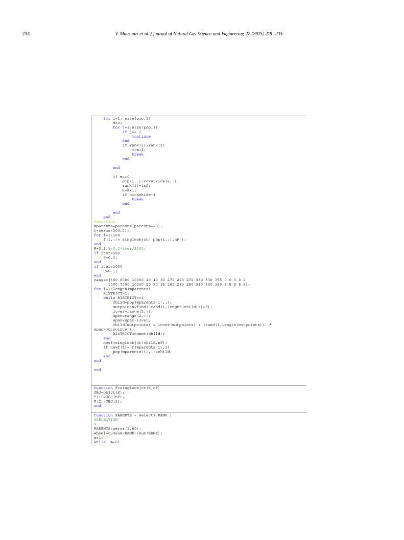
MATLAB code listing for single objective GA to solve deviatedwellbore trajectories using the radius of curvature method.


References

Aadnøy, B.S., Andersen, K., 2001. Design of oil wells using analytical friction models.J. Pet. Sci. Eng. 32, 53e71.

Aadnøy, B.S., Fazaelizadeh, M., Hareland, G., 2010. A 3-D analytical model forwellbore friction (SPE paper 141515). J. Can. Pet. Technol. 49 (10), 25e36.

Adams, J.N., Charrier, T., 1985. Drilling Engineering: a Complete Well PlanningApproach. PennWell Publishing Company, Tulsa, Oklahoma, pp. 342e345.

Atashnezhad, A., Wood, D.A., Fereidounpour, A., Khosravanian, R., 2014. Designingand optimizing deviated wellbore trajectories using novel particle swarm al-gorithms. J. Nat. Gas Sci. Eng. 21, 1184e1204.

Fazaelizadeh, M., 2013. Real Time Torque and Drag Analysis during DirectionalDrilling (PhD thesis). University of Calgary, Alberta, Canada.

Guria, C., Goli, K., Pathak, A., 2014. Multi-objective optimization of oil well drillingusing elitist non-dominated sorting genetic algorithm. J. Pet. Sci. Eng. 11,97e110.

Gen, M., Cheng, R., 2008. Network Models and Optimization. Springer, p. 692.Haupt, R.L., Haupt, S.E., 2004. Practical Genetic Algorithms, second ed. Wiley

Interscience.Johancsik, C.A., Friesen, D.B., Dawson, R., 1984. Torque and drag in directional

wellseprediction and measurement. J. Pet. Technol. 987e992. June 1984.Joshi, S.D., 2003. Cost/benefits of horizontal wells, 2003 (SPE paper 83621). In: SPE/

AAPG Joint Meeting at Long Beach, California, U.S.A., 19e24 May 2003.Khaled, A/El, Fattah, S., El-Tayeb, A., Dahab, A., Khalaf, F., 1999. 3-D well design using

computer optimization model. In: 4th Computer Conference, SPE Egypt Section,Cairo, Egypt.

Li, A., 2010. The operator of genetic algorithms to improve its properties. J. Mod.Appl. Sci. 4 (3), 60e62.

Lin, W.Y., Lee, W.Y., Hong, T.P., 2003. Adapting crossover and mutation rates ingenetic algorithms. J. Inf. Sci. Eng. 19, 889e903.

McCormick, J.E., Chiu, T.F., 2011. The practice and evolution of torque and dragreduction: theory and field results (SPE conference paper 147100). In: SPEAnnual Technical Conference and Exhibition, 30 October-2 November, Denver,Colorado, USA.

Shokir, E.M., Emera, M.K., Eid, S.M., Wally, A.W., 2004. A new optimization model for3-D well design. Emir. J. Eng. 9 (1), 67e74.

Sheppard, M.C., Wick, C., Burgess, T., 1987. Designing well paths to reduce torqueand drag (SPE Paper 15463). SPE Drill. Eng. 2 (4), 344e350.

Sivanandam, S.N., Deepa, S.N., 2008. Introduction to Genetic Algorithms. Springer,p. 442.

Xie, L., Moran, D., Yan, L., et al., 2012. Sophisticated software analysis system and useof torque/drag modeling for complex well operations increase operational ef-ficiency (SPE Paper 152056). In: Presented at the Western Regional Meeting,Bakersfield, USA, 21e23 March.

Yasari, E., Pishvaie, M.R., Khorasheh, F., Salahshoor, K., Kharrat, R., 2013. Applicationof multi-criterion robust optimization in water-flooding of oil reservoir. J. Pet.Sci. Eng. 74, 147e153.

http://refhub.elsevier.com/S1875-5100(15)30116-5/sref1





























































journal of natural gas science and engineering · previous studies indicate that the cost of...

Documents