Journal of

Mechanics ofMaterials and Structures

GRADIENT REPRODUCING KERNEL PARTICLE METHOD

Alireza Hashemian and Hossein M. Shodja

Volume 3, Nº 1 January 2008

mathematical sciences publishers

JOURNAL OF MECHANICS OF MATERIALS AND STRUCTURESVol. 3, No. 1, 2008

GRADIENT REPRODUCING KERNEL PARTICLE METHOD

ALIREZA HASHEMIAN AND HOSSEIN M. SHODJA

This paper presents an innovative formulation of the RKPM (reproducing kernel particle method) pio-neered by Liu. A major weakness of the conventional RKPM is in dealing with the derivative boundaryconditions. The EFGM (element free Galerkin method) pioneered by Belytschko shares the same diffi-culty. The proposed RKPM referred to as GRKPM (gradient RKPM), incorporates the first gradients ofthe function in the reproducing equation. Therefore in three-dimensional space GRKPM consists of fourindependent types of shape functions. It is due to this feature that the corrected collocation method canbe readily generalized and combined with GRKPM to enforce the EBCs (essential boundary conditions),involving both the field quantity and its first derivatives simultaneously. By considering several plateproblems it is observed that GRKPM yields solutions of higher accuracy than those obtained using theconventional approach, while for a desired accuracy the number of particles needed in GRKPM is muchless than in the traditional methodology.

1. Introduction

Boundary value problems (BVPs) often have essential boundary conditions (EBCs) that involve deriva-tives, for example, in beams and plates, where slopes are commonly enforced at the boundaries. Suchproblems are solved numerically using meshless techniques like the reproducing kernel particle method(RKPM) and the element free Galerkin method (EFGM), pioneered by Liu et al. [1995] and Belytschkoet al. [1994b], respectively. However, both methods require an often awkward auxiliary method forenforcing the EBCs. Li and Liu [2002] gives a useful review of the previous methodologies.

We summarize the major contributions specifically aimed at remedying the issue of EBCs. The methodof Lagrange multipliers is a classic approach [Belytschko et al. 1994b]. However, it is unattractivebecause it increases the number of unknowns, causes a loss of positive definiteness, and leads to anawkward system of linear equations. Another method is a modified variational principle [Lu et al. 1994]that interprets the Lagrange multipliers and replaces them by physical quantities. Although it leadsto a banded set of equations, the coefficient matrix is not necessarily positive definite and the resultsare less accurate than those obtained by using Lagrange multipliers. The penalty method [Belytschkoet al. 1994a; Zhu and Atluri 1998] is a very simple and effective approach which does not increase thenumber of unknowns. However, it does not satisfy the EBCs exactly, and its accuracy depends on thepenalty factor. Yet another approach couples EFGM and finite element method (FEM) [Krongauz andBelytschko 1996; Liu et al. 1997] by using FEM for the boundaries and their neighboring domains andusing EFGM elsewhere. This technique dramatically simplifies enforcing the EBCs. However, it losesthe advantage of the meshfree technology near the boundaries. Another idea uses the singular kernelfunction to enforce the Kronecker delta property [Lancaster and Salkauskas 1981]. It enforces the EBCs

Keywords: meshfree, RKPM, gradient, mixed boundary conditions, plates.

127

128 ALIREZA HASHEMIAN AND HOSSEIN M. SHODJA

efficiently, but it works only when the dilation parameter falls within a limited range. When it is toolarge, the convergence rate deteriorates rapidly. Finally, the transformation technique, first proposed byChen et al. [1996], can efficiently impose the EBCs for meshless methods. However, it cannot be appliedwhen the EBCs involve derivatives.

Liu et al. [1996a] took advantage of the Hermite polynomials and proposed the Hermite reproducingkernel method (HRKM), which incorporates the derivative terms into the reproducing equation. In theone-dimensional formulation, four admissible forms were presented for selecting the modified kernelsassociated with the derivative terms. However, they claimed that the only form that can be generalized tohigher dimensions violates the second order reproducing condition. As a result, it reconstructs the func-tion less accurately than the standard RKPM. Moreover, the EBCs were enforced by an auxiliary methodwhich was not stated explicitly. Atluri et al. [1999] extended the conventional moving least squares (MLS)interpolant, first presented by Lancaster and Salkauskas [1981], to Hermite-type interpolation and calledit generalized MLS (GMLS). For illustration, Atluri et al. [1999] considered a one-dimensional thinbeam and imposed the EBC using the penalty method. Later, Tiago and Leitao [2004] used GMLS tosolve the isotropic Kirchhoff plate. They enforced the EBCs using Lagrange multipliers. Li et al. [2003]and Lam et al. [2006] employed the Hermite theorem to construct the Hermite–Cloud method based onthe classical RKPM but used a fixed kernel instead of a moving one. They chose the strong form ofgoverning partial differential equations; that is, they used the point collocation technique to discretizethe governing partial differential equations. Liu et al. [2004] combined a meshfree and a finite elementinterpolant by introducing a hybrid fundamental equation that incorporates the concepts of both RKPMand FEM. In this manner, they generated a class of hybrid interpolation functions that may achieve ahigher order of smoothness in multiple dimensions. They called this technology the reproducing kernelelement method (RKEM) and pointed out that it has a great advantage over the traditional FEM. Liet al. [2004] proposed that, by extending the RKEM interpolant to a Hermite-type interpolant, one canobtain higher order Kronecker delta properties suitable for solving BVPs involving higher order partialdifferential equations. It should be emphasized that RKEM is a mesh-based technique which requireselement defining and mapping.

In 1999, we were working on a Master’s thesis that studied solving beam-column problems by mesh-less methods, particularly RKPM. During our work, we found it difficult to enforce the EBCs associatedwith the deflection and rotation of beam-columns. As the work progressed, we realized that the usualtransformation method, however efficient, cannot apply to the derivative type of EBCs. We generalizedthe transformation technique so that it could accommodate not only the function but also the derivativetype of EBCs. In so doing, we modified the RKPM formulation extensively and successfully linked itto the generalized transformation technique. We added a gradient term to the reproducing equation, and,for this reason, we called the new approach the gradient RKPM (GRKPM). The advantage of GRKPMover RKPM is that, in addition to exactly enforcing the EBCs without resorting to the penalty methodor Lagrange multipliers, it gives more accurate results and converges faster. Moreover, it gives a bandedset of equations with a positive definite matrix [Hashemian 2000].

The one-dimensional formulation of GRKPM of [Hashemian 2000] is not extended straightforwardlyto multiple dimensions. In three dimensions, a major difficulty is in choosing the correction functions toproduce a well-conditioned system. However, once that has been done, the formulation can be reducedeasily back to one or two dimensions. In this work, we present GRKPM in three dimensions, and

GRADIENT REPRODUCING KERNEL PARTICLE METHOD 129

hence one and two as well. Besides affirming its accuracy and good convergence, we establish thatthe approach enforces mixed EBCs by reexamining several thin plate problems solved previously byother methods. Next, we further demonstrate the method’s efficacy by considering more complex andphysically important problems that are poorly solved by the existing meshless techniques (RKPM andEFGM).

2. Formulating the GRKPM

2.1. Reproducing equation. The starting point for the conventional RKPM is that a given function u(x)in the three-dimensional space (with coordinates xk) can be expressed by the reproducing formula

u R(x)=

∫�

φ0a(x; x − y)u( y)d�,

where u R(x) is the reproduced function, a is a dilation parameter, and φ0a(x; x − y) is the modified kernel

function associated with the function. We propose expressing u R(x) as

u R(x)=

∫�

φ0a(x; x − y)u( y)d�+

3∑k=1

∫�

φka(x; x − y)u,k( y)d�. (1)

In Equation (1), u,k( y)= ∂u( y)/∂yk and φka(x; x − y) for k 6= 0 is the modified kernel function associated

with u,k( y). For k = 0, 1, 2, 3, we define

φka(x; x − y)= Ck(x; x − y)φa(x − y),

where φa(x − y) is the kernel function and Ck(x; x − y) are correction functions, which are derived froma reference function

C(x; x − y)= b0(x)+3∑

i=1

bi (x)(xi − yi )+12

3∑i=1

3∑j=1

bi j (x)(xi − yi )(x j − y j ),

by the relations

C0(x; x − y)= b0(x)+3∑

i=1

bi (x)(xi − yi ),

Ck(x; x − y)= −∂C(x; x − y)

∂yk, k = 1, 2, 3.

(2)

In the reference function, bi and bi j (bi j = b j i ) are unknown coefficients to be determined by the com-pleteness conditions. It should be noted that C0(x; x − y) is just the part of C(x; x − y) affine in y.

130 ALIREZA HASHEMIAN AND HOSSEIN M. SHODJA

Using the previous three equations, one obtains

φ0a(x; x − y)=

[b0(x)+

3∑i=1

bi (x)(xi − yi )

]φa(x − y),

φka(x; x − y)=

[bk(x)+

3∑i=1

bki (x)(xi − yi )

]φa(x − y), k = 1, 2, 3.

In this result, note that the forms chosen in Equation (2) for the correction functions assure the linearindependence of the modified kernels.

2.2. Completeness. Consider the Taylor’s series of u( y) around point x up to second order:

u( y)∼= u(x)−3∑

i=1

(xi − yi )u,i (x)+12

3∑i=1

3∑j=1

(xi − yi )(x j − y j )u,i j (x),

Upon substituting this into Equation (1), it follows that

u R(x)= u(x)R0(x)−3∑

m=1

u,m(x)Rm(x)+12

3∑m=1

3∑n=1

u,mn(x)Rmn(x)+ Err, (4)

where Err denotes the cumulative truncation error and

R0(x)=

∫�

φ0a(x − y)d�,

Rm(x)=

∫�

(xm − ym)φ0a(x − y)d�−

∫�

φma (x − y)d�, m = 1, 2, 3,

Rmn(x)= Rnm(x)=

∫�

(xm − ym)(xn − yn)φ0a(x − y)d�

−

∫�

(xm − ym)φna (x − y)d�−

∫�

(xn − yn)φma (x − y)d�, m, n = 1, 2, 3.

In view of Equation (4), the completeness condition on u R(x) leads to 10 independent conditions [Liuet al. 1996b; Liu et al. 1996a]. Introducing the ijkth moment at the point x with respect to the kernelfunction φa(x − y) as

mi jk(x)=

∫�

(x1 − y1)i (x2 − y2)

j (x3 − y3)kφa(x − y)d�, (5)

it follows that

M(x)β(x)= H, (6)

GRADIENT REPRODUCING KERNEL PARTICLE METHOD 131

in which M(x) is

m000 m100 m010 m001 0 0 0 0 0 0m100 m200 − m000 m110 m101 −m100 −m010 −m001 0 0 0m010 m110 m020 − m000 m011 0 −m100 0 −m010 −m001 0m001 m101 m011 m002 − m000 0 0 −m100 0 −m010 −m001m200 m300 − 2m100 m210 m201 −2m200 −2m110 −2m101 0 0 0m110 m210 − m010 m120 − m100 m111 −m110 −m020 − m200 −m011 −m110 −m101 0m101 m201 − m001 m111 m102 − m100 −m101 −m011 −m200 − m002 0 −m110 −m101m020 m120 m030 − 2m010 m021 0 −2m110 0 −2m020 −2m011 0m011 m111 − m001 m021 m012 − m010 0 −m101 −m110 −m011 −m020 − m002 −m011m002 m102 m012 m003 − 2m001 0 0 −2m101 0 −2m011 −2m002

,

the vector containing the unknown coefficients

βT (x)=[b0(x) b1(x) b2(x) b3(x) b11(x) b12(x) b13(x) b22(x) b23(x) b33(x)

],

andHT

=[1 0 0 0 0 0 0 0 0 0

].

The unknown bi and bi j are readily determined by solving Equation (6). We compute the first derivativesof β(x) by differentiating Equation (6)

M(x)β,m(x)= −M ,m(x)β(x), m = 1, 2, 3,

and compute the second derivatives by differentiating the above, as

M(x)β,mn(x)= −M ,mn(x)β(x)− M ,m(x)β,n(x)− M ,n(x)β,m(x), m, n = 1, 2, 3,

in the order shown above.

2.3. Shape functions. To extract the shape functions and their associated derivatives, one must discretizethe integral in Equation (1). In this paper, we use the trapezoidal rule, and the equation becomes

u R(x)=

NP∑i=1

ψ0i (x)u

i+

3∑k=1

NP∑i=1

ψki (x)u

i,k, (7)

where NP is the number of particles,1 ui= u( yi ), ui

,k = ∂u( y)/∂yk | y= yi , and

ψ0i (x)=

[b0(x)+

3∑j=1

b j (x)(x j − yij )

]φa(x − yi )1 yi ,

ψki (x)=

[bk(x)+

3∑j=1

bk j (x)(x j − yij )

]φa(x − yi )1 yi ,

(8)

1 Smooth particle hydrodynamics (SPH) is a meshfree method which was first proposed by Lucy [1977]. Utilizing thismethod, he modeled the collective behavior of a discrete set of physical particles in astrophysics. For this reason, in RKPM[Liu et al. 1995] and in the present work, the yi are called particles rather than nodes.

132 ALIREZA HASHEMIAN AND HOSSEIN M. SHODJA

in which ψki (x) is the kth shape function for the i th particle evaluated at x, and 1 yi is the area belonging

to the i th particle.Many authors, for example Donning and Liu [1998] and Liu [2003], have extensively studied various

window functions and their effects. In the present work, we use the cubic spline

φ(z)=

23

− 4z2+ 4z3, 0 ≤ |z| ≤

12,

43

− 4z + 4z2−

43

z3,12< |z| ≤ 1,

0, otherwise,

and construct the three-dimensional window function by multiplying the one-dimensional window func-tions:

φa(x − y)=

3∏i=1

1aiφ

(xi − yi

ai

),

in which ai is the dilation parameter associated with the xi -direction.Numerically evaluating the unknowns bi , bi j , and their derivatives requires discretizing the integral

in Equation (5) and subsequently calculating the moment mi jk(x). To satisfy the consistency condition,the technique used for discretizing the reproducing equation must be used also for the moment equation[Chen et al. 1996].

The first derivatives of the shape functions are obtained by differentiating Equation (8):

[ψ0

i (x)],m =

{[b0(x)],m +

3∑j=1

[b j (x)],m(x j − yij )+ bm(x)

}φa(x − yi )1 yi

+

{b0(x)+

3∑j=1

b j (x)(x j − yij )

}[φa(x − yi )

],m1 yi ,

[ψk

i (x)],m =

{[bk(x)

],m +

3∑j=1

[bk j (x)],m(x j − yij )+ bkm(x)

}φa(x − yi )1 yi

+

{bk(x)+

3∑j=1

bk j (x)(x j − yij )

}[φa(x − yi )

],m1 yi , k = 1, 2, 3,

GRADIENT REPRODUCING KERNEL PARTICLE METHOD 133

with i = 1, 2, . . . ,NP and m = 1, 2, 3. Differentiating again leads to the shape functions’ second deriva-tives:

[ψ0

i (x)],mn =

{[b0(x)],mn +

3∑j=1

[b j (x)],mn(x j − yij )+ [bn(x)],m + [bm(x)],n

}φa(x − yi )1 yi

+

{[b0(x)],n +

3∑J=1

[b j (x)],n(x j − yij )+ bn(x)

}[φa(x − yi )],m1 yi

+

{[b0(x)],m +

3∑j=1

[b j (x)],m(x j − yij )+ bm(x)

}[φa(x − yi )],n1 yi

+

{b0(x)+

3∑j=1

b j (x)(x j − yij )

}[φa(x − yi )],mn1 yi ,

[ψk

i (x)],mn =

{[bk(x)],mn +

3∑j=1

[bk j (x)],mn(x j − yij )+ [bkn(x)],m + [bkm(x)],n

}φa(x − yi )1 yi

+

{[bk(x)],n +

3∑j=1

[bk j (x)],n(x j − yij )+ bkn(x)

}[φa(x − yi )],m1 yi

+

{[bk(x)],m +

3∑j=1

[bk j (x)],m(x j − yij )+ bkm(x)

}[φa(x − yi )],n1 yi

+

{bk(x)+

3∑j=1

bk j (x)(x j − yij )

}[φa(x − yi )],mn1 yi , k = 1, 2, 3,

with i = 1, 2, . . . ,NP and m, n = 1, 2, 3.

3. Presenting the shape functions: departure from the conventional type

The aim of this section is to present the shape functions that follow from the proposed reproducingequation, and for this purpose we consider two-dimensional shape functions.

In two dimensions, Equation (8) yields three different types of shape functions ψ0i (x), ψ

1i (x) and

ψ2i (x):

ψ0i (x)=

[b0(x)+

2∑j=1

b j (x)(x j − yij )

]φa(x − yi )1 yi ,

ψki (x)=

[bk(x)+

2∑j=1

bk j (x)(x j − yij )

]φa(x − yi )1 yi , k = 1, 2,

134 ALIREZA HASHEMIAN AND HOSSEIN M. SHODJA

with i = 1, 2, . . . ,NP. We emphasize that the conventional RKPM has only one shape function ψi (x),regardless of the dimension of the problem, whereas the present method gives rise to k additional shapefunctions, ψk

i (x), for k-dimensional Euclidean space.Figure 1 shows the shape functions for the conventional RKPM, and Figures 2 and 3 depict the shape

functions corresponding to GRKPM. In these figures, the region [0, 5]2 contains 11 × 11 uniformly

distributed particles. The dilation parameter is chosen to be twice the particle spacing in each direction.For illustration, Figures 1–3 display the shape functions associated with certain particles. Specificallyselected are the corners located at (0, 0), (5, 0), (5, 5), and (0, 5); the mid-edge points (2.5, 0), (5, 2.5),(2.5, 5), and (0, 2.5); and the center (2.5, 2.5). From Figures 1 and 2, the ψ0

i (x) from GRKPM are,modulo amplitude, the same as the ψi (x) from RKPM. Comparing within Figure 3 reveals that theψ2

i (x) are simply the ψ1i (x) rotated 90◦ counterclockwise about the region’s center. We point out that

ψ1i (x) and ψ2

i (x) are the shape functions associated with the first derivative of the function in the x1 andx2-direction.

4. Applying essential boundary conditions

In the meshfree methods (RKPM/EFGM), enforcing EBCs has been a controversial issue among inves-tigators. The basic shortcoming of the methods is that the shape functions do not possess the Kroneckerdelta property. For this reason, enforcing the EBCs is not as convenient as in FEM.

4.1. Statement of the problem. Consider a three-dimensional domain � with the boundary 0 and theassociated BVP

Lu(x)= f (x), x ∈�, (9)

in which L is a linear differential operator. Natural boundary conditions may have arbitrary form, whereasEBCs may prescribe the field quantity and/or its first derivatives

u,k(x)= gk(x), x ∈ 0keb, k = 0, 1, 2, 3, (10)

where 00eb and 0k

eb are the set of all points x at which u(x) and u,k(x) are prescribed. Thus the essentialboundary is

0eb =

3⋃k=0

0keb.

It is interesting to note that 0ieb ∩0

jeb may not be empty for i 6= j . Suppose S is the space of all H (2)

2 (�)

functions that satisfy the boundary conditions (10), and define V to be the space of all H (2)2 (�) functions

that satisfy the homogeneous EBCs. The spaces S and V may be expressed as

S ≡{u | u ∈ H (2)

2 (�), u,k(x)= gk(x) on 0keb, k = 0, 1, 2, 3

}, (11a)

V ≡{w | w ∈ H (2)

2 (�),w,k(x)= 0 on 0keb, k = 0, 1, 2, 3

}, (11b)

where H (2)2 (�) is a Sobolev space. The governing Equation (9) is cast into the weak form∫

�

w(x)[Lu(x)− f (x)]2d�= 0. (12)

GRADIENT REPRODUCING KERNEL PARTICLE METHOD 135

0

1

2

3

4

5 0

1

2

3

4

5

0.5

1\

1x2x

Figure 1. Conventional RKPM shape functions plotted at the corners, mid-edges, andcenter of the 11 × 11 uniformly distributed particles with dilation parameter a = 21 y.

0

1

2

3

4

5 0

1

2

3

4

5

0.5

1\

1x 2x

0

Figure 2. The first type of GRKPM shape functions plotted at the corners, mid-edges,and center of the 11×11 uniformly distributed particles with dilation parameter a = 21 y.

12

34

5 0

1

2

3

4

5

-0.05

0

0.05

\

2x

1

x1

12

34

5 0

1

2

3

4

5

-0.05

0

0.05

\

2x

2

x1

Figure 3. The second and third types of GRKPM shape functions plotted at the cor-ners, mid-edges, and center of the 11 × 11 uniformly distributed particles with dilationparameter a = 21 y.

136 ALIREZA HASHEMIAN AND HOSSEIN M. SHODJA

Employing the shape functions developed in Section 2.3, u R(x) and wR(x) may be written as

u R(x)= ψ(x)d, (13a)

wR(x)= ψ(x)c, (13b)

with

ψ(x)=[ψ1(x) ψ2(x) · · · ψNP(x)

], (14a)

ψ i (x)=[ψ0

i (x) ψ1i (x) ψ

2i (x) ψ

3i (x)

], (14b)

where ψki (x), k = 0, 1, 2, 3 is given by Equation (8). The vector d contains the unknowns associated

with the degrees of freedom (DOF) u and u,k , k = 1, 2, 3. We prefer to represent d as

d =[d1

T d2T

· · · dNPT ], (15a)

diT

=[d0

i d1i d2

i d3i

]. (15b)

The unknown vector c pertains to the test function wR(x), which we arrange to have the same structureas d. In view of Equations (13)–(15), Equation (12) may be written as

cT r = 0, (16)

where

r = K d − f , K =

∫�

ψT (x)Lψ(x)d�, f =

∫�

ψT (x) f (x)d�.

The matrix K depends on the operator L . In the next section, we show that the set problem (16) can berigorously solved for d by extending the corrected collocation method.

4.2. Extending the corrected collocation method to GRKPM. In collocation methods, the EBCs areenforced exactly at the boundary particles. A number of collocation methods have been developed. Thetraditional collocation methods, including direct [Lu et al. 1994] and modified [Zhu and Atluri 1998],lead to some inconsistencies when applied to the conventional RKPM [Wagner and Liu 2000]. These in-consistencies exist because the conventional RKPM’s shape functions do not possess the Kronecker deltaproperty. Wagner and Liu [2000] give a remedy. Their work is based on the transformation technique[Chen et al. 1996] and is limited to enforcing the EBCs for the function itself. Moreover, the conventionalRKPM deals with only one type of shape function. Therefore, in the present situation, where the EBCsinvolve the function and/or its first derivatives and there are four types of shape functions, the collocationgiven in [Wagner and Liu 2000] is not applicable and must be modified appropriately.

The starting point is to partition each of the vectors d, c, and r into two subvectors

r =

[reb

r∼eb

], c =

[ceb

c∼eb

], d =

[deb

d∼eb

]. (17)

The subscript eb labels the neb parameters that pertain to the EBCs of Equation (10), whereas ∼ eb labelsthe remaining n∼eb parameters. (Hence neb + n∼eb counts the total DOF of the system.) Note that each

GRADIENT REPRODUCING KERNEL PARTICLE METHOD 137

particle is allowed to have four DOF in u and u,k, k = 1, 2, 3. Once the shape function ψ(x) in Equation(14a) and its first derivatives are evaluated for the i th particle xi , we may define the matrix

ψT(xi )=

[ψT (xi ) ψT

,1(xi ) ψT,2(xi ) ψT

,3(xi )].

The square matrix containing the shape functions and their derivatives for a system with NP particlesmay written as

9T

=

[ψ

T(x1) ψ

T(x2) · · · ψ

T(xNP)

]. (18)

DefininguT(xi )=

[u(xi ) u,1(xi ) u,2(xi ) u,3(xi )

],

we replace Equation (13a) byu(xi )= ψ(xi )d,

and, with the aid of Equation (18), we have

U = 9d, (19)

whereU

T=

[uT(x1) uT

(x2) · · · uT(xNP)

].

Next, we define the vector

WT

=

[w

T(x1) w

T(x2) · · · w

T(xNP)

],

wherew

T(xi )=

[w(xi ) w,1(xi ) w,2(xi ) w,3(xi )

],

so that, from Equation (18), we haveW = 9c. (20)

Repeating for the vectors W and c the partition scheme in Equation (17), Equation (20) takes the form[W eb

W∼eb

]=

[E FG H

] [ceb

c∼eb

]. (21)

This, in conjunction with Equation (11b), implies that W eb = 0 and W∼eb is arbitrary, hence[E F

] [ceb

c∼eb

]= 0,

and c∼eb is arbitrary.Let

T =

[E F0 I

], and c = T c,

then

ceb = 0, (22a)

c∼eb = c∼eb = Arbitrary. (22b)

138 ALIREZA HASHEMIAN AND HOSSEIN M. SHODJA

Likewise, letting d = T d, then, in view of Equation (19),

deb = Ueb, d∼eb = d∼eb, (23)

which relates the elements of deb to the prescribed function gk(x), as defined in Equation (10). Followingthe procedure given by Wagner and Liu [2000],

[cT

eb cT∼eb

] ([K eb,eb K eb,∼eb

K∼eb,eb K∼eb,∼eb

] [deb

d∼eb

]−

[f eb

f ∼eb

])= 0,

where

K = (T−1)T K T−1, f = (T−1)T f ,

and, using Equation (22) and Equation (23), we have

K∼eb,∼eb d∼eb = f ∼eb − K∼eb,ebUeb.

This equation can be readily solved for d∼eb.

5. Kirchhoff plate

Consider a symmetric laminated composite plate on an elastic foundation of varying stiffness k f (x1, x2),as shown in Figure 4. The boundary conditions and the transverse applied loading q(x1, x2) are arbitrary.The plate is also subjected to edge forces Ni j , i, j = 1, 2. According to the classical plate theory knownas Kirchhoff theory, the governing partial differential equation associated with the deflection u3 becomes[Reddy 1984]

(−N11u3,1 + N12u3,2),1 + (−N22u3,2 + N12u3,1),2 + M11,11 + M22,22 + 2M12,12 + k f u3 = q, (24)

Figure 4. Schematic of a rectangular laminated composite plate with arbitrary loadingand boundary conditions.

GRADIENT REPRODUCING KERNEL PARTICLE METHOD 139

and the admissible boundary conditions for the present experiments consist of

on x1 = 0, l1 :

{either − N11u3,1 + N12u3,2 + M11,1 + 2M12,2 = 0 or u3 specified,

either M11 = 0 or u3,1 specified,

on x2 = 0, l2 :

{either − N22u3,2 + N12u3,1 + M22,2 + 2M12,1 = 0 or u3 specified,

either M22 = 0 or u3,2 specified,

at the corners: either M12 = 0 or u3 specified.

(25)

In relations (24) and (25), M11

M22

M12

=

D11 D12 0D12 D22 00 0 D66

u3,11

u3,22

2u3,12

, (26)

where the Di j are called the bending stiffnesses; see [Reddy 1997] for details. For a single isotropiclayer with Young’s modulus E and Poisson ratio ν, the Di j become

D11 = D22 = D, D12 = νD, D66 =1 − ν

2D, (27)

in which D = Eh3/(12 − 12ν2) is called the flexural rigidity of the plate.The discretized weak form of Equation (24), employing the shape functions for two-dimensional space,

ψ(x1, x2), yields

cT r = 0,

r = K d − f ,

K =

∫ l2

0

∫ l1

0dx1 dx2

[N11ψ

T,1ψ ,1 + N22ψ

T,2ψ ,2 + N12(ψ

T,1ψ ,2 +ψT

,2ψ ,1)

+ D11ψT,11ψ ,11 + D22ψ

T,22ψ ,22 + 4D66ψ

T,12ψ ,12

+D12(ψT,22ψ ,11 +ψT

,11ψ ,22)+ k fψ

Tψ],

f =

∫ l2

0

∫ l1

0qψT dx1dx2.

(28)

For studying the stability of the plate, we put f = 0. This and Equation (28) give

cT (K L− λK G)d = 0, (29)

140 ALIREZA HASHEMIAN AND HOSSEIN M. SHODJA

(a) (b)

(c)

Figure 5. Midplane of an isotropic plate subjected to (a) uniaxial compression, (b) bi-axial compression, and (c) uniform shear.

where

K L=

∫ l2

0

∫ l1

0dx1 dx2

[D11ψ

T,11ψ ,11 + D22ψ

T,22ψ ,22 + 4D66ψ

T,12ψ ,12

+ D12(ψT,22ψ ,11 +ψT

,11ψ ,22)+ k fψ

Tψ],

K G=

∫ l2

0

∫ l1

0dx1 dx2

[N11ψ

T,1ψ ,1 + N22ψ

T,2ψ ,2 + N12(ψ

T,1ψ ,2 +ψT

,2ψ ,1)],

λ= −N11

N11= −

N22

N22= −

N12

N12.

(30)

Equation (29) is an eigenvalue problem, in which λ is the eigenvalue corresponding to the critical loadand d is the eigenvector associated with the DOF. The eigenvector is normalized to have Euclidean lengthone. Therefore, the displacement obtained from Equation (13a) is dimensionless.

Standard Gaussian quadratures carry out the numerical integrations in Equations (28) and (30). Forthis, a background mesh is needed, and we set the nodes of the background mesh to coincide with themeshless particles and compute a 4 × 4 quadrature in each cell.

6. Numerical experiments

In this section, we demonstrate the applicability and efficacy of the proposed method in treating variousboundary conditions encountered in plate problems. We compare the accuracy of the results with analyt-ical solutions, whenever they are available. We investigate the method’s advantages over conventionalmeshfree methods by considering several examples.

GRADIENT REPRODUCING KERNEL PARTICLE METHOD 141

6.1. GRKPM versus RKPM. Consider a clamped square plate with elastic modulus and Poisson ratioof E = 2×109 N/m2 and ν = 0.3. For each of the loading conditions in Figure 5, we solve for the criticalload and the corresponding mode shape.

The expression for the critical load is

Ni j = λπ2 D

l2 , i, j = 1, 2,

in which the analytical values for λ [Timoshenko and Gere 1961] are

λAnal. =

10.07, Uniform uniaxial compression,

5.30, Uniform biaxial compression,

14.71, Uniform shear.

(31)

For numerical calculations, we set the plate dimensions to l = 5 m and h = 0.05 m, distribute theparticles distributed uniformly in the x1 and x2-directions, and employ the linear correction function. Weset the dilation parameter in the x1 and x2-directions to 1.8 times the corresponding interparticle distance1yi .

Each loading condition in Figure 5 leads to an eigenvalue problem, with analytical solutions givenin Equation (31). Numerically, we solve each by RKPM combined with the penalty method, and alsoby our GRKPM. For RKPM, Table 1 displays the required CPU time and the percent error for selectednumbers of particles; Table 2 does the same for GRKPM.

The GRKPM gives fair accuracy in all cases, even for relatively small numbers of particles. In thevery worst case — in shear loading with a 5 × 5 distribution of particles — the error is only 5.8%. Incomparison, the best result (in biaxial loading) for conventional RKPM has 22.5% error, and that wasfor a considerably larger 16 × 16 number of particles. In that case, the GRKPM already gives an error of0.0% (to two-digit accuracy) with the smallest 5 × 5 number of particles. The GRKPM does cost more inCPU time for a fixed number of particles, but, because it achieves better accuracy using smaller numberof particles, the GRKPM significantly outperforms RKPM at fixed CPU time.

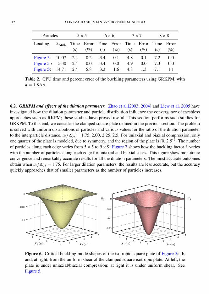
We have computed the critical mode shapes using our method with an 8 × 8 distribution of particles;these are shown in Figure 6. Note that the symmetric loading conditions shown in Figure 5a and b allowus to consider only one-quarter of the plate. For the unsymmetric loading conditions of Figure 5c, theentire plate must be modeled.

Particles 11 × 11 13 × 13 14 × 14 16 × 16

Loading λAnal. Time Error Time Error Time Error Time Error(s) (%) (s) (%) (s) (%) (s) (%)

Figure 5a 10.07 2.3 34.5 3.5 28.8 4.5 26.7 7.6 23.4Figure 5b 5.30 2.3 33.0 3.6 27.5 4.5 25.7 7.8 22.5Figure 5c 14.71 2.6 39.0 3.8 31.3 4.8 28.7 7.8 24.7

Table 1. CPU time and percent error of the buckling parameters using RKPM, with a = 1.81 y.

142 ALIREZA HASHEMIAN AND HOSSEIN M. SHODJA

Particles 5 × 5 6 × 6 7 × 7 8 × 8

Loading λAnal. Time Error Time Error Time Error Time Error(s) (%) (s) (%) (s) (%) (s) (%)

Figure 5a 10.07 2.4 0.2 3.4 0.1 4.8 0.1 7.2 0.0Figure 5b 5.30 2.4 0.0 3.4 0.0 4.9 0.0 7.3 0.0Figure 5c 14.71 2.4 5.8 3.3 1.6 4.8 1.3 7.1 1.1

Table 2. CPU time and percent error of the buckling parameters using GRKPM, witha = 1.81 y.

6.2. GRKPM and effects of the dilation parameter. Zhao et al.[2003; 2004] and Liew et al. 2005 haveinvestigated how the dilation parameter and particle distribution influence the convergence of meshlessapproaches such as RKPM; these studies have proved useful. This section performs such studies forGRKPM. To this end, we consider the clamped square plate defined in the previous section. The problemis solved with uniform distributions of particles and various values for the ratio of the dilation parameterto the interparticle distance, ai/1yi = 1.75, 2.00, 2.25, 2.5. For uniaxial and biaxial compression, onlyone quarter of the plate is modeled, due to symmetry, and the region of the plate is [0, 2.5]

2. The numberof particles along each edge varies from 5 × 5 to 9 × 9. Figure 7 shows how the buckling factor λ varieswith the number of particles along each edge for uniaxial and biaxial cases. This figure show monotonicconvergence and remarkably accurate results for all the dilation parameters. The most accurate outcomesobtain when ai/1yi = 1.75. For larger dilation parameters, the results are less accurate, but the accuracyquickly approaches that of smaller parameters as the number of particles increases.

12

34

51

23

45

-0.1

-0.05

0

Fig. 7

3u

1x (m)2x (m)

12

34

51

23

45

-0.15

-0.1

-0.05

0

Fig. 8

3u

1x (m)2x (m)

Figure 6. Critical buckling mode shapes of the isotropic square plate of Figure 5a, b,and, at right, from the uniform shear of the clamped square isotropic plate. At left, theplate is under uniaxial/biaxial compression; at right it is under uniform shear. SeeFigure 5.

GRADIENT REPRODUCING KERNEL PARTICLE METHOD 143

9.85

9.90

9.95

10.00

10.05

10.10

4 5 6 7 8 9 10

Particle distribution along each edge

O

1.75

2.00

2.25

2.50

(a i / ' y i ) :

Fig. 9

5.15

5.20

5.25

5.30

5.35

4 5 6 7 8 9 10

Particle distribution along each edge

O

1.75

2.00

2.25

2.50

(a i / ' y i ) :

Fig. 10

Figure 7. Convergence of the buckling parameter λ with increasing number of particlesalong each edge and for various dilation parameters. At left, the clamped square plate isunder uniaxial compression; at right, it is under biaxial compression. See Section 6.1.

For the uniform shear test, we model the entire plate, and the region of analysis is [0, 5]2. We consider

various uniform distributions of paricles ranging from 6 × 6 to 10 × 10. (The number of particles variesfrom 36 to 100.) Figure 8 displays how the buckling factor λ varies with the number of particles alongeach edge. The results converge monotonically and, for any distribution of particles, are always closestwhen ai/1yi = 1.75. Because we reached the same conclusion before in uniform uniaxial and biaxialcompression tests, we adopt the value ai/1yi = 1.75 for further experiments.

14.5

14.6

14.7

14.8

14.9

5 6 7 8 9 10 11

Particle distribution along each edge

O

1.75

2.00

2.25

2.50

(a i / ' y i ) :

Fig. 11

Figure 8. Convergence of the buckling parameter λ with increasing number of particlesalong each edge and for various dilation parameters. The clamped square plate is underuniform shear. See Section 6.1.

144 ALIREZA HASHEMIAN AND HOSSEIN M. SHODJA

6.3. GRKPM versus EFGM. Consider a thin rectangular plate of thickness h and dimensions l1 and l2

in x1 and x2. To compare the performance of EFGM and GRKPM, we compute the critical bucklingload for various aspect ratios l1/ l2 and different types of boundary conditions by both methods. Theedge load is applied in the x1-direction, as shown in Figure 5a. In the numerical calculations, we usel2 = 10 m and h = 0.06 m and assume the plate to be isotropic with E = 2.45 × 106 N/m2 and ν = 0.23.The buckling load N and the buckling factor λ are related as

N = λπ2 D

l22.

Table 3 tabulates the analytical [Timoshenko and Gere 1961] and computed values of λ for simplysupported boundary conditions along all the edges and for different aspect ratios l1/ l2. The numericalcalculations used a 13 × 13 uniform distribution of particles. The results of EFGM in conjunction withthe penalty method are cited from [Liu 2003]. There, Liu [2003] notes that the optimal dilation parameteris somewhere between 3.5 to 3.9 times the interparticle distance. Accordingly, for each l1/ l2, the dilationparameter is tuned within this rather tight range [Liu 2003]. Moreover, this particular EFGM uses thesecond-order base function instead of the first. In contrast, the GRKPM here employs the first-order basefunction. Moreover, for each l1/ l2, we examine two rather different dilation parameters, ai = 1.721yi

and ai = 3.51yi . Even though these dilation parameters differ by more than a factor of two, the resultsin either case are much better than those given by the EFGM with restricted dilation parameters. Weconclude that the GRKPM is somewhat indifferent to the dilation parameter.

Method Analytical EFGM GRKPM

ai/1yi − 3.5–3.9 1.72 3.5

I1/I2 λ Percent error

0.20 27.00 0.33 0.15 0.150.30 13.20 0.15 0.00 0.000.40 8.41 0.12 0.00 0.000.50 6.25 0.00 0.00 −0.160.60 5.14 −0.19 0.00 0.000.70 4.53 0.00 0.00 0.000.80 4.20 0.00 0.00 0.000.90 4.04 0.00 0.00 0.001.00 4.00 1.00 0.00 0.001.10 4.04 0.25 0.00 0.001.20 4.13 0.00 0.00 0.001.30 4.28 0.00 0.00 0.001.40 4.47 0.22 0.00 −0.45

Table 3. Buckling factor for the simply supported rectangular plate.

GRADIENT REPRODUCING KERNEL PARTICLE METHOD 145

Method Analytical EFGM GRKPM

ai/1yi − 3.5–3.9 1.72 3.5

I1/I2 λ Percent error

0.4 9.44 0.42 0.00 0.000.5 7.69 0.39 0.00 0.000.6 7.05 0.85 0.00 0.000.7 7.00 0.71 −0.14 0.000.8 7.29 1.23 0.14 0.140.9 7.83 1.66 0.26 0.261.0 7.69 1.04 0.00 0.00

Table 4. Buckling factor for the rectangular plate with simply supported, and clamped edges.

Table 4 displays the analytical [Timoshenko and Gere 1961] and computed values of λ when theedges x1 = 0, l1 are simply supported and the edges x2 = 0, l2 are fixed. All the other conditions andparameters are kept from the previous case. Again, for a given particle distribution, GRKPM allowsmore flexibility in choosing the dilation parameter and yields more accurate results. As before, EFGMuses the second-order base function, while the GRKPM uses first-order base function.

6.4. GRKPM and various types of boundary conditions. Figure 9 shows a schematic of a cross-plylaminate (90/0/90). The mark × locates the origin of the Cartesian coordinate system. The edges x2 = 0, lare assumed to be simply supported and under a uniform compressive load along the x2-direction. Forthe other two edges, x1 = 0, l, we consider various combinations of free, simply supported, and clampedboundary conditions, denoted respectively by F, S, and C. We put l = 5 m and the thickness of eachlamina to 0.05 m. We assume that each lamina is made of carbon-epoxy with the material propertiesE1 = 40E2, G12 = 0.6E2 and ν12 = 0.25.

Figure 9. Square cross-ply laminate (90/0/90) subjected to uniform compressive loadalong the x2 axis.

146 ALIREZA HASHEMIAN AND HOSSEIN M. SHODJA

Levy GRKPM

BC λ Particles λ % Err. Particles λ % Err.

FF 31.76 5 × 5 31.41 −1.10 9 × 9 31.66 −0.33FS 32.34 9 × 5 31.85 −1.49 17 × 9 32.22 −0.37FC 32.81 9 × 5 32.18 −1.92 17 × 9 32.65 −0.48SS 36.16 5 × 5 35.97 −0.52 9 × 9 36.12 −0.11SC 39.43 9 × 5 39.36 −0.17 17 × 9 39.41 −0.05CC 45.06 5 × 5 44.78 −0.63 9 × 9 45.02 −0.10

Table 5. Buckling factor for the cross-ply (90/0/90) square plate with mixed boundary conditions.

For this problem, the buckling load N and the buckling factor λ are related as

N = λl2

E2h3 . (32)

The Levy method [Reddy 1997] is used to calculate the analytical values of λ. In our GRKPM, we find λusing a uniform distribution of particles and a dilation parameter of 1.75 times the interparticle distance.For SS, CC, and FF boundary conditions, we model only one quarter of the plate, whereas, for FS, FC,and SC conditions, we model half the plate. Table 5 compares the results with the analytical solutions.The BVPs associated with FF, SS and CC boundary conditions are solved for 5 × 5 and 9 × 9 particles,whereas, for the cases FS, FC and SC, we use 9 × 5 and 17 × 9 particles. Table 5 shows that the GRKPMyields satisfactory results even with the smallest number of particles. The maximum error obtains withthe FC boundary conditions; the error is −1.92% for 9 × 5 particles and −0.48% for 17 × 9 particles.The SC boundary conditions, on the other hand, minimize the error; it is −0.17% for 9 × 5 and −0.05%for 17 × 9 particles. Table 5 shows clearly that the results improve as the number of particles increases.

6.5. Symmetric laminated composite plate under the most general conditions via GRKPM. To imple-ment the proposed approach, we have developed a powerful program we call ALCP-GRKPM (analysisof laminated composite plates via GRKPM) for analyzing symmetric laminated composite plates witharbitrary loading and boundary conditions. For example, consider the laminated composite (70/− 20)S

shown in Figure 10, in which the thicknesses of the layers are (0.02 m/0.03 m)S . Each lamina is made ofcarbon-epoxy (AS4/3501-6) with E1 = 148 GPa, E2 = 10.5 GPa, G12 = G13 = 5.61 GPa, G23 = 3.17 GPa,ν12 = ν13 = 0.3 and ν23 = 0.59. The edge x2 = 0 is free and the remaining edges are clamped. A rollertype support is placed in the middle of the plate, and part of the plate is placed on elastic foundation. Wesolve this set problem for two different cases: (1) uniform spring constant and distributed load; and (2)variable spring constant and distributed load. For both cases, a concentrated load of P = 50 kN is appliedat the location marked � in Figure 10. In this computation, we intend to find the location and value ofthe maximum deflection. We use 9 × 5, 17 × 9, 33 × 17, and 65 × 33 uniformly distributed particles. Weset the dilation parameter equal to 1.75 times the interparticle distance.

Case 1: Uniform spring constant and uniformly distributed load. In this case the spring constant anddistributed load are k f = 105 kN/m3 and q = 80 kN/m2. For reference, we analyze the problem by

GRADIENT REPRODUCING KERNEL PARTICLE METHOD 147

Figure 10. An example of a rectangular symmetric laminate (70/− 20)s under a set ofcomplex loadings and boundary conditions.

Method Particles (u3)max (cm) x1 (m) x2 (m)

GRKPM

9 × 5 −2.002 5.6250 0.00017 × 9 −2.003 5.6250 0.00033 × 17 −2.005 5.6250 0.00065 × 33 −2.006 5.6250 0.000

ANSYS 65 × 33 −2.072 5.6250 0.000

Table 6. Location and value of the maximum deflection for the plate shown in Figure 10with a uniform elastic constant and a uniformly distributed load.

148 ALIREZA HASHEMIAN AND HOSSEIN M. SHODJA

12

34

56

78 0

1

2

3

4

-1

0

Fig. 14

u3

x2

(cm)

1x (m) (m)

Figure 11. ALCP-GRKPM result for the deflection corresponding to the exampleshown in Figure 10 with uniform elastic constant and a uniformly distributed load.

ANSYS using 65 × 33 uniformly spaced nodes. In employing ANSYS, we use the 8-node ‘Shell 99’element. Appendix A gives its interpolation functions, assumptions, and restrictions. At each node, theelement has three displacement and three rotational DOF. Because of this, the DOF per node in ANSYSis twice the DOF per particle GRKPM. Table 6 shows the maximum deflection of the plate and whereit occurs. GRKPM with 45 particles already gives a satisfactory result, and making more particles onlyaffects the third decimal digit in the maximum deflection. The small discrepancy between the results ofANSYS and GRKPM for the maximum deflection arises because ANSYS applies the first-order sheardeformation laminated plate theory (FSDT) [Reddy 1997] which considers shear deflections, whereaswe use the classical plate theory which disregards these deflections. To suppress the shear deflectionsin FSDT, the lateral shear moduli G13 and G23 should be assigned significantly larger than G12. Ansys[1997] recommends taking G13 = G23 = 1000G12. By doing so, the computed maximum deflectionequals 2.006, which agrees with the GRKPM result to within three decimal places. The deflection,u3(x1, x2), is computed by GRKPM with 65 × 33 particles, and its variation is shown in Figure 11.

Case 2: Variable spring constant and variably distributed load. The program ALCP-GRKPM can acceptq(x1) and k f (x1, x2) as functions. For example, consider the plate shown in Figure 10 with the springconstant and distributed load assigned to vary as

k f =106

x1 + x2kN/m3, q = 55(x1 − 4)(x1 − 7) kN/m2.

Table 7 gives the corresponding results for 9 × 5, 17 × 9, 33 × 17 and 65 × 33 uniformly distributedparticles. As in the previous example, increasing the number of particles only affects the third decimaldigit in the maximum displacement.

7. Conclusions

We have demonstrated that our method is robust by considering plate boundary value problems. Theresults demonstrate that the method succeeds in treating different kinds of EBCs including those with

GRADIENT REPRODUCING KERNEL PARTICLE METHOD 149

Method Particles (u3)max (cm) x1 (m) x2 (m)

GRKPM

9 × 5 −2.363 5.5625 0.00017 × 9 −2.366 5.6250 0.00033 × 17 −2.368 5.6250 0.00065 × 33 −2.370 5.6250 0.000

Table 7. Location and value of the maximum deflection for the plate shown in Figure10 for variable elastic constant and a variably distributed load.

derivatives of the field function. The examples compute buckling load and analyze deflection undervarious types of loading and support, including elastic foundation with variable stiffness as explored inSection 6.5.

In the example of Section 6.1, comparing the performance of GRKPM and conventional RKPM revealsthat using GRKPM with much smaller numbers of particles leads to results of excellent accuracy. InSection 6.2, from studying how the number of particles and the dilation parameter affect the performanceof GRKPM, we conclude the GRKPM converges well as the number of particles increases. In Section6.3, we conclude that for GRKPM the base function of order one suffices for obtaining better accuracythan from EFGM with the second-order base function. Moreover, for the cross-ply laminate with varioustypes of EBCs considered in Section 6.4, the GRKPM solution converges rapidly with growing numberof particles.

The presently formulated GRKPM achieves high performance because it expands the degrees of free-doms to include slopes and because it enforces EBCs by generalizing the corrected collocation method.Hence, the advantages become more pronounced for plates clamped at the boundaries. Given its so-farexcellent features, GRKPM may hold promise for other problems of engineering science.

Appendix A

‘Shell 99’ is an 8-node quadrilateral element in 3-dimensions with rotational DOF and shear deflection[Ansys 1997]. It is suitable for laminate composites and can accept up to 100 different layers. Thiselement is discussed by Yunus et al. [1989]. A planner view of this element is given in Figure 12.

Let define the shape functions for each node as

ψ1 =(1 − s)(1 − t)(−s − t − 1)

4, ψ2 =

(1 + s)(1 − t)(s − t − 1)4

,

ψ3 =(1 + s)(1 + t)(s + t − 1)

4, ψ4 =

(1 − s)(1 + t)(−s + t − 1)4

,

ψ5 =(1 − s2)(1 − t)

2, ψ6 =

(1 + s)(1 − t2)

2,

ψ7 =(1 − s2)(1 + t)

2, ψ8 =

(1 − s)(1 − t2)

2.

150 ALIREZA HASHEMIAN AND HOSSEIN M. SHODJA

Figure 12. A planner view of the ‘Shell 99’ element used by ANSYS.

Subsequently, the interpolation functions areu1

u2

u3

=

8∑i=1

ψi

ui1

ui2

ui3

+

8∑i=1

ψir ti2

ai1 bi

1ai

2 bi2

ai3 bi

3

[θ i

1θ i

2

], (A.1)

where ui1, ui

2, and ui3 are motions of node i , r is the coordinate along the thickness, and ti is the thickness

at node i . a is the unit vector in the s direction and b is the unit vector in the plane of element and normalto a. θ i

1 and θ i2 are the rotations of node i about vector a and b, respectively. An interesting observation

is made by comparing the interpolation functions (A.1) with those of GRKPM given by Equation (7).The latter gives four different types of shape functions for the displacements and rotations of each node,whereas Equation (A.1) gives only one.

There are some assumptions and restrictions for this element:

• Normals to the center plane are assumed to remain straight after deformation, but not necessarilynormal to the center plane.

• Each pair of integration points in the r direction is assumed to have the same material orientation.

• There is no significant stiffness associated with rotation about the element r axis. However, anominal value of stiffness is present to prevent free rotation at the node.

Acknowledgement

This work was in part supported by the center of excellence in structures and earthquake engineering atSharif University of Technology.

References

[Ansys 1997] Ansys, “ANSYS 5.4 Documentation”, Technical report, ANSYS Incorporated, 1997.

[Atluri et al. 1999] S. N. Atluri, J. Y. Cho, and H.-G. Kim, “Analysis of thin beams, using the meshless local Petrov–Galerkinmethod, with generalized moving least squares interpolations”, Comput. Mech. 24:5 (1999), 334–347.

GRADIENT REPRODUCING KERNEL PARTICLE METHOD 151

[Belytschko et al. 1994a] T. Belytschko, L. Gu, and Y. Y. Lu, “Fracture and crack growth by element free Galerkin methods”,Model. Simul. Mater. Sc. 2:3A (1994), 519–534.

[Belytschko et al. 1994b] T. Belytschko, Y. Y. Lu, and L. Gu, “Element-free Galerkin methods”, Int. J. Numer. Meth. Eng. 37:2(1994), 229–256.

[Chen et al. 1996] J. S. Chen, C. Pan, C. T. Wu, and W. K. Liu, “Reproducing kernel particle methods for large deformationanalysis of non-linear structures”, Comput. Method. Appl. M. 139:1-4 (1996), 195–227.

[Donning and Liu 1998] B. M. Donning and W. K. Liu, “Meshless methods for shear-deformable beams and plates”, Comput.Method. Appl. M. 152:1-2 (1998), 47–71.

[Hashemian 2000] A. Hashemian, “A study of Columns’ buckling loads and modes by meshfree methods”, Master’s Thesis,Sharif University of Technology, Tehran, 2000.

[Krongauz and Belytschko 1996] Y. Krongauz and T. Belytschko, “Enforcement of essential boundary conditions in meshlessapproximations using finite elements”, Comput. Method. Appl. M. 131:1-2 (1996), 133–145.

[Lam et al. 2006] K. Y. Lam, H. Li, Y. K. Yew, and T. Y. Ng, “Development of the meshless Hermite-Cloud method forstructural mechanics applications”, Int. J. Mech. Sci. 48:4 (2006), 440–450.

[Lancaster and Salkauskas 1981] P. Lancaster and K. Salkauskas, “Surfaces generated by moving least squares methods”, Math.Comput. 37:155 (1981), 141–158.

[Li and Liu 2002] S. Li and W. K. Liu, “Meshfree and particle methods and their applications”, Appl. Mech. Rev. (Trans. ASME)55:1 (2002), 1–34.

[Li et al. 2003] H. Li, T. Y. Ng, J. Q. Cheng, and K. Y. Lam, “Hermite-Cloud: a novel true meshless method”, Comput. Mech.33:1 (2003), 30–41.

[Li et al. 2004] S. Li, H. Lu, W. Han, W. K. Liu, and D. C. Simkins, “Reproducing kernel element method, II: globallyconforming I m/Cn hierarchies”, Comput. Method. Appl. M. 193:12-14 (2004), 953–987.

[Liew et al. 2005] K. M. Liew, T. Y. Ng, and X. Zhao, “Free vibration analysis of conical shells via the element-free kp-Ritzmethod”, J. Sound Vib. 281:3-5 (2005), 627–645.

[Liu 2003] G. R. Liu, Mesh free methods: moving beyond the finite element method, CRC Press, Boca Raton, FL, 2003.

[Liu et al. 1995] W. K. Liu, S. Jun, and Y. F. Zhang, “Reproducing kernel particle methods”, Int. J. Numer. Meth. Fl. 20:8-9(1995), 1081–1106.

[Liu et al. 1996a] W. K. Liu, Y. J. Chen, R. A. Uras, and C. T. Chang, “Generalized multiple scale reproducing kernel particlemethods”, Comput. Method. Appl. M. 139:1-4 (1996), 91–157.

[Liu et al. 1996b] W. K. Liu, S. Jun, J. S. Chen, T. Belytschko, C. Pan, R. A. Uras, and C. T. Chang, “Overview and applicationsof the reproducing kernel particle methods”, Arch. Comput. Method E 3 (1996), 3–80.

[Liu et al. 1997] W. K. Liu, R. A. Uras, and Y. Chen, “Enrichment of the finite element method with reproducing kernel particlemethod”, J. Appl. Mech. (Trans. ASME) 64 (1997), 861–870.

[Liu et al. 2004] W. K. Liu, W. Han, H. Lu, S. Li, and J. Cao, “Reproducing kernel element method, I: theoretical formulation”,Comput. Method. Appl. M. 193:12-14 (2004), 933–951.

[Lu et al. 1994] Y. Y. Lu, T. Belytschko, and L. Gu, “A new implementation of the element free Galerkin method”, Comput.Method. Appl. M. 113:3-4 (1994), 397–414.

[Lucy 1977] L. B. Lucy, “A numerical approach to the testing of the fission hypothesis”, The Astro. J. 82 (1977), 1013–1024.

[Reddy 1984] J. N. Reddy, Energy and variational methods in applied mechanics: with an introduction to the finite elementmethod, John Wiley & Sons, New York, 1984.

[Reddy 1997] J. N. Reddy, Mechanics of laminated composite plates: theory and analysis, CRC Press, Boca Raton, FL, 1997.

[Tiago and Leitão 2004] C. Tiago and V. M. A. Leitão, “Further developments on GMLS: plates on elastic foundation”, pp.1378–1383 in Proceedings of the 2004 international conference on computational and experimental engineering and science(Madeira, Portugal), edited by A. Tadeu and S. N. Atluri, Tech Science Press, 2004, Available at http://www.civil.ist.utl.pt/~ctf/docs/04b madeira.pdf.

[Timoshenko and Gere 1961] S. P. Timoshenko and J. M. Gere, Theory of elastic stability, 2nd ed., McGraw-Hill, New York,1961.

152 ALIREZA HASHEMIAN AND HOSSEIN M. SHODJA

[Wagner and Liu 2000] G. J. Wagner and W. K. Liu, “Application of essential boundary conditions in mesh-free methods: acorrected collocation method”, Int. J. Numer. Meth. Eng. 47:8 (2000), 1367–1379.

[Yunus et al. 1989] S. M. Yunus, P. C. Kohnke, and S. Saigal, “An efficient through-thickness integration scheme in an unlimitedlayer doubly curved isoparametric composite shell element”, Int. J. Numer. Meth. Eng. 28:12 (1989), 2777–2793.

[Zhao et al. 2003] X. Zhao, K. M. Liew, and T. Y. Ng, “Vibration analysis of laminated composite cylindrical panels via ameshfree approach”, Int. J. Solids Struct. 40:1 (2003), 161–180.

[Zhao et al. 2004] X. Zhao, T. Y. Ng, and K. M. Liew, “Free vibration of two-side simply-supported laminated cylindricalpanels via the mesh-free kp-Ritz method”, Int. J. Mech. Sci. 46:1 (2004), 123–142.

[Zhu and Atluri 1998] T. Zhu and S. N. Atluri, “A modified collocation method and a penalty formulation for enforcing theessential boundary conditions in the element free Galerkin method”, Comput. Mech. 21:3 (1998), 211–222.

Received 16 Oct 2006. Accepted 31 May 2007.

ALIREZA HASHEMIAN: al.hash@gmail.comCenter of Excellence in Structures and Earthquake Engineering, Department of Civil Engineering, Sharif University ofTechnology, P.O. Box 11365-9311, Tehran, Iran

HOSSEIN M. SHODJA: shodja@sharif.eduCenter of Excellence in Structures and Earthquake Engineering, Department of Civil Engineering, Sharif University ofTechnology, P.O. Box 11365-9311, Tehran, Iran