journal of mechanics of materials and...

Journal of

Mechanics ofMaterials and Structures

ON THE ELASTIC MODULI AND COMPLIANCES OFTRANSVERSELY ISOTROPIC AND ORTHOTROPIC MATERIALS

Vlado A. Lubarda and Michelle C. Chen

Volume 3, Nº 1 January 2008

mathematical sciences publishers

JOURNAL OF MECHANICS OF MATERIALS AND STRUCTURESVol. 3, No. 1, 2008

ON THE ELASTIC MODULI AND COMPLIANCES OF TRANSVERSELYISOTROPIC AND ORTHOTROPIC MATERIALS

VLADO A. LUBARDA AND MICHELLE C. CHEN

The relationships between the elastic moduli and compliances of transversely isotropic and orthotropicmaterials, which correspond to different appealing sets of linearly independent fourth-order base tensorsused to cast the elastic moduli and compliances tensors, are derived by performing explicit inversionsof the involved fourth-order tensors. The deduced sets of elastic constants are related to each other andto common engineering constants expressed in the Voigt notation with respect to the coordinate axesaligned along the directions orthogonal to the planes of material symmetry. The results are applied to atransversely isotropic monocrystalline zinc and an orthotropic human femural bone.

1. Introduction

There has been a significant amount of research devoted to tensorial representation of elastic constantsof anisotropic materials, which are the components of the fourth-order tensors in three-dimensionalgeometrical space, or the second-order tensors in six-dimensional stress or strain space. This was par-ticularly important for the spectral decompositions of the fourth-order stiffness and compliance tensorsand the determination of the corresponding eigenvalues and eigentensors for materials with differenttypes of elastic anisotropy. The spectral decomposition, for example, allows an additive decompositionof the elastic strain energy into a sum of six or fewer uncoupled energy modes, which are given bytrace products of the corresponding pairs of stress and strain eigentensors. The representative referencesinclude [Rychlewski 1984; Walpole 1984; Theocaris and Philippidis 1989; Mehrabadi and Cowin 1990;Sutcliffe 1992; Theocaris and Sokolis 2000]. A study of the fourth-order tensors of elastic constants, andtheir equivalent matrix representations, is also important in the analysis of the invariants of the fourth-order tensors and identification of the invariant combinations of anisotropic elastic constants [Srinivasanand Nigam 1969; Betten 1987; Zheng 1994; Ting 1987; 2000; Ting and He 2006]. Furthermore, astudy of the representation of the fourth-order tensors with respect to different bases can facilitate tensoroperations and the analytical determination of the inverse tensors [Kunin 1981; 1983; Walpole 1984;Lubarda and Krajcinovic 1994; Nadeau and Ferrari 1998; Gangi 2000].

The objective of the present paper is to derive the relationships between the elastic moduli and compli-ances of transversely isotropic and orthotropic materials, which correspond to different appealing sets oflinearly independent fourth-order base tensors used to cast the elastic stiffness and compliance tensors.In the case of transversely isotropic materials we begin the analysis with a stress-strain relationshipwhich follows from the representation theorem for transversely isotropic tensor functions of a symmetricsecond-order tensor and a unit vector. This leads to the representation of the stiffness tensor in terms of

Keywords: algebra of tensors, elastic constants, human femur, orthotropic materials, transverse isotropy, zinc.Research support from the Montenegrin Academy of Sciences and Arts is kindly acknowledged.

153

http://www.jomms.org

http://dx.doi.org/10.2140/pjm.2008.3-1

154 VLADO A. LUBARDA AND MICHELLE C. CHEN

6 linearly independent tensors (Ir ) forming a basis of an algebra of fourth-order tensors that are madeof the Kronecker delta and the unit vector. The corresponding elastic moduli are denoted by cr . Sincethe multiplication table for Ir tensors is dense with nonzero tensors, and thus operationally less practical,we introduce a set of new base tensors (Jr ) following the procedure developed by Kunin [1981] andWalpole [1984]. The corresponding elastic moduli, denoted by cr , are related to the original moduli cr .We then derive the explicit expressions for the elastic compliances tensor with respect to both bases, andthe relationships between the corresponding parameters sr and sr and the original moduli cr and cr . Thetwo sets of elastic constants are also expressed in terms of the engineering constants, defined with respectto the coordinate system in which one of the axes is parallel to the axis of material symmetry.

Extending the analysis to orthotropic materials, three different representations of the elastic modulitensor are constructed by using three different sets of 12 linearly independent fourth-order base tensors.This is achieved on the basis of the representation theorems for orthotropic tensor functions of a sym-metric second-order tensor and the structural tensors associated with the principal axes of orthotropy[Spencer 1982; Boehler 1987]. The three sets of different elastic moduli, denoted by cr , crs and crs (nineof which are independent in each case) are related to each other. The tensor of elastic compliances isthen deduced by explicit inversion of the stiffness tensor expressed with respect to all three sets of basetensors. The corresponding compliances, denoted by sr , srs , and srs , are related to each other and to themoduli cr , crs , and crs . The three sets of elastic constants are then expressed in terms of engineeringconstants, appearing in the Voigt notation as the entries of 6 × 6 matrices [Voigt 1928], which do notconstitute the components of the second-order tensor [Hearmon 1961; Nye 1964; Cowin and Mehrabadi1995] and which are thus not amenable to easy tensor manipulations. The results are applied to calculatethe different sets of elastic constants for a transversely isotropic monocrystalline zinc and an orthotropichuman femur.

2. Elastic moduli of transversely isotropic materials

The stress-strain relationship for a linearly elastic transversely isotropic material, based on the represen-tation theorems for transversely isotropic tensor function of a strain tensor and a unit vector [Spencer1982], can be written as

σi j = λεkkδi j + 2µεi j + α(nknlεklδi j + ni n jεkk) + 2(µ0 − µ)(ni nkεk j + n j nkεki ) + βni n j nknlεkl . (1)

The rectangular components of the unit vector parallel to the axis of transverse isotropy are ni . Theelastic shear modulus within the plane of isotropy is µ, the other Lame constant is λ, and the out-of-plane elastic shear modulus is µ0. The remaining two moduli reflecting different elastic properties in theplane of isotropy and perpendicular to it are denoted by α and β.

The elastic stiffness tensor 3 corresponding to Equation (1), and defined such that σi j = 3i jklεkl , is

3 =

6∑r=1

cr Ir , (2)

ELASTIC MODULI AND COMPLIANCES OF TRANSVERSELY ISOTROPIC AND ORTHOTROPIC MATERIALS 155

where the fourth-order base tensors Ir are defined by

I1 =12 δ ◦ δ, I2 = δ δ, I3 = p δ, I4 = δ p,

I5 =12 p ◦ δ, I6 = p p.

(3)

The second order tensor p has the components pi j = ni n j . The tensor products between the second-ordertensors p and δ are such that

(p δ)i jkl = pi jδkl, (p ◦ δ)i jkl =12 (pikδ jl + pilδ jk + p jlδik + p jkδil). (4)

In the component form, the fourth-order tensors Ir are

I (1)i jkl =

12(δikδ jl + δilδ jk), I (2)

i jkl = δi jδkl,

I (3)i jkl = ni n jδkl, I (4)

i jkl = δi j nknl,

I (5)i jkl =

12(δikn j nl + δiln j nk + δ jlni nk + δ jkni nl), I (6)

i jkl = ni n j nknl .

(5)

The material parameters (elastic moduli), appearing in Equation (2), are

c1 = 2µ, c2 = λ, c3 = c4 = α, c5 = 2(µ0 − µ), c6 = β. (6)

The set of linearly independent tensors Ir forms a basis of an algebra (of order 6) of the fourth-ranktensors made up of the Kronecker delta and the unit vector, symmetric with respect to first and secondpair of indices, but not necessarily with respect to permutation of pairs. All such fourth-rank tensors canbe represented as a linear combination of the base tensors.

Since the multiplication table of the tensors Ir is dense with nonzero tensors (see the upper left cornerof Table 9 in the Appendix), and thus less convenient for tensor operations and the determination of theinverse tensors, we recast the elastic stiffness tensor (2) in terms of an alternative set of base tensors Jr ,which is characterized by a simple multiplication table, in which each product is equal to either zerotensor or to one of the tensors from the basis. Thus,

3 =

6∑r=1

cr Jr , (7)

where the modified elastic moduli are

c1 = c1 + c2 + 2c3 + 2c5 + c6 = λ + 4µ0 − 2µ + 2α + β,

c2 = c1 + 2c2 = 2(λ + µ),

c3 = c4 =√

2 (c2 + c3) =√

2 (λ + α),

c5 = c1 = 2µ, c6 = c1 + c5 = 2µ0,

(8)


with the inverse relationships

c1 = c5, c2 =12 (c2 − c5), c5 = c6 − c5,

c3 = c4 =1

√2

c3 −12 (c2 − c5),

c6 = c1 +12 c2 −

√2 c3 +

12 c5 − 2c6.

(9)

The base tensors Jr are defined by Walpole [1984], 1

J1 = p p, J2 =12 q q,

J3 =1

√2

p q, J4 =1

√2

q p,

J5 =12 (q ◦ q − q q), J6 = p ◦ q.

(10)

The second order tensor q is introduced such that

qi j = δi j − pi j , pi j = ni n j . (11)

When applied to an arbitrary vector v j , the tensors p and q decompose that vector into its componentsparallel to ni , pi jv j = (v j n j )ni , and orthogonal to it, qi j n j = vi − pi jv j . It readily follows that

pik pk j = pi j ,

qikqk j = qi j ,

pi j pi j = 1,

qi j qi j = 2,

pi i = 1,

qi i = 2,

pikqk j = 0, qik pk j = 0. (12)

The two types of tensor products between the involved second-order tensors are defined by the typeEquation (4), that is,

(p q)i jkl = pi j qkl, (p ◦ q)i jkl =12 (pikq jl + pilq jk + p jlqik + p jkqil). (13)

It can be easily verified thatp ◦ q = q ◦ p, p ◦ p = 2 p p. (14)

The trace products of the tensors Jr : Js of the type J (r)i jmn J (s)

mnkl can be readily evaluated by usingEquation (12), with the results listed in Table 1. The symbol � indicates that the products are in theorder: a tensor from the left column traced with a tensor from the top row.

2.1. Elastic compliances of transversely isotropic materials. To derive the elastic compliances tensor,it is more convenient to invert the elastic stiffness tensor 3 in its representation (7) than (2). Thus, bywriting

3−1=

6∑r=1

sr Jr , (15)

and by using Table 1 to expand the trace products appearing in

3 : 3−1= 3−1

: 3 = I1, (16)

1An alternative set of base tensors was used by Kunin[1981; 1983] and Lubarda and Krajcinovic [1994].


� J1 J2 J3 J4 J5 J6

J1 J1 0 J3 0 0 0

J2 0 J2 0 J4 0 0

J3 0 J3 0 J1 0 0

J4 J4 0 J2 0 0 0

J5 0 0 0 0 J5 0

J6 0 0 0 0 0 J6

Table 1. Table of products Jr : Js .

there follows

s1 = c2/c, s2 = c1/c, s3 = s4 = −c3/c, s5 = 1/c5, s6 = 1/c6, (17)

wherec = c1c2 − c2

3. (18)

Note that the fourth-order identity tensor I1 can be expressed in terms of the base tensors Jr as

I1 = J1 + J2 + J5 + J6,

which was used in Equation (16).The elastic compliances tensor can be expressed in the original basis Ir by using the connections

between the two bases, which are

I1 =12 δ ◦ δ = p p + p ◦ q +

12 q ◦ q = J1 + J2 + J5 + J6,

I2 = δ δ = (p + q)(p + q) = J1 + 2J2 +√

2(J3 + J4),

I3 = p δ = p p + p q = J1 +√

2 J3,

I5 = p ◦ δ = 2p p + p ◦ q = 2J1 + J6,

I4 = δ p = p p + q p = J1 +√

2 J4,

I6 = p p = J1.(19)

Their inverse relationships are

J1 = I6, J2 =12 (I2 − I3 − I4 + I6),

J3 =1

√2

(I3 − I6), J4 =1

√2

(I4 − I6),

J5 =12 (2I1 − I2 + I3 + I4 − 2I5 + I6), J6 = I5 − 2I6.

(20)

The elastic compliance tensor is expressed in terms of the base tensors Ir by substituting (20) into (15).The result is

3−1=

6∑r=1

sr Ir , (21)


with the corresponding compliances

s1 = s5, s2 =12 (s2 − s5),

s3 = s4 =1

√2

s3 −12 (s2 − s5), s5 = s6 − s5,

s6 = s1 +12 s2 −

√2 s3 +

12 s5 − 2s6. (22)

The same type of relationships hold between the moduli cr and cr appearing in Equation (2) and (7). Theinverse expressions to (22) are

s1 = s1 + s2 + 2s3 + 2s5 + s6, s2 = s1 + 2s2,

s3 = s4 =√

2 (s2 + s3), s5 = s1,

s6 = s1 + s5. (23)

2.2. Relationships to engineering constants in Voigt notation. The parameters cr are related to com-monly used engineering moduli Ci j (in Voigt notation, with the axis of isotropy along the x3 direction)by

c1 = C11 − C12 = 2C66, c2 = C12, c3 = c4 = C13 − C12,

c5 = 2(C55 − C66), c6 = C11 + C33 − 2C13 − 4C55,(24)

which is in accord with [Boehler 1987]. The (symmetric) elastic moduli Ci j are defined such that

σ11

σ22

σ33

σ23

σ31

σ12

=

C11 C12 C13 0 0 0C21 C22 C23 0 0 0C31 C32 C33 0 0 00 0 0 C44 0 00 0 0 0 C55 00 0 0 0 0 C66

·

ε11

ε22

ε33

2ε23

2ε31

2ε12

, (25)

where for transversely isotropic materials: C11 = C22, C23 = C31, C44 = C55, and C66 = (C11 − C12)/2.The relationships between cr and Ci j are deduced from Equation (8) and (24). They are

c1 = C33, c2 = C11 + C12, c3 = c4 =√

2C13, (26)

c5 = 2C66, c6 = 2C55. (27)

The compliance constants si are related to the engineering compliances Si j by

s1 = S11 − S12 = S66/2, s2 = S12, s3 = s4 = S13 − S12, (28)

s5 = (S55 − S66)/2, s6 = S11 + S33 − 2S13 − S55. (29)


The compliances Si j are also defined with respect to the coordinate system in which the axis of isotropyis along the x3 direction, so that, in Voigt notation,

ε11

ε22

ε33

2ε23

2ε31

2ε12

=

S11 S12 S13 0 0 0S21 S22 S23 0 0 0S31 S32 S33 0 0 00 0 0 S44 0 00 0 0 0 S55 00 0 0 0 0 S66

·

σ11

σ22

σ33

σ23

σ31

σ12

, (30)

where S11 = S22, S23 = S31, S44 = S55, and S66 = 2(S11 − S12). The well known connections between Si j

and Ci j are

S11 =C11 − C2

13/C33

C11 − C12S, S12 = −

C12 − C213/C33

C11 − C12S,

S13 = −C13

C33S, S33 =

C11 + C12

C33S,

S44 =1

C44, S66 =

1C66

,

S =1

C11 + C12 − 2C213/C33

. (31)

The inverse relationships are obtained by reversing the role of C’s and S’s in Equation (31). The rela-tionships between sr and Si j are obtained by substituting (28) into (23), with the result

s1 = S33, s2 = S11 + S12, s3 = s4 =√

2S13, (32)

s5 =12 S66, s6 =

12 S55. (33)

Let E and E0 be the Young’s moduli in the plane of isotropy and in the direction perpendicular toit; ν is the Poisson ratio characterizing transverse contraction in the plane of isotropy due to appliedtension in the orthogonal direction within the plane of isotropy; ν0 is the same due to applied tensionperpendicular to the plane of isotropy; µ is the shear modulus in the plane of isotropy, and µ0 in anyplane perpendicular to the plane of isotropy (see [Lekhnitskii 1981]). Then, the elastic compliances Si j

in Equation (30) are

S11 = S22 =1E

,

S23 = S31 = −ν0

E0,

S33 =1E0

,

S44 = S55 =1µ0

,

S12 = −ν

E,

S66 = 2(S11 − S12) =1µ

=2(1 + ν)

E.

(34)


The matrices [Si j ] and [Ci j ] are inverse to each other, although their components are not the componentsof the second-order tensors [Hearmon 1961; Nye 1964]. The substitution of (34) into (28) gives

s1 =1 + ν

E=

12µ

, s2 = −ν

E, s3 = s4 =

ν

E−

ν0

E0, (35)

s5 =1µ0

−1µ

, s6 =1E

+1 + 2ν0

E0−

1µ0

. (36)

The inverse relations are

E =1

s1 + s2, ν = −Es2, µ =

12s1

,

E0 =1

s1 + s2 + 2s3 + s5 + s6, ν0 = −E0(s2 + s3), µ0 =

12s1 + s5

.

(37)

These expressions reveal the relationships between the original moduli appearing in Equation (6) and theengineering moduli. For example, the Young’s modulus in the plane of isotropy is

E = 4[

λ + 4µ0 − 2µ + 2α + β

(λ + µ)(λ + 4µ0 − 2µ + 2α + β) − (λ + α)2 +1µ

]−1

. (38)

If α = β = 0 and µ0 = µ this reduces to the isotropic elasticity result E = µ(3λ + 2µ)/(λ + µ).

2.3. Elastic constants of a monocrystalline zinc. The elastic moduli Ci j of a transversely isotropicmonocrystalline zinc, in units of GPa and with x3 axis as the axis of isotropy, are [Landolt-Bornstein1979] C11 C12 C13

C21 C22 C23

C31 C32 C33

=

160.28 29.04 47.8429.04 160.28 47.8447.84 47.84 60.28

,

C44

C55

C66

=

39.5339.5365.62

.

The moduli ci and ci follow from Equation (24) and Equation (26) and are listed in Table 2. The moduliµ, λ, µ0, α, and β, calculated from Equation (6), are listed in Table 3. The elastic compliances Si j (inunits of TPa−1), corresponding to elastic moduli Ci j given above, areS11 S12 S13

S21 S22 S23

S31 S32 S33

=

8.22 0.6 −70.6 8.22 −7−7 −7 27.7

,

S44

S55

S66

=

25.325.315.24

.

c1 c2 c3 = c4 c5 c6

131.24 29.04 18.80 −52.18 −33.24

c1 c2 c3 = c4 c5 c6

60.28 189.32 67.66 131.24 79.06

Table 2. Elastic moduli ci and ci (in units of GPa).


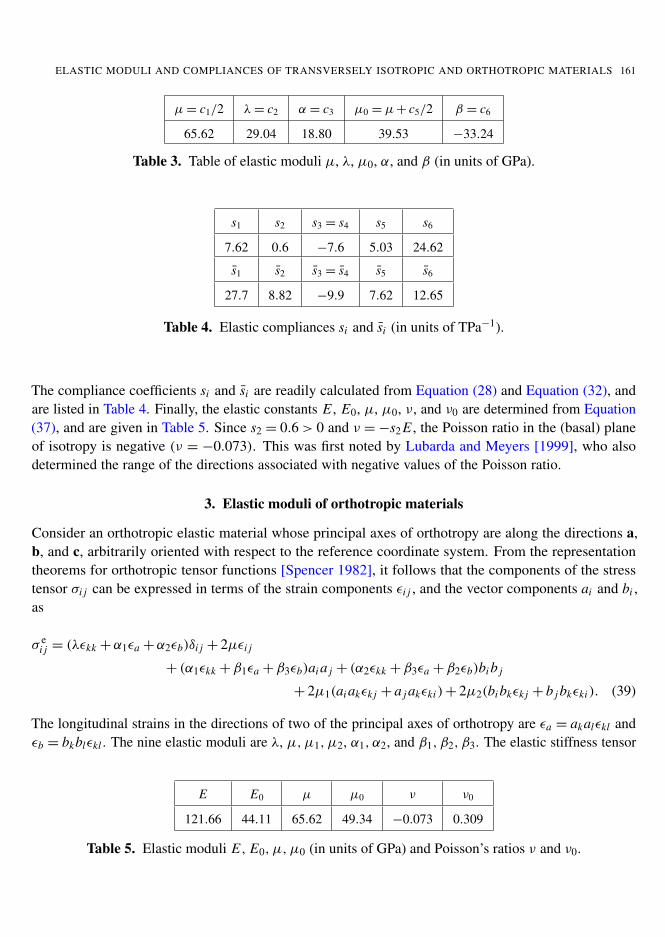
µ = c1/2 λ = c2 α = c3 µ0 = µ + c5/2 β = c6

65.62 29.04 18.80 39.53 −33.24

Table 3. Table of elastic moduli µ, λ, µ0, α, and β (in units of GPa).

s1 s2 s3 = s4 s5 s6

7.62 0.6 −7.6 5.03 24.62

s1 s2 s3 = s4 s5 s6

27.7 8.82 −9.9 7.62 12.65

Table 4. Elastic compliances si and si (in units of TPa−1).

The compliance coefficients si and si are readily calculated from Equation (28) and Equation (32), andare listed in Table 4. Finally, the elastic constants E , E0, µ, µ0, ν, and ν0 are determined from Equation(37), and are given in Table 5. Since s2 = 0.6 > 0 and ν = −s2 E , the Poisson ratio in the (basal) planeof isotropy is negative (ν = −0.073). This was first noted by Lubarda and Meyers [1999], who alsodetermined the range of the directions associated with negative values of the Poisson ratio.

3. Elastic moduli of orthotropic materials

Consider an orthotropic elastic material whose principal axes of orthotropy are along the directions a,b, and c, arbitrarily oriented with respect to the reference coordinate system. From the representationtheorems for orthotropic tensor functions [Spencer 1982], it follows that the components of the stresstensor σi j can be expressed in terms of the strain components εi j , and the vector components ai and bi ,as

σ ei j = (λεkk + α1εa + α2εb)δi j + 2µεi j

+ (α1εkk + β1εa + β3εb)ai a j + (α2εkk + β3εa + β2εb)bi b j

+ 2µ1(ai akεk j + a j akεki ) + 2µ2(bi bkεk j + b j bkεki ). (39)

The longitudinal strains in the directions of two of the principal axes of orthotropy are εa = akalεkl andεb = bkblεkl . The nine elastic moduli are λ, µ, µ1, µ2, α1, α2, and β1, β2, β3. The elastic stiffness tensor

E E0 µ µ0 ν ν0

121.66 44.11 65.62 49.34 −0.073 0.309

Table 5. Elastic moduli E, E0, µ, µ0 (in units of GPa) and Poisson’s ratios ν and ν0.


corresponding to Equation (39) is

3 =

12∑r=1

cr Ir , (40)

where the material parameters cr are

c1 = 2µ, c2 = λ, c3 = c4 = α1, c5 = c6 = α2,

c7 = 2µ1, c8 = 2µ2, c9 = β1, c10 = β2, c11 = c12 = β3.(41)

The fourth-order tensors Ir are defined by

I1 =12 δ ◦ δ, I2 = δ δ,

I3 = A δ, I4 = δ A,

I5 = B δ, I6 = δ B,

I7 = A ◦ δ, I8 = B ◦ δ,

I9 = A A, I10 = B B,

I11 = A B, I12 = B A.

(42)

In these expressions the (idempotent) tensors A, B, and C have the components

Ai j = ai a j , Bi j = bi b j , Ci j = ci c j , (43)

which are related by the identity Ai j + Bi j + Ci j = δi j . Two types of tensor products are defined by theformulas of the following type:

(A B)i jkl = Ai j Bkl,

(A ◦ B)i jkl =12 (Aik B jl + Ail B jk + A jl Bik + A jk Bil). (44)

It can be easily verified thatA ◦ B = B ◦ A, A ◦ A = 2A A. (45)

The symmetric tensors such as A A, and A ◦ B are also idempotent.The multiplication table for tensors Ir (Table 9 of the Appendix) is dense with nonzero entries, al-

though these are simple multiples of one of the Ir tensors, except for

I7 : I7 = I7 + 2I9, I8 : I8 = I8 + 2I10, (46)

andI7 : I8 = I8 : I7 = A ◦ B. (47)

The latter can be expressed as a linear combination of Ir tensors, given by the tensor E66 introduced inthe sequel.

The elastic stiffness Equation (40) can be recast in terms of a more convenient set of base tensors Ers ,such that

3 =

3∑r,s=1

crsErs + c44E44 + c55E55 + c66E66. (48)


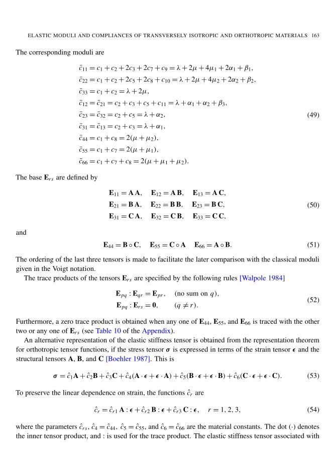
The corresponding moduli are

c11 = c1 + c2 + 2c3 + 2c7 + c9 = λ + 2µ + 4µ1 + 2α1 + β1,

c22 = c1 + c2 + 2c5 + 2c8 + c10 = λ + 2µ + 4µ2 + 2α2 + β2,

c33 = c1 + c2 = λ + 2µ,

c12 = c21 = c2 + c3 + c5 + c11 = λ + α1 + α2 + β3,

c23 = c32 = c2 + c5 = λ + α2,

c31 = c13 = c2 + c3 = λ + α1,

c44 = c1 + c8 = 2(µ + µ2),

c55 = c1 + c7 = 2(µ + µ1),

c66 = c1 + c7 + c8 = 2(µ + µ1 + µ2).

(49)

The base Ers are defined by

E11 = A A, E12 = A B, E13 = A C,

E21 = B A, E22 = B B, E23 = B C,

E31 = C A, E32 = C B, E33 = C C,

(50)

and

E44 = B ◦ C, E55 = C ◦ A E66 = A ◦ B. (51)

The ordering of the last three tensors is made to facilitate the later comparison with the classical moduligiven in the Voigt notation.

The trace products of the tensors Ers are specified by the following rules [Walpole 1984]

Epq : Eqr = Epr , (no sum on q),

Epq : Ers = 0, (q 6= r).(52)

Furthermore, a zero trace product is obtained when any one of E44, E55, and E66 is traced with the othertwo or any one of Ers (see Table 10 of the Appendix).

An alternative representation of the elastic stiffness tensor is obtained from the representation theoremfor orthotropic tensor functions, if the stress tensor σ is expressed in terms of the strain tensor ε and thestructural tensors A, B, and C [Boehler 1987]. This is

σ = c1A + c2B + c3C + c4(A · ε + ε · A) + c5(B · ε + ε · B) + c6(C · ε + ε · C). (53)

To preserve the linear dependence on strain, the functions cr are

cr = cr1 A : ε + cr2 B : ε + cr3 C : ε, r = 1, 2, 3, (54)

where the parameters crs , c4 = c44, c5 = c55, and c6 = c66 are the material constants. The dot (·) denotesthe inner tensor product, and : is used for the trace product. The elastic stiffness tensor associated with


Equation (53) and (54) is

3 =

3∑r,s=1

crsErs + c44A ◦ δ + c55B ◦ δ + c66C ◦ δ. (55)

3.1. Elastic compliances of orthotropic materials. If the elastic moduli tensor Equation (48) is symbol-ically written, with respect to the basis of Ers tensors, as

3 =

c11 c12 c13

c21 c22 c23

c31 c32 c33

, c44, c55, c66

, (56)

then its inverse, the elastic compliances tensor, can be symbolically written as [Walpole 1984]

3−1=

c11 c12 c13

c21 c22 c23

c31 c32 c33

−1

, c −144 , c −1

55 , c −166

. (57)

Thus,

3−1=

3∑r,s=1

srsErs + s44E44 + s55E55 + s66E66, (58)

where

s11 = (c22c33 − c223)/c,

s23 = s32 = (c12c31 − c11c23)/c,

s44 = 1/c44,

s12 = s21 = (c31c23 − c12c33)/c,

s31 = s13 = (c12c23 − c31c22)/c,

s55 = 1/c55,

s22 = (c11c33 − c231)/c,

s33 = (c11c22 − c212)/c,

s66 = 1/c66,

(59)

and

c = c11c22c33 + 2c12c23c31 − c11c223 − c22c2

31 − c33c212. (60)

The results for transversely isotropic materials can be recovered from the above results by takingc22 = c11, c23 = c31, and c55 = c44 = c11 − c12.

The compliances tensor can also be derived by the inversion of the elastic moduli tensor expressedwith respect to the set of base tensors used in Equation (55). This gives

3−1=

3∑r,s=1

srsErs + s44A ◦ δ + s55B ◦ δ + s66C ◦ δ, (61)

with the corresponding compliances

s11 = s11 − s66 + s44 − s55,

s12 = s12,

s44 =12 (s55 + s66 − s44),

s22 = s22 − s44 + s55 − s66,

s23 = s23,

s55 =12 (s44 + s66 − s55),

s33 = s33 − s44 + s66 − s55,

s31 = s31,

s66 =12 (s44 + s55 − s66).

(62)


3.2. Relationships to engineering constants in Voigt notation. The elastic moduli cr are related to com-monly used engineering moduli Ci j , appearing in Equation (25), by

c1 = 2(C44+C55−C66),

c5 = c6 = C23−c2,

c9 = C11+C33−2C31−4C55,

c2 = C33−c1,

c7 = 2(C66−C44),

c10 = C22+C33−2C23−4C44,

c3 = c4 = C31−c2,

c8 = 2(C66−C55),

c11 = c12 = c2+C12−C23−C31.

(63)

The relationships between ci j and Ci j are

c11 = C11,

c12 = C12,

c44 = 2C44,

c22 = C22,

c23 = C23,

c55 = 2C55,

c33 = C33,

c31 = C31,

c66 = 2C66.

(64)

To derive the relationship between the moduli ci j appearing the stiffness representation Equation (55)and the moduli ci j or Ci j , we first note that

C ◦ δ = (δ − A − B) ◦ δ = 2I1 − I7 − I8. (65)

It then readily follows that

c11 = c11 − c66 + c44 − c55,

c22 = c22 − c44 + c55 − c66,

c33 = c33 − c44 + c66 − c55,

c12 = c12,

c44 =12 (c55 + c66 − c44),

c31 = c31,

c23 = c23,

c55 =12 (c44 + c66 − c55),

c66 =12 (c44 + c55 − c66),

(66)

in agreement with the corresponding expressions derived by other means in [Boehler 1987].The compliance coefficients si j are related to the usual engineering constants of orthotropic materials

(defined with respect to its principal axes of orthotropy a, b, and c) by

s11 =1

Ea,

s22 =1

Eb,

s44 =1

2Gbc,

s12 = −νab

Ea,

s23 = −νbc

Eb,

s55 =1

2Gac,

s13 = −νac

Ea,

s33 =1Ec

,

s66 =1

2Gab.

(67)

The compliances si j are actually equal to Si j , except for the shear compliances which are related by thecoefficient of 2 (that is, S44 = 2s44, S55 = 2s55, and S66 = 2s66).


To express the elastic compliances tensor in terms of the original base tensors, we first express thetensors Ir in terms of the tensors Ers . The connections are

I1 = E11 + E22 + E33 + E44 + E55 + E66,

I2 = E11 + E12 + E13 + E21 + E22 + E23 + E31 + E32 + E33,

I3 = E11 + E12 + E13, I4 = E11 + E21 + E31,

I5 = E21 + E22 + E23, I6 = E12 + E22 + E32,

I7 = 2E11 + E55 + E66, I8 = 2E22 + E44 + E66,

I9 = E11, I10 = E22, I11 = E12, I12 = E21,

(68)

with the inverse expressions

E11 = I9, E12 = I11, E13 = I3 − I9 − I11,

E21 = I12, E22 = I10, E23 = I5 − I10 − I12,

E31 = I4 − I9 − I12, E32 = I6 − I10 − I11,

E33 = I2 − I3 − I4 − I5 − I6 + I9 + I10 + I11 + I12,

E44 = I1 − I2 + I3 + I4 + I5 + I6 − I7 − 2I10 − I11 − I12,

E55 = I1 − I2 + I3 + I4 + I5 + I6 − I8 − 2I9 − I11 − I12

E66 = −I1 + I2 − I3 − I4 − I5 − I6 + I7 + I8 + I11 + I12.

(69)

The substitution of Equation (69) into (58) then gives

3−1=

12∑r=1

sr Ir . (70)

The corresponding elastic compliances are

s1 = s55 + s66 − s44,

s3 = s4 = s13 − s33 − s44 + s55 + s66,

s7 = s44 − s55,

s9 = s11 − 2s31 + s33 − 2s66,

s2 = s33 + s44 − s55 − s66,

s5 = s6 = s23 − s33 − s44 + s55 + s66,

s8 = s44 − s66,

s10 = s22 − 2s23 + s33 − 2s55,

s11 = s12 = s21 − s23 − s31 + s33 + s44 − s55 − s66. (71)

Since srs are specified in terms of crs by Equation (59), and crs in terms of cr by Equation (49), thecompliances sr in Equation (71) are all expressed in terms of the elastic moduli cr .

The relationships Equation (71) reveal the connections between the original moduli appearing inEquation (41) and the engineering moduli. The resulting expressions in an explicit form are lengthy, buttheir numerical evaluations are simple. For example, the Young’s modulus in the direction of principalorthotropy a is

Ea =1

s11=

cc22c33 − c2

23, (72)


c1 c2 c3=c4 c5=c6 c7 c8 c9 c10 c11=c12

14.64 12.96 −2.86 −2.26 −3.42 −2.18 2.96 1.48 2.14

Table 6. Elastic moduli ci (in units of GPa).

where ci j are given by Equation (49) and c by (60). In the case of transverse isotropy, with the axis ofisotropy parallel to c (c22 = c11, c23 = c31, and c55 = c44 = c11 − c12), this reduces to Equation (72),while in the isotropic case (α1 = α2 = β1 = β2 = β3 = 0 and µ1 = µ2 = µ), we recover the resultE = µ(3λ + 2µ)/(λ + µ).

3.3. Elastic constants of a human femur. Elastic moduli Ci j of a human femural bone, determined byultrasound measurement technique, were reported in Ashman and Buskirk (1987) asC11 C12 C13

C21 C22 C23

C31 C32 C33

=

18 9.98 10.19.98 20.2 10.710.1 10.7 27.6

,

C44

C55

C66

=

6.235.614.52

(GPa).

The corresponding moduli ci j and ci j follow from (64) and (66). In units of GPa, they arec11 c12 c13

c21 c22 c23

c31 c32 c33

=

18 9.98 10.19.98 20.2 10.710.1 10.7 27.6

,

c44

c55

c66

=

12.4611.229.04

,

c11 c12 c13

c21 c22 c23

c31 c32 c33

=

10.2 9.98 10.19.98 9.92 10.710.1 10.7 12.96

,

c44

c55

c66

=

3.95.147.32

.

The moduli ci , calculated from Equation (63), are listed in Table 6.The elastic compliances Si j (in units of TPa−1), corresponding to elastic moduli Ci j given above, areS11 S12 S13

S21 S22 S23

S31 S32 S33

=

83.24 −31.45 −18.27−31.45 74.18 −17.25−18.27 −17.25 49.60

,

S44

S55

S66

=

160.52178.26221.24

.

The compliances si j and si j follow from (59) and (62). In units of TPa−1, they ares11 s12 s13

s21 s22 s23

s31 s32 s33

=

83.24 −31.45 −18.27−31.45 74.18 −17.25−18.27 −17.25 49.60

,

s44

s55

s66

=

80.2689.13

110.62

,

s11 s12 s13

s21 s22 s23

s31 s32 s33

=

−36.24 −31.45 −18.27−31.45 −27.57 −17.25−18.27 −17.25 −9.16

,

s44

s55

s66

=

59.7450.8729.38

.

The above results show that for human femur Si j and si j are negative for i 6= j , while si j are nega-tive for all i , j = 1, 2, 3. The compliance coefficients si , calculated from Equation (71), are listed inTable 7. The longitudinal and shear moduli and the Poisson ratios, with respect to the principal axes of


s1 s2 s3=s4 s5=s6 s7 s8 s9 s10 s11=s12

119.49 −69.88 51.61 52.63 −8.87 −30.36 −51.85 −19.97 −65.81

Table 7. Elastic compliances si (in units of TPa−1).

Ea Eb Ec Gab Gbc Gac νab νbc νac

12.01 13.48 20.16 4.52 6.23 5.61 0.378 0.233 0.219

Table 8. Longitudinal and shear moduli (in units of GPa) and the Poisson ratios.

orthotropy, follow from Equation (67) and are given in Table 8. The remaining three Poisson’s ratiosare determined from the well known connections νba = νab Eb/Ea = 0.424, νcb = νbc Ec/Eb = 0.348,and νca = νac Ec/Ea = 0.368.

4. Conclusion

In this paper we have derived the relationships between the elastic moduli and compliances of transverselyisotropic materials, which correspond to two different sets of linearly independent fourth-order basetensors used to cast the tensorial representation of the elastic moduli and compliances tensors. The twosets of elastic constants are related to engineering constants defined with respect to the coordinate systemin which one of the axes is parallel to the axis of material symmetry. Extending the analysis to orthotropicmaterials, three different representations of the elastic moduli tensor are constructed by choosing threeappealing sets of twelve linearly independent fourth-order base tensors. This was accomplished onthe basis of the representation theorems for orthotropic tensor functions of a symmetric second-ordertensor and the structural tensors associated with the principal axes of orthotropy. The three sets of thecorresponding elastic moduli are related to each other. The compliances tensor is deduced by an explicitinversion of the stiffness tensor for all considered sets of the base tensors. The different compliances arerelated to each other, and to classical engineering constants expressed in the Voigt notation. The formulasare applied to calculate the elastic constants for a transversely isotropic monocrystalline zinc and anorthotropic human femural bone. Apart from the analytical point of view, the derived results may be ofinterest for the analysis of anisotropic elastic and inelastic material response (with an elastic componentof strain or stress) in the mechanics of fiber reinforced composite materials [Hyer 1998; Vasiliev andMorozov 2001], creep mechanics [Drozdov 1998; Betten 2002], damage-elastoplasticity [Lubarda 1994],mechanics of brittle materials weakened by anisotropic crack distributions [Krajcinovic 1996; Voyiadjisand Kattan 1999], and biological materials (membranes or tissues) with embedded filament networks[Evans and Skalak 1980; Fung 1990; Humphrey 2002; Lubarda and Hoger 2002; Asaro and Lubarda2006].


� I1 I2 I3 I4 I5 I6 I7 I8 I9 I10 I11 I12

I1 I1 I2 I3 I4 I5 I6 I7 I8 I9 I10 I11 I12

I2 I2 3I2 I2 3I4 I2 3I6 2I4 2I6 I4 I6 I6 I4

I3 I3 3I3 I3 3I9 I3 3I11 2I9 2I11 I9 I11 I11 I9

I4 I4 I2 I2 I4 0 I6 2I4 0 I4 0 I6 0

I5 I5 3I5 I5 3I12 I5 3I10 2I12 2I10 I12 I10 I10 I12

I6 I6 I2 0 I4 I2 I6 0 2I6 0 I6 0 I4

I7 I7 2I3 2I3 2I9 0 2I11 I7 + 2I9 A ◦ B 2I9 0 2I11 0

I8 I8 2I5 0 2I12 2I5 2I10 A ◦ B I8 + 2I10 0 2I10 0 2I12

I9 I9 I3 I3 I9 0 I11 2I9 0 I9 0 I11 0

I10 I10 I5 0 I12 I5 I10 0 2I10 0 I10 0 I12

I11 I11 I3 0 I9 I3 I11 0 2I11 0 I11 0 I9

I12 I12 I5 I5 I12 0 I10 2I12 0 I12 0 I10 0

Table 9. Table of products Ir : Is .

� E11 E12 E13 E21 E22 E23 E31 E32 E33 E44 E55 E66

E11 E11 E12 E13 0 0 0 0 0 0 0 0 0

E12 0 0 0 E11 E12 E13 0 0 0 0 0 0

E13 0 0 0 0 0 0 E11 E12 E13 0 0 0

E21 E21 E22 E23 0 0 0 0 0 0 0 0 0

E22 0 0 0 E21 E22 E23 0 0 0 0 0 0

E23 0 0 0 0 0 0 E21 E22 E23 0 0 0

E31 E31 E32 E33 0 0 0 0 0 0 0 0 0

E32 0 0 0 E31 E32 E33 0 0 0 0 0 0

E33 0 0 0 0 0 0 E31 E32 E33 0 0 0

E44 0 0 0 0 0 0 0 0 0 E44 0 0

E55 0 0 0 0 0 0 0 0 0 0 E55 0

E66 0 0 0 0 0 0 0 0 0 0 0 E66

Table 10. Table of products Ers : Epq .


Appendix: Multiplication tables for tensors Ir and Ers

The trace products Ir : Is are listed in Table 9. The tensors Ir are defined in Equation (42). The symbol� indicates that the products are in the order: a tensor from the left column traced with a tensor from thetop row. The products Ers : Epq , where the tensors Ers are defined in Equation (50) and (51), are listedin Table 10.

References

[Asaro and Lubarda 2006] R. J. Asaro and V. A. Lubarda, Mechanics of solids and materials, Cambridge University Press,Cambridge, 2006.

[Betten 1987] J. Betten, “Invariants of fourth-order tensors”, pp. 203–226 in Applications of tensor functions in solid mechanics,edited by J. P. Boehler, CISM Courses and Lectures 292, Springer-Verlag, Wien, 1987.

[Betten 2002] J. Betten, Creep mechanics, Springer-Verlag, Berlin, 2002.

[Boehler 1987] J. P. Boehler, “Representations for isotropic and anisotropic non-polynomial tensor functions”, pp. 31–53 inApplications of tensor functions in solid mechanics, edited by J. P. Boehler, CISM Courses and Lectures 292, Springer, Wien,1987.

[Cowin and Mehrabadi 1995] S. C. Cowin and M. M. Mehrabadi, “Anisotropic symmetries in linear elasticity”, Appl. Mech.Rev. 48 (1995), 247–285.

[Drozdov 1998] A. D. Drozdov, Mechanics of Viscoelastic Solids, John Wiley & Sons, New York, 1998.

[Evans and Skalak 1980] E. A. Evans and R. Skalak, Mechanics and thermodynamics of biomembranes, CRC Press, BocaRaton, Florida, 1980.

[Fung 1990] Y.-C. Fung, Biomechanics: motion, flow, stress, and growth, Springer-Verlag, New York, 1990.

[Gangi 2000] A. F. Gangi, “Fourth-order elastic-moduli tensors by inspection”, pp. 1–10 in Fractures, converted waves andcase studies–proceedings of the ninth international workshop on seismic anisotropy, Tulsa, OK, 2000.

[Hearmon 1961] R. F. E. Hearmon, An introduction to applied anisotropic elasticity, Clarendon Press, Oxford, 1961.

[Humphrey 2002] J. D. Humphrey, Cardiovascular solid mechanics: cells, tissues, and organs, Springer-Verlag, New York,2002.

[Hyer 1998] M. W. Hyer, Stress analysis of fiber-reinforced composite materials, McGraw-Hill, Boston, 1998.

[Krajcinovic 1996] D. Krajcinovic, Damage mechanics, Elsevier, New York, 1996.

[Kunin 1981] I. A. Kunin, “An algebra of tensor operations and its applications to elasticity”, Int. J. Engng. Sci. 19 (1981),1551–1561.

[Kunin 1983] I. A. Kunin, Elastic media with microstructure, part II, Springer-Verlag, Berlin, 1983.

[Landolt-Börnstein 1979] Landolt-Börnstein, Numerical data and functional relationships in science and technology, vol. 11,edited by K.-H. Hellwege and A. M. Hellwege, Group III, Springer-Verlag, Berlin, 1979.

[Lekhnitskii 1981] S. G. Lekhnitskii, Theory of elasticity of an anisotropic elastic body, Mir Publishers, Moscow, 1981.

[Lubarda 1994] V. A. Lubarda, “An analysis of large-strain damage elastoplasticity”, Int. J. Solids Struct. 31 (1994), 2951–2964.

[Lubarda and Hoger 2002] V. A. Lubarda and A. Hoger, “On the mechanics of solids with a growing mass”, Int. J. Solids Struct.39 (2002), 4627–4664.

[Lubarda and Krajcinovic 1994] V. A. Lubarda and D. Krajcinovic, “Tensorial representation of the effective elastic propertiesof the damaged material”, Int. J. Damage Mech. 3 (1994), 38–56.

[Lubarda and Meyers 1999] V. A. Lubarda and M. A. Meyers, “On the negative Poisson ratio in monocrystalline zinc”, ScriptaMater. 40 (1999), 975–977.

[Mehrabadi and Cowin 1990] M. M. Mehrabadi and S. C. Cowin, “Eigentensors of linear anisotropic elastic materials”, Q. Jl.Mech. Appl. Math. 43 (1990), 15–41.


[Nadeau and Ferrari 1998] J. C. Nadeau and M. Ferrari, “Invariant tensor-to-matrix mappings for evaluation of tensorial ex-pressions”, J. Elasticity 52 (1998), 43–61.

[Nye 1964] J. F. Nye, Physical properties of crystals: their representation by tensors and matrices, Clarendon Press, Oxford,1964.

[Rychlewski 1984] J. Rychlewski, “On Hooke’s law”, J. Appl. Mech. Math. 48 (1984), 303–314.

[Spencer 1982] A. J. M. Spencer, “The formulation of constitutive equation for anisotropic solids”, pp. 2–26 in Mechanicalbehavior of anisotropic solids, edited by J. P. Boehler, Martinus Nijhoff Publishers, The Hague, 1982.

[Srinivasan and Nigam 1969] T. P. Srinivasan and S. D. Nigam, “Invariant elastic constants for crystals”, J. Math. Mech. 19(1969), 411–420.

[Sutcliffe 1992] S. Sutcliffe, “Spectral decomposition of the elasticity tensor”, J. Appl. Mech. 59 (1992), 762–773.

[Theocaris and Philippidis 1989] P. S. Theocaris and T. P. Philippidis, “Elastic eigenstates of a medium with transverseisotropy”, Arch. Mech. 41 (1989), 717–724.

[Theocaris and Sokolis 2000] P. S. Theocaris and D. P. Sokolis, “Spectral decomposition of the compliance fourth-rank tensorfor orthotropic materials”, Arch. Appl. Mech. 70 (2000), 289–306.

[Ting 1987] T. C. T. Ting, “Invariants of anisotropic elastic constants”, Q. Jl. Mech. Appl. Math. 40 (1987), 431–448.

[Ting 2000] T. C. T. Ting, “Anisotropic elastic constants that are structurally invariant”, Q. Jl. Mech. Appl. Math. 53 (2000),511–523.

[Ting and He 2006] T. C. T. Ting and Q.-C. He, “Decomposition of elasticity tensors and tensors that are structurally invariantin three dimensions”, Q. Jl. Mech. Appl. Math. 59 (2006), 323–341.

[Vasiliev and Morozov 2001] V. V. Vasiliev and E. V. Morozov, Mechanics and analysis of composite materials, Elsevier,Amsterdam, 2001.

[Voigt 1928] W. Voigt, Lehrbuch der Kristallphysik, Johnson Reprint Corporation, New York, 1928. (1966 reprint).

[Voyiadjis and Kattan 1999] G. Z. Voyiadjis and P. I. Kattan, Advances in damage mechanics: metals and metal matrix com-posites, Elsevier, New York, 1999.

[Walpole 1984] L. J. Walpole, “Fourth-rank tensors of the thirty-two crystal classes: multiplication tables”, Proc. Royal Soc.London A 391 (1984), 149–179.

[Zheng 1994] Q.-S. Zheng, “Theory of representations for tensor functions—a unified invariant approach to constitutive equa-tions”, Appl. Mech. Rev. 47 (1994), 545–587.

Received 19 Mar 2007. Revised 8 Jun 2007. Accepted 11 Jun 2007.

VLADO A. LUBARDA: [email protected] of Mechanical and Aerospace Engineering, University of California, San Diego, 9500 Gilman Drive,La Jolla, CA 92093-0411, United States

MICHELLE C. CHEN: [email protected] of Structural Engineering, University of California, San Diego, 9500 Gilman Drive, La Jolla, CA 92093-0085,United States

mailto:[email protected]

mailto:[email protected]

journal of mechanics of materials and...

Documents