journal of lightwave technology, vol. 27, no. 13, july … · journal of lightwave technology, vol....

JOURNAL OF LIGHTWAVE TECHNOLOGY, VOL. 27, NO. 13, JULY 1, 2009 2315

Cost Comparison of Optical Circuit-Switched andBurst-Switched Networks

Rajendran Parthiban, Member, IEEE, Christopher Leckie, Andrew Zalesky, Moshe Zukerman, Fellow, IEEE, andRodney S. Tucker, Fellow, IEEE, Fellow, OSA

Abstract—This paper examines the economic viability of twotechnologies—optical circuit-switched (OCS) networks and op-tical burst-switched (OBS) networks—in the core network. Weanalyze and dimension OCS network (OCSN) and OBS network(OBSN) architectures for a range of traffic demands given theconstraints on the network element capacities. We investigatethe effect of traffic grooming for both of these architectures. Weevaluate these network architectures for a national core networkin Australia in terms of their capital costs and packet-blockingprobabilities. We observe that OBSNs with traffic grooming atthe optical layer may become more cost effective than OCSNswith traffic grooming at both the IP and optical layers for thesame quality of service in terms of blocking probability. The costadvantage of OBSNs over OCSNs grows as the capacity of thecore network increases. Hence, among the all-optical networkingoptions that do not involve buffering at the core, OBS appears tobe an attractive option especially for high-capacity core networks.

Index Terms—IP aggregation, optical burst-swtiched (OBS), op-tical circuit-switched (OCS), traffic grooming, waveband, wave-length conversion.

I. INTRODUCTION

O PTICAL networks are expected to provide a platform forthe next generation of very high bandwidth applications

[1], [2]. Many candidate architectures have been proposedfor future optical networks, including optical circuit-switchednetworks (OCSNs) [3] and optical burst-switched networks(OBSNs) [4], [5]. The final choice of architecture depends ona number of factors, such as the capital expenditure (CAPEX)cost, operational expenditure (OPEX) cost, and energy con-sumption of the network for a given level of performance.

Manuscript received April 18, 2008; revised October 03, 2008. First pub-lished April 21, 2009; current version published June 26, 2009. This work wassupported by the Australian Research Council. Most of the work on this paperwas done when the authors were with the ARC Special Research Centre forUltra-Broadband Information Networks.

R. Parthiban is with the School of Engineering, Monash University, SelangorDarul Ehsan 46150, Malaysia (e-mail: [email protected]).

C. Leckie is with the Department of Computer Science and SoftwareEngineering, University of Melbourne, 3010 Victoria, Australia (e-mail:[email protected]).

A. Zalesky with with the ARC Special Research Centre for Ultra-BroadbandInformation Networks. He is now with the University of Melbourne, 3010 Vic-toria, Australia (e-mail: [email protected]).

M. Zukerman is with the Electronic Engineering Department, City Universityof Hong Kong, Kowloon, Hong Kong (e-mail: [email protected]).

R. S. Tucker is with the ARC Special Research Centre for Ultra-BroadbandInformation Networks, University of Melbourne, 3010 Victoria, Australia(e-mail: [email protected]).

Color versions of one or more of the figures in this paper are available onlineat http://ieeexplore.ieee.org.

Digital Object Identifier 10.1109/JLT.2008.2007854

However, the suitability of different network architectures interms of these costs has not been a major focus of researchin the literature. In this paper, we compare different typesof OCSN and OBSN architectures in terms of their CAPEXrequirements for a clean build of a national core network.

In OCSN architectures for the core network, traffic is carriedon dedicated lightpaths between routers at the edge of the net-work via wavelength division multiplexed (WDM) links and op-tical cross connects (OXCs). In such a network, it is important tointroduce some form of traffic grooming to reduce the numberof lightpaths and OXC ports used, which have been shown to bemajor contributors to the CAPEX cost of the network [6]. Trafficgrooming can be introduced in both the optical domain usingwaveband grooming, and in the IP domain using routers to ag-gregate traffic from multiple lightpaths [7]–[11]. However, theuse of IP routers has an associated cost in terms of the numberof Optical-to-Electrical-to-Optical (OEO) interfaces and routerports required [6], [12].

An alternative approach that has been proposed to reducethe cost of optical networks is optical burst switching (OBS)[4], [5]. In an OBS network (OBSN), IP packets are assem-bled into variable-size data units, called bursts, by burst as-sembly routers (BARs). In order to send bursts from a sourceBAR to a destination BAR, a control packet is sent in advanceto request and reserve bandwidth in the optical burst switches(OBXs) along a prespecified route [5]. After an offset period,bursts are sent along this route. An attractive feature of OBSNsis that they provide routing without requiring OEO interfaces[4], [5], or optical buffering [13]. However, OBSNs tend to havehigh blocking probability [14], [15], and hence require a largenumber of lightpaths.

The aim of this paper is to compare the effects of differenttraffic grooming techniques on the CAPEX cost of future opticalcore networks. In particular, we consider the merits of using IProuters to groom traffic in OCSNs, as well as using wavebandgrooming in both OCSNs and OBSNs, so that multiple light-paths can be switched using a single OXC or OBX port [16].We also consider burst segmentation [17]–[22] and deflectionrouting [23]–[26] to enable OBSNs to use fewer lightpaths [27].By making such a comparison, we aim to provide a baseline forassessing different optical network architectures in the future.

II. PREVIOUS COST COMPARISONS

In this section, we survey the literature on cost comparisonsbetween OCSNs and OBSNs. Several studies have been madeon the performance of OCSNs and OBSNs in terms of thenumber of wavelengths required to achieve a given blockingprobability or grade of service. If there are no routers in the

0733-8724/$25.00 © 2009 IEEE

2316 JOURNAL OF LIGHTWAVE TECHNOLOGY, VOL. 27, NO. 13, JULY 1, 2009

core of the OCSN, then traffic can only be groomed at thegranularity of a wavelength. In contrast, OBSNs can use OBXsto statistically multiplex traffic from multiple streams onto thesame wavelength. Consequently, for bursty traffic, studies suchas [28]–[32] have shown that OBSNs can achieve a higherperformance than ordinary OCSNs, i.e., OCSNs without IProuters or grooming above the wavelength level.

In practice, some form of additional traffic grooming is usedin OCSNs. Traffic can be groomed using IP routers to provideswitching with subwavelength granularity [6], or by usingwaveband switching (WS) to switch multiple wavelengthsusing a single OXC port [10], [11]. We have previously shown[33] that by using WS and IP routers for traffic grooming inOCSNs, we can significantly reduce network cost comparedto an OBSN architecture, based on an empirical model [34] tocalculate the blocking probability in routers at the edge of thenetwork. In this paper, we consider whether introducing WS inOBSNs (i.e., Waveband BS or WBS) can achieve similar costsavings in OBSNs.

Most studies have considered a comparison of OCSNs andOBSNs based on conventional teletraffic performance measuressuch as packet-blocking probability and delay. See [14], [17],[26], [35]–[44] and references therein for blocking performancemodels and their analyses. In this paper, we consider how todimension different OCSN and OBSN architectures under statictraffic conditions, and compare these architectures in terms oftheir CAPEX cost for a range of target-blocking probabilities.We also take traffic grooming into account, and consider a high-capacity core network.

In [33], we considered a nonbursty traffic model for dimen-sioning the optical core network. However, it has been observedthat Internet traffic is bursty and exhibits self-similar and long-range dependence (LRD) characteristics [45], [46]. It has beensuggested that OBSNs should outperform OCSNs for burstytraffic [5]. Hence, considering self-similar LRD arrival trafficappears to be more realistic [47], and reasonable for OBSNs[5]. For this reason, in the present paper, we extend our previouswork by using a self-similar LRD traffic model.

The remainder of this paper is organized as follows. We de-scribe the general network model, and the architectures of theOBSNs and OCSNs in Section III. Section IV describes the di-mensioning and analysis process we use for the comparison. InSection V, we evaluate these architectures and discuss the re-sults. Since we use many acronyms, we spell them out in Table Iin alphabetical order for easy reference.

III. NETWORK MODEL AND ARCHITECTURES

In this section, we describe the different types of networkarchitectures that we consider in this study. Our general net-work model is based on a model proposed by the ITU for back-bone networks [48], and has been the basis for similar studies[49], [50]. Based on this general model, we consider five dif-ferent OCSN architectures—(i) OXC, (ii) OXC(WC), (iii) op-tical IP, (iv) waveband, and (v) waveband IP—and three OBSNarchitectures—(i) OBS, (ii) OBS(WC), and (iii) WBS(WC). Ineach case, we explain how each architecture affects the requirednumber of ports in an OXC, and the number of lightpaths in thenetwork. Fig. 1 shows the general network model.

TABLE ILIST OF ACRONYMS

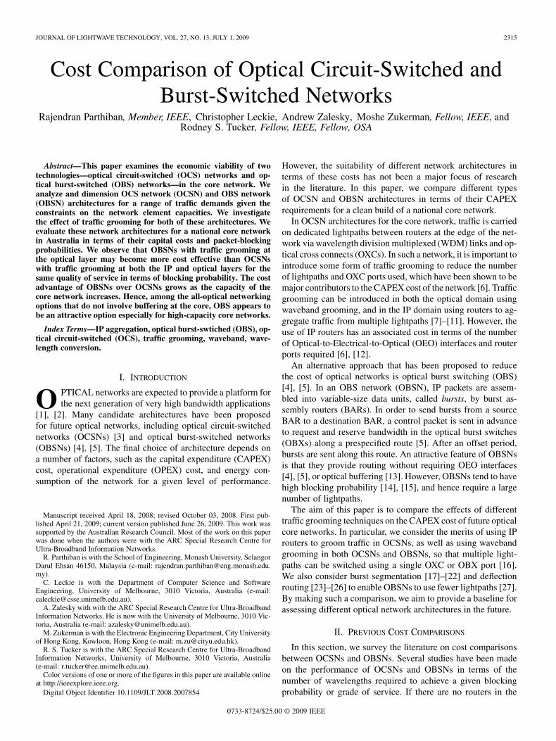
Fig. 1. General network model.

In Fig. 1, edge routers (ERs) are used to groom IP traffic fromusers, and exchange data through the core network. There aretwo types of nodes in the core network: edge nodes and corenodes. Edge nodes are directly connected to the ERs, whereascore nodes are not. Core nodes are used to manage pass-throughtraffic, which goes through a node without originating or ter-minating at that node. An edge node can manage both pass-through traffic and add-drop traffic originating or terminatingat the node. We refer to the ports required for pass-through andadd-drop traffics in each edge node as pass-through ports andadd-drop ports, respectively. Separate links are used to managethe incoming and outgoing traffic from an ER to an edge node.

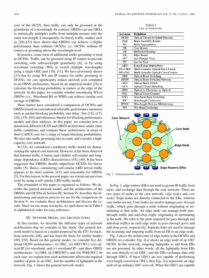
Fig. 2 shows the architecture of edge nodes in the OCSNs andOBSNs we consider. Fig. 2(a) shows an edge node of an OXCOCSN. In this network, outgoing lightpaths to and from ERsare not groomed. In other words, all the lightpaths from ERsare sent directly to an OXC, and the ERs exchange data onlythrough OXCs. If these OXCs are not capable of performingwavelength conversion (WC), then Fig. 2(a) represents an edgenode of an ordinary OXC network. When the OXCs are capable

PARTHIBAN et al.: COST COMPARISON OF OPTICAL CIRCUIT-SWITCHED AND BURST-SWITCHED NETWORKS 2317

Fig. 2. Edge node architectures. (a) OXC and OXC(WC). (b) Optical IP.(c) Waveband. (d) Waveband IP. (e) OBS and OBS(WC). (f) WBS(WC).

of performing WC, then Fig. 2(a) represents an edge node of anOXC(WC) OCSN.

Fig. 2(b) shows an edge node of an optical IP OCSN. InFig. 2(b), outgoing lightpaths from ERs are groomed at the IPlayer using core IP routers (CRs). The core IP routers aggregatethe traffic from ERs, and reduce the number of lightpaths in-jected to the OXC [6]. Hence, the number of lightpaths used inan optical IP network is less than the number of lightpaths usedin an OXC network. Therefore, there is a tradeoff here betweenthe savings due to the reduced number of lightpaths and the costof extra core IP routers in the OXC OCSN.

Fig. 2(c) shows the edge node architecture of anotherOCSN—the waveband network. In Fig. 2(c), outgoing light-paths from edge nodes are groomed at the optical layer.Multiplexers (MUXs) are used to groom the lightpaths intoa waveband, and multiple wavebands into a fiber. In order toswitch lightpaths, wavebands and fibers, we use a multi-gran-ular OXC (MG-OXC) in the edge nodes [10], [11]. Since we canswitch a group of lightpaths using a single port in an MG-OXC,waveband networks require fewer ports in MG-OXCs thanOXC networks. If the savings in reduced ports in the OXCsoutweigh the cost of these extra components such as MUXs andDeMUXs, then waveband grooming is of benefit in reducingthe cost of an OCSN.

Fig. 2(d) shows an edge node of the waveband IP OCSN.In Fig. 2(d), outgoing lightpaths from edge nodes are groomedat both the IP and optical layers. Hence, this network type re-quires fewer lightpaths and fewer ports per OXC than the OXCnetwork.

Fig. 2(e) shows an edge node of an OBSN. In this network, thetraffic between ERs is exchanged using bursts. The IP packetsfrom ERs are assembled into bursts by a burst assembly router(BAR), and switched by an optical burst switch (OBX). Thebursts from the destination OBX are converted to IP packets by aburst dis-assembly router [5]. If the OBXs in an OBSN have nowavelength conversion (WC) capability, then this is an ordinaryOBS network type. If the OBXs have the ability to perform full

WC, where each incoming wavelength has a wavelength con-verter that spans the entire wavelength range of a fiber, then thisis an OBS(WC) network.

Fig. 2(f) shows an edge node of a WBS(WC) network, which isan OBS(WC) network that includes wavelength grooming [27].We identify apriori bursts that traverse the same set of consecu-tive links. We assign adjacent wavelengths to these bursts in theWDM spectrum. Then, we group these bursts into a super burston a waveband. This enables all the wavelengths in a wavebandto be switched using a single port in an OBX [27]. In order toswitch wavebands, we use a multi-granular OBX (MG-OBX) inthe edge nodes [16]. A WBS(WC) network requires fewer portsper MG-OXC, and hence fewer MG-OXCs than an OBS(WC)network. Additional features such as burst segmentation (BS)and deflection routing (DR) can also be added to this network[27].

Burst segmentation and deflection routing are two distinctstrategies that have been proposed to resolve wavelength con-tention, and thereby reduce the packet-blocking probability.Wavelength contention occurs when a header seeks to reservea wavelength for a period that overlaps an existing reservation.The traditional solution to the contention problem is to buffera contending burst until a wavelength in the desired outgoinglink is available. However, buffering electronically defeats theall-optical nature of OBS, while buffering optically is costlyand technically challenging.

Burst segmentation and deflection routing provide viable al-ternatives to buffering. With deflection routing, a contendingburst is switched to an outgoing link other than its preferred out-going link. The alternative outgoing link forms the first hop ofa deflection route leading to the contending burst’s destination.Deflection routing in OBS suffers the same shortcomings as de-flection routing in electronic packet-switched networks. In par-ticular, delay is increased due to bursts traversing longer routeson average, packets arriving out of sequence and positive feed-back resulting in instability [26].

The reservation period sought by a contending burst mayoverlap only a certain portion of an existing reservation pe-riod. In this case, the burst can be divided into two smallerbursts. One of the smaller bursts contains all the packets of theparent burst that do not overlap the existing reservation. Thissmaller burst proceeds to traverse the same route as its parent.The other smaller burst containing all the packets that do overlapis blocked. This approach is referred to as burst segmentation.Burst segmentation allows some packets to be salvaged from aburst that would otherwise be blocked in its entirety. Further de-tails can be found in [20].

Several performance models have quantified the substantialreduction in packet-blocking probability that can be effectedwith burst segmentation and/or deflection routing (e.g., [14],[44], [51]), though implementing either of these techniques inpractice may prove to be technically challenging.

We now explain the architecture of the core nodes of thesenetworks. A core node of the OXC, OXC(WC), and optical IPnetworks has an OXC. However the OXCs of the OXC(WC) net-works are capable of performing WC. A core node of the wave-band and waveband IP networks contains a MG-OXC. Simi-larly, a core node of the OBS and OBS(WC) networks consists


TABLE IIFEATURES AND CHARACTERISTICS OF THE NETWORK ARCHITECTURES CONSIDERED

TABLE IIIINPUTS TO ANALYTICAL FRAMEWORK

of an OBX. The OBXs in the OBS(WC) network have the abilityto perform WC. A core node of the WBS(WC) network has aMG-OBX capable of performing WC.

Table II summarizes the main features of the architectures wediscussed above and their important characteristics.

IV. ANALYTICAL FRAMEWORK

In this section, we develop an analytical framework to dimen-sion and compare OCSNs and OBSNs. In both types of net-works, the traffic from users arrives at ERs, and is then routedbetween ERs through the core network.

We model the arrival of traffic flows into the core network asGaussian LRD due to the bursty nature of IP traffic [45], [46].We assume this traffic is then evenly distributed among all thesource-destination pairs of ERs. This assumption is necessaryto allow for a tractable framework that is amenable to analysis.

We now describe how we dimension each network type forthis given input traffic flow, and analyze each network type interms of its overall network cost.

A. Dimensioning and Analysis of Network Types

In this sub-section, we explain the major steps in our analyt-ical framework. Inputs to this framework are shown in Table III.We now describe the steps involved. These steps are shown as aflowchart in Fig. 3.

Fig. 3. Flowchart describing analytical framework.

1) Calculate Total Traffic and Number of ERs: First, wecalculate the total arrival traffic to the core network, and thenumber of ERs required to exchange this traffic through the corenetwork.

The total traffic is , where the number of users ,the average access rate per user , and the effective ratio are


known. We define the access rate as the maximum rate that a usercan access the network over an extended time during a busy pe-riod. The effective ratio accounts for traffic burstiness and net-work overheads. Its value can be derived using traffic measure-ments as in [34]. By examining the traffic added to and droppedfrom the core network by ERs, the number of ERs required inthe network can be calculated as [6], [12], where

is the capacity of an ER in bits/s and is a known parameter.The factor 2 is included in this expression to account for the in-coming and outgoing traffic from an ER to the core network.

2) Choose a Target Blocking Probability: We choose aquality of service requirement within a target-blocking proba-bility range . In this paper, this range is . Foreach target-blocking probability, we dimension each networkand find outputs such as the overall network cost.

3) Find Number of Edge Nodes and CRs: In the third step ofour analytical framework, we start dimensioning each networktype to satisfy the network element constraints on the numberof lightpaths per fiber, the number of ports per switch, and thecapacity of CRs/BARs. In this step, for the given set of trafficdemands, we find the number of edge nodes , core nodes , andCRs/BARs , and their hierarchical interconnection topologythrough an iterative process.

We start by setting the add-drop ports per edge node . Thenumber of edge nodes is inversely proportional to [6], [12].For this reason, we vary the value of from the maximumnumber of ports per switch to 1 to find the minimum pos-sible number of edge nodes. For each value of , we followthe steps outlined below and check whether the network ele-ment constraints are satisfied. If they are not satisfied, then wedecrement the value of and follow the same process.

When the value of is known, we find the number of edgenodes using the following equation by examining the trafficflow in each edge node (see [6], [12] for details).

(1)

Then, we examine the incoming and outgoing traffic of eachedge node and find the number of CRs by taking into accountthe maximum capacity of a CR/BAR . Our results show that,in general, the number of CRs is , where is a positiveinteger that can be determined [12].

4) Select Number of Core Nodes: All network architectureshave a hierarchical topology with edge nodes and core nodes.We find the number of core nodes for each value of usinganother iterative process. We vary the value of from 1 toand follow the steps discussed below for each value. We stopiterating once the number of ports in each core node is sufficientto accommodate the traffic flow requirements through the corenodes in the network (see [12] for details).

5) Set Number of Destinations: The maximum number ofdestinations from each ER is , where is the number ofERs. If we cannot achieve the target-blocking probability usingthis value, then we set the number of destinations as , whereis a positive integer that needs to be determined. The maximumvalue for is . Our analysis shows that with ,we can achieve all the target-blocking probabilities in the range

for all network architectures.

Similarly, the maximum of number of destinations from eachCR is , where is the number of edge nodes. This value issufficient for CRs to achieve all the target-blocking probabilitiesin the range .

6) Identify Network Elements With Blocking: We findthe number of lightpaths required in the core network (i.e.,from ERs and CRs/BARs) in order to achieve an end-to-endblocking probability that is less than or equal to thetarget-blocking probability. Assuming independence ofblocking events, the end-to-end blocking probability is

. A switch can be an OXC, MG-OXC, OBXor MG-OBX, depending on the type of network. Therefore,

. Inother words, for a packet/burst to be successfully transmitted,it must not be blocked at an ER, CR, or a switch. We makesure that the end-to-end blocking probability is the same forOCSNs and OBSNs.

We consider a static OCSN whereby it is not possible forlightpaths to be set up and torn down dynamically. In otherwords, the lightpaths in our OCSN model are permanent, andthus it is not possible for packet loss to occur at an interme-diate switch. We ensure that a sufficient number of wavelengthshave been deployed to ensure at least one dedicated lightpathcan be established between each source and destination pair.More specifically, we dimension the OCSNs so that a sufficientnumber of lightpaths can be established between each sourceand destination pair to ensure the end-to-end blocking proba-bility for each source and destination pair does not exceed aprescribed value. For this reason, we can assign wavelengthsto lightpaths on an end-to-end basis for an OCSN, i.e., a globalwavelength assignment scheme can be adopted at ERs and/orCRs. Hence, multiple simultaneous lightpath connections canbe provided in the switches of an OCSN without wavelengthconflicts. In the dimensioning stage of an OCSN, we provide asufficient number of switches (and ports in switches) to accom-modate the lightpath traffic requirement between ERs and/orCRs, and assign wavelengths to these lightpaths. This results inzero blocking in the switches of an OCSN. However, we shouldnote that the extra ports and switches of the OCSN add to theoverall network cost.

If we model OCSNs as we have specified above, theend-to-end blocking probability for OCSNs is

. Some OCSNs(such as OXC, OXC(WC) and waveband) have ERs and noCRs. For them, the end-to-end blocking probability of a packetis due to the buffer overflow in ERs, i.e., .Other OCSNs (such as optical IP and waveband IP) have ERsand CRs. For these OCSNs, the end-to-end blocking proba-bility is due to the buffer overflow in ERs and CRs, and hence

.In the case of an OBSN, we can only assign wavelengths to

bursts locally on a node-to-node basis. For this reason, in thedimensioning stage, we cannot avoid blocking in OBX nodesof an OBSN in contrast to no blocking in the switches of anOCSN. For OBSNs, the causes of a packet being blocked can beeither buffer overflow in an ER or a BAR, or wavelength con-tention at an intermediate OBX. Hence, the end-to-end blocking


probability for OBSNs is.

These differences in blocking in OCSNs and OBSNs affectthe method we use to calculate the blocking probability forthese network types. In Sections IV-A-7, IV-A-8, and IV-A-9,we discuss the details of these blocking probability calculationmethods. In order to understand the subsequent steps clearly,we should note the following points.

• We can change the blocking probability in all networks bychanging the number of lightpaths/wavelengths from anER/CR/BAR (as we will see in Sections IV-A-7, IV-A-8,and IV-A-9). In order to achieve a lower target-blockingprobability, the required number of lightpaths from anER/CR/BAR need to be increased.

• In order to make the comparison fair for all networks, westart from a common reference point, in which the blockingat ERs is the target probability . Then, we decrease thisprobability by increasing the number of lightpaths fromERs to accommodate the blocking in other network ele-ments, if necessary. Note that while this process increasesthe number of lightpaths/wavelengths from an ER for a par-ticular architecture, that architecture may still have fewerlightpaths overall due to the savings accrued by aggre-gating traffic onto fewer lightpaths by using a CR or OBX.

We now explain the details of how we achieve an end-to-endblocking probability of for each OCSN and OBSN type. Wefirst discuss the general approach we use for this purpose in ourframework in Sections IV-A-7, IV-A-8, and IV-A-9. The sameapproach can be repeated for each blocking probability.

7) Find Number of Lightpaths From ERs: As we discussedearlier, OCSNs such as OXC, OXC(WC) and waveband haveERs and no CRs. They have an end-to-end blocking probabilityof . For these network types, it is suffi-cient to adjust the number of lightpaths from ERs to achieve thetarget-blocking probability . We now explain the relationshipbetween the number of lightpaths from ERs and the blockingprobability in more detail.

We use an LRD traffic model [46] to calculate the blockingprobability for each source-destination (s-d) pair. There areERs in the network. The number of destinations from each ERis as discussed in Section IV-A-5. Hence, there are s-dpairs. If the mean packet size is , then the average packetarrival rate per s-d pair is . The values of , ,and are known. The value of is also fixed in a particulariteration, hence can be set. The service rate for an s-dpair is the packet service rate for the pair. This is the product ofthe packet service rate per lightpath, and the number of outputlightpaths in an s-d pair. Hence, , whereis the number of lightpaths from each ER, is the numberof lightpaths in an s-d pair, is the bit-rate per lightpath, and

is the packet service rate per lightpath. Recall that andare known quantities. So, if is known, can be obtained.

We set , where is a positive integer that needs tobe determined. The value of cannot exceed the maximumpossible packet throughput allocated for an s-d pair from an ER.Hence, . We can vary the value of by varyingthe number of lightpaths from an ER . Since we cannot choosenon-integer values for , the lightpaths in an OCSN may notbe fully utilized.

From each ER, there are s-d pairs. We share the buffermemory in an ER equally among these pairs. Hence, the buffersize for an s-d pair is

(2)

where , and is the delay in each port of an ER. Wedivide the capacity of an ER equally for incoming and outgoingtraffic. For this reason, we use to find the buffer memoryrequirements for traffic in one direction. Furthermore, isthe product of the number of ports in one traffic direction andthe capacity of each port. Hence, the product of and thedelay in a port equals as expected. We assume andare known quantities. Since we know the value of for eachiteration, the value of can be obtained. Equation (3) showsthe probability that the queue-length exceeds for an s-dpair. This equation is used to estimate the blocking probabilityfor buffer size [46]:

(3)

where

and

and is the Hurst parameter, which represents the degree ofself-similarity or the “burstiness” of the traffic. The values of

and can be estimated empirically using actual traffic mea-surements (see Section V-A for details of empirical measure-ments). In particular, the standard deviation is determinedby scaling up empirical measurements while keeping the coef-ficient of variation constant.

The overall path blocking probability is the average of all thes-d pairs’ blocking probabilities. The traffic between any twoERs is the same. Since the blocking is only in the ERs, the pathblocking probability is also the same for all s-d pairs. Therefore,the overall blocking probability is .

All quantities in the expression for are known orcan be measured, except the number of lightpaths from an ER

. Hence, any target-blocking probability in the rangecan be achieved by varying the value of (or ).

We can also characterize a network in terms of its utilization,which measures the effective use of lightpaths in the network. Inother words, if fewer lightpaths are used to carry the total traffic,the utilization will be higher. We define utilization as the ratioof the total number of incoming lightpaths to the core network

, to the total number of lightpaths used in the network .Hence, the utilization is inversely proportional to the numberof lightpaths used in the network. The utilization is given by

(4)


8) Find Number of Lightpaths From CRs: Recall fromSection III that optical IP and waveband IP networks areOCSNs with both ERs and CRs. Since they are OCSNs, thereis no blocking in switches. So, their end-to-end blocking prob-ability is .We start at a reference point, at which the blocking at ERs isthe target probability . If packets are exclusively blocked atERs, then the blocking at CRs has to be zero. In order to haveblocking both at ERs and CRs, we decrease the blocking proba-bility at ERs from to a comparatively small value ,and increase the blocking probability at CRs to . This can beachieved by increasing the number of lightpaths from ERs. Atthe end of this process, the end-to-end blocking probability forthese OCSNs is 1— . Inorder to make the comparison fair for all networks, we includethe cost of the increased number of lightpaths from ERs in thefinal cost calculation. Using (3), we determine the number ofadditional lightpaths, and denote this as . The exact methodfor the calculation of blocking probabilities at CRs is discussedbelow.

As before, we use an LRD traffic model [46] to calculate theblocking probability for each source-destination (s-d) pair fromCRs in an edge node. We find the number of edge nodes in thenetwork, , during the dimensioning process. There aredestinations from each edge node and s-d pairs intotal. Using the same methodology as in the previous sub-sec-tion, we find that the average packet arrival rate per s-d pair is

, and the service rate per s-d pair is, where is the number of lightpaths from

each edge node, is the mean packet size, and is the bit-rate per lightpath. Since all other quantities are known, if isknown, and can be determined. The buffer size for eachs-d pair is

(5)

where the buffer memory in a CR is and is thedelay in each port of a CR, and is the number of CRs in eachedge node. We assume the same delay in a port of an ER anda CR for simplicity. The delay , the number of CRs per node

and the mean packet size are known quantities. Sincethe number of nodes is fixed for each iteration, can be ob-tained. The following equation is used to estimate the blockingprobability for each s-d pair for buffer size [46]:

(6)

where , , , and are obtained in the sameway as in the previous sub-section. The overall path blockingprobability is the average of all the s-d pairs’ blocking probabil-ities. Each CR in a node has the same capacity, and the trafficbetween all CRs is also the same. Hence, the path blocking prob-ability is the same for all s-d pairs. For this reason, the overallblocking probability is itself. In order to find , all quantitiesare known or can be measured, except the number of lightpathsfrom a CR . Hence, we can vary the overall blocking proba-bility by varying the value of .

In order to make the comparison fair for all networks, weconsider the cost of the additional lightpaths required from ERs

in order to decrease the blocking probability from to. These lightpaths are taken into account in the calculation of

utilization as well. For this reason, the total number of lightpathsin the network comprises the lightpaths from CRs and

. Hence, the utilization of this network is

(7)

9) Find Number of Lightpaths From Switches: The OBSNssuch as OBS, OBS(WC) and WBS(WC) have blocking at ERs,BARs, and OBXs, and hence,

for these networks. Once again, we start at a reference point,at which ERs have the target end-to-end blocking probability

. In order to have blocking at ERs, BARs, and OBXs, wedecrease the blocking probability at BARs to a small value

, and the blocking probability at ERs to a much smallervalue . Since the other blocking probabilitiesare negligible, we also increase the blocking probabilitycontributed by the set of all OBXs to . We achieve thespecified blocking probabilities by increasing the number oflightpaths from ERs and BARs. As a result of this process, the

. As before, weinclude the cost of these increased number of lightpaths in theoverall network cost. Using (3) and (6), we find the increasednumber of lightpaths needed from ERs , and from BARs

. Note that for OBSNs, denotes the number of BARs aswell as the number of edge nodes in the network. We now findthe number of lightpaths in the links of the OBSNs to achievethe target-blocking probability .

If a sufficiently large number of lightpaths arrive at an OBXfrom BARs, then these traffic arrivals can be modeled as aPoisson process [52]. With this model, we use a reduced-loadapproximation to calculate the blocking in OBX nodes. Thereduced-load approximation was initially conceived by Cooperand Katz [53], and later generalized to OBSNs in [14], [28],[44] based on the following assumptions:

A1) Arrivals of bursts at each node follow an independentPoisson process.A2) The header itself does not offer any load.A3) Burst sizes follow an independent exponential distri-bution.A4) A blocked burst is cleared and never returns.A5) The residual offset time at each intermediate node doesnot vary from header-to-header.A6) The distribution of the number of busy wavelengths ina link is mutually independent of any other link.A7) The total traffic offered to a link is the superpositionof several independent Poisson processes and is thereforeitself a Poisson process.

Assumption A1 is made for simplicity and can be partly justi-fied by smoothing in the burst assembly process and the inde-pendence of traffic transmitted by different edge routers. All theother assumptions we have invoked above are common and havebeen made before in the literature. See for example [14], [44].


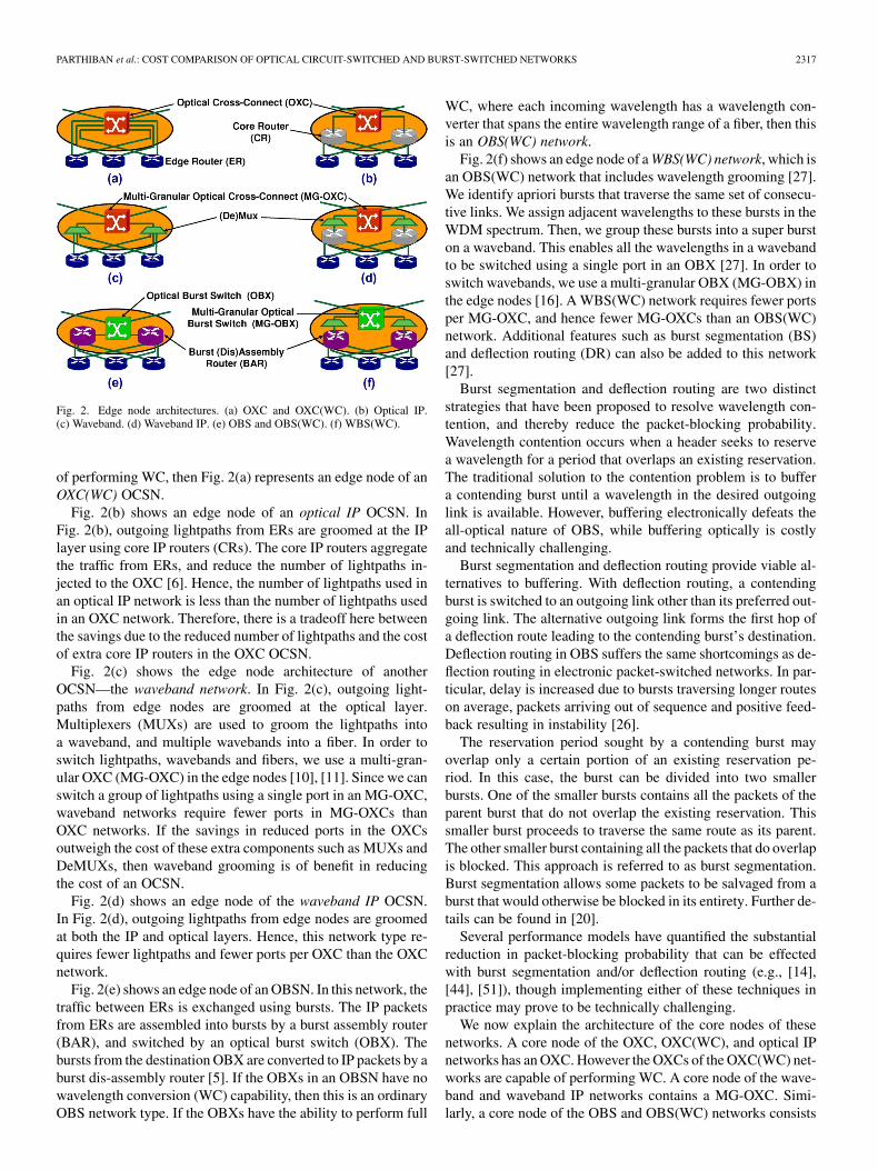
Fig. 4. OBS signaling timing diagram for a route � � �� , wherethe control packet is represented with a solid line, � denotes the length of theelectronic processing period at each switch, � denotes propagation delay and �

denotes switch configuration time; switch � begins to configure at time � .

The error owing to most of these assumptions has been quanti-fied in the literature by computer simulations, and is sufficientlysmall, so it does not affect the conclusions of our analysis.

We adopt a model for OBS in which a burst occupies at mostone link at any instant of its transmission. In reality, however, aburst may occupy two links, or even more, during its transmis-sion. In particular, we adopt a model such that the first packetof a burst begins transmission on link only as soon as thelast packet of that burst ends transmission on link (SeeFig. 4). Furthermore, we assume the residual offset time doesnot vary from burst to burst. (The residual offset time is thetime offset between a control packet and the endmost packetof its corresponding burst. At each core node, the residual offsettime shrinks in increments of the per-node control packet pro-cessing delay.) The optimal burst scheduling policy for the casein which the residual offset time does not vary from burst to burstis simple: schedule a new burst to any free wavelength channel.See [54] for a proof of the optimality of this policy. A form ofOBS called dual-header OBS has been proposed in [54], whichensures constant residual offset periods are maintained.

We remark that this simple scheduling policy is optimal interms of minimizing blocking probability and is a lower boundon the blocking probability achievable with other void-fillingscheduling algorithms that have been proposed for the case inwhich residual offset times may vary from burst to burst. Inthis way, our model is optimistic to the blocking performanceachievable with OBS.

The last two assumptions A6 and A7 are probably the mostnoteworthy. They are synonymous with the usual reduced-loadapproximation and have been discussed in this context and tosome degree justified in [53], [55]–[57]. We use these assump-tions in our reduced-load approximation. The details of ourapproximation have been presented in [14], [28], [44]. In thispaper, we only provide a brief qualitative description.

In the dimensioning stage, we find the network topology, thetotal number of edge nodes , and the number of fibers in eachlink. The packets from ERs are assembled into bursts in BARs in

edge nodes, and then sent to OBXs. Edge nodes as well as corenodes are interconnected via a network of directed links. Letbe the set of all links, and let be the set of all s-dpairs. Each s-d pair is assigned a single route, which is definedas an ordered set of continuous links from its source edge nodeto its destination edge node. Let denote the route usedby s-d pair . Each link consists of fibers that arealigned in the same direction, each of which in turn containwavelengths.

Bursts arrive at each s-d pair according to an independentPoisson process with rate , where isthe mean burst size, and is the total traffic. The load offered toeach route is thus , where .Recall that is the bit-rate per wavelength.

The first step in the calculation of the blocking probability isto compute the blocking probability perceived by a burst at eachlink, denoted as , . We calculate the blocking probabilityat a link using an model (Erlang B model) [52].This blocking probability is a function of the load that is offered.In consideration of the assumptions defined above, we can write

(8)

where: if link strictly precedes link ,otherwise ; is the Erlang B formula given anoffered load with servers; and, for no wavelengthconversion, while for full wavelength conversion.

In general, (8) cannot be solved explicitly for , .Therefore, an iterative procedure must be used to solve (8) nu-merically. In particular, we iterate according to an appropriatefixed-point mapping until an error criterion is met. Althoughthere is no certainty that the sequence generated by iteratingconverges, divergence is rare in practice and can often be over-come by periodically re-initializing with a convex combinationof the most recent iterations.

The second step of our reduced-load approximation involvescomputing the blocking probability perceived by each s-d pairgiven the link blocking probabilities , , that were com-puted in the first step. According to the link independence as-sumption, we have

(9)

where is the blocking probability perceived by bursts as-signed to s-d pair . The final blocking probability of theOBSNs is the average of all s-d pairs’ blocking probabilities.

Once we find the final blocking probability, we can also findthe number of lightpaths in each link. Using this information,we find the number of lightpaths, , in the core network (see[12] for details). Thus, the utilization of the OBSNs is

(10)

where and are the increased number of lightpaths re-quired from BARs and ERs respectively.

10) Satisfy Network Element Constraints: We allow mul-tiple CRs/BARs per node to manage the incoming and outgoingtraffic in a node (i.e., ). In other words, we either use


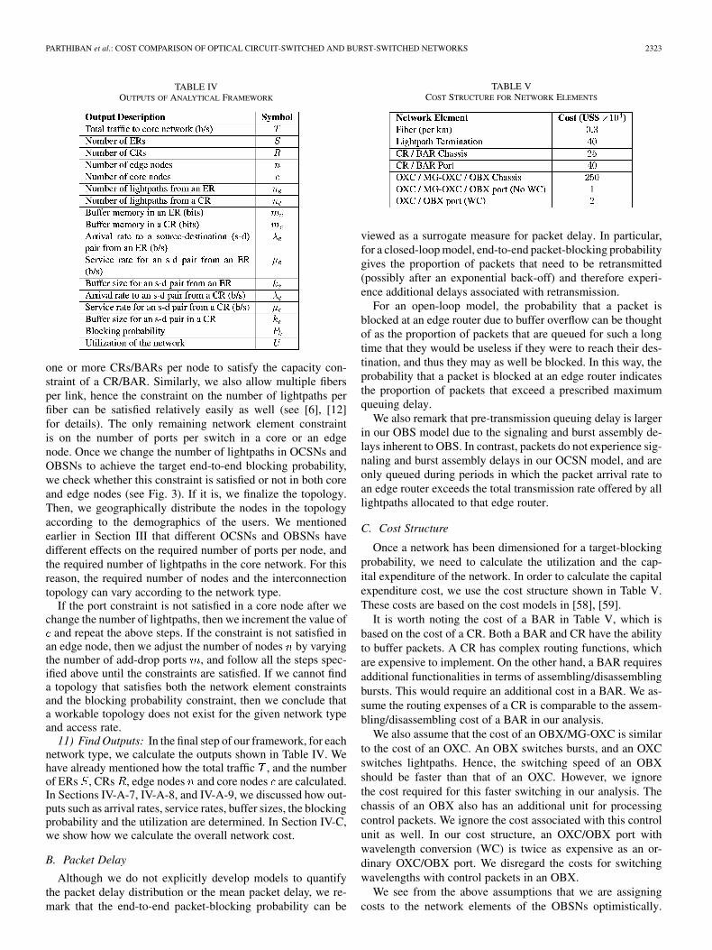
TABLE IVOUTPUTS OF ANALYTICAL FRAMEWORK

one or more CRs/BARs per node to satisfy the capacity con-straint of a CR/BAR. Similarly, we also allow multiple fibersper link, hence the constraint on the number of lightpaths perfiber can be satisfied relatively easily as well (see [6], [12]for details). The only remaining network element constraintis on the number of ports per switch in a core or an edgenode. Once we change the number of lightpaths in OCSNs andOBSNs to achieve the target end-to-end blocking probability,we check whether this constraint is satisfied or not in both coreand edge nodes (see Fig. 3). If it is, we finalize the topology.Then, we geographically distribute the nodes in the topologyaccording to the demographics of the users. We mentionedearlier in Section III that different OCSNs and OBSNs havedifferent effects on the required number of ports per node, andthe required number of lightpaths in the core network. For thisreason, the required number of nodes and the interconnectiontopology can vary according to the network type.

If the port constraint is not satisfied in a core node after wechange the number of lightpaths, then we increment the value of

and repeat the above steps. If the constraint is not satisfied inan edge node, then we adjust the number of nodes by varyingthe number of add-drop ports , and follow all the steps spec-ified above until the constraints are satisfied. If we cannot finda topology that satisfies both the network element constraintsand the blocking probability constraint, then we conclude thata workable topology does not exist for the given network typeand access rate.

11) Find Outputs: In the final step of our framework, for eachnetwork type, we calculate the outputs shown in Table IV. Wehave already mentioned how the total traffic , and the numberof ERs , CRs , edge nodes and core nodes are calculated.In Sections IV-A-7, IV-A-8, and IV-A-9, we discussed how out-puts such as arrival rates, service rates, buffer sizes, the blockingprobability and the utilization are determined. In Section IV-C,we show how we calculate the overall network cost.

B. Packet Delay

Although we do not explicitly develop models to quantifythe packet delay distribution or the mean packet delay, we re-mark that the end-to-end packet-blocking probability can be

TABLE VCOST STRUCTURE FOR NETWORK ELEMENTS

viewed as a surrogate measure for packet delay. In particular,for a closed-loop model, end-to-end packet-blocking probabilitygives the proportion of packets that need to be retransmitted(possibly after an exponential back-off) and therefore experi-ence additional delays associated with retransmission.

For an open-loop model, the probability that a packet isblocked at an edge router due to buffer overflow can be thoughtof as the proportion of packets that are queued for such a longtime that they would be useless if they were to reach their des-tination, and thus they may as well be blocked. In this way, theprobability that a packet is blocked at an edge router indicatesthe proportion of packets that exceed a prescribed maximumqueuing delay.

We also remark that pre-transmission queuing delay is largerin our OBS model due to the signaling and burst assembly de-lays inherent to OBS. In contrast, packets do not experience sig-naling and burst assembly delays in our OCSN model, and areonly queued during periods in which the packet arrival rate toan edge router exceeds the total transmission rate offered by alllightpaths allocated to that edge router.

C. Cost Structure

Once a network has been dimensioned for a target-blockingprobability, we need to calculate the utilization and the cap-ital expenditure of the network. In order to calculate the capitalexpenditure cost, we use the cost structure shown in Table V.These costs are based on the cost models in [58], [59].

It is worth noting the cost of a BAR in Table V, which isbased on the cost of a CR. Both a BAR and CR have the abilityto buffer packets. A CR has complex routing functions, whichare expensive to implement. On the other hand, a BAR requiresadditional functionalities in terms of assembling/disassemblingbursts. This would require an additional cost in a BAR. We as-sume the routing expenses of a CR is comparable to the assem-bling/disassembling cost of a BAR in our analysis.

We also assume that the cost of an OBX/MG-OXC is similarto the cost of an OXC. An OBX switches bursts, and an OXCswitches lightpaths. Hence, the switching speed of an OBXshould be faster than that of an OXC. However, we ignorethe cost required for this faster switching in our analysis. Thechassis of an OBX also has an additional unit for processingcontrol packets. We ignore the cost associated with this controlunit as well. In our cost structure, an OXC/OBX port withwavelength conversion (WC) is twice as expensive as an or-dinary OXC/OBX port. We disregard the costs for switchingwavelengths with control packets in an OBX.

We see from the above assumptions that we are assigningcosts to the network elements of the OBSNs optimistically.


TABLE VIVALUES OF INPUTS TO ANALYTICAL FRAMEWORK

Hence, even with this optimistic approach, if the OBSNs aremore expensive than the OCSNs for the same quality of ser-vice, then the commercial viability of a possible evolution fromOCSNs to OBSNs is questionable.

The costs in Table V may be quite optimistic, because someof the considered network elements are still experimental andthus it is difficult to predict their commercial cost at this stage.However, these costs provide a starting point for our analysis.We have observed that moderate changes in these costs do notaffect the general conclusions of this paper.

V. EVALUATION

We evaluate the OCSNs and OBSNs we described inSection III for a backbone network based on the demographicsand geography of Australia. In particular, we consider theWBS(WC) network with deflection routing (DR) and burstsegmentation (BS). The number of users is million,which covers both business and residential users. Although ourgeneral analytical framework is applicable to any large-scalenetwork such as the US backbone network, we chose the Aus-tralian core network, since it is computationally manageable.We evaluate the networks for two average access rates per user:

and . The values of other inputs areshown in Table VI.

We calculate the number of lightpaths and the overallnetwork cost for the target-blocking probabilities ,

, , , , and 0.8. When choosingand , we need to consider two issues: 1) they

should be sufficiently low so that the approximation1—holds, 2) they should not be so low that we inflate the cost ofthe network by using an excessive number of lightpaths fromERs/CRs/BARs. After trialling with many values, we observedthat the ranges and donot inflate the network costs excessively, and at the same timedo not alter the final conclusions of this paper. We show theresults for and in this paper.

The LRD (3) and (6) used to calculate blocking probabilityare valid primarily for very large (or asymptotically large) buffersizes [46]. Hence, we require and in (2) and (5) to be verylarge. Our analysis shows that a delay of 0.1 s in each port of anER or CR is sufficient to satisfy this condition. For this reason,we use a delay value of 0.1 s as shown in Table VI.

A. Estimating Self-similar Traffic Parameters

In Sections IV-A-7 and IV-A-8, we noted that the Hurst pa-rameter , and the standard deviations and need to beestimated empirically. In this sub-section, we explain how weestimate these parameters. We have been unable to find mea-surements for high access rates such as and

in the literature. Consequently, we have relied onmeasurements from [65]. The mean rate of the traffic streammeasured is . For thismean rate, the variance is , and the Hurstparameter is .

Our goal is to use these measurements to find the variancefor the average access rates and .

Since these measurements are in bytes/100 ms, we expressour inputs and outputs in bytes/100 ms. As we described inSection IV-C, we have considered a scenario that is optimisticfor the OBSNs, i.e., bursty traffic from users [5]. If the ratio ofstandard deviation to mean rate is kept constant, then the trafficremains bursty for high mean rates [46]. Hence, we keep thisratio constant to find using the measurements.

This enables us to determine the mean rate and the standarddeviation of the traffic from a user. The traffic from manyusers is aggregated at an ER. In order to find the variance ofthe aggregated arrival traffic at an ER, , we use the additivityof the mean and variance of independent flows. In other words,the ratio of variance to mean rate is kept constant during aggre-gation. Hence, using the assumption that the traffic flows fromcustomers are independent, the variance of the aggregated ar-rival traffic to an ER is

We use a similar method to find the variance of the arrival trafficrate to a CR/BAR.

In contrast, the Hurst parameter can be assumed unchanged withaggregation [46], i.e., in all cases.

B. 100 Mb/s Access Rate Per User

We first consider the results of dimensioning OCSNs andOBSNs for an average access rate per user of 100 Mb/s. Inthe dimensioning stage, we calculate the number of network


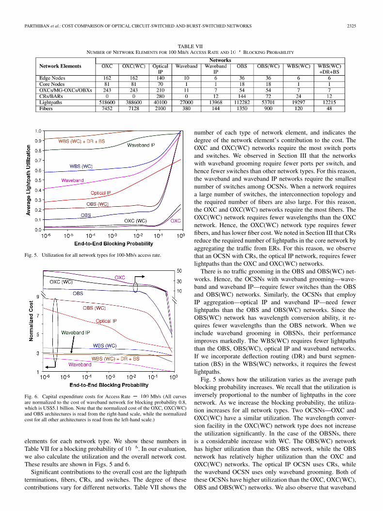
TABLE VIINUMBER OF NETWORK ELEMENTS FOR 100 MB/S ACCESS RATE AND �� BLOCKING PROBABILITY

Fig. 5. Utilization for all network types for 100-Mb/s access rate.

Fig. 6. Capital expenditure costs for Access Rate � �� Mb/s (All curvesare normalized to the cost of waveband network for blocking probability 0.8,which is US$5.1 billion. Note that the normalized cost of the OXC, OXC(WC)and OBS architectures is read from the right-hand scale, while the normalizedcost for all other architectures is read from the left-hand scale.)

elements for each network type. We show these numbers inTable VII for a blocking probability of . In our evaluation,we also calculate the utilization and the overall network cost.These results are shown in Figs. 5 and 6.

Significant contributions to the overall cost are the lightpathterminations, fibers, CRs, and switches. The degree of thesecontributions vary for different networks. Table VII shows the

number of each type of network element, and indicates thedegree of the network element’s contribution to the cost. TheOXC and OXC(WC) networks require the most switch portsand switches. We observed in Section III that the networkswith waveband grooming require fewer ports per switch, andhence fewer switches than other network types. For this reason,the waveband and waveband IP networks require the smallestnumber of switches among OCSNs. When a network requiresa large number of switches, the interconnection topology andthe required number of fibers are also large. For this reason,the OXC and OXC(WC) networks require the most fibers. TheOXC(WC) network requires fewer wavelengths than the OXCnetwork. Hence, the OXC(WC) network type requires fewerfibers, and has lower fiber cost. We noted in Section III that CRsreduce the required number of lightpaths in the core network byaggregating the traffic from ERs. For this reason, we observethat an OCSN with CRs, the optical IP network, requires fewerlightpaths than the OXC and OXC(WC) networks.

There is no traffic grooming in the OBS and OBS(WC) net-works. Hence, the OCSNs with waveband grooming—wave-band and waveband IP—require fewer switches than the OBSand OBS(WC) networks. Similarly, the OCSNs that employIP aggregation—optical IP and waveband IP—need fewerlightpaths than the OBS and OBS(WC) networks. Since theOBS(WC) network has wavelength conversion ability, it re-quires fewer wavelengths than the OBS network. When weinclude waveband grooming in OBSNs, their performanceimproves markedly. The WBS(WC) requires fewer lightpathsthan the OBS, OBS(WC), optical IP and waveband networks.If we incorporate deflection routing (DR) and burst segmen-tation (BS) in the WBS(WC) networks, it requires the fewestlightpaths.

Fig. 5 shows how the utilization varies as the average pathblocking probability increases. We recall that the utilization isinversely proportional to the number of lightpaths in the corenetwork. As we increase the blocking probability, the utiliza-tion increases for all network types. Two OCSNs—OXC andOXC(WC) have a similar utilization. The wavelength conver-sion facility in the OXC(WC) network type does not increasethe utilization significantly. In the case of the OBSNs, thereis a considerable increase with WC. The OBS(WC) networkhas higher utilization than the OBS network, while the OBSnetwork has relatively higher utilization than the OXC andOXC(WC) networks. The optical IP OCSN uses CRs, whilethe waveband OCSN uses only waveband grooming. Both ofthese OCSNs have higher utilization than the OXC, OXC(WC),OBS and OBS(WC) networks. We also observe that waveband


TABLE VIIINUMBER OF NETWORK ELEMENTS FOR 1-GB/S ACCESS RATE AND �� BLOCKING PROBABILITY

grooming performs better in reducing the required numberof lightpaths than IP aggregation due to CRs. When we useboth waveband grooming and IP aggregation in an OCSN(the waveband IP OCSN), it requires fewer lightpaths than theWBS(WC) network. The WBS(WC) network with DR andBS has the highest utilization. This highlights the benefits ofwaveband grooming, DR and BS for OBSNs.

Fig. 6 shows the normalized network cost for all networksas a function of the average path blocking probability. Thesecosts are normalized to the cost of the least expensive networktype, the waveband network for the blocking probability 0.8,which is US$5.1 billion. The OXC and OXC(WC) networksare the most expensive, since they require the most lightpathsand fibers. Since the OXC(WC) network has a lower fiber andlightpath termination cost than the OXC network, the overallcost of the OXC(WC) is also less. The OBS networks are lessexpensive than the OXC and OXC(WC) networks, since theOBS networks require far fewer lightpaths than the OXC andOXC(WC) OCSNs. This result is consistent with the finding of[31]. We observed earlier that there is a trade-off between thelightpath termination cost and CR/BAR cost, when we use IPaggregation. For the optical IP network, the CR cost carries lessweight than the lightpath termination cost. We also see fromTable VII that the optical IP requires fewer lightpaths than theOBS and OBS(WC) networks. Hence, the optical IP networkis less expensive than the OBS and OBS(WC) networks. Thewaveband IP OCSN requires the least CR cost, and achieveslower lightpath termination cost than all other networks exceptthe WBS(WC) network with DR and BS. Both the waveband IPnetwork and WBS(WC) network with DR and BS also requirethe fewest switching ports due to waveband grooming. For thesereasons, the waveband IP OCSN is less expensive than all othernetworks except the waveband OCSN and WBS(WC) networkwith DR and BS. For all networks with waveband grooming andCRs/BARs, the cost of extra CRs/BARs outweighs the savingsdue to reduced lightpaths. For this reason, the waveband OCSNis the least expensive network for the 100 Mb/s access rate.

C. 1 Gb/s Access Rate Per User

The OCSN with only one type of grooming, namely wave-band grooming, is the least expensive in Fig. 6. However, thecost advantage of the waveband OCSN is undermined, if weincrease the average access rate per user to 1 Gb/s. To showthis, we evaluate the OCSN and OBSN types for an averageaccess rate of 1 Gb/s per user, while keeping all the otherinput parameters the same. We leave out the most expensiveOCSNs—OXC and OXC(WC)—in this evaluation, because a

Fig. 7. Utilization for all network types for 1-Gb/s access rate.

workable topology cannot be found for these networks duringthe dimensioning stage due to the OXC port constraint.

Table VIII shows the number of network elements for eachnetwork type for a blocking probability of . We observethat OCSNs and OBSNs with waveband grooming require thefewest switches. Similarly, the OCSNs with IP aggregationrequire fewer lightpaths than all other networks except theWBS(WC) networks. The OBSNs with waveband groomingrequire fewer switches than the networks without wavebandgrooming. When we use waveband grooming, DR and BS, theOBSN requires the fewest switches and lightpaths.

Fig. 7 shows how utilization varies as the average pathblocking probability increases for the 1 Gb/s access rate. In thiscase, the OBS network has the lowest utilization. Once again,the average lightpath utilization of the OBS(WC) networkis higher than that of the OBS network. There are two maindifferences in Fig. 7 compared to Fig. 5: 1) The WBS(WC)network outperforms the waveband IP network for 1 Gb/s ac-cess rate, and 2) The optical IP network performance improvesfor 1 Gb/s access rate compared to the waveband OCSN. Thesecond difference ensures that the optical IP network has acomparable utilization with the waveband network. Hence, IPaggregation and waveband grooming have similar effects inreducing the number of lightpaths in an OCSN for the 1 Gb/saccess rate. However, the combined effect of both wavebandand IP aggregation is better in reducing the number of light-paths for OCSNs. The WBS(WC) has higher utilization thanthe OBS(WC) and waveband IP networks. The WBS(WC)network with DR and BS has the highest utilization.


Fig. 8. Capital expenditure cost for Access Rate � � Gb/s (All curves arenormalized to the cost of waveband network for blocking probability 0.8, whichis US$64.4 billion. Note that the normalized cost of the Optical IP, OBS, andOBS(WC) architectures is read from the right-hand scale, while the normalizedcost for all other architectures is read from the left-hand scale.)

Fig. 8 shows how the normalized network cost for each net-work type varies with the average path blocking probability. Asbefore, these costs are normalized with respect to the cost ofthe least expensive network, i.e., the waveband network for theblocking probability 0.8, which is US$64.4 billion. The OBSnetwork has the lowest utilization, and hence requires a largenumber of lightpaths, which makes it more expensive than theother networks for this access rate. For 1 Gb/s, the cost of CRports for the optical IP has more weight than the savings in thenumber of lightpaths. For this reason, the optical IP network hasa comparable cost with the OBS(WC) network. The trade-offbetween the lightpath termination cost and CR/BAR cost playsa major role in determining the cost advantage among all thenetworks that use waveband grooming. For high blocking prob-abilities or when the traffic load is comparatively low in the corenetwork, the cost of CRs/BARs outweighs the savings in light-paths. Hence, the waveband OCSN is less expensive for theseblocking probabilities. When the traffic load is high, i.e., forlow blocking probabilities, the reverse occurs in the trade-off.Hence, other networks with waveband grooming become lessexpensive. This shows that for a network with high traffic load,the WBS(WC) OBSNs and the waveband IP OCSN are morelikely to compete for the lowest cost rather than the wavebandOCSN. The waveband IP OCSN requires fewer CRs and fibersthan the WBS(WC) network. For this reason, the waveband IPOCSN is still less expensive than the WBS(WC) network. How-ever, when we use DR and BS in the WBS(WC) OBSN, it isthe least expensive network for blocking probabilities less than

.Note that our comparison is based on the design of networks

for static traffic conditions. An open issue for further research ishow to analyse the effect of dynamic optical circuits on the costof OCSNs in comparison to OBSNs.

VI. CONCLUSION

We have developed an analytical framework to compare theCAPEX costs of OCSNs and OBSNs. Using this framework,we have shown that OBS networks are in general less expensivethan OCS networks. If waveband grooming is employed only inOCSNs, then they are more cost effective than OBSNs. Once weinclude waveband grooming, deflection routing and burst seg-mentation in OBSNs, OBS becomes the most cost-effective ar-chitecture especially for low blocking probabilities. Our resultsapply to a national network, and take into account the demo-graphics of the Australian population. Although we have chosenthe Australian core network for evaluation, our framework isapplicable to any large-scale core network such as the US back-bone network.

We have shown that, for an Australian national network,the key benefits of OBSNs arise through the cost advantagesachieved by waveband grooming, deflection routing and burstsegmentation. As the access rate of users increases, the costadvantage of OBSNs over OCSNs increases. Hence, as thecapacity of the core network increases, OBS appears to be anattractive option compared to OCS technology.

REFERENCES

[1] R. Ramaswami, “Optical fiber communication: From transmission tonetworking,” IEEE Commun. Mag., vol. 40, no. 5, pp. 138–147, May2002, 50th Anniversary Commemorative Issue.

[2] V. Chan and J. LoCicero, “Editorial,” IEEE J. Sel. Areas Commun.,vol. 21, no. 9, pp. 1365–1366, Nov. 2003.

[3] P. B. Chu, S. S. Lee, and S. Park, “MEMS: The path to large opticalcross-connects,” IEEE Commun. Mag., vol. 40, no. 3, pp. 80–87, Mar.2002.

[4] C. Qiao and M. Yoo, “Choices, features and issues in optical burstswitching,” Opt. Netw. Mag., vol. 1, no. 2, pp. 36–44, 2000.

[5] C. Qiao, Y. Chen, and J. Staley, “The potentials of optical burstswitching (OBS),” in Proc. OFC, Atlanta, GA, Mar. 2003, p. TuJ5.

[6] R. Parthiban, R. S. Tucker, and C. Leckie, “Waveband grooming andIP aggregation in optical networks,” J. Lightw. Technol., vol. 21, no.11, pp. 2476–2488, Nov. 2003.

[7] P. Ho and H. T. Mouftah, “Routing and wavelength assignment withmultigranularity traffic in optical networks,” J. Lightw. Technol., vol.20, no. 8, pp. 1292–1303, Aug. 2002.

[8] H. Harai, “Design of reconfigurable lightpaths in IP over WDM net-works,” IEICE Trans. Commun., vol. E83-B, no. 10, pp. 2234–2244,Oct. 2000.

[9] A. Rodriguez-Moral, “The optical internet: Architectures and protocolsfor the global infrastructure of tomorrow,” IEEE Commun. Mag., vol.39, no. 7, pp. 152–159, Jul. 2001.

[10] R. Lingampillai and P. Vengalam, “Effect of wavelength and wave-band grooming on all-optical networks with single layer photonicswitching,” in Proc. OFC, Anaheim, CA, Mar. 2002, p. ThP4.

[11] X. Cao, V. Anand, and C. Qiao, “Waveband switching in optical net-works,” IEEE Commun. Mag., vol. 41, no. 4, pp. 105–112, Apr. 2003.

[12] R. Parthiban, “Modeling and analysis of optical backbone net-works” Ph.D. dissertation, Dept. Elect. Electron. Eng., Uni-versity of Melbourne, Victoria, Australia [Online]. Available:http://www.ee.unimelb.edu.au/multimedia/research/\\cubin_Rajen-dran_Parthiban_thesis.pdf

[13] M. Nord, “Demonstration of optical packet switching scheme forheader-payload separation and class-based forwarding,” in Proc. OFC,Los Angeles, CA, Mar. 2004, p. TuQ2.

[14] Z. Rosberg, “Performance analysis of optical burst-switching net-works,” IEEE J. Sel. Areas Commun., vol. 21, no. 7, pp. 1187–1197,Sep. 2003.

[15] J. Li, “Maximizing throughput for optical burst switching networks,”in Proc. INFOCOM, Hong Kong, Mar. 2004, pp. 1853–1863.


[16] Y. Huang, “A new node architecture employing waveband-selectiveswitching for optical burst-switched networks,” IEEE Commun. Lett.,vol. 11, no. 9, pp. 756–758, Sep. 2007.

[17] A. Detti, V. Earmo, and M. Listanti, “Performance evaluation of a newtechnique for IP support in a WDM optical network: Optical com-posite burst switching (OCBS),” J. Lightw. Technol., vol. 20, no. 2, pp.154–165, Feb. 2002.

[18] M. Neuts, “Performance analysis of optical composite burst switching,”IEEE Commun. Lett., vol. 6, no. 8, pp. 346–348, Aug. 2002.

[19] Z. Rosberg, H. L. Vu, and M. Zukerman, “Burst segmentation benefitin optical switching,” IEEE Commun. Lett., vol. 7, no. 3, pp. 127–129,Mar. 2003.

[20] V. M. Vokkarane, J. P. Jue, and S. Sitaraman, “Burst segmentation: Anapproach for reducing packet loss in optical burst switched networks,”in Proc. ICC, Apr./May 2002, vol. 5, pp. 2673–2677.

[21] V. M. Vokkarane and J. P. Jue, “Prioritized burst segmentation andcomposite burst-assembly techniques for QoS support in optical burst-switched networks,” IEEE J. Sel. Areas Commun., vol. 21, no. 7, pp.1198–1209, Jul. 2003.

[22] V. M. Vokkarane and J. P. Jue, “Segmentation-based nonpreemptivechannel scheduling algorithms for optical burst-switched networks,” J.Lightw. Technol., vol. 23, no. 10, pp. 3125–3137, Oct. 2005.

[23] C. Cameron, A. Zalesky, and M. Zukerman, “Prioritized deflectionrouting in optical burst switching networks,” IEICE Trans. Commun.,vol. E88B, no. 5, pp. 1861–1867, May 2005.

[24] Y. Chen, “Performance analysis of optical burst switched node withdeflection routing,” in Proc. ICC IEEE Int. Conf. Commun., vol. 2, pp.1355–1359.

[25] C.-F. Hsu, T.-L. Liu, and N.-F. Huang, “Performance analysis of de-flection routing in optical burst-switched networks,” in Proc. INFCOM21st Annu. Joint Conf. IEEE Comput. Commun. Soc., vol. 1, pp. 66–73.

[26] A. Zalesky, “Stabilizing deflection routing in optical burst switchednetworks,” IEEE J. Sel. Areas Commun., vol. 25, no. 6, pp. 3–19, Aug.2007.

[27] R. Parhiban, “Waveband burst switching—A new approach to net-working,” in Proc. OFC, Anaheim, CA, Mar. 2006, Paper JThB47.

[28] J. Widjaja, “Performance analysis of burst admission-control proto-cols,” IEE Proc. Commun., vol. 142, no. 1, Feb. 1995.

[29] A. Bragg, I. Baldine, and D. Stevenson, “A parametric, first-order costanalysis of optical burst switched (OBS) networks,” in Proc. WOBS,San Jose, CA, Nov. 2004.

[30] B. Feng, “Direct comparison between OCS and OBS/OPS usingsimulations,” in Proc. OECC/COIN, Yokohama, Japan, Jul. 2004, p.14A2-2.

[31] F. Xue, “Performance comparison of optical burst and circuit switchednetworks,” in Proc. OFC, Anaheim, CA, Mar. 2005, p. OWC1.

[32] L. Sofman, A. Agrawal, and T. El-Bawab, “Traffic grooming and band-width efficiency in packet and burst switched networks,” in Proc. 2003Appl. Telecommun. Symp., 2003, pp. 3–8.

[33] R. Parthiban, “Does OBS have a role in the core network?,” in Proc.OFC, Anaheim, CA, Mar. 2005, p. OWC2.

[34] M. D. Vaughn and R. E. Wagner, “A bottom-up traffic demand modelfor LH and metro optical networks,” in Proc. OFC, Atlanta, GA, Mar.2003, p. MF11.

[35] A. Zalesky, “To burst or circuit switch?,” IEEE/ACM Trans. Netw., vol.17, no. 1, pp. 305–318, Feb. 2009.

[36] L. Xu, H. G. Perros, and G. N. Rouskas, “A queuing network model ofan edge optical burst switching node,” in Proc. IEEE INFOCOM’03,San Francisco, CA, Mar./-pr. 2003, vol. 3, pp. 2019–2029.

[37] J. Yates, J. Lacey, and D. Everitt, “Blocking in multiwavelength TDMnetworks,” Telecommun. Syst., vol. 12, no. 1, pp. 1–19, 1999.

[38] R. Srinivasan and A. K. Somani, “A generalized framework for an-alyzing time-space switched optical networks,” in Proc. INFOCOM,Anchorage, AK, Apr. , vol. 1, pp. 179–188.

[39] V. Eramo, M. Listanti, and A. Germoni, “Cost evaluation of opticalpacket switches equipped with limited-range and full-range convertersfor contention resolution,” J. Lightw. Technol., vol. 28, no. 4, pp.390–407, Feb. 2008.

[40] J. Fang, R. Srinivasan, and A. K. Somani, “Performance analysis ofWDM optical networks with wavelength usage constraint,” Photon.Netw. Commun., vol. 5, no. 2, pp. 137–146, Mar. 2003.

[41] J. Li, C. Qiao, and Y. Chen, “Recent progress in the scheduling algo-rithms in optical burst-switched networks,” J. Opt. Netw., vol. 3, pp.229–241, Apr. 2004.

[42] X. Lu and B. L. Mark, “Performance modeling of optical-burstswitching with fiber delay lines,” IEEE Trans. Commun., vol. 52, no.12, pp. 2175–2183, Dec. 2004.

[43] T. Battestilli and H. Perros, “A performance study of an opticalburst switched network with dynamic simultaneous link possession,”Comput. Networks, vol. 50, no. 2, pp. 219–236, Feb. 2006.

[44] A. Zalesky, “OBS contention resolution performance,” PerformanceEvaluation, vol. 64, no. 4, pp. 357–373, 2007.

[45] V. Paxon and S. Floyd, “Wide-area traffic: The failure of Poisson mod-eling,” IEEE/ACM Trans. Netw., vol. 3, no. 3, pp. 226–244, Jun. 1995.

[46] R. G. Addie, M. Zukerman, and T. D. Neame, “Broadband traffic mod-eling: Simple solutions to hard problems,” IEEE Commun. Mag., vol.36, no. 8, pp. 88–95, Aug. 1998.

[47] J. Wang, R. Vemuri, and B. Mukherjee, “Towards IP-centric opti-mization: On the topology design of WDM-mesh networks,” [Online].Available: http://www.cs.ucdavis.edu/~vemuri/papers/IP_netplan.pdf

[48] “Architecture for the Automatically Switched Optical Network,”International Telecommunication Union-Telecommunication(ITU-T), Recommendation G.8080, Nov. 2001 [Online]. Avail-able: http://www.itu.int

[49] S. Dixit and Y. Ye, “Streamlining the internet-fiber connection,” IEEESpectrum, vol. 38, no. 4, pp. 52–57, Apr. 2001.

[50] A. Richter, “Field trial of an ASON in the metropolitan area,” in Proc.OFC, Anaheim, California, Mar. 2002, p. TuH3.

[51] H. L. Vu, “Scalable performance evaluation of a hybrid optical switch,”J. Lightw. Technol., vol. 23, Special Issue on Optical Networks, no. 10,pp. 2961–2973, Oct. 2005.

[52] D. Bertsekas and R. Gallager, Data Networks. Englewood Cliffs, NJ:Prentice-Hall, 1987.

[53] R. B. Cooper and S. Katz, “Analysis of Alternate Routing NetworksWith Account Taken of Nonrandomness of Overflow Traffic,” BellTelephone Lab. Memo, 1964, Tech. Rep..

[54] N. Barakat and E. H. Sargent, “Dual-header optical burst switching: Anew architecture for WDM burst-switched networks,” in Proc. IEEEINFOCOM, Mar. 2005, vol. 1, pp. 685–693.

[55] S. P. Chung, A. Kashper, and K. W. Ross, “Computing approximateblocking probabilities for large loss networks with state-dependentrouting,” IEEE/ACM Trans. Netw., vol. 1, no. 1, pp. 105–115, Feb.1993.

[56] F. P. Kelly, “Blocking probabilities in large circuit-switched networks,”Adv. Appl. Prob., vol. 18, pp. 473–505, 1986.

[57] W. Whitt, “Blocking when service is required from several facilitiessimultaneously,” AT&T Tech. J., vol. 64, pp. 1807–1856, 1985.

[58] P. M. A. Ferreira, B. Cossa, and F. Naud, “A cost model for opticalbackbones,” J. Technol. Forecasting and Social Change, vol. 69, pp.741–758, 2002.

[59] S. Sengupta, V. Kumar, and D. Saha, “Switched optical backbone forcost-effective scalable core IP networks,” IEEE Commun. Mag., vol.41, no. 6, pp. 60–70, Jun. 2003.

[60] S. Bigo, “10.2 Tb/s (256 � 42.7 Gb/s) transmission over 100 km tera-light fiber with 1.28 bits/s/Hz spectral efficiency,” in Proc. OFC, Ana-heim, CA, Mar. 2001, p. PD25-1.

[61] K. Fukuchi, “10.92 Tb/s (273 � 40 Gb/s) triple-band/ultra-denseWDM optical-repeatered transmission experiment,” in Proc. OFC,Anaheim, CA, Mar. 2001, p. PD24-1.

[62] R. Ryf, “1296-port MEMS transport optical cross-connect with 2.07petabit/s switch capacity,” in Proc. OFC, Anaheim, CA, Mar. 2001, p.PD28-1.

[63] D. Greenfield, “Terabit routers: A lesson in carrier-class confusion,”IEEE Netw., vol. 15, no. 3, pp. 78–84, Mar. 2000.

[64] “Cisco Delivers the Foundation for Next-Generation IP Networks: ANew Carrier Routing System,” Cisco Online Sources [Online]. Avail-able: http://newsroom.cisco.com/dlls/2004/prod_052504.html

[65] R. G. Addie, T. D. Neame, and M. Zukerman, “Performance evaluationof a queue fed by a Poisson Pareto burst process,” Comput. Netw., vol.40, no. 3, pp. 377–397, Oct. 2002.

Rajendran Parthiban (M’04) received the B.Eng.degree (with first class honors) and the Ph.D.degree in optical networks from the University ofMelbourne, Victoria, Australia, in 1997 and 2004,respectively.

He was with Akbar Brothers Pvt. Ltd., Sri Lanka,from 1998 to 2000, where he computerized many ofthe company functions. In 2004, he joined the ARCSpecial Research Centre for Ultra-Broadband Infor-mation Networks (CUBIN) at the University of Mel-bourne. At CUBIN, he conducted research in devel-

oping new and cost-effective optical network architectures for carrying futureInternet traffic. Currently, he is a Senior Lecturer with the School of Engineeringin Monash University, Malaysia. His research interests are in design and man-agement of optical and wireless sensor networks, and grid computing.


Christopher Leckie received the B.Sc. degree, theB.E. degree in electrical and computer systems engi-neering (with first class honours), and the Ph.D. de-gree in computer science from Monash University,Australia, in 1985, 1987, and 1992, respectively.

He joined Telstra Research Laboratories in 1988,where he conducted research and development intoartificial intelligence techniques for various telecom-munication applications. In 2000, he joined the Uni-versity of Melbourne, Victoria, Australia, as a SeniorResearch Fellow with the Department of Electrical

and Electronic Engineering. He is currently an Associate Professor with the De-partment of Computer Science and Software Engineering, University of Mel-bourne. His research interests include using artificial intelligence for networkmanagement, as well as the design and management of optical networks.

Andrew Zalesky received the B.E.(Hons) and theB.Sc. degrees and the Ph.D. degree in engineeringfrom the University of Melbourne, Victoria,Australia, where he then received the Ph.D. degreein Engineering in 2003 and 2006, respectively.

Dr. Zalesky is an ARC International Fellow.He has developed queuing models to evaluatethe impact of design choices in next-generationtelecommunications networks. He is currentlydeveloping tracking algorithms to virtually chartthe living brain’s circuitry with the use of magnetic

resonance imaging.Dr. Zalesky was recently awarded the ARC International Fellowship,

American Australian Association Fellowship and grants from the AustralianAcademy of Science and CASS Foundation to pursue research abroad.

Moshe Zukerman (F’09) received the B.Sc. degreein industrial engineering and management and theM.Sc. degree in operations research from Tech-nion–Israel Institute of Technology, Haifa, and thePh.D. degree in engineering from the University ofCalifornia, Los Angeles, in 1985.

Dr. Zukerman was an independent consultant withIRI Corporation and a Post-Doctoral Fellow withthe University of California, Los Angeles, during1985–1986. During 1986–1997, he was with TelstraResearch Laboratories (TRL), first as a Research

Engineer and, between 1988 and 1997, as a Project Leader managing a teamof researchers providing expert advice to Telstra on network design and trafficengineering, and on traffic aspects of evolving telecommunications standards.Between 1997 and 2008, he was with The University of Melbourne, as a SeniorResearch Fellow (1997–1998), Associate Professor (1998–2001), and Professor(2001–2008). In December 2008, he joined the Electronic Engineering Depart-ment of City University of Hong Kong as a Chair Professor of InformationEngineering and a group leader. Since 1990, he has also taught and supervisedgraduate students at Monash University. He has authored or coauthored over200 publications in scientific journals and conference proceedings.

Dr. Zukerman was the recipient of the Telstra Research Laboratories Out-standing Achievement Award in 1990. He has served on various editorial boardsincluding the IEEE JOURNAL OF SELECTED AREAS IN COMMUNICATIONS, theIEEE/ACM TRANSACTIONS ON NETWORKING, COMPUTER NETWORKS, andIEEE Communications Magazine.

Rodney S. Tucker (F’90) is a Laureate Professorwith the University of Melbourne, Victoria, Aus-tralia, and Research Director of the AustralianResearch Council Special Research Centre forUltra-Broadband Information Networks. He has heldpositions with the University of California, Berkeley,Cornell University, Plessey Research (Caswell),AT&T Bell Laboratories, Hewlett Packard Labora-tories, and Agilent Technologies.

Dr. Tucker is a Fellow of the Australian Academyof Science, the Australian Academy of Technolog-

ical Sciences and Engineering, and the Optical Society of America. He was therecipient of the Australia Prize in 1977 for his contributions to telecommunica-tions and the IEEE LEOS Aron Kressel Award in 2007 for his contributions tosemiconductor optoelectronics.

journal of lightwave technology, vol. 27, no. 13, july … · journal of lightwave technology, vol....

Documents