JOURNAL OF LATEX CLASS FILES, VOL. 14, NO. 8, AUGUST 2015 1

Tracking-by-Fusion via Gaussian ProcessRegression Extended to Transfer Learning

Jin Gao, Qiang Wang, Junliang Xing, Member, IEEE, Haibin Ling, Member, IEEE,Weiming Hu, Senior Member, IEEE, Stephen Maybank, Fellow, IEEE

Abstract—This paper presents a new Gaussian Processes (GPs)-based particle filter tracking framework. The framework non-triviallyextends Gaussian process regression (GPR) to transfer learning, and, following the tracking-by-fusion strategy, integrates closely two trackingcomponents, namely a GPs component and a CFs one. First, the GPs component analyzes and models the probability distribution of theobject appearance by exploiting GPs. It categorizes the labeled samples into auxiliary and target ones, and explores unlabeled samples intransfer learning. The GPs component thus captures rich appearance information over object samples across time. On the other hand, tosample an initial particle set in regions of high likelihood through the direct simulation method in particle filtering, the powerful yet efficientcorrelation filters (CFs) are integrated, leading to the CFs component. In fact, the CFs component not only boosts the sampling quality, butalso benefits from the GPs component, which provides re-weighted knowledge as latent variables for determining the impact of eachcorrelation filter template from the auxiliary samples. In this way, the transfer learning based fusion enables effective interactions between thetwo components. Superior performance on four object tracking benchmarks (OTB-2015, Temple-Color, and VOT2015/2016), and incomparison with baselines and recent state-of-the-art trackers, has demonstrated clearly the effectiveness of the proposed framework.

Index Terms—Visual tracking, Gaussian processes, correlation filters, transfer learning, tracking-by-fusion.

F

1 INTRODUCTION

UNDERSTANDING how objects of interest move throughvideo is one of the most fundamental problems in

computer vision, as it can facilitate content-based semanticanalysis for better video retrieval, real time human-computerinteraction for more efficient computer understanding ofhuman environments, object re-identification for multi-cameratracking in automated video surveillance, and registration orcorrect alignment of the virtual world with the real one foraugmented reality, to name a few applications. There hasbeen significant progress on accurate object detection andsegmentation of interest over the recent years due largely tothe use of convolutional neural networks [1], [2]. Online, robusttracking of the detected objects in video is required.

Given a detected object of interest, it is tempting to focuson distinguishing between the object and its neighboringbackground in subsequent frames. Meanwhile, adaptivelyupdating the object observation model on the fly using thelabeled samples obtained while tracking is widely adoptedin many discriminative classifier based trackers [3], [4],[5], [6], [7], [8], [9], [10]. However, many of them [3],[4], [5], [6], [10] using particle filters simply estimate theprobability distribution of object appearance by making itslogistic transformation equivalent to the confidence of theclassifier outputs. The optimization inconsistency resultingfrom the gap between maximizing the margin for classification

• J. Gao, Q. Wang, J. Xing and W. Hu are with the CAS Center for Excellencein Brain Science and Intelligence Technology, National Laboratory of PatternRecognition, Institute of Automation, Chinese Academy of Sciences, Beijing100190, P. R. China.E-mail: jin.gao, qiang.wang, jlxing, wmhu@nlpr.ia.ac.cn

• H. Ling is with the Department of Computer and Information Sciences,Temple University, Philadelphia, PA 19122, USA.E-mail: hbling@temple.edu

• S. Maybank is with the Department of Computer Science and InformationSystems, Birkbeck College, Malet Street WC1E 7HX, London, UK.E-mail: sjmaybank@dcs.bbk.ac.uk

(online labeled samples) and maximizing the conditionalobservation probability density of object appearance fortracking (unlabeled samples) is mostly ignored.

The past four years have witnessed an expeditious de-velopment in online visual tracking with several benchmarksproposed, e.g., OTB [11], [12], Temple-Color [13] and VOT [14],[15], etc. The soundness and fairness of these evaluationsystems attract increasing attention from researchers in thetracking field. This also gives rise to many excellent trackingmethods [9], [16], [17], [18], [19], [20], [21], [22], [23], [24],[25] in which the aforementioned inconsistency is reduced oravoided. The new methods include structured learning, multi-expert strategy, correlation filters (CFs) and deep learning.For example, the structured bounding box output in [9], themultiple instance partial-label learning setting for multi-experttracking in [16], the ridge-regression based CFs in [17], [18],[19], [20], [21], [22], the attached bounding box regressionin [24], the cross correlation in [25] and the saliency-map-based generative model in [23] preceded by a CNNare all dedicated to preventing the inconsistency betweenclassification and tracking. Despite the lack of an explicitdefinition for the probability distribution of object appearance,all these inconsistency-preventing trackers compensate for thegap between classification and tracking adequately.

This paper has a new starting point for addressing theinconsistency issue in the traditional sequential Bayesianinference based particle filtering tracking framework [26], [27].Specifically, inspired by GP classification from regression [28],[29], [30], GP regression [29] is extended to re-formulatethe objective of the observation model in terms of transferlearning. Thus an approximation is obtained to the observationprobability distribution directly from the GP model learningprocedure, which is in contrast different from the logistictransformation with a separately learnt classifier. In this newapproach to tracking, the online labeled samples collected after

JOURNAL OF LATEX CLASS FILES, VOL. 14, NO. 8, AUGUST 2015 2

tracking in the previous frames and the unlabeled samples thatare tracking candidates corresponding to the particles in thecurrent frame are fully exploited using GPs. An analyticallytractable solution is achieved by introducing continuous latentvariables for the unlabeled samples. These variables assist inpredicting the tracking candidates’ labels. On considering thedifferent distortions of the object appearance over time (e.g.,intrinsic object scale and pose variations, and variations causedby extrinsic illumination change, camera motion, occlusionsand background clutter), it is necessary to have a large anddiverse training set for updating the object observation model.

However, not all the labeled samples from the previousframes fit the current tracking task; in addition, temporarytracking failure, occlusions and potential sample misalignmentin the previous frames can degrade the observation modelupdate in the current frame. Therefore, in our transfer learningbased new formulation, the labeled samples are divided intotwo categories, namely the auxiliary domain and the targetdomain. The auxiliary domain consists of samples from muchearlier frames (auxiliary frames). The auxiliary samples coverthe object appearance diversity. The target domain consists ofsamples from the most recent frames (target frames). Thesetarget samples are very closely related to the current trackingtask. Continuous latent variables are introduced again for theauxiliary samples in each auxiliary frame and connected tothe observed labels of themselves. This connection is basedon a sigmoid noise output model so that the latent variableshere can be thought of as the indicators for evaluating theextent to which the auxiliary samples in each auxiliary frameare related to the current tracking task. The indicators of thepositive auxiliary samples also re-weight the relevance of theauxiliary frames to the current tracking task. In other words,our formulation can evaluate each auxiliary frame to see if it isrelevant to the current tracking. The more closely the auxiliaryframe is related to the current tracking task, the more importantthe role it may play in fitting the current tracking.

This new formulation is semi-supervised. The unlabeledsamples contribute to the prior of GPs. The distribution ofunlabeled samples influences both the re-weighting of theauxiliary frames and the final prediction of the trackingcandidates’ labels. So it is very important to generate theunlabeled samples properly according to a correct distribution.Encouraged by the most recently successful CFs-based trackingmethods, we propose to use the response maps generatedby the CFs as an approximation to the correct distributionfor generating the corresponding particles. To this end, therejection sampling based direct simulation method [31], [32]is used. The CF response maps enable us to evaluate thelikelihood values in the rejection sampling process moreefficiently as the values are only associated with each particle’slocation and scale in the current frame. This process encouragesthe particles to be in the right place both for our GP modellearning and the final particle filters based tracking withthe current observation incorporated. This is superior to thetraditional particle filtering tracking methods which only usethe prior transition probability for particle generation withoutincorporating the current observation.

As [19] demonstrates that down-weighting the corruptedsamples while increasing the weights of the correct onesimproves the robustness of CFs in the SRDCF work [18], weexploit the re-weighting of the auxiliary frames for updatingCFs. The re-weighted knowledge learnt from the auxiliary

Auxiliary Frames

Current Frame

Target Frames

Correlation Filters

Unlabeled Samples

Target Samples

Auxiliary Samples

Prior of GPs

Observation Model Inference

Re-weighted Knowledge

Fusion Track

Transfer Learning Extension of GPs

①

③③

②

④

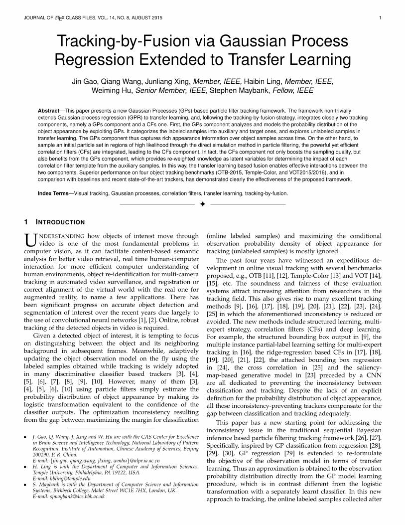
Fig. 1. The overview and system flowchart of the proposed formulation. Theiteration loop labeled as steps 1©, 2© and 3© shows the interactions betweenthe CFs and the transfer learning extension of GPs.

domain is exploited to generate the response maps in thecurrent frame. The unlabeled samples corresponding to theparticles generated from the current response maps influencethe next re-weighting of the auxiliary frames. This iterationloop (see Fig. 1) generates unlabeled samples (step 1©) both forre-weighting the auxiliary frames and inferencing GPs-basedtracking task solution with transfer learning extension in theGPs component (step 2©). Finally, we use the updated CFs (step3©) based on the re-weighted knowledge in the current frame

to re-evaluate those unlabeled samples (step 4©) and achievean auxiliary CFs-based tracking task solution in the CFscomponent. This solution is fused with the GPs-based to makethe final decision, leading to the transfer learning based fusion.Note that CFs are integrated naturally, and the interactionswith GPs (steps 1©, 2© and 3©) play an important role to achievestate-of-the-art performance. Superior results were achieved byintegrating the CFs-based SRDCF tracker [18].

2 RELATED WORK

2.1 Tracking-by-FusionTracking-by-fusion has proved valuable in numerous recenttrackers. An advantage of this hybrid multi-expert strategy isthat the information or knowledge from different sources canbe used to model different distortions of the object appearance.Feature combination, expert ensemble and expert collaborationare three major paradigms in the tracking-by-fusion literature.Each paradigm can reduce the drift resulting from the directMaximum a Posterior (MAP) estimation using a single expert.

Some local/global feature combination methods aredescribed in [8], [33], [34]. Kwon et al. [35] integrate severaldecorrelated generative tracking models with different featuresin an interactive Markov Chain Monte Carlo (IMCMC)framework. The authors improved this original work usingdifferent estimation criteria [36], [37]. Some expert-ensemble-based methods also achieve impressive tracking performance.The base experts in each method are combined by a boostingalgorithm [3], [4], or bootstrapped by structural constraintsbased P-N learning [38], or assigned different weightsvia randomized weighting vectors from a non-stationarydistribution [39], or constructed with different features [40],or collected temporally from previous snapshots [16], or basedon the hierarchical convolutional features from different CNNlayers [41], [42]. Note that the base experts here for eachmethod are always homogeneous. In contrast, there are manyworks which employ diverse tracking experts. These expertsplay complementary roles and offer different viewpoints. Byusing these experts that are biased in opposite directions andconsidering their results as alternatives, the true tracking resultcan be bracketed. This expert collaboration paradigm includessome generative-discriminative methods [8], [43], [44], [45],

JOURNAL OF LATEX CLASS FILES, VOL. 14, NO. 8, AUGUST 2015 3

[46], re-detection based methods [47], [48], [49], and methodscombining template and colour-based models [50]. Ourproposed tracking-by-fusion strategy bears some similarityto the expert collaboration paradigm, whereas the CFs andGPs based experts in our formulation are included in oneloop (See Fig. 1) and hence interact more closely with eachother, leading to mutual enhancement. This differs from thetraditional expert collaboration methods, in which the expertshave few interactions. It is noted that the novel joint learningframework for generative-discriminative experts based low-rank tracking methods proposed in [44], [45], [46] also havethe advantage of expert mutual enhancement.2.2 Transfer learningThere have been many efforts to use deep neural networks(DNNs) for transfer learning in online visual tracking. Thefirst application of a DNN to robust visual tracking wasmade by Wang et al. [51] and based on unsupervised transferlearning. They exploit a stacked denoising autoencoder (SDAE)for unsupervised pre-training and representation learningfrom auxiliary data and then transfer the learnt featuresto the online tracking task. Since the hierarchical featureslearnt from convolutional neural networks (CNNs) outperformhandcrafted features in numerous visual tasks such as imageclassification, recognition and detection on the ImageNet LargeScale Visual Recognition Challenge (ILSVRC), some supervisedinductive transfer learning based CNN trackers [23], [24],[52] have been proposed. They pre-train (offline) networksusing other tracking benchmarks or ILSVRC as source tasksand datasets, and then adapt the networks online to achievehigh performance in the object visual tracking task. A cleardeficiency in these approaches is the high computationaldemand. Contrary to these approaches, some supervisedtransfer learning based trackers using CNNs, but without fine-tuning, have been recently proposed to exploit the featuresfrom different hierarchical convolutional layers, to achievecomparable state-of-the-art results [20], [25], [41], [42], [53].These three approaches all transfer the prior knowledge fromoffline training on the source tasks to the current online objecttracking task. In contrast, we use prior knowledge extractedfrom the online GPs learning with the auxiliary samples.

Li et al. [4] first proposed to extend the semi-supervisedon-line boosting tracker [3] using “Covariate Shift”, leadingto a novel semi-supervised transfer learning based tracker. Itcan utilize auxiliary and unlabeled samples effectively to trainthe strong classifier for tracking. The auxiliary samples’ re-weighting in [4] is based on an online boosting classifier.2.3 Correlation filteringRecently, it has become increasingly popular to track bydetecting patterns in image sequences by correlation with someexample templates [17], [54], [55], [56]. Initially, Bolme et al. [54]develop a Minimum Output Sum of Squared Error (MOSSE)filter, and use a single feature channel, typically an intensityfeature channel, for tracking. The success of the MOSSEtracker motivates a subsequent seminal work of Henriques etal. [17], [55], which presents a more robust kernelized CFs-based tracker (KCF) using a novel circular correlation solutionin the Fourier domain for ridge regression based tracking. Itsflexibility in incorporating multi-dimensional feature channels(ie., HOGs) and non-linear kernels produces a remarkableadvance in performance, despite its high computationalefficiency. There are four examples of research topics on CFs-based tracking dedicated to improving MOSSE and KCF.

First, some work adapts the CFs-based tracking frameworkto incorporate scale [56], [57] and rotation [58] estimates.Second, many researchers focus on making conceptualimprovements in filter learning, such as alleviating the periodiceffects of circular correlation [18], and modifying the filterupdate strategy to decrease the impact of corrupted trainingsamples resulting from occlusions, misalignments and otherperturbations [19]. Third, some trackers cast CFs as the baseexperts for ensemble [41], [42] or combine them with someinstance-level object detectors [48], [49] to build multi-expertcollaboration trackers. Finally, in addition to the incorporationof multi-dimensional feature channels, such as HOGs [17] andColor Names [59], many CFs-based trackers [20], [53], [60]exploit the CNN feature hierarchies for visual tracking. Ourmethod is similar in spirit to the second and third topics in thatwe also integrate CFs into our formulation, and the CFs areupdated using the learnt re-weighted knowledge. However,the ingredients (i.e., CFs and GPs) in our formulation have animpact on each other because they interact in a single loop (SeeFig. 1). This is very different from the prior work [48], [49].

2.4 Subsequent work and ContributionsA preliminary version of this work, namely TGPR, waspresented earlier [61]. TGPR analysed for the first timethe probability distribution of object appearance in theBayesian tracking framework using GPs, contrary to thecommon discriminative tracking approaches which by defaultformulate this probability distribution by making its logistictransformation equivalent to the confidence of the classifieroutputs. The nontrivial extension of GPR to the transferlearning based tracking formulation equips TGPR withtwo properties, auxiliary samples’ re-weighting and multi-expert collaboration; they both substantially improve thetracking performance on the OTB-2013 benchmark [11]. TGPRoutperformed the other trackers by a large margin.

Afterwards, some authors built robust trackers in thespirit of our initial work on TGPR. In [19], a unifiedlearning formulation is proposed to jointly optimize the objectobservation model parameters and the sample quality weights.This resembles TGPR, especially in the learning of real-valuedweights to decrease the impact of corrupted samples. In [62],two differentially fine-tuned CNNs, one tuned conservativelyand the other aggressively, make their own tracking decisionsindividually and the final integrated estimation is simplythe more confident one. This method bears some similarityto TGPR, in that decisions from two differentially updatedtracking experts are fused in order to reduce drifting. Inrecent work [63], a diversified ensemble discriminative trackeris proposed, which also draws support from an auxiliaryclassifier to break the self-learning loop using the effect of long-term memory and avoid the tracking drift.

In the present work, we add some important improvementsto TGPR. We note the importance of the distribution ofunlabeled samples for optimizing the performance of the GPs-based expert and assume that the response maps generated bythe CFs approximate to the correct distribution (Section 3.3).In other words, the greater the response value a region has,the higher the probability of generating an unlabeled samplefrom that region. The optimized GPs-based expert provides theknowledge required to revise the re-weighting of the samplesfrom the auxiliary frames for the update of the CFs-basedexpert. At the end of Section 3.2.4, we give more insight intohow the distribution of unlabeled samples influences the re-

JOURNAL OF LATEX CLASS FILES, VOL. 14, NO. 8, AUGUST 2015 4

weighting of auxiliary samples. The newly updated CFs-basedexpert re-evaluates those unlabeled samples more accuratelyand is again utilized for generating unlabeled samples inthe next frame. Thus, we are able to fuse this auxiliarytracking task solution based on CFs with the target trackingtask solution based on GPs to make the final decision. Itis noted that the update of our CFs-based expert using there-weighted knowledge is very different from the recentlyproposed unified formulation for adaptive decontamination ofthe training set in [19] in two aspects. First, our re-weightingonly concentrates on the much earlier auxiliary frames whilethe latter decontamination includes the whole training setwith the most recently collected training samples. Second, ourupdate of the CFs-based expert in the current frame also relieson the extracted unlabeled samples, whereas the update in [19]only relies on the extracted labeled samples.

In addition, by integrating our formulation with SRDCF,we extend the original experiments on the OTB-2013 andVOT2013 benchmarks to the recent popular OTB-2015, Temple-Color, and VOT2015/2016 benchmarks. More comprehensiveexperiments are performed using the evaluation criteriaTRE and SRE. All the tracking results are compared withmany recent impressive state-of-the-art trackers. The expectedaverage overlap (EAO) graphs and scores on VOT2015/2016are also considered. Some variants of the new tracker areadded for ablation study. We demonstrate the important roleof the interactions between the integrated CFs and GPs in ourformulation by making a comparison with experiments thatomit these interactions. More considerable new analyses andintuitive explanations for these results are also provided.

3 OUR TRANSFER LEARNING BASED FORMULATION

In the following, we first analyse the objective of theobservation model in the particle filters based trackingframework. Then we re-formulate it as a new transfer learningbased formulation and extend GPs to approximately obtainits probability distribution. This process involves three sets ofsamples for robust tracking: auxiliary samples, target samples,and unlabeled samples. Two latent variables are introduced:one for re-weighting the auxiliary samples, and the other fordeciding which tracking candidates are the best in the GPs-based tracking task solution. After giving more insight into theinfluence of the distribution of the unlabeled samples on there-weighting of the auxiliary frames and hence on the updateof CFs, we furthermore show how the unlabeled samples aregenerated from the response maps of the learnt CFs. Finally,we present a high level tracking pipeline to integrate the abovefundamental components and describe the fusion strategy inour transfer learning based tracking formulation.

3.1 Byesian Inference Formulation Using Particle FiltersAs detailed in [26], [27], visual tracking can be cast as aBayesian inference problem in the particle filters based trackingframework. Given a set of observations It of the object up tothe t-th frame, the optimal state variable ˆ

t, which describesthe object center location and scale at time t, can be estimatedusing the true posterior state density p (`t|It) with respectto different criteria, such as the minimum mean-square error(MMSE) estimate with the conditional mean taken and themaximum a posteriori (MAP) estimate with the mode taken.The posterior density p (`t|It) can be inferred using Bayesiantheorem recursively through two steps,

p (`t|It) ∝ p (Xt|`t) p (`t|It−1) (1)

p (`t|It−1) =

∫p (`t|`t−1) p (`t−1|It−1) d`t−1 (2)

where Xt denotes the observation in the t-th frame, or morespecifically the image region enclosed by `t, Eq. (2) involvesthe prediction step, and Eq. (1) carries out the update step. Agood likelihood function p (Xt|`t) (also called the observationmodel) in the update step should modify the prior densityp (`t|It−1) to obtain the sharply peaked posterior density.

Typically, there are two types of particle filters basedMonte Carlo approximation approaches to solve this recursionproblem by generating recursively a set of nU particles,`it, i = 1, 2, . . . , nU. The first type is based on the sequentialimportance sampling (SIS) algorithm, which involves recursivepropagation of importance weights and support particlesas each measurement is received sequentially. One of thevariants of SIS is the sampling importance re-sampling(SIR) algorithm which uses the prior transition probabilityp (`t|`t−1) as the proposal density without incorporating thecurrent observation. Despite the fact that SIR is sensitive tooutliers, it has the advantage that the importance weightsare easily evaluated when set to the likelihood values andthe proposal density is also easily sampled. Thus, the MMSEestimate [27] can be taken as

ˆMMSEt ≈

nU∑i=1

p(Xt|`t = `it

)∑nU

j=1 p(Xt|`t = `jt

)`it (3)

and the MAP estimate asˆMAPt ≈ arg max

`it

p(Xt|`t = `it

). (4)

The second type is the method of direct simulation [31], [32]which is a slight improvement over SIR based on the rejectionsampling algorithm. This method directly uses the likelihoodfunction to reject any proposed particles if they lead to unlikelypredicted distributions for the observed data. The acceptedparticles then lead to the final required posterior distribution.

For each particle `it, the image region Xit associated with it

is the measurement used in the likelihood function. This resultsin an image patch sample set XU = Xi

t, i = 1, 2, . . . , nU, alsocalled the unlabeled sample set in this paper. We concentrateon building a good GPs-based observation model by exploitingall the samples including these unlabeled samples. So there is ahigh demand for generating the particles properly according toa correct distribution. That means we can not directly use thisobservation model to conduct the direct simulation method fortracking. The SIR algorithm also suffers the disadvantage ofincorporating no current observation into the proposal densityfor generating particles. So, we propose to first introduce theCFs-based likelihood function to conduct the direct simulationmethod and draw the particles approximately satisfying theposterior density. Then the SIR algorithm is conducted forMAP estimate using both the target and auxiliary observationmodels based on GPs and the updated CFs respectively. Notethat the generated particles have uniform weights for theattached SIR algorithm. Finally, our transfer learning basedtracking-by-fusion formulation is detailed in Section 3.3. Belowwe detail the GPs-based observation model firstly.

3.2 GPs-Based Observation ModelWe specify our GP observation model based on the trackingresults ˆ

f , f = 1, 2, . . . , t − 1 up to the (t − 1)-st frame. Wecollect nL training samples, each with an indicator belongingto −1,+1, from the previous t − 1 frames and maintainthem over time. We call them the labeled data. The indicator

JOURNAL OF LATEX CLASS FILES, VOL. 14, NO. 8, AUGUST 2015 5

“+1” means the labeled sample has the “same” observationto the object, and vice versa. Furthermore, we divide thesetraining samples into two categories and treat them differently:the auxiliary samples are updated slowly and carefully; thetarget samples are updated quickly and aggressively. LetDT = (Xj , yj), j = 1, 2, . . . , nT denote the target sampleset, and DA = (Xj , yj), j = nT + 1, nT + 2, . . . , nT +nA theauxiliary sample set, where nL = nT+nA and yj ∈ −1,+1 isthe indicator variable. Then, our GPs-based observation modelis specified as: for each particle `it, the measurement densityvalue p

(Xt|`t = `it

)is proportional to the probability of the

measurement Xit having the “same” observation to the object,

i.e., Pr (yi = +1|XU ,DA,DT ), where yi is the indicator for Xit.

We can also cast these conditional probabilities as a regressionfunction of the unlabeled samples for the indicator variables.

As in our initial work TGPR [61], we pick out our favoritesmoother and directly estimate this regression function for allyi in yU = [y1, y2, . . . , ynU

]>. Denote the observed indicators

of the target and auxiliary samples as yT = [y1, y2, . . . , ynT]>

and yA = [ynT+1, ynT+2, . . . , ynL]>. Let 1 = [+1,+1, . . . ,

+1]>, then the regression function for yU can be written asR = Pr (yU = 1|XU ,DA,DT ) (5)

where Pr (yU = 1|XU ,DA,DT ) = [Pr(y1 = +1|XU ,DA,DT ), . . . ,Pr(ynU

= +1|XU ,DA,DT )]>. Inspired by GPclassification from regression [28], [29], [30], we introduce tworeal-valued latent variables zA = [znT+1, znT+2, . . . , znL

]>

∈ RnA and zU = [z1, z2, . . . , znU]> ∈ RnU corresponding to

yA and yU respectively to analyse the regression R directly,and marginalize R over zA, zU at DA and XU ,

Pr (yU = 1|XU ,DA,DT )

=EzA,zU |XU ,DA,DT[ Pr (yU = 1|zA, zU ,XU ,DA,DT ) ]

=

∫ ∫Pr (yU = 1|zU ) p (zA, zU |XU ,DA,DT ) dzA dzU (6)

where p (zA, zU |XU ,DA,DT ) is a probability density function.

3.2.1 Label generation process.As in [28], [29], [30], We also model Pr (yU |zU ) as a noisylabel generation process XU → zU → yU with the sigmoidnoise output model:

Pr (yi|zi) =eγziyi

eγziyi + e−γziyi=

1

1 + e−2γziyi, (7)

∀i = 1, 2, . . . , nU , where γ is a parameter controlling thesteepness of the sigmoid. Intuitively, the larger |zi|, the morelikely that the candidate Xi

t has the indicator variable yi =sign(zi). This generation process is also transferable to theauxiliary data generation, i.e., XA → zA → yA, whereXA = Xj , j = nT + 1, nT + 2, . . . , nT + nA. In this case, zAcan be thought as the re-weighted knowledge extracted fromthe regression R and is related with yA via a sigmoid noiseoutput model similar to Eq. (7). Thus, zA plays a linking rolebetween the regression of GPs-based tracking task solution inSection 3.2.2 and the indicators of the auxiliary samples. Thereplacement of yA by zA in the decision making of this solutionreduces the impact of the corrupted auxiliary samples.3.2.2 GPs extended to transfer learning.We use Bayesian theorem to analyse the density in Eq. (6):

p (zA, zU |XU ,DA,DT )

=Pr (yA|zA, zU ,XA,XU ,DT ) p (zA, zU |XA,XU ,DT )

Pr (yA|XA,XU ,DT )

∝Pr (yA|zA) p (zA, zU |XA,XU ,DT ) . (8)

Note that the normalization term Pr (yA|XA,XU ,DT ) isskipped without altering the analysis of Eq. (6) as this term canbe taken out of the integrand. The term p(zA, zU |XA, XU ,DT )is assumed to define a Gaussian stochastic process, which is acollection of random variables indexed by the samples in XAand XU . It is specified by giving the expected value µ and the(nA + nU )× (nA + nU ) covariance matrix G:

p (zA, zU |XA,XU ,DT ) = N (µ,G) . (9)We can determine µ and G based on XA,XU and DT .

Initially, we define a Gram matrix Gall (symmetric, positive-semidefinite) based on all samples (auxiliary, target andunlabeled), and it can be thought as the prior of GPs forour observation model inference. Typically, elements of aGram matrix store the dot-products in a higher-dimensionalspace between all pairs of samples by transforming theoriginal sample to that space. Without creating vectors inthat space, we only need to evaluate dot-products using akernel function. If we introduce an additional latent variablezT = [zn1

, zn2, . . . , znT

]> ∈ RnT corresponding to yT , Eq. (9)

can be represented as a conditional probability density function

p (zA, zU |XA,XU ,DT ) =p (zA, zU , zT |XA,XU ,XT )

p (zT |XA,XU ,XT ), (10)

where the joint probability density function p(zA, zU , zT |XA,XU ,XT ) also defines a Gaussian stochastic processspecified by N (0,Gall), and the marginal probability densityfunction p (zT |XA,XU ,XT ) has a constant value at a givenzT = yT . Thus, we derive µ and G as follows.Proposition 1. Take the logarithm of p(zA, zU |XA, XU ,DT )

ln (p (zA, zU |XA,XU ,DT ))

=− 1

2

( (y>T z>A z>U

)G−1all

yTzAzU

)+ c , (11)

where c is a constant value. Let

G−1all =

(A B

B> M

), (12)

we determine µ and G as: µ = −M−1B>yT and G = M−1.

The derivation of this proposition is given in Appendix A.2.From Eq. (8) we see that, the non-Gaussianity of Pr (yA|zA)

makes the posterior p (zA, zU |XU ,DA,DT ) no longer Gaus-sian, consequently Eq. (6) becomes analytically intractable.According to [28], [29], [64], assuming p (zA, zU |XU ,DA,DT )to be uni-modal, we can consider instead its Laplaceapproximation. In place of the correct density we use an(nA+nU )-dimensional Gaussian measure with expected valueµ′ ∈ RnA+nU and covariance Σ ∈ R(nA+nU )×(nA+nU ), where

µ′ = arg maxzA∈RnA ,zU∈RnU

p(zA, zU |XU ,DA,DT ) . (13)

We decompose this maximization over zA and zU separately.Taking the logarithm of Eq. (8), we get the following

objective function to maximize

J = ln (Pr (yA|zA))︸ ︷︷ ︸Q1(zA)

+ ln (p (zA, zU |XA,XU ,DT ))︸ ︷︷ ︸Q2(zA,zU )

. (14)

Note zU only appears in Q2, and we can independentlymaximize Q2(zA, •) w.r.t. zU given zA, where (zA, zU ) =arg maxzA,zU

Q1 +Q2. Let

Gall =

(GLL GLU

GUL GUU

). (15)

JOURNAL OF LATEX CLASS FILES, VOL. 14, NO. 8, AUGUST 2015 6

According to [28], [64], by taking derivative of Q2(zA, •) w.r.t.zU , the optimal value zU can be analytically derived as:

zU = GULG−1LL

(yTzA

). (16)

Thus we can derive zA from Eq. (14) as follows.

Proposition 2. The optimal value zA is formally given by:

zA = arg maxzA∈RnA

nL∑j=nT+1

ln (Pr (yi|zi))

− 1

2

(y>T z>A

)G−1LL

(yTzA

)+ c . (17)

The derivation of this proposition is given in Appendix A.3.The above derivations in Eqs. (16) and (17) help us to

analytically compute µ′. In fact, we can also analyticallycompute the covariance Σ and thus Eq. (6) is computationallyfeasible. That is because determining Eq. (6) reduces to

Pr (yU = 1|XU ,DA,DT )

=

∫RnU

Pr (yU = 1|zU ) p(zU |XU ,DA,DT )dzU , (18)

where p (zU |XU ,DA,DT ) is approximatively a Gaussiandensity N (zU ,ΣUU ), and ΣUU is the bottom-right block ofΣ (see [28] for more details). However, in practice, we onlyneed to exploit the fact that the larger zi in zU , the more likelyXit has the “same” observation to the object (yi = +1).

3.2.3 Iterative solution for the re-weighted knowledge.We use an iterative Newton-Raphson update to find theoptimal value zA in Proposition 2. Let ρ(zj) = 1/

(1 + e−2γzj

),

where j = nT +1, nT +2, . . . , nT +nA. Because yj ∈ −1,+1,the auxiliary data generation model can be written as

Pr (yj |zj) =1

1 + e−2γzjyj= ρ(zj)

yj+1

2 (1− ρ(zj))1−yj

2 , (19)

therefore

Q1(zA) = γ (yA − 1)>

zA −nL∑

j=nT+1

ln(1 + e−2γzj

). (20)

Let

G−1LL =

(FTT FTAFAT FAA

), (21)

we can obtain zA by taking derivative of Q1 +Q2 w.r.t. zA,

∂(Q1 +Q2)

∂zA= γ(yA − 1) + 2γ (1− ρ(zA))

− FAAzA −1

2F>TAyT −

1

2FATyT , (22)

where ρ(zA) = [ρ(znT+1), ρ(znT+2), . . . , ρ(znL)]>. The term

ρ(zA) makes it impossible to compute the roots zA in a closedform. We instead solve it with the Newton-Raphson algorithm,

zm+1A ← zmA − η ·H−1 ·

∂(Q1 +Q2)

∂zA

∣∣∣zmA

(23)

where η ∈ R+ is chosen such that (Q1+Q2)m+1 > (Q1+Q2)m,and H is the Hessian matrix defined as

H =

[∂2(Q1 +Q2)

∂zi∂zj

∣∣∣zA

]= −FAA − P (24)

where P is a diagonal matrix with Pii = 4γ2ρ(zi)(1− ρ(zi)).

3.2.4 Construction of the Gram matrix.A very important aspect of GPs for our observation modelinference lies in constructing the prior Gram or kernel matrixGall in Eq. (11). Some methods define the entries of suchmatrices in a “local” manner. For example, in a radial basisfunction (RBF) kernel matrix K, the matrix entry kij =exp(−d2ij/α2) depends only on the distance dij between thei, j-th items. In this case unlabeled samples are useless forcalculating zA because the influence of such samples in solvingEq. (17) is marginalized out. Addressing this issue, we insteaddefine the Gram matrix Gall based on a weighted graph toexplore the manifold structure of all samples (both labeled andunlabeled), as suggested in [64], [65], following the intuitionthat similar samples often share similar labels.

Consider a graph G = (V,E) with node set V = T ∪A ∪Ucorresponding to all the n = nL+nU samples, T = 1, . . . , nT the labeled target samples, A = nT + 1, . . . , nT + nA thelabeled auxiliary samples, and U = nL + 1, . . . , nL + nUthe unlabeled samples. We define an n × n symmetric weightmatrix W = [wij ] on the edges of the graph mimicking the localpatch representation method in [66]. This benefits the robusttracking, especially under partial occlusion. For the i-th and j-th samples, the weight wij is defined by the spatially weightedEuclidean metric over the image representation, i.e., HOGs inparticular Felzenszwalb’s variant [67]. Specifically, for the i-thsample, we divide its image representation into Nr ×Nc non-overlapping blocks, and then describe its (p, q)-th block usinga feature vector hpqi obtained by concatenating the histogramorientation bins in that block. Thus, wij is defined as

wij =1∑

p,q βp,q

∑p,q

βp,q exp(−‖hpqi − hpqj ‖2

σpqi σpqj

)(25)

where σpqi is a local scaling factor proposed by [68]; βp,q =exp(−‖pospq−poso‖2/2σ2

spatial) is the spatial weight, in whichpospq indicates the position of the (p, q)-th block, poso theposition of the block center, and σspatial the scaling factor.

Instead of connecting all the pairs of nodes in V , we restrictthe edges to be within k-nearest-neighborhood, where largedistance between two nodes corresponds to small edge weightbetween them. The parameter k controls the density of thegraph and thus the sparsity of W. We define the combinatorialLaplacian of G in the matrix form as ∆ = D − W, whereD = diag(Dii) is the diagonal matrix with Dii =

∑j wij .

Finally, we define the Gram matrix or kernel by Gall = (∆+I/λ2)−1, where the regularization term I/λ2 guards ∆ + I/λ2

from being singular. From the definition of Gall we can see that,the prior covariance in Eq. (11) between any two samples i, j ingeneral depends on all entries in ∆ – the distances between allthe pairs of the target and unlabeled samples are used to definethe prior. Thus, distribution of target and unlabeled samplesmay strongly influence the kernel, which is desired both forextracting the re-weighted knowledge zA and solving the GPs-based tracking task solution in Eq. (16). We can trace back toEq. (17) and see more discussion details about it below.

Discussion. In Eq. (17), the first term Q1(zA) in the objectivefunction is to measure the consistencies between the elementsof latent variable zA and their corresponding observedindicators in yA with the relationship modeled as the sigmoidnoisy label generation process as in Eq. (7).

As for the second term in Eq. (17), we let Gall = ∆−1

without loss of generality to facilitate the analysis of how thedistribution of unlabeled samples influences the re-weighting

JOURNAL OF LATEX CLASS FILES, VOL. 14, NO. 8, AUGUST 2015 7

of auxiliary samples. Recall Eq. (15) and let

∆ =

(∆LL ∆LU

∆UL ∆UU

). (26)

Using the partitioned matrix inversion theorem given inEq. (35) of Appendix A.1, we can derive G−1LL in the secondterm of Eq. (17) as follows:

G−1LL = ∆LL −∆LU∆−1UU∆UL . (27)

Meanwhile, according to Eq. (34) in Appendix A.1, it isstraightforward to have

∆−1UU∆UL =(∆LU∆−1UU

)>= −GULG−1LL . (28)

Denote y =

(yTzA

), then the second term of Eq. (17) can be

decomposed into:

y>G−1LLy =y>∆LLy + y>∆LUGULG−1LLy

=y>∆LLy + y>∆LUzU

=y>∆LLy + y>∆LUzU + z>U∆ULy + z>U∆UUzU

=1

2

nL∑j,j∗=1,j 6=j∗

wjj∗ (zj − zj∗)2

+nU∑i=1

nL∑j=1

wij (zi − zj)2

+1

2

nU∑i,i∗=1,i6=i∗

wii∗ (zi − zi∗)2, (29)

where zi = yi for i = 1, . . . , nT .From the above derivations, we can easily find that the

second term in Eq. (17) measures the inconsistencies betweenthe re-weighted knowledge zi of auxiliary samples and theobserved indicators yi of target samples, and there is a highdemand for the minimization of these inconsistencies. Morespecifically, we can interpret this minimization as follows. i)For each of the auxiliary samples directly linked to the targetsamples, zi is forced to be similar to yi of the nearby targetsamples. ii) For the auxiliary samples directly linked to eachother, they will have similar zi if they are nearby. iii) Forthe auxiliary samples linked to the target samples indirectlythrough the unlabeled samples, the unlabeled samples mayforce the nearby auxiliary samples to have zi be similar toyi of the nearby target samples. Until now we have givenmore insight into how the distribution of unlabeled samplesinfluences the re-weighting of auxiliary samples. Moreover, ourtransfer learning based formulation can be interpreted as thelearning of re-weighted knowledge for the auxiliary samples,which are mostly influenced by the target and unlabeledsamples related to the current tracking task. The more closelythe auxiliary samples are related to the current tracking taskwhen the inconsistencies in Eq. (17) are minimized, the moreimportant role they may play in fitting the current tracking taskproperly and the larger absolute weight they may be given.

3.3 Building Blocks Using Correlation FiltersSince our transfer learning based formulation is inferred ina semi-supervised fashion as detailed in Section 3.2.4, thequestion is how to generate such a suitable particle set tofacilitate this formulation. The ideal manner is by setting theproposal density function to the true posterior density p (`t|It)itself, however, this is unrealistic. The SIR-based trackingmethods generate the particles only by using p (`t|`t−1) as theproposal density without the current observation incorporated,and hence tend to cause tracking drift.

Recently, CFs-based trackers (e.g., [17], [18], [20]) haveobtained much attention in the literature. They approximatethe true posterior state density as the generated response mapsand obtain the state of the object with the maximum responsevalue. This approximation is much better, but still not enough.The limitation is that CFs are updated by combining the newtemplate computed using the new tracking result with theprevious template only using a rolling average manner, whichtends to miss the chance to fully exploit the relationshipsbetween the historic tracking results and the current frame.Based on these observations, we derive some inspiration fromCFs and propose to cast the generated response maps in thecurrent frame as an approximation to the correct density forgenerating the particles using the direct simulation method.The advantage is not only that the current observation isincorporated into the particle generation process, but also thatthis process relies on another complementary expert with adifferent viewpoint, which is beneficial for fusion.

In the next, we first give some preliminary knowledgeabout CFs in the tracking literature. To concretize our idea ofgenerating particles, we then detail the procedure of samplingusing the direct simulation method. Finally, we update CFsusing the re-weighted knowledge learnt from our transferlearning based formulation and then re-evaluate the unlabeledsamples using the updated CFs, leading to a tracking-by-fusionstrategy for making the final decision.

3.3.1 Preliminaries.We extend the depiction of the formulation of multi-channelCFs in [18] to a more general multi-channel multi-resolutioncase. Specifically, the correlation filter h is learnt from a set oftraining examples (Φ( ˆ

s,f(a)), ys)S,|A|s=1,a=1, where S denotes

the number of resolutions, f(·) is the time index for the framesin the training set A of |A| frames. Each training sampleΦ( ˆ

s,f(a)) consists of a d-dimensional feature map extractedfrom the image region in the frame f(a) from the training set,with the center set to the object location of tracking result ˆ

f(a)

and the scale to br relative to the padded object scale of ˆf(a)

including a context region. Here r ∈ b 1−S2 c, . . . , bS−12 c, and

b is the scale increment factor. All samples are obtained byfeature computation after the corresponding padded imageregions are resized according to br and the ratio betweenthe scales of ˆ

f(a) and ˆ1, leading to the same spatial size

H × W . At each spatial location (u, v, s) ∈ Ω, where Ω :=1, . . . ,H×1, . . . ,W×1, . . . , S, we have a d-dimensionalfeature vector and we denote feature layer l ∈ 1, . . . , d ofΦ( ˆ

s,f(a)) by Φl( ˆs,f(a)). We use a 3-D scalar-valued Gaussian

function y = ysSs=1 defined over the joint scale-positionspace Ω as the desired correlation output, which includes alabel ys(u, v) for each location in Φ( ˆ

s,f(a)). To simplify thenotation we denote Φ( ˆ

s,f(a)) and Φl( ˆs,f(a)) as Φs,a and Φl

s,a

respectively below.The desired filter h consists of one H ×W correlation filter

hl per feature layer. The correlation response of h on oneH×Wsample Φs,a (the desired output is ys) is given by

Rh(Φs,a) =d∑l=1

hl ?Φls,a , (30)

where ? denotes circular cross-correlation [60]. Similar to [60],we use δτ,ς to denote the translated Dirac delta functionδτ,ς(u, v) = δ(u−τ, v−ς), and ∗ to denote circular convolution.Then, the desired filter hl should satisfy that its inner productwith each cyclic shift of the feature layer Cu,v(Φl

s,a) = Φls,a ∗

JOURNAL OF LATEX CLASS FILES, VOL. 14, NO. 8, AUGUST 2015 8

δ−u,−v is as close as possible to the label ys(u, v), which isequivalent to minimizing∑(u,v)

(d∑l=1

⟨Cu,v(Φl

s,a), hl⟩− ys(u, v)

)2

=

∥∥∥∥∥d∑l=1

hl ?Φls,a − ys

∥∥∥∥∥2

(31)Here convolution with the translated δ function is equivalent totranslation

(Φls,a∗δτ,ς

)(u, v)=Φl

s,a(u−τ modH, v−ς modW ).Finally, the filter h is obtained by minimizing (31) over all

the training examples as follows:

εh =

|A|∑a=1

(αa

(S∑s=1

‖Rh(Φs,a)− ys‖2)

+ λαa

d∑l=1

∥∥∥w · hl∥∥∥2)(32)

where the weight αa ≥ 0 determines the impact of eachtraining sample from frame f(a), λ ≥ 0 is the weight of theregularization term, w is the Tikhonov regularization weightsdefined as in [18], and αa can be set to 1

|A| (see Section 4.2for more details). Note that the weights in w determine theimportance of the filter coefficients in hl, and the coefficientsresiding inside the padded background context region aresuppressed by assigning higher weights in w. The abovelinear least squares problem can be solved efficiently in theFourier domain using Parseval’s theorem. The discrete Fouriertransformed (DFT) filters hl = Fhl can then be obtained,where the bar denote the DFT of a function.3.3.2 Generating unlabeled samples and final fusion.Once the desired correlation filter h is trained based on thetracking results ˆ

f(a)|A|a=1 in the training set A and updated

up to the (t− 1)-st frame, we are ready to generate a responsemap in the current t-th frame. Similar to most of the CFs-basedtrackers, we extract the test samples Ψ( ˆ

s,t−1)Ss=1 from thecorresponding image regions in frame t, each of which hasthe center set to the previous location of ˆ

t−1 and the scaleto br relative to the padded object scale of ˆ

t−1. We denotethe test sample Ψ( ˆ

s,t−1) at resolution s as Ψs. Then, theresponse map Rh(Ψs)Ss=1 can be generated efficiently bysome operations such as DFT, inverse DFT and point-wisemultiplication. This map provides an initial hypothesis for thetracking result in frame t. The result can be determined byobtaining the highest maximal response score with the sub-gridinterpolation strategy applied as in the SRDCF tracker [18].However, this initial hypothesis does not fully exploit therelationships between the historic tracking results and thecurrent frame. In our formulation, we propose to integrateSRDCF with our GPs-based observation likelihood model. Theinteractions between these two ingredients are two-fold.

First, given the importance of the approximately correctdistribution of unlabeled samples, we generate the particlescorresponding to these unlabeled samples based on theresponse maps of CFs. The deployment of this procedure isrealized by using the direct simulation method and detailedin step 2 of Algorithm 1. Second, we note that the weight αain Eq. (32) is critical for the effectiveness of trained correlationfilter h. Surprisingly, the transfer learning extension of GPRin our proposed observation model has provided us withsome re-weighted knowledge zA in Eq. (17) for the auxiliarysamples, each of which corresponds with a latent variable zjindicating how this sample is related to the current trackingtask. For each auxiliary frame, we collect only one positiveauxiliary sample based on the tracking result, and hence thevariable zj corresponding with this sample can be used todefine the weight αa of this auxiliary frame in training CFs (see

Algorithm 1: Tracking-by-Fusion via GPR Extended toTransfer Learning

Input: Target sample set DT , auxiliary sample set DA, framet, latest updated correlation filter ht−1, previoustracking result ˆ

t−1 of frame t− 1.Output: updated correlation filter ht, tracking result ˆ

t.1 Obtain the response map Rht−1(Ψs)Ss=1 in the frame t

based on ht−1 and ˆt−1 to approximate the correct

distribution of unlabeled samples2 Generate particles `itnU

i=1 and the corresponding unlabeledsamples XU based on Rht−1(Ψs)Ss=1:

beginAt iteration iter = 0, initialize each particle `it,0 ∼p(`t,0| ˆt−1) = N (`t,0; ˆt−1,Θ) where i = 1, 2, . . . , nU

repeatiter = iter + 1, and set the particle count num = 0repeat

Sample a particle i ∼ Uniform(1, 2, . . . , nU )Sample a proposal`∗t ∼ p(`t,iter|`it,iter−1) = N (`t,iter; `

it,iter−1,Θ)

Assess the likelihood R∗ht−1given `∗t according

to Rht−1(Ψs)Ss=1 and the translation andscale relationships between `∗t and ˆ

t−1

Sample θ ∼ Uniform(0, 1)If θ < R∗ht−1

, accept the proposal, set num =num+ 1, and set `num

t,iter = `∗tuntil num = nU

until iter = Threshold

3 Construct and solve the GPs-based target task solution ofEq. (16), and obtain zA and the target decision zU

4 Update the correlation filter to ht by defining the weight αa

based on zA and the response map to Rht(Ψs)Ss=1

5 Re-evaluate the unlabeled samples and make the auxiliarydecision by assessing the likelihood Rht = [R1

ht, . . . ,

RnUht

]> given `itnUi=1 according to Rht(Ψs)Ss=1 and the

translation and scale relationships between `it and ˆt−1

6 Fusing two decisions, “pool” is the size of candidate poolbegin

[·, IdxA] = sort(Rht ,’descend’)[·, IdxT ] = sort(zU ,’descend’)VA = IdxA(1 : pool) \ i : IdxA(i) /∈ IdxT (1 : pool)VT = IdxT (1 : pool) \ i : IdxT (i) /∈ IdxA(1 : pool)if |VA| > pool/2 then ˆ

t = `VA(1)t

else if |VA| = 0 then ˆt = `

IdxA(1)t

else ˆt = `

VT (1)t

Fig. 2). We only use the auxiliary frames for training CFs, andthe weights are updated using the latent variables of positiveauxiliary samples, normalized to ensure

∑|A|a=1 αa = 1.

Finally, when the CFs are updated in the current frame,we update the response map and re-evaluate the unlabeledsamples by finding the correspondence between the responsevalues and the locations and scales of the correspondingparticles. This new tracking task solution, namely auxiliarytask solution, is fused with the GPs-based target task solutionto make the final decision based on the MAP estimate Eq. (4) ofSIR. A heuristic fusion strategy is adopted. Specifically, whenobtaining two positive candidate sets according to these twosolutions separately, we check the two sets’ coincidence degree,e.g., |VA| in Algorithm 1. When the degree is high, it doesnot matter whether we rely on the auxiliary decision or thetarget decision; when the degree is small, we rely more onthe target decision to ensure the consistency of the trackingresults; when the degree is zero, we rely more on the auxiliarydecision to recover from the severe appearance variation and

JOURNAL OF LATEX CLASS FILES, VOL. 14, NO. 8, AUGUST 2015 9

560 580 600 620 640 660Frame number

680 700 720 740 7600

0.05

0.1

0.15

0.2

0.25

0.3

0.35

Fram

e w

eigh

t

564 600

618624

636

672696

732

Auxiliary Domain

Target Domain

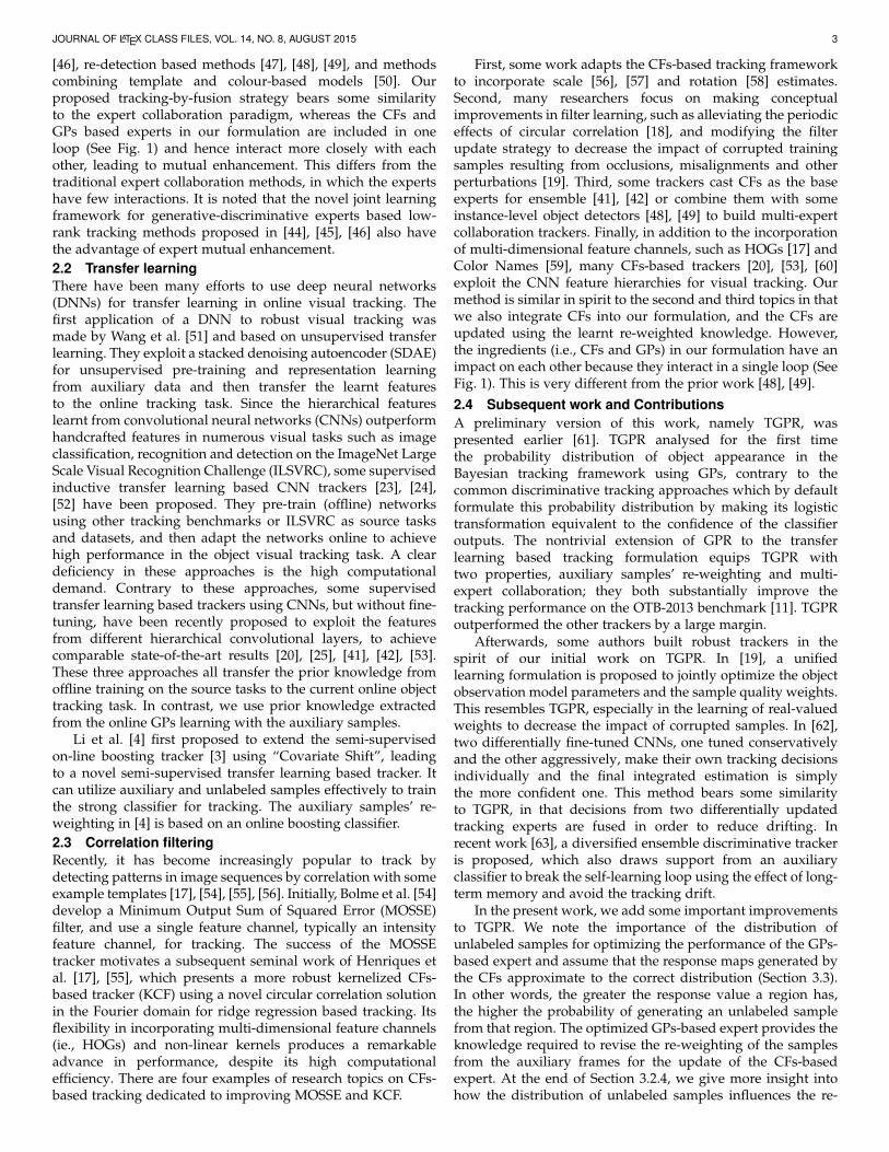
Fig. 2. An illustration of the un-normalized auxiliary frame weights fortraining CFs at the exemplary frame instance #762 on the example trackingsequence Panda in the OTB-2015 benchmark. The weights are obtainedfrom the re-weighting of our GPs-based transfer learning formulation. Theimage patches in the auxiliary domain are shown for example frames,which are obtained from the auxiliary frames by padding the correspondingtracking results’ scales (blue box) to include the context regions. The aimof our tracking is to estimate the location and scale of the panda at frame#762 in the target domain. It can be easily found that the auxiliary framesmostly related to the current tracking task (frames #618 and #624) areconsiderably up-weighted for training CFs, while the others are down-weighted or even useless (frames #564 and #600).

heavy occlusion. We outline this procedure in Algorithm 1.

4 EXPERIMENTS

The principal aim of our experiments is to investigatethe effectiveness of incorporating CFs into our GPs-basedobservation likelihood model, where the interactions betweenthe integrated CFs and GPs lead to a new transfer learningbased formulation for tracking-by-fusion. To validate thatthis formulation yields results comparable with recent state-of-the-art trackers, we conduct extensive experiments onfour benchmarks, i.e., OTB-2015 [12], Temple-Color [13], andVOT2015/2016 [14], [15], by integrating SRDCF into ourformulation. The results are also compared with some baselinesand variants of our approach.

Section 4.1 describes the used benchmark datasets withcorresponding evaluation criteria and the platform forexperimental evaluation. In Section 4.2, we present thedetails about fusion settings, features, samples collection, andparameters in our experiments. Note that all our settingsare fixed for all experiments. The setup of the baselines andour variants as well as the comparisons for illustrating theproperties of our tracking formulation are given in Section 4.3.Finally, Section 4.4 presents the comparison with state-of-the-art trackers. More detailed experimental results are also givenas the supplementary material.4.1 Experimental SetupWe evaluate the proposed tracking formulation thoroughlyover OTB-2015, Temple-Color, and VOT2015/2016 by follow-ing rigorously the evaluation protocols.

The OTB-2015 dataset can be generalized to two sub-benchmarks, namely TB-100 and TB-50. TB-100 includes allthe 100 objects in the 98 challenging image sequences, while50 difficult and representative ones are selected to constituteTB-50 for an in-depth analysis since some of the objects inTB-100 are similar or less challenging. The tracking results onthe OTB dataset are reported in terms of the mean overlapprecision (OP ) and the mean distance precision (DP ). TheOP score is the fraction of frames in a sequence where theintersection-over-union overlap of the predicted and groundtruth rectangles exceeds a given threshold; the DP score is the

fraction of frames where the Euclidean distance between thepredicted and ground truth centroids is smaller than a giventhreshold. Based on these two evaluation metrics, the OTB-2015 benchmark provides two kinds of plots to quantify theperformance of the trackers. i) In the success plot, the successrate refers to the mean OP over all sequences in each sub-benchmark and is plotted against a uniform range of somethresholds between 0 and 1. An area-under-the-curve (AUC)criterion can also be computed from this success plot. ii) Inthe precision plot, the precision refers to the mean DP overall sequences in each sub-benchmark and is plotted against auniform range of some thresholds between 0 and 50 (pixels).Except for One-Pass Evaluation (OPE) which evaluates trackersby running them until the end of a sequence (no-reset) withinitialization from the ground truth in the first frame, there aretwo other evaluation criteria to analyse a tracker’s robustnessto initialization: Temporal Robustness Evaluation (TRE) andSpatial Robustness Evaluation (SRE). TRE starts the tracker at20 different frame snapshots while SRE initializes the trackerwith perturbed bounding boxes. The Temple-Color benchmarkcompiles a large set of 128 color sequences to demonstrate thebenefit of encoding color information for tracking. It uses thesame evaluation protocol to OTB-2015.

In contrast, the VOT2015/2016 benchmarks have manydifferent but more challenging sequences than the aforemen-tioned benchmarks and a reset-based methodology is appliedin the toolkit. Whenever a failure (zero overlap of the predictedand ground truth rectangles) is detected, the tracker is re-initialized five frames after the failure. Thus, two weaklycorrelated performance measures can be used: the accuracy(A) measures how well the predicted bounding box overlapswith the ground truth, i.e., the average overlap computedover the successfully tracked frames; the robustness (R) isestimated by considering how many times the trackers failedduring tracking, i.e., the failure rate measure (Rfr) computedas the average number of failures, or the reliability (RS) whichcan be interpreted as a probability that the tracker will stillsuccessfully track the object up to S frames since the last failure

RS = exp

(−S Rfr

Nframes

),

where Nframes is the average length of the sequences. Then,the A-RS pair can be visualized as a 2-D scatter AR-rawplot. The trackers can be ranked with respect to each measurein this plot separately, leading to another AR-rank plot. Toquantitatively reflect both robustness and accuracy in a moreprincipled manner while ranking the trackers, the expectedaverage overlap (EAO) measure is proposed to measure theexpected no-reset average overlap (AO) of a tracker run ona short-term sequence, although it is computed from the VOTreset-based methodology. In addition, the VOT2016 benchmarksupports the OTB no-reset OPE evaluation to measure the trueno-reset AO of a tracker. The VOT tracking speed (frames persecond) is reported in equivalent filter operation (EFO) units(frames per unit). It is computed by dividing the measuredtracking time for a whole sequence with the time required fora predefined filtering operation and then dividing the framenumber of the sequence with the computed new tracking timein EFO units.

All experiments are performed on a workstation withIntel(R) Xeon(R) CPU E5-2630 v4 @ 2.20GHz, and the runningtime is about 3 fps. The Matlab code and raw results will beavailable at https://github.com/Amgao/TGPRfSRDCF.

JOURNAL OF LATEX CLASS FILES, VOL. 14, NO. 8, AUGUST 2015 10

TABLE 1Ablation Study of the Proposed Tracking-by-Fusion Formulation; We Conduct the Experiments in Terms of OPE on the OTB-2015 Benchmark; the

Results Are Reported as Mean OP (%) / Mean DP (%) Scores at Thresholds of 0.5 / 20 Pixels Respectively; We Select SRDCF and Our Initial WorkTGPR with HOG Settings as Baselines Since Our Formulation Is Implemented by Fusing SRDCF with TGPR; Two Kinds of Simplified Variants Are

Compared: i) TGPRfSRDCF D without (w/o) Distribution Adaptation and ii) TGPRfSRDCF W w/o Using the Re-weighted Knowledge; Five DifferentLearning Rate Values for TGPRfSRDCF W Are Tested, i.e., 0.015, 0.02, 0.025, 0.03, 0.035.

TGPR HOG [61] SRDCF [18] TGPRfSRDCF D TGPRfSRDCF W TGPRfSRDCFLearning Rate - 0.025 - 0.015 0.02 0.025 0.03 0.035 -TB-100 63.9/69.7 72.8/78.9 73.1/77.2 78.6/81.4 78.0/81.0 76.8/80.4 77.9/82.0 75.9/79.1 78.5/81.9TB-50 53.5/59.7 66.6/73.2 65.5/70.7 70.9/74.9 71.4/75.6 70.2/74.9 70.7/76.9 68.3/72.6 73.5/78.4

4.2 Implementation DetailsFusion with SRDCF. We explore the representative CFs-basedtracker SRDCF for building our blocks, leading to a new trackernamed TGPRfSRDCF. Specifically, if we set αa = 1

|A| andS = 1 in Eq. (32), then it degenerates to SRDCF, where a 2-D translation filter is learnt and applied to different resolutionsto generate the response map over the translation and multi-resolution scale spaces. We borrow the publicly available codeof SRDCF for integration, and follow the original settings.

Features and samples collection. We use HOG of theversion in [67] for image representation of both GPs and CFs.For generating particles `it

nUi=1 from the current frame t, we

only consider the variations of 2-D translation (xt,

yt) and

scale (st) in the affine transformation. We set the number nUof particles to 300, and the covariance of

xt,yt, st in Θ to

σx, σy, 0.05, where σx = σy = max(8,min(10, (widtht−1 +heightt−1)/8)), widtht−1 and heightt−1 are the width andheight of previous tracking result ˆ

t−1. As for DT , we use thetracking results of past 24 frames t − 24, . . . , t − 1 (or lessthan 24 at the beginning of the track) for extracting positivetarget samples. The negative target samples are collected fromthe frame t − 1 around its tracking result ˆ

t−1 using densesampling method in the sliding region, where the Euclideandistances between the center locations of the sampled negativetarget samples and ˆ

t−1 lie in a certain range (r/4, r/3),where r = (width2t−1 + height2t−1)

12 /4. Then, we randomly

sample 100 negative target samples. To update the auxiliarysample set slowly, we collect the auxiliary samples DA fromthe frames before t − 24 at intervals of 6 frames, if theseframes are available. The collection in such frames is the sameas the collection of labeled samples in [4], except that weadd 4 more negative auxiliary samples along the directionsof x and

y symmetrically with respect to the tracking resultcenter of the corresponding frame. We set the size limit of thepositive auxiliary sample buffer to 35, and thus the negativeauxiliary sample buffer to 280. All those samples used in GPsare obtained by re-sizing the corresponding image regions totemplates of size 32 × 32 and extracting the HOG descriptorswith a cell size of 4 pixels, leading to a d-dimensional featurevector for each cell, where d = 31. In Eq. (25) of Section 3.2.4,we set Nr = Nc = 2 to calculate the weights of W. Thus, eachblock consists of 16 cells, and the dimension of hpqi is 496.

Other parameter settings. In Eq. (25), σpqi is calculated fromthe 7th nearest neighbor. The parameter k for controlling thesparsity of W is set to 50. Gall is defined by setting λ = 1000.In Section 3.2.3, γ in Eq. (7) is set to 10, η in Eq. (23) is 0.2, andthe number of iterations for calculating zA from Eq. (23) is 40.In Algorithm 1, Threshold is set to 10, and pool is 30.

4.3 Experiment 1: Ablation StudyTo provide more insights into the effectiveness of theinteractions between the integrated CFs and GPs in ourformulation, we explore variants of our approach without the

0 0.2 0.4 0.6 0.8 1

Overlap threshold

0

0.2

0.4

0.6

0.8

1

Suc

cess

rat

e

TB-100 Success plots of OPE

TGPRfSRDCF [0.628]TGPRfSRDCF_W

0.03 [0.626]

TGPRfSRDCF_W0.015

[0.622]

TGPRfSRDCF_W0.025

[0.619]

TGPRfSRDCF_W0.02

[0.619]

TGPRfSRDCF_W0.035

[0.609]

SRDCF [0.598]TGPRfSRDCF_D [0.595]TGPR HOG [0.510]

0 0.2 0.4 0.6 0.8 1

Overlap threshold

0

0.2

0.4

0.6

0.8

1

Suc

cess

rat

e

TB-50 Success plots of OPE

TGPRfSRDCF [0.583]TGPRfSRDCF_W

0.03 [0.568]

TGPRfSRDCF_W0.025

[0.565]

TGPRfSRDCF_W0.02

[0.561]

TGPRfSRDCF_W0.015

[0.555]

TGPRfSRDCF_W0.035

[0.549]

SRDCF [0.539]TGPRfSRDCF_D [0.528]TGPR HOG [0.429]

Fig. 3. Success plots showing an ablation study comparison of our proposedformulation with two kinds of variants and some baselines in terms of OPEon the OTB-2015 benchmark. The legend contains the AUC scores foreach method. Best viewed in color.interactions for ablation study. Specifically, these simplifiedvariants include, i) variant abbreviated as TGPRfSRDCF D,which generates unlabeled samples only using the initializedparticles `it,0

nUi=1 in step 2 of Algorithm 1 without distribution

adaptation (adapting them to fit the response maps from CFs);and ii) variant abbreviated as TGPRfSRDCF W, which updatesCFs by defining αa in step 4 of Algorithm 1 according tothe commonly used exponentially decaying weights with afixed learning rate. We test 5 different learning rate values forTGPRfSRDCF W, i.e., 0.015, 0.02, 0.025, 0.03, 0.035. In addition,we collect some baselines for comparison, including SRDCFand our previous work TGPR. Note that we substitute thefeature representation in the original TGPR with HOGs to alignwith our new approaches for fair comparison.

We start by summarizing the ablation study in terms ofOPE on the OTB-2015 dataset in Table 1 and Fig. 3. Table 1shows the results in mean DP and mean OP , and Fig. 3 showsthe success plots of the participants indexed using the AUCscore. We remark that our complete version TGPRfSRDCFfurther consistently improves the performance over all the twosub-benchmarks by providing a significant mean OP scoregain of 5.7 ∼ 6.9% and AUC score gain of 3.0 ∼ 4.4%compared to the baseline SRDCF tracker when fusing it withour initial work TGPR. It also worth mentioning that allthe improvements achieve the highest gains on the mostchallenging sub-benchmark TB-50.

Table 1 and Fig. 3 also show a comparison of the proposedformulation and its simplified variants. From the comparisonwe see that, our complete version always performs better thanthe two kinds of variants, or at least not worse, which showsthe benefit of using distribution adaptation for generatingunlabeled samples and re-weighted knowledge for the updateof CFs. Moreover, the variant without distribution adaptationtends to perform worse than the variants without using there-weighted knowledge, which suggests that the distributionadaptation is a little more crucial factor than using the re-weighted knowledge, although they both play important rolesin our formulation. This may be due to our newly designedformulation which starts with generating approximatelycorrect distribution of unlabeled samples. These generated

JOURNAL OF LATEX CLASS FILES, VOL. 14, NO. 8, AUGUST 2015 11

TABLE 2Comparison of Our Proposed Formulation (Complete Version) with Some Participating Algorithms in the OTB-2015 Benchmark and Other Latest

State-of-the-Art Trackers; We Conduct the Experiments in Terms of OPE, TRE and SRE on OTB-2015, and Only OPE on Temple-Color; the Results AreReported as AUC (%) / Mean OP (%, at 0.5) / Mean DP (%, at 20 Pixels) Scores.

TB-100 TB-50 Temple-ColorOPE TRE SRE OPE TRE SRE OPE

C-COT [20] 67.1/82.0/89.8 67.4/81.9/88.8 63.0/79.8/86.7 61.4/74.9/84.3 62.9/75.9/86.4 57.9/72.4/82.0 57.4/70.2/78.1TGPRfSRDCF 62.8/78.5/81.9 63.1/78.3/81.3 57.5/74.9/77.4 58.3/73.5/78.4 58.5/73.5/78.0 51.3/66.8/71.0 54.9/67.5/73.5DeepSRDCF [53] 63.5/77.9/85.1 64.6/77.9/85.5 59.4/75.4/82.1 56.0/67.6/77.2 59.2/71.0/81.6 52.7/66.7/75.3 53.7/65.2/73.8SRDCFdecon [19] 62.7/76.6/82.5 62.8/76.3/80.4 57.1/73.1/76.9 56.0/69.7/76.4 56.5/69.5/74.9 50.9/65.4/70.3 53.5/65.6/72.7SRDCF [18] 59.8/72.8/78.9 61.5/74.9/79.1 56.1/71.1/75.6 53.9/66.6/73.2 56.3/69.3/74.8 50.1/64.1/69.1 51.0/62.0/69.4Staple [50] 58.1/70.9/78.4 59.7/72.8/77.9 54.5/68.2/74.6 50.9/61.2/68.1 53.0/64.4/70.4 49.4/61.2/68.3 -/-/-SAMF [69] 55.3/67.4/75.1 58.6/72.0/77.5 52.2/65.1/72.4 46.9/57.1/65.0 52.1/64.1/71.3 45.8/56.4/64.7 -/-/-MEEM [16] 53.0/62.2/78.1 56.5/68.3/79.5 50.2/59.8/73.0 47.3/54.2/71.2 50.9/60.6/74.7 44.5/51.7/65.4 45.9/56.0/63.9TGPR HOG [61] 51.0/63.9/69.7 53.8/66.2/71.9 46.9/59.5/64.8 42.9/53.5/59.7 47.6/58.9/64.7 39.2/49.7/55.4 41.8/52.2/58.4DSST [57] 51.3/60.1/68.0 53.8/64.4/69.6 48.5/59.8/65.8 45.2/53.8/60.4 47.3/56.6/62.8 42.2/51.8/58.5 40.7/47.3/53.5DLR [46] 49.6/58.5/67.3 -/-/- -/-/- 43.4/49.9/59.7 -/-/- -/-/- -/-/-KCF [17] 44.6/51.0/65.5 51.3/61.1/71.1 43.4/50.9/63.9 35.3/38.3/54.3 43.3/50.6/62.6 35.5/39.6/53.9 38.4/46.1/54.9Struck [9] 46.2/52.0/63.9 52.1/61.2/70.2 44.0/50.7/61.8 38.2/41.1/53.7 44.9/51.2/61.7 37.3/41.8/53.7 44.1/51.4/61.2TLD [38] 42.7/50.2/59.6 44.6/51.9/60.6 40.4/47.4/55.9 36.2/42.0/49.5 38.1/43.2/52.0 34.2/40.0/47.6 -/-/-MIL [6] 33.3/33.4/44.2 39.7/43.5/52.3 32.7/33.1/44.1 26.5/24.4/35.1 31.9/33.1/42.6 26.2/25.3/35.9 33.4/35.7/44.6IVT [26] 31.6/36.6/43.1 36.9/42.4/47.7 29.2/34.5/40.3 23.7/27.8/32.6 27.7/31.2/36.6 21.5/25.6/30.2 28.9/33.1/41.1

0 0.2 0.4 0.6 0.8 1

Overlap threshold

0

0.2

0.4

0.6

0.8

1

Suc

cess

rat

e

TB-100 Success plots of OPE

CCOT [0.671]DeepSRDCF [0.635]TGPRfSRDCF [0.628]SRDCFdecon [0.627]SRDCF [0.598]Staple [0.581]SAMF [0.553]MEEM [0.530]DSST [0.513]TGPR HOG [0.510]DLR [0.496]

0 0.2 0.4 0.6 0.8 1

Overlap threshold

0

0.2

0.4

0.6

0.8

1

Suc

cess

rat

e

TB-50 Success plots of OPE

CCOT [0.614]TGPRfSRDCF [0.583]SRDCFdecon [0.560]DeepSRDCF [0.560]SRDCF [0.539]Staple [0.509]MEEM [0.473]SAMF [0.469]DSST [0.452]DLR [0.434]TGPR HOG [0.429]

0 0.2 0.4 0.6 0.8 1

Overlap threshold

0

0.2

0.4

0.6

0.8

1

Suc

cess

rat

e

Temple-Color Success plots of OPE

C-COT [0.574]TGPRfSRDCF [0.549]DeepSRDCF [0.537]SRDCFdecon [0.535]SRDCF [0.510]MEEM [0.459]Struck [0.441]TGPR HOG [0.418]DSST [0.407]KCF [0.384]

Fig. 4. Success plots showing the performance of our formulation (complete version) compared to some representative tracking algorithms provided withOTB-2015 and some latest state-of-the-art trackers in terms of OPE on the OTB-2015 and Temple-Color benchmarks. The legends of the success plotscontain the AUC scores for each method. Only some top-performing trackers are displayed in the legend for clarity. Best viewed in color.

0 0.2 0.4 0.6 0.8 1

Overlap threshold

0

0.2

0.4

0.6

0.8

1

Suc

cess

rat

e

TB-100 Success plots of TRE

CCOT [0.674]DeepSRDCF [0.646]TGPRfSRDCF [0.631]SRDCFdecon [0.628]SRDCF [0.615]Staple [0.597]SAMF [0.586]MEEM [0.565]DSST [0.538]TGPR HOG [0.538]

0 0.2 0.4 0.6 0.8 1

Overlap threshold

0

0.2

0.4

0.6

0.8

1

Suc

cess

rat

e

TB-100 Success plots of SRE

CCOT [0.630]DeepSRDCF [0.594]TGPRfSRDCF [0.575]SRDCFdecon [0.571]SRDCF [0.561]Staple [0.545]SAMF [0.522]MEEM [0.502]DSST [0.485]TGPR HOG [0.469]

0 0.2 0.4 0.6 0.8 1

Overlap threshold

0

0.2

0.4

0.6

0.8

1

Suc

cess

rat

e

TB-50 Success plots of TRE

CCOT [0.629]DeepSRDCF [0.592]TGPRfSRDCF [0.585]SRDCFdecon [0.565]SRDCF [0.563]Staple [0.530]SAMF [0.521]MEEM [0.509]TGPR HOG [0.476]DSST [0.473]

0 0.2 0.4 0.6 0.8 1

Overlap threshold

0

0.2

0.4

0.6

0.8

1

Suc

cess

rat

e

TB-50 Success plots of SRE

CCOT [0.579]DeepSRDCF [0.527]TGPRfSRDCF [0.513]SRDCFdecon [0.509]SRDCF [0.501]Staple [0.494]SAMF [0.458]MEEM [0.445]DSST [0.422]TGPR HOG [0.392]

Fig. 5. Success plots showing the performance of our formulation (completeversion) compared to some representative tracking algorithms providedwith OTB-2015 and some latest state-of-the-art trackers in terms of TREand SRE on the OTB-2015 benchmark. The legends of the success plotscontain the AUC scores for each method. Only some top-performingtrackers are displayed in the legend for clarity. Best viewed in color.

unlabeled samples influence not only the auxiliary/target tasksolution, but also the learning of the re-weighted knowledge.The comparison with the variants using the exponentiallydecaying weights with 5 different learning rates also showsthat our automatically learnt re-weighted knowledge can avoidusing the tediously hand-tuned different learning rates ondifferent benchmarks to achieve the superior results.

4.4 Experiment 2: State-of-the-Art ComparisonIn this section, we conduct a comprehensive comparisonof our proposed formulation (complete version) with somerepresentative tracking algorithms provided with the OTB-2015 benchmark including MIL [6], IVT [26], TLD [38],Struck [9], etc., and also with some latest state-of-the-arttrackers including MEEM [16], our initial work TGPR [61] withHOGs, MDNet [24], EBT [70], SiamFC [25], DLR [46], and alarge family of CFs-based trackers, i.e., KCF [17], DSST [57],SAMF [69], Staple [50], SRDCF [18], SRDCFdecon [19],DeepSRDCF [53], C-COT [20].

C-COT was appraised as the best tracker on VOT-2016 [15]for its significant innovation in relaxing the constant featuremap dimension assumption of SRDCF and allowing thespatially regularized CFs to be learnt on the feature mapsof multiple different resolutions from the pre-trained CNNs.This breakthrough enhances the effectiveness of using thedeep feature maps at different layers and boosts the trackingperformance significantly in the literature. DeepSRDCF can beseen as a simplified single-resolution version of C-COT whenusing the combination of convolutional layers. SRDCFdeconalso goes in the direction of improving the baseline SRDCF,and its property of learning continuous weights for decreasingthe impact of corrupted samples also exists in our formulation.

OTB-2015 and Temple-Color datasets. We summarize thecomparison results by reporting them in terms of AUC, meanOP and mean DP scores in Table 2 and showing the successplots of some top trackers indexed using the AUC score inFigs. 4 and 5. From these results we see that, despite the inferiorperformance compared to C-COT using the deep features,our complete version TGPRfSRDCF consistently improves

JOURNAL OF LATEX CLASS FILES, VOL. 14, NO. 8, AUGUST 2015 12

TABLE 3Comparison of Our Proposed Formulation (Complete Version) with Some Participating Algorithms on the VOT2015/2016 Benchmarks; the Results Are

Reported as EAO, A, Rfr or RS (S = 100), No-Reset AO, and VOT Tracking Speed in EFO. A Large Value in EFO Indicates a High Tracking Speed.VOT SRDCF [18] MDNet N [24] SRDCFdecon [19] SiamFC R [25] DeepSRDCF [53] Staple [50] TGPRfSRDCF EBT [70] SSAT TCNN C-COT [20]

2015EAO 0.288 - 0.299 - 0.318 0.300 0.311 0.313 - - 0.303A 0.551 - 0.552 - 0.562 0.563 0.572 0.453 - - 0.535Rfr 1.242 - 1.095 - 1.046 1.385 1.254 1.021 - - 0.821

2016

EAO 0.247 0.257 - 0.277 0.276 0.295 0.279 0.291 0.321 0.325 0.331A 0.536 0.542 - 0.550 0.529 0.547 0.551 0.465 0.579 0.555 0.541

− lnRS 0.419 0.337 - 0.382 0.326 0.378 0.376 0.252 0.291 0.268 0.238AO 0.398 0.458 - 0.422 0.428 0.390 0.410 0.370 0.516 0.487 0.470EFO 1.990 0.534 - 5.444 0.380 11.114 1.563 3.011 0.475 1.049 0.507

102030405060

Robustness rank

10

20

30

40

50

60

Acc

urac

y ra

nk

Pooled AR ranks

TGPRfSRDCF

0 0.2 0.4 0.6 0.8 1

Robustness (S = 100.00)0

0.1

0.2

0.3

0.4

0.5

0.6

0.7

0.8

0.9

1

Acc

urac

y

Pooled AR values

TGPRfSRDCF

161116212631364146515661660

0.05

0.1

0.15

0.2

0.25

0.3

0.35

0.4MDNet [0.378]DeepSRDCF [0.318]EBT [0.313]TGPRfSRDCF [0.311]C-COT [0.303]Staple [0.300]SRDCFdecon [0.299]SRDCF [0.288]LDP [0.279]sPST [0.277]SC-EBT [0.255]NSAMF [0.254]Struck [0.246]RAJSSC [0.242]

TGPRfSRDCF

ACT AOG ASMS CMT CT DAT DFT DSST DeepSRDCF EBT FoT FragTrack HMMTxD HoughTrack IVT KCF2

L1APG LDP LGT LT-FLO MCT MDNet MEEM MIL OAB OACF PKLTF RobStruck SCBT SODLT STC TGPR

PTZ-MOSSE HRP BDF CMIL Dtracker FCT G2T MTSA-KCF KCFDP KCFv2 LOFT-Lite MatFlow MKCF+ MUSTer

MvCFT NCC NSAMF RAJSSC S3Tracker sKCF sPST SAMF SC-EBT SME SRAT SRDCF Struck SumShift TRIC-track

ZHANG C-COT SRDCFdecon TGPRfSRDCF Staple

Fig. 6. The AR-rank plot (left) and AR-raw plot (middle) using the A-RS pairs generated by sequence pooling on VOT2015, and the corresponding expectedaverage overlap graph (right) with trackers ranked from right to left. Best viewed in color.

SRDCF in terms of OPE, TRE and SRE over all the TB-100, TB-50 and Temple-Color benchmarks as other improvedversions (i.e., C-COT, DeepSRDCF and SRDCFdecon) havedone. We also expect consistent improvement over C-COTwhen integrating C-COT into our formulation. TGPRfSRDCFachieves comparable performance with DeepSRDCF, and evensuperior performance in terms of AUC of OPE over themore challenging TB-50 and Temple-Color benchmarks byproviding gains ranging from 1.2 ∼ 2.3%. As for SRDCFdecon,TGPRfSRDCF significantly outperforms it in terms of all theperformance criteria over TB-50 and Temple-Color.

In addition, it is worth noting that in Table 2 TGPRfSRDCFmostly outperforms DeepSRDCF in terms of mean OP at thethreshold of 0.5 while being inferior with respect to AUCand mean DP . This is consistent with the observation inFigs. 4 and 5, where DeepSRDCF always achieves much highermean OP scores at the lower overlap thresholds. The reasonis that DeepSRDCF can always at least capture part of theobject while encountering large object variations so that theoverlap with the ground truth is always above zero and thedistance to the center of the ground truth below 20 pixels.This can be attributed to the deep convolutional featureslearnt from the large ImageNet dataset for object detectionand classification. These features can capture different colorsand edges over image regions (the feature dimension is 96),and hence more robust to object variations including deviationfrom the predicted location.

VOT2015/2016 datasets. We show the comparative resultson VOT2015/2016 in Table 3 and Figs. 6, 7 and 8. Among thecompared methods, TGPRfSRDCF achieves favorable resultsin terms of accuracy (see the AR-rank plots of Figs. 6 and7), while still being comparable with the top-performingtrackers C-COT, TCNN, SSAT, MDNet (or MDNet N), EBT,Staple and DeepSRDCF in terms of the other measurements.Note that MDNet N and SSAT on VOT2016 are variationsof the VOT2015 winner MDNet which is derived from

CNN, except that MDNet N eliminates the multi-domain pre-training process using other tracking datasets. Further more,TCNN extends MDNet N to a tree-structured appearancemodel for tracking.

In addition, TGPRfSRDCF significantly exceeds the baselinetracker SRDCF without sacrificing much tracking speed.TGPRfSRDCF also exceeds the VOT2015 and VOT2016published state-of-the-art bounds (gray horizontal lines in theexpected average overlap graphs of Figs. 6 and 7), whichdemonstrates the superiority of our proposed formulation.

5 CONCLUSIONIn this work, we demonstrated that it is possible to directlyanalyse the probability density function for target appearancein the sequential Bayesian inference based tracking frameworkusing GPs. The resulting transfer learning based trackingformulation provides an interface for tracking-by-fusion withCFs. Specifically, the transfer learning extension of GPRreceives the response maps of CFs as the approximately correctdistribution for generating unlabeled samples, while in returnproviding more conscious re-weighted knowledge to CFs forupdating. We have applied this new formulation to integratethe baseline tracker SRDCF, leading to significant improvementand state-of-the-art performances.

Since the preliminary version of this work, learningcontinuous weights for decreasing the impact of corruptedsamples has been exploited successfully for CFs based trackerin [19]. C-COT was appraised as the best tracker on VOT-2016 for its significant innovation in relaxing the constantfeature map dimension assumption. An interesting directionfor further work is to integrate C-COT into our formulationto gain further improvement. Another interesting direction forfurther work is to learn affinity in Eq. (25) using deep learningand directly output all the similarities in a purely data-drivenmanner [71], instead of designing the similarity kernels onimage features.

JOURNAL OF LATEX CLASS FILES, VOL. 14, NO. 8, AUGUST 2015 13

10203040506070

Robustness rank

10

20

30

40

50

60

70

Acc

urac

y ra

nk

Pooled AR ranks

TGPRfSRDCF

0 0.2 0.4 0.6 0.8 1

Robustness (S = 100.00)

0

0.1

0.2

0.3

0.4

0.5

0.6

0.7

0.8

0.9

1

Acc

urac

y

Pooled AR values

TGPRfSRDCF

16111621263136414651566166710

0.05

0.1

0.15

0.2

0.25

0.3

0.35

0.4C-COT [0.331]TCNN [0.325]SSAT [0.321]MLDF [0.311]Staple [0.295]DDC [0.293]EBT [0.291]SRBT [0.290]STAPLE+ [0.286]TGPRfSRDCF [0.279]DNT [0.278]SSKCF [0.277]SiamFC-R [0.277]DeepSRDCF [0.276]

TGPRfSRDCF

ACT

ANT

ART_DSST

ASMS

BDF

BST

CCCT

C-COT

CDTT

CMT

CTF

ColorKCF

DAT

DDC

DFST

DFT

DNT DPT DPCF DSST2014 DeepSRDCF EBT FCF FCT FT FoT GCF GGTv2 HCF HMMTxD HT IVT

KCF2014 SMACF LGT LT_FLO LoFT_Lite MAD MDNet_N MIL MLDF MvCFT MatFlow Matrioska NSAMF OEST

PKLTF RFD_CF2 SAMF2014 SCT SHCT SMPR SRBT SRDCF SSAT SSKCF STAPLE+ STC STRUCK2011 SWCF

SiamFC-A SiamFC-R Staple TCNN TGPR TRIC-track deepMKCF NCC sKCF SO-DLT TGPRfSRDCF

0 0.1 0.2 0.3 0.4 0.5 0.6 0.7 0.8 0.9 10

0.5

1AR plot for experiment baseline (mean)

ACT ANT ART_DSST ASMS BDF BST CCCT C-COT CDTT CMT CTF ColorKCF DAT DDC DFST DFT

Fig. 7. The AR-rank plot (left) and AR-raw plot (middle) using the A-RS pairs generated by sequence pooling on VOT2016, and the corresponding expectedaverage overlap graph (right) with trackers ranked from right to left. Best viewed in color.

101 102 103

Sequence length0

0.1

0.2

0.3

0.4

0.5

0.6

0.7

0.8

0.9

1

MDNetDeepSRDCFEBTTGPRfSRDCFC-COTStapleSRDCFdeconSRDCFLDPsPST

101 102 103

Sequence length0

0.1

0.2

0.3

0.4

0.5

0.6

0.7

0.8

0.9

1

C-COTTCNNSSATMLDFStapleDDCEBTSRBTSTAPLE+TGPRfSRDCF

0 0.2 0.4 0.6 0.8 1

Threshold0

0.1

0.2

0.3

0.4

0.5

0.6

0.7

0.8

0.9

1

Pos

itive

SSAT [0.516]TCNN [0.487]C-COT [0.470]MDNet_N [0.458]TGPRfSRDCF [0.455]GGTv2 [0.434]MLDF [0.430]DeepSRDCF [0.428]DNT [0.427]SiamFC-R [0.422]

OPE

Fig. 8. Expected average overlap curves on VOT2015 (left) and VOT2016 (middle), and the OPE no-reset plot for AO curves on VOT2016 (right). Bestviewed in color.

APPENDIX AA.1 Partitioned Matrix Inversion LemmaIn a special case of partitioned matrix inversion lemma, let asymmetric, positive semidefinite matrix S and its inverse S−1

be partitioned intop︷ ︸︸ ︷ q︷︸︸︷

S =

[C O

O> D

] pq

p︷ ︸︸ ︷ q︷︸︸︷S−1 =

[J Q

Q> L

] pq

then we haveL =

(D−O>C−1O

)−1, (33)

Q = −C−1OL , (34)

J =(

C−OD−1O>)−1

= C−1 + OL−1O> . (35)

A.2 Proof of Proposition 1Taking the logarithm of Eq. (10), we have

ln (p (zA, zU |XA,XU ,DT )) = ln (p (zA, zU ,yT |XA,XU ,XT ))

− ln (p (yT |XA,XU ,XT )) (36)

Denote z =

(zAzU

)and z> =

(z>A z>U

). Recall G−1all =(

A BB> M

)and let Gall =

(GTT GTZ

GZT GZZ

), then

ln (p (zA, zU ,yT |XA,XU ,XT ))

=− 1

2

(ln(2π)nT+nA+nU + ln|Gall|+

(y>T z>

)G−1all

(yTz

)),

ln (p (yT |XA,XU ,XT ))

=− 1

2

(ln(2π)nT + ln|GTT |+ y>T G−1TTyT

),

where GTT = (A− BM−1B>)−1. Because

ln (p (zA, zU |XA,XU ,DT ))

=− 1

2

(ln(2π)nA+nU + ln|G|+ (z− µ)

>G−1 (z− µ)),

it is then trivial to follow the partitioned matrix inversionlemma in Appendix A.1 to prove that µ = −M−1B>yT andG = M−1 satisfy Eq. (36). Thus, the logarithm of Eq. (10) canalso be represented as

ln (p (zA, zU |XA,XU ,DT )) = −1

2

( (y>T z>

)G−1all

(yTz

))+ c ,

where the constant value c = − 12 (y>T (BM−1B> − A)yT +

ln|G|+ ln(2π)nA+nU ).

A.3 Proof of Proposition 2

Denote y =

(yTzA

)and y> =

(y>T z>A

). Recall Gall =(

GLL GLU

GUL GUU

)and let G−1all =

(AL BLB>L ML

). Then, replacing

the second termQ2(zA, zU ) = − 12

((y> z>U

)G−1all

(yzU

))+c

in Eq. (14) results in

J = ln

nL∏j=nT+1

Pr (yi|zi)

− 1

2

((y> z>U

)G−1all

(yzU

))+ c .

JOURNAL OF LATEX CLASS FILES, VOL. 14, NO. 8, AUGUST 2015 14

Let zU = GULG−1LL

(yTzA

)= GULG−1LLy, then(

y> z>U)

G−1all

(yzU

)=y>ALy + z>UB>Ly + y>BLzU + z>UMLzU

=y>ALy−2y>G−1LLGLUMLGULG−1LLy+z>UMLzU

=y>(

G−1LL+BLM−1L B>L)

y−y>G−1LLGLUMLGULG−1LLy

=y>G−1LLy+y>BLM−1L B>Ly−y>BLM−1L B>Ly

=y>G−1LLy

=(y>T z>A

)G−1LL

(yTzA

). (37)

So J can be written as

J =nL∑

j=nT+1

ln (Pr (yi|zi))−1

2

(y>T z>A

)G−1LL

(yTzA

)+ c .

ACKNOWLEDGMENTS

The authors would like to thank the anonymous reviewersfor their constructive comments and suggestions. This workis supported by Natural Science Foundation of China (GrantNo. 61602478, 61751212 and 61472421), Beijing Natural ScienceFoundation (Grant No. L172051), the NSFC-general technologycollaborative Fund for basic research (Grant No. U1636218),the Key Research Program of Frontier Sciences, CAS (GrantNo. QYZDJ-SSW-JSC040), the CAS External cooperation keyproject, and the Research Project of ForwardX Robotics, Inc.Prof. Ling is supported in part by US NSF Grants 1350521,1618398 and 1814745.

REFERENCES

[1] R. Girshick, J. Donahue, T. Darrell, and J. Malik, “Region-based convolutional networks for accurate object detection andsegmentation,” IEEE Trans. Pattern Anal. Mach. Intell., vol. 38, no. 1,pp. 142–158, Jan. 2016.

[2] J. Redmon, S. Divvala, R. Girshick, and A. Farhadi, “You Only LookOnce: Unified, real-time object detection,” in Proc. IEEE Conf. Comput.Vis. Pattern Recognit., 2016, pp. 779–788.

[3] H. Grabner, C. Leistner, and H. Bisshof, “Semi-supervised on-lineboosting for robust tracking,” in Proc. Eur. Conf. Comput. Vis., 2008,pp. 234–247.

[4] G. Li, L. Qin, Q. Huang, J. Pang, and S. Jiang, “Treat samplesdifferently: Object tracking with semi-supervised online CovBoost,”in Proc. IEEE Int. Conf. Comput. Vis., 2011, pp. 627–634.

[5] X. Li, A. Dick, H. Wang, C. Shen, and A. van den Hengel, “Graphmode-based contextual kernels for robust svm tracking,” in Proc. IEEEInt. Conf. Comput. Vis., 2011, pp. 1156–1163.

[6] B. Babenko, M.-H. Yang, and S. Belongie, “Robust object tracking withonline multiple instance learning,” IEEE Trans. Pattern Anal. Mach.Intell., vol. 33, no. 8, pp. 1619–1632, Aug. 2011.

[7] X. Li, C. Shen, A. Dick, and A. van den Hengel, “Learning compactbinary codes for visual tracking,” in Proc. IEEE Conf. Comput. Vis.Pattern Recognit., 2013, pp. 2419–2426.

[8] W. Zhong, H. Lu, and M.-H. Yang, “Robust object tracking viasparsity-based collaborative model,” in Proc. IEEE Conf. Comput. Vis.Pattern Recognit., 2012, pp. 1838–1845.

[9] S. Hare, A. Saffari, and P. H. Torr, “Struck: Structured output trackingwith kernels,” IEEE Trans. Pattern Anal. Mach. Intell., vol. 38, no. 10,pp. 2096–2109, Oct. 2016.

[10] W. Hu, J. Gao, J. Xing, C. Zhang, and S. Maybank, “Semi-supervisedtensor-based graph embedding learning and its application to visualdiscriminant tracking,” IEEE Trans. Pattern Anal. Mach. Intell., vol. 39,no. 1, pp. 172–188, Jan. 2017.

[11] Y. Wu, J. Lim, and M.-H. Yang, “Online object tracking: Abenchmark,” in Proc. IEEE Conf. Comput. Vis. Pattern Recognit., 2013,pp. 2411–2418.

[12] ——, “Object tracking benchmark,” IEEE Trans. Pattern Anal. Mach.Intell., vol. 37, no. 9, pp. 1834–1848, Sept. 2015.

[13] P. Liang, E. Blasch, and H. Ling, “Encoding color information forvisual tracking: Algorithms and benchmark,” IEEE Trans. on ImageProcess., vol. 24, no. 12, pp. 5630–5644, Dec. 2015.

[14] M. Kristan, J. Matas, A. Leonardis, M. Felsberg, L. Cehovin,G. Fernandez, T. Vojır, G. Hager, G. Nebehay, and R. Pflugfelder, “Thevisual object tracking VOT2015 challenge results,” in Proc. IEEE Int.Conf. Comput. Vis. Workshop, 2015, pp. 564–586.

[15] M. Kristan, A. Leonardis, J. Matas, M. Felsberg, R. Pflugfelder,L. Cehovin, T. Vojır, G. Hager, A. Lukezic, and G. Fernandez, “Thevisual object tracking VOT2016 challenge results,” in Proc. Eur. Conf.Comput. Vis. Workshop, 2016, pp. 777–823.

[16] J. Zhang, S. Ma, and S. Sclaroff, “MEEM: Robust tracking via multipleexperts using entropy minimization,” in Proc. Eur. Conf. Comput. Vis.,2014, pp. 188–203.

[17] J. F. Henriques, R. Caseiro, P. Martins, and J. Batista, “High-speedtracking with kernelized correlation filters,” IEEE Trans. Pattern Anal.Mach. Intell., vol. 37, no. 3, pp. 583–596, Mar. 2015.

[18] M. Danelljan, G. Hager, F. S. Khan, and M. Felsberg, “Learningspatially regularized correlation filters for visual tracking,” in Proc.IEEE Int. Conf. Comput. Vis., 2015, pp. 4310–4318.

[19] ——, “Adaptive decontamination of the training set: A unifiedformulation for discriminative visual tracking,” in Proc. IEEE Conf.Comput. Vis. Pattern Recognit., 2016, pp. 1430–1438.

[20] M. Danelljan, A. Robinson, F. S. Khan, and M. Felsberg, “Beyondcorrelation filters: Learning continuous convolution operators forvisual tracking,” in Proc. Eur. Conf. Comput. Vis., 2016, pp. 472–488.

[21] Y. Sui, Z. Zhang, G. Wang, Y. Tang, and L. Zhang, “Real-time visualtracking: Promoting the robustness of correlation filter learning,” inProc. Eur. Conf. Comput. Vis., 2016, pp. 662–678.

[22] M. Mueller, N. Smith, and B. Ghanem, “Context-aware correlationfilter tracking,” in Proc. IEEE Conf. Comput. Vis. Pattern Recognit., 2017,pp. 1387–1395.

[23] S. Hong, T. You, S. Kwak, and B. Han, “Online tracking by learningdiscriminative saliency map with convolutional neural network,” inProc. 32nd Int. Conf. Mach. Learn., 2015, pp. 597–606.

[24] H. Nam and B. Han, “Learning multi-domain convolutional neuralnetworks for visual tracking,” in Proc. IEEE Conf. Comput. Vis. PatternRecognit., 2016, pp. 4293–4302.

[25] L. Bertinetto, J. Valmadre, J. F. Henriques, A. Vedaldi, and P. H. Torr,“Fully-convolutional siamese networks for object tracking,” in Proc.Eur. Conf. Comput. Vis. Workshop, 2016, pp. 850–865.

[26] D. A. Ross, J. Lim, R.-S. Lin, and M.-H. Yang, “Incremental learningfor robust visual tracking,” Int. J. Comput. Vis., vol. 77, no. 1-3, pp.125–141, May 2008.

[27] B. Ristic, N. Gordon, and S. Arulampalam, Beyond the Kalman Filter:Particle Filters for Tracking Applications. USA: Artech House, 2004.

[28] R. Herbrich, Learning kernel classifiers: Theory and algorithms.Cambridge, Mass.: MIT Press, 2001.

[29] C. E. Rasmussen and C. K. I. Williams, Gaussian Processes for MachineLearning. Cambridge, Mass.: MIT Press, 2006.

[30] C. M. Bishop, Pattern Recognition and Machine Learning. CambridgeCB3 0FB, U.K.: Springer, 2006.

[31] M. Steyvers, Computational Statistics with Matlab, Univ. of California,Irvine, Calif., 2011. [Online]. Available: http://psiexp.ss.uci.edu/research/teachingP205C/205C.pdf

[32] M. Hurzeler and H. Kunsch, “Monte Carlo approximation for generalstate space model,” J. Comput. Graph. Statist., vol. 7, no. 2, pp. 175–193,1998.

[33] X. Lan, A. J. Ma, and P. C. Yuen, “Multi-cue visual tracking usingrobust feature-level fusion based on joint sparse representation,” inProc. IEEE Conf. Comput. Vis. Pattern Recognit., 2014, pp. 1194–1201.

[34] Z. Zhang and K. H. Wong, “Pyramid-based visual tracking usingsparsity represented mean transform,” in Proc. IEEE Conf. Comput.Vis. Pattern Recognit., 2014, pp. 1226–1233.

[35] J. Kwon and K. M. Lee, “Visual tracking decomposition,” in Proc. IEEEConf. Comput. Vis. Pattern Recognit., 2010, pp. 1269–1276.

[36] ——, “Minimum uncertainty gap for robust visual tracking,” in Proc.IEEE Conf. Comput. Vis. Pattern Recognit., 2013, pp. 2355–2362.

[37] ——, “Interval tracker: Tracking by interval analysis,” in Proc. IEEEConf. Comput. Vis. Pattern Recognit., 2014, pp. 3494–3501.

[38] Z. Kalal, K. Mikolajczyk, and J. Matas, “Tracking-learning-detection,”IEEE Trans. Pattern Anal. Mach. Intell., vol. 34, no. 7, pp. 1409–1422,July 2012.

[39] Q. Bai, Z. Wu, S. Sclaroff, M. Betke, and C. Monnier, “Randomizedensemble tracking,” in Proc. IEEE Int. Conf. Comput. Vis., 2013, pp.2040–2047.

[40] D.-Y. Lee, J.-Y. Sim, and C.-S. Kim, “Multihypothesis trajectoryanalysis for robust visual tracking,” in Proc. IEEE Conf. Comput. Vis.Pattern Recognit., 2015, pp. 5088–5096.

JOURNAL OF LATEX CLASS FILES, VOL. 14, NO. 8, AUGUST 2015 15

[41] C. Ma, J.-B. Huang, X. Yang, and M.-H. Yang, “Hierarchicalconvolutional features for visual tracking,” in Proc. IEEE Int. Conf.Comput. Vis., 2015, pp. 3074–3082.

[42] Y. Qi, S. Zhang, L. Qin, H. Yao, Q. Huang, J. Lim, and M.-H. Yang,“Hedged deep tracking,” in Proc. IEEE Conf. Comput. Vis. PatternRecognit., 2016, pp. 4303–4311.

[43] D. Chen, Z. Yuan, G. Hua, Y. Wu, and N. Zheng, “Description-discrimination collaborative tracking,” in Proc. Eur. Conf. Comput. Vis.,2014, pp. 345–360.

[44] Y. Sui, Y. Tang, and L. Zhang, “Discriminative low-rank tracking,” inProc. IEEE Int. Conf. Comput. Vis., 2015, pp. 3002–3010.

[45] Y. Sui, G. Wang, L. Zhang, and M.-H. Yang, “Exploiting spatial-temporal locality of tracking via structured dictionary learning,” IEEETrans. on Image Process., vol. 27, no. 3, pp. 1282–1296, Mar. 2018.

[46] Y. Sui, Y. Tang, L. Zhang, and G. Wang, “Visual tracking via subspacelearning: A discriminative approach,” Int. J. Comput. Vis., vol. 126,no. 5, p. 515536, May 2018.

[47] J. Santner, C. Leistner, A. Saffari, T. Pock, and H. Bischof, “PROST:Parallel robust online simple tracking,” in Proc. IEEE Conf. Comput.Vis. Pattern Recognit., 2010, pp. 723–730.

[48] Z. Hong, Z. Chen, C. Wang, X. Mei, D. Prokhorov, and D. Tao, “MUlti-Store Tracker (MUSTer): A cognitive psychology inspired approachto object tracking,” in Proc. IEEE Conf. Comput. Vis. Pattern Recognit.,2015, pp. 749–758.

[49] C. Ma, X. Yang, C. Zhang, and M.-H. Yang, “Long-term correlationtracking,” in Proc. IEEE Int. Conf. Comput. Vis., 2015, pp. 5388–5396.

[50] L. Bertinetto, J. Valmadre, S. Golodetz, O. Miksik, and P. H. Torr,“Staple: Complementary learners for real-time tracking,” in Proc. IEEEConf. Comput. Vis. Pattern Recognit., 2016, pp. 1401–1409.

[51] N. Wang and D.-Y. Yeung, “Learning a deep compact imagerepresentation for visual tracking,” in Adv. Neural Info, Proc. Syst. 26,2013, pp. 809–817.

[52] L. Wang, W. O. X. Wang, and H. Lu, “Visual tracking with fullyconvolutional networks,” in Proc. IEEE Int. Conf. Comput. Vis., 2015,pp. 3119–3127.

[53] M. Danelljan, G. Hager, F. S. Khan, and M. Felsberg, “Convolutionalfeatures for correlation filter based visual tracking,” in Proc. IEEE Int.Conf. Comput. Vis. Workshop, 2015, pp. 621–629.

[54] D. S. Bolme, J. R. Beveridge, B. A. Draper, and Y. M. Lui, “Visualobject tracking using adaptive correlation filters,” in Proc. IEEE Conf.Comput. Vis. Pattern Recognit., 2010, pp. 2544–2550.

[55] J. F. Henriques, R. Caseiro, P. Martins, and J. Batista, “Exploiting thecirculant structure of tracking-by-detection with kernels,” in Proc. Eur.Conf. Comput. Vis., 2012, pp. 702–715.

[56] K. Zhang, L. Zhang, Q. Liu, D. Zhang, and M.-H. Yang, “Fast visualtracking via dense spatio-temporal context learning,” in Proc. Eur.Conf. Comput. Vis., 2014, pp. 127–141.

[57] M. Danelljan, G. Hager, F. S. Khan, and M. Felsberg, “Discriminativescale space tracking,” IEEE Trans. Pattern Anal. Mach. Intell., vol. PP,no. 99, pp. 1–1, Sept. 2016.

[58] M. Zhang, J. Xing, J. Gao, X. Shi, Q. Wang, and W. Hu, “Joint scale-spatial correlation tracking with adaptive rotation estimation,” inProc. IEEE Int. Conf. Comput. Vis. Workshop, 2015, pp. 595–603.

[59] M. Danelljan, F. S. Khan, M. Felsberg, and J. van de Weijer, “Adaptivecolor attributes for real-time visual tracking,” in Proc. IEEE Conf.Comput. Vis. Pattern Recognit., 2014, pp. 1090–1097.

[60] J. Valmadre, L. Bertinetto, J. Henriques, A. Vedaldi, and P. H.Torr, “End-to-end representation learning for Correlation Filter basedtracking,” in Proc. IEEE Conf. Comput. Vis. Pattern Recognit., 2017, pp.2805–2813.

[61] J. Gao, H. Ling, W. Hu, and J. Xing, “Transfer learning based visualtracking with Gaussian processes regression,” in Proc. Eur. Conf.Comput. Vis., 2014, pp. 188–203.

[62] N. Wang, S. Li, A. Gupta, and D.-Y. Yeung, “Transferring richfeature hierarchies for robust visual tracking,” CoRR, 2015. [Online].Available: http://arxiv.org/abs/1501.04587

[63] K. Meshgi, S. Oba, and S. Ishii, “Efficient diverse ensemble fordiscriminative co-tracking,” in Proc. IEEE Conf. Comput. Vis. PatternRecognit., 2018, pp. 4814–4823.

[64] X. Zhu, J. Lafferty, and Z. Ghahramani, “Semi-supervised learning:From Gaussian fields to Gaussian processes,” Carnegie Mellon Univ.,Pittsburgh, Penn., Tech. Rep. CMU-CS-03-175, 2003.

[65] X. Zhu, Z. Ghahramani, and J. Lafferty, “Semi-supervised learningusing Gaussian fields and harmonic functions,” in Proc. 20th Int. Conf.Mach. Learn., 2003, pp. 912–919.

[66] W. Hu, X. Li, W. Luo, X. Zhang, S. Maybank, and Z. Zhang,“Single and multiple object tracking using log-Euclidean Riemanniansubspace and block-division appearance model,” IEEE Trans. PatternAnal. Mach. Intell., vol. 34, no. 12, pp. 2420–2440, Dec. 2012.

[67] P. F. Felzenszwalb, R. B. Girshick, D. McAllester, and D. Ramanan,“Object detection with discriminatively trained part-based models,”IEEE Trans. Pattern Anal. Mach. Intell., vol. 32, no. 9, pp. 1627–1645,Sept. 2010.

[68] L. Zelnik-Manor and P. Perona, “Self-tuning spectral clustering,” inAdv. Neural Info, Proc. Syst. 17, 2005, pp. 1601–1608.

[69] Y. Li and J. Zhu, “A scale adaptive kernel correlation filter trackerwith feature integration,” in Proc. Eur. Conf. Comput. Vis. Workshop,2014, pp. 254–265.

[70] G. Zhu, F. Porikli, and H. Li, “Beyond local search: Tracking objectseverywhere with instance-specific proposals,” in Proc. IEEE Conf.Comput. Vis. Pattern Recognit., 2016, pp. 943 – 951.

[71] S. Liu, S. D. Mello, J. Gu, G. Zhong, M.-H. Yang, and J. Kautz,“Learning afnity via spatial propagation networks,” in Adv. NeuralInfo, Proc. Syst. 30, 2017, pp. 1520–1530.

Jin Gao received the B.S. degree from theBeihang University, Beijing, China in 2010, andthe Ph.D. degree from the University of ChineseAcademy of Sciences (UCAS) in 2015. Nowhe is an assistant professor with the NationalLaboratory of Pattern Recognition, Institute ofAutomation, Chinese Academy of Sciences (CA-SIA). His research interests include visual tracking,autonomous vehicles, and service robots.

Qiang Wang received the B.S. degree in automa-tion from University of Science and TechnologyBeijing, Beijing, China, in 2015. Now, he is workingtowards the Ph.D. degree from the Institute ofAutomation, University of Chinese Academy ofSciences (UCAS). His research interests are boththeory and applications of single object tracking.

Junliang Xing received the B.S. degree in Com-puter Science from Xi’an Jiaotong University,Shaanxi, China, in 2007, and the Ph.D. degree inComputer Science and Technology from TsinghuaUniversity, Beijing, China, in 2012. He is currently anAssociate Professor with the Institute of Automation,Chinese Academy of Sciences (CASIA), Beijing,China. His research interests mainly focus oncomputer vision problems like object detection,tracking, segmentation, and recognition.

Haibin Ling received the BS and MS degrees fromPeking University, China, in 1997 and 2000, re-spectively, and the PhD degree from the Universityof Maryland, College Park, in 2006. From 2006to 2007, he worked as a postdoctoral scientist atUCLA. In 2008, he joined Temple University wherehe is now an associate professor. He received theBest Student Paper Award at ACM UIST in 2003,and the NSF CAREER Award in 2014. He servesas Associate Editors for IEEE T-PAMI, PatternRecognition, and CVIU. He has also served as Area

Chairs for CVPR 2014, CVPR 2016 and CVPR 2019.Weiming Hu received the Ph.D. degree fromthe Dept. of Computer Science and Engineering,Zhejiang University, Zhejiang, China. Since 1998,he has been with the Institute of Automation,Chinese Academy of Sciences (CASIA), Beijing,where he is currently a Professor. He has pub-lished more than 200 papers on peer reviewedinternational conferences and journals. His currentresearch interests include visual motion analysisand recognition of harmful Internet multimedia.

Stephen Maybank received a BA in Mathematicsfrom King’s college Cambridge in 1976 and aPh.D. in computer science from Birkbeck college,University of London in 1988. Now he is a professorin the School of Computer Science and InformationSystems, Birkbeck College. His research interestsinclude the geometry of multiple images, cameracalibration, visual surveillance, etc.He is a fellow ofthe IEEE and fellow of the Royal Statistical Society.