journal of la adaptive image sampling using deep learning … · 2019-11-19 · journal of latex...

JOURNAL OF LATEX CLASS FILES, VOL. 11, NO. 4, DECEMBER 2012 1

Adaptive Image Sampling using Deep Learning andits Application on X-Ray Fluorescence Image

ReconstructionQiqin Dai, Henry Chopp, Emeline Pouyet, Oliver Cossairt, Marc Walton,

and Aggelos K. Katsaggelos, Fellow, IEEE

Abstract—This paper presents an adaptive image samplingalgorithm based on Deep Learning (DL). It consists of an adaptivesampling mask generation network which is jointly trained withan image inpainting network. The sampling rate is controlledby the mask generation network, and a binarization strategy isinvestigated to make the sampling mask binary. In addition tothe image sampling and reconstruction process, we show how itcan be extended and used to speed up raster scanning such asthe X-Ray fluorescence (XRF) image scanning process. RecentlyXRF laboratory-based systems have evolved into lightweight andportable instruments thanks to technological advancements inboth X-Ray generation and detection. However, the scanningtime of an XRF image is usually long due to the long exposurerequirements (e.g., 100µs − 1ms per point). We propose anXRF image inpainting approach to address the long scanningtimes, thus speeding up the scanning process, while being ableto reconstruct a high quality XRF image. The proposed adaptiveimage sampling algorithm is applied to the RGB image of thescanning target to generate the sampling mask. The XRF scanneris then driven according to the sampling mask to scan a subsetof the total image pixels. Finally, we inpaint the scanned XRFimage by fusing the RGB image to reconstruct the full scanXRF image. The experiments show that the proposed adaptivesampling algorithm is able to effectively sample the image andachieve a better reconstruction accuracy than that of existingmethods.

Index Terms—Adaptive sampling, convolutional neural net-work, X-Ray fluorescence, inpainting

I. INTRODUCTION

W ITH the increasing demand for multimedia content,there has been more and more interest in visual data

acquisition. Many visual data, such as Lidar depth map,scanning probe microscopy (SPM) image, XRF image, etc,is acquired by the time consuming raster scan process. Thussampling techniques need to be investigated to speed up theacquisition process. Compressed sensing (CS) has shown thatit is possible to acquire and reconstruct natural images underthe Nyquist sampling rates [1], [2]. Rather than full imageacquisition followed by compression, CS combines sensingand compression into one step, and has the advantages of fasteracquisition time, smaller power consumption, and lighter datathroughput. Adaptive image sampling is a sub-problem of CS

Q. Dai, H. Chopp, O. Cossairt and A. K. Katsaggelos are with theDepartment of Electrical Engineering and Computer Science, NorthwesternUniversity, Evanston, IL, 60208 USA. E. Pouyet and M. Walton are withthe Northwestern University / Art Institute of Chicago Center for ScientificStudies in the Arts (NU-ACCESS), Evanston, IL, 60208 USA.

Manuscript received September 15, 2018.

that aims for a sparse representation of signals in the imagedomain. In this paper, we present a novel adaptive imagesampling algorithm based on Deep Learning and show itsapplication to RGB image sampling and recovery. We alsoapplied the proposed adaptive sampling technique to speedup the raster scan process of XRF imaging, based on thecorrelation between RGB and XRF signals.

Irregular sampling techniques have long been studied inthe image processing and computer graphics fields to achievecompact representation of images. Such irregular samplingtechniques, such as stochastic sampling [3], may have bet-ter anti-aliasing performance compared to uniform samplingintervals if frequencies greater than the Nyquist limit arepresent. Further performance improvement can be obtained ifthe sampling distribution is not only irregular but also adaptiveto the signal itself. The limited samples should be concentratedin parts of the image rich in detail, so as to simulate human vi-sion [4]. Several works have been reported in the literature onadaptive sampling techniques. An early significant work in thisdirection is made by Eldar et al. [5]. A farthest point strategyis proposed which permits progressive and adaptive samplingof an image. Later, Rajesh et al. [6] proposed a progressiveimage sampling technique inspired by the lifting scheme ofwavelet generation. A similar method is developed by Demaretet al. [7] by utilizing an adaptive thinning algorithm. Ramponiet al. [8] developed an irregular sampling method based on ameasure of the local sample skewness. Lin et al. [9] viewedgrey scale images as manifolds with density and sampled themaccording to the generalized Ricci curvature. Liu et al. [10]proposed an adaptive progressive image acquisition algorithmbased on kernel construction. Recently, Taimori et al. [11]investigated adaptive image sampling approaches based onthe space-frequency-gradient information content of imagepatches.

Most of these irregular sampling and adaptive samplingtechniques [3], [5]–[11] need their own specific reconstructionalgorithm to reconstruct the fully sampled signal. Furthermore,all these sampling techniques are model-based approaches re-lying on predefined priors, and according to our knowledge, nowork has been done on utilizing machine learning techniquesto design the adaptive sampling mask.

Inspired by the recent successes of convolutional neural net-works (CNNs) [12]–[15] in high level computer vision tasks,deep neural networks (DNNs) emerged in addressing lowlevel computer vision tasks as well [16]–[23]. For the task of

arX

iv:1

812.

1083

6v3

[cs

.CV

] 1

7 N

ov 2

019


image inpainting, Pathak et al. [21] presented an auto-encoderto perform context-based image inpainting. The inpaintingperformance is improved by introducing perceptual loss [22]and on-demand learning [23]. Iliadis et al. [19] utilized a deep-fully-connected network for video compressive sensing whilealso learning an optimal binary sampling mask [20]. However,the learned optimal binary sampling mask is not adaptive tothe input video signals. According to our knowledge, no workhas been made on generating the adaptive binary samplingmask for the image inpainting problem using deep learning.

With the proposed adaptive sampling algorithm, we canefficiently sample points based on the local structure of theinput images. Besides the application of Progressive ImageTransmission (PIT) [24], compressed image sampling, imagecoding [25]–[29], etc., we also show that the proposed adaptivesampling algorithm can speed up many raster scan processessuch as XRF imaging. In detail, the binary sampling mask canbe obtained using one modality (RGB image for example)of the target, and then applied on the raster scan processfor another modality (XRF image for example). A detailedintroduction to XRF imaging is in Section II.

The contribution of this paper lies in the following aspects:

• We proposed an effective way to binarize and control thesparseness of the output of a CNN.

• We proposed an efficient network structure to generatethe binary sampling mask and showed its advantages overother state-of-the-art adaptive sampling algorithms.

• We proposed an adaptive sampling framework that canbe applied to speed up many raster scan processes.

• We proposed a fusion-based image reconstruction algo-rithm to restore the fully sampled XRF image.

• We experimentally showed that the benefits of the adap-tive sampling and the fusion-based inpainting algorithmare additive.

This paper is organized as follows: Section II introducesXRF imaging with adaptive sampling. We illustrate the adap-tive sampling mask design in Section III. We describe theXRF image inpainting problem in Section IV. In Section V,we provide the experimental results with both synthetic dataand real data to evaluate the effectiveness of the proposedapproach. The paper is concluded in Section VI.

(a) (b)

Fig. 1. (a) XRF map showing the distribution of Pb Lη XRF emission line(sum of channel #582 - 602) of the “Bloemen en insecten” (ca 1645), byJan Davidsz. de Heem, in the collection of Koninklijk Museum voor SchoneKunsten (KMKSA) Antwerp and (b) the HR RGB image.

(a) (b)

Fig. 2. (a) Random binary sampling mask that skips 80% of pixels and (b)Adaptive binary sampling mask that skips 80% of pixels based on the inputRGB images in Fig 1 (b).

II. XRF IMAGING USING ADAPTIVE SAMPLING

During the past few years, XRF laboratory-based systemshave evolved to lightweight and portable instruments thanksto technological advancements in both X-Ray generation anddetection. Spatially resolved elemental information can beprovided by scanning the surface of the sample with a focusedor collimated X-ray beam of (sub) millimeter dimensionsand analyzing the emitted fluorescence radiation in a nonde-structive in-situ fashion entitled Macro X-Ray Fluorescence(MA-XRF). The new generations of XRF spectrometers areused in the Cultural Heritage field to study the manufacture,provenance, authenticity, etc. of works of art. Because oftheir fast noninvasive set up, we are able to study large,fragile, and location-inaccessible art objects and archaeologi-cal collections. In particular, XRF has been used extensivelyto investigate historical paintings by capturing the elementaldistribution images of their complex layered structure. Thismethod reveals the painting history from the artist creation torestoration processes [30], [31].

As with other imaging techniques, high spatial resolutionand high quality spectra are desirable for XRF scanning sys-tems; however, the acquisition time is usually limited, resultingin a compromise between dwell time, spatial resolution, anddesired image quality. In the case of scanning large scalemappings, a choice may be made to reduce the dwell timeand increase the step size, resulting in noisy XRF spectra andlow spatial resolution XRF images.

An example of an XRF scan is shown in Figure 1 (a). Chan-nel #582 − 602 corresponding to the Pb Lη XRF emissionline was extracted from a scan of Jan Davidsz. de Heem’s“Bloemen en insecten” painted in 1645 (housed at KoninklijkMuseum voor Schone Kunsten (KMKSA) Antwerp). Theimage is color coded for better visibility. This XRF image wascollected by a home-built XRF spectrometer (courtesy of Prof.Koen Janssens) with 2048 channels in spectrum and spatialresolution 680 × 580 pixels. This scan has a relatively shortdwell time, resulting in low Signal-to-Noise Ratio (SNR), yetit still took 18 hours to acquire it. Faster scanning speed willbe desirable for promoting the popularity of the XRF scanningtechnique, since the slow acquisition process impedes the useof XRF scanning instruments as high resolution widefieldimaging devices. The RGB image of the painting of resolution680× 580 pixels is shown in Figure 1 (b).

Image inpainting [32]–[34] is the process of recovering


Fig. 3. The proposed pipeline for the XRF image inpainting utilizing an adaptive sampling mask. The binary adaptive sampling mask is generated based onthe RGB image of the scan target. Then, the XRF scanner sampled the target object based on the binary sampling mask. Finally, the subsampled XRF imageand the RGB image are fused to reconstruct the fully sampled XRF image.

Reconstructed XRF ImageVisible Component

Yv

Reconstructed XRF ImageNon-Visible Component

Ynv

Input Subsampled XRF ImageNon-Visible Component

Xnv

Reconstrcuted XRF ImageY

+ =

Input Subsampled XRF ImageVisible Component

Xv

Input RGB ImageI

Input Subsampled XRF ImageX

Fig. 4. Proposed pipeline of XRF image inpainting. The visible componentof the input subsampled XRF image is fused with the input RGB imageto obtain the visible component of the reconstructed XRF image. The non-visible component of the input XRF image is super-resolved to obtain thenon-visible component of the reconstructed XRF image. The reconstructedvisible and non-visible component of the output XRF image are combined toobtain the final output.

missing pixels in images. The XRF images are acquiredthrough a raster scan process. We could therefore speed upthe scanning process by skipping pixels and then utilizing animage inpainting technique to reconstruct the missing pixels.If we are to skip 80% of the pixels during acquisition (a 5xspeedup), we could use a random sampling mask (shown inFigure 2 (a)), or we could design one utilizing the availableRGB image (shown in Figure 2 (b)). The idea of the adaptivebinary sampling mask is based on the assumption that the XRFimage is highly correlated with the RGB image. We would liketo allocate more pixels to the informative parts of the image,such as high frequency textures, sharp edges, and high contrastdetails, and spend fewer pixels on the uninformative parts ofthe image.

With the proposed adaptive sampling algorithm, we proposean image inpainting approach to speed up the acquisitionprocess of the XRF image with the aid of a conventionalRGB image, as shown in Figure 3. The proposed XRFimage inpainting algorithm can also be applied to spectralimages obtained by any other raster scanning processes, suchas Scanning Electron Microscope (SEM), Energy DispersiveSpectroscopy (EDS), and Wavelength Dispersive Spectroscopy(WDS). First, the RGB image of the scanning target isutilized to generate the adaptive sampling mask. Then, theXRF scanner will scan the corresponding pixels accordingto the binary sampling mask. The speedup in acquisitionis achieved since many pixels will be skipped. Finally, thesubsampled XRF image is fused with the conventional RGBimage to reconstruct the full scan XRF image, utilizing animage inpainting algorithm. For the fusion-based XRF imageinpainting algorithm, similarly to our previous super-resolution(SR) approach [35], [36], we model the spectrum of eachpixel using a linear mixing model [37]. Because the hiddenpart of the painting is not visible in the conventional RGBimage, but it can be captured in the XRF image [38], thereis no direct one-to-one mapping between the visible RGBspectrum and the XRF spectrum. We model the XRF signalas a combination of the visible signal (on the surface) andthe non-visible signal (hidden under the surface), as shown inFigure 4. We emphasize that while our framework is generalenough to handle separation of visible and hidden layers,it easily handles the case of fully visible layers. To inpaintthe visible component XRF signal, we follow an approachsimilar to the one applied to hyper-spectral image SR [39]–[41]. A coupled XRF-RGB dictionary pair is learned to explorethe correlation between XRF and RGB signals. For the non-visible part, we inpaint its missing pixels using a standardtotal variation regularizer. Finally, the reconstructed visibleand non-visible XRF signals are combined to obtain the finalXRF reconstruction result. The input subsampled XRF imageis not explicitly separated into visible and non-visible parts inadvance. Instead, the whole inpainting problem is formulated


Fig. 5. Pipeline for adaptive sampling mask generation utilizing CNNs.

as an optimization problem. By alternately optimizing over thecoupled XRF-RGB dictionary and the visible/non-visible fullysampled coefficient maps, the fidelity of the estimated fullysampled output to both the subsampled XRF and RGB inputsignals is improved, thus resulting in a better inpainting output.Real experiments show the effectiveness of our proposedmethod in terms of both reconstruction error and visual qualityof the inpainting result.

While there is a large body of work on inpainting con-ventional RGB images [21]–[23], [32]–[34], [42]–[44], verylittle work has appeared in the literature on inpainting XRFimages [32], and there is no work on fusing a conventionalRGB image during the inpainting process. Some learningbased approaches [45], [46] have been proposed to performmulti-modality image inpainting. However, due to the limitedamount of high quality XRF image training data, they cannot be applied yet. XRF image inpainting poses a particularchallenge because the acquired spectrum signal usually haslow SNR. In addition, the correlation among spectral channelsneeds to be preserved for the inpainted pixels. In our previouswork on spatial-spectral representation for XRF image super-resolution [36], the spatial resolution of the visible componentXRF signal is increased by fusing an HR conventional RGBimage while the spatial resolution of the non-visible part isincreased by using a standard total variation regularizer [47],[48]. Here we propose an XRF image inpainting algorithm byfusing an HR conventional RGB image, which can be regardedas an extension of our previous XRF SR approach.

III. ADAPTIVE SAMPLING MASK GENERATION UTILIZINGCONVOLUTIONAL NEURAL NETWORK

In this section, we present our proposed adaptive samplingmask generation using a CNN. In other words, we describe thedetails of the “Sampling Mask Generation” block in Figure 3.We first formulate the problem of adaptive sampling maskdesign, followed by the presentation of the overall networkarchitecture consisting of both the inpainting network and themask generation network.

A. Problem Formulation

As shown in Figure 5, we denote by z an input originalimage. Our mask generation network NetM produces a binarysampling mask m = NetM(z, c), where c ∈ [0 1] is thepredefined sampling percentage. The entries of m are equal to1 for the sampled and 0 otherwise. The corrupted image z′ isobtained by

z′ = z �m = z �NetM(z, c), (1)

where � is the element-wise product operation. The recon-structed image z is obtained by the inpainting network NetE,

z = NetE(z′) = NetE(z �NetM(z, c)). (2)

The overall pipeline is shown in Figure 5. We could regardthe whole pipeline (Equation 2) as one network with inputz and output z and perform an end to end training. If wesimultaneously optimize the mask generation network NetMand the inpainting network NetE according to the followingloss function,

L(z) = ‖z − z‖2 = ‖z −NetE(z �NetM(z, c))‖2, (3)

NetM will perform an optimized adaptive sampling strategyaccording to the input image, and NetE will perform opti-mized image inpainting. After the mask has been generatedby the network NetM , we can replace the inpainting networkNetE with other image inpainting algorithms. The detailednetwork architecture of NetE and NetM are discussed inthe following two subsections III-B and III-C, respectively.The detailed training procedure of NetM and NetE will bediscussed in Section V-A2

B. Deep Learning Network Architecture for Inpainting Net-work

The network architecture in [23] is used for the inpaintingnetwork, as shown in Figure 6. The network is an encoder-decoder pipeline. The encoder takes a corrupted image z′ ofsize 64×64 as input and encodes it in the latent feature space.The decoder takes the feature representation and outputs therestored image z = NetE(z′). The encoder and decoder areconnected through a channel-wise fully-connected layer. Forthe encoder, four convolutional layers are utilized. A batch nor-malization layer [49] is placed after each convolutional layer toaccelerate the training speed and stabilize the learning process.The Leaky Rectified Linear Unit (LeakyReLU) activation [50],[51] is used in all layers in the encoder.

The convolutional layers in the encoder only connect allthe feature maps together, but there are no direct connec-tions among different locations within each specific featuremap. Fully-connected layers are then applied to handle thisinformation propagation. To reduce the number of parametersin the fully connected layers, a channel-wise fully-connectedlayer is used to connect the encoder and decoder, as in [21].The channel-wise fully connected layer is designed to onlypropagate information within activations of each feature map.This significantly reduces the number of parameters in thenetwork and accelerates the training process.


Fig. 6. Network architecture for the image inpainting network (NetE). The inpainting framework is an autoencoder style network with the encoder anddecoder connected by a channel-wise fully-connected layer.

The decoder consists of four deconvolutional layers [52]–[54], each of which is followed by a ReLU activation exceptfor the output layer. The tanh function is used in the outputlayer to restrict the pixel range of the output image. The seriesof up-convolutions and nonlinearities perform a nonlinearweighted upsampling of the feature produced by the encoderand generates an inpainted image of the target size (64× 64).

C. Deep Learning Network Architecture for the Mask Gener-ation Network

According to our knowledge, no prior work has beenreported on generating the adaptive binary sampling maskutilizing CNNs. The desired mask generation network NetMshould satisfy the following criteria:• The output image should have the same spatial resolution

as the input image.• The network architecture should be fully convolutional to

handle arbitrary input sizes.• The output image should be binary.• The output image should have a certain percentage c of

1’s.Inspired by [55], a network architecture with residual blocks

is applied here, as shown in Figure 7. The network NetMconsists of B residual blocks with identical layout. Followingthe method used in [56], we use two convolutional layers withsmall 3 × 3 kernels and 64 feature maps followed by batch-normalization layers [49] and ParametricReLU [57] as the ac-tivation function. The network NetM is fully convolutional tohandle an arbitrary input size. To keep the spatial dimensionsat each layer the same, the images are padded with zeros.At the end of each residual block is a final elementwise sumlayer, followed by a Sigmoid activation layer. Let us denoteby Lij the (i, j)th element of L, which is the output of theSigmoid activation layer, and mapped to the range [0 1]. TheMean Adjustment layer F is defined as

Dij = F (Lij) =c

L× Lij , (4)

where Dij is the (i, j)th element of matrix D ∈ R2, which isthe output of the Mean Adjustment layer, and L is the meanof L. Then Dij ∈ [0 1] and the mean value of D, denoted byD, will be equal to c. Finally, the Bernoulli distribution Ber()is applied to binarize the values of D; that is,

Bij = Ber(Dij) =

{1, p = Dij

0, p = 1−Dij

. (5)

Notice that

B ≈ 1

N2

N∑i=1

N∑j=1

E(Bij) =1

N2

N∑i=1

N∑j=1

Dij = c, (6)

where N2 is the total number of pixels of L and E(Bij) isthe expected value of Bij . Therefore, B is binary matrix withmean value equal to c, implying that it has c percent of 1’s.

Since applying the function Ber(F (·)) on the input L willmake the output of the network be binary and have c percentof 1’s, we then make it the last Binarization layer activationfunction. Notice that function Ber(D) is not continuous andits derivatives do not exist, making the back propagationoptimization during training impractical. We use its expectedvalue D to approximate it during training and apply theoriginal function Ber(D) during testing.

IV. SPATIAL-SPECTRAL REPRESENTATION FOR X-RAYFLUORESCENCE IMAGE INPAINTING

In this section, we propose the XRF image inpainting algo-rithm by fusing it with a conventional RGB image, detailingthe “Proposed Inpainting Algorithm” block in Figure 3. Theproposed fusion style inpainting approach has similarities withour previous fusion style SR approach [36]. We first formulatethe XRF image inpainting problem, then demonstrate ourproposed solution to this inpainting problem.

Fig. 7. Network architecture for the mask generation network (NetM ). Residual blocks with skip connections are used in the binary sampling mask network.


A. Problem FormulationAs shown in Figure 4, we are seeking the estimation of

a reconstructed XRF image Y ∈ RW×H×B that is fullysampled, with W , H , and B the image width, height, andnumber of spectral bands, respectively. We have two inputs:a subsampled XRF image X ∈ RW×H×B with the knownbinary sampling mask S ∈ RW×H (X(i, j, :) is equal to thezero vector if not sampled, i.e., corresponding to S(i, j) = 0),and a conventional RGB image I ∈ RW×H×b with the samespatial resolution as the target XRF image Y , but a smallnumber (equal to 3) of spectral bands, i.e., b � B. Scanneddata X and I is linearly scaled to [0 1], i.e., 0 ≤ X(i, j, k) ≤ 1and 0 ≤ I(i, j, k) ≤ 1. Note that the RGB image is fullysampled, and therefore the primary goal of the reconstructionalgorithm is to transfer image information from the RGBimage to regions of the XRF where no samples are acquired.The input subsampled XRF image X can be separated into twoparts: the visible component Xv ∈ RW×H×B and the non-visible component Xnv ∈ RW×H×B , with the same binarysampling mask S as X . We propose to estimate the fullysampled visible component Y ∈ RW×H×B by fusing theconventional RGB image I with the visible component of theinput subsampled XRF image Xv , and the fully sampled non-visible component Ynv ∈ RW×H×B by using standard totalvariation inpainting methods.

To simplify notation, the image cubes are written as ma-trices, i.e., all pixels of an image are concatenated, suchthat every column of the matrix corresponds to the spectralresponse at a given pixel, and every row corresponds toa lexicographically ordered spectral band. Those unsampledpixels are skipped in this matrix representation. Accordingly,the image cubes are written as Y ∈ RB×Nh , X ∈ RB×Ns ,I ∈ Rb×Nh , Xv ∈ RB×Ns , Xnv ∈ RB×Ns , Yv ∈ RB×Nh ,Ynv ∈ RB×Nh , where Nh = W ×H and Ns = W ×H × cis the number of sampled XRF pixels. We therefore have

X = Xv +Xnv, (7)

Y = Yv + Ynv, (8)

according to the visible/non-visible component separationmodels as shown in Figure 4.

Let us denote by y ∈ RB , yv ∈ RB , and ynv ∈ RB theone-dimensional spectra at the same pixel location of Y , Yvand Ynv , respectively. That is, a column of Yv and Ynv isrepresented according to the linear mixing model [58], [59]described as

yv =

M∑j=1

dxrfv,j αv,j , Yv = Dxrfv Av, (9)

ynv =

M∑j=1

dxrfnv,jαnv,j , Ynv = Dxrfnv Anv, (10)

where dxrfv,j and dxrfnv,j are column vectors representingrespectively the endmembers for the visible and non-visible components, M is the total number of endmem-bers, Dxrf

v ≡ [dxrfv 1 , dxrfv 2 , . . . , d

xrfv M ] ∈ RB×M , Dxrf

nv ≡

[dxrfnv 1, dxrfnv 2, . . . , d

xrfnv M ] ∈ RB×M , and αv,j and αnv,j are

the corresponding per-pixel abundances. Equation 8 can bewritten per column, by utilizing the same column in each ofthe three matrices involved, that is y = yv + ynv . We takethe corresponding αv,j,j=1,...,M and stack them into an M×1column vector. This vector then becomes the kth column of thematrix Av ∈ RM×Nh . In a similar manner, we construct matrixAnv ∈ RM×Nh . The endmembers Dxrf

v and Dxrfnv act as basis

dictionaries representing Yv and Ynv in a lower-dimensionalspace RM , with rank{Yv} ≤M,and rank{Ynv} ≤M .

The visible Xv and non-visible Xnv components of the in-put subsampled XRF image are spatially subsampled versionsof Yv and Ynv respectively; that is

Xv = YvS = Dxrfv AvS, (11)

Xnv = YnvS = Dxrfnv AnvS, (12)

where S ∈ RNh×Ns is the subsampling operator that describesthe spatial degradation from the fully sampled XRF image tothe subsampled XRF image.

Similarly, the input RGB image I can be described by thelinear mixing model [58], [59],

I = DrgbAv, (13)

where Drgb ∈ Rb×M is the RGB dictionary. Notice that thesame abundance matrix Av is used in Equations 9 and 11.This is because the visible component of the scanning object iscaptured by both the XRF and the conventional RGB images.Matrix Av encompasses the spectral correlation between thevisible component of the XRF and the RGB images.

B. Proposed Solution

To solve the XRF image inpainting problem, we need toestimate Av , Anv , Drgb, Dxrf

v and Dxrfnv simultaneously.

Utilizing Equations 7, 11, 12, and 13, we formulate thefollowing constrained least-squares problem:

minAv,Anv,D

rgb,

Dxrfv ,Dxrf

nv

‖X −Dxrfv AvS −Dxrf

nv AnvS‖2F

+ γ‖∇I(Dxrfv Av)‖2F + λ‖∇(Dxrf

nv Anv)‖2F+ ‖I −DrgbAv‖2F

(14a)

s.t. 0 ≤ Dxrfv ij ≤ 1,∀i, j (14b)

0 ≤ Dxrfnv ij ≤ 1,∀i, j (14c)

0 ≤ Drgbij ≤ 1,∀i, j (14d)

Av ij ≥ 0,∀i, j (14e)Anv ij ≥ 0,∀i, j (14f)

1T(Av +Anv) = 1T, (14g)‖Av +Anv‖0 ≤ s, (14h)

with ‖ · ‖F denoting the Frobenius norm and ‖ · ‖0 the `0norm, i.e., the number of nonzero elements of the given matrix.Dxrfv,ij , Dxrf

nv,ij , Drgbij , Av,ij , and Anv,ij are the (i, j) elements


of matrices Dxrfv , Dxrf

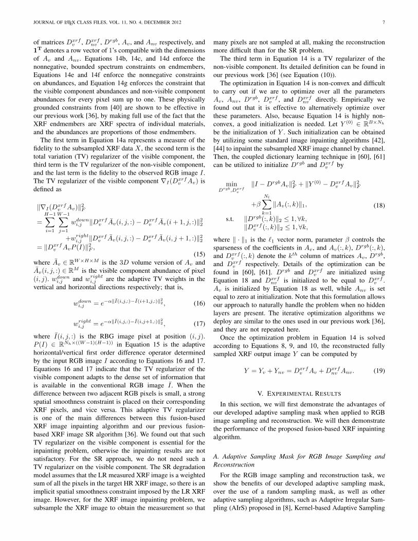
nv , Drgb, Av , and Anv respectively, and1T denotes a row vector of 1’s compatible with the dimensionsof Av and Anv . Equations 14b, 14c, and 14d enforce thenonnegative, bounded spectrum constraints on endmembers,Equations 14e and 14f enforce the nonnegative constraintson abundances, and Equation 14g enforces the constraint thatthe visible component abundances and non-visible componentabundances for every pixel sum up to one. These physicallygrounded constraints from [40] are shown to be effective inour previous work [36], by making full use of the fact that theXRF endmembers are XRF spectra of individual materials,and the abundances are proportions of those endmembers.

The first term in Equation 14a represents a measure of thefidelity to the subsampled XRF data X , the second term is thetotal variation (TV) regularizer of the visible component, thethird term is the TV regularizer of the non-visible component,and the last term is the fidelity to the observed RGB image I .The TV regularizer of the visible component ∇I(Dxrf

v Av) isdefined as

‖∇I(Dxrfv Av)‖2F

=

H−1∑i=1

W−1∑j=1

wdowni,j ‖Dxrfv Av(i, j, :)−Dxrf

v Av(i+ 1, j, :)‖22

+wrighti,j ‖Dxrfv Av(i, j, :)−Dxrf

v Av(i, j + 1, :)‖22= ‖Dxrf

v AvP (I)‖2F ,(15)

where Av ∈ RW×H×M is the 3D volume version of Av andAv(i, j, :) ∈ RM is the visible component abundance of pixel(i, j). wdowni,j and wrighti,j are the adaptive TV weights in thevertical and horizontal directions respectively; that is,

wdowni,j = e−α‖I(i,j,:)−I(i+1,j,:)‖22 , (16)

wrighti,j = e−α‖I(i,j,:)−I(i,j+1,:)‖22 , (17)

where I(i, j, :) is the RBG image pixel at position (i, j).P (I) ∈ RNh×((W−1)(H−1)) in Equation 15 is the adaptivehorizontal/vertical first order difference operator determinedby the input RGB image I according to Equations 16 and 17.Equations 16 and 17 indicate that the TV regularizer of thevisible component adapts to the dense set of information thatis available in the conventional RGB image I . When thedifference between two adjacent RGB pixels is small, a strongspatial smoothness constraint is placed on their correspondingXRF pixels, and vice versa. This adaptive TV regularizeris one of the main differences between this fusion-basedXRF image inpainting algorithm and our previous fusion-based XRF image SR algorithm [36]. We found out that suchTV regularizer on the visible component is essential for theinpainting problem, otherwise the inpainting results are notsatisfactory. For the SR approach, we do not need such aTV regularizer on the visible component. The SR degradationmodel assumes that the LR measured XRF image is a weightedsum of all the pixels in the target HR XRF image, so there is animplicit spatial smoothness constraint imposed by the LR XRFimage. However, for the XRF image inpainting problem, wesubsample the XRF image to obtain the measurement so that

many pixels are not sampled at all, making the reconstructionmore difficult than for the SR problem.

The third term in Equation 14 is a TV regularizer of thenon-visible component. Its detailed definition can be found inour previous work [36] (see Equation (10)).

The optimization in Equation 14 is non-convex and difficultto carry out if we are to optimize over all the parametersAv , Anv , Drgb, Dxrf

v , and Dxrfnv directly. Empirically we

found out that it is effective to alternatively optimize overthese parameters. Also, because Equation 14 is highly non-convex, a good initialization is needed. Let Y (0) ∈ RB×Nh

be the initialization of Y . Such initialization can be obtainedby utilizing some standard image inpainting algorithms [42],[44] to inpaint the subsampled XRF image channel by channel.Then, the coupled dictionary learning technique in [60], [61]can be utilized to initialize Drgb and Dxrf

v by

minDrgb,Dxrf

v

‖I −DrgbAv‖2F + ‖Y (0) −Dxrfv Av‖2F

+β

Nl∑k=1

‖Av(:, k)‖1,

s.t. ‖Drgb(:, k)‖2 ≤ 1,∀k,‖Dxrf

v (:, k)‖2 ≤ 1,∀k,

(18)

where ‖ · ‖1 is the `1 vector norm, parameter β controls thesparseness of the coefficients in Av , and Av(:, k), Drgb(:, k),and Dxrf

v (:, k) denote the kth column of matrices Av , Drgb,and Dxrf

v respectively. Details of the optimization can befound in [60], [61]. Drgb and Dxrf

v are initialized usingEquation 18 and Dxrf

nv is initialized to be equal to Dxrfv .

Av is initialized by Equation 18 as well, while Anv is setequal to zero at initialization. Note that this formulation allowsour approach to naturally handle the problem when no hiddenlayers are present. The iterative optimization algorithms wedeploy are similar to the ones used in our previous work [36],and they are not repeated here.

Once the optimization problem in Equation 14 is solvedaccording to Equations 8, 9, and 10, the reconstructed fullysampled XRF output image Y can be computed by

Y = Yv + Ynv = Dxrfv Av +Dxrf

nv Anv. (19)

V. EXPERIMENTAL RESULTS

In this section, we will first demonstrate the advantages ofour developed adaptive sampling mask when applied to RGBimage sampling and reconstruction. We will then demonstratethe performance of the proposed fusion-based XRF inpaintingalgorithm.

A. Adaptive Sampling Mask for RGB Image Sampling andReconstruction

For the RGB image sampling and reconstruction task, weshow the benefits of our developed adaptive sampling mask,over the use of a random sampling mask, as well as otheradaptive sampling algorithms, such as Adaptive Irregular Sam-pling (AIrS) proposed in [8], Kernel-based Adaptive Sampling


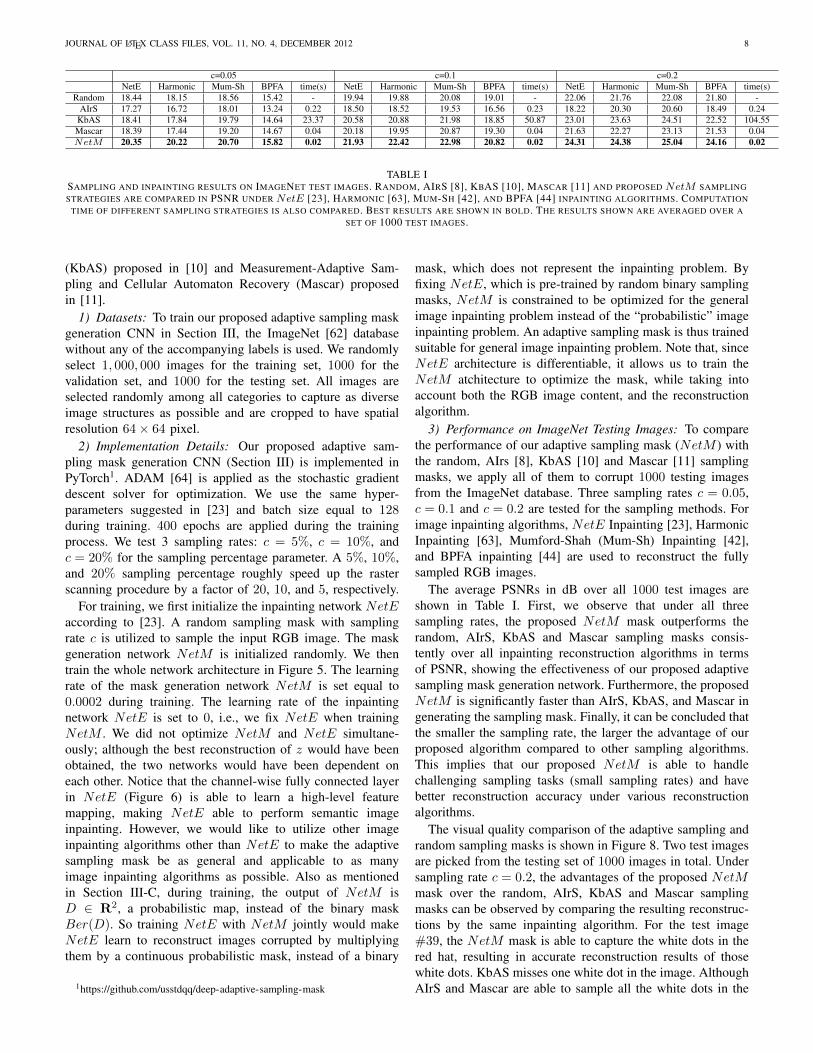
c=0.05 c=0.1 c=0.2NetE Harmonic Mum-Sh BPFA time(s) NetE Harmonic Mum-Sh BPFA time(s) NetE Harmonic Mum-Sh BPFA time(s)

Random 18.44 18.15 18.56 15.42 - 19.94 19.88 20.08 19.01 - 22.06 21.76 22.08 21.80 -AIrS 17.27 16.72 18.01 13.24 0.22 18.50 18.52 19.53 16.56 0.23 18.22 20.30 20.60 18.49 0.24

KbAS 18.41 17.84 19.79 14.64 23.37 20.58 20.88 21.98 18.85 50.87 23.01 23.63 24.51 22.52 104.55Mascar 18.39 17.44 19.20 14.67 0.04 20.18 19.95 20.87 19.30 0.04 21.63 22.27 23.13 21.53 0.04NetM 20.35 20.22 20.70 15.82 0.02 21.93 22.42 22.98 20.82 0.02 24.31 24.38 25.04 24.16 0.02

TABLE ISAMPLING AND INPAINTING RESULTS ON IMAGENET TEST IMAGES. RANDOM, AIRS [8], KBAS [10], MASCAR [11] AND PROPOSED NetM SAMPLINGSTRATEGIES ARE COMPARED IN PSNR UNDER NetE [23], HARMONIC [63], MUM-SH [42], AND BPFA [44] INPAINTING ALGORITHMS. COMPUTATION

TIME OF DIFFERENT SAMPLING STRATEGIES IS ALSO COMPARED. BEST RESULTS ARE SHOWN IN BOLD. THE RESULTS SHOWN ARE AVERAGED OVER ASET OF 1000 TEST IMAGES.

(KbAS) proposed in [10] and Measurement-Adaptive Sam-pling and Cellular Automaton Recovery (Mascar) proposedin [11].

1) Datasets: To train our proposed adaptive sampling maskgeneration CNN in Section III, the ImageNet [62] databasewithout any of the accompanying labels is used. We randomlyselect 1, 000, 000 images for the training set, 1000 for thevalidation set, and 1000 for the testing set. All images areselected randomly among all categories to capture as diverseimage structures as possible and are cropped to have spatialresolution 64× 64 pixel.

2) Implementation Details: Our proposed adaptive sam-pling mask generation CNN (Section III) is implemented inPyTorch1. ADAM [64] is applied as the stochastic gradientdescent solver for optimization. We use the same hyper-parameters suggested in [23] and batch size equal to 128during training. 400 epochs are applied during the trainingprocess. We test 3 sampling rates: c = 5%, c = 10%, andc = 20% for the sampling percentage parameter. A 5%, 10%,and 20% sampling percentage roughly speed up the rasterscanning procedure by a factor of 20, 10, and 5, respectively.

For training, we first initialize the inpainting network NetEaccording to [23]. A random sampling mask with samplingrate c is utilized to sample the input RGB image. The maskgeneration network NetM is initialized randomly. We thentrain the whole network architecture in Figure 5. The learningrate of the mask generation network NetM is set equal to0.0002 during training. The learning rate of the inpaintingnetwork NetE is set to 0, i.e., we fix NetE when trainingNetM . We did not optimize NetM and NetE simultane-ously; although the best reconstruction of z would have beenobtained, the two networks would have been dependent oneach other. Notice that the channel-wise fully connected layerin NetE (Figure 6) is able to learn a high-level featuremapping, making NetE able to perform semantic imageinpainting. However, we would like to utilize other imageinpainting algorithms other than NetE to make the adaptivesampling mask be as general and applicable to as manyimage inpainting algorithms as possible. Also as mentionedin Section III-C, during training, the output of NetM isD ∈ R2, a probabilistic map, instead of the binary maskBer(D). So training NetE with NetM jointly would makeNetE learn to reconstruct images corrupted by multiplyingthem by a continuous probabilistic mask, instead of a binary

1https://github.com/usstdqq/deep-adaptive-sampling-mask

mask, which does not represent the inpainting problem. Byfixing NetE, which is pre-trained by random binary samplingmasks, NetM is constrained to be optimized for the generalimage inpainting problem instead of the “probabilistic” imageinpainting problem. An adaptive sampling mask is thus trainedsuitable for general image inpainting problem. Note that, sinceNetE architecture is differentiable, it allows us to train theNetM atchitecture to optimize the mask, while taking intoaccount both the RGB image content, and the reconstructionalgorithm.

3) Performance on ImageNet Testing Images: To comparethe performance of our adaptive sampling mask (NetM ) withthe random, AIrs [8], KbAS [10] and Mascar [11] samplingmasks, we apply all of them to corrupt 1000 testing imagesfrom the ImageNet database. Three sampling rates c = 0.05,c = 0.1 and c = 0.2 are tested for the sampling methods. Forimage inpainting algorithms, NetE Inpainting [23], HarmonicInpainting [63], Mumford-Shah (Mum-Sh) Inpainting [42],and BPFA inpainting [44] are used to reconstruct the fullysampled RGB images.

The average PSNRs in dB over all 1000 test images areshown in Table I. First, we observe that under all threesampling rates, the proposed NetM mask outperforms therandom, AIrS, KbAS and Mascar sampling masks consis-tently over all inpainting reconstruction algorithms in termsof PSNR, showing the effectiveness of our proposed adaptivesampling mask generation network. Furthermore, the proposedNetM is significantly faster than AIrS, KbAS, and Mascar ingenerating the sampling mask. Finally, it can be concluded thatthe smaller the sampling rate, the larger the advantage of ourproposed algorithm compared to other sampling algorithms.This implies that our proposed NetM is able to handlechallenging sampling tasks (small sampling rates) and havebetter reconstruction accuracy under various reconstructionalgorithms.

The visual quality comparison of the adaptive sampling andrandom sampling masks is shown in Figure 8. Two test imagesare picked from the testing set of 1000 images in total. Undersampling rate c = 0.2, the advantages of the proposed NetMmask over the random, AIrS, KbAS and Mascar samplingmasks can be observed by comparing the resulting reconstruc-tions by the same inpainting algorithm. For the test image#39, the NetM mask is able to capture the white dots in thered hat, resulting in accurate reconstruction results of thosewhite dots. KbAS misses one white dot in the image. AlthoughAIrS and Mascar are able to sample all the white dots in the

https://github.com/usstdqq/deep-adaptive-sampling-mask


Test ImageSampling

MaskSampled

ImageNetE

ReconstructionHarmonic

ReconstructionMum-Sh

ReconstructionBPFA

Reconstruction

#39

Ran

dom

AIr

SK

bAS

Mas

car

NetM

#91

Ran

dom

AIr

SK

bAS

Mas

car

NetM

Fig. 8. Visual Comparison of the reconstructed images using random, AIrS, KbAS, and NetM sampling masks at sampling rate c = 0.2. The first column isthe input test image and the second column is the sampling mask, either random, AIrS, KbAS, or NetM , the third column is the sampled image obtained by thesampling mask, and the rest of the columns are the reconstruction results of NetE Inpainting [23], Harmonic Inpainting [63], Mumford-Shah Inpainting [42],and BPFA inpainting [44] respectively.

image, they fail to capture the structure of these white dots.For test image #91, compared to random sampling mask, theproposed NetM mask samples the contour structure of thebird, resulting in its better reconstruction. When compared toAIrS, KbAS and Mascar masks, the proposed NetM masksamples the whole image more evenly, resulting in fewer

artifacts in the inpainted images. The improved performanceof the adaptive sampling mask over other sampling masksis consistent over all inpainting reconstruction algorithms wetested.

4) Performance on Painting Images: We also tested ourproposed adaptive sampling algorithm on painting images at


Test Image Sampling Mask Harmonic Reconstruction Mum-Sh Reconstruction BPFA Reconstruction

Ori

gina

lR

GB

Imag

e

Ran

dom

(a) (c) time: - (d) PSNR: 25.85 dB (e) PSNR: 25.07 dB (f) PSNR: 24.59 dB

Cro

pped

Ori

gina

l

AIr

S

(b) (g) time: 468.15s (h) PSNR: 23.34 dB (i) PSNR: 23.24 dB (j) PSNR: 21.65 dB

KbA

S

(k) time: 32533.10s (l) PSNR: 14.41 dB (m) PSNR: 28.43 dB (n) PSNR: 27.48 dB

Mas

car

(o) time: 3.08s (p) PSNR: 19.77 dB (q) PSNR: 27.22 dB (r) PSNR: 26.83 dB

NetM

(s) time: 0.26s (t) PSNR: 28.13 dB (u) PSNR: 28.57 dB (v) PSNR: 28.57 dB

Fig. 9. Visualization of sampling and inpainting result of the “Bloemen en insecten” painting. (a) original RGB image with red bounding box. (b) regioninside the bounding box of (a) for visualization purposes. (c), (g), (k), (o) and (s) random, AIrS, KbAS, Mascar and NetM sampling masks respectively. (d),(h), (l), (p) and (t) reconstruction results of each sampling mask using Harmonic algorithms. (e), (i), (m), (q) and (u) reconstruction results of each samplingmask using Mumford-Shah algorithm. (f), (j), (n), (r) and (v) reconstruction results of each sampling mask using BPFA algorithm. Computation time of eachsampling mask and PSNR of the entirety of each reconstructed images are also shown.

sampling rate c = 0.1. As shown in Figures 9 (a), the RGBimage of the painting “Bloemen en insecten” is tested. It hasspatial resolution 580 × 680 pixels. Random, AIrS, KbAS,Mascar and NetM sampling masks are generated as shownin Figures 9(c), (g), (k), (o) and (s) with the correspondingcomputation time. Harmonic Inpainting [63], Mumford-ShahInpainting [42], and BPFA [44] algorithms are utilized toreconstruct the sampled RGB images, and the reconstructionresults are shown in Figures 9 (d)-(f), (h)-(j), (l)-(n), (p)-(r) and(t)-(v) with the corresponding PSNR values. By comparing therows of different sampling masks, it can be concluded that ourproposed NetM mask outperforms other sampling masks interms of both visual quality of the reconstructed images andthe PSNR values. Notice that NetM is significantly fasterthan AIrS, KbAS and Mascar in computation speed. AlthoughKbAS samples densely on the foreground, it still misses manydetails due to the complexity of the flower structure. Similarly,Mascar samples densely on the foreground, while it misses theflower stem structure. NetE Inpainting [23] is not utilized

in this experiment since it is trained to inpaint RGB imageswith spatial resolution 64 × 64 pixels. The network structureshown in Figure 6 is not fully convolutional, as there is thechannel-wise fully connected layer in the middle. NetM isfully convolutional (Figure 7) so that it can generate samplingmasks of input images with arbitrary resolution.

B. Adaptive Sampling Mask for X-Ray Fluorescence ImageInpainting

In the previous section (Section V-A), we demonstratedthe effectiveness of our proposed NetM sampling mask onthe RGB image sampling and inpainting problem. To furtherevaluate the effectiveness of the NetM sampling mask andevaluate the performance of our proposed fusion-based in-painting algorithm (Section IV), we have performed experi-ments on XRF images. The basic parameters of the proposedreconstruction method are set as follows: the number of atomsin the dictionaries Drgb, Dxrf

nv and Dxrfv is M = 200;


parameter λ and γ in Equation 14 are set equal to 0.1;parameter α in Equation 16 and Equation 17 is set to 16.The optional constraint in Equation 14h is not applied here.

1) Error Metrics: The root mean squared error (RMSE),the peak-signal-to-noise ratio (PSNR), and the spectral anglemapper (SAM, [65]) between the estimated fully sampled XRFimage Y and the ground truth image Y gt are used as the errormetrics.

2) Comparison Methods: According to our knowledge, nowork has been reported on solving the XRF (or Hyperspectral)image inpainting problem by fusing a conventional RGBimage. So, we can only compare our results with traditionalimage inpainting algorithms such as Harmonic Inpainting [63],Mumford-Shah Inpainting [42], and BPFA inpainting [44].Harmonic Inpainting and Mumford-Shah Inpainting methodsare for image inpainting, so we have to inpaint the XRFimage channel by channel. BPFA inpainting [44] is able toinpaint multiple channels simultaneously. For the samplingmask comparison, we still compare with random, AIrS [8],KbAS [10] and Mascar [11] sampling masks.

3) Real Experiment: For this experiment, real data werecollected by a home-built X-ray fluorescence spectrometer(courtesy of Prof. Koen Janssens), with 2048 channels in spec-trum. Studies from the XRF image scanned from Jan Davidsz.de Heem’s “Bloemen en insecten” (ca 1645), in the collec-tion of Koninklijk Museum voor Schone Kunsten (KMKSA)Antwerp, are presented here. We utilize the super-resolvedXRF image in our previous work [36] as the ground truth. Theground truth XRF image has dimensions 680×580×2048. Wefirst extract 20 regions of interest (ROI) spectrally and workon them, to decrease the spectral dimension from 2048 to 20.We decrease the spectral dimension so as to compare withother inpainting algorithms, e.g., [42], [63], which thereforereconstruct the subsampled XRF image channel by channeland large spectral dimensions will make the computationaltime very long. The sampling ratio c is set to be 0.05,0.1, and 0.2. Different sampling strategies are applied andanalyzed. Various inpainting methods are subsequently appliedto reconstruct those subsampled XRF images.

As shown in Table II, our proposed fusion-based inpaintingalgorithm with the proposed adaptive sampling mask providesthe closest reconstruction to the ground truth XRF image com-pared to all other methods. Our proposed algorithm utilizesas guidance a conventional fully sampled and high contrastRGB image (Figure 9 (a)), resulting in better inpaintingperformance. By comparing the difference between results by“Mum-Sh” and results by “Proposed” under various samplingrates, it can be concluded that the benefit gained by ourproposed fusion-based inpainting is large when the adaptivesampling masks are applied. For example, at sampling ratec = 0.2, there is a 0.78 dB improvement in PSNR by ap-plying our proposed fusion-based inpainting algorithm when arandom sampling masks are applied, while there is a 6.71 dB,7.94 dB, 9.06 dB and 7.33 dB improvement in PSNRwhen an AIrS, KbAS, Mascar and NetM sampling mask isapplied, respectively. This is because the adaptive samplingmasks sampled the corresponding visible component of theXRF image efficiently and the fusion inpainting propagated

0 0.2 0.4 0.6 0.8 1 1.2 1.4 1.6 1.8 2x 104

0.013

0.014

0.015

0.016

0.017

0.018

0.019

0.02

Iteration

RM

SE

Random Sampling + Mumford−Shah ReconstructionRandom Sampling + Mumford−Shah Initialiazation + Proposed Fusion ReconstructionAIrS sampling + Mumford−Shah ReconstructionAIrS Sampling + Mumford−Shah Initialiazation + Proposed Fusion ReconstructionKbAS Sampling + Mumford−Shah ReconstructionKbAS Sampling + Mumford−Shah Initialiazation + Proposed Fusion ReconstructionMascar Sampling + Mumford−Shah ReconstructionMascar Sampling + Mumford−Shah Initialiazation + Proposed Fusion ReconstructionNetM Sampling + Mumford−Shah ReconstructionNetM Sampling + Mumford−Shah Initialiazation + Proposed Fusion Reconstruction

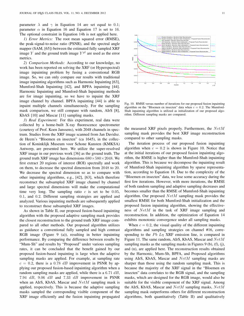
Fig. 10. RMSE versus number of iterations for our proposed fusion inpaintingalgorithm on the “Bloemen en insecten” data when c = 0.2. The Mumford-Shah inpainting algorithm is utilized as initialization of our proposed algo-rithm. Different sampling masks are compared.

the measured XRF pixels properly. Furthermore, the NetMsampling mask provides the best XRF image reconstructioncompared to other sampling masks.

The iteration process of our proposed fusion inpaintingalgorithm when c = 0.2 is shown in Figure 10. Notice thatat the initial iterations of our proposed fusion inpainting algo-rithm, the RMSE is higher than the Mumford-Shah inpaintingalgorithm. This is because we decompose the inpainting resultof Mumford-Shah inpainting algorithm by sparse representa-tion, according to Equation 18. Due to the complexity of the“Bloemen en insecten” data, we lose some accuracy during thefirst few iterations. However, with more iterations, the RMSEof both random sampling and adaptive sampling decreases andbecomes smaller than the RMSE of Mumford-Shah inpaintingalgorithm. Our proposed NetM sampling mask provides thesmallest RMSE for both Mumford-Shah initialization and theproposed fusion inpainting algorithm, showing the effective-ness of NetM in the task of XRF image sampling andreconstruction. In addition, the optimization of Equation 14exhibits monotonic convergence under all sampling masks.

When c = 0.2, the visual quality of the different inpaintingalgorithms and sampling strategies on channel #16, corre-sponding to the Pb Lη XRF emission line, is compared inFigure 11. The same random, AIrS, KbAS, Mascar and NetMsampling masks as the sampling masks in Figures 9 (b), (f), (j),and (n), are applied here. The reconstruction results obtainedby the Harmonic, Mum-Sh, BPFA, and Proposed algorithmsusing AIrS, KbAS, Mascar and NetM sampling masks aresharper than those using the random sampling mask. This isbecause the majority of the XRF signal in the “Bloemen eninsecten” data correlates to the RGB signal, and the samplingmasks, which are designed for the RGB image, would also besuitable for the visible component of the XRF signal. Amongthe AIrS, KbAS, Mascar and NetM sampling masks, NetMsampling mask outperforms others for different reconstructionalgorithms, both quantitatively (Table II) and qualitatively


c=0.05Harmonic Mum-Sh BPFA Proposed

RMSE PSNR SAM RMSE PSNR SAM RMSE PSNR SAM RMSE PSNR SAMRandom 0.0428 27.37 5.06 0.0319 29.93 3.85 0.1141 22.57 8.27 0.0300 30.45 3.67

AIrS 0.1224 18.24 8.20 0.0378 28.45 4.33 0.1446 17.80 13.49 0.0355 37.03 4.14KbAS 0.2374 12.49 12.62 0.0309 30.19 3.95 0.1791 15.08 19.51 0.0297 39.25 3.85Mascar 0.2374 12.49 12.62 0.0309 30.19 3.95 0.1791 15.08 19.51 0.0297 39.25 3.85NetM 0.0333 29.56 4.22 0.0279 31.09 3.43 0.0910 24.22 7.21 0.0261 39.54 3.27







TABLE IIEXPERIMENTAL RESULTS ON THE “BLOEMEN EN INSECTEN” DATA COMPARING DIFFERENT INPAINTING METHODS, UNDER RANDOM, AIRS, KBAS, ANDNetM SAMPLING STRATEGIES, DISCUSSED IN SECTION V-B2 IN TERMS OF RMSE, PSNR, AND SAM. BEST SAMPLING MASKS UNDER THE EACH

RECONSTRUCTION ALGORITHM ARE SHOWN IN ITALIC. BEST RECONSTRUCTION RESULTS ARE SHOWN IN BOLD.

(Figure 11). The proposed fusion inpainting algorithm furtherimproves the contrast and resolves more fine details in (q).When compared to the ground truth image (b), we canconclude that those resolved details have high fidelity to theground truth image (b).

Our proposed adaptive sampling algorithm NetM is notdesigned and trained for the task of XRF image samplingand reconstruction. However, NetM still outperforms randomsampling, as well as three other adaptive sampling algorithms,under various XRF reconstruction algorithms and under differ-ent sampling rates. This illustrates the effectiveness of NetMin extracting image information with limited sampling budget.This also demonstrates that NetM can generalize well intosome other imaging tasks.

4) XRF Inpainting v.s. XRF Super-Resolution: In this ex-periment, we further compare the proposed XRF inpaintingutilizing NetM adaptive sampling with our previous XRF-SR approach [36]. The XRF scanner can perform regularsub-sampling with a sampling step size K on both imagedimensions. An upscale factor K SR can be applied toreconstruct the fully sampled XRF images. We set K = 5 tomatch the SR setting of [36]. We retrain NetM with samplingrate c = 0.04, which has the same number of samples as aK = 5 regular sub-sampling. The training procedure is thesame as described in Section V-A2.

As shown in Table III, as expected, the proposed XRFinpainting algorithm utilizing NetM outperforms the XRF-SRapproach. Please notice that both methods fuse an RGB imageduring the XRF reconstruction, and the main difference is thesampling pattern. This experiment further argues the improvedeffectiveness of the proposed NetM based sampling.

RMSE PSNR SAMXRF-SR 0.0382 28.36 4.77Proposed 0.0278 31.12 3.55

TABLE IIIEXPERIMENTAL RESULTS ON THE “BLOEMEN EN INSECTEN” DATA

COMPARING PROPOSED XRF INPAINTING UTILIZING NetM ADAPTIVESAMPLING WITH XRF SR. BEST RECONSTRUCTION RESULTS ARE SHOWN

IN BOLD.

NetE Harmonic Mum-ShRandom 19.94 19.88 20.08

AIrS 18.50 18.52 19.53KbAS 20.58 20.88 21.98Mascar 20.18 19.95 20.87

NetM pre train joint 19.53 19.72 19.89NetM rand init joint 15.37 19.87 20.08NetM sequential 21.93 22.42 22.98

TABLE IVSAMPLING AND INPAINTING RESULTS ON IMAGENET TEST IMAGES.

RANDOM, AIRS [8], KBAS [10], MASCAR [11],NetM pre train joint , NetM rand init joint AND PROPOSEDNetM SAMPLING STRATEGIES ARE COMPARED IN TERMS OF PSNR (IN

DB) UNDER NetE [23], HARMONIC [63] AND MUM-SH [42] INPAINTINGALGORITHMS. BEST RESULTS ARE SHOWN IN BOLD. THE RESULTS SHOWN

ARE AVERAGED OVER A SET OF 1000 TEST IMAGES.

5) Simultaneous Training of NetE and NetM : With aninitial look at Fig. 5, it would seem meaningful to trainNetE and NetM simultaneously and not sequentially, asdescribed in Section V-A2. In this experiment, we performedcertain experiments to test such approach and eventuallysupport our proposed sequential training procedure. Thereare two approaches in training NetE and NetM simulta-neously. The first one is to train NetE individually first,


Ground Truth Harmonic Mum-Sh BPFA Proposed

Ran

dom

Mas

k

(a) (c) (d) (e) (f)

AIr

SM

ask

(b) (g) (h) (i) (j)

KbA

SM

ask

(k) (l) (m) (n)

Mas

car

Mas

k

(o) (q) (p) (r)

NetM

Mas

k

(s) (t) (u) (v)

Fig. 11. Visualization of inpainting results on the “Bloemen en insecten” data when c = 0.2. Channel #16 related to the Pb Lη XRF emission line is selected.(a) ground truth XRF image with black bounding box. (b) region inside the bounding box of (a), shown for visual comparison purposes. The sampling masksfor random, AIrS, KbAS, Mascar and NetM are the same as the sampling masks in Figures 9 (c), (g), (k), (o) and (s) respectively. (c)-(v) reconstructionresults of different inpainting algorithms for different sampled XRF image within the same region of (a) as (b).

and then train NetE with NetM jointly using Equation 3.The second one is to perform random initialization on bothNetE and NetM , and then simultaneously train them usingEquation 3. We tested both of these training approaches atsampling rate c = 0.1. We henceforth refer to the firstapproach as NetM pre train joint, to the second approachas NetM rand init joint and to the proposed trainingapproach as NetM sequential. Notice that we quantize theprobabilistic map D generated by NetM during testing.

We tested these two above described networks utilizingthe same 1000 ImageNet test set and compared them withthe other inpainting approaches considered in this paper interms of PSNR (in dB). As is clear from Table IV, theresults obtained by the networks NetM pre train joint andNetM rand init joint , with which NetM and NetE weretrained simultaneously, are not competitive with the resultsobtained by the proposed sequential training of NetE andNetM , i.e., NetM sequential. It is mention again here that

NetE in both of these simultaneous training approaches wastrained with input images corrupted by a probabilistic map D.The resulting sampling masks from these two approaches can-not also get good reconstruction accuracy using Harmonic [63]and Mum-Sh [42] inpainting. There is approximately a 2dB difference in reconstruction accuracy, indicating that thetrained NetM is not as effective. When comparing thesetwo simultaneous optimization approaches to each other, it isobserved that using the pre-trained NetE before joint trainingprovides some benefit on both NetE and NetM .

VI. CONCLUSION

In this paper, we presented a novel adaptive sampling maskgeneration algorithm based on CNNs and a novel XRF imageinpainting framework based on fusing a conventional RGBimage. For the adaptive sampling mask generation, we trainedthe mask generation network NetM along with the inpaintingnetwork NetE to obtain an optimal binary sampling mask


based on the input RGB image. For the fusion-based XRFimage inpainting algorithm, the XRF spectrum of each pixelis represented by an endmember dictionary, as well as the RGBspectrum. The input subsampled XRF image is decomposedinto visible and non-visible components, making it possibleto find the nonlinear mapping from the RGB to the XRFspectrum. Experiments show the effectiveness of our proposednetwork NetM in both RGB and XRF image samplingand reconstruction tasks. Higher reconstruction accuracy isachieved in both RGB and XRF image sampling, and also thecomputation time of mask generation is significantly smallerthan other adaptive sampling methods.

REFERENCES

[1] E. J. Candes, J. Romberg, and T. Tao, “Robust uncertainty principles:Exact signal reconstruction from highly incomplete frequency informa-tion,” IEEE Transactions on information theory, vol. 52, no. 2, pp. 489–509, 2006.

[2] D. L. Donoho, “Compressed sensing,” IEEE Transactions on informationtheory, vol. 52, no. 4, pp. 1289–1306, 2006.

[3] R. L. Cook, “Stochastic sampling in computer graphics,” ACM Trans-actions on Graphics (TOG), vol. 5, no. 1, pp. 51–72, 1986.

[4] M. Soumekh, “Multiresolution dynamic image representation with uni-form and foveal spiral scan data,” IEEE transactions on image process-ing, vol. 7, no. 11, pp. 1627–1635, 1998.

[5] Y. Eldar, M. Lindenbaum, M. Porat, and Y. Y. Zeevi, “The farthest pointstrategy for progressive image sampling,” IEEE Transactions on ImageProcessing, vol. 6, no. 9, pp. 1305–1315, 1997.

[6] S. Rajesh, K. Sandeep, and R. Mittal, “A fast progressive imagesampling using lifting scheme and non-uniform b-splines,” in IndustrialElectronics, 2007. ISIE 2007. IEEE International Symposium on. IEEE,2007, pp. 1645–1650.

[7] L. Demaret, N. Dyn, and A. Iske, “Image compression by linear splinesover adaptive triangulations,” Signal Processing, vol. 86, no. 7, pp.1604–1616, 2006.

[8] G. Ramponi and S. Carrato, “An adaptive irregular sampling algorithmand its application to image coding,” Image and Vision Computing,vol. 19, no. 7, pp. 451–460, 2001.

[9] A. S. Lin, B. Z. Luo, C. J. Zhang, and D. E. Saucan, “Generalizedricci curvature based sampling and reconstruction of images,” in SignalProcessing Conference (EUSIPCO), 2015 23rd European. IEEE, 2015,pp. 604–608.

[10] J. Liu, C. Bouganis, and P. Y. Cheung, “Kernel-based adaptive imagesampling,” in Computer Vision Theory and Applications (VISAPP), 2014International Conference on, vol. 1. IEEE, 2014, pp. 25–32.

[11] A. Taimori and F. Marvasti, “Adaptive sparse image sampling andrecovery,” IEEE Transactions on Computational Imaging, vol. 4, no. 3,pp. 311–325, 2018.

[12] A. Krizhevsky, I. Sutskever, and G. E. Hinton, “Imagenet classificationwith deep convolutional neural networks,” in Advances in neural infor-mation processing systems, 2012, pp. 1097–1105.

[13] C. Szegedy, W. Liu, Y. Jia, P. Sermanet, S. Reed, D. Anguelov, D. Erhan,V. Vanhoucke, and A. Rabinovich, “Going deeper with convolutions,”in Proceedings of the IEEE Conference on Computer Vision and PatternRecognition, 2015, pp. 1–9.

[14] H. Xie, D. Yang, N. Sun, Z. Chen, and Y. Zhang, “Automated pulmonarynodule detection in ct images using deep convolutional neural networks,”Pattern Recognition, vol. 85, pp. 109–119, 2019.

[15] H. Xie, S. Fang, Z.-J. Zha, Y. Yang, Y. Li, and Y. Zhang, “Convolutionalattention networks for scene text recognition,” ACM Transactions onMultimedia Computing, Communications, and Applications (TOMM),vol. 15, no. 1s, p. 3, 2019.

[16] P. Vincent, H. Larochelle, Y. Bengio, and P.-A. Manzagol, “Extract-ing and composing robust features with denoising autoencoders,” inProceedings of the 25th international conference on Machine learning.ACM, 2008, pp. 1096–1103.

[17] C. Dong, C. C. Loy, K. He, and X. Tang, “Learning a deep convolu-tional network for image super-resolution,” in European Conference onComputer Vision. Springer, 2014, pp. 184–199.

[18] A. Kappeler, S. Yoo, Q. Dai, and A. K. Katsaggelos, “Video super-resolution with convolutional neural networks,” IEEE Transactions onComputational Imaging, vol. 2, no. 2, pp. 109–122, 2016.

[19] M. Iliadis, L. Spinoulas, and A. K. Katsaggelos, “Deep fully-connectednetworks for video compressive sensing,” Digital Signal Processing,vol. 72, pp. 9–18, 2018.

[20] ——, “Deepbinarymask: Learning a binary mask for video compressivesensing,” arXiv preprint arXiv:1607.03343, 2016.

[21] D. Pathak, P. Krahenbuhl, J. Donahue, T. Darrell, and A. A. Efros,“Context encoders: Feature learning by inpainting,” in Proceedings of theIEEE Conference on Computer Vision and Pattern Recognition, 2016,pp. 2536–2544.

[22] R. Yeh, C. Chen, T. Y. Lim, M. Hasegawa-Johnson, and M. N. Do,“Semantic image inpainting with perceptual and contextual losses,”arXiv preprint arXiv:1607.07539, 2016.

[23] R. Gao and K. Grauman, “From one-trick ponies to all-rounders:On-demand learning for image restoration,” arXiv preprintarXiv:1612.01380, 2016.

[24] K.-H. Tzou, “Progressive image transmission: a review and comparisonof techniques,” Optical engineering, vol. 26, no. 7, p. 267581, 1987.

[25] C. Deng, W. Lin, B.-s. Lee, and C. T. Lau, “Robust image coding basedupon compressive sensing,” IEEE Transactions on Multimedia, vol. 14,no. 2, pp. 278–290, 2012.

[26] H. Liu, B. Song, F. Tian, and H. Qin, “Joint sampling rate and bit-depthoptimization in compressive video sampling.” IEEE Trans. Multimedia,vol. 16, no. 6, pp. 1549–1562, 2014.

[27] L. Y. Zhang, K.-W. Wong, Y. Zhang, and J. Zhou, “Bi-level protectedcompressive sampling,” IEEE Transactions on Multimedia, vol. 18,no. 9, pp. 1720–1732, 2016.

[28] Z. Chen, X. Hou, X. Qian, and C. Gong, “Efficient and robust imagecoding and transmission based on scrambled block compressive sens-ing,” IEEE Transactions on Multimedia, vol. 20, no. 7, pp. 1610–1621,2018.

[29] H. Xie, Z. Mao, Y. Zhang, H. Deng, C. Yan, and Z. Chen, “Double-bit quantization and index hashing for nearest neighbor search,” IEEETransactions on Multimedia, 2018.

[30] M. Alfeld, J. V. Pedroso, M. van Eikema Hommes, G. Van der Snickt,G. Tauber, J. Blaas, M. Haschke, K. Erler, J. Dik, and K. Janssens,“A mobile instrument for in situ scanning macro-xrf investigation ofhistorical paintings,” Journal of Analytical Atomic Spectrometry, vol. 28,no. 5, pp. 760–767, 2013.

[31] A. Anitha, A. Brasoveanu, M. Duarte, S. Hughes, I. Daubechies, J. Dik,K. Janssens, and M. Alfeld, “Restoration of x-ray fluorescence imagesof hidden paintings,” Signal Processing, vol. 93, no. 3, pp. 592–604,2013.

[32] M. Bertalmio, G. Sapiro, V. Caselles, and C. Ballester, “Image in-painting,” in Proceedings of the 27th annual conference on Computergraphics and interactive techniques. ACM Press/Addison-WesleyPublishing Co., 2000, pp. 417–424.

[33] A. Criminisi, P. Perez, and K. Toyama, “Region filling and objectremoval by exemplar-based image inpainting,” IEEE Transactions onimage processing, vol. 13, no. 9, pp. 1200–1212, 2004.

[34] M. Bertalmio, L. Vese, G. Sapiro, and S. Osher, “Simultaneous structureand texture image inpainting,” IEEE transactions on image processing,vol. 12, no. 8, pp. 882–889, 2003.

[35] Q. Dai, E. Pouyet, O. Cossairt, M. Walton, F. Casadio, and A. Kat-saggelos, “X-ray fluorescence image super-resolution using dictionarylearning,” in Image, Video, and Multidimensional Signal ProcessingWorkshop (IVMSP), 2016 IEEE 12th. IEEE, 2016, pp. 1–5.

[36] Q. Dai, E. Pouyet, O. Cossairt, M. Walton, and A. Katsaggelos, “Spatial-spectral representation for x-ray fluorescence image super-resolution,”IEEE Transactions on Computational Imaging.

[37] D. Manolakis, C. Siracusa, and G. Shaw, “Hyperspectral subpixel targetdetection using the linear mixing model,” Geoscience and RemoteSensing, IEEE Transactions on, vol. 39, no. 7, pp. 1392–1409, 2001.

[38] M. Alfeld, W. De Nolf, S. Cagno, K. Appel, D. P. Siddons,A. Kuczewski, K. Janssens, J. Dik, K. Trentelman, M. Walton et al.,“Revealing hidden paint layers in oil paintings by means of scanningmacro-xrf: a mock-up study based on rembrandt’s an old man in militarycostume,” Journal of Analytical Atomic Spectrometry, vol. 28, no. 1, pp.40–51, 2013.

[39] N. Akhtar, F. Shafait, and A. Mian, “Sparse spatio-spectral represen-tation for hyperspectral image super-resolution,” in Computer Vision–ECCV 2014. Springer, 2014, pp. 63–78.

[40] C. Lanaras, E. Baltsavias, and K. Schindler, “Hyperspectral super-resolution by coupled spectral unmixing,” in Proceedings of the IEEEInternational Conference on Computer Vision, 2015, pp. 3586–3594.

[41] W. Dong, F. Fu, G. Shi, X. Cao, J. Wu, G. Li, and X. Li, “Hyperspectralimage super-resolution via non-negative structured sparse representa-tion,” 2016.


[42] S. Esedoglu and J. Shen, “Digital inpainting based on the mumford–shah–euler image model,” European Journal of Applied Mathematics,vol. 13, no. 04, pp. 353–370, 2002.

[43] J. Shen and T. F. Chan, “Mathematical models for local nontextureinpaintings,” SIAM Journal on Applied Mathematics, vol. 62, no. 3, pp.1019–1043, 2002.

[44] M. Zhou, H. Chen, J. Paisley, L. Ren, L. Li, Z. Xing, D. Dunson,G. Sapiro, and L. Carin, “Nonparametric bayesian dictionary learningfor analysis of noisy and incomplete images,” IEEE Transactions onImage Processing, vol. 21, no. 1, pp. 130–144, 2012.

[45] P. Song and M. R. Rodrigues, “Multi-modal image processing based oncoupled dictionary learning,” in 2018 IEEE 19th International Workshopon Signal Processing Advances in Wireless Communications (SPAWC).IEEE, 2018, pp. 1–5.

[46] S. S. Shivakumar, T. Nguyen, S. W. Chen, and C. J. Taylor, “Dfusenet:Deep fusion of rgb and sparse depth information for image guided densedepth completion,” arXiv preprint arXiv:1902.00761, 2019.

[47] S. D. Babacan, R. Molina, and A. K. Katsaggelos, “Total variation superresolution using a variational approach,” in Image Processing, 2008.ICIP 2008. 15th IEEE International Conference on. IEEE, 2008, pp.641–644.

[48] A. Marquina and S. J. Osher, “Image super-resolution by tv-regularization and bregman iteration,” Journal of Scientific Computing,vol. 37, no. 3, pp. 367–382, 2008.

[49] S. Ioffe and C. Szegedy, “Batch normalization: Accelerating deepnetwork training by reducing internal covariate shift,” arXiv preprintarXiv:1502.03167, 2015.

[50] A. L. Maas, A. Y. Hannun, and A. Y. Ng, “Rectifier nonlinearitiesimprove neural network acoustic models,” in Proc. ICML, vol. 30, no. 1,2013.

[51] B. Xu, N. Wang, T. Chen, and M. Li, “Empirical evaluation of rectifiedactivations in convolutional network,” arXiv preprint arXiv:1505.00853,2015.

[52] J. Long, E. Shelhamer, and T. Darrell, “Fully convolutional networksfor semantic segmentation,” in Proceedings of the IEEE Conference onComputer Vision and Pattern Recognition, 2015, pp. 3431–3440.

[53] A. Dosovitskiy, J. Tobias Springenberg, and T. Brox, “Learning togenerate chairs with convolutional neural networks,” in Proceedingsof the IEEE Conference on Computer Vision and Pattern Recognition,2015, pp. 1538–1546.

[54] M. D. Zeiler and R. Fergus, “Visualizing and understanding convolu-tional networks,” in European conference on computer vision. Springer,2014, pp. 818–833.

[55] J. Johnson, A. Alahi, and L. Fei-Fei, “Perceptual losses for real-time style transfer and super-resolution,” in European Conference onComputer Vision. Springer, 2016, pp. 694–711.

[56] G. Sam and W. Michael. (2016, February) Training and investigatingresidual nets. [Online]. Available: http://torch.ch/blog/2016/02/04/resnets.html

[57] K. He, X. Zhang, S. Ren, and J. Sun, “Delving deep into rectifiers:Surpassing human-level performance on imagenet classification,” inProceedings of the IEEE international conference on computer vision,2015, pp. 1026–1034.

[58] J. M. Bioucas-Dias, A. Plaza, N. Dobigeon, M. Parente, Q. Du, P. Gader,and J. Chanussot, “Hyperspectral unmixing overview: Geometrical,statistical, and sparse regression-based approaches,” Selected Topics inApplied Earth Observations and Remote Sensing, IEEE Journal of,vol. 5, no. 2, pp. 354–379, 2012.

[59] N. Keshava and J. F. Mustard, “Spectral unmixing,” Signal ProcessingMagazine, IEEE, vol. 19, no. 1, pp. 44–57, 2002.

[60] J. Yang, J. Wright, T. Huang, and Y. Ma, “Image super-resolution assparse representation of raw image patches,” in Computer Vision andPattern Recognition, 2008. CVPR 2008. IEEE Conference on. IEEE,2008, pp. 1–8.

[61] J. Yang, J. Wright, T. S. Huang, and Y. Ma, “Image super-resolution viasparse representation,” Image Processing, IEEE Transactions on, vol. 19,no. 11, pp. 2861–2873, 2010.

[62] J. Deng, W. Dong, R. Socher, L.-J. Li, K. Li, and L. Fei-Fei, “Imagenet:A large-scale hierarchical image database,” in Computer Vision andPattern Recognition, 2009. CVPR 2009. IEEE Conference on. IEEE,2009, pp. 248–255.

[63] T. F. Chan and J. Shen, “Nontexture inpainting by curvature-drivendiffusions,” Journal of Visual Communication and Image Representation,vol. 12, no. 4, pp. 436–449, 2001.

[64] D. Kingma and J. Ba, “Adam: A method for stochastic optimization,”arXiv preprint arXiv:1412.6980, 2014.

[65] R. H. Yuhas, A. F. Goetz, and J. W. Boardman, “Discrimination amongsemi-arid landscape endmembers using the spectral angle mapper (sam)algorithm,” 1992.

http://torch.ch/blog/2016/02/04/resnets.html

http://torch.ch/blog/2016/02/04/resnets.html

journal of la adaptive image sampling using deep learning … · 2019-11-19 · journal of latex...

Documents