journal of international commerce & economics ... - usitc · journal of international commerce...

The Boom in Brazilians Traveling to the United States(January 2013)David Riker and Jessica Vila-Goulding

Korea’s Demand for U.S. Beef (January 2013)John Giamalva

Feeding the Dragon and the Elephant: How Agricultural Policies and TradingRegimes Influence Consumption in China and India (May 2013)Katherine Baldwin and Joanna Bonarriva

The USITC’s Roundtable on the Labor Market Effects of Trade:Discussion Summary(August 2013)Samira Salem and John Benedetto

Geographically Disaggregated Import Data and Consumer Gains from Trade(December 2013)David Riker

Publication 4447

Volume 5 Number 1 December 2013

United States International Trade Commission

A Cross-Disciplinary Journal of International Trade Issues

Journal of InternationalCommerce & Economics

Journal of InternatIonal CommerCe & eConomICs

Editorial Board Members

Jennifer Powell, Editor in Chief

Joanne Guth, Managing Editor

Katherine Baldwin

Renee Berry

Jeffrey Clark

Joann Peterson

David Riker

James Stamps

Craig Thomsen

Series Description

The Journal of International Commerce and Economics (JICE) is published on a periodic basis (ISSN 2152-6877) by the U.S. International Trade Commission (USITC). The journal contributes to the public policy dialogue by provid-ing insightful and in-depth analysis related to international trade. It provides rigorous but accessible articles for readers concerned about the broad spectrum of issues related to trade, industry competitiveness, and economic integration. The journal highlights the wide-ranging expertise of USITC staff by presenting cross-disciplinary research and analysis on trade-related topics.

Submissions

The Journal of International Commerce and Economics is an in-house publication of the USITC and is therefore unable to accept articles written by individuals not employed by the Commission. Articles co-authored with Commission staff, however, are welcome.

Please fill out the JICE submission form (available on the jour-nal website) and submit proposed topics or original articles Joanne Guth, JICE Managing Editor ~ [email protected].

Submissions will undergo an internal USITC review to determine appropriateness for the Journal series. Submitted articles will undergo a referee process and any feedback will be provided to the author. Approved articles will be distribut-ed electronically as they are ready, and will also be compiled into a volume and published online periodically. Further information and submission guidelines can be found at: www.usitc.gov/journals/submissions.htm.

http://www.usitc.gov/journals/JICEArticleSubmissionForm.doc

[email protected]

www.usitc.gov/journals/submissions.htm

Journal of International Commerce & Economics

Contents

The Boom in Brazilians Traveling to the United StatesDaviD RikeR anD Jessica vila-GoulDinG 1

Korea’s Demand for U.S. Beef John Giamalva 16

Feeding the Dragon and the Elephant: How Agricultural Policies and Trading Regimes Influence Consumption in China and India katheRine BalDwin anD Joanna BonaRRiva 33

The USITC’s Roundtable on the Labor Market Effects of Trade: Discussion SummarysamiRa salem anD John BeneDetto 49

Geographically Disaggregated Import Data and Consumer Gains from TradeDaviD RikeR 65

Web Version: January 2013

Authors1: David Riker and Jessica Vila-Goulding

AbstractIn this article, we examine the economic factors driving the recent boom in Brazilians traveling to the United States. First, we present several measures of the increase in Brazilian travelers and the consequent increase in U.S. services exports to Brazil. Then, we review the economics literature to identify factors that generally affect international tourism demand, including relative prices and income levels. Finally, we present statistical evidence and popular press accounts indicating the relevance and contribution of each of these factors to the recent boom in international travel from Brazil.

1 This article is part of the Brazil Research Initiative in the Office of Economics, Country and Regional Analysis Division. It represents the views of the authors and not the views of the United States International Trade Commission or any of its individual Commissioners. We are grateful to Arona Butcher, Justino De La Cruz, Eric Forden, Martha Lawless, George Serletis, and an anonymous referee for their comments and criticisms. All remain-ing errors are our own. Please direct correspondence to David Riker, Office of Economics, U.S. International Trade Commission, 500 E Street SW, Washington, DC 20436, or by email to [email protected].

The Boom in Brazilians Traveling to

the United States

Suggested citation: Riker, David and Jessica Vila-Goulding. “The Boom in Brazilians Traveling to the United States.” Journal of International Commerce and Economics. Published electronically January 2013. http://www.usitc.gov/journals.

The Boom in Brazilians Traveling to the United States

2 | Journal of International Commerce & Economics

INTRODUCTIONOver the last decade, there has been a boom in the number of Brazilians traveling to the United States. How large is the tourism boom and the resulting growth in U.S. services exports to Brazil? We present a series of economic statistics that demonstrate that the boom has been eco-nomically significant. What are the causes of the tourism boom? We investigate this question in several steps. We review the economics literature to identify factors that generally affect interna-tional tourism demand, including relative prices and income levels. Then, we examine statistical evidence and popular press accounts of the recent boom in order to gauge the contribution of each of these economic factors to the boom in international travelers from Brazil. Finally, we discuss policy initiatives that may further facilitate the tourism boom.

THE TOURISM BOOM Between 2004 and 2011, the number of annual U.S. arrivals from Brazil increased by 292 per-cent, from 385,000 to 1,508,000.2 The U.S. share of Brazil’s outbound travelers increased from 13 percent in 2004 to 18 percent in 2010.3 The expenditures of these visitors are counted as U.S. services exports. These expenditures include purchases of travel and tourism-related goods and services like food, lodging, recreation, gifts, entertainment, and local transportation within the United States, as well as the fares paid to U.S. air carriers involved in the international travel.4 In 2004, these expenditures totaled $1.9 billion. By 2011, they had reached $8.5 billion.5 These estimated expenditures are based on the Survey of International Air Travelers (SIAT) of the U.S. Department of Commerce.

Credit card charges provide an alternative measure of tourism expenditures that do not rely on the SIAT data. This is a narrower measure, however, since it is limited to spending that is fi-nanced with credit cards. It excludes cash expenditures.6 The credit card and financial company Visa reports that “Brazilians increased international tourism spending on their Visa accounts

2 These statistics are from U.S. Department of Commerce (2012a).3 Tourism Australia reports the total number of outbound travelers from Brazil in these years in its Brazil

market profile for 2013, available on-line at http://www.tourism.australia.com/documents/Markets/MP-2013_Brazil-Web.pdf.

4 The list of items included in this account is published at http://travel.trade.gov/outreachpages/inbound.gen-eral_information.inbound_overview.html.

5 U.S. Department of Commerce (2012c).The Bureau of Economic Analysis statistics reported in Koncz-Bruner and Flatness (2011) indicate that international travel was the single largest category of U.S. exports of private services in 2010.

6 A second difference between the two measures of tourism expenditures is that the Visa reports on credit card charges are only available for 2010 and 2011.

http://travel.trade.gov/outreachpages/inbound.general_information.inbound_overview.html

http://travel.trade.gov/outreachpages/inbound.general_information.inbound_overview.html

Journal of International Commerce & Economics | 3


by 32 percent in 2011, from $4.8 billion in 2010 to more than $6.3 billion in 2011. Of the total amount spent on their Visa accounts on travel, 43 percent took place in the United States.”7 The most significant spending categories on the Visa cards of these tourists from Brazil are retail-related purchases, such as electronic goods, at specialty retail stores and department stores.

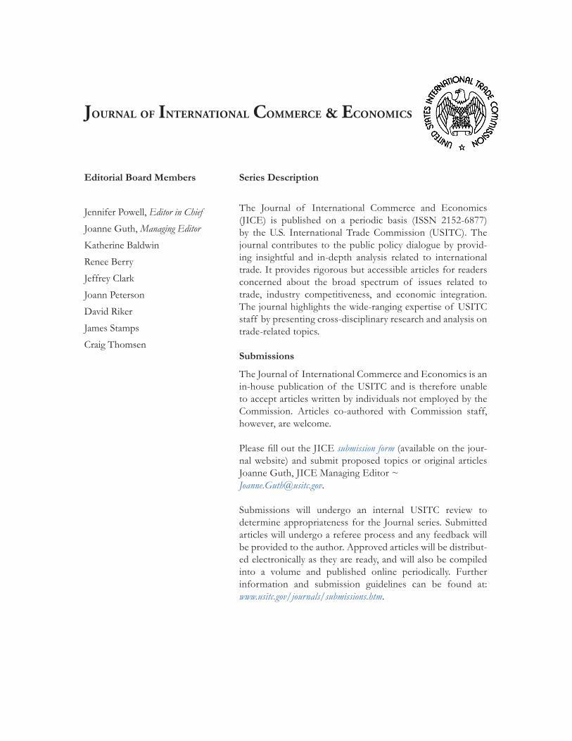
Figure 1 reports the monthly profile of Brazilian arrivals in the United States in 2011, with the highest number of arrivals in December, followed by July, and then January. We expect that the economic impact of this international tourism -- through increased revenues and employment in U.S. tourism-related industries -- to be greatest during those months and to be geographically concentrated. For example, travelers from Brazil are much more likely to visit New York City (a focus of visitors from all over the world) and southern Florida, which is relatively close to Brazil. In 2011, out of the top ten destination cities for international travelers from Brazil, five were in the Unites States. These were Orlando, New York, Miami, Las Vegas, and Los Angeles. The non-U.S. cities in the top ten were Buenos Aires, London, Paris, Rome, and Santiago.8

According to the SIAT results reported in U.S. Department of Commerce (2012a), 66 percent of travelers from Brazil identified leisure, recreation, or holiday as the main purpose of their trip to the United States, while 16 percent identified business or professional activities as the main purpose (table 1). This is significantly greater than the leisure, recreation, or holiday share for all overseas visitors to the United States, which is 53 percent. On the other hand, the share whose main purpose was to visit friends or relatives was much lower for travelers from Brazil (9 per-cent) than for all overseas visitors to the United States (21 percent). The share of Brazilian visi-tors that identified business or conferences as the main purpose of their trip was very similar to the business or conferences share of all overseas visitors to the United States. The most common activities on trips to the United States were shopping (95 percent of visitors from Brazil), dining in restaurants (89 percent), visiting historical places (51 percent) and visiting amusement theme parks (47 percent). In all of these categories, the shares of Brazilian travelers were higher than the comparable average shares for all overseas visitors to the United States (table 2).

According to the same survey, the average length of stay in the United States, among all of the visitors from Brazil, was 16.7 nights in 2011. This was down from an average of 18.6 nights in 2004.9 Twenty-six percent of the visitors in 2011 reported that their trip to the United States was

7 Information on Brazil’s financed transactions is available at http://corporate.visa.com/_media/visa-brazil-2012-report.pdf. With the April 2011 increase in the tax rate on international credit card transactions of Brazilians, from 2.4 percent to 6.4 percent, international purchases of Brazilians with credit cards have declined. Brazilian Central Bank authorities report that Brazilians continue to travel abroad in significant volumes, but they are now using cash more frequently. (http://g1.globo.com/economia/noticia/2011/06/gasto-de-brasileiros-no-exterior-sobe-45-ate-maio-e-bate-recorde.html.)

8 The top destination cities for international travelers from Brazil are listed in a March 14, 2012 article in InfoMoney, titled “Orlando e principal destino dos turistas brasileiros no exterior, revela pesquisa.” Available on-line at http://economia.uol.com.br/ultimas-noticias/infomoney/2012/03/14/orlando-e-principal-destino-dos-turistas-brasileiros-no-exterior-revela-pesquisa.jhtm.

9 The data on travelers from Brazil to the United States in 2004 are from the 2004 market profile for Brazil, available at http://tinet.ita.doc.gov/view/f-2004-141-001/index.html.



their first experience traveling abroad. This share increased sharply from 10 percent in 2004, as international travel became more broadly popular among Brazilians.

ECONOMIC FACTORS IDENTIFIED IN THE LITERATURE

We are not aware of any econometric studies that specifically focus on the determinants of in-ternational travel from Brazil to the United States. However, there is a large body of academic literature that examines the economic determinants of international travel between other pairs of countries, typically countries for which there is greater data availability. The insights from this broader literature provide guidance for our analysis of the demand for travel from Brazil to the United States, as they highlight the economic factors that are most important to interna-tional tourism.

Eilat and Einav (2004) provide econometric estimates of the price and income elasticities of international tourism demand. They estimate a conditional logit econometric model of destina-tion choice, using aggregate travel data for a large panel of countries for the period from 1985 to 1998.10 They find that the price elasticity of demand for travel to high income countries is approximately -1.0. This means that the number of travelers that choose a destination increases by 10 percent for every 10 percent reduction in the price of tourism services in the destination, holding fixed the prices of tourism services in the other international destinations. The authors also report that greater political risk and international distance have significant negative effects on international tourism, while an increase in the Gross National Product per capita of the country of origin has a significant positive effect.

Han, Durbarry, and Sinclair (2006) focus on the U.S. demand for travel to major European des-tinations. The authors estimate an almost ideal demand system (AIDS) model using aggregate travel data for the period from 1965 to 1996.11 They model the destination shares of France, Italy, Spain, and the United Kingdom as functions of relative prices, exchanges rates, and the total expenditure levels of the travelers. They also find that an increase in the general price level in the destination country has a significant negative effect on international tourism demand, with own-price elasticities of demand that range from -2.1 to -0.9, depending on the destination country, while increases in the travelers’ income levels have a significant positive effect on the demand for international tourism.

10 Discrete choice econometric models like the conditional logit model are useful for modeling travelers’ choice of international destination, but they are not models of travelers’ expenditure levels.

11 In contrast to the conditional logit models, AIDS models are well-suited for modeling the expenditure levels of the international travelers. The conditional logit models incorporate information about which destination is cho-sen but not how much is spent overseas. The AIDS models, on the other hand, incorporate data on the allocation of expenditures across the overseas destinations. The two types of models also adopt different mathematical assump-tions about the functional form of international tourism demand curves.



Belenkiy and Riker (forthcoming) reexamines the determinants of international tourism de-mand using individual traveler data rather than aggregate data. The authors estimate a con-stant elasticity of substitution (CES) log-linear econometric model, using data on U.S. tourists who traveled to forty-three overseas countries in 2009.12 They find that price increases in the destination countries had a significant negative effect on overseas expenditures, with a con-ditional price elasticity of international tourism demand equal to -0.8. The level of economic development of the destination country, the international distance, and the income and age of the individual travelers all had significant positive effects on the individual travelers’ overseas expenditures.

Riker (forthcoming) examines the relationship between the aging of the population of the coun-try of origin and international travel, using individual survey responses of overseas recreational travelers from the United States to seventy-seven overseas countries in 2009. The econometric analysis indicates that there are significant differences across age groups in the propensity to travel, the length of stay, and the level of expenditure overseas that are consistent with the differ-ent economic incentives and constraints that each age group faces. The oldest and youngest age groups have a lower opportunity cost of time and lower income on average, and this is reflected in longer but less expensive international trips. For this reason, the growth and aging of the pop-ulation in the country of origin has a significant positive effect on aggregate international travel flows. The study uses the econometric models to project the changes in aggregate international travel expenditures that will likely result from anticipated demographic changes over the next decade. While Riker (forthcoming) specifically focuses on outbound travelers from the United States in 2009, it has broader implications for international travel. The study indicates that the aging of the population, as well as overall population growth in the country of origin, can have a significant positive effect on the travelers’ average length of stay and the level of expenditures overseas. This is similar to findings for international tourists from Japan in Mak, Carlile, and Dai (2005).

Li, Song, and Witt (2005) and Song and Li (2008) provide comprehensive and insightful surveys of the entire literature on modeling international tourism demand. Like the individual stud-ies described above, these reviews emphasize that international tourism demand is moderately sensitive to prices in the destination country, both in absolute levels and relative to prices in the country of origin. International tourism demand is also very sensitive to the level of the trav-eler’s disposable income.

12 The CES econometric model provides direct estimates of the demand elasticities.



RELEVANCE OF THE ECONOMIC FACTORS FOR TRAVEL FROM BRAZIL TO THE UNITED STATES

In this section, we examine the recent trends in Brazil’s economic data, with a particular empha-sis on the economic factors identified in the previous section, including incomes, relative prices, exchange rates, and population demographics.

As noted by Han, Durbarry, and Sinclair (2006), the Gross Domestic Product (GDP) of the country of origin is an important determinant of leisure travel. Table 3 reports the increase in incomes in Brazil between 2004 and 2011, in terms of total GDP and GDP per capita, and the coinciding increase in the number of Brazilians visiting the United States.13 Brazil’s per capita real GDP increased by 23 percent between 2004 and 2011, while the number of visitors to the United States increased by 292 percent.

Of the five countries with the most international tourist spending in the United States, Brazil exhibited the highest GDP growth rates in 2008, 2009, and 2010 and the second highest (after Mexico) in 2011. The relatively robust growth in the Brazilian economy helped to mitigate the overall downturn in the U.S. economy.14 Table 4 reports the annual growth rates of GDP (in constant local currency) for Canada, Japan, the United Kingdom, Mexico, and Brazil. These are the top five countries of origin of travelers to the United States.

Popular press accounts attribute the tourism boom at least in part to the growth of the middle class in Brazil.15 Since international trips are expensive, typically costing thousands of dollars, the rise of the new middle class influenced the tourism boom by making trips to the United States affordable for a greater share of the Brazilian population.16

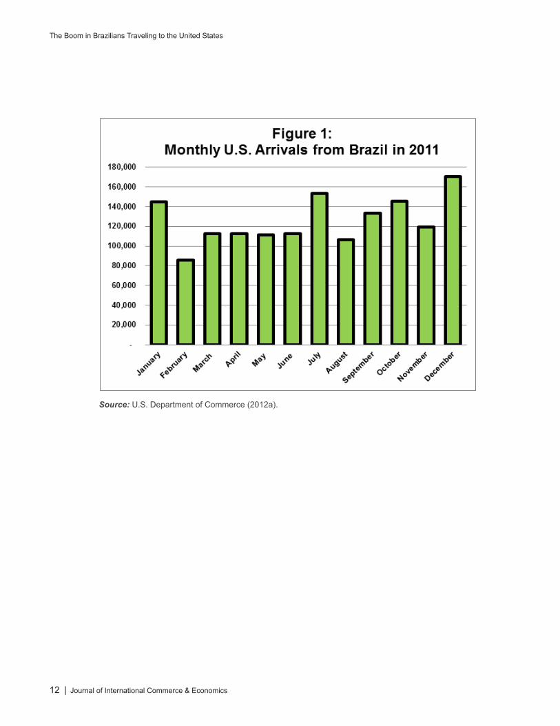
Likewise, the significant appreciation of the Brazilian Real has likely contributed to the tourism boom by making international travel relatively less expensive and more attractive to Brazilians. Figure 2 shows the increase in the value of the Brazilian Real, in terms of U.S. dollars, between 2004 and 2011. Figure 3 shows the 88 percent appreciation of Brazil’s real effective exchange rate (REER) between 2004 and 2011. The REER index is a trade-flow weighted average of the country’s bilateral exchange rates, adjusted for the nominal price levels in Brazil and in its trade partners.

13 The income data are from the World Bank’s World Development Indicators.14 Ritchie, Molinar, and Frechtling (2010) find that the global financial crisis had a significant negative effect

on tourism in the United States, with a drop in travel demand that was twice the rate of the decline in GDP. In turn, the economic downturn in the United States may have stimulated travel demand by reducing the relative prices of services in the United States.

15 “Brazil’s New Consumer Class Spending Time and Cash in the U.S.” (March 12, 2012). Jenny Barchfield and Gisela Salomon reporting for the Associated Press.“The Brazil Shopping Spree.” Ewa Josefsson reporting for Global Blue at http://www.globalblue.com/corporate/intelligence/the-brazilian-shopping-spree/. The size of Brazil’s middle class has increased in part due to a series of policies described in Riker and Vila-Goulding (2012).

16 “Brazilians, the Real Spenders.” (December 21, 2011). John Lyons and PauloTrevisani reporting for the Wall Street Journal.



Figure 4 compares the cost of consumption in Brazil, based on the purchasing power parity indices in the most recent Penn World Table (version 7), to the cost of consumption in France, Japan, and the United States, three of the major overseas destinations of Brazilian tourists. The relative price of consumption in all three countries dropped sharply between 2004 and 2009, which made international travel more attractive to Brazilians. The one exception to this trend was in 2008, when the Brazilian Real briefly depreciated. The United States was consistently the lowest cost of the three international destinations in Figure 4.

Finally, recent demographic changes in Brazil have also contributed to the international tour-ism boom. Table 5 reports the increase in the total population of Brazil between 2004 and 2011 and the increase in the share of its population between the ages of 25 and 64, the age group with the highest propensity to travel. While the population of Brazil grew by 7.5 percent over the period, this age group grew by 16.1 percent. The share of the population between the ages of 25 and 64 increased from 47.2 percent of the total Brazilian population in 2004 to 51.0 percent in 2011.17 Riker (forthcoming) demonstrates that this middle age group has a higher propensity to travel overseas than any other age group, and therefore this change in population demographics is likely to have further fueled the boom in international tourism.

POLICY INITIATIVES TO FACILITATE THE BOOMAs part of its National Tourism and Travel Strategy, the federal government of the United States has initiated a series of programs targeted at facilitating international travel from Brazil to the United States. These actions include streamlining the visa process, expanding existing facilities, and increasing consular staffing.18 These changes are intended to improve the speed of visa pro-cessing, with the hope that increased international tourism will contribute to the growth of the U.S. economy.19 U.S. non-immigrant visa issuances to Brazilians increased by 57 percent in the first half of fiscal year 2012, relative to the first half of fiscal year 2011. These policy initiatives may have contributed to this increase.

17 These population estimates are from the International Population Database of the U.S. Census Bureau. They are available at http://www.census.gov/population/international/data/idb/informationGateway.php.

18 See “Increasing International Tourism to the U.S.: A National Strategy.” U.S. Department of State (May 10, 2012) at http://fpc.state.gov/189650.htm. Also “Fact Sheet: the United States and Brazil Facilitating Travel and Exchange.” White House Office of the Press Secretary (April 9, 2012) at http://www.whitehouse.gov/the-press-office/2012/04/09/fact-sheet-united-states-and-brazil-facilitating-travel-and-exchange.

19 See “Increasing International Tourism to the U.S.: A National Strategy.” U.S. Department of State (May 10, 2012) at http://fpc.state.gov/189650.htm. Also “Fact Sheet: the United States and Brazil Facilitating Travel and Exchange.” White House Office of the Press Secretary (April 9, 2012) at http://www.whitehouse.gov/the-press-office/2012/04/09/fact-sheet-united-states-and-brazil-facilitating-travel-and-exchange.



CONCLUSIONSeveral factors likely contributed to the recent boom in Brazilians traveling to the United States. First, incomes have risen for an increasing share of the Brazilian population. Second, the ap-preciation of the Brazilian currency has made international travel and overseas shopping more attractive and relatively more affordable. Finally, the demographic shift in Brazil has increased international travel.

The next step in this line of research is to quantify the individual contribution of each of these economic fundamentals to the tourism boom. An econometric model of international tourism demand like Belenkiy and Riker (forthcoming) would serve that purpose, though that particu-lar model is based on outbound travel from the United States, and it would be preferable to re-estimate the model for inbound travel to the United States. With a forecast of future trends in these economic factors and an econometric model that relates these factors to international travel outcomes, it would be possible to estimate whether the boom in tourists from Brazil is transitory or is likely to continue unabated.



REFERENCESBelenkiy, Maksim and David Riker.“Modeling the International Tourism Expenditures of

Individual Travelers.”Journal of Travel Research, Forthcoming.

Eilat, Yair and Liran Einav. “Determinants of International Tourism: a Three-Dimensional Panel Data Analysis.” Applied Economics, 2004, Volume 36, Pages 1315-1327.

Han, Zhongwei, Ramesh Durbarry, and M. Thea Sinclair.“Modelling U.S. Tourism Demand for European Destinations.”Tourism Management, 2006, Volume 27, Pages 1-10.

Heston, Alan, Robert Summers, and Bettina Aten. Penn World Table Version 7.0, Center for International Comparisons of Production, Income and Prices at the University of Pennsylvania, 2011.

Koncz-Bruner, Jennifer and Anne Flatness.“U.S. International Services: Cross-Border Trade in 2010 and Services Supplied Through Affiliates in 2009.” Survey of Current Business, October 2011.

Li, Gang, Haiyan Song, and Stephen Witt.“Recent Developments in Econometric Modeling and Forecasting.”Journal of Travel Research, 2005, Volume 44, Pages 82-99.

Mak, James, Lonny E. Carlile, and Sally Dai.“Impact of Population Aging on Japanese International Travel to 2025.”Journal of Travel Research, 2005, Volume 44, Pages 82-99.

Riker, David. “Population Aging and the Economics of International Travel.” Tourism Economics, Forthcoming.

Riker, David and Jessica Vila-Goulding.“Income Distribution and the Demand for Imports in Brazil.” U.S. International Trade Commission, Office of Economics Working Paper No. 2012-07A, 2012.

Ritchie, J.R. Brent, Carlos Mario Amaya Molinar, and Douglas C. Frechtling: “Impacts of the World Recession and Economic Crisis on Tourism: North America.” Journal of Travel Research, 2010, Volume 49, Pages 5-15.

Song, Haiyan and Gang Li. “Tourism Demand Modelling and Forecasting – A Review of Recent Research.” Tourism Management, 2008, Volume 29, Pages 203-220.

U.S. Department of Commerce. 2011 Market Profile: Brazil. International Trade Administration, Office of Travel and Tourism Industries, 2012a.

U.S. Department of Commerce. Profile of Overseas Travelers to the United States: 2011 Inbound. International Trade Administration, Office of Travel and Tourism Industries, 2012b.

U.S. Department of Commerce. Top 10 International Markets, 2011 Visitation and Spending. International Trade Administration, Office of Travel and Tourism Industries, 2012b.



Table 1: Main Purpose of the International Trip

Top Four PurposesTravelers from Brazil in 2011

All Travelers from Overseas in 2011

Leisure, recreation, or holiday 66% 53%

Business or professional 16% 17%

Visit friends or relatives 9% 21%

Convention or conference 5% 4%

Source: U.S. Department of Commerce (2012a).

Table 2: Most Common Activities of International Travelers While in the United States

Activity (Multiple responses possible)Travelers from Brazil in 2011

All Travelers from Overseas in 2011

Shopping 95% 88%

Dining in restaurants 89% 84%

Visit historical places 51% 41%

Amusement theme parks 47% 30%


Table 3: Income Levels and Income per Capita in Brazil

Year

GDP in Billions of Constant 2005

Dollars

GDP per Capita in Constant 2005

Dollars

Number of Visitors to the U.S. from Brazil

in Thousands

2004 1,543 8,344 385

2005 1,583 8,509 485

2006 1,645 8,753 525

2007 1,745 9,196 639

2008 1,836 9,584 769

2009 1,830 9,468 893

2010 1,968 10,093 1,198

2011 2,201 10,278 1,508

Source: World Bank World Development Indicators database (http://data.worldbank.org/data-catalog/world-development-indicators) and U.S. Department of Commerce (2012a).



Table 4: Annual GDP Growth Rates of the Top Five Countries of Origin of Travelers to the U.S.

Country of Origin 2008 2009 2010 2011

Canada 0.69% (2.77%) 3.22% 2.46%

Japan (1.04%) (5.53%) 4.44% (0.70%)

United Kingdom (1.10%) (4.37%) 2.09% 0.66%

Mexico 1.19% (6.24%) 5.52% 3.94%

Brazil 5.17% (0.33%) 7.53% 2.73%

Note: The table reports the percentage annual growth rate of each country’s GDP, in constant 2005 local currency units. Source: World Bank World Development Indicators database. (http://data.worldbank.org/data-catalog/world-development-indicators)

Table 5: Population and Population Shares of Middle Age Group in Brazil

Year Total PopulationShare of Population Between

Ages 25 and 64

2004 183,827,544 47.16%

2005 186,020,004 47.71%

2006 188,131,059 48.25%

2007 190,167,417 48.80%

2008 192,130,270 49.36%

2009 194,019,058 49.93%

2010 195,834,188 50.47%

2011 197,595,498 50.95%

Source: International Population Database of the U.S. Census Bureau.



Source: International Monetary Fund’s International Financial Statistics.



Source: Penn World Table, Version 7, in Heston, Summers, and Aten (2011).

Web Version: January 2013

Author1: John Giamalva

AbstractThis paper uses a price-adjusted index of demand to estimate the change in Korean consumers’ demand for U.S. beef from 2003 through 2011. The paper provides an overview of Korea’s consumption, production, and imports of beef over this period, which included Korea’s ban on imports of U.S. beef following discovery of bovine spongiform encephalopathy (BSE) in the U.S. cattle herd in December 2003, the signing of the U.S.-Korea Beef Protocol in April 2008, and the subsequent recovery of U.S. beef imports. The paper also includes back-ground information on BSE and Korean consumers’ perceptions of the safety of U.S. beef. Korean demand for U.S. beef is estimated to have increased substan-tially since 2009 (the first full year after signing of the Beef Protocol), but in 2011 remained well below the level observed in 2003.

1 This article represents solely the views of the author and not the views of the United States International Trade Commission or any of its individual Commissioners. This paper should be cited as the work of the author only, and not as an official Commission document. Please direct all correspondence to John Giamalva, Office of Industries, U.S. International Trade Commission, 500 E Street, SW, Washington, DC 20436, or by email to [email protected].

Korea’s Demand for U.S. Beef

Suggested citation: Giamalva, John. “Korea’s Demand for U.S. Beef.” Journal of International Commerce and Economics. Published electronically January 2013. http://www.usitc.gov/journals.

mailto:john.giamalva%40usitc.gov?subject=Korea%27s%20Demand%20for%20U.S.%20Beef


Korea's Demand for U.S. Beef

INTRODUCTIONIn 2003, Korea was the second-largest export market for U.S. beef, after Japan.2

In December 2003, a dairy cow in Washington State was discovered to have bovine spongiform encephalopathy (BSE), and in response many countries, including Korea, closed their markets to U.S. beef. Since the discovery of BSE, U.S. beef producers and regulators have put in place a series of measures designed to control the risk of BSE, and in 2008 an agreement to reopen Korea’s market to U.S. beef, the U.S.-Korea Beef Protocol, was reached. Since then, Korea’s im-ports of U.S. beef have resumed, but at a much lower volume. This paper will examine Korean consumers’ demand for U.S. beef, compared to demand in 2003, and since 2009, the first full year after imports resumed. This will help determine the extent to which improved access to the Korean market would be expected to lead to greater exports of U.S. beef.

Since 2003, changes have occurred in the Korean beef market that have led to a decline in Korean consumers’ demand for U.S. beef. There have been changes in Korea’s domestic produc-tion of beef and pork, as well as changes in the volume and composition of Korea’s beef imports from other sources, particularly Australia. Additionally, the discovery of BSE in the U.S. cattle herd and errors made in U.S. beef shipments to Korea have reportedly undermined Korean consumers’ perceptions of the safety of U.S. beef. (See box 1 for a description of BSE.)

The goal of this paper is to estimate changes in Korean consumers’ demand for U.S. beef relative to a base year of 2003 and since 2009, the first full year after trade was resumed. A price-adjusted index of demand will be used to estimate Korean consumer’s demand for U.S. beef through 2011. A price-adjusted index of demand compares the actual quantity purchased (in this case, imported) to the quantity that would be expected had there been no change in demand. The index will control for changes in population, price, and inflation. The paper will also identify possible causes for the changes in demand.

KOREA’S MARKET FOR BEEF

Domestic ProductionThe closure of the Korean market to U.S. beef in 2004 led to higher beef prices in Korea, which stimulated domestic Korean cattle and beef production (table 1). Cattle numbers and beef pro-duction increased more than 50 percent in 2003–11. Domestic beef production as a share of to-tal beef supply (self-sufficiency ratio) reached a high of 45 percent in 2009, but dropped slightly in 2010 and 2011 as imports expanded rapidly with the reopening of the Korean market to U.S. beef in 2008.3

2 Korea was the third-largest export market by volume, after Japan and Mexico. USDA, Foreign Agricultural Service (FAS), Production, Supply, and Distribution (PS&D) database.

3 USDA, FAS, PS&D database.



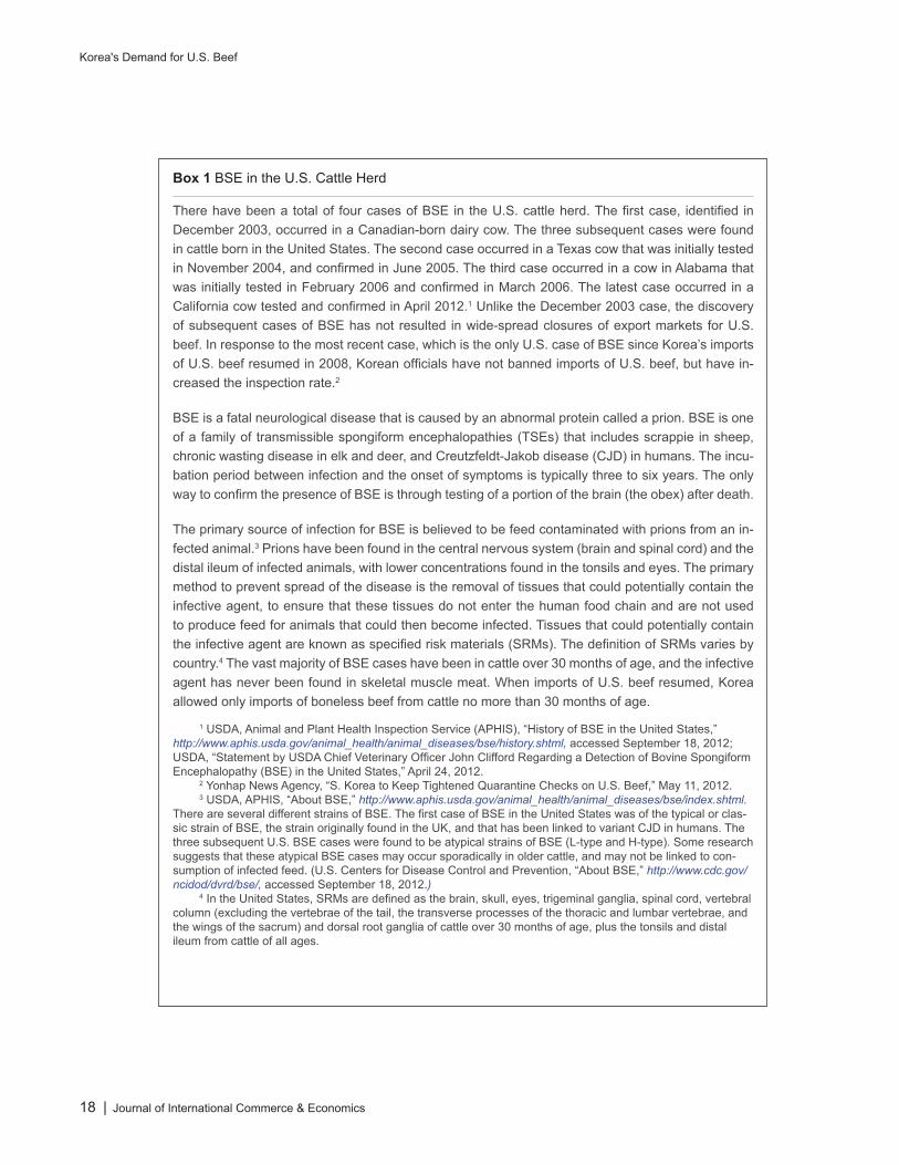
Box 1 BSE in the U.S. Cattle Herd

There have been a total of four cases of BSE in the U.S. cattle herd. The first case, identified in December 2003, occurred in a Canadian-born dairy cow. The three subsequent cases were found in cattle born in the United States. The second case occurred in a Texas cow that was initially tested in November 2004, and confirmed in June 2005. The third case occurred in a cow in Alabama that was initially tested in February 2006 and confirmed in March 2006. The latest case occurred in a California cow tested and confirmed in April 2012.1 Unlike the December 2003 case, the discovery of subsequent cases of BSE has not resulted in wide-spread closures of export markets for U.S. beef. In response to the most recent case, which is the only U.S. case of BSE since Korea’s imports of U.S. beef resumed in 2008, Korean officials have not banned imports of U.S. beef, but have in-creased the inspection rate.2

BSE is a fatal neurological disease that is caused by an abnormal protein called a prion. BSE is one of a family of transmissible spongiform encephalopathies (TSEs) that includes scrappie in sheep, chronic wasting disease in elk and deer, and Creutzfeldt-Jakob disease (CJD) in humans. The incu-bation period between infection and the onset of symptoms is typically three to six years. The only way to confirm the presence of BSE is through testing of a portion of the brain (the obex) after death.

The primary source of infection for BSE is believed to be feed contaminated with prions from an in-fected animal.3 Prions have been found in the central nervous system (brain and spinal cord) and the distal ileum of infected animals, with lower concentrations found in the tonsils and eyes. The primary method to prevent spread of the disease is the removal of tissues that could potentially contain the infective agent, to ensure that these tissues do not enter the human food chain and are not used to produce feed for animals that could then become infected. Tissues that could potentially contain the infective agent are known as specified risk materials (SRMs). The definition of SRMs varies by country.4 The vast majority of BSE cases have been in cattle over 30 months of age, and the infective agent has never been found in skeletal muscle meat. When imports of U.S. beef resumed, Korea allowed only imports of boneless beef from cattle no more than 30 months of age.

1 USDA, Animal and Plant Health Inspection Service (APHIS), “History of BSE in the United States,” http://www.aphis.usda.gov/animal_health/animal_diseases/bse/history.shtml, accessed September 18, 2012; USDA, “Statement by USDA Chief Veterinary Officer John Clifford Regarding a Detection of Bovine Spongiform Encephalopathy (BSE) in the United States,” April 24, 2012.

2 Yonhap News Agency, “S. Korea to Keep Tightened Quarantine Checks on U.S. Beef,” May 11, 2012. 3 USDA, APHIS, “About BSE,” http://www.aphis.usda.gov/animal_health/animal_diseases/bse/index.shtml.

There are several different strains of BSE. The first case of BSE in the United States was of the typical or clas-sic strain of BSE, the strain originally found in the UK, and that has been linked to variant CJD in humans. The three subsequent U.S. BSE cases were found to be atypical strains of BSE (L-type and H-type). Some research suggests that these atypical BSE cases may occur sporadically in older cattle, and may not be linked to con-sumption of infected feed. (U.S. Centers for Disease Control and Prevention, “About BSE,” http://www.cdc.gov/ncidod/dvrd/bse/, accessed September 18, 2012.)

4 In the United States, SRMs are defined as the brain, skull, eyes, trigeminal ganglia, spinal cord, vertebral column (excluding the vertebrae of the tail, the transverse processes of the thoracic and lumbar vertebrae, and the wings of the sacrum) and dorsal root ganglia of cattle over 30 months of age, plus the tonsils and distal ileum from cattle of all ages.

http://www.aphis.usda.gov/animal_health/animal_diseases/bse/history.shtml

http://www.aphis.usda.gov/animal_health/animal_diseases/bse/index.shtml

http://www.cdc.gov/ncidod/dvrd/bse/




TABLE 1 Korea’s production, supply, and distribution of beef, 2003–11 (carcass weight equivalent)

Attribute 2003 2004 2005 2006 2007 2008 2009 2010 2011

Beginning stocks (1,000 mt) 40 61 1 3 5 10 15 47 49

Production (1,000 mt) 182 186 195 200 219 246 267 247 280

Imports (1,000 mt) 457 224 250 298 308 295 315 366 431

Exports (1,000 mt) 0 0 0 0 0 0 4 2 3

Total supply (1,000 mt) 679 471 446 501 531 551 597 660 760

Consumption (1,000 mt) 618 470 443 496 522 536 546 609 677

Self-sufficiency ratio (percent) 27 39 44 40 41 45 45 37 37

Per capita consumption (kg) 12.97 9.82 9.23 10.31 10.82 11.08 11.26 12.5 13.9Source: USDA, FAS, Production, Supply, and Distribution database, accessed June 13, 2012.

Further increases in Korea’s cattle herd are not expected for several reasons. U.S. beef has re-captured a significant share of Korea’s beef market since the market was reopened in 2008. Also, Korean domestic regulations enacted in the aftermath of the recent outbreak of foot and mouth disease (FMD), discussed below, have increased costs for Korean cattle producers. As a result, cattle demand has fallen and cattle prices in Korea have begun to decline. Korea’s beef produc-tion is expected to increase in the short-run, as farmers decrease cattle inventories.4 In the first four months of 2012, cattle slaughter in Korea was 35 percent above the corresponding level of 2011. Slaughter of heifers and cows was up 63 percent.5

Imports In 2003, Korea’s imports of beef reached a record high, and imports accounted for 73 percent of supply. The United States, which had been a large and growing supplier of beef to Korea, sup-plied about two-thirds of Korea’s beef imports in 2003. Australia was second with approximately 20 percent of imports.

Following the ban on imports of U.S. beef, Korea’s imports of beef from Australia more than doubled in volume between 2003 and 2005. Korean buyers were initially unable to find suffi-cient supplies of grain-fed beef, which is preferred in many Korean dishes. Australia produces primarily grass-fed beef, and it took time for producers in Australia to increase the supply of grain-fed beef. Also, Koreans prefer a limited number of cuts, and producers in Australia typi-cally provided only full sets or half-sets.6 As a result, imports from Australia did not fully re-place the loss of imports from the United States, and overall Korean beef imports fell by 47 percent in value and 52 percent in volume between 2003 and 2004. Since then, Korea’s global beef imports have gradually increased, but have not reached the volume of imports observed in 2003 (table 2).

4 USDA, FAS, Korea: Livestock and Products Semiannual, March 6, 2012, 4-6. 5 The BeefSite, “High Korean Cattle Slaughter Continues,” June 13, 2012. 6 ABARE Research Report, Korean beef market, 2009, 36. Selling in “full sets” or “half-sets” forces buyers to

purchase a wider range of cuts, including some less-desirable ones, rather than the specific cuts most preferred.



TABLE 2 Korea’s imports, by leading suppliers, 2003–11Partner 2003 2004 2005 2006 2007 2008 2009 2010 2011

Million dollarsAustralia 197.4 355.3 539.7 693.7 761.6 679.9 482.3 633.9 849.3United States 886.6 103.2 4.0 0.0 94.0 197.1 285.5 421.6 653.0New Zealand 71.7 138.7 178.6 163.5 161.9 155.9 88.7 120.4 156.8Mexico (a) 2.2 11.8 21.5 19.0 17.7 5.3 9.2 18.4ROW 21.1 0.9 0.9 0.3 0.6 0.3 0.1 0.4 0.4World 1,176.9 600.3 735.0 879.0 1,037.1 1,050.9 862.0 1,185.6 1,678.0

Metric tonsAustralia 78,018 99,066 139,798 180,386 179,942 151,918 144,306 155,406 170,111United States 248,645 27,790 760 8 14,112 32,446 61,527 92,649 128,445New Zealand 28,962 47,735 51,829 49,038 44,891 42,718 36,250 38,945 39,427Mexico (a) 852 3,585 6,791 5,366 5,201 2,678 4,452 5,929ROW 8,318 500 379 115 291 103 37 87 128World 363,943 175,943 196,351 236,338 244,602 232,386 244,798 291,539 344,040

Average unit value (dollars per kg)Australia 2.53 3.59 3.86 3.85 4.23 4.48 3.34 4.08 4.99United States 3.57 3.71 5.25 3.80 6.66 6.07 4.64 4.55 5.08New Zealand 2.48 2.90 3.45 3.33 3.61 3.65 2.45 3.09 3.98Mexico NA 2.59 3.29 3.16 3.54 3.41 1.98 2.07 3.11ROW 2.53 1.75 2.38 2.95 1.92 2.52 3.53 4.75 3.30World 3.23 3.41 3.74 3.72 4.24 4.52 3.52 4.07 4.88

Source: Global Trade Atlas, accessed June 13, 2012. (a) Less than $50,000 or 500 kg.

Australia has been the largest source of Korea’s beef imports in every year since 2004. The volume of imports from Australia has declined slightly since 2006, but in 2011 Korea’s beef imports from Australia were four times the value and nearly twice the volume observed in 2003. Australian producers now supply more of the specific cuts favored by Korean consumers. Producers in Australia have increased the share of beef that is grain-fed to approximately 28 percent in 2007 and 31 percent in 2011.7 The changes in the composition of imports coupled with the “clean and safe image” of Australian beef likely improved the competitive position of Australian beef 8 in the Korean market and resulted in less demand for U.S. beef.

Beginning in early 2008, several bilateral agreements have been instrumental in reopening the Korean market to U.S. beef.

• The 2008 Beef Protocol: On April 18, 2008, U.S. and Korean negotiators reached agreement to reopen the Korean market to U.S. beef. The new Beef Protocol provided for Korean imports of boneless and bone-in beef from the United States from cattle less than 30 months of age. Additionally, in an addendum to the Protocol, the Korean government agreed to open the Korean market to U.S. beef from cattle of any age

7 ABARE Research Report, Korean Beef Market, 2009, 1, 36; Australian Lot Feeders’ Association, “Grain Fed Cattle Numbers Rebound Slightly,” February 20, 2012; USDA, FAS, PS&D database, accessed June 13, 2012.

8 ABARE Research Report, Korean Beef Market, 2009, 2.



once the United States announced its enhanced feed ban. Notice of the U.S. enhanced feed ban was published one week after the signing of the Beef Protocol, on April 25, 2008.9 Announcement of the Beef Protocol and the enhanced feed ban were followed by widespread public protests in Korea due to concerns about the safety of U.S. beef.10 Box 2 describes Korean consumers’ perceptions of the safety of U.S. beef.

• Private sector initiative: Because of consumer concerns, U.S. exporters and Korean importers agreed to a separate “transitional private sector initiative” published by the Korean government as an addendum to the Beef Protocol. The private sector initia-tive restricted Korea’s imports of U.S. beef to beef from cattle less than 30 months of age “until Korean consumer confidence in U.S. beef improves.” Currently, U.S. beef exports to Korea must be from establishments participating in the USDA Agricultural Marketing Service (AMS) Quality Systems Assessment (QSA) program that verifies that the beef being certified is from cattle less than 30 months of age. Other conditions of the initiative include the requirement that beef not be sourced from cattle imported from Canada for immediate slaughter in the United States.11

• The KORUS FTA: The U.S.-Korea Free Trade Agreement (KORUS) was ap-proved by the U.S. Congress on October 12, 2011 and ratified by the Korean National Assembly on November 22, 2011. It entered into force on March 15, 2012.12

In May 2011, the United States Trade Representative announced that after KORUS enters into force, he intends to consult with Korea under the terms of the Beef Protocol to regain access for U.S. beef from cattle of any age. KORUS provides for the reduc-tion and eventual elimination of tariffs on Korea’s imports of U.S. beef, but does not directly address the Beef Protocol or the private sector initiative.

9 A ban on cattle feed containing meat and bone meal derived from cattle is considered to be an impor-tant control step in preventing the risk of infection from BSE. The 1997 U.S. feed ban prohibited the use of most proteins derived from mammals in the feed of all ruminants. Because of the possibility of cross-contamination, the 2008 enhanced feed ban prohibited the use of “certain cattle origin materials” in the feed of any ruminant.

10 Clemens, “U.S. Beef Faces Challenges in Korea,” Iowa Ag Review, Center for Agricultural and Rural Development, Winter 2009, 5.

11 United States Trade Representative, letter from Susan Schwab (USTR) and Edward T. Schafer (Secretary of Agriculture) to Minister Jong Hoon Kim and Minister Woon Chun Chung, June 25, 2008.

12 Office of the United States Trade Representative, “U.S.-Korea Free Trade Agreement.”



Box 2 Consumer Perceptions of Safety

The discovery of BSE in the U.S. cattle herd has negatively impacted Korean consumers’ percep-tions of U.S. beef. In addition to the BSE cases themselves, Korean public perception has been influenced by the discovery of bones in several shipments of U.S. beef to Korea, including a vertebral column (considered at the time to be a specified risk material or SRM by Korea) in a shipment of U.S. beef in 2007.

In a survey conducted by the Korea Rural Economic Institute following the December 2003 ban on imports of U.S. beef, 87.4 percent of survey respondents indicated they were concerned about the safety of U.S. beef and only 4.2 percent said it was safe. Respondents also expressed little confidence in Korea’s country-of-origin labeling system (COOL). A majority of respondents were concerned about the safety of imports from Australia, and one-third were concerned about the safety of Korea’s domestic Hanwoo beef. 1

Later surveys show that Korean consumers’ concerns over the safety of U.S. beef continued, and were reflected in beef sales. In August 2007 when part of a vertebral column was found in a ship-ment of U.S. beef, U.S. beef imports were suspended for three weeks. Publicity over consumer concerns depressed demand for U.S. beef and retail sales of U.S. beef in Korea declined in August and September, relative to July.2 In October 2007, another shipment of U.S. beef to Korea was found to contain part of a vertebral column. In reaction, all U.S. beef exports to Korea were suspended.

At the time the Beef Protocol was negotiated (April 2008), Korean consumers reportedly considered the risk of BSE in U.S. beef to be very high. In a May 2008 survey on U.S. beef food safety risks, 78 percent of Korean respondents agreed with the statement that “U.S. beef is not safe.”3 More than one year after the private sector agreement that allowed U.S. beef back into the Korean market, few consumers were willing to purchase U.S. beef. In a survey conducted in December 2009, only 21.7 percent of Korean respondents reported plans to purchase U.S. beef, and only 22.1 percent reported having purchased U.S. beef in the past.4

1 USDA, FAS, Korea: Livestock and Products Semiannual 2004, February 5, 2004, 3. 2 USDA, FAS, Korea: Livestock and Products Semiannual 2008, February 29, 2008, 9–11.3 U.S. industry representative, Korean market briefing for Commission staff, Seoul, Korea, June 4, 2008.4 USDA, FAS, Korea: Livestock and Products Semiannual, March 2, 2011, 7.



The Resumption of Imports from the United States Following the reopening of the Korean market to U.S. beef in 2008, imports from the United States increased significantly. In 2011, Korea’s U.S. beef imports reached 74 percent of the value, but only 56 percent of the volume, of Korea’s U.S. beef imports in 2003. In 2011, Korea’s U.S. beef imports accounted for approximately 22 percent of Korea’s beef consumption. In comparison, imports from Australia, the largest supplier of Korea’s beef imports in 2011, accounted for ap-proximately 29 percent of consumption.

The increase in imports of U.S. beef after 2008 has been due to both a decline in prices relative to other sources of beef and marketing campaigns designed to promote U.S. beef in Korea. In 2003, the average unit value (AUV) of Korea’s U.S. beef imports was 41 percent higher than the AUV of imports from Australia, reflecting the Korean preference for grain-fed beef. The AUV of U.S. imports has been higher than that for imports from Australia in every subsequent year except 2006, when Korea’s imports of U.S. beef totaled only 8 tons. In 2010, the AUV of U.S. imports was 12 percent higher than that of Australian imports, and in 2011, the AUV of U.S. im-ports was only 2 percent higher (table 2). The premium for U.S. beef has declined substantially, and the decline in U.S. prices relative to those for Australian beef has likely been responsible for some of the 2010 and 2011 gains in U.S. market share.

Since 2008, U.S. beef exporters and the U.S. Meat Exporter’s Federation (USMEF) have carried out a series of promotions intended to raise Korean consumers’ awareness of and confidence in U.S. beef. In 2010, the USMEF “Trust” campaign was reportedly successful in allaying some Korean consumers’ concerns about U.S. beef. Surveys conducted in December 2009 and February 2011 found that the share of consumers planning to purchase U.S. beef increased from 21.7 per-cent of those surveyed in December 2009 to 39.3 percent of those surveyed in February 2011.13

A survey in January 2012 found that the share of consumers surveyed who had purchased U.S. beef more than doubled since December 2009, from 22.1 percent of those surveyed in December 2009 to 52.3 percent in January 2012.14

MEASURING DEMANDA demand index can be used to estimate changes in demand over time. One method that has been used to measure changes in demand for beef, pork, and chicken over time is the quantity-adjusted index of demand.15 The quantity-adjusted index of demand controls for changes in pop-ulation and inflation. For a given level of consumption and given an estimate of the own-price demand elasticity, the actual price in any given period is compared to the price that theoreti-cally would have been associated with that level of consumption had there been no changes in

13 USDA, FAS, Korea: Livestock and Products Semiannual, March 2, 2011, 7.14 USDA, FAS, Korea: Livestock and Products Semiannual, March 6, 2012, 6.15 Purcell, Measures of Changes in Demand for Beef, Pork, and Chicken, 1975-1998, 1998. The index controls

for changes in the price of the good and in population.



demand from the base period (PD=Do). Calculations use inflation-adjusted prices and per capita consumption. The index is the ratio of the actual price to PD=Do multiplied by 100.

An alternative to a quantity-adjusted index of demand is a price-adjusted index of demand. At a prevailing price and given an estimate of the own-price demand elasticity, actual consumption in any given period is compared to the level of consumption that theoretically would have been associated with that price had there been no changes in demand from the base period (QD=Do). Calculations use inflation-adjusted prices and per-capita consumption. The index is the ratio of the actual quantity to QD=Do multiplied by 100. A graphical representation of the use of a price-adjusted index of demand is presented in the Appendix, Figure A1.

As Korean beef purchasers are assumed to have little influence on the price of U.S. beef, a price-adjusted index of demand is used in this analysis. Korean consumers’ demand for U.S. beef relative to demand in a base year is estimated from the quantity imported in a given year at the average unit value of imports. The price-adjusted index of demand is calculated below.

Korea’s Demand for U.S. Beef Since 2003To calculate the price-adjusted index of demand for U.S. beef, the following data are required: (1) the real change in U.S. beef prices in Korea, (2) Korea’s per capita consumption of U.S. beef, and (3) the elasticity of demand. The real change in U.S. beef prices in Korea is approximated by the change in the nominal AUV of Korea’s U.S. beef imports, divided by the change in Korea’s consumer price index.16 Korea’s per-capita consumption of U.S. beef is approximated by the vol-ume of imports, divided by the population.17 Several studies have estimated the Korean demand for U.S. beef, and estimates of the demand elasticity can be drawn from this literature. These estimates vary, but generally range between approximately -0.7 and 0.9.18 A demand elasticity of -0.7 was used to construct table 3.19 (The Appendix presents a comparison of the price-adjusted demand index for U.S. beef at own-price elasticities of -0.5 and -0.9.)

16 Data on Korea’s consumer price index are from the IMF, “International Financial Statistics,” http://elibrary-data.imf.org/.

17 Consumer price index and population data were obtained from the International Monetary Fund statistical database.

18 Henneberry and Hwang, “Meat Demand in South Korea,” April 2007, 56; Lee and Kennedy, “Effects of Price and Quality Differences in Source Differentiated Beef,” April 2009, 246. Henneberry and Hwang found that the price elasticity of demand for U.S. beef in Korea was -0.904. Lee and Kennedy found that the price elasticity of demand for U.S. beef in Korea was -0.7217.

19 Estimates of the own-price demand elasticity for U.S. beef in Korea vary and the calculated price index could be sensitive to changes in this estimate.

http://elibrary-data.imf.org/

http://elibrary-data.imf.org/



TABLE 3 Price-adjusted index of Korea’s demand for U.S. beef relative to 2003, Ed= -0.7

YearQuantity of U.S.

beef imports (mt)Per capita

consumption (kg)Deflated AUV

(won/kg)Consumption

at QD=Do (kg) Index2003 248,645 5.272 4,523 5.272 100.0

2004 27,790 0.587 4,372 5.396 10.9

2005 760 0.016 5,373 4.579 0.3

2006 8 0.000 3,548 6.068 0.0

2007 14,112 0.294 5,904 4.144 7.1

2008 32,446 0.674 6,098 3.986 16.9

2009 61,527 1.273 5,254 4.675 27.2

2010 92,649 1.910 4,530 5.265 36.3

2011 128,445 2.629 4,665 5.156 51.0

A demand index with 2003 as the baseline period provides an estimate of how much Korean demand for U.S. beef has recovered since the high-water mark of Korea’s U.S. beef imports. The inflation adjusted AUV of Korea’s 2011 imports of U.S. beef was 3.1 percent higher than in 2003. Therefore, other factors being equal, the increase in price, operating through the demand elasticity, would be expected to lead to a very small decrease in the consumption of U.S. beef. If the demand for U.S. beef in Korea in 2011 had been equal to that observed in 2003, Korea’s per-capita consumption of U.S. beef in 2011 would have been 5.156 kg, compared to consumption in 2003 of 5.272 kg. In fact, per capita consumption was 2.629 kg. The estimated demand index in 2011, relative to 2003 was 51.0.

Sample Calculation:

Percent change in real price of U.S. beef 2003–11 = (4665-4523)/(4523) = 3.1%Expected change in per-capita consumption = 3.1% * -0.7 = -2.2%Expected per-capita consumption QD=Do = (1.0 -0.022) * 5.272 = 5.156Actual per-capita 2011 consumption of U.S. beef = 2.629 kgIndex = (2.629 / 5.156) * 100 = 51.0

Therefore, Korean consumers’ demand for U.S. beef in 2011 was far short of demand in 2003, approximately 49 percent lower. Use of an alternate demand elasticity does not lead to a large change in this index. As shown in the Appendix, use of an estimated demand elasticity of -0.5 or 0.9 leads to an estimated demand index of 50.7 or 51.3, respectively.



Demand in 2010 and 2011 Relative to 2009Comparing changes in price and consumption to a fixed base period understates changes in later periods if there has been a substantial decline in consumption.20 For instance, Korea’s im-ports of U.S. beef in 2010 were roughly 50 percent higher than in 2009, the first full year after the signing of the Beef Protocol and the subsequent private sector agreement. However, this change was equivalent to only 12 percent of 2003 consumption. It is therefore also useful to estimate demand changes on an annual basis, using 2009 as the base period. A demand index relative to 2009 provides a measure of changes in demand since the resumption of trade.

2010 Since the resumption of imports in mid-2008, U.S. producers and organizations have heavily promoted health and flavor aspects of U.S. beef in the Korean market. This promotion would be expected to increase Korean consumers’ demand for U.S. beef and contribute to a higher value for the demand index. The AUV of Korea’s imports of U.S. beef also declined in 2010, on an ab-solute basis and relative to the AUV of imports from Australia, even though Korea’s consumer price index increased in 2010. This decline in price would also be expected to lead to an increase in Korean consumers’ consumption of U.S. beef. Given the increased promotion and decline in price, an increase in import volume is attributable to both relatively lower prices for U.S. beef, and an increase in demand.

Given the estimated demand elasticity of -0.7 and the observed 13.8 percent decline in the infla-tion-adjusted AUV of Korea’s U.S. beef imports 2009–10, we would expect per-capita consump-tion to have increased by 9.7 percent between 2009 and 2010 to 1.396 kg, if there were no change in demand. In fact, Korean per-capita consumption of U.S. beef in 2010 was an estimated 1.910 kg. This yields an index value of 136.8.

Annual Demand Index Change 2009–10:

Percent change in real price of U.S. beef 2009–10 = (4530-5254)/(5254) = -13.8%Expected change in per-capita consumption = -13.8% * -0.7 = 9.7%Expected per-capita consumption QD=Do = (1.0 + 0.097) * 1.273 = 1.396Actual per-capita 2010 consumption of U.S. beef = 1.910 kgIndex = (1.910 / 1.396) * 100 = 136.8

20 Purcell, Measures of Changes in Demand for Beef, Pork, and Chicken, 1975-1998, 2008; Marsh, “Impacts of Declining U.S. Retail Beef Demand on Farm-Level Beef Prices and Production,” November 2003, 903.



2011 In 2011, the AUV of imported U.S. beef increased slightly more than the Korean consumer price index. The higher price, all else being equal, would be expected to lead to a lower volume of imports. Therefore the increase in 2011 was attributable to increased demand. One of the most significant factors that likely led to a continued increase in imports was an outbreak of foot and mouth disease (FMD) in Korea. The outbreak affected more swine than cattle, but would be expected to increase demand for imported beef as a substitute for domestic pork. Promotions of U.S. beef continued in 2011, which would also be expected to increase demand for U.S. beef.

In late November 2010, an outbreak of FMD was confirmed in Andong, North Gyeongsang, Korea. The widespread outbreaks of FMD led to culling of over 150,000 cattle and over 3 mil-lion swine in an effort to stop the spread of the disease.21 Korea also initiated widespread vac-cination of livestock.22 On March 24, 2011, Korea lowered its FMD alert status, and on March 25 declared that the outbreak was over.23

The 150,000 cattle culled were a small fraction of the nearly 3 million head of cattle in Korea, and Korea’s domestic beef production increased in 2011.24 However, approximately one-third of Korea’s swine were culled in the effort to control the outbreaks of FMD, and Korea’s produc-tion of pork is not expected to recover to 2010 levels until 2014. Korea is a major consumer of pork, and in recent years, Koreans have consumed more than twice as much pork as beef.25 As a competing product, beef demand would be expected to increase in response to the decline in pork production.26

Marketing efforts to promote U.S. beef have continued. The USDA awarded an additional $1 million to USMEF for U.S. beef promotion in Korea in fiscal year 2011, and USMEF has begun the second phase of its Trust campaign. USMEF plans to spend an additional $10 million over the next 5 years on initiatives to expand Korea’s consumption of U.S. beef.27 An estimated 65 per-cent of Korea’s imports of U.S. beef is used by the restaurant sector, and the current phase of the Trust campaign includes advertisements in restaurant trade magazines, as well as ads targeting

21 USDA, FAS, Korea: Livestock and Products Semiannual, March 2, 2011, 2. 22 The Korean government announced the first vaccinations for cattle in areas surrounding FMD outbreaks in

December 2010, and expanded the vaccination effort to swine on January 6, 2011. 23 There has not been a reported outbreak since February 26, 2011. Yonhap News Agency, “S. Korea Lowers

Foot-and-mouth Alert Level,” March 24, 2011; Joongang Daily, “With FMD Over, New Precautions Unveiled by Gov’t,” March 25, 2011.

24 USDA, FAS, Korea: Livestock and Products Annual, September 2, 2011, 12; USDA, FAS, PS&D database, accessed June 13, 2012.

25 USDA, FAS, PS&D database; USDA, FAS, Livestock and Poultry: World Markets and Trade, April 2011, 9. 26 USDA, FAS, Korea: Livestock and Products Semiannual, March 2, 2011, 10; USDA, FAS, Korea: Livestock

and Products Annual, September 2, 2011, 10. 27 U.S. Meat Export Federation (USMEF), “USMEF Announces Expanded South Korea Initiative,” May 4,

2011.



consumers.28 The continued promotion is expected to have a positive impact on Korean con-sumers’ attitudes and perceptions of U.S. beef, following the success of past promotions.

Although the AUV of Korea’s imports of U.S. beef increased slightly more rapidly than con-sumer prices in 2011, consumption increased over 2010 to an estimated 2.629 kg per capita, more than twice that of 2009. The demand index relative to 2009 was 191.5.

ConclusionThere has been a substantial decline in Korean consumers’ demand for U.S. beef since 2003. Since 2003, Korea’s domestic beef production has increased substantially, and producers in Australia now supply more grain-fed beef and more of the specific cuts in greatest demand by Korean consumers. The decline in demand is likely attributable to both increased availability of substitute products and a shift in consumer preference away from U.S. beef.

Although Korea’s demand for U.S. beef in 2011 remains well below the 2003 level, demand has increased significantly since 2009. There have not been substantial changes in the availability of Korean domestic beef and Australian grain-fed beef as substitute products since 2009, but there have been reported improvements in consumer attitudes towards U.S. beef. The increase in Korean consumers’ demand for U.S. beef is likely due to these changes in consumer percep-tions. Given the structural changes that have taken place in Australia’s beef production, as well as Korea’s increased domestic production, demand for U.S. beef may not reach the high reached in 2003 in the near future, but continued promotions that improve consumer perceptions of the quality and safety of U.S. beef are expected to increase demand further.

28 USMEF, “USMEF Announces Phase 2 of U.S. Beef ‘Trust’ Campaign in South Korea.”



BIBLIOGRAPHYAustralian Bureau of Agricultural and Resource Economics. Korean Beef Market:

Developments and Prospects, May 2009. ABARE Research Report 09.11.

Australian Lot Feeders’ Association media release. “Grain Fed Cattle Numbers Rebound Slightly as Trading Environment Remains Tough.” February 20, 2012.

Clemens, Roxanne. “U.S. Beef Faces Challenges in Korea Before Reaching Full Potential,” Iowa Ag Review, Center for Agricultural and Rural Development, Winter 2009, 5-6.

Hankooki.com. “The Government Considers to Withdraw ‘50% Open Registration’ on Beef Imported from the U.S.” http://news.hankooki.com/lpage/economy/201206/h2012061202331221500.htm. English translation provided by USDA, FAS, Korea.

Henneberry, Shida and Seong-huyk Hwang. “Meat Demand in South Korea,” Journal of Agricultural and Applied Economics, 39, no. 1 (April 2007), 47-60.

Joongang Daily. “With FMD Over, New Precautions Unveiled by Gov’t,” March 25, 2011.

Lee, Youngjae and P. Lynn Kennedy. “Effects of Price and Quality Differences in Source Differentiated Beef on Market Demand,” Journal of Agricultural and Applied Economics, 41, no. 1 (April 2009):241–252.

Marsh, John N. “Impacts of Declining U.S. Retail Beef Demand on Farm-Level Beef Prices and Production,” American Journal of Agricultural Economics, 85(4), November 2003, 902-13.

Mutondo, Joao and Shida Henneberry. “Competitiveness of U.S. Meats in Japan and South Korea: A Differentiated Market Study.” Presented at the Western Agricultural Economics Association Annual Meeting. Portland, OR, July 29-August 1, 2007.

Purcell, Wayne D. Measures of Changes in Demand for Beef, Pork, and Chicken, 1975-1998. Research Bulletin 3-98, Virginia Polytechnic Institute and State University, Research Institute on Livestock Pricing, 1998.

The Beefsite. “High Korean Cattle Slaughter Continues.” http://www.thebeefsite.com/news/38761/high-korean-cattle-slaughter-continues, June 13, 2012.

U.S. Centers for Disease Control and Prevention. “About BSE,” http://www.cdc.gov/ncidod/dvrd/bse/, accessed September 18, 2012.

USDA. “Statement by USDA Chief Veterinary Officer John Clifford Regarding a Detection of Bovine Spongiform Encephalopathy (BSE) in the United States.” Press Release 0132.12, April 24, 2012.

USDA, Animal and Plant Health Inspection Service (APHIS). “History of BSE in the United States.” http://www.aphis.usda.gov/animal_health/animal_diseases/bse/history.shtml, accessed September 18, 2012.

http://news.hankooki.com/lpage/economy/201206/h2012061202331221500.htm

http://news.hankooki.com/lpage/economy/201206/h2012061202331221500.htm

http://www.thebeefsite.com/news/38761/high-korean-cattle-slaughter-continues

http://www.thebeefsite.com/news/38761/high-korean-cattle-slaughter-continues



http://www.aphis.usda.gov/animal_health/animal_diseases/bse/history.shtml



USDA, APHIS. “Update from APHIS Regarding a Detection of Bovine Spongiform Encephalopathy (BSE) in the United States.” May 2, 2012.

USDA, Foreign Agricultural Service (FAS). Livestock and Poultry: World Markets and Trade. April 2011.

USDA, FAS. Korea: Livestock and Products Annual, GAIN Report No. KS1135, (Ban, Yong Keun and Michael G. Francom) September 2, 2011.

USDA, FAS. Korea: Livestock and Products Semiannual, GAIN Report No. KS8011, (Ban, Yong Keun and Susan Phillips) February 29, 2008.

USDA, FAS. Korea: Livestock and Products Semiannual, GAIN Report No. KS4004, (Ban, Yong Keun and Stan Phillips) February 5, 2004.

USDA, FAS. Korea: Livestock and Products Semiannual, GAIN Report No. KS1218. (Ban, Yong Keun and Michael G. Francom) March 6, 2012.

USDA, FAS. Korea: Livestock and Products Semiannual, GAIN Report No. KS1110. (Ban, Yong Keun and Michael G. Francom) March 2, 2011.

USDA, FAS. Korea: Livestock and Products Annual, GAIN Report No. KS1023. (Ban, Yong Keun and Michael G. Francom) September 10, 2010.

USDA, FAS, Livestock and Poultry: World Markets and Trade, April 2011.

USDA, FAS, Production, Supply, and Distribution database, http://www.fas.usda.gov/psdonline/psdHome.aspx.

U.S. Meat Export Federation (USMEF). “USMEF Announces Expanded South Korea Initiative.” http://www.usmef.org/news-statistics/press-releases/usmef-announces-expanded-south-korea-initiative/, May 4, 2011.

USMEF. “USMEF Announces Phase 2 of U.S. Beef ‘Trust’ Campaign in South Korea,” http://www.usmef.org/news-statistics/member-news-archive/usmef-launches-phase-2-of-u-s-beef-%e2%80%9ctrust%e2%80%9d-campaign-in-south-korea/, accessed May 17, 2011.

United States Trade Representative. Letter from Susan Schwab (USTR) and Edward T. Schafer (Secretary of Agriculture) to Minister Jong Hoon Kim and Minister Woon Chun Chung, June 25, 2008. http://www.ustr.gov/archive/assets/Document_Library/Fact_Sheets/2008/asset_upload_file470_14958.pdf.

USTR. “U.S.-Korea Free Trade Agreement.” http://www.ustr.gov/trade-agreements/free-trade-agreements/korus-fta.

Yonhap News Agency. “S. Korea to Keep Tightened Quarantine Checks on U.S. Beef.” May 11, 2012. http://english.yonhapnews.co.kr/business/2012/05/11/7/0501000000AEN20120511003900320F.HTML.

Yonhap News Agency. “S. Korea Lowers Foot-and-mouth Alert Level,” March 24, 2011.

http://www.fas.usda.gov/psdonline/psdHome.aspx

http://www.fas.usda.gov/psdonline/psdHome.aspx

http://www.usmef.org/news-statistics/press-releases/usmef-announces-expanded-south-korea-initiative/

http://www.usmef.org/news-statistics/press-releases/usmef-announces-expanded-south-korea-initiative/

http://www.usmef.org/news-statistics/member-news-archive/usmef-launches-phase-2-of-u-s-beef-%e2%80%9ctrust%e2%80%9d-campaign-in-south-korea/



http://www.ustr.gov/trade-agreements/free-trade-agreements/korus-fta

http://www.ustr.gov/trade-agreements/free-trade-agreements/korus-fta

http://english.yonhapnews.co.kr/business/2012/05/11/7/0501000000AEN20120511003900320F.HTML

http://english.yonhapnews.co.kr/business/2012/05/11/7/0501000000AEN20120511003900320F.HTML

http://www.ustr.gov/archive/assets/Document_Library/Fact_Sheets/2008/asset_upload_file470_14958.pdf

http://www.ustr.gov/archive/assets/Document_Library/Fact_Sheets/2008/asset_upload_file470_14958.pdf



APPENDIXFigure A1 Graphical Example of a Price-Adjusted Index of Demand

Given the estimated demand curve represented by “Base Period Demand,” the demand index is calculated as the actual quantity consumed in a given period divided by the quantity that would have been consumed at that price assuming there were no changes in demand from the base period, multiplied by 100. In this example, the demand index is equal to (6 /4.65)* 100 = 129.

The estimated demand elasticity has an impact on the calculated demand index. The following tables present Korean consumers’ calculated indices of demand using alternative estimates of the demand elasticity, relative to demand in 2003 and 2009.

Table A1 Price-adjusted index of Korea’s demand for U.S. beef compared to 2003, Ed= -0.5 and Ed= -0.9

Ed= -0.5 Ed= -0.9

Year Quantity (mt)Per capita

consumption (kg)Deflated AUV(won per kg) QD=Do Index QD=Do Index

2003 248,645 5.272 4,523

2004 27,790 0.587 4,372 5.360 10.9 5.431 10.8

2005 760 0.016 5,373 4.777 0.3 4.381 0.4

2006 8 0.000 3,545 5.842 0.0 6.298 0.0

2007 14,112 0.294 5,904 4.467 6.6 3.824 7.7

2008 32,446 0.674 6,098 4.354 15.5 3.619 18.6

2009 61,527 1.273 5,254 4.846 26.3 4.505 28.3

2010 92,649 1.910 4,530 5.268 36.3 5.265 36.3

2011 128,445 2.629 4,665 5.190 50.7 5.123 51.3



Table A2 Price-adjusted index of Korea’s demand for U.S. beef compared to 2009, Ed= -0.5 and Ed= -0.9

Ed= -0.5 Ed= -0.9

Year Quantity (mt)Per capita

consumption (kg)Deflated AUV(won per kg) QD=Do Index QD=Do Index

2009 61,527 1.273 5,254

2010 92,649 1.910 4,530 1.361 140.3 1.131 133.5

2011 128,445 2.629 4,665 1.344 195.5 1.402 187.6

Web Version: May 2013

Authors1: Katherine Baldwin Joanna Bonarriva

AbstractChina and India have posted impressive growth rates over the past decade, but face a number of challenges to sustained growth, including bureaucratic hurdles, large swaths of populations in poverty, and policy regimes that are sometimes at odds with global trade norms. These issues factor heavily in the evolving agri-cultural sectors of each country. Both China’s and India’s agricultural policies are developed out of a concern for domestic food security, and both nations use that objective as a justification for their policy regimes. But aside from this overarch-ing goal, what do these countries have in common when it comes to agricultural trade? In this paper, we undertake a systematic analysis of the agricultural sectors of China and India, comparing and contrasting both domestic policies and trade regimes, and exploring how these regimes affect agricultural trade levels in both countries.

1 This article represents solely the views of the author and not the views of the United States International Trade Commission or any of its individual Commissioners. This paper should be cited as the work of the author only, and not as an official Commission document. Please direct all correspondence to Katherine Baldwin or Joanna Bonarriva, Office of Industries, U.S. International Trade Commission, 500 E Street, SW, Washington, DC 20436, or by email to [email protected] or [email protected].

Feeding the Dragon and the Elephant: How Agricultural

Policies and Trading Regimes Influence

Consumption in China and India

Suggested citation: Baldwin, Katherine and Joanna Bonarriva. “Feeding the Dragon and the Elephant: How Agricultural Policies and Trading Regimes Influence Consumption in China and India.” Journal of International Commerce and Economics. Published electronically May 2013. http://www.usitc.gov/journals.

Feeding the Dragon and the Elephant


INTRODUCTIONAs the two most populous nations on Earth, China and India have drawn considerable attention regarding their respective development paths. Both are large emerging economies that have exhibited annual GDP growth greater than 7.5 percent over the past decade.2 China and India have both increased their integration into the global trading regime over the past few decades, but with respect to some segments of the economy such as agriculture, both countries have taken a more selective stance toward participating in global markets. What is the source of this reticence, and exactly how has it been manifested in the agricultural trade policies of each country?

In this paper, we undertake a broad-based analysis that compares and contrasts the agricultural sectors of China and India and uses that background as a framework to explain their current agricultural trade policy regimes. Specifically, we strive to answer three questions: how have conditions in domestic agriculture affected how these two nations approach trade in agricul-tural goods, to what degree have these countries utilized global markets to fulfill domestic food consumption needs, and what are the impacts of agricultural trade policies in these countries?

AGRICULTURE IN THE DOMESTIC CONTEXTIn order to understand how and why China and India participate in global agricultural markets, a preliminary discussion of agriculture in a domestic context is necessary. As both countries experienced widespread famine in their recent histories, the goal of maintaining self-sufficiency in important food grains is a national political issue. Additionally, as agriculture continues to make a substantial contribution to these nations’ economies, the respective governments have a vested interest in the health of the sector. Despite these similarities, China and India’s divergent histories, cultures, and resource endowments have led to different production systems in the two nations, influencing how each country deals with a wealthier and increasingly urbanized population.

Agriculture’s role in the national economyAgriculture is a vital component of the national economies of China and India, accounting for a significant portion of both employment and overall economic output. In China, agriculture accounted for more than 60 percent of total national employment in 2011, while 54 percent of India’s population worked in agriculture.3 Agricultural workers are important to both nations; however, farmers have much more political sway in India due to that country’s democratic po-

2 World Bank, “World Development Indicators” database (accessed August 1, 2012).3 FAOSTAT, “India Country Profile,” (accessed August 1, 2012); FAOSTAT, “China Country Profile,” (ac-

cessed August 1, 2012).



litical system, and are one of India’s most unified voting blocs. Although Chinese farmers lack voting rights, they are not a completely overlooked demographic. Both central and provincial governments in China are aware of the potential for civil unrest in rural areas as a result of poor living conditions and scarce economic opportunities.

Given the large number of agriculture workers in both China and India, it is not surprising that agriculture is economically important in both countries. Agriculture accounts for approximate-ly 10 and 19 percent of GDP in China and India, respectively, as compared to less than 2 percent in the United States.4 Furthermore, China and India had the first and third highest estimated total agricultural production values in the world in 2010.5

Agriculture is also an important political issue due to each country’s respective history of food shortages and famine, and achieving and maintaining agricultural self-sufficiency is a major political objective. Both countries have become self-sufficient largely due to the adoption of high-yielding varieties of seeds and chemical fertilizers and large public investments in irriga-tion. These measures, stemming from the “Green Revolution,”6 boosted agricultural output by improving productivity (expressed in crop yield per hectare (ha)) rather than through increases in cultivated area. More recently, however, rates of productivity growth have slowed in both countries as the gains from new seed technology and modern farming practices in some sectors have run their course, and overuse of chemical inputs has led to deteriorating soils and shrink-ing groundwater supplies.7 Slowed productivity growth has been particularly acute in India, where recent expenditures on input support programs and migrant farm labor payments have crowded out public funding for agricultural research, extension services, irrigation, and other rural infrastructure projects that would support agricultural sustainability in the long-run.8

Divergent agricultural production systems and crop mixProduction systemsUnequal land resource endowments have led to great differences in the agricultural production systems of China and India. Only about 13 percent of China’s total land area is arable or planted to permanent crops, in contrast with 57 percent in India.9 In 2009, India’s total quantity of ar-able land (158 million ha) was second only to the United States (163 million ha), while China

4 World Bank, “World Development Indicators” database (accessed August 1, 2012).5 FAOSTAT, “Value of agricultural production,” (accessed August 1, 2012).6 The Green Revolution refers to a period of intense agricultural research (roughly 1940-70) into new high-

yielding staple crop varieties to boost food production in developing countries. Hazell, The Asian Green Revolution, November 2009, 1.

7 USITC, India: Effects of Tariffs and Nontariff Measures, November 2009, 4-1 and USITC, China’s Agricultural Trade, March 2011, 5-24.

8 USITC, India: Effects of Tariffs and Nontariff Measures, November 2009, 4-3.9 FAOSTAT, “China Country Profile,” (accessed August 1, 2012); FAOSTAT, “India Country Profile,” (ac-

cessed August 1, 2012).



lagged both with an estimated 110 million ha.10 A comparison of agricultural land availability per agricultural worker yields a still more stark result––0.64 ha in India versus 0.25 ha in China.

While both countries improved productivity due to widespread adoption of Green Revolution technologies, China overcame its relative land deficit through higher average crop yields com-pared to those achieved in India. Average yields of corn and rice in China are double the level observed in India, and wheat yields are more than 50 percent greater.11 This higher productivity is the result of several factors. First, China has almost twice as many agricultural laborers as India, despite a much smaller arable land base.12 Second, Chinese agriculture is characterized by more intensive input usage. For example, the Food and Agricultural Organization of the United Nations (FAO) estimates that in 2009, average fertilizer consumption exceeded 400 kg per ha in China, and stood at roughly 150 kg per ha in India.13 Last, Chinese farmers are able to achieve more consistent crop yields through greater access to irrigation. In 2009, nearly 60 percent of China’s arable land was equipped for irrigation.14 Indian farmers, with only 42 percent of arable land equipped for irrigation, are much more likely to rely on monsoon rains, leading to more variable crop yields and a higher probability of crop failure due to erratic rainfall in any given year.15

Crop mixAgriculture in both China and India is structured to satisfy national food grain consumption needs first, with a secondary focus on all other agricultural products. China is the world’s top producer of rice and wheat, and India ranks second for both products. The diets of China and India are centered around these two grains, with about half of daily per capita caloric consump-tion coming from wheat and rice combined.16

China also produces a significant amount of coarse grains17 (specifically corn) largely used for feed in poultry, pork, and beef production. In 2010, production of coarse grains in China was more than five times higher than that of India, and meat production in China was nearly 13 times larger than in India.18 Although India produces some livestock, the prevalence of veg-

10 FAOSTAT, “China Country Profile,” (accessed August 1, 2012); FAOSTAT, “India Country Profile,” (ac-cessed August 1, 2012); FAOSTAT, “United States of America Country Profile,” (accessed August 1, 2012).

11 USDA, FAS, PSD Database (accessed August 1, 2012).12 FAOSTAT, “China Country Profile,” (accessed August 1, 2012); FAOSTAT, “India Country Profile,” (ac-

cessed August 1, 2012).13 FAOSTAT, “China Country Profile,” (accessed August 1, 2012); FAOSTAT, “India Country Profile,” (ac-

cessed August 1, 2012).14 FAOSTAT, “China Country Profile,” (accessed August 1, 2012).15 FAOSTAT, “India Country Profile,” (accessed August 1, 2012).16 FAOSTAT, “Food Balance Sheets,” (accessed August 1, 2012).17 The FAO definition of coarse grains includes barley, buckwheat, canary seed, fonio, maize, millet, oats,

popcorn, quinoa, rye, sorghum, triticale, mixed grains, and other miscellaneous cereals.18 FAOSTAT, China Country Profile, (accessed August 1, 2012); FAOSTAT, India Country Profile, (accessed

August 1, 2012).



etarianism among that country’s Hindu population translates into most animals being raised for milk production rather than for meat. A comparison of commodity production by countries illustrates this divergence (table 1). While pork, chicken, and beef rank highly for China, no meat products appear on India’s list. Similarly, while buffalo and cow milk are two of India’s largest commodities, they do not rank among China’s top ten.

TABLE 1 Top ten domestically produced agricultural commodities, by value

Rank China India1 Pork Rice

2 Rice Buffalo milk

3 Fresh vegetables Cow milk

4 Hen eggs Wheat

5 Chicken Mangoes/guavas

6 Beef Bananas

7 Wheat Sugarcane

8 Tomatoes Cotton

9 Apples Fresh vegetables

10 Other bird eggs PotatoesSource: FAOSTAT, China and India Country Profiles (accessed August 1, 2012).

It should also be noted that both countries also have large, diverse fruit and vegetable produc-tion sectors. China leads the world in the production of labor-intensive vegetables such as as-paragus, garlic, and tomatoes, while India’s diverse agro-economic zones help the country to be the world’s leading producer of bananas, dry beans, and mangoes.

The challenge of feeding larger and more affluent populationsBoth China and India face unique agricultural challenges due to changing national diets as a consequence of economic development. Generally, as countries develop economically and urbanize, traditional diets heavy in staples (such as grains and tubers) gradually shift to more meats, vegetable oils, dairy, aquatic products, fruits, vegetables, and processed foods. As in-comes rise, attitudes towards foods can change and consumers place greater emphasis on food safety and quality. Urbanization also influences food preferences because urban dwellers have higher average incomes and different food consumption patterns than their rural counterparts. Urban populations not only consume fewer staples, such as grains, but tend to consume more food overall.

These changing demographic and consumption patterns are clearly evident in both China and India. China’s per capita gross national income (GNI) more than quadrupled between 2000 and 2011 to $4,940,19 and this increased income has been accompanied by higher consumption

19 World Bank, “World Development Indicators” database (accessed April 26, 2013).



of meats and processed food products.20 Since 2000, domestic meat supplies in China have grown 13 percent, with beef and poultry up 19 percent and pork supplies up 7 percent.21 Most of the increase in China’s meat supplies can be attributed to greater domestic production, and given China’s relative dearth of arable land, larger domestic livestock production has increased demand for feed grains. In India, per capita income tripled between 2000 and 2011 to $1,420, but was still less than a third of GNI in China.22 India’s smaller per capita income, combined with the prevalence of a vegetarian diet, has led to increased demand of different foods than in China—per capita consumption of vegetable oils, sugars and sweeteners, animal products (in-cluding meat and dairy), and fruits have all increased, while calories from rice and wheat have declined. The rise in demand of oils, sweeteners, and animal products has led to fundamental shifts in the agricultural sectors and the overall food systems of both India and China.

AGRICULTURAL TRADEDespite similarities including large agricultural production and the shared challenge of feeding large populations, China and India exhibit vastly different degrees of participation in global agricultural markets. In 2011, the value of Chinese agricultural imports and exports accounted for 11 percent and 5 percent, respectively, of global agricultural trade, compared to just 2 per-cent and 3 percent for India.23 China depends on international markets for a number of key products, making it the world’s second largest agricultural product importer. In contrast, only about 3 percent of Indian food and agricultural demand is met by imports, compared with 13 percent for Asia as a whole.24

China’s agricultural tradeChina’s engagement in global trade began in the late 1990s with trade liberalizing reforms that reduced agricultural protection and barriers to imports. After China’s WTO accession in 2001, its agricultural exports steadily expanded, growing from about $12 billion in 2001 to $43 billion in 2011. China became a net importer of agricultural goods for the first time in 2003, and im-ports have continued to grow faster than exports, reaching almost $90 billion in 2011 (figure 1).

20 USITC, China’s Agricultural Trade, March 2011, 3-4, 3-7—3-9.21 FAOSTAT, “Food Balance Sheets,” (accessed August 1, 2012).22 World Bank, “World Development Indicators” database (accessed April 26, 2013).23 GTIS, GTA database (accessed August 1, 2012).24 Narayanan and Walmsley, Global Trade, Assistance, and Production, 2008.



FIGURE 1 China’s Balance of Trade in Agricultural Goods

Source: GTIS, GTA database (accessed August 1, 2012).

Although total Chinese agricultural imports have increased by value, imports are concentrated in a handful of products. Almost 70 percent of China’s imports in 2011 were in just 6 product categories: soybeans, vegetable oils, cotton, hides, wool, and dairy. Since China is a global leader in production of labor-intensive goods, such as horticultural products, and owing to its rela-tive scarcity of arable land, it tends to import large volumes of land-intensive products, such as cotton and soybeans. Soybeans accounted for about 35 percent of China’s total imports, and together with cotton, accounted for close to half of its agricultural imports in 2011. Soybeans are used in animal feed, an important input into its rapidly growing livestock sector. Cotton im-ports are important inputs into the Chinese textile and apparel industry, as are hides and wool.

Higher incomes and diet diversification are evident in the widening range of imported products in China over time. While the vast majority of China’s agricultural imports continue to be bulk, relatively unprocessed products, China has experienced strong import growth in several high-valued product categories in recent years, albeit from a small base. For example, since 2006, there has been a 30 percent annual increase in Chinese cheese imports, likely associated with the growing fast food sector. Fresh fruit imports (specifically grapes, cherries, and apples) are on the rise, as are imports of wine which experienced 70 percent annual growth over the past five years.

China also has a large and growing agricultural trade deficit with the United States. Over the past 10 years, Chinese imports from the United States grew from under $3 billion to over $22



billion, and in 2011 China was the United States’ second leading agricultural export market behind Canada. Much of this growth can be attributed to rising soybean and cotton demand in China, as the United States is the dominant global exporter of these two products. In 2011, soybeans accounted for 57 percent, and cotton for another 13 percent, of U.S. agricultural ex-ports to China. Chinese imports of soybeans from the United States more than quadrupled between 2000 and 2011, and imports of products in most other agricultural import categories have grown since 2007. After soybeans and cotton, the largest increases in Chinese agricultural imports from the United States (by value) were for other oils, dairy, fresh fruit, and processed foods.

India’s agricultural tradeIn stark contrast to China, India engages relatively little in global agricultural trade. India is one of the top three global producers of wheat, rice, sorghum, sugarcane, and many fruits and vegetables (including bananas, mangoes, broccoli, cauliflower, garlic, lentils, and onions), but is only the 14th largest global agricultural exporter. Further, although India is the world’s second most populated country, it ranks 16th among global agricultural importers. India’s total agricul-tural exports were approximately $31 billion in 2011 while imports were $17 billion (figure 2).

FIGURE 2 India’s Balance of Trade in Agricultural Goods

Source: GTIS, GTA database (accessed August 1, 2012).

As is the case for China, India’s imports occur mainly in product categories for which India has a low comparative advantage, such that domestic supply is unable to meet domestic demand. While China’s demand for feed grains for its livestock industry fuels a huge portion of its im-ports, the Indian preponderance of vegetarianism limits its demand for meat and feedgrains



for meat production. Instead, vegetable oils are a staple food product in India, and imports accounted for more than 50 percent of Indian vegetable oil consumption in 2011.25 India’s pri-mary agricultural imports in 2011 were palm oil (40 percent), pulses (peas, beans, and lentils) (10 percent), and soybean oil (7 percent). Since 2009, India’s agricultural imports have grown mainly to combat food price inflation. As in China, rising incomes have also fueled imports of processed foods, high-valued foods, and snack foods, including nuts.

Unlike China, India’s imports from the United States are extremely limited. In 2011, the United States exported $776 million in agricultural products to India, which accounted for only 5 per-cent of total Indian agricultural imports.26 U.S. exports to India are concentrated in nuts (mainly almonds and pistachios), soybean oil, pulses, and cotton. Limited imports from the United States reflect, in part, price competition in the Indian market from other suppliers. For many products, India is a price-sensitive market, and some U.S. products are of a higher quality—and hence higher priced—than similar products supplied by other countries.

APPROACHES TO AGRICULTURAL TRADE IN CHINA AND INDIA

Although both China and India have a measured view of agricultural trade, evolving consump-tion patterns and slowing productivity growth are transforming agricultural trade policy in these countries. In both China and India, domestic agricultural policy and trade policy are generally crafted in tandem with the intent of achieving three overarching goals: stability of supplies, stability of prices, and stability of farmer incomes. Both countries have historically preferred to meet national consumption needs of staple foods (wheat, rice, and pulses in India; and wheat, corn, and rice in China) with domestic production if possible, but will relax this objective if trade will help keep domestic prices under control for the benefit of poor consum-ers. At the same time, both countries strive to boost farmer incomes through income support because of the large number of poor residing in rural areas and the large share of employment based in smallholder agriculture.

Achieving these outcomes requires the balancing of various policy tools, particularly given their somewhat contradictory objectives. Both governments employ a wide range of subsidies and policy measures intended to increase farmer incomes while maintaining low and stable

25 USDA, FAS, PSD Database (accessed August 1, 2012).26 This compares to U.S. agricultural exports to China that represented 25 percent of China’s total agricultural

imports in 2011.



consumer food prices.27 A basic framework outlining the policy environment, objectives, and instruments for both countries can be seen in figure 3, below.

FIGURE 3 Comparative agricultural policy frameworks for China and India

China India

Source: USITC, India: Effects of Tariffs and Nontariff Measures, November 2009; USITC, China’s Agricultural Trade, March 2011.

27 Tension exists between the goals of increasing farm incomes and lowering consumer food prices because they are inherently contradictory. For example, policy interventions that support producer incomes by increasing crop prices may lead to higher food prices that negatively affect poor consumers. Food security requires low and stable prices of food staples for poor consumers, yet the drive for food self-sufficiency requires sufficiently high crop prices to expand domestic food production. USITC, India: Effects of Tariffs and Nontariff Measures, November 2009, 1-9.



As is evident from the figure, agricultural policy measures in China and India include both domestic policies and trade-related actions. We explore these two broad types of interventions in further detail below.

Domestic agricultural policy interventionsIn maintaining domestic supplies of staple food grains, China and India have both shown a preference for boosting domestic production over participation in the global market. China’s two most recent 5-year plans28 aim to alleviate poor conditions in the rural sector by improving basic services in rural areas, boosting farmer incomes, and creating non-farm rural employ-ment to slow the flow of rural to urban migration. To ensure basic nutrition and food security for all citizens, China intends to expand domestic production by promoting the increased use of agricultural technology, mechanization, and extension services. Imports are viewed as second-ary in attaining food security.

Similarly, the Indian government actively regulates the agricultural sector, including produc-tion, marketing, consumption, and international trade. In the view of Indian policymakers, the large number of poor people whose livelihoods depend on agriculture makes the risks of agri-cultural trade liberalization high and requires the management of many aspects of agriculture.

Regulation of agricultural trade in China and IndiaEven though competitively priced imports could lower prices for domestic consumers and exports could provide higher incomes for Indian and Chinese farmers, Chinese and Indian policymakers appear to focus on the possible negative effects of lower-priced imports on the incomes of domestic producers, and the possibility that large volumes of exports could cause shortages in the domestic market of key products, thus creating higher prices for domestic consumers. To avoid these possible negative outcomes for key foodstuffs, tariffs and nontariff measures (NTMs) are used strategically to increase or decrease food supplies in these countries, thereby raising or lowering food prices when domestic policy instruments fail or in response to drought or other natural disasters. In fact, many trends in Chinese and Indian agricultural trade are better explained by domestic and trade policy initiatives than by changing market factors of supply or demand.29

India’s agricultural trade policy is consistent with the government’s long-standing attempts to strictly regulate trade in order to protect domestic producers from foreign competition and in-sulate consumers from global price fluctuations. The Indian government explicitly links tariffs to its domestic policies, stating that agricultural import duties should be carefully calibrated with domestic support prices to meet price stability goals. Likewise, China uses tariff rate quotas

28 China’s 5-year plans lay out policymakers’ objectives, policies, and targets for achieving them.29 USITC, India: Effects of Tariffs and Nontariff Measures, November 2009, 2-1.



(TRQs)30 and other trade mechanisms to regulate imports of staple foods. Both countries also appear to link NTMs to domestic policies by relaxing these barriers when policymakers deter-mine that imports are needed to relieve food price inflation or food shortages.31

Tariffs and tariff rate quotasWhile China’s bound and applied tariffs on agricultural products are generally low, India’s are among the highest in the world. The average bound rate for agricultural imports in India is 113 percent, much higher than other developing countries such as Brazil (35 percent) and China (16 percent), and higher than its 37 percent average bound rate for nonagricultural products.32 Indian applied tariffs across all agricultural goods are typically much lower than bound rates, but tariff peaks occur for certain sensitive products that are key to employment and food se-curity, such as sugar and grains. Market conditions, industry stability, and the importance of a particular product to Indian consumers are other factors that contribute to significant differ-ences in applied tariff rates for certain products at certain times.

The disparity between India’s high bound tariff rates and lower applied rates allows the gov-ernment to modify tariffs to counter domestic and international market conditions, while still complying with its WTO commitments. For example, when there are shortages in the Indian market of important food products––a situation that threatens sharp price increases––tariffs can be lowered or eliminated completely to encourage imports into the Indian market. As an example, poor domestic harvests and rising prices led to the elimination of duties on sugar in 2009 and 2010, on wheat between September 2006 and January 2009, on rice from March 2008 to March 2009, on pulses in June 2006, and on vegetable oils in 2007. Although lower tariff rates theoretically encourage imports, frequent changes in tariffs, as well as the complex process for notifying India’s trading partners of tariff-rate changes, creates uncertainty for global exporters to India and can discourage imports over the long term. Tariffs may also be raised to protect domestic concerns; for example, the Indian cut flower tariff was raised from 30 to 60 percent in the FY 2005/06 budget, reportedly to protect an infant industry with expanding employment and export potential.33

TRQs are one of the key mechanisms that China employs to regulate trade. China converted absolute quotas to TRQs as a condition of its WTO accession and maintains TRQs for wheat, corn, rice, cotton, sugar, and wool. These TRQs represent very small shares of Chinese domestic consumption of these products and fill rates are extremely low in most years (except for cotton and wool), which can be an indication that an import barrier exists. In addition, the administra-tion of the TRQs, including the fact that majority shares of TRQ allocations are controlled by Chinese state trading enterprises, has been characterized as nontransparent.34 For example, 90

30 A tariff rate quota is an import quota that allows a limited quantity of a good to be imported at a reduced tariff rate during a specified period.

31 USITC, India: Effects of Tariffs and Nontariff Measures, November 2009, 1-10.32 WTO, World Tariff Profiles, 2011, 14.33 USITC, India: Effects of Tariffs and Nontariff Measures, November 2009, 5-7—5-9.34 USITC, China’s Agricultural Trade, March 2011, 7-9.



percent of the Chinese TRQ for wheat is allocated to the Cereals, Oils and Foodstuffs Import and Export Company (COFCO), a state trading enterprise. Under the terms of China’s WTO agreement, any quota volume that remains unfilled in the first 3 quarters of the quota year is to be reallocated to any firms wishing to import, yet this is reportedly not the case in practice.35 Considering the importance of these TRQ products to achieving the Chinese goal of food secu-rity through self-sufficiency, these practices can be interpreted as efforts to regulate the flow of key products into China.

Nontariff measuresNTMs—or nontariff measures that impact trade volumes, prices, or both—may raise the cost of imports or bar them completely from a given market.36 Globally, as tariff rates have been reduced through international agreements, the prominence of NTMs in certain countries has increased.37 Indian NTMs have included quality standards on certain processed foods; fumiga-tion requirements for pulses; government monitoring of import volumes of fruits and nuts, cot-ton, and alcoholic beverages; stringent purity standards in wheat; health standards for poultry, swine, and dairy inconsistent with international norms; and effective bans on most products containing genetically modified organisms. For example, the Indian government maintains very low or zero tolerances for certain contaminants in wheat imports that are reportedly virtually impossible for shippers to meet. However, in the face of domestic shortages, the government re-laxed certain standards for wheat during a short period in 2007, clearing the way for imports.38

Chinese NTMs have included bans on U.S. beef inconsistent with the World Organization for Animal Health (OIE) recommendations; zero tolerance for pathogens in meat and poultry; restrictions on apples, potatoes, and strawberries; unnecessary labeling and customs require-ments; and value added tax (VAT) policies that disadvantage imports over domestically pro-duced goods. Like India, China sometimes relaxes NTMs when policymakers determine that imports are needed to relieve food price inflation or shortages. For example, China does not allow imports of fresh strawberries on sanitary and phytosanitary (SPS) grounds. However, strawberries exported from the United States were permitted in China in advance of the Beijing Olympic Games in 2008, apparently because of the increased demand from international visitors. However, since the Games ended, U.S. exporters have been denied clearance for shipments.39

35 Because of the lack of transparency, the volumes reallocated to individual private traders are unknown, and U.S. exporters report that unused within-quota volumes are not reallocated. USITC, China’s Agricultural Trade, March 2011, 9-17.

36 USITC, China’s Agricultural Trade, March 2011, 9-1; WTO Secretariat, “Data Day at the WTO,” May 18–19, 2009, 25.

37 USITC, India: Effects of Tariffs and Nontariff Measures, November 2009, 6-1.38 USITC, India: Effects of Tariffs and Nontariff Measures, November 2009, 6-7.39 USTR, 2010 Report on Sanitary and Phytosanitary Measures, March 31, 2010, 36–37.



Impacts of trade regulation in China and IndiaEmpirical research supports the finding that China and India selectively apply trade restrictions in order to manage agricultural trade. USITC simulations of the effects of selected agricultural tariffs and NTMs found that these measures significantly reduced U.S. exports to these coun-tries. Simulations suggest that U.S. agricultural exports to China were reduced by up to $2.1 billion in 2009, and that U.S. wheat and poultry exports would have experienced particularly significant gains absent these tariffs. China would have also seen greater imports from the rest of the world, mainly for pork offal, wheat, and soybean oil. A simulation of the removal of China’s NTMs suggests that such measures have an even greater impact on trade—U.S. agri-cultural exports to China were reduced by up to $3.1 billion by NTMs, and world exports to China were reduced by up to $4.1 billion in 2009. The analysis suggests that large amounts of U.S. wheat, cotton, pork offal, frozen pork, and potatoes are being kept out of China because of Chinese NTMs.

For India, USITC simulations suggest that Indian tariffs reduced U.S. agricultural exports by $200–291 million in 2007. The removal of Indian tariffs on U.S. agricultural products would have resulted in higher imports of almonds, soybean oil, apples, and cotton. Similarly, a simu-lated removal of India’s NTMs suggests that U.S. agricultural exports to India would have been at least $187 million greater in the absence of these restrictions, with U.S. exports of wheat expe-riencing the largest increase.40 While the absolute effects of the simulations for India are much lower than those for China, these results can largely be attributed to India’s much smaller base level of U.S. agricultural imports.41

CONCLUSIONS AND OUTLOOKRapid population growth, rising incomes, and urbanization are having important effects on Chinese and Indian societies, and these countries’ domestic agriculture sectors struggle to keep up with the growth in demand for increased volumes of a more diverse array of agricultural products. Land constraints, low labor productivity, environmental degradation, and slowing crop productivity pose significant hurdles for both countries to overcome even with signifi-cant additional investments in domestic agriculture. Both countries address these challenges, in part, through policies that impact international trade.

40 These simulation results are based on 2007 levels of trade. USITC, India: Effects of Tariffs and Nontariff Measures, November 2009, 5-18 and 6-19.

41 In fact, on a percentage basis, the simulations suggest that the increase in U.S. agricultural imports to India as a share of total agricultural imports absent tariffs would have been larger than that for China, or 42-61 percent higher in India versus 11-19 percent higher in China. For more information on the USITC simulations on India and China, see USITC, India: Effects of Tariffs and Nontariff Measures, November 2009 and USITC, China’s Agricultural Trade, March 2011.



At present, the agricultural trade policy regimes in both China and India are restricting the flow of imported agricultural goods. However, as gaps between food demand and domestic food production grow, pressure will mount on policymakers to liberalize import barriers, par-ticularly those affecting land intensive products in China, and high value/high quality products demanded by the increasingly wealthy in both countries. Moreover, relaxing self-sufficiency goals could have major implications for global agricultural trade given the size of the domestic markets of both China and India. In the past, relaxing such goals led to an increase in Chinese soybean imports from virtually zero in 1990 to more than 50 million metric tons in 2010, ac-counting for 57 percent of total global soybean trade. Future relaxation of self-sufficiency in production could have even greater market repercussions—for example, if Chinese production of pork fell by just 10 percent, the amount of imports required to meet Chinese demand would be equivalent to 92 percent of total global pork trade, potentially leading to large price increases and pork shortages in other import markets.

Regardless of how China and India confront resource constraints in producing primary agri-cultural products, import demand for processed final food and agricultural products in these countries is likely to continue growing. Nonetheless, tariff and NTM trade barriers such as those documented above are likely to persist in the short term (and become increasingly ad hoc) as the governments of China and India continue the balancing act of protecting selected domestic sectors, including farmers and nascent food processors, through these transitions.



BIBLIOGRAPHYFAOSTAT Database. China Country Profile. http://faostat.fao.org (accessed August 1, 2012).

FAOSTAT Database. Food Balance Sheets. http://faostat.fao.org (accessed August 1, 2012).

FAOSTAT Database. India Country Profile. http://faostat.fao.org (accessed August 1, 2012).

FAOSTAT Database. United States of America Country Profile. http://faostat.fao.org (accessed August 1, 2012).

FAOSTAT Database. Value of agricultural production. http://faostat.fao.org (accessed August 1, 2012).

Global Trade Information Services (GTIS). Global Trade Atlas database. http://www.gtis.com/gta/usitc/ (accessed August 1, 2012).

Hazell, Peter B.R. “The Asian Green Revolution.” IFPRI (International Food Policy Research Institute) Discussion Paper 00911, November 2009.

Narayanan, B., and T. Walmsley (eds.). Global Trade, Assistance, and Production: The GTAP 7 Data Base. W. Lafayette, IN: Center for Global Trade Analysis, Purdue University, 2008.

U.S. Department of Agriculture (USDA). Foreign Agriculture Service (FAS). Production, Supply, and Distribution (PSD) Database. http://www.fas.usda.gov/psdonline (accessed August 1, 2012).

U.S. International Trade Commission (USITC). China’s Agricultural Trade: Competitive Conditions and Effects on U.S. Exports. USITC Publication 4219. Washington, DC: USITC, March 2011. http://www.usitc.gov/publications/332/pub4219.pdf.

U.S. International Trade Commission (USITC). India: Effects of Tariffs and Nontariff Measures on U.S. Agricultural Exports. USITC Publication 4107. Washington, DC: USITC, November 2009. http://www.usitc.gov/publications/332/pub4107.pdf.

U.S. Trade Representative (USTR). 2010 Report on Sanitary and Phytosanitary Measures. Washington, DC: USTR, March 31, 2010. http://www.ustr.gov/sites/default/files/SPS%20Report%20Final(2).pdf.

World Bank. World Development Indicators database. http://databank.worldbank.org (accessed August 1, 2012).

World Trade Organization (WTO). World Tariff Profiles 2011. Geneva, Switzerland: WTO, 2011. http://www.wto.org/english/res_e/booksp_e/tariff_profiles11_e.pdf.

World Trade Organization (WTO) Secretariat. “Data Day at the WTO: Trade and Market Access Data for Policy Makers,” May 18-19, 2009. http://www.wto.org/english/res_e/statis_e/data_day_may09_e/brochure_dataday_may09_e.pdf.

http://www.wto.org/english/res_e/statis_e/data_day_may09_e/brochure_dataday_may09_e.pdf

http://www.wto.org/english/res_e/statis_e/data_day_may09_e/brochure_dataday_may09_e.pdf

http://www.ustr.gov/sites/default/files/SPS%20Report%20Final(2).pdf

http://www.ustr.gov/sites/default/files/SPS%20Report%20Final(2).pdf

Web Version: August 2013

Authors1: Samira Salem John Benedetto

AbstractOn October 4, 2012, the United States International Trade Commission (USITC) hosted a roundtable discussion on the labor market effects of trade. The USITC assembled a group of 29 professionals representing a variety of perspectives and experiences for the roundtable discussion. The participants expressed wide-rang-ing views on how the business cycle influences the labor market effects of trade liberalization, and on the relationship between offshoring and domestic employ-ment. The discussion highlighted recent methodological advances incorporating transition dynamics to measure the costs that workers face in switching sectors. Participants identified four overarching themes. First, recent empirical research suggests that short-term adjustment costs may be more important than previ-ously thought, so there is a need to incorporate labor mobility into trade models in order to better analyze the effects of trade on labor. Second, research also suggests there is a need for comparative general equilibrium (CGE) modeling efforts to continue to expand into examining trade and labor under conditions of less-than-full employment, as well as to examine the impact on the labor market of reducing nontariff barriers in the services sector. Third, participants called for improved access to data—services data, value-added data, and U.S. firm-level data—and proposed new levels of data analysis, that might allow for research on topics like the possible effects of trade on the quality of jobs.

1 This article represents solely the views of the authors and not the views of the United States International Trade Commission or any of its individual Commissioners. This paper should be cited as the work of the authors only, and not as an official Commission document. Please direct all correspondence to John Benedetto, Office of Economics, U.S. International Trade Commission, 500 E Street, SW, Washington, DC 20436, or by email to [email protected].

The USITC’s Roundtable on

the Labor Market Effects of Trade:

Discussion Summary

Suggested citation: Salem, Samira and John Benedetto. “The USITC’s Roundtable on the Labor Market Effects of Trade: Discussion Summary.” Journal of International Commerce and Economics. Published electronically August 2013. http://www.usitc.gov/journals.

The USITC’s Roundtable on the Labor Market Effects of Trade: Discussion Summary


INTRODUCTIONThe USITC Roundtable on the Labor Market Effects of Trade brought together professionals from government, intergovernmental organizations, academia, think tanks, labor, and indus-try, along with USITC staff, to discuss the linkages between trade, offshoring, and labor market outcomes. The roundtable discussion was divided into two panels, each moderated by a USITC Commissioner who asked a series of questions. The first panel discussion focused on under-standing the insights from recent research on the labor market effects of trade and on identifying important open research questions. The second focused on advances in the methodological and theoretical frameworks used to analyze the relationship between trade, offshoring, and labor market outcomes, areas of methodological convergence between trade and labor economists, and challenges surrounding data availability. Participants presented diverse opinions on discus-sion topics, including: business cycle influences on the effects of trade liberalization on the labor market; labor mobility and trade; offshoring and domestic employment; and methodological advances, gaps, and data challenges. A brief summary of both panel discussions follows.

Panel I—Labor Market Effects of Trade and Offshoring: Research Insights and Open QuestionsThe goal of the first panel was to take stock of recent empirical research on the labor market ef-fects of trade. It focused on understanding insights from the research and identifying important open research questions in order to advance analysis aimed at informing trade policy. Key top-ics addressed in this panel included the impact of business cycles and trade liberalization on the labor market, the state of current research examining the impact of trade on labor mobility, and the impact of offshoring on the domestic labor market.

The Business Cycle, Trade Liberalization, and Labor Market OutcomesParticipants were asked to discuss what impact business cycles have on the labor market effects of trade liberalization.

The Business Cycle and the Labor MarketThe participants put forward divergent views on this question. One speaker stated that trade agreements are phased in over a long period of time while business cycle fluctuations are short-run phenomena, making the latter irrelevant when it comes to the USITC’s analysis of the eco-nomic impact of trade liberalization.

On the other hand, a number of panelists indicated that the business cycle makes a difference when it comes to the effects of trade liberalization on labor markets. One respondent added that the effect depends on the level of a country’s development.

Another attendee suggested that trade liberalization could possibly be modeled as occurring both during periods of strong and weak labor markets, as the attendee’s understanding was that trade liberalization could be problematic for workers if the trade flows start when the labor



market is depressed. Others supported the idea of countries being prepared with policy re-sponses to minimize the negative labor market effects of future shocks. These attendees de-scribed such complementary policies (e.g., social protection policies, an enabling regulatory environment, investments in human resources) as strategies that can help countries be prepared for future shocks, as well as complementing the benefits of trade.

According to a different panelist, it is not clear that current research has addressed the ques-tion of whether where a country stands in the business cycle may influence the effect of trade liberalization on labor market outcomes. The panelist further noted that trade economists are not equipped with the tools needed to examine short-run effects, as both theory and empirics in international trade analysis are designed to understand long-run effects or transitions between different points of equilibrium. In addition, the panelist indicated that because a significant portion of the past literature relied on partial equilibrium models, the literature may not have captured broader effects, such as manufacturing workers that were able to obtain employment in services sectors.

Some argued that in addition to thinking about the effects of trade flows in the context of the business cycle, we should also consider the impacts of investment flows and investment provi-sions in trade agreements because U.S. trade agreements do much more than reduce tariffs. One attendee suggested that while investment may have a large impact on the labor market, it is not clear that there are sufficient data and research on this topic to really understand what is oc-curring. Later, another participant posited that in order for economic models to do a better job of determining the effects of trade liberalization, they need to do a better job of capturing how investment provisions and tariff commitments in trade agreements shift incentives and busi-ness behavior. This participant continued that economists need to be able to put more context around economic projections.

Various Issues in Trade and Labor EconomicsThe Endogeneity of TradeSome panelists discussed the importance of accounting for the endogeneity of trade. One par-ticipant stated that trade is an endogenous and not necessarily a causal variable. That is, trade may cause changes in some variables, but other variables could cause changes in trade, and this endogeneity or two-way causation needed to be accounted for in empirical work. The partici-pant stated that the real problem with a lot of discussion about the effects of trade is that it as-sumes that trade causes labor market outcomes instead of identifying the variables that actually are generating the outcomes and then tracing how those have an impact. Another respondent stated that an example of trade being endogenous was recent research by Autor, Dorn, and Hanson (2011) that accounts for the increase in U.S. imports from China caused by China’s increased productivity.2

2 Autor, Dorn, and Hanson, “The China Syndrome,” 2011.



Aggregate Employment versus Job DisplacementOne participant described the need to clearly distinguish between the concepts of aggregate employment and job displacement. The participant stated that aggregate employment is a mac-roeconomic phenomenon while displacement is a microeconomic phenomenon experienced by particular workers. The participant gave the example of how these concepts get conflated when analysts move from aggregate numbers on trade (e.g., the value of imports) to infer a job equivalence, and then imply that there has been job displacement due to trade. Responding to this point, another panelist noted that there is long-recognized value in performing micro analysis, and added that a lot of interesting effects of trade on individual workers can be discov-ered at the micro level that might not be visible using macro level data.

Trade and WagesAn attendee stressed the integration of approximately 3 billion new low-wage workers in China and India and other countries into the global labor market. The attendee characterized this change as putting more workers into direct competition with workers in the United States, in turn putting downward pressure on wages for U.S. workers.

Another participant responded that the fact that Chinese wages are significantly lower than U.S. wages does not necessarily imply that it is impossible for U.S. workers to compete. As per the traditional Ricardian model of trade, U.S. productivity is high enough for the United States to support a much higher level of wages without losing the ability to compete in the global mar-ketplace. One speaker suggested that despite productivity gains, U.S. wages are stagnant, and stated that on a global basis, the share of income going to labor has declined. The speaker added that this is not just true for unskilled labor, and a recent study out of the Wharton Business School suggests that employers are not willing to pay market rates at any skill level in addition to further trying to drive down wages by not hiring the unemployed. Another speaker noted that the increased global share of income going to capital was likely due to the fact that there is now more capital per worker, and less likely to be due to the strength of collective bargaining or international competition.

Trade Deficits, Intermediate Inputs, and Labor MarketsA speaker suggested that trade deficits displace large numbers of workers and pointed to the pa-per by Autor, Dorn, and Hanson (2011) as supporting this conclusion.3 Another participant re-sponded by stating that the paper shows that despite the large negative impacts of imports from China on local U.S. labor markets, the overall gains from trade exceed the adjustment costs.

An attendee warned that it is important to distinguish the effects of the trade deficit from other general equilibrium effects. The attendee noted that the trade deficit is a macroeconomic phe-nomenon connected to the current account deficit and as such is a cause for concern. However, the attendee cautioned that focusing simply on trade will not have an effect on the current ac-count deficit right away in the absence of offsetting domestic adjustments.

3 Ibid.



Other speakers emphasized the importance of recognizing that most trade today is in inter-mediate goods, that is, goods that are used to produce another good (such as steel that may be used to produce automobiles). One participant stressed the offsetting effects of imports of intermediate goods on the ability of producers to compete in export markets and grow. The participant mentioned that such imports can have positive effects on jobs in the industry that uses the imported inputs, but the effects may adversely affect workers in import-competing sec-tors. While trade liberalization can be important for enhancing competitiveness and generating employment, it is difficult to disentangle the employment effects of trade at either the micro or macro levels, especially given the large share of intermediate inputs in trade.

Another implication of increased trade in intermediate goods is that because firms and workers across different industries may perform similar tasks, competition between different nations’ firms and workers increasingly takes place at this task level. In some instances, imported inter-mediate inputs may lead to wage losses associated with shifting from one type of task to another. However, some imported intermediate inputs complement labor and productivity.

Trade and Labor MobilityThe moderator noted that while traditional trade models assume perfect mobility and substi-tutability of labor, there has been recent work that relaxes those assumptions. Participants were asked to describe the state of the research examining the mobility of labor and to identify gaps that need to be addressed.

Trade and Occupational and Geographic Mobility of LaborSeveral speakers shared findings from recent research by Ebenstein et al. (2009) and other stud-ies that suggests that the effects of trade are difficult to detect at the industry level, but easier to identify at the occupational level.4 One speaker noted that this research has shown that workers adversely impacted by trade are much less mobile across occupations than across industries. The upshot, according to the speaker, is that there is not as much mobility across occupations as was previously thought. Another participant supported this point by providing more detail on the research findings, noting that it shows that workers can face an approximately 10 to 15 percent loss in income if they switch occupations.

Various speakers then pointed to recent research by Autor, Dorn, and Hanson (2011) that sug-gests that the geographic locations of industries also matter in analyzing the extent of labor mobility in response to increased trade.5 One speaker indicated that geographic constraints to labor mobility may arise because some unemployed workers begin obtaining long-term dis-ability benefits, and then find it difficult to re-enter the labor market. The speaker went on to say that there is research that then links this type of geographic immobility to housing prices, whereby depressed areas with few job opportunities also enjoy the most affordable housing, making workers there less likely to move to more expensive areas.

4 Ebenstein et al., “Estimating the Impact of Trade and Offshoring on American Workers,” 2009.5 Autor, Dorn, and Hanson, “The China Syndrome,” 2011.



Another speaker indicated that research on labor adjustment in response to increased imports in Brazil complement the findings of Autor, Dorn, and Hanson (2011) and suggests that the costs of mobility are more important than sector-specific human capital.6 The speaker added that the costs of mobility across industries may be capturing geographic mobility costs since industries tend to be located in different regions.

Worker Mobility and Adjustment Policy ChallengesPanelists then discussed the related challenges faced by policy makers when it comes to iden-tifying incentives to facilitate mobility and adjustment for workers, especially in a less than favorable economic environment. One speaker indicated that research, especially on Europe, has found that once workers receive unemployment insurance they do not have an incentive to search for jobs because their welfare benefits are generous. On the other hand, the speaker noted that other research has shown that if, out of desperation, unemployed workers accept jobs that do not fit their skills because they do not have access to adequate social safety nets, those workers lose skills by taking such jobs. Other participants disagreed over whether U.S. benefits are generous enough to discourage worker relocation in response to trade effects, or whether U.S. benefits are considerably less generous both compared to those of other developed nations and to the lifetime earnings losses of displaced workers.

Several speakers confirmed that there is overwhelming evidence that at the firm-specific, oc-cupation-specific, and geographic-specific levels, there are high costs of dislocation. However, one speaker argued that it is important to recognize that the real costs come from dislocation in general as opposed to those attributable to import competition.

One of the speakers pointed to recent research that suggests that complementary policies (e.g., an enabling regulatory environment for businesses to create jobs) are needed to leverage the benefits of globalization for workers. As a corollary, this speaker indicated that institutions mat-ter a lot (i.e., workers having a voice, collective bargaining, social safety nets to assist workers with adjustment, active labor market policies) when it comes to the effects of trade on the labor market. Other panelists noted that labor market skill requirements are becoming higher and often very specific. They asked how to get the right mix of people being adaptable enough and having the general skills needed to switch from one sector to another, from one firm to another, and maybe from one occupation to another. The panelists suggested that matching people to jobs as well as providing better information to both employers and workers to assist in the em-ployment/adjustment process are challenges that workforce and training systems need to meet.

Offshoring and Domestic LaborThe participants were asked to consider the relationship between offshoring and domestic jobs. Specifically, when does offshoring complement domestic jobs and when does it substitute for domestic jobs?

6 Ibid.



Offshoring as a Complement or Substitute for Domestic JobsParticipants held a wide range of views on the relationship between offshoring and domestic jobs. One respondent pointed to recent research using Danish data that has found that offshor-ing may be complementing the jobs of skilled workers and substituting for the jobs of unskilled workers. The respondent noted that this research finds that those workers displaced by offshor-ing suffer higher earnings losses than those displaced from firms that do not increase their offshoring substantially.

Another speaker posited that the advent of offshoring and outsourcing have introduced a situ-ation where, for certain labor markets, workers across borders share a common destiny. The speaker stated that raising the costs of trade and offshoring by reversing NAFTA would jeop-ardize jobs on both sides of the border given the depth of the value chains that span the two countries.

One speaker responded that offshoring substitutes for domestic labor and that this becomes clear when one looks at the activities of U.S. multinational corporations (MNCs). According to this speaker, MNCs are creating significantly more jobs abroad than they are at home and the net impact in terms of American workers is negative. However, another participant posited that offshoring and domestic employment are complementary. The foreign affiliates of U.S. MNCs are the principal way in which U.S. companies sell their goods and services around the world. Thus, this speaker stated that it is misleading to suggest that increases in employment in those affiliates mean job loss in the United States. The speaker added that when the economy is go-ing well, prominent U.S. MNCs expand hiring both in the United States and abroad. This par-ticipant indicated that the investment of foreign multinational corporations in the U.S. and the numerous jobs created here as a result should also be considered.

Offshoring and the Types and Quality of JobsNext, panelists turned their attention to the effects of offshoring on the types and quality of do-mestic jobs. One speaker highlighted that what has been happening in the U.S. labor market is a hollowing of the middle. That is, there is relatively high demand for high-skilled occupations and relatively high demand for low-skilled occupations, but the demand for the middle-skilled occupations has been declining. The speaker indicated that researchers have not been able to pinpoint whether or not offshoring has been contributing to this hollowing of the middle. The speaker noted that a large part of the problem may be that there is weak data on offshoring. Echoing what others had implied previously, this speaker pointed out that data currently mea-sures trade in gross flows and what is needed to better examine the effects of offshoring on workers is data that measures trade in value added.

Another respondent gave the example of the state of Georgia having lost the auto manufactur-ing sector and having a foreign direct investor bring jobs back in. The respondent suggested that the jobs created and their quality (i.e., retirement security, salaries, and work performed) were not the same. The jobs were located in a different region where workers were now compet-ing with workers on the other side of the state border where they might have lower standards, wages, less organized workforces and lower retirement benefits. According to this respondent,



this example suggests that economists should also be considering additional levels of competi-tion (i.e., regional and state). Yet another participant brought up the importance of considering labor market conditions when measuring the likely impact of a trade agreement and suggested that this might be especially important in a weak labor market.

Panel II—Labor Market Effects of Trade and Offshoring: Theoretical Frameworks, Methods, and DataThe second panel examined methods used to analyze the relationship between trade and em-ployment. The goal was to discuss recent theoretical and methodological advances, and to ex-amine data limitations in the current research.

Disaggregated Analysis of Trade-Labor LinkagesParticipants were asked to discuss in which areas of economic activity policymakers could use disaggregated analysis most fruitfully. Key topics examined in this panel included areas for improvement in the collection of disaggregated economic data, and ways to better incorporate real-world labor market imperfections into trade models.

Improved Analysis of ServicesOne participant described the lack of empirical research on the impact of trade on services employment, especially given the importance (50 to 80 percent of U.S. employment) of ser-vices employment.7 Other participants described services data as inadequate and needing more detail. In addition, even data on services trade policies are scant. To address that gap, one par-ticipant advocated joining USITC, OECD, and WTO efforts to develop databases of non-tariff measures (NTMs) so as to avoid duplication of efforts. However, another participant cautioned that describing the treatment of regulations in empirical analysis as technical barriers to trade is problematic because doing so might overlook the reasons for the regulations and obfuscate a broader understanding of their impact.

Increased Use of Value-added AnalysisSeveral participants described value-added data as important to understanding the interaction of trade policy and labor markets, and noted that the WTO and OECD are developing a value-added trade database. Some of these participants described China as not adding much value to its exports. However, another participant questioned whether current value-added analysis had underestimated China’s value-added because of difficulties with Chinese data, as well as inadequately-measured transshipments. This participant also noted that the increased global-ization of supply chains did not change the fact that multinational corporations account for over half of the U.S. trade deficit.

7 However, a later participant noted that there are still 11 million U.S. manufacturing workers, and that manufacturing remains a large portion of U.S. GDP.



Expanded ModelingThe panel also addressed expanding trade modeling into other non-traditional but important areas such as modeling under conditions of less-than-full employment or outside of equilib-rium, modeling nontariff barriers, modeling the effects of improved trade facilitation, and mod-eling adjustment processes in labor markets. One participant noted that recent work has begun to examine issues of how workers adjust to trade and what restricts their mobility to move to new employers in other regions.

Expanded Data AnalysisPanel participants proposed new levels of data analysis. One participant noted that limitations in the employment data made it difficult to analyze trade in tasks, i.e., what contribution par-ticular individuals make to value-added. Another participant advocated the use of more firm-level data in general equilibrium analysis. Such data may help capture job churning within a sector. (This job churning is not captured in standard CGE models that estimate sector-specific effects.) Other participants noted that ideal analysis would track workers and firms over time, and link worker and firm data (including data on foreign direct investment abroad). Several participants expressed an interest in improving access to U.S. data that matches workers to individual firms. They pointed out that these data are accessible in some European and Latin American countries, facilitating more in-depth research on the effects of trade and offshoring on the labor markets in these countries. In the United States, there has been some work linking data on individuals and firms, but future potential work here depends on government agencies granting access to data.

One discussant asked researchers to focus on not only level of employment, but also quality of employment, both for jobs in the United States and abroad. Do new jobs offer the same work-place conditions as old jobs did? Another participant noted that some research has shown that workers often take a significant pay cut when moving from manufacturing to services, and that future research from international institutions should focus on the quality of employment.

Future DirectionsGoing forward, one participant forecast that the demographic mismatch between the global north and global south would provide an incentive for northerners to move to the south to access less expensive healthcare and education services, with potentially progressive distribu-tional consequences. This participant also forecast that royalty payments would be an increas-ingly important issue in global trade flows. Other participants requested that the Commission analyze the effect of antidumping and countervailing duties on downstream producers. One of those participants also requested that future USITC Import Restraints studies focus on distri-butional issues resulting from U.S. tariffs, such as the U.S. sugar tariffs.

Labor Market Imperfections in Trade ModelsParticipants were asked to identify real-world labor market imperfections that should be inte-grated into trade models and discuss how this might be accomplished.



Labor Regulations and TradeOne participant characterized a recent USITC literature review on trade and labor as showing that increased worker rights do not increase costs for firms, but rather raise productivity.8 A later participant added that one study had found that relatively open economies deliver better employment conditions, but that the effects are linked to a country’s level of development and only indirectly to trade insofar as trade helps fuel economic development.

A discussant encouraged researchers to focus on issues of the effects of increased trade on union density (i.e., union membership as a percentage of all eligible workers) and bargaining power, and added that many regulations were not designed as barriers to trade, but rather to protect consumers and workers. Another participant added that some regulations, especially in the services sector, can improve market functions, especially when there are existing information asymmetries.

Trade, Investment, and the Quality of Services JobsAnother participant noted that some recent international studies suggest that while increased trade may lead to growth in jobs, those jobs may be predominantly low wage jobs with little op-portunity for advancement. Other participants developed this point, noting that some services subsectors (e.g., business services in law and finance) often generate high-quality jobs, while other services subsectors (e.g., retail) may not offer jobs of the same quality.

One participant stressed that business services in the United States accounts for two-and-a-half times more U.S. jobs than manufacturing does, and offers higher wages and growth. However, another participant added that business services jobs tend to go to college-educated workers, while manufacturing employs non-college educated workers. This participant continued that without manufacturing jobs, non-college workers (who can have significant skills) will more likely face a labor market consisting of retail jobs, not well-paid business services jobs, as an alternative. A discussant also urged examination of what it means for the U.S. labor market if the U.S. economy is mostly services-oriented.

In a similar vein, participants argued that the developed world should be “kicking down” devel-oping-world barriers to exports of services such as engineering, finance, insurance, and logistic support, areas in which the developed world has a comparative advantage. One discussant ad-vocated continuing efforts to quantify services trade restrictiveness, in the hopes that doing so would help lead to more liberalization of the services sector. Another participant questioned whether services exports translate into domestic jobs to the same degree that good exports do, as some U.S. firms’ services activities overseas involves hiring labor in that country rather than U.S. labor.

8 Salem and Rozental, “Labor Standards and Trade,” 2012.



Modeling Labor ImperfectionsOther participants discussed the use of CGE modeling. An early participant stated that it was important to consider the results of econometric results in the context of general equilibrium analysis, which will take into account economy-wide effects, including those in nontradable sectors. A later participant critiqued USITC’s 2011 modeling update of the Korean FTA, noting that when the model incorporated an assumption of some unemployment, the model produced estimates of job growth in nontradable sectors. This participant encouraged integrating work of trade and labor economists in order to better model economies without full employment or not at equilibrium. Another described CGE models as typically assuming perfect competition, and not taking into account the growing concentration of wealth and power toward corporations and away from labor unions. Another participant suggested that CGE models could be en-hanced if they took account of the adjustment that takes place between equilibria. For example, there is a good deal of job market churning; worker transitions in the actual economy exceed those that are captured in CGE model experiments.

Methodological AdvancesParticipants also described recent methodological advances in analyzing the effects of trade on labor. One participant noted that since 2005, there had been six or seven papers incorporat-ing transition dynamics and measuring the costs that workers face in switching sectors. These papers also examined how these costs vary across demographic characteristics. Another par-ticipant described using Census data on individual workers over time to see whether workers moved from manufacturing to services as a result of trade. An additional attendee noted recent work on identifying services trade restrictions (including World Bank efforts and USITC work on retail trade restrictions) and examining which services sectors are exposed to competition from overseas.

CONCLUSIONRoundtable participants identified a number of insights and methodological advances from re-cent research efforts on the labor market effects of trade. These include insights from the analy-sis of trade and labor mobility that identify frictions at the occupational and geographic level, as well as the high costs of dislocation and switching sectors. Some participants called for relaxing the assumption of full employment in CGE models, modeling trade and labor with non-tariff barriers and complementing CGE models with case studies that examine firm-level effects. The speakers generally agreed that the analysis of the labor market effects of trade is challenging due to data constraints. In particular, they pointed to the need for increased value-added data, improved access to U.S. firm-level data, and more detail in services data. They also called for linking worker and firm data (including data on foreign direct investment abroad) over time in order to gain a better understanding of how trade and offshoring impact labor markets. They also noted that important research questions remain open. For example, participants pointed to the need for more research in several areas: services trade and its labor market effects; the relationship between offshoring and the hollowing of the middle in the U.S. labor market; the



relationship between services liberalization, immigration, and skilled labor; and the effects of trade and offshoring on the type and quality of jobs. The panel concluded with the moderator thanking the attendees for their participation, noting that the panel had identified many chal-lenging questions for future research into the relationship between trade and labor economics, and expressing an interest in staying abreast of progress in the field.



LIST OF PARTICIPANTS AT THE USITC ROUNDTABLE ON THE LABOR MARKET EFFECTS OF TRADE ON

OCTOBER 4, 2012

Participants1. Claude Barfield

Resident Scholar, American Enterprise Institute

2. Douglas Bell Assistant U.S. Trade Representative for Trade Policy and Economics, U.S. Trade Representative

3. John Benedetto International Economist, United States International Trade Commission

4. Rafael Dix-Carneiro Assistant Professor Department of Economics, University of Maryland

5. Nancy Donaldson Director, ILO Washington Office

6. Celeste Drake Trade & Globalization Policy Specialist, AFL-CIO

7. Daniel Griswold President, National Association of Free Trade Zones

8. Marilyn Ibarra-Caton Economist, Research Branch of the Balance of Payment Division, Bureau of Economic Analysis, U.S. Department of Commerce

9. Marion Jansen Counsellor, Economic Research and Statistics Division, WTO

10. J. Bradford Jensen Professor of International Business and Economics, Georgetown University

11. Seward (Skip) L. Jones, Jr. Deputy Assistant Secretary for Trade Agreements and Compliance International Trade Administration, U.S. Department of Commerce, International Trade Administration

12. Lewis Karesh Assistant U.S. Trade Representative for Labor Affairs, U.S. Trade Representative



13. Behnaz Kibria Minority Trade Counsel to the Committee on Ways and Means in the U.S. House of Representatives

14. Anne O. Krueger Senior Research Professor of International Economics, Johns Hopkins School of Advanced International Studies (SAIS) and Senior Fellow at the Stanford Center for International Development

15. Robert Z. Lawrence Professor of International Trade and Investment, Harvard University

16. Daniel Lederman Lead Economist, International Trade Department, World Bank

17. Thea Lee Deputy Chief of Staff, AFL-CIO

18. Douglas Lippoldt Senior Trade Policy Analyst, OECD

19. Renée Mathieu International Economist, Trade Office, U.S. Department of the Treasury

20. Aaditya Mattoo Research Manager, Trade and Integration, World Bank

21. Margaret McMillan Associate Professor of Economics, Tufts University, Senior Research Fellow, Senior Research Fellow Development, Strategy, and Governance Division (DSGD), International Food Policy Research Institute (IFPRI) Development

22. Nina Pavcnik Niehaus Family Professor of International Studies and Professor of Economics, Dartmouth College, Bureau for Research and Economic Analysis of Development (BREAD), Center for Economic Policy Research (CEPR), & National Bureau of Economic Research (NBER)

23. Howard Rosen Resident Visiting Fellow, Peterson Institute for International Economics and Executive Director of the Trade Adjustment Assistance Coalition

24. Samira Salem Senior International Trade Analyst for Labor, United States International Trade Commission



25. Robert E. Scott Director of Trade and Manufacturing Policy Research, Economic Policy Institute

26. Gregory Schoepfle Director, Office of Trade and Labor Affairs, U.S. Department of Labor

27. Jamilla Thompson Senior Policy Advisor, Office of Representative John Lewis

28. Marinos Tsigas Lead International Economist, United States International Trade Commission

29. Chong Xiang Associate Professor of Economics, and Director of Graduate Studies, Purdue University



REFERENCESAutor, David H., David Dorn, and Gordon H. Hanson. “The China Syndrome: Local Labor

Market Effects of Import Competition in the United States.” Massachusetts Institute of Technology (MIT).

Ebenstein, Avraham, Ann Harrison, Margaret McMillan, and Shannon Phillips. “Estimating the Impact of Trade and Offshoring on American Workers Using the Current Population Surveys.” NBER Working Paper no. 15107, 2009.

Salem, Samira and Faina Rozental. “Trade and Labor Standards: A Review of Recent Empirical Evidence.” Journal of International Trade and Commerce (JICE) 4, no. 2 (2012): 63-98.

Web Version: December 2013

Author1: David Riker

AbstractThis article examines the geographic concentration of manufacturing imports as they enter the United States. Variations in import shares at the U.S. Customs district level can be explained in part by the distances between the districts and the exporting countries, and in part by the districts’ proximity to the U.S. consumers who will buy the imports. The patterns in the import data indicate that shipping costs within the United States affect consumption patterns for imported goods. They also identify the consumers that are likely to gain the most from trade liberalization—those living in the states closest to the most frequent ports of entry of imports. These patterns suggest that the geographically disaggregated data contain economically relevant information that could be incorporated into models of international trade.

1 This article represents solely the views of the author and not the views of the United States International Trade Commission or any of its individual Commissioners. This paper should be cited as the work of the author only, and not as an official Commission document. Please direct all correspondence to David Riker, Office of Economics, U.S. International Trade Commission, 500 E Street, SW, Washington, DC 20436, or by email to [email protected].

Geographically Disaggregated Import

Data and Consumer Gains from Trade

Suggested citation: Riker, David. “Geographically Disaggregated Import Data and Consumer Gains from Trade.” Journal of International Commerce and Economics. Published electronically December 2013. http://www.usitc.gov/journals.

mailto:[email protected]

Geographically Disaggregated Import Data and Consumer Gains from Trade


INTRODUCTIONMost models of international trade treat entire countries as the geographic unit of analysis. When they predict gains for consumers from an increase in import supply—for example, due to tariff liberalization—they are predicting that all consumers in the country will benefit, or at least that a representative consumer will benefit, without distinguishing between consumers who live in different parts of the country. This modeling simplification (sometimes called a point market assumption because it ignores the distances within the country) is a useful simplifica-tion in countries where the costs of shipping goods between different areas in the country are insignificant. However, in large and diverse countries like the United States, the impact of trade may vary significantly among regions. Evidence from commodity flows between states, includ-ing that cited in Hillberry and Hummels (2008), demonstrate that manufactured goods that are shipped within the United States do not travel far on average, probably to avoid incurring these shipping costs.2

Models that do not recognize the geographic segmentation of product markets within the coun-try can miss a lot of diversity in economic outcomes. A reduction in tariffs, an increase in the productivity of the exporting country, or other factors that increase the supply of imports can generate gains for U.S. consumers by reducing the price of the imports and increasing the con-sumers’ total purchasing power.3 The magnitude of gains from a reduction in import prices is greater for consumers who spend a larger share of their income on imports. With geographi-cally segmented product markets, it is likely that the expenditure share of imports (often called the import penetration rates) will vary significantly within the country. Consumers in areas with higher import shares—in states closest to the most frequent ports through which imports enter—will generally benefit the most from an increase in import supply.4

As a practical application, it is possible to improve estimates of the consumers’ gains from trade liberalization by using geographically disaggregated data on import entry. For example, im-port data at the level of U.S. customs districts can be useful for quantifying the benefits to U.S. consumers of the U.S.-Korea Free Trade Agreement, which recently went into force. The agree-ment includes provisions to reduce tariffs on U.S. imports from Korea. These imports have been disproportionately concentrated in ports on the U.S. West Coast. In 2010, Korea supplied 4.40 percent of total U.S. imports in West Coast ports, compared to 1.32 percent of total U.S. im-ports in East Coast ports. These shares suggest that the consumer gains from trade under this

2 Hillberry and Hummels analyze microdata from the 1997 U.S. Commodity Flow Survey. Hillberry and Hummels, “Trade Responses to Geographic Frictions,” 2008.

3 An increase in the supply of imports may also increase the variety of products available to the consumers.4 At the same time, domestic producers in areas with higher import shares will face a greater reduction in the

local demand for their products.



agreement—the increases in their purchasing power—are likely to be much greater for consum-ers on the West Coast.5

The purpose of this article is to examine the patterns in the geographic concentration of manu-facturing imports as they enter the United States and, in the process, demonstrate the usefulness of the geographically disaggregated import data. The next section discusses the geographically disaggregated data on U.S. manufacturing imports in 2010. The following sections analyze the regional shares of the imports, first by exporting country and then by industry.

DATA AND THE DEFINITION OF AN IMPORT REGIONThe data analysis in this article focuses on the landed duty-paid value of U.S. manufacturing imports in 2010, disaggregated by exporting country, industry, and U.S. customs district.6 The source of the import data is the U.S. International Trade Commission’s Interactive Tariff and Trade DataWeb (DataWeb), which uses official data of the U.S. Department of Commerce (USDOC).7 There are more than 40 customs districts in the 50 states and the District of Columbia.8 Each district includes a combination of several ports that are located close to each other. In some districts, a district’s ports are located in more than one state.

The data analysis also uses measures of state-level gross domestic product (GDP) in 2010. The source of the GDP data is the USDOC’s Bureau of Economic Analysis (BEA).9 BEA’s state-level estimates of all-industry GDP serve as proxies for total consumer expenditures in the state.

Table 1 lists 27 import regions constructed for the purposes of this study by aggregating the U.S. customs districts and states. Each of the regions includes at least one customs district and at least one state. The regions combine the customs districts that have ports in the same state (for example, the Miami and Tampa districts are combined in the Florida region), and they also combine the states that have ports in the same customs district (for example, the Maine district includes ports in Maine and New Hampshire, and the Dallas district includes ports in Texas and Oklahoma). The districts are aggregated into these 27 regions in order to create a one-to-one correspondence between the state-level GDP data and the customs districts, which sometimes span several states.

5 It is straightforward to calculate the percentage change in a consumer’s purchasing power due to a 1 percent reduction in the price of only one component of the consumption basket (in this case, imports from Korea). It is approximately equal to the component’s share of the consumer’s total expenditures.

6 Industry classification is based on the three-digit codes in the North American Industry Classification System (NAICS).

7 These data are publicly available at http://dataweb.usitc.gov.8 Annex C, Schedule D of the Harmonized Tariff Schedule of the United States (2010) lists the ports in each

customs district. There are two additional customs districts in the U.S. territories of Puerto Rico and the Virgin Islands. This analysis does not include these two districts.

9 These data are publicly available at http://www.bea.gov/regional/index.htm.

http://dataweb.usitc.gov

http://www.bea.gov/regional/index.htm



Table 1: Definition of the 27 U.S. import regions in the data analysis

U.S. import regions

Customs districts included (percent of the region’s imports in 2010)

States included

Alaska Anchorage (100) AK

Arizona Nogales (100) AZ

Baltimore Baltimore (78); Washington, DC (22) DC, MD

Boston Boston (100) CT, MA

California Los Angeles (74), San Diego (9),San Francisco (17) CA, NV

Chicago Chicago (100) IL

Cleveland Cleveland (100) IN, KY, OH

Detroit Detroit (100) MI

Florida Miami (65), Tampa (35) FL

Great Falls Great Falls (100) CO, ID, MT, UT, WY

Hawaii Honolulu (100) HI

Maine Portland (100) ME, NH

Minnesota Duluth (26), Minneapolis (27), Pembina (43), Milwaukee (3)

IA,MN,ND,NE,SD,WI

Mobile Mobile (100) AL, MS

New Orleans New Orleans (100) AR, LA, TN

New York Buffalo (14), New York City (76), Ogdensburg (10) NY

Norfolk Norfolk (100) VA, WV

N. Carolina Charlotte (100) NC

Oregon Columbia-Snake (100) OR

Philadelphia Philadelphia (100) DE, NJ, PA

Rhode Island Providence (100) RI

St. Louis St. Louis (100) KS, MO

Savannah Savannah (100) GA

Seattle Seattle (100) WA

S. Carolina Charleston (100) SC

Texas El Paso (17), Laredo (39), Pt. Arthur (3), Dallas (15), Houston (26)

NM, OK, TX

Vermont St. Albans (100) VT



One limitation of the geographically disaggregated import data, and possibly a reason why they are rarely included in models of international trade, is that the data do not directly identify the location of the consumer of the imports.10 The import data only identify a point along the path from the exporting country to the consumer—the point where the imports clear U.S. customs. After clearing customs, the imports can be shipped anywhere in the United States. However, as shown below, the correlation between regional import shares and regional GDP shares suggests that the location of an import’s entry does provide economically relevant information: the im-port mostly benefits consumers within the region where it clears customs.

ANALYSIS OF THE REGIONAL SHARES OF THE EXPORTING COUNTRIES

Table 2 summarizes the distribution of import entry for the 50 countries that were the largest sources of U.S. manufacturing imports in 2010. The table reports the region and district with the largest share of total U.S. manufacturing imports from each of the exporting countries, as well as the size of these shares. The top regional shares range from 14.7 percent for Germany’s relatively unconcentrated imports to 71.7 percent for imports from Mexico, which are much more concentrated. The top district shares range from 13.7 percent for imports from Germany to 56.9 percent for imports from Honduras. The district with the largest share is usually in the region with the largest share, but there are several exceptions (Australia, Iraq, Nigeria, and Peru). Within some regions, imports are highly concentrated in a single district. In these cases, the import shares of the top region and district are very similar. These include all of the single-district regions and some of the multidistrict regions.11

The region with the largest share of imports is often the region closest to the country of origin of the imports. This pattern suggests that differences in the costs of international shipping to dif-ferent U.S. ports are important determinants of the location of import entry, and it explains why the location of import entry varies significantly across the countries of origin. For example, in table 2, Los Angeles receives the largest share of imports from all of the Asian countries, Detroit receives the largest share of imports from Canada, and Laredo, Texas, receives the largest share of imports from Mexico. Most imports from Latin America and the Caribbean clear customs in Florida. Imports from Europe typically clear customs in New York, as do imports from India, Pakistan, and Bangladesh.12

10 Blonigen and Wilson (2008) is an interesting example of a trade model that uses geographically disag-gregated U.S. imports. However, the authors use these trade data to quantify port efficiency, not to estimate the consumer gains from trade. Blonigen and Wilson, “Port Efficiency and Trade Flows,” 2008.

11 Chicago is an example of a single-district region. New York is an example of a multidistrict region.12 Denmark and Ireland are the two exceptions among the European countries in table 2.



Table 2: Largest U.S. region and district for each exporting country in 2010

Exporting country

Region with the largest share of

importsShare of the

region

District with the largest share of

importsShare of

the districtAlgeria Texas 0.514 Houston 0.464

Australia California 0.225 New York City 0.165

Austria New York 0.187 New York City 0.165

Bangladesh New York 0.328 New York City 0.324

Belgium New York 0.311 New York City 0.309

Brazil Texas 0.180 Houston 0.139

Canada Detroit 0.418 Detroit 0.418

Chile Florida 0.362 Tampa 0.338

China California 0.381 Los Angeles 0.335

Colombia Florida 0.528 Miami 0.486

Costa Rica Texas 0.453 Houston 0.438

Denmark Chicago 0.332 Chicago 0.332

Dominican Republic Florida 0.581 Miami 0.521

Finland New York 0.211 New York City 0.203

France New York 0.218 New York City 0.210

Germany New York 0.147 New York City 0.137

Honduras Florida 0.571 Miami 0.569

Hong Kong California 0.324 Los Angeles 0.279

India New York 0.371 New York City 0.369

Indonesia California 0.445 Los Angeles 0.385

Iraq Texas 0.409 Los Angeles 0.286

Ireland Chicago 0.196 Chicago 0.196

Israel New York 0.474 New York City 0.472

Italy New York 0.339 New York City 0.331

Japan California 0.314 Los Angeles 0.218

Korea California 0.317 Los Angeles 0.236

Kuwait New Orleans 0.542 New Orleans 0.542

Malaysia California 0.298 Los Angeles 0.189

Mexico Texas 0.717 Laredo 0.496

Netherlands New York 0.251 New York City 0.245

Nigeria New Orleans 0.361 Savannah 0.380

Norway New York 0.263 New York City 0.260

Pakistan New York 0.329 New York City 0.327

Peru Florida 0.173 New York City 0.143



Exporting country

Region with the largest share of

importsShare of the

region

District with the largest share of

importsShare of

the districtPhilippines California 0.470 Los Angeles 0.311

Poland New York 0.326 New York City 0.258

Russia Texas 0.303 Houston 0.284

Saudi Arabia New Orleans 0.358 New Orleans 0.358

Singapore California 0.279 Los Angeles 0.157

South Africa New York 0.480 New York City 0.479

Spain New York 0.344 New York City 0.340

Sweden New York 0.224 New York City 0.217

Switzerland New York 0.356 New York City 0.354

Taiwan California 0.314 Los Angeles 0.220

Thailand California 0.386 Los Angeles 0.299

Turkey New York 0.306 New York City 0.298

United Kingdom New York 0.192 New York City 0.152

Venezuela Texas 0.461 Houston 0.402

Vietnam California 0.482 Los Angeles 0.429Source: Author’s calculations based on 2010 data from the USITC DataWeb/USDOC.

For a second group of exporting countries, the distribution of import entry clearly reflects the location of the U.S. petroleum products industry’s operations in the Gulf States. This is evident in table 2, even though the regional shares in this table are calculated for total manufactur-ing imports, not only petroleum products. Texas and New Orleans have the largest shares of imports from the major petroleum product exporters in table 2: Algeria, Brazil, Iraq, Kuwait, Nigeria, Russia, Saudi Arabia, and Venezuela.



ANALYSIS OF THE REGIONAL SHARES OF TOTAL U.S. MANUFACTURING IMPORTS

The next analysis examines the regional shares of total U.S. manufacturing imports in 2010, summing across all of the exporting countries. Figure 1 is a map of the United States that is color coded to indicate the share of imports that enters each of the 27 regions defined in table 1. The imports were moderately concentrated in California, in Texas and the states that border it, in New York, and to a lesser extent the Midwestern states.

Figure 1: Share of U.S. manufacturing imports in each import region in 2010

share > 10% 10% ≥ share > 5% 5% ≥ share

Source: Author’s calculations based on 2010 data from the USITC DataWeb/USDOC.

As long as there are significant costs of shipping between the U.S. regions, the share of imports that enter each region should be positively correlated with the region’s share of national expen-ditures (proxied by the region’s share of U.S. GDP). There are two economic reasons why the shares might not be correlated. First, if the ports in the region simply serve as a gateway to the rest of the country (because the costs of shipping between the regions are relatively small), then the region’s share of imports would not be closely correlated with the region’s share of national expenditures. Second, there could be preference-based differences in the import shares of re-gional consumer expenditures if one relaxes the assumptions about demand that are conven-tional in trade models (i.e., that consumer preferences are identical and homothetic).

While the regional GDP shares in figure 2 are not a perfect match for the regional import shares in figure 1, they are positively correlated. Across the 27 regions, the correlation between the



regional import and GDP shares is 0.701. This pattern suggests that the costs of shipping be-tween the regions are significant.

Figure 2: Share of U.S. gross domestic product in each import region in 2010

share > 10% 10% ≥ share > 5% 5% ≥ share

Source: Author’s calculations based on 2010 data from the USITC DataWeb/USDOC.

Table 3 lists the regional shares that underlie these two maps.13 The regional shares of imports range from less than 1 percent for Hawaii, Rhode Island, Vermont, and Maine to over 9 percent for California, Texas, and New York. The top 3 regions account for about 50 percent of total U.S. manufacturing imports; the top 10 regions, for about 80 percent. The regional shares of U.S. GDP range from close to zero for Vermont to over 13 percent for California.

13 This analysis does not use the district-level import shares because they do not correspond one-to-one with the state-level GDP data.



Table 3: Comparison of regional import shares to regional GDP shares in 2010

Import regionRegion’s share

of importsRegion’s share

of U.S. GDPDifference in shares

California 0.201 0.136 0.066

Texas 0.158 0.098 0.060

New York 0.148 0.076 0.071

Chicago 0.066 0.044 0.023

Detroit 0.060 0.025 0.035

New Orleans 0.055 0.040 0.014

Savannah 0.043 0.027 0.016

Cleveland 0.041 0.061 –0.019

Florida 0.028 0.050 –0.022

Seattle 0.028 0.046 –0.018

Baltimore 0.023 0.027 –0.004

Philadelphia 0.022 0.075 –0.053

South Carolina 0.018 0.011 0.007

Minnesota 0.016 0.056 –0.040

Norfolk 0.014 0.033 –0.019

Boston 0.011 0.041 –0.030

Alaska 0.009 0.003 0.006

Arizona 0.008 0.017 –0.009

Oregon 0.008 0.013 –0.005

North Carolina 0.008 0.029 –0.021

Great Falls 0.007 0.034 –0.027

Mobile 0.007 0.018 –0.011

St. Louis 0.007 0.025 –0.018

Maine 0.004 0.008 –0.004

Vermont 0.004 0.002 0.002

Rhode Island 0.004 0.003 0.000

Hawaii 0.002 0.004 –0.003Source: Author’s calculations based on 2010 data from USITC DataWeb/USDOC and the BEA.

The final column of table 3 reports the difference between the import and GDP shares of each re-gion. The largest differences are the exceptions that moderate the correlation of the shares: these regions are New York and California (with the largest positive differences) and Philadelphia and Minnesota (with the largest negative differences).



Table 4 provides another view of the data that more directly addresses the likely magnitude of the consumer gains from trade: it lists the ratio of imports to GDP within each of the 27 regions.14

Table 4: Ratio of imports to GDP within each region in 2010

Import region Ratio of imports to GDPAlaska 0.311

Detroit 0.262

Vermont 0.250

New York 0.210

Texas 0.175

South Carolina 0.175

Savannah 0.172

Chicago 0.164

California 0.161

New Orleans 0.148

Rhode Island 0.120

Baltimore 0.091

Cleveland 0.074

Oregon 0.068

Seattle 0.065

Florida 0.062

Maine 0.058

Arizona 0.053

Norfolk 0.046

Mobile 0.041

Hawaii 0.038

Philadelphia 0.032

Minnesota 0.031

North Carolina 0.030

Boston 0.029

St. Louis 0.029

Great Falls 0.023Source: Author’s calculations based on 2010 data from the USITC DataWeb/USDOC and the BEA.

14 Again, the percentage change in a consumer’s purchasing power for every 1 percent reduction in the price of imports, holding domestic prices constant, is approximately equal to the expenditure share of the imports.



DISTRICT SHARES BY MANUFACTURING INDUSTRYThe final calculations examine the import data by manufacturing industry (classified using the 3-digit NAICS code), aggregated across all of the exporting countries. Table 5 reports the region and districts with the largest and second-largest share of imports for each of the 21 industries, as well as the size of these district shares.

Table 5: Regional and district shares of U.S. imports in 2010 by industry

Manufacturing industry (NAICS code)

District with the largest share

of importsShare of the first district

District with the second-largest

share of imports

Share of the second

districtFood manufacturing (311) New York 0.184 Los Angeles 0.103

Beverage and tobacco products (312)

New York 0.257 Los Angeles 0.091

Textile mills (313) Los Angeles 0.209 New York 0.155

Textile product mills (314) Los Angeles 0.246 New York 0.151

Apparel (315) Los Angeles 0.332 New York 0.212

Leather products (316) Los Angeles 0.414 New York 0.148

Wood products (321) Seattle 0.123 Los Angeles 0.093

Paper products (322) Detroit 0.147 Ogdensburg 0.100

Printing and publishing (323)


Petroleum products (324) Houston 0.209 New Orleans 0.181

Chemicals (325) Chicago 0.102 New York 0.102

Rubber and plastic products (326)

Los Angeles 0.215 Detroit 0.116

Nonmetallic mineral products (327)

Los Angeles 0.140 New York 0.131

Primary metals (331) Detroit 0.111 New York 0.111

Fabricated metals (332) Los Angeles 0.132 Chicago 0.104

Machinery (333) Los Angeles 0.116 Chicago 0.103

Electronics (334) Los Angeles 0.202 Chicago 0.118

Electrical equipment (335)

Los Angeles 0.196 Laredo 0.150

Transportation equipment (336)

Detroit 0.173 Laredo 0.136

Furniture (337) Los Angeles 0.244 New York 0.111

Miscellaneous manufacturing (339)


Source: Author’s calculations based on 2010 data from USITC DataWeb/USDOC.



CONCLUSIONSThis article has illustrated how differences in import and GDP shares across exporting coun-tries, importing regions, and industries may help us to better understand the impact of the im-ports on consumers in different regions of the United States. The analysis shows that consumers in regions with higher import shares will generally benefit the most from an increase in import supply. The patterns in the geographically disaggregated imports suggest that the data con-tain economically relevant information that could be incorporated into models of international trade, including analyses of the benefits of trade agreements/liberalization.



BIBLIOGRAPHYBlonigen, Bruce, and Wesley Wilson. “Port Efficiency and Trade Flows.” Review of

International Economics 16 (2008): 21–36.

Hillberry, Russell, and David Hummels. “Trade Responses to Geographic Frictions: A Decomposition Using Micro-Data.” European Economic Review 52 (2008): 527–50.

U.S. International Trade Commission DataWeb (USITC DataWeb)/U.S. Department of Commerce (USDOC) http://dataweb.usitc.gov/ (accessed May 2012).

http://dataweb.usitc.gov/

journal of international commerce & economics ... - usitc · journal of international commerce...

Documents