journal of health economics - faculty of medicine, mcgill ...€¦ · journal of health economics...

Journal of Health Economics 28 (2009) 444–464

Contents lists available at ScienceDirect

Journal of Health Economics

journa l homepage: www.e lsev ier .com/ locate /econbase

The value of a statistical life: A meta-analysis with a mixed effectsregression model

Francois Bellavancea, Georges Dionneb,c,∗, Martin Lebeauc

a Department of Management Sciences, HEC Montréal, Canadab Canada Research Chair in Risk Management, HEC Montréal, 3000 Chemin de la Cote-Ste-Catherine, Montreal, QC, Canada H3T 2A7c Department of Finance, HEC Montréal, Canada

a r t i c l e i n f o

Article history:Received 21 December 2006Received in revised form 25 August 2008Accepted 20 October 2008Available online 8 November 2008

JEL classification:D80D13D61H43H51H53I18J38J58

Keywords:Value of a statistical lifeMeta-analysisMixed effects regression modelHedonic wage methodRisk

a b s t r a c t

The value of a statistical life (VSL) is a very controversial topic, but one which is essential tothe optimization of governmental decisions. We see a great variability in the values obtainedfrom different studies. The source of this variability needs to be understood, in order to offerpublic decision-makers better guidance in choosing a value and to set clearer guidelines forfuture research on the topic. This article presents a meta-analysis based on 39 observationsobtained from 37 studies (from nine different countries) which all use a hedonic wagemethod to calculate the VSL. Our meta-analysis is innovative in that it is the first to usethe mixed effects regression model [Raudenbush, S.W., 1994. Random effects models. In:Cooper, H., Hedges, L.V. (Eds.), The Handbook of Research Synthesis. Russel Sage Foundation,New York] to analyze studies on the value of a statistical life. We conclude that the variabilityfound in the values studied stems in large part from differences in methodologies.

© 2008 Elsevier B.V. All rights reserved.

1. Introduction

More than ever before, our society must face numerous risks, notably in spheres such as health, the environment, naturaldisasters, transportation, as well as occupational safety. Cost–benefit analysis is a very popular project-evaluation tool forreducing these social risks. What the government has to do from a national perspective is to set up projects or regulationswhose benefits will outweigh the costs of their implementation. It is usually quite easy to determine costs. But how is oneto evaluate the benefits linked to protecting a human life?

Individuals are everyday making decisions that reflect the value they put on their health, life, and limb, whether whenat the wheel of their car, smoking a cigarette, or working at a dangerous job. Risk evaluation is in some sort a matter of

∗ Corresponding author. Tel.: +1 514 340 6596; fax: +1 514 340 5019.E-mail addresses: [email protected] (F. Bellavance), [email protected] (G. Dionne), [email protected] (M. Lebeau).

0167-6296/$ – see front matter © 2008 Elsevier B.V. All rights reserved.doi:10.1016/j.jhealeco.2008.10.013

http://www.sciencedirect.com/science/journal/01676296

http://www.elsevier.com/locate/econbase

mailto:[email protected]



dx.doi.org/10.1016/j.jhealeco.2008.10.013

F. Bellavance et al. / Journal of Health Economics 28 (2009) 444–464 445

individual preference. Each individual, to some degree, chooses his optimal level of exposure to risk and the correspondingvalue of his life. The number of studies conducted on this topic since the 1970s is quite impressive. Many values of humanlife have been estimated with the help of several different methods. The wide variability of the results obtained makes ithard for governments to choose a value. In effect, the VSLs observed range from $0.5 million up to $50 million (US$ 2000).

The principal objective of this article is to help in understanding the source of this great variability in results. We thuswish to find out just how sensitive the values obtained empirically are to the population under study (average income, levelof initial risk, race, sex, etc.). We shall also look to see whether the results obtained are influenced by differences in themethodologies of the studies. To attain these objectives we shall use meta-analysis, a statistical tool of growing popularityin the financial and economic literature.

The methodology selected for our meta-analysis is based on the mixed effects regression model (Raudenbush, 1994)which accounts for heterogeneity in different value estimations. We are the first to use this approach to analyze studies onthe value of a statistical life and this is which distinguishes our research from other meta-analyses.

The next section presents the willingness-to-pay (WTP) approach. This section serves to clarify the concepts to be usedin the meta-analysis. This approach is based on an individual’s willingness to pay to reduce the risk of death. It is worthmentioning that we are here speaking of a completely anonymous member of society. To avoid any confusion, we use theterm “value of a statistical life” (VSL). We shall at no time touch on any of the sentimental and ethical aspects that such anissue might engender. It is also imperative to understand that the value-of-statistical-life concept is not based on the valueof the risk of “certain” death, but rather on the value of a variation in the risk of death (Viscusi, 2005).

Section 3 presents the meta-analysis tool. It offers a survey of some of the meta-analyses associated with the VSL to befound in the literature. It also discusses the different methodological issues associated with the estimation of a VSL. In thefourth section, we go on to give a descriptive analysis of the studies selected. The fifth section deals with the results of themeta-analysis, which are presented and analyzed in full. In conclusion, we summarize the main results and we discuss somepotential extensions and implications for public decision-makers.

2. Theoretical model

Based on the willingness-to-pay (WTP) concept, the standard model for evaluating the VSL was formulated by Drèze(1962). It was subsequently popularized mainly by Schelling (1968), Mishan (1971), Jones-Lee (1976), and Weinstein et al.(1980).

The model stipulates that each individual is endowed with an initial wealth w and is subject to only two possible statesof nature in relation to his existence, either to be alive (a) or to be dead (d). The probabilities associated with these states arerespectively (1 − p) and p. The individual’s well-being is represented by his expected utility:

EU(w) = (1 − p)Ua(w) + pUd(w), (1)

where Ua(w) and Ud(w) represent, respectively, his state-dependent von Neumann–Morgenstern utility functions during hisexistence as well as at his death.

Intuitively, one may suppose that the individual will prefer life to death and that the utility drawn from his wealth willtherefore be greater in state a than in state d. Thus we have the following inequality:

Ua(w) > Ud(w) ∀w. (2)

Wealth is the same in both states of nature, since it is supposed that the individual has access to an insurance marketproviding coverage for all financial and material losses (Dionne and Lanoie, 2004). The literature often proposes that themarginal utility drawn from wealth is greater in the state of survival than in the state of death:

U ′a(w) ≥ U ′

d(w) > 0 ∀w. (3)

This hypothesis comes from the intuition that the individual must necessarily profit more from increasing his wealth whilehe is alive rather than when he is deceased. It also implies that the optimal insurance plan does not cover all pain andsuffering (Cook and Graham, 1977; Dionne, 1982). The individual has aversion to risk in both states of nature. This meansthat his marginal utility is strictly decreasing in both states:

U ′′a (w), U ′′

d(w) < 0 ∀w. (4)

As mentioned above, willingness-to-pay corresponds to the amount a person is ready to pay to reduce his exposure to risk.In this model, it is a matter of asking what amount x of his initial wealth w the individual would be ready to pay to see hisprobability of death p reduced to p*, while keeping his expected utility constant. So we need only find the value of x thatsatisfies this equality:

EU(w) = (1 − p)Ua(w) + pUd(w) = (1 − p∗)Ua(w − x) + p∗Ud(w − x). (5)

446 F. Bellavance et al. / Journal of Health Economics 28 (2009) 444–464

To find the WTP, we take the total differentiation of the above equation with respect to w and p, under the hypothesis that(5) remains constant. With this we obtain:

WTP = dw

dp= Ua(w) − Ud(w)

(1 − p)U ′a(w) + pU ′

d(w)

, (6)

where the marginal WTP corresponds to the marginal substitution rate between wealth and the initial probability of death.The term in the numerator on the right hand side of (6) represents the difference (in terms of utility) between life and death.The denominator represents the marginal expected utility of wealth. With this marginal amount (WTP) that the individualis willing to pay to avoid a small variation in risk (dp), we can determine the corresponding VSL: (dw/dp)/�p, �p being thenon-marginal variation of initial probability.

Using the hypothesis in (2), we can verify that the individual may ask for positive remuneration before accepting anincrease in his risk. To determine the variation of WTP in function of risk exposure, we must derive the willingness-to-payin relation to p in order to see how it reacts to a variation in exposure to the initial risk:

dWTPdp

= d2w

dp2= − (Ua(w) − Ud(w))(U ′

d(w) − U ′

a(w))

[pU ′d(w) + (1 − p)U ′

a(w)]2. (7)

The result is ambiguous and depends on the hypothesis in (3). If we accept (3) and affirm that the marginal utility of wealthis greater in the state of survival, we can then say that Eq. (7) is positive. The individual’s willingness-to-pay (WTP) thusincreases with his initial level of risk. One economic interpretation of this result is that individuals previously exposed tohigher risks (firefighters, miners, etc.) should generally be more reluctant to increase their risk than others with the samelevel of variation, since they do not have full coverage for pain and suffering. However, this result is not unanimously acceptedamong authors writing on the subject. Using a questionnaire, Smith and Desvousges (1987) obtain conflicting results wherethe WTP is higher for lower risks. Breyer and Felder (2005) focus their analysis precisely on the relation between the initialrisk of death and individuals’ willingness-to-pay in various circumstances. They try to determine whether the intuitivereasoning that the individual profits more from increasing his health when he is alive holds the road. They come to twobroad conclusions. The first is that an egoist with an aversion to risk will always see his WTP increase with the risk of death.The authors then affirm that the result may be just the opposite for an altruist and that the WTP sometimes decreases withthe initial risk. A sufficient condition for this would consist in the loss of a significant portion of potential wealth at thedeath of the individual (as human capital). A negative relation in (7) can also be explained by greater marginal utility whendead than when alive. This possibility may be due to the fact that heirs are taken into account. Cook and Graham (1977)use this difference between marginal utilities to show that optimal insurance would be greater than full monetary loss andwould include compensation for pain and suffering. This over-insurance result must, however, contain an upper bound inthe presence of moral hazard (Dionne, 1982). This argument involving inheritance utility is akin to what Breyer and Felder(2005) have to say about altruism. For the interpretation of the empirical results, it will be important to remember thatassumption (3) affects the optimal insurance compensation for risk and the sign of (7).

It is also worth analyzing the way WTP varies in relation to w, in order to find the effect of initial wealth on WTP. Intuitively,one might expect that a richer person would be willing to pay more than a poorer one. After a few calculations we find:

dWTPdw

= d2w

dpdw= EU ′(w)(U ′

a(w) − U ′d(w)) − EU ′′(w)(Ua(w) − Ud(w))

[EU ′(w)]2. (8)

We can verify that Eq. (8) is usually positive. Willingness-to-pay increases with the initial level of the individual’s wealth. Thisresult does not truly constitute a problem, since it is unanimously accepted in the literature and can be obtained whateverthe opinion about (3). This is risk aversion that matters here. The result does however raise a question about equity. AsMichaud (2001) points out, projects involving the prosperous are likely to seem preferable to those meant for people withless money. One of our objectives is to analyze empirically the predictions in (7) and (8).

3. Meta-analysis

3.1. Meta-analysis of the value of a statistical life

A few meta-analyses have recently attempted to synthesize information drawn from studies estimating the value of astatistical life. These meta-analyses differ in the composition of their samples, in the regression models they use, as well asin the explanatory variables of their specifications. In this section, we shall make a brief survey of these meta-analyses.

Liu et al. (1997) were probably among the first researchers to do a meta-analysis of studies estimating the value of astatistical life. They studied 17 VSLs for which average income and average probabilities of death were available. Theseobservations were selected from Viscusi’s Table 2 (1993) which, for the most part, contains American studies. The authorsuse a simple ordinary least squares (OLS) regression containing only two explanatory variables (income and risk). The naturallogarithm of the values of a statistical life is used as the dependent variable. They obtain a positive but non-significantcoefficient for the income variable and a negative and significant coefficient for the risk variable. The income-elasticityobtained by the regression shows a value of 0.53, but it is not statistically significant.


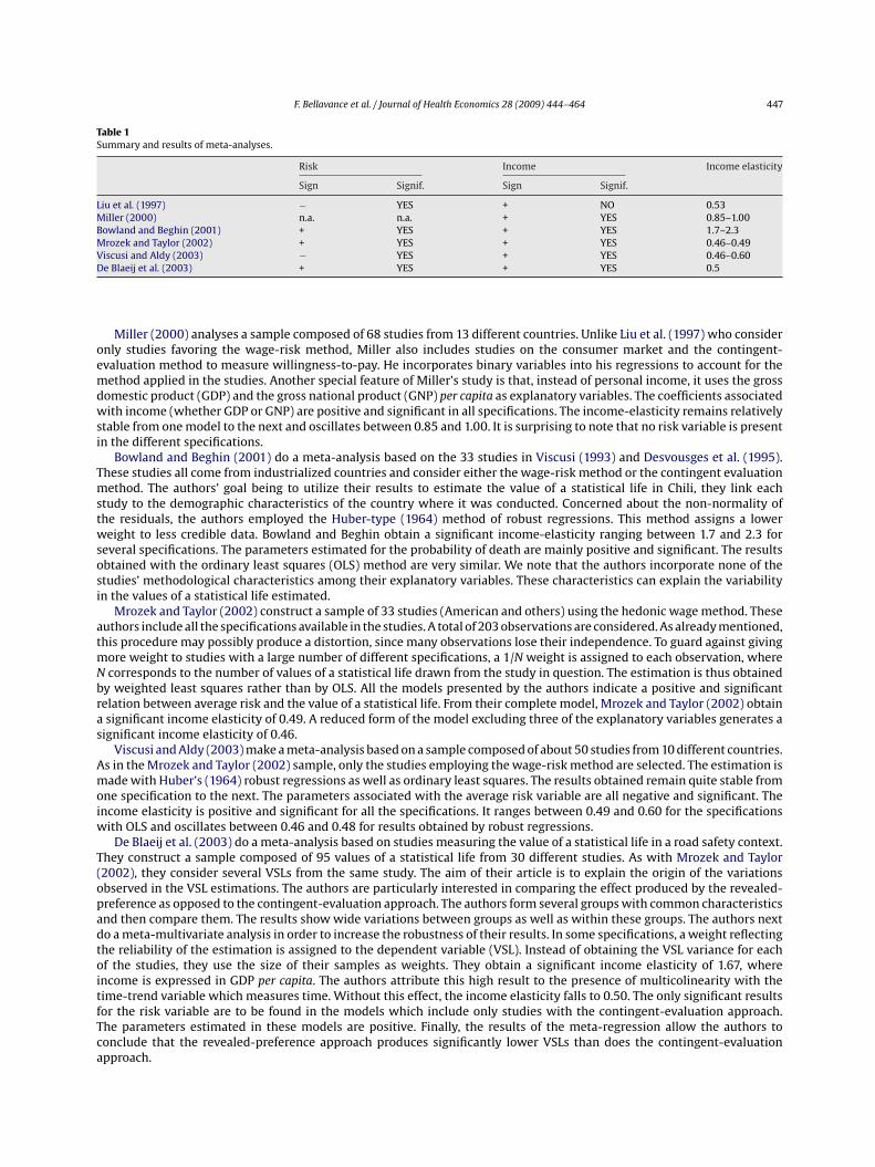
Table 1Summary and results of meta-analyses.

Risk Income Income elasticity

Sign Signif. Sign Signif.

Liu et al. (1997) − YES + NO 0.53Miller (2000) n.a. n.a. + YES 0.85–1.00Bowland and Beghin (2001) + YES + YES 1.7–2.3Mrozek and Taylor (2002) + YES + YES 0.46–0.49Viscusi and Aldy (2003) − YES + YES 0.46–0.60De Blaeij et al. (2003) + YES + YES 0.5

Miller (2000) analyses a sample composed of 68 studies from 13 different countries. Unlike Liu et al. (1997) who consideronly studies favoring the wage-risk method, Miller also includes studies on the consumer market and the contingent-evaluation method to measure willingness-to-pay. He incorporates binary variables into his regressions to account for themethod applied in the studies. Another special feature of Miller’s study is that, instead of personal income, it uses the grossdomestic product (GDP) and the gross national product (GNP) per capita as explanatory variables. The coefficients associatedwith income (whether GDP or GNP) are positive and significant in all specifications. The income-elasticity remains relativelystable from one model to the next and oscillates between 0.85 and 1.00. It is surprising to note that no risk variable is presentin the different specifications.

Bowland and Beghin (2001) do a meta-analysis based on the 33 studies in Viscusi (1993) and Desvousges et al. (1995).These studies all come from industrialized countries and consider either the wage-risk method or the contingent evaluationmethod. The authors’ goal being to utilize their results to estimate the value of a statistical life in Chili, they link eachstudy to the demographic characteristics of the country where it was conducted. Concerned about the non-normality ofthe residuals, the authors employed the Huber-type (1964) method of robust regressions. This method assigns a lowerweight to less credible data. Bowland and Beghin obtain a significant income-elasticity ranging between 1.7 and 2.3 forseveral specifications. The parameters estimated for the probability of death are mainly positive and significant. The resultsobtained with the ordinary least squares (OLS) method are very similar. We note that the authors incorporate none of thestudies’ methodological characteristics among their explanatory variables. These characteristics can explain the variabilityin the values of a statistical life estimated.

Mrozek and Taylor (2002) construct a sample of 33 studies (American and others) using the hedonic wage method. Theseauthors include all the specifications available in the studies. A total of 203 observations are considered. As already mentioned,this procedure may possibly produce a distortion, since many observations lose their independence. To guard against givingmore weight to studies with a large number of different specifications, a 1/N weight is assigned to each observation, whereN corresponds to the number of values of a statistical life drawn from the study in question. The estimation is thus obtainedby weighted least squares rather than by OLS. All the models presented by the authors indicate a positive and significantrelation between average risk and the value of a statistical life. From their complete model, Mrozek and Taylor (2002) obtaina significant income elasticity of 0.49. A reduced form of the model excluding three of the explanatory variables generates asignificant income elasticity of 0.46.

Viscusi and Aldy (2003) make a meta-analysis based on a sample composed of about 50 studies from 10 different countries.As in the Mrozek and Taylor (2002) sample, only the studies employing the wage-risk method are selected. The estimation ismade with Huber’s (1964) robust regressions as well as ordinary least squares. The results obtained remain quite stable fromone specification to the next. The parameters associated with the average risk variable are all negative and significant. Theincome elasticity is positive and significant for all the specifications. It ranges between 0.49 and 0.60 for the specificationswith OLS and oscillates between 0.46 and 0.48 for results obtained by robust regressions.

De Blaeij et al. (2003) do a meta-analysis based on studies measuring the value of a statistical life in a road safety context.They construct a sample composed of 95 values of a statistical life from 30 different studies. As with Mrozek and Taylor(2002), they consider several VSLs from the same study. The aim of their article is to explain the origin of the variationsobserved in the VSL estimations. The authors are particularly interested in comparing the effect produced by the revealed-preference as opposed to the contingent-evaluation approach. The authors form several groups with common characteristicsand then compare them. The results show wide variations between groups as well as within these groups. The authors nextdo a meta-multivariate analysis in order to increase the robustness of their results. In some specifications, a weight reflectingthe reliability of the estimation is assigned to the dependent variable (VSL). Instead of obtaining the VSL variance for eachof the studies, they use the size of their samples as weights. They obtain a significant income elasticity of 1.67, whereincome is expressed in GDP per capita. The authors attribute this high result to the presence of multicolinearity with thetime-trend variable which measures time. Without this effect, the income elasticity falls to 0.50. The only significant resultsfor the risk variable are to be found in the models which include only studies with the contingent-evaluation approach.The parameters estimated in these models are positive. Finally, the results of the meta-regression allow the authors toconclude that the revealed-preference approach produces significantly lower VSLs than does the contingent-evaluationapproach.


Table 1 presents a summary of the results from the different meta-analyses performed.1 We can affirm that there isdefinitively a positive relation between incomes and estimations of the value of a statistical life. We also observe that, exceptfor the Bowland and Beghin study (2001), the income elasticity obtained by these different meta-analyses is always equal toor lower than 1. However, we can reach no conclusion as to the relation between average risk and the value of a statisticallife. In some cases, the authors obtain positive and significant coefficients but in other cases negative and significant ones.This relation seems ambiguous, as predicted by the theory.

3.2. Methodological approach

As already mentioned, wide variations in values of a statistical life are observed. These variations complicate the workof public decision-makers who must choose a value to insert in their cost–benefit calculations. In order for them to make amore enlightened choice, it is of primary importance that they understand the origin of this variability in results. To graspthe sources of this variability, we shall perform a meta-analysis with a different methodology. By employing a mixed effectsregression model (Raudenbush, 1994), we want to distinguish our contribution from all the other meta-analyses performedso far and to test the robustness of their results.

Suppose that each study uses a perfectly identical methodology and that their samples are all the same size and con-structed randomly from the same population. The VSLs obtained will not be identical because the samples studied are mostlikely different. However, this variation in the results is entirely due to the variance in sampling (Raudenbush, 1994). It canalso be called a variance in estimation, since the variations in the samples will have an impact on the VSL estimations. Butseveral methodological differences are observable across the studies. These differences likely explain, in part, the variationsin the VSL estimations. And even if each author used exactly the same methodology, several other non-observable anduncontrollable factors could influence the results. The mixed effects regression model takes this heterogeneity into account,hypothesizing that the estimation variance is not the only source of the variations observed.

Therefore, the value of a statistical life VSLj in each of the m studies selected is modeled with the following mixed effectsregression model:

VSLj = ˇ0 +p∑

k=1

ˇkXjk + uj + ej, (9)

where ˇ0 is the constant; Xjk is the characteristic k of study j which is used to estimate VSLj; ˇ1, . . ., ˇp are the coefficients ofthe regression which capture the fixed effects of the study characteristics on VSL; uj is a random effect term associated withstudy j which takes into account the non-observed effects that influence VSLj. Each random effect is independent, with amean of zero and a variance of �2

u ; ej, j = 1 . . . m, are the estimation errors; they are independent, of null mean and of varianceequal to �2

VSLj.

In a fixed effects model, the random effect is simply withdrawn from Eq. (9). The fixed effects model thus supposes thatthe characteristics of the studies fully explain the variations in VSLs between these studies. The mixed effects regressionmodel accounts for the existence of the heterogeneity caused by non-observed characteristics which cannot be consideredin the model but which explain in part the variations in the VSLs. This model’s special feature is that it has two elements inthe error term: the random effect and the estimation error. The variance of VSLj (�2∗

VSLj), as conditioned by the characteristics

of Xjk, is equal to

�2∗VSLj

= Var(uj + ej) = �2u + �2

VSLj. (10)

As Raudenbush (1994) maintains, it would not be appropriate to use an OLS regression to estimate Eq. (9), since this methodretains homoskedasticity as its hypothesis—meaning that the errors in the regression model would have the same variance.Our model is instead based on a hetereoskedasticity hypothesis. The residual variance in our model (�2∗

VSLj) is not constant,

since �2VSLj

differs from one study to the next. We must therefore use the weighted least squares method where the optimal

weights (weight∗j) are the inverse of the variances obtained in each of the studies:

weight∗j = 1

�2∗VSLj

= 1

�2u + �2

VSLj

. (11)

If �2u is null, then the fixed-effects model will not be rejected and the optimal weights will be 1/�2

VSLj. The calculation of

�2VSLj

is rather straightforward and requires only certain data contained in the studies. As we see in Eq. (11), calculating the

optimal weights for the mixed effects regression model requires an additional term—the variance of the random effect (�2u ).

This effect is not given in the studies and must thus be estimated.

1 The six meta-analyses just presented are, to our knowledge, the only ones published in a scientific journal. For other unpublished meta-analyses, thereader can consult Desvousges et al. (1995), Day (1999), and Dionne and Michaud (2002).


Our meta-analysis is concerned with the hedonic wage method. The corresponding econometric specification for a givenstudy j estimating VSL with this method is the following:

ln(wi) = Xiˇ + pi � + ui, (12)

where wi is the wage of individual i, Xi is a vector of explanatory variables comprising the characteristics of this individual,pi represents his probability of death, ˇ and � are the parameters to be estimated, and ui ∼ N(0, �2). Index j is omitted in (12)to simplify notation.

By using a linear regression with ordinary least squares or other methods to estimate the parameters of Eq. (12), we obtain�, which is the average wage premium for a marginal increase in the probability of death. Based on Eq. (12), we can obtainthe average WTP of the sample by multiplying � by the average income. The WTP must be adjusted so that it is expressedin annual dollars. Finally, to calculate the value of a statistical life, the WTP must be divided by the non-marginal variationin the probability of death. In the regression analysis, this variation in the probability of death corresponds to a unit of thevariable pi.2 We can then express the estimate of the value of a statistical life of the population j studied as follows:

VSLj = �j (sample average of annual income)j

(unit of probability of death)j, (13)

where the numerator corresponds to the WTP in annual dollars, the denominator to the non-marginal variation in theprobability of death, and �j = ∂ln(wi)/∂pi. We must mention that the studies we analyze are limited to the data from workershaving accepted the risk. They may thus contain a sample bias (Ashenfelter, 2006). Moreover, the values obtained may be verysensitive to the econometric specifications used. Our objective is to identify the methodological differences which renderVSL evaluations most sensitive.

We can use Eq. (13) to calculate the value of a statistical life for each study retained. When the specification containsinteraction of some variables with the risk of death, the value of a statistical life is calculated with the average of eachvariable. For example, a specification may contain a squared risk variable as well as a risk variable interacting with age:

ln(wi) = Xiˇ + pi�1 + p2i �2 + pi agei�3 + ui. (14)

The corresponding VSL calculation for this study will take this form:

(�1j + 2pj�2j + agej �3j)(sample average of annual income)j

(unit of probability of death)j,

where pj = (1/nj)∑nj

i=1pi and agej = (1/nj)∑nj

i=1agei are, respectively, the average probability of death and the average ageof the nj individuals in study j.

Since most of the studies come from the United States, we employed the US$ 2000 as the common monetary unit. Thismakes it possible to minimize the number of conversions required. The first step consists in converting the values intoAmerican currency. For non-American studies, we have used purchasing power parity (PPP) as the exchange factor.3 AsSummers and Heston (1991) point out, when comparing incomes from several countries, it is more appropriate to take thePPP into account, rather than just making a conversion based on the exchange rate. Goods and services usually cost less inpoor countries as compared to rich ones and using the exchange rate as the conversion factor will not allow comparison ofthe intrinsic value of salaries. The second step consists in applying the consumer price index (CPI)4 to adjust VSL and averageincome values to US$ 2000.

In Eq. (11) the value-of-a-statistical-life variance (�2VSLj

) is needed for each study to construct the weights. We calculate

this variance from the standard deviation associated with coefficient �j . This statistic is often included in regression analysesto measure the accuracy of estimations. The standard error (SE) of the value of a statistical life on a given study j is calculatedin this manner:

SE(VSLj) = SE(�j)(sample average of annual income)j

(unit of probability of death)j. (15)

The sample average of annual income and the unit of probability of death in Eq. (15) correspond exactly to the same variablesin Eq. (13). If there are one or more terms of interaction between the probability of death and other explanatory variables,the calculation of the standard error will then require covariance terms. For example, take the case of a single interactionterm in the wage equation:

ln(wi) = Xiˇ + pi�1 + (pi × agei)�2 + ui. (16)

2 In the majority of studies, the variable measuring the probability of death is expressed in deaths per 10,000 workers. In these cases, the unit of thevariable pj is 1/10,000.

3 These values are drawn from PennWorld Table 6.0 (http://pwt.econ.upenn.edu).4 This index can be obtained from the Council of Economic Advisers (2005).

http://pwt.econ.upenn.edu/


We obtain the expression of the value of a statistical life for the study:

VSLj = (�1j + agej�2j)(sample average of annual income)j


The standard error of the value of a statistical life is thus obtained as follows:

SE(VSLj) =

[√SE2(�1j) + (agej)

2 SE2(�2j) + 2 agej cov(�1j, �2j)

](sample average of annual income)j


However, the covariances needed to calculate the standard errors are not usually published by the authors. This preventsus from calculating with Eq. (18) the standard deviations for VSLs drawn from articles using terms of interaction. We shallevaluate them with an indirect procedure for a sensitivity analysis (see Section 5.3).

3.3. Methodological choices

In each of the studies estimating the value of a statistical life, the authors are obliged to make methodological choices,whether in constructing the sample or in doing the technical analysis. These different choices may certainly influence theresults obtained and probably explain the wide variability in the values of a statistical life published. In this section we shalltouch on a few of these choices and predict their direct or indirect impact on the value of a statistical life.

3.3.1. Choice of samplesOne of the main explanations of the variations in values of a statistical life arises from the differences in the characteristics

of the samples used. Here are a few of the characteristics which may have a strong impact. We know that wealth andprobability of death can have an impact on individuals’ WTP and thus on the value of a statistical life. As theory indicated,studies using samples of more wealthy individuals should obtain higher estimations of the value of a statistical life. As tosamples of persons more at risk, the results expected are ambiguous.

As a rule, women are rarely to be found in dangerous occupations. Even within the same occupational field, the riskiesttasks were traditionally assigned to men (Leigh, 1987). It is thus not surprising to note that most deaths, whether classifiedby industry or by occupation, are those of men. Some authors exclude women from their sample, others include them butincorporate a binary variable (man or woman) in their regressions.5

Many authors have studied the effect of unionization on workers’ WTP. Several conclude that union membership isassociated with a higher WTP. The main reason explaining this higher wage premium among unionized workers is theiraccess to more accurate information concerning their safety. What is more, unions can be good mechanisms for lettingcorporate directors know about workers’ safety concerns and for negotiating better salaries. However, certain authors (Marinand Psacharopoulos, 1982; Meng, 1989; Sandy and Elliott, 1996) obtain higher WTPs for non-unionized workers and lowerones for workers who are union members.6 In most studies, the authors account for this effect by simply introducing a binaryvariable without interaction.

Racial differences may also influence the values of a statistical life obtained in the studies. Viscusi (2003) obtains con-siderably lower values of a statistical life among black as compared to white workers. Viscusi proposes two reasons whichmay explain this result. First, one observes that black workers are, in general, employed in more dangerous jobs than whiteworkers. It is possible that the preferences for risk differ among races. Second, there may be fewer work opportunities forblacks. Several studies still illustrate the presence of racial discrimination on the job market, as is apparent in the wagedifferences between whites and blacks doing the same job.7

Certain authors pay special attention to workers’ occupation, particularly to the impact of including blue and white collarworkers in the same sample. Since blue collars are victims of four to five times more accidents (Root and Sebastian, 1981),some authors exclude them from their studies. For this same reason, others will instead exclude white collar workers. Thesechoices will have an impact on the value of a statistical life as well as on the meaningfulness of the results.

3.3.2. Choice of the risk variableThe variable measuring workers’ risk of death is one of the most important in the hedonic wage method. The ideal risk

measurement would be the one perceived by workers. However, the majority of researchers use risk measurements producedby organizations which count the number of deaths by industry or occupation.8

The Bureau of Labor Statistics (BLS), a section of the U.S. Department of Labor, is the source used by most Americanresearchers. From the 1960s to the early 1990s, the BLS obtained its data from an annual survey distributed to hundreds of

5 Leigh (1987) obtains only a slight difference in the value of a statistical life when he excludes women from his sample.6 For a more complete review of studies analyzing the impact of unionization, see Sandy et al. (2001) as well as Viscusi and Aldy (2003).7 According to Dionne and Lanoie (2004), workers’ mobility is essential to the wage-risk analysis.8 Researchers usually average probabilities of death over a few years. This prevents the distortions caused by a catastrophe which might occur in a specific

year in a specific industry.


thousands of firms in several industries. These data were then compiled with the two- or three-digit Standard Industrial Clas-sification (SIC) code—thus in a rather aggregated fashion. This method of obtaining and compiling data left some researchersconcerned about the possibility of measurement errors (Moore and Viscusi, 1988a). As already specified, it is important toobtain a disaggregated measurement of risk. Assigning the same probability of death to every worker in the same industrymay cause measurement errors, for none of these workers holds the same job and faces the same risk.

The National Institute of Occupational Safety and Health (NIOSH) has been allowing researchers to utilize their occu-pational data since 1980. The NIOSH obtains its information from the death certificates issued after workplace accidents.According to Moore and Viscusi (1988a), this method is more suitable, since it is based on a census rather than a survey.The authors also compare the statistics from the two organizations. They observe that the probabilities of death with NIOSHdata are approximately the double of those constructed with BLS data. Since 1992, the BLS has also been relying on a censuscalled the Census of Fatal Occupational Injuries (CFOI) to gather its data. Comparing the probabilities of death over the periodrunning from 1992 to 1995, the differences between the two bodies are smaller; we note that it is now the BSL’s turn to posthigher probabilities of death.9

Some studies also consider actuarial data10 drawn from a study published in 1967 by the Society of Actuaries (SOA). Onevery important characteristic of this study is that it measures the number of deaths that exceed a certain expected value.11 Itsmeasurement of risk is thus not identical to that of the BLS and the NIOSH. A second important characteristic of this sourceis its particular interest in the riskiest jobs. Consequently, samples of studies with this source show average probabilities ofdeath which are much higher compared to others. Non-American studies usually draw their data from government sources.Canadian studies, for example, often use data collected by Statistics Canada and the Ministry of Revenue. Each provinceallows access to their data on work accidents. These comparisons between different organizations allow us to grasp thesignificance and impact of choosing the source of the risk variable. The data can vary widely depending on the organizationchosen and will probably generate widely different values of a statistical life.

3.3.3. Choice of models and control variablesMost of the studies use the ordinary least squares method (OLS) to estimate Eq. (12). These models often treat the risk

variable as an exogenous one. Simple OLS estimates may bias the results associated with endogenous risk (Kniesner et al.,2007). As a rule, higher values of a statistical life are observed in studies with endogenous risk (Garen, 1988; Siebert andWei, 1994; Sandy and Elliott, 1996; Shanmugam, 2001; Gunderson and Hyatt, 2001).

Researchers must also choose the other independent variables to be inserted in their models. These choices are rathersubjective, but they will certainly influence the results. Some authors use not only a linear form of the risk variable butalso the squared form. This makes it possible to take the non-linear relation between wage and risk into account. The riskvariable can also be used in interaction with certain characteristics of workers (race, age, sex, unionization, region, etc.).These interactions allow segmentation of the job market (Day, 1999). For example, it may happen that individuals from twodifferent regions will not receive the same pay for the same risk or that individuals in a given age bracket will be moreaccepting of certain risks.

In principle, workers should demand a higher wage not only for the risk of death but also for the risk of injury. However,including the injury variable in models does raise a number of questions. First, omitting this variable can put a positivebias on the coefficient linked to the risk of death. Though, as Viscusi and Aldy (2003) point out, the risk of death is closelycorrelated with the risk of injury. So, owing to colinearity, the use of both variables in the same specification may producevery large standard errors. But Arabsheibani and Marin (2000) maintain that including or excluding the injury variable hasno significant effect on the coefficient for the risk-of-death variable.

In the literature, many researchers seem to forget the existence of work-accident compensation. As discussed in Section2, the presence of insurance compensation may affect the link between WTP and p. Arnould and Nichols (1983) argue thatrecipients of compensation usually demand lower salaries for increased risk of death. Empirical evidence has shown that theexistence of compensation implies big reductions in wage levels (Fortin and Lanoie, 2000). These authors claim that studiesomitting this variable must necessarily obtain biased results.

4. Choice of studies

Most of the studies have been drawn from literature reviews in the works of Viscusi (1993), Michaud (2001), and Viscusiand Aldy (2003). Other articles have been retrieved by key-word searches with the search engines Proquest, ScienceDirect,JSTOR, EconLit and SSRN and by systematically looking at the references of the articles identified. By retaining only the studiesthat use the hedonic wage method to calculate the value of a statistical life, we come up with a total of 49 articles.

We excluded the Lott and Manning (2000) study, since their work focuses solely on the risks of death from cancercontracted in the workplace. Next, to get a more homogeneous sample, we withdrew the studies whose estimation was notobtained with a regression similar to Eq. (12). The studies by Melinek (1974) and Needleman (1980) were thus eliminated.

9 We must mention that serious criticisms have been aimed at the official statistics on occupational risks in the U.S. (see, for example, Leigh et al., 1997).10 See Thaler and Rosen (1975), Brown (1980), Arnould and Nichols (1983) as well as Gegax et al. (1991).11 This expected value is computed in terms of the age structure within each occupation, and with survival tables.


Table 2Average value of a statistical life according to country of origin.

Number Average Median Standard deviation

United States 16 6,273,000 4,648,493 5,045,182Canada 7 9,160,083 4,041,961 10,392,347United Kingdom 3 16,995,764 14,181,264 12,592,129Australia 2 11,173,881 11,173,881 9,625,769South Korea 1 1,552,525 1,552,525 –India 1 16,070,278 16,070,278 –Japan 1 12,812,755 12,812,755 –Taiwan 1 1,198,975 1,198,975 –

Total 32 8,420,568 4,955,810 7,890,597

We also wanted each VSL estimate to be carried out on different samples. Of the remaining 46 articles, 3 had to be withdrawnbecause their samples had already been used in other studies. The three articles in question are those of Moore and Viscusi(1990a), Sandy et al. (2001), and Kniesner and Viscusi (2005).12

Since the value of a statistical life obtained based on each study constitutes the dependent variable of our meta-analysis,all the studies for which we could not calculate this value ourselves with Eq. (13) were removed. Among these studies are tobe found those of Moore and Viscusi (1988b, 1989, 1990b), of Herzog and Schlottmann (1990), as well as that of Dorman andHagstrom (1998). Finally, the Leigh study (1987) was not selected, since the author fails to publish the average probability ofdeath in his sample. This variable is one of the most important in our meta-analysis.

The final sample is thus made up of 37 studies. In most cases, they contain several regressions and thus several estimationsof the value of a statistical life. As we do not want more than one estimation from the same sample, only one value of astatistical life is chosen from studies that use only one sample. To select the most suitable specification, we set selectioncriteria. First, to compute the standard error of the estimated VSL with Eq. (15), we chose specifications containing no terms ofinteraction between the probability of death and other explanatory variables. A second criterion is based on the homogeneityof the specifications across studies. Thus the specification selected must coincide as closely as possible with the specificationsand models of the other studies included in the meta-analysis. For example, in Kniesner and Leeth (1991), we had the choicebetween specifications which took account injuries and others which did not. Since most articles include an injury variablewhich is encouraged by most authors in the literature, we chose a specification that incorporates it. A third criterion relatesto the sample used. In articles with overlapping samples, our choice was influenced by the size and the characteristics of thesamples; larger samples with characteristics most similar to the other studies were preferred. In a few studies, the goodness-of-fit of the regression model and the statistical significance of the results also influenced the choice, but were never theonly criteria used. Sometimes the author’s opinion was the selection criterion. Indeed, certain authors, like Smith (1974),point out the best specification in their article. Finally, the opinion of other authors helped in our selection. For example, theViscusi and Aldy (2003) article helped us decide which specification to select in the Leigh (1995) article.

Several estimations can be drawn from the same study, provided that they were calculated based on different and inde-pendent samples. We are aware that adding these estimations may have an impact on the independence of our observations,since they were produced in the framework of the same article and thus from the same analytical viewpoint. This decisionconcerns only one article (Kniesner and Leeth, 1991), for a total of three observations. So we have a potential of 39 obser-vations for our meta-analysis. The characteristics of these 39 selected observations are presented in Appendix 1 along withtwo examples to illustrate the corresponding calculation of the VSL. Note that we were unable to compute the standard errorof VSL for seven of these observations (Appendix 1, italicized rows in table) due to their interaction with the risk of deathin the specification. Therefore, we did not use these observations in the main analyses presented in the next section. Wereintroduce these seven observations in Section 5.3, for a sensitivity analysis.

5. Results

5.1. Descriptive analysis of the sample

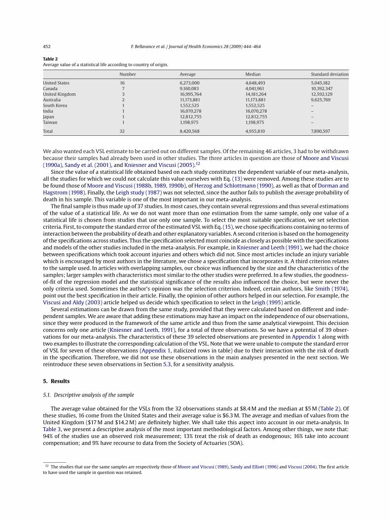
The average value obtained for the VSLs from the 32 observations stands at $8.4 M and the median at $5 M (Table 2). Ofthese studies, 16 come from the United States and their average value is $6.3 M. The average and median of values from theUnited Kingdom ($17 M and $14.2 M) are definitely higher. We shall take this aspect into account in our meta-analysis. InTable 3, we present a descriptive analysis of the most important methodological factors. Among other things, we note that:94% of the studies use an observed risk measurement; 13% treat the risk of death as endogenous; 16% take into accountcompensation; and 9% have recourse to data from the Society of Actuaries (SOA).

12 The studies that use the same samples are respectively those of Moore and Viscusi (1989), Sandy and Elliott (1996) and Viscusi (2004). The first articleto have used the sample in question was retained.


Table 3Descriptive statistics of the sample (n = 32).

Variables Average

Average income (US$ 2000) 29,559Average probability (10,000×) 2.05White-workers only sample 13%Men only sample 47%Unionized only sample 13%Sample without white collars 41%Injuries taken into account 56%Compensation taken into account 16%Endogenous risk 13%Observed risk 94%SOA 9%

Standard deviation of income = 9576; standard deviation of probability = 2.32.

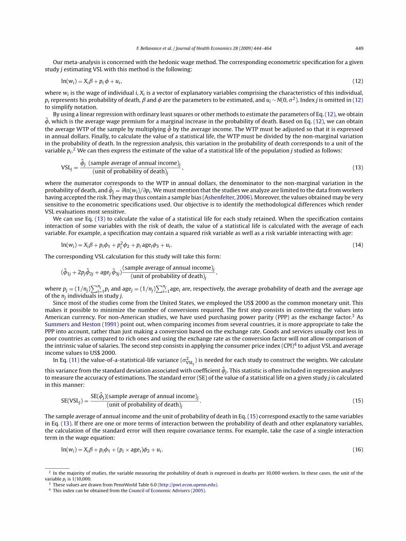
Fig. 1. Estimation of the value of statistical life over time.

After 30 years of research and publication on the topic, we might expect a certain convergence in the values obtained.When we examine Fig. 1, we note quite the contrary. The most recent studies seem to diverge instead. And it is also interestingto observe a positive relation between the values of a statistical life and the year of publication. Several hypotheses havebeen advanced to explain this result. First, as we mentioned earlier, using the probability of death as an endogenous variableusually produces higher values. This technique has only been applied since 1988. We can suppose that workers are betterinformed than before concerning the risks inherent in their jobs and that they are now demanding more adequate pay.Finally, it is possible that, given their longer life expectancy and potential period of retirement, workers are now simplyassigning a higher value to their life.

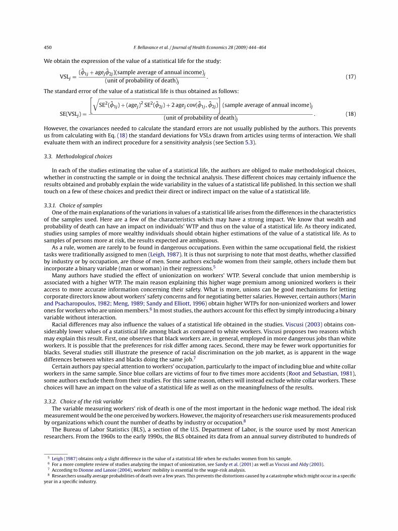
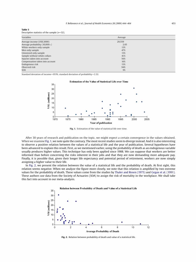
In Fig. 2, we present the relation between the value of a statistical life and the probability of death. At first sight, thisrelation seems negative. When we analyze the figure more closely, we note that this relation is amplified by two extremevalues for the probability of death. These values come from the studies by Thaler and Rosen (1975) and Gegax et al. (1991).These authors use data from the Society of Actuaries (SOA) to assign the risk of mortality in the workplace. We shall takethis fact into account in our meta-analysis.

Fig. 2. Relation between probability of death and value of a statistical life.


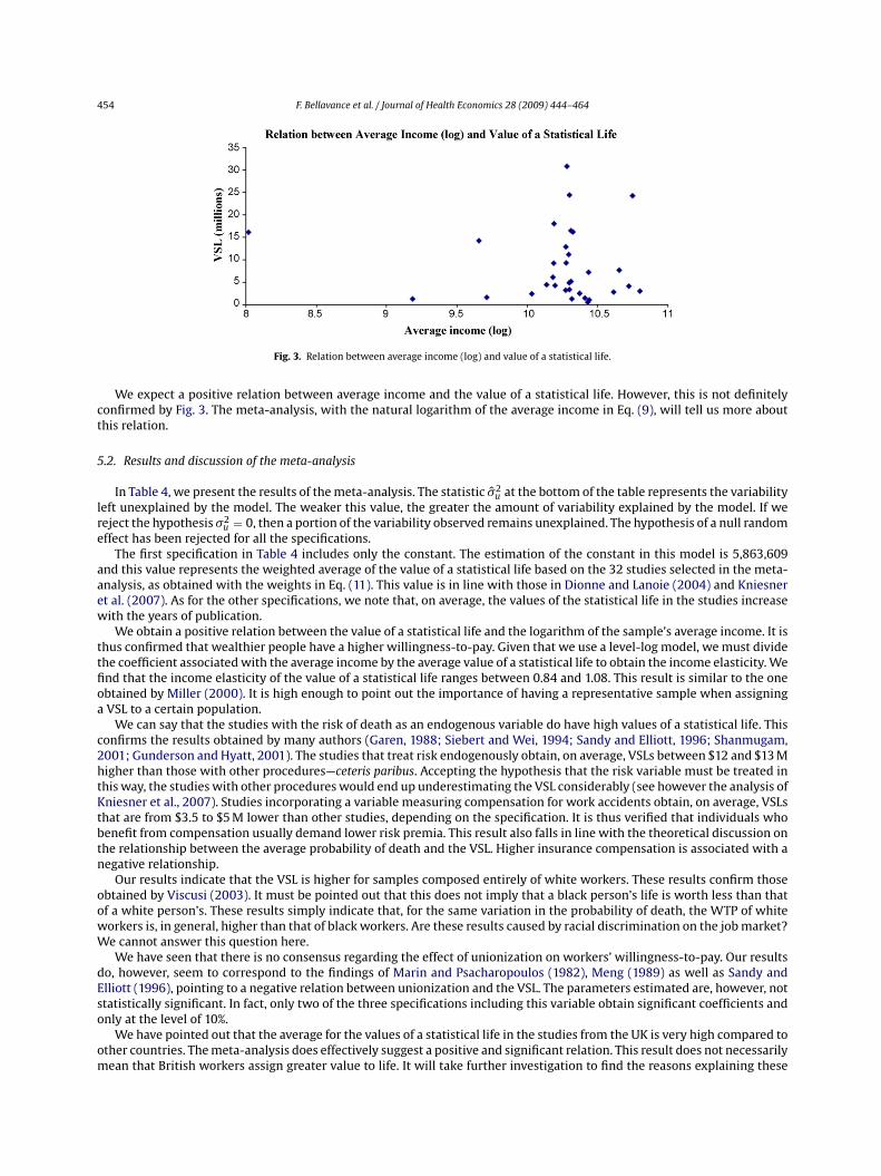
Fig. 3. Relation between average income (log) and value of a statistical life.

We expect a positive relation between average income and the value of a statistical life. However, this is not definitelyconfirmed by Fig. 3. The meta-analysis, with the natural logarithm of the average income in Eq. (9), will tell us more aboutthis relation.

5.2. Results and discussion of the meta-analysis

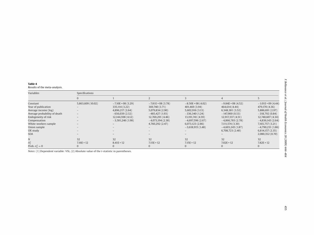
In Table 4, we present the results of the meta-analysis. The statistic �2u at the bottom of the table represents the variability

left unexplained by the model. The weaker this value, the greater the amount of variability explained by the model. If wereject the hypothesis �2

u = 0, then a portion of the variability observed remains unexplained. The hypothesis of a null randomeffect has been rejected for all the specifications.

The first specification in Table 4 includes only the constant. The estimation of the constant in this model is 5,863,609and this value represents the weighted average of the value of a statistical life based on the 32 studies selected in the meta-analysis, as obtained with the weights in Eq. (11). This value is in line with those in Dionne and Lanoie (2004) and Kniesneret al. (2007). As for the other specifications, we note that, on average, the values of the statistical life in the studies increasewith the years of publication.

We obtain a positive relation between the value of a statistical life and the logarithm of the sample’s average income. It isthus confirmed that wealthier people have a higher willingness-to-pay. Given that we use a level-log model, we must dividethe coefficient associated with the average income by the average value of a statistical life to obtain the income elasticity. Wefind that the income elasticity of the value of a statistical life ranges between 0.84 and 1.08. This result is similar to the oneobtained by Miller (2000). It is high enough to point out the importance of having a representative sample when assigninga VSL to a certain population.

We can say that the studies with the risk of death as an endogenous variable do have high values of a statistical life. Thisconfirms the results obtained by many authors (Garen, 1988; Siebert and Wei, 1994; Sandy and Elliott, 1996; Shanmugam,2001; Gunderson and Hyatt, 2001). The studies that treat risk endogenously obtain, on average, VSLs between $12 and $13 Mhigher than those with other procedures—ceteris paribus. Accepting the hypothesis that the risk variable must be treated inthis way, the studies with other procedures would end up underestimating the VSL considerably (see however the analysis ofKniesner et al., 2007). Studies incorporating a variable measuring compensation for work accidents obtain, on average, VSLsthat are from $3.5 to $5 M lower than other studies, depending on the specification. It is thus verified that individuals whobenefit from compensation usually demand lower risk premia. This result also falls in line with the theoretical discussion onthe relationship between the average probability of death and the VSL. Higher insurance compensation is associated with anegative relationship.

Our results indicate that the VSL is higher for samples composed entirely of white workers. These results confirm thoseobtained by Viscusi (2003). It must be pointed out that this does not imply that a black person’s life is worth less than thatof a white person’s. These results simply indicate that, for the same variation in the probability of death, the WTP of whiteworkers is, in general, higher than that of black workers. Are these results caused by racial discrimination on the job market?We cannot answer this question here.

We have seen that there is no consensus regarding the effect of unionization on workers’ willingness-to-pay. Our resultsdo, however, seem to correspond to the findings of Marin and Psacharopoulos (1982), Meng (1989) as well as Sandy andElliott (1996), pointing to a negative relation between unionization and the VSL. The parameters estimated are, however, notstatistically significant. In fact, only two of the three specifications including this variable obtain significant coefficients andonly at the level of 10%.

We have pointed out that the average for the values of a statistical life in the studies from the UK is very high compared toother countries. The meta-analysis does effectively suggest a positive and significant relation. This result does not necessarilymean that British workers assign greater value to life. It will take further investigation to find the reasons explaining these

F.Bellavanceet

al./JournalofHealth

Economics

28(2009)

444–464455

Table 4Results of the meta-analysis.

Variables Specifications

0 1 2 3 4 5

Constant 5,863,609 (10.02) −7.10E + 08 (3.29) −7.81E + 08 (3.78) −8.50E + 08 (4.02) −9.84E + 08 (4.52) −1.01E + 09 (4.44)Year of publication – 335,114 (3.22) 369,740 (3.71) 401,469 (3.94) 464,614 (4.44) 479,170 (4.36)Average income (log) – 4,896,217 (2.64) 5,079,834 (2.90) 5,602,916 (3.13) 6,348,381 (3.52) 5,886,691 (2.97)Average probability of death – −656,039 (2.52) −485,427 (1.93) −336,340 (1.24) −147,900 (0.53) −318,792 (0.84)Endogeneity of risk – 12,144,598 (4.12) 12,769,291 (4.46) 13,191,741 (4.59) 12,917,337 (4.51) 12,740,607 (4.34)Compensation – −3,581,246 (1.98) −4,073,194 (2.38) −4,697,596 (2.67) −4,866,783 (2.78) −4,836,143 (2.64)White-workers sample – – 4,760,292 (2.47) 6,073,123 (2.86) 7,111,574 (3.30) 7,165,757 (3.21)Union sample – – – −3,618,915 (1.48) −4,603,245 (1.87) −4,790,231 (1.86)UK study – – – – 6,708,723 (2.40) 6,814,157 (2.35)SOA – – – – – 2,080,352 (0.70)

N 32 32 32 32 32 32�2

u 7.16E + 12 8.41E + 12 7.15E + 12 7.15E + 12 7.02E + 12 7.82E + 12Prob. �2

u = 0 0 0 0 0 0 0

Notes: (1) Dependent variable: VSL. (2) Absolute value of the t-statistic in parentheses.


Table 5Results of the meta-analysis (without studies using SOA).


0 1 2 3 4

Constant 6,519,243 (9.88) −8.29E + 08 (3.38) −9.02E + 08 (3.81) −8.78E + 08 (3.82) −9.96E + 08 (4.22)Year of publication – 397,154 (3.35) 432,049 (3.77) 419,944 (3.77) 475,149 (4.17)Average income (log) – 4,661,556 (2.23) 4,914,203 (2.47) 4,948,056 (2.56) 5,606,813 (2.88)Average probability of death – −1,928,822 (3.29) −1,590,198 (2.77) −1,543,579 (2.79) −1,239,987 (2.18)Endogeneity of risk – 11,129,173 (3.67) 11,746,697 (3.98) 12,260,997 (4.19) 12,120,680 (4.16)Compensation – −3,928,681 (2.03) −4,394,831 (2.39) −4,567,507 (2.55) −4,725,900 (2.66)White-workers sample – – 3,901,022 (1.89) 4,979,976 (2.23) 5,996,964 (2.63)Union sample – – – −3,445,325 (1.08) −4,216,413 (1.32)UK study – – – – 5,696,197 (1.99)

N 29 29 29 29 29�2

u 8.18E + 12 9.29E + 12 7.99E + 12 7.31E + 12 7.15E + 12Prob. �2

u = 0 0 0 0 0 0

Notes: (1) Dependent variable: VSL. (2) Absolute value of t-statistic in parentheses.

differences between countries. Do British institutions use different procedures when collecting information on workers? Oris it rather British researchers who apply particular methodologies that push the VSL higher?

We have seen that the relation between the average probability of death and the value of a statistical life is in theoryambiguous. According to our results, this relation seems to be negative. For specifications 1 and 2, we obtain a coefficientthat is significant at the 5% and 10% level respectively. However, for the next three specifications, we observe non-significantcoefficients. Thus we cannot say with any certainty that the relation is negative. It might be that this drop in the variable’ssignificance is due to a multicolinearity problem. By analyzing the correlation matrix in Appendix 2, we find a significantcorrelation coefficient between the probability of death and SOA, a variable which takes the value of 1 when the Society ofActuaries is the source of the probability of death and 0 otherwise.13 This result is not very surprising. However, the SOAvariable is present only in specification 5 and thus cannot explain the results obtained in specifications 3 and 4. Since theSOA is the only variable in the models which is significantly correlated with the probability of death, we do not believe thatmulticolinearity is the source of the weak levels of significance.

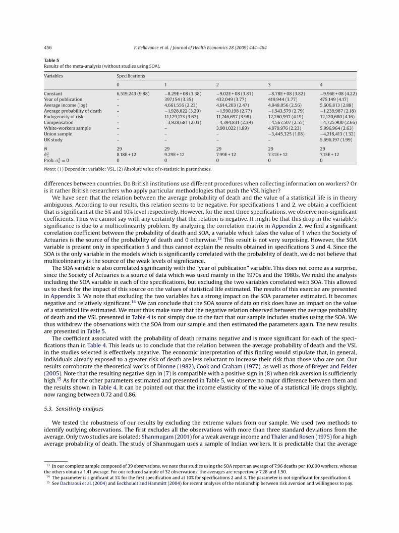
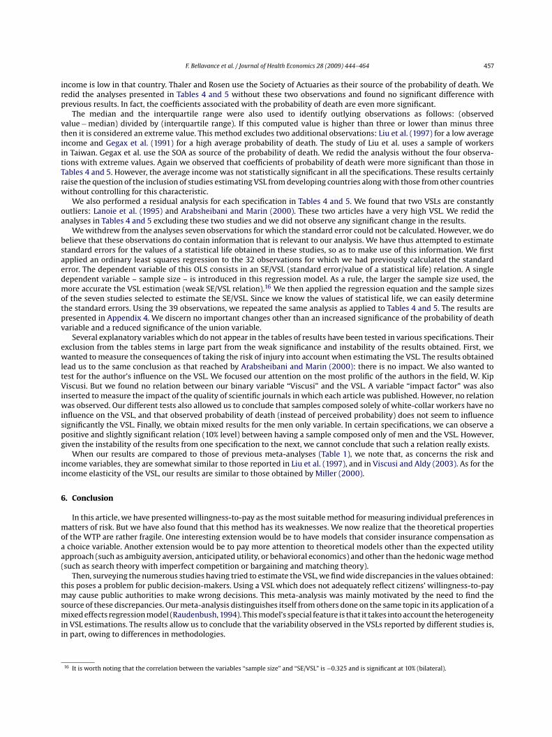
The SOA variable is also correlated significantly with the “year of publication” variable. This does not come as a surprise,since the Society of Actuaries is a source of data which was used mainly in the 1970s and the 1980s. We redid the analysisincluding the SOA variable in each of the specifications, but excluding the two variables correlated with SOA. This allowedus to check for the impact of this source on the values of statistical life estimated. The results of this exercise are presentedin Appendix 3. We note that excluding the two variables has a strong impact on the SOA parameter estimated. It becomesnegative and relatively significant.14 We can conclude that the SOA source of data on risk does have an impact on the valueof a statistical life estimated. We must thus make sure that the negative relation observed between the average probabilityof death and the VSL presented in Table 4 is not simply due to the fact that our sample includes studies using the SOA. Wethus withdrew the observations with the SOA from our sample and then estimated the parameters again. The new resultsare presented in Table 5.

The coefficient associated with the probability of death remains negative and is more significant for each of the speci-fications than in Table 4. This leads us to conclude that the relation between the average probability of death and the VSLin the studies selected is effectively negative. The economic interpretation of this finding would stipulate that, in general,individuals already exposed to a greater risk of death are less reluctant to increase their risk than those who are not. Ourresults corroborate the theoretical works of Dionne (1982), Cook and Graham (1977), as well as those of Breyer and Felder(2005). Note that the resulting negative sign in (7) is compatible with a positive sign in (8) when risk aversion is sufficientlyhigh.15 As for the other parameters estimated and presented in Table 5, we observe no major difference between them andthe results shown in Table 4. It can be pointed out that the income elasticity of the value of a statistical life drops slightly,now ranging between 0.72 and 0.86.

5.3. Sensitivity analyses

We tested the robustness of our results by excluding the extreme values from our sample. We used two methods toidentify outlying observations. The first excludes all the observations with more than three standard deviations from theaverage. Only two studies are isolated: Shanmugam (2001) for a weak average income and Thaler and Rosen (1975) for a highaverage probability of death. The study of Shanmugam uses a sample of Indian workers. It is predictable that the average

13 In our complete sample composed of 39 observations, we note that studies using the SOA report an average of 7.96 deaths per 10,000 workers, whereasthe others obtain a 1.41 average. For our reduced sample of 32 observations, the averages are respectively 7.28 and 1.50.

14 The parameter is significant at 5% for the first specification and at 10% for specifications 2 and 3. The parameter is not significant for specification 4.15 See Dachraoui et al. (2004) and Eeckhoudt and Hammitt (2004) for recent analyses of the relationship between risk aversion and willingness to pay.


income is low in that country. Thaler and Rosen use the Society of Actuaries as their source of the probability of death. Weredid the analyses presented in Tables 4 and 5 without these two observations and found no significant difference withprevious results. In fact, the coefficients associated with the probability of death are even more significant.

The median and the interquartile range were also used to identify outlying observations as follows: (observedvalue − median) divided by (interquartile range). If this computed value is higher than three or lower than minus threethen it is considered an extreme value. This method excludes two additional observations: Liu et al. (1997) for a low averageincome and Gegax et al. (1991) for a high average probability of death. The study of Liu et al. uses a sample of workersin Taiwan. Gegax et al. use the SOA as source of the probability of death. We redid the analysis without the four observa-tions with extreme values. Again we observed that coefficients of probability of death were more significant than those inTables 4 and 5. However, the average income was not statistically significant in all the specifications. These results certainlyraise the question of the inclusion of studies estimating VSL from developing countries along with those from other countrieswithout controlling for this characteristic.

We also performed a residual analysis for each specification in Tables 4 and 5. We found that two VSLs are constantlyoutliers: Lanoie et al. (1995) and Arabsheibani and Marin (2000). These two articles have a very high VSL. We redid theanalyses in Tables 4 and 5 excluding these two studies and we did not observe any significant change in the results.

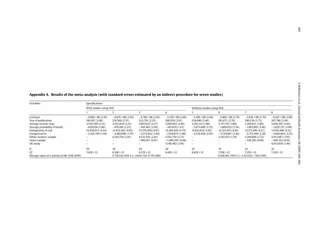
We withdrew from the analyses seven observations for which the standard error could not be calculated. However, we dobelieve that these observations do contain information that is relevant to our analysis. We have thus attempted to estimatestandard errors for the values of a statistical life obtained in these studies, so as to make use of this information. We firstapplied an ordinary least squares regression to the 32 observations for which we had previously calculated the standarderror. The dependent variable of this OLS consists in an SE/VSL (standard error/value of a statistical life) relation. A singledependent variable – sample size – is introduced in this regression model. As a rule, the larger the sample size used, themore accurate the VSL estimation (weak SE/VSL relation).16 We then applied the regression equation and the sample sizesof the seven studies selected to estimate the SE/VSL. Since we know the values of statistical life, we can easily determinethe standard errors. Using the 39 observations, we repeated the same analysis as applied to Tables 4 and 5. The results arepresented in Appendix 4. We discern no important changes other than an increased significance of the probability of deathvariable and a reduced significance of the union variable.

Several explanatory variables which do not appear in the tables of results have been tested in various specifications. Theirexclusion from the tables stems in large part from the weak significance and instability of the results obtained. First, wewanted to measure the consequences of taking the risk of injury into account when estimating the VSL. The results obtainedlead us to the same conclusion as that reached by Arabsheibani and Marin (2000): there is no impact. We also wanted totest for the author’s influence on the VSL. We focused our attention on the most prolific of the authors in the field, W. KipViscusi. But we found no relation between our binary variable “Viscusi” and the VSL. A variable “impact factor” was alsoinserted to measure the impact of the quality of scientific journals in which each article was published. However, no relationwas observed. Our different tests also allowed us to conclude that samples composed solely of white-collar workers have noinfluence on the VSL, and that observed probability of death (instead of perceived probability) does not seem to influencesignificantly the VSL. Finally, we obtain mixed results for the men only variable. In certain specifications, we can observe apositive and slightly significant relation (10% level) between having a sample composed only of men and the VSL. However,given the instability of the results from one specification to the next, we cannot conclude that such a relation really exists.

When our results are compared to those of previous meta-analyses (Table 1), we note that, as concerns the risk andincome variables, they are somewhat similar to those reported in Liu et al. (1997), and in Viscusi and Aldy (2003). As for theincome elasticity of the VSL, our results are similar to those obtained by Miller (2000).

6. Conclusion

In this article, we have presented willingness-to-pay as the most suitable method for measuring individual preferences inmatters of risk. But we have also found that this method has its weaknesses. We now realize that the theoretical propertiesof the WTP are rather fragile. One interesting extension would be to have models that consider insurance compensation asa choice variable. Another extension would be to pay more attention to theoretical models other than the expected utilityapproach (such as ambiguity aversion, anticipated utility, or behavioral economics) and other than the hedonic wage method(such as search theory with imperfect competition or bargaining and matching theory).

Then, surveying the numerous studies having tried to estimate the VSL, we find wide discrepancies in the values obtained:this poses a problem for public decision-makers. Using a VSL which does not adequately reflect citizens’ willingness-to-paymay cause public authorities to make wrong decisions. This meta-analysis was mainly motivated by the need to find thesource of these discrepancies. Our meta-analysis distinguishes itself from others done on the same topic in its application of amixed effects regression model (Raudenbush, 1994). This model’s special feature is that it takes into account the heterogeneityin VSL estimations. The results allow us to conclude that the variability observed in the VSLs reported by different studies is,in part, owing to differences in methodologies.

16 It is worth noting that the correlation between the variables “sample size” and “SE/VSL” is −0.325 and is significant at 10% (bilateral).


Several methodological factors have a strong impact on the VSLs estimated. For example, researchers who take theendogenous nature of the risk variable into account obtain higher VSLs. Results are also influenced by the form of econometricspecifications used. When a variable measuring workers’ compensation is included in the models, we obtain lower VSLs. Thepopulation under study is also important. Samples composed of wealthier economic agents generate higher VSLs. Samplescomposed of altruistic agents generate a negative relationship between VSL and accident probability. These agents may alsobe more compensated by insurance. Finally, we note that the VSL is significantly influenced by a study’s country of origin,by year of publication, by race, and by the source of the risk variable. These results inform public decision-makers of theimportance of using appropriate methodologies and representative samples or of adjusting the estimated values to the targetpopulation when making a decision.

Acknowledgements

Financial support by CREF and CIRRELT is acknowledged as well comments from two referees. Claire Boisvert improvedsignificantly the preparation of the different versions.

F.Bellavanceet

al./JournalofHealth

Economics

28(2009)

444–464459

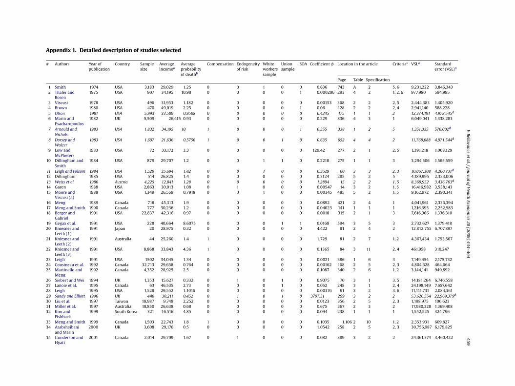
Appendix 1. Detailed description of studies selected

# Authors Year ofpublication

Country Samplesize

Averageincomea

Averageprobabilityof deathb

Compensation Endogeneityof risk

Whiteworkerssample

Unionsample

SOA Coefficient � Location in the article Criteriac VSLa Standarderror (VSL)a

Page Table Specification

1 Smith 1974 USA 3,183 29,029 1.25 0 0 1 0 0 0.636 743 A 2 5, 6 9,231,222 3,846,3432 Thaler and

Rosen1975 USA 907 34,195 10.98 0 0 0 0 1 0.000286 293 4 2 1, 2, 6 977,980 594,995

3 Viscusi 1978 USA 496 31,953 1.182 0 0 0 0 0 0.00153 368 2 2 2, 5 2,444,383 1,405,9204 Brown 1980 USA 470 49,019 2.25 0 0 0 0 1 0.06 128 2 2 2, 4 2,941,140 588,2285 Olson 1981 USA 5,993 33,509 0.9508 0 0 0 0 0 0.4245 175 1 1 2 12,374,191 4,978,545d

6 Marin andPsacharopoulos

1982 UK 5,509 26,415 0.93 0 0 0 0 0 0.229 836 4 3 1 6,049,041 1,338,283

7 Arnould andNichols

1983 USA 1,832 34,195 10 1 0 0 0 1 0.355 338 1 2 5 1,351,335 570,002d

8 Dorsey andWalzer

1983 USA 1,697 21,636 0.5756 1 0 0 1 0 0.635 652 4 4 2 11,768,688 4,971,544d

9 Low andMcPheters

1983 USA 72 33,172 3.3 0 0 0 0 0 129.42 277 2 1 2, 5 1,391,218 1,008,129

10 Dillingham andSmith

1984 USA 879 29,707 1.2 0 0 1 1 0 0.2218 275 1 1 3 3,294,506 1,565,559

11 Leigh and Folsom 1984 USA 1,529 35,694 1.42 0 0 1 0 0 0.3629 60 3 3 2, 3 10,067,308 4,260,731d

12 Dillingham 1985 USA 514 26,825 1.4 0 0 0 0 0 0.3124 285 5 2 5 4,189,995 2,323,00613 Weiss et al. 1986 Austria 4,225 12,841 1.28 0 0 0 0 0 1.2894 15 2 2 1, 5 8,369,952 3,436,763d

14 Garen 1988 USA 2,863 30,013 1.08 0 1 0 0 0 0.00547 14 3 2 1, 5 16,416,982 3,538,14315 Moore and

Viscusi (a)1988 USA 1,349 26,559 0.7918 0 0 1 0 0 0.00345 485 5 2 1, 5 9,162,972 2,390,341

16 Meng 1989 Canada 718 45,313 1.9 0 0 0 0 0 0.0892 421 2 4 1 4,041,961 2,336,39417 Meng and Smith 1990 Canada 777 30,236 1.2 0 0 0 0 0 0.04023 141 1 1 1 1,216,395 2,252,58318 Berger and

Gabriel1991 USA 22,837 42,316 0.97 0 0 0 0 0 0.0018 315 2 1 3 7,616,966 1,336,310

19 Gegax et al. 1991 USA 228 40,664 8.6075 0 0 0 1 1 0.0168 594 3 5 3 2,732,627 1,379,41820 Kniesner and

Leeth (1)1991 Japan 20 28,975 0.32 0 0 0 0 0 4.422 81 2 4 2 12,812,755 6,707,897

21 Kniesner andLeeth (2)

1991 Australia 44 25,260 1.4 1 0 0 0 0 1.729 81 2 7 1, 2 4,367,434 1,753,567

22 Kniesner andLeeth (3)

1991 USA 8,868 33,843 4.36 1 0 0 0 0 0.1365 84 3 11 2, 4 461,958 310,247

23 Leigh 1991 USA 1502 34,045 1.34 0 0 0 0 0 0.0021 386 1 6 3 7,149,454 2,175,73224 Cousineau et al. 1992 Canada 32,713 29,658 0.764 0 0 0 0 0 0.00162 168 2 5 2, 3 4,804,628 464,66425 Martinello and

Meng1992 Canada 4,352 28,925 2.5 0 0 0 0 0 0.1087 340 2 6 1, 2 3,144,141 949,892

26 Siebert and Wei 1994 UK 1,353 15,627 0.332 0 1 0 1 0 0.9075 70 3 1 3, 5 14,181,264 6,746,55827 Lanoie et al. 1995 Canada 63 46,535 2.73 0 0 0 1 0 0.052 248 3 1 2, 4 24,198,149 7,657,64228 Leigh 1995 USA 1,528 29,552 1.1016 0 0 0 0 0 0.00376 91 3 2 3, 6 11,111,731 2,084,36129 Sandy and Elliott 1996 UK 440 30,211 0.452 0 1 0 1 0 3797.31 299 3 2 2 53,626,554 22,969,379d

30 Liu et al. 1997 Taiwan 18,987 9,748 2.252 0 0 0 0 0 0.0123 356 2 5 2, 3 1,198,975 106,62331 Miller et al. 1997 Australia 18,850 26,638 0.68 0 0 0 0 0 0.675 367 2 3 2 17,980,328 1,369,40832 Kim and

Fishback1999 South Korea 321 16,516 4.85 0 0 0 0 0 0.094 238 1 1 1 1,552,525 324,796

33 Meng and Smith 1999 Canada 1,503 22,743 1.8 1 0 0 0 0 0.1035 1,106 2 10 1, 2 2,353,931 609,82734 Arabsheibani

and Marin2000 UK 3,608 29,176 0.5 0 0 0 0 0 1.0542 258 2 5 2, 3 30,756,987 6,179,825

35 Gunderson andHyatt

2001 Canada 2,014 29,709 1.67 0 1 0 0 0 0.082 389 3 2 2 24,361,374 3,460,422

460F.Bellavance

etal./JournalofH

ealthEconom

ics28

(2009)444–464

Appendix 1 (Continued)

# Authors Year ofpublication

Country Samplesize

Averageincomea

Averageprobabilityof deathb

Compensation Endogeneityof risk

Whiteworkerssample

Unionsample

SOA Coefficient � Location in the article Criteriac VSLa Standarderror (VSL)a

Page Table Specification

36 Shanmugam 2001 India 522 3,038 1.04407 0 1 0 0 0 0.0529 270 2 2 1, 2, 5 16,070,278 7,183,85337 Leeth and Ruser 2003 USA 45,001 24,860 0.9757 1 0 0 0 0 0.116 268 3 2 3 2,723,710 598,605d

38 Viscusi 2003 USA 83,625 30,449 0.362 1 0 1 0 0 0.0053 29 5 1 3 16,137,876 1,522,44139 Viscusi 2004 USA 99,033 30,041 0.402 1 0 0 0 0 0.0017 39 3 1 3 5,106,991 600,822

a In US$ 2000.b Number of deaths per 10,000 workers.c Criteria used to select the specification: (1) S.E. of VSL calculable; (2) specification and model similar to the other studies; (3) sample size and characteristics; (4) goodness of fit/statistical significance of results; (5) author’s

opinion; (6) other author’s opinion.d Study not included in the main analyses; the standard error was estimated by linear regression with the study sample size (see Section 5.3 for details) for sensitivity analyses.


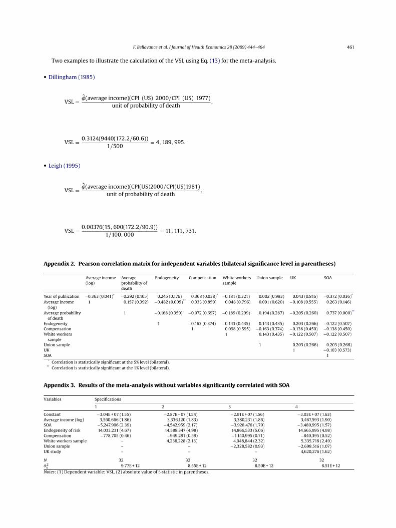
Two examples to illustrate the calculation of the VSL using Eq. (13) for the meta-analysis.

• Dillingham (1985)

VSL = �(average income)(CPI (US) 2000/CPI (US) 1977)unit of probability of death

,

VSL = 0.3124(9440(172.2/60.6))1/500

= 4, 189, 995.

• Leigh (1995)

VSL = �(average income)(CPI(US)2000/CPI(US)1981)unit of probability of death

,

VSL = 0.00376(15, 600(172.2/90.9))1/100, 000

= 11, 111, 731.

Appendix 2. Pearson correlation matrix for independent variables (bilateral significance level in parentheses)

Average income(log)

Averageprobability ofdeath

Endogeneity Compensation White workerssample

Union sample UK SOA

Year of publication −0.363 (0.041)* −0.292 (0.105) 0.245 (0.176) 0.368 (0.038)* −0.181 (0.321) 0.002 (0.993) 0.043 (0.816) −0.372 (0.036)*

Average income(log)

1 0.157 (0.392) −0.482 (0.005)** 0.033 (0.859) 0.048 (0.796) 0.091 (0.620) −0.108 (0.555) 0.263 (0.146)

Average probabilityof death

1 −0.168 (0.359) −0.072 (0.697) −0.189 (0.299) 0.194 (0.287) −0.205 (0.260) 0.737 (0.000)**

Endogeneity 1 −0.163 (0.374) −0.143 (0.435) 0.143 (0.435) 0.203 (0.266) −0.122 (0.507)Compensation 1 0.098 (0.595) −0.163 (0.374) −0.138 (0.450) −0.138 (0.450)White workers

sample1 0.143 (0.435) −0.122 (0.507) −0.122 (0.507)

Union sample 1 0.203 (0.266) 0.203 (0.266)UK 1 −0.103 (0.573)SOA 1

* Correlation is statistically significant at the 5% level (bilateral).** Correlation is statistically significant at the 1% level (bilateral).

Appendix 3. Results of the meta-analysis without variables significantly correlated with SOA


1 2 3 4

Constant −3.04E + 07 (1.55) −2.87E + 07 (1.54) −2.91E + 07 (1.56) −3.03E + 07 (1.63)Average income (log) 3,560,666 (1.86) 3,336,120 (1.83) 3,380,231 (1.86) 3,467,593 (1.90)SOA −5,247,906 (2.39) −4,542,959 (2.17) −3,928,476 (1.79) −3,480,995 (1.57)Endogeneity of risk 14,033,231 (4.67) 14,588,347 (4.98) 14,866,533 (5.06) 14,665,995 (4.98)Compensation −778,705 (0.46) −949,291 (0.59) −1,140,995 (0.71) −840,395 (0.52)White workers sample – 4,238,228 (2.13) 4,948,844 (2.32) 5,335,718 (2.49)Union sample – – −2,328,582 (0.93) −2,698,516 (1.07)UK study – – – 4,620,276 (1.62)

N 32 32 32 32�2

u 9.77E + 12 8.55E + 12 8.50E + 12 8.51E + 12

Notes: (1) Dependent variable: VSL. (2) absolute value of t-statistic in parentheses.

462F.Bellavance

etal./JournalofH

ealthEconom

ics28

(2009)444–464

Appendix 4. Results of the meta-analysis (with standard errors estimated by an indirect procedure for seven studies)


With studies using SOA Without studies using SOA

1 2 3 4 5 6 7 8

Constant −4.06E + 08 (2.16) −4.67E + 08 (2.59) −4.76E + 08 (2.62) −5.53E + 08 (2.99) −5.30E + 08 (2.44) −5.86E + 08 (2.79) −5.83E + 08 (2.76) −6.41E + 08 (2.98)Year of publication 189,187 (2.08) 219,560 (2.51) 223,701 (2.55) 260,520 (2.91) 254,040 (2.40) 281,671 (2.76) 280,236 (2.72) 307,788 (2.94)Average income (log) 3,554,709 (2.13) 3,532,810 (2.23) 3,607,623 (2.27) 3,956,852 (2.49) 3,391,112 (1.80) 3,371,767 (1.88) 3,369,811 (1.89) 3,626,391 (2.03)Average probability of death −620,056 (2.86) −470,189 (2.23) −445,461 (2.04) −343,874 (1.55) −2,073,689 (3.72) −1,809,023 (3.36) −1,801,905 (3.40) −1,629,751 (3.00)Endogeneity of risk 12,936,013 (4.54) 13,472,562 (4.85) 13,576,268 (4.87) 13,204,929 (4.74) 11,622,614 (3.92) 12,125,413 (4.20) 12,172,100 (4.21) 11,936,488 (4.12)Compensation −2,201,799 (1.50) −2,469,896 (1.79) −2,572,852 (1.84) −2,610,875 (1.88) −3,524,430 (2.03) −3,724,861 (2.26) −3,715,599 (2.28) −3,666,063 (2.25)White workers sample – 4,247,376 (2.41) 4,521,541 (2.43) 5,102,759 (2.73) – 3,347,475 (1.78) 3,399,806 (1.72) 3,913,987 (1.95)Union sample – – −980,187 (0.47) −1,409,395 (0.68) – – −158,385 (0.06) −430,322 (0.16)UK study – – – 5,148,482 (1.94) – – – 4,033,856 (1.44)

N 39 39 39 39 35 35 35 35�2

u 7.63E + 12 6.54E + 12 6.57E + 12 6.45E + 12 8.82E + 12 7.59E + 12 7.35E + 12 7.32E + 12Average value of a statistical life (US$ 2000) 5,718,516 (95% C.I.: 4,645,724; 6,791,308) 6,568,461 (95% C.I.: 5,315,621; 7,821,300)


References

Arabsheibani, G.R., Marin, A., 2000. Stability of estimates of the compensation for danger. Journal of Risk and Uncertainty 10 (3), 247–269.Arnould, R.J., Nichols, L.M., 1983. Wage-risk premiums and worker’s compensation: a refinement of estimates of compensating wage differentials. Journal

of Political Economy 91, 332–340.Ashenfelter, O., 2006. Measuring the value of a statistical life: problems and prospects. The Economic Journal 116, C10–C23.Berger, M.C., Gabriel, P.E., 1991. Risk aversion and the earnings of U.S. immigrants and natives. Applied Economics 23, 311–318.Bowland, B.J., Beghin, J.C., 2001. Robust estimates of value of a statistical life for developing economies. Journal of Policy Modeling 23, 385–396.Breyer, F., Felder, S., 2005. Mortality risk and the value of a statistical life: the dead-anyway effect revis(it)ed. The Geneva Risk and Insurance Review 30 (1),

41–56.Brown, C., 1980. Equalizing differences in the labor market. Quarterly Journal of Economics 94 (1), 113–134.Cook, P.J., Graham, D.A., 1977. The demand for insurance and protection: the case of irreplaceable commodities. Quarterly Journal of Economics 91, 143–156.Council of Economic Advisers, 2005. Economic Report of the President. Government Printing Office, Washington, DC.Cousineau, J.-M., Lacroix, R., Girard, A.M., 1992. Occupational hazard and wage compensating differentials. The Review of Economics and Statistics 74,

166–169.Dachraoui, K., Dionne, G., Eeckhoudt, L., Godfroid, P., 2004. Comparative mixed risk aversion: definition and application to self-protection and willingness

to pay. Journal of Risk and Uncertainty 29 (3), 261–276.Day, B., 1999. A Meta-analysis of Wage-risk Estimates of the Value of Statistical Life. Centre for Social and Economic Research on the Global Environment,

University College London, mimeo.De Blaeij, A., Florax, R.J.G.M., Rietveld, P., Verhoef, E., 2003. The value of statistical life in road safety: a meta-analysis. Accident Analysis and Prevention 35,

973–986.Desvousges, W.H., Johnson, F.R., Banzhaf, H.S., Russell, R.R., Fries, E.E., Dietz, K.J., Helms, S.C., 1995. Assessing the Environmental Externality Costs for

Electricity Generation. Triangle Economic Research, Research Triangle Park, NC.Dillingham, A.E., 1985. The influence of risk variable definition on value-of-life estimates. Economic Inquiry 24, 227–294.Dillingham, A.E., Smith, R.S., 1984. Union effects on the valuation of fatal risk. In: Proceedings of the Industrial Relations Research Association 36th Annual

Meeting, San Francisco.Dionne, G., 1982. Moral hazard and state-dependent utility function. Journal of Risk and Insurance 49, 405–422.Dionne, G., Lanoie, P., 2004. Public choice about the value of a statistical life for cost–benefit analyses: the case of road safety. Journal of Transport Economics

and Policy 38 (2), 247–274.Dionne, G., Michaud, P.C., 2002. Statistical analysis of value-of-life estimates using hedonic wage method. Working Paper 02-01. Risk Management Chair,

HEC Montréal.Dorman, P., Hagstrom, P., 1998. Wage compensation for dangerous work revisited. Industrial and Labor Relations Review 52 (1), 116–135.Dorsey, S., Walzer, N., 1983. Workers compensation, job hazards, and wages. Industrial and Labor Relations Review 36, 642–654.Drèze, J., 1962. L’utilité sociale d’une vie humaine. Revue francaise de recherche opérationnelle 1, 93–118.Eeckhoudt, L., Hammitt, J.K., 2004. Does risk aversion increase the value of mortality risk? Journal of Environmental Economics and Management 47, 13–29.Fortin, B., Lanoie, P., 2000. Effects of workers’ compensation: a survey. In: Dionne, G. (Ed.), Handbook of Insurance. Kluwer Academic Publishers, Boston.Garen, J., 1988. Compensating wage differentials and the endogeneity of job riskiness. Review of Economics and Statistics 70, 9–16.Gegax, D., Gerking, S., Schulze, W., 1991. Perceived risk and the marginal value of safety. The Review of Economics and Statistics 73, 589–597.Gunderson, M., Hyatt, D., 2001. Workplace risks and wages: Canadian evidence from alternative models. Canadian Journal of Economics 34 (2), 377–395.Herzog, H.W., Schlottmann, A.M., 1990. Valuing risk in the workplace: market price, willingness to pay, and the optimal provision of safety. Review of

Economics and Statistics, 463–470.Huber, P.J., 1964. Robust estimation of a location parameter. Annals of Mathematical Statistics 35, 73–101.Jones-Lee, M.W., 1976. The Value of a Statistical Life: An Economic Analysis. University of Chicago Press, Chicago.Kim, S.-W., Fishback, P.V., 1999. The impact of institutional change on compensating wage differentials for accident risk: South Korea, 1984–1990. Journal

of Risk and Uncertainty 18, 231–248.Kniesner, T.J., Leeth, J.D., 1991. Compensating wage differentials for fatal injury risk in Australia, Japan and the United States. Journal of Risk and Uncertainty

4 (1), 75–90.Kniesner, T.J., Viscusi, W.K., 2005. Value of a statistical life: relative position vs. relative age, Harvard Law and Economics. Discussion Paper No 502.Kniesner, T.J., Viscusi, W.K., Wook, C., Ziliak, J.P., 2007. Pinning down the value of statistical life. Working Paper IZA No. 3107, 32 pp.Lanoie, P., Pedro, C., Latour, R., 1995. The value of a statistical life: a comparison of two approaches. Journal of Risk and Uncertainty 10, 235–257.Leeth, J.D., Ruser, J., 2003. Compensating wage differentials for fatal and nonfatal injury risk by gender and race. Journal of Risk and Uncertainty 27 (3),

257–277.Leigh, J.P., 1987. Gender, firm size, industry and estimates of the value-of-life. Journal of Health Economics 6 (3), 255–273.Leigh, J.P., 1991. No evidence of compensating wages for occupational fatalities. Industrial Relations 30 (3), 382–395.Leigh, J.P., 1995. Compensating wages, value of a statistical life, and inter-industry differentials. Journal of Environmental Economics and Management 28,

83–97.Leigh, J.P., Folsom, R.N., 1984. Estimates of the value of accident avoidance at the job depend on the concavity of the equalizing differences curve. Quarterly

Review of Economics and Business 24 (1), 56–66.Leigh, J.P., Markovitz, S.B., Fahs, N., Shin, C., Landrigan, P.J., 1997. Occupational injury and illness in the United States. Estimation of costs, morbidity, and

mortality. Archives of Internal Medicine, 157.Liu, J.T., Hammitt, J.K., Liu, J.L., 1997. Estimated hedonic wage function and value of a statistical life in a developing country. Economics Letters 57 (3),

353–358.Lott, J., Manning, R., 2000. Have changing liability rules compensated workers twice for occupational hazards? Earnings premiums and cancer risks. Journal

of Legal Studies 29, 99–130.Low, S.A., McPheters, L.R., 1983. Wage differentials and risk of death: an empirical analysis. Economic Inquiry 21 (2), 271–280.Marin, A., Psacharopoulos, G., 1982. The reward for risk in the labor market: evidence from the United Kingdom and a reconciliation with other studies.

Journal of Political Economy 90, 827–853.Martinello, F., Meng, R., 1992. Workplace risks and the value of hazard avoidance. Canadian Journal of Economics 25 (2), 333–345.Melinek, S.J., 1974. A method of evaluating human life for economic purposes. Accident Analysis and Prevention 6, 103–114.Meng, R., 1989. Compensating differences in the Canadian labor market. Canadian Journal of Economics 22, 413–424.Meng, R., Smith, D.A., 1990. The valuation of risk of death in public sector decision-making. Canadian Public Policy 16, 137–144.Meng, R., Smith, D.A., 1999. The impact of workers’ compensation on wage premiums for job hazards in Canada. Applied Economics 31, 1101–1108.Michaud, P.-C., 2001. Évaluation des bénéfices et choix des projets impliquant la sauvegarde de vies humaines. Mémoire présenté en vue de l’obtention du

grade de maître ès sciences, HEC Montréal.Miller, P., Mulvey, C., Norris, K., 1997. Compensating differentials for risk of death in Australia. Economic Record 73, 363–372.Miller, T.R., 2000. Variations between countries in values of statistical life. Journal of Transport Economics and Policy 34 (2), 169–188.Mishan, E.J., 1971. Evaluation of life and limb: a theoretical approach. Journal of Political Economy 79, 687–705.Moore, M., Viscusi, W.K., 1988a. Doubling the estimated value of a statistical life: results using new occupational fatality data. Journal of Policy Analysis and

Management 7, 476–490.


Moore, M., Viscusi, W.K., 1988b. The quantity-adjusted value of a statistical life. Economic Inquiry 26 (3), 369–388.Moore, M., Viscusi, W.K., 1989. Rates of time preference and valuations of the duration of life. Journal of Public Economics 38 (3), 297–317.Moore, M., Viscusi, W.K., 1990a. Discounting environmental health risks: new evidence and policy implications. Journal of Environmental Economics and

Management 18, 51–62.Moore, M., Viscusi, W.K., 1990b. Models for estimating discount rates for long-term health risks using labor market data. Journal of Risk and Uncertainty 3,

381–401.Mrozek, J.R., Taylor, L.O., 2002. What determines the value of a statistical life? A meta-analysis. Journal of Policy Analysis and Management 21 (2), 253–270.Needleman, L., 1980. The valuation of changes in the risk of death by those at risk. Manchester School of Economics and Social Studies 48 (3), 229–254.Olson, C.A., 1981. An analysis of wage differentials received by workers on dangerous jobs. Journal of Human Resources 16, 167–185.Raudenbush, S.W., 1994. Random effects models. In: Cooper, H., Hedges, L.V. (Eds.), The Handbook of Research Synthesis. Russel Sage Foundation, New York.Root, N., Sebastian, D., 1981. BLS develops measure of job risk by occupation. Monthly Labor Review 106, 26–30.Sandy, R., Elliott, R.F., 1996. Unions and risk: their impact on the compensation for fatal risk. Economica 63 (250), 291–309.Sandy, R., Elliott, R.F., Siebert, W.S., Wie, X., 2001. Measurement error and the effects of unions on the compensating differentials for fatal workplace risks.

Journal of Risk and Uncertainty 23 (1), 33–56.Shanmugam, K.R., 2001. Self selection bias in the estimates of compensating differentials for job risks in India. Journal of Risk and Uncertainty 22 (3),

263–275.Schelling, T.C., 1968. The life you save may be your own. In: Chase, S. (Ed.), Problems in Public Expenditure Analysis. Brookings Institution, Washington.Siebert, W.S., Wei, X., 1994. Compensating wage differentials for workplace accidents: evidence for union and nonunion workers in the UK. Journal of Risk

and Uncertainty 9, 61–76.Smith, R.S., 1974. The feasibility of an “Injury Tax” approach to occupational safety. Law and Contemporary Problems 38, 730–744.Smith, V.K., Desvousges, W.H., 1987. An empirical analysis of the economic value of risk changes. Journal of Political Economy 95, 89–114.Summers, R., Heston, A., 1991. The Penn World Table (Mark 5): an expanded set of international comparisons, 1950–1988. Quarterly Journal of Economics

106, 327–368.Thaler, R., Rosen, S., 1975. The value of saving a life: evidence from the labor market. In: Terleckyj, N. (Ed.), Household Production and Consumption. NBER

Press/Columbia University.Viscusi, W.K., 1978. Labor market valuations of life and limb: empirical evidence and policy implications. Public Policy 26, 359–386.Viscusi, W.K., 1993. The value of risks to life and health. Journal of Economic Literature 31, 1912–1946.Viscusi, W.K., 2003. Racial differences in labor market values of a statistical life. Journal of Risk and Uncertainty 27 (3), 239–256.Viscusi, W.K., 2004. The value of a statistical life: estimates with risks by occupation and industry. Economic Inquiry 42 (1), 29–48.Viscusi, W.K., 2005. The value of a statistical life. Discussion Paper No. 517. Harvard Law School, Cambridge.Viscusi, W.K., Aldy, J.E., 2003. The value of a statistical life: a critical review of market estimates throughout the world. Journal of Risk and Uncertainty 27,

5–76.Weinstein, M.C., Shepard, D.S., Pliskin, J.S., 1980. The economic value of changing mortality probabilities: a decision-theoretic approach. The Quarterly

Journal of Economics 94, 373–396.Weiss, P., Maier, G., Gerking, S., 1986. The economic evaluation of job safety: a methodological survey and some estimates for Austria. Empirica 13 (1), 53–67.

journal of health economics - faculty of medicine, mcgill ...€¦ · journal of health economics...

Documents