journal of computational and applied mathematics · elsevier journal of computational and applied...

ELSEVIER Journal of Computational and Applied Mathematics 68 (1996) 221-238

JOURNAL OF COMPUTATIONAL AND APPLIED MATHEMATICS

Finite analogues of Euclidean space

A. Medrano, P. Myers, H.M. Stark, A. Terras* Mathematics Department, University of California at San Diego, La Jolla, CA 92093-0112, USA

Received 30 October 1994; revised 10 August 1995

Abstract

Graphs are attached to ~:q, where DZq is the field with q elements, q odd, using an analogue of the Euclidean distance. The graphs are shown to be asymptotically Ramanujan for large q (better than Ramanujan in half the cases). Comparisons are made with finite upper half planes constructed in a similar way using an analogue of Poincar6's non-Euclidean distance. The eigenvalues of the adjacency operators of the finite Euclidean graphs are shown to be Kloosterman sums.

Keywords." Finite symmetric space; Ramanujan graph; Kloosterman sum

AMS classification." primary 11T99; 05C25; secondary 11T23; 20H30

I. Introduction

Here we study the simplest finite symmetric space, namely, the finite Euclidean space DZq over the finite field 0Zq with q = ps elements using a finite analogue of the usual Euclidean distance. The study of finite symmetric spaces G/K has been carried out by many authors, using the methods of group representations and association schemes (see [7, 8,21, 37, 38]). Here we have chosen to use only the abelian group 0:~ rather than the non-abelian group G of isometrics in order to keep the discussion elementary. This was also possible for ordinary Euclidean space over the real number field (see [39, Ch. 1]). To see the connection of q-analogues of special functions with finite symmetric spaces G/K associated to finite groups G, see Askey's preface and Stanton's article in [6].

The tools needed in the present paper are very well known. For example, we require only standard properties of the characters of the abelian group U:~ to obtain the necessary formulas for the eigenvalues of our Euclidean graphs. The eigenvalues turn out to be the well-known exponential sums called Kloosterman sums (see Eq. (10)). We will also need Weil's estimate for the Kloosterman

* Corresponding author. E-mail: [email protected].

0377-0427/96/$15.00 © 1996 Elsevier Science B.V. All rights reserved SSDI 0377-0427(95 )00261-8

222 A. Medrano et aL /Journal of Computational and Applied Mathematics 68 (1996) 221-238

sums (to be found in [42, pp. 386-389]). See Schmidt [34] for a more elementary approach. And we will be interested in the results on these sums to be found in [18] and [19].

Kloosterman sums provide another connection with q-series, since they are Fourier coefficients of the modular forms known as Poincar6 series (see [33, Ch. 1]). They have been used by many authors to estimate the Fourier coefficients of modular forms (see [35, pp. 506-520]) in a quest to prove the Ramanujan conjecture bounding the Fourier coefficients of holomorphic modular forms such as the discriminant function A. Ultimately, Deligne proved this conjecture using algebraic geometric methods (see [13]).

One of the objects of this paper is to compare our finite Euclidean spaces and graphs with the non-Euclidean analogues studied in [3, 4, 12, 40]. Recall that the Poincard upper half plane is

H={z=x+iy Ix, yEN, y > O }

with the non-Euclidean distance

d x 2 -~- d y 2 d s 2 -

y2

The finite upper half plane Hq is constructed by replacing N with the finite field ~q and y > 0 with y ~ 0. The non-Euclidean distance is replaced with an analogue on Hq having values in the finite field. Then we obtain graphs by connecting points at a fixed "distance" from one another.

Part of the motivation is to find new examples of Ramanujan 9raphs (as defined in [26]). A connected k-regular graph is Ramanujan if for every eigenvalue 2 of the adjacency matrix with ]21 ¢ k, we have

12[ ~< 2v/k - - 1.

Ramanujan graphs are of interest, for example, in the construction of communications networks because they have good expansion properties (see [25]). The Ramanujan conjecture was used to show that the graphs in [26] were Ramanujan. Thus the name of Ramanujan was given to these graphs. The proof that the non-Euclidean graphs in [3, 4, 12, 40] are Ramanujan requires an estimate of certain exponential sums of Soto-Andrade [37] - - an estimate which was made first by Katz [20] and then by Winnie Li [24], the latter using a more elementary method.

Aside from the discovery of new Ramanujan graphs, this paper is part of an attempt to find finite models for the symmetric spaces discussed in [39]. This has been of interest to physicists for some time (see e.g. [29]).

An outline of the paper follows. Let ~q be a finite field with q - - p r elements, for p a prime, p7~2. We define a distance d (x, y) = t ( x -y ) . (x -y ) for column vectors x, y E ~:~ with tx = transpose of x. Then the Euclidean graph Eq (n,a) associated to D:~ has as vertices the elements of 0:~. Two vertices x, y E [F~ are joined by an edge if d (x, y) = a.

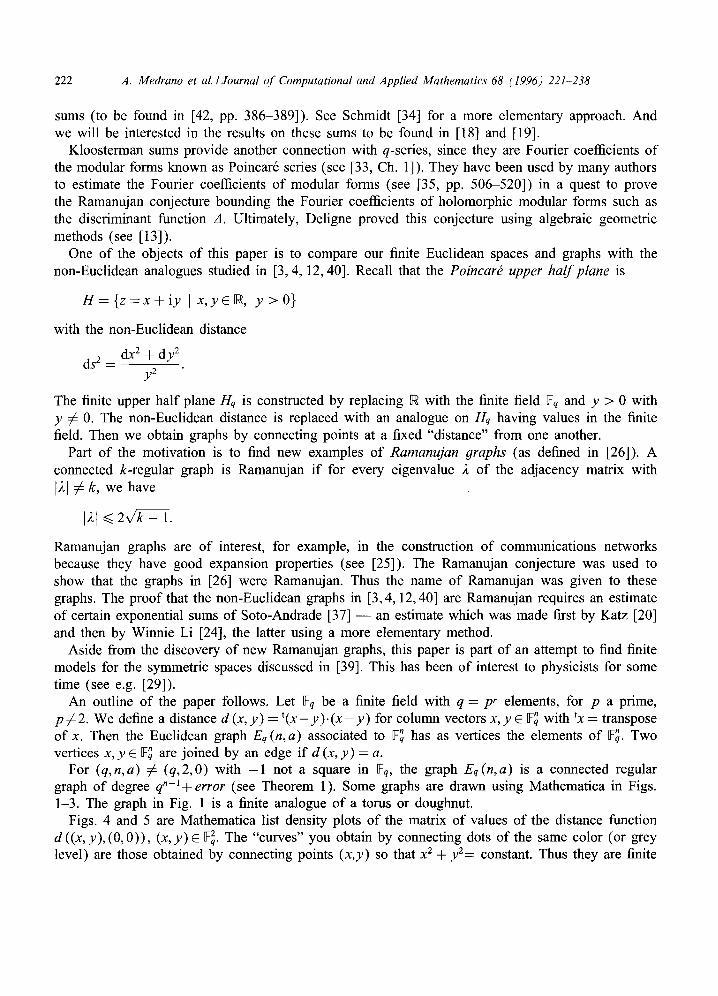
For (q,n,a) 7 ~ (q,2,0) with - 1 not a square in DZq, the graph Eq(n,a) is a connected regular graph of degree qn-~+error (see Theorem 1). Some graphs are drawn using Mathematica in Figs. 1-3. The graph in Fig. 1 is a finite analogue of a torus or doughnut.

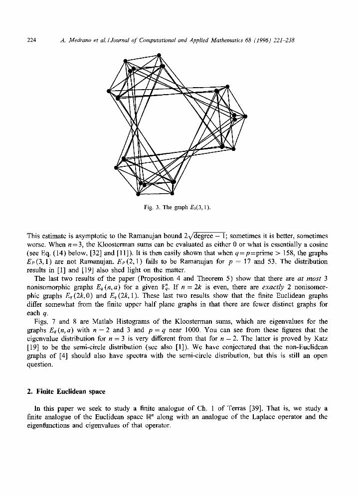
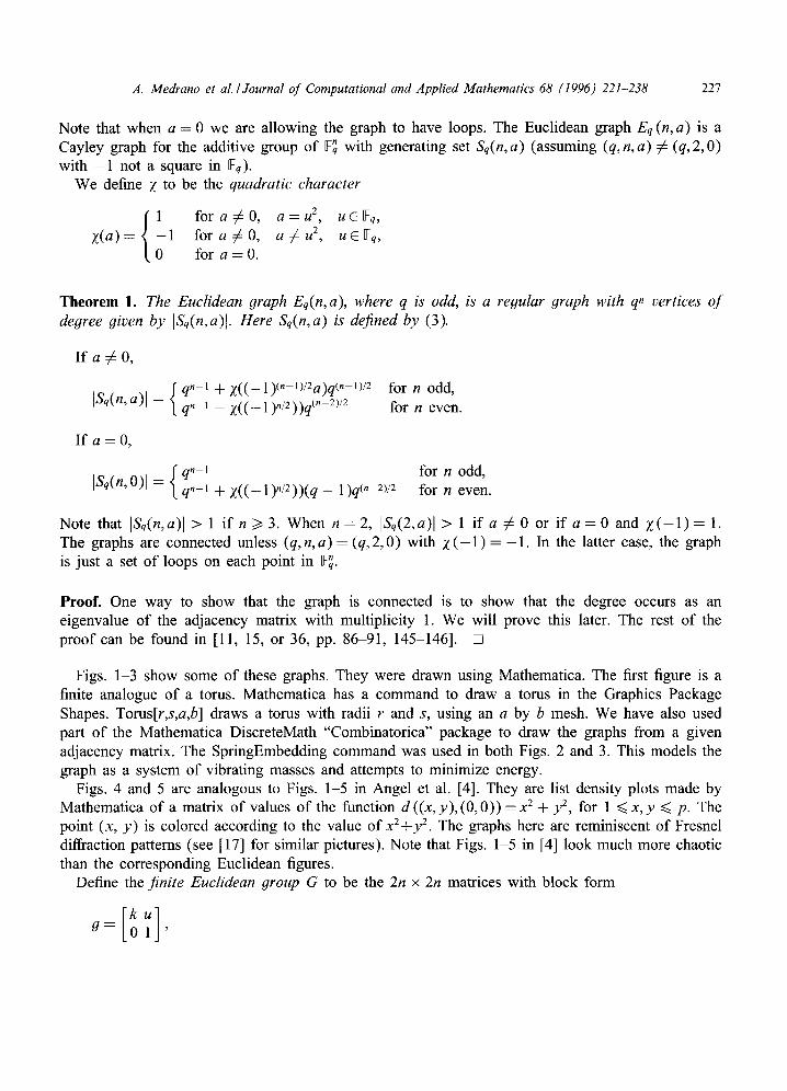
Figs. 4 and 5 are Mathematica list density plots of the matrix of values of the distance function d ((x, y), (0, 0)), (x, y) C 1:2. The "curves" you obtain by connecting dots of the same color (or grey level) are those obtained by connecting points (x,y) so that x 2 + y2= constant. Thus they are finite

A. Medrano et al./ Journal of Computational and Applied Mathematics 68 (1996) 221-238 223

Fig. 1. The graph E5(2, 1), a finite torus.

Fig. 2. The graph E7(2, 1).

analogues of circles. The pictures are most beautiful in color, and should be compared with those produced for the finite analogue of the Poincar6 distance in [4]. The latter graphs are much more chaotic. The Euclidean list density plots look like Fresnel diffraction patterns (see [17]). These list density plots can be considered to give finite analogues of the level curves of the eigenfunctions of the Laplacian in the real plane R 2. See the cover of Powers [31] which shows a vibrating drum covered with dust. The dust forms circles which are nodal lines for the eigenfunctions of the Laplacian. This is another way to see that the curves of constant color in Figs. 4 and 5 are finite analogues of circles.

If 2 is an eigenvalue of the adjacency operator of Eq (n, a) with 2 ¢ degree of the graph, then 2 is a Kloosterman sum as in Eq. (10). Thus by Weil's estimate of these sums (see [42, pp. 386-389])

121 ~ 2q (n-1)/2.

224 A. Medrano et al./ Journal of Computational and Applied Mathematics 68 (1996) 221-238

Fig. 3. The graph E3(3, 1).

This estimate is asymptotic to the Ramanujan bound 2x/degree - 1; sometimes it is better, sometimes worse. When n=3 , the Kloosterman sums can be evaluated as either 0 or what is essentially a cosine (see Eq. (14) below, [32] and [11]). It is then easily shown that when q = p = p r i m e > 158, the graphs Ep(3 ,1) are not Ramanujan. Ep(2 ,1) fails to be Ramanujan for p = 17 and 53. The distribution results in [1] and [19] also shed light on the matter.

The last two results of the paper (Proposition 4 and Theorem 5) show that there are at most 3 nonisomorphic graphs Eq(n,a) for a given ~:~. If n = 2k is even, there are exactly 2 nonisomorphic graphs Eq (2k,0) and Eq (2k, 1). These last two results show that the finite Euclidean graphs differ somewhat from the finite upper half plane graphs in that there are fewer distinct graphs for each q.

Figs. 7 and 8 are Matlab Histograms of the Kloosterman sums, which are eigenvalues for the graphs Eq(n,a) with n = 2 and 3 and p = q near 1000. You can see from these figures that the eigenvalue distribution for n = 3 is very different from that for n = 2. The latter is proved by Katz [19] to be the semi-circle distribution (see also [1]). We have conjectured that the non-Euclidean graphs of [4] should also have spectra with the semi-circle distribution, but this is still an open question.

2. Finite Euclidean space

In this paper we seek to study a finite analogue of Ch. 1 of Terras [39]. That is, we study a finite analogue of the Euclidean space •n along with an analogue of the Laplace operator and the eigenfunctions and eigenvalues of that operator.


60

50

40

30

20

i0

0

0 i0 20 30 40 50 60

Fig. 4. List density plot in Mathematica for p = 67 with point (x,y) in a 67×67 grid given a color determined by x 2 + y2 ( m o d 67).

Let UZq be a finite field with q = pr elements, where p is an odd prime. Then the finite analogue of the Euclidean n-space is defined to be

~2q-- X X = , X j E ~ 2 q ' (1 )

n

We define the distance between two column vectors x and y in Uz~ by n

d(x, y ) = ~-~(xj - yj)2 = t(x _ y ) (x - y) . (2) j= l

This distance is not a metric in the sense o f analysis since it is not real-valued, but it is a metric in the sense o f algebra (see [24, p. 356]). It has values in ~q and it is point-pair invariant

d ( x + u , y + u ) = d ( x , y ) , V x , y, uEgCq.

226 A. Medrano et al./Journal of Computational and Applied Mathematics 68 (1996) 221-238

120

I00

80

60

40

20

o 0 20 40 60 80 100 120

Fig. 5. List density plot in Mathematica for p = 127 with point (x,y) in a 127× 127 grid given a color determined by x 2 + y2 (mod 127).

It is also invariant under all the elements of the orthogonal group

0(11, ~q)= {g E aL(n, ~q) [ g preserves the quadratic form x~ + - . . + x ] } .

That is,

g E O(n, g:q) ¢==~ t g . g = I.

Definition. Given a E 0Zq, the Euclidean graph associated to I:~ is Eq(n,a). The vertices o f the graph are the points in F~. Two vertices are adjacent iff d(x, y ) = a. Note that this is a Cayley graph for the additive group of Uz~.

A Cayley graph for a group G and a symmetric set of generators S has as vertices the elements o f G and edges between vertices x and y = x • s, s E S. The set S is symmetr ic i f s E S implies s -1 ES.

Let

Sq(n,a) = {xE Qz~ ] d(x,O) = a } . (3)


Note that when a = 0 we are allowing the graph to have loops. The Euclidean graph Eq (n,a) is a Cayley graph for the additive group of Yq with generating set Sq(n, a) (assuming (q, n, a) ~ (q, 2, 0) with - 1 not a square in •q).

We define Z to be the quadratic character

1 f o r a ¢ 0 , a = u 2, uC~:q, z ( a ) = - 1 f o r a ¢ 0 , a C u 2, uCg:q,

0 for a = 0 .

Theorem 1. The Euclidean graph Eq(n,a), where q & odd, is a regular graph with qn vertices of degree given by ]Sq(n,a)l. Here Sq(n,a) is defined by (3).

I f a ¢ 0 ,

{ q,-i + Z((_l)(,-1)/2a)q(n-1)/2 for n odd, ISq(n,a)l = qn-i _ g((_l),/2))q~,-2)/2 for n even.

If a = 0,

{q n-i for n odd, [Sq(n,O)[ = q,-1 + X((_ l ) , / 2 ) ) (q_ 1)q(n-2)/2 for n even.

Note that [Sq(n,a)[ > 1 if n/> 3. When n = 2, [Sq(2,a)[ > 1 if a ¢ 0 or if a = 0 and Z ( - 1 ) = 1. The graphs are connected unless (q,n,a)= (q,2,0) with ~ ( - 1 ) = -1 . In the latter case, the graph is just a set of loops on each point in F~.

Proof. One way to show that the graph is connected is to show that the degree occurs as an eigenvalue of the adjacency matrix with multiplicity 1. We will prove this later. The rest of the proof can be found in [11, 15, or 36, pp. 86-91, 145-146]. []

Figs. 1-3 show some of these graphs. They were drawn using Mathematica. The first figure is a finite analogue of a toms. Mathematica has a command to draw a toms in the Graphics Package Shapes. Toms[r,s,a,b] draws a torus with radii r and s, using an a by b mesh. We have also used part of the Mathematica DiscreteMath "Combinatorica" package to draw the graphs from a given adjacency matrix. The SpringEmbedding command was used in both Figs. 2 and 3. This models the graph as a system of vibrating masses and attempts to minimize energy.

Figs. 4 and 5 are analogous to Figs. 1-5 in Angel et al. [4]. They are list density plots made by Mathematica of a matrix of values of the function d ((x, y), (0, 0)) = x 2 + y2, for 1 ~< x, y ~< p. The point (x, y) is colored according to the value of xZ+y 2. The graphs here are reminiscent of Fresnel diffraction patterns (see [17] for similar pictures). Note that Figs. 1-5 in [4] look much more chaotic than the corresponding Euclidean figures.

Define the finite Euclidean group G to be the 2n x 2n matrices with block form

u] 9 = 1 '


where kEO(n,~-q) , u is an n x 1 matrix, 0 is a 1 × n matrix of 0's. Then g acts on xE~:~ by

1 "

Note that this is a group action: 9(9 ' x )= (99')x, Ix = x, where I is the identity matrix. This action preserves the distance defined by formula (2).

Now define K to be the subgroup of G consisting of matrices of the form

Then,

C t K ~ o

The space G/K ~- ~ is a symmetric space since we have a commutative algebra L 2 ([F~) of functions f : F~ ~ C with multiplication defined by convolution

( f * g ) ( x ) = ~ f ( y ) 9 ( x - y). (4) y E ~~

Rudvalis notes that if v and w are nonzero elements of Sq (n,a), the set defined by formula (3), then there is an element k E K so that kv = w. Here we use Witt's theorem (see [22]). Thus the K-orbits of points in Dz~ - {0} are the sets Sq (n, a) with 0 removed, if necessary. We must remove 0 since if a = 0, we have K . 0 = {0}, but ]Sq (n,0)] = q,-1, for n odd, and q,-1 + error, for n even, by Theorem 1. Only when ( q , n , a ) = (q,2,0) with Z ( - 1 ) = - 1 does Sq(2 ,0)= {0}.

2.1. Remarks on other 9raphs one can view as finite analogues o f Euclidean space

(a) Grids and connections with Riemann surface theory. (Motivated by finite difference approxi- mations to the Laplace operator.)

Consider a p x p square with lower left vertex at the origin. Identify the vertical sides and the horizontal sides to get a toms ~2/(p7/)2. This can be identified with a union of translates of the unit square with sides identified

~2/(p7/)2 = L.J (~2/7/2 + a) •

aE(Z/pZ) 2

Obtain a graph from this grid by considering the vertices to be the unit squares in the grid (which can be thought of as the a E (7//p7/)2). Call 2 vertices adjacent if the unit squares have a side in common. In Fig. 6 we show the case p = 11, with the adjacent squares to the black square shaded grey.

This construction also gives a Cayley graph for •2. The set of generators is {(+1,0) ,(0, 4-1)). Fig. 1 shows the graph E5(2, 1). In this case, the graph from the grid is the same as that from our Euclidean "distance". The same thing happens for E3(2, 1).

One can do a similar Cayley graph for ~ with 9eneratin9 set

Sq c = {±ej ] j = 1,...,n}.

A. Medrano et al./Journal of Computational and Applied Mathematics 68 (1996) 221-238 229

11 II II , I I I I I I

I I I I II I I I 1 ~ 1 I I I I I I

I I II I I , , I I I I I , J

0 "

I I I I I I I I I I l,II~ I I I I I I I I I I

11

Fig. 6. A grid from which a graph can be created with vertices the 121 squares and edges between adjoining squares; for example, the black square is adjacent to the grey ones adjoining it.

Here ej is the vector with 0 everywhere except in the j th place, where there is a 1. Thus,

Isgl = 2n,

(b) Hamming distance in coding theory. From coding theory, we have the Hamming distance: For a, b C D:~, set

d I4 (a, b) = # {i I ai # bi}.

Set

Sq u = {a [ d(a ,O) = 1} DSq G,

[SqHI = n ( q - - 1 ) .

Again we can construct a Cayley graph using S H as a set of generators. Call this graph a Hamming graph. Only in the case q = 3 do we have S~ = S H.

The Hamming graphs have been much studied thanks to their importance for coding theory. The associated spherical functions are Krawtchouk polynomials (see [8, 14, 38], as well as Stanton's article in [6], and [41]).

(c) Finite Euclidean graphs. Our generating set Sq(n, 1 ) is usually a much larger set of generators than S G or S H - - e x c e p t

when n = 2. Then we find

]Sq (2, 1)l = q - Z ( - 1 ) .

This will be smaller than ]S~] = 2 ( q - 1) for q > 3. I f q = 3, we get 3 - Z ( - 1 ) = 3 + 1 = 4 and $ 3 ( 2 , 1 ) = S c = S H. But, if n / > 3 ,

q, - i + Z((_l)(,-1)/2)q(,-1)/2 for n odd, ISq(n, 1)l = q , - i + Z((_l)n/Z)q(n-2)/2 for n even,

and

q , - 1 >~ n (q - 1 ) + q(n- ~)/2 .~ n(q - 1) ,,. q(n- 1 )/2 ~ + l , q(n- 1 )/2

for all q /> 3, n >~ 3. Note that Sq (n, 1 ) D Sq G, since 12 = 1. Thus, Sq (n, 1 ) generates ~ .


3. Spectrum of adjacency operators

We want to study the spectrum of the adjacency operator A acting on f • F~ + C via

A = A a f ( X ) = Z f ( Y ) " (5) d(x,y )=a

The combinatorial Laplacian is Aa = Aa - kI if k is the degree of the graph and I is the identity operator; i.e. 19 = g. So A~ has the same eigenfunctions as A~, for all a E Fq.

Since our group F~ is abelian, it is easy to find simultaneous eigenfunctions of Aa for all a E Fq. We will use the notation

e(u) = exp {2rciTr(u)/p} .

Here, Tr(u)=Trace~/~, (u) = u + u p + .. • + u p~-~ if q = ps and u E ~Zq. For each b c U:~, define

eb (x) = e(tb • x) for x C Fq. (6)

The following result is very old. Any book on applications of group representations contains some version of it as well as many number theory books (e.g., [10, p. 421]). Many papers on Ramanujan graphs have used it as well (see e.g., [23]).

Proposition 2. For b E ~:~, eb is an eigenfunction o f Aa corresponding to the eigenvalue

d(s,O)=a

Moreover, as b runs through F~ we obtain a complete orthonormal set o f eigenfunctions o f A. Thus, every eigenvalue o f A has the form }~b for some b C ~ . The inner product on f , g EL 2 (~:~) is

( f , g) = ~ f ( x ) g (x).

Proof . Note that

Aeb(x) = ~ e 6 ( y ) = ~ e b ( s + x ) d(x,y)=a y=s+x,d(s,O)=a

The rest comes from standard facts about Fourier analysis on D:~ (see [14, 41]). []

Our next problem is to estimate the eigenvalues "~b, b C Dry. Note that by Theorem 1, the bound given in Theorem 3 is asymptotic to the Ramanujan bound 2x/[S q (n,a)[ - 1 as q ~ exp. Sometimes this bound is as good as or better than the Ramanujan bound (when the error in Theorem 1 is positive), and sometimes it is worse. It is possible for the graphs to be non-Ramanujan (e.g., Ep(3, 1 )

A. Medrano et at/Journal of Computational and Applied Mathematics 68 (1996) 221-238 231

for p sufficiently large, as we will see later). After writing this paper, we found part of the proof of the following Theorem in [11]. We will thus give only a sketch of that part of the proof.

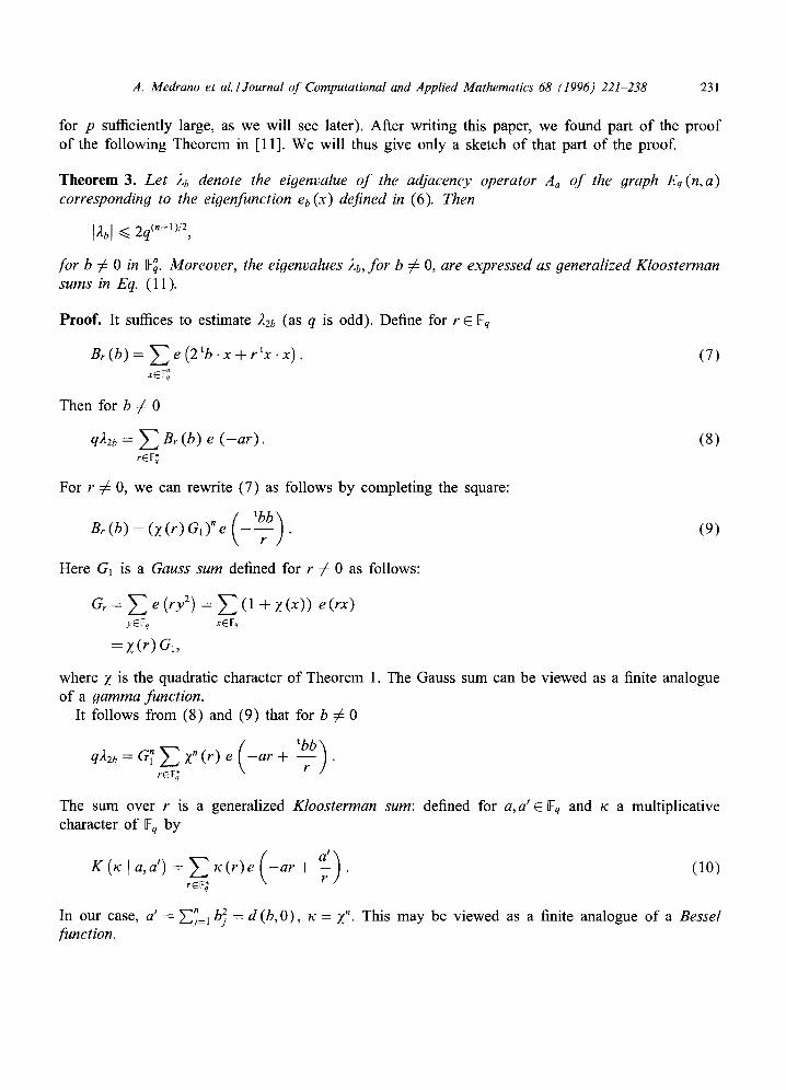
Theorem 3. Let 2b denote the eigenvalue of the adjacency operator Aa o f the graph Eq(n,a) corresponding to the eigenfunction eb (X) defined in (6). Then

12b[ ~< 2q(,-1)/2

for b # 0 in g:~. Moreover, the eigenvalues ,~b, for b ~ 0, are expressed as generalized Kloosterman sums in Eq. (1 1 ).

Proofi It suffices to estimate /~2b (as q is odd). Define for r E ~q

Br(b) = ~ e (2 t b ' x q- Ftx • x ) . (7) x E Y,~

Then for b ¢ 0

q22b = ~ Br (b) e ( -a r ) . (8) rEF~

For r ¢ 0, we can rewrite (7) as follows by completing the square:

Br(b )=(z ( r )G1)"e ( - ~ ) . (9)

Here G1 is a Gauss sum defined for r ¢ 0 as follows:

G~ = ~ e (ry 2) = ~ ( 1 + Z(x)) e( rx) yE~-q xEff-q

= Z (r) Ga,

where Z is the quadratic character of Theorem 1. The Gauss sum can be viewed as a finite analogue of a gamma function.

It follows from (8) and (9) that for b ¢ 0

( t b b ) q22b = G~ ~ Z" (r) e - a r +

rEy;

The sum over r is a generalized Kloosterman sum: defined for a,a'E ~-q and t c a multiplicative character of UZq by

K (x , a,a') = ~-~ tc(r)e ( - a r + ~ ) . (10) r6G"

In our case, a' = ~ = ~ b~ = d (b, 0), tc = Z n. This may be viewed as a finite analogue of a Bessel function.


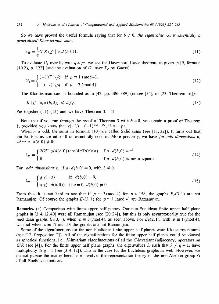
So we have proved the useful formula saying that for b ~ O, the eigenvalue ~2b is essentially a generalized Kloosterman sum:

! 22b = "-G~K ()~" l a, d(b,O)). (11)

q

To evaluate G1 over ~q with q = ps, we use the Davenport-Hasse theorem, as given in [9, formula (10.2), p. 122] (and the evaluation of G1 over DZp by Gauss).

f (-1)s-1 v ~ if p - 1 (mod4) , G1

- ( - i ) s v ~ i f p - 3 ( m o d 4 ) . (12)

The Kloosterman sum is bounded as in [42, pp. 386-389] (or see [34], or [23, Theorem 16]):

IK (z" [ a,d(b,O))l 2x/ . (13)

Put together (11 )--(13) and we have Theorem 3. []

Note that if you run through the proof of Theorem 3 with b = 0, you obtain a proof of Theorem 1, provided you know that Z ( - 1 ) = ( - 1 ) '(p-1)/2, if q = p,.

When n is odd, the sums in formula (10) are called Sali6 sums (see [11, 32]). It turns out that the Sali6 sums are either 0 or essentially cosines. More precisely, we have for odd dimensions n, when a. d(b, 0) ¢ 0:

{ 2G~-lz(d(b,O))cos(4rcTr(c)/p) if a. d(b,O) = c 2, 22b = (14)

0 if a. d(b,O) is not a square.

For odd dimensions n, if a. d(b, 0) = 0, with b 7~ 0,

22b = ~ q z ( - a ) if d(b,O) = O, (15) t q )~(-d(b,O)) if a = 0, d(b,O) 7~ O.

From this, it is not hard to see that if p -- 3 (mod4) for p > 158, the graphs Ep(3,1) are not Ramanujan. Of course the graphs Ep(3, 1) for p =- 1 (mod 4) are Ramanujan.

Remarks. (a) Comparison with finite upper half planes. Our non-Euclidean finite upper half plane graphs in [3, 4, 12, 40] were all Ramanujan (see [20, 24]), but this is only asymptotically true for the Euclidean graphs Ep(3, 1 ), when p - 3 (mod 4), as seen above. For Ep(2, 1), with p -- 1 (mod 4), we find when p = 17 and 53 the graphs are not Ramanujan.

Some of the eigenfunctions for the non-Euclidean finite upper half planes were Kloosterman sums (see [12, Proposition 2]). All of the eigenfunctions for the finite upper half planes could be viewed as spherical functions; i.e., K-invariant eigenfunctions of all the G-invariant (adjacency) operators on G/K (see [4]). For the finite upper half plane graphs, the eigenvalues 2, such that 2 ~ q + 1, have multiplicity /> q - 1 (see [3,4, 12]). This is the case for the Euclidean graphs as well. However, we do not pursue the matter here, as it involves the representation theory of the non-Abelian group G of all Euclidean motions.

A. Medrano et al./Journal of Computational and Applied Mathematics 68 (1996) 221-238

Table 1 Eigenvalues of finite Euclidean graphs Eq (2,a) (all graphs tabulated are Ramanujan when connected)

(n, p, a) Eigenvalue Multiplicity

(2,3,0) (not connected) 1 9

(2,3,a), a ¢ 0 - 2 4 1 4 4 1

(2,5,0) - 1 16 4 8 9 1

(2,5,a), a ¢ 0 -3.2361 4 - 1 8

0.3820 4 1.2361 4 2.6180 4 4 1

(2,7,0) (not connected) 1 49

(2,7,a), a ¢ 0 -4 .4940 8 -2 .0489 8 -1 .1099 8

1.6039 8 2.3569 8 2.6920 8 8 1

233

For the finite upper half plane graphs, eigenvalues are also eigenfunctions (see [4, Theorem 1, Part 3]). This is also the case for our finite Euclidean graphs. By Proposition 2, 2b is a sum over s of eb (S)= es (b) and es (b) is an eigenfunction of the adjacency operator.

Formula (11) says that when b e 0 , •2b is a function of d(b,O) only. Thus, 2b, b e 0 , is a "radial" eigenfunction of the adjacency operator Aa, if we view d (b, 0) as a radial coordinate. This is what happened for the finite upper half plane graphs also.

It follows that the eigenvalues 2b, b ¢ 0, of Aa, can have at most q distinct values, each with multiplicity given by I Sq (n, d (n, O))l = q,-1 + error. See Theorem 1 for the formula. Thus, the spectrum of a graph Eq(n,a) has at most q + 1 points, each eigenvalue 2b, b ~ 0, having high multiplicity. See Tables 1 and 2 for eigenvalues and their multiplicities for some small graphs.

Figs. 7 and 8 (created using Matlab) show the distribution of the Kloosterman sums giving the eigenvalues 2b, b ¢ 0, for the graphs El021 (2, 1) and E1019 (3, 1). The two distributions look very different. For n = 2, Katz [20] shows that, as p goes to infinity, the distribution of Kloosterman sums approaches the Wigner semi-circle distribution (alias the Sato-Yate distribution) (see also [1]). This is the limiting distribution of the spectrum of a large random graph according to McKay [27]. And we conjecture that the spectrum of the finite non-Euclidean upper half plane graphs approach the semi-circle distribution in [4]. But this question is still open.

(b) Comparison with Euclidean spaces over ~ and Kloosterman sums as finite Bessel functions

234 A. Medrano et aL /Journal of Computational and Applied Mathematics 68 (1996) 22!-238

Table 2 Eigenvalues of finite Euclidean graphs Eq(4,a) (all graphs tabulated are Ramanujan)

(n,p, a) Eigenvalue Multiplicity

(4,3,0) - 3 48 6 32

33 1

(4,3,a), a ~ 0 - 3 56 6 24

24 1

(4,5,0) - 5 480 20 144

145 1

(4,5,a), a ~ 0 -16.1803 120 - 5 144

1.9098 120 6.1803 120

13.0902 120 120 1

35

30

25

20

15

10

0 -80 -60 -40 -20 0 20 40 60

Fig. 7. Histogram of values of Kloosterman sums for E1021(2, 1).

80

A. Medrano et aL / Journal of Computational and Applied Mathematics 68 (1996) 221-238

600 , , , , ,

235

500

400

300

200

100

-3000 -2000 - 1000 0 1000 2000 3000

Fig. 8. Histogram of values of Kloosterman (Sali6) sums for E1019(3, 1).

Radial eigenfunctions of A = ~2/~X2 "~''" "~ ~2/~X2 on E" are J-Bessel functions; see [39, Ch. 2, p. 109, Exercise 5], for the case n = 3.

The Kloosterman sums are usually viewed as finite analogues of Bessel functions. There are finite counterparts for many special functions e.g. the Gauss sum is an analogue of the gamma function (see [16]).

Kloosterman sums have been almost as important to number theorists as Bessel functions have been to engineers. One reason is that they occur as Fourier coefficients (or q-expansion coefficients) of modular forms (see [33, 35, pp. 506-520]).

(c) A natural question is: How many nonisomorphic 9raphs Eq (n,a) are there for fixed q and n? Proposition 4 says that there are at most 3 nonisomorphic Eq (n,a) for each ~z~. Theorem 5 says

that for even n, there are exactly 2 nonisomorphic graphs Eq (n,a) for each fixed Urn. For finite upper half planes Hq we found that there appear to be q distinct graphs Xq (6, a) for each HZq. It remains to be proved that they are really nonisomorphic in general, however (see [3, 12]). So there appear to be more finite upper half plane graphs for fixed q. The Euclidean case differs from the non-Euclidean here.

Proposition 4 (Some graph isomorphisms). All graphs Eq (n ,a) , for square a ~ 0 are &omorphic; i.e., a=b2, for some b~O. Also, all graphs for nonsquare a are isomorphic. So, there are at most 2 isomorphism classes of graphs for a7~O.

Proof. If c E ~ q - - 0 , let y* = cy, for y E Uz~. Then,

d (y*, O) = c2d (y, 0).


Thus, the mapping y ~-~ y* ---cy provides a graph isomorphism between the graphs Eq (n,a) and Eq (n, c2a). []

Theorem 5 (More graph isomorphisms in even dimensions). For even n the graphs Eq (n,a) are isomorphic for all nonzero a and f ixed q. Thus, for each g:~ we have exactly 2 nonisomorphic graphs when n is even: Eq (n,0) and Eq (n, 1 ).

Proof. The case n = 2. F o r c E ~Sq _ { 0 } t a k e x = t ( x l , x 2 ) s o l v i n g x~ -q-x 2 = c . Set

M x = [ x'x2-x2 l x , " (16)

Note that det(Mx) =x~ +x~ = d(x,O). Given a solution y = t (y l ,y : ) of y~ + y~ = a, a~O, set

Then My* =MxMy and det(My.) = det(Mx)det(My) :. d(y*,O) = d(x,O)d(y,O) = c . a . Thus, the map y H Mxy = y* gives a graph isomorphism of Eq (2, a) onto Eq (2, c . a). Note that

if y , t are adjacent vertices of Eq (2,a) , we have

d (y*, t* ) = d (Mxy, Mxt) = d (Mxy - Mxt, O)

= d ( M x ( y - t ) , 0 ) - - c , a.

So, y*,t* are adjacent vertices in Eq (2 ,c . a). General even n = 2k. We know that for c E ~q - {0}, there is x = t(x~,x2) with x~ + x~ = c. Set

-Xl --X2

X 2 X 1 0

m x =

X 1 - -X 2

X2 Xl (k 2 x 2 blocks down the diagonal).

°°o

0 X 1 - -X 2

X2 Xl

Given y E D :2k, let y * = Mxy. Then

d ( y * , 0 ) = (y r2+ y~2)+ ( y ; 2 + y : 2 ) + ' " + (Yf-1 + Yn 2)

=c(y, + +e(y + Yl) + ' " + c ( Y L , + Y n) Thus, the map y ~-+ Mxy = y* gives a graph isomorphism of Eq(2,a) with Eq(2,c . a).

To see that the graphs Eq (2k, 0) and Eq (2k, 1) are not isomorphic, use Theorem 1 to show that they have different degrees. []

A. Medrano et al./Journal of Computational and Applied Mathematics 68 (1996) 221-238 237

Last Remarks. There is another interesting question to be asked. Is 0 an eigenvalue for Eq (n,a)? We have seen that the answer to this question is "yes" for n odd. What if n is even? Then the answer is "no" using a result of Katz [18, p. 13].

Rudvalis notes that we should look at more general distances than that given in Eq. (2); e.g., for c E F~ consider

dc(x, y) = f i cj(xj - y j ) 2 .

j - 1

With given q and n, one can produce more Ramanujan graphs by varying c. The figures analogous to Figs. 4 and 5 turn out to be even more interesting (see [28]).

One can also ask what happens if ~q is replaced by Y_/qY_. We answered the analogous question for the non-Euclidean finite upper half planes in [5]. The graphs over rings were shown to be mostly non-Ramanujan, unlike those over fields.

Finally, one wonders if one can create analogous graphs corresponding to the symmetric space which is the sphere. In particular, what is the finite analogue of the Riemannian metric on the sphere?

Acknowledgements

We would like to thank the referee as well as R. Evans, N. Katz, S. Picciotto, A. Rudvalis, and P. Sarnak for helpful discussions while writing this paper.

References

[1] A. Adolphson, On the distribution of angles of Kloosterman sums, J. ffir die Reine Angew. Math. 395 (1989) 214-220.

[2] J. Angel, Finite upper half planes over finite rings and their associated graphs, Ph.D. Thesis, U.C.S.D., CA, 1993. [3] J. Angel, N. Celniker, S. Poulos, A. Terras, C. Trimble and E. Velasquez, Special fimctions on finite upper half

planes, Contemporary Math. 138 (1992) 1-26. [4] J. Angel, S. Poulos, A. Terras, C. Trimble and E. Velasquez, Spherical functions and transforms on finite upper half

planes: eigenvalues of the combinatorial Laplacian, uncertainty, traces, Contemporary Math. 173 (1994) 15-70. [5] J. Angel, B. Shook, A. Terras and C. Trimble, Graph spectra for finite upper half planes over rings, Linear Algebra

Appl. 226-228 (1995) 423-457. [6] R.A. Askey et al. Eds., Special Functions: Group Theoretical Aspects and Applications (D. Reidel, Dordrecht,

1984). [7] E. Bannai, Character tables of commutative association schemes, in: Finite Geometries, Buildings, and Related

Topics (Oxford Science Pub., Oxford, 1990) 105-128. [8] E. Bannai and T. Ito, Algebraic Combinatorics I: Association Schemes (Benjamin/Cummings, Menlo Park, CA,

1984). [9] B. Berndt and R. Evans, The determination of Gauss sums, Bull. Amer. Math. Soc. 5 (1981) 107-129.

[10] Z.I. Borevich and I.R. Shafarevich, Number Theory (Academic Press, New York, 1966). [11] L. Carlitz, Weighted quadratic partitions over a finite field, Can. J. Math. 5 (1953) 317-323. [12] N. Celniker, S. Poulos, A. Terras, C. Trimble and E. Velasquez, Is there life on finite upper half planes?,

Contemporary Math. 143 (1993) 65-88.


[13] P. Deligne, La conjecture de Weil, Publ. I.H.E.S. 43 (1974) 273-307. [14] P. Diaconis, Group Representations in Probability and Statistics (Inst. Math. Statistics, Hayward, CA, 1988). [15] L.E. Dickson, Linear Groups (Dover, New York, 1958). [16] R. Evans, Character sums over finite fields, in: G. Mullen and P. Shiue, Eds., Finite Fields, Coding Theory and

Advances in Communications and Computing (M. Dekker, New York, 1993) 57-73. [17] P. Goetgheluck, Fresnel zones on the screen, Experimental Math. 2 (1993) 301-309. [18] N. Katz, Sommes exponentielles, Astkrisque 79 (1980). [19] N. Katz, Gauss Sums, Kloosterman Sums, and Monodromy Groups (Princeton Univ. Press, Princeton, 1988). [20] N. Katz, Estimates for Soto-Andrade Sums, J. ffir die Reine Angew. Math. 438 (1993) 143-161. [21] W.M. Kwok, Character tables of association schemes of affine type, Eur. J. Combin. 13 (1992) 167-182. [22] S. Lang, Algebra (Addison-Wesley, Reading, MA, 1965). [23] W.-C.W. Li, Character sums and Abelian Ramanujan graphs, J. Number Theory 41 (1992) 199-217. [24] W.-C.W. Li, Nmnber-theoretic constructions of Ramanujan graphs, preprint. [25] A. Lubotzky, Discrete Groups, Expanding Graphs and lnvariant Measures (Birkhguser, Basel, 1994). [26] A. Lubotzky, R. Phillips and P. Sarnak, Ramanujan graphs, Combin. 8 (1988) 261-277. [27] B.D. McKay, The expected eigenvalue distribution of a large regular graph, Linear Algebra Appl. 40 (1981) 203-

216. [28] P. Myers, Euclidean and Heisenberg graphs: spectral properties and applications, Ph.D. Thesis, U.C.S.D., CA, 1995. [29] Y. Nambu, Field theory of Galois fields, in: I.A. Batalin et al., Eds., Quantum Field Theory and Quantum Statistics,

Vol. I (Hilger, Bristol, 1987) 625-636. [30] S. Poulos, Graph theoretic properties of finite upper half planes, Ph.D. Thesis, U.C.S.D., CA, 1991. [31] D.L. Powers, Boundary Value Problems (Saunders (Harcourt Brace), Ft. Worth, TX, 1987). [32] H. Salir, 0ber die Kloostermanschen Summen S(u,v;q), Math. Z. 34 (1932) 91-109. [33] P. Sarnak, Some Applications of Modular Forms (Cambridge Univ Press, Cambridge, 1990). [34] W. Schmidt, Equations over Finite Fields: An Elementary Approach, Lecture Notes in Math., Vol. 536 (Springer,

New York, 1976). [35] A. Selberg, Collected Papers, I (Springer, New York, 1989). [36] C. Small, Arithmetic of Finite Fields (Dekker, New York, 1991). [37] J. Soto-Andrade, Geometrical Gel'fand models, tensor quotients, and Weil representations, Proc. Symp. Pure Math.,

Vol. 47 (Amer. Math. Soc., Providence, 1987) 305-316. [38] D. Stanton, An introduction to group representations and orthogonal polynomials, in: P. Nevai and M.E.H. Ismail,

Eds., Orthogonal Polynomials." Theory and Practice (Kluwer, Dordrecht, 1990) 419-433. [39] A. Terras, Harmonic Analysis on Symmetric Spaces and Applications, Vols. I, II (Springer, New York, 1985)

1988. [40] A. Terras, Eigenvalue problems related to finite analogues of upper half planes, in: S.A. Fulling and F.J. Narcowich,

Eds., 40 More Years of Ramifications: Spectral Asymptotics and its Applications, The Series Discourses in Math., Vol. 1 (Math. Dept., Texas A&M, College Station, TX, 1991) 237-263.

[41] A. Tetras, Fourier Analysis on Finite Groups and Applications, U.C.S.D. Lectures. [42] A. Weil, Collected Works, Vol. I (Springer, New York, 1980).

journal of computational and applied mathematics · elsevier journal of computational and applied...

Documents