Journal of Colloid and Interface Science 360 (2011) 262–271

Contents lists available at ScienceDirect

Journal of Colloid and Interface Science

www.elsevier .com/locate / jc is

Streaming current and wall dissolution over 48 h in silica nanochannels

Mathias Bækbo Andersen a,⇑, Henrik Bruus a, Jaydeep P. Bardhan b, Sumita Pennathur c

a Department of Micro- and Nanotechnology, Technical University of Denmark, DTU Nanotech Building 345 East, DK-2800 Kongens Lyngby, Denmarkb Department of Molecular Biophysics and Physiology, Rush University Medical Center, Chicago, IL 60612, USAc Department of Mechanical Engineering, University of California, Santa Barbara, CA 93106, USA

a r t i c l e i n f o a b s t r a c t

Article history:Received 30 November 2010Accepted 7 April 2011Available online 16 April 2011

Keywords:NanofluidicsSilica dissolutionGouy–Chapman–Stern modelStreaming currentCyanosilane surface coating

0021-9797/$ - see front matter � 2011 Elsevier Inc. Adoi:10.1016/j.jcis.2011.04.011

⇑ Corresponding author.E-mail address: mathias.andersen@nanotech.dtu.d

We present theoretical and experimental studies of the streaming current induced by a pressure-drivenflow in long, straight, electrolyte-filled nanochannels. The theoretical work builds on our recent one-dimensional model of electro-osmotic and capillary flow, which self-consistently treats both the ion con-centration profiles, via the nonlinear Poisson–Boltzmann equation, and the chemical reactions in the bulkelectrolyte and at the solid–liquid interface. We extend this model to two dimensions and validate itagainst experimental data for electro-osmosis and pressure-driven flows, using eight 1-lm-wide nano-channels of heights varying from 40 nm to 2000 nm. We furthermore vary the electrolyte compositionusing KCl and borate salts, and the wall coating using 3-cyanopropyldimethylchlorosilane. We find goodagreement between prediction and experiment using literature values for all parameters of the model,i.e., chemical reaction constants and Stern-layer capacitances. Finally, by combining model predictionswith measurements over 48 h of the streaming currents, we develop a method to estimate the dissolutionrate of the silica walls, typically around 0.01 mg/m2/h, equal to 45 pm/h or 40 nm/yr, under controlledexperimental conditions.

� 2011 Elsevier Inc. All rights reserved.

1. Introduction

Advances in nanofabrication technology promise to allow theemergence of nanofluidic devices as enabling technologies in a di-verse set of emerging applications, including pharmaceuticals,environmental health and safety, and bioanalytical systems. Nano-scale coupling of surface chemistry, electrokinetics, and fluiddynamics provides a rich set of phenomena not available in largerdevices, which in turn allow nanofluidic systems to offer novelfunctional capabilities. To fully exploit the potential of nanoflui-dics, a detailed understanding of electrokinetic phenomena is thusrequired including the distributions of ions in electrical double lay-ers, surface charge effects, and electric potential effects on the fluid[1–5].

Because fused silica is one of the most prevalent materials usedto fabricate nanochannels, its behavior in electrolyte solutions isparticularly important and has received much specialized atten-tion. Two important aspects pertaining to the use of silica for nano-systems are deterioration due to dissolution [6–9] and the effectsinduced by corners in channels where a full 2D modeling of thechannel cross section is necessary rather than the usual planar1D approximation [10–13].

ll rights reserved.

k (M.B. Andersen).

Regarding the dissolution rate, it is important to determinewhether dissolution of silica is significant when it is used to con-fine electrolytes in nanometer-sized channels. For example, Greeneet al. [9] studied the dissolution rates in systems of electrolytes innanometer-sized confinement under pressure between quartz(SiO2) and mica. They found that the dissolution rate of quartz ini-tially is 1–4 nm/min and that this drops over several hours to aconstant rate around 0.01 nm/min or 5 lm/yr. Such rates mightinfluence the long-term stability and operability of silica nanoflui-dic devices, and devising ways to inhibit such dissolution phenom-ena, by surface coatings [14], is therefore important.

Regarding 2D corner effects in pressure-driven flows in nano-meter-sized geometries, some studies involved complex or poorlydefined networks of nanochannels, such as those found in porousglass [15], columns packed with latex beads [16], and sandstonecores [17], while other studies on desalination [18–20] and energyconversion [15,21–24] involved geometries where simpler 1Dmodels sufficed. In the latter studies, streaming currents weremeasured in individual rectangular silica nanochannels as func-tions of varying pressure, channel height, as well as salt concentra-tion. Good agreement was obtained between measurements andpredictions from different 1D models for the electrostatic proper-ties of the surface, including chemical-equilibrium models. The1D planar-wall chemical-equilibrium model has proved successfulin several other studies [25–28]. Recently, we extended the chem-ical-equilibrium model to allow surface-related parameters, such

(a)

(b)

Fig. 1. (a) Sketch of a silica wall (brown) and its Stern layer (blue), with surfacecapacitance Cs, in contact with an aqueous KCl solution. The four regions of maininterest are identified as: the silica wall, the immobile Stern layer, the diffusivelayer, and the bulk. The dashed vertical line denoted ‘‘o-plane’’ is where the boundsurface charge ro resides, while the dashed black line denoted ‘‘d-plane’’ marks the

M.B. Andersen et al. / Journal of Colloid and Interface Science 360 (2011) 262–271 263

as Stern-layer capacitance Cs and the surface equilibrium pKa con-stants, to vary with the composition of the solid-liquid interfaceand validated it experimentally by both capillary filling methodsand electrokinetic current monitoring [14,29]. However, as rectan-gular nanochannels with low aspect ratios are now readily fabri-cated and operated with significant overlap of the electric doublelayer, as in this work and by others [10–13], it is relevant to studyhow the presence of side walls and corners affects the electrokinet-ics of chemical-equilibrium models.

The structure of the paper is as follows. We present our theoret-ical 2D model in Section 2 and describe its numerical implementa-tion along with a theoretical 1D–2D modeling comparison inSection 3. In contrast to our previous work [14,29], this model con-tains no adjustable parameters. We validate our model by compar-ing predicted values of electro-osmotic flow velocity and ofstreaming currents to those measured in eight different bare andcyanosilane-coated nanochannels with depths ranging nominallybetween 40 nm and 2000 nm. The experimental setup and proce-dure are described in Section 4, while the theoretical and experi-mental results are presented and discussed in Section 5. At theend of Section 5, we combine model prediction with 48 h ofstreaming current measurements to estimate the dissolution rateof the silica walls under controlled experimental conditions. Weend with concluding remarks in Section 6.

beginning of the diffuse, mobile layer, a layer stretching from the d-plane to thebulk, and in which a mobile screening charge per area rd = �ro resides. Theelectrical potential at the o- and d-plane is denoted /o and /d, respectively. (b)Same as panel (a) except now for an electrolyte containing sodium borate ions. Alsoindicated is a surface coating of cyanosilane Si(CH2)5CN molecules. Cs is constantalong the surface, while ro and /o vary. (For interpretation of the references to colorin this figure legend, the reader is referred to the web version of this article.)

2. Theory

Theoretical modeling of ionic transport in nanochannels is tra-ditionally based on three components: the Gouy–Chapman–Sternmodel of electrostatic screening, a position-independent boundarycondition at the wall (either given potential, given surface charge,or equilibrium deprotonation reactions [25–28,30,31,14,29]), andcontinuum fluid dynamics equations [32,33,21–24,34,5,29]. Inthe present work, we extend the prior chemical-equilibrium mod-eling by allowing the surface charge, potential and pH (the concen-tration of the hydronium ion H+) to vary with position along thesurface through a full 2D modeling of the channel cross section.The bulk pH is a function of the composition of the electrolyte,and the entire bulk chemistry is modeled using chemical-equilib-rium acid–base reactions described in Section 2.1; the physicalparameters used in our model are listed in Table 1. After solvingthe nonlinear electrostatic Poisson–Boltzmann equation in the full2D cross-sectional geometry, we determine the electro-osmoticflow or the streaming current arising in the system by applyingan external electrical potential drop or a pressure drop along thechannel, respectively.

Our extended 2D electrokinetic chemical-equilibrium modelthus consists of four parts: (i) chemical reactions in the bulk, whichdetermine the concentrations of the ions in our electrolyte½Hþ; OH�;HCO�3 ;CO2�

3 ;Kþ;Cl�; Naþ;BðOHÞ�4 �, (ii) chemical reac-

Table 1Basic physical parameters used in our model.

Quantity Symbol Value Unit

Temperature T 296 KViscosity, electrolyte solution g 930 lPa sPermittivity, electrolyte solution e 691 pF m�1

Length of nanochannel L 20 mmStern capacitance, bare silicaa Cs 0.3 F m�2

Stern capacitance, coated silicab Cs 0.2 F m�2

Surface site density, bare silica c C 5.0 nm�2

Surface site density, coated silica d C 3.8 nm�2

a From Ref. [21].b From Refs. [35,14,29].c From Refs. [35–37,27,29].d From Ref. [38].

tions at the surface, which determine the electric potential andcharge of the bare or coated silica surface, (iii) the 2D Poisson–Boltzmann equation for the electrical potential combining the firsttwo parts, and (iv) the 2D Stokes equation including external forcedensities from the externally applied drop along the channel inpressure or electrical potential. We solve parts (i)–(iii) self-consis-tently and then insert the resulting distributions of charged speciesin part (iv) to calculate the flow velocity and the current density.The silica wall is sketched in Fig. 1.

2.1. Bulk chemistry

As in our previous work [14,29], we calculate all bulk ionic con-centrations of the reservoirs using the method of ‘‘chemical fami-lies’’ [39,40]. Briefly, this approach provides a simple, yetpowerful means to manage the book-keeping associated withmodeling multiple protonatable species. For example, the chemicalfamily for H2CO3 has three members: the fully protonated H2CO3

(valence 0), the singly deprotonated HCO�3 (valence �1), and thedoubly deprotonated HCO�2

3 (valence �2). We define the limitsfor the valence zX of a chemical family X as nX 6 zX 6 pX, so herenX = �2 and pX = 0. The chemical families relevant for this work,the associated dissociation reactions, and the reaction constantspKX,zX

are listed in Table 2. We next employ two assumptions aboutthe bulk solutions in the reservoirs: the total concentration ctot

X ofevery chemical family is known, and the bulk solution is homoge-neous and electrically neutral. This allows us to calculate the bulkconcentrations cb

X;zXfrom the equations

KX;zX cbX;zXþ1 ¼ cb

X;zXcb

H; dissociation reactions; ð1aÞXpX

zX¼nX

cbX;zX¼ ctot

X ; conservation of mass; ð1bÞXX;zX

zXcbX;zX¼ 0; charge neutrality; ð1cÞ

Table 2List of the chemical families X used in this work together with charge states zX, theassociated reaction schemes, and reaction constants pKX,zX

= �log10(KX,zX/1 M). Notethat the pKX,zX

values are for dissociation processes. The silanol family involvessurface reactions, while all other families involve bulk reactions.

Chemical family X zX Reaction scheme (dissociation) pKX,zX

Potassium 0 KOH –hydroxide +1 KOH �K+ + OH� 14.00 a

Sodium 0 NaOH –hydroxide +1 NaOH �Na+ + OH� 14.00 a

Hydrochloric 0 HCl –acid �1 HCl �Cl� + H+ �7.00 a

Boric 0 HB(OH)4 –acid +1 HB(OH)4 �BðOHÞ�4 þ Hþ 9.24 a

Carbonic 0 H2CO3 –acid �1 H2CO3 � HCO�3 þHþ 6.35a

�2 HCO�3 �CO2�3 þHþ 10.33a

Water 0 H2O±1b H2O � OH� + H+ 14.00

Silanol 0 SiOH –�1 SiOH � SiO� + H+ 6.6

±0.6 c

a From Ref. [41] at 25 �C.b For sum over OH� and H+ ions see the remark after Eq. (1c).c From Refs. [42,25,31,43,27,29].

264 M.B. Andersen et al. / Journal of Colloid and Interface Science 360 (2011) 262–271

where cbH is the bulk concentration of hydronium ions. Note that the

index zX includes neither H+ nor OH� for any family X, except forwater where zX includes both H+ and OH�. A more detailed accountof the reactions is given in the Supplementary information.

Once the bulk concentrations cbX;zX

are known, two parameterscharacterizing the electrolyte can be determined: the ionicstrength cI and the Debye screening length kD,

cI ¼12

XX;zX

ðzXÞ2cbX;zX

; ð2aÞ

kD ¼�kBT2e2cI

� �12

: ð2bÞ

The two ionic strengths used in this work are cI = 1 mM and 20 mM,for which kD � 10 nm and 2 nm, respectively.

2.2. Surface chemistry

In Fig. 1 is shown a sketch of the interface between the silicawall and the electrolyte. We model the solid/liquid interface inthree parts [14]: the silanol surface (the ‘‘o-surface’’ with surfacecharge ro and potential /o), the electrically charged, diffusivescreening layer (extending a few times the Debye length kD fromthe ‘‘d-surface’’ and having space charge per area rd and zeta po-tential /d), and the immobile Stern layer in between having capac-itance per unit area Cs. For bare silica surfaces, we useCs = 0.3 F m�2 [21], and for cyanosilane-coated silica, we useCs = 0.2 F m�2 consistent with Ref. [14].

For the pH range relevant in this work, deprotonation of silica isthe only important surface reaction, making SiOH and SiO� theonly significant surface groups, and the corresponding equilibriumequation is,

SiOH� SiO� þHþo ; ð3aÞ10�pKCSiOH ¼ CSiO�co

H; ð3bÞ

where Hþo is a hydronium ion at the o-surface, Ci is the surface sitedensity of surface group i, co

H is the concentration of hydronium ionsat the o-surface, and pK = 6.6 ± 0.6 [42,25,31,43,27,29], see Table 2.The sum of the site densities equals the known total site density C[36,37,35,27,29,38],

CSiOH þ CSiO� ¼ C ¼ 5:0 nm�2; bare silica;3:8 nm�2; coated silica;

(ð4Þ

and the surface charge is given by the site density of negative sur-face groups as

ro ¼ �eCSiO� : ð5Þ

Assuming a Boltzmann distribution of ions, we obtain

coH ¼ cb

H exp � ekBT

/o

� �; ð6Þ

and the usual linear capacitor model of the immobile Stern layerbecomes

Csð/o � /dÞ ¼ ro: ð7Þ

Finally, the diffuse-layer potential /d can be expressed in terms ofthe surface charge ro [25] by combining Eqs. (3b)–(7)

/dðroÞ ¼kBT

eln

�ro

eCþ ro

� �� pHb � pK

log10ðeÞ

� �� ro

Cs; ð8Þ

where pHb = �log10(cbH/1 M). This equation constitutes a nonlinear

mixed boundary condition for the 2D Poisson–Boltzmann equationdescribed in the following section.

2.3. Electrohydrodynamics in the 2D channel cross section

Much work in nanochannels has involved very large width-to-height ratios making a 1D approximation valid. However, for smal-ler aspect ratios, this approximation breaks down and a full 2Dtreatment of the channel cross section should at least be checked.Here, we set out to investigate the model predictions from such a2D treatment using the chemical-equilibrium surface charge mod-el of the previous section. For the experimental systems of interestin this work, the aspect ratio of the rectangular nanochannelsranges from 27 to 0.5, and in some cases involve overlapping ornearly overlapping electrical double layers, see Section 4. We verifyour theoretical model by comparing the predictions with two inde-pendent sets of measurements: electro-osmotically driven flowand pressure-generated streaming currents.

For a straight nanochannel of length L along the x-axis, width walong the y-axis, and height 2h along the z-axis, the domain ofinterest is the 2D cross-sectional geometry of the nanochannel par-allel to the yz-plane. The electrohydrodynamics of the electrolyte isgoverned by the Poisson–Boltzmann equation of the electric poten-tial /(y,z) coupled to the Stokes equation of the axial velocity fieldu(y,z). The electric potential obeys the Poisson equation

��r2/ðy; zÞ ¼ qelðy; zÞ; ð9Þ

where qel is the electric charge density, which for Boltzmann-distributed ions is given by

qelðy; zÞ ¼ eX

X

XpX

zX¼nX

zXcbX;zXðy; zÞ exp � zXe/ðy; zÞ

kBT

� �: ð10Þ

Together, Eqs. (9) and (10) form the Poisson–Boltzmann equation.The nonlinear, mixed boundary condition for / is

n � $/ ¼ �1�roð/dÞ; at the d-surface; ð11Þ

where n is the surface normal vector pointing into the electrolyte.Together with Eq. (8) this constitutes a mixed nonlinear boundarycondition which can be neatly implemented using the weak form,finite element modeling formalism in COMSOL as described in theSupplementary information.

The Reynolds number for the flow of the electrolyte in the long,straight nanochannel is much smaller than unity, so the velocity

M.B. Andersen et al. / Journal of Colloid and Interface Science 360 (2011) 262–271 265

field is governed by the Stokes equation with a body-force density.From symmetry considerations, it follows that only the axial veloc-ity component is non-zero and depends only on the transversecoordinates. In this work, the flow is either purely electro-osmoti-cally driven or purely pressure driven, and the resulting velocityfield is denoted ueo and up, respectively. The Stokes equation forthe two cases becomes

r2ueoðy; zÞ ¼ �qelðy; zÞDVgL

; ð12aÞ

r2upðy; zÞ ¼ �DpgL

; ð12bÞ

where we have assumed that the gradients along x in the electricpotential and in the pressure, due to the applied potential differenceDV and applied pressure difference Dp, respectively, are constant.For both velocity fields, the usual no-slip boundary condition ap-plies at the wall (the d-surface)

ueo ¼ up ¼ 0; at the d-surface: ð13Þ

Note that in our model the electric and hydrodynamic fields / and uare only coupled in the electro-osmotic case, Eq. (12a).

Once the electric charge density qel(y,z), the electro-osmoticallydriven velocity field ueo(y,z), and the pressure-driven flow velocityup(y,z) have been determined, the area-averaged electro-osmoticflow velocity hueo i and the streaming current Ip can be found as

hueoi ¼1

hw

Z w

0dy

Z h

0dz ueoðy; zÞ; ð14aÞ

Ip ¼ 2Z w

0dy

Z h

0dz qelðy; zÞupðy; zÞ: ð14bÞ

2.4. Non-dimensionalization

To facilitate our numerical implementation, we non-dimension-alize our equations. We introduce the thermal voltage /T, thevelocity scale uo, the capacitance scale Co, and the streaming cur-rent scale Io

p

/T ¼kBT

e; uo ¼

k2DDpgL

; ð15aÞ

Co ¼e2CkBT

; Iop ¼ ecI

k4DDpgL

: ð15bÞ

Grouping quantities with dimension of length r = {y,z,h,w}, we de-fine our dimensionless quantities, denoted by a tilde, as

~r ¼ rkD; ~u ¼ u

uo; eC s ¼

Cs

C o; eCdl ¼

Cdl

Co; ð16aÞ

~/d ¼/d

/T; ~ro ¼

ro

eC; ~qel ¼

qel

ecI; eIp ¼

Ip

Iop; ð16bÞ

Table 3The cross-sectional geometry of the eight different 20-mm-long channels used in expedeviation Dh), aspect ratio w/(2h), dimensionless channel half-height ~h ¼ h=kD, and relativare listed for the 1 mM KCl solution (pH 5.6 and kD = 10 nm) and for the 10 mM borate bu

# w ± Dw (nm) width 2h ± Dh (nm) height w/(2h) aspect ratio

1 1043 ± 100 38.6 ± 0.6 27.02 1090 ± 100 68.8 ± 0.8 15.03 1113 ± 100 82.5 ± 0.5 13.54 1118 ± 100 103 ± 0.6 10.95 1021 ± 100 251 ± 0.8 4.16 1099 ± 100 561 ± 1.0 2.07 1181 ± 100 1047 ± 2.0 1.18 1067 ± 100 2032 ± 2.0 0.5

where Cdl = �/kD is the low-voltage diffuse-layer capacitance. As weare especially interested in the effects occurring when the electricdouble-layers overlap, kD is chosen as normalization for the lengthscales. The non-dimensionalized governing equations become

~r2 ~/ð~y;~zÞ ¼ �12

~qelð~y;~zÞ; ð17aÞ~r2~ueoð~y;~zÞ ¼ �v~qelð~y;~zÞ; ð17bÞ~r2~upð~y;~zÞ ¼ �1; ð17cÞ

where v = cIeDV/Dp is the dimensionless electrohydrodynamic cou-pling constant. The corresponding dimensionless boundary condi-tions at the d-surface are

~/d ¼ ln�~ro

1þ ~ro

� �� pHb � pK

log10ðeÞ�

~roeC s

; ð18aÞ

n � ~$~/ ¼ �~roeCdl

; ð18bÞ

~ueo ¼ ~up ¼ 0: ð18cÞ

The non-dimensionalized area-averaged electro-osmotic velocityand streaming current eIp become

h~ueoi ¼1

~h ~w

Z ~w

0d~y

Z ~h

0d~z ~ueoð~y;~zÞ; ð19aÞ

eIp ¼ 2Z ~w

0d~y

Z ~h

0d~z ~qelð~y;~zÞ~upð~y;~zÞ: ð19bÞ

3. Numerical simulation

Numerical simulations are performed using the finite-element-method software COMSOL combined with Matlab by implementingin 2D the dimensionless coupled equations of Section 2.4. Thenonlinear, mixed boundary condition Eqs. (18a) and (18b) for theelectrostatic problem is conveniently implemented using the meth-od of Lagrange multipliers as described in the Supplementaryinformation.

Due to the two symmetry lines of the rectangular cross section,we only consider the lower left quarter of the channel cross sec-tion. At the symmetry lines, we apply standard symmetry bound-ary conditions

n � ~$~/ ¼ 0; ð20aÞn � ~$~ueo ¼ 0; ð20bÞn � ~$~up ¼ 0: ð20cÞ

To avoid numerical convergence problems near the corners of thecross section and to mimic fabrication resolution, we representthe corners by 1-nm-radius quarter circles.

The simulation accuracy has been checked in several ways. Forvery large aspect ratios, the 2D results agree well with those ob-

riments: average width w (±standard deviation Dw), average height 2h (±standarde deviation in the streaming current between 1D and 2D modeling d1D,2D. ~h and d1D,2D

ffer (pH 9.24 and kD = 2 nm).

~h KCl 1 mM d1D,2D KCl (%) ~h borate 10 mM d1D,2D borate (%)

2.0 1.0 10 0.33.6 1.3 16 0.34.3 1.3 19 0.35.4 1.4 24 0.313 1.6 59 0.429 1.6 131 0.355 1.5 245 0.3106 1.7 475 0.4

(a)

(b)

Fig. 3. The effect of corners calculated in 2D. (a) Relative deviation between thelocally varying value from the 2D model and the constant value from a 1D model ofthe zeta potential /d (thick red curve) and surface charge ro (thin blue curve) versusthe normalized arc-length along the d- and o-surface for channel #1 in Table 3 with1 mM KCl, ~h ¼ 2 and w/(2h) = 27. The inset shows the case of ~h ¼ 0:5 and w/(2h) = 5.(b) Relative deviation of the value from the 2D model of the area-averaged electro-osmotic velocity hueoi (black), the streaming current Ip (black), the surface-averageof /d (inset, blue), and the surface-average of ro (inset, red) to the correspondingvalues from a 1D model versus the aspect ratio w/(2h) for ~h ¼ 0:5 (full curves), ~h ¼ 2(dashed curves) and ~h ¼ 13 (dotted curves). (For interpretation of the references tocolor in this figure legend, the reader is referred to the web version of this article.)

(a)

(b)

Fig. 2. Color plots (blue = zero, red = maximum) of calculated electric potential~/ð~y;~zÞ, electro-osmotic flow velocity ~u eoð~y;~zÞ, and pressure-driven flow velocity~upð~y;~zÞ in the lower left corner of the rectangular nanochannel cross section. Fulllines are the silica walls, while dashed lines are symmetry lines. Parameterscorrespond to the case of an aqueous 1 mM KCl solution (pH 5.6 and kD ’ 10 nm) inbare silica channels (Cs = 0.3 F m�2, C = 5.0 nm�2, and pK = 6.6). (a) The shallowestchannel used in our study; channel #1 in Table 3 with w/(2h) = 27 and ~h ¼ 2. (b) Thetallest channel used in our study; channel #8 in Table 3 with w/(2h) = 0.5 and~h ¼ 106. (For interpretation of the references to color in this figure legend, thereader is referred to the web version of this article.)

266 M.B. Andersen et al. / Journal of Colloid and Interface Science 360 (2011) 262–271

tained by a standard 1D method from the literature (data notshown). In addition, mesh convergence tests have been performedand show good convergence properties; an example is given in theSupplementary information of a plot of the calculated streamingcurrent Ip as a function of the number of finite elements. Adequateconvergence is achieved when employing more than a few thou-sand elements. Finally, by direct substitution of the computedsolution, we have verified that the nonlinear, mixed boundary con-dition Eqs. (18a) and (18b) is obeyed. All tests we have performedsupport the claim that our predicted currents should be accurate toa relative error of 10�4 or better.

Qualitative color plots of calculated ~/ð~y;~zÞ; ~ueoð~y;~zÞ, and ~upð~y;~zÞare shown in Fig. 2 for the nanochannel cross sections having thelargest and smallest aspect ratio, w/(2h) = 27 in panel (a) and 0.5in panel (b), respectively. Parameters correspond to the case ofan aqueous 1 mM KCl solution (pH 5.6 and kD ’ 10 nm) in bare sil-ica channels (Cs = 0.3 F m�2, C = 5.0 nm�2, and pK = 6.6). In theshallow channel, panel (a), corresponding to channel #1 in Table 3with w/(2h) = 27 and ~h ¼ 2, all three fields ~/; ~ueo, and ~up, dependonly on the z-coordinate except for the small edge region; thus, a1D approximation is valid. In contrast, for smaller aspect ratio,see panel (b), corresponding to channel #8 in Table 3 with w/(2h) = 0.5 and ~h ¼ 106, only ~/ and ~ueo can locally be approximatedby a 1D model, whereas this is clearly not the case for the pressure-driven velocity field ~up.

Furthermore, using our 2D model, we find that employingeither constant-potential or constant-surface-charge boundaryconditions is not accurate for small aspect-ratio channels. For thesmallest channel height, ~h ¼ 2:0, we plot in Fig. 3a the relativedeviation for quantity f

d1D;2D ¼f1D � f2D

f2D; ð21Þ

of the locally varying value from the 2D model to that from a corre-sponding 1D model for the zeta potential /d (thick red curve) and

the surface charge ro (thin blue curve) along the normalized arc-length s of the d- and o-surfaces. This clearly shows the dependenceof these variables on the position along the boundary of the 2Dcross section: near the corners, the value of the potential increasesabout 25% and the surface charge drops about 30%. The inset inFig. 3a shows the case with a higher degree of double-layer overlap,~h ¼ 0:5, and with smaller aspect ratio w/(2h) = 5. Comparing the in-set with the figure, it is clear that as the double-layer overlap be-comes larger and the aspect ratio smaller 2D corner effectsbecomes increasingly significant as compared to a 1D model. Wecan therefore conclude that significant changes can be induced atcorners in 2D domains in the chemical-equilibrium model. Wenow turn to look at how the combined effects from the equilibriummodel and the presence of side-walls due to finite aspect-ratiogeometries influence the difference between 1D and 2D modeling.

In Fig. 3b is shown a log-log plot of the relative deviation d1D,2D ofthe value from the 2D model of the area-averaged electro-osmoticvelocity hueoi ¼

RX ueoðy; zÞdA (black), the streaming current Ip

(black), the surface-averaged zeta-potentialR@X /dds (inset, red),

and the surface-averaged surface-chargeR@X r ods (inset, blue) to

the corresponding values from a 1D model as a function of the as-pect ratio w/(2h). Three different cases are shown: strong double-

(a)

(b)

(c)

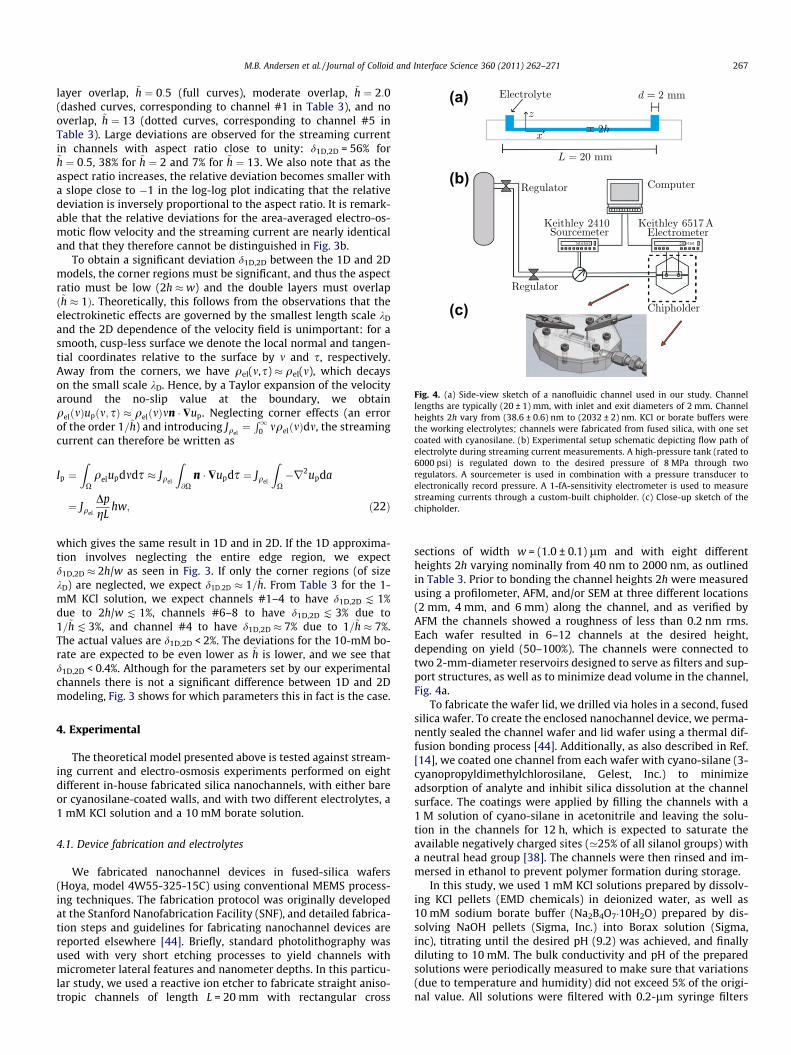
Fig. 4. (a) Side-view sketch of a nanofluidic channel used in our study. Channellengths are typically (20 ± 1) mm, with inlet and exit diameters of 2 mm. Channelheights 2h vary from (38.6 ± 0.6) nm to (2032 ± 2) nm. KCl or borate buffers werethe working electrolytes; channels were fabricated from fused silica, with one setcoated with cyanosilane. (b) Experimental setup schematic depicting flow path ofelectrolyte during streaming current measurements. A high-pressure tank (rated to6000 psi) is regulated down to the desired pressure of 8 MPa through tworegulators. A sourcemeter is used in combination with a pressure transducer toelectronically record pressure. A 1-fA-sensitivity electrometer is used to measurestreaming currents through a custom-built chipholder. (c) Close-up sketch of thechipholder.

M.B. Andersen et al. / Journal of Colloid and Interface Science 360 (2011) 262–271 267

layer overlap, ~h ¼ 0:5 (full curves), moderate overlap, ~h ¼ 2:0(dashed curves, corresponding to channel #1 in Table 3), and nooverlap, ~h ¼ 13 (dotted curves, corresponding to channel #5 inTable 3). Large deviations are observed for the streaming currentin channels with aspect ratio close to unity: d1D,2D = 56% for~h ¼ 0:5, 38% for ~h ¼ 2 and 7% for ~h ¼ 13. We also note that as theaspect ratio increases, the relative deviation becomes smaller witha slope close to �1 in the log-log plot indicating that the relativedeviation is inversely proportional to the aspect ratio. It is remark-able that the relative deviations for the area-averaged electro-os-motic flow velocity and the streaming current are nearly identicaland that they therefore cannot be distinguished in Fig. 3b.

To obtain a significant deviation d1D,2D between the 1D and 2Dmodels, the corner regions must be significant, and thus the aspectratio must be low (2h � w) and the double layers must overlapð~h � 1Þ. Theoretically, this follows from the observations that theelectrokinetic effects are governed by the smallest length scale kD

and the 2D dependence of the velocity field is unimportant: for asmooth, cusp-less surface we denote the local normal and tangen-tial coordinates relative to the surface by m and s, respectively.Away from the corners, we have qel(m,s) � qel(m), which decayson the small scale kD. Hence, by a Taylor expansion of the velocityaround the no-slip value at the boundary, we obtainqelðmÞupðm; sÞ � qelðmÞmn � $up. Neglecting corner effects (an errorof the order 1=~h) and introducing Jqel

¼R1

0 mqelðmÞdm, the streamingcurrent can therefore be written as

Ip ¼Z

Xqelupdmds � Jqel

Z@X

n � $upds ¼ Jqel

ZX�r2upda

¼ Jqel

DpgL

hw; ð22Þ

which gives the same result in 1D and in 2D. If the 1D approxima-tion involves neglecting the entire edge region, we expectd1D,2D � 2h/w as seen in Fig. 3. If only the corner regions (of sizekD) are neglected, we expect d1D;2D � 1=~h. From Table 3 for the 1-mM KCl solution, we expect channels #1–4 to have d1D,2D [ 1%due to 2h/w [ 1%, channels #6–8 to have d1D,2D [ 3% due to1=~h K 3%, and channel #4 to have d1D,2D � 7% due to 1=~h � 7%.The actual values are d1D,2D < 2%. The deviations for the 10-mM bo-rate are expected to be even lower as ~h is lower, and we see thatd1D,2D < 0.4%. Although for the parameters set by our experimentalchannels there is not a significant difference between 1D and 2Dmodeling, Fig. 3 shows for which parameters this in fact is the case.

4. Experimental

The theoretical model presented above is tested against stream-ing current and electro-osmosis experiments performed on eightdifferent in-house fabricated silica nanochannels, with either bareor cyanosilane-coated walls, and with two different electrolytes, a1 mM KCl solution and a 10 mM borate solution.

4.1. Device fabrication and electrolytes

We fabricated nanochannel devices in fused-silica wafers(Hoya, model 4W55-325-15C) using conventional MEMS process-ing techniques. The fabrication protocol was originally developedat the Stanford Nanofabrication Facility (SNF), and detailed fabrica-tion steps and guidelines for fabricating nanochannel devices arereported elsewhere [44]. Briefly, standard photolithography wasused with very short etching processes to yield channels withmicrometer lateral features and nanometer depths. In this particu-lar study, we used a reactive ion etcher to fabricate straight aniso-tropic channels of length L = 20 mm with rectangular cross

sections of width w = (1.0 ± 0.1) lm and with eight differentheights 2h varying nominally from 40 nm to 2000 nm, as outlinedin Table 3. Prior to bonding the channel heights 2h were measuredusing a profilometer, AFM, and/or SEM at three different locations(2 mm, 4 mm, and 6 mm) along the channel, and as verified byAFM the channels showed a roughness of less than 0.2 nm rms.Each wafer resulted in 6–12 channels at the desired height,depending on yield (50–100%). The channels were connected totwo 2-mm-diameter reservoirs designed to serve as filters and sup-port structures, as well as to minimize dead volume in the channel,Fig. 4a.

To fabricate the wafer lid, we drilled via holes in a second, fusedsilica wafer. To create the enclosed nanochannel device, we perma-nently sealed the channel wafer and lid wafer using a thermal dif-fusion bonding process [44]. Additionally, as also described in Ref.[14], we coated one channel from each wafer with cyano-silane (3-cyanopropyldimethylchlorosilane, Gelest, Inc.) to minimizeadsorption of analyte and inhibit silica dissolution at the channelsurface. The coatings were applied by filling the channels with a1 M solution of cyano-silane in acetonitrile and leaving the solu-tion in the channels for 12 h, which is expected to saturate theavailable negatively charged sites (’25% of all silanol groups) witha neutral head group [38]. The channels were then rinsed and im-mersed in ethanol to prevent polymer formation during storage.

In this study, we used 1 mM KCl solutions prepared by dissolv-ing KCl pellets (EMD chemicals) in deionized water, as well as10 mM sodium borate buffer (Na2B4O7�10H2O) prepared by dis-solving NaOH pellets (Sigma, Inc.) into Borax solution (Sigma,inc), titrating until the desired pH (9.2) was achieved, and finallydiluting to 10 mM. The bulk conductivity and pH of the preparedsolutions were periodically measured to make sure that variations(due to temperature and humidity) did not exceed 5% of the origi-nal value. All solutions were filtered with 0.2-lm syringe filters

(a)

(b)

(c)

(d)

(e)

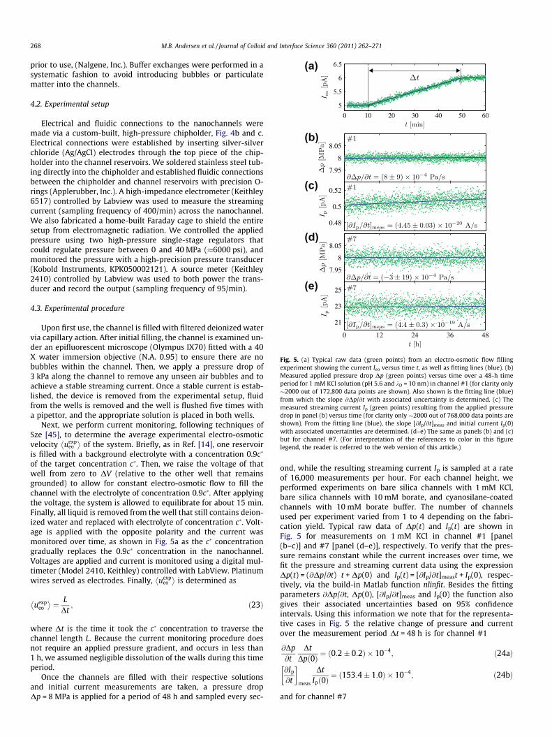
Fig. 5. (a) Typical raw data (green points) from an electro-osmotic flow fillingexperiment showing the current Ieo versus time t, as well as fitting lines (blue). (b)Measured applied pressure drop Dp (green points) versus time over a 48-h timeperiod for 1 mM KCl solution (pH 5.6 and kD = 10 nm) in channel #1 (for clarity only2000 out of 172,800 data points are shown). Also shown is the fitting line (blue)from which the slope @Dp/@t with associated uncertainty is determined. (c) Themeasured streaming current Ip (green points) resulting from the applied pressuredrop in panel (b) versus time (for clarity only 2000 out of 768,000 data points areshown). From the fitting line (blue), the slope [@Ip/@t]meas and initial current Ip(0)with associated uncertainties are determined. (d–e) The same as panels (b) and (c)but for channel #7. (For interpretation of the references to color in this figurelegend, the reader is referred to the web version of this article.)

268 M.B. Andersen et al. / Journal of Colloid and Interface Science 360 (2011) 262–271

prior to use, (Nalgene, Inc.). Buffer exchanges were performed in asystematic fashion to avoid introducing bubbles or particulatematter into the channels.

4.2. Experimental setup

Electrical and fluidic connections to the nanochannels weremade via a custom-built, high-pressure chipholder, Fig. 4b and c.Electrical connections were established by inserting silver-silverchloride (Ag/AgCl) electrodes through the top piece of the chip-holder into the channel reservoirs. We soldered stainless steel tub-ing directly into the chipholder and established fluidic connectionsbetween the chipholder and channel reservoirs with precision O-rings (Applerubber, Inc.). A high-impedance electrometer (Keithley6517) controlled by Labview was used to measure the streamingcurrent (sampling frequency of 400/min) across the nanochannel.We also fabricated a home-built Faraday cage to shield the entiresetup from electromagnetic radiation. We controlled the appliedpressure using two high-pressure single-stage regulators thatcould regulate pressure between 0 and 40 MPa (�6000 psi), andmonitored the pressure with a high-precision pressure transducer(Kobold Instruments, KPK050002121). A source meter (Keithley2410) controlled by Labview was used to both power the trans-ducer and record the output (sampling frequency of 95/min).

4.3. Experimental procedure

Upon first use, the channel is filled with filtered deionized watervia capillary action. After initial filling, the channel is examined un-der an epifluorescent microscope (Olympus IX70) fitted with a 40X water immersion objective (N.A. 0.95) to ensure there are nobubbles within the channel. Then, we apply a pressure drop of3 kPa along the channel to remove any unseen air bubbles and toachieve a stable streaming current. Once a stable current is estab-lished, the device is removed from the experimental setup, fluidfrom the wells is removed and the well is flushed five times witha pipettor, and the appropriate solution is placed in both wells.

Next, we perform current monitoring, following techniques ofSze [45], to determine the average experimental electro-osmoticvelocity uexp

eo� �

of the system. Briefly, as in Ref. [14], one reservoiris filled with a background electrolyte with a concentration 0.9c�

of the target concentration c�. Then, we raise the voltage of thatwell from zero to DV (relative to the other well that remainsgrounded) to allow for constant electro-osmotic flow to fill thechannel with the electrolyte of concentration 0.9c�. After applyingthe voltage, the system is allowed to equilibrate for about 15 min.Finally, all liquid is removed from the well that still contains deion-ized water and replaced with electrolyte of concentration c�. Volt-age is applied with the opposite polarity and the current wasmonitored over time, as shown in Fig. 5a as the c� concentrationgradually replaces the 0.9c� concentration in the nanochannel.Voltages are applied and current is monitored using a digital mul-timeter (Model 2410, Keithley) controlled with LabView. Platinumwires served as electrodes. Finally, uexp

eo� �

is determined as

uexpeo

� �¼ L

Dt; ð23Þ

where Dt is the time it took the c� concentration to traverse thechannel length L. Because the current monitoring procedure doesnot require an applied pressure gradient, and occurs in less than1 h, we assumed negligible dissolution of the walls during this timeperiod.

Once the channels are filled with their respective solutionsand initial current measurements are taken, a pressure dropDp = 8 MPa is applied for a period of 48 h and sampled every sec-

ond, while the resulting streaming current Ip is sampled at a rateof 16,000 measurements per hour. For each channel height, weperformed experiments on bare silica channels with 1 mM KCl,bare silica channels with 10 mM borate, and cyanosilane-coatedchannels with 10 mM borate buffer. The number of channelsused per experiment varied from 1 to 4 depending on the fabri-cation yield. Typical raw data of Dp(t) and Ip(t) are shown inFig. 5 for measurements on 1 mM KCl in channel #1 [panel(b–c)] and #7 [panel (d–e)], respectively. To verify that the pres-sure remains constant while the current increases over time, wefit the pressure and streaming current data using the expressionDp(t) = (@Dp/@t) t + Dp(0) and Ip(t) = [@Ip/@t]meast + Ip(0), respec-tively, via the build-in Matlab function nlinfit. Besides the fittingparameters @Dp/@t, Dp(0), [@Ip/@t]meas and Ip(0) the function alsogives their associated uncertainties based on 95% confidenceintervals. Using this information we note that for the representa-tive cases in Fig. 5 the relative change of pressure and currentover the measurement period Dt = 48 h is for channel #1

@Dp@t

DtDpð0Þ ¼ ð0:2� 0:2Þ � 10�4; ð24aÞ

@Ip

@t

� �meas

DtIpð0Þ

¼ ð153:4� 1:0Þ � 10�4; ð24bÞ

and for channel #7

(a)

(b)

(c)

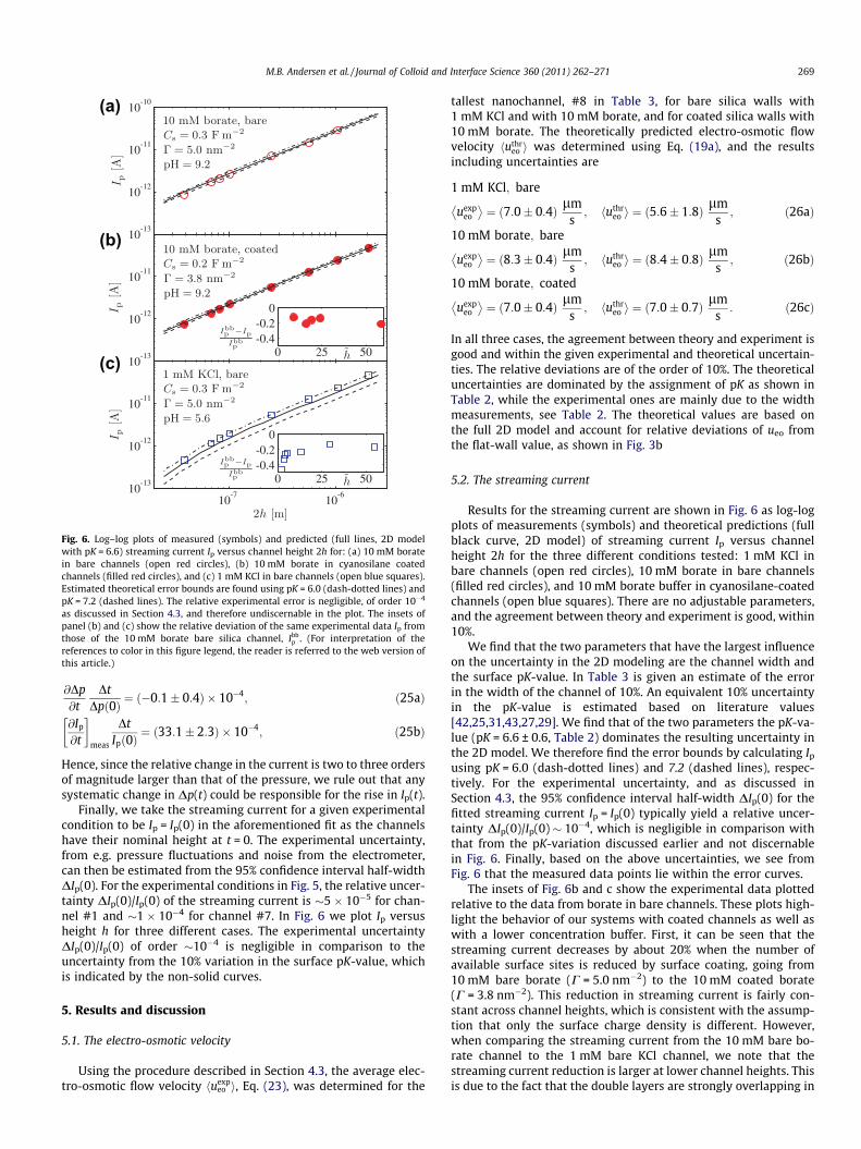
Fig. 6. Log–log plots of measured (symbols) and predicted (full lines, 2D modelwith pK = 6.6) streaming current Ip versus channel height 2h for: (a) 10 mM boratein bare channels (open red circles), (b) 10 mM borate in cyanosilane coatedchannels (filled red circles), and (c) 1 mM KCl in bare channels (open blue squares).Estimated theoretical error bounds are found using pK = 6.0 (dash-dotted lines) andpK = 7.2 (dashed lines). The relative experimental error is negligible, of order 10�4

as discussed in Section 4.3, and therefore undiscernable in the plot. The insets ofpanel (b) and (c) show the relative deviation of the same experimental data Ip fromthose of the 10 mM borate bare silica channel, Ibb

p . (For interpretation of thereferences to color in this figure legend, the reader is referred to the web version ofthis article.)

M.B. Andersen et al. / Journal of Colloid and Interface Science 360 (2011) 262–271 269

@Dp@t

DtDpð0Þ ¼ ð�0:1� 0:4Þ � 10�4; ð25aÞ

@Ip

@t

� �meas

DtIpð0Þ

¼ ð33:1� 2:3Þ � 10�4; ð25bÞ

Hence, since the relative change in the current is two to three ordersof magnitude larger than that of the pressure, we rule out that anysystematic change in Dp(t) could be responsible for the rise in Ip(t).

Finally, we take the streaming current for a given experimentalcondition to be Ip = Ip(0) in the aforementioned fit as the channelshave their nominal height at t = 0. The experimental uncertainty,from e.g. pressure fluctuations and noise from the electrometer,can then be estimated from the 95% confidence interval half-widthDIp(0). For the experimental conditions in Fig. 5, the relative uncer-tainty DIp(0)/Ip(0) of the streaming current is 5 � 10�5 for chan-nel #1 and 1 � 10�4 for channel #7. In Fig. 6 we plot Ip versusheight h for three different cases. The experimental uncertaintyDIp(0)/Ip(0) of order 10�4 is negligible in comparison to theuncertainty from the 10% variation in the surface pK-value, whichis indicated by the non-solid curves.

5. Results and discussion

5.1. The electro-osmotic velocity

Using the procedure described in Section 4.3, the average elec-tro-osmotic flow velocity huexp

eo i, Eq. (23), was determined for the

tallest nanochannel, #8 in Table 3, for bare silica walls with1 mM KCl and with 10 mM borate, and for coated silica walls with10 mM borate. The theoretically predicted electro-osmotic flowvelocity huthr

eo i was determined using Eq. (19a), and the resultsincluding uncertainties are

1 mM KCl; bare

uexpeo

� �¼ ð7:0� 0:4Þ lm

s; huthr

eo i ¼ ð5:6� 1:8Þ lms; ð26aÞ

10 mM borate; bare

uexpeo

� �¼ ð8:3� 0:4Þ lm

s; huthr

eo i ¼ ð8:4� 0:8Þ lms; ð26bÞ

10 mM borate; coated

uexpeo

� �¼ ð7:0� 0:4Þ lm

s; huthr

eo i ¼ ð7:0� 0:7Þ lms: ð26cÞ

In all three cases, the agreement between theory and experiment isgood and within the given experimental and theoretical uncertain-ties. The relative deviations are of the order of 10%. The theoreticaluncertainties are dominated by the assignment of pK as shown inTable 2, while the experimental ones are mainly due to the widthmeasurements, see Table 2. The theoretical values are based onthe full 2D model and account for relative deviations of ueo fromthe flat-wall value, as shown in Fig. 3b

5.2. The streaming current

Results for the streaming current are shown in Fig. 6 as log-logplots of measurements (symbols) and theoretical predictions (fullblack curve, 2D model) of streaming current Ip versus channelheight 2h for the three different conditions tested: 1 mM KCl inbare channels (open red circles), 10 mM borate in bare channels(filled red circles), and 10 mM borate buffer in cyanosilane-coatedchannels (open blue squares). There are no adjustable parameters,and the agreement between theory and experiment is good, within10%.

We find that the two parameters that have the largest influenceon the uncertainty in the 2D modeling are the channel width andthe surface pK-value. In Table 3 is given an estimate of the errorin the width of the channel of 10%. An equivalent 10% uncertaintyin the pK-value is estimated based on literature values[42,25,31,43,27,29]. We find that of the two parameters the pK-va-lue (pK = 6.6 ± 0.6, Table 2) dominates the resulting uncertainty inthe 2D model. We therefore find the error bounds by calculating Ip

using pK = 6.0 (dash-dotted lines) and 7.2 (dashed lines), respec-tively. For the experimental uncertainty, and as discussed inSection 4.3, the 95% confidence interval half-width DIp(0) for thefitted streaming current Ip = Ip(0) typically yield a relative uncer-tainty DIp(0)/Ip(0) 10�4, which is negligible in comparison withthat from the pK-variation discussed earlier and not discernablein Fig. 6. Finally, based on the above uncertainties, we see fromFig. 6 that the measured data points lie within the error curves.

The insets of Fig. 6b and c show the experimental data plottedrelative to the data from borate in bare channels. These plots high-light the behavior of our systems with coated channels as well aswith a lower concentration buffer. First, it can be seen that thestreaming current decreases by about 20% when the number ofavailable surface sites is reduced by surface coating, going from10 mM bare borate (C = 5.0 nm�2) to the 10 mM coated borate(C = 3.8 nm�2). This reduction in streaming current is fairly con-stant across channel heights, which is consistent with the assump-tion that only the surface charge density is different. However,when comparing the streaming current from the 10 mM bare bo-rate channel to the 1 mM bare KCl channel, we note that thestreaming current reduction is larger at lower channel heights. Thisis due to the fact that the double layers are strongly overlapping in

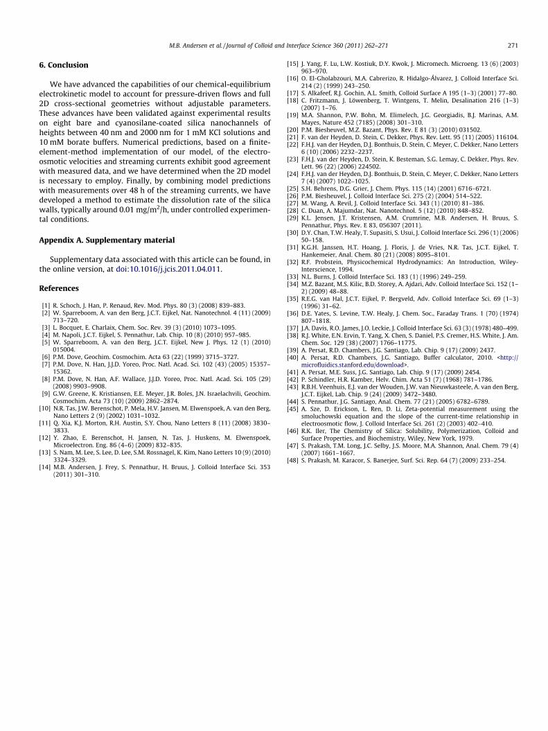
Fig. 7. One proposed mechanism for silica dissolution presented in, and imageadapted from, Ref. [46].

Fig. 8. Predicted silica dissolution rate dm/dt vs. channel height 2h based, via Eq.(29), on measured [@Ip/@t]meas and calculated [@Ip/@l]calc (numerical values are givenin the Supplementary information). The three curves are for: 1 mM KCl in barechannel (dash-dotted red curve), 10 mM borate in bare channel (full black curve),and 10 mM borate in cyanosilane-coated channel (dashed blue curve). (Forinterpretation of the references to color in this figure legend, the reader is referredto the web version of this article.)

270 M.B. Andersen et al. / Journal of Colloid and Interface Science 360 (2011) 262–271

this regime (whereas with 10 mM borate the double layers are stillnon-overlapping), which clearly reduces the streaming current.

Having verified the accuracy of the model for the forward prob-lem, i.e., predicting streaming currents in the nanochannels ofinterest, we next turn to the inverse problem of estimating disso-lution rates given extended time-sensitive streaming currentmeasurements.

5.3. Method for determining dissolution rates

In geological systems, it has been found that saline solutionsflowing through porous silicates dissolve the solid matrix at a rateof approximately 0.01 mg/m2/h [46]. Given that the density offused silica is 2203 kg/m3, we obtain

1mg

m2h 0:4539

nmh¼ 1:26� 10�13 m

s; ð27aÞ

or conversely

1ms¼ 7:93� 1012 mg

m2h: ð27bÞ

The mechanism of silica dissolution is complex and not yet wellunderstood, but one mechanism for the dissolution discussed inthe literature [46] is shown in Fig. 7.

Here, we propose a method for determining dissolution ratesunder controlled experimental conditions using our model andexperimental data. Referring back to Fig. 5b and c, we note thatalthough the applied pressure drop remains constant over a periodof 48 h, the streaming current steadily rises. This fact, togetherwith the following three assumptions, forms the basis of the meth-od: (i) all changes in current are due solely to dissolution of thewall, aided by the continuous renewal of fresh buffer by the axialflow; (ii) ionized silanol radicals are few and highly unstable andthus do not contribute to the current; (iii) spatial variations inthe dissolution rate are averaged out over the entire surface ofthe channel.

To calculate dissolution rates, we use Eq. (14b) to obtain anumerical estimate for the change dIp in the streaming current asa function of the change dA = 2(w + h) d‘ in the cross-sectional areaA, in terms of the (small) thickness d‘ of the dissolved layer,

@Ip

@‘

� �calc¼ @Ip

@A@A@‘� 1

d‘IpðAþ dAÞ � IpðAÞ�

; ð28Þ

where we choose d‘ = 0.01h. Combining this with the experimen-tally measured rate of change [@Ip/@t]meas of the streaming current,Fig. 5c, yields the dissolution rate dm/dt per unit area (in units ofmg/m2/h) as,

dmdt¼ 7:93� 1012 mg

m2hsm� @Ip

@t

� �meas� @Ip

@‘

� ��1

calc: ð29Þ

In the Supplementary information, we list the numerical values of[@Ip/@t]meas, [@Ip/@l]calc, and dm/dt for each experimental condition.

The theoretically predicted dissolution rates based on measured[@Ip/@t]meas for our experimental nanochannel system are shownin Fig. 8. We note that the estimated rates are on the same orderof magnitude as previous results in the field of geological systems[46], which allows us to believe that our method is viable for silicadissolution studies. Furthermore, also in agreement with earlierfindings [9], the dissolution rate increases as pH and ionic strengthincrease going from 1 mM KCl (pH 5.6) to 10 mM borate (pH 9.2) inbare silica channels. Other studies have pointed out that electricdouble-layer interaction in un-confined geometries increases thedissolution rates [9]. This we also see in our calculations, as the dis-solution rate increases when the double layers start to overlap asthe channel half-height h is decreased. A final point that corrobo-rates our model is the prediction of a negligible dissolution rate(fluctuates around zero) for the cyanosilane-coated channel, awell-known feature from other studies [38,47,48].

On top of this, we can use our model for novel studies of silicadissolution, for example the influence of extreme confinement.From Fig. 8 we note that the increase in dissolution rate starts ear-lier for 1 mM KCl than 10 mM borate as channel height decreases,indicating that this may be due to electric double layer effects.However, because the peak is roughly at the same height for bothcases, diffusion-limited dissolution may be the dominating physicsat small channel heights. This is in line with a common viewpointabout dissolution, which holds that charges such as OH� near thewall catalyze de-polymerization and that the newly dissolved sila-nol radicals diffuse away from the surface.

In general, using our method of hours-long streaming currentmeasurements will enable systematic studies of the mechanismunderlying dissolution of silica in a number of controlled experi-ments: The channel geometry can be varied from the case of thinnon-overlapping double layers in very tall microchannels to thatof strongly overlapping double layers at extreme confinement invery shallow nanochannels. Diffusion limited dissolution ratesand the effect of continuous renewal of buffer can be studiedthrough varying the imposed pressure-driven electrolyte flow.The chemical conditions can be varied through the detailed com-position and ionic strength of the buffer as well as the coating con-ditions of the surface. The small size of micro- and nanofluidicsystems facilitates accurate temperature control. These advantagessuggest that our method may be useful for future studies of silicadissolution.

M.B. Andersen et al. / Journal of Colloid and Interface Science 360 (2011) 262–271 271

6. Conclusion

We have advanced the capabilities of our chemical-equilibriumelectrokinetic model to account for pressure-driven flows and full2D cross-sectional geometries without adjustable parameters.These advances have been validated against experimental resultson eight bare and cyanosilane-coated silica nanochannels ofheights between 40 nm and 2000 nm for 1 mM KCl solutions and10 mM borate buffers. Numerical predictions, based on a finite-element-method implementation of our model, of the electro-osmotic velocities and streaming currents exhibit good agreementwith measured data, and we have determined when the 2D modelis necessary to employ. Finally, by combining model predictionswith measurements over 48 h of the streaming currents, we havedeveloped a method to estimate the dissolution rate of the silicawalls, typically around 0.01 mg/m2/h, under controlled experimen-tal conditions.

Appendix A. Supplementary material

Supplementary data associated with this article can be found, inthe online version, at doi:10.1016/j.jcis.2011.04.011.

References

[1] R. Schoch, J. Han, P. Renaud, Rev. Mod. Phys. 80 (3) (2008) 839–883.[2] W. Sparreboom, A. van den Berg, J.C.T. Eijkel, Nat. Nanotechnol. 4 (11) (2009)

713–720.[3] L. Bocquet, E. Charlaix, Chem. Soc. Rev. 39 (3) (2010) 1073–1095.[4] M. Napoli, J.C.T. Eijkel, S. Pennathur, Lab. Chip. 10 (8) (2010) 957–985.[5] W. Sparreboom, A. van den Berg, J.C.T. Eijkel, New J. Phys. 12 (1) (2010)

015004.[6] P.M. Dove, Geochim. Cosmochim. Acta 63 (22) (1999) 3715–3727.[7] P.M. Dove, N. Han, J.J.D. Yoreo, Proc. Natl. Acad. Sci. 102 (43) (2005) 15357–

15362.[8] P.M. Dove, N. Han, A.F. Wallace, J.J.D. Yoreo, Proc. Natl. Acad. Sci. 105 (29)

(2008) 9903–9908.[9] G.W. Greene, K. Kristiansen, E.E. Meyer, J.R. Boles, J.N. Israelachvili, Geochim.

Cosmochim. Acta 73 (10) (2009) 2862–2874.[10] N.R. Tas, J.W. Berenschot, P. Mela, H.V. Jansen, M. Elwenspoek, A. van den Berg,

Nano Letters 2 (9) (2002) 1031–1032.[11] Q. Xia, K.J. Morton, R.H. Austin, S.Y. Chou, Nano Letters 8 (11) (2008) 3830–

3833.[12] Y. Zhao, E. Berenschot, H. Jansen, N. Tas, J. Huskens, M. Elwenspoek,

Microelectron. Eng. 86 (4–6) (2009) 832–835.[13] S. Nam, M. Lee, S. Lee, D. Lee, S.M. Rossnagel, K. Kim, Nano Letters 10 (9) (2010)

3324–3329.[14] M.B. Andersen, J. Frey, S. Pennathur, H. Bruus, J. Colloid Interface Sci. 353

(2011) 301–310.

[15] J. Yang, F. Lu, L.W. Kostiuk, D.Y. Kwok, J. Micromech. Microeng. 13 (6) (2003)963–970.

[16] O. El-Gholabzouri, M.A. Cabrerizo, R. Hidalgo-Álvarez, J. Colloid Interface Sci.214 (2) (1999) 243–250.

[17] S. Alkafeef, R.J. Gochin, A.L. Smith, Colloid Surface A 195 (1–3) (2001) 77–80.[18] C. Fritzmann, J. Löwenberg, T. Wintgens, T. Melin, Desalination 216 (1–3)

(2007) 1–76.[19] M.A. Shannon, P.W. Bohn, M. Elimelech, J.G. Georgiadis, B.J. Marinas, A.M.

Mayes, Nature 452 (7185) (2008) 301–310.[20] P.M. Biesheuvel, M.Z. Bazant, Phys. Rev. E 81 (3) (2010) 031502.[21] F. van der Heyden, D. Stein, C. Dekker, Phys. Rev. Lett. 95 (11) (2005) 116104.[22] F.H.J. van der Heyden, D.J. Bonthuis, D. Stein, C. Meyer, C. Dekker, Nano Letters

6 (10) (2006) 2232–2237.[23] F.H.J. van der Heyden, D. Stein, K. Besteman, S.G. Lemay, C. Dekker, Phys. Rev.

Lett. 96 (22) (2006) 224502.[24] F.H.J. van der Heyden, D.J. Bonthuis, D. Stein, C. Meyer, C. Dekker, Nano Letters

7 (4) (2007) 1022–1025.[25] S.H. Behrens, D.G. Grier, J. Chem. Phys. 115 (14) (2001) 6716–6721.[26] P.M. Biesheuvel, J. Colloid Interface Sci. 275 (2) (2004) 514–522.[27] M. Wang, A. Revil, J. Colloid Interface Sci. 343 (1) (2010) 81–386.[28] C. Duan, A. Majumdar, Nat. Nanotechnol. 5 (12) (2010) 848–852.[29] K.L. Jensen, J.T. Kristensen, A.M. Crumrine, M.B. Andersen, H. Bruus, S.

Pennathur, Phys. Rev. E 83, 056307 (2011).[30] D.Y. Chan, T.W. Healy, T. Supasiti, S. Usui, J. Colloid Interface Sci. 296 (1) (2006)

50–158.[31] K.G.H. Janssen, H.T. Hoang, J. Floris, J. de Vries, N.R. Tas, J.C.T. Eijkel, T.

Hankemeier, Anal. Chem. 80 (21) (2008) 8095–8101.[32] R.F. Probstein, Physicochemical Hydrodynamics: An Introduction, Wiley-

Interscience, 1994.[33] N.L. Burns, J. Colloid Interface Sci. 183 (1) (1996) 249–259.[34] M.Z. Bazant, M.S. Kilic, B.D. Storey, A. Ajdari, Adv. Colloid Interface Sci. 152 (1–

2) (2009) 48–88.[35] R.E.G. van Hal, J.C.T. Eijkel, P. Bergveld, Adv. Colloid Interface Sci. 69 (1–3)

(1996) 31–62.[36] D.E. Yates, S. Levine, T.W. Healy, J. Chem. Soc., Faraday Trans. 1 (70) (1974)

807–1818.[37] J.A. Davis, R.O. James, J.O. Leckie, J. Colloid Interface Sci. 63 (3) (1978) 480–499.[38] R.J. White, E.N. Ervin, T. Yang, X. Chen, S. Daniel, P.S. Cremer, H.S. White, J. Am.

Chem. Soc. 129 (38) (2007) 1766–11775.[39] A. Persat, R.D. Chambers, J.G. Santiago, Lab. Chip. 9 (17) (2009) 2437.[40] A. Persat, R.D. Chambers, J.G. Santiago, Buffer calculator, 2010. <http://

microfluidics.stanford.edu/download>.[41] A. Persat, M.E. Suss, J.G. Santiago, Lab. Chip. 9 (17) (2009) 2454.[42] P. Schindler, H.R. Kamber, Helv. Chim. Acta 51 (7) (1968) 781–1786.[43] R.B.H. Veenhuis, E.J. van der Wouden, J.W. van Nieuwkasteele, A. van den Berg,

J.C.T. Eijkel, Lab. Chip. 9 (24) (2009) 3472–3480.[44] S. Pennathur, J.G. Santiago, Anal. Chem. 77 (21) (2005) 6782–6789.[45] A. Sze, D. Erickson, L. Ren, D. Li, Zeta-potential measurement using the

smoluchowski equation and the slope of the current-time relationship inelectroosmotic flow, J. Colloid Interface Sci. 261 (2) (2003) 402–410.

[46] R.K. Iler, The Chemistry of Silica: Solubility, Polymerization, Colloid andSurface Properties, and Biochemistry, Wiley, New York, 1979.

[47] S. Prakash, T.M. Long, J.C. Selby, J.S. Moore, M.A. Shannon, Anal. Chem. 79 (4)(2007) 1661–1667.

[48] S. Prakash, M. Karacor, S. Banerjee, Surf. Sci. Rep. 64 (7) (2009) 233–254.