journal of biomedical informatics - eth zpeople.inf.ethz.ch/ioannisl/jbi2014.pdf · the...

1

3

4

5

6 Q1

789

10

111213

1 5

16171819

202122232425

2 6

44

45

46

47

48

49

50

51

52

53

54

55

56

57

58

59

60

61

Q2Q1

Journal of Biomedical Informatics xxx (2014) xxx–xxx

YJBIN 2180 No. of Pages 16, Model 5G

31 May 2014

Q1

Contents lists available at ScienceDirect

Journal of Biomedical Informatics

journal homepage: www.elsevier .com/locate /y jb in

Disassociation for electronic health record privacy

http://dx.doi.org/10.1016/j.jbi.2014.05.0091532-0464/� 2014 Published by Elsevier Inc.

⇑ Corresponding author. Tel.: +353 18103096.E-mail addresses: [email protected] (G. Loukides), [email protected]

(J. Liagouris), [email protected] (A. Gkoulalas-Divanis), [email protected] (M. Terrovitis).

Please cite this article in press as: Loukides G et al. Disassociation for electronic health record privacy. J Biomed Inform (2014), http://dx.doi.org/1j.jbi.2014.05.009

Grigorios Loukides a, John Liagouris b, Aris Gkoulalas-Divanis c,⇑, Manolis Terrovitis d

a School of Computer Science and Informatics, Cardiff University, United Kingdomb Department of Electrical and Computer Engineering, NTUA, Greecec IBM Research – Ireland, Dublin, Irelandd IMIS, Research Center Athena, Greece

27282930313233343536

a r t i c l e i n f o

Article history:Received 23 August 2013Accepted 16 May 2014Available online xxxx

Keywords:PrivacyElectronic health recordsDisassociationDiagnosis codes

373839404142

a b s t r a c t

The dissemination of Electronic Health Record (EHR) data, beyond the originating healthcare institutions,can enable large-scale, low-cost medical studies that have the potential to improve public health. Thus,funding bodies, such as the National Institutes of Health (NIH) in the U.S., encourage or require the dis-semination of EHR data, and a growing number of innovative medical investigations are being performedusing such data. However, simply disseminating EHR data, after removing identifying information, mayrisk privacy, as patients can still be linked with their record, based on diagnosis codes. This paper pro-poses the first approach that prevents this type of data linkage using disassociation, an operation thattransforms records by splitting them into carefully selected subsets. Our approach preserves privacy withsignificantly lower data utility loss than existing methods and does not require data owners to specifydiagnosis codes that may lead to identity disclosure, as these methods do. Consequently, it can beemployed when data need to be shared broadly and be used in studies, beyond the intended ones.Through extensive experiments using EHR data, we demonstrate that our method can construct data thatare highly useful for supporting various types of clinical case count studies and general medical analysistasks.

� 2014 Published by Elsevier Inc.

43

62

63

64

65

66

67

68

69

70

71

72

73

74

75

76

77

78

79

1. Introduction

Healthcare data are increasingly collected in various forms,including Electronic Health Records (EHR), medical imaging dat-abases, disease registries, and clinical trials. Disseminating thesedata has the potential of offering better healthcare quality at lowercosts, while improving public health. For instance, large amountsof healthcare data are becoming publicly accessible at no cost,through open data platforms [4], in an attempt to promote account-ability, entrepreneurship, and economic growth ($100 billion areestimated to be generated annually across the US health-care sys-tem [11]). At the same time, sharing EHR data can greatly reduceresearch costs (e.g., there is no need for recruiting patients) andallow large-scale, complex medical studies. Thus, the NationalInstitutes of Health (NIH) calls for increasing the reuse of EHR data[7], and several medical analytic tasks, ranging from building pre-dictive data mining models [8] to genomic studies [14], are beingperformed using such data.

80

81

82

83

84

Sharing EHR data is highly beneficial but must be performed ina way that preserves patient and institutional privacy. In fact, thereare several data sharing policies and regulations that govern thesharing of patient-specific data, such as the HIPAA privacy rule[48], in the U.S., the Anonymization Code [6], in the U.K., and theData Protection Directive [3], in the European Union. In addition,funding bodies emphasize the need for privacy-preserving health-care data sharing. For instance, the NIH requires data involved inall NIH-funded Genome-Wide Association Studies (GWAS) to bedeposited into a biorepository, for broad dissemination [45], whilesafeguarding privacy [1]. Alarmingly, however, a large number ofprivacy breaches, related to healthcare data, still occur. For exam-ple, 627 privacy breaches, which affect more than 500 and up to4.9 M individuals each, are reported from 2010 to July 2013 bythe U.S. Department of Health & Human Services [15].

One of the main privacy threats when sharing EHR data is iden-tity disclosure (also referred to as re-identification), which involvesthe association of an identified patient with their record in thepublished data. Identity disclosure may occur even when dataare de-identified (i.e., they are devoid of identifying information).This is because publicly available datasets, such as voter registra-tion lists, contain identifying information and can be linked to pub-lished datasets, based on potentially identifying information, such

0.1016/

http://dx.doi.org/10.1016/j.jbi.2014.05.009

mailto:[email protected]






http://www.sciencedirect.com/science/journal/15320464

http://www.elsevier.com/locate/yjbin



85

86

87

88

89

90

91

92

93

94

95

96

97

98

99

100

101

102

103

104

105

106

107

108

109

110

111

112

113

114

115

116

117

118

119

120

121

122

123

124

125

126

127

128

129

130

131

132

133

134

135

136

137

138

139

140

141

142

143

144

145

146

147

148

149

150

151

152

153

154

155

156

157

158

159

160

161

162

163

164

165

166

167

168

169

170

171

172

173

174

175

176

177

178

179

180

181

182

183

184

185

186

187

188

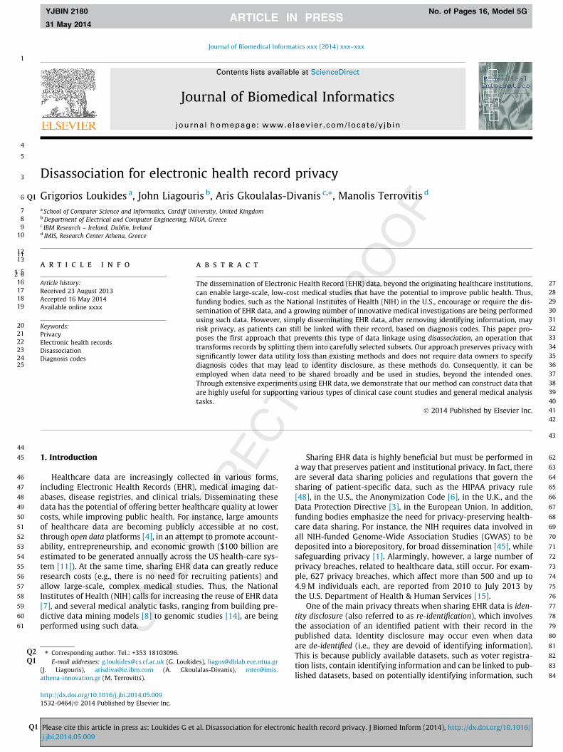
Fig. 1. Original dataset D.

2 G. LoukidesQ1 et al. / Journal of Biomedical Informatics xxx (2014) xxx–xxx


31 May 2014

Q1

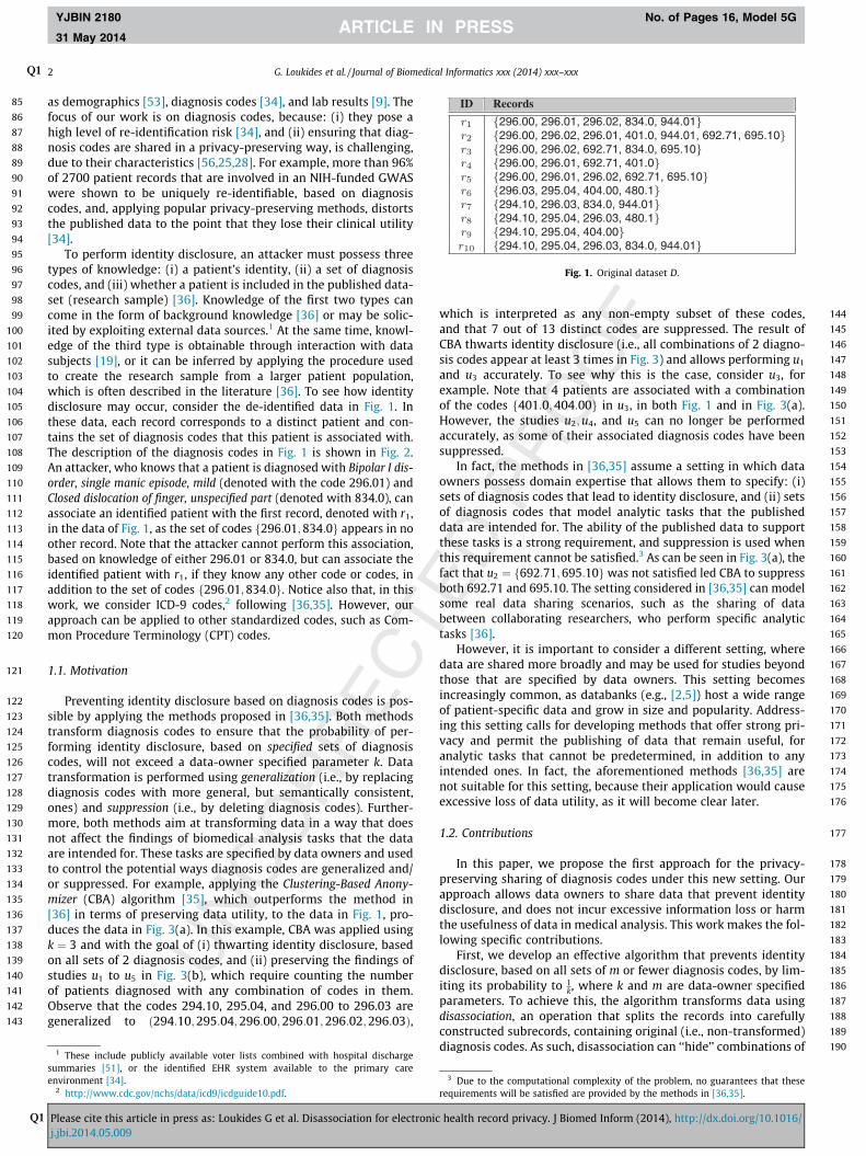
as demographics [53], diagnosis codes [34], and lab results [9]. Thefocus of our work is on diagnosis codes, because: (i) they pose ahigh level of re-identification risk [34], and (ii) ensuring that diag-nosis codes are shared in a privacy-preserving way, is challenging,due to their characteristics [56,25,28]. For example, more than 96%of 2700 patient records that are involved in an NIH-funded GWASwere shown to be uniquely re-identifiable, based on diagnosiscodes, and, applying popular privacy-preserving methods, distortsthe published data to the point that they lose their clinical utility[34].

To perform identity disclosure, an attacker must possess threetypes of knowledge: (i) a patient’s identity, (ii) a set of diagnosiscodes, and (iii) whether a patient is included in the published data-set (research sample) [36]. Knowledge of the first two types cancome in the form of background knowledge [36] or may be solic-ited by exploiting external data sources.1 At the same time, knowl-edge of the third type is obtainable through interaction with datasubjects [19], or it can be inferred by applying the procedure usedto create the research sample from a larger patient population,which is often described in the literature [36]. To see how identitydisclosure may occur, consider the de-identified data in Fig. 1. Inthese data, each record corresponds to a distinct patient and con-tains the set of diagnosis codes that this patient is associated with.The description of the diagnosis codes in Fig. 1 is shown in Fig. 2.An attacker, who knows that a patient is diagnosed with Bipolar I dis-order, single manic episode, mild (denoted with the code 296.01) andClosed dislocation of finger, unspecified part (denoted with 834.0), canassociate an identified patient with the first record, denoted with r1,in the data of Fig. 1, as the set of codes f296:01;834:0g appears in noother record. Note that the attacker cannot perform this association,based on knowledge of either 296.01 or 834.0, but can associate theidentified patient with r1, if they know any other code or codes, inaddition to the set of codes f296:01;834:0g. Notice also that, in thiswork, we consider ICD-9 codes,2 following [36,35]. However, ourapproach can be applied to other standardized codes, such as Com-mon Procedure Terminology (CPT) codes.

1.1. Motivation

Preventing identity disclosure based on diagnosis codes is pos-sible by applying the methods proposed in [36,35]. Both methodstransform diagnosis codes to ensure that the probability of per-forming identity disclosure, based on specified sets of diagnosiscodes, will not exceed a data-owner specified parameter k. Datatransformation is performed using generalization (i.e., by replacingdiagnosis codes with more general, but semantically consistent,ones) and suppression (i.e., by deleting diagnosis codes). Further-more, both methods aim at transforming data in a way that doesnot affect the findings of biomedical analysis tasks that the dataare intended for. These tasks are specified by data owners and usedto control the potential ways diagnosis codes are generalized and/or suppressed. For example, applying the Clustering-Based Anony-mizer (CBA) algorithm [35], which outperforms the method in[36] in terms of preserving data utility, to the data in Fig. 1, pro-duces the data in Fig. 3(a). In this example, CBA was applied usingk ¼ 3 and with the goal of (i) thwarting identity disclosure, basedon all sets of 2 diagnosis codes, and (ii) preserving the findings ofstudies u1 to u5 in Fig. 3(b), which require counting the numberof patients diagnosed with any combination of codes in them.Observe that the codes 294.10, 295.04, and 296.00 to 296.03 aregeneralized to ð294:10;295:04;296:00;296:01;296:02;296:03Þ,

189

1901 These include publicly available voter lists combined with hospital discharge

summaries [51], or the identified EHR system available to the primary careenvironment [34].

2 http://www.cdc.gov/nchs/data/icd9/icdguide10.pdf.

Please cite this article in press as: Loukides G et al. Disassociation for electronicj.jbi.2014.05.009

which is interpreted as any non-empty subset of these codes,and that 7 out of 13 distinct codes are suppressed. The result ofCBA thwarts identity disclosure (i.e., all combinations of 2 diagno-sis codes appear at least 3 times in Fig. 3) and allows performing u1

and u3 accurately. To see why this is the case, consider u3, forexample. Note that 4 patients are associated with a combinationof the codes f401:0;404:00g in u3, in both Fig. 1 and in Fig. 3(a).However, the studies u2;u4, and u5 can no longer be performedaccurately, as some of their associated diagnosis codes have beensuppressed.

In fact, the methods in [36,35] assume a setting in which dataowners possess domain expertise that allows them to specify: (i)sets of diagnosis codes that lead to identity disclosure, and (ii) setsof diagnosis codes that model analytic tasks that the publisheddata are intended for. The ability of the published data to supportthese tasks is a strong requirement, and suppression is used whenthis requirement cannot be satisfied.3 As can be seen in Fig. 3(a), thefact that u2 ¼ f692:71;695:10g was not satisfied led CBA to suppressboth 692.71 and 695.10. The setting considered in [36,35] can modelsome real data sharing scenarios, such as the sharing of databetween collaborating researchers, who perform specific analytictasks [36].

However, it is important to consider a different setting, wheredata are shared more broadly and may be used for studies beyondthose that are specified by data owners. This setting becomesincreasingly common, as databanks (e.g., [2,5]) host a wide rangeof patient-specific data and grow in size and popularity. Address-ing this setting calls for developing methods that offer strong pri-vacy and permit the publishing of data that remain useful, foranalytic tasks that cannot be predetermined, in addition to anyintended ones. In fact, the aforementioned methods [36,35] arenot suitable for this setting, because their application would causeexcessive loss of data utility, as it will become clear later.

1.2. Contributions

In this paper, we propose the first approach for the privacy-preserving sharing of diagnosis codes under this new setting. Ourapproach allows data owners to share data that prevent identitydisclosure, and does not incur excessive information loss or harmthe usefulness of data in medical analysis. This work makes the fol-lowing specific contributions.

First, we develop an effective algorithm that prevents identitydisclosure, based on all sets of m or fewer diagnosis codes, by lim-iting its probability to 1

k, where k and m are data-owner specifiedparameters. To achieve this, the algorithm transforms data usingdisassociation, an operation that splits the records into carefullyconstructed subrecords, containing original (i.e., non-transformed)diagnosis codes. As such, disassociation can ‘‘hide’’ combinations of

3 Due to the computational complexity of the problem, no guarantees that theserequirements will be satisfied are provided by the methods in [36,35].

health record privacy. J Biomed Inform (2014), http://dx.doi.org/10.1016/

http://www.cdc.gov/nchs/data/icd9/icdguide10.pdf



191

192

193

194

195

196

197

198

199

200

201

202

203

204

205

206

207

208

209

210

211

212

213

214

215

216

217

218

219

220

221

222

223

224

225

226

227

228

229

230

231

232

233

Fig. 2. Diagnosis codes in D and their description.

Fig. 3. CBA example.

G. LoukidesQ1 et al. / Journal of Biomedical Informatics xxx (2014) xxx–xxx 3


31 May 2014

Q1

diagnosis codes that appear few times in the original dataset, byscattering them in the subrecords of the published dataset. Forinstance, consider the record r1 in Fig. 1 and its counterpart, whichhas produced by applying disassociation with k ¼ 3 and m ¼ 2, inFig. 4. Note that the codes in r1 are split into two subrecords inFig. 4, which contain the sets of codes f296:00;296:01;296:02gand f834:0;401:0;944:01g, respectively. Moreover, the setf834:0;401:0;944:01g is associated with the first 5 records inFig. 4. Thus, an attacker who knows that a patient is diagnosedwith the set of codes f296:01;834:00g cannot associate them withfewer than 3 records in Fig. 4. Thus, strong privacy requirementscan be specified, without knowledge of potentially identifyingdiagnosis codes, and they can be enforced with low informationloss. In addition, published data can still remain useful for intendedanalytic tasks. For instance, as can be seen in Fig. 4, applying ouralgorithm to the data in Fig. 1, using k ¼ 3 and m ¼ 2, achievesthe same privacy, but significantly better data utility, than CBA,whose result is shown in Fig. 3(a). This is because, in contrast toCBA, our algorithm does not suppress diagnosis codes and retainsthe exact counts of 8 out of 13 codes (i.e., those in u1 and u3). More-over, our algorithm is able to preserve the findings of the first twostudies in Fig. 3(b).

Second, we experimentally demonstrate that our approach pre-serves data utility significantly better than CBA [35]. Specifically,


when applied to a large EHR dataset [8], our approach allows moreaccurate query answering and generates data that are highly usefulfor supporting various types of clinical case count studies and gen-eral medical analysis tasks. In addition, our approach is more effi-cient and scalable than CBA.

1.3. Paper organization

The remainder of the paper is organized as follows. Section 2reviews related work and Section 3 presents the concepts that arenecessary to introduce our method and formulate the problem weconsider. In Sections 4 and 6, we discuss and experimentally evalu-ate our algorithm, respectively. Subsequently, we explain how ourapproach can be extended to deal with different types of medicaldata and privacy requirements in Section 7. Last, Section 8 con-cludes the paper.

2. Related work

There are considerable research efforts for designing privacy-preserving methods [52,49,57,22,10,23,24,51,19,44,36]. Our workis closely related to methods which aim to publish patient-leveldata, in a way that prevents identity disclosure. Thus, we review




234

235

236

237

238

239

240

241

242

243

244

245

246

247

248

249

250

251

252

253

254

255

256

257

258

259

260

261

262

263

264

265

266

267

268

269

270

271

272

273

274

275

276

277

278

279

280

281

282

283

284

285

286

287

288

289

290

291

292

293

294

295

296

297

298

299

300

301

302

303

304

305

306

307

308

309

310

311

312

313

314

315

316

317

318

319

320

321

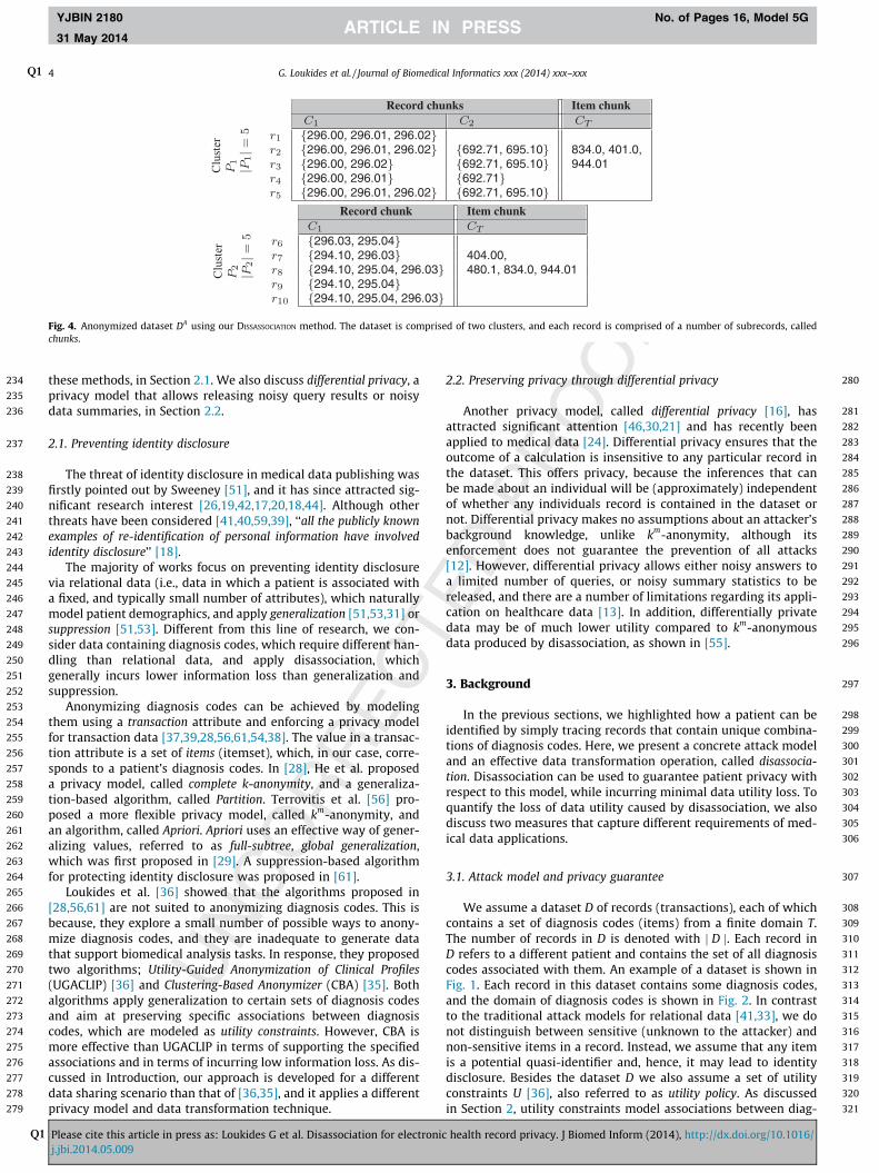
Fig. 4. Anonymized dataset DA using our DISSASSOCIATION method. The dataset is comprised of two clusters, and each record is comprised of a number of subrecords, calledchunks.



31 May 2014

Q1

these methods, in Section 2.1. We also discuss differential privacy, aprivacy model that allows releasing noisy query results or noisydata summaries, in Section 2.2.

2.1. Preventing identity disclosure

The threat of identity disclosure in medical data publishing wasfirstly pointed out by Sweeney [51], and it has since attracted sig-nificant research interest [26,19,42,17,20,18,44]. Although otherthreats have been considered [41,40,59,39], ‘‘all the publicly knownexamples of re-identification of personal information have involvedidentity disclosure’’ [18].

The majority of works focus on preventing identity disclosurevia relational data (i.e., data in which a patient is associated witha fixed, and typically small number of attributes), which naturallymodel patient demographics, and apply generalization [51,53,31] orsuppression [51,53]. Different from this line of research, we con-sider data containing diagnosis codes, which require different han-dling than relational data, and apply disassociation, whichgenerally incurs lower information loss than generalization andsuppression.

Anonymizing diagnosis codes can be achieved by modelingthem using a transaction attribute and enforcing a privacy modelfor transaction data [37,39,28,56,61,54,38]. The value in a transac-tion attribute is a set of items (itemset), which, in our case, corre-sponds to a patient’s diagnosis codes. In [28], He et al. proposeda privacy model, called complete k-anonymity, and a generaliza-tion-based algorithm, called Partition. Terrovitis et al. [56] pro-posed a more flexible privacy model, called km-anonymity, andan algorithm, called Apriori. Apriori uses an effective way of gener-alizing values, referred to as full-subtree, global generalization,which was first proposed in [29]. A suppression-based algorithmfor protecting identity disclosure was proposed in [61].

Loukides et al. [36] showed that the algorithms proposed in[28,56,61] are not suited to anonymizing diagnosis codes. This isbecause, they explore a small number of possible ways to anony-mize diagnosis codes, and they are inadequate to generate datathat support biomedical analysis tasks. In response, they proposedtwo algorithms; Utility-Guided Anonymization of Clinical Profiles(UGACLIP) [36] and Clustering-Based Anonymizer (CBA) [35]. Bothalgorithms apply generalization to certain sets of diagnosis codesand aim at preserving specific associations between diagnosiscodes, which are modeled as utility constraints. However, CBA ismore effective than UGACLIP in terms of supporting the specifiedassociations and in terms of incurring low information loss. As dis-cussed in Introduction, our approach is developed for a differentdata sharing scenario than that of [36,35], and it applies a differentprivacy model and data transformation technique.


2.2. Preserving privacy through differential privacy

Another privacy model, called differential privacy [16], hasattracted significant attention [46,30,21] and has recently beenapplied to medical data [24]. Differential privacy ensures that theoutcome of a calculation is insensitive to any particular record inthe dataset. This offers privacy, because the inferences that canbe made about an individual will be (approximately) independentof whether any individuals record is contained in the dataset ornot. Differential privacy makes no assumptions about an attacker’sbackground knowledge, unlike km-anonymity, although itsenforcement does not guarantee the prevention of all attacks[12]. However, differential privacy allows either noisy answers toa limited number of queries, or noisy summary statistics to bereleased, and there are a number of limitations regarding its appli-cation on healthcare data [13]. In addition, differentially privatedata may be of much lower utility compared to km-anonymousdata produced by disassociation, as shown in [55].

3. Background

In the previous sections, we highlighted how a patient can beidentified by simply tracing records that contain unique combina-tions of diagnosis codes. Here, we present a concrete attack modeland an effective data transformation operation, called disassocia-tion. Disassociation can be used to guarantee patient privacy withrespect to this model, while incurring minimal data utility loss. Toquantify the loss of data utility caused by disassociation, we alsodiscuss two measures that capture different requirements of med-ical data applications.

3.1. Attack model and privacy guarantee

We assume a dataset D of records (transactions), each of whichcontains a set of diagnosis codes (items) from a finite domain T.The number of records in D is denoted with j D j. Each record inD refers to a different patient and contains the set of all diagnosiscodes associated with them. An example of a dataset is shown inFig. 1. Each record in this dataset contains some diagnosis codes,and the domain of diagnosis codes is shown in Fig. 2. In contrastto the traditional attack models for relational data [41,33], we donot distinguish between sensitive (unknown to the attacker) andnon-sensitive items in a record. Instead, we assume that any itemis a potential quasi-identifier and, hence, it may lead to identitydisclosure. Besides the dataset D we also assume a set of utilityconstraints U [36], also referred to as utility policy. As discussedin Section 2, utility constraints model associations between diag-




322

323

324

325

326

327

328

329

330

331

332

333

334

335

336

337

338

339

340

341

342

343

344

345

346

347

348

349

350

351

352

353

354

355

356

357

358

359

360

361

362

363

364

365

366

367

368

369

370

371

372

373

374

375

376

377

378

379

380

381

382

383

384

385

386

387

388

389

390

391

392

393

394

395

396

397

398

399

400

401

402

403

404

405

406

407

408

409

410

411

412

413

414

415

416

417

418

419

420

421

422

423

424

425

426

427

428

429

430



31 May 2014

Q1

nosis codes that anonymized data are intended for. Each utilityconstraint u in U is a set of items from T, and all constraints in Uare disjoint. Fig. 3(b) illustrates an example of a set of utilityconstraints.

We now explain the attack model considered in this work. Inthis model, an attacker knows up to m items of a record r in D,where m P 1. The case of attackers with no background knowl-edge (i.e., m ¼ 0) is trivial, and it is easy to see that the results ofour theoretical analysis are applicable to this setting as well. Notethat, different from the methods in [36,35], the items that may beexploited by attackers are considered unknown to data owners.Also, there may be multiple attackers, each of which knows a(not necessarily distinct) set of up to m items of a record r. Otherattacks and the ability of our method to thwart them are discussedin Section 7.

Based on their knowledge, an attacker can associate the identi-fied patient with their record r, breaching privacy. To thwart thisthreat, our work employs the privacy model of km-anonymity[56]. km-anonymity is a conditional form of k-anonymity, whichensures that an attacker with partial knowledge of a record r, asexplained above, will not be able to distinguish r from k� 1 otherrecords in the published dataset. In other words, the probabilitythat the attacker performs identity disclosure is upperboundedby 1

k. More formally:

Definition 1. An anonymized dataset DA is km-anonymous if noattacker with background knowledge of up to m items of a record rin DA can use these items to identify fewer than k candidaterecords in DA.

For the original dataset D and its anonymized counterpart DA,we define two transformations A and I . The anonymization trans-formation A takes as input a dataset D and produces an anony-mized dataset DA. The inverse transformation I takes as inputthe anonymized dataset DA and outputs all possible (non-anony-mized) datasets that could produce DA, i.e., IðDAÞ ¼fD0 j DA ¼ AðDÞg. Obviously, the original dataset D is one of thedatasets in IðAðDÞÞ. To achieve km-anonymity (Definition 1) inour setting, we enforce the following privacy guarantee (from[55]).

Guarantee 1. Consider an anonymized dataset DA and a set S of upto m items. Applying IðDAÞ, will always produce at least onedataset D0 2 IðDAÞ for which there are at least k records thatcontain all items in S.

Intuitively, an attacker, who knows any set S of up to m diagno-sis codes about a patient, will have to consider at least k candidaterecords in a possible original dataset. We provide a concrete exam-ple to illustrate this in the next subsection.

431

432

433

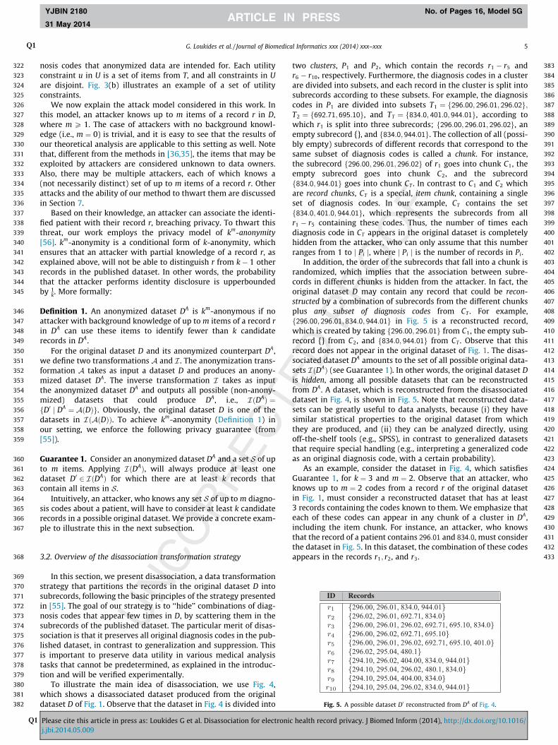
Fig. 5. A possible dataset D0 reconstructed from DA of Fig. 4.

3.2. Overview of the disassociation transformation strategy

In this section, we present disassociation, a data transformationstrategy that partitions the records in the original dataset D intosubrecords, following the basic principles of the strategy presentedin [55]. The goal of our strategy is to ‘‘hide’’ combinations of diag-nosis codes that appear few times in D, by scattering them in thesubrecords of the published dataset. The particular merit of disas-sociation is that it preserves all original diagnosis codes in the pub-lished dataset, in contrast to generalization and suppression. Thisis important to preserve data utility in various medical analysistasks that cannot be predetermined, as explained in the introduc-tion and will be verified experimentally.

To illustrate the main idea of disassociation, we use Fig. 4,which shows a disassociated dataset produced from the originaldataset D of Fig. 1. Observe that the dataset in Fig. 4 is divided into


two clusters, P1 and P2, which contain the records r1 � r5 andr6 � r10, respectively. Furthermore, the diagnosis codes in a clusterare divided into subsets, and each record in the cluster is split intosubrecords according to these subsets. For example, the diagnosiscodes in P1 are divided into subsets T1 ¼ f296:00; 296:01; 296:02g;T2 ¼ f692:71; 695:10g, and TT ¼ f834:0; 401:0; 944:01g, according towhich r1 is split into three subrecords; f296:00; 296:01; 296:02g, anempty subrecord {}, and f834:0; 944:01g. The collection of all (possi-bly empty) subrecords of different records that correspond to thesame subset of diagnosis codes is called a chunk. For instance,the subrecord f296:00; 296:01; 296:02g of r1 goes into chunk C1, theempty subrecord goes into chunk C2, and the subrecordf834:0; 944:01g goes into chunk CT . In contrast to C1 and C2 whichare record chunks, CT is a special, item chunk, containing a singleset of diagnosis codes. In our example, CT contains the setf834:0; 401:0; 944:01g, which represents the subrecords from allr1 � r5 containing these codes. Thus, the number of times eachdiagnosis code in CT appears in the original dataset is completelyhidden from the attacker, who can only assume that this numberranges from 1 to j Pi j, where j Pi j is the number of records in Pi.

In addition, the order of the subrecords that fall into a chunk israndomized, which implies that the association between subre-cords in different chunks is hidden from the attacker. In fact, theoriginal dataset D may contain any record that could be recon-structed by a combination of subrecords from the different chunksplus any subset of diagnosis codes from CT . For example,f296:00; 296:01; 834:0; 944:01g in Fig. 5 is a reconstructed record,which is created by taking f296:00; 296:01g from C1, the empty sub-record {} from C2, and f834:0; 944:01g from CT . Observe that thisrecord does not appear in the original dataset of Fig. 1. The disas-sociated dataset DA amounts to the set of all possible original data-sets IðDAÞ (see Guarantee 1). In other words, the original dataset Dis hidden, among all possible datasets that can be reconstructedfrom DA. A dataset, which is reconstructed from the disassociateddataset in Fig. 4, is shown in Fig. 5. Note that reconstructed data-sets can be greatly useful to data analysts, because (i) they havesimilar statistical properties to the original dataset from whichthey are produced, and (ii) they can be analyzed directly, usingoff-the-shelf tools (e.g., SPSS), in contrast to generalized datasetsthat require special handling (e.g., interpreting a generalized codeas an original diagnosis code, with a certain probability).

As an example, consider the dataset in Fig. 4, which satisfiesGuarantee 1, for k ¼ 3 and m ¼ 2. Observe that an attacker, whoknows up to m ¼ 2 codes from a record r of the original datasetin Fig. 1, must consider a reconstructed dataset that has at least3 records containing the codes known to them. We emphasize thateach of these codes can appear in any chunk of a cluster in DA,including the item chunk. For instance, an attacker, who knowsthat the record of a patient contains 296:01 and 834:0, must considerthe dataset in Fig. 5. In this dataset, the combination of these codesappears in the records r1; r2, and r3.




434

435

436

437

438

439

440

441

442

443

444

445

446

447

448

449

450

451

452

453

454

455

456

457

467

468

469

470

471

472

473

474

475

476

477

478

479

480

481

482483

485485

486

487

488

489

490

491

492

493

494

495

496497

499499

500

501

502

503

504

505

506

507

508

509

510

511

512

513

514

515

516

517

518

519

520

521

522

523



31 May 2014

Q1

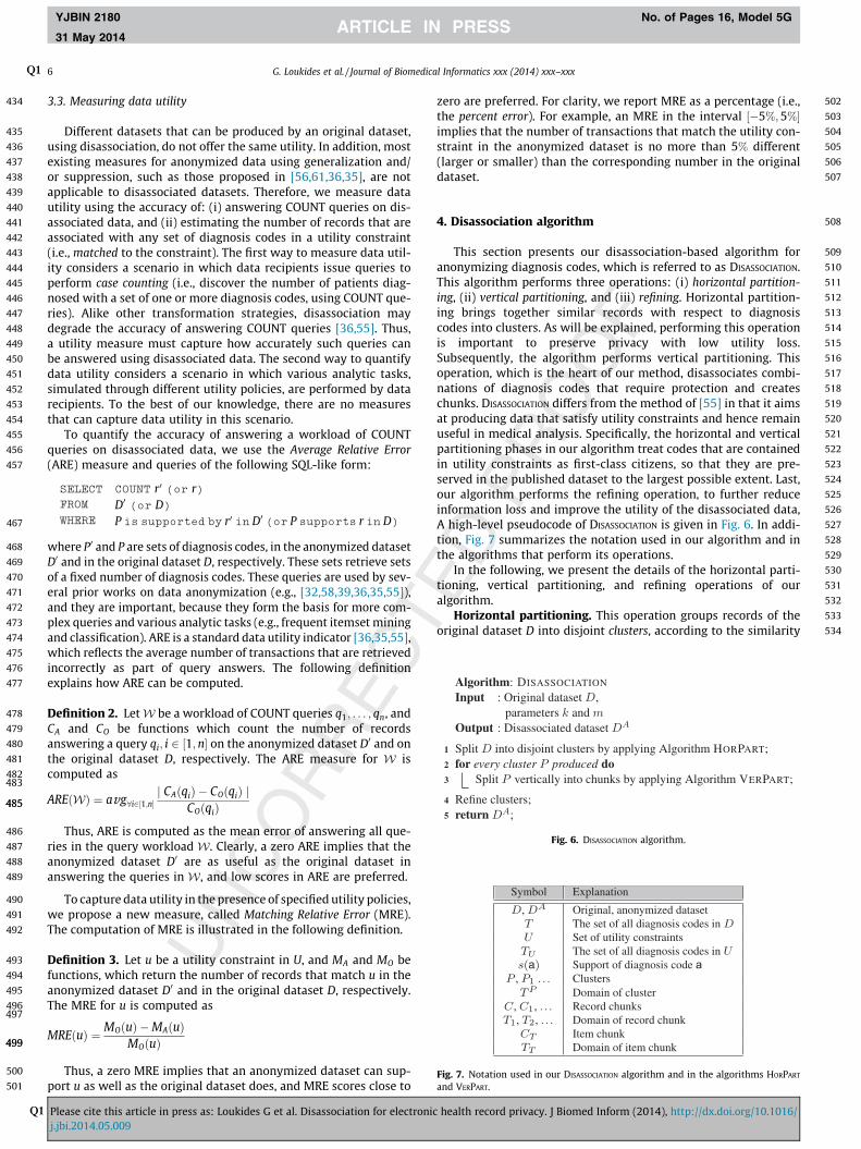
3.3. Measuring data utility

Different datasets that can be produced by an original dataset,using disassociation, do not offer the same utility. In addition, mostexisting measures for anonymized data using generalization and/or suppression, such as those proposed in [56,61,36,35], are notapplicable to disassociated datasets. Therefore, we measure datautility using the accuracy of: (i) answering COUNT queries on dis-associated data, and (ii) estimating the number of records that areassociated with any set of diagnosis codes in a utility constraint(i.e., matched to the constraint). The first way to measure data util-ity considers a scenario in which data recipients issue queries toperform case counting (i.e., discover the number of patients diag-nosed with a set of one or more diagnosis codes, using COUNT que-ries). Alike other transformation strategies, disassociation maydegrade the accuracy of answering COUNT queries [36,55]. Thus,a utility measure must capture how accurately such queries canbe answered using disassociated data. The second way to quantifydata utility considers a scenario in which various analytic tasks,simulated through different utility policies, are performed by datarecipients. To the best of our knowledge, there are no measuresthat can capture data utility in this scenario.

To quantify the accuracy of answering a workload of COUNTqueries on disassociated data, we use the Average Relative Error(ARE) measure and queries of the following SQL-like form:

524

525

Pj.

SELECT

lease cite thjbi.2014.05

COUNT r0 (or r)

526
FROM D0 (or D)
527
WHERE P is supported by r0 in D0 (or P supports r in D)
528

529

530

531

532

533

534

Algorithm: DISASSOCIATION

Input : Original dataset ,parameters and

Output : Disassociated dataset

1 Split into disjoint clusters by applying Algorithm HORPART;2 for every cluster produced do3 Split vertically into chunks by applying Algorithm VERPART;

4 Refine clusters;5 return

Fig. 6. DISASSOCIATION algorithm.

Symbol Explanation

Original, anonymized datasetThe set of all diagnosis codes inSet of utility constraintsThe set of all diagnosis codes inSupport of diagnosis code aClustersDomain of clusterRecord chunksDomain of record chunkItem chunkDomain of item chunk

Fig. 7. Notation used in our DISASSOCIATION algorithm and in the algorithms HORPART

and VERPART.

where P0 and P are sets of diagnosis codes, in the anonymized datasetD0 and in the original dataset D, respectively. These sets retrieve setsof a fixed number of diagnosis codes. These queries are used by sev-eral prior works on data anonymization (e.g., [32,58,39,36,35,55]),and they are important, because they form the basis for more com-plex queries and various analytic tasks (e.g., frequent itemset miningand classification). ARE is a standard data utility indicator [36,35,55],which reflects the average number of transactions that are retrievedincorrectly as part of query answers. The following definitionexplains how ARE can be computed.

Definition 2. LetW be a workload of COUNT queries q1; . . . ; qn, andCA and CO be functions which count the number of recordsanswering a query qi; i 2 ½1;n� on the anonymized dataset D0 and onthe original dataset D, respectively. The ARE measure for W iscomputed as

AREðWÞ ¼ avg8i2½1;n�j CAðqiÞ � COðqiÞ j

COðqiÞ

Thus, ARE is computed as the mean error of answering all que-ries in the query workload W. Clearly, a zero ARE implies that theanonymized dataset D0 are as useful as the original dataset inanswering the queries in W, and low scores in ARE are preferred.

To capture data utility in the presence of specified utility policies,we propose a new measure, called Matching Relative Error (MRE).The computation of MRE is illustrated in the following definition.

Definition 3. Let u be a utility constraint in U, and MA and MO befunctions, which return the number of records that match u in theanonymized dataset D0 and in the original dataset D, respectively.The MRE for u is computed as

MREðuÞ ¼ MOðuÞ �MAðuÞMOðuÞ

Thus, a zero MRE implies that an anonymized dataset can sup-port u as well as the original dataset does, and MRE scores close to

is article in press as: Loukides G et al. Disassociation for electronic.009

zero are preferred. For clarity, we report MRE as a percentage (i.e.,the percent error). For example, an MRE in the interval ½�5%;5%�implies that the number of transactions that match the utility con-straint in the anonymized dataset is no more than 5% different(larger or smaller) than the corresponding number in the originaldataset.

4. Disassociation algorithm

This section presents our disassociation-based algorithm foranonymizing diagnosis codes, which is referred to as DISASSOCIATION.This algorithm performs three operations: (i) horizontal partition-ing, (ii) vertical partitioning, and (iii) refining. Horizontal partition-ing brings together similar records with respect to diagnosiscodes into clusters. As will be explained, performing this operationis important to preserve privacy with low utility loss.Subsequently, the algorithm performs vertical partitioning. Thisoperation, which is the heart of our method, disassociates combi-nations of diagnosis codes that require protection and createschunks. DISASSOCIATION differs from the method of [55] in that it aimsat producing data that satisfy utility constraints and hence remainuseful in medical analysis. Specifically, the horizontal and verticalpartitioning phases in our algorithm treat codes that are containedin utility constraints as first-class citizens, so that they are pre-served in the published dataset to the largest possible extent. Last,our algorithm performs the refining operation, to further reduceinformation loss and improve the utility of the disassociated data,A high-level pseudocode of DISASSOCIATION is given in Fig. 6. In addi-tion, Fig. 7 summarizes the notation used in our algorithm and inthe algorithms that perform its operations.

In the following, we present the details of the horizontal parti-tioning, vertical partitioning, and refining operations of ouralgorithm.

Horizontal partitioning. This operation groups records of theoriginal dataset D into disjoint clusters, according to the similarity




535

536

537

538

539

540

541

542

543

544

545

546

547

548

549

550

551

552

553

554

555

556

557

558

559

560

561

562

563

564

565

566

567

568

569

570

571

572

573

574

575

576

577

578

579

580

581

582

583

584

585

586

587

588

589

590

591

592

593

594

595

596

597

598

599

600

601

602

603

604

605

606

607

608

609

610

611

612



31 May 2014

Q1

of diagnosis codes. For instance, cluster P1 is formed by recordsr1 � r5, which have many codes in common, as can be seen inFig. 4. The creation of clusters is performed with a light-weight,but very effective heuristic, called HORPART. The pseudocode of HOR-

PART is provided in Fig. 8. This heuristic aims at creating coherentclusters, whose records will require the least possible disassocia-tion, during vertical partitioning.

To achieve this, the key idea is to split the dataset into twoparts, D1 and D2, according to: (i) the support of diagnosis codesin D (the support of a diagnosis code a, denoted with sðaÞ, is thenumber of records in D in which a appears), and (ii) the participa-tion of diagnosis codes in the utility policy U. At each step, D1 con-tains all records with the diagnosis code a, whereas D2 contains theremaining records. This procedure is applied recursively, to each ofthe constructed parts, until they are small enough to become clus-ters. Diagnosis codes that have been previously used for partition-ing are recorded in a set ignore and are not used again.

In each recursive call, Algorithm HORPART selects a diagnosiscode a, in lines 3–10. In the first call, a is selected as the most fre-quent code (i.e., the code with the largest support), which is con-tained in a utility constraint. At each subsequent call, a isselected as the most frequent code, among the codes containedin u (i.e., the utility constraint with the code chosen in the previouscall) (line 4). When all diagnosis codes in u have been considered, ais selected as the most frequent code in the set fT � ignoreg, whichis also contained in a utility constraint (line 6). Of course, if nodiagnosis code is contained in a utility constraint, we simply selecta as the most frequent diagnosis code (line 9).

Horizontal partitioning reduces the task of anonymizing theoriginal dataset to the anonymization of small and independentclusters. We opted for this simple heuristic, because it achieves agood trade-off between data utility and efficiency, as shown inour experiments. However, we note that any other algorithm forcreating groups of at least k records could be used instead.

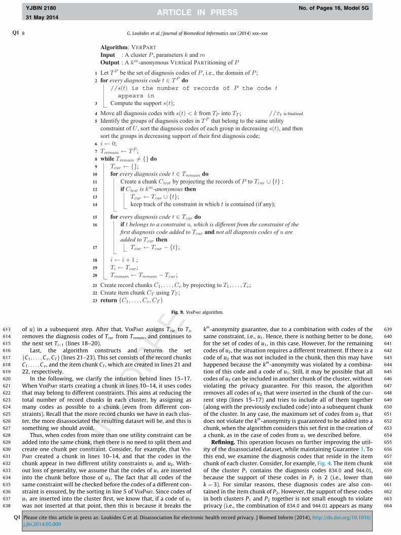
Vertical partitioning. This operation partitions the clusters intochunks, using a greedy heuristic that is applied to each clusterindependently. The intuition behind the operation of this heuristic,called VERPARTZ, is twofold. First, the algorithm tries to distributeinfrequent combinations of codes into different chunks to preserve

Fig. 8. HORPART


privacy, as in [55]. Second, it aims at satisfying the utility con-straints, in which the diagnosis codes in the cluster are contained.To achieve this, the algorithm attempts to create record chunks,which contain as many diagnosis codes from the same utility con-straint as possible. Clearly, creating a record chunk that contains allthe diagnosis codes of one or more utility constraints is beneficial,as tasks involving these codes (e.g., clinical case count studies) canbe performed as accurately as in the original dataset.

The pseudocode of VERPART is provided in Fig. 9. This algorithmtakes as input a cluster P, along with the parameters k and m,and returns a set of km-anonymous record chunks C1; . . . ;Cv , andthe item chunk CT of P. Given the set of diagnosis codes TP in P, VER-

PART computes the support sðtÞ of every code t in P and moves alldiagnosis codes having lower support than k from TP to a set TT

(lines 2–4). As the remaining codes have support at least k, theywill participate in some record chunk. Next, it orders TP accordingto: (i) sðtÞ, and (ii) the participation of the codes in utility con-straints (line 5). Specifically, the diagnosis codes in P that belongto the same constraint u in U form groups, which are orderedtwo times; first in decreasing sðtÞ, and then in decreasing sðtÞ oftheir first (most frequent) diagnosis code.

Subsequently, VERPART computes the sets T1; . . . ; Tv (lines 6–20).To this end, the set Tremain, which contains the ordered, non-assigned codes, and the set Tcur , which contains the codes that willbe assigned to the current set, are used. To compute Tið1 6 i 6 vÞ,VERPART considers all diagnosis codes in Tremain and inserts a code tinto Tcur , only if the Ctest chunk, constructed from Tcur [ ftg, remainskm-anonymous (line 13). Note that the first execution of the forloop in line 10, will always add t into Tcur , since Ctest ¼ ftg is km-anonymous. If the insertion of t to Tcur does not renderTcur [ ftg km-anonymous, t is skipped and the algorithm considersthe next code. While assigning codes from Tremain to Tcur , VERPART

also tracks the utility constraint that each code is contained in (line14). Next, VERPART iterates over each code t in Tcur and removes itfrom Tcur , if two conditions are met: (i) t is contained in a utilityconstraint u that is different from the constraint of the first codeassigned to Tcur , and (ii) all codes in u have also been assigned toTcur (lines 16–17). Removing t enables the algorithm to insert thecode into another record chunk (along with the remaining codes

algorithm.




613

614

615

616

617

618

619

620

621

622

623

624

625

626

627

628

629

630

631

632

633

634

635

636

637

638

639

640

641

642

643

644

645

646

647

648

649

650

651

652

653

654

655

656

657

658

659

660

661

662

663

664

Fig. 9. VERPART algorithm.



31 May 2014

Q1

of u) in a subsequent step. After that, VERPART assigns Tcur to Ti,removes the diagnosis codes of Tcur from Tremain, and continues tothe next set Tiþ1 (lines 18–20).

Last, the algorithm constructs and returns the setfC1; . . . ;Cv ; CTg (lines 21–23). This set consists of the record chunksC1; . . . ;Cv , and the item chunk CT , which are created in lines 21 and22, respectively.

In the following, we clarify the intuition behind lines 15–17.When VERPART starts creating a chunk in lines 10–14, it uses codesthat may belong to different constraints. This aims at reducing thetotal number of record chunks in each cluster, by assigning asmany codes as possible to a chunk (even from different con-straints). Recall that the more record chunks we have in each clus-ter, the more disassociated the resulting dataset will be, and this issomething we should avoid.

Thus, when codes from more than one utility constraint can beadded into the same chunk, then there is no need to split them andcreate one chunk per constraint. Consider, for example, that VER-

PART created a chunk in lines 10–14, and that the codes in thechunk appear in two different utility constraints u1 and u2. With-out loss of generality, we assume that the codes of u1 are insertedinto the chunk before those of u2. The fact that all codes of thesame constraint will be checked before the codes of a different con-straint is ensured, by the sorting in line 5 of VERPART. Since codes ofu1 are inserted into the cluster first, we know that, if a code of u1

was not inserted at that point, then this is because it breaks the


km-anonymity guarantee, due to a combination with codes of thesame constraint, i.e., u1. Hence, there is nothing better to be done,for the set of codes of u1, in this case. However, for the remainingcodes of u2, the situation requires a different treatment. If there is acode of u2 that was not included in the chunk, then this may havehappened because the km-anonymity was violated by a combina-tion of this code and a code of u1. Still, it may be possible that allcodes of u2 can be included in another chunk of the cluster, withoutviolating the privacy guarantee. For this reason, the algorithmremoves all codes of u2 that were inserted in the chunk of the cur-rent step (lines 15–17) and tries to include all of them together(along with the previously excluded code) into a subsequent chunkof the cluster. In any case, the maximum set of codes from u2 thatdoes not violate the km-anonymity is guaranteed to be added into achunk, when the algorithm considers this set first in the creation ofa chunk, as in the case of codes from u1 we described before.

Refining. This operation focuses on further improving the util-ity of the disassociated dataset, while maintaining Guarantee 1. Tothis end, we examine the diagnosis codes that reside in the itemchunk of each cluster. Consider, for example, Fig. 4. The item chunkof the cluster P1 contains the diagnosis codes 834:0 and 944:01,because the support of these codes in P1 is 2 (i.e., lower thank ¼ 3). For similar reasons, these diagnosis codes are also con-tained in the item chunk of P2. However, the support of these codesin both clusters P1 and P2 together is not small enough to violateprivacy (i.e., the combination of 834:0 and 944:01 appears as many




665

666

667

668

669

670

671

672

673

674

675

676

677

678

679

680

681

682

683

684

685

686

687

688

689

690

691

692

693

694

695

696

697

698

699

700

701

702

703

704

705

706

707

708

709

710

711

712

713

714

715

716

717

718

719

720

721

722

723

724

725

726

727

728

729

730

731

732

733

734

735

736

737

738

739

740

741

742

743

744

745

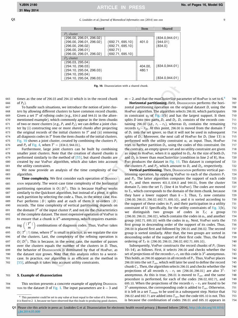
Fig. 10. Disassociation with a shared chunk.



31 May 2014

Q1

times as the one of 296:03 and 294:10 which is in the record chunkof P2).

To handle such situations, we introduce the notion of joint clus-ters by allowing different clusters to have common record chunks.Given a set Ts of refining codes (e.g., 834:0 and 944:01 in the afore-mentioned example), which commonly appear in the item chunksof two or more clusters (e.g., P1 and P2), we can define a joint clus-ter by (i) constructing one or more shared chunks after projectingthe original records of the initial clusters to Ts and (ii) removingall diagnosis codes in Ts from the item chunks of the initial clusters.Fig. 10 shows a joint cluster, created by combining the clusters P1

and P2 of Fig. 4, when Ts ¼ f834:0; 944:01g.Furthermore, large joint clusters can be built by combining

smaller joint clusters. Note that the creation of shared chunks isperformed similarly to the method of [55], but shared chunks arecreated by our VERPART algorithm, which also takes into accountthe utility constraints.

We now provide an analysis of the time complexity of ouralgorithm.

Time complexity. We first consider each operation of DISASSOCI-

ATION separately. The worst-case time complexity of the horizontal

partitioning operation is Oðj Dj2Þ. This is because HORPART workssimilarly to the Quicksort algorithm, but instead of a pivot, it splitseach partition by selecting the code a. Thus, in the worst case, HOR-

PART performs j D j splits and at each of them it re-orders j D jrecords. The time complexity of vertical partitioning depends onthe domain TP of the input cluster P, and not on the characteristicsof the complete dataset. The most expensive operation of VERPART isto ensure that a chunk is km-anonymous, which requires examin-

ing j TP jm

� �combinations of diagnosis codes. Thus, VERPART takes

Oðj TP j !Þ time, where TP is small in practice, as we regulate the sizeof the clusters. Last, the complexity of the refining operation is

Oðj Dj2Þ. This is because, in the worst case, the number of passesover the clusters equals the number of the clusters in D. Thus,the behavior of DISASSOCIATION is dominated by that of HORPART, asthe dataset size grows. Note that this analysis refers to a worst-case. In practice, our algorithm is as efficient as the method in[55], although it takes into account utility constraints.

746

747

748

749

750

751

5. Example of disassociation

This section presents a concrete example of applying DISASSOCIA-

TION to the dataset D of Fig. 1. The input parameters are k ¼ 3 and
752
753

754

4 This parameter could be set to any value at least equal to the value of k. However,it is fixed to 2 � k, because we have observed that this leads to producing good clusters.


m ¼ 2, and that the maxClusterSize parameter of HORPART is set to 6.4

Horizontal partitioning. First, DISASSOCIATION performs the hori-zontal partitioning operation on the original dataset D, using theHORPART algorithm. The algorithm selects 296:00, which participatesin constraint u1 of Fig. 3(b) and has the largest support. It thensplits D into two parts, D1 and D2. D1 consists of the records con-taining 296:00 (i.e., r1 � r5), whereas D2 contains the remainingrecords r6 � r10. At this point, 296:00 is moved from the domain Tof D1 into the set ignore, so that it will not be used in subsequentsplits of D1. Moreover, the next call of HORPART for D1 (line 13) isperformed with the utility constraint u1 as input. Thus, HORPART

tries to further partition D1, using the codes of this constraint. Onthe contrary, an empty ignore set and no utility constraint are givenas input to HORPART, when it is applied to D2. As the size of both D1

and D2 is lower than maxClusterSize (condition in line 2 of 8), HOR-

PART produces the dataset in Fig. 11. This dataset is comprised ofthe clusters P1 and P2, which amount to D1 and D2, respectively.

Vertical partitioning. Then, DISASSOCIATION performs vertical par-titioning operation, by applying VERPART to each of the clusters P1

and P2. The latter algorithm computes the support of each codein P1, and then moves 401:0; 834:0 and 944:01, from the clusterdomain TP into the set TT (line 4 in VERPART). The codes are movedto TT , which corresponds to the domain of the item chunk, becausethey have a lower support than k ¼ 3. Thus, TP now containsf296:00; 296:01; 296:02; 692:71; 695:10g, and it is sorted according tothe support of these codes in P1 and their participation in a utilityconstraint of U. Specifically, for the utility constraints of Fig. 3(b),we distinguish two groups of codes in TP; a groupf296:00; 296:01; 296:02g, which contains the codes in u1, and anothergroup f692:71; 695:10g with the codes in u2. Next, VERPART sorts thefirst group in descending order of the support of its codes. Thus,296:00 is placed first and followed by 296:01 and 296:02. The secondgroup is sorted similarly. After that, the two groups are sorted indescending order of the support of their first code. Thus, the finalordering of TP is f296:00; 296:01; 296:02; 692:71; 695:10g.

Subsequently, VERPART constructs the record chunks of P1 (lines10–14), as follows. First, it selects 296:00 and checks whether theset of projections of the records r1-r5 on this code is 32-anonymous.This holds, as 296:00 appears in all records of P1. Thus, VERPART places296:00 into the set Tcur , which will later be used to define the recordchunk C1. Then, the algorithm selects 296:01 and checks whether theprojections of all records r1 � r5 on f296:00; 296:01g are also 32-anonymous. As this is true, 296:01 is moved to Tcur , and the sameprocedure is performed, for each of the codes 296:02; 692:71, and695:10. When the projections of the records r1 � r5 are found to be32-anonymous, the corresponding code is added to Tcur . Otherwise,it is left in a set Tremain to be used in a subsequent step. Notice that296:02 and 692:71 are added into Tcur , but the code 695:10 is not. Thisis because the combination of codes 296:01 and 695:10 appears in




755

756

757

758

759

760

761

762

763

764

765

766

767

768

769

770

771

772

773

774

775

776

777

778

779

780

781

782

783

784

785

786

787

788

789

790

791

792

793

794

795

796

797

798

799

800

801

802

803

804

805

806

807

808

809

810

811

812

813

814

815

816

817

818

819

820

821

822

823

824

825

826

827

828

829

830

831

832

833

834

835

836

837

838

839

Fig. 11. Output of horizontal partitioning on D.

Table 1Description of the dataset.

Dataset j D j Distinct codes Max, Avg # codes/record

INFORMS 58,302 631 43, 5.11



31 May 2014

Q1

only two records of P1 (i.e., r2 and r5), hence, the projections ofrecords r1 � r5 on f296:00; 296:01; 296:02; 692:71; 695:10g are not 32-anonymous.

After considering all codes in TP , VERPART checks whether thecodes of a constraint u 2 U are only partially added to Tcur . This istrue for 692:71, which is separated from 695:10 of the same constraintu2. Hence, 692:71 is moved from Tcur back to Tremain (line 17), so that itcan be added to the chunk C2 of P1 along with 695:10. After that, thealgorithm finalizes the chunk C1, according to Tcur , empties the latterset, and proceeds to creating C2. By following this procedure for thecluster P2, VERPART constructs the dataset DA in Fig. 4.

Refining. During this operation, DISASSOCIATION constructs theshared chunks, which are shown in Fig. 10, as follows. It inspectsthe item chunks of P1 and P2 in Fig. 4, and it identifies that eachof the codes 834:0 and 944:01 appears in two records of P1, as wellas in two records of P2. Note that the actual supports of codes initem chunks are available to the algorithm after the vertical parti-tioning operation, although they are not evident from Fig. 4(because they are completely hidden in the published dataset).Since the total support of 834:0 and 944:01 in both clusters is2þ 2 ¼ 4 > k ¼ 3, the algorithm reconstructs the projections ofr1 � r5 and r6 � r10 on the item chunk domain of P1 and P2 respec-tively, and calls VERPART, which creates the shared chunk of Fig. 10.

840

841

842

843

844

845

846

847

848

849

850

851

852

853

854

855

5 Sections and Chapters are internal nodes in the ICD hierarchy, which modelaggregate concepts http://www.cdc.gov/nchs/data/icd9/icdguide10.pdf.

6. Experimental evaluation

6.1. Experimental data and setup

We implemented all algorithms in C++ and applied them to theINFORMS dataset [8], whose characteristics are shown in Table 1.This dataset was used in INFORMS 2008 Data Mining contest,whose objective was to develop predictive methods for identifyinghigh-risk patients, admitted for elective surgery. In our experi-ments, we retained the diagnosis code part of patient records only.

We evaluated the effectiveness of our DISASSOCIATION algorithm,referred to as Dis, by comparing to CBA, which employs generaliza-tion to prevent identity disclosure based on diagnosis codes. Thedefault parameters were k ¼ 5 and m ¼ 2, and the hierarchies usedin CBA were created as in [35]. All experiments ran on an Intel Xeonat 2.4 GHz with 12 GB of RAM.

To evaluate data utility, we employed the ARE and MRE mea-sures, discussed in Section 3.3. For the computation of ARE, weused two different types of query workloads. The first workloadtype, referred to as W1, contains queries asking for sets of


diagnosis codes that a certain percentage of all patients have. Inother words, these queries retrieve frequent itemsets (i.e., sets ofdiagnosis codes that appear in at least a specified percentage ofrecords (transactions), expressed using a minimum support thresh-old). Answering such queries accurately is crucial in various bio-medical data analysis applications [35], since frequent itemsetsserve as building blocks in several data mining models [32]. Thesecond workload type we considered is referred to asW2 and con-tains 1000 queries, which retrieve sets of diagnosis codes, selecteduniformly at random. These queries are important, because it maybe difficult for data owners to predict many of the analytic tasksthat will be applied to anonymized data by data recipients.

In addition, we evaluated MRE using three classes of utility pol-icies: hierarchy-based, similarity-based, and frequency-based. Thefirst two types of policies have been introduced in [35] and modelsemantic relationships between diagnosis codes. For hierarchy-based policies, these relationships are formed using the ICD hierar-chy. Specifically, hierarchy-based utility policies are constructed byforming a different utility constraint for all 5-digit ICD codes thathave a common ancestor (other than the root) in the ICD hierarchy.The common ancestor of these codes is a 3-digit ICD code, Section,or Chapter,5 for the case of level 1, level 2, and level 3 hierarchy-basedpolicies, respectively. For example, consider a utility constraint u forSchizophrenic disorders. The 5-digit ICD codes in u are of the form295:xy, where x ¼ f0; . . . ;9g and y ¼ f0; . . . ;5g, and they have the3-digit ICD code 295 as their common ancestor. The utility constraintu is shown in the first row of Table 2. By forming a different utilityconstraint, for each 3-digit ICD code in the hierarchy (e.g., 296,297, etc.), we construct a level 1, hierarchy-based policy. Alterna-tively, the common ancestor of the codes in the utility constraint umay be a Section. For example, u is comprised of Psychoses, whosecommon ancestor is 295� 299, in the second row of Table 2. In thiscase, u will be contained in a level 2, hierarchy-based policy. Inanother case, the common ancestor for the codes in u may be a Chap-ter. For example, u may correspond to Mental disorders that have290� 319 as their common ancestor (see the last row of Table 2).In this case, u is contained in a level 3, hierarchy-based policy.

The similarity-based utility policies are comprised from utilityconstraints that contain the same number of sibling 5-digit ICDcodes in the hierarchy. Specifically, we considered similarity-basedconstraints containing 5, 10, 25, and 100 codes and refer to theirassociated utility policies as sim 5, 10, 25, and 100, respectively.Consider, for instance, a utility constraint that contains 5 siblingICD codes; 295.00, 295.01, 295.02, 295.03, and 295.04. This con-straint, as well as all other constraints that contain 5 sibling ICDcodes (e.g., a utility constraint that contains 296.00, . . ., 296.04),will be contained in a sim 5 utility policy. Last, we considered fre-quency-based utility policies that model frequent itemsets. Wemined frequent itemsets using the FP-Growth algorithm [27],which was configured with a varying minimum support thresholdin f0:625;1:25;2:5;5g. Thus, the generated utility constraintscontain sets of diagnosis codes that appear in at least0:625%;1:25%;2:5%, and 5% percent of records, respectively. Theutility policies associated with such constraints are denoted withsup 0.625, 1.25, 2.5, and 5, respectively. Unless otherwise stated,we use level 1, sim 10, and sup 0.625, as the default hierarchy, sim-ilarity, and frequency based utility policy, respectively.

6.2. Feasibility of identity disclosure

The risk of performing identity disclosure was quantified bymeasuring the number of records that share a set of m diagnosis


http://www.cdc.gov/nchs/data/icd9/icdguide10.pdf



856

857

858

859

860

861

862

863

864

865

866

867

868

869

870

871

872

873

874

875

876

877

878

879

880

881

882

883

884

885

886

887

888

889

890

891

892

893

894

895

896

897

898

899

900

901

902

903

904

905

906

907

908

909

910

911

912

913

914

915

916

917

918

919

920

921

922

923

924

925

926

927

928

929

930

931

932

933

934

935

936

937

938

939

940

941

942

943

944

945

946

947

948

949

950

951

952

953

954

955

956

957

Table 2Examples of hierarchy-based utility constraints.

Type Codes in utility constraint

level 1 f295:00;295:01; . . . ;295:95glevel 2 f295:00;295:01; . . . ;295:95;296:00; . . . ;299:91glevel 3 f290:10;295:00;295:01; . . . ;295:95;296:00; . . . ;299:91; . . . ;299:91;

. . . ;319g

0

20

40

60

80

100

(%)

ofco

deco

mbi

natio

ns

1 2 3 4 5 6 7 8 9 10 >10

# records they appear

2 codes

3 codes

4 codes

5 codes

Fig. 12. Number of records in which a percentage of combinations, containing 2 to5 diagnosis codes, appears.



31 May 2014

Q1

codes. This number equals the inverse of the probability of per-forming identity disclosure, using these codes. Fig. 12 shows thatmore than 17% of all sets of 2 diagnosis codes appear in one record.Consequently, more than 17% of patients are uniquely re-identifi-able, if the dataset is released intact. Furthermore, fewer than 5%of records contain a diagnosis code that appears at least 5 times.Thus, approximately 95% of records are unsafe, based on the prob-ability threshold of 0:2 that is used typically [19]. Moreover, thenumber of times a set of diagnosis codes appears in the datasetincreases with m. For example, 96% of sets containing 5 diagnosiscodes appear only once. As we will see shortly, our algorithm canthwart attackers with such knowledge, by enforcing km-anonymitywith m ¼ 5, while preserving data utility.

6.3. Comparison with CBA

In this set of experiments, we demonstrate that our method canenforce km-anonymity, while allowing more accurate queryanswering than CBA. We also examine the impact of dataset sizeon the effectiveness and efficiency of both methods.

We first report ARE for query workloads of typeW1 and for thefollowing utility policies: level 1 (hierarchy-based), sim 10 (similar-ity-based), and sup 1.25 (frequency-based). For a fair comparison,the diagnosis codes retrieved by all queries are among those thatare not suppressed by CBA. Fig. 13(a) illustrates the results forthe level 1 policy. On average, the ARE scores for Dis and CBA are0.055 and 0.155, respectively. This shows that the use of disassoci-ation instead of generalization allows enforcing km-anonymitywith low information loss. Figs. 13(b) and (c) show the correspond-ing results for the similarity-based and frequency-based policies,respectively. Again, our method outperformed CBA, achieving AREscores that are substantially lower (better). Of note, the differencebetween the ARE scores for Dis and CBA, in each of the experimentsin Figs. 13(a)–(c), was found to be statistically significant, accord-ing to Welch’s t-test ðp < 0:01Þ. It is also worth noting that the dif-ference of Dis and CBA with respect to ARE, increases as the utilitypolicies get less stringent. For instance, the ARE scores for Dis andCBA are 0.129 and 0.163, respectively, for level 1, hierarchy-basedpolicies, but 0.006 and 0.1, respectively, for level 3, hierarchy-basedpolicies. This suggests that both algorithms perform reasonably


well with respect to query answering, for restrictive constraints.However, CBA does so by suppressing a large number of diagnosiscodes, as will be discussed later. Thus, the result of CBA is generallyof lower utility (e.g., it does not allow queries on suppressed codesto be answered). Quantitatively similar results were obtained forquery workloads of type W2 (omitted, for brevity).

Next, we report the number of distinct diagnosis codes that aresuppressed when k is set to 5, m is 2 or 3, and the utility policies ofthe previous experiment are used. The results in Fig. 14 show thatCBA suppressed a relatively large number of diagnosis codes, par-ticularly when strong privacy is required and the utility constraintsare stringent. For instance, 23:6% (i.e., 149 out of 631) of distinctdiagnoses codes were suppressed, when m ¼ 3 and the level 1 util-ity policy was used. On the contrary, our method released all diag-noses codes intact, as it does not employ suppression. This isparticularly useful for medical studies (e.g., in epidemiology),where a large number of codes are of interest.

Then, we examined the effect of dataset size on ARE, by apply-ing Dis and CBA on increasingly larger subsets of the dataset. Thesmallest and largest of these subsets contain the first 2:5K and25K records of the dataset, respectively. In addition, we used queryworkloads of typeW2 and the sup 1.25 utility policy. The results inFig. 15(a) show that both algorithms incurred more informationloss to anonymize smaller datasets. This is expected, because alldatasets contain at least 79% of the diagnosis codes of the entiredataset, and many sets of diagnosis codes have a lower supportthan k. The ARE scores for Dis were always low, and substantiallylower than those for CBA, for smaller datasets. For example, forthe smallest dataset, the ARE scores for Dis and CBA were 0.95and 11.57. The difference between the ARE scores for Dis andCBA, in all the results in Fig. 15(a), was found to be statistically sig-nificant, according to Welch’s t-test ðp < 0:01Þ. Furthermore, asshown in Fig. 15(b), CBA suppressed a relatively large percentageof diagnosis codes, which decreased as the dataset size grows, forthe reason explained before.

Last, we compared the runtime of Dis to that of CBA. We usedthe same parameters as in Fig. 15(b), and report the results inFig. 15(c). As can be seen, both algorithms required less than 5 s.However, Dis is more efficient than CBA, and the performance gainincreases with the dataset size. Specifically, Dis needed 1.2 s toanonymize the largest dataset, while Dis needed 4.9 s. In addition,the computation cost of Dis remained sub-quadratic, for all testeddatasets.

Having established that our method outperforms CBA, we donot include results for CBA in the remainder of the section.

6.4. Supporting clinical case count studies

In the following, we demonstrate the effectiveness of ourmethod at producing data that support clinical case count studies.

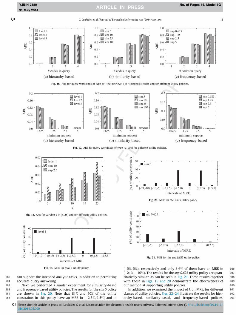
Fig. 16(a) illustrates the results for all three hierarchy-basedpolicies and for query workloads of type W2. These workloadsrequire retrieving a randomly selected set of 1 to 4 diagnosis codes.For consistency, we add a random code to a set of c diagnosis codesto produce a larger set of c þ 1 codes. For instance, a random codeis added to a set of 1 diagnosis code to obtain a set containing 2diagnosis codes. Observe that the error in query answering is fairlysmall and increases with the size of sets of diagnosis codes. This isbecause larger sets appear in few records and are more difficult tobe made km-anonymous. Furthermore, low ARE scores areachieved, even for the level 1 utility policy, which is difficult to sat-isfy using generalization. Similar observations can be made forother types of constraints, as can be seen in Figs. 16(b) and (c).

Fig. 17(a) shows the results, for hierarchy-based constraints andquery workloads of typeW1. The corresponding results for similar-ity-based and frequency-based constraints are reported in Figs.




958

959

960

961

962

963

964

965

966

967

968

969

970

971

972

973

974

975

976

977

978

979

(a) level 1 (b) sim 10 (c) sup 1.25

Fig. 13. Comparison with CBA with respect to ARE for query workloads of type W1 and for different utility policies.

Fig. 14. Percentage of distinct diagnosis codes that are suppressed by CBA (nodiagnosis codes are suppressed by our method, by design).



31 May 2014

Q1

17(b) and (c), respectively. Note that ARE scores are very low. Inaddition, queries involving more frequent sets of diagnosis codescan be answered highly accurately.

Next, we examined the impact of k on ARE, by varying thisparameter in ½5;25�, and considering the level 1, sim 10, and sup

(a)

0

1

2

3

4

5

6

Tim

e (s

ec)

2.5K 5K

# record

CBA

Dis

Quadratic

Fig. 15. Impact of dataset size on (a) ARE, (b) percentage of dis


2.5 utility policies. As can be seen in Fig. 18, ARE increases with k,as it is more difficult to retain associations between diagnosis codes,when clusters are large. However, the ARE scores are low, whichindicates that our method permits accurate query answering.

6.5. Effectiveness in medical analytic tasks

In this set of experiments, we evaluate our method in terms ofits effectiveness at supporting different utility policies. Given autility policy, we measure MRE, for all constraints in the policy,and report the percentage of constraints, whose MRE falls into acertain interval. Recall from Section 6.1 that intervals whose end-points are close to zero are preferred.

Fig. 19 reports the results, for the level 1 utility policy. The MREof all constraints in this policy is in ½�24%;5%Þ, while the MRE ofthe vast majority of constraints falls into much narrower intervals.Furthermore, the percentage of constraints with an MRE scoreclose to zero is generally higher compared to those with MRE isfar from zero. This confirms that the data produced by our method

(b)

10K 25K

s in dataset(c)

tinct codes that are suppressed by CBA, and (c) efficiency.




980

981

982

983

984

985

986

987

988

989

990

991

992

993

0.0

0.2

0.4

0.6

0.8

1.0A

RE

# codes in query

level 1level 2level 3

(a) hierarchy-based

0.0

0.2

0.4

0.6

0.8

1.0

AR

E

# codes in query

sim 5sim 10sim 25sim 100

(b) similarity-based

0.0

0.2

0.4

0.6

0.8

1.0

AR

E

1 2 3 4 1 2 3 4 1 2 3 4

# codes in query

sup 0.625sup 1.25sup 2.5sup 5

(c) frequency-based

Fig. 16. ARE for query workloads of type W2 that retrieve 1 to 4 diagnosis codes and for different utility policies.

0.0

0.04

0.08

0.12

0.16

0.2

AR

E

minimum support

level 1level 2level 3

(a) hierarchy-based

0.0

0.04

0.08

0.12

0.16

0.2A

RE

minimum support

sim 5sim 10sim 25sim 100

(b) similarity-based

0.0

0.05

0.1

0.15

0.2

AR

E

0.625 1.25 2.5 5 0.625 1.25 2.5 5 0.625 1.25 2.5 5

minimum support

sup 0.625sup 1.25sup 2.5sup 5

(c) frequency-based

Fig. 17. ARE for query workloads of type W1 and for different utility policies.

0.0

0.01

0.02

0.03

0.04

0.05

AR

E

2 5 10 15 25

k

level 1sim 10sup 2.5

Fig. 18. ARE for varying k in ½5;25� and for different utility policies.

0

20

40

60

(%)

ofut

ility

cons

trai

nts

intervals of MRE

level 1

[-24,-10) [-10,-5) [-5,2.5) [-2.5,0) 0 (0,2.5) [2.5,5)

Fig. 19. MRE for level 1 utility policy.

0

20

40

60

(%)

ofut

ility

cons

trai

nts

[-21,-10) [-10,-5) [-5,2.5) [-2.5,0) 0 (0,2.5) [2.5,5)

intervals of MRE

sim 5

Fig. 20. MRE for the sim 5 utility policy.

0

20

40

60

80

100

(%)

ofut

ility

cons

trai

nts

[-10,-5) [-5,2.5) [-2.5,0) 0 (0,2.5)

intervals of MRE

sup 0.625

Fig. 21. MRE for the sup 0.625 utility policy.



31 May 2014

Q1

can support the intended analytic tasks, in addition to permittingaccurate query answering.

Next, we performed a similar experiment for similarity-basedand frequency-based utility policies. The results for the sim 5 policyare shown in Fig. 20. Note that 81% and 90% of the utilityconstraints in this policy have an MRE in ½�2:5%;2:5%� and in


½�5%;5%Þ, respectively and only 3:6% of them have an MRE in½�21%;�10%Þ. The results for the sup 0.625 utility policy are quan-titatively similar, as can be seen in Fig. 21. These results togetherwith those in Figs. 19 and 20 demonstrate the effectiveness ofour method at supporting utility policies.

In addition, we examined the impact of k on MRE, for differentclasses of utility policies. Figs. 22–24 illustrate the results for hier-archy-based, similarity-based, and frequency-based policies,




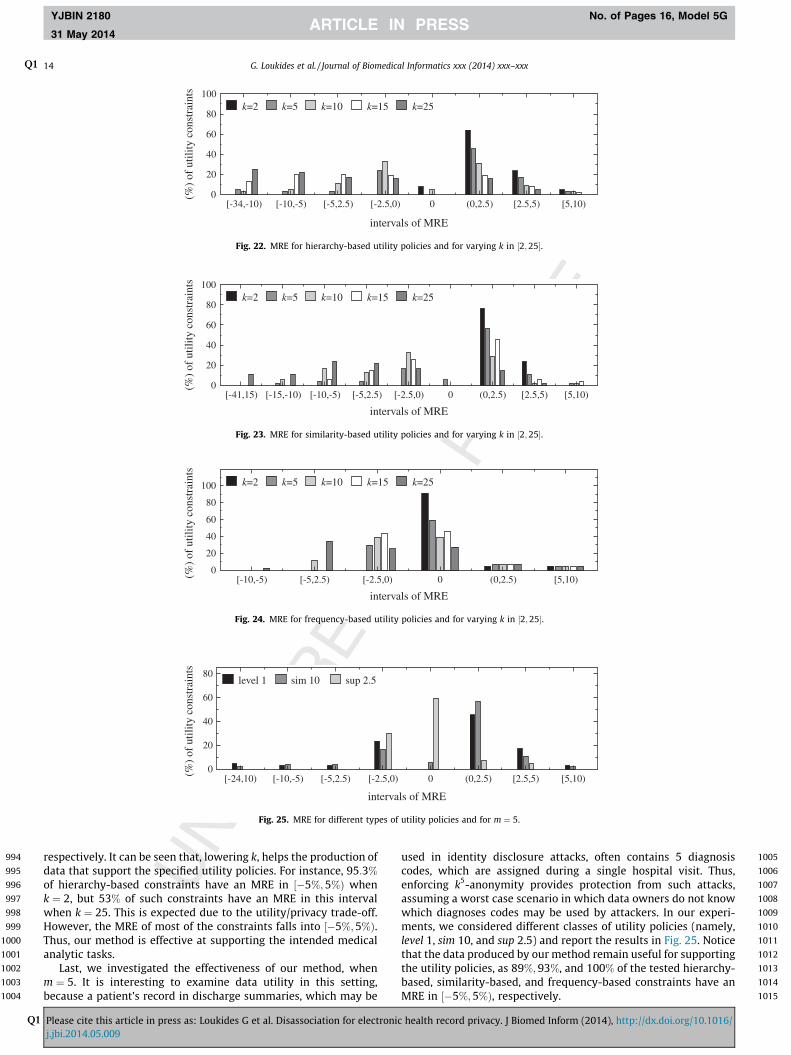
994

995

996

997

998

999

1000

1001

1002

1003

1004

1005

1006

1007

1008

1009

1010

1011

1012

1013

1014

1015

0

20

40

60

80

100

(%)

ofut

ility

cons

trai

nts

[-34,-10) [-10,-5) [-5,2.5) [-2.5,0) 0 (0,2.5) [2.5,5) [5,10)

intervals of MRE

k=2 k=5 k=10 k=15 k=25

Fig. 22. MRE for hierarchy-based utility policies and for varying k in ½2;25�.

0

20

40

60

80

100

(%)

ofut

ility

cons

trai

nts

intervals of MRE

k=2 k=5 k=10 k=15 k=25

[-41,15) [-15,-10) [-10,-5) [-5,2.5) [-2.5,0) 0 (0,2.5) [2.5,5) [5,10)

Fig. 23. MRE for similarity-based utility policies and for varying k in ½2;25�.

0

20

40

60

80

100

(%)

ofut

ility

cons

trai

nts

[-10,-5) [-5,2.5) [-2.5,0) 0 (0,2.5) [5,10)

intervals of MRE

k=2 k=5 k=10 k=15 k=25

Fig. 24. MRE for frequency-based utility policies and for varying k in ½2;25�.

0

20

40

60

80

(%)

ofut

ility

cons

trai

nts

[-24,10) [-10,-5) [-5,2.5) [-2.5,0) 0 (0,2.5) [2.5,5) [5,10)

intervals of MRE

level 1 sim 10 sup 2.5

Fig. 25. MRE for different types of utility policies and for m ¼ 5.



31 May 2014

Q1

respectively. It can be seen that, lowering k, helps the production ofdata that support the specified utility policies. For instance, 95:3%

of hierarchy-based constraints have an MRE in ½�5%;5%Þ whenk ¼ 2, but 53% of such constraints have an MRE in this intervalwhen k ¼ 25. This is expected due to the utility/privacy trade-off.However, the MRE of most of the constraints falls into ½�5%;5%Þ.Thus, our method is effective at supporting the intended medicalanalytic tasks.

Last, we investigated the effectiveness of our method, whenm ¼ 5. It is interesting to examine data utility in this setting,because a patient’s record in discharge summaries, which may be


used in identity disclosure attacks, often contains 5 diagnosiscodes, which are assigned during a single hospital visit. Thus,enforcing k5-anonymity provides protection from such attacks,assuming a worst case scenario in which data owners do not knowwhich diagnoses codes may be used by attackers. In our experi-ments, we considered different classes of utility policies (namely,level 1, sim 10, and sup 2.5) and report the results in Fig. 25. Noticethat the data produced by our method remain useful for supportingthe utility policies, as 89%;93%, and 100% of the tested hierarchy-based, similarity-based, and frequency-based constraints have anMRE in ½�5%;5%Þ, respectively.




1016

1017

1018

1019

1020

1021

1022

1023

1024

1025

1026

1027

1028

1029

1030

1031

1032

1033

1034

1035

1036

1037

1038

1039

1040

1041

1042

1043

1044

1045

1046

1047

1048

1049

1050

1051

1052

1053

1054

1055

1056

1057

1058

1059

1060

1061

1062

1063

1064

1065

1066

1067

1068

1069

1070

1071

1072

1073

1074

1075

1076

1077

1078

1079

1080

1081



31 May 2014

Q1

7. Discussion

This section explains how our approach can be extended to dealwith different types of medical data and privacy requirements. Inaddition, it discusses the limitations of our approach, which sug-gest opportunities for further research.

1082

1083

1084

1085

1086

1087

1088

1089

1090

1091

1092

7.1. Dealing with data containing repeated diagnosis codes

Our work considers records comprised of a set of diagnosiscodes, following [34,36,35]. However, some applications that aimat identifying phenotypes in the context of genetic associationstudies require data, in which a record contains repeated diagnosiscodes (i.e., a multiset of diagnosis codes). Dealing with these appli-cations is straightforward, as it requires a pre-processing in whichdifferent instances of the same diagnosis code in the dataset, andthe utility constraints, are mapped to different values (e.g., the firstoccurrence of 250.01 is mapped to 250.011, the second to 250.012etc.) [35].

1093

1094

1095

1096

1097

1098

1099

1100

1101

1102

1103

1104

1105

1106

1107

1108

1109

1110

1111

1112

1113

1114

1115

1116

1117

1118

1119

1120

1121

1122

1123

1124

1125

1126

1127

1128

1129

1130

1131

1132

1133

1134

1135

1136

7.2. Dealing with different privacy requirements

Our work focuses on preventing identity disclosure which is themost important privacy requirement in the healthcare domain. Itensures that an attacker with background knowledge of up to mcodes in a record cannot associate this record with fewer than kcandidate patients. However, the anonymization framework wepropose is not restricted to guarding against attackers with onlypartial knowledge of the codes in a record in D. In fact, by settingm to the maximum number of codes in a record of D, data ownerscan prevent attacks based on knowledge of all codes in a record.This is because the dataset that is produced by our method in thiscase satisfies Guarantee 1. Regardless of the specific values of k andm, we do not consider collaborative attacks, where two or moreattackers combine their knowledge in order to re-identify a patientnor attackers with background knowledge of multiple records in D.Such powerful attack schemes can only be handled within strongerprivacy principles, such as differential privacy (see Section 2).However, applying these principles usually results in significantlylower utility, compared to the output of our method, which offersa reasonable tradeoff.

Furthermore, we do not assume any distinction between sen-sitive and non-sensitive diagnosis codes (see Section 3). Instead,we treat all codes as potentially identifying. However, whenthere is clear distinction between sensitive and non-sensitivecodes in a record, i.e., data owners know that some codes (thesensitive ones) are not known to any attacker, then our frame-work allows thwarting attribute disclosure as well. An effectiveprinciple for preventing attribute disclosure is ‘-diversity [41].Enforcing ‘-diversity using our framework is rather straightfor-ward, as it simply requires (i) ignoring all sensitive codes duringthe horizontal partitioning operation, and (ii) placing all sensitivecodes in the item chunk during vertical partitioning. This pro-duces a dataset DA, in which all sensitive codes are contained inthe item chunks. This dataset limits the probability of any asso-ciation between sensitive codes and any other subrecord or codeto 1

jPj, where j P j is the size of the cluster. Clearly, the desireddegree of ‘-diversity can be achieved in this case, by adjustingthe size of the clusters.

In general, protection from attribute disclosure within ourframework tends to incur higher information loss than simplyprotecting from identity disclosure. This is because sensitivecodes are not necessarily infrequent, i.e., they may appear morethan k times in a cluster. Thus, the frequent sensitive codes thatwould be placed in a km-anonymous record chunk, when only


identity disclosure is prevented, are now placed in the itemchunk and each of them is completely disassociated from anyother. In this case, the utility constraints that include sensitivecodes are not preserved in the published dataset to the extentthey would be preserved when only guarding against identitydisclosure is required. Of course, this does not hold for theremaining utility constraints. The evaluation of our method withprotection from both identity and attribute disclosure is left asfuture work.

7.3. Limitations

The proposed approach is limited in three main aspects. First, itconsiders data containing diagnosis codes. Some applications,however, require releasing data that contains both diagnosis codesand demographics. Anonymizing such data has been consideredvery recently by Poulis et al. [50] and by Mohammed et al. [47].The method in [50] employs generalization and is not directlyapplicable to publishing patient information, while the method in[47] employs differential privacy and releases noisy summary sta-tistics. Extending our approach, so that it can deal with such data isinteresting but very challenging. This is because: (i) minimizingthe information loss for both demographics and diagnosis codesis computationally infeasible, and (ii) existing optimization strate-gies do not achieve a ‘‘good’’ trade-off between the informationloss in these two attribute types. For example, as proved in [50],to construct a dataset with the minimum information loss indemographics, we need to apply generalization to ‘‘small’’ groupsof records independently, but we must apply generalization to allrecords in the dataset, to minimize information loss in diagnosiscodes. The reason is that demographics and diagnosis codes havedifferent semantics; a patient is associated with a fixed, typicallysmall, number of demographics, but with a large number of diag-nosis codes, that is not the same for all patients.

Second, as is true of all data anonymization methods, ourapproach assumes that data owners are able to select appropriatevalues for k and m. Configuring these parameters to find the ‘‘best’’trade-off between data utility and privacy is, however, notstraightforward. For example, if the dataset is ‘‘too’’ small and con-tains a ‘‘large’’ number of ‘‘rare’’ diagnosis codes, applying km-ano-nymity with ‘‘large’’ k and m values may incur high informationloss. It is therefore important to develop tools that help data own-ers in assessing data utility and privacy, so as to achieve a ‘‘good’’utility/privacy trade-off.

Third, although our approach improves upon existing work interms of minimizing information loss, it does not guarantee thatthe information loss will be bounded from the optimal. The designof approximation algorithms that offer such guarantees is animportant open problem, which is challenging due to its computa-tional hardness [37].

8. Conclusions

Ensuring that diagnosis codes cannot be used in identity disclo-sure attacks is necessary but challenging, particularly when dataneed to be shared broadly and to support a range of medical ana-lytic tasks that may not be determined prior to data dissemination.To this end, we proposed a novel, disassociation-based approachthat enforces km-anonymity with low information loss. Ourapproach does not require data owners to specify diagnosis codes,as existing methods do, and takes into account analytic tasks thatpublished data are intended for. Extensive experiments using EHRdata show that our approach can produce data that permit varioustypes of clinical case count studies and general medical analysistasks to be performed accurately.




1137

1138 Q3

1139

114011411142114311441145114611471148114911501151115211531154115511561157115811591160116111621163116411651166116711681169117011711172117311741175117611771178117911801181118211831184118511861187118811891190119111921193119411951196119711981199120012011202120312041205

1206120712081209121012111212121312141215121612171218121912201221122212231224122512261227122812291230123112321233123412351236123712381239124012411242124312441245124612471248124912501251125212531254125512561257125812591260126112621263126412651266126712681269127012711272127312741275127612771278

1279



31 May 2014

Q1

9. Uncited references

[43,60].

References

[1] National Institutes of Health. Policy for sharing of data obtained in NIHsupported or conducted genome-wide association studies. NOT-OD-07-088;2007.

[2] The Clinical Practice Research Datalink. <http://www.cprd.com/>.[3] EU Directive 95/46/EC of the European Parliament and of the Council. <http://

eur-lex.europa.eu/LexUriServ/LexUriServ.do?uri=CELEX:31995L0046:en:HTML>.

[4] Health data initiative. Institute of Medicine and the U.S. Department of Healthand Human Services (HHS). <http://www.hhs.gov/open/initiatives/hdi/>.

[5] The Secure Anonymised Information Linkage (SAIL) Databank. <http://www.ehi2.swansea.ac.uk/en/sail-databank.htm>.

[6] UK Anonymization Code. Information Commissioner’s Office. <http://www.ico.org.uk/for_organisations/data_protection/topic_guides/anonymisation/>.

[7] Widening the use of Electronic Health Record data for research. NationalCenter for Research Resources (US); 2009. <http://videocast.nih.gov/summary.asp?live=8062>.

[8] INFORMS Data Mining Contest; 2008. <https://sites.google.com/site/informsdataminingcontest/>.

[9] Atreya RV, Smith JC, McCoy AB, Malin B, Miller RA. Reducing patient re-identification risk for laboratory results within research datasets. J Am MedInform Assoc 2013;20(1):95–101.

[10] Canim M, Kantarcioglu M, Malin B. Secure management of biomedical datawith cryptographic hardware. IEEE Trans Inform Technol Biomed2012;16(1):166–75.

[11] Cattell J, Chilukuri S, Levy M. How big data can revolutionize pharmaceuticalR&D. McKinsey Company, Insights and Publications; 2013. <http://www.mckinsey.com/insights/health_systems_and_services>.

[12] Cormode G. Personal privacy vs. population privacy: learning to attackanonymization. In: KDD; 2011. p. 1253–61.

[13] Dankar FK, El Emam K. The application of differential privacy to health data.In: EDBT/ICDT workshops; 2012. p. 158–66.

[14] Denny JC. Chapter 13: mining electronic health records in the genomics era.PLoS Comput Biol 2012;8(12):e1002823. 12.

[15] U.S. Department of Health & Human Services. Breaches affecting 500 or moreindividuals; 2013. <http://www.hhs.gov/ocr/privacy/hipaa/administrative/breachnotificationrule/breachtool.html>.

[16] Dwork C. Differential privacy. In: ICALP; 2006. p. 1–12.[17] Elliot M, Purdam K, Smith D. Statistical disclosure control architectures for

patient records in biomedical information systems. J Biomed Inform2008;41(1):58–64.

[18] El Emam K. Methods for the de-identification of electronic health records.Genome Med 2010;3(25).

[19] El Emam K, Dankar FK. Protecting privacy using k-anonymity. J Am MedInform Assoc 2008;15(5):627–37.

[20] El Emam K, Kamal Dankar F, Issa R, Jonker E, Amyot D, Cogo E, et al. A globallyoptimal k-anonymity method for the de-identification of health data. J AmMed Inform Assoc 2009;16(5):670–82.

[21] Fan L, Xiong L, Sunderam VS. Fast: differentially private real-time aggregatemonitor with filtering and adaptive sampling. In: SIGMOD; 2013. p. 1065–8.

[22] Fienberg S, Fulp W, Slavkovic A, Wrobel T. Secure log-linear and logisticregression analysis of distributed databases. In: Privacy in statisticaldatabases; 2006. p. 277–90.

[23] Fung BCM, Wang K, Chen R, Yu PS. Privacy-preserving data publishing: asurvey of recent developments. ACM Comput Surv 2010;42(4):14:1–14:53.

[24] Gardner JJ, Xiong L, Xiao Y, Gao J, Post AR, Jiang X, et al. Share: system designand case studies for statistical health information release. J Am Med InformAssoc 2013;20(1):109–16.

[25] Ghinita G, Tao Y, Kalnis P. On the anonymization of sparse high-dimensionaldata. In: ICDE; 2008. p. 715–24.

[26] Gkoulalas-Divanis A, Loukides G. Anonymization of Electronic Medical Recordsto Support Clinical Analysis. Springer; 2013.

[27] Han J, Pei J, Yin Y. Mining frequent patterns without candidate generation.SIGMOD Rec 2000;29(2):1–12.

[28] He Y, Naughton JF. Anonymization of set-valued data via top-down, localgeneralization. Proc VLDB Endow 2009;2(1):934–45.


[29] Iyengar VS. Transforming data to satisfy privacy constraints. In: KDD; 2002. p.279–88.

[30] Kifer D, Machanavajjhala A. No free lunch in data privacy. In: SIGMOD; 2011. p.193–204.

[31] LeFevre K, DeWitt DJ, Ramakrishnan R. Incognito: efficient full-domain k-anonymity. In: SIGMOD; 2005. p. 49–60.

[32] LeFevre K, DeWitt DJ, Ramakrishnan R. Workload-aware anonymization. In:KDD; 2006. p. 277–86.

[33] Li N, Li T, Venkatasubramanian S. t-closeness: Privacy beyond k-anonymityand l-diversity. In: ICDE; 2007. p. 106–15.

[34] Loukides G, Denny JC, Malin B. The disclosure of diagnosis codes can breachresearch participants’ privacy. J Am Med Inform Assoc 2010;17:322–7.

[35] Loukides G, Gkoulalas-Divanis A. Utility-aware anonymization of diagnosiscodes. IEEE J Biomed Health Inform 2013;17(1):60–70.

[36] Loukides G, Gkoulalas-Divanis A, Malin B. Anonymization of electronicmedical records for validating genome-wide association studies. Proc NatlAcad Sci USA 2010;107:7898–903.

[37] Loukides G, Gkoulalas-Divanis A, Malin B. COAT: constraint-basedanonymization of transactions. Knowl Inform Syst 2011;28(2):251–82.

[38] Loukides G, Gkoulalas-Divanis A, Shao J. Anonymizing transaction data toeliminate sensitive inferences. In: DEXA; 2010. p. 400–15.

[39] Loukides G, Gkoulalas-Divanis A, Shao J. Efficient and flexible anonymizationof transaction data. Knowl Inform Syst 2013;36(1):153–210.

[40] Loukides G, Shao J. Capturing data usefulness and privacy protection in k-anonymisation. In: SAC; 2007. p. 370–4.

[41] Machanavajjhala A, Gehrke J, Kifer D, Venkitasubramaniam M. l-diversity:Privacy beyond k-anonymity. In: ICDE; 2006. p. 24.

[42] Malin B, Sweeney L. How (not) to protect genomic data privacy in a distributednetwork: using trail re-identification to evaluate and design anonymityprotection systems. J Biomed Inform 2004;37(3):179–92.

[43] Marsden-Haug N, Foster VB, Gould PL, Elbert E, Wang H, Pavlin JA. Code-based syndromic surveillance for influenzalike illness by internationalclassification of diseases, ninth revision. Emerg Infect Diseases 2007;13(2):207–16.

[44] MartíNez Sergio, SáNchez David, Valls Aida. A semantic framework to protectthe privacy of electronic health records with non-numerical attributes. JBiomed Inform 2013;46(2):294–303.

[45] Mailman MD MD, Feolo M M, Jin Y, et al. The ncbi dbgap database of genotypesand phenotypes. Nature Genet 2007;39:1181–6.

[46] Mohammed N, Chen R, Fung BCM, Yu PS. Differentially private data release fordata mining. In: KDD; 2011. p. 493–501.

[47] Mohammed N, Jiang X, Chen R, Fung BCM, Ohno-Machado L. Privacy-preserving heterogeneous health data sharing. J Am Med Inform Assoc2013;20:462–9.

[48] National Committee on Vital and Health Statistics. HIPAA code set rule.<http://www.ncvhs.hhs.gov/091210p06b.pdf>.

[49] Pinkas B. Cryptographic techniques for privacy-preserving data mining. ACMSpecial Interest Group Knowl Disc Data Min Explorat 2002;4(2):12–9.

[50] Poulis G, Loukides G, Gkoulalas-Divanis A, Skiadopoulos S. Anonymizing datawith relational and transaction attributes. In: ECML/PKDD; 2013. p. 353–69.

[51] Samarati P. Protecting respondents identities in microdata release. IEEE TransKnowl Data Eng 2001;13(9):1010–27.

[52] Sandhu RS, Coyne EJ, Feinstein HL, Youman CE. Role-based access controlmodels. IEEE Comput 1996;29(2):38–47.

[53] Sweeney L. k-anonymity: a model for protecting privacy. Int J UncertainFuzziness Knowl-based Syst 2002;10:557–70.

[54] Tamersoy A, Loukides G, Denny JC, Malin B. Anonymization of administrativebilling codes with repeated diagnoses through censoring. In: Proceedings ofthe 2010 AMIA annual symposium; 2010. p. 782–6.

[55] Terrovitis M, Liagouris J, Mamoulis N, Skiadopoulos S. Privacy preservation bydisassociation. Proc VLDB Endow 2012;5(10):944–55.

[56] Terrovitis M, Mamoulis N, Kalnis P. Privacy-preserving anonymization of set-valued data. Proc VLDB Endow 2008;1(1):115–25.

[57] Wang S, Jiang X, Wu Y, Cui L, Cheng S, Ohno-Machado L. Expectationpropagation logistic regression (explorer): distributed privacy-preservingonline model learning. J Biomed Inform 2013;46(3):480–96.

[58] Xiao X, Tao Y. Anatomy: simple and effective privacy preservation. In: VLDB;2006. p. 139–50.

[59] Xiao X, Tao Y. Personalized privacy preservation. In: SIGMOD; 2006. p. 229–40.[60] Xu J, Wang W, Pei J, Wang X, Shi B, Fu AW-C. Utility-based anonymization

using local recoding. In: KDD; 2006. p. 785–90.[61] Xu Y, Wang K, Fu AW-C, Yu PS. Anonymizing transaction databases for

publication. In: KDD; 2008. p. 767–75.


http://www.cprd.com/

http://eur-lex.europa.eu/LexUriServ/LexUriServ.do?uri=CELEX:31995L0046:en:HTML



http://www.hhs.gov/open/initiatives/hdi/

http://www.ehi2.swansea.ac.uk/en/sail-databank.htm

http://www.ehi2.swansea.ac.uk/en/sail-databank.htm

http://www.ico.org.uk/for_organisations/data_protection/topic_guides/anonymisation/



http://videocast.nih.gov/summary.asp?live=8062

http://videocast.nih.gov/summary.asp?live=8062

http://https://sites.google.com/site/informsdataminingcontest/

http://https://sites.google.com/site/informsdataminingcontest/

http://www.mckinsey.com/insights/health_systems_and_services

http://www.mckinsey.com/insights/health_systems_and_services

http://www.hhs.gov/ocr/privacy/hipaa/administrative/breachnotificationrule/breachtool.html

http://www.hhs.gov/ocr/privacy/hipaa/administrative/breachnotificationrule/breachtool.html

http://www.ncvhs.hhs.gov/091210p06b.pdf



journal of biomedical informatics - eth zpeople.inf.ethz.ch/ioannisl/jbi2014.pdf · the...

Documents