journal of accounting and finance...one reason students do not major in accounting is the perception...

Journal of Accounting and Finance

North American Business Press Atlanta – Seattle – South Florida - Toronto

Journal of Accounting and Finance

Dr. Samanthala Hettihewa Co-Editor

Dr. Christopher Wright

Co-Editor

Dr. David Smith, Editor-In-Chief

NABP EDITORIAL ADVISORY BOARD

Dr. Andy Bertsch - MINOT STATE UNIVERSITY Dr. Jacob Bikker - UTRECHT UNIVERSITY, NETHERLANDS Dr. Bill Bommer - CALIFORNIA STATE UNIVERSITY, FRESNO Dr. Michael Bond - UNIVERSITY OF ARIZONA Dr. Charles Butler - COLORADO STATE UNIVERSITY Dr. Jon Carrick - STETSON UNIVERSITY Dr. Mondher Cherif - REIMS, FRANCE Dr. Daniel Condon - DOMINICAN UNIVERSITY, CHICAGO Dr. Bahram Dadgostar - LAKEHEAD UNIVERSITY, CANADA Dr. Deborah Erdos-Knapp - KENT STATE UNIVERSITY Dr. Bruce Forster - UNIVERSITY OF NEBRASKA, KEARNEY Dr. Nancy Furlow - MARYMOUNT UNIVERSITY Dr. Mark Gershon - TEMPLE UNIVERSITY Dr. Philippe Gregoire - UNIVERSITY OF LAVAL, CANADA Dr. Donald Grunewald - IONA COLLEGE Dr. Russell Kashian - UNIVERSITY OF WISCONSIN, WHITEWATER Dr. Jeffrey Kennedy - PALM BEACH ATLANTIC UNIVERSITY Dr. Jerry Knutson - AG EDWARDS Dr. Dean Koutramanis - UNIVERSITY OF TAMPA Dr. Malek Lashgari - UNIVERSITY OF HARTFORD Dr. Priscilla Liang - CALIFORNIA STATE UNIVERSITY, CHANNEL ISLANDS Dr. Tony Matias - MATIAS AND ASSOCIATES Dr. Patti Meglich - UNIVERSITY OF NEBRASKA, OMAHA Dr. Robert Metts - UNIVERSITY OF NEVADA, RENO Dr. Adil Mouhammed - UNIVERSITY OF ILLINOIS, SPRINGFIELD Dr. Roy Pearson - COLLEGE OF WILLIAM AND MARY Dr. Veena Prabhu - CALIFORNIA STATE UNIVERSITY, LOS ANGELES Dr. Sergiy Rakhmayil - RYERSON UNIVERSITY, CANADA Dr. Robert Scherer - CLEVELAND STATE UNIVERSITY Dr. Ira Sohn - MONTCLAIR STATE UNIVERSITY Dr. Reginal Sheppard - UNIVERSITY OF NEW BRUNSWICK, CANADA Dr. Carlos Spaht - LOUISIANA STATE UNIVERSITY, SHREVEPORT Dr. Ken Thorpe - EMORY UNIVERSITY Dr. Robert Tian - MEDIALLE COLLEGE Dr. Calin Valsan - BISHOP'S UNIVERSITY, CANADA Dr. Anne Walsh - LA SALLE UNIVERSITY Dr. Thomas Verney - SHIPPENSBURG STATE UNIVERSITY

Volume 13(4) ISSN 2158-3625 Authors have granted copyright consent to allow that copies of their article may be made for personal or internal use. This does not extend to other kinds of copying, such as copying for general distribution, for advertising or promotional purposes, for creating new collective works, or for resale. Any consent for republication, other than noted, must be granted through the publisher:

North American Business Press, Inc. Atlanta – Seattle – South Florida - Toronto

©Journal of Accounting and Finance 2013 For submission, subscription or copyright information, contact the editor at: [email protected] Subscription Price: US$ 310/yr Our journals are indexed by UMI-Proquest-ABI Inform, EBSCOhost, GoogleScholar, and listed with Cabell's Directory, Ulrich's Listing of Periodicals, Bowkers Publishing Resources, the Library of Congress, the National Library of Canada. Our journals have been accepted through precedent as scholarly research outlets by the following business school accrediting bodies: AACSB, ACBSP, & IACBE.

This Issue

Return Attribution: A Modified Bootstrapping Approach ................................................................... 11 John M. Geppert, Donna M. Dudney The return to an investment strategy results from the combined effect of three types of decisions: (1) which assets to consider (selection), (2) the proportion of wealth to allocate to each asset (allocation) and (3) when to rebalance the portfolio (rebalancing). In this paper, we develop an easy to implement, bootstrapping procedure which can disentangle the total ex-post investment return into its component parts. Rebalancing results in transactions cost that partially offset returns. Our procedure allows one to assess ex-post whether the additional cost of rebalancing is justified by higher returns. Exploring the Cognitive Effects of Persuasive Messaging on Students’ Perceptions about Accounting ................................................................................................................. 23 Joseph C. Ugrin, Darla Honn, Heber Garcia, Richard L. Ott One reason students do not major in accounting is the perception that accounting is dull and boring. Through the lens of media richness theory, this study explores how perceptions can be changed by promotional media. The results show that promotional media aimed at perception change can influence perceptions about accounting if the message is presented with rich media that incorporates auditory and visual stimuli. Positive changes in perception occurred through an affective response which influenced perception directly, and influenced perception indirectly through increased involvement with the details of the message. The results of the study offer theoretical and practical contributions. Decoupled or Not? What Drives Chinese Stock Markets: Domestic or Global Factors? .................. 40 Priscilla Liang A Vector Error Correction Model (VECM) is used in this paper to identify the factors that affect Chinese stock returns. Test results show that Chinese stock performance has long run equilibrium relationships with both its domestic economic fundamentals and foreign national stock indices. Chinese stocks are sensitive to policy driven economic variables such as exchange rate and bank loans and deposits, but not to real economic forces such as the industrial production. Stock performance in China is closely “coupled” with that in India, Russia, the U.S., Germany, Japan, South Korea, and Mexico. The U.S. has the most influence on China. Reciprocal Cost Allocations for Many Support Departments Using Spreadsheet Matrix Functions ...................................................................................................... 55 Dennis Togo The reciprocal method for allocating costs of support departments is the only method that recognizes all services provided to other departments. Yet, even as the number of support departments and their costs increase, the adoption of the reciprocal method has been hampered since it requires solving simultaneous equations for reciprocated costs of each support department. Matrix functions in spreadsheets will solve for reciprocated costs of many support departments. The Sasha Case illustrates the use of matrices to model services among support and operating departments, to solve simultaneous equations for the reciprocated costs of support departments, and to allocate the reciprocated costs to other departments.

Is the Loss of Tax-Exempt Status For Previous Filers Related to Indicators of Financial Distress? ........................................................................................... 60 John M. Trussel The US Congress passed the Pension Protection Act of 2006 (PPA) that automatically revokes the tax-exempt status of any organization that does not file with the IRS for three consecutive years. This study focuses on charities that previously filed with the IRS, and it examines whether or not the loss of tax-exempt status is related to indicators of financial distress. The results show that charities that lost their tax-exempt status have smaller equity reserves, higher revenue concentration, lower operating margins, more debt (relative to assets) and are younger and smaller than their counterparts. Analysis of REITs and REIT ETFs Cointegration during the Flash Crash ........................................ 74 Stoyu I. Ivanov In this study I revisit the “disintegration hypothesis” of financial assets around a major crisis event. I examine whether the Vanguard Real Estate Investment Trust and iShares Dow Jones US Real Estate Index Fund exchange traded funds disintegrate from the ten largest Real Estate Investment Trusts during the 14:45 Flash Crash on May 6, 2010. I find that six of the ten largest REITs are not cointegrated with the Vanguard Real Estate Investment Trust prior to the Flash Crash and that five of the ten largest REITs are not cointegrated with iShares Dow Jones US Real Estate Index Fund prior to the Flash Crash. After the Flash Crash all REITs are cointegrated with the two REIT ETFs. This clearly refutes the “disintegration hypothesis” of REITs and REIT ETFs. ROE and Corporate Social Responsibility: Is There a Return On Ethics? ......................................... 82 Omid Sabbaghi, Min Xu In light of the financial crisis of 2008, this study examines the return performance of U.S. companies that exhibit high ratings for ethics and corporate social responsibility (CSR). The highly rated CSR firms are identified via Corporate Responsibility (CR) Magazine’s Best 100 Corporate Citizens list for 2010, known as one of the world’s top corporate responsibility ranking. We employ traditional event study methodology to assess the effects of the CSR news announcement. In our study, we find that the return performance of socially responsible firms exhibits similar time-series dynamics to that of a broad market portfolio comprising of all NYSE, Nasdaq, and AMEX stocks. While several CSR firms may provide exceptionally high returns, we find that on average, the socially responsible portfolio’s risk-return profile does not differ significantly from that of the broad-based market portfolio. While we document a rise in the cumulative abnormal return for the CSR portfolio prior to the news announcement, we find that the upward drift in asset prices disappears following the announcement date and after controlling for market-wide sources of risk. This study is one of the first investigations that focuses on the return performance of CSR firms in the aftermath of the global financial crisis of 2008. Our results collectively provide evidence in support of the Efficient Markets Hypothesis and suggest that the CSR rankings announcement provided by Corporate Responsibility Magazine is indicative of good news for these firms.

Private Equity Firms: Decisions Influenced by Time and the Implications for Value Harvesting .......................................................................................................... 96 Lachlan R. Whatley, Bill Doucette This paper combines existing theory on approaches to organizational change interventions and links this theory to the price earnings ratio method of valuation. In doing so, this paper introduces levers for value creation that are determined by the appropriate change intervention typology and are influenced by the constraint of time. This paper then takes this new theory and applies it to a case study1. As a result, this theoretical paper seeks to showcase the importance of time and the possible implications for the chosen intervention method, which ultimately influence value harvesting for private equity firms. Is Community Bank Creating Value for Shareholders? ..................................................................... 107 John S. Walker, Victoria Geyfman The questions posed by the CEO of Community Bank were quite direct: “Is our bank creating value for shareholders?” Mindful of recent industry consolidation, he also asked, “Should the board consider selling the bank to another bank?” Many banks are asking the same questions now that the operating environment for banks has changed. Prior to the credit crisis, banks had to implement new regulatory procedures prompted by the passage of Sarbanes-Oxley. Since the crisis, the Dodd-Frank Act and Basel III are keeping bankers awake at night wondering if the community bank model can survive the added regulations and weak economy.

GUIDELINES FOR SUBMISSION

Journal of Accounting and Finance (JAF)

Domain Statement The Journal of Accounting and Finance (JAF) is dedicated to the advancement and dissemination of research across all the leading fields of financial inquiry by publishing, through a blind, refereed process, ongoing results of research in accordance with international scientific or scholarly standards. Articles are written by business leaders, policy analysts and active researchers for an audience of specialists, practitioners and students in all areas related to financial and accounting in business and education. Studies reflecting issues concerning budgeting, taxation, process, investments, regulatory procedures, and business financial analysis are suitable themes. JAF also covers theoretical and empirical analysis relating to financial reporting, asset pricing, financial markets and institutions, corporate finance, and corporate governance. Articles of regional interest are welcome, especially those dealing with lessons that may be applied in other regions around the world. Submission Format Articles should be submitted following the American Psychological Association format. Articles should not be more than 30 double-spaced, typed pages in length including all figures, graphs, references, and appendices. Submit two hard copies of manuscript along with a disk typed in MS-Word. Make main sections and subsections easily identifiable by inserting appropriate headings and sub-headings. Type all first-level headings flush with the left margin, bold and capitalized. Second-level headings are also typed flush with the left margin but should only be bold. Third-level headings, if any, should also be flush with the left margin and italicized. Include a title page with manuscript which includes the full names, affiliations, address, phone, fax, and e-mail addresses of all authors and identifies one person as the Primary Contact. Put the submission date on the bottom of the title page. On a separate sheet, include the title and an abstract of 100 words or less. Do not include authors’ names on this sheet. A final page, “About the Authors,” should include a brief biographical sketch of 100 words or less on each author. Include current place of employment and degrees held. References must be written in APA style. It is the responsibility of the author(s) to ensure that the paper is thoroughly and accurately reviewed for spelling, grammar and referencing.

Review Procedure Authors will receive an acknowledgement by e-mail including a reference number shortly after receipt of the manuscript. All manuscripts within the general domain of the journal will be sent for at least two reviews, using a double blind format, from members of our Editorial Board or their designated reviewers. In the majority of cases, authors will be notified within 45 days of the result of the review. If reviewers recommend changes, authors will receive a copy of the reviews and a timetable for submitting revisions. Papers and disks will not be returned to authors. Accepted Manuscripts When a manuscript is accepted for publication, author(s) must provide format-ready copy of the manuscripts including all graphs, charts, and tables. Specific formatting instructions will be provided to accepted authors along with copyright information. Each author will receive two copies of the issue in which his or her article is published without charge. All articles printed by JAF are copyrighted by the Journal. Permission requests for reprints should be addressed to the Editor. Questions and submissions should be addressed to:

North American Business Press 301 Clematis Street, #3000

West Palm Beach, FL USA 33401 [email protected]

866-624-2458

Return Attribution: A Modified Bootstrapping Approach

John M. Geppert University of Nebraska- Lincoln

Donna M. Dudney

University of Nebraska- Lincoln

The return to an investment strategy results from the combined effect of three types of decisions: (1) which assets to consider (selection), (2) the proportion of wealth to allocate to each asset (allocation) and (3) when to rebalance the portfolio (rebalancing). In this paper, we develop an easy to implement, bootstrapping procedure which can disentangle the total ex-post investment return into its component parts. Rebalancing results in transactions cost that partially offset returns. Our procedure allows one to assess ex-post whether the additional cost of rebalancing is justified by higher returns. INTRODUCTION The question of whether markets price assets in an efficient manner is of primary importance in financial theory and has considerable implications for practitioners. While the exact definition of an “efficient” market may differ depending on the context, Fama (1991) organizes tests for market efficiency into three categories: 1) tests for return predictability, 2) event studies, and 3) tests for market responses to private information. Many tests of strategies designed to exploit possible market inefficiencies are based upon the application of a trading rule whereby investors buy or sell based upon some signal (e.g., a technical trading rule or earnings surprises). Often, the metric of a strategy’s success is simply whether it results in more accumulated wealth than some reference strategy. The reference strategy is typically the performance of some benchmark or likely investment alternative such as a risk-free asset or an unmanaged market index (see for example Andrade, Babenko and Tserlukevich, (2006)). Various return performance measures are reported, but often the emphasis is on total return with perhaps some risk adjustment. Alternately, profits from the trading strategy may be compared to profits from applying the same trading rule to data created using a bootstrapping procedure that simulates a random walk, AR(1), GARCH or similar return process (see for example Brock, Lakonisok and LeBaron, (1992); Osler and Chang, (1995); Marshall, Cahan, and Cahan, (2008); and Park and Irwin, (2008)). The bootstrap approach is an improvement over simple t-tests of differences in mean profits between a trading strategy and a strategy of buying and holding a benchmark asset. The t-test assumes normal, stationary and time independent distributions, whereas the bootstrap methodology allows modeling of a wide range of distributions that capture the leptokurtosis, autocorrelation, and conditional heteroskedasticity documented in stock market returns. Return differences between the trading strategy and a bootstrapped or benchmark strategy may be due to either investing in assets that differ from the benchmark (selection), investing in the same assets as

Journal of Accounting and Finance vol. 13(4) 2013 11

the benchmark but in different proportions (allocation) or shifting the composition of the assets in a manner different from the benchmark (rebalancing). Previous approaches do not allow decomposition of returns into these component parts. However, disentangling the impact on return of these three components provides insight into the economic value of the trading strategy. For example, if the majority of the strategy’s returns were derived from allocation and selection, then the rebalancing activity simply resulted in excessive transactions costs. This paper introduces a new procedure for measuring the performance of a wide range of investment strategies. Our bootstrap procedure allows ex-post returns from an investment strategy to be separated into rebalancing and allocation components. By holding constant the allocation decision, our approach ensures that benefits from allocation are not falsely attributed to rebalancing (timing) efforts1. Since many trading strategies (particularly technical trading rules), are essentially timing strategies, this separation is critical. Our approach is particularly useful in evaluating the performance of portfolio managers, and in determining whether efforts expended on portfolio rebalancing produce incremental returns in excess of the incremental costs. Our approach is described intuitively below, followed by an application of our technique to a trading rule based on Federal Reserve discount rate signals. EXPLANATION OF OUR APPROACH We consider the sources of return as selection, allocation and rebalancing. The allocation decision is simply the proportion of one’s wealth in each of the portfolio’s assets. For simplicity, we can subsume the selection decision into the allocation decision by defining the investment choice set as all conceivable assets and then assigning a portfolio weight of zero to those assets not selected. With this convention, any ex-post investment strategy can be decomposed into allocation and rebalancing decisions. This approach is illustrated in Figure 1.

FIGURE 1 DEFINING AN INVESTMENT STRATEGY

Time Line Month 1 Month 2 Month 3 Month 4 Month 5 Month 6 Month 7 Month 8 Month 9 Month 10 Month 11 Month 12

Stock Index Monthly Return 0.25% 0.42% 0.58% 0.33% -0.17% 0.08% 0.08% -0.17% -0.25% -0.25% 0.33% 0.42%Bond Index Monthly Return 0.08% 0.17% 0.08% 0.08% 0.08% 0.04% 0.08% 0.17% 0.08% 0.08% 0.08% 0.08%

INITIAL INVESTMENT STRATEGY

END OF MONTH BALANCE

The top panel gives the ex-post monthly returns from the stock and bond indices used in the investment strategy. The middle panel gives the allocation and rebalancing decisions that constitute the initial investment strategy. There are six “allocation/buy-and-hold” blocks A1-A6 and five rebalancing decisions. The bottom panel indicates the wealth accumulation resulting from the allocation and rebalancing decisions. Figure 1 shows an example investment strategy that spans twelve months and considers only stock and bond indices as possible assets. The top panel of Figure 1 shows the ex-post monthly returns from the stock and bond indices over the twelve month horizon considered. The middle panel shows the allocation

Time Line Month 1 Month 2 Month 3 Month 4 Month 5 Month 6 Month 7 Month 8 Month 9 Month 10 Month 11 Month 12Stock Index Proportion 0.8 0.75 0.8 0.75 0.85 0.6Bond Index Proportion 0.2 0.25 0.2 0.25 0.15 0.4

A1 A2 A3 A4 A5 A6

Time Line Month 1 Month 2 Month 3 Month 4 Month 5 Month 6 Month 7 Month 8 Month 9 Month 10 Month 11 Month 12Stock Account 0.8020$ 0.8053$ 0.8100$ 0.7606$ 0.7593$ 0.8106$ 0.7605$ 0.8605$ 0.8583$ 0.6050$ 0.6070$ 0.6095$ Bond Account 0.2002$ 0.2005$ 0.2007$ 0.2529$ 0.2531$ 0.2026$ 0.2535$ 0.1524$ 0.1525$ 0.4047$ 0.4050$ 0.4053$ Total Wealth 1.0022$ 1.0058$ 1.0107$ 1.0134$ 1.0124$ 1.0131$ 1.0140$ 1.0128$ 1.0108$ 1.0096$ 1.0120$ 1.0148$

12 Journal of Accounting and Finance vol. 13(4) 2013

and rebalancing decisions that constitute the initial investment strategy. The initial allocation decision is to apportion 80 percent of the investment into the stock index and 20 percent into the bond index (A1 in Figure 1). No further action is taken by the investor until the end of month three. Note that the portfolio weights in months two and three are likely to passively change as market values of the asset classes fluctuate. However, no active allocation changes are initiated by the investor during this period. This mimics a buy-and-hold strategy until the end of month three. Because it is common to think of buy-and-hold as “unmanaged,” we define the first three months to be one allocation decision, since after the initial allocation no action is taken by the investor. We call each string of non-trading a “buy-and-hold” block. At the end of month three, there is a rebalancing decision that downplays the stock index and rebalances toward bonds (A2 in Figure 1). The second rebalancing decision allocates 75 percent to stocks and 25 percent to bonds. This starts the second buy-and-hold block which remains through month five at which time the third rebalancing decision is made. The allocation and rebalancing continues through month twelve. Using this convention, Figure 1 shows that there are six active allocation decisions (six buy-and-hold blocks labeled A1 through A6) and five rebalancing decisions (A2 through A6). The pattern of allocation and rebalancing in Figure 1 fully characterizes the ex-post decisions used in our example investment strategy and the resulting return path. The wealth accumulation over the twelve month period is shown in the third panel of Figure 1 and is illustrated graphically in Figure 2.

FIGURE 2 INITIAL INVESTMENT STRATEGY WEALTH ACCUMULATION

Figure 2 shows the wealth accumulation from a one dollar investment in the initial investment strategy shown in Figure 1. The investment strategy shown in Figure 1 is just one of a large number of possible allocation and rebalancing strategies for a twelve month investment horizon with stock and bond indices. We want to compare it to other possible strategies that one might have taken over the same twelve month period. Each other alternative strategy would in general have resulted in a different cumulative twelve-month return. In addition, the source of each strategy’s return (from allocation or from rebalancing), would also differ. For the investment strategy illustrated in Figure 1, our objective is to isolate the returns derived from allocation from those derived from rebalancing by holding constant the impact of allocation decisions. We accomplish this by randomly shuffling the buy-and-hold allocation blocks, a process we refer to as a bootstrap shuffle.

$0.9900

$0.9950

$1.0000

$1.0050

$1.0100

$1.0150

$1.0200


To understand the intuition behind our shuffle process, we need to highlight when rebalancing affects returns. Profitable rebalancing is predicated on variation in asset return distributions. To see this, consider a world where the distribution of asset returns is fixed for all time. Also assume that an investor alternates between two possible investment allocations, A1 and A2 over a two month horizon. With fixed return distributions, the statistical properties of the two investment alternatives shown below would be identical, in spite of the different time periods associated with each allocation: PDF[(1 + Rt

A1)(1 + Rt+1A2)] = PDF[(1 + Rt

A2)(1 + Rt+1A1)], where PDF is the probability density function

of the associated accumulated wealth distributions. On the left-hand side of the equation the investor first invests with allocation A1 in period t and then rebalances to allocation A2 in period t+1. On the right-hand side, the time periods for allocations A1 and A2 are reversed. The ordering of the allocations is irrelevant when the return distributions are fixed; only the amount of time in each allocation is relevant, not when the allocations are implemented. It is important to note that the ex-post results for the two alternatives will not in general be the same - only the expected values and other statistical properties of the two strategies will be identical. Figure 3 illustrates the concept with our twelve-period example from Figure 1.

FIGURE 3 SHUFFLING ILLUSTRATION

The initial investment strategy consists of six allocation buy-and-hold blocks. The first block, A1, has an initial allocation of 80 percent of wealth to the stock index and 20 percent in the bond index. This buy-and-hold position remains through month three. The corresponding allocation buy-and-hold block in the alternative investment strategy is in month eleven. Because we are trying to separate the effects of rebalancing from allocation, the alternative investments we consider preserve the allocation proportions and buy-and-hold block lengths, but alter the timing of the rebalancing. We call these “allocation preserving strategies.” For ease of comparison, the top two panels of Figure 3 repeat the pattern of allocation and rebalancing of the initial investment strategy shown in Figure 1. In the third panel, we show one possible allocation preserving strategy alternative where the allocation decisions remain unaltered, while the location of the rebalancing decisions is changed. For example, the allocation decision A5, was located in month 8 in the Figure 1 strategy. For the alternative strategy, A5 has been moved to month 11. Similarly, the two month block labeled A2 in the Figure 1 strategy has been moved to month 8 in the alternative strategy. With a fixed

Initial Investment Strategy from Figure 1Time Line Month 1 Month 2 Month 3 Month 4 Month 5 Month 6 Month 7 Month 8 Month 9 Month 10 Month 11 Month 12

Stock Index Proportion 0.8 0.75 0.8 0.75 0.85 0.6Bond Index Proportion 0.2 0.25 0.2 0.25 0.15 0.4

A1 A2 A3 A4 A5 A6

Initial Investment Strategy End of Month BalanceTime Line Month 1 Month 2 Month 3 Month 4 Month 5 Month 6 Month 7 Month 8 Month 9 Month 10 Month 11 Month 12

Stock Account 0.8020$ 0.8053$ 0.8100$ 0.7606$ 0.7593$ 0.8106$ 0.7605$ 0.8605$ 0.8583$ 0.6050$ 0.6070$ 0.6095$ Bond Account 0.2002$ 0.2005$ 0.2007$ 0.2529$ 0.2531$ 0.2026$ 0.2535$ 0.1524$ 0.1525$ 0.4047$ 0.4050$ 0.4053$ Total Wealth 1.0022$ 1.0058$ 1.0107$ 1.0134$ 1.0124$ 1.0131$ 1.0140$ 1.0128$ 1.0108$ 1.0096$ 1.0120$ 1.0148$

Alternative StrategyTime Line Month 1 Month 2 Month 3 Month 4 Month 5 Month 6 Month 7 Month 8 Month 9 Month 10 Month 11 Month 12

Stock Index Proportion 0.6 0.8 0.8 0.75 0.75 0.85Bond Index Proportion 0.4 0.2 0.2 0.25 0.25 0.15

A6 A1 A3 A2 A4 A5

Alternative Strategy End of Month BalanceTime Line Month 1 Month 2 Month 3 Month 4 Month 5 Month 6 Month 7 Month 8 Month 9 Month 10 Month 11 Month 12

Stock Account 0.6015$ 0.6040$ 0.6075$ 0.8098$ 0.8084$ 0.8091$ 0.8097$ 0.7578$ 0.7559$ 0.7541$ 0.8596$ 0.8632$ Bond Account 0.4003$ 0.0401$ 0.4013$ 0.2019$ 0.2021$ 0.2022$ 0.2024$ 0.2535$ 0.2537$ 0.2539$ 0.1513$ 0.1514$ Total Wealth 1.0018$ 1.0050$ 1.0089$ 1.0117$ 1.0105$ 1.0113$ 1.0121$ 1.0113$ 1.0096$ 1.0079$ 1.0109$ 1.0146$


return distribution for stocks and bonds, the Figure 1 strategy and the alternative investment panel strategies would have the same twelve month cumulative distribution, however if the return distribution is not fixed, the timing of the allocation blocks will affect the cumulative wealth distribution. We use the term “shuffling” to describe how we reorder the buy-and-hold blocks to different time periods, while simultaneously preserving their length. It is important to note that we are not shuffling returns. In each month, the stock and bond returns used to calculate the twelve-month cumulative returns are the same for each investment strategy. What changes across strategies is the allocation to stocks and bonds in a particular month. Figure 4 shows how the accumulated wealth for the initial and alternative investment strategy differ over the twelve month horizon.

FIGURE 4 MONTHLY WEALTH ACCUMULATION OF INITIAL INVESTMENT STRATEGY AND ON POSSIBLE ALTERNATIVE ALLOCATION PRESERVING THE INVESTMENT STRATEGY

The figure shows two possible ex-post wealth accumulation paths derived from the ex-post stock and bond return series. Both investment alternatives consist of six buy-and-hold blocks with identical initial allocation proportions and investment lengths. The investment strategies differ only in the timing of rebalancing decisions. See Figure 3 for details on the initial allocations and block lengths. Because the allocation effects of the alternative investment strategy are identical to the initial investment strategy shown in Figure 1, the difference in accumulated wealth between the initial investment strategy and the alternative strategy must be due solely to the timing effect and not an allocation effect. This isolating consequence is the basis of the bootstrap shuffling approach. This approach is different from the bootstrapping procedure used by Brock, Lakonishok and LeBaron (1992) that generates a return series based upon an underlying return process such as a random walk, AR(1), or GARCH. Bootstrapping procedures generally do not assure that investors are in or out of the market for the same number of periods, and the bootstrapping procedures do not preserve the length of the allocation blocks. Because of this, standard bootstrapping procedures blur the distinction between allocation and timing effects and may falsely attribute excess returns to superior timing ability. The particular randomization of the allocation block shown in Figure 4 is just one of many. The bootstrap shuffle repeats this randomization a large number of times and records the distribution of wealth


across the various simulations.2 Figure 5 gives a hypothetical result of the shuffling process. To construct the 5th and 95th percentile bands, the buy-and-hold allocation blocks are randomly shuffled and accumulated wealth is calculated for each random shuffle. This process is repeated to generate a distribution of accumulated wealth values associated with alternative rebalancing (timing) decisions. Note that by construction, all of the alternate investment strategies have the same allocation decisions (i.e., all have the same number of allocation blocks of the same lengths), so any differences in wealth are a result of when the rebalancing occurred.

FIGURE 5 ACCUMULATED WEALTH OF INITIAL INVESTMENT STRATEGY VERSUS BOOTSTRAP

SHUFFLE DISTRIBUTION OF ACCUMULATED WEALTH

$0.7000 $0.7500 $0.8000 $0.8500 $0.9000 $0.9500 $1.0000 $1.0500 $1.1000 $1.1500

Initial InvestmentStrategy

95th Percentile ofBootstrap ShuffleDistribution

Median of BootstrapShuffle Distribution

5th Percentile ofBootstrap ShuffleDistribution

The bootstrap shuffle distribution of accumulated wealth was calculated by randomly shuffling the buy-and-hold allocation blocks shown in Figure 1. The accumulated wealth associated with each random shuffle is calculated using the monthly returns for the stock and bond indices shown in Figure 1. This process is repeated 1,000 times to generate the bootstrap shuffle distribution. The accumulated wealth value associated with the initial investment strategy from Figure 1 falls above the mean of the bootstrap distribution, but below the 95th percentile of the distribution. We interpret this to mean that, holding the allocation decisions constant, the profits from the particular rebalancing decisions made in the initial investment strategy are not statistically different from the profits associated with a random assignment of the rebalancing decisions. Consequently the rebalancing decisions in the initial investment strategy were not value adding and resulted in unnecessary transactions costs. To summarize, we can decompose the ex-post profits/returns from any investment strategy by breaking the profit/return sequence into allocation buy-and-hold blocks and rebalancing decisions. We generate an empirical distribution by shuffling the allocation decisions many times in such a way as to preserve the allocation decisions and holding period lengths. The 5th and 95th percentile bounds for this distribution give the confidence interval for the null that the initial investment strategy’s rebalancing decisions are superior to random rebalancing. The mean of this distribution gives the amount of the initial investment strategy’s accumulated wealth that derives from allocation. The difference between the initial investment strategy’s accumulated wealth and the mean of the distribution is attributed to rebalancing (timing). The bootstrap shuffle technique has broad applicability to many tests of market efficiency, including technical trading rules based on past price or volume patterns and trading rules based on public


information signals such as phases of the business cycle, the weak dollar/strong dollar cycle, or disclosures of officer and director trading activity. If a market efficiency test can be characterized by a change in portfolio composition based upon a signal, our method can be used to separate the ex-post return into allocation and rebalancing components. AN EMPIRICAL APPLICATION OF THE BOOTSTRAP SHUFFLE TECHNIQUE We illustrate our technique using a trading rule based on the monetary policy environment. Research by Johnson and Jensen (1998) and Conover, Jensen, Johnson and Mercer (2005) finds that periods of decreasing discount rates (an expansive monetary policy) are associated with higher stock market returns and lower variability of returns. This finding implies that investors should be able to earn superior returns by using monetary policy signals to time stock market purchases. Specifically, when monetary policy shifts from restrictive to expansionary, investors should shift from bonds into stocks, and conversely should shift from stocks into bonds when monetary policy shifts from expansionary to restrictive. We use our bootstrap shuffle technique to determine whether profits from this trading rule are attributable to timing or asset allocation. For our trading strategy we use the value weighted CRSP index cum-dividends as a proxy for a stock portfolio that mimics the market portfolio. We use the CRSP 30-year bond return for our bond portfolio. The data are monthly and run from October of 1957 to December of 2009. The timing strategy we examine is based on whether the monetary environment is expansive or restrictive as defined by Johnson and Jensen (1998) and Conover, Jensen, Johnson and Mercer (2005). In their definition, an expansionary period begins when the Federal Reserve Bank (Fed) lowers the discount rate and continues until the Fed raises the discount rate, at which point a restrictive period begins. The restrictive period lasts until the Fed again lowers the discount rate. If we code a restrictive monetary regime as 1 and an expansive regime as 0, we have a trading signal just as described in our original example. In the first monetary timing strategy, the investor starts with $1. At the beginning of each month he observes whether the monetary environment is expansive or restrictive. He then invests the dollar and any subsequent accumulated wealth in a stock portfolio if the monetary environment is expansionary and in a bond portfolio if the monetary environment is restrictive. In each subsequent month he switches his entire wealth between the stock and bond portfolio depending on the monetary environment. Figures 6 and 7 show the accumulated wealth from such a strategy and its resulting bootstrap attribution to timing and allocation.


FIGURE 6 MONETARY REGIMES AND ASSET RECOMMENDATIONS

Monetary Regime Start End # of Months Type of Regime Portfolio Recommendation 1957:10 1957:11 2 Expansive Stock 1957:12 1958:08 9 Restrictive Bond 1958:09 1960:06 22 Expansive Stock 1960:07 1963:07 37 Restrictive Bond 1963:08 1967:04 45 Expansive Stock 1967:05 1967:11 7 Restrictive Bond 1967:12 1968:08 9 Expansive Stock 1968:09 1968:12 4 Restrictive Bond 1969:01 1970:11 23 Expansive Stock 1970:12 1971:07 8 Restrictive Bond 1971:08 1971:11 4 Expansive Stock 1971:12 1973:01 14 Restrictive Stock 1973:02 1974:12 23 Expansive Bond 1975:01 1977:08 32 Restrictive Stock 1977:09 1980:05 33 Expansive Bond 1980:06 1980:09 4 Restrictive Stock 1980:10 1981:11 14 Expansive Bond 1981:12 1984:04 29 Restrictive Stock 1984:05 1984:11 7 Expansive Bond 1984:12 1987:09 34 Restrictive Stock 1987:10 1990:12 39 Expansive Bond 1991:01 1994:05 41 Restrictive Stock 1994:06 1996:01 20 Expansive Bond 1996:02 1999:08 43 Restrictive Stock 1999:09 2000:12 16 Expansive Bond 2001:01 2004:06 42 Restrictive Stock 2004:07 2007:08 38 Expansive Bond 2007:09 2009:12 28 Restrictive Stock

The table entries define whether the monetary regime is expansive or restrictive and the number of months for each regime. The corresponding asset recommendation is also given. Columns 3 and 5 give the 28 allocation blocks that define the monetary regime strategy for the 627 month period from 1957:10 to 2009:12. These 28 blocks determine the return (wealth accumulation) for the strategies and are what is shuffled in the bootstrap simulations.


FIGURE 7 ATTRIBUTING WEALTH ACCUMULATION TO TIMING OR ALLOCATION

The table gives the accumulated wealth from following the monetary timing rule and a stock only buy-and-hold strategy. In addition, the 5th and 95th percentiles for accumulated wealth are given for a bootstrap simulation that preserves the allocation of the timing strategy. If the timing strategy accumulated wealth falls within the 5th to 95th bounds, the timing strategy is not statistically different from a random strategy with the same allocation blocks. Statistically significant timing results are shaded. The mean of the bootstrap distribution gives the expected wealth accumulation for the strategy allocation blocks. The difference between the actual strategy accumulated wealth and the average is the dollar return attributed to timing. Accumulated wealth for various sub-periods is shown for holding periods of 60, 120 and 180 months. Figure 6 shows 627 months of the “signal” for the monetary regime timing strategy. The Fed alters its posture between restrictive and expansive over this 52-year period in durations from 2 to 45 months as shown. For example, with a 10 year (120-month) horizon beginning in 1957:10, the trading strategy would have recommended an initial allocation of $1 into the stock portfolio. The funds would remain there for two months at which time the Fed would have altered its posture from expansive to restrictive and the investor would rebalance his initial $1 investment and proceeds to the bond portfolio. The funds would remain in the bond portfolio for 9 months and then get rebalanced back into stocks. The process

Mean Accumulated Wealth Bootstrap

Accumulated Wealth from a Buy-and-Hold 5th Percentile 95th Percentile (Allocation Timing Holding Period Number of Months from Trading Strategy Stock Only Strategy Bootstrap Bootstrap Effect) Effect

1957:10 - 1962:09 60 $1.32 $1.65 $1.02 $1.58 $1.31 0.01 $ 1957:10 - 1969:09 120 $2.04 $3.45 $1.60 $2.57 $2.05 (0.01) $ 1957:10 - 1972:09 180 $3.49 $4.54 $1.67 $3.80 $2.67 0.82 $

1962:10 - 1967:09 60 $1.54 $2.09 $1.40 $1.70 $1.52 0.02 $ 1962:10 - 1972:09 120 $2.64 $2.75 $1.47 $2.70 $2.10 0.54 $ 1962:10 - 1977:09 180 $5.29 $2.88 $1.54 $4.83 $2.94 2.34 $

1967:10 - 1972:09 60 $1.76 $1.35 $0.94 $1.84 $1.38 0.38 $ 1967:10 - 1977:09 120 $3.53 $1.41 $1.30 $3.33 $2.11 1.41 $ 1967:10 - 1982:09 180 $6.02 $2.49 $1.63 $4.89 $2.96 3.06 $

1972:10 - 1977:09 60 $1.99 $1.04 $1.24 $2.08 $1.78 0.21 $ 1972:10 - 1982:09 120 $3.39 $1.81 $1.27 $3.23 $2.22 1.17 $ 1972:10 - 1987:09 180 $10.43 $5.72 $2.60 $7.44 $4.77 5.65 $

1977:10 - 1982:09 60 $1.70 $1.84 $1.39 $2.07 $1.74 (0.04) $ 1977:10 - 1987:09 120 $5.22 $5.58 $3.00 $5.56 $4.28 0.94 $ 1977:10 - 1992:09 180 $8.91 $8.28 $3.76 $6.97 $5.23 3.68 $

1982:10 - 1987:09 60 $2.75 $2.71 $2.22 $2.75 $2.40 0.34 $ 1982:10 - 1992:09 120 $4.69 $4.03 $2.30 $3.81 $2.95 1.74 $ 1982:10 - 1997:09 180 $9.04 $10.11 $4.34 $8.61 $6.15 2.88 $

1987:10 - 1992:09 60 $1.70 $1.92 $1.64 $1.70 $1.67 0.02 $ 1987:10 - 1997:09 120 $3.27 $4.81 $2.08 $3.81 $3.00 0.27 $ 1987:10 - 2002:09 180 $3.03 $4.31 $1.83 $5.99 $3.49 (0.46) $

1992:10 - 1997:09 60 $1.91 $2.48 $1.78 $2.25 $1.98 (0.07) $ 1992:10 - 2002:09 120 $1.77 $2.22 $1.29 $3.62 $2.21 (0.44) $ 1992:10 - 2007:09 180 $3.09 $4.98 $2.15 $4.78 $3.03 0.06 $

1997:10 - 2002:09 60 $0.96 $0.93 $0.74 $1.40 $1.06 (0.10) $ 1997:10 - 2007:09 120 $1.68 $2.08 $1.14 $2.04 $1.40 0.28 $ 1997:10 - 2009:09 147 $1.25 $1.64 $0.89 $3.17 $1.59 (0.34) $


would continue until 1967:09. Figure 7 gives the accumulated wealth for the trading positions in Figure 6. Accumulated wealth is calculated for holding periods of 5 years (60 months), 10 years (120 months) and 15 years (180 months) for various data sub-periods. As seen in row 2 of Figure 7, from 1957:10 to 1969:09 the strategy of rebalancing wealth between a stock portfolio in expansive monetary regimes and a bond portfolio in restrictive regimes would have accumulated $2.04 for every dollar invested. Randomly shuffling the six trading blocks associated with the 120 month horizon in Table 7 results in 5th and 95th percentile values of $1.60 and $2.57 respectively. Because the realized wealth accumulation of $2.04 lies within these bounds, we can conclude that with this horizon and over this time period, the monetary regime timing strategy is not statistically different from a random timing strategy with the same allocation blocks. The mean bootstrap value indicates that the allocation blocks given by the 120 month monetary regime timing strategy would be expected to earn $2.05, which is close to the $2.04 actually earned. This implies that the realized strategy’s earnings are substantially due to allocation and not timing. Finally, we see that a simple buy-and-hold stock investment would have earned $3.45 over the same investment horizon. Statistically significant timing results are shown by the shaded cells in Figure 7. The monetary regime timing strategy generally fares better for longer investment horizons and also for time periods beginning in the late 1960’s to the mid 1980’s. For example, following the trading strategy of rebalancing wealth between a stock portfolio in expansive monetary regimes and a bond portfolio in restrictive regimes for the 180-month holding period beginning 1982:10 and ending 1997:09 would have accumulated $9.04 for every dollar invested. This is well outside the 5th and 95th percentile bounds of $4.35 and $8.61 calculated by applying the block shuffling procedure. The expected wealth accumulation from the bootstrapped block shuffling strategy is $6.15. As a result, for this period and investment horizon, the timing implied by the monetary regime adds an additional $2.88 to the wealth accumulation for every dollar invested. The trading strategy has been less successful for the most recent sub-periods beginning in the late 1980’s and thereafter as the accumulated wealth from the trading strategy in these periods is generally well below the mean of the bootstrapped distributions. For comparative purposes, the accumulated wealth from a stock-only buy-and-hold strategy is also shown in Figure 7. This comparison highlights the dangers of confounding the effects of allocation and timing decisions on returns. To see this, consider the 60-month holding period from 1972:10 to 1977:09. The accumulated wealth from the trading strategy for this period was $1.99 per $1.00 invested. This is substantially higher than the $1.04 accumulated wealth from a buy-and-hold investment in the stock index. However, the $1.99 in accumulated wealth from the trading strategy is below the 95th percentile of the bootstrap shuffle distribution of $2.08 and is only slightly above the mean of the bootstrap shuffle distribution of $1.78. In this case, the superior performance of the trading strategy was due to allocation, not timing effects, yet a comparison to the buy-and-hold result would have falsely presumed that the trading rule was a successful strategy for timing investments. INCORPORATING TRANSACTIONS COSTS Figure 7 shows that a monetary regime timing strategy generated statistically significant timing returns in several sub-periods of the data set. However, the rebalancing from stocks to bonds was done disregarding transactions costs which would certainly be present. In addition, the presence of transactions costs biases the choice of investment strategy toward buy-and-hold since buy-and-hold incurs only the initial investing and liquidation fees. Figure 8 repeats the investment strategy shown in Figure 7, but each time the portfolio switches from stocks to bonds or from bonds to stocks, the accumulated wealth is reduced by 2 percent as a transactions fee. The transaction fee is also incorporated into the bootstrapping 5th and 95th percentiles and the bootstrap mean to make a fair comparison. While the dollar amounts in Figure 8 are necessarily lower than those in Figure 7, we see that the pattern of statistically significant timing returns is persistent even with a 2 percent transactions cost for 6 of the 8 sub-periods identified in Table 7.


FIGURE 8 ATTRIBUTION WEALTH ACCUMULATION TO TIMING OF ALLOCATION

2 PERCENT REBALANCING COSTS

The table shows the effect of a 2 percent rebalancing cost for the trades in Figure 7 that were statistically significant assuming zero transactions costs. The table figures show the accumulated wealth starting from a $1 investment at the beginning date and following a rebalancing strategy based on the monetary regime, either expansive or restrictive. In a given month if the monetary regime is expansive, the portfolio is invested in the CRSP value-weighted portfolio. If the monetary regime is restrictive, the portfolio is invested in a 30-year Treasury bond portfolio. The entire accumulated wealth is switched from the stock to bond portfolio with each change in monetary regime. For comparison, the 5th and 95th percentiles give the accumulated values of rebalancing in a random fashion that exactly mimics the percentage of time the funds are in the stock and bond portfolios given by the strategy, but “shuffles” the timing. In this way allocation decisions are preserved and the only difference is timing. Shaded cells indicate a statistically significant timing strategy. Six of the eight significant trading periods remain significant even with a 2 percent rebalancing cost. CONCLUSION Standard tests of trading strategies designed to exploit market inefficiencies typically compare the profits from implementation of the trading strategy to profits from a buy and hold strategy or a reference strategy calculated using bootstrapping techniques. Higher profits for the trading strategy are attributed to timing, but may in fact be caused by asset allocation differences between the trading strategy and the reference strategy. We propose a modification of the bootstrapping simulation technique that allows a decomposition of trading profit into allocation and timing components. This approach holds constant the allocation decision by ensuring that the reference strategy incorporates the same allocation decisions as the timing strategy (both in terms of the total length of time in the market and the length of each allocation block). The decomposition technique is illustrated using a monetary policy timing strategy, however, the approach can be applied to a wide variety of trading strategies based on technical trading rules or trading rules designed to exploit semi-strong form market inefficiencies. Use of this technique allows a more accurate measurement of the true profit to these trading strategies, and allows portfolio managers to determine whether efforts expended on rebalancing (timing) activities are justified by higher portfolio returns. ENDNOTES

1. Our use of the term “timing” indicates a rebalancing event triggered by some observed signal. 2. In the actual applications of our technique, we repeat the bootstrapping 1,000 times.

Mean Accumulated Wealth Bootstrap

Accumulated Wealth from a Buy-and-Hold 5th Percentile 95th Percentile (Allocation Timing Holding Period Number of Months from Trading Strategy Stock Only Strategy Bootstrap Bootstrap Effect) Effect

1962:10 - 1977:09 180 $4.23 $2.88 $1.39 $4.05 $2.56 1.68 $

1967:10 - 1977:09 120 $2.94 $1.41 $1.18 $3.01 $1.87 1.07 $ 1967:10 - 1982:09 180 $4.63 $2.49 $1.37 $4.20 $2.55 2.08 $

1972:10 - 1982:09 120 $2.94 $1.81 $1.19 $2.94 $2.03 0.91 $ 1972:10 - 1987:09 180 $8.69 $5.72 $2.30 $6.85 $4.29 4.40 $

1977:10 - 1992:09 180 $7.58 $8.28 $3.33 $6.35 $4.73 2.85 $

1982:10 - 1992:09 120 $4.24 $4.03 $2.12 $3.59 $2.75 1.49 $ 1982:10 - 1997:09 180 $7.84 $10.11 $3.88 $8.10 $5.64 2.21 $


REFERENCES Andrade, S., Babenko, I., Tserlukevich, Y. (2006). Market timing with CAY: Using deviation from the long-run aggregate log consumption-wealth ratio. Journal of Portfolio Management 32, 70-80. Brock, W., Lakonishok J., LeBaron, B. (1992). Simple technical trading rules and the stochastic properties of stock returns. Journal of Finance 47, 1731-1764. Conover, C. M., Jensen G., Johnson R., Mercer J. (2005). Is Fed policy still relevant for investors? Financial Analysts Journal 61, 70-79. Fama, E. (1991). Efficient capital markets II. Journal of Finance 46, 1575-1617 Johnson, R., Jensen, G. (1998). Stocks, bonds, bills and monetary policy. Journal of Investing 7, 30-37. Marshall, B., Cahan, R. Cahan, J. (2008). Does intraday technical analysis in the U.S. equity market have value? Journal of Empirical Finance 15, 199-210. Osler, C.L., Chang, P.H. K. (1995). Head and shoulders: Not just a flaky pattern. Federal Reserve Bank of New York Staff Report No. 4, 1-67. Available at SSRN: http://ssrn.com/abstract=993938. Park, C., Irwin, S. (2008). The profitability of technical trading rules in U.S. futures markets: A data snooping free test,” SSRN Working Paper available at SSRN: http://ssrn.com/abstract=722264


http://ssrn.com/abstract=993938�

Exploring the Cognitive Effects of Persuasive Messaging on Students’ Perceptions about Accounting

Joseph C. Ugrin

Kansas State University

Darla Honn University of Central Missouri

Heber Garcia

Kansas State University

Richard L. Ott Kansas State University

One reason students do not major in accounting is the perception that accounting is dull and boring. Through the lens of media richness theory, this study explores how perceptions can be changed by promotional media. The results show that promotional media aimed at perception change can influence perceptions about accounting if the message is presented with rich media that incorporates auditory and visual stimuli. Positive changes in perception occurred through an affective response which influenced perception directly, and influenced perception indirectly through increased involvement with the details of the message. The results of the study offer theoretical and practical contributions. INTRODUCTION

Students’ general perceptions about the accounting profession are a significant factor in their decision to select accounting as a major (Simons, Lowe and Stout, 2003). Unfortunately, the majority of prospective students harbor negative perceptions about accounting and these negative perceptions are an impediment to the recruitment of students into the accounting profession (Taylor, 2000). In recent years, the academic and professional communities have become increasingly concerned about the impact of student perceptions on recruitment, particularly in light of expected supply and demand changes in the job market (Pathways, 2012).

The Bureau of Labor Statistics predicts employment growth for accountants and auditors will be higher than average through 2008-2018 (BLS, 2010), while at the same time, over 75% of accounting professionals are expected to reach retirement in the next 15 years (Trabulsi, 2008). Unfortunately, there are indications that fewer new accounting graduates will be available to fill those vacancies. Although current enrollments in collegiate accounting programs are at record high levels, the Department of Education projects that overall high school enrollments will decline in the next decade (Hussar, 2011).


These projections suggest that accounting will be challenged to compete with other professions for the diminishing supply of high school graduates while trying to satisfy an increasing demand for entry level accountants.

It is clear that effective recruitment is critical to the future of the accounting profession and students’ perceptions are an important ingredient in recruitment success. However, literature suggests that prospective students’ perceptions about accounting are generally negative (e.g. Simons, Lowe, and Stout, 2003), and targeted recruitment efforts have little impact on reversing the makeup of accounting students and their preferences (Kovar et al., 2003). These findings are clearly impediments to successful recruitment, yet there has been little research to determine what can be done to effectively change students’ perceptions. Currently, there is no framework in the accounting literature which explains how persuasive messaging can be used to induce perception change. This void in the literature provides the motivation for the current study.

The current study applies theories from the literature on persuasive messaging and cognitive processing that have not previously been used in the context of understanding students’ perceptions of accounting. These theories suggest that the extent to which a persuasive message changes perception largely depends on the richness of the media (Daft and Lengle, 1986, 1987), the affective response induced by the message (Petty et al., 1981; Forgas, 1995), and the individual’s level of cognitive involvement in the message (Petty et al., 1983). The current research extends existing accounting literature by developing a model that explains the cognitive processes that underlie successful persuasive messaging. This model can be used by the profession to design recruitment strategies that are more effective in changing students’ negative perceptions of accounting.

The professional accounting community has been keenly aware of the difficulties involved with recruiting top talent into the field. In response, over the last two decades the American Institute of Certified Public Accountants (AICPA) has invested considerable resources into endeavors aimed at attracting students through use of advertising campaigns comprised of brochures, videos, and online media. The AICPA’s current recruiting effort is the Start Here Go Places initiative, a campaign designed to positively influence prospective students’ perceptions of the accounting profession and increase the number of students majoring in accounting and ultimately pursuing CPA certification. The nucleus of Start Here Go Places is an interactive website that rebukes the stereotype that accounting profession is dull and repetitive, and highlights the challenging and rewarding opportunities available to accounting professionals.

The AICPA has described the Start Here Go Places campaign as highly successful overall (AICPA, 2010), and the website is the most innovative, large scale persuasive messaging tool used to date in the context of student recruitment. Yet, existing literature provides no empirical evidence of the effectiveness of persuasive messaging used in the website. Thus, the website and the content within it provide an ideal platform to test the model presented in this study, and the results provide practical feedback to the developers of the Start Here Go Places campaign.

In an experimental analysis, 87 non-accounting college students were randomly exposed to persuasive content from the Start Here Go Places website in one-way communication exchanges (e.g., the students received communication, the students did not offer return communication) under four different audio/visual treatment conditions. Pre and post-tests of students’ perceptions of accounting were collected and the findings show that the message within the Start Here Go Places website can change students’ perceptions about accounting, but the effect is highly contingent on the mode in which the message is presented and the affective response the message creates. Perception change occurred when media rich presentations of the web content included both auditory and visual components of communication. The presence of richer media induced a stronger affective response which influenced students’ perceptions directly and indirectly by increasing the students’ involvement with the message.

The current study makes important theoretical and practical contributions. It introduces a theoretical framework that explains the cognitive processes through which perception change occurs, and it tests that framework using content from the accounting professions’ most significant investment in student


recruitment, the Start Here Go Places website. The outcomes of the current research can be used by the accounting profession to improve the efficacy of persuasive messaging within its recruitment campaigns.

The remainder of the paper begins with a review of the literature and development of the hypotheses. The research design is presented and results from the hypotheses testing are reported. The paper concludes with a discussion of the results and their implications for the accounting profession. BACKGROUND AND HYPOTHESES DEVELOPMENT

A large body of accounting literature directed toward understanding students’ choice of accounting as a major has emerged over the last two decades (see Simons et al., 2003), and a significant factor that has received considerable attention is potential students’ (mis)perceptions of the accounting field. The literature suggests that students’ (mis)perceptions about accounting, and the nature of accounting work, make it difficult to recruit top talent into the field (Albrecht and Sack, 2000; Kreiser, McKeon, and Post, 1990; Nouri, Parker, and Sumanta, 2005; Simons, Lowe, and Stout, 2003). Prospective students typically perceive accountants’ work as boring, tedious and monotonous “number-crunching” and they often believe the profession offers a work environment that is orderly and predictable (Taylor, 2000). Research also shows it is difficult to reverse students’ preferences. For example, over an eight-year period, Kovar et al (2003), implemented targeted recruitment efforts designed to change student’s personality preferences. They found, however, that the recruitment efforts did not result in attracting a more diverse student population which they attribute, in part, to negative mis-perceptions of the accounting profession.

Other studies on student perceptions of accounting show that students are more likely to major in accounting when they perceive the field to be interesting (Seamann and Crooker, 1999; Taylor, 2000). This conclusion continues to be supported by more recent literature (e.g. Byrne and Willis, 2005; Sugahara, Boland, and Cilloni, 2008), including a study by Allen (2004) that found that the primary benefit students found in majoring in a field other than accounting was that other fields are not as boring. Although prior research has established that students’ perceptions of accounting tend to be generally negative, none of these studies have explained why even targeted recruitment strategies seem to have little success in changing those perceptions.

Although there has been little research on perception change in the accounting literature, the AICPA been proactive in its efforts to influence perceptions since the early 1990s. Their efforts have evolved through a number of iterations to the current version, the Start Here Go Places campaign. The showcase of the current campaign is a website designed to appeal to a web-savvy generation of prospective students. In a one-way exchange of information, the website allows students to point and click through a visually based media presentation which highlights the positive aspects of various accounting careers. Even though the visual information is specifically designed to portray accounting work as interesting, exciting and non-repetitive, preliminary survey results suggest the website’s message may have limited persuasive appeal1. A possible explanation can be found using theories from the communications and cognitive psychology literature. Using Media to Change Perceptions: A Theoretical Model

Media Richness Theory (MRT) provides a basis for understanding how various modes of communication influence perceptions differently. MRT is one of the most widely used theories for explaining the effects of communication media (Kinney, Watson, and El-Shinnawy, 1998). The theory was originally used to explain traditional forms of media, but continues to be widely accepted as researchers have found it applicable to newer forms of communication including websites (e.g. Brunelle, 2009). According to the hierarchy of media richness by Daft et al. (1987), general face-to-face verbal communication provides the richest communication, with written documents such as bulletins, fliers, and standard reports providing the lowest. Based on MRT and the hierarchy of media richness within it, computer-based communication mediums like websites should provide minimal communication quality if they are purely visual and lack a more rich combination of auditory and visual stimuli.


MRT suggests that less rich media are relatively less effective than more rich media at conveying a persuasive message because less rich media create ambiguity and confusion about what the message intends to convey (Daft and Lengle, 1986; Daft et al., 1987). Similarly, the research on web-based media shows that websites with richer media are more appealing to users and more effective at persuading individuals to purchase a product (Sewak et al., 2005; Brunelle, 2009). From a practical perspective, making the Start Here Go Places message available online may increase students’ motivation to view the information, but the richness of media used to convey the online message will determine its degree of persuasiveness. In its current form, the website contains only text and still photos, which ranks the persuasive message near the bottom of the MRT hierarchy. The same message delivered with audio and video components, similar to a face-to-face delivery would rank the message higher on the MRT hierarchy, increasing its persuasiveness.

H1: The effectiveness of the persuasive message in changing students’ perceptions about accounting varies directly with the media richness.

According to MRT, using more rich media in online persuasive messaging will increase the

likelihood that the information presented will induce a positive change in students’ perceptions about accounting. However, this knowledge alone does not completely explain why researchers have found it so difficult to influence students’ perceptions about accounting. A more comprehensive approach requires also understanding the cognitive processes that underlie students’ evaluation of persuasive messages. A clear model of these processes will help developers improve the efficacy of persuasive messaging, regardless of type of media used to deliver the message. Affective Response

Individuals’ emotions, or affective responses, play an important role in the cognitive processing of a persuasive message, particularly when individuals are not motivated to process the persuasive message (Petty, Desteno, and Rucker, 2001). Since the majority of the potential student population harbor negative perceptions about accounting, they are highly susceptible to implications of affect as they cognitively process messages aimed at inducing perception change. According to Forgas’ (1995) Affect Infusion Model, the impact of affect on decision making becomes amplified in complex situations that demand substantial cognitive processing. In cases where information is lacking, the affective response to the available information, rather than details within the information, can strongly influence an individual’s attitude and perception. This would suggest that the degree of richness of the media used to deliver a persuasive message has a direct link to the intensity and nature (positive vs. negative) of affect induced.

Recall that under MRT, communication levels and richness vary across different delivery mediums. Face-to-face verbal communication provides the highest communication richness while other mediums, such as text based messages, provide comparatively lower communication richness. As the richness of communication decreases within the hierarchy, informational cues become more ambiguous and confusing. As a result, the recipient is more likely to experience cognitive overload. Cognitive overload can be induced by the structure and design of the informational delivery system (Rose, 2002; Rose and Wolfe, 2000) and although most research shows that too much information induces overload, other literature suggests overload can also be induced by too little information. When presented with low quality information, individuals tend to search for missing informational cues, amplifying the extraneous portion of cognitive overload. By contrast, media that include both auditory and visual components can reduce overload (Leahy, Chandler, and Sweller, 2003; Mousavi, Low, and Sweller, 1995). Cognitive overload makes it difficult to focus on the important details of the message and induces a negative affective response (Bohner, Shaiken, and Piroska, 2006; Barta and Stephens, 1994). Thus, it is proposed that the richness of media used to deliver a persuasive message will contribute to the positive or negative nature of an individual’s affective response.

H2: Affective response varies directly with media richness.


It is clear that a student’s affective response to a persuasive message is largely determined by the richness of media used to deliver the message. However, a complete model of perceptional change must also consider the conditions under which affective response actually induces a change in perception. Theories suggest affective response induced by a persuasive message has both a direct and an indirect influence on perceptional change, depending upon the individual’s level of involvement with the message. The Relationship between Affect and Perception Change

A model of perceptional change must also consider how affective response induces a change in perception. Theories suggest that affective responses induced by persuasive messages have both a direct and indirect influence on perceptional change. The direct influence is a “peripheral route” where external cues surrounding the message, such as music or background, shape attitudes and perceptions (Petty et al., 1983). In the peripheral route, affective response directly influences perception change, at the subconscious level, without requiring the individual to become actively involved with the details of the message.

H3: Participants’ perceptions of accounting vary directly with their affective response.

In addition to a direct relationship between affect and perception change, research indicates there is also an indirect path that is a function of how deeply recipients consider the arguments presented to them. According to the cognitive response approach to persuasion (e.g., Petty, Ostrom, and Brock, 1981), a persuasive message is one that motivates a receiver to carefully consider the content of an idea or argument and analytically reason through it, and this involvement is piqued by the individual’s emotional response to the message. Petty, Cacioppo, and Schumann (1983), describe this as the “central route” to attitude change; a state in which attitude change is a reaction to a persuasive message and a function of cognitive responses to external information, justification, comprehension, and preexisting beliefs. Others also note that this type of persuasion occurs through attention, involvement, and assimilation of information (Johnson and Eagly, 1989; Buck et al., 2004). An individual is more likely to become involved with a message when the message has “greater personal relevance and consequences or elicits more personal connections” (Petty et al., 1983, pg. 136)

As individuals become more involved with a persuasive message, they tend to pay more attention to the details within the message. In a high-involvement state, persuasion occurs through a “central route” where the informational cues (e.g. details) within the persuasive message are more salient and influential in shaping attitudes (Petty et al., 1983). In the “central route,” emotional response indirectly influences perception change, but only to the extent the individual becomes actively involved in the processing details of the message. Therefore, in persuasive messaging, involvement works as a mediating factor in the relationship between affective response and perceptional change.

H4: Students’ level of involvement with the persuasive message will determine the extent to which affective response influences their perceptions of accounting.

The hypothesized relationships are presented in Figure 1.


FIGURE 1 HYPOTHESIZED MODEL

METHODOLOGY Participants

The sample was comprised of 87 college students who were not intending to major in accounting. Non-accounting college students are appropriate participants for several reasons. First, most students that major in accounting do not decide on the major until they reach the university (Mauldin, Crain, and Mounce, 2000; Geiger and Ogilby, 2000). Second, the objective is to influence the perceptions of and recruit students who are intending to choose majors other than accounting. Finally, the baseline perceptions of these participants are less likely to be biased by an existing interest in the profession and all of students in our sample indicated they did not have a preexisting interest in accounting. The participants’ primary academic interests represented a wide range of majors including engineering, pre-medicine, textile design, and education. Demographic information is presented in Table 1. Experimental Procedures and Variables

Prior to starting the experimental task, each participant completed a questionnaire designed to capture his or her perceptions about the accounting profession (hereafter PRE_PERCEPT). Perceptions were measured using a composite of four questions taken from a 36-item seven-point, likert-scaled instrument originally introduced by Seamann and Crooker (1999). The instrument has been widely used in the accounting literature to measure perception (e.g. Byrne and Willis, 2005; Sugahara et al., 2008). The four questions used from the instrument measure the degree to which individuals perceive the accounting profession to be interesting; these scales have also been shown to correlate with an individual’s tendency to major in accounting (Seamann and Crooker, 1999). The Cronbach alpha values for the four items measuring perception were .766 for PRE_PERCEPT.

For the experimental task, participants were randomly assigned to one of four treatment groups with low (1) to high (4) richness of media (hereafter TREATMENTS): 1) Self-Directed Group; 2) Website Group; 3) Multi-Media Group; 4) Face-to-Face Group. All four treatments were administered in controlled group settings and required approximately 40 minutes to complete. Participants in the Self-Directed Group used the Start Here Go Places website, without guidance. Treatment groups 2, 3 and 4 were exposed only to specific pages of the Start Here Go Places website which focused directly on persuasive reasons for choosing a career in accounting2. Participants in the Website Group viewed the specific pages, as prompted by written instructions, by clicking through the presentation and reading the on-screen text3. The Multi-Media treatment group viewed the specific website pages in an online video format. In the video presentation, visuals of the specific website pages were incorporated into a PowerPoint presentation narrated by an actual accounting professional who could be seen in a box on the screen. The Face-to-Face group viewed/listened to the exact same information as the Multi-Media group, except the PowerPoint was delivered in-person by the accounting professional. To eliminate potential presenter bias, the same presenter was used for the Multi-Media and Face-to-Face groups, and the presenter did not interact with the Face-to-Face participants during the PowerPoint presentation (see Appendix E for an example PowerPoint Slide and Appendix F for an example screenshot of the

Involvement with the message (INVOLVEMENT)

Affective Response (AFFECT)

Message Presentations (TREATMENT)

Change in Perception (PERCEPTDIF)


multimedia presentation). As a manipulation control, participants in groups two, three and four completed a 23-item quiz (hereafter QUIZ) which asked about the content of the specific website pages.

Immediately following the experimental task, the perception scale was administered as a post-test (hereafter POST_PERCEPT). The Chronbach alpha for POST_PERCEPT was .828 indicating reliability. A difference between participants’ PRE_PERCEPT and POST_PERCEPT was computed (hereafter PERCEPT_DIF). Participants then completed questions related to their affective response (hereafter AFFECT) and their level of involvement with the details of the presentation (hereafter INVOLVEMENT). AFFECT was measured using composite of three seven-point likert type scale items introduced by Kim, Allen, and Kardes (1996) (Appendix B). INVOLVEMENT was measured using composite of five seven-point likert type scale questions introduced by Laczniak, Muehling, and Grossbart (1989) (Appendix C). The Cronbach alpha was calculated for AFFECT and INVOLVEMENT and the alpha values were .897 and .907 respectively, indicating both are reliable measures of their respective underlying constructs.

Data for a number of other factors was also collected to control for possible bias. Prior research has shown that an individual’s relationship with someone in the accounting profession can influence their choice of accounting as a major (Leppel, Williams, and Waldauer, 2001), and by extension influence their perception of accounting. Therefore, participants were also asked, with dichotomous (yes/no) questions, whether they personally know an accountant (hereafter KNOWACCT) and whether they have accountants in their family (hereafter ACCTFAMILY). Finally, additional demographic variables including GENDER, AGE, ETHNICITY and MAJOR were reported by the participants.

TABLE 1 DESCRIPTIVE STATISTICS BY TREATMENT CONDITION

Self-Directed Website (n = 22)

Directed Website

(n = 21)

Multimedia Presentation

(Online Video) (n = 23)

Face-to-Face Presentation (PowerPoint)

(n = 21)

Overall

(n = 87)

Group Diff(e)

Panel A: Variables Used in Analyses PRE_PERCEPT(a) 15.5(2.2) 15.0(4.3) 15.0(2.8) 16.0(3.2) 15.4(3.2) p > .05 POST_PERCEPT(a) 16.6(1.6) 16.5(3.4) 19.8(2.9) 20.8(3.2) 18.4(3.4) p < .05 PERCEPT_DIF(a) 1.1(2.3) 1.5(2.2) 4.8 (2.6) 4.8(3.2) 3.0(3.1) p < .05 AFFECT(a) 12.2(3.4) 14.5(3.6) 14.7 (2.6) 16.8(4.5) 14.6(4.1) p < .05 INVOLVEMENT(a) 18.2(2.8) 21.8(5.2) 26.8 (6.5) 25.2(6.1) 23.0(6.0) p < .05 QUIZ(a) NA 22.2(1.4) 22.0 (1.6) 22.2(1.2) 22.2(1.4) p > .05 Panel B: Demographics GENDER(b) 14(8) 11(10) 12 (11) 11(10) 48(39) p > .05 AGE(a) 21.6(2.9) 21.8(2.0) 24.2 (6.0) 22.8(4.0) 22.6(4.1) p > .05 ETHNICITY Caucasian 16 16 16 12 60 African American 0 1 1 2 3 p > .05 Other 6 4 6 7 23 MAJOR(c) 1(21) 5(16) 4(19) 4(17) 14(73) P > .05 KNOWACCT(d) 14(8) 14(7) 14(9) 12(9) 54(33) P > .05 FAMILYACCT (d) 1(21) 0(21) 3(20) 2(19) 6(81) P > .05 (a) Mean (Std. Dev) (b) Male (Female) (c) Business School (Non-Business School) (d) Yes (No) (e) Significance of the overall F statistic


RESULTS Preliminary Analyses

A preliminary correlation analysis was performed to examine the relationships among the variables and test for bias in responses to the outcome variables (not tabulated). Specifically, we were concerned if significant correlations existed between the outcome variables, POST_PERCEPT, PERCEPT_DIF, AFFECT, and INVOLVEMENT, and preexisting factors such as preexisting perceptions (PRE_PERCEPT), potential covariates (KNOWACCT and ACCTFAMILY), and preexisting individual characteristics (e.g. AGE, GENDER, ETHNIC and MAJOR). No correlations between the preexisting factors and the outcome variables of interest were found suggesting that responses to POST_PERCEPT, PERCEPT_DIF, AFFECT, and INVOLVEMENT are not confounded by preexisting factors. A correlation analysis between the manipulation control variable QUIZ and INVOLVEMENT was also performed (not tabulated). Recall that the webpage content quiz (QUIZ) served as a manipulation control for the Directed Website, Multi-Media, and Face-to-Face groups. The QUIZ required participants to complete the QUIZ while navigating and/or watching the presentation increased the likelihood that sufficient time and attention was devoted to the specific web pages in the experimental task. It was possible that participants’ efforts applied to the QUIZ could have influenced their responses on the INVOLVEMENT assessment. This did not appear to be the case, as INVOLVEMENT and QUIZ were not significantly correlated (p > .10).

To test for randomization of the participants across treatment conditions, relationships among participant demographics and the treatments were examined. None of the demographic variables differed significantly across TREATMENTS; thus, they should not systematically influence results (all p > .05; see Table 1).

As a result of these analyses, none of the preexisting factors or demographics were considered in the subsequent hypotheses testing. Hypotheses Tests

Hypothesis one proposed a persuasive message will be more/less effective at changing students’ perceptions about accounting when delivery of the message includes more/less rich forms of media. To test hypothesis one, an analysis was performed to determine whether changes in participants’ interest in accounting (differences between PRE_PERCEPT and POST_PERCEPT scores) were significant for each treatment group. For the Self-directed Website Group the mean (std. dev.) of participants’ PRE_PERCEPT changed from 15.5 (2.2) to 16.6 (1.6) for the POST_PERCEPT. The change was not significant (p > .05). For the Directed Website Group the mean (std. dev.) changed from 15.0 (4.3) to 16.5 (3.4). The change was not significant (p > .05). For the Multimedia Group the mean (std. dev.) changed from 15.0 (2.8) to 19.8 (2.9). The change was significant (p < .05). For the Face-to-face Group the mean (std. dev.) changed 16.0 (3.2) to 20.8 (3.2). That change was also significant (p < .05).

An ANOVA and post-hoc analysis was performed to test if the changes between the PRE_PERCEPT and POST_PERCEPT (PERCEPT_DIF) differed across treatment conditions. The ANOVA results (not tabulated) show an overall difference between the treatments (F (3, 86) = 13.089, p < .05). A post-hoc analysis using Tukey’s Honestly Significant Difference (HSD) revealed two homogeneous subsets where the mean PERCEPT_DIF scores of the Self-directed Website Group and the Directed Website Group were significantly different than the means of the Multimedia and Face-to-face groups (p < .05) but not significantly different from one another (p > .05) (Group A in Figure 2, Panel C). The mean PERCEPT_DIF scores of the Multimedia and Face-to-face groups were significantly different than the means of the Self-directed and Directed Website groups (p < .05) but not significantly different from one another (p > .05) (Group B in Figure 2, Panel C). A summary of the PERCEPT_DIF means and standard deviations across treatments is presented in Table 1. The findings show that perceptions about accounting changed for all groups but the change was only significantly different for the richer types of communication; the Multimedia Group and the Face-to-face Group. The results support H1.


FIGURE 2 TEST OF HYPOTHESIS ONE

Mean Pre and Post – Test Scores and PERCEPT_DIF Scores Across Treatment Conditions (Homogenous Subsets Indicated)

* The mean scores for Group A are significantly different than Group B.

15.5 15.0 15.016.0

12.0

14.0

16.0

18.0

Self-Directed Website Directed Website MultimediaPresentation (Online

Video)

Face-to-FacePresentation(PowerPoint)

Panel A: Pre - Test Scores

Group A

16.6 16.519.8 20.8

0.05.0

10.015.020.025.0


Video)


Panel B: Post - Test Scores

Group AGroup B

1.09 1.48

4.78 4.71

0.01.02.03.04.05.06.0


Video)


Panel C: Pre - Post Difference Scores

Group A

Group B


Hypothesis two proposed that richer media used to deliver a persuasive message will result in a more positive affective response. To test hypothesis two, AFFECT was regressed on TREATMENT (Table 2, Panel A). This relationship was significant (p < .05), and supports hypothesis two4.

Hypothesis three proposed that the affective response induced by a persuasive message will directly influence a participant’s perception of accounting. To test hypothesis three, PERCEPT_DIF was regressed on AFFECT (Table 2, Panel B). The relationship was significant (p < .05), supporting hypothesis three.

TABLE 2 REGRESSION RESULTS FOR TESTS OF HYPOTHESES TWO AND THREE

Hypotheses four proposed that a participant’s level of involvement with a persuasive message will

determine the extent to which affective response influences his/her perception of accounting. To test hypothesis four, a mediation analysis was performed, pursuant to procedures outlined in Baron and Kenny (1986). First, INVOLVEMENT was regressed on AFFECT (p32 in figure 3). This path was significant (p < .05) and the unstandardized regression coefficient (std. error) was .734 (.140). PERCEPT_DIF was regressed on AFFECT (p42 in figure 3). That path was significant (p < .05) and the unstandardized regression coefficient (std. error) was .368 (.069). Then, PERCEPT_DIF was regressed on INVOLVEMENT (p43 in figure 3). The relationship was significant (p < .05) and the unstandardized regression coefficient (std. error) was .265 (.046). Finally, PERCEPT_DIF was regressed on both INVOLVEMENT and AFFECT. The path between AFFECT and PERCEPT_DIF remained significant (p < .05) but the unstandardized regression coefficient (std. error) for TREATMENT was reduced to .229 (.074) suggesting partial mediation. Partial mediation was confirmed by performing a Sobel test (p < .05). This supports hypothesis four.


FIGURE 3 TEST OF HYPOTHESIS FOUR

Mediating Effect of Attention to the Persuasive Message on Affective Response’s Influence on Perceptions about Accounting

* Unstandardized Regression Coefficient (Std. Error) Robustness Testing

To test the robustness of the findings, we analyzed whether the website groups were influenced by website design. Recall that the website treatments were the least effective, but that does not appear to be due to a poorly designed website. We collected additional data from the self-directed website group and the directed website group to test that. We used Srinivasan, Anderson, and Ponnavolu’s (2002) five item scale to measure the ease-of-use of the website. In short, ease-of-use measures how easy the website is to navigate. The participants rated the website with a mean (std. dev.) of 26.5 (4.7) out of a possible score of 35 on the 7 point 5 item scale, which was well into the upper half of the scale’s range and suggests the website is indeed easy to use and navigate. In addition, the ease-of-use measure did not correlate significantly with the POST_PERCEPT or PERCEPT_DIF scores for either the self-directed website group (p > .10) or the directed website group (p > .10) (not tabulated). Thus, the design of the website did not impact participants’ perceptions about accounting. DISCUSSION AND CONCLUSION

The current study has explored how persuasive messaging can be used to impart a change in students’ negative perceptions about accounting. The first hypothesis suggested that the richness of media used to deliver a persuasive message largely determines whether the message will be successful in changing a student’s perception. As expected, the multimedia and face-to-face presentations, both of which included audio and visual properties, were more effective in changing perceptions than was the web based message which used only visual (i.e., text-based) media. This result provides immediate, practical feedback to the accounting profession as it seeks to develop more effective recruitment strategies, and it provides empirical support for the recent recommendation of the Pathways Commission to increase the use of technology in recruitment Although the AICPA has been innovative in designing a recruitment tool that is appealing to a web-savvy population of students, the efficacy of website could be improved by including video or other forms of rich media.

The remaining hypotheses were aimed to explain the cognitive processes through which perception change occurs. The hypotheses suggested that when a persuasive message induces an affective response from the recipient, that affective response influences’ perception directly, and indirectly influences perceptions by increasing the recipient’s involvement with the message. The results reveal that richer presentation modes (face-to-face and multimedia presentation) induce a more positive affective response from the participants, which resulted in the participants becoming more involved with the message. Prior to the current study, the accounting literature had no model which explained the mechanism by which

PERCEPTDIF (Z4) AFFECT (Z2)

INVOLVEMENT (Z3) P32: .734 (.140) p < .05

P42: .368 (.069) p < .05 P42’: .229 (.074) p < .05

P43: .265 (.046) p < .05


persuasive messaging influences students’ perceptions about accounting. The results from this study may explain why prior research has found that recruitment campaigns have had little impact on student perceptions. It is possible that the media used in those studies was not sufficiently rich to increase the students’ involvement with the messaging.

The current study has presented and tested a model of perception change using persuasive content from the AICPA’s Start Here Go Places website. An interesting extension would be to examine this framework in the context of other types of recruitment material, and within a high school student population. Unlike engineering and science majors who decide on their major while in high school, most accounting majors do not consider majoring in accounting until they reach the university (Mauldin, Crain, and Mounce, 2000; Geiger and Ogilby, 2000). Given an expected increase in competition for new recruits in the coming decade, the accounting profession has recognized the need to influence students’ perceptions even before they begin their college experience and efforts to do just that. An example of one such program is the AICPA’s new “Project Innovation” which is a “Competition of creative excellence that encourages (high school) student teams to submit ideas of what new feature they’d like to see on startheregoplaces.com. Students behind the most original, creative ideas will be awarded scholarships, and their schools will receive funds” (AICPA, 2012). Another example of a program that can target students at an earlier stage is a college level accounting class that is taught in high school with links to college/university accounting programs (Deines, 2012). The Accounting Pilot and Bridge Project has created a program modeled after the College Board’s Advanced Placement program. The Project has created a college level accounting course that is taught in high school by specially trained accounting teachers and gives students who take the course and pass a qualifying exam the opportunity to receive college credit. The ultimate goal of the Accounting Pilot and Bridge Project is to have the College Board add accounting to its Advanced Placement (AP) curriculum and in turn provide access to the nearly 2 million high school students who take AP exams each year. Such a course with its high achieving students would be the perfect outlet for a media rich “Start Here Go Places”. These examples offer excellent real-life context that could be used to further develop theoretical models of recruitment.

The study has other limitations that should be noted. Namely, the selection of the persuasive sections of the website limits the evaluation of the website to those sections only since the website was not examined in its entirety. However, the Why Accounting section was selected for use because it targets users’ perceptions of accounting which is our variable of interest. There could be a number of reasons for the way in which the self-directed website participants responded to the perception measures considering they surfed the website at random. This group was more-or-less a non-treatment group and we elected to incorporate this type of condition to obtain a picture of the effects the website is having on individuals that surf the site in real life.

In conclusion, students’ perceptions about accounting can be influenced and a website like the Start Here Go Places website can be an effective tool if it is enhanced with multimedia and auditory information and coupled with other programs that can get the potential students engaged in the website. A shortage in accounting personnel is looming and the allocation of recruiting resources should be driven by results. Recruitment programs should be regularly evaluated with empirical and experimental evidence and if they are ineffectual, they should be disbanded or enhanced in a way that will make them a success. ENDNOTES

1. As part of this study, a preliminary of survey of 194 accounting majors at three large AACSB accredited universities was performed. The results showed that 15% of students were aware of the Start Here Go Places website, but virtually none (0%) indicated that the website had influenced their decision to major in accounting.

2. The sections of the website that were used the experiment were under the main section titled “Why Accounting”. Under the main section Why Accounting, the information under subheadings “Career Options”, “Salary and Demand”, “CPA Skills”, and “Real-Life CPAs” were used in treatments two, three, and four.


3. Online navigation for the real-life CPA profiles utilized in the experiment was changed following the experiment and the search feature used in the experiment is no longer functional.

4. Hypothesis two was tested with a regression rather than an ANOVA as a matter of consistency with the tests of hypotheses three and four. The results are not affected.

REFERENCES AICPA (2010). Start Here, Go Places – Overview, found at https://aicpa-sco.custhelp.com/app/answers/detail/a_id/548/~/start-here,-go-places---overview AICPA (2012) Project Innovation, found at http://www.startheregoplaces.com/projectinnovation/. Albrecht, S., & R. Sack (2000). Accounting education: charting the course through a perilous future Sarasota, FL: The American Accounting Association. Allen, C. (2004). Business students' perception of the image of accounting. Managerial Auditing Journal, 19(2), 235 – 258. Barta, R., & D. Stephens (1994). Attitude effects of ad-evoked moods and emotions: The moderating role of motivation. Psychology and Marketing, 11(3), 1999-215. Bohner, G., Shaiken, S., & H. Piroska (2006). The role of mood and message ambiguity in the interplay of heuristic and systematic processing. European Journal of Social Psychology, 24(1), 207-221. Baron, R., & D. Kenny (1986). The moderator-mediator variable distinction in social psychological research: Conceptual, strategic, and statistical considerations. Journal of Personality and Social Psychology, 51(6), 1173-1182. Brunelle, E. (2009). Introducing media richness into an integrated model of consumers’ intentions to use online stores in their purchase process. Journal in Internet Commerce, 8(3-4), 222-245. Buck, R., Anderson, E., Chaudhuri, A., & I. Ray (2004). Emotion and reason in persuasion: Applying the ARI model and the CASC scale. Journal of Business Research, 57, 647-656. Bureau of Labor Satistics (2010). Occupational Outlook Handbook, 2010-11 Edition Available at: http://www.bls.gov/oco/ocos001.htm. Byrne, M., & P. Willis (2005). Irish secondary students’ perceptions of the work of an accountant and the accounting profession. Accounting Education: An International Journal, 14(4), 367-381. Damasio, A. (1994). Descartes' Error: Emotion, Reason, and the Human Brain New York, NY: Putnam Publishing. Daft, R., & R. Lengel (1986). Organizational information requirements, media richness and structural design. Management Science, 32(5), 554-571. Daft, R., Lengel, R., & L. Trevino (1987). Message equivocality, media selection, and manager performance: Implications for information systems. MIS Quarterly, 11(3), 355-366. Deines, D. (2012). The accounting pilot and bridge project. Issues in Accounting Education forthcoming.


Forgas, J. (1995). Mood and Judgment: The affect infusion model (AIM). Psychological Bulettin, 117(1), 39-66. Geiger, M., & S. Ogilby (2000). The first course in accounting: students’ perceptions and their effect on the decision to major in accounting. Journal of Accounting Education, 18, 63-78. Johnson, B., & A. Eagly (1989). Effect of involvement on persuasion: A meta-analysis. Psychological Bulletin, 106(2), 290-314. Hussar, W. & T. Bailey (2011). Projections of Education Statistics to 2019 (NCES 2011-017). National Center for Education Statistics, Institute of Education Sciences, U.S. Department of Education. Washington, DC. Kempf, D. (1999). Attitude formation from product trial: Distinct role of cognition and affect for hedonic and functional products. Psychology and Marketing, 16(1), 35-50. Kim, J., Allen C., & F. Kardes (1996). An investigation of the meditational mechanisms underlying attitudinal conditioning. Journal of Marketing Research, 33(August), 318-328. Kinney, S. , Watson, R.. & M. El-Shinnawy, (1998). The effect of media and task on dyadic communication. IEEE Transactions on Professional Communication, 41(2), 140-142. Kovar, S., Ott, R., & D. Fisher. (2003). Personality preferences of accounting students: a longitudinal case study. Journal of Accounting Education, 21(2), 75-94. Kreiser, L., McKeon, J., & A. Post (1990). A Personality Profile of CPAs in Public Practice. The Ohio CPA Journal, Winter. Laczniak, R., Muehling, D., & S. Grossbart (1989). Manipulating message involvement in advertising research. Journal of Advertising, 18(2), 28-38. Leahy, W., Chandler, P., & J. Sweller (2003). When auditory presentations should and should not be a component of multimedia instruction. Applied Cognitive Psychology, 17, 401-418. Lerner, J., & D. Keltner (2000). Beyond valence: Toward a model of emotion-specific influences on judgment and choice. Cognition and Emotion, 14(4), 473–493. Leppel, K., Williams, M., & C. Waldauer (2001). The impact of parental occupation and socioeconomic status on choice of college major. Journal of Family and Economic issues, 22, 373-394. Mauldin, S., Crain, J., & P. Mounce (2000). The Accounting Principles Instructor’s influence on Student’s Decision to Major In Accounting. Journal of Education for Business, 75(3), 142-148. Mousavi S, Low, R., & J. Sweller (1995). Reducing cognitive load by mixing auditory and visual presentation modes. Journal of Educational Psychology, 87, 319–334. Nouri, H., Parker R., & S. Sumanta (2005). Students' Perceptions of Work in Public Accounting and Employment Preferences. Accounting Education: an International Journal, 14(3), 293-311. Park, W., & M. Young (1986). Consumer response to television commercials: The impact of involvement and background music on brand attitude formation. Journal of Marketing Research, 23(February), 11-24.


Pathways (2012). The Pathways Commission: Charting a National Strategy for the Next Generation of Accountants. Sponsored by the American Accounting Association and the American Institute of Certified Public Accountants. Pavio, A. (1986). Mental Representations: A Dual Coding Approach. Oxford, England: Oxford University Press. Petty, R., Cacioppo, J., & D. Schumann (1983). Central and peripheral routes to advertising effectiveness: the moderating role of involvement. Journal of Consumer Research, 10, 135-146. Petty, R., DeSteno, D., & D. Rucker (2001). The role of affect in attitude change. In, The Handbook of Affect and Social Cognition. Ed.J. Forgas, Hilldale, NJ, Lawrence Erlbaum, 212-236. Petty, R., Ostrom, T., & C. Brock (1981). Historical foundations of the cognitive response approach to attitudes and persuasion. In Cognitive Response in Persuasion. Eds. Richard E. Petty, Thomas Ostrom and timothy C. Brock, Hillsdale, NJ, Lawrence Earlbaum, 5-29. Phan, M., Cohen, J., Pracejus, J., & G. Hughes (2001). Affect monitoring and the primacy of feelings in judgment, Journal of Consumer Research, 28(September), 167-188. Rose J. (2002). The effects of cognitive load on decision aid users. Advances in Accounting Behavioral Research, 5(1), 15–40. Rose J, & C. Wolfe (2000). The effects of system design alternatives on the acquisition of tax knowledge from a computerized tax decision aid. Accounting Organizations and Society, 25, 285–306. Rose, S., Futterweit, L., & J. Jankowski (1999). The relation of affect to attention and learning infancy. Child Development, 70(3), 549-559. Saemann, G., & J. Crooker (1999). Student perceptions of the profession and its effect on decisions to major in accounting. Journal of Accounting Education, 17(1), 1-22. Sewak, S., Wilkin, N., Bentley, J., & M. Smith (2005). Direct’to-consumer advertising via the internet: The role of website design. Research in Social and Administrative Pharmacy, 1, 289-309. Simons, K., Lowe, D., & D. Stout (2003). Comprehensive Literature Review: Factors Influencing Choice of Accounting as a Major. Proceedings of the 2003 Academy of Business Education Conference, Vol. 4, Available at http://www.abe.sju.edu/proc2003/simons.pdf. Srinivasan, S., Anderson, R., & K. Ponnavolu (2002). Customer Loyalty in E-Commerce: An Exploration of Its Antecedents and Consequences. Journal of Retailing, 78 (1), 41–50. Stiff, J. (1986). Cognitive processing of persuasive message cues: A meta-analytic review of the effects of supporting information on attitudes. Communications Monographs, 53, 75-89. Sugahara, S., Boland, G., & A. Cilloni (2008). Factors influencing student’s choice of an accounting major in Australia. Accounting Education: An International Journal, 17(September), 37-54. Sundar, S. (2000). Multimedia effects on processing and perception of online news: A study of picture, audio, and video downloads. Journalism and Mass Communications Quarterly, 77(3), 480-499.


Tan, L., & F. Laswad (2006). Student’s beliefs, attitudes and intentions to major in accounting, Accounting Education: An International Journal, 15(2), 167-187. Taylor Research and Consulting Group, Inc. (2000). Student & Academic Research Study. Available at http://www.aicpa.org/InterestAreas/AccountingEducation/ NewsAndPublications/DownloadableDocuments/Taylor_2000_FullReport.pdf. Trabulsi, M. (2008). The Pipeline: Encouraging Students to Become CPAs. Florida CPA Today, March/Apr, 14. Wickens, C. (1991). Processing resources in attention. in Varieties of Attention Ed. Parasuraman, R., and D. Davies New York, NY: Academic Press, 63-102. APPENDIX A (Interesting Scale) I find accounting to be: Boring (1) to Interesting (7) Dull (1) to Exciting (7) Tedious (1) to Absorbing (7) Fascinating (1) to Monotonous (7) *(Reverse Coded) APPENDIX B (Affective Response Scale) I found the presentation (website or video) to be: Unpleasant (1) to Pleasant (7) In regards to the presentation (website or video), I: Dislike very much (1) to Like very much (7) The presentation (website or video): Left me with a bad feeling (1) to Left me with a good feeling (7) APPENDIX C (Involvement Scale) How much attention did you pay to the PowerPoint presentation (website or video)? None (1) to Very Much (7) How much did you concentrate on the presentation (website or video)? Not at all (1) to Very Much (7) How involved were you with the presentation (website or video)? Not at all (1) to Very Much (7) How much thought did you put into evaluating the PowerPoint presentation (website or video)? None (1) to Very Much (7) How much did you notice the presentation (website or video)? Not at all (1) to Very Much (7) APPENDIX D (Website Ease-of-Use Scale) Navigation through the Start Here Go Places website is intuitive. Not at all (1) to Very Much (7) A first-time user can use the Start Here Go Places website without much help. Not at all (1) to Very Much (7) It takes a long time to use the Start Here Go Places website. Not at all (1) to Very Much (7) *(Reverse Coded) The Start Here Go Places website is a user-friendly site. Not at all (1) to Very Much (7) The Start Here Go Places website is very convenient to use. Not at all (1) to Very Much (7)


http://www.aicpa.org/InterestAreas/AccountingEducation/�

APPENDIX E (Example PowerPoint Presentation Slide)

Why Accounting?The amazingly good stuff no one has told you yet.

• You can turn any of your random interests into a career.

APPENDIX F (Multimedia Presentation Screenshot)


Decoupled or Not? What Drives Chinese Stock Markets: Domestic or Global Factors?

Priscilla Liang

California State University, Channel Islands

A Vector Error Correction Models (VECM) is used in this paper to identify the factors that affect Chinese stock returns. Test results show that Chinese stock performance has long run equilibrium relationships with both its domestic economic fundamentals and foreign national stock indices. Chinese stocks are sensitive to policy driven economic variables such as exchange rate and bank loans and deposits, but not to real economic forces such as the industrial production. Stock performance in China is closely “coupled” with that in India, Russia, the U.S., Germany, Japan, South Korea, and Mexico. The U.S. has the most influence on China. INTRODUCTION

2012 marks another year of uncertainty in emerging market investment. On one hand, emerging markets, led by the BRICs, produced significant economic growths in 2011 and the trend is expected to continue. On the other, financial investments in these countries have ended the year with gloomy results (Table 1). Predictions for the new years to come are even more unreliable.

Since the Global Financial Crisis started, investors have bet their money in the countries that are considered as new growth engines for global economic recovery but have received little reward. For example, Chinese GDP increased 9.5% in 2011, a sizzling growth envied by the rest of the world. But its financial performance was more than dismal. Shanghai Composite Index dropped nearly 22 percent during the year. Some commented that nothing made sense anymore, “Chinese stock performance has decoupled from its macroeconomic fundamentals” (Bloomberg, 2012). In the beginning of 2012, predictions for Chinese economic growth were robust at around 7 to 8 percent, but forecasts for its stock performance came to a complete split. Some analysts considered that the Chinese stocks have been undervalued since 2008, and it is time for a big rebound (Bloomberg, 2012). But others thought the Chinese stocks have been in a bubble all along, and more correction should be on its way and investors should avoid investing in China at all cost (Lazeaway, 2011). Can we use economic fundamentals in China to forecast its stock variation anymore? Have Chinese financial performance decoupled from its real economy?

Not only were Chinese stock markets considered decoupled from its domestic fundamentals but also from the rest of the world. Chinese financial markets are young and relatively segmented in the 1990s (Liang, 2007). It has become gradually more integrated, or coupled, with the global markets since 2000 (Johansson, 2009). When the Subprime Crisis dragged down the entire US and Europe, China and the rest of the major emerging markets were still booming. Thus, economists have been debating on whether emerging markets, with China as their leader, have become decoupled from developed ones. However,


when the Subprime Crisis worsened and prolonged since the end of 2007, Chinese stocks tanked. 2011 was an especially disastrous year. It seemed China once again recoupled with the developed markets, which made some wonder whether China is truly decoupled, and is able to shelter negative impact from the ongoing global turmoil.

Has the Chinese financial performance decoupled from its domestic macroeconomic fundamentals? Or from economic and financial performance in developed countries? Furthermore, is there a long term relationship between the economic fundamentals and financials in China? Which economic variables are the most significant in determining Chinese stock performance? Can we use economic factors to forecast Chinese stock prices? Is there a long run relationship between stock markets in China and those in other nations? Is there an exaggerated benefit of global diversification? What are the policy implications?

This paper intends to answer these questions raised. The structure of the paper is as follows: Section 2 of the paper reviews literature on emerging market decoupling history and the relationship between domestic economic fundamental and financial market performance. Section 3 hypothesizes testing theories and relationship. Section 4 and 5 explain testing model and results. Section 6 concludes. LITERATURE REVIEW Definition of Decoupling

Definition of decoupling has not been clear. In this paper, I define decoupling as discontinuation of relationships. Two types of relationships are tested in this paper: relationship between macroeconomic factors and stock performance within a country and relationship between financial performance in two or more countries/regions. Relationships Between Domestic Economic Fundamentals and Financial Performance

It is well established that long-run relationships exist between stock prices and economic variables (Chen, Roll, & Ross, 1986). Macroeconomic forces affect corporations’ expected future cash flows, dividend payments, and discount rates, therefore, indirectly determine stock prices at the firm level (Fama, 1981).

Initial studies often focus on developed countries where financial markets are well developed and more efficient in responding to economic and financial news. Testing results usually confirm the existence of such relationship in the U.S. and developed European nations (Mun, 2012; Hsing, 2011; Nikiforos, 2011). Results from emerging and developing countries are not so consistent, however. For example, Gay (2008) found nonexistence of long-run relationships between economic factors and BRIC’s stock returns as well as among BRIC’s stock markets. But others found that economic variables such as interest rates, inflation, exchange rate, money supply, and GDP growth, etc. have significant impact on emerging financial markets regardless of their relative inefficiency (Omran, 2003; Frimpong, 2009). In the Asian Pacific region, Vuyyuri (2005) found the causality relationship between the financial and the real sectors of the Indian economy. Wongbanpo & Sharma (2002) discovered that stock prices are positively related to output growth and negatively to increases in price level for the ASEAN-5 countries of Indonesia, Malaysia, the Philippines, Singapore, and Thailand. Chong and Koh (2003) derived similar results in Malaysia. Singh, Mehta & Varsha (2011) constructed stock portfolios for Taiwan and found that exchange rate and GDP affect returns of all portfolios, but inflation rate, exchange rate, and money supply only have negative impact to the portfolio of big and medium companies.

Since Chinese financial markets are newly established, research in China is limited. Among the few, Chen & Jin (2010) revealed that factors such as inflation, exchange rate, money supply, and loans and deposits by commercial banks influence Chinese stock returns. Hosseini, Ahmad & Lai (2011) found that there are both long and short run causality from crude oil price, money supply, industrial production, and inflation rate to the stock indices in China and India.


Relationship among Global Financial Markets and Instruments One often finds discussions of such relationship appeared as decoupling debates in recent economic

literature. In global context, decoupling means to break the relationship between “environmental bad” and “economic good” between two or more nations or regions. More specifically, it means “to have rates of increasing wealth greater than the rates of increasing impacts” (OECD, 2002). In general, decoupling means emerging markets have their own internal source of growth and will not depend on the developed nations for economic expansion. Therefore, negative economic impacts, like the current European Debt Crisis and economic stagnation in the US, will have no effect, or minimal effect on emerging nations, in particular, big ones like the BRICs.

Decoupling debate has appeared and disappeared several times on the global economic stage, with timing exactly in sync with outperformance of emerging economies. The first appearance of decoupling was in the 1980s when “strong domestic demand and confident consumer became hallmarks of Asian countries” (Liang & Qiao, 2007). However, the 1997-1998 Asian Financial Crisis wiped this concept out of investors’ minds quickly. The buzzword reappeared after September 11, 2001 when the US and Europe sank into recession but emerging countries like India and China continued to grow at mid to high single digits. Emerging nations sustained high growth from 2002 to 2007. The rally continued in spite of deepening of the Subprime Crisis in the US during 2007, which made many start to believe that emerging markets finally decoupled from the US and other developed countries. Nonetheless, the entire global financial system came down after Lehman Brothers collapsed in fall 2008. Emerging economies, in particularly, Emerging Asian, got caught in the downfall, selling of China and India led the way. The triumph of decoupling disappeared again when the BRIC index dropped 57% in 10 months (Hawser, 2008). Yet starting in 2009, when Europe and the US still showed signs of contraction, China and India quickly rebounded and were growing strong. Decoupling was, once again, a hot topic. Decoupling vs. recoupling is still an ongoing dialogue, especially now that the Chinese economy showed signs of slow growth in 2012.

To add complexity to the decoupling study, there are two branches of decoupling theory - decoupling of economic growth and decoupling of financials, including financial markets and financial assets (Willett, Liang, & Zhang, 2011). Some argue that regardless of emerging nations having accelerated economic growth and increasing consumption, decoupling of emerging financial markets from the developed ones is almost impossible (Felices & Wieladek, 2012). Increased globalization has created a common international investor base that is subjected to leveraged investing and cross-border market sentiment (Yeyati & Williams, 2012). Thus, negative impact of a systemic crisis can spread global wide quickly. For example, many believed the selling of emerging assets in the beginning of 2008 was partially a deleveraging process by global funds. ECONOMIC THEORIES AND HYPOTHESIZED RELATIONSHIPS Data

I selected nine economic variables to test the impact of domestic economic factors to stock markets in China. They are: exchange, rates, Consumer Price Index, domestic credit and deposits of Chinese banks, short and long term interest rates, export, Industrial Production Index, and M2 money supply. I used Shanghai Composite Index to proxy overall stock market performance in China. Chinese stock markets have only been established since 1990 and are relatively new. I assumed they become more efficient in later time and more responsive to macroeconomic shocks. Thus I used monthly data from January 2000 to December 2011 to capture the robust long term relationship between economic fundamentals and stock market performance in China.

I used a total of eleven national stock indices to study the integrated relationship between Chinese stock markets and those of other nations. I selected national stock indices of the U.S., Japan, South Korea, Germany, Australia, Malaysia, Brazil, and India. These countries are significant trading partners of China. Volatilities in their financial markets may spillover to China and “couple” them together. I added Russia and United Kingdom to the list since the former is a main raw material supplier to China


and the latter is its main exporter in non-EU region. In addition, study shows that “Chinese macroeconomic variables granger causes Mexican and Chilean stock market indices” (Garza-García & Vera-Juárez, 2010), indicating Latin American markets are now more influenced by Chinese economic development, therefore, I also added Mexican index as one of the independent variables to see if causality effect can be the other way around.

Table 2 describes variables used. All variables are transformed into natural logarithms and their first differences are taken for testing purpose. Hypothesized Relationships

Exchange ra te. The popular argument reasons that appreciation of the Chinese Yuan will make Chinese goods more expensive in the global markets, reduce competitiveness of its exports and lower Chinese companies’ earnings and their stock returns. But I hypothesize that exchange rate changes may have both positive and negative effects on stock prices. On a positive note, Yuan appreciation may reduce the price of imported goods. China is one of the largest process exporters in the world. Approximately eighty percent of the values of goods that are said to be “Made in China” are actually imported to China from other countries (Koopman, Wang, & Ii, 2008). For this reason, I am uncertain about the balancing effect between benefit of import price reduction and cost of export price hike in the country. In addition, China still has the largest pool of low cost labors and such significant competitive advantage is not easily offset by a very slow crawling Yuan.

Interest ra te. In general, increase of benchmark interest rates will have three negative effects on stock prices. First, it will increase firms’ discount rates and decrease their stock prices. Second, it will increase firms’ cost of borrowing and reduce their capital investment and growth. Third, it will reduce overall activities of stock markets since investors tend to invest in less risky debt instruments when they offer higher returns. I expect increase of interest rates will have a negative effect on stock prices. However, the Chinese government has maintained tight control on interest rates by setting a ceiling on deposit rates and a floor on lending rates. I suspect the impact of interest rate changes on Chinese stock performance may not be as strong as that in a free market.

Inflation. Inflation drives up overall prices of the economy and reduces stock market activities. Increase of inflation also increases interest rates and costs of capital at the firms’ level. I expect increase of inflation will have a negative effect on stock prices.

Money s upply. Changes of money supply may have mixed effects on stock prices. On one hand, expansion of money will drive up inflation and drive down stock prices. On the other, increasing of money supply will stimulate the economy and increase cash flows of the firms and their stock returns.

Export. Export has been a significant driving force of Chinese economy. China has pursued export-led growth since its economic reform in 1976. During 2000-2010, export as a percentage of GDP averaged approximately 34 percent in China. I foresee export growth will have a positive effect on stock returns.

Deposits o f banks. I theorize a negative relationship between deposits of banks and stock returns. Increasing of bank deposits indicates investors are more risk averse and less willing to invest in risky financial assets such as stocks. Thus supply of funds in stock markets goes down and so does the stock performance.

Loans of banks. Expansions of loans from banks have just the opposite effect. It will increase supply of funds to stock markets and drive up stock prices. In addition, an increase of credit supplies will increase capital injections to companies; therefore, stimulate expenditures and overall economic growth.

Industrial production. Fama (1981) found that industrial production has a positive relationship with stock returns. I hypothesize the same. Rise in industrial production represents increase of real economic growth, which will lead to higher expected stock performance in general.

Global s tock indic es. Since all eleven national stock indices I selected are of nations that have significant economic and financial relationships with China, I expect statistically significant relationships between the Chinese stock index and the rest of the indices being tested.


METHODOLOGY

I intend to conduct two tests in this paper. One, to test the relationships between domestic macroeconomic factors and stock market performance in China; and two, to test the relationships between the Chinese stock index and indices from other countries that have significant economic and financial relationships with China. A variety of methodologies are available to exam these dynamic relationships. Commonly used methods include different variations of Vector Autoregression (VAR), Granger Causality test, asset pricing model, correlation models, common factor models, and event study, etc.

I used the Vector Error Correction Model (VECM) in this paper. Johansen & Juselius (1990)’s VECM serves the purposes of both my testing agendas and has several advantages compared to other econometric methods. VECM is a system of equations estimated in one step without carrying over the error term. It does not make a priori assumptions of arbitrary exogeneity or endogeneity. VECM is a special type of restricted VAR. It helps capture both the dynamic and interdependent relationships among tested variables, and also corrects short term distortions that may cause the system to deviate from its long run equilibria.

I followed these three steps to estimate the VECM: Test Stationarity

Only stationary variables or a linear combination of variables that are stationary will ensure that long run equilibrium exists. Since most of the time series variables are nonstationary and will derive spurious regression results, I used Augmented Dickey-Fuller (ADF) and Phillips-Peron (PP) tests to perform unit roots test for stationarity. Akaike Information Criterion (AIC) and Newey-West are used to choose lag length and automatically select bandwidth for testing. Estimate the Cointegration Vectors

When variables are cointegrated and share a common stochastic trend, there exists a long term equilibrium relationship among them. Variables are cointegrated if they are integrated of the same order and a linear combination of them is stationary. Only linear cointegrating relations can be modeled with the standard VECM framework. Johansen-Juselius Multivariate Co-integration model is given as equation 1.

∆𝑋𝑡 = ∑ Γ𝑗𝑘−1𝑗 ∆𝑋𝑡−𝑗 + Π𝑋𝑡−𝑘 + 𝜇 + 𝜖𝑡 (1)

Where 𝑋𝑡 represent p x 1 vector of I(1) variables. ∑ Γ𝑗𝑘−1

𝑗 ∆𝑋𝑡−𝑗 and Π𝑋𝑡−𝑘 are the vector autoregressive component and error-correction components which represent short and long run adjustment to changes in 𝑋𝑡. 𝜇 is a p x 1 vector of constants. 𝜖𝑡 is a p x 1 vector of error terms. Γ𝑗 is a p x p matrix that represents short run adjustments among variables across p equations at the jth lag. K is a lag structure. Π𝑋𝑡−𝑘 is the error correction term. Π is two separate matrices such that Π = 𝛼𝛽′, where 𝛽′ denotes a p x r matrix of cointegrating parameters, and 𝛼 is a p x r matrix of speed of adjustment parameters, measuring the speed of convergence to the long run equilibrium.

In this step, I used Johansen’s cointegration method to test the number of cointegrating relationships. λtrace and λmax are used to determine maximum cointegrating relationships, or the ranks of cointegration. Estimate the Long Term and Short Term Coefficients

If the cointegrating relationship exists and long run equilibrium condition is satisfied, I can estimate short and long term coefficients in step 3. I also used F statistics and Chi-square results of Wald statistics to test for statistical significance of joint coefficients. Even if an individual coefficient is not significant, if their joint coefficients across k lags are statistically significant, the combined power of independent variables still explain variations in the dependent variable meaningfully.


TESTING RESULTS Stationarity Test

In order to derive long run cointegrating relationships among variables, the time series data I used have to be stationary and integrated of the same order. ADF/PP test results for stationarity are reported in Table 3. Except export (EX), all other variables are nonstationary at the level but stationary at the first difference. At order 1, EX has a probability of Chi-square statistic that is greater than 5 percent, which means one cannot reject the null hypothesis that EX still has a unit root and is nonstationary, therefore, it cannot be cointegrated with other testing variables.

At the first differences, these are the variables that are stationary at the 5 percent significance level, hence, will be included in the next step of cointegration test: Macroeconomic Variables - ER, CPI, CR, DP, LR, SR, IP, M2, and a dummy variable to proxy the Subprime Financial Crisis; Global Stock Indices-BR, DE, IN, JP, KR, MX, RU, UK, US, MY, AU. I used Shanghai Composite Index (CN) as the dependent variable in both sets of tests. Cointegration Ranks

I used Johansen method to determine the number of cointegrating ranks. Testing results are shown in Table 4. At 5 percent significant level, macroeconomic Variables yield 4 cointegration vectors and global stock indices yield 11 cointegration vectors. Long Term and Short Term Coefficients

VECM model provides valid testing results for both tests. Probabilities of F statistics are 0.6485 percent and 0.0499 percent respectively, at less than 5 percent significance level. Both equations have R-squared at 0.64, confirming that independent variables combined explain the variations of the Chinese stock performance well.

Test results show that speed of adjustment parameters are statistically significant, indicating that there may be short run deviations, but corrections toward long run equilibria process exist in both models. Table 5 reports Wald statistics results of combined effect of error correction coefficients. Both F-statistics and Chi-squares are statistically significant at the 1 percent level, proving that long run equilibrium relationships exist among the variables tested. Thus, the Chinese stock market is decoupled from neither its domestic economic factors nor global financial factors. On the contrary, both set of factors have significant explanatory powers to the fluctuations of Chinese stocks in the long run.

Some interesting short term relationships are revealed in Table 6. Among the Macroeconomic variables tested, exchange rate, bank deposits and loans explain Chinese stock performance at the 5 percent significant level, while inflation and long term interest rates have a lesser explanatory power at the 10 percent level. Industrial production, money supply, and the Subprime dummy do not influence Chinese stock prices.

Exchange rate has the largest negative coefficients, which means when Chinese Yuan appreciates, stock prices increase in China. This finding is counter-intuitive since appreciations of an exchange rate often hurt export and decreases stock market performance. However, with its massive volume of process trade, Chinese companies seem to benefit more from import price reduction since Yuan depegged in 2005. In addition, the slowness of Yuan adjustment, a more diversified trade, and robustness of economic growth in China may have reduced negative appreciation effect. Investors may see a stronger Yuan as an image of a stronger China, therefore, causing them to be more confident of their investments in China.

Domestic credits provided by Chinese Banks have the largest positive coefficients. This impact is consistent and lagged. Bank lending has an immediate positive effect on stock performance, and such effect can be felt in a 6-month length (5 percent significance at lag 1, 3, 4, 5, and 6). This confirms my theory that increases of bank loans increase companies’ capital expenditures and potential earning. Further, I suspect that part of increased bank loans have been channeled to the Chinese stock markets and driven up speculative trading and caused excess demand for stocks.


Bank deposits have a negative effect on stock price. There is less capital supplied to the stock market when more deposits are made at banks. However, one only observes such negative effect 3 months later (5 percent significance at lag 3, 4, 5). This shows that poor performance in Chinese stock markets was not due to immediate panic selling, but rather built up gradually over a certain time period.

It is well known that the Chinese government is determined and has made a great effort to keep inflation under control in recent years. Average Consumer Price Index (CPI) in China was 0.32 percent during 2000-2011. CPI influences stock performance at month 4 with a 7 percent significance, which means investors waited for the Chinese government to take action to control inflation first instead of responding to the negative CPI news immediately. Similar results can be found in interest rate changes. Due to tight interest rate controls, the short term interest rates have no influence on Chinese stock prices at all, and the long term rates only have a one month lagged impact at the 8 percent significance.

Among the global stock indices tested, indices of India, Russia, the U.S., Germany, and Japan explain variations of Chinese stocks at the 5% significant level. Four countries’ (India, Russia, Mexico, and the U.S.) financial performance are positively correlated with that in China. The U.S. has the largest positive impact on the Chinese market, indicating China is more integrated to the U.S. compared to other nations. Stock returns in Germany and Japan negatively influence returns in China. Even though Japan is close to China both geographically and economically, the impact from Japan to China is lagged. It is also interesting to see that stocks in Germany instead of those in the UK affect China. It may be explained that Germany is part of the EU, and China is more sensitive to changes in EU since it is China’s largest trading partner.

Wald Statistics results in Table 5 show that joint lagged coefficients of South Korea is statistically significant at the 7 percent level, indicating variation of Chinese stocks can also be partially explained by changes of KOSPI Composite Index.

Robustness tests were conducted using different lags and results are consistent. CONCLUSION

In this paper, I intend to investigate whether stock market performance in China is decoupled from its domestic economic fundamentals or from financial performance in other countries. The test results show that instead of “decoupled,” financial performance in China is closely “coupled” with both domestic economic factors and financial markets worldwide. Chinese stock markets are closely integrated with 7 global stock indices. The S&P 500 Index of the U.S. is the most influential one. The study validates the increasingly important role of China on the global stage. China is not only closely related to its Asian Pacific neighbors, but also to its Latin American counterparts.

Financial market performance in China is determined by domestic economic factors, not by the growth of its real economy, however, but rather by economic and financial policies. Test results show that Chinese stocks are insensitive to changes of real factors such as the industrial production. This partially explains the underperformance of Chinese stocks regardless of its amazing economic growth in the beginning of the twenty-first century. This study confirms that Chinese financial performance is policy driven (Li & Zou, 2009). Economic variables that have significant impact on Chinese stocks are policy related and managed by the government. For example, changes of deposits and loans by Chinese banks are the direct results of changes of deposit rate ceilings and government stimulus. Chinese financial markets are dominated by State controlled banks. These banks help implement national economic strategies and have strong presence in determining the stock market performance. Changes of other economic factors, such as exchange rate, inflation, and long term interest rate, are consequences of supply and demand in a free market, but are products of Chinese government policies. Announcement of these key economic factors could potentially pose serious policy shocks to Chinese financial markets, which make policy decision making extremely important in China.

Chinese financial markets are unique. They are new but evolving quickly. The majority of investors are domestic residents instead of international institutional investors. Lacking of investment alternatives also increase the attractiveness of Chinese stocks, making them vehicles of speculation and sensitive to


policy changes and market sentiment shifts. Sound financial and economic policy making and a well-constructed regulatory framework will help Chinese financial markets to be better protected from shocks originated elsewhere in the world and to make Chinese stock performance more reflective of its real domestic economic growth. REFERENCES Bloomberg (2012, May 23). Liu Says Investors Joke China Stocks Akin to Gambling. Retrieved from http://www.youtube.com/watch?v=BDkNlu6ACyU Bloomberg (2012, May 23). Oberweis Is `Long-Term Optimistic' on Chinese Stocks. Retrieved from http://www.youtube.com/watch?v=JUuBCyfST1I Chen, N.F., Roll, R., & Ross, S. (1986). Economic forces and the stock market. Journal of Business, 59(3), 83-40. Chen, X., & Jin, X. (2010). Detecting the Macroeconomic Factors in Chinese Stock Market Returns: A Generalized Dynamic Factor Model Approach. 2nd IEEE International Conference on Information and Financial Engineering (ICIFE). China: Chongqing. Chong, C.S., & Goh, K. L. (2005). Inter-Temporal linkages of economic activity, stock prices and monetary policy: the case of Malaysia. The Asia Pacific Journal of Economics and Business, 9(1), 48-61. Devlin, W., & McKay, H. (2008). The Macroeconomic Implications of Financial Deleveraging. Economic Roundup, 4. Retrieved from http://archive.treasury.gov.au/documents/1451/HTML/ docshell.asp?URL=05%20Financial%20deleveraging.htm Fama, E. (1981). Stock returns, real Activity, inflation and money. The American Economic Review, 71(4), 545-565. Felices, G., & Wieladek, T. (2012). Are Emerging Market Indicators of Vulnerability to Financial Crises Decoupling from Global Factors? Journal of Banking and Finance, 36(2), 321-31. Frimpong, J. M. (2009). Economic Forces and the Stock Markets in a Developing Economy: Cointegration Evidence from Ghana. European Journal of Economics, Finance and Administrative Science, 16. Garza-García, J. G., & Vera-Juárez, M. E. (2010). Who Influences Latin American Stock Market Returns? China versus USA. International Research Journal of Finance and Economics, 55. ISSN 1450-2887. Gay, R. D. (2008). Effect of Macroeconomic Variables on Stock Market Returns for Four Emerging Economies: Brazil, Russia, India, and China. International Business & Economics Research Journal, 7(3), 1-8. Hawser, A. (2008, December). Breaking Up or Breaking Down. Global Finance. Retrieved from http://www.gfmag.com/archives/32-dec2008/382-features.html#axzz1wUJ2Vc00 Hosseini, S. M., Ahmad, Z., & Lai, Y.W. (2011). The Role of Macroeconomic Variables on Stock Market Index in China and India. International Journal of Economics and Finance, 3(6).


http://www.youtube.com/watch?v=BDkNlu6ACyU�

http://www.youtube.com/watch?v=JUuBCyfST1I�

http://archive.treasury.gov.au/documents/1451/HTML/%20docshell.asp?URL=05%20Financial%20deleveraging.htm�

http://archive.treasury.gov.au/documents/1451/HTML/%20docshell.asp?URL=05%20Financial%20deleveraging.htm�

http://www.gfmag.com/archives/32-dec2008/382-features.html#axzz1wUJ2Vc00�

Hsing, Y. (2011). Impacts of Macroeconomic Variables on the U.S. Stock Market Index and Policy Implications. Economics Bulletin, 31(1), 883-892. Johansson, A. (2009). China’s Financial Market Integration with the World. CERC Working Paper, 10. Johansen, S., & Juselius, K. (1990). Maximum Likelihood Estimation and Inferences on Cointegration - with applications to the demand for money. Oxford Bulletin of Economics and Statistics, 52, 169–210. Koopman, R., Wang, Z., & Ii, S. J. (2008). How much of Chinese exports is really made in China? Assessing domestic value-added when processing trade is pervasive. NBER Working Paper, 14109. Cambridge, MA: National Bureau of Economic Research. Laopodis, N. T. (2011). Equity Prices and Macroeconomic Fundamentals: International Evidence. Journal of International Financial Markets, Institutions and Money, 21(2), 247-76. Lazeaway (2011, October 2). Breaking News China: 2012 China Stock Market Crash. Retrieved from http://www.youtube.com/watch?v=CYx7UH3a0qg Li, X.M., & Zou, L. P. (2009). How Do Policy and Information Shocks Impact Co-movements of China's T-Bond and Stock Markets? Journal of Banking and Finance, 32(3), 347-59. Liang, H., & Qiao, H. (2007, September 24). China: Decoupling - Why do I believe this time would be different? Asian Economics Flash, Goldman Sachs Economic Research. Retrieved from http://www.goldmansachs.com/china/ideas/chinese-observations/research-docs/res-9.pdf Liang, P. (2007). Explaining the Risk/Return Mismatch of the MSCI China Index: A Systematic Risk Analysis. Review of Pacific Basin Financial Markets and Policies, 10(1), 63-80. Mun, K.C. (2012). The Joint Response of Stock and Foreign Exchange Markets to Macroeconomic Surprises: Using US and Japanese Data. Journal of Banking and Finance, 36(2), 383-394. OECD (2002). Indicators to Measure Decoupling of Environmental Pressure from Economic Growth. Retrieved from http://www.oecd.org/dataoecd/0/52/1933638.pdf Omran, M. (2003). Time series analysis of the impact of real interest rates on stock market activity and liquidity in Egypt: Co-integration and error correction model approach. International Journal of Business, 8(3). Singh, T., Mehta, S., & Varsha, M.S. (2011). Macroeconomic factors and stock returns: Evidence from Taiwan. Journal of Economics and International Finance, 2(4), 217-227. Vuyyuri, S. (2005). Relationship between Real and Financial Variables in India: A Cointegration Analysis. Retrieved from http://dx.doi.org/10.2139/ssrn.711541 Willett, T., Liang, P., & Zhang, N. (2011). Global Contagion and the Decoupling Debate. In Y.W. Cheung., V. Kakkar., & G. Ma. (Eds.). The Evolving Role of Asia in Global Finance. Series: Frontiers of Economics and Globalization (pp.215-234). United Kingdom: Emerald Group Publishing Limited. Wongbanpo, P., & Sharma, S. C. (2002). Stock market and macroeconomic fundamental dynamic interactions: ASEAN-5 countries. Journal of Asian Economics, 13, 27-51.


http://www.youtube.com/watch?v=CYx7UH3a0qg�

http://www.goldmansachs.com/china/ideas/chinese-observations/research-docs/res-9.pdf�

http://www.oecd.org/dataoecd/0/52/1933638.pdf�

http://dx.doi.org/10.2139/ssrn.711541�

Yeyati, E. L., & Williams, T. (2012). Emerging Economies in the 2000s: Real Decoupling and Financial Recoupling. Policy Research Working Paper Series 5961. The World Bank. APPENDICES

TABLE 1 ECONOMIC AND FINANCIAL PERFORMANCE OF THE U.S. AND THE BRICS IN 2011(%)

Real GDP Growth National Stock Index Return

United States 1.5 -2.2 Brazil 2.8 -14.8 Russia 4.3 -26.1 India 7.8 -15.7 China 9.5 -21.2 Source: CIA World Factbook

TABLE 2

DEFINITIONS OF VARIABLES

Variables

Definitions of Variables

Sources of Data

LER Natural logarithm of the month-end exchange rate of China IFS LCPI Natural logarithm of the month-end Consumer Price Index of China IFS LCR Natural logarithm of the month-end domestic credit of Chinese banks IFS LDP Natural logarithm of the month-end deposit of Chinese banks IFS LLR Natural logarithm of the month-end rate on working capital loans to

Chinese state industrial enterprises of one-year maturity IFS LSR Natural logarithm of the month-end Bank Rate:

Rate charged by the People's Bank of China on 20-day loans to financial institutions. IFS

LEX Natural logarithm of the month-end export of China IFS LIP Natural logarithm of the month-end Industrial Production Index of China World Bank LM2 Natural logarithm of the month-end M2 supply of China IFS LCN Natural logarithm of the month-end Shanghai Composite Index of China Yahoo. Finance LRU Natural logarithm of the month-end RTS Index of Russia Yahoo. Finance LUS Natural logarithm of the month-end S&P 500 Index of the U.S. Yahoo. Finance LUK Natural logarithm of the month-end FTSE100 Index of the U.K. Yahoo. Finance LIN Natural logarithm of the month-end Bovespa Index of Brazil Yahoo. Finance LBR Natural logarithm of the month-end BSE SENSEX 30 of India Yahoo. Finance LAU Natural logarithm of the month-end All Ordinaries of Australia Yahoo. Finance LJP Natural logarithm of the month-end Nikkei 225 of Japan Yahoo. Finance LMX Natural logarithm of the month-end Bolsa IPC Index of Mexico Yahoo. Finance LDE Natural logarithm of the month-end DAX Index of Germany Yahoo. Finance LKR Natural logarithm of the month-end KOSPI Index of Korea Yahoo. Finance LMY Natural logarithm of the month-end FTSE Bursa Malaysia KLCI of

Malaysia Yahoo. Finance


TABLE 3 RESULTS OF UNIT ROOT TESTS

Economic Variables PP ADF National Stock Indices PP ADF Levels Levels LCPI 0.2109 0.3702 LAU 0.4723 0.5422 LCR 0.9919 0.9919 LBR 0.826 0.8494 LDP 0.9335 0.9335 LCN 0.341 0.592 LER 0.999 0.9828 LDE 0.4073 0.4794 LEX 0.6139 0.6609 LIN 0.8481 0.8836 LIP 0.9702 0.9723 LJP 0.2508 0.2294 LLR 0.3656 0.3815 LKR 0.7948 0.8344 LM2 0.999 0.9986 LMX 0.8923 0.9045 LCN 0.341 0.592 LMY 0.8439 0.8721 LSR 0.1532 0.2345 LRU 0.464 0.3625

LUK 0.2735 0.3768 LUS 0.1862 0.227

First Difference First Difference D(LCPI) 0 0 D(LAU) 0 0 D(LCR) 0 0 D(LBR) 0 0 D(LDP) 0 0 D(LCN) 0 0 D(LER) 0 0.0308 D(LDE) 0 0 D(LEX) 0 0.2254 D(LIN) 0 0 D(LIP) 0 0 D(LJP) 0 0 D(LLR) 0 0 D(LKR) 0 0 D(LM2) 0 0 D(LMX) 0 0 D(LSHCI) 0 0 D(LMY) 0 0 D(LSR) 0 0 D(LRU) 0.0001 0.0001

D(LUK) 0 0 D(LUS) 0 0


TA

BL

E 4

A

JOH

AN

SEN

CO

INT

EG

RA

TIO

N R

AN

KS

FOR

CH

INE

SE D

OM

EST

IC M

AC

RO

EC

ON

OM

IC V

AR

IAB

LE

S

Hyp

othe

size

d Tr

ace

0.05

Hyp

othe

size

d M

ax-E

igen

0.

05

N

o. o

f CE(

s)

Eige

nval

ue

Stat

istic

C

ritic

al V

alue

Pr

ob.*

* N

o. o

f CE(

s)

Eige

nval

ue

Stat

istic

C

ritic

al V

alue

Pr

ob.*

* N

one

* 0.

3932

78

253.

3905

19

7.37

09

0 N

one

* 0.

3932

78

63.4

6004

58

.433

54

0.01

49

At m

ost 1

*

0.31

2547

18

9.93

04

159.

5297

0.

0004

A

t mos

t 1

0.31

2547

47

.594

67

52.3

6261

0.

142

At m

ost 2

*

0.28

4613

14

2.33

58

125.

6154

0.

0032

A

t mos

t 2

0.28

4613

42

.536

33

46.2

3142

0.

1182

A

t mos

t 3 *

0.

2713

88

99.7

9942

95

.753

66

0.02

56

At m

ost 3

*

0.27

1388

40

.21

40.0

7757

0.

0483

A

t mos

t 4

0.15

3567

59

.589

42

69.8

1889

0.

2482

A

t mos

t 4

0.15

3567

21

.173

91

33.8

7687

0.

6711

A

t mos

t 5

0.14

0939

38

.415

51

47.8

5613

0.

2842

A

t mos

t 5

0.14

0939

19

.293

29

27.5

8434

0.

3922

A

t mos

t 6

0.08

7119

19

.122

22

29.7

9707

0.

4841

A

t mos

t 6

0.08

7119

11

.575

98

21.1

3162

0.

5898

A

t mos

t 7

0.05

052

7.54

6246

15

.494

71

0.51

51

At m

ost 7

0.

0505

2 6.

5837

97

14.2

646

0.53

95

At m

ost 8

0.

0075

5 0.

9624

49

3.84

1466

0.

3266

A

t mos

t 8

0.00

755

0.96

2449

3.

8414

66

0.32

66

T

AB

LE

4B

JO

HA

NSE

N C

OIN

TE

GR

AT

ION

RA

NK

S FO

R G

LO

BA

L S

TO

CK

IND

ICE

S

Hyp

othe

size

d Tr

ace

0.05

Hyp

othe

size

d M

ax-E

igen

0.

05

N

o. o

f CE(

s)

Eige

nval

ue

Stat

istic

C

ritic

al V

alue

Pr

ob.*

* N

o. o

f CE(

s)

Eige

nval

ue

Stat

istic

C

ritic

al V

alue

Pr

ob.*

* N

one

* 0.

8827

44

853.

9319

33

4.98

37

0 N

one

* 0.

8827

44

184.

3318

76

.578

43

0 A

t mos

t 1 *

0.

7818

93

669.

6001

28

5.14

25

0 A

t mos

t 1 *

0.

7818

93

130.

9581

70

.535

13

0 A

t mos

t 2 *

0.

7429

6 53

8.64

19

239.

2354

0

At m

ost 2

*

0.74

296

116.

8329

64

.504

72

0 A

t mos

t 3 *

0.

699

421.

809

197.

3709

0

At m

ost 3

*

0.69

9 10

3.25

53

58.4

3354

0

At m

ost 4

*

0.58

2003

31

8.55

37

159.

5297

0

At m

ost 4

*

0.58

2003

75

.016

2 52

.362

61

0.00

01

At m

ost 5

*

0.52

3029

24

3.53

75

125.

6154

0

At m

ost 5

*

0.52

3029

63

.665

71

46.2

3142

0.

0003

A

t mos

t 6 *

0.

4822

87

179.

8718

95

.753

66

0 A

t mos

t 6 *

0.

4822

87

56.6

1679

40

.077

57

0.00

03

At m

ost 7

*

0.39

944

123.

255

69.8

1889

0

At m

ost 7

*

0.39

944

43.8

5085

33

.876

87

0.00

24

At m

ost 8

*

0.29

5313

79

.404

16

47.8

5613

0

At m

ost 8

*

0.29

5313

30

.100

18

27.5

8434

0.

0233

A

t mos

t 9 *

0.

2678

56

49.3

0398

29

.797

07

0.00

01

At m

ost 9

*

0.26

7856

26

.812

92

21.1

3162

0.

0071

A

t mos

t 10

* 0.

2298

37

22.4

9105

15

.494

71

0.00

38

At m

ost 1

0 *

0.22

9837

22

.459

14

14.2

646

0.00

21

At m

ost 1

1 0.

0003

71

0.03

1912

3.

8414

66

0.85

82

At m

ost 1

1 0.

0003

71

0.03

1912

3.

8414

66

0.85

82


TABLE 5 WALD TEST RESULTS OF JOINT EFFECTS OF VECM COEFFICIENTS

F-statistic Probability Chi-square Probability Long Run Speed Adjustment Coefficients

Domestic Macroeconomic Variables 7.335404** 0.0001 29.34162** 0

Global Stock Indices 3.699634** 0.0006 40.69597** 0 Short Run Macroeconomic Coefficients LCPI 1.644984 0.1496 9.869903 0.1302 LCR 3.500063** 0.0047 21.00038** 0.0018 LDP 3.433953** 0.0054 20.60372** 0.0022 LLR 0.628373 0.7069 3.77024 0.7077 LSR 0.593945 0.734 3.563673 0.7355 LIP 1.076389 0.3862 6.458333 0.3738 LM2 0.734339 0.6238 4.406033 0.6219 LER 2.811491** 0.0173 16.86895** 0.0098 Short Run Stock Index Coefficients LAU 0.346766 0.7086 0.693532 0.707 LBR 0.439848 0.6465 0.879697 0.6441 LDE 2.375834 0.103 4.751667* 0.0929 LIN 3.330547** 0.0435 6.661093** 0.0358 LJP 2.297702 0.1106 4.595405 0.1005 LKR 2.632934* 0.0814 5.265869* 0.0719 LMX 3.400952** 0.0409 6.801905** 0.0333 LMY 1.158078 0.3221 2.316156 0.3141 LRU 6.206271** 0.0038 12.41254** 0.002 LUK 0.609397 0.5475 1.218795 0.5437 LUS 3.590238** 0.0346 7.180475** 0.0276

The coefficients with ** and * are statistically significant at the 5% and 10% respectively


TABLE 6A SHORT TERM COEFFICIENTS FOR CHINESE DOMESTIC

MACROECONOMIC VARIABLES

Coefficient Std. Error t-Statistic Prob. ∆𝑙𝑛𝐶𝑃𝐼𝑡−1 2.119484 1.353133 1.566353 0.1223 ∆𝑙𝑛𝐶𝑃𝐼𝑡−2 1.249731 1.409567 0.886606 0.3787 ∆𝑙𝑛𝐶𝑃𝐼𝑡−3 1.041559 1.440596 0.723006 0.4724 ∆𝑙𝑛𝐶𝑃𝐼𝑡−4 -2.43718* 1.350552 -1.804578 0.0759 ∆𝑙𝑛𝐶𝑃𝐼𝑡−5 -1.00673 1.275536 -0.789263 0.4329 ∆𝑙𝑛𝐶𝑃𝐼𝑡−6 0.038598 1.236259 0.031222 0.9752 ∆𝑙𝑛𝐶𝑅𝑡−1 3.569818** 1.234373 2.89201 0.0052 ∆𝑙𝑛𝐶𝑅𝑡−2 1.609395 1.089416 1.477301 0.1446 ∆𝑙𝑛𝐶𝑅𝑡−3 2.463599** 1.090335 2.259489 0.0273 ∆𝑙𝑛𝐶𝑅𝑡−4 2.778421** 1.052536 2.63974 0.0104 ∆𝑙𝑛𝐶𝑅𝑡−5 2.899505** 1.056531 2.744363 0.0079 ∆𝑙𝑛𝐶𝑅𝑡−6 2.357845** 0.920855 2.560495 0.0129 ∆𝑙𝑛𝐷𝑃𝑡−1 -1.44781 1.428116 -1.013792 0.3146 ∆𝑙𝑛𝐷𝑃𝑡−2 -0.6909 1.252729 -0.551514 0.5832 ∆𝑙𝑛𝐷𝑃𝑡−3 -1.21255 1.29995 -0.932764 0.3545 ∆𝑙𝑛𝐷𝑃𝑡−4 -2.88646** 1.200837 -2.403704 0.0192 ∆𝑙𝑛𝐷𝑃𝑡−5 -2.45056** 1.082371 -2.264071 0.027 ∆𝑙𝑛𝐷𝑃𝑡−6 -3.25995** 0.91674 -3.556026 0.0007 ∆𝑙𝑛𝐿𝑅𝑡−1 -0.37669 0.651672 -0.578032 0.5653 ∆𝑙𝑛𝐿𝑅𝑡−2 -1.25828* 0.724982 -1.7356 0.0875 ∆𝑙𝑛𝐿𝑅𝑡−3 -0.73972 0.778855 -0.949758 0.3459 ∆𝑙𝑛𝐿𝑅𝑡−4 -0.149 0.704723 -0.211435 0.8332 ∆𝑙𝑛𝐿𝑅𝑡−5 -0.07129 0.732436 -0.09733 0.9228 ∆𝑙𝑛𝐿𝑅𝑡−6 0.152032 0.673458 0.225748 0.8221 ∆𝑙𝑛𝑆𝑅𝑡−1 0.621787 0.515803 1.205474 0.2325 ∆𝑙𝑛𝑆𝑅𝑡−2 0.735101 0.517065 1.421679 0.1601 ∆𝑙𝑛𝑆𝑅𝑡−3 0.234576 0.481199 0.487481 0.6276 ∆𝑙𝑛𝑆𝑅𝑡−4 -0.05323 0.444673 -0.119696 0.9051 ∆𝑙𝑛𝑆𝑅𝑡−5 0.01614 0.402704 0.040078 0.9682 ∆𝑙𝑛𝑆𝑅𝑡−6 0.032405 0.324433 0.099882 0.9208 ∆𝑙𝑛𝐼𝑃𝑡−1 -0.63762 1.182585 -0.539171 0.5917 ∆𝑙𝑛𝐼𝑃𝑡−2 -0.25857 1.092092 -0.236768 0.8136 ∆𝑙𝑛𝐼𝑃𝑡−3 -0.66461 1.114928 -0.596103 0.5532 ∆𝑙𝑛𝐼𝑃𝑡−4 1.466441 1.181776 1.240879 0.2193 ∆𝑙𝑛𝐼𝑃𝑡−5 -1.26103 1.10276 -1.143518 0.2572 ∆𝑙𝑛𝐼𝑃𝑡−6 -0.97116 1.043436 -0.93073 0.3555 ∆𝑙𝑛𝑀2𝑡−1 -0.45597 1.12855 -0.404034 0.6876 ∆𝑙𝑛𝑀2𝑡−2 0.473603 1.095154 0.432453 0.6669 ∆𝑙𝑛𝑀2𝑡−3 -0.47734 1.175961 -0.405915 0.6862 ∆𝑙𝑛𝑀2𝑡−4 -0.97728 1.155831 -0.845525 0.401 ∆𝑙𝑛𝑀2𝑡−5 -0.15825 1.180467 -0.134053 0.8938 ∆𝑙𝑛𝑀2𝑡−6 1.631682 1.111257 1.468322 0.147 ∆𝑙𝑛𝐸𝑅𝑡−1 -7.5814** 3.530015 -2.147696 0.0356 ∆𝑙𝑛𝐸𝑅𝑡−2 -0.95522 3.562855 -0.268106 0.7895 ∆𝑙𝑛𝐸𝑅𝑡−3 -8.15146** 3.589665 -2.270812 0.0266 ∆𝑙𝑛𝐸𝑅𝑡−4 8.607757** 3.503684 2.456773 0.0168 ∆𝑙𝑛𝐸𝑅𝑡−5 -9.15977** 3.608909 -2.5381 0.0136 ∆𝑙𝑛𝐸𝑅𝑡−6 3.182305 3.858952 0.824655 0.4127 Constant 0.007633 0.049207 0.155121 0.8772 Subprime Dummy -0.06438 0.064144 -1.003702 0.3194



TABLE 6B SHORT TERM COEFFICIENTS FOR GLOBAL STOCK INDICES

Coefficient Std. Error t-Statistic Prob. ∆𝑙𝑛𝐴𝑈𝑡−1 0.201669 0.677126 0.297831 0.767 ∆𝑙𝑛𝐴𝑈𝑡−2 -0.418347 0.63967 -0.654005 0.516 ∆𝑙𝑛𝐵𝑅𝑡−1 -0.28879 0.317418 -0.909811 0.3671 ∆𝑙𝑛𝐵𝑅𝑡−2 0.003581 0.298577 0.011994 0.9905 ∆𝑙𝑛𝐷𝐸𝑡−1 -1.050452** 0.483839 -2.171076 0.0345 ∆𝑙𝑛𝐷𝐸𝑡−2 -0.590047 0.463534 -1.27293 0.2087 ∆𝑙𝑛𝐼𝑁𝑡−1 0.597024** 0.236391 2.525581 0.0146 ∆𝑙𝑛𝐼𝑁𝑡−2 0.316151 0.244162 1.29484 0.2011 ∆𝑙𝑛𝐽𝑃𝑡−1 -0.286946 0.27064 -1.060249 0.2939 ∆𝑙𝑛𝐽𝑃𝑡−2 -0.546473** 0.266239 -2.052564 0.0452 ∆𝑙𝑛𝐾𝑅𝑡−1 -0.398477 0.299461 -1.330649 0.1891 ∆𝑙𝑛𝐾𝑅𝑡−2 0.35405 0.283782 1.247611 0.2178 ∆𝑙𝑛𝑀𝑋𝑡−1 -0.35206 0.334422 -1.052741 0.2973 ∆𝑙𝑛𝑀𝑋𝑡−2 0.577641* 0.321016 1.799416 0.0778 ∆𝑙𝑛𝑀𝑌𝑡−1 0.35004 0.502816 0.69616 0.4894 ∆𝑙𝑛𝑀𝑌𝑡−2 -0.321673 0.396754 -0.810762 0.4212 ∆𝑙𝑛𝑅𝑈𝑡−1 0.560289** 0.199225 2.812333 0.0069 ∆𝑙𝑛𝑅𝑈𝑡−2 0.060581* 0.031683 1.912103 0.0614 ∆𝑙𝑛𝑈𝐾𝑡−1 -0.7466 0.720558 -1.036141 0.3049 ∆𝑙𝑛𝑈𝐾𝑡−2 -0.049351 0.631061 -0.078203 0.938 ∆𝑙𝑛𝑈𝑆𝑡−1 1.681609** 0.656095 2.563057 0.0133 ∆𝑙𝑛𝑈𝑆𝑡−2 0.317523 0.626342 0.506948 0.6143 Constant -0.009468 0.010935 -0.865871 0.3905



Reciprocal Cost Allocations for Many Support Departments Using Spreadsheet Matrix Functions

Dennis Togo

University of New Mexico

The reciprocal method for allocating costs of support departments is the only method that recognizes all services provided to other departments. Yet, even as the number of support departments and their costs increase, the adoption of the reciprocal method has been hampered since it requires solving simultaneous equations for reciprocated costs of each support department. Matrix functions in spreadsheets will solve for reciprocated costs of many support departments. The Sasha Case illustrates the use of matrices to model services among support and operating departments, to solve simultaneous equations for the reciprocated costs of support departments, and to allocate the reciprocated costs to other departments. INTRODUCTION The objective of support department cost allocations is to have accurate product, service and customer costs. For many businesses in which the number of support departments and their costs and services provided are increasing, the selection of an allocation method is critical in tracking costs. Textbook authors (e.g., Hansen and Mowen, 2011; Horngren, Datar and Rajan, 2012) identify the reciprocal method as the most accurate support department cost allocation because it captures all services provided to other support and operating departments. However, most accounting practitioners continue to use the over-simplifying direct and step-down methods even with their shortcomings of not recognizing all services provided to support departments. The continued use of cost allocation methods not conducive to current business practices is perpetuated when accounting textbooks and instructors do not emphasize the reciprocal method. Spreadsheet matrix functions facilitate the use of the reciprocal method as they easily model and solve the set of independent simultaneous equations formulated by the reciprocal method. Furthermore, the computed reciprocated costs of each support department can be allocated to the other support and operating departments using matrices. The following section briefly summarizes the benefits and disadvantages of the direct, step-down and reciprocal methods for support department cost allocations. In another section, the Sasha Company illustrates the facilitative matrix functions for performing reciprocal cost allocations of support departments. COST ALLOCATION METHODS Horngren et al. (2012) present the direct, step-down, and reciprocal methods to allocate support department costs to operating departments. The direct method is the most popular and simplest to use as support department costs are allocated only to operating departments based on services consumed. Hence,


the direct method does not recognize support services provided to other support departments. The step-down method improves cost allocations with partial recognition of support services to other support departments. The step-down method allocates costs at each “step” based on services consumed by remaining support and operating departments. A drawback to the step-down method is that previously closed support departments cannot receive cost allocations when closing the remaining support departments. Another drawback to the step-down method is that the order of closing support departments may vary depending on the criterion used (e.g., largest percentage of services provided to other support departments, or largest cost of support departments). Hence, cost allocations using the step-down method will vary depending on the criterion selected. The reciprocal method should be used because it recognizes all services among support and operating departments. The reciprocated cost of a support department is defined as its own department cost and costs allocated from all the other support departments. Horngren et al. (2012) recognized that while a service department may provide services to itself, the reciprocated costs of a service department include the costs for services provided to its own department. There are n reciprocated cost variables for n support departments. The reciprocal method requires solving n simultaneous linear equations modeling the interrelationships of support departments. Adopters of the reciprocal method often incur difficulty having to solve for reciprocated costs for many support departments. Spreadsheet matrix functions facilitate the reciprocal method with their ability to model and solve complex scenarios of support services. The following Sasha Company case illustrates spreadsheet matrix techniques for the reciprocal method. SASHA COMPANY: A CASE FOR MATRIX-BASED RECIPROCAL COST ALLOCATIONS Background Sasha Company is a large manufacturer of popular electronic games for children. It incurs significant costs in support Departments A, B, C, D and E. In the past, management has used the direct method to allocate support department costs to operating Departments X, Y and Z. Sasha Company expects to increase its product line and incur more support services; consequently, there is a need to have better product cost information. After a review of the accounting literature, management concludes the company should adopt the reciprocal cost allocation method and use matrices available in spreadsheets to a) model relationships among support and operating departments, b) solve the simultaneous equations for support departments’ reciprocated costs, and c) allocate the reciprocated costs of support departments to the operating departments. Input Data for Support Services The costs for the five support departments A, B, C, D and E and three operating departments X, Y, and Z are presented below. In addition, each support department percentages of services provided to other departments are displayed. For example, Department A has costs of $1,400,000 and services can be traced to Departments B, C, D, E, X, Y and Z in the amounts of 0.15, 0.15, 0.10, 0.10, 0.25, 0.15 and 0.10, respectively. Each support department costs will be allocated to the other departments and that is represented with a -1.00. Hence, the total of support services for each department after its allocation is equal to 0.00. The array for percentages of services provided by departments A, B, C, D and E is also presented as a 5x8 |P| matrix to be discussed in a following section.


Dept A Dept B Dept C Dept D Dept E Dept X Dept Y Dept Z Total Costs: 1,400,000 1,200,000 1,000,000 800,000 600,000 3,000,000 2,500,000 2,000,000 12,500,000 Services: P Dept A -1.00 0.15 0.15 0.10 0.10 0.25 0.15 0.10 0.00 Dept B 0.20 -1.00 0.15 0.05 0.05 0.25 0.15 0.15 0.00 Dept C 0.15 0.05 -1.00 0.10 0.10 0.20 0.25 0.15 0.00 Dept D 0.10 0.10 0.05 -1.00 0.10 0.25 0.25 0.15 0.00 Dept E 0.05 0.10 0.05 0.10 -1.00 0.30 0.35 0.05 0.00 Linear Equations of Reciprocated Costs Sasha Company generates algebraic equations for reciprocated costs A, B, C, D and E of the five support departments. For example, Equation 1 for Department A has the reciprocated cost +1.00A equal to its own cost of $1,400,000 plus 0.20B, 0.15C, 0.10D and 0.05E. An equivalent linear expression Equation 1a for Department A is better suited for matrix algebra. Similarly, equations for reciprocated costs of support Departments B, C, D and E are expressed as Equations 1b, 1c, 1d, and 1e. Dept A +1.00A = 1,400,000 + 0.20B + 0.15C + 0.10D + 0.05E Equation 1 Dept A +1.00A – 0.20B – 0.15C – 0.10D – 0.05E = 1,400,000 Equation 1a Dept B –0.15A + 1.00B – 0.05C – 0.10D – 0.10E = 1,200,000 Equation 1b Dept C –0.15A – 0.15B + 1.00C – 0.05D – 0.05E = 1,000,000 Equation 1c Dept D –0.10A – 0.05B – 0.10C + 1.00D – 0.10E = 800,000 Equation 1d Dept E –0.10A – 0.05B – 0.10C – 0.10E + 1.00D = 600,000 Equation 1e Matrix Relationship for Reciprocated Costs The matrix relationship |S| x |X| = |K| is presented as Equation 2 for the set of five simultaneous Equations 1a, 1b, 1c, 1d and 1e. For example, Equation 1a is equivalent to multiplying the first row of the |S| matrix with the first and only column of the |X| matrix and then setting it equal to 1,400,000. The 5x5 |S| matrix represents the reciprocated services among support departments, the 5x1 |X| matrix represents the reciprocated costs as unknown variables A, B, C, D and E, and the 5x1 |K| matrix represents the individual cost of each department. Each value within a matrix may be identified by its row and column; for example, (s1,2) is equal to -0.20 of the |S| matrix at row 1 and column 2. An array of numbers is noted as (s1,1:s5,5), which is equivalent to the |S| matrix. The percentages of services presented previously can be represented as an array of numbers noted as (p1,1:p5,8) or the 5x8 |P| matrix. The EXCEL function TRANSPOSE may be used to obtain the |S| matrix. After selecting a (5x5) area in the spreadsheet for the |S| matrix, enter the EXCEL formula =-transpose(p1,1:p5,5) where the 5x5 array within the |P| matrix represents services among support departments. Then enter Ctrl Shift Enter keys together.

| S | x | X | = | K | Equation 2 +1.00 –0.20 –0.15 –0.10 –0.05 A 1,400,000 –0.15 +1.00 –0.05 –0.10 –0.10 B 1,200,000 –0.15 –0.15 +1.00 –0.05 –0.05 x C = 1,000,000 –0.10 –0.05 –0.10 +1.00 –0.10 D 800,000 –0.10 –0.05 –0.10 –0.10 +1.00 E 600,000


Solving Reciprocated Costs Using Matrix Functions The solution for reciprocated costs of each support department is computed mathematically below by multiplying both sides of the matrix Equation 2 with the inverse of |S| or |S-1|. The |S-1| matrix multiplied with the |S| matrix equals the identity matrix |I|. The identity matrix |I| multiplied with the |X| matrix equals just the |X| matrix. Therefore, Equation 3 solves for |X|, the reciprocated costs of each support department, by multiplying the |S-1| matrix with |K|. The related EXCEL formula for multiplying the two matrices is =mmult(minverse(|S|),|K|) or =mmult(minverse(s1,1:s5,5),k1,1:k5,1). The solution matrix for the reciprocated costs for departments A, B, C, D and E is shown below.

| S | x | X | = | K | Equation 2 | S-1 | x | S | x | X | = | S-1 | x | K | | I | x | X | = | S-1 | x | K | | X | = | S-1 | x | K | Equation 3

A 2,244,439 B 1,889,686 | X | = C = 1,752,809 D 1,417,808 E 1,235,990 Allocating Reciprocated Costs Using Matrix Functions The final step of the reciprocal method is to allocate the reciprocated costs of each support department to the other departments. Equation 4 is |D| x |P| = |A|, which multiplies the 5x5 |D| matrix with the 5x8 |P| matrix of service percentages found in a previous section. The diagonal |D| matrix is used to facilitate matrix multiplication and it has the reciprocated costs of each support department along the diagonal with all other values being zero. The resultant 5x8 allocated |A| matrix has reciprocated costs of each support department allocated to all other departments. The EXCEL formula for this matrix multiplication is =mmult(|D|,|P|) or =mmult((d1,1:d5,5),(p1,1:p5,8)).

| D | x | P | = | A | Equation 4 | D | x | P | = | A |

2,244,439 0.00 0.00 0.00 0.00 0.00 1,889,686 0.00 0.00 0.00 0.00 0.00 1,752,809 0.00 0.00 x P = A 0.00 0.00 0.00 1,417,808 0.00 0.00 0.00 0.00 0.00 1,235,990

The resultant |A| matrix is placed in the cost allocation found below. All reciprocated costs of the support departments have been allocated leaving zero balances for Departments A, B, C, D and E. All services performed by support departments have been recognized, and the operating departments X, Y and Z now account for the total costs of $12,500,000.


Dept A Dept B Dept C Dept D Dept E Dept X Dept Y Dept Z Total Costs: 1,400,000 1,200,000 1,000,000 800,000 600,000 3,000,000 2,500,000 2,000,000 12,500,000 Dept Allocations: A A -2,244,439 336,666 336,666 224,444 224,444 561,109 336,666 224,444 0 B 377,937 -1,889,686 283,453 94,484 94,484 472,422 283,453 283,453 0 C 262,921 87,640 -1,752,809 175,281 175,281 350,563 438,202 262,921 0 D 141,781 141,781 70,890 -1,417,808 141,781 354,452 354,452 212,671 0 E 61,800 123,599 61,800 123,599 -1,235,990 370,796 432,596 61,800 0

Total 0 0 0 0 0 5,109,342 4,345,369 3,045,289 12,500,000 SUMMARY The reciprocal method is the best approach for allocating support department costs, especially in complex business organizations. Yet, its adoption and instruction has been hampered by math skills necessary to model, compute and allocate reciprocated costs of support departments. Matrix functions found in spreadsheets remove the difficulties associated with the reciprocal method. The Sasha Company case illustrates the matrix-based reciprocal method for allocating support department costs. REFERENCES Hansen, D. & Mowen, M. (2011). Cornerstones of Cost Accounting, Mason, Ohio: South-Western Cengage Learning. Horngren, C.T., Datar, S.M. & Rajan, M. (2012). Cost Accounting: A Managerial Emphasis, Upper Saddle River, New Jersey: Prentice-Hall.


Is the Loss of Tax-Exempt Status For Previous Filers Related to Indicators of Financial Distress?

John M. Trussel

University of Tennessee at Chattanooga

The US Congress passed the Pension Protection Act of 2006 (PPA) that automatically revokes the tax-exempt status of any organization that does not file with the IRS for three consecutive years. This study focus on charities that previously filed with the IRS, and it examines whether or not the loss of tax-exempt status is related to indicators of financial distress. The results show that charities that lost their tax-exempt status have smaller equity reserves, higher revenue concentration, lower operating margins, more debt (relative to assets) and are younger and smaller than their counterparts. INTRODUCTION

The Pension Protection Act of 2006 (PPA) had two very important repercussions for tax-exempt entities. First, the law requires that almost all tax exempt organizations file either a notification of tax exempt status (Form 990N) or an informational return (Form 990 or 990EZ) with the Internal Revenue Service (IRS). Prior to the passage of this law, smaller organizations did not have to file with the IRS. Churches and certain other religious organizations, however, maintain their exclusion from this new filing requirement. Second, if an organization fails to file with the IRS for three consecutive years, then its tax-exempt status will be automatically revoked (IRS 2011a). In June of 2011, the IRS released a list of the first group of tax-exempt organizations that lost their tax exemption under the PPA.

The IRS anticipated that many of the smaller organizations that never filed before the passage of the PPA would still not file due to ignorance of the law or the prohibitive cost of filing. However, some of the larger organizations that previously filed (“previous filers”) also lost their tax-exempt status. For this latter group, the failure to file could be due to financial problems that caused them to cease operations. In other words, their loss of tax exemption may be due to financial distress. The purpose of this study is to determine if the loss of tax exemption by previous filers is related to indicators of financial distress.

If contributions are tax deductible to the donor, then the loss of tax exemption could have a serious impact on the finances of the organizations. Donors would likely seek other avenues for their contribution funds. Financial distress would likely have an impact on donations, too. Parsons and Trussel (2007), for example, find that indicators of financial distress provide donors with incremental information beyond that contained in efficiency ratios alone. The loss of tax exemption has even more important implications to those organizations in which contributions are deductible by the donor; thus, I focus on public charities (“charities”), since donations to most charities are tax deductible. Also, charities are the largest sub-sector of tax exempt organizations.

In this study, I use indicators of financial distress based on previous studies to determine if there is a relationship between the loss of tax exemption and these indicators. I hypothesize that charities that are


previous filers and that lost their tax-exempt status will have smaller equity reserves, higher revenue concentration, lower operating margins, more debt (relative to assets) and will be younger and smaller than their counterparts that did not lose their tax-exempt status. Using logistic regression on a sample of previous filers, these hypothesized relationships are confirmed. The results indicate that the loss is tax exemption is related to indicators of financial distress.

I also use the logistic regression model to determine the likelihood of tax exemption revocation. The model can correctly predict up to 98 percent of the charities as having their exemption status revoked or not. The regression model also allows for the determination of the impact of each indicator on the likelihood of tax exemption revocation. The financial indicator with the biggest influence on the risk of exemption revocation is revenue concentration. Donors, creditors, regulators and other stakeholders can use the model to predict whether or not a charity will have its tax exemption revoked, which will aid in donation and credit decisions. Managers and board members of charities can use the results to detect and mitigate financial distress that could lead to a revocation of tax exemption.

The paper is organized as follows: Section 2 provides background on the tax-exempt sector and how the PPA impacts this sector. Section 3 discusses the financial indicators used in the model. Section 4 includes a discussion of the results of empirical tests of the model, and Section 5 concludes the paper. BACKGROUND ON THE TAX-EXEMPT SECTOR

Organizations that meet the requirements of Internal Revenue Code (IRC) Section 501(a) are exempt from federal income taxation. The size of the tax-exempt sector is immense. According to the National Center for Charitable Statistics (NCCS), there are over 1.6 million organizations that meet the requirements of IRC Section 501(a) (“tax-exempt organizations”) and are registered with the IRS. Of those registered, 70 percent filed informational returns with the IRS in 2009, reporting total revenues of over $1.7 trillion (NCCS 2011).

The vast majority (1,162,634 or 72 percent) of the tax-exempt organizations meet the requirements of IRC Section 501(c)(3), which include public charities (“charities”) (1,046,719 or 90 percent of this sub-sector) and private foundations (115,915 or 10 percent of this sub-sector). The remainder of the tax-exempt organizations (454,667 or 28 percent) is tax-exempt under other IRC 501 sections, such as social welfare organizations under Section 501 (c)(4), agricultural and horticultural organizations under Section 501 (c)(5), labor organizations and trade associations under Section 501 (c)(6), and social clubs under Section 501 (c)(7).

Under federal and state laws, organizations qualifying under IRC Section 501(c)(3) receive several types of tax benefits. Most of these organizations are eligible for exemption from federal corporate income tax and may accept tax-deductible contributions. State laws typically offer tax benefits such as exemption from sales, property and income taxes. However, the cost of maintaining the tax-exempt status is very high, especially for smaller organizations. Such costs include accounting, training, legal and filing fees, among others (Blumenthal and Kalambokidis 2006).

Charitable contributions made to most IRC Section 501(c)(3) organizations by individuals and corporations are deductible under IRC Section 170. In 2009, public charities and private foundations received nearly $304 billion in donations, which represents over 20 percent of the total revenues for these organizations (Giving USA 2011). Thus, the loss of the federal tax exemption would likely impact the donations to these organizations dramatically.

In 2006, the United States Congress passed the Pension Protection Act (PPA), which requires that most tax-exempt organizations file an annual information return or notice with the IRS. For small organizations, the law imposed a filing requirement for the first time in 2007. In addition, the law automatically revokes the tax-exempt status of any organization that does not file required returns or notices for three consecutive years. Automatic revocation occurs when an exempt organization that is required to file an annual return (for example, Form 990, 990-EZ or 990-PF) or submit an annual electronic notice (Form 990-N or “e-Postcard”) does not do so for three consecutive years (IRS 2011a).


Prior to the passage of this law, a tax-exempt organization (other than a private foundation) that normally has annual gross receipts of $25,000 or less was not required to file. Beginning with tax years that end on or after December 31, 2007, these smaller tax-exempt organizations must provide either an annual electronic notice (Form 990-N) or an annual information return (Form 990 or Form 990 EZ). Exceptions to the filing requirement include organizations that are included in a group return, as well as churches, their integrated auxiliaries, conventions or associations of churches, and some other religious organizations. (Private foundations of any size have always been required to file Form 990 PF). This new requirement impacted over 400,000 registered tax-exempt organizations that previously were not required to file but now must file. This paper does not focus on these organizations that were required to file for the first time; rather, the focus is on those charities that previously filed but subsequently loss their tax-exempt status due to failure to file for three consecutive years.

An automatic revocation of tax exemption (“exemption revocation”) is effective on the original filing due date of the third annual return or notice. On June 8, 2011, the IRS published the initial list of organizations whose tax-exempt status was automatically revoked because of failure to file a required Form 990, 990-EZ, 990-PF or Form 990-N for three consecutive years (2007-2009). There were 279,599 organizations on this initial list. Of those, 176,959 (63 percent) were public charities or private foundations under IRC Section 501(c)(3), which is below the proportion in the total population of tax-exempt organizations (that is, 72 percent of the total are public charities or private foundations).

The primary issue in this paper is the financial condition of organizations that previously filed but then lost their tax-exempt status due to failure to subsequently file. The research question is whether or not financial distress contributed to the loss of tax exemption by charities that filed previous to the PPA. This paper focuses on charities in particular for two reasons. First, as previously noted, contributions made to charities are deductible under IRC section 170. Second, charities represent the largest proportion of organizations (64 percent) relative to the total tax-exempt sector. Charities represent diverse missions that include those related to arts, education, health, human services, religion and others. INDICATORS OF FINANCIAL DISTRESS IN CHARITIES

This paper addresses whether or not the recent exemption revocation by many charities is related to indicators of financial distress. Financial distress is a condition in which an organization is experiencing financial problems that could lead to a variety of undesirable consequences including reducing or eliminating programs, eliminating workforce, missing debt service, or, ultimately, ceasing to exist. Operationalizing the state of financial distress is difficult, and researchers have used a variety of constructs. Tuckman and Chang (1991), for example, define an organization as “at risk” of financial distress if it is in the bottom quartile using one of four indicators. Greenlee and Trussel (2000) define a public charity as financially distressed if it reduces its program expenses (scaled by total expenses) for three consecutive years. Trussel (2002) and Trussel and Greenlee (2004) classify a public charity as financially distressed if its fund balance declines by more than 20 percent or 50 percent. Hager (2001) defines an arts organization as “dead” if it fails to file a return for three consecutive years using IRS databases. Although Hager’s construct is similar to the IRS definition for automatic revocation of tax-exempt status, he was not able to know for sure if the organization lost its tax exemption due to the limitations of the database that he utilized.

All of the prior research uses indicators of financial distress to determine if there is a relationship between the indicators and the state of financial distress. The indicators are typically financial ratios from the year prior to entering the state of financial distress. In this study, I use a similar methodology with indicators based on the extant literature. I develop a model that uses indicators to proxy the determinants of financial distress. Tuckman and Chang (1991) argue that a charity is vulnerable to financial distress if it has a relatively low equity reserve, high revenue concentration, low administrative costs, or a low operating margin. Greenlee and Trussel (2000) Hager (2001), and Trussel and Greenlee (2004) utilize similar constructs, as well. These indicators are discussed below based on Trussel (2002).


The Indicators Equity Reserve (EQUITY)

Equity, the fund balance, can be considered a reserve available to offset a reduction of revenues. Equity can also be used as collateral for borrowing funds from capital markets or other creditors. Defined as the fund balance divided by total revenues, the equity reserve can be interpreted as the number of years that the organization can operate with no additional revenues. Charities with a small reserve of equity (relative to revenues) are more likely to have difficulties when faced with a financial shock. I hypothesize that organizations with lower equity reserves will have a higher likelihood of exemption revocation. Thus, I predict a negative relationship between EQUITY and exemption revocation. Revenue Concentration (CONCEN)

Charities receive funds from several sources such as grants, donations, gifts, program services, membership dues, and investments. Charities with few sources of revenues are likely to be vulnerable to financial shock because they cannot rely on alternatives. To avoid cutting program services when financially distressed, charities need to develop multiple sources of revenues. I compute the revenue concentration index by taking each revenue source as a percentage of total revenues, squaring this percentage and then summing these values. By construction, the index equals one if a charity earns all of its revenue from one source and approaches zero for a charity with multiple sources of revenues. This index does not measure the concentration within a source of revenue, such as one large donor verses several small ones. It measures the concentration among the types of revenues, such as donations versus membership dues. I predict a positive relationship between CONCEN and the likelihood of exemption revocation. Administrative Costs

An alternative for charities facing financial difficulties is to reduce administrative expenses. Tuckman and Chang (1991) suggest that charities with high administrative costs (relative to total expenses) are less likely to be financially distressed. The ratio of administrative expenses to total expenses is essentially a measure of organizational slack, since these charities have more opportunity to cut discretionary administrative costs without having an impact on program services. Some studies, such as Tinkelman (1999), Trussel (2003), Krishnan, et al. (2006) and Jones and Roberts (2006) suggest that certain administrative and fundraising expenses are systematically understated due to the incentive to overstate program expenses. Following Trussel (2002), I omit this variable from the study. This omission is reasonable in light of previous studies that indicate that this variable is likely to be systematically misstated. Also, results from previous studies, such as Greenlee and Trussel (2000) and Trussel and Greenlee (2004), are mixed concerning this variable as an indicator of financial distress. Operating Margin (MARGIN)

Operating margin is the excess of total revenues over total expenses as a percentage of total revenues. A negative operating margin means that the charity must reduce its fund balance to cover the deficit. Charities are not in business to generate profits; however, charities with low or negative operating margins are more likely to deplete their equity over time and are less likely to survive. Thus, I predict a negative relationship between MARGIN and the likelihood of exemption revocation.

In addition to the variables identified by Tuckman and Chang (1991), I examine additional variables from other studies of charities— debt usage (Trussel 2002), age (Tinkelman 1999), and size (Trussel and Greenlee 2004). Debt Ratio (DEBT)

An organization that relies heavily on debt to finance its operations is more susceptible to financial problems than an organization that relies less on debt. The use of debt requires servicing even when an organization faces financial difficulties. Further, during a period of financial problems, it is less likely that a charity can raise capital from banks or capital markets to fund its programs. Following Trussel (2002), I


∑

2

revenues TotalRevenue j

predict a positive relationship between DEBT, measured as the ratio of total liabilities to total assets, and exemption revocation. Age of the Organization (AGE)

The age of an organization is typically related to the reputation and ability to survive alternative business cycles (Tinkelman 1999). Older charities are more likely to survive, and I predict a negative relation between AGE and exemption revocation. I measure age as the difference between the current year and the ruling date. The ruling date is the year in which the charity received its tax-exempt status. The year in which the charity began operations is not readily available. Size of the Organization (SIZE)

Trussel and Greenlee (2004) find that larger charities are less vulnerable to financial distress. Factors such as economies of scale related to costs are normally correlated with size (Ohlson 1980; Tinkelman 1999). Thus, larger charities are more likely to survive, and I predict a negative relation between SIZE and exemption revocation. I use the natural log of total assets as a measure of SIZE.

In summary, I hypothesize that the revocation of tax exemption status (“exemption revocation”) is related to certain indicators of financial distress. I predict that the likelihood of exemption revocation is directly related to a charity's revenue concentration and debt ratio. Also, I hypothesize that the likelihood of exemption revocation is inversely related to a charity's equity reserve, operating margin, age and size. The variables are summarized in Table 1 along with their expected impact on the likelihood of exemption revocation.

I also control for the sector of the charity. I divide the sample into five major sectors, as determined by the National Taxonomy of Exempt Entities’ (NTEE). These sectors are Arts, Education, Healthcare, Human Services, and Other (the reference sector for the regressions).

TABLE 1 INDICATORS OF FINANCIAL DISTRESS

Indicator

Measure

Expected Relationship with Loss of Tax Exemption

Equity reserve (EQUITY) Total Equity Total Revenue

-

Revenue concentration (CONCEN)

+

Operating margin (MARGIN)

Total Revenues – Total Expenses Total Revenues

-

Debt ratio (DEBT) Total Liabilities Total Assets

+

5. Age of organization (AGE)

Current Year – Ruling Date -

6. Size of organization (SIZE)

ln (Total Assets) -

7. Sector (SECTOR) NTEE Five Major Sector Code ? Note: All variables are measured from the 2006 tax year. Subscripts are dropped for ease of presentation. The sectors are Arts, Education, Healthcare, Human Services, and Other (the reference sector for the regressions).


THE RESULTS OF TESTING THE EXEMPTION REVOCATION MODEL

This study focuses on the indicators of financial distress related to exemption revocation. Certain financial distress indicators are hypothesized to be related to exemption revocation and are described in the previous section and are summarized in Table 1. This section presents the sample criteria and the empirical tests of the exemption revocation model. Sample Selection and Descriptive Statistics

On June 8, 2011, the IRS reported that there were 279,599 organizations that failed to file their notices or returns for the years 2007-2009. These organizations received an automatic revocation of tax exemption from the IRS. Of these 176,959 organizations were charities or private foundations. The IRS suggests that a large number of these are smaller organizations were never required to file before the passage of the PPA in 2006 (IRS 2011a). I focus on charities that filed in 2006 (“previous filers”) and were on the list of those that received automatic revocation of their tax-exempt status due to failing to file for the tax years 2007-2009. The number of charities that filed a return prior to the passage of the PPA is a small subset of the total number of those received automatic revocations. As previously noted, this is due to the new reporting requirements under the PPA for smaller organizations. I omit those that did not previously file, since I cannot ascertain whether they did not file due to ignorance of the law or some other reason.

I obtain the sample of charities from the IRS Core database developed by the National Center for Charitable Statistics (NCCS) for the tax year 2006. This database includes all charities that filed a 2006 Form 990 return with the IRS. Using the filing requirements prior to the passage of the PPA, smaller charities (those with gross receipts normally less than $25,000) and certain religious organizations were not required to file. As previously stated, charities are those organizations that are tax-exempt under Internal Revenue Code Section 501(c)(3) and represent approximately 64 percent of all tax-exempt organizations. The IRS Core database is biased toward larger charities, which will limit the ability to generalize the results to very small or religious-based charities.

There are 303,077 charities on the 2006 Core Files database, and 7,571 of those are also included on the IRS list of those that received automatic revocation of tax exemption. To remain in the sample for testing, the charities must have all of the data available to compute the independent variables and must not be an outlier. SIZE is the natural log of total revenues with a lower bound of zero and no upper bound. I find no outliers with this indicator based on a variety of techniques, including an examination of data in each percentile. Using percentiles for the other continuous variables, I find that those in the 99th percentile appear to be outliers due to their extreme distance from the 99th percentile cutoff and are thus truncated. Winsorizing the data at the 99th percentile (results not shown) does not alter the result significantly. The final sample includes 269,250 charities. There are 5,927 charities in the sample (2.2 percent) that are on the initial list of tax-exempt organizations that received automatic revocation of their tax exemption published by the IRS on June 8, 2011 (“revoked” status). The remaining charities in the sample did not receive an automatic revocation of their tax exemption (“not revoked” status). The sample is summarized by status (revoked or not revoked) and sector in Table 2.


TABLE 2 THE SAMPLE AND SAMPLE PARTITIONS

Panel A: The Sample Charities Count Percent Total charities on NCCS Core database 303,077 100.0% Outliersa 4,728 1.6% Data not available for all variables 29,099 9.6% Final sample of charities 269,250 88.8% Panel B: The Sample Partitioned by Sector and Status Sector

Status Percent Revoked Not Revoked Revokedb Total

ARTS 28,618 562 29,180 1.9% EDUCATION 49,004 654 49,658 1.3% HEALTH 33,569 664 34,233 1.9% HUMAN SERVICES 90,770 2,415 93,185 2.6% OTHER 61,362 1,632 62,994 2.6%

Total 263,323 5,927 269,250 2.2% aOutliers are defined as those charities with an independent variable (except SIZE) (from Table 1) in the extreme 99th percentile. bRevoked charities represent the number of charities in the sample that had their tax-exempt status revoked by the IRS after not filing for the years 2007-2009.

Summary statistics for the sample of charities partitioned by revocation status are included in Table 3. I hypothesize that the likelihood of exemption revocation is a direct function of CONCEN and DEBT and an inverse function of EQUITY, MARGIN, AGE and SIZE. As presented in Panel A of Table 3, all of the variables are statistically significant at less than the 0.01 level, according to the t-statistic. Also, all of the signs are as anticipated.

Panel B of Table 3 displays the Pearson correlation coefficients between pairs of the independent variables. Although the correlations are statistically significant, there does not seem to be a problem with multicollinearity in the regressions. The highest correlation is 0.304 between AGE and SIZE.


TABLE 3 DESCRIPTIVE STATISTICS

Panel A: Descriptive Statistics Indicator Status Mean Std. Deviation t-statistic

EQUITY Not Revoked 1.8681 3.717 38.061***

Revoked 0.7855 2.118

CONCEN Not Revoked 0.7745 0.213 -26.267***

Revoked 0.8449 0.204

MARGIN Not Revoked 0.0657 0.325 11.901***

Revoked 0.0082 0.368

DEBT Not Revoked 0.2359 0.450 -8.399***

Revoked 0.3061 0.640

AGE Not Revoked 18.2512 15.241 65.831***

Revoked 9.4512 10.034

SIZE Not Revoked 12.1515 2.623 60.605***

Revoked 9.9285 2.796 ***. Significant at the 0.01 level (one-tailed).

Panel B: Pearson Correlation Coefficients (Significance) Indicator EQUITY CONCEN MARGIN DEBT AGE

CONCEN -0.057***

(0.001)

MARGIN 0.055*** 0.022***

(0.001 (0.001)

DEBT -0.207*** 0.074*** -0.136***

(0.001) (0.001) (0.001)

AGE 0.084*** -0.165*** -0.055*** -0.020***

(0.001) (0.001) (0.001) (0.001)

SIZE 0.290*** -0.081*** 0.098*** 0.140*** 0.304***

(0.001) (0.001) (0.001) (0.001) (0.001) ***. Significant at the 0.01 level (two-tailed). The Multivariate Model

Since the dependent variable is categorical, tax exemption revoked or not revoked, the significance of the multivariate model is addressed using logistic regression analysis. The underlying latent dependent


variable is the probability of exemption revocation for charity i, which is related to the observed variable, Statusi, through the relation:

Statusi = 0 if the organization’s tax exemption was not revoked, Statusi = 1 if the organization’s tax exemption was revoked.

The model includes all of the independent variables from Table 1. The predicted probability of the kth status for charity i, P(Statusik) is calculated as:

1( )1ik ZP Status

e−=+ (1)

where ?

7654321 SECTORSIZEAGEDEBTMARGINCONCENEQUITYZ i βββββββα +++++++=−++−++

I use a random sample of approximately one-half of the charities to develop the model (the estimation

sample) and the other half to test the model (the holdout sample). The results of the logistic regression model are included in Table 4. Overall, the model is statistically significant, using the chi-square statistic, which means that the model fits the data well. All of the independent variables are significantly related to the probability of exemption revocation (at the 0.05 level) with the predicted signs. These results show that the loss of tax-exemption status is related to the indicators of financial distress for charities that filed with the IRS in 2006.

TABLE 4 RESULTS OF THE MULTIVARIATE MODEL OF EXEMPTION REVOCATION

1( )

1ik ZP Statuse−=

+

?

7654321 SECTORSIZEAGEDEBTMARGINCONCENEQUITYZ i βββββββα +++++++=−++−++

Variable

B S.E. Wald Sig. Exp(B):

Odds Ratio Impact Constant -1.662 0.114 213.678 0.001 0.190

EQUITY -0.032 0.009 12.590 0.001 0.968 -0.003 CONCEN 0.887 0.097 82.809 0.001 2.427 0.093 MARGIN -0.364 0.058 40.029 0.001 0.695 -0.036 DEBT 0.237 0.031 60.119 0.001 1.268 0.024 AGE -0.045 0.002 458.758 0.001 0.956

SIZE -0.198 0.006 1,085.827 0.001 0.820 -0.020 SECTOR(ARTS) -0.179 0.072 6.118 0.013 0.836

SECTOR(EDUCATION) -0.498 0.066 56.681 0.001 0.608 SECTOR(HEALTH) 0.021 0.067 .098 0.754 1.021 SECTOR(HUMAN SERVICES) 0.056 0.047 1.387 0.239 1.057 Notes: The model chi-square is 2,752.561 and is significant at the 0.01 level. The Negelkerke R2 is 0.107. Exp(B)

represents the odds ratio, the change in the odds of exemption revocation due to a one unit change in the covariate. For ratios, a one-unit change is not plausible. Thus, for the continuous variables except AGE, the impact column represents the impact on the odds of exemption revocation due to a 0.10 increase in the variable. The impact is computed as Exp(B)0.10-1. For the AGE variable, a one-unit change is an increase in the age of the organization. For the SECTOR variables, the odds ratio represents the impact on the odds of revocation due to belonging to the particular sector relative to the “Other” sector (the reference sector).


The results of the regression analysis also allow one to address the impact of a change in an indicator of financial distress on the likelihood of exemption revocation. In Table 5, Exp(B) is the odds ratio, which is the change in the odds of the event (exemption revocation) occurring for a one-unit change in the indicator. For the continuous variables except AGE, the last column in Table 4 represents the impact on the likelihood of exemption revocation due to a 0.10 increase in the value of the indicator, since a one-unit change is not reasonable for these variables. The impact is computed as Exp(B)0.10 - 1. Revenue concentration (CONCEN) has the biggest influence on the likelihood of exemption revocation. An increase in CONCEN of 0.10 increases the predicted likelihood of exemption revocation by 0.093. Based on the indicators in this model, charities attempting to reduce the likelihood of exemption revocation will have the greatest impact by decreasing CONCEN, meaning a diversification of their revenue streams will have the largest impact. Changes in the other indicators do not have nearly the same impact on the likelihood of exemption revocation. For the AGE variable, a one-unit change is an increase in the age of the organization. For the categorical variable, SECTORj, the last column represents the impact on the predicted likelihood of exemption revocation due to membership in a particular sector relative to belonging to the “Other” sector. For example, charities in the education sector reduce the odds of revocation by 0.392 compared to charities in the “Other” sector. Of course, sector membership is not controllable other than at inception of the organization. Predicting Exemption Revocation

I use the results of the logistic regression analysis to test the predictive ability of the exemption revocation model. The predicted dependent variable, P(i,t): the probability of exemption revocation for charity i, is computed using the actual indicators for each charity in the estimation sample. The resulting probabilities are used to classify charities as revoked or not. Jones (1987) suggests adjusting the cutoff probability for classifying as revoked or not revoked in two ways. Following the suggestion of Jones (1987) and Trussel (2002), I first incorporate the prior probability of exemption revocation and then include the expected cost of misclassification.

Using logit, the proportion of revoked charities in the sample must be the same as the proportion in the population to account for the prior probability of revocation. If the proportion is not the same, then the constant must be adjusted (Maddala, 1991). This is more of a problem when a paired sample method is used, which is not the case here. Since I do not know the proportion of revoked entities in the population of all charities, I assume that the proportion of charities with a revoked status in the sample (2.2 percent) is an unbiased estimator of the proportion in the population of all charities. Since 2.2 percent of the charities in the sample have a revoked status, I assume that the prior probability of exemption revocation is 0.022. I evaluated the sensitivity of the model to other assumptions of the prior probability of revocation by using prior probabilities of 0.01, 0.05 and 0.10. These assumptions did not alter the results significantly.

The ratios of the cost of Type I errors (incorrectly classifying revoked charities as not revoked) to Type II errors (incorrectly classifying charities that are not revoked as revoked) also must be determined. The particular cost function is difficult to ascertain and will depend on the user of the information. For example, a creditor wants to minimize loan losses (and thus Type I errors); however, he or she will suffer an opportunity cost (Type II error) if credit is granted to another borrower at a lower rate. In most cases, the cost of a Type II error is likely to be much smaller than a Type I error. Thus, I incorporate several relative cost ratios (and cutoff probabilities) into my analysis, allowing the cost of Type I error to be as much as 100 times the cost of a Type II error. Specifically, I include the relative costs of Type I to Type II errors of 1:1, 10:1, 20:1, 30:1, 40:1, 60:1, and 100:1 (Beneish, 1999; Trussel, 2002).

The results of using the logit model to classify charities as revoked or not are included in Table 5, Panel A, for the estimation sample and Panel B for the holdout sample. The cutoff probabilities presented are those that minimize the expected cost of misclassification. Following Beneish (1999), the expected cost of misclassification (ECM) is computed as:

ECM = P(FD)PICI + [1 - P(FD)]PIICII.


P(FD) is the prior probability of revocation; PI and PII are the conditional probabilities of Type I and Type II errors, respectively; and CI and CII are the costs of Type I and Type II errors, respectively. The results indicate that the model can identify revoked charities with 43 percent (at a cost ratio of 100:1) to 98 percent (at a cost ratio of 1:1) of the charities in the estimation sample correctly classified. The overall predictive ability is very high with the lower cost ratios, but the Type I error rate is high at these levels. As the cost ratio increases the Type I error rate decreases, but the Type II error rate increases due to the large proportion in the sample of those that did not have their tax exemptions revoked. The validity of the model is tested on the holdout sample using the same cutoff probabilities from the estimation sample. In the holdout sample, the results are very similar to the estimation sample.

TABLE 5 THE PREDICTIVE ABILITY OF THE EXEMPTION REVOCATION MODEL

Panel A: Estimation Sample

The Ratio of the Cost of Type I to Type II Misclassification

1 10 20 30 40 60 100

Cutoff 0.310 0.065 0.042 0.033 0.024 0.019 0.012 Type I Error 0.997 0.810 0.577 0.440 0.294 0.201 0.098 Type II Error 0.001 0.036 0.111 0.182 0.299 0.394 0.576 Overall Error 0.022 0.052 0.121 0.188 0.299 0.390 0.566 ECM Model 0.022 0.213 0.362 0.469 0.551 0.651 0.779 ECM Naïve 0.022 0.220 0.440 0.660 0.880 0.978 0.978 Relative Costs 1.021 0.968 0.823 0.710 0.626 0.666 0.796 Overall Correct 0.978 0.948 0.879 0.812 0.701 0.610 0.434

Panel B: Holdout Sample

The Ratio of the Cost of Type I to Type II Misclassification

1 10 20 30 40 60 100

Cutoff 0.310 0.065 0.042 0.033 0.024 0.019 0.012 Type I Error 0.996 0.813 0.587 0.449 0.278 0.198 0.094 Type II Error 0.000 0.035 0.111 0.182 0.300 0.396 0.581 Overall Error 0.023 0.053 0.121 0.187 0.298 0.389 0.567 ECM Model 0.022 0.214 0.367 0.474 0.538 0.649 0.776 ECM Naïve 0.022 0.220 0.440 0.660 0.880 0.978 0.978 Relative Costs 1.018 0.971 0.833 0.719 0.612 0.664 0.793 Overall Correct 0.977 0.947 0.879 0.813 0.702 0.611 0.433

Note: The cutoff is the probability of fiscal distress that minimizes the expected cost of misclassification, ECM. ECM is computed as ECM = P(FD)PICI + [1 - P(FD)]PIICII, where P(FD) is the prior probability of fiscal distress (0.022), PI and PII are the conditional probabilities of Type I and Type II errors, respectively. CI and CII are the costs of Type I and Type II errors, respectively. The relative costs are the ECM Model divided by the ECM Naïve.

To test the usefulness of the model, I compare these results to a naïve strategy. This strategy classifies all charities as revoked (not revoked) when the ratio of relative costs is greater than (less than or equal to) the prior probability of revocation. This switch in strategy between classifying all organizations as not fiscally distressed to classifying all of them as fiscally distressed occurs at relative cost ratios of 45:1 (1 / 0.022). If all charities are classified as revoked (not revoked), then the naïve strategy makes no Type I (Type II) errors. In this case, PI (PII) is zero, and PII (PI) is one. The expected cost of misclassification for the naïve strategy of classifying all charities as not revoked (revoked) reduces to 0.978CII (0.022CI).


I also report the relative costs or the ratio of the ECM for the model to the ECM for the naïve strategy in both panels of Table 5. Relative costs below 1.0 indicate a cost-effective model. For both the estimation and holdout samples, my model has a lower ECM than the naïve strategy all cost ratios above 1:1. These results provide evidence to suggest that the exemption revocation model is cost-effective in relation to a naïve strategy for the all ranges of the ratio of Type I and Type II errors except 1:1. It is very unlikely that the cost of Type I errors would be the same as the cost of Type II errors. Table 6 shows an example of how to apply the model.

TABLE 6 APPLYING THE PREDICTION MODEL

P(i,t) = 1/(1+e-Zi)

where:

SECTORSIZEAGEDEBTMARGINCONCENEQUITYZ i 7198.0045.0237.0364.0887.0032.0662.1 β+−−+−+−−= Indicator Model Parameter

(Table 4) Example

(Actual Data) Result

(Parameter x Data)

Constant -1.662 N/A -1.662

EQUITY -0.032 1.442 -0.046

CONCEN 0.887 0.519 0.460

MARGIN -0.364 0.032 -0.012

DEBT 0.237 0.044 0.010

AGE -0.045 36 -1.620

SIZE -0.198 13.881 -2.748

SECTOR -0.179 Arts -0.179

Sum (Z) -5.796

P = 1 / (1+e5.796)

0.003

Note: I use a sample charity from the Arts sector to illustrate the model. The model allows one to predict the status of the charity as revoked or not revoked. Table 5, Panel A, shows that the selected charity is predicted not to be revoked for all cost ratios, since the predicted probability of exemption revocation (0.003) is less than the cutoff at all levels of the ratio of Type I to Type II errors. The entity's actual status is not revoked; thus, the model correctly predicted the exemption revocation status of this charity. CONCLUSION

The PPA of 2006 has serious consequences for tax exempt organizations. The new filing requirements for smaller organizations and the potential for automatic revocation of tax-exempt status have dramatically impacted thousands of organizations. This paper suggests that for charities that filed with the IRS prior to the passage of the PPA, the revocation of tax exemption is related to indicators of


financial distress. Specifically, those previous filers that lost their tax exemptions have smaller equity reserves, higher revenue concentration, lower operating margins, more debt (relative to assets) and are younger and smaller than their counterparts that did not lose their tax exemptions. This exemption revocation model correctly predicts up to 98 percent of the charities as having their exemptions status either revoked or not revoked.

The results of this paper contribute the growing literature on financial distress in charities (for example, Trussel and Greenlee 2004). This study measures the state of financial distress as the revocation of tax exemption. Previous studies use reductions in program expenditures or fund balances to measure this state. There are limitations to the application of the model, however. The sample used to develop the model only includes charities that previously filed with the IRS before the enactment of the PPA and only includes a brief time period. Future research could expand the results to smaller organizations, to different types of tax exempt organizations other than charities, and to different time periods.

The results also have important implications for decision-makers. Donors, creditors, regulators and other stakeholders can use the model to predict whether or not a charity will have its tax exemption revoked, which will aid in donation and credit decisions. Managers and board members of charities can use the results to detect and mitigate financial distress that could lead to a revocation of tax exemption. REFERENCES Beneish, M. The Detection of Earnings Manipulation. (1999). Financial Analysts Journal, 55, September/October, 24-41. Blumenthal M., and Kalambokidis, L. (2006). The Compliance Costs of Maintaining Tax Exempt Status. National Tax Journal, 44, (2), 235-252. Greenlee, J., and Trussel, J.M. (2000). Estimating the Financial Distress of Charitable Organizations. Nonprofit Management and Leadership, 11, 199-210. Hagar, M. (2001). Financial Distress among Arts Organizations: A Test of the Tuckman-Chang Measures. Nonprofit and Voluntary Sector Quarterly, 30, 376-392. Internal Revenue Service, Automatic Revocation of Exemption. Available online at http://www.irs.gov/charities/article/0,,id=239696,00.html [Accessed June 11, 2011a]. Internal Revenue Service, IRS Identifies Organizations that have Lost Tax-exempt Status. Available online at http://www.irs.gov/newsroom/article/0,,id=240239,00.html [Accessed June 11, 2011b]. Jones, C. L. and Roberts, A.A.. (2006). Management of Financial Information in Charitable Organizations. The Accounting Review 81, 135-158. Jones, F. Current Techniques in Bankruptcy Prediction. (1987). Journal of Accounting Literature, 6, 131-164. Krishnan, R., Yetman, M. and Yetman, R. (2006). Expense Misreporting in Nonprofit Organizations. The Accounting Review, 81, 399-420. Maddala, G. (1991). Perspective on the Use of Limited-Dependent and Qualitative Variables Models in Accounting Research. Accounting Review, 66, 4, 788-807. National Center on Charitable Statistics. Number of Nonprofit Organizations in the United States 1996-2006. Available online at http://nccs.urban.org/statistics/quickfacts.cfm [Accessed June 11, 2011].


http://www.irs.gov/charities/article/0,,id=239696,00.html�

http://www.irs.gov/newsroom/article/0,,id=240239,00.html�

Ohlson, J. (1980). Financial Ratios and the Probabilistic Prediction of Bankruptcy. Journal of Accounting Research, 18, 109-131. Parsons, L., and Trussel, J.M. (2007) Fundamental Analysis of Not-for-Profit Financial Statements: An Examination of Financial Vulnerability Measures. Research in Governmental and Nonprofit Accounting, 12. Tinkelman, D. (1999). Factors Affecting the Relation between Donations to Not-For-Profit Organizations and an Efficiency Ratio. Research in Government and Nonprofit Accounting, 10, 135-161. Trussel, J.M. (2002). Revisiting the Prediction of Financial Distress. Nonprofit Management and Leadership, 13, 17-31. Trussel, J.M., and Greenlee, J. (2004). A Financial Rating System for Charitable Nonprofit Organizations. Research in Governmental and Nonprofit Accounting, 11, 105-127. Trussel, J.M. and Parsons, L. (2007). Financial Factors affecting Donations to Charitable Organizations. Advances in Accounting, 23, 265-287. Tuckman, H, and Chang, C. (1991). A Methodology for Measuring the Financial Distress of Charitable Nonprofit Organizations. Nonprofit and Voluntary Sector Quarterly, 20, 445-460. US Congress. (2006). Pension Protection Act of 2006. Public Law 109-280. Washington, D.C., August 17.


Analysis of REITs and REIT ETFs Cointegration during the Flash Crash

Stoyu I. Ivanov San José State University

In this study I revisit the “disintegration hypothesis” of financial assets around a major crisis event. I examine whether the Vanguard Real Estate Investment Trust and iShares Dow Jones US Real Estate Index Fund exchange traded funds disintegrate from the ten largest Real Estate Investment Trusts during the 14:45 Flash Crash on May 6, 2010. I find that six of the ten largest REITs are not cointegrated with the Vanguard Real Estate Investment Trust prior to the Flash Crash and that five of the ten largest REITs are not cointegrated with iShares Dow Jones US Real Estate Index Fund prior to the Flash Crash. After the Flash Crash all REITs are cointegrated with the two REIT ETFs. This clearly refutes the “disintegration hypothesis” of REITs and REIT ETFs. INTRODUCTION

In this study I test the “disintegration hypothesis” on Real Estate Investment Trusts (REITs) and REIT Exchange Traded Funds (ETFs) during the Flash Crash of May 6, 2010 which started at 14:45. On this day all financial markets experienced extreme market fluctuations within the trading day that had never been observed before. I examine whether the Vanguard REIT ETF (VNQ) and iShares Dow Jones US Real Estate Index Fund (IYR) REIT ETFs disintegrate from the ten most popular REITs. A study by Hoesli and Oikarinen (2012) examines the cointegration between REITs and the stock market, which in my opinion has no theoretical basis. The cointegration between REITs and REIT ETFs on the other hand has a strong theoretical basis. REITs and REIT ETFs both track the real estate market. During the Flash Crash the S&P 500 index and its affiliated ETFs experienced the most severe corrections. That is why most studies of the Flash Crash, such as Ivanov (2011), Easley, Lopez and O’Hara (2011) and Madhaven (2012) among many, focus on S&P 500 index products since the overall consensus is that the crash has been prompted in the S&P 500 futures market. This is the first study to the best of my knowledge to examine the behavior of assets other than S&P 500 index products on the day of the Flash Crash.

REIT ETFs are designed to track a REIT index. The REIT ETFs that I study are VNQ and IYR. VNQ has as an underlying index the MSCI US REITs index (symbol RMZ). IYR has as an underlying index the Dow Jones U.S. Real Estate Index (symbol DJUSRE). To qualify as a REIT a trust is required to invest at least 75% of all of their assets in real estate and derive at least 75% of all revenue from real estate or mortgages. Like other investment companies REITs are also required to distribute at least 90% of all income to their investors and to have at least 100 investors (http:\\www.reit.com). REITs trade on an exchange just like stocks, closed-end funds and ETFs.

This study contributes to our knowledge of the relation of assets during extreme market events. The understanding of how assets behave in times of crisis further our understanding of the diversification benefits of REITs and REIT ETFs. The overall consensus among investors is that in times of crises:


“Cash is king”. Because all investors liquidate financial assets to obtain cash simultaneously in time of crisis all financial asset prices move in one direction – down. Therefore, overall correlations among assets increase and gravitate toward one. However, the “disintegration hypothesis” suggests the contrary. There is evidence indicating that some financial assets diverge from other assets which causes them to behave differently. These are the assets that would contribute most to diversification and only studies like this one can help us identify assets with these appealing characteristics. LITERATURE REVIEW

Harris (1989) examines the S&P 500 spot-futures basis during the October 1987 crash. He documents an increase in the spot-futures basis around this event and suggests that nonsynchronous trading might be the cause. This evidence he interprets as being in support of the proposed by him “disintegration hypothesis” of spot and futures markets. Blume, Mackinlay and Terker (1989) do not specifically state that they test the “disintegration hypothesis.” However, they find a linkage-breakdown between S&P 500 and non-S&P 500 stocks and futures and cash markets on both October 19, 1987 and October 20, 1987 which can be interpreted as being in support of the “disintegration hypothesis” between S&P 500 and non-S&P 500 stocks. Additionally, Jones, Nachtmann and Phillips-Patrick (1993) also study the linkage breakdown between S&P 500 and non-S&P 500 index stocks during the October 1987 and October 1989 crises. Jones, Nachtmann and Phillips-Patrick (1993) for the first time use cointegration analysis and document that the linkage between S&P 500 and non-S&P 500 NYSE listed stocks does not breakdown, which is contrary to the “disintegration hypothesis.”

Ivanov (2011) examines the cointegration between the S&P 100 and the S&P 500 indexes around the crises of Black Monday of October 19, 1987, the Friday the 13th mini-crash of October 13, 1989, the 1997 mini-crash of October 27, 1997, the Flash Crash of May 6, 2010 and the Japanese Earthquake of March 11, 2011. He provides evidence in support of the “disintegration hypothesis” in the relation between the S&P 100 and the S&P 500.

Ivanov (2012) examines if the Vanguard Real Estate Investment Trust ETF and the iShares Dow Jones US Real Estate Index Fund ETF disintegrate from their underlying indexes during the recent financial crisis. He fails to find support for the “disintegration hypothesis” of these ETFs and their underlying indexes. He finds that the financial crisis instead has improved the relation between REIT ETFs and their underlying indexes. DATA AND METHODOLOGY

The two REIT ETFs that are used in this study are the Vanguard REIT ETF (VNQ) and the iShares Dow Jones US Real Estate Index Fund (IYR). VNQ’s underlying index is the MSCI US REITs index and IYR’s underlying index is the Dow Jones U.S. Real Estate Index. There are other REIT ETFs traded in the financial markets today. However, I focus on VNQ and IYR because they represent 71% of all assets under management and 84% of all trading activity in terms of volume as of 01/23/2012. The REIT and REIT ETFs data are from pitrading.com. Table 1 provides summary information on the two REIT ETFs and the ten REITs used in this study. Table 1 Panel A provides information on REIT ETFs whereas Panel B provides basic information on REITs.

TABLE 1

SUMMARY INFORMATION

Panel A. REIT ETFs Ticker ETF Name Underlying Index Exp Net Assets Avg. Vol VNQ Vanguard REIT ETF MSCI US REIT Index 0.12 29.71B 2,486,890

IYR iShares Dow Jones US Real Estate Index Fund

Dow Jones U.S. Real Estate Index 0.47 4.59B 9,656,920


TABLE 1 (CONTINUED) SUMMARY INFORMATION

Panel B. REITs

Symbol Name Type Market Cap Avg. Vol. SPG Simon Property Group Retail 49.46B 1,171,160 PSA Public Storage Diversified 25.79B 703,862 HCP HCP Inc. Healthcare Facilities 21.01B 2,469,360 VTR Ventas Inc. Healthcare Facilities 19.43B 1,360,040 EQR Equity Residential Residential 18.79B 2,047,390 BXP Boston Properties Inc. Office 16.27B 847,992 PLD ProLogis Inc. Industrial 18.17B 2,644,970 VNO Vornado Realty Trust Diversified 15.75B 902,000 AVB AvalonBay Communities Inc. Residential 15.75B 877,000 HCN Health Care REIT Inc. Healthcare Facilities 16.11B 1,788,440

Note: Data as of January 21, 2013, retrieved from finance.yahoo.com

The REITs that are examined are the largest in the industry. They represent a range of industries within the REIT segment, such as retail, Healthcare Facilities, Industrial, Office, Residential and Diversified REITs. The ten REITs are the largest components of these two REIT ETFs. For example, the ten REITs represent approximately 30% of IYR’s net assets (information retrieved from http://www.djindexes.com/mdsidx/downloads/fact_info/Dow_Jones_US_Real_Estate_Index_Fact_Sheet.pdf on January 23, 2013).

The question that this study addresses is: “Are REIT ETFs disintegrating from REITs during the Flash Crash?” The Flash Crash starts at 14:45 and I examine the cointegration of REITs and REIT ETFs before and after this time of the trading day.

The theoretical association between REITs and REIT ETFs and the Granger Representation Theorem suggest that cointegration might exist between these two assets. The Granger Representation Theorem (Engle and Granger, 1987) states that if two series are both integrated of order one there might exist a joint long-term error correction representation of their relation. I use the Augmented Dickey Fuller and Phillips Perron Unit Root tests to establish whether the price series are integrated of order one. The most widely used method to test for cointegration is the Johansen Test using Trace Statistic (Johansen, 1991) naturally before first establishing that the price series are integrated of order one. I use this method because it allows for the identification of multiple cointegrating vectors. The alternative to this method is the Engle-Granger two-step cointegration methodology (Engle and Granger, 1987) but it is limited to testing only for one cointegrating vector. ANALYSIS

Table 2 reports summary statistics for prices before and after the Flash Crash. Judging by the summary statistics on REITs and REIT ETFs it is difficult to discern the gravity of the Flash Crash. The average prices before and after 14:45 on the day of the Flash Crash are relatively close, even though after the Flash Crash the average prices are lower. Volatility has not changed as much either before versus after the event. This indicates that based on the univariate analysis and at first glance both periods before and after 14:45 are not much different.


TABLE 2 REIT AND REIT ETFs PRICES BEFORE AND DURING THE FLASH CRASH

Before After N Mean Std Dev Min Max N Mean Std Dev Min Max VNQ 4666 50.77 0.93 48.12 52.08 1971 49.56 0.95 45.00 50.97 IYR 10509 51.26 0.86 48.59 52.59 3770 50.04 0.97 44.84 51.42 AVB 1721 101.50 1.91 97.25 105.14 1227 99.44 1.59 93.41 101.73 BXP 1984 78.71 1.32 75.51 80.76 1489 78.06 1.24 73.81 79.87 EQR 2551 45.03 0.96 42.82 46.56 1695 44.13 0.77 41.56 47.33 HCN 1936 41.85 0.82 40.02 43.06 1414 40.56 0.59 38.47 41.62 HCP 2515 31.05 0.56 29.49 31.89 1705 30.65 0.59 28.53 31.61 PLD 2484 12.03 0.36 11.19 12.62 1744 11.75 0.31 10.65 12.17 PSA 1725 95.24 1.54 91.38 97.48 1306 93.68 1.38 89.04 96.07 SPG 2281 85.57 1.78 81.28 88.80 1491 83.95 1.42 78.91 86.44 VNO 1855 78.74 1.77 74.86 82.04 1403 77.43 1.40 72.73 79.61 VTR 1774 45.92 0.62 44.20 46.94 1345 45.50 0.67 43.14 46.58

To further examine the basic characteristics of REITs and REIT ETFs I also examine the behavior of

the intradaily rates of return of these assets. Table 3 reports summary statistics for REITs and REIT ETFs returns before and after the Flash Crash at 14:45. The rates of return exhibit different pattern – the average returns prior to the event are negative whereas they are positive after the event. The REIT ETFs volatility has increased significantly after the event but the same cannot be said for REITs. Some REITs such as AVB, HCN, SPG and VNQ experience an increase in volatility, whereas the rest experience decrease in the returns volatility after the Flash Crash. These differences indicate that further analysis rather than simple univariate analysis is needed to understand what happens to the relation of REITs and REIT ETFs in an extreme event.

TABLE 3 RATES OF RETURN BEFORE AND DURING THE FLASH CRASH

Before After Mean Std Dev Min Max Mean Std Dev Min Max VNQ -0.00001 0.0005 -0.0094 0.0094 0.00004 0.0068 -0.1001 0.1126 IYR -0.00001 0.0005 -0.0309 0.0321 0.00003 0.0057 -0.0767 0.0831 AVB -0.00004 0.0006 -0.0033 0.0046 0.00003 0.0034 -0.0367 0.0470 BXP -0.0001 0.0046 -0.2039 0.0061 0.00003 0.0034 -0.0392 0.0436 EQR -0.0002 0.0082 -0.4115 0.0084 0.00003 0.0043 -0.0461 0.0482 HCN -0.0001 0.0012 -0.0485 0.0028 0.00002 0.0021 -0.0255 0.0275 HCP -0.0001 0.0045 -0.2246 0.0044 0.00003 0.0033 -0.0584 0.0636 PLD -0.0003 0.0119 -0.5936 0.0082 0.00005 0.0058 -0.0474 0.0536 PSA 0.0041 0.1707 -0.0046 7.0905 0.00003 0.0024 -0.0209 0.0259 SPG -0.0001 0.0015 -0.0666 0.0035 0.00004 0.0039 -0.0497 0.0395 VNO -0.0001 0.0013 -0.0449 0.0065 0.00003 0.0030 -0.0353 0.0350 VTR -0.0003 0.0096 -0.4024 0.0044 0.00003 0.0029 -0.0325 0.0299

The first step in the cointegration analysis is to visually inspect the behavior of the REIT and REIT

ETFs prices on the day of the Flash Crash. Figure 1 provides the plot of the REIT and REIT ETFs prices. Clearly, both the REIT and the REIT ETF experience downward trends prior to the Flash Crash at 14:45 and upward trends after 14:45. The trends indicate that unit roots might be present.


FIGURE 1 REIT AND REIT ETF PRICES DURING THE DAY OF THE FLASH CRASH, MAY 6, 2010


To formally test for the presence of unit roots I employ standard Augmented Dickey Fuller and Phillips-Perron Unit Root tests. Table 4 reports results of the Augmented Dickey Fuller and Phillips-Perron Unit Root tests. Both tests have null hypothesis of unit roots. Both tests fail to reject the null hypothesis of unit roots in each REIT and REIT ETF log price for the zero mean model specification. For the single mean and trend models the results before and after the Flash Crash are mixed. The presence of unit roots in the log price series indicates that I can use the Granger representation theorem (Engle and Granger, 1987) to formally test for cointegration between REITs and REIT ETFs.

TABLE 4 AUGMENTED DICKEY FULLER AND PHILLIPS-PERRON UNIT ROOT TESTS RESULTS

Augmented Dickey Fuller Test Philips Perron Test Before After Before After VNQ Zero Mean 0.6791 0.6849 0.6791 0.6849 Single Mean 0.9992 0.0019 0.9992 0.0019 Trend 0.9378 0.0008 0.9241 0.0008 IYR Zero Mean 0.6791 0.6849 0.6791 0.6852 Single Mean 0.9985 0.0019 0.9997 0.0019 Trend 0.4911 0.0001 0.9538 0.0008 AVB Zero Mean 0.6794 0.6845 0.6796 0.6846 Single Mean 0.9729 0.1347 0.9766 0.1827 Trend 0.7065 0.3082 0.4503 0.3507 BXP Zero Mean 0.6801 0.6847 0.6801 0.6848 Single Mean 0.9956 0.0376 0.9951 0.0962 Trend 0.3601 0.1161 0.2261 0.2448 EQR Zero Mean 0.6789 0.6849 0.6790 0.6850 Single Mean 0.9935 0.0081 0.9929 0.0091 Trend 0.4761 0.0271 0.2659 0.0226 HCN Zero Mean 0.6800 0.6842 0.6799 0.6842 Single Mean 0.9982 0.2107 0.9979 0.3198 Trend 0.1626 0.2090 0.1431 0.3278 HCP Zero Mean 0.6788 0.6859 0.6787 0.6860 Single Mean 0.9992 0.0885 0.9986 0.2054 Trend 0.7819 0.1426 0.7067 0.3100 PLD Zero Mean 0.6733 0.6883 0.6731 0.6885 Single Mean 0.9904 0.0519 0.9881 0.0904 Trend 0.6169 0.0380 0.6111 0.0279 PSA Zero Mean 0.6803 0.6846 0.6804 0.6844 Single Mean 0.9971 0.2229 0.9970 0.3303 Trend 0.5545 0.1700 0.2781 0.2143 SPG Zero Mean 0.6793 0.6851 0.6792 0.6851 Single Mean 0.9929 0.0651 0.9896 0.0527 Trend 0.4965 0.0526 0.4230 0.0118 VNO Zero Mean 0.6791 0.6852 0.6791 0.6852 Single Mean 0.9845 0.2776 0.9818 0.2929 Trend 0.0816 0.3922 0.0318 0.3103 VTR Zero Mean 0.6798 0.6850 0.6798 0.6850 Single Mean 0.9950 0.1689 0.9933 0.1555 Trend 0.5126 0.2329 0.3565 0.1263


Table 5 reports the Johansen Cointegration Test results on the logarithms of REIT and REIT ETF prices before and after the Flash Crash. AVB, BXP, PLD, PSA, VNO and VTR are not cointegrated with VNQ prior to the Flash Crash, which is surprising. It is surprising because the REIT ETFs consist of REITs and both reflect real estate market conditions. However, the ten largest REITs examined in the study represent about 30% of IYR and most likely a similar proportion in VNQ. This means that about 70% of their composition is smaller REITs and the behavior of smaller REITs might be different from the behavior of larger REITs.

Naturally, this is an empirical question, which unfortunately I cannot address in this study due to data limitation. Of course, if such data becomes available to me I would perform the analysis in a future study. At this point I can only infer, based on the Ivanov (2011) study, what these relations might be and this seems like a plausible explanation for the lack of cointegration. Ivanov (2011) documents evidence in support of the “disintegration hypothesis” of smaller firms members of the S&P 500 index and the larger firms members of the S&P 100 index. Similarly, AVB, BXP, PLD, PSA and VTR are not cointegrated with IYR prior to the Flash Crash. After the Flash Crash started all REITs and REIT ETFs are cointegrated. This supports the notion that in times of crisis “cash is king” and every investor is moving to safety. These facts clearly refute the “disintegration hypothesis” and as such suggest that REITs and REIT ETFs do not provide diversification benefits in “bad” times.

TABLE 5 JOHANSEN TRACE COINTEGRATION TEST RESULTS

VNQ IYR Before After Before After

H0: Rank=r Trace Trace Trace Trace 5% Critical Value

Drift in ECM

Drift in Process

AVB 0 11.61 48.47** 14.31 56.47** 15.34 Const Linear 1 0.61 2.56 1.54 3.08 3.84 BXP 0 12.30 90.03** 11.07 62.00** 15.34 Const Linear 1 1.10 4.37 2.31 3.78 3.84 EQR 0 23.10** 56.02** 25.39** 64.50** 15.34 Const Linear 1 1.61 5.56 2.88 4.64 3.84 HCN 0 33.02** 75.00** 31.98** 66.52** 15.34 Const Linear 1 1.86 2.60 2.75 2.60 3.84 HCP 0 19.09** 98.25** 25.79** 90.33** 15.34 Const Linear 1 2.25 3.80 4.94 4.05 3.84 PLD 0 8.57 132.94** 12.94 119.27** 15.34 Const Linear 1 2.09 3.54 2.91 4.38 3.84 PSA 0 9.92 116.91** 13.08 64.85** 15.34 Const Linear 1 0.78 2.42 2.05 3.24 3.84 SPG 0 18.39** 94.31** 22.68** 91.66** 15.34 Const Linear 1 0.34 4.10 0.92 3.97 3.84 VNO 0 12.57 115.30** 24.70** 128.79** 15.34 Const Linear 1 0.42 3.29 1.10 3.56 3.84 VTR 0 10.53 87.07** 11.14 92.25** 15.34 Const Linear 1 0.41 3.67 1.16 3.49 3.84

Note: ** represents statistical significance at the 5% level.


CONCLUSION

In this study the “disintegration hypothesis” of REITs and REIT ETFs is examined. This is the first study to examine assets other than S&P 500 index products during the day of the Flash Crash. This study contributes to our knowledge of the relation of assets during extreme events. The understanding of how assets behave in times of crisis further our understanding of the diversification benefits of these instruments.

I find evidence refuting the “disintegration hypothesis” in that all REITs and REIT ETFs are cointegrated during the Flash Crash but only a few prior to the crash. This indicates that the diversification benefits of REITs and REIT ETFs are minimal and as such REITs and REIT ETFs might be considered substitutes for investment purposes. REFERENCES Blume, M. E., Mackinlay, A.C.& Terker, B. (1989). Order Imbalances and Stock Price Movements on October 19 and 20, 1987. The Journal of Finance, 44(4), 827-848. Chen, H., Noronha, G.,& Singal, V. (2006). Index Changes and Losses to Index Fund Investors. Financial Analysts Journal, 62(4), 31-47. Easley, D., de Prado, M.L., & O'Hara, M. (2011). The Microstructure of the ‘Flash Crash’: Flow Toxicity, Liquidity Crashes and the Probability of Informed Trading. The Journal of Portfolio Management, 37(2), 118-128. Engle, R., & Granger, C. W. J. (1987). Co-Integration and Error Correction: Representation, Estimation, and Testing. Econometrica, 55(2), 251-276. John, L. G., Michayluk, D., & Neuhauser, K. (2004). The Riskiness of REITs Surrounding the October 1997 Stock Market Decline. The Journal of Real Estate Finance and Economics, 28(4), 339-354. Harris, L. (1989). The October 1987 S&P 500 Stock-Futures Basis. The Journal of Finance, 44(1), 77-99. Martin, H., & Oikarinen, E. (2012). Are REITs real estate? Evidence from international sector level data. Journal of International Money and Finance, 31(7), 1823-1850. Ivanov, S. (2011). The Effects of Crisis on the Cointegration between the S&P 100 and the S&P 500 indexes. The International Journal of Finance, 23(2), 6783-6797. Ivanov, S. (2012). REIT ETFs Performance During the Financial Crisis. Journal of Finance and Accountancy, 10, 1-9. Johansen, S. (1991). Estimation and Hypothesis Testing of Cointegration Vectors in Gaussian Vector Autoregressive Models. Econometrica, 59(6), 1551–1580. Jones, J. D., Nachtmann, R., & Phillips-Patrick, F. (1993). Linkage between S&P and non-S&P stocks on the NYSE. Applied Financial Economics, 3(2), 127-144. Madhavan, A. (2012). Exchange-Traded Funds, Market Structure, and the Flash Crash. Financial Analysts Journal, 68(4), 20–35.


ROE and Corporate Social Responsibility: Is There a Return On Ethics?

Omid Sabbaghi University of Detroit Mercy

Min Xu

University of Detroit Mercy

In light of the financial crisis of 2008, this study examines the return performance of U.S. companies that exhibit high ratings for ethics and corporate social responsibility (CSR). The highly rated CSR firms are identified via Corporate Responsibility (CR) Magazine’s Best 100 Corporate Citizens list for 2010, known as one of the world’s top corporate responsibility ranking. We employ traditional event study methodology to assess the effects of the CSR news announcement. In our study, we find that the return performance of socially responsible firms exhibits similar time-series dynamics to that of a broad market portfolio comprising of all NYSE, Nasdaq, and AMEX stocks. While several CSR firms may provide exceptionally high returns, we find that on average, the socially responsible portfolio’s risk-return profile does not differ significantly from that of the broad-based market portfolio. While we document a rise in the cumulative abnormal return for the CSR portfolio prior to the news announcement, we find that the upward drift in asset prices disappears following the announcement date and after controlling for market-wide sources of risk. This study is one of the first investigations that focuses on the return performance of CSR firms in the aftermath of the global financial crisis of 2008. Our results collectively provide evidence in support of the Efficient Markets Hypothesis and suggest that the CSR rankings announcement provided by Corporate Responsibility Magazine is indicative of good news for these firms. INTRODUCTION

The recent financial collapse of 2008 has led many investors to re-assess their portfolio holdings. In particular, there is increasing attention on socially responsible investing (SRI) as well as on companies that exhibit unethical leadership and corporate social irresponsibility (CSI). SRI investing attracts the attention of university endowments, foundations, pension funds, governments, as well as mutual fund managers. Approaches to SRI investing include screening stocks on the basis of social, environmental and corporate governance criteria, shareholder advocacy, and community investing. For example, community investing involves directing capital from lenders and investors to communities that are underserved by traditional financial services institutions. Recently, large institutional investors are placing a greater emphasis on investing in firms that pursue Corporate Social Responsibility (CSR) activities (Guenster et al. 2011). The financial performance of U.S. firms that have been identified as socially responsible in the post-2008 time period provides the motivation for the present study.

On the one hand, recent research has focused on the returns that accrue to investments in sin stocks. Sin stocks are defined as equity for companies that are associated with sin-type activities, such as alcohol,


adult entertainment, gaming, tobacco, and weapons manufacturing. Many financial advisors often tout these stocks as stellar investments, capable of outperforming index funds and common benchmarks. Fabozzi et al. (2008) find that a portfolio comprised of sin stocks earns an annual return of 19%, outperforming the S&P500 equity index benchmark. Hong and Kacperczyk (2009) find that sin stocks are less held by norm-constrained institutions such as pension funds when compared to mutual or hedge funds. Their study argues that sin stocks exhibit higher expected returns since they are neglected by norm-constrained investors. The incomplete information model of Merton (1987) provides additional insight with respect to the expected returns of sin stocks. Specifically, Merton (1987) shows that market segmentation is the result of an information asymmetry that allows a stock to be neglected by investors, because they are not aware of the stock. Thus, sin stocks trade at a discount because they have a smaller investor base, which implies limited risk sharing. Consistent with Merton (1987), Angel and Rivoli (1997) predict that a sin stock that investors shun has a higher expected return, and that the expected return increases with the proportion of socially responsible investors in the market.

On the other hand, recent studies examine the relationship between CSR and financial performance. For example, Derwall et al. (2011) find that while SRI stocks earn abnormal returns in the short run, their profit-generating performance do not persist in the long run. Statman (2000) examines the financial performance of socially responsible mutual funds during the 1990-1998 period and finds that the socially responsible funds achieve returns that are similar to conventional mutual funds. Similarly, Bauer et al. (2006) investigate the return performance of retail ethical funds in the Australian market, and find no evidence of significant differences in risk-adjusted returns between ethical and conventional funds during the 1992 – 2003 time period. Bello (2005) compares socially responsible stock mutual funds and randomly selected conventional funds in terms of assets held and portfolio diversification. The latter study also finds no significant differences between the two types of funds and, additionally, finds that both groups of funds underperform the Domini 400 Social Index and the S&P500 over the sample period. Renneboog et al. (2008) examine SRI funds in the US, the UK, and in many continental European and Asia-Pacific countries. Their study finds that SRI funds underperform their domestic benchmarks by −2.2 to −6.5 percent. Furthermore, with the exception of some countries such as France, Japan and Sweden, their study finds that the risk-adjusted returns of SRI funds are not statistically different from the performance of conventional funds.

While there has been a substantial amount of research reporting mixed findings for the CSR stock return effect, there has also been substantial empirical evidence suggesting otherwise. For example, Jiao (2010) finds that firms meeting the expectations of their non-shareholder stakeholders, such as employees, customers, communities, and environment, tend to be associated with positive valuation effects. Hill et al. (2007) provide evidence of positive risk-adjusted excess returns for socially responsible corporations in the US, Asian, and European markets when examining time horizons of 10 years. Kempf and Osthoff (2007) investigate an investment strategy that buys stocks with high socially responsible ratings and sells stocks with low socially responsible ratings. Their study finds that such a strategy leads to abnormal returns of up to 8.7 percent per year. In addition, the documented abnormal returns remain significant after including reasonable transaction costs. Similarly, Statman and Glushkov (2009) find that stocks of companies with high social responsibility scores yield higher returns than stocks of companies with low scores. Specifically, their results document excess returns that range from 3 percent to 6 percent when adopting an investment strategy that buys high corporate social responsibility (CSR) score stocks financed by a short position in low CSR score stocks. Recently, El Ghoul et al. (2011) find that firms with higher CSR scores have access to cheaper equity financing. In other words, CSR firms exhibit a lower equity cost of capital. Orlitzsky et al. (2003) conduct a meta-analysis of 52 studies dealing with the association between corporate social performance and financial performance and finds a determined true score correlation of 0.36.

The present study differs from prior work in important ways, and provides several contributions to the intersection of business ethics and finance. One, this paper is one of the first studies to identify companies that have been ranked as the best corporate citizens in the aftermath of the 2008 global financial collapse. Specifically, we focus on the top 100 companies that are ranked by Corporate Responsibility (CR)


Magazine in 2010. In particular, the list of the 100 Best Corporate Citizens provided by CR is known as the world's top corporate responsibility ranking based on publicly available information. In addition, it has been recognized as one of America's most important business rankings.

Second, we examine the financial performance for the identified socially responsible firms surrounding the CSR news announcement. We investigate this issue using several techniques. Specifically, we construct a portfolio with equal investment weights for the 100 identified companies, henceforth referred to as the CR100, or socially responsible portfolio. Having constructed an equity portfolio that proxies for corporate social responsibility, we then compare its annualized return dynamics to a market benchmark. Specifically, we consider a value-weighted market portfolio that comprises of all NYSE, AMEX, and Nasdaq stocks, henceforth referred to as the Market portfolio. Importantly, we examine the time-series evidence for the cumulative return performance of our CR100 portfolio in relation to the Market portfolio.

Third, our study differs from prior research in that we focus on the immediate effects of being perceived ethical in the global financial markets. While the marketing literature has provided evidence that firms use corporate social responsibility initiatives to influence consumers and differentiate product offerings (see for instance, Stanaland et al. 2011; Becker-Olson et al. 2006), the financial implications of being perceived ethical in real-time has received less attention. We examine this issue by examining financial returns in different event windows across time, employing techniques from traditional event study methodology. By conducting an event study on the rankings announcement, we are able to assess its impact on the value of the firms. Given rationality in the marketplace, the effects of the CSR rankings announcement will be reflected immediately in security prices. Moreover, if the CSR announcement has information content of a good news nature, the identified firms should be associated with increases in the value of the equity. Prior studies add to the mixed evidence surrounding ethics and financial performance since they differ in terms of their sample periods. In our study, we examine the financial returns in event windows following the news announcement date as well as the returns for the identified companies prior to the announcement date while simultaneously adjusting for economy-wide sources of risk. Continual upward drifts in asset prices following the CSR rankings announcement suggest that socially responsible stocks exhibit persistent abnormal profits. Tables and Figures are in the Appendix. SAMPLE AND METHODOLOGY Data sample

We identify the 100 Best Corporate Citizens using the rankings provided by the Corporate Responsibility (CR) magazine. These rankings are released on an annual basis and are an important instrument in allowing for widespread visibility of firms exhibiting high corporate social responsibility ratings. Select members of the Corporate Responsibility Officer (CRO) Association serve on a special committee devoted to developing and revising the rankings methodology. The CRO Association is comprised of business executives, government officials, and academic professors whom share the common mission statement of enhancing the status and practice of corporate responsibility.

The CRO Association considers numerous categories when ranking the companies. These categories include the Environment, Climate Change, Human Rights, Employee Relations, Governance, Philanthropy, and Financial dimensions. In particular, the categories are weighted by a certain percentage in arriving at the final standings. The percentages are 19.5, 16.5, 16, 19.5, 7, 9, and 12.5 percent, respectively. Hence, the different categories capture the various dimensions that characterize corporate social responsibility in today’s global markets.

CR's 100 Best Corporate Citizens list for 2010 is the eleventh list to have been disseminated by the magazine and is especially important to study given the recent financial scandals that have pervaded Wall Street. In particular, the 2010 rankings involve revising the metric for the Financial category of the rankings methodology. In prior years, the financial metric was limited to a single point, namely the 3 year total return. For the 2010 rankings, the committee concluded that the 3 year total return is insufficient since companies such as Enron, Worldcom, and Tyco had scored well on this one metric just prior to


collapse as the result of fraud. Consequently, the 2010 rankings methodology is the first post-crisis rankings methodology to differ from that of prior years in that it incorporates 7 scandal-resistant metrics within the Financial category, thus providing the motivation for the present study.

As in previous years, the data used to rank the companies was gathered from 100-percent, publicly-available sources and computed by IW Financial, the Portland, Maine-based financial analysis firm serving the ESG (Environment, Social, Governance) investment community. Data in each category is of two types: true/false or numerical. “True” counts as a positive value, whereas “False” counts as a negative value, and “no answer” counts as neutral. Numerical values are compared with all of the companies’ other numerical answers in order to generate a ranking.

The list of Corporate Responsibility’s Best Corporate Citizens for 2010 is available online through the Corporate Responsibility website at http://www.thecro.com. Using the stock ticker symbols provided by the rankings list, we retrieve available price data for each firm using the Standard & Poor’s Research Insight Database. Similar to prior event studies, the announcement date of the CR rankings, March 2, 2010, is referred to and denoted as Day 0. Using the Standard & Poor’s database, we extract price data that ranges from March 2009 through the end of December 2010 for each of the sample firms. Empirical Methodology

This study examines the financial performance of stocks that are widely perceived as socially responsible. Several approaches are employed. First, we examine the annualized return dynamics for the socially responsible portfolio in comparison to the Market portfolio, prior to and following the news announcement. Specifically, we calculate the annualized arithmetic and geometric average returns. In addition, we compute the annualized standard deviation of returns for the different portfolios. A comparison of the annualized metrics allows us to analyze the risk-return tradeoff.

Second, we conduct a CAPM time-series regression analysis for the socially responsible portfolio. Specifically, we regress the excess returns of our socially responsible portfolio (returns in excess of the risk free rate) on the excess returns of the Market portfolio for the March 2009 – December 2010 time period, as well as for the sub-periods that follow and precede the Corporate Responsibility news announcement. Similar to Hill et al. (2007), we estimate Jensen’s α, a proxy for the risk-adjusted excess return, as a result of the CAPM regression. In addition, we assess the market risk of the socially responsible portfolio with the estimated β regression coefficient. Formally, our CAPM asset pricing test is given by the following time-series regression:

( )p f p p M f pr r r r eα β− = + − + (1)

where pr is the daily return of the socially responsible portfolio, fr is the daily return of the 30-day U.S.

Treasury bills, Mr is the daily return of the Market portfolio, and pe is the residual. Third, we calculate the excess standard-deviation-adjusted return, or eSDAR .This metric is a

modified version of the Sharpe ratio and leverages the socially responsible portfolio to have the Market portfolio’s standard deviation. In other words, the eSDAR allows us to examine the extent to which higher returns add to performance more than its higher standard deviation adding to it. Prior studies have implemented the eSDAR to compare assets with differing standard deviations. For example, Statman (1987) proposes the use of the eSDAR when examining portfolios of stocks versus bonds. Similarly, Modigliani and Modigliani (1997) calculate the eSDAR when adjusting the performance of different portfolios for risk.

Fourth, our study provides cross-sectional descriptive statistics of the daily compounded returns over different event windows for our sample stocks. Formally, the daily compounded return of stock i’s return over the event window (1,T) is given by Eqn.(2):


http://www.thecro.com/�

( ),1

1 1T

i tt

r=

+ −∏ (2)

where ,i tr is the continuously compounded return for stock i on day t. The event windows constructed for the present study range in horizon from 2 days through 251 days. Per convention, we define Day 0 as the announcement date for Corporate Responsibility (CR) Magazine's list of the 100 Best Corporate Citizens for 2010. The choice of different event windows allows for a robust analysis of the financial performance for these companies following and preceding the news announcement.

Finally, our study measures the economic impact of Corporate Responsibility’s announcement by examining the cumulative abnormal return for the socially responsible portfolio via traditional event study methodology. The event study has many applications in accounting and finance research. For example, event studies have been applied to examine the effects of mergers and acquisitions, earnings announcements, and issues of new equity or debt. The focus of the majority of event studies is on the price of common equity. In the present study, we assess the information content of the Corporate Responsibility news announcement by employing a 41-day event window, comprised of 20 pre-event days, the event day, and 20 post-event days. An assessment of this event’s impact requires a measure of abnormal return, which is given by the difference between the actual ex post return of the security and the model-generated expected, or normal, return over the event window. Our study considers several different models for our normal performance model. First, we consider a market model to estimate abnormal returns. The stock return, ri,t , for firm i and period t, is expressed mathematically as:

ri,t = a + brm,t + ei,t (3)

where rm,t is the market’s rate of return during the period and ei,t is the part of a security’s return resulting from firm-specific events. Given the normal performance model in Eqn. (3), an estimation window is necessary to estimate the parameters of the market model. The most common choice is to use the 1 year daily data prior to the news announcement in estimating parameters a and b in Eqn. (3). The parameter b measures sensitivity to market risk, and a is the average rate of return the stock would realize in a period with a zero market return. The firm specific or abnormal return, ei,t, is thus the unexpected return that follows from the event and is mathematically given by:

ei,t = ri,t – ( a + b rm,t ) (4) where parameters a and b have been estimated using the March 2009 – March 2010 estimation window. The abnormal return captures the price effects of the announcement which occur after the stock market closes on the announcement day. If the CSR announcement conveys information to investors, one would expect the announcement impact on the market’s valuation of the firms’ equity to depend on the magnitude of the unexpected component of the announcement. The period prior to the CSR event is also of interest: investors may acquire information about the CSR rankings prior to the actual announcement day and such would be reflected in the pre-event returns, given rationality in the marketplace.

In addition to the market model, we also estimate expected returns by incorporating the size and value risk factors of Fama and French (1993) and the momentum factor of Carhart (1997). Fama and French (1993) add firm size and book-to-market ratio to the market index to explain average returns, motivated by the observations that average returns on stocks of small firms and on stocks of firms with a high ratio of book value of equity to market value of equity have historically been higher. In the context of the present study, we augment the market model to include the Fama-French risk factors, expressed mathematically as:

ri,t = a + b1rm,t + b2rhml,t + b3rsmb,t + ei,t (5)


In Eqn. (5), rsmb,t is the return on a portfolio that has a long position in small stocks, financed with a short position in the large stocks. Similarly, rhml,t is the return on a portfolio that has a long position in high book-to-market ratio stocks, financed with a short position in low book-to-market ratio stocks. Augmenting the Fama-French risk factors to include the momentum factor yields Eqn. (6):

ri,t = a + b1rm,t + b2rhml,t + b3rsmb,t + b4rumd,t + ei,t (6)

In Eqn. (6), rumd,t is the return on a portfolio that has a long position in high prior return stocks,

financed with a short position in the low prior return stocks. In sum, the size, book-to-market, and momentum factors are important market-wide risk factors in explaining observed stock returns. Similar to the market model, we estimate the sensitivities to the risk factors for each company using data prior to the news announcement. Specifically, for each firm, we estimate the regression coefficients in Eqns. (5) and (6) by estimating a time-series regression using the 251 trading days prior to the news announcement as the corresponding estimation window.

Since the event windows of the included securities overlap in calendar time, the abnormal returns of our sample firms can be aggregated into a portfolio dated using event time. This approach allows for the cross correlation of the abnormal returns (MacKinlay 1997). Specifically, following the estimation of the company-specific abnormal returns, we aggregate across the different firms by taking the cross-sectional average of the daily firm-specific abnormal return at each point in time to arrive at the abnormal return for the socially responsible portfolio on a given day t, provided in Eqn. (7):

, ,1

1 N

p t i ti

AR eN =

= ∑ (7)

Finally, the cumulative abnormal return (CAR) for our socially responsibly portfolio p through time T

is then given by Eqn. (8):

, ,1

T

p T p tt

CAR AR=

=∑ (8)

In sum, the cumulative abnormal return of the CSR portfolio allows us to evaluate the impact of

Corporate Responsibility magazine’s news announcement. We investigate this issue in what follows. RESULTS

Figure 1 plots the cumulative returns for the Market portfolio and the portfolio of socially responsible firms. The time series plot provides visual confirmation that the behavior of CSR returns closely matches the market index. Specifically, for the days that follow the news announcement date of March 2, 2010, the CR100 portfolio returns increase in tandem with that of the Market portfolio: cumulative returns for the socially responsible firms closely track the Market when examining the time period extending from March 2010 through the end of December 2010. In particular, we find that towards the end of the sample period, the socially responsible portfolio earns a cumulative rate of return of 14.64 percent versus the Market portfolio’s 16.56 percent. Thus the socially responsible portfolio attains a cumulative return very similar to that of the broad-based Market portfolio.1

While the return behavior of the socially responsible firms is similar to the Market portfolio following the announcement date, we also examine the return behavior preceding the rankings announcement in early 2010. In particular, Figure 1 also suggests that there is no distinguishable difference between the cumulative returns of the CR100 portfolio and the market benchmark prior to the release of the CSR rankings in January through March 2010. This finding suggests that being perceived ethical does not


immediately translate into increases in short-run financial performance. Furthermore, the evidence suggests that the CSR portfolio does not outperform a passive buy-and-hold investment strategy for the broad-based market portfolio.

Table 1 presents descriptive statistics of the annualized return dynamics for the socially responsible portfolio and the Market portfolio for different time periods. In Panel A, we report summary statistics and performance measures for the March 2009 – December 2010 time period. During this time, we find that the socially responsible portfolio earns an annualized arithmetic average return of 37.25 percent, whereas the broad-based Market portfolio attains a higher average return of 39.35 percent commensurate with its higher realized standard deviation. Dynamics for the annualized average geometric return are similar: the socially responsible portfolio earns 65.35 percent versus the Market’s 68.35 percent. We find similar patterns in the average and geometric returns for the March 2009 – March 2010 and March 2010 – December 2010 sub-periods, tabulated in Panels B and C respectively: the socially responsible firms attain lower rates of return relative to the Market portfolio. This is expected given the lower realized standard deviations for the CR100 portfolio. Following the news announcement, we find that the CR100 portfolio earns an average return of 17.2 percent and a geometric return of 13.3 percent, whereas the Market portfolio attains an average return of 19.85 percent and a geometric return of 15.26 percent. Thus, the risk-return profile of the socially responsible firms is similar to the passive Market portfolio, providing further evidence in support of efficient markets.

In terms of portfolio risk, Table 1 presents the annualized standard deviation of returns for both the CR100 portfolio and the Market portfolio. Specifically, we find that the average returns are consistent with the risk-return tradeoff that is usually observed in the financial markets. In particular, we find that the socially responsible portfolio exhibits a lower annualized standard deviation relative to the Market portfolio across the different time periods. For example, in Panel A, we find that the CR100 and Market portfolios exhibit return standard deviations of 19.62 and 21.99 percent, respectively. Following the news announcement, we find that the CR100 portfolio exhibits a return standard deviation of 17.09 percent, whereas the Market’s return standard deviation is 18.94 percent. Thus the portfolio comprising of socially responsible firms tend to exhibit lower risk, as proxied by the standard deviation.

Results of the Capital Asset Pricing Model (CAPM) pricing tests are presented in Table 1. In Panel A, we find that Jensen’s α is statistically indistinguishable from zero, suggesting that the CSR portfolio is neither underpriced nor overpriced. Similarly, we find that Jensen’s α is statistically insignificant prior to and following the news announcement in Panels B and C, respectively. Our results are in agreement with Hill et al. (2007) who report statistically insignificant estimates for Jensen’s α when examining U.S. CSR stocks in the short-run.

Further examination of the CAPM pricing regression suggests that the socially responsible portfolio exhibits lower market risk, as proxied by the market β. Consistent with the reported annualized standard deviations, we find that the CR100 portfolio’s estimated CAPM β is less than unity across the different time periods. In particular, the socially responsible portfolio attains a market β near 0.88 across time, highlighting the defensive return nature of the socially responsible firms. In addition, we find that the CAPM pricing regression explains over 96 percent of the time-series variation in returns for the CR100 portfolio.

The degree to which the positive returns of the socially responsible portfolio add to its relative performance is presented in Table 1. Specifically, we find that the eSDAR of the CR100 portfolio is close to 90 basis points, suggesting that the CSR portfolio exhibits a minimal degree of higher positive returns adding to its performance when leveraged to have the Market portfolio’s standard deviation over the March 2009 – December 2010 time period. Similarly, the eSDAR are near zero values in Panels B and C, further suggesting that the CSR and Market portfolios do not differ significantly in terms of their return performances when adjusting for standard deviations.

Table 2 presents cross-sectional descriptive statistics for the compounded actual rate of returns. Specifically, using Eqn. (1), realized compounded rates of returns are computed for different event windows, ranging in horizon from 2 days through 251 days. Several findings are evident in Table 2. Specifically, in the 40 days prior to the announcement date, the cross-sectional average of the daily


realized compounded returns is negative. Similarly, the cross-sectional median return is also negative. In contrast, the cross-sectional average and median returns are positive for the various event windows following the announcement date. Additionally, the mean and median compounded rates of return generally increase as the interval of the event window increases, suggesting that the CSR firms experience higher returns as time progresses in the long run. For the event window that extends from March 3, 2010 through December 31, 2010, we observe that the cross-sectional mean return amounts to 13.5 percent.

In Table 2, we observe significant dispersion in the return performance across the different firms. Specifically, the cross-sectional standard deviation conveys the extent to which the firm returns differ from one another across time. In Table 2, we observe that as the event window increases, the standard deviation increases as well. For example, while the first 50 trading days yields a standard deviation of 10.3 percent, we observe that the cross-sectional standard deviation amounts to 16.5 percent for the event window extending from March 3, 2010 through December 31, 2010. Thus, the dispersion in return performance suggests the possibility of several firms benefiting tremendously from the CSR rankings. For the identical event window, one firm experienced a positive compounded rate of return of 76 percent.

Figure 2 presents a time-series plot of the cumulative abnormal returns when adjusting for different sources of risk. The goal is to see if the release of the CSR rankings information provides information to the marketplace. Specifically, we focus on the abnormal return performance for the twenty days that precede the news announcement date as well as for the twenty days that follow the media announcement. In agreement with Derwall et al. (2011), we uncover positive abnormal returns for our socially responsibly portfolio. Specifically, we find that the cumulative abnormal return is gradually drifting upwards in days -20 through -1, reflecting the good news nature of the CSR announcement. This finding is consistent with the Efficient Market Hypothesis of Fama (1970): investors are acquiring information about the CSR rankings prior to the actual announcement and the upwards drift suggest that prices do respond to new information.

While the market model suggests continual upward drifts in asset prices after the announcement date, we find that there is no further drift in prices when adjusting for the size, value, and momentum risk factors. Thus the results provided by the market model suggest incomplete risk-adjustment (Fama and French 1993). In other words, the evidence provided in Figure 2 suggests prices reflect the new information and no further abnormal return is present following the news announcements when appropriately adjusting for risk via the size, value, and momentum factors. In a related study, Krüger (2009) finds that positive CSR-related events do not have a significant association with share price increases. CONCLUSIONS

In the aftermath of the 2008 financial collapse, this paper provides one of the first investigations of return dynamics for socially responsible firms. Identifying a unique sample of firms from Corporate Responsibility Magazine, we examine the return dynamics of a socially responsible portfolio in comparison to a broad-based market portfolio as the performance benchmark. Our findings provide several contributions to the existing literature on corporate social responsibility and financial performance. First, we find that while the news announcement for CSR rankings represents good news, the CSR firms experience similar return behavior to that of a passive market index in the days that follow the news announcement. That is, we find that the socially responsible portfolio attains average returns that are commensurate with its risk relative to the market.

Second, we draw several important insights from the CAPM pricing model. Specifically, we find that the socially responsible portfolio is neither underpriced nor overpriced. In addition, we find that the estimated market β for the socially responsible portfolio is less than unity, suggesting that the CSR portfolio exhibits lower risk than that of the Market portfolio and thus appeals to investors who have relatively risk-averse appetites. We also find that the CAPM pricing regression explains over 96 percent of the time-series variation in the socially responsible portfolio returns.


Third, we find that the average return performance of firms increases as the length of the event window increases. These findings suggest the possibility of several firms benefiting significantly from the CSR rankings in the long-run, and that for some firms, record high financial returns are possible. However, we do not find evidence of superior positive excess standard-deviation adjusted returns for the socially responsible portfolio. This finding suggests that the CSR portfolio exhibits similar return dynamics to the Market portfolio when leveraged to have the identical return standard deviation. Finally, we present evidence of an increase in cumulative abnormal returns prior to the CSR news announcement. Our finding is consistent with the good news nature of the announcement by Corporate Responsibility magazine. However we find that the drift in the average cumulative abnormal return stabilizes following the news announcement, suggesting that there are no further abnormal profits after adjusting for the size, value, and momentum risk factors.

Several avenues exist for further research. In particular, it is interesting to examine whether the rank ordering of the socially responsible firms may lead to higher returns. For example, one may conduct long-short investment strategies using the sample identified in the present study. Extending the CSR – return relationship documented in this paper, it is interesting to examine whether the top 50 of Corporate Magazine’s 100 Best Corporate Citizens are outperforming the firms that comprise the bottom 50 spots on the list. Alternatively, the rank-ordering of the list may not matter for the purposes of evaluating financial performance among the competing firms.

Second, the role of trading volume for Corporate Responsibility Magazine’s Best 100 Corporate Citizens remains to be investigated. In particular, do retail investors transact in greater trading volume levels for these stocks? Intuition suggests that a firm’s increase in its social responsibility and ethical reputation may lead investors to flock to such stocks. In other words, does trading volume for these stocks subsequently increase following the release of the CSR rankings? Moreover, do the rises in trading volume lead to increased levels of volatility? We leave these topics for future research. ENDNOTE

1. When conducting a t-test on the time-series consisting of the differenced daily returns, we are unable to reject the null hypothesis of zero average daily returns across time. Results are available from the authors upon request.

REFERENCES Angel, J.J., Rivoli, P. (1997). Does ethical investing impose a cost upon the firm? A theoretical perspective. Journal of Investing, 6, 57–61. Bauer, R., Otten, R., & Tourani Rad, A. (2006). Ethical investing in Australia: Is there a financial penalty? Pacific-Basin Finance Journal, 14, 33-48. Becker-Olson, K. L., Cudmore, B. A. & Hill, R. P. (2006). The Impact of Perceived Corporate Social Responsibility on Consumer Behavior, Journal of Business Research, 59, 46–53. Bello, Z.Y. (2005). Socially responsible investing and portfolio diversification. Journal of Financial Research, 28, 41-57. Carhart, M.M. (1997). On Persistence in Mutual Fund Performance. Journal of Finance, 52, 57-82. Derwall, J., Koedijk, K., & Ter Horst, J. (2011). A tale of values-driven and profit-seeking social investors. Journal of Banking & Finance, 35, 2137–2147.


El Ghoul, S., Guedhami, O., Kwok, C.C.Y., & Mishra, D.R. (2011). Does corporate social responsibility affect the cost of capital? Journal of Banking & Finance, 35, 2388–2406. Fabozzi, F.J., Ma, K.C., & Oliphant, B.J. (2008). Sin stock returns. The Journal of Portfolio Management, 35, 82-94. Fama, E.F. (1970). Efficient Capital Markets: A Review of Theory and Empirical Work. Journal of Finance, 25, 383-417. Fama, E.F., French, K.R. (1993). Common Risk Factors in the Returns on Stocks and Bonds. Journal of Financial Economics, 33, 3-56. Guenster, N., Bauer, R., Derwall, J., & Koedijk, K. (2011). The economic value of corporate eco-efficiency. European Financial Management, 17, 679-704. Hill, R.P., Ainscough, T., Shank, T., & Manullang, D. (2007). Corporate social responsibility and socially responsible investing: A global perspective. Journal of Business Ethics, 70, 165-174. Hong, H., Kacperczyk, M. (2009). The price of sin: The effects of social norms on markets. Journal of Financial Economics, 93, 15-36. Jiao, Y. (2010). Stakeholder welfare and firm value. Journal of Banking and Finance, 34, 2549–2561. Kempf, A., Osthoff, P. (2007). The effects of socially responsible investing on portfolio performance. European Financial Management, 13, 908-922. Krüger, P. (2009). Stakeholder Information and Shareholder Value. Toulouse School of Economics, Working Paper. MacKinlay, A.C. (1997). Event Studies in Economics and Finance. Journal of Economic Literature, 35, 13-39. Merton, R.C. (1987). A simple model of capital market equilibrium with incomplete information. Journal of Finance, 42, 483–510. Modigliani, F., Modigliani, L. (1997). Risk-Adjusted Performance. Journal of Portfolio Management, 23, 45-54. Orlitzky, M., Schmidt, F.L., & Rynes, S.L. (2003). Corporate social and financial performance: A meta-analysis. Organization Studies, 24, 403-441. Renneboog, L., Horst, J.T., & Zhang, C. (2008). The price of ethics and stakeholder governance: The performance of socially responsible mutual funds. Journal of Corporate Finance, 14, 302-322. Stanaland, A.J.S., Lwin, M.O., & Murphy, P.E. (2011). Consumer Perceptions of the Antecedents and Consequences of Corporate Social Responsibility. Journal of Business Ethics, 102, 47-55. Statman, M. (1987). Bonds versus stocks: Another look. The Journal of Portfolio Management, 13, 33-38. Statman, M. (2000). Socially responsible mutual funds. Financial Analysts Journal, 56, 30-39.


Statman, M., Glushkov, D. (2009). The wages of social responsibility. Financial Analysts Journal, 65, 33-46. APPENDIX

FIGURE 1

We plot the cumulative returns of a portfolio comprising the Corporate Responsibility (CR) Magazine’s Top 100 Corporate Citizens for 2010 (CR100) and the Market portfolio over time at the daily frequency. The Market portfolio is defined as the value-weight portfolio comprising of all NYSE, AMEX, and NASDAQ stocks. Data is obtained from Standard & Poor’s Research Insight database and range from January 2010 through December 2010.

-10

-5

0

5

10

15

20

Cumulative Returns: CR100 vs Market Portfolio

CR100 Market

Retu

rn (%

)


FIGURE 2 We plot the cumulative abnormal returns for the portfolio comprising of companies that are in the Corporate Responsibility (CR) Magazine’s Top 100 Corporate Citizens list for 2010 at the daily frequency for Event Days -20 through 20. Event Day 0 is the news announcement date (March 2, 2010). The market model (blue), Fama-French 3 factor model (red), and Carhart’s 4-factor model (dotted black) are used to estimate the abnormal return for each stock. Data is obtained from Standard & Poor’s Research Insight database.


TA

BL

E 1

This

tabl

e pr

esen

ts th

e an

nual

ized

arit

hmet

ic m

ean

retu

rn, a

nnua

lized

geo

met

ric m

ean

retu

rn, a

nnua

lized

sta

ndar

d de

viat

ion

of re

turn

, Jen

sen’

s α,

the

CA

PM β

and

adj

uste

d R

-squ

ared

(2 R

), an

d th

e ex

cess

sta

ndar

d-de

viat

ion-

adju

sted

ret

urn

(eSD

AR

) of

the

CR

100

portf

olio

rel

ativ

e to

the

Mar

ket p

ortfo

lio. T

he M

arke

t por

tfolio

is d

efin

ed a

s th

e va

lue-

wei

ght p

ortfo

lio c

ompr

isin

g of

all

NY

SE, A

MEX

, and

NA

SDA

Q s

tock

s. T-

ratio

s fo

r th

e C

APM

reg

ress

ion

estim

ates

are

in

pare

nthe

ses.

The

CR

100

portf

olio

is

cons

truct

ed a

s an

equ

al w

eigh

t po

rtfol

io o

f C

orpo

rate

R

espo

nsib

ility

’s B

est C

orpo

rate

Citi

zens

for 2

010.

The

ann

ualiz

ed m

ean

retu

rn is

cal

cula

ted

as 2

52 ti

mes

the

mea

n da

ily re

turn

. The

ann

ualiz

ed

stan

dard

dev

iatio

n of

retu

rns i

s cal

cula

ted

as th

e da

ily st

anda

rd d

evia

tion

mul

tiplie

d by

the

squa

re ro

ot o

f 252

. Pric

e da

ta is

obt

aine

d fr

om S

tand

ard

& P

oor’

s Res

earc

h In

sigh

t Dat

abas

e an

d ra

nge

from

Mar

ch 2

009

thro

ugh

Dec

embe

r 201

0. P

anel

s A, B

, and

C p

rese

nt th

e pe

rfor

man

ce m

etric

s for

th

e M

arch

200

9 –

Dec

embe

r 201

0, M

arch

200

9 –

Mar

ch 1

, 201

0, a

nd M

arch

3, 2

010

– D

ecem

ber 2

010

time

perio

ds, r

espe

ctiv

ely.

Pa

nel A

: 3/2

009-

12/2

010

Inde

x

Ann

ualiz

ed

Arit

hmet

ic

Mea

n R

etur

n

Ann

ualiz

ed

Geo

met

ric

Mea

n R

etur

n

Ann

ualiz

ed

Stan

dard

D

evia

tion

of

Ret

urns

Je

nsen

’s

α

C

APM

β

2 R

eS

DA

R

CR

100

37.2

5%

65.3

5%

19.6

2%

0.00

01

0.88

97

%

0.00

9 pp

s

(0.9

9)

(119

.83)

***

Mar

ket P

ortfo

lio

39.3

5 68

.35

21.9

9 na

na

na

na

Pa

nel B

: 3/2

009-

Bef

ore

CR

100

53.8

9 51

.58

21.5

4 0.

0002

0.

87

96

0.00

02

(1.3

3)

(81.

07)*

**

Mar

ket P

ortfo

lio

55.5

5 52

.62

24.3

0 na

na

na

na

Pa

nel C

: Afte

r-12

/201

0

CR

100

17.2

0 13

.30

17.0

9 -3

.2E-

05

0.89

98

-0

.003

(-0.

29)

(99.

22)*

**

Mar

ket P

ortfo

lio

19.8

5 15

.26

18.9

4 na

na

na

na

na

= n

ot a

pplic

able

**

*,**

,* d

enot

es st

atis

tical

sign

ifica

nce

at th

e 1,

5, a

nd 1

0 pe

rcen

t lev

els,

resp

ectiv

ely


TABLE 2 This table presents cross-sectional descriptive statistics for compounded actual rate of returns for the sample stocks. Event Window corresponds to the sample period (in days) preceding and following the announcement date of the 100 Best Corporate Citizens by Corporate Responsibility Magazine. For example, (1, 2) is for the first two return days following the announcement date; (1, 200) is for the first two hundred returns days following the announcement date. End denotes the last trading day of the sample. The announcement date is on Day 0. We present the mean, median, maximum, minimum, and standard deviation (SD). Data is obtained from Standard & Poor’s Research Insight database and range from January 2010 through December 2010.

Event Window (-40,0) (1,2) (1,50) (1,100) (1,150) (1,End) Mean -0.001 0.003 0.045 -0.002 0.027 0.135 Median -0.003 0.002 0.037 0.004 0.045 0.124 Maximum 0.246 0.056 0.461 0.262 0.444 0.760 Minimum -0.220 -0.029 -0.241 -0.265 -0.350 -0.195 SD 0.077 0.013 0.103 0.104 0.140 0.165


Private Equity Firms: Decisions Influenced by Time and the Implications for Value Harvesting

Lachlan R. Whatley

Trinity Western University Benedictine University

Bill Doucette NES Rentals

Benedictine University

This paper combines existing theory on approaches to organizational change interventions and links this theory to the price earnings ratio method of valuation. In doing so, this paper introduces levers for value creation that are determined by the appropriate change intervention typology and are influenced by the constraint of time. This paper then takes this new theory and applies it to a case study1. As a result, this theoretical paper seeks to showcase the importance of time and the possible implications for the chosen intervention method, which ultimately influence value harvesting for private equity firms. PROLOGUE

Emery and Trist (1965) were the first to stress the importance of environment or ‘context’ on organizations. Over time, Clarke (1994) and others (Mirvis, 1988, 1990; Van De Ven & Poole, 1995; Nadler & Tushman, 1999; Pettigrew, Woodman, & Cameron, 2001; Morgan, 2006) have reaffirmed these observations. Weisbord (2004) borrowed the term “permanent whitewater” (p. 185) from Vaill (1996) to depict a world of “accelerated change, growing uncertainty, [and] increasingly unpredictable global connections of economics, technology, and people … producing [relentless and often unfathomable] ‘irreversible general change’” (p. 186). Pettigrew, Woodman, and Cameron suggested that our understanding of change is changing, while Morgan posited that the very idea of change as manageable should be questioned. Whatley and Kliewer (2012) asserted that we are only just beginning to appreciate the importance of how we interpret change, suggesting that “change is social construction in flight” (p. 2). In light of this observation — the move toward change being viewed as socially constructed — there are significant implications: firstly, that a sound understanding of the context is even more important; and secondly, that the correct selection of intervention method will be more dependent on an accurate assessment of the context than ever before.

It is against this backdrop that this paper combines Whatley and Kliewer’s (2012) Approaches to change: Consultant use of self in change complexity model (see Fig. 1) with Doucette’s (2011) Liquidity Time Frame model (see Fig. 2). As a result, this paper showcases some very important implications for private equity firms (PEFs). Specifically, the paper discusses how a self-determined focus on time may be “leaving money on the table” when it comes time to value harvesting. Firstly, we will introduce our


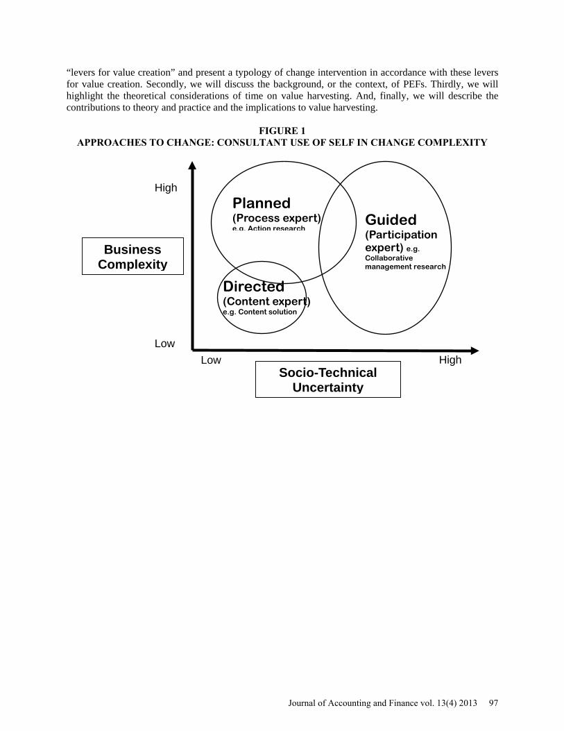
“levers for value creation” and present a typology of change intervention in accordance with these levers for value creation. Secondly, we will discuss the background, or the context, of PEFs. Thirdly, we will highlight the theoretical considerations of time on value harvesting. And, finally, we will describe the contributions to theory and practice and the implications to value harvesting.

FIGURE 1 APPROACHES TO CHANGE: CONSULTANT USE OF SELF IN CHANGE COMPLEXITY

Business Complexity

Socio-Technical Uncertainty

High

Low High Low

Planned (Process expert) e.g. Action research

Guided (Participation expert) e.g. Collaborative management research

Directed (Content expert) e.g. Content solution


FIGURE 2 LIQUIDITY TIME FRAME

LEVERS FOR VALUE CREATION

Firm value is always a topic of much discussion and debate, and there are many alternative methods for determining value, such as goodwill based methods, cash flow discounting, and breakup value, to name a few (Fernandez, 2002/2007). One of the most commonly used methods is the income approach method often referred to as the Price Earnings Ratio (PER). Under this method, firm value or Equity Value is calculated as PER x Earnings. This simple formula is powerful because of its ease of use and its clarity of focus around the importance of the firms’ earnings. Additionally this method is important as it highlights one fundamental truth for value creation — the foundational purpose of all change efforts — that there are essentially two ways to create value: firstly, by increasing or stabilizing earnings, which is often represented by the specific income statement item EBITDA (earnings before interest, tax, depreciation and, amortization); and secondly, by increasing the multiple itself, which is a more subjective number representing factors such as management’s ability, talent pool, the firm’s market position, etc. Unless the change intervention is designed to do one of these two things then any improvement in value may be occurring due to other unmanageable aspects and thus considered chance. In this paper we have classified change efforts by identifying which element of the PER equation we are attempting to improve and our classification results in a typology of change intervention based on the lever of value creation.

Years 2 4

Strategic

Tactical

Sale Prep Optimistic Uncertain

Sale

Dec

isio

n M

akin

g

Minor

Significant

6


FIGURE 3 CHANGE INTERVENTION TYPOLOGIES AS LEVERS OF VALUE CREATION

Lever one: Increasing or stabilizing earnings — improving ‘efficiency’ or ‘effectiveness’

• Lean production, TQM, • Outsourcing • Cost saving measures • Process consultation and reengineering

Lever two: Improving the multiple – improving ‘organizational capacity’ • Systems change, organizational assessments • Structural change, work design or flow • Strategic planning implementation • Appreciative inquiry • Organizational cultural intervention • Relational intervention • Life coaching and mentoring

As a result of this classification we have identified two distinct types of change levers. Firstly, the “efficiency and effectiveness levers” — tactical in nature — are designed to improve the current operations. These levers are interventions that are designed essentially around the idea the organization needs to continue doing what it is doing but needs to do it faster or better. These levers have a shorter implementation time horizon (one to two years), and would be more characterized as a hard systems change intervention by Senior and Swailes (2010). Secondly, the “organizational capacity levers” — strategic in nature — are essentially designed around the idea that the organization needs to build future skills and capacity within the organization to: 1) consistently replicate desired outcomes (meaning it may be able to accomplish these outcomes occasionally but it needs to be able to repeat them consistently), or 2) achieve a particular goal for which it currently does not have the necessary skills. We assert that these organizational capacity levers have longer time horizons (three to five years), and would be characterized as soft systems change interventions by Senior and Swailes (2010). All of these distinctions can be seen in Fig 3. PRIVATE EQUITY FIRMS (PEFS) AND THEIR REOCCURRING THEMES

Private Equity Funds are designed as an alternative for investors seeking to obtain a higher long-term return than other traditional investments such as stock market index funds (Cendrowski, Martin, Petro, & Wadecki, 2008, p. 63; Kaplan & Schoar, 2005). Between 1970 and 2007 there were more than 21,000 transactions with an estimated transaction value of $3.6 trillion, out of which 40% or $2.7 trillion was associated with deals after 2000 (Strömberg, 2008, pp. 3-4). The British Venture Capital Association and the European Venture Capital Association suggest that the private equity business model is an increasingly dynamic and efficient component of the capital market that has the capability to deliver substantial reward to fund investors, partners and management (Clark, 2009, p. 2033). However, in light of the levers of value creation, we assert that this has to be questioned as there are only limited levers being used under this investment vehicle (see further discussion below).

The logic is that private equity funds are formed by inviting like-minded investors who combine their capital to increase their purchasing power in the marketplace (Cendrowski, et al., 2008, p. 5). Private equity funds raise investment funds based on the premise investors will be provided with a certain level of return and the opportunity to liquidate their investment after a specified period of time. Private equity funds buy companies to sell them which is different than corporations or standard firms who tend to keep them for long term strategic reasons (Barber & Goold, 2007). The typical investment structure for private


equity funds is a limited partnership. The investors in private equity funds are considered “limited partners” since they do not have active control or influence over the investments (De Clercq, Fried, Lehtonen, & Sapienza, 2006, p. 91). Private equity funds then serve as the ‘general partner’ and are in control of the fund, investments, and typically serve on the boards of portfolio companies. Institutional investors and individuals invest capital in private equity funds to diversify their investments and seek better than market returns over a set period of time (Cendrowski, et al., 2008, p. 63). Essentially agreement between the private equity fund and the investors enables the private equity fund to invest the investors’ capital for a specified period of time (usually 10-12 years). This commitment to “time” places an additional burden/stress on the contextual elements experienced by the PEF that other investments vehicles do not experience. Thus, the important difference from other investment vehicles is the closed and finite nature of the fund. The pivotal question or focus of this paper is to explore exactly how this reoccurring theme — the constraint of time — impacts the decisions of those involved, if at all, and how it could lead to higher value. THE THEORETICAL CONSIDERATIONS OF TIME ON VALUE HARVESTING

In this section we introduce the implications of time on decision making within PEFs by combining Whatley and Kliewer’s (2012) Approaches to change: Consultant use of self in change complexity model and the concept of time (see Fig. 4).

FIGURE 4 CONSULTANT USE OF SELF IN CHANGE COMPLEXITY MODEL AND THE

CONCEPT OF TIME

We assert that low social-technical uncertainty when combined with low business complexity only requires a small time horizon (1-2 years) for a change intervention and would only contribute to improving or stabilizing earnings — lever one of the levers for value creation. While medium social-technical uncertainty when combined with medium business complexity produces the need for a medium time horizon (2-3 years) and would only contribute to improving or stabilizing earnings — lever one of

Business Complexity

Socio-Technical Uncertainty

High

High

Time

Directed

(Content expert)

e.g. Content solution

Planned (Process expert)

e.g. Action research

Guided (Participation expert)

e.g. Collaborative management research


the levers for value creation. Finally, a high social-technical uncertainty when combined with high business complexity produces a need for a long time horizon (3 to 5 years) — lever two of the levers for value creation. Thus we assert that lever two change interventions, the most impactful, are only possible and likely successful when the time horizon is greater than three years.

We then introduce Doucette’s (2011) Liquidity Time Frame model and match it against the typologies and their related lever for value creation (see Fig. 5). In doing this we can see that it is not possible for PEFs to make consistent substantive returns since they are only ever able or choose (avoiding risk) to implement level one levers for value creation. Unless PEFs are purchasing undervalued assets in the first place, the important question is whether the purpose of the private equity fund is to aid the increase in portfolio company value or is it to simply identify undervalued firms.

FIGURE 5 LIQUIDITY TIME FRAME AND INTERVENTION TYPOLOGY

ONE PARTICULAR PLAY Scene One v Case Background

The original PEF that founded CFGC never intended to hold it for very long and this is evident in that it was formed in 1996 and publically traded by 1998. For all intents and purposes it was what is referred as a classic ‘roll-up and sell strategy’. While at the same time, the U.S. insulation industry was a highly fragmented $25 billion industry with a few major corporations at the top. Most of the industry was made up of local or regional players who benefited from the booming U.S. economy, strong building sector and available credit. CFGC focused on acquiring as many businesses as possible so that it could be eventually sold to a competitor or other interested investor for a large multiple of EBITDA. At the time, if you owned an insulation business, were interested in selling, and your organization fit into the metrics of CFGC, it was likely you would be offered a competitive deal (usually in cash) to sell your business to CFGC. Beyond the cash, the seller was told they would be able to run their business as they had in the

Years 2 4

Strategic

Tactical

Sale Prep Optimistic Uncertain

Sale

Dec

isio

n M

akin

g

Res

ista

nce

to C

hang

e

Minor

Significant

6

Appreciative Inquiry

Continuous Improvement

Project Oriented

Change Interventions


past with little interference from CFGC. Over an eighteen-month period CFGC had acquired some forty businesses.

In light of the events of September 11, 2001, there was a subsequent downturn in the economy that impacted many businesses and the insulation industry was no exception. As a result, CFGC and its competitors began to see a significant drop in business. Similar to other industries, those firms without the burden of debt would fare better than others, however CFGC had significant amounts of debt. Additionally, CFGC was a loosely held group of individual companies with no ability or commitment by ‘legacy owners’ (original owners) to seek leverage of possible synergies. The premise of selling to CFGC was that the acquired firm could run the business the way they always did with little interference. This is evidence that the entire management process at CFGC was purely lever one intervention as CFGC really only represented the attempt to consolidate EBITDA. At the onset, there was no attempt to stabilize earnings (otherwise causing less debt) or to enter into lever two interventions. This was further compounded when the economy softened and the firm lacked the ‘organization capacity’ to change. Lever two change interventions can build organizational capacity and, as result, CFGC was heading towards a financial hurricane with clear signs of financial distress.

The pressure to ‘run’ the business was placed on a PEF not prepared or interested with this type of challenge. Specifically, the CEO at that time was a considered a relationship builder focused on ‘making deals’, not on running a $600 million company during turbulent economic times. After a series of events, the confidence in the CEO by the Board eroded and he was removed. CEO #2 was hired in September 2002 to ‘turn around the business’. As part of the turnaround, CFGC voluntarily filed for a pre-arranged Chapter 11 bankruptcy in June 2003. As a result of the bankruptcy, the previous stockholders were essentially removed and the bondholders were given control of the company. The plan was to emerge quickly once the debt was restructured and the courts approved the reorganization plan. In August 2003, CEO #2 left CFGC to pursue other interests. Enter CEO #3 or, more specifically, a ‘Chief Restructuring Officer’ (CRO). He and his firm were hired to oversee CFGC during the restructuring process until a “permanent” CEO could be found. In February 2004, CFGC successfully emerged from bankruptcy with a plan to repay vendors 100% within eighteen months. The search for CEO #4 was completed in June 2004 and a new era had begun for CFGC. Jimmy C who recently left a major ice cream provider as their Chief Operating Officer was anxious to assume his first CEO role. Selling to Private Equity

Once Jimmy arrived, the direction of the reluctant bondholders turned owners through bankruptcy was to sell the company. Generally, bondholders do not want to be shareholders and the CFGC bondholders wanted to exit the business quickly with a reasonable return. As a result, CFGC was entering a 1-2 year period of little change related to people and process (low social-technical uncertainty) and a very specific financial target and timing (low business complexity). The chosen focus was earnings or EBITDA growth in order to improve the eventual sale price — lever one focus appears again. There was no significant time or resources given by the bondholders to focus on building organizational skills or capacity (organizational capacity levers or lever two) in an attempt to affect a multiple of EBITDA. In a rating agency presentation immediately after Jimmy’s arrival, the 2004 Strategic and Operational Initiatives included such initiatives as: branch profit management; insulation fleet optimization through capital expenditures and aggressive preventative maintenance plans; continued critical analysis to drive revenue and cost containment; and a focus on internal growth (vs. acquisition). The topics of discussion throughout the first two years were lever one, tactical decisions designed to improve or stabilize EBITDA.

Beginning in the fall of 2005, CFGC was involved in a marketing process to sell the company. The presentation to potential buyers emphasized investment highlights such as: favorable industry growth trends; strong operating performance and momentum; strong cash flows and insulation equipment values; experienced management team; diversified geographical footprint; standardized operating procedures; and cash benefit from NOL carry forward. The investment highlights genuinely reflected the accomplishments of the organization’s work since Jimmy’s arrival in June 2004. Certainly, there was a


marketing flare to the presentation, but the target audience was the financially minded professional looking for an investment with potential. Unlike the bondholders turned stockholders, the next owners of CFGC would presumably have a longer runway to focus not only on earnings stability and growth but a larger EBITDA multiple based on improved organization capability. In July 2006, CFGC was successfully sold to a private equity firm called TGP. With the purchase of the company by a PEF, the 5-7 year liquidity time frame was underway.

In May 2006, a letter of intent was signed and CFGC began to respond to TGP due diligence requests. The focus of the due diligence requests were mainly financial and regulatory in nature. For example, TGP did not conduct deep human capital inquires, cultural assessments, or management team interviews. TGP relied on informal interactions with CFGC’s top management team (TMT) to gain comfort with the human capital aspects of the business. Further, TGP had no in-depth discussions with CFGC’s TMT regarding planned organizational capability changes. The only exception was some initial direction by TGP to shed two non-related divisions in order to harvest additional cash and pay down debt. The pre-assessment stage was financially thorough (lever one) but hardly investigated how CFGC’s TMT would build organization capability (lever two) in order to improve the EBITDA drive multiple. Even though CFGC’s TMT had a vision regarding how to grow organization capability, TGP did not conduct a deep inquiry into this area. Given the estimated liquidity time frame, the opportunity to implement large-scale and capability driven organizational changes was beginning to slip away from TGP investors.

The first several years of TGP ownership focused on the sale of two major divisions of the CFGC. One division was sold at a premium and the proceeds used to make a sizeable reduction in debt. The sale of the second division was a move to exit a low margin, highly volatile, people intensive (as opposed to capital) business unlike the core insulation business. Even though the second division was sold for a very low price, the divestiture freed a large portion of the TMTs energy and redirected it to the more profitable core business. The sales of these divisions were important to a long-term strategy of becoming attractive to a strategic buyer. CFGC did not want to have a non-core or low margin business that might detract strategic buyers. Despite the longer strategy play, the transaction was designed around efficiency and effectiveness (lever one). Lever one value creation efforts continued at the start of 2008 with familiar organizational goals such as: safety; improving the operating performance and increasing the EBITDA margins; refining the rate disciplines and pricing strategies to profitably grow the business; continuing training of the outside sales force and implementing training of the operating managers and inside sales force; balancing the insulation fleet to optimize CAPEX spending; implementing cost reductions in alignment with core operations; improving customer satisfaction; and strengthening employee morale. Although some of the 2008 goals hint of improving organizational capability (lever two) the reality was that many initiatives were tactical in nature. After two years, CFGC had successfully executed the divestitures, but had not added value to the business nor created a compelling reason for potential buyers to pay a higher multiple.

The next three years (2008-2010) were occupied by a brief taste of success and then desperate actions to survive. The economy began to falter at the latter end of 2008 and CFGC immediately felt the decline in business. EBITDA declined from $135 million in 2008 to $70 in 2010. With an almost 50% decline in EBITDA, reductions in force, pay freezes, deferral of capital expenditures, and an increase in the sale of insulation equipment were necessary to stay solvent. Years three through five were exclusively focused on survival using lever one initiatives. The planning horizon went from 12 to 24 months down to six months and in some cases monthly adjustments were made by the TMT. Clearly this time period was about protecting the core business with the hope of a comeback when the economy recovered. Yet again, tactical initiatives designed to address the moment replaced strategic growth and capability initiatives focused on increasing organizational value.

The last two years (2011-2012) has seen a more positive turn in the economy and financial stability for CFGC. Slowly, CFGC has begun to emerge from a deep recession and will likely see EBITDA of around a $100 million in 2012. TGP will have owned CFGC for six years in July 2012. As results continue to improve, it is likely TGP will be open to selling the company in the next 12-24 months assuming the offer is conducive to covering debt and providing a reasonable return. What remains


difficult to grasp is the lost value creation based on TGP and CFGC’s TMT focus on efficiency and effectiveness. Throughout the past six years under TGP ownership, there has been little time spent on capability building. Maybe TGP and CFGC TMT had no other options except to focus on lever one activities. In the end, TGP will sell CFGC and most likely do so at a reasonable return because of improved and growing EBITDA. However, if lever two value creation initiatives were introduced early would the multiple (based on organization capability) of EBITDA have been higher? CONTRIBUTIONS TO THEORY AND PRACTICE AND THE IMPLICATIONS TO VALUE HARVESTING

This paper has logically developed the theory that value creation within firms is provided via two key levers: lever one — the efficiency and effectiveness levers — involve an improvement in earnings or an improvement in the stability of earnings; and lever two — the organizational capacity levers — involve building skills and capacity. The theory then links these levers to the appropriate change invention method by a contextually constant factor— that is, time. In doing so, several observations can be made for PEFs, private equity investors, and the managers of pooled funds, and, without question, private equity firms are “leaving money on the table” at the time of value harvesting.

Firstly, we assert that there needs to be a clearer understanding of the overall objective of the private equity fund. Perhaps it is to acquire undervalued companies with the intention of holding for a few years and then selling, or perhaps it is to acquire companies with specific change interventions in mind. In either event, this paper stresses that a pre-assessment stage, which is prior to “due diligence”, would be the most critical aspect of a private equity fund’s acquisitions, and, although this concept is not new to theory, the linkages to specific types of change interventions moving forward and a reduction in the type of change interventions recommended due to time constraints, are contributions to theory.

The second significant assertion of this paper is that the time horizon significantly reduces the intervention methods available/recommended for all firms and this is particularly evident within PEFs. And, as a result, there are no “organizational capacity levers” — type two — available within PEFs that have a preference for short holding periods (7 years or less).

The third contribution is that the longer a portfolio company is held by the private equity fund the less likely that long-term value is being created. The private equity fund partners are so concerned and oriented to not adversely impacting earnings that all level two value creation levers are rarely considered.

Finally, in light of the fact there are only two ways in which value is created, this paper contends that much of the activity within private equity funds is not actually adding underlying value to the portfolio company and, as such, the underlying philosophy of private equity funds is perhaps questionable given the inability to develop a long term ‘development’ plan. POSTLUDE

This paper has stressed the importance of the levers of value creation. Additionally this paper has linked the levers of value creation to various change intervention typologies and contextual influence of time. In doing so, this paper suggests that appropriate intervention methods are influenced by time horizons and, in the case of PEFs, this is the most prevalent contextual concern. Finally, this paper has shown that because of the time constraint private equity firms are not considering significant value harvesting opportunities, and are, thus, leaving money on the table when it comes time to sell. ENDNOTE

1. The names of the firms, the principle actors, and the industry specifics have been changed for the purposes of confidentiality.


REFERENCES Axelson, U. L. F., Stromberg, P. E. R., & Weisbach, M. S. (2009). Why are buyouts levered? The financial structure of private equity funds. Journal of Finance, 64(4), 1549-1582. Barber, F., & Goold, M. (2007). The strategic secret of private equity. Harvard Business Review, 85(9), 53-61. Cameron, K. S., Dutton, J. E., & Quinn, R. E. (Eds.). (2003). Positive organizational scholarship: Foundations of a new discipline. San Francisco, CA: Berrett-Koehler. Clarke, L. (1994). The essence of change. Hemel Hempstead, UK: Prentice Hall. Cendrowski, H., Martin, J. P., Petro, L. W., & Wadecki, A. A. (2008). Private Equity; History, Governance, and Operations. Hoboken, NJ: John Wiley & Sons, Inc. Clark, I. (2009). The private equity business model and associated strategies for HRM: evidence and implications? International Journal of Human Resource Management, 20(10), 2030-2048. De Clercq, D., Fried, V. H., Lehtonen, O., & Sapienza, H. J. (2006). An Entrepreneur's Guide to the Venture Capital Galaxy. Academy of Management Perspectives, 20(3), 90-112. Doucette, B. (2011). Midwest Academy of Management 54rd Annual Conference entitled “The Power of Positivity: Research and Practice that Makes a Sustainable Difference”. Presented a paper entitled, “Changing Private Equity Firms for the Better”. Omaha, Nebraska, October 20-22, 2011. Emery, F. E., & Trist, E. L. (1965). The causal texture of organizational environments. Human Relations, 18(1), 21-32. Fernandez, P. (2002/2007). Company valuation methods. The most common errors in valuations. Working Paper #449. IESE University of Navara. Kaplan, S. N., & Schoar, A. (2005). Private equity performance: Returns, persistence, and capital flows. Journal of Finance, 60(4), 1791-1823. Mirvis, P. H. (1988). Organization development: Part I – An evolutionary perspective. Research in organizational change and development: Vo1. 2. Stamford, CT: JAI Press. Inc. Mirvis, P. H. (1990). Organization Development: Part II – A revolutionary perspective. Research in Organizational Change and Development (Vol. 4), p. 1-66. Morgan, G. (2006). Images of organizations: Updated edition of the international bestseller. Thousand Oaks, CA: Sage Publication Inc. Nadler, D., & Tushman, M. (1999). The organization of the future: Principles of design for the 21st Century. Organizational Dynamics, 28(1), 45-60. Pettigrew, A. M., Woodman, R. W., & Cameron; K. S. (2001). Studying organizational change and development: Challenges for future research. Academy of Management Journal, 44(4), 697-713. Senior, B., & Swailes, S. (2010). Organizational change. Essex, England: Pearson Education.


Strömberg, P. (2008). The new demography of private equity. Geneva: World Economic Forum. Vaill, P. B. (1996). Learning as a way of being: Strategies for survival in a world of permanent while water. San Francisco: Jossey-Bass. Weisbord, M. R. (2004). Productive workplaces revisited: Dignity, meaning, and community in the 21st century. San Francisco: Jossey-Bass. Whatley, L. R., & Kliewer, H. (2012). Contextual influences on team effectiveness & consultant identity: Implications for consulting & consultation. In Press. Journal of Leadership, Accountability and Ethics, 10(1).


Is Community Bank Creating Value for Shareholders?

John S. Walker Kutztown University of Pennsylvania

Victoria Geyfman

Bloomsburg University of Pennsylvania

The questions posed by the CEO of Community Bank were quite direct: “Is our bank creating value for shareholders?” Mindful of recent industry consolidation, he also asked, “Should the board consider selling the bank to another bank?” Many banks are asking the same questions now that the operating environment for banks has changed. Prior to the credit crisis, banks had to implement new regulatory procedures prompted by the passage of Sarbanes-Oxley. Since the crisis, the Dodd-Frank Act and Basel III are keeping bankers awake at night wondering if the community bank model can survive the added regulations and weak economy. INTRODUCTION

Some believe that the community bank model will eventually become extinct, with larger regional and money center banks absorbing the market shares of these smaller banks. In an article titled, “Don’t Let Your Babies Grow Up to Be Community Bankers” written by Stephen N. Ashman and published in the trade publication American Banker (2012), Ashman asserts that “community bankers are a vanishing breed.” Some of the industry numbers support his assertion. For example, over the last 10 years the number of banks in the U.S. has fallen from 9,616 to 7,358. Furthermore, the top 10 U.S. banks now control 60 percent of the market, whereas 10 years ago their market share was 45 percent. The final nail in the coffin so to speak could be the higher capital levels that Basel III would require. Ashman states, “We have not yet invented a new business model for community banks, one that produces sufficient risk-adjusted returns to attract new talent.”

Not surprisingly, not all industry experts agree with Ashman’s outlook for community banking. A few weeks after Ashman’s article, Nancy Bush (2012), writing on her blog in SNL Financial, titled her rebuttal, “You Cannot Be Serious” after the well-known professional tennis player John McEnroe. She observed that Ashman “recited the usual dreary litany of community banking ills.” Yet, she did go on to discuss asset size and the belief that depositors will likely feel more comfortable dealing with larger banks, say on the order of $10 billion. She also believes that as communities change, community banks will need to adjust their products to meet those changes. Nevertheless, she expects that Americans will continue to choose to “patronize smaller and more familiar institutions.”

Ultimately, any observer of the banking industry knows that it is going through a number of macro changes. But isn’t that true of all industries in our economy to some extent? It is likely that regulatory changes and the cost of compliance could shift the cost structure of the banking industry, affecting


economies of scale and scope and, perhaps, the optimal size and number of institutions. From a micro standpoint, it’s the board of directors’ responsibility, working with the CEO, to decide how much capital to allocate to the business. In turn, capital allocation decisions should be made based on the bank’s belief about its ability to generate sufficient returns for its providers of capital, i.e., shareholders. The board of directors has several alternatives. It can choose to increase, decrease, or maintain the current level of reinvestment into the business. Or, a more significant decision, it can elect to sell the bank to another bank that might see synergistic advantages to combining banks.

In this case study, we analyze the recent performance of a community bank that we will call “Community Bank” in order to conceal its identity. The lead author of this case study has consulted with this bank for over a decade and is periodically asked to meet with the board to present an objective evaluation of the bank’s performance relative to other banks in the industry and to highlight areas that should be addressed for improvements during the strategic planning process. For example, several years ago, the bank was struggling with a thin capital structure and a falling margin. Both issues have since been addressed and rectified by the board. For the 2012 visit to the bank, the CEO wanted answers to several fundamental questions: Is our bank creating value for shareholders and is the bank headed in the right direction? The CEO also wanted to know whether the board should consider selling the bank to another bank. Arguably, given the precarious position that many banks find themselves in since the financial crisis, these are some of the most important questions that all banks should contemplate. Banks with a high proportion of bad loans and/or thin capital bases are of particular concern to regulators.

The case study is organized in three parts. Part I looks at the bank’s stock performance compared to two important benchmarks to see how returns to shareholders have compared to other investment alternatives. Part II looks at key fundamentals to provide an assessment of the bank’s operating performance for the most recently completed fiscal year. Then Part III analyzes the first quarter of the current year to determine if the bank’s trends are favorable. The case study makes heavy use of statistics, which provides students an example of how valuable statistics can be for assessing the performance of a bank relative to a peer group. As Ott and Longnecker (2010) say, “statistics is the science of learning from data.” Indeed, this case shows just how much can be learned about a bank through a statistical analysis of its performance. PART I: COMMUNITY BANK’S STOCK PERFORMANCE

How do you fairly evaluate a firm’s stock performance? People tend to have short memories and will focus on the most recent performance. Also, investors often focus on price appreciation and forget that dividends paid are an important and, in many cases, a significant component of total return.

Typically, Community Bank schedules board retreats every three years to discuss certain strategic issues, including stock performance. Therefore, it is appropriate to examine the bank’s stock performance for the prior three years. (Prior stock performance reviews over the last decade have all shown Community Bank’s stock to exceed benchmark comparisons.) Figure 1 shows the total return performance for Community Bank’s stock over the three years prior to the meeting with management. For the three-year period, the stock delivered a cumulative total return of 120.32 percent, but the trend was anything but steady. In particular, note the run-up in performance due to a surge in the stock price toward the end of the three-year look-back period.

In addition to selecting a suitable timeframe for comparison, a second parameter that needs to be selected is an appropriate benchmark. If a student scores a 65 percent on an exam, has he performed poorly? If the average score for the class is 85 percent, then a 65 percent is not a good score. However, if the class average is 45 percent, then a 65 percent is quite good. Stock performance, like exam grades, should be considered relative to a benchmark.


FIGURE 1 COMMUNITY BANK’S THREE-YEAR STOCK PERFORMANCE (TOTAL RETURN)

Community Bank, as with many firms in the U.S., is accustomed to comparing its stock to the S&P

500, as shown in Figure 2. For the three years shown, the bank’s stock (solid line) is up 120.32 percent on a cumulative basis. This cumulative return far exceeds the 54.72 percent gain by the S&P 500 (dashed line). When the board first considered the prior three years, the stock’s total return of 120.32 percent looked very strong. Then when they saw the comparison to the S&P 500, they saw that on a relative basis the bank was outperforming the stock market by more than double. This confirmed that the bank’s stock has performed extremely well since the financial crisis. A five-year comparison looking back further showed market-beating performance as well, as the bank’s stock delivered a total return of 63.30 percent compared to the S&P’s return of negative 2.28 percent.

FIGURE 2 COMMUNITY BANK’S STOCK PERFORMANCE COMPARISON TO THE S&P 500

Source: SNL Financial

While the comparison to the S&P 500 is valid in that it tells investors how a stock compares to the overall market—or, at least, 500 widely-held companies that represent roughly 75 percent of the U.S. stock market—it does not tell them how the stock compares to the bank’s peers. Sectors of the economy can go in and out of favor from year to year. Therefore, we explained to the board at Community Bank that there are other comparisons that we often recommend. For example, it makes sense to select a peer group of banks of comparable size. Bank efficiency is linked to size, so larger banks should be more


efficient and this will impact earnings and stock performance. The peer group that was selected is a group of banks with assets between $1 billion to $5 billion compiled by SNL Financial.1 There are other bank benchmarks that can be used for comparison. For example, America’s Community Bankers and the NASDAQ Stock Market created a broadly diversified stock index in 2003 for community banks termed the “ACB NASDAQ Index.”

Figure 3 shows Community Bank’s overall stock performance (solid line) relative to its peers (dashed line). This comparison finds the bank’s three-year total return (120.32 percent) is roughly 12 times the return for its peers (9.66 percent). Based on the total return analysis of the bank’s stock over the last three years, the conclusion is definitive: Community Bank has delivered outstanding stock performance to its shareholders. Yet, in finance we teach that financial performance should be analyzed using a risk-versus-reward framework. When you look at graphs such as Figure 2 and Figure 3, often the individual firm has a more volatile return pattern than the index. This is not a surprise. The S&P 500 reflects the aggregated returns for 500 companies; thus, there is a diversifying effect reflected in the total return profile for the index. Likewise, the peer index is comprised of 149 banks.2 The peer index would capture sector risk, but firm specific risk would be diversified among the many banks. In contrast, the time series of cumulative total return for the individual bank reflects the market risk, sector risk, and firm-specific risk on a nondiversified, standalone basis.

FIGURE 3 COMMUNITY BANK’S STOCK PERFORMANCE COMPARISON TO ITS PEERS


Another consultant who visited Community Bank during the prior year made an interesting observation. He told the bank’s board of directors that Community Bank “is a high-performing bank operating with low risk.” Yet, he did not say how he was measuring the bank’s risk. The Office of the Comptroller of the Currency lists nine categories of banking risk (see p. 23 of the Comptroller’s Handbook, 2007), including credit, interest-rate, liquidity, and price risk. The reason that many of these risks, such as price risk, are so important for banks to monitor is that these financial institutions usually operate with low equity ratios, often less than 10 percent equity-to-assets.3 Thus, one way to assess a bank’s risk is to analyze its capital ratios. When we looked at Community Bank’s tangible-equity-to-tangible-assets ratio over the last three years, we found that the bank had operated with a below-median ratio throughout this period. In fact, for 2011 it was operating at the 23rd percentile, which put it in the first quartile for its capital cushion. That suggests that the bank was more leveraged than most of its peers; thus, from a financial leverage perspective, it was running a more risky operation, not less.

However, the risk that is most closely associated with stock performance is a firm’s market risk, as measured by its beta. A firm’s beta can be found through regression analysis, where the independent variable is a proxy for market return, such as the S&P 500, and the dependent variable is the stock’s


return. For our presentation, we used a three-year beta that was reported by SNL Financial. We have used SNL Financial extensively while working in industry and have found its data to be reliable. Nevertheless, the discussion here is illustrative of portfolio concepts, and an analyst doing similar comparative work might elect to estimate the bank’s beta using regression analysis. For this analysis, we felt comfortable using the beta reported by SNL Financial, which is just 0.16 for Community Bank.4 A beta this low suggests that holding stock in Community Bank contributes very little market risk to a portfolio.

In order to make a comparison to the bank’s peers, the three-year betas for all peers reported in SNL were compiled and treated as a sample of the peer group’s betas. The point estimate found is 0.76 with a lower limit of 0.67 and an upper limit of 0.84, based on a 95 percent confidence interval. Obviously, the beta for Community Bank is well below the lower end of the confidence interval for the peer group, meaning that we can conclude with 95 percent confidence that the bank’s systematic risk is less than the average risk for the banks in its peer group. Therefore, based on the beta risk, we can conclude that Community Bank produced higher returns on a total return basis and on a risk-adjusted basis.

Yet, if some other measure of risk were considered, such as financial risk (i.e., the degree of leverage), then the conclusion might be different. Both the total return and financial risk for the bank are higher. But how do you use a measure of financial risk to determine a risk-adjusted return?5 Even more difficult to quantify, some would argue that credit risk is the most lethal risk for a bank. How would you measure and compare a bank’s credit risk to a sample of its peers without having access to each institution’s loan portfolio? That would be a nearly impossible feat. Yet, there are some proxies that could be used, such as comparing the bank’s nonperforming assets ratio and/or charge-offs to its peers. During the years 2009–2011, Community Bank’s nonperforming assets were 57 percent to 61 percent less than its peers, and the net charge-offs were 27 percent to 49 percent less. These favorable variances suggest that the bank had lower credit risk during this period. PART II: WHAT DOES A FUNDAMENTAL ANALYSIS OF THE BANK TELL US?6

Higgins (p. 58–59, 2012) asks the rhetorical question: “Can ROE substitute for share price?” He

presents data for companies in the specialty chemicals, packaged foods, and meats industry, as well as data for 80 “large corporations” that show a reasonable relationship between return on equity and price-to-book ratios—R-squares around 41 percent to 45 percent and t-statistics between 5.9 and 8.2. In unpublished work by Walker (2012), a similar analysis was done using community bank data and the R-square is around 29 percent with a t-statistic of 8.6. Anecdotally, we have seen bankers assuming that the market will reward them with higher stock prices when they produce high ROAs and ROEs. Of course, one often discussed shortcoming of ROA and ROE measures is that they don’t reveal how much risk a firm is taking. However, if you examine a time series of ROE data, the consistency, or lack thereof, in the numbers can provide some insight into the risk inherent in a firm’s operation.

If you look at a Uniform Bank Performance Report (UBPR), you find a plethora of statistics that can be analyzed when assessing a bank’s performance. UBPRs are prepared by the Federal Financial Examination Council, which, according to their tagline, “promotes the uniformity and consistency in the supervision of financial institutions.” Moreover, the UBPR is:

An analytical tool created for bank supervisory, examination, and management purposes. In a concise format, it shows the impact of management decisions and economic conditions on a bank’s performance and balance-sheet composition. The performance and composition data contained in the report can be used as an aid in evaluating the adequacy of earnings, liquidity, capital, asset and liability management, and growth management. Bankers and examiners alike can use this report to further their understanding of a bank’s financial condition and, through such understanding, perform their duties more effectively. (http://www.ffiec.gov/UBPR.htm)


Financial management textbooks often show the analysis of ROE using the DuPont equation, which includes the profit margin, asset turnover, and financial leverage in multiplicative form.7 During the authors’ time in industry, they were analyzing the financial performance of upwards of 100 community banks each quarter. They found that a quick assessment could be made of a bank’s ROE by looking at six fundamental areas: (1) net interest income, (2) net overhead, (3) capital, (4) the balance between earning/nonearning assets, (5) provisioning for loan losses, and (6) the tax burden. Further drilldown into the operations is possible, but these six areas give a balanced snapshot of the bank’s performance. While these statistics offer a useful static view of a bank’s performance, it is also valuable to examine several growth trends that will be discussed below.

In Table 1 we show Community Bank’s return on average assets (ROAA) and return on average equity (ROAE) for 2011, both on a core and noncore basis, along with the 50th percentile values for the bank’s peer group. (The difference between core and noncore is the removal of nonrecurring items, such as one-time accounting adjustments.) Banks are constantly writing new loans, seeking new deposits and adding to retained earnings. Consequently, their balance sheets—and, specifically, the level of assets and equity—are normally growing quickly, even from one quarter to the next. This is why analysts use average assets and average equity when calculating return ratios. Another return measure that banks often use (not shown in Table 1) is return on tangible equity (ROTE). The difference between ROAE and ROTE is that a bank’s average equity often includes what are termed intangible assets on the balance sheet. When one bank acquires another bank, the premium over book value is accounted for as goodwill. Historically, banks would use the pooling or purchase method when accounting for an acquisition. Starting in 2001, banks were required to begin using the purchase method for all acquisitions. The booking of intangible assets on the balance sheet explains why ROAE figures are less than ROTE.

TABLE 1 RETURN COMPARISONS FOR 2011

50th Percentile

Bank Value

Percentile Ranking Grade

Core ROAA 0.70% 0.82% 61st B ROAA 0.76% 0.90% 63rd B Core ROAE 6.77% 9.92% 70th B ROAE 7.44% 10.78% 75th B+


The data reveal that Community Bank’s ROAA is in the 63rd percentile. Recall from statistics that this means that at least 63 percent of the bank’s peers have an equal or lower ROAA while at least 37 percent have an equal or higher ROAA.8 If the ROAA values are well dispersed, which you would expect, you can interpret this to mean that Community Bank is “beating” roughly 63 percent of the banks in its peer group. If we divide the distribution of ROAAs into quartiles, this enables us to assign letter grades, similar to how a professor might assign final grades to a class. For example, the first (lowest) quartile is assigned a D, the second a C, the third a B and the fourth an A. Plus and minus grades can be assigned based on how close the ranking is relative to the values for Q1 (25th percentile), Q2 (50th percentile, and Q3 (75th percentile). For our work, we used ±5 percentile as the range for plus and minus grades. For example, from the 71st to the 75th percentile, a grade of B+ is assigned; thus, Community Bank earned a B+ for its ROAE. (An ROAA falling in the 76th to 80th percentile would be assigned an A−.) The CEO of Community Bank remarked that this grading system was very helpful to board members.

Notice that Community Bank’s ROAA earned a B, while its ROAE earned a B+. Often a bank’s relative performance for its ROAA is different than for its ROAE. This can be explained by the capital structure decision, specifically the leverage ratio. Suppose two banks achieve an ROAA of 1 percent. If


the first bank has an equity-to-assets ratio of 10 percent, its ROAE will be 10 times its ROAA or 10 percent. The equity multiplier for the first bank is 1/0.10=10×. If the second bank has an equity-to-assets ratio of 8 percent, its ROAE will be 12.5 times its ROAA or 12.5 percent. In the second example, the equity multiplier is 1/0.085=12.5×. Ultimately, a bank’s ROAE is determined by its ROAA performance and the degree of leverage used. Typically, a bank will have a policy on how much leverage is permissible. With the passage of Basel III, banks are now revisiting their capital policies to ensure that they meet the new guidelines.

The next step is to drill down to inspect the fundamentals that determine the bank’s ROAA and ROAE. A bank’s revenues are a combination of net interest income and noninterest income. There are two statistics commonly used to compare a bank’s net interest income performance to other banks: net interest margin and net interest spread. The net interest margin is defined as the difference between interest income and interest expense divided by the bank’s average assets or average earning assets. In contrast, the net interest spread is defined as the difference between a bank’s yield on earning assets (interest income divided by earning assets) and cost of funds (interest expense divided by liabilities). From Table 2, we find that Community Bank’s margin and spread are close to the median (i.e., 50th percentile), leading to the next drill-down question. Is the near-median margin and spread a result of a near-median yield on earning assets (YEA) and a near-median cost of funds (COF), or is there some other combination of YEA/COF that explains the performance? The answer to this question is important if the bank wants to generate ideas for improving its net interest income performance.

TABLE 2 NET INTEREST INCOME ANALYSIS FOR 2011

50th Percentile

Bank Value


Margin 3.79% 3.81% 51st B− Spread 3.57% 3.58% 51st B− YEA 4.70% 4.98% 73rd B+ COF 0.96% 1.27% 21st D+


Before we continue with the discussion of Community Bank’s performance, it’s important that we explain what we did with the COF statistic and several other statistics presented later. A suggestion for how to present the performance statistics was given to us by a colleague who teaches statistics at Penn State. All else equal, a bank wants a low COF. Thus, a low percentile ranking is preferred. An analogy to one’s golf handicap is useful. A lower handicap indicates a better golfer than a higher handicap. Again, this means that a low percentile ranking in golf indicates better performance. However, with most performance statistics, a higher value is better, thus we tend to think in terms of higher percentile rankings as being better than lower percentile rankings. In the field of banking, higher values are better than lower values with most statistics, such as ROAA, ROAE, and margin, but not so with other statistics, such as COF and the ubiquitous efficiency ratio that we discuss later. For the handful of performance measures, such as COF, where lower is better, we have reversed the percentile rankings, as suggested by our colleague. For example, in Table 2, the COF’s percentile ranking was originally found to be the 79th percentile. By reporting 100th − 79th = 21st as the percentile ranking, this enables us to look at all performance numbers in the same way—higher percentile rankings are better than lower. If we had not made this transformation, board members at Community Bank could have been confused during the review of their numbers.

The bank is well above the median YEA and well below the median COF meaning that, relative to its peers, its asset yields are high (good) while its funding costs are high (bad). Let’s first focus on the bank’s


high YEA. There is a model in psychology termed “the four stages of competence” (see Mukherjee, Basu, Faiz, and Paul, 2012, for a note on who might deserve credit for this model). The third stage is termed “conscience competence” where someone or an organization is doing something well and they know how they are doing it. Sometimes banks are performing well in an area and they can’t explain why. In order to maintain high performance, it seems obvious that it helps to know how this is being achieved and then to build on that success. Community Bank’s higher-than-median YEA could be a result of setting higher-than-average rates on their loans or by a higher-than-average allocation to higher-risk lending, such as commercial loans. We did not investigate this issue further for this consulting assignment, but this points an analyst to the next level of drill-down analysis that could be done in order to better understand what is driving the bank’s performance.

While Community Bank wants to maintain its high performance in the YEA area, it also would like to improve its COF performance. This can often be very challenging because management is working within the economic reality of supply and demand of loanable funds. If a bank’s cost of funds is high, this points to an expensive mix of liabilities and/or rates that might be too generous relative to the local deposit market. Yet, banks are under constant pressure to grow their deposit base in order to obtain funding for loans, so higher-than-average deposit rates—if that is the case—can be explained, if not justified, by the need for funding. The deposit offerings of a community bank are fairly plain vanilla, meaning that virtually all banks offer demand deposit accounts (DDAs), negotiable order of withdrawal accounts (NOWs), savings accounts, money market deposit accounts (MMDAs), and certificates of deposit (CDs) with various maturities and features, such as “step-up” CDs. The DDAs are the preferred funding source as a bank pays zero interest for these funds. The first thought that a banker might have if its COF is high is to lower the rates. However, someone who has a rudimentary understanding of economics and the forces of supply and demand knows that if they offer lower rates, depositors will likely supply fewer deposits to the bank, which could choke off the funding needed for loan growth. Of course, the resultant reduction in supply depends on the elasticity between rates and supply. If the supply falls appreciably, then a bank can find itself underfunded for the asset growth it needs.

Another reason a bank might have a high COF is that it depends more heavily on borrowings relative to other banks. Borrowing from the Federal Loan Home Bank system and other sources tends to come with higher rates than those paid on deposits. At Community Bank, their level and structure of borrowings is reasonable. Unfortunately, they have found that they need to pay higher-than-average rates to attract the volume of deposit funding needed to keep pace with their asset growth. At least for now, the higher loan yields that they are achieving are offsetting the higher deposit rates they are paying.

When evaluating a bank’s cost structure, analysts usually examine the net overhead and efficiency ratios. Net overhead is the difference between a bank’s noninterest expense and noninterest income. The difference between expenses and income is always positive for a community bank, meaning that noninterest expense exceeds noninterest income. Lower net overhead numbers are better than higher. In contrast, the efficiency ratio is the bank’s noninterest expense as a percentage of revenue (net interest income plus noninterest income). As with the net overhead ratio, the lower the efficiency ratio is the better. We see from Table 3 that Community Bank’s net overhead ratio positions it in the 61st percentile, which corresponds to a B grade for its net overhead. This better-than-peer performance for net overhead is a nice complement to the bank’s near-median margin and helps explain the bank’s better-than-median ROAA and ROAE. The reason the bank is doing well with its net overhead is that it is excellent at generating noninterest income, such as fee income and income from bank-owned life insurance. Less impressive, the bank’s noninterest expenses place it in the high end of the second quartile. (If the bank were one percentile notch higher, it would have earned a C+.) The category of noninterest expense includes compensation and benefits, marketing and promotional expenses, professional fees, technology and communication expenses, amortization of intangibles, and goodwill impairment. Banks also lump a lot of noninterest expenses into the “other expense” category. Nearly 50 percent of Community Bank’s noninterest expenses are in the first category, compensation and benefits.

For years, banks have worked hard at growing noninterest income. There are newsletters and conference sessions targeting community banks to help them in this area. Board members can lose track


of the fact that in order to generate noninterest income the bank usually must incur incremental costs. For example, if a bank launches a successful financial planning business or travel agency, there are costs associated with these new businesses that impact noninterest expenses. As a bank adds to its portfolio of noninterest income businesses, the question is, do the incremental revenues more than offset the incremental costs? While working in industry, we once visited a bank that touted its success at generating noninterest income. While the bank’s noninterest income ratio was much higher than its peers, so was its noninterest expense ratio! Indeed, the unfavorable variance on the bank’s higher expense ratio was more than the favorable variance on the noninterest income ratio, and the bank was not aware that, relative to other banks, its net overhead ratio was poor. Ultimately, if a bank can’t improve its net overhead number when it adds noninterest income-generating businesses, the value of these businesses needs to be questioned. The only way to justify a noninterest income-generating business that does not cover incremental noninterest expense is if it leads to sufficient cross-selling opportunities that produce enough profit to cover the cost.

TABLE 3 NET OVERHEAD AND EFFICIENCY ANALYSIS FOR 2011

50th Percentile

Bank Value


Net Overhead 2.12% 1.95% 61st B Noninterest Income 0.94% 1.28% 76th A− Noninterest Expense 3.10% 3.23% 45th C Efficiency Ratio 65.04% 66.05% 44th C

Source: SNL Financial While Community Bank is graded a solid B for its net overhead ratio, unfortunately its efficiency

ratio is only in the 44th percentile for a grade of C. This difference shows that the net overhead and efficiency ratio do not always follow hand-in-hand and can convey different information about a bank’s cost structure. The formula for net overhead does not include net interest income; in contrast, the calculation of the efficiency ratio does include net interest income. The reason that Community Bank’s efficiency ratio does not rank as highly as its net overhead ratio is that the bank’s net interest income is very close to the 50th percentile. Most community banks’ revenue streams are heavily tilted toward the net interest income component of revenue. Community Bank is no exception. Its split between net interest income and noninterest income for 2011 is 72/28 on an unadjusted basis and 74/26 on a fully taxable-equivalent (FTE) basis.9 Thus, the bank’s overall revenue stream is more than 2.5 times more dependent on net interest income than noninterest income. For comparison, the net interest income/noninterest income split for Community Banks’ peers is 78/22 on both an unadjusted and a fully taxable-equivalent (FTE) basis. Thus, the peers are more dependent on net interest income than Community Bank.

When it comes to assessing a bank’s capital position, there are ratios based on generally accepted accounting principles (GAAP) and ratios based on regulatory definitions to consider. While there are several different capital ratio definitions, the general objective of all the ratios is to measure how much equity a bank has relative to its assets as a cushion against losses. In Table 4, the equity-to-assets-ratio and the Tier 1 risk-based equity ratio for Community Bank are shown. The first ratio is the bank’s book value of equity as a percentage of its book value of assets, including what are termed intangible assets, such as goodwill. The values used for equity and assets are consistent with GAAP. In contrast, the Tier 1 ratio was first defined in the Basel I capital accord, and the equity category includes common stock, retained earnings, and other items, such as nonredeemable and noncumulative preferred stock. As for the assets used for the Tier 1 ratio, these are termed “risk-based” because some assets are weighted differently than others based on the inherent risk. For example, a commercial loan is weighted 100 percent, while cash is weighted zero percent. Capital can be viewed in two ways. From a regulatory


standpoint, more capital is better than less because it makes the bank less likely to become insolvent. If a bank becomes insolvent, FDIC insurance covers depositors against losses, provided the balances don’t exceed regulatory limits—currently $250,000 per account. Obviously, regulators don’t want banks to fail because that puts a greater burden on the insurance fund and, ultimately, taxpayers if the fund becomes fully depleted. The bank’s Tier 1 ratio is in the 39th percentile for a grade of C. From the regulator’s perspective, Community Bank is more thinly capitalized than most banks.

TABLE 4 CAPITAL ANALYSIS FOR 2011

50th Percentile

Bank Value


Equity/Assets (R) 9.68% 7.85% 20th D Equity/Assets (S) 9.68% 7.85% 80th A− Tier 1 Equity (R) 13.94% 12.94% 39th C


Note that the equity-to-assets ratio in Table 4 is shown twice—once labeled with an “R” for regulators and once labeled with an “S” for shareholders. The purpose of these two labels is to make the point that regulators and shareholders often have different perspectives on capital. For regulators, the more capital a bank has relative to assets the better. In contrast, from the shareholders’ perspective, they want a high return on equity. For a given ROAA level, the more leveraged the bank is, the higher the ROAE. Obviously, shareholders do not want a bank to operate on the edge of insolvency; however, if a bank holds “excess” capital, this puts downward pressure on the ROAE. From a regulator’s perspective (R), the bank’s equity-to-assets ratio is below the median value for the peers meaning that it has a smaller equity cushion and is graded a D. Yet, the bank’s Tier 1 ratio exceeds six percent, the level needed to be characterized as “well capitalized” by regulators. The second line in the table shows the same value for the 50th percentile (i.e., the median) and the bank’s value, but now the bank is ranked in the 80th percentile with a grade of A−. From the shareholders’ perspective (S), the bank has a solid equity cushion, but is “more efficient” with its capital than most of its peers. Capital should be viewed like any resource—it has a cost to it and it should be used prudently. Since the passage of Basel III, bankers are concerned that they will need to boost their capital ratios to levels that will make it difficult to produce the ROAEs needed to generate stock returns comparable to other sectors of the economy.

To complete our analysis of the key fundamentals, Table 5 shows the bank’s provisioning, tax burden, and level of earning assets for 2011. All three performance areas are graded a B. The bank’s provisioning—funds put into reserves to cover bad loans—and tax burden are better than the median values, indicating strong performance in those areas. Likewise, the balance between earning and nonearning assets at Community Bank is healthy.

TABLE 5 ANALYSIS OF OTHER PERFORMANCE MEASURES FOR 2011

50th Percentile

Bank Value


Provisioning 0.48% 0.37% 61st B Tax Burden 27.40% 24.65% 60th B Earning Assets 92.51% 93.36% 65th B



Most community banks are termed “brick and mortar banks” unless they are operated as an Internet bank. But even banks that collect deposits and make loans through the Internet need some office space. Thus, all banks will have some assets that fall into the category of “nonearning,” but the objective is to minimize the amount of assets that are not generating income.

Building shareholder value depends heavily on the growth rates of the firm’s earnings and dividends, often given on a per share basis (e.g., EPS and DPS). Dividend discount models, such as the constant growth model introduced by Gordon (1959), and variations on that model, estimate the value of a firm’s shares based on the last dividend paid, the expected growth rate in the dividend, and an appropriate risk factor for discounting the future dividend stream. In other valuation models, such as the residual income model (Walker, 1997), a key variable is earnings per share. Regardless of model, the valuation is tied to the dividends that shareholders expect to receive in the future, which in turn are dependent on the earnings stream. In Table 6 we show Community Bank’s five-year compound annualized growth rates (CAGR) for both EPS and DPS. Note that the median growth rates for the peers’ EPS and DPS are negative, reflecting the difficulties banks have had at generating earnings since the financial crisis, primarily because of the write-down of bad loans. Community Bank has done an admirable job of growing EPS and DPS since the crisis, earning an A− and A, respectively, relative to its peers.

TABLE 6 FIVE-YEAR GROWTH RATES FOR KEY CATEGORIES

50th Percentile

Bank Value


EPS −3.14% 4.80% 76th A− DPS −13.23% 4.56% 82nd A Assets 6.28% 4.82% 41st C Loans 4.44% 2.90% 42nd C Deposits 6.56% 2.01% 19th D


Highly-regarded finance professor Robert Higgins says on his webpage, “Unless a company is about to go out of business, its value is in the income stream it generates, and its assets are simply a necessary means to this end. The best possible company would be one that produced income without any assets. Short of this fantasy, financial performance improves as asset turnover rises.” The assets and liabilities on a community bank’s balance sheet are extremely revealing of the health and profitability of the institution. Correspondingly, the growth rates of the major categories are vital to building value.

In Table 6, the CAGR of assets, loans and deposits are shown. Up to this point, the fundamental analysis of Community Bank has shown the bank to be a solid performer. However, it has a growth problem, specifically on the funding side of the balance sheet. Community banks depend on low-cost deposit funding to finance their writing of loans, and Community Bank earns a grade of D in this category as it is ranked in only the 19th percentile for deposit growth over the last five years. We saw earlier that the bank’s cost of funds is higher than the peers’, earning it a D+; now we see that the high COF is coupled with low growth. One would think that a bank with a higher-than-median COF would have deposit rates that exceed the rates offered by its peers, resulting in higher growth rates for its various deposit accounts. Yet, that is not the case for Community Bank. In a nutshell, Community Bank’s number one strategic goal is to grow its deposit accounts faster without allowing the variance between its COF and the peer median COF to increase. This is easier said than done.


PART III: ARE COMMUNITY BANK’S TRENDS FAVORABLE?

The authors’ years in industry taught them a valuable lesson about bank analysis. A bank’s performance can improve or weaken very quickly; if one quarterly analysis cycle is skipped, a bank’s numbers could look surprisingly better or worse just six months later when analysis is resumed. Therefore, bank management and the board should be monitoring performance statistics each and every quarter to quickly detect any changes in performance and to try to identify the causes, especially if a particular statistic is weakening. In this section, we report results for the first quarter of 2012 for Community Bank. (At the time that our meeting with Community Bank was held, it had not yet reported second quarter results.) As Table 7 indicates, Community Bank’s first quarter results are quite different than the numbers achieved for 2011. One obvious factor is that the bank completed an acquisition during the first half of 2012. Consequently, heavy due diligence expenses affected the bank’s cost structure in 2011; then, expenses incurred during the first quarter of 2012 are much less because due diligence work was nearly complete. This shift in performance points to the value of separating core and nonrecurring revenues and expenses in order to assess a bank’s underlying fundamentals.

TABLE 7 RETURN COMPARISONS FOR 1Q12

50th Percentile

Bank Value

Percentile Ranking

Change in Rank

Core ROAA 0.79% 1.28% 88th +27 ROAA 0.81% 1.23% 85th +22 Core ROAE 7.90% 15.31% 96th +26 ROAE 7.99% 14.73% 95th +20


For a quarterly review, the approach taken is to compare the bank’s most recent quarterly performance compared to the prior quarter and/or the last 12 months. In this case, we look at the first quarter 2012 (1Q12) performance compared to the 2011 results. In Table 7 we see that the bank’s 1Q12 ROAA is 1.23 percent, which is 42 basis points (bps) higher than the 50th percentile for its peer group. What’s interesting to observe over time, particularly for yield and rate statistics, is the volatility in the performance of the banking sector. To be thorough, an analyst not only needs to track a bank’s absolute performance, but he also needs to see how a bank’s performance changes relative to the peer group. For example, Community Bank’s ROAA corresponds to the 85th percentile, which is 22 percentile units better than its 2011 performance (see Table 1). Likewise, the bank’s 1Q12 ROAE is sufficiently strong to catapult it to the 95th percentile for a 20-step improvement. A board member seeing this significant improvement should be asking, “How did the bank improve so much so quickly, and can we sustain this?”

Systematically, the bank’s performance statistics for the 1Q12 can be examined, and the executives and board can decide how far down to drill in order to understand why a statistic improved or weakened. The data in Table 8 show Community Bank’s net interest income performance for the 1Q12. Relative to 2011 (see Table 2), the bank’s YEA and COF decreased. For example, the COF fell by a substantial 21 basis points, which was not surprising given the low-interest-rate environment. Yet, the bank’s percentile ranking did not change, which is important to recognize. The bank’s COF improved on an absolute basis, but not on a relative basis. The reason the bank’s ranking didn’t change is that the peer group’s COF also fell by 21 basis points. The identical reduction in the COF for the bank and peers is a reminder that all banks face the same interest rate environment. Thus, notable changes to a bank’s funding costs relative to a peer group are often a result of differences in the funding mix. As for YEA, the bank’s yield slipped 7


basis points, yet the peers’ yield fell 14 basis points. Thus, Community Bank’s ranking improved by eight places.

Another important observation from Table 8 is that the bank’s margin and spread rankings changed in opposite directions. This seeming paradox is best explained by recalling the earlier definitions of margin and spread given in the last section. A bank’s margin is based on assets or earning assets, while the spread is dependent on the bank’s level of liabilities. If liabilities are rising or falling disproportionately to asset (or earning asset) growth, meaning the bank’s capital structure is shifting, this can lead to some diverging trends between a bank’s margin and spread, even though these statistics are designed to measure the same thing, i.e., the health of the bank’s net interest income. Therefore, diverging changes in a bank’s spread and margin might indirectly convey useful information regarding funding and capital structure. However, the same information can be more directly observed from the balance sheet.

TABLE 8 NET INTEREST INCOME ANALYSIS FOR 1Q12

50th Percentile

Bank Value

Percentile Ranking

Change in Rank

Margin 3.76% 3.74% 49th −2 Spread 3.60% 3.73% 58th +7 YEA 4.56% 4.91% 81st +8 COF 0.75% 1.06% 21st +0

Source: SNL Financial The most dramatic improvements seen for Community Bank are in its cost structure. Above we

mentioned that the bank had incurred due diligence costs during 2011 that were mostly behind them at the start of 2012. The impact to the bank’s financials is substantial. As shown in Table 9, the bank’s noninterest expense performance rose 13 places to the 58th percentile. We don’t award grades for the first quarter, but if a grade were given, the bank would have been raised from a C to a solid B for its noninterest expenses. In turn, this better expense control helped the bank push its net overhead ratio down to an excellent 1.56 percent, raising the bank up to the 79th percentile. The largest change is seen in Community Bank’s efficiency ratio, as it rose 27 percentile places to the 71st percentile. Unless the bank can gain an edge in its net interest income business, it will need to rely on peer-beating revenues from its noninterest income sources, along with a lean cost structure.

TABLE 9 NET OVERHEAD AND EFFICIENCY ANALYSIS FOR 1Q12

50th Percentile

Bank Value

Percentile Ranking

Change in Rank

Net Overhead 2.03% 1.56% 79th +18 Noninterest Income 0.96% 1.37% 79th +3 Noninterest Expense 3.06% 2.93% 58th +13 Efficiency Ratio 65.13% 59.38% 71st +27


At the time of our consulting visit to Community Bank, the implementation stage of Basel III in the U.S. had not started. Indeed, well after our visit to the bank, FDIC Director Thomas Hoenig, on September 14, 2012, said during the American Banker’s Symposium, that it is “illogical” to apply


international capital standards to community banks. Thus, at the time of our visit, we did not expect to see any dramatic changes to the bank’s capital structure…and we didn’t. Several years earlier, the bank had raised preferred capital through the government’s Troubled Asset Relief Program (TARP), and then later repaid this in full. Part of the paydown was funded by preferred stock issued through the government’s Small Business Lending Fund.10 Since then, the bank has been operating at a reasonably strong capital level, but has not yet taken any direct steps to raise capital to meet anticipated new guidelines outlined by Basel III other than regular earnings retention. The data in Table 10 show that the changes to the bank’s equity-to-assets ratio and Tier 1 equity ratio at the beginning of 2012 are minor. Unless the bank is feeling regulatory pressure to raise the level of its capital, the steadiness reflected in the capital ratios is what you’d expect and hope to see. Once a bank is within its target capital boundaries, stability in capital ratios is evidence of a bank that is managing its capital well in terms of retaining enough to fund growth, provisioning enough to cover bad loans, and paying dividends.

TABLE 10 CAPITAL ANALYSIS FOR 1Q12

50th Percentile

Bank Value

Percentile Ranking

Change in Rank

Equity/Assets (R) 9.64% 8.16% 24th +4 Equity/Assets (S) 9.64% 8.16% 76th −4 Tier 1 Equity (R) 14.07% 13.28% 41st +2


Table 11 includes the remaining fundamentals that we reviewed with Community Bank’s board of directors during our summer 2012 visit. The bank improved in provisioning relative to its peers, but lost some ground on its tax burden. However, provisioning and taxes can vary from quarter to quarter for minor reasons; thus, unless there is a sizable worsening in either of these two categories, the board should not be too concerned. As for the management of earning assets, the earning-assets-to-total-assets ratio tends to be fairly stable for most banks.

TABLE 11 ANALYSIS OF OTHER PERFORMANCE MEASURES FOR 1Q12

50th Percentile

Bank Value

Percentile Ranking

Change in Rank

Provisioning 0.32% 0.15% 69th +8 Tax Burden 29.72% 30.33% 48th −12 Earning Assets 92.49% 93.82% 71st +6


It is rare to see a large shift in the balance between earning and nonearning assets over a short period of time. If a bank has a lower-than-median level of earning assets, one can suspect that the bank’s brick-and-mortar facilities, i.e., its premises, are plusher or more expensive than its peers and/or the bank has a high level of cash and due on hand. In the many years that we analyzed community banks, seldom did we see a bank with a persistent problem of low earning assets (relative to total assets). Initially, a de novo bank can be expected to have a low portion of earning assets, but as it grows its loan portfolio, the balance improves.


Of course, the drill-down process of looking at a bank’s fundamentals can continue into greater detail. The fundamentals presented in this case are what we believe are the most important to discuss with a board of directors of a community bank. You can always debate how many details to present to a board. When we consult with bank boards, we tend to present more of a “big picture” perspective. In contrast, when we meet with executives or managers of a bank, we tend to examine and discuss the numbers using a more “granular” approach. Nevertheless, some board members desire more in-depth analysis than others. Earlier we discussed the DuPont equation for examining the major components of ROE. This sort of factor analysis can be extended. For example, Community Bank has a funding problem: its COF is high and its growth of deposits is low. To probe the problem more thoroughly, rates on individual deposit categories (i.e., NOW, savings, MMDA and CD accounts) should be compared to local banks in and around the bank’s footprint, and the funding split should be presented. As for the borrowings, the rates, structure, and maturity dates should be summarized and presented to the board, or at least to the ALCO committee for its critical review. Generating a sufficient supply of low-cost deposit funding should be Community Bank’s top priority. SUMMARY

What was accomplished by our visit to Community Bank during the summer of 2012? To answer that question, let’s return to the initial questions posed by the CEO: “Is the bank creating value for shareholders; is the bank headed in the right direction; and should we consider selling the bank?” Many banks saw their performance significantly impacted by the financial crisis and then what has become known as “the Great Recession” that followed. For community banks in general, loan demand has been slow to recover, and interest rates have been historically low. Plus, there has been this growing belief that banks will need to raise their capital levels in order to meet new regulatory requirements. Despite all the challenges and uncertainty facing Community Bank, the stock analysis presented in Section I shows without question that the bank’s stock has performed very well over the last three years. The bank’s total return has been well above peer returns and broader measures of the overall market. Although not presented in Section I, there were additional benchmarks used for comparison during the board presentation, such as an index for a regional peer group and a world equity index, and in all cases, Community Bank’s stock has performed better than the benchmarks. Thus, shareholders should be satisfied with the dividends and share appreciation over the last three years.

In terms of going forward, will this stellar performance continue? Obviously nobody knows. There is great uncertainty in how the U.S. and international economies will fare in the years ahead. Likewise, nobody knows how the banking sector will perform relative to other sectors in the economy. Some think that community banks will continue to have a strong niche. Others believe these small financial institutions will go the way of the dinosaurs. What our fundamental analysis shows in Section II is that Community Bank has been performing quite well relative to other banks. Not only was its last full fiscal year of operation (2011) impressive, but the results for the first quarter of 2012 showed that the bank was maintaining or improving in virtually all areas. Thus, if there is a survival of the fittest and an evolution that results in further consolidation in the industry, there is no obvious reason why Community Bank cannot be one of the banks to survive and, if the industry does well, thrive.

As for whether a bank should sell, that is a complex question. While details of that discussion are not presented in this case, an “investment banker’s perspective” was given to Community Bank’s board of directors during our visit. It all comes down to price. Consider the extremes to understand the point. If a bank generating positive cash flow were offered $0 per share for all understanding shares, it would be ludicrous to sell the bank. Conversely, if the bank were offered an infinite price per share, then it obviously should sell. These two extreme scenarios help make a point; there’s a price where the board should sell the bank and a price where it should not. Thus, the $64,000 question is: where is the crossover point—the price where the board should be indifferent to a sale? An analysis that arrives at this indifference price could be a separate case study; the objective would be to find a price of indifference where shareholders would expect to earn an equal rate of return far into the future. Then, if a bidder offers


a price that exceeds the indifference price, a responsible board should accept that price. Realistically, community banks tend to weigh heavily the concerns of other stakeholders, such as the employees, the community, and customers. In fact, some community banks proudly market that they will never sell to another bank in order to give customers the reassurance that their banking relationship will go on uninterrupted indefinitely. In the case of Community Bank, its board is committed to keeping the bank independent.

Estimating a fair takeout price was beyond the scope of our consulting assignment. However, while we did not advocate selling the bank, we encouraged the board to remain open-minded and to allow investment bankers to show them offers—both offers to buy and sell. Arguably, a board is doing its shareholders a disservice by closing the door to any possible offer that another bank might make. Announcing to the capital markets that your bank is not for sale could eliminate any takeover speculation and hurt the bank’s stock, at least in the short term. In addition to the possible adverse impact to the stock price, putting up a “not for sale sign” weakens the incentive for executives to work hard to grow shareholder value and to make a takeover less likely, as a bank’s management knows that a takeover would likely mean the end of their jobs. Nevertheless, we were able to objectively demonstrate to the board that the bank’s fundamentals were some of the best in the industry, suggesting that Community Bank is viable as an independent bank going forward. The primary way for a bank merger to be successful is when the acquiring bank is able to markedly improve the target bank’s efficiency. While Community Bank’s efficiency ratio was around the median for 2011, its current and past efficiency ratios have been solid enough to conclude that material improvements to the bank’s efficiency in the future through a merger are unlikely. ENDNOTES

1. SNL Financial collects, standardizes and disseminates corporate, financial, market and M&A data—plus news and analysis—for the following industries: banking, financial services, insurance, real estate, energy and media/communications.

2. The SNL U.S. Bank $1B–$5B Index includes all major exchange (NYSE, NYSE Amex, and NASDAQ) banks in SNL’s coverage universe with $1B to $5B in assets.

3. One exception to this in the community bank space is Beal Bank USA. Its 2011 end-of-year equity-to-assets ratio is 34.20 percent, one of the highest in the industry.

4. A one-year beta coefficient for Community Bank is 0.53 as reported by SNL Financial. 5. Some would argue that a bank’s beta is a “leveraged beta” and does incorporate financial risk. SNL

Financial does not report unleveraged betas and we did not calculate it for Community Bank. 6. The framework used in this section follows that used by Walker and Check (2009). 7. Some refer to the DuPont equation as the DuPont “system” (see Brealey, Myers, and Allen, 2008). 8. Not all statistics books use this definition for percentiles. This definition is consistent with Anderson,

Sweeney, and Williams (2012). In contrast, Ott and Longnecker (p. 87, 2010) say, “The pth percentile of a set of n measurements arranged in order of magnitude is that value that has at most p% of the measurements below it and at most (100 − p)% above it.

9. When comparing net interest income to noninterest income, SNL Financial provides numbers for unadjusted net interest income and FTE net interest income. The FTE net interest income includes interest income, on a (fully) tax-equivalent basis, less interest expense. SNL reports that, “Tax-equivalent interest income is interest income plus the taxes that would have been paid had tax-exempt securities been taxable. This number attempts to enhance the comparability of the performance of assets that have different tax liabilities.”

10. The acceptance of TARP funds among community banks was common. In the case of Community Bank, the CEO publicly stated at the time his bank accepted TARP funds that, “The program is a voluntary initiative designed primarily for healthy financial institutions to build capital and increase the flow of credit to support the economy.” Note that the majority of community banks weathered the financial crisis well, some taking TARP funds while others did not.


REFERENCES Anderson, D. R., Sweeney, D. J., & Williams, T. A. (2012). Modern Business Statistics with Microsoft Office Excel (4th ed.). Mason, OH: South-Western Cengage Learning. Ashman, S. N. (2012, June 21). Don’t Let Your Babies Grow Up to Be Community Banks. American Banker, Retrieved from http://www.americanbanker.com/bankthink/Community-bankers-are-a-vanishing-breed-1050227-1.html. Brealey, R. A., Myers, S. C., & Allen, F. (2008). Principles of Corporate Finance (9th ed.). New York, NY: McGraw-Hill Irwin. Bush, N., (2012, July 10). You CANNOT Be Serious…[Web log comment]. Retrieved from: http://www.snl.com/interactivex/article.aspx?id=15263941&KPLT=6. Gordon, M. J. (1959). Dividends, Earnings and Stock Prices. Review of Economics and Statistics, 41, (2), 99–105. Higgins, R. C. (n.d.). Quote from his webpage at the Foster School of Business, University of Washington. Retrieved from http://www.foster.washington.edu/centers/facultyresearch/facultyprofiles/ Lists/Faculty%20Contact%20Info/DispProfile.aspx?ID=40334151273148. Higgins, R. C. (2012). Analysis for Financial Management (10th ed.). New York, NY: McGraw-Hill Irwin. Mukherjee, A. N., Basu, S., Faiz, B., & Paul, P. (2012). HRD in SME: A Study in Inculcation of the Practice of Conscious Competence Learning in Moonlight Engineering Company, International Journal of Management, IT and Engineering, 2, (7), 329–344. Office of the Comptroller of the Currency. (2007). Bank Supervision Process: Comptroller’s Handbook September 2007. Washington, DC: U.S. Government Printing Office. Ott, R. L. & Longnecker, M. (2010). An Introduction to Statistical Methods and Data Analysis (6th ed.). Belmont, CA: Brooks/Cole Cengage Learning. Walker, J. S. & Check, Jr., H. F. (2009). Financial Management Decision-Making at a Community Bank: A Case Study of Two Banks, Journal of Financial Education, 35, 122–142. Walker, M. (1997). Clean Surplus Accounting Models and Market-Based Accounting Research: A Review. Journal of Accounting and Business Research, 27, (4), 341–355.
