jon fernandez de antona beng project excerpt3
TRANSCRIPT
DEVELOPMENT OF A FULL
VEHICLE DYNAMIC MODEL OF A
PASSENGER CAR USING
ADAMS/CAR
Excerpt from my BEng Project at
Oxford Brookes University.
Jon Fernandez de Antona
This work is licensed under the Creative
Commons Attribution-NonCommercial-
NoDerivs 3.0 Unported License. To view
a copy of this license, visit: http://creativecommons.org/licenses/by-nc-nd/3.0/
Development of a full vehicle dynamic model of a passenger car using Adams/Car
Jon Fernandez de Antona
1
Abstract
Multibody simulation (MBS) software is a key dynamic simulation tool for
engineers working in the automotive industry, in which the use of predictive
methods is vital to increase the efficiency of concurrent engineering processes.
The aim of this project was to create a multibody model of a mid-size passenger
car, comprising of a Macpherson front suspension and a multilink rear
suspension. This model was to be valid for simulating the primary ride and
handling responses of the vehicle.
In order to achieve this, component-level parameters were experimentally
measured and template-based MSC ADAMS® products such as ADAMS/Car
were used to build the multibody model.
Subsequently, system- and vehicle-level tests, focusing on suspension
compliances and full vehicle dynamic responses, were carried out in a MTS
329® road simulator. These tests were used to compare and validate the MBS
results with reality.
The correlation study showed that, although the model followed trends
accurately, the magnitudes of the computational and experimental results were
not always equivalent. The effect of the model implementation and validation
methods on these magnitudes was discussed.

Development of a full vehicle dynamic model of a passenger car using Adams/Car
Jon Fernandez de Antona
2
Table of Contents
1. Introduction ............................................................................................................................ 10
1.1. Background and motivation ............................................................................................. 10
1.2. Vehicle Dynamics and Multibody Simulation .................................................................... 10
1.3. Project Sponsor ................................................................................................................ 11
1.4. Research goals and approach ........................................................................................... 12
1.4.1. Project aim ....................................................................................................................... 12
1.4.2. Objectives ........................................................................................................................ 12
1.4.3. Methodology ................................................................................................................... 13
1.4.4. Report outline .................................................................................................................. 14
2. Literature Review .................................................................................................................... 15
2.1. Overview.......................................................................................................................... 15
2.2. Vehicle to be modelled..................................................................................................... 15
2.3. Typical components of an automotive multibody model .................................................. 17
2.4. Tyre models ..................................................................................................................... 19
2.5. Suspension configurations................................................................................................ 19
2.6. Influence of suspension isolator models on MBS .............................................................. 20
2.7. Target specifications of a multibody model ...................................................................... 22
2.8. Typical methodologies for implementing and validating multibody models ...................... 23
2.8.1. Techniques for measuring component-level parameters .................................................. 23
2.8.2. Techniques for measuring system-level parameters ......................................................... 24
2.8.2.1. Kinematics and Compliance testing ................................................................... 24
2.8.2.2. Full vehicle dynamic testing .............................................................................. 26
2.8.3. Correlation ....................................................................................................................... 27
2.9. Use of MBS within the automotive industry ..................................................................... 27
2.10. Summary ...................................................................................................................... 28
3. Measurement of system and component-level parameters ..................................................... 29
3.1. Instrumentation ............................................................................................................... 29
3.2. Suspension topology measurement.................................................................................. 32
3.3. Estimation of mass properties .......................................................................................... 33
3.4. Steering ratio and wheel alignment .................................................................................. 35
3.5. Measurement of the damper force-velocity curves .......................................................... 37
3.6. Tyre static radial stiffness measurement .......................................................................... 37
Development of a full vehicle dynamic model of a passenger car using Adams/Car
Jon Fernandez de Antona
3
3.7. Spring stiffness measurement .......................................................................................... 38
3.8. Anti Roll Bar stiffness measurement ................................................................................. 39
3.9. Bushing stiffness measurement ........................................................................................ 43
3.10. Characterisation of Bumpstops ..................................................................................... 47
4. Multibody model implementation ........................................................................................... 49
4.1. Model characteristics ....................................................................................................... 49
4.2. Templates and model topology ........................................................................................ 50
4.3. Modelling force elements................................................................................................. 54
4.4. Static suspension alignment ............................................................................................. 58
4.5. Modelling full vehicle mass properties ............................................................................. 58
4.6. Additional requests .......................................................................................................... 59
5. Road simulator testing ............................................................................................................. 60
5.1. Characteristics of the road simulator ................................................................................ 60
5.2. Using the road simulator to validate the multibody model ............................................... 61
5.2.1. Vertical excitation tests .................................................................................................... 62
5.2.1.1. Experimental setup ........................................................................................... 62
5.2.1.2. Procedure ......................................................................................................... 64
5.2.2. Compliance tests .............................................................................................................. 66
6. Multibody model validation ..................................................................................................... 69
6.1. Suspension parameter analyses ....................................................................................... 69
6.1.1. Correlation of suspension compliance simulations ........................................................... 69
6.1.1.1. Front suspension compliances .......................................................................... 69
6.1.1.2. Rear suspension compliances............................................................................ 77
6.1.1.3. Conclusion on the compliance tests .................................................................. 79
6.1.2. Simulated front suspension kinematics and rates ............................................................. 81
6.1.2.1. Quasi-static front PWT simulations ................................................................... 82
6.1.2.2. Quasi-static front roll angle simulations ............................................................ 85
6.1.3. Rear suspension kinematics and rates .............................................................................. 87
6.2. Full-vehicle excitation analyses ........................................................................................ 89
6.2.1. Full-vehicle simulation characteristics .............................................................................. 89
6.2.2. Data post-processing ........................................................................................................ 90
6.2.3. Discussion of full vehicle excitation data .......................................................................... 91
6.2.3.1. Damper displacements and vertical wheel forces .............................................. 91
6.2.3.2. Chassis accelerations ........................................................................................ 97

Development of a full vehicle dynamic model of a passenger car using Adams/Car
Jon Fernandez de Antona
4
6.2.3.3. A study on validating suspension kinematics and rates during vertical excitation
tests. 99
6.2.3.4. Conclusion on the vertical excitation tests ...................................................... 101
7. Conclusion and future work ................................................................................................... 103
8. Original contribution.............................................................................................................. 105
9. Bibliography .......................................................................................................................... 106
10. Appendix ............................................................................................................................... 111
11.1. Appendix A: Miscellaneous information ..................................................................... 111
11.2. Appendix B: Suspension hardpoint coordinates .......................................................... 113
11.3. Appendix C: Component mass properties ................................................................... 115
11.4. Appendix D: Exploded view of the suspension assemblies .......................................... 117
11.5. Appendix E:Technical drawings for bushing sleeves (next page).................................. 119
11.6. Appendix F: Bushing stiffness measurements ............................................................. 123
11.6.1. Trailing arm bushing ....................................................................................................... 123
11.6.2. Rear track rod outboard bushing .................................................................................... 126
11.6.3. Rear track rod inboard bushing ...................................................................................... 130
11.6.4. Lateral link bushing ........................................................................................................ 133
11.6.5. Lower control arm rear bushing ..................................................................................... 137
11.7. Appendix G: Normalized inertias for a variety of vehicles ........................................... 141
11.8. Appendix H: Road Simulator testing ........................................................................... 142
11.9. Appendix I: Signal post-processing using MATLAB ...................................................... 143
11.10. Appendix J: Full vehicle excitation test results ............................................................ 150
Development of a full vehicle dynamic model of a passenger car using Adams/Car
Jon Fernandez de Antona
5
List of Figures
Figure 2.2.1: Front suspension (MacPherson) .................................................................................................. 16
Figure 2.2.2: Rear suspension (Multilink) ......................................................................................................... 16
Figure 2.6.1: Vehicle performance classifications arranged by primary frequency range .................................. 21
Figure 2.6.2: Effect of FD bushings on vertical body acceleration. .................................................................... 21
Figure 2.10.1: The process of validating an ADAMS model, synthesized (45). ................................................... 28
Figure 3.1.1: Front RVDT installation ............................................................................................................... 29
Figure 3.1.2: Rear RVDT Installation ................................................................................................................ 30
Figure 3.1.3: Installation of the handwheel torque and angle transducer ......................................................... 30
Figure 3.1.4: Installation of the capacitive uniaxial accelerometers.................................................................. 31
Figure 3.1.5: The ADMA Gyro/accelerometer, the Data acquisition system and the display .............................. 31
Figure 3.2.1: Coordinate Measuring Machine (CMM) ...................................................................................... 32
Figure 3.3.1: Weighting of the front track rod ................................................................................................. 33
Figure 3.3.2: Full vehicle CoG position measurement by axle lift method.......................................................... 34
Figure 3.4.1: Wheel alignment gauge.............................................................................................................. 35
Figure 3.4.2: Steering ratio analysis ................................................................................................................ 36
Figure 3.4.3: Changes in front RVDT readings due to steer ............................................................................... 36
Figure 3.5.1: Front and rear damper force versus velocity ................................................................................ 37
Figure 3.6.1: Experimental set-up for tyre characterisation.............................................................................. 37
Figure 3.6.2: Force-displacement curves for tyres at different pressures. ......................................................... 38
Figure 3.7.1: Experimental set-up for the characterisation of springs ............................................................... 38
Figure 3.7.2: Front and rear spring force vs. displacement ............................................................................... 39
Figure 3.8.1: Experimental set-up for the ARB measurements .......................................................................... 39
Figure 3.8.2: Mechanism comprised by the ARB, the swivel rod end and the actuator. ..................................... 40
Figure 3.8.3: ADAMS/View model of the experimental set-up .......................................................................... 40
Figure 3.8.4: ADAMS/View results for ARB displacement as a function of actuator force .................................. 41
Figure 3.8.5: FARB torque vs. angular displacement (fixed end) ....................................................................... 41
Figure 3.8.6: FARB torque vs. angular displacement (free end) ........................................................................ 42
Figure 3.8.7: RARB torque vs. angular displacement (fixed end) ....................................................................... 42
Figure 3.8.8: RARB torque vs. angular displacement (free end) ........................................................................ 42
Figure 3.9.1: Housing and sleeves used to fix the bushings .............................................................................. 44
Figure 3.9.2: Applying axial preload to the bushings ........................................................................................ 44
Figure 3.9.3: Bushing test configuration 1 - axial rotation ................................................................................ 45
Figure 3.9.4: Bushing test configuration 2 - radial rotation .............................................................................. 45
Figure 3.9.5: Bushing test configuration 3 - radial translation .......................................................................... 46
Figure 3.9.6: Bushing test configuration 4 - axial translation ........................................................................... 46
Figure 3.9.7: Averaging hysteresis loops .......................................................................................................... 47
Figure 3.10.1: Bumpstop characterisation experiment set-up .......................................................................... 47
Figure 3.10.2: front bumpstop force vs. displacement ..................................................................................... 48
Figure 3.10.3: rear bumpstop force vs. displacement ....................................................................................... 48
Figure 4.2.1: Graphical representation of the front suspension model (MacPherson) ....................................... 51
Figure 4.2.2: Graphical representation of the rear suspension model (Multilink) .............................................. 51
Figure 4.2.3: A schematic representation of the full vehicle topology ............................................................... 53
Figure 4.3.1: Geometrical parameters of the bushing model ............................................................................ 55
Figure 4.3.2: Top view of the LCA in a front MacPherson suspension, showing the effect of the front (element D)
and rear (el. 4) LCA bushing stiffnesses on compliant toe angles caused by braking and rolling resistance loads
(12). ............................................................................................................................................................... 57
Figure 4.5.1: Subsystems and full vehicle mass properties ............................................................................... 59
Development of a full vehicle dynamic model of a passenger car using Adams/Car
Jon Fernandez de Antona
6
Figure 5.1.1: MTS 329 Road Simulator layout (one corner) (53) ....................................................................... 60
Figure 5.2.1: Experimental setup of the road simulator (front and rear axles shown in operation, respectively) 63
Figure 5.2.2: Input signal for PWT vertical excitation tests ............................................................................... 65
Figure 6.1.1: Comparison of lateral force compliance test results for the front axle .......................................... 70
Figure 6.1.2: Comparison of overturning moment compliance test results for the front axle ............................. 70
Figure 6.1.3 Comparison of aligning moment compliance test results for the front axle ................................... 71
Figure 6.1.4: First scenario - effect on maximum simulated camber angle and change required to achieve the
target response for different bushing stiffnesses. ............................................................................................ 74
Figure 6.1.5: Second scenario - effect on maximum simulated camber angle for different bushing stiffnesses. . 76
Figure 6.1.6: Comparison of lateral force compliance test results for the rear axle ........................................... 77
Figure 6.1.7: Comparison of overturning moment compliance test results for the rear axle .............................. 78
Figure 6.1.8: Comparison of aligning moment compliance test results for the rear axle ................................... 78
Figure 6.1.9: A summary of the measured and simulated compliances for front and rear suspensions .............. 79
Figure 6.1.10: Quasi-static PWT and roll angle tests for the front suspension ................................................... 81
Figure 6.1.11: Simulated front axle camber angle vs. wheel position for kinematic and compliant configurations
...................................................................................................................................................................... 82
Figure 6.1.12: Simulated front axle toe angle vs. wheel position for kinematic and compliant configurations ... 82
Figure 6.1.13: Simulated front axle wheel rate vs. wheel position for kinematic and compliant configurations . 83
Figure 6.1.14: Simulated front axle camber angle (Y axis) vs. roll angle (X axis) for kinematic and compliant
configurations ................................................................................................................................................ 85
Figure 6.1.15: Simulated front axle toe angle (Y axis) vs. roll angle (X axis) for kinematic and compliant
configurations ................................................................................................................................................ 85
Figure 6.1.16: Simulated front axle roll rate vs. roll angle for kinematic and compliant configurations ............. 86
Figure 6.1.17: Simulated rear axle wheel rate, camber and toe angle vs. wheel position .................................. 87
Figure 6.1.18: Simulated rear axle roll rate, camber and toe angle (Y axes) versus roll angle (X axis) ................ 88
Figure 6.2.1: Graphical representation of the computational setup.................................................................. 90
Figure 6.2.2: Data post-processing flowchart .................................................................................................. 90
Figure 6.2.3: Simulated and experimental responses to FPWT excitations - time-domain analysis of damper
displacements and vertical spindle forces. ....................................................................................................... 92
Figure 6.2.4: Simulated and experimental responses to FOWT excitations - time-domain analysis of damper
displacements and vertical spindle forces. ....................................................................................................... 93
Figure 6.2.5: Simulated and experimental responses to FPWT excitations - ...................................................... 96
Figure 6.2.6: Simulated and experimental responses to FOWT excitations - ..................................................... 96
Figure 6.2.7: Simulated and experimental responses to FPWT excitations - ...................................................... 98
Figure 6.2.8: Simulated and experimental responses to FOWT excitations - ..................................................... 98
Figure 6.2.9: Camber and toe angle versus suspension displacement plots, obtained from experimental and
simulated vertical excitations tests. .............................................................................................................. 100
Figure 10.1.1: Typical applications for different tyre models [4] ..................................................................... 111
Figure 10.1.2: The SAE Tyre Axis System [8] ................................................................................................... 112
Figure 10.4.1: Exploded view of the rear suspension, including the upright (no.14), ....................................... 117
Figure 10.4.2: Exploded view of the rear suspension, including the upright (no.16), the hub (no.29), the trailing
arm (no.2), the lateral link (no.7), the upper link (no.13) and the subframe (2) .............................................. 118
Figure 10.4.3: Exploded view of the front suspension, including the LCA (no.3), ............................................. 119
Figure 10.6.1: Trailing arm bushing - Reference axis ...................................................................................... 123
Figure 10.6.2: Trailing arm bushing - Translation along X .............................................................................. 123
Figure 10.6.3: Trailing arm bushing - Translation along Y .............................................................................. 124
Figure 10.6.4: Trailing arm bushing - Translation along Z .............................................................................. 124
Figure 10.6.5: Trailing arm bushing - Rotation around X ................................................................................ 125
Figure 10.6.6: Trailing arm bushing - Rotation around Y ................................................................................ 125

Development of a full vehicle dynamic model of a passenger car using Adams/Car
Jon Fernandez de Antona
7
Figure 10.6.7: Trailing arm bushing - Rotation around Z ................................................................................ 126
Figure 10.6.8: Rear track rod outboard bushing - Reference axis.................................................................... 127
Figure 10.6.9: Rtrod outbd bushing - Translation along X and Y (axisymmetric) ............................................. 127
Figure 10.6.10: Rtrod outbd bushing - Translation along Z ............................................................................. 128
Figure 10.6.11: Rtrod outbd bushing - Rotation around X and Y (axisymmetric) ............................................. 128
Figure 10.6.12: Rtrod outbd bushing - Rotation around Z .............................................................................. 129
Figure 10.6.13: Rear track rod inboard bushing - Reference axis .................................................................... 130
Figure 10.6.14: Rtrod inbd bushing - Translation along X and Y (axisymmetric) .............................................. 130
Figure 10.6.15: Rtrod inbd bushing - Translation along Z ............................................................................... 131
Figure 10.6.16: Rtrod inbd bushing - Rotation around X and Y (axisymmetric)................................................ 131
Figure 10.6.17: Rtrod inbd bushing - Rotation around Z ................................................................................. 132
Figure 10.6.18: Lateral link bushing - Reference axis...................................................................................... 133
Figure 10.6.19: Lateral link bushing - Translation along X .............................................................................. 133
Figure 10.6.20: Lateral link bushing - Translation along Y .............................................................................. 134
Figure 10.6.21: Lateral link bushing - Translation along Z .............................................................................. 134
Figure 10.6.22: Lateral link bushing - Rotation around X ................................................................................ 135
Figure 10.6.23: Lateral link bushing - Rotation around Y ................................................................................ 135
Figure 10.6.24: Lateral link bushing - Rotation around Z ................................................................................ 136
Figure 10.6.25: Lower control arm rear bushing - Reference axis ................................................................... 137
Figure 10.6.26: LCA rear bushing: Translation along X ................................................................................... 137
Figure 10.6.27: LCA rear bushing: Translation along Y ................................................................................... 138
Figure 10.6.28: LCA rear bushing: Translation along Z ................................................................................... 138
Figure 10.6.29: LCA rear bushing: Rotation around X ..................................................................................... 139
Figure 10.6.30: LCA rear bushing: Rotation around Y ..................................................................................... 139
Figure 10.6.31: LCA rear bushing: Rotation around Z ..................................................................................... 140
Figure 10.7.1: Normalized roll inertias for different vehicles (52) ................................................................... 141
Figure 10.7.2: Normalized pitch inertias for different vehicles (52) ................................................................. 141
Figure 10.7.3: Normalized yaw inertias for different vehicles (52) .................................................................. 141
Figure 10.8.1: Mounting of a MTS SWIFT wheel force transducer on a MTS 329 road simulator (55) .............. 142
Figure 10.10.1: Simulated and experimental responses to FPWT excitations - ................................................ 150
Figure 10.10.2: Simulated and experimental responses to FPWT excitations - ................................................ 151
Figure 10.10.3: Simulated and experimental responses to FPWT excitations - ................................................ 151
Figure 10.10.4: Simulated and experimental responses to FOWT excitations - ............................................... 151
Figure 10.10.5: Simulated and experimental responses to FOWT excitations - ............................................... 151
Figure 10.10.6: Simulated and experimental responses to FOWT excitations - ............................................... 151
Development of a full vehicle dynamic model of a passenger car using Adams/Car
Jon Fernandez de Antona
8
List of Tables
Table 2.2.1: Technical specifications of the vehicle to be modelled................................................................... 15
Table 2.3.1: Degrees of freedom removed by joints ......................................................................................... 17
Table 3.3.1: Full vehicle centre of gravity coordinates ...................................................................................... 35
Table 4.2.1: Modifications to original templates.............................................................................................. 50
Table 4.2.2: Legend showing the abbreviation of each joint type. .................................................................... 53
Table 4.2.3: Legend showing the force elements. ............................................................................................ 53
Table 4.3.1: Methods followed to model different bushings ............................................................................. 54
Table 4.3.2: Approximate characteristics of non-tested bushings ..................................................................... 56
Table 4.4.1: Static camber and toe values at nominal operating conditions ..................................................... 58
Table 4.5.1: Normalized and absolute vehicle inertias from bibliography [52] .................................................. 59
Table 5.2.1: Actuator control modes for vertical excitation tests ...................................................................... 64
Table 5.2.2: Description of the input signal for PWT vertical excitation tests .................................................... 66
Table 5.2.3: Load ranges for front compliance tests......................................................................................... 67
Table 5.2.4: Actuator control modes for the front Fy compliance test .............................................................. 68
Table 5.2.5: Actuator control modes for the front Mx compliance test ............................................................. 68
Table 5.2.6: Actuator control modes for the front Mz compliance test ............................................................. 68
Table 5.2.7: Load ranges for rear compliance tests .......................................................................................... 68
Table 6.1.1: First scenario - change required to achieve the target response for different bushing stiffnesses ... 75
Table 6.2.1: RMSD of the simulated and experimental results for damper displacements and wheel forces ...... 94
Table 10.2.1: Front suspension hardpoint coordinates ................................................................................... 113
Table 10.2.2: Rear suspension hardpoint coordinates .................................................................................... 114
Table 10.3.1: Front suspension component mass properties .......................................................................... 115
Table 10.3.2: Rear suspension component mass properties ........................................................................... 116
Table 10.8.1: Model 329 6DOF Spindle-coupled road simulator specifications [53] ......................................... 142
Development of a full vehicle dynamic model of a passenger car using Adams/Car
Jon Fernandez de Antona
9
Acronyms and abbreviations
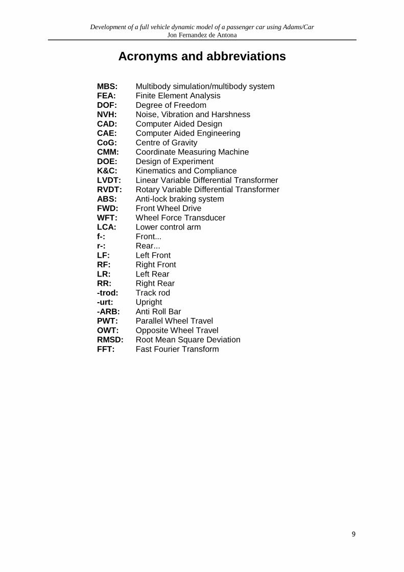
MBS: Multibody simulation/multibody system FEA: Finite Element Analysis DOF: Degree of Freedom NVH: Noise, Vibration and Harshness CAD: Computer Aided Design CAE: Computer Aided Engineering CoG: Centre of Gravity CMM: Coordinate Measuring Machine DOE: Design of Experiment K&C: Kinematics and Compliance LVDT: Linear Variable Differential Transformer RVDT: Rotary Variable Differential Transformer ABS: Anti-lock braking system FWD: Front Wheel Drive WFT: Wheel Force Transducer LCA: Lower control arm f-: Front... r-: Rear... LF: Left Front RF: Right Front LR: Left Rear RR: Right Rear -trod: Track rod -urt: Upright -ARB: Anti Roll Bar PWT: Parallel Wheel Travel OWT: Opposite Wheel Travel RMSD: Root Mean Square Deviation FFT: Fast Fourier Transform

Development of a full vehicle dynamic model of a passenger car using Adams/Car
Jon Fernandez de Antona
10
1. Introduction
1.1. Background and motivation
Computer Aided Engineering (CAE) in general, and Multibody Simulation (MBS) in
particular, have gradually transformed the former unidirectional, sequential product
design process into a concurrent process in which it is not necessary for the
preceding tasks to have ended before engineers can start working on the next tasks
downstream.
MBS enables engineers to numerically solve complex dynamic problems which
would have taken a lot of effort by simply using analytical methods. Virtual dynamic
models of products which do not physically exist can be created, hence providing
valuable information early in the design stage.
In addition, even when the product has already been produced, MBS can help
reduce the amount of costly physical testing required to optimise it.
1.2. Vehicle Dynamics and Multibody Simulation
In order to be competitive, automotive manufacturers are forced to reduce the
duration and cost of the design process of their new products, while meeting the
ever-increasing customer expectations in terms of quality, comfort, efficiency and
performance.
MBS software is a key dynamic simulation tool for engineers working in the
automotive industry, in which the use of predictive methods is vital to increase the
efficiency of the engineering process.
Within the automotive industry, MBS software has been traditionally used by vehicle
dynamicists for a variety of tasks, including, but not limited to:
Ride comfort analysis (isolation from external and internal disturbances)
Analysis of suspension kinematics and elastokinematics.
Full vehicle handling analysis (cornering and straight line performance, roll
over behaviour)
Determining the dynamic loads on suspension components for later use in
FEA.
Creating envelopes of moving components and checking for collisions
between them.
As one of the industry-standard multibody simulation packages for vehicle dynamics,
MSC ADAMS/Car is the software on which this investigation will be based.
Development of a full vehicle dynamic model of a passenger car using Adams/Car
Jon Fernandez de Antona
11
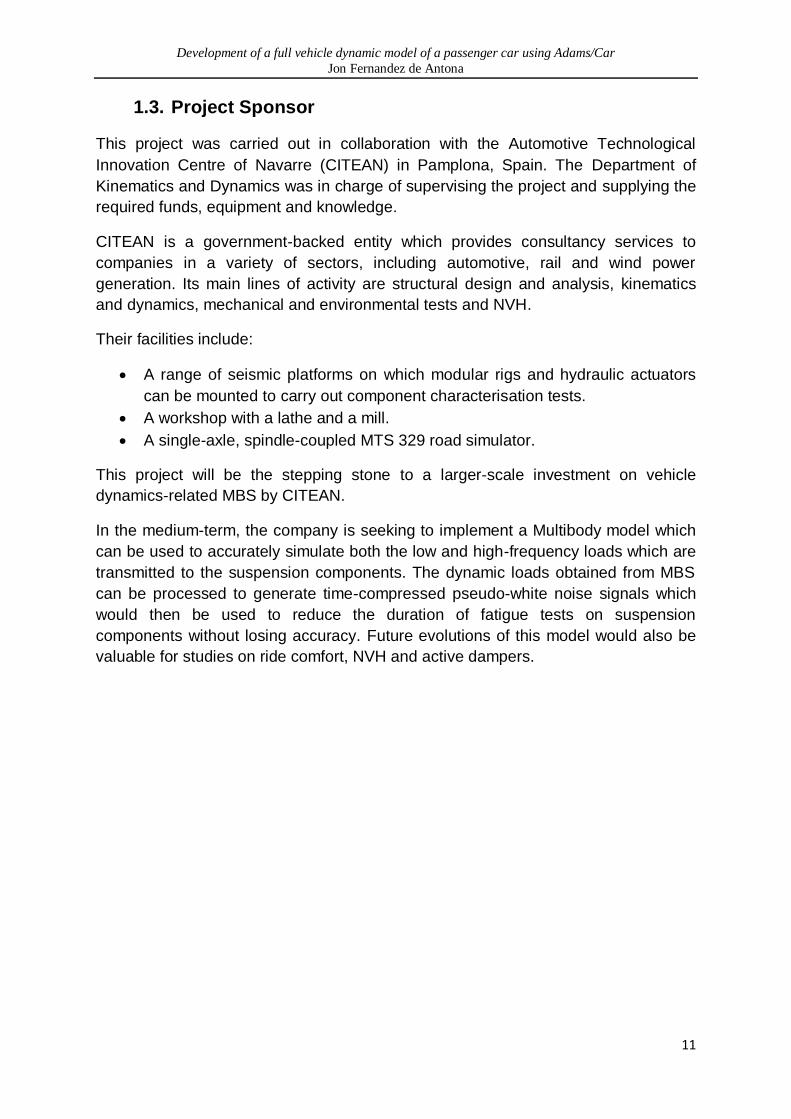
1.3. Project Sponsor
This project was carried out in collaboration with the Automotive Technological
Innovation Centre of Navarre (CITEAN) in Pamplona, Spain. The Department of
Kinematics and Dynamics was in charge of supervising the project and supplying the
required funds, equipment and knowledge.
CITEAN is a government-backed entity which provides consultancy services to
companies in a variety of sectors, including automotive, rail and wind power
generation. Its main lines of activity are structural design and analysis, kinematics
and dynamics, mechanical and environmental tests and NVH.
Their facilities include:
A range of seismic platforms on which modular rigs and hydraulic actuators
can be mounted to carry out component characterisation tests.
A workshop with a lathe and a mill.
A single-axle, spindle-coupled MTS 329 road simulator.
This project will be the stepping stone to a larger-scale investment on vehicle
dynamics-related MBS by CITEAN.
In the medium-term, the company is seeking to implement a Multibody model which
can be used to accurately simulate both the low and high-frequency loads which are
transmitted to the suspension components. The dynamic loads obtained from MBS
can be processed to generate time-compressed pseudo-white noise signals which
would then be used to reduce the duration of fatigue tests on suspension
components without losing accuracy. Future evolutions of this model would also be
valuable for studies on ride comfort, NVH and active dampers.

Development of a full vehicle dynamic model of a passenger car using Adams/Car
Jon Fernandez de Antona
12
1.4. Research goals and approach
1.4.1. Project aim
The aim of this project is to implement and correlate a multibody dynamic model of a
mid-size passenger car, comprising a Macpherson front suspension and a multilink
rear suspension, in order to simulate its handling and primary ride behaviour. MSC
ADAMS/Car software will be used.
1.4.2. Objectives
A. Identify and measure the unknown variables required to implement the ADAMS/Car model, such as:
a. Mass properties of individual components and of the complete vehicle. b. Topology of the vehicle c. Steering ratio d. Damper curves e. Tyre characteristics f. Component stiffness:
i. Springs ii. Anti Roll bars iii. Bushings iv. Bumpstops and droopstops
B. Build the ADAMS/Car model using the measured data.
C. Design appropriate tests to measure the system- and vehicle-level
characteristics of the vehicle, both in ADAMS/Car and in real life.
D. Run the selected simulations in ADAMS/Car.
E. Carry out the experimental tests.
F. Process the results and produce a correlation study which can be used to draw conclusions and suggest further work on the subject.

Development of a full vehicle dynamic model of a passenger car using Adams/Car
Jon Fernandez de Antona
13
1.4.3. Methodology
A. All the characterisation tests were carried in-house within CITEAN’s premises
and existing resources were used where possible.
a. The masses of all the suspension components were measured using a
precision scale. The components were drawn in CAD in order to
estimate the positions of their centres of gravity and inertias. In order to
measure the mass and the CoG position of the full vehicle an axle lift
test was carried out as specified in ISO 10392 [1]. No equipment was
available to measure the full vehicle inertias so these were derived
from bibliography.
b. Suspension hardpoint coordinates were acquired by lifting the vehicle
and using a CMM. Wheel plane orientations were measured using
wheel alignment gauges.
c. The handwheel to road wheel steering ratio was measured using a
handwheel angle sensor and a wheel alignment gauge.
d. Damper force-velocity curves were acquired using a hydraulic damper
dynamometer.
e. The static radial stiffness of the tyre was measured using a hydraulic
actuator coupled to a strain gauge. Measurements were carried out at
different inflation pressures. No additional tyre data was available.
f. A variety of component stiffness characterisation tests were carried out
using one or two hydraulic actuators coupled to strain gauges,
generating a range of quasi-static axial forces and moments. The effect
of displacement frequency on the stiffness was ignored in all tests.
B. Subsystems and assemblies which were specific to the vehicle's topology and
characteristics were implemented based on ADAMS/Car default templates.
C. On the experimental side, a series of dynamic excitation and suspension compliance tests were planned using the MTS 329 road simulator. These tests were equivalent to the virtual tests offered in ADAMS/Car.
D. Virtual 4 post excitation and compliance tests were carried out in ADAMS/Car
using the same actuator signals as in the experimental tests. In addition, basic
elastokinematic tests were also run.
E. Initially track tests had been scheduled to take place. However, due to the
lack of time and resources, vehicle-level tests were eventually limited to road
simulator testing. The vehicle was equipped with sensors and vertical
excitation and compliance tests were carried out on the rig. These tests were
repeated for both front and rear axles.
Development of a full vehicle dynamic model of a passenger car using Adams/Car
Jon Fernandez de Antona
14
F. The logged data from the experimental tests was filtered and resampled for ease of analysis. Subsequently, the quality of curve fitting was numerically quantified where possible.
1.4.4. Report outline
The project report consists of 8 main sections plus an appendix. Section 1 explains
the project background and states the project goals, outlining the approach followed
to achieve them.
Section 2 contains a detailed review of literature on automotive MBS applications
and dynamic model correlation.
The process of measuring system- and component-level parameters of the vehicle,
along with the results of these measurements, are described in section 3.
Section 4 shows how these measurements are then used to build the multibody
model.
The use of road simulator tests as a tool to correlate the multibody model is
explained in section 5 and the correlation between experimental data and multibody
simulations is discussed in section 6.
Finally the conclusion and suggestions for future work are presented in section 7,
followed by a statement of the original contribution of this project, in section 8.

Development of a full vehicle dynamic model of a passenger car using Adams/Car
Jon Fernandez de Antona
15
2. Literature Review
2.1. Overview
At the time of this investigation, extensive work is still being done in optimising,
adding new functionalities and finding new applications to the existing MBS software.
However, the application of MBS to vehicle dynamics has been a standard practice
in industry since the early nineties, which means that a vast amount of literature is
available in this field, a portion of which is shown here.
2.2. Vehicle to be modelled
A Volkswagen Passat B6 (2006) was the vehicle chosen for this project. The primary
reason for this choice was the fact that the sponsoring company had previously
worked with it and some data was readily available.
Those specifications which are relevant to the purposes of this project can be seen
in Table 2.2.1 [2][3]:
Brand/Model Volkswagen Passat B6 (2006)
Body style 4 door sedan
Layout Front engine, front wheel drive
Engine 2.0 litre, inline 4, TDi
Transmission 5 speed manual
Wheelbase 2709mm
Track (front, rear) 1552mm, 1551mm
Front suspension MacPherson
Rear suspension Multilink
Tyres Pirelli P7 215/55 R16 97 W
Table 2.2.1: Technical specifications of the vehicle to be modelled
Phantom views of the front and rear suspensions can be seen in Figure 2.2.1 and
Figure 2.2.2, respectively[2].

Development of a full vehicle dynamic model of a passenger car using Adams/Car
Jon Fernandez de Antona
16
Figure 2.2.1: Front suspension (MacPherson)
Figure 2.2.2: Rear suspension (Multilink)

Development of a full vehicle dynamic model of a passenger car using Adams/Car
Jon Fernandez de Antona
17
2.3. Typical components of an automotive multibody model
A multibody system, as the name implies, can be understood as an assembly of
multiple bodies, connected to each other or to the "ground" by constraints and/or
forces.
The constraints limit the number of independent kinematical possibilities, or degrees
of freedom (DOF), the bodies have to move. Therefore they can be used to
understand what movement the bodies (members of a mechanical system) will follow,
i.e. their kinematic behaviour.
Typical constraint elements, or joints, are shown in Table 2.3.1 [4]. It can be seen
that some joints in this table remove "half-constraints". This is because these joints
relate translational and rotational motion, generating a single, coupled DOF for both
motions:
Joint Translational
DOF removed
Rotational
DOF removed
Total DOF
removed
Constant velocity 3 1 4
Cylindrical 2 2 4
Fixed 3 3 6
Hooke 3 1 4
Planar 1 2 3
Rack and pinion 0.5 0.5 1
Revolute 3 2 5
Screw 0.5 0.5 1
Spherical 3 0 3
Translational 2 3 5
Universal 3 1 4
Table 2.3.1: Degrees of freedom removed by joints
On the other hand, the bodies in a MBS, which can either be perfectly rigid or flexible,
have a mass and a specific inertia tensor. If the forces acting on the bodies are
known, mass properties can be used to analyse their dynamic behaviour by
calculating the rate of change in their momentum [5].
Development of a full vehicle dynamic model of a passenger car using Adams/Car
Jon Fernandez de Antona
18
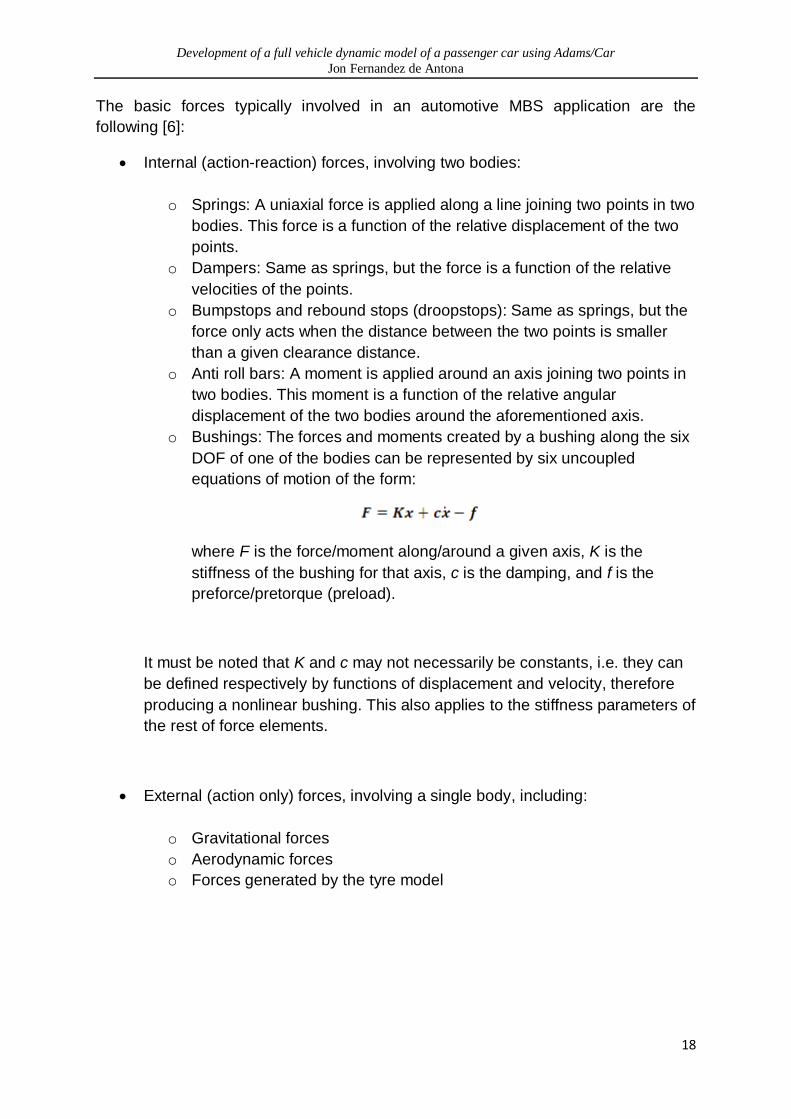
The basic forces typically involved in an automotive MBS application are the
following [6]:
Internal (action-reaction) forces, involving two bodies:
o Springs: A uniaxial force is applied along a line joining two points in two
bodies. This force is a function of the relative displacement of the two
points.
o Dampers: Same as springs, but the force is a function of the relative
velocities of the points.
o Bumpstops and rebound stops (droopstops): Same as springs, but the
force only acts when the distance between the two points is smaller
than a given clearance distance.
o Anti roll bars: A moment is applied around an axis joining two points in
two bodies. This moment is a function of the relative angular
displacement of the two bodies around the aforementioned axis.
o Bushings: The forces and moments created by a bushing along the six
DOF of one of the bodies can be represented by six uncoupled
equations of motion of the form:
where F is the force/moment along/around a given axis, K is the
stiffness of the bushing for that axis, c is the damping, and f is the
preforce/pretorque (preload).
It must be noted that K and c may not necessarily be constants, i.e. they can
be defined respectively by functions of displacement and velocity, therefore
producing a nonlinear bushing. This also applies to the stiffness parameters of
the rest of force elements.
External (action only) forces, involving a single body, including:
o Gravitational forces
o Aerodynamic forces
o Forces generated by the tyre model
Development of a full vehicle dynamic model of a passenger car using Adams/Car
Jon Fernandez de Antona
19
2.4. Tyre models
Tyres are the only contact point between a vehicle and the road. Thus, the forces
and moments generated by the tyres are of crucial importance for the dynamic
behaviour of the road vehicle.
In order to predict these forces and moments under a variety of operating conditions,
different tyre models have been developed during the last few decades. These
models are usually based on a large amount of experimental data, which can be
obtained via different types of tests [7][8].
Different models have different strengths and weaknesses and therefore each of
them is best suited for a given application. Figure 10.1.1 in appendix A shows typical
applications for different tyre models. The 2002 version of the Pacejka tyre model [7]
and the FTire flexible ring tyre model [9] are arguably the most complete and
polyvalent models offered in ADAMS. In general terms, the Pacejka model is used
for all applications except for those involving high excitation frequencies (over 15Hz),
or those requiring modelling of non-linear tyre enveloping effects, such as durability
studies[4].
2.5. Suspension configurations
The main functions of automotive suspensions are[10]:
To keep the tyres at optimal angles with respect to the road in order to
generate the desired forces on the tyre contact patches.
To transmit these forces into the sprung mass while maximizing the isolation
of occupants from road disturbances
And vice versa, to react the forces caused by the motion of the sprung mass,
while reducing/optimising the vertical load variations on the tyre contact
patches.
Ever since the automobile was invented a wide range of suspension systems has
been developed in a quest to improve the fulfilment of the aforementioned functions.
However, only two types of suspensions will be treated here, as mentioned in section
2.2: the MacPherson strut (front) and the Multilink suspension (rear).
The MacPherson suspension consists of a lower control arm (LCA), which reacts
most of the longitudinal and lateral forces generated by the tyre, and a strut
containing a spring-damper system, which reacts most of the vertical forces (Figure
2.2.1).

Development of a full vehicle dynamic model of a passenger car using Adams/Car
Jon Fernandez de Antona
20
This suspension configuration is very popular on the front axles of modern
transverse-engined, FWD cars, as its inherent geometry provides enough space for
a wide engine bay and unrivalled design simplicity [10].
However, the fact that the strut acts effectively as an infinitely long upper control arm
generally means that negative camber is lost with bump[11]. This reduces the lateral
force generation capabilities of the tyres. In a cornering situation, an increase in
negative camber is desired on the outside wheel [11]. This can be explained by
phenomena such as "camber thrust" [7].
Multilink suspensions normally consist of four or five links. If non-compliant (a.k.a
"kinematic") joints were used between all the links, the fifth link, when present, would
effectively over-constrain the mechanism, leaving no remaining DOFs for it to move.
However, due to the fact that bushings are widely used instead of kinematic joints in
real life, the compliance of the joints has to be taken into account. In this case, the
fifth link provides more accurate control of the compliant toe angles caused by the
cornering forces and moments [10].
Increased control on the system compliances affecting the wheel plane orientation
(a.k.a "elastokinematics") is beneficial in many ways: optimised suspension
elastokinematics improve the handling of the vehicle, help reduce tyre wear, and
provide a better ride quality due to the possibility of achieving greater longitudinal
compliances without detriment to suspension kinematics[12].
2.6. Influence of suspension isolator models on MBS
It has been mentioned in section 2.3 that bushings can be modelled as sets of
nonlinear forces and moments. The nonlinearities are caused primarily by two
reasons:
Coupling of different modes of deformation: In automotive suspensions the
bushing is mostly deformed in such a way that multiaxial rotations and
translations occur simultaneously. However, the torsional stiffness of the
bushing is significantly affected by the amount of axial displacement.[13]
The elastomers (rubbers, generally) used in the bushing construction behave
viscoelastically[14].
Two phenomena that can be typically associated to viscoelastic materials are the
fact that their stiffness is dependent on the rate of application of the load (a.k.a.
frequency dependence) and the fact that they present a phase lag or history
dependence when subjected to cyclic loadings (a.k.a. hysteresis)[15].
Development of a full vehicle dynamic model of a passenger car using Adams/Car
Jon Fernandez de Antona
21
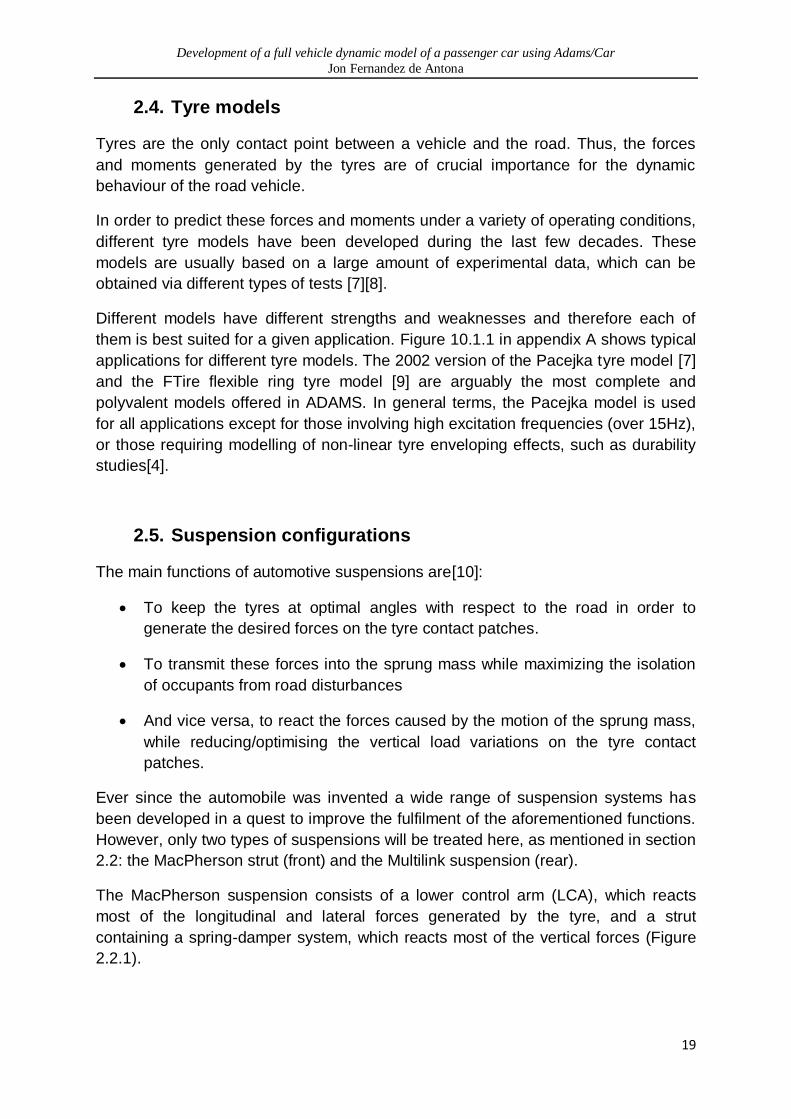
The effects of these phenomena on automotive suspensions are best appreciated at
relatively high road disturbance frequencies, well within the "secondary ride" area, as
shown in Figure 2.6.1 [16]
Figure 2.6.1: Vehicle performance classifications arranged by primary frequency range
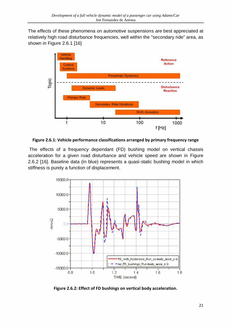
The effects of a frequency dependant (FD) bushing model on vertical chassis
acceleration for a given road disturbance and vehicle speed are shown in Figure
2.6.2 [16]. Baseline data (in blue) represents a quasi-static bushing model in which
stiffness is purely a function of displacement.
Figure 2.6.2: Effect of FD bushings on vertical body acceleration.

Development of a full vehicle dynamic model of a passenger car using Adams/Car
Jon Fernandez de Antona
22
Computational effort is a major factor to be considered when modelling bushings for
MBS. FD and hysteretic bushing models require more time to compute than quasi-
static models. For this reason, quasi-static models are still widely used for primary
ride simulations. In these cases, the damping ratio is generally defined as a direct
proportion of the instantaneous stiffness. In most cases this value is considered to
be in the region of 1% [17][4].
Another factor having an influence on computational effort is the value of the bushing
stiffness. High stiffness bushing models require small step-sizes in the numerical
integration[18]. This can be explained by the fact that bushings generate higher
frequency responses than vehicle dynamic responses [19]. One way to work around
this is the subsystem synthesis method, in which separate equations of motion (EOM)
are generated for the chassis and suspension subsystem [18].
2.7. Target specifications of a multibody model
Back in 1992, Lotus obtained good correlation of yaw rate between their ADAMS
model and real tests for an 80km/h single lane change manoeuvre [20]. In order to
achieve this, the multibody model they used had in excess of 200 DOF and used a
complex Pacejka tyre model.
Ever-increasing computing power can be a temptation to keep increasing the
complexity and amount of DOF of multibody models. However, excessive complexity
can lead to a “paralysis of analysis”[21], in which the large number of parameters
required to build the model and the time required to gather them actually reduce the
usefulness of the model.
It is recommended that the level of complexity of the model to be implemented
should just match the complexity of the problem to be solved [22]. The ideal model
would be the least complex one which provides a solution of an “acceptable”
accuracy/correctness, where the task to define “acceptable” is left to the judgement
of the engineer.
Development of a full vehicle dynamic model of a passenger car using Adams/Car
Jon Fernandez de Antona
23
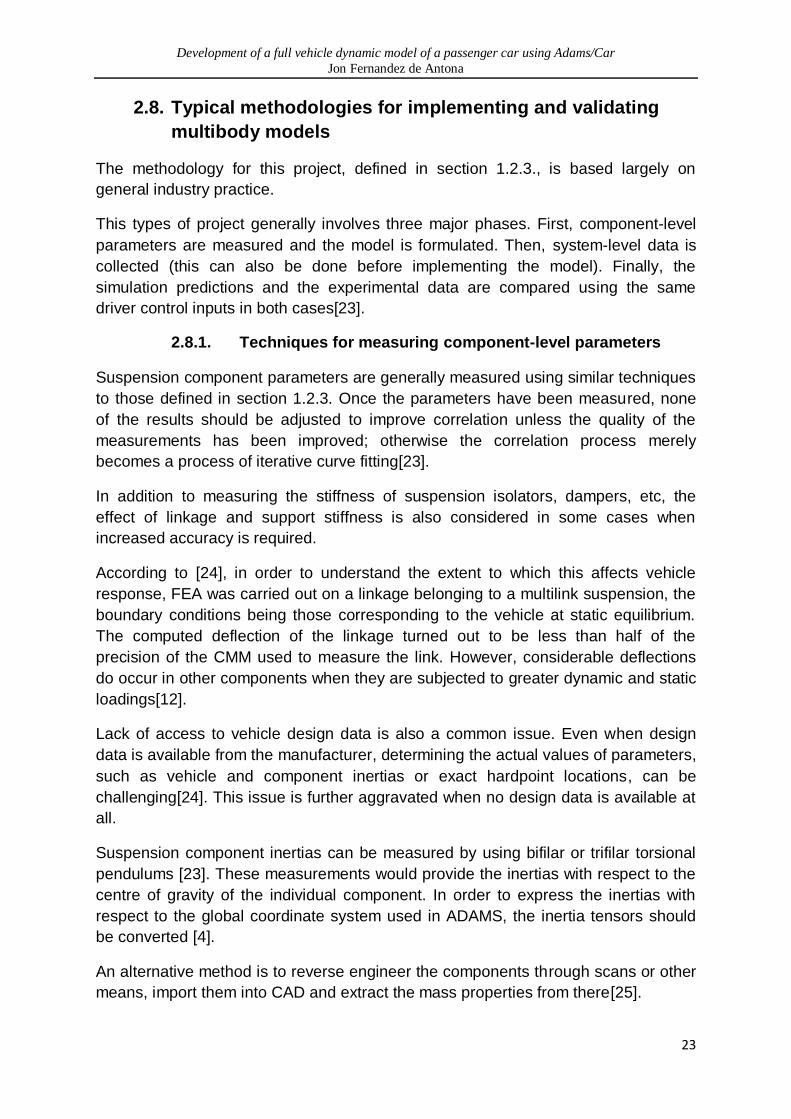
2.8. Typical methodologies for implementing and validating
multibody models
The methodology for this project, defined in section 1.2.3., is based largely on
general industry practice.
This types of project generally involves three major phases. First, component-level
parameters are measured and the model is formulated. Then, system-level data is
collected (this can also be done before implementing the model). Finally, the
simulation predictions and the experimental data are compared using the same
driver control inputs in both cases[23].
2.8.1. Techniques for measuring component-level parameters
Suspension component parameters are generally measured using similar techniques
to those defined in section 1.2.3. Once the parameters have been measured, none
of the results should be adjusted to improve correlation unless the quality of the
measurements has been improved; otherwise the correlation process merely
becomes a process of iterative curve fitting[23].
In addition to measuring the stiffness of suspension isolators, dampers, etc, the
effect of linkage and support stiffness is also considered in some cases when
increased accuracy is required.
According to [24], in order to understand the extent to which this affects vehicle
response, FEA was carried out on a linkage belonging to a multilink suspension, the
boundary conditions being those corresponding to the vehicle at static equilibrium.
The computed deflection of the linkage turned out to be less than half of the
precision of the CMM used to measure the link. However, considerable deflections
do occur in other components when they are subjected to greater dynamic and static
loadings[12].
Lack of access to vehicle design data is also a common issue. Even when design
data is available from the manufacturer, determining the actual values of parameters,
such as vehicle and component inertias or exact hardpoint locations, can be
challenging[24]. This issue is further aggravated when no design data is available at
all.
Suspension component inertias can be measured by using bifilar or trifilar torsional
pendulums [23]. These measurements would provide the inertias with respect to the
centre of gravity of the individual component. In order to express the inertias with
respect to the global coordinate system used in ADAMS, the inertia tensors should
be converted [4].
An alternative method is to reverse engineer the components through scans or other
means, import them into CAD and extract the mass properties from there[25].
Development of a full vehicle dynamic model of a passenger car using Adams/Car
Jon Fernandez de Antona
24
In order to measure full vehicle inertias, devices such as the Vehicle Inertia
Measurement Facility (VIMF) [26], have been widely used [19][27].
As far as suspension hardpoints are concerned, the difficulty of measuring their
coordinates accurately can be overcome by creating an approximate multibody
model, carrying out a statistical design of experiments (DOE), comparing the
simulated results to actual test results, and thus adjusting the coordinates in the
model to achieve correlation. DOE can be carried out using commercial simulation
software such as ADAMS/Insight [4], although this method usually involves high
computational costs [24].
2.8.2. Techniques for measuring system-level parameters
Full-vehicle behaviour depends on system level parameters (weight distribution, roll
stiffness, etc.), rather than on individual component parameters [28]. In order to
acquire data at system level, two main methods are generally used: K&C testing and
full vehicle dynamic testing. Aerodynamic testing would also be required if higher-
speed manoeuvres are to be modelled[23]. Regardless of which tests are to be
carried out, the design process of the system-level tests should be completely
independent from the component parameter identification phase to avoid bias on the
selected tests[23].
2.8.2.1. Kinematics and Compliance testing
There is a range of commercial and in-house designed K&C rigs in the market, and
different operating principles can be found. Some rigs fix the vehicle body to the
ground and use actuators to apply vertical and horizontal forces on the tyre contact
patch via high-friction wheel platforms. Another approach is to move the entire body
of the vehicle in heave, pitch and roll while the wheel platforms are allowed to move
within the road plane to apply lateral and longitudinal forces. In all cases, the linear
and angular displacements of the wheel reference planes, under different loading
conditions, are measured[29]. When carrying out a K&C test, the vehicle body has to
be fixed to the rig in multiple places to reduce the influence of body stiffness on the
measurements. One way to avoid this is to test single axles individually[30]. If the
body is modelled as a flexible component in the MBS, additional measurements will
be required to determine its torsional stiffness [11].
Very slow displacement rates are used in K&C tests to minimize inertial effects and
the effect of frequency on the component stiffness[19]. However, significant
hysteresis can still be found in some measurements, as opposed to the quasi-static
“suspension simulations” in ADAMS/Car, in which history dependence is not
considered [31].

Development of a full vehicle dynamic model of a passenger car using Adams/Car
Jon Fernandez de Antona
25
A K&C test can be used to obtain valuable data for the multibody model [28][31]:
Vertical suspension rates and hysteresis: Mainly the stiffness of springs and
bumpstops, and the clearance distance of the latter ones are measured. The
contribution of the bushings can be measured by removing the springs.[32]
Front/rear roll stiffness distribution: same as before, but ARB stiffness is also
taken into account1.
Change of toe and camber angles with bump/roll.
Instant centre locations : geometrical parameters such as roll centre and anti-
ratios are measured.
Longitudinal compliance: the compliances of bushings, subframes and wheel
hub assemblies2 under braking forces are measured. Their effect on toe angle
is assessed.
Lateral compliance: when forces are opposing, the compliances of the
bushings and the wheel hub assembly are measured. When forces are
parallel, the compliances of the subframe3 and the steering system are added
to these. The effect of all this on toe angle and camber is assessed.
Aligning moment compliances: when moments are opposing, mainly wheel
hub and bushing compliance is measured. When parallel, steering system
behaviour is measured. The steering ratio and feedback can be measured by
installing a handwheel angle and moment sensor. The effect of power
steering can be evaluated by switching the engine on and off.
Due to the fact that K&C rigs are very specialized machinery, attempts have been
made to use other devices to achieve similar results in a more economical way. For
instance, there have been reports of 90% correlation between traditional K&C tests
and measurements taken using a combination of a MTS 329® road simulator, MTS
SWIFT® wheel force transducers and wheel vector sensors[33].
1 The contribution of ARBs to roll stiffness can be calculated by repeating the test with the ARBs removed [62] 2 Hub compliance can be modelled as a bushing element [31]. 3 As can be seen in Figure 2.2.2, the rear suspension of the VW Passat is mounted on a subframe, bolted to the chassis via four vertical rubber bushings. These add compliances between the subframe and the chassis, and effectively couple the responses of both corners of the axle. These compliances can be measured on a K&C rig by placing six LVDTs between the subframe and the chassis[32]
Development of a full vehicle dynamic model of a passenger car using Adams/Car
Jon Fernandez de Antona
26
2.8.2.2. Full vehicle dynamic testing
Track acquisitions are the most common method of obtaining information on full
vehicle dynamic behaviour. In these tests, vehicles are equipped with sensors to
acquire data on the parameters of interest, and standard manoeuvres are performed
in accordance with ISO 15037-1:2006 [34]
The most frequent standard manoeuvres are listed below [35]:
Steady-state cornering: This can be achieved by either driving at a constant
radius while increasing the speed, by maintaining a fixed handwheel angle
while increasing the speed, or by maintaining a constant speed while
increasing the handwheel angle. The increments can either be discrete or
continuous[36].
o Swept steer: This is a particularly popular version of the steady-state
cornering manoeuvres. The handwheel is turned at a constant angular
velocity at an order of magnitude of 10deg/s, while the vehicle is
travelling at a constant speed[23].
(Pseudo) step steer: Used to evaluate the lateral frequency response
functions of the vehicle to transient inputs; a pseudo-discrete step of
approximately 40° is applied to the handwheel angle, at an approximate
angular velocity of 500 deg/s[23].
Pulse steer: A linear increment and a linear decrement are applied
consecutively on the steering wheel angle, producing a "fishhook" or "J-turn"
type manoeuvre which excites both steady-state an transient responses of the
vehicle. This manoeuvre is progressively replacing the traditional swept sine
handwheel angle inputs. If suitably short step sizes are chosen, step steer
inputs are able to excite the full range of vehicle directional frequencies in a
similar way to swept sine inputs, while being quicker and simpler to
perform[35]. It must be noted that frequency responses are dependent on
vehicle speed, and therefore can only be derived from constant speed
maneouvres[23].
Single lane change, double lane change and on-centre
handling[37][38][39][40]: Even though they produce similar results to the pulse
steer, these can be performed on a narrower and longer test area.
Straight line braking and acceleration: Useful to correlate powertrain,
drivetrain, brake and mechatronic models such as ABS [41] or traction control.
Road disturbance: The forces, moments and deflections caused by known
road profiles (potholes, curbs, etc.) are measured.

Development of a full vehicle dynamic model of a passenger car using Adams/Car
Jon Fernandez de Antona
27
Whenever it is possible to have repeatable control inputs, manoeuvres should be
repeated until an estimation of the random error level can be obtained by statistical
methods. This can be achieved after approximately 10 repetitions. The calculated
random error level can be used as a reference when validating the simulations.[23]
2.8.3. Correlation
"A model will be considered to be valid if, within some specified
operating range and for some given inputs, the simulation’s
predictions agree with the physical system’s responses within some
specified level of accuracy" [23]
Simulation predictions can only be correct within a portion of the operating range of
the vehicle. For instance, out of a given input frequency range predictions will
become progressively worse. In order to understand these phenomena, simulations
should be validated within both time and frequency domains[23].
As mentioned in section 2.8.1, when a simulation is found to be poorly correlating,
the only parameters allowed to be changed are those for which no accurate data is
available. Parameters could either be iterated manually (by changing one at a time)
or by using more efficient software-enabled statistical DOE. However, if this method
is used there is a risk of obtaining good correlation with a model that is not
representative of reality, due to the fact that the solutions to the MBS may not be
unique[24]. In order to avoid this, parameters should be identified as accurately as
possible and sanity checks carried out on the model regularly to ensure that the
results are logical[35].
2.9. Use of MBS within the automotive industry
Multibody models of varying complexity have been implemented in recent years by
most major automotive manufacturers, including Ford[42], Volkswagen [43], BMW
[44], Jaguar [45] and Nissan [46]. In general, the process of implementing the initial
multibody models is strongly dependant on the traditional product development
process: the vehicle and its components are designed, prototypes are produced and
finally “physically” tested; i.e. when implementing the very first multibody model of a
product in the absence of a previous knowledge-base, the product (or at least a
prototype of it) has to physically exist in the first place.

Development of a full vehicle dynamic model of a passenger car using Adams/Car
Jon Fernandez de Antona
28
2.10. Summary
Modelling the behaviour of automotive suspensions is a complex task. In order to
implement a multibody model of a vehicle, all relevant component-level parameters
must be identified and measured by experimental tests.
Once the component-level parameters are measured, they are incorporated into the
multibody model, and simulations are run.
Subsequently, a correlation study is carried out to see if the simulated behaviour of
the vehicle at system level is comparable to the actual behaviour.
In order to certify this, two main methods are used: The loading-induced changes in
wheel plane orientations and positions are measured, and the response of the whole
vehicle to different dynamic events is analysed (Figure 2.10.1). The first method
generally involves using a Kinematics and Compliance (K&C) rig, and the second
generally consists of driving the vehicle on a test track.
Figure 2.10.1: The process of validating an ADAMS model, synthesized [45].
Once the initial MB models have been correlated with reality and validated as
predictive tools, they can be used in early design stages of future projects to
optimise and validate the designs.

Development of a full vehicle dynamic model of a passenger car using Adams/Car
Jon Fernandez de Antona
29
3. Measurement of system and component-level
parameters
3.1. Instrumentation
In order to acquire the required data, a variety of sensors were installed on the
vehicle.
Suspension displacements were measured by installing one string potentiometer
(RVDT) in each corner. The body of the front potentiometer was fixed to the spring
perch, while the string was attached to one of the bolts of the upper strut mount
(Figure 3.1.1)
Figure 3.1.1: Front RVDT installation
Similarly, rear string potentiometers were fixed to the damper body by an in-house
built clamp. The strings were attached to the top damper mount (Figure 3.1.2).

Development of a full vehicle dynamic model of a passenger car using Adams/Car
Jon Fernandez de Antona
30
Figure 3.1.2: Rear RVDT Installation
A handwheel torque and angle sensor was also installed, making sure that the pulley
of the angle transducer remained in tension throughout a full turn of the handwheel
(the outer perimeter of the handwheel is not concentric with its turning axis) (Figure
3.1.3).
Figure 3.1.3: Installation of the handwheel torque and angle transducer
Development of a full vehicle dynamic model of a passenger car using Adams/Car
Jon Fernandez de Antona
31
In order to measure the angular orientation of the vehicle and all six accelerations, a
Genesys® ADMA (Automotive Dynamic Motion Analyser) accelerometer and
gyroscope system was installed on the central console, between the driver and
passenger seats (see Figure 3.1.5). This was the closest position available from the
estimated CoG of the vehicle. The exact position of the CoG was to be estimated
later, experimentally.
Its orientation was adjusted with a digital scale so that its top face was completely
horizontal with the car standing at its nominal operating ride height. The nominal
operating conditions meant that the fuel tank was completely full (in order to
minimize fluid oscillations), all the sensors and acquisition systems were installed,
and a driver was sitting in the vehicle.
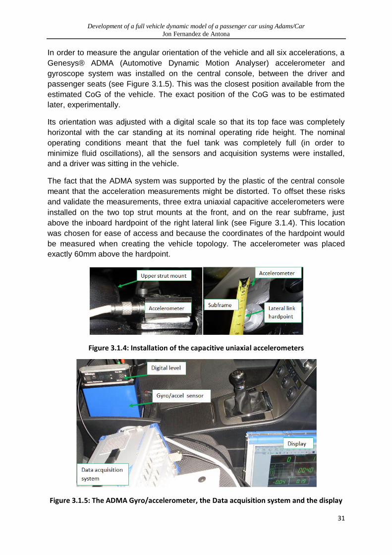
The fact that the ADMA system was supported by the plastic of the central console
meant that the acceleration measurements might be distorted. To offset these risks
and validate the measurements, three extra uniaxial capacitive accelerometers were
installed on the two top strut mounts at the front, and on the rear subframe, just
above the inboard hardpoint of the right lateral link (see Figure 3.1.4). This location
was chosen for ease of access and because the coordinates of the hardpoint would
be measured when creating the vehicle topology. The accelerometer was placed
exactly 60mm above the hardpoint.
Figure 3.1.4: Installation of the capacitive uniaxial accelerometers
Figure 3.1.5: The ADMA Gyro/accelerometer, the Data acquisition system and the display

Development of a full vehicle dynamic model of a passenger car using Adams/Car
Jon Fernandez de Antona
32
3.2. Suspension topology measurement
The topology of the suspension was measured using a CMM (see Figure 3.2.1). The
centres of cylindrical bushings were estimated by measuring three points on each
boundary of the cylinder to create two circumferences, and finding the midpoint
between their centres. All measurements were taken with the vehicle at the nominal
operating ride height. Bushing centre displacements caused by preloads at nominal
ride height were not taken into account, and could therefore be a source of error in
the measurements.
It must be noted that the arm of the CMM could not reach both axles without moving
the base. A reference axis was created at a point underneath the front subframe and
the translation of the CMM base was measured with respect to it, in order to obtain
the relative positions of the rear axle hardpoints. This might be a source of erroneous
offsets between the front and rear axle measurements.
Figure 3.2.1: Coordinate Measuring Machine (CMM)
The measured suspension hardpoint coordinates, along with some auxiliary points,
are shown in Appendix B.
Development of a full vehicle dynamic model of a passenger car using Adams/Car
Jon Fernandez de Antona
33
3.3. Estimation of mass properties
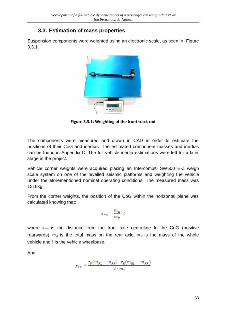
Suspension components were weighted using an electronic scale, as seen in Figure
3.3.1.
Figure 3.3.1: Weighting of the front track rod
The components were measured and drawn in CAD in order to estimate the
positions of their CoG and inertias. The estimated component masses and inertias
can be found in Appendix C. The full vehicle inertia estimations were left for a later
stage in the project.
Vehicle corner weights were acquired placing an Intercomp® SW500 E-Z weigh
scale system on one of the levelled seismic platforms and weighting the vehicle
under the aforementioned nominal operating conditions. The measured mass was
1518kg.
From the corner weights, the position of the CoG within the horizontal plane was
calculated knowing that:
where is the distance from the front axle centreline to the CoG (positive
rearwards), is the total mass on the rear axle, is the mass of the whole
vehicle and is the vehicle wheelbase.
And:
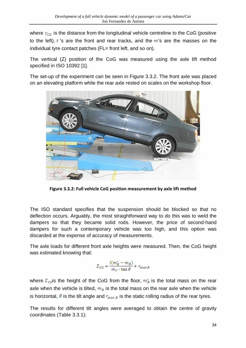
Development of a full vehicle dynamic model of a passenger car using Adams/Car
Jon Fernandez de Antona
34
where is the distance from the longitudinal vehicle centreline to the CoG (positive
to the left), 's are the front and rear tracks, and the 's are the masses on the
individual tyre contact patches (FL= front left, and so on).
The vertical (Z) position of the CoG was measured using the axle lift method
specified in ISO 10392 [1].
The set-up of the experiment can be seen in Figure 3.3.2. The front axle was placed
on an elevating platform while the rear axle rested on scales on the workshop floor.
Figure 3.3.2: Full vehicle CoG position measurement by axle lift method
The ISO standard specifies that the suspension should be blocked so that no
deflection occurs. Arguably, the most straightforward way to do this was to weld the
dampers so that they became solid rods. However, the price of second-hand
dampers for such a contemporary vehicle was too high, and this option was
discarded at the expense of accuracy of measurements.
The axle loads for different front axle heights were measured. Then, the CoG height
was estimated knowing that:
where is the height of the CoG from the floor, is the total mass on the rear
axle when the vehicle is tilted, is the total mass on the rear axle when the vehicle
is horizontal, is the tilt angle and is the static rolling radius of the rear tyres.
The results for different tilt angles were averaged to obtain the centre of gravity
coordinates (Table 3.3.1):

Development of a full vehicle dynamic model of a passenger car using Adams/Car
Jon Fernandez de Antona
35
XCG 1070mm
YCG -3mm
ZCG 460mm
Table 3.3.1: Full vehicle centre of gravity coordinates
3.4. Steering ratio and wheel alignment
The suspension alignment was measured using a FACOM® GTR 300 suspension
geometry set-up device. The vehicle body was lifted using the elevating platform and
measurements were carried out at different suspension displacements. The
measured parameters included camber, toe, kingpin inclination and castor.
In addition, the suspension set-up device was used for measuring the steering ratio
(Figure 3.4.1).
Figure 3.4.1: Wheel alignment gauge
In order to achieve this, the steering angle was increased at regular intervals and the
readings of the handwheel angle sensor and the suspension set up device were
recorded. The results are shown in Figure 3.4.2. It can be seen that the road wheels
are turned 0.0633° for every handwheel degree. This relationship is linear between -
20° and 20° of roadwheel steer. No measurements were taken for greater steering
angles.
On the other hand, it must be noted that when the handwheel is completely straight
(0°), the roadwheel is steered at 1.24°. This misalignment was noticed by those who
had driven the vehicle on the road.
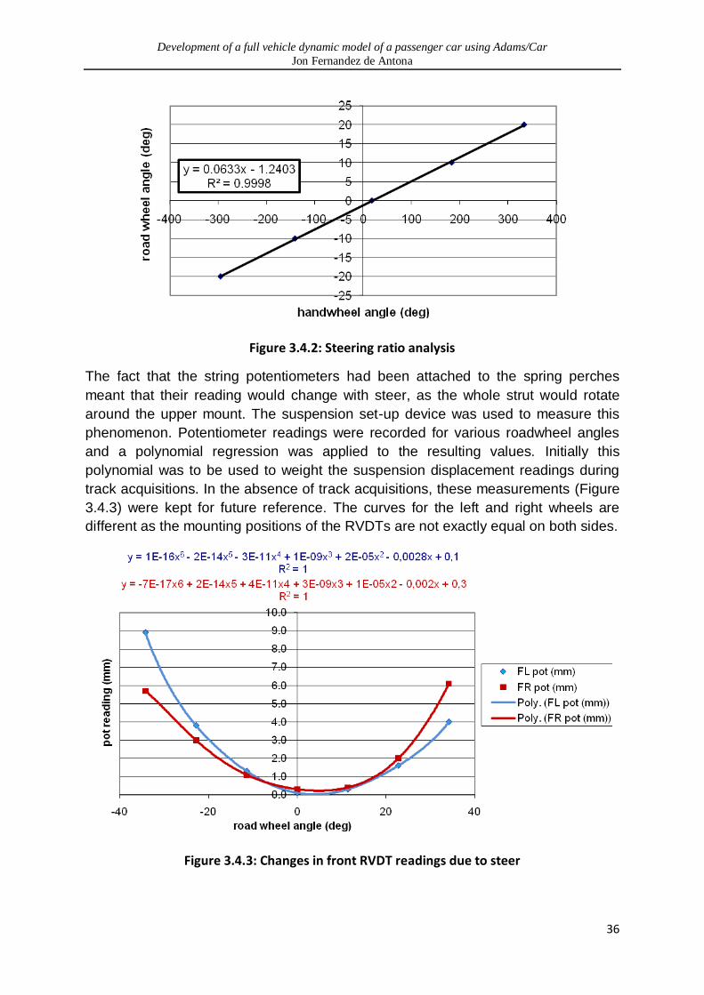
Development of a full vehicle dynamic model of a passenger car using Adams/Car
Jon Fernandez de Antona
36
Figure 3.4.2: Steering ratio analysis
The fact that the string potentiometers had been attached to the spring perches
meant that their reading would change with steer, as the whole strut would rotate
around the upper mount. The suspension set-up device was used to measure this
phenomenon. Potentiometer readings were recorded for various roadwheel angles
and a polynomial regression was applied to the resulting values. Initially this
polynomial was to be used to weight the suspension displacement readings during
track acquisitions. In the absence of track acquisitions, these measurements (Figure
3.4.3) were kept for future reference. The curves for the left and right wheels are
different as the mounting positions of the RVDTs are not exactly equal on both sides.
Figure 3.4.3: Changes in front RVDT readings due to steer

Development of a full vehicle dynamic model of a passenger car using Adams/Car
Jon Fernandez de Antona
37
3.5. Measurement of the damper force-velocity curves
Damper curves were obtained using a hydraulic dynamometer. The results for front
and rear dampers can be seen in Figure 3.5.1.
Figure 3.5.1: Front and rear damper force versus velocity
3.6. Tyre static radial stiffness measurement
The radial stiffness of the tyres was measured using an actuator attached to an axial
force transducer, as seen in Figure 3.6.1.
Figure 3.6.1: Experimental set-up for tyre characterisation
Measurements were carried out for tyre pressures ranging from 1.6bar to 2.6bar, at
0.2bar increments. The actuator speed was set at 0.2mm/s in order to generate only
quasi-static loadings. Although hysteresis for these speeds was minimal, only the
compression cycle was considered. Results are shown in Figure 3.6.2.

Development of a full vehicle dynamic model of a passenger car using Adams/Car
Jon Fernandez de Antona
38
Figure 3.6.2: Force-displacement curves for tyres at different pressures.
3.7. Spring stiffness measurement
Front and rear springs were tested in a similar way to the tyres. Actuator speeds of
1mm/s were used and hysteresis was negligible. The experimental set up can be
seen in Figure 3.7.1 and the results can be seen in Figure 3.7.2.
Figure 3.7.1: Experimental set-up for the characterisation of springs

Development of a full vehicle dynamic model of a passenger car using Adams/Car
Jon Fernandez de Antona
39
Figure 3.7.2: Front and rear spring force vs. displacement
3.8. Anti Roll Bar stiffness measurement
The front and rear ARBs were fixed through its bushing mounts to a universal jig. In
order to apply a torque to the ARBs, one of their ends was attached to the actuator
via an in-house fabricated attachment fork. The opposite end was first left free in
order to measure the bushing stiffness, and then fixed to the jig to measure the
stiffness of the whole assembly. The experimental set-up can is shown in Figure
3.8.1.
Figure 3.8.1: Experimental set-up for the ARB measurements

Development of a full vehicle dynamic model of a passenger car using Adams/Car
Jon Fernandez de Antona
40
An inherent problem of this setup was that the swivel rod end of the actuator and the
fabricated attachment fork created a four-bar mechanism, which made it laborious to
identify the moment applied on the ARB and its rotation purely using the actuator
force and displacement data. This difficulty is illustrated in Figure 3.8.2.
Figure 3.8.2: Mechanism comprised by the ARB, the swivel rod end and the actuator.
Although the problem of calculating the moment and angular displacement at "C"
from the actuator force and displacement data could have been solved analytically,
ADAMS/View was used to facilitate the process. The positions of points "A", "B" and
"C" were measured and an equivalent multibody model was created, the ARB torque
being simulated by a torsional spring of unit stiffness (see Figure 3.8.3). The input
variables were the force and displacement of the actuator, and the output variables
were the angular displacement and the reaction torque at point "C".
Figure 3.8.3: ADAMS/View model of the experimental set-up
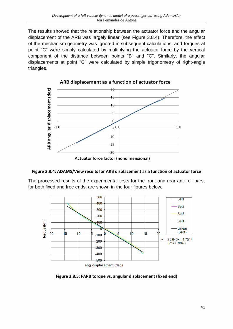
Development of a full vehicle dynamic model of a passenger car using Adams/Car
Jon Fernandez de Antona
41
The results showed that the relationship between the actuator force and the angular
displacement of the ARB was largely linear (see Figure 3.8.4). Therefore, the effect
of the mechanism geometry was ignored in subsequent calculations, and torques at
point "C" were simply calculated by multiplying the actuator force by the vertical
component of the distance between points "B" and "C". Similarly, the angular
displacements at point "C" were calculated by simple trigonometry of right-angle
triangles.
Figure 3.8.4: ADAMS/View results for ARB displacement as a function of actuator force
The processed results of the experimental tests for the front and rear anti roll bars,
for both fixed and free ends, are shown in the four figures below.
Figure 3.8.5: FARB torque vs. angular displacement (fixed end)
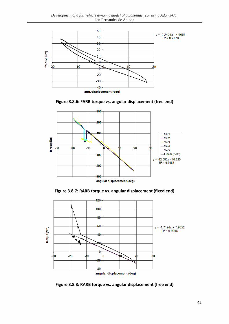
Development of a full vehicle dynamic model of a passenger car using Adams/Car
Jon Fernandez de Antona
42
Figure 3.8.6: FARB torque vs. angular displacement (free end)
Figure 3.8.7: RARB torque vs. angular displacement (fixed end)
Figure 3.8.8: RARB torque vs. angular displacement (free end)

Development of a full vehicle dynamic model of a passenger car using Adams/Car
Jon Fernandez de Antona
43
In the free end tests, a considerable hysteresis can be seen between the
compression and expansion cycles, despite the relatively low actuator speed
(1mm/s). This behaviour is typical of the polymers employed in the bushings that
support the ARBs.
In addition, in Figure 3.8.8 a peak can be appreciated due to the clash between the
free end of the ARB and the jig supporting it, which effectively makes the ARB start
working in torsion. All results beyond the contact point were ignored for bushing
stiffness determination. However, the linear slope generated provides a good idea of
the linear contribution that the torsion of purely elastic steel brings to the overall ARB
stiffness.
In fixed end tests, hysteresis is hidden by the fact that the measured stiffness is
considerably higher and it is produced mainly by the torsion of highly elastic steel.
The "steps" seen in Figure 3.8.7 could be due to sticktion or stick/slip behaviour at
the steel/rubber interface in the ARB bushings.
3.9. Bushing stiffness measurement
The stiffness of the bushings around and along their three axes had to be measured
for the multibody model.
Given the large number of bushings present in the suspension assemblies, it was
decided that the most representative bushing models should be selected for
experimentation, and the same measurements would be used for other similar
bushing constructions.
Bushings were chosen according to their accessibility and their characteristic
features. Some bushings were found to be unique in shape due to their specific
distribution of voids and reinforcements, features which are commonly used to tailor
their stiffness independently along each axis. However, those bushings which were
solid cylinders of rubber were only characterised once.
The selected bushings were the rear track rod outboard (component 2, Figure
10.4.1), the rear track rod inboard (component 3, Figure 10.4.1), the trailing arm
(component 3, Figure 10.4.2) and the lateral link inboard (component 8, Figure
10.4.2).
In order to enable quick bushing changes between tests and reduce costs, a
common housing was used to fix the bushings to the test bench. A series of sleeves
was designed and manufactured in-house to fit different bushing diameters and
lengths (see Figure 3.9.1). The technical drawings of the sleeves can be found in
Appendix E.
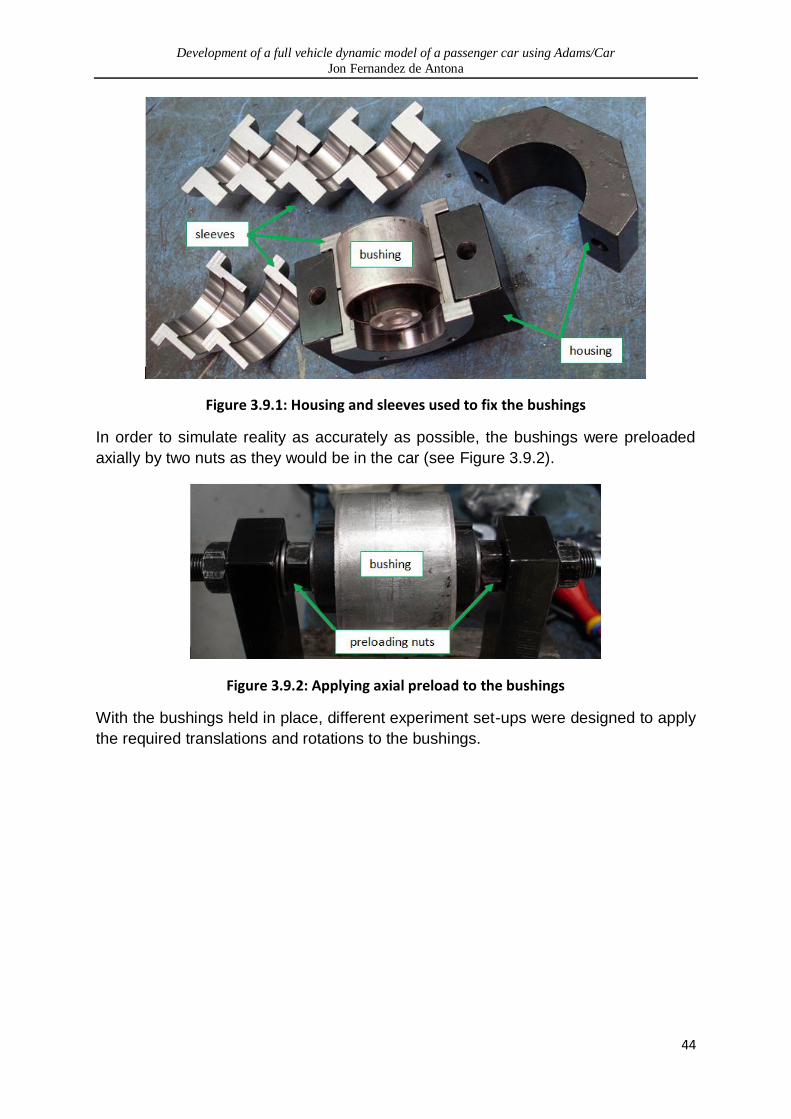
Development of a full vehicle dynamic model of a passenger car using Adams/Car
Jon Fernandez de Antona
44
Figure 3.9.1: Housing and sleeves used to fix the bushings
In order to simulate reality as accurately as possible, the bushings were preloaded
axially by two nuts as they would be in the car (see Figure 3.9.2).
Figure 3.9.2: Applying axial preload to the bushings
With the bushings held in place, different experiment set-ups were designed to apply
the required translations and rotations to the bushings.

Development of a full vehicle dynamic model of a passenger car using Adams/Car
Jon Fernandez de Antona
45
Figure 3.9.3: Bushing test configuration 1 - axial rotation
Figure 3.9.4: Bushing test configuration 2 - radial rotation

Development of a full vehicle dynamic model of a passenger car using Adams/Car
Jon Fernandez de Antona
46
Figure 3.9.5: Bushing test configuration 3 - radial translation
Figure 3.9.6: Bushing test configuration 4 - axial translation
For test configurations 2 (Figure 3.9.4) and 3 (Figure 3.9.5), bushings were tested at
two orthogonal angles, making sure that the two radial axes were lined up with
relevant features such as voids. Whenever the bushings were axisymmetric, radial
tests were carried out only once.
Knowing the distance between the actuator axis and the centre of the bushing at all
times, moments were calculated from the axial force transducer readings by simple
trigonometric calculations. Whenever two actuators were used, the moments applied
by each of them were added up. In order to reduce frequency-dependant effects,
actuator velocities were set to between 0.2mm/s and 1mm/s, depending on the
radius of the bushing.
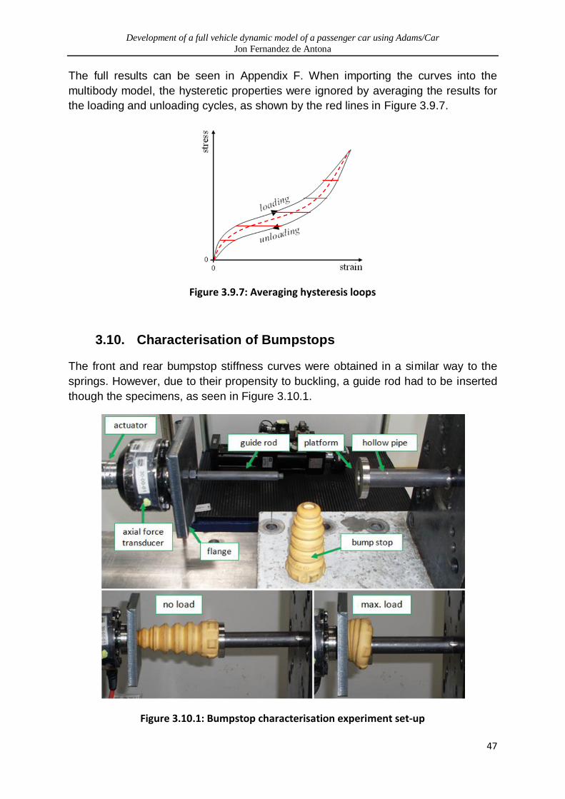
Development of a full vehicle dynamic model of a passenger car using Adams/Car
Jon Fernandez de Antona
47
The full results can be seen in Appendix F. When importing the curves into the
multibody model, the hysteretic properties were ignored by averaging the results for
the loading and unloading cycles, as shown by the red lines in Figure 3.9.7.
Figure 3.9.7: Averaging hysteresis loops
3.10. Characterisation of Bumpstops
The front and rear bumpstop stiffness curves were obtained in a similar way to the
springs. However, due to their propensity to buckling, a guide rod had to be inserted
though the specimens, as seen in Figure 3.10.1.
Figure 3.10.1: Bumpstop characterisation experiment set-up
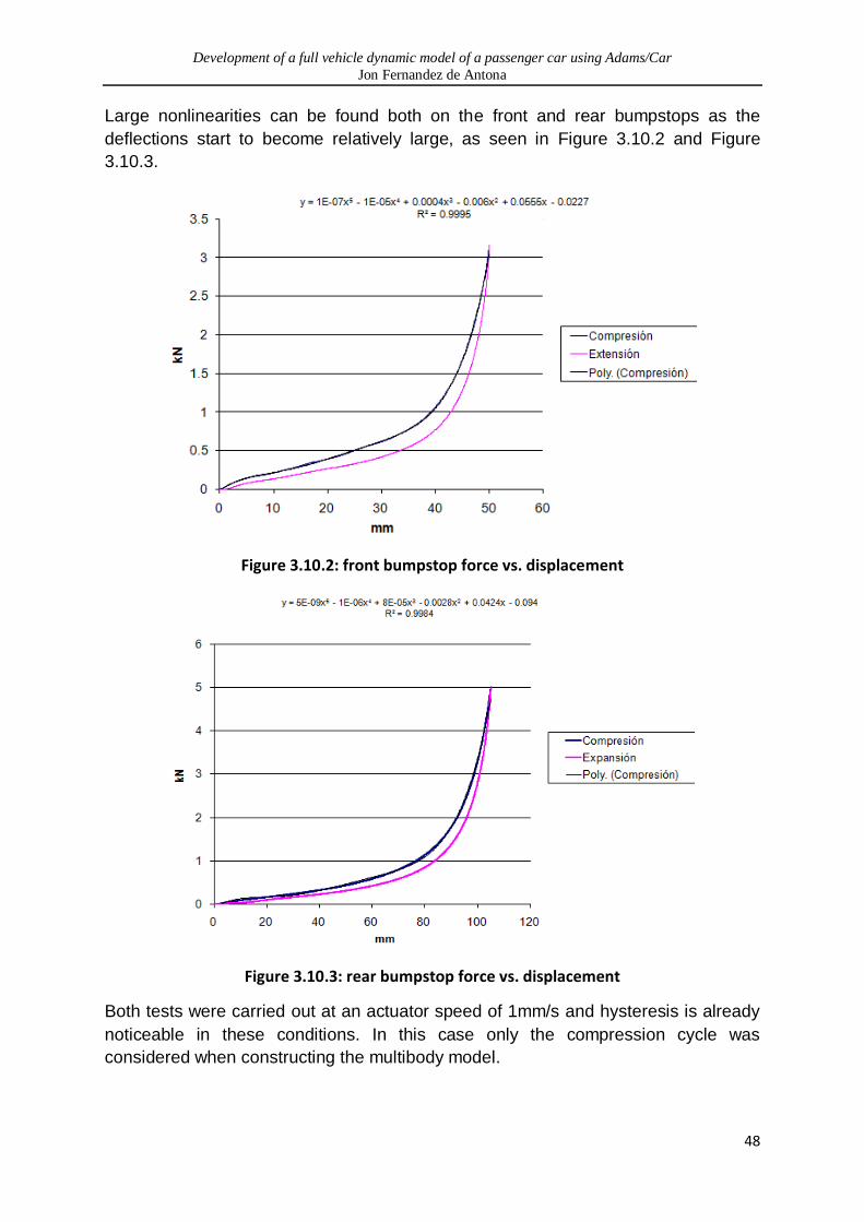
Development of a full vehicle dynamic model of a passenger car using Adams/Car
Jon Fernandez de Antona
48
Large nonlinearities can be found both on the front and rear bumpstops as the
deflections start to become relatively large, as seen in Figure 3.10.2 and Figure
3.10.3.
Figure 3.10.2: front bumpstop force vs. displacement
Figure 3.10.3: rear bumpstop force vs. displacement
Both tests were carried out at an actuator speed of 1mm/s and hysteresis is already
noticeable in these conditions. In this case only the compression cycle was
considered when constructing the multibody model.
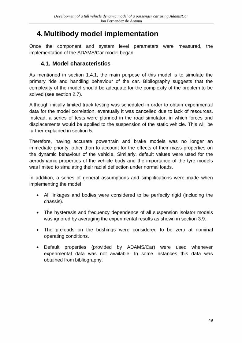
Development of a full vehicle dynamic model of a passenger car using Adams/Car
Jon Fernandez de Antona
49
4. Multibody model implementation
Once the component and system level parameters were measured, the
implementation of the ADAMS/Car model began.
4.1. Model characteristics
As mentioned in section 1.4.1, the main purpose of this model is to simulate the
primary ride and handling behaviour of the car. Bibliography suggests that the
complexity of the model should be adequate for the complexity of the problem to be
solved (see section 2.7).
Although initially limited track testing was scheduled in order to obtain experimental
data for the model correlation, eventually it was cancelled due to lack of resources.
Instead, a series of tests were planned in the road simulator, in which forces and
displacements would be applied to the suspension of the static vehicle. This will be
further explained in section 5.
Therefore, having accurate powertrain and brake models was no longer an
immediate priority, other than to account for the effects of their mass properties on
the dynamic behaviour of the vehicle. Similarly, default values were used for the
aerodynamic properties of the vehicle body and the importance of the tyre models
was limited to simulating their radial deflection under normal loads.
In addition, a series of general assumptions and simplifications were made when
implementing the model:
All linkages and bodies were considered to be perfectly rigid (including the
chassis).
The hysteresis and frequency dependence of all suspension isolator models
was ignored by averaging the experimental results as shown in section 3.9.
The preloads on the bushings were considered to be zero at nominal
operating conditions.
Default properties (provided by ADAMS/Car) were used whenever
experimental data was not available. In some instances this data was
obtained from bibliography.
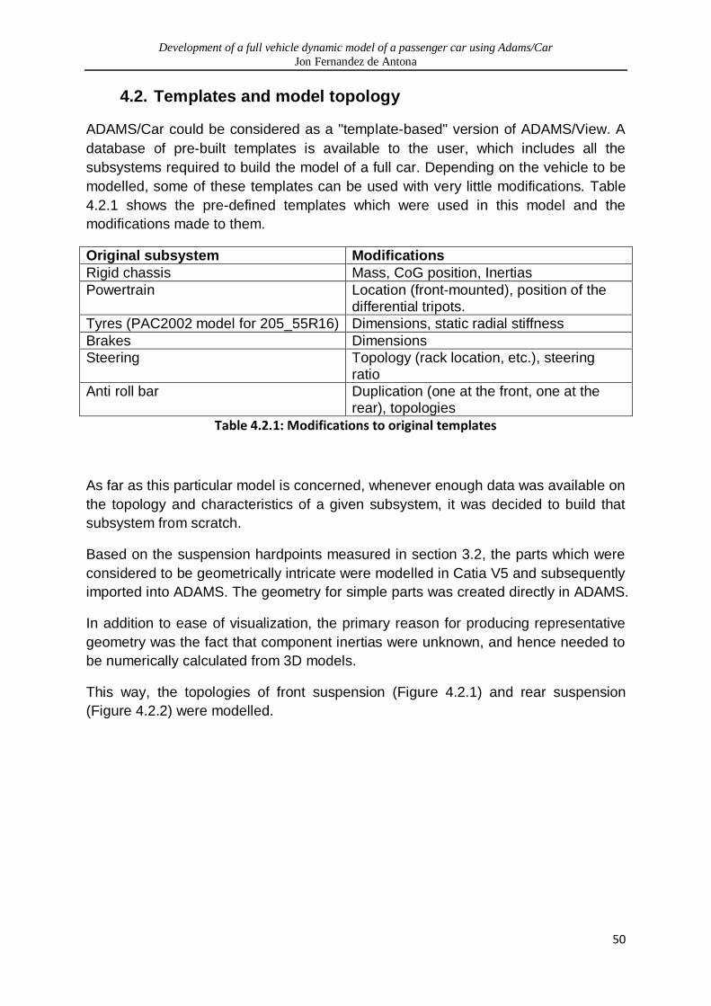
Development of a full vehicle dynamic model of a passenger car using Adams/Car
Jon Fernandez de Antona
50
4.2. Templates and model topology
ADAMS/Car could be considered as a "template-based" version of ADAMS/View. A
database of pre-built templates is available to the user, which includes all the
subsystems required to build the model of a full car. Depending on the vehicle to be
modelled, some of these templates can be used with very little modifications. Table
4.2.1 shows the pre-defined templates which were used in this model and the
modifications made to them.
Original subsystem Modifications
Rigid chassis Mass, CoG position, Inertias
Powertrain Location (front-mounted), position of the differential tripots.
Tyres (PAC2002 model for 205_55R16) Dimensions, static radial stiffness
Brakes Dimensions
Steering Topology (rack location, etc.), steering ratio
Anti roll bar Duplication (one at the front, one at the rear), topologies
Table 4.2.1: Modifications to original templates
As far as this particular model is concerned, whenever enough data was available on
the topology and characteristics of a given subsystem, it was decided to build that
subsystem from scratch.
Based on the suspension hardpoints measured in section 3.2, the parts which were
considered to be geometrically intricate were modelled in Catia V5 and subsequently
imported into ADAMS. The geometry for simple parts was created directly in ADAMS.
In addition to ease of visualization, the primary reason for producing representative
geometry was the fact that component inertias were unknown, and hence needed to
be numerically calculated from 3D models.
This way, the topologies of front suspension (Figure 4.2.1) and rear suspension
(Figure 4.2.2) were modelled.
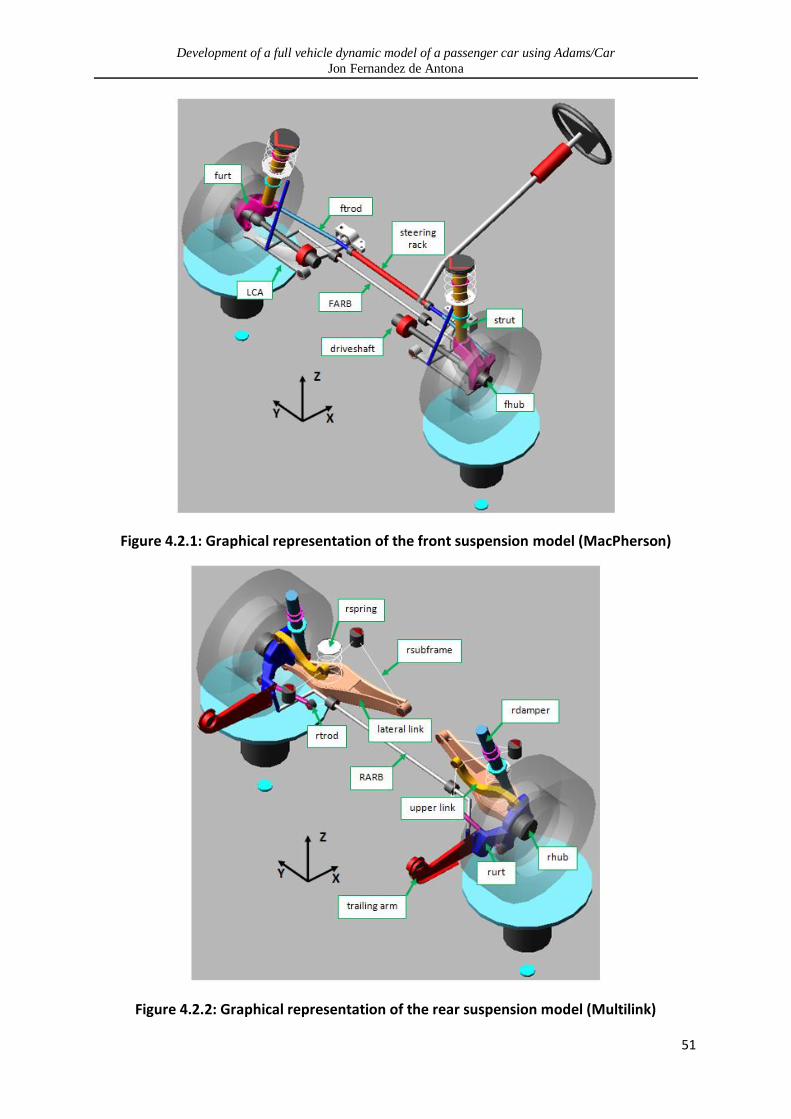
Development of a full vehicle dynamic model of a passenger car using Adams/Car
Jon Fernandez de Antona
51
Figure 4.2.1: Graphical representation of the front suspension model (MacPherson)
Figure 4.2.2: Graphical representation of the rear suspension model (Multilink)

Development of a full vehicle dynamic model of a passenger car using Adams/Car
Jon Fernandez de Antona
52
It must be noted that, as mentioned in section 2.8.1, ADAMS calculates the
component inertias with respect to the absolute origin of a given model. This is the
reason why geometry was imported from CATIA V5 to ADAMS and why inertias
were calculated within ADAMS. The results of this process can be seen in appendix
C.
Once the parts and their geometries were produced, the next step was to join the
parts together appropriately. ADAMS/Car enables the user to build kinematic (non-
compliant) joints in such a way that they can be switched by bushings at a later
stage by using a simple toggle button. This is particularly useful when comparing the
kinematic and compliant behaviour of a subsystem.
Figure 4.2.3 shows how the parts were joined together. If the diagram is considered
to represent the plan view of the vehicle, the upper half (in blue) would represent the
front subsystems in the car and the bottom half (in orange) would represent the rear
subsystems. Only the driver's side (left) is shown, along with single or non-symmetric
parts (those which are inside the coloured rectangles).
Rigid bodies and embedded subsystems (such as the powertrain) are shown inside
ovals and the links between them are represented by lines: a single line for a single
joint, multiple lines for multiple joints. Each joint has a unique number. This number
is sometimes followed by a letter, representing the type of joint. A legend for these
letters is shown in Table 4.2.2. The numbers which are not followed by a letter
correspond to force elements such as springs, dampers, bumpstops or rebound
stops; Table 4.2.3 contains the legend for these. In addition, some of the joint
numbers are followed by an asterisk: switchable kinematic and compliant
characteristics will be assigned to these, as mentioned above.
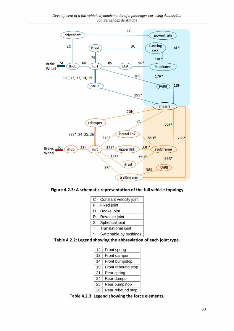
Development of a full vehicle dynamic model of a passenger car using Adams/Car
Jon Fernandez de Antona
53
Figure 4.2.3: A schematic representation of the full vehicle topology
C Constant velocity joint
F Fixed joint
H Hooke joint
R Revolute joint
S Spherical joint
T Translational joint
* Switchable by bushings
Table 4.2.2: Legend showing the abbreviation of each joint type.
12 Front spring
13 Front damper
14 Front bumpstop
15 Front rebound stop
21 Rear spring
24 Rear damper
25 Rear bumpstop
26 Rear rebound stop
Table 4.2.3: Legend showing the force elements.

Development of a full vehicle dynamic model of a passenger car using Adams/Car
Jon Fernandez de Antona
54
4.3. Modelling force elements
Whereas the nature of kinematic joints shown in Figure 4.2.3 is self explanatory (see
Table 2.3.1 for more info on the DOF removed by each of them), the compliant joints,
or bushings, need additional parameters to define them.
As far as the front suspension is concerned, Figure 4.2.3 shows that the front
subframe is rigidly fixed to the chassis at all times, effectively forming an integral part
of it. However, whenever the subsystem is simulated in compliant mode, all the
components attached to the subframe are linked by bushings.
When in compliant mode, the rear suspension has a different layout: the whole rear
subframe is linked to the chassis through bushings. In addition, due to the nature of
the multilink suspension (see section 2.5 for more information), all the linkages which
are connected to the subframe use bushings too.
One of the main issues encountered when creating the multibody model of the car
was that some bushings could not be characterised, as it would have been
necessary to destroy some suspension components in order to extract them from
their housings. Table 4.3.1 shows how the different bushings have been modelled
and which assumptions/simplifications have been made in the process.
ID Name Method
4 fsubframe to powertrain Default ADAMS/Car values
9a fsubframe to LCA (front) Estimated
9b fsubframe to LCA (rear) Experimental measurements (pp. 137 to 140)
10 fsubframe to steering rack Default ADAMS/Car values
17 fsubframe to FARB Experimental measurements (Figure 3.8.6)
19 chassis to strut Estimated
22 chassis to rsubframe Estimated
23 rurt to rdamper Default ADAMS/Car values
27 lateral link to rurt Copied from "rsubframe to rtrod"
28 rsubrame to lateral link Experimental measurements (pp. 133 to 136)
29 trailing arm to chassis Experimental measurements (pp. 123 to 126)
32 upper link to rurt Copied from "rsubframe to rtrod"
33 rsubframe to upper link Copied from "rsubframe to rtrod"
34 rtrod to rurt Experimental measurements (pp. 127 to 129)
35 rsubframe to rtrod Experimental measurements (pp. 130 to 132)
36 rsubframe to RARB Experimental measurements (Figure 3.8.8)
Table 4.3.1: Methods followed to model different bushings
As it can be seen above, when absolutely no data was known about a given bushing,
default ADAMS/Car values were used for its stiffness and damping. This is the case
for those bushings which were difficult to access, such as the engine mounts, the
steering rack mounts or the damper-to-upright bushings.
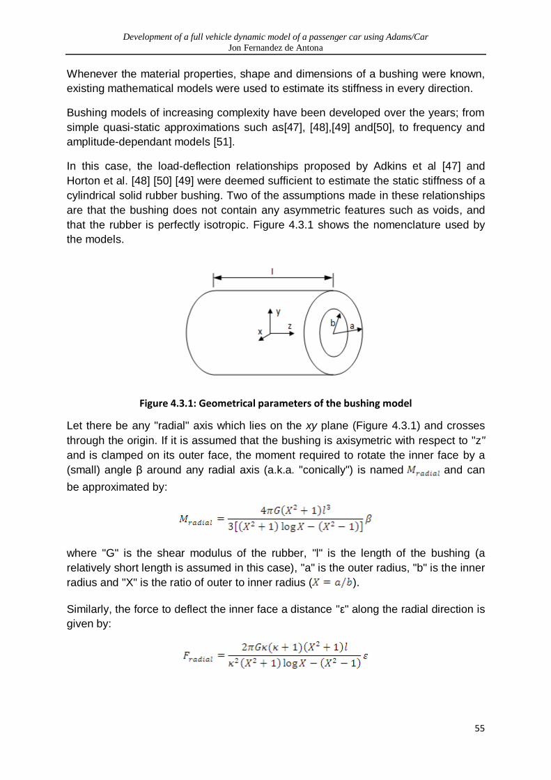
Development of a full vehicle dynamic model of a passenger car using Adams/Car
Jon Fernandez de Antona
55
Whenever the material properties, shape and dimensions of a bushing were known,
existing mathematical models were used to estimate its stiffness in every direction.
Bushing models of increasing complexity have been developed over the years; from
simple quasi-static approximations such as[47], [48],[49] and[50], to frequency and
amplitude-dependant models [51].
In this case, the load-deflection relationships proposed by Adkins et al [47] and
Horton et al. [48] [50] [49] were deemed sufficient to estimate the static stiffness of a
cylindrical solid rubber bushing. Two of the assumptions made in these relationships
are that the bushing does not contain any asymmetric features such as voids, and
that the rubber is perfectly isotropic. Figure 4.3.1 shows the nomenclature used by
the models.
Figure 4.3.1: Geometrical parameters of the bushing model
Let there be any "radial" axis which lies on the xy plane (Figure 4.3.1) and crosses
through the origin. If it is assumed that the bushing is axisymetric with respect to "z"
and is clamped on its outer face, the moment required to rotate the inner face by a
(small) angle β around any radial axis (a.k.a. "conically") is named and can
be approximated by:
where "G" is the shear modulus of the rubber, "l" is the length of the bushing (a
relatively short length is assumed in this case), "a" is the outer radius, "b" is the inner
radius and "X" is the ratio of outer to inner radius ( ).
Similarly, the force to deflect the inner face a distance "ε" along the radial direction is
given by:
Development of a full vehicle dynamic model of a passenger car using Adams/Car
Jon Fernandez de Antona
56
where the value of constant " " is dependent on whether "l" is very large ( ) or
very small ( ). In order to use this formula on bushings whose aspect ratio
( ) was roughly 1, the calculated stiffness for the two limiting cases was averaged.
On the other hand, the axial moment which produces a (torsional) deflection of " "
degrees around "z" is:
Finally, the axial force required to deflect the inner face by "ω" millimetres along "z"
is given by:
where:
and
Table 4.3.2 shows the approximate dimensions and material properties of the three
bushings whose stiffness was estimated by this method.
ID Name l (mm) a (mm) b (mm) Material G (MPa) 9a fsubframe to LCA (front) 50 20 8 rubber 1.5 19 chassis to strut 25 70 50 polyurethane 100 22 chassis to rsubframe 70 30 10 rubber 1.5
Table 4.3.2: Approximate characteristics of non-tested bushings
It must be noted that these values were calculated assuming that the bushings were
completely uniform in shape. However, the "chassis to strut" bush/mount had a steel
race, which engaged to a bearing, enabled the MacPherson strut to steer freely
around the "z" axis of the bushing. This was simulated by making its axial rotational
stiffness equal to zero.
Although the radial and stiffnesses of the "fsubframe to LCA (front)" bushing were
calculated by the aforementioned method, the conical and torsional stiffnesses
where estimated in relation to the experimental measurements made for the
"fsubframe to LCA (rear)" bushing. The reason for this is that rotational stiffnesses of
both bushings had to be modelled concurrently in order to produce reasonable toe

Development of a full vehicle dynamic model of a passenger car using Adams/Car
Jon Fernandez de Antona
57
angle compliances (Figure 4.3.2). The effect of these stiffnesses on suspension
compliances will be further explained in section 6.1.1.
Figure 4.3.2: Top view of the LCA in a front MacPherson suspension, showing the effect of the front (element D) and rear (el. 4) LCA bushing stiffnesses on compliant toe angles
caused by braking and rolling resistance loads [12].
As far as the "chassis to rsubframe" bushings is concerned, it was noticed that their
construction was not axisimmetrical, as they were reinforced by a lump of rubber
along one radial direction. However, no more data was available on their
construction and it was decided to model them as axisimmetric bushings.
On the other hand Table 4.3.1 shows that some experimental measurements were
reused for various bushings. This resource was used whenever more than one
bushing shared similar characteristics, such as shape, material, and construction.
Bushing damping values were set to 1% of the corresponding stiffness in all cases
(see section 2.6 for more information).
Subsequently the remaining force elements were included in the model by assigning
the stiffness values measured in the experimental tests to springs, dampers, anti roll
bars and bumpstops.
The stiffness of the rebound stops was not measured directly, but since the loads
going though them are relatively small under normal circumstances, their stiffness
was set to an arbitrarily large value in order to reduce deflections to a minimum. In
order to estimate the clearance distances to the front and rear bump and droop stops,
the vehicle was raised on the elevating platform until the wheels were no longer
touching the floor (damper pistons sitting on the rebound stops). Then the distances
from the top ends of the damper cylinders to the bumpstops were measured in all
four corners. When the vehicle was brought back to its static operating ride height,
the suspension positions on each corner were given by the RVDT readings, and
hence the clearance distances could be calculated.

Development of a full vehicle dynamic model of a passenger car using Adams/Car
Jon Fernandez de Antona
58
4.4. Static suspension alignment
Once all force elements were modelled, the next step was to assign static camber
and toe values to the front and rear suspension, using the measurements carried out
in section 3.4. The alignment of both axles was considered to be symmetrical, hence
the toe and camber values for the left and right wheels were assumed to be equal.
Table 4.4.1 shows the input values.
Camber (deg) Toe (deg)
Front suspension -1 0
Rear suspension 0 0
Table 4.4.1: Static camber and toe values at nominal operating conditions
The reason for the lack of decimal figures in the aforementioned values is the
significant error of the experimental measurements. Repeatability between
measurements was poor, and it was noticed that the camber and toe readings on the
rear right corner were consistently offset, even when measurements were carried out
on different vehicles. This suggested that the FACOM® GTR 300 suspension
geometry set-up device was either poorly calibrated or faulty. In order to overcome
this problem, approximate figures were used at the expense of accuracy of
simulation.
4.5. Modelling full vehicle mass properties
Once all the suspension components were modelled and their individual mass
properties were known, the next step was to define full vehicle inertias and the
position of the vehicle centre of gravity.
The main difficulty when setting full vehicle mass properties can be illustrated by
Figure 4.5.1; the full car model consists of many subsystems, each having its own
mass properties and contributing in a different way to the full car.
To mention an example, the full car CoG location had been measured experimentally
(section 3.3), and therefore became the target to be achieved for the model. In order
to adjust the full vehicle CoG location, the mass of subassemblies would have had to
be modified by calculating their contribution to the mass properties of the rest of the
vehicle. While this would have been relatively simple to do with CoG locations, it
would have required carrying out more complex calculations when inertias were
being adjusted.
Conveniently, ADAMS/Car enables the user to set the target mass properties of the
full vehicle model, and automatically adjusts the mass properties of a chosen
subsystem (generally the chassis) to reach that target.

Development of a full vehicle dynamic model of a passenger car using Adams/Car
Jon Fernandez de Antona
59
Figure 4.5.1: Subsystems and full vehicle mass properties
Another issue found during this process was the fact that the full vehicle inertias
were unknown. As mentioned in the literature review, specific equipment is required
to measure this, which the sponsoring company did not have access to.
It was decided that the most straightforward way to overcome this problem was to
refer to bibliography. The National Highway Traffic Safety Administration's (NHTSA)
Light Vehicle Inertial Parameter Database [52] was used to obtain data on the typical
moments of inertia of passenger cars. Appendix G shows the normalized roll, pitch
and yaw inertias of a variety of road vehicles of different masses. The normalization
is achieved by dividing the measured inertia by (for Ixx) or by
(for Iyy and Izz), where "M" is the vehicle mass, "T" is the track and "L" is the
wheelbase.
Knowing that for the Passat, under nominal operating conditions, M=1518kg
T≈1551,5mm and L=2709mm, the values in Table 4.5.1 could be estimated.
Ixx Iyy Izz
Normalized 0.7 0.9 1 Absolute 600 kgm2 3000 kgm2 3000 kgm2
Table 4.5.1: Normalized and absolute vehicle inertias from bibliography [52]
4.6. Additional requests
Whenever a simulation is submitted to the solver, ADAMS sends "requests", asking
for a series of parameters to be calculated when solving the system. Although
ADAMS/Car has a list of standard requests for each type of simulation, additional
requests can be added whenever a specific parameter has to be measured. This is
the case of the accelerometers which were installed in both front strut mounts and in
the rear subframe (see section 3.1).
In order to achieve this, three markers were created in ADAMS in the same
coordinates as the actual accelerometers. Subsequently, requests were created to
measure the acceleration of each marker in the vertical direction.

Development of a full vehicle dynamic model of a passenger car using Adams/Car
Jon Fernandez de Antona
60
5. Road simulator testing
5.1. Characteristics of the road simulator
MTS 329® 6DOF road simulators are generally used to recreate the multiaxial
stresses that the suspension assemblies encounter during their operating life. Real-
life events such as cornering, braking, road disturbances or any combination of them
can be recreated in a controlled environment, which improves the repeatability and
accuracy of tests as opposed to road testing. Due to these characteristics, these
kinds of rigs are specially suited for component fatigue testing [53].
The layout of one corner of the model 329 road simulator can be seen in Figure 5.1.1.
The road simulator in CITEAN is comprised of one axle (two corners), the remaining
axle being supported in a static platform.
Figure 5.1.1: MTS 329 Road Simulator layout (one corner) [53]
The vehicle can be set either in a "floating" configuration, in which the vehicle
chassis is free to move, or in a "clamped" configuration, in which the chassis is fixed
to the ground.
Six hydraulic actuators are used to apply all 6 forces and moments to the wheel hub
or spindle (see Figure 10.1.2). Instead of being directly attached to the wheel spindle,
the actuators are connected to pushrod and rocker mechanisms by bearings and
bushings in order to reduce the non-axial forces going through them.
Table 10.8.1 in appendix H shows the performance characteristics of a MTS 329
road simulator. Like with any other mechanisms powered by hydraulic actuators, the
right mass flow and pressure of hydraulic fluid must be provided by the pumps in
order to achieve the aforementioned performance figures.
Development of a full vehicle dynamic model of a passenger car using Adams/Car
Jon Fernandez de Antona
61
All moments and forces are measured by a MTS SWIFT® wheel force transducer
(WFT) bolted to the wheel hub (see appendix H). These measurements can be used
to control the actuators in a closed loop. Each of the six DOF of each corner can be
controlled in force or displacement mode. In displacement control mode, the user
input is the position of the spindle along a particular DOF and the actuator movement
matches the input. Whenever a DOF is controlled in force mode, the user inputs the
spindle forces and moments, and the relevant actuators constantly adjust their
position to match the WFT readings to the target values.
As far as the force control mode is concerned, it must be noted that the control
system will tend to induce an oscillatory motion on the actuators in its quest to match
the target force readings. Although this might not be an issue when the vehicle is set
to a clamped configuration, it could produce large, uncontrollable oscillations if the
vehicle was in a floating configuration and large asymmetrical forces were applied
laterally.
When the vehicle is in a floating configuration, the risk of uncontrollable oscillations
can be reduced by setting one corner of the car to force control while the other
corner is kept in displacement control.
5.2. Using the road simulator to validate the multibody model
Although originally conceived for fatigue testing, MTS 329 road simulators have
previously been used for non-standard applications such as K&C testing, as
mentioned in section 2.8.2.1. In that instance, in order to achieve an acceptable
accuracy, the vehicle body was clamped to the floor and wheel vector sensors were
used to measure the position and orientation of the wheel at all times [33].
As far as this project is concerned, the lack of access to a four-post rig and the lack
of time to carry out track testing meant that interest was not only limited to the K&C
testing capabilities of the road simulator, but a way of measuring the dynamic
responses of the car was also required. Therefore new ways of using the road
simulator for model validation were implemented, producing a series of vertical
excitation tests and compliance tests.
It must be noted that the purpose of these tests was not to measure absolute
vehicle-level parameters, but simply to obtain experimental data that could be
compared with ADAMS/Car simulations.
Development of a full vehicle dynamic model of a passenger car using Adams/Car
Jon Fernandez de Antona
62
5.2.1. Vertical excitation tests
The relatively high-frequency, high-amplitude operating capabilities of the road
simulator along the vertical axis meant that, if the vehicle was set to a floating
configuration, the rig could be used effectively as a 4-post shaker. Two main issues
were brought into play when considering this application.
Firstly, and as mentioned before, CITEAN's road simulator is comprised of only one
axle, which meant that only a limited number of excitation modes could be applied to
the car.
Secondly, the road simulator is not conceived to be a precision instrument. The
actuators are joined to the rockers and pushrods through compliant joints, which
means that input displacements are not as accurate as in a 4 post-rig (however the
forces measured by the WFT are very accurate).
Once these issues were understood, it was decided that the resulting inaccuracies
would still be acceptable for the purposes of validating the model behaviour at high-
amplitude, low-frequency road disturbances. Inaccuracies due to the construction of
the road simulator were expected to become larger as input frequencies increased.
However, it must be noted that the multibody model was not adapted to simulate the
vehicle response at high input frequencies accurately. In addition, if track testing had
been carried out, the roughness of the tarmac would have added a high frequency
component anyway, so the road simulator option was assumed to be the best option
available given the absence of a 4 post rig.
5.2.1.1. Experimental setup
The general layout of the experiment can be seen in Figure 5.2.1. The car had to be
raised into position by a bridge crane. In order to avoid damaging the car's
underbody and bodywork with the lifting straps a structure was built out of standard
UPN channel section beams and machined nylon blocks. The structure was
dimensioned so that the jacking points in the underbody of the car rested on the
nylon blocks, while having enough overhang on both sides of the car to keep the
lifting straps away from the bodywork.
Once the car was lifted into position, one axle was attached through the WFT to the
road simulator, while the other was strapped to a rigid platform, whose height had
previously been adjusted to keep the vehicle at a near-zero pitch angle.
The vehicle was equipped with the required data acquisition systems (see section
3.1). In order to reduce the fluid oscillations, it was ensured that the fuel tank was full.
All wheels were kept free to rotate (i.e. in neutral gear and no handbrake applied).
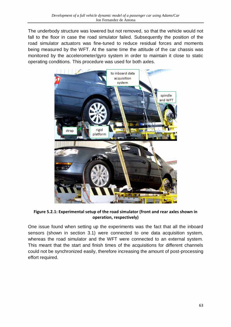
Development of a full vehicle dynamic model of a passenger car using Adams/Car
Jon Fernandez de Antona
63
The underbody structure was lowered but not removed, so that the vehicle would not
fall to the floor in case the road simulator failed. Subsequently the position of the
road simulator actuators was fine-tuned to reduce residual forces and moments
being measured by the WFT. At the same time the attitude of the car chassis was
monitored by the accelerometer/gyro system in order to maintain it close to static
operating conditions. This procedure was used for both axles.
Figure 5.2.1: Experimental setup of the road simulator (front and rear axles shown in operation, respectively)
One issue found when setting up the experiments was the fact that all the inboard
sensors (shown in section 3.1) were connected to one data acquisition system,
whereas the road simulator and the WFT were connected to an external system.
This meant that the start and finish times of the acquisitions for different channels
could not be synchronized easily, therefore increasing the amount of post-processing
effort required.

Development of a full vehicle dynamic model of a passenger car using Adams/Car
Jon Fernandez de Antona
64
5.2.1.2. Procedure
Four different vertical excitation tests were carried out:
A “Front Parallel Wheel Travel” (FPWT) test, in which both wheels of the front
axle were moved in phase.
A “Front Opposite Wheel Travel” (FOWT) test, in which both wheels of the
front axle were moved in inverse phase.
A “Rear Parallel Wheel Travel” (RPWT) test, in which both wheels of the rear
axle were moved in phase.
A “Rear Opposite Wheel Travel” (ROWT) test, in which both wheels of the
rear axle were moved in inverse phase.
The same actuator control modes were used for both corners in all four tests. These
are shown in Table 5.2.1.
DOF Control mode (target value)
Dx (longitudinal position) Displacement (zero)
Dy (lateral position) Displacement (zero)
Dz (vertical position) Displacement (input)
Rx (camber angle) Force (zero)
Ry (wheel rotation ) Displacement (zero)
Rz (steer angle) Force (zero)
Table 5.2.1: Actuator control modes for vertical excitation tests
From Table 5.2.1 it can be seen that the only input for the vertical excitation tests is
the vertical position of the wheel. When deciding which input signals to use, three
main possibilities were studied: using pre-recorded road input signals, using a
random white noise signal, or using a sinusoidal input. The last option turned out to
be the easiest one to generate and post-process.
It was decided that the input signal had to have a high-amplitude, low-frequency
content that could be used for time-domain analysis, as well as a high-frequency
content that could be used to analyse frequency-dependant effects. In order to keep
the actuator velocities within a controllable range, the amplitude had to be reduced
as frequency was increased. This was achieved by generating a decreasing-
amplitude swept sine signal in which the amplitude was inversely proportional to
frequency. For such signal, the amplitude "y" as a function of sample point "i" is
given by:

Development of a full vehicle dynamic model of a passenger car using Adams/Car
Jon Fernandez de Antona
65
and
where "A" is the peak (initial) amplitude, "n" is the number of samples, " " is the
starting frequency and " " is the finishing frequency.
A 5 cycle-long standard sine wave of amplitude "A" and frequency " " was added
before the start of the swept sine, so that redundant low-frequency data would be
available for repeatability checks during time-domain analysis. Finally the signal was
tapered at the beginning and at the end.
As far as the parallel wheel travel (PWT) tests were concerned, a (relatively large)
peak amplitude of 50mm and a frequency range of 0.5Hz to 10Hz were deemed
appropriate. It must be noted that, in PWT tests, the vehicle was expected to rotate
in "pitch" around the fixed axle, so large displacements did not suppose a structural
risk for the vehicle. However, for opposite wheel travel (OWT) tests, the peak
amplitude was reduced to 20mm in order to avoid applying excessive stresses on
the anti roll bars and the chassis, caused by the "warp" motion.
The resulting signal for PWT tests is shown in Figure 5.2.2.
Figure 5.2.2: Input signal for PWT vertical excitation tests
The signal above consists of four different parts, which are shown in Table 5.2.2:
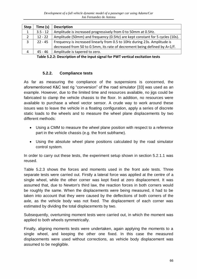
Development of a full vehicle dynamic model of a passenger car using Adams/Car
Jon Fernandez de Antona
66
Step Time (s) Description
1 3.5 - 12 Amplitude is increased progressively from 0 to 50mm at 0.5Hz.
2 12 - 22 Amplitude (50mm) and frequency (0.5Hz) are kept constant for 5 cycles (10s).
3 22 - 45 Frequency is increased linearly from 0.5 to 10Hz during 23s. Amplitude is decreased from 50 to 0.5mm, its rate of decrement being defined by A=1/f.
4 45 - 46 Amplitude is tapered to zero. Table 5.2.2: Description of the input signal for PWT vertical excitation tests
5.2.2. Compliance tests
As far as measuring the compliance of the suspensions is concerned, the
aforementioned K&C test rig “conversion” of the road simulator [33] was used as an
example. However, due to the limited time and resources available, no jigs could be
fabricated to clamp the vehicle chassis to the floor. In addition, no resources were
available to purchase a wheel vector sensor. A crude way to work around these
issues was to leave the vehicle in a floating configuration, apply a series of discrete
static loads to the wheels and to measure the wheel plane displacements by two
different methods:
Using a CMM to measure the wheel plane position with respect to a reference
part in the vehicle chassis (e.g. the front subframe).
Using the absolute wheel plane positions calculated by the road simulator
control system.
In order to carry out these tests, the experiment setup shown in section 5.2.1.1 was
reused.
Table 5.2.3 shows the forces and moments used in the front axle tests. Three
separate tests were carried out. Firstly a lateral force was applied at the centre of a
single wheel, while the other corner was kept fixed at zero displacement. It was
assumed that, due to Newton's third law, the reaction forces in both corners would
be roughly the same. When the displacements were being measured, it had to be
taken into account that they were caused by the deflections of both corners of the
axle, as the vehicle body was not fixed. The displacement of each corner was
estimated by dividing the total displacements by two.
Subsequently, overturning moment tests were carried out, in which the moment was
applied to both wheels symmetrically.
Finally, aligning moments tests were undertaken, again applying the moments to a
single wheel, and keeping the other one fixed. In this case the measured
displacements were used without corrections, as vehicle body displacement was
assumed to be negligible.
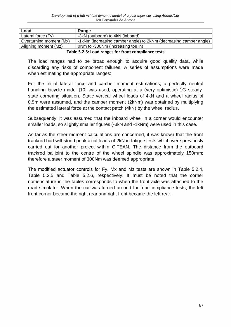
Development of a full vehicle dynamic model of a passenger car using Adams/Car
Jon Fernandez de Antona
67
Load Range
Lateral force (Fy) -3kN (outboard) to 4kN (inboard)
Overturning moment (Mx) -1kNm (increasing camber angle) to 2kNm (decreasing camber angle)
Aligning moment (Mz) 0Nm to -300Nm (increasing toe in)
Table 5.2.3: Load ranges for front compliance tests
The load ranges had to be broad enough to acquire good quality data, while
discarding any risks of component failures. A series of assumptions were made
when estimating the appropriate ranges:
For the initial lateral force and camber moment estimations, a perfectly neutral
handling bicycle model [10] was used, operating at a (very optimistic) 1G steady-
state cornering situation. Static vertical wheel loads of 4kN and a wheel radius of
0.5m were assumed, and the camber moment (2kNm) was obtained by multiplying
the estimated lateral force at the contact patch (4kN) by the wheel radius.
Subsequently, it was assumed that the inboard wheel in a corner would encounter
smaller loads, so slightly smaller figures (-3kN and -1kNm) were used in this case.
As far as the steer moment calculations are concerned, it was known that the front
trackrod had withstood peak axial loads of 2kN in fatigue tests which were previously
carried out for another project within CITEAN. The distance from the outboard
trackrod balljoint to the centre of the wheel spindle was approximately 150mm;
therefore a steer moment of 300Nm was deemed appropriate.
The modified actuator controls for Fy, Mx and Mz tests are shown in Table 5.2.4,
Table 5.2.5 and Table 5.2.6, respectively. It must be noted that the corner
nomenclature in the tables corresponds to when the front axle was attached to the
road simulator. When the car was turned around for rear compliance tests, the left
front corner became the right rear and right front became the left rear.

Development of a full vehicle dynamic model of a passenger car using Adams/Car
Jon Fernandez de Antona
68
DOF LF Control mode (target value)
RF Control mode (target value)
Dx (longitudinal position) Displacement (zero) Displacement (zero)
Dy (lateral position) Force (input) Displacement (zero)
Dz (vertical position) Displacement (zero) Displacement (zero)
Rx (camber angle) Force (zero) Force (zero)
Ry (wheel rotation ) Displacement (zero) Displacement (zero)
Rz (steer angle) Force (zero) Force (zero)
Table 5.2.4: Actuator control modes for the front Fy compliance test
DOF LF Control mode (target value)
RF Control mode (target value)
Dx (longitudinal position) Displacement (zero) Displacement (zero)
Dy (lateral position) Displacement (zero) Displacement (zero)
Dz (vertical position) Displacement (zero) Displacement (zero)
Rx (camber angle) Force (input) Force (input)
Ry (wheel rotation ) Displacement (zero) Displacement (zero)
Rz (steer angle) Force (zero) Force (zero)
Table 5.2.5: Actuator control modes for the front Mx compliance test
DOF LF Control mode (target value)
RF Control mode (target value)
Dx (longitudinal position) Displacement (zero) Displacement (zero)
Dy (lateral position) Displacement (zero) Displacement (zero)
Dz (vertical position) Displacement (zero) Displacement (zero)
Rx (camber angle) Force (zero) Force (zero)
Ry (wheel rotation ) Displacement (zero) Displacement (zero)
Rz (steer angle) Force (input) Displacement (zero)
Table 5.2.6: Actuator control modes for the front Mz compliance test
As mentioned before, once the front axle tests were finished, the vehicle was turned
around and the same tests were carried out on the rear axle. However, having seen
that the method for CMM measurements was very time-consuming for the accuracy
it provided, it was decided that the wheel positions would only be acquired from the
road simulator control system. In this case, using discrete, static loads was no longer
required as there was no need to stop for CMM measurements to be taken.
Therefore low speed sweeps were carried out through the load ranges (Table 5.2.7).
Load Range
Lateral force (Fy) -2kN (outboard) to 3kN (inboard)
Overturning moment (Mx) -500Nm (increasing camber angle) to 1.5kNm (decreasing camber angle)
Aligning moment (Mz) 500Nm to -500Nm (increasing toe in)
Table 5.2.7: Load ranges for rear compliance tests
Development of a full vehicle dynamic model of a passenger car using Adams/Car
Jon Fernandez de Antona
69
6. Multibody model validation
It has been previously stated that, whenever possible, the experimental data was to
be compared with simulated data in order to validate the multibody model. This
simulated data was based on a range of quasi-static, single axle suspension
parameter analyses and full vehicle dynamic analyses, to be described in this
section.
6.1. Suspension parameter analyses
In order to extract system-level parameters from the multibody model, front and rear
suspensions were analysed individually by carrying out a series of single-axle
analyses. The data obtained from the simulations was useful to understand the
general characteristics of the suspension model. However, not all suspension
parameter simulations had an equivalent experimental test, and therefore could not
be directly correlated.
6.1.1. Correlation of suspension compliance simulations
6.1.1.1. Front suspension compliances
The front suspension compliance tests (section 5.2.2) provided a variety of
experimental data which was to be compared with the multibody simulations. When
carrying out multibody simulations, the loads shown in Table 5.2.3 were applied to
the wheels in the form of quasi-static sweeps.
However, the exact boundary conditions of the experimental tests could not be
replicated using the default simulation options provided by ADAMS/Car. The
experimental tests were carried out with the chassis set to a floating configuration,
whereas the multibody simulations clamped the body to the ground. The default
boundary conditions of the simulations could not be edited, as this would require
advanced programming skills and the time and resources available were limited. The
movement of the chassis in the experimental tests had not been measured, which
made it impossible to apply any corrections to the multibody simulations.
In order to compare different sources of data, the simulated results were plotted
against the experimental measurements taken from both the road simulator control
system and the CMM.
In general, the correlation was poor between simulated and experimental results, as
well as between the measurements taken from the CMM and the road simulator
control system.

Development of a full vehicle dynamic model of a passenger car using Adams/Car
Jon Fernandez de Antona
70
Figure 6.1.1: Comparison of lateral force compliance test results for the front axle
For lateral force compliance tests, the lateral stiffness of the wheel plane measured
on the road simulator control system turned out to be roughly three times smaller
than the simulated stiffness (Figure 6.1.1). However, if the "noise" due to the poor
precision of the method is ignored, it can be seen that the CMM measurements
correlate remarkably well with the simulated data. This would make sense if the
compliance of the road simulator mechanisms was being considered: the controller
calculates the wheel plane position based on the displacement of the individual
actuators, but ignores the deflection of the joints which connect the actuators to the
rockers, hence recording a larger-than-real wheel plane displacement.
However, the results for overturning moment compliance (Figure 6.1.2) suggest the
opposite: the results for both experimental methods are coherent, while the
difference between experiments and simulations becomes very large.
Figure 6.1.2: Comparison of overturning moment compliance test results for the front axle

Development of a full vehicle dynamic model of a passenger car using Adams/Car
Jon Fernandez de Antona
71
While the camber angle at zero load is similar for all the measurements, the
experimental rates of change in camber angle are two orders of magnitude larger
than the simulated results. This could be related to the aforementioned differences in
boundary conditions between the experimental and the computational results. The
fact that the experimental measurements also take into account the movement of the
chassis would explain the larger compliances.
As far as the aligning moment compliance is concerned (Figure 6.1.3), the
experimental compliances are again approximately four times larger than the
simulated compliances. Noticeably, the compliances for the two experimental
methods are identical. However, considerable offset is observed on the steer angles
at zero load. Compared to the simulated offset (-0.12°), CMM results show an
exaggerated static toe out (-1.22°), while the road simulator control system is
indicating a toe in attitude (0.47°).
Figure 6.1.3 Comparison of aligning moment compliance test results for the front axle
An explanation for this offset could be the fact that the road simulator control system
measures the absolute position of the wheel plane while the CMM measures its
relative position with respect to the vehicle body. The method by which the vehicle
was positioned on the road simulator was not very accurate, and it is likely that the
chassis lies at a given "yaw" angle with respect to the x axis of the road simulator.
Having analysed the results for all the compliance tests, it was seen that the
correlation for the front overturning compliance results (Figure 6.1.2) was
considerably worse than for the remaining parameters.
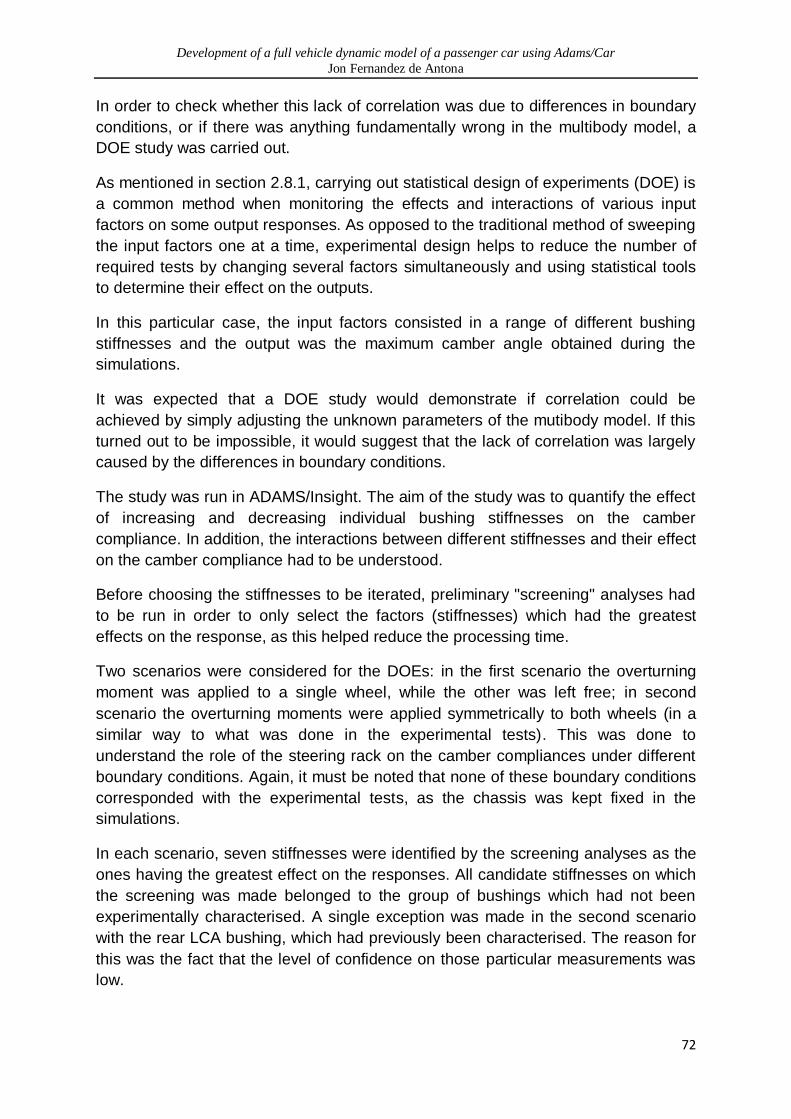
Development of a full vehicle dynamic model of a passenger car using Adams/Car
Jon Fernandez de Antona
72
In order to check whether this lack of correlation was due to differences in boundary
conditions, or if there was anything fundamentally wrong in the multibody model, a
DOE study was carried out.
As mentioned in section 2.8.1, carrying out statistical design of experiments (DOE) is
a common method when monitoring the effects and interactions of various input
factors on some output responses. As opposed to the traditional method of sweeping
the input factors one at a time, experimental design helps to reduce the number of
required tests by changing several factors simultaneously and using statistical tools
to determine their effect on the outputs.
In this particular case, the input factors consisted in a range of different bushing
stiffnesses and the output was the maximum camber angle obtained during the
simulations.
It was expected that a DOE study would demonstrate if correlation could be
achieved by simply adjusting the unknown parameters of the mutibody model. If this
turned out to be impossible, it would suggest that the lack of correlation was largely
caused by the differences in boundary conditions.
The study was run in ADAMS/Insight. The aim of the study was to quantify the effect
of increasing and decreasing individual bushing stiffnesses on the camber
compliance. In addition, the interactions between different stiffnesses and their effect
on the camber compliance had to be understood.
Before choosing the stiffnesses to be iterated, preliminary "screening" analyses had
to be run in order to only select the factors (stiffnesses) which had the greatest
effects on the response, as this helped reduce the processing time.
Two scenarios were considered for the DOEs: in the first scenario the overturning
moment was applied to a single wheel, while the other was left free; in second
scenario the overturning moments were applied symmetrically to both wheels (in a
similar way to what was done in the experimental tests). This was done to
understand the role of the steering rack on the camber compliances under different
boundary conditions. Again, it must be noted that none of these boundary conditions
corresponded with the experimental tests, as the chassis was kept fixed in the
simulations.
In each scenario, seven stiffnesses were identified by the screening analyses as the
ones having the greatest effect on the responses. All candidate stiffnesses on which
the screening was made belonged to the group of bushings which had not been
experimentally characterised. A single exception was made in the second scenario
with the rear LCA bushing, which had previously been characterised. The reason for
this was the fact that the level of confidence on those particular measurements was
low.

Development of a full vehicle dynamic model of a passenger car using Adams/Car
Jon Fernandez de Antona
73
Subsequently, the stiffnesses estimated in section 4.3 were used as nominal values
for the chosen input factors. These stiffnesses were then scaled down and up using
a "linear" model, in order to obtain a "lower" and a "higher" response for each input
factor. In order to interpolate the values between the lower and higher responses,
the investigation strategy was set to "DOE Response Surface". In addition, every
possible combination of factors had to be run so that the interactions between them
could be understood. Therefore, the DOE design type was set to "full factorial".
If "v" is the number of values per factor and "f" is the number of factors, the number
of simulation runs required for a full factorial DOE for each scenario is given by:
Although this number of runs is practical (it took a processing time of 7 minutes per
scenario using 5 simulation steps per run4), it can be seen that if quadratic or cubic
models were used instead of the linear one, 2187 and 16384 runs would have been
required per scenario, respectively. At the same time, the processing time would
have increased exponentially as the order of the model was increased.
The analyses made it possible to quantify the effect of each individual stiffness on
the maximum simulated camber angles. Figure 6.1.4 and Figure 6.1.5 show that
most effects are negative, meaning that increasing the value of the factors will
decrease the value of the response (i.e. the maximum simulated camber value, or
the change in camber, will be smaller if the bushing stiffnesses are increased). While
the sign convention seems logical, it should be noted that what the effects are
showing is the change in response between the "higher" and "lower" values of the
given factor. Therefore the magnitude of this number will depend on the higher and
lower values used in each scenario.
When the overturning moment was being applied to a single wheel (1st scenario),
the lower values of all the factors were set to 1/10th nominal, while the upper values
were set to 10 times nominal. This range was expected to give a good idea about
whether the orders of magnitude of the bushing stiffnesses were reasonable.
The results for effects in this scenario (Figure 6.1.4, in blue) showed that the main
factor determining the camber compliance was the axial stiffness of the steering rack
mount bushings. Changing the scale of this factor from 1/10th to 10 produced a
decrement of almost 1.6° on the maximum simulated camber angle.
4 Intel Core i7 2.67GHz, 8GB RAM (DDR3), Win7 x64
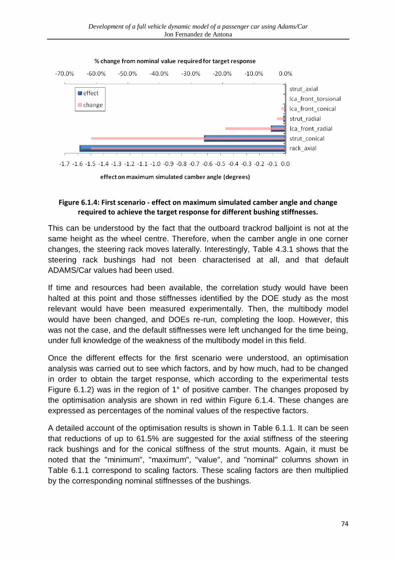
Development of a full vehicle dynamic model of a passenger car using Adams/Car
Jon Fernandez de Antona
74
Figure 6.1.4: First scenario - effect on maximum simulated camber angle and change required to achieve the target response for different bushing stiffnesses.
This can be understood by the fact that the outboard trackrod balljoint is not at the
same height as the wheel centre. Therefore, when the camber angle in one corner
changes, the steering rack moves laterally. Interestingly, Table 4.3.1 shows that the
steering rack bushings had not been characterised at all, and that default
ADAMS/Car values had been used.
If time and resources had been available, the correlation study would have been
halted at this point and those stiffnesses identified by the DOE study as the most
relevant would have been measured experimentally. Then, the multibody model
would have been changed, and DOEs re-run, completing the loop. However, this
was not the case, and the default stiffnesses were left unchanged for the time being,
under full knowledge of the weakness of the multibody model in this field.
Once the different effects for the first scenario were understood, an optimisation
analysis was carried out to see which factors, and by how much, had to be changed
in order to obtain the target response, which according to the experimental tests
Figure 6.1.2) was in the region of 1° of positive camber. The changes proposed by
the optimisation analysis are shown in red within Figure 6.1.4. These changes are
expressed as percentages of the nominal values of the respective factors.
A detailed account of the optimisation results is shown in Table 6.1.1. It can be seen
that reductions of up to 61.5% are suggested for the axial stiffness of the steering
rack bushings and for the conical stiffness of the strut mounts. Again, it must be
noted that the "minimum", "maximum", "value", and "nominal" columns shown in
Table 6.1.1 correspond to scaling factors. These scaling factors are then multiplied
by the corresponding nominal stiffnesses of the bushings.
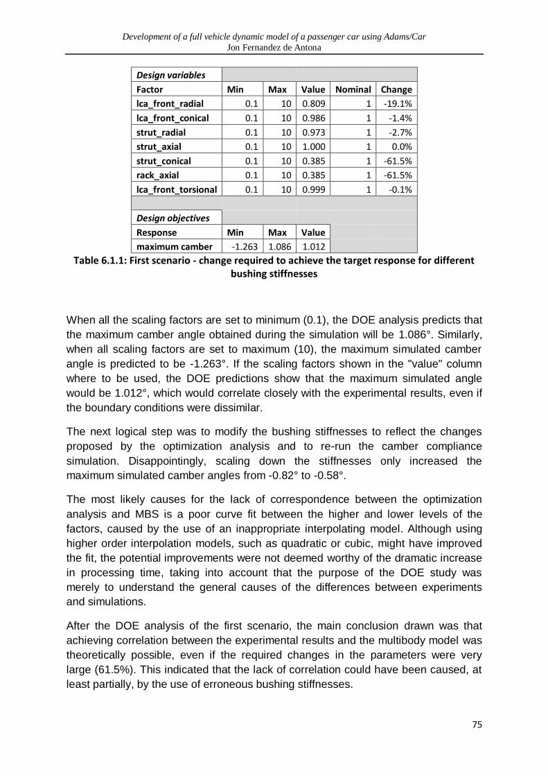
Development of a full vehicle dynamic model of a passenger car using Adams/Car
Jon Fernandez de Antona
75
Design variables Factor Min Max Value Nominal Change
lca_front_radial 0.1 10 0.809 1 -19.1%
lca_front_conical 0.1 10 0.986 1 -1.4%
strut_radial 0.1 10 0.973 1 -2.7%
strut_axial 0.1 10 1.000 1 0.0%
strut_conical 0.1 10 0.385 1 -61.5%
rack_axial 0.1 10 0.385 1 -61.5%
lca_front_torsional 0.1 10 0.999 1 -0.1%
Design objectives Response Min Max Value
maximum camber -1.263 1.086 1.012 Table 6.1.1: First scenario - change required to achieve the target response for different
bushing stiffnesses
When all the scaling factors are set to minimum (0.1), the DOE analysis predicts that
the maximum camber angle obtained during the simulation will be 1.086°. Similarly,
when all scaling factors are set to maximum (10), the maximum simulated camber
angle is predicted to be -1.263°. If the scaling factors shown in the "value" column
where to be used, the DOE predictions show that the maximum simulated angle
would be 1.012°, which would correlate closely with the experimental results, even if
the boundary conditions were dissimilar.
The next logical step was to modify the bushing stiffnesses to reflect the changes
proposed by the optimization analysis and to re-run the camber compliance
simulation. Disappointingly, scaling down the stiffnesses only increased the
maximum simulated camber angles from -0.82° to -0.58°.
The most likely causes for the lack of correspondence between the optimization
analysis and MBS is a poor curve fit between the higher and lower levels of the
factors, caused by the use of an inappropriate interpolating model. Although using
higher order interpolation models, such as quadratic or cubic, might have improved
the fit, the potential improvements were not deemed worthy of the dramatic increase
in processing time, taking into account that the purpose of the DOE study was
merely to understand the general causes of the differences between experiments
and simulations.
After the DOE analysis of the first scenario, the main conclusion drawn was that
achieving correlation between the experimental results and the multibody model was
theoretically possible, even if the required changes in the parameters were very
large (61.5%). This indicated that the lack of correlation could have been caused, at
least partially, by the use of erroneous bushing stiffnesses.

Development of a full vehicle dynamic model of a passenger car using Adams/Car
Jon Fernandez de Antona
76
As far as the second scenario is concerned, the screening studies revealed that the
axial stiffness of the steering rack mountings was no longer an important factor when
the overturning moment was being applied simultaneously to both wheels, as the
lateral loads applied on the rack were cancelled out.
On the other hand, the addition of the LCA rear bushing stiffnesses to the group of
candidates meant that the lca_front_torsional and strut_axial stiffnesses were
discarded, due to their minimal effects. The scaling of the factors for the second
scenario was changed between 0.01 and 100. The reason for varying the factors by
two orders of magnitude was that the effect of the factors on the response was
considerably smaller, and the results of single-order-of-magnitude changes would
have barely been perceptible.
Figure 6.1.5: Second scenario - effect on maximum simulated camber angle for different bushing stiffnesses.
The results for the linear, full factorial, response surface study for the second
scenario can be seen in Figure 6.1.5. This time the most important factor turned out
to be the conical stiffness of the strut mount bushing. In a similar way to what
happened with the steering rack bushings in the first scenario, it was revealed that
the strut mount bushing had not been experimentally characterised (Table 4.3.1).
On the other hand, the small effects meant that, when the optimization analysis was
carried out, the target camber compliance could not be reached, even if a scaling
factor of 0.01 was applied to all the stiffnesses. The maximum camber angle
achieved under these extreme conditions was merely 0.47°, far away from the 1° set
as the target.
In the experimental compliance tests the overturning moment had been applied
symmetrically to both wheels. Therefore this DOE study demonstrated that the lack
of correlation could not be caused solely by poorly characterised bushing stiffnesses.
Consequently the differences in boundary conditions were assumed to have a
significant effect on the lack of correlation.
Development of a full vehicle dynamic model of a passenger car using Adams/Car
Jon Fernandez de Antona
77
6.1.1.2. Rear suspension compliances
The road simulator control system was the only information source for the rear
compliance acquisitions, as mentioned in section 5.2.2. The decision not to use the
CCM for rear compliance tests was taken before correlation checks were carried out,
and it was based purely on the fact that CMM measurements were very time
consuming. This decision meant that no additional sources of data were available to
check whether the road simulator acquisitions were representative of the
displacements of the wheel with respect to the chassis.
As was done with the front suspension compliances, the load ranges used in the
experimental tests (Table 5.2.7) were used again for the multibody simulations. Once
more, the boundary conditions of the simulations did not match those of the
experimental tests, and this was taken into account when comparing the results.
Figure 6.1.6: Comparison of lateral force compliance test results for the rear axle
The correlation for the rear axle lateral force compliances (Figure 6.1.6) turned out to
be even worse than in the front axle. The experimental displacements turned out to
be an order of magnitude larger than the simulated displacements. The most
plausible explanation for this could be the fact that the chassis was floating in the
experimental tests, unlike in the multibody simulations.

Development of a full vehicle dynamic model of a passenger car using Adams/Car
Jon Fernandez de Antona
78
Figure 6.1.7: Comparison of overturning moment compliance test results for the rear axle
As far as the rear axle overturning moment compliances are concerned (Figure
6.1.7), the correlation between the simulated and experimental rates was much
better than for the front axle tests, although the simulated rates were still twice as
large as the experimental ones. Again, this could have been related to the
aforementioned differences in boundary conditions.
On the other hand, at zero load the road simulator control system measured -1.57°
of camber, while the simulation predicted -0.18°. The differences in zero offset could
have been related to the fact that static camber values were not accurately set in the
multibody model.
Finally, the same behaviour described above was found in the aligning moment
compliance results, both in terms of rates and offsets (Figure 6.1.8).
Figure 6.1.8: Comparison of aligning moment compliance test results for the rear axle
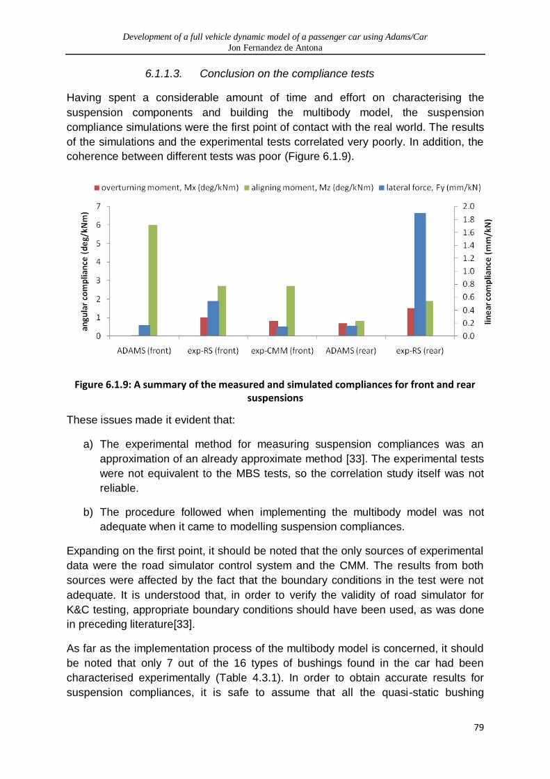
Development of a full vehicle dynamic model of a passenger car using Adams/Car
Jon Fernandez de Antona
79
6.1.1.3. Conclusion on the compliance tests
Having spent a considerable amount of time and effort on characterising the
suspension components and building the multibody model, the suspension
compliance simulations were the first point of contact with the real world. The results
of the simulations and the experimental tests correlated very poorly. In addition, the
coherence between different tests was poor (Figure 6.1.9).
Figure 6.1.9: A summary of the measured and simulated compliances for front and rear suspensions
These issues made it evident that:
a) The experimental method for measuring suspension compliances was an
approximation of an already approximate method [33]. The experimental tests
were not equivalent to the MBS tests, so the correlation study itself was not
reliable.
b) The procedure followed when implementing the multibody model was not
adequate when it came to modelling suspension compliances.
Expanding on the first point, it should be noted that the only sources of experimental
data were the road simulator control system and the CMM. The results from both
sources were affected by the fact that the boundary conditions in the test were not
adequate. It is understood that, in order to verify the validity of road simulator for
K&C testing, appropriate boundary conditions should have been used, as was done
in preceding literature[33].
As far as the implementation process of the multibody model is concerned, it should
be noted that only 7 out of the 16 types of bushings found in the car had been
characterised experimentally (Table 4.3.1). In order to obtain accurate results for
suspension compliances, it is safe to assume that all the quasi-static bushing

Development of a full vehicle dynamic model of a passenger car using Adams/Car
Jon Fernandez de Antona
80
stiffnesses should have been known, without exception. The fact that each bushing
has 6 stiffnesses (one per each DOF of its inner ring) meant that rough estimates
were being used for 54 parameters which had a direct effect on suspension
compliances.
In addition, all bodies in the model were assumed to be perfectly rigid, when the
effect of component deflections on suspension compliances cannot be neglected by
any means [12].
With the time and resources available for this project, it was impossible to resolve
these issues. However, when analysing the suspension compliance results, the
overall aim of this project must be taken into account. As stated in section 1.4.1, the
multibody model being implemented in this project must simulate the primary ride
and handling responses of the actual vehicle. In addition, it is assumed that the level
of detail of the model should simply match the complexity of the aim to be achieved,
without exceeding it (section 2.7).
The next logical step was to question the effect of having poorly correlated
suspension compliances on the aims of this project.
It is generally understood that, when actual road disturbances are being considered,
the effect of suspension compliances on the vehicle ride is paramount [12]. Actual
road inputs apply all force and moment components to the wheel, and therefore the
compliances measured herein would come into play in a real life situation.
However, if only vertical force components were considered (e.g. in a vertical
excitation test), the effect of suspension compliances on vehicle responses is
expected to be reduced.
The fact that track acquisitions had been discarded and the remaining experimental
data was to be acquired via vertical excitation tests meant that poorly correlated
suspension compliances were not expected to greatly affect the remaining
correlation studies.
Therefore, the multibody model was left unchanged and the validation process
continued, under full knowledge of the weaknesses of the model in this area.
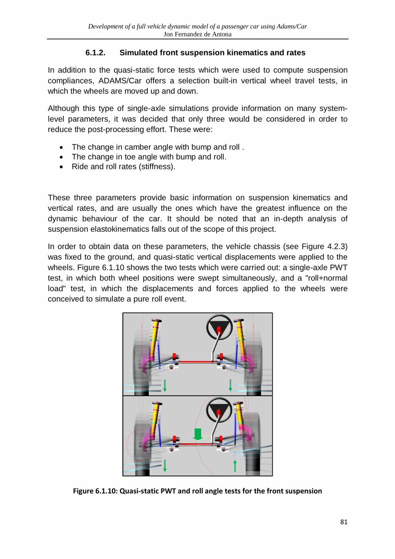
Development of a full vehicle dynamic model of a passenger car using Adams/Car
Jon Fernandez de Antona
81
6.1.2. Simulated front suspension kinematics and rates
In addition to the quasi-static force tests which were used to compute suspension
compliances, ADAMS/Car offers a selection built-in vertical wheel travel tests, in
which the wheels are moved up and down.
Although this type of single-axle simulations provide information on many system-
level parameters, it was decided that only three would be considered in order to
reduce the post-processing effort. These were:
The change in camber angle with bump and roll .
The change in toe angle with bump and roll.
Ride and roll rates (stiffness).
These three parameters provide basic information on suspension kinematics and
vertical rates, and are usually the ones which have the greatest influence on the
dynamic behaviour of the car. It should be noted that an in-depth analysis of
suspension elastokinematics falls out of the scope of this project.
In order to obtain data on these parameters, the vehicle chassis (see Figure 4.2.3)
was fixed to the ground, and quasi-static vertical displacements were applied to the
wheels. Figure 6.1.10 shows the two tests which were carried out: a single-axle PWT
test, in which both wheel positions were swept simultaneously, and a "roll+normal
load" test, in which the displacements and forces applied to the wheels were
conceived to simulate a pure roll event.
Figure 6.1.10: Quasi-static PWT and roll angle tests for the front suspension
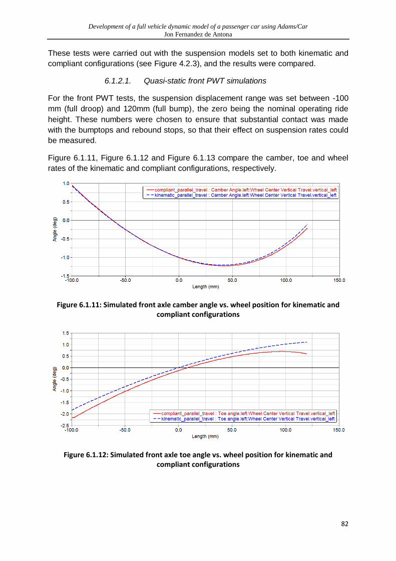
Development of a full vehicle dynamic model of a passenger car using Adams/Car
Jon Fernandez de Antona
82
These tests were carried out with the suspension models set to both kinematic and
compliant configurations (see Figure 4.2.3), and the results were compared.
6.1.2.1. Quasi-static front PWT simulations
For the front PWT tests, the suspension displacement range was set between -100
mm (full droop) and 120mm (full bump), the zero being the nominal operating ride
height. These numbers were chosen to ensure that substantial contact was made
with the bumptops and rebound stops, so that their effect on suspension rates could
be measured.
Figure 6.1.11, Figure 6.1.12 and Figure 6.1.13 compare the camber, toe and wheel
rates of the kinematic and compliant configurations, respectively.
Figure 6.1.11: Simulated front axle camber angle vs. wheel position for kinematic and compliant configurations
Figure 6.1.12: Simulated front axle toe angle vs. wheel position for kinematic and compliant configurations
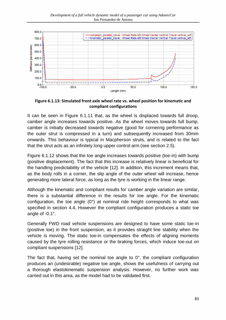
Development of a full vehicle dynamic model of a passenger car using Adams/Car
Jon Fernandez de Antona
83
Figure 6.1.13: Simulated front axle wheel rate vs. wheel position for kinematic and compliant configurations
It can be seen in Figure 6.1.11 that, as the wheel is displaced towards full droop,
camber angle increases towards positive. As the wheel moves towards full bump,
camber is initially decreased towards negative (good for cornering performance as
the outer strut is compressed in a turn) and subsequently increased from 30mm
onwards. This behaviour is typical in Macpherson struts, and is related to the fact
that the strut acts as an infinitely long upper control arm (see section 2.5).
Figure 6.1.12 shows that the toe angle increases towards positive (toe-in) with bump
(positive displacement). The fact that this increase is relatively linear is beneficial for
the handling predictability of the vehicle [12]. In addition, this increment means that,
as the body rolls in a corner, the slip angle of the outer wheel will increase, hence
generating more lateral force, as long as the tyre is working in the linear range.
Although the kinematic and compliant results for camber angle variation are similar,
there is a substantial difference in the results for toe angle. For the kinematic
configuration, the toe angle (0°) at nominal ride height corresponds to what was
specified in section 4.4. However the compliant configuration produces a static toe
angle of -0.1°.
Generally FWD road vehicle suspensions are designed to have some static toe-in
(positive toe) in the front suspension, as it provides straight line stability when the
vehicle is moving. The static toe-in compensates the effects of aligning moments
caused by the tyre rolling resistance or the braking forces, which induce toe-out on
compliant suspensions [12].
The fact that, having set the nominal toe angle to 0°, the compliant configuration
produces an (undesirable) negative toe angle, shows the usefulness of carrying out
a thorough elastokinematic suspension analysis. However, no further work was
carried out in this area, as the model had to be validated first.
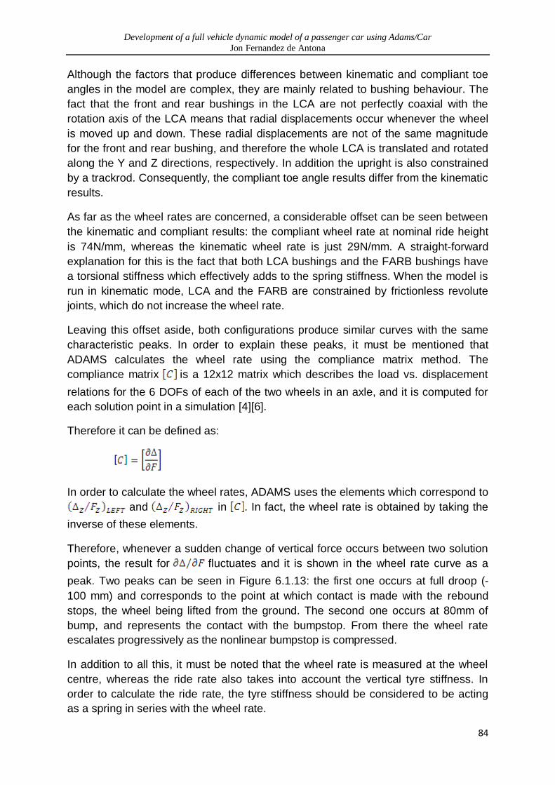
Development of a full vehicle dynamic model of a passenger car using Adams/Car
Jon Fernandez de Antona
84
Although the factors that produce differences between kinematic and compliant toe
angles in the model are complex, they are mainly related to bushing behaviour. The
fact that the front and rear bushings in the LCA are not perfectly coaxial with the
rotation axis of the LCA means that radial displacements occur whenever the wheel
is moved up and down. These radial displacements are not of the same magnitude
for the front and rear bushing, and therefore the whole LCA is translated and rotated
along the Y and Z directions, respectively. In addition the upright is also constrained
by a trackrod. Consequently, the compliant toe angle results differ from the kinematic
results.
As far as the wheel rates are concerned, a considerable offset can be seen between
the kinematic and compliant results: the compliant wheel rate at nominal ride height
is 74N/mm, whereas the kinematic wheel rate is just 29N/mm. A straight-forward
explanation for this is the fact that both LCA bushings and the FARB bushings have
a torsional stiffness which effectively adds to the spring stiffness. When the model is
run in kinematic mode, LCA and the FARB are constrained by frictionless revolute
joints, which do not increase the wheel rate.
Leaving this offset aside, both configurations produce similar curves with the same
characteristic peaks. In order to explain these peaks, it must be mentioned that
ADAMS calculates the wheel rate using the compliance matrix method. The
compliance matrix is a 12x12 matrix which describes the load vs. displacement
relations for the 6 DOFs of each of the two wheels in an axle, and it is computed for
each solution point in a simulation [4][6].
Therefore it can be defined as:
In order to calculate the wheel rates, ADAMS uses the elements which correspond to
and in . In fact, the wheel rate is obtained by taking the
inverse of these elements.
Therefore, whenever a sudden change of vertical force occurs between two solution
points, the result for fluctuates and it is shown in the wheel rate curve as a
peak. Two peaks can be seen in Figure 6.1.13: the first one occurs at full droop (-
100 mm) and corresponds to the point at which contact is made with the rebound
stops, the wheel being lifted from the ground. The second one occurs at 80mm of
bump, and represents the contact with the bumpstop. From there the wheel rate
escalates progressively as the nonlinear bumpstop is compressed.
In addition to all this, it must be noted that the wheel rate is measured at the wheel
centre, whereas the ride rate also takes into account the vertical tyre stiffness. In
order to calculate the ride rate, the tyre stiffness should be considered to be acting
as a spring in series with the wheel rate.

Development of a full vehicle dynamic model of a passenger car using Adams/Car
Jon Fernandez de Antona
85
6.1.2.2. Quasi-static front roll angle simulations
For roll angle tests, ADAMS/Car fixes the chassis to the ground and applies
opposing displacement to the wheels. The magnitude of these displacements is a
function of the roll angle range and the total axle load selected by the user. As the
suspension position at zero roll is a direct function of the normal load, it is vital that
this load is representative of real-world operating conditions of the vehicle. For front
axle tests, a (relatively wide) roll angle range of -10° to 10° and a normal load of 9kN
were deemed appropriate.
The results for such input parameters can be seen in the next three figures:
Figure 6.1.14: Simulated front axle camber angle (Y axis) vs. roll angle (X axis) for kinematic and compliant configurations
Figure 6.1.15: Simulated front axle toe angle (Y axis) vs. roll angle (X axis) for kinematic and compliant configurations
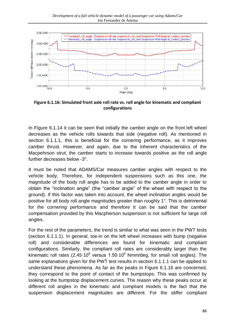
Development of a full vehicle dynamic model of a passenger car using Adams/Car
Jon Fernandez de Antona
86
Figure 6.1.16: Simulated front axle roll rate vs. roll angle for kinematic and compliant configurations
In Figure 6.1.14 it can be seen that initially the camber angle on the front left wheel
decreases as the vehicle rolls towards that side (negative roll). As mentioned in
section 6.1.1.1, this is beneficial for the cornering performance, as it improves
camber thrust. However, and again, due to the inherent characteristics of the
Macpehrson strut, the camber starts to increase towards positive as the roll angle
further decreases below -3°.
It must be noted that ADAMS/Car measures camber angles with respect to the
vehicle body. Therefore, for independent suspensions such as this one, the
magnitude of the body roll angle has to be added to the camber angle in order to
obtain the “inclination angle” (the “camber angle” of the wheel with respect to the
ground). If this factor was taken into account, the wheel inclination angles would be
positive for all body roll angle magnitudes greater than roughly 1°. This is detrimental
for the cornering performance and therefore it can be said that the camber
compensation provided by this Macpherson suspension is not sufficient for large roll
angles.
For the rest of the parameters, the trend is similar to what was seen in the PWT tests
(section 6.1.1.1). In general, toe-in on the left wheel increases with bump (negative
roll) and considerable differences are found for kinematic and compliant
configurations. Similarly, the compliant roll rates are considerably larger than the
kinematic roll rates (2.45∙106 versus 1.50∙106 Nmm/deg, for small roll angles). The
same explanations given for the PWT test results in section 6.1.1.1 can be applied to
understand these phenomena. As far as the peaks in Figure 6.1.16 are concerned,
they correspond to the point of contact of the bumpstops. This was confirmed by
looking at the bumpstop displacement curves. The reason why these peaks occur at
different roll angles in the kinematic and compliant models is the fact that the
suspension displacement magnitudes are different. For the stiffer compliant

Development of a full vehicle dynamic model of a passenger car using Adams/Car
Jon Fernandez de Antona
87
configuration, the vertical tyre deflection is larger, which means that, for the same roll
angle, the suspension displacement is smaller.
6.1.3. Rear suspension kinematics and rates
The same simulations shown in section 6.1.1 were repeated for the rear axle. In this
case it must be noted that this kind of multilink suspensions are inherently over-
constrained by their design and depend on bushing compliances in order to move
(see section 2.5). The reason why the kinematic configuration of the rear suspension
had been fully modelled (see section 4.2) was to demonstrate that indeed the rear
suspension would not have any remaining DOFs in kinematic mode. This was
confirmed as soon as the first kinematic simulations for the rear axle were attempted.
Figure 6.1.17 shows that, for small displacements, rear PWT results are similar to
those of the front axle. The toe angle increases towards toe-in with bump, improving
straight line stability. Meanwhile, camber angle decreases towards negative values
with bump, which is beneficial for lateral force generation. However, as
displacements become larger towards full bump, the inversion in camber gain rate,
characteristic of Macpherson suspensions, is no longer encountered and the camber
angle keeps decreasing progressively until it reaches nearly -2.3°.
As far as the wheel rate is concerned, a relatively constant stiffness of approximately
28N/mm is obtained for small displacements. Full droop is reached at -77mm, and
contact with the bumpstops is made at 29mm of suspension displacement, which
can be appreciated as a small step in Figure 6.1.17.
Figure 6.1.17: Simulated rear axle wheel rate, camber and toe angle vs. wheel position
The rear roll angle tests also provided similar results as the front ones. As the car
body rolls towards the left in a right-hand corner, the camber angle on the rear left
wheel decreases towards negative (Figure 6.1.18). A small kink is found in the slope
of the rear left camber curve at the point at which contact is made with the rebound
stop of the opposite side (rear right wheel). A similar thing happens to the rear left

Development of a full vehicle dynamic model of a passenger car using Adams/Car
Jon Fernandez de Antona
88
toe angle curve when the car is rolling to the right. These phenomena occur at
roughly ±6° of body roll.
This might be explained by the fact that the rebound stop forces are transmitted to
the wheel through the damper (Figure 4.2.2). The top mounts of the rear dampers
are tilted inboards and forwards with respect to the vehicle chassis, and therefore
any forces transmitted through them have lateral components. In addition, the entire
rear subframe is mounted to the chassis through compliant bushings. After observing
the subframe bushing displacements, it was discovered that the whole subframe was
tilting and moving laterally by as much as 0.5mm throughout the roll angle simulation.
When one of the rebound stops was reached, the rate of displacement (velocity) of
the subframe suddenly increased (the rebound stops are relatively stiff). The fact that
the subframe couples the displacements of the left and right corners of the axle
means that this is the origin of the kinks seen on the camber and toe angle curves in
the opposite corner.
On the other hand, left wheel toe angle is increased towards positive (toe-in) as the
chassis rolls to the left. This is typically done by automakers to ensure that the rear
axle induces understeer when the car rolls into a corner. Leaving optimum cornering
performance aside, an understeering car is desirable for the average driver as it
behaves more predictably [12].
As far as roll stiffness is concerned, the rear roll rate is in the region of 1.06∙106
Nmm/deg for small roll angles. The steps at ±3.6° of roll correspond to the bumpstop
contact points, contact with the rebound stops occurring at ±6°, as mentioned above.
Figure 6.1.18: Simulated rear axle roll rate, camber and toe angle (Y axes) versus roll angle (X axis)

Development of a full vehicle dynamic model of a passenger car using Adams/Car
Jon Fernandez de Antona
89
6.2. Full-vehicle excitation analyses
Once the system-level suspension parameters were studied, the next step was to
understand the vehicle-level behaviour. In order to achieve this, the experimental
method for full vehicle analyses (section 5.2.1) was compared with MBS.
6.2.1. Full-vehicle simulation characteristics
As it had happened in section 6.1.1, the default ADAMS/Car analyses did not allow
for the experimental boundary conditions to be replicated exactly. In the
experimental set-up for vertical excitation tests (section 5.2.1.1), the front axle was
rigidly attached to the road simulator through the wheel hubs, while the rear wheels
were strapped to static platforms.
ADAMS/Car allows the user to choose between applying the forces at the wheel
contact patches or at the hubs, but this option has to be changed simultaneously for
both the front and rear axles. Modifying this configuration would have required
considerable time and effort which could have not been afforded.
In the experimental tests, both the WFT and the road simulator actuators were
mounted on the same axle (Figure 5.2.1). This meant that the forces that had been
measured belonged to the axle which was constrained through the spindles. In
addition, the platforms to which the remaining axle was attached were not flat
horizontal plates, but “U”-shaped fabricated structures. If, in the simulations, the
forces had been applied at the contact patches, ADAMS/Car would have assumed
that the tyres were resting on a flat surface. Therefore it was decided that the least
detrimental solution would be to apply the forces at the wheel hubs (spindles) for all
four wheels.
The input vertical displacement signals for the simulations were the same as those
used in the experimental tests (Figure 5.2.2). The setup of the simulations can be
seen in Figure 6.2.1. It should be noted that, although circular plates are shown
underneath the tyres, the forces were applied at the wheel hubs, as said before. The
yellow sphere behind the handwheel represents the vehicle body.
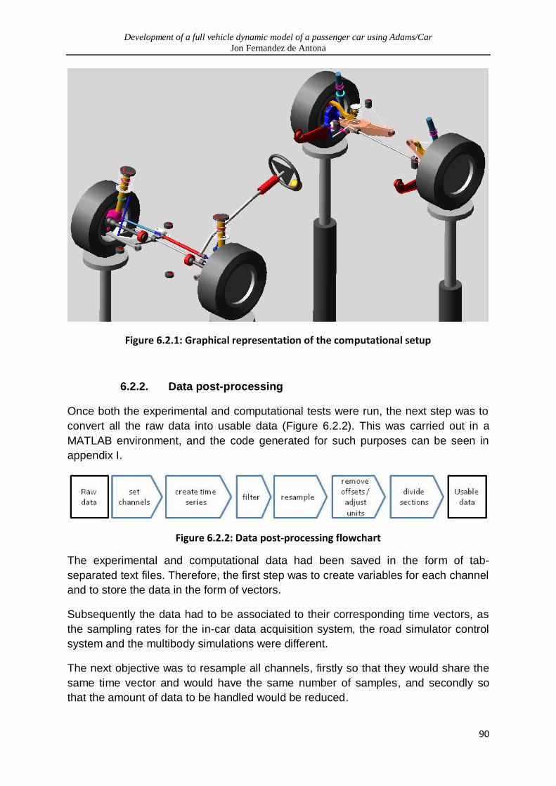
Development of a full vehicle dynamic model of a passenger car using Adams/Car
Jon Fernandez de Antona
90
Figure 6.2.1: Graphical representation of the computational setup
6.2.2. Data post-processing
Once both the experimental and computational tests were run, the next step was to
convert all the raw data into usable data (Figure 6.2.2). This was carried out in a
MATLAB environment, and the code generated for such purposes can be seen in
appendix I.
Figure 6.2.2: Data post-processing flowchart
The experimental and computational data had been saved in the form of tab-
separated text files. Therefore, the first step was to create variables for each channel
and to store the data in the form of vectors.
Subsequently the data had to be associated to their corresponding time vectors, as
the sampling rates for the in-car data acquisition system, the road simulator control
system and the multibody simulations were different.
The next objective was to resample all channels, firstly so that they would share the
same time vector and would have the same number of samples, and secondly so
that the amount of data to be handled would be reduced.

Development of a full vehicle dynamic model of a passenger car using Adams/Car
Jon Fernandez de Antona
91
In order to achieve this, the data was filtered first in order to reduce the high-
frequency noise and hence minimise aliasing. Knowing that the largest frequency in
the input signal was 10Hz, the “idealfilter” function [54] was used to remove all the
power outside the 0-20Hz frequency range.
Once the data was resampled, all units homogenised and the offsets removed, the
next step was to divide the acquisitions into sections which corresponded to the
different parts of the input signal (Figure 5.2.2). This step was especially important,
as the acquisition starting times for the different data acquisition systems were
different, as mentioned in section 5.2.1.1. The time vector of each individual division
was restarted from zero to cancel offsets in the time domain.
6.2.3. Discussion of full vehicle excitation data
Understandably, analysing the results took considerably longer than carrying out the
tests themselves. Although both front and rear axles had been excited in the test (not
simultaneously, as the road simulator did not allow it), only the front axle excitation
results were analysed due to the limited time available. Among the front axle results,
only four sets of parameters were considered. These were: suspension
displacements, spindle positions, chassis accelerations and vertical loads at the
spindles.
These parameters, although they represented a small fraction of all the data
available, provided enough information to understand the dynamic response of the
chassis to the excitations.
As the input signal consisted of two main parts (Figure 5.2.2), the acquisitions were
divided accordingly into a "sine" part, which was to be analysed in the time domain,
and a "sweep" part, which was to be analysed in the frequency domain. The results
for the different parameters are discussed below.
6.2.3.1. Damper displacements and vertical wheel forces
The full experimental and computational acquisitions for the damper displacements
and vertical wheel forces are shown in appendix J. In general, the correlation
between the simulated and experimental results was better for the forces than for the
damper displacements.
Time-domain comparisons between the sinusoidal part of the signals for the FPWT
and FOWT tests are shown in Figure 6.2.3 and Figure 6.2.4, respectively.

Development of a full vehicle dynamic model of a passenger car using Adams/Car
Jon Fernandez de Antona
92
Figure 6.2.3: Simulated and experimental responses to FPWT excitations - time-domain analysis of damper displacements and vertical spindle forces.

Development of a full vehicle dynamic model of a passenger car using Adams/Car
Jon Fernandez de Antona
93
Figure 6.2.4: Simulated and experimental responses to FOWT excitations - time-domain analysis of damper displacements and vertical spindle forces.

Development of a full vehicle dynamic model of a passenger car using Adams/Car
Jon Fernandez de Antona
94
In order to quantify the fit between the simulated and experimental results for the
sinusoidal parts of the tests, the root mean square deviation (RMSD) between the
two signals was calculated:
where is the experimental signal, is the simulated signal, is the i-th
experimental sample, is the i-th simulated sample, and n is the total number of
samples.
LF_Fz
(kN)
RF_Fz
(kN)
LF_damperpot
(mm)
RF_damperpot
(mm)
LR_damperpot
(mm)
RR_damperpot
(mm)
FPWT 0.15 0.21 1.97 1.92 0.21 0.28
FOWT 0.16 0.21 3.26 3.03 4.62 4.47
Table 6.2.1: RMSD of the simulated and experimental results for damper displacements and wheel forces
As far as the front axle parallel wheel travel (FPWT) excitations are concerned
(Figure 6.2.3), rear damper acquisitions (first plot from the top) show very small
displacements, in the region of ±0.4mm. Therefore a relatively large proportion of the
experimental results is noise.
It can be observed that the rear dampers operate mainly in the negative
displacement region, which is these tests represents bump (as opposed to the
results in section 6.1.2., for which bump was positive). The fact that the experimental
and computational curves correlate well in the bump region but not in the droop
region suggests that the rear tyre, instead of the suspension, might be deflecting
under compressive loads. In fact, it was observed during all experimental tests (both
FPWT and FOWT) that the rear axle was visibly moving around within the static
platforms, due to the compliance of the tyres. Obviously this deflection is not
accounted for in the simulation, as the forces are applied to the wheels through the
hubs.
At the other end of the car, the amplitude of the experimental front damper
displacements (second plot) is less than half of the simulated displacements, the
mean deviation being roughly 2mm. This might be caused by either differences in
spring rates between the model and reality, or by differences in mass properties.
However, vertical forces at the front wheels (third plot) show a relatively good
correlation, with an offset of less than 300N between the simulated and experimental
results, possibly due to inaccuracies in static weight distribution of the multibody
model.
This would suggest that the lack of correlation in the front damper displacements is
caused by differences in wheel rates. This could be related to the fact that many of
Development of a full vehicle dynamic model of a passenger car using Adams/Car
Jon Fernandez de Antona
95
the front suspension bushings were not experimentally tested. For instance, a poorly
characterised torsional stiffness on the LCA bushings would have a considerable
effect on the resulting wheel rate.
Moving on to Figure 6.2.4, it can be seen that the trend for the FOWT test results is
similar; the correlation between the spindle forces being better than the correlation
between the damper displacements.
For the rear damper displacements (first plot), the amplitudes of experimental
displacements are approximately 25% less than the simulated ones (a mean
deviation of less than 5mm). The most plausible explanation for this is that the roll
stiffnesses of the model differ from reality, probably due to the aforementioned lack
of experimental characterisation in some of the suspension bushings. In addition to
this, a phase shift of about 20° is found between experimental and computational
results, suggesting that rear tyre deflection has again an important effect on
suspension displacements.
As far as the front damper displacements are concerned (second plot) the two
signals are in phase, but again the amplitudes are approximately half of each other,
with a mean deviation of less than 4mm.
It should be noted that, both in the simulated and experimental results, the amplitude
of damper displacements is considerably larger for the rear axle than for the front
axle. This is a clear indication of the fact that the rear roll stiffness is smaller than the
front, which is a typical characteristic in cars with a forward weight distribution and an
understeering tendency. This corresponds with what was said in sections 6.1.2 and
6.1.3.
Interestingly, the vertical force plot shows that the behaviour of the left and right
corners in the front suspension is asymmetrical, when compared to the simulated
results. The reason for this is not well understood, but it is suspected that it could be
related again to differences in the static weight distribution between the model and
reality.
When it came to analysing the responses to the swept sine input signal,
periodograms (essentially the Fast Fourier Transforms, or FFTs) of the vertical
spindle loads were used to convert the time-domain signal into the frequency domain
and hence compare the spectra of the experimental and simulated results.
It should be noted that, if the exact values of the resonant frequencies where needed,
the use of simple periodograms for spectral density estimation would not have been
the most accurate method. The reasons for this lack of accuracy are beyond the
scope of this project, but are related to phenomena such as spectral leakage and
spectral bias, or to the fact that the statistical variance of the periodogram does not
tend to zero as the length of the available data tends to infinite [54]. However, for the
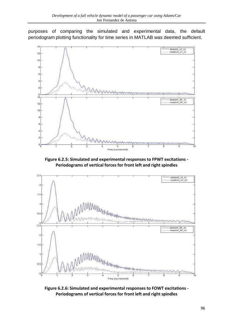
Development of a full vehicle dynamic model of a passenger car using Adams/Car
Jon Fernandez de Antona
96
purposes of comparing the simulated and experimental data, the default
periodogram plotting functionality for time series in MATLAB was deemed sufficient.
Figure 6.2.5: Simulated and experimental responses to FPWT excitations - Periodograms of vertical forces for front left and right spindles
Figure 6.2.6: Simulated and experimental responses to FOWT excitations - Periodograms of vertical forces for front left and right spindles

Development of a full vehicle dynamic model of a passenger car using Adams/Car
Jon Fernandez de Antona
97
In general terms, the periodograms showed that the frequency spectra for the left
and right spindle loads were almost identical for both the FPWT and FOWT tests. As
far as comparing the experimental and simulated data is concerned, the peaks of
amplitude were located at similar frequencies, but the magnitude of these peaks
differed significantly between the experimental and simulated results.
For the FPWT tests (Figure 6.2.5) a single and clear resonant frequency was found
at 1.6Hz, and the amplitude progressively reduced thereafter as the frequency
increased. This peak amplitude corresponds to the mode at which the vehicle body
started to resonate in a combined pitch and heave motion, rotating around some
point close to the fixed rear axle.
On the other hand, the magnitude of the simulated peak response was roughly three
times larger than the experimental. This effect was also observed in the time-domain
results shown in Figure 10.10.3 (appendix J), in which the amplitude of the simulated
signal at around t=25s was considerably larger than the experimental.
Again, the most probable cause for these differences in magnitude is the
aforementioned lack of correlation in the experimental and simulated wheel rates.
When it came to the FOWT tests, an extra peak was found in addition to the
expected body mode, both in the experimental and simulated results. The first, larger
peak occurred at 0.8Hz, followed by a smaller one at around 3Hz. Again, the
experimental peaks had a considerably lower magnitude than the computational
ones, with the second peak being barely noticeable in the experimental results.
At this stage, additional sources of data were required in order to interpret such
results. In this situation, chassis accelerations were the next point of call.
6.2.3.2. Chassis accelerations
In section 3.1, mention was made of the ADMA accelerometer/gyroscope system,
and it was explained that additional accelerometers were placed at known points of
the vehicle, in order to back up the acquisitions of the first system. Subsequently
requests were made to measure the chassis accelerations of the multibody model at
exactly the same points (section 4.6).
Eventually, such accelerations turned out to be the most reliable way to correlate the
actual and simulated responses of the vehicle chassis when the input frequencies
started to become larger. This was mainly due to the fact that the measured position
of the ADMA system with respect to the chassis was subjected to a significant error.
In addition, the gyroscope system tended to develop a drift during the length of each
acquisition. This drift, if not compensated by accelerometer readings, produced
inaccurate angular displacement results.
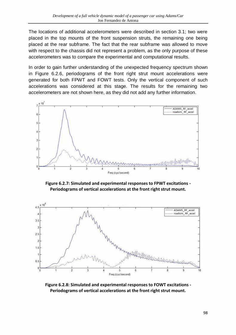
Development of a full vehicle dynamic model of a passenger car using Adams/Car
Jon Fernandez de Antona
98
The locations of additional accelerometers were described in section 3.1; two were
placed in the top mounts of the front suspension struts, the remaining one being
placed at the rear subframe. The fact that the rear subframe was allowed to move
with respect to the chassis did not represent a problem, as the only purpose of these
accelerometers was to compare the experimental and computational results.
In order to gain further understanding of the unexpected frequency spectrum shown
in Figure 6.2.6, periodograms of the front right strut mount accelerations were
generated for both FPWT and FOWT tests. Only the vertical component of such
accelerations was considered at this stage. The results for the remaining two
accelerometers are not shown here, as they did not add any further information.
Figure 6.2.7: Simulated and experimental responses to FPWT excitations - Periodograms of vertical accelerations at the front right strut mount.
Figure 6.2.8: Simulated and experimental responses to FOWT excitations - Periodograms of vertical accelerations at the front right strut mount.
Development of a full vehicle dynamic model of a passenger car using Adams/Car
Jon Fernandez de Antona
99
Looking at Figure 6.2.7, it can be seen that the frequency spectrum is very similar to
the one shown in Figure 6.2.5. This makes sense as the vertical loads at the
spindles should be directly proportional to the acceleration of the chassis, according
to Newton's second law.
A small increase in amplitude can be seen at the higher end of the frequency range
for the experimental results, which is not replicated by the simulations. This might
have been caused by the fact that the accelerometers were stuck to the chassis
using a relatively thick layer of blue-tac, which allowed the sensor to move relative to
the base.
As far as the FOWT results are concerned (Figure 6.2.8), the differences with Figure
6.2.6 are much more important. To start with, the peak at 0.8Hz has disappeared
and only the 3Hz mode is present in the simulated results. This would suggest that
the initial peak in Figure 6.2.6 might be related to the fact that the rate of change of
frequency during the sweep was too large, meaning that not enough cycles were
available for every discretized value of frequency, and hence producing a variety of
issues during the internal computation of the FFT.
Therefore, it could be said that the body mode when the vehicle is undergoing a
combined roll/warp motion is in the region of 3Hz, for both the experimental and
simulated results.
On the other hand, the experimental results show an additional peak at roughly 6Hz,
with a valley at around 5Hz. Interestingly, a smaller version of this valley can also be
appreciated in the experimental results within Figure 6.2.6. The cause of this is
unknown at this stage.
6.2.3.3. A study on validating suspension kinematics and rates
during vertical excitation tests.
One of the issues of not being able to fix the vehicle chassis to the ground during the
experimental tests was the fact that no experimental data was available on the
suspension kinematics and vertical rates; it was not possible to apply quasi-static
vertical displacements to the wheels while the chassis was in a floating configuration.
In order to overcome this issue, the feasibility of a potential new application for the
road simulator was studied. The idea consisted of using readily available data from
the in-car data acquisition system and the road simulator control system to produce
X-Y plots of vertical load, steer angle and camber angle versus suspension
displacements. Obviously these results would have been affected by the fact that the
acquisitions had been made under fully dynamic conditions, while suspension
kinematics and rates are usually measured under quasi-static conditions (see
sections 6.1.2 and 6.1.3).

Development of a full vehicle dynamic model of a passenger car using Adams/Car
Jon Fernandez de Antona
100
However, if such acquisitions were compared with the simulated results under
identical (dynamic) conditions, it was expected that valuable information could have
been gathered on general trends and quality of fit.
For this purpose, efforts were focused only on the FPWT tests and on the kinematics
of the right front wheel. This way the amount of data processing required was
minimized and attention was focused on the most interesting parameters (dynamic
wheel rate estimations can also be achieved in a 4 post rig, whereas the dynamic
analyses of suspension kinematics are specific to the capabilities of a road
simulator).
Figure 6.2.9: Camber and toe angle versus suspension displacement plots, obtained from experimental and simulated vertical excitations tests.
The results of this experiment, shown in Figure 6.2.9, were quite revealing. Right
from section 3, it was made clear that all component characterisations for the
multibody model implementation were carried out quasi-statically, neglecting
hysteretic and frequency-dependant effects.
Development of a full vehicle dynamic model of a passenger car using Adams/Car
Jon Fernandez de Antona
101
The result of this is that, for the simulated results ("adams", in red), the camber and
toe angles are almost purely a direct function of suspension displacement,
represented by the relatively thin, linear curves. The fact that these are not perfect
curves is related to residual force components rather than to history dependence.
However, when it comes to the road simulator acquisitions, a considerable
hysteresis can be appreciated for both the camber and toe angle results. In order to
interpret this, it should be noted that all DOF were operated in force control (the
target being zero force), except the vertical translation, which was controlled by the
input displacement (see Table 5.2.1).
This meant that the actuators were required to adjust their position constantly in
order to compensate for the changes in wheel plane orientation as the suspension
moved up and down. Therefore, part of the hysteresis seen in Figure 6.2.9 could be
attributed to delays in high frequency actuator adjustments. A way of measuring and
quantifying this effect would be to carry out a similar test in a four-post shaker rig,
and to measure the wheel plane orientations with a wheel vector sensor. The
difference in the results would provide a good picture of the effect of actuator control
in the road simulator.
On the other hand, it can be seen that the displacement range for the experimental
results is roughly one third of the simulated range. This is coherent with what it was
shown in Figure 6.2.5 and Figure 10.10.1, and is therefore not an inherent problem
of the method described herein.
As far as the magnitudes of the camber and toe angle curves are concerned, it can
be seen that the correlation is poor, with large offsets between simulation and
experiment. However, the rates of change for these parameters are reasonably close.
Overall, it could be said that this method is valid for predicting trends (e.g. to know
whether the camber increases or decreases with bump). However, it is of very little
use if the magnitudes of the kinematic parameters are being measured. In such case,
the use of a conventional K&C rig would be required.
6.2.3.4. Conclusion on the vertical excitation tests
As had happened in the suspension compliance tests, the boundary conditions for
the experimental and simulated vertical excitation tests were not identical. This
problem was related to the fact that the road simulator in the sponsoring company
only acted on a single axle, while the remaining axle was rigidly fixed to the ground.
The main issue was that the method which had been used for fixing the rear axle in
reality could not be replicated in ADAMS. The complex compliances of the tyres on
the non-planar rigid supports turned out to be an important factor to be considered in
the dynamic tests. These compliances would have been relatively simple to eliminate
Development of a full vehicle dynamic model of a passenger car using Adams/Car
Jon Fernandez de Antona
102
by fabricating a rigid, spindle-coupled support. However, and once more, time and
resources were scarce and this was not feasible.
Having said this, the purpose of the excitation tests was not to measure the absolute
magnitudes of vehicle-level parameters, but to obtain experimental data which could
have been used as a reference to compare with the simulated results. When this
was considered, the excitation tests turned out to be a reasonable way to achieve
this aim in the absence of a four-post rig, using available resources.
As far as the quality of correlation between the experimental and simulated results is
concerned, the results were generally better for the vertical forces at the spindles
than for the damper displacements.
It was assumed that, for both FPWT and FOWT tests, the most likely cause of this
issue was the fact that many of the front suspension bushings had not been
experimentally characterised. However, this point was difficult to prove as the
experimental wheel rates could not have been measured accurately without fixing
the vehicle chassis to the ground.
Something similar happened in the frequency-domain analyses; the resonant
frequencies correlated very well in most cases, but the amplitudes did not. The
reasons for this were assumed to be related to inaccurate wheel rate modelling.
Again, and for the aforementioned reasons, there was no way of demonstrating this.
Finally, the method of using the excitation tests to measure suspension kinematics
only proved to be good enough for indentifying trends, but the correlation was very
poor.
Development of a full vehicle dynamic model of a passenger car using Adams/Car
Jon Fernandez de Antona
103
7. Conclusion and future work
The complexity of implementing a multibody model of a passenger car is determined
by the complexity of its required function. In this case, the function of the model was
to simulate the handling and primary ride responses of the vehicle.
In order to implement a multibody model whose aim is to replicate reality, the model
building phase must be followed by a correlation phase. During the build phase of
this model the constituent components were characterised, while in the correlation
phase the system- and vehicle-level responses of the model were compared with
experimental data.
As the function of the model was limited to simulating the low-frequency responses
of the vehicle, history and frequency dependence was ignored in all the component
stiffness characterisation tests. Similarly, the characterization of tyres was limited to
measuring their static vertical stiffness. In addition, several subsystems, such as the
powertrain or the brakes, were not characterised at all, as the model was not
required to perform any road manoeuvres at this stage. It should also be noted that
all bodies in the model were considered to be perfectly rigid.
While some of the model limitations were attributable to conscious decisions on
limiting the model complexity, others were not. In this respect, the shortage of
available time and resources played an important role in the model implementation
process.
Firstly, several bushings (most of them located at the front suspension) could not be
experimentally characterised, and mathematical models or plain estimations were
used instead. Secondly, the only way to measure the mass properties at component
and system level was to either reverse engineer the parts in CAD and use numerical
integration methods, or to resort to existing literature. Thirdly, the static nominal
wheel plane orientations could not be accurately measured, due to equipment
limitations.
Once the initial model had been built, two sets of experiments were carried out: a
first set in which quasi static forces and moments were applied to the wheels and a
second one in which the vehicle was excited by applying vertical displacements to
the wheels. The aim of the first set of experiments was to compare the suspension
compliances of the actual vehicle with the model compliances, while the second set
of tests was designed to compare the responses of the vehicle and the model to
dynamic excitations.
It should be noted that the purpose of these tests was not to measure absolute
system- and vehicle level parameters, but to gather data which could be used for
comparative purposes.
Development of a full vehicle dynamic model of a passenger car using Adams/Car
Jon Fernandez de Antona
104
The resulting correlation in both sets of tests was not always good, partly due to the
fact that the boundary conditions for the experimental and simulated results were not
equivalent. The reason for this was that the jigs required to apply the different
constraints could not be built.
On the other hand, the static bushing stiffnesses had not been thoroughly
characterised in the first place, which resulted in the magnitudes of the model
compliances and responses differing from those of the actual vehicle.
Although the correlation was not always good, these two sets of tests turned out to
be very valuable as they provided evidence on the weaknesses of both the model
implementation and testing methods. Based on the aforementioned results,
important information was gathered on the behaviour of both the vehicle and the
model, and basic knowledge was established on how to optimize the validation
method.
The results showed that the use of K&C and 4-post shaker rigs is completely justified
when it comes to validating multibody models. Nevertheless, it was also concluded
that, in the absence of these devices, road simulator testing would have been able to
provide reasonably accurate data if the correct boundary conditions could have been
applied. This would have included fixing the vehicle body to the ground for the
compliance tests and cancelling the effect of tyre stiffness for the excitation tests.
Overall, the main lesson learnt from this project was that it is not possible to take
shortcuts when implementing and validating a multibody model. If one or more
parameters are unknown in the model, it ends up being difficult to ascertain whether
the lack of correlation in the validation tests is caused by errors in model
characterization or by inaccuracies in the methodology of the experiment itself.
Although creating a fully detailed multibody model of a vehicle has its obvious
advantages, using simpler dynamic models should be considered if the basic
requirements of implementing a multibody model cannot be met. Furthermore, it
should be noted that increasing model complexity will not necessarily provide an
improved correlation with reality.
If these implications are understood and the decision is made to improve this model
in the future, initial efforts should be focused on completing the characterization of all
remaining components first. Then the correlation study should be carried out again,
using equivalent boundary conditions in the simulations and the experiments. Once a
properly correlated baseline model is available, further work could be carried out on
modelling more advanced aspects such as the frequency dependence of bushings or
the deflection of components.

Development of a full vehicle dynamic model of a passenger car using Adams/Car
Jon Fernandez de Antona
105
8. Original contribution
Although the use of multibody systems to model the dynamic behaviour of
passenger vehicles is nothing new, the way in which the validation study was carried
out in this project is innovative.
Some precedents [33] exist on the use of MTS 329 road simulators to measure the
kinematics and compliances of suspensions. However, no published work has been
found on the method of using the road simulator to apply vertical excitations to the
vehicle when it is set to a floating configuration, and on using the measured
responses to validate a model.
The main findings of this project, especially those related to the use of the road
simulator as a model validation tool, have been summarized in the following
technical paper:
Use of a spindle-coupled multiaxial road simulator to validate a multibody
vehicle dynamic model of a passenger car. Olazagoitia, JL., Biera, J. and
Fernandez de Antona, J.
The paper is due to be presented in Multibody Dynamics 2011, an ECCOMAS
thematic conference which will be held in Brussels (Belgium), 4th-7th July, 2011.

Development of a full vehicle dynamic model of a passenger car using Adams/Car
Jon Fernandez de Antona
106
9. Bibliography
[1]. International Organization for Standardization. Road vehicles with two axles - Determination of
centre of gravity. Geneva, Switzerland : s.n., 1992. ISO 10392:1992.
[2]. Volkswagen of America. Volkswagen Passat 2006, 2007, 2008, 2009 Repair Manual on DVD-
ROM. [DVD-ROM] Cambridge, MA, Massachusetts, USA : Bentley Publishers, 2009. ISBN: 978-0-
8376-1361-1.
[3]. Wikipedia. Volkswagen Passat. Wikipedia. [Online] [Cited: 09 11 2010.]
http://en.wikipedia.org/wiki/Volkswagen_Passat#Passat_B6_and_B7_.282005.E2.80.93present_day.
29.
[4]. MSC Software Corporation. MD ADAMS 2008 documentation. 2008.
[5]. García de Jalón, J. and Bayo, E. Kinematic and Dynamic Simulation of Multibody Systems. The
Real-Time Challenge. New York : Springer-Verlag, 1994. ISBN: 0-387-94096-0.
[6]. Blundell, M. and Harty, D. The multibody systems approach to vehicle dynamics. Oxford :
Butterworth-Heinemann Elsevier, 2004. ISBN: 978-0-7506-5112-7.
[7]. Pacejka, Hans B. Tire and Vehicle Dynamics. s.l. : Butterworth-Heinemann, 2005. ISBN 978-0-
7506-6918-4.
[8]. The Formula SAE Tire Test Consortium - Tire Testing and Data Handling. Kasprzak, Edward M.
and Gentz, David. Dearborn, USA : SAE International, 2006. Motorsports Engineering Conference &
Exposition. SAE 2006-01-3606.
[9]. Software, Cosin Scientific. FTire Product Brief. Cosin Scientific Software. [Online] [Cited: 17
November 2010.] http://www.cosin.eu/.
[10]. Gillespie, Thomas D. Fundamentals of Vehicle Dynamics. Warrendale, PA : SAE International,
1992. ISBN: 978-1-56091-199-9.
[11]. Milliken, William F. and Milliken, Douglas L. Race car vehicle dynamics. Warrendale, PA : SAE
International, 1995. ISBN: 1-56091-526-9.
[12]. Reimpell, Jörnsen, Stoll, Helmut and Betzler, Jürgen W. The automotive chassis: Engineering
principles. Oxford : Butterworth-Heinemann, 2001. ISBN: 0-7506-5054-0.
[13]. Coupled axial–torsional behavior of cylindrical elastomer bushings. Kadlowec, Jennifer, Gerrard,
David and Pearlman, Howard. s.l. : Elsevier, 2009, Polymer Testing, Vol. 28, pp. 139–144.
[14]. Improved bushing models for general multibody systems and vehicle dynamics. Ambrósio, Jorge
and Verissimo, Paulo. s.l. : Springer Netherlands, 2009.
[15]. Wineman, Alan S. and Rajagopal, K. R. Mechanical Response of Polymers : An Introduction. s.l. :
Cambridge University Press, 2000. p. ISBN: 9780521644099.
Development of a full vehicle dynamic model of a passenger car using Adams/Car
Jon Fernandez de Antona
107
[16]. General modeling of nonlinear isolators for vehicle ride studies. Koppenaal, Jacco, et al. 1, s.l. :
SAE International, 2010, SAE International Journal of Materials and Manufacturing, Vol. 3. (MSC
Software Corp.). SAE 2010-01-0950.
[17]. Sensitivity of a vehicle ride to the suspension bushing characteristics. Ambrósio, Jorge and
Verissimo, Paulo. s.l. : The Korean Society of Mechanical Engineers, 2009, Journal of Mechanical
Science and Technology, Vol. 23, pp. 1075-1082. 1738-494X.
[18]. Real-time multibody vehicle model with bush compliance effect using quasi-static analysis for
HILS. Sung-Soo, Kim and Wan Hee, Jeong. s.l. : Springer, 2009, Multibody System Dynamics, Vol. 22,
pp. 367-382.
[19]. Parameter Determination and Vehicle Dynamics Modeling for the National Advanced Driving
Simulator of the 2006 BMW 330i. Salaani, Mohamed Kamel et al. Detroit : SAE International, 2007.
SAE World Congress & Exhibition. SAE 2007-01-0818.
[20]. Design and prediction of vehicle handling and stability. Hogg, A. S. et al. London : Institution of
Mechanical Engineers, 1992. FISITA congress. IMechE paper C389/122.
[21]. The myth of accuracy. Harty, D. January 1999, The Journal of Engineering Integrity Society.
[22]. Computer codes for road vehicle dynamic models. Sharp, R. S. Birmingham : Institution of
Mechanical Engineers, 1991. Autotech. IMechE paper 427/16/064.
[23]. Methodology for validating the National Advanced Driving Simulator's vehicle dynamics
(NADSdyna). Garrott, W. R. et al. Detroit : SAE International, 1997. International Congress &
Exposition. 970562.
[24]. Geometric identification of an elastokinematic model in a car suspension. Meissonnier, J. et al.
9, s.l. : Professional Engineering Publishing, 2006, Proceedings of the Institution of Mechanical
Engineers, Part D: Journal of Automobile Engineering, Vol. 220, pp. 1209-1220. IMechE paper 0954-
4070.
[25]. Developing an ADAMS Model of an Automobile Using Test Data. Rao, P. S. et al. s.l. : SAE
International, 2002. Proceedings of the 2002 SAE Automotive Dynamics and Stability Conference and
Exhibition. p. 337. SAE 2002-01-1567.
[26]. The design of a Vehicle Inertia Measurement Facility. Heydinger, Gary J. et al. Detroit : SAE
International, 1995. SAE International Congress and Exposition. SAE 950309.
[27]. Vehicle dynamics modeling and validation for the 2003 Ford Expedition with ESC using ADAMS
View. Rao, Sughosh J. et al. Detroit : SAE International, 2009. SAE World Congress & Exhibition. SAE
2009-01-0453.
[28]. Using K&C measurements for practical suspension tuning and development. Morse, Phillip.
Dearborn, Michigan : SAE International, 2004. Motorsports engineering conference and exhibition.
SAE 2004-01-3547.

Development of a full vehicle dynamic model of a passenger car using Adams/Car
Jon Fernandez de Antona
108
[29]. Design and operation of a new vehicle suspension kinematics and compliance facility. Best,
Tony, et al. Detroit : SAE International, 1997. SAE International Congress and Exposition. SAE 970096.
[30]. Suspension kinematics and compliance - measuring and simulation. Holdmann, Peter, et al.
Detroit : SAE International, 1998. SAE International Congress and Exposition. SAE 980897.
[31]. A Model Validation Methodology for Evaluating Rollover Resistance Performance of a Ford
Commercial Vehicle. Ozan, Berzah, et al. (Ford Otosan A.S.). Detroit : SAE International, 2010. SAE
World Congress & Exhibition. SAE 2010-01-0107.
[32]. Elastokinematic modeling and study of five-rod suspension with subframe. Knapczyk, Józef and
Maniowski, Michał. 9, s.l. : Elsevier, September 2006, Mechanism and Machine Theory, Vol. 41, pp.
1031–1047. 0094-114X.
[33]. Somashekhar, Mathad G., Bhaskar, Chaturvedi and Subramaniam, L. An integrated approach
to extract basic suspension data through integration of tri-axial spindle coupled road simulator,
wheel force transducer and a wheel vector sensor. s.l. : SAE International, 2009. SAE 2009-28-0027.
[34]. International Organization for Standardization. Road vehicles - Vehicle dynamics test methods
- Part1: General conditions for passenger cars. Geneva, Switzerland : s.n., 2006. ISO 15037-1:2006.
[35]. Model validation of the 2006 BMW 330i for the National Advanced Driving Simulator.
Heydinger, Gary J. et al. Detroit : SAE International, 2007. SAE World Congress & Exhibition. SAE
2007-01-0817.
[36]. International Organization for Standardization. Passenger cars - Steady-state circular driving
behaviour - Open-loop test methods. Geneva, Switzerland : s.n., 2004. ISO 4138:2004.
[37]. —. Passenger cars - Test track for a severe line-change maneouvre - Part 1: Double-lane change.
Geneva, Switzerland : s.n., 1999. ISO 3888-1:1999.
[38]. —. Passenger cars - Test track for a severe line-change maneouvre - Part 2: Obstacle avoidance.
Geneva, Switzerland : s.n., 2002. ISO 3888−2:2002.
[39]. —. Road vehicles - Test method for the quantification of on-centre handling - Part1: Weave test.
Geneva, Switzerland : s.n., 2003. ISO 3674−1:2003.
[40]. —. Road vehicles - Test method for the quantification of on-centre handling - Part2: Transition
test. Geneva, Switzerland : s.n., 2006. ISO 13674-2:2006.
[41]. —. Passenger cars - Stopping distance at straight-line braking with ABS - Open-loop test
method. Geneva, Switzerland : s.n., 2007. ISO 21994:2007.
[42]. Verification of vehicle dynamic CAE methods on system and vehicle level. Haifmann, E. et al.
(Ford Motor Co.). Paris : MSC Software Corporation, 1999.
[43]. Full vehicle models at VW. Kieltsch, M. (Volkswagen). Orlando, FL : MSC Software Corporation,
2000. North American ADAMS Users Conference.
Development of a full vehicle dynamic model of a passenger car using Adams/Car
Jon Fernandez de Antona
109
[44]. ADAMS/Car-AT in the chassis development at BMW. Fischer, E. (BMW). Berchtesgaden : MSC
Software Corporation, 2001. European ADAMS User Conference.
[45]. Vehicle dynamics CAE within a development programme. Fussey, N.W. et al. (Jaguar Cars Ltd.).
Berchtesgaden : MSC Software Corporation, 2001. European ADAMS User Conference.
[46]. An application of full vehicle ADAMS modelling with detailed force elements: collaborative
activity among design, experiment, & CAE in the field of vehicle dynamics. Sakai, Y. et al (Nissan
Motor Co.). London : MSC Software Corporation, 2002. European ADAMS User Conference.
[47]. Load-deflexion relations of rubber bush mountings. Adkins, J. E. and Gent, A. N. 10, London :
The Institute of Physics, October 1954, British Journal of Applied Physics, Vol. 5. DOI: 10.1088/0508-
3443/5/10/305.
[48]. Approximate radial stiffness of rubber bush mountings. Horton, J. M. and Tupholme, G. E. 3,
s.l. : Elsevier, 2006, Materials and Design, Vol. 27, pp. 226-229. DOI: 10.1016/j.matdes.2004.10.012.
[49]. Stiffness of rubber bush mountings subjected to radial loading. Horton, J. M., Gover, M. J. C.
and Tupholme, G. E. s.l. : American Chemical Society, 2000, Rubber chemistry and technology, Vol.
73, pp. 253-264.
[50]. Stiffness of rubber bush mountings subjected to tilting deflection. Horton, J. M., Gover, M. J. C.
and Tupholme, G. E. s.l. : American Chemical Society, 2000, Rubber Chemistry and Technology, Vol.
73, pp. 619-633. ISSN: 0035-9475 .
[51]. Torsion stiffness of a rubber bushing: a simple engineering design formula including amplitude
dependence. García, Maria José, et al. 1, s.l. : Sage Publications, 2007, The journal of strain analysis
for engineering design, Vol. 42, pp. 13-21. DOI: 10.1243/03093247JSA246.
[52]. Measured vehicle inertial parameters - NHTSA's data through November 1998. Heydinger, Gary
J., et al. Detroit : SAE International, 1999. International Congress & Exposition. SAE 1999-01-1336.
[53]. MTS Systems Corporation. Model 329 multiaxial spindle-coupled road simulators. [Online]
[Cited: 10 November 2010.] http://www.mts.com/en/vehicles/durability/ssLINK/CM3_002014.
[54]. The Mathworks, Inc. MATLAB Help.
[55]. MTS SWIFT. [Online] MTS Systems Corporation. [Cited: 28 February 2011.]
http://www.mts.com/downloads/100-023-513c_SWIFT05.pdf.
[56]. A feasibility study on elastokinematic parameter identification for a multilink suspension. Rocca,
E. and Russo, R. 2, s.l. : Professional Engineering Publishing, 2002, Proceedings of the Institution of
Mechanical Engineers. Part D: Journal of Automotive engineering, Vol. 216, pp. 153-160. IMechE
paper 0954-4070.
[57]. International Organization for Standardization. Passenger cars - Braking in a turn - Open-loop
test method. Geneva, Switzerland : s.n., 2006. ISO 7975:2006.
[58]. —. Passenger cars - Straight-line braking on surfaces with split coefficient of friction - Open-
loop test method. Geneva, Switzerland : s.n., 1999. ISO 14512:1999.
Development of a full vehicle dynamic model of a passenger car using Adams/Car
Jon Fernandez de Antona
110
[59]. —. Passenger cars - Power-off reaction of a vehicle in a turn - Open-loop test method. Geneva,
Switzerland : s.n., 2006. ISO 9816:2006.
[60]. —. Passenger cars - Free-steer behaviour - Part2: Steering-pulse open-loop test method.
Geneva, Switzerland : s.n., 2004. ISO 17288-2:2004.
[61]. —. Passenger cars - Free steer behaviour - Part1: Steering-release open-loop test method.
Geneva, Switzerland : s.n., 2002. ISO 17288-1:2002.
[62]. Integration of kinematics and compliance measurement with vehicle dynamics validation for a
shared platform. Jen, Ming Une and Lu, Ming-Hung. Detroit : SAE International, 2007. SAE World
Congress. SAE 2007-01-0832.
[63]. Typical vehicle parameters for dynamics studies revised for the 1980's. Riede, Peter M., et al.
Detroit : SAE International, 1984. SAE International Congress and Exposition. SAE 840561.

Development of a full vehicle dynamic model of a passenger car using Adams/Car
Jon Fernandez de Antona
111
10. Appendix