joint optimization of asset and inventory management in a

Industrial and Manufacturing Systems EngineeringPublications Industrial and Manufacturing Systems Engineering

2014

Joint Optimization of Asset and InventoryManagement in a Product–Service SystemXiang WuIowa State University

Sarah M. RyanIowa State University, [email protected]

Follow this and additional works at: http://lib.dr.iastate.edu/imse_pubs

Part of the Industrial Engineering Commons, and the Systems Engineering Commons

The complete bibliographic information for this item can be found at http://lib.dr.iastate.edu/imse_pubs/14. For information on how to cite this item, please visit http://lib.dr.iastate.edu/howtocite.html.

This Article is brought to you for free and open access by the Industrial and Manufacturing Systems Engineering at Iowa State University DigitalRepository. It has been accepted for inclusion in Industrial and Manufacturing Systems Engineering Publications by an authorized administrator ofIowa State University Digital Repository. For more information, please contact [email protected].

http://lib.dr.iastate.edu/?utm_source=lib.dr.iastate.edu%2Fimse_pubs%2F14&utm_medium=PDF&utm_campaign=PDFCoverPages

http://lib.dr.iastate.edu/?utm_source=lib.dr.iastate.edu%2Fimse_pubs%2F14&utm_medium=PDF&utm_campaign=PDFCoverPages

http://lib.dr.iastate.edu/imse_pubs?utm_source=lib.dr.iastate.edu%2Fimse_pubs%2F14&utm_medium=PDF&utm_campaign=PDFCoverPages


http://lib.dr.iastate.edu/imse?utm_source=lib.dr.iastate.edu%2Fimse_pubs%2F14&utm_medium=PDF&utm_campaign=PDFCoverPages


http://network.bepress.com/hgg/discipline/307?utm_source=lib.dr.iastate.edu%2Fimse_pubs%2F14&utm_medium=PDF&utm_campaign=PDFCoverPages

http://network.bepress.com/hgg/discipline/309?utm_source=lib.dr.iastate.edu%2Fimse_pubs%2F14&utm_medium=PDF&utm_campaign=PDFCoverPages

http://lib.dr.iastate.edu/imse_pubs/14

http://lib.dr.iastate.edu/imse_pubs/14

http://lib.dr.iastate.edu/howtocite.html

http://lib.dr.iastate.edu/howtocite.html

mailto:[email protected]

Joint Optimization of Asset and Inventory Management in aProduct–Service System

AbstractWe propose an integrated model of the asset management decisions for a fleet of identical product units andthe inventory management decisions for a closed-loop supply chain in the context of a product-service system,in which the two types of decisions are closely coupled. A joint optimization technique is developed to obtainthe parameters of the operational policy for the integrated model that minimize the long run average cost rate.A numerical example is provided to illustrate the computational procedures. In addition, the effect of asimplifying assumption that the replaced products have no quality difference is evaluated and the resultssuggest that as long as the quality difference between the preventively replaced products and failure replacedproducts is not too big, the simplification to treat them as one category is reasonable.

Keywordsdecision support systems, closed-loop supply chain, computational procedures, integrated modeling,inventory management, long-run average cost, management decisions, product-services systems, inventorycontrol

DisciplinesIndustrial Engineering | Systems Engineering

CommentsThe Version of Record of this manuscript has been published and is available in The Engineering Economist2014, http://www.tandfonline/ 10.1080/0013791X.2013.873844. Posted with permission.

This article is available at Iowa State University Digital Repository: http://lib.dr.iastate.edu/imse_pubs/14

http://dx.doi.org/10.1080/0013791X.2013.873844

http://lib.dr.iastate.edu/imse_pubs/14?utm_source=lib.dr.iastate.edu%2Fimse_pubs%2F14&utm_medium=PDF&utm_campaign=PDFCoverPages

1

JOINT OPTIMIZATION OF ASSET AND INVENTORY MANAGEMENT IN A PRODUCT-SERVICE SYSTEM

ABSTRACT

We propose an integrated model of the asset management decisions for a fleet of products and the

inventory management decisions for a closed-loop supply chain in the context of a product-service

system, in which the two types of decisions are closely coupled. A joint optimization technique is

developed to obtain the parameters of the operational policy for the integrated model that minimize the

long run average cost per unit time. A numerical example is provided to illustrate the computational

procedures. In addition, the effect of a simplifying assumption that the replaced products have no

quality difference is evaluated and the results suggest that as long as the quality difference between the

preventively replaced products and failure replaced products is not too big, the simplification to treat

them as one category is reasonable.

Keywords: Joint optimization, product-service system, preventive maintenance, inventory management,

closed-loop supply chain

1 INTRODUCTION

A product-service system (PSS), or servicizing1, is a strategy in which producers provide the use as

well as the maintenance of products while retaining ownership. Prospective customers who become the

clients pay fees for receiving the services or functions of products rather than purchasing them, and so

are free of the risk, responsibility and cost burdens that are commonly associated with ownership. Since

the introduction of this attractive concept in 1999 (Goedkoop et al., 1999, White et al., 1999), a diverse

range of PSS examples in the literature have demonstrated its economic success, but most have tended

1 We use the terms “servicizing” and “PSS” interchangeably.

The Version of Record of this manuscript has been published and is available in The Engineering Economist 2014, http://www.tandfonline/ 10.1080/0013791X.2013.873844. Posted with permission.

2

to emphasize its significant environmental benefits and social gains (Luiten et al., 2001, Manzini et al.,

2001). Although a variety of tools and methodologies have been developed for designing a servicizing

system, such as those in Manzini et al., 2001), Maxwell and van der Vorst, 2003), and Van Halen et al.,

2004), how to effectively structure an organization to be competent at designing, making and delivering

PSS is still difficult (Baines and Lightfoot, 2007). Most literature in this area provides qualitative

description and analysis of servicizing. There is a lack of in-depth and rigorous research to develop

models, methods and theories; to assess the implications of competitiveness; and to help manufacturers

configure their products, technologies, operations, and supply chain (Baines and Lightfoot, 2007).

The motivation for this research is to improve the economic viability of PSS. The economic impacts

may include:

• Lower overall investment in equipment because incentive realignment reduces the

manufacturer’s motive to sell more units and because existing units may be redeployed

rather than sitting idle;

• A shift from manufacturing to remanufacturing with increased modularity of design

allowing easy upgrade;

• Higher operational and maintenance costs due to more intensive equipment usage; and

• Increased investment in sensing and monitoring equipment to mitigate the risk to the

manufacturer of equipment abuse by the customer.

We analyze and model the operation of the PSS and identify optimal parameters of an operational

policy to minimize the long-run average replacement cost and inventory management cost incurred in

the PSS when condition monitoring can drive replacement decisions.

We focus on “customer-user servicizing,” in which the customer operates the equipment while the


3

manufacturer retains responsibility for design, manufacturing, ownership, maintenance, repair,

redeployment, reclamation and disposal (Toffel, 2008). The service contracts usually include

replacement of the initial machines with newer or better ones, and the machines coming off lease are

remanufactured extensively (Thierry et al., 1995). Service providers must balance the cost of built-in

durability and reusability against the lifecycle cost savings, choose when to take old products out of

service, and decide whether to remanufacture them or to replace them with newly manufactured

products. Servicizing motivates the use of condition monitoring; i.e., using sensors, information and

communication technology to increase visibility of the product’s condition and performance in the field,

so as to improve asset utilization and make better maintenance decisions (Baines and Lightfoot, 2007).

Under servicizing, the remanufacturing facilities frequently operate together with a manufacturing plant

to satisfy the demand. Such systems are known as hybrid manufacturing and remanufacturing systems,

and involve both forward and reverse flows of products.

For the service paradigm to be viable from the provider’s perspective, the fee for service must allow

for a profit margin over the cost of providing the service. The cost of service provision depends largely

on the ability to manage and maintain products effectively in a closed-loop system. In particular,

manufacturers who servicize must engage in reverse as well as forward logistics; and in addition, they

must make maintenance decisions for their products. Unlike the common closed-loop supply chain for

sold products, a distinctive feature of the closed-loop supply chain in PSS is that the demands are driven

by maintenance actions on the products and/or a capacity expansion requirement, and the returns are

generated by out-of-service products, replaced either preventively or due to failure. In other words, the

demands and returns are controllable by the servicizing manufacturers via the maintenance decision. On

one hand, replacement costs are affected by the inventory management policy; on the other hand, the


4

inventory management cost is affected by maintenance decisions. Therefore, the maintenance decisions

are closely coupled with the inventory management decisions of this closed-loop supply chain. This

coupling makes the decision making under servicizing significantly more complicated than that under

traditional product sales.

Maintenance policies for deteriorating systems have been studied extensively for decades (Aven

and Bergman, 1986, Lam and Yeh, 1994, Liu et al., 2010, Giorgio et al., 2011). The recent research

effort has been focused on the problem of optimal replacement when certain condition information

about the system is available (which is often the case in PSS), such as temperature, humidity, vibration

levels, or the amount of metal particles in a lubricant (Banjevic et al., 2001, Ghasemi et al., 2007,

Kharoufeh et al., 2010, Wu and Ryan, 2010). Some authors have also studied the effect of technological

advances on the optimal lifetime and the optimal replacement of the assets (Yatsenko and Hritonenko,

2009, Mardinab and Araib, 2012). As to the inventory management policies, a rapidly growing body of

research in the operations management of closed-loop supply chains recognizes and tries to mitigate the

complexities of managing the supply chain involving remanufacturable products under traditional

product sales (Fleischmann et al., 1997, Guide, 2000, Aras et al., 2004, Guide and Van Wassenhove,

2009).

However, little research has been done to consider the joint optimization of the maintenance policy

and the closed-loop supply chain inventory management, which is needed to develop optimal decisions

in the context of PSS. Some relevant work appears in the context of production inventory systems. For

example, Das and Sarkar, 1999) considered the optimal maintenance policies for a production inventory

system where inventory is controlled according to an (S, s) policy. Rezg et al., 2004) studied the joint

optimization problem of preventive maintenance and inventory control in a production line using


5

simulation, and proposed a methodology combining simulation with genetic algorithms to obtain the

optimal policy. In those cases, the maintenance is applied to the machines in the production line, rather

than the service products in the fleet under PSS. Thus, their problems differ in nature from the one in

PSS.

More relevant work in the existing literature investigates the joint optimization of maintenance and

inventory policies for deteriorating systems with spare-part inventory. In particular, Armstrong and

Atkins, 1996) examined the age replacement and ordering decisions for a system subject to random

failure and with room for only one spare in stock, and several extensions have been made to generalize

the cost terms and the order lead time in their subsequent paper (Armstrong and Atkins, 1998).

Brezavscek and Hudoklin, 2003) considered the problem of joint optimization of block replacement and

periodic review spare-provisioning policy for deteriorating systems to minimize the expected total cost

per unit time. A joint condition-based maintenance and spare part inventory control strategy is

suggested by Rausch and Liao, 2010) to minimize the expected total operating cost with constraints on

stockout probability, production lot size and due date. Berthaut et al., 2011) proposed a modified block

replacement policy combining with the hedging point inventory control policy for a failure-prone single

machine and confirmed the superiority of their proposed model. Still, those studies differ fundamentally

from the one we conduct in this paper, because they do not involve the production process of the spare

parts.

In this work, we present an integrated model that takes into account both the maintenance decisions

and the inventory management decisions of a closed-loop supply chain in the context of a

product-service system to minimize the total cost per unit time. For maintenance, we consider a

condition-based replacement policy that uses the proportional hazards model (PHM) with a


6

semi-Markovian covariate process to model the degradation of the products (Wu and Ryan, 2011). For

inventory management of the closed-loop supply chain, a continuous review base stock policy is

adopted due to its easy implementation and proven effectiveness in practice. Identifying and

formulating the couplings between asset and inventory management in this context, we develop an

optimization technique to obtain the optimal parameters for the two policies simultaneously in the

integrated model.

This paper is organized as follows. Section 3 presents the development and mathematical

formulation of the integrated model. In section 4, an optimization technique is developed and a two-step

algorithm is presented to obtain the optimal policy parameters and cost. This is followed by a numerical

example in Section 5 to illustrate the computational procedures of the optimization algorithm. Section 6

revisits the single return category assumption and evaluates its impact on the optimal cost by comparing

with the analysis of a system with two categories of returns. Section 7 concludes with a discussion of

future research directions.

2 SYSTEM DESCRIPTION

We assume the service provider has a fleet of N identical products in service. The objective is to

develop an operational policy for the PSS to keep every product in the fleet in working condition at all

times with minimum cost. The products deteriorate with age and operation, and are subject to failure.

When a product is preventively replaced or fails, it is collected for remanufacturing and replaced by a

new product. The output of the remanufacturing facility may not be able to fulfill all the demand for

new products. We assume a manufacturing facility exists with sufficient capacity to cover any

unsatisfied demand.


7

The PSS consists of two subsystems: a service subsystem (SS) and a remanufacturing subsystem

(RS) which is supplemented as needed by the manufacturing facility. The service subsystem employs

products to provide service to clients and sends replaced products to the remanufacturing subsystem.

The (hybrid) remanufacturing subsystem satisfies the demands of the service subsystem for

replacement products through remanufacturing or manufacturing.

The flow of products through the whole system is depicted in Figure 1. In the SS, the operational

conditions of the products are continuously monitored and a condition-based replacement policy is

applied to each product independently. The demand of the remanufacturing system is driven by the

replacement of products in the fleet. When a product is taken out of service due to preventive

replacement or failure, it is replaced immediately with either a remanufactured or a newly manufactured

product.

Figure 1 Product flow through the whole system

The RS is a remanufacturing facility that replenishes serviceable inventory. The replaced products

directly go to the remanufacturing process if needed to maintain a base stock level; otherwise, they are

discarded to save storage costs. We focus on the remanufacturing facility and do not represent the


8

manufacturing plant in detail. Priority is given to remanufactured products when satisfying demand.

Based on the conventional wisdom that remanufacturing is cheaper than manufacturing, newly

manufactured products are viable only when the serviceable inventory is unable to fulfill the demand

(i.e., is empty). . We assume manufactured products are available whenever necessary.

The goal of the study is to investigate the replacement problem of the SS and the inventory

management of the RS jointly in the context of PSS. Considering the coupling between two subsystems,

an integrated model is built to address the uncertainties residing not only in the replacement problem

but also in the inventory management, and a joint operational policy is developed to minimize the

long-run average cost incurred in the whole system per unit time. In what follows, we shall first

introduce the replacement policy for the SS and the inventory management policy for the RS

respectively, and then present the integrated model. First, we summarize the notations and assumptions

used in this paper here.

2.1 Notation

Input parameters

N : Number of products in the fleet.

1C : The cost of preventive replacement with a remanufactured product in the SS, which is also the

unit remanufacture (production) cost in the RS; 1 0C > .

2C : The cost of preventive replacement with a manufactured product in the SS, which is also the

aggregate acquisition cost for a newly manufactured product in the RS; 2 1C C> .

K : The additional cost for a failure replacement; 0K > .

{ , 0}tZ Z t= ≥ : A continuous semi-Markov process with a finite state space {0,1,..., 1}S n= −

and 0 0Z ≡ , which depicts the evolution of the working condition of a product.


9

0 ( )h t : The baseline hazard rate, which depends only on the age of the product.

( )Ψ ⋅ : A link function; : SΨ ℜ .

T : The time to failure of the product.

μ : Processing rate for remanufacturing.

Sh : Unit serviceable inventory holding cost.

Wh : Unit remanufacturing work in process (WIP) holding cost.

Internal variables

0 1 1{ , , , }nt t tδ −= : A replacement policy which replaces at failure or at age it when in state

i S∈ , whichever occurs first.

( )M δ : The expected length of a replacement cycle under policy δ .

( )Q δ : The probability of failure under policy δ .

( )I t : The number of products in the serviceable inventory at time t .

( )W t : The number of products in WIP at time t .

c : Base stock level of the serviceable inventory position.

Lp : The proportion of time that the serviceable inventory is empty.

Output variables

*δ : Optimal replacement policy

*c : Optimal base stock level

2.2 Assumptions

1 The service provider has a large fleet of identical products in service and maintains an inventory

of serviceable products to satisfy the demand for replacements.


10

2 Manufactured and remanufactured products are perfectly substitutable; that is, remanufactured

products are considered as good as new.

3 Setup cost for remanufacturing is negligible and there is no holding cost associated with the

remanufacturable inventory.

4 Remanufacturing capacity is unlimited and the time required to remanufacture a replaced product

is exponentially distributed with rate μ .

5 The newly manufactured products are always available and there is no lead time for acquiring

one.

6 We consider the replaced products as one category, whether they are replaced preventively or

due to failure. In section 6, we will re-evaluate this assumption.

7 The baseline hazard rate, 0 ( )h t , is strictly increasing with the product age and unbounded as the

age approaches infinity; that is, the product deteriorates with time. In addition, 0 (0) 0h = .

8 The covariate process Z changes state according to a pure birth process; i.e., whenever a

transition occurs, the state of the process always increases by one, and state 1n − is absorbing.

9 The link function, ( )Ψ ⋅ , is non-decreasing with (0) 1Ψ ≡ .

10 The fleet of products must be kept in working order at all times. Replacement is instantaneous.

3 MODEL DEVELOPMENT AND FORMULATION

3.1 Replacement policy for the service subsystem

In a PSS, the service provider retains ownership and maintains direct access to its products. This

allows it to continuously collect data on the condition of products in service using condition monitoring

technologies. Such data can help the service provider to improve the performance of products, lower


11

failure probability, improve asset utilization and so reduce the total cost. For systems under continuous

monitoring, a condition-based maintenance policy is natural.

Assume that replacement is the only maintenance option in our PSS setting. The condition-based

replacement policy developed in Wu and Ryan, 2011) well suits the service subsystem, where the PHM

(Cox and Oakes, 1984) is employed to account for the impact of dynamic working conditions on the

failure process of the system. Herein we adopt the policy described in Wu and Ryan, 2011) as the

replacement policy for the SS. Because the replacement policy is applied to each product independently,

we first consider the replacement policy for a single product.

We assume that { , 0}tZ Z t= ≥ is a continuous-time semi-Markov covariate process that depicts

the evolution of the working condition of the product, and is under continuous monitoring. Under the

proportional hazards model, the hazard rate of the product at time t is expressed as

0( ) ( ) ( ), 0th t h t Z t≡ Ψ ≥ (1)

Denote the replacement policy as 0 1 1{ , , , }nt t tδ −= , 0 1 1 0nt t t −≥ ≥ ≥ ≥ , where it is the

threshold age for replacement if the covariate process of the product is in state i . According to renewal

theory (Ross, 2003), the long run average replacement cost per unit time for a single product can be

expressed as the ratio of the expected cost per replacement cycle to the expected length of a replacement

cycle, which is given by

1 2 1 2 1( ( ))(1 ) ( ( )) ( ) ( )( ) ( )

L L LR

C KQ p C KQ p C C C p KQM M

δ δ δφδ δ

+ − + + + − += = (2)

Here Lp is the proportion of products in the fleet replaced with manufactured products, which will be

discussed further in the context of the remanufacturing subsystem. The explicit expressions for the

expected length of a replacement cycle, ( )M δ , and the failure probability, ( )Q δ , in terms of

0 1 1, , , nt t t − given ( )Z t , 0 ( )h t and ( )Ψ ⋅ can be found using the method described in Wu and Ryan,


12

2011). We detail those expressions for a three-state Z process and their partial derivatives with respect

to it in Appendix A for convenience. Obviously, ( )M δ is an increasing function of the threshold age

for replacement it , i∀ .

3.2 Inventory policy for the remanufacturing subsystem

For systems involving remanufacturing, two inventory control strategies are generally applied:

“push” and “pull”. Under the push strategy, the returned products are batched and pushed into the

remanufacturing process as soon as the remanufacturable inventory has sufficient products. Under the

pull strategy, the timing of the remanufacturing process depends on the demands as well as inventory

positions. Van der Laan et al., 1999) shows that pull control is preferable if the holding cost in

remanufacturable inventory is lower than the holding cost in the serviceable inventory, which is true in

most practical situations.

Based on above findings, the inventory in the remanufacturing subsystem is assumed to be

managed by a continuous review base stock policy. This policy aims at keeping the serviceable

inventory position at a base stock level c at all times, which is achieved by pulling returned products

into the remanufacturing process each time a demand is served from the serviceable inventory. The

serviceable inventory position at time t includes the on-hand serviceable inventory ( )I t and the work

in process (WIP) of remanufacturing ( )W t . Thus we have

( ) ( ) 0I t W t c t+ = ∀ ≥ . (3)

The policy is easy to implement and is efficient when the setup cost for remanufacturing is negligible,

which we assume is true in our PSS setting.

Under the continuous review base stock policy, the remanufacturing subsystem is a pull system.

An execution flowchart is shown in Figure 2. Priority is given to remanufactured products when


13

satisfying demand. Following the flowchart, we can see that Lp defined in Section 3.1 equals the

probability that the serviceable inventory is empty; i.e., ( ( ) 0)P I t = .

The cost 1C defined in Section 3.1 is equivalent to the unit remanufacturing cost, and 2C is equivalent

to the unit acquisition cost for a manufactured product, which is incurred every time we resort to

manufacturing.

Figure 2 Flowchart of the remanufacturing subsystem

For the serviceable inventory and remanufacturing WIP, we adopt a similar holding cost structure

to that in Aras et al., 2004). The unit holding cost rate for serviceable inventory is 1Sh h Cα= + , and

the unit holding cost rate for remanufacturing WIP is 1Wh h Cβα= + ( 1β < ). Here, h denotes the

basic holding cost and α denotes the opportunity cost of capital. WIP is considered to have

approximately 100β % value added and the serviceable inventory has all the value added.

In addition, we assume there is no capacity limitation on the remanufacturing process, so it could

be modeled as an infinite-server station. The time for remanufacturing is highly variable due to various


14

conditions of the replaced products. Thus, the service time of each server is assumed to be exponentially

distributed with rate μ . In fact, since the WIP in the remanufacturing subsystem is bounded by the base

stock level c , only c servers are needed to avoid blocking in the remanufacturing process, and the

subsystem can achieve steady state. Then the loss probability, Lp is the limiting value

( )( )lim 0L tp P I t

→∞= = (4)

and the long run average cost incurred in the remanufacturing subsystem is given by

( )( ) ( )( )limI S Wth E I t h E W tφ

→∞= + (5)

In the following, we assume steady state and suppress the t in the notation for ( )I t and ( )W t . Only

inventory costs are considered for the RS because we already account for the costs 1C and 2C in the

SS.

We consider the returns as a single category, regardless of whether they are preventively replaced

or replaced due to failure. We do not differentiate the returned products in terms of inventory cost,

processing time and cost. Therefore the remanufacturing node together with the serviceable inventory

node can be modeled as a single-stage produce-to-stock system with a single product type.

Examining our system carefully, we find that the inventory is virtually controlled by a target-level

production authorization mechanism with lost sales as discussed in Buzacott and Shanthikumar, 1993).

In our case, the target-level is c . Production authorization is transmitted to the remanufacturing facility

when the inventory position falls by one. A "lost sale" occurs when the serviceable inventory is empty,

in which situation we resort to manufactured products and no new remanufacturing is authorized.

According to Buzacott and Shanthikumar, 1993), the performance of this produce-to-stock system may

be obtained from the analysis of a fictitious / / /G M c c queue, also known as / /G M c loss system.

The correspondence between our system and the fictitious system is as follows:


15

The demand process to the RS is the arrival process to the fictitious queue.

The probability that a demand is satisfied by manufacturing, Lp , is the loss probability of the

fictitious queue.

The WIP of the RS is the number of products in the fictitious queue.

The demand process of the RS is generated from the replacements of products in the SS. Since the

replacement policy is applied to each product independently, the replacement flow of each individual

product is a renewal process. The demand process, which is a pool of N such renewal processes, is

called a superposed renewal process (SRP) in the literature. In general, if the number of products in a

service fleet, N , is sufficiently large, then the superposed renewal process can be approximated by a

Poisson process with rate λ (Cinlar and Lewis, 1972). Then the fictitious queue may be approximated

by a / /M M c loss system, also known as the Erlang loss system.

For each product, the renewal rate 1( )

rM δ

= . Then the overall arrival rate is

( )NNr

Mλ

δ= = (6)

Let L be the steady-state average number of products in the / /M M c loss system and nq be the

steady-state probability that there are n products in the queue. From the performance of / /M M c

loss system in steady state, we have

00

0

( / )1/!

( / ) , 1, 2,.,!

(1 )

kc

k

n

n

c

qk

q q n cn

L q

λ μ

λ μ

λμ

=

=

= =

= −

∑

For our system,

( )E W L= (7)


16

( )E I c L= − (8)

From equations (5)-(8),

( ) (1 )I S W S Lh c h h pλφμ

= + − − (9)

where the probability that a demand must be satisfied by manufacturing is

0

( / )( , ) lim ( ( ) 0)( / )!

!

c

L L c kct

k

p p c P I t qc

k

λ μδλ μ→∞

=

≡ = = = =

∑ (10)

with / ( )N Mλ δ= .

We state two important properties of Lp as below.

Lemma 1 0LpM∂

<∂

.

Proof.

The loss probability Lp is a increasing function of the arrival rate λ , and thus a decreasing

function of ( )M δ . Therefore 0LpM∂

<∂

. ■

Lemma 2 LpM∂∂

is increasing in its parameter ,it i∀ .

Proof.

According to Proposition 3 of Harel, 1990), for fixed number of servers and fixed arrival rate, the

Erlang loss formula is strictly convex in service rate. The symmetric positions of μ and ( )M δ in the

loss formula (10) imply that Lp is strictly convex in ( )M δ for fixed c and μ . Thus 2

2 0LpM∂

>∂

,

which means LpM∂∂

is increasing in ( )M δ . And since ( )M δ is an increasing function of it , LpM∂∂

is

increasing in it , i∀ . ■


17

3.3 Integrated model

The service subsystem (SS) and the remanufacturing subsystem (RS) discussed above are closely

coupled in terms of the demands and returns. The RS satisfies the demand of the SS, while the SS

generates returns to the RS. A distinctive feature of this closed-loop system is that the demands and the

returns are generated simultaneously.

In particular, the decision making process couples the two subsystem. The decision variable in the

SS, the replacement policy δ , affects the demand and return flows of the supply chain in the RS and,

thus, affects the average cost incurred in the RS. On the other hand, the base stock level c has a direct

impact on Lp , the proportion of products replaced with manufactured products and thus, influences the

average cost incurred in the SS.

To account for the coupling, we must optimize the decision variables of the two subsystems

simultaneously. Treating them separately would lead to an inferior solution.

Integrating the costs of subsystems, the total cost per unit time for the whole system can be

expressed as

1 11 2 1( ) ( ) [ ( ) ]( , )

( )W S W S L

I R SC h h KQ C C h h pc N h c N

Mμ δ μφ δ φ φ

δ

− −+ − + + − − −= + = + (11)

which incorporates the production cost for remanufactured products ( 1C per unit), the acquisition cost

for manufactured products ( 2C per unit), additional cost for failure replacement ( K per unit) and the

inventory holding costs ( Sh per unit per unit time for serviceable inventory and Wh per unit per unit

time for WIP).

4 OPTIMIZATION TECHNIQUE

Our objective function is the total cost per unit time given by (11). The decision variables are the

parameters of the replacement policy 0 1 1{ , , , }nt t tδ −= and the base stock level c , where


18

0 1 1 0nt t t −≥ ≥ ≥ ≥ and c is a positive integer. The key variables are Lp , expressed in (10); and

( )M δ and ( )Q δ , whose expressions can be obtained from Appendix A.

The objective function is a complicated function that appears to lack "nice" structure (such as

convexity) and closed-form solutions are hard to achieve. To obtain the global minimum, we resort to a

special optimization method -- the lambda minimization technique (Aven and Bergman, 1986) which is

summarized in Appendix B. For simplicity, we consider a three-state covariate process Z to illustrate

the optimization technique, which can be generalized to any number of states.

In what follows, we find the optimal parameters *c and * * * *0 1 2{ , , }t t tδ = , and the global minimum

through a two step process:

1) For a fixed c , we find the optimal 0 1 2{ , , }c c c ct t tδ = to minimize the objective using the lambda

minimization technique.

2) From the objective value obtained in last step, we find an upper bound for c . By enumerating

from the minimum base stock level ( 1c = ) to the upper bound, we can find the optimal

parameters and the global minimum of the objective function.

With c fixed, minimizing (11) is equivalent to minimizing

1 2( , ) ( )( )( )

S Lc h c b KQ b pvN M

φ δ δδδ

− + += = . (12)

where 1 1 2 2 1( ) ( ), 0W S W Sh h h hb C b C C

μ μ− −

= + = − − > .

To apply the lambda minimization technique, define the γ -function (analogous to the λ -function

in Appendix B) as

1 2( , ) ( , ( )) ( ) ( )Lu b b p c M KQ Mγ δ δ δ γ δ= + + − . (13)

For a fixed γ , with n = 3 states we have the following optimization problem, where 0 1 2{ , , }t t tδ = :


19

0 1 2

min ( , ). . 0

us t t t t

γ δ≥ ≥ ≥

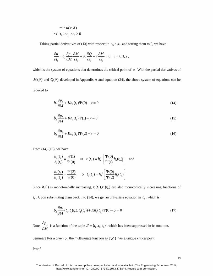
Taking partial derivatives of (13) with respect to 0 1 2, ,t t t and setting them to 0, we have

2 0, 0,1, 2L

i i i i

pu M Q Mb K it M t t t

γ∂∂ ∂ ∂ ∂= + − = =

∂ ∂ ∂ ∂ ∂,

which is the system of equations that determines the critical point of u . With the partial derivatives of

( )M δ and ( )Q δ developed in Appendix A and equation (24), the above system of equations can be

reduced to

2 0 0( ) (0) 0Lpb Kh tM

γ∂Ψ+ − =

∂ (14)

2 0 1( ) (1) 0Lpb Kh tM

γ∂Ψ+ − =

∂ (15)

2 0 2( ) (2) 0Lpb Kh tM

γ∂Ψ+ − =

∂ (16)

From (14)-(16), we have

10 01 0 0 0 0

0 1

( ) (1) (0)( ) ( )( ) (0) (1)

h t t t h h th t

− ⎡ ⎤Ψ Ψ= ⇒ = ⎢ ⎥Ψ Ψ⎣ ⎦

and

10 02 0 0 0 0

0 2

( ) (2) (0)( ) ( )( ) (0) (2)

h t t t h h th t

− ⎡ ⎤Ψ Ψ= ⇒ = ⎢ ⎥Ψ Ψ⎣ ⎦

Since 0 ( )h ⋅ is monotonically increasing, 1 0 2 0( ), ( )t t t t are also monotonically increasing functions of

0t . Upon substituting them back into (14), we get an univariate equation in 0t , which is

2 0 1 0 2 0 0 0( , ( ), ( )) ( ) (0) 0Lpb t t t t t Kh tM

γ∂+ − =

∂Ψ (17)

Note, LpM∂∂

is a function of the tuple 0 1 2{ , , }t t tδ = , which has been suppressed in its notation.

Lemma 3 For a given γ , the multivariate function ( , )u γ δ has a unique critical point.

Proof.


20

From Lemma 1 and Lemma 2, we know that 0 1 0 2 0( , ( ), ( ))Lp t t t t tM∂∂

is always negative and is a

increasing function of 0t . In addition, 0 ( )h ⋅ is an increasing function with 0 (0) 0h = and is unbounded

as its parameter approaches infinity. Thus, the function

2 0 1 0 2 0 0 0( , ( ), ( )) ( ) (0)Lpb t t t t t Kh tM

+ Ψ∂∂

equals the positive constant γ at a unique point.

Therefore equation (17) has a unique solution, which means that for a given γ , ( , )u γ δ has a

unique critical point, denoted as 0 1 2{ , , }t t tγ γ γ γδ = . ■

The following theorem shows how to find the global minimum of ( , )u γ δ .

Theorem 1 For a given γ , function ( , )u γ δ achieves global minimum at its critical point

0 1 2{ , , }t t tγ γ γ γδ = .

The proof of Theorem 1 is in Appendix C.

In light of Theorem 1 and the lambda minimization technique, we state the following algorithm to

find the optimal δ that minimizes ( )v δ for a given c .

Algorithm I

1. Initialize the iteration counter 0m = and 0γ γ= .

2. For mγ , use Theorem 1 to find , , , ,0 1 2{ , , } arg min ( , )c m c m c m c m mt t t u

δδ γ δ= = .

3. Use the replacement policy , , , ,0 1 2{ , , }c m c m c m c mt t tδ = obtained in step 2 and equation (12) to

update 1 ,( )m c mvγ δ+ = .

4. If 1m mγ γ+ = , stop with 1c mv γ += and ,c c mδ δ= ; otherwise, set 1m m← + and go to step 2.


21

In addition, an upper bound on the optimal stock level c can be obtained. Denote the optimal

parameters as * * * *0 1 2{ , , }t t tδ = and *c . Let 0

0 0( , )ccφ φ δ= , which is the optimal cost when c is fixed

at 0c . Then we have

1 * 1* * * *1 1

0 *

( ) ( ) ( ) ( )( , )( ) ( )

W S W SS S

C h h KQ C h h KQc h c N h c NM M

μ δ μ δφ φ δδ δ

− − ′+ − + + − +≥ ≥ + ≥ +

′

where the second inequality follows by omitting the Lp term in * *( , )cφ δ , and the third inequality

holds if δ ′ is the replacement policy that minimizes the term

1

1 ( ) ( )( )

W SC h h KQM

μ δδ

−+ − +.

Using the methods developed in (Wu and Ryan, 2011), we can obtain δ ′ as an optimal policy for the

condition-based replacement model described there with preventive replacement cost

11 ( )W SC h h μ−+ − and additional failure cost K . Thus an upper bound for *c is given by

1

110

( ) ( )( )

W SS

C h h KQc N hM

μ δφδ

−−⎢ ⎥′⎛ ⎞+ − +

= −⎢ ⎥⎜ ⎟′⎝ ⎠⎣ ⎦ (18)

In light of the above discussion, the following algorithm is presented to find the optimal parameters

and the global minimum of (11).

Algorithm II

1 Initialize 0c c= .

2 For fixed 0c , using Algorithm I to find the optimal parameters 0 , 0,1, 2cit i = . Set

0 0 000 0 1 2( , , , )c c cc t t tφ φ= .

3 Obtain an upper bound c for *c using equation (18).

4 For 1, ,c c= , find the optimal , 0,1, 2cit i = and the corresponding optimal cost

*0 1 2( , , , )c c c

c c t t tφ φ= . Then the optimal stock level * *arg min cc

c φ= , the optimal replacement

policy * * * *0 1 2{ , , }t t tδ = and the global minimum is *min cφ .


22

5 NUMERICAL EXAMPLE

Suppose the covariate process ( )Z t is a pure birth process with three states {0,1,2} and transition

rates 0 1 2ln(0.4), 0v v v= = − = . Let 0 ( ) 2h t t= and ( ) exp(2 )t tZ ZΨ = . Assume

1 25, 15, 25, 10, 0.2, 0.5, 0.5, 5.C C K N hα β μ= = = = = = = =

The total cost per unit time is

4.9 10.1 ) 25 ( )( , ) 1.5 10

( )( ,Lp Qc c c

Mδ δφ δδ

+ += + .

Let 0 10c = . In Algorithm I step 1, initialize 0 12γ = . As shown in Table 1, the

lambda-minimization converges after four iterations with 0 24.7330cv = and optimal parameter

0 0.5440, 0.0736, 0.0 }00{ 1cδ = . The corresponding total cost 00 0 262.33c

SNv h cφ = + = .

Table 1 Illustration of Algorithm I and the lambda-minimization process

m γ Critical point ,c mδ Value of u at critical point

,( )c mv δ

0 12 (0.3853, 0.0521, 0.0070) 4.4924 26.4098 1 26.4908 (0.5705, 0.0772, 0.0104) -0.6750 24.7573 2 24.7573 (0.5444, 0.0737, 0.0100) -0.0096 24.7330 3 24.7330 (0.5440, 0.0736, 0.0100) 0 24.7330

Based on methods developed in (Wu and Ryan, 2011), the replacement policy that minimizes term

4.9 25 ( )( )

QM

δδ

+ is {0.4826,0.0653,0.0088}δ ′ = and the minimal value of the term is 24.1302. Thus

from equation (18), an upper bound for c is

4.9 25 ( ) 1262.33 10 14

( ) 1.5Q

Mc δ

δ⎢ ⎥′⎛ ⎞+

− =⎢ ⎥⎜ ⎟′⎝ ⎠⎣ ⎦= .

In step 4 of Algorithm II, when c ranges from 1 to 14, the resulting total costs are shown in Figure

3. The optimal parameters are * 12c = and * {0.5048, 0.0683, 0.0092}δ = . The global minimal cost

is * 260.827φ = .


23

Figure 3 The minimized total cost when c varies from 1 to its upper bound

6 EVALUATION OF THE SINGLE CATEGORY RETURN ASSUMPTION

In the previous analysis, we consider the returns as a single category. However, in reality, there is

usually a quality difference between the preventively replaced products and failure replaced products in

terms of remanufacturing time and remanufacturing cost.

To understand the effect of the single category assumption, in this section, we will examine the

case when we categorize the returns into two types: Type 1 (T1), preventively replaced products and

Type 2 (T2), failure replaced products, estimate its cost and compare to the cost of the no categorization

case.

In general, T1 products have better quality than T2 products, so it typically requires less

remanufacturing effort to bring them to the "as good as new" condition. To quantify the quality

difference, assume the statement “T1 is x% better than T2 in quality” implies that


24

1 The unit remanufacturing cost of T1, 11C , is x% lower than that of T2, 12C ; i.e.,

11 12 (1 %)C C x= − .

2 The remanufacturing time of T1, 11/ μ , is x% shorter than that of T2, 21/ μ ; i.e.,

1 21/ (1 %) / .xμ μ= −

6.1 Model analysis

Let 1 2( ), ( )W t W t be the number of T1, T2 products, respectively, in WIP at time t .Then

1 2( ) ( ) ( ) .W t W t I t c+ + =

And let 1 2,λ λ be the arrival rate of T1, T2 products, respectively. Assume the product mix that enters

the remanufacturing process is the same as the product mix that enters the remanufacturable inventory

at all times. Then under replacement policy δ ,

1 2(1 ( )), ( )Q Qλ λ δ λ λ δ= − =

where / ( )N Mλ δ= .

It is not hard to see that 1 2( ( ), ( ) : 0)W t W t t ≥ consists of a continuous-time Markov chain with a

finite state space

{( , ) : , 0,1, , , 0,1, , }S i j i j c i c j c= + ≤ = … = …

A typical portion of the transition diagram among those states is shown in Figure 4. Although on

the boundaries, one or more of the states depicted in the figure may not exist, the transition rates for the

rest are valid. It can be verified that this continuous-time Markov chain is irreducible and ergodic, so it

has a limiting distribution.


25

Figure 4: Part of transition diagram

Define the indicator function

1 if ( , )( , )

0 if ( , )S

i j SI i j

i j S∈⎧

= ⎨ ∉⎩

Then the balance equations of the limiting probabilities are

2 1

2 1

2 1

2 1

( , 1) ( , 1) ( 1, ) ( 1, )( 1) ( , 1) ( , 1) ( 1) ( 1, ) ( 1, )

[ ( , 1) ( 1, )( , 1) ( 1, )] ( , ) for all ( , )

S S

S S

S S

S S

P i j I i j P i j I i jj P i j I i j i P i j I i j

j I i j i I i jI i j I i j P i j i j S

λ λμ μ

μ μλ λ

− − + − −

+ + + + + + + += − + −+ + + + ∈

Let 1 1 2 2/ , /a bλ μ λ μ= = . The solution to the balance equations is

0 0

1(0,0)

!

!

i jc c i

i j

Pa bi j

−

= =

=

∑∑ (19)

( , ) (0,0) for all ( ,! !

)i ja bP i j P i j S

i j= ∈ (20)

Therefore

1 20

( )( ( ) ( ) ) ( , ) (0,0)!

mm

i

a bP W t W t m P i m i Pm=

++ = = − =∑

, 1 2( )( ( ) ( ) ) (0,0)

!

c

L cata bp P W t W t c P

c+

= + = = (21)

11

1 20

( )( ) ( ( ) ( )) (0,0)!

kc

catk

a bE W E W t W t Pk

+−

=

+= + = ∑ (22)

With categorization, the replacement cost per unit time for a single product is


26

, 11 22 , 2,

11 12 11 , 2 11 12 11

(1 )[(1 ( ))( ( )) ( )( ( ))] ( ( ))( )

( ) ( ) [ ( )( )]( )

L cat L catR cat

L cat

p Q C KQ Q C KQ p C KQM

C K C C Q p C C Q C CM

δ δ δ δ δφ

δδ δ

δ

− − + + + + +=

+ + − + − − −=

and the total cost per unit time is

,( , ) ( ) ( )cat R cat S W S catc N h c h h E Wφ δ φ= + + − . (23)

We can follow the two step process as described in section 4 to optimize this objective function.

However, since this objective function involves more complicated expressions of the loss probability

and mean WIP than that of (11), minimizing the γ -function in the lambda minimization technique is

challenging. Thus for step 1, we resort to some numerical optimization methods to minimize the

objective function for a given c . Because first derivatives are available, we adopt the BFGS method

(Fletcher, 1987), which is generally considered as the best quasi-Newton method.

The BFGS method cannot guarantee the global optimality of the obtained policy. However, for the

single category case, we have verified that the policy and cost obtained using the BFGS method is the

same as the optimal policy and cost obtained using lambda minimization technique. Since objective

function for the two category case shares the same basic structure with the objection function for single

category case, we use the result of BFGS method to approximate the optimal policy and cost in the two

category case.

6.2 Cost impact of the single category assumption

Here we illustrate the cost impact of the single category assumption through a numerical example.

Assume T1 products are 20% better than T2 products in quality. Let 11 15, 5C μ= = . Then

12 26.125, 4C μ= = . Assume all the other parameters stay the same. Then the optimal cost

* 265.789catφ = and the optimal parameters are * 12catc = , * {0.4911,0.0620,0.0091}catδ = .


27

If the decision maker uses the single category assumption, then first he must estimate the

equivalent unit remanufacturing cost

1 11 12(1 ( )) ( )C C Q C Qδ δ= − +

and equivalent unit processing rate

(1 )( ) Lp

E Wλμ = −

where / ( )N Mλ δ= . The estimation requires a realization of the operation policy { , }c δ . Assume the

policy maker can observe the results of * *{ , }cat catc δ . Then under policy * *{ , }cat catc δ

( ) 0.1619Q δ = , ( ) 0.3707M δ = , 0.0075Lp = , ( ) 5.5710E W =

and the estimation would be

1 5.182, 5.000C μ= = .

With those parameters, the optimal policy under the single category assumption is

_ 12no catc = , _ {0.5120,0.0693,0.0094}no catδ = .

Under this policy, the actual total cost is _ 265.916no catφ = , which is 0.05% bigger than *catδ . This

negligible cost difference indicates that the single category return assumption is acceptable in this

instance.

Intuitively, the cost difference between the categorized and non-categorized cases depends on the

quality difference between T1 and T2. To further evaluate the impact of single category assumption, we

vary the quality difference, while keeping 11 15, 5C μ= = unchanged, and then obtain the

corresponding cost differences following a similar procedure as above. The results are summarized in

Table 2.

As expected, for bigger quality difference, the additional cost introduced by the single category

assumption is more substantial. And we can see that for our example, as long as the quality difference is


28

below 50%, the cost error caused by the single category assumption is under 1%. Another observation is

that as the quality difference increases, we tend to perform the preventive replacement more frequently

and keep the stock level higher in the two category case, which are reasonable because, with a wider

quality difference, it is more costly and time consuming to remanufacture a failure-replaced product.

Table 2 The impact of single category assumption under various quality difference between the two types of products

Quality difference

x%

*catc *

catδ *catφ _no catc _no catδ _no catφ

Cost difference ( _no catφ - *

catφ )/ *catφ

20% 12 {0.4911, 0.0620, 0.0091}

265.789 12 {0.5120, 0.0693, 0.0094}

265.916 0.05%

40% 13 {0.4697, 0.0638, 0.0088}

276.206 12 {0.5387, 0.0729, 0.0105}

277.673 0.53%

50% 13 {0.4603, 0.0622, 0.0087}

283.546 12 {0.5323, 0.0720, 0.0102}

285.766 0.78%

60% 14 {0.4364, 0.0591, 0.0081}

294.168 12 {0.5710, 0.0773, 0.0016}

301.289 2.42%

80% 17 {0.3634, 0.0492, 0.0069}

341.987 13 {0.6146, 0.0832, 0.0116}

374.794 9.60%

7 CONCLUSION

This paper investigates a joint operation problem in the context of a product-service system, which

to the best of our knowledge has not been addressed in the literature. The system consists of a service

subsystem and a remanufacturing subsystem where the replacement decision and the inventory

management decision must be made at the same time. Identifying and formulating the couplings

between the two subsystems, an integrated model aiming to minimize the total cost per unit time of the

system is developed and an algorithm is presented to jointly optimize the replacement policy and the

inventory management policy. Then we evaluate the cost impact of treating the preventively replaced

products and products replaced due to failure as one category. A numerical example demonstrates that


29

as long as the quality difference between the two types of replaced products is not too large, where how

large depends on other parameters in the model, the single category assumption is reasonable.

In this paper, for illustration the covariate process is assumed to have three states, which could be

characterized as “like new,” “deteriorated,” and “critical.” It is straightforward to generalize our model

to accommodate a finer-grained approximation of a continuous state space by adding more discrete

states. The additional effort required for formulation mainly lies in obtaining the explicit expressions of

the mean replacement time and the failure probability for a given replacement policy, which is

discussed in detail in Wu and Ryan, 2011). Correspondingly, the additional computational effort lies in

the evaluation of the mean replacement time and the failure probability. In particular, for an n-state

covariate process, the expressions of the mean replacement time and the failure probability consist of

several n-fold integrals. Monte Carlo integration methods are essential to evaluate them efficiently

(Press et al., 2007).

Other possible extensions to this paper are as follows. First, in our analysis, the demand process of

the fleet for new products, which is a superposed renewal process, is approximated by a Poisson process

assuming that the number of products in the fleet is sufficiently large. Evaluating the impact of this

approximation in the situation of moderate or small fleet sizes is a possible extension of this research.

Second, considering the capacity expansion problem of service subsystem in addition to maintenance

would be an interesting and challenging problem, which is a natural generalization of the model

presented in this study. Third, in a hybrid business model, where the producers operate traditional

product sales as well as a PSS, the external returns in addition to the internal replaced products will

become part of the input to the remanufacturing system. In this case, the inventory model needs to be

reconsidered. Last but not least, the accelerated failure time (AFT) model (Meeker and Escobar, 1998)


30

is considered as a strong competitor to the proportional hazards model when incorporating the covariate

information into system failure time estimation. In case it is hard to decide which model to use, the

general proportional hazards model (Bagdonavicius and Nikulin, 2001), which includes PHM and the

AFT model as special cases, might be appropriate.

ACKNOWLEDGEMENT

This material is based upon work supported by the National Science Foundation under grant

CNS-0540293.

REFERENCES

Aras, N., Boyaci, T., and Verter, V. (2004). The effect of categorizing returned products in remanufacturing. IIE Transactions, 36(4):319–331.

Armstrong, M. J. and Atkins, D. R. (1996). Joint optimization of maintenance and inventory policies for a simple system. IIE Transactions, 28:415–424.

Armstrong, M. J. and Atkins, D. R. (1998). A note on joint optimization of maintenance and inventory. IIE Transactions, 30:143–149.

Aven, T. and Bergman, B. (1986). Optimal replacement times – a general set-up. Journal of Applied Probability, 23:432–442.

Bagdonavicius, V. and Nikulin, M. (2001). Accelerated life models: modeling and statistical analysis. Chapman and Hall/CRC.

Baines, T. S. and Lightfoot, H. W. (2007). State-of-the-art in product-service systems. Proceedings of the Institution of Mechanical Engineers, Part B: Journal of Engineering Manufacture, 221:1543–1552.

Banjevic, D., Jardine, A. K. S., Makis, V., and Ennis, M. (2001). A control-limit policy and software for condition-based maintenance optimization. INFOR, 39:32–50.

Berthaut, F., Gharbi, A., and Dhouib, K. (2011). Joint modified block replacement and production/inventory control policy for a failure-prone manufacturing cell. Omega, 39:642–654.


31

Brezavscek, A. and Hudoklin, A. (2003). Joint optimization of block-replacement and periodic-review spare-provisioning policy. IEEE Transactions on Reliability, 52:112 – 117.

Buzacott, J. A. and Shanthikumar, J. G. (1993). Stochastic Models of Manufacturing Systems. Prentice-hall, Inc., Englewood Cliffs, NJ.

Cinlar, E. and Lewis, P. A. W. (1972). Superposition of point processes. In Stochastic Point Processes, pages 546–606. Wiley-Interscience, New York.

Cox, D. R. and Oakes, D. (1984). Analysis of Survival Data. Chapman & Hall, London.

Das, T. K. and Sarkar, S. (1999). Optimal preventive maintenance in a production inventory system. IIE Transactions, 31:537–551.

Fleischmann, M., Bloemhof-Ruwaard, J. M., Dekker, R., Van der Laan, E., and Van Numen, J. A. E. E. (1997). Quantitative models for reverse logistics: A review. European Journal of Operational Research, 103:1–17.

Fletcher, R. (1987). Practical Methods of Optimization. John Wiley & Sons Ltd, 2nd edition.

Ghasemi, S., Yacout, S., and Ouali, M. S. (2007). Optimal condition based maintenance with imperfect information and the proportional hazards model. International Journal of Production Research, 45(4):989–1012.

Giorgio, M., Guida, M., and Pulcini, G. (2011). An age- and state-dependent Markov model for degradation processes. IIE Transactions, 43:621–632.

Goedkoop, M., van Halen, C., and te Riele, H. (1999). Product service-systems, ecological and economic basics. Report for Dutch ministries of environment (VROM) and economic affairs (EZ). http://www.pre.nl/download/ProductService.zip.

Guide, V. D. R. (2000). Production planning and control for remanufacturing: Industry practice and research needs. Journal of Operations Management, 18:467–483.

Guide, V. D. R. and Van Wassenhove, L. N. (2009). The evolution of closed-loop supply chain research. Operations Research, 57(1):10–18.

Harel, A. (1990). Convexity properties of the erlang loss formula. Operations Research, 38:499–505.

Kharoufeh, J. P., Solo, C. J., and Ulukus, M. Y. (2010). Semi-Markov models for degradation-based reliability. IIE Transactions, 42:599–612.

Lam, C. T. and Yeh, R. H. (1994). Optimal maintenance policies for deteriorating systems under various maintenance strategies. IEEE Transactions on Reliability, 43(3):423–430.


32

Liu, Y., Li, Y., Huang, H.-Z., Zuo, M. J., and Sun, Z. (2010). Optimal preventive maintenance policy under fuzzy bayesian reliability assessment environments. IIE Transactions, 42:734–745.

Luiten, H., Knot, M., and van der Horst, T. (2001). Sustainable product-service-systems: the kathalys method. In Proceedings of the Second International Symposium on Environmentally conscious design and inverse manufacturing, pages 190–197.

Manzini, E., Vezzoli, C., and Clark, G. (2001). Product service-systems: using an existing concept as a new approach to sustainability. Journal of Design Research, 1(2).

Mardinab, F. and Araib, T. (2012). Capital equipment replacement under technological change. The Engineering Economist, 57(2):119–129.

Maxwell, I. and van der Vorst, R. (2003). Developing sustainable products and services. Journal of Clearner Production, pages 883–895.

Meeker, W. Q. and Escobar, L. A. (1998). Statistical Methods for Reliability Data. Wiley, New York.

Press, W. H., Teukolsky, S. A., Vetterling, W. T., and P., F. B. (2007). Numerical recipes: the art of scientific computing. Cambridge University Press, third edition.

Rausch, M. and Liao, H. (2010). Joint production and spare part inventory control strategy driven by condition based maintenance. IEEE Transactions on Reliability, 59.

Rezg, N., Xie, X., and Mati, Y. (2004). Joint optimization of preventive maintenance and inventory control in a production line using simulation. International Journal of Production Research, 42:2029–2046.

Ross, S. M. (2003). Introduction to Probability Models. Academic Press, San Diego, CA, 8th edition.

Stewart, J. (1999). Calculus. Brooks/Cole Pub Co, 4th edition.

Thierry, M. C., Salomon, M., and Van Nunen, J. A. E. E. (1995). Strategic production and operations management issues in product recovery management. California Management Review, 37:114–135.

Toffel, M. W. (2008). Contracting for servicizing. Harvard Business School Technology & Operations Mgt. Unit Research Paper No. 08-063. Available at SSRN: http://ssrn.com/abstract=1090237 or http://dx.doi.org/10.2139/ssrn.1090237.

Van der Laan, E., Salomon, M., Dekker, R., and Wassenhove, L. V. (1999). Inventory control in hybrid systems with remanufacturing. Management Science, 45(5):733–747.

Van Halen, C., Vezzoli, C., and Wimmer, R. (2004). MEPSS Handbook. Royal Van Gorcum, Assen,


33

Netherlands.

White, A., Stoughton, M., and Feng, L. (1999). Servicizing: The Quiet Transition to Extended Producer Responsibility. Tellus Institute, Boston.

Wu, X. and Ryan, S. M. (2010). Value of condition monitoring for optimal replacement in the proportional hazards model with continuous time degradation. IIE Transactions, 42:553–563.

Wu, X. and Ryan, S. M. (2011). Optimal replacement in the proportional hazards model with semi-Markovian covariate process and continuous monitoring. IEEE Transactions on Reliability, 60:580–589.

Yatsenko, Y. and Hritonenko, N. (2009). Technological breakthroughs and asset replacement. The Engineering Economist, 54(2):81–100.

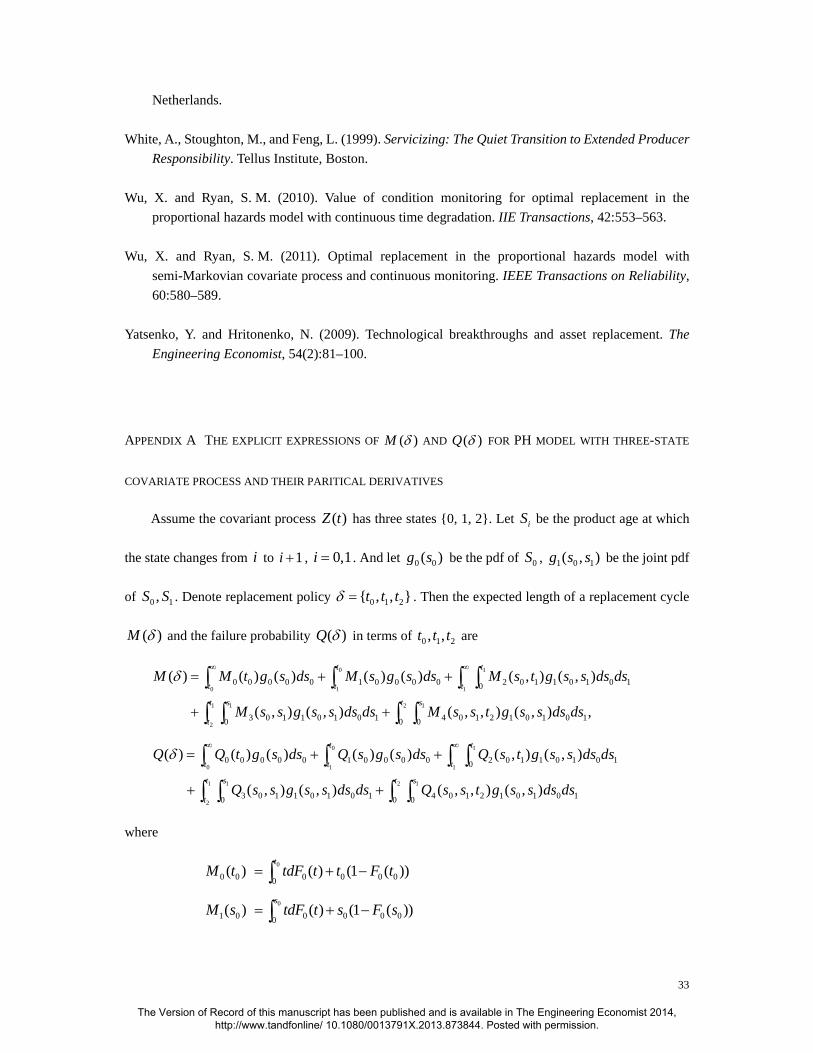
APPENDIX A THE EXPLICIT EXPRESSIONS OF ( )M δ AND ( )Q δ FOR PH MODEL WITH THREE-STATE

COVARIATE PROCESS AND THEIR PARITICAL DERIVATIVES

Assume the covariant process ( )Z t has three states {0, 1, 2}. Let iS be the product age at which

the state changes from i to 1i + , 0,1i = . And let 0 0( )g s be the pdf of 0S , 1 0 1( , )g s s be the joint pdf

of 0 1,S S . Denote replacement policy 0 1 2{ , , }t t tδ = . Then the expected length of a replacement cycle

( )M δ and the failure probability ( )Q δ in terms of 0 1 2, ,t t t are

0 1

0 1 1

1 1 2 1

2

0 0 0 0 0 1 0 0 0 0 2 0 1 1 0 1 0 10

3 0 1 1 0 1 0 1 4 0 1 2 1 0 1 0 10 0 0

( ) ( ) ( ) ( ) ( ) ( , ) ( , )

( , ) ( , ) ( , , ) ( , ) ,

t t

t t t

t s t s

t

M M t g s ds M s g s ds M s t g s s ds ds

M s s g s s ds ds M s s t g s s ds ds

δ∞ ∞

= + +

+ +

∫ ∫ ∫ ∫

∫ ∫ ∫ ∫

0 1

0 1 1

1 1 2 1

2

0 0 0 0 0 1 0 0 0 0 2 0 1 1 0 1 0 10

3 0 1 1 0 1 0 1 4 0 1 2 1 0 1 0 10 0 0

( ) ( ) ( ) ( ) ( ) ( , ) ( , )

( , ) ( , ) ( , , ) ( , )

t t

t t t

t s t s

t

Q Q t g s ds Q s g s ds Q s t g s s ds ds

Q s s g s s ds ds Q s s t g s s ds ds

δ∞ ∞

= + +

+ +

∫ ∫ ∫ ∫

∫ ∫ ∫ ∫

where

0

0 0 0 0 0 00( ) ( ) (1 ( ) )

tM t tdF t t F t= + −∫

0

1 0 0 0 0 00( ) ( ) (1 ( ) )

sM s tdF t s F s= + −∫


34

0 1

02 0 1 0 1 0 1 1 0 10( , ) ( ) ( , ) (1 ( ) , )

s t

sM s t tdF t tdF s t t F s t= + + −∫ ∫

0 1

03 0 1 0 1 0 1 1 0 10( , ) ( ) ( , ) (1 ( ) , )

s s

sM s s tdF t tdF s t s F s s= + + −∫ ∫

0 1 2

0 14 0 1 2 0 1 0 2 0 1 2 2 0 1 20( , , ) ( ) ( , ) ( , , ) (1 ( , , ))

s t t

s sM s s t tdF t tdF s t tdF s s t t F s s t= + + + −∫ ∫ ∫

0 0 0 0( ) ( )Q t F t= 1 0 0 0( ) ( )Q s F s=

2 0 1 1 0 1( , ) ( , )Q s t F s t= 3 0 1 1 0 1( , ) ( , )Q s s F s s=

4 0 1 2 2 0 1 2( , , ) ( , , )Q s s t F s s t=

and

( )0 0 00( ) 1 (0) ( ) ,

tF t exp h u du t s= − −Ψ ≤∫

( )0

01 0 0 0 0 10( , ) 1 ( 0) ( ) (1) ( ) ,

s t

sF s t exp h u du h u du s t s= − −Ψ −Ψ ≤ ≤∫ ∫

( )0 1

0 12 0 1 0 0 0 10( , , ) 1 (0) ( ) (1) ( ) (2) ( ) , .

s s t

s sF s s t exp h u du h u du h u du s t= − −Ψ −Ψ −Ψ ≤∫ ∫ ∫

The partial derivatives of ( )M δ and ( )Q δ with respect to it are

( )0

1

1

2 1

0 0 0 0 000

1 0 1 1 0 1 0 101

2 0 1 2 1 0 1 0 10 02

( ) 1 ( ) (1 ( ))

( ) (1 ( , )) ( , )

( ) (1 ( , , )) ( , )

t

t

t

t s

M g s ds F tt

M F s t g s s ds dst

M F s s t g s s ds dst

δ

δ

δ

∞

∂= − −

∂∂

= −∂

∂= −

∂

∫

∫ ∫

∫ ∫

( )0

1

1

2 1

0 0 0 0 0 0 000

0 1 1 0 1 1 0 1 0 101

0 2 2 0 1 2 1 0 1 0 10 02

( ) ( ) (0) 1 ( ) (1 ( ))

( ) ( ) (1) (1 ( , )) ( , )

( ) ( ) (2) (1 ( , , )) ( , )

t

t

t

t s

Q h t g s ds F tt

Q h t F s t g s s ds dst

Q h t F s s t g s s ds dst

δ

δ

δ

∞

∂= Ψ − −

∂∂

= Ψ −∂

∂= Ψ −

∂

∫

∫ ∫

∫ ∫

Note that

0( ) ( )( ) ( ) ,ii i

Q Mh t i it tδ δ∂ ∂

= Ψ ∀∂ ∂

. (24)


35

APPENDIX B LAMBDA MINIMIZATION TECHNIQUE

In this section, we will give a brief introduction to the lambda minimization technique developed in

Aven and Bergman, 1986), aiming to minimizing a function with the following form

( )( )( )

M XB XS X

= , (25)

where nX ∈ℜ and ( ) 0,S X X> ∀ .

Define the λ -function

( , ) ( ) ( )C X M X S Xλ λ= − , ( , )λ∈ −∞ +∞ .

For each λ , denote the value of X that minimizes ( , )C X λ as X λ .

Now we will show how the problem of minimizing ( )B X can be solved by minimizing the

λ -function ( , )C X λ . Aven and Bergman proved the following proposition which associates the

optimality of ( )B X with the optimality of ( , )C X λ .

Proposition 1: If X λ minimizes ( , )C X λ and ( , ) 0C X λ λ = , then X λ is optimal for (25) and the

optimal value of ( )B X is *( )B X λ λ λ= ≡ .

Aven and Bergman then proved another important proposition, stated below, which leads to an

iterative algorithm that always produces a sequence converging to *λ .

Proposition 2: Choose any 1λ and set iteratively 1 ( )nn B X λλ + = , 1,2,3, .n = Then

*lim nnλ λ

→∞= .

Propositions 1 and 2 imply that the minimization of ( )B X can be transformed into the problem of

minimizing ( , )C X λ plus a succession of iterations. This is the essence of the lambda minimization

technique. This technique is very suitable for situations where it is easy to find the optimal solutions to

the λ -function ( , )C X λ while it is hard to minimize ( )B X directly; this is often the case in

replacement/maintenance applications. The optimal solution and the optimal value of ( )B X can be


36

attained simultaneously when the algorithm converges.

APPENDIX C PROOF OF THEOREM 1

For readability, first we list all the monotonicity properties of various functions that are related to

the proof of Theorem 1 in the following.

1) ( )M δ is increasing in it , i∀ .

2) LpM∂∂

is increasing in it , i∀ .

3) 0 ( )h ⋅ is increasing in its parameter.

4) 1t is increasing in 0t if 11 0 0 0

(0) ( )(1)

t h h t− ⎡ ⎤Ψ= ⎢ ⎥Ψ⎣ ⎦

and 2t is increasing in 0t if

12 0 0 0

(0) ( )(2)

t h h t− ⎡ ⎤Ψ= ⎢ ⎥Ψ⎣ ⎦

.

Since γ is fixed, in the following discussion, it is suppressed in the notation of u .

The feasible region of ( )u δ is 0 1 2{ : 0}R t t tδ= ≥ ≥ ≥ . Divide this region into two sets: a closed

and bounded set 0 1 2{ : 0}D t t tδ= Λ ≥ ≥ ≥ ≥ where Λ is an arbitrary large positive number, and set

\B R D= ; i.e., { , }B D is a partition of R . Define it = +∞ represent failure replacement in state i.

Lemma C.1 ( )u δ achieves its minimum at the critical point 0 1 2{ , , }t t tγ γ γ γδ = in D .

Proof

Since u is a continuous function on the closed and bounded region D , according to the extreme

value theorem for multivariate functions (Stewart, 1999), u has a global minimum which happens

either at its critical point or a certain point on the boundary.

The boundaries of ( )u δ are where 0 1t t= , 1 2t t= , 2 0t = or 0t = Λ within the feasible region

0 1 2{ : 0}D t t tδ= Λ ≥ ≥ ≥ ≥ . We prove by contradiction that points on the boundaries are not optimal

to ( )u δ .


37

1) Points on the boundary where 0 1t t= .

Suppose an optimal point exists on this boundary and denote it as 0 0 2{ , , }a a aδ = , 0 2 0a a≥ ≥ .

Recall that the partial derivative of ( )u δ with respect to 0 1 2, ,t t t are

2 0 1 2 0( , , ) ( ) ( ) , 0,1, 2Li

i i

pu M b t t t Kh t i it t M

γ∂∂ ∂ ⎛ ⎞= + − =⎜ ⎟∂ ∂ ∂⎝ ⎠Ψ ,

and 0,i

M it

∂> ∀

∂.

i. If 2 0 0 2 0 0( , , ) ( ) (0) 0Lpb a a a Kh aM

γΨ∂

+ − ≥∂

it follows that

2 0 0 2 0 0( , , ) ( ) (1) 0Lpb a a a Kh aM

γΨ∂

+ − >∂

.

According to the definition of a continuous function,

1 2 0( , )a a a∃ ∈ , s.t. 2 0 1 2 0 1( , , ) ( ) (1) 0Lpb a a a Kh aM

γΨ∂

+ − >∂

.

From assumption #7 and Lemma 2, we know that 2 0 1 2 0 1( , , ) ( ) ( )Lpb t t t Kh t iM

Ψ∂

+∂

is increasing in 1t .

Thus

0 1 21

( , , ) 0u a t at∂

>∂ 1 1 0[ , ]t a a∀ ∈ ,

which means u is an increasing function for 1 1 0[ , ]t a a∈ with fixed 0 0 2 2,t a t a= = . Therefore

0 1 2 0 0 2({ , , }) ({ , , })u a a a u a a a< . Contradiction.

ii. If 2 0 0 2 0 0( , , ) ( ) (0) 0Lpb a a a Kh aM

γΨ∂

+ − <∂

It follows that

0 0a a′∃ > , s.t. 2 0 0 2 0 0( , , ) ( ) (0) 0Lpb a a a Kh aM

γ∂ ′ ′ Ψ+ − <∂

.


38

Thus 0 0 20

( , , ) 0u t a at∂

<∂

, 0 0 0[ , ]t a a′∀ ∈ , which means u is an decreasing function for 0 0 0[ , ]t a a′∈

with fixed 1 0 2 2,t a t a= = . Therefore 0 0 2 0 0 2({ , , }) ({ , , })u a a a u a a a′ < . Contradiction.

2) Points on the boundary where 1 2t t=

Using the same argument as in 1), we can prove that points on this boundary are not optimal.

3) Points on the boundary where 2 0t =

Assume 0 1( , ,0)a a is optimal.

Since 0LpM∂

<∂

, 0 (0) 0h = and 0γ > , 2 0 1 0( , ,0) (0) (2) 0Lpb a a KhM

γ∂+ − <

∂Ψ

It follows

2 1(0, )a a∃ ∈ , s.t. 2 0 1 2 0 2( , , ) ( ) (2) 0Lpb a a a Kh aM

γΨ∂

+ − <∂

.

Thus 0 1 22

( , , ) 0u a a tt∂

<∂

, 2 2[0, ]t a∀ ∈ , which mean u is an decreasing function for 2 2[0, ]t a∈ with

fixed 0 0 1 1,t a t a= = . Therefore 0 1 2 0 1({ , , }) ({ , ,0})u a a a u a a< . Contradiction.

4) Points on the boundary where 0t = Λ

Since K is arbitrary large and 0 ( )h ⋅ is increasing and unbounded, then we have

2 1 2 0( , , ) ( ) (0) 0Lpb a a KhM

γ∂ΨΛ + Λ − >

∂

It follows

0 1[ , )a a∃ ∈ Λ , s.t. 2 0 1 2 0 0( , , ) ( ) (0) 0Lpb a a a Kh aM

γΨ∂

+ − >∂

.

Thus 0 1 2 0 00

( , , ) 0 [ , )u t a a t at∂

> ∀ ∈ Λ∂

, which means u is an increasing function for 0 0[ , )t a∈ Λ with

fixed 1 1 2 2,t a t a= = . Therefore 0 1 2 1 2({ , , }) ({ , , })u a a a u a a< Λ . Contradiction.

In summary, in region D , ( )u δ can not achieve its global minimum at its boundaries; which


39

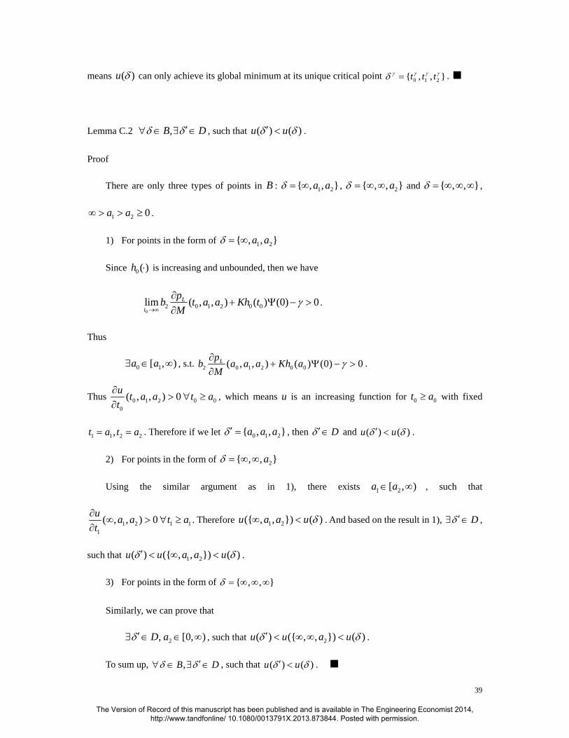
means ( )u δ can only achieve its global minimum at its unique critical point 0 1 2{ , , }t t tγ γ γ γδ = . ■

Lemma C.2 ,B Dδ δ ′∀ ∈ ∃ ∈ , such that ( ) ( )u uδ δ′ < .

Proof

There are only three types of points in B : 1 2{ , , }a aδ = ∞ , 2{ , , }aδ = ∞ ∞ and { , , }δ = ∞ ∞ ∞ ,

1 2 0a a∞ > > ≥ .

1) For points in the form of 1 2{ , , }a aδ = ∞

Since 0 ( )h ⋅ is increasing and unbounded, then we have

0

2 0 1 2 0 0lim ( , , ) ( ) (0) 0L

t

pb t a a Kh tM

γ→∞

∂+ −Ψ >

∂.

Thus

0 1[ , )a a∃ ∈ ∞ , s.t. 2 0 1 2 0 0( , , ) ( ) (0) 0Lpb a a a Kh aM

γΨ∂

+ − >∂

.

Thus 0 1 2 0 00

( , , ) 0u t a a t at∂

> ∀ ≥∂

, which means u is an increasing function for 0 0t a≥ with fixed

1 1 2 2,t a t a= = . Therefore if we let 0 1 2{ , , }a a aδ ′ = , then Dδ ′∈ and ( ) ( )u uδ δ′ < .

2) For points in the form of 2{ , , }aδ = ∞ ∞

Using the similar argument as in 1), there exists 1 2[ , )a a∈ ∞ , such that

1 2 1 11

( , , ) 0u a a t at∂

∞ > ∀ ≥∂

. Therefore 1 2({ , , }) ( )u a a u δ∞ < . And based on the result in 1), Dδ ′∃ ∈ ,

such that 1 2( ) ({ , , }) ( )u u a a uδ δ′ < ∞ < .

3) For points in the form of { , , }δ = ∞ ∞ ∞

Similarly, we can prove that

2, [0, )D aδ ′∃ ∈ ∈ ∞ , such that 2( ) ({ , , }) ( )u u a uδ δ′ < ∞ ∞ < .

To sum up, ,B Dδ δ ′∀ ∈ ∃ ∈ , such that ( ) ( )u uδ δ′ < . ■


40

From Lemma C.1 and Lemma C.2, we conclude that for a given γ , function ( , )u γ δ achieves a

global minimum at its unique critical point, 0 1 2{ , , }t t tγ γ γ γδ = .


joint optimization of asset and inventory management in a

Documents