joint institute for aeronautics and … institute for aeronautics and acoustics national aeronautics...

NASA-CR-201483

JOINT INSTITUTE FOR AERONAUTICS AND ACOUSTICS

National Aeronautics and

Space Administration

Ames Research Center

/t V .'2_ _'/ •

_7_,;.,.

#

Stanford University

JIAA TR 117

EXPERIMENTAL STUDY OF VORTEX

BREAKDOWN IN A CYLINDRICAL,SWIRLING FLOW

L_

!;

!LI:

J. L. Stevens, Z. Z. Celik, B. J. Cantwell,J. M. Lopez

Department of Aeronautics and Astronautics

Stanford UniversityStanford, CA 94305

June 1996

https://ntrs.nasa.gov/search.jsp?R=19960041438 2018-07-03T21:56:21+00:00Z

Abstract

The stability of a steady, vortical flow in a cylindrical container with one rotating end-

wall has been experimentally examined to gain insight into the process of vortex break-

down. The dynamics of the flow are governed by the Reynolds number (Re) and the aspect

ratio of the cylinder. Re is given by _R2/v, where _2 is the speed of rotation of the endwall,

R is the cylinder radius, and v is the kinematic viscosity of the fluid filling the cylinder. The

aspect ratio is H/R, where H is the height of the cylinder. Numerical simulation studies dis-

agree whether or not the steady breakdown is stable beyond a critical Reynolds number,

Re c. Previous experimental researches have considered the steady and unsteady flows near

Re c, but have not explored the stability of the steady breakdown structures beyond this val-

ue. In this investigation, laser induced fluorescence was utilized to observe both steady and

unsteady vortex breakdown at a fixed H/R of 2.5 with Re varying around Re c. When the Re

of a steady flow was slowly increased beyond Rec, the breakdown structure remained

steady even though unsteadiness was possible. In addition, a number of hysteresis events

involving the oscillation periods of the unsteady flow were noted. The results show that

both steady and unsteady vortex breakdown occur for a limited range of Re above R%. Al-

so, with increasing Re, complex flow transformations take place that alter the period at

which the unsteady flow oscillates.

Acknowledgements

We would like to thank the many people who have provided

invaluable advice and help:

Wei-Ping Cheng, John Pye, Karl yon Ellenrider, and the rest of

our research group for providing crucial help with the

experiments and analysis.

• The machinists Aldo, Tom, Matt, and Bob for their expertise

and help in consU_cting the experimental apparatus.

• The financial support of NASA's Graduate Student Researcher's

Program, and the Joint Institute for Aeronautics and Acoustics.

°.°

111

Table of Contents

2

Abstract

Acknowledgments

Table of Contents

List of Tables

List of Figures

Nomenclature

Introduction

1.1

1.2

1.3

1.4

1.5

ii

oooIll

iv

vii

oolvln

xi

1

Background .................................................... 1

Examples of Vortex Breakdown .................................... 2

Vortex Breakdown Studies ........................................ 5

1.3.1 Swirling Pipe Flow ........................................ 5

1.3.2 Swirling Flow in an Enclosed Cylinder ........................ 7

Outline of Current Work ......................................... 12

Summary of Experiments ........................................ 16

1.5.1 Continuation of the Steady Flow ............................ 16

1.5.2 Characteristics of Periodic Flow ............................. 17

Experimental Apparatus 19

2.1 Flow Support .................................................. 19

iv

3

2.1.1

2.1.2

2.1.3

2.1.4

Test Fluid .............................................. 19

Test Section ............................................. 20

Drive Motor ............................................ 21

Height Adjustment Mechanism ............................. 22

2.2 Measuring Instruments .......................................... 23

2.2.1 Height and Radius ........................................ 23

2.2.2 Disk Frequency .......................................... 23

2.2.3 Viscosity ............................................... 24

2.2.4 Temperature ............................................ 25

2.2.5 Voltage and Current ...................................... 29

2.3 Flow Visualization and Recording ................................. 29

2.3.1 Fluorescein Dye ......................................... 29

2.3.2 Dye Injection ............................................ 30

2.3.3 Dye Illumination ......................................... 30

2.3.4 Recording an Experiment .................................. 31

2.4 Experiment Management ........................................ 32

2.4.1 Phase-Locked Loop Motor Controller ........................ 32

2.4.2 LabVIEW Control Program ................................ 33

2.5 Ancillary Equipment ............................................ 34

Experimental Considerations 39

3.1 Minimization of Perturbations .................................... 39

3.1.1 Disk Jitter .............................................. 40

3.1.2 Disk Wobble ............................................ 41

3.1.3 Dye Injection System ..................................... 41

3.2 Minimization of Non-Axisymmetries ............................... 42

3.2.1 Disk Centering .......................................... 42

3.2.2 Endwall Alignment ....................................... 43

3.3 Measurement Accuracies ........................................ 44

3.3.1 Length Measurements ..................................... 44

4

5

6

A

B

C

3.3.2 Disk Frequency .......................................... 44

3.3.3 Viscosity Measurement .................................... 45

3.4 Parameter Uncertainties ......................................... 46

3.4.1 Absolute Uncertainty ..................................... 46

3.4.2 Relative Uncertainty ...................................... 47

Experimental Results 49

4.1 Comparison of Initial Flow Structures .............................. 49

4.2 Continuation of the Steady Flow .................................. 51

4.3 Characteristics of Periodic Flow ................................... 58

Discussion 75

5.1 Characterization of Flow Imperfections ............................. 75

5.2 Bifurcation Events ............................................. 78

5.3 Influence of Imperfections upon Bifurcation Sequence ................. 82

Conclusions 85

6.1 Continuation of the Steady Flow .................................. 85

6.2 Characteristics of Periodic Flow ................................... 86

Phase-Locked Loop (PLL) Motor Controller 89

Additional Steady Flow Experiments 99

B.1 June 25, 1995 Experiment ....................................... 100

B.2 July 9, 1995 Experiment ........................................ 103

B.3 February 7, 1996 .............................................. 105

B.4 Summary of Experiments ....................... . ............... 108

Image Processing 109

C.1 Qualitative process ............................................ 109

C.2 Quantitative process ........................................... 110

Bibliography 113

vi

List of Tables

2-1 Thermistor resistance vs. temperature .............................. 25

3-1 Parameter uncertainties .......................................... 46

6-1 Hysteresis events for H/R = 2.5 (x1=36.1, x2=28.6, and x3=57.3) ......... 87

A-1 PLL component values .......................................... 95

B-1 Experiment results ............................................ 108

vii

List of Figures

1-1 Vortex breakdown with recirculation bubbles ......................... 2

1-2 Meridional view of axial velocity ................................... 3

1-3 Swirl combustor burning pulverized coal ............................. 4

1-4 Vortex breakdown over a delta wing ................................ 4

1-5 Swirl generator ................................................. 6

1-6 Spiral (top) vs. bubble (bottom) breakdown type ....................... 7

1-7 Enclosed cylinder flow with a rotating lid ............................ 8

1-8 Escudier's stability diagram ...................................... 12

1-9 Bifurcation of solutions .......................................... 15

2-1 Schematic of apparatus .......................................... 20

2-2 Test section ................................................... 21

2-3 Height adjustment mechanism .................................... 22

2-4 Curve fit for thermistor resistance values ............................ 27

2-5 Wheatstone bridge circuit for thermistor ............................ 27

2-6 Optical arrangement ............................................ 31

2-7 Experiment Manager flow chart ................................... 35

3-1 Disk alignment parameters ....................................... 43

4-1 Structures for flows at a Re of (a) 1918, (b) 1942, (c) 1994, (d) 2126,

and (e) 2494 .................................................. 50

..,Vlll

4-2

4-3

4-4

4-5

4-6

4-7

4-8

4-9

4-10

4-11

4-12

4-13

4-14

4-15

4-16

4-17

4-18

(a) Experiment Re history. O, II, and • denote times of Fig. 4-3(a), Fig. 4-3(b'),

and Fig. 4-6, respectively. (b) Oscillation amplitude of hyperbolic fixed point

during experiment .............................................. 52

Re = 2715, H/R = 2.5; steady flows at (a) 5 and (b) 5400 endwall rotations from

beginning of constant Re ......................................... 54

Unsteady flow, Re = 2690 and H/R = 2.5, at non-dimensional times

_2t (a) 0, (b) 9.2, (c) 18.4, (d) 27.3, (e) 36.5. Note the mixing, and the

stretching and folding of the upstream recirculation bubble .............. 55

Close-up view of one side of the upstream recirculation bubble for Re slightly

greater than Rec and H/R = 2.5, at non-dimensional times _2t (a) 0,

(b) 8.1, (c) 16.1, (d) 24.2, (e) 32.3, (f) 40.3, (g) 48.4, (h) 56.5, (i) 64.5,

(j) 72.6 ....................................................... 56

Re = 2702, H/R = 2.5; 4000 endwall rotations after reducing from 2705 .... 57

Experiment Re history for 2700 < Re < 3750 ......................... 59

Re = 2800, H/R = 2.5 at _t (a) 0, (b) 9.2, (c) 18.3, (d) 27.5, and (e) 36.7... 60

Re = 3000, H/R = 2.5 at f_t (a) 0, (b) 9.2, (c) 18.3, (d) 27.1, and (e) 36.3... 60

Re = 3200, H/R = 2.5 at f_t (a) 0, (b) 9.0, (c) 18.1, (d) 27.1, and (e) 36.2... 61

Re = 3500, H/R = 2.5 (a) Position of hyperbolic fixed point vs. _t, and

(b) Power spectral density of signal ................................. 62

Re = 3750, H/R = 2.5 (a) Position of hyperbolic fixed point vs. _t, and

(b) Power spectral density of signal ................................. 63

Re = 3600, H/R = 2.5 at times _t (a) 0, (b) 6.5, (c) 12.6, (d) 19.1,

(e) 26.4, (f) 32.9, (g) 39.3, (h) 45.4, (i) 51.9, (j) 58.4 ................... 64

Re = 3400, H/R = 2.5 approached from lower Re (a) Position of hyperbolic

fixed point vs. _t, and (b) Power spectral density of signal .............. 65

Re = 3400, H/R = 2.5 approached from higher Re (a) Position of hyperbolic

fixed point vs. f_t, and (b) Power spectral density of signal .............. 66

Re = 3200, H/R = 2.5 approached from higher Re (a) Position of hyperbolic

fixed point vs. f2t, and (b) Power spectral density of signal .............. 67

Hysteresis of oscillation periods. (a) experimental results, (b) numericalsimulation data ................................................ 69

a) "c2 limit cycles in (vl, v2) phase space for H/R = 2.5 and 3500 < Re < 4000.

b) "c3 limit cycles in (vl, v2) phase space for H/R = 2.5 and Re = 3730 ..... 70

ix

4-19

4-20

B-8

B-9

B-10

B-11

B-12

a) 1:1 limit cycles in (vl, v2) phase space for H/R = 2.5 and 2705 < Re < 3200.

b) "c3 limit cycles in (vl, v2) phase space for H/R = 2.5 and Re = 3225 ..... '71

Re = 4400 at fat (a) 0, (b) 154, (c) 308, (d) 463, (e) 617, (f)771, (g) 925,

(h) 1080, (i) 1234, (j) 1388 ....................................... 73

5-1 Supercritical bifurcation. - Stable, -- unstable ......................... 80

5-2 Sketch of the morphogenesis of the bifurcation curves for imperfectsupercritical stability as the imperfection changes ..................... 81

A-1 Block diagram of PLL .......................................... 90

A-2 Block diagram of motor control system ............................. 90

A-3 Low-pass filter/charge pump network .............................. 91

A-4 Lead-lag filter circuit ........................................... 92

A-5 Gain adjustment schematic ....................................... 93

A-6 Motor response to a step input of 0.4894 V at t = 0 sec ................. 94

A-7 Root locus of PLL transfer function ................................ 96

A-8 Bode plot of PLL system with a root locus gain of 0.39 ................ 97

B-1 Re history of June 25, 1995 experiment ............................ 100

B-2 Steady flow for Re -- 2690 (June 25, 1995) ......................... 101

B-3 Unsteady flow at Re = 2695. Images are equally spaced in time within a total

period of 4.27 sec ('c = 36.4) (June 25, 1995) ........................ 102

B-4 Steady flow for Re = 2665 after 1720 endwall rotations (June 25, 1995)... 102

B-5 Re history for the July 9, 1995 experiment .......................... 103

B-6 Steady flow for Re = 2690 (July 9, 1995) ........................... 104

B-7 Unsteady flow at Re = 2695. Images are equally spaced in time within a total

period of 4.39 sec ('_ = 36.6) (July 9, 1995) .......................... 104

Steady flow for Re = 2670 after 2400 endwall rotations (July 9, 1995) .... 105

Re history for the February 7, 1996 experiment ...................... 106

Steady flow for Re = 2720 (February 7, 1996) ....................... 107

Unsteady flow at Re = 2695. Images are equally spaced in time within a total

period of 3.95 sec ('_ = 36.6) (February 7, 1996) ...................... 107

Steady flow for Re = 2705 after 600 endwall rotations (February 7, 1996). 108

Nomenclature

Roman Symbols

AM

ASTM

C1

C2

C3

C4

cm

cS

D

D/A

DC

DMM

e

amplitude modulation

American Society for Testing and Materials

low-pass filter capacitor

charge pump capacitor

lag capacitor

lead capacitor

centimeter

centiStoke - measure of viscosity 1 cS = 1 mm2/sec

phase detector pump down signal

digital to analog converter

direct current

digital multimeter

gain adjustment output

xi

Roman Symbols

e0

el

F(s)

FM

GPIB

GUI

H

HP

Hz

il, i2

in

K

KAM

Kohm

Kp

K,mA

mg

min

ml

mm

mV

low-pass filter/charge pump output

lead-lag network output

Laplace transform of f(t)

frequency modulation

general purpose interface bus

graphical user interface

height of cylinder

Hewlett-Packard

Hertz - cycles/sec

Wheatstone bridge loop currents

inch

PLL adjustable gain

Kolmogorov-Arnol' d-Moser

kilohm

plant gain

phase detector gain

milliamperes

milligram

minute

milliliter

millimeter

milliVolt

xii

Roman Symbols

mW

am

Op amp

PLL

ppm

R

R1, R2, R3

RC

Re

Re c

Re1

Re2

Re3

Rp4

gp5

Rp6

rad

rpm

RT

sec

t

T

milliWatt

nanometer

operational amplifier

phase-locked loop

parts per million

radius of cylinder

resistors in Wheatstone bridge for temperature mesurement

resistor-capacitor

Reynolds number

critical Reynolds number

low-pass filter/charge pump resistor

charge pump resistor

lag resistor

lead resistor

gain input resistor

gain feedback resistor

radian

rotations per minute

thermistor resistance

seconds

time variable

temperature variable

xiii

Roman Symbols

tljse

Tu

U

V

vl, v2

VCO

vi

Win, Vout

w a

rise time of plant

actual temperature minus nominal temperature

phase detector pump up signal

Volt

computed azimuthal vorticity at R/3, 4H/5 and 2R/3, 4I-U5

voltage-controlled oscillator

virtual instrument (subprogram in LabVIEW)

Wheatstone bridge input and output voltages

uncertainty in a

Greek Letters

Oi

Oo

_F

gV

V

Vo

reference phase input to PLL

phase output from encoder

microFarad

microVolt

kinematic viscosity of working fluid

nominal viscosity

non-dimensional time, Y_t

xiv

Greek Letters

'_1, "C2, '_3

"l;p

"Cp1

'_P2

"_P3

"Cp4

'_LP

f2

COO

first, second, and third mode periods of oscillation

plant time constant

charge pump time constant (acts as gain)

charge pump time constant (inverse of bandwidth)

lag time constant

lead time constant

low-pass filter time constant

endwall rotational speed

plant output frequency

bandwidth of plant

Miscellaneous

°C

oK

_a

_b

degree Centigrade

degree Kelvin

partial differential equation of a with respect to b

XV

Chapter I

Introduction

1.1 Background

Figure 1-1 depicts a vortex core undergoing breakdown with a recirculation bubble on

its axis. The core consists of swirling fluid with an axial velocity imparted to it. When the

axial velocity is sufficiently retarded, a stagnation point is created. Several mechanisms

may cause the retardation: adverse pressure gradients, diverging nozzles, and friction. In

the axisymmetric case, the stagnation point is followed by a recirculation zone and then a

second stagnation point which closes the recirculation bubble. The flow can be steady or

unsteady as well as three-dimensional. In the latter case, the simple picture depicted in

Fig. 1-1 no longer applies and the recirculation bubble can be open to convective

exchange of fluid with its surroundings.

The abruptness of the breakdown in the axisymmetric case is explained well by Brown

and Lopez 1. The adverse pressure gradient along the axis allows the core streamlines to

diverge causing the axial velocity near the centerline to become slower than the axial

velocity outside of the core due to mass conservation (Fig. 1-2). This velocity profile sets

up a stronger azimuthal vorticity which opposes the core axial velocity, slowing the core

fluid even more. This is a positive feedback system that abruptly turns the core fluid away

from the centerline and explains the abruptness of the 'burst'. As the fluid moves away

from the centerline, it loses azimuthal velocity in order to conserve angular momentum.

2 Chapter 1 Introduction

Figure 1-1 Vortex breakdown with recirculation bubbles

The pressure is then sufficient to overcome the centripetal acceleration of the fluid (pro-

portional to azimuthal velocity squared), and turn the flow back towards the centerline,

hence, closing the recirculation zone.

1.2 Examples of Vortex Breakdown

Vortex breakdown occurs in many technologically important situations. In some

instances, it is encouraged and even necessary. For example, swift combustors (Fig. 1-3,

after Smart and Weber 2) use the recirculation zone following the breakdown to mix a fuel

with oxidizer. The fuel is injected axially and the oxidizer in the surrounding flow mixes

through a turbulent, swirling action. In combination with the divergence of the combus-

tion chamber, the swirl causes the vortex tube to burst forming a trailing recirculation

zone. Within this zone, the fuel and oxidizer are mixed at rates up to five times higher than

rates which occur in a simple jet 3. The secondary burnout zone is where the rest of the fuel

is burned, since not all of the products are consumed in the rich, primary combustion zone.

1.2 Examples of Vortex Breakdown 3

Velocity Prof'fle inAxial Direction (w) Azimuthal

\ Vorticity 0q)

" _ Streamlknes

velocity(/Ta.ngenti.v_

Figure 1-2 Meridional view of axial velocity

Another advantage is that much of the excess heat is carried away by the non-burning,

swirling flow. This reduces the heat that the walls of the combustion chamber experience

and simplifies the cooling requirements.

Sometimes vortex breakdown can cause a problem and needs to be controlled or

removed altogether. When delta-winged aircraft fly at low speeds, they must use a high

angle-of-attack to generate sufficient lift. The cost of this lift is an adverse pressure

gradient over the upper surface of the wing. When the leading edge vortices encounter the

increased pressure, the axial velocity stagnates leading to breakdown (Fig. 1-4 from Van

Dyke 4 after H. Werl6 Rech. A&onaut. no. 74:23-30, 1960a). This becomes a problem


Foe or,==.

Figure 1-3 Swirl combustor burning pulverized coal

Figure 1-4 Vortex breakdown over a delta wing

1.3 Vortex Breakdown Studies 5

during high angle-of-attack maneuvers and also at take-off and landing. The control

surfaces become ineffective and this makes management of the aircraft difficult. Also, the

aircraft's control surfaces are buffeted by the turbulence caused by the chaotic flow behind

the vortex breakdown, further complicating flight control. Moreover, if the breakdowns

are asymmetric, the aircraft may be subject to rolling forces.

The wing vortices are manifested by the rolling up of the shear layer over the wing

leading edge. The breakdown in these vortices was first studied by Peckham and

Atkinson 5. Harvey 6 points out that large asymmetries in this flow are causedby the contin-

ual feeding of vorticity by the shear layer, and shedding at the rear of the wing complicates

matters even more. He also determined that the flow is too sensitive to probes, which

cause the breakdown to occur unnaturally. More recently, Gursul and Yang 7 have shown

the unsteady nature of vortex breakdown location over a delta wing through the use of

flow visualization and velocity measurements.

1.3 Vortex Breakdown Studies

1.3.1 Swirling Pipe Flow

Therefore Harvey proposed to study the phenomenon visually in a pipe with guidev-

anes to create the swirl as shown in Fig. 1-5, which depicts a similar apparatus used by

Escudier and Keller 8. The flow is given an azimuthal component of velocity by the guide-

vanes, and axial velocity is imparted by gravity and the nozzle located at the end of the

center body.

In order to narrow his search for the appropriate values of the governing parameters

(swirl velocity controlled by guidevane angle and axial velocity controlled by volume

flow rate), Harvey used Squire's 9 criterion for creation of vortex breakdown: the tangent

of the swirl angle (tangential velocity / axial velocity) must be between 1.0 and 1.2. Har-

vey ruled out instability as the cause of vortex breakdown because the recirculation zone,


Figure 1-5 Swirl generator

or 'bubble', had a well organized structure and the flow was reversible indicating a 'criti-

cal' phenomenon, not an instability. He describes the breakdown as a transition between

subcritical and supercritical flows.

As explained by Escudier and Keller 8, the flow is subcritical if the maximum swirl

velocity exceeds the maximum axial velocity, which is very similar to Squire's criterion.

Two related analogies are shock waves in air and hydraulic-jumps in open-channel flows.

Similar to the way a subsonic flow can 'feel' the downstream state, subcritical flows are

influenced by the downstream boundary conditions, while supercritical and supersonic

flows are independent of these effects. Also, Escudier and Keller pointed out that many

investigators have witnessed markedly different flow fields downstream of a vortex break-

down due to the different flow states downstream of the breakdown, and also due to the

inherent asymmetries in pipe flow. The asymmetries are a result of the possible asymme-

tries in the pipe flow entrance and exit velocity profiles 1°-13.


According to Escudier 12 the axisymmetric or 'bubble' vortex breakdown is the basi'c

form, and the spiral form is a consequence of instabilities of the bubble form which lead to

three dimensionality. Figure 1-6 (from Van Dyke 4 after T. Sarpkaya, J. Fluid Mech.

45:545-559, 1971) illustrates the difference between the spiral and bubble types of vortex

breakdown. Lambourne and Bryer TM and Hall 15 observed that in a spiral breakdown, the

fluid particles do not spiral although the dye filament does. They inferred that an oscilla-

tory disturbance upstream of the stagnation point sets successive particles on different

paths over the stagnant regions. In other words, the dye lines in a spiral breakdown are

tracing out streaklines.

::::::::::::::::::::::::::::::::::::::::::::....... ::::::::::::::::::::::::::::::::::::: ::::::::.:!:i::i:::: ::::::: ::: : :::::i:i i;iii:ii::iii::i::iii;iiii!iii_ii!iiii!i!ii

_iiiiii;iii;iiiiiiiiii_iiiiii_i_.... ':iiiiiiiiiiiii_il;iiiiiiiiiiiiiii;iiiiii;i_;iiiiiiiii_;iiii;iiiii;;iiiii::i;_:,::_:,_::::::::':i_iiiiii_iiiiiii_:_:::::_iiii_

:i:i:i:i:i:i:i:!:i:_:_:. .iL " " _

;',iii',iiiilUii!iiiii' !ii!iiiii!iiii!i .... diiliii!liiiiiiiii!!!iiiiiiiii!iiiiiiiii , : ........ , iiiiiiiliililli

:!!!_ .............. ..,._::_

::::_::_._::: :::::::..'::.,.:_.,.. ==============================

::: _.:::::_:: :::::=::.2:..:::::::: ..::::::::_.:.::::._?_:::.:.'.:._4:::::•

Figure 1-6 Spiral (top) vs. bubble (bottom) breakdown type

1.3.2 Swirling Flow in an Enclosed Cylinder

In order to create a more controlled and nearly axisymmetric vortex flow, an enclosed

cylinder is used (Fig. 1-7). The vortex is created by rotating one endwall. An Ekman

boundary layer is created on the spinning wall which convects fluid towards the cylinder

8 Chapter I Introduction

Axial

velocityprofile

i ! ! !ii̧̧ ¸i_!i_ii_i_i!_i!ii_!i!_i_,_i_i_i_i_:ilil_ ilili

II

I

Figure 1-7 Enclosed cylinder flow with a rotating lid

sides. Here the fluid is tumed to flow through the Stewartson boundary layer attached to

the cylinder walls. Upon reaching the stationary endwall, the fluid is swirled towards the

center and picks up azimuthal velocity due to the conservation of angular momentum.

Finally the fluid is drawn towards the Ekman layer on the rotating endwall forming a vor-

tex line on the central axis of the cylinder. The momentum deficit at the centerline of the

cylinder is attributable to the axial and azimuthal components of velocity imparted to the

flow by the boundary layers. In the Eckman layer attached to the spinning disk, the fluid

closest to the wall receives more azimuthal velocity than the particles futher away. How-


ever, the greatest radial velocities are imparted to the fluid just outside the boundary layer.

As the fluid turns the corner at the edge of the disk, both the azimuthal and axial velocities

are retarded by the Stewartson boundary layer along the cylinder wall. Along the lower

endwall, the fluid is swirled towards the center and once again, particles in the boundary

layer lose velocity. But to conserve angular momentum, the particles just outside of the

boundary layer experience an increase in azimuthal velocity. So, once the fluid turns

towards the rotating endwall, the fluid on the very axis of the cylinder has lower axial and

azimuthal velocities since this fluid is brought out of the boundary layer. Just outside of

the boundary layer-vortex core layer, the fluid has more azimuthal and axial velocity. As

the disk speed is increased and the disparity between the velocities in the boundary layer

and just outside the boundary layer becomes greater, the axial momentum deficit becomes

more pronounced. Furthermore, the centripetal acceleration of the particles outside of the

central core is enough to overcome the radial pressure gradient, thereby creating bulges in

the meridional streamlines along the axis as the fluid particles move to greater radius. As

the fluid moves out, it must lose azimuthal velocity to sustain angular momentum. With

the corresponding drop in centripetal acceleration, the radial pressure gradient is sufficient

to push the fluid back towards the axis, thus creating an isolated bulge in the meridional

streamlines. Eventually, the effects of both the momentum deficit (creating stronger and

stronger azimuthal vorticity near the axis) and the bulging streamlines cause a stagnation

point followed by a recirculation bubble to form on the axis. Further along the axis, this

process may repeat itself creating a second and even a third recirculation bubble.

As proof for the basic axisymmetric bubble, two studies have shown how an asymmet-

ric introduction of dye can give the appearance of a spiral even in the enclosed, axisym-

metric cylinder flow describe above. Neitzel's 16 numerical calculations show how a very

small offset in flow tracer origin (from center to slightly off-center) can transform a bubble

region into spiral streaklines. Hourigan, et. al. 17 have gone further to show both numeri-

cally and experimentally how "deceptive and illusory flow structures can appear even in


the case of steady flow in the absence of vortex breakdown." In the experiment, it was '

noticed that just before the first recirculation bubble appears, the dye line forms a steady

spiral streakline even though the dye is injected nominally in the center of the cylinder.

But once the critical paramters for the formation of the vortex breakdown had been sur-

passed, a steady, axisymmetric bubble was formed. The numerical simulations with trac-

ers introduced just slightly off the centerline showed the same spiral form before the

bubble developed. Naturally, when the tracers are released exactly on the centerline, no

spiral streaklines are evident before the formation of the bubble. This is an important fact

to remember when analysis of the results are presented in Chapter 4.

The flow produced inside an enclosed cylinder by the constant rotation of one of its

endwalls exhibits a number of complex fluid motions. The dynamics of the flow are deter-

mined by two non-dimensional parameters. One of these is the non-dimensional measure

of the driving force, the Reynolds number Re = D,R2/v, where f2 is the speed of rotation of

the endwall, R is the radius of the cylinder, and v is the kinematic viscosity of the fluid.

The other governing parameter is the aspect ratio of the cylinder H/R, where H is the

height. The earliest published experimental results of the flow exhibiting a region of recir-

culation on the axis were produced by Vogel TM. Ronnenberg 19 reported detailed measure-

ments of the entire flow structure for H/R = 1.59 and Re = 1580. Escudier n extended

Vogel's results and created a stability diagram in H/R, Re - space defining regions of one,

two and three breakdown regions, and observed two 'stability' limits (Fig. 1-8). By stable,

Escudier refers to the existence of a steady flow. When the steady flow is not stable, it is

transformed into an unsteady flow. This unsteadiness is characterized by an oscillation in

the upstream stagnation point of the breakdown region, and a stretching out from the core

and a folding towards the rotating endwall of the bubbles. In reality, the unsteadiness is

apparent in the total flow field with oscillations in velocities, vorticities, etc. However, in

visualizations of the flow, the most readily observed indication of the periodic flow is the

deformation of the central structure.


There have been numerous computational studies of this flow. 1'13'16"17'20-28' Most of

these researchers report numerical simulations based on the axisymmetric Navier-Stokes

equations that generally agree with the results obtained by Escudier. The advantage of

numerical simulations over experimental data is the amount of detail available for study.

In an experimental investigation, it is difficult to measure the desired quantities without

disturbing the flow, while a numerical simulation provides very detailed data. However,

numerical calculations are always limited to a certain level of numerical accuracy. In the

case of an unsteady or unstable flow, the time required for an instability to develop may

exceed the time for which the computation can be carried out. However, no matter what

the flow, an experiment develops at real time and sampling rates allow the compilation of

large amounts of data in a short period of time. Nevertheless, numerical simulations allow

the creation of perfect boundary conditions which, at today' s current state of machine pre-

cision, can never be reproduced flawlessly in a physical apparatus. Therefore, computa-

tional shcemes and physical experiments must go hand in hand, playing off each other's

advantages to truly begin to understand the complexities evident in nearly all fluid flows.

After validating their simulations using Escudier's results, Brown and Lopez I went on

to study the vortex breakdown in more detail. The numerical simulation results show that

the bulges along the axis are initiated well downstream of the viscous, endwall boundary

layer, and are associated with a change in sign of the azimuthal component of vorticity.

This suggests that the breakdown characteristics are related to the total head and angular

momentum imparted to the flow by the Ekman boundary layer attached to the rotating

disk. Upstream of the breakdown, angular momentum is conserved on the stream surfaces.

As the fluid moves radially outward around the breakdown, it gains angular momentum,

and as it turns back towards the centefline downstream of the bubble, some of the angular

momentum is lost. In the region downstream of the breakdown, the flow corresponds to an

essentially solid-body rotation of the fluid. Therefore, the breakdown behaves as a transi-

tion region from concentrated vortical flow to solid-body rotation.


4000

3000

Re

2000

1000.0

/_/ 3 Break downs

/' -7/

/-;'- $_ / I/ / /."

/ </ e owns(_I/B\__ t re lakd°wr_ I

2.0 3.0

H/R

Re = f2R2V

Figure 1-8 Escudier's stability diagram

1.4 Outline of Current Work

The present study has been modeled after the studies of Escudier with the exception of

disk placement and motor control. The disk is located above the test fluid rather than

below as in Escudier's setup. The motor speed can be changed in nearly infinitesimal

increments of rotations-per-minute (rpm) instead of the much coarser adjustment of 1 rpm

obtained by Escudier (§ 2.4.1). With a step of 1 rpm and assuming Escudier's maximum

viscosity of 60 centi-Stokes (cS), the step in Re is about 16. This is a large jump which,

when carried out near an instability boundary, can be considered to perturb the flow suffi-

ciently to destabilize the steady flow, thereby causing the stable unsteady flow to occur.

1.4 Outline of Current Work 13

The most popular view 23'25'27'28 has been that the onset of time-dependence is via a

supercritical Hopf bifurcation, where at a critical value of Re, dependent upon the aspect

ratio H/R, the steady solution branch loses stability to a time periodic solution branch. For

example, Tsitverblit 25, using a combination of perturbation theory and numerical analysis,

reports the existence of a steady solution branch reaching into the unsteady region of the

flow. The steady solutions were successfully continued into the region where only non-

steady flows had been observed in experimental and time-dependent numerical studies.

Although Tsitverblit cannot detect a Hopf bifurcation in this continuation analysis, he

claims it exists as proven by simulations of the stability of the computed steady solutions

with an imposed initial disturbance. The flow did not converge to steady state as it

approached Escudier's critical boundary, but became oscillatory. Therefore, Tsitverblit

concluded that a Hopf bifurcation had been reached.

Numerical evidence to the contrary, for H/R = 2.5, was recently presented by Lopez

and Perry. 24 The steady solutions co-existing with the periodic solutions were found by

Lopez and Perry using the time-average of a periodic solution as the initial condition for a

time-dependent calculation at the same values of (Re, H/R). A more in-depth study by

Lopez 26 also confirms the co-existence of a stable, steady branch and a stable, unsteady

branch. The unsteady branch originates from a turning point bifurcation. Lopez claims

that Tsitverblit did not observe the stable, steady branch because the initial conditions used

were outside the 'basin of attraction' of the steady solutions. There are other problems

with the numerical study done by Tsitverblit: coarse spatial resolution and the use of a

first-order time stepping algorithm.

The determination of the stability nature of equilibria, such as that of the steady solu-

tion branch in the cylindrical flow, is a non-trivial matter. The equilibrium solution is not

known analytically, but rather in terms of an equilibrium state of a discrete system which

approximates the continuous system. A proper linear stability analysis of the steady solu-

tion needs to be done to see if the steady flow is unstable to time-periodic perturbations,


i.e. linearization about the steady solution and checking if there are any eigenvalues with a _'

positive real part and a non-zero imaginary part. A similar, but very detailed analysis for

bifurcating Taylor-Couette flow has been carried out by Benjamin. 29'3° More details of this

work are brought out and related to current results below and in § 5.2. It has been claimed

by Lopez 26 that the unsteady branch is the only axisymmetric flow to be expected in any

physical experiment as the basin of attraction of the steady branch is so small. A main

focus of this experimental investigation is to examine the nature of the flow in the neigh-

borhood of the bifurcation at H/R = 2.5.

For H/R = 2.5, Lopez 26 monitored the maximum azimuthal vorticity as Re was slowly

increased (Fig. 1-9). At a Re = 2669.5, he discovered a turning point bifurcation that pro-

duced the stable, unsteady branch that coexists with the stable, steady branch. The

unsteady branch is represented by the lower curve which is the value of the time-averaged

maximum azimuthal vorticity of the flow. The steady branch is the continuous curve that

extends from a Re of zero to approximately 3700. To the right of the graph are three insets

that schematically depict several possible forms the bifurcation point can take. The top

inset is the turning point bifurcation that represents the event described by Lopez: the

steady branch remains stable with increasing Re and the unsteady branch exists as a dis-

jointed solution with a stable and an unstable part represented by the dashed curve. The

unstable flow is never realized in numerical simulations or experiments since both natu-

rally converge to either of the stable branches. As described by Benjamin 29, the bifurcation

diagram can go through a transformation depending on the symmetry, disturbances and

imperfections inherent in the flow. The middle inset is the Hopf, or pitchfork, bifurcation.

As Tsitverblit finds, the steady solution becomes unstable at the critical Re and the flow

necessarily becomes unsteady. The third inset is the midpoint between the turning and

pitchfork bifurcations. The fold in the steady, or primary, solution is seen as hysteresis

between two continuous branches of the same steady flow. For instance, if 'A' were a mea-

sure of maximum azimuthal vorticity as Lopez uses, then with increasing Re, the value of

1.4 Outline of Current Work 15

azimuthal vorticity would discontinuously change at the bottom of the s-curve as the solu-

tion jumped to the upper continuous, stable steady branch. A similar discontinuity would

be experienced as the Re was lowered past the upper part of the s-curve, but occurring at a

lower Re.

0.6

0.5

0.4

0.3

0.2

0.1

0.£

i i

1000 2000 3000 4000 Re

Figure 1-9 Bifurcation of solutions


1.5 Summary of Experiments

1.5.1 Continuation of the Steady Flow

In order to evaluate the numerical studies, a routine was developed that shows the

match between previous experimental and numerical simulation characteristics with the

characteristics of the current apparatus. All comparisons are done with H/R = 2.5. The first

test was to track the development of the initial breakdown, and then match the occurrence

of two breakdowns and their subsequent development.

To investigate the oscillatory behavior, the Re is increased through Escudier's critical

point. Upon reaching a Re sufficiently above critical, the Re is held constant for thousands

of endwall rotations. After observing the steady flow to ensure that no unsteady transitions

are occurring, oscillations are induced by disturbing the flow with a relatively large pertur-

bation in Re. At this point, the flow becomes unsteady. This unsteady flow is observed for

thousands of endwall rotations to ensure that no transition to steady flow occurs. Each

rotation lasts for approximately 0.7 sec. The Re is then reduced in steps until the critical

Re is reached. At each step, the flow is observed for thousands of endwall rotations.

From the experiments and numerical simulations, it is apparent that two flow states

exist beyond a critical Re number: a stable, steady and a stable, periodic state. In the

experiments, steady flow is observed up to Re = 2715 and periodic flow is observed down

to Re = 2705. The numerical results indicate a critical Re of approximately 2705 above

which the two states exist. This falls within Re = 2705, where the periodic flow exists, and

Re = 2702 where only a steady flow was found in the experimental investigation.

Escudier n reports periodic flow for H/R = 2.5 only for Re > 2680, below which, according

to his experiments, only steady flow exists.

1.5 Summary of Experiments 17

1.5.2 Characteristics of Periodic Flow

The unsteady flow at H/R = 2.5 has been explored by us for 2705 < Re < 5000. There

are no previous detailed experimental results reported for this range of Re. The motivation

for this study is the finding of a second critical Re by Lopez 26 at approximately 3500

where the characteristic frequency of the oscillation changes. This change is reflected in

Fig. 1-9 at Re = 3500, where there is a discontinuity in the maximum azimuthal vorticity

of the flow. In the experiment, the Re was increased and held fixed similar to the experi-

ment described in § 1.5.1. At each of the holding intervals, the frequency of oscillation

was measured. For Re between 2705 and 3400, the characteristic time of oscillation, I: =

_2t, is approximately 36. Above a Re of 3500, x changes to approximately 28. These

results are consistent with the findings of Lopez 26. There is also evidence of a hysteresis

loop involving the characteristic time of oscillation.

18 Chapter l Introduction

Chapter 2

Experimental Apparatus

In this chapter, the setup used to generate vortex breakdown is described. Details of

the supporting equipment are provided along with relevant analysis. The sections are

divided into flow support, measuring instruments, flow visualization and recording, exper-

iment management, and ancillary equipment.

2.1 Flow Support

This section includes descriptions of the test fluid, test section, drive motor, and height

adjustment mechanism. Figure 2-1 is a schematic of the flow apparatus and will be

referred to throughout this chapter and others.

2.1.1 Test Fluid

The working fluid is a 3:1 mixture by volume of glycerin and water. Glycerin is a col-

orless, oily liquid that is completely miscible with water. This mixture provides a higher

viscosity than water alone. With a higher viscosity, a more practical (higher) disk fre-

quency can be used for the same Re allowing a faster evolution of the flow. The drawback

of this fluid is the strong dependence of the viscosity upon the temperature (§ 2.2.3).

19

20 Chapter 2 Experimental Apparatus

To Controller

1000 lines/rev

Encoder

From

Amplifier

Air

Dumbbell

Stationary

Cylinder

Figure 2-1 Schematic of apparatus

2.1.2 Test Section

Figure 2-2 depicts the test section with both endwalls. The vortex flow is formed

within a circular cylinder with a diameter of 19.126 cm. The cylinder has one stationary

endwall and one rotating endwall. The non-rotating endwall contains two ports for drain-

ing/filling and seven ports for dye injection. The drain/fill holes are located at the outer

radius of the endwall. One dye port is positioned in the center of the wall with the other six

spread out radially, three on a side. These ports have a diameter of 0.038 cm while the

drain/fill holes are 0.318 cm in diameter.

2.1 Flow Support 21

The rotating endwall is a Plexiglas disk attached to a motor by a stainless steel shaft.

The disk (as well as the bottom endwall) are made of Plexiglas since the test fluid (glyc-

erin and water) corrodes aluminum. The cylinder has a lid (not shown) made of aluminum

that keeps contaminants out of the test section.

Disk

Dye Ports

Holes

Figure 2-2 Test section

2.1.3 Drive Motor

The drive motor is a PMI Motion Technologies JR16M4CH-1/F9T/ENC servo-motor.

This type of motor was considered ideal for this particular application because of the low

friction inherent in its pancake design. Instead of having an iron core, the armature is

made of several layers of copper conductors in a fiat-disk configuration. Since there is no

iron, the magnets in the motor do not force the armature into a desired position. Hence,

there is no cogging. The motor is sized for experiments at high Reynolds number. Thus,

the operating frequency for the present experiment is at the low end of the linear range of

the motor and has presented some control challenges.


2.1.4 Height Adjustment Mechanism

The height of the cylinder is variable using linear bearings and brackets at the comers

of the aluminum base plate (Fig. 2-3). A weight and pulley system has been incorporated

to allow easy height adjustment. Two linear bearings are on each column of the aluminum

motor support structure. The lower one is a linear ball bearing which had too much play

for accurate height adjustment. A second bearing with a Teflon inner sleeve was manufac-

tured to constrain the set of two bearings to run vertically with very little play. These bear-

ings are attached to aluminum brackets which support the comers of the base plate. By

using weights and pulleys with ropes attached to the support brackets, the effective height

of the cylinder is continuously adjustable from 14.29 to 28.58 cm. This translates into a

height-to-radius ratio (H/R) range of 1.5 to 3.0. On two diagonally opposing supports,

between the two bearings, are clamps which secure the cylinder at the desired height.

Pulleys

Base

Linear Teflon

Bearings

Linear B allBearings Clamp

Figure 2-3 Height adjustment mechanism

WeightAttachment.

PointBrackets

2.2 Measuring Instruments 23

2.2 Measuring Instruments

Several types of measurements are necessary to determine at which point in parameter

space (Re, H/R) the experiment is operating. To determine the H/R ratio, the height of the

disk and radius of the cylinder are accurately measured. The Re is a more difficult param-

eter to quantify because it requires accurate knowledge of the angular velocity of the disk,

radius of the cylinder and viscosity of the test fluid. The latter requires accurate measure-

ment of the temperature. The motor voltage and current are also monitored.

2.2.1 Height and Radius

The height of the cylinder is the distance between the lower endwall and the bottom of

the rotating disk. By holding a scale parallel to the cylinder wall, the height is determined

to within 0.04 cm.

The radius of the cylinder is measured with a vernier caliper precise to 0.003 cm

(0.001 in). The thickness of the Plexiglas cylinder may vary up to 0.03 cm over its surface.

2.2.2 Disk Frequency

Attached to the motor shaft is an optical encoder with 1000 lines of resolution. On

each rotation of the disk, the encoder outputs 1000 equally spaced pulses. The encoder

signal is read by a Hewlett-Packard 34401A Digital Multimeter (DMM). On frequency

mode, the DMM is capable of reading to a hundreth (0.010) of a Hertz (Hz). Although the

disk runs a thousand times slower than the frequency produced by the function generator,

the clock signal is not steady to less than a tenth of a Hz. Therefore, the disk speed is read

to a ten-thousandth (0.0001) of a Hz, although the measurement is better by one order of

magnitude.


2.2.3 Viscosity :_

As noted by Escudier 11, the viscosity of the test fluid is very sensitive to temperature

which must be carefully monitored. The viscosity changes by approximately 5 % per

degree Centigrade (°C). The test section was enclosed in a water bath in an endeavor to

keep the operating temperature constant. This method did not work to satisfaction since

the bath did not maintain a reasonably constant temperature. During the day, from about

six a.m. to eleven p.m., air-conditioning keeps the room at a comfortable, but not very

constant, temperature. Depending on how the air is circulated throughout the laboratory,

changes in temperature up to 1 °C are experienced over a time scale of approximately fif-

teen minutes. Therefore, the water bath was abandoned in favor of a totally enclosed air

bath. Since air has a low thermal conductivity, its insulation properties are good. Once the

air-conditioning is turned off, it is no longer feasible to operate the experiment since no

reasonable temperature can be maintained. Although the temperature fluctuations are

small within the test cylinder, it is still necessary to know the viscosity over a range of

temperatures since the operating temperature is not known before hand. A linear fit of vis-

cosity vs. temperature is created for each experiment. In this fashion, the viscosity is deter-

mined simply by measuring the temperature in the test section.

A sample of the fluid in the test section is siphoned to the lower timing mark of a size

200 (for viscosities between 20 and 100 centi-Stokes (cS)) Cannon-Fenske Routine Vis-

cometer. The viscometer is then suspended in a water bath with an insulating top. (The

water bath is the original, aluminum-bottomed test section cylinder.) The two upper tubes

must be within 1° of vertical. A level capable of measuring within this limit is used to

insure the proper alignment of the instrument. The meniscus of the test fluid is then drawn

past the first timing mark and allowed to fall. The viscosity of the fluid is determined in cS

by multiplying the number of seconds the meniscus takes to fall from the upper to the

lower timing marks by the viscometer constant (0.1014 cS per second for experiment


operating temperatures). During the whole procedure the temperature must be prevented

from varying by more than 0.01 °C. This measurement procedure conforms to ASTM

Standards D 445 and D 446.

2.2.4 Temperature

Several methods for measuring temperature were tried. The first attempt was made

using E type thermocouples. The sensor is a junction of nickel-chromium and copper-

nickel metals. When heated to a certain temperature, these two metals create a known

potential. The voltage output of this sensor is approximately 0.06 mV per °C31. The reso-

lution of the voltage measurement device is 0.04 mV. Therefore, using this thermocouple,

the temperature can be measured in increments of - 0.7 °C. Since the viscosity of the fluid

changes - 5 % per °C, this reflects a 3.5 % uncertainty in viscosity alone.

A more precise instrument for measuring temperature is the thermistor. The resistance

of this device depends on the temperature. Table 2-131 shows the temperature dependence

of the Omega Engineering part number 44004 thermistor. The recommended curve fit is

given as:

1 = A+B.lnR T+C- (lnRT) 3 (2-1)T

Table 2-1 Thermistor resistance vs. temperature

T (°C) RT (ohms)

15 3539

16 3378

17 3226

18 3081

19 2944

20 2814


Table 2-1 Thermistorresistance vs. _mperature

W (°C) RT (ohms)

21 2690

22 2572

23 2460

24 2354

25 2252

Using Equ. (2-1), the values can be fitted such th_ the resolution for _mperature is

± 0.01 °C31 or bette_ Figure 2-4 displays the curve fit with the following values for A, B,

and C:

A = 1.474e- 03

B = 2.370e- 04

C = 1.091e-07

A Wheatstone bridge circuit (Fig. 2-5) enables the accurate determination of the ther-

mistor resistance. R 1, R 2, and R 3 can be calculated such that the resolution in temperature

is adequate. Vou t is given by:

R 2 • R T -R 1 • R 3

Wou t = Win. (R 1 + R2 ) . (R 3 + RT ) (2-2)

Since the thermistors are self-heating, it's important to limit the power through the

device. By limiting the current to 0.5 mA at 25 °C, there should be negligible self-heating.

From Figure 2-5, i2 is given by:

Vin (2-3)i 2 - R3 + R T


Mo

CD

CD

CD

300

298

296

294

292

290

288

286 ! 1 i i i I

2200 2400 2600 2800 3000 3200 3400 3600

Gauge Resistance (ohms)

Figure 2-4 Curve fit for thermistor resistance values

Lm

Vin

il

, Vout _ 'x

Figure 2-5 Wheatstone bridge circuit for thermistor


By setting Equ. (2-3) equal to 0.5 mA, using the value for RT at 25 °C, and assuming'

an input voltage of 2 V, R 3 is found to be 1748 ohms. Another assumption is to set Vou t

equal to zero when the temperature is 20 °C. From Equ. (2-2), the following relation is

found:

R 1 • R 3 = R2.RT20 (2-4)

where RT20 is the value of RT at 20 °C. From Equ. (2-4), the ratio of R 1 to R 2 is found to

be 1.61. Therefore, R 1 was chosen to be 16100 ohms and R 2 was chosen to be 10000

ohms. Using these values in Equ. (2-2), Vou t equals -108 mV at 25 °C and 105 mV at

15 °C. With this 213 mV range over a 10 °C temperature difference and data acquisition

set for a full scale of 2.5 V with 16-bit resolution (discussed in § 2.2.5), a resolution of

2.5V 10°C ° is achievable. This is more than satisfactory since the 44004 ther-216 21-'_'-mV = 0.002 C

mistor is known to be precise to + 0.004 °C.

The power the thermistor experiences is given by i22RT . At 25 °C i2 is 0.5 rnA and RT

is 2252 ohms giving a power of 0.56 milliWatts (mW). The power required to raise a ther-

mistor 1 °C above the surrounding temperature is 8 mW/°C in a well stirred oil bath or 1

mW/°C in still air. 31 Since the thermistor is immersed in glycerin/water, the dissipation

value should be between 1 and 8 mW/°C. Assuming a value of 4 mW/°C, the thermistor

will measure a temperature 0.14 °C above ambient. But as long as both thermistors agree

well with one another, an accurate reading of viscosity is obtainable by measuring the

temperature in the test section and calculating the viscosity from the viscosity vs. temper-

ature calibration curve created for each experiment.

2.3 Flow Visualization and Recording 29

2.2.5 Voltage and Current

Both voltage and current are read by the on-board computer data acquisition card.

Manufactured by National Instruments, the NB-MIO-16XH is capable of reading analog

voltages with a resolution of 16 bits over a range of 20 V. The board also has amplifiers

which can achieve gains of 1, 2, 4, and 8. At a gain of 8, the effective full scale reading is

reduced to 2.5 V. With the 16 bit resolution, this translates into a maximum voltage resolu-

tion of 38 _tV.

The voltage between the motor terminals is read directly by the board. Since this volt-

age is usually greater than 4, but no more than 10 volts, a gain of 1 is used. This gives a

precision of 305 ].tV.

Reading the current is a more difficult task since the board cannot take a current input.

Therefore a current shunt manufactured by Hewlett-Packard (model 34330A) with an out-

put of 1 mV/A is utilized. The current never exceeds 0.5 A which produces a voltage of

0.5 mV from the shunt allowing a gain of 8 on the data acquisition board to be used. This

leads to a precision of 38 mA in current.

2.3 Flow Visualization and Recording

Several items are necessary to view the flow. Since the fluid is clear, a dye is used to

make the flow structure visible. The dye is fluorescent and can be illuminated with a laser.

To make a record of the qualitative (and some quantitative) aspects of the flow, a cam-

corder documents the experiments. Video frames are captured for analysis by a frame

grabber video board installed on the computer (Macintosh IIci).

2.3.1 Fluorescein Dye

Fluorescein is a water soluble powder that has a deep yellow color. However, when

light with a wavelength between 400 and 500 nm illuminates the dye, the substance radi-

ates in the green spectrum. The injected dye is made using 200 mg of Fluorescein powder


dissolved in 100 ml of the glycerin/water solution. Twenty-five drops of this concentrated'

dye are mixed with 300 ml of glycerin/water solution to create the dye solution. The final

concentration is 5.4 ppm by weight of Fluorescein powder in the solution that is injected

into the vortex column.

2.3.2 Dye Injection

A Harvard Apparatus infusion pump (model 975) can drive one or two syringes at 30

different speeds, 1 being the fastest and 30 the slowest. The volume flow rate depends on

the diameter of the syringe. Since the dye is injected directly into the vortex column, it is

important to keep the pump rate slow enough as not to disturb the flow. But it is also

important to keep it high enough so that there is enough dye to be sufficiently illuminated

by the laser. Through trial and error, with the given dye concentration and laser power, the

range of pump rates between 19 and 24 (0.11 and 0.02 cm3/minute) was found to be ade-

quate for a 50 ml syringe. Nineteen gives the best fluorescence, but twenty-four allows

longer experiment runs since the dye is introduced more slowly and contamination of the

cylinder fluid occurs more slowly. These volume flow rates translate into exit velocities

from 0.3 to 1.6 cm/sec through a 0.038 cm hole.

2.3.3 Dye Illumination

A thin sheet of light is needed to fluoresce a cross-section of the flow. This sheet is

produced using a Helium-Cadmium (He-Cd) laser (wavelength = 442 nm) and several

optical lenses and mirrors. Figure 2-6 shows the optical arrangement. The beam is first

directed through a steering mirror (two mirrors set 90 ° apart on a vertical shaft) to change

the height and direction of the laser light. The piano-convex lens (focal length of 622 ram)

focuses the beam so that it wiU be narrowest in the middle of the test section. By passing

the beam through a cylindrical lens, the light is spread into a sheet which is directed

2.3 Flow Visualization and Recording 31

Cylindrical DiaphragmLens

DFocusing

Lens

SteeringMirrors

Figure 2-6 Optical arrangement

through the center of the cylinder. The cross-section of the flow is made visible when the

dye fluoresces. The diaphragm cuts back on the reflections from the lenses and cylinder

sides.

2.3.4 Recording an Experiment

A Canon L2 Hi8 video camcorder is used to record the experiments. The high record-

ing quality of the Hi8 system allows detailed visuals of the flow in action. Also the low

light capabilities of the camera are indispensable for this experiment. Since the dye must

flow continuously for hours on end, it's necessary to keep the concentration of the dye as

low as possible. The fluorescence is strong enough to see by eye, but an ordinary video

camera would not be sensitive enough to pick up the fluorescent light. Initially the cam-

corder is electronically shuttered to an eighth (1/8) of a second. (Electronic shuttering is a

built-in function of the camera.) After the experiment has run for a while, more of the flow

fluoresces making it necessary to change the shutter's open period to a shorter time. The

reflections of the laser light from the cylinder walls and small particles in the flow are fil-

tered out by a yellow filter (Y 52) placed in front of the camera lens.


Besides having the camera record the session, some live images are captured directly'

to computer memory. The frame grabber board is black & white and captures one frame at

a time. By digitizing the picture live, the image quality is enhanced.

2.4 Experiment Management

There are several aspects of controlling and monitoring an experiment. For a precise

disk rotation rate, a phase-locked loop (PLL) controls the frequency of the motor. This fre-

quency is updated using a slow modulation signal generated through LabVIEW2 TM. Lab-

VIEW is a graphical programming language that interfaces with the data acquisition board

allowing voltages to be inputted and outputted in a number of ways. The program also

interfaces through GPIB and serial ports on the computer. Using LabVIEW, all of the mea-

sured quantities are digitized and stored.

2.4.1 Phase-Locked Loop Motor Controller

In a PLL circuit, the elements are a phase detector, loop filter, and voltage controlled

oscillator (WCO) 32'33. In the current set up, the phase detector is the Motorola MC4044

Phase-Frequency Detector chip; the loop filter is constructed from common resistor-

capacitor (RC) networks; and the VCO consists of a linear power amplifier, servo motor,

and optical encoder. Appendix A describes the circuit in detail.

The optical encoder produces one-thousand pulses per revolution of the motor. The

PLL actually controls the instantaneous position of the motor by having the phase detector

compare the encoder signal with a clock signal set at one-thousand times the desired

motor frequency. The detector outputs two error signals that are proportional to the phase

difference between the encoder and clock signals. These error signals are then directed

through the RC network with operational amplifiers which transform the signals into DC

voltages that are applied to the power amplifier. The power amplifier supplies the appro-

priate voltage and current to run the motor at a very constant angular velocity.

2.4 Experiment Management 33

The clock signal is produced using a function generator (HP model 3312A) set'to

square wave output. This signal is modulated to produce frequency ramps that can

increase or decrease the Re of the experiment. The modulation signal is created through

LabVIEW2 giving excellent control over the shape, speed, and coarseness of the ramp. A

subprogram, or sub vi (virtual instrument), loads a digital array into a buffer. The buffer is

accessed by the D/A converter and puts out a voltage depending on the value of the

current element in the array. The 12-bit D/A can output between -10 and 10 volts.

Therefore, the smallest voltage step possible is 4.9 mV. The step and range in frequency is

controlled by the position of the AF (change in frequency) knob on the function generator.

2.4.2 LabVIEW Control Program

LabVIEW allows easy control and reading of experiment parameters using a graphical

user interface (GUI) that simplifies communications between the computer and the exper-

imental control and measurement devices. The flow chart in Figure 2-7 shows how the

Experiment Manager program works. First, one of the analog output channels is set to two

volts to supply the thermistor Wheatstone bridge network. Then the program sets up the

duration of the frequency sweep and the time between updates in the frequency. This also

allows indirect control of the step in Re per unit time. Next, both the frame grabber board

and the DMM are set up to acquire images and frequency respectively.

At this point, if the 'Save Run?' option is chosen, a file is created and the user is

prompted for the file name. If saving is not wanted, the program continues without creat-

ing a data file. The point 'A' in the flow chart marks a return point. If the frequency is to be

held, then the program halts the modulation voltage sweep. 'Resume' will start the sweep

after a hold has been executed. The next section of the program is the actual data acquisi-

tion.


The 'DATA GRAB' sub vi reads the following quantities continuously until the sam-'

pie period is over: frequency modulation voltage, thermistor supply voltage, fluid ther-

mistor voltage, room thermistor voltage, motor current as measured by the current shunt,

motor terminal voltage, and the disk frequency as read by the DMM.

After the sample period is over, the measured quantities are averaged. Using these val-

ues, both the viscosity and Reynolds number are calculated. If the 'Grab Image and Save'

option is chosen, the frame grabber is instructed to take a snapshot of the flow and the pro-

gram saves it with the current Re as the file name. If 'Display Image' is chosen, the frame

grabber takes a snapshot and the program displays the image in its own window.

If one-hundred sample periods have been completed and the 'Save Run?' option was

chosen at the beginning, the data is saved and the data array in the computer memory is

cleared for new values. If the 'Stop' option is not selected, the program returns to point 'A'

where the frequency modulation sweep options are monitored and the data queries are

executed again. If 'Stop' is selected, the program checks to see if the 'Save Run?' option

was selected at the beginning of the experiment. If 'Save Run?' was chosen, the data is

saved and the data array is cleared. If the data is not to be saved, the program simply resets

the DMM and sets the thermistor supply voltage back to zero. Note that the modulation

voltage is not set to zero. Therefore, if the program accidentally quits, the flow state is pre-

served.

2.5 Ancillary Equipment

A few more pieces of equipment are necessary to ensure that the experiment is carried

out properly. These include filters for the fluid, an oscilloscope, a flywheel, and a counter.

An ordinary fish tank filter with activated charcoal removes the Fluorescein dye from the

glycerin/water solution. After approximately two weeks of constant filtering, the fluid can

be used in two or three experiments before filtering becomes necessary again. Another fil-

ter is used to catch small particles in the fluid so that laser scatter is reduced. The filtering

215 Ancillary Equipment 35

( BEGIN

Set Thermistor Supply

Voltage to 2V

)

Set Up Board for Modula-

tion Signal to SweepFunction Generator with

Inputted Values

Configure Image GrabberBoard

Configure DMM for Fre- [

quency Measurement

False

Create File for Data

Storage

(

se

+False

DATA GRAB )

Set Sweep to Hold

Freq. @ CurrentValue

Resume Sweeping

Through Frequency

Ramp

Figure 2-7 Experiment Manager flow chart

36 Chapter2 Experimental Apparatus

( DATA GRAB

Read Modulation

Voltage

Read Thermistor

Power Supply Volt-

age

Read Fluid Ther-

mistor Voltage

Read Room Ther-

mistor Voltage

Read Motor Current

Shunt Voltage

Read Motor Termi-

nal Voltage

I Read DMM Freq.Measurement

False

Figure 2-6 (Continued) Experiment Manager flow chart

2.5 Ancillary Equipment 37

Take Average of

Measured Quantities

Calculate Viscosity ]

Calculate Re ]

age

\

False

True Grab Image andSave as 'Re=...'

True

False

Grab Image and dis-

play in separatewindow

AND

_ave Run'

Save Data in StorageFile and Clear Data

Array for New Values

Button False


38 Chapter2 Experimental Apparatus

Reset DMM and

Set Thermistor Sup-

ply Voltage To 0

Save Data in StorageFile and Clear Data

Array for New Values


is done prior to filling the test cylinder. This crucial filter procedure was found necessary

for preventing particles in the flow from clogging the capillary tube of the viscometer. If

the fluid from the test section is filtered again, prior to filling the viscometer, the fluid will

have different properties since the filter paper has a tendency to leech water from the solu-

tion.

The oscilloscope monitors the motor shaft encoder and clock signals to ensure that the

motor speed is locked as well as possible. By triggering on the clock signal, the encoder

signal can be studied for variations from the desired signal. A flywheel (a.k.a. dumbbell) is

attached to the motor shaft to damp out high frequency jitter in the motor speed. An HP

model 5315B universal counter measures the reference clock output frequency and allows

precise tuning of the function generator.

Chapter 3

Experimental Considerations

This chapter explores the techniques used to set up the equipment and examines the

accuracies of measurements. It is important to minimize the disturbances and deviations

from axisymmetry inherent in the flow since comparisons are made to numerical simula-

tions which do not have these imperfections. The uncertainties in parameter measurements

determine how closely the Re and aspect ratio (H/R) of the experiment are estimated.

3.1 Minimization of Perturbations

Although the overall experiment is a complex integration of equipment and measuring

instruments, the actual creation of the recirculatlon bubbles is done with only one moving

part: the rotating endwall. The rotating endwall drives the flow and also contributes extra-

neous disturbances. There are a number of ways these perturbations can be created. The

angular velocity of the disk has some jitter about the desired rotation rate. Also, the disk

may not be perfectly aligned and may exhibit a slight wobble. The dye injection system

also disturbs the flow to a certain extent depending on the smoothness and velocity of the

dye injection process.

39

40 Chapter 3 Experimental Considerations

3.1.1 Disk Jitter

The phase-locked loop (PLL) motor controller (Appendix A) does a good job of con-

trolling the disk rotation, but is not perfect. The motor controller is the most complex sys-

tem in the experiment and is susceptible to the most problems. In theory, a PLL will

control an oscillator with zero error and no deviation from the mean velocity. However in

this experiment, the oscillator is in fact a DC motor which is subject to frictional torques,

particularly when operated at low speed. Normally, friction can be overcome if it is pre-

dictable and smooth. However, at low rotation speeds the friction in the motor is highly

non-linear. At a few points in the rotation position, large friction areas are present, whereas

most of the rotation is dominated by very low friction. These large friction areas are abrupt

and cause the motor to brake. Upon entering a friction region, the controller reacts quickly

and corrects the error by applying more voltage. As the friction region passes, the control-

ler senses this and reduces the voltage swiftly. Although the circuit is fast, it is not fast

enough to zero out the jitter caused by the abrupt voltage swings necessary to keep the

motor speed locked onto the reference signal. In theory, the circuit can be fine tuned to

damp out this jitter. But due to the physical limitations, the PLL cannot be designed for

this speed since this frequency coincides with the reference frequency. If the PLL were

allowed to operate at the reference frequency, the signal would feed through the control

loop and destroy any attempt at controlling the motor.

The jitter was unacceptable without some modifications to the system. The friction

forces were too strong and affected the motor too quickly. Therefore, the influence of these

non-linear forces had to be greatly reduced. Since the angular acceleration (change in

angular velocity) of the disk is proportional to the applied torque divided by the inertia of

the disk, increasing the inertia and/or decreasing the friction torque will decrease the angu-

lar acceleration. This is analogous to a light car and a heavy car crossing a bump in the

road. The heavier car will roll over the bump with a smaller decrease in velocity than the

lighter car would in the same situation. Increasing the inertia is easier to implement than

3.1 Minimization of Perturbations 41

decreasing the friction. In this case, a fly 'dumbbell' has been added to the disk shaft (_ee

Fig. 2-1). Addition of a flywheel to the motor shaft has a destabilizing effect on the PLL

system since the added inertia changes the dynamic characteristics of the loop. After

tweaking the PLL circuitry, the motor jitter was reduced to acceptable, although non-zero,

levels.

3.1.2 Disk Wobble

The disk was machined after attachment to its own shaft and has very little inherent

wobble. Some wobble is introduced when the disk shaft is attached to the motor shaft.

There are four set screws that protrude through the disk shaft to squeeze the motor shaft.

Care must be taken to tighten the screws properly to ensure that the disk stays on with very

little wobble, especially since there is a heavy dumbbell attached to the shaft.

By measuring the runout at the edge of the disk with a dial gauge precise to 0.0003 cm

(0.0001 in), most of the wobble can be removed by slowly tuming the disk and tightening

the correct set screw in the correct order. After careful alignment, the disk has 0.0013 cm

of wobble at the edge. This corresponds to less than 0.01 ° of tilt (Fig. 3-1).

3.1.3 Dye Injection System

Early experiments showed that the flow was extremely sensitive to the dye injection

rate. Using a medium setting on the infusion pump, the Re was set to ramp slowly. Know-

ing that the first recirculation bubble occurs relatively close to the stationary endwall, it

was uncharacteristic to see the bubble appear closer to the rotating endwall. After this

observation, the dye injection rate was lowered. Accordingly, the bubble appeared to move

away from the rotating endwall. The injection rate was lowered until no further movement

of the bubble was apparent. Adequate dye injection rates vary from 0.02 to 0.11 cm3/min

corresponding to flow velocities from 0.3 to 1.6 cm/sec.


By injecting the dye at a high rate, momentum is added to the core. This extra momen- '

tum overcomes the retarding effects of the azimuthal vorticity for a longer distance along

the core, delaying the formation of the bubble to a point closer to the rotating disk.

The infusion pump that injects the dye is a hospital grade system. Since it is used in

critical situations, the pump has a very precise rate of injection. The only time any amount

of unsteadiness appears while the pump is depressing the syringe is when the resistance is

large. The resistance can become large if the fluid is very viscous, the pump rate is too

high, or the line is crimped. When any of these situations occur, the gears in the pump

backlash on every revolution causing a pulse to be sent through the injection port. Since

the fluid is not too viscous and the pump rates must be kept low so as not to affect the flow,

backlash can be eliminated with careful arrangement of the injection tube.

3.2 Minimization of Non-Axisymmetries

Asymmetries can appear in the flow due to poor alignment of the disk with the center

of the cylinder, or if the non-rotating endwall is not leveled with the rotating endwall. In

the first case, one side of the recirculation bubble will be stretched radially more than the

other side destroying the axisymmetry. The latter case causes azimuthal waves to appear.

(These imperfections are examined more fully in Chapter 5: Discussion.) Figure 3-1

shows the alignment parameters, but not to scale.

3.2.1 Disk Centering

The cylinder has a nominal diameter of 19.126 cm and varies as much as _+0.005 cm.

The disk has a diameter of 18.791 cm. Therefore, the gap between the cylinder wall and

the edge of the disk is nominally 0.168+0.003 cm due to the imperfections in the cylinder.

Since the gap can be as small as 0.165 cm, a 0.160 cm diameter pin gauge is used to center

the disk in the cylinder. By tapping the Plexiglas endwall that the cylinder rests on with a

rubber mallet, the disk and cylinder can be centered to _+0.008 cm.

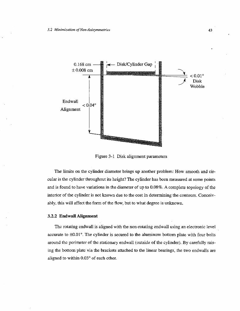
3.2 Minimization of Non-Axisymmetries 43

I I

0.168 cm i._--- Disk/Cylinder Gap I+ 0.008 cm .....

<0.01o

__ DiskWobble

Endwall< 0_04 °

Alignment

Figure 3-1 Disk alignment parameters

The limits on the cylinder diameter brings up another problem: How smooth and cir-

cular is the cylinder throughout its height? The cylinder has been measured at some points

and is found to have variations in the diameter of up to 0.08%. A complete topology of the

interior of the cylinder is not known due to the cost in determining the contours. Conceiv-

ably, this will affect the form of the flow, but to what degree is unknown.

3.2.2 Endwall Alignment

The rotating endwall is aligned with the non-rotating endwall using an electronic level

accurate to _+0.01 °. The cylinder is secured to the aluminum bottom plate with four bolts

around the perimeter of the stationary endwall (outside of the cylinder). By carefully rais-

ing the bottom plate via the brackets attached to the linear bearings, the two endwalls are

aligned to within 0.03 ° of each other.


3.3 Measurement Accuracies

Measuring the experiment parameters accurately is important in determining where

the flow is located in terms of (Re, H/R) space. By knowing the parameters, accurate com-

parisons can be made with other experiments and numerical simulations.

3.3.1 Length Measurements

The height and radius of the disk are the only two length measurements. The accuracy

of the height measurement is 0.04 cm. During these experiments H/R is kept constant at

2.5. The nominal radius of the cylinder is 9.563 cm. Therefore, the height is required to be

23.91 cm. Since the resolution is only 0.04 cm, the uncertainty in the measurement is

0.17 %. The accuracy of the radius measurement is better at 0.003 cm (0.001 in). There-

fore, the uncertainty in this measurement is 0.03%.

3.3.2 Disk Frequency

Due to angle dependent frictional torques which arise at low £"2,the motor exhibited

small residual phase variations leading to speed variations on the order of 0.003 Hz

(0.18 rpm). These are greatly reduced by a dumbbell-shaped flywheel attached to the

motor shaft (§ 3.1.1). When compared with an HP model 5315B universal counter and an

HP model 34401A multi-meter, the two signals were found not to vary by more than

2 x 10 -7 Hz. Hence, the motor frequency remains within 0.0002 Hz of the desired fre-

quency (reference frequency divided by 1000). The nominal operating disk frequency for

the experiments is between 1.3 and 1.4 Hz. The frequency variations are approximately

0.02%, but the error in reading the speed is small at - 0.008% due to a combination of fac-

tors: the precision of the frequency measurement devices (§ 2.2.2) and the large number of

lines per revolution output by the encoder. Therefore, the error in disk frequency is repre-

sented by the variations in control of the disk.

3.3 Measurement Accuracies 45

3.3.3 Viscosity Measurement

The viscosity accuracy depends on two measurements: viscosity and temperature.

Temperature accuracy is important since the viscosity of the test fluid is inferred from the

temperature reading in the cylinder.

In the ASTM Standard D 445, the viscometer uncertainty is given as - 0.35%. The

error due to temperature accuracy is not so important as the error due to temperature

repeatability. The accuracy is not important because the thermistors used to measure the

temperature are calibrated against each other. Therefore, knowing how the two thermistors

compare with one another will give the uncertainty in viscosity due to temperature mea-

surement accuracy. Using the uncertainty method given by Holman 34, we can write vis-

cosity, v, as a function of some nominal viscosity, v o, and the actual temperature minus the

nominal temperature, Tu:

V = v o+B.T u (3-1)

where B is the slope of the v vs. T plot with a value of - -0.016 cm2/sec/°C. The quantity

v o has a nominal value of 0.285 cm2/sec with an uncertainty of 0.35%. T u is nominally

zero (0) with an uncertainty of 0.004 °C. (The thermistors compare to +0.004 °C.) The

partial derivatives of Equ. (3-1) with respect to v o and T u are needed to compute total

bv _ 0vuncertainty in v._-_o - 1 and 0Tum= B = -0.016-

2cm

sec °C" The uncertainty in v follows:

w 2 1/'2

: t TuWv _o w -,I- _-(3-2)

= [ (1) e (0.0035.0.285) ; + (-0.016) e (0.004) 21 1/'2

2

= 1.OOxlO-3 cmsec

The absolute uncertainty in viscosity is 0.35% which includes temperature effects.


3.4 Parameter Uncertainties

There are two types of uncertainties: absolute and relative. Absolute uncertainties give

an estimate of how well the calculations of the parameters match the true values. Compar-

isons with other studies are made by taking into account how well the measurements pre-

dict the absolute parameters. Relative uncertainties, however, give a measure of the

precision of the calculated parameters. Control of the experiment can be inferred from the

values of these relative calculation errors.

3.4.1 Absolute Uncertainty

All of the measurement errors are taken into account to calculate the absolute uncer-

tainty in Re and H/R. In summary, these accuracies are given in Table 3-1.

Table 3-1 Parameter uncertainties

Measurement Accuracy (w) Nominal value

R 0.003 cm 9.563 cm

H 0.04 cm 23.91 cm

_2 0.0013 rad/s 8.304 rad/s

v 0.0010 cmZ/s 0.285 cmZ/s

T 0.004 °C 23.0 °C

The partial derivatives of Re = _2R2/v are as follow:

_Re 2_2R

_gR v

_Re R 2

3_ v

(3-3)

(3-4)

3.4 Parameter Uncertainties 47

_Re _2R 2

_v 2 (3-5)v

Using Equs. (3-3), (3-4), and (3-5) to calculate the absolute uncertainty in Re, the fol-

lowing equation is obtained:

r{"2_R'_ 2 2 /"? 4+_v-' (w_) + (w v) j (3-6)v2 )

1/2

Inserting the values from Table 3-1 into Equ. (3-6), the uncertainty in Re is found to be

9.5 or approximately 0.36%. As can be seen, the majority of the doubt comes from the vis-

cosity measurement.

The absolute uncertainty in H/R is calculated in a similar manner:

E(1 2 2 ('IN 2 2] 1/2WH/R p__) (WH)= q" _-.2j (wR) (3-7)

Substituting the values from Table 3-1 into Equ. (3-7), the uncertainty in H/R is calcu-

lated to be 0.004 or close to 0.17%, mostly due to the coarse measurement of H.

3.4.2 Relative Uncertainty

In the calculation of the quality of relative estimates, the uncertainty in parameters

whose value do not change during a particular experiment is excluded in the analysis. The

measurements that affect the relative uncertainty in Re are endwall speed and fluid tem-

perature. Effects of fluid temperature measurement error are reflected in the viscosity esti-

mate. The uncertainty in Viscosity due to error in the viscometer is ignored for this

analysis since the same instrument bias applies for all of the experiments and does not

change for the duration of an experiment. H and R are held constant for the experiments,

hence, they are excluded from the computation of relative uncertainty.


First, the effect of temperature measurement precision on the uncertainty of viscosity'

must be investigated. From Equ. (3-2), w v is calculated by assuming that wv o = 0 and by

substituting the appropriate values from Table 3-1. Therefore, solely due to temperature

effects, the uncertainty in viscosity is 64 x 10 -6 cm2/sec or close to 0.002%.

Thus, using w R = 0 cm and w v = 64 x 10 -6 cm2/sec in Equ. (3-6), the relative uncer-

tainty in Re is found to be 0.7 (0.03%). There is no relative uncertainty for H/R since H

and R remain constant for the duration of the experiment.

Chapter 4

Experimental Results

4.1 Comparison of Initial Flow Structures

Some confidence is gained in the estimate of Re by comparing the values of Re at

which certain flow structures appear with those of Escudier 11. Since most numerical simu-

lations have concurred with this sequence of events, this is deemed a good reliability test

for the moment. Later on this assumption will be re-examined. Figure 4-1 shows the same

sequence Escudier produced in his Fig. 4. Recall that the current flow is upside down rela-

tive to Escudier's flow, and beware that, in subsequent figures, the inverse of the captured

images is shown so as to reduce the amount of black. Image processing techniques are dis-

cussed in Appendix C.

At a Re of 1918, there is clearly one bubble formed with a hint of a second one. As the

Re increases, the second bubble takes shape and grows rapidly as evidenced by the flow at

Re's of 1942, 1994, and 2126. As the bubble grows it moves downward towards the first

bubble. Eventually, the upper bubble merges with the lower one at a Re slightly less than

2494. This sequence of events is identical to previous numerical and experimental results.

49

50 Chapter 4 Experimental Results

(a) (b) " (c)

Figure 4-1 Structures for flows at a Re of (a) 1918, (b) 1942, (c) 1994, (d) 2126,and (e) 2494

4.2 Continuation of the Steady Flow 51

4.2 Continuation of the Steady Flow

The usual view 23'25'27'28 has been that the onset of time-dependence occurs via a super-

critical Hopf bifurcation where, at a critical value of the Re, dependent upon the aspect

ratio, the steady solution branch loses stability to a time-periodic solution branch. Numer-

ical evidence to the contrary was recently presented by Lopez and Perry 24 and Lopez. 26 In

this work the steady solution branch from a second-order-accurate time integration of the

axisymmetric Navier-Stokes equations was continued in Re beyond the Re where time-

periodic solutions - following an impulsive start from rest - were previously found to be

unique.

Here, results from an experimental investigation are reported where both steady and

time-periodic flows were observed for several thousand endwall rotations at the same Re

and H/R values. Our study supports the numerical findings z6 that the steady branch is sta-

ble beyond the Re where the time-periodic branch exists, and hence, the conclusion that

the onset of time-dependence is not via a supercritical Hopf bifurcation.

Although results from one experiment are presented, the following described behavior

was found to be robust after repeating the experiment several times. Appendix B describes

three similar experiments.

Figure 4-2(a) shows the Re history of one experimental run. Figure 4-2(b) will be dis-

cussed after the periodic nature of the flow is described. Initially, Re was held at 2650 to

allow transients to die out. The ramp was then started and allowed to increase over about

one hour. Upon reaching Re = 2715 (f_ = 8.9077 rad/sec, v = 0.3001 cm2/sec), the ramp

was halted and the flow allowed to develop. The flow remained steady for approximately

2400 endwall rotations (approximately 1.5 x 104 non-dimensional time units, where time

is scaled by 1/_). At this point, small azimuthal oscillations became apparent. These oscil-

lations are characterized by an asymmetric stretching and contracting of thin fingers of

dye (fringes) at the downstream end of the second recirculation bubble. (The streamwise


2750 i i t i 1 , i

/,

2730

2710

ID

2690

2670

2650

3

(D

&2_D

<

0 1 2

Artificial Disturbance toinduce oscillations

I | I

3 4 5

Time (lws)

i :r

6 !7

i ,ii j t

3 4 5

0 (b) , _, r _.._.

0 1 2 6 7

Time (hrs)

8

Figure 4-2 (a) Experiment Re history. 0, II, and • denote times of

Fig. 4-3(a), Fig. 4-3(b), and Fig. 4-6, respectively. (b) Oscillation amplitude

of hyperbolic fixed point during experiment.


direction is the axial direction from the stationary to the rotating endwall.) It is believed

that this is an apparatus induced disturbance of the stable, steady solution and not a char-

acteristic of the stable, unsteady solution. The rotational oscillations may be caused by

small imperfections of the cylinder and misalignment of the centers of the disk and cylin-

der. An earlier series of runs showed more oscillations of this form, which were consider-

ably reduced by realigning the rotating endwall. These oscillations are very different in

nature to the axial oscillations reported below and by Escudier. 11The fringe oscillations

were watched for another 3000 rotations. Although the magnitude grew slightly, these azi-

muthal waves never progressed to the full, unsteady oscillatory motion. In another experi-

ment, when Re was increased beyond 2720, the flow did not remain steady for more than

500 endwall rotations. The periodic motion would begin with an asymmetric folding and

stretching of the upstream bubble around the downstream bubble. Eventually (- 1200 end-

wall rotations later), the large, symmetric oscillations ensued.

It is important to point out that for Re = 2715 the downstream fringes were moving,

but the bubbles did not migrate axially as they do for the unsteady flow. Figure 4-3 depicts

the flow at the beginning and end of the constant Re flow. In Fig. 4-3(b), the upper fringe

pattern is asymmetric and rotates in the azimuthal direction. During this whole time

sequence, 5400 endwall rotations, the first stagnation point on the axis remained station-

ary. The temperature change between Fig. 4-3(a) and Fig. 4-3(b) was no more than the

precision of the gauges (0.004 °C).

After the 5400 endwall rotations at Re = 2715, a controlled, large amplitude distur-

bance was applied to the steady flow. The Re was momentarily increased to 2744 and then

reduced back to 2715. Unsteady oscillations began immediately and are characterized by

an axial movement of the bubbles and a periodic stretching and folding of the upstream

recirculation bubble around the downstream bubble. Figure 4-2(a) gives the time history

of Re and Figure 4-2(b) gives the amplitude of the axial distance travelled by the bubble

during one period of the oscillation. (Relative motions are measured by taking the cross-


Fringes

Figure 4-3

No

mixing

correlation between successive digital images. The change in the peak position of the

cross-correlation is a good measure of the relative amplitude of oscillation. Appendix C

describes the image processing techniques more fully.) This axial motion of the bubble is

also depicted by Lopez and Perry 24 in the computations of the unstable manifold of the

upstream hyperbolic fixed point of the flow (the periodic analog of the steady stagnation

point). These oscillations reached a constant amplitude and were observed for about 7200

endwall rotations. Figure 4-4 portrays a non-dimensional period of this flow (using 1/_2 as

the time scale).


i_'_. _.__ :_._;_'!':. .:_'_i;_:__: ._.__..... _: _ _i_::_::

!i_ __ _i_ _li

'_' iiiiiiii!iiiil!:,_i_ii!ii!iiiiiii_iiiiiiiiii',_'_i _

i_i_ii!_i_::_:_i_i_:_ii_:_iiii_iii_:i_i_ii_iii_ii:_i_i_!_ii_!_:ii_!_:_i_:i_i_i_i!i_i_ii_i_iiii:!iiiiiii!!iii_i_!i_ii_i!iii_ii_i_i_i_i_iiiiii_i!!i_i_i_i_i!_!i_ii_iiii_iii_iiiii_iii_!i!i_ii_i_ii_i_i_i_i_i:_:_ii_i_i_i_!_!_i_iiii_:_:i:_:_i_!i_!_!!!i_iiiiiiii!iiiiiiiiiiii'iiiiiiiiiiiiiiii!_i_l

Figure 4-4 Unsteady flow, Re = 2690 and I-I/R = 2.5, at non-dimensional times

£2t (a) 0, (b) 9.2, (c) 18.4, (d) 27.3, (e) 36.5. Note the mixing, and the

stretching and folding of the upstream recirculation bubble.

In Fig. 4-5, a close-up view of one side of the upstream recirculation bubble is shown

over two complete periods. Due to the quality of the visualizations of the flow, this image

is taken from a different experiment (§ B.2) that better displays the features within the

recirculation bubble. After some digital enhancement of the images has been done, it is

evident that regions within the bubble are kept clear of dye. Furthermore, the two outer

zones of clear fluid are seen to orbit the central one completing a revolution for every two

periods of the fundamental vertical oscillation. This phenomena is also observed in the

numerical computations of Lopez & Perry 24 as depicted in their Fig. 6(a). Commonly

known as KAM tori (after Kolmogorov-Arnol'd-Moser) and cantori, these regions are

barriers across which fluid cannot pass. 35'24 Cantori provide only partial barriers to the

flow, allowing small amounts of mixing over long periods of time. Evidence of KAM/can-


Figure 4-5 Close-up view of one side of the upstream recirculation bubble for Re slightly

greater than Re c and I-I/R = 2.5, at non-dimensional times _t (a) 0, (b) 8.1, (c) 16.1,

(d) 24.2, (e) 32.3, (f) 40.3, (g) 48.4, (h) 56.5, (i) 64.5, (j) 72.6.

toil can be seen in Fig. 4-4 in the upstream, or lower, bubble. While mixing is going on

inside the bubble, a small region of clear fluid can be seen into which no dye has pene-

trated.

Re was then reduced and held at several lower values: 2710, 2705, and 2702. At

Re = 2710 (_ = 8.8788 rad/sec, v = 0.2996 cm2/sec), the amplitude of the oscillations was

smaller. This periodic flow was observed for 7200 endwall rotations. At Re = 2705

(_=8.8624 rad/sec, v=0.2997 cm2/sec), the amplitude reduced further and the


oscillations appeared asymmetric, although the hyperbolic fixed point continue'd

oscillating very slightly and the bubbles were stretched and folded. At Re = 2705, the flow

seemed to be shifting between the steady and unsteady flow states, most likely due to

apparatus induced disturbances of the flow (see § 5.1). These fluctuations were observed

for 6900 endwall rotations. Upon reducing Re to 2702 (f2 = 8.8580 radlsec, v = 0.2997

cm2/sec), the flow became completely steady within 4000 endwall rotations (Fig. 4-6).

Figure 4-6 Re = 2702, H/R = 2.5; 4000 endwall rotations after reducing from 2705.

Some of the asymmetry observed in the experiment has been attributed to imperfec-

tions in the alignment of the cylinder and disk, and some is attributable to the cylinder not

being perfectly cylindrical. These would contribute real asymmetries to the flow, as

58 Chapter4 Experimental Results

opposed to apparent asymmetries. Even very small imperfections in the alignment of the'

dye injection port with the cylinder axis can provide an apparent asymmetry to the struc-

ture.16,17,24

The experiments were not able to continue the steady branch beyond Re = 2720,

whereas in the computations it was continued to Re -- 3700, and not continued further due

to the cost. The higher the Re, the smaller the increment in Re has to be to prevent the

associated perturbation from upsetting the steady flow. It should be remembered that the

perturbation levels in the apparatus have a finite value and are always applied to the flow

through motor speed variations, temperature fluctuations, and geometry imperfections. In

contrast, the main perturbation in the computations is due to the initial condition at a dif-

ferent Re. This is only present at t = 0 and can be made arbitrarily small; of course, the

effects of truncation and round-off are always present. It is then not surprising that the

continuation of the steady branch in the computations can be carried further than in the

experiment.

4.3 Characteristics of Periodic Flow

In previous experimental investigations in a closed circular cylinder n,27, it has been

reported that the flow remains axisymmetric until well into the unsteady flow domain. The

evolution of this flow has not been fully described, nor the dependence of oscillation fre-

quency upon Re. This section describes the flow region from a Re of 2800 to approxi-

mately 5200. It is observed that the flow loses axisymmetry, but not to a degree to where

the flow structures cannot be identified.

In these experiments, Re was slowly varied and held at several values as shown in

Fig. 4-7. At each level, Re was held constant for at least 4500 endwall rotations (i.e.,

= 2.8 x 10 4 non-dimensional time units). As the experiment evolved, dramatic changes

occurred in the stretching and folding of the leading recirculation zone. For larger Re, the

stretching becomes more pronounced. This is most visible in the upstream bubble region,

4.3 Characteristics of Periodic Flow 59

©

3800

3600

3400

3200

3000

2800

i i i i

5-

/_U

l l I

4 6 8 10 12

Time (hrs)

Figure 4-7 Experiment Re history for 2700 < Re < 3750.

which is stretched more with the lobes reaching farther along the axis. The cross-section

of the bubble clearly indicates the stretching and folding of the dye-sheet forming the

elongated lobes (fringes) typical of chaotic advection in a periodic flow (e.g. Re = 2800 in

Fig. 4-8).

Upon reaching Re = 3000 (Fig. 4-9), several observations are made. First, it seems as

if the dye-line emanating from the stationary endwall is precessing about the axis of the

cylinder. As discussed previously (§ 1.3.2, page 9), even a small misalignment of the dye


>..................... _.,._,.......,............ _., , _ ••...,,.,............ :......,,...._._...............

::::::::::::::::::::::::::::::::::::::::::::::::::::::::::: ::_::::!:i:::_')._., ::::::_:.'::.";::::::. :::::::::::::::::::::: :::::::::::::::::::::::::::::::::::::::::::::::::

:::::::::::::::::::::::::::::::::: :::::::::::::::::::::::::::::::::::::

>_ :_ :_':::_:_:!_'_'_'_ _:_':_:...... ":__:_ _'_*i_ii_i :iiiiiii

i;ii;iii_iiiii_iiiiiii_!i!ii_i!i* _i_iiiii_i_!_i_ii!_iiii!ii!iii_i

Figure 4-8 Re = 2800, I-I/R = 2.5 at f_t (a) 0, (b) 9.2, (c) 18.3, (d) 27.5, and (e) 36.7.

injection port with the cylinder axis will cause apparent asymmetries. 16'_7'24 Evidence that

the flow is still axisymmetric is provided by the symmetric stretching and folding of the

upstream bubble. Eventually, with increasing Re, this is not the case and asymmetries

appear along the entire length of the breakdown structure.

_il!___!_._._.:::_::._:_:._.__:_i:__:i__:

!i!l_,. .

_::_:: _:: :_::.:!:::_:_:_:_:?._:_.'...,.'..

i_!!: i_!i:::!_! i_ii:;. ,..:_

ii i!i!ii!ii ,i ,ii ii ,iii',iii iiiii',ii!i!i!_.:."iii_!..*.....+._i!i!_!iiiiiii!i!_!iiiiiiiiii!i!i

___:"i.;'_'".i_...............i_......._....................__iii_!_ii_!__"......._':_'_" ":'_"

H_

::::::::::::::::::::::::::::::::::::::::::::::::::::::::::::::::::::::::::::

_;:_ii!_:_::_._._:_:_._"!_:iiii_

_._._:..'.'_:.• . .:_,.._,.,,..... ,,>,: .,.+.'::(,_• _:_

ii_..... _,':

,.. ., _._:,.:_.::.:.$:_..:_.:::::::

_li!i_iiiii_iii!i!!i!i!iiii!i!!iii:i_:i:i_:ii#_t_i_:i:g:i_i:i:i!:i:i_i:i:i:i:i:i:i:i:ili:i:i:_ii:iii:_i

___il'''_:_ ":• ._:_i_

i !iiiiiiiiiiiiiiiiiiiiiiiiiiiiiii!

Figure 4-9 Re = 3000, H/R = 2.5 at £2t (a) 0, (b) 9.2, (c) 18.3, (d) 27.1, and (e) 36.3.


The second observation when Re = 3000 is that the regions devoid of dye (presumabl_¢

delineated by either KAM tori or cantori) in the downstream bubble have been consider-

ably reduced in size. The KAM tori/cantori of the upstream bubble are no longer detect-

able by Re = 2750; periodic orbits have broken up into higher order islands and there is

increased tangling of the stable and unstable manifolds of the hyperbolic fixed points that

dyed fluid is able to penetrate deeply, but not completely, into the inner-most regions of

the bubble. By Re = 3200, the KAM tori and/or cantori have essentially disappeared, yet

the breakdown structure still oscillates symmetrically as shown in Fig. 4-10.

IF:.:.:.:.:.:.:......... ..::_!i!_!i:i_i!!!i_

_!i_::_ii_iiiiii_i!iiiiili!ilililiiii

_:_:_:?" _. '_'" '_-_.:i_A_:.::_i:i_:;:

::::::::::::::::::::::::::::::::::::::::::::::::::::::::::::::::::::::::::::

×. "_ e_::,,.::_.._'-'.'.'.:_:,,.::::_:._'.._.:::..'_:::

....i:_:_:_i:i:_izi:i:i:i:i:i

iliiiiiii_ii_if_ii_iiiiiiiiiiiiiii_iiiii_iii_iiiiiii_iiiiiiii_i

_'."_""....... :. _54

iiiiiiiiiiiiiiiiiiiiiiiiiiilWiiiiiiiiiiiiiiiiilUiiiiiiiiliU!iiiiii__:_ ";.'.'_:_" :_." "_.__ :_ _.:,.'_._.__:,.'_i __: _____::

• , .... .,....,. _;;_:_:_.,........::_....

• •_

Figure 4-10 Re = 3200, H/R= 2.5 at £2t (a) 0, (b) 9.0, (c) 18.1, (d) 27.1, and (e) 36.2.

Some asymmetries of the breakdown structure appear at Re -- 3400, just before a fun-

damental period change from "q -- 36 to x 3 = 57 takes place in the region

3400 < Re < 3500. The non-axisymmetric oscillation is manifested through the slightly

uneven stretching of the upstream bubble. One side of the bubble reaches full extension

just ahead of the other side. This asymmetry may arise due to the impending change in the

characteristic period of the flow. The new fundamental frequency can be seen in Fig. 4-11.

This figure shows the oscillation of the hyperbolic fixed point at Re = 3500 along with the

power spectral density of the signal. It is observed from the power spectrum that the fun-

damental frequency of 0.01732 (1:3 --- 57) is accompanied by a signal with a frequency of


301 I I I I I I I I

._15

o

<

-300

[a) i i i i i i i i i

200 400 600 800 1000 1200 1400 1600 1800Time (in units of 1/omega)

2000

104

102

100

10-2

0

I I I I I I I I I

(b) , , , , , , , , ,0.01 0.02 0.03 0.04 0.05 0.06 0.07 0.08 0.09

Frequency(in units ofomega)0.1

Figure 4-11 Re = 3500, H/R = 2.5 (a) Position of hyperbolic fixed point vs. f_t, and

(b) Power spectral density of signal.

0.03505 ('172 = 28); this resembles a period doubling of '1_2,but is merely a harmonic. The

distinction between a period doubling and an independent third flow is discussed later in

this section. At a Re of 3600, the flow features from Re = 3500 are retained with similar

frequencies. Another frequency, incommensurate with "c3, is also apparent in the signals at

these Re with a value approximated to be 0.0009 (x ---1100) that does not show strongly in


30 _ ,

-300 200 400 600

i I l I I I

800 1000 1200 1400 1600 1800Time (in units of 1/omega)

2000

104

lO2

lO0

10-2

0

I I I

(b) , , ,

0.01 0.02 0.03

I I I I I I

I I I r I I

0.04 0.05 0.06 0.07 0.08 0.09 0.1Frequency (in units of omega)

Figure 4-12 Re = 3750, H/R = 2.5 (a) Position of hyperbolic fixed point vs. _2t, and

(b) Power spectral density of signal.

the power spectral density because there are not enough cycles to resolve this low fre-

quency. The frequency is evident in Fig. 4-11 as a long period modulation of the signal. It

also shows up indirectly in the power spectral density as side-bands on the fundamental.


Figure 4-13 Re = 3600, H/R = 2.5 at times _t (a) 0, (b) 6.5, (c) 12.6, (d) 19.1,

(e) 26.4, (f) 32.9, (g) 39.3, (h) 45.4, (i) 51.9, (j) 58.4.

Once a Re of 3750 is achieved, there is evidence that the _3 period and low frequency

wave have died out. As seen in Fig. 4-12, the character of the oscillations has changed and

the dominant frequencies are concentrated almost on top of each other at frequencies of

0.03503 and 0.03618 (z = 28.5 and 27.6).

Although the flow contains many, but a finite, number of frequencies at Re' s between

3400 and 3750, the breakdown structure retains a high degree of symmetry. Figure 4-13 is

a sequence of images at Re = 3600 showing a complete cycle for the "c3 = 57 mode of

oscillation. This figure shows how evenly the unstable manifolds of the bubble are

stretched and folded along the downstream part of the breakdown structure. Also shown in


40I I I i I I I I I

20

0

.

_-20<

-400

Ca)

200 400 600 800 1000 1200 1400 1600 1800 2000Time (in units of 1/omega)

104

102

10°

10 .2(b) , , , , , ,

0 0.02 0.04 0.06 0.08 0.1 0.12

Frequency (in units of omega)

0.14

Figure 4-14 Re = 3400, H/R = 2.5 approached from lower Re (a) Position of hyperbolic

fixed point vs. _t, and (b) Power spectral density of signal.

Fig. 4-13 is the jagged appearance of the recirculation bubble which is characteristic of the

flow with a fundamental period of "c= 28.6 in agreement with Fig. 6(b) of Lopez and

Perry. 24

After observing the flow at Re - 3750, the Re is reduced to 3400. Two observations

are made. First, the fundamental period is % instead of % as it was when Re = 3400 was

approached from lower Re. Second, the structure is affected by the long period signal as

66Chapter 4 Experimental Results

40

20

-_ 0

. ,,-.-i

-20<

-400

1 I I I I I I I I

a) I I I I I I I I I

200 400 600 800 1000 1200 1400 1600 1800Time (in units of 1/omega)

200C

104

lO

lOo

10-2

0

I I I I l I

(b) , ,0.02 0.04

I I I I

0.06 0.08 0.1 0.12 0.14Frequency (in units of omega)

Figure 4-15 Re = 3400, H/R = 2.5 approached from higher Re (a) Position of hyperbolic

fixed point vs. _t, and (b) Power spectral density of signal.

were the flows at Re of 3500 and 3600. Figures 4-14 and 4-15 show the two states at a Re

of 3400 represented by the signal and the power spectral density. Figure 4-14 is the state

as approached from lower Re, and Fig. 4-15 is the state as approached from higher Re.

Upon reducing the Re to 3200, the fundamental period remains at %, but hints of the "q

period are beginning to show (Fig. 4-16). Reduction to Re = 3150 restores -c1 = 36.2 as the

fundamental period.


40

--_ 20

©-_ 0

-20<

-41

104

i _ i i i i i i i

a) i i i i I i i i

200 400 600 800 1000 1200 1400 1600 1800 2000Time (in units of 1/omega)

10 2

100

104

I i I i I i

_(b) , , , , ,

0 0.02 0.04 0.06 0.08 0.1 0.12 0.14

Frequency (in units of omega)

Figure 4-16 Re = 3200, H/R = 2.5 approached from higher Re (a) Position of hyperbolicfixed point vs. _t, and (b) Power spectral density of signal.

A separate experiment was conducted to search for hysteresis between '172and '_3 flows.

The Re was slowly reduced from 3800 to 3600 and observed at points in between. The

results of the downward sweep revealed that the "c2 flow continues down to Re = 3625,

below which the "c3 period becomes dominant. The next part of this experiment revealed

that the quasi-periodic I:3 flow exists up to a Re between 3650 and 3675. With this addi-

68 Chapter 4 Experimental Results ,

tional information about the existence of the oscillation periods, a complete hysteresis dia-'

gram is drawn in Fig. 4-17. The most recent results of Lopez are also given. These data

will be published in the near future. 36

The distinction between a period doubling of the "c2flow and a distinct "c3flow is now

addressed using results from the numerical simulations of Lopez. The observation that the

"c3 flow has a period twice that of the % flow suggests that they are related by a period dou-

bling bifurcation. However, an examination of the phase portraits from the computed solu-

tions reveals that the two flows are not connected by a supercritical period doubling

bifurcation. If they were related in this way, then the % and "c3 ftow phase portraits would

merge near the Re above which "c3dies out and "c2exists (Re = 3730 for the computations).

Figure 4-18 demonstrates that this is not the case. Figure 4-18(a) shows the phase portraits

of the % oscillations for 3500 < Re < 4000, and Fig. 4-18(b) gives the phase portrait of the

% oscillations for Re = 3725. The notation vl represents the azimuthal vorticity at

one-third the radius and four-fifths the height, and v2 represents the azimuthal vorticity at

two-thirds the radius and four-fifths the height of the cylinder. The phase portrait of the 'c2,

Re = 3700 flow is radically different from that of the "c3, Re = 3725 flow. Figure 4-19

shows phase portraits of the % flows and the % flow at Re = 3225. As shown, the two limit

cycles for the Re = 3200 flows also do not resemble each other. Neither the computational

nor the experimental approach is able to unambiguously distinguish between disconnected

branches and subcritically connected branches. Therefore, all that can be concluded is that

none of the three periodic branches are connected via supercritical bifurcations.

At the Re examined here, the three-dimensional effects are small allowing extraction

of useful data. Eventually, however, the three-dimensional perturbations prevent relevant

analysis of the flow. The seemingly non-axisymmetric stretching of the upstream bubble

leads to a more pronounced precession of the breakdown structure about the cylinder axis.

This effect is not prominent for Re < 4000. The precession seems to cause the dye to be

concentrated alternately on the axis of the cylinder then in the branches of the breakdown


60

55

5O

45

4O

35

30

252500

i

"c3

"c2

3000 3500 4000Re

6O

55

5O

45

4O

35

3O

25 ,2500

i

x3

"el

"c2

, ! , , , , ! , ,

3000 3500Re

4000

Figure 4-17 Hysteresis of oscillation periods. (a) experimental results, (b) numericalsimulation data


V2

0.0

-0.1

-0.2

-0.3

-0.4

V2

°0 • i . i - i - i - D • i • i • | - i - g - _ -

-0.1

-0.2

-0.3

-0.4

Figure 4-18 a) "_2limit cycles in (vl, v2) phase space for H/R = 2.5 and 3500 < Re < 4000.

b) "c3 limit cycles in (vl, v2) phase space for H/R = 2.5 and Re = 3730.


o0 • i • | • i • n • I " i " i • i ' u • u • u "

v2

-0.1

-0.2

-0.3

-0.4

2_3400 _ 3200

°0 • * • u • t • _ • a • i - J • i • u • n - | •

v2

-0.1

-0.2

-0.3

-0.4

Figure 4-19 a) "c1 limit cycles in (vl, v2) phase space for H/R = 2.5 and 2705 < Re < 3200.

b) x3 limit cycles in (vl, v2) phase space for H/R = 2.5 and Re = 3225.


structure. Actually, the structure precesses about the center of the cylinder, and therefore, '

travels back and forth through the laser sheet. When the axis of the structure coincides

with the laser sheet, the tree-like structure of the lower Re flow is visible. However, when

the core of the breakdown structure is out of the laser sheet, the only fluoresced dye is

located at the edges of the branches (or even further from the breakdown core) giving the

impression of dye concentrated on the axis of the cylinder. Since this experiment did not

continue beyond Re -- 3750, images are taken from a similar experiment that extended Re

up to 7000. Figure 4-20 shows different stages of the precession of the structure about the

cylinder axis over about 1400 non-dimensional time units. By Re ---4700, the flow has

become very three-dimensional and no useful data can be inferred from the images except

that the non-dimensional period remains at = 28 up to Re = 5200. Beyond this Re, extrac-

tion of relevant data is very difficult.

The observation that the non-dimensional frequencies of the oscillations are essen-

tially, to within measurement error bounds, independent of Re (the dynamic governing

parameter) in both the experiments and the numerical simulations at H/R = 2.5, along with

the observation from the numerical model 37 that the frequencies do vary with H/R (the

kinematic governing parameter), suggest that the frequencies are modes of the finite cylin-

der, with the frequency for Re < 3500 being more fundamental than that of the higher

mode found for Re > 3500. Furthermore, the ratio "cl/'_2 is approximately the ratio of the

height to the diameter of the cylinder, or t-I/2R - 1.25. This seems to indicate a mode

change from horizontal to vertical since the lower mode frequency (1/I: 0 is shorter than

the higher mode frequency (1/1:2), and the diameter (horizontal length) is shorter than the

height (vertical length).


Figure 4-20 Re -- 4400 at _2t (a) 0, (b) 154, (c) 308, (d) 463, (e) 617, (f)771, (g) 925,

(h) 1080, (i) 1234, (j) 1388.

Chapter 5

Discussion

5.1 Characterization of Flow Imperfections

Due to the simplicity of the flow set up, many numerical studies have been imple-

mented as an exercise in flow transition/bifurcation investigations. 13,2°-28,37Surprisingly,

not many have considered in detail the transition from a steady to a periodic flow. The

most detailed numerical studies have been done by Lopez. Unfortunately, no experimental

results were available for comparison until the present work. Either the experimental (or

numerical) investigator had assumed that the transition from steady to periodic flow

occurred through a supercritical Hopf bifurcation based upon earlier work; or the nature of

the equipment precluded investigation of this subtle region due to built in handicaps such

as coarse motor control, unaccounted viscosity fluctuations through temperature devia-

tions and geometrical imperfections. The effects of each of these perturbations send the

system into largely unknown territory in terms of the bifurcation process, but through the

diligent minimization of each of these disturbances, the consequences of each can be

inferred.

A large effort has been put into precise motor control through the use of a phase-

locked loop (PLL) controller (§ 2.4.1). Not only was smooth rotation required, but the

ability to (nearly) continuously alter the rotation rate was indispensable. The results of a

coarse adjustment are readily observed from the present work and that of Escudier. H (It is

75

76 Chapter 5 Discussion

not the purpose of this discussion to detract from the work of Escudier since it represents'

the most thorough and precise experiment of this type over a large range of the invariant

space, and indeed, has greatly influenced the current study.) In the case of Escudier, the

penalty for a coarse controller is the absence of any extension of the steady flow beyond

the critical Reynolds number, Re c. Even with the current level of precision, there were

occasions, when the PLL was not accurately tuned, that the steady branch soon decayed

into the periodic flow. The stability of the steady branch is so precarious that any type of

relatively large disturbance will destabilize the flow. Although the PLL does an excellent

job, the rotation cannot be completely disturbance free. At one point, with a disturbance on

the order of one magnitude larger than the current jitter size, it was impossible to preserve

steady flow above Re c for more than a few thousand time units (measured in 1/f_). The

best obtainable fluctuation in motor speed causes a continuous perturbation of -0.4 in Re.

Temperature fluctuations cause similar departures from the ideal as does motor jitter.

This is readily seen through the relationship of Re with disk speed and temperature. The

Re is directly proportional to both these parameters. This is easily verified with the motor

speed since it appears explicitly in the calculation of Re. Temperature fluctuations are

manifested through kinematic viscosity fluctuations in the determination of Re. Since vis-

cosity is proportional to the negative of the temperature (Re is inversely proportional to

viscosity), the Re is ultimately proportional to temperature. As temperature increases

(decreases) there is a proportional decrease (increase) in viscosity. Therefore, a rise (or

fall) in temperature causes a subsequent proportional rise (or fall) in Re. Due to the large

thermal mass of the fluid, these fluctuations do not happen on the time scale of the disk

speed fluctuations, but instead cause a continuous perturbation in Re through the constant

increase or decrease in temperature. Any change in Re must be followed by a period of

tranquility in order to allow transients associated with the change to die out. Obviously,

this tranquil period never occurs, so the temperature perturbations are reduced by ther-

mally isolating the experiment from the ambient environment. In a sense, the thermal box

5.i Characterization of Flow Imperfections 77

adds thermal mass to the fluid and changes in temperature occur only over a very long

time scale which can be further manipulated by adjusting the ambient temperature appro-

priately to influence the direction of change. With these measures, changes in temperature,

and ultimately Re, can be made quite small if not negligible.

There are many types of geometrical imperfections, of which a few can be adjusted:

alignment of disk and cylinder centers, disk wobble and endwall alignment. When the

centers of the disk and cylinder are misaligned, the flow is no longer axisymmetric. This

non-axisymmetry is observed in the radial stretching of one side of the breakdown struc-

ture. The fluid particles no longer follow a circular path with respect to a radial cross-sec-

tion. Therefore, the fluid particle properties no longer depend only on axial and radial

position, but also depend on the azimuthal position; the flow becomes three-dimensional

to a certain extent. Effects are seen as a non-axisymmetric stretching and folding of the

recirculation bubbles for the periodic flow state.

Disk wobble and endwall alignment present similar perturbations through a varying

effective cylinder height. In either case, as the disk turns, the fluid is periodically forced

downward besides being advected towards the cylinder walls. This type of forcing pro-

duces azimuthal waves throughout the cylinder. Visually, the structure supports the waves

as a non-axisymmetric stretching and contracting of the fringes of dye at the downstream

ends of the bubbles. Indeed, for large wobble and/or misalignment, these waves persist

even for Re well below the first critical point. One would assume that the frequency of

these waves would match the frequency of the disk except that the oscillatory nature of the

enclosed fluid only allows modes of the cylinder to exist. Therefore, these waves have the

same frequency as the unsteady flow itself. Since it is impossible to perfectly align the

endwalls and have no wobble, this type of perturbation will always be present. At lower

Re (below -3000), the azimuthal waves caused by wobble/alignment are not visible but

certainly present. As the Re increases, the boundary layer thickness decreases (boundary


layer thickness is proportional to Re -1/2) corresponding to a larger effective wobble. This

may be the cause of the apparent loss of axisymmetric oscillating flow at Re greater than

-3400.

Evidently, the point at which three-dimensional effects and eventually turbulence

takes over is affected by the imperfections in the conditions used to implement this flow.

In the case of experiments, the imperfections arise through many avenues including geo-

metrical, thermal, dynamical and visualization properties. Numerical simulations generate

perturbations in the choice of time-step size, grid resolution, and accuracy of Navier-

Stokes approximations. Truncation and round-off errors contribute to the imperfect real-

ization of the flow as well. As can be seen, a truly ideal flow of this type cannot be created

either experimentally or numerically.

5.2 Bifurcation Events

Now that it has been established that the ideal flow has not been studied, the discus-

sion turns towards non-ideal events near bifurcation points. A very thorough study of these

phenomena has been carried out by Benjamin 29,3° especially with regard to Taylor-Couette

flow. A general overview of these bifurcation events has been presented by Drazin and

Reid 38 who tie together some of the work done in relation to hydrodynamic stability over

the last few decades. In theory, for an ideal, viscous, and symmetric flow, the development

of the flow as one of the parameters is varied (usually the Re) will exhibit a Hopf bifurca-

tion event when the steady flow loses stability and periodicity prevails. However, this state

is a specific condition and not the generic characteristic displayed by most realizable sys-

tems.

In order to pursue this reasoning, the Hopf bifurcation must be described, particularly

the supercritical form which is generally believed to dominate this flow. The varying

parameter will be Re, although this is not necessarily the case for all viscous flows. At low

values of the Re, a stable and steady flow exists, but as Re is increased to a critical value, a

5.2 Bifurcation Events 79

bifurcation event occurs. For supercritical bifurcations, the steady solution is no longer

stable and the solution branches onto periodic curves as shown in Fig. 5-1. 38The ordinate

represents the amplitude of a parameter in the flow (e.g. position of hyperbolic fixed point,

velocity at a point in the flow, vorticity at a point in the flow, etc.), and the abscissa delin-

eates Re. However, this diagram undergoes a transformation when perturbation or imper-

fections are introduced. Even a break in the symmetry of the flow will cause an alteration

in the bifurcation diagram. This morphogenesis is best diagrammed by Benjamin 29 and is

reproduced here as interpreted by Drazin and Reid 38 in Fig. 5-2. The solid curves repre-

sent stable flows whereas the dashed ones imply unstable solutions. This morphogenesis

of events is the general result found by Benjamin, but confirmed in a finite Taylor-Couette

experiment with the morphogenesis parameter being the width between the endwalls. (a)

shows that the primary solution continues with increasing Re indefinitely unless a destabi-

lizing perturbation is applied causing the solution to "jump" to the lower part of the 'c'

curve (secondary solution). In (b), the primary locus becomes folded with an unstable

solution between the upper and lower portions of the 's' curve. This signals a hysteresis

loop with respect to Re in the flow. (c) portrays a transcritical bifurcation which is proba-

bly the closest thing to a supercritical Hopf bifurcation this flow would experience. (d) is

similar to (a), but flipped with respect to the abscissa.

Thus the primary solution of an imperfect system does not become unstable at all;

it changes continuously with R slowly as R increases below R c and more rapidly as

R increases above R c. In short, there is no abrupt change in the character of the pri-

mary solution as R increases. The other stable solution, called the secondary solu-

tion, which exists for R > R 1, can be realized only by a strong disturbance of the

primary solution. If R decreases slowly after the secondary solution has been real-

ized, then one expects a 'catastrophe', or sudden transition to the primary solution,

as R decreases through R 1.

(From Drazin and Reid, p 413) Here, R is Re and R 1 = Re c + E.


A

Figure 5-1 Supercritical bifurcation. - Stable, -- unstable.

Now it can be seen that cylindrical swirling flow exhibits much more complicated

bifurcation phenomena than originally thought. Similar to Taylor-Couette flow, it may be

possible that the bifurcation events change as H/R is varied. Presently, there are no known

studies conducted on this topic. Furthermore, it is difficult, maybe even impossible, to say

which of the diagrams in Fig. 5-2 represent the bifurcation phenomena encountered in this

study.

Let's recall the salient features near the first critical Re (2702 < Re < 2705): hysteresis

between a steady and unsteady flow, a relatively smooth transition from unsteady to steady

flow as Re is reduced from above 2705, and no steady flow above Re = 2720 for any sig-

nificant time. Because of the hysteresis event encountered, one would be inclined to point

out diagram (b) as most representative due to the hysteresis present in the 's' curve. Yet,

this would imply hysteresis between two slightly different steady states instead of one

steady and one unsteady solution. Perhaps (c) is more characteristic of the flow. Indeed, if

the upper curve represents unsteady flow, then hysteresis is accounted for and the primary

5.2 Bifurcation Events 81

A_

/_am_n_e

(a)

AJ

(c)

AA

(b)

%

AJ

(d)

Figure 5-2 Sketch of the morphogenesis of the bifurcation curves for imperfect

supercritical stability as the imperfection changes.

solution would end at Re = 2715 with the upper, stable unsteady branch reaching back to

Re -- 2705. But the transition from unsteady to steady flow would be an abrupt jump in

amplitude, unlike the smooth transition witnessed. Diagrams (a) and (d) seem to offer the

best alternative. If the basin of attraction of the steady solution at Re > 2705 decreases

with increasing Re, it may be hypothesized that the always present minimum perturbation

level in the experiment is too great to allow the steady flow to survive above 2720 for any


reasonable amount of time. Lopez's study z6 showed the existence of a steady solution up

to a Re of at least 3700. His investigation also showed that the basin of attraction shrinks

as Re is increased evidenced by the smaller allowable increase to preserve the steady flow

at higher Re.

5.3 Influence of Imperfections upon Bifurcation Sequence

The discussion now turns to connecting the various imperfections with the possible

transformation in the bifurcation sequence. First to be examined is the disk jitter, which

provides a continuous perturbation to the flow and may destabilize the steady solution

allowing periodic structures to appear. Large jitter will certainly destroy the steady solu-

tion almost as soon as Re c is surpassed giving the appearance of a supercritical or slightly

transcritical bifurcation. The steady branch will be deemed unstable since no significant

amount of time would pass before unsteady flow dominates.

Since temperature fluctuations happen on a long time scale, their effects are usually

nullified. But, if one is not careful, the temperature rise or fall may provide a destabilizing

or stabilizing effect, respectively, if allowed to occur continuously without precautions to

keep the Re held steady at the desired point. From these imperfections no helpful insights

can be drawn as to the effect upon the bifurcation events.

For the non-axisymmetric flow (disk and cylinder centers misaligned), the steady flow

seemed more stable beyond the critical Re than did the more axisymmetric flow. The evi-

dence is inconclusive since in re-aligning the disk, it may be that some other parameters

were made less ideal, but the offset flow seemed better able to withstand the same pertur-

bation level endured by the centered flow. Perhaps this type of offset increases the domain

of attraction of the steady flow by moving the primary solution curve farther from the sec-

ondary solution curve.

5.3 Influence of Imperfections upon Bifurcation Sequence 83

Periodic forcing (disk wobble/non-parallel endwalls) seem to cause the most apparent

change in the bifurcation sequence. Since the forcing manifested itself in the fluid not at

the frequency of the disk but at the fundamental frequency of the cylinder, the unsteady

flow was being encouraged through the excitation of its fundamental mode. (This could

also be the case for disk jitter since it also would excite the fundamental mode.) Forcing of

the unsteady flow would severely limit the range and duration of the steady flow beyond

Re c. This would resemble at least transcritical bifurcation if not supercritical Hopf bifurca-

tion.

Although there are definite imperfections in the circular cylinder, it is impossible with

the given results to formulate the effects upon bifurcation events since no other cylinder

was included in the experiment.

Chapter 6

Conclusions

In light of the discussion of the previous chapter, it stands to reason to expect a much

more complicated flow transformation sequence than seen before. Indeed, although the

experiments reported herein dealt only with one slice of a rich and diverse flow domain -

namely, H/R = 2.5 - it has been found that the cylinder with one rotating endwall supports

hysteresial flows with at least primary, secondary, and tertiary branches. These findings

have never been observed in previous experimental investigations of this type.

6.1 Continuation of the Steady Flow

The first set of experiments lend support to the recent numerical results of Lopez. 26 It

is apparent that two flow states exist beyond a critical Reynolds number: a stable steady

and a stable periodic state. Steady flow is observed up to Re = 2715 and periodic flow

exists down to Re = 2705. Lopez 26 originally reports a critical Re of approximately 2670

above which two states exist. In more recent numerical simulations not yet published,

Lopez has used a stretched grid to resolve the boundary layer flow better and reduced the

time-step size, which in turn affected the critical Re, the most recent being 2705 in very

good agreement with the experiments. Although the experiments cannot sustain a steady

flow for long periods beyond Re = 2720, Lopez has extended the steady solution to

85

86 Chapter 6 Conclusions

Re = 2800. It is suspected that the steady branch extends further, but due to the cost in'

computing the solutions, Lopez has not done so. In his earlier work with a regular grid and

larger time-step, Lopez 26 was able to extend the steady branch to a Re of 3700.

Escudier 11reports periodic flow at H/R = 2.5 only for Re > 2680, but does not find any

steady flow above this Re. Tsitverblit z5 ultimately finds that the steady flow loses stability

to a periodic flow for 2630 < Re < 2650. He finds that the two solutions do not exist at the

same Re. This estimate of Re c is low, indicating a coarse time-step and, therefore, a large

perturbation. Upon reducing the time-step and refining the mesh, some numerical

studies 27'39 found an upward modification of Re c.

6.2 Characteristics of Periodic Flow

The second set of experiments regards the nature of the oscillation of the unsteady

flow. These investigations further support the concept of complicated ftow processes intro-

duced earlier. Not only were two other regions of hysteresis found - between two periodic

flows this time - but a third periodic flow was discovered. Periodic flow with x = 36.1

exists up to Re = 3400. Between a Re of 3400 and 3500, the period of oscillation changes

to x ----57.3 (§ 4.3). Oscillations with x = 57.3 exist up to Re = 3675 at which point a pure

period of x --- 28.6 exists in the flow. Reducing the Re showed a return of x = 57.3 for

3600 < Re < 3200. Reducing Re to 3150 restores x -- 36.1 as the oscillation period for the

flow. Lopez has numerically duplicated these results in a paper soon to be published 36,

with more precise values of the critical Reynolds numbers.


In summary, the known regions of hysteresis are listed in the table below:

Table 6-1 Hysteresis events for H/R = 2.5 (1:1=36.1, "_2=28.6, and "c3=57.3 )

Re range Possible "c

2705 - 2715 0 and "_1

3200 - 3400 "c1 and "_3

3625 - 3675 "c2 and 1:3

88 Chapter 6 Conclusions

Appendix A

Phase-Locked Loop (PLL) Motor Controller

PLL's have been around for quite some time used in applications such as FM receiv-

ers, color television, missile tracking loops, space telemetry, and AM demodulation. 32The

superior speed control accuracy of the PLL, which regulates motor frequency up to

0.002% of the desired frequency 33, has proven ideal to use in this situation. In a normal

servo-motor control loop, the feedback is provided by a tachometer in the form of a volt-

age proportional to the frequency of the motor. Therefore, the speed accuracy is dependent

on the quality of the signal provided by the tachometer which is a generator attached to the

motor shaft in this case. The tachometer voltage is inherently noisy and greatly limits the

resolution of the signal. In a PLL, however, the feedback is a digital signal that precludes

distortion due to noise, thereby providing a very accurate indication of position which is

compared to a reference position. If the reference position is continuously ramped, the

result is a very accurate frequency. Since the output is locked to the reference signal, the

motor is forced to rotate at the same accurate frequency as the reference.

The basic block diagram of the PLL is shown in Fig. A-1. The voltage controlled

oscillator (VCO) signal is compared with the reference signal by the phase detector.

Depending on which signal is leading in phase, the output voltage of the phase detector is

either increased or decreased. The output signal, or error signal, has noise and the refer-

89

90 Appendix A Phase-Locked Loop (PLL) Motor Controller

l hase1Detector "_

I V°ltage I1Controlled I_

I Oscillator

Figure A-1 Block diagram of PLL

ence signal removed by the loop filter which also determines the stability and dynamic

performance of the loop. The filtered voltage drives the VCO and alters its frequency in

such a way as to minimize the phase error between the VCO and reference signals.

In this application the VCO is the motor/encoder combination, and the loop filter has

three jobs: conversion of the digital commands from the phase detector to analog voltages,

removal of high frequency and noise signals, and stabilization of the loop. With the addi-

tion of the dumbbell, the loop stabilization became more sophisticated. Figure A-2 depicts

the block diagram of the motor controller loop.

For the phase detector, a Motorola MC4044 phase-frequency detector chip is used. As

given by the chip's data sheet, the transfer function of the phase detector, I_, is approxi-

mately 0.12 volts/tad and can be written as:

D-U

19i -- K_ (A-l)

O i _1 Phase I (D-U) _ e ,_DC Power I V i_, I I I_ COo

"-_Detect°r_Amplifier_-_erv°m°tor_Dumbbell_l 191 Voltage I I|

I o [ Controlled [ _ , I

I [ Oscillator ] II- ..I

Plant

Figure A-2 Block diagram of motor control system

91

U

Phase

Detector

D

Rp1 Rp1

2 2

t510 TC1

Rp1 Rp1

2 2

C 2Rp2

m

_44

+c1 2--

e o

Figure A-3 Low-pass filter/charge pump network

The filter is made up of several circuits: a combination low-pass filter and charge

pump, a lead-lag filter, and a gain adjustment network. The job of the low-pass filter/

charge pump is to convert the digital signals from the phase detector to an analog signal

without high frequency components. Figure A-3 is a schematic of the low-pass filter/

charge pump circuit. The transfer function is found to be:

e o = 1 -I- "17p2S (A-2)D-U 'l;p1 S ( 1 + 'I;LpS )

where

and

RpiC 1

_LP - 4

TP1 = Rp1C2

2:p2 = Rp2C 2


eom

Rp3

C 3

Rp4

e 1

Figure A-4 Lead-lag filter circuit

The lead-lag filter is shown in Fig. A-4 and can be represented by the following trans-

fer function:

el= _nC3 . ( 1 + "cp4s )

e 0 C 4 ( 1 -I-'_p3 S)(A-3)

where

"_P3 = Rp3C3

and

"l_p4 = Rp4C 4

Figure A-5 depicts the gain adjustment circuit and has a relatively simple transfer

function:

e Rp6-- = -_ (A-4)el Rp5

93

Rp5

1

Figure A-5 Gain adjustment schematic

The transfer function for the plant, which includes the power amplifier, servomotor,

dumbbell and encoder, was determined experimentally. A step input voltage was applied

to the plant, and the response was measured via the encoder output which is shown in

Fig. A-6. The gain and bandwidth can be calculated from the plot. First, the gain is found

by dividing the steady output frequency (4.4 rad/sec) by the steady input voltage

(0.4894 V) giving a value of Kp = 9.0 rad/sec/V. The bandwidth is calculated by measur-

ing the rise time, trise, defined as the time the motor speed takes to increase from ten per-

cent of the final value to ninety percent of the final value. 40 From Fig. A-6, trise = 2.45 s.

The bandwidth of the plant is given as 41:

0.77t 0 90 radfop-- -- --

trise " sec


Therefore, the transfer function of the plant is:

f-Oo Kp

e ( 1 + "lTpS)

where

(A-5)

o

ocD

o

o

4

3

2

0

..............................................................................................................................::_.::'-.:..................................................-:.:::::::::::.:::::::.........:::::::::_i_::::::::::::............================================.........:::........................://

/

,/ i

//" i

//

/

/

//

0

/,/

/'

/"

/

/'/l

.4_r--At = 2.45 sec----_

time (sec)

9

Figure A-6 Motor response to a step input of 0.4894 V at t = 0 sec.

95

Although the encoder is included in the plant, the integration performed by this devl"ce

was negated by differentiating the data for ease of analysis. The integration must be re-

introduced by including a 1/s term in the complete transfer function. By assembling the

individual component transfer functions from Equ. (A-2) to Equ. (A-5) and including the

integration at the end, the overall transfer function can be written as:

Oo /el] e /Oo];01 + "CpaS C 3 ( 1 + "17p4S ) Rp6 Kp 1

= K_ ......'l;plS(l+'CLpS ) C4(l+'l:p3S ) Rp5 (l+'l;pS) s

In Table A-1, the values of the PLL components can be found. After appropriate sub-

stitutions and rewriting in the root locus form, the transfer function becomes:

__19°= (s + 0.30) (s + 416) (A-6)®i 0.196K as (s+0.90) (s+2.0) (s+ 119)

where

Rp6K-

Rp5

Table A- 1 PLL com 9onent values

Component Value Comments

K_ 0.12 V/rad phase detector gain

Kp 9.0 rad/sec/V plant gain

Rp1 200 Kohms low-pass/charge pump resistor

Rp2 33.3 Kohms low-pass/charge pump resistor

Rp3 4.99 Kohms lag resistor

Rp4 51.1 ohms lead resistor

Rp5 540 ohms gain adjustment resistor


Table A- 1 PLL corn 9onent values

Component Value Comments

Rp6 26 Kohms + 25 Kohms gain circuit potentiometer inseries with 1 Kohm resistor

C 1 0.168 gF low-pass capacitor

C 2 100 gF charge pump capacitor

C 3 100 gF lag capacitor

C 4 47 gF lead capacitor

Op amp LM324N quad operational amplifier

0.8

0.4

ra_ov,,_

<0 -x

-0.4

-0.8

-0'.8

/:/

÷

i.i •1 '

\ .

?

//i,

f •

\:\.\i

I'¸, _ I

-014 0 014 018

Real Axis

Figure A-7 Root locus of PLL transfer function

97

Using Equ. (A-6), the root locus of the system is plotted in Fig. A-7. Note that t'he

scale of the plot has been reduced such that the region of interest about the origin is the

only part of the graph that is displayed. The nominal operating point is shown by the '+'

marks.

Along with the root locus plot, the Bode plots can also be examined. Figure A-8 shows

both the magnitude and phase plots associated with the PLL with a root locus gain of 0.39,

which is the nominal operating gain. The root locus reveals that the damping ratio is low

with a value of approximately 0.12, and the natural frequency is about 0.66 rad/sec. These

results are reflected in the Bode plots as well. The phase margin is only approximately 10 °

at a cross-over frequency of 0.67 rad/sec, indicative of small damping.

105

10 -4

, , , ,,,,,

0 ........

10q -2 10-1F I I II fill I I I I I IIII r I I I I_11I ii

101 102 103 104

-150

-200

-250

-= -300

................................................ .Q.

\

\

---..

_ ,.,.,,10-1 , , ,,,,,,100 P i i irll_ll01 , _ . ,,,.1.102 i i i iir111103 , , ..,i,04

03 (rad/sec)

Figure A-8 Bode plot of PLL system with a root locus gain of 0.39


The design is a result of compromises between stability, speed of acquisition, an_t

steadiness once the desired frequency is achieved. The final product proved to have small

jitter with good reference frequency following characteristics as long as the change was

done relatively slowly; i.e. no more than about 1.7 Hz (10.7 rad/sec) per minute.

Appendix B

Additional Steady Flow Experiments

There are three other experiments that show the continuation of the steady flow

beyond a critical Re where periodic flow can exist. Two earlier experiments have critical

Re estimates lower than the later experiment presented in § 4.2 (hence referred to as the

Feb. 11 experiment) with a value between 2665 and 2775. These experiments were con-

ducted before the dumbbell was attached to the motor shaft. The difference between these

critical Re can mostly be attributed to the fluid temperature probe. In the earlier experi-

ments, the thermistor used in the stationary endwall of the cylinder was a metal sheathed

probe. The length of the sheath did not allow the whole probe to be immersed in the test

fluid. Therefore, the temperature measured was not the fluid temperature, but rather a

combination of the fluid and air bath temperatures. Although these temperatures are close,

there is enough difference to affect the viscosity estimate. The sheathed probe was eventu-

ally replaced by an element probe covered by a small bead of epoxy which allowed com-

plete immersion in the test fluid within the fill/drain hole. This technique enabled accurate

measurements of the test fluid temperature, thereby giving a good estimate of kinematic

viscosity.

The three experiments will be presented in chronological order with Re history graphs

and images depicting the steady flow at the beginning and end of the observation period

along with a sequence showing the unsteady flow with the same Re. One final image of

steady flow at or just below the critical Re is shown last.

99

100 Appendix B Additional Steady Flow Experiments

B.1 June 25, 1995 Experiment

Figure B-1 is the Re history of this experiment. The Re of the steady flow was slowly

increased by 1.1 per minute and held at Re -- 2690 (_2 = 8.5264 rad/sec, v = 28.99 cS) for

approximately 7200 endwall rotations. Figure B-2 shows the steady flow at the start and

end of the holding period. The second image shows the form of the azimuthal wave

evident in the downstream fringes. As can be seen in Fig. B-1, the Re for this portion of

the experiment drifted slowly upward from 2688 to 2695 due to a slow increase in the

fluid temperature, which had a destabilizing affect on the steady flow. Also recall that the

2720

2700

2680

2660

2640

2620

2600

//

fI

/

/

0

/

?#

}S

/.i

f

/,s

j/

/

//

Time (hrs)

6

Figure B- 1 Re history of June 25, 1995 experiment

B.i June 25, 1995 Experiment 101

Figure B-2 Steady flow for Re = 2690 (June 25, 1995)

dumbbell system had not been incorporated yet and the perturbations in Re due to disk

speed fluctuations was an order of magnitude greater than the Re fluctuations during the

Feb. 11 experiment.

Figure B-3 is a sequence of one complete period of the unsteady flow which was

induced by applying a disturbance in Re from 2695 to 2720 and back to 2695. The

unsteady flow at Re = 2695 was observed for 6425 endwall rotations after which the Re

was reduced to 2685 (f_ = 8.4910 rad/sec, v = 28.92 cS). Periodic flow at a Re of 2685 was

recorded for 4700 endwall rotations. After reducing the Re to 2675 (_2 = 8.4561 rad/sec,

v = 28.91 cS), the periodic flow was observed for only 1810 endwall rotations before

reducing the Re to 2665 (_ = 8.4282 rad/sec, v = 28.92 cS). After 1720 endwall rotations,

the steady flow shown in Fig. B-4 was recovered.

"(g66I 'g_ zunf) suo!_eloa Ileaxpuz 0_LI _olje g99Z = z_t aoj axol3 ,(pezlS i7-_t zan_!_t

"(g66I 'gE zunf) (_'9g = a_) ozs LE'lz jo po!zod

IelOl e u!ql!A_ OtU!l Ui pooeds ,(Ii_nbo oae so_em I "g69E = o_I le A_oI3 _peolsufl g-_t oIn_id

::::::::::::::::::::::::::i:ii_:::::::::::::::::::::::::::::::::::::::::::::::::::::::::::::::::::::::::::::::: i:i:i:i:i:i:i:!:i:i:i:i:i:i:i:_:;::_" i:i:!:i:i:i:i:!:_:i:i:i:i::.:.:.. !:i:i:i:i:!:!:i:i:!:ii:i:i:!:i:i:i:_:_:_:_:i:i:i:i:i:i:!:i:!:i:!:i:i:!:i:!:i:i:i:?:

i!iiii!iiiiii_i!iii::ii_i::iz,""_'_%i!iii!ii!iiii!ii_i_iii!iiiiiiiiiiiiiii!i!iiiiiii!::" !ii:iiiiiiiii!iiii_::iiii!ii_::" i_i:iiiii_!iii!iii;i!iiiii"_':_ .!i_iiii!iiiiiii!iiiiii_!ii_iiii._i_":;:"'_:;iiiiiiiii?iiiiiii!i!iii!ilili!iii]iiii!ii::"...... "':'_:i_iii i_!_?'" ii_i:_.'" _._:_78:._:::_'" "_iii!i_::::"".)::._::__i' ":'i:iiiiiiil..........

::::::_.::::.. _:_ :':::i:i:i:i:i

I::::i::iii::::i# ._ig!iig .:i!ig!gi::i::!

sluouq.tadx_t mOld _Cp_ig lr_UOy_.ppV It xl.puoddv Z0I

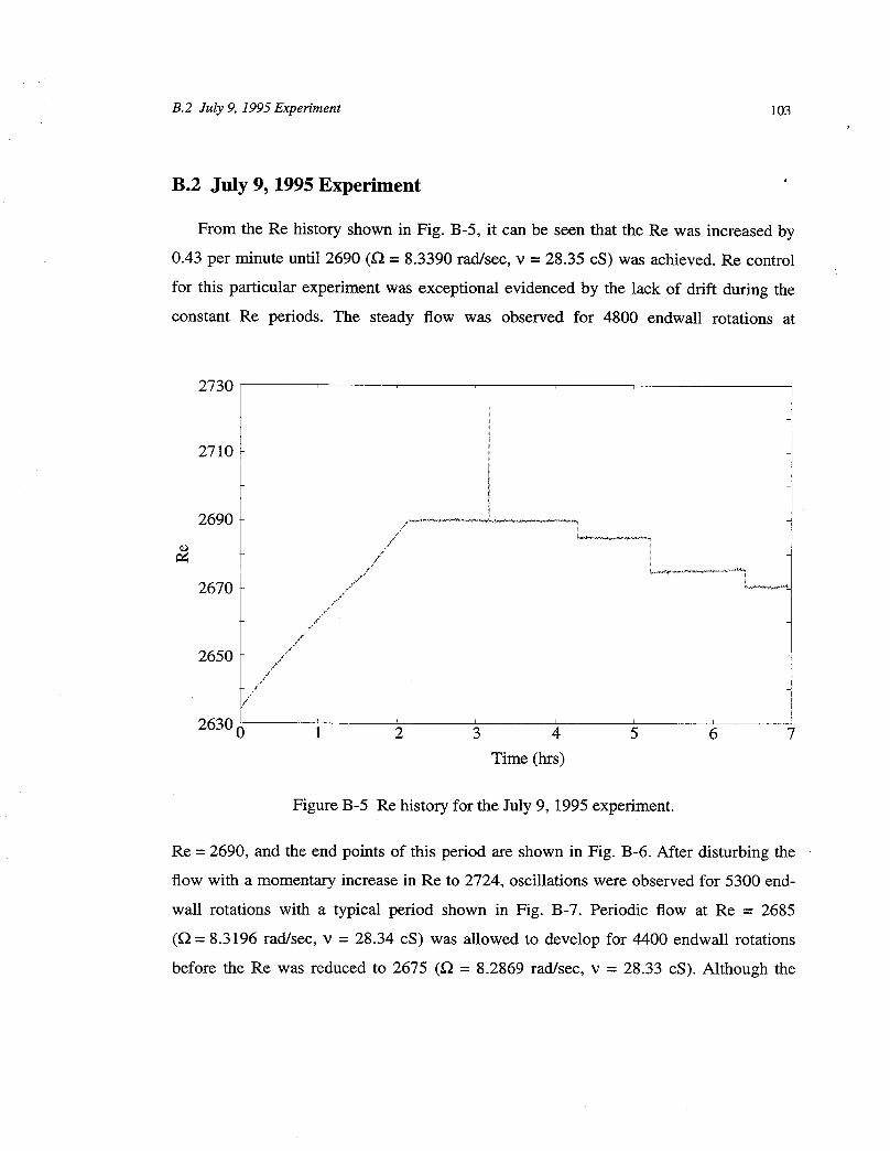
B.2 July 9, 1995 Experiment 103

B.2 July 9, 1995 Experiment

From the Re history shown in Fig. B-5, it can be seen that the Re was increased by

0.43 per minute until 2690 (_ = 8.3390 rad/sec, v = 28.35 cS) was achieved. Re control

for this particular experiment was exceptional evidenced by the lack of drift during the

constant Re periods. The steady flow was observed for 4800 endwall rotations at

2730

2710

2690

2670

2650

2630 0 J 2 3 4 5 6 7

Time (hrs)

Figure B-5 Re history for the July 9, 1995 experiment.

Re = 2690, and the end points of this period are shown in Fig. B-6. After disturbing the

flow with a momentary increase in Re to 2724, oscillations were observed for 5300 end-

wall rotations with a typical period shown in Fig. B-7. Periodic flow at Re = 2685

(_ = 8.3196 rad/sec, v = 28.34 cS) was allowed to develop for 4400 endwall rotations

before the Re was reduced to 2675 (£2 = 8.2869 rad/sec, v = 28.33 cS). Although the


Figure B-6 Steady flow for Re = 2690 (July 9, 1995)

_!:i:!:!:3__.. " ' ::]:i:_:_:i.'.':_

_i!ii_ ....:!._ t _:_1 _:::_

_:i...._i:_##_

Figure B-7 Unsteady flow at Re = 2695. Images are equally spaced in time within a total

period of 4.39 sec (x = 36.6) (July 9, 1995).

motions were small towards the end of the period, oscillations were observed for 5600

endwall rotations at Re = 2675. Steady flow for Re = 2670 (_ = 8.2693 rad/sec, v = 28.32

cS) was achieved after approximately 2400 endwall rotations, and is shown in Fig. B-8.

B.3 February 7, 1996 105

Figure B-8 Steady flow for Re = 2670 after 2400 endwall rotations (July 9, 1995).

B.3 February 7, 1996

Before this experiment was conducted, the dumbbell was incorporated into the PLL

control system, and the sheathed thermistor probe was replaced with the element probe.

Therefore, this experiment had less fluctuations in Re and better estimates of Re.

Figure B-9, the Re history, indicates that the Re was increased from 2658 to 2720 at a

rate of 0.6 per minute. The steady flow at Re = 2720 (_ = 9.2865 rad/sec, v = 31.22 cS)

was held for 5500 endwall rotations before being disturbed. Figure B-10 shows images

from the beginning and end of the period. Towards the end of this period, significant azi-

muthal waves were present indicating that the limit of the basin of attraction of the steady

flow was being approached. This was the reason that the Feb. 11, 1996 experiment (§ 4.2)

was observed at a Re of 2715 instead of 2720.


2750

2730

2710

2690

Z IJ

j z"

/2670 /"

2650 0 i 2 3 4Time (hrs)

Figure B-9 Re history for the February 7, 1996 experiment.

After the 5500 endwall rotations with steady flow, the disturbance was applied with a

momentary increase in Re to 2745. The periodic flow that ensued (Fig. B-11) was

observed for 5000 endwall rotations before the Re was decreased to 2710 (_ = 9.2243 rad/

sec, v = 31.13 cS). The periodic flow continued throughout the holding period of 5500

endwall rotations, but after reducing Re to 2705 (f_ = 9.1898 rad/sec, v = 31.07 cS), the

oscillations died out after approximately 6000 endwall rotations. The large number of end-

wall rotations required for steady flow (Fig. B-12) indicates that Re = 2705 is very close to

the critical Re.

B.3 February 7, 1996 107

Figure B-10 Steady flow for Re = 2720 (February 7, 1996)

:::_::...::. • _:_.,.':_:_:::!:_:_

_i_ ......_'__ "_')'%:""i!Y "

:::::::::::::::::::::::::::::::::::::::::::::::::::::::::::::::::::::::::::::::::

ili:ii_iiiii_iii_]ii_ii::iiii::iii:.i::iiiiii::iiiiiiii::::ii:::::::.i::i::::::i::i_:_:!:_:_:_:_:_:_:_:_:_:_:_:_:_:_:i:i:_:i:i:i:i:i:i:_:!:!:i:i:_:_:_:_:_:_:_:_:_:i...............................................................................................................................

Figure B-11 Unsteady flow at Re = 2695. Images are equally spaced in time within a total

period of 3.95 sec ('_ = 36.6) (February 7, 1996).


Figure B-12 Steady flow for Re = 2705 after 600 endwall rotations (February 7, 1996).

B.4 Summary of Experiments

Table B-1 Experiment results

HighestDate Critical Re

Steady Re

June 25, 1995 2665 < Re c < 2675 2690

July 9, 1995 2670 < Re c < 2675 2695

February 7, 1996 = 2705 2720

February 11, 1996 2702 < Re c < 2705 2715

Appendix C

Image Processing

I

There are two types of image processing used to present the data. First, a qualitative

procedure is used to obtain the images shown in Chapter 4 and Appendix B. Second, a

quantitative method is used to produce the signal and power spectral density (PSD) figures

presented in Chapter 4.

C.1 Qualitative process

In order to present the most clear and easiest images to interpret without resorting to

invasive enhancements, several video frames are used for each image. While invasive

enhancements rely on the interpretation of a video, a composite image of several frames

naturally brings out hard-to-see detail. Each individual frame contains information, but

since the data is from a low light video, it is inevitable that some of the detail will be

missed. The interpreter, who must judge which areas of the image to highlight or de-

emphasize, is taken out of the process. The frame overlaying method can be tailored such

that each frame enhances the whole image, building up detail where appropriate. Depend-

ing on the particular circumstances of an image, the number of frames used to create the

image is varied. For very low light, up to thirty frames are used; whereas for brighter pic-

tures, five frames may be enough to produce high quality images. In some cases, the dye

contaminates the experiment to a degree that precludes sharp detail, i.e. Fig. B-11 from the

February 7, 1996 experiment.

109

110 Appendix C Image Processing

For the steady images, frames are chosen at random to form a complete image. The

periodic images require overlaying frames depicting the same phase of the oscillation.

Some images, though, only contain one frame because of the quasi-periodic nature of the

flow. The result of the quasi-periodic oscillations is that each frame is unique, and combi-

nations of frames would produce confusing ghost images. Figure 4-13 and 4-20 are

sequences of quasi-periodic flows made of individual frames.

C.2 Quantitative process

To create the signal and PSD figures in Chapter 4, the periodic flow video must be

quantified. By using a video capture board, sequential, evenly timed frames are digitized.

Also, instead of capturing the entire frame, which significantly reduces the frame rate and

length of record, a region of interest about the stagnation point and injection port is

selected.

Once the frames have been collected, they are cross-correlated with a reference frame,

which is the first frame of the sequence. In a correlation, the location of a prominent fea-

ture, i.e. the dye line emanating from the injection port and ending at the stagnation point,

is calculated. The cross-correlation compares the difference of the clustering location

between two data sets. Therefore, a cross-correlation performed on the periodic flow will

reveal how the dye line moves from frame to frame.

A PSD analysis of the signal obtained from the cross-correlation will show which fre-

quencies contain the most power, which signify the prominent modes of oscillation. The

PSD is calculated by taking the fast Fourier transform (FFT) of the signal data and multi-

plying by the complex conjugate of the FFT, then dividing by the length of the FFT, which

should be a power of two. Windowing of the data is important to prevent the folding back

of higher frequencies into the domain of interest. 42 Also, care must be taken in generating

the proper frequency scale by taking into account the sample rate at which the original sig-

nal was captured.

C.2 Quantitative process 111

A certain amount of error is introduced into these data capturing techniques, especial'ly

due to the slightly non-uniform dye injection, which causes discrepancies in the calculated

position of the dye line. As the Re is increased, especially through quasi-periodic regimes,

the technique becomes less accurate. But, overall, the method proved adequately robust

for the purposes of mode identification.

112 Appendix C Image Processing

113

Bibliography

[1] G.L. Brown and J.M. Lopez, "Axisymmetric vortex breakdown. Part 2. Physical

Mechanisms", J. Fluid Mech., 221, pp 553-576 (1990)

[2] J.P. Smart and R. Weber, "Reduction of NO x and optimisation of burnout with an

aerodynamically air-staged bumer and an air -staged precombustor burner", J. Inst.

Energy, pp. 237-245 (1989)

[3] R.-H. Chen and J.F. Driscoll, "The role of the recirculation vortex in improving fuel-

air mixing within swirling flames", Twenty-Second Symp. (Intern'l) on Comb./The

Comb. Inst., pp. 531-540 (1988)

[4] M. Van Dyke, An Album of Fluid Motion, The Parabolic Press, Stanford, CA (1982)

[51 D.H. Peckham and S.A. Atkinson, "Preliminary results of low speed wind tunnel

tests on a gothic wing of aspect ratio 1.0", A.R.C. Technical Report C.P. No. 508, TN

No. Aero. 2504 (1957)

[6] J.K. Harvey, "Some observations of the vortex breakdown phenomenon", J. Fluid

Mech., 14, pp. 585-592 (1962)

[7] I. Gursul and H. Yang, "On fluctuations of vortex breakdown location", Phys. Fluids,

7, 229, (1995)

[8] M.P. Escudier and JJ. Keller, "Recirculation in Swirling Flow: A Manifestation of

Vortex Breakdown", AIAA Journal, 23, No. 1, pp. 111-116 (1985)

[9] H.B. Squire, "Analysis of the 'vortex breakdown' phenomenon, Part 1", Imperial

College of Sci. and Tech. Dept. of Aero. Rep. no. 102 (1960)

[10] S. Leibovich, "Vortex stability and breakdown: survey and extension", AIAA Jour-

nal, 22, pp. 1192-1206 (1983)

114 Bibliography

[11] M.P. Escudier, "Observations of the flow produced in a cylindrical container by a ro-'

tating endwall", Experiments in Fluids, 2, pp. 189-196 (1984)

[12] M.P. Escudier, "Vortex Breakdown: Observations and Explanations", Prog. Aero-

space Sci., 25, pp. 189-229 (1988)

[13] H.J. Lugt and M. Abboud, "Axisymmetric vortex breakdown with and without tem-

perature effects in a container with a rotating lid", J. Fluid Mech., 179, pp. 179-200

(1987)

[14] N.C. Lambourne and D.W. Bryer, "The bursting of leading-edge vortices -- some

observations and discussion of the phenomenon", Aeronautical Research Council,

Reports & memoranda R. & M. No. 3282, pp. 1-36 (1961)

[15] M.G. Hall, "Vortex Breakdown", Annual Review of Fluid Mechanics, 4, pp. 195-218

(1972)

[ 16] G.P. Neitzel, "Streak-line motion during steady and unsteady axisymmetric vortex

breakdown", Phys. Fluids, 31,958, (1988)

[17] K. Hourigan, L. J. W. Graham and M. C. Thompson, "Spiral streaklines in pre-vortex

breakdown regions of axisymmetric swirling flows", Phys. Fluids, 7, 3126, (1995)

[18] H.U. Vogel, "Experimentelle Ergebnisse tiber die laminare Strrmung in einem zylin-

drischen Geh_tuse mit darin rotierender Scheibe", Max-Planck-Inst. for Strtimungs-

forschung, Bericht 6/1968 (1968)

[19] B. Ronnenberg, "Ein selbstjustierendes 3-Komponenten-Laserdoppleranemometer

nach dem Vergleichstrahlverfahren, angewandt ftir Untersuchungen in einer station-

/iren zylindersymmetrischen Drehstrrmung mit einem ROckstromgebiet", Max-

Planck-Inst. fur Strrmungsforschung, Bericht 20/1977 (1977)

[20] H.J. Lugt and H. J. Haussling, "Axisymmetric Vortex Breakdown in Rotating Fluid

Within a Container", Journal of Applied Mechanics, 49, pp 921-923, (1982)

[21] J. N. Sorensen and O. Daube, "Direct simulation of flow structures initiated by a ro-

tating cover in a cylindrical vessel", In Advances in Turbulence, H. H. Fernholz & H.

E. Fielder, pp. 383. Springer (1989)

[22] J.M. Lopez, "Axisymmetric vortex breakdown. Part 1. Confined swirling flow", J.

Fluid Mech., 221, pp. 533-552 (1990)

115

[23]

[24]

O. Daube,"Numericalsimulationsof axisymmetricvortexbreakdownin a closedcylinder",Lecturesin AppliedMath.,28, 131 (1991)

J.M. Lopez and A.D. Perry, "Axisymmetric vortex breakdown. Part 3. Onset of peri-

odic flow and chaotic advection.", J. Fluid Mech., 234, pp. 449-471 (1992)

[25] N. Tsitverblit, "Vortex breakdown in a cylindrical container in the light of continua-

tion of a steady solution", Fluid Dynamics Research, 11, pp. 19-35 (1993)

[26] J.M. Lopez, "Note on the Nature of the Onset of Periodic Flow in an Enclosed Cyl-

inder with a Rotating Endwall", Penn State Dept. of Math., Report No. AM131(1993)

[27] J.N. SCrensen and E. A. Christensen, "Direct numerical simulation of rotating fluidflow in a closed cylinder", Phys. Fluids, 7, 764, (1995)

[28] A. Yu. Gelfgat, P. Z. Bar-Yoseph and A. Solan, "Stability of confined swirling flowwith and without vortex breakdown", J. Fluid Mech., 311, 1 (1996)

[29] T.B. Benjamin, "Bifurcation phenomena in steady flows of a viscous fluid I. Theo-

ry", Proc. R. Soc. Lond. A, 359, pp. 1-26, (1978)

[30] T.B. Benjamin, "Bifurcation phenomena in steady flows of a viscous fluid II. Exper-

iments", Proc. R. Soc. Lond. A, 359, pp. 27-43, (1978)

[31] Omega Engineering, Inc., The Temperature Handbook, (1992)

[32] N.K. Sinha and N.H. Bailey, "Speed Control of a DC Servomotor Using Phase-Locked Loop: Some Test Results of a Practical Design", IEEE Transactions, IEC1-

23, No. 1, pp. 22-26, (1976)

[33] A.W. Moore, "Phase-locked loops for motor-speed control", IEEE Spectrum, April(1973)

[34] J.P. Holman, Experimental Methods for Engineers, McGraw-Hill Book Company,(1984)

[35] V. Rom-Kedar, A. Leonard and S. Wiggins, "An analytical study of transport, mixing

and chaos in an unsteady vortical flow", J. Fluid Mech., 214, 347, (1990)

116 ' Bibliography

[36] J.L. Stevens, J. M. Lopez, and B. J. Cantwe11, "Periodic flow states in an enclosed'

cylinder with a rotating endwall", Phys. Fluids (to be submitted 1996)

[37] J. M. Lopez, "Unsteady vortex breakdown in an enclosed cylinder flow", Tenth Aus-

tralasian Fluid Mechanics Conference, University of Melbourne, December 1989,

Paper 9A-1 (1989)

[38] P.G. Drazin and W. H. Reid, Hydrodynamic stability, Cambridge University Press,

(1981)

[39] J.M. Lopez, Private communication, Jan. 1996.

[40] J.J. D'Azzo and C. H. Houpis, Linear Control System Analysis and Design: Conven-

tional and Modern, Third Edition, McGraw-Hill, p. 90 (1988)

[41] J.K. Roberge, Operational amplifiers : theory and practice, Wiley, p. 95 (1975)

[42] W. H. Press, B. P. Flannery, S. A. Teukolsky, and W. T. Vetterling, Numerical Rec-

ipes, the Art of Scientific Computing (FORTRAN Version), Cambridge University

Press, pp. 423-429 (1989)

joint institute for aeronautics and … institute for aeronautics and acoustics national aeronautics...

Documents