Int J Comput Vis (2016) 119:23–45DOI 10.1007/s11263-016-0894-5

Joint Inference in Weakly-Annotated Image Datasets via DenseCorrespondence

Michael Rubinstein1 · Ce Liu1 · William T. Freeman1,2

Received: 6 July 2013 / Accepted: 15 February 2016 / Published online: 21 March 2016© The Author(s) 2016. This article is published with open access at Springerlink.com

Abstract We present a principled framework for inferringpixel labels in weakly-annotated image datasets. Most previ-ous, example-based approaches to computer vision rely on alarge corpus of densely labeled images. However, for large,modern image datasets, such labels are expensive to obtainand are often unavailable. We establish a large-scale graph-ical model spanning all labeled and unlabeled images, thensolve it to infer pixel labels jointly for all images in the datasetwhile enforcing consistent annotations over similar visualpatterns. This model requires significantly less labeled dataand assists in resolving ambiguities by propagating inferredannotations from images with stronger local visual evidencesto images with weaker local evidences. We apply our pro-posed framework to two computer vision problems, namelyimage annotation with semantic segmentation, and objectdiscovery and co-segmentation (segmenting multiple imagescontaining a common object). Extensive numerical evalua-tions and comparisons show that our method consistentlyoutperforms the state-of-the-art in automatic annotation andsemantic labeling, while requiring significantly less labeled

Communicated by Antonio Torralba and Alexei Efros.

This work was done while Michael Rubinstein was a Ph.D. student atMIT, during his two summer internships at Microsoft Research, andwhile Ce Liu was a researcher at Microsoft Research.

B Michael Rubinsteinmrub@google.com

Ce Liuceliu@google.com

William T. Freemanwfreeman@google.com

1 Google Research, Cambridge, MA, USA

2 MIT CSAIL, Cambridge, MA, USA

data. In contrast to previous co-segmentation techniques, ourmethod manages to discover and segment objects well even inthe presence of substantial amounts of noise images (imagesnot containing the common object), as typical for datasetscollected from Internet search.

Keywords Inference · Image graph · Semanticsegmentation · Image annotation · Object discovery ·Co-segmentation

1 Introduction

Natural images consist of many repetitive patterns, such ascorners, boundaries and textures, as well as repetitive parts,objects and scenes. Such repetitions occur not only withinan image, but also across images. For example, when query-ing an image search engine using a textual phrase, we oftenobtain many visually similar images consisting of the objector scene of interest.

There are two main approaches in computer vision tomodel such visual repetitions. One approach—the para-metric approach—explicitly learns a dictionary of visualpatterns and their variations. Such parametric models havebeen successfully used for texture synthesis (Zhu et al. 1998),image denoising (Zoran and Weiss 2012), and object recogni-tion (Fergus et al. 2003; Felzenszwalb et al. 2008). The otherapproach is the nonparametric approach, which attemptsto build a graph for the patterns such that each pattern isconnected to its lookalikes, also known as its “neighbors”.Information can then be conveniently propagated or trans-ferred from the nearest neighbors to the query pattern withoutthe need to explicitly model the pattern. Such methods havebeen widely used for super resolution (Freeman et al. 2000),texture synthesis (Liang et al. 2001), and image understand-

123

24 Int J Comput Vis (2016) 119:23–45

ing (Liu et al. 2011a; Karsch et al. 2012), and, despite theirrelative simplicity, they often turn out to perform better theirparametric, model-based counterparts.

Recent techniques for establishing dense correspondencesbetween images of different scenes, such as SIFT flow (Liuet al. 2011b) and PatchMatch (Barnes et al. 2009), have facil-itated the design and implementation of such nonparametric,information-transfer systems, where the information can belabels (Liu et al. 2011a), motion (Liu et al. 2011b), depth(Karsch et al. 2012), or pixel color (Tappen and Liu 2012).The general design of these systems is illustrated at the topof Fig. 1. For a query image x , the system first finds a set ofimages xi that are visually similar to x within a dataset ofimages, where each xi is associated with some known infor-mation yi (e.g. semantic labels, depth, or motion). After densecorrespondence is established between x and each xi , eachyi is warped to x based on the computed correspondence,and an estimate of y for x is typically obtained by integrat-ing multiple warped yi ’s. Such a system performs well ingenerating the function x → y.

The main drawback of information-transfer methods,however, is that they rely on regularities in a large corpus oftraining images for which the information to be transferred(e.g. depth, motion, 3D) is “clean” and known. In large, mod-ern image datasets, such information is expensive to obtainand is often noisy or unavailable. Moreover, when classifyingmultiple new images, these methods typically solve for eachnew image independently, which often results in inconsistentannotations across images due to visual ambiguities.

We therefore propose a new framework for dealing withweakly-annotated datasets. In such datasets, it may be thatnone of the closest neighbors of an image is labeled, andso traditional, correspondence-based approaches cannot beused. Instead, we gradually infer the pixel labels and prop-agate the information through the dataset jointly in all theimages. In essence, our framework can be seen as an exten-sion of the seminal work of Freeman et al. (2000) on learningmodels for low-level vision, to cases with scarce trainingdata.

By means of dense image correspondence, we establisha large-scale Markov Random Field model (MRF) spanningall labeled and unlabeled images (Fig. 3), and infer pixellabels jointly for the entire dataset rather than for a singleimage. Pixel correspondences are used to capture the visualvariability of semantically-related features across the dataset,and for inferring labels that are consistent over similar imagepatterns across different images.

Our model is effectively optimized by efficient beliefpropagation algorithms embedded within an expectation–maximization (EM) scheme, alternating between estimatingthe likelihood of pixel labels and pixel-wise label infer-ence, while optionally refining the image graph structureduring the optimization. Our optimization technique is not

Image correspondence+ information transfer

Annotated dataset(label, depth, motion, …)

Image correspondence+ joint inference

Query image Image +transferred info

Unannotated/partially-annotated dataset

(label, depth, motion, …)

Dataset +propagated info

Standard information transfer

Information transfer in weakly-annotated datasets

Fig. 1 Information transfer in fully-annotated and weakly-annotateddatasets. Top a standard example-based framework for computer vision.Information such as class labels, depth or motion, is transferred bymeans of pixel correspondences from a large pool of labeled images toan unlabeled query.Bottom our framework for joint inference in weakly-annotated datasets. A large graphical model is established spanning alllabeled and unlabeled images, then solved to infer annotations jointlyin all the images

fundamentally new, but is designed to make full use ofthe available (sparse) annotations, and leverages moderncomputer architectures to scale efficiently for parallel com-putation.

To illustrate the potential breadth of our framework,we apply it to two important computer vision applications(Fig. 2). The first is image annotation and sematic labeling,where the goal is to automatically annotate many images witha set of word tags and a pixel-wise map showing where eachword tag occurs (Fig. 2a). The second is object discovery and

123

Int J Comput Vis (2016) 119:23–45 25

Input database + sparse annotations Fully annotated database (our results)

tree, sky, rivermountain

sky, mountaintree

tree, staircase, skyroad, plant, door

sidewalk, car, building

tree, sky, roadcar, building

tree, sky, sidewalkroad, car, building

tree, sky, riverperson, mountain

tree, sky, plantgrass

sky, buildingtree

mountain, field,building, sky, tree

tree, sky, carbuilding

sky, riverbuilding, bridge

Annotationpropagation

sidewalk, road, carbuilding, tree, sky

sky, mountaintree

tree, sky, rivermountain

sidewalk, road, carbuilding, tree, sky

sky, riverbuilding, bridge

“Car”

Images downloaded from the Internet Automatic segmentation (our results)

Imagesearch

Objectdiscovery

(a)

(b)

Fig. 2 Applications supported by our framework. a Automatic annota-tion (Sect. 4): the input is a weakly-annotated image dataset with sparseimage-level tags and few (or none) pixel labels, and the output datasetconsists of a set of word tags for each image and a pixel-wise mapshowing where each word tag occurs. b Object discovery and segmen-

tation (Sect. 5): the input is a large image dataset containing a commonobject, such as the set of images returned by an image search engine fora given query (e.g. when searching for “car”), and the goal is to labeleach pixel in the dataset according to whether or not it belongs to theunderlying common object

segmentation, in which we seek to automatically segmentmultiple images containing a common object (Fig. 2b). Weconsider the first application in a weakly-labeled setup, whereonly sparse image-level tags and relatively few (or none)pixel labels are given. In the latter application, we assumethat other than the fact that the image set contains some com-mon object, there is no additional information available onthe images or the common object class. Both applicationscan be useful for automatic generation of large-scale trainingsets for object detectors/classifiers, data-driven image syn-thesis, as well as for improving image-to-text relevance andInternet image search. They can also support applicationsin other domains, such as robotics, surveillance, and publicsafety.

We show how each of these two problems can be castedas a specific configuration of our proposed joint infer-ence framework, and demonstrate that existing approachesto these problems do not perform well in more challeng-ing, weakly-labeled scenarios. For image annotation, weconducted extensive experiments on standard large-scale

datasets, namely LabelMe (Russell et al. 2008), ESP (VonAhn and Dabbish 2004) and IAPR (Grubinger et al. 2006),showing that our system consistently outperforms the state-of-the-art in automatic annotation and semantic labeling,while requiring significantly less labeled data. For objectdiscovery, our algorithm produces state-of-the-art results onthe established MSRC and iCoseg co-segmentation datasets,and provides considerable improvement over previous co-segmentation methods on several new challenging Internetdatasets containing rigid and non-rigid object categories.

The rest of the chapter is organized as follows. In Sect. 2we review previous work related to our approach and theapplications we explored. In Sect. 3 we formulate our frame-work. In Sects. 4 and 5 we apply the framework to theaforementioned applications. In each of these sections wefirst formulate the problem as a specific configuration of ourframework, and then present experiments and results. Weconclude our findings in Sect. 6.

A prior version of this work appeared in the 12th Euro-pean Conference on Computer Vision (ECCV), Florence

123

26 Int J Comput Vis (2016) 119:23–45

Ψ

Ψ

Φ

Fig. 3 The graphical model. Each pixel in the dataset is represented bya node in the graph, connected to spatially adjacent pixels in its imageand corresponding pixels in similar images, which indicate statisticaldependency. Connections between images are depicted by edges in theimage graph on the left (these edges are directed, although visualizedin this figure as undirected for clarity). In practice we connect everyimage to the K images most similar to it based on global image statis-

tics (Sect. 3). For each such connection, dense pixel correspondences arecomputed, connecting each pixel in the source image to some pixel inthe target image (right). The image graph is shown here for the LabelMeOutdoors dataset (Russell et al. 2008) using 400 sampled images andK = 10. The size of each image corresponds to its visual pagerankscore (Sect. 4.4)

2012 (Rubinstein et al. 2012) and in the 26th IEEE Confer-ence on Computer Vision and Pattern Recognition (CVPR),Portland 2013 (Rubinstein et al. 2013). Supplementary mate-rials, additional results and code are available on the projetweb pages: http://people.csail.mit.edu/mrub/annotation andhttp://people.csail.mit.edu/mrub/ObjectDiscovery.

2 Related Work

Image Graphs Large-scale image graphs are becoming afundamentally important representation for image datasets.Several works have utilized it in the past for exploring andnavigating image collections. For example, “Image Webs”(Heath et al. 2010) discovers corresponding regions betweenimages and uses spectral graph theory to capture the con-nectivity in an image dataset. The discovered connectivity isthen used for revealing global structures in the dataset (suchas paths linking between images), and for supporting a Photo-Tourism-style navigation (Snavely et al. 2006). Videoscapes(Tompkin et al. 2012) added the temporal domain to theimage graph construction, aligning video frames not onlyin space, but also in time, in order to interactively exploreunstructured video collections.

Recently, Liu et al. (2012) proposed a label propagationalgorithm for joint image parsing, combining relationshipsamong patches and mutual information in subgraphs of theimage graph. Faktor and Irani (2012) efficiently estimatecorresponding regions between images to automatically clus-

ter an image dataset. Kim and Xing (2013) jointly discovermatching images and parse their content in multiple photostreams to detect collective storylines. All these work, whichwere applied to specific problems, demonstrate the powerof exploiting regularities and structures in image datasets toperform nontrivial inference tasks.

Image Annotation and Semantic Segmentation In computervision, scholars have investigated image annotation in twodirections. One methodology uses image similarities to trans-fer textual annotation from labeled images to unlabeledsamples, under the assumption that similar images shouldhave similar annotations. Notably, Makadia et al. (2010)recently proposed a simple baseline approach for auto-annotation based on global image features and a greedyalgorithm for transferring tags from similar images. ARISTA(Wang et al. 2010) automatically annotates a web dataset ofbillions of images by transferring tags via near-duplicates.Although those methods have clearly demonstrated the mer-its of using similar images to transfer annotations, they doso only between globally very similar images, and cannotaccount for locally similar patterns.

Consequently, the other methodology focused on denseannotation of images, known as semantic labeling (Shottonet al. 2006, 2008; Liu et al. 2011a; Tighe and Lazebnik 2010),where correspondences between text and local image fea-tures are established for annotation propagation: similar localfeatures should have similar labels. These methods often aimto label each pixel in an image using models learned from a

123

Int J Comput Vis (2016) 119:23–45 27

training database. In Blei et al. (2003) and Feng et al. (2004),relationships between text and visual words are characterizedby conventional language translation models. More recently,Shotton et al. (2006) proposed to train a discriminative modelbased on the texton representation, and to use conditionalrandom fields (CRF) to combine various cues to generatespatially smooth labeling. The authors later extended theirapproach (Shotton et al. 2008) by using randomized decisionforests for a significant speedup. Liu et al. (2011a) proposeda nonparametric approach to semantic labeling, where textlabels are transferred from a labeled database to parse a queryimage via dense scene correspondences.

Since predicting annotation from image features is bynature ambiguous (e.g. textureless regions can be sky,wall, orceiling), such methods rely on regularities in a large corpus oftraining data of pixel-wise densely labeled images. However,for large image databases, high-quality pixel labels are veryexpensive to obtain. Furthermore, the annotation is typicallycomputed independently for each test image, which oftenresults in inconsistent annotations due to visual ambiguities.

Object Discovery and Segmentation The task of simul-taneously segmenting multiple images is known as Co-segmentation, where joint segmentation essentially serves asa means of compensating for the lack of supervisory data,allowing to infer the visual properties of the foregroundobject even in the absence of a priori information about theobject or the images.

While numerous co-segmentation methods have been pro-posed, they were shown to work well mostly on smalldatasets, namely MSRC and iCoseg, containing salient andsimilar objects. In fact, in most of the images in thosedatasets the foreground can be quite easily separated fromthe background based on each image alone (i.e. without co-segmentation, see Sect. 5.4).

However, Internet image collections, such as the onesreturned by image search engines for a given user query, aresignificantly larger and more diverse (Fig. 2b). Not only dothe objects in images downloaded from the Internet exhibitdrastically different style, color, texture, shape, pose, size,location and view-point; but such image collections also con-tain many noise images—images which do not contain theobject of interest at all. These challenges, as we demonstrate,pose great difficulties on existing co-segmentation tech-niques. In particular, most co-segmentation methods assumeevery image contains the object of interest, and hence areunable to handle dataset noise.

Object discovery has been intensively studied in com-puter vision. In a supervised setup, objects were treatedas topics and images as documents, and generative modelssuch as Latent Dirichlet Allocation (LDA) and HierarchicalPitman-Yor (HPY) have been used to learn the distributionand segmentation of multiple classes simultaneously (Sivic

et al. 2005; Russell et al. 2006). Winn and Jojic (2005)propose a generative model for the distribution of mask,edge and color for visual objects with respect to a smoothdeformation field. Although good object recovery resultswere reported, the model is limited to particular views of anobject.

Recently, PageRank (Jing and Baluja 2008) was used todiscover regions of interest in a bounding box represen-tation (Kim and Torralba 2009), and self-similarities wereused to discover a common pattern in several images (Bagonet al. 2010). Although in these works no generative mod-els were used to learn the distribution of visual objects,reliable matching and saliency are found to be helpful forobject discovery. The notions of matching and saliency werealso successfully applied by Faktor and Irani (2012), a workdone in parallel to ours, for unsupervised discovery of imagecategories.

Co-segmentation was first introduced by Rother et al.(2006), who used histogram matching to simultaneously seg-ment the same object in two different images. Since then,numerous methods were proposed to improve and refinethe co-segmentation (Mukherjee et al. 2009; Hochbaum andSingh 2009; Batra et al. 2010; Joulin et al. 2010), manyof which work in the context of a pair of images with theexact same object (Rother et al. 2006; Mukherjee et al. 2009;Hochbaum and Singh 2009) or require some form of userinteraction (Batra et al. 2010; Collins et al. 2012).

These techniques were later extended in various ways.Joulin et al. (2010) used a discriminative clustering frame-work that can handle multiple images, and Kim et al. (2011)proposed an optimization which scales up to even largerdatasets. Vicente et al. (2011) introduced the notion of”objectness” to the co-segmentation framework, showingthat requiring the foreground segment to be an object oftenimproves co-segmentation results significantly. All thesetechniques, however, maintain the strong assumption that theobject is present in all of the images, which is not true forInternet image collections.

Other methods were proposed to handle images whichmight not contain the common object, either implicitly(Joulin et al. 2012) or explicitly (Kim and Xing 2012). In par-ticular, Kim and Xing (2012) show promising results givenadditional user input, but do not show significant improve-ment in the unsupervised setting. It is clear that in the contextof image search and web browsing, user input cannot be used.

Co-segmentation was also explored in weakly-supervisedsetups with multiple object categories (Rubinstein et al. 2012;Kuettel et al. 2012). While image annotations may facili-tate object discovery and segmentation, image tags are oftennoisy, and bounding boxes or class labels are usually unavail-able. In this work we show that it is plausible to automaticallydiscover visual objects from the Internet using image searchalone.

123

28 Int J Comput Vis (2016) 119:23–45

3 Joint Inference via Dense Correspondence

In this section we describe our basic joint inference frame-work. We will start by defining the terminology and setupthat will guide us through the rest of the chapter.

The input to our framework is a dataset � = (I, V, A)

that is comprised of N RGB images I = {I1, . . . , IN }, afinite vocabulary V = {l1, . . . , lL} of L possible labels eachpixel can attain, and possibly additional image annotationsA = {A1, . . . , AN }. Image annotations can include a range ofauxiliary information about an image. For example, it can be acollection of textual words describing the image, a time stampspecifying when the image was taken, GPS coordinates indi-cating where it was taken, and even pixel-level information,such as the location of faces or other objects in the image.In this chapter, we will consistently refer to semantic, pixel-level information as “labeling” and to textual, image-levelannotation as “tags”. Our goal is to produce the labelingsC = {c1, . . . , cN } for all the images in the dataset, where forpixel x = (x, y), ci (x) ∈ {1, . . . , L} indexes into the vocab-ulary V. We formulate this discrete labeling problem withinan optimization framework to solve for the most likely labelsfor all pixels in the dataset.

To exploit the dataset structure and similarity betweenimage regions, we establish correspondences between pixelsin different images. We denote by wi j the correspondencefield—or flow field—from image Ii to image I j , mappingeach pixel in Ii to a pixel in I j . For small datasets, we canestimate the correspondences between any pair of images,however for large datasets such computation is generallyprohibitive. Therefore, we restrict the correspondences ofeach image Ii to a subset of the images, Ni , that are mostsimilar to it, based on global image statistics that are moreefficient to compute. In our experiments we fixed the size ofNi of each image Ii to be the same constant, K , however ingeneral this size can be allowed to vary. Finally, we denoteby W the set of all pixel correspondences in the dataset:W = ∪N

i=1 ∪I j∈Ni wi j .Given the input image dataset, �, the pixel correspon-

dences W, and additional parameters of the model, � (will bedefined shortly), we define the cost function, E(C;�, W,�)

for the joint labeling C, as:

E(C;�, W,�)

=N∑

i=1

∑

x∈Λi

[Φ i (x)︸ ︷︷ ︸

Likelihood (local evidence)

+ Φ iθ (x,�)︸ ︷︷ ︸

Model parameters

+∑

y∈N ix

λintΨiint(x, y)

︸ ︷︷ ︸Intra-image compatibility

+∑

j∈Ni

λextΨi jext(x, x + wi j (x))

︸ ︷︷ ︸Inter-image compatibility

],

(1)

where N ix is the spatial neighbors of pixel x (we use the four

pixels directly connect to x as the spatial neighborhood), andΛi is image Ii ’s lattice.

This objective function defines a (directed) graphicalmodel over the entire image dataset (Fig. 3). The likeli-hood term, Φ i (x), captures the cost of assigning the labelci (x) to pixel x in image Ii . The definition of this term isproblem-specific. Φ i

θ is a unary energy term that accounts foradditional parameters of the model. In our implementations(will be described in the upcoming sections) these parame-ters include per-image color models, as well as dataset-wideparameters such as spatial distribution of labels, and labelco-occurrences. These parameters are estimated during theoptimization, and provide a simple mechanism to account forhigher-order and longer-range connections between nodesin the graph (Freeman et al. 2000; Krähenbühl and Koltun2012). The regularization terms, Ψ i

int and Ψi jext, penalize dis-

continuous labeling within the image and between images,respectively, subject to image structures and similaritiesbetween corresponding pixels. λint and λext balance the con-tribution of these terms.

This graphical model extends traditional discrete MRFformulations used extensively in computer vision (see e.g.Freeman et al. 2000; Rother et al. 2004; Shotton et al. 2006;Liu et al. 2011a, and also Szeliski et al. 2008 for an in-depthreview) in two important ways: (a) it involves an inter-imagecompatibility term, regularizing the solution across imagesand not just within each image, and (b) it involves all theimages in the dataset as opposed to just a single one. Optimiz-ing this objective function collectively using all the imagesis key for inferring plausible pixel labels in cases where onlysparse and/or noisy information is given about the images.

Equation 1 encapsulates a gigantic inference problem, andits optimization is by no means trivial. For a dataset contain-ing 104 images, each of size 256 × 256, there are 6.55 × 108

nodes (pixels). Each node has an order of 102 edges, and sothere are in total 6.55×1010 edges in the graph! We designedan efficient parallel message passing algorithm to solve thishuge graph inference problem, which will be described inthe upcoming sections. The algorithm is comprised of beliefpropagation algorithms embedded in a coordinate descentscheme. The objective function is highly non-convex andthis optimization is not guaranteed to reach the global mini-mum, however we show that it yields plausible solutions thatimprove the state-of-the-art for the applications we explored.

In the upcoming sections, we will demonstrate howthis framework can be applied to two computer visionapplications: semantic labeling, and object discovery andsegmentation. Each of these problems can be casted as aspecific configuration of this framework, and demonstratesdifferent aspects in which it can be utilized. For example,pixel correspondences are used only for regularization (Ψ i j

ext)in semantic labeling, but are used both for regularization and

123

Int J Comput Vis (2016) 119:23–45 29

as part of the likelihood function (Φ i ) in object discovery;the image graph is constructed once in our implementationof semantic labeling, but is iteratively updated and refinedin object discovery, as the lower complexity of the latterproblem allows to accommodate updates to the image graphduring the optimization.

4 Application: Annotation Propagation

In this section we describe how to apply the inference frame-work we presented in the previous section to one specificproblem—semantic segmentation of images in weakly-labeled datasets. The method exploits visual similaritiesamong the different images to help auto-annotation succeedwith relatively few human-provided labels.

4.1 Formulation

Following the definitions in Sect. 3, we assume each pixelcan obtain one of L+1 possible labels: V = {l1, . . . , lL , ∅},where the additional label ∅ denotes the pixel is determinedto be unlabeled, in case it cannot be associated with any otherlabel with sufficient confidence. Initially, we may be givenannotations in the form of image tags and pixel labels forsome images in the dataset, A = {Tt , Cl}, where we denoteby It and Tt , and Il and Cl , the corresponding subsets oftagged images with their tags, and labeled images with theirlabels, respectively. The set of tags of an image is comprisedof words from the vocabulary V, which can be specified by auser, or obtained from text surrounding an image on a web-page. Notice that unlike traditional approaches that propagateknown pixel labels to new images, here we assume most ofthe pixels in the dataset are unlabeled. That is, |Cl | is assumedto be only a small fraction of the dataset size.

Since image tags are important for image indexing andsearch, we also return (and evaluate in our experimentsin Sect. 4.5) the tags associated with the images, T ={t1, . . . , tN : ti ⊆ {1, ..., L}}, which we define directly as theset union of the pixel labels in the image: ti = ∪x∈Λi ci (x)

(ignoring unlabeled pixels).

4.1.1 Image Graph

As previously mentioned, since computing (and storing)dense pixel correspondences between every pair of imagesis prohibitive for large datasets, we restrict the intra-imagecompatibility to a set of K images that are the most similarto the image. Here, similarly to Liu et al. (2011a), we definethe set of nearest neighbors of each image Ii ,Ni , as its top〈K , ε〉 similar images, where K is the maximum numberof neighbors, and ε is a threshold on the distance betweenthe images (above which neighbors are discarded). We use

L2-norm between Gist descriptors (Oliva and Torralba 2001)as the image similarity measure, although other image-levelmeasures such as bag of words histograms or spatial pyra-mids can be used.1 Some analysis of the influence of thechoice of K on the performance is given in Sect. 4.5.

Once the set of neighbors for each image is determined,we use SIFT-flow (Liu et al. 2011b) to compute the pixelcorrespondences between an image and each of its neighbors.We use the original implementations of Gist and SIFT-flowas provided by the authors, which are available online.

4.1.2 Objective Function Terms

Likelihood From tags associated with the images and pos-sibly some pixel labels (if available), we need to define thelikelihood term, Φi (x), that a pixel x in image Ii attains thelabel l ∈ V. For example, an image might be tagged with carand road, but their locations within the image are unknown.We characterize this text-to-image correspondence by meansof local visual appearance. We leverage the large number ofimages and the available tags to correlate the dataset vocabu-lary with visual statistics. We first extract local image featuresfor every pixel, and then learn a visual appearance modelfor each vocabulary word by utilizing visual commonalitiesamong images with similar tags, as well as the given pixellabels, if available. The result is an estimate of the probabil-ity distribution over the labels, Pa(x), at each pixel x. Thisprocess is described in Sect. 4.2.

We then define the likelihood directly based on this dis-tribution estimate:

Φ i (x) = − log Pa(x). (2)

Model Parameters. For this application this term is com-prised of three components:

Φiθ (x,�) = − log Pi

t (ci (x)) − λs log Ps(x) − λc log Pic (x),

(3)

where Pit (ci (x)) is a tag likelihood term that estimates the

probability of image Ii having the label ci (x) somewherein it (and thus having l as one of its tags), and Ps(ci (x))

and Pic (ci (x)) capture the probability of the label l occurring

at pixel x based on its relative spatial position and color,respectively. We use superscript i in Pi

t and Pic to emphasize

that they are estimated separately for each image, while Psis estimated globally for the entire dataset. λs, λc balance thecontribution of Ps and Pi

c , respectively.

1 In our experiments, we did not notice significant difference in theresults when computing the nearest neighbor set using pyramid match-ing (Lazebnik et al. 2006) instead of Gist.

123

30 Int J Comput Vis (2016) 119:23–45

The term Pit is used to bias the labels used in an

image towards ones with higher frequency and co-occurrenceamong its neighbors. We estimate the likelihood of image Iihaving the label l as

Pit (l) = β

|Ni |∑

j∈Ni

δ[l ∈ t j

] + 1 − β

Z

∑

j∈Ni

∑

m∈t j

ho(l,m),

(4)

where the indicator function [·] is 1 when its argument istrue, and 0 otherwise, ho is the L×L row-normalized tag co-occurrence matrix, computed from the current tag estimatesand initialized from the known tags, and Z = ∑

j∈Ni|t j |.

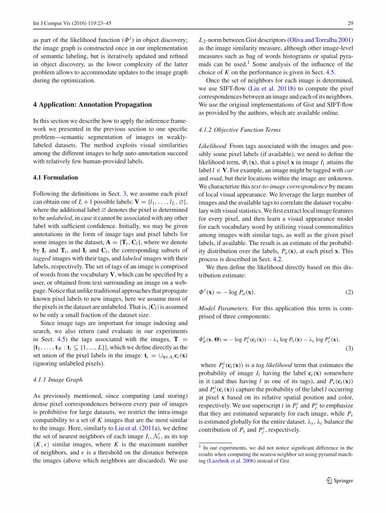
The first term in Eq. 4 measures the frequency of word lamong image Ii ’s neighbors, and the second term is the meanco-occurrence rate of word l within its neighbors’ tags. Wetypically set β = 0.5, assigning equal contribution to thetwo terms. This term is inspired by Makadia et al. (2010),but we do not set a hard threshold on the number of tagsto infer for an image as they do. Figure 4 demonstrates thecontribution of this term. It can be seen that when using thisterm we manage to obtain a much better initial guess for thelabeling of the image (which will then be refined during theoptimization).

Both the spatial and color terms are computed from thecurrent pixel label estimates. The spatial location term iscomputed as

Ps(x) = hci (x)s (x), (5)

where hls(x) is the normalized spatial histogram of word l

across all images in the dataset (Fig. 9). This term will assistin places where the appearance and pixel correspondencemight not be as reliable.

The color term will assist in refining the labels internallywithin the image, and is computed as

Pic (x) = hi,ci (x)

c (Ii (x)) (6)

Fig. 4 The effect of tag likelihood, Pit (ci (x)), on pixel classifica-

tion, shown on an image from the LabelMe Outdoors dataset (seeSect. 4.5 for details on the experiment). a The source image. b MAPper-pixel classification using the learned appearance models only:maxci Pa(ci (x)). c Similar to (b), with the additional tag likelihood

term: maxci

{Pa(ci (x)) + Pi

t (ci (x))}

where hi,lc is the color histogram of word l in image Ii . We

use 3D histograms of 64 bins in each of the color channels torepresent hi,l

c instead of the Gaussian mixture models usedin Rother et al. (2004) and Shotton et al. (2006).

Overall, the parameters of the model are�={hi,lc , hl

s, ho},i = 1..N , l = 1..L .

Regularization The intra-image compatibility betweenneighboring pixels is defined based on tag co-occurrenceand image structures. For image Ii and spatial neighborsx, y ∈ N i

x ,

Ψ iint (x, y) = −λo log ho (ci (x), ci (y))

+ δ[ci (x) �= ci (y)

]λint exp

(− ‖Ii (x) − Ii (y)‖2

2

).

(7)

Finally, we define the inter-image compatibility between apixel x in image Ii and its corresponding pixel z = x+wi j (x)

in image I j as

Ψi jext(x, z) =δ [ci (x) �= ci (z)]

α j

αiλext exp

(− ∥∥Si (x) − S j (z)

∥∥1

), (8)

where αi , α j are the image weights as defined in Sect. 4.2.2,and Si are the (dense) SIFT descriptors for image Ii . Intu-itively, better matching between corresponding pixels willresult in higher penalty when assigning them different labels,weighted by the relative importance of the neighbor’s label.Notice that SIFT features are used for the inter-image com-patibility metric in Eq. 8 whereas RGB intensities are usedfor the intra-image compatibility in Eq. 7.

4.2 Text-to-Image Correspondence

4.2.1 Local Image Descriptors

We selected features used prevalently in object and scenerecognition to characterize local image structures and colorfeatures. Structures are represented using both SIFT andHOG (Dalal and Triggs 2005) features. We compute denseSIFT descriptors with 3 and 7 cells around a pixel to accountfor scales. We then compute HOG features and stack togetherneighboring HOG descriptors within 2×2 patches (Xiao et al.2010). Color is represented using a 7 × 7 patch in L*a*bcolor space centered at each pixel. Stacking all the featuresyields a 527-dimensional descriptor Di (x) for every pixel xin image Ii . We use PCA to reduce the descriptor to d = 50dimensions, capturing approximately 80 % of the features’variance.

123

Int J Comput Vis (2016) 119:23–45 31

Fig. 5 Text-to-image and dense image correspondences. a An imagefrom LabelMe Outdoors dataset. b Visualization of text-to-image pixellikelihood, Pa , for the four most probable labels, colored from black(low probability) to white (high probability). c The maximum likelihoodpixel classification (computed independently at each pixel). d The pixel

classification with spatial regularization (Eq. 7). e–g Nearest neighborsof the image in (a) and dense pixel correspondences with (a). h Sameas (b), shown for each of the neighbors, warped towards the image (a)based on the computed correspondences. i The final MAP labeling usingboth intra- and inter-image regularization (Eq. 8)

4.2.2 Learning Appearance Models

We use a generative model based on Gaussian mixturesto represent the distribution of the above continuous fea-tures. More specifically, we model each word in the databasevocabulary using a full-covariance Gaussian Mixture Model(GMM) in the 50D descriptor space. Such models have beensuccessfully applied in the past to model object appearancefor image segmentation (Delong et al. 2011). Note that oursystem is not limited to work with this particular model. Infact, we also experimented with a discriminative approach,Randomized Forests (Geurts et al. 2006), previously used forsemantic segmentation (Shotton et al. 2008) as an alternativeto GMM. We found that GMM produces better results thanrandom forests in our system (see Sect. 4.5).

For pixel x in image Ii , we define

P(Di (x);�) =L∑

l=1

(ρl

M∑

k=1

πl,kN(Di (x);μl,k,�l,k

))

+ ρεN(Di (x);με,�ε

), (9)

where ρl is the weight of model (word) l in generating thefeature Di (x), M is the number of components in each model(M = 5), and θ l = (

πl,k,μl,k,�l,k)

is the mixture weight,mean and covariance of component k in model l, respec-tively. We use a Gaussian outlier model with parametersθ ε = (

με,�ε

)and weight ρε . The intuition for the out-

lier model is to add an unlabeled word to the vocabulary V.

� = ({ρl}l=1:L , ρε, θ1, . . . , θ L , θ ε) is a vector containingall parameters of the model.

We optimize for � in the maximum likelihood sense usinga standard EM algorithm. We initialize the models by par-titioning the descriptors into L clusters using k-means andfitting a GMM to each cluster. The outlier model is initial-ized from randomly selected pixels throughout the database.We also explicitly restrict each pixel to contribute its data tomodels of words corresponding to its estimated (or given)image tags only. That is, we clamp the posteriors to zero forall l /∈ ti . For labeled images Il , we keep the posteriors fixedaccording to the given labels (setting zero probability to allother labels). To account for partial annotations, we introducean additional weight αi for all descriptors of image Ii , set toαt , αl or 1 (we use αt = 5, αl = 10) according to whetherimage Ii was tagged, labeled, or inferred automatically bythe algorithm, respectively. More details can be found in thesupplementary material. Given the learned model parame-ters, �, and an observed descriptor, Di (x), the probability ofthe pixel belonging to word l is computed by

Pa(ci (x) = l; Di (x),�)

= ρl∑M

k=1 πl,kN(Di (x);μl,k,�l,k

)

P(Di (x);�), (10)

where P(Di (x);�) is defined in Eq. 9.Figure 5c shows an example pixel classification based on

the model learned with this approach, and more results areavailable on the project web page.

123

32 Int J Comput Vis (2016) 119:23–45

4.3 Optimization

The optimization alternates between estimating the appear-ance model and propagating pixel labels. The appearancemodel is initialized from the images and partial annotationsin the dataset. Then, we partition the message passing schemeinto intra- and inter-image updates, parallelized by distrib-uting the computation of each image to a different core.The belief propagation algorithm starts from spatial mes-sage passing (TRW-S) for each image for a few iterations,and then updates the outgoing messages from each image forseveral iterations. The inference algorithm iterates betweenmessage passing and estimating the color histograms in aGrabCut fashion (Rother et al. 2004), and converges in a fewiterations. Once the algorithm converges, we compute theMAP labeling that determines both labels and tags for all theimages.

4.4 Choosing Images to Annotate

As there is freedom to choose images to be labeled by the user,intuitively, we would want to strategically choose “imagehubs” that have many similar images, since such images havemany direct neighbors in the image graph to which they canpropagate labels efficiently. We use visual pagerank (Jingand Baluja 2008) to find good images to label, again usingthe Gist descriptor as the image similarity measure. To makesure that images throughout the dataset are considered, weinitially cluster the images and use a non-uniform dampingfactor in the visual rank computation (Eq. 2 in Jing and Baluja2008), assigning higher weight to the images closest to thecluster centers. Given an annotation budget (rt , rl), where rtdenotes the percentage of images tagged in the dataset, andrl denotes the percentage of the images labeled, we then setIl and It as the rl and rt top ranked images, respectively.Figure 6 shows the top image hubs selected automaticallywith this approach, which nicely span the variety of scenesin the dataset.

4.5 Results

We conducted extensive experiments with the proposedmethod using several datasets: SUN (Xiao et al. 2010)(9556 256 × 256 images, 522 words), LabelMe Outdoors(LMO, subset of SUN) (Russell et al. 2008) (2688 256 ×

256 images, 33 words), the ESP game dataset (Von Ahnand Dabbish 2004) (21, 846 images, 269 words) and IAPRbenchmark (Grubinger et al. 2006) (19,805 images, 291words). Since both LMO and SUN include dense humanlabeling, we use them to simulate human annotations forboth training and evaluation. We use ESP and IAPR data asused by Makadia et al. (2010). They contain user tags but nopixel labeling.

We implemented the system using MATLAB and C++and ran it on a small cluster of three machines with a totalof 36 CPU cores. We tuned the algorithm’s parameters onLMO dataset, and fixed the parameters for the rest of theexperiments to the best performing setting: λs = 1, λc =2, λo = 2, λint = 60, λext = 5. In practice, 5 iterationsare required for the algorithm to converge to a local mini-mum. The EM algorithm for learning the appearance model(Sect. 4.2.2) typically converge within 15 iterations, and themessage passing algorithm (Sect. 4.3) converges in 50 itera-tions. Using K = 16 neighbors for each image gave the bestresult (Fig. 10c), and we did not notice significant changein performance for small modifications to ε (Sect. 4.1.1), d(Sect. 4.2.1), nor the number of GMM components in theappearance model, M (Eq. 9). For the aforementioned set-tings, it takes the system 7 h to preprocess the LMO dataset(compute descriptors and the image graph) and 12 h to prop-agate annotations. The run times on SUN were 15 and 26 hrespectively.

Results on SUN and LMO Figure 7a shows some annota-tion results on SUN using (rt = 0.5, rl = 0.05). All imagesshown were initially unannotated in the dataset. Our systemsuccessfully infers most of the tags in each image, and thelabeling corresponds nicely to the image content. In fact, thetags and labels we obtain automatically are often remarkablyaccurate, considering that no information was initially avail-able on those images. Some of the images contain regionswith similar visual signatures, yet are still classified correctlydue to good correspondences with other images. More resultsare available on the project web page.

To evaluate the results quantitatively, we compared theinferred labels and tags against human labels. We computethe global pixel recognition rate, r , and the class-averagerecognition rate r̄ for images in the subset I \ Il , where thelatter is used to counter the bias towards more frequent words.We evaluate tagging performance on the image set I \ It in

0.0103 0.0091 0.0076 0.0069 0.0068 0.0066 0.0063 0.0062 0.0061 0.0059 0.0057

Fig. 6 Top-ranked images selected automatically for human annotation. The images are ordered from left (larger hub) to right (smaller hub).Underneath each image is its visual pagerank score (Sect. 4.4)

123

Int J Comput Vis (2016) 119:23–45 33

sea

sky

tree

person

sand

sea

sky

mountain

sea

sky

grass

person

sky

tree

ground

person

plant

building

car

road

sidewalk

sky

tree

ceilingceiling lampchairfloorpaperpostertelevisiontreewallwindow

building

chimney

ground

plant

sky

steps

tree

mountain

sky

tree

airplane

building

road

sky

tree

building

car

fence

mountain

road

sky

tree

mountain

sky

building

sky

tree

buildingdoorhung outpersonpipeplantroadshutterskywindow

ceiling

floor

heater

wall

window

boat

sea

sky

palm tree

palm trees

plant

sand

sea

sky

building

grass

plant

sky

stone

blackboard

ceiling

ceiling lamp

chair

cupboard

table

ceiling

chair

floor

picture

sign

table

wall

buildingcarroadsky

buildingdoorskytreewindow

awningbuildingcartreewindow

buildingdoortreewallwindow

building

grass

sky

tree

window

door

floor

plant

wall

mountain

sky

tree

building

mountain

sky

grass

house

tree

white

black

green

man

white

world

crowd

group

sky

tree

blue

feet

purple

sand

shoes

flower

green

leaf

pink

plant

doll

green

helmet

man

toy

grass

house

sky

tree

crowdgrouppeoplephotopicture

building

column

flag

palm

pinnacle

sky

tower

cliff

front

people

sign

wall

brick

one

rail

wall

car

cobblestone

front

house

lot

plant

tree

desert

mountain

people

rock

sky

city

cloud

house

sky

view

lamp

night

square

street

tower

canyon

landscape

lookout

road

sky

bush

city

house

roof

sky

valley

view

classroom

clock

front

tourist

writing

lamp

people

square

street

tower

bed

curtain

room

wall

white

window

wood

(a) SUN [55] (9556 images, 522 words)

(b) ESP [52] (21,846 images, 269 words)

(c) IAPR-TC12 [15] (19,805 images, 291 words)

Fig. 7 Automatic annotation results (best viewed on a monitor). a SUNresults were produced using (rt = 0.5, rl = 0.05) (4778 images taggedand 477 images labeled, out of 9556 images). All images shown inthis figure were initially unannotated in the dataset. b, c For ESP andIAPR, the same training set as in Makadia et al. (2010) was used, hav-ing (rt = 0.9, rl = 0). For each example we show the source image

on the left, and the resulting labeling and tags on the right. The wordcolormap for SUN is the average pixel color based on the ground truthlabels, while for ESP and IAPR each word is assigned an arbitraryunique color (since ground truth pixel labels are not provided with thedatasets). More results can be found in Fig. 2 and the project web page

123

34 Int J Comput Vis (2016) 119:23–45

landscapemountainrangeview

buildingdoormountainplantroadsidewalkstaircasetreewindow

mountainskytree

Neighbor image Neighbor image

buildingdoorroadskywindow

skytree

buildingroad

(a)

(c)

(b)

Fig. 8 Example failure cases. a Our system occasionally misclassi-fies pixels with classes that have similar visual appearance. Here, therooftops in the left image are incorrectly labeled as “mountain”, and thepeople in the right image are incorrectly labeled as “tree”. b Generic andabstract words, such as “view”, do not fit our model that assumes labelscorrespond to specific regions in the image (and that every pixel belongs

to at most one class). c Incorrect correspondences may introduce errors.Here we show two examples of outdoor images that get connected toindoor images in the image graph, leading to misinterpretation of thescene (floor gets labeled as “road”, boxes in a warehouse get labeled as“building”)

terms of the ratio of correctly inferred tags, P (precision),and the ratio of missing tags that were inferred, R (recall).We also compute the corresponding, unbiased class-averagemeasures P̄ and R̄ (Figs. 8, 9).

The global and class-average pixel recognition rates are63 and 30 % on LMO, and 33 and 19 % on SUN, respec-tively. In Fig. 10 we show for LMO the confusion matrix andbreakdown of the scores into the different words. The diago-nal pattern in the confusion matrix indicates that the systemrecognizes correctly most of the pixels of each word, exceptfor less frequent words such as moon and cow. The verticalpatterns (e.g. in the column of building and sky) indicate atendency to misclassify pixels into those words due to theirfrequent co-occurrence with other words in that dataset. Fromthe per-class recognition plot (Fig. 10b) it is evident that thesystem generally performs better on words which are morefrequent in the dataset.

Components of the model To evaluate the effect of eachcomponent of the objective function on the performance,we repeated the above experiment where we first enabledonly the likelihood term (classifying each pixel indepen-dently according to its visual signature), and gradually addedthe other terms. The results are shown in Fig. 10d for varyingvalues of rl . Each term clearly assists in improving the result.It is also evident that image correspondences play importantrole in improving automatic annotation performance.

Comparison with state-of-the-art We compared our tag-ging and labeling results with state-of-the-art in semanticlabeling—Semantic Texton Forests (STF) (Shotton et al.2008) and Label Transfer (Liu et al. 2011a)—and imageannotation (Makadia et al. 2010). We used our own imple-

mentation of Makadia et al. (2010) and the publicly availableimplementations of Shotton et al. (2008) and Liu et al.(2011a). We set the parameters of all methods according tothe authors’ recommendations, and used the same taggedand labeled images selected automatically by our algorithmas training set for the other methods [only tags are consideredby Makadia et al. (2010)]. The results of this comparison aresummarized in Table 1. On both datasets our algorithm showsclear improvement in both labeling and tagging results. OnLMO, r̄ is increased by 5 % compared to STF, and P̄ isincreased by 8 % over Makadia et al.’s baseline method.STF recall is higher, but comes at the cost of lower preci-sion as more tags are associated on average with each image(Fig. 11). In Liu et al. (2011a), pixel recognition rate of74.75 % is obtained on LMO at 92 % training/test split withall the training images containing dense pixel labels. How-ever, in our more challenging (and realistic) setup, their pixelrecognition rate is 53 % and their tag precision and recall arealso lower than ours. Liu et al. (2011a) also report the recog-nition rate of TextonBoost (Shotton et al. 2006), 52 %, on thesame 92 % training/test split they used in their paper, whichis significantly lower than the recognition rate we achieve,63 %, while using only a fraction of the densely labeledimages. The performance of all methods drops significantlyon the more challenging SUN dataset, yet our algorithm stilloutperforms STF by 10 % in both r̄ and P̄ , and achieves 3 %increase in precision over (Makadia et al. 2010) with similarrecall.

We show qualitative comparison with STF in Fig. 11. Ouralgorithm generally assigns less tags per image comparedto STF, for two reasons. First, dense correspondences areused to rule out improbable labels due to ambiguities in localvisual appearance. Second, we explicitly bias towards more

123

Int J Comput Vis (2016) 119:23–45 35

Estimated Ground-truth

sky building mountain

tree road sea

field grass river

plant car sand

rock sidewalk window

desert door bridge

Fig. 9 An example of a model parameter, in this case the spatial dis-tribution of words (Eq. 5), estimated while propagating annotations.The spatial distributions are shown here for several words in the LMOdataset, ordered from top left to bottom right according to the frequencyof the word (number of occurrences in the data). For each word, the leftimage is the estimated spatial distribution and the right image is the truedistribution according to human labeling available with the dataset. Thecolor for each word is the average RGB value across all images accord-ing to the human labeling, with saturation corresponding to probability,from white (zero probability) to saturated (high probability)

frequent words and word co-occurrences in Eq. 4, as thosewere shown to be key factors for transferring annotations(Makadia et al. 2010).

Results on ESP and IAPR We also compared our taggingresults with Makadia et al. (2010) on the ESP image set andIAPR benchmark using the same training set and vocabularythey used (rt = 0.9, rl = 0). Our precision (Table 2) is2 % better than Makadia et al. (2010) on ESP, and is on parwith their method on IAPR. IAPR contains many words thatdo not relate to particular image regions (e.g. photo, front,range), which do not fit our text-to-image correspondencemodel. Moreover, many images are tagged with colors (e.g.white), while the image correspondence algorithm we useemphasizes structure. Makadia et al. (2010) assigns strongercontribution to color features, which seems more appropriatefor this dataset. Better handling of such abstract keywords, as

awni

ngba

lcon

ybi

rdbo

atbr

idge

build

ing

bus

car

cow

cros

swal

kde

sert

door

fenc

efi

eld

gras

sm

oon

mou

ntai

npe

rson

plan

tpo

leri

ver

road

rock

sand se

asi

dew

alk

sign sky

stai

rcas

est

reet

light

sun

tree

win

dow

unla

bele

d

awningbalcony

birdboat

bridgebuilding

buscar

cowcrosswalk

desertdoor

fencefieldgrassmoon

mountainperson

plantpoleriverroadrocksand

seasidewalk

signsky

staircasestreetlight

suntree

window

0.1

0.2

0.3

0.4

0.5

0.6

0.7

0 4 8 16 320.5

0.55

0.6

0.65

0.7

Number of Neighbors

Pixe

l rec

ogni

tion

rate

0 0.01 0.05 0.1 0.50.3

0.35

0.4

0.45

0.5

0.55

0.6

0.65

Ratio of images labeled

Pixe

l rec

ogni

tion

rate

LikelihoodLikelihood + intraLikelihood + intra + inter

0.51

1.52

2.53

3.54

4.5 x 108

Ener

gy

Iteration1 2 3 4 50.3

0.350.40.450.50.550.60.650.7

Pixe

l rec

ogni

tion

rate

(a) (b)

(c) (d)

(e)

Fig. 10 Recognition rates on LMO dataset. a The pattern of confusionacross the dataset vocabulary. b The per-class average recognition rate,with words ordered according to their frequency in the dataset (mea-sured from the ground truth labels), colored as in Fig. 7. c Recognitionrate as function of the number of nearest neighbors, K . d Recognitionrate versus ratio of labeled images (rl ) with different terms of the objec-tive function enabled. e System convergence. Pixel recognition rate andthe objective function energy (Eq. 1) are shown over 5 iterations of thesystem, where one iteration is comprised of learning the appearancemodel and propagating pixel labels (see Sect. 4.3)

well as improving the quality of the image correspondencesare both interesting directions for future work.

4.6 Training Set Size and Running Time

Training set size. As we are able to efficiently propagateannotations between images in our model, our methodrequires significantly less labeled data than previous methods(typically rt = 0.9 in Makadia et al. (2010), rl = 0.5 in Shot-ton et al. (2008)). We further investigate the performance ofthe system w.r.t the training set size on SUN dataset.

We ran our system with varying values of rt = 0.1,

0.2, . . . , 0.9 and rl = 0.1rt . To characterize the system per-formance, we use the F1 measure, F (rt , rl) = 2PR

P+R , with Pand R the precision and recall as defined above. Followingthe user study by Vijayanarasimhan and Grauman (2011),fully labeling an image takes 50 s on average, and we furtherassume that supplying tags for an image takes 20 s. Thus,

123

36 Int J Comput Vis (2016) 119:23–45

Table 1 Tagging and labelingperformance on LMO and SUNdatasets

Labeling Tagging

r r̄ P P̄ R R̄

(a) Results on LMO

Makadia et al. (2010) − − 53.87 30.23 60.82 25.51

STF (Shotton et al. 2008) 52.83 24.9 34.21 30.56 73.83 58.67

LT (Liu et al. 2011a) 53.1 24.6 41.07 35.5 44.3 19.33

AP (ours) 63.29 29.52 55.26 38.8 59.09 22.62

AP-RF 56.17 26.1 48.9 36.43 60.22 24.34

AP-NN 57.62 26.45 47.5 35.34 59.83 24.01

(b) Results on SUN

Makadia et al. (2010) − − 26.67 11.33 39.5 14.32

STF (Shotton et al. 2008) 20.52 9.18 11.2 5.81 62.04 16.13

AP (ours) 33.29 19.21 32.25 14.1 47 13.74

Bold values indicate the highest valuer stands for the overall pixel recognition rate, and P and R for the precision and recall, respectively(numbers are given in percentages)The bar notation for each measure represents the per-class average (to account for class bias in the dataset).In (a), AP-RF replaces the GMM model in the annotation propagation algorithm with Random Forests(Geurts et al. 2006); AP-NN replaces SIFT-flow with nearest neighbour correspondences

Table 2 Tagging performanceon ESP and IAPR. P, R andP̄, R̄ represent the global andper-class average precision andrecall, respectively (numbers arein percentages)

ESP IAPR

P R P̄ R̄ P R P̄ R̄

Makadia et al. (2010) 22 25 − − 28 29 − −AP (Ours) 24.17 23.64 20.28 13.78 27.89 25.63 19.89 12.23

Bold values indicate the highest valueThe top row is quoted from Makadia et al. (2010)

Sour

ceST

F[4

3]

field

grass

mountain

plant

sea

sky

tree

arcadebalconybasketbeambenchbookbreadceilingceiling lampchaircolumncountertopcubiclecupboarddecorationdesk lampdrawerdummyextractor hoodfan

awningboatbuildingcarmountainpersonroadrocksandseasidewalkskystreetlighttree

buildingcardoormountainpersonroadsidewalkskytreewindow

Our

s

building

mountain

sea

sky

tree

floor

wall

window

mountain

road

sky

tree

building

car

road

sidewalk

sky

Fig. 11 Comparison with Sematic Texton Forests (STF) (Shotton et al.2008) on SUN dataset (best viewed on a monitor). More comparisonsare available on the project web page

for example, tagging 20 % and labeling 2 % of the imagesin SUN requires 13.2 human hours. The result is shown inFig. 12. The best performance of Makadia et al. (2010), whichrequires roughly 42 h of human effort, can be achieved withour system with less than 20 human hours. Notice that ourperformance increases much more rapidly, and that both sys-tems converge, indicating that beyond a certain point addingmore annotations does not introduce new useful data to thealgorithms.

Running time While it was clearly shown that dense corre-spondences facilitate annotation propagation, they are alsoone of the main sources of complexity in our model. Forexample, for 105 images, each 1 mega-pixel on average,and using K = 16, these add O(1012) edges to the graph.This requires significant computation that may be prohibitivefor very large image datasets. To address these issues, wehave experimented with using sparser inter-image connec-tions using a simple sampling scheme. We partition eachimage Ii into small non-overlapping patches, and for eachpatch and image j ∈ Ni we keep a single edge for the pixelwith best match in I j according to the estimated correspon-dence wi j . Figure 12 shows the performance and runningtime for varying sampling rates of the inter-image edges(e.g. 0.06 corresponds to using 4 × 4 patches for sam-pling, thus using 1

16 of the edges). This plot clearly showsthat the running time decreases much faster than perfor-mance. For example, we achieve more than 30 % speedupwhile sacrificing 2 % accuracy by using only 1

4 of the inter-image edges. Note that intra-image message passing is stillperformed in full pixel resolution as before, while fur-ther speedup can be achieved by running on sparser imagegrids.

123

Int J Comput Vis (2016) 119:23–45 37

Makadia [1]AP (Ours)

0 10 20 30 40 50 60

0.25

0.3

0.35

0.4

0.45

0.5

Human Annotation Time (hours)

Perf

orm

ance

(F)

10

12

14

16

18

20

Run

ning

Tim

e (h

ours

)

1 0.25 0.06 0.016 00.4

0.45

0.5

0.55

0.6

0.65

0.7

Pixe

l Rec

ogni

tion

Rat

e

Ratio of inter−image edges

(a) (b)

Fig. 12 a Performance F (F1 measure; see text) as function of humanannotation time of our method and (Makadia et al. 2010) on SUNdataset. b Performance and running time using sparse inter-image edges

4.7 Limitations

Some failure cases are shown in Fig. 8. Occasionally the algo-rithm mixes words with similar visual properties (e.g. doorand window, tree and plant), or semantic overlap ( e.g. build-ing and balcony). We noticed that street and indoor scenes aregenerally more challenging for the algorithm. Dense align-ment of arbitrary images is a challenging task, and incorrectcorrespondences can adversely affect the solution. In Fig. 8cwe show examples of inaccurate annotation due to incor-rect correspondences. More failure cases are available on theproject web page.

5 Application: Object Discovery and Segmentation

In this section we describe how to use the framework to inferforeground regions among a set of images containing a com-mon object. A particular use case is image datasets returnedfrom Internet search. Such datasets vary considerably in theirappearance, and typically include many noise images that donot contain the object of interest (Fig. 2). Our goal is to auto-matically discover and segment out the common object in theimages, with no additional information on the images or theobject class.

5.1 Formulation

As we want to label each pixel as either belonging ornot belonging to the common object, the dataset vocabu-lary in this case is comprised of only two labels: V ={“background”, “foreground”}. The pixel labels C = {c1,

. . . , cN } are binary masks, such that ci (x) = 1 indicatesforeground (the common object), and ci (x) = 0 indicatesbackground (not the object) at location x of image Ii . We alsoassume no additional information is given on the images orthe object class: A = ∅.

5.1.1 Image Graph

We construct the image graph slightly differently than theway it was constructed for annotating images in the previoussection. We again use SIFT flow (Liu et al. 2011b) as thecore algorithm to compute pixel correspondences, howeverinstead of establishing the correspondence between all pix-els in a pair of images as done before, we solve and updatethe correspondences based on our estimation of the fore-ground regions. This helps in ignoring background clutterand ultimately improves the correspondence between fore-ground pixels (Fig. 14), which is a key factor in separatingthe common object from the background and visual noise.

Formally, given (binary masks) ci , c j , the SIFT flowobjective function becomes

E(wi j ; ci , c j

)

=∑

x∈Λi

ci (x)(

c j (x + wi j (x))∥∥Si (x) − S j (x + wi j (x))

∥∥1

+ (1−c j (x+wi j (x))C0+∑

y∈N ix

α∥∥wi j (x)−wi j (y)

∥∥2

),

(11)

where wi j is the flow field from image Ii to image I j , Si areagain the dense SIFT descriptors of image Ii , α weighs thesmoothness term, and C0 is a large constant.

The difference between this objective function and theoriginal SIFT flow (Liu et al. 2011b) is that it encouragesmatching foreground pixels in image Ii with foreground pix-els in image I j . We also use an L2-norm for the smoothnessterm instead of the truncated L1-norm in the original formu-lation (Liu et al. 2011b) to make the flow more rigid in order tosurface mismatches between the images. Figure 14(a) showsthe contribution of this modification for establishing reliablecorrespondences between similar images.

We use the Gist descriptor (Oliva and Torralba 2001) tofind nearest neighbors, and similarly modify it to accountfor the foreground estimates by giving lower weight in thedescriptor to pixels estimated as background. Figure 14b,c demonstrate that better sorting of the images is achievedwhen using this weighted Gist descriptor, which in turnimproves the set of images with which pixel correspondencesare computed.

5.1.2 Objective Function Terms

Likelihood Our implementation is designed based on theassumption that pixels (features) belonging to the commonobject should be: (a) salient, i.e. dissimilar to other pixelswithin their image, and (b) sparse, i.e. similar to pixels (fea-tures) in other images with respect to smooth transformationsbetween the images (e.g. with possible changes in color, size

123

38 Int J Comput Vis (2016) 119:23–45

Fig. 13 One of these things is not like the others. An illustration ofjoint object discovery and segmentation by our algorithm on two smalldatasets of five images each. The images are shown at the top row, withtwo images common to the two datasets—the face and horse images incolumns 1 and 2, respectively. Left when adding to the two commonimages three images containing horses (columns 3–5), our algorithmsuccessfully identifies horse as the common object and face as “noise”,resulting in the horses being labeled as foreground and the face beinglabeled as background (bottom row). Right when adding to the two

common images three images containing faces, face is now recognizedas common and horse as noise, and the algorithm labels the faces asforeground and the horse as background. For each dataset, the sec-ond row shows the saliency maps, colored from black (less salient) towhite (more salient); the third row shows the correspondences betweenimages, illustrated by warping the nearest neighbor image to the sourceimage; and the fourth row shows the matching scores based on the cor-respondences, colored from black (worse matching) to white (bettermatching)

and position). The likelihood term is thus defined in termsof the saliency of the pixel, and how well it matches to otherpixels in the dataset (Fig. 13):

Φ i (x) ={

Φ isaliency(x) + λmatchΦ

imatch(x), ci (x) = 1,

β, ci (x) = 0,

(12)

where β is a constant parameter for adjusting the likelihoodof background pixels. Decreasing β makes every pixel morelikely to belong to the background, thus producing a moreconservative estimation of the foreground.

The saliency of a pixel or a region in an image can bedefined in numerous ways and extensive research in computerand human vision has been devoted to this topic. In our exper-iments, we used an off-the-shelf saliency measure—Chenget al. contrast-based saliency (Cheng et al. 2011)—that pro-duced sufficiently good saliency estimates for our purposes,but our formulation is not limited to a particular saliencymeasure and others can be used (Figs. 14, 15).

Briefly, Cheng et al. (2011) define the saliency of a pixelbased on its color contrast to other pixels in the image (howdifferent it is from the other pixels). Since high contrast to sur-

rounding regions is usually a stronger evidence for saliencyof a region than high contrast to far away regions, they weighthe contrast by the spatial distances in the image.

Given a saliency map, M̂i , for each image Ii , we first com-pute the dataset-wide normalized saliency, Mi (with valuesin [0, 1]), and define the term

Φ isaliency (x) = − log Mi (x). (13)

This term will encourage more (resp. less) salient pixels tobe labeled foreground (resp. background) later on.

The matching term is defined based on the computed cor-respondences:

Φ̂ imatch(x) = 1

|Ni |∑

j∈Ni

∥∥Si (x) − S j (x + wi j (x)∥∥

1 , (14)

where smaller values indicate higher similarity to the cor-responding pixels. Similarly to the saliency, we compute adataset-wide normalized term (with values in[0, 1]),Φ i

match .

Model Parameters We additionally learn the color his-tograms of the background and foreground of image Ii ,

123

Int J Comput Vis (2016) 119:23–45 39

Source image

Neighbor image

Standard Sift flow and warped neighbor

Weighted Sift flow and warped neighbor

Flowcolor coding

Foreground estimates

x

y

(a) Comparison between standard and weighted Sift flow.

(b) Nearest neighbor ordering (left to right) for the source image in

(a), computed with the standard Gist descriptor.

(c) Nearest neighbor ordering (bottom row; left to right) for the sourceimage in (a), computed with a weighted Gist descriptor using the

foreground estimates (top row).

Fig. 14 Weighted Gist and Sift flow for improved image correspon-dence. We use the foreground mask estimates to remove backgroundclutter when computing correspondences (a), and to improve theretrieval of neighbor images (compared to (b), the ordering in (c) placesright-facing horses first, followed by left-facing horses, with the (noise)image of a person last)

exactly as done in the previous section for propagating anno-tations (Eq. 6):

Φ iθ (ci (x) = l,�) = − log hi,l

c (Ii (x)). (15)

Here, the models parameters are comprised of only thosecolor histograms: � = {hi,0

c , hi,1c }, i = 1..N .

Regularization The regularization terms too are similar tothe ones we defined for image annotation (Eqs. 7, 8). Namely,the intra-image compatibility between a pixel, x, and its spa-tial neighbor, y ∈ N i

x , is given by

Ψ iint (x, y) = [

ci (x) �= ci (y)]

exp(−‖Ii (x)−Ii (y)‖2

2

), (16)

and the inter-image compatibility is defined as

Ψi jext (x, z) = [

ci (x) �= c j (z)]

exp(

− ‖Si (x) − S j (z)‖1

),

(17)

where z = x + wi j (x) in the pixel corresponding to x inimage I j .

5.2 Optimization

The state space in this problem contains only two possiblelabels for each node: background (0) and foreground (1),which is significantly smaller than the state space for prop-agating annotations, whose size was in the hundreds. Wecan therefore optimize equation 1 more efficiently, and alsoaccommodate updating the graph structure within reasonablecomputational time.

Hence, we alternate between optimizing the correspon-dences W (Eq. 11), and the binary masks C (Eq. 1). Insteadof optimizing Eq. 1 jointly over all the dataset images, we usecoordinate descent that already produces good results. Morespecifically, at each step we optimize for a single image byfixing the segmentation masks for the rest of the images.After propagating labels from other images, we optimizeeach image using a Grabcut-like (Rother et al. 2004) alterna-tion between optimizing equation 1 and estimating the colormodels {hi,0

c , hi,1c }, as before. The algorithm then rebuilds

0

0.2

0.4

0.6

0.8

1

Ave

rage

bike bird car

cat

chai

rco

wdo

gfa

ceflo

wer

hous

epl

ane

shee

psig

ntre

e

Pnoi

sice

r

0

0.2

0.4

0.6

0.8

1

Ave

rage

Chris

tH

otBa

lloon

sK

endo

Ken

do2

Live

rpoo

lM

onks

Stat

ueof

Libe

rtyTr

acka

ndFi

eld

Win

dmill

Wom

anSo

ccer

Wom

anSo

ccer

2ba

seba

llbe

ar2

brow

n_be

arch

eeta

hel

epha

ntfe

rrari

goos

egy

mna

stic1

gym

nasti

c2gy

mna

stic3

helic

opte

rpa

nda1

pand

a2py

ram

idsk

ate

skat

e2sk

ate3

stone

heng

eta

j_m

ahal

Joulin et al. [21] Joulin et al. [22] Kim et al. [25] Ours

Fig. 15 Segmentation accuracy on MSRC (left) and iCoseg (right),measured as the ratio of correctly labeled pixels (both foreground andbackground), and compared to state-of-the-art co-segmentation meth-ods (we performed a separate comparison with Object Cosegmentation

(Vicente et al. 2011); see the text and Table 3). Each plot shows theaverage per-class precision on the left, followed by a breakdown of theprecision for each class in the dataset

123

40 Int J Comput Vis (2016) 119:23–45

the image graph by recomputing the neighboring images andpixel correspondences based on the current foreground esti-mates, and the process is repeated for a few iterations untilconvergence (we typically used 5–10 iterations).

5.3 Results

We conducted extensive experiments to verify our approach,both on standard co-segmentation datasets (Sect. 5.4) andimage collections downloaded from the Internet (Sect. 5.5).We tuned the algorithm’s parameters manually on a smallsubset of the Internet images, and vary β to control theperformance. Unless mentioned otherwise, we used the fol-lowing parameter settings: λmatch = 4, λint = 15, λext =1, λcolor = 2, α = 2, K = 16. Our implementation of thealgorithm is comprised of distributed Matlab and C++ code,which we ran on a small cluster with 36 cores.

We present both qualitative and quantitative results, aswell as comparisons with state-of-the-art co-segmentationmethods on both types of datasets. Quantitative evaluationis performed against manual foreground-background seg-mentations that are considered as “ground truth”. We usetwo performance metrics: precision, P (the ratio of correctlylabeled pixels, both foreground and background), and Jac-card similarity, J (the intersection over union of the resultand ground truth segmentations). Both measures are com-monly used for evaluation in image segmentation research.We show a sample of the results and comparisons in the paper,and refer the interested reader to many more results that weprovide in the supplementary material.

5.4 Results on Co-segmentation datasets

We report results for the MSRC dataset (Shotton et al. 2006)(14 object classes; about 30 images per class) and iCosegdataset (Batra et al. 2010) (30 classes; varying number ofimages per class), which have been widely used by previ-ous work to evaluate co-segmentation performance. Bothdatasets include human-given segmentations that are usedfor the quantitative evaluation.

We ran our method on these datasets both with and with-out the inter-image components in our objective function(i.e. when using the parameters above, and when settingλmatch = λext = 0, respectively), where the latter effectivelyreduces the method to segmenting every image indepen-dently using its saliency map and spatial regularization(combined in a Grabcut-style iterative optimization). Inter-estingly, we noticed that using the inter-image terms hadnegligible effect on the results for these datasets. Moreover,this simple algorithm—an off-the-shelf, low-level saliencymeasure combined with spatial regularization—which doesnot use co-segmentation, is sufficient to produce accurate

Fig. 16 Sample results on MSRC (top two rows) and iCoseg (bottomtwo rows). For each image we show a pair of the original (left) and oursegmentation result (right). More results and qualitative comparisonswith state-of-the-art are available on the project web page

Table 3 Comparison with Object Cosegmentation (Vicente et al. 2011)on MSRC and iCoseg

Method MSRC iCoseg

P̄ J̄ P̄ J̄

Vicente et al. (2011) 90.2 70.6 85.34 62.04

Ours 92.16 74.7 89.6 67.63

Bold values indicate the highest valueP̄ and J̄ denote the average precision and Jaccard similarity, respec-tively. The per-class performance and visual results are available on theproject web page

results (and outperforms recent techniques; see below) onthe standard co-segmentation datasets!

The reason is twofold: (a) all images in each visual cate-gory in those datasets contain the object of interest, and (b) formost of the images the foreground is quite easily separatedfrom the background based on its relative saliency alone.A similar observation was recently made by Vicente et al.(2011), who noticed that their single image classifier outper-formed recent co-segmentation methods on these datasets, afinding that is reinforced by our experiments. We thus reportthe results when the inter-image components are disabled.Representative results from a sample of the classes of eachdataset are shown in Fig. 16.

Comparison with Co-segmentation Methods We comparedour results with the same three state-of-the-art co-segment-ation methods as in Sect. 5.5. The per-class precision is shownin Fig. 15 and the Jaccard similarities are available in thesupplemental material on the project web page. Our overallprecision (87.66 % MSRC, 89.84 % iCoseg) shows signifi-cant improvement over (Joulin et al. 2012) (73.61 % MSRC,70.21 % iCoseg) and (Kim et al. 2011) (54.65 % MSRC,70.41 % iCoseg).

Comparison with Object Cosegmentation (Vicente et al.2011) Vicente et al.’s method (Vicente et al. 2011) is cur-

123

Int J Comput Vis (2016) 119:23–45 41

Fig. 17 Automatic discovery of cars, horses and airplanes downloadedfrom the Internet, containing 4,347, 6,381 and 4,542 images, respec-tively. For each image, we show a pair of the original (left) and thesegmentation result (right). Notice how images that do not contain the

object are labeled as background. The last row of each dataset showssome failure cases where no object was discovered or where the discov-ery is wrong or incomplete. Quantitative results are available in Table 4,and more visual results can be found on the project web page

123

42 Int J Comput Vis (2016) 119:23–45

Table 4 Segmentation accuracy on the Internet datasets, with and with-out utilizing image correspondences

Method Car (7.5 %) Horse (7.8 %) Airplane (16 %)

P J P J P J

Without corr. 72.25 46.10 74.88 50.06 80.53 51.18

With corr. 83.38 63.36 83.69 53.89 86.14 55.62

Bold values indicate the highest valueNext to the name of each dataset is its percentage of noisy images(images that do not contain the object). P denotes precision and Jdenotes Jaccard similarity. Qualitative results for these datasets areshown in Fig. 17

Table 5 Comparison with previous co-segmentation methods on theInternet datasets

Method Car (11 %) Horse (7 %) Airplane (18 %)P J P J P J

Baseline 1 68.91 0 81.54 0 87.48 0

Baseline 2 31.09 34.93 18.46 19.85 12.52 15.26

Joulin et al. (2010) 58.7 37.15 63.84 30.16 49.25 15.36

Joulin et al. (2012) 59.2 35.15 64.22 29.53 47.48 11.72

Kim et al. (2011) 68.85 0.04 75.12 6.43 80.2 7.9

Ours 85.38 64.42 82.81 51.65 88.04 55.81

Bold values indicate the highest value

rently considered state-of-the-art on these datasets.2 Theircode is not publicly available, however they provided us withthe segmentation masks for the subsets of MSRC and iCosegthey used in their paper. We performed a separate comparisonwith their method using only the subset of images they used.Our method outperforms theirs on all classes in MSRC and9/16 of the classes in iCoseg (see supplementary material),and our average precision and Jaccard similarity are slightlybetter than theirs (Table 3). We note that despite the incre-mental improvement over their method on these datasets, ourresults in this case were produced by segmenting each imageseparately using generic, low-level image cues, while theirmethod segments the images jointly and requires training.

5.5 Results on Internet Datasets

Using the Bing API, we automatically downloaded imagesfor three queries with query expansion through Wikipedia:car (4, 347 images), horse (6, 381 images), and airplane(4, 542 images). With K = 16 nearest neighbors, it took10 h on average for the algorithm to process each dataset.

Some discovery results are shown in Fig. 17. Overall,our algorithm is able to discover visual objects despite largevariation in style, color, texture, pose, scale, position, and

2 Concurrently to releasing our paper, Kuettel et al. (2012) managed toimprove the state-of-the-art precision on the iCoseg dataset (91.4 %).

Fig. 18 Comparison with state-of-the-art co-segmentation methods onthe airplane Internet dataset. More comparisons can be found on theproject web page.

viewing-angle. For the objects under a uniform backgroundor with distinct colors, our method is able to output nearlyperfect segmentation. Many objects are not very distinc-tive from the background in terms of color, but they werestill successfully discovered due to good correspondences toother images. For car, some car parts are occasionally miss-ing as they may be less salient within their image or notwell aligned to other images. Similarly, for horse, the bodyof horses gets consistently discovered but sometimes legsare missing. More flexible transforms might be needed forestablishing correspondences between horses. For airplane,saliency plays a more important role as the uniform skiesalways match best regardless of the transform. However thealgorithm manages to correctly segment out airplanes evenwhen they are less salient, and identifies noise images, suchas that of plane cabins and jet engines, as background, sincethose have an overall worse matching to other images in thedataset.

For qualitative evaluation, we collected partial humanlabels for each dataset using the LabelMe annotation tool-box (Russell et al. 2008) and a combination of volunteers andMechanical Turk workers, resulting in 1, 306 car, 879 horse,and 561 airplane images labeled. All labels were manuallyinspected and refined.

In Table 4 we show the precision and Jaccard similarity ofour method on each dataset, with and without using image

123

Int J Comput Vis (2016) 119:23–45 43

Table 6 The main differences in the implementation of image annotation and object discovery using our joint inference framework

Image annotation (Sect. 4) Object discovery (Sect. 5)

Input image annotations Sparse tags and pixel labels −Vocabulary (|V|) Words (hundreds) Foreground, Background (2)

Likelihood Text-to-image (appearance model) Saliency + matching

Pixel correspondences used for Regularization Likelihood + regularization

Image graph Static (computed once) Dynamic (updated iteratively)

Parameters Per-image color model, per-class spatial dist., word co-occurrence Per-image color model

correspondences. The performance on airplane is slightlybetter than horse and car as in many of the images the airplanecan be easily segmented out from the uniform sky back-ground. Image correspondences helped the most on the cardataset (+11 % precision, +17 % Jaccard similarity), proba-bly because in many of the images the cars are not that salient,while they can be matched reliably to similar car images tobe segmented correctly.

Comparison with Co-segmentation Methods We compareour results with three previously proposed methods (Joulinet al. 2010, 2012; Kim et al. 2011). For all three methodswe used the original implementations by the authors that arepublicly available, and verified we are able to reproduce theresults reported in their papers when running their code. Sincethe competing methods do not scale to large datasets, werandomly selected 100 of the images with available groundtruth labels from each dataset. We re-ran our method on thesesmaller datasets for a fair comparison. We also compared totwo baselines, one where all the pixels are classified as back-ground (“Baseline 1”), and one where all pixels are classifiedas foreground (“Baseline 2”). Table 5 summarizes this com-parison, showing again that our method produces much betterresults according to both performance metrics (ours resultsare not exactly the same as in Table 4 bottom row, since onlysubsets of the full datasets are used here). The largest gain inprecision by our method is on the airplane dataset, which hasthe highest noise level of these three datasets. Some visualcomparisons are shown in Fig. 18 and more are available inthe supplementary material.

5.6 Limitations

Some failures of the algorithm are shown in Fig. 17 (last rowof each dataset). False positives include a motorcycle and aheadlight in the car dataset, and a tree in the horse dataset.This indicates that although matching image structures oftenleads to object-level correspondence, exceptions occur espe-cially when context is not taken into account.

The algorithm also fails occasionally to discover objectswith unique views or background. This is because Gist is a

global image descriptor, and unique view and backgroundmake it difficult to retrieve similar objects in the dataset.

Finally, our algorithm makes the implicit assumption ofnon-structured dataset noise. That is, repeating visual pat-terns are assumed to be part of some “common” object.For example, had a dataset of 100 car images contained80 images of cars and 20 images of car wheels, then usingK = 16 neighbor images by our algorithm may result inintra-group connections, relating images of cars to otherimages of cars and images of wheels with others alike. Insuch case the algorithm may not be able to infer that onecategory is more common than the other, and both cars andwheels would be segmented as foreground. Fortunately, thefixed setting of K we used seems to perform well in practice,however in the general case K needs to be set according towhat the user considers as “common”.

6 Conclusion

We described an approach for correspondence-driven (a.k.a.example-based) computer vision under sparse training data.We utilize dense image correspondences to construct a large-scale graphical model spanning both labeled and unlabeledimages, and solve it to infer pixel labels jointly in all theimages by gradually propagating information from labeledimages to unlabeled samples.

Our method differs from previous work in three impor-tant aspects. First, we use dense image correspondences toexplicitly enforce coherent labeling across images, allowingto resolve visual ambiguities due to similar visual patterns.Second, we define an energy function over the entire dataset,and optimize it jointly for all the images. Third, unlike previ-ous approaches which rely on large training sets of denselylabeled images, our method can make do with significantless data by efficiently leveraging regularities and structuresin the dataset.

We showed how our approach can be applied to two dif-ferent computer vision problems—image annotation, andautomatic visual object discovery and segmentation fromthe Internet—each of which can be casted as a particular

123

44 Int J Comput Vis (2016) 119:23–45

configuration of our general joint inference framework. Themachinery we used for solving these problems is very sim-ilar, and only requires adapting the objective function termsto the problem at hand (Table 6). We believe our frameworkcan be similarly applied to infer depth, geometry, and edgelabels, in large datasets with sparse labeled data.

For image annotation, our experiments show that the pro-posed system produces reasonable semantic labeling andtagging, and outperforms state-of-the-art methods on sev-eral large-scale image dataset while requiring significantlyless human annotations. For object discovery, our methodis able to naturally handle the visual variation and noisein Internet image collections, and improves upon existingco-segmentation techniques on standard co-segmentationdatasets and several challenging Internet datasets.

Acknowledgments We thank Antonio Torralba for his help in col-lecting human foreground-background segmentations for our objectdiscovery and segmentation Internet datasets. This work was donewhile Michael Rubinstein was a Ph.D. student at MIT, supported bythe Microsoft Research Ph.D. Fellowship.

Open Access This article is distributed under the terms of the CreativeCommons Attribution 4.0 International License (http://creativecommons.org/licenses/by/4.0/), which permits unrestricted use, distribution,and reproduction in any medium, provided you give appropriate creditto the original author(s) and the source, provide a link to the CreativeCommons license, and indicate if changes were made.

References

Bagon, S., Brostovski, O., Galun, M., & Irani, M. (2010). Detectingand sketching the common. In IEEE computer society conferenceon computer vision and pattern recognition (CVPR) (pp. 33–40).

Barnes, C., Shechtman, E., Finkelstein, A., & Goldman, D. (2009).Patchmatch: a randomized correspondence algorithm for structuralimage editing. ACM Transactions on Graphics, 28(3), 24.

Batra, D., Kowdle, A., Parikh, D., Luo, J., & Chen, T. (2010). icoseg:Interactive co-segmentation with intelligent scribble guidance. InIEEE computer society conference on computer vision and patternrecognition (CVPR) (pp. 3169–3176).

Blei, D. M., Ng, A. Y., & Jordan, M. I. (2003). Latent dirichlet allocation.Journal of Machine Learning Research, 3, 993–1022.

Cheng, M. M., Zhang, G. X., Mitra, N. J., Huang, X., & Hu, S. M. (2011).Global contrast based salient region detection. In IEEE computersociety conference on computer vision and pattern recognition(CVPR) (pp. 409–416).

Collins, M. D., Xu, J., Grady, L., & Singh, V. (2012). Random walksbased multi-image segmentation: Quasiconvexity results and gpu-based solutions. In IEEE computer society conference on computervision and pattern recognition (CVPR) (pp. 1656–1663).

Dalal, N., & Triggs, B. (2005). Histograms of oriented gradients forhuman detection. In IEEE computer society conference on com-puter vision and pattern recognition (CVPR) (pp. 886–893).

Delong, A., Gorelick, L., Schmidt, F. R., Veksler, O., & Boykov, Y.(2011). Interactive segmentation with super-labels. InEnergy min-imization methods in computer vision and pattern recognition (pp.147–162).

Faktor, A., & Irani, M. (2012). Clustering by composition–unsuperviseddiscovery of image categories. In European conference on com-puter vision (ECCV) (pp. 474–487).

Felzenszwalb, P., McAllester, D., & Ramanan, D. (2008). A discrim-inatively trained, multiscale, deformable part model. In IEEEcomputer society conference on computer vision and patternrecognition (CVPR) (pp. 1–8).

Feng S, Manmatha R, & Lavrenko, V. (2004). Multiple bernoulli rele-vance models for image and video annotation. In IEEE computersociety conference on computer vision and pattern recognition(CVPR) (pp. II–1002).

Fergus, R., Perona, P., & Zisserman, A. (2003). Object class recognitionby unsupervised scale-invariant learning. In IEEE computer soci-ety conference on computer vision and pattern recognition (CVPR)(Vol. 2, pp. II–264).

Freeman, W. T., Pasztor, E. C., & Carmichael, O. T. (2000). Learninglow-level vision. International Journal of Computer Vision (IJCV),40(1), 25–47.

Geurts, P., Ernst, D., & Wehenkel, L. (2006). Extremely randomizedtrees. Machine Learning, 63(1), 3–42.

Grubinger, M., Clough, P., Müller, H., & Deselaers, T. (2006). The iaprtc-12 benchmark: A new evaluation resource for visual informationsystems. In International conference on language resources andevaluation (pp. 13–23).

Heath, K., Gelfand, N., Ovsjanikov, M., Aanjaneya, M., & Guibas, L.J. (2010). Image webs: Computing and exploiting connectivity inimage collections. In IEEE computer society conference on com-puter vision and pattern recognition (CVPR) (pp. 3432–3439).

Hochbaum, D. S., & Singh, V. (2009). An efficient algorithm forco-segmentation. In IEEE international conference on computervision (ICCV) (pp. 269–276).

Jing, Y., & Baluja, S. (2008). Visualrank: Applying pagerank to large-scale image search. IEEE Transactions on Pattern Analysis andMachine Intelligence (TPAMI), 30(11), 1877–1890.

Joulin, A., Bach, F., & Ponce, J. (2010). Discriminative clustering forimage co-segmentation. In IEEE computer society conference oncomputer vision and pattern recognition (CVPR) (pp. 1943–1950).

Joulin, A., Bach, F., & Ponce, J. (2012). Multi-class cosegmentation. InIEEE computer society conference on computer vision and patternrecognition (CVPR) (pp. 542–549).

Karsch, K., Liu, C., & Kang, S. B. (2012). Depth extraction from videousing non-parametric sampling. In European conference on com-puter vision (ECCV) (pp. 775–788).

Kim, G., & Torralba, A. (2009). Unsupervised detection of regions ofinterest using iterative link analysis. In Advances in neural infor-mation processing systems (NIPS) (pp. 961–969).

Kim, G., Xing, E. P. (2012). On multiple foreground cosegmentation. In:IEEE computer society conference on computer vision and patternrecognition (CVPR) (pp. 837–844).

Kim, G., & Xing, E. P. (2013). Jointly aligning and segmenting multipleweb photo streams for the inference of collective photo storylines.In IEEE computer society conference on computer vision and pat-tern recognition (CVPR) (pp. 620–627).

Kim, G., Xing, E. P., Fei-Fei, L., & Kanade, T. (2011). Distributed coseg-mentation via submodular optimization on anisotropic diffusion.In IEEE international conference on computer vision (ICCV) (pp.169–176).

Krähenbühl, P., & Koltun, V. (2012). Efficient inference in fullyconnected crfs with gaussian edge potentials. arXiv preprintarXiv:1210.5644.

Kuettel, D., Guillaumin, M., & Ferrari, V. (2012). Segmentation prop-agation in imagenet. In European conference on computer vision(ECCV) (pp. 459–473).

Lazebnik, S., Schmid, C., & Ponce, J. (2006). Beyond bags of features:Spatial pyramid matching for recognizing natural scene categories.

123

Int J Comput Vis (2016) 119:23–45 45

In IEEE computer society conference on computer vision and pat-tern recognition (CVPR) (Vol. 2, pp. 2169–2178).

Liang, L., Liu, C., Xu, Y. Q., Guo, B., & Shum, H. Y. (2001). Real-timetexture synthesis by patch-based sampling. ACM Transactions onGraphics (ToG), 20(3), 127–150.

Liu, C., Yuen, J., & Torralba, A. (2011a). Nonparametric scene pars-ing via label transfer. IEEE Transactions on Pattern Analysis andMachine Intelligence (TPAMI), 33(12), 2368–2382.

Liu, C., Yuen, J., & Torralba, A. (2011b). Sift flow: Dense correspon-dence across scenes and its applications. IEEE Transactions onPattern Analysis and Machine Intelligence (TPAMI), 33(5), 978–994.

Liu, S., Yan, S., Zhang, T., Xu, C., Liu, J., & Lu, H. (2012). Weaklysupervised graph propagation towards collective image parsing.IEEE Transactions on Multimedia, 14(2), 361–373.

Makadia, A., Pavlovic, V., & Kumar, S. (2010). Baselines for imageannotation. International Journal of Computer Vision (IJCV),90(1), 88–105.

Mukherjee, L., Singh, V., & Dyer, C. R. (2009). Half-integrality basedalgorithms for cosegmentation of images. In IEEE computer soci-ety conference on computer vision and pattern recognition (CVPR)(pp. 2028–2035).

Oliva, A., & Torralba, A. (2001). Modeling the shape of the scene: Aholistic representation of the spatial envelope. International Jour-nal of Computer Vision (IJCV), 42(3), 145–175.

Rother, C., Kolmogorov, V., & Blake, A. (2004). Grabcut: Interactiveforeground extraction using iterated graph cuts.ACMTransactionson Graphics (Proc SIGGRAPH), 23(3), 309–314.

Rother, C., Minka, T., Blake, A., & Kolmogorov, V. (2006). Coseg-mentation of image pairs by histogram matching-incorporating aglobal constraint into mrfs. In IEEE computer society conferenceon computer vision and pattern recognition (CVPR) (Vol. 1, pp.993–1000).

Rubinstein, M., Liu, C., & Freeman, W. T. (2012). Annotationpropagation in large image databases via dense image correspon-dence. In European conference on computer vision (ECCV) (pp.85–99).

Rubinstein, M., Joulin, A., Kopf, J., & Liu, C. (2013). Unsupervisedjoint object discovery and segmentation in internet images. InIEEE computer society conference on computer vision and pat-tern recognition (CVPR) (pp. 1939–1946).

Russell, B. C., Freeman, W. T., Efros, A. A., Sivic, J., & Zisserman, A.(2006). Using multiple segmentations to discover objects and theirextent in image collections. In IEEE computer society conferenceon computer vision and pattern recognition (CVPR) (Vol. 2, pp.1605–1614).

Russell, B. C., Torralba, A., Murphy, K. P., & Freeman, W. T. (2008).Labelme: a database and web-based tool for image annotation.International Journal of Computer Vision (IJCV), 77(1–3), 157–173.

Shotton, J., Winn, J., Rother, C., & Criminisi, A. (2006). Textonboost:Joint appearance, shape and context modeling for multi-classobject recognition and segmentation. In European conference oncomputer vision (ECCV) (pp. 1–15).

Shotton, J., Johnson, M., & Cipolla, R. (2008). Semantic texton forestsfor image categorization and segmentation. In IEEE computersociety conference on computer vision and pattern recognition(CVPR) (pp. 1–8).

Sivic, J., Russell, B. C., Efros, A. A., Zisserman, A., & Freeman, W. T.(2005). Discovering objects and their location in images. In IEEEinternational conference on computer vision (ICCV) (Vol. 1, pp.370–377).

Snavely, N., Seitz, S. M., & Szeliski, R. (2006). Photo tourism: exploringphoto collections in 3D. ACM Transactions on Graphics (ProcSIGGRAPH), 25(3), 835–846.

Szeliski, R., Zabih, R., Scharstein, D., Veksler, O., Kolmogorov, V.,Agarwala, A., et al. (2008). A comparative study of energyminimization methods for markov random fields with smoothness-based priors. IEEE Transactions on Pattern Analysis and MachineIntelligence (TPAMI), 30(6), 1068–1080.

Tappen, M. F., & Liu, C. (2012). A bayesian approach to alignment-based image hallucination. In European conference on computervision (ECCV) (pp. 236–249).

Tighe, J., & Lazebnik, S. (2010). Superparsing: scalable nonparamet-ric image parsing with superpixels. In European conference oncomputer vision (ECCV) (pp. 352–365).

Tompkin, J., Kim, K. I., Kautz, J., & Theobalt, C. (2012). Videoscapes:Exploring sparse, unstructured video collections. ACM Transac-tions on Graphics, 31(4), 68.

Vicente, S., Rother, C., & Kolmogorov, V. (2011). Object cosegmen-tation. In IEEE computer society conference on computer visionand pattern recognition (CVPR) (pp. 2217–2224).

Vijayanarasimhan, S., & Grauman, K. (2011). Cost-sensitive activevisual category learning. International Journal of Computer Vision(IJCV), 91(1), 24–44.

Von Ahn, L., & Dabbish, L. (2004). Labeling images with a computergame. InACM conference on human factors in computing systems.Proceedings of SIGCHI (pp. 319–326).

Wang, X. J., Zhang, L., Liu, M., Li, Y., & Ma, W. Y. (2010). Arista-imagesearch to annotation on billions of web photos. In IEEE computersociety conference on computer vision and pattern recognition(CVPR) (pp. 2987–2994).

Winn, J., & Jojic, N. (2005). Locus: Learning object classes withunsupervised segmentation. In IEEE international conference oncomputer vision (ICCV) (Vol. 1, pp. 756–763).

Xiao, J., Hays, J., Ehinger, K. A., Oliva, A., & Torralba, A. (2010).Sun database: Large-scale scene recognition from abbey to zoo. InIEEE computer society conference on computer vision and patternrecognition (CVPR) (pp. 3485–3492).

Zhu, S. C., Wu, Y., & Mumford, D. (1998). Filters, random fields andmaximum entropy (frame): Towards a unified theory for texturemodeling. International Journal ofComputerVision (IJCV),27(2),107–126.

Zoran, D., & Weiss, Y. (2012). Natural images, gaussian mixtures anddead leaves. InAdvances in neural information processing systems(NIPS) (pp. 1736–1744).

123