joining meshes with a local approximation and a wavelet

Joining Meshes with a Local Approximationand a Wavelet Transform

Anh-Cang PHANAix-Marseille UniversityCNRS, LSIS UMR 729613009, Marseille, France

[email protected]

Romain RAFFINAix-Marseille UniversityCNRS, LSIS UMR 729613009, Marseille, France

[email protected]

Marc DANIELAix-Marseille UniversityCNRS, LSIS UMR 729613009, Marseille, [email protected]

ABSTRACTConstructing a smooth surface of a 3D object is an important problem in many graphics applications. Subdivisionmethods permit to pass easily from a discrete mesh to a continuous surface. A generic problem arising fromsubdividing two meshes initially connected along a common boundary is the occurrence of cracks or holes betweenthem. Therefore, we propose a new method for joining two meshes with different resolutions using a tangent planelocal approximation and a Lifted B-spline wavelet transform. This method generates a connecting mesh wherecontinuity is controlled from one boundary to the other. This guarantees that the discrete continuity between thesemesh areas is preserved and the connecting mesh can change gradually in resolution between coarse and fine areas.

KeywordsMesh connection, smoothness, local approximation, B-spline wavelets.

1 INTRODUCTION

3D object models with complex shapes are generatedby a set of assembled patches or separate mesh areaswhich may be at different resolution levels, even withdifferent subdivision schemes. Cracks, gaps or holesmay appear on their surfaces because of having a dif-ference in subdivision schemes or a difference in reso-lution levels between adjacent faces.

In order to overcome these drawbacks and particu-larly cracks, this paper presents a new technique cre-ating a smooth connecting surface linking two mesheswith different resolutions and with different subdivisionschemes. We aim at constructing a high quality con-necting mesh between two selected areas of a modelso that we can preserve the “continuity” between theseselected mesh areas to generate a smooth surface. Itmeans that the curvatures must be “continuous” on theboundaries, which must be studied in terms of discretecurvatures, the latter being not presented here. The dis-crete boundary curves of the connecting mesh are cre-ated by a linear interpolation, a tangent plane local ap-proximation, and a Lifted B-spline wavelet transform.They respect the local curvatures and change their point

Permission to make digital or hard copies of all or part ofthis work for personal or classroom use is granted withoutfee provided that copies are not made or distributed for profitor commercial advantage and that copies bear this notice andthe full citation on the first page. To copy otherwise, or re-publish, to post on servers or to redistribute to lists, requiresprior specific permission and/or a fee.

densities gradually from coarse to fine and conversely.Our contributions are as follows: 1) Provide a meshjoining solution by constructing a high quality connect-ing mesh (CM) between two meshes defined with sub-division surfaces, each mesh being at a different subdi-vision level; 2) Detect and remove cracks on the surfacecaused by a difference in resolution between neighbor-ing faces; 3) Apply a local tangent plane reconstructionand a wavelet transform to position newly inserted ver-tices on the expected surface. This enables us to re-construct smooth connecting surfaces from boundaryvertices of the two meshes. Therefore, the continuitybetween the meshes will be preserved; 4) Allow fillingholes, pasting meshes, and joining 3D objects to gener-ate a smooth discrete surface with a natural shape andvisually fair connectivity.

The remaining of the paper is organized as follows:Section 2 and 3 detail the previous and related worksfor mesh connection. Our algorithm is described in sec-tion 4 and details are given in section 5. We show andcompare results of our algorithm in section 6. Finally,we draw the conclusion in section 7.

2 PREVIOUS WORKSSubdivision surfaces have been used widely in fields ofgeometric modeling, computer graphics for shape de-sign, animation, multi-resolution modeling or even asmovie production, game engines and many other engi-neering applications. Today one can find a variety ofsubdivision schemes for geometric design and graphi-cal applications such as Catmull-Clark [Cat98], Doo-Sabin [Doo78], Butterfly [Dyn90], Loop [Loo87], etc.

21st International Conference on Computer Graphics, Visualization and Computer Vision 2013

Full papers proceedings 29 ISBN 978-80-86943-74-9

In addition, the theory of wavelets has been applied suc-cessfully in the areas of computer graphics as surfacereconstruction, subdivision, multi-resolution analysis,etc. Many subdivision methods applying wavelet-basedmultiresolution analysis of an arbitrary surface were in-troduced in [Sto96, Lou97, Mal98, Zor00], etc. More-over, subdivision wavelets with the lifting scheme havebeen developed in [Swe98, Ber04a]. This latter couldbe an interesting approach for CAD applications, likesurface reconstruction.Commonly, a subdivision of the entire input mesh isnot necessary nor desired while one only needs to sub-divide some areas of the mesh to add details on theobject or obtain a smoother surface. This is impor-tant to reduce the number of faces of the mesh as wellas the unnecessary subdivision levels, and save the re-finement time or the storage space. Some research[Hus10, Hus11, Pak07] are related to the incrementalsubdivision method with Butterfly, Loop and Catmull-Clark schemes. The main goal of these methods is togenerate a smooth surface by refining only some se-lected areas of a mesh and remove cracks by simpletriangulation. However, this simple triangulation hassome undesired side-effects. It changes the connectiv-ity, the valence of odd vertices, and produces high va-lence vertices leading to long faces. This not only al-ters the limit subdivision surface, but also reduces itssmoothness. It creates ripple effects on the subdivisionsurface. Moreover, these methods recommend adap-tively refining the areas of interest using the same sub-division scheme. A surrounding part of the area out-side the adaptively subdivided area is also refined inthe most common case in order to reduce brutal nor-mal deviation. The error is computed at each step andthe subdivision is stopped once this error reaches a userspecified threshold. Users need to compute and controlover a number of subdivision steps.On the other hand, such models of 3D objects areformed by assembled patches or meshes. Thus,available methods to join these meshes along boundarycurves between them are of immediate practicalinterest. The main challenge in designing a meshconnection algorithm is to guarantee that the continuitybetween the meshes is preserved, while the resolutionbetween them is changed gradually. In addition, thealgorithm would be simple, and efficient. This problemhas been studied extensively and there are severalconsiderable research works relevant to connectingor joining meshes in [Bar95, Fu04]. These methodsconsist in connecting the meshes of a surface at thesame resolution level which adopt various criteria tocompute the planar shape from a 3D surface patch byminimizing their differences. They are computationallyexpensive and memory consuming. Recently, Di Jiangand F. Stewart [Jia07] introduced the joining algorithmsbased on the use (as a supplement to absolute error

criteria) of normal-vector error criteria for the dis-crepancy between the surface patch and the associatedmesh patch. They join given meshes together whilemaintaining a proxy for the normal-vector error, as wellas the absolute error. However, these algorithms adjustthe vertices of the input meshes in a way that constrainsthem to lie in a transfinite interpolation defined byWhitney extension. Therefore, they can produce largechanges in the normal direction of triangles near themesh boundary, even turn the triangles upside down bythe joining process. Moreover, the algorithms do notmention the continuity and the progressive change inresolution between meshes after joining them together.

In [Phan12], a mesh connection method based on a RBFlocal interpolation and a wavelet transform has beenintroduced. In this paper we propose a more reliablemethod for mesh connection which allows us to con-struct a high quality connecting mesh and a continuoussurface. The goal is to gain in both time of compu-tation and surface quality. This new method is basedon a tangent plane local approximation and a wavelettransform without solving any linear system, handlingcracks, modifying the original boundaries of mesh areasof a model and the closest faces around the boundariesduring the connecting process. We will compare bothmethods in section 6.

3 BACKGROUND3.1 Wavelet-based Multiresolution repre-

sentation of curves and surfacesWavelet is receiving a lot of attention due to the prac-tical interest of 3D modeling in a large range of appli-cations, such as Computer Graphics and CAD [Mal98,Ols08]. Wavelet tool can be used to derive a hier-archical multi-resolution representation of curves andsurfaces [Lou97]; a smooth curve at different resolu-tion levels [Ols08]; an overall shape edition of a curvewhile preserving its details [Suc09]; and a curve ap-proximation [Kho00]. Wavelet analysis provides a setof tools to represent functions hierarchically [Sto96].The coarse scaling function represents coarse curves orsurfaces and encodes an approximation of the function,while the wavelet function represents the difference be-tween coarse and fine curves or surfaces, and encodesthe missing details. Many subdivision wavelets havebeen proposed in [Ber02, Ber04a, Sam04]. They allowa decomposition of curves and surfaces at different res-olutions while maintaining geometric details. In addi-tion, the combination of B-splines and wavelets leadsto the idea of B-spline wavelets [Ber04a]. B-splinewavelets form a hierarchical basis for the space of B-spline curves and surfaces in which every object has aunique representation. Taking advantage of the liftingscheme [Swe96b], the Lifted B-spline wavelet [Ber02]is a fast computational tool for multiresolution analysis



of a given B-spline curve with a computational com-plexity linear in the number of control points. They al-low representing B-spline curves at multiple resolutionlevels, editing curves, etc.

The Lifted B-spline wavelet transform includes the for-ward and backward B-spline wavelet transform. Froma fine curve at the resolution level J, CJ , the forward B-spline wavelet transform decomposes CJ into a coarserapproximation of the curve, CJ−1, and detail (error)vectors. The detail vectors are a set of wavelet cœf-ficients containing the geometric differences with re-spect to the finer levels. The backward B-spline wavelettransform can be used to reconstruct fine curves from acoarse curve and detail vectors. Given a coarse curve atthe resolution level J−1, CJ−1, the backward B-splinewavelet transform synthesizes CJ−1 and the detail vec-tors into a finer curve, CJ .

In our approach, we apply the Lifted B-spline wavelettransform for multiresolution analysis of discreteboundary curves of a connecting mesh.

3.2 Tangent Plane Local Approximationfor implicit surface reconstruction

Reconstruction of 3D surfaces from point samples is awell-studied problem in computer graphics. It allowsfitting of scanned data, filling of surface holes, connect-ing and remeshing of 3D complex models. Implicitsurface methods can directly reconstruct approximat-ing surfaces from 3D scattered data set, such as mov-ing least squares (MLS) [Lev03], implicit surface meth-ods [Car01, Cas05], etc. We can classify the meth-ods as either global or local approaches. Global fit-ting methods use the whole input data to compute im-plicit functions. Their disadvantage is that the computa-tional complexity rapidly increases consequently to thedata set size. Moreover, they present the well-knownfeats to discard local details (which can be an advan-tage or also a disadvantage). Therefore, it is difficult touse these methods directly to reconstruct implicit sur-faces from large point sets consisting of more than sev-eral thousands of input points. Practical solutions onlarge point sets involve the local fitting methods to re-construct the surfaces such as RBF local interpolations[Bra06, Cas05], adaptive RBF reduction and fast RBFmethods [Car01]. Both methods require the construc-tion of linear constraints on the control points for eachinterpolation point and thus the definition of a system oflinear equations. The surface reconstruction can be ob-tained by solving this system. However, without addingoff-surface constraints, the linear system may becometrivial and we cannot solve it to specify implicit func-tion values.

In order to extrapolate local frames (tangents, curva-tures) between two meshes, we need a local approx-imation method on the points that will be projected

[Hop92, Ale04, Lev03]. We choose a tangent planebased local method to approximate the expected surfaceusing a set of local tangent planes computed at eachsample point (see in Fig. 1b) because this method doesnot require such information as methods depending onoff-surface constraints. This method enables us to re-construct smooth implicit surfaces from a set of controlpoints.

Figure 1: Nearest neighbors for tangent plane estima-tion.

It first considers subsets of nearest neighboring pointsto estimate local tangent planes as shown in Fig. 1a,and then defines an implicit function as a signed dis-tance to the tangent plane for the data points. For ex-ample, Hoppe’s method [Hop92] reconstructs a surfacefrom a set of all unorganized points scattered on or nearthe surface using a contouring algorithm and the param-eters k,ρ,δ defined by the user, where k is the num-ber of nearest neighbors, ρ and δ are the thresholds ofthe density and noise. Thus, the considered data set islarge and can contain noise. Our approach is inspiredfrom this method. However, since our model is alreadya mesh model and not a set of sparse data points, wecan completely determine nearest neighbors based onthe connecting edges without using the parameters k,ρ,and δ . Additionally, the connecting mesh is constructedfrom boundary vertices of meshes and their neighbors.Thus, the cardinality of the data set is reduced. We arealso able to compute the approximation error (RMS er-ror).Given a set of data points P = {pi} ∈ R3 of a surfaceCM, we would like to find a signed distance functionf (p) from an arbitrary point p ∈ R3 to the surface CM.However, because CM is an unknown surface, the au-thors approximate the surface using a set of tangentplanes computed at each data point as shown in Fig.1b. The tangent plane and the signed distance functionare computed as described in the following section.

Figure 2: Estimation of a tangent plane and the projec-tion of an arbitrary point onto it.

3.2.1 Estimation of a tangent planeLet T p(pi) be the tangent plane corresponding to pointpi and passing through a centroid point oi. An arbitrary



point p is projected onto tangent plane T p(pi) whichhas point oi closest to point p. A point pnew is an or-thogonal projection of point p onto T p(pi) as illustratedin Fig. 2.

Tangent plane T p(pi) is determined by passing throughpoint oi with unit surface normal ni as follows:

• Find local neighbors of each data point: For eachpoint pi ∈ R3, we find a set of nearest neighbors ofpi denoted Neighbors(pi).

• Compute a centroid point on a tangent plane: Foreach point pi ∈R3, we compute the centroid point oibased on all nearest neighbors of pi:

oi =∑p j∈Neighbors(pi) p j

N(1)

Where N is the number of the neighbors of pi.

• Estimate a normal vector of a tangent plane: Theprincipal component analysis (PCA) method is usedto estimate normal ni of T p(pi). The point covari-ance matrix CVi ∈ R3×3 from the neighbors of pi isfirst computed:

CVi = ∑p j∈Neighbors(pi)

(p j−oi)T (p j−oi) (2)

We then compute eigenvalues λi,1 ≥ λi,2 ≥ λi,3 of CViassociated with unit eigenvectors vi,1,vi,2,vi,3. Sincenormal ni is the eigenvector corresponding to the small-est eigenvalue, we choose to be either vi,3 or −vi,3.The choice determines the tangent plane orientation[Hop92].

3.2.2 Construction of a signed distance function

Our goal is to find a signed distance function f (p) froman arbitrary p∈R3 to CM. The function f (p) is the dis-tance between p and the closest point pnew ∈ CM. SinceCM is the unknown surface, we find a tangent planeT p(pi) which is a local linear approximation of CM andpasses through the centroid oi closest to p. Therefore,the signed distance f (p) to CM is represented as thesigned distance dist(p, pnew) between p and its projec-tion pnew onto T p(pi) (see in Fig. 2). The function f (p)satisfies the local approximation constraint defined by:

f (p) = dist(p, pnew) = (p−oi).ni (3)

and pnew by:

pnew = p− ( f (p).ni) (4)

3.2.3 Evaluation of the error of the tangent planebased local approximation

The local constraint (3) is too strict. Thus, if the dataare noisy, the accuracy of the surface reconstruction isevaluated by the error of the approximation defined byequation (3). Since the approximation is based on fit-ting a plane to a set of local neighboring points, the min-imize least squares (MLS) error [Ale03, Dor97, Lev03]is commonly used to evaluate the local approximationerror. The MLS error evaluated at pi ∈P is calculated asthe sum of the squared distances from the local neigh-bors of point pi to T p(pi):

EMLS(pi) = ∑p j∈Neighbors(pi)

((p j−oi).ni)2 (5)

Additionally, we can use the root mean square (RMS)error [Sar11] to evaluate the local approximation error.The RMS error evaluated at pi is:

ERMS(pi) =

√∑p j∈Neighbors(pi)((p j−oi).ni)2

Nk(6)

4 METHOD OVERVIEW4.1 NotationIn order to lighten notations, we decided not to use vec-torial notations for all the notations or equations havingvectorial relations. Moreover, we denote the positionvector

−→Op of a vertex p by p, where O is the frame ori-

gin. Each multiplication of a scalar value and a vectoris understood as the vector components multiplied bythe scalar value.

Let M1 and M2 be two meshes subdivided at differentresolution levels, and pi, qk their vertices. An edge con-necting pi to qk is denoted ei or piqk. An edge is usuallyshared by two faces. If it is shared by only one, it cor-responds to a boundary edge and its end vertices arecalled boundary vertices. We need to construct a con-necting mesh CM between meshes M1 and M2 so thatthe continuity between them can be preserved as illus-trated in Fig. 3. First we will introduce the notationsrelevant to the algorithm:

Figure 3: Topology representation of the algorithm.



• s: number of intermediate discrete curves (alsocalled the number of newly created boundarycurves) of CM created between M1 and M2 (see Fig.4). It is a user parameter computed based on thedistance between two original boundaries of M1 andM2 and it controls the resolution of CM.

• j: order number of the decomposition step to createintermediate discrete curves, also called the level.Since two boundary curves between M1 and M2 willbe created at each level j, j is in [1, s

2 ].

• C j1 and C j

2: two boundary curves of CM at level j.C0

1 and C02 are the two original boundary curves of

meshes M1 and M2.

• N(C j1): number of vertices of boundary curve C j

1 atlevel j. It corresponds to the density of vertices ofboundary curve C j

1.

• p ji , q j

i : vertices i on boundary curves C j1 and C j

2. (p0i

= pi and q0i = qi)

• L j1: list of the boundary vertex pairs (p j−1

i , q j−1k ).

• L j2: list of the boundary vertex pairs (q j−1

k , p j−1i ).

4.2 CM2D-TPW algorithmThe idea is to create new boundary curves C j

1 and C j2

between M1 and M2 based on the previously createdboundary curves C j−1

1 and C j−12 using the tangent plane

local approximation and the Lifted B-spline wavelettransform. After that, we connect each new bound-ary curve C j

1 to C j−11 , and C j

2 to C j−12 . C j

1 is createdin a direction from C j−1

1 to C j−12 and conversely for

C j2. Therefore, this algorithm is called the algorithm

of connecting mesh in two directions based on thetangent plane local approximation and the Wavelettransform (CM2D-TPW). The algorithm consists ofthe following main steps detailed in the next sections:

• Step 1. Boundary detection: read the input geom-etry model of two meshes M1 and M2. Detect andmark boundary vertices of the two boundaries C0

1and C0

2 in M1 and M2.

• Step 2. Boundary vertex pairs and boundary curvecreation: for each level j, we pair the boundary ver-tices of C j−1

1 and C j−12 based on the distance be-

tween them. If this distance is too narrow (smallerthan a certain threshold), we go to Step 3 to connectthe boundary curve pair (C j−1

1 , C j−12 ). In contrast,

we create two new boundary curves C j1, C j

2. Theboundary curve creation first produces vertices oftwo new boundary curves from the paired boundaryvertices by a linear interpolation, and then projects

them onto the expected surface CM using a tan-gent plane local approximation. It finally refinesor coarsens these new boundary curves by applyingwavelet transforms and vertex insertion and deletionoperations.

• Step 3. Boundary curve connection: perform aboundary triangulation for each boundary curve pair(C j−1

1 ,C j1) and (C j−1

2 ,C j2).

• Step 4. Repeat steps 2 and 3 until both mesh areasM1 and M2 have been connected or patched by allnewly created triangles.

5 MESH CONNECTION5.1 Boundary vertex pairsIn order to create boundary curves between two meshesM1 and M2 by interpolating previously created bound-ary curves, we pair the boundary vertices p j−1

i ∈C j−11

with q j−1k ∈C j−1

2 and vice versa based on the distancesbetween them. Since the densities of vertices of bothboundary curves are different, we need to create twolists of the closest boundary vertex pairs L j

1 and L j2.

Assume that j is the current level, for each boundaryvertex p j−1

i ∈ C j−11 , we search for and insert into L j

1the corresponding paired vertex q j−1

k ∈C j−12 such that:(

∀q ∈C j−12 ,dist(p j−1

i ,q j−1k )≤ dist(p j−1

i ,q))

, where

the notation dist(p j−1i ,q j−1

k ) = ||p j−1i − q j−1

k || is theEuclidean distance between p j−1

i and q j−1k . The list of

boundary vertex pairs L j2 is created similarly.

5.2 Boundary curve creationThe basic idea is to create two new boundary curves C j

1and C j

2 from the paired vertices at each level j. Pairedvertices are obtained by the shortest distances betweenvertices of each boundary. New boundary vertices p j

i ∈C j

1 and q jk ∈ C j

2 are created by boundary vertex pairs(p j−1

i , q j−1k ) ∈ L j

1 and (q j−1k , p j−1

i ) ∈ L j2 respectively.

A new boundary curve C j1 is created in a direction from

C j−11 to C j−1

2 and a new boundary curve C j2 is created in

a direction from C j−12 to C j−1

1 as shown in Fig. 4.

Figure 4: Boundary curves created in two directions.



We assume N(C01) ≤ N(C0

2) and let the density of ver-tices of the two boundary curves C j

1 and C j2 be two func-

tions N(C j1) and N(C j

2) defined by:

N(C j1) = N(C0

1)+j

s+1[N(C0

2)−N(C01)]

N(C j2) = N(C0

2)−j

s+1[N(C0

2)−N(C01)] (7)

The boundary curves are created in three phases.

5.2.1 Phase 1: Create vertices of two newboundary curves by a linear interpolation.

• Create vertices of the discrete boundary curve C j1 in

a direction from C j−11 to C j−1

2 (see Fig. 4): for eachboundary vertex pair (p j−1

i ,q j−1k ) ∈ L j

1, we applythe linear interpolation equation (8) to create newboundary vertices p j

i ∈C j1.

p ji = p j−1

i +j

s+1(q j−1

k − p j−1i ) (8)

Where i are the subscripts of boundary vertices ofC j

1, 1 ≤ i ≤ N(C j−11 ), and k are the subscripts of

boundary vertices of C j−12 , 1≤ k ≤ N(C j−1

2 ).

• In the same way, we create the new boundary ver-tices q j

k ∈C j2 by (9).

q jk = q j−1

k +j

s+1(p j−1

i −q j−1k ) (9)

Where k are the subscripts of boundary vertices ofC j

2, 1 ≤ k ≤ N(C j−12 ), and i are the subscripts of

boundary vertices of C j−11 , 1≤ i≤ N(C j−1

1 ).

Equations (8) and (9) have been chosen with a locallinear expansion classically used in marching methods.We recursively compute (8) and (9) based on verticesof curves C j−1

1 and C j−12 but not C0

1 and C02 . In addition,

since C j−11 and C j−1

2 are then refined or coarsened bywavelet transforms, their resolutions are increased orreduced respectively.

5.2.2 Phase 2: Project created boundary ver-tices onto surface CM using a tangentplane based local approximation.

Figure 5: The connecting mesh CM created with andwithout using a local tangent plane approximation.

The goal of phase 2 is to improve the resulting surfaceCM after applying phase 1. Since new boundary ver-tices p j

i and q jk of curves C j

1 and C j2 are created by a

Figure 6: The vertices projected onto the surface CM.

linear interpolation in phase 1, they can lie on a flat sur-face H producing a flat surface CM as shown in Fig. 5a.

When CM is a complex curved surface, these newlycreated boundary vertices may not be on the expectedsurface CM because we did not consider the curva-ture information in phase 1. As a result, the bound-ary curves are produced without respect of local cur-vatures. Therefore, the generated connecting meshwill not respect the expected continuity between themeshes. To solve this problem, we construct the con-necting surface CM by a tangent plane local approxi-mation. We first apply phase 1 (linear interpolation) tocreate new boundary vertices. We then project thesevertices onto tangent planes as shown in Fig. 6. Pro-jecting the created vertices q j

k ∈C j2 onto surface CM is

performed as follows: First, for each vertex q jk, we find

the closest vertex q j−1k ∈ C j−1

2 and its local neighborsNeighbors(q j−1

k ) which have edges connected to q j−1k

to determine the local control vertices of q jk (see Fig. 7).

Next, we estimate the local tangent plane T p(q j−1k ) of

surface CM. The plane Tp(q j−1k ) passes through the

centroid vertex o j−1k (using (1)) with the unit normal

vector n j−1k (using (2)). We construct the local signed

Figure 7: Selection of the local neighbors to constructa local tangent plane and a signed distance function.



distance function f (q jk) using (3) whose value is re-

ferred to as the signed projection distance between q jk

and T p(q j−1k ). Then, we use (4) to project them onto

surface CM with the projection distances f (q jk) along

surface normals (see in Fig. 6). Finally, we update ver-tices q j

k by their projections. We perform the same op-eration for vertices p j

i ∈C j1.

When the two boundary curves C j−11 and C j−1

2 are closetogether, we take the neighboring vertices from bothcurves to define the set of local neighboring vertices (orcontrol vertices). For each vertex q j

k, we keep the twoclosest vertices p j−1

i ∈C j−11 and q j−1

k ∈C j−12 with their

neighbors. It permits us to take into account the localcurvatures on both sides.

5.2.3 Phase 3: Refine or coarsen the new bound-ary curves with wavelet transforms.

Since the densities of vertices of C j1 and C j

2 are nowN(C j−1

1 ) and N(C j−12 ), we need to increase and reduce

their densities to be N(C j1) and N(C j

2). Taking advan-tage of the Lifted B-spline wavelet transform presentedin section 3.1, we apply this transform for the multires-olution analysis of the boundary curves C j

1 and C j2 to

refine the curve C j1, coarsen the curve C j

2. Then, weperform the vertex insertion or deletion operations tocontrol the densities of vertices of C j

1 and C j2. Thus,

the created boundary curves C j1, C j

2, and the associatedconnecting mesh CM are changed gradually in resolu-tion between both mesh areas.

5.3 Boundary curve connectionAfter creating two boundary curves C j

1 and C j2, we con-

nect each new boundary curve to each previously cre-ated boundary curve, C j−1

1 to C j1 and C j−1

2 to C j2, based

on the method of stitching the matching borders pro-posed by G. Barequet et al. [Bar95]. The basic idea isthe implementation of the boundary triangulation basedon the distance between boundary vertices. We con-sider the distance between three adjacent vertices of twoboundaries before connecting them together to createa triangular face (see Fig. 8). This process terminateswhen we reach the last vertices of both boundaries.

Figure 8: Figure shows a boundary curve connection.

6 RESULTS AND COMPARISONSIn this section we give some examples with experimen-tal results to illustrate our algorithm. We also com-pare CM2D-TPW method with CM2D-RBFW method

which is a mesh connection method based on a RBFlocal interpolation and a wavelet transform. CM2D-RBFW method is built on the work by Anh-Cang Phanet al. [Phan12] in which the connecting mesh is con-structed by adding triangle strips to each boundary upto the time they are close enough to be linked. Thismethod needs to solve a linear system that addition-ally requires off-surface constraints to specify implicitfunction values. It creates off-surface points by project-ing on-surface points along the surface normals witha signed projection distance d. These points are usedto construct RBF support and are mandatory to obtainvalid solutions. Both methods have been implementedin Matlab to make possible their comparisons. All re-sults were obtained on a PC 2.27GHz CPU Corei5 with3GB Ram.

In Fig. 9, CM2D-TPW algorithm produces a connect-ing mesh of the Tiger model which consists of twomeshes defined by subdivision surfaces (Loop and But-terfly), each mesh being at a different level of subdivi-sion. From two original coarse meshes of this model,we first apply a Loop subdivision at level 2 and a But-terfly subdivision at level 1 to obtain two meshes M1and M2 of different resolutions. We then implement ouralgorithm to connect them together. To understand thequality of the result, we plot the image of the connect-ing mesh and its zoom. Based on a set of tests, s = 4is an empirical good value to apply CM2D-TPW algo-rithm for two subdivided meshes of the Tiger model asshown in Fig. 9. From the resulting mesh, we can seethat our new method can generate a smooth connectingmesh with the progressive change in resolution betweenmeshes because it is possible to constrain the surface tohave specified tangent planes at subsets of control ver-tices to be interpolated.

To draw comparisons, we have chosen examples of asphere to have accurate evaluations of the error and run-time. We have developed a test on four density-baseddiscretizations of the sphere, since analytical descrip-tion permits to compute the exact surface and relativeerrors. The numbers of vertices are 240, 3840, 61440,983040 and the numbers of vertices of the removedstrips are 66, 720, 5982, 70743, respectively. In thisway, both meshes M1 and M2 have the same density ofvertices for a given discretization level, and the processto obtain the compatible number of vertices of CM isthe same for both methods. Hence, we define the errors

Edist and Emax as follows: Edist =

√∑pi∈CM(R−dist(c,pi))2

N ;Emax = sup(R−di), 1 ≤ i ≤ N; where: di = dist(c, pi)is the Euclidean distance between c and vertices pi ofCM; R,c are the radius and center of the sphere, respec-tively (in our tests, c = (0,0,0) and R = 10). N is thenumber of vertices of CM.

Figs. 10-11 and Table 1 summarize the results. First,we apply CM2D-TPW algorithm for the discretiza-



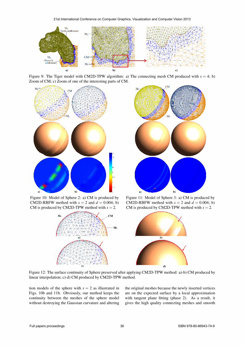
Figure 9: The Tiger model with CM2D-TPW algorithm: a) The connecting mesh CM produced with s = 4; b)Zoom of CM; c) Zoom of one of the interesting parts of CM.

Figure 10: Model of Sphere 2: a) CM is produced byCM2D-RBFW method with s = 2 and d = 0.004; b)CM is produced by CM2D-TPW method with s = 2.

Figure 11: Model of Sphere 3: a) CM is produced byCM2D-RBFW method with s = 2 and d = 0.004; b)CM is produced by CM2D-TPW method with s = 2.

Figure 12: The surface continuity of Sphere preserved after applying CM2D-TPW method: a)-b) CM produced bylinear interpolation; c)-d) CM produced by CM2D-TPW method.

tion models of the sphere with s = 2 as illustrated inFigs. 10b and 11b. Obviously, our method keeps thecontinuity between the meshes of the sphere modelwithout destroying the Gaussian curvature and altering

the original meshes because the newly inserted verticesare on the expected surface by a local approximationwith tangent plane fitting (phase 2). As a result, itgives the high quality connecting meshes and smooth



Model CM Edist Emax Runtime (secs)V F RBFW TPW RBFW TPW RBFW TPW

Sphere 1 38 40 0.9265 0.7581 2.3663 2.0479 0.4061 0.3159Sphere 2 159 240 0.2022 0.0646 0.4861 0.2216 0.4592 0.3762Sphere 3 639 960 0.034 0.0153 0.0578 0.0293 1.3859 0.917Sphere 4 2641 3963 0.0634 0.0329 0.1453 0.0764 14.4955 9.0221

Table 1: Comparison of errors and runtimes of CM2D-RBFW and CM2D-TPW algorithms for spheres with centerc = (0,0,0), and radius R = 10; the numbers of vertices and faces of CM are in columns V and F.

surfaces. Then, we also use CM2D-RBFW method onthese models (see Fig. 10a and Fig. 11a).

Figs. 12a-b show the connecting mesh and surface CMproduced with linear interpolation by applying phase 1and 3 of CM2D-TPW algorithm without phase 2. Asa result, CM is hyperbolic and the surface continuity isnot guaranteed. While Figs.12c-d present CM after ap-plying all phases of the algorithm. Obviously, CM2D-TPW method generates a smooth surface with naturalshape where continuity between meshes is preserved.

According to these experimental results, we can see thatCM2D-TPW method gives better results compared toCM2D-RBFW method since errors to the real surfaceare smaller and Gaussian curvatures are much better re-spected. In addition, a well-known drawback of RBFbased reconstruction methods is the difficulty to pro-vide abrupt changes in a small distance (see [Luo08]).It requires much more estimation which includes esti-mating the linear constraints on the control vertices aswell as the off-surface constraints to construct and solvea linear system for each interpolated vertex. Therefore,the time of computation will be inevitably longer orthe memory requirements may exceed the capacity ofthe computer. As a consequence, the runtime of thisalgorithm is rapidly increasing when the vertex num-bers of the models increase as illustrated in Table 1.We have applied the algorithm to various 3D objectswith complex shapes. The runtime increases quadrati-cally. Moreover, the most critical disadvantage is thatit is very important for the user to make a decision onthe choice of the basis functions and the user parametervalues, i.e d-the signed distance and h-the shape param-eter. This leads to the fact that the user chooses themby a rather costly trial and performs their numerical ex-periments over and over again until they end up with asatisfactory result consisting of the well-chosen valuesand an interpolated surface with a natural shape. In or-der to overcome these disadvantages, we have proposeda more reliable method to join two meshes. It pro-duces surfaces of good approximation, computationallymore efficient and occupied less memory compared tothe C2MD-RBFW method. The memory storage willnot become a problem when the numbers of verticesof the given meshes are large in practical applications.The computing time of this algorithm is smaller thanCM2D-RBFW algorithm as shown in Table 1 while we

have not taken into account the execution time of ex-periments for values d, h in CM2D-RBFW method.

7 CONCLUSIONWe have introduced a new simple and efficient meshconnection method which produces a high quality con-necting mesh and finally a smooth surface. The meshis changed gradually in resolution from one area to theother one. CM2D-TPW method joins two meshes withdifferent resolutions while maintaining the surface con-tinuity and not destroying local curvatures. It keeps theoriginal boundaries of the meshes and the closest facesaround these boundaries while connecting them. Theadvantages of this method are: 1) It is simple, efficient,and local; 2) It generates smooth connecting surfaces;3) There is no need to solve a system of linear equa-tions. As a consequence, our algorithm is then numeri-cally stable. These features make CM2D-TPW methodbecome feasible and suitable for designing, joining andmodeling 3D objects with complex shapes. Thus, it canbe extended to applications related to pasting meshes,and filling holes.

ACKNOWLEDGMENTSWe would like to thank all reviewers for their valuablecomments which help us to improve the paper.

8 REFERENCES[Ale03] M. Alexa, J. Behr, D. Cohen-Or, S. Fleish-

man, D. Levin, and C. T. Silva. Computing andrendering point set surfaces. IEEE Trans. on Vi-sualization and Comp. Graph.,9(1):3-15,2003.

[Ale04] M. Alexa, S. Rusinkiewicz, M. Alexa, and A.Adamson. On normals and projection operatorsfor surfaces defined by point sets. In Eurograph.Symp. on Point-Based Graph., p. 149-155, 2004.

[Ber02] M. Bertram. Biorthogonal wavelets for subdi-vision volumes. In Proc. of the SMA’02, p. 72-82,New York, USA, 2002. ACM.

[Ber04a] M. Bertram, M. A. Duchaineau, B. Hamann,and K. I. Joy. Generalized B-spline subdivision-surface wavelets for geometry compression.IEEE, 10:326-338, 2004.

[Bra06] John Branch, Flavio Prieto, and PierreBoulanger. Automatic hole-filling of triangular



meshes using local Radial Basis Function. In3DPVT, pages 727-734, 2006.

[Bar95] Gill Barequet and Micha Sharir. Filling gapsin the boundary of a polyhedron. Comp. AidedGeometric Design, 12(2):207-229, 1995.

[Car01] J. C. Carr, R. K. Beatson, J. B. Cherrie, T. J.Mitchell, W. R. Fright, B. C. McCallum, and T. R.Evans. Reconstruction and representation of 3Dobjects with radial basis functions. In Proc. of theSIGGRAPH’01, p.67-76, ACM, NY, USA, 2001.

[Cat98] E. Catmull and J. Clark. Recursively generatedB-spline surfaces on arbitrary topological meshes,p.183-188. ACM, NY, USA, 1998.

[Cas05] G. Casciola, D. Lazzaro, L. B. Monte-fusco,and S. Morigi. Fast surface reconstruction andhole filling using radial basis functions, numericalalgorithms, 2005.

[Dyn90] N. Dyn, D. Levin, and J. A. Gregory. A But-terfly subdivision scheme for surface interpola-tion with tension control. ACM Transactions onGraphics, 9:160-169, 1990.

[Doo78] D. Doo and M. Sabin. Behaviour of recursivesubdivision surfaces near extraordinary points.CAD, 10(6):356-360, 1978.

[Dor97] Chitra Dorai, John Weng, and Anil K. Jain.Optimal registration of object views using rangedata. IEEE Trans. Pattern Anal. Mach. Intell.,19(10):1131-1138, 1997.

[Fu04] Hongbo Fu, Chiew-Lan Tai, and HongxinZhang. Topology free cut and paste editing overmeshes. In GMP, pages 173-184, 2004.

[Hus10] N. A. Husain, A. Bade, R. Kumoi, and M. S.M. Rahim. Iterative selection criteria to improvesimple adaptive subdivision surfaces method inhandling cracks for triangular meshes. In Pro. ofthe VRCAI’10, p. 207-210, USA, 2010. ACM.

[Hop92] Hugues Hoppe, Tony DeRose, TomDuchamp, John McDonald, and Werner Stuetzle.Surface reconstruction from unorganized points.SIGGRAPH Comput. Graph., 26:71-78, 1992.

[Jia07] D. Jiang and N. F. Stewart. Reliable joining ofsurfaces for combined mesh-surface models. InPro. of 21st ECMS, pages 297-303, 2007.

[Kho00] A. Khodakovsky, P. Schröder, and W.Sweldens. Progressive geometry compression. InProc. of the Comp. Graph. Conf., SIGGRAPH,pages 271-278, New York, 2000. ACM.

[Lev03] D. Levin. Mesh-independent surface inter-polation. In Geometric Modeling for ScientificVisualization, volume 2, pages 37-49, 2003.

[Loo87] Charles Loop. Smooth subdivision surfacesbased on triangles. Master’s thesis, University ofUtah, 1987.

[Lou97] M. Lounsbery, T. DeRose, and J. D. Warren.Multiresolution analysis for surfaces of arbitrarytopological type. ACM, p.34-73, 1997.

[Luo08] W. Luo, M. C. Taylor, and S. R. Parker. Acomparison of spatial interpolation methods toestimate continuous wind speed surfaces usingirregularly distributed data from England andWales. Inter. Journal of Climatology, 28(7):947-959, 2008.

[Mal98] S. G. Mallat. A Wavelet Tour of Signal Pro-cessing. Academic Press, 1998.

[Hus11] N. A. Husain, M. S. M. Rahim, and A. Bade.Iterative process to improve simple adaptive sub-division surfaces method with Butterfly scheme.In World Academy of Science, Engineering andTech., pages 622-626, 2011.

[Ols08] L. J. Olsen and F. F. Samavati. A discrete ap-proach to multiresolution curves and surfaces. InProc. of the 2008 International Conf. on Compu-tational Sciences and Its App., p. 468-477, Wash-ington, DC, USA, 2008. IEEE.

[Phan12] Anh-Cang Phan, R. Raffin, and M. Daniel.Mesh connection with RBF local interpolationand wavelet transform. In Pro. of the SoICT ’12,pages 81-90, New York, NY, USA, 2012. ACM.

[Pak07] H. Pakdel and F. F. Samavati. Incrementalsubdivision for triangle meshes. In Journal ofComputational Science Engineering, vol 3, No. 1,pages 80-92, 2007.

[Sam04] F. F. Samavati. Local filters of B-splinewavelets. In Proc. of International Workshop onBiometric Tech. 2004, p.105-110, 2004.

[Sar11] Scott A. Sarra. Radial basis function approx-imation methods with extended precision float-ing point arithmetic. Engineering Analysis withBoundary Elements, 35(1):68-76, 2011.

[Sto96] E. J. Stollnitz, T. D. DeRose, and D. H.Salesin. Wavelets for Computer Graphics: Theoryand Applications. Morgan Kaufmann Pub., 1996.

[Suc09] N. Suciati and K. Harada. Wavelets-basedmultiresolution surface as framework for edit-ing the global and local shapes. Inter. Journal ofComp. Science and Net. Security, 5:77-83, 2009.

[Swe96b] W. Sweldens and P. Schröder. Building yourown wavelets at home. In Waveletes in ComputerGraphics, p. 15-87, 1996.

[Swe98] Wim Sweldens. The lifting scheme: A con-struction of second generation wavelets. SIAM J.Math. Anal., 29:511-546, 1998.

[Zor00] Denis Zorin and P. Schröder. Subdivision forModeling and Animation. Technical report, SIG-GRAPH 2000, Course Notes, 2000.



joining meshes with a local approximation and a wavelet

Documents