JOHANNES KEPLER UNIVERSITY LINZ

Institute of Computational Mathematics

On the Best Uniform Approximation byLow-Rank Matrices

Irina GeorgievaInstitute of Mathematics and Informatics

Bulgarian Academy of SciencesAcad. G. Bonchev St., Bl. 8, 1113 Sofia, Bulgaria

Clemens HofreitherInstitute of Computational Mathematics, Johannes Kepler University

Altenberger Str. 69, 4040 Linz, Austria

NuMa-Report No. 2016-10 December 2016

A–4040 LINZ, Altenbergerstraße 69, Austria

Technical Reports before 1998:1995

95-1 Hedwig BrandstetterWas ist neu in Fortran 90? March 1995

95-2 G. Haase, B. Heise, M. Kuhn, U. LangerAdaptive Domain Decomposition Methods for Finite and Boundary ElementEquations.

August 1995

95-3 Joachim SchoberlAn Automatic Mesh Generator Using Geometric Rules for Two and Three SpaceDimensions.

August 1995

199696-1 Ferdinand Kickinger

Automatic Mesh Generation for 3D Objects. February 199696-2 Mario Goppold, Gundolf Haase, Bodo Heise und Michael Kuhn

Preprocessing in BE/FE Domain Decomposition Methods. February 199696-3 Bodo Heise

A Mixed Variational Formulation for 3D Magnetostatics and its Finite ElementDiscretisation.

February 1996

96-4 Bodo Heise und Michael JungRobust Parallel Newton-Multilevel Methods. February 1996

96-5 Ferdinand KickingerAlgebraic Multigrid for Discrete Elliptic Second Order Problems. February 1996

96-6 Bodo HeiseA Mixed Variational Formulation for 3D Magnetostatics and its Finite ElementDiscretisation.

May 1996

96-7 Michael KuhnBenchmarking for Boundary Element Methods. June 1996

199797-1 Bodo Heise, Michael Kuhn and Ulrich Langer

A Mixed Variational Formulation for 3D Magnetostatics in the Space H(rot)∩H(div)

February 1997

97-2 Joachim SchoberlRobust Multigrid Preconditioning for Parameter Dependent Problems I: TheStokes-type Case.

June 1997

97-3 Ferdinand Kickinger, Sergei V. Nepomnyaschikh, Ralf Pfau, Joachim SchoberlNumerical Estimates of Inequalities in H

12 . August 1997

97-4 Joachim SchoberlProgrammbeschreibung NAOMI 2D und Algebraic Multigrid. September 1997

From 1998 to 2008 technical reports were published by SFB013. Please seehttp://www.sfb013.uni-linz.ac.at/index.php?id=reports

From 2004 on reports were also published by RICAM. Please seehttp://www.ricam.oeaw.ac.at/publications/list/

For a complete list of NuMa reports seehttp://www.numa.uni-linz.ac.at/Publications/List/

On the Best Uniform Approximation by Low-RankMatrices

Irina Georgieva∗ Clemens Hofreither†

December 7, 2016

Abstract

We study the problem of best approximation, in the elementwise maximum norm, of agiven matrix by another matrix of lower rank. We generalize a recent result by Pinkus thatdescribes the best approximation error in a class of low-rank approximation problems andgive an elementary proof for it. Based on this result, we describe the best approximationerror and the error matrix in the case of approximation by a matrix of rank one less thanthe original one. For the case of approximation by matrices with arbitrary rank, we givelower and upper bounds for the best approximation error in terms of certain submatrices ofmaximal volume. We illustrate our results using 2 × 2 matrices as examples, for which wealso give a simple closed form of the best approximation error.

1 IntroductionWe consider the problem of approximating a given matrix as closely as possible by a matrixof the same size, but lower rank. When measuring the approximation error in the spectral orFrobenius norms, a full description of the best approximation and its error is given in termsof the singular value decomposition [10, 3]. In different matrix norms, very little was knownabout this approximation problem until a recent article by Pinkus [8], where approximation bya class of elementwise norms, and there in particular `1-like norms, was studied. Pinkus derivesexpressions for the best approximation error in such norms and, in particular cases, shows thata best approximating matrix matches the original matrix in a number of rows and columns.

In the present paper, we derive analogues of several of Pinkus’ results for the case of approx-imation in the elementwise maximum norm. In the process, we generalize one core result from[8] and prove it using only known basic results on best approximation, whereas the proof of theoriginal result relied heavily on the theory of n-widths. Building on this result, we obtain anexpression for the best approximation error of a matrix by another one with rank one less, aswell as a characterization of the matrix of best approximation.

For approximation where the difference in ranks is greater than one, we have no closedformula for the best approximation error, but give lower and upper bounds for it involvingcertain submatrices of maximal volumes, that is, with greatest modulus of their determinants.These results are similar to some given by Babaev [1] in the continuous setting. The relevance of∗Institute of Mathematics and Informatics, Bulgarian Academy of Sciences, Acad. G. Bonchev St., Bl. 8, Sofia,

Bulgaria. irina@math.bas.bg†Institute of Computational Mathematics, Johannes Kepler University, Altenberger Str. 69, 4040 Linz, Austria.

chofreither@numa.uni-linz.ac.at

1

submatrices of maximal volume to the problem of low-rank approximation was first establishedby Goreinov and Tyrtyshnikov [4].

The remainder of the paper is structured as follows. In Section 2, we state the low-rankapproximation problem and prove a result on the best approximation error which generalizesa result by Pinkus. In Section 3, we focus on the case of approximating a matrix by anothermatrix of rank one less, where the best approximation error can be described quite closely and weobtain an equioscillation result for the error matrix. In Section 4, we deal with approximationsof arbitrary rank and give lower and upper bounds for the best approximation error in terms ofcertain submatrices of maximal volume. Finally, in Section 5, we illustrate some of our resultsin the simple case of 2× 2-matrices, where we are also able to give a simple closed form for thebest approximation error.

2 Approximation with low-rank matrices

2.1 Problem statementLet A ∈ Rm×n and p, q ∈ [1,∞]. We define the entrywise matrix norm

|A|p,q :=

m∑i=1

n∑j=1

|aij |qp/q

1/p

,

where as usual p = ∞ or q = ∞ means the maximum norm in the corresponding direction.The two most common special cases are the entrywise maximum (or Chebyshev) norm and theFrobenius norm,

|A|max := |A|∞,∞ = maxi,j|aij |, |A|F := |A|2,2 =

∑i,j

a2ij

1/2

.

For vectors, we denote by ‖ · ‖p the usual `p-vector norm.

Definition 1. For p, q ∈ [1,∞] and k ∈ N0, we define the best approximation error

Ekp,q(A) := infrankG≤k

|A−G|p,q,

where G runs over all m× n matrices of rank at most k.

The only completely solved instance of the above best approximation problem is in the Frobe-nius norm | · |F = | · |2,2 (and the spectral norm, which however does not fall into our class ofelementwise norms) [10, 3]. In this case, given the singular value decomposition

A = UΣV >, U ∈ Rm×K , Σ = diag(σ1, . . . , σK), V ∈ Rn×K ,

where K = rankA, both U and V have mutually orthonormal columns, and σ1 ≥ . . . ≥ σK > 0are the singular values of A, the best approximation of rank k ≤ K is given by the truncatedsingular value decomposition

Ak = U diag(σ1, . . . , σk, 0, . . . , 0)V >

and the best approximation error is given by

|A−Ak|2F = σ2k+1 + . . .+ σ2

K .

2

2.2 Characterization of the best approximation errorThe following theorem yields an expression for the best low-rank approximation error in arbitraryelementwise norms. Here and in what follows, for q ∈ [1,∞], we denote its Hölder conjugate byq′ such that 1/q + 1/q′ = 1.

Theorem 1. Let A ∈ Rm×n with rows (ai)mi=1 be of rank n and p, q ∈ [1,∞]. Then the best

approximation error by a matrix of rank k ∈ {0, . . . , n} in the | · |p,q-norm is given by

Ekp,q(A) = infUn−k

∥∥∥∥∥∥∥ maxh∈Un−k‖h‖q′=1

|h · ai|

i=1,...,m

∥∥∥∥∥∥∥p

,

where the infimum runs over all subspaces Un−k ⊂ Rn of dimension n− k.For k = n− 1, we have

En−1p,q (A) = minh6=0

‖Ah‖p‖h‖q′

. (1)

Remark 1. The statement for the case k = n−1 of the above theorem is already given by Pinkusin [8, Corollary 2.3]. However, whereas Pinkus arrived at this result via the theory of n-widths,we give below a more direct proof which relies only on a fundamental result from approximationtheory and allows us to cover also the case k < n− 1. However, our approach does not yield theresult on n-widths which is also a part of [8, Corollary 2.3].

For the proof of Theorem 1, we make use of the following classical characterization of bestapproximation by duality.

Theorem 2 ([12, 2]). Let (X, ‖ · ‖) a normed linear space and U ⊂ X a closed subspace. Thenu ∈ U is a best approximant in U to x ∈ X \ U if and only if there exists a

h ∈ U⊥ := {h ∈ X∗ : 〈h, u〉 = 0 ∀u ∈ U}

with the properties

‖h‖∗ = 1,

〈h, x− u〉 = ‖x− u‖.

Furthermore, the best approximation error is given by

infu∈U‖x− u‖ = sup

h∈U⊥‖h‖∗=1

〈h, x〉.

Here, X∗ denotes the continuous dual, ‖ · ‖∗ the dual norm and 〈·, ·〉 the duality product.Applying this result to the space (Rn, ‖ · ‖p), p ∈ [1,∞], which has dual space (Rn, ‖ · ‖p′),

1/p+ 1/p′ = 1, we immediately obtain the following statements.

Corollary 1. For x ∈ Rn and Uk ⊂ Rn a k-dimensional subspace, let U⊥k ⊂ Rn denote theorthogonal complement to Uk. Then

infu∈Uk

‖x− u‖p = maxh∈U⊥k‖h‖p′=1

|h · x|. (2)

For x ∈ Rn and Un−1 ⊂ Rn a (n − 1)-dimensional subspace, let h ∈ Rn orthogonal to Un−1with ‖h‖p′ = 1. Then

infu∈Un−1

‖x− u‖p = |h · x|. (3)

3

By treating the low-rank matrix approximation problem as a simultaneous approximationproblem for the rows of the matrix, we obtain the following proof.

Proof of Theorem 1. The problem of rank k approximation is equivalent to finding a k-dimensionalsubspace Uk ⊂ Rn and approximating each row in Uk with error

ei := infu∈Uk

‖ai − u‖q, i = 1, . . . ,m. (4)

The total error is then given by‖(e1, . . . , em)‖p.

Thus the first statement follows by using the identity (2) to represent the errors (4).For k = n− 1, we can identify each subspace Un−1 with a vector h ∈ Rn, ‖h‖q′ = 1, which is

orthogonal to Un−1. Thus, from (3) we obtain

En−1p,q (A) = min‖h‖q′=1

‖(|h · ai|)i=1,...,m‖p .

Since the vector (h · ai)i=1,...,m is nothing but Ah, the second statement follows.

3 Approximation with rank reduced by oneDue to the simple form of the best approximation error (1) given in the case k = n − 1 inTheorem 1, much more can be said for approximation of a matrix of rank n by one of rank atmost n− 1.

3.1 Description of the best approximation errorWe introduce, for any square matrix B of size n, a quantity αp,q(B) which we will show to bea lower bound for the best approximation error in the | · |p,q norm by a matrix of rank at mostn− 1. As we will see, in certain cases this quantity coincides with the best approximation error.

Definition 2. For any square matrix B ∈ Rn×n and any p, q ∈ [1,∞], we let

αp,q(B) :=

1

|B−1|p,q, detB 6= 0,

0, detB = 0.

In the following, we let 〈n〉 := {1, . . . , n}. For a matrix A ∈ Rm×n and vectors of indicesI ⊂ 〈m〉, J ⊂ 〈n〉, we write AI,J ∈ R|I|×|J| for the submatrix of A formed by taking the rowsfrom the index vector I and the columns from the index vector J . We denote the set of all squaresubmatrices of A with size k by

Sk(A) := {AI,J : I ⊂ 〈m〉, J ⊂ 〈n〉, |I| = |J | = k}.

The rank of a nonzero matrix can be characterized as

rank(A) = max{k ∈ N : ∃Bk ∈ Sk(A) : detBk 6= 0}.

In addition to the entrywise matrix norms | · |p,q, we will also make use of the operator norms

‖A‖p,q := maxx6=0

‖Ax‖p‖x‖q

= max‖x‖q=1

‖Ax‖p.

The following simple lemma gives a relation between these two classes of norms. It is notnew, but we prove it here for the sake of completeness.

4

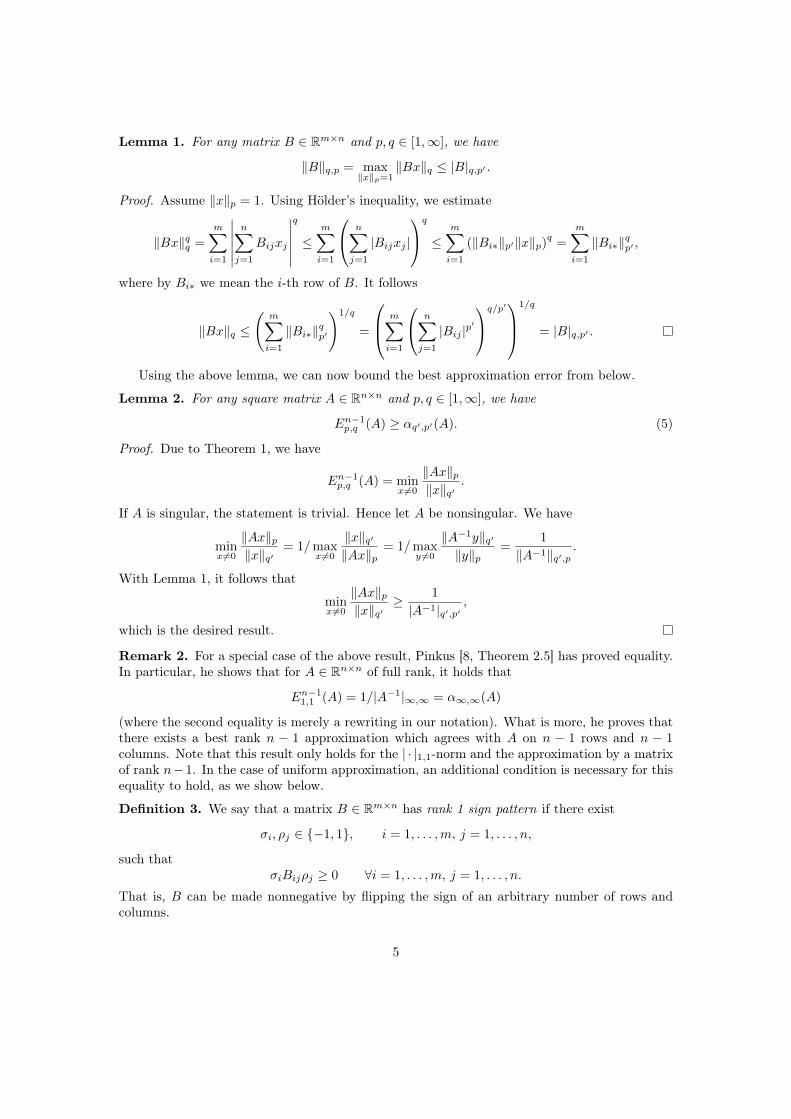
Lemma 1. For any matrix B ∈ Rm×n and p, q ∈ [1,∞], we have

‖B‖q,p = max‖x‖p=1

‖Bx‖q ≤ |B|q,p′ .

Proof. Assume ‖x‖p = 1. Using Hölder’s inequality, we estimate

‖Bx‖qq =

m∑i=1

∣∣∣∣∣∣n∑j=1

Bijxj

∣∣∣∣∣∣q

≤m∑i=1

n∑j=1

|Bijxj |

q

≤m∑i=1

(‖Bi∗‖p′‖x‖p)q =

m∑i=1

‖Bi∗‖qp′ ,

where by Bi∗ we mean the i-th row of B. It follows

‖Bx‖q ≤

(m∑i=1

‖Bi∗‖qp′

)1/q

=

m∑i=1

n∑j=1

|Bij |p′

q/p′

1/q

= |B|q,p′ .

Using the above lemma, we can now bound the best approximation error from below.

Lemma 2. For any square matrix A ∈ Rn×n and p, q ∈ [1,∞], we have

En−1p,q (A) ≥ αq′,p′(A). (5)

Proof. Due to Theorem 1, we have

En−1p,q (A) = minx 6=0

‖Ax‖p‖x‖q′

.

If A is singular, the statement is trivial. Hence let A be nonsingular. We have

minx6=0

‖Ax‖p‖x‖q′

= 1/maxx 6=0

‖x‖q′‖Ax‖p

= 1/maxy 6=0

‖A−1y‖q′‖y‖p

=1

‖A−1‖q′,p.

With Lemma 1, it follows that

minx 6=0

‖Ax‖p‖x‖q′

≥ 1

|A−1|q′,p′,

which is the desired result.

Remark 2. For a special case of the above result, Pinkus [8, Theorem 2.5] has proved equality.In particular, he shows that for A ∈ Rn×n of full rank, it holds that

En−11,1 (A) = 1/|A−1|∞,∞ = α∞,∞(A)

(where the second equality is merely a rewriting in our notation). What is more, he proves thatthere exists a best rank n − 1 approximation which agrees with A on n − 1 rows and n − 1columns. Note that this result only holds for the | · |1,1-norm and the approximation by a matrixof rank n−1. In the case of uniform approximation, an additional condition is necessary for thisequality to hold, as we show below.

Definition 3. We say that a matrix B ∈ Rm×n has rank 1 sign pattern if there exist

σi, ρj ∈ {−1, 1}, i = 1, . . . ,m, j = 1, . . . , n,

such thatσiBijρj ≥ 0 ∀i = 1, . . . ,m, j = 1, . . . , n.

That is, B can be made nonnegative by flipping the sign of an arbitrary number of rows andcolumns.

5

For this class of matrices and the maximum norm, the inequality in Lemma 2 becomes anequality, giving us a characterization of the best approximation error. This is the statement ofthe following theorem. Here and in the sequel we write Ekmax for Ek∞,∞.

Theorem 3. For A ∈ Rn×n of full rank whose inverse has rank 1 sign pattern, we have

En−1max (A) = α1,1(A).

Proof. As in the proof of Lemma 2, we have

En−1max (A) = 1/‖A−1‖1,∞.

For convenience, denote B := A−1. Its norm is given by

‖B‖1,∞ = max‖x‖∞=1

‖Bx‖1 = max‖x‖∞=1

n∑i=1

∣∣∣∣∣∣n∑j=1

Bijxj

∣∣∣∣∣∣ . (6)

By assumption, we have σi, ρj ∈ {−1, 1} such that, for fixed i, the products Bijρj are eithernonnegative or nonpositive for all j. Therefore, the maximum in (6) is clearly attained for thechoice xj := ρj , and it follows

‖B‖1,∞ =

n∑i=1

n∑j=1

|Bij | = |B|1,1 = 1/α1,1(A).

Remark 3. By inspection of the proof, it becomes clear that A−1 having rank 1 sign patternis both a sufficient and a necessary condition for (5) to become an equality when using themaximum norm.

3.2 Properties of the error matrixWe now derive some properties of the error matrix between A and its best approximation withlower rank. For this, we first prove a characterization of minimizers of the type of expressionsappearing in (1).

Lemma 3. Let A ∈ Rn×n of full rank. Let p ∈ {1,∞} and q ∈ [1,∞]. There exists a minimizerh∗ ∈ Rn for

minh 6=0

‖Ah‖p‖h‖q

with ‖h∗‖q = 1 and the following properties.

• For p = 1, it satisfies Ah∗ = ±cej for some j = 1, . . . , n, where c > 0 and ej denotes theunit vector in the positive direction of the j-th coordinate axis.

• For p =∞, it satisfies Ah∗ = c(±1, . . . ,±1) for some c > 0.

Proof. Since‖Ah‖p‖h‖q

=

(‖A−1(Ah)‖q‖Ah‖p

)−1,

the minimum for ‖Ah‖p‖h‖q is attained at h∗ ∈ Rn \ {0} if and only if the maximum for ‖A−1g‖q‖g‖p is

attained at g∗ = Ah∗. Therefore we can equivalently consider

max‖g‖p≤1

‖A−1g‖q.

6

We note that ‖A−1g‖q is a convex function of g for all q ∈ [1,∞]. Therefore, its maximum overthe bounded, convex polytope {‖g‖p ≤ 1} is attained at an extreme point of that polytope (see,e.g., [9, Corollary 32.3.4]). Therefore, for p = 1, the maximizing argument has the form g∗ = ±ejfor some j = 1, . . . , n. For p =∞, it has the form g∗ = (±1, . . . ,±1) ∈ Rn. The minimum in theoriginal expression is attained at h∗ = A−1g∗, i.e.,

minh6=0

‖Ah‖p‖h‖q

=‖g∗‖p‖A−1g∗‖q

.

In both cases, the constant c is determined by c = 1/‖A−1g∗‖q.

Using the above lemma, we can now prove certain properties of the error matrices in bestlow-rank approximation. In particular, for p = 1, the error is zero on n − 1 rows, whereas forp = q = ∞, the error matrix equioscillates elementwise, that is, all of its entries have the samemodulus.

Theorem 4. Let A ∈ Rn×n of full rank. Let p ∈ {1,∞} and q ∈ [1,∞]. There exists a bestapproximation matrix G ∈ Rn×n of rank n− 1 satisfying

En−1p,q (A) = |A−G|p,q

with the following properties.

• If p = 1, the matrix G agrees with A on n− 1 rows.

• If p =∞, the row-wise error is constant, i.e., for the rows ai and gi of A and G respectively,it holds

‖ai − gi‖q = En−1∞,q (A) ∀i = 1, . . . , n. (7)

If in addition q =∞, then the error matrix equioscillates in the sense that

|aij − gij | = En−1∞,∞(A) ∀i, j = 1, . . . , n. (8)

Proof. Let h∗ ∈ Rn be a minimizer as described in Lemma 3 for

‖Ah‖p‖h‖q′

.

Let G be the best approximation matrix constructed as in the proof of Theorem 1, where each rowgi is the best approximation to ai with respect to the norm ‖·‖q in Un−1 := {x ∈ Rn : x ·h∗ = 0}.It was shown there that the vector of row-wise errors e ∈ Rn has the components

ei := ‖ai − gi‖q = |[Ah∗]i|, i = 1, . . . , n.

If p = 1, due to Lemma 3, the vector Ah∗ has exactly one non-zero component. This impliesthat the error ei is zero in n− 1 rows, which proves the desired statement.

If p = ∞, due to Lemma 3, the components of the vector Ah∗ all have equal magnitude,which shows that ei is constant, proving (7). If, in addition, q = ∞, recall that each row gi ischosen as a minimizer of

mingi∈Un−1

‖ai − gi‖∞.

Due to standard results on best uniform approximation in the linear space Un−1, (see, e.g., [12,Chapter II, Theorem 1.3]), the error ai − gi equioscillates in the sense that

|aij − gij | = ‖ai − gi‖∞ = En−1∞,∞(A) ∀i, j = 1, . . . , n.

7

Remark 4. The case p = 1 of the above theorem was already proved by Pinkus [8, Proposition2.4] by different means. Even more, for p = q = 1, he proved that there exists a best approxi-mation matrix which agrees with A on n − 1 rows and n − 1 columns. The result for p = ∞ isnew.

4 Approximations with arbitrary rankIn the case where the difference in rank between A and its approximation is greater than one,we cannot give an explicit characterization of the best approximation error; instead, we providelower and upper bounds. To this end, we first recall some results from the theory of skeletonapproximations.

4.1 Skeleton approximationRecall that we denoted 〈n〉 := {1, . . . , n}. Given a matrix A ∈ Rm×n, assume we have row andcolumn indices I = (i1, . . . , ik) and J = (j1, . . . , jk) such that the submatrix A := AI,J situatedon rows I and columns J is nonsingular. With the matrices

C := A〈m〉,J ∈ Rm×k, R := AI,〈n〉 ∈ Rk×n

containing k columns and rows of A, respectively, we can define a rank k approximation

CA−1R ∈ Rm×n

which agrees with A on the k rows I and the k columns J . If A has rank k, then A = CA−1R.These facts are easily verified by the Schur complement factorization formulae (see, e.g., [7]). Atheoretical framework for skeleton and pseudo-skeleton approximation is given in [6].

We define, for i ∈ 〈m〉, j ∈ 〈n〉, the matrix

Ek(i, j) :=

Ai,j Ai,j1 . . . Ai,jkAi1,j Ai1,j1 . . . Ai1,jk...

.... . .

...Aik,j Aik,j1 . . . Aik,jk

∈ R(k+1)×(k+1)

which contains A in its lower right block. The following representation of the error matrixresulting from skeleton approximation is the discrete version of an analogous identity for functionsgiven by Schneider [11].

Lemma 4. Let index vectors I and J be given and assume that AI,J is nonsingular. Then theentries of the error matrix for the skeleton approximation

E = A−A〈m〉,J(AI,J)−1AI,〈n〉

are given by

Ei,j =det Ek(i, j)

detAI,J, i = 1, . . . ,m, j = 1, . . . , n.

Proof. By developing the determinant of Ek(i, j) along the first row and then the resulting de-terminants along the first column, we obtain

det Ek(i, j) = Aij detAI,J −k∑

α,β=1

(−1)α+β detB(α, β)Ai,jβAiα,j ,

8

where B(α, β) ∈ R(k−1)×(k−1) denotes the matrix AI,J with the α-th row and the β-th columnremoved. Thus we obtain

det Ek(i, j)

detAI,J= Aij −

k∑α,β=1

Ai,jβ(−1)α+β detB(α, β)

detAI,JAiα,j .

Since the entries of the inverse matrix are given by the well-known cofactor identity

[A−1I,J ]β,α =(−1)α+β detB(α, β)

detAI,J,

the statement follows.

4.2 Upper and lower bounds on the approximation errorBefore we derive approximation error bounds, we need the simple result that submatrices can beapproximated at least as well as the whole matrix.

Lemma 5. Let A ∈ Rm×n. For any submatrix B of A, we have

Ekp,q(B) ≤ Ekp,q(A).

Proof. Let GA ∈ Rm×n be a matrix of rank at most k which realizes the best approximationerror to A. Such a matrix always exists since the set of matrices of rank at most k is closed. Bydeleting the appropriate rows and columns from GA, we obtain a matrix GB which has the samesize as B and rank at most k. Clearly, Ekp,q(B) ≤ |B −GB |p,q ≤ |A−GA|p,q = Ekp,q(A).

The next result generalizes Lemma 2 to the case of approximation by matrices with arbitraryrank.

Lemma 6. Let A ∈ Rm×n and p, q ∈ [1,∞]. Then

Ek−1p,q (A) ≥ maxB∈Sk(A)

αq′,p′(B).

Proof. For any submatrix B ∈ Sk(A), using Lemma 2 we have

Ek−1p,q (B) ≥ αq′,p′(B).

The statement then follows from Lemma 5.

Using Lemma 6, we can now prove a lower and upper bound for the best approximationerror with low rank matrices in the maximum norm. The quantity which we use in the lowerand upper bounds involves the maximally achievable modulus of determinants of submatrices ofcertain sizes. Goreinov and Tyrtyshnikov [4] use such “maximal volumes” to derive some errorestimates for skeleton approximation of matrices. In the following, we follow their nomenclatureand call the modulus of the determinant the “volume” of a matrix.

Let

βk(A) :=maxBk∈Sk(A) |detBk|

maxBk−1∈Sk−1(A) |detBk−1|,

that is, the quotient of the maximal volumes obtainable in a size k and a size k − 1 submatrix,respectively. If the denominator is zero, then so is the numerator and we set βk(A) := 0 in thiscase. If k = 1, the denominator is considered to be 1 so that β1(A) = |A|max.

9

The following result is similar to one obtained by Babaev [1] in the continuous setting usinghis technique of exact annihilators. It is possible to employ this proof technique also in ourdiscrete setting. However, we found that using the approximation result stated in Theorem 1yields a much shorter proof.

Theorem 5. Let A ∈ Rm×n and k ≤ min{m,n} an integer. We have the bounds

1/k2βk(A) ≤ Ek−1max(A) ≤ βk(A).

Proof. We first prove the lower bound. Let Bk ∈ Sk(A) be of maximal volume. From Lemma 6we have

Ek−1max(A) ≥ α1,1(Bk).

If Bk is singular, then A has rank at most k − 1 and the statement is trivial. Otherwise, usingthe cofactor identity for the entries of B−1k , we obtain

α1,1(Bk) =1

|B−1k |1,1=

|detBk|∑C∈Sk−1(Bk)

|detC|≥ |detBk|k2 maxC∈Sk−1(Bk) |detC|

≥ |detBk|k2 maxBk−1∈Sk−1(A) |detBk−1|

= 1/k2βk(A).

To prove the upper bound, we let Bk−1 ∈ Sk−1(A) and Bk ∈ Sk(A) be of maximal volume.We denote by I = (i1, . . . , ik−1) and J = (j1, . . . , jk−1) the rows and columns on which Bk−1 islocated within A, that is, Bk−1 = AI,J . We construct the skeleton approximation

Ak−1 = A〈m〉,J(Bk−1)−1AI,〈n〉 ∈ Rm×n,

which has rank at most k − 1. Therefore,

Ek−1max(A) ≤ |A−Ak−1|max.

Due to Lemma 4, the entries of the error matrix satisfy

|A−Ak−1|ij =|det Ek−1(i, j)||detBk−1|

(9)

Since Ek−1(i, j) is a submatrix of size k × k of A and Bk is the maximal volume submatrix ofthat size, we have

|det Ek−1(i, j)| ≤ |detBk|

and thus|A−Ak−1|max ≤ βk(A), (10)

which finishes the proof.

Remark 5. The low-rank approximation Ak−1 used in the above proof is just the skeleton ap-proximation where the skeleton component is chosen as the submatrix Bk−1 of maximal volume,cf. [6]. Equation (10) thus also gives an error estimate for this approximation method, and bycombining it with the lower bound from Theorem 5 we obtain the quasi-optimality estimateproven in [5],

|A−Ak−1|max ≤ k2Ek−1max(A).

10

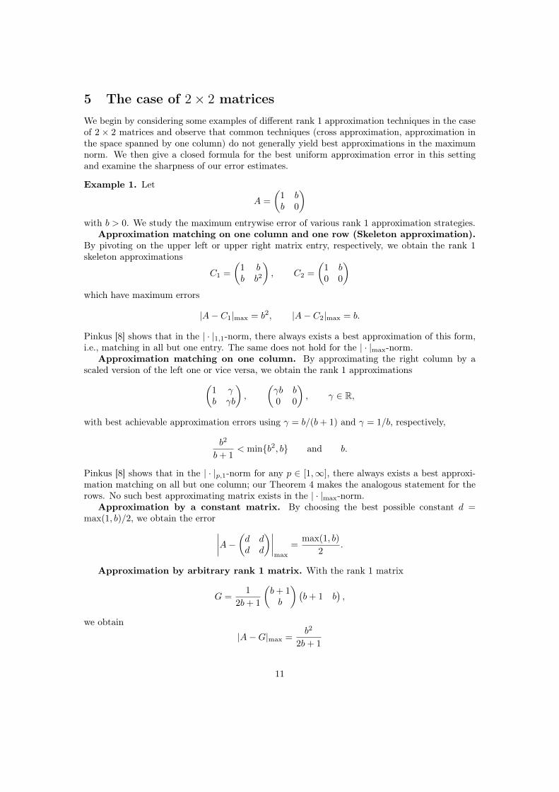
5 The case of 2× 2 matricesWe begin by considering some examples of different rank 1 approximation techniques in the caseof 2 × 2 matrices and observe that common techniques (cross approximation, approximation inthe space spanned by one column) do not generally yield best approximations in the maximumnorm. We then give a closed formula for the best uniform approximation error in this settingand examine the sharpness of our error estimates.

Example 1. Let

A =

(1 bb 0

)with b > 0. We study the maximum entrywise error of various rank 1 approximation strategies.

Approximation matching on one column and one row (Skeleton approximation).By pivoting on the upper left or upper right matrix entry, respectively, we obtain the rank 1skeleton approximations

C1 =

(1 bb b2

), C2 =

(1 b0 0

)which have maximum errors

|A− C1|max = b2, |A− C2|max = b.

Pinkus [8] shows that in the | · |1,1-norm, there always exists a best approximation of this form,i.e., matching in all but one entry. The same does not hold for the | · |max-norm.

Approximation matching on one column. By approximating the right column by ascaled version of the left one or vice versa, we obtain the rank 1 approximations(

1 γb γb

),

(γb b0 0

), γ ∈ R,

with best achievable approximation errors using γ = b/(b+ 1) and γ = 1/b, respectively,

b2

b+ 1< min{b2, b} and b.

Pinkus [8] shows that in the | · |p,1-norm for any p ∈ [1,∞], there always exists a best approxi-mation matching on all but one column; our Theorem 4 makes the analogous statement for therows. No such best approximating matrix exists in the | · |max-norm.

Approximation by a constant matrix. By choosing the best possible constant d =max(1, b)/2, we obtain the error∣∣∣∣A− (d d

d d

)∣∣∣∣max

=max(1, b)

2.

Approximation by arbitrary rank 1 matrix. With the rank 1 matrix

G =1

2b+ 1

(b+ 1b

)(b+ 1 b

),

we obtain

|A−G|max =b2

2b+ 1

11

which is better than all previous approximations. In fact, we have α1,1(A) = b2

2b+1 , and thus itfollows from Lemma 2 that G is the best rank 1 approximation in the | · |max-norm. The errormatrix

A−G =b2

2b+ 1

(−1 11 −1

)equioscillates in the sense of Theorem 4.

We point out that an invertible 2×2 matrix, due to the way its inverse is formed, has a rank 1sign pattern (in the sense of Definition 3) if and only if its inverse has a rank 1 sign pattern. ThusA satisfies the assumptions of Theorem 3, which is another way to show that α1,1(A) = b2

2b+1 isits best approximation error.

The following theorem gives a closed formula for the best uniform approximation error of a2× 2 matrix by a rank 1 matrix.

Theorem 6. A nonsingular real matrix A =

(a bc d

)has uniform best approximation error

E1max(A) =

|detA|max{|a+ c|+ |b+ d|, |a− c|+ |b− d|}

by a matrix of rank 1 or less.

Proof. From Theorem 1, we have

E1max(A) = min

h 6=0

‖Ah‖∞‖h‖1

.

As in the proof of Lemma 3, it follows that

E1max(A) = min

g 6=0

‖g‖∞‖A−1g‖1

=

(maxg 6=0

‖A−1g‖1‖g‖∞

)−1and that the maximum is attained in one of the four corners of [−1, 1]2. Since

A−1 =1

detA

(d −b−c a

),

the statement follows by considering the four cases

max{‖A−1 ( 1

1 ) ‖1, ‖A−1(−1

1

)‖1, ‖A−1

(1−1)‖1, ‖A−1

(−1−1)‖1},

of which the first and last as well as the second and third have identical values.

Since α1,1(A) = | detA||a|+|b|+|c|+|d| as one can compute directly, and recalling that an invertible

2× 2 matrix has a rank 1 sign pattern if and only if its inverse does, Theorem 6 illustrates thatthe condition given in Definition 3 is both necessary and sufficient for the statement of Theorem 3to hold, i.e., for the best approximation error to be equal to α1,1(A), in the 2 × 2 setting. Thefollowing example illustrates a case where the rank 1 sign pattern condition does not hold andtherefore the inequality in Lemma 2 is strict, i.e., the best approximation error is strictly greaterthan α1,1(A).

Example 2. Let A =

(1 11 −1

). Then α1,1(A) = 1

2 . However, Theorem 6 shows that the best

rank 1 approximation G has |A−G|max = 1 (realized, for instance, by the zero matrix).

12

Remark 6. For A =

(a bc d

)of full rank, we have

E1max(A) =

|detA|max{|a+ c|+ |b+ d|, |a− c|+ |b− d|}

, β2(A) =|detA|

max{|a|, |b|, |c|, |d|}.

In Theorem 5, which holds for approximations with arbitrary ranks, we proved the lower andupper bounds

14β2(A) ≤ E1

max(A) ≤ β2(A).

Without loss of generality, assume that a is the maximum entry of A in modulus. If the upperbound in the above estimate were to be sharp, we would have

max{|a+ c|+ |b+ d|, |a− c|+ |b− d|} = |a|.

If c 6= 0, the above maximum is greater than |a|. If c = 0, the only way to achieve equality is bysetting b = d = 0, in which case A does not have full rank.

For the lower bound in Theorem 5 to be sharp, we would require

4|a| = max{|a+ c|+ |b+ d|, |a− c|+ |b− d|},

and by similar arguments, one easily sees that this cannot hold if A has full rank.This shows that, in the case of 2 × 2 matrices of full rank, both the lower and the upper

bounds in Theorem 5 are never sharp, i.e., we have

14β2(A) < E1

max(A) < β2(A).

AcknowledgmentsThe authors would like to thank Matúš Benko (JKU Linz) for helpful discussions.

The authors acknowledge the support by Grant DNTS-Austria 01/6 funded by the BulgarianNational Science Fund. The second author was supported by the National Research Network“Geometry + Simulation” (NFN S117, 2012–2016), funded by the Austrian Science Fund (FWF).

References[1] M.-B. A. Babaev. Best approximation by bilinear forms. Mathematical Notes, 46(2):588–596,

1989. doi: 10.1007/BF01137621.

[2] R.A. DeVore and G.G. Lorentz. Constructive Approximation, volume 303 of Grundlehrender mathematischen Wissenschaften. Springer Berlin Heidelberg, 1993. ISBN 978-3-540-50627-0.

[3] C. Eckart and G. Young. The approximation of one matrix by another of lower rank.Psychometrika, 1(3):211–218, 1936. ISSN 1860-0980. doi: 10.1007/BF02288367.

[4] S. A. Goreinov and E. E. Tyrtyshnikov. The maximal-volume concept in approximation bylow-rank matrices. Contemporary Mathematics, 280:47–52, 2001.

[5] S. A. Goreinov and E. E. Tyrtyshnikov. Quasioptimality of skeleton approximation of amatrix in the Chebyshev norm. Doklady Mathematics, 83(3):374–375, 2011. ISSN 1531-8362. doi: 10.1134/S1064562411030355.

13

[6] S. A. Goreinov, E. E. Tyrtyshnikov, and N. L. Zamarashkin. A theory of pseudoskeletonapproximations. Linear Algebra and its Applications, 261(1):1–21, 1997. doi: 10.1016/S0024-3795(96)00301-1.

[7] R. A. Horn and F. Zhang. Basic properties of the Schur complement. In F. Zhang, editor,The Schur Complement and Its Applications, pages 17–46. Springer US, Boston, MA, 2005.ISBN 978-0-387-24273-6. doi: 10.1007/0-387-24273-2_2.

[8] A. Pinkus. On best rank n matrix approximations. Linear Algebra and its Applications, 437(9):2179–2199, 2012. ISSN 0024-3795. doi: 10.1016/j.laa.2012.05.016.

[9] R. T. Rockafellar. Convex Analysis. Princeton University Press, Princeton, N.J., 1970.ISBN 0691015864.

[10] E. Schmidt. Zur Theorie der linearen und nichtlinearen Integralgleichungen. MathematischeAnnalen, 63(4):433–476, 1907. ISSN 1432-1807. doi: 10.1007/BF01449770.

[11] J. Schneider. Error estimates for two-dimensional cross approximation. J. Approx. Theory,162(9):1685–1700, September 2010. ISSN 0021-9045. doi: 10.1016/j.jat.2010.04.012.

[12] I. Singer. Best Approximation in Normed Linear Spaces by Elements of Linear Subspaces,volume 171 of Grundlehren der mathematischen Wissenschaften. Springer Berlin Heidelberg,1970. ISBN 978-3-662-41583-2. doi: 10.1007/978-3-662-41583-2.

14

Latest Reports in this series2009 - 2014

[..]

2015[..]2015-09 Peter Gangl, Samuel Amstutz and Ulrich Langer

Topology Optimization of Electric Motor Using Topological Derivative for Non-linear Magnetostatics

June 2015

2015-10 Clemens Hofreither, Stefan Takacs and Walter ZulehnerA Robust Multigrid Method for Isogeometric Analysis using Boundary Correc-tion

July 2015

2015-11 Ulrich Langer, Stephen E. Moore and Martin NeumullerSpace-time Isogeometric Analysis of Parabolic Evolution Equations September 2015

2015-12 Helmut Gfrerer and Jirı V. OutrataOn Lipschitzian Properties of Implicit Multifunctions Dezember 2015

20162016-01 Matus Benko and Helmut Gfrerer

On Estimating the Regular Normal Cone to Constraint Systems and Station-arity Conditions

May 2016

2016-02 Clemens Hofreither and Stefan TakacsRobust Multigrid for Isogeometric Analysis Based on Stable Splittings of SplineSpaces

June 2016

2016-03 Helmut Gfrerer and Boris S. MordukhovichRobinson Stability of Parametric Constraint Systems via Variational Analysis August 2016

2016-04 Helmut Gfrerer and Jane J. YeNew Constraint Qualifications for Mathematical Programs with EquilibriumConstraints via Variational Analysis

August 2016

2016-05 Matus Benko and Helmut GfrererAn SQP Method for Mathematical Programs with Vanishing Constraints withStrong Convergence Properties

August 2016

2016-06 Peter Gangl and Ulrich LangerA Local Mesh Modification Strategy for Interface Problems with Application toShape and Topology Optimization

September 2016

2016-07 Bernhard Endtmayer and Thomas WickA Partition-of-Unity Dual-Weighted Residual Approach for Multi-ObjectiveGoal Functional Error Estimation Applied to Elliptic Problems

October 2016

2016-08 Matus Benko and Helmut GfrererNew Verifiable Stationarity Concepts for a Class of Mathematical Programswith Disjunctive Constraints

November 2016

2016-09 Dirk Pauly and Walter ZulehnerOn Closed and Exact Grad grad- and div Div-Complexes, Corresponding Com-pact Embeddings for Tensor Rotations, and a Related Decomposition Result forBiharmonic Problems in 3D

November 2016

2016-10 Irina Georgieva and Clemens HofreitherOn the Best Uniform Approximation by Low-Rank Matrices December 2016

From 1998 to 2008 reports were published by SFB013. Please seehttp://www.sfb013.uni-linz.ac.at/index.php?id=reports

From 2004 on reports were also published by RICAM. Please seehttp://www.ricam.oeaw.ac.at/publications/list/

For a complete list of NuMa reports seehttp://www.numa.uni-linz.ac.at/Publications/List/