jörg lehmann, michael schindler, andré wobst - …pyx.sourceforge.net/manual.pdf · pyx manual...
TRANSCRIPT
PyX ManualRelease 0.14.1
Jörg Lehmann, Michael Schindler, André Wobst
2015/11/02

CONTENTS
1 Introduction 31.1 Organisation of the PyX package . . . . . . . . . . . . . . . . . . . . . . . . . . . . . . . . . . 3
2 Basic graphics 52.1 Introduction . . . . . . . . . . . . . . . . . . . . . . . . . . . . . . . . . . . . . . . . . . . . . 52.2 Path operations . . . . . . . . . . . . . . . . . . . . . . . . . . . . . . . . . . . . . . . . . . . . 72.3 Attributes: Styles and Decorations . . . . . . . . . . . . . . . . . . . . . . . . . . . . . . . . . . 8
3 Module path 113.1 Class path — PostScript-like paths . . . . . . . . . . . . . . . . . . . . . . . . . . . . . . . . . 113.2 Path elements . . . . . . . . . . . . . . . . . . . . . . . . . . . . . . . . . . . . . . . . . . . . . 123.3 Class normpath . . . . . . . . . . . . . . . . . . . . . . . . . . . . . . . . . . . . . . . . . . 143.4 Class normsubpath . . . . . . . . . . . . . . . . . . . . . . . . . . . . . . . . . . . . . . . . 143.5 Predefined paths . . . . . . . . . . . . . . . . . . . . . . . . . . . . . . . . . . . . . . . . . . . 15
4 Module metapost.path 174.1 Class path — MetaPost-like paths . . . . . . . . . . . . . . . . . . . . . . . . . . . . . . . . . 174.2 Knots . . . . . . . . . . . . . . . . . . . . . . . . . . . . . . . . . . . . . . . . . . . . . . . . . 174.3 Links . . . . . . . . . . . . . . . . . . . . . . . . . . . . . . . . . . . . . . . . . . . . . . . . . 18
5 Module deformer: Path deformers 19
6 Module canvas 216.1 Class canvas . . . . . . . . . . . . . . . . . . . . . . . . . . . . . . . . . . . . . . . . . . . . 216.2 Class clip . . . . . . . . . . . . . . . . . . . . . . . . . . . . . . . . . . . . . . . . . . . . . . 23
7 Module document 257.1 Class page . . . . . . . . . . . . . . . . . . . . . . . . . . . . . . . . . . . . . . . . . . . . . . 257.2 Class document . . . . . . . . . . . . . . . . . . . . . . . . . . . . . . . . . . . . . . . . . . 257.3 Class paperformat . . . . . . . . . . . . . . . . . . . . . . . . . . . . . . . . . . . . . . . . 26
8 Text 278.1 Rationale . . . . . . . . . . . . . . . . . . . . . . . . . . . . . . . . . . . . . . . . . . . . . . . 278.2 TeX interface . . . . . . . . . . . . . . . . . . . . . . . . . . . . . . . . . . . . . . . . . . . . . 288.3 Module level functionality . . . . . . . . . . . . . . . . . . . . . . . . . . . . . . . . . . . . . . 318.4 TeX output parsers . . . . . . . . . . . . . . . . . . . . . . . . . . . . . . . . . . . . . . . . . . 328.5 TeX/LaTeX attributes . . . . . . . . . . . . . . . . . . . . . . . . . . . . . . . . . . . . . . . . 348.6 Using the graphics-bundle with LaTeX . . . . . . . . . . . . . . . . . . . . . . . . . . . . . . . 378.7 Configuration . . . . . . . . . . . . . . . . . . . . . . . . . . . . . . . . . . . . . . . . . . . . . 37
9 Graphs 419.1 Introduction . . . . . . . . . . . . . . . . . . . . . . . . . . . . . . . . . . . . . . . . . . . . . 419.2 Component architecture . . . . . . . . . . . . . . . . . . . . . . . . . . . . . . . . . . . . . . . 439.3 Module graph.graph: Graph geometry . . . . . . . . . . . . . . . . . . . . . . . . . . . . . 439.4 Module graph.data: Graph data . . . . . . . . . . . . . . . . . . . . . . . . . . . . . . . . . 469.5 Module graph.style: Graph styles . . . . . . . . . . . . . . . . . . . . . . . . . . . . . . . 49
i

9.6 Module graph.key: Graph keys . . . . . . . . . . . . . . . . . . . . . . . . . . . . . . . . . 54
10 Axes 5510.1 Component architecture . . . . . . . . . . . . . . . . . . . . . . . . . . . . . . . . . . . . . . . 5510.2 Module graph.axis.axis: Axes . . . . . . . . . . . . . . . . . . . . . . . . . . . . . . . . 5510.3 Module graph.axis.tick: Axes ticks . . . . . . . . . . . . . . . . . . . . . . . . . . . . . 5810.4 Module graph.axis.parter: Axes partitioners . . . . . . . . . . . . . . . . . . . . . . . . 5910.5 Module graph.axis.texter: Axes texter . . . . . . . . . . . . . . . . . . . . . . . . . . . 6010.6 Module graph.axis.painter: Axes painter . . . . . . . . . . . . . . . . . . . . . . . . . . 6210.7 Module graph.axis.rater: Axes rater . . . . . . . . . . . . . . . . . . . . . . . . . . . . 6310.8 Module graph.axis.positioner: Axes positioners . . . . . . . . . . . . . . . . . . . . . 64
11 Module box: Convex box handling 6711.1 Polygon . . . . . . . . . . . . . . . . . . . . . . . . . . . . . . . . . . . . . . . . . . . . . . . . 6711.2 Functions working on a box list . . . . . . . . . . . . . . . . . . . . . . . . . . . . . . . . . . . 6811.3 Rectangular boxes . . . . . . . . . . . . . . . . . . . . . . . . . . . . . . . . . . . . . . . . . . 68
12 Module connector 6912.1 Class line . . . . . . . . . . . . . . . . . . . . . . . . . . . . . . . . . . . . . . . . . . . . . . 6912.2 Class arc . . . . . . . . . . . . . . . . . . . . . . . . . . . . . . . . . . . . . . . . . . . . . . 6912.3 Class curve . . . . . . . . . . . . . . . . . . . . . . . . . . . . . . . . . . . . . . . . . . . . . 6912.4 Class twolines . . . . . . . . . . . . . . . . . . . . . . . . . . . . . . . . . . . . . . . . . . 70
13 Module epsfile: EPS file inclusion 71
14 Module svgfile: SVG file inclusion 73
15 Bitmaps 7515.1 Introduction . . . . . . . . . . . . . . . . . . . . . . . . . . . . . . . . . . . . . . . . . . . . . 7515.2 Bitmap module: Bitmap support . . . . . . . . . . . . . . . . . . . . . . . . . . . . . . . . . . 76
16 Module bbox 7716.1 bbox constructor . . . . . . . . . . . . . . . . . . . . . . . . . . . . . . . . . . . . . . . . . . . 7716.2 bbox methods . . . . . . . . . . . . . . . . . . . . . . . . . . . . . . . . . . . . . . . . . . . . 77
17 Module color 7917.1 Color models . . . . . . . . . . . . . . . . . . . . . . . . . . . . . . . . . . . . . . . . . . . . . 7917.2 Example . . . . . . . . . . . . . . . . . . . . . . . . . . . . . . . . . . . . . . . . . . . . . . . 7917.3 Color gradients . . . . . . . . . . . . . . . . . . . . . . . . . . . . . . . . . . . . . . . . . . . . 7917.4 Transparency . . . . . . . . . . . . . . . . . . . . . . . . . . . . . . . . . . . . . . . . . . . . . 80
18 Module pattern 8118.1 Class pattern . . . . . . . . . . . . . . . . . . . . . . . . . . . . . . . . . . . . . . . . . . . 81
19 Module unit 8319.1 Class length . . . . . . . . . . . . . . . . . . . . . . . . . . . . . . . . . . . . . . . . . . . . 8319.2 Predefined length instances . . . . . . . . . . . . . . . . . . . . . . . . . . . . . . . . . . . . . 8419.3 Conversion functions . . . . . . . . . . . . . . . . . . . . . . . . . . . . . . . . . . . . . . . . . 84
20 Module trafo: Linear transformations 8520.1 Class trafo . . . . . . . . . . . . . . . . . . . . . . . . . . . . . . . . . . . . . . . . . . . . . 8520.2 Subclasses of trafo . . . . . . . . . . . . . . . . . . . . . . . . . . . . . . . . . . . . . . . . 86
21 Appendix: Named colors 87
22 Appendix: Named gradients 89
23 Appendix: path styles 91
24 Appendix: Arrows in deco module 93
ii

Python Module Index 95
Index 97
iii
iv
PyX Manual, Release 0.14.1
Abstract
PyX is a Python package for the creation of PostScript, PDF, and SVG files. It combines an abstraction of thePostScript drawing model with a TeX/LaTeX interface. Complex tasks like 2d and 3d plots in publication-ready quality are built out of these primitives.
CONTENTS 1
PyX Manual, Release 0.14.1
2 CONTENTS
CHAPTER
ONE
INTRODUCTION
PyX is a Python package for the creation of vector graphics. As such it readily allows one to generate encap-sulated PostScript files by providing an abstraction of the PostScript graphics model. Based on this layer and incombination with the full power of the Python language itself, the user can just code any complexity of the figurewanted. PyX distinguishes itself from other similar solutions by its TeX/LaTeX interface that enables one to makedirect use of the famous high quality typesetting of these programs.
A major part of PyX on top of the already described basis is the provision of high level functionality for complextasks like 2d plots in publication-ready quality.
1.1 Organisation of the PyX package
The PyX package is split into several modules, which can be categorised in the following groups
Functionality Modulesbasic graphics functionality canvas, path, deco, style, color, and connectortext output via TeX/LaTeX text and boxlinear transformations and units trafo and unitgraph plotting functionality graph (including submodules) and graph.axis (including
submodules)EPS file inclusion epsfile
These modules (and some other less import ones) are imported into the module namespace by using
from pyx import *
at the beginning of the Python program. However, in order to prevent namespace pollution, you may also simplyuse import pyx. Throughout this manual, we shall always assume the presence of the above given import line.
3

PyX Manual, Release 0.14.1
4 Chapter 1. Introduction
CHAPTER
TWO
BASIC GRAPHICS
2.1 Introduction
The path module allows one to construct PostScript-like paths, which are one of the main building blocks for thegeneration of drawings. A PostScript path is an arbitrary shape consisting of straight lines, arc segments and cubicBézier curves. Such a path does not have to be connected but may also comprise several disconnected segments,which will be called subpaths in the following.
Todoexample for paths and subpaths (figure)
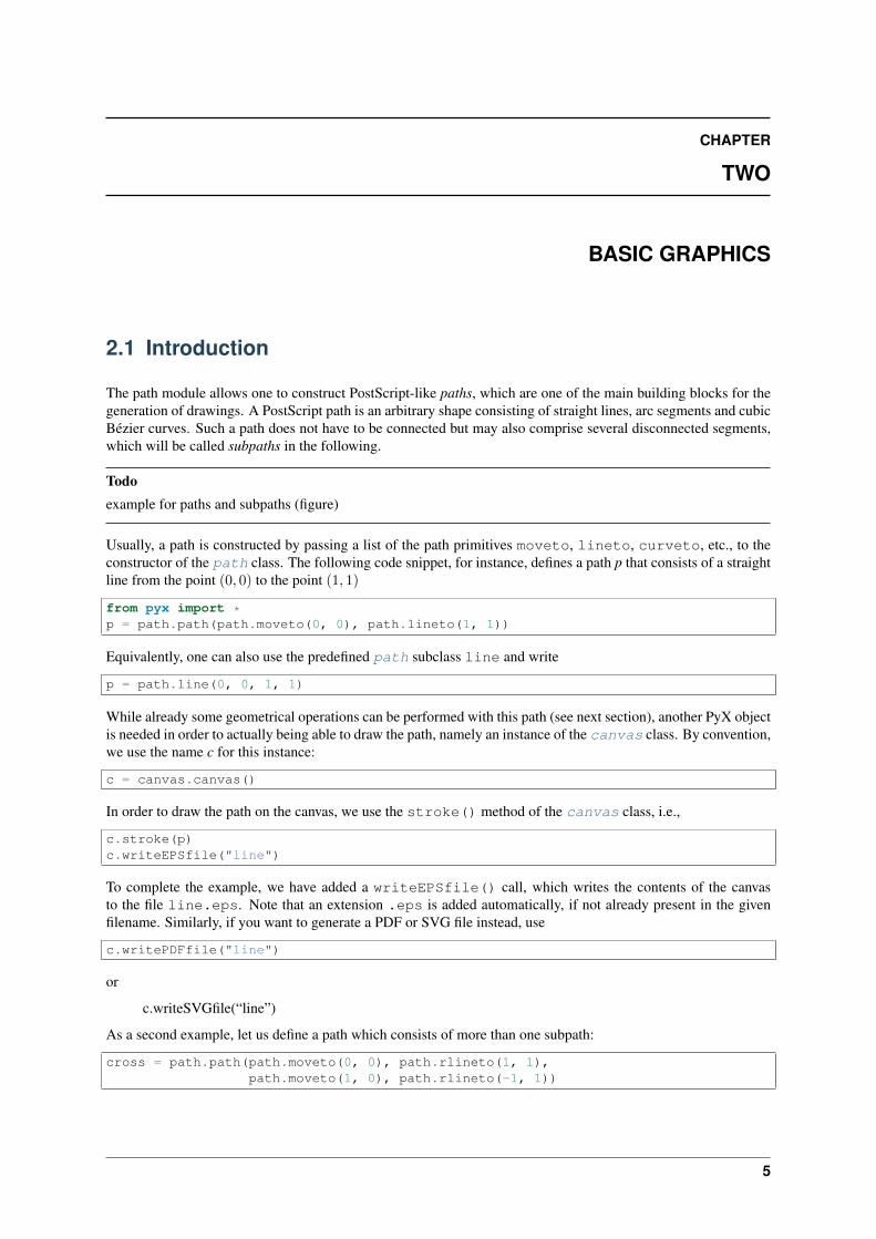
Usually, a path is constructed by passing a list of the path primitives moveto, lineto, curveto, etc., to theconstructor of the path class. The following code snippet, for instance, defines a path p that consists of a straightline from the point (0, 0) to the point (1, 1)
from pyx import *p = path.path(path.moveto(0, 0), path.lineto(1, 1))
Equivalently, one can also use the predefined path subclass line and write
p = path.line(0, 0, 1, 1)
While already some geometrical operations can be performed with this path (see next section), another PyX objectis needed in order to actually being able to draw the path, namely an instance of the canvas class. By convention,we use the name c for this instance:
c = canvas.canvas()
In order to draw the path on the canvas, we use the stroke() method of the canvas class, i.e.,
c.stroke(p)c.writeEPSfile("line")
To complete the example, we have added a writeEPSfile() call, which writes the contents of the canvasto the file line.eps. Note that an extension .eps is added automatically, if not already present in the givenfilename. Similarly, if you want to generate a PDF or SVG file instead, use
c.writePDFfile("line")
or
c.writeSVGfile(“line”)
As a second example, let us define a path which consists of more than one subpath:
cross = path.path(path.moveto(0, 0), path.rlineto(1, 1),path.moveto(1, 0), path.rlineto(-1, 1))
5

PyX Manual, Release 0.14.1
The first subpath is again a straight line from (0, 0) to (1, 1), with the only difference that we now have used therlineto class, whose arguments count relative from the last point in the path. The second moveto instanceopens a new subpath starting at the point (1, 0) and ending at (0, 1). Note that although both lines intersect atthe point (1/2, 1/2), they count as disconnected subpaths. The general rule is that each occurrence of a movetoinstance opens a new subpath. This means that if one wants to draw a rectangle, one should not use
rect1 = path.path(path.moveto(0, 0), path.lineto(0, 1),path.moveto(0, 1), path.lineto(1, 1),path.moveto(1, 1), path.lineto(1, 0),path.moveto(1, 0), path.lineto(0, 0))
which would construct a rectangle out of four disconnected subpaths (see Fig. Rectangle example a). In a bettersolution (see Fig. Rectangle example b), the pen is not lifted between the first and the last point:
(a) (b) (c) (d)
Fig. 2.1: Rectangle exampleRectangle consisting of (a) four separate lines, (b) one open path, and (c) one closed path. (d) Filling a path always closes it
automatically.
rect2 = path.path(path.moveto(0, 0), path.lineto(0, 1),path.lineto(1, 1), path.lineto(1, 0),path.lineto(0, 0))
However, as one can see in the lower left corner of Fig. Rectangle example b, the rectangle is still incomplete. Itneeds to be closed, which can be done explicitly by using for the last straight line of the rectangle (from the point(0, 1) back to the origin at (0, 0)) the closepath directive:
rect3 = path.path(path.moveto(0, 0), path.lineto(0, 1),path.lineto(1, 1), path.lineto(1, 0),path.closepath())
The closepath directive adds a straight line from the current point to the first point of the current subpath andfurthermore closes the sub path, i.e., it joins the beginning and the end of the line segment. This results in theintended rectangle shown in Fig. Rectangle example c. Note that filling the path implicitly closes every opensubpath, as is shown for a single subpath in Fig. Rectangle example d), which results from
c.stroke(rect2, [deco.filled([color.grey(0.5)])])
Here, we supply as second argument of the stroke() method a list which in the present case only consistsof a single element, namely the so called decorator deco.filled. As its name says, this decorator specifiesthat the path is not only being stroked but also filled with the given color. More information about decorators,styles and other attributes which can be passed as elements of the list can be found in Sect. Attributes: Styles andDecorations. More details on the available path elements can be found in Sect. Path elements.
To conclude this section, we should not forget to mention that rectangles are, of course, predefined in PyX, soabove we could have as well written
rect2 = path.rect(0, 0, 1, 1)
Here, the first two arguments specify the origin of the rectangle while the second two arguments define its widthand height, respectively. For more details on the predefined paths, we refer the reader to Sect. Predefined paths.
6 Chapter 2. Basic graphics
PyX Manual, Release 0.14.1
2.2 Path operations
Often, one wants to perform geometrical operations with a path before placing it on a canvas by stroking or fillingit. For instance, one might want to intersect one path with another one, split the paths at the intersection points,and then join the segments together in a new way. PyX supports such tasks by means of a number of path methods,which we will introduce in the following.
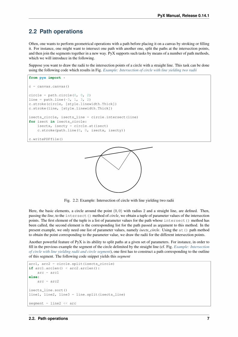
Suppose you want to draw the radii to the intersection points of a circle with a straight line. This task can be doneusing the following code which results in Fig. Example: Intersection of circle with line yielding two radii
from pyx import *
c = canvas.canvas()
circle = path.circle(0, 0, 2)line = path.line(-3, 1, 3, 2)c.stroke(circle, [style.linewidth.Thick])c.stroke(line, [style.linewidth.Thick])
isects_circle, isects_line = circle.intersect(line)for isect in isects_circle:
isectx, isecty = circle.at(isect)c.stroke(path.line(0, 0, isectx, isecty))
c.writePDFfile()
Fig. 2.2: Example: Intersection of circle with line yielding two radii
Here, the basic elements, a circle around the point (0, 0) with radius 2 and a straight line, are defined. Then,passing the line, to the intersect() method of circle, we obtain a tuple of parameter values of the intersectionpoints. The first element of the tuple is a list of parameter values for the path whose intersect() method hasbeen called, the second element is the corresponding list for the path passed as argument to this method. In thepresent example, we only need one list of parameter values, namely isects_circle. Using the at() path methodto obtain the point corresponding to the parameter value, we draw the radii for the different intersection points.
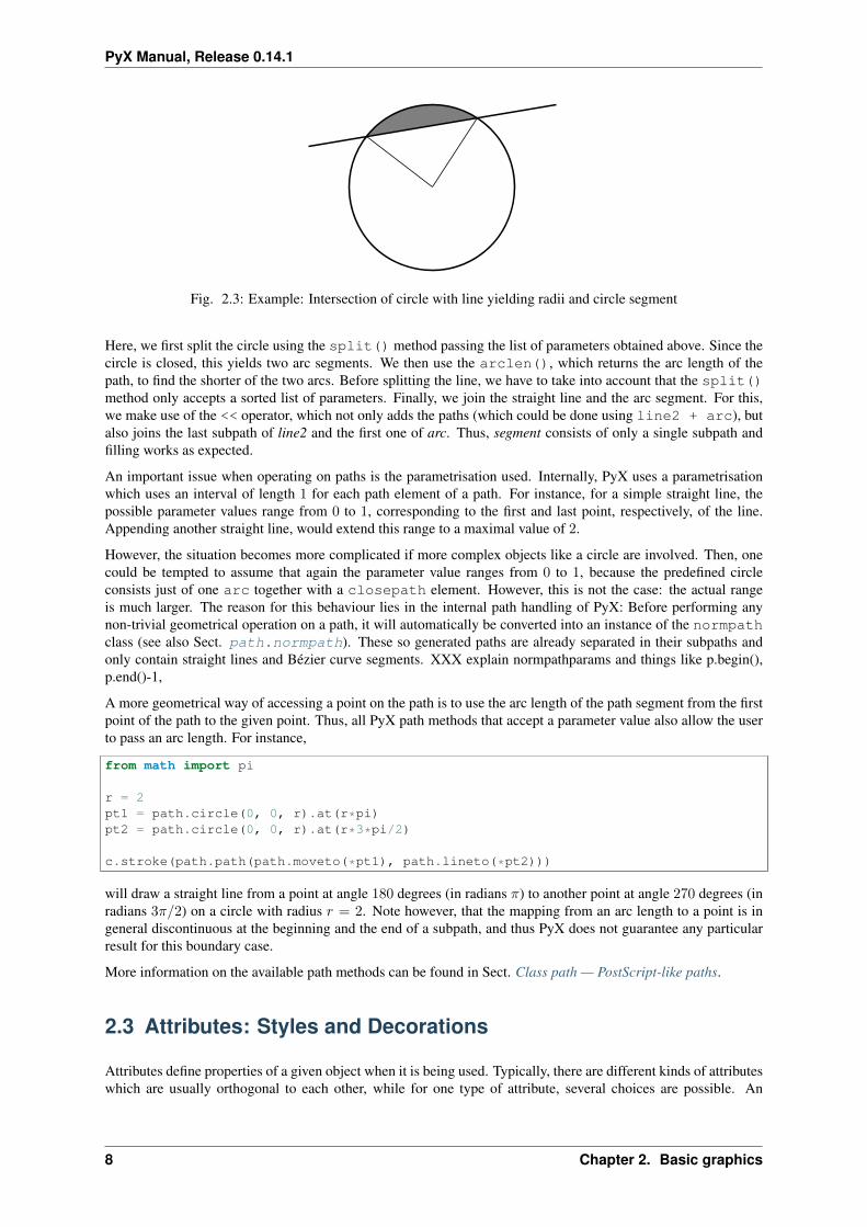
Another powerful feature of PyX is its ability to split paths at a given set of parameters. For instance, in order tofill in the previous example the segment of the circle delimited by the straight line (cf. Fig. Example: Intersectionof circle with line yielding radii and circle segment), one first has to construct a path corresponding to the outlineof this segment. The following code snippet yields this segment
arc1, arc2 = circle.split(isects_circle)if arc1.arclen() < arc2.arclen():
arc = arc1else:
arc = arc2
isects_line.sort()line1, line2, line3 = line.split(isects_line)
segment = line2 << arc
2.2. Path operations 7
PyX Manual, Release 0.14.1
Fig. 2.3: Example: Intersection of circle with line yielding radii and circle segment
Here, we first split the circle using the split() method passing the list of parameters obtained above. Since thecircle is closed, this yields two arc segments. We then use the arclen(), which returns the arc length of thepath, to find the shorter of the two arcs. Before splitting the line, we have to take into account that the split()method only accepts a sorted list of parameters. Finally, we join the straight line and the arc segment. For this,we make use of the << operator, which not only adds the paths (which could be done using line2 + arc), butalso joins the last subpath of line2 and the first one of arc. Thus, segment consists of only a single subpath andfilling works as expected.
An important issue when operating on paths is the parametrisation used. Internally, PyX uses a parametrisationwhich uses an interval of length 1 for each path element of a path. For instance, for a simple straight line, thepossible parameter values range from 0 to 1, corresponding to the first and last point, respectively, of the line.Appending another straight line, would extend this range to a maximal value of 2.
However, the situation becomes more complicated if more complex objects like a circle are involved. Then, onecould be tempted to assume that again the parameter value ranges from 0 to 1, because the predefined circleconsists just of one arc together with a closepath element. However, this is not the case: the actual rangeis much larger. The reason for this behaviour lies in the internal path handling of PyX: Before performing anynon-trivial geometrical operation on a path, it will automatically be converted into an instance of the normpathclass (see also Sect. path.normpath). These so generated paths are already separated in their subpaths andonly contain straight lines and Bézier curve segments. XXX explain normpathparams and things like p.begin(),p.end()-1,
A more geometrical way of accessing a point on the path is to use the arc length of the path segment from the firstpoint of the path to the given point. Thus, all PyX path methods that accept a parameter value also allow the userto pass an arc length. For instance,
from math import pi
r = 2pt1 = path.circle(0, 0, r).at(r*pi)pt2 = path.circle(0, 0, r).at(r*3*pi/2)
c.stroke(path.path(path.moveto(*pt1), path.lineto(*pt2)))
will draw a straight line from a point at angle 180 degrees (in radians 𝜋) to another point at angle 270 degrees (inradians 3𝜋/2) on a circle with radius 𝑟 = 2. Note however, that the mapping from an arc length to a point is ingeneral discontinuous at the beginning and the end of a subpath, and thus PyX does not guarantee any particularresult for this boundary case.
More information on the available path methods can be found in Sect. Class path — PostScript-like paths.
2.3 Attributes: Styles and Decorations
Attributes define properties of a given object when it is being used. Typically, there are different kinds of attributeswhich are usually orthogonal to each other, while for one type of attribute, several choices are possible. An
8 Chapter 2. Basic graphics
PyX Manual, Release 0.14.1
example is the stroking of a path. There, linewidth and linestyle are different kind of attributes. The linewidthmight be thin, normal, thick, etc., and the linestyle might be solid, dashed etc.
Attributes always occur in lists passed as an optional keyword argument to a method or a function. Usually,attributes are the first keyword argument, so one can just pass the list without specifying the keyword. Again, forthe path example, a typical call looks like
c.stroke(path, [style.linewidth.Thick, style.linestyle.dashed])
Here, we also encounter another feature of PyX’s attribute system. For many attributes useful default values arestored as member variables of the actual attribute. For instance, style.linewidth.Thick is equivalent tostyle.linewidth(0.04, type="w", unit="cm"), that is 0.04 width cm (see Sect. Module unit formore information about PyX’s unit system).
Another important feature of PyX attributes is what is call attributed merging. A trivial example is the following:
# the following two lines are equivalentc.stroke(path, [style.linewidth.Thick, style.linewidth.thin])c.stroke(path, [style.linewidth.thin])
Here, the style.linewidth.thin attribute overrides the preceding style.linewidth.Thick decla-ration. This is especially important in more complex cases where PyX defines default attributes for a certainoperation. When calling the corresponding methods with an attribute list, this list is appended to the list of de-faults. This way, the user can easily override certain defaults, while leaving the other default values intact. Inaddition, every attribute kind defines a special clear attribute, which allows to selectively delete a default value.For path stroking this looks like
# the following two lines are equivalentc.stroke(path, [style.linewidth.Thick, style.linewidth.clear])c.stroke(path)
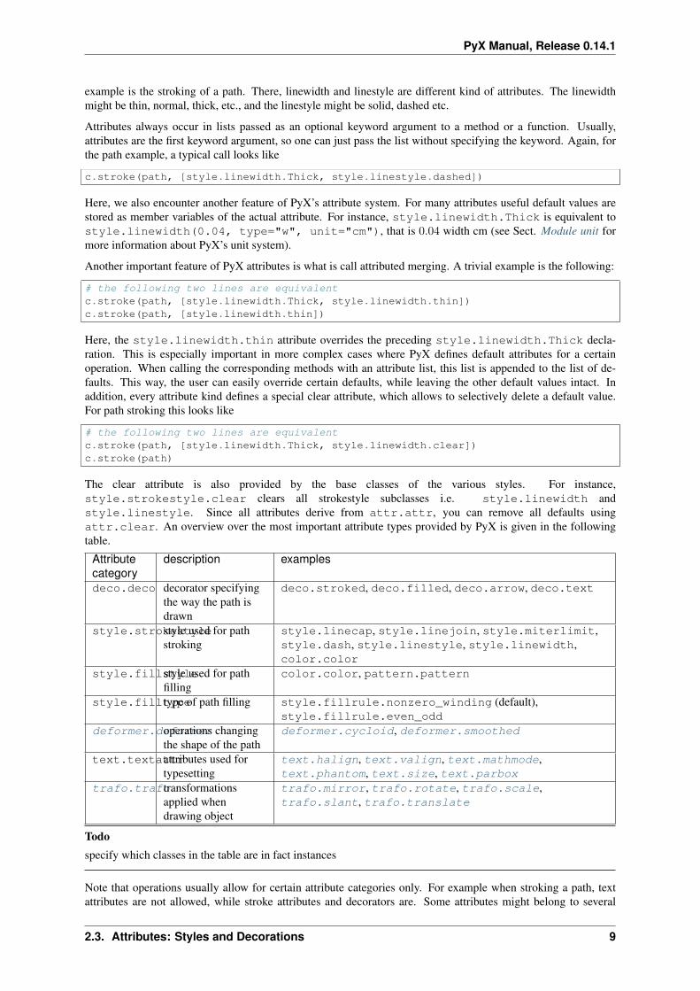
The clear attribute is also provided by the base classes of the various styles. For instance,style.strokestyle.clear clears all strokestyle subclasses i.e. style.linewidth andstyle.linestyle. Since all attributes derive from attr.attr, you can remove all defaults usingattr.clear. An overview over the most important attribute types provided by PyX is given in the followingtable.
Attributecategory
description examples
deco.deco decorator specifyingthe way the path isdrawn
deco.stroked, deco.filled, deco.arrow, deco.text
style.strokestylestyle used for pathstroking
style.linecap, style.linejoin, style.miterlimit,style.dash, style.linestyle, style.linewidth,color.color
style.fillstylestyle used for pathfilling
color.color, pattern.pattern
style.filltypetype of path filling style.fillrule.nonzero_winding (default),style.fillrule.even_odd
deformer.deformeroperations changingthe shape of the path
deformer.cycloid, deformer.smoothed
text.textattrattributes used fortypesetting
text.halign, text.valign, text.mathmode,text.phantom, text.size, text.parbox
trafo.trafotransformationsapplied whendrawing object
trafo.mirror, trafo.rotate, trafo.scale,trafo.slant, trafo.translate
Todospecify which classes in the table are in fact instances
Note that operations usually allow for certain attribute categories only. For example when stroking a path, textattributes are not allowed, while stroke attributes and decorators are. Some attributes might belong to several
2.3. Attributes: Styles and Decorations 9
PyX Manual, Release 0.14.1
attribute categories like colours, which are both, stroke and fill attributes.
Last, we discuss another important feature of PyX’s attribute system. In order to allow the easy customisationof predefined attributes, it is possible to create a modified attribute by calling of an attribute instance, therebyspecifying new parameters. A typical example is to modify the way a path is stroked or filled by constructingappropriate deco.stroked or deco.filled instances. For instance, the code
c.stroke(path, [deco.filled([color.rgb.green])])
draws a path filled in green with a black outline. Here, deco.filled is already an instance which is modifiedto fill with the given color. Note that an equivalent version would be
c.draw(path, [deco.stroked, deco.filled([color.rgb.green])])
In particular, you can see that deco.stroked is already an attribute instance, since otherwise you were notallowed to pass it as a parameter to the draw method. Another example where the modification of a decorator isuseful are arrows. For instance, the following code draws an arrow head with a more acute angle (compared to thedefault value of 45 degrees):
c.stroke(path, [deco.earrow(angle=30)])
Todochangeable attributes
10 Chapter 2. Basic graphics
CHAPTER
THREE
MODULE PATH
The path module defines several important classes which are documented in the present section.
3.1 Class path — PostScript-like paths
class path.path(*pathitems)This class represents a PostScript like path consisting of the path elements pathitems.
All possible path items are described in Sect. Path elements. Note that there are restrictions on the first pathelement and likewise on each path element after a closepath directive. In both cases, no current pointis defined and the path element has to be an instance of one of the following classes: moveto, arc, andarcn.
Instances of the class path provide the following methods (in alphabetic order):
path.append(pathitem)Appends a pathitem to the end of the path.
path.arclen()Returns the total arc length of the path. 1
path.arclentoparam(lengths)Returns the parameter value(s) corresponding to the arc length(s) lengths. 1
path.at(params)Returns the coordinates (as 2-tuple) of the path point(s) corresponding to the parameter value(s) params. 1
2
path.atbegin()Returns the coordinates (as 2-tuple) of the first point of the path. 1
path.atend()Returns the coordinates (as 2-tuple) of the end point of the path. 1
path.bbox()Returns the bounding box of the path.
path.begin()Returns the parameter value (a normpathparam instance) of the first point in the path.
path.curveradius(params)Returns the curvature radius/radii (or None if infinite) at parameter value(s) params. 2 This is the inverse ofthe curvature at this parameter. Note that this radius can be negative or positive, depending on the sign ofthe curvature. 1
1 This method requires a prior conversion of the path into a normpath instance. This is done automatically (using the precision epsilonset globally using path.set()). If you need a different epsilon for a normpath, you also can perform the conversion manually.
2 In these methods, params may either be a single value or a list. In the latter case, the result of the method will be a list consisting of theresults for each parameter. The parameter itself may either be a length (or a number which is then interpreted as a user length) or an instanceof the class normpathparam. In the former case, the length refers to the arc length along the path.
11
PyX Manual, Release 0.14.1
path.end()Returns the parameter value (a normpathparam instance) of the last point in the path.
path.extend(pathitems)Appends the list pathitems to the end of the path.
path.intersect(opath)Returns a tuple consisting of two lists of parameter values corresponding to the intersection points of thepath with the other path opath, respectively. 1 For intersection points which are not farther apart then epsilon(defaulting to 10−5 PostScript points), only one is returned.
path.joined(opath)Appends opath to the end of the path, thereby merging the last subpath (which must not be closed) of thepath with the first sub path of opath and returns the resulting new path. 1 Instead of using the joined()method, you can also join two paths together with help of the << operator, for instance p = p1 << p2.
path.normpath(epsilon=None)Returns the equivalent normpath. For the conversion and for later calculations with this normpath anaccuracy of epsilon is used. If epsilon is None, the global epsilon of the path module is used.
path.paramtoarclen(params)Returns the arc length(s) corresponding to the parameter value(s) params. 2 1
path.range()Returns the maximal parameter value param that is allowed in the path methods.
path.reversed()Returns the reversed path. 1
path.rotation(params)Returns a transformation or a list of transformations, which rotate the x-direction to the tangent vector andthe y-direction to the normal vector at the parameter value(s) params. 2 1
path.split(params)Splits the path at the parameter values params, which have to be sorted in ascending order, and returns acorresponding list of normpath instances. 1
path.tangent(params, length=1)Return a line instance or a list of line instances, corresponding to the tangent vectors at the parametervalue(s) params. 2 The tangent vector will be scaled to the length length. 1
path.trafo(params)Returns a transformation or a list of tranformations, which translate the origin to a point on the path corre-sponding to parameter value(s) params and rotate the x-direction to the tangent vector and the y-directionto the normal vector. 1
path.transformed(trafo)Returns the path transformed according to the linear transformation trafo. Here, trafo must be an instanceof the trafo.trafo class. 1
3.2 Path elements
The class pathitem is the superclass of all PostScript path construction primitives. It is never used directly, butonly by instantiating its subclasses, which correspond one by one to the PostScript primitives.
Except for the path elements ending in _pt, all coordinates passed to the path elements can be given as number(in which case they are interpreted as user units with the currently set default type) or in PyX lengths.
The following operation move the current point and open a new subpath:
class path.moveto(x, y)Path element which sets the current point to the absolute coordinates (x, y). This operation opens a newsubpath.
12 Chapter 3. Module path
PyX Manual, Release 0.14.1
class path.rmoveto(dx, dy)Path element which moves the current point by (dx, dy). This operation opens a new subpath.
Drawing a straight line can be accomplished using:
class path.lineto(x, y)Path element which appends a straight line from the current point to the point with absolute coordinates (x,y), which becomes the new current point.
class path.rlineto(dx, dy)Path element which appends a straight line from the current point to the point with relative coordinates (dx,dy), which becomes the new current point.
For the construction of arc segments, the following three operations are available:
class path.arc(x, y, r, angle1, angle2)Path element which appends an arc segment in counterclockwise direction with absolute coordinates (x, y)of the center and radius r from angle1 to angle2 (in degrees). If before the operation, the current point isdefined, a straight line from the current point to the beginning of the arc segment is prepended. Otherwise,a subpath, which thus is the first one in the path, is opened. After the operation, the current point is at theend of the arc segment.
class path.arcn(x, y, r, angle1, angle2)Same as arc but in clockwise direction.
class path.arct(x1, y1, x2, y2, r)Path element consisting of a line followed by an arc of radius r. The arc is part of the circle inscribed to theangle at x1, y1 given by lines in the directions to the current point and to x2, y2. The initial line connectsthe current point to the point where the circle touches the line through the current point and x1, y1. The arcthen continues to the point where the circle touches the line through x1, y1 and x2, y2.
Bézier curves can be constructed using:
class path.curveto(x1, y1, x2, y2, x3, y3)Path element which appends a Bézier curve with the current point as first control point and the other controlpoints (x1, y1), (x2, y2), and (x3, y3).
class path.rcurveto(dx1, dy1, dx2, dy2, dx3, dy3)Path element which appends a Bézier curve with the current point as first control point and the other controlpoints defined relative to the current point by the coordinates (dx1, dy1), (dx2, dy2), and (dx3, dy3).
Note that when calculating the bounding box (see Sect. bbox) of Bézier curves, PyX uses for performancereasons the so-called control box, i.e., the smallest rectangle enclosing the four control points of the Bézier curve.In general, this is not the smallest rectangle enclosing the Bézier curve.
Finally, an open subpath can be closed using:
class path.closepathPath element which closes the current subpath.
For performance reasons, two non-PostScript path elements are defined, which perform multiple identical opera-tions:
class path.multilineto_pt(points_pt)Path element which appends straight line segments starting from the current point and going through the listof points given in the points_pt argument. All coordinates have to be given in PostScript points.
class path.multicurveto_pt(points_pt)Path element which appends Bézier curve segments starting from the current point. points_pt is a sequenceof 6-tuples containing the coordinates of the two control points and the end point of a multicurveto segment.
3.2. Path elements 13
PyX Manual, Release 0.14.1
3.3 Class normpath
The normpath class is used internally for all non-trivial path operations, cf. footnote 1 in Sect. Class path —PostScript-like paths. It represents a path as a list of subpaths, which are instances of the class normsubpath.These normsubpaths themselves consist of a list of normsubpathitems which are either straight lines(normline) or Bézier curves (normcurve).
A given path p can easily be converted to the corresponding normpath np by:
np = p.normpath()
Additionally, the accuracy that is used in all normpath calculations can be specified by means of the argumentepsilon, which defaults to 10−5, where units of PostScript points are understood. This default value can also bechanged using the module function path.set().
To construct a normpath from a list of normsubpath instances, they are passed to the normpath constructor:
class path.normpath(normsubpaths=[])Construct a normpath consisting of subnormpaths, which is a list of subnormpath instances.
Instances of normpath offer all methods of regular path instances, which also have the same semantics. An ex-ception are the methods append() and extend(). While they allow for adding of instances of subnormpathto the normpath instance, they also keep the functionality of a regular path and allow for regular path elementsto be appended. The latter are converted to the proper normpath representation during addition.
In addition to the path methods, a normpath instance also offers the following methods, which operate on theinstance itself, i.e., modify it in place.
normpath.join(other)Join other, which has to be a path instance, to the normpath instance.
normpath.reverse()Reverses the normpath instance.
normpath.transform(trafo)Transforms the normpath instance according to the linear transformation trafo.
Finally, we remark that the sum of a normpath and a path always yields a normpath.
3.4 Class normsubpath
class path.normsubpath(normsubpathitems=[], closed=0, epsilon=1e-5)Construct a normsubpath consisting of normsubpathitems, which is a list of normsubpathitem in-stances. If closed is set, the normsubpath will be closed, thereby appending a straight line segment fromthe first to the last point, if it is not already present. All calculations with the normsubpath are performedwith an accuracy of epsilon (in units of PostScript points).
Most normsubpath methods behave like the ones of a path.
Exceptions are:
normsubpath.append(anormsubpathitem)Append the normsubpathitem to the end of the normsubpath instance. This is only possible if thenormsubpath is not closed, otherwise an NormpathException is raised.
normsubpath.extend(normsubpathitems)Extend the normsubpath instances by normsubpathitems, which has to be a list of normsubpathiteminstances. This is only possible if the normsubpath is not closed, otherwise an NormpathExceptionis raised.
14 Chapter 3. Module path
PyX Manual, Release 0.14.1
normsubpath.close()Close the normsubpath instance by appending a straight line segment from the first to the last point, ifnot already present.
3.5 Predefined paths
For convenience, some often used paths are already predefined. All of them are subclasses of the path class.
class path.line(x0, y0, x1, y1)A straight line from the point (x0, y0) to the point (x1, y1).
class path.curve(x0, y0, x1, y1, x2, y2, x3, y3)A Bézier curve with control points (x0, y0), . . ., (x3, y3).
class path.rect(x, y, w, h)A closed rectangle with lower left point (x, y), width w, and height h.
class path.circle(x, y, r)A closed circle with center (x, y) and radius r.
3.5. Predefined paths 15

PyX Manual, Release 0.14.1
16 Chapter 3. Module path
CHAPTER
FOUR
MODULE METAPOST.PATH
The metapost subpackage provides some of the path functionality of the MetaPost program. Themetapost.path presents the path construction facility of MetaPost.
Similarly to the normpath, there is a short length epsilon (always in Postscript points pt) used as accuracyof numerical operations, such as calculating angles from short path elements, or for omitting such short pathelements, etc. The default value is 10−5 and can be changed using the module function metapost.set().
4.1 Class path — MetaPost-like paths
class metapost.path.path(pathitems, epsilon=None)This class represents a MetaPost-like path which is created from the given list of knots and curves/lines. Itcan find an optimal way through given points.
At points (knots), you can either specify a given tangent direction (angle in degrees) or a certain curlyness(relative to the curvature at the other end of a curve), or nothing. In the latter case, both the tangent andthe mock curvature (an approximation to the real curvature, introduced by J. D. Hobby in MetaPost) will becontinuous.
The shape of the cubic Bezier curves between two points is controlled by its tension, unless you choose toset the control points manually.
All possible path items are described below. They are either Knots or Links. Note that there is no explicitclosepath class. Whether the path is open or closed depends on the type of knots used, begin endpoints ornot. Note also that the number of knots and links must be equal for closed paths, and that you cannot createa path comprising closed subpaths.
The epsilon argument governs the accuracy of the calculations implied in creating the path (see above). Thevalue None means fallback to the default epsilon of the module.
Instances of the class path inherit all properties of the Postscript paths in path.
4.2 Knots
class metapost.path.beginknot(x, y, curl=1, angle=None)The first knot, starting an open path at the coordinates (x, y). The properties of the curve in that point caneither be given by its curlyness (default) or the angle of its tangent vector (in degrees). The curl parameteris (as in MetaPost) the ratio of the curvatures at this point and at the other point of the curve connecting it.
class metapost.path.startknot(x, y, curl=1, angle=None)Synonym for beginknot.
class metapost.path.endknot(x, y, curl=1, angle=None)The last knot of an open path. Curlyness and angle are the same as in beginknot.
17

PyX Manual, Release 0.14.1
class metapost.path.smoothknot(x, y)This knot is the standard knot of MetaPost. It guarantees continuous tangent vectors and mock curvaturesof the two curves it connects.
Note: If one of the links is a line, the knot is changed to a roughknot with either a specified angle (if thekeepangles parameter is set in the line) or with curl=1.
class metapost.path.roughknot(x, y, left_curl=1, right_curl=None, left_angle=None,right_angle=None)
This knot is a possibly non-smooth knot, connecting two curves or lines. At each side of the knot (left/right)you can specify either the curlyness or the tangent angle.
Note: If one of the links is a line with the keepangles parameter set, the angles will be set eplicitly, regardlessof any curlyness set.
class metapost.path.knot(x, y)Synonym for smoothknot.
4.3 Links
class metapost.path.line(keepangles=False)A straight line which corresponds to the MetaPost command “–”. The option keepangles will guaranteea continuous tangent. (The curvature may become discontinuous, however.) This behavior is achieved byturning adjacent knots into roughknots with specified angles. Note that a smoothknot and a roughknot withgiven curlyness do behave differently near a line.
class metapost.path.tensioncurve(ltension=1, latleast=False, rtension=None, ratleast=None)The standard type of curve in MetaPost. It corresponds to the MetaPost command ”..” or to ”...” if theatleast parameters are set to True. The tension parameters indicate the tensions at the beginning (l) and theend (r) of the curve. Set the parameters (l/r)atleast to True if you want to avoid inflection points.
class metapost.path.controlcurve(lcontrol, rcontrol)A cubic Bezier curve which has its control points explicity set, similar to the path.curveto class of thePostscript paths. The control points at the beginning (l) and the end (r) must be coordinate pairs (x, y).
class metapost.path.curve(ltension=1, latleast=False, rtension=None, ratleast=None)Synonym for tensioncurve.
18 Chapter 4. Module metapost.path

CHAPTER
FIVE
MODULE DEFORMER: PATH DEFORMERS
The deformer module provides techniques to generate modulated paths. All classes in the deformer modulecan be used as attributes when drawing/stroking paths onto a canvas. Alternatively new paths can be created bydeforming an existing path by means of the deform() method.
All classes of the deformer module provide the following methods:
class deformer.deformer
deformer.__call__((specific parameters for the class))Returns a deformer with modified parameters
deformer.deform(path)Returns the deformed normpath on the basis of the path. This method allows using the deformers outsideof a drawing call.
The deformer classes are the following:
class deformer.cycloid(radius, halfloops=10, skipfirst=1*unit.t_cm, skiplast=1*unit.t_cm, curves-perhloop=3, sign=1, turnangle=45)
This deformer creates a cycloid around a path. The outcome looks similar to a 3D spring stretched alongthe original path.
radius: the radius of the cycloid (this is the radius of the 3D spring)
halfloops: the number of half-loops of the cycloid
skipfirst and skiplast: the lengths on the original path not to be bent to a cycloid
curvesperhloop: the number of Bezier curves to approximate a half-loop
sign: for sign>=0 the cycloid starts to the left of the path, whereas for sign<0 it starts to the right.
turnangle: the angle of perspective on the 3D spring. At turnangle=0 results in a sinusoidal curve,whereas for turnangle=90 one essentially obtains a circle.
class deformer.smoothed(radius, softness=1, obeycurv=0, relskipthres=0.01)This deformer creates a smoothed variant of the original path. The smoothing is done on the basis of thecorners of the original path, not on a global scope! Therefore, the result might not be what one would drawby hand. At each corner (or wherever two path elements meet) a piece of twice the radius is taken out of theoriginal path and replaced by a curve. This curve is determined by the tangent directions and the curvaturesat its endpoints. Both are taken from the original path, and therefore, the new curve fits into the gap in ageometrically smooth way. Path elements that are shorter than radius × relskipthres are ignored.
The new curve smoothing the corner consists either of one or of two Bezier curves, depending on thesurrounding path elements. If there are straight lines before and after the new curve, then two Bezier curvesare used. This optimises the bending of curves in rectangular boxes or polygons. Here, the curves have anadditional degree of freedom that can be set with softness ∈ (0, 1]. If one of the concerned path elements iscurved, only one Bezier curve is used that is (not always uniquely) determined by its geometrical constraints.There are, nevertheless, some caveats:
A curve that strictly obeys the sign and magnitude of the curvature might not look very smooth in somecases. Especially when connecting a curved with a straight piece, the smoothed path contains unwantedovershootings. To prevent this, the parameter default obeycurv=0 releases the curvature constraints a little:
19
PyX Manual, Release 0.14.1
The curvature may then change its sign (still looks smooth for human eyes) or, in more extreme cases, evenits magnitude (does not look so smooth). If you really need a geometrically smooth path on the basis ofBezier curves, then set obeycurv=1.
class deformer.parallel(distance, relerr=0.05, sharpoutercorners=0, dointersection=1, checkdis-tanceparams=[0.5], lookforcurvatures=11)
This deformer creates a parallel curve to a given path. The result is similar to what is usually referred to asthe set with constant distance to the set of points on the path. It differs in one important respect, becausethe distance parameter in the deformer is a signed distance. The resulting parallel normpath is constructedon the level of the original pathitems. For each of them a parallel pathitem is constructed. Then, they areconnected by circular arcs (or by sharp edges) around the corners of the original path. Later, everything thatis nearer to the original path than distance is cut away.
There are some caveats:
•When the original path is too curved then the parallel path would contain points with infinte curvature.The resulting path stops at such points and leaves the too strongly curved piece out.
•When the original path contains on or more self-intersections, then the resulting parallel path is notcontinuous in the parameterisation of the original path. This may result in the surprising behaviourthat a piece that corresponding to a “later” parameter value is followed by an “earlier” one.
The parameters are the following:
distance is the minimal (signed) distance between the original and the parallel paths.
relerr is the allowed relative error in the distance.
sharpoutercorners connects the parallel pathitems by a wegde made of straight lines, instead of takingcircular arcs. This preserves the angle of the original corners.
dointersection is a boolean for performing the last step, the intersection step, in the path construction.Setting this to 0 gives the full parallel path, which can be favourable for self-intersecting paths.
checkdistanceparams is a list of parameter values in the interval (0,1) where the distance is checked on eachparallel pathitem.
lookforcurvatures is the number of points per normpathitem where its curvature is checked for criticalvalues.
20 Chapter 5. Module deformer: Path deformers
CHAPTER
SIX
MODULE CANVAS
In addition it contains the class canvas.clip which allows clipping of the output.
6.1 Class canvas
This is the basic class of the canvas module. Instances of this class collect visual elements like paths, othercanvases, TeX or LaTeX elements. A canvas may also be embedded in another one using its insert method.This may be useful when you want to apply a transformation on a whole set of operations.
class canvas.canvas(attrs=[], texrunner=None, ipython_bboxenlarge=1*unit.t_pt)Construct a new canvas, applying the given attrs, which can be instances of trafo.trafo,canvas.clip, style.strokestyle or style.fillstyle. The texrunner argument can be usedto specify the texrunner instance used for the text() method of the canvas. If not specified, it defaultsto text.defaulttexrunner. ipython_bboxenlarge defines the bboxenlarge document.page for IPython’s_repr_png_ and _repr_svg_.
Paths can be drawn on the canvas using one of the following methods:
canvas.draw(path, attrs)Draws path on the canvas applying the given attrs. Depending on the attrs the path will be filled, stroked,ornamented, or a combination thereof. For the common first two cases the following two conveniencefunctions are provided.
canvas.fill(path, attrs=[])Fills the given path on the canvas applying the given attrs.
canvas.stroke(path, attrs=[])Strokes the given path on the canvas applying the given attrs.
Arbitrary allowed elements like other canvas instances can be inserted in the canvas using
canvas.insert(item, attrs=[])Inserts an instance of base.canvasitem into the canvas. If attrs are present, item is inserted into a newcanvas instance with attrs as arguments passed to its constructor. Then this canvas instance is inserteditself into the canvas.
Text output on the canvas is possible using
canvas.text(x, y, text, attrs=[])Inserts text at position (x, y) into the canvas applying attrs. This is a shortcut forinsert(texrunner.text(x, y, text, attrs)).
To group drawing operations, layers can be used:
canvas.layer(name, above=None, below=None)This method creates or gets a layer with name name.
A layer is a canvas itself and can be used to combine drawing operations for ordering purposes, i.e., what isabove and below each other. The layer name name is a dotted string, where dots are used to form a hierarchyof layer groups. When inserting a layer, it is put on top of its layer group except when another layer instanceof this group is specified by means of the parameters above or below.
21
PyX Manual, Release 0.14.1
The canvas class provides access to the total geometrical size of its element:
canvas.bbox()Returns the bounding box enclosing all elements of the canvas (see Sect. bbox).
A canvas also allows to set its TeX runner:
canvas.settexrunner(texrunner)Sets a new texrunner for the canvas.
The contents of the canvas can be written to a file using the following convenience methods, which wrap thecanvas into a single page document.
canvas.writeEPSfile(file, **kwargs)Writes the canvas to file using the EPS format. file either has to provide a write method or it is usedas a string containing the filename (the extension .eps is appended automatically, if it is not present).This method constructs a single page document, passing kwargs to the document.page constructor forall kwargs starting with page_ (without this prefix) and calls the writeEPSfile() method of thisdocument.document instance passing the file and all kwargs starting with write_ (without this pre-fix).
canvas.writePSfile(file, *args, **kwargs)Similar to writeEPSfile() but using the PS format.
canvas.writePDFfile(file, *args, **kwargs)Similar to writeEPSfile() but using the PDF format.
canvas.writeSVGfile(file, *args, **kwargs)Similar to writeEPSfile() but using the SVG format.
canvas.writetofile(filename, *args, **kwargs)Determine the file type (EPS, PS, PDF, or SVG) from the file extension of filename and call the correspond-ing write method with the given arguments arg and kwargs.
canvas.pipeGS(device, resolution=100, gs=”gs”, gsoptions=[], textalphabits=4, graphicsal-phabits=4, ciecolor=False, input=”eps”, **kwargs)
This method pipes the content of a canvas to the ghostscript interpreter to generate other output formats.The output is returned by means of a python BytesIO object. device specifies a ghostscript output deviceby a string. Depending on the ghostscript configuration "png16", "png16m", "png256", "png48","pngalpha", "pnggray", "pngmono", "jpeg", and "jpeggray" might be available among oth-ers. See the output of gs --help and the ghostscript documentation for more information.
resolution specifies the resolution in dpi (dots per inch). gs is the name of the ghostscript executable.gsoptions is a list of additional options passed to the ghostscript interpreter. textalphabits and graphicsal-phabits are convenient parameters to set the TextAlphaBits and GraphicsAlphaBits options ofghostscript. The addition of these options can be skipped by setting their values to None. ciecolor addsthe -dUseCIEColor flag to improve the CMYK to RGB color conversion. input can be either "eps" or"pdf" to select the input type to be passed to ghostscript (note slightly different features available in thedifferent input types regarding e.g. epsfile inclusion and transparency).
kwargs are passed to the writeEPSfile() method (not counting the file parameter), which is used togenerate the input for ghostscript. By that you gain access to the document.page constructor arguments.
canvas.writeGSfile(filename=None, device=None, **kwargs)This method is similar to pipeGS, but the content is written into the file filename. If filename is None it isauto-guessed from the script name. If filename is “-”, the output is written to stdout. In both cases, a deviceneeds to be specified to define the format (and the file suffix in case the filename is created from the scriptname).
If device is None, but a filename with suffix is given, PNG files will be written using the png16m deviceand JPG files using the jpeg device.
All other arguments are identical to those of the canvas.pipeGS().
For more information about the possible arguments of the document.page constructor, we refer to Sect.document.
22 Chapter 6. Module canvas
PyX Manual, Release 0.14.1
6.2 Class clip
In addition the canvas module contains the class canvas.clip which allows for clipping of the output bypassing a clipping instance to the attrs parameter of the canvas constructor.
6.2. Class clip 23

PyX Manual, Release 0.14.1
24 Chapter 6. Module canvas
CHAPTER
SEVEN
MODULE DOCUMENT
The document module contains two classes: document and page. A document consists of one or severalpages.
7.1 Class page
A page is a thin wrapper around a canvas, which defines some additional properties of the page.
class document.page(canvas, pagename=None, paperformat=None, rotated=0, centered=1, fitto-size=0, margin=1 * unit.t_cm, bboxenlarge=1 * unit.t_pt, bbox=None)
Construct a new page from the given canvas instance. A string pagename and the paperformat can bedefined. See below, for a list of known paper formats. If rotated is set, the output is rotated by 90 degrees onthe page. If centered is set, the output is centered on the given paperformat. If fittosize is set, the output isscaled to fill the full page except for a given margin. Normally, the bounding box of the canvas is calculatedautomatically from the bounding box of its elements. Alternatively, you may specify the bbox manually. Inany case, the bounding box is enlarged on all sides by bboxenlarge.
7.2 Class document
class document.document(pages=[])Construct a document consisting of a given list of pages.
A document can be written to a file using one of the following methods:
document.writeEPSfile(file, title=None, strip_fonts=True, text_as_path=False,mesh_as_bitmap=False, mesh_as_bitmap_resolution=300)
Write a single page document to an EPS file or to stdout if file is set to -. title is used as the documenttitle, strip_fonts enabled font stripping (removal of unused glyphs), text_as_path converts all text to pathsinstead of using fonts in the output, mesh_as_bitmap converts meshs (like 3d surface plots) to bitmaps (toreduce complexity in the output) and mesh_as_bitmap_resolution is the resolution of this conversion in dotsper inch.
document.writePSfile(file, writebbox=False, title=None, strip_fonts=True, text_as_path=False,mesh_as_bitmap=False, mesh_as_bitmap_resolution=300)
Write document to a PS file or to to stdout if file is set to -. writebbox add the page bounding boxes to theoutput. All other parameters are identical to the writeEPSfile() method.
document.writePDFfile(file, title=None, author=None, subject=None, keywords=None,fullscreen=False, writebbox=False, compress=True, compresslevel=6,strip_fonts=True, text_as_path=False, mesh_as_bitmap=False,mesh_as_bitmap_resolution=300)
Write document to a PDF file or to stdout if file is set to -. author, subject, and keywords are used forthe document author, subject, and keyword information, respectively. fullscreen enabled fullscreen modewhen the document is opened, writebbox enables writing of the crop box to each page, compress enablesoutput stream compression and compresslevel sets the compress level to be used (from 1 to 9). All otherparameters are identical to the writeEPSfile().
25
PyX Manual, Release 0.14.1
document.writeSVGfile(file, text_as_path=True, mesh_as_bitmap_resolution=300)Write document to a SVG file or to stdout if file is set to -. The text_as_path andmesh_as_bitmap_resolution have the same meaning as in writeEPSfile(). However, not the differ-ent default for text_as_path due to the missing SVG font support by current browsers. In addition, there isno mesh_as_bitmap flag, as meshs are always stored using bitmaps in SVG.
document.writetofile(filename, *args, **kwargs)Determine the file type (EPS, PS, PDF, or SVG) from the file extension of filename and call the correspond-ing write method with the given arguments arg and kwargs.
7.3 Class paperformat
class document.paperformat(width, height, name=None)Define a paperformat with the given width and height and the optional name.
Predefined paperformats are listed in the following table
instance name width heightdocument.paperformat.A0 A0 840 mm 1188 mmdocument.paperformat.A0b 910 mm 1370 mmdocument.paperformat.A1 A1 594 mm 840 mmdocument.paperformat.A2 A2 420 mm 594 mmdocument.paperformat.A3 A3 297 mm 420 mmdocument.paperformat.A4 A4 210 mm 297 mmdocument.paperformat.A5 A5 148.5 mm 210 mmdocument.paperformat.Letter Letter 8.5 inch 11 inchdocument.paperformat.Legal Legal 8.5 inch 14 inch
26 Chapter 7. Module document
CHAPTER
EIGHT
TEXT
8.1 Rationale
The text module is used to create text output. It seamlessly integrates Donald E. Knuths famous TeX typesettingengine1. The module is a high-level interface to an extensive stack of TeX and font related functionality in PyX,whose details are way beyond this manual and completely irrelevant for the typical PyX user. However, thebasic concept should be described briefly, as it provides important insights into essential properties of the wholemachinery.
PyX does not apply any limitations on the text submitted by the user. Instead the text is directly passed to TeX.This has the implication, that the text to be typeset should come from a trusted source or some special securitymeasures should be applied (see Typesetting insecure text). PyX just adds a light and transparent wrapper usingbasic TeX functionality for later identification and output extraction. This procedure enables full access to all TeXfeatures and makes PyX on the other hand dependent on the error handling provided by TeX. However, a detailedand immediate control of the TeX output allows PyX to report problems back to the user as they occur.
While we only talked about TeX so far (and will continue to do so in the rest of this section), it is important tonote that the coupling is not limited to plain TeX. Currently, PyX can also use LaTeX for typesetting, and otherTeX variants could be added in the future. What PyX really depends on is the ability of the typesetting programto generate DVI2.
As soon as some text creation is requested or, even before that, a preamble setting or macro definition is submitted,the TeX program is started as a separate process. The input and output is bound to a SingleRunner instance.Typically, the process will be kept alive and will be reused for all future typesetting requests until the end of thePyX process. However, there are certain situations when the TeX program needs to be shutdown early, which arebe described in detail in the TeX ipc mode section.
Whenever PyX sends some commands to the TeX interpreter, it adds an output marker at the end, and waits forthis output marker to be echoed in the TeX output. All intermediate output is attributed to the commands justsent and will be analysed for problems. This is done by texmessage parsers. Here, a problem could be loggedto the PyX logger at warning level, thus be reported to stderr by default. This happens for over- or underfulboxes or font warnings emitted by TeX. For other unknown problems (i.e. output not handled by any of thegiven texmessage parsers), a TexResultError is raised, which creates a detailed error report including thetraceback, the commands submitted to TeX and the output returned by TeX.
PyX wraps each text to be typeset in a TeX box and adds a shipout of this box to the TeX code before forwardingit to TeX. Thus a page in the DVI file is created containing just this output. Furthermore TeX is asked to outputthe box extent. By that PyX will immediately know the size of the text without referring to the DVI. This alsoallows faking the box size by TeX means, as you would expect it.
Once the actual output is requested, PyX reads the content of the DVI file, accessing the page related to the outputin question. It then does all the necessary steps to transform the DVI content to the requested output format, likesearching for virtual font files, font metrices, font mapping files, and PostScript Type1 fonts to be used in thefinal output. Here a present limitation has been mentioned: PyX presently can use PostScript Type1 fonts only togenerate text output. While this is a serious limitation, all the default fonts in TeX are available in Type1 nowadaysand current TeX installations are alreadily configured to use them by default.
1 https://en.wikipedia.org/wiki/TeX2 https://en.wikipedia.org/wiki/Device_independent_file_format
27
PyX Manual, Release 0.14.1
8.2 TeX interface
class text.SingleRunner(cmd, texenc=”ascii”, usefiles=[], texipc=config.getboolean(“text”, “tex-ipc”, 0), copyinput=None, dvitype=False, errordetail=errordetail.default,texmessages_start=[], texmessages_end=[], texmessages_preamble=[],texmessages_run=[])
Base class for the TeX interface.
Note: This class cannot be used directly. It is the base class for all texrunners and provides most of theimplementation. Still, to the end user the parameters except for cmd are important, as they are preserved inderived classes usually.
Parameters
• cmd (list of str) – command and arguments to start the TeX interpreter
• texenc (str) – encoding to use in the communication with the TeX interpreter
• usefiles (list of str) – list of supplementary files to be copied to and from the tem-porary working directory (see Debugging for usage details)
• texipc (bool) – TeX ipc mode flag.
• copyinput (None or str or file) – filename or file to be used to store a copy of all theinput passed to the TeX interpreter
• dvitype (bool) – flag to turn on dvitype-like output
• errordetail (errordetail) – verbosity of the TexResultError
• texmessages_start (list of texmessage parsers) – additional message parsersat interpreter startup
• texmessages_end (list of texmessage parsers) – additional message parsers atinterpreter shutdown
• texmessages_preamble (list of texmessage parsers) – additional messageparsers for preamble output
• texmessages_run (list of texmessage parsers) – additional message parsers fortypset output
texmessages_start_default = [<function texmessage.start at 0x10707f730>]default texmessage parsers at interpreter startup
texmessages_end_default = [<function texmessage.end at 0x10707f950>, <function texmessage.font_warning at 0x10707fd90>, <function texmessage.rerun_warning at 0x10707fea0>, <function texmessage.nobbl_warning at 0x10707ff28>]default texmessage parsers at interpreter shutdown
texmessages_preamble_default = [<function texmessage.load at 0x10707f9d8>]default texmessage parsers for preamble output
texmessages_run_default = [<function texmessage.font_warning at 0x10707fd90>, <function texmessage.box_warning at 0x10707fd08>, <function texmessage.package_warning at 0x10707fe18>, <function texmessage.load_def at 0x10707fa60>, <function texmessage.load_graphics at 0x10707fae8>]default texmessage parsers for typeset output
preamble(expr, texmessages=[])Execute a preamble.
Parameters
• expr (str) – expression to be executed
• texmessages (list of texmessage parsers) – additional message parsers
Preambles must not generate output, but are used to load files, perform settings, define macros, etc.In LaTeX mode, preambles are executed before \begin{document}. The method can be calledmultiple times, but only prior to SingleRunner.text() and SingleRunner.text_pt().
28 Chapter 8. Text
PyX Manual, Release 0.14.1
text_pt(x_pt, y_pt, expr, textattrs=[], texmessages=[], fontmap=None, singlecharmode=False)Typeset text.
Parameters
• x_pt (float) – x position in pts
• y_pt (float) – y position in pts
• expr (str) – text to be typeset
• textattrs (list of textattr, :class:‘trafo.trafo_pt, andstyle.fillstyle) – styles and attributes to be applied to the text
• texmessages (list of texmessage parsers) – additional message parsers
• fontmap (None or fontmap) – force a fontmap to be used (instead of the defaultdepending on the output format)
• singlecharmode (bool) – position each character separately
Returns text output insertable into a canvas.
Return type textbox_pt
Raises TexDoneError: when the TeX interpreter has been terminated already.
text(x, y, *args, **kwargs)Typeset text.
This method is identical to text_pt() with the only difference of using PyX lengths to position theoutput.
Parameters
• x (PyX length) – x position
• y (PyX length) – y position
class text.SingleTexRunner(cmd=config.getlist(“text”, “tex”, [”tex”]), lfs=”10pt”, **kwargs)Plain TeX interface.
This class adjusts the SingleRunner to use plain TeX.
Parameters
• cmd (list of str) – command and arguments to start the TeX interpreter
• lfs (str or None) – resemble LaTeX font settings within plain TeX by loading a lfs-file
• kwargs – additional arguments passed to SingleRunner
An lfs-file is a file defining a set of font commands like \normalsize by font selection commands inplain TeX. Several of those files resembling standard settings of LaTeX are distributed along with PyX inthe pyx/data/lfs directory. This directory also contains a LaTeX file to create lfs files for differentsettings (LaTeX class, class options, and style files).
class text.SingleLatexRunner(cmd=config.getlist(“text”, “latex”, [”latex”]), doc-class=”article”, docopt=None, pyxgraphics=True, texmes-sages_docclass=[], texmessages_begindoc=[], **kwargs)
LaTeX interface.
This class adjusts the SingleRunner to use LaTeX.
Parameters
• cmd (list of str) – command and arguments to start the TeX interpreter in LaTeX mode
• docclass (str) – document class
• docopt (str or None) – document loading options
8.2. TeX interface 29
PyX Manual, Release 0.14.1
• pyxgraphics (bool) – activate graphics bundle support, see Using the graphics-bundle with LaTeX
• texmessages_docclass (list of texmessage parsers) – additional messageparsers at LaTeX class loading
• texmessages_begindoc (list of texmessage parsers) – additional messageparsers at \begin{document}
• kwargs – additional arguments passed to SingleRunner
texmessages_docclass_default = [<function texmessage.load at 0x10707f9d8>]default texmessage parsers at LaTeX class loading
texmessages_begindoc_default = [<function texmessage.load at 0x10707f9d8>, <function texmessage.no_aux at 0x10707f840>]default texmessage parsers at \begin{document}
The SingleRunner classes described above do not handle restarts of the interpreter when the actuall DVI resultis required and is not available via the TeX ipc mode feature.
The MultiRunner classes below are not derived from SingleRunner even though the pro-vide the same functional interface (MultiRunner.preamble(), MultiRunner.text(), andMultiRunner.text_pt()), but instead wrap a SingleRunner instance, and provide an automatic (ormanual by the MultiRunner.reset() function) restart of the interpreter as required.
class text.MultiRunner(cls, *args, **kwargs)A restartable SingleRunner class
Parameters
• cls (SingleRunner class) – the class being wrapped
• args (list) – args at class instantiation
• kwargs (dict) – keyword args at at class instantiation
preamble(expr, texmessages=[])resembles SingleRunner.preamble()
text_pt(*args, **kwargs)resembles SingleRunner.text_pt()
text(*args, **kwargs)resembles SingleRunner.text()
reset(reinit=False)Start a new SingleRunner instance
Parameters reinit (bool) – replay preamble() calls on the new instance
After executing this function further preamble calls are allowed, whereas once a text output has beencreated, preamble() calls are forbidden.
class text.TexRunner(*args, **kwargs)A restartable SingleTexRunner class
Parameters
• args (list) – args at class instantiation
• kwargs (dict) – keyword args at at class instantiation
class text.LatexRunner(*args, **kwargs)A restartable SingleLatexRunner class
Parameters
• args (list) – args at class instantiation
• kwargs (dict) – keyword args at at class instantiation
30 Chapter 8. Text
PyX Manual, Release 0.14.1
class text.textbox_pt(x_pt, y_pt, left_pt, right_pt, height_pt, depth_pt, do_finish, fontmap, sin-glecharmode, fillstyles)
Text output.
An instance of this class contains the text output generated by PyX. It is a baseclasses.canvasitemand thus can be inserted into a canvas.
marker(name)Return the position of a marker.
Parameters name (str) – name of the marker
Returns position of the marker
Return type tuple of two PyX lengths
This method returns the position of the marker of the given name within, previously defined by the\PyXMarker{name} macro in the typeset text. Please do not use the @ character within your nameto prevent name clashes with PyX internal uses (although we don’t the marker feature internally rightnow).
Similar to generating actual output, the marker function accesses the DVI output, stopping. The TeXipc mode feature will allow for this access without stopping the TeX interpreter.
textbox_pt.leftleft extent of the text (PyX length)
textbox_pt.rightright extent of the text (PyX length)
textbox_pt.widthwidth of the text (PyX length)
textbox_pt.heightheight of the text (PyX length)
textbox_pt.depthheight of the text (PyX length)
8.3 Module level functionality
The text module provides the public interface of the SingleRunner class by module level functions. For that,a module level MultiRunner is created and configured by the set() function. Each time the set() functionis called, the existing module level MultiRunner is replaced by a new one.
text.default_runnerthe current MultiRunner instance for the module level functions
text.preambledefault_runner.preamble (bound method)
text.text_ptdefault_runner.text_pt (bound method)
text.textdefault_runner.text (bound method)
text.resetdefault_runner.reset (bound method)
text.set(cls=TexRunner, mode=None, *args, **kwargs)Setup a new module level MultiRunner
Parameters
• cls (MultiRunner object, not instance) – the module level MultiRunner to beused, i.e. TexRunner or LatexRunner
8.3. Module level functionality 31
PyX Manual, Release 0.14.1
• mode (str or None) – "tex" for TexRunner or "latex" for LatexRunner witharbitraty capitalization, overwriting the cls value
deprecated use the cls argument instead
• args (list) – args at class instantiation
• kwargs (dict) – keyword args at at class instantiation
text.escapestring(s, replace={” ”: “~”, “$”: “\$”, “&”: “\&”, ” “_”: “\_”, “%”: “\%”, “^”:“\string^”, “~”: “\string~”, “<”: “{$<$}”, “>”: “{$>$}”, “{”: “{${$}”,“}”: “{$}$}”, “\”: “{$setminus$}”, “|”: “{$mid$}”})
Escapes ASCII characters such that they can be typeset by TeX/LaTeX
8.4 TeX output parsers
While running TeX (and variants thereof) a variety of information is written to stdout like status messages,details about file access, and also warnings and errors. PyX reads all the output and analyses it. Some of theoutput is triggered as a direct response to the TeX input and is thus easy to understand for PyX. This includes pageoutput information, but also workflow control information injected by PyX into the input stream. PyX uses it tocheck the communication and typeset progress. All the other output is handled by a list of texmessage parsers,an individual set of functions applied to the TeX output one after the other. Each of the function receives the TeXoutput as a string and return it back (maybe altered). Such a function must perform one of the following actionsin response to the TeX output is receives:
1. If it does not find any text in the TeX output it feals responsible for, it should just return the unchangedstring.
2. If it finds a text it is responsible for, and the message is just fine (doesn’t need to be communicated to theuser), it should just remove this text and return the rest of the TeX output.
3. If the text should be communicated to the user, a message should be written the the pyx logger at warninglevel, thus being reported to the user on stderr by default. Examples are underfull and overfull boxwarnings or font warnings. In addition, the text should be removed as in 2 above.
4. In case of an error, TexResultError should be raised.
This is rather uncommon, that the fourth option is taken directly. Instead, errors can just be kept in the output asPyX considers unhandled TeX output left after applying all given texmessage parsers as an error. In additionto the error message, information about the TeX in- and output will be added to the exception description text bythe SingleRunner according to the errordetail setting. The following verbosity levels are available:
class text.errordetailConstants defining the verbosity of the TexResultError.
none = 0Without any input and output.
default = 1Input and parsed output shortend to 5 lines.
full = 2Full input and unparsed as well as parsed output.
exception text.TexResultErrorError raised by texmessage parsers.
To prevent any unhandled TeX output to be reported as an error, texmessage.warn ortexmessage.ignore can be used. To complete the description, here is a list of all available texmessageparsers:
class text.texmessageCollection of TeX output parsers.
32 Chapter 8. Text
PyX Manual, Release 0.14.1
This class is not meant to be instanciated. Instead, it serves as a namespace for TeX output parsers, whichare functions receiving a TeX output and returning parsed output.
In addition, this class also contains some generator functions (namely texmessage.no_file andtexmessage.pattern), which return a function according to the given parameters. They are usedto generate some of the parsers in this class and can be used to create others as well.
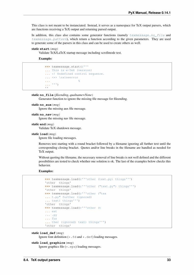
static start(msg)Validate TeX/LaTeX startup message including scrollmode test.
Example:
>>> texmessage.start(r'''... This is e-TeX (version)... *! Undefined control sequence.... <*> \raiseerror... %... ''')''
static no_file(fileending, qualname=None)Generator function to ignore the missing file message for fileending.
static no_aux(msg)Ignore the missing aux file message.
static no_nav(msg)Ignore the missing nav file message.
static end(msg)Validate TeX shutdown message.
static load(msg)Ignore file loading messages.
Removes text starting with a round bracket followed by a filename ignoring all further text until thecorresponding closing bracket. Quotes and/or line breaks in the filename are handled as needed forTeX output.
Without quoting the filename, the necessary removal of line breaks is not well defined and the differentpossibilities are tested to check whether one solution is ok. The last of the examples below checks thisbehavior.
Examples:
>>> texmessage.load(r'''other (text.py) things''')'other things'>>> texmessage.load(r'''other ("text.py") things''')'other things'>>> texmessage.load(r'''other ("tex... t.py" further (ignored)... text) things''')'other things'>>> texmessage.load(r'''other (t... ext... .py... fur... ther (ignored) text) things''')'other things'
static load_def(msg)Ignore font definition (*.fd and *.def) loading messages.
static load_graphics(msg)Ignore graphics file (*.eps) loading messages.
8.4. TeX output parsers 33

PyX Manual, Release 0.14.1
static ignore(msg)Ignore all messages.
Should be used as a last resort only. You should write a proper TeX output parser function for theoutput you observe.
static warn(msg)Warn about all messages.
Similar to ignore, but writing a warning to the logger about the TeX output. This is considered tobe better when you need to get it working quickly as you will still be prompted about the unresolvedoutput, while the processing continues.
static pattern(p, warning, qualname=None)Warn by regular expression pattern matching.
static box_warning(msg)Warn about overfull/underfull box.
static font_warning(msg)Warn about font substitutions of NFSS.
static package_warning(msg)Warn about generic package messages.
static rerun_warning(msg)Warn about rerun required message.
static nobbl_warning(msg)Warn about no-bbl message.
8.5 TeX/LaTeX attributes
TeX/LaTeX attributes are instances to be passed to a texrunners text() method. They stand for TeX/LaTeXexpression fragments and handle dependencies by proper ordering.
class text.halign(boxhalign, flushhalign)Instances of this class set the horizontal alignment of a text box and the contents of a text box to be left,center and right for boxhalign and flushhalign being 0, 0.5, and 1. Other values are allowed as well,although such an alignment seems quite unusual.
Note that there are two separate classes boxhalign and flushhalign to set the alignment of the box andits contents independently, but those helper classes can’t be cleared independently from each other. Some handyinstances available as class members:
halign.boxleftLeft alignment of the text box, i.e. sets boxhalign to 0 and doesn’t set flushhalign.
halign.boxcenterCenter alignment of the text box, i.e. sets boxhalign to 0.5 and doesn’t set flushhalign.
halign.boxrightRight alignment of the text box, i.e. sets boxhalign to 1 and doesn’t set flushhalign.
halign.flushleftLeft alignment of the content of the text box in a multiline box, i.e. sets flushhalign to 0 and doesn’t setboxhalign.
halign.raggedrightIdentical to flushleft.
halign.flushcenterCenter alignment of the content of the text box in a multiline box, i.e. sets flushhalign to 0.5 and doesn’tset boxhalign.
34 Chapter 8. Text

PyX Manual, Release 0.14.1
halign.raggedcenterIdentical to flushcenter.
halign.flushrightRight alignment of the content of the text box in a multiline box, i.e. sets flushhalign to 1 and doesn’t setboxhalign.
halign.raggedleftIdentical to flushright.
halign.leftCombines boxleft and flushleft, i.e. halign(0, 0).
halign.centerCombines boxcenter and flushcenter, i.e. halign(0.5, 0.5).
halign.rightCombines boxright and flushright, i.e. halign(1, 1).
spam &eggs
valign.top
valign.middle
valign.bottom
parbox.top
parbox.middle
parbox.bottom
Fig. 8.1: valign example
class text.valign(valign)Instances of this class set the vertical alignment of a text box to be top, center and bottom for valign being0, 0.5, and 1. Other values are allowed as well, although such an alignment seems quite unusual. See theleft side of figure valign example for an example.
Some handy instances available as class members:
valign.topvalign(0)
valign.middlevalign(0.5)
valign.bottomvalign(1)
valign.baselineIdentical to clearing the vertical alignment by clear to emphasise that a baseline alignment is not a box-related alignment. Baseline alignment is the default, i.e. no valign is set by default.
class text.parbox(width, baseline=top)Instances of this class create a box with a finite width, where the typesetter creates multiple lines in. Note,that you can’t create multiple lines in TeX/LaTeX without specifying a box width. Since PyX doesn’t knowa box width, it uses TeXs LR-mode by default, which will always put everything into a single line. Since ina vertical box there are several baselines, you can specify the baseline to be used by the optional baselineargument. You can set it to the symbolic names top, parbox.middle, and parbox.bottom only,which are members of valign. See the right side of figure valign example for an example.
Since you need to specify a box width no predefined instances are available as class members.
8.5. TeX/LaTeX attributes 35
PyX Manual, Release 0.14.1
class text.vshift(lowerratio, heightstr=”0”)Instances of this class lower the output by lowerratio of the height of the string heigthstring. Note, that youcan apply several shifts to sum up the shift result. However, there is still a clear class member to removeall vertical shifts.
Some handy instances available as class members:
vshift.bottomzerovshift(0) (this doesn’t shift at all)
vshift.middlezerovshift(0.5)
vshift.topzerovshift(1)
vshift.mathaxisThis is a special vertical shift to lower the output by the height of the mathematical axis. The mathematicalaxis is used by TeX for the vertical alignment in mathematical expressions and is often usefull for verticalalignment. The corresponding vertical shift is less than middlezero and usually fits the height of theminus sign. (It is the height of the minus sign in mathematical mode, since that’s that the mathematical axisis all about.)
There is a TeX/LaTeX attribute to switch to TeXs math mode. The appropriate instances mathmode andclearmathmode (to clear the math mode attribute) are available at module level.
text.mathmodeEnables TeXs mathematical mode in display style.
The size class creates TeX/LaTeX attributes for changing the font size.
class text.size(sizeindex=None, sizename=None, sizelist=defaultsizelist)LaTeX knows several commands to change the font size. The command names are stored inthe sizelist, which defaults to ["normalsize", "large", "Large", "LARGE", "huge","Huge", None, "tiny", "scriptsize", "footnotesize", "small"].
You can either provide an index sizeindex to access an item in sizelist or set the command name by sizename.
Instances for the LaTeXs default size change commands are available as class members:
size.tinysize(-4)
size.scriptsizesize(-3)
size.footnotesizesize(-2)
size.smallsize(-1)
size.normalsizesize(0)
size.largesize(1)
size.Largesize(2)
size.LARGEsize(3)
size.hugesize(4)
size.Hugesize(5)
36 Chapter 8. Text
PyX Manual, Release 0.14.1
There is a TeX/LaTeX attribute to create empty text boxes with the size of the material passed in. The appropriateinstances phantom and clearphantom (to clear the phantom attribute) are available at module level.
text.phantomSkip the text in the box, but keep its size.
8.6 Using the graphics-bundle with LaTeX
The packages in the LaTeX graphics bundle (color.sty, graphics.sty, graphicx.sty, ...) make ex-tensive use of \\special commands. PyX defines a clean set of such commands to fit the needs of the LaTeXgraphics bundle. This is done via the pyx.def driver file, which tells the graphics bundle about the syntaxof the \\special commands as expected by PyX. You can install the driver file pyx.def into your LaTeXsearch path and add the content of both files color.cfg and graphics.cfg to your personal configura-tion files3. After you have installed the cfg files, please use the text module with unset pyxgraphicskeyword argument which will switch off a convenience hack for less experienced LaTeX users. You can thenimport the LaTeX graphics bundle packages and related packages (e.g. rotating, ...) with the option pyx,e.g. \\usepackage[pyx]{color,graphicx}. Note that the option pyx is only available with unset pyx-graphics keyword argument and a properly installed driver file. Otherwise, omit the specification of a driver whenloading the packages.
When you define colors in LaTeX via one of the color models gray, cmyk, rgb, RGB, hsb, then PyX will usethe corresponding values (one to four real numbers). In case you use any of the named colors in LaTeX, PyXwill use the corresponding predefined color (see module color and the color table at the end of the manual). Theadditional LaTeX color model pyx allows to use a PyX color expression, such as color.cmyk(0,0,0,0)directly in LaTeX. It is passed to PyX.
When importing Encapsulated PostScript files (eps files) PyX will rotate, scale and clip your file like you expectit. Other graphic formats can not be imported via the graphics package at the moment.
For reference purpose, the following specials can be handled by PyX at the moment:
PyX:color_begin (model) (spec) starts a color. (model) is one of gray, cmyk, rgb, hsb,texnamed, or pyxcolor. (spec) depends on the model: a name or some numbers
PyX:color_end ends a color.
PyX:epsinclude file= llx= lly= urx= ury= width= height= clip=0/1 includes an En-capsulated PostScript file (eps files). The values of llx to ury are in the files’ coordinate system andspecify the part of the graphics that should become the specified width and height in the outcome. Thegraphics may be clipped. The last three parameters are optional.
PyX:scale_begin (x) (y) begins scaling from the current point.
PyX:scale_end ends scaling.
PyX:rotate_begin (angle) begins rotation around the current point.
PyX:rotate_end ends rotation.
8.7 Configuration
While the PyX configuration technically has nothing to do with the text module, we mention it here as part of thetext module since its main purpose is the configuration of various aspects related to the typesetting of text.
PyX comes with reasonable defaults which should work out of the box on most TeX installations. The defaultvalues are defined in the PyX source code itself and are repeated in the system-wide config file in INI file formatlocated at pyx/data/pyxrc. This file also contains a description of each of the listed config values and is readat PyX startup. Thus the system-wide configuration can be adjusted by editing this file.
3 If you do not know what this is all about, you can just ignore this paragraph. But be sure that the pyxgraphics keyword argument isalways set!
8.6. Using the graphics-bundle with LaTeX 37
PyX Manual, Release 0.14.1
In addition, a user-specific configuration can be setup by a ~/.pyxrc on unix-like Systems (including OS X)or pyxrc in the directory defined by the environment variable APPDATA on MS Windows. This user-specificconfiguration will overwrite the system-wide settings.
Yet another configuration can be set by the environment variable PYXRC. The given file will is loaded on top ofthe configuration defined in the previous steps.
8.7.1 TeX ipc mode
For output generation of typeset text and to calculate the positions of markers (see textbox_pt.marker())the DVI output of the TeX interpreter must be read. In contrast, the text extent (textbox_pt.left,textbox_pt.right, textbox_pt.width, textbox_pt.height, textbox_pt.depth) is avail-able without accessing the DVI output, as the TeX interpreter is instructed by PyX to output it to stdout, which isread and analysed at the typesetting step immediately.
Since TeX interpreters usually buffer the DVI output, the interpreter itself needs to be terminated to get the DVIoutput. As MultiRunner instances can start a new interpreter when needed, this does not harm the functionalityand happens more or less unnoticable. Still it generates some penalty in terms of execution speed, which canbecome huge for certain situations (alternation between typesetting and marker access).
One of the effects of the texipc option available in almost all present TeX interpreters is to flush the DVI outputafter each page. As PyX reads the DVI output linearily, it can successfully read all output whithout stopping theTeX interpreter. It is suggested to enable the texipc feature in the system-wide configuration if available in theTeX interpreter being used.
8.7.2 Debugging
PyX provides various functionality to collect details about the typesetting process. First off all, PyX reads theoutput generated by the TeX interpreter while it processes the text provided by the user. If the given texmessageparsers do not validate this output, an TexResultError is raised immediately. The verbosity of this output canbe adjusted by the errordetail setting of the SingleRunner. This might help in some cases to identify anerror in the text passed for typesetting, but for more complicated problems, other help is required.
One possibility is to output the actual code passed to the TeX interpreter. For that you can pass a file name ora file handle to the copyinput argument of the SingleRunner. You can then process the text by the TeXinterpreter yourself to reproduce the issue outside of PyX.
Similarily you can also save the log output from the TeX interpreter. For that you need to pass a log file name(with the suffix .log) in the usefiles argument (which is a list of files) of the SingleRunner. This list offiles are saved and restored in the temporary directory used by the TeX interpreter. While originally it is meant toshare, for example, a .aux file between several runs (for which the temporary directory is different and removedafter each run), it can do the same for the .log file (where the restore feature is needless, but does not harm).PyX takes care of the proper \jobname, hence you can choose the filename arbitrarily with the exception of thesuffix, as the suffix is kept during the save and restore. Still, all this might not help to fully understand the problemyou’re facing. For example there might be situations, where it is not clear which TeX interpreter is actually used(when several executables are available and the path setup within the Python interpreter differs from the one usedon the shell). In those situations it might help to enable some additional logging output created by PyX. PyX usesthe logging module from the standard library and logs to a logger named "pyx". By default, various informationabout executing external programms and locating files will not be echoed, as it is written at info level, but PyXprovides a simple convenience function to enable the output of this logging level. Just call the pyxinfo()function defined on the PyX package before actually start using the package in your Python program:
pyx.pyxinfo()Make PyX a little verbose (for information or debugging)
This function enables info level on the "pyx" logger. It also adds some general information about thePython interpreter, the PyX installation, and the PyX configuration to the logger.
38 Chapter 8. Text
PyX Manual, Release 0.14.1
8.7.3 Typesetting insecure text
When typesetting text it is passed to a TeX interpreter unchanged4. This is a security problem if the text doesnot come from a trusted source. While full access to all typesetting features is not considered a problem, youshould bear in mind that TeX code can be used to read data from any other file accessible to the TeX process. Tosurely prevent this process from accessing any other data unrelated to the TeX installation, you can setup a chrootenvironment for the TeX interpreter and configure PyX to use it. This can be achieved by setting the chrootoption and adjusting the TeX interpreter call and the filelocator configuration in the pyxrc.
4 The text is actually passed as an argument of a TeX command defined by PyX, but this is a minor detail and has no effect regardingpossible attacks.
8.7. Configuration 39
PyX Manual, Release 0.14.1
40 Chapter 8. Text
CHAPTER
NINE
GRAPHS
9.1 Introduction
PyX can be used for data and function plotting. At present x-y-graphs and x-y-z-graphs are supported only.However, the component architecture of the graph system described in section Component architecture allows foradditional graph geometries while reusing most of the existing components.
Creating a graph splits into two basic steps. First you have to create a graph instance. The most simple form wouldlook like:
from pyx import *g = graph.graphxy(width=8)
The graph instance g created in this example can then be used to actually plot something into the graph. Supposeyou have some data in a file graph.dat you want to plot. The content of the file could look like:
1 22 33 84 135 186 21
To plot these data into the graph g you must perform:
g.plot(graph.data.file("graph.dat", x=1, y=2))
The method plot() takes the data to be plotted and optionally a list of graph styles to be used to plot the data.When no styles are provided, a default style defined by the data instance is used. For data read from a file by aninstance of graph.data.file, the default are symbols. When instantiating graph.data.file, you notonly specify the file name, but also a mapping from columns to axis names and other information the styles mightmake use of (e.g. data for error bars to be used by the errorbar style).
While the graph is already created by that, we still need to perform a write of the result into a file. Since the graphinstance is a canvas, we can just call its writeEPSfile() method.
g.writeEPSfile("graph")
The result graph.eps is shown in figure A minimalistic plot for the data from file graph.dat..
Instead of plotting data from a file, other data source are available as well. For example function data is createdand placed into plot() by the following line:
g.plot(graph.data.function("y(x)=x**2"))
You can plot different data in a single graph by calling plot() several times before writing the output to a file.Note that a calling plot() will fail once a graph was forced to “finish” itself. This happens automatically, whenthe graph is written to a file. Thus it is not an option to call plot() after writing the output. The topic of thefinalization of a graph is addressed in more detail in section graph.graph. As you can see in figure Plottingdata from a file together with a function., a function is plotted as a line by default.
41
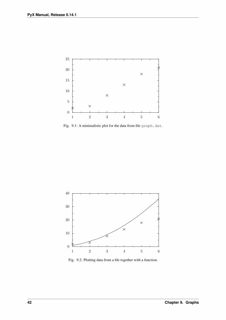
PyX Manual, Release 0.14.1
0
5
10
15
20
25
1 2 3 4 5 6
Fig. 9.1: A minimalistic plot for the data from file graph.dat.
1 2 3 4 5 60
10
20
30
40
Fig. 9.2: Plotting data from a file together with a function.
42 Chapter 9. Graphs
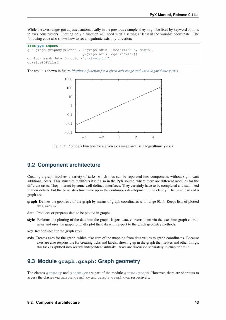
PyX Manual, Release 0.14.1
While the axes ranges got adjusted automatically in the previous example, they might be fixed by keyword optionsin axes constructors. Plotting only a function will need such a setting at least in the variable coordinate. Thefollowing code also shows how to set a logathmic axis in y-direction:
from pyx import *g = graph.graphxy(width=8, x=graph.axis.linear(min=-5, max=5),
y=graph.axis.logarithmic())g.plot(graph.data.function("y(x)=exp(x)"))g.writePDFfile()
The result is shown in figure Plotting a function for a given axis range and use a logarithmic y-axis..
0.001
0.01
0.1
1
10
100
1000
−4 −2 0 2 4
Fig. 9.3: Plotting a function for a given axis range and use a logarithmic y-axis.
9.2 Component architecture
Creating a graph involves a variety of tasks, which thus can be separated into components without significantadditional costs. This structure manifests itself also in the PyX source, where there are different modules for thedifferent tasks. They interact by some well-defined interfaces. They certainly have to be completed and stabilizedin their details, but the basic structure came up in the continuous development quite clearly. The basic parts of agraph are:
graph Defines the geometry of the graph by means of graph coordinates with range [0:1]. Keeps lists of plotteddata, axes etc.
data Produces or prepares data to be plotted in graphs.
style Performs the plotting of the data into the graph. It gets data, converts them via the axes into graph coordi-nates and uses the graph to finally plot the data with respect to the graph geometry methods.
key Responsible for the graph keys.
axis Creates axes for the graph, which take care of the mapping from data values to graph coordinates. Becauseaxes are also responsible for creating ticks and labels, showing up in the graph themselves and other things,this task is splitted into several independent subtasks. Axes are discussed separately in chapter axis.
9.3 Module graph.graph: Graph geometry
The classes graphxy and graphxyz are part of the module graph.graph. However, there are shortcuts toaccess the classes via graph.graphxy and graph.graphxyz, respectively.
9.2. Component architecture 43
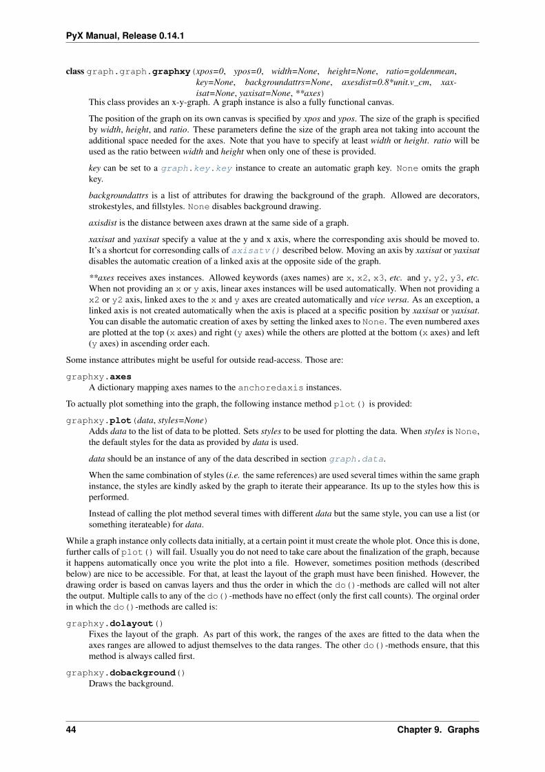
PyX Manual, Release 0.14.1
class graph.graph.graphxy(xpos=0, ypos=0, width=None, height=None, ratio=goldenmean,key=None, backgroundattrs=None, axesdist=0.8*unit.v_cm, xax-isat=None, yaxisat=None, **axes)
This class provides an x-y-graph. A graph instance is also a fully functional canvas.
The position of the graph on its own canvas is specified by xpos and ypos. The size of the graph is specifiedby width, height, and ratio. These parameters define the size of the graph area not taking into account theadditional space needed for the axes. Note that you have to specify at least width or height. ratio will beused as the ratio between width and height when only one of these is provided.
key can be set to a graph.key.key instance to create an automatic graph key. None omits the graphkey.
backgroundattrs is a list of attributes for drawing the background of the graph. Allowed are decorators,strokestyles, and fillstyles. None disables background drawing.
axisdist is the distance between axes drawn at the same side of a graph.
xaxisat and yaxisat specify a value at the y and x axis, where the corresponding axis should be moved to.It’s a shortcut for corresonding calls of axisatv() described below. Moving an axis by xaxisat or yaxisatdisables the automatic creation of a linked axis at the opposite side of the graph.
**axes receives axes instances. Allowed keywords (axes names) are x, x2, x3, etc. and y, y2, y3, etc.When not providing an x or y axis, linear axes instances will be used automatically. When not providing ax2 or y2 axis, linked axes to the x and y axes are created automatically and vice versa. As an exception, alinked axis is not created automatically when the axis is placed at a specific position by xaxisat or yaxisat.You can disable the automatic creation of axes by setting the linked axes to None. The even numbered axesare plotted at the top (x axes) and right (y axes) while the others are plotted at the bottom (x axes) and left(y axes) in ascending order each.
Some instance attributes might be useful for outside read-access. Those are:
graphxy.axesA dictionary mapping axes names to the anchoredaxis instances.
To actually plot something into the graph, the following instance method plot() is provided:
graphxy.plot(data, styles=None)Adds data to the list of data to be plotted. Sets styles to be used for plotting the data. When styles is None,the default styles for the data as provided by data is used.
data should be an instance of any of the data described in section graph.data.
When the same combination of styles (i.e. the same references) are used several times within the same graphinstance, the styles are kindly asked by the graph to iterate their appearance. Its up to the styles how this isperformed.
Instead of calling the plot method several times with different data but the same style, you can use a list (orsomething iterateable) for data.
While a graph instance only collects data initially, at a certain point it must create the whole plot. Once this is done,further calls of plot() will fail. Usually you do not need to take care about the finalization of the graph, becauseit happens automatically once you write the plot into a file. However, sometimes position methods (describedbelow) are nice to be accessible. For that, at least the layout of the graph must have been finished. However, thedrawing order is based on canvas layers and thus the order in which the do()-methods are called will not alterthe output. Multiple calls to any of the do()-methods have no effect (only the first call counts). The orginal orderin which the do()-methods are called is:
graphxy.dolayout()Fixes the layout of the graph. As part of this work, the ranges of the axes are fitted to the data when theaxes ranges are allowed to adjust themselves to the data ranges. The other do()-methods ensure, that thismethod is always called first.
graphxy.dobackground()Draws the background.
44 Chapter 9. Graphs
PyX Manual, Release 0.14.1
graphxy.doaxes()Inserts the axes.
graphxy.doplotitem(plotitem)Plots the plotitem as returned by the graphs plot method.
graphxy.doplot()Plots all (remaining) plotitems.
graphxy.dokeyitem()Inserts a plotitem in the graph key as returned by the graphs plot method.
graphxy.dokey()Inserts the graph key.
graphxy.finish()Finishes the graph by calling all pending do()-methods. This is done automatically, when the output iscreated.
The graph provides some methods to access its geometry:
graphxy.pos(x, y, xaxis=None, yaxis=None)Returns the given point at x and y as a tuple (xpos, ypos) at the graph canvas. x and y are anchoredaxisinstances for the two axes xaxis and yaxis. When xaxis or yaxis are None, the axes with names x and y areused. This method fails if called before dolayout().
graphxy.vpos(vx, vy)Returns the given point at vx and vy as a tuple (xpos, ypos) at the graph canvas. vx and vy are graphcoordinates with range [0:1].
graphxy.vgeodesic(vx1, vy1, vx2, vy2)Returns the geodesic between points vx1, vy1 and vx2, vy2 as a path. All parameters are in graph coordinateswith range [0:1]. For graphxy this is a straight line.
graphxy.vgeodesic_el(vx1, vy1, vx2, vy2)Like vgeodesic() but this method returns the path element to connect the two points.
Further geometry information is available by the axes instance variable, with is a dictionary mapping axisnames to anchoredaxis instances. Shortcuts to the anchoredaxis positioner methods for the x- and y-axis become available after dolayout() as graphxy methods Xbasepath, Xvbasepath, Xgridpath,Xvgridpath, Xtickpoint, Xvtickpoint, Xtickdirection, and Xvtickdirectionwhere the pre-fix X stands for x and y.
graphxy.axistrafo(axis, t)This method can be used to apply a transformation t to an anchoredaxis instance axis to modify theaxis position and the like. This method fails when called on a not yet finished axis, i.e. it should be usedafter dolayout().
graphxy.axisatv(axis, v)This method calls axistrafo() with a transformation to move the axis axis to a graph position v (ingraph coordinates).
The class graphxyz is very similar to the graphxy class, except for its additional dimension. In the followingdocumentation only the differences to the graphxy class are described.
class graph.graph.graphxyz(xpos=0, ypos=0, size=None, xscale=1, yscale=1, zs-cale=1/goldenmean, xy12axesat=None, xy12axesatname=”z”,projector=central(10, -30, 30), key=None, **axes)
This class provides an x-y-z-graph.
The position of the graph on its own canvas is specified by xpos and ypos. The size of the graph is specifiedby size and the length factors xscale, yscale, and zscale. The final size of the graph depends on the projectorprojector, which is called with x, y, and z values up to xscale, yscale, and zscale respectively and scalingthe result by size. For a parallel projector changing size is thus identical to changing xscale, yscale, andzscale by the same factor. For the central projector the projectors internal distance would also need to bechanged by this factor. Thus size changes the size of the whole graph without changing the projection.
9.3. Module graph.graph: Graph geometry 45
PyX Manual, Release 0.14.1
xy12axesat moves the xy-plane of the axes x, x2, y, y2 to the given value at the axis xy12axesatname.
projector defines the conversion of 3d coordinates to 2d coordinates. It can be an instance of central orparallel described below.
**axes receives axes instances as for graphxy . The graphxyz allows for 4 axes per graph dimension x,x2, x3, x4, y, y2, y3, y4, z, z2, z3, and z4. The x-y-plane is the horizontal plane at the bottom and thex, x2, y, and y2 axes are placed at the boundary of this plane with x and y always being in front. x3, x4,y3, and y4 are handled similar, but for the top plane of the graph. The z axis is placed at the origin of thex and y dimension, whereas z2 is placed at the final point of the x dimension, z3 at the final point of the ydimension and z4 at the final point of the x and y dimension together.
graphxyz.centralThe central attribute of the graphxyz is the central class. See the class description below.
graphxyz.parallelThe parallel attribute of the graphxyz is the parallel class. See the class description below.
Regarding the 3d to 2d transformation the methods pos(), vpos(), vgeodesic(), and vgeodesic_el()are available as for class graphxy and just take an additional argument for the dimension. Note that a similartransformation method (3d to 2d) is available as part of the projector as well already, but only the graph acknowl-edges its size, the scaling and the internal tranformation of the graph coordinates to the scaled coordinates. As theprojector also implements a zindex() and a angle() method, those are also available at the graph level in thegraph coordinate variant (i.e. having an additional v in its name and using values from 0 to 1 per dimension).
graphxyz.vzindex(vx, vy, vz)The depths of the point defined by vx, vy, and vz scaled to a range [-1:1] where 1 is closest to the viewer.All arguments passed to the method are in graph coordinates with range [0:1].
graphxyz.vangle(vx1, vy1, vz1, vx2, vy2, vz2, vx3, vy3, vz3)The cosine of the angle of the view ray thru point (vx1, vy1, vz1) and the plane defined by thepoints (vx1, vy1, vz1), (vx2, vy2, vz2), and (vx3, vy3, vz3). All arguments passed tothe method are in graph coordinates with range [0:1].
There are two projector classes central and parallel:
class graph.graph.central(distance, phi, theta, anglefactor=math.pi/180)Instances of this class implement a central projection for the given parameters.
distance is the distance of the viewer from the origin. Note that the graphxyz class uses the range-xscale to xscale, -yscale to yscale, and -zscale to zscale for the coordinates x, y, andz. As those scales are of the order of one (by default), the distance should be of the order of 10 to givenice results. Smaller distances increase the central projection character while for huge distances the centralprojection becomes identical to the parallel projection.
phi is the angle of the viewer in the x-y-plane and theta is the angle of the viewer to the x-y-plane.The standard notation for spheric coordinates are used. The angles are multiplied by anglefactor which isinitialized to do a degree in radiant transformation such that you can specify phi and theta in degreewhile the internal computation is always done in radiants.
class graph.graph.parallel(phi, theta, anglefactor=math.pi/180)Instances of this class implement a parallel projection for the given parameters. There is no distance forthat transformation (compared to the central projection). All other parameters are identical to the centralclass.
9.4 Module graph.data: Graph data
The following classes provide data for the plot() method of a graph. The classes are implemented ingraph.data.
46 Chapter 9. Graphs
PyX Manual, Release 0.14.1
class graph.data.file(filename, commentpattern=defaultcommentpattern, columnpat-tern=defaultcolumnpattern, stringpattern=defaultstringpattern, skiphead=0,skiptail=0, every=1, title=notitle, context={}, copy=1, replacedollar=1,columncallback=”__column__”, **columns)
This class reads data from a file and makes them available to the graph system. filename is the name of thefile to be read. The data should be organized in columns.
The arguments commentpattern, columnpattern, and stringpattern are responsible for identifying the datain each line of the file. Lines matching commentpattern are ignored except for the column name search ofthe last non- empty comment line before the data. By default a line starting with one of the characters ’#’,’%’, or ’!’ as well as an empty line is treated as a comment.
A non-comment line is analysed by repeatedly matching stringpattern and, whenever the stringpattern doesnot match, by columnpattern. When the stringpattern matches, the result is taken as the value for the nextcolumn without further transformations. When columnpattern matches, it is tried to convert the result to afloat. When this fails the result is taken as a string as well. By default, you can write strings with spacessurrounded by ’"’ immediately surrounded by spaces or begin/end of line in the data file. Otherwise ’"’is not taken to be special.
skiphead and skiptail are numbers of data lines to be ignored at the beginning and end of the file while everyselects only every every line from the data.
title is the title of the data to be used in the graph key. A default title is constructed out of filename and**columns. You may set title to None to disable the title.
Finally, columns define columns out of the existing columns from the file by a column number or a mathe-matical expression (see below). When copy is set the names of the columns in the file (file column names)and the freshly created columns having the names of the dictionary key (data column names) are passed asdata to the graph styles. The data columns may hide file columns when names are equal. For unset copy thefile columns are not available to the graph styles.
File column names occur when the data file contains a comment line immediately in front of the data (exceptfor empty or empty comment lines). This line will be parsed skipping the matched comment identifier as ifthe line would be regular data, but it will not be converted to floats even if it would be possible to convertthe items. The result is taken as file column names, i.e. a string representation for the columns in the file.
The values of **columns can refer to column numbers in the file starting at 1. The column 0 is also availableand contains the line number starting from 1 not counting comment lines, but lines skipped by skiphead,skiptail, and every. Furthermore values of **columns can be strings: file column names or complex math-ematical expressions. To refer to columns within mathematical expressions you can also use file columnnames when they are valid variable identifiers. Equal named items in context will then be hidden. Alterna-tively columns can be access by the syntax $<number> when replacedollar is set. They will be translatedinto function calls to columncallback, which is a function to access column data by index or name.
context allows for accessing external variables and functions when evaluating mathematical expressions forcolumns. Additionally to the identifiers in context, the file column names, the columncallback function andthe functions shown in the table “builtins in math expressions” at the end of the section are available.
Example:
graph.data.file("test.dat", a=1, b="B", c="2*B+$3")
with test.dat looking like:
# A B C1.234 1 25.678 3 4
The columns with name "a", "b", "c" will become "[1.234, 5.678]", "[1.0, 3.0]", and"[4.0, 10.0]", respectively. The columns "A", "B", "C" will be available as well, since copy isenabled by default.
When creating several data instances accessing the same file, the file is read only once. There is an inherentcaching of the file contents.
9.4. Module graph.data: Graph data 47
PyX Manual, Release 0.14.1
For the sake of completeness we list the default patterns:
file.defaultcommentpatternre.compile(r"(#+|!+|%+)\s*")
file.defaultcolumnpatternre.compile(r"\"(.*?)\"(\s+|$)")
file.defaultstringpatternre.compile(r"(.*?)(\s+|$)")
class graph.data.function(expression, title=notitle, min=None, max=None, points=100, con-text={})
This class creates graph data from a function. expression is the mathematical expression of the function. Itmust also contain the result variable name including the variable the function depends on by assignment. Atypical example looks like "y(x)=sin(x)".
title is the title of the data to be used in the graph key. By default expression is used. You may set title toNone to disable the title.
min and max give the range of the variable. If not set, the range spans the whole axis range. The axis rangemight be set explicitly or implicitly by ranges of other data. points is the number of points for which thefunction is calculated. The points are choosen linearly in terms of graph coordinates.
context allows for accessing external variables and functions. Additionally to the identifiers in context, thevariable name and the functions shown in the table “builtins in math expressions” at the end of the sectionare available.
class graph.data.paramfunction(varname, min, max, expression, title=notitle, points=100, con-text={})
This class creates graph data from a parametric function. varname is the parameter of the function. min andmax give the range for that variable. points is the number of points for which the function is calculated. Thepoints are choosen lineary in terms of the parameter.
expression is the mathematical expression for the parametric function. It contains an assignment of a tupleof functions to a tuple of variables. A typical example looks like "x, y = cos(k), sin(k)".
title is the title of the data to be used in the graph key. By default expression is used. You may set title toNone to disable the title.
context allows for accessing external variables and functions. Additionally to the identifiers in context,varname and the functions shown in the table “builtins in math expressions” at the end of the section areavailable.
class graph.data.values(title=”user provided values”, **columns)This class creates graph data from externally provided data. Each column is a list of values to be used forthat column.
title is the title of the data to be used in the graph key.
class graph.data.points(data, title=”user provided points”, addlinenumbers=1, **columns)This class creates graph data from externally provided data. data is a list of lines, where each line is a listof data values for the columns.
title is the title of the data to be used in the graph key.
The keywords of **columns become the data column names. The values are the column numbers startingfrom one, when addlinenumbers is turned on (the zeroth column is added to contain a line number in thatcase), while the column numbers starts from zero, when addlinenumbers is switched off.
class graph.data.data(data, title=notitle, context=, copy=1, replacedollar=1, columncall-back=”__column__”, **columns)
This class provides graph data out of other graph data. data is the source of the data. All other parameterswork like the equally called parameters in graph.data.file. Indeed, the latter is built on top of thisclass by reading the file and caching its contents in a graph.data.list instance.
48 Chapter 9. Graphs

PyX Manual, Release 0.14.1
class graph.data.conffile(filename, title=notitle, context=, copy=1, replacedollar=1, columncall-back=”__column__”, **columns)
This class reads data from a config file with the file name filename. The format of a config file is describedwithin the documentation of the ConfigParser module of the Python Standard Library.
Each section of the config file becomes a data line. The options in a section are the columns. The nameof the options will be used as file column names. All other parameters work as in graph.data.file andgraph.data.data since they all use the same code.
class graph.data.cbdfile(filename, minrank=None, maxrank=None, title=notitle, context=,copy=1, replacedollar=1, columncallback=”__column__”, **columns)
This is an experimental class to read map data from cbd-files. Seehttp://sepwww.stanford.edu/ftp/World_Map/ for some world-map data.
The builtins in math expressions are listed in the following table:
name valueneg lambda x: -xabs lambda x: x < 0 and -x or xsgn lambda x: x < 0 and -1 or 1sqrt math.sqrtexp math.explog math.logsin math.sincos math.costan math.tanasin math.asinacos math.acosatan math.atansind lambda x: math.sin(math.pi/180*x)cosd lambda x: math.cos(math.pi/180*x)tand lambda x: math.tan(math.pi/180*x)asind lambda x: 180/math.pi*math.asin(x)acosd lambda x: 180/math.pi*math.acos(x)atand lambda x: 180/math.pi*math.atan(x)norm lambda x, y: math.hypot(x, y)splitatvalue see the splitatvalue description belowpi math.pie math.e
math refers to Pythons math module. The splitatvalue function is defined as:
graph.data.splitatvalue(value, *splitpoints)This method returns a tuple (section, value). The section is calculated by comparing value with thevalues of splitpoints. If splitpoints contains only a single item, section is 0 when value is lower or equalthis item and 1 else. For multiple splitpoints, section is 0 when its lower or equal the first item, Nonewhen its bigger than the first item but lower or equal the second item, 1 when its even bigger the seconditem, but lower or equal the third item. It continues to alter between None and 2, 3, etc.
9.5 Module graph.style: Graph styles
Please note that we are talking about graph styles here. Those are responsible for plotting symbols, lines, barsand whatever else into a graph. Do not mix it up with path styles like the line width, the line style (solid, dashed,dotted etc.) and others.
The following classes provide styles to be used at the plot() method of a graph. The plot method accepts a listof styles. By that you can combine several styles at the very same time.
Some of the styles below are hidden styles. Those do not create any output, but they perform internal data handlingand thus help on modularization of the styles. Usually, a visible style will depend on data provided by one or more
9.5. Module graph.style: Graph styles 49
PyX Manual, Release 0.14.1
hidden styles but most of the time it is not necessary to specify the hidden styles manually. The hidden stylesregister themself to be the default for providing certain internal data.
class graph.style.pos(usenames={}, epsilon=1e-10)This class is a hidden style providing a position in the graph. It needs a data column for each graph dimen-sion. For that the column names need to be equal to an axis name, or a name translation from axis namesto column names need to be given by usenames. Data points are considered to be out of graph when theirposition in graph coordinates exceeds the range [0:1] by more than epsilon.
class graph.style.range(usenames={}, epsilon=1e-10)This class is a hidden style providing an errorbar range. It needs data column names constructed out of aaxis name X for each dimension errorbar data should be provided as follows:
data name descriptionXmin minimal valueXmax maximal valuedX minimal and maximal deltadXmin minimal deltadXmax maximal delta
When delta data are provided the style will also read column data for the axis name X itself. usenamesallows to insert a translation dictionary from axis names to the identifiers X.
epsilon is a comparison precision when checking for invalid errorbar ranges.
class graph.style.symbol(symbol=changecross, size=0.2*unit.v_cm, symbolattrs=[])This class is a style for plotting symbols in a graph. symbol refers to a (changeable) symbol function with theprototype symbol(c, x_pt, y_pt, size_pt, attrs) and draws the symbol into the canvas cat the position (x_pt, y_pt) with size size_pt and attributes attrs. Some predefined symbols areavailable in member variables listed below. The symbol is drawn at size size using symbolattrs. symbolattrsis merged with defaultsymbolattrs which is a list containing the decorator deco.stroked. Aninstance of symbol is the default style for all graph data classes described in section graph.data exceptfor function and paramfunction.
The class symbol provides some symbol functions as member variables, namely:
symbol.crossA cross. Should be used for stroking only.
symbol.plusA plus. Should be used for stroking only.
symbol.squareA square. Might be stroked or filled or both.
symbol.triangleA triangle. Might be stroked or filled or both.
symbol.circleA circle. Might be stroked or filled or both.
symbol.diamondA diamond. Might be stroked or filled or both.
symbol provides some changeable symbol functions as member variables, namely:
symbol.changecrossattr.changelist([cross, plus, square, triangle, circle, diamond])
symbol.changeplusattr.changelist([plus, square, triangle, circle, diamond, cross])
symbol.changesquareattr.changelist([square, triangle, circle, diamond, cross, plus])
symbol.changetriangleattr.changelist([triangle, circle, diamond, cross, plus, square])
50 Chapter 9. Graphs
PyX Manual, Release 0.14.1
symbol.changecircleattr.changelist([circle, diamond, cross, plus, square, triangle])
symbol.changediamondattr.changelist([diamond, cross, plus, square, triangle, circle])
symbol.changesquaretwiceattr.changelist([square, square, triangle, triangle, circle, circle, diamond, diamond])
symbol.changetriangletwiceattr.changelist([triangle, triangle, circle, circle, diamond, diamond, square, square])
symbol.changecircletwiceattr.changelist([circle, circle, diamond, diamond, square, square, triangle, triangle])
symbol.changediamondtwiceattr.changelist([diamond, diamond, square, square, triangle, triangle, circle, circle])
The class symbol provides two changeable decorators for alternated filling and stroking. Those are especiallyuseful in combination with the change()-twice()-symbol methods above. They are:
symbol.changestrokedfilledattr.changelist([deco.stroked, deco.filled])
symbol.changefilledstrokedattr.changelist([deco.filled, deco.stroked])
class graph.style.line(lineattrs=[], epsilon=1e-10)This class is a style to stroke lines in a graph. lineattrs is merged with defaultlineattrswhich is a listcontaining the member variable changelinestyle as described below. An instance of line is the de-fault style of the graph data classes function and paramfunction described in section graph.data.epsilon is a precision in graph coordinates for line clipping.
The class line provides a changeable line style. Its definition is:
line.changelinestyleattr.changelist([style.linestyle.solid, style.linestyle.dashed, style.linestyle.dotted,style.linestyle.dashdotted])
class graph.style.impulses(lineattrs=[], fromvalue=0, frompathattrs=[], valueaxisindex=1)This class is a style to plot impulses. lineattrs is merged with defaultlineattrs which is a list con-taining the member variable changelinestyle of the line class. fromvalue is the baseline value of theimpulses. When set to None, the impulses will start at the baseline. When fromvalue is set, frompathattrsare the stroke attributes used to show the impulses baseline path.
class graph.style.errorbar(size=0.1*unit.v_cm, errorbarattrs=[], epsilon=1e-10)This class is a style to stroke errorbars in a graph. size is the size of the caps of the errorbars and errorbarattrsare the stroke attributes. Errorbars and error caps are considered to be out of the graph when their positionin graph coordinates exceeds the range [0:1] by more that epsilon. Out of graph caps are omitted and theerrorbars are cut to the valid graph range.
class graph.style.text(textname=”text”, dxname=None, dyname=None, dxunit=0.3*unit.v_cm,dyunit=0.3*unit.v_cm, textdx=0*unit.v_cm, textdy=0.3*unit.v_cm, textat-trs=[])
This class is a style to stroke text in a graph. The text to be written has to be provided in the data columnnamed textname. textdx and textdy are the position of the text with respect to the position in the graph.Alternatively you can specify a dxname and a dyname and provide appropriate data in those columnsto be taken in units of dxunit and dyunit to specify the position of the text for each point separately. tex-tattrs are text attributes for the output of the text. Those attributes are merged with the default attributestextmodule.halign.center and textmodule.vshift.mathaxis.
class graph.style.arrow(linelength=0.25*unit.v_cm, arrowsize=0.15*unit.v_cm, lineattrs=[], ar-rowattrs=[], arrowpos=0.5, epsilon=1e-10, decorator=deco.earrow)
This class is a style to plot short lines with arrows into a two-dimensional graph to a given graph position.The arrow parameters are defined by two additional data columns named size and angle define the sizeand angle for each arrow. size is taken as a factor to arrowsize and linelength, the size of the arrow and the
9.5. Module graph.style: Graph styles 51
PyX Manual, Release 0.14.1
length of the line the arrow is plotted at. angle is the angle the arrow points to with respect to a horizontalline. The angle is taken in degrees and used in mathematically positive sense. lineattrs and arrowattrs arestyles for the arrow line and arrow head, respectively. arrowpos defines the position of the arrow line withrespect to the position at the graph. The default 0.5 means centered at the graph position, whereas 0 and1 creates the arrows to start or end at the graph position, respectively. epsilon is used as a cutoff for shortarrows in order to prevent numerical instabilities. decorator defines the decorator to be added to the line.
class graph.style.rect(colorname=”color”, gradient=color.gradient.Grey, coloraxis=None, key-graph=_autokeygraph)
This class is a style to plot colored rectangles into a two-dimensional graph. The size of the rectangles istaken from the data provided by the range style. The additional data column named colorname specifiesthe color of the rectangle defined by gradient. The translation of the data values to the gradient is done bythe coloraxis, which is set to be a linear axis if not provided by coloraxis. A key graph, a graphx instance,is generated automatically to indicate the color scale if not provided by keygraph. If a keygraph is given, itsx axis defines the color conversion and coloraxis is ignored.
class graph.style.histogram(lineattrs=[], steps=0, fromvalue=0, frompathattrs=[], fillable=0,rectkey=0, autohistogramaxisindex=0, autohistogrampointpos=0.5,epsilon=1e-10)
This class is a style to plot histograms. lineattrs is merged with defaultlineattrs which is[deco.stroked]. When steps is set, the histrogram is plotted as steps instead of the default being aboxed histogram. fromvalue is the baseline value of the histogram. When set to None, the histogramwill start at the baseline. When fromvalue is set, frompathattrs are the stroke attributes used to show thehistogram baseline path.
The fillable flag changes the stoke line of the histogram to make it fillable properly. This is important onnon-steped histograms or on histograms, which hit the graph boundary. rectkey can be set to generate arectanglar area instead of a line in the graph key.
In the most general case, a histogram is defined by a range specification (like for an errorbar) in one graphdimension (say, along the x-axis) and a value for the other graph dimension. This allows for the widths of thehistogram boxes being variable. Often, however, all histogram bin ranges are equally sized, and instead ofpassing the range, the position of the bin along the x-axis fully specifies the histogram - assuming that thereare at least two bins. This common case is supported via two parameters: autohistogramaxisindex, whichdefines the index of the independent histogram axis (in the case just described this would be 0 designatingthe x axis). autohistogrampointpos, defines the relative position of the center of the histogram bin: 0.5means that the bin is centered at the values passed to the style, 0 (1) means that the bin is aligned at theright-(left-)hand side.
XXX describe, how to specify general histograms with varying bin widths
Positions of the histograms are considered to be out of graph when they exceed the graph coordinate range[0:1] by more than epsilon.
class graph.style.barpos(fromvalue=None, frompathattrs=[], epsilon=1e-10)This class is a hidden style providing position information in a bar graph. Those graphs need to contain aspecialized axis, namely a bar axis. The data column for this bar axis is named Xname where X is an axisname. In the other graph dimension the data column name must be equal to an axis name. To plot severalbars in a single graph side by side, you need to have a nested bar axis and provide a tuple as data for nestedbar axis.
The bars start at fromvalue when provided. The fromvalue is marked by a gridline stroked using frompathat-trs. Thus this hidden style might actually create some output. The value of a bar axis is considered to be outof graph when its position in graph coordinates exceeds the range [0:1] by more than epsilon.
class graph.style.stackedbarpos(stackname, addontop=0, epsilon=1e-10)This class is a hidden style providing position information in a bar graph by stacking a new bar on top ofanother bar. The value of the new bar is taken from the data column named stackname. When addontop isset, the values is taken relative to the previous top of the bar.
class graph.style.bar(barattrs=[], epsilon=1e-10, gradient=color.gradient.RedBlack)This class draws bars in a bar graph. The bars are filled using barattrs. barattrs is
52 Chapter 9. Graphs
PyX Manual, Release 0.14.1
merged with defaultbarattrs which is a list containing [color.gradient.Rainbow,deco.stroked([color.grey.black])].
The bar style has limited support for 3d graphs: Occlusion does not work properly on stacked bars ormultiple dataset. epsilon is used in 3d to prevent numerical instabilities on bars without hight. Whengradient is not None it is used to calculate a lighting coloring taking into account the angle between theview ray and the bar and the distance between viewer and bar. The precise conversion is defined in thelighting() method.
class graph.style.changebar(barattrs=[])This style works like the bar style, but instead of the barattrs to be changed on subsequent data instancesthe barattrs are changed for each value within a single data instance. In the result the style can’t be appliedto several data instances and does not support 3d. The style raises an error instead.
class graph.style.gridpos(index1=0, index2=1, gridlines1=1, gridlines2=1, gridattrs=[],epsilon=1e-10)
This class is a hidden style providing rectangular grid information out of graph positions for graph dimen-sions index1 and index2. Data points are considered to be out of graph when their position in graph coor-dinates exceeds the range [0:1] by more than epsilon. Data points are merged to a single graph coordinatevalue when their difference in graph coordinates is below epsilon.
class graph.style.grid(gridlines1=1, gridlines2=1, gridattrs=[], epsilon=1e-10)Strokes a rectangular grid in the first grid direction, when gridlines1 is set and in the second grid direction,when gridlines2 is set. gridattrs is merged with defaultgridattrs which is a list containing themember variable changelinestyle of the line class. epsilon is a precision in graph coordinates forline clipping.
class graph.style.surface(gridlines1=0.05, gridlines2=0.05, gridcolor=None, back-color=color.gray.black, **kwargs)
Draws a surface of a rectangular grid. Each rectangle is divided into 4 triangles.
If a gridcolor is set, the rectangular grid is marked by small stripes of the relative (compared to eachrectangle) size of gridlines1 and gridlines2 for the first and second grid direction, respectively.
backcolor is used to fill triangles shown from the back. If backcolor is set to None, back sides are notdrawn differently from the front sides.
The surface is encoded using a single mesh. While this is quite space efficient, it has the following implica-tions:
• All colors must use the same color space.
• HSB colors are not allowed, whereas Gray, RGB, and CMYK are allowed. You can convert HSB col-ors into a different color space by means of rgbgradient and class:cmykgradient before passing itto the surface style.
• The grid itself is also constructed out of triangles. The grid is transformed along with the trianglesthus looking quite different from a stroked grid (as done by the grid style).
• Occlusion is handled by proper painting order.
• Color changes are continuous (in the selected color space) for each triangle.
Further arguments are identical to the graph.style.rect style. However, if no colornamecolumn exists, the surface style falls back to a lighting coloring taking into account the anglebetween the view ray and the triangle and the distance between viewer and triangle. The preciseconversion is defined in the lighting() method.
density(epsilon=1e-10, **kwargs):Density plots can be created by the density style. It is similar to a surface plot in 2d, but it does not usea mesh, but a bitmap representation instead. Due to that difference, the file size is smaller and no colorinterpolation takes place. Furthermore the style can be used with equidistantly spaced data only (afterconversion by the axis, so logarithmic raw data and such are possible using proper axes). Further argumentsare identical to the graph.style.rect style.
9.5. Module graph.style: Graph styles 53
PyX Manual, Release 0.14.1
9.6 Module graph.key: Graph keys
The following class provides a key, whose instances can be passed to the constructor keyword argument key of agraph. The class is implemented in graph.key .
class graph.key.key(dist=0.2*unit.v_cm, pos=”tr”, hpos=None, vpos=None, hinside=1, vinside=1,hdist=0.6*unit.v_cm, vdist=0.4*unit.v_cm, symbolwidth=0.5*unit.v_cm,symbolheight=0.25*unit.v_cm, symbolspace=0.2*unit.v_cm, textattrs=[],columns=1, columndist=0.5*unit.v_cm, border=0.3*unit.v_cm, keyattrs=None)
This class writes the title of the data in a plot together with a small illustration of the style. The style isresponsible for its illustration.
dist is a visual length and a distance between the key entries. pos is the position of the key with respect tothe graph. Allowed values are combinations of "t" (top), "m" (middle) and "b" (bottom) with "l" (left),"c" (center) and "r" (right). Alternatively, you may use hpos and vpos to specify the relative positionusing the range [0:1]. hdist and vdist are the distances from the specified corner of the graph. hinside andvinside are numbers to be set to 0 or 1 to define whether the key should be placed horizontally and verticallyinside of the graph or not.
symbolwidth and symbolheight are passed to the style to control the size of the style illustration. symbolspaceis the space between the illustration and the text. textattrs are attributes for the text creation. They are mergedwith [text.vshift.mathaxis].
columns is a number of columns of the graph key and columndist is the distance between those columns.
When keyattrs is set to contain some draw attributes, the graph key is enlarged by border and the key areais drawn using keyattrs.
54 Chapter 9. Graphs
CHAPTER
TEN
AXES
10.1 Component architecture
Axes are a fundamental component of graphs although there might be applications outside of the graph system.Internally axes are constructed out of components, which handle different tasks axes need to fulfill:
axis Implements the conversion of a data value to a graph coordinate of range [0:1]. It does also handle the properusage of the components in complicated tasks (i.e. combine the partitioner, texter, painter and rater to findthe best partitioning).
An anchoredaxis is a container to combine an axis with an positioner and provide a storage area for all kindof axis data. That way axis instances are reusable (they do not store any data locally). The anchoredaxisand the positioner are created by a graph corresponding to its geometry.
tick Ticks are plotted along the axis. They might be labeled with text as well.
partitioner, we use “parter” as a short form Creates one or several choices of tick lists suitable to a certain axisrange.
texter Creates labels for ticks when they are not set manually.
painter Responsible for painting the axis.
rater Calculate ratings, which can be used to select the best suitable partitioning.
positioner Defines the position of an axis.
The names above map directly to modules which are provided in the directory graph/axis except for theanchoredaxis, which is part of the axis module as well. Sometimes it might be convenient to import the axisdirectory directly rather than to access iit through the graph. This would look like:
from pyx import *graph.axis.painter() # and the like
from pyx.graph import axisaxis.painter() # this is shorter ...
In most cases different implementations are available through different classes, which can be combined in variousways. There are various axis examples distributed with PyX, where you can see some of the features of the axiswith a few lines of code each. Hence we can here directly come to the reference of the available components.
10.2 Module graph.axis.axis: Axes
The following classes are part of the module graph.axis.axis. However, there is a shortcut to access thoseclasses via graph.axis directly.
Instances of the following classes can be passed to the **axes keyword arguments of a graph. Those instancesshould only be used once.
55
PyX Manual, Release 0.14.1
class graph.axis.axis.linear(min=None, max=None, reverse=0, divisor=None, title=None,parter=parter.autolinear(), manualticks=[], density=1,maxworse=2, rater=rater.linear(), texter=texter.mixed(),painter=painter.regular(), linkpainter=painter.linked(), fall-backrange=None)
This class provides a linear axis. min and max define the axis range. When not set, they are adjustedautomatically by the data to be plotted in the graph. Note, that some data might want to access the range ofan axis (e.g. the function class when no range was provided there) or you need to specify a range whenusing the axis without plugging it into a graph (e.g. when drawing an axis along a path). In cases where thedata provides a range of zero (e.g. a when plotting a constant function), then a fallbackrange can be set toguarantee a minimal range of the axis.
reverse can be set to indicate a reversed axis starting with bigger values first. Alternatively you can fix theaxis range by min and max accordingly. When divisor is set, it is taken to divide all data range and positioninformations while creating ticks. You can create ticks not taking into account a factor by that. title is thetitle of the axis.
parter is a partitioner instance, which creates suitable ticks for the axis range. Those ticks are merged withticks manually given by manualticks before proceeding with rating, painting etc. Manually placed tickswin against those created by the partitioner. For automatic partitioners, which are able to calculate severalpossible tick lists for a given axis range, the density is a (linear) factor to favour more or less ticks. It shouldnot be stressed to much (its likely, that the result would be unappropriate or not at all valid in terms of ratinglabel distances). But within a range of say 0.5 to 2 (even bigger for large graphs) it can help to get less ormore ticks than the default would lead to. maxworse is the number of trials with more and less ticks whena better rating was already found. rater is a rater instance, which rates the ticks and the label distances forbeing best suitable. It also takes into account density. The rater is only needed, when the partitioner createsseveral tick lists.
texter is a texter instance. It creates labels for those ticks, which claim to have a label, but do not have a labelstring set already. Ticks created by partitioners typically receive their label strings by texters. The painteris finally used to construct the output. Note, that usually several output constructions are needed, since therater is also used to rate the distances between the labels for an optimum. The linkedpainter is used as theaxis painter, when automatic link axes are created by the createlinked() method.
class graph.axis.axis.lin(...)This class is an abbreviation of linear described above.
class graph.axis.axis.logarithmic(min=None, max=None, reverse=0, divisor=None,title=None, parter=parter.autologarithmic(),manualticks=[], density=1, maxworse=2,rater=rater.logarithmic(), texter=texter.mixed(),painter=painter.regular(), linkpainter=painter.linked(),fallbackrange=None)
This class provides a logarithmic axis. All parameters work like linear. Only two parameters have adifferent default: parter and rater. Furthermore and most importantly, the mapping between data and graphcoordinates is logarithmic.
class graph.axis.axis.log(...)This class is an abbreviation of logarithmic described above.
class graph.axis.axis.bar(subaxes=None, defaultsubaxis=linear(painter=None,linkpainter=None, parter=None, texter=None), dist=0.5,firstdist=None, lastdist=None, title=None, reverse=0,painter=painter.bar(), linkpainter=painter.linkedbar())
This class provides an axis suitable for a bar style. It handles a discrete set of values and maps them todistinct ranges in graph coordinates. For that, the axis gets a tuple of two values.
The first item is taken to be one of the discrete values valid on this axis. The discrete values can be anyhashable type and the order of the subaxes is defined by the order the data is received or the inverse of thatwhen reverse is set.
The second item is passed to the corresponding subaxis. The result of the conversion done by the subaxisis mapped to the graph coordinate range reserved for this subaxis. This range is defined by a size attribute
56 Chapter 10. Axes

PyX Manual, Release 0.14.1
of the subaxis, which can be added to any axis. (see the sized linear axes described below for some axesalready having a size argument). When no size information is available for a subaxis, a size value of 1 isused. The baraxis itself calculates its size by suming up the sizes of its subaxes plus firstdist, lastdist anddist times the number of subaxes minus 1.
subaxes should be a list or a dictionary mapping a discrete value of the bar axis to the corresponding subaxis.When no subaxes are set or data is received for an unknown discrete axis value, instances of defaultsubaxisare used as the subaxis for this discrete value.
dist is used as the spacing between the ranges for each distinct value. It is measured in the same units as thesubaxis results, thus the default value of 0.5 means half the width between the distinct values as the widthfor each distinct value. firstdist and lastdist are used before the first and after the last value. When set toNone, half of dist is used.
title is the title of the split axes and painter is a specialized painter for an bar axis and linkpainter is used asthe painter, when automatic link axes are created by the createlinked() method.
class graph.axis.axis.nestedbar(subaxes=None, defaultsubaxis=bar(dist=0, painter=None,linkpainter=None), dist=0.5, firstdist=None, last-dist=None, title=None, reverse=0, painter=painter.bar(),linkpainter=painter.linkedbar())
This class is identical to the bar axis except for the different default value for defaultsubaxis.
class graph.axis.axis.split(subaxes=None, defaultsubaxis=linear(), dist=0.5, firstdist=0,lastdist=0, title=None, reverse=0, painter=painter.split(),linkpainter=painter.linkedsplit())
This class is identical to the bar axis except for the different default value for defaultsubaxis, firstdist,lastdist, painter, and linkedpainter.
Sometimes you want to alter the default size of 1 of the subaxes. For that you have to add a size attribute to theaxis data. The two classes sizedlinear and autosizedlinear do that for linear axes. Their short namesare sizedlin and autosizedlin. sizedlinear extends the usual linear axis by an first argument size.autosizedlinear creates the size out of its data range automatically but sets an autolinear parter withextendtick being None in order to disable automatic range modifications while painting the axis.
The axis module also contains classes implementing so called anchored axes, which combine an axis with anpositioner and a storage place for axis related data. Since these features are not interesting for the average PyXuser, we’ll not go into all the details of their parameters and except for some handy axis position methods:
class graph.axis.axis.anchoredaxis
anchoredaxis.basepath(x1=None, x2=None)Returns a path instance for the base path. x1 and x2 define the axis range, the base path should cover.For None the beginning and end of the path is taken, which might cover a longer range, when the axis isembedded as a subaxis. For that case, a None value extends the range to the point of the middle betweentwo subaxes or the beginning or end of the whole axis, when the subaxis is the first or last of the subaxes.
anchoredaxis.vbasepath(v1=None, v2=None)Like basepath() but in graph coordinates.
anchoredaxis.gridpath(x)Returns a path instance for the grid path at position x. Might return None when no grid path is available.
anchoredaxis.vgridpath(v)Like gridpath() but in graph coordinates.
anchoredaxis.tickpoint(x)Returns the position of x as a tuple (x, y).
anchoredaxis.vtickpoint(v)Like tickpoint() but in graph coordinates.
anchoredaxis.tickdirection(x)Returns the direction of a tick at x as a tuple (dx, dy). The tick direction points inside of the graph.
10.2. Module graph.axis.axis: Axes 57
PyX Manual, Release 0.14.1
anchoredaxis.vtickdirection(v)Like tickdirection() but in graph coordinates.
anchoredaxis.vtickdirection(v)Like tickdirection() but in graph coordinates.
However, there are two anchored axes implementations linkedaxis and anchoredpathaxis which areavailable to the user to create special forms of anchored axes.
class graph.axis.axis.linkedaxis(linkedaxis=None, errorname=”manual-linked”,painter=_marker)
This class implements an anchored axis to be passed to a graph constructor to manually link the axis toanother anchored axis instance linkedaxis. Note that you can skip setting the value of linkedaxis in theconstructor, but set it later on by the setlinkedaxis() method described below. errorname is printedwithin error messages when the data is used and some problem occurs. painter is used for painting thelinked axis instead of the linkedpainter provided by the linkedaxis.
linkedaxis.setlinkedaxis(linkedaxis)This method can be used to set the linkedaxis after constructing the axis. By that you can create severalgraph instances with cycled linked axes.
class graph.axis.axis.anchoredpathaxis(path, axis, direction=1)This class implements an anchored axis the path path. direction defines the direction of the ticks. Allowedvalues are 1 (left) and -1 (right).
The anchoredpathaxis contains as any anchored axis after calling its create() method the paintedaxis in the canvas member attribute. The function pathaxis() has the same signature like theanchoredpathaxis class, but immediately creates the axis and returns the painted axis.
10.3 Module graph.axis.tick: Axes ticks
The following classes are part of the module graph.axis.tick.
class graph.axis.tick.rational(x, power=1, floatprecision=10)This class implements a rational number with infinite precision. For that it stores two integers, the numeratornum and a denominator denom. Note that the implementation of rational number arithmetics is not at allcomplete and designed for its special use case of axis partitioning in PyX preventing any roundoff errors.
x is the value of the rational created by a conversion from one of the following input values:
• A float. It is converted to a rational with finite precision determined by floatprecision.
• A string, which is parsed to a rational number with full precision. It is also allowed to provide a frac-tion like "1/3".
• A sequence of two integers. Those integers are taken as numerator and denominator of the rational.
• An instance defining instance variables num and denom like
rational itself.
power is an integer to calculate x**power. This is useful at certain places in partitioners.
class graph.axis.tick.tick(x, ticklevel=0, labellevel=0, label=None, labelattrs=[], power=1,floatprecision=10)
This class implements ticks based on rational numbers. Instances of this class can be passed to themanualticks parameter of a regular axis.
The parameters x, power, and floatprecision share its meaning with rational.
A tick has a tick level (i.e. markers at the axis path) and a label lavel (e.i. place text at the axis path),ticklevel and labellevel. These are non-negative integers or None. A value of 0 means a regular tick or label,1 stands for a subtick or sublabel, 2 for subsubtick or subsublabel and so on. None means omitting the tickor label. label is the text of the label. When not set, it can be created automatically by a texter. labelattrsare the attributes for the labels.
58 Chapter 10. Axes
PyX Manual, Release 0.14.1
10.4 Module graph.axis.parter: Axes partitioners
The following classes are part of the module graph.axis.parter. Instances of the classes can be passed tothe parter keyword argument of regular axes.
class graph.axis.parter.linear(tickdists=None, labeldists=None, extendtick=0, extendla-bel=None, epsilon=1e-10)
Instances of this class creates equally spaced tick lists. The distances between the ticks, subticks, sub-subticks etc. starting from a tick at zero are given as first, second, third etc. item of the list tickdists.For a tick position, the lowest level wins, i.e. for [2, 1] even numbers will have ticks whereas subticksare placed at odd integer. The items of tickdists might be strings, floats or tuples as described for the posparameter of class tick.
labeldists works equally for placing labels. When labeldists is kept None, labels will be placed at each tickposition, but sublabels etc. will not be used. This copy behaviour is also available vice versa and can bedisabled by an empty list.
extendtick can be set to a tick level for including the next tick of that level when the data exceeds the rangecovered by the ticks by more than epsilon. epsilon is taken relative to the axis range. extendtick is disabledwhen set to None or for fixed range axes. extendlabel works similar to extendtick but for labels.
class graph.axis.parter.lin(...)This class is an abbreviation of linear described above.
class graph.axis.parter.autolinear(variants=defaultvariants, extendtick=0, epsilon=1e-10)Instances of this class creates equally spaced tick lists, where the distance between the ticks is adjusted tothe range of the axis automatically. Variants are a list of possible choices for tickdists of linear. Furthervariants are build out of these by multiplying or dividing all the values by multiples of 10. variants shouldbe ordered that way, that the number of ticks for a given range will decrease, hence the distances between theticks should increase within the variants list. extendtick and epsilon have the same meaning as in linear.
autolinear.defaultvariants[[tick.rational((1, 1)), tick.rational((1, 2))], [tick.rational((2,1)), tick.rational((1, 1))], [tick.rational((5, 2)), tick.rational((5,4))], [tick.rational((5, 1)), tick.rational((5, 2))]]
class graph.axis.parter.autolin(...)This class is an abbreviation of autolinear described above.
class graph.axis.parter.preexp(pres, exp)This is a storage class defining positions of ticks on a logarithmic scale. It contains a list pres of positions𝑝𝑖 and exp, a multiplicator 𝑚. Valid tick positions are defined by 𝑝𝑖𝑚
𝑛 for any integer 𝑛.
class graph.axis.parter.logarithmic(tickpreexps=None, labelpreexps=None, extendtick=0,extendlabel=None, epsilon=1e-10)
Instances of this class creates tick lists suitable to logarithmic axes. The positions of the ticks, subticks,subsubticks etc. are defined by the first, second, third etc. item of the list tickpreexps, which are all preexpinstances.
labelpreexps works equally for placing labels. When labelpreexps is kept None, labels will be placed ateach tick position, but sublabels etc. will not be used. This copy behaviour is also available vice versa andcan be disabled by an empty list.
extendtick, extendlabel and epsilon have the same meaning as in linear.
Some preexp instances for the use in logarithmic are available as instance variables (should be used read-only):
logarithmic.pre1exp5preexp([tick.rational((1, 1))], 100000)
logarithmic.pre1exp4preexp([tick.rational((1, 1))], 10000)
10.4. Module graph.axis.parter: Axes partitioners 59
PyX Manual, Release 0.14.1
logarithmic.pre1exp3preexp([tick.rational((1, 1))], 1000)
logarithmic.pre1exp2preexp([tick.rational((1, 1))], 100)
logarithmic.pre1exppreexp([tick.rational((1, 1))], 10)
logarithmic.pre125exppreexp([tick.rational((1, 1)), tick.rational((2, 1)), tick.rational((5,1))], 10)
logarithmic.pre1to9exppreexp([tick.rational((1, 1)) for x in range(1, 10)], 10)
class graph.axis.parter.log(...)This class is an abbreviation of logarithmic described above.
class graph.axis.parter.autologarithmic(variants=defaultvariants, extendtick=0, extendla-bel=None, epsilon=1e-10)
Instances of this class creates tick lists suitable to logarithmic axes, where the distance between the ticksis adjusted to the range of the axis automatically. Variants are a list of tuples with possible choices fortickpreexps and labelpreexps of logarithmic. variants should be ordered that way, that the number ofticks for a given range will decrease within the variants list.
extendtick, extendlabel and epsilon have the same meaning as in linear.
autologarithmic.defaultvariants[([log.pre1exp, log.pre1to9exp], [log.pre1exp, log.pre125exp]),([log.pre1exp, log.pre1to9exp], None), ([log.pre1exp2, log.pre1exp],None), ([log.pre1exp3, log.pre1exp], None), ([log.pre1exp4,log.pre1exp], None), ([log.pre1exp5, log.pre1exp], None)]
class graph.axis.parter.autolog(...)This class is an abbreviation of autologarithmic described above.
10.5 Module graph.axis.texter: Axes texter
The following classes are part of the module graph.axis.texter. Instances of the classes can be passed tothe texter keyword argument of regular axes. Texters are used to define the label text for ticks, which request tohave a label, but for which no label text has been specified so far. A typical case are ticks created by partitionersdescribed above.
class graph.axis.texter.decimal(prefix=””, infix=””, suffix=””, equalprecision=0, dec-imalsep=”.”, thousandsep=””, thousandthpartsep=””,plus=””, minus=”-”, period=r”\overline{%s}”, labelat-trs=[text.mathmode])
Instances of this class create decimal formatted labels.
The strings prefix, infix, and suffix are added to the label at the beginning, immediately after the plus orminus, and at the end, respectively. decimalsep, thousandsep, and thousandthpartsep are strings used toseparate integer from fractional part and three-digit groups in the integer and fractional part. The strings plusand minus are inserted in front of the unsigned value for non-negative and negative numbers, respectively.
The format string period should generate a period. It must contain one string insert operators %s for theperiod.
labelattrs is a list of attributes to be added to the label attributes given in the painter. It should be used tosetup TeX features like text.mathmode. Text format options like text.size should instead be set atthe painter.
60 Chapter 10. Axes
PyX Manual, Release 0.14.1
class graph.axis.texter.exponential(plus=”“, minus=”-“, mantis-saexp=r”{{%s}\cdot10^{%s}}”, skipexp0=r”{%s}”,skipexp1=None, nomantissaexp=r”{10^{%s}}”,minusnomantissaexp=r”{-10^{%s}}”, man-tissamin=tick.rational((1, 1)), mantis-samax=tick.rational((10L, 1)), skipmantissa1=0,skipallmantissa1=1, mantissatexter=decimal())
Instances of this class create decimal formatted labels with an exponential.
The strings plus and minus are inserted in front of the unsigned value of the exponent.
The format string mantissaexp should generate the exponent. It must contain two string insert operators %s,the first for the mantissa and the second for the exponent. An alternative to the default is r"{{%s}{\rme}{%s}}".
The format string skipexp0 is used to skip exponent 0 and must contain one string insert operator %s forthe mantissa. None turns off the special handling of exponent 0. The format string skipexp1 is similar toskipexp0, but for exponent 1.
The format string nomantissaexp is used to skip the mantissa 1 and must contain one string insert operator%s for the exponent. None turns off the special handling of mantissa 1. The format string minusnomantis-saexp is similar to nomantissaexp, but for mantissa -1.
The tick.rational instances mantissamin*< *mantissamax are minimum (including) and maximum(excluding) of the mantissa.
The boolean skipmantissa1 enables the skipping of any mantissa equals 1 and -1, when minusnoman-tissaexp is set. When the boolean skipallmantissa1 is set, a mantissa equals 1 is skipped only, when allmantissa values are 1. Skipping of a mantissa is stronger than the skipping of an exponent.
mantissatexter is a texter instance for the mantissa.
class graph.axis.texter.mixed(smallestdecimal=tick.rational((1, 1000)), biggestdec-imal=tick.rational((9999, 1)), equaldecision=1, deci-mal=decimal(), exponential=exponential())
Instances of this class create decimal formatted labels with an exponential, when the unsigned values aresmall or large compared to 1.
The rational instances smallestdecimal and biggestdecimal are the smallest and biggest decimal values,where the decimal texter should be used. The sign of the value is ignored here. For a tick at zero thedecimal texter is considered best as well. equaldecision is a boolean to indicate whether the decision for thedecimal or exponential texter should be done globally for all ticks.
decimal and exponential are a decimal and an exponential texter instance, respectively.
class graph.axis.texter.rational(prefix=””, infix=””, suffix=””, numprefix=””, numin-fix=””, numsuffix=””, denomprefix=””, denomin-fix=””, denomsuffix=””, plus=””, minus=”-”, minus-pos=0, over=r”%s\over%s”, equaldenom=0, skip1=1,skipnum0=1, skipnum1=1, skipdenom1=1, labelat-trs=[text.mathmode])
Instances of this class create labels formated as fractions.
The strings prefix, infix, and suffix are added to the label at the beginning, immediately after the plus orminus, and at the end, respectively. The strings numprefix, numinfix, and numsuffix are added to the labelsnumerator accordingly whereas denomprefix, denominfix, and denomsuffix do the same for the denominator.
The strings plus and minus are inserted in front of the unsigned value. The position of the sign is defined byminuspos with values 1 (at the numerator), 0 (in front of the fraction), and -1 (at the denominator).
The format string over should generate the fraction. It must contain two string insert operators %s, the firstfor the numerator and the second for the denominator. An alternative to the default is "{{%s}/{%s}}".
Usually, the numerator and denominator are canceled, while, when equaldenom is set, the least commonmultiple of all denominators is used.
10.5. Module graph.axis.texter: Axes texter 61
PyX Manual, Release 0.14.1
The boolean skip1 indicates, that only the prefix, plus or minus, the infix and the suffix should be printed,when the value is 1 or -1 and at least one of prefix, infix and suffix is present.
The boolean skipnum0 indicates, that only a 0 is printed when the numerator is zero.
skipnum1 is like skip1 but for the numerator.
skipdenom1 skips the denominator, when it is 1 taking into account denomprefix, denominfix, denomsuffixminuspos and the sign of the number.
labelattrs has the same meaning as for decimal.
10.6 Module graph.axis.painter: Axes painter
The following classes are part of the module graph.axis.painter. Instances of the painter classes can bepassed to the painter keyword argument of regular axes.
class graph.axis.painter.rotatetext(direction, epsilon=1e-10)This helper class is used in direction arguments of the painters below to prevent axis labels and titles beingwritten upside down. In those cases the text will be rotated by 180 degrees. direction is an angle to be usedrelative to the tick direction. epsilon is the value by which 90 degrees can be exceeded before an 180 degreerotation is performed.
The following two class variables are initialized for the most common applications:
rotatetext.parallelrotatetext(90)
rotatetext.orthogonalrotatetext(180)
class graph.axis.painter.ticklength(initial, factor)This helper class provides changeable PyX lengths starting from an initial value initial multiplied by factoragain and again. The resulting lengths are thus a geometric series.
There are some class variables initialized with suitable values for tick stroking. They are namedticklength.SHORT, ticklength.SHORt, . . . , ticklength.short, ticklength.normal,ticklength.long, . . . , ticklength.LONG. ticklength.normal is initialized with a length of 0.12and the reciprocal of the golden mean as factor whereas the others have a modified initial value obtained bymultiplication with or division by appropriate multiples of
√2.
class graph.axis.painter.regular(innerticklength=ticklength.normal, outerticklength=None,tickattrs=[], gridattrs=None, basepathattrs=[], labeld-ist=”0.3 cm”, labelattrs=[], labeldirection=None, la-belhequalize=0, labelvequalize=1, titledist=”0.3 cm”,titleattrs=[], titledirection=rotatetext.parallel, titlepos=0.5,texrunner=None)
Instances of this class are painters for regular axes like linear and logarithmic axes.
innerticklength and outerticklength are visual PyX lengths of the ticks, subticks, subsubticks etc. plottedalong the axis inside and outside of the graph. Provide changeable attributes to modify the lengths of tickscompared to subticks etc. None turns off the ticks inside and outside the graph, respectively.
tickattrs and gridattrs are changeable stroke attributes for the ticks and the grid, where None turns off thefeature. basepathattrs are stroke attributes for the axis or None to turn it off. basepathattrs is merged with[style.linecap.square].
labeldist is the distance of the labels from the axis base path as a visual PyX length. labelattrs is a list of textattributes for the labels. It is merged with [text.halign.center, text.vshift.mathaxis].labeldirection is an instance of rotatetext to rotate the labels relative to the axis tick direction or None.
The boolean values labelhequalize and labelvequalize force an equal alignment of all labels for straightvertical and horizontal axes, respectively.
62 Chapter 10. Axes
PyX Manual, Release 0.14.1
titledist is the distance of the title from the rest of the axis as a visual PyX length. titleattrs is a list of textattributes for the title. It is merged with [text.halign.center, text.vshift.mathaxis].titledirection is an instance of rotatetext to rotate the title relative to the axis tick direction or None. titleposis the position of the title in graph coordinates.
texrunner is the texrunner instance to create axis text like the axis title or labels. When not set the texrunnerof the graph instance is taken to create the text.
class graph.axis.painter.linked(innerticklength=ticklength.short, outerticklength=None,tickattrs=[], gridattrs=None, basepathattrs=[], labeld-ist=”0.3 cm”, labelattrs=None, labeldirection=None,labelhequalize=0, labelvequalize=1, titledist=”0.3 cm”, ti-tleattrs=None, titledirection=rotatetext.parallel, titlepos=0.5,texrunner=None)
This class is identical to regular up to the default values of labelattrs and titleattrs. By turning off thosefeatures, this painter is suitable for linked axes.
class graph.axis.painter.bar(innerticklength=None, outerticklength=None, tickattrs=[],basepathattrs=[], namedist=”0.3 cm”, nameattrs=[], namedirec-tion=None, namepos=0.5, namehequalize=0, namevequalize=1,titledist=”0.3 cm”, titleattrs=[], titledirection=rotatetext.parallel,titlepos=0.5, texrunner=None)
Instances of this class are suitable painters for bar axes.
innerticklength and outerticklength are visual PyX lengths to mark the different bar regions along the axisinside and outside of the graph. None turns off the ticks inside and outside the graph, respectively. tickattrsare stroke attributes for the ticks or None to turn all ticks off.
The parameters with prefix name are identical to their label counterparts in regular. All other parametershave the same meaning as in regular.
class graph.axis.painter.linkedbar(innerticklength=None, outerticklength=None, tick-attrs=[], basepathattrs=[], namedist=”0.3 cm”,nameattrs=None, namedirection=None, namepos=0.5,namehequalize=0, namevequalize=1, titledist=”0.3cm”, titleattrs=None, titledirection=rotatetext.parallel,titlepos=0.5, texrunner=None)
This class is identical to bar up to the default values of nameattrs and titleattrs. By turning off thosefeatures, this painter is suitable for linked bar axes.
class graph.axis.painter.split(breaklinesdist=”0.05 cm”, breaklineslength=”0.5 cm”,breaklinesangle=-60, titledist=”0.3 cm”, titleattrs=[], titledi-rection=rotatetext.parallel, titlepos=0.5, texrunner=None)
Instances of this class are suitable painters for split axes.
breaklinesdist and breaklineslength are the distance between axes break markers in visual PyX lengths.breaklinesangle is the angle of the axis break marker with respect to the base path of the axis. All otherparameters have the same meaning as in regular.
class graph.axis.painter.linkedsplit(breaklinesdist=”0.05 cm”, breaklineslength=”0.5cm”, breaklinesangle=-60, titledist=”0.3 cm”, ti-tleattrs=None, titledirection=rotatetext.parallel,titlepos=0.5, texrunner=None)
This class is identical to split up to the default value of titleattrs. By turning off this feature, this painteris suitable for linked split axes.
10.7 Module graph.axis.rater: Axes rater
The rating of axes is implemented in graph.axis.rater. When an axis partitioning scheme returns severalpartitioning possibilities, the partitions need to be rated by a positive number. The axis partitioning rated lowest isconsidered best.
10.7. Module graph.axis.rater: Axes rater 63
PyX Manual, Release 0.14.1
The rating consists of two steps. The first takes into account only the number of ticks, subticks, labels and so onin comparison to optimal numbers. Additionally, the extension of the axis range by ticks and labels is taken intoaccount. This rating leads to a preselection of possible partitions. In the second step, after the layout of preferredpartitionings has been calculated, the distance of the labels in a partition is taken into account as well at a smallerweight factor by default. Thereby partitions with overlapping labels will be rejected completely. Exceptionallysparse or dense labels will receive a bad rating as well.
class graph.axis.rater.cube(opt, left=None, right=None, weight=1)Instances of this class provide a number rater. opt is the optimal value. When not provided, left is set to 0and right is set to 3*opt. Weight is a multiplicator to the result.
The rater calculates width*((x-opt)/(other-opt))**3 to rate the value x, where other is left(x‘‘<*opt*) or *right* (‘‘x>*opt*).
class graph.axis.rater.distance(opt, weight=0.1)Instances of this class provide a rater for a list of numbers. The purpose is to rate the distance between labelboxes. opt is the optimal value.
The rater calculates the sum of weight*(opt/x-1) (x‘‘<*opt*) or ‘‘weight*(x/opt-1)(x>*opt*) for all elements x of the list. It returns this value divided by the number of elements in the list.
class graph.axis.rater.rater(ticks, labels, range, distance)Instances of this class are raters for axes partitionings.
ticks and labels are both lists of number rater instances, where the first items are used for the number ofticks and labels, the second items are used for the number of subticks (including the ticks) and sublabels(including the labels) and so on until the end of the list is reached or no corresponding ticks are available.
range is a number rater instance which rates the range of the ticks relative to the range of the data.
distance is an distance rater instance.
class graph.axis.rater.linear(ticks=[cube(4), cube(10, weight=0.5)], labels=[cube(4)],range=cube(1, weight=2), distance=distance(“1 cm”))
This class is suitable to rate partitionings of linear axes. It is equal to rater but defines predefined valuesfor the arguments.
class graph.axis.rater.lin(...)This class is an abbreviation of linear described above.
class graph.axis.rater.logarithmic(ticks=[cube(5, right=20), cube(20, right=100,weight=0.5)], labels=[cube(5, right=20), cube(5,right=20, weight=0.5)], range=cube(1, weight=2),distance=distance(“1 cm”))
This class is suitable to rate partitionings of logarithmic axes. It is equal to rater but defines predefinedvalues for the arguments.
class graph.axis.rater.log(...)This class is an abbreviation of logarithmic described above.
10.8 Module graph.axis.positioner: Axes positioners
The position of an axis is defined by an instance of a class providing the following methods:
class graph.axis.positioners.positioner
positioner.vbasepath(v1=None, v2=None)Returns a path instance for the base path. v1 and v2 define the axis range in graph coordinates the base pathshould cover.
positioner.vgridpath(v)Returns a path instance for the grid path at position v in graph coordinates. The method might return Nonewhen no grid path is available (for an axis along a path for example).
64 Chapter 10. Axes
PyX Manual, Release 0.14.1
positioner.vtickpoint_pt(v)Returns the position of v in graph coordinates as a tuple (x, y) in points.
positioner.vtickdirection(v)Returns the direction of a tick at v in graph coordinates as a tuple (dx, dy). The tick direction pointsinside of the graph.
The module contains several implementations of those positioners, but since the positioner instances are createdby graphs etc. as needed, the details are not interesting for the average PyX user.
10.8. Module graph.axis.positioner: Axes positioners 65
PyX Manual, Release 0.14.1
66 Chapter 10. Axes
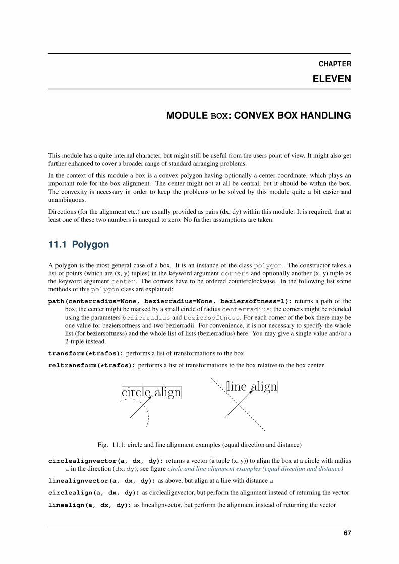
CHAPTER
ELEVEN
MODULE BOX: CONVEX BOX HANDLING
This module has a quite internal character, but might still be useful from the users point of view. It might also getfurther enhanced to cover a broader range of standard arranging problems.
In the context of this module a box is a convex polygon having optionally a center coordinate, which plays animportant role for the box alignment. The center might not at all be central, but it should be within the box.The convexity is necessary in order to keep the problems to be solved by this module quite a bit easier andunambiguous.
Directions (for the alignment etc.) are usually provided as pairs (dx, dy) within this module. It is required, that atleast one of these two numbers is unequal to zero. No further assumptions are taken.
11.1 Polygon
A polygon is the most general case of a box. It is an instance of the class polygon. The constructor takes alist of points (which are (x, y) tuples) in the keyword argument corners and optionally another (x, y) tuple asthe keyword argument center. The corners have to be ordered counterclockwise. In the following list somemethods of this polygon class are explained:
path(centerradius=None, bezierradius=None, beziersoftness=1): returns a path of thebox; the center might be marked by a small circle of radius centerradius; the corners might be roundedusing the parameters bezierradius and beziersoftness. For each corner of the box there may beone value for beziersoftness and two bezierradii. For convenience, it is not necessary to specify the wholelist (for beziersoftness) and the whole list of lists (bezierradius) here. You may give a single value and/or a2-tuple instead.
transform(*trafos): performs a list of transformations to the box
reltransform(*trafos): performs a list of transformations to the box relative to the box center
circle align line align
Fig. 11.1: circle and line alignment examples (equal direction and distance)
circlealignvector(a, dx, dy): returns a vector (a tuple (x, y)) to align the box at a circle with radiusa in the direction (dx, dy); see figure circle and line alignment examples (equal direction and distance)
linealignvector(a, dx, dy): as above, but align at a line with distance a
circlealign(a, dx, dy): as circlealignvector, but perform the alignment instead of returning the vector
linealign(a, dx, dy): as linealignvector, but perform the alignment instead of returning the vector
67
PyX Manual, Release 0.14.1
extent(dx, dy): extent of the box in the direction (dx, dy)
pointdistance(x, y): distance of the point (x, y) to the box; the point must be outside of the box
boxdistance(other): distance of the box to the box other; when the boxes are overlapping,BoxCrossError is raised
bbox(): returns a bounding box instance appropriate to the box
11.2 Functions working on a box list
circlealignequal(boxes, a, dx, dy): Performs a circle alignment of the boxes boxes using theparameters a, dx, and dy as in the circlealign method. For the length of the alignment vector itslargest value is taken for all cases.
linealignequal(boxes, a, dx, dy): as above, but performing a line alignment
tile(boxes, a, dx, dy): tiles the boxes boxes with a distance a between the boxes (in addition themaximal box extent in the given direction (dx, dy) is taken into account)
11.3 Rectangular boxes
For easier creation of rectangular boxes, the module provides the specialized class rect. Its constructor firsttakes four parameters, namely the x, y position and the box width and height. Additionally, for the definitionof the position of the center, two keyword arguments are available. The parameter relcenter takes a tuplecontaining a relative x, y position of the center (they are relative to the box extent, thus values between 0 and 1should be used). The parameter abscenter takes a tuple containing the x and y position of the center. Thisvalues are measured with respect to the lower left corner of the box. By default, the center of the rectangular boxis set to this lower left corner.
68 Chapter 11. Module box: Convex box handling
CHAPTER
TWELVE
MODULE CONNECTOR
This module provides classes for connecting two box-instances with lines, arcs or curves. All constructors ofthe following connector-classes take two box-instances as the two first arguments. They return a connecting pathfrom the first to the second box. The overall geometry of the path is such that is starts/ends at the boxes’ centers.It is then cut by the boxes’ outlines. The resulting connector will additionally be shortened by lengths given inthe boxdists (a list of two lengths, default [0,0]).
Angle keywords can be either absolute or relative. The absolute angles refer to the angle between x-axis and therunning tangent of the connector, while the relative angles are between the direct connecting line of the box-centersand the running tangent (see figure. The angle-parameters of the connector.arc (left panel) and the connector.curve(right panel) classes.).
The bulge-keywords parameterize the deviation of the connector from the connecting line. It has different mean-ings for different connectors (see figure. The angle-parameters of the connector.arc (left panel) and the connec-tor.curve (right panel) classes.).
12.1 Class line
The constructor of the line class accepts only boxes and the boxdists.
12.2 Class arc
The constructor takes either the relangle or a combination of relbulge and absbulge. The “bulge” is meant to bea hint for the greatest distance between the connecting arc and the straight connection between the box-centers.(Default: relangle=45, relbulge=None, absbulge=None)
Note that the bulge-keywords override the angle-keyword.
If both relbulge and absbulge are given, they will be added.
12.3 Class curve
The constructor takes both angle- and bulge-keywords. Here, the bulges are used as distances between the controlpoints of the cubic Beziér-curve. For the signs of the angle- and bulge-keywords refer to figure The angle-parameters of the connector.arc (left panel) and the connector.curve (right panel) classes..
absangle1 or relangle1 — absangle2 or relangle2, where the absolute angle overrides the relative if both are given.(Default: relangle1=45, relangle2=45, absangle1=None, absangle2=None)
absbulge and relbulge, where they will be added if both are given. — (Default: absbulge=None,relbulge=0.39; these default values produce output similar to the defaults of arc.)
69
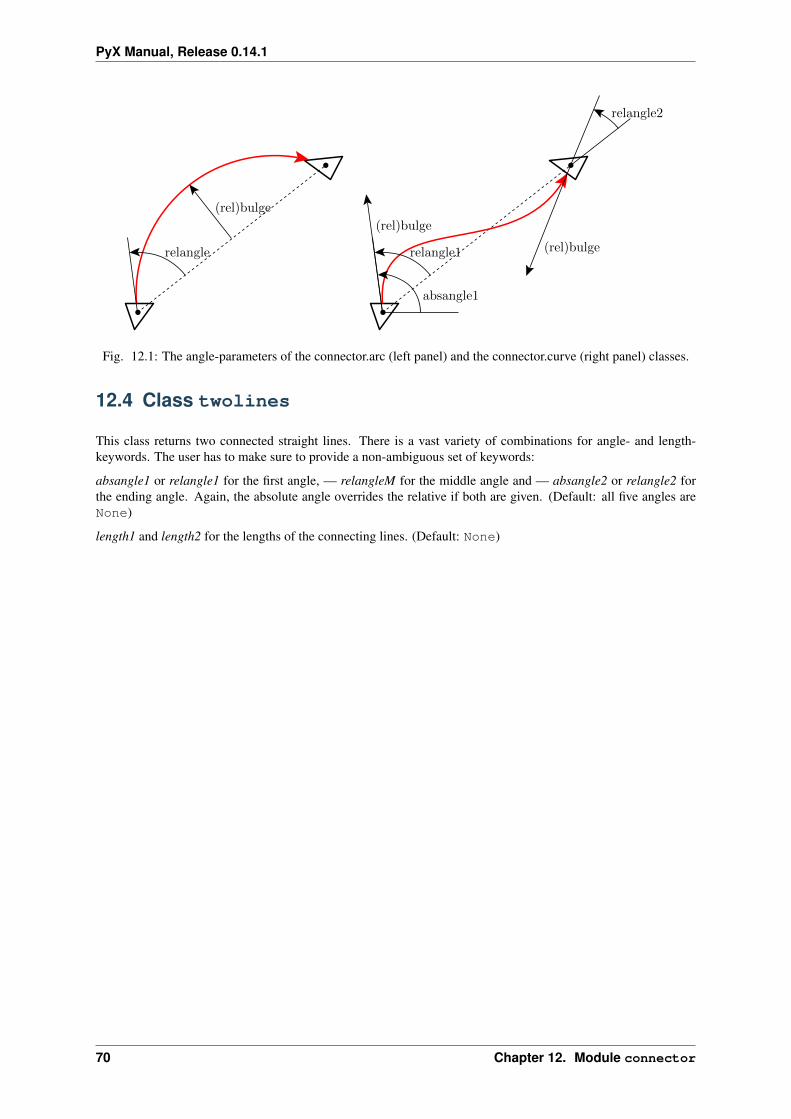
PyX Manual, Release 0.14.1
relangle
(rel)bulge
relangle1
absangle1
relangle2
(rel)bulge
(rel)bulge
Fig. 12.1: The angle-parameters of the connector.arc (left panel) and the connector.curve (right panel) classes.
12.4 Class twolines
This class returns two connected straight lines. There is a vast variety of combinations for angle- and length-keywords. The user has to make sure to provide a non-ambiguous set of keywords:
absangle1 or relangle1 for the first angle, — relangleM for the middle angle and — absangle2 or relangle2 forthe ending angle. Again, the absolute angle overrides the relative if both are given. (Default: all five angles areNone)
length1 and length2 for the lengths of the connecting lines. (Default: None)
70 Chapter 12. Module connector
CHAPTER
THIRTEEN
MODULE EPSFILE: EPS FILE INCLUSION
With the help of the epsfile.epsfile class, you can easily embed another EPS file in your canvas, therebyscaling, aligning the content at discretion. The most simple example looks like
from pyx import *c = canvas.canvas()c.insert(epsfile.epsfile(0, 0, "file.eps"))c.writeEPSfile("output")
All relevant parameters are passed to the epsfile.epsfile constructor. They are summarized in the followingtable:
argumentname
description
x 𝑥-coordinate of position.y 𝑦-coordinate of position.filename Name of the EPS file (including a possible extension).width=None Desired width of EPS graphics or None for original width. Cannot be combined with scale
specification.height=NoneDesired height of EPS graphics or None for original height. Cannot be combined with scale
specification.scale=None Scaling factor for EPS graphics or None for no scaling. Cannot be combined with width or
height specification.align="bl" Alignment of EPS graphics. The first character specifies the vertical alignment: b for bottom,
c for center, and t for top. The second character fixes the horizontal alignment: l for left, cfor center r for right.
clip=1 Clip to bounding box of EPS file?translatebbox=1Use lower left corner of bounding box of EPS file? Set to 0 with care.bbox=None If given, use bbox instance instead of bounding box of EPS file.kpsearch=0 Search for file using the kpathsea library.
71
PyX Manual, Release 0.14.1
72 Chapter 13. Module epsfile: EPS file inclusion
CHAPTER
FOURTEEN
MODULE SVGFILE: SVG FILE INCLUSION
With the help of the svgfile.svgfile class, you can easily embed another SVG file in your canvas, therebyscaling, aligning the content at discretion. The most simple example looks like
from pyx import *c = canvas.canvas()c.insert(svgfile.svgfile(0, 0, "file.svg"))c.writeSVGfile("output")
All relevant parameters are passed to the svgfile.svgfile constructor. They are summarized in the followingtable:
argumentname
description
x 𝑥-coordinate of position.y 𝑦-coordinate of position.filename Name of the SVG file.width=NoneDesired width of SVG graphics or None for original width.height=NoneDesired height of SVG graphics or None for original height.ratio=NoneFor a given width or height set the other dimension with the given ratio. If None and either
width or height is set, the other dimension is scaled proportionally, which is different from aratio 1.
parsed=FalseParsed mode flag, see below.resolution=96SVG resolution in “dpi”, see below.
In parsed mode a filled PyX canvas containing the SVG data is created. At the moment the parser handles pathswith styles, transformations, canvas nesting etc. but no other SVG constructs. While some features might be addedin the future, the parsed mode will probably always have limitations, like not being able to take into account CSSstyling and other things. On the other hand the parsed mode has some major advantages. You can access the pathsas PyX paths within the canvas and you can output the parsed SVG data to PostScript and PDF.
Even though SVG is a vector format, inserting an SVG file depends on a resolution most of the time. Thisresolution defines the unit scale, when no unit like pt, in, mm, or cm is used. This user unit is meant to be pixels,thus viewer programs are adviced to use the screen resolution. Tools to SVG files often use 90 dpi as in the w3.orgSVG Recommendation. However, note that Adobe (R) Illustrator (R) uses 72 dpi. In browsers 96 dpi is commonlyused, which is thus set as the default. However, all this might vary between plattforms and configurations.
Note that the SVG output of PyX defines the its size using units. Still, when reading such a file in un-parsedmode PyX need to make assumtions on how the final viewer will insert (i.e. scale and position) the SVG file, thusneeding a resolution. Only in parsed mode it becomes resolution independent.
Unfortunately it is rather uncommon to store the size of the SVG in coordinates with units. You then need toprovide the correct resolution in both modes, parsed and unparsed, to get proper alignment.
73

PyX Manual, Release 0.14.1
74 Chapter 14. Module svgfile: SVG file inclusion
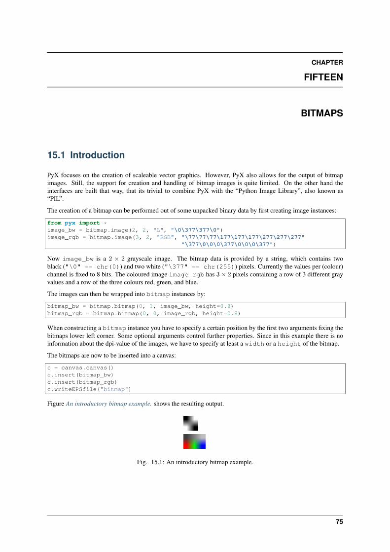
CHAPTER
FIFTEEN
BITMAPS
15.1 Introduction
PyX focuses on the creation of scaleable vector graphics. However, PyX also allows for the output of bitmapimages. Still, the support for creation and handling of bitmap images is quite limited. On the other hand theinterfaces are built that way, that its trivial to combine PyX with the “Python Image Library”, also known as“PIL”.
The creation of a bitmap can be performed out of some unpacked binary data by first creating image instances:
from pyx import *image_bw = bitmap.image(2, 2, "L", "\0\377\377\0")image_rgb = bitmap.image(3, 2, "RGB", "\77\77\77\177\177\177\277\277\277"
"\377\0\0\0\377\0\0\0\377")
Now image_bw is a 2 × 2 grayscale image. The bitmap data is provided by a string, which contains twoblack ("\0" == chr(0)) and two white ("\377" == chr(255)) pixels. Currently the values per (colour)channel is fixed to 8 bits. The coloured image image_rgb has 3× 2 pixels containing a row of 3 different grayvalues and a row of the three colours red, green, and blue.
The images can then be wrapped into bitmap instances by:
bitmap_bw = bitmap.bitmap(0, 1, image_bw, height=0.8)bitmap_rgb = bitmap.bitmap(0, 0, image_rgb, height=0.8)
When constructing a bitmap instance you have to specify a certain position by the first two arguments fixing thebitmaps lower left corner. Some optional arguments control further properties. Since in this example there is noinformation about the dpi-value of the images, we have to specify at least a width or a height of the bitmap.
The bitmaps are now to be inserted into a canvas:
c = canvas.canvas()c.insert(bitmap_bw)c.insert(bitmap_rgb)c.writeEPSfile("bitmap")
Figure An introductory bitmap example. shows the resulting output.
Fig. 15.1: An introductory bitmap example.
75
PyX Manual, Release 0.14.1
15.2 Bitmap module: Bitmap support
class bitmap.image(width, height, mode, data, compressed=None)This class is a container for image data. width and height are the size of the image in pixel. mode is oneof "L", " RGB" or "CMYK" for grayscale, rgb, or cmyk colours, respectively. data is the bitmap data asa string, where each single character represents a colour value with ordinal range 0 to 255. Each pixel isdescribed by the appropriate number of colour components according to mode. The pixels are listed row byrow one after the other starting at the upper left corner of the image.
compressed might be set to " Flate" or "DCT" to provide already compressed data. Note that those datawill be passed to PostScript without further checks, i.e. this option is for experts only.
class bitmap.jpegimage(file)This class is specialized to read data from a JPEG/JFIF-file. file is either an open file handle (it only hasto provide a read() method; the file should be opened in binary mode) or a string. In the latter casejpegimage will try to open a file named like file for reading.
The contents of the file is checked for some JPEG/JFIF format markers in order to identify the size anddpi resolution of the image for further usage. These checks will typically fail for invalid data. The dataare not uncompressed, but directly inserted into the output stream (for invalid data the result will be invalidPostScript). Thus there is no quality loss by recompressing the data as it would occur when recompressingthe uncompressed stream with the lossy jpeg compression method.
class bitmap.bitmap(xpos, ypos, image, width=None, height=None, ratio=None, storedata=0,maxstrlen=4093, compressmode=”Flate”, flatecompresslevel=6, dctqual-ity=75, dctoptimize=1, dctprogression=0)
xpos and ypos are the position of the lower left corner of the image. This position might be modified bysome additional transformations when inserting the bitmap into a canvas. image is an instance of image orjpegimage but it can also be an image instance from the “Python Image Library”.
width, height, and ratio adjust the size of the image. At least width or height needs to be given, when no dpiinformation is available from image.
storedata is a flag indicating, that the (still compressed) image data should be put into the printers mem-ory instead of writing it as a stream into the PostScript file. While this feature consumes memory of thePostScript interpreter, it allows for multiple usage of the image without including the image data severaltimes in the PostScript file.
maxstrlen defines a maximal string length when storedata is enabled. Since the data must be kept in thePostScript interpreters memory, it is stored in strings. While most interpreters do not allow for an arbitrarystring length (a common limit is 65535 characters), a limit for the string length is set. When more data needto be stored, a list of strings will be used. Note that lists are also subject to some implementation limits.Since a typical value is 65535 entries, in combination a huge amount of memory can be used.
Valid values for compressmode currently are "Flate" (zlib compression), "DCT" (jpeg compression),or None (disabling the compression). The zlib compression makes use of the zlib module as it is part ofthe standard Python distribution. The jpeg compression is available for those image instances only, whichsupport the creation of a jpeg-compressed stream, e.g. images from the “Python Image Library” with jpegsupport installed. The compression must be disabled when the image data is already compressed.
flatecompresslevel is a parameter of the zlib compression. dctquality, dctoptimize, and dctprogression areparameters of the jpeg compression. Note, that the progression feature of the jpeg compression should beturned off in order to produce valid PostScript. Also the optimization feature is known to produce errors oncertain printers.
76 Chapter 15. Bitmaps
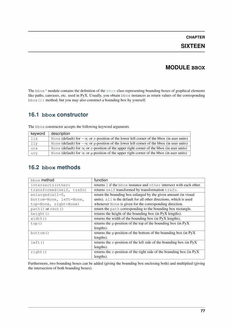
CHAPTER
SIXTEEN
MODULE BBOX
The bbox‘ module contains the definition of the bbox class representing bounding boxes of graphical elementslike paths, canvases, etc. used in PyX. Usually, you obtain bbox instances as return values of the correspondingbbox()) method, but you may also construct a bounding box by yourself.
16.1 bbox constructor
The bbox constructor accepts the following keyword arguments
keyword descriptionllx None (default) for −∞ or 𝑥-position of the lower left corner of the bbox (in user units)lly None (default) for −∞ or 𝑦-position of the lower left corner of the bbox (in user units)urx None (default) for ∞ or 𝑥-position of the upper right corner of the bbox (in user units)ury None (default) for ∞ or 𝑦-position of the upper right corner of the bbox (in user units)
16.2 bbox methods
bbox method functionintersects(other) returns 1 if the bbox instance and other intersect with each other.transformed(self, trafo) returns self transformed by transformation trafo.enlarged(all=0,bottom=None, left=None,top=None, right=None)
return the bounding box enlarged by the given amount (in visualunits). all is the default for all other directions, which is usedwhenever None is given for the corresponding direction.
path() or rect() return the path corresponding to the bounding box rectangle.height() returns the height of the bounding box (in PyX lengths).width() returns the width of the bounding box (in PyX lengths).top() returns the 𝑦-position of the top of the bounding box (in PyX
lengths).bottom() returns the 𝑦-position of the bottom of the bounding box (in PyX
lengths).left() returns the 𝑥-position of the left side of the bounding box (in PyX
lengths).right() returns the 𝑥-position of the right side of the bounding box (in PyX
lengths).
Furthermore, two bounding boxes can be added (giving the bounding box enclosing both) and multiplied (givingthe intersection of both bounding boxes).
77
PyX Manual, Release 0.14.1
78 Chapter 16. Module bbox
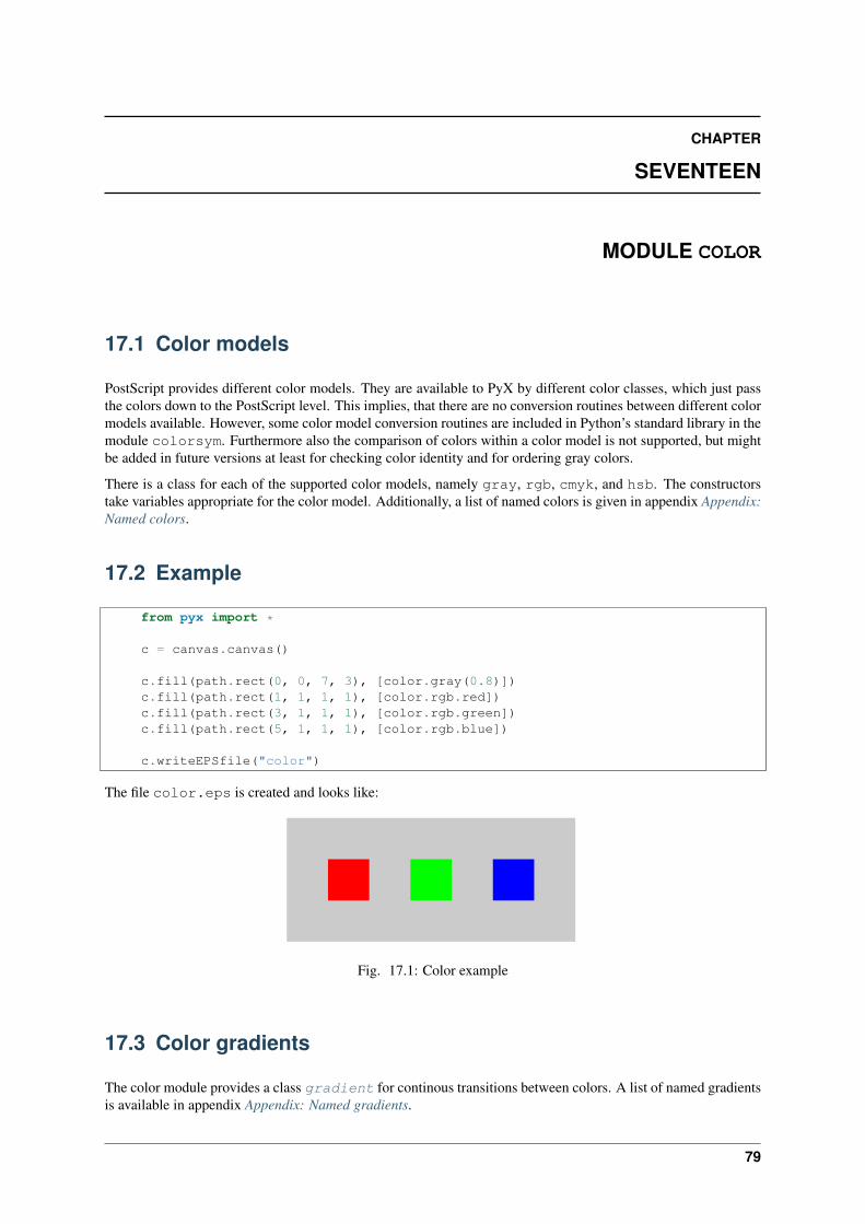
CHAPTER
SEVENTEEN
MODULE COLOR
17.1 Color models
PostScript provides different color models. They are available to PyX by different color classes, which just passthe colors down to the PostScript level. This implies, that there are no conversion routines between different colormodels available. However, some color model conversion routines are included in Python’s standard library in themodule colorsym. Furthermore also the comparison of colors within a color model is not supported, but mightbe added in future versions at least for checking color identity and for ordering gray colors.
There is a class for each of the supported color models, namely gray, rgb, cmyk, and hsb. The constructorstake variables appropriate for the color model. Additionally, a list of named colors is given in appendix Appendix:Named colors.
17.2 Example
from pyx import *
c = canvas.canvas()
c.fill(path.rect(0, 0, 7, 3), [color.gray(0.8)])c.fill(path.rect(1, 1, 1, 1), [color.rgb.red])c.fill(path.rect(3, 1, 1, 1), [color.rgb.green])c.fill(path.rect(5, 1, 1, 1), [color.rgb.blue])
c.writeEPSfile("color")
The file color.eps is created and looks like:
Fig. 17.1: Color example
17.3 Color gradients
The color module provides a class gradient for continous transitions between colors. A list of named gradientsis available in appendix Appendix: Named gradients.
79

PyX Manual, Release 0.14.1
Note that all predefined non-gray gradients are defined in the RGB color space, except for gradient.Rainbow,gradient.ReverseRainbow, gradient.Hue, and gradient.ReverseHue, which are naturally defined in the HSB colorspace. Converted RGB and CMYK versions of these latter gradients are also defined under the names rgbgradi-ent.Rainbow and cmykgradient.Rainbow, etc.
class color.gradientThis class defines the methods for the gradient.
getcolor(parameter)Returns the color that corresponds to parameter (must be between min and max).
select(index, n_indices)When a total number of n_indices different colors is needed from the gradient, this method returns theindex-th color.
class color.functiongradient_cmyk(f_c, f_m, f_y, f_k)
class color.functiongradient_gray(f_gray)
class color.functiongradient_hsb(f_g, f_s, f_b)
class color.functiongradient_rgb(f_r, f_g, f_b)This class provides an arbitray transition between colors of the same color model.
The functions f_c, etc. map the values [0, 1] to the respective components of the color model.
color.lineargradient_cmyk(mincolor, maxcolor)
color.lineargradient_gray(mincolor, maxcolor)
color.lineargradient_hsb(mincolor, maxcolor)
color.lineargradient_rgb(mincolor, maxcolor)These factory functors for the corresponding functiongradient_ classes provide a linear transition betweentwo given instances of the same color class. The linear interpolation is performed on the color componentsof the specific color model.
mincolor and maxcolor must be colors of the corresponding color class.
class rgbgradient(gradient)This class takes an arbitrary gradient and converts it into one in the RGB color model. This is useful forinstance in bitmap output, where only certain color models are supported in Postscript/PDF.
class cmykgradient(gradient)This class takes an arbitrary gradient and converts it into one in the CMYK color mode. This is useful forinstance in bitmap output, where only certain color models are supported in Postscript/PDF.
17.4 Transparency
class color.transparency(value)Instances of this class will make drawing operations (stroking, filling) to become partially transparent. valuedefines the transparency factor in the range 0 (opaque) to 1 (transparent).
Transparency is available in PDF output only since it is not supported by PostScript. However, for certainghostscript devices (for example the pdf backend as used by ps2pdf) proprietary PostScript extension allowsfor transparency in PostScript code too. PyX creates such PostScript proprietary code, but issues a warningwhen doing so.
80 Chapter 17. Module color
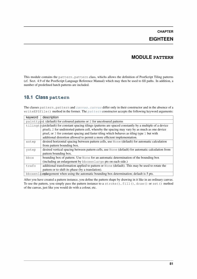
CHAPTER
EIGHTEEN
MODULE PATTERN
This module contains the pattern.pattern class, whichs allows the definition of PostScript Tiling patterns(cf. Sect. 4.9 of the PostScript Language Reference Manual) which may then be used to fill paths. In addition, anumber of predefined hatch patterns are included.
18.1 Class pattern
The classes pattern.pattern and canvas.canvas differ only in their constructor and in the absence of awriteEPSfile() method in the former. The pattern constructor accepts the following keyword arguments:
keyword descriptionpainttype1 (default) for coloured patterns or 2 for uncoloured patternstilingtype1 (default) for constant spacing tilings (patterns are spaced constantly by a multiple of a device
pixel), 2 for undistorted pattern cell, whereby the spacing may vary by as much as one devicepixel, or 3 for constant spacing and faster tiling which behaves as tiling type 1 but withadditional distortion allowed to permit a more efficient implementation.
xstep desired horizontal spacing between pattern cells, use None (default) for automatic calculationfrom pattern bounding box.
ystep desired vertical spacing between pattern cells, use None (default) for automatic calculation frompattern bounding box.
bbox bounding box of pattern. Use None for an automatic determination of the bounding box(including an enlargement by bboxenlarge pts on each side.)
trafo additional transformation applied to pattern or None (default). This may be used to rotate thepattern or to shift its phase (by a translation).
bboxenlargeenlargement when using the automatic bounding box determination; default is 5 pts.
After you have created a pattern instance, you define the pattern shape by drawing in it like in an ordinary canvas.To use the pattern, you simply pass the pattern instance to a stroke(), fill(), draw() or set() methodof the canvas, just like you would do with a colour, etc.
81
PyX Manual, Release 0.14.1
82 Chapter 18. Module pattern
CHAPTER
NINETEEN
MODULE UNIT
With the unit module PyX makes available classes and functions for the specification and manipulation oflengths. As usual, lengths consist of a number together with a measurement unit, e.g., 1 cm, 50 points, 0.42 inch.In addition, lengths in PyX are composed of the five types “true”, “user”, “visual”, “width”, and “TeX”, e.g., 1user cm, 50 true points, 0.42 visual + 0.2 width inch. As their names indicate, they serve different purposes. Truelengths are not scalable and are mainly used for return values of PyX functions. The other length types can berescaled by the user and differ with respect to the type of object they are applied to:
user length: used for lengths of graphical objects like positions etc.
visual length: used for sizes of visual elements, like arrows, graph symbols, axis ticks, etc.
width length: used for line widths
TeX length: used for all TeX and LaTeX output
When not specified otherwise, all types of lengths are interpreted in terms of a default unit, which, by default, is 1cm. You may change this default unit by using the module level function
unit.set(uscale=None, vscale=None, wscale=None, xscale=None, defaultunit=None)When uscale, vscale, wscale, or xscale is not None, the corresponding scaling factor(s) is redefined to thegiven number. When defaultunit is not None, the default unit is set to the given value, which has to be oneof "cm", "mm", "inch", or "pt".
For instance, if you only want thicker lines for a publication version of your figure, you can just rescale all widthlengths using
unit.set(wscale=2)
Or suppose, you are used to specify length in imperial units. In this, admittedly rather unfortunate case, just use
unit.set(defaultunit="inch")
at the beginning of your program.
19.1 Class length
class unit.length(f, type=”u”, unit=None)The constructor of the length class expects as its first argument a number f, which represents the prefactorof the given length. By default this length is interpreted as a user length (type="u") in units of the currentdefault unit (see set() function of the unit module). Optionally, a different type may be specified,namely "u" for user lengths, "v" for visual lengths, "w" for width lengths, "x" for TeX length, and "t"for true lengths. Furthermore, a different unit may be specified using the unit argument. Allowed values are"cm", "mm", "inch", and "pt".
Instances of the length class support addition and substraction either by another length or by a number whichis then interpeted as being a user length in default units, multiplication by a number and division either by anotherlength in which case a float is returned or by a number in which case a length instance is returned. When twolengths are compared, they are first converted to meters (using the currently set scaling), and then the resultingvalues are compared.
83

PyX Manual, Release 0.14.1
19.2 Predefined length instances
A number of length instances are already predefined, which only differ in there values for type and unit.They are summarized in the following table
name type unitm user mcm user cmmm user mminch user inchpt user pointst_m true mt_cm true cmt_mm true mmt_inch true incht_pt true pointsu_m user mu_cm user cmu_mm user mmu_inch user inchu_pt user pointsv_m visual mv_cm visual cmv_mm visual mmv_inch visual inchv_pt visual pointsw_m width mw_cm width cmw_mm width mmw_inch width inchw_pt width pointsx_m TeX mx_cm TeX cmx_mm TeX mmx_inch TeX inchx_pt TeX points
Thus, in order to specify, e.g., a length of 5 width points, just use 5*unit.w_pt.
19.3 Conversion functions
If you want to know the value of a PyX length in certain units, you may use the predefined conversion functionswhich are given in the following table
function resulttom(l) l in units of mtocm(l) l in units of cmtomm(l) l in units of mmtoinch(l) l in units of inchtopt(l) l in units of points
If l is not yet a length instance but a number, it first is interpreted as a user length in the default units.
84 Chapter 19. Module unit
CHAPTER
TWENTY
MODULE TRAFO: LINEAR TRANSFORMATIONS
With the trafo module PyX supports linear transformations, which can then be applied to canvases, Bézier pathsand other objects. It consists of the main class trafo representing a general linear transformation and subclassesthereof, which provide special operations like translation, rotation, scaling, and mirroring.
20.1 Class trafo
The trafo class represents a general linear transformation, which is defined for a vector �⃗� as
�⃗�′ = A �⃗�+ �⃗� ,
where A is the transformation matrix and �⃗� the translation vector. The transformation matrix must not be singular,i.e. we require detA ̸= 0.
Multiple trafo instances can be multiplied, corresponding to a consecutive application of the respective transfor-mation. Note that trafo1*trafo2 means that trafo1 is applied after trafo2, i.e. the new transformationis given by A = A1A2 and �⃗� = A1⃗𝑏2 + �⃗�1. Use the trafo methods described below, if you prefer thinking theother way round. The inverse of a transformation can be obtained via the trafo method inverse(), definedby the inverse A−1 of the transformation matrix and the translation vector −A−1⃗𝑏.
class trafo.trafo(matrix=((1, 0), (0, 1)), vector=(0, 0))create new trafo instance with transformation matrix and vector
trafo.apply(x, y)apply trafo to point vector (x, y).
trafo.inverse()returns inverse transformation of trafo.
trafo.mirrored(angle)returns trafo followed by mirroring at line through (0, 0) with direction angle in degrees.
trafo.rotated(angle, x=None, y=None)returns trafo followed by rotation by angle degrees around point (x, y), or (0, 0), if not given.
trafo.scaled(sx, sy=None, x=None, y=None)returns trafo followed by scaling with scaling factor sx in 𝑥-direction, sy in 𝑦-direction (sy = sx, if notgiven) with scaling center (x, y), or (0, 0), if not given.
trafo.slanted(a, angle=0, x=None, y=None)returns trafo followed by slant by angle around point (x, y), or (0, 0), if not given.
trafo.translated(x, y)returns trafo followed by translation by vector (x, y).
85
PyX Manual, Release 0.14.1
20.2 Subclasses of trafo
The trafo module provides a number of subclasses of the trafo class, each of which corresponds to onetrafo method.
class trafo.mirror(angle)mirroring at line through (0, 0) with direction angle in degrees.
class trafo.rotate(angle, x=None, y=None)rotation by angle degrees around point (x, y), or (0, 0), if not given.
class trafo.scale(sx, sy=None, x=None, y=None)scaling with scaling factor sx in 𝑥-direction, sy in 𝑦-direction (sy = sx, if not given) with scaling center(x, y), or (0, 0), if not given.
class trafo.slant(a, angle=0, x=None, y=None)slant by angle around point (x, y), or (0, 0), if not given.
class trafo.translate(x, y)translation by vector (x, y).
86 Chapter 20. Module trafo: Linear transformations
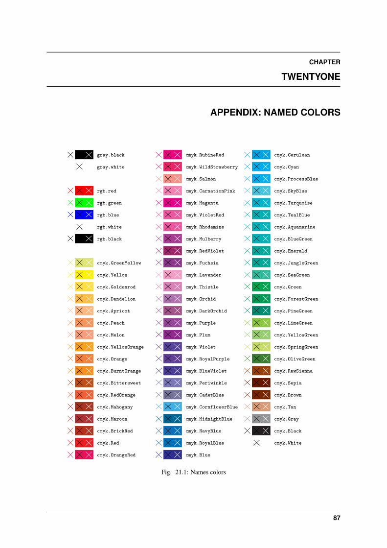
CHAPTER
TWENTYONE
APPENDIX: NAMED COLORS
gray.black
gray.white
rgb.red
rgb.green
rgb.blue
rgb.white
rgb.black
cmyk.GreenYellow
cmyk.Yellow
cmyk.Goldenrod
cmyk.Dandelion
cmyk.Apricot
cmyk.Peach
cmyk.Melon
cmyk.YellowOrange
cmyk.Orange
cmyk.BurntOrange
cmyk.Bittersweet
cmyk.RedOrange
cmyk.Mahogany
cmyk.Maroon
cmyk.BrickRed
cmyk.Red
cmyk.OrangeRed
cmyk.RubineRed
cmyk.WildStrawberry
cmyk.Salmon
cmyk.CarnationPink
cmyk.Magenta
cmyk.VioletRed
cmyk.Rhodamine
cmyk.Mulberry
cmyk.RedViolet
cmyk.Fuchsia
cmyk.Lavender
cmyk.Thistle
cmyk.Orchid
cmyk.DarkOrchid
cmyk.Purple
cmyk.Plum
cmyk.Violet
cmyk.RoyalPurple
cmyk.BlueViolet
cmyk.Periwinkle
cmyk.CadetBlue
cmyk.CornflowerBlue
cmyk.MidnightBlue
cmyk.NavyBlue
cmyk.RoyalBlue
cmyk.Blue
cmyk.Cerulean
cmyk.Cyan
cmyk.ProcessBlue
cmyk.SkyBlue
cmyk.Turquoise
cmyk.TealBlue
cmyk.Aquamarine
cmyk.BlueGreen
cmyk.Emerald
cmyk.JungleGreen
cmyk.SeaGreen
cmyk.Green
cmyk.ForestGreen
cmyk.PineGreen
cmyk.LimeGreen
cmyk.YellowGreen
cmyk.SpringGreen
cmyk.OliveGreen
cmyk.RawSienna
cmyk.Sepia
cmyk.Brown
cmyk.Tan
cmyk.Gray
cmyk.Black
cmyk.White
Fig. 21.1: Names colors
87
PyX Manual, Release 0.14.1
88 Chapter 21. Appendix: Named colors
CHAPTER
TWENTYTWO
APPENDIX: NAMED GRADIENTS
89
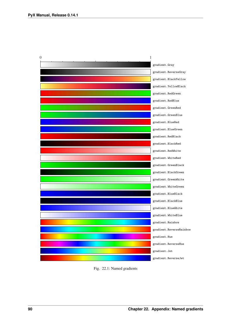
PyX Manual, Release 0.14.1
0 1
gradient.Gray
gradient.ReverseGray
gradient.BlackYellow
gradient.YellowBlack
gradient.RedGreen
gradient.RedBlue
gradient.GreenRed
gradient.GreenBlue
gradient.BlueRed
gradient.BlueGreen
gradient.RedBlack
gradient.BlackRed
gradient.RedWhite
gradient.WhiteRed
gradient.GreenBlack
gradient.BlackGreen
gradient.GreenWhite
gradient.WhiteGreen
gradient.BlueBlack
gradient.BlackBlue
gradient.BlueWhite
gradient.WhiteBlue
gradient.Rainbow
gradient.ReverseRainbow
gradient.Hue
gradient.ReverseHue
gradient.Jet
gradient.ReverseJet
Fig. 22.1: Named gradients
90 Chapter 22. Appendix: Named gradients
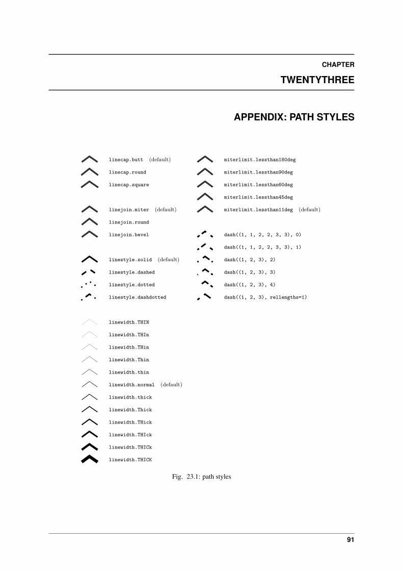
CHAPTER
TWENTYTHREE
APPENDIX: PATH STYLES
linecap.butt (default)
linecap.round
linecap.square
linejoin.miter (default)
linejoin.round
linejoin.bevel
linestyle.solid (default)
linestyle.dashed
linestyle.dotted
linestyle.dashdotted
linewidth.THIN
linewidth.THIn
linewidth.THin
linewidth.Thin
linewidth.thin
linewidth.normal (default)
linewidth.thick
linewidth.Thick
linewidth.THick
linewidth.THIck
linewidth.THICk
linewidth.THICK
miterlimit.lessthan180deg
miterlimit.lessthan90deg
miterlimit.lessthan60deg
miterlimit.lessthan45deg
miterlimit.lessthan11deg (default)
dash((1, 1, 2, 2, 3, 3), 0)
dash((1, 1, 2, 2, 3, 3), 1)
dash((1, 2, 3), 2)
dash((1, 2, 3), 3)
dash((1, 2, 3), 4)
dash((1, 2, 3), rellengths=1)
Fig. 23.1: path styles
91
PyX Manual, Release 0.14.1
92 Chapter 23. Appendix: path styles
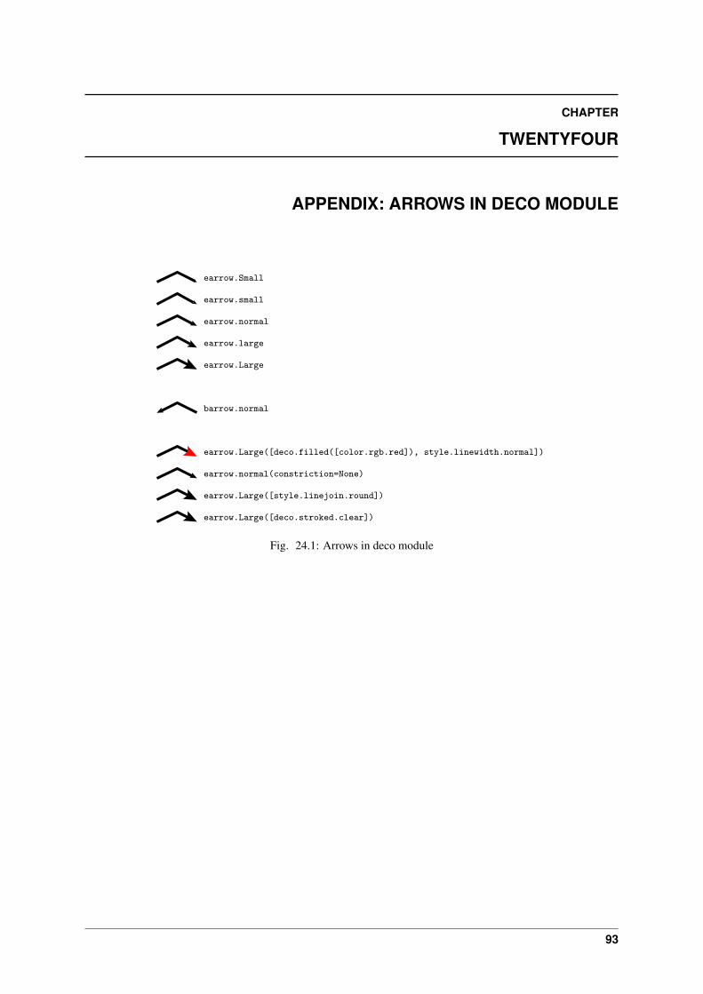
CHAPTER
TWENTYFOUR
APPENDIX: ARROWS IN DECO MODULE
earrow.Small
earrow.small
earrow.normal
earrow.large
earrow.Large
barrow.normal
earrow.Large([deco.filled([color.rgb.red]), style.linewidth.normal])
earrow.normal(constriction=None)
earrow.Large([style.linejoin.round])
earrow.Large([deco.stroked.clear])
Fig. 24.1: Arrows in deco module
93
PyX Manual, Release 0.14.1
94 Chapter 24. Appendix: Arrows in deco module
PYTHON MODULE INDEX
bbbox, 76bitmap, 75box, 65
ccanvas, 20color, 77connector, 68
ddeformer, 18document, 23
eepsfile, 70
ggraph, 39graph.axis, 54graph.axis.axis, 55graph.axis.painter, 62graph.axis.parter, 58graph.axis.positioners, 64graph.axis.rater, 63graph.axis.texter, 60graph.axis.tick, 58graph.data, 46graph.graph, 43graph.key, 53graph.style, 49
mmetapost.path, 15
ppath, 10pattern, 80pyx, 38
sstyle, 89svgfile, 71
ttext, 26
trafo, 84
uunit, 81
95
PyX Manual, Release 0.14.1
96 Python Module Index
INDEX
Symbols__call__() (deformer.deformer method), 19
Aanchoredaxis (class in graph.axis.axis), 57anchoredpathaxis (class in graph.axis.axis), 58append() (path.normsubpath method), 14append() (path.path method), 11apply() (in module trafo), 85arc (class in path), 13arclen() (path.path method), 11arclentoparam() (path.path method), 11arcn (class in path), 13arct (class in path), 13arrow (class in graph.style), 51at() (path.path method), 11atbegin() (path.path method), 11atend() (path.path method), 11autolin (class in graph.axis.parter), 59autolinear (class in graph.axis.parter), 59autolog (class in graph.axis.parter), 60autologarithmic (class in graph.axis.parter), 60axes (graph.graph.graphxy attribute), 44axisatv() (graph.graph.graphxy method), 45axistrafo() (graph.graph.graphxy method), 45
Bbar (class in graph.axis.axis), 56bar (class in graph.axis.painter), 63bar (class in graph.style), 52barpos (class in graph.style), 52baseline (text.valign attribute), 35basepath() (graph.axis.axis.anchoredaxis method), 57bbox (module), 76bbox() (canvas.canvas method), 22bbox() (path.path method), 11begin() (path.path method), 11beginknot (class in metapost.path), 17bitmap (class in bitmap), 76bitmap (module), 75bottom (text.valign attribute), 35bottomzero (text.vshift attribute), 36box (module), 65box_warning() (text.texmessage static method), 34boxcenter (text.halign attribute), 34boxleft (text.halign attribute), 34
boxright (text.halign attribute), 34
Ccanvas (class in canvas), 21canvas (module), 20cbdfile (class in graph.data), 49center (text.halign attribute), 35central (class in graph.graph), 46central (graph.graph.graphxyz attribute), 46changebar (class in graph.style), 53changecircle (graph.style.symbol attribute), 50changecircletwice (graph.style.symbol attribute), 51changecross (graph.style.symbol attribute), 50changediamond (graph.style.symbol attribute), 51changediamondtwice (graph.style.symbol attribute), 51changefilledstroked (graph.style.symbol attribute), 51changelinestyle (graph.style.line attribute), 51changeplus (graph.style.symbol attribute), 50changesquare (graph.style.symbol attribute), 50changesquaretwice (graph.style.symbol attribute), 51changestrokedfilled (graph.style.symbol attribute), 51changetriangle (graph.style.symbol attribute), 50changetriangletwice (graph.style.symbol attribute), 51circle (class in path), 15circle (graph.style.symbol attribute), 50close() (path.normsubpath method), 14closepath (class in path), 13color (module), 77conffile (class in graph.data), 48connector (module), 68controlcurve (class in metapost.path), 18cross (graph.style.symbol attribute), 50cube (class in graph.axis.rater), 64curve (class in metapost.path), 18curve (class in path), 15curveradius() (path.path method), 11curveto (class in path), 13cycloid (class in deformer), 19
Ddata (class in graph.data), 48decimal (class in graph.axis.texter), 60default (text.errordetail attribute), 32default_runner (in module text), 31defaultcolumnpattern (graph.data.file attribute), 48defaultcommentpattern (graph.data.file attribute), 48
97
PyX Manual, Release 0.14.1
defaultstringpattern (graph.data.file attribute), 48defaultvariants (graph.axis.parter.autolinear attribute),
59defaultvariants (graph.axis.parter.autologarithmic at-
tribute), 60deform() (deformer.deformer method), 19deformer (class in deformer), 19deformer (module), 18depth (text.textbox_pt attribute), 31diamond (graph.style.symbol attribute), 50distance (class in graph.axis.rater), 64doaxes() (graph.graph.graphxy method), 44dobackground() (graph.graph.graphxy method), 44document (class in document), 25document (module), 23dokey() (graph.graph.graphxy method), 45dokeyitem() (graph.graph.graphxy method), 45dolayout() (graph.graph.graphxy method), 44doplot() (graph.graph.graphxy method), 45doplotitem() (graph.graph.graphxy method), 45draw() (canvas.canvas method), 21
Eend() (path.path method), 11end() (text.texmessage static method), 33endknot (class in metapost.path), 17epsfile (module), 70errorbar (class in graph.style), 51errordetail (class in text), 32escapestring() (in module text), 32exponential (class in graph.axis.texter), 60extend() (path.normsubpath method), 14extend() (path.path method), 12
Ffile (class in graph.data), 46fill() (canvas.canvas method), 21finish() (graph.graph.graphxy method), 45flushcenter (text.halign attribute), 34flushleft (text.halign attribute), 34flushright (text.halign attribute), 35font_warning() (text.texmessage static method), 34footnotesize (text.size attribute), 36full (text.errordetail attribute), 32function (class in graph.data), 48functiongradient_cmyk (class in color), 80functiongradient_gray (class in color), 80functiongradient_hsb (class in color), 80functiongradient_rgb (class in color), 80
Ggradient (class in color), 80gradient.getcolor() (in module color), 80gradient.select() (in module color), 80graph (module), 39graph.axis (module), 54graph.axis.axis (module), 55graph.axis.painter (module), 62
graph.axis.parter (module), 58graph.axis.positioners (module), 64graph.axis.rater (module), 63graph.axis.texter (module), 60graph.axis.tick (module), 58graph.data (module), 46graph.graph (module), 43graph.key (module), 53graph.style (module), 49graphxy (class in graph.graph), 43graphxyz (class in graph.graph), 45grid (class in graph.style), 53gridpath() (graph.axis.axis.anchoredaxis method), 57gridpos (class in graph.style), 53
Hhalign (class in text), 34height (text.textbox_pt attribute), 31histogram (class in graph.style), 52Huge (text.size attribute), 36huge (text.size attribute), 36
Iignore() (text.texmessage static method), 33image (class in bitmap), 76impulses (class in graph.style), 51insert() (canvas.canvas method), 21intersect() (path.path method), 12inverse() (in module trafo), 85
Jjoin() (path.normpath method), 14joined() (path.path method), 12jpegimage (class in bitmap), 76
Kkey (class in graph.key), 54knot (class in metapost.path), 18
LLARGE (text.size attribute), 36Large (text.size attribute), 36large (text.size attribute), 36LatexRunner (class in text), 30layer() (canvas.canvas method), 21left (text.halign attribute), 35left (text.textbox_pt attribute), 31length (class in unit), 83lin (class in graph.axis.axis), 56lin (class in graph.axis.parter), 59lin (class in graph.axis.rater), 64line (class in graph.style), 51line (class in metapost.path), 18line (class in path), 15linear (class in graph.axis.axis), 55linear (class in graph.axis.parter), 59linear (class in graph.axis.rater), 64
98 Index
PyX Manual, Release 0.14.1
lineargradient_cmyk() (in module color), 80lineargradient_gray() (in module color), 80lineargradient_hsb() (in module color), 80lineargradient_rgb() (in module color), 80lineto (class in path), 13linked (class in graph.axis.painter), 63linkedaxis (class in graph.axis.axis), 58linkedbar (class in graph.axis.painter), 63linkedsplit (class in graph.axis.painter), 63load() (text.texmessage static method), 33load_def() (text.texmessage static method), 33load_graphics() (text.texmessage static method), 33log (class in graph.axis.axis), 56log (class in graph.axis.parter), 60log (class in graph.axis.rater), 64logarithmic (class in graph.axis.axis), 56logarithmic (class in graph.axis.parter), 59logarithmic (class in graph.axis.rater), 64
Mmarker() (text.textbox_pt method), 31mathaxis (text.vshift attribute), 36mathmode (in module text), 36metapost.path (module), 15middle (text.valign attribute), 35middlezero (text.vshift attribute), 36mirror (class in trafo), 86mirrored() (in module trafo), 85mixed (class in graph.axis.texter), 61moveto (class in path), 12multicurveto_pt (class in path), 13multilineto_pt (class in path), 13MultiRunner (class in text), 30
Nnestedbar (class in graph.axis.axis), 57no_aux() (text.texmessage static method), 33no_file() (text.texmessage static method), 33no_nav() (text.texmessage static method), 33nobbl_warning() (text.texmessage static method), 34none (text.errordetail attribute), 32normalsize (text.size attribute), 36normpath (class in path), 14normpath() (path.path method), 12normsubpath (class in path), 14
Oorthogonal (graph.axis.painter.rotatetext attribute), 62
Ppackage_warning() (text.texmessage static method), 34page (class in document), 25paperformat (class in document), 26parallel (class in deformer), 20parallel (class in graph.graph), 46parallel (graph.axis.painter.rotatetext attribute), 62parallel (graph.graph.graphxyz attribute), 46paramfunction (class in graph.data), 48
paramtoarclen() (path.path method), 12parbox (class in text), 35path (class in metapost.path), 17path (class in path), 11path (module), 10pattern (module), 80pattern() (text.texmessage static method), 34phantom (in module text), 37pipeGS() (canvas.canvas method), 22plot() (graph.graph.graphxy method), 44plus (graph.style.symbol attribute), 50points (class in graph.data), 48pos (class in graph.style), 50pos() (graph.graph.graphxy method), 45positioner (class in graph.axis.positioners), 64pre125exp (graph.axis.parter.logarithmic attribute), 60pre1exp (graph.axis.parter.logarithmic attribute), 60pre1exp2 (graph.axis.parter.logarithmic attribute), 60pre1exp3 (graph.axis.parter.logarithmic attribute), 59pre1exp4 (graph.axis.parter.logarithmic attribute), 59pre1exp5 (graph.axis.parter.logarithmic attribute), 59pre1to9exp (graph.axis.parter.logarithmic attribute), 60preamble (in module text), 31preamble() (text.MultiRunner method), 30preamble() (text.SingleRunner method), 28preexp (class in graph.axis.parter), 59pyx (module), 38pyxinfo() (in module pyx), 38
Rraggedcenter (text.halign attribute), 34raggedleft (text.halign attribute), 35raggedright (text.halign attribute), 34range (class in graph.style), 50range() (path.path method), 12rater (class in graph.axis.rater), 64rational (class in graph.axis.texter), 61rational (class in graph.axis.tick), 58rcurveto (class in path), 13rect (class in graph.style), 52rect (class in path), 15regular (class in graph.axis.painter), 62rerun_warning() (text.texmessage static method), 34reset (in module text), 31reset() (text.MultiRunner method), 30reverse() (path.normpath method), 14reversed() (path.path method), 12right (text.halign attribute), 35right (text.textbox_pt attribute), 31rlineto (class in path), 13rmoveto (class in path), 12rotate (class in trafo), 86rotated() (in module trafo), 85rotatetext (class in graph.axis.painter), 62rotation() (path.path method), 12roughknot (class in metapost.path), 18
Index 99
PyX Manual, Release 0.14.1
Sscale (class in trafo), 86scaled() (in module trafo), 85scriptsize (text.size attribute), 36set() (in module text), 31set() (in module unit), 83setlinkedaxis() (graph.axis.axis.linkedaxis method), 58settexrunner() (canvas.canvas method), 22SingleLatexRunner (class in text), 29SingleRunner (class in text), 28SingleTexRunner (class in text), 29size (class in text), 36slant (class in trafo), 86slanted() (in module trafo), 85small (text.size attribute), 36smoothed (class in deformer), 19smoothknot (class in metapost.path), 17split (class in graph.axis.axis), 57split (class in graph.axis.painter), 63split() (path.path method), 12splitatvalue() (in module graph.data), 49square (graph.style.symbol attribute), 50stackedbarpos (class in graph.style), 52start() (text.texmessage static method), 33startknot (class in metapost.path), 17stroke() (canvas.canvas method), 21style (module), 89surface (class in graph.style), 53svgfile (module), 71symbol (class in graph.style), 50
Ttangent() (path.path method), 12tensioncurve (class in metapost.path), 18texmessage (class in text), 32texmessages_begindoc_default
(text.SingleLatexRunner attribute), 30texmessages_docclass_default
(text.SingleLatexRunner attribute), 30texmessages_end_default (text.SingleRunner attribute),
28texmessages_preamble_default (text.SingleRunner at-
tribute), 28texmessages_run_default (text.SingleRunner attribute),
28texmessages_start_default (text.SingleRunner at-
tribute), 28TexResultError, 32TexRunner (class in text), 30text (class in graph.style), 51text (in module text), 31text (module), 26text() (canvas.canvas method), 21text() (text.MultiRunner method), 30text() (text.SingleRunner method), 29text_pt (in module text), 31text_pt() (text.MultiRunner method), 30text_pt() (text.SingleRunner method), 28
textbox_pt (class in text), 30tick (class in graph.axis.tick), 58tickdirection() (graph.axis.axis.anchoredaxis method),
57ticklength (class in graph.axis.painter), 62tickpoint() (graph.axis.axis.anchoredaxis method), 57tiny (text.size attribute), 36top (text.valign attribute), 35topzero (text.vshift attribute), 36trafo (class in trafo), 85trafo (module), 84trafo() (path.path method), 12transform() (path.normpath method), 14transformed() (path.path method), 12translate (class in trafo), 86translated() (in module trafo), 85transparency (class in color), 80triangle (graph.style.symbol attribute), 50
Uunit (module), 81
Vvalign (class in text), 35values (class in graph.data), 48vangle() (graph.graph.graphxyz method), 46vbasepath() (graph.axis.axis.anchoredaxis method), 57vbasepath() (graph.axis.positioners.positioner method),
64vgeodesic() (graph.graph.graphxy method), 45vgeodesic_el() (graph.graph.graphxy method), 45vgridpath() (graph.axis.axis.anchoredaxis method), 57vgridpath() (graph.axis.positioners.positioner method),
64vpos() (graph.graph.graphxy method), 45vshift (class in text), 35vtickdirection() (graph.axis.axis.anchoredaxis method),
57, 58vtickdirection() (graph.axis.positioners.positioner
method), 65vtickpoint() (graph.axis.axis.anchoredaxis method), 57vtickpoint_pt() (graph.axis.positioners.positioner
method), 64vzindex() (graph.graph.graphxyz method), 46
Wwarn() (text.texmessage static method), 34width (text.textbox_pt attribute), 31writeEPSfile() (canvas.canvas method), 22writeEPSfile() (document.document method), 25writeGSfile() (canvas.canvas method), 22writePDFfile() (canvas.canvas method), 22writePDFfile() (document.document method), 25writePSfile() (canvas.canvas method), 22writePSfile() (document.document method), 25writeSVGfile() (canvas.canvas method), 22writeSVGfile() (document.document method), 25writetofile() (canvas.canvas method), 22
100 Index
PyX Manual, Release 0.14.1
writetofile() (document.document method), 26
Xxbasepath() (graphxy method), 45xgridpath() (graphxy method), 45xtickdirection() (graphxy method), 45xtickpoint() (graphxy method), 45xvbasepath() (graphxy method), 45xvgridpath() (graphxy method), 45xvtickdirection() (graphxy method), 45xvtickpoint() (graphxy method), 45
Yybasepath() (graphxy method), 45ygridpath() (graphxy method), 45ytickdirection() (graphxy method), 45ytickpoint() (graphxy method), 45yvbasepath() (graphxy method), 45yvgridpath() (graphxy method), 45yvtickdirection() (graphxy method), 45yvtickpoint() (graphxy method), 45
Index 101