job scheduling mechanisms for cloud computing · in this dissertation, we develop deadline-aware...
TRANSCRIPT

Job Scheduling Mechanisms for
Cloud Computing
Jonathan Yaniv
Technion - Computer Science Department - Ph.D. Thesis PHD-2017-03 - 2017

Job Scheduling Mechanisms for
Cloud Computing
Research Thesis
Submitted in partial fulfillment of the requirements
for the degree of Doctor of Philosophy
Jonathan Yaniv
Submitted to the Senate of
the Technion — Israel Institute of Technology
Tevet 5777 Haifa January 2017
Technion - Computer Science Department - Ph.D. Thesis PHD-2017-03 - 2017

The research thesis was done under the supervision of Prof. Seffi Naor in the Computer
Science Department.
Some results in this thesis have been published as articles by the author and research col-
laborators in conferences and journals during the course of the author’s doctoral research
period, the most up-to-date versions of which being:
Navendu Jain, Ishai Menache, Joseph Naor, and Jonathan Yaniv. Near-optimal scheduling mecha-nisms for deadline-sensitive jobs in large computing clusters. Transactions on Parallel Computing,2(1):3, 2015.
Brendan Lucier, Ishai Menache, Joseph Naor, and Jonathan Yaniv. Efficient online scheduling fordeadline-sensitive jobs. In SPAA, pages 305–314, 2013.
Peter Bodık, Ishai Menache, Joseph Naor, and Jonathan Yaniv. Brief announcement: deadline-aware scheduling of big-data processing jobs. In SPAA, pages 211–213, 2014.
Yossi Azar, Inna Kalp-Shaltiel, Brendan Lucier, Ishai Menache, Joseph Naor, and Jonathan Yaniv.Truthful online scheduling with commitments. In EC, pages 715–732, 2015.
Sangeetha Abdu Jyothi, Carlo Curino, Ishai Menache, Shravan Matthur Narayanamutrhy, AlexeyTumanov, Jonathan Yaniv, Ruslan Mavlyutov, Inigo Goiri, Subru Krishnan, Janardhan Kulkarni,and Sriram Rao. Morpheous: Towards automated SLOs for enterprise clusters. In OSDI, pages117–134, 2016.
Acknowledgements. I am indebted to Seffi Naor and Ishai Menache for their guidance,
patience and advice throughout our work. Thank you for providing me with the tools to
become a better researcher. I am honored to be your student.
I am extremely grateful to the Technion CS department for giving me the opportunity to
learn from the most inspiring and profound teachers, to collaborate with incredibly talented
colleagues, and to teach so many brilliant students. I would like to thank Dan Geiger and
Nader Bshouty for their countless advice. Special thanks goes to the administrative staff,
who has always been there for me.
I would like to thank my co-authors for their collaboration and their contribution to our
research. I owe a great deal of thanks to Microsoft Research for hosting me and supporting
this work. My visits to MSR were the highlights of my studies.
I had the privelege of sharing this journey with my fellow peers at the department.
Amongst many are David Wajc, Kira Radisnky, Omer Strulovich, Hanna Mazzawi, Alex
Libov and Yohay Kaplan – my brothers (and sisters) in arms. Thank you for all the unfor-
gettable moments. Finally, I would like to thank my family and friends for their love and
support. I am fortunate to have you in my life.
This thesis is dedicated to Alex, Judith and Lior Yaniv.
The generous financial support of the Technion is gratefully acknowledged.
Technion - Computer Science Department - Ph.D. Thesis PHD-2017-03 - 2017
Contents
Abstract 1
Abbreviations and Notation 3
1 Introduction 5
1.1 Motivation . . . . . . . . . . . . . . . . . . . . . . . . . . . . . . . . . . . . . 5
1.2 General Model . . . . . . . . . . . . . . . . . . . . . . . . . . . . . . . . . . . 6
1.3 Thesis Overview . . . . . . . . . . . . . . . . . . . . . . . . . . . . . . . . . . 8
1.4 Related Work . . . . . . . . . . . . . . . . . . . . . . . . . . . . . . . . . . . . 10
2 Preliminaries 12
2.1 Algorithmic Design . . . . . . . . . . . . . . . . . . . . . . . . . . . . . . . . . 12
2.1.1 Evaluation Metrics . . . . . . . . . . . . . . . . . . . . . . . . . . . . . 12
2.1.2 The Dual Fitting Technique . . . . . . . . . . . . . . . . . . . . . . . . 12
2.2 Algorithmic Mechanism Design . . . . . . . . . . . . . . . . . . . . . . . . . . 16
2.2.1 Definitions . . . . . . . . . . . . . . . . . . . . . . . . . . . . . . . . . 16
2.2.2 Truthfulness and Monotonicity . . . . . . . . . . . . . . . . . . . . . . 17
2.2.3 Profit Maximization in Bayesian Settings . . . . . . . . . . . . . . . . 19
2.2.4 Related Literature . . . . . . . . . . . . . . . . . . . . . . . . . . . . . 20
3 Near-Optimal Schedulers for Identical Release Times 22
3.1 Scheduling Model . . . . . . . . . . . . . . . . . . . . . . . . . . . . . . . . . . 24
3.2 Approximation Algorithms . . . . . . . . . . . . . . . . . . . . . . . . . . . . 24
3.2.1 A Simple Greedy Approach . . . . . . . . . . . . . . . . . . . . . . . . 24
3.2.2 The GreedyRTL Algorithm . . . . . . . . . . . . . . . . . . . . . . . . 29
3.3 Truthfulness . . . . . . . . . . . . . . . . . . . . . . . . . . . . . . . . . . . . . 35
3.4 Coping with Demand Uncertainties . . . . . . . . . . . . . . . . . . . . . . . . 36
3.5 Empirical Study . . . . . . . . . . . . . . . . . . . . . . . . . . . . . . . . . . 38
i
Technion - Computer Science Department - Ph.D. Thesis PHD-2017-03 - 2017

3.5.1 Simulation Setup . . . . . . . . . . . . . . . . . . . . . . . . . . . . . . 38
3.5.2 Resource Utilization . . . . . . . . . . . . . . . . . . . . . . . . . . . . 39
3.5.3 Revenue Maximization . . . . . . . . . . . . . . . . . . . . . . . . . . . 40
3.6 Summary . . . . . . . . . . . . . . . . . . . . . . . . . . . . . . . . . . . . . . 42
3.A Appendix A: Improved Analysis of the Simple Greedy Approach . . . . . . . 43
4 Online Scheduling with Deadline Slackness 45
4.1 Preliminaries . . . . . . . . . . . . . . . . . . . . . . . . . . . . . . . . . . . . 48
4.1.1 Scheduling Model . . . . . . . . . . . . . . . . . . . . . . . . . . . . . . 48
4.1.2 Definitions . . . . . . . . . . . . . . . . . . . . . . . . . . . . . . . . . 48
4.2 The Necessity of Preemption and Resume . . . . . . . . . . . . . . . . . . . . 49
4.3 Online Algorithms . . . . . . . . . . . . . . . . . . . . . . . . . . . . . . . . . 50
4.3.1 Single Server . . . . . . . . . . . . . . . . . . . . . . . . . . . . . . . . 50
4.3.1.1 Algorithm . . . . . . . . . . . . . . . . . . . . . . . . . . . . 50
4.3.1.2 Analysis . . . . . . . . . . . . . . . . . . . . . . . . . . . . . 52
4.3.2 Multiple Servers . . . . . . . . . . . . . . . . . . . . . . . . . . . . . . 59
4.3.2.1 No Parallel Execution (k = 1) . . . . . . . . . . . . . . . . . 59
4.3.2.2 Identical Parallelism Bounds (k > 1) . . . . . . . . . . . . . . 61
4.4 Truthful Mechanisms . . . . . . . . . . . . . . . . . . . . . . . . . . . . . . . . 62
4.4.1 Single Server . . . . . . . . . . . . . . . . . . . . . . . . . . . . . . . . 62
4.4.2 Multiple Servers . . . . . . . . . . . . . . . . . . . . . . . . . . . . . . 66
4.A Appendix A: Proof of Stretching Lemma . . . . . . . . . . . . . . . . . . . . . 69
4.B Appendix B: Non-Truthfulness of Section 4.3 . . . . . . . . . . . . . . . . . . 70
5 Online Scheduling with Commitments 72
5.1 Impossibility Result for Commitment upon Arrival . . . . . . . . . . . . . . . 74
5.2 Reductions for β-Responsive Committed Scheduling . . . . . . . . . . . . . . 75
5.2.1 Reduction for a Single Server . . . . . . . . . . . . . . . . . . . . . . . 75
5.2.1.1 Correctness . . . . . . . . . . . . . . . . . . . . . . . . . . . . 76
5.2.1.2 Competitive Ratio . . . . . . . . . . . . . . . . . . . . . . . . 78
5.2.2 Reductions for Multiple Servers . . . . . . . . . . . . . . . . . . . . . . 80
5.2.2.1 Non-Migratory Case . . . . . . . . . . . . . . . . . . . . . . . 81
5.2.2.2 Migratory Case . . . . . . . . . . . . . . . . . . . . . . . . . 81
5.3 Truthful β-Responsive Committed Scheduling . . . . . . . . . . . . . . . . . . 83
5.3.1 Public Arrival Times . . . . . . . . . . . . . . . . . . . . . . . . . . . . 83
5.3.2 Full Truthfulness . . . . . . . . . . . . . . . . . . . . . . . . . . . . . . 84
5.4 Improved Explicit Bounds . . . . . . . . . . . . . . . . . . . . . . . . . . . . . 89
ii
Technion - Computer Science Department - Ph.D. Thesis PHD-2017-03 - 2017
6 Offline Scheduling of DAG-Structured Jobs 90
6.1 Scheduling Model . . . . . . . . . . . . . . . . . . . . . . . . . . . . . . . . . . 93
6.2 DAG Scheduling . . . . . . . . . . . . . . . . . . . . . . . . . . . . . . . . . . 95
6.2.1 Step 1: Solving a Linear Program . . . . . . . . . . . . . . . . . . . . 95
6.2.2 Step 2: Balancing . . . . . . . . . . . . . . . . . . . . . . . . . . . . . 98
6.2.3 Step 2: Decomposing a Balanced Solution . . . . . . . . . . . . . . . . 100
6.2.4 Step 4: Randomized Rounding . . . . . . . . . . . . . . . . . . . . . . 103
6.2.5 Obtaining a Constant Approximation Factor . . . . . . . . . . . . . . 107
6.3 Model Extensions . . . . . . . . . . . . . . . . . . . . . . . . . . . . . . . . . . 108
6.3.1 Monotone Node Allocations . . . . . . . . . . . . . . . . . . . . . . . . 108
6.3.2 Multiple Sinks . . . . . . . . . . . . . . . . . . . . . . . . . . . . . . . 109
6.4 Conclusions . . . . . . . . . . . . . . . . . . . . . . . . . . . . . . . . . . . . . 109
7 Scheduling Algorithms for Hadoop YARN 110
7.1 Scheduling Model . . . . . . . . . . . . . . . . . . . . . . . . . . . . . . . . . . 111
7.2 Planning Algorithms . . . . . . . . . . . . . . . . . . . . . . . . . . . . . . . . 112
7.2.1 Greedy – The Existing Scheduling Algorithm . . . . . . . . . . . . . . 113
7.2.2 LowCost – A New Cost-Based Planning Algorithm . . . . . . . . . . . 114
7.3 Evaluation . . . . . . . . . . . . . . . . . . . . . . . . . . . . . . . . . . . . . . 117
7.3.1 Methodology . . . . . . . . . . . . . . . . . . . . . . . . . . . . . . . . 117
7.3.2 Simulations . . . . . . . . . . . . . . . . . . . . . . . . . . . . . . . . . 118
7.3.3 Experiments on Real Clusters . . . . . . . . . . . . . . . . . . . . . . . 120
8 Summary 123
iii
Technion - Computer Science Department - Ph.D. Thesis PHD-2017-03 - 2017

List of Figures
3.1 Average resource utilization over time of GreedyRTL and the Decompose-
Randomly-Draw (DRD) mechanism [41] compared to the optimal fractional
resource utilization, which is an upper bound to the optimal resource utiliza-
tion. Results show that GreedyRTL utilizes nearly all of the cloud resources. 40
3.2 Revenue ratio between GreedyRTL and OFP, compared against different in-
put slackness values. The truthful GreedyRTL mechanism is nearly as good
as an ideal optimal fixed-price mechanism. For this experiment, we overload
the system such that the total demand exceeds the cloud capacity, so that
truthful pricing is strictly positive. . . . . . . . . . . . . . . . . . . . . . . . . 41
5.1 Illustration of the proof to Theorem 5.2.1. . . . . . . . . . . . . . . . . . . . . 77
6.1 A job j and its fractional allocation. (1) DAG structure of job j; (2) fractional
solution x (only job j shown); (3) weighted decomposition of x. . . . . . . . 98
7.1 An intermediate execution state of LowCost-A. . . . . . . . . . . . . . . . . . 116
7.2 Simulation results on a 4K cluster as a function of the number of submitted
jobs (300-1000). Results averaged over 5 runs. . . . . . . . . . . . . . . . . . . 118
7.3 Simulation results on a 4K cluster as a function of the number of submitted
jobs (1100-1500). Results averaged over 5 runs. . . . . . . . . . . . . . . . . . 119
7.4 Visualization of the plans at some point throughout the execution of the two
algorithms. These snapshots are taken at high-load conditions. . . . . . . . . 122
iv
Technion - Computer Science Department - Ph.D. Thesis PHD-2017-03 - 2017

Abstract
The rise of cloud computing as a leading platform for large-scale computation has introduced
a wide range of challenges to the field of scheduling. In the cloud paradigm, users receive on-
demand access to shared pools of computing resources, to which they submit applications.
The primary goal of a cloud scheduler is to provide and satisfy service level agreements (SLA)
for running applications. For example, businesses run production-level jobs that must meet
strict deadlines on their completion time. Since the underlying physical resources are limited,
the scheduler must decide which service requests to accept in view of the required SLAs;
and furthermore, incorporate clever resource allocation algorithms to increase the utility
from completed jobs. In general, designing schedulers for the cloud is challenging. First,
jobs differ significantly in their value, urgency, structure and resource requirements. Second,
job requests are not always known in advance, and therefore the schedulers must make
irreversible decisions on-the-fly. Finally, users may attempt to manipulate the scheduler
into processing their own jobs in favor of others.
In this dissertation, we develop deadline-aware job scheduling mechanisms for cloud en-
vironments. Our main theoretical study begins with the fundamental problem of online
deadline scheduling. In its most general form, the problem admits super-constant lower
bounds on the competitive ratio of any scheduler. Nevertheless, we develop constant com-
petitive algorithms under a natural deadline slackness assumption, which requires that no job
deadline is tight. Moreover, our worst-case bounds improve as the input jobs exhibit large
deadline slackness. We then extend the basic allocation model to handle practical aspects of
cloud scheduling, such as scheduling jobs with complex inner dependencies, scheduling jobs
with uncertain requirements, and providing upfront commitments on SLAs.
Another aspect of our work studies truthful scheduling mechanisms, where users are
incentivized not to manipulate the system by falsely reporting job parameters. Such mecha-
nisms are essential not only for public clouds, but also private clouds shared by entities that
belong to the same organization. Based on our allocation algorithms, we develop truthful
mechanisms and provide performance guarantees similar to their non-truthful counterparts.
Finally, inspired by our theoretical study, we implement a deadline-aware job scheduling
1
Technion - Computer Science Department - Ph.D. Thesis PHD-2017-03 - 2017

algorithm for Hadoop YARN. The algorithm was evaluated against existing benchmark
algorithms through extensive experiments, and show substantial improvements over state-
of-the-art. The algorithm will be incorporated in the upcoming Hadoop 2.8 distribution.
2
Technion - Computer Science Department - Ph.D. Thesis PHD-2017-03 - 2017

Abbreviations and Notation
System Parameters
C — capacity; number of servers in the cluster.
T — number of time slots; for discrete timeline only.
T — the timeline.
Job Parameters
j — an index of a job (user).
aj — arrival time of job j.
dj — deadline of job j.
Dj — requested demand (workload) of job j; given in resource units.
Gj — task dependency graph of job j.
kj — parallelism bound of job j.
vj — the value of job j.
Pj — property set of job j.
ρj — value density of job j: vj/Dj .
τj — the type of job j.
General Parameters
k — maximal parallelization bound over jobs: maxjkj.n — number of jobs.
s — deadline slackness.
κD — ratio between maximal and minimal job value.
κv — ratio between maximal and minimal job demand.
κρ — ratio between maximal and minimal value density.
3
Technion - Computer Science Department - Ph.D. Thesis PHD-2017-03 - 2017

Algorithm Design
cr(A) — competitive ratio of algorithm A.
crA(s) — competitive ratio of algorithm A with respect to input instances with slackness s.
IG(s) — integrality gap of a linear program, with respect to input instances with slackness s.
OPT — optimal offline algorithm.
OPT ∗ — optimal fractional algorithm.
v(A(τ)) — total value of completed jobs by algorithm A on input instance τ .
A — scheduling algorithm.
A(τ) — output allocation of algorithm A on input τ .
J — set of jobs.
τ — input instance.
Primal and Dual Variables
yij(t) — primal variable; allocation indicator of job j on server i at time t.
yj(t) — primal variable; total amount of resources allocated to job j at time t.
αj — dual variable; associated with each job j.
β(t) — dual variable; associated with time t.
πj(t) — dual variable; by-product of primal gap decreasing program.
Mechanism Design
bj — bid of user j.
f — allocation algorithm.
p — payment scheme.
uj — utility function of user j.
M — mechanism: M = (f, p).
4
Technion - Computer Science Department - Ph.D. Thesis PHD-2017-03 - 2017

Chapter 1
Introduction
1.1 Motivation
Batch jobs constitute a significant portion of the computing load across internal clusters and
public clouds. Examples include big data analytics, search index updates, video rendering,
and eScience applications. The timely execution of such jobs is often crucial for business
operation. For instance, financial trading firms must deliver the output of their analytics
before the next trading day commences, and delays in uploading website content can lead
to a significant loss in revenue. Since end-users do not own the compute infrastructure, they
must require strict service level agreements (SLAs) on their job completion time – this can
be obtained by enforcing strict deadlines on their completion time. The cloud provider, who
only controls a limited amount of physical resources, must implement scheduling mechanisms
that decide which job requests to accept, and manage the resource allocation such that no
accepted SLA contract is violated.
Unfortunately, the allocation schemes currently used in practice do not provide satisfying
solutions for deadline-sensitive jobs. A common approach for internal clusters is to divide
computing resources in some fair manner between jobs [37]; yet, this approach completely
neglects job deadlines. Another approach is to give strict priority to deadline-sensitive jobs;
however, such heavy-handed schemes risk unnecessary termination of low-priority jobs, low-
ering overall throughput – see [28] for an overview. Public clouds eschew scheduling concerns
by only offering on-demand rental of cloud resources (e.g., virtual machines). This leaves
users with the task of managing resource utilization levels to guarantee that their jobs are
completed by their deadlines. Furthermore, users must pay for their resource consumption,
even if their jobs fail to meet their deadline.
The purpose of our work is to develop deadline-aware job scheduling mechanisms for
cloud environments. Such mechanisms must cope with diverse jobs that vary by several
5
Technion - Computer Science Department - Ph.D. Thesis PHD-2017-03 - 2017
dimensions. First, they vary in urgency. To exemplify, stock data analysis is crucial to
the financial firm and must be performed within several hours; whereas, simulation tasks
are typically less urgent and can be completed within a matter of days. Second, they
vary in utility : some jobs are more important than others, and as a result have higher
value assessments for meeting predefined deadlines. Finally, they vary in their resource
requirements: jobs differ by the amount of resources required to complete them and by their
internal structure.
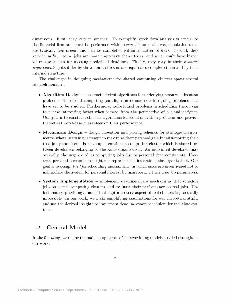
The challenges in designing mechanisms for shared computing clusters spans several
research domains.
• Algorithm Design – construct efficient algorithms for underlying resource allocation
problems. The cloud computing paradigm introduces new intriguing problems that
have yet to be studied. Furthermore, well-studied problems in scheduling theory can
take new interesting forms when viewed from the perspective of a cloud designer.
Our goal is to construct efficient algorithms for cloud allocation problems and provide
theoretical worst-case guarantees on their performance.
• Mechanism Design – design allocation and pricing schemes for strategic environ-
ments, where users may attempt to maximize their personal gain by misreporting their
true job parameters. For example, consider a computing cluster which is shared be-
tween developers belonging to the same organization. An individual developer may
overvalue the urgency of its computing jobs due to personal time constraints. How-
ever, personal assessments might not represent the interests of the organization. Our
goal is to design truthful scheduling mechanisms, in which users are incentivized not to
manipulate the system for personal interest by misreporting their true job parameters.
• System Implementation – implement deadline-aware mechanisms that schedule
jobs on actual computing clusters, and evaluate their performance on real jobs. Un-
fortunately, providing a model that captures every aspect of real clusters is practically
impossible. In our work, we make simplifying assumptions for our theoretical study,
and use the derived insights to implement deadline-aware schedulers for real-time sys-
tems.
1.2 General Model
In the following, we define the main components of the scheduling models studied throughout
our work.
6
Technion - Computer Science Department - Ph.D. Thesis PHD-2017-03 - 2017

System. A computing system that consists of C identical servers (resources) receives job
requests over time. The timeline T is either continuous or discrete; in the latter case, the
timeline T is divided into T time slots of equal length 1, 2, . . . , T. We assume that the
servers are fully available throughout time, and that each server can process at any time one
job at most.
Jobs. Each job request j submitted to the system is associated with a type τj . The type
encodes the various parameters of the job, and its definition difs between models. Yet, all
definitions share some common components.
Arrival time. The arrival time aj represents the earliest time during which job j can
be processed. Following standard literature, we distinguish between two settings: online
and offline. Online scheduling problems assume that jobs are not known to the scheduler in
advance, and are only revealed to the schedulferer at the time of their arrival. The scheduler
must make scheduling decisions without knowledge of future arrivals, and without the ability
to modify past allocations. Offline scheduling problems assume that all jobs are known in
advance to the scheduler. This is common when scheduling recurring production jobs, e.g.,
jobs that run on an hourly basis. We discuss evaluation methods for online and offline
algorithms in Section 2.1.
Valuation function. In addition, each job type holds a valuation function vj : T → R+,0.
The value vj(t) represents the value gained from completing job j at time t. We will mostly
focus on deadline valuation functions: step functions which equal to a constant vj up to a
predefined deadline dj and 0 afterwards; the notation of vj is abused to simplify exposition.
The goal of the scheduler is to maximize the total value gained from completed jobs.
Resource requirements. Finally, the job request includes its resource requirements. We
will mostly study a flexible allocation model, where the number of resources allocated per
job can change over time. In this model, each job specifies a demand Dj , which is the
total amount of resource units required to complete the job. The job completion time is the
earliest time by which the job is allocated Dj resource units. At each time, the scheduler
may allocate job j any number of resources between 0 and a parallelism bound kj specified
by the job type. In Chapter 6, we consider a more general allocation model, where each job
consists of multiple stages having execution dependencies.
We introduce several notations used throughout the dissertation. The value-density of
job j is defined as ρj = vj/Dj . The deadline slackness of the input is defined1 as the smallest
s ≥ 1 such that dj − aj ≥ s(Dj/kj) for every job j.
1When the timeline is discrete, we require dj − aj ≥ sdDj/kje.
7
Technion - Computer Science Department - Ph.D. Thesis PHD-2017-03 - 2017

1.3 Thesis Overview
This dissertation is organized as follows. We begin by considering a special offline variant
of the allocation model, where all jobs share the same arrival time (Chapter 3). This allows
us to focus on other aspects of our model. We show that under two realistic assumptions,
the resulting resource allocation problem can be solved efficiently using simple greedy-like
algorithms. First, we assume that no job can simultaneously accommodate most of the
cluster resources, i.e., the parallelism bound of each job is notably smaller than the cluster
capacity. Second, we assume that all deadline requirements exhibit a minimal level of slack-
ness; specifically, no job request enforces a tight deadline. To obtain theoretical performance
guarantees for our algorithms, we develop a proof methodology based on the dual-fitting2
technique for our greedy-like algorithms. In addition, we show that these algorithms can be
used to construct truthful mechanisms3 with no performance loss.
We then proceed to study online scheduling with job deadlines (Chapter 4). For the
most general form of the problem, several impossibility results are known to rule out the
existence of online schedulers that guarantee constant competitive ratios. Nevertheless, we
show that under the same deadline slackness assumption as before, we can obtain truthful,
online, constant competitive-ratio mechanisms for the problem. Moreover, we provide similar
results to a stronger family of committed schedulers, that must guarantee the completion
of any admitted job (Chapter 5). We then broaden our allocation model to incorporate
DAG-structured jobs, i.e., jobs composed of tasks with inner dependencies (Chapter 6).
We show that if the cluster size is significantly larger than the parallelism level of any job,
the offline problem can be solved using a randomized rounding algorithm; the online case
remains subject to future work. Finally, we use insights from our theoretical study to design
and implement a deadline scheduler for Hadoop YARN, which has been accepted by the
open-source community (Chapter 7).
In the following, we provide an overview of our results in each chapter.
Chapter 3: Near-Optimal Schedulers for Identical Arrival Times
We first study the special case of identical arrival times. In this simplified model, we assume
that all jobs arrive at the same time and that each job j is associated with a deadline valua-
tion function (i.e., the scheduler must meet a predefined deadline dj in order to gain a value
vj for completing the job). Since all arrival times are identical, the problem reduces to an
offline scheduling problem. Our main result is a new near-optimal approximation algorithm
for maximizing the social welfare (i.e., total value gained from completed jobs). Based on
2For a comprehensive description of dual fitting, see Section 2.1.2.3For more on truthful mechanisms, see Section 2.2.
8
Technion - Computer Science Department - Ph.D. Thesis PHD-2017-03 - 2017

the new approximation algorithm, we construct truthful allocation and pricing mechanisms,
in which reporting the true value and other properties of the job (deadline, work volume
and the parallelism bound) is a dominant strategy for all users. The mechanisms obtain
near-optimal approximation to the social welfare and to the optimal expected profit, respec-
tively; the latter holds under Bayesian assumptions. We empirically evaluate the benefits
of our approach through simulations on data-center job traces, and show that the revenues
obtained under our mechanism are comparable with an ideal fixed-price mechanism, which
sets an on-demand price using oracle knowledge of users’ valuations. Finally, we discuss how
our model can be extended to accommodate uncertainties in job work volumes, which is a
practical challenge in cloud environments. Joint work with Ishai Menache, Brendan Lucier
and Navendu Jain. Results published in [42, 51].
Chapter 4: Online Scheduling with Deadline Slackness
We study the fundamental problem of online deadline scheduling. In this problem, a sched-
uler receives job requests over time. Each job has an arrival time, deadline, size (demand)
and value. The goal of the scheduler is to maximize the total value of jobs that meet their
deadline. We circumvent known lower bounds for this problem by assuming that the input
has slack, meaning that any job could be delayed and still finish by its deadline. Under the
slackness assumption, we design a preemptive scheduler with a constant-factor worst-case
performance guarantee. Along the way, we pay close attention to practical aspects, such as
runtime efficiency, data locality and demand uncertainty. We then present a truthful variant
of the scheduling algorithm which obtains nearly the same competitive ratio. Joint work
with Ishai Menache and Brendan Lucier. Results published in [51].
Chapter 5: Online Scheduling with Commitments
We extend our study of online deadline scheduling. We show that if the slackness parameter
s is large enough, then we can construct truthful scheduling mechanisms that satisfy a
commitment property: the scheduler decides for each job, well in advance before its deadline,
whether the job is admitted or rejected. If the job is admitted, then the scheduler guarantees
to complete the job by its deadline, and moreover, the required payment is specified at the
time of admission. This is notable, since in practice users with strict deadlines may find it
unacceptable to discover near their deadline that their job has been rejected. Joint work
with Ishai Menache and Brendan Lucier. Results published in [4].
9
Technion - Computer Science Department - Ph.D. Thesis PHD-2017-03 - 2017

Chapter 6: Offline Scheduling of DAG-Structured Jobs
We generalize our allocation model to accommodate job requests with complex inner struc-
tures, as common for most big data jobs. In this work, each job is represented by a Directed
Acyclic Graph (DAG) consisting of several stages linked by precedence constraints. The
resource allocation per stage is malleable, in the sense that the processing time of a stage
depends on the resources allocated to it (the dependency can be arbitrary in general). The
goal of the scheduler is to maximize the total value of completed jobs, where the value for
each job depends on its completion time. We design a novel offline approximation algorithm
for the problem which guarantees an expected constant approximation factor when the clus-
ter capacity is sufficiently high. To the best of our knowledge, this is the first constant-factor
approximation algorithm for the problem. However, the algorithm suffers from several short-
comings: it requires solving a large linear program (which is inefficient in practice), and it
is not truthful. We note that many open challenges remain regarding DAG scheduling with
job deadlines. Joint work with Ishai Menache and Peter Bodık. Results published in [14].
Chapter 7: New Scheduling Algorithm for Hadoop YARN
Apache Hadoop is one of the leading open-source frameworks for cluster resource manage-
ment and big data processing. Using the Rayon [23] abstraction, we design, implement and
evaluate LowCost – a new cost-based planning algorithm for the Hadoop resource negotiator
YARN [63]. Through simulations and experiments on a test cluster, we show that LowCost
substantially outperforms the existing algorithm on a variety of important performance met-
rics. Our open-source contributions can be found in YARN-3656 and YARN-4359. LowCost
has been recently used as an allocation mechanism for periodic jobs, and is part of the
Morpheous system [45]. Joint work with Ishai Menache, Calro Curino and Subru Krishnan.
1.4 Related Work
Scheduling problems have been extensively studied in operations research and computer
science (see [15] for a broad survey). This dissertation focuses on designing deadline-sensitive
schedulers which aim to maximize the value of completed jobs. The allocation models we
consider, as highlighted in Section 1.2, significantly extends the work on basic problems,
such as job interval scheduling [5, 7, 22] and bandwidth allocation [5, 6, 57]. Our review
of related literature is spread throughout the dissertation as follows: offline variants of our
model are covered in Chapter 3; online variants are overviewed in Chapter 4; literature on
DAG-scheduling models is discussed in Chapter 6; and recent work related to datacenter
resource allocation can be found in Chapter 7.
10
Technion - Computer Science Department - Ph.D. Thesis PHD-2017-03 - 2017

11
Technion - Computer Science Department - Ph.D. Thesis PHD-2017-03 - 2017

Chapter 2
Preliminaries
2.1 Algorithmic Design
2.1.1 Evaluation Metrics
The scheduling algorithms presented in this work are evaluated using standard worst-case
performance metrics. Separate metrics are used throughout literature for offline and online
settings, though they are similar in nature. In the following, we define these metrics. Denote
by OPT (τ) the optimal offline solution for an input instance τ . The performance of an online
algorithm A is measured by the competitive ratio, which is the worst-case ratio between the
values gained by the optimal offline solution and the online algorithm. In our work, we are
mainly interested in bounding the competitive ratio as a function of the input slackness:
crA(s) = maxτ :s(τ)=s
v(OPT (τ))
v(A(τ))
. (2.1)
In general, the competitive ratio of an online algorithm A is defined as cr(A) = maxs crA(s).
The performance of an offline algorithm A is measured by the approximation ratio ar(A),
which is also defined as the worst-case ratio between the values gained by the optimal
solution and the algorithm. These two definitions are mathematically identical, however
have different implications.
2.1.2 The Dual Fitting Technique
A core element in the analysis of our mechanisms is a dual fitting argument. Dual fitting is
a common technique for bounding the worst-case performance of algorithms. The technique
obtains an upper bound on the value gained by the optimal solution OPT (τ) through the
12
Technion - Computer Science Department - Ph.D. Thesis PHD-2017-03 - 2017
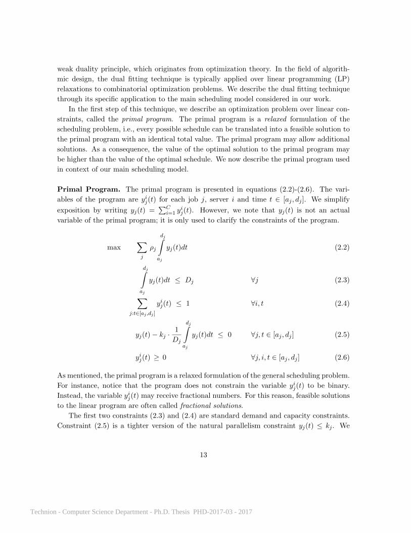
weak duality principle, which originates from optimization theory. In the field of algorith-
mic design, the dual fitting technique is typically applied over linear programming (LP)
relaxations to combinatorial optimization problems. We describe the dual fitting technique
through its specific application to the main scheduling model considered in our work.
In the first step of this technique, we describe an optimization problem over linear con-
straints, called the primal program. The primal program is a relaxed formulation of the
scheduling problem, i.e., every possible schedule can be translated into a feasible solution to
the primal program with an identical total value. The primal program may allow additional
solutions. As a consequence, the value of the optimal solution to the primal program may
be higher than the value of the optimal schedule. We now describe the primal program used
in context of our main scheduling model.
Primal Program. The primal program is presented in equations (2.2)-(2.6). The vari-
ables of the program are yij(t) for each job j, server i and time t ∈ [aj , dj ]. We simplify
exposition by writing yj(t) =∑C
i=1 yij(t). However, we note that yj(t) is not an actual
variable of the primal program; it is only used to clarify the constraints of the program.
max∑j
ρj
dj∫aj
yj(t)dt (2.2)
dj∫aj
yj(t)dt ≤ Dj ∀j (2.3)
∑j:t∈[aj ,dj ]
yij(t) ≤ 1 ∀i, t (2.4)
yj(t)− kj ·1
Dj
dj∫aj
yj(t)dt ≤ 0 ∀j, t ∈ [aj , dj ] (2.5)
yij(t) ≥ 0 ∀j, i, t ∈ [aj , dj ] (2.6)
As mentioned, the primal program is a relaxed formulation of the general scheduling problem.
For instance, notice that the program does not constrain the variable yij(t) to be binary.
Instead, the variable yij(t) may receive fractional numbers. For this reason, feasible solutions
to the linear program are often called fractional solutions.
The first two constraints (2.3) and (2.4) are standard demand and capacity constraints.
Constraint (2.5) is a tighter version of the natural parallelism constraint yj(t) ≤ kj . We
13
Technion - Computer Science Department - Ph.D. Thesis PHD-2017-03 - 2017

further elaborate on this constraint later. Notice that some of the constraints of the original
problem are relaxed and replaced by linear constraints. For example, the original constraint
yij(t) ∈ 0, 1 is replaced by yij(t) ≥ 0 (the capacity constraint (2.4) implies that yij(t) ≤ 1);
furthermore, the demand constraint now allows a fractional solution to partially satisfy
demand requests. But, constraint relaxation must be done carefully. In general, over-
relaxing constraints might cause undesired fractional solutions to become legal. As a result,
the relaxed formulation could become meaningless. One way to prevent this is introducing
additional constraints that limit the strength of fractional solutions. In our context, the
standard parallelism constraint yj(t) ≤ kj is replaced by a tighter constraint (2.5). This
constraint limits the strength of a fractional solution by imposing a tighter restriction on
yj(t). Notice that 1Dj
∫ djajyj(t)dt represents the completed fraction of job j. To exemplify,
if a fractional solution allocates half of the demand requested by job j, then every variable
yj(t) in the fractional solution y cannot exceed 0.5kj . The strengthened constraints (2.5)
for this problem were first introduced by [41] and are a reminiscent of the knapsack cover
inequalities [18].
The objective function (2.2) represents the value gained from completed jobs. However,
in this relaxed LP formulation, a fractional solution may gain partial value over partially
completed jobs. We denote by OPT ∗(τ) the optimal fractional solution of the primal pro-
gram for an instance τ . Since the primal program is a relaxed formulation of the scheduling
problem, OPT ∗(τ) is super-optimal, meaning that v(OPT (τ)) ≤ v(OPT ∗(τ)).
Dual Program. The following dual optimization problem is associated with the primal
program we described. By weak duality, every feasible solution to the dual program admits
an upper bound to v(OPT ∗(τ)).
min∑j∈J
Djαj +
C∑i=1
∞∫0
βi(t)dt (2.7)
s.t. αj + βi(t) + πj(t)−kjDj
dj∫aj
πj(τ)dτ ≥ ρj ∀j, i, t ∈ [aj , dj ] (2.8)
αj , βi(t), πj(t) ≥ 0 ∀j, i, t ∈ [aj , dj ] (2.9)
The dual program holds a constraint (2.8) for every tuple (j, i, t). We say that a constraint
is covered by a dual solution (α, β, π) if it is satisfied by (α, β, π). A solution that covers all
of the dual constraints is called feasible. We refer to (2.7) as the dual cost of a feasible dual
solution. The dual cost of every feasible solution is an upper bound to v(OPT ∗(τ)).
14
Technion - Computer Science Department - Ph.D. Thesis PHD-2017-03 - 2017

There are three kinds of dual variables. Every job j has a variable αj that appears in all
of the dual constraints associated with j. Notice that setting αj = ρj satisfies all of the dual
constraints of job j at a dual cost of Djαj = Djρj = vj . The second type of dual variable
βi(t) appears in every dual constraint that corresponds to a server i at time t. We typically
think of these variables as continuous functions, one per server. The last set of variables
πj(t) are a result of the strengthened parallelism constraints (2.5). In most cases, we set
these variables to 0. However, they can be used to lower the cost of dual solutions.
Dual Fitting. The dual fitting technique bounds the competitive ratio (or approximation
factor thereof) of an algorithm A by explicitly constructing a feasible solution to the dual
program and bounding its cost, without having to solve the linear program itself. Formally
speaking, given an input instance τ with slackness s = s(τ), we construct a feasible solution
(α, β, π) to the corresponding dual program and bound its dual cost by r(s) · v(A(τ)) for
some r(s). This proves that crA(s) ≤ r(s), since by weak duality:
v(A(τ)) ≤ v(OPT (τ)) ≤ v(OPT ∗(τ)) ≤ r(s) · v(A(τ)). (2.10)
Equation (2.10) reveals an inherent lower bound on the capability of dual fitting arguments.
Definition 2.1.1. The integrality gap of the primal program on instances τ with slackness
s = s(τ) is defined as:
IG(s) = maxτ :s(τ)=s
v(OPT ∗(τ))
v(OPT (τ))
. (2.11)
The integrality gap essentially measures the quality of a relaxed formulation. Equation
(2.10) indicates that any bound r(s) that can be proven through dual fitting arguments is
limited by the integrality gap IG(s) of the primal program. It is important to understand
that the integrality gap does not bound the competitive ratio of any algorithm, only those
that rely solely on weak duality to prove their performance guarantees. On the other hand,
if we are able to prove through dual fitting that crA(s) ≤ r(s) for an algorithm A, then r(s)
is also an upper bound on the integrality gap. The following theorem summarizes the dual
fitting technique.
Theorem 2.1.2 (Dual Fitting [64]). Consider an online scheduling algorithm A. If for
every instance τ with slackness s = s(τ) there exists a feasible dual solution (α, β, π) with a
dual cost of at most r(s) · v(A(τ)), then IG(s) ≤ crA(s) ≤ r(s).
15
Technion - Computer Science Department - Ph.D. Thesis PHD-2017-03 - 2017

2.2 Algorithmic Mechanism Design
Mechanism design is a sub-field of economic theory which has received recent attention from
computer scientists. In its algorithmic aspect, the goal is to design computationally efficient
choice mechanisms, such as auctions or resource allocation, while optimizing an objective
function. Some examples of objective functions include the social welfare (total value), or the
total profit accrued by the mechanism. The difficulty of algorithmic mechanism design is that
unlike classic algorithmic design, participants act rationally in a game theoretic sense and
may deviate in order to maximize their personal utilities. Since participants’ preferences are
usually kept private from the mechanism, we search for efficient mechanisms that implement
certain strategic properties to deal with participants’ incentives, e.g., incentivize users to
truthfully report their preferences, while attempting to optimize an objective function.
An extensive amount of work has been carried out in the field of algorithmic mechanism
design, starting with the seminal paper of Nisan and Ronen [54]. Prior to their paper,
mechanism design received much attention by economists who focused on exact solutions
or characterizations of truthful mechanisms, mostly under Bayesian settings and typically
without taking into account time or communication complexity limitations. The subfield of
algorithmic mechanism design addresses these challenges from the perspective of a computer
scientist. In the following, we describe the basic definitions of mechanism design and the
main theorems on which we rely in our work. We refer the reader to [55] for a survey book.
2.2.1 Definitions
Every user j is associated with a private true type τj = 〈vj ,Pj〉, where vj is the user value and
Pj is a set of properties. In our context, Pj = 〈Dj , kj , aj , dj〉 is the set of job properties. The
true type of user j is taken from a known type space Tj . Denote T = T1×T2× · · ·×Tn. We
study direct revelation mechanisms, where each user participates by announcing a reported
type (bid type) bj ∈ Tj to the mechanism. Note that the reported type bj may differ from
the true type τj .
A mechanism M = (f, p) consists of an allocation rule f : T → O, where O is the set
of possible outcomes, and a pricing rule pj : T → R for every user j. Given a reported
bid vector b = (b1, b2, . . . , bn), the mechanism allocates jobs according f(b) and charges a
non-negative payment pj(b) from each user j. The goal of the mechanism is to optimize an
objective function g : O → R such as the social welfare or the mechanism revenue.
We focus on single-value domains1, in which user valuation of outcomes is encoded by a
single scalar vj ∈ R. We define fj(b) ∈ 0, 1 as a binary function that indicates whether
1General value models consider value functions of the form vj : O → R and user utilities of the formuj(b) = vj(f(b))− pj(b).
16
Technion - Computer Science Department - Ph.D. Thesis PHD-2017-03 - 2017

job j is scheduled properly with respect to the job properties; that is, whether j is allocated
Dj resource units in the interval [aj , dj ] without violating the parallelism bound kj . Every
user strives to maximize its utility uj(b), defined as the following quasilinear function:
uj(b) = vjfj(b)− pj(b). (2.12)
Notice that the job properties do not affect the value vj gained by the user, only the allo-
cation fj(b). Models where the user type consists of a single value scalar and multiple type
properties (e.g., deadline, demand) are called single-value multi-property models.
2.2.2 Truthfulness and Monotonicity
Mechanism design involves additional complications due to the selfish nature of participants.
A mechanism must be sensitive to potential manipulation by users, as users striving to
maximize their personal gain may attempt to do so by reporting false values or parameters.
To prevent false behavior, the mechanism must incentivize users to act truthfully.
Given a vector x, we denote by x−j the vector x without entry j. Specifically, τ−jrepresents a type profile of all users except j. We use (xj , x−j) to denote the concatenation
of xj with x−j .
Definition 2.2.1 (Truthfulness). A mechanism M = (f, p) is called truthful or incentive
compatible (IC) if for every user j and for every choice of τ−j , truth-telling is a dominant
strategy for every user j. Formally, for every type τ ′j ∈ Tj :
uj(τj , τ−j) ≥ uj(τ′j , τ−j) (2.13)
If (2.13) holds in expectation, the mechanism is called truthful-in-expectation.
Truthful mechanisms in single-value domains have been completely characterized by
[52, 2]. For an allocation algorithm f to be implementable as a truthful mechanism, i.e., for
there to exist a corresponding pricing rule p that admits a truthful mechanism, the allocation
algorithm f must be monotone, and vice-versa. This characterization has been extended by
[34] for single-value multi-property domains similar to those studied here. In the following,
we present their characterization with specific relevance to job scheduling mechanisms. We
note that the framework presented in [34] can similarly be extended to other single-value
multi-property domains, however we focus here on job scheduling domains alone.
Following [34], we adopt several assumptions on the types τ ′j = 〈v′j , D′j , k′j , a′j , d′j〉 that
can be reported to the scheduling mechanism. These assumptions are all justifiable in the
context of allocating cloud resources, as we show next.
17
Technion - Computer Science Department - Ph.D. Thesis PHD-2017-03 - 2017

• No Early Arrival Times (a′j ≥ aj). The true arrival time represents the earliest time
in which a job can be processed. The mechanisms we propose require that submitted
jobs are ready for execution. Hence, it is natural to assume that a user cannot submit
a job before it can be processed.
• No Late Deadlines (d′j ≤ dj). In general, unallocated users might manage to guarantee
timely completion by reporting late deadlines. To prevent this behavior, the truthful
mechanisms we construct in our work will release the job output only at its reported
deadline. This suppresses any incentive to report a late deadline, since by doing so the
job would certainly miss its deadline. Henceforth, we assume that users do not report
deadlines which are later than their actual deadlines.
• No Insufficient Demands (D′j ≥ Dj). Jobs cannot complete without receiving the
necessary amount of resources required for completion. As long as the scheduling
algorithms do not allocate unnecessary resources to jobs, a user cannot benefit from
requesting an insufficient amount of resources.
• No Overestimated Parallelism Bounds (k′j ≤ kj). In practice, bounds on the desired
level of parallelism are either enforced by the scheduler or a result of computation
overheads (e.g., software limitations, network delays). Exceeding the job resource
limitations would result in slower execution, and therefore failure to complete the job
within its requested amount of resources.
We now define monotonicity in context of the single-value multi-property scheduling
domain studied in this work. We first define a partial order over the job property sets used
in our model.
Definition 2.2.2. Property set P ′j is dominated by property set P ′′j if D′j ≥ D′′j , k′j ≤ k′′j ,
a′j ≥ a′′j , and d′j ≤ d′′j . We use P ′j P ′′j to denote that P ′j is dominated by P ′′j .
Now, we can define monotonicity for single-value multi-property domains.
Definition 2.2.3. Type τ ′j = 〈v′j ,P ′j〉 is dominated by type τ ′′j = 〈v′′j ,P ′′j 〉 if v′j ≤ v′′j and
P ′j P ′′j . We use τ ′j τ ′′j to denote that τ ′j is dominated by τ ′′j .
Definition 2.2.4 (Monotonicity). An allocation algorithm f is called monotone if for every
j, τ−j , and τ ′j τ ′′j we have fj(τ′j , τ−j) ≤ fj(τ ′′j , τ−j).
As stated before, monotonicity provides a complete characterization of truthful mecha-
nisms in single-value multi-property domains. This has been proven in [34] for the special
case of unit-sized demands. However, their proof extends directly for general demands with
restrictions on parallelism.
18
Technion - Computer Science Department - Ph.D. Thesis PHD-2017-03 - 2017

Theorem 2.2.5 (Restatement of [34]). Let f be an allocation rule. Assume no earky arrival
times, no late deadlines, no insufficient demands and no overestimated parallelism bounds.
Then, there exists a payment rule p such that the mechanism M = (f, p) is truthful if and
only if f is monotone. In the latter case, the pricing rule takes the following form, where
τ ′j = 〈v′j ,P ′j〉 is the reported type of job j:
pj(τ′j , τ−j) = v′j · fj(τ ′j , τ−j) −
v′j∫0
fj
(〈x,P ′j〉 , τ−j
)dx. (2.14)
Theorem 2.2.5 also holds for randomized mechanisms. In this case, fj represents the expected
allocation of user j. Before continuing, it is worth noting that for binary allocation rules,
each allocated user j pays the lowest value which guarantees that j is still allocated.
2.2.3 Profit Maximization in Bayesian Settings
The objective of profit maximizing is of course significant for public commercial clouds.
When assuming no a-priori knowledge on clients’ private valuation functions, it is well known
that a truthful mechanism might charge very low payments from clients to ensure truthful-
ness, yielding low revenues. Thus, following a standard approach in game-theory, we consider
a Bayesian setting, in which the true value vj of each user j is assumed to be drawn from a
distribution with a probability density function gj , which is common knowledge. We denote
by Gj the respective cumulative distribution function (cdf). Job properties are assumed, as
before, to be private information with no additional distribution information.
The goal of the mechanism in the current context is to maximize the optimal expected
profit, with the expectation taken over the random draws of clients’ values. For single-
value domains, it is well known that the problem of maximizing profits can be reduced to
the problem of maximizing social welfare over virtual values; this basic property is due to
celebrated work by Myerson [52], and has been extended in different contexts (see [55]). To
formally state the result, we first need the following definitions.
Definition 2.2.6. Define the revenue curve associated with user j as Rj(q) = q ·G−1j (1−q).
The ironed virtual valuation function φj of j is defined as: φj(v) = ddq [ConcaveClosure (Rj(·))]
for q = 1−Gj(v).
That is, φj(v) the derivative of the concave closure2 of R(·). Note that φj(·) is monotonically
non-decreasing. Thus, if a single-value allocation rule fsv is monotone, then so is fsv(φ(·)
).
2The concave closure of a function f(·) is the pointwise supremum of the set of convex functions that liebelow f .
19
Technion - Computer Science Department - Ph.D. Thesis PHD-2017-03 - 2017

Theorem 2.2.7 ([52, 55]). For any single-value truthful mechanism Msv that guarantees
an α-approximation to the optimal social surplus, the mechanism Msv(φ(·)) guarantees an
α-approximation to the optimal expected profit.
For our purposes, we prove that the reduction proposed by Myerson [52] extends to
domains of single value and multiple properties. Formally:
Theorem 2.2.8. Let f be a binary allocation rule for a single-value multi-property problem,
such that f is monotone and guarantees an α-approximation to the optimal social welfare.
Let fφ be an allocation rule that replaces every type 〈vj ,Pj〉 with 〈φj(vj),Pj〉 and calls f .
Then, the mechanism Mφ with allocation rule fφ that charges payments according to (2.14),
with respect to fφ, is truthful, and is an α-approximation to the optimal expected profit under
Bayesian assumptions.
Proof. Fix the set of properties Pj of each job j. This makes f a single-value allocation
rule. By the characterization theorem of single-value allocation functions [2], since f is
monotone, the mechanismM = (f, p) with p set as in (2.14) is truthful. By Theorem 2.2.7,
the mechanism Mφ gives an α-approximation to the optimal expected profit.
It remains to show that fφ admits a truthful mechanism. Notice that since φj(·) is
monotone for every j, fφ is a monotone allocation rule. Therefore, we can apply Theorem
2.2.5 and conclude that the mechanism Mφ is truthful.
2.2.4 Related Literature
We focus on the algorithmic aspect of designing implementable allocation rules, i.e., allo-
cation rules that can be transformed into truthful mechanisms. For an extensive study on
algorithmic mechanism design, we refer the reader to [55].
Characterization of Truthful Mechanisms. As discussed, monotonicity provides a full
characterization of implementable allocation rules for single-value domains [52, 2], as well as
for single-value multiple-property domains [34]. However, much less is known for the general
multiple-value domain, where the valuation function of each user is not necessarily scalar.
Rochet [59] presented an equivalent property to monotonicity called cyclic monotonicity,
which is a necessary and sufficient condition for truthfulness. Yet, it is unclear how to use
this property to easily construct truthful mechanisms from it and only few successful efforts
are known (for example, [49]). Saks and Yu [60] showed that for deterministic settings, cyclic
monotonicity is equivalent to a simpler property called weak monotonicity, which conditions
only on cycles of length 2 (see also [3]). However, this result is not valid for randomized
mechanisms [13].
20
Technion - Computer Science Department - Ph.D. Thesis PHD-2017-03 - 2017

Black-Box Reductions. Much work has been dedicated to the existence of black-box
reductions from algorithmic mechanism design to algorithm design; namely, reductions that
can convert any (approximation) algorithm into a truthful (approximation) mechanism,
preferably without loss of performance. Unfortunately, recent work by Chawla, Immorlica
and Lucier [21] disproved the existence of many types of black-box reductions. For social
welfare maximization, [21] proved that there cannot exist a general reduction that pre-
serves the worst-case approximation ratio by a subpolynomial factor, even for truthfulness
in expectation. For makespan minimization, the same bound applies even for average-case
guarantees and under Bayesian assumptions. General reductions for social welfare maxi-
mization are only known to exist under Bayesian assumptions. Hartline and Lucier [36]
showed that any approximation algorithm for a single-value problem can be transformed
into a Bayesian Incentive-Compatible (BIC) mechanism. This result has been improved
since then for multiple-value settings by Hartline, Kleinberg and Malekian [35], and by Bei
and Huang [11] independently.
Several black-box reductions have been suggested for large classes of social welfare max-
imization problems, without prior assumptions on the input. Lavi and Swamy [48] con-
structed a truthful-in-expectation mechanism for packing problems that are solved through
LP-based approximation algorithms. Their reduction maintains the approximation factor of
the original algorithm. However, for their reduction to work, the approximation algorithm
must bound the integrality gap of the ”natural” LP for the problem - and this is not al-
ways possible. Dughmi and Roughgarden [26] proved that packing problems that admit an
FPTAS can be turned into a truthful-in-expectation mechanism which is also an FPTAS.
Finally, we mention that any optimal algorithm for welfare maximization problems can be
converted into a truthful mechanism via the celebrated VCG mechanism [55].
21
Technion - Computer Science Department - Ph.D. Thesis PHD-2017-03 - 2017

Chapter 3
Near-Optimal Schedulers for
Identical Release Times
Nowadays, cloud providers offer three pricing schemes to users: (i) on-demand instances,
where a user pays a fixed price for a virtual machine (VM) per unit time (e.g., an hour)
and can acquire or release VMs on demand, (ii) spot-instances, where users bid for spot
instances and get allocation when the spot market price falls below their bid, and (iii) reser-
vations, where users pay a flat fee for long term reservation (e.g., 1-3 years) of instances and
a discounted price during actual use. Despite their simplicity, these approaches have several
shortcomings for batch computing. First, they offer only best-effort execution without any
guarantees on the job completion time. This might not be adequate for all users. For exam-
ple, the financial firm discussed in the introduction requires SLA on the job completion time
rather than how VMs are allocated over time. Second, current resource allocation schemes
do not differentiate jobs based on their importance. For instance, financial applications have
(and are willing to pay for) strict job deadlines, while scientific jobs are likely willing to trade
a bounded delay for lower costs. As a result, cloud systems lose the opportunity to increase
profits (e.g., by prioritizing jobs with strict SLAs), improve utilization (e.g., by running low
priority jobs at night), or both. Finally, existing schemes do not have in-built incentives to
prevent fluctuations between high and low resource utilization. Perhaps the most desired
goal of cloud operators is to keep all their resources constantly utilized.
In this chapter, we consider an alternative approach to resource allocation and pricing
in cloud computing environments based on an offline scheduling problem of multiple batch
jobs. In our approach, we explicitly incorporate the importance of the completion time of a
job to its owner, rather than the number of instances allocated to the job at any given time.
We exemplify the benefits of our approach through a special case of the general scheduling
22
Technion - Computer Science Department - Ph.D. Thesis PHD-2017-03 - 2017

problem (Section 1.2) of identical release (arrival) times. In this case, all jobs are available
for execution when the scheduler computes the allocation. This scenario is common when
the resource plan is computed periodically.
We develop novel truthful mechanisms for the problem. Our main result is a truthful
mechanism called GreedyRTL, which guarantees a(
CC−k
)(ss−1
)-approximation for social
welfare maximization, where k is the maximal parallelism bound over all jobs, C is the
cloud capacity, and s is the input slackness. Note that the approximation factor approaches
1 under the (plausible) assumptions that k C and s is sufficiently large. Our results
are presented as follows. We first focus on the pure algorithmic problem, disregarding
incentive concerns. We present in Section 3.2.1 a simple greedy algorithm that obtains the
desired competitive ratio, however with an additional +1 factor. Based on the simple greedy
approach, we develop the GreedyRTL algorithm in Section 3.2.2.
Related Work. The identical arrival model has been studied in our prior work [41] for
general user valuation functions. The paper proposed the first algorithm for the objective
of maximizing social welfare, which obtained a(1 + C
C−k)(
1 + ε)-approximation factor.
The algorithm served as the basis for designing a truthful-in-expectation mechanism where
reporting valuations truthfully maximized the expected utility for each user. However, it
has four key practical shortcomings. First, from the mechanism design perspective, job
work volume and parallelism bounds are assumed to be truthfully reported and hence it is
only necessary to guarantee truthfulness with respect to values and deadlines. Second, to
guarantee truthfulness, the proposed mechanism risks low utilization with at least half of
the resources unutilized. Further, the solution cannot be extended to deal with uncertainties
in job resource demand. Finally, the solution requires solving a linear program, which might
be computationally expensive to run frequently for a large number of jobs.
Of specific relevance to our work is the work of Lawler [50]. In his work, Lawler studied
the problem of designing a preemptive job scheduler on a single server to maximize the social
welfare. We note that the model can be simply generalized to multiple servers without
parallelism bounds. Lawler solved the problem optimally in pseudo-polynomial time via
dynamic programming. However, his algorithm cannot be extended to the case where jobs
have parallelization limits. The model studied here significantly extends the basic job interval
scheduling problem studied by [5, 7]. In this problem, each job is associated with a set of
time intervals. Allocating a job corresponds to selecting one of the intervals, and executing
the job during that interval. The overall set of selected intervals must not intersect (this
corresponds to allocating jobs on a single server). The best known approximation factor for
this problem is 2. For identical values, the approximation ratio was improved by Chuzoy
et al. [22] to 1.582. Several papers extended the interval scheduling problem by associated
23
Technion - Computer Science Department - Ph.D. Thesis PHD-2017-03 - 2017

each interval with a width (corresponds to parallelism requirements). When each job has
only one interval, Calinescu et al. [16] developed a (2 + ε) approximation algorithm. For
multiple intervals, Phillips et al. [57] and Bar-Noy et al. [5] obtain constant approximations.
3.1 Scheduling Model
We consider a single cloud provider which allocates resources (CPUs) to jobs over time. The
cloud capacity C is fixed throughout time. The time horizon is divided into T time slots
T = 1, 2, . . . , T of equal size. There are n jobs, denoted 1, 2, . . . , n. Our focus in this
chapter is the identical release time model, where all jobs arrive to the system by time 0
and can be executed immediately. Every job j is associated with a type τj = 〈vj , Dj , kj , dj〉,where vj is the job value, dj is the job deadline, Dj is the job demand, and kj is the job
parallelism bound. An input to the problem is a type profile τ = τ1, . . . τn. We consider
a flexible allocation model. For each job j, the amount of resources allocated to a job can
change over time, given that it does not exceed kj . A feasible allocation of resources to job
j is a function yj : [0, dj ] → [0, kj ] in which j is allocated a total of Dj resources by its
deadline dj . Our goal is to maximize the social welfare, which is the aggregate value of jobs
that are completed before their deadline. We remind that partial execution of a job does
not yield partial value.
Before we describe our approximation algorithms, we give some definitions and notations
that we will use later on. Given a solution consisting of allocations yj , we define W (t) =∑nj=1 yj(t) to be the total workload at time t and W (t) = C −W (t) to be the amount of
available resources at time t. A time slot is saturated if W (t) < k and unsaturated otherwise.
Finally, given a time slot t, we define:
R(t) = maxt′ ≥ t : ∀t′′ ∈
(t, t′], W (t′′) < k
. (3.1)
Intuitively, if there are saturated time slots adjacent to t to the right, R(t) is the rightmost
time slot out of the saturated block to the right of t. Otherwise, R(t) = t.
3.2 Approximation Algorithms
3.2.1 A Simple Greedy Approach
We present a simple greedy algorithm which serves as a basis for developing GreedyRTL.
The full implementation of the simple greedy algorithm is given in Algorithm 1. Notice that
several lines have been faded out. These lines are only necessary for the analysis, and they
can be omitted from the implementation.
24
Technion - Computer Science Department - Ph.D. Thesis PHD-2017-03 - 2017

The algorithm works as follows. An empty solution y ← 0 is initialized. The jobs are then
sorted in non-increasing order of their value-densities ρj ; we assume thereof that jobs are
numbered such that ρ1 ≥ ρ2 ≥ · · · ≥ ρn. For every job j in this order, the algorithm checks
whether the request of job j can be satisfied without violating any constraint; that is, whether
Dj resource units can be allocated by time dj without exceeding the maximum allocation kjper time unit. If so, job j is accepted and scheduled resources arbitrarily, without violating
constraints. Otherwise, job j is rejected. In the latter case, the algorithm calls an auxiliary
procedure called β-cover(j) (line 4.2.1). We describe the β-cover procedure later, however
we note that β-cover does not affect the scheduling algorithm.
Algorithm 1: The simple greedy algorithm
SimpleGreedy(τ)1. initialize α← 0, β ← 0, ξ ← 02. initialize an empty allocation y ← 0.3. sort jobs in non-increasing order of value-densities (ρ1 ≥ ρ2 ≥ · · · ≥ ρn).4. for (j = 1, . . . , n) do
4.1. if (j can be allocated) then4.1.1. Allocate(j)
4.2. else if (β(dj) = 0) then4.2.1. β-cover(j)
Allocate(j)1. Allocate Dj resource units arbitrarily to job j in [0, dj), without violating
the parallelism bound kj at each time slot.2. αj ← ρj
β-cover(j)1. for (t = 0 . . . R(dj))) do
1.1. set β(t)← minβ(t), ρj1.2. for (i = 1 . . . j − 1) do
1.2.1. if (yi(t) > 0 and ξi(t) = 0) then
1.2.1.1. set ξi(t)←[
CC−k ·
ss−1
]· ρj · yi(t)
At this point, one might consider the job allocation phase of the algorithm to be too
permitting, since allocated jobs are assigned resources arbitrarily. Nevertheless, in the fol-
lowing we prove a relatively good bound on the guaranteed social welfare.
25
Technion - Computer Science Department - Ph.D. Thesis PHD-2017-03 - 2017

Analysis. We bound the total value gained by the simple greedy algorithm using the dual
fitting technique. Let τ = τ1, . . . τn be an input instance and consider the dual program
for an input τ . We construct a feasible solution(α, β, π
)to the dual program and bound
its dual cost. Recall the dual constraints (2.8). Each constraint that corresponds to a job
j and time slot t ≤ dj must be covered by the variables αj , β(t) and πj(t) by at least ρj .
Initially, we set all dual variables to be 0. For allocated jobs j, we set αj = ρj . This covers
all the dual constraints associated with j, since the variable αj is common to all of them.
Note that the cost added to the dual objective function is exactly Djαj = vj .
Dual constraints of unallocated jobs are covered by the β(t) variables. Note that the
variable β(t) appears in all of the dual constraints associated with t. Setting β(t) allows
us to cover all dual constraints of unallocated jobs at time t. To that end, consider an
unallocated job j. When j is rejected, the algorithm calls a method called β-cover(j) used
to construct the dual solution. The method guarantees that each variable β(t) in the range
[0, R(dj)] is set to at least ρj . As a result, all of the dual constraints corresponding to j are
covered, since dj ≤ R(dj) and all π variables are set to 0. We note that the feasibility of
the dual solution can be ensured by only increasing β(t) only in the range [0, dj ]. However,
extending the range to R(dj) will be critical when we analyze GreedyRTL. To simplify
exposition, we perform this extension here.
Corollary 3.2.1. The dual solution (α, β, π) constructed by the greedy algorithm is feasible.
Before continuing, it is important to understand the form β(t) takes. Notice that a
variable β(t) is always set as the value density of a rejected job. We claim that since jobs
are considered in non-increasing order of value densities, the β(t) function obtains the form
of a decreasing step function.
Claim 3.2.2. The β(t) variables are monotonically non-increasing in t.
Proof. We prove the claim by induction on the number of jobs considered by the algorithm.
Initially, β(t) = 0 for every t and the claim trivially holds. Let j be a job considered by the
algorithm and assume that β(t) is monotonically non-increasing in t. If j is allocated, then
the claim holds since β(t) is not modified. Now, assume that j is rejected by the algorithm
due to insufficient free resources. Define tcov = maxt | β(t) > 0. Recall that the algorithm
sets entries of β(t) to be value densities of rejected jobs. Since the algorithm considers
jobs in non-increasing order of value densities, any job j′ rejected by now satisfies ρj′ ≥ ρj .Specifically, β(tcov) ≥ ρj . Moreover, the inductive assumption implies that β(t) ≥ ρj for
every t ≤ tcov. Therefore, the call to β-cover(j) only sets β(t) = ρj for every t ∈ (tcov, R(dj)].
We conclude that β(t) is monotonically non-increasing in t.
26
Technion - Computer Science Department - Ph.D. Thesis PHD-2017-03 - 2017

It remains to bound the dual cost of the constructed dual solution. Let S denote the set
of jobs allocated by the algorithm. The cost of covering the dual constraints associated with
allocated jobs is exactly∑n
j=1Djαj =∑
j∈S vj . The remaining cost∑
tCβ(t) is bounded
through a charging argument. Namely, we charge allocated jobs for the dual cost of setting
the β(t) variables, and then prove that the total amount charged is at least∑
tCβ(t); finally,
we bound the total amount charged through relatively simple arguments.
We charge allocated jobs at time slots in which they were allocated resources. Formally,
denote by ξi(t) the amount charged from job i in time slot t. We charge job i at time t an
amount proportional to yi(t), the number of resources it received at time t. Every pair (i, t)
will be charged only once, according to the following rule: whenever a job j is rejected and
β-cover(j) is called, the pair (i, t) is charged:
ξi(t)←[
C
C − k· s
s− 1
]· ρj · yi(t). (3.2)
Notice that ρi ≥ ρj , since i has been allocated before j was considered by the algorithm.
This implies that the total amount charged from all jobs is at most:
∑i∈S
∑t≤di
ξi(t) ≤[
C
C − k· s
s− 1
]∑i∈S
∑t≤di
ρi · yi(t)
=
[C
C − k· s
s− 1
]·∑i∈S
vi. (3.3)
It remains to prove that total amount charged from jobs is an upper bound to∑
tCβ(t).
Define Ej to be the set of unsaturated time slots (i.e., W (t) ≥ k) up to time R(dj) during
the call to β-cover(j).
Lemma 3.2.3. After every call to β-cover(j):
j−1∑i=1
∑t≤di:W (t)<k
ξi(t)−T∑t=1
Cβ(t) ≥ C · ρj ·s
s− 1·[R(dj)
s− |Ej |
]. (3.4)
Proof. By Induction. Initially, both sides equal 0 and the claim trivially holds. Let j′ be the
last unallocated job for which β-cover(j′) was called prior to j and assume that the claim
holds after β-cover(j′) was called. We examine the change in both sides of the inequality
from after the call to β-cover(j′) and until after the call to β-cover(j). We begin with the
left hand side (LHS). Note that the set of saturated time slots t satisfying W (t) < k can
only grow, since saturated time slots cannot become unsaturated. Between the two calls,
27
Technion - Computer Science Department - Ph.D. Thesis PHD-2017-03 - 2017

LHS is updated as follows:
• R(dj)−R(dj′)− |Ej \Ej′ | new saturated time slots in the interval(R(dj′), R(dj)
]are
included in the LHS. Let t be such a time slot. Every job i allocated job during time
slot t is either charged when β-cover(j) is called or during a previous call. In both
cases, it is charged at least(
CC−k ·
ss−1
)· ρj · yi(t). Therefore:
j−1∑i=1
ξi(t) ≥ C
C − k· s
s− 1·j−1∑i=1
ρj · yi(t) ≥ C · s
s− 1· ρj .
The inequality follows since t is saturated. The cost of setting β(t) = ρj for a time
slot t is C · ρj . Overall, LHS increases by at least:(R(dj)−R(dj′)− |Ej \ Ej′ |
)· C ·
( 1
s− 1
)· ρj .
• |Ej′ \Ej | time slots in the interval[1, R(dj′)
]became saturated. Since β(t) has already
been set for such time slots, LHS increases by at least:∣∣Ej′ \ Ej∣∣ · C · ( s
s− 1
)· ρj .
• |Ej \ Ej′ | unsaturated time slots have been covered at cost:∣∣Ej \ Ej′∣∣ · C · ρj .By applying the inductive assumption on the value of LHS before the call to β-cover(j)
and rearranging terms, we have:
LHS ≥ C · ρj′ ·s
s− 1·[R(dj′)
s− |Ej′ |
]+
C · ρj ·[R(dj)−R(dj′)
s− 1−|Ej \ Ej′ |s− 1
]+
C · ρj ·[
s
s− 1· |Ej′ \ Ej | − |Ej \ Ej′ |
]≥ C · ρj ·
[R(dj)
s− 1− s
s− 1|Ej |
]+
C · ρj ·s
s− 1·[|Ej | − |Ej′ | − |Ej \ Ej′ |+ |Ej′ \ Ej |
]
28
Technion - Computer Science Department - Ph.D. Thesis PHD-2017-03 - 2017
= C · ρj ·s
s− 1·[R(dj)
s− |Ej |
],
since |Ej | − |Ej′ | = |Ej \ Ej′ | − |Ej′ \ Ej |.
Theorem 3.2.4. The simple greedy algorithm guarantees a(1 + C
C−k ·ss−1
)-approximation.
Proof. Denote by S the set of jobs allocated by the simple greedy algorithm. Let j be the last
job for which β-cover has been called. Since j was not allocated, we must have |Ej | < lenj ,
otherwise j could have been allocated. By the slackness assumption and since by definition,
dj ≤ R(dj), we have s · |Ej | < s · lenj ≤ dj ≤ R(dj). By Lemma 3.2.3 and by (3.3), the dual
cost of the dual solution constructed by the algorithm is at most(1+ C
C−k ·ss−1
)·∑
j∈S vj .
In Appendix 3.A we show that the analysis of the simple greedy algorithm can be further
improved, and that it actually guarantees an approximation factor of 1 + ss−1 . Neverthe-
less, the proof of the weaker bound presented in this section is essential to the analysis of
GreedyRTL, which guarantees near optimal performance. We leave the improved analysis
of the simple greedy algorithm to the appendix.
3.2.2 The GreedyRTL Algorithm
The GreedyRTL algorithm presented here is similar in nature to the simple greedy algorithm.
GreedyRTL (Algorithm 2) sorts the jobs according to their value densities in non-increasing
order. Also, a job is scheduled if a feasible allocation for it exists. The main difference
between the two algorithms is the allocation rule of a single job. In the previous section, we
allowed any arbitrary allocation of resources to scheduled jobs. Here, we construct a spe-
cific single-job allocation rule called AllocateRTL. Also, we allow AllocateRTL to reallocate
previously scheduled jobs; to be described later.
Before beginning, we provide some intuition. Our goal is to reduce the dual cost associ-
ated with an allocated job j. This consists of Djαj and ξj(t) for every time slot t in which
resources are allocated to j. Consider the monotonically non-increasing vector β and ignore
for now the π variables. To satisfy the dual constraints of an allocated job j, we must set
αj as ρj − β(dj); the monotonicity of β implies that all constraints are covered. However,
β(dj) might be 0, hence the dual cost might not decrease. An alternative approach would
be to allocate j during later time slots, where jobs are charged less to cover the β variables.
Ideally, we would want job allocations to be aligned to the right as much as possible; for-
mally, each job j would be allocated kj resources from the deadline dj backwards, perhaps
less during the earliest time slot if kj does not divide Dj . This makes sense, since fewer jobs
can be allocated during later time slots. However, a solution in which all jobs are allocated
29
Technion - Computer Science Department - Ph.D. Thesis PHD-2017-03 - 2017

ideally does not always exist. Moreover, it is still unclear how to reduce the dual cost by
only using α and β.
We start by defining a “nearly ideal” form of allocation, called β-consistent allocations.
The GreedyRTL algorithm we design maintains a β-consistent allocation for each job. To
define β-consistentcy, we require a preliminary definition.
Definition 3.2.5. The breakpoint bp(yj) of an allocation yj of job j is defined as:
bp(yj) = max t | yj(t) < kj ∪ st(yj)
. (3.5)
The breakpoint bp(yj) is essentially the first time slot t, starting from the deadline moving
towards earlier time slots, during which yj(t) does not coincide with the ideal aligned-to-
right form of allocation. If such a time slot does not exist, bp(yj) = st(yj). Alternatively,
bp(yj) is defined such that each yj(t) = kj for every t ∈(bp(yj), dj
].
Definition 3.2.6. A job allocation yj is called β-consistent if every t ∈(st(yj),bp(yj)
]is
either saturated or satisfies β(t) > 0.
The single job allocation algorithm AllocateRTL(j) produces a β-consistent allocation
for a job j, while preserving the β-consistency of existing allocations. The algorithm works
as follows. First, an empty allocation yj ← 0 is initialized. The algorithm iterates over the
time slots from the deadline dj backwards (hence, the name Right-To-Left). During each
time slot t, the algorithm attempts to allocate ∆ = minkj , Dj−∑
t≤dj yj(t) resource units
to job j; this is either the maximal amount of resources kj that can be allocated to j at
a time slot t, or the remaining resources required to complete j. If there are at least ∆
free resources at time t, then the algorithm sets yj(t) = ∆ and continues. Otherwise, the
algorithm attempts to free resources allocated at time t by moving workload from time t to
earlier time slots. This is done as follows. AllocateRTL searches for the latest unsaturated
time slot t′ in the range(R(tfix), t,
], where tfix is the latest deadline of an unallocated job.
Notice that R(tfix) is also the maximal time slot in the support of β. Hence, t′ is the latest
unsaturated time slot that also satisfies β(t′) = 0. If no such t′ exists, then the allocation is
guaranteed to be β-consistent. In this case, the algorithm can allocate the remaining portion
of j arbitrarily in the interval [1, t] (for the sake of consistency, we will keep allocating j
from right to left, giving j in each time slot the maximal amount of resources it can get).
Otherwise, the key idea is that there must be a job j′ with yj′(t) > yj′(t′), since t is saturated
and t′ is unsaturated. As long as this condition holds, we increase yj′(t) in expense of yj(t),
until either (i) W (t) = ∆, in which case we set yj(t) = ∆ and continue; or (ii) j′ is exhausted
(yj′(t) = 0 or yj′(t′) = kj′), for which we keep repeating this process. It is easy to see that
30
Technion - Computer Science Department - Ph.D. Thesis PHD-2017-03 - 2017

Algorithm 2: GreedyRTL
GreedyRTL(τ)1. call SimpleGreedy(τ); replace Allocate(j) with AllocateRTL(j)2. foreach (allocated job j) do
2.1. call α-correct(j)
AllocateRTL(j)1. initialize yj ← 02. set t← dj3. while (j has not been fully allocated) do
3.1. set ∆← minkj , Dj −
∑djt′=t+1 yj(t
′)
3.2. while(W (t) < ∆
)do
3.2.1. set tfix ← maxdj′ | j′ has been rejected 3.2.1. set t′ ← latest unsaturated time slot earlier in
(R(tfix), t
]3.2.2. if (t′ does not exist) then
3.2.2.1. ∆← W (t)3.2.2.2. break
3.2.3. set j′ ← job satisfying yj′(t) > yj′(t′)
3.2.4. set ε← min
∆− W (t) , yj′(t) , kj′ − yj′(t′)
3.2.5. call Reallocate(j,j′,t,t′,ε)
3.3. set yj(t)← ∆3.4. set t← t− 1
Reallocate(j,j′,t,t′,ε)1. set yj′(t)← yj′(t)− ε2. set yj′(t
′)← yj′(t′) + ε
3. set yj(t)← yj(t) + ε4. set yj(t
′)← yj(t′)− ε
α-correct(j)1. set α(j)← ρj − β(bp(yj))2. for (t = (bp(yj) + 1) . . . dj) do
2.1. set πj(t)← β(bp(yj))− β(t)
2.2. set αj ← αj +kjDj· πj(t)
31
Technion - Computer Science Department - Ph.D. Thesis PHD-2017-03 - 2017

this operation does not violate the parallelism bound of j′. The completion time of j′ might
decrease, however this does not violate the deadline dj′ .
Analysis of GreedyRTL
We first prove that GreedyRTL maintains the β-consistency of all job allocations throughout
its execution. For this, we need to make two preliminary observations.
Claim 3.2.7. The total workload W (t) of every time slot t does not decrease after a call
to AllocateRTL(j). Specifically, GreedyRTL does not turn a saturated time slot into an
unsaturated one.
Proof. The only stage of the algorithm in which we decrease the total workload W (t) for
some time slot t is when we cannot allocate ∆ resource units during a call to AllocateRTL.
Since we decrease W (t) up to the point where W (t) = C −∆ and then allocate ∆ resource
units to j, time slot t becomes full. Specifically, saturated time slots remain saturated
throughout the algorithm.
Claim 3.2.8. Let j be an uncharged job with a β-consistent allocation yj. Once j is charged
by GreedyRTL, yj remains fixed during the remainder of the execution of GreedyRTL.
Proof. Consider the call β-cover(j′) in which j is charged for the first time. Recall that an
allocation yj is modified by GreedyRTL only if there exists two time slots t,t′ such that: (1)
t′ is the latest unsaturated time slot for which t′ < t and β(t′) = 0; and (2) yj(t) > yj(t′).
The monotonicity of β implies that β(t) = 0.
We claim that it suffices to prove that β(bp(yj)) > 0 after the call to β-cover(j′). This
would imply that bp(yj) < t′, t, since β is monotonic, and therefore yj(t′) = yj(t) = kj .
Hence, once β(bp(yj)) > 0 the algorithm does not modify j anymore. We prove that
β(bp(yj)) > 0. Since j is charged after the call to β-cover(j′), we must have st(yj) ≤ R(dj′).
By the definition of bp(yj), all of the time slots in the range(st(yj),bp(yj)
]are saturated.
This implies that bp(yj) ≤ R(dj), by the definition of R(·). Therefore, after the call to
β-cover(j′), we have β(bp(yj)) ≥ ρj′ > 0, as desired.
Claim 3.2.9. The GreedyRTL algorithm guarantees that all job allocations are β-consistent
throughout its execution.
Proof. By induction on the number of jobs considered by the algorithm. The claim trivially
holds initially and when the considered job is rejected. Consider the case where a job
j is scheduled and assume that all existing allocations are β-consistent. We first claim
that AllocateRTL produces a β-consistent allocation for job j. If at the end of the call
32
Technion - Computer Science Department - Ph.D. Thesis PHD-2017-03 - 2017

bp(yj) = st(yj) then the allocation is β-consistent. Otherwise, at time slot t = bp(yj) the
algorithm fails to allocate kj resources to job j. This can only happen if all time slots up to
t are saturated, meaning that the allocation generated for job j is β-consistent.
Now, consider an allocation yj′ of an allocated job j′ modified by the AllocateRTL rule.
Recall that an existing job allocation yj′ can only change when some time slot t is sat-
urated and there exists an unsaturated time slot t′ for which j′ satisfies yj′(t) > yj′(t′).
Notice that t′ ≤ bp(yj′); otherwise yj′(t′) = kj and then the algorithm would not have
selected to reallocate j′. Furthermore, the definition of t′ implies that all of the time slots
in the range (t′, t] are saturated. The same holds for the range (st(yj), bp(yj)], since yjis initially β-consistent and saturated time slots remain saturated. Denote by yj′ the re-
sulting job allocation of j′ after performing the reallocation step. After reallocating, we
have: (1) st(yj′) = min st(yj), t′, and (2) bp(yj′) = max
bp(yj′), t
. This implies that(st(yj′), bp(yj′)
]= (st(yj),bp(yj)] ∪ (t′, t]. We conclude that yj′ remains β-consistent.
It remains to show how the dual variables αj and πj(t) are set for a β-consistent job
allocation yj . Recall the dual constraints:
αj + βi(t) + πj(t)−kjDj
∑t′≤dj
πj(t′) ≥ ρj ∀j, t ≤ dj
For every allocated job, we apply a method called α-correct(j) to set the dual variables
of job j. Notice that by setting a variable πj(t) to be some ε, we incur a loss of (kj/Dj) · εin all of the dual constraints associated with job j. To overcome this loss, we increase αjby (kj/Dj) · ε. We describe this fully. Initially, the dual variables are set to 0. We first set
πj(t) = β(bp(yj))− β(t) for time slots t ∈(bp(yj), dj
]and increase αj accordingly to cover
the loss incurred from setting the πj(t) variables. Notice that all dual of the dual constraints
are covered by at least β(bp(yj)). To finish, we increase αj by ρj−β(bp(yj)). The following
theorem summarizes our analysis. We prove the constructed dual solution is feasible and
bound its total dual cost compared to the total value gained by GreedyRTL.
Theorem 3.2.10. The GreedyRTL algorithm guarantees a(
CC−k ·
ss−1
)-approximation to
the optimal social welfare.
Proof. First we show that the dual solution (α, β, π) constructed by GreedyRTL is feasible.
The dual constraints of an unallocated job are covered by the β(t) variables; this follows from
the correctness of β-cover. Now, consider an allocated job j. We set πj(t) = β(bp(yj))−β(t)
for every time slot t ∈(bp(yj), dj
]. Notice that whenever a variable πj(t) is set to some value
ε, every time slot (including t) incurs a ”punishment” of −kj/Dj · ε. To balance this, the
routine α-correct increases αj by kj/Dj · ε. Notice that every such time slot t also satisfies
33
Technion - Computer Science Department - Ph.D. Thesis PHD-2017-03 - 2017

yj(t) = kj . As a result, αj is increased by a total of at most ρj−β(bp(yj)). Overall, covered
each dual constraint by at least β(bp(yj)) (by the monotonicity of β). Increasing αj by an
additional amount of ρj − β(bp(yj)) guarantees that all dual constraints are covered. We
conclude that (α, β, π) is feasible.
We now bound the cost of the dual solution (α, β, π). Notice that unallocated jobs do
not contribute to the dual objective function, since they are not charged and their α value is
0. By Claim 3.2.8, once an allocated job is charged for the first time, its allocation becomes
fixed and is not modified by GreedyRTL. Therefore, we can apply Lemma 3.2.3 and bound
the total dual cost by:
n∑j=1
Djαj +
n∑j=1
∑t≤di:W (t)<k
ξi(t) ≤n∑j=1
Djαj +
n∑j=1
∑t≤dj
ξi(t). (3.6)
An unallocated job j does not contribute to (3.6), since αj = 0 and ξi(t) = 0 for every t.
Consider an allocated job j. The first contribution of j to (3.6) is Djαj , which equals:
Dj ·
ρj − β(bp(yj)) +
dj∑t=bp(yj)+1
kjDj· (β(bp(yj))− β(t))
=
= vj −∑
t≤bp(yj)
yj(t)β(bp(yj)) −dj∑
t=bp(yj)+1
kj β(t). (3.7)
The equality follows since yj is β-consistent (Claim 3.2.9). It remains to bound the total
amount charged from j. Let j′ be the first job for which the call to β-cover(j′) charges j,
and let yj denote the allocation of j at that point. Claim 3.2.8 states that the allocation yjremains fixed henceforth. The call to β-cover(j′) charges job j up until time R(dj′). As in the
proof of Claim 3.2.8, we have β(bp(yj)) ≤ R(dj′). Hence, we have ξj(t) = CC−k ·
ss−1 ·ρj′ ·yj(t)
and β(t) = ρj′ for every t ∈[st(yj), bp(yj)
]. We can deduce that the total amount charged
from job j is:
(C
C − k· s
s− 1
)·
∑t≤bp(yj)
β(bp(yj)) yj(t) +
dj∑t=bp(yj)+1
β(t) yj(t)
. (3.8)
Moreover, the previous paragraph implies that β(t) ≤ ρj for every t ∈[st(yj), dj
]. Combin-
34
Technion - Computer Science Department - Ph.D. Thesis PHD-2017-03 - 2017

ing this with (3.7) and (3.8) gives us:
Djαj +∑t≤dj
ξj(t) ≤(
C
C − k· s
s− 1
)· vj . (3.9)
The theorem follows by summing (3.9) over the jobs allocated by GreedyRTL.
3.3 Truthfulness
We prove that the GreedyRTL allocation rule is monotone, and therefore it can be imple-
mented as a truthful mechanism.
Claim 3.3.1. GreedyRTL is monotone.
Proof. Consider some job j. Throughout the proof, we fix the types τ−j of all jobs beside j.
Let fj(τj , τ−j) indicate whether j is completed or not by GreedyRTL when reporting type τj .
Our goal is to prove that for any two types τ ′j τ ′′j the inequality fj(τ′j , τ−j) ≤ fj(τ
′′j , τ−j)
holds. Since fj is binary, it is enough to prove that if j is scheduled when reporting τ ′j , then
j is also scheduled when reporting τ ′′j .
We prove that fj is monotone with respect to each parameter individually. We begin
with the job value. Consider some property set Pj = 〈dj , Dj , kj〉 and let v′j ≤ v′′j be two
job values. Assume that j is scheduled by GreedyRTL when reporting 〈v′j ,Pj〉 and assume
towards contradiction that j is rejected when reporting 〈v′′j ,Pj〉. Recall that GreedyRTL
iterates over all jobs in decreasing order of their value-densities. Therefore, both executions
of GreedyRTL behave identically for jobs with value-densities of at least v′′j /Dj . Consider
the case where 〈v′′j ,Pj〉 is reported by job j. The job is rejected since GreedyRTL cannot
complete it using the remaining available resources. Claim 3.2.7 states that the workload
W (t) at any time t does not decrease between calls to AllocateRTL. Hence, j must also be
rejected when it reports a lower value v′j . This contradicts the initial assumption.
We now prove the monotonicity of f on each job parameter. Consider two demands
D′j ≥ D′′j . Notice that reporting a lower demand D′′j increases the value-density of the
job. Moreover, a lower demand request is easier to satisfy. Hence, if job j is scheduled
when requesting D′j demand units, it will also be scheduled when requesting D′′j demand
units. Finally, consider the case where an earlier arrival time a′′j ≤ a′j or a later deadline
d′′j ≥ d′j is reported. This does not change the value-density of the job. In both cases,
satisfying the demand request of j becomes easier, since more time slots become available.
The monotonicity of f follows.
This leads to the main result of this section.
35
Technion - Computer Science Department - Ph.D. Thesis PHD-2017-03 - 2017
Corollary 3.3.2. GreedyRTL implements a truthful mechanism obtaining a(
CC−k ·
ss−1
)-
approximation to the optimal social welfare. Moreover, if the value vj of every user is drawn
from a known distribution Gj, then GreedyRTL applied on virtual values φj(vj) implements
an incentive compatible mechanism obtaining a(
CC−k ·
ss−1
)-approximation to the optimal
expected profit.
3.4 Coping with Demand Uncertainties
Up until now, we have assumed that the job work volume (or demand) Dj is a deterministic
quantity. However, this might be a restrictive assumption in practice, as the exact volume
is either unknown, predicted based on prior executions, or often overestimated. Further, the
demand might be sensitive to stochastic fluctuations, especially in jobs where some tasks
have dependencies on the completion of other tasks (see, e.g., [1] and references therein).
From a theoretical perspective, these demand uncertainties introduce new challenges for
mechanism design and impossibility results can indeed be shown ([27]). In this section,
we discuss how to address demand uncertainties, while still maintaining the benefits of our
scheduling framework. We study below one plausible model for representing user knowledge
of job demand. A more comprehensive study of alternative models is left for future work.
We consider a more general job model where the true demand Dj of each job j is taken
from a range [DLj , D
Hj ] which is known to the scheduler (either reported by the user, or
estimated by the scheduler). However, the exact amount of resource units required by
the job is only revealed upon completion of the job. We propose the following solution.
We incorporate demand uncertainties into the GreedyRTL allocation rule by taking the
requested demand of each job j to be DHj . On one hand, this guarantees that the mechanism
can always complete scheduled jobs. If the mechanism allocates an insufficient amount of
resources to scheduled jobs, it may not always be able to provide additional resources due to
cluster congestion. The lack of additional assumptions on the true demand justifies allocating
resources according to the worst-case scenario, where all DHj resources are needed. On the
other hand, this approach can lead to a considerable amount of unused resources, which in
hindsight could have been used to process other jobs. In practice, real-time systems can
use these resources to process jobs ad-hoc, thus improving the resource utilization. Yet, we
focus our analysis on the offline scheduling phase alone.
Theorem 3.4.1. Assume the demand of each job j satisfies Dj ∈ [DLj , D
Hj ], and denote
by µ = maxjDHj /D
Lj the input demand uncertainty factor. Running GreedyRTL with
demands DHj provides a µ ·
(C
C−k)(
ss−1
)-approximation to the optimal offline schedule with
true demands Dj.
36
Technion - Computer Science Department - Ph.D. Thesis PHD-2017-03 - 2017

Proof. As before, our proof relies on the dual fitting technique. Specifically, we generate a
feasible dual solution (α, β, π) to the dual program with true demands Dj , and bound the
dual cost of the solution in terms of v(S), where we recall that S denotes the set of jobs
completed by GreedyRTL. Consider the execution of GreedyRTL with job demands DHj .
By the analysis of GreedyRTL (Theorem 3.2.10), there exists a dual solution (αH , βH , πH)
that satisfies the following dual constraint:
αHj + βH(t) + πHj (t)− kj
DHj
∑t′≤dj
πj(t′) ≥ vj
DHj
∀j, t ≤ dj (3.10)
with a dual cost∑n
j=1DHj α
Hj +
∑tCβ
H(t) which is at most(
CC−k
)(ss−1
)· v(S).
We define the following dual solution. For every job j, set αj = µ · (DHj /Dj) · αHj . For
every time slot t, we define β(t) = µ · βH(t). Finally, for every job j and time slot t ≤ dj ,
we define πj(t) = µ · πHj (t). We claim that (α, β, π) is a feasible dual solution for the dual
program corresponding to true demands Dj . This implies that the dual cost of (α, β, π) is
an upper bound on the optimal offline schedule with true demands Dj . Notice that:
µ · vjDHj
≥DHj
DLj
· vjDHj
≥DHj
Dj· vjDHj
=vjDj
= ρj (3.11)
which implies that µ ·[αHj + βH(t) + πHj (t) − kj
DHj
∑t′≤dj π
Hj (t)
]≥ ρj . Therefore, for each
job j and t ≤ dj :
αj + β(t) + πj(t) −kjDj
∑t′≤dj
πj(t′) ≥
≥ ρj + µ ·
(DHj
Dj− 1
)αHj − µ ·
(kjDj− kj
DHj
)·∑t′≤dj
πHj (t′) =
= ρj + µ ·
(DHj
Dj− 1
)αHj − µ ·
(DHj
Dj− 1
)· kjDHj
·∑t′≤dj
πHj (t′) ≥ ρj (3.12)
The last inequality follows since αHj satisfies αHj ≥kjDHj
∑t′≤dj π
Hj (t′). Hence, we conclude
that (α, β, π) is a feasible dual solution for demands Dj . It remains to bound the dual cost:
n∑j=1
Djαj +∑t
Cβ(t) ≤n∑j=1
Dj · µ ·DHj
Dj· αHj +
∑t
C · µ · βH(t) (3.13)
37
Technion - Computer Science Department - Ph.D. Thesis PHD-2017-03 - 2017

≤ µ ·n∑j=1
DHj α
Hj + µ
∑t
CβH(t) (3.14)
≤ µ
(C
C − k
)(s
s− 1
)· v(S) (3.15)
and therefore we obtain a µ ·(
CC−k
)(ss−1
)approximation.
We note that the approximation quality depends linearly on the uncertainty factor µ.
This is an appealing property, as we expect the uncertainty factor to be less than 1.15, as
current execution engines can utilize fairly accurate job profiling tools (see, e.g., [23] and
reference therein).
3.5 Empirical Study
In this section, we describe some of the experiments we carried out to further evaluate the
benefits of our scheduling framework. We begin by describing the simulation setup that has
been used throughout this section.
3.5.1 Simulation Setup
Our simulations evaluates the performance of the mechanisms over a set of 529 jobs, taken
from empirical job traces of a large batch computing cluster. The original workload consisted
of MapReduce jobs, comprising multiple phases with the constraint that phase i + 1 can
only start after phase i has finished. The available information included the runtime of
the job (totT ime), the overall amount of consumed CPU hours (totCPUHours), the total
number of servers allocated to it (totServers), the number of phases (numPhases) and the
maximum number of servers allocated to a phase (maxServersPerPhase). Since our model
is not a MapReduce model, we need to adjust the raw data that was available to us, while
preserving the workload characteristics. We describe below the details of the simulation
choices we make.
Demand Dj. The totCPUHours field is used to represent the demand of the job.
Parallelism bound kj. Since the cloud capacity is given in units of server hours per time
slot, the parallelism bound must be given in server CPU hour units as well. The data
available to us does not contain information on the actual running time per job of each of
servers allocated to it. Thus, we use the available information to estimate the parallelism
bound. Our estimation of kj mainly relies on the maxServersPerPhase field, which gives
the closest indication to the real parallelism bound. However, the maxServersPerPhase
38
Technion - Computer Science Department - Ph.D. Thesis PHD-2017-03 - 2017

field indicates the maximum amount of servers that have been allocated to a phase, whereas
the units of kj should be CPU hour per time slot. To set kj , we first estimate the maximal
number of servers allocated per time unit by dividing maxServersPerPhase by the aver-
age execution time of a phase totT ime/numPhases. Then, we multiply the result by the
average runtime of a server totCPUHours/totServers. To conclude, the parallelism bound
is estimated via the following formula:
kj =maxServersPerPhase
(totT ime/numPhases)· totCPUHours
totServers.
Values vj and deadlines dj. Our job traces do not contain any information regarding job
deadlines nor any indication on job value. Hence, they are synthetically generated as follows.
The deadline is set according the effective length of the job, defined as lenj = dDj/kje,multiplied by the slackness parameter s. The value of the job is uniformly drawn from [0, 1].
Cloud parameters C, T . The capacity C is set so that the total demand exceeds the total
amount of available resources. T is set according to the maximal deadline.
3.5.2 Resource Utilization
High utilization is certainly one of the main goals in the area of cloud computing (see, e.g.,
[32]). For the scheduling model studied in this paper, the only truthful mechanism known
until now is the Decompose-Randomly-Draw (DRD) mechanism, presented in [41]. The
main practical drawback of the DRD mechanism is that on average, the mechanism leaves
at least half of the resources unallocated. In fact, this property is essential for proving the
truthfulness of DRD. We note that without considering incentives, the utilization of DRD
could be improved by adding unscheduled jobs to the solution in a greedy manner, whenever
possible. Yet, it is unclear how to improve utilization under the framework of [41] without
affecting the truthfulness of the mechanism.
In our first experiment, we compare the average utilization of the DRD and GreedyRTL
mechanisms. Since the maximum possible utilization level generally depends on the job char-
acteristics, we should compare the resource utilization with the optimal resource allocation.
However, finding the optimal resource allocation is an NP-hard problem. Instead, we com-
pare the resource utilization of DRD and GreedyRTL with the optimal fractional resource
utilization, which is obtained by solving the relaxed primal program (P) with vj := Dj for
every job j (equivalently, the marginal value of each job is 1). We denote the optimal frac-
tional resource utilization by OPT ∗Util, and notice that it is an upper bound on the optimal
resource allocation.
Figure 3.1 compares the average resource utilization of DRD and GreedyRTL with the
39
Technion - Computer Science Department - Ph.D. Thesis PHD-2017-03 - 2017

Figure 3.1: Average resource utilization over time of GreedyRTL and the Decompose-Randomly-Draw (DRD) mechanism [41] compared to the optimal fractional resource uti-lization, which is an upper bound to the optimal resource utilization. Results show thatGreedyRTL utilizes nearly all of the cloud resources.
optimal fractional resource utilization, as a function of the number of jobs. Each point was
averaged over 20 runs, in which the set of jobs were randomly selected from our dataset. We
see that GreedyRTL reaches a utilization level which is very close to OPT ∗Util (within 2%
thereof), while the mechanism of [41] achieves around 35% of the upper bound on utilization.
The results are consistent regardless of the number of jobs that we consider. The utilization
results not only provide an explanation to the social welfare improvements we obtain, but
also stand on their own – given the significance of achieving high utilization in large cloud
clusters. The same behavior was observed when measuring the average resource utilization
as a function of the deadline slackness.
3.5.3 Revenue Maximization
In the next experiment, we evaluate the potential revenue gain of the GreedyRTL mechanism.
In Section 3.3 we showed that given distribution knowledge on the input job types (Bayesian
model), GreedyRTL can be modified such that it nearly gains the optimal expected revenue.
Yet, in many cases such distribution knowledge is unavailable. The unmodified GreedyRTL
mechanism does not set prices to maximize revenue. Instead, prices are set to guarantee
truthfulness, with the mechanism goal being social welfare maximization. Nonetheless, it is
interesting to see how high can the revenue of GreedyRTL be compared to currently deployed
pricing schemes. Nowadays, most cloud providers incorporate fixed-price schemes, in which
40
Technion - Computer Science Department - Ph.D. Thesis PHD-2017-03 - 2017

Figure 3.2: Revenue ratio between GreedyRTL and OFP, compared against different inputslackness values. The truthful GreedyRTL mechanism is nearly as good as an ideal optimalfixed-price mechanism. For this experiment, we overload the system such that the totaldemand exceeds the cloud capacity, so that truthful pricing is strictly positive.
41
Technion - Computer Science Department - Ph.D. Thesis PHD-2017-03 - 2017
the system sets a price per resource unit (e.g., CPU hour) and users are charged according
to their resource usage. GreedyRTL differs from fixed-price schemes, since prices are set to
enforce truthfulness and are not necessarily proportional to the requested demands.
We examine the revenues of GreedyRTL against an idealized fixed-price mechanism,
which we term the Optimal Fixed Price (OFP) mechanism. In general, fixed-price mecha-
nisms charges each scheduled job some fixed price q per server CPU hour, regardless of the
job identity. Given that the mechanism charges a fixed price q, it would only schedule a job
j with non-negative net utility, namely, vj ≥ q · Dj . Define J(q) = j ∈ [n] | vj ≥ q ·Dj.Notice that given a fixed price q, maximizing revenue is equivalent to maximizing resource
utilization over the jobs in J(q). To maximize revenues, the OFP mechanism charges a
fixed price q∗ which maximizes the revenue gained by a resource utilization maximization
algorithm on J(q∗). As stated in Section 3.5.2, finding the optimal resource utilization is
an NP-hard problem. However, notice that the resource utilization problem is equivalent to
maximizing social welfare when the value of each job equals its size. Hence, OFP approxi-
mates the resource utilization problem by running the near-optimal GreedyRTL allocation
algorithm on J(q∗), with the value of each job j taken as Dj . Notice that q∗ must equal ρjfor some input job j; otherwise, the revenue of OFP can be increased. Therefore, we can
effectively determine q∗ by repeating the allocation algorithm for n different prices ρjnj=1,
and setting q∗ to be the revenue-maximizing price among this set. We emphasize that OFP
is an ideal mechanism. First, OFP sets the fixed price q∗ only after users submit their jobs
to the mechanism. In practice, it is unlikely that users would agree to participate in such
a mechanism. Second, OFP uses full knowledge of the private values of users (and other
job parameters). That is, users are assumed to report true values, although the mechanism
does not guarantee that.
Figure 3.2 depicts the ratio of revenues between GreedyRTL and OFP as a function of
the slackness parameter s for two different cluster sizes. Each point in the graph corresponds
to an average of 20 runs; each run uses a different subset of 400 jobs, which are randomly
selected from our dataset. Surprisingly, despite the fact that OFP has significant value
information that GreedyRTL is not assumed to have, GreedyRTL revenues are comparable
with those of OFP (roughly between 90% and 105% of the optimal fixed price revenue).
3.6 Summary
In this chapter, we designed truthful mechanisms for scheduling deadline-sensitive jobs with
identical arrival times under a flexible allocation model with parallelism bounds. Assuming
deadline slackness, we provided near-optimal performance guarantees when implementing
42
Technion - Computer Science Department - Ph.D. Thesis PHD-2017-03 - 2017

our mechanisms on large computing clusters. In addition, these mechanisms are efficient
and easy to implement, which makes them appealing solutions for practical applications.
Yet, while the “identical arrival times” assumption is justifiable for many practical sce-
narios, in general job requests are submitted to computing clusters over time in an online
manner. Developing truthful online mechanisms for social welfare maximization is one of the
key challenges in the field. However, as we discuss in the next chapters, online truthful mech-
anisms are inherently limited due to algorithmic impossibility results for online scheduling.
Interestingly, these impossibility results assume tightness of deadlines (s = 1). In Chapter
4, we prove that constant-competitive algorithms exist for online scheduling, provided that
the input jobs exhibit some level of deadline slackness (s > 1).
3.A Appendix A: Improved Analysis of the Simple Greedy
Approach
We improve the analysis of the the simple greedy algorithm. Our improved analysis rids the
assumption that k C, thus providing a constant approximation for any s > 1.
Theorem 3.A.1. The simple greedy algorithm guarantees a(1 + s
s−1
)-approximation to the
optimal social welfare.
Proof. We improve our original analysis by providing an improved bound to the total cost
of β(t), i.e.,∑T
t=1Cβ(t). We do so by improving the bound stated in Lemma 3.2.3. First,
we simplify the charging process performed by β-cover. Now, we charge from each allocated
job i at any time t an amount of ξi(t) ← ss−1 · ρi · yi(t). Notice that the overall charge is
exactly ss−1 ·
∑i∈S vi, where S is the set of allocated jobs. To complete the analysis, we show
that at the end of each call to β-cover(j), the following inequality holds:
j∑i=1
∑t≤di
ξi(t)−T∑t=1
Cβ(t) ≥j∑i=1
∑t≤di
ρj ·s
s− 1· yi(t) − Cρjdj . (3.16)
The remainder is twofold: first, we need to prove that the right hand side of (3.16) is non-
negative; and second, that (3.16) holds after every call to β-cover(j). The later can be
proven by a simple induction similar to Lemma 3.2.3. Let j′ be the job for which β-cover
was called previously to j. The inductive claim follows since jobs are ordered according
to their value-demand ratio in non-increasing order, and since the expression∑T
t=1Cβ(t)
changes by exactly Cρj(dj − dj′).
43
Technion - Computer Science Department - Ph.D. Thesis PHD-2017-03 - 2017

Hence, it remains to show that the right hand side of (3.16) is non-negative. To do so,
we bound the amount of unallocated resources in the interval [1, dj ] when considering an
unscheduled job j. Recall that Ej represents the time slots that are not saturated when the
algorithm considers job j, and that |Ej | < Dj/k, otherwise j could have been scheduled.
The amount of free resources at this point is at most: C · |Ej |+ (Dj − k|Ej |). This follows
since only time slots in Ej can be completely empty. This expression is maximized when
|Ej | = Dj/k. Since Dj/k ≤ dj/s (slackness assumption), the total amount of free resources
in the interval [1, dj ] is at most: C · (dj/s). Therefore:
j∑i=1
∑t≤di
yi(t) ≥ Cdj ·s− 1
s(3.17)
which means that the right hand side of (3.16) is non-negative.
44
Technion - Computer Science Department - Ph.D. Thesis PHD-2017-03 - 2017

Chapter 4
Online Scheduling with Deadline
Slackness
The mismatch between current approaches for resource allocation and the evident need
for deadline-aware scheduling mechanisms is due, in part, to the algorithmic difficulties
of online deadline scheduling. The problem, even in its most basic form, admits several
impossibility results on the existence of online schedulers. Interestingly, these impossibility
results are valid only when all deadlines are tight (s = 1). In this chapter, we revisit the basic
scheduling problem under a deadline slackness assumption (s > 1), which has strong evidence
in practice. Under this assumption, we design the first algorithm to obtain a constant
competitive-ratio for general job values and demands. Then, we present a truthful variant
of the algorithm with a slightly worse guarantee on its competitive ratio. Our algorithmic
approach is efficient, robust, and simple to implement. Therefore, we believe that these
results may provide a foundation for developing an efficient deadline-aware ecosystem for
computing clusters.
The scheduling problem studied in the current and next chapters is a basic online schedul-
ing problem. In this problem, a scheduler receives job requests over time which are only
revealed upon arrival. Each job request j is associated with an arrival time aj , a demand Dj ,
a deadline dj and a value vj . The goal is to maximize the total value of jobs that meet their
deadline. Preemption is allowed; that is, the scheduler may stop the execution of a running
job in favor of other jobs. Note that allowing preemption is necessary, since non-preemptive
schedulers cannot accept jobs that arrive and depart while the cluster is busy – this can lead
to arbitrarily high loss.
Without making any input restrictions, it is well known that no scheduler for the problem
can provide any worst-case guarantees on the value it gains. This has initiated a search for
45
Technion - Computer Science Department - Ph.D. Thesis PHD-2017-03 - 2017

simplifying assumptions that induce meaningful results. The most common assumptions
limit on one of the parameters κv, κD and κρ, which denote the ratio between the maximal
and minimal value (for κv), demand (for κD) and value-density (for κρ) across jobs. We
summarize here the main results for the various restrictions.
• Restricted values: Canetti and Irani [17] designed a randomized O(log κv)-competitive
algorithm that assumes a priori knowledge of κv. On the other hand, they proved that
the competitive ratio of any randomized algorithm must be at least Ω(√
log κvloglog κv
).
For deterministic algorithms, their lower bound is κv.
• Restricted demands: The work of Canetti and Irani [17] also proved a randomized lower
bound of Ω(√
log κDloglog κD
)and a deterministic lower bound of
√κD for the problem. Ting
[62] improved the deterministic lower bound to κD2 ln(κD) − 1. Canetti and Irani gave
a randomized O(log κD)-competitive algorithm when κD is known in advance. Haji-
aghayi et al. [34] designed an O(log κD)-competitive randomized truthful mechanism.
Their work also introduced a 5-competitive truthful deterministic mechanism and a
corresponding lower bound of 2 for the special case of unit demands (κD = 1).
• Restricted value-densities: Baruah et al. [10] established a lower bound of (1 +√κρ)
2
for the competitive ratio of any algorithm, whereas Koren and Shasha [46] constructed
an optimal (1 +√κρ)
2 algorithm when κρ is known in advance. For truthful mecha-
nisms, Porter [58] proved a tight deterministic bound of (1 +√κρ)
2 + 1. The special
case of identical value-densities1 (κρ = 1) has also been studied [30, 24, 31]. The best
known result for κρ = 1 is by Garay et al. [30], who constructed a 5.828-competitive
algorithm for identical value-densities. A lower bound of 4 for deterministic algorithms
can be deduced by the work of Baruah et al. [10].
Unfortunately, the worst-case algorithmic guarantees that are obtained under these restricted
models are insufficient for practical use, since κv, κD and κρ can all be arbitrarily high.
This has lead the community to use heuristic methods which do not have explicit worst-case
guarantees, but turn out to work reasonably well, empirically. The question is: what aspects
of practical inputs enable such heuristics to perform well? It turns out that the lower bounds
[17, 62, 10, 58] only apply when all job deadlines are tight (i.e., dj = aj +Dj for every job j).
Practical inputs, on the other hand, rarely exhibit tight deadlines. Thus, one might suspect
that the loose time restrictions allow heuristic methods to perform well in general.
Our contribution is based on the following idea: if the existence of slackness in deadline
constraints provides an empirical mean for escaping worst-case lower bounds, then one can
1The case of κρ = 1 is referred in literature as throughput/busy-time maximization.
46
Technion - Computer Science Department - Ph.D. Thesis PHD-2017-03 - 2017

revisit the general theoretical problem under the same slackness assumption. Specifically,
we will assume that no job pressures the system by requiring immediate and continuous
execution in order to meet its deadline – a natural and justifiable in practice.
Slackness assumptions have been used in the past to obtain improved results for deadline
scheduling. Dasgupta and Palis [24] developed a(1+ 1
s−1
)-competitive algorithm for the case
of identical value-densities (κρ = 1), which improves the known constant competitive ratio
5.83 when s > 1.207. Our work generalizes the scheduling model to incorporate arbitrary
job values and demands, where it is necessary to circumvent the known barriers to obtain
constant factor approximations.
Any reasonable solution, in addition to overcoming the theoretical difficulties, must cope
with practical constraints, such as inaccurate estimation of resource requirements, data
locality (i.e., resuming preempted jobs on the same physical location, to avoid large data
transfers) and provider commitments (i.e., completion guarantees for admitted jobs). In
this chapter, we will focus on preserving data locality and handling inaccurate demand
estimations. Provider commitments are the focus of Chapter 5.
Our Results. We design new scheduling algorithms and truthful mechanisms for online
scheduling with job deadlines, and prove worst-case bounds on their competitive ratios of
the form:
2 +O
(1
3√s− 1
)+O
(1
( 3√s− 1)d
)where d = 2, 3 for non-truthful and truthful scheduling, respectively. We emphasize that
algorithms that obtain constant competitive ratios under slackness assumptions and general
job specifications have not been previously known, and that our work closes a large gap open
for nearly a decade between positive and negative results related to this fundamental online
scheduling problem.
To obtain the main results, we rely on a proof methodology developed in Chapter 3 for
the special case of identical arrival times. First, we formulate the scheduling problem as a
linear program with additional gap-reducing constraints, which are somewhat reminiscent of
knapsack constraints [18]. Then, using insights from Chapter 3, we develop new algorithms
for the more challenging online scheduling problem. To bound the competitive ratio of
the suggested algorithms, we utilize the dual fitting technique together with sophisticated
charging arguments tailored to this specific context.
47
Technion - Computer Science Department - Ph.D. Thesis PHD-2017-03 - 2017

4.1 Preliminaries
4.1.1 Scheduling Model
A computing cluster that consists of C identical servers, denoted 1, 2, . . . , C, receives job
requests over time. The C servers are available throughout time and each server can process
at most one job at any given time. The cluster is managed by a service provider (scheduler)
which determines the resource allocation.
The input is a finite set2 of batch jobs, represented by the set J . These jobs arrive to
the system online, over the (continuous) time interval [0,∞). Each job in J is associated
with a type τj = 〈vj , Dj , kj , aj , dj〉, which is revealed to the system only upon its arrival
time aj . The interval [aj , dj ] is called the availability window of job j.
The goal of the scheduler is to maximize the total value of jobs fully completed by their
deadlines. The scheduler is not required to complete all jobs. Specifically, if a job reaches
its deadline without being completed, there is no benefit to allocating additional servers to
it. We assume that at most k servers can be allocated to a single job at any given time.
This parameter may stand for a common parallelism bound across jobs3, or represent a
management constraint such as a virtual cluster. For example, k = 1 means that every
job can be processed on at most one server at any time. At any given time, the scheduler
may allocate any number of servers between 0 and k to any job, subject to the capacity
constraint C. In particular, jobs may be preempted. Execution of preempted jobs may be
resumed from the point during which they were preempted (assuming proper checkpointing
of intermediate states).
4.1.2 Definitions
The following definitions refer to the execution of an online allocation algorithm A over an
input set J of jobs. We drop A and J from notation when they are clear from context.
Job Allocations. Denote by jiA(t) the job running on server i at time t and by ρiA(t) its
value-density. Denote by JA(t) the set of all jobs running at time t. We use yij(t) as a binary
variable indicating whether job j is running on server i at time t, i.e., whether j = jiA(t)
or not. We often refer to the function yij as the allocation of job j on server i. Define
yj(t) =∑C
i=1 yij(t) to be the total number of servers allocated to j at time t. The starting
2Algorithms described in this chapter are well-defined for infinite job sequences; we assume finiteness fornotational convenience.
3E.g., if jobs have different parallelism bounds, then k is the minimum thereof. We note that more involvedparallelism models, such as Amdahl’s law, are beyond the scope of this work. Nevertheless, we believe thatthe insights and design principles obtained here may carry over to such models.
48
Technion - Computer Science Department - Ph.D. Thesis PHD-2017-03 - 2017

point st(yij) = mint | yij(t) = 1∪ ∞
of job j on server i is the first time during which
j is allocated to server i. If no such t exists, st(yij) =∞.
Job Final Execution Status. We divide the job set J into three sets J F ,J P and J E ,
depending on the jobs’ final execution status: (1) J F - fully processed (completed) jobs, which
have been completed by their corresponding job deadlines; (2) J P - partially processed jobs,
which have been allocated resources, yet not enough to complete by their corresponding
deadlines; and (3) J E - unprocessed (empty) jobs, which have not been allocated resources
at all. We say that a job is admitted if it has been allocated resources, i.e., it is in J \ J E .
We denote by J Pi the set of jobs that have been partially processed on server i.
4.2 The Necessity of Preemption and Resume
As mentioned, preemption is mandatory for obtaining bounded competitive ratios, since
non-preemptive schedulers might lose jobs of arbitrarily high value while the system is busy.
To complete a preempted job, the scheduler must either save its intermediate state to allow
its resumption later on, or terminate and restart its execution. In the following, we prove
(for deterministic schedulers) that supporting “job resume” is also mandatory for proving
theoretical worst-case bounds.
Theorem 4.2.1. Any deterministic scheduling algorithm that supports preemption, but not
job resume, cannot guarantee a constant competitive ratio for any slackness s.
Proof. Let A be a deterministic online scheduler which can only restart the execution of
preempted jobs, and assume that the system consists of a single server. We prove that
crA(s) ≥ x for any constant x. To do so, consider an adversary which controls the flow
of input jobs to the algorithm. The adversary begins by submitting a single job A of
type 〈vA, DA, aA, dA〉 = 〈1, 1, 0, s〉. Note that if the algorithm does not process A, then
the competitive ratio is clearly unbounded. Therefore, we can assume that the algorithm
attempts to complete A.
Whenever the algorithm completes 50% of A, the adversary starts to submit a stream of
small type B jobs. A stream of jobs is defined as a collection of N jobs submitted consec-
utively, that is, the next job in the stream is submitted at the deadline of its predecessor.
Here, the stream includes NB = 2sx(x+ 1) type B jobs, each with demand DB = (2sN)−1
and deadline slackness s. Notice that each stream stretches throughout half a time unit.
Each type B job in the stream has a value of vB = (2sx)−1. Notice that the total value of
jobs in the stream is larger than x. If, at some point, the algorithm decides to preempt A
49
Technion - Computer Science Department - Ph.D. Thesis PHD-2017-03 - 2017

and run a type B job, the adversary immediately stops submitting the stream of B jobs.
Therefore, whenever the algorithm preempts A, it can only gain vB value.
Consider the possible cases. Notice that job A can be preempted at most 2s times, since
each preemption occurs after half of job A was processed. If the algorithm completes job A,
then it can gain at most (2s − 1)vB + vA ≤ 1 + 1/x. However, the optimal solution could
have completed a single stream, which has a total value of x+ 1. If the algorithm does not
complete job A, then it can gain at most 2svB = 1/x. However, completing A would have
yielded a value of 1. We can conclude that crA(s) ≥ x.
4.3 Online Algorithms
In this section we present our main theoretical result - an online scheduling algorithm with
guaranteed constant competitive ratios for every s > 1. We first present an algorithm A for
the single server case in Section 4.3.1. Then, we extend A to incorporate multiple identical
servers in Section 4.3.2.
4.3.1 Single Server
4.3.1.1 Algorithm
Throughout this subsection we assume that the computing system is composed of a single
server (C = 1), therefore we drop the server index i from our notation. We define two
parameters γ and µ, each representing a simple principle that our scheduling algorithm will
follow. The first principle incorporates the conditions for preempting a running job, and it
is characterized by a threshold parameter γ > 1.
Principle 4.3.1. A pending job j′ can preempt a running job j only if ρj′ > γρj.
Roughly speaking, the algorithm prioritizes jobs by their value-densities. This may seem
counter-intuitive at first, since large high-valued jobs might be preempted by small low-
valued jobs that have much higher value densities. Nevertheless, we shall see that our
algorithms produce overall high values, mainly due to the slackness assumption. To do so, we
incorporate a second principle, which restricts the starting time of jobs and is parameterized
by a gap parameter µ (1 ≤ µ ≤ s).
Principle 4.3.2. A job j may not begin its execution after time dj − µDj.
We provide brief intuition for the selection of these two principles. First, if some job j has
not been processed at all, any other job that has been processed during [aj , dj − µDj ] must
have a value-density of at least ρj/γ. Second, for a job j to be partially processed (i.e.,
50
Technion - Computer Science Department - Ph.D. Thesis PHD-2017-03 - 2017

began execution, yet incompleted), any other job executed during [dj−µDj , dj ] must have a
value-density of at least γρj . This will become more clear once we analyze the performance
of the algorithm.
Algorithm 3: Algorithm A (single server)
∀t, JP (t) = j ∈ J | j partially processed by A at time t ∧ t ∈ [aj , dj ]JE(t) = j ∈ J | j unallocated by A at time t ∧ t ∈ [aj , dj − µDj ]
Event: On arrival of job j at time t = aj :1. call ThresholdPreemptionRule(t)
Event: On job completion at time t:1. resume execution of job j′ = arg max
ρj′ | j′ ∈ JP (t)
2. call ThresholdPreemptionRule(t)
Threshold Preemption Rule (t):1. j ← job currently being processed.2. j∗ ← arg max
ρj∗ | j∗ ∈ JE(t)
3. if (ρj∗ > γ · ρj) then
3.1. preempt j and run j∗
The algorithmA presented here for online preemptive single server scheduling (Algorithm
3) follows these two principles. The algorithm maintains two job sets. The first set JE(t)
represents jobs j that have been partially processed by time t and can still be executed,
whereas the second set JE(t) represents all jobs j that have not been allocated by time t
such that t ≤ dj − µDj . The decision points of the algorithm occur at one of two events:
either when a new job arrives, or when a processed job is completed. The algorithm handles
both events similarly. When a new job arrives, the algorithm invokes a threshold preemption
rule, which decides whether to preempt the running job or not. The preemption rule selects
the pending job j∗ ∈ JE(t) of maximal value-density (ties broken arbitrarily) and replaces
the currently running job j with j∗ only if ρj∗ > γρj . Note that it is always possible to
complete any j∗ ∈ JE(t) before its deadline, since µ ≥ 1. The second type of event refers to
a completion of a job. In this case, the algorithm temporarily resumes the preempted job in
JP (t) of highest value-density and calls the threshold preemption rule. Before we proceed to
analyze the competitive factor of A, we summarize some of the properties of the algorithm
in the following claims.
Claim 4.3.3. Any job j 6∈ J E allocated by A satisfies st(yj) ≤ dj − µDj
51
Technion - Computer Science Department - Ph.D. Thesis PHD-2017-03 - 2017

Proof. The claim follows directly from the threshold preemption rule. For job j to start at
time t it must satisfy j ∈ JE(t), which implies that t ≤ dj − µDj .
Claim 4.3.4. Consider some time t. Let j = jA(t) denote the job processed at time t by Aand let j′ either be an allocated job such that t ∈ [aj′ , dj′ ], or an unallocated job such that
t ∈ [aj′ , dj′ − µDj ]. Then, ρj′ ≤ γρj.
Proof. Assume towards contradiction that ρj′ > γρj . Let t∗ denote the earliest time job
inside the interval[aj′ , t
]during which j is allocated. Note that t∗ must exist, since the
claim assumes that j has being processed at time t. At time t∗, the algorithmA either started
processing j or resumed the execution of j. For A to start j, the threshold preemption rule
must have preferred j over j′, which is impossible. The second case where A resumed the
execution of job j is also impossible, since either j′ would have been resumed instead of j,
or the threshold preemption rule would have immediately preempted j. We conclude that
ρj′ ≤ γρj .
Claim 4.3.5. Let j′ be a job partially processed by A. Any job j 6= j′ running during
[st(yj′), dj′ ] satisfies ρj > γρj′ and st(yj′) < st(yj).
Proof. Assume towards contradiction that st(yj) < st(yj′). The assumption implies that
the execution of job j is paused at time st(yj′). Hence, ρj′ > γρj ; otherwise, j′ would not
start. Denote by t the earliest time after st(yj′) during which j is allocated. Following the
initial assumption that st(yj) < st(yj′), we can deduce that job j resumed execution at
time t. Since j can only resume execution once another job completes, and since j′ is never
completed, we can also deduce that job j′ was paused at time t. Since j was eventually
selected, we have ρj > ρ′j , which is a contradiction. Therefore, st(yj′) < st(yj). The claim
that ρj > γρj′ follows since at time st(yj) job j starts execution while job j has not been
completed.
4.3.1.2 Analysis
We bound the competitive ratio of the single server algorithmA. Our analysis is post factum,
meaning, we measure the performance of the online algorithm only after all jobs have been
considered. As we soon show, we strongly rely on the dual fitting technique described in
Section 2.1.2 to bound the competitive ratio of the algorithm. The analysis proceeds in two
parts. In the first part of our analysis we show how to construct a feasible solution to the
dual program, and bound its dual cost in terms of∫∞
0 ρA(t)dt (recall that ρA(t) represents
the value-density of the job processed by A at time t). Notice that the integral does not
necessarily represent the total value gained by the algorithm, as it may include times t during
52
Technion - Computer Science Department - Ph.D. Thesis PHD-2017-03 - 2017

which incomplete jobs were processed. Hence, the second part of our analysis bounds the
ratio between∫∞
0 ρA(t)dt and the total value v(J F ) gained by the algorithm.
Dual Fitting The first part of our analysis can be summarized by the following theorem.
Theorem 4.3.6. Consider an execution of the online algorithm A over a set of arriving
jobs J . Let ρA : R → R be a function representing the value-density of the job executed by
A at time t. Then, there exists a solution(α, β, π
)to the dual program with a dual cost of
at most:
v(J F ) + γ · s
s− µ·∞∫
0
ρA(t)dt. (4.1)
Before proving Theorem 4.3.6 we need to make several preliminary observations and
develop additional machinery. The πj(t) variables are not necessary for the single server
analysis of our algorithm, so for the remainder of this section we set them to 0. As a result,
the dual constraints reduce to the following form:
αj + β(t) ≥ ρj ∀j, t ∈ [aj , dj ] (4.2)
We proceed to construct a feasible solution to the dual program that satisfies (covers) the
dual constraints (4.2). Notice that the dual constraints of each completed job j ∈ J F can
be covered by setting αj = ρj . This increases the dual cost by exactly∑
j∈J F Djαj =∑j∈J F Djρj = v(J F ). Hence, it remains to cover the dual constraints corresponding to
incomplete jobs. To do so, we use the β(t) function. Notice that the variable β(t) is
common to all of the dual constraints (4.2) corresponding to time t. This allows us to
cover the dual constraints of incomplete jobs j 6∈ J F all at once without having to cover
them separately using their corresponding αj variables, as done for completed jobs. To
obtain a feasible solution to the dual program, we require that β(t) satisfies β(t) ≥ ρj for
every job j 6∈ J F and time t ∈ [aj , dj ]. The requirement can be written alternatively as
β(t) ≥ maxρj | j 6∈ J F ∧ t ∈ [aj , dj ]
for every t. Now, consider the following function
β−µ : R+ → R+, defined by:
β−µ(t) = maxρj | j 6∈ J F ∧ t ∈ [aj , dj − µDj ]
. (4.3)
The function β−µ satisfies two useful properties. First, the function satisfies β−µ(t) ≤ γ·ρA(t)
for every time t by Claim 4.3.4. Second, the function β−µ covers the dual constraints of
every incomplete job j 6∈ J F and time t ∈ [aj , dj − µDj ]. This nearly completes the analysis,
since most of the dual constraints (4.2) can be covered by the β−µ function, and we can
bound its cost in terms of ρA. Yet, it remains to cover the constraints corresponding to
53
Technion - Computer Science Department - Ph.D. Thesis PHD-2017-03 - 2017

times [dj − µDj , dj ]. To cover the remaining constraints, we “stretch” the function β−µ by
using the following lemma.
Lemma 4.3.7 (Stretching Lemma). Assume that a function β−µ : R+ → R+ satisfies
β−µ(t) ≥ ρj for every incomplete job j 6∈ J F and time t ∈ [aj , dj − µDj ]. Then, there exists
a function β : R+ → R+ satisfying: β(t) ≥ ρj for every j 6∈ J F and t ∈ [aj , dj ], such that:
∞∫0
β(t)dt ≤ s
s− µ·∞∫
0
β−µ(t)dt.
In fact, we prove a stronger variant of the stretching lemma, where the assumption on
β−µ for every job j 6∈ J F only holds for the interval [aj , aj + s−µs · (dj − aj)]. Due to its
technicality, the proof can be found in Appendix 4.A. We can now prove Theorem 4.3.6 by
incorporating the stretching lemma into the construction of the dual solution. The remaining
details are given next.
Proof of Theorem 4.3.6. Set αj = ρj for every completed job j ∈ J F and αj = 0 otherwise.
To cover the remaining dual constraints, we apply the stretching lemma on the function
β−µ defined in (4.3) to obtain β. The πj(t) variables are all set to 0. It follows that the
constructed solution is feasible. The total cost of the dual solution (α, β, π) is bounded by:
∑j∈J
Djαj +
∞∫0
β(t)dt ≤ v(J F ) +s
s− µ
∞∫0
β−µ(t)dt
≤ v(J F ) + γ · s
s− µ
∞∫0
ρA(t)dt.
The last inequality follows since β−µ(t) ≤ γ · ρA(t) for every t ∈ R+.
Cost Analysis The second part of our analysis bounds the integral∫∞
0 ρA(t)dt in terms
of v(J F ). Theorem 4.3.8 summarizes our result.
Theorem 4.3.8. Let ρA : R+ → R+ be a function representing the value-density of the job
executed by A at time t. Let J F be the set of jobs completed by A with input J , and denote
by v(J F ) the total value gained by the algorithm. Then:
∞∫0
ρA(t)dt ≤ v(J F ) ·[
(γ − 1)(µ− 1)
(γ − 1)(µ− 1)− 1
].
54
Technion - Computer Science Department - Ph.D. Thesis PHD-2017-03 - 2017

We divide the timeline T into two disjoint sets T F = t ∈ T | jA(t) ∈ J F and
T P = T \ T F . Notice that integrating ρA(t) over T F gives us exactly v(J F ). To prove
the theorem, it remains to bound∫T P ρA(t)dt. which is the total partial value lost by the
algorithm for not completing partially processed jobs, i.e., jobs in J P .
Consider a partially processed job j ∈ J P . Define the admission window of job j as
Adj = [st(yj), dj ] as the interval between the job start time (admission time) and its deadline.
By Claim 4.3.3, the size of the admission window is at least µDj . Let Ij ⊆ Adj represent the
times during which job j has been processed. Since job j has not been completed, its total
execution time is at most Dj . Hence, the total time in Adj during which A processed jobs
different than j is at least (µ − 1)Dj ; denote this set of times by Oj . According to Claim
4.3.5, each of the jobs executed during Oj has a value-density of at least γρj . Integrating
ρA(t) over Oj gives us a total value of at least γ(µ − 1)vj . Intuitively, we would like Ojto account for the partial value corresponding to Ij , during which the algorithm processed
the incompleted job j. However, the jobs processed during Oj have not necessarily been
completed; specifically, we cannot directly link between the value gained during Oj and the
value gained by the algorithm. Thus, a more rigorous analysis is required.
We bound∫∞
0 ρA(t)dt using a charging argument motivated by the previous discussion.
Initially, we charge every job running at some time t a value of ρA(t). We then apply a
charging procedure that iteratively transfers charges away from incomplete jobs, until fi-
nally only completed jobs are charged. Finally, we bound the total amount each completed
job is charged for (Lemma 4.3.9).
The Charging Procedure. Let ξ : R+ → R+ be a charging function, representing an
amount charged from the job that has been processed per time t. Initially, we set ξ(t) = ρA(t)
for every time t. We describe a procedure that shifts values of ξ(t) towards completed jobs,
that is, time slots in T F . After initializing ch, we sort the partially executed jobs in J P
according to their starting time st(yj). For each job j ∈ J P in this order, we do the
following:
1. Define: Ij = t ∈ R+ | j = jA(t).
2. Define: Oj = Adj \ Ij .
3. Let ψj : Ij → Oj be some bijection from Ij to Oj .
4. For every t ∈ Ij , increase ξ (ψ(t)) by (|Ij | / |Oj |) ξ(t) and set ξ(t) to 0.
Let ξ′(t) denote the value of ξ(t) at the end of the procedure. At each iteration of the
charging procedure, some incomplete job j ∈ J P transfers all of the charges associated with
55
Technion - Computer Science Department - Ph.D. Thesis PHD-2017-03 - 2017

it towards jobs that execute during Oj . Claim 4.3.5 implies that jobs processed in Oj have
either been completed or have started executing after j. Since we sorted jobs by start times,
this implies that after we transfer charges away from a job j ∈ J P , we never subsequently
transfer charges back to j. This will imply that, at the end of the procedure, only jobs in J F
are charged. Our goal now is to obtain a good bound on ch′(t) as a function of ξ(t). This
goal is complicated by the fact that charges can be transferred multiple times, and along
multiple paths, before reaching jobs from J F . The following is our main technical lemma,
which analyzes the structure of the charging procedure in order to bound ch′(t).
Lemma 4.3.9. At the end of the charging procedure:
1.∫∞
0 ρA(t)dt =∫∞
0 ξ′(t)dt.
2. For every t ∈ T F , ξ′(t) ≤ ρA(t) · (γ−1)(µ−1)(γ−1)(µ−1)−1 .
3. For every t 6∈ T F , ξ′(t) = 0.
Proof. Clause 1 holds since every iteration of the charging procedure (lines 1-4) does not
change the value of∫∞
0 ξ(t)dt. We now prove clause 3. Recall that the charging procedure
sorts jobs in J P according to their starting times. Every job j ∈ J P transfers all of its
charges towards jobs in Adj , which are either completed jobs or other jobs in J P . Claim
4.3.5 states that a job in J P processed in Adj must have started after job j. This guarantees
that at the end of the charging procedure, ξ′(t) = 0 for every t 6∈ T F .
The rest of the proof is dedicated to proving clause 2. Our goal is to bound the ratio
between ch′(t) and ρA(t) for every time t ∈ T F . Up until now we treated entries of the
function ρA as value that has or has not been gained by the algorithm. However, the notion
of value may be confusing in the current context of analyzing a charging argument. To
avoid confusion, in this proof we refer to entries of ρA as costs that need to be paid for.
Specifically, we are interested in costs that eventually affect ch′(t).
Consider some time ti ∈ T P . The role of i will be explained later on, and at this point can
be ignored. Let ji be the job that has been processed at time ti. Consider the cost ρA(ti).
Initially, ξ(ti) is charged for the cost of ρA(ti). When the iterative loop of the charging
procedure reaches job ji, the cost ρA(ti) is transferred to a different time ti−1 = ψji(ti) and
scaled down by a factor of 1/(µ−1), at least4. Let i represent how many times the cost ρA(ti)
has been transferred, and let tFi represent the final time to which the cost is transferred. By
clause 3, the job processed at tFi must have been completed by the algorithm.
4We note that the transferred value, ξ(ti), may be larger than ρA(ti), because of other costs transferredto ti at an earlier stage. However, at this point in the analysis we are only interested in the portion of thetransferred value corresponding to ρA(ti).
56
Technion - Computer Science Department - Ph.D. Thesis PHD-2017-03 - 2017

Now consider an incomplete job j′ ∈ J P , and some time t. We say that job j′ charges
time t after i transfers if there some time ti for which tFi = t. We would like to understand
how much of the final charge at t, ch′(t), was transferred from job j′. A complication is
that j′ can charge time t in multiple ways. For example, it may be that t ∈ Oj′ , so that the
charge at t increases when j′ is handled by the charging procedure. However, there may be
another job incomplete j′′ that was also being processed in the interval Oj′ , which receives
part of the charge of j′; when j′′ is handled by the charging procedure, it might also transfer
some of its charge – which includes charge received from j′ – to time t. In general, charge
may transfer from j′ to time t via multiple paths of varying lengths; we will bound this
transfer over all possible paths.
Let k be the number of incomplete jobs that have started between st(yj′) and t (not
including j′). We are interested in bounding the number of times that job j′ charges t after
i transfers. We claim this number is at most(ki−1
). To see this, consider a cost ρA(ti). Let
ti → ti−1 → · · · → t0 = tFi denote the path through which the cost ρA(ti) is transferred, and
by ji, ji−1, . . . , j0 the corresponding jobs processed during those times. Notice that the set
ji, ji−1, . . . , j0 is unique for each such ti, since every ψ is a bijection. Moreover, notice that
the jobs ji, ji−1, j1 must be sorted in ascending order of starting time, since by Claim 4.3.5
an incomplete job only charges jobs that have started after it. Hence, the number of options
for such a ti is the number of unique paths from ji to j0, which is the number of options to
choose ji−1, . . . , j1 out of k jobs. Notice that i can range between 1 and k + 1.
The last step of the proof is to bound ρj′ . Without loss of generality, we assume that j′
actually charges t after some amount of transfers, otherwise j′ is irrelevant for the discussion.
Consider the k incomplete jobs that started between st(yj′) and t in ascending order of their
starting times. Each job in this order must be contained in the admission window of its
predecessor. By Claim 4.3.4, we get that ρj′ ≤ ρA(t)γk+1 . Since each job j′ is uniquely identified
by the number k of jobs that start between time t and the start of j′, and each path to such
a j′ from t has length at most k + 1, this gives us the following:
ξ′(t) ≤ ρA(t) +∞∑k=0
k+1∑i=1
(k
i− 1
)ρA(t)
γk+1 (µ− 1)i
= ρA(t) +
∞∑k=0
ρA(t)
γk+1(µ− 1)
k+1∑i=1
(k
i− 1
)1
(µ− 1)i−1
= ρA(t) +
∞∑k=0
ρA(t)
γk+1(µ− 1)
(1 +
1
µ− 1
)k
57
Technion - Computer Science Department - Ph.D. Thesis PHD-2017-03 - 2017

= ρA(t)
[1 +
1
γ(µ− 1)
∞∑k=0
(µ
γ(µ− 1)
)k]
= ρA(t)
[1 +
1
γ(µ− 1)− µ
]= ρA(t)
[(γ − 1)(µ− 1)
(γ − 1)(µ− 1)− 1
],
which is exactly what was required in clause 2, thus completing the lemma.
Theorem 4.3.8 follows by simply integrating over t and applying Lemma 4.3.9. Combining
Theorems 4.3.6 and 4.3.8 leads to our main result.
Corollary 4.3.10. The competitive ratio of A for the single server case is at most:
cr (A) ≤ 1 + γ · s
s− µ·[
(γ − 1)(µ− 1)
(γ − 1)(µ− 1)− 1
].
In fact, we can obtain a stronger variant of Theorem 4.3.8 by making minor adjustments
to our proof. Instead of bounding∫∞
0 ρA(t)dt, we can prove the exact upper bound on
v(J F )+v(J P ), the total value of jobs that have been either fully or partially processed. The
strengthened variant will be useful in subsequent sections. Before continuing our analysis,
we describe the changes required to strengthen the theorem.
Theorem 4.3.11. Let J F and J P be the set of jobs fully completed and partially completed
by A with input J , respectively, and let v(J F ) and v(J P ) denote their overall values. Then:
v(J F ) + v(J P ) ≤ v(J F ) ·[
(γ − 1)(µ− 1)
(γ − 1)(µ− 1)− 1
].
Proof. We revisit the charging procedure and slightly modify it to obtain the tighter bound
stated in this lemma. Instead of initializing the charge vector to ξ(t) = ρA(t), we set the
initial values differently. Initially, we set ξ(t) = vj/ |Ij | for every time t, where j = jA(t).
Notice first that after initializing, we have∫∞
0 ξ(t)dt = v(J F ) + v(J P ). Consider the point
where the charging procedure iterates over a partially completed job j ∈ J P . Note that the
factor added to ξ(ψ(t)) in step 4 is exactly (|Ij | / |Oj |)ξ(t) = vj/ |Oj |. By Claim 4.3.3, this
expression is at most ρj/(µ − 1). Notice that original proof of the charging lemma obtains
the same bound on the added factor. The theorem follows.
Optimizing the bound The bound on cr(A) given in Corollary 4.3.12 can be further op-
timized. A straightforward calculation shows that for any value of µ, the bound is minimized
for a unique optimal value of γ∗(µ) =√µ√µ−1 ; at this value, the bound becomes:
58
Technion - Computer Science Department - Ph.D. Thesis PHD-2017-03 - 2017

cr(A) ≤ 1 +s
s− µ·√µ+ 1√µ− 1
.
There are two ways to interpret the above result. One may think of µ as a constraint set
by the service provider. For example, by setting µ = s/2, the service provider can limit
the starting time of jobs to the first half of their availability window; as a result, the bound
becomes 3 + O (1/√s) for s > 2. On the other hand, the bound can be further minimized
by setting µ ≈ s2/3; this leads to the following form:
cr(A) = 2 +O
(1
3√s− 1
)+O
(1
( 3√s− 1)2
).
The analysis follows from basic calculus, hence we omit details for brevity.
4.3.2 Multiple Servers
In the next following sections we extend our solution to handle multiple servers. We first
consider the non-parallel allocation model (k = 1), where a job cannot be simultaneously
processed on more than one server. We then extend our solution to a general allocation
model, where each job can be allocated any number of servers between 0 and a parallelism
bound k common to all jobs.
4.3.2.1 No Parallel Execution (k = 1)
The algorithm works as follows. Each server runs a local copy of the single server algorithm.
In addition, we enforce an additional restriction called job locality (no migration) rule. The
job locality rule forbids a preempted job to resume execution on a different server; specifi-
cally, a job preempted from server i may only resume execution on server i. The detailed
implementation of the algorithm is given fully in Algorithm 4. The algorithm follows the
general approach described here in an efficient manner. Upon arrival of a job j at time t,
we only invoke the threshold preemption rule on server imin(t), which is the server running
the job with lowest value-density (unused servers run idle jobs of value-density 0). Notice
that it suffices to invoke the threshold preemption rule of server imin(t): if job j is rejected,
it would be rejected by the threshold preemption rule of any other server. When job j
completes on server i, we first load the job with maximal value-density out of JPi (t), the
jobs preempted from server i by time t (event 2, line 1), and then invoke the threshold pre-
emption rule. Following the job locality rule, the threshold preemption rule only considers
completely unallocated jobs as candidates for j∗ (line 2). Specifically, a job preempted from
59
Technion - Computer Science Department - Ph.D. Thesis PHD-2017-03 - 2017

server i can only resume execution once it is the job with the highest value-density among
those preempted from server i.
Algorithm 4: Algorithm A (multiple servers; no parallelism)
∀t, JPi (t) = j ∈ J | j partially processed on server i by A at time t ∧ t ∈ [aj , dj ].JE(t) = j ∈ J | j unallocated by A at time t ∧ t ∈ [aj , dj − µDj ].
Event: On arrival of job j at time t = aj :1. call ThresholdPreemptionRule(imin(t), t), where:
imin(t) = arg minρiA(t) | 1 ≤ i ≤ C
Event: On completion of job j on server i at time t:
1. resume execution of job j′ = arg maxρj′ | j′ ∈ JPi (t)
2. call ThresholdPreemptionRule(i, t).
ThresholdPreemptionRule(i, t):1. j ← job currently processed on server i.2. j∗ ← arg max
ρj∗ | j∗ ∈ JE(t)
.
3. if (ρj∗ > γ · ρj) then3.1. preempt j and run j∗ on server i.
The competitive ratio analysis of the multiple server algorithm is quite similar to its single
server counterpart. As before, we bound the competitive ratio by constructing a feasible
solution to the dual program and bounding its dual cost. Notice that the dual program now
holds a constraint for each tuple (j, i, t). One would hope that the dual solution for a single
server could be simply extended to a dual solution for multiple servers. Unfortunately, this
is not the case. We explain this intuitively. Consider an incomplete job j ∈ J P and assume
that the job was processed on server i at time t. Recall that we set αj = 0 and πj(t′) = 0 for
all t′ ∈ [aj , dj ]. Hence, we must require that βi′(t) ≥ ρj for every server i′. When analyzing
the single server algorithm, we obtained the values for the β(t) function by applying the
stretching lemma on β−µ(t) = γρA(t). Similarly, for the multiple server case, we can stretch
the function β−µi (t) = γ ·ρiA(t) to obtain βi(t). Obviously, βi(t) ≥ ρj . However, this does not
necessarily guarantee that βi′(t) ≥ ρj on any other server i′ 6= i. Fixing the βi′(t) functions
to cover the dual constraints of job j may increase the dual cost of our solution drastically.
Luckily, we can resolve this issue by setting αj = ρj for every incomplete job j ∈ J P ; this
increases the dual cost by v(J P ), which we have already bounded (Theorem 4.3.11). The
bound we obtain on the competitive ratio of the multiple server algorithm is presented in
the following theorem.
60
Technion - Computer Science Department - Ph.D. Thesis PHD-2017-03 - 2017

Theorem 4.3.12. The competitive ratio of the multiple server algorithm A is at most:
cr (A) ≤[1 + γ · s
s− µ
]·[
(γ − 1)(µ− 1)
(γ − 1)(µ− 1)− 1
].
Proof. We construct a feasible dual solution (α, β, π) as follows. For each job j ∈ J F ∪J P ,
set αj = 0. We generate the values of βi(t) for each server i by applying the stretching
lemma on β−µi (t) = γ ·ρA(t). All π variables are set to 0. The feasibility of the dual solution
follows from the correctness of the stretching lemma. The dual cost of the obtained solution
is at most:
v(J F ) + v(J P ) + γ · s
s− µ·C∑i=1
∫ ∞0
ρiA(t)dt. (4.4)
By Theorem 4.3.11, we have:
v(J F ) + v(J P ) ≤ v(J F ) ·[
(γ − 1)(µ− 1)
(γ − 1)(µ− 1)− 1
].
The remainder of (4.4) can be bounded by applying Theorem 4.3.8 on each server separately
and aggregating over all servers. This gives us:
C∑i=1
∞∫0
ρiA(t)dt ≤ v(J F ) ·[
(γ − 1)(µ− 1)
(γ − 1)(µ− 1)− 1
].
Combining the two inequalities leads to our result.
4.3.2.2 Identical Parallelism Bounds (k > 1)
Up to now we have restricted the execution of every job to at most one server at any
moment. In the following, we consider a more general model, in which each job may be
processed simultaneously on any number of servers between 0 and a parallelism bound k set
by the service provider. The service provider may flexibly change the resource usage of each
job at any point.
Our solution is based on a simple reduction to the non-parallel case. We divide the C
servers into C/k equal-sized “virtual clusters” (VCs); we assume k divides C for ease of
exposition. In our solution, jobs are allocated to VCs rather than to individual servers.
When a job is allocated to a VC, it runs on all of its k servers in parallel.
Note the difference between the model assumptions and the obtained allocations in terms
of parallelism. The model allows any job to receive any amount of resources between 0 and
k, whereas Algorithm 5 either allocates k resources to a job or none at all. Nevertheless,
61
Technion - Computer Science Department - Ph.D. Thesis PHD-2017-03 - 2017

Algorithm 5: Algorithm A (multiple servers; identical parallelism bound)
1. divide the C servers into C/k equal-sized virtual clusters.2. run Algorithm 4 under the following modifications:
- capacity: C ′ = C/k.- demand: D′j = Dj/k for each job j.
the reduction preserves the competitive ratio guaranteed by the algorithm. The analysis is
rather straightforward due to the use of the dual fitting technique. A dual solution (α′, β′, π′)
to the reduced problem (k = 1) can be easily transformed into a feasible solution (α, β, π)
to the general case (k > 1). First, set α = α′ and π = π′. Then, for each server i associated
with a virtual cluster i′, set βi(t) = β′i(t)/k. Notice that ρ′j = kρj and s′ = s. This implies
that the dual solution is feasible and that the cost is preserved.
We note that the algorithm we provide overcomes some concerns that may arise in
practical settings. For example, the dynamic allocation of resources might in principle
incur high network costs due to large data transfers. However, the job locality feature of
our algorithm prevents jobs from migrating across VCs, thereby minimizing communication
overheads. We emphasize that imposing this feature does not affect performance, as we
guarantee the same competitive ratio of the single server algorithm. In other words, while
our algorithm does not migrate jobs across VCs, and only ever allocates 0 or k resources to
a job at any given time, our performance bounds are with respect to an optimal schedule
without any such restrictions.
4.4 Truthful Mechanisms
Unfortunately, the scheduling algorithm A developed in Section 4.3 does not implement a
truthful mechanism, since it is not monotone. We refer the reader to Appendix 4.A for a
counterexample, in which a job that would otherwise not be completed can manipulate the
mechanism by reporting a lower value and consequently be completed by its deadline.
In the following, we suggest a variant AT of A which implements a truthful mechanism
and guarantees a constant competitive ratio for every s > 1. We first present AT for the
single server case, and then extend the algorithm to accommodate multiple servers.
4.4.1 Single Server
We divide the jobs into classes C` =j | ρj ∈
[γ`, γ`+1
)that are characterized by the range
of value-densities they accept. Notice that every job j belongs to class C` for ` = blogγ(ρj)c.
62
Technion - Computer Science Department - Ph.D. Thesis PHD-2017-03 - 2017

We think of a job j′ as dominating another job j if j′ belongs to a higher class. More
formally, we use the following notation throughout the section.
Definition 4.4.1. We write j′ j if blogγ(ρj′)c > blogγ(ρj)c.
The truthful scheduling algorithm AT is obtained by making the following two modifica-
tions to A. First, we refine the threshold preemption rule to prioritize jobs according to .
The preemption rule guarantees that the running jobs belong to the highest classes out of
all available jobs (proven later, see Claim 4.4.2). This prevents users from benefiting from
a misreport of their values. Second, we prevent jobs from completing before their deadline.
Namely, when a job completes, we do not immediately send its output to the user. Instead,
we delay the completion of the job until its submitted deadline dj . Intuitively, this prevents
job j from potentially reporting a later deadline d′j > dj . We explain this intuitively. As-
sume that when reporting a deadline of dj the job is not allocated at all until time dj−µDj .
Consequentially, j is rejected by the algorithm. However, if the job reports a later deadline
d′j , the algorithm might choose to allocate resources to j before time d′j − µDj . As a result,
j may continue to receive allocations even after time d′j − µDj . If j is allocated enough re-
sources by time dj , then it would meet its actual deadline. By deliberately delaying outputs
to the reported deadlines, we eliminate any incentive to report a false late deadlines.
Algorithm 6: Algorithm AT (truthful; single server)
∀t, JP (t) = j ∈ J | j partially processed by AT at time t ∧ t ∈ [aj , dj ].JE(t) = j ∈ J | j unallocated by AT at time t ∧ t ∈ [aj , dj − µDj ].
Event: On arrival of job j at time t = aj :1. call ClassPreemptionRule(t).
Event: On completion of job j at time t:1. resume execution of job j′ = arg max
ρj′ | j′ ∈ JP (t)
.
2. call ClassPreemptionRule(t).3. delay the output response of j until time dj .
ClassPreemptionRule (t):1. j ← job currently being processed.2. j∗ ← arg max
ρj∗ | j∗ ∈ JE(t)
.
3. if (j∗ j) :3.1. preempt j and run j∗.
The full implementation of AT appears in Algorithm 6. Notice that the threshold pre-
emption rule of A has been replaced by a class preemption rule, which favors jobs of higher
63
Technion - Computer Science Department - Ph.D. Thesis PHD-2017-03 - 2017

classes. More formally:
Claim 4.4.2. Let j = jAT (t) be the job processed at time t by AT . Let j′ ∈ JP (t) ∪ JE(t)
be an allocated job such that t ∈ [aj′ , dj′ ] or an unallocated job such that t ∈ [aj′ , dj′ − µDj ].
Then, j′ 6 j.
Proof. Assume towards contradiction that j′ j. Let t∗ denote the earliest time job inside
the interval[aj′ , t
]during which j is allocated. Note that t∗ must exist, since the claim
assumes that j is processed at time t. At time t∗, the algorithm A either started processing
j or resumed the execution of j. For A to start j, the class preemption rule must have
preferred j over j′, which is impossible. The second case where A resumed the execution of
job j is also impossible, since either j′ would have been resumed instead of j or the class
preemption rule would have immediately preempted j. We conclude that j′ 6 j.
Claim 4.4.2 implies that at any point in time, the job allocated by AT belongs to the
highest class among the jobs that can be processed, i.e., either an unallocated job j such
that t ∈ [aj , dj−µDj ] or a partially processed job j such that t ∈ [aj , dj ]. Notice further that
equalities in job classes are broken in favor of partially processed jobs. This feature is crucial
for proving the truthfulness and the performance guarantees of our algorithm. Using Claim
4.4.2 we prove an additional property, which is also required for establishing truthfulness.
Claim 4.4.3. At any time t, the set JP (t) contains at most one job from each class.
Proof. By induction. Assume the claim holds and consider one of the possible events. Upon
arrival of a new job j∗ at time t, the threshold preemption rule allocates j∗ only if j∗ j.
Since j is the maximal job in JP (t), with respect to , if j∗ is allocated then it is the single
job in JP (t) from its class. Upon completion of job j, it is removed from JP (t) and the
threshold preemption rule is invoked. As before, if a new job is allocated, it belongs to a
unique class.
We now prove that AT is truthful, i.e., AT can be used to design a truthful online
scheduling mechanism.
Theorem 4.4.4. The algorithm AT (single server) is truthful.
Proof. By Theorem 2.2.5, it suffices to show that AT is monotone. Consider some job j.
Throughout the proof, we fix the types τ−j of all jobs beside j. To ease exposition, we
drop τ−j from our notation. Write τj = 〈vj , Dj , aj , dj〉 for the true type of job j. Suppose
that AT (τj , τ−j) completes job j. We must show that AT will still complete job j under
a reported type of τ ′j , where τ ′j τj . Since one can modify each component of a reported
64
Technion - Computer Science Department - Ph.D. Thesis PHD-2017-03 - 2017

type in sequence, it will suffice to establish monotonicity with respect to each coordinate
independently.
Step 1: Value Monotonicity. Let us first establish value monotonicity. Consider some
v′j > vj and assume j is completed when reporting vj . Let ρ′j = v′j/Dj be the value-density
and let `′j = blogγ(ρ′j)c be the class of job j when reporting v′j . Let st′(yj) be the starting
time of j when reporting v′j . Similarly, denote ρj , `j and st(yj) with respect to vj . Notice
that if `j = `′j , then the behavior of AT is identical regardless of value reported; hence j is
completed. We therefore assume `′j > `j . Note then that st′(yj) ≤ st(yj), since if j does not
start by time st(yj) under reported value v′j , then it will start at that time since it has only
a higher class.
Now, consider the case where j reports a value of v′j . Observe JP (t) at time t = st′(yj).
Claims 4.4.2 and 4.4.3 imply that no existing job can preempt job j. Specifically, any job
that can run instead of j during the interval [st′(yj), dj ] must have arrived after time st′(yj).
If j did not complete, then during this interval the algorithm processed higher priority jobs
during more than dj − st′(yj) − Dj time units. These jobs would also be preferred by ATwhen j reports a lower value of vj . Hence, j could not have been completed when the value
vj was reported, a contradiction.
Step 2: Monotonicity of Other Properties. Next consider misreporting a demand
D′j ≤ Dj , and suppose the job completes under report Dj . Then the job’s value density is
higher under report D′j , and its latest possible starting time is increased to dj − µD′j . This
only extends the possibilities of j being completed, and hence job j would be completed
under report D′j as well. Following similar arguments, a later deadline d′j instead of dj only
increases the latest possible start time of j, and increases the time slots in which the job
can be completed, which again can only increase the allocation to j. Finally, we show that
a later arrival time a′j ≤ aj cannot be detrimental. We assume that j is completed when
the job is submitted at time aj . It remains to prove that j is completed when submitting at
time a′j . This follows in a similar fashion to our argument for value monotonicity. If when
reporting a′j the job is not processed until aj , then both executions of AT are identical, hence
j is completed. Otherwise, j necessarily begins earlier than when aj is reported, and again
job j is completed. We reach the same conclusion as before.
Since AT satisfies all required monotonicity conditions, we conclude that AT is truthful.
The competitive-ratio analysis of AT is similar to the analysis of the non-truthful algo-
rithm A [51], and proceeds via the dual fitting methodology. Our result is the following.
65
Technion - Computer Science Department - Ph.D. Thesis PHD-2017-03 - 2017

Theorem 4.4.5. The algorithm AT (single-server) obtains a competitive ratio of:
cr (AT ) ≤ 1 + γ · s
s− µ·[
(γ − 1)µ
(γ − 1)(µ− 1)− 1
].
For γ∗(µ) =√µ√µ−1 and µ = s2/3, the bound takes the following form.
crAT (s) = 2 + Θ
(1
3√s− 1
)+ Θ
(1
( 3√s− 1)3
), s > 1
Proof. We retrace the steps that lead to the competitive ratio bound for the non-truthful
case. Claim 4.4.2 implies that at any time t, the value density of any pending job is at most
γ · ρAT (t), since the job jAT (t) running at time t belongs to the highest class amongst these
jobs. As a consequence, Theorem 4.3.6 holds for AT . Therefore:
cr(AT ) ≤ 1 + γ · s
s− µ·∫ ∞
0ρAT (t)dt.
It remains to bound∫∞
0 ρAT (t)dt. We revisit the charging procedure presented in Section
4.3.1.2. At this point, it is important to understand the differences between the two cases.
to that end, consider a partially processed job j, and let j0 be some job processed after time
st(yj). Claim 4.4.2 implies that j1 j0. But, this only means that ρj1 > ρj0 , as opposed
to the inequality ρj1 > γρj0 which we have shown for the non-truthful case. Nevertheless, if
we have ji ji−1 · · · j0, then ρji > γi−1ρj0 , as opposed to ρji > γiρj0 which we proved
for the non-truthful case. Plugging this into the proof of Lemma 4.3.9 gives us:∫ ∞0
ρAT (t)dt ≤ v(J F ) ·[1 +
γ
(γ − 1)(µ− 1)− 1
]= v(J F ) ·
[(γ − 1)µ
(γ − 1)(µ− 1)− 1
].
The theorem follows.
4.4.2 Multiple Servers
We extend AT to accommodate multiple servers. In the multiple server variant, each server
runs a local copy of the single server algorithm. Specifically, if a job j has not been executed
on a server i during the interval [aj , dj − µDj ], then the algorithm prevents it from running
on server i. The detailed implementation of the algorithm is given fully in Algorithm 7. The
algorithm follows the general approach described here in an efficient manner. Upon arrival
of a job j at time t, we only invoke the class preemption rule on server imin(t), which is the
server running the job belonging to the lowest class (unused servers run idle jobs of class
66
Technion - Computer Science Department - Ph.D. Thesis PHD-2017-03 - 2017

−∞). Ties are broken in favor of the job with the later start time in the system. This is
crucial for proving truthfulness. Notice also that it suffices to invoke the class preemption
rule of server imin(t): if job j is rejected, it would be rejected by the class preemption rule
of any other server. When job j completes on server i, we first load the job with maximal
value-density out of the jobs preempted from server i, and then invoke the class preemption
rule. Notice that the class preemption rule allows preempted jobs to migrate between servers.
That is, a job preempted from server i might start executing on a different server at time t,
provided that t ≤ dj − µDj .
Algorithm 7: Algorithm AT (truthful; multiple servers; no parallelism)
∀t, JPi (t) = j ∈ J | j partially processed on server i at time t ∧ t ∈ [aj , dj ].JEi (t) = j ∈ J | j unallocated on server i at time t ∧ t ∈ [aj , dj − µDj ].JA(t) =
jiA(t) | 1 ≤ i ≤ C
.
Event: On arrival of job j at time t = aj :1. call ClassPreemptionRule(imin(t), t), where:
imin(t) = argmin blogγ ρiA(t)c | 1 ≤ i ≤ C (ties broken by later start time)
Event: On completion of job j on server i at time t:1. resume execution of job j′ = arg maxρj′ | j′ ∈ JPi (t).2. call ClassPreemptionRule(i,t).3. delay the output response of j until time dj .
ClassPreemptionRule(i,t):1. j ← job currently being processed on server i.2. j∗ ← argmax
ρj∗ | j ∈ JEi (t) \ JA(t)
(ties broken by earlier start time)
3. if (j∗ j)3.1. preempt j and run j∗.
We argue that the proposed mechanism is truthful. Note that claims 4.4.2 and 4.4.3 apply
on each server separately. However, this is insufficient for proving truthfulness. Instead, we
prove the following useful claim.
Claim 4.4.6. Let j = jiAT (t) be the job processed on server i at time t by AT . Let j′ be
any job not running at time t, and assume j′ is either an allocated job such that t ∈ [aj′ , dj′ ]
or an unallocated job such that t ∈ [aj′ , dj′ − µDj ]. Let C`, C`′ denote the classes of j, j′,
respectively. Then, either ` > `′ or ` = `′ ∧ st(yj) < st(yj′).
Proof. Since each server runs a local copy of the single server algorithm, Claim 4.4.2 implies
67
Technion - Computer Science Department - Ph.D. Thesis PHD-2017-03 - 2017

that j′ 6 j, therefore ` ≥ `′. It remains to prove that if ` = `′ then st(yj) < st(yj′). Assume
towards contradiction that st(yj′) < st(yj) (equality is impossible, since we assume j is
running at time t and j′ is not). This implies that the algorithm always prioritizes j′ over
j. Notice that at time st(yj) job j′ must be running; otherwise, the algorithm would have
not started processing job j. Therefore, at time st(yj) both jobs are running, and at time
t only job j is running. We show that this scenario is impossible. Notice that j′ cannot
be preempted while j is running, since the algorithm would choose to preempt j instead.
Hence, sometime during the interval [st(yj), dj ] both jobs were preempted and j resumed
execution. This is impossible, since j′ would have been resumed instead of j. We reach a
contradiction. Therefore, the claim holds.
The claim implies that at every time t the algorithm is processing the C top available jobs,
where the jobs are ordered first by their class (high to low), and in case of equality ordered
by their start times (low to high). This observation is essential for proving truthfulness.
Theorem 4.4.7. The algorithm AT (multiple servers) is truthful.
Proof. The proof follows directly from the equivalent single server proof. Consider some
job j and two value-densities ρ′j ≤ ρ′′j . Let `′, `′ denote the corresponding classes and let
st′(yj), st′′(yj) denote the corresponding start times. Notice that `′ ≤ `′′. We prove that
also st′′(yj) ≤ st′(yj). Consider the case where j has a value-density of ρ′′j . If j is processed
before time st′(yj), the claim holds. Otherwise, the behavior of the algorithm up to time
st′(yj) is identical in both cases. Since now j has a higher value density, it will also begin
processing. We conclude that increasing the value-density only increases the priority of j,
with respect to the algorithm AT . Therefore, we can repeat the arguments that lead to
prove the truthfulness of the single server algorithm.
Similar to the non-truthful case, the bound on crAT (s) obtained in Theorem 4.4.5 can be
extended to the multiple server case. The proof follows directly by incorporating Theorem
4.4.5 in the proof of Theorem 4.3.12.
Corollary 4.4.8. The algorithm AT (multiple-servers) obtains a competitive ratio of:
cr (A) ≤[1 + γ · s
s− µ
]·[
(γ − 1)µ
(γ − 1)(µ− 1)− 1
].
For γ∗(µ) =√µ√µ−1 and µ = s2/3, the bound takes the following form.
crAT (s) = 2 + Θ
(1
3√s− 1
)+ Θ
(1
( 3√s− 1)3
), s > 1
68
Technion - Computer Science Department - Ph.D. Thesis PHD-2017-03 - 2017

4.A Appendix A: Proof of Stretching Lemma
We prove a slightly stronger formulation of the Stretching Lemma which is simpler to prove.
The formulation given in Lemma 5.2.3 follows directly. For every job j, define τj = aj +s−µs · (dj − aj). Notice that τj ≤ dj − µDj for slackness s.
Lemma 4.A.1. Let β−µ : R+ → R+ be a function satisfying: β−µ(t) ≥ ρj for every
j 6∈ J F and t ∈ [aj , τj ]. Then, there exists a function β : R+ → R+ satisfying: β(t) ≥ ρj for
every j 6∈ J F and t ∈ [aj , dj ], such that:
∞∫0
β(t)dt ≤ s
s− µ·∞∫
0
β−µ(t)dt.
Renumber the incomplete jobs J P ∪ J E = 1, 2, . . . , n such that ρ1 ≥ ρ2 ≥ · · · ≥ ρn.
Define ρn+1 = 0. We construct β(t) as follows. Initially, set β(t) ← β−µ(t) for every t.
Now, for every incomplete job j and for every t ∈ [τj , dj ], set β(t) ← max β(t), ρj. This
guarantees that β(t) ≥ ρj for every incomplete job j and t ∈ [aj , dj ].
It remains to bound the expression∫∞
0 β(t)dt. Define the following functions β(j) : R+ →R+ and β−µ(j) : R+ → R+ for 1 ≤ j ≤ n+ 1:
β(j)(t) = max 0, β(t)− ρj ; β−µ(j) (t) = max
0, β−µ(t)− ρj. (4.5)
Also, define the following sets:
W(j) =
j⋃j′=1
[aj′ , dj′
]; W−µ(j) =
j⋃j′=1
[aj′ , τj′
](4.6)
and denote by∣∣∣W(j)
∣∣∣ and∣∣∣W−µ(j)
∣∣∣ their total length (as opposed to the size of the union,
which is simply j). We prove by induction on j that:∫W(j)
β(j)(t)dt ≤s
s− µ
∫W−µ
(j)
β−µ(j) (t)dt (4.7)
The lemma follows by assigning j = n + 1, since ρn+1 = 0. The base case is trivial, since
for j = 1 both functions are identically equal to 0. Assume correctness for j − 1. Consider
69
Technion - Computer Science Department - Ph.D. Thesis PHD-2017-03 - 2017

equation (4.7) for j− 1 and for j. The left hand side increases by exactly (ρj − ρj−1)∣∣W(j)
∣∣,whereas the right hand side increases by exactly s
s−µ (ρj − ρj−1)∣∣∣W−µ(j)
∣∣∣. Thus, it suffices to
show that∣∣W(j)
∣∣ ≤ ss−µ
∣∣∣W−µ(j)
∣∣∣.Claim 4.A.2. For every incomplete job j,
∣∣W(j)
∣∣ ≤ ss−µ
∣∣∣W−µ(j)
∣∣∣Proof. Consider a sequence of incomplete jobs 1, 2, . . . , j. Without loss of generality, we
relabel the jobs such that a1 ≤ a2 ≤ · · · ≤ aj . We prove the claim by induction over j. The
base j = 1 holds trivially, since by the definition of τj we have: dj − aj = ss−µ · (τj − aj).
Assume correctness for j − 1 and observe job j. Define j∗ = arg maxj′<jdj′. By the
relabeling, we have aj∗ ≤ aj . Notice that by including [aj , dj ] inW(j−1), we increase its total
length by max0, dj − dj∗. Similarly, including [aj , τj ] in W(j−1) increases its total length
by at most max0, τj − τj∗. If dj ≤ dj∗ , then the claim holds since∣∣∣W(j)
∣∣∣ =∣∣∣W(j−1)
∣∣∣ and
the inductive assumption applies. Assume dj > dj∗ . This implies that τj > τj∗ . Therefore,
we must show that: dj − dj∗ ≤ ss−µ · (τj − τj∗). This holds, since:
s
s− µ· (τj − τj∗) =
s
s− µ·(aj +
s− µs· (dj − aj)
)+
+s
s− µ·(aj∗ +
s− µs· (dj∗ − aj∗)
)=
µ
s− µ· (aj − aj∗) + dj − dj∗ ≥ dj − dj∗
concluding the claim.
4.B Appendix B: Non-Truthfulness of Section 4.3
We prove that the scheduling algorithm A developed in Section 4.3 does not satisfy mono-
tonicity, and therefore cannot implement a truthful mechanism. Assume the system consists
of a single server. Consider four job types: A,B,C and D. Assume ρA = 1, ρB = γ, ρC = γ2
and ρD = ∞. Specifically, type B jobs cannot preempt type A jobs; type C jobs cannot
preempt type B jobs; however, type C jobs can preempt type A jobs. We use type D jobs
to maintain the server busy when needed. Our input consists of one type A job (which we
simply refer to as A), one type B job (referred as B) and s type C jobs. We construct an
instance such that A is not completed due to type C jobs. However, by decreasing the value
of A, job B blocks the type C jobs from running. This allows A to complete.
Set DA = 2µ and dA = s + µ. Set aB = 0.5µ and DB = s − 0.5µ. Finally, set aC = µ,
dC = s + µ and DC = 1. Assume all other parameters are set such every job j satisfies
70
Technion - Computer Science Department - Ph.D. Thesis PHD-2017-03 - 2017

vj = ρjDj and dj − aj = sDj . Type D jobs are set such that the server is busy until time
t = 0. We describe two executions of A.
Case 1 - ρA = 1.
t < 0 The algorithm processes type D jobs.t = 0 The algorithm begins to process A.t = 0.5µ Job B arrives. The algorithm decides not to preempt A.t = µ All type C jobs arrive. Job A is preempted.
The algorithm processes s type C jobs until time t = s+ µ.t = s+ µ The type C jobs are all processed, but A is not completed by its deadline.
Case 2 - ρA < 1.
t < 0 The algorithm processes type D jobs.t = 0 The algorithm begins to process A.t = 0.5µ Job B arrives. The algorithm preempts A and begins to process B.t = µ All type C jobs arrive. Job B is not preempted.t = s The algorithm completes B. The type C were not allocated by dC − µDC = s.
Hence, all type C jobs are rejected. The algorithm resumes processing A.t = s+ µ The algorithm completes A by its deadline.
Therefore, A is not monotone.
71
Technion - Computer Science Department - Ph.D. Thesis PHD-2017-03 - 2017

Chapter 5
Online Scheduling with
Commitments
The preemptive allocation model studied in Chapter 4 does not require the scheduler to
guarantee the completion of jobs. Namely, the schedulers are allowed to accept a job,
process it, but not necessarily complete it. While in terms of pure optimization this behavior
may be justified, in many real-life scenarios it is not acceptable, since users might be left
empty-handed right before their deadline. In reality, users with business-critical jobs require
an indication, well before their deadline, of whether their jobs can be timely completed.
Since sustaining deadlines is becoming a key requirement for modern computation clusters
(e.g., [23] and references therein), it is essential that schedulers provide some degree of
commitment.
The question is, at what point of time should the scheduler commit? One option is
to require the scheduler to commit to jobs upon arrival. Namely, once a job arrives, the
scheduler immediately decides whether it accepts the job (and then it is required to complete
it) or rejects the job. Such a scheduler exists when all value-densities are identical [24, 30],
and it obtains a competitive ratio of 1 + 1s−1 . However, it is simple to prove that for
general value-densities no such scheduler can provide any performance guarantees, even
when assuming deadline slackness; see Section 5.1. Therefore, a more plausible alternative
from the user perspective is to allow the committed scheduler to delay the decision, but only
up to some predetermined point.
Definition 5.0.1. A scheduling mechanism is called β-responsive (for β ≥ 0) if, for every
job j, by time dj − β ·Dj it either (a) rejects the job, or (b) guarantees that the job will be
completed by its deadline and specifies the required payment.
Note that β-responsiveness requires deadline slackness s ≥ β for feasibility. Schedulers that
72
Technion - Computer Science Department - Ph.D. Thesis PHD-2017-03 - 2017

do not provide advance commitment are by default 0-responsive; we often refer to them as
being non-committed. Useful levels of commitments are typically obtained when β ≥ 1,
as this provides rejected users an opportunity to execute their job elsewhere and complete
before their deadline. One might consider different definitions for responsiveness in online
scheduling. In a sense, the definition given here is additive: for each job j, the mechanism
must make its decision βDj time units before the deadline. An alternative definition could
be fractional: the decision must be made before some fraction of job execution window,
e.g., dj − ω(dj − aj) for some ω ∈ (0, 1). It turns out that many of our results1 also satisfy
responsiveness under this alternative definition, as well as other useful properties2. We
discuss this further at the end of the chapter.
The β-responsive property is also useful when designing truthfulness online scheduling
mechanisms. In general, truthful mechanisms charge each scheduled job j a payment pjequal to the minimal reported value that would have guaranteed the completion of j (see
Section 2.2 for details). However, calculating the payment pj in online settings might not be
possible until the job deadline, since jobs that arrive beforehand might affect the calculation.
A β-responsive mechanisms can compute payments upon decision, i.e., at time dj−βDj . The
ability to specify payments in advance is significant for real-time scheduling mechanisms.
In this chapter, we continue to investigate the scheduling model described in Chapter 4.
Our main result can be abstracted as follows.
Main Theorem (informal): For every β ≥ 0, given sufficiently large slackness s ≥ s(β),
there is a truthful, β-responsive, O(1)-competitive mechanism for online deadline scheduling
on C identical servers.
The precise competitive ratios achieved by our mechanism depends on the level of input
slackness, the number of servers (single server vs. multiple servers), and the desired level
of truthfulness. We establish the main result in two steps. First, we develop a reduction
from the problem of scheduling with responsive commitment to the problem of scheduling
without commitment, as studied in the previous chapter. This solves the algorithmic aspect.
Ideally, we could apply the reduction on the truthful non-committed mechanism (Section
4.4) to obtain a truthful committed mechanism. In fact, the reduction preserves truthfulness
with respect to all parameters except arrival time. We can therefore immediately obtain,
for all s > 4, a scheduling algorithm for a single server that is (s/2)-responsive and truthful,
given that agent arrivals are not manipulated. To yield our most general result, we explicitly
1Specifically, all of the results except those in Section 5.3.2.2Such as the no-early-processing property: the scheduler cannot begin to process a job without committing
first to its completion. This implies that any job that begins processing is guaranteed to complete.
73
Technion - Computer Science Department - Ph.D. Thesis PHD-2017-03 - 2017

construct a scheduling mechanism that obtains full truthfulness based on the truthful non-
committed scheduler and a general reduction from committed scheduling to non-committed
scheduling. The construction is rather technical and significantly increases the competitive
ratio.
Finally, we note that [4] presented a lower bound for β-responsive mechanisms that
satisfy no early processing, i.e., that are forbidden to process a job before committing to its
completion. They show that no such scheduler can guarantee a constant competitive ratio
when s < 4/C. This result reveals a very interesting behavior for the single server case, as
the committed scheduler presented here obtains a constant competitive ratio for s > 4.
Related Work. Committed schedulers have been constructed for the special case of busy-
time maximization (corresponds to unit value-densities) by [24, 30]. Our work generalizes
their results by considering general values and demands.
5.1 Impossibility Result for Commitment upon Arrival
The strict requirement of making the scheduling decision upon arrival leads to the following
negative result.
Theorem 5.1.1. Any online algorithm that commits to jobs on arrival has an unbounded
competitive ratio for any slackness parameter s.
Proof. We show this for deterministic online algorithms on a single server. To do so, consider
an adversary controlling the flow of all input jobs and let x be a parameter. All of the jobs
in our example have the same size Dj = 1, arrival time aj = 0 (differing by some arbitrary
small deviation) and deadline dj = s. We submit s+1 jobs 1, 2, . . . , s+1 one at a time, each
with value vj = x·∑j−1
k=1 vk. If the scheduling algorithm rejects some job j ≤ s, the adversary
halts and does not submit jobs j+1, . . . , s+1. Notice that in this case the competitive ratio
is at least x, since the value of vj is x times larger than the total value of all proceeding jobs,
thus an optimal offline solution could have at least gained vj . If the algorithm committed
to the first s jobs, it cannot complete job s + 1 due to capacity limitations. Thus, the
competitive ratio is at least x, for every x. These arguments can easily be extended to cover
randomized scheduling algorithms. Set vj = 2x ·∑j−1
k=1 vk. If the algorithm takes a job with
a probability lower than 1/2x, the adversary will halt. By taking 2sx+1 jobs, we can obtain
the same result for randomized scheduling algorithms.
74
Technion - Computer Science Department - Ph.D. Thesis PHD-2017-03 - 2017

5.2 Reductions for β-Responsive Committed Scheduling
In this section we develop the first committed (i.e., responsive) scheduler for online scheduling
with general job types, assuming deadline slackness. Our solution is based on a novel reduc-
tion of the problem to the “familiar territory” of non-committed scheduling. We introduce
a parameter ω ∈ (0, 1) that affects the time by which the scheduler commits. Specifically,
the scheduler we propose decides whether to admit jobs during the first (1− ω)-fraction of
their availability window, i.e., by time dj −ω(dj −aj) for each job j. The deadline slackness
assumption (dj − aj ≥ sDj) then implies that our scheduler is (ωs)-responsive.
We start with the single server case (Section 5.2.1), where we highlight the main mecha-
nism design principles. We then extend our solution to accommodate multiple servers, which
requires some subtle changes in our proof methodology (Section 5.2.2).
5.2.1 Reduction for a Single Server
Our reduction consists of two key components: (1) simulator : a virtual server used to
simulate an execution of a non-committed algorithm A; and (2) server : the real server used
to process jobs. The speeds of the simulator and server are the same. We emphasize that
the simulator does not utilize actual job resources. It is only used to determine which jobs
to admit. We use the simulator to simulate an execution of the non-committed algorithm.
Upon arrival of a new job, we submit the job to the simulator with a virtual type, defined
below. If a job is completed on the simulator, then the committed scheduler admits it to the
system and processes it on the server (physical machine). We argue later that the overall
value gained by the algorithm is relatively high, compared to the value guaranteed by A.
We pause briefly to highlight the challenges in such simulation-based approach. The
underlying idea is to admit and process jobs on the server only after they are “virtually”
completed by A on the simulator. If the simulator completes all jobs near their actual
deadlines, the scheduler might not be able to meet its commitments. This motivates us to
restrict the latest time in which a job can be admitted. The challenge is to guarantee that
all admitted jobs are completed, while still guaranteeing relatively high value.
We now provide more details on how the simulator and server are handled by the com-
mitted scheduler throughout execution.
Simulator. The simulator runs an online non-committed scheduling algorithm A. Every ar-
riving job j is automatically sent to the simulator with a virtual type τ(v)j = 〈vj , D(v)
j , aj , d(v)j 〉,
where d(v)j = dj − ω(dj − aj) is the virtual deadline of j, and D
(v)j = Dj/ω is the virtual
demand of j. If A completes the virtual request of job j by its virtual deadline, then j is
75
Technion - Computer Science Department - Ph.D. Thesis PHD-2017-03 - 2017

admitted and sent to the server.
Server. The server receives admitted jobs once they have been completed by the simulator,
and processes them according to the Earliest Deadline First (EDF) allocation rule. That is,
at any time t the server processes the job with the earliest deadline out of all admitted jobs
that have not been completed.
The reduction effectively splits the availability window to two subintervals. The first
(1−ω) fraction is the first subinterval and the remainder is the second. The virtual deadline
d(v)j serves as the breakpoint between the two intervals. During the first subinterval, the
algorithm uses the simulator to decide whether to admit j or not. Then, at time d(v)j , it
communicates the decision to the job. In practical settings, this may allow a rejected job
to seek other processing alternatives during the remainder of the time. Furthermore, if j is
admitted, the scheduler is left with at least ω(dj − aj) time to process the job on the server.
The virtual demand of each job j is increased to Dj/ω. We use this in our analysis to
guarantee that the server meets the deadlines of admitted jobs. Note that we must require
Dj/ω ≤ (1 − ω)sDj , otherwise j could not be completed on the simulator. By rearranging
terms, we get a constraint on the values of s for which our algorithm is feasible: s ≥ 1ω(1−ω) .
5.2.1.1 Correctness
We now prove that when the reduction is applied, each accepted job is guaranteed to finish
by its deadline. Note that the simulator can complete a job before its virtual deadline,
hence it may be admitted earlier. However, in the analysis below, we assume without loss
of generality that jobs are admitted at their virtual deadline. Accordingly, We define the
admitted type of job j as τ(a)j = 〈vj , Dj , d
(v)j , dj〉.
Recall that AC(τ) represents the jobs completed by the committed algorithm. Equiv-
alently, these are the jobs completed by the non-committed algorithm A on the simulator.
To prove that AC can meet its guarantees, we must show that the EDF rule deployed by
the server completes all jobs in AC(τ), when submitted with their admitted types. It is well
known that for every set of jobs S, if S can be feasibly allocated on a single server (i.e.,
before their deadline), then EDF produces a feasible schedule of S. Hence, it suffices to
prove that there exists a feasible schedule of AC(τ). We prove the following general claim,
which implies the correctness of our algorithm.
Theorem 5.2.1. Let S be a set of jobs. For each job j ∈ S, define the virtual deadline of j as
d(v)j = dj − ω(dj − aj). If there exists a feasible schedule of S on a single server with respect
to the virtual types τ(v)j =
⟨vj , Dj/ω, aj , d
(v)j
⟩for each j ∈ S, then there exists a feasible
76
Technion - Computer Science Department - Ph.D. Thesis PHD-2017-03 - 2017

Figure 5.1: Illustration of the proof to Theorem 5.2.1.
schedule of S on a single server with respect to the admitted types τ(a)j =
⟨vj , Dj , d
(v)j , dj
⟩for each j ∈ S.
Proof. We describe an allocation algorithm that generates a feasible schedule of S with
respect to admitted types. That is, the algorithm produces a schedule where a each job
j ∈ S is processed for Dj time units inside the time interval [d(v)j , dj ]. The algorithm we
describe allocates jobs in decreasing order of their virtual deadlines. For two jobs j, j′ ∈ S,
we write j′ j when d(v)j′ > d
(v)j . In each iteration, the algorithm considers some job j ∈ S
by the order induced by , breaking ties arbitrarily. We say that time t is used when
considering j if the algorithm has allocated some job j′ at time t; otherwise, we say that t is
free. We denote by Uj and Fj the set of used and free times when the algorithm considers
j, respectively. The algorithm works as follows. Consider an initially empty schedule. We
iterate over jobs in S in decreasing order of their virtual deadlines, breaking ties arbitrarily;
this order is induced by . Each job j in this order is allocated during the latest possible Dj
free time units. Formally, define t′ = arg maxt : |[t, dj ] ∩ Fj | = Dj as the latest time such
that there are exactly Dj free time units during [t′, dj ]. The algorithm allocates j during
those free Dj time units [t′, dj ] ∩ Fj .We now prove that the algorithm returns a feasible schedule of S, with respect to the
admitted job types. It is enough to show that when a job j ∈ S is considered by the
algorithm, there is enough free time to process it; namely, there should be at least Dj free
time units during [d(v)j , dj ]. Consider the point where the algorithm allocates a job j ∈ S.
Define `R = max` | [dj , dj + `] ⊆ Uj and denote tR = dj + `R. By definition, the time
interval [dj , tR] is the longest continuous block that starts at dj in which all times t ∈ [dj , tR]
are used. Define tL = aj − `R · (1 − ω)/ω. We claim that any job j′ j allocated in the
interval [d(v)j , tR] must satisfy [aj′ , dj′ ] ⊆ [tL, tR]. Assume the claim holds. We show how the
claim leads to the theorem. Denote by JLR all jobs j′ j that have been allocated sometime
during the interval [d(v)j , tR]. Obviously, we also have [aj , dj ] ⊆ [tL, tR]. Now, since we know
77
Technion - Computer Science Department - Ph.D. Thesis PHD-2017-03 - 2017

there exists a feasible schedule of S with respect to the virtual types, we can conclude that
the total virtual demand of jobs in JLR ∪ j is at most tR − tL, since the interval [tL, tR]
contains the availability windows of all these jobs. Notice that tR− tL = (tR−d(v)j )/ω. Since
the virtual demand is 1/ω times larger than the admitted demand, we can conclude that
the total amount of used time slots during [d(v)j , tR] is at most (tR − d(v)
j )−Dj . Thus, there
have to be Dj free time units during [d(v)j , dj ] since [dj , tR] is completely full. It remains to
prove the claim. Let j′ ∈ JLR. Notice that dj′ ≤ tR; otherwise, the allocation algorithm
could have allocated j′ after time tR, and since we assume j′ has been allocated sometime
between [d(v)j , dj ], this would contradict the definition of tR. Also, j′ j means d
(v)j′ ≥ d
(v)j .
Therefore:
aj′ =1
ω· d(v)
j′ −1− ωω· dj′ ≥
1
ω· d(v)
j −1− ωω· tR
=1
ω· dj − (dj − aj)−
1− ωω· (dj + `R) = aj −
1− ωω· `R = tL
which completes the proof.
5.2.1.2 Competitive Ratio
We now analyze the competitive ratio obtained via the single server reduction. The compet-
itive ratio is bounded using dual fitting arguments. Specifically, for every instance τ with
slackness s = s(τ), we construct a feasible dual solution (α, β) with dual cost proportional to
v(AC(τ)), the total value gained by AC on τ . Recall the dual constraints (2.8) corresponding
to types τj =⟨vj , Dj , aj , dj
⟩. For the single server case, we make two simplifications. First,
we denote β(t) = β1(t) to simplify notation. Second, we assume that π = 0 without loss of
generality3. The dual constraints corresponding to τ reduce to:
αj + β(t) ≥ ρj ∀j ∈ J , t ∈[aj , dj
]. (5.1)
Our goal is to construct a dual solution which satisfies (5.1) and has a dual cost of at most
r · v(AC(τ)) for some r. Note that v(AC(τ)) = v(A(τ (v))). To do so, we transform a dual
solution corresponding to virtual types τ (v) to a dual solution satisfying (5.1). The dual
constraints corresponding to the virtual types are:
αj + β(t) ≥ ωρj ∀j ∈ J , t ∈[aj , d
(v)j
](5.2)
3This assumption is valid due to the redundancy of the primal constraints corresponding to π for a singleserver.
78
Technion - Computer Science Department - Ph.D. Thesis PHD-2017-03 - 2017

Assume that the non-committed algorithm A induces an upper bound on IG(s(v)), where
s(v) = s · ω(1 − ω) is the slackness of the virtual types τ (v). This implies that the optimal
dual solution (α∗, β∗) satisfying (5.2) has a dual cost of at most crA(s(v)) · v(A(τ (v))) =
crA(s(v)) · v(AC(τ)). Yet, (α∗, β∗) satisfies (5.2), while we require a solution that satisfies
(5.1). To construct a feasible dual solution corresponding to the original job types τ , we
perform two transformations on (α∗, β∗) called stretching and resizing.
Lemma 5.2.2 (Resizing Lemma). Let (α, β) be a feasible solution for the dual program
corresponding to a type profile τj =⟨vj , Dj , aj , dj
⟩. There exists a feasible solution (α′, β′)
for the dual program with demands D′j = f ·Dj for some f > 0, with a dual cost of:
∑j∈J
D′jα′j +
∞∫0
β′(t)dt =∑j∈J
Djαj +1
f·∞∫
0
β(t)dt.
Proof. Notice that the value density corresponding to D′j = f · Dj is ρ′j = ρj/f . Hence,
by setting α′j = αj/f for every job j ∈ J and β(t) = β(t)/f for every time t, we obtain a
feasible dual solution corresponding to resized demands D′j . The dual cost is as stated since
D′jα′j = Djαj for every job j.
Lemma 5.2.3 (Stretching Lemma; reformulated). Let (α, β) be a feasible solution for the
dual program corresponding to a type profile τj =⟨vj , Dj , aj , dj
⟩. There exists a feasible
solution (α′, β′) for the dual program with deadlines d′j = dj + f · (dj − aj) for some f , with
a dual cost of:
∑j∈J
Djα′j +
∞∫0
β′(t)dt =∑j∈J
Djαj + (1 + f) ·∞∫
0
β(t)dt.
The stretching lemma has been proven in Chapter 4. These two lemmas allow us to
bound the competitive ratio of AC .
Theorem 5.2.4. Let A be a single server scheduling algorithm that induces an upper bound
on the integrality gap IG(s(v)) for s(v) = s ·ω(1−ω) and ω ∈ (0, 1). Let AC be the committed
algorithm obtained by the single server reduction. Then AC is ωs-responsive and
crAC (s) ≤crA
(s · ω(1− ω)
)ω(1− ω)
, s >1
ω(1− ω).
Proof. We first prove that the scheduler is ωs-responsive. Note that each job j is either
committed or rejected by its virtual deadline d(v)j = dj − ω(dj − aj). The deadline slackness
79
Technion - Computer Science Department - Ph.D. Thesis PHD-2017-03 - 2017
assumption states that dj − aj ≥ sDj for every job j. Hence, each job is notified by time
dj − ωsDj , as required.
We now bound the competitive ratio. Consider an input instance τ and denote its
slackness by s = s(τ). Let τ (v) denote the virtual types corresponding to τ , and let s(v) =
s · ω(1 − ω) denote their slackness. We prove the theorem by constructing a feasible dual
solution (α, β) satisfying (5.1) and bounding its total cost. By the assumption on A, the
optimal fractional solution (α∗, β∗) corresponding to τ (v) has a dual cost of at most crA(s(v))·v(A(τ (v))) = crA(s(v)) · v(AC(τ)). We transform (α∗, β∗) into a feasible solution (α, β)
corresponding to τ by applying the resizing lemma and the stretching lemma, as follows.
• We first apply the resizing lemma for f = 1ω to cover the increased job demands during
simulation. The dual cost increases by a multiplicative factor of 1ω .
• We then apply the stretching lemma to cover the remaining constraints; that is, the
times in the jobs’ execution windows not covered by the execution windows of the
virtual types. We choose f such that dj = d(v)j + f ·
(d
(v)j − aj
); hence, f = ω
1−ω . As a
result, the competitive ratio is multiplied by an additional factor of 1 + f = 11−ω .
After applying both lemmas, we obtain a feasible dual solution that satisfies the dual con-
straints (5.1). The dual cost of the solution is at most 1ω(1−ω) ·crA
(s·ω(1−ω)
)·v(AC(τ)). The
theorem follows through the correctness of the dual fitting technique, Theorem 2.1.2.
5.2.2 Reductions for Multiple Servers
We extend our single server reduction to incorporate multiple servers. We distinguish be-
tween two cases based on the following definition.
Definition 5.2.5. A scheduler is called non-migratory if it does not allow preempted jobs
to resume their execution on different servers. Specifically, a job is allocated at most one
server throughout its execution.
Constant-competitive non-migratory schedulers are known to exist in the presence of
deadline slackness [51]. Given such a scheduler, we can easily construct a committed al-
gorithm for multiple servers by extending the single server reduction. We prove that our
extension preserves the guaranteed competitive ratio. This allows us do obtain efficient
schedulers for committed scheduling; see Section 5.4 for details. However, this solution
cannot be used to design a committed scheduler which is truthful, since it requires that
the non-committed scheduler is both truthful and non-migratory; unfortunately, we are not
aware of such schedulers.
80
Technion - Computer Science Department - Ph.D. Thesis PHD-2017-03 - 2017

Therefore, we construct below a second reduction, which does not require a non-migratory
non-committed scheduler. This is essential for Section 5.3, where we design a truthful com-
mitted scheduler. We note that the first reduction leads to better competitive-ratio guaran-
tees, hence should be preferred in domains where users are not strategic.
5.2.2.1 Non-Migratory Case
In the following, let A be a non-committed scheduler for multiple servers which does not
allow job migration. We extend our single server reduction to obtain a committed scheduler
AC for multiple servers. The reduction remains essentially the same: the simulator runs the
non-committed scheduler on a system with C virtual servers. When a job is completed on
virtual server i, it is admitted and processed on server i. Each server runs the EDF rule on
the jobs admitted to it. To prove correctness (i.e., the scheduler meets all commitments), we
simply apply Theorem 5.2.1 on each server independently. The bound on the competitive
ratio obtained in Theorem 5.2.4 can be extended directly to the non-migratory model.
Corollary 5.2.6. Let A be a multiple server, non-migratory scheduling algorithm that in-
duces an upper bound on the integrality gap IG(s(v)) for s(v) = s ·ω(1−ω) and ω ∈ (0, 1). Let
AC be the committed algorithm obtained by the multiple server reduction for non-migratory
schedulers. Then AC is ωs-responsive and
crAC (s) ≤crA
(s · ω(1− ω)
)ω(1− ω)
, s >1
ω(1− ω).
We note that an improved bound can be obtained by applying the reduction on the
specific non-migratory multiple-server algorithm of [51]; see Section 5.4 for details.
5.2.2.2 Migratory Case
We now assume that A allows migrations. Unfortunately, the reduction proposed for the
non-migratory case does not work here. We explain why: consider some job j that is
admitted after being completed on the simulator; note that j may have been processed on
more than one virtual server. Our goal is to process j by time dj . Assume each server runs
the EDF rule on the jobs assigned to it, as suggested in Section 5.2.2.1. Since j has been
processed on more than one virtual server, it is unclear how to assign j to a server in a way
that guarantees the completion of all admitted jobs. One might suggest to assign each server
i the portion of j that was processed on virtual server i. However, this does not necessarily
generate a legal schedule. If each server runs EDF independently, a job might be allocated
simultaneously on more than one server.
81
Technion - Computer Science Department - Ph.D. Thesis PHD-2017-03 - 2017

We propose the following modification. Instead of running the EDF rule on each server
independently, we run a global EDF rule. That is, at each time t the system processes
the (at most) C admitted jobs with earliest deadlines. This is known as the EDF rule for
multiple servers (also known as f-EDF [29]). It is well known that the EDF rule is not
optimal on multiple servers; formally, for a set S of jobs that can be feasibly scheduled on
C servers with migration, EDF does not necessarily produce a feasible schedule on input
S [39]. Nevertheless, it is known that EDF produces a feasible schedule of S when the
servers are twice as fast [56]. Server speedup is directly linked with demand inflation.
Formally, when processing S on C servers, processing demands Dj on servers with α-speedup
is equivalent to processing demands αDj on servers with 1-speedup. Thus, we suggest a
second adjustment. We modify the virtual demand of each job submitted to the simulator.
That is, the virtual demand of each job j is increased to 2(3 + 2√
2) ·Dj/ω. The additional
factor of 3 + 2√
2 ≈ 5.828 is necessary for correctness, which is established in the following
theorem.
Theorem 5.2.7. Let A be a multiple server scheduling algorithm that induces an upper
bound on the integrality gap IG(s(v)) for s(v) = s · ω(1 − ω) and ω ∈ (0, 1). Let AC be the
committed algorithm AC obtained by the multiple server reduction. Then AC is ωs-responsive
and
crAC (s) ≤ 11.656
ω(1− ω)· crA
(s · ω(1− ω)
11.656
), s >
11.656
ω(1− ω).
Proof. Let S denote the set of jobs admitted by the committed algorithm AC on an instance
τ . To prove correctness, we must show that there exists a feasible schedule in which each job
j ∈ S is allocated 2Dj demand during [d(v)j , dj ]. If so, then [56] implies that EDF completes
all admitted jobs by their deadline. This follows since:
1. There exists a feasible schedule of S with types 〈vj , 11.656ω · Dj , aj , d
(v)j 〉 on C servers
with migration. This is the schedule produced by the non-committed algorithm A.
2. Cham et al. [20] proved that any set S of jobs that can be scheduled with migration on
C servers can also be scheduled without migration on C servers with 5.828-speedup.
As a result, there exists a feasible non-migratory schedule of S on C servers with types
〈vj , 2ω ·Dj , aj , d
(v)j 〉.
3. By applying Theorem 5.2.1 on each server separately, we obtain a feasible non-migratory
schedule of S with types 〈vj , 2Dj , d(v)j , dj〉 on C servers, as desired.
4. Therefore, EDF produces a feasible schedule of S with types 〈vj , Dj , d(v)j , dj〉.
82
Technion - Computer Science Department - Ph.D. Thesis PHD-2017-03 - 2017
We note that step 4 (i.e., using EDF) is necessary. Even though Step 3 establishes that
a feasible schedule of S exists, it cannot necessarily be generated online, unlike EDF. The
competitive ratio can be bounded by following the same steps as in the single server case
(Theorem 5.2.4), however the resizing lemma must be applied with f = 11.656ω. Finally,
note that the slackness s must satisfy s(1 − ω) ≥ 11.656/ω, otherwise jobs could not be
completed on the simulator.
We use this migratory reduction in Section 5.3 to design a truthful committed scheduler
for multiple servers.
5.3 Truthful β-Responsive Committed Scheduling
In this section we construct a scheduling mechanism that is both truthful and committed.
As it turns out, the reductions presented in the previous section preserve monotonicity with
respect to values, deadlines, and demands, but not necessarily with respect to arrival times.
Therefore, by plugging in an existing truthful non-committed scheduler (Section 5.2), we can
obtain a committed mechanism that is truthful assuming all arrival times not manipulated.
Later, we construct an explicit mechanism which is both truthful and committed, however
obtains a higher competitive ratio.
5.3.1 Public Arrival Times
In this subsection, we consider the case where job arrival times are common knowledge, i.e.,
users cannot misreport the arrival times of their jobs. To construct the partially truthful
mechanism, we apply one of the reductions from committed scheduling to non-committed
scheduling (Section 5.2) on a truthful non-committed mechanism, which we denote by AT .
We denote by ATC the resulting mechanism. In the following, we prove that ATC is almost
truthful: it is monotone with respect to values, deadlines, and demands, but not with respect
to arrival times.
Claim 5.3.1. Let AT be a truthful scheduling algorithm, and let ATC be a committed mecha-
nism obtained by applying one of the reductions from committed scheduling to non-committed
scheduling (assume all required preconditions apply). Then, ATC is monotone with respect
to values, demands and deadlines.
Proof. Recall that upon an arrival of a new job j, the job is submitted to AT with a virtual
type of τ(v)j = 〈vj , αDj , aj , d
(v)j 〉 for some constant α ≥ 1 (the constant differs between the
reductions for a single server and for multiple servers). Also recall that d(v)j = dj−ω(dj−aj)
is the virtual deadline of job j, which is a monotone function of dj . Moreover, ATC then
83
Technion - Computer Science Department - Ph.D. Thesis PHD-2017-03 - 2017

completes job j on input τ precisely if AT completes job j on input τ (v). But since AT is
monotone, and since vj , αDj , and d(v)j are appropriately monotone functions of vj , Dj , and
dj (respectively), it follows that ATC is monotone with respect to vj , Dj , and dj .
Hence, the reductions from committed to non-committed scheduling (Theorems 5.2.4 and
5.2.7) can be extended to guarantee truthfulness (public arrival times), as long as the given
(non-committed) scheduler is monotone.
Recall that the definition of β-responsiveness for mechanisms requires not only that al-
location decisions be made sufficiently early, but also that requisite payments be calculated
in a timely fashion as well. To obtain a β-responsive mechanism we must therefore establish
that it is possible to compute payments at the time of commitment, for each job j. For-
tunately, because the time of commitment is independent of a job’s reported value, this is
straightforward. At the time of commitment, it is possible to determine the lowest value
at which the job would have been accepted (i.e., scheduled by the simulator). This critical
value is the appropriate payment to guarantee truthfulness (see, e.g., [34]), so it can be
offered promptly.
It is important to understand why ATC may give incentive to misreport arrival times.
Consider the single server case, take ω = 1/2, and suppose there are two jobs τ1 =
〈v1, D1, a1, d1〉 = 〈1, 1, 0, 8〉 and τ2 = 〈v2, D2, a2, d2〉 = 〈10, 2, 0, 100〉. In this instance, job 1
would not be accepted: the simulator will process job 2 throughout the interval [0, 4] (recall
that demands are doubled in the simulation), blocking the execution of job 1. Since time
4 is the virtual deadline of job 1 (half of its execution window), the job will be rejected at
that time. However, if job 1 instead declared an arrival time of 4, then the simulator would
successfully complete the job by its virtual deadline of 6, and the job would be accepted.
5.3.2 Full Truthfulness
In this subsection, we explicitly construct a truthful, committed scheduling mechanism.
For ease of readability we will drop the parametrization with respect to ω, and simply set
ω = 1/2 in all invocations of earlier results.
Recall that our method for building responsive schedulers is to split the execution window
of each job into a simulation phase and an execution phase. As discussed in the previous
section, the reason ATC is not truthful with respect to arrival time is that a job may benefit
by influencing the time interval in which the simulation phase is executed. By declaring a
later arrival, a job may shift the simulation to a later, less-congested time, increasing the
likelihood that the simulator accepts the job.
Our strategy for addressing this issue is to impose additional structure on the timing of
simulations. Roughly speaking, we will imagining partitioning (part of) each job’s execution
84
Technion - Computer Science Department - Ph.D. Thesis PHD-2017-03 - 2017

window into many sub-intervals. A simulation will be run for each subinterval, and the job
will be admitted if any of these simulations are successful. Our method for selecting these
simulation intervals will be monotone: reporting a smaller execution window or a larger job
can only result in smaller simulation intervals. Using the truthful scheduling algorithm from
Section 4.4 as a simulator will then result in an overall truthful scheduler. The competitive
ratio analysis will follow by extending our dual-fitting technique to allow multiple simulations
for a single job.
Defining Simulation Intervals Our method of choosing sub-intervals will be as follows.
Choose a parameter σ > 1 to be fixed later; σ will determine a minimal slackness constraint
for our simulations. Given slackness parameter s and a job τj = 〈vj , Dj , aj , dj〉, let kjbe the minimal integer such that 2kj ≥ 2σDj . The value 2kj will be the minimal length
of a simulation window. Simulation intervals will have lengths that are powers of 2, and
endpoints aligned to consecutive powers of 2.
Definition 5.3.2. We say an interval [a, b] is aligned for job j if:
1. [a, b] ⊆ [aj , dj ],
2. [b, b+ (b− a)] ⊆ [aj , dj ], and
3. a = t · 2k and b = (t+ 1) · 2k for some integers t ≥ 0 and k ≥ kj .
Write Cj for the collection of maximal aligned intervals for job j, where maximality is
with respect to set inclusion. For example, if kj = 2 and [aj , dj ] = [9, 50], then Cj =
[12, 16], [16, 32], [32, 40], [40, 44]. Note that [16, 20] is not in Cj because it is not maximal:
it is contained in [16, 32]. Also, [32, 48] is not in Cj because it is not aligned for job j: the
second condition of alignment is not satisfied, since [48, 64] 6⊆ [9, 50].
We refer to Cj as the simulation intervals for job j; it is precisely the set of intervals
on which the execution of job j will be simulated. We now make a few observations about
simulation intervals.
Proposition 5.3.3. If σ ≤ s/12 then Cj is non-empty.
Proof. We prove the contrapositive. If Cj is empty, then there is no subinterval of [aj , dj ] of
the form [t · 2kj , (t + 2) · 2kj ]. It must therefore be that [aj , dj ] is contained in an interval
of the form (t · 2kj , (t + 3) · 2kj ). Thus (dj − aj) < 3 · 2kj . From the definition of kj , we
have 2kj < 4σDj , and hence (dj − aj) < 12σDj . Since job j has slackness s, we conclude
σ > s/12.
85
Technion - Computer Science Department - Ph.D. Thesis PHD-2017-03 - 2017

Proposition 5.3.4. If Cj is non-empty then Cj is a disjoint partition of an interval I ⊆[aj , dj ], with |I| ≥ 1
4(dj − aj).
Proof. Disjointness follows because the intervals in Cj are aligned to powers of 2 and are
maximal. That their union forms an interval follows from the fact that, for each k, the
aligned intervals of length 2k together form a contiguous interval. It remains to bound the
length of the interval I.
Choose k such that the maximal-length interval in Cj has length 2k. Choose t1 and t2so that aj ∈ ((t1 − 1)2k, t12k] and dj ∈ [t22k, (t2 + 1)2k). Then (dj − aj) ≤ (t2 − t1 + 2) · 2k.Also, since Cj contains an interval of length 2k, we must have (t2 − t1) ≥ 2. Moreover, each
interval [t2k, (t+1)2k] with t1 ≤ t ≤ t2−1 is aligned for job j, and hence |I| ≥ (t2−t1−1)2k.
We conclude
|I| ≥ (t2 − t1 − 1)2k ≥ (dj − aj) ·t2 − t1 − 1
t2 − t1 + 2≥ (dj − aj) ·
1
4
where in the last inequality we used (t2 − t1) ≥ 2.
Single Server We now describe our truthful committed scheduler, denoted ATC . We
begin by describing the construction for the single-server case. The main idea is a straight-
forward extension of the simulation methodology described in Section 5.2. For each job j
that arrives with declared type τj = 〈vj , Dj , aj , dj〉, and for each subinterval [a(i)j , b
(i)j ] ∈ Cj ,
we create a new phantom job τ(i)j = 〈vj , 2Dj , a
(i)j , b
(i)j 〉. We then employ the online, truthful,
non-committed scheduling algorithm AT from Section 4.4, using these phantom jobs as in-
put. If a phantom job τ(i)j completes, then all subsequent phantoms for the corresponding
job j are removed from the input, and job j is subsequently processed on the “real” server
(using an EDF scheduler). That is, a job is admitted if any of its phantom jobs complete;
otherwise, if none of its phantoms completes, then it is rejected. Note that since the phan-
tom jobs have disjoint execution windows, it is known whether a given phantom completes
before any subsequent phantom jobs arrive, and hence phantom jobs can be “removed” in
an online fashion.
Theorem 5.3.5. Choose σ > 1 and suppose s ≥ 12σ. Then the scheduler ATC described
above is 2σ-responsive, truthful, and has competitive ratio bounded by
crATC (s) ≤ 8 · crA (σ) .
We prove each property of the theorem in turn. To establish responsiveness, note that
the scheduler will always commit to executing a job j by the end of the last interval in
Cj . Since each aligned interval has length at most 2kj , and since an aligned interval of
86
Technion - Computer Science Department - Ph.D. Thesis PHD-2017-03 - 2017

length ` must end before time dj − ` (condition 2 in the definition of aligned intervals), this
endpoint occurs at least 2kj ≥ 2σDj time units before dj . This implies that the scheduler is
2σ-responsive.
We next bound the competitive ratio of the modified scheduler.
Claim 5.3.6. The competitive ratio of the scheduler ATC described above is at most
crATC (s) ≤ 8 · crAT (σ) .
Proof. Consider an input instance τ with slackness s. Let τ (v) denote the following “phan-
tom” input instance: for each job j in τ we include all phantom jobs up to and including
the first phantom accepted by A, but not those that follow. Note then that running AT on
inputs τ (v) generates the same total value as running ATC on input instance τ . Also note
that the slackness of the phantom input instance is at least σ.
We prove the claim by constructing a feasible dual solution (α, β) satisfying (5.1) and
bounding its total cost. Let (α∗, β∗) denote the optimal fractional solution of the dual
program corresponding to τ (v). We assume A induces an upper bound on the integrality
gap for slackness σ. Therefore, the dual cost of (α∗, β∗) is at most crA(σ) · v(AT (τ (v))) =
crA(σ) · v(ATC(τ)).
The claim follows by applying the resizing lemma and the stretching lemma to (α∗, β∗).
First, we apply the resizing lemma for f = 2, as each phantom corresponding to job j has
demand at most 2Dj . This increases the dual cost by a multiplicative factor of 2. Second, we
apply the stretching lemma to all of the phantom jobs corresponding to job j, so that their
execution windows remain disjoint and contiguous, their last deadline becomes dj , and their
earliest arrival time becomes aj . By Proposition 5.3.4, this involves invoking the stretching
lemma with f = 4. Denote by (α′, β′) the resulting resized and stretched dual solution.
Finally, for each job j we take αj to be the maximum of the entries of α′ corresponding to
phantoms of j, and we take β = β′.
After applying both lemmas, we obtain a feasible dual solution that satisfies the dual
constraints (5.1). The dual cost of the solution is at most:
8 · crAT (σ) · v(ACT (τ))
and therefore by applying the dual fitting theorem (Theorem 2.1.2) we obtain our desired
result.
Finally, we argue that the resulting mechanism is truthful.
Claim 5.3.7. ATC is truthful with respect to job parameters 〈vj , Dj , aj , dj〉.
87
Technion - Computer Science Department - Ph.D. Thesis PHD-2017-03 - 2017

Proof. Consider a job j and fix the reports of other jobs. Consider two types for job j, say
τj and τ ′j , with τj dominating τ ′j . Let Cj and C′j denote the sets of simulation intervals under
reports τj and τ ′j , respectively. We claim that for every interval I ′ ∈ C′j there exists some
I ∈ Cj such that I ′ ⊆ I.
Before proving the claim, let us show how it implies ATC is truthful. Recall from the
definition of AT that a job is successfully scheduled in the simulator if the set of times
in which a higher-priority job is being run satisfies a certain downward-closed condition.
Moreover, the times in which higher-priority jobs are run is independent of the reported
properties of lower-priority jobs, including all phantoms of job j. Thus, a job j is accepted if
and only if there is some I ∈ Cj for which the corresponding phantom would complete in the
simulator, and this is independent of the other intervals in Cj . (Note that this independence
is the only point in the argument where we use the specific properties of algorithm AT ,
beyond truthfulness.) But now reporting τ ′j dominated by τj can only result in smaller
simulation intervals (in the sense of set inclusion), which can only result in lower acceptance
chance for any given simulation interval by the truthfulness of AT . Thus, if job j is not
accepted under type τj , it would also not be accepted under type τ ′j .
It remains to prove the claim about C′j and Cj . It suffices to consider changes to each
parameter of job j separately. Changing the value vj has no impact on the simulation
intervals. Increasing the demand Dj can only raise kj , which can only serve to exclude some
intervals from being aligned. Likewise, increasing aj or decreasing dj can also only exclude
some intervals from being aligned. But if the set of aligned intervals is reduced, and some
interval [a, b] lies in C′t but not in Ct, then it must be that [a, b] is an aligned interval under
reports τj and τ ′j , but is not maximal under report τj . In other words, there must be some
[a′, b′] ∈ Ct such that [a, b] ⊆ [a′, b′], as required.
Multiple Servers We can extend our construction to multiple identical servers in precisely
the same manner as in Theorem 5.2.7. Specifically, when generating phantom jobs, we
increase their demand by an additional factor of 11.656. As in Theorem 5.2.7, this allows
us to argue that the simulated migratory schedule implies the existence of a non-migratory
schedule of shorter phantom jobs, which in turn implies that passing accepted jobs to a
global EDF scheduler results in a feasible schedule. We obtain the following result.
Theorem 5.3.8. Choose σ > 1 and suppose s ≥ (12 · 11.656) · σ. Then the scheduler ATCdescribed above is 2σ-responsive, truthful, and has competitive ratio bounded by
crATC (s) ≤ (8 · 11.656) · crA (σ) .
88
Technion - Computer Science Department - Ph.D. Thesis PHD-2017-03 - 2017

5.4 Improved Explicit Bounds
In the previous section, we described general reductions from committed scheduling to non-
committed scheduling. In this section, we state the specific results we obtain by plugging in
the existing non-committed scheduler; namely, the non-committed scheduler A developed in
Chapter 4. Explicit bounds can be obtained by plugging the algorithms directly. However,
we can improve the constants by relying on their analysis. Recall that the competitive ratio of
A is bounded by explicitly constructing a feasible dual solution (α, β) and bounding its dual
cost. By deeply inspecting the competitive ratio analysis, we see that more specific bounds
can be given. For the non-truthful algorithm A, the following bounds can be obtained.
∑j
Djαj = v(A(τ)) ·[1 + Θ
(1
3√s− 1
)](5.3)
C∑i=1
∞∫0
βi(t)dt = v(A(τ)) ·[1 + Θ
(1
3√s− 1
)+ Θ
(1
( 3√s− 1)2
)](5.4)
When analyzing the competitive ratio of the reduction to committed scheduling, we applied
the resizing lemma and the stretching lemma on the dual solution (α, β) constructed for
A. However, notice that the constant blowup only affects the β term. By applying these
theorems on (α, β) directly, we can obtain improved bounds. For example:
Corollary 5.4.1. For any s > 4, there is a (s/2)-prompt scheduler for multiple identical
servers that obtains a competitive ratio of
crAC (s) = 5 + Θ
(1
3√s/4− 1
)+ Θ
(1
( 3√s/4− 1)2
).
The corollary can be generalized to any β-prompt requirement for β ∈ [0, s − 1] by setting
ω = β/s. We omit the general theorem statements for brevity.
Note that the same arguments can be applied for the truthful non-committed scheduler
AT presented in Section 4.4. For the truthful algorithm AT , the power in the last asymptotic
bound is 3 instead of 2.
89
Technion - Computer Science Department - Ph.D. Thesis PHD-2017-03 - 2017

Chapter 6
Offline Scheduling of
DAG-Structured Jobs
In this chapter, we develop an offline algorithm for scheduling complex jobs, where each job
consists of several stages that are malleable (i.e., take several forms of allocation), and the
dependencies between stages are given by a Directed Acyclic Graph (DAG).
Frameworks such as MapReduce [25] or Cosmos [19] process numerous big data jobs to
gain valuable insights from data patterns and behavior that previously were not observable.
These jobs are often used for business critical decisions and have strict deadlines associated
with them. For example, outputs of some jobs are used by business analysts; delaying job
completion would significantly lower their productivity. In other cases, a job computes the
charges to customers in cloud computing settings, and delays in sending the bill might have
serious business consequences. If the output of a job is used by external customers, missing
a deadline often results in actual financial penalty.
In practice, production jobs vary significantly in many aspects. First, they vary in ur-
gency : some jobs cannot suffer delays, whereas other jobs have looser time constraints and
can be pushed back. Second, they vary in utility : some jobs are more important than others,
and as a result users have higher value assessments for their jobs meeting predefined dead-
lines. Finally, they vary in structure. Big data jobs typically have complex internal structure
which makes their scheduling challenging. Jobs are composed of computation stages, where
each stage represents a logical operation on the data, such as extraction of raw data, filter-
ing of data, or aggregation of certain columns. The number of stages varies between jobs;
for example, MapReduce jobs have only two stages, while several large production jobs in
Cosmos can have up to hundreds of stages. Stages are linked by input-output dependencies
that induce precedence constraints between stages. These constraints form a directed acyclic
90
Technion - Computer Science Department - Ph.D. Thesis PHD-2017-03 - 2017

graph (DAG) structure that must be preserved when scheduling the job.
However, schedulers currently used in production typically do not support hard or soft
deadlines. In most cases, a user simply submits a job with a certain resource requirement
which is not necessarily matched with a concrete desired completion time. The purpose of
this chapter is to design a deadline-aware scheduler with provable performance guarantees
for executing complex job structures on large computation clusters.
The question is, up to what level of granularity should jobs be broken into? Stages
themselves typically consist of numerous vertices (also known as worker nodes) that also
induce a DAG structure. In principle, one can think of a scheduler that bypasses the stage
hierarchy, treating each job as a large DAG of vertices and assigning vertices to compute
slots. While a vertex-level scheduler could lead in principle to efficient allocations, it might
not scale to multiple big-data jobs having millions of vertices each, which are fairly common.
Consequently, allocating resources at stage-level becomes an appealing scalable alternative.
On the other extreme, allocating resources at the job level would significantly reduce the scale
of the problem, but might lead to very inefficient schedules. For example, different stages in
a job require different level of parallelism and process different amounts of data (up to five or
more orders of magnitude) and should thus be treated differently by the scheduler. Rather
than allocating a fixed amount of resources to the entire job, the stage-level scheduler can
assign a different number of resources for each stage, based on the number of vertices, the
amount of data to be processed within a stage, etc. Towards this end, stages are treated as
malleable tasks, i.e., tasks that can be allocated different amounts of resources, such that
increasing the number of allocated slots can reduce the stage processing time.
In this chapter, we consider the problem of scheduling a set of big-data jobs on a cluster
with C identical computing resources (e.g., a server or a core within a server). We summarize
below the main aspects of our model.
1. Jobs consist of stages that are DAG-structured: A directed dependency edge between
two stages symbolizes a precedence constraint, that is, a stage cannot be processed
before its dependencies have been completed.
2. Allocations are malleable, assuming arbitrary speedups: Each stage can be allocated
different amounts of resources. For example, the user may specify per stage low and
high thresholds on the required amount of resources. The number of resources per stage
is fixed during the execution of the stage. As mentioned, we assume that speedups
can be arbitrary, i.e., the relation between the number of allocated resources and stage
processing time can arbitrary. Our allocation model also enables the processing time
to depend not only on the number of resources dedicated to processing the stage, but
also the specific time during which the stage started its processing. For example, the
91
Technion - Computer Science Department - Ph.D. Thesis PHD-2017-03 - 2017

processing time can increase during times when the cluster is known to be congested.
3. Value gained by completing jobs depends on completion time: Each job j is associated
with a value function vj(t) which represents the value gained by completing job j at a
time t. The value functions can be arbitrary. Note that our model generalizes the single
deadline scenario1, as it allows for several “soft” deadlines when delayed completion
time is still somewhat valuable to the user. The objective of the scheduler is to find a
feasible assignment maximizing the total value extracted from fully completed jobs.
4. Jobs are known in advance (offline allocation model): In practice, deadline-bound jobs
tend to be recurring, i.e., they are scheduled periodically, e.g., on an hourly or daily
basis. One can thus use the execution statistics from past instances of these jobs
to produce per-stage response curves which can serve as input to the scheduler. For
example, [28] describe a method for estimating the duration of a stage with n vertices,
by forming empirical distributions for each vertex which rely on past executions of
the stage, and then estimating the stage duration via Monte Carlo simulations, where
vertex latencies are drawn from the per vertex distributions.
Our results. We present the first offline approximation algorithm for scheduling DAG-
structured jobs with malleable stages to maximize the total value of completed jobs. The
algorithm guarantees an expected constant approximation factor when C = Ω(ωk lnn),
where n is the size of the largest input DAG, k is the maximal number of resources that
can be allocated to a stage, and ω is the largest graph width of a DAG-structured job (see
Section 6.1 for formal definitions). The approximation algorithm is based on the randomized
rounding technique, where a relaxed fractional formulation of the problem is optimally solved
and then rounded to a feasible schedule of the DAG-structured jobs via randomized meth-
ods. We start by writing an integer program to describe the scheduling problem using linear
constraints, including an efficient representation of the inner-job precedence constraints as a
set of linear inequalities. The integer program is then relaxed to a linear problem and solved
optimally. At this point, a standard rounding approach would select at random entries of
the fractional optimal solution to generate a feasible solution for the problem. However,
in our case, a fractional solution does not clearly provide legal job allocations that can be
simply rounded. The linear constraints used to formulate stage dependencies for the in-
teger program rely on the program variables being integer. Once variables are allowed to
be fractional, the constraints receive a different connotation, in which stage dependencies
are not truly preserved. Despite this difficulty, the first step of our algorithm manages to
extract meaningful job allocation structures, each satisfying stage precedence constraints.
1 A single strict deadline dj can be modeled by setting vj(t) to some constant for t ≤ dj and 0 otherwise.
92
Technion - Computer Science Department - Ph.D. Thesis PHD-2017-03 - 2017

However, designing a randomized rounding algorithm based on these job allocation struc-
tures is still extremely difficult, since their complex shape is not easy to schedule properly
without violating capacity limitations. Nevertheless, we manage to overcome this difficulty
by presenting a somewhat unexpected approach that bypasses the complexity of job alloca-
tions for scheduling the DAG-structured jobs. Finally, we consider several extensions to our
model and discuss how our algorithm can be modified to handle them.
Related work. Scheduling DAG-structured jobs has been widely studied in the parallel
processing literature; see [47] for a survey. Papers on scheduling DAG jobs with malleable
tasks mainly focused on global system objectives such as makespan minimization (see [33, 44]
and references therein). Recently, a deadline-aware scheduler for malleable tasks has been
proposed [28], however the paper only proposed heuristics for the single job case. To the
best of our knowledge, the objective of maximizing aggregate (completion-time) values has
not been considered.
Several research papers have considered flexible allocation models, where the allocation of
a stage may vary over time, yet under a simplifying assumption that parallel processing does
not induce overhead execution. In particular, Nagarajan et al. [53] designed approximation
algorithms for scheduling flexible jobs with precedence constraints to minimize several cost
functions, including the total and maximum completion time; however, their results do not
cover maximization objectives, such as total value, and do not generalize to the malleable
scheduling model which we study here. Additional related papers [57, 5, 8, 9] considered
similar objectives to ours. However, their job models are simpler (e.g., single-stage jobs, or
fixed-length chains) and do not quite cover big-data job structures.
6.1 Scheduling Model
We define the components of the scheduling model studied in this chapter.
System. The system consists of a computing cluster containing C identical compute units
(we use the terms compute units, resources, servers interchangeably). We assume that the
timeline is divided into a discrete set of slots 1, 2, . . . , T and that all of the servers are avail-
able throughout each time slot. The cluster receives a set of job processing requests. We
consider the offline allocation model, in which all jobs are fully known in advance, and the
goal is to schedule the jobs on the C servers during the time slots 1, 2, . . . , T .
Jobs. Each job request j is encoded as a directed acyclic graph Gj = (Vj , Ej). Nodes
of the graph represent stages of the job, while edges represent the dependencies between
93
Technion - Computer Science Department - Ph.D. Thesis PHD-2017-03 - 2017

stages. For clarity, we use the term “node” instead of “stage” to maintain consistency with
graph notation. Each job j consists of nj nodes, denoted Vj = 1, 2, . . . , nj. We assume
that the nodes in Gj are topologically ordered, such that (v, v′) ∈ Ej implies v < v′. An
edge (v, v′) ∈ Ej in the graph symbolizes a precedence constraint between nodes, meaning,
node v′ cannot begin its execution before node v has been completed. We define the width
ωj of a directed acyclic graph Gj as the largest number of nodes in Gj that can be simulta-
neously processed without violating precedence constraints. Denote by n = maxjnj and
ω = maxjωj the largest graph size and graph width of the input jobs.
The completion time of a job is defined as the latest completion time of all its nodes. In
Section 6.2 we assume each DAG has a single sink nj , and thus the completion time of the
sink nj is the completion time of job j. In Section 6.3 we relax this assumption and discuss
extensions to the model which also allow multiple sinks.
Each job is associated with a value function vj(t) that specifies the value gained by fully
completing job j at any time t. For example, a deadline can be represented by setting
vj(t) = 0 for any t after the deadline. We note, however, that we make no assumptions
on the value functions. The value functions are given explicitly to the scheduler, which
attempts to maximize the total value gained by completed jobs.
Node Allocations. Allocations of resources to nodes are shaped as rectangles. A rectangle
A describes an allocation of resources to a node during a time slot interval [s(A), e(A)],
where s(A) and e(A) are the processing start and end times, respectively. The height of
the rectangle k(A) represents the number of resources allocated2 to the node. A tuple
(k(A), s(A), e(A)) is termed a node allocation and is denoted by A. For a time slot t, we
shorten the notation of t ∈ [s(A), e(A)] to simply t ∈ A.
Each job j specifies a set Aj,v of feasible node allocations per node3 v ∈ Vj . To allocate
node v, the system must choose exactly one node allocation from Aj,v. For a node allocation
A ∈ Aj,v, we use the notation j(A) = j and v(A) = v. We note that we make no addi-
tional assumptions on the relation between the number of allocated resources and the node
processing time, though in practice the processing time typically decreases in the number
of allocated resources. We denote by k = max k(A) | j, v, A ∈ Aj,v the largest number of
resources that may be allocated to a node.
Job Allocations. A legal allocation of a job j consists of a set of node allocations
2Though we use rectangles to describe legal allocations, the set of resources which are allocated to a nodeneed not be a contiguous (i.e., adjacent) set of resources.
3Each set Aj,v is specified by the job owner and is part of the input to the problem. We note that the setAj,v need not necessarily include all possible node allocations; in practice it may include only a small subsetof “attractive” allocation options as perceived by the job owner.
94
Technion - Computer Science Department - Ph.D. Thesis PHD-2017-03 - 2017

J =A1, A2, . . . , Anj
, one allocation Av ∈ Aj,v per node v ∈ Vj , which satisfies allocation
precedence constraints. Formally, for every dependency edge (v, v′) ∈ Ej and corresponding
node allocations Av, Av′ ∈ J we have e(Av) < s(Av′). We use j(J) = j to denote the job
which J corresponds to.
6.2 DAG Scheduling
We present here the main result of this chapter, which is an algorithm for scheduling DAG-
structured jobs with malleable nodes. For the objective of maximizing total gained value,
the algorithm guarantees an expected constant approximation factor, assuming the cluster
capacity is sufficiently large. The algorithm consists of four steps, each described in the
following subsections 6.2.1-6.2.4. In Section 6.2.1 we formulate and solve a relaxed linear
program. The optimal solution to the linear program by itself is not necessarily a legal
schedule. In the remaining sections, we transform the optimal solution to the linear program
into a legal schedule, while proving the performance guarantees stated in the introduction.
The scheduling algorithm Schedule() is given in Alg 8. Each of its components are described
in a separate following subsection.
Algorithm 8: Algorithm for scheduling DAG-structured jobs
Schedule()1. x∗ ← SolveLP()2. x∗ ← Balance(x∗)3. (S∗, y∗) ← Decompose(x∗)4. x ← Round(S∗, y∗)5. return x
6.2.1 Step 1: Solving a Linear Program
We start by formulating the DAG scheduling problem as an integer program. We define a
binary variable x(A) for every node allocation A ∈ Aj,v of a node v ∈ Vj that is part of a
job j, such that x(A) = 1 if v is allocated resources according to the node allocation A or
x(A) = 0 otherwise.
Integer Program (IP):
95
Technion - Computer Science Department - Ph.D. Thesis PHD-2017-03 - 2017

max∑j
∑A∈Aj,nj
vj(e(A)) · x(A) (6.1)
s.t.∑
A∈Aj,v
x(A) ≤ 1 ∀j, v (6.2)
∑j,v
∑A∈Aj,v :t∈A
k(A) · x(A) ≤ C ∀t (6.3)
∑A∈Aj,v :e(A)<t
x(A) ≥∑
A′∈Aj,v′ :
s(A′)≤t
x(A′) ∀j, (v, v′) ∈ Ej , t (6.4)
x(A) ∈ 0, 1 ∀j, v, A ∈ Aj,v (6.5)
A feasible solution to (IP) is often called an integer solution. Every integer solution x
can select at most one node allocation per node (constraint (6.2)) and may not exceed
the capacity constraints (constraint (6.3)). We call the last constraint (6.4) the precedence
constraint of the integer program. This constraint enforces the dependency requirements of
jobs in the solution x. Specifically, for each dependency edge (v, v′) ∈ Ej , the constraint
allows node v′ to start by time t only if the dependent node v has completed before time t4. The objective function (6.1) may gain value from completing job j only if its sink node
nj is completed. The value gained by completing job j depends on the end time e(A) of the
allocation A ∈ Aj,nj chosen for nj . For a solution x, we refer to the value of x as the value
of the objective function (6.1) obtained by x.
Solving the integer program to optimality is an NP-hard problem, since it generalizes
well known NP-hard problems (e.g., knapsack). The algorithm we design gives an approx-
imately optimal solution to the DAG scheduling problem, based on relaxing the integrality
constraints of x to convert the integer program into a linear program (LP). The linear pro-
gram allows each entry of the solution x to assume any value in [0, 1].
Linear Program (LP):
max (6.1)
s.t. (6.2), (6.3), (6.4)
x(A) ≥ 0 ∀j, v, A ∈ Aj,v (6.6)
4 There are several ways to write precedence constraints for the DAG scheduling problem; however, theyincrease the size of the integer program drastically. We found (6.4) to be the most efficient.
96
Technion - Computer Science Department - Ph.D. Thesis PHD-2017-03 - 2017

Notice that (6.2) implies that x(A) ≤ 1 for every node allocation A, hence we do not need
to require so explicitly. A feasible solution x to (LP) is often called a fractional solution,
and it is well known that finding an optimal fractional solution can be done efficiently. This
is the first step of our scheduling algorithm.
Algorithm 9: Finding an optimal fractional solution to (LP)
SolveLP()1. find an optimal fractional solution x∗ to (LP) via any linear program solver2. return x∗
We denote by x∗ the optimal fractional solution of (LP). Before continuing, notice that
fractional solutions need not fully complete scheduled jobs, and moreover, they may gain
partial value for partially completing a job.
The remainder of the proposed scheduling algorithm constructs a feasible solution based
on the optimal fractional solution x∗. These next steps are based on the well-known random-
ized rounding paradigm, in which a fractional solution x is converted into an integer solution
x by rounded entries of x according to a randomized rule. We prove that our randomized
rounding algorithm decreases the value of x by a multiplicative factor of at most α for some
guaranteed α. Eventually, this process is applied on x∗ to obtain an α-approximation.
However, in the context of DAG scheduling, rounding a fractional solution x can be
challenging due to the inherit structure of x. To understand why, consider some job j and
a dependency edge (v, v′) ∈ Ej between two nodes of j. A natural approach to random-
ized rounding would be to randomly select node allocations from the support of x, defined
supp(x) = A | x(A) > 0. Notice that the support of x may contain more than one node
allocation for each of the nodes v and v′. To complete j, the randomized rounding algorithm
must select one node allocation per node in Vj . Obviously, such a selection must satisfy the
overall capacity constraints, but moreover it would have to maintain the DAG dependency
structure of job j. One would hope that no dependency constrains would be violated due to
(6.4). However, not every choice of node allocations from supp(x) satisfies the node depen-
dencies. Namely, there might exist node allocations A,A′ ∈ supp(x) corresponding to v, v′,
respectively, that cannot coexist, since they violate the dependency requirement (v, v′), i.e.,
s(A′) ≤ e(A). The precedence constraints (6.4) prevent dependency violations only when x
is an integer solution. When x is fractional, the interpretation of the precedence constraints
becomes weaker. See Fig. 6.1 for an example.
To overcome this difficulty, we first extract meaningful job allocations from x. The
extracted job allocations are then used to construct a feasible solution. Formally, we de-
compose the fractional solution x into a weighted set of job allocations, each satisfying node
97
Technion - Computer Science Department - Ph.D. Thesis PHD-2017-03 - 2017

2 3
1
4
1
12 1
3
42 4
0.3 0.2 0.3 0.30.2 0.20.5
2
1 3 2 4
1 3 2 4
1 2 3 4
0.2
0.1
0.2
3
Figure 6.1: A job j and its fractional allocation. (1) DAG structure of job j; (2) fractionalsolution x (only job j shown); (3) weighted decomposition of x.
dependency requirements; this is explained fully in Section 6.2.3. Once we obtain a weighted
decomposition, we apply a randomized rounding rule on the decomposition of x to create
the rounded solution x; see Section 6.2.4. Before describing the decomposition process, we
require a preliminary step, called balancing.
6.2.2 Step 2: Balancing
Balancing is a preliminary step which simplifies the decomposition process of a fractional so-
lution x. For a fractional solution x, job j and node v ∈ Vj , we define xj,v =∑
A∈Aj,v x(A) as
the total completed fraction of node v according to x. Notice that the precedence constraints
(6.4) imply that xj,v ≥ xj,v′ for every job j and edge (v, v′) ∈ Ej .
Definition 6.2.1. A fractional solution x is called balanced if for every job j and nodes
v, v′ ∈ Vj we have xj,v = xj,v′ .
We can require (LP) to return a balanced solution by adding the following set of constraints:∑A∈Aj,v
x(A) =∑
A′∈Aj,v′
x(A′) ∀j, (v, v′) ∈ Ej . (6.7)
Adding (6.7) to (LP) still gives us a relaxed formulation of the DAG scheduling problem,
since every integer solution also satisfies (6.7). However, adding (6.7) to (LP) increases its
complexity. Instead, we present an efficient algorithm that balances a fractional solution x.
The Balance(x) algorithm (Alg. 10) works on each job individually. For each job j, the
algorithm iterates over the nodes in Vj in reverse topological order. For each node v ∈ Vj ,
98
Technion - Computer Science Department - Ph.D. Thesis PHD-2017-03 - 2017

the algorithm repeatedly decreases the tail allocation of v until xj,v = xj,nj .
Definition 6.2.2. The tail allocation of a node v ∈ Vj in a fractional solution x, defined
TailAlloc(x, j, v) = argmaxA∈Aj,v e(A) | x(A) > 0, is a node allocation with the latest end
time among the node allocations both in Aj,v and in the support of x. If there is more than
one such node, the tail allocation is chosen arbitrarily.
Algorithm 10: Balancing an LP solution
Balance(x)1. foreach (job j) do
1.1. foreach (node v ∈ Vj in reverse topological order) do1.1.1. BalanceNode(x, j, v)
BalanceNode(x, j, v)1. while (xj,v > xj,nv) do
1.1. A← TailAlloc(x, j, v)1.2. decrease x(A) by min
0, xj,v − xj,nv
We prove the correctness of the balancing algorithm.
Claim 6.2.3. After every iteration of BalanceNode(x, j, v) (lines 1.1-1.2):
(i) x is a feasible fractional solution.
(ii) Every node v′ that succeeds v in the topological ordering of Gj satisfies xj,v′ = xj,nj .
Proof. We prove the claim by induction on the number of balancing steps performed by the
algorithm. Consider a step of the balancing procedure where the fractional allocation of
some node v ∈ Vj is being balanced. Let x be the fractional solution at that point, and
assume that the inductive claim holds. Denote by A∗ = TailAlloc(x, j, v) the tail allocation
of v in x. Recall that the balancing step decreases x(A∗) by min
0, xj,v−xj,nj
. Denote by
x′ the vector x after the balancing step has been applied. Notice that x′j,v ≥ x′j,nj , thus (ii)
still holds after the balancing step. The vector x′ does not violate constraints (6.2) and (6.3),
since x(A∗) has only been decreased, but it might inviolate a precedence constraint (6.4)
corresponding to an outgoing edge of v. Assume towards contradiction that a precedence
constraint (6.4) corresponding to an edge (v, v′) ∈ Ej and some time t is violated, that is:∑A∈Aj,v :e(A)<t
x′(A) <∑
A′∈Aj,v′ :
s(A′)≤t
x′(A′). (6.8)
99
Technion - Computer Science Department - Ph.D. Thesis PHD-2017-03 - 2017

First, notice that since x(A∗) is the only entry of x that has changed, (6.8) can only corre-
spond to a time unit t > e(A∗). Since A∗ is the tail allocation, the left hand side of (6.8) is
exactly xj,v. The right hand side of (6.8) can be upper bounded by x′j,v′ = xj,v′ = xj,nj ; the
first equality holds since we are only modifying v, the second equality holds by the inductive
assumption. From this, we get that xj,v < xj,v′ , which is a contradiction.
Claim 6.2.4. The Balance(x) algorithm does not change the value (6.1) of x.
Proof. Recall that the objective function (6.1) only depends on the node allocations of njfor every j. The claim holds since the balancing algorithm does not modify any entry x(A)
corresponding to A ∈ Aj,nj for every j.
The total number of balancing steps performed by the algorithm is at most |supp(x)|and each takes constant time to execute. Hence, the balancing algorithm runs in polynomial
time. Before continuing, we note that the implementation of Balance(x) does not need to
go over nodes in reverse topological order. In practice, the balancing step can be performed
independently for each job. The reverse topological ordering is only used to simplify the
proof of correctness; otherwise it is redundant.
The following corollary concludes this section.
Corollary 6.2.5. Every fractional solution x of (LP) can be transformed in polynomial
time to a balanced feasible solution without changing the value (6.1) of x.
6.2.3 Step 2: Decomposing a Balanced Solution
As discussed in Section 6.2.1, the inherent structure of x does not necessarily maintain the
dependency structures of each DAG. In the next step, we decompose x∗ into a weighted set
of job allocations. Recall that a job allocation of job j is a set of node allocations, one per
each node of j, that satisfy the dependency requirements of Gj . These job allocations will
eventually be used to construct the rounded solution.
Definition 6.2.6. A decomposition of a balanced fractional solution x is a tuple (S, y) where
S is a set of job allocations and y : S → [0, 1] is a weight function, such that for every job
j, node v ∈ Vj and node allocation A ∈ Aj,v:
x(A) =∑
J∈S:A∈Jy(J) (6.9)
An decomposition can be viewed as an alternate representation of a balanced fractional
solution. Node allocations in x are grouped into job allocations, each corresponding to some
job j. Each job allocation J ∈ S is assigned a weight y(J), such that the fractional allocation
100
Technion - Computer Science Department - Ph.D. Thesis PHD-2017-03 - 2017

x(A) of every node allocation A is distributed over job allocations in S. Before describing
the decomposition algorithm, we slightly extend the definition of the tail allocation.
Definition 6.2.7. Let TailAlloc(x,j,v,t) = argmaxA∈Aj,v e(A) ≤ t | x(A) > 0 be the node
allocation with the latest end time among the node allocations in Aj,v that end before t
and are part of supp(x). If there is more than one such node, the node allocation is chosen
arbitrarily.
Algorithm 11: Decomposing a balanced solution
Decompose(x)1. foreach (job j) do
1.1. (Sj , yj)← DecomposeJob(x,j)
2. return(⋃
j Sj ,⋃j yj)
DecomposeJob(x, j)1. initialize: Sj ← ∅2. initialize: yj ← 03. while (xj,nj > 0) do
3.1. foreach (node v ∈ Vj in reverse topological order) do3.1.1. t← mins(Aj,v′) | (v, v′) ∈ Ej3.1.2. Aj,v ← TailAlloc(x, j, v, t)
3.2. J ←⋃v∈VjAj,v
3.3. S ← S ∪ J
3.4. ∆← min x(Aj,v) | v ∈ Vj3.5. y(J)← ∆3.6. x(Aj,v)← x(Aj,v)−∆ for every v ∈ Vj
4. return (Sj , yj)
The algorithm we present (Decompose(x); Alg. 11) generates a decomposition of a
balanced fractional solution x. It does so by creating a decomposition for each job separately
and combining the results. The decomposition algorithm iteratively extracts job allocations
from x and adds them to the decomposition. This is done as follows. In each iteration
the decomposition algorithm traverses the node allocations of a job j in reverse topological
order. For each node v, the node allocation Aj,v = TailAlloc(x, j, v, t) is selected, where
t is the earliest start time of the selected node allocations that depend on v. Then, the
101
Technion - Computer Science Department - Ph.D. Thesis PHD-2017-03 - 2017

algorithm creates a new job allocation J by taking a copy of Aj,v for each node (line 3.2).
The job allocation J is then added to the decomposition with a weight of ∆, where ∆ is the
minimal existing fractional allocation of all node allocations in J (lines 3.3-3.5). Finally, J
is extracted from x (lines 3.6).
Claim 6.2.8. If x is a balanced feasible solution, then the job allocation extracted from x
after each iteration of DecomposeJob is a legal job allocation.
Proof. Notice that at each step of the decomposition algorithm TailAlloc(x, j, v, t) exists for
t = mins(Aj,v′) | (v, v′) ∈ Ej. For the sink node nj , this follows since xj,nj > 0; for other
nodes, this follows directly from (6.4). Furthermore, the decomposition algorithm guarantees
that all dependency constraints are met, since each selected node allocation Aj,v ends before
any of its dependencies began. Hence, the constructed job allocation is legal.
Claim 6.2.9. After each iteration of DecomposeJob, x remains feasible and balanced.
Proof. Consider the fractional solution x before an iteration of DecomposeJob, and assume
x is balanced and feasible. Let x denote the value of x at the end of the iteration. It is
clear why x remains balanced once we extract a job allocation J from it. Hence, to prove
the claim we must show that x is feasible. Notice that since entries of x are only decreased
throughout the iteration, the demand constraints (6.2) and the capacity constraints (6.3)
are not violated. Therefore, x also satisfies these constraints. The only constraints of (LP)
that might be violated are precedence constraints (6.4). Consider some dependency edge
(v, v′) ∈ Ej . Define:
f(t) =∑
A∈Aj,v :e(A)<t
x(A) −∑
A′∈Aj,v′ :s(A)≤t
x(A′) (6.10)
and define f(t) similarly for x. Since x is feasible, we have f(t) ≥ 0 for every t. To conclude,
we must show that f(t) ≥ 0 for every t. Notice that the only modified entries of x that may
affect f(t) are x(Aj,v) and x(Aj,v′), which are both decreased by ∆. Consider the following
cases for t:
• Assume t ≤ e(Aj,v). Both x(Aj,v) and x(Aj,v′) are not included in any of the summa-
tions in f(t). Hence, f ′(t) = f(t) ≥ 0.
• Assume e(Aj,v) < t < s(Aj,v′). Notice that by the definition of TailAlloc(x, j, v, t) there
cannot exist any node allocation A ∈ Aj,v which is both in the support of x and also
satisfies e(Aj,v) < e(A) < s(Aj,v′). Hence, for every t′ such that e(Aj,v) < t′ < s(Aj,v′)
we have f(t′) ≥ x(Aj,v′). Since x(Aj,v′) is decreased by ∆, this implies that f ′(t′) ≥ 0
for each such t′.
102
Technion - Computer Science Department - Ph.D. Thesis PHD-2017-03 - 2017

• Assume s(Aj,v′) ≤ t. It follows that e(Aj,v′) ≤ t. Both summations of f(t) are
decreased by ∆. Therefore f ′(t) = f(t) ≥ 0.
Hence, x′ is feasible.
Notice that the number of iterations performed by the decomposition algorithm is at
most |supp(x)|, since in each iteration at least one entry x(A) for some node allocation A is
set to 0. Hence, the total runtime of the algorithm is polynomial.
Corollary 6.2.10. A decomposition (S, y) of a balanced feasible solution x for (LP) can be
generated in polynomial time.
6.2.4 Step 4: Randomized Rounding
We proceed to the final step of the algorithm, where we round a fractional solution using its
decomposition. The rounding algorithm (Round(S,y); Alg. 12) receives a decomposition
of some fractional solution x and returns a rounded integer solution x.
Algorithm 12: Randomized rounding of a decomposition
Round(S, y)1. foreach (job j) do
1.1. Draw a job allocation Jj ∈ Sj with probability y(J)/λ for each J ∈ Sj
2. N ←⋃j Jj
3. N ← ∅4. foreach (node allocation A ∈ N in increasing order of s(A)) do
4.1. if (w(s(A)) + k(A) ≤ C) then4.1.1. add A to N
4.2. else4.2.1. Jj - job allocation to which A belongs4.2.2. remove all node allocations in Jj from N and N
5. return a binary vector x satisfying x(A) = 1⇔ A ∈ N
Let λ > 1 be a parameter. The rounding algorithm starts by randomly drawing at most
one job allocation from Sj for each job j (recall that Sj represents the job allocations of job
j in the decomposition S). Each job allocation J ∈ Sj is selected with probability y(J)/λ;
with probability 1 −∑
J∈Sj y(J)/λ no job allocation is drawn. We denote by Jj the job
allocation drawn for job j. If no job allocation was drawn, then Jj = ∅. Let N =⋃j Jj
103
Technion - Computer Science Department - Ph.D. Thesis PHD-2017-03 - 2017

denote the union set of all selected job allocations. The union set N contains any node
allocation that appears in one of the job allocations Jj .
We now describe how the feasible solution is constructed from N . The algorithm iterates
over N in increasing order of starting times s(·) and selects node allocations to the solution.
The set N maintains the node allocations selected by the algorithm. We explain the selection
process. Consider the iteration where a node allocation A ∈ N is considered by the rounding
algorithm. Let Jj be the job allocation to which A belongs. The rounding algorithm adds
A to N only if A can be added to the solution without violating capacity constraints. If A
is rejected by the algorithm, then all node allocations in Jj are discarded from N and N .
Notice that a job allocation is scheduled only if none of its node allocations were rejected.
Finally, the rounded solution x takes the node allocations in N .
To verify that adding a node allocation A does not violate capacity constraints, we simply
check whether k(A) resources are available at time s(A). The following claim proves the
correctness of this step. Define w(t) =∑
A′∈N :t∈A′ k(A′) as the total load of N at time t.
Claim 6.2.11. Let A ∈ N be a node allocation considered by the rounding algorithm while
iterating over N . At this point, adding A to N violates capacity constraints if and only if
the number of free resources at time s(A) is at most k(A), i.e., w(s(A)) > C − k(A).
Proof. Consider some node allocation A′ ∈ N . We say that node allocations A,A′ inter-
sect if their processing time intervals intersect, that is, the two intervals [s(A), e(A)] and
[s(A′), e(A′)] intersect. Recall that the rounding algorithm iterates over N in increasing or-
der of starting times. Hence, when the algorithm considers adding A, every node allocation
A′ ∈ N satisfies s(A′) ≤ s(A). Hence, any node allocation A′ ∈ N that intersects with A
must satisfy s(A) ∈ A′. This implies that w(t) is maximized in the interval [s(A), e(A)] for
t = s(A). The claim follows.
To analyze the performance of the rounding algorithm, we show that the probability of
completing each job allocation J in the decomposition (S, y) is proportional to y(J); more
formally, we show that it is at least y(J)/α for some α > 0. This implies that each node
allocation A is selected with probability of at least x(A)/α. By linearity of expectation, we
can then deduce that x obtains 1/α of the (fractional) value gained by x. The first step of
the analysis bounds the probability of rejecting a node (Claim 6.2.12). Once we have this
bound, we are able to complete the analysis by finding the probability of scheduling a job
allocation (Theorem 6.2.13).
Claim 6.2.12. Let A ∈ N be a node allocation considered by the rounding algorithm while
104
Technion - Computer Science Department - Ph.D. Thesis PHD-2017-03 - 2017

iterating over N . At that point of the rounding algorithm:
Pr[w(s(A)) > C − k(A)
]≤ e−
(1− 1λ)C−k2ωk
·ln(λ·(1− kC ))
Proof. We prove the claim by using standard concentration bounds. Notice that the expected
value of w(t) for every t satisfies at any stage of the rounding algorithm:
E [w(t)] ≤∑A′∈N :t∈A′
∑J′∈S:A′∈J′
k(A′) · y(J ′)
λ=
∑A′∈N :t∈A′
k(A′) · x(A′)
λ≤ C
λ(6.11)
The remainder of the proof uses the Bennett Inequality [12] to bound the probability of the
event: w(s(A)) > C − k(A).
Bennett’s Inequality. Let X1, . . . , Xm be independent random variables such that
∀i, |Xi − E[Xi]| ≤ a for some value a, and let σ2 =∑n
i=1 Var[Xi]. Then, for every τ > 0:
Pr
[m∑i=1
(Xi − E[Xi]) ≥ τ
]≤ e
−σ2
a2h(aτσ2
)
where h(z) = (1 + z) ln(1 + z)− z.
A slightly weaker version of Bennett’s inequality, yet easier to use, can be obtained by
applying the inequality: h(z) ≥ 12z ln(1 + z) for every z ≥ 0.
Pr
[m∑i=1
(Xi − E[Xi]) ≥ τ
]≤ e
− τ2a
ln(
1+ aτσ2
)
We show how Bennett’s inequality is used to prove the claim. For every job allocation J ,
define: k(J, t) =∑
A′∈J :t∈A′ k(A′) as the number of resources required by the job allocation
J at time t. Notice that k(J, t) ≤ ωk for every job allocation J and time t, since J can have
at most ω node allocations simultaneously processed at time t, and each node allocation can
receive at most k resources. We shorten notation by writing kJ = k(J, s(A)). For each job j,
let Xj be a random variable representing the number of resources allocated by the rounding
algorithm to node allocations of job j at time s(A). Following the notation of Bennett’s
inequality, we have:
E [Xj ] =∑J∈Sj
y(J)
λ· kJ (6.12)
105
Technion - Computer Science Department - Ph.D. Thesis PHD-2017-03 - 2017

Var [Xj ] =∑j∈Sj
y(J)
λ· k2
J −
∑j∈Sj
y(J)
λ· kJ
2
≤∑j∈Sj
(y(J)
λ−(y(J)
λ
)2)k2J =
∑j∈Sj
y(J)
λ
(1− y(J)
λ
)k2J
σ2 ≤∑j
∑j∈Sj
y(J)
λ
(1− y(J)
λ
)· k2
J
≤
∑j
∑j∈Sj
y(J)
λ· kJ ·
∑j∈Sj
(1− y(J)
λ
)· kJ
(6.13)
τ = C − k −∑j
∑J∈Sj
y(J)
λ· kJ (6.14)
a = maxj
max
E[Xj ]−min
j∈SjkJ , max
j∈SjkJ − E[Xj ]
(6.15)
Notice that a ≤ ωk and a ≥∑
j∈Sj
(1− y(J)
λ
)kJ for every j. Thus:
τ
2a≥
(1− 1
λ
)C − k
2ωk(6.16)
aτ
σ2≥
C − k −∑
j
∑j∈Sj
y(J)λ · kJ∑
j
(∑j∈Sj
y(J)λ · kJ
) ≥ C − kC/λ
− 1 = λ
(1− k
C
)− 1 (6.17)
The last inequality follows since∑
J∈S kJ · y(J) ≤ C. Therefore, by Bennett’s inequality,
we have:
Pr[w(s(A)) > C − k(A)
]≤ e−
(1− 1λ)C−k2ωk
·ln(λ·(1− kC )) (6.18)
as required.
Theorem 6.2.13. The DAG scheduling problem admits a randomized approximation algo-
rithm that obtains an expected approximation ratio of α(λ) for every λ > 1, where:
α(λ) ,1
λ·
[1− e−
(1− 1λ)C−k2ωk
·ln(λ·(1− kC ))
]n.
106
Technion - Computer Science Department - Ph.D. Thesis PHD-2017-03 - 2017

By replacing λ with CC−k · λ
′, we get:
α(λ′) ,C − kC
· 1
λ′·[1− e−
C−k2ωk· (λ′−1) ln(λ′)
λ′
]nProof. Let x∗ be a balanced optimal fractional solution found by the algorithm and let
(S∗, y∗) be its decomposition. We show that the probability of completing each job allocation
J ∈ S∗ at the rounding step is at least y∗(J)/α(λ). From this, it follows that the algorithm
is an α(λ)-approximation algorithm. Consider a job allocation J and denote by j = j(J)
the job it represents. For J to be scheduled by the algorithm, two conditions must hold:
1. J was drawn by the rounding algorithm. This happens with probability:
y(J)
λ. (6.19)
2. Every node allocation in J was selected by the rounding algorithm. Following Claim
6.2.12, this happens with probability of at least:[1− e−
(1− 1λ)C−k2ωk
·ln(λ·(1− kC ))
]n. (6.20)
The theorem follows by multiplying (6.19) and (6.20).
6.2.5 Obtaining a Constant Approximation Factor
The approximation factor α(λ′) given in Theorem 6.2.13 also depends on C, k, ω and n,
which are all input parameters. To obtain a constant guaranteed approximation factor, it is
enough to require:C − k2ωk
· (λ′ − 1) ln(λ′)
λ′≤ ln(δn) (6.21)
for some constant δ > 0. By reorganizing terms, we get:
C ≥ 2λ′
(λ′ − 1) ln(λ′)· ωk ln(δn) + k (6.22)
If (6.22) holds, we obtain an approximation of at least 1λ′ · e
−1/δ = C−kC · 1
λ · e−1/δ. We can
conclude that if C = Ω(ωk ln(n)), then the approximation factor is constant. For example,
if λ = 3.2 and C ≥ 2.5ωk ln(10n), the approximation factor roughly equals 0.28. We note
that this condition holds in a typical Cosmos cluster with 16 cores per machine (cores are
the basic compute units), ω ≈ 10, k ≈ 1000 and n ≈ 100.
107
Technion - Computer Science Department - Ph.D. Thesis PHD-2017-03 - 2017

Given values of C, k, ω and n, the guaranteed expected approximation factor can be
optimized over λ′ and δ. However, the approximation factor we obtain results from a worst-
case analysis that might not reflect the behavior of the algorithm for real input jobs. Since λ′
is the only true parameter of the algorithm (δ is only used for analysis), it might be possible
to obtain better results in practice for different values of λ′.
6.3 Model Extensions
The approximation algorithm presented in Section 6.2 can be extended to various job allo-
cation models, including job allocations that allow monotonic resource allocation for nodes
and multiple-sink DAG structured jobs. We discuss these extensions here.
6.3.1 Monotone Node Allocations
In Section 6.2 we considered a resource allocation model in which each node allocation was
rectangular shaped, i.e., the number of resources allocated to a node was fixed over its
processing interval. We now consider cases where the allocation may vary over time. For a
node allocation A ∈ Aj,v, denote by k(A, t) the number of resources allocated to node v at
time t according to A. Thus, we update our integer program formulation by replacing (6.3)
with the constraint: ∑j,v
∑A∈Aj,v :t∈A
k(A, t) · x(A) ≤ C ∀t (6.23)
We claim that the scheduling algorithm constructed in Section 6.2 can be applied when
all the node allocations are monotone non-increasing, i.e., for every node allocation A, the
function k(A, t) is monotonically non-increasing in t for every t ∈ [s(A), e(A)]. The balancing
and decomposition steps are still valid in this setting, since they do not make any assumptions
on the shape of each node allocation. In fact, the only part of the proof that might not hold
is Claim 6.2.11, where we prove during the rounding step that adding a node allocation A
to N violates capacity constraints if and only if w(s(A)) > C − k(A). A similar argument
is proved in [41], yet we shortly repeat the proof for completeness. Recall that the rounding
algorithm iterates over node allocations in N in increasing order of starting times s(·).Consider the node allocation A and recall that by the original proof of Claim 6.2.11, any
node allocation A′ ∈ N intersecting with A must satisfy s(A) ∈ A′. Since all node allocations
are monotonically non-increasing, we have w(s(A)) ≥ w(t) for every t ≥ s(A). Moreover,
we know that k(A, s(A)) ≥ k(A, t) for every t ≥ s(A). We can deduce that A can be added
to the solution N if and only if w(s(A)) + k(A, s(A)) ≤ C, which is what we required.
108
Technion - Computer Science Department - Ph.D. Thesis PHD-2017-03 - 2017

Hence, we can obtain the same guaranteed expected approximation factor even when node
allocations are monotonically non-increasing. We note that our scheduling algorithm can
also handle the case when all allocations are monotonically non-decreasing, yet here the
rounding algorithm would have to iterate over node allocations in N in decreasing order of
end times e(·).
6.3.2 Multiple Sinks
Up until now we have made a simplifying assumption that each DAG-structured job had a
single sink. In this section we consider the general case, where each DAG-structured jobs
can have multiple sinks (i.e., a general DAG). The value gained from completing each job
still depends on the job completion time, which is now the latest completion time among its
sink nodes. General DAG-structured jobs can be simply reduced to single-sinked DAG by
adding a zero-sized sink that all other sinks connect to. A node allocation A corresponding
to a zero-sized sink node v would have k(A) = 0 and e(A) = s(A)−1. It is not hard to verify
that incorporating zero-sized node allocations to our scheduling algorithm do not violate its
correctness, therefore we omit the discussion due to its technicality.
6.4 Conclusions
Time-critical big-data jobs play an important role in the operation of many businesses. In
this chapter, we designed and analyzed a novel algorithm for scheduling such jobs, incor-
porating their hard (or soft) deadlines. Our algorithm guarantees an expected constant
approximation factor under plausible assumptions. Importantly, our algorithm and results
are established for general job topologies, resource malleability models and value functions.
As such, we believe that the algorithm and tools we develop are applicable for a variety of
present and future scheduling scenarios.
109
Technion - Computer Science Department - Ph.D. Thesis PHD-2017-03 - 2017

Chapter 7
Scheduling Algorithms for Hadoop
YARN
Our final contribution is a new deadline scheduler for big data jobs on Hadoop systems.
Apache Hadoop is considered as one of the leading open-source frameworks for cluster re-
source management and big data processing (e.g., the MapReduce paradigm [25]). One of its
key components is YARN [63], the Hadoop resource negotiator, which handles the allocation
of cluster resources between running applications. The traditional YARN scheduler follows a
weighted fair-share policy. Initially, the cluster is divided into logical queues, to which users
can submit job requests. Cluster resources are divided between active queues (i.e., queues
containing at least one job request) proportionally to their predefined weight. Finally, each
queue schedules its job requests according to a First-Come-First-Serve order, depending on
its available share of resources. Weighted fair share scheduling allows the cluster manager to
distinguish between job by their importance, e.g., production and best effort jobs. However,
it does not respect deadline requirements, and may lead to starvation of low priority queues.
Recently, a new reservation mechanism was built on top of YARN. The mechanism, called
Rayon [23], accepts complex DAG-structured job requests through a rich API and reserves in
advance resources over time for accepted jobs. The promise of Rayon is to support SLAs (e.g.,
deadlines) for production jobs, while minimizing the latency of best effort jobs. However,
the current implementation of Rayon relies on a simple Greedy allocation algorithm which
tends to create spiky allocations; as a result, best effort jobs are often substantially delayed.
In this work, we design, implement and evaluate LowCost – a new cost-based planning
algorithm for Hadoop YARN based on the Rayon abstraction. LowCost strives to maintain
the overall allocation balanced, and hence to decrease the latency of instantaneous jobs while
meeting SLAs of production jobs. Moreover, the algorithm satisfies two key requirements
110
Technion - Computer Science Department - Ph.D. Thesis PHD-2017-03 - 2017

which improve the user experience: first, the decision whether to schedule an incoming job
request is made upon arrival (i.e., LowCost is committed-on-arrival); second, the algorithm
guarantees to allocate a job request if there is a feasible way to allocate it. The design
of LowCost is inspired by insights from our theoretical work. In particular, we use similar
local, greedy, computationally-efficient allocation rules that optimize global performance
metrics. We show, through simulations and experiments on a test cluster, that LowCost
substantially outperforms the existing algorithm Greedy on several important performance
metrics. Our open-source contributions are documented in YARN-3656 and YARN-4359.
LowCost has been recently used as an allocation mechanism for periodic jobs, and is part of
the Morpheous system [45].
The chapter is organized as follows. First, we describe in Section 7.1 the allocation
model of Rayon, which resembles the DAG allocation model studied in Chapter 6. Then,
we describe in Section 7.2 the algorithms Greedy and LowCost, including several variants.
Finally, we present our evaluation results in Section 7.3.
Related Work. Most existing solutions for datacenter resource allocation do not concen-
trate on satisfying deadline requirements. Common frameworks, such as Mesos [38], Quincy
[40], Omega [61] and YARN [63], are all oriented towards fair-share scheduling. Jockey [28]
is a system that aims at finishing data-processing jobs (SCOPE) by their deadlines using
dynamic allocation of CPU resources, based on offline and online profiling of jobs. However,
Jockey focuses on the single job case, and does not explicitly address the scheduling of mul-
tiple jobs. Bazaar [43] considers the assignment of both bandwidth and CPU resources for
meeting deadlines of multiple batch jobs. Their basic idea is to profile jobs in advance and
form an estimate of job completion time as a function of (bandwidth, CPU), then heuris-
tically allocate resources to maximize the number of jobs that complete by their deadline.
However, Bazaar does not consider resource preemption. Our work improves the Rayon
[23] architecture, which exposes an API for scheduling complex-structured jobs over Hadoop
that must meet deadline requirements.
7.1 Scheduling Model
Reservation requests (RR) are submitted to the cluster over time. Each RR has a release
time, a deadline, and a specification of resource requirements. When a new RR arrives, the
scheduler must decide immediately whether to schedule the job or reject it. The resource
requirements of a RR are encoded using the Reservation Definition Language (RDL), which
was introduced as part of the Rayon abstraction [23]. RDL is a recursive language used
to express the resource requirements of malleable jobs with DAG-structured constraints.
111
Technion - Computer Science Department - Ph.D. Thesis PHD-2017-03 - 2017

In this work, we focus on a subset of the language, which is sufficient for most common
scenarios. We note that the algorithms presented in this work can be generalized to handle
the full RDL language; their implementing is left for future work.
The planning algorithms discussed here accept the following RDL expressions.
RDL Atom. An RDL atom a represents the resource requirements of a single atomic task
(stage). Each atomic task requires a number of allocation units, called containers. The
RDL atom a specifies several requirements on the requested containers, which are encoded
through the following parameters.
• capability: the required capability from a single container, given as a multi-dimensional
bundle of resources, e.g., 〈8GB RAM, 4 cores〉.
• duration: minimum lease duration of a single container; each container must persist
for at least duration time steps.
• numContainers: the total amount of containers requested by a.
• gang (concurrency): parallelism requirements on the allocation; the number of con-
tainers allocated to a at each time must be an integer multiplication of gang.
RDL Expressions. The planner accepts the following type of RDL requests:
• any(a1, . . . , an): requires that at least one of the atomic requests a1, . . . , an is satisfied.
• all(a1, . . . , an): requires that all the atomic requests ai are satisfied.
• order(a1, . . . , an): a dependency expression which requires for every i that the allocation
of ai strictly precedes the allocation of ai+1.
7.2 Planning Algorithms
We first describe a general planning mechanism which is common to the algorithms we
discuss; see Algorithm 13 for pseudo-code. Each job request submitted to the general planner
is composed of an RDL expression e and a time interval I during which the job should be
allocated. The general planner treats job requests differently, depending on the type of
e. An order request is placed by allocating the atomic tasks in reverse topological order.
Each atom is placed using the PlanAtom procedure, which receives an RDL atom r and
a subinterval Ir during which r is allocated. The planner enforces dependencies between
atoms by setting the right endpoint of Ir as the starting time of the successor of r. The
specific implementation of PlanAtom is algorithm-specific, hence described separately for
112
Technion - Computer Science Department - Ph.D. Thesis PHD-2017-03 - 2017

each algorithm in the subsequent sections. The general planner handles all requests in a
similar manner, except that Ir is set to I for each atom. For any requests, the planner
simply selects the first alternative which is successfully allocated by PlanAtom.
Algorithm 13: General Planning Algorithm
PlanRDL(Plan p, RDL e, Interval I)switch (e.type) do
case (order) dot← I.end()for (RDLAtom r : reverse(e.requests) do
alloc← PlanAtom(p,e,r,new Interval(I.start(),t))if (!alloc) then fail()t← alloc.start()
case (all) dofor (RDLAtom r : reverse(e.requests) do
alloc← PlanAtom(p,e,r,I)if (!alloc) then fail()
case (any) dofor (RDLAtom r : reverse(e.requests) do
alloc← PlanAtom(p,e,r,I)if (alloc) then success()
fail();
success();
7.2.1 Greedy – The Existing Scheduling Algorithm
Currently, Rayon implements the following Greedy allocation rule (Algorithm 14). Given
an atomic request r and an interval I, the algorithm allocates gangs of r starting from the
rightmost possible duration interval in I, while meeting the capacity constraints of the plan.
Greedy is optimal for a single job request. Namely, for every job represented by an RDL
expression e: if there exists a feasible allocation of e, then Greedy is guaranteed to succeed
in allocating e. However, using Greedy for multiple requests has several shortcomings:
1. Greedy is not aware of the plan “state”. This can cause the algorithm to allocate jobs
during loaded intervals, instead of spreading the plan allocation throughout time.
113
Technion - Computer Science Department - Ph.D. Thesis PHD-2017-03 - 2017

Algorithm 14: Greedy
PlanAtom.Greedy(Plan p, RDL e, Atom r, Interval I)t← I.endwhile (r is not fully allocated) do
if (t < I.start) then fail()allocate as many gangs in the interval [t− r.duration, t]
without exceeding the capacity of pt← t− 1
return p.allocation(r)
2. Greedy generates tall and skinny allocations of atomic tasks. This significantly in-
creases the amount of task preemptions, and moreover, causes the allocation to become
more sensitive to outliers.
3. Greedy creates “peaks” in the global plan allocation, which might prevent future re-
quests from being allocated.
7.2.2 LowCost – A New Cost-Based Planning Algorithm
Our algorithms rely on a cost-based approach: each time slot t is associated with a cost
c(t). The cost c(I) for a time interval I is defined as the total cost of time slots within the
interval. The cost function c : N → R typically represents the current state of the cluster.
However, more generally, cost functions can also incorporate expected future demand, pro-
jected capacity changes, etc. In our current implementation, the cost function represents
the dominant resource (DR),
cDR(t) = max
p.load(t).mem
p.capacity(t).mem,
p.load(t).cores
p.capacity(t).cores
. (7.1)
We note that finding an allocation for a single RDL expression e that minimizes the total
incurred cost is NP-hard in general, even when the cluster consists of a single resource.
Nevertheless, the algorithms we develop produce a “good enough” global allocation without
requiring to find the optimal cost-effective allocation per request.
We now present LowCost, our cost-based planning algorithms. We note that LowCost has
different variants, which we describe below . Similar to Greedy, LowCost follows the general
planning scheme described in Algorithm 13. The difference between the algorithms is in the
PlanAtom phase (Algorithm 15): The LowCost algorithm for allocating a single RDL atom
r consists of two phases. The purpose of the first phase is to identify a subinterval Ir of I
114
Technion - Computer Science Department - Ph.D. Thesis PHD-2017-03 - 2017

Algorithm 15: LowCost
PlanAtom.LowCost(Plan p, RDL e, Atom r, Interval I)Phase 1:
t ← GetAtomEarliestStartTime(p,e,r,I)Ir ← new Interval(t, I.end)
Phase 2:return AllocateAtom(p,e,r,Ir)
GetAtomEarliestStartTime(Plan p, RDL e, Atom r, Interval I)if (e.type != order) then return I.start
R← all atoms in e.atoms up to r (including)totnoDur ← I.end− I.start−
∑r′∈R r
′.duration
`← r.duration + totnoDur · weight(r)∑r′∈R weight(r′)
return (I.end - `)
AllocateAtom(Plan p, RDL e, Atom r, Interval Ir)while (r is not fully allocated) do
S ← collection of intervals of length r.duration contained in IrDI ← argminDI∈S cDR(DI) | a gang allocated in DI can fit in p if (!DI) then fail()p.allocate(r, r.gang * r.capability, DI)
return p.allocation(r)
in which r will be allocated. This phase is only required for order requests, since its purpose
is to verify that the chain dependencies are preserved; for any other request, we simply set
Ir = I. Recall that the atoms of an order request are allocated in reverse order, and that
when PlanAtom is called with an atom r and interval I, all succeeding atoms have already
been allocated later than I.
The first phase essentially partitions I between all atoms preceding r (including r), such
that each atom receives a weighed fraction of I; the weight of an atom corresponds to its
total requested workload. Each atom is then allocated within its segment. Specifically, Iris set as the segment corresponding to r when PlanAtom allocates r. In case an atom does
not utilize all of its segment, the partition is updated dynamically.
115
Technion - Computer Science Department - Ph.D. Thesis PHD-2017-03 - 2017

1 2 3 4
4
12 ×
3
𝑑𝑗𝑎𝑗
DurationIntervals
4 ×6 × 8 ×
Existing allocations
New job
Figure 7.1: An intermediate execution state of LowCost-A.
The second phase of the algorithm allocates a single atom within the segment Ir assigned
to it. This is done iteratively. In each iteration, the algorithm considers a set S of allocation
options for a single gang, i.e., an interval of length r.duration contained in Ir. We refer to
each such option as a duration interval. Variants of the LowCost algorithm set S as follows.
• LowCost-E (E-Exhaustive): The set S contains all of the durations intervals in I that
can fit a gang.
• LowCost-S (S-Sample): The set S is a sample of N duration intervals contained in I
that can fit a gang.
• LowCost-A (A-Aligned): The set S contains duration intervals that can fit a gang and
are of the form [I.end− i · r.duration, I.end− (i+ 1) · r.duration] for any i that defines
an interval within I.
If S is empty, then the algorithm fails. Otherwise, the algorithm finds a duration interval
in S of minimal cost, allocates a single gang within that duration interval and repeats until
all gangs have been allocated1. We evaluate the different variants of LowCost in Section
1In our implementation, in order to reduce running-time, we actually allocate G > 1 gangs in every
116
Technion - Computer Science Department - Ph.D. Thesis PHD-2017-03 - 2017
7.3. For now, we provide a qualitative discussion. LowCost-E considers all of the possible
duration intervals. This minimizes the cost of allocating the current gang, however it might
generate “spiky” allocations due to misalignment between allocated gangs. Moreover, the
runtime of this exhaustive approach is significantly larger compared to others. LowCost-S
could reduce the runtime by sampling only a subset of duration intervals. However, the
allocations it produces are imbalanced and discontinuous; further, if the sample size is too
small, performance would not be good enough. LowCost-A restricts the duration intervals it
considers such that all options are “aligned” to each other (i.e., their respective time intervals
are disjoint). This prevents the creation of short spikes, results smoother allocations, and
is computationally efficient. Intuitively, although not all options are examined, LowCost-A
attempts to provide adequate coverage of the available options in I. Finally, we note that
unlike Greedy, the cost-based algorithms described here do not guarantee that an RDL
request can always be satisfied, given that a feasible allocation for it exists. To recover this
property, all variants of LowCost run Greedy if they initially fail to allocate an RDL request.
An execution example of LowCost-A is portraited in Figure 7.1. To simplicity our pre-
sentation, we only illustrate the CPU dimension. The scheduler is given an order job with
4 stages. When allocating stage number 3, which requests four containers of size 2 × 2 ,
LowCost-A restricts the allocation of stage 3 to the the last 8 time slots. Each of the 2× 2
containers is allocated in the feasible duration intervals with minimal cost.
7.3 Evaluation
In this section we evaluate our algorithms against Greedy. This section is organized as
follows. We first outline our evaluation methodology (Section 7.3.1). Then, we describe the
main results of our simulations (Section 7.3.2) and our experiments on a test cluster (Section
7.3.3).
7.3.1 Methodology
The basic setting of our evaluation involves jobs that arrive online, each with a reservation
requirement specified via RDL. The algorithm handles one job at a time. It either finds
a feasible allocation for the job (which satisfies the RDL requirement), or rejects the job.
In case it accepts the job, it assigns a reservation to it. The assigned reservation is fixed,
i.e., it cannot be transformed later on to another feasible reservation (modifying existing
reservations is a future research direction). We considered the following metrics to evaluate
iteration. G is determined as a function of Ir, the total number of gangs that need to be allocated, and theduration of a gang.
117
Technion - Computer Science Department - Ph.D. Thesis PHD-2017-03 - 2017

the algorithms.
• Acceptance Ratio: percentage of accepted jobs.
• Area: measures the total containers hours that have been allocated.
• Preemption: measures the variability of the per-job allocation (summed over all jobs);
specifically, we count the decreases in container allocation for the job across time, sum
over all jobs and normalize by the total area.
• Variance: measures the variability of the entire plan.
• Running Time: average handling time of a single job.
0
0.2
0.4
0.6
0.8
1
1.2
300 400 500 600 700 800 900 1000
Acc
ep
tan
ce R
atio
Number of Jobs
GREEDY
LowCost-S
LowCost-E
LowCost-A
(a) Acceptance ratio.
0
500000000
1E+09
1.5E+09
2E+09
2.5E+09
300 400 500 600 700 800 900 1000
Are
a
Number of Jobs
GREEDY
LowCost-S
LowCost-E
LowCost-A
(b) Area.
0
0.001
0.002
0.003
0.004
0.005
0.006
0.007
0.008
300 400 500 600 700 800 900 1000
Pre
em
pti
on
/Are
a
Number of Jobs
GREEDY
LowCost-S
LowCost-E
LowCost-A
(c) Preemption.
0
0.2
0.4
0.6
0.8
1
1.2
1.4
300 400 500 600 700 800 900 1000
Var
ian
ce
Number of Jobs
GREEDY
LowCost-S
LowCost-E
LowCost-A
(d) Variance.
Figure 7.2: Simulation results on a 4K cluster as a function of the number of submitted jobs(300-1000). Results averaged over 5 runs.
7.3.2 Simulations
The simulations allow us to efficiently test different flavors of LowCost. In addition, we are
able to control the cluster size, and examine the algorithms in the scale that we aim for in
production systems (thousands of machines).
118
Technion - Computer Science Department - Ph.D. Thesis PHD-2017-03 - 2017

0
0.1
0.2
0.3
0.4
0.5
0.6
0.7
0.8
0.9
1
1100 1200 1300 1400 1500
Acc
ep
tan
ce r
atio
Number of Jobs
GREEDY
LowCost-E
LowCost-A
(a) Acceptance ratio.
0
500000000
1E+09
1.5E+09
2E+09
2.5E+09
3E+09
1100 1200 1300 1400 1500
Are
a
Number of Jobs
GREEDY
LowCost-E
LowCost-A
(b) Area.
0
0.001
0.002
0.003
0.004
0.005
0.006
1100 1200 1300 1400 1500
Pre
em
pti
on
Number of Jobs
GREEDY
LowCost-E
LowCost-A
(c) Preemption.
0
1
2
3
4
5
6
1100 1200 1300 1400 1500
Var
ian
ce
Number of Jobs
GREEDY
LowCost-E
LowCost-A
(d) Variance.
Figure 7.3: Simulation results on a 4K cluster as a function of the number of submitted jobs(1100-1500). Results averaged over 5 runs.
The general setting of each simulation is as follows. We set the total number of jobs and
the cluster size. All jobs are generated at time zero using Hadoop GridMix 3.0. However,
the jobs are revealed to the algorithm one by one in an online manner, and the algorithm
has to decide whether to accept the job or reject it. As mentioned above, accepting a job
comes with its reservation, which cannot be later changed.
In our first set of simulations we consider a moderate number of jobs (300-1000). The
cluster size is set to 4000 machines. Simulation results are summarized in Figure 7.2.
As can be seen from the figure, all variants of LowCost perform better than Greedy in
terms of Acceptance Ratio, Area and Variance. In terms of Preemption, LowCost-A is the
best, Greedy is comparable with LowCost-E, and LowCost-S is the worse; this is expected
since LowCost-S may inherently choose slots without time-continuity, which increases the
preemption. In terms of runtime (not shown in the figure), Greedy is the fastest, while
LowCost-A, LowCost-E and LowCost-S are around 4x, 20x and 200x slower, respectively.
Because LowCost-S turned out too slow, and has not resulted in better performance, we
would not consider it further. LowCost-E is a bit better than LowCost-A in terms of Area,
119
Technion - Computer Science Department - Ph.D. Thesis PHD-2017-03 - 2017

but much slower and also worse in terms of Preemption. Overall, LowCost-A seems the most
promising so far.
To reinforce our conclusions, we carried out a second set of experiments with a larger
number of jobs. Results are summarized in Figure 7.3. Results remain qualitatively similar,
and the improvements compared to Greedy are even higher.
Conclusion. LowCost-A is the best algorithm. Compared to Greedy, it improves Area
by 15%, accepts 30% more jobs, with 20-40% less preemption and 20% less variance. The
runtime increase is by less than 5x.
7.3.3 Experiments on Real Clusters
We now describe our experiments on a real cluster. We divide the cluster capacity (around
240 nodes) into two equal parts. One part runs Greedy, and the other part runs our winning
variant of LowCost, LowCost-A. Throughput this section we refer to the latter algorithm
simply as LowCost.
The workload we use is based on GridMix. In order to perform a substantial number of
different experiments, we use a modified version of Gridmix in the bulk of our experiments. In
particular, we truncate the original time-distributions of GridMix (which originally captures
one week of activity) by nullifying the probability of jobs arriving at a time later than our
desired experiment time. We perform two sets of experiments: (i) shorter-term: jobs arrive
within one hour2; (ii) longer term experiments: jobs arrive within 100, 000 seconds (≈ 28
hours).
A note on the experiment settings and their limitations. Besides the obvious differences
from simulation conditions – such as machines can fail, potential communication issues, etc.
– there are yet other notable differences. Rather than all jobs being submitted at time zero,
jobs are submitted gradually, as a function of their potential start time. This changes the
conditions under which the algorithms operate. Intuitively, there is a bit less flexibility to the
algorithm. In addition, the number of machines is relatively small. This implies that a large
job (“elephant”) can occupy the entire cluster for some time, in which case all algorithms
will fail to admit new jobs. Due to the above, one might expect that the gains that we
obtain would be less than in the simulation settings in which we had thousands of machines.
Nevertheless, we obtain similar gains (and even better ones) in most of the scenarios that
we consider below.
2Before truncating entries with times greater than one our, we divide the distribution times by 100, tomake things more “interesting” closer to time zero.
120
Technion - Computer Science Department - Ph.D. Thesis PHD-2017-03 - 2017

Shorter-Term Experiments. We consider both high-load (around 750 submitted jobs)
and medium-load (around 140 submitted jobs). The acceptance rate statistics are summa-
rized in Table 7.1. LowCost accepts around %30 (%55) more jobs at medium (high) load.
In addition (not seen in the table), we note that LowCost strictly dominates Greedy, in the
sense that it admits more jobs in each individual run.
We point out that the relatively small cluster size prevents us to experiment with low-load
scenario in which most jobs are accepted - for that to happen in the one-hour time window,
we need to submit a very small number of jobs, which will make the results statistically
insignificant.
Algorithm Medium Load High Load
Greedy 32.8%± 4.9% 15.7%± 3.1%
LowCost 43.3%± 3.1% 24.4%± 5.3%
Table 7.1: Acceptance ratios for Greedy and LowCost. Results averaged over 5 runs.
Extracting the other performance metrics is tricky. This is because the system keeps track
of the metrics only for active reservations. To still get meaningful statistics, we output their
values after every ten additional jobs that have been accepted. We summarize the average
gains of LowCost relative to Greedy in Table . Due to the above mentioned limitation,
we provide results only for Preemption and Variance, whose instantaneous values are more
meaningful than for the Area metric. The results show substantial gains for LowCost.
Metric Medium Load High Load
Preemption 46.9%± 9.5% 45.1%± 6.7%
Variance 22.1%± 16.3% 26.9%± 16.7%
Table 7.2: Reductions in Preemption and Variance relative to Greedy. Results averagedover 5 runs.
Finally, we zoom-in on an individual run, and show the visualization of the different plans
(Figure 7.4). In general, Greedy results in tall and skinny reservations, while LowCost leads
to shorten, more spread-out reservations. Intuitively, this allows LowCost more flexibility to
accept new jobs, as less period in times are completely booked.
Long-Term Experiments. Recall that in the longer-term experiments jobs are submitted
over a period of roughly 28 hours. We test medium load conditions by submitting around
950 jobs over that period. The acceptance rate results are summarized in Table 7.3. As
before, LowCost obtains better Acceptance Ratio than Greedy (although the margins are
121
Technion - Computer Science Department - Ph.D. Thesis PHD-2017-03 - 2017

(a) Greedy (b) LowCost
Figure 7.4: Visualization of the plans at some point throughout the execution of the twoalgorithms. These snapshots are taken at high-load conditions.
less than in the shorter-term experiments). The results for the other metrics are summarized
in Table 7.4, and are fairly similar to what observed before.
Algorithm Medium Load
Greedy 48.8%± 0.9%
LowCost 54.8%± 1.1%
Table 7.3: Acceptance ratios of Greedy and LowCost for the longer-term experiments.Results averaged over 3 runs.
Metric Medium Load
Preemption 40.2%± 22.4%
Variance 24.6%± 14.8%
Table 7.4: Reductions in Preemption and Variance relative to Greedy. Results averagedover 3 runs.
Conclusion. The results obtained in the real-cluster experiment are qualitatively similar
to those we got in simulations. We expect similar gains on larger clusters.
122
Technion - Computer Science Department - Ph.D. Thesis PHD-2017-03 - 2017

Chapter 8
Summary
In this dissertation, we designed allocation algorithms and truthful mechanisms for schedul-
ing deadline-sensitive jobs in cloud-like environments. Our contribution is threefold. First,
we constructed new algorithms for offline and online allocation problems, and proved the-
oretical bounds using dual-fitting and rounding techniques. Second, we designed truthful
mechanisms based on our allocation algorithms, that preserved (or nearly preserved) the
bounds on the competitive ratio of the underlying algorithm. Finally, we used insights from
our theoretical work to implement a deadline-aware mechanism (LowCost) for scheduling
DAG-structured jobs over Hadoop.
There are several interesting directions for future work. One obvious direction is to
improve the constants in our results. For example, the truthful, committed mechanism con-
structed for our most general case involves large constants that can potentially be improved.
One particularly interesting question along these lines is whether one can obtain competitive
ratios that approach one as the number of servers C grows large. An additional avenue of
future work is to extend our results to more sophisticated scheduling problems. One might
investigate the impact of non-uniform (unrelated) servers, time-varying capacity, server fail-
ures and so on. The primary question is then to determine to what extent deadline slackness
helps to construct constant-competitive mechanisms for variations of the online scheduling
problem. Another interesting question is to improve our results for offline scheduling of
DAG-structured jobs, or provide algorithms with provable guarantees for the online case.
123
Technion - Computer Science Department - Ph.D. Thesis PHD-2017-03 - 2017

Bibliography
[1] Ganesh Ananthanarayanan, Srikanth Kandula, Albert G. Greenberg, Ion Stoica, Yi Lu,
Bikas Saha, and Edward Harris. Reining in the outliers in map-reduce clusters using
mantri. In OSDI, pages 1–16, 2010.
[2] Aaron Archer and Eva Tardos. Truthful mechanisms for one-parameter agents. In
FOCS, pages 482–491, 2001.
[3] Aaron Archer and Robert Kleinberg. Characterizing truthful mechanisms with convex
type spaces. SIGecom Exchanges, 7(3), 2008.
[4] Yossi Azar, Inna Kalp-Shaltiel, Brendan Lucier, Ishai Menache, Joseph Naor, and
Jonathan Yaniv. Truthful online scheduling with commitments. In EC, pages 715–
732, 2015.
[5] Amotz Bar-Noy, Reuven Bar-Yehuda, Ari Freund, Joseph Naor, and Baruch Schieber.
A unified approach to approximating resource allocation and scheduling. Journal of the
ACM, 48(5):1069–1090, 2001.
[6] Amotz Bar-Noy, Ran Canetti, Shay Kutten, Yishay Mansour, and Baruch Schieber.
Bandwidth allocation with preemption. SIAM Journal on Computing, 28(5):1806–1828,
1999.
[7] Amotz Bar-Noy, Sudipto Guha, Joseph Naor, and Baruch Schieber. Approximating the
throughput of multiple machines in real-time scheduling. SIAM Journal on Computing,
31(2):331–352, 2001.
[8] Reuven Bar-Yehuda, Magnus M. Halldorsson, Joseph Naor, Hadas Shachnai, and Irina
Shapira. Scheduling split intervals. SIAM Journal on Computing, 36(1):1–15, 2006.
[9] Reuven Bar-Yehuda and Dror Rawitz. Using fractional primal-dual to schedule split
intervals with demands. Discrete Optimization, 3(4):275–287, 2006.
124
Technion - Computer Science Department - Ph.D. Thesis PHD-2017-03 - 2017

[10] Sanjoy K. Baruah, Gilad Koren, Decao Mao, Bhubaneswar Mishra, Arvind Raghu-
nathan, Louis E. Rosier, Dennis Shasha, and Fuxing Wang. On the competitiveness of
on-line real-time task scheduling. Real-Time Systems, 4(2):125–144, 1992.
[11] Xiaohui Bei and Zhiyi Huang. Bayesian incentive compatibility via fractional assign-
ments. In SODA, pages 720–733, 2011.
[12] George Bennett. Probability inequalities for the sum of independent random variables.
Journal of the American Statistical Association, 57(297):33–45, 1962.
[13] Sushil Bikhchandani, Shurojit Chatterji, Ron Lavi, Ahuva Mualem, Noam Nisam, and
Arunava Sen. Weak monotonicity characterizes deterministic dominant strategy imple-
mentations. Econometrica, 74(4):1109–1132, 2006.
[14] Peter Bodık, Ishai Menache, Joseph Naor, and Jonathan Yaniv. Brief announcement:
deadline-aware scheduling of big-data processing jobs. In SPAA, pages 211–213, 2014.
[15] Peter Brucker. Scheduling Algorithms. Springer, 4th edition, 2004.
[16] Gruia Calinescu, Amit Chakrabarti, Howard J. Karloff, and Yuval Rabani. Improved
approximation algorithms for resource allocation. In IPCO, pages 401–414, 2002.
[17] Ran Canetti and Sandy Irani. Bounding the power of preemption in randomized schedul-
ing. SIAM Journal on Computing, 27(4):993–1015, 1998.
[18] Robert D. Carr, Lisa K. Fleischer, Vitus J. Leung, and Cynthia A. Phillips. Strength-
ening integrality gaps for capacitated network design and covering problems. In SODA,
pages 106–115, 2000.
[19] Ronnie Chaiken, Bob Jenkins, Perke Larson, Bill Ramsey, Darren Shakib, Simon
Weaver, and Jingren Zhou. SCOPE: Easy and Efficient Parallel Processing of Mas-
sive Datasets. PVLDB, 1(2):1265–1276, 2008.
[20] Ho-Leung Chan, Tak Wah Lam, and Kar-Keung To. Nonmigratory online deadline
scheduling on multiprocessors. SIAM Journal of Computing, 34(3):669–682, 2005.
[21] Shuchi Chawla, Nicole Immorlica, and Brendan Lucier. On the limits of black-box
reductions in mechanism design. In STOC, pages 435–448, 2012.
[22] Julia Chuzhoy, Rafail Ostrovsky, and Yuval Rabani. Approximation algorithms for
the job interval selection problem and related scheduling problems. Mathematics of
Operations Research, 31(4):730–738, 2006.
125
Technion - Computer Science Department - Ph.D. Thesis PHD-2017-03 - 2017

[23] Carlo Curino, Djellel Eddine Difallah, Chris Douglas, Subru Krishnan, Raghu Ramakr-
ishnan, and Sriram Rao. Reservation-based scheduling: If you’re late don’t blame us!
In SoCC, pages 2:1–2:14, 2014.
[24] Bhaskar DasGupta and Michael A. Palis. Online real-time preemptive scheduling of
jobs with deadlines. In APPROX, pages 96–107, 2000.
[25] Jeffrey Dean and Sanjay Ghemawat. MapReduce: simplified data processing on large
clusters. Communications of the ACM, 51(1):107–113, 2008.
[26] Shaddin Dughmi and Tim Roughgarden. Black-box randomized reductions in algorith-
mic mechanism design. In FOCS, pages 775–784, 2010.
[27] Uriel Feige and Moshe Tennenholtz. Mechanism design with uncertain inputs: (to err
is human, to forgive divine). In STOC, pages 549–558, 2011.
[28] Andrew D. Ferguson, Peter Bodık, Srikanth Kandula, Eric Boutin, and Rodrigo Fon-
seca. Jockey: guaranteed job latency in data parallel clusters. In EuroSys, pages 99–112,
2012.
[29] Shelby Hyatt Funk. EDF Scheduling on Heterogeneous Multiprocessors. PhD thesis,
University of North Carolina, 2004.
[30] Juan A. Garay, Joseph Naor, Bulent Yener, and Peng Zhao. On-line admission control
and packet scheduling with interleaving. In INFOCOM, 2002.
[31] Michael H. Goldwasser. Patience is a virtue: The effect of slack on competitiveness for
admission control. In SODA, pages 396–405, 1999.
[32] Albert G. Greenberg, James R. Hamilton, David A. Maltz, and Parveen Patel. The
cost of a cloud: research problems in data center networks. ACM SIGCOMM Computer
Communication Review, 39(1):68–73, 2008.
[33] Elisabeth Gunther, Felix G. Konig, and Nicole Megow. Scheduling and packing mal-
leable and parallel tasks with precedence constraints of bounded width. Journal of
Combinatorial Optimization, 27(1):164–181, 2014.
[34] Mohammad Taghi Hajiaghayi, Robert D. Kleinberg, Mohammad Mahdian, and
David C. Parkes. Online auctions with re-usable goods. In EC, pages 165–174, 2005.
[35] Jason D. Hartline, Robert Kleinberg, and Azarakhsh Malekian. Bayesian incentive
compatibility via matchings. Games and Economic Behavior, 92:401–429, 2015.
126
Technion - Computer Science Department - Ph.D. Thesis PHD-2017-03 - 2017

[36] Jason D. Hartline and Brendan Lucier. Bayesian algorithmic mechanism design. In
STOC, pages 301–310, 2010.
[37] H. Herodotou, F. Dong, and S. Babu. No one (cluster) size fits all: automatic cluster
sizing for data-intensive analytics. In Proceedings of the 2nd ACM Symposium on Cloud
Computing, page 18. ACM, 2011.
[38] Benjamin Hindman, Andy Konwinski, Matei Zaharia, Ali Ghodsi, Anthony D. Joseph,
Randy H. Katz, Scott Shenker, and Ion Stoica. Mesos: A platform for fine-grained
resource sharing in the data center. In NSDI, 2011.
[39] Kwang Soo Hong and Joseph Y.-T. Leung. Preemptive scheduling with release times
and deadlines. Real-Time Systems, 1(3):265–281, 1989.
[40] Michael Isard, Vijayan Prabhakaran, Jon Currey, Udi Wieder, Kunal Talwar, and An-
drew V. Goldberg. Quincy: fair scheduling for distributed computing clusters. In
SIGOPS, pages 261–276, 2009.
[41] Navendu Jain, Ishai Menache, Joseph Naor, and Jonathan Yaniv. A truthful mecha-
nism for value-based scheduling in cloud computing. Theory of Computing Systems,
54(3):388–406, 2014.
[42] Navendu Jain, Ishai Menache, Joseph Naor, and Jonathan Yaniv. Near-optimal schedul-
ing mechanisms for deadline-sensitive jobs in large computing clusters. Transactions on
Parallel Computing, 2(1):3, 2015.
[43] Virajith Jalaparti, Hitesh Ballani, Paolo Costa, Thomas Karagiannis, and Antony I. T.
Rowstron. Bridging the tenant-provider gap in cloud services. In SoCC, page 10, 2012.
[44] Klaus Jansen and Hu Zhang. Scheduling malleable tasks with precedence constraints.
Journal of Computer and System Sciences, 78(1):245–259, 2012.
[45] Sangeetha Abdu Jyothi, Carlo Curino, Ishai Menache, Shravan Matthur Narayana-
murthy, Alexey Tumanov, Jonathan Yaniv, Ruslan Mavlyutov, Inigo Goiri, Subru Kr-
ishnan, Janardhan Kulkarni, and Sriram Rao. Morpheus: Towards automated SLOs
for enterprise clusters. In OSDI, pages 117–134, 2016.
[46] Gilad Koren and Dennis Shasha. Dover; an optimal on-line scheduling algorithm for
overloaded real-time systems. In RTSS, pages 290–299, 1992.
[47] Yu-Kwong Kwok and Ishfaq Ahmad. Static scheduling algorithms for allocating directed
task graphs to multiprocessors. ACM Computing Surveys, 31(4):406–471, 1999.
127
Technion - Computer Science Department - Ph.D. Thesis PHD-2017-03 - 2017

[48] Ron Lavi and Chaitanya Swamy. Truthful and near-optimal mechanism design via
linear programming. In FOCS, pages 595–604, 2005.
[49] Ron Lavi and Chaitanya Swamy. Truthful mechanism design for multi-dimensional
scheduling via cycle monotonicity. In EC, pages 252–261, 2007.
[50] Eugene L. Lawler. A dynamic programming algorithm for preemptive scheduling of
a single machine to minimize the number of late jobs. Annals of Operation Research,
26:125–133, 1991.
[51] Brendan Lucier, Ishai Menache, Joseph Naor, and Jonathan Yaniv. Efficient online
scheduling for deadline-sensitive jobs. In SPAA, pages 305–314, 2013.
[52] Roger Myerson. Optimal auction design. Mathematics of Operations Research, 6(1):58–
73, 1981.
[53] Viswanath Nagarajan, Joel L. Wolf, Andrey Balmin, and Kirsten Hildrum. Flowflex:
Malleable scheduling for flows of mapreduce jobs. In Middleware, pages 103–122, 2013.
[54] Noam Nisan and Amir Ronen. Algorithmic mechanism design. Games and Economic
Behavior, 35(1-2):166–196, 2001.
[55] Noam Nisan, Tim Roughgarden, Eva Tardos, and Vijay V. Vazirani. Algorithmic game
theory. Cambridge University Press, 2007.
[56] Cynthia A. Phillips, Clifford Stein, Eric Torng, and Joel Wein. Optimal time-critical
scheduling via resource augmentation. In STOC, pages 140–149, 1997.
[57] Cynthia A. Phillips, R. N. Uma, and Joel Wein. Off-line admission control for general
scheduling problems. In SODA, pages 879–888, 2000.
[58] Ryan Porter. Mechanism design for online real-time scheduling. In EC, pages 61–70,
2004.
[59] Jean Charles Rochet. A necessary and sufficient condition for rationalizability in a
quasi-linear context. Journal of Mathematical Economics, 16(2):191–200, 1987.
[60] Michael Saks and Lan Yu. Weak monotonicity suffices for truthfulness on convex do-
mains. In EC, pages 286–293, 2005.
[61] Malte Schwarzkopf, Andy Konwinski, Michael Abd-El-Malek, and John Wilkes. Omega:
flexible, scalable schedulers for large compute clusters. In EuroSys, pages 351–364, 2013.
128
Technion - Computer Science Department - Ph.D. Thesis PHD-2017-03 - 2017

[62] Hing-Fung Ting. A near optimal scheduler for on-demand data broadcasts. Theoretical
Computer Science, 401(1-3):77–84, 2008.
[63] Vinod Kumar Vavilapalli, Arun C. Murthy, Chris Douglas, Sharad Agarwal, Mahadev
Konar, Robert Evans, Thomas Graves, Jason Lowe, Hitesh Shah, Siddharth Seth, Bikas
Saha, Carlo Curino, Owen O’Malley, Sanjay Radia, Benjamin Reed, and Eric Balde-
schwieler. Apache hadoop YARN: yet another resource negotiator. In SoCC, pages
5:1–5:16, 2013.
[64] Vijay V. Vazirani. Approximation Algorithms. Springer, 2001.
129
Technion - Computer Science Department - Ph.D. Thesis PHD-2017-03 - 2017

Technion - Computer Science Department - Ph.D. Thesis PHD-2017-03 - 2017

לביצוע בקשות מחקרנו התיאורטי מתחיל בבעיה יסודית בתחום התזמון, בה מערכת מחשוב מקבלת עם הזמן
ומטרתה למקסם את התועלת הכוללת עבור משימות (online deadline scheduling) משימות בעלות זמני יעד
קבוע.יחס תחרותיות עבור גרסתה הכללית ביותר של הבעיה, ידוע כי לא קיים אלגוריתם המבטיח . שהסתיימו בזמן
ה. יחס התחרותיות אנו מראים כי אם זמני היעד אינם הדוקים, ניתן לפתח אלגוריתם בעל יחס תחרותיות קבוע לבעי
לאחר מכן, אנו מרחיבים את מודל ההקצאה הבסיסי כך שאנו מבטיחים משתפר ככל שזמני היעד הדוקים פחות.
שיתמודד עם היבטים פרקטיים של תזמון משימות בענן, כגון תזמון משימות בעלות מבנה תלויות פנימי מורכב,
דויק, ומתן הבטחות מראש על עמידה בזמני היעד של תזמון משימות בעלות דרישות משאבים שאינן ידועות במ
(.SLA commitmentsמשימות )
תמריצים לענן. מנגנונים אלו הכרחיים לא רק בעננים פומביים, אלא -כוללת פיתוח מנגנוני תזמון מתאמותתרומתנו
מנגנונים בהתבסס על גם בעננים פרטיים אשר משותפים בין משתמשים השייכים לאותו הארגון. בעבודתנו, פיתחנו
האלגוריתמים שהצענו לבעיה, והוכחנו חסמי קירוב דומים עבורם.
פתוח -, שהינה מערכת הקודHadoop YARNלסיום, מימשנו אלגוריתם תזמון לעמידה בזמני יעד עבור מערכת
הנפוצה ביותר למערכות ענן. האלגוריתם שפיתחנו התבסס על עקרונות ורעיונות ממחקרנו התיאורטי. בכדי לאמת
את טיב האלגוריתם, השוונו את ביצוע האלגוריתם כנגד פתרונות קיימים לבעיה דרך הדמיות והרצות אמיתיות על
.Hadoopהקרובה של מערכת 2.8 ענן ניסוי. אלגוריתם זה ישולב בגירסא
Technion - Computer Science Department - Ph.D. Thesis PHD-2017-03 - 2017

תקציר מורחב
מגוון רחב של בעיות חדשות בפני חוקרים בתחום חשפהת חישוב כפלטפורמ הפופולריות העולה של מערכות ענן
שולחים בקשות מצידם כיום, מערכות ענן מספקות גישה משותפת למשאביהן בין משתמשי המערכת, אשר התזמון.
עמידה בזמן הסכמי רמת שירות למשתמשים, כמו לדוגמאלספק הוא מפעיל הענן של חובתו . לענן חישוב נתונים
בענן משאביםהכמות היות ו. של חברות (production jobsמשימות ייצור )דרש עבור נכפי ש (deadline) יעד
כיצד תתבצע משימות תתבצענה, ובנוסף אילו נדרש לממש מנגנוני תזמון שתפקידן להחליט מפעיל הענן , מוגבלת
.השירות רמתמבלי להפר הסכמי משאבי המערכת בין המשימות שהתקבלוהקצאת
כיום אינן מממשות מנגנוני תזמון שמספקות מענה מספק למשימות בעלות זמני יעד. מערכות ענן, לצערנו
ת במערכות ענן פרטיות היא לחלק את משאבי המערכת באופן הוגן בין משתמשי המערכת ומקובלאחת הגישות ה
יפות היא לספק עדשניתן לנקוט בה , גישה זו מזניחה את נושא העמידה בזמנים. גישה נוספת עם זאת; [37]
להשהייה או לביטול משימות בעלות תעדוף מביא, תעדוף קיצוני מסוג זה אך. זמני יעדמירבית למשימות בעלות
. כלל מערכות ענן פומביות אינן מתייחסות לנושא עמידה בזמנים[. 27ירידה בהספק המערכת ] וגוררנמוך יותר,
פין תשלום לפי כמות פעולות החישוב הכוללת השכרת משאבי חישוב, או לחילו ותמאפשרמערכות ענן פומביות
משתמשים נאלצים לשלם שבוצעה. תחת גישה זו, האחריות לעמידה בזמני יעד נופלת על המשתמשים. יתר על כן,
על שימוש במשאבים גם כאשר משימתיהן מסתיימות באיחור.
הקושי עמידה בזמני יעד.מטרת עבודה זו היא לפתח מנגנוני תזמון משימות למערכות ענן אשר מבטיחות
:בדחיפותן, משימות אלו נבדלות ראשיתנובע מאופיין המגוון של המשימות הנשלחות לביצוע. בעבודתנו המרכזי
חברות פיננסיות צריכות לעבד את נתוני המסחר האלקטרוני בכל יום מסחר לפני תחילת יום המסחר הבא, בעוד
: ישנן משימות שסיומן בעל עדיפות בחשיבותןנית, משימות אלו נבדלות שסימולציות מחקריות לרוב סובלות דיחוי. ש
צריכת המשאבים משתנה בין משימה למשימה, כמו גם :בדרישותיהןגבוהה יותר. שלישית, משימות אלו נבדלות
מבנה התלויות בין חלקי כל משימה.
.מתחומי מחקר רביםמשלב אתגרים פיתוח מנגנונים למערכות חישוב משותפות, כגון הענן,
פיתוח אלגוריתמים יעילים לבעיות הקצאות משאבים. פרדיגמת חישוב הענן הציגה –תכנון אלגוריתמים
מטרתנו היא אתגרי תזמון רבים, חלק כבעיות חדשות וחלק כגירסאות חדשות של בעיות תזמון מוכרות.
תוצאות אשר יפיקו.לתכנן אלגוריתמי תכנון יעילים ולספק חסמים תיאורטיים על טיב ה
ותמחור משאבים בסביבות אסטרטגיות, בהן משתמשים הקצאה מערכות תכנון –תכנון מנגנונים
עלו למקסם את טובתם האישית ע"י דיווח מטעה של מאפייני עבודתם. כדי להמחיש זאת, אינטרסנטיים יפ
אישיים, יתכן ועובד ידווח נקח לדוגמא ענן המשמש עובדים השייכים לאותו ארגון. בכדי לעמוד ביעדים
דחיפות גבוהה יותר לעבודתו, על אף שיעדיו האישיים אינם בהכרח עומדים בקנה אחד עם יעדי החברה.
(, בהן למשתמשי truthful; incentive compatibleתמריצים )-מטרתנו הינה לפתח מנגנוני תזמון מתאמות
המערכת אין אינטרס לתמרן את המערכת.
עמידה בזמני יעד של משימות במערכות הקצאות משאבים ומימוש אלגוריתמי תזמון ל –מימוש מערכות
לצערנו, אף מחשוב גדולות, ושיערוך טיב ביצוען ע"י סימולציות שיבוצעו על משימות אמיתיות בזמן אמת.
של הענן. לכן, תוצאות תיאורטיות למודלים יםפרקטיה יםבטיכל האת מודל תיאורטי לא יוכל למדל
הנובעות מניתוחים תיאורטיים ישמשו תובנות עם זאת, לשימוש מעשי.מתאימות פשטים לא בהכרח מו
לפיתוח פתרונות למערכות אמת אשר נדרשות לעמוד בזמני יעד.בסיס
Technion - Computer Science Department - Ph.D. Thesis PHD-2017-03 - 2017

המחקר נעשה בהנחיית פרופ' ספי נאור בפקולטה למדעי המחשב.
אני מודה לטכניון על התמיכה הכספית הנדיבה בהשתלמותי.
Technion - Computer Science Department - Ph.D. Thesis PHD-2017-03 - 2017

Technion - Computer Science Department - Ph.D. Thesis PHD-2017-03 - 2017

לתזמון משימות במחשוב ענןמנגנונים
חיבור על מחקר
לשם מילוי חלקי של הדרישות לקבלת תואר דוקטור בפילוסופיה
יונתן יניב
מכון טכנולוגי לישראל –הוגש לסנט הטכניון
2017 ינואר חיפה זתשע" טבת
Technion - Computer Science Department - Ph.D. Thesis PHD-2017-03 - 2017

Technion - Computer Science Department - Ph.D. Thesis PHD-2017-03 - 2017

לתזמון משימות במחשוב ענןמנגנונים
יונתן יניב
Technion - Computer Science Department - Ph.D. Thesis PHD-2017-03 - 2017