Job Polarisation and the Spanish Local Labour

Market

Raquel Sebastian ∗1

1Applied Economics Department, University of Salamanca, Salamanca, Spain

September 5, 2017

Abstract

This paper provides first empirical evidence on the effect of technological exposure

on local labour markets in Spain. The analysis combines the Spanish Labour Force

Survey for the years 1994 and 2008, and the O*Net. The identification strategy

exploits spatial variation in the exposure to technological progress which arises due

to initial regional specialization in routine task-intensive activities. Results con-

firm that technology partially explains the decline of middle-paid workers, and its

subsequent relocation at the bottom part of the employment distribution. However

—and different to the US— technology does not explain the increase found at the

top of the employment distribution.

JEL Classification: J21, J23, J24.

Keywords: Job polarisation, structural change, local labour market, technology.

∗Marie Curie Phd Student. Email: raquel.sebastian@usal.es. Despacho 113, Facultad de Derecho,

Campus Miguel de Unamuno, zip: 37007, Salamanca, Spain. ORCID ID: 0000-0003-4420-7604

1

1 Introduction

A consensus has emerged among labour economists that there is an increase in both

“good” and “bad” jobs relative to “middling jobs”, a fact first introduced by Wright

and Dwyer (2003) and later corroborated by Goos and Manning (2007). One of the key

findings is the U-shaped relationship between growth in employment share and occupa-

tion’s percentile in the wage distribution. Goos and Manning (2007) have termed this

phenomenon as job polarisation basing their discussion on UK data. This fact is later

corroborated in other developed countries such as the US (Autor and Dorn, 2013; Au-

tor et al., 2006) and Germany (Dustmann et al., 2009; Kampelmann and Rycx, 2011;

Spitz-Oener, 2006). However, results are mixed for Spain (Anghel et al., 2014; Oesch and

Rodrıguez Menes, 2011; Sebastian, 2017).

The economic literature highlights the role of technology as one of the main deter-

minants of job polarisation (Autor, Levy and, Murnane, 2003; thereafter ALM). Goos

and Manning (2007) explain job polarisation through the routine biased technical change

hypothesis (RBTC, thereafter): driven by persistently cheaper computerisation, technol-

ogy replaces human labour in routine tasks, ceteris paribus. Since non-routine tasks are

located at the low and high end of the occupational distribution and routine tasks in the

middle, the RBTC predicts two effects: 1) there is an employment decline in the middle

of the occupational distribution, and 2) there is an employment growth at the bottom

and top of the occupational distribution. Hence, the polarisation effect of recent technical

change is explained by the RBTC.

The RBTC model fits well with the evidence provided so far (Autor and Dorn, 2013;

Goos et al., 2014; Michaels et al., 2014). However, this prominent theory is not able

to explain three new empirical facts in the US during the 2000s. First, a decrease of

the employment share in high-skilled occupations (Autor, 2015; Beaudry et al., 2016)

where the supply of graduates grew faster than the demand of high-skilled jobs. Second,

low-skilled jobs are growing more than middle- and high-skilled jobs. Job growth is

therefore concentrated at the bottom of the employment distribution (Beaudry et al.,

2016). Finally, Beaudry et al. (2016) show little evidence of wage porlarisation in the US.

It has also not been found in other countries, such as Canada (Green and Sand, 2015),

the UK (Salvatori, 2015) and Spain (Sebastian, 2017).1 In light of the available evidence,

1Wage polarisation is defined as follows: if we rank all occupations according to their mean wage at

2

it is clear that the relationship between technology and labour is more complex than the

one assumed by the RBTC literature.

Alongside technological changes, change in the labour force supply constitutes another

determinant of job polarisation advanced in the literature. Oesch and Rodrıguez Menes

(2011) highlight its importance as the driving force affecting occupational change to

some extent. Their study graphically shows two new ideas: first, the increase at the

bottom is partially explained by migrants. Second, the increase at the top reflects a

rapid educational upgrading. This paper casts some doubts on the role of technology as

the main driver behind occupational changes and suggests that supply-side changes are

likely to be important in order to understand the phenomenon.

On the policy side, the phenomenon of job polarisation raises two significant issues in

terms of job quality and occupational mobility. Firstly, the shrinking of middle jobs has

consequences in the possibilities of moving up of low-skilled workers. Secondly, middle-

paid workers are more likely to be reallocated in bottom-paid jobs. Therefore, for policy

makers and governments it is important to understand the main determinants of job

polarisation; this information will help them design economic policies that best promote

sustainable growth.

Focusing on the case of Spain, this work contributes to the existing literature on

polarisation in Spain by analysing novel evidence at the level of local labour markets

inspired by the analysis of Autor and Dorn (2013). To the best of our knowledge we are

the first ones exploring this issue outside the US. Therefore, using the Spanish Labour

Force Survey and O*Net, we exploit geographical variation across Spanish provinces

in their specialisation in the routine-intensive employment share, to identify the effect

between technology and employment changes.

The study also contributes to the wider literature on job polarisation since we take

into account other determinants beyond technology. In this case, and as pointed out by

Munoz de Bustillo and Anton (2012) and by Sebastian and Harrison (2017), two main

factors have changed the Spanish labour market: the increase of migrants and increase in

graduates. For migrants, in 1994 they represented only 0.62 per cent of total employment,

whereas fourteen years later, the proportion has climbed up to almost 13 per cent. The

date t-1, then wage polarisation between t-1 and t means that the mean wage of occupations situatedin the middle of the ranking has decreased relative to occupations at the top and bottom of the wageranking in t-1.

3

increase of graduates has shifted from 21 per cent to 33 per cent of total employment

from 1994 to 2008 respectively. Therefore we aim to disentangle the effect of technology

and the role of supply changes in shaping the structure of employment in Spain between

1994 and 2008.

Our empirical findings are not completely in accord with the predictions of Author’s

and Dorn model (2013). In line with them, we show that Spanish provinces with initially

higher degree of routine task exhibit larger declines in middle-paid occupations and its

subsequent displacement to bottom-paid occupations. However, no technological effect

is found at the high-paid occupations where the graduate share and the high-skilled

migrants share are the main drivers in explaining the growth at the top of the employment

distribution.

Evidence on the long-run effects of demographic factors is then presented. At the

bottom of the occupational distribution, a higher local graduate share has a negative

effect on employment growth. At the top part of the occupational distribution, high-

skilled migrant concentrations are positively associated with the growth of employment.

Regarding the concentration of graduates, it has a different effect depending on the

decade: during the 1990s is negative and, during the 2000s, is positive. This is due to the

possible catch-up in the first decade: provinces with initial lower human capital increase

more than provinces with high initial human capital.

In the last part, because of potential endogeneity, we construct an instrumental vari-

able based on the industrial information across Spanish provinces in the year 1977, almost

two decades before the boom of computerisation in the workplace. Although the instru-

ments are not strong, the findings obtained do not significantly differ from those of the

baseline analysis.

Overall, this paper provides new evidence on the main drivers behind job polarisation.

On the one hand, technology explains the decrease in middle-skilled workers and its

subsequent reallocation at the lower part of the employment distribution. On the other

hand, technology does not play any role in explaining the growth at the top of the

employment distribution. Graduate and high-skilled migrants supply changes are the

main determinants behind the increase at the upper part of the employment distribution.

The paper is organised as follow: Section 2 presents an overview of the relevant

literature relating to job polarisation and local labour markets. In Section 3, we describe

4

the data, the definition of local labour markets, the routine task intensity index, and

the routine intensity measure. Section 4 presents initial evidence on job polarisation

by occupation, demographic groups and by Spanish provinces. Section 5 discusses the

empirical specification and the identification strategy. Section 6 reports results from the

empirical analysis. In Section 7 we perform a sensitivity analysis and several robustness

checks. Section 8 summarizes the main findings of the work.

2 Literature review

In the ALM model (2003), firms substitute routine tasks for technology, a process driven

by the falling price in computers while complement abstract tasks. Manual tasks are not

directly affected by technology.

Autor and Dorn (2013) build on the RBTC model and present a general equilibrium

model for routine replacement. In their economy there are two sectors which produce

“goods” and “services” using computer capital and three labour task inputs: abstract,

routine, and manual. The good production function uses abstract and routine labour

while the service production function uses only manual labour. They assume that com-

puter capital is a relative complement for abstract tasks and a relative substitute for

routine tasks. In their model, there are two types of workers: high-skilled and low-skilled

workers. High-skilled workers have a comparative advantage in abstract tasks, while low-

skilled workers have a comparative advantage in routine and manual tasks. The main

driver of the model is the exogenous falling price in computers. The basic implications in

equilibrium are: 1) technological progress replaces low-skilled workers in routine occupa-

tions, and 2) since middle-workers have a comparative advantage in manual occupations;

a greater reallocation at the bottom of the occupational distribution is expected.

The RBTC model has been empirically proven in the UK (Akcomak et al., 2013; Goos

and Manning, 2007), Germany (Kampelmann and Rycx, 2011), Portugal (Fonseca et al.,

2016), and Spain (Sebastian, 2017). These studies conclude that the RBTC hypothe-

sis provides a convincing explanation for the role that technology plays in shaping the

structure of labour market.

A more recent paper by Sebastian and Harrison (2017) complements the previous

studies in two ways: first, job polarisation is studied through a shift-share analysis pre-

5

senting changes within and between skills groups. Second, they study to which extent

compositional changes could explain changes in the employment distribution. Results

suggest that the growth at the top of the employment distribution is explained by the

increase in the number of graduates.

As far as our understanding goes, no Spanish study has tried to test alternative

hypotheses of job polarisation, i.e., the increasing supply share of graduates and migrants,

the gaining of the population, or the growing offshorability of job tasks. This paper aims

at understanding the effect of technology on employment and at the same time provides

evidence on the role of labour supply. To the best of our knowledge, this is the first paper

proving a complete view on the determinants affecting the employment distribution using

the Spanish local labour markets.

3 Data source and measurements

This section is concerned with a description of the data sets as well as the construction

of the Routine Task Index. The main data set is the Spanish Labour Force Survey

(Encuesta de Poblacion Activa EPA, in Spanish) for the years 1994 to 2008, providing a

representative sample of the Spanish workforce. We exclude the 2008-2014 years because

of substantial changes in the ISCO code (from ISCO-88 to ISCO-08). In addition, we

boost the sample size by pooling together 1994, 2000 and 2008 waves. The EPA is a

continuous household survey of the employment circumstances of the Spanish population.

It is conducted by the Statistical National Institute (Instituto Nacional de Estadıstica,

INE). The EPA has been running on a quarterly basis from 1964 to 1968, it then became

biannually from 1969 to 1974, and finally quarterly again from 1975 onwards. Each

quarter covers 65,000 individuals, making up about 0.2 per cent of the Spanish population.

In order to avoid problems with seasonality, we only retain the second quarter of each

relevant year. Sampling weights adjusted for responses are used through the analysis.

We restrict the analysis to employees in paid work (i.e., employees and self-employed),

aged between 16 and 64 in Spain. Occupations in the EPA are classified using the Spanish

Classification Code (CNO-94). We recode occupations according to the International

Standard Classification of Occupations (ISCO-88). Occupations are defined at the two-

digit level. We exclude from our analysis workers associated with armed forces (ISCO

6

01), legislators and senior officials (ISCO 11), and agricultural occupations (ISCO 61 and

ISCO 92). Employment in these occupations represents a small share of the total working

population.2

The EPA does not include information on wages. To overcome this problem, we

integrate our main source with the Structure of Earnings Survey (in Spanish Encuesta

de Estructura Salarial, ESS). The ESS provides information on employee’s wages and

occupations. The survey has been carried out three times during the period of analysis

(1995, 2002, and 2006). Throughout our paper, we use the 1995 survey results, rather

than the 2002 or the 2006, as our results remain invariant and is the closest to our

starting period of analysis, 1994.34 Average hourly wages are computed by first converting

annual data into weekly income and then dividing by the weekly working hours (including

overtime).

Our study needs time-consistent definitions of local labour areas. The area study, by

Autor and Dorn (2013), interprets local labour markets as US commuting zones. The EPA

does not include commuting zones; as such we choose 50 provinces as our econometric

unit of analysis. Ceuta and Melilla are excluded from the analysis.

In order to properly measure the impact of technology on local labour markets, the

assumption of low or null mobility of workers between provinces as a result of the effect

of technological change must hold. If there were internal migration of workers, this would

disperse the effect of technology exposure across the Spanish economy and undermine

the effect. In Spain, the results are clear. Using Labor Force Survey data, Bentolila and

Dolado (1990) show little evidence of any significant trend in regional mobility during

the period 1960 to 1990. More recently, Gonzalez and Ortega (2011) find a very week

correlation between Spanish-born mobility and immigrant inflows at the level of local

areas between 2001 and 2006. We can argue that the assumption that labour markets

are regional in scope is a reasonable one.

2Results remain invariant with the exclusion of those occupations. There results are available upon

request.3There results are available upon request.4The high value of the Spearman correlation coefficients (0.92 between ESS1995 and ESS2002, 0.96

between ESS1995 and ESS2006, and 0.98 between ESS2002 and ESS2006) suggest that the wage rank is

remarkably stable over time.

7

3.1 The Routine Task Intensity (RTI) and the Routine Employ-

ment Share (RSH)

In order to investigate the effect that technological exposure has on local labour markets,

we need information on routine task activities within provinces. Following Autor and

Dorn (2013), we measure routine task activities with the Routine Task Intensity (RTI)

index at the occupational level from an additional source, O*Net.5 This index combines

the routine, abstract, and manual task content of occupations, to create a summary

measure, measuring the importance of routine tasks by removing measures of abstract

and manual tasks. The index is calculated as follows:

RTIk = lnTRk,1994 − lnTA

k,1994 − lnTMk,1994 = ln

TRk,1994

TAk,1994T

Mk,1994

(1)

where lnTRk,1994, lnTA

k,1994, and lnTMk,1994 are the routine, abstract, and manual task abilities

for each occupation k in the sample base year, 1994.

To contextualise the RTI, we derive our RTI at the occupational level from O*Net.

This source is provided by the US Department of Labor. In O*Net, analysts at the

Department of Labor assign scores to each task according to standardised guidelines,

to describe their importance within each occupation.6 Therefore, O*Net is a primary

source of occupational information, providing data on key attributes and characteristics

of occupations. O*Net data is collected for 812 occupations based on the Standard

Occupation Classification (SOC2000). We convert SOC2000 codes into International

Standard Classification of Occupations (ISCO-88) using a crosswalk made available by

the Cambridge Social Interaction and Stratification Scale (CAMSIS) project.7

We follow the literature as close as possible by selecting components from O*Net

which resemble those selected by Autor and Dorn (2013). We retain responses on “Harm-

hand steadiness” and “Manual dexterity” for the manual aspect, on “GED math”, and

“Administration and management” for the abstract tasks, and on “Finger dexterity” and

“Customer and personal services” for the routine dimension. After mapped into our

ISCO-88 classification, we then normalized the RTI to have zero mean and unit standard

5We use the framework by Autor and Dorn (2013) because they create the RTI. Other frameworks are

Fernandez-Macıas and Hurley (2016), Fernandez-Macıas and Bisello (2017), and Matthes et al. (2014).6We use version 11.0 of the survey, available at: http://www.onet.org7Available at: http://www.cardiff.ac.uk/socsi/CAMSIS/occunits/us00toisco88v2.sps

8

deviation.

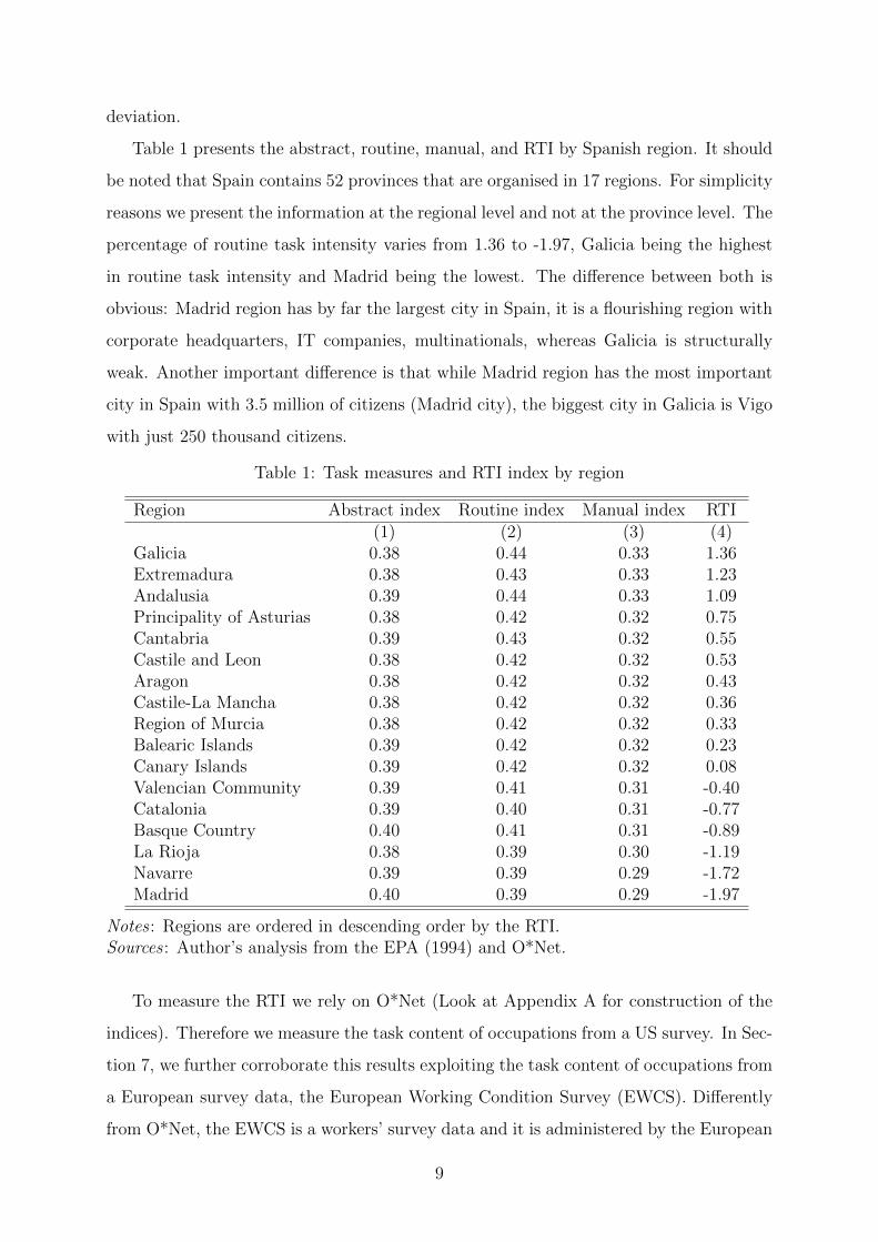
Table 1 presents the abstract, routine, manual, and RTI by Spanish region. It should

be noted that Spain contains 52 provinces that are organised in 17 regions. For simplicity

reasons we present the information at the regional level and not at the province level. The

percentage of routine task intensity varies from 1.36 to -1.97, Galicia being the highest

in routine task intensity and Madrid being the lowest. The difference between both is

obvious: Madrid region has by far the largest city in Spain, it is a flourishing region with

corporate headquarters, IT companies, multinationals, whereas Galicia is structurally

weak. Another important difference is that while Madrid region has the most important

city in Spain with 3.5 million of citizens (Madrid city), the biggest city in Galicia is Vigo

with just 250 thousand citizens.

Table 1: Task measures and RTI index by region

Region Abstract index Routine index Manual index RTI(1) (2) (3) (4)

Galicia 0.38 0.44 0.33 1.36Extremadura 0.38 0.43 0.33 1.23Andalusia 0.39 0.44 0.33 1.09Principality of Asturias 0.38 0.42 0.32 0.75Cantabria 0.39 0.43 0.32 0.55Castile and Leon 0.38 0.42 0.32 0.53Aragon 0.38 0.42 0.32 0.43Castile-La Mancha 0.38 0.42 0.32 0.36Region of Murcia 0.38 0.42 0.32 0.33Balearic Islands 0.39 0.42 0.32 0.23Canary Islands 0.39 0.42 0.32 0.08Valencian Community 0.39 0.41 0.31 -0.40Catalonia 0.39 0.40 0.31 -0.77Basque Country 0.40 0.41 0.31 -0.89La Rioja 0.38 0.39 0.30 -1.19Navarre 0.39 0.39 0.29 -1.72Madrid 0.40 0.39 0.29 -1.97

Notes : Regions are ordered in descending order by the RTI.Sources : Author’s analysis from the EPA (1994) and O*Net.

To measure the RTI we rely on O*Net (Look at Appendix A for construction of the

indices). Therefore we measure the task content of occupations from a US survey. In Sec-

tion 7, we further corroborate this results exploiting the task content of occupations from

a European survey data, the European Working Condition Survey (EWCS). Differently

from O*Net, the EWCS is a workers’ survey data and it is administered by the European

9

Foundation for the Improvement of Living and Working Conditions (Eurofound) and has

become an established source of information about working conditions and the quality of

work and employment. With six waves (one every five years) having been implemented

since 1990, it enables monitoring of long-term trends in working conditions in Europe.

At each wave, information on employment status, working time arrangements, work or-

ganisation, learning and training, and work-life balance among others is collected. In this

research we focus on the second wave (1995). More information on the items selected is

found in Section 7.

In order to measure the Routine Employment Share (RSH) within province we follow

Autor and Dorn (2013), and we take take two more steps. First, using the RTI we classify

as routine-intensity occupations those in the highest employment-weighted third share of

RTI in 1994. Table 2 reports the 24 two-digit occupations, ranked in descending order by

the RTI values. It also presents the employment distribution in 1994 and the cumulative

distribution. Lastly, occupations that are considered routine-intensive occupations are

indicated: “Other craft and related trades workers” (ISCO 74), “Machinery operators

and assemblers” (ISCO 82), “Precision, handicraft, printing, and trades workers” (ISCO

73), “Metal, machinery, and related trades workers” (ISCO 72), and “Extraction and

building trade workers” (ISCO 71).

Second, we compute for each province j, a routine employment share (RSH), calculated

as:

RSHpt = (k∑

k=1

Lpkt ∗ 1[RTIk > RTI66])(k∑

k=1

Lpkt)(−1) (2)

where Lpkt is employment in occupation k in province p at time t, 1[.] is a indicator

function taking value of one if it is routine intensity. In other words, it is the routine em-

ployment share divided by employment share. The mean of RSH is 0.23 in 1994, and the

interquartile (Iqr, henceforth) is 7 percentage points (RSHp25=0.163 and RSHp75=0.303).

Accordingly, Table 3 shows the 1994 RSH by region ranked from low to high values where

a higher RSH indicates a higher initial routine concentration.

10

Tab

le2:

Tas

km

easu

res

and

RT

Iin

dex

by

occ

upat

ion

Occ

upat

ion

ISC

O-8

8R

TI

1994

Cum

ula

tive

Top

33p

erce

nt

(1)

(2)

(3)

(4)

Oth

ercr

aft

and

rela

ted

trad

esw

orke

rs74

1.63

4.40

4.40

XM

achin

eop

erat

ors

and

asse

mble

rs82

1.34

4.67

9.07

XP

reci

sion

,han

dic

raft

,pri

nti

ng

and

rela

ted

trad

esw

orke

r73

1.02

1.17

10.2

4X

Met

al,

mac

hin

ery

and

rela

ted

trad

esw

orke

rs72

0.89

7.26

17.4

9X

Extr

acti

onan

dbuildin

gtr

ades

wor

kers

710.

898.

8926

.38

XD

rive

rsan

dm

obile-

pla

nt

oper

ator

s83

0.83

6.69

33.0

7Sta

tion

ary-p

lant

and

rela

ted

oper

ator

s81

0.82

1.25

34.3

2L

abou

rers

inm

inin

gco

nst

ruct

ion,

and

man

ufa

cturi

ng

930.

765.

4839

.80

Sal

esan

dse

rvic

esel

emen

tary

occ

upat

ions

910.

369.

3449

.14

Physi

cal

and

engi

nee

ring

scie

nce

asso

ciat

epro

fess

ional

s31

0.26

1.73

50.8

7M

odel

s,sa

lesp

erso

ns

and

dem

onst

rato

rs52

0.21

6.19

57.0

6P

erso

nal

and

pro

tect

ive

serv

ices

wor

kers

510.

1410

.02

67.0

8L

ife

scie

nce

and

hea

lth

asso

ciat

epro

fess

ional

s32

-0.0

20.

6067

.69

Lif

esc

ience

and

hea

lth

pro

fess

ional

s22

-0.1

82.

6270

.30

Offi

cecl

erks

41-0

.38

8.03

78.3

3C

ust

omer

serv

ices

cler

ks

42-0

.68

4.94

83.2

7P

hysi

cal,

mat

hem

atic

alan

den

ginee

ring

scie

nce

pro

fess

ion

21-0

.95

1.80

85.0

6O

ther

asso

ciat

epro

fess

ional

s34

-1.1

25.

2790

.34

Oth

erpro

fess

ional

s24

-1.1

90.

4890

.81

Cor

por

ate

man

ager

s12

-1.2

42.

0792

.88

Busi

nes

sas

soci

ate

pro

fess

ional

s33

-1.3

30.

1593

.03

Tea

chin

gpro

fess

ional

s23

-2.0

56.

9710

0.00

Not

es:

Reg

ions

are

order

edin

des

cendin

gor

der

by

the

RT

I.S

ourc

es:

Auth

or’s

anal

ysi

sfr

omth

eE

PA

(199

4)an

dO

*Net

.

11

Table 3: RSH by region

Region RSHCanary Islands 0.14Andalusia 0.19Galicia 0.19Extremadura 0.20Principality of Asturias 0.20Balearic Islands 0.21Cantabria 0.22Castile and Leon 0.24Region of Murcia 0.24Aragon 0.25Catalonia 0.26Castile-La Mancha 0.26Basque Country 0.27Valencian Community 0.27Madrid 0.28La Rioja 0.32Navarre 0.33

Notes : Regions are ordered in ascending order by the RSH.Sources : Author’s analysis from the EPA (1994) and O*Net.

4 Initial evidence of job polarisation

4.1 By occupational groups

We start our analysis by documenting the evolution of employment changes between

1994 and 2008. First, we compute employment shares for each job and their changes

over time.8 Second, we rank jobs according to their 1995 mean hourly wage.9 Finally, we

aggregate them into five equally sized groups containing almost the same percentage of

employment in the initial year.10 In Figure 1, we show the changes in employment share

from 1994 to 2008 by job wage quintile. The figure shows a clear U-shaped curve of job

polarisation: there is an increasing employment share at the bottom and top of the wage

distribution (low and high-skilled jobs) and a decline in the employment share at the

middle of the wage distribution (middle-skilled jobs). Figure 1 reveals a similar pattern

as found by Anghel et al. (2014) and Sebastian (2017) for Spain, which is different from

8In this occasion jobs are defined as the combination between two-digit occupation (ISCO-88) and

one-digit industry (CNAE-93).9Results remain invariant if we use the median.

10Jobs are defined as inseparable units therefore it is not possible to create groups that contain exactly

the same percentage of employment.

12

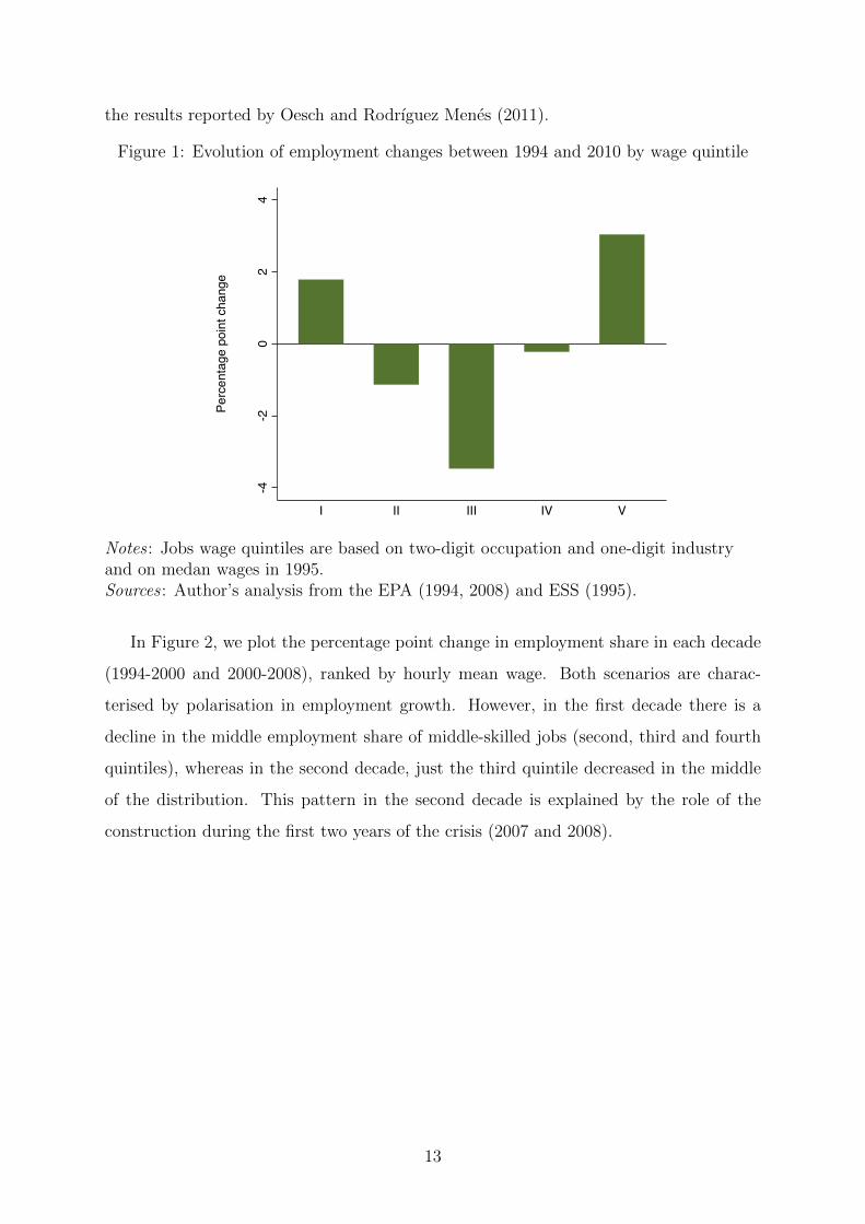
the results reported by Oesch and Rodrıguez Menes (2011).

Figure 1: Evolution of employment changes between 1994 and 2010 by wage quintile

-4-2

02

4

Perc

enta

ge p

oint

cha

nge

I II III IV V

Notes : Jobs wage quintiles are based on two-digit occupation and one-digit industryand on medan wages in 1995.Sources : Author’s analysis from the EPA (1994, 2008) and ESS (1995).

In Figure 2, we plot the percentage point change in employment share in each decade

(1994-2000 and 2000-2008), ranked by hourly mean wage. Both scenarios are charac-

terised by polarisation in employment growth. However, in the first decade there is a

decline in the middle employment share of middle-skilled jobs (second, third and fourth

quintiles), whereas in the second decade, just the third quintile decreased in the middle

of the distribution. This pattern in the second decade is explained by the role of the

construction during the first two years of the crisis (2007 and 2008).

13

Figure 2: Evolution of employment changes by time periods

050

01,

000

Thou

sand

s of

wor

kers

I II III IV V

1994-2000

050

01,

000

Thou

sand

s of

wor

kers

I II III IV V

2000-2008

Notes : Jobs wage quintiles are based on two-digit occupation and one-digit industryand on mean wages in 1995.Sources : Author’s analysis from the EPA (1994, 2000, 2008) and ESS (1995).

To provide a more in depth analysis of these effects, we further analyse at the ISCO-88

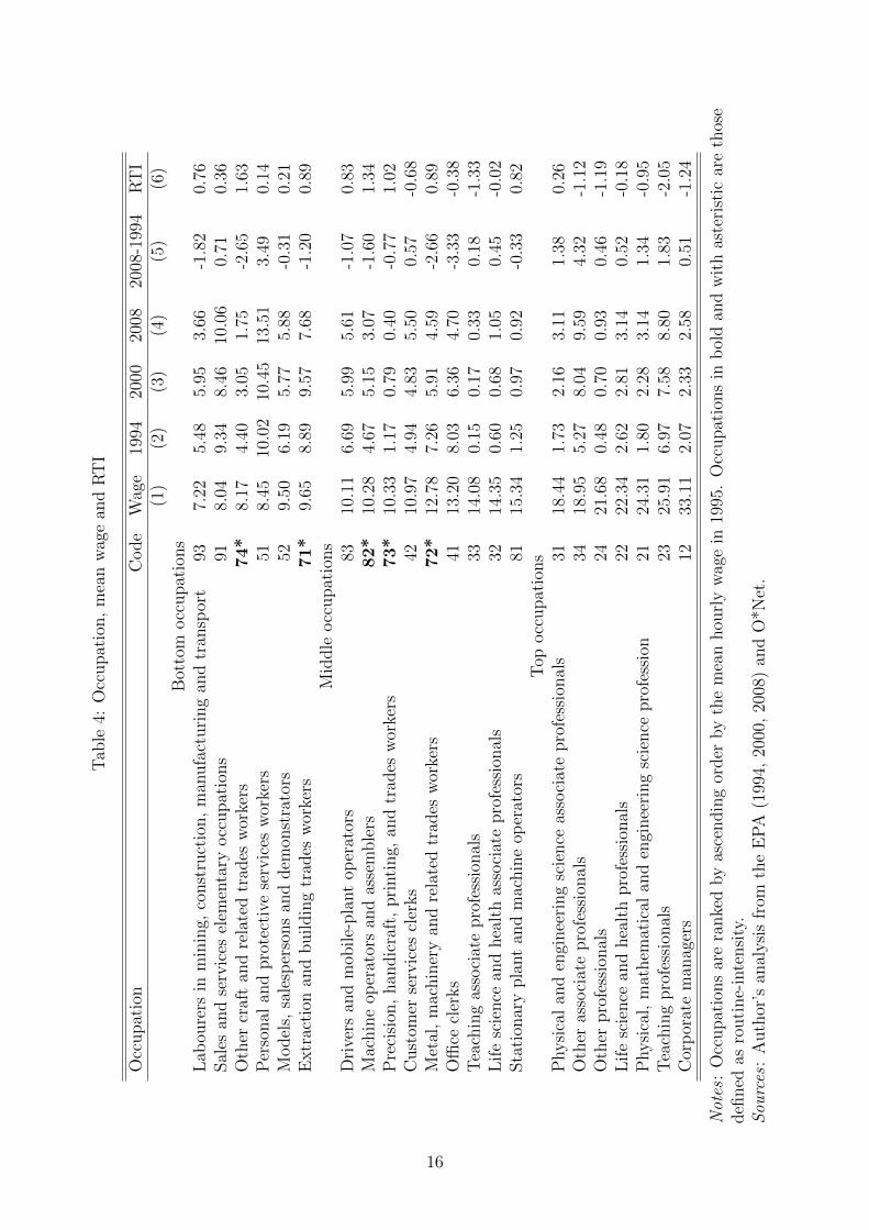
two-digit level. Table 4 presents the major occupational groups ranked by their initial

hourly mean wage (column 1), the level of employment during the period 1994 and 2008

(column 2 to 4), and the percentage point change in their employment between 1994

and 2008 (column 5). Drawing on Goos et al. (2014) we classify occupations into three

groups which we label bottom, middle, and top-paid occupations. We again observe the

job polarisation phenomenon among occupations: middling occupations are the ones with

the higher decline (-8.56pp) compared to the bottom and top-paid occupations (-1.78pp

and +10.35pp, respectively). Among the bottom-paid occupations, two out of six have

a growing employment share. This group is driven by a mix effect: on the one hand

service workers experience a significant positive employment growth (+3.49pp), while on

the other hand, handicraft and printing workers exhibit a negative employment growth

(-2.65pp). Within the middle-paid occupations, clerks (-3.33pp), metal, machinery and

related workers (-2.66pp), and assemblers (+1.60pp) are those that experience the most

significant employment losses. Concerning the group of top-paid occupations, those gain-

ing more employment share between 1994 and 2008 are legal, social and related associate

professionals (+4.32pp), and teaching professionals (+1.83pp).

14

To focus on the relevance RTI has in understanding job polarisation, Table 5 reports

the average values of task occupations as well as the RTI in 1994. The middle-paid occu-

pations have the highest positive values of RTI, therefore consistent with job polarisation.

Occupations at the bottom are positive, occupations at the middle are either positive or

negative, while occupations at the top score higher on the abstract measure and show

negative values in RTI.

From Table 5 we classify these occupations into three major groups: routine, manual,

and abstract occupations. First, the occupations with the highest RTI are defined as

routine-intensive occupations (RI), as explained in Section 3 (occupational categories in

bold). Second, we define the occupations in the top as non routine abstract (NRA).

Finally, the remaining occupations in the bottom and middle category are defined as non

routine manual (NRM).

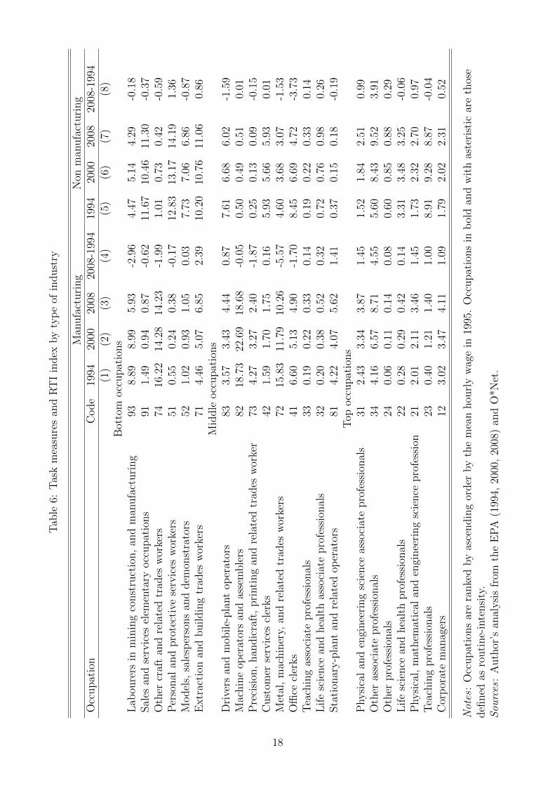
One important question is whether the polarisation trend occurs in the manufacturing

industry. For this purpose, we disentangle Table 4 by two sectors: manufacturing and

non-manufacturing. Table 6 shows that job polarisation happens in both sectors: middle-

paid occupations exhibit the highest declining shares with respect to the bottom and the

top. One important difference is the manufacturing sector in the bottom is declining by

3.31 points, whereas the non-manufacturing sector is increasing by 0.21. Specifically, the

manufacturing sector occupational categories losing the most are “Metal, machinery, and

related trades worker” (ISCO 72), and “Handicraft and printing workers” (ISCO 74); in

the non-manufacturing sector, it is “General and keyboard clerks” (ISCO 41). This result

aligns with previous results from Autor et al. (2015), where they find job polarisation

across economic sectors.

15

Tab

le4:

Occ

upat

ion,

mea

nw

age

and

RT

I

Occ

upat

ion

Code

Wag

e19

9420

0020

0820

08-1

994

RT

I(1

)(2

)(3

)(4

)(5

)(6

)B

otto

mocc

upat

ions

Lab

oure

rsin

min

ing,

const

ruct

ion,

man

ufa

cturi

ng

and

tran

spor

t93

7.22

5.48

5.95

3.66

-1.8

20.

76Sal

esan

dse

rvic

esel

emen

tary

occ

upat

ions

918.

049.

348.

4610

.06

0.71

0.36

Oth

ercr

aft

and

rela

ted

trad

esw

orke

rs74*

8.17

4.40

3.05

1.75

-2.6

51.

63P

erso

nal

and

pro

tect

ive

serv

ices

wor

kers

518.

4510

.02

10.4

513

.51

3.49

0.14

Model

s,sa

lesp

erso

ns

and

dem

onst

rato

rs52

9.50

6.19

5.77

5.88

-0.3

10.

21E

xtr

acti

onan

dbuildin

gtr

ades

wor

kers

71*

9.65

8.89

9.57

7.68

-1.2

00.

89M

iddle

occ

upat

ions

Dri

vers

and

mob

ile-

pla

nt

oper

ator

s83

10.1

16.

695.

995.

61-1

.07

0.83

Mac

hin

eop

erat

ors

and

asse

mble

rs82*

10.2

84.

675.

153.

07-1

.60

1.34

Pre

cisi

on,

han

dic

raft

,pri

nti

ng,

and

trad

esw

orke

rs73*

10.3

31.

170.

790.

40-0

.77

1.02

Cust

omer

serv

ices

cler

ks

4210

.97

4.94

4.83

5.50

0.57

-0.6

8M

etal

,m

achin

ery

and

rela

ted

trad

esw

orke

rs72*

12.7

87.

265.

914.

59-2

.66

0.89

Offi

cecl

erks

4113

.20

8.03

6.36

4.70

-3.3

3-0

.38

Tea

chin

gas

soci

ate

pro

fess

ional

s33

14.0

80.

150.

170.

330.

18-1

.33

Lif

esc

ience

and

hea

lth

asso

ciat

epro

fess

ional

s32

14.3

50.

600.

681.

050.

45-0

.02

Sta

tion

ary

pla

nt

and

mac

hin

eop

erat

ors

8115

.34

1.25

0.97

0.92

-0.3

30.

82T

opocc

upat

ions

Physi

cal

and

engi

nee

ring

scie

nce

asso

ciat

epro

fess

ional

s31

18.4

41.

732.

163.

111.

380.

26O

ther

asso

ciat

epro

fess

ional

s34

18.9

55.

278.

049.

594.

32-1

.12

Oth

erpro

fess

ional

s24

21.6

80.

480.

700.

930.

46-1

.19

Lif

esc

ience

and

hea

lth

pro

fess

ional

s22

22.3

42.

622.

813.

140.

52-0

.18

Physi

cal,

mat

hem

atic

alan

den

ginee

ring

scie

nce

pro

fess

ion

2124

.31

1.80

2.28

3.14

1.34

-0.9

5T

each

ing

pro

fess

ional

s23

25.9

16.

977.

588.

801.

83-2

.05

Cor

por

ate

man

ager

s12

33.1

12.

072.

332.

580.

51-1

.24

Not

es:

Occ

upat

ions

are

ranke

dby

asce

ndin

gor

der

by

the

mea

nhou

rly

wag

ein

1995

.O

ccupat

ions

inb

old

and

wit

has

teri

stic

are

thos

edefi

ned

asro

uti

ne-

inte

nsi

ty.

Sou

rces

:A

uth

or’s

anal

ysi

sfr

omth

eE

PA

(199

4,20

00,

2008

)an

dO

*Net

.

16

Tab

le5:

Tas

km

easu

res

and

RT

Iin

dex

by

occ

upat

ion

Occ

upat

ion

Code

Gro

up

Abst

ract

index

Rou

tine

index

Man

ual

index

RT

I(1

)(2

)(3

)(4

)B

otto

mocc

upat

ions

Lab

oure

rsin

min

ing,

const

ruct

ion,a

nd

man

ufa

cturi

ng

93N

RM

0.34

0.48

0.38

0.76

Sal

esan

dse

rvic

esel

emen

tary

occ

upat

ions

91N

RM

0.30

0.38

0.30

0.36

Oth

ercr

aft

and

rela

ted

trad

esw

orke

rs74*

RI

0.24

0.60

0.45

1.63

Per

sonal

and

pro

tect

ive

serv

ices

wor

kers

51N

RM

0.33

0.33

0.32

0.14

Model

s,sa

lesp

erso

ns

and

dem

onst

rato

rs52

NR

M0.

340.

400.

290.

21E

xtr

acti

onan

dbuildin

gtr

ades

wor

kers

71*

RI

0.35

0.50

0.42

0.89

Mid

dle

occ

upat

ions

Dri

vers

and

mob

ile-

pla

nt

oper

ator

s83

NR

M0.

300.

450.

370.

83M

achin

eop

erat

ors

and

asse

mble

rs82*

RI

0.29

0.58

0.44

1.34

Pre

cisi

on,

han

dic

raft

,pri

nti

ng

and

rela

ted

trad

esw

orke

r73*

RI

0.35

0.52

0.45

1.02

Cust

omer

serv

ices

cler

ks

42N

RM

0.40

0.28

0.23

-0.6

8M

etal

,m

achin

ery

and

rela

ted

trad

esw

orke

rs72*

RI

0.40

0.53

0.45

0.89

Offi

cecl

erks

41N

RM

0.40

0.35

0.24

-0.3

8T

each

ing

asso

ciat

epro

fess

ional

s33

NR

M0.

320.

410.

07-1

.33

Lif

esc

ience

and

hea

lth

asso

ciat

epro

fess

ional

s32

NR

M0.

450.

330.

38-0

.02

Sta

tion

ary

pla

nt

and

mac

hin

eop

erat

ors

81N

RM

0.38

0.53

0.41

0.82

Top

occ

upat

ions

Physi

cal

and

engi

nee

ring

scie

nce

asso

ciat

epro

fess

ional

s31

NR

A0.

450.

410.

390.

26O

ther

asso

ciat

epro

fess

ional

s34

NR

A0.

470.

290.

18-1

.12

Oth

erpro

fess

ional

s24

NR

A0.

470.

320.

15-1

.19

Lif

esc

ience

and

hea

lth

pro

fess

ional

s22

NR

A0.

570.

360.

38-0

.18

Physi

cal,

mat

hem

atic

alan

den

ginee

ring

scie

nce

pro

fess

ion

21N

RA

0.62

0.39

0.20

-0.9

5T

each

ing

pro

fess

ional

s23

NR

A0.

520.

300.

09-2

.05

Cor

por

ate

man

ager

s12

NR

A0.

590.

300.

20-1

.24

Not

es:

Occ

upat

ions

are

ranke

dby

asce

ndin

gor

der

by

the

mea

nhou

rly

wag

ein

1995

.O

ccupat

ions

inb

old

and

wit

has

teri

stic

are

thos

edefi

ned

asro

uti

ne-

inte

nsi

ty.

Sou

rces

:A

uth

or’s

anal

ysi

sfr

omth

eE

PA

(199

4)an

dO

*Net

.

17

Tab

le6:

Tas

km

easu

res

and

RT

Iin

dex

by

typ

eof

indust

ry

Man

ufa

cturi

ng

Non

man

ufa

cturi

ng

Occ

upat

ion

Code

1994

2000

2008

2008

-199

419

9420

0020

0820

08-1

994

(1)

(2)

(3)

(4)

(5)

(6)

(7)

(8)

Bot

tom

occ

upat

ions

Lab

oure

rsin

min

ing

const

ruct

ion,

and

man

ufa

cturi

ng

938.

898.

995.

93-2

.96

4.47

5.14

4.29

-0.1

8Sal

esan

dse

rvic

esel

emen

tary

occ

upat

ions

911.

490.

940.

87-0

.62

11.6

710

.46

11.3

0-0

.37

Oth

ercr

aft

and

rela

ted

trad

esw

orke

rs74

16.2

214

.28

14.2

3-1

.99

1.01

0.73

0.42

-0.5

9P

erso

nal

and

pro

tect

ive

serv

ices

wor

kers

510.

550.

240.

38-0

.17

12.8

313

.17

14.1

91.

36M

odel

s,sa

lesp

erso

ns

and

dem

onst

rato

rs52

1.02

0.93

1.05

0.03

7.73

7.06

6.86

-0.8

7E

xtr

acti

onan

dbuildin

gtr

ades

wor

kers

714.

465.

076.

852.

3910

.20

10.7

611

.06

0.86

Mid

dle

occ

upat

ions

Dri

vers

and

mob

ile-

pla

nt

oper

ator

s83

3.57

3.43

4.44

0.87

7.61

6.68

6.02

-1.5

9M

achin

eop

erat

ors

and

asse

mble

rs82

18.7

322

.69

18.6

8-0

.05

0.50

0.49

0.51

0.01

Pre

cisi

on,

han

dic

raft

,pri

nti

ng

and

rela

ted

trad

esw

orke

r73

4.27

3.27

2.40

-1.8

70.

250.

130.

09-0

.15

Cust

omer

serv

ices

cler

ks

421.

591.

701.

750.

165.

935.

665.

930.

01M

etal

,m

achin

ery,

and

rela

ted

trad

esw

orke

rs72

15.8

311

.79

10.2

6-5

.57

4.60

3.68

3.07

-1.5

3O

ffice

cler

ks

416.

605.

134.

90-1

.70

8.45

6.69

4.72

-3.7

3T

each

ing

asso

ciat

epro

fess

ional

s33

0.19

0.22

0.33

0.14

0.19

0.22

0.33

0.14

Lif

esc

ience

and

hea

lth

asso

ciat

epro

fess

ional

s32

0.20

0.38

0.52

0.32

0.72

0.76

0.98

0.26

Sta

tion

ary-p

lant

and

rela

ted

oper

ator

s81

4.22

4.07

5.62

1.41

0.37

0.15

0.18

-0.1

9T

opocc

upat

ions

Physi

cal

and

engi

nee

ring

scie

nce

asso

ciat

epro

fess

ional

s31

2.43

3.34

3.87

1.45

1.52

1.84

2.51

0.99

Oth

eras

soci

ate

pro

fess

ional

s34

4.16

6.57

8.71

4.55

5.60

8.43

9.52

3.91

Oth

erpro

fess

ional

s24

0.06

0.11

0.14

0.08

0.60

0.85

0.88

0.29

Lif

esc

ience

and

hea

lth

pro

fess

ional

s22

0.28

0.29

0.42

0.14

3.31

3.48

3.25

-0.0

6P

hysi

cal,

mat

hem

atic

alan

den

ginee

ring

scie

nce

pro

fess

ion

212.

012.

113.

461.

451.

732.

322.

700.

97T

each

ing

pro

fess

ional

s23

0.40

1.21

1.40

1.00

8.91

9.28

8.87

-0.0

4C

orp

orat

em

anag

ers

123.

023.

474.

111.

091.

792.

022.

310.

52

Not

es:

Occ

upat

ions

are

ranke

dby

asce

ndin

gor

der

by

the

mea

nhou

rly

wag

ein

1995

.O

ccupat

ions

inb

old

and

wit

has

teri

stic

are

thos

edefi

ned

asro

uti

ne-

inte

nsi

ty.

Sou

rces

:A

uth

or’s

anal

ysi

sfr

omth

eE

PA

(199

4,20

00,

2008

)an

dO

*Net

.

18

4.2 By demographic groups

We proceed with our analysis by examining changes in demographic groups, measured by

educational qualification, migration status, and type of industry. Figure 3 plots changes

in total employment in each decade from 1994 to 2008 by occupation wage quintiles.

Graduates are represented by individuals with a university degree. Non-graduates are

divided in two: low (primary and secondary education) and medium (upper secondary

and post-secondary, non-tertiary education).11

Figure 3 shows that the low educated workers are losing employment in the middle

of the wage distribution. Moreover, medium- and highly educated workers are gaining

employment along the whole distribution, but medium educated workers have gained at

the bottom whereas high educated at the top of the wage distribution. We further use

number of years of education instead of using the categorical variable consisting in the

highest level of educational attainment reached by workers. Results are robust to this

alternative specification.

Figure 3: Evolution of employment changes by educational qualification and decade

-500

050

01,

000

Thou

sand

s of

wor

kers

I II III IV V

1994-2000

Low

Medium

High

-500

050

01,

000

I II III IV V

2000-2010

Low

Medium

High

Notes : Jobs wage quintiles are based on two-digit occupation and one-digit industryand on mean wages in 1995. Figure 3 shows absolute net employment change in jobquintiles (in thousands of workers) by educational classification.Sources : Author’s analysis from the EPA(1994, 2000, 2008) and ESS(1995).

11The usual ISCED division into low, medium and high is adopted where low is equivalent to ISCED0-2 (i.e., primary and lower secondary education), medium is given by ISCED 3-4 (i.e., upper secondaryand post-secondary non-tertiary education) and high is ISCED 5-7 (i.e., tertiary education).

19

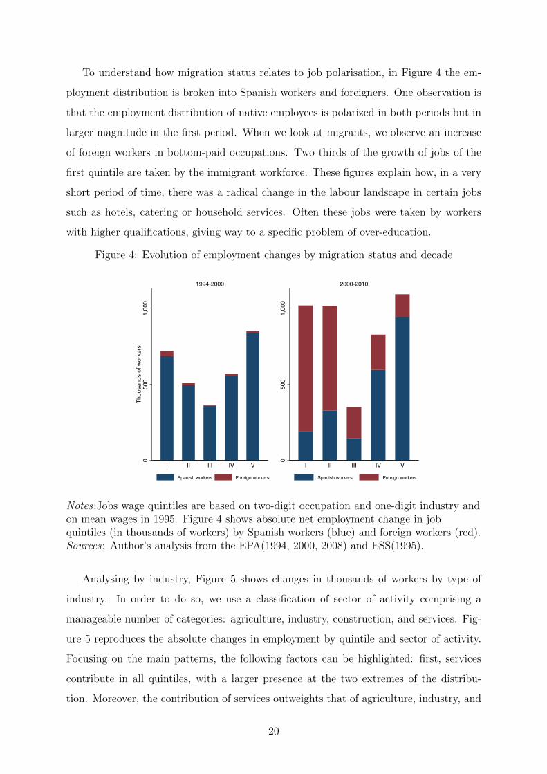
To understand how migration status relates to job polarisation, in Figure 4 the em-

ployment distribution is broken into Spanish workers and foreigners. One observation is

that the employment distribution of native employees is polarized in both periods but in

larger magnitude in the first period. When we look at migrants, we observe an increase

of foreign workers in bottom-paid occupations. Two thirds of the growth of jobs of the

first quintile are taken by the immigrant workforce. These figures explain how, in a very

short period of time, there was a radical change in the labour landscape in certain jobs

such as hotels, catering or household services. Often these jobs were taken by workers

with higher qualifications, giving way to a specific problem of over-education.

Figure 4: Evolution of employment changes by migration status and decade

050

01,

000

Thou

sand

s of

wor

kers

I II III IV V

1994-2000

Spanish workers Foreign workers

050

01,

000

I II III IV V

2000-2010

Spanish workers Foreign workers

Notes :Jobs wage quintiles are based on two-digit occupation and one-digit industry andon mean wages in 1995. Figure 4 shows absolute net employment change in jobquintiles (in thousands of workers) by Spanish workers (blue) and foreign workers (red).Sources : Author’s analysis from the EPA(1994, 2000, 2008) and ESS(1995).

Analysing by industry, Figure 5 shows changes in thousands of workers by type of

industry. In order to do so, we use a classification of sector of activity comprising a

manageable number of categories: agriculture, industry, construction, and services. Fig-

ure 5 reproduces the absolute changes in employment by quintile and sector of activity.

Focusing on the main patterns, the following factors can be highlighted: first, services

contribute in all quintiles, with a larger presence at the two extremes of the distribu-

tion. Moreover, the contribution of services outweights that of agriculture, industry, and

20

construction. Second, the growth of construction is located, most of it, in the second

quintile. Third, in the second decade, the destruction of employment is explained by the

industry.

Figure 5: Evolution of employment changes by type of industry and decade0

500

1,00

0

Thou

sand

s of

wor

kers

I II III IV V

1994-2000

Agriculture, forestry and fishing

Industry

Construction

Services

050

01,

000

I II III IV V

2000-2010

Agriculture, forestry and fishing

Industry

Construction

Services

Notes : Jobs wage quintiles are based on two-digit occupation and one-digit industryand on mean wages in 1995. Figure 5.5 shows absolute net employment change in jobquintiles (in thousands of workers) by type of industry.Sources : Author’s analysis from the EPA (1994, 2008) and ESS (1995).

To complete the initial analysis, in Figure 6 we replicate the analysis by gender.

Our findings are in line with previous figures. There are several highlights found in

the chart: first, overall the gender perspective does not change the conclusion presented

in relation to the nature of employment distribution. Both men and women have an

employment distribution that fits with the polarisation phenomenon: losing employment

in the middle of the wage distribution while gaining at the extremes. Second, within this

general shared pattern, the employment change of women during both decades is more

intensively polarizing. Third, the lack of growth of female employment in the second

quintile. This “anomaly” is explained by the role of construction in this segment of the

job distribution, a male dominated industry.

21

Figure 6: Evolution of employment changes by gender and decade

050

01,

000

Thou

sand

s of

wor

kers

I II III IV V

1994-2000

Men Women0

500

1,00

0I II III IV V

2000-2008

Men Women

Notes :Jobs wage quintiles are based on two-digit occupation and one-digit industry andon mean wages in 1995. Figure 5.4 shows absolute net employment change in jobquintiles (in thousands of workers) by gender.Sources : Author’s analysis from the EPA(1994, 2000, 2008) and ESS(1995).

4.3 By labour market area

Table 7 presents descriptive statistics of the sample for a number of measures. This

includes the routine employment share in local labour markets (RSH), the relative grad-

uate share (GradSH), the migrant population share (MigSh), and the manufacturing

population share (ManfSH) in 1994, 2000 and 2008.

As one can expect, the employment share in routine-intensity occupations decreases

by 4 percentage points in two decades (from 1994 to 2008). Similarly, the relative share

of manufacturing looses 2 percentage points in the period under study. On the contrary,

the relative share of graduates and relative share of migrants increases over time. In the

case of relative share of graduates grows in 6 percentage points in each decade, almost

doubling between 1994 and 2008. The relative share of migrants increases during both

decades and has accelerated during the second decade (+0.1pp), being almost explained

by the increased in high-skilled migrants.

22

Table 7: Summary statistics

1994 2000 2008Mean Std. Dev Iqr Mean Std. Dev Iqr Mean Std. Dev Iqr

RSH 0.233 0.050 0.070 0.213 0.047 0.061 0.190 0.030 0.033GradSH 0.193 0.052 0.060 0.255 0.056 0.064 0.316 0.068 0.086MigSH 0.004 0.004 0.004 0.009 0.010 0.010 0.109 0.070 0.113HigMigSH 0.001 0.001 0.002 0.003 0.003 0.002 0.022 0.018 0.023LowMigSH 0.003 0.003 0.002 0.006 0.007 0.007 0.087 0.055 0.094ManufSh 0.143 0.058 0.082 0.131 0.055 0.076 0.119 0.038 0.051

Sources : Author’s analysis from the EPA(1994, 2000, 2008).

In the light of the above findings, Figure 7 shows the graphical distribution of rou-

tine, manufacturing, graduates, and migrants across Spanish province in 1994. Several

important insights are revealed; first, higher levels in routine and manufacturing are

concentrated in the same provinces, i.e., Navarra, La Rioja, and Basque country. Two

exceptions to this rule are Madrid and Barcelona where they are more intense in rou-

tine employment than manufacturing specialization. Second, the two provinces with

higher levels of graduates shares are Madrid and Barcelona, provinces that are typically

specialised towards professionals, scientific and technical activities. Moreover, graduates

share is more concentrated in the north with high presence in Asturias, Cantabria, Basque

Country, Navarra and La Rioja. Third, migrants working share are instead more spread

geographically, with high concentration in the Mediterranean area.

23

Figure 7: Graphical distribution of routine, manufacturing, graduates and migrantsemployment share in 1994

1234

Routine

1234

Manufacturing

1234

Graduates

1234

Migrants

Notes : We include the same number of provinces inside each group. As we have 50provinces, our groups are uneven: the first group includes 12 provinces, the secondgroup 13 provinces, the third group 13 provinces, and the fourth group 12 provinces.Sources : Author’s analysis from the EPA (1994, 2008).

5 Model specification

Until now, the descriptive statistics in Table 1 to Table 7, and Figure 1 through Figure

7 showed preliminary evidence of the displacement of labour on routine tasks, leading to

a polarized employment distribution.

To test more rigorously the effect that technology has on labour and exploiting our

regional database, we follow the Routine Biased Technical Change (RBTC) hypothesis.

RBTC predicts that recent technological change is biased towards replacing labour in

routine tasks (tasks that require methodological repetition, therefore being easier to auto-

24

mate). This progressive substitution of technology leads to two different effects depending

on workers’ relative comparative advantage: first, technology fosters workers who have a

relative advantage in abstract tasks, expecting therefore a growth in high-skill occupa-

tions. Second, since technology substitutes routine workers with a comparative advantage

in low-skill tasks (rather than in high-skilled tasks), we expect a greater reallocation of

workers in jobs with routine tasks in non-manual occupations.

In the local labour market, we expect that provinces that initially have higher routine

employment share, experience two different effects: first, a higher relative employment

decline in routine occupations; second, a higher relative employment increase in manual

(low-skilled workers) and abstract (high-skilled workers).

To test this hypothesis, we build on Autor and Dorn (2013) to analyse variation across

the Spanish local market. We use the following model:

∆Ypct = αt + β1RSHpt−1 + β4X′

pt−1 + γc + δt + εpct (3)

where ∆Ypct is the change in local employment shares in (1) routine, (2) manual,

and (3) abstract occupations, in province p located in region c, between the initial year

and the final year considered (1994-2008). The RSHpt−1 is the variable capturing the

initial local employment share of routine occupations in province p (see Section 3.1 for

further details on how is derived). In order to control for potential shifts in local supply

and demand, a vector of covariates is included (X′

jt−1). This includes information on

the local initial relative shares of graduates and migrants, and the local initial share of

manufacturing employment. To be more precise, the latter variable tries to capture the

international import competition. To control for region-specific time trends, we include

a dummy for regions in Spain (NUTS-2). The stacked regression also includes a dummy

for time periods to account for changes over time.

6 Results and discussion

6.1 Changes in routine employment occupations

The first test is to identify whether historically routine intensive provinces have larger de-

clines in routine occupations. We estimate equation (3) by ordinary least squares (OLS).

25

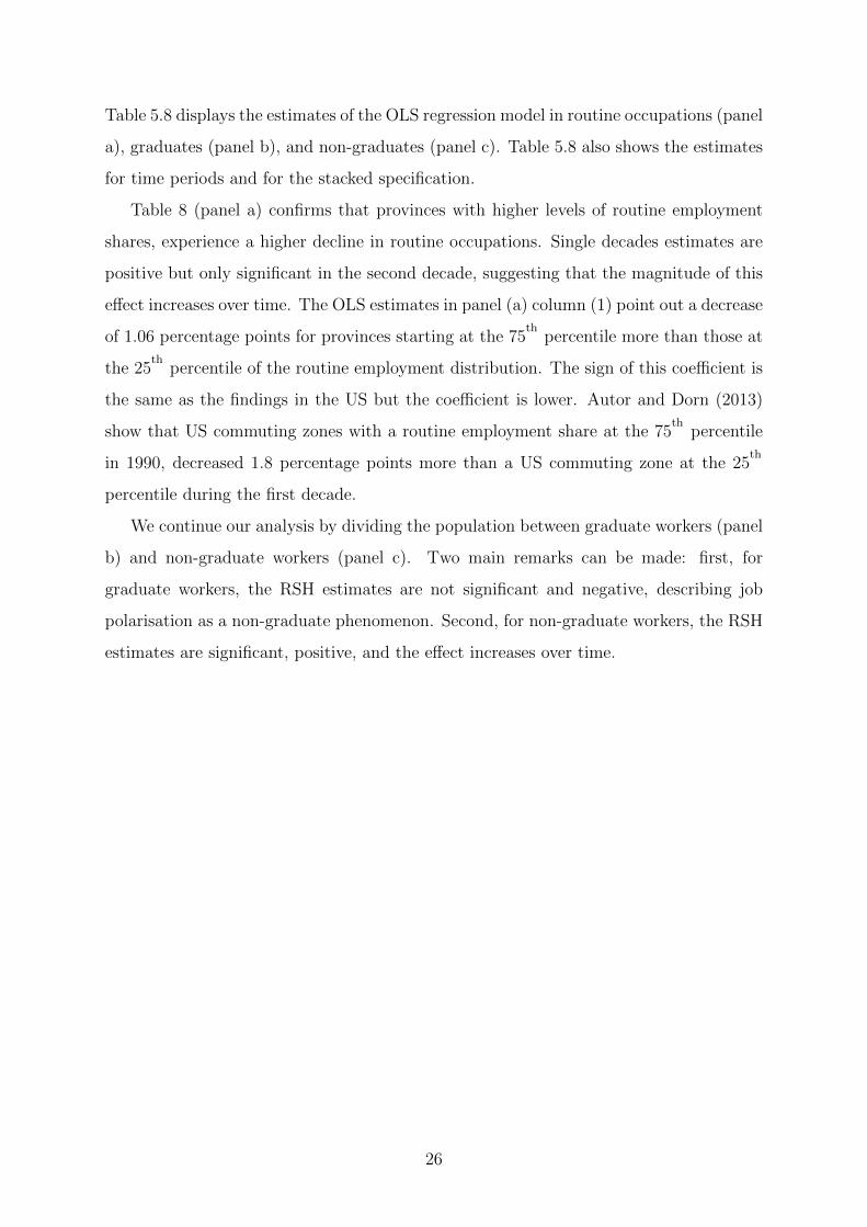
Table 5.8 displays the estimates of the OLS regression model in routine occupations (panel

a), graduates (panel b), and non-graduates (panel c). Table 5.8 also shows the estimates

for time periods and for the stacked specification.

Table 8 (panel a) confirms that provinces with higher levels of routine employment

shares, experience a higher decline in routine occupations. Single decades estimates are

positive but only significant in the second decade, suggesting that the magnitude of this

effect increases over time. The OLS estimates in panel (a) column (1) point out a decrease

of 1.06 percentage points for provinces starting at the 75th

percentile more than those at

the 25th

percentile of the routine employment distribution. The sign of this coefficient is

the same as the findings in the US but the coefficient is lower. Autor and Dorn (2013)

show that US commuting zones with a routine employment share at the 75th

percentile

in 1990, decreased 1.8 percentage points more than a US commuting zone at the 25th

percentile during the first decade.

We continue our analysis by dividing the population between graduate workers (panel

b) and non-graduate workers (panel c). Two main remarks can be made: first, for

graduate workers, the RSH estimates are not significant and negative, describing job

polarisation as a non-graduate phenomenon. Second, for non-graduate workers, the RSH

estimates are significant, positive, and the effect increases over time.

26

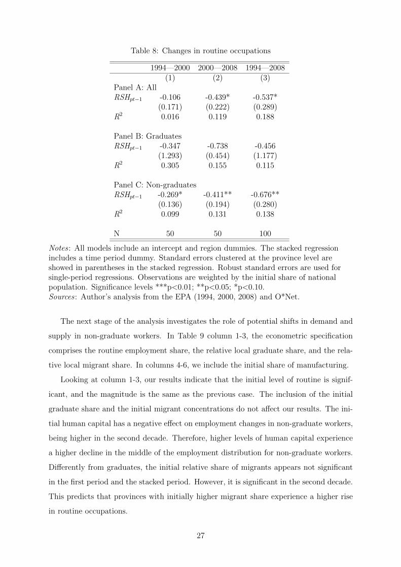
Table 8: Changes in routine occupations

1994—2000 2000—2008 1994—2008(1) (2) (3)

Panel A: AllRSHpt−1 -0.106 -0.439* -0.537*

(0.171) (0.222) (0.289)R2 0.016 0.119 0.188

Panel B: GraduatesRSHpt−1 -0.347 -0.738 -0.456

(1.293) (0.454) (1.177)R2 0.305 0.155 0.115

Panel C: Non-graduatesRSHpt−1 -0.269* -0.411** -0.676**

(0.136) (0.194) (0.280)R2 0.099 0.131 0.138

N 50 50 100

Notes : All models include an intercept and region dummies. The stacked regressionincludes a time period dummy. Standard errors clustered at the province level areshowed in parentheses in the stacked regression. Robust standard errors are used forsingle-period regressions. Observations are weighted by the initial share of nationalpopulation. Significance levels ***p<0.01; **p<0.05; *p<0.10.Sources : Author’s analysis from the EPA (1994, 2000, 2008) and O*Net.

The next stage of the analysis investigates the role of potential shifts in demand and

supply in non-graduate workers. In Table 9 column 1-3, the econometric specification

comprises the routine employment share, the relative local graduate share, and the rela-

tive local migrant share. In columns 4-6, we include the initial share of manufacturing.

Looking at column 1-3, our results indicate that the initial level of routine is signif-

icant, and the magnitude is the same as the previous case. The inclusion of the initial

graduate share and the initial migrant concentrations do not affect our results. The ini-

tial human capital has a negative effect on employment changes in non-graduate workers,

being higher in the second decade. Therefore, higher levels of human capital experience

a higher decline in the middle of the employment distribution for non-graduate workers.

Differently from graduates, the initial relative share of migrants appears not significant

in the first period and the stacked period. However, it is significant in the second decade.

This predicts that provinces with initially higher migrant share experience a higher rise

in routine occupations.

27

For columns 4-6, the initial share of manufacturing employment is included. It should

be noted that the correlation between the main regressor of interest (RSH) and the initial

share of manufacturing is high (0.48). When all the controls are added, the initial routine

share is significant and increases its magnitude. The control variables are not significant in

the first decade and the specification with stacked periods. However, during the 2000s, the

initial migrant concentration has a positive effect and the initial share of manufacturing

has a negative effect on employment changes in non-graduate workers.

Considering the effect of technology in routine occupations, provinces with initially

higher specialization in routine-intensive occupations experience larger declines in non-

graduate routine-intensive occupations.

Table 9: Changes in routine occupations

1994 2000 1994 1994 2000 19942000 2008 2008 2000 2008 2008(1) (2) (3) (4) (5) (6)

RSHpt−1 -0.301** -0.314* -0.616*** -0.196* -0.841** -1.225***(0.131) (1.165) (0.045) (0.099) (0.391) (2.02)

GradShpt−1 -0.134** -0.176* -0.306** -0.034 0.053 0.026(0.060) (.103) (.142) (0.083) (.075) (0.129)

MigShpt−1 0.063 0.244** 0.248 -0.189 0.189* 0.165(0.677) (0.116) (0.157) (0.571) (0.098) (0.126)

ManufShpt−1 -0.370 -0.852*** -1.030(0.333) (0.290) (0.747)

R2 0.185 0.233 0.237 0.297 0.555 0.529N 50 50 100 50 50 100

Notes : All models include an intercept and region dummies. The stacked regressionincludes a time period dummy. Standard errors clustered at the province level areshowed in parentheses in the stacked regression. Robust standard errors are used forsingle-period regressions. Observations are weighted by the initial share of nationalpopulation. Significance levels ***p<0.01; **p<0.05; *p<0.10.Sources : Author’s analysis from the EPA (1994, 2000, 2008) and O*Net.

6.2 Changes in manual employment occupations

In analysing changes in manual jobs, we expect that low-skilled workers reallocate from

routine to manual tasks at the bottom of the employment distribution. This follows Autor

and Dorn (2013) framework. The assumption behind the previous idea is that low-skilled

workers comparative advantage is higher in low-skilled than in high-skilled tasks.

The results contained in Table 10 confirm this hypothesis. It displays the estimates of

28

the regression model for all the workers (panel a), graduates (panel b), and non-graduates

(panel c). OLS results point out a significant and positive effect of technological exposure

on non-graduates in every decade as well as stacked periods. Therefore, provinces with

initially higher routine tasks have a larger increase in non-graduate, manual occupations.

Table 10: Changes in manual occupations

1994—2000 2000—2008 1994—2008(1) (2) (3)

Panel A: AllRSHpt−1 0.243 0.296 0.554

(0.237) (0.193) (0.433)R2 0.084 0.143 0.128

Panel B: GraduatesRSHpt−1 1.227 0.726 2.075

(0.742) (0.843) (1.558)R2 0.221 0.162 0.165

Panel C: Non-graduatesRSHpt−1 0.146* 0.255* 0.409**

(0.079) (0.133) (0.180)R2 0.134 0.156 0.167

N 50 50 100

Notes : All models include an intercept and region dummies. The stacked regressionincludes a time period dummy. Standard errors clustered at the province level areshowed in parentheses in the stacked regression. Robust standard errors are used forsingle-period regressions. Observations are weighted by the initial share of nationalpopulation. Significance levels ***p<0.01; **p<0.05; *p<0.10.Sources : Author’s analysis from the EPA (1994, 2000, 2008) and O*Net.

Table 11 shows the results of the analysis on the reallocation of non-graduate workers

in manual occupations. Again, we include the initial relative labour supply shares of grad-

uates and low-skilled migrants (column 1-3) and the initial local share of manufacturing

(column 3-6).

With respect to the initial labour supply share (column 1-3), the RSH coefficients are

significant and positive. Therefore, the main results still hold when the control variables

are plugged-in. Looking at the initial share of graduates, the results are significant, mean-

ing that provinces with higher graduate share in the first year are negatively associated

with employment changes in non-graduate manual occupations during the whole period.

Therefore, the higher the graduate shares, the larger the decline in non-graduate manual

29

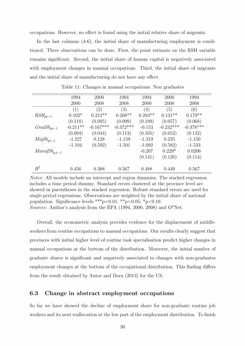
occupations. However, no effect is found using the initial relative share of migrants.

In the last columns (4-6), the initial share of manufacturing employment is condi-

tioned. Three observations can be done. First, the point estimate on the RSH variable

remains significant. Second, the initial share of human capital is negatively associated

with employment changes in manual occupations. Third, the initial share of migrants

and the initial share of manufacturing do not have any effect.

Table 11: Changes in manual occupations: Non graduates

1994 2000 1994 1994 2000 19942000 2008 2008 2000 2008 2008(1) (2) (3) (4) (5) (6)

RSHpt−1 0.102* 0.212** 0.208** 0.283** 0.131** 0.179**(0.118) (0.095) (0.099) (0.109) (0.057) (0.068)

GradShpt−1 -0.211** -0.167*** -0.372*** -0.153 -0.232*** -0.378***(0.094) (0.044) (0.113) (0.105) (0.052) (0.132)

MigShpt−1 -1.227 0.128 -1.159 -1.319 0.235 -1.150-1.104 (0.592) -1.501 -1.092 (0.582) -1.533

ManufShp,t−1 -0.207 0.229* 0.0206(0.141) (0.120) (0.114)

R2 0.456 0.388 0.567 0.488 0.449 0.567

Notes : All models include an intercept and region dummies. The stacked regressionincludes a time period dummy. Standard errors clustered at the province level areshowed in parentheses in the stacked regression. Robust standard errors are used forsingle-period regressions. Observations are weighted by the initial share of nationalpopulation. Significance levels ***p<0.01; **p<0.05; *p<0.10.Sources : Author’s analysis from the EPA (1994, 2000, 2008) and O*Net.

Overall, the econometric analysis provides evidence for the displacement of middle-

workers from routine occupations to manual occupations. Our results clearly suggest that

provinces with initial higher level of routine task specialisation predict higher changes in

manual occupations at the bottom of the distribution. Moreover, the initial number of

graduate shares is significant and negatively associated to changes with non-graduates

employment changes at the bottom of the occupational distribution. This finding differs

from the result obtained by Autor and Dorn (2013) for the US.

6.3 Change in abstract employment occupations

So far we have showed the decline of employment share for non-graduate routine job

workers and its next reallocation at the low part of the employment distribution. To finish

30

the puzzle, we need to study employment changes in abstract occupations at the upper

part of the occupational distribution. As explained in Section 5, due to a complementarity

effect between high-skilled workers and technology, the model predicts an increased level

of employment share for graduate abstract task workers.

In Table 12, we investigate the effect that technology has at the top of the employment

distribution. Table 12 presents changes in abstract occupations for the total number

of workers (panel a), graduate workers (panel b), and non-graduate workers (panel c).

One expectation can be formulated from the model: a positive effect of technological

exposure on employment in abstract occupations. However, the initial relative share of

routine labour is not statistically significant in any of our three scenarios. Therefore, we

can conclude that technological change has not caused an upward shift of the marginal

high-skilled workers.

Table 12: Changes in abstract occupations

1994—2000 2000—2008 1994—2008(1) (2) (3)

Panel A: AllRSHpt−1 0.165 0.129 0.165

(0.106) (0.088) (0.106)R2 0.037 0.193 0.194

Panel B: GraduatesRSHpt−1 0.001 2.897 3.226*

(0.625) (1.828) (1.897)R2 0.062 0.155 0.158

Panel C: Non-graduatesRSHpt−1 0.405 0.709 1.102

(0.345) (0.556) (0.782)R2 0.099 0.221 0.227

N 50 50 100

Notes : All models include an intercept and region dummies. The stacked regressionincludes a time period dummy. Standard errors clustered at the province level areshowed in parentheses in the stacked regression. Robust standard errors are used forsingle-period regressions. Observations are weighted by the initial share of nationalpopulation. Significance levels ***p<0.01; **p<0.05; *p<0.10.Sources : Author’s analysis from the EPA (1994, 2000, 2008) and O*Net.

Because of the absence of technological effect, the focus of the analysis shifts to the

role of labour supply and demand shifter in increasing of graduate employment in top

31

occupations. The results of the analysis are presented in Table 13.

Table 13 includes the initial local routine employment, the initial share of graduate

concentrations, and the initial share of high-skilled migrants. The initial relative share of

graduates is significant and negatively associated with high-educated workers changes in

the first decade, while it is significant and positively associated with this variable during

the second decade. The explanation behind this is a general education catch-up across

areas during the first decade. Provinces with a larger proportion of worker with university

degrees experiences the smallest increases in education, while in the 2000s, initial local

graduate share has a positive effect on changes in graduate abstract occupations. For

migrant share, the initial local high-skilled migration is significant and has a positive

effect on changes in graduate abstract occupations. Provinces with higher high-skilled

migration share have a larger increase in abstract occupations. Our intuition is that this

variable is capturing the expanding process of the European Union.

In column 4-6, the full set of explanatory variables is included, incorporating the initial

share of manufacturing employment. The introduction of initial share of manufacturing

employment does not alter our results.

Table 13: Changes in abstract occupations: Graduates

1994 2000 1994 1994 2000 19942000 2008 2008 2000 2008 2008(1) (2) (3) (4) (5) (6)

RSHpt−1 0.114 0.127 0.240 0.668 0.074 0.663(0.315) (0.179) (0.393) (0.720) (0.380) -1.022

GradShpt−1 -0.317** 0.205** -0.112 -0.193** 0.233** 0.0315(0.124) (0.101) (0.214) (0.093) (0.112) (0.302)

MigShpt−1 0.407** 0.609*** 1.017*** 0.401** 0.637*** 1.010***(0.172) (0.176) (0.318) (0.190) (0.173) (0.341)

ManufShpt−1 -0.558 -0.107 -0.645(0.590) (0.231) (0.798)

R2 0.226 0.367 0.489 0.293 0.427 0.519

Notes : All models include an intercept and region dummies. The stacked regressionincludes a time period dummy. Standard errors clustered at the province level areshowed in parentheses in the stacked regression. Robust standard errors are used forsingle-period regressions. Observations are weighted by the initial share of nationalpopulation. Significance levels ***p<0.01; **p<0.05; *p<0.10.Sources : Author’s analysis from the EPA(1994, 2000, 2008) and O*Net.

To summarise, technology exposure (the initial routine share) does not play any role in

32

explaining changes in graduate abstract occupations. An important observation different

from Autor and Dorn (2013) is that the initial share of graduates and migrants are

positively related to changes in graduate abstract occupations.

7 Extensions and robustness checks

7.1 Potential endogeneity

The measurement of the causal effect of technology on local labour markets could require

one identification assumption which is discussed in the literature. The assumption of

OLS estimates is that the variation of routine occupation shares (RSH) is exogenous and

is not driven by time-varying local specific unobservable. In what follows, we discuss this

problem.

In order to understand the previous problem, a simplified version of equation (3) is

used to replace the main regressor of interest:

RSHpt−1 = RSH∗p + υpt−1 (4)

Replacing now (4) in (3), the latter equation can be rewritten as:

∆Ypct = α′

t + β′

1RSH∗p + β

′

2υpt−1 + ε′

pt (5)

where RSH∗p represents the long-run quasi-fixed component of industrial structure

which in our model determines provinces’ routine occupation shares. Additionally, υpt−1

stands for unobservables. In other words, time-varying attributes that affect at the same

time changes in employment share (∆Ypt) and local routine occupation shares (RSH).

If that is the case, we will obtain biased OLS estimates in equation (3). There are two

possibilities:

(1) If β′2 > β

′1 and Var (υ1) > 0 in equation (5), OLS estimates of β1 in equation (3)

will be upward biased.

(2) If β′2 < β

′1 and Var (υ1) > 0 in equation (5), OLS estimates of β1 in equation (3)

will be downward biased.

To address this endogeneity problem, we construct an instrumental variable for the

33

routine employment share levels based on the Autor and Dorn’s (2013) instrument. It con-

sists of exploiting historical local industry information to remove the long-run quasi-fixed

component of the routine occupation share. The instrument is constructed as follows:

RSHIVp =

∑Ei,p,1977 ∗ Ri,−p,1977 (6)

where Ei,p,1977 is the employment share in industry i in province p, and Ri,−p,1977 is the

routine occupation employment share in industry i in all the Spanish provinces except p.

This measure is an appropriate instrumental variable for RSH: we expect that past

industrial information is correlated with the long-run component and uncorrelated with

current economic shocks. Therefore, we can obtain an exogenous measure for the routine

employment share.

In Table 14, we estimate equation (6) by two-stage least squares (2SLS) regression

model. Panel (a) displays the changes in routine occupations, panel (b) shows the changes

in manual occupations, and panel (c) indicates the changes in abstract occupations.

Table 14 reports as well the the Kleibergen-Papp F-statistics from each of the first-stage

regression.12

As can be seen from Table 14, the initial routine employment share coefficient for

the routine, manual, and abstract do not differ from the main analysis. However, the

Kleibergen-Papp F-statistics is below the Staiger and Stock’s (1997) rule of thumb thresh-

old of 10. Although the instrument is not strong, the results are in line with those of the

baseline analysis.

12Look at Appendix B for the first stage.

34

Table 14: Changes in occupations

1994—2008

Panel A: Routine occupationsRSHpt−1 -0.406**

(0.192)

Panel B: Manual OccuparionsRSHpt−1 -0.505*

(0.286)

Panel C: Abstract occupationsRSHpt−1 -0.094

(0.104)

First stageF-K test 6.990N 100

Notes : All models include an intercept and region dummies. The stacked regressionincludes a time period dummy. Standard errors clustered at the province level areshowed in parentheses in the stacked regression. Robust standard errors are used forsingle-period regressions. Observations are weighted by the initial share of nationalpopulation. Significance levels ***p<0.01; **p<0.05; *p<0.10.Sources : Author’s analysis from the EPA(1977, 1994, 2000, 2008) and O*Net.

35

7.2 Contemporaneous labour supply changes

To explore the effect of the technology, the model must control for contemporaneous

labour supply changes. The analysis addresses this by including the relative growth of

graduates and migrants. Table 15 reports the estimates from OLS for the routine (panel

a), manual (panel b) and abstract (panel c) specifications. It contains information on

single decades and stacked periods.

Looking now to non-graduates routine occupations (panel a), results are in line with

the main analysis: the decline at the middle part of the employment distribution is

explained by technology exposure.

Panel b displays changes in manual occupations. The initial relative share of routine

is positive related with changes in manual occupations. It suggests that the growth

at the bottom part of employment distribution is explaining by technological exposure,

confirming previous results. However, OLS results show a more substantial relevance of

labour of labour supply changes. Initial local graduates’ concentrations are significantly

related to manual occupations and this association grows over time.

Finally, panel c reports changes in graduate abstract employment. Different from

what we found previously, OLS results suggest a significant positive effect of technology

exposure on graduate workers. As in the main analysis, findings indicate that the initial

graduate and high-skilled migrant share are positively correlated with changes in abstract

occupations, and therefore, explain top employment growth.

36

Table 15: Conditional on local labour supply

1994 2000 1994 1994 2000 19942000 2008 2008 2000 2008 2008(1) (2) (3) (4) (5) (6)

Panel A. Non-graduates routine occupationsRSHpt−1 -0.269* -0.411** -0.676** -0.269* -0.415** -0.689**

(0.137) (0.194) (0.281) (0.137) (0.195) (0.278)GradShpt−1 -0.067 -0.243* -0.301***

(0.0577) (0.131) (0.112)MigShpt−1 0.0137 0.00750 0.0213

(0.0110) (0.0198) (0.0189)

Panel B. Non-graduate manual occupationsRSHpt−1 0.146 0.255* 0.409 0.138 0.256*** 0.398**

(0.238) (0.135) (0.341) (0.154) (0.078) (0.161)GradShpt−1 -0.365** -0.312*** -0.675***

(0.136) (0.037) (0.153)MigShpt−1 -0.019 -0.005 -0.025

(0.013) (0.010) (0.015)

Panel C. Graduate abstract occupationsRSHpt−1 0.405 0.709 1.102 0.378 0.671* 1.108*

(0.345) (0.556) (0.782) (0.354) (0.375) (0.635)GradShpt−1 0.0184 0.727** 0.719

(0.217) (0.313) (0.493)MigShpt−1 0.052* 0.002 0.057

(0.026) (0.049) (0.064)N 50 50 100 50 50 100

Notes : All models include an intercept and region dummies. The stacked regressionincludes a time period dummy. Standard errors clustered at the province level areshowed in parentheses in the stacked regression. Robust standard errors are used forsingle-period regressions. Observations are weighted by the initial share of nationalpopulation. Significance levels ***p<0.01; **p<0.05; *p<0.10.Sources : Author’s analysis from the EPA (1994, 2000, 2008) and O*Net.

37

7.3 Alternative database: EWCS

Until now, and following previous research, the study relied on O*Net to measure the RTI

index. To test whether the results are robust to the use of this database (designed for

the US), the same analysis is performed using the European Working Condition Survey

(EWCS) dataset. One advantage is that assumptions on task composition between the US

and Spain can be relaxed, the EWCS collect information on the latter country. However,

there is no perfect correspondence between the two datasets, we selected those items that

are similar in both databases (see Appendix C for more detailed).

Table 16 reports OLS and 2SLS estimates using the EWCS. Following Autor and

Dorn (2013) as close as possible, a measure of task intensity at the occupational level

was constructed. For the abstract tasks, responses on “learning new things”, “solving

unforeseen problems”, and “assessing yourself the quality of your job” are retained. For

the manual tasks, we selected questions on “physical strength” (e.g., carrying or moving

heavy loads), “skill or accuracy in using fingers/hands” (e.g., repetitive hand or finger

movements), and “physical stamina” (e.g., painful positions at work). For routine tasks,

we opt for routine activities they performed within their job: “does your main job involve

(1) dealing with people, (2) repetitive tasks, (3) dealing with customers”. The items for

manual and routine tasks are on a 7-point scale ranging from 1 (“all of the time”) to

7 (“never”). These variables in Likert scale are then normalized to range from 0 to 1.

After collapsing each index at the ISCO-88 two-digit level, weighting each observation

for the Spanish sampling weight, we merge the EWCS index to the EU LFS. The results

obtained employing this database are very similar to the ones reported above, both in

terms of statistical significance and size of the coefficients.

38

Table 16: Finding using EWCS

1994 2000 1994 1994 2000 19942000 2008 2008 2000 2008 2008(1) (2) (3) (4) (5) (6)

Panel A. Non-graduates routine occupationsRSHpt−1 -0.0676 -0.264* -0.316* -0.176 -0.240* -0.416**

(0.108) (0.155) (0.181) (0.136) (0.134) (0.204)GradShpt−1 -0.164** -0.216* -0.373**

(0.0704) (0.109) (0.155)MigShpt−1 0.043 0.273** 0.312

(0.083) (0.127) (0.187)Panel B. Non-graduate manual occupationsRSHpt−1 0.344 0.341*** 0.691* 0.065 0.232** 0.304*

(0.238) (0.135) (0.341) (0.154) (0.078) (0.161)GradShpt−1 -0.204** -0.130** -0.328***

(0.097) (0.052) (0.120)MigShpt−1 -0.019 -0.005 -0.025

(0.013) (0.010) (0.015)

Panel C. Graduate abstract occupationsOLSRSHpt−1 0.144 1.016* 1.156 0.0414 0.212 0.171

(0.374) (0.579) (0.882) (0.296) (0.188) (0.341)GradShpt−1 -0.324*** 0.177 -0.148

(0.117) (0.115) (0.215)MigShpt−1 0.450** 0.596*** 1.047***

(0.183) (0.179) (0.329)N 50 50 100 50 50 100

Notes : All models include an intercept and region dummies. The stacked regressionincludes a time period dummy. Standard errors clustered at the province level areshowed in parentheses in the stacked regression. Robust standard errors are used forsingle-period regressions. Observations are weighted by the initial share of nationalpopulation. Significance levels ***p<0.01; **p<0.05; *p<0.10.Sources : Author’s analysis from the EPA(1994, 2000, 2008) and EWCS (2000, 2005,2010, 2015).

39

7.4 Alternative definition of RSH

The overall analysis indicates that in Spanish provinces with higher routine specialization

experience declines in routine occupations and larger increases in manual occupations.

Nevertheless, the routine task specialisation is not able to explain the increases in high-

skilled occupations. The initial graduate share and the initial high-skilled migrants are

the main drivers of the employment growth at the top of the employment distribution.

One limitation is that the study relies on Autor and Dorn’s measure to define the

local routine share employment (RSH). However, the 30 per cent top of routine-intensive

occupations of the RTI index may not be that restrictive. To test this, we re-construct the

technology exposure measure using the top 40 per cent. Table 17 reports the estimates

obtained by the new definition. In line with the baseline results, the estimates on the

alternative routine share measures are similar in magnitude to the baseline, although

they are less precisely estimated. We confirm the results presented above.

40

Table 17: Robustness check: top employment-weighted 40 per cent

1994 2000 1994 1994 2000 19942000 2008 2008 2000 2008 2008(1) (2) (3) (4) (5) (6)

Panel A. Non-graduates routine occupationsOLSRSHpt−1 -0.206 -0.431** -0.639* -0.298* -0.400* -0.713*

(0.172) (0.199) (0.330) (0.174) (0.209) (0.348)GradShpt−1 -0.258** -0.336* -0.591

(0.123) (0.171) (0.261)*MigShpt−1 -0.018 0.268* 0.240

(0.080) (0.136) (0.162)

Panel B. Non-graduate manual occupationsOLSRSHpt−1 0.193 0.291** 0.229** 0.022 0.235* 0.142

(0.254) (0.122) (0.107) (0.116) (0.119) (0.158)GradShpt−1 -0.386** -0.248*** -0.624***

(0.143) (0.085) (0.185)MigShpt−1 -0.146 0.044 -0.109

(0.151) (0.081) (0.208)

Panel C. Graduate abstract occupationsOLSRSHpt−1 0.405 0.709 1.102 0.125 0.271 0.395

(0.345) (0.556) (0.782) (0.362) (0.189) (0.464)GradShpt−1 -0.512** 0.399* -0.113

(0.229) (0.203) (0.403)MigShpt−1 0.509** 0.719** 1.228**

(0.245) (0.273) (0.481)

Notes : All models include an intercept and region dummies. The stacked regressionincludes a time period dummy. Standard errors clustered at the province level areshowed in parentheses in the stacked regression. Robust standard errors are used forsingle-period regressions. Observations are weighted by the initial share of nationalpopulation. Significance levels ***p<0.01; **p<0.05; *p<0.10.Sources : Author’s analysis from the EPA(1994, 2000, 2008) and O*Net.

41

8 Conclusion

During the last two decades, the employment structure of many developed economies

has undergone substantial changes. On the supply side, many economies experience the

simultaneous effects of an ageing and more feminine labour force, as well as increasing

supplies of higher-education and foreign workers. On the demand side, economists have

paid attention to employment effects of technological change and trade. This paper

contributes to this literature by examining the relationship between technological progress

and employment polarisation in Spain exploiting the spatial variation of technological

exposure at the local labour market.

We find that provinces with initial higher level of routine task adopted technology

faster and witnessed a larger reallocation of routine employment at the bottom of the

employment distribution. However, technology does not have any effect at the top of the

employment distribution, countering Autor and Dorn’s (2013) predictions. Our econo-

metric analysis highlights the importance of supply side factors in order to understand

the main drivers behind the growth at the upper part of the employment distribution.

Concretely, initial high-skilled migrants concentrations and initial local graduates’ con-

centrations show larger increases at the top part of the employment distribution.

In the last section we further cope with the potential endogeneity of the share of

routine work within territories, we assess the robustness of OLS analysis employing the

historical pattern of specialisation in each province as an instrumental variable. Results

are in line with the OLS.

One important observation can be made from the study. While employment in Spain

experienced a polarising trend at the occupational level between 1994 and 2008, technol-

ogy is far from being represented as the only explanation for this phenomenon. As we

can see from our analysis, there is a strong importance of demographic factors on em-

ployment changes. The dramatic changes in graduate labour supply affect the downward

shift of middle-skilled workers as well as the increase in graduate abstract occupations.

While the economic literature highlights the role of technology as the main driver behind

job polarisation, this paper highlights that understanding the main drivers behind job

polarisation is more difficult than expected. Much remains to be understood specially

when making predictions on the future of jobs.

42

Acknowledgement

I am particularly indebted to Dr. Jose Ignacio Anton (University of Salamanca)

and Dr. Martin Kahanec (CEU University) for their invaluable insights, and for an

ongoing lively and helpful discussion. I acknowledge the financial support of the Eduworks

Marie Curie Initial Training Network Project (PITN-GA-2013-608311) of the European

Commission’s 7th Framework Program. I thank participants of the AIAS lunch seminar,

2016 Barcelona GSE Summer Forum, the 2016 EALE in Ghent, and the 2016 SAEe in

Bilbao for comments and useful discussions.

43

References

Akcomak, S., Kok, S., and Rojas-Romagosa, H. (2013). The effects of technology and

offshoring on changes in employment and task-content of occupations. Technical report,

CPB Netherlands Bureau for Economic Policy Analysis. Discussion Paper No. 233.

Anghel, B., De la Rica, S., and Lacuesta, A. (2014). The impact of the Great Recession

on employment polarization in Spain. SERIEs, 5(2-3):143–171.

Autor, D. (2015). Why are there still so many jobs? The history and future of workplace

automation. The Journal of Economic Perspectives, 29(3):3–30.

Autor, D. and Dorn, D. (2013). The growth of low-skill service jobs and the polarization

of the US labor market. American Economic Review, 103(5):1553–1597.

Autor, D., Katz, L. F., and Kearney, M. S. (2006). The polarization of the US labor

market. Technical report, National Bureau of Economic Research. Discussion paper

No. 11986.

Beaudry, P., Green, D. A., and Sand, B. M. (2016). The great reversal in the demand

for skill and cognitive tasks. Journal of Labor Economics, 34(S1):S199–S247.

Bentolila, S. and Dolado, J. J. (1990). Mismatch and internal migration in Spain, 1962-

1986. Technical report, Banco de Espana, Servicio de Estudios. Discussion Paper No.

9006.

Dustmann, C., Ludsteck, J., and Schonberg, U. (2009). Revisiting the German wage

structure. The Quarterly Journal of Economics, 124(2):843–881.

Fernandez-Macıas, E. and Bisello, M. (2017). What do you do at work and how: A

framework to measure tasks across occupations. Technical report, Eurofound Working

paper.

Fernandez-Macıas, E. and Hurley, J. (2016). Routine-biased technical change and job

polarization in Europe. Socio-Economic Review, page forthcoming.

Fonseca, T., Lima, F., and Pereira, S., editors (2016). Job polarisation, technological

change and routinisation: Evidence for Portugal. Annual Meeting of the Portuguese

Economic Journal.

44

Gonzalez, L. and Ortega, F. (2011). How do very open economies adjust to large immi-

gration flows? Evidence from Spanish regions. Labour Economics, 18(1):57–70.

Goos, M. and Manning, A. (2007). Lousy and lovely jobs: The rising polarization of work

in Britain. The Review of Economics and Statistics, 89(1):118–133.

Goos, M., Manning, A., and Salomons, A. (2014). Explaining job polarization: Routine-

biased technological change and offshoring. American Economic Review, 104(8):2509–

2526.

Green, D. A. and Sand, B. M. (2015). Has the Canadian labour market polarized?

Canadian Journal of Economics/Revue canadienne d’economique, 48(2):612–646.

Kampelmann, S. and Rycx, F. (2011). Task-biased changes of employment and remuner-

ation: The case of occupations. Technical report, IZA Discussion Paper No. 5470.

Matthes, B., Christoph, B., Janik, F., and Ruland, M. (2014). Collecting information on

job tasks: An instrument to measure tasks required at the workplace in a multi-topic

survey. Journal for Labour Market Research, 47(4):273–297.

Michaels, G., Natraj, A., and Van Reenen, J. (2014). Has ICT polarized skill demand?

Evidence from eleven countries over twenty-five years. Review of Economics and Statis-

tics, 96(1):60–77.

Munoz de Bustillo, R. and Anton, J. I. (2012). Immigration and Labour Market Seg-

mentation in Europe. In Fernandez-Macıas, E. Hurley, J. and Storrie, D. (eds.) Trans-

formation of the employment structure in the EU and the USA, 1995-2007, London:

Palgrave Macmillan, 111-146.

Oesch, D. and Rodrıguez Menes, J. (2011). Upgrading or polarization? Occupational

change in Britain, Germany, Spain and Switzerland, 1990–2008. Socio-Economic Re-

view, 9(3):503–531.

Salvatori, A. (2015). The anatomy of job polarisation in the UK. Technical report, IZA

working paper: 9193.

Sebastian, R. (2017). Explaining job polarisation in Spain from a task perspective. Tech-

nical report, AIAS working paper. Discussion Paper No.176.

45

Sebastian, R. and Harrison, S. (2017). Beyond technological explanations, understanding

employment polarization in Spain. Technical report, AIAS Working paper. Discussion

paper No. 178.

Spitz-Oener, A. (2006). Technical change, job tasks, and rising educational demands:

Looking outside the wage structure. Journal of Labor Economics, 24(2):235–270.

Wright, E. O. and Dwyer, R. E. (2003). The patterns of job expansions in the USA: a

comparison of the 1960s and 1990s. Socio-Economic Review, 1(3):289–325.

46

Appendix

A The construction of the indices

The procedure we have followed for constructing the indices can be summarized in a

number of steps:

1. Identification of variables: we first selected the variables that could match the

elements in our model.

2. Normalization of variables to a 0-1 scale: in the original sources, the individual

variables use different scales which are not directly comparable. Therefore, they

had to be normalized before they could be aggregated. We opted for a normative

rescaling to 0-1, with 0 representing the lowest possible intensity of performance of

the task in question, and 1 the highest possible intensity.

3. Correlation analysis: once the variables related to an individual element in our

model were normalized, we proceeded to analyse the correlations between them.

In principle, different variables measuring the same underlying concept should be

highly correlated, although there are situations in which they may legitimately not

be (for instance, when two variables measure two compensating aspects of the same

underlying factor). Beside standard pairwise correlations, we computed Cronbach’s

Alpha to test the overall correlation of all the items used for computing a particular

index, and a Principal Components Factor Analysis to evaluate the consistency of

the variables and identify variables that did not fit our concept well.

4. Once we selected the variables to be combined into a single index, we proceeded

to combine them, by simply averaging.13 Unless we had a particular reason to do

otherwise, all the variables used for a particular index received the same weight.

5. Finally, we proceeded to compute their average scores for all the occupation combi-

nations at the two-digit level and one-digit level. When the data source included the

information at the individual worker level, we computed also the standard deviation

and number of workers in the sample, for later analysis.

13The results remained invariant if we use the first component of the principal component analysis

47

6. Data from the European Union-Labour Force Survey (EU-LFS) on the level of

employment in each job was added to the dataset holding the task indices. These

employment figures were later used for weighting the indices.

48

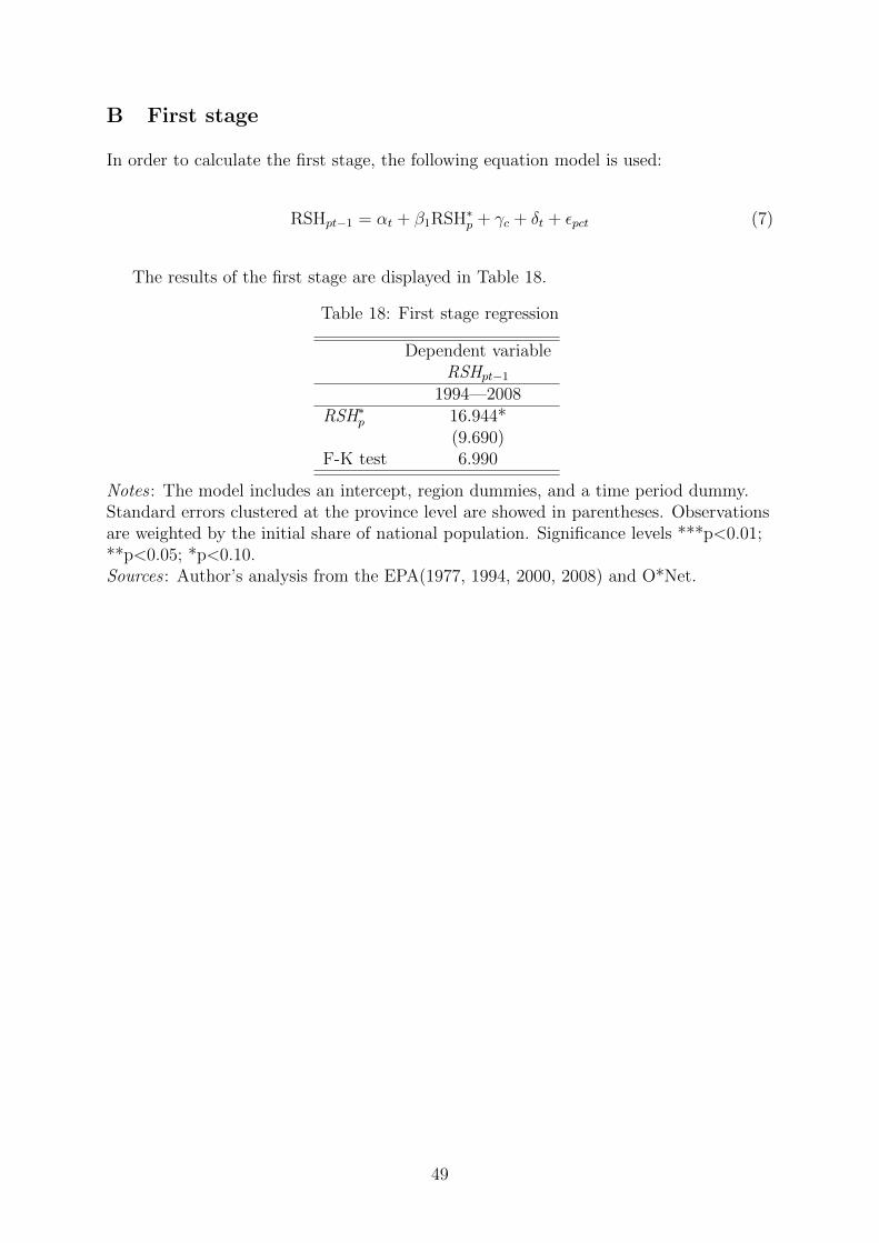
B First stage

In order to calculate the first stage, the following equation model is used:

RSHpt−1 = αt + β1RSH∗p + γc + δt + εpct (7)

The results of the first stage are displayed in Table 18.

Table 18: First stage regression

Dependent variableRSHpt−1

1994—2008RSH∗

p 16.944*(9.690)

F-K test 6.990

Notes : The model includes an intercept, region dummies, and a time period dummy.Standard errors clustered at the province level are showed in parentheses. Observationsare weighted by the initial share of national population. Significance levels ***p<0.01;**p<0.05; *p<0.10.Sources : Author’s analysis from the EPA(1977, 1994, 2000, 2008) and O*Net.

49

C Task items

Table 19: Task items among O*Net, EWCS, and PIAAC

Skill sub-type O*Net EWCSAbstract tasks 1) GED match 1) Learning new things

2) Administration and management 2) Solving unforeseen problems

Routine tasks 1) Finger dexterity 1) Physical stenght2)Customer and personal services 2) Repetitive hand or finger movements

3) Painful positions at work

Manual tasks 1)Harm-hand steadiness Does your main job involve:2) Manual dexterity a) dealing with people

b) repetitive tasksc) dealing with customers

Notes : Items selected in O*Net and EWCS.Sources : O*Net and EWCS.

50