jiquan chen university of toledo

Wavelet Analysis

Jiquan Chen University of Toledo

EEES6980/MATH5798, UT

OVERVIEW

• What is wavelet?

– Wavelets are mathematical functions

• What does it do?

– Cut up data into different frequency components , and then study each component with a resolution matched to its scale

• Why it is needed?

– Analyzing discontinuities and sharp spikes of the signal

– Applications as image compression, human vision, radar, and earthquake prediction

by : Tilottama Goswami

5 Dec. 2000 15-859B - Introduction to Scientific

Computing

3

Wavelet History

• 1805 Fourier analysis developed

• 1965 Fast Fourier Transform (FFT) algorithm

…

• 1980’s beginnings of wavelets in physics, vision, speech processing (ad hoc)

• … little theory … why/when do wavelets work?

• 1986 Mallat unified the above work

• 1985 Morlet & Grossman continuous wavelet transform … asking: how can you get perfect reconstruction without redundancy?

Author: Paul Heckbert


Computing

4

• 1985 Meyer tried to prove that no orthogonal wavelet other than Haar exists, found one by trial and error!

• 1987 Mallat developed multiresolution theory, DWT, wavelet construction techniques (but still noncompact)

• 1988 Daubechies added theory: found compact, orthogonal wavelets with arbitrary number of vanishing moments!

• 1990’s: wavelets took off, attracting both theoreticians and engineers


Wavelet History

• Pre-1930 – Joseph Fourier (1807) with his theories of frequency analysis

• The 1930s

– Using scale-varying basis functions; computing the energy of a function

• 1960-1980 – Guido Weiss and Ronald R. Coifman; Grossman and Morlet

• Post-1980 – Stephane Mallat; Y. Meyer; Ingrid Daubechies; wavelet

applications today

Bhushan D Patil, IIT, India

Wavelet History

What existed before this technique?

• Approximation using superposition of functions has existed since the early 1800's

• Joseph Fourier discovered that he could superpose sines and cosines to represent other functions , to approximate choppy signals

• These functions are non-local (and stretch out to infinity)

• Do a very poor job in approximating sharp spikes


What’s wrong with Fourier?

• Solve differential equations.

• Accurately store and transmit data.

• Obtain a different perspective for a signal.

Well what is it used for? To:

What need do wavelets satisfy?

Author Unknown


Very helpful for this signal!


The Fourier Transform (Series) method is used to decompose a signal into its global frequency components. EXAMPLE 1:

Author Unknown


Not quite as helpful here.


The Fourier Transform (Series) method is used to decompose a signal into its global frequency components. EXAMPLE 2:

Author Unknown

What’s wrong with Fourier?.....


ANSWER: 1.) The Fourier Transform is unable to pick out local frequency content.

2.) It has a “hard time” representing functions that are oscillatory.

Author Unknown

The STFT

So how can we get at the local frequency information? Most obvious solution: use a window!

What’s wrong with Fourier?.....

Author Unknown

The STFT (aka WFT, Windowed Fourier Transform)

The STFT

Example of what happens when you window a function, with a given window function g(t-5).

STEP 1: Window the function using g(t – t0)

Author Unknown

STEP 2: Take the Fourier Transform of the resulting signal

Complex

conjugate

The STFT

Author Unknown


STEP 2: Take the Fourier Transform of the resulting signal

Complex conjugate

The STFT

A function of two variables.

Author Unknown


Summary of the STFT

• 1.) To get local frequency information, a window function, g(t), is first chosen.

• 2.) The STFT is taken as follows:

The STFT

3.) The STFT is a function of two variables, time and frequency. It allows one to observe the time-frequency distribution of the energy of a signal.

4.) With each window function, g, is associated both a time and a frequency minimum resolution. Once g is chosen, these resolutions are fixed and are the same at all frequencies and times. These resolutions are related by an uncertainty relation.

Author Unknown

Our first wavelet transform:

The CWT

Note that as alpha increases: the frequency decreases, and the window function expands.

This is just here for weighting.

Author Unknown

Our first wavelet transform

The CWT

Time shift now also in exponential. Can write:

Author Unknown

Our first wavelet transform:

The CWT

This is an inner product:

The basis is called a “wavelet” basis and consists of all the translated and dilated versions of the “mother” wavelet.

The mother Morlet

wavelet.

Two other Morlet

wavelets

Author Unknown

The General CWT:

The CWT

Can use any mother wavelet, h(t), you want. Some typical examples:

Pic from wikipedia.org

Author Unknown

The General CWT:

The CWT


The task of determining which wavelet basis to use for a given application or signal is tough. One should consult with the Adapted Wavelet literature on this.

WHICH

ONE?!

Author Unknown


Computing

21

What Are Wavelets?

In general, a family of representations using:

• hierarchical (nested) basis functions

• finite (“compact”) support

• basis functions often orthogonal

• fast transforms, often linear-time


• Discrete Wavelet Transform

When your signal is in vector form (or pixel form), the discrete wavelet transform may be applied. The idea of scale becomes slightly more difficult to define here.

Discrete Versions

Author Unknown

Moving on: Discrete Versions



Effectively, the DWT is nothing but a system of filters. There are two filters involved, one is the “wavelet filter”, and the other is the “scaling filter”. The wavelet filter, is a high pass filter, while the scaling filter is a low pass filter.

Scaling Filter ~ Averaging Filter

Wavelet Filter ~ Details Filter


Discrete Versions

Author Unknown


Example calculation: the Haar Wavelet. Observe: 1.) how

the “scale” is

changed 2.) the high

pass is the QMF of

the low pass

(quadrature mirror

filter.)


Discrete Versions

Author Unknown


• Discrete Wavelet Transform For the DWT, it is difficult to construct orthogonal,

continuous filters. Luckily other people have already done it for us. Ingrid Daubechies developed many such sets.


Discrete Versions

Author Unknown


PRINCIPLES OF WAELET TRANSFORM

• Split Up the Signal into a Bunch of Signals

• Representing the Same Signal, but all Corresponding to Different Frequency Bands

• Only Providing What Frequency Bands Exists at What Time Intervals


Fourier Transforms

• Fourier transform have single set of basis functions

– Sines

– Cosines

• Time-frequency tiles

• Coverage of the time-frequency plane


Wavelet Transforms

• Wavelet transforms have a infinite set of basis functions

• Daubechies wavelet basis functions

• Time-frequency tiles

• Coverage of the time-frequency plane


Some Applications

WAVELAB

“Most of the basic wavelet theory has been done… The future of wavelets lies in the as-yet uncharted territory of applications.” – Amara Graps, 1995

Available at:

http://www.stat.stanford.edu/~wavelab/

Created by David Donoho et. al. (including Ofer Levi)

Pic from wavelab site Applications

Author Unknown

http://www.stat.stanford.edu/~wavelab/

From www.eetimes.com

Thresholding for file size reduction.

(Pioneered by David Donoho)

Applications

Author Unknown

Some Applications

From D. Donoho via Amara Graps

Wavelet Introduction

Thresholding for noise reduction.

(Pioneered by David Donoho)

Applications

Author Unknown

Some Applications

Image Enhancement.

From: “Wavelet-based image enhancement in

x-ray imaging and tomography”, by Bronnikov

and Duifhuis

Applications

Author Unknown

Some Applications

How do wavelets look like?

• Trade-off between how compactly the basis functions are localized in space and how smooth they are.

• Classified by number of vanishing moments

• Filter or Coefficients

– smoothing filter (like a moving average)

– data's detail information


DEFINITION OF CONTINUOUS WAVELET TRANSFORM

• Wavelet – Small wave

– Means the window function is of finite length

• Mother Wavelet – A prototype for generating the other window functions

– All the used windows are its dilated or compressed and shifted versions

dts

ttx

sss xx

*1 , ,CWT

Translati

on (The location of

the window)

Scale

Mother Wavelet


SCALE

• Scale

– S>1: dilate the signal

– S<1: compress the signal

• Low Frequency -> High Scale -> Non-detailed Global View of Signal -> Span Entire Signal

• High Frequency -> Low Scale -> Detailed View Last in Short Time

• Only Limited Interval of Scales is Necessary


COMPUTATION OF CWT

dts

ttx

sss xx

*1 , ,CWT

Step 1: The wavelet is placed at the beginning of the signal, and set s=1 (the most compressed wavelet); Step 2: The wavelet function at scale “1” is multiplied by the signal, and integrated over all times; then multiplied by ; Step 3: Shift the wavelet to t= , and get the transform value at t= and s=1; Step 4: Repeat the procedure until the wavelet reaches the end of the signal; Step 5: Scale s is increased by a sufficiently small value, the above procedure is repeated for all s; Step 6: Each computation for a given s fills the single row of the time-scale plane; Step 7: CWT is obtained if all s are calculated.


DISCRETIZATION OF CWT

• It is Necessary to Sample the Time-Frequency (scale) Plane. • At High Scale s (Lower Frequency f ), the Sampling Rate N can be Decreased. • The Scale Parameter s is Normally Discretized on a Logarithmic Grid. • The most Common Value is 2. • The Discretized CWT is not a True Discrete Transform • Discrete Wavelet Transform (DWT)

– Provides sufficient information both for analysis and synthesis – Reduce the computation time sufficiently – Easier to implement – Analyze the signal at different frequency bands with different resolutions – Decompose the signal into a coarse approximation and detail information


RECONSTRUCTION

• What – How those components can be assembled back into

the original signal without loss of information? – A Process After decomposition or analysis. – Also called synthesis

• How – Reconstruct the signal from the wavelet coefficients – Where wavelet analysis involves filtering and down

sampling, the wavelet reconstruction process consists of up sampling and filtering


Small-Block Pine Pine-Oak-Aspen Forest

Large-Block Pine Oak Pine Barrens

Landscape Level (Four Landscapes)

Do differences among landscape-level disturbance regimes influence patterns of understory plant diversity or composition?

Length: 3000+ m n=600+ plots Plot size: 1x1 m

Transect Measurements

•percent cover by species

•canopy cover (%)

•litter cover (%)

•litter depth (cm)

•cwd (%)

•duff depth (cm)

•species, dbh, % cover overstory trees

•patch type

Select Species Distributions

OP

B

OPB BOPB OPB PA SPB CC YA2 H2

H1 JPO SPB

MA

YA

1

0 5

0 100

0

1

0 20

0

15 3

0

0 40 80

0 3

6

0

1

2

1000 0 2000 3000

Pe

rce

nt C

ove

r

Distance (m)

Pteridium aquilinum Amelanchier arborea Hieracium aurantiacum Conyza canadensis Trientalis borealis Trifolium pratense

Cumulative Species Richness

0

40

80

120

160

0 1000 2000 3000

RR

P

MP

TRP60 RJP RP12

OC

C

RP

7

RP

7

OC

C

OC

C

TRP60

C C

0

40

80

120

160

MA

BO

PB

OPB

PA

SPB CC YA2

H2

H1

JPO SPB

OP

B

YA

2

OC

C

OC

C

OBCC OCC H H H F F2

JP

O

RP5 MP

NC

C

PO

A

RP

15

OR

P15

0 1000 2000 3000

H2

MP

F2

H H H H H F2

F H2

C

RP

60

Distance (m)

Nu

mb

er

of

Sp

ec

ies

Pine Barrens Large-Block PO

Small-Block Pine POA Forest

Old

Harvest

Landing

Sand Road-

Mod. Use

Sand Road-

Light Use

Clearing

Access Road

ATV Trail

Dry

Streambed

Grassy

Roadside

Brosofske et al. 2006

Wavelet Analysis of Shannon Diversity (H’) 1500

Old Harvest

Landing

Sand Road-

Mod. Use

Sand Road-

Light Use

Clearing

Access Road

0

1000

500

Re

so

luti

on

(m

)

OPB BOPB OPB PA SPB CC YA2 H2

H1 JPO SPB

OP

B M

A

YA

2

1000 0 2000 3000 Distance (m)

H’

0

1.0

2.0

1000

1500

500

0

0 0.6 1.2

W. Var.

Sca

le

W E

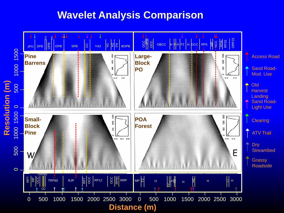
Wavelet Analysis Comparison

1000 500 0 1500 2000 2500 3000

BOPB OPB PA

SPB CC

YA2 H2

H1

JPO SPB O

PB

M

A

YA

2

OC

C

OC

C

OBCC OCC H H H F F2 JP

O

RP5 MP

NC

C

PO

A

RP

15

OR

P1

5

1000 500 0 1500 2000 2500 3000

0

500

1000

1500

0

500

1000

1500

Re

so

luti

on

(m

)

Distance (m)

Pine

Barrens

POA

Forest

Small-

Block

Pine

Large-

Block

PO

MP F2

H H H H H

F2 H

2

F H2

C TRP60 RJP RP12 RRP

OC

C

RP

7

RP

7

RP

60

OC

C

MP

OC

C TRP60

C C

W E

Old

Harvest

Landing

Sand Road-

Mod. Use

Sand Road-

Light Use

Clearing

Access Road

ATV Trail

Dry

Streambed

Grassy

Roadside

Cross-Correlations Between Wavelet Transform Values

Pine Barrens Large-Block Pine-Oak

Small-Block Pine Pine-Oak-Aspen Forest

COARSE

WOODY

DEBRIS

OV

ER

AL

L S

PE

CIE

S

RIC

HN

ES

S

EX

OT

IC S

PE

CIE

S

RIC

HN

ES

S

CANOPY

COVER

DUFF

DEPTH

SLOPE

STEEPNESS

DISTANCE-TO-

NEAREST-EDGE

-1

-0.8

-0.6

-0.4

-0.2

0

0.2

0.4

0.6

0.8

1

Corr

ela

tion

0 250 500 750 1000Scale (m)

-1

-0.8

-0.6

-0.4

-0.2

0

0.2

0.4

0.6

0.8

1

Corr

ela

tion

0 250 500 750 1000Scale (m)

-1

-0.8

-0.6

-0.4

-0.2

0

0.2

0.4

0.6

0.8

1

Corr

ela

tion

0 250 500 750 1000Scale (m)

-1

-0.8

-0.6

-0.4

-0.2

0

0.2

0.4

0.6

0.8

1

Corr

ela

tion

0 250 500 750 1000Scale (m)

-1

-0.8

-0.6

-0.4

-0.2

0

0.2

0.4

0.6

0.8

1

Corr

ela

tion

0 250 500 750 1000Scale (m)

-1

-0.8

-0.6

-0.4

-0.2

0

0.2

0.4

0.6

0.8

1

Corr

ela

tion

0 250 500 750 1000Scale (m)

-1

-0.8

-0.6

-0.4

-0.2

0

0.2

0.4

0.6

0.8

1

Corr

ela

tion

0 250 500 750 1000Scale (m)

-1

-0.8

-0.6

-0.4

-0.2

0

0.2

0.4

0.6

0.8

1

Corr

ela

tion

0 250 500 750 1000Scale (m)

-1

-0.8

-0.6

-0.4

-0.2

0

0.2

0.4

0.6

0.8

1

Corr

ela

tion

0 250 500 750 1000Scale (m)

-1

-0.8

-0.6

-0.4

-0.2

0

0.2

0.4

0.6

0.8

1

Corr

ela

tion

0 250 500 750 1000Scale (m)

Exercise with R and Matlab

Data1=xlsread(‘H:/fc_data.xls’);

Load (“x.dat’);

Ts=Data1(:,6);

Save Ts;

Fc=Data1(:,7);

Save Fc;

Re=Data1(:,8);

Save Re;

GPP=data1(:,9);

Save GPP;

Help wcoher

Wcoher (Fc, Ts, 1:4, ‘Haar’, ‘plot’, ‘all’);

Subplot ()

Diary()

Wavemenu

Wavedemo

Help wavelet

Qs:

• Wavelet variance? • Exporting data and individual

figures? • Cross-wavelets, >3? • 2-D, 3-D wavelet? • Different families? • …

Questions?

http://research.eeescience.utoledo.edu/lees/

jiquan chen university of toledo

Documents