Lossless Bayesian inference in infinite dimensionwithout discretisation or truncation: a case study on

Λ-coalescents

Jere KoskelaJoint work with Paul A. Jenkins and Dario Spano

International conference on Monte Carlo techniques5-8 July 2016, Paris

Outline

Exposition: Likelihood-informed subspaces

The finite alleles Λ-coalescent

Projection onto moments

Consistency

Sampling posterior moments

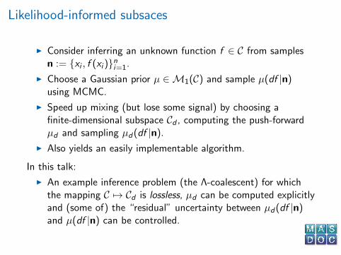
Likelihood-informed subsaces

I Consider inferring an unknown function f ∈ C from samplesn := {xi , f (xi )}ni=1.

I Choose a Gaussian prior µ ∈M1(C) and sample µ(df |n)using MCMC.

I Speed up mixing (but lose some signal) by choosing afinite-dimensional subspace Cd , computing the push-forwardµd and sampling µd(df |n).

I Also yields an easily implementable algorithm.

In this talk:

I An example inference problem (the Λ-coalescent) for whichthe mapping C 7→ Cd is lossless, µd can be computed explicitlyand (some of) the “residual” uncertainty between µd(df |n)and µ(df |n) can be controlled.

The finite alleles Λ-coalescent

● ● ●

●

●

●

●

I In reverse time, each k ≤ n lineagesmerges at rate

λn,k :=

∫[0,1]

rk−2(1− r)n−kΛ(dr).

I Each lineage mutates with rate θ.

I Sample type of most recent commonancestor.

I Mutations resolved forwards in timethrough stochastic matrix M.

The inference problem

● ● ●

●

●

●

●

I Data: a vector of observed typefrequencies n ∈ Nd .

I Missing data: the ancestral tree andmutation events.

I The likelihood

PΛ,θ,M(n) =

∫A1{n}(A0)PΛ,θ,M(dA)

has no known closed form expression.

I (Relatively) efficient importancesampling algorithms are available forpointwise evaluation.

I Standing assumption: M and θ areknown.

Proposition 1

Let genetic labels be identified with {1, . . . , d} and letn = (n1, . . . , nd) denote the observed type frequencies. Thelikelihood PΛ(n) is constant across any measures Λ which share thefirst n − 2 moments.

Proof. The likelihood solves

PΛ(n) =θ

nθ − qnn

d∑i ,j=1

(nj − 1 + δij)MjiPΛ(n− ei + ej)

+1

nθ − qnn

∑i :ni≥2

ni∑k=2

(n

k

)λn,k

ni − k + 1

n − k + 1PΛ(n− (k − 1)ei ).

with boundary condition PΛ(ei ) = m(i), where m is the uniqueM-invariant distribution on {1, . . . , d}.

Parametrisation

I Let ∼n denote the equivalence relation on Λ’s of agreement offirst n − 2 moments.

I Let µ ∈M1(M1([0, 1])) denote a prior. Proposition 1 impliesµ(dΛ| ∼n) = µ(dΛ)|∼n .

I This suggests parametrising an inference problem with nobservations with n − 2 moments.

I Procedure can be interpreted as analytically integrating“∞− (n − 2)” dimensions, and leaving n − 2 to sample(Rao-Blackwellisation)...

I ...provided a suitable prior can be found.

The Dirichlet process mixture model

I {zi}∞i=1i.i.d∼ H.

I {β′i}∞i=1i.i.d∼ Beta(1, α).

I βi :=∏i−1

j=1(1− β′j)β′j .

I {σi}∞i=1i.i.d∼ F .

I Λ(r) =∑∞

i=1 βiφ(σ−1i (r − zi )), where φ is the standard

Gaussian density conditioned on [η, 1] for any η > 0.

I Easy (and exponentially accurate) to truncate, or...

Moments of the Dirichlet process mixture model

Let C0, . . . ,Cn ∈ Rn+1 solve

Cn = −1,

n−r−1∑k=0

(n − r

k

)Cr+k = 1 for r ∈ {0, . . . , n − 1}.

Then

(−1)n+12nFn(σ, gn, α) = C0 +n∑

k=1

Ck

(πi)k×

×∑

1≤j1<...<jk≤n

∫ ∞0

. . .

∫ ∞0

hk(sk ; gj1 − σj1 , . . . , gjk − σjk ;α)

s1 × · · · × skdsk ,

where hk is the characteristic function of a γα-random measureand Fn is the joint distribution of n moments µ(g1), . . . , µ(gn).

Proposition 2

If the observed allele frequencies come from a bounded number oftime points, then the posterior is always inconsistent.

0.0 0.2 0.4 0.6 0.8 1.0

0.0

0.5

1.0

1.5

2.0

2.5

3.0

3.5

Theta = 0.1

x

Den

sity

0.0 0.2 0.4 0.6 0.8 1.0

0.0

0.5

1.0

1.5

2.0

2.5

3.0

3.5

0.0 0.2 0.4 0.6 0.8 1.0

0.0

0.5

1.0

1.5

2.0

2.5

3.0

3.5

0.0 0.2 0.4 0.6 0.8 1.0

0.0

0.5

1.0

1.5

2.0

2.5

3.0

3.5

0.0 0.2 0.4 0.6 0.8 1.0

0.0

0.5

1.0

1.5

2.0

2.5

3.0

3.5

Theta = 10

x

Den

sity

0.0 0.2 0.4 0.6 0.8 1.0

0.0

0.5

1.0

1.5

2.0

2.5

3.0

3.5

0.0 0.2 0.4 0.6 0.8 1.0

0.0

0.5

1.0

1.5

2.0

2.5

3.0

3.5

0.0 0.2 0.4 0.6 0.8 1.0

0.0

0.5

1.0

1.5

2.0

2.5

3.0

3.5

Figure 1 : µ = 12 (δδ0 + δδ1 ). Two types. Single-time sampling

distributions of the limn→∞ type fractions in blue and green,corresponding posterior probabilities in black and red. At θ = 1everything is uniform.

Proposition 3

Let ∆ > 0 be a fixed sampling interval, and let n := (n1, . . . ,nk)

denote samples of size n sampled at times {∆j}k−1j=0 . Suppose the

prior µ places full mass on a Dη, set of strictly positive, boundeddensities on [η, 1] for some η > 0, and for any ε > 0 and φ0 ∈ Dηsuppose that

µ

(φ ∈ Dη :

∫ 1

η

{∣∣∣ log(φ0(r)

φ(r)

) ∣∣∣+ ∣∣∣φ0(r)

φ(r)− 1∣∣∣} r−2φ0(r)dr < ε

)> 0.

Then the posterior is consistent as both n and k →∞.

Consistency of a finite number of moments follows immediatelysince φ 7→

∫ 1η r jφ(r)dr is continuous and bounded.

Pseudo-marginal MCMC

Algorithm 1 The pseudo-marginal algorithm

Require: Prior P(x), unbiased likelihood estimator L(x), transitionkernel q(x , y), and run length n.

1: Initialise X0 = x and L0 = L(x).2: for i = 1, . . . , n do3: Sample y ∼ q(x , ·) and L = L(y).

4: Set a = 1 ∧ q(y ,x)LP(y)q(x ,y)Li−1P(x) and sample u ∼ U(0, 1).

5: if u < a then6: Set Xi = y and Li = L.7: else8: Set Xi = Xi−1 and Li = Li−1.9: end if

10: end for11: return X

Algorithm 2 The noisy pseudo-marginal algorithm

Require: Prior P(x), unbiased likelihood estimator L(x), transitionkernel q(x , y), and run length n.

1: Initialise X0 = x and L0 = L(x).2: for i = 1, . . . , n do3: Sample y ∼ q(x , ·) and L = L(y).4: Sample L′ = L(x).

5: Set a = 1 ∧ q(y ,x)LP(y)q(x ,y)L′P(x) and sample u ∼ U(0, 1).

6: if u < a then7: Set Xi = y and Li = L.8: else9: Set Xi = Xi−1 and Li = L′.

10: end if11: end for12: return X

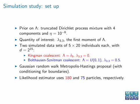
Simulation study: set up

I Prior on Λ: truncated Dirichlet process mixture with 4components and η = 10−6.

I Quantity of interest: λ3,3, the first moment of Λ.I Two simulated data sets of 5× 20 individuals each, with

d = 215:I Kingman coalescent: Λ = δ0, λ3,3 = 0.I Bolthausen-Sznitman coalescent: Λ = U(0, 1), λ3,3 = 0.5.

I Gaussian random walk Metropolis-Hastings proposal (withconditioning for boundaries).

I Likelihood estimator uses 180 and 75 particles, respectively.

Simulation study: short runs

0 5000 10000 15000 20000

0.0

0.2

0.4

0.6

0.8

1.0

Exact

Kingman (dotted), 5.2 days, acc. pr. = 8% Bolthausen−Sznitman (solid), 1.9 days, acc. pr. = 9%

1st M

omen

t

0 5000 10000 15000 20000

0.0

0.2

0.4

0.6

0.8

1.0

0 5000 10000 15000 20000

0.0

0.2

0.4

0.6

0.8

1.0

Noisy

Kingman (dotted), 9.3 days, acc. pr. = 35% Bolthausen−Sznitman (solid), 3.1 days, acc. pr. = 49%

1st M

omen

t

0 5000 10000 15000 20000

0.0

0.2

0.4

0.6

0.8

1.0

0 5000 10000 15000 20000

0.0

0.2

0.4

0.6

0.8

1.0

Exact Delayed Acceptance

Kingman (dotted), 1.1 days, acc. pr. = 14%, 35% (overall 5%) Bolthausen−Sznitman (solid), 0.8 days, acc. pr. = 27%, 24% (overall 6%)

1st M

omen

t

0 5000 10000 15000 20000

0.0

0.2

0.4

0.6

0.8

1.0

0 5000 10000 15000 20000

0.0

0.2

0.4

0.6

0.8

1.0

Noisy Delayed Acceptance

Kingman (dotted), 1.5 days, acc. pr. = 11%, 67% (overall 7%) Bolthausen−Sznitman (solid), 0.9 days, acc. pr. = 13%, 54% (overall 7%)

1st M

omen

t

0 5000 10000 15000 20000

0.0

0.2

0.4

0.6

0.8

1.0

Simulation study: long runs

0 50000 100000 150000 200000

0.0

0.2

0.4

0.6

0.8

1.0

Exact Delayed Acceptance

Kingman (dotted), 11.7 days, acc. pr. = 16%, 27% (overall 4%) Bolthausen−Sznitman (solid), 6.2 days, acc. pr. = 17%, 21% (overall 4%)

1st M

omen

t

0 50000 100000 150000 200000

0.0

0.2

0.4

0.6

0.8

1.0

Prior and posterior densities

1st MomentD

ensi

ty

0.0 0.2 0.4 0.6 0.8 1.0

0.0

0.5

1.0

1.5

2.0

2.5

3.0

3.5