jenks_algoritimos geneticos.pdf

Using Genetic Algorithms to Create MulticriteriaClass Intervals for Choropleth Maps

Marc P. Armstrong*,**, Ningchuan Xiao*, and David A. Bennett*

*Department of Geography, The University of Iowa**Program in Applied Mathematical and Computational Sciences, The University of Iowa

During the past three decades a large body of research has investigated the problem of specifying class intervals forchoropleth maps. This work, however, has focused almost exclusively on placing observations in quasi-continuousdata distributions into ordinal bins along the number line. All enumeration units that fall into each bin are thenassigned an areal symbol that is used to create the choropleth map. The geographical characteristics of the data areonly indirectly considered by such approaches to classification. In this article, we design, implement, and evaluate anew approach to classification that places class-interval selection into amulticriteria framework. In this framework,we consider not only number–line relationships, but also the area covered by each class, the fragmentation of theresulting classifications, and the degree towhich they are spatially autocorrelated.This task is accomplished throughthe use of a genetic algorithm that creates optimal classifications with respect to multiple criteria. These results canbe evaluated and a selection of one or more classifications can be made based on the goals of the cartographer. Aninteractive software tool to support classification decisions is also designed anddescribed.KeyWords: choropleth, classintervals, genetic algorithms.

Even a casual observer would recognize that arevolution in access to mapping technologies andgeographic information has taken place during the

past decade. Inexpensive microcomputers and softwareare now routinely used with Internet-available dataresources to offer map production capabilities that, inthe past, were the exclusive provenance of nationalgovernments (Buisseret 1992; Kain and Baigent 1992)and, more recently, were available only to large govern-ment agencies, map-production companies, and a fewadvanced research laboratories. These changes, hinted atin Monmonier’s (1985) examination of the effects oftechnology on cartography, have engendered new waysof thinking about maps. One particularly importantchange has been a transition toward end-user manipula-tion of digital spatial data (Morrison 1993) and fromsupply-driven to demand-driven cartography (Kraak1998). Users of route-planning Websites, for example,often change map scale either because they need greaterdetail around their destination (such as residential streetnames) or because they would like to place their currentmap in a broader geographical context. The consequenceof these changes has been to enlarge enormously the poolof people who make maps.

This shift toward cartographic catholicity can beexamined using a conceptual model of map use (Figure 1)that MacEachren and others have developed (see, forexample, MacEachren and Kraak 2001, 5). The modelhas three axes: level of interaction (low-high), map audi-

ence (public-private), and data relationships (known-unknown). For example, if a map were prepared for apublic audience to show a known set of data relationships,the level of interaction might be low. On the other hand,for private uses, and especially when data have unknownrelationships, the expected amount of interaction re-quired to support data exploration is considerably greater.Monmonier, however, has repeatedly argued that carto-graphers should not continue to insist that there is a singlemap to present (this is a major premise of How to Liewith Maps [1996]; see also Egbert and Slocum 1992;Monmonier 1992; MacEachren 1995). One interpreta-tion of this position is that even in the presentational(public, known, low-interaction) parts of the conceptualspace shown in Figure 1, additional support for userinteraction—or at leastmapped alternatives—would helpmap-readers gain additional information about the geog-raphical phenomena of interest to them.

Though technology is now able to support increasedlevels of user interaction—especially given the currentproliferation ofWeb-basedmap servers (Kraak and Brown2001)—problems remain with implementation in therealm of statistical cartography. Choropleth maps areperhaps the most commonly created type of statisticalmap, even though it has long been recognized that theyhave significant liabilities when used to communicategeographically distributed information (Raisz 1948, 249).Nevertheless, choropleth maps are widely used inexploratory spatial-data analysis (see Andrienko and

Annals of the Association of American Geographers, 93(3), 2003, pp. 595–623r 2003 by Association of American GeographersPublished by Blackwell Publishing, 350 Main Street, Malden, MA 02148, and 9600 Garsington Road, Oxford OX4 2DQ, U.K.

Andrienko 1999; Anselin 1999), because most socio-economic statistical information is tabulated for prede-fined jurisdictions. Choropleth maps also serve as thecornerstone of Internet-based statistical map services andare produced prodigiously using the current generation ofGIS software. TheU.S. Bureau of theCensus, for example,has a Web browser interface that allows users to createthematic maps of statistical information collected as partof the decennial census. However, a map-reader’s abilityto understand a choropleth map is shaped by severalinteracting factors, such as the shading scheme, thenumber of classes, and classificationmethod used (or not)to generalize the data. Each of these factors can bemanipulated to yield large collections of maps createdfrom the same statistical information.

Classification, by itself, has been the focus of aconsiderable amount of cartographic research. Most ofthis work has examined classification on the basis of thetabular statistical properties of the data. In stark contrast,only a few studies have considered the geographicalcharacteristics of data distributions during the classifica-tion process. These geographical considerations wouldinclude, for example, attempts to place contiguous unitsinto a single class to promote the visual assessment ofhomogenous regions. The purpose of this article is todevelop a general approach that can be used to helpcartographers bridge the existing gap between the tabularand geographical dimensions of choropleth class-intervalselection and to elucidate the wide range of classificationoptions that are open to them. Our approach, derivedfrom the field of evolutionary computation, uses a gene-tic algorithm to create a distribution of solutions thatsatisfy alternative classification criteria. The spirit of thisapproach derives from work in interactive scientificvisualization and spatial decision support systems andis consistent with the view that there is no single ‘‘true’’

map. Instead, when media allow it, the cartographer ispresented with classification alternatives based not onlyon conventional manipulations of tabular statistical data,but also on less frequently performedmanipulations of thegeographical relationships that exist among enumerationunits. This enlarged set of geographically based optionsallows cartographers to select classification optionsfrom those that best meet their statistical and geograph-ical criteria.

Following a review of previous research on class-interval selection, we reestablish that it is a multicriteriadecision problem, integrate concepts from spatial statisticsinto the class-interval selection process, and discuss how agenetic algorithm can be used to help cartographersremain involved in shaping the geographical and sta-tistical characteristics of the map. We describe how ourgenetic algorithm was designed and implementedand demonstrate its effectiveness, first by applying thealgorithm to six synthetic gridded datasets that weredeveloped to illustrate the conceptual basis of ourapproach and then by using three geographical datasetsmeant to reflect a range of conditions typically en-countered in geographic research and education. Weconclude with a summary of results, a discussion aboutthe role of evolutionary algorithms in classification, somecomments on strategies for enhancing performance, andsome suggestions about how our approach could beextended to include other criteria not explicitly consid-ered in this article.

Background and Problem Elaboration

Classification matters. It serves as a filter throughwhich we attempt to make sense of a complex world.Though Bowker and Star (1999) focus on categorical(nominal) data, the power of their argument about howclassification privileges some things and renders othersinvisible is easily sustained in cartographic contexts. Inparticular, it is well known that the way in which data aretransformed from interval/ratio scaled tabular observa-tions to ordinally based areal symbols can enhance orattenuate the communication of specific types of sta-tistical information on choropleth maps (Cuff andMattson 1982, 37–39; Robinson et al. 1995, 516–19;Dent 1999, 139–56; Slocum1999, 60–82). Consequently,class-interval selection is arguably the most importantproblem faced by cartographers when they contemplatethe construction of a choropleth map ( Jenks and Caspall1971, 220). Though considerable discussion has occurredabout the methods and merits of classification in thecartographic literature (e.g., Jenks and Coulson 1963;

synthesize

interaction

datarelations

audi

ence

private

public

unknown

known

high low

present

analyze

explore

Figure 1. Three dimensions of map use. Source: After MacEachrenand Kraak (2001).

Armstrong, Xiao, and Bennett596

Peterson 1979; MacEachren 1982), many of the resultsreported in the literature, unfortunately, are eithercontradictory or difficult to compare directly. Tobler(1973) has argued persuasively that classification isunnecessary, and, depending on the purpose of the map,there is evidence that his view can be substantiated(Muller 1979).However,many cartographers feel that theunclassed approach Tobler advocates leads to cognitiveconfusion (Dobson 1973, 1980). They assert that dataclassification reduces map-processing times (Gilmartinand Shelton 1989) and increases accuracy of datarecovery across a variety of map-reading tasks (Mersey1990). Moreover, it is certainly true that almost alldesktop mapping and GIS software supports the crea-tion of choropleth maps with classed data. Con-sequently, classification remains a viable topic forfurther investigation.

Textbook approaches to choropleth class-intervalselection focus almost exclusively on the statisticalproperties of tabular thematic information (Table 1) andeffectively divorce the statistical distribution from itsgeographic context. In practice, choroplethic classifica-tion pedagogy has encouraged students and practitionersto use, among other approaches, ‘‘round numbers,’’exogenously determined values as breakpoints (e.g., zero,if relevant, or poverty level on an incomemap), or to selectfrom among equal intervals, quantiles, natural breaks,mathematical progressions, limits derived from measuresof central tendency and dispersion, and, more recently,‘‘optimal’’ approaches. Though Jenks and Caspall (1971,225) single out the nested-means method advocated byArmstrong (1969) as the most extreme of the statisticallyoriented approaches, their optimal method stands, in fact,as the exemplar of statistical approaches. The objective oftheir optimal method, as described in greater detail byJenks (1977), is to develop an ordinal classification, basedentirely on the position of observations along the numberline, in which within-class variance is minimized. Alter-native approaches use absolute deviation from the

mean (Jenks 1977) and median (Lindberg 1990; Slocum1999) to assess the level of within-class variability(Declerq 1995).

This statistically oriented classification orthodoxy hasemerged for several reasons. First, statistical methodsare well developed, emerge from an established body ofknowledge, and—with few exceptions—can be easilyexplained. Second, despite advances in GIS software,methods for handling geographical relationships remaindifficult to implement; this continues to present a practicalbarrier to improvements in class-interval selection. Third,existing map-creation software builds upon the first tworeasons to effectively maintain the status quo: it classifiesdata in the tabular statistical domain and inertiallyreinforces this approach to the exclusion of others,presenting it as a fait accompli. In almost all cases,geographical orderings are only indirectly manifested inthe form of maps that emerge as a consequence ofstatistical manipulations imposed by a specific class-interval selection method. In our view, this tabular biasnot onlymay excessively constrain the search for solutionsto the class-interval selection problem but may also, infact, blinker the views or needs of the cartographer. Thisposition is not ours alone, of course, as we discuss in thenext section. But our placement of the problem in amulticriteria framework enables cartographers to morefully investigate alternative classification objectives thatremain outside of the traditional focus on the statisticalproperties of tabular information.

Reintroducing Choropleth ClassIntervals to Geography

There are a few notable exceptions to the exclusivefocus on the statistical domain in choropleth classifica-tion.MacEachren (1995, 166), in particular, questions thechoropleth classification orthodoxy in the following way:‘‘Why, then, do we ignore space when classifying datafor a choropleth map? Jenks’s statistical classification

Table 1. Coverage of Classification Methods in Five Recently (Post-1990) Published Cartography Textbooks

Textbook Tabular Characteristics Jenks Optimal Geographical Characteristics

Tyner (1992) Yes Yes NoRobinson et al. (1995)a Yes Yes NoKraak and Ormeling (1996) Yes No NoDent (1999) Yes Yes NoSlocum (1999) Yes Yes Yes

Note: Only one author discusses geographically informed approaches, while four of the five texts mention or describe the ‘‘optimal’’ approach.aThe previous edition of this title was published in 1984 and contains a more elaborate discussion of both the ‘‘optimal’’ and ideas related to the consideration of

geographical characteristics: it discusses a geographical quantiles (equalization of area in each class) approach.

Using Genetic Algorithms to Create Multicriteria Class Intervals for Choropleth Maps 597

procedures seem to have (if only coincidentally) takeninto account the principle of basic-level categories. Thenext step in our evolution of quantitative data classifica-tion, then, should be to add space to the equation.’’ Weagree. This view is also supported by research conductedmore than two decades ago by Chang (1978), who foundthat map-readers tended to prefer choropleth maps thathad simpler (more organized, less fragmented) patterns(see also Olson 1975).

As we suggest above, other researchers have notcompletely ignored the idea of using geographical char-acteristics to shape the process of forming classes onchoropleth maps. In particular, early work by Monmonier(1972, 1973) advocated the use of optimization modelsand grouping algorithms to yield class intervals thatexplicitly considered the ‘‘clumping’’ of classes in geo-graphical space. Monmonier’s (1972) grouping approachoccurs in a series of transformative stages and allowsthe user to adjust the relative weighting of variables in thegrouping procedure. It also disallows overlapping classes.Monmonier’s later (1973) optimum-seeking approachdoes not specifically address contiguity, but this constraintcould be added through an appropriate set of datatransformations (see Armstrong et al. 1991 and Lolonisand Armstrong 1993 for examples). Evans (1977, 103),however, suggests that Monmonier’s results ‘‘give verylittle improvement in contiguity, at the expense ofconsiderable declines in intra-class homogeneity.’’ MakandCoulson (1991, 110) go so far as to suggest that theuseof an optimal classification in the tabular domain will, ineffect, take care of the geographical domain. Coulson(1987, 25) articulates this argument even more forcefullywhen he suggests that ‘‘class intervals generated by theJenks Optimal Method have the incidental effect ofresolving concerns about spatial contiguity. When withinclass variance is minimized, spatially adjacent units withsimilar data values are almost certain to fall in the sameclass. If they do not, then they are probably not ‘thatsimilar.’ ’’ This position, of course, is valid only if the dataare highly (positively) spatially autocorrelated.

Despite such skepticism, however,MacDougall (1992),Cromley (1996), Cromley and Mrozinski (1999), andMurray and Shyy (2000) have picked up the cold trail ofgeographical arrangement and describe approaches inwhich contiguity is used as a factor to determine classbreaks on choropleth maps. Cromley (1996) suggests away to optimize Jenks and Caspall’s (1971) notion ofboundary error, while Cromley and Mrozinski (1999)focus on maps created from ordinal data. Such datapresent a classification problem, since they lack atheoretically based statistical distribution, and, as aconsequence, methods based on commonly accepted

statistical assumptions cannot be legitimately applied.However,most datamapped using the choroplethmethodare not ordinal in their original form. Murray and Shyy(2000) examine the choropleth class-interval selectionproblem and place it into the context of spatial datamining. In their approach, clustering methods are used totease out relationships from large amounts of data forwhich no relationships are posited a priori. Though theirapproach is interesting and related, in spirit, to the oneadvanced in this article, it has three main limitations: (1)Euclidean distance between polygon centroids is used, forthe sake of convenience, as ameasure of proximity, thoughfor areal data contiguity relations are better suited tosupport region-building; (2) the resulting classes overlap,which is inappropriate for choropleth maps ( Jenks andCoulson 1963, 120); and (3) they make an underlying,implicit assumption that the solution space has knowncharacteristics (e.g., that it is convex), so that linearprogramming methods can be employed.

In summary, our approach is inspired by the originalwork of Jenks and Caspall (1971), extends notions aboutthe role of contiguity described by Monmonier (1972),handles ordinal-, interval-, and ratio-scale data distribu-tions (Cromley and Mrozinski 1999) and is exploratory inthe vein of theworkofMurray andShyy (2000).Aswewilldemonstrate below, our approach also explicitly considerscontiguity, does not yield overlapping classes, and makesno assumptions about the form of the solution space.

Choropleth Class Interval Selectionas a Multicriteria Problem

Cromley (1996) compared several classification meth-ods (in addition to boundary error, mentioned above) andwas the first to suggest that the choropleth classificationproblem could be specified explicitly as a multicriteriaproblem. Subsequently, Slocum (1999) has documentedthe challenges that cartographers face when they mustcreate categories for choropleth maps. He devotes anentire chapter to a discussion of various approaches toclassification and suggests that the choice of a classifica-tion method should be made on the basis of severalcriteria. Though these criteria fall into the tabularstatistical domain, the last section of his work reintroducesthe often-ignored work on geographical criteria initiatedby Jenks and Caspall. It is interesting to note, how-ever, that while Slocum (1999) covers the concepts,he provides only a sketchy discussion about how tomake them operational. This is understandable, since thesupporting research on which his and other textbooks arerightly based is inadequately developed.


To facilitate further discussion about multiple factorsand classification criteria, the following set of defini-tions are used throughout the remainder of this article.A cluster is defined as a set of contiguous units that areassigned to the same class (i.e., polygons or grid cells,depending on the representation used by the map). Theother definitional nomenclature used is as follows:

8 � 85 an operator that gives the number of elementsin a set or arraya5 a chain that contains a pair of left and right units, (r, l)ai5 the area of the i-th observationAi5 total area of class i for two classes i and j; if i4j,then AjZAi

Aij5 the area of polygon i in class jA5 total area of all classesC5 a set consisting of all pairs of contiguous clustersG5 an array of all possible chains with the sequence ofits elements sorted so that for any two chains i and i11,we have zir � zil

�� ziþ1r � ziþ1

l

��

H5 a set consisting of all chains where, for eachchain, the left and right units are not in the sameclassk5 number of classesM5 number of clustersN5 number of observationsNj5 number of observations within class j, 1rjrkxi5mean value of the observations within cluster i,1rirM�xx5mean values of all clusterszi5 i-th observationzij5 i-th observation in class j, 1rjrk�zzj 5mean of class j, 1rjrk�zz5mean of all observationszra5 observation to the right of chain azla5 observation to the left of chain aFigure 2 illustrates these terms, showing values for five

polygons placed into two classes, one of which forms twodiscontiguous clusters.

Polygon Class Cluster Label ID Observation

(Zi) Area(ai)

Index Area(Ai)

Value (Zij)

Index Area(Ai)

Value (xi)

A 1 0.55 12 1 40 0.43 1 27 0.625B 2 0.70 15 1 - - 1 - - C 3 1.80 25 2 46 2.15 2 46 2.15D 4 2.50 21 2 - - 2 - - E 5 0.05 13 1 - - 3 13 0.05

1.12 86 86 86

a = (1,2), (1,3), (2,3), (3,4), (3,5), or (4,5)

ia = 12, 15, 25, 21, or 13

iA = 40, or 46

A = 86C = {(1,2), (2,3)}

C = 2

G = {(4,5), (3,4), (3,5), (1,3), (2,3), (1,2)}

G = 6

H = {(1,3), (2,3), (3,5), (4,5)}

H = 4

k = 2 m = 3

N = 5

jN = N1= 3, N2=2

ix = x1= 0.625, x2 = 2.15, x3 = 0.05

x = 0.94

iz = (see the above table)

ijz = (see the above table)

iz = (see the above table)

z = 1.12arz = 0.55 for a = (1,3) alz = 1.8 for a = (1,3)

A

B

CD

E

Figure 2. An example of the variables used in the calculations.


Jenks and Caspall (1971) suggest that there are threepurposes for which a choropleth map can be used: (1) togain an overview of a statistical distribution; (2) to form anareal table from which specific values for areas can bedetermined; and (3) to serve as a way of determiningborders between regions with a common or similarshading. They go on to define three types of errors(described in greater detail below) that fit into thesedomains. In their overview, they (1971, 231) see tabular,overview and boundary errors as ‘‘three opposing forces’’that form a space defined by orthogonal axes. Theyespouse the idea of seeking a compromise among thesefactors, represented as a vector in this 3-D space. Jenksand Caspall (1971), however, acknowledge that thesefactors are not, in fact, orthogonal, but they leaveunresolved the complexity of combining them in anappropriate way.

To make their concept of error on choropleth mapsoperational, Jenks and Caspall (1971) treat each errorindependently and define three measures that can beoptimized. However, they (1971, 232) liken the searchfor an optimal solution in these three resulting dimen-sions to ‘‘searching for a needle in a haystack.’’ The size ofthe metaphorical haystack—in this case, the numberof possible classifications—increases rapidly as a functionof the number of classes and number of units to beclassified. In fact, the class-interval problem, in which Ndata values are grouped into k classes, can yield (N� 1)!/(N� k)!(k� 1)! different groups (see Fisher 1958; JenksandCaspall 1971; Cromley andMrozinski 1999). In termsof asymptotic computational complexity (‘‘Big O’’ nota-tion), brute-force choropleth classification is O(Nk� 1)(for N@ k). However, Fisher (1958) has suggested aclassification algorithm that is a considerably simplerO(N2k) (see Hartigan 1975).

Because of the combinatorial complexity of theproblem, Jenks and Caspall (1971) assert that a completeenumeration of the solution space is infeasible and suggestways to search for good solutions using their three errormeasures. The first measure that can be optimized iscalled the tabular accuracy index (TAI), and they deve-lop a heuristic algorithm to maximize this measure ofwithin-class homogeneity.

TAI ¼ 1�

Pk

j¼1

PNj

i¼1

zij � �zzj��

PN

i¼1

zi � �zzj j: ð1Þ

This general approach is often described as ‘‘Jenksoptimal’’ in the choropleth-mapping literature.

In a later article, Jenks (1977) more explicitly eluci-dates this approach by providing computer code. The TAIhas also been made operational in modified form (see, forexample,Dent 1999, 148) through the use of the goodnessof variance fit (GVF) measure:

GVF ¼ 1�

Pk

j¼1

PNj

i¼1

ðzij � �zzjÞ2

PN

i¼1

ðzi � �zzÞ2: ð2Þ

Though, as shown in Table 1, the TAI approach is widelydocumented in several cartography textbooks (cf. Smith1986, 67), the remaining two measures describedby Jenks and Caspall, overview accuracy index (OAI)and boundary accuracy index (BAI), are not usuallydiscussed. Moreover, they are not optimized as partof a class-interval selection process by any choro-pleth map production software that we were able toidentify. The OAI takes the area of each zone intoconsideration:

OAI ¼ 1�

Pk

j¼1

PNj

i¼1

zij � �zzj�� Aij

PN

i¼1

zi � �zzj jai: ð3Þ

In effect, the OAI is an area-weighted TAI. If all zones areroughly identical in size, it will yield results that are similarto the TAI. This is the case in the Illinois exampledescribed by Jenks and Caspall (1971). Consequently,we did not include this measure in the analyses re-ported below.

Even though OAI controls for area, it fails to con-sider geographical context, in the form of contiguitymaintenance. Jenks and Caspall (1971, 238), there-fore, next turn their attention to the BAI, which con-siders the values of topological neighbors, and state thatthe geographical manipulations needed to optimize itare complex:

Since boundary differences are not related to the intensityvalue being moved but are controlled by the relationship ofthat value to all neighboring intensity values, the problemof identifying the most promising enumeration unit maneu-ver is not readily soluble. Unable to resolve this groupingdilemma by using the reiterative and forcing technique, wehave temporized by attempting touse alternative procedures.(emphasis added)

One approach that Jenks and Caspall suggest asa way to address the BAI problem is based on manualmanipulation of geographical relationships. They discard


this approach, however, because it performed poorly.The alternative choice is to return to the tabular domainand use, once again, grouping methods to yield regionsthat are most similar. This part of the procedure, however,is rather opaque in the original article. Consequently, wewere required to recreate the specific approach used.

In our view, the efforts of Jenks and Caspall werefrustrated by the technological and conceptual inadequa-cies of their times, since computing resources were thenquite limited and knowledge about spatial data struc-tures—especially those that explicitly encode topologicalrelations (Peucker and Chrisman 1975)—was not yetwidely disseminated.Weassume, therefore, that theywerenot (directly) manipulating the topological structure ofthe enumeration units. A decade later, MacEachren(1982) described measures of map complexity that could,in an iterative fashion, be optimized to attack the BAIproblem. MacEachren represented the topological struc-ture of enumeration units as a type of graph: eachpolygonal unit is a face, each shared boundary is an edge,and each node is a vertex in the graph (see also Declerq1995; Cromley 1996; Slocum 1999, 57). In a choroplethicrepresentation, when contiguous polygons are placed intothe same class, the commonedge andvertices are omitted.MacEachren’s measures were derived by enumeratingthe graph for the original (unclassified) base map and thegraph that results after classification. In particular, wehave adopted the measure called CF, which is the ratio ofthe observed postclassification number of faces divided bythe number of faces in the original graph.

Based on this reasoning we have adopted the followingdefinition of BAI, which was not defined formally in Jenksand Caspall (1971):

BAI ¼

PHk k

i¼1

Pðr;lÞ2H

zir � zil��

PHk k

i¼1

Pðr;lÞ2G

zir � zil��

: ð4Þ

The numerator is the sum of the absolute differencesbetween observations separated by class boundaries, andthe denominator is the sum of largest kHk absolutedifferences across all possible boundaries. Note that,in equation (4), G is sorted in descending order, sothe sum of its first kHk elements will give the sum of thegreatest breaks.

In addition to the measurements suggested by Jenksand Caspall (1971), several other, possibly conflictingcriteria can be used to control the efficacy of a choroplethmap. One of these criteria would equalize the ‘‘visualweight’’ assigned to each class, and such equal-areaclassification methods (also referred to as ‘‘geographic

quantile’’; see Robinson et al. 1984, 354) have beenimplemented in several commercial GIS packages. In thisarticle, to ensure the objective that the areas of all classesare approximately equal, we optimize a Gini coefficient(e.g., Smith 1977) that measures the areal inequalityamong classes:

GEA ¼ maxiþ 1

k� 1

A

Xi

j¼1

Aj

��

��; i ¼ ð1; . . . ; kÞ: ð5Þ

Note that the vector of areas A1 . . . Ak is sorted inascending order.

The spatial structure of the symbols applied toenumeration units represents an additional dimensionto the look of choropleth maps. Olson (1975) developedan approach to characterizing this structure through theuse of an ordinal-level measure of spatial autocorrelation.Though the study of spatial statistics has advancedconsiderably since then (Goodchild 1988; Odland 1988;Getis and Ord 1992; Anselin 1995; Griffith 2000), andmeasures of spatial autocorrelation are both better knownandmore widely applied, a problem remains: substantiallydifferent patterns can yield values of a spatial autocorrela-tion coefficient that are not significantly different. Never-theless, spatial autocorrelation coefficients do measurethe degree to which similar values are close (or contig-uous), and this is an appropriate way to formalize anobjective that seeks to form aggregated regions containingmembers of the same class. In this research, we use aslightly reformulated Moran’s I statistic, which we refer toas Moran’s cluster coefficient (MIC), where a cluster is aflexibly defined set of contiguous polygons that belong toa single class:

MIC ¼M

Pði;jÞ2C

ðxi � �xxÞðxj � �xxÞ

Ck kPM

i¼1

ðxi � �xxÞ2: ð6Þ

Though Moran’s I is theoretically unconstrained (Good-child 1988, 30; Bailey and Gatrell 1995, 270; O’Sullivanand Unwin 2003, 200), results in this research were foundin the range of [� 1, 1].

To summarize, the four objectives to be minimized inthis article are defined as follows:

minEVF ¼ 1�GVF

minGEA

minMIC1 ¼ 1�MIC

minBE ¼ 1� BAI;

ð7Þ


where EVF is error of variance fit, GEA is geographicalarea equalization, MIC1 refers to the opposite sense ofspatial autocorrelation, and BE is boundary error. Notethat the range for EVF,GEA,and BE is from 0 to 1, whilethe range for MIC1 is from 0 to 2 (after transformation).Each of these objectives is minimized to maintaincomputational consistency and to enable results to becompared more easily. By including variance minimiza-tion, boundary conditions, area equivalency, and spatialstructure as objectives, we have specified a problem withfour potentially conflicting criteria that can be traded offdepending on the wishes of the cartographer. For exam-ple, in one dimension of the problem, the cartographermay wish to adhere strictly to the traditional conceptof statistical optimization (a la Jenks) and attempt tomaximize within-class homogeneity. This objective, how-ever, excludes the geographical dimension of the map, inwhich the cartographer may wish to maximize a goal ofregional simplification by ensuring that contiguous unitsare, to the greatest extent possible, included in the sameclass. Pursuit of this objective, however, might yield aclassification in which within-class variance is not mini-mized. Another objective, one that competes with theprevious two, is to attempt to equalize the total area ofthe polygons included in each class. However, an equal-area classification does not guarantee the spatialcontiguity of clusters of polygons on the map. It is clearthat the satisfaction of multiple classification criteria is acomplex problem. In the following section, we describe anapproach to generating solutions to it.

Methods

Jenks and Caspall (1971), Declerq (1995), Cromley(1996), Slocum (1999), and Brewer (2001) agree in sug-gesting that the class-interval selection problem involvesthe satisfaction of multiple criteria. As noted above,however, the number of classifications thatmay need to beexamined grows rapidly as a function of problem size andnumber of classes required. Furthermore, as additionalcriteria are introduced, the complexity of the problemincreases rapidly. Consequently, for large problems, acomplete enumeration of the set of possible solutionsmay be infeasible. Fortunately, several types of optimi-zation methods have been developed to addresssuch problems.

There are two general classes of optimization methods(Sait and Youssef 1999). Members of the first type, exact,seek the best solution to a problem either by enumeratinga search space and restricting the search by using differentapproaches that attempt to prune sequences of deci-

sions that will not yield a correct result (e.g., branchand bound), or, in the case of linear programming, byevaluating vertices, created by systems of inequalities, thatform a multidimensional convex polytope. For example,Cromley (1996), Cromley and Mrozinski (1999), andMurray and Shyy (2000) all adopted an exact-solutionapproach to class-interval selection.

In many cases, however, exact approaches are inade-quate. They are often inefficient when applied to large,realistic problems; in other cases, the problems do notmeet the required linearity assumptions. Because of theselimitations, researchers have developed several computer-based methods that will yield solutions to problems thatcannot be addressed adequately by linear or enumerativeapproaches. This class of combinatorial optimizationmethods, referred to as approximation methods, usesprinciples based on heuristic search. Heuristics are usedto limit search to a subset of the problem, and even thoughthey do not guarantee a global optimum solution, theynormally yield very good solutions to large problems (Saitand Youssef 1999; see also Monmonier 1973).

The heuristic approximation approach that we haveadopted is called a genetic algorithm (GA). Holland(1975, 1986, 1998) developed GAs as an adaptiveapproach to solving computationally complex problemsin a way that is loosely based on the concept of biologicalevolution. In a GA, individual solutions to a problem arerepresented in an appropriate discrete structure (e.g., asequence of bits that can be set according to the presenceor absence of a specific characteristic), a population ofindividuals is created, each with different characteristicsas defined by the representation, and genetic operations(e.g., mutation and crossover) are applied over successivegenerations of the population to produce new individuals.Each individual is then evaluated according to its fitnessand, in a eugenic sense, only the most fit are allowed toreproduce and create a new generation. Solutions thatevolve in this fashion support a wide variety of induc-tive approaches to solving complex problems (Hollandet al. 1986).

Though GAs have several characteristics that makethem different from other heuristic approaches, animportant distinction is that search is conducted from amultiplicity of points. This approach is quite unlike simpleheuristics, which search from a single point and usetransition rules that governmovement through the searchspace. Such approaches can easily become trapped in alocal (false) optimum. In contrast, whenmultiple searchesare conducted using a GA, it is much more likely that thepresence of local optima will not impede the discovery ofnovel solutions. Because GAs search robustly, they canbe used in nonlinear, discontinuous, and multicriteria


search spaces and can be applied to a wide variety ofdifficult-to-solve problem contexts (Bennett, Wade, andArmstrong 1999; Sait and Youssef 1999; Xiao, Bennett,and Armstrong 2002).

Another advantage that GAs exhibit is that thecollection of searches usually yields a diverse set ofoptimal and near-optimal solutions that can be evaluatedby humans. This is especially advantageous in multi-criteria optimization, when decision makers may wish toinclude criteria that were not included in the explicitmathematical formulation of the problem. Such criteriaare often encountered in real problem-solving and mayinvolve, for example, unstated (and unmeasurable)political, justice-related, or ethical considerations. In thespecial case examined here, we expect that subjectivedecisions will need to be made in order to satisfyunarticulated design or aesthetic objectives. As Thrower(1972, 1) eloquently suggests, ‘‘Cartography, like archi-tecture, has attributes of both a scientific and an artisticpursuit, a dichotomy which is certainly not satisfactorilyreconciled in all presentations.’’

Genetic Algorithms and Multiobjective Optimization

When multiobjective problems are addressed, usingeither GAs or some other search method, two approachesto goal search can be taken. In the first approach, theobjectives are somehow combined so that they can berepresented as a single objective function that is thenoptimized (Cohon 1978). This is often accomplishedthrough the use of an additive set of weights that sum toone. Carver (1991), Jankowski (1995), and Malczewski(1999) provide several clear examples that describe howthis approach can be implemented in a GIS environ-ment. The problem, of course, is the specification of anappropriate set of weights, since different weights yielddifferent results. Weights, unfortunately, are normallydifficult to specify a priori.

This general problem of criteria combination has led tothe development of a different approach,which rejects theidea that a single optimal solution to each multiobjectiveproblem exists. This approach suggests that there arenumerous ‘‘Pareto optimal’’ solutions, each of which isnondominated by others on one of themultiple objectives.To understand the concept of Pareto optimality andnondominated solutions, let us consider k objectives~ffð~xxÞ ¼ f1ð~xxÞ; f2ð~xxÞ; :::; fkð~xxÞ½ �T that are to be minimized,where a feasible solution~xx is a vector of decision variables.A solution vector~xx � is said to dominate~xx if and only if8i fð~xx �Þr fð~xxÞ^9i fð~xx �Þo fð~xxÞ; i 2f1; . . . ; kg: In Figure 3,where k5 2, the solutions on the Pareto front dominatethose that are not on the front. However, for any two

solutions on the front, no one can be said to dominate theother. Pareto (1971) suggested that an optimum alloca-tion of resources in society is not attained so long as it ispossible to make at least one or more individuals better off(in their estimation) while keeping others as well off asbefore. Our search, therefore, becomes one of findingsolutions along (or close to) the ‘‘Pareto front’’ that isdefined by tradeoffs among the set of nondominatedsolutions.

Genetic Algorithm Implementation

Problem-specific decisions about representation, fit-ness, selection, and crossover can affect the ability of aGAto search efficiently and effectively for solutions onor closeto thePareto front of the solution space of eachproblem.Asolution representation strategy is the first issue that mustbe confronted. Although a canonical GA uses binarystrings to represent solutions to a problem (Holland1986),more recent research suggests that other representationsmay bemore effective (Michalewicz 1996, 1–10; Fogel andAngeline 1997). In the implementation reported here(MoCho—multiobjective genetic algorithm/choropleth),we used breakpoints in the data array to representclass intervals (Figure 4). The search for optimum classintervals can be viewed as a process ofmaking adjustmentsto the position of these class breakpoints along the numberline. Our implementation of this representation forces thecreation of discontinuous classes (e.g., 1–7, 9–13, 16–25,

objective1

rank 1

rank 2

rank 3a

b

c

obje

ctiv

e 2

Figure 3. Pareto optimality for a two-objective problem. All pointsenclosed in the band are nondominated when the objective is tominimize both objective1 and objective2. Part a has three solutions thatare good for objective1, while solutions in part c are good for objective2.A good solution-generation process, however, should provide resultsin all parts of the solution space, including the area of tradeoffsindicated by b.


31–50), which is an often-recommended option, since itavoids spurious or ‘‘empty’’ parts of ranges (Dent 1999,152). The number of combinations of these class break-points will, except for small problems, preclude anexpedient, brute-force enumeration of possibilities.

In GAs, operations such as selection, crossover, andmutation guide the search for optimal solutions. Theselection process is designed to ensure that the bestsolutions survive to the next generation; in this way, thebuilding blocks for optimal solutions can emerge andconverge (Goldberg 1989; Holland 1975). Additionalconcerns, however, must be taken into consideration in amultiobjective context. In such cases, the nondominatedsolutions must be given a higher chance to survive andthus ensure the emergence of the Pareto front. Pareto-optimum selection approaches have been developed tosupport this concept (see Goldberg 1989; Srinivas andDeb 1995). In such approaches, each individual isassigned a rank that indicates its nondomination in theentire population (Figure 3). Specifically, all nondomi-nated individuals in the entire population are assigned tothe highest rank, rank5 1. Then, among the remaining un-ranked individuals, the nondominated ones are assignedrank5 2. This process continues until all individuals areranked. At the completion of the ranking process, thoseindividuals with the highest ranks lie closest to the Paretofront and are therefore assigned a higher fitness value.Individual solutions that are selected because of theirhigh fitness values are then manipulated by crossoveroperations to create individuals for the next generation.

In our implementation, we designed two crossoveroperations to increase crossover variability during the

search process (Figure 5); the program randomly choosesone of the two operations as it executes. These methodsdiffer in whether new breakpoints are generated duringthe crossover process: each child solution generated byMethod 1 only ‘‘inherits’’ information (breakpoints) thatalready exists in the parents’ string, while inMethod 2newbreakpoints not present in the parents’ string can becreated.Thoughcrossover operations are important to theeffective implementation of a GA, the search for Pareto-optimal solutions is normally unsuccessful without intro-ducing an additional approach to searching for newsolutions. This is typically achieved using mutationoperations. MoCho uses three kinds of mutation oper-ations. The first randomly adjusts the position of abreakpoint upward or downward on the gene, the secondinverts the sequence of the breakpoints in a solution,and the third randomly reinitializes the breakpoints ina solution.

In many cases, selection and crossover operationswork together effectively but generate an undesirableoutcome: they drive a GA to create a populationof fit individuals that are almost identical. This isproblematic because when a population consists ofsimilar individuals, the likelihood of finding novel solu-tions will decrease. Maintaining population diversityis especially critical in a multiobjective context becauseof the overarching need to search for tradeoff solutions.While we may wish to determine good solutions forindividual objectives (i.e., in Figure 3, the best values forobjectives 1 and 2 are in the areas a and c, respectively),the nondominated solutions lying between the bestvalues of the individual conflicting objectives are desirable

37

31

25

29 25 32 34

52

44

1618

30

3528

18

13

Original observations

1063

An array with three elementsholding position of break points

Positions ofbreak pointsnonrepeated)

Values (sorted,

2528293031323435374452

181613

Choropleth map

3rd

6th

10th

Figure 4. The encoding process used. The original observations are shown within the areal units on the left-hand side of the figure. Theseobservations are then listed in a sorted array, where three breakpoints are specified to indicate four classes. These breakpoints are used in thegenetic algorithm to form an individual and are also used to produce the choropleth map.


points from which to evolve additional solutions(see b in Figure 3). This problem of ‘‘premature con-vergence’’ to a limited part of the search space (e.g.toward the single-objective optima a and c in Figure 3)can be avoided by maintaining a diverse population.

To address this diversity problem, we designed aspecialized island model (SIM) that is derived from theisland model of parallel GAs (see Martin, Lienig, andCohoon 1997; Cantu-Paz and Goldberg 2000). In theSIM, several subpopulations are maintained and devel-oped in a partially isolated (virtual) island environment.Each subpopulation is operated onby a complete set ofGAfunctions, and individuals from each subpopulation areexchanged between islands through a mechanism calledmigration. In addition, the taskof an island is specialized inthe way that objectives are handled. Some subpopulationsare specialized to solve a single objective and some a subsetof objectives, while others are specialized for all objectives.In this research, we designed an island model withnine subpopulations; Table 2 shows the settings for each

subpopulation. Although use of the SIM approachrequires a greater amount of computer time (which couldbe reduced by parallelism), it allows for a more completeexploration of the solution space to be conducted. Inaddition, because population diversity is the goal of theSIM, the size of each subpopulation need not be as large aswould be required if this approach were not adopted,which effectively reduces some of the increased computa-tional overhead.

Results

We conducted two sets of experiments to evaluate theaccuracy, robustness, and efficacy of theMoCho approachto class-interval selection. In the first set, we created sixsmall test datasets and used an exhaustive search strategy(complete enumeration of all possible classifications) tostudy the relations among the criteria discussed above.MoChowas also applied to these small datasets to validate

Algorithm Crossover Algorithm Variables chromlen the length of chromosome which equals (number of classes – 1)

cross_method an integer indicating which crossover method is to be usedp1[ ] parent 1, an array of long int of size chromlenp2[ ] parent 2, an array of long int of size chromlenc[ ] child, an array of long int of size chromlenv[ ] an array of long int of size 2*chromlen

Functions xflip0(p) returns 1 if a random number between 0 and 1 is smaller than p,returns 0 otherwise

sort(v) sorts the array v in an ascending manner validate(c) ensures that chromosome c is validxnrandom(n1, n2) returns a random integer between n1 and n2xrand0( ) returns a random float number between 0 and 1

for (i=0; i<chromlen; i++) { v[2*i] = p1[i]; v[2*i+1] = p2[i];

} sort(v); /* ensure the ascending order of breaking points */cross_method = xnrandom(0, 2); /* randomly select a crossover method */switch (cross_method) { case 0: /*** Method 1. modified one point crossover */

int xp = xnrandom(0, chromlen-1); /* get a random crossover point */for (i=0; i<xp; i++)

c[i] = v[2*i]; for (i=xp; i<chromlen; i++)

c[i] = v[2*i+1]; break;

case 1: /*** Method 2. weighted crossover */float w = xrand0(); /* get a random weight between 0 and 1 */for (i=0; i<chromlen; i++)

c[i] = w*v[2*i] + (1-w)*v[2*i+1]; break;

} validate(c);

Figure 5. A code fragment for crossover algorithms.


its performance. In the second set of experiments, we usedMoCho to classify three ‘‘real’’ geographical datasets(Table 3), including the relatively small dataset (grossvalue per acre of farm products in Illinois during 1959)used by Jenks and Caspall (1971), a moderate-sized,multistate county dataset, and a large classificationproblem (all counties in the conterminous USA).

For each dataset, MoCho needs the followinginformation:

� an array of all observations, used to calculate GVF,GEA, and BAI;

� an array of nonrepeated observations, to which thebreakpoints are applied;

� an array of areas for each enumeration unit; and� the topological neighborhood relation betweenenumeration units. This is straightforward forgrids. For a polygon dataset, an array of linkedlists is used in which each element in the arrayis a linked list consisting of the IDs of the neighborsof a polygon the ID of which is the index ofthe array. This information is used to calculateMIC, because clusters are configured from theneighborhood relations of the original enumera-tion units.

To run MoCho, a set of initial solutions is randomlygenerated and evaluated according to the four objectives(equation [7]). The representations of these solutions arethen modified by the crossover and mutation operations.The algorithm is executed iteratively, and at the end ofeach iteration, the individuals that have lower rank valuesare selected (recall that we are minimizing all objectives)

Table 3. Datasets and Their Genetic Algorithm Configurations

Number of Observations TotalNumber of

Subpopu-lation Sampling

Type Name Description Total Nonrepeated Classifications Size Generations Rate

TT1 Random grid with asymmetrical distributionof the histogram

49 46 148,995 50 150 45%

TT2 Random grid with a positivelyskewed distribution of thehistogram

49 43 123,410 40 150 43%

Smalldataset

TTL1 Linear trend surface witha symmetrical distributionof the histogram

49 45 135,751 50 150 49%

TTL2 Linear trend surface witha positively skeweddistribution of the histogram

49 47 163,185 40 150 33%

F22 Fractal surface, fractaldimension5 2.2

49 33 35,960 40 150 150%

F24 Fractal surface, fractaldimension5 2.4

49 36 52,360 40 150 103%

IL59 Illinois 1959 farm products 102 101 3,921,225 40 150 1.38%Largedataset

5State90 1990 county populationdensity (mi� 2) of Iowa,Minnesota, North Dakota,Nebraska, and South Dakota

398 92 2,672,670 40 150 2.02%

USA90 1990 county population density (mi� 2)of conterminous USA

3111 534 3,325,048,545 66 90 0.0016%

Table 2. Specification of Objectives to Be Optimized andTypes of Interactions Allowed for Each Island Subpopulation

Subpopulation Objectivesa Migration destinationb

0 0111 41 1101 42 1011 43 1110 44 1111 � 15 0001 � 16 0010 � 17 0100 � 18 1000 � 1aTheobjectives used for a subpopulation are indicatedby a binary string,where

a 1 on i-th element means that the i-th objective is applied, and otherwise it is

0. For example, 0111 means this subpopulation is specialized to find solutions

with respect to the first, second, and third objectives.bA positive integer indicates the index of the destination subpopulation, and –

1 means to randomly migrate to all other subpopulations.


and then used to create the next generation of solutions.In this case, different ‘‘families’’ of solutions explore thedecision space. For example, some solutions evolve tostates in which the internal variability of each class isminimized, while others equalize the area included in eachclass, and still others arrive at a compromise betweenextremes. In this way, the decision space is explored, andthe set of good solutions that defines the best tradeoffsamong solutions emerges. To facilitate comparison amongthese solutions, data were placed into five classes and asequential shading scheme (Brewer 1994) was used toproduce maps in all the cases examined in this article.

Experiments with Small Test Datasets

To evaluate the effectiveness of MoCho in a controlledset of experiments, we created six 7 x 7 grids (Table 3; also,see the appendix for details) and applied MoCho to findthe nondominated classifications. These small datasets

were designed to represent a variety of challenges tothe GA classification procedure. In particular, we usedsymmetrical and positively skewed statistical distributionsfor both linear-trend and random surfaces, as well astwo fractal surfaces to test our algorithms. Table 3 listsconfigurations of MoCho (size of subpopulation andnumber of generations). The MoCho results were com-pared to the universe of all possible classifications that wascalculated using a brute-force enumeration. Table 3 alsocontains a column labeled ‘‘Sampling Rate’’: a small valueof this rate reflects an effective GA search. Since ninesubpopulations are used, we can calculate this rate as:

sampling rate ¼9�subpopulation size�number of generations

total number of classifications:

ð8Þ

In Figures 6–11, each ‘‘small-multiple’’ graph (Tufte1997) shows the tradeoff between pairs of the four criteria

Figure 6. The results for TT1. This figure consists of two main parts: the leftmost column and a scatterplot matrix with four rows and fourcolumns. The leftmost column contains four displays of the dataset. Each represents the best classification with respect to the objective marked inthe diagonal cells of the scatterplot matrix. The diagonal cells indicate the objectives used to form the two axes of the plots in the other cells. Theobjective in a diagonal cell is the vertical axis of the cells in the same row and is the horizontal axis of the cells in the same column. For example, thesecond rowof the rightmost column is a plot the vertical axis ofwhich isGEAand the horizontal axis of which is BE.This is a symmetricmatrix, andthe difference between a panel in the upper-right triangle and its lower-bottom counterpart is that the positions of vertical and horizontal axes arereversed. Light gray dots represent possible classifications; dark gray dots represent the nondominated solutions.


Figure 7. The results of TT2 (see caption of Figure 6 for description).

Figure 8. The results of TTL1 (see caption of Figure 6 for description).


Figure 9. The results of TTL2 (see caption of Figure 6 for description).

Figure 10. The results of F22 (see caption of Figure 6 for description).


evaluated in this research. Each light gray dot representsone instanceof all possible class-interval selections plottedin the 2-D criteria space of the problem; the dark gray dotsin these figures indicate the nondominated solutionsgenerated by MoCho, where the best trade-off solu-tions lie close to the origin of each graph. In some cases, thevisible striations in these figures are a consequence ofthe discrete values used in the test datasets (see theappendix), and in all cases, the shapes of the plots result fromthe statistical distribution of the original data. Finally, theleft-hand side shows the optimal solution for the singleobjective in that row.

Based on the results obtained from the test datasets,it is apparent that most of the criteria we examinedshowed clearly that tradeoffs could be made among them.The results are slightly disquieting in only one case: thetrade-off between EVF and BE (and, equivalently, GVF/TAI and BAI) is not clear. That is, unlike the other cases,the number of nondominated solutions is relatively small.For the TTL2 dataset, for example, there is only a singlenondominated solution,whichmeans that EVFandBEdonot significantly conflict and sometimes do not conflict atall. Consequently, we were able to find a single solution

that is optimal for both objectives. In all other cases,however, it can be observed that there are clear tradeoffsto be made. For all five of these remaining cases (i.e.,EVF-GEA, EVF-MIC1,GEA-MIC1,GEA-BE,MIC1-BE),it is also evident that MoCho consistently finds thenondominated points since the dark gray dots lie closeto the origin of each figure and are well-spaced alongeach axis.

These results support the validity of the GA approachto finding Pareto-optimal solutions for multiobjectivechoropleth classification problems. We therefore appliedMoCho to the three realistic—andmuch larger—datasetsrepresentative of those encountered in geographical-research and cartographic-production environments.

Experiments with Large Geographical Datasets

Table 3 provides a description of these larger data-sets and their MoCho configurations. Table 4 provides anoverview of the performance of MoCho when it is appliedto the geographical datasets. For the small (IL59) andmedium (5State90) datasets, Figures 12 and 13, res-pectively, compare MoCho results with a brute-force

Figure 11. The results of F24 (see caption of Figure 6 for description).


enumeration of all solutions. For the USA90 dataset, thesize of the problem made it difficult to search the entiresolution space exhaustively. Consequently, we adopteda Monte Carlo (MC) approach (see Conley 1984) togenerate 10,000 random solutions, which we thencompared with the MoCho results (Figure 14). Whilewe are unable tomake the claim that all possible classes areincluded in this set of 10,000, it is likely that the rangecontains solutions that are both on and close to the Paretofront. Thus, when the multicriteria decision space of theUSA90 dataset is considered, we can compare the Paretofront found by MoCho with the random solutions.

We obtained the optimal solution for EVF of USA90using Fisher’s algorithm (Fisher 1958).We also conductedan MC evaluation for the IL59 and 5State90 datasets forthe purpose of comparison. In addition, to supportcomparison with other ‘‘traditional’’ classification approa-ches available inGIS software, we include in Figures 12–14the results of an equal interval and quantile classification.

When compared with an exhaustive search (Figures 12and 13), the solutions generated by MoCho (dark points)are Pareto-optimal along most of the front (the lower-leftedge of the area formed by the light points), and, for theremaining part, are very close to the front.When comparedwith the Monte Carlo solutions, the results are clear:MoCho consistently outperforms the MC approach andfinds the Pareto front that defines the tradeoff between thecriteria used in this research (Table 4 and Figure 14). Asshown inTable 4, whenwe consider only one objective, it isclear that MoCho consistently found the best solutions forall four objectives. In addition, MoCho found bettersolutions than the ‘‘optimal’’ solutions found by the MCapproach. We also compared the best GVF value obtainedusing MoCho with that reported by Jenks and Caspall(1971) and found that MoCho found the optimal solution.This lends strength to the use ofMoCho in other contexts.Unfortunately, we found it impossible to compare the bestBAI found by MoCho with that reported by Jenks and

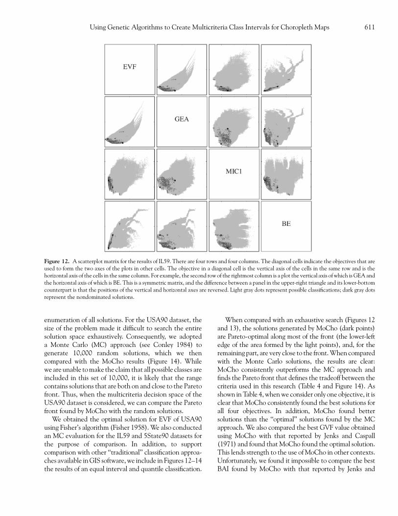
Figure 12. A scatterplot matrix for the results of IL59. There are four rows and four columns. The diagonal cells indicate the objectives that areused to form the two axes of the plots in other cells. The objective in a diagonal cell is the vertical axis of the cells in the same row and is thehorizontal axis of the cells in the same column. For example, the second row of the rightmost column is a plot the vertical axis of which is GEA andthe horizontal axis of which is BE. This is a symmetric matrix, and the difference between a panel in the upper-right triangle and its lower-bottomcounterpart is that the positions of the vertical and horizontal axes are reversed. Light gray dots represent possible classifications; dark gray dotsrepresent the nondominated solutions.


Caspall (1971), because we used a digital version of anIllinois county map. If we declare that a boundary existswhen two polygons have at least two common sequentialpoints, in IL59, the total number of boundaries is 265. Jenks

and Caspall (1971), on the other hand, report the numberof boundaries as 258. It is difficult to determine how thisdiscrepancy arose, though one might speculate that acounting error occurred.

Figure 13. A scatterplot matrix for the results of 5State90 (see caption of Figure 12 for description).

Table 4. An Overview of the Results for Three Datasets

Optimalb GA MC

EVF 0.068662 0.068662 0.069585IL59a GEA 0.006119 0.006119 0.036077

MIC1 0.160681 0.160681 0.218831BE 0.043713 0.043713 0.064065EVF 0.021963 0.021963 0.024425

5State90 GEA 0.031507 0.031507 0.087830MIC1 0.506293 0.506293 0.546108BE 0 0 0.027794EVF 0.040344 0.040344 0.113400

USA90 GEA – 0.013462 0.100915MIC1 – 0.232920 0.471010BE – 0.007024 0.044339

Note: In all cases considered, the GA found the best solution, obtained either by brute-force enumeration (IL59 and 5State90) or by Fisher’s algorithm (USA90).aFor the IL59 dataset, the ‘‘best’’ TAI value in Jenks and Caspall (1971) is 0.73455, which has classes of (15.57–41.20, 41.21–58.50, 58.51–75.51, 75.52–100.10,

100.10–155.30). In terms of EVF, this classification yields 1-GVF5 0.705823. The intervals found by our GA are (15.57–41.20, 41.21–60.66, 60.67–77.29, 77.30–

100.10, 100.10–155.30).bFisher’s algorithm is used to obtain the optimal values for EVF (Fisher 1958).Many implementations of this algorithmare available (seeHartigan 1975; Lindberg 1990); we

used a Fortran program provided byHartigan (1975, 130–42). For the small (IL59) andmedium (5State90) datasets, the results from Fisher’s algorithm are identical to the

results found by using brute force enumerations.


Table 5 gives the time used to runMoChousing the gridand the polygon datasets used in this article. It shows that,for the IL59 and 5State90 datasets, MoCho uses approxi-

mately 1 percent of the time required to conduct anexhaustive search of these two polygon datasets. Thispercentage is consistent with the sampling rates listed in

Figure 14. Ascatterplotmatrix for the results ofUSA90.There are four rows and four columns.Thediagonal cells indicate the objectives that areused to form the two axes of the plots in other cells. The objective in a diagonal cell is the vertical axis of the cells in the same row and is thehorizontal axis of the cells in the same column. For example, the second row of the rightmost column is a plot the vertical axis of which is GEA andthe horizontal axis of which is BE. This is a symmetric matrix, and the difference between a panel in the upper-right triangle and its lower-bottomcounterpart is that the positions of the vertical and horizontal axes are reversed. Light gray dots represent solutions generated using the MonteCarlo approach; dark gray dots represent the nondominated solutions.

Table 5. Real Computing Time Used on a Pentium 4 1.4 GHz Computer with an SCSI Hard Drive

Dataset TGA (seconds) TES (seconds) TMC (seconds) TGA/TES

TT1 22.169 36.29 – 61.1%TT2 12.153 30.414 – 40.0%TTL1 12.523 27.302 – 45.9%TTL2 9.643 30.061 – 32.1%F22 8.689 6.851 – 126.9%F24 10.19 11.952 – 85.3%IL59 33.749 3280.203 (0.91 hr) 6.667 1.0%5State90 123.171 7236.225 (2.01 hr) 26.964 1.7%USA90 963.462 82988556.620* (23052.38 hr) 249.586 0.0012%a

TGA5 time in seconds used to compute GA with the configuration listed in Table 3.

TES5 time in seconds used to complete an exhaustive search.

TMC5 time in seconds used to compute 10,000 Monte Carlo solutions.aEstimated value; see text for calculation.


Table 3. Though the exact time used to exhaustivelyenumerate all classifications for USA90 is unknown, ifwe assume that the computing time for every 10,000classifications is approximately the same, it can beestimated using the following equation:

TES ¼TMC�ðtotal number of classificationsÞ=10000¼ 23052:38hr42yrs ð9Þ

The estimated TGA/TES rate is 0.0012 percent, which isconsistent with the GA sampling rate of the USA90dataset (Table 3).

Figures 15–17 illustrate the classifications for theminimum values of the four objectives in each ofthe three geographical datasets. Because of the uneven

(skewed) distribution of observations in these datasets,especially LATO90 and USA90, the EVF and BEobjectives fail to serve as good (single) classificationcriteria if a visual assessment of the results is pursued.Considering the specific example of USA90 (Figure 17),EVF gives the best classification froma statistical view, butspatial information is difficult to discern from the mappedresult. GEA gives the best classification from the per-spective of equal class area, but the spatial structure is notclear (itsMIC5 1�MIC15 1� 0.87325 0.1268 on theresulting map). For MIC1, though the spatial structure isclear, the differentiation of the five classes is still not clear.The result for the best BE solutions is similar to that ofEVF. Consequently, a cartographer might select a classi-fication between these extreme solutions (see Figure 18).

15.57−41.20

41.21−60.66

60.67−77.29

77.30 −100.10

100.11−155.30

15.57−38.2238.23−52.0552.06−59.8959.90−75.5175.52−155.30

15.57−32.2832.29−33.8233.83−57.2257.23−58.5058.51−155.30

15.57− 41.2041.21−66.32

66.33−96.7896.79−119.90

119.91−155.30

Best for EVF Best for GEA

Best for MIC1 Best for BE

Figure 15. The four best class intervals for IL59.


Discussion and Conclusions

When producing choropleth maps, cartographersnormally generalize data into a small number of classes.Setting Tobler’s (1973) argument aside, the maximumrecommended number of classes is always less than adozen, even if hue is used as a visual variable. Theselection of data values that delimit the boundariesbetween these classes is a key cartographic designdecision, as even minor changes in these boundaries canhave significant impacts on the visual efficacy of theresulting map.

In the thirty years since Jenks and Caspall (1971) firstsuggested that choropleth class-interval selection is amulticriteria problem, surprisingly little progress has beenmade toward finding solutions that are based on criteriaother than statistical ones. Researchers have beenparticularly reluctant to investigate the geographical

characteristics of their data during the class-intervalselectionprocess. ThoughMonmonier (1972, 1973)madeimportant progress in the midseventies, his originalwork was not advanced for decades. Recently, however,Cromley (1996), Cromley and Mrozinski (1999), andMurray and Shyy (2000) have applied optimizationand data-mining approaches to the derivation of classesthat specifically consider the geographical characteristicsof a problem. While this work is important, the general-izability of these approaches is limited by assumptionsabout the measurement scale of the data to be mapped,the form of the solution space, and the suitability of theresults for choropleth mapping; classes, for example,should not overlap ( Jenks and Coulson 1963). Despitethese problems, however, researchers have developed avariety of indices that can be used to measure how wellalternative classification schemes meet different criteria.In addition to those chosen for this implementation,

Best for EVF Best for GEA

Best for MIC1 Best for BE

1 − 64

65 − 253

254 − 551

552 − 1687

1688 − 2953

1 − 3

4 − 7

8 −15

16 − 29

30 − 2953

1 − 16

17 − 337

338 − 1212

1213 − 1687

1688 − 2953

1 − 232

233 − 327

328 − 551

552 − 1687

1688 − 2953

Figure 16. The four best class intervals for 5State90.


Cromley (1996), for example, has used minimax error todefine boundary error. Other objectives, such as OAI(equation [3]) and round numbers (Monmonier 1982;Brewer 2001), could also be introduced into our multi-criteria optimization framework.

Evenmore fundamental, however, has been an implicitassumption that choropleth class-interval selection is adeterministic process and, thus, amenable to algorithmicsolutions. Cartographers may rely on qualitative judg-ments derived from experience and design philosophy, as

0 − 1332

1333 − 6605

6606 − 18533

18534 − 38478

38479 − 65275

0 − 3

4 − 11

12 − 29

30 − 71

72 − 65275

Best for EVF

Best for GEA

Figure 17. The four best class intervals for USA90.


well as statistical analyses of the data, to construct amap that is suited to its intended use. Choropleth mapconstruction is, therefore, best viewed as a semistructuredproblem and, like other cartographic generalizationproblems (Buttenfield and McMaster 1991), it may defyexact solution throughadeterministic automated solution

process. Cartography, after all, has been defined as ‘‘[t]heart, science, and technology of making maps, togetherwith their study as scientific documents and works ofart’’ (Meynen 1973,1). Robinson (1952), MacEachren(1995), Keates (1996), and Thrower (1972), amongothers, have expressed nearly identical sentiments. If it is

0 165

166 3206

3207 9660

9661 −

−

−

−

30107

30108 − 65275

0 −

−

−

−

−

3431

3432 9187

9188 15323

15324 30107

30108 65275

Best for MIC1

Best for BE

Figure 17. (Continued).


accepted that cartography has a distinctly artistic compo-nent, this aesthetic and subjective element cannot bedirectly incorporated into traditional multicriteria eval-uation techniques. What is required in this case is a toolthat helps cartographers explore the class-interval solu-tion space. This will enable them to integrate the science,

art, and technology of map-making into cartographicproducts.

A prototype of such a tool, called ChoroWare, wasdeveloped as part of this research (Xiao, Armstrong, andBennett 2002). The analytical engine of this tool followsthe original formulation by Jenks and Caspall (1971), as

00

0.2

0.2

0.4

0.4

0.6

0.6

0.8

0.8

GEA

0

0.2

0.4

0.6

0.8

GEA

EVF

0 0.2 0.4 0.6 0.8 EVF

0 − 66

67 − 2957

2958 − 18533

18534 − 38478

38479 − 65275

0 − 3

4 − 68

69 − 2412

2413 − 18533

18534 − 65275

Figure 18. A set of four classifications with objective values in between the extreme objective values. Each choropleth map is associated with aplot, where the dark point shows the position of the current classification in the trade-off between GEA and EVG.


updated by researchers such as Cromley (1996), Declerq(1995), and Slocum (1999), and recasts the class-intervalproblem into a multicriteria format. A GA is used tosearch for promising alternative solutions, which are thenreported to the cartographer for their evaluation. Ourresults show that GAs are able to generate a rangeof nondominated choropleth classification solutions. To

facilitate the use of this approach, our exploratorygraphical tool is designed to help cartographers as theyexamine the tradeoffs among alternative classificationobjectives and thus gain a greater understanding of howthese tradeoffs affect the resulting map. The graphicalinterface of this tool presents users with linked car-tographic, tabular, and graphical views of alternative

0 − 13

14 − 37

38 − 105

106 − 18533

18534 − 65275

0 − 4

5 − 17

18 − 54

55 − 3328

3329 − 65275

0 0.2 0.4 0.6 0.8 EVF

0 0.2 0.4 0.6 0.8 EVF

0

0.2

0.4

0.6

0.8

GEA

0

0.2

0.4

0.6

0.8

GEA

Figure 18. (Continued).


classification schemes (Figure 19). This graphical repre-sentation plots howwell alternative schemes performwithrespect to selected criteria and focuses attention onalternatives at or near the Pareto front of the objectivesincluded in the formulation of the problem. When aparticular classification is selected in the classification-solution space, the tabular and cartographic views areautomatically updated to illustrate it.

Though our multicriteria choropleth classification toolworkswell, adding additional features to it could produce apowerful choropleth-mapping support system. Examplesof software extensions include tools that allow users to (1)selectmultiple schemes in the tabular or graphical views toproduce small-multiples that facilitate subjective evalua-tion of multiple data views, (2) define new objectives andthus find the most suitable classification scheme toaccomplish user-specific goals, (3) search for an ‘‘optimal’’number of data classes, (4) search for effective symboliza-tion schemes, and (5) use immersive visual environmentsto examine higher-dimension criteria spaces directly.

At this point, one might reasonably imagine that thereare drawbacks to the approachdescribed in this article.Wehave identified two, though we suggest that neither is aparticularly critical limitation. The first grows directlyfrom the conceptual complexity of the overall approach.The multicriteria GA approach is far more complex thanan equal-interval classification, for example. Our rejoin-

der to that criticism is that while simple classificationmethods may be appropriate in some contexts, we shouldnot remain ignorant about alternatives, especially thosethat obviate problems associated with conventionalapproaches (e.g., empty classes). The computational per-formance ofMoCho remains a drawback to its application.One approach to improving the performance of an island-model GA such as ours is to allocate the processing ofgenerations on each virtual island to a separate processor.Since this is a relatively coarse-grained problem, it can beaccomplished using networked personal computers or theincreasingly accessible processing power of the computa-tional grid (Foster andKesselman 1999; Foster 2002), andthe overall reduction in computation time will be nearly alinear function of the number of processors used. Thiswould place the process of multicriteria class-intervalselection into the near-real-time temporal domain, allow-ing cartographers to specify and define their objectivesinteractively, search for solutions that meet these objec-tives, and select those thatmeet their goals. This will bringchoropleth-map production into a newera consistentwithprogress in other areas of visualization. Multicriteriachoropleth classification will equip new generations ofcartographers with tools that will spring choropleth-mapproduction from its narrow range of arbitrary choices into arealm in which users retain amore substantial control overthe map-production process.

Figure 19. The prototype of a visualization tool to help users select class intervals.


Acknowledgments

We wish to thank Ronghai Sa, R. Rajagopal, and thereviewers for their comments on previous drafts of thisarticle.

References

Andrienko, G. L., and N. V. Andrienko. 1999. Interactive mapsfor visual data exploration. International Journal of Geog-raphical Information Science 13 (4): 355–74.

Anselin, L. 1995. Local indicators of spatial association—LISA.Geographical Analysis 27 (2): 93–115.

FFF. 1999. Intractive techniques and exploratory spatial dataanalysis. InGeographical information systems, vol. 1, Principlesand technical issues, ed. P. A. Longley, M. F. Goodchild, D. J.Maquire, and D. W. Rhind, 253–66. New York: John Wileyand Sons.

Armstrong, M. P., G. Rushton, R. Honey, B. T. Dalziel, P. Lolonis,S. De, and P. J. Densham. 1991. Decision supportfor regionalization: A spatial decision support system forregionalizing service delivery systems. Computers, Environ-ment and Urban Systems 15 (1): 37–53.

Armstrong, R.W. 1969. Standardized class intervals and ratecomputation in statistical maps of mortality. Annals of theAssociation of American Geographers 59:382–90.

Bailey, T. C., and A. C. Gatrell. 1995. Interactive spatial dataanalysis. Harlow, Essex: Longman.

Bennett,D.A.,G.A.Wade, andM.P.Armstrong. 1999. Exploringthe solution space of semistructured geographical prob-lems using genetic algorithms. Transactions in GIS 3 (1):51–71.

Bowker, G. C., and S. L. Star. 1999. Sorting things out: Classificationand its consequences. Cambridge, MA: MIT Press.

Brewer, C. A. 1994. Color use guidelines for mapping andvisualization. InVisualization in modern cartography, ed. A.M.MacEachren and D. R. F. Taylor, 123–47. Tarrytown, NY:Elsevier.

FFF. 2001. Reflections onmappingCensus 2000.Cartographyand Geographic Information Science 28 (4): 213–35.

Buisseret, D., ed. 1992. Monarchs, ministers, and maps: Theemergence of cartography as a tool of government in early modernEurope. Chicago: University of Chicago Press.

Buttenfield, B. P., and R. B. McMaster eds. 1991. Map general-ization: Making rules for knowledge representation. New York:John Wiley and Sons.

Cantu-Paz, E., and D. E. Goldberg. 2000. Efficient parallel gene-tic algorithms: Theory and practice. Computer Methods inApplied Mechanics and Engineering 186:221–38.

Carver, S. J. 1991. Integrating multicriteria evaluation withgeographical information systems. International Journal ofGeographical Information Systems 5 (3): 321–39.

Chang, K. 1978. Visual aspects of class intervals in choroplethicmapping. The Cartographic Journal 15 (1): 42–48.

Cohon, J. L. 1978. Multiobjective programming and planning.London: Academic Press.

Conley, W. 1984. Computer optimization techniques. New York:Petrocelli Books.

Appendix

TT1 TT291 147 157 151 273 260 258 511 397 70 100 449 14 195

260 254 387 306 371 338 351 103 84 673 28 438 130 100362 396 303 386 358 355 341 64 280 106 70 86 187 295394 360 319 322 386 357 331 180 90 92 500 152 36 183322 319 392 340 314 433 452 194 17 168 120 187 10 79402 472 470 448 408 439 464 14 43 319 133 122 41 726407 524 514 649 641 770 786 161 60 129 290 203 500 10

TTL1 TTL291 147 157 151 273 260 258 90 97 100 53 66 88 94

260 254 387 306 371 338 351 32 6 91 65 78 14 61362 396 303 386 358 355 341 2 30 31 31 20 80 37394 360 319 322 386 357 331 2 67 19 199 147 126 151322 319 392 340 314 433 452 187 165 116 180 142 150 293402 472 470 448 408 439 464 203 271 275 260 303 375 467407 524 514 649 641 770 786 465 470 544 605 686 773 741

F22 F240.47 0.58 0.77 0.59 0.59 0.51 0.50 0.13 0.18 0.16 0.37 0.69 0.66 0.480.50 0.56 0.71 0.60 0.54 0.50 0.47 0.18 0.30 0.52 0.31 0.24 0.51 0.960.65 0.66 0.88 0.59 0.64 0.53 0.48 0.28 0.35 0.44 0.25 0.12 0.70 0.880.60 0.69 0.48 0.61 0.55 0.51 0.27 0.29 0.25 0.32 0.34 0.44 0.50 0.530.52 0.50 0.47 0.45 0.63 0.32 0.26 0.14 0.19 0.33 0.31 0.55 0.52 0.440.51 0.47 0.43 0.44 0.32 0.27 0.29 0.24 0.40 0.41 0.34 0.40 0.42 0.300.51 0.40 0.34 0.25 0.32 0.20 0.22 0.31 0.53 0.51 0.36 0.23 0.58 0.17


Coulson, M. R. C. 1987. In the matter of class intervals forchoropleth maps: With particular reference to the work ofGeorge F. Jenks. Cartographica 24 (2): 16–39.

Cromley, R. G. 1996. A comparison of optimal classificationstrategies for choroplethic displays of spatially aggregateddata. International Journal of Geographical Information Systems10 (4): 404–24.

Cromley, R. G., and R. D. Mrozinski. 1999. The classificationof ordinal data for choropleth mapping. The CartographicJournal 36 (2): 101–9.

Cuff, D. J., and M. T. Mattson. 1982. Thematic maps: Their designand production. New York: Methuen.

Declerq, F.A.N. 1995. Choroplethmap accuracy and the numberof class intervals.Proceedings of the 17thConference and the 10th

General Assembly of the International CartographicAssociation,vol. 1, 918–22. Barcelona: Institute Cartografic de Catalu-nya.

Dent, B. D. 1999. Cartography: Thematic map design. 5th ed.Boston: McGraw-Hill.

Dobson, M.W. 1973. Choropleth maps without class intervals? Acomment. Geographical Analysis 5 (4): 358–60.

FFF. 1980. Commentary: Perception of continuously shadedmaps. Annals of the Association of American Geographers70 (1): 106–7.

Egbert, S. L., and T. A. Slocum. 1992. EXPLOREMAP: Anexploration system for choropleth maps. Annals of theAssociation of American Geographers 82 (2): 275–88.

Evans, I. S. 1977. The selection of class intervals. Transactions ofthe Institute of British Geographers 2 (1): 98–124.

Fisher, W. D. 1958. On grouping for maximum homogeneity.American Statistical Association Journal 53:789–98.

Fogel, D. B., and P. J. Angeline. 1997. Guidelines for a suitableencoding. In Handbook of evolutionary computation, ed. T.Back, D. B. Fogel, and Z. Michalewicz. C1.7, 1–2. New York:Oxford University Press.

Foster, I. 2002. The grid: A new infrastructure for 21st-centuryscience. Physics Today February:42–47.

Foster, I., andC.Kesselman, eds. 1999.The grid: Blueprint for a newcomputing infrastructure. San Francisco: Morgan KaufmannPublishers.

Getis, A., and J. K. Ord. 1992. The analysis of spatial associationby the use of distance statistics. Geographical Analysis24:189–206.

Gilmartin, P., and E. Shelton. 1989. Choropleth maps on high-resolution CRTs: The effects of number of classes and hue oncommunication. Cartographica 26 (2): 40–52.

Goldberg,D. E. 1989.Genetic algorithms in search, optimization, andmachine learning. Reading, MA: Addison-Wesley.

Goodchild, M. F. 1988. Spatial autocorrelation, Concepts andTechniques in Modern Geography (CATMOG) no. 47.Norwich, UK: Geobooks.

Griffith, D. A. 2000. A linear regression solution to the spatialautocorrelation problem. Journal of Geographical Systems2:141–56.

Hartigan, J. A. 1975.Clustering algorithms. New York: JohnWileyand Sons.

Holland, J. H. 1975. Adaptation in natural and artificial systems.Ann Arbor: University of Michigan Press.

FFF. 1986. Escaping brittleness: The possibilities of general-purposemachine learning algorithms applied to parallel rule-based systems. In Machine learning: An artificial intelligenceapproach, vol. 2, ed. R. S. Michalski, J. G. Carbonell, andT.M.Mitchell, 593–623. LosAltos, CA:MorganKaufmann.

FFF. 1998. Emergence: From chaos to order. Reading, MA:Addison-Wesley.

Holland, J. H., K. J. Holyoak, R. E. Nisbett, and P. R. Thagard.1986. Induction: Processes of inference, learning, and discovery.Cambridge, MA: MIT Press.

Jankowski, P. 1995. Integrating geographical informationsystems and multiple criteria decision-making methods.International Journal ofGeographical Information Systems9 (3):251–73.

Jenks, G. F. 1977. Optimal data classification for choropleth maps.Occasional Paper no. 2. Lawrence: Department of Geog-raphy, University of Kansas.

Jenks, G. F., and F. C. Caspall. 1971. Error on choroplethic maps:Definition, measurement, reduction. Annals of the Associa-tion of American Geographers 61 (2): 217–44.

Jenks, G. F., and M. R. C. Coulson. 1963. Class intervals forstatistical maps. International Yearbook of Cartography 3:119–34.

Kain, R. J. P., and E. Baigent. 1992.The cadastral map in the serviceof the state. Chicago: University of Chicago Press.

Keates, J. S. 1996. Understanding maps. 2nd ed. Harlow, UK:Addison Wesley Longman Ltd.

Kraak, M.-J. 1998. The cartographic visualization process: Frompresentation to exploration.The Cartographic Journal 35 (1):11–15.

Kraak, M.-J., and A. Brown. 2001.Web cartography: Developmentsand prospects. New York: Taylor and Francis.

Kraak, M.-J., and F. J. Ormeling. 1996. Cartography: Visualizationof spatial data. Essex, UK: Longman.

Lindberg, M. B. 1990. FISHER: A Turbo Pascal unit for optimalpartitions. Computers and Geosciences 16 (5): 717–32.

Lolonis, P., and M. P. Armstrong. 1993. Location-allocationmodels as decision aids in delineating administrative regions.Computers, Environment, and Urban Systems 17 (2): 153–74.

MacDougall, E. B. 1992. Exploratory analysis, dynamic statisticalvisualization, and geographic information systems. Carto-graphy and Geographic Information Systems 19 (4): 237–46.

MacEachren, A. M. 1982. Map complexity: Comparison andmeasurement. The American Cartographer 9 (1): 31–46.

FFF. 1995. How maps work: Representation, visualization,design. New York: Guilford Press.

MacEachren, A.M., andM. -J. Kraak. 2001. Research challengesin geovisualization. Cartography and Geographic InformationScience 28 (1): 3–12.

Mak, K., and M. R. C. Coulson. 1991. Map user response tocomputer-generated choropleth maps: Comparative experi-ments in classification and symbolization. Cartography andGeographic Information Systems 18 (2): 109–24.

Malczewski, J. 1999. GIS and multicriteria decision analysis. NewYork: John Wiley and Sons.

Martin,W.N., J. Lienig, and J. P.Cohoon. 1997. Island (migration)models: Evolutionary algorithms based on punctuatedequilibria. In Handbook of evolutionary computation, ed. T.Back,D.B. Fogel, andZ.Michalewicz.C6.3: 1–16.NewYork:Oxford University Press.

Mersey, J. E. 1990. Colour and thematic map design: The role ofcolour scheme and map complexity in choropleth map commu-nication. Cartographica Monograph no. 41. Toronto: Uni-versity of Toronto Press.

Meynen, E, ed. 1973. Multilingual dictionary of technical terms incartography. Weisbaden: Franz Steiner Verlag.

Michalewicz, Z. 1996. Genetic algorithms1 data structures5 evo-lution programs. 3rd ed. Berlin: Springer-Verlag.


amanthea

Realce

Monmonier, M. S. 1972. Contiguity-biased class-interval selec-tion: A method for simplifying patterns on statistical maps.Geographical Review 62:203–28.

FFF. 1973. Analogs between class-interval selection andlocation-allocation models. The Canadian Cartographer10:123–31.

FFF. 1982. Flat laxity, optimization, and rounding in theselection of class intervals. Cartographica 19 (1): 16–27.

FFF. 1985. Technological transition in cartography. Madison:University of Wisconsin Press.

FFF. 1992. Authoring graphic scripts: Experiences andprinciples. Cartography and Geographic Information Systems19 (4): 247–60.

FFF. 1996.How to lie with maps. 2nd ed. Chicago: University ofChicago Press.

Morrison, J. L. 1993. Cartography and the spatially literatepopulace of the 21st century. Cartography and GeographicInformation Systems 20 (4): 204–9.

Muller, J.-C. 1979. Perception of continuously shaded maps.Annals of the Association of American Geographers 69 (2):240–49.

Murray, A. T., and T. -K. Shyy. 2000. Integrating attribute andspace characteristics in choropleth display and spatial datamining. International Journal of Geographical InformationScience 14 (7): 649–67.

O’Sullivan, D., and D. Unwin. 2003. Geographic informationanalysis. Hoboken, NJ: John Wiley and Sons.

Odland, J. 1988. Spatial autocorrelation. Newbury Park, CA: Sage.Olson, J. 1975. Autocorrelation and visual map complexity.

Annals of the Association of American Geographers 65 (2):189–204.

Pareto, V. 1971.Manual of political economy. Trans. A. S. Schwierfrom French edition first published in 1896. New York:Augustus M. Kelley.

Peterson, M. P. 1979. An evaluation of unclassed crossed-linechoroplethmapping.TheAmericanCartographer6 (1): 21–37.

Peucker, T. K., and N. R. Chrisman. 1975. Cartographic datastructures. The American Cartographer 2:55–69.

Raisz, E. 1948. General cartography. New York: McGraw-Hill.Robinson, A. H. 1952. The look of maps: An examination of

cartographic design. Madison: University of Wisconsin Press.

Robinson, A. H., R. D. Sale, J. L. Morrison, and P. C. Muehrcke.1984. Elements of cartography. 5th ed. New York: John Wileyand Sons.

Robinson, A. H., J. L. Morrison, P. C. Muehrcke, A. J. Kimerling,and S. C. Guptill. 1995. Elements of cartography. 6th ed. NewYork: John Wiley and Sons.

Sait, S. M., andH. Youssef. 1999. Iterative computer algorithms withapplications in engineering: Solving combinatorial Optimizationproblems. Los Alamitos, CA: IEEE Press.

Slocum, T. A. 1999. Thematic cartography and visualization. UpperSaddle River, NJ: Prentice Hall.

Smith, D. M. 1977. Human geography: A welfare approach. NewYork: St Martin’s Press.

Smith, R. M. 1986. Comparing traditional methods for selectingclass intervals on choropleth maps. The Professional Geogra-pher 38 (1): 62–67.

Srinivas, N., andK.Deb. 1995.Multiobjective optimization usingnondominated sorting in genetic algorithms. EvolutionaryComputation 2 (3): 221–48.

Thrower, N. J. W. 1972. Maps and man: An examination ofcartography in relation to culture and civilization. EnglewoodCliffs, NJ: Prentice Hall.

Tobler, W. 1973. Choropleth maps without class intervals.Geographical Analysis 5 (3): 262–65.

Tufte, E. R. 1997. Visual explanations: Images and quantities,evidence and narrative. Cheshire, CT: Graphics Press.

Tyner, J. 1992. Introduction to thematic cartography. EnglewoodCliffs, NJ: Prentice Hall.

U.S. Bureau of the Census. American FactFinder. http://factfinder.census.gov/servlet/BasicFactsServlet (last accessed 1 May2003).

Xiao, N., M. P. Armstrong, and D. A. Bennett. 2002. ChoroWare:A software toolkit for choropleth map classification. InNewtools for spatial data analysis: Proceedings of CSISS SpecialistMeeting, ed. L. Anselin and S. J. Rey, CD-ROM. SantaBarbara, CA: The Center for Spatially Integrated SocialScience.

Xiao, N., D. A. Bennett, and M. P. Armstrong. 2002. Usingevolutionary algorithms to generate alternatives for multi-objective site search problems. Environment and Planning A34 (4): 639–56.

Correspondence: Department of Geography and Program in Applied Mathematical and Computational Sciences, The University of Iowa,Iowa City, IA 52242, e-mail: [email protected] (Armstrong); Department of Geography, The University of Iowa, Iowa City,IA 52242, e-mail: [email protected] (Xiao); Department of Geography, The University of Iowa, Iowa City, IA 52242, e-mail:[email protected] (Bennett).


jenks_algoritimos geneticos.pdf

Documents

map scale

mapproduction companies

map production capabilities

data relationships

genetic algorithms

known set of data

map audience publicprivate

optimal classifications