jaya latent variable models

8/6/2019 Jaya Latent Variable Models

http://slidepdf.com/reader/full/jaya-latent-variable-models 1/20

Multivariate Analysis MSE 2010 1

Latent Variable Approach

Jaya Krishnakumar, University of GenevaMain idea:

� The theoretical concept is not directly

observable; it is latent (hidden)� The observed indicators /outcomes or

responses are partial/imperfect measures

of the underlying theoretical concept

� How to make inference about the latent

variable using the observed indicators?




An Example in Economics

� Latent variable: human wellbeing or

welfare

� Observed indicators: achievement or

outcome indicators

� Other relevant information: personal

characteristics of the individual and some

features of the µworld¶ in which s/he lives




Main Models

� Factor Analysis (FA)

� Multiple Indicators Multiple Causes

(MIMIC)

� Structural Equation Models (SEM)

� Extensions with covariates (exogenous

variables) and qualitative outcomes




Factor Analysis

� In this model, the observed values are

postulated to be (linear) functions of a

certain number (fewer) of unobservedlatent variables (called factors). These

latent factors represent our capabilities.

� However this model does not explain the

latent variables (or the capabilities)

themselves.




Factor Analysis (contd.)

� The Model

I 0 f y ==* =)(=)( I V and f V

.= =0d0*7




Factor Analysis (contd.)

� Maximum likelihood procedure is applied

to the model to estimate and given .

Given , one can derive minimumvariance estimators or predictors of f as

follows:

� Or as below for an unbiased version

y I f 11)(=Ö =0d+

y y f 11111* )(==Ö

=0d0=0d=0d+



Factor Analysis: Path Diagram


1 f

11 ,..., p y y

p p y y ,...,12

211,..., p p y y

2 f

3 f




Principal Components

� What about principal components (PC)? PC is

not a latent variable model, but a data reduction

technique. This method seeks linear

combinations of the observed indicators in such

a way as to reproduce the original variance as

closely as possible.

� It is widely used in empirical applications as an

µaggregating¶ technique� Under certain conditions PC's can be shown to

be equivalent to the factor scores obtained in FA




Link between PC and FA

� The estimators of the latent variablesobtained when = I can be shown to beproportional to the (first m) principal

components say p*.� This identity between the µunbiased¶versions of PC's and factor scoresprovides the theoretical justification for the

possible interpretation of principalcomponents as latent variable estimatorsunder special conditions.




MIMIC Models

� Multiple Indicators Multiple Causes

� This model goes a step further in theexplanation.

� Here the observed variables are taken tobe manifestations of a latent concept (asin the FA model) but the latent factor(s)

are in turn ³caused´ by exogenouselements.



MIMIC: Path Diagram


1 f 11 ,..., p y y

p p y y ,...,12

211,..., p p y y

2 f

k x

x

x

/

2

1

3 f




MIMIC Models (contd.)

According to this model, the observed variablesresult from the latent factors and the latent factors

themselves are caused by other exogenous

variables denoted here as x 1, «, x k . Thus we have

µmeasurement equations' and µcausal' relationships.

I

I

0

x B f

f y

=

=

I V V 2=)(,=)( W I I =




MIMIC Models (contd.)

� The estimator of f is given by

� The above equation shows that the MIMIC latent

factor estimator is a sum of two terms: the first

one is the ³causes´ term (function of ) and the

second one can be called the ³indicators´ term.� If there are no µcauses' then it reduces to the

pure FA estimator.

).()(=Ö 111 y Bx I f =0d0;0d




Structural Equations Models (SEM)

� These are systems of equations involving

several latent endogenous variables

accounting for the i nterdependence

among the latent variables as well as theinfluence of exogenous ³causes´.

� They also have equations describing the

µmeasurement¶ of the µlatent¶ factorsthrough a set of indicators.




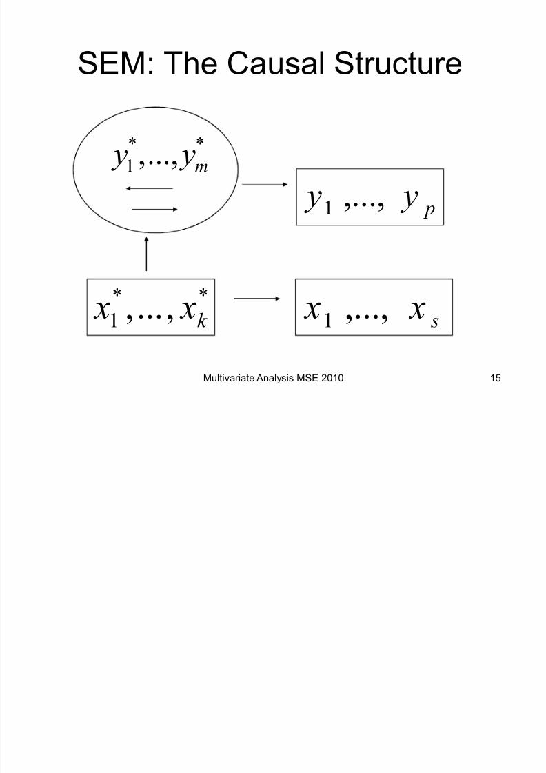
SEM: The Causal Structure

**

1 ...,,m

y y

p y y ,...,1

**

1 ,..., k x x s x x ,...,1




SEM (contd.)

Thus there are two parts:The structural part explains the latent variables

y* (which are the endogenous variables of the

model) by a set of exogenous (also latent)

variables x* and including mutual effects of the

endogenous variables on one another.

0=** u B x Ay




SEM (contd.)

The measurement part specifies the

relations linking the latent factors to the

observed indicators.

We have

<=7 =)(,=)(,=)( I I V V uV

^ c*

= x x

I 0*

= y y




Extension with covariates

(exogenous variables)

I 0 w D y y*

=

^ c z F x x *=




Extension with qualitative outcomes

� For a dichotomous indicator , say literate or not,we have:

� For an ordered categorical indicator with Ccategories (say different levels of education):

0*if 0and)liter atesay(0*if 1 !"! y y y y

inf inf ,,...1,*if 11 !!!! C cc s sC c s y sc y

^ ! )*,( w yh y




SEM: Estimation

� The unknown parameters can be estimated byconditional generalised method of moments(GMM) or conditional maximum likelihood (ML).

� Once the parameter estimates are obtained,

the latent factors are estimated by their posterior means given the sample, replacingthe parameter values by their estimates. In thecase of only continuous indicators, we get:

? A 0=0d7007 d

d

ii B x A A A A A I y 111111* )('=Ö

)()'(' 11111

iiwC y A A A A =07007

dd

jaya latent variable models

Documents