jason murphy may 13, 2017
TRANSCRIPT

Introduction to Partial Differential Equations
Jason Murphy
May 13, 2017

Contents
1 Introduction 4
1.1 Derivation of some common PDE . . . . . . . . . . . . . . . . 4
2 Review of Topology and Calculus 7
2.1 Properties of Rd . . . . . . . . . . . . . . . . . . . . . . . . . 7
2.2 Calculus Review . . . . . . . . . . . . . . . . . . . . . . . . . 8
2.3 Further Topics . . . . . . . . . . . . . . . . . . . . . . . . . . 9
2.4 Convolution and Distributions . . . . . . . . . . . . . . . . . . 9
3 The Laplace Equation 13
3.1 The Fundamental Solution . . . . . . . . . . . . . . . . . . . . 13
3.2 Green’s Functions . . . . . . . . . . . . . . . . . . . . . . . . 16
3.3 Properties of Solutions . . . . . . . . . . . . . . . . . . . . . . 21
4 The Heat Equation 25
4.1 The Fundamental Solution . . . . . . . . . . . . . . . . . . . . 25
4.2 The Mean Value Property . . . . . . . . . . . . . . . . . . . . 28
4.3 The Maximum Principle and Uniqueness . . . . . . . . . . . . 30
5 The Wave Equation 34
5.1 The Fundamental Solution . . . . . . . . . . . . . . . . . . . . 34
5.1.1 The Case d = 1 . . . . . . . . . . . . . . . . . . . . . . 35
5.1.2 The Case d = 3 . . . . . . . . . . . . . . . . . . . . . . 36
5.1.3 The Case d = 2 . . . . . . . . . . . . . . . . . . . . . . 38
5.2 Energy Methods . . . . . . . . . . . . . . . . . . . . . . . . . 40
6 Separation of Variables 43
6.1 Linear Algebra Review . . . . . . . . . . . . . . . . . . . . . . 43
6.2 Separation of Variables . . . . . . . . . . . . . . . . . . . . . . 44
6.3 Fourier Series . . . . . . . . . . . . . . . . . . . . . . . . . . . 45
2

CONTENTS 3
7 The Fourier Transform 527.1 The Fourier Transform . . . . . . . . . . . . . . . . . . . . . . 527.2 Higher Dimensions . . . . . . . . . . . . . . . . . . . . . . . . 577.3 Application to PDEs . . . . . . . . . . . . . . . . . . . . . . . 587.4 Tempered Distributions . . . . . . . . . . . . . . . . . . . . . 607.5 Duhamel’s Principle . . . . . . . . . . . . . . . . . . . . . . . 63
8 The Method of Characteristics 678.1 The Method of Characteristics . . . . . . . . . . . . . . . . . 67
8.1.1 The Linear Case. . . . . . . . . . . . . . . . . . . . . . 678.1.2 The Quasilinear Case. . . . . . . . . . . . . . . . . . . 69
8.2 Scalar Conservation Laws . . . . . . . . . . . . . . . . . . . . 708.2.1 Rankine–Hugoniot Condition for Shocks. . . . . . . . 738.2.2 Entropy Solutions . . . . . . . . . . . . . . . . . . . . 74
9 Calculus of Variations 769.1 Several Examples . . . . . . . . . . . . . . . . . . . . . . . . . 76
10 Numerical Methods 8210.1 Finite Difference Schemes . . . . . . . . . . . . . . . . . . . . 8210.2 Numerical Stability . . . . . . . . . . . . . . . . . . . . . . . . 8410.3 Finite Element Method . . . . . . . . . . . . . . . . . . . . . 86
11 Topics from Physics 8811.1 Classical Mechanics . . . . . . . . . . . . . . . . . . . . . . . . 8811.2 Quantum Mechanics . . . . . . . . . . . . . . . . . . . . . . . 9011.3 Electromagnetism . . . . . . . . . . . . . . . . . . . . . . . . . 10011.4 Elementary Particles . . . . . . . . . . . . . . . . . . . . . . . 102

Chapter 1
Introduction
These notes are based on an undergraduate introductory PDE course I gaveat UC Berkeley in the Fall of 2014. While searching for a textbook, I couldnot find exactly what I was looking for. Between the textbooks of Straussand Evans, I could find essentially everything I wanted to cover; however,I found that I wanted something a bit more in-depth than the book ofStrauss and a bit more basic than the book of Evans. Inspired largely bythese two textbooks, I prepared my own notes, which formed the basis ofthis document.
The prerequisites for this class consisted of multivariable calculus, linearalgebra, and differential equations. In particular, I could not assume famil-iarity with real analysis. Thus, many issues related to convergence are dealtwith rather informally, and many technical details are glossed over.
These notes are a work in progress and will be updated over time.
1.1 Derivation of some common PDE
Example 1.1.1 (Heat equation). Let Ω ⊂ Rd be an open region of space. Letu(t, x) denote the density of some quantity in Ω (e.g. ‘heat’) at time t andposition x. The goal is to describe how the distribution of heat evolves intime.
Denote by F(t, x) the ‘flux density’ of the heat at (t, x). Heat flows fromregions of high density to low density, so we approximate F = −k∇u forsome k > 0.
4

1.1. DERIVATION OF SOME COMMON PDE 5
Now fix a small subregion V ⊂ Ω. The amount of heat in V is given by∫Vu(t, x) dx.
We wish to measure
ddt
∫Vu(t, x) dx =
∫V
∂u∂t (t, x) dx.
To do so, we need to measure the flow of heat through the boundary ∂V .Let n(x) be the outward-pointing unit normal vector at x ∈ ∂V . Then∫
V
∂u∂t dx = −
∫∂V
F · n dS =
∫∂Vk∇u · n dS.
Applying the divergence theorem, we find∫V
∂u∂t dx =
∫V
div k∇u dx =
∫Vk∆u dx. (∗)
For any (t, x), we now consider regions V ⊂ Ω that ‘shrink down’ to(t, x). As (∗) holds on each V , we conclude
∂u∂t (t, x) = k∆u(t, x).
This is the heat equation.
Example 1.1.2 (Laplace equation). We revisit the setting of Example 1, butsuppose the system has reached equilibrium. In particular, u = u(x). (Thedensity is constant in time).
Consider a subregion V ⊂ Ω. As the system is at equilibrium,∫Vu dx
is constant. Thus the flow through ∂V is zero:∫∂Vk∇u · n dS = 0.
Applying the divergence theorem, we find∫V
∆u dx = 0.
As V was arbitrary, we deduce
∆u(x) = 0.
This is the Laplace equation.

6 CHAPTER 1. INTRODUCTION
Definition 1.1.1. Solutions to Laplace’s equation are called harmonic.
Example 1.1.3 (Wave equation). Let Ω ⊂ Rd be an open region of spaceinhabited by an elastic object (for example, a string if d = 1, a drumheadif d = 2). Let u(t, x) denote the displacement of the object in some fixeddirection. The goal is to derive an equation for u. We will primarily use‘F = ma’.
Let V ⊂ Ω be a small subregion. Force (tension) acts on the objectthrough the boundary ∂V . For elastic bodies, a reasonable approximationis F = −k∇u for some k > 0.
The net force on the object in the region V is thus
−∫∂V
F · n dS =
∫∂Vk∇u · n dS.
The acceleration of the object within V is given by
d2
∂t2
∫Vu dx =
∫V
∂2u∂t2
dx.
Assuming constant mass density ρ, Newton’s law (F = ma) gives∫∂Vk∇u · n dS = ρ
∫V
∂2u∂t2
dx.
Applying the divergence theorem we find∫V
(∂2u∂t2− c∆u) dx = 0, c = k
ρ .
As V was arbitrary, we deduce
∂2u∂t2− c∆u = 0.
This is the wave equation.

Chapter 2
Review of Topology andCalculus
2.1 Properties of Rd
We work in Euclidean space Rd, which is a vector space with the stan-dard basis e1, . . . , ed, where e1 = (1, 0, . . . , 0), etc. For x ∈ Rd, we writex = (x1, . . . , xd) to denote x = x1e
1 + · · · + xded. We call x1, . . . , xd the
components of x.
The standard inner product on Rd is given by x · y = x1y1 + · · ·+ xdyd.The norm of a vector is defined by |x| =
√x · x. The distance between two
points is given by d(x, y) = |x− y|.We use the metric on Rd to define its topology, that is, the notion of
open/closed sets and convergence/limits.
For x ∈ Rd and r > 0, we define the open ball
Br(x) = y ∈ Rd : d(x, y) < r.
A set Ω ⊂ Rd is open if for any x ∈ Ω, there exists r > 0 such thatBr(x) ⊂ Ω. A set C ⊂ Rd is closed if its complement Rd\C := x ∈ Rd :x /∈ C is open.
The closure of Ω, denoted Ω, is the intersection of all closed sets con-taining Ω
A sequence xn∞n=1 ⊂ Rd converges to ` ∈ Rd if
for any ε > 0 there exists N such that |xn − `| < ε for all n ≥ N.
We call ` the limit of the sequence and write xn → `
7

8 CHAPTER 2. REVIEW OF TOPOLOGY AND CALCULUS
A set C is closed if whenever xn∞n=1 ⊂ C and xn → `, we have ` ∈ C.A set K ⊂ Rd is compact if it is closed and bounded. (This is not a
definition of compact, but rather a theorem about compact sets in Rd.)
2.2 Calculus Review
Fix an open set Ω ⊂ Rd and a function f : Ω→ R.A function f is continuous at x ∈ Ω if whenever xn∞n=1 ⊂ Ω and
xn → x, we have f(xn) → f(x). The function f is continuous if it iscontinuous at each x ∈ Ω
A function f is differentiable at x ∈ Ω if there exists v ∈ Rd such thatfor any hn∞n=1 ⊂ Rd\0 such that hn → 0, we have
f(x+hn)−f(x)−v·hn|hn| → 0.
We call v the gradient of f at x, and we write v = ∇f(x).The components of ∇f(x) are the partial derivatives of f , denoted
∂f∂xi
(x). That is, ∇f(x) =( ∂f∂x1
(x), . . . , ∂f∂xd (x)).
The function f is differentiable if it is differentiable at each x ∈ Ω.Note that ∂f
∂xidefines a function from Ω → R, which may also be dif-
ferentiable. Thus we have second order derivatives ∂2f∂xj∂xi
, as well as higher
order derivatives. Clairaut’s theorem states that ‘mixed’ partial derivatives
(e.g. ∂2f∂xi∂xj
versus ∂2f∂xj∂xi
) are equal if they are continuous.
We say f is smooth if it has continuous derivatives of every order —we write f ∈ C∞.
The support of f is defined as follows: supp(f) := x : f(x) 6= 0. Iff is smooth and supp(f) is compact, we write f ∈ C∞c .
A vector field is a function F : Rd → Rd. We write F in terms of itscomponent functions: F = (F1, . . . , Fd).
We use the following notation for a function u : R × Rd → R, with(t, x) ∈ R× Rd:
ut = ∂tu = ∂u∂t ,
uxi = ∂xiu = ∂iu = ∂u∂xi,
∂2u∂xi∂xj
= uxixj = ∂xixju = ∂iju, etc.,
∇u = (ux1 , . . . , uxd) = gradu.
The divergence of F : Rd → Rd is given by div F = ∇ · F =∑d
i=1∂Fi∂xi
.
The Laplacian of u is given by ∆u = div∇u =∑d
i=1 uxixi .

2.3. FURTHER TOPICS 9
2.3 Further Topics
Theorem 2.3.1 (Gauss–Green formula). Let Ω ⊂ Rd be an open regionwith smooth boundary ∂Ω. Let f : Ω → R be a smooth function. Letn(x) = (n1(x), . . . , nd(x)) denote the outward-pointing unit normal vectorat x ∈ ∂Ω. Then for i ∈ 1, . . . , d,∫
Ωuxi dx =
∫∂Ωuni dS.
• Change of variables:∫Rdf(x+ x0) dx =
∫Rdf(y) dy︸ ︷︷ ︸
y=x+x0, dy=dx
,
∫Rdf(cx) dx = |c|−d
∫Rdf(y) dy︸ ︷︷ ︸
y=cx, dy=|c|ddx
.
• Polar coordinates:∫Rdf(x) dx =
∫ ∞0
∫∂B1(0)
f(rθ) rd−1 dS dr︸ ︷︷ ︸x=rθ, dx=rd−1 dr dS(θ)
.
• An operator is a function whose input/output are functions.
Important examples include differential operators, for example
– ∂xi (partial derivative)
– ∆ (Laplacian)
– ∂t −∆ (heat operator)
– ∂2t −∆ (d’Alembertian)
2.4 Convolution and Distributions
Definition 2.4.1. Let f, g ∈ C∞c (Rd). The convolution of f and g is thefunction
f ∗ g : Rd → R
defined by
f ∗ g(x) =
∫Rdf(x− y)g(y) dy.

10 CHAPTER 2. REVIEW OF TOPOLOGY AND CALCULUS
Note: this makes sense even if g is merely continuous, and even in muchmore general settings.
Properties.
• f ∗ g = g ∗ f
• ∂i(f ∗ g) = (∂if) ∗ g = f ∗ (∂ig) (similarly for differential operators)
• for f, g ∈ C∞c , we have f ∗ g ∈ C∞c
Approximate identities.
• Let φ ∈ C∞c (Rd) satisfy∫φdx = 1, with supp(φ) ⊂ B1(0).
• Define φn∞n=1 via φn(x) = ndφ(nx). (draw picture)
• Note ∫φn(x) dx =
∫ndφ(nx) dx =
∫φ(y) dy︸ ︷︷ ︸
y=nx, dy=nd dx
= 1
with supp(φ) ⊂ B1/n(0).
• Fact: For f ∈ C∞c (Rd), we have f ∗ φn(x)→ f(x) for all x
Question. Is there a function δ0 such that f ∗ δ0(x) = f(x) ?
Answer. No, there is no such function. But there is such a “distribu-tion”.
Definition 2.4.2. A distribution is a functional u : C∞c (Rd)→ R that is
(i) linear, i.e. u(αf + βg) = αu(f) + βu(g)
(ii) continuous, i.e. if fk → f then u(fk)→ u(f).
We denote the set of distributions byD(Rd). Distributions are sometimescalled ‘generalized functions’. In this context, elements of C∞c are oftencalled ‘test functions’. The space D is the “dual space” of C∞c .
Example 2.4.1.
• if u ∈ C∞c , then we may think of u as a distribution by defining
u(f) =
∫u(x)f(x) dx. (∗)

2.4. CONVOLUTION AND DISTRIBUTIONS 11
• even for more general functions u, we may think of u as a distributionvia (∗)
• Dirac delta: δ0(f) = f(0)
Remark 2.4.3. We will define f ∗u for f ∈ C∞c and u ∈ D below and showf ∗ δ0 = f .
Derivatives of distributions. For u ∈ D, we would like to define∂iu ∈ D.
First, suppose u ∈ C∞c and take a ‘test function’ f ∈ C∞c .
By the integration by parts formula,∫∂iu f dx︸ ︷︷ ︸∂iu(f)
= −∫u ∂if dx︸ ︷︷ ︸−u(∂if)
.
Thus for u ∈ D, we can define ∂iu ∈ D by
∂iu(f) := −u(∂if) for f ∈ C∞c .
This is very powerful: now we can take derivatives of non-differentiablefunctions!
Similarly, if L is a differential operator we can make sense of Lu.
Convolution with distributions. We would like to define f ∗ u forf ∈ C∞c and u ∈ D.
First, suppose f, u ∈ C∞c . Then
f ∗ u(x) = u ∗ f(x) =
∫u(y)f(x− y) dy
Notation: τxf(y) = f(y − x) (translation)
f(y) = f(−y) (reflection)
Then we have f(x− y) = τxf(y), so that we can write
f ∗ u(x) =
∫u(y)τxf(y) dy︸ ︷︷ ︸
u(τxf)
.
Thus for f ∈ C∞c and u ∈ D we define f ∗ u to be the function
f ∗ u(x) := u(τxf).

12 CHAPTER 2. REVIEW OF TOPOLOGY AND CALCULUS
General principle. Whatever you can define for C∞c you can alsodefine for D, provided the definitions agree when restricted to C∞c .
Let’s verify that f ∗ δ0 = f for all f ∈ C∞c :
f ∗ δ0(x) = δ0(τxf) = τxf(0) = f(x).
Definition 2.4.4. Let L be a differential operator. A distribution Φ ∈ Dis a fundamental solution for L if L(Φ) = δ0.
The key property of the fundamental solution is the following: if Φ is afundamental solution for L, then the solution to Lu = f is given by
u = f ∗ Φ.
Indeed,
L(u) = L(f ∗ Φ) = f ∗ L(Φ) = f ∗ δ0 = f.
Question: why does f ∗ φn(x)→ f(x) ?

Chapter 3
The Laplace Equation
3.1 The Fundamental Solution
We seek the fundamental solution for the Laplace operator −∆, that is, adistribution Φ such that −∆Φ = δ0. Then we can solve Poisson’s equation−∆u = f on Rd by defining u = f ∗ Φ.
We focus on d ≥ 3 (see the exercises for d = 1, 2). We begin by tryingto find a function u such that ∆u = 0 on Rd\0.
The key observation is the following: the Laplace equation is invariantunder rotations (see the exercises). So we look for a function that is alsoinvariant under rotations:
u(x) = v(r), r = |x| =√x2
1 + · · ·+ x2d.
We compute:
∂iu = v′(r)∂ir = v′(r)xi|x|, ′ =
d
dr,
∂i∂iu = v′′(r)x2i
|x|2+ v′(r)
[1
|x|− x2
i
|x|3
],
∆u =d∑i=1
∂i∂iu = v′′(r) + d−1r v′(r)
13

14 CHAPTER 3. THE LAPLACE EQUATION
Thus
∆u = 0 if and only if v′′ + d−1r v′ = 0,
=⇒ v′′
v′ = −d−1r
=⇒ [log(v′)]′ = −d−1r ,
=⇒ log(v′) = −(d− 1) log r + C1 = log r−(d−1) + C1,
=⇒ v′ = C2r−(d−1)
=⇒ v = −Cr−(d−2).
Therefore
u(x) = C|x|−(d−2) solves −∆u = 0 on Rd\0 for d ≥ 3.
We now show show that we can choose C so that Φ(x) = C|x|−(d−2) is afundamental solution, that is, −∆Φ = δ0. We consider Φ(x) as a distributionand take a test function f ∈ C∞c . Then
−∆Φ(f) = f(0) ⇐⇒ −Φ(∆f) = f(0)
⇐⇒ −∫
Φ(x)∆f(x) dx = f(0)
⇐⇒ −∫C|x|−(d−2)∆f(x) dx = f(0)
⇐⇒∫|x|−(d−2)∆f(x) dx = − 1
C f(0).
Therefore we need to compute∫|x|−(d−2)∆f(x) dx for an arbitrary test
function f .First let ε > 0 and write∫|x|−(d−2)∆f(x) dx =
∫Bε(0)
|x|−(d−2)∆f(x) dx︸ ︷︷ ︸I
+
∫Rd\Bε(0)
|x|−(d−2)∆f(x) dx︸ ︷︷ ︸II
.
For I, first use polar coordinates:∫Bε(0)
|x|−(d−2) dx =
∫ ε
0
∫∂B1(0)
r−d+2rd−1 dS dr =
∫ ε
0r dr = 1
2ε2.
So|I| ≤ max
x∈Rd|∆f(x)| · 1
2ε2 ≤ cε2.

3.1. THE FUNDAMENTAL SOLUTION 15
For II, we integrate by parts: (draw picture)∫Rd\Bε(0)
|x|−(d−2)∆f(x) dx = −∫Rd\Bε(0)
∇(|x|−(d−2)) · ∇f(x) dx III
+
∫∂Bε(0)
|x|−(d−2)∇f(x) · n(x) dS IV
We have
|IV | ≤ ε−(d−2) maxx∈Rd
|∇f(x)| ·Area(∂Bε(0)) ≤ cε−(d−2)εd−1 ≤ cε.
For III we integrate by parts again: (draw picture)
III =
∫Rd\Bε(0)
∆(|x|−(d−2)
)f(x) dx (≡ 0)
−∫∂Bε(0)
∇(|x|−(d−2)
)f(x) · n(x) dS. V
For x ∈ ∂Bε(0) we have
∇(|x|−(d−2)
)= −(d− 2)|x|−dx = −(d− 2)ε−dx,
n(x) = − x
|x|= −ε−1x,
∇(|x|−(d−2)
)· n(x) = (d− 2)ε−d−1|x|2 = (d− 2)ε−(d−1).
Let αd = Volume(B1(0)), so that Area(∂Bε(0)) = dεd−1αd.
V = −(d−2)ε−(d−1)
∫∂Bε(0)
f(x) dS = −(d−2)dαd1
Area(∂Bε(0))
∫∂Bε(0)
f(x) dS.
Putting it all together: for any ε > 0, we have∫|x|−(d−2)∆f(x) dx = −d(d− 2)αd
1
Area(∂Bε(0))
∫∂Bε(0)
f(x) dS︸ ︷︷ ︸average value of f on ∂Bε(0)
+O(ε)
We send ε→ 0 to find∫|x|−(d−2)∆f(x) dx = −d(d− 2)αdf(0).
We conclude thatΦ(x) = 1
d(d−2)αd|x|−(d−2)
is a fundamental solution for −∆ for d ≥ 3.Conclusion. The solution to Poisson’s equation −∆u = f on Rd is
given by
u(x) = f ∗ Φ(x) = 1d(d−2)αd
∫Rd
f(y)
|x−y|(d−2) dy.

16 CHAPTER 3. THE LAPLACE EQUATION
3.2 Green’s Functions
So far, we have solved Poisson’s equation −∆u = f on all of Rd byconvolution with the fundamental solution Φ. We turn to the Dirichletproblem, which is an example of a boundary value problem.
Let Ω ⊂ Rd be an open, bounded set with smooth boundary ∂Ω. Givenfunctions f and g, we study the problem
−∆u = f on Ωu = g on ∂Ω.
(∗)
We will break (∗) into two subproblems:
−∆u = f on Ω
u = 0 on ∂Ω(∗1)
−∆u = 0 on Ω
u = g on ∂Ω(∗2)
Note if u1 solves (∗1) and u2 solves (∗2), then u = u1 + u2 solves (∗).We first turn to (∗1). For the case of Ω = Rd, we computed −∆Φ = δ0,
so that
u(x) =
∫Rd
Φ(x− y)f(y) dy solves −∆u = f.
The key fact about Φ was the following: u = −∆u ∗ Φ, that is,
−∫Rd
Φ(x− y)∆u(y) dy = u(x).
We will look for a solution to (∗1) of the form
u(x) =
∫ΩG(x, y)f(y) dy.
The function G will be called the Green’s function for Ω.We need to find G so that
(i) −∫
ΩG(x, y)∆u(y) dy = u(x) whenever u = 0 on ∂Ω.
This will guarantee −∆u = f on Ω. To have u = 0 on ∂Ω we also need
(ii) G(x, y) = 0 for x ∈ ∂Ω, y ∈ Ω.
First try: can we just take G(x, y) = Φ(x− y) again, as in the case ofRd?

3.2. GREEN’S FUNCTIONS 17
For x ∈ Ω, we have
−∫
ΩΦ(x− y)∆u(y) dy
=
∫Ω∇[Φ(x− y)] · ∇u(y) dy −
∫∂Ω
Φ(x− y)∇u(y) · n(y) dS
= −∫
Ω∆Φ(x− y)u(y) dy +
∫∂Ωu(y)∇[Φ(x− y)] · n(y) dS︸ ︷︷ ︸
u=0 on ∂Ω
−∫∂Ω
Φ(x− y)∇u(y) · n(y) dS
=
∫Ωδ0(x− y)u(y) dy −
∫∂Ω
Φ(x− y)∇u(y) · n(y) dS.
= u(x)−∫∂Ω
Φ(x− y)∇u(y) · n(y) dS.
We missed...Second try: How aboutG(x, y) = Φ(x−y)−e(x, y) for some “corrector”
function e?Computing as above (using u = 0 on ∂Ω), we find∫
Ωe(x, y)∆u(y) =
∫Ω
∆e(x, y)u(y) dy +
∫∂Ωe(x, y)∇u(y) · n(y) dS.
So
−∫
ΩG(x, y)∆u(y) dy = u(x)
+
∫Ω
∆e(x, y)u(y) dy +
∫∂Ω
[e(x, y)− Φ(x− y)]∇u(y) · n(y) dS
We should therefore choose e(x, y) such that
(a) −∆ye(x, y) = 0 for x, y ∈ Ω
(b) e(x, y) = Φ(x− y) for x ∈ Ω, y ∈ ∂Ω.
Together (a) and (b) guarantee that G(x, y) = Φ(x − y) − e(x, y) satisfies(i).
Moreover (b) implies
(ii′) G(x, y) = 0 for x ∈ Ω, y ∈ ∂Ω.
This is not quite condition (ii). However, we will show the following:
Claim: G(x, y) = G(y, x).

18 CHAPTER 3. THE LAPLACE EQUATION
Then it is clear that (ii′) implies (ii).
Proof of claim. Fix x, y ∈ Ω. Define v(z) = G(x, z). By (ii′), we knowv = 0 on ∂Ω. Thus
G(x, y) = v(y)
= −∫
ΩG(y, z)∆v(z) dz
= −∫
ΩG(y, z)∆G(x, z) dz
=
∫ΩG(y, z)δ0(x− z) dz
= G(y, x).
Conclusion (part one). Suppose Ω ⊂ Rd is an open, bounded set withsmooth boundary ∂Ω. Suppose that e is a “corrector” function satisfying
−∆ye(x, y) = 0 for x, y ∈ Ωe(x, y) = Φ(x− y) for x ∈ Ω, y ∈ ∂Ω.
(∗∗)
Then
G(x, y) = Φ(x− y)− e(x, y)
is the Green’s function for Ω.
The function
u(x) =
∫ΩG(x, y)f(y) dy
solves (∗1), that is: −∆u = f on Ω
u = 0 on ∂Ω.
Remark 3.2.1. The question of the existence of the Green’s function is stillopen, since we still do not know how to solve (∗∗).
How about (∗2)? We can actually the solution to (∗1). Suppose v solves−∆v = −∆g on Ω
v = 0 on ∂Ω.
Then
u = g − v solves (∗2),
since we have −∆u = 0 on Ω and u = g on ∂Ω.

3.2. GREEN’S FUNCTIONS 19
From above, we know
v(x) = −∫
ΩG(x, y)∆g(y) dy
=
∫Ω∇G(x, y) · ∇g(y) dy −
∫∂ΩG(x, y)∇g(y) · n(y) dS︸ ︷︷ ︸G(x,y)=0 for x∈Ω, y∈∂Ω
= −∫
Ω∆G(x, y) g(y) dy +
∫∂Ωg(y)∇G(x, y) · n(y) dS
=
∫Ωδ0(x− y) g(y) dy +
∫∂Ωg(y)∇G(x, y) · n(y) dS
= g(x) +
∫∂Ωg(y)∇G(x, y) · n(y) dS.
Hence
u(x) = g(x)− v(x) = −∫∂Ωg(y)∇G(x, y) · n(y) dS solves (∗2).
Conclusion (part two). If G is the Green’s function for Ω, then thefunction
u(x) =
∫ΩG(x, y)f(y) dy −
∫∂Ωg(y)∇yG(x, y) · n(y) dS
solves −∆u = f on Ω
u = g on ∂Ω.
We will next study a few cases when the Green’s function can be explic-itly computed.
Recall that for Ω ⊂ Rd, the Green’s function for Ω is the function
G(x, y) = Φ(x− y)− e(x, y),
where Φ is the fundamental solution for −∆ and e is a “corrector” functionsatisfying
−∆ye(x, y) = 0 for x, y ∈ Ωe(x, y) = Φ(x− y) for x ∈ Ω, y ∈ ∂Ω.
(∗)
We compute the Green’s function for two specific cases.

20 CHAPTER 3. THE LAPLACE EQUATION
Example 3.2.1 (Half-space). Let
Ω = Rd+ = x ∈ Rd : xd ≥ 0.
Then ∂Ω = x ∈ Rd : xd = 0.For a point y ∈ Ω, define the reflection of y by
y = (y1, . . . , yd−1,−yd).
We let
e(x, y) = Φ(x− y) = Φ(x− y) ←− Φ = Φ(|x|) (draw picture).
Then for x, y ∈ Ω, we have x /∈ Ω, and hence
−∆ye(x, y) = −∆yΦ(x− y) = δ0(x− y) = 0.
Moreover for y ∈ ∂Ω we have y = y, and hence
e(x, y) = Φ(x− y) = Φ(x− y) for x ∈ Ω, y ∈ ∂Ω.
Thus the Green’s function for the half-space is given by
G(x, y) = Φ(x− y)− Φ(x− y), x = (x1, . . . , xd−1,−xd).
Example 3.2.2 (Unit Ball). Let Ω = B1(0), so ∂Ω = ∂B1(0).For a point x ∈ Ω\0, define the inversion of x by
x =x
|x|2.
As a first try, suppose we let e(x, y) = Φ(x−y) again, since −∆Φ(x−y) =0. However, in this case we will not have Φ(x − y) = Φ(x − y) for x ∈ Ω,y ∈ ∂Ω, since |x− y| 6= |x− y|. Indeed, let x ∈ Ω and y ∈ ∂Ω. Then |y| = 1,so
|x− y|2 = |x|2 − 2x · y + |y|2
= 1|x|2 − 2 x
|x|2 · y + 1
= 1|x|2[1− 2x · y + |x|2
]= 1|x|2[|y|2 − 2x · y + |x|2
]= 1|x|2 |x− y|
2.

3.3. PROPERTIES OF SOLUTIONS 21
So we find |x− y| = |x| |x− y| for x ∈ Ω and y ∈ ∂Ω.For a second try, let us take
e(x, y) = Φ(|x| |x− y|).
Then e(x, y) = Φ(x− y) for x ∈ Ω, y ∈ ∂Ω.But do we have −∆ye(x, y) = 0 ? In fact we do! Recall Φ(z) = c|z|−(d−2)
(in dimensions d ≥ 3). Then
Φ(|x| |x− y|) = |x|−(d−2)Φ(x− y),
so−∆ye(x, y) = −|x|−(d−2)∆Φ(x− y) = 0
as above.Thus the Green’s function for the unit ball is given by:
G(x, y) = Φ(x− y)− Φ(|x|(x− y)
), x = x
|x|2 .
So far, we have attempted to find solutions to the Laplace and Poissonequation. We next discuss some properties of solutions.
3.3 Properties of Solutions
Theorem 3.3.1 (Mean Value Property). Let u be a smooth solution to−∆u = 0 on an open set Ω ⊂ Rd. If BR(x) ⊂ Ω, then
u(x) =1
Area(∂BR(x))
∫∂BR(x)
u(y) dS (average of u over ∂BR(x))
Proof. Let
AR := dαdRd−1 = Area(∂BR(x)) ←− recall αd = Volume(B1(0))
Define f : (0, R]→ R via
f(r) :=1
Ar
∫∂Br(x)
u(y) dS =rd−1
Ar
∫∂B1(0)
u(x+ rz) dS︸ ︷︷ ︸z= y−x
r, dS(z)=r−(d−1) dS(y)
=1
A1
∫∂B1(0)
u(x+rz) dS.
By the continuity of u, we have
u(x) = limr→0
f(r). (1)

22 CHAPTER 3. THE LAPLACE EQUATION
On the other hand, we can compute
f ′(r) =1
A1
∫∂B1(0)
∇u(x+ rz) · z dS(z) (y = x+ rz)
= 1rd−1A1
∫∂Br(x)
∇u(y) · y−xr dS(y)
= 1Ar
∫∂Br(x)
∇u(y) · n(y) dS(y)
= 1Ar
∫Br(x)
∆u(y) dy (Gauss–Green formula)
= 0.
Thus f is constant. In particular f(r) = f(R) for all r ∈ (0, R]. Therefore,from (1) we deduce
u(x) = f(R) =1
AR
∫∂BR(x)
u(y) dS.
In fact, we will prove that we also have
u(x) =1
Volume(BR(x))
∫BR(x)
u(y) dy.
Corollary 3.3.2. We also have that
u(x) =1
Volume(BR(x))
∫BR(x)
u(y) dy =1
αdRd
∫BR(x)
u(y) dy.
Proof. Indeed, using polar coordinates:∫BR(x)
u(y) dy =
∫ R
0
∫∂B1(x)
u(rθ) dS rd−1 dr
=
∫ R
0
∫∂Br(x)
u(z) dS dr(z = rθ, dS(z) = rd−1 dS(θ)
)=
∫ R
0dαdr
d−1u(x) dr (mean value property)
= αdRdu(x).

3.3. PROPERTIES OF SOLUTIONS 23
Thus if u is harmonic, then u satisfies the mean value property. Theconverse is true as well! (This can be shown by using similar computations.)
Next we will prove the maximum principle for harmonic functions. First,we need a definition.
Definition 3.3.3. A set Ω ⊂ Rd is connected if Ω cannot be written asa disjoint union of non-empty open sets.
Remark 3.3.4. Ω connected ⇐⇒ only subsets of Ω that are both openand closed (in Ω) are ∅ and Ω.
(Indeed, if Ω = A∪B where A,B are disjoint non-empty open sets thenA and B are both open and closed.)
Theorem 3.3.5 (Maximum principle). Suppose u is smooth and Ω ⊂ Rd isopen, bounded, and connected. Suppose
−∆u = 0 in Ω and let M := maxx∈Ω
u(x).
If there exists x0 ∈ Ω such that u(x0) = M , then u ≡M in Ω.
That is, non-constant harmonic functions attain their maximum valueon the boundary.
Proof. We letA = x ∈ Ω : u(x) = M.
First notice that A 6= ∅, since x0 ∈ A by assumption.Second, we claim A is closed. Indeed, suppose xn ⊂ A and xn → x ∈
Ω. Then since u is continuous, we have u(xn) → u(x). But since xn ∈ A,we have u(xn) ≡M . Thus u(x) = M . That is, x ∈ A.
Third, we claim A is open. Indeed, suppose x ∈ A. Then since Ω isopen, we may find R > 0 so that BR(x) ⊂ Ω. Then using the mean valueproperty, we have
M = u(x) =1
Vol(BR(x))
∫BR(x)
u(y) dy ≤ 1
Vol(BR(x))
∫BR(x)
M dy ≤M.
This implies that u(y) = M for y ∈ BR(x). That is BR(x) ⊂ A. Thisshows that A is open.
As Ω is connected and A is non-empty, open, and closed, we concludethat A = Ω. That is, u(x) ≡M on Ω.
The maximum principle has an important corollary:

24 CHAPTER 3. THE LAPLACE EQUATION
Corollary 3.3.6 (Uniqueness for Poisson’s equation). Let Ω ⊂ Rd be open,bounded, and connected. Suppose u1 and u2 are both smooth solutions to
−∆u = f on Ωu = g on ∂Ω
Then u1 ≡ u2 on Ω.
Proof. Let u = u1 − u2. Then u solves −∆u = 0 on Ω, with u = 0 on ∂Ω.By the maximum principle, we get u ≤ 0 on Ω. That is, u1 ≤ u2 on Ω.Next let u = u2 − u1. Then u solves −∆u = 0 on Ω with u = 0 on ∂Ω. Bythe maximum principle, we get u ≤ 0 on Ω. That is, u2 ≤ u1 on Ω. Weconclude u1 ≡ u2 on Ω.

Chapter 4
The Heat Equation
4.1 The Fundamental Solution
We turn to the heat equation ∂tu−∆u = 0. (∆ =∑d
i=1∂2
∂x2i)
We study the initial-value problem (also called the Cauchy prob-lem):
∂tu−∆u = 0 for (t, x) ∈ (0,∞)× Rdu(0, x) = f(x) for x ∈ Rd (IV P )
We first find the fundamental solution. We look for a function so that∂tu−∆u = 0 away from (t, x) = (0, 0).
Observation 1: if u solves ∂tu−∆u = 0, then so does u(λ2t, λx) for anyλ > 0.
We look for a solution that is invariant under this rescaling, for example
u(t, x) = v( x√t) for some function v. (∗)
However, this is not a good guess. To see why not, we need the following:
Observation 2: if u solves ∂tu−∆u = 0, then∫u(t, x) dx is constant in
t.
(Physically, this is clear. For a proof, see HW.)
If we make the guess of (∗), however, we find∫u(t, x) dx =
∫v( x√
t) dx
= td/2∫v(y) dy (y = x√
t, dy = t−d/2dx)
6= constant in t
25

26 CHAPTER 4. THE HEAT EQUATION
To fix this, we look for a solution of the form
u(t, x) = t−d/2v( x√t).
Then we have scaling invariance and∫u dx constant in t.
As before, we also assume v(x) = v(|x|). Then
u(t, x) = t−d/2v( |x|√
t
).
Let’s write y = |x|√t, so that u(t, x) = t−d/2v(y).
Then
∂tu = t−d2 v′(y) · −1
2 t− 3
2 |x| − d2 t− d
2−1v
= −12 t− d
2−1yv′ − d
2 t− d
2−1v.
uxi = t−d2 v′(y) · t−
12xi|x|
= t−d2− 1
2 v′(y) xi|x|
uxixi = t−d2− 1
2 v′(y)[
1|x| −
x2i|x|3]
+ t−d2−1v′′
x2i|x|2
∆u = t−d2− 1
2 v′(y)d−1|x| + t−
d2−1v′′
= t−d2−1v′(y)d−1
y + t−d2−1v′′
∂tu−∆u = −t−d2−1[
12yv′ + d
2v + v′′ + d−1y v′
].
So we want 12yv′ + d
2v + v′′ + d−1y v′ = 0.
Or, multiplying by yd−1:
12y
dv′ + d2vy
d−1 + v′′yd−1 + (d− 1)yd−2v′ = 0
12(vyd)′ + (v′yd−1)′ = 0
12vy
d + v′yd−1 = 0
v′ = −12yv

4.1. THE FUNDAMENTAL SOLUTION 27
v = Ce−y2/4
u(t, x) = Ct−d/2e−|x|2/4t.
The fundamental solution will be Φ(t, x) = Ct−d/2e−|x|2/4t for some
C > 0. (See below)Consider again the problem (IVP).Define
u(t, x) = [f ∗ Φ(t, ·)](x) =
∫Rdf(y)Φ(t, x− y) dx. (∗∗)
Note ∂tu = f ∗ ∂tΦ and ∆u = f ∗∆Φ, so
∂tu−∆u = f ∗ [∂tΦ−∆Φ] = 0 for (t, x) ∈ (0,∞)× Rd.
So u solves the PDE. What about the initial condition?Note Φ(t, x) form approximate identities as t→ 0, provided∫
Φ(t, x) dx = Ct−d/2∫e−|x|
2/4t dx = 1.
In particular, we will have
limt→0
u(t, x) = limt→0
[f ∗ Φ(t, ·)](x) = f(x),
so that (∗∗) defines a solution to (IVP).Claim: (4πt)−d/2
∫e−|x|
2/4t dx = 1 (see homework)Therefore
Φ(t, x) = (4πt)−d/2e−|x|2/2t
is the fundamental solution for the heat equation.The function
u(t, x) = (4πt)−d/2∫Rde−|x−y|
2/4tf(y) dy
solves ∂tu−∆u = 0 for (t, x) ∈ (0,∞)× Rdu(0, x) = f(x) for x ∈ Rd (IV P ).
Remark 4.1.1. (i) Infinite speed of propagation.(ii) Inhomogeneous problem ut−∆u = F . Solved by ‘Duhamel’s princi-
ple’ (more later)

28 CHAPTER 4. THE HEAT EQUATION
4.2 The Mean Value Property
Definition 4.2.1.
(i) (Parabolic cylinder) For Ω ⊂ Rd and T > 0 we define ΩT ⊂ R×Rdby ΩT = Ω× (0, T ].
(ii) (Parabolic boundary) We define ΓT = ΩT \ΩT .
(iii) (Heat ball) For t ∈ R, x ∈ Rd, and r > 0 define
Er(t, x) = (s, y) ∈ R× Rd : s ≤ t and Φ(t− s, x− y) ≥ 1rd.
To understand the heat ball definition, consider E1(0, 0). For s ≤ 0,
(4π|s|)−d/2e−|y|2/4|s| ≥ 1 ⇐⇒ |y|2 ≤ −2d|s| log(4π|s|).
Thus for − 14π ≤ s ≤ 0 we get y in a ball of radius
√−2d|s| log(4π|s|).
For Er(0, 0): for− r2
4π ≤ s ≤ 0 we get y in a ball of radius√−2d|s| log(4π|s|
r2).
Theorem 4.2.2 (Mean value property.). Let u solve ∂t −∆u = 0 on ΩT .Suppose ER(t, x) ⊂ ΩT . Then
u(t, x) =1
4Rd
∫∫ER(t,x)
u(s, y)|x− y|2
(t− s)2dy ds.
Proof. Without loss of generality, suppose (t, x) = (0, 0). (see home-work)
Define f : (0, R]→ R by
f(r) =1
4rd
∫∫Er(0,0)
u(s, y)|y|2
s2dy ds.
We will show that
(i) limr→0 f(r) = u(0, 0)
(ii) f ′(r) ≡ 0
With (i) and (ii) we can conclude u(0, 0) = f(R) =∫∫ER(0,0) u(s, y) |y|
2
s2dy ds,
as needed.
For (i), we need the following
Fact.1
4rd
∫∫Er(0,0)
|y|2
s2dy ds = 1 for all r > 0. (long computation)

4.2. THE MEAN VALUE PROPERTY 29
Thus
|f(r)− u(0, 0)| ≤ 1
4rd
∫∫Er(0,0)
∣∣u(s, y)− u(0, 0)∣∣ |y|2s2
dy ds.
≤ max(s,y)∈Er(0,0)
|u(s, y)− u(0, 0)|
→ 0 as r → 0,
since u is continuous and |(s, y)| → 0 for all (s, y) ∈ Er(0, 0) as r → 0.For (ii), we change variables via
y = rz and s = r2σ.
Then
dy ds = rd+2 dz dσ and|y|2
s2= r−2 |z|2
σ2.
Moreover
(4π|s|)−d/2e−|y|2/4|s| ≥ r−d
⇐⇒ (4πr2|σ|)−d/2e−|z|2/4|σ| ≥ r−d
⇐⇒ (4π|σ|)−d/2e−|z|2/4|σ| ≥ 1
so (s, y) ∈ Er(0, 0) ⇐⇒ (σ, z) ∈ E1(0, 0). Thus
f(r) =1
4
∫∫E1(0,0)
u(r2σ, rz)|z|2
σ2dz dσ.
We compute and undo the change of variables:
f ′(r) =1
4
∫∫E1(0,0)
[2rσ[∂σu](r2σ, rz) + [∇zu](r2σ, rz) · z
]|z|2
σ2dz dσ
=1
4rd+1
∫∫Er(0,0)
2∂su(s, y)|y|2
s︸ ︷︷ ︸I
+∇u(s, y) · y |y|2
s2︸ ︷︷ ︸II
dy ds.
We now introduce an auxiliary function ψ = ψ(r, s, y) such that ψ = 0 on∂Er(0, 0), that is:
(4π|s|)−d/2e−|y|2/4|s|rd = 1 =⇒ ψ = 0
We take ψ(r, s, y) = −d2 log(−4πs) + |y|2
4s + d log r.

30 CHAPTER 4. THE HEAT EQUATION
Note ∇yψ = y2s , ∂sψ = − d
2s −|y|24s2.
We now rewrite things and integrate by parts:
I =1
rd+1
∫∫Er(0,0)
∂su y · ∇yψ ds dy
=1
rd+1
∫∫Er(0,0)
−d ∂suψ − y · ∇∂suψ ds dy (parts in y)
= − 1
rd+1
∫∫Er(0,0)
−d ∂suψ + y · ∇u ∂sψ ds dy (parts in s)
=1
rd+1
∫∫Er(0,0)
−d ∂suψ − y · ∇u( d
2s+|y|2
4s2
)ds dy
=1
rd+1
∫∫Er(0,0)
−d ∂suψ −d
2sy · ∇u ds dy − II.
So, using ut = ∆u,
f ′(r) =1
rd+1
∫∫Er(0,0)
−d ∂suψ −d
2sy · ∇u ds dy
=1
rd+1
∫∫Er(0,0)
−d∆uψ − d
2sy · ∇u ds dy
=1
rd+1
∫∫Er(0,0)
d∇u · ∇ψ − d
2sy · ∇u ds dy
=1
rd+1
∫∫Er(0,0)
d
2sy · ∇u− d
2sy · ∇u ds dy
= 0.
4.3 The Maximum Principle and Uniqueness
Recall for Ω ⊂ Rd and T > 0 we define ΩT = Ω×(0, T ] and ΓT = ΩT \ΩT .
Theorem 4.3.1 (Maximum principle). Suppose Ω ⊂ Rd is open, bounded,and connected. Suppose ut − ∆u = 0 on ΩT for some T > 0. Let M :=max(t,x)∈ΩT
u(t, x). If there exists (t0, x0) ∈ ΩT such that u(t0, x0) = M ,
then u(t, x) ≡M on Ωt0.
In particular, solutions attain their maximum on ΓT .

4.3. THE MAXIMUM PRINCIPLE AND UNIQUENESS 31
Proof. Notice that for r > 0 small enough, we have Er(t0, x0) ⊂ ΩT . By themean value formula,
M = u(t0, x0) =1
4rn
∫∫Er(t0,x0)
u(s, y)|x0 − y|2
(t0 − s)2dy ds ≤M,
since
1
4rn
∫∫Er(t0,x0)
|x0 − y|2
(t0 − s)2dy ds = 1 (long computation).
Thus u = M for (t, x) ∈ Er(t0, x0).Now suppose (s0, y0) ∈ ΩT is a point with s0 < t0 that can be connected
to to (t0, x0) by a line segment L ⊂ ΩT . We will show u = M on L.Let
r0 = mins ≥ s0 : u(t, x) = M for (t, x) ∈ L, s ≤ t ≤ t0.
We need to show that r0 = s0. Suppose toward a contradiction that r0 > s0.Then we can find z0 ∈ Ω so that (r0, z0) ∈ ΩT ∩ L and u(r0, z0) = M .
But then as above we have u = M on Er(r0, z0) for some small r > 0.But Er(r0, z0) contains points (s, y) ∈ L with s < r0, which is a contra-
diction.Thus u ≡M on L.Finally fix any (t, x) ∈ ΩT with t < t0. We want to show u(t, x) = M .We can connect (t0, x0) to (t, x) by a piecewise linear path in ΩT .By the arguments above, u = M on each segment, so we finally get that
u(t, x) = M .
Corollary 4.3.2 (Uniqueness). Let Ω ⊂ Rd be open, bounded, and con-nected, and let T > 0. Suppose u1 and u2 are smooth solutions to
ut −∆u = f on ΩT
u = g on ΓT .
Then u1 ≡ u2 on ΩT .
Proof. Define v = u1 − u2. Then v solvesvt −∆v = 0 on ΩT
v = 0 on ΓT .
Thus the maximum principle implies that v ≤ 0 on ΩT , so u1 ≤ u2 on ΩT .Similarly, with w = u2− u1 we deduce u2 ≤ u1 on ΩT . Thus u1 = u2 on
ΩT .

32 CHAPTER 4. THE HEAT EQUATION
There is also maximum principle/uniqueness for the case Ω = Rd, butthey require an extra condition.
Proposition 4.3.3 (Maximum principle, Rd version). Suppose u solvesut −∆u = 0 (t, x) ∈ (0, T ]× Rdu(0, x) = f(x) x ∈ Rd
If u satisfiesu(t, x) ≤ Aea|x|2 for (t, x) ∈ [0, T ]× Rd,
thensup
(t,x)∈[0,T ]×Rdu(t, x) = sup
x∈Rdg(x).
Remark 4.3.4. Here sup means...
Proposition 4.3.5 (Uniqueness, Rd version). Suppose u1, u2 solveut −∆u = 0 (t, x) ∈ (0, T ]× Rdu(0, x) = f(x) x ∈ Rd
Suppose that u1, u2 satisfy
u1(t, x), u2(t, x) ≤ Aea|x|2 for (t, x) ∈ [0, T ]× Rd.
Then u1 ≡ u2.
To see why this extra condition is necessary, consider the following ex-ample.
Example 4.3.1. Consider the heat equation in dimension d = 1:ut − uxx = 0 (t, x) ∈ (0,∞)× Ru(0, x) = 0 x ∈ R (∗)
Clearly u(x) ≡ 0 is a solution to (∗) However, we can define a second solutionv as follows. Let
g(t) =
e−1/t2 t > 00 t = 0
Thenv(t, x) = g(t) + g′(t)x
2
2! + g′′(t)x4
4! + g′′′(t)x6
6! + . . .
is also a solution to (∗). (Non-trivial issue: convergence of this series.)Indeed,
vxx = 0 + g′(t) + g′′(t)x2
2! + g′′′(t)x4
4! + . . . ,

4.3. THE MAXIMUM PRINCIPLE AND UNIQUENESS 33
vt = g′(t) + g′′(t)x2
2! + g′′′(t)x4
4! + . . . ,
andv(0, x) = g(0) + g′(0)x
2
2! + g′′(0)x4
4! + · · · = 0.
(Note that v has rapid growth as |x| → ∞.)

Chapter 5
The Wave Equation
5.1 The Fundamental Solution
We turn to the wave equation: utt −∆u = 0 (t, x) ∈ R× Rd.Here u = u(t, x), utt = ∂2u
∂t2, ∆u =
∑dj=1
∂2u∂x2j
.
We write u = utt−∆u. The operator is called the d’Alembertian.We study the following initial value problem.
(IV P )
u = 0 (t, x) ∈ (0,∞)× Rdu(0, x) = f(x) x ∈ Rdut(0, x) = g(x) x ∈ Rd.
(This time we need to impose two initial conditions since the equation issecond order in t.)
As usual, we want to compute the fundamental solution Φ. We will solveΦ = 0Φ(0) = 0, Φt(0) = δ0.
(∗)
Then the solution to (IVP) will be given by
u(t, x) = [f ∗ ∂tΦ(t, ·)](x) + [g ∗ Φ(t, ·)](x).
We can write this more succintly as
u(t) = f ∗ ∂tΦ(t) + g ∗ Φ(t).
Indeed, first we have
u = f ∗ ∂t(Φ) + g ∗Φ = 0,
34

5.1. THE FUNDAMENTAL SOLUTION 35
so that u solves the PDE.
For the initial conditions: First, u(0) = f ∗ δ0 + f ∗ 0 = f. Next, since
ut = f ∗ Φtt + g ∗ Φt = f ∗∆Φ + g ∗ Φt = ∆(f ∗ Φ) + g ∗ Φt,
we have ut(0) = ∆(f ∗ 0) + g ∗ δ0 = g.
5.1.1 The Case d = 1
Then (∗) reads Φtt − Φxx = 0,Φ(0) = 0, Φt(0) = δ0.
Inspired by the factorization ∂tt−∂xx = (∂t−∂x)(∂t+∂x), we introduce thevariables
ξ = x+ t, η = x− t, t = 12(ξ − η), x = 1
2(ξ + η).
We write
Φ(t, x) = Φ( ξ−η2 , ξ+η2 ) =: v(ξ, η).
We have
vξ = 12Φt + 1
2Φx
vξη = −14Φtt + 1
4Φtx − 14Φtx + 1
4Φxx
= −14(Φtt − Φxx).
Thus we want vξη = 0. The general solution to this ODE is given by
v(ξ, η) = a(ξ) + b(η) =⇒ Φ(t, x) = a(x+ t) + b(x− t)
for some a, b.
Imposing the initial conditions we get
a(x) + b(x) = 0, a′(x)− b′(x) = δ0.
This implies
a′(x) = −b′(x) = 12δ0.
So we should take
a(x) = 12H(x) + C, b(x) = −[1
2H(x) + C]

36 CHAPTER 5. THE WAVE EQUATION
for some C, where
H(x) =
0 x < 01 x > 0
“Heaviside function”. (See homework)
Thus
Φ(t, x) = 12 [H(x+ t)−H(x− t)] =
12sign(t) −|t| ≤ x ≤ |t|0 otherwise,
where
sign(t) =
1 t > 0−1 t < 0.
So the solution to (IVP) in dimension d = 1 for t ≥ 0 is given by
u(t, x) = f ∗ [12δ0(x+ t) + 1
2δ0(x− t)] + g ∗ Φ(t)
= 12f(x+ t) + 1
2f(x− t) + 12
∫ t
−tg(x− y) dy
= 12f(x+ t) + 1
2f(x− t) + 12
∫ x+t
x−tg(y) dy.
(This is called d’Alembert’s formula.)
Remark 5.1.1. Note that the value u(t, x) depends on f at x ± t and gon y ∈ (x − t, x + t). (An example of finite speed of propagation/Huygensprinciple.)
5.1.2 The Case d = 3
We want to solve (IVP). Suppose we have a smooth solution u(t, x).For r > 0 define the spherical means
u(t, x, r) =1
4πr2
∫∂Br(x)
u(t, y) dS(y) (z =y − xr
, dS(z) = r−2 dS(y))
=1
4π
∫∂B1(0)
u(t, x+ rz) dS(z).
By the continuity of u, we have
limr→0
u(t, x, r) = u(t, x).
We also define
f(x, r) =1
4πr2
∫∂Br(x)
f(y) dS, g(x, r) =1
4πr2
∫∂Br(x)
g(y) dS.

5.1. THE FUNDAMENTAL SOLUTION 37
We compute
ur =1
4π
∫∂B1(0)
∇u(t, x+ rz) · z dS
=1
4πr2
∫∂Br(x)
∇u(t, y) · y−xr dS
=1
4πr2
∫Br(x)
∆u(t, y) dy
=1
4πr2
∫Br(x)
utt(t, y) dy.
So
r2ur =1
4π
∫Br(x)
utt dy.
Thus
∂r(r2ur) = ∂r
(1
4π
∫Br(x)
utt dS
)=
1
4π
∫∂Br(x)
utt dS = r2 14πr2
∫∂Br(x)
utt dS = r2utt.
That is,
2rur + r2urr = r2utt rutt − rurr − 2ur = 0.
Now let v(t, x, r) = ru(t, x, r). Then
vtt = rurr, vr = rur + u, vrr = urr + 2ur.
Thenvtt − vrr = rutt − rurr − 2ur = 0.
So for fixed x, v solves the one dimensional wave equation for t ∈ R,r > 0!
We conclude that v(t, x, r) := ru(t, x, r) solvesvtt − vrr = 0 for t ∈ R, r > 0,v(0, x, r) = F (x, r) r > 0,vt(0, x, r) = G(x, r) r > 0,
where F = rf and G = rg.Applying the result from your homework, we find that for 0 ≤ r ≤ t:
v(t, x, r) = 12 [F (x, t+ r)− F (x, t− r)] + 1
2
∫ t+r
t−rG(x, y) dy,

38 CHAPTER 5. THE WAVE EQUATION
that is,
u(t, x, r) = 12r [F (x, t+ r)− F (x, t− r)] + 1
2r
∫ t+r
t−rG(x, y) dy.
Then
u(t, x) = limr→0
u(t, x, r) = ∂tF (x, t) +G(x, t). (∗)
Note
G(x, t) =t
4πt2
∫∂Bt(x)
g(y) dS(y).
F (x, t) =t
4πt2
∫∂Bt(x)
f(y) dS(y) =t
4π
∫∂B1(0)
f(x+ tz) dS(z),
so
∂tF =1
4π
∫∂B1(0)
f(x+ tz) dS(z) +t
4π
∫∂B1(0)
∇f(x+ tz) · z dS(z)
=1
4πt2
∫∂Bt(x)
f(y) dS(y) +t
4πt2
∫∂Bt(x)
∇f(y) dS(y) · y − xt
dS(y)
=1
4πt2
[ ∫∂Bt(x)
f(y) +∇f(y) · (y − x) dS(y)
].
Continuing from (∗), we find that the solution to (IVP) in dimension d = 3is given by
u(t, x) =1
4πt2
∫∂Bt(x)
f(y) +∇f(y) · (y − x) + tg(y) dS(y).
(This is called Kirchhoff’s formula.)
Remark 5.1.2. (Strong Huygens principle). The value of u at a point (t, x)depends only the initial data on the sphere ∂Bt(x). (This is true in all odddimensions.)
5.1.3 The Case d = 2
We use “Hadamard’s method of descent”.Suppose u(t, x) is a solution to (IVP) with d = 2. Then let us define
u : (0,∞)× R3 → R by
u(t, x1, x2, x3) = u(t, x1, x2).

5.1. THE FUNDAMENTAL SOLUTION 39
Then u solvesu = 0, u(0) = f , ut(0) = g,
wheref(x1, x2, x3) = f(x1, x2), g(x1, x2, x3) = g(x1, x2).
Let’s write x = (x1, x2) ∈ R2 and x = (x1, x2, 0) ∈ R3.Using (∗) above we write
u(t, x) = u(t, x) =∂
∂t
(t
4πt2
∫∂Bt(x)
f dS(y)
)+
t
4πt2
∫∂Bt(x)
g dS(y). (∗∗)
Here Bt(x) is the 3d-ball around x. We parametrize ∂Bt(x) by defining
h± : Bt(x)→ ∂Bt(x), h±(y) = (y1, y2,±z(y)),
wherez(y) = (t2 − |x− y|2)1/2.
Indeed|x− h±(y)|2 = |x− y|2 + t2 − |x− y|2 = t2.
Note that
∇z = − y − x(t2 − |x− y|2)1/2
=⇒√
1 + |∇z|2 =t
(t2 − |x− y|2)1/2. (check)
Thust
4πt2
∫∂Bt(x)
g dS(y) =1
2π
∫Bt(x)
g(y)
(t2 − |x− y|2)1/2dy.
and
t
4πt2
∫∂Bt(x)
f dS(y) =t2
2πt2
∫Bt(x)
f(y)
(t2 − |x− y|2)1/2dy =
t
2π
∫B1(0)
f(x+ tz)
(1− |z|2)1/2dz
Hence
∂
∂t(...) =
1
2π
∫B1(0)
f(x+ tz)
(1− |z|2)1/2+
t
2π
∫B1(0)
∇f(x+ tz) · z(1− |z|2)1/2
dy
=1
2πt2
∫Bt(x)
tf(y) + t∇f(y) · (y − x)
(t2 − |x− y|2)1/2dy
Putting it all together: the solution to (IVP) in dimension d = 2 is givenby
u(t, x) =1
2πt2
∫Bt(x)
tf(y) + t∇f(y) · (y − x) + t2g(y)
(t2 − |x− y|2)1/2dy
(This is Poisson’s formula).

40 CHAPTER 5. THE WAVE EQUATION
Remark 5.1.3. (Weak Huygens principle) The value of u at (t, x) dependsonly on the initial data in the ball Bt(x). This is true for all even dimensions.
So far we have solved the wave equation in dimensions d ∈ 1, 2, 3. Ford = 1 we can solve the PDE by changing variables ξ = x+t and η = x−t. Ford = 3 we reduced the problem to the 1d case by taking spherical means.Ford = 2 we used the method of descent. In general, for odd dimensions onecan use spherical means and for even dimensions one can use the method ofdescent. We do not pursue the general case here.
5.2 Energy Methods
There is no maximum principle for the wave equation:
Example 5.2.1. Considerutt − uxx = 0,u(0, x) = 0, ut(0, x) = χ(−1,1)(x).
The solution is
u(t, x) = 12
∫ x+t
x−tχ(−1,1)(y) dy = 1
2 length[(x− t, x+ t) ∩ (−1, 1)
].
Draw the solution at t = 1, t = 2, t = 3.
We do have uniqueness for the wave equation. To prove it we will useenergy methods.
Suppose u = 0 and u and its derivatives are integrable. We define theenergy of a solution u by
E[u(t)] =
∫Rd
12 [ut(t, x)]2 + 1
2 [∇u(t, x)]2 dx.
Notice that
ddtE[u(t)] =
∫Rduttut +∇u · ∇ut dx =
∫Rduttut −∆uut dx =
∫Rd
(u)ut = 0.
Thus E[u(t)] ≡ E[u(0)]. This is conservation of energy.
Let Ω ⊂ Rd be an open, bounded set with smooth boundary ∂Ω.
As before, for T > 0 we let ΩT = (0, T ]× Ω and ΓT = ΩT \ΩT .

5.2. ENERGY METHODS 41
Proposition 5.2.1 (Uniqueness). Suppose u1, u2 are smooth solutions tou = F on ΩT
u = f on ΓTut = g on t = 0 × Ω
Then u1 ≡ u2.
Proof. Define w = u1 − u2. Then w solvesw = 0 on ∈ ΩT
w = 0 on ΓTwt = 0 on t = 0 × Ω
Define
EΩ[w(t)] =
∫Ω
12 [wt(t, x)]2 + 1
2 [∇w(t, x)]2 dx.
Then
ddtEΩ[w(t)] =
∫Ωwtwtt +∇w · ∇wt dx
=
∫Ωwtwtt − wt∆w dx+
∫∂Ωwt∇w · n dS
=
∫Ω
(w)wt = 0.
Thus EΩ[w(t)] ≡ EΩ[w(0)] = 0. This implies that wt ≡ 0 and ∇w ≡ 0 onΩT . As w(0, x) = 0, we conclude w ≡ 0. That is, u1 ≡ u2.
Remark 5.2.2. ‘Energy methods’ may also be applied to Laplace/heatequations.
Proposition 5.2.3 (Finite speed of propagation.). Suppose u = 0. Fix(t0, x0) ∈ (0,∞)× Rd and define the cone
C = (t, x) : 0 ≤ t ≤ t0, |x− x0| ≤ t0 − t .
If u(0, x) = ut(0, x) = 0 for x ∈ Bt0(x0), then u ≡ 0 for (t, x) ∈ C.
Proof. For dimensions d ∈ 1, 2, 3, we can deduce this from the explicitformulas we derived.
However, energy methods provide a simpler proof (in all dimensions).

42 CHAPTER 5. THE WAVE EQUATION
For t ∈ [0, t0] we define
e(t) =
∫Bt0−t(x0)
12 [ut(t, x)]2 + 1
2 |∇u(t, x)|2 dx
In your homework, you show
∂
∂r
∫Br(x)
f(y) dy =
∫∂Br(x)
f(y) dS(y).
Similarly,
∂
∂r
∫Br(x)
f(r, y) dy =
∫Br(x)
∂rf(r, y) dy +
∫∂Br(x)
f(r, y) dS(y).
Thus
ddte(t) =
∫Bt0−t(x0)
ututt +∇u · ∇ut dy −∫∂Bt0−t(x0)
12u
2t + 1
2 |∇u|2 dS
=
∫Bt0−t(x0)
(u)ut dy +
∫∂Bt0−t(x0)
ut∇u · n− 12u
2t − 1
2 |∇u|2 dS
=
∫∂Bt0−t(x0)
ut∇u · n− (12u
2t + 1
2 |∇u|2) dS.
Now, we have|ut∇u · n| ≤ |ut| |∇u| ≤ 1
2u2t + 1
2 |∇u|2,
thus continuing from above we see
ddte(t) ≤ 0.
But notice that e(t) ≥ 0 by definition, while e(0) = 0. Thus e(t) ≡ 0 foreach t.
As before, this implies u ≡ 0 on each Bt0−t(x0). Thus u ≡ 0 on C.
From these computations we can also prove the energy flux identity.This states that if a region of space moves at the speed of light then the
energy trapped in the (time-dependent) region is non-increasing.In particular, the energy flux through the boundary is non-negative.Indeed, we proved that for u = 0, we have
ddte(t) = −
∫∂Bt0−t(x0)
12u
2t + 1
2 |∇u|2 − ut∇u · n dS,
so that
e(t2) = e(t1)−∫ t2
t1
∫∂Bt0−t(x0)
12u
2t + 1
2 |∇u|2 − ut∇u · n dS.

Chapter 6
Separation of Variables
6.1 Linear Algebra Review
Linear algebra review 1: Let X be a vector space and A : X → X alinear transformation. A nonzero vector v ∈ X is an eigenvector of A ifthere exists λ ∈ C such that Av = λv. We call λ the eigenvalue associatedto v.
Linear algebra review 2: Let X be a vector space over C.An inner product on X is a function b : X ×X → C such that
• b(v, w) = b(w, v)
• b(αv + βw, z) = αb(v, z) + βb(w, z)
• b(v, v) ≥ 0
• b(v, v) = 0 =⇒ v = 0
We use the notation 〈v, w〉 = b(v, w).We call v, w orthogonal if 〈v, w〉 = 0. We write v ⊥ w.
A set vn ⊂ X is called orthonormal if 〈vn, vm〉 =
1 n = m0 n 6= m.
A set vn ⊂ X is called an orthonormal basis if it is orthonormaland forms a basis.
If vn is an orthonormal basis then for any x ∈ X we have x =∑n〈x, vn〉vn. Linear algebra review 3:If 〈·, ·〉 is an inner product on X then we can define the norm of a vector
x ∈ X by‖x‖ =
√〈x, x〉.
43

44 CHAPTER 6. SEPARATION OF VARIABLES
We have the following important facts:(i) triangle inequality: ‖x+ y‖ ≤ ‖x‖+ ‖y‖(ii) Cauchy–Schwarz inequality: |〈x, y〉| ≤ ‖x‖‖y‖(iii) Pythagorean theorem: if x ⊥ y then ‖x+ y‖2 = ‖x‖2 + ‖y‖2.
6.2 Separation of Variables
We turn to the study of initial value problems with boundary conditions:(t, x) ∈ (0,∞)× Ω.
The problems have three components:(i) the equation (PDE)(ii) the initial conditions (IC) (t = 0)(iii) the boundary conditions (BC) (x ∈ ∂Ω)We focus on the following boundary conditions:
• Dirichlet: u(t, x) is specified for x ∈ ∂Ω
• Neumann: ∇u(t, x) · n(x) is specified for x ∈ ∂Ω
We focus on homogeneous BCs (that is, u = 0 or ∇u · n = 0).The idea of separation of variables is to look for solutions of the form
u(t, x) = p(t)q(x).Example. Consider the heat equation (with some BCs):
ut = ∆u ⇐⇒ p′(t)q(x) = p(t)∆q(x) ⇐⇒ −p′(t)p(t)
=−∆q(x)
q(x).
Thus we look for non-trivial p, q so that
−p′(t)p(t)
= λ =−∆q(x)
q(x)for some λ.
In particular, we look for λ and q such that
−∆q = λq.
This is the eigenfunction/eigenvalue problem for −∆.However there is an additional twist: the eigenfunction must satisfy the
BCs for u to be a solution.Depending on the BCs you may find different eigenvalues/eigenfunctions.Now suppose qλ is an eigenfunction of ∆ with eigenvalue λ (satisfying
the BCs).

6.3. FOURIER SERIES 45
Then we get a solution
uλ(t, x) = pλ(t)qλ(x)
where pλ(t) = e−λt. Note uλ satisfies the PDE and BCs.What about the IC, say u(0) = f ? In general we won’t have f = qλ for
any λ.Key observation:
∑λ cλuλ still solves the PDE and BCs.
Thus IF we could write
f(x) =∑λ
cλqλ(x),
then we could solve the PDE/BC/IC by writing
u(t, x) =∑λ
cλpλ(t)qλ(x).
We are led to the following problems:1. Solve the eigenvalue problem for −∆ with prescribed BCs.2. Write functions satisfying BCs as a linear combination of eigenfunc-
tions.If we can solve 1 and 2, then we can use separation of variables to solve
the PDE/BC/IC.We restrict attention to the case Ω = [0, L] ⊂ R.You will address Problem 1 (homework) and find:(i) (Dirichlet) eigenvalues λn = (nπL )2, eigenfunctions qn(x) = sin(nπL x)
(n > 0)(ii) (Neumann) eigenvalues are λn = (nπL )2, eigenfunctions qn(x) =
cos(nπL x) (n ≥ 0)
6.3 Fourier Series
We discuss Problem 2. In fact, we will show:
Theorem 6.3.1. If F : [−L,L] → C is periodic (that is, F (−L) = F (L))and smooth, then we can write F (x) in a Fourier series:
F (x) =∞∑
n=−∞cne
inπLx.
In fact, this will imply (see homework):

46 CHAPTER 6. SEPARATION OF VARIABLES
Corollary 6.3.2.(i) if f : (0, L) → R satisfies homogeneous Dirichlet BCs, then f(x) =∑∞n=1 cn sin(nπL x)(ii) if f : (0, L)→ R satisfies homogeneous Neumann BCs, then f(x) =∑∞n=0 cn cos(nπL x).
For (i)/(ii), extend f to (−L,L) by odd/even reflection and show thatthe Fourier expansion reduces to a sine/cosine series.
We turn to the Theorem.We rephrase the Theorem in these terms. Defining the vector space
X = F : [−L,L]→ C | F is periodic and smooth,
Theorem 1 says: the set einπLxn∈Z forms a basis for X.
(In fact we will see that they form an orthonormal basis if we define theright inner product.)
Notation: en(x) := einπLx.
With
X = f : [−L,L]→ C | f is periodic and smooth,
the Theorem says: the set enn∈Z forms a basis for X.Our first task is to figure out what the cn ‘should’ be.Key observation: en forms an orthonormal set with respect to the
inner product
〈f, g〉 = 12L
∫ L
−Lf(x)g(x) dx, f, g ∈ X.
Indeed, for n 6= m we have
〈en, em〉 = 12L
∫ L
−Lei(n−m)π
Lx dx = 1
2L
[L
iπ(n−m)ei(n−m)π
Lx
]L−L
= 0,
since ei(n−m)π = e−i(n−m)π. Moreover
〈en, en〉 = 12L
∫ L
−L1 dx = 1.
Thus en is an orthonormal set.So if en formed a basis, we would have
f(x) =
∞∑n=−∞
cnen(x) with cn = 〈f, en〉 = 12L
∫ L
−Lf(x)en(x) dx.

6.3. FOURIER SERIES 47
Motivated by this computation, for f ∈ X we define SNf by
SNf(x) =N∑
n=−N〈f, en〉en(x).
Our goal is to show that SNf → f as N → ∞. (Question: in whatsense?)
Let us first study SNf .
SNf(x) =N∑
n=−N〈f, en〉en(x) = 1
2L
N∑n=−N
∫ L
−Lf(y)en(y)en(x) dy
=
∫ L
−Lf(y)
(1
2L
N∑n=−N
en(x− y)
)dy = f ∗DN (x),
where
DN (x) = 12L
N∑n=−N
en(x) for x ∈ [−L,L]. (‘Dirichlet kernel’)
If DN formed approximate identities as N → ∞, we would be done.Unfortunately, they don’t. (They become very oscillatory for large N .)
Thus we don’t get a simple proof that SNf(x)→ f(x) for each x.However, if we define the Cesaro means
σNf(x) = 1N
N−1∑n=0
Snf(x),
then we find
σNf(x) = f ∗ FN (x), FN (x) = 1N
N−1∑n=0
Dn(x). (‘Fejer kernel’)
It turns out that averaging eliminates the oscillation and FN form approxi-mate identities as N →∞.
Thus σNf(x)→ f(x) as N →∞ (in fact, uniformly in x).Conclusion 1. SNf → f uniformly in an averaged sense.
Remark 6.3.3. Note
σNf = 1N
N−1∑n=0
n∑m=−n
〈f, em〉em =N∑
n=−Nbnen for some bn (∗)

48 CHAPTER 6. SEPARATION OF VARIABLES
As a consequence of Conclusion 1 and (∗), we find: for any ε > 0 there existsN and bnNn=−N such that
∣∣∣∣f(x)−N∑
n=−Nbnen(x)
∣∣∣∣ < ε for x ∈ (−L,L).
Our next goal is to show ‘mean-square (L2) convergence’ of SNf .
We can define a norm on X via
‖f‖2 = 〈f, f〉 = 12L
∫ L
−Lf(x)f(x) dx = 1
2L
∫ L
−L|f(x)|2 dx.
This is called the L2-norm. We will show:
limN→∞
‖f − SNf‖ = 0.
This says that SNf → f in the L2-norm.
For f : [−L,L]→ C periodic and smooth we defined
SNf(x) =
N∑n=−N
〈f, en〉en(x),
where
en(x) = einπLx, 〈f, g〉 = 1
2L
∫ L
−Lf(x)g(x) dx.
The ‘Cesaro means’ converge to f uniformly, which implies
For any ε > 0 there exists M and bnMn=−M such that
∣∣∣∣f(x)−M∑
n=−Mbnen(x)
∣∣∣∣ < ε for x ∈ (−L,L). (∗)
Goal.
limN→∞
‖f − SNf‖ = 0, where ‖f‖ = 〈f, f〉1/2.
Proof. Let ε > 0. We need to find M so that ‖f − SNf‖ ≤ ε for N ≥M .
Key facts: for any M
A. (f − SMf) ⊥ en for any −M ≤ n ≤M
B. (f − SMf) ⊥∑M
n=−M cnen for any cn

6.3. FOURIER SERIES 49
C. ‖f − SNf‖ ≤ ‖f − SMf‖ for N > M .
For (A) we note
〈f − SMf, en〉 = 〈f, en〉 − 〈M∑
m=−M〈f, em〉em, en〉 = 〈f, en〉 −
M∑m=−M
〈f, em〉〈em, en〉
= 〈f, en〉 − 〈f, en〉 〈en, en〉︸ ︷︷ ︸=1
= 0.
Now (B) follows from (A).
For (C) we note
f − SMf = f − SNf +∑
M<|n|≤N
〈f, en〉en.
Using (B) and the Pythagorean theorem we have
‖f − SMf‖2 = ‖f − SNf‖2 + ‖∑
M<|n|≤N
〈f, en〉en‖2 ≥ ‖f − SNf‖2.
Now let ε > 0. We choose M and bn so that (∗) holds.
Squaring and integrating, (∗) implies
‖f −M∑
n=−Mbnen‖ < ε.
But now we write
f −M∑
n=−Mbnen = f − SMf +
M∑n=−M
[〈f, en〉 − bn]en,
so that using (B) and the Pythagorean theorem we find
ε2 > ‖f−M∑
n=−Mbnen‖2 = ‖f−SMf‖2+‖
M∑n=−M
[〈f, en〉−bn]en‖2 ≥ ‖f−SMf‖2
That is,
‖f − SMf‖ < ε.
Using (C), we conclude ‖f − SNf‖ < ε for all N ≥M .

50 CHAPTER 6. SEPARATION OF VARIABLES
Remark 6.3.4. Using the ‘key facts’ above we can show
‖f‖2 = ‖f − SNf‖2 +
N∑n=−N
|〈f, en〉|2.
Thus∞∑
n=−∞|〈f, en〉|2 = ‖f‖2 (‘Parseval’s identity’).
In particular,
〈f, en〉 → 0 as n→ ±∞ (‘Riemann–Lebesgue lemma’)
Using the Riemann–Lebesgue lemma and a more careful analysis of theDirichlet kernel, one can show that if f is differentiable at x0 then SNf(x0)→f(x0) pointwise.
However, beware: if f is merely continuous then its Fourier series maydiverge at a point. (Beyond the scope of this course.)
Example 6.3.1. Considerut − uxx = 0 (t, x) ∈ (0,∞)× (0, L)u(0, x) = f(x) x ∈ [0, L]∂xu(t, 0) = ∂xu(t, L) = 0.
(∗)
Writing u(t, x) = p(t)q(x) leads to the eigenvalue problem
−p′(t)p(t) = λ = −q′′(x)
q(x) , q′(0) = q′(L) = 0.
The eigenfunctions are qn(x) = cos(nπL x) for n ≥ 0, with eigenvalues (nπL )2.
So we get a family of solutions un(t, x) = e−(nπ/L)2t cos(nπL x), n ≥ 0.
If we could write
f(x) =
∞∑n=0
cn cos(nπ
Lx) (∗∗)
then we can solve (∗) via
u(t, x) =
∞∑n=0
cne−(nπ/L)2t cos(nπL x).

6.3. FOURIER SERIES 51
Extending f to [−L,L] by even reflection and using the Fourier series, onecan find
c0 = 1L
∫ L
0f(x) dx, cn = 2
L
∫ L
0f(x) cos(nπL x) dx.
(See Homework 5 Problem 5.)Then for reasonable f the series expansion in (∗∗) will be valid.

Chapter 7
The Fourier Transform
7.1 The Fourier Transform
The theory of Fourier series says that for f : [−L,L] → C periodic andsmooth we can write f as a linear combination of waves of frequencies n
2L ,
f(x) =∞∑
n=−∞〈f, en〉e
inπLx, (∗)
where the Fourier coefficients are given by
〈f, en〉 = 12L
∫ L
−Lf(x)e−
inπLx dx.
The Fourier transform extends these ideas to the case L → ∞: for f :R→ C we define f : R→ C (formally) by
f(ξ) = 1(2π)1/2
∫Rf(x)e−ixξ dx.
Thus f(ξ) is the ‘Fourier coefficient’ at a frequency ξ ∈ R.Question. Can we recover f from f? Do we have an analogue of (∗)?Suppose f : R → C has compact support, say f(x) = 0 for |x| > M .
Choose L > M . Then
〈f, en〉 = 12L
∫ L
−Lf(x)e−
inπLx dx = π
L1
2π
∫Rf(x)e−
inπLx dx = 1
(2π)1/2πL f(nπL ).
Thus for fixed x, we have
f(x) = 1(2π)1/2
∞∑n=−∞
πL f(nπL )e
inπLx.
52

7.1. THE FOURIER TRANSFORM 53
Let us write ε = πL and G(y) = f(y)eiyx and send L→∞ (that is, ε→ 0).
Then
f(x) = 1(2π)1/2
∞∑n=−∞
εG(εn)→ 1(2π)1/2
∫RG(ξ) dξ = 1
(2π)1/2
∫Rf(ξ)eixξ dy.
We arrive (formally) at the Fourier inversion formula
f(x) = 1(2π)1/2
∫Rf(ξ)eixξ dξ, f(ξ) = 1
(2π)1/2
∫Rf(x)e−ixξ dx.
We turn now to the details.
Definition 7.1.1. (Schwartz space)
S(R) = f ∈ C∞(R) : xkf (`)(x) is bounded for all k, ` ≥ 0.
If f ∈ S then f is absolutely integrable, and so f is a bounded functionf : R→ C. In fact we will show f ∈ S.
Lemma 7.1.2. Let f ∈ S(R).
• if g(x) = f ′(x) then g(ξ) = iξf(ξ)
• if g(x) = −ixf(x) then g(ξ) = ddξ f(ξ)
Proof. If g(x) = f ′(x), then
g(ξ) = 1(2π)1/2
∫Re−ixξf ′(x) dx
= − 1(2π)1/2
[ ∫R
ddx(e−ixξ)f(x) dx+ [f(x)e−ixξ]∞x=−∞
]= 1
(2π)1/2iξ
∫Re−ixξf(x) dx = iξf(ξ).
If g(x) = −ixf(x), then
g(ξ) = 1(2π)1/2
∫R−ixf(x)e−ixξ dx = 1
(2π)1/2
∫Rf(x) ddξ (e−ixξ) dx = d
dξ f(ξ).
Remark 7.1.3. We can now see the connection of the F to PDE: it inter-changes derivatives and multiplication by x.
Proposition. If f ∈ S then f ∈ S.

54 CHAPTER 7. THE FOURIER TRANSFORM
Proof. Using the lemma, for any f ∈ S and any k, ` ≥ 0 we have
ξk(ddξ
)`f(ξ) = g(ξ), where g = (1
iddx)k(−ix)`f ∈ S.
As g ∈ S, we have g is bounded. We conclude f ∈ S.
Thus if we write Ff = f , we have F : S → S. In fact:
Theorem. F : S → S is a bijection, and the Fourier inversion formulaholds.
Lemma. (Multiplication formula) If f, g ∈ S then∫Rf(x)g(x) dx =
∫Rf(y)g(y) dy.
Proof.∫Rf(x)g(x) dx = (2π)−1/2
∫R
∫Rf(x)e−ixyg(y) dy dx
= (2π)−1/2
∫Rg(y)
(∫Rf(x)e−ixy dx
)dy =
∫Rf(y)g(y) dy.
Lemma.
• if g(x) = f(−x) then g(ξ) = f(−ξ)
• if g(x) = f(x− h) then g(ξ) = e−ihξ f(ξ)
• if g(x) = f(λx) then g(ξ) = 1λ f( ξλ)
Proof.∫Rf(−x)e−ixξ dx =
∫Rf(y)eiyξ dx =
∫Rf(y)e−iy(−ξ) dx. (y = −x)
∫Rf(x−h)e−ixξ dx =
∫Rf(y)e−i(y+h)ξ dy = e−ihξ
∫Rf(y)e−iyξ dy. (y = x−h)∫
Rf(λx)e−ixξ dx = 1
λ
∫Rf(y)e−iyξ/λ dy. (y = λx)

7.1. THE FOURIER TRANSFORM 55
Corollary. If g(y) = f(x− y) then g(y) = e−ixyf(−y).Recall:Schwartz space:
S(R) = f ∈ C∞(R) : xkf (`)(x) is bounded for all k, ` ≥ 0.
Fourier transform: F : S → S defined by
Ff(ξ) = f(ξ) = 1(2π)1/2
∫Rf(x)e−ixξ dx.
Our first goal is the followingTheorem. F : S → S is a bijection and the Fourier inversion for-
mula holds:
f(x) = 1(2π)1/2
∫Rf(ξ)eixξ dξ.
So far we proved:
(i)
∫Rf(x)g(x) dx =
∫Rf(x)g(x) dx.
(ii) if g(y) = f(x− y) then g(y) = e−ixyf(−y)
(iii) if g(y) = f(λy) then g(y) = 1λ f( yλ).
Lemma. Let f(x) = e−x2/2. Then f ∈ S and f = f .
Proof. (You check that f ∈ S.) We have
f ′(x) = −xf(x) = 1i (−ixf(x))
Thusiξf(ξ) = 1
iddξ f(ξ). =⇒ d
dξ f = −ξf ,
sof(ξ) = e−ξ
2/2f(0).
Now we note
f(0) = 1(2π)1/2
∫Re−x
2/2 dx = 1.
We define K(x) = (2π)−1/2e−x2/2. For ε > 0 we define Kε(x) = 1
εK(xε ).Then
• Kε form approximate identities as ε→ 0,

56 CHAPTER 7. THE FOURIER TRANSFORM
• Using (iii): if Gε(x) = K(εx), then Gε = Kε.
Proof of Theorem. We first show the inversion formula.
Let f ∈ S, x ∈ R, and ε > 0. Let g(y) = f(x− y).
f ∗Kε(x) =
∫Rf(x− y)Kε(y) dy =
∫Rg(y)Gε(y) dy
=
∫Rg(y)Gε(y) dy =
∫Re−ixyf(−y)K(εy) dy
=
∫Rf(y)eixyK(−εy) dy.
Now send ε→ 0. Then f∗Kε(x)→ f(x), whileK(−εy)→ K(0) = (2π)−1/2.
Thus
f(x) = 1(2π)1/2
∫Rf(y)eixy dy.
We can now see that F is a bijection: we define F∗ : S → S by
F∗g(x) = 1(2π)1/2
∫Rg(ξ)eixξ dξ.
The Fourier inversion formula says that F∗ F = Id on S.
Combining this with the fact that F∗f(y) = Ff(−y), we can see thatF F∗ = Id.
We conclude that F∗ = F−1 and F is a bijection on S.
We next prove the Plancherel theorem for the Fourier transform.
As before, we introduce the L2 inner product and norm on S(R) bydefining
〈f, g〉 =
∫Rf(x)g(x) dx for f, g ∈ S,
‖f‖ =√〈f, f〉 =
(∫R|f(x)|2 dx
)1/2
.
Theorem 7.1.4 (Plancherel). For f, g ∈ S we have 〈f, g〉 = 〈f , g〉. Inparticular ‖f‖ = ‖f‖.
Remark 7.1.5. This says that F is a unitary transformation.
Lemma. F(f ∗ g)(ξ) = (2π)1/2f(ξ)g(ξ).

7.2. HIGHER DIMENSIONS 57
Proof.
F(f ∗ g)(ξ) = (2π)−1/2
∫R
(f ∗ g)(x)e−ixξ dx
= (2π)−1/2
∫Rg(y)e−iyξ
(∫Rf(x− y)e−i(x−y)ξ dx
)dy
= (2π)1/2f(ξ)g(ξ).
Proof of Theorem. Let f, g ∈ S. Define G(x) = g(−x). Then G(ξ) =g(ξ). Then∫
Rf(x)g(x) dx = f ∗G(0) = (2π)−1/2
∫RF(f ∗G)(ξ) dξ
=
∫Rf(ξ)G(ξ) dξ =
∫Rf(ξ)g(ξ) dξ.
7.2 Higher Dimensions
We next discuss the Fourier transform in higher dimensions. Let d ≥ 1. Amulti-index α is an element of Nd, where N = 0, 1, 2, . . . .
For α = (α1, . . . αd), we define
|α| =d∑i=1
|αi|,
xα = xα11 · · ·x
αdd ,
∂αf =∂|α|f
∂xα11 · · · ∂x
αdd
.
Definition 7.2.1 (Schwartz space). S(Rd) = f ∈ C∞(Rd) : xα∂βf is bounded for all α, β
For f ∈ S we define
f(ξ) = 1(2π)d/2
∫Rdf(x)e−ix·ξ dx.
Then F is a bijection on S (in fact unitary) and the Fourier inversionformula holds:
f(x) = 1(2π)d/2
∫Rdf(ξ)eix·ξ dξ.

58 CHAPTER 7. THE FOURIER TRANSFORM
We have the Fourier transform F : S(Rd)→ S(Rd):
Ff(ξ) = f(ξ) = 1(2π)d/2
∫Rdf(x)e−ix·ξ dx.
This is a bijection, and F−1 : S(Rd)→ S(Rd) is given by
F−1f(x) = f(x) = 1(2π)d/2
∫Rdf(x)eix·ξ dx.
In particular we have the Fourier inversion formula:
f(x) = 1(2π)d/2
∫Rdf(ξ)eix·ξ dξ.
We have also the Plancherel theorem
〈f, g〉 = 〈f , g〉, 〈f, g〉 =
∫Rdf(x)g(x) dx
and the convolution identities
F(f ∗ g)(ξ) = (2π)d/2f(ξ)g(ξ), F−1(f g)(x) = (2π)−d/2(f ∗ g)(x).
7.3 Application to PDEs
Let us finally discuss the application of the Fourier transform to PDEs.Similar to the 1d case we have the following:
• if g(x) = ∂αf(x) then g(ξ) = (iξ)αf(ξ)
• if g(x) = (−ix)αf(x) then g(ξ) = ∂αf(ξ)
Here α = (α1, . . . , αd) ∈ Nd, with |α| =∑d
i=1 |αi|, xα = xα11 · · ·x
αdd ,
∂αf = ∂|α|f
∂xα11 ···∂x
αdd
.
Example 7.3.1. Consider α = (1, 0, . . . , 0). We have
F( ∂f∂x1 )(ξ) = iξ1f(ξ).
Similarly with α = (2, 0, . . . , 0) we get
F(∂2f∂x21
)(ξ) = −ξ21 f(ξ).
Thus we findF(−∆f)(ξ) = |ξ|2f(ξ).

7.3. APPLICATION TO PDES 59
Example 7.3.2 (Laplace/Poisson equation). Consider the equation −∆u = fon Rd. Taking the Fourier transform, we find
F(−∆u)(ξ) = f(ξ) ⇐⇒ |ξ|2u(ξ) = f(ξ) ⇐⇒ u(ξ) = f(ξ) 1|ξ|2 .
Thus the solution is given by
u(x) = F−1[f(ξ) 1|ξ|2 ](x) = (2π)−d/2[f ∗ F−1( 1
|ξ|2 )](x).
Evidently the fundamental solution is given by
Φ(x) = (2π)−d/2F−1( 1|ξ|2 )(x).
However, notice that 1|ξ|2 is not a Schwartz function. Thus to make sense
of this we need to extend our theory of the Fourier transform.
Example 7.3.3 (Heat equation).ut −∆u = 0 (t, x) ∈ (0,∞)× Rdu(0, x) = f(x) x ∈ Rd.
We apply the Fourier transform in the x variables only. We find
ut(t, ξ) = F(∆u)(t, ξ) ⇐⇒ ut(t, ξ) = −|ξ|2u(t, ξ).
For each ξ, this is an ODE in t that we can solve:
u(t, ξ) = u(0, ξ)e−t|ξ|2
= e−t|ξ|2f(ξ).
Thus
u(t, x) = F−1[f e−t|ξ|2](x) = (2π)−d/2[f ∗ F−1(e−t|ξ|
2)](x).
Evidently (2π)−d/2F−1(e−t|ξ|2)(x) is the fundamental solution, and hence
we must have
(2π)−d/2F−1(e−t|ξ|2)(x) = (4πt)−d/2e−|x|
2/2t. (∗)
In fact, recall that we showed F(e−x2/2)(ξ) = e−ξ
2/2 in d = 1.
In the same way we have F(e−|x|2/2)(ξ) = e−|ξ|
2/2 in dimension d.
Thus F(e−|x|2/2t)(ξ) = td/2e−t|ξ|
2/2 (see Homework 6 Problem 5)
We conclude F−1(e−t|ξ|2/2)(x) = t−d/2e−|x|
2/2t, which gives (∗).

60 CHAPTER 7. THE FOURIER TRANSFORM
Example 7.3.4 (Wave equation).utt −∆u = 0 (t, x) ∈ (0,∞)× Rdu(0, x) = f(x), ut(0, x) = g(x) x ∈ Rd.
Taking the Fourier transform in the x variables:
utt(t, ξ) = −|ξ|2u(t, ξ).
For each ξ this is an ODE that we can solve:
u(t, ξ) = A(ξ) cos(t|ξ|) +B(ξ) sin(t|ξ|).
Imposing the initial conditions:
f(ξ) = u(0, ξ) = A(ξ),
while
ut(t, ξ) = −|ξ|A(ξ) sin(t|ξ|) + |ξ|B(ξ) cos(t|ξ|),
so
g(ξ) = ut(0, ξ) = |ξ|B(ξ).
Thus
u(t, ξ) = f(ξ) cos(t|ξ|) + g(ξ)sin(t|ξ|)|ξ|
= f(ξ)∂t
[sin(t|ξ|)|ξ|
]+ g(ξ)
sin(t|ξ|)|ξ|
.
Defining
W (t, x) = (2π)−d/2F−1[ sin(t|ξ|)|ξ|
](x),
we get
u(t, x) = [f ∗ ∂tW (t, ·)](x) + [f ∗W (t, ·)](x).
Evidently the the fundamental solution is given by W .
Once again, however, sin(t|ξ|)ξ is not a Schwartz function, and hence to
make sense of this we need to extend our theory of the Fourier transform.
7.4 Tempered Distributions
We now extend the theory of the Fourier transform.

7.4. TEMPERED DISTRIBUTIONS 61
Definition 7.4.1. A tempered distribution is a functional u : S(Rd)→C that is
(i) linear, i.e. u(αf + βg) = αu(f) + βu(g)(ii) continuous, i.e. if fk → f then u(fk)→ u(f).
We denote the space of tempered distributions by S ′(Rd). In this contextelements of S are called test functions. The space S ′ is the ‘dual space’ ofS.
As before, we can embed S into S ′: for u ∈ S we can define Tu ∈ S ′ by
Tu(f) =
∫Rdu(x)f(x) dx.
The map T is injective (cf. Homework 1 Problem 8). Thus we need noteven distinguish between u and Tu.
In fact, we can define Tu ∈ S ′ for any ‘locally integrable’ function u,which includes many more functions than just Schwartz functions.
As before, we use integration by parts to motivate the definition ofderivatives of distributions:∫
Rd∂αu(x)f(x) dx = (−1)|α|
∫Rdu(x)∂αf(x) dx for u, f ∈ S.
So we define:∂αu(f) := (−1)|α|u(∂αf).
Similarly we can define f ∗ u ∈ S ′ for f ∈ S and u ∈ S ′ as follows.First, if f, u, g ∈ S then∫
Rd(f ∗ u)(x) g(x) dx =
∫Rd
∫Rdu(y)f(x− y)g(x) dy dx
=
∫Rdu(y)
(∫Rdf(y − x)g(x) dx
)dy (f(x) := f(−x))
=
∫Rdu(y)(f ∗ g)(y) dy.
Thus we define(f ∗ u)(g) = u(f ∗ g).
In fact, we can define f ∗ u as a function for f ∈ S and u ∈ S ′ via theformula
(f ∗ u)(x) = u(τxf), τxf(y) = f(y − x).
Finally for u ∈ S ′ and a function f we define fu ∈ S ′ by [fu](g) = u(fg).

62 CHAPTER 7. THE FOURIER TRANSFORM
We now turn to the theory of the Fourier transform on tempered distri-butions.
Recall that for u, f ∈ S we have the multiplication identity:∫Rdu(x)f(x) dx =
∫Rdu(x)f(x) dx.
Moreover for f ∈ S we have f ∈ S.This motivates the following:
Definition 7.4.2. For u ∈ S ′ we define u : S(Rd)→ C by u(f) = u(f).
We also write u = Fu.As F : S → S is linear and continuous, we find that u ∈ S ′. Thus
F : S ′ → S ′.Similarly we can define F∗ : S ′ → S ′ by F∗u(f) = u(F−1f). Then
F∗u(f) = u(F−1f) = u(FF−1f) = u(f) =⇒ F∗u = u.
Similarly FF∗(u) = u. Thus F∗ = F−1 and F is a bijection on S ′.Moreover, all of the nice algebraic properties of F continue to hold on
S ′.
A. ∂αu = (iξ)αu
B. (−ix)αu = ∂αu
C. F(f ∗ u) = (2π)d/2f u
Moral. You can safely do ‘formal’ computations with the Fourier trans-form even if you are not working with Schwartz functions.
Proof: for (A) we have:
∂αu(f) = ∂αu(f) = (−1)|α|u(∂αf)
= (−1)|α|u( (−ix)αf) = u((ix)αf)
= (ix)αu(f)
For (B) we have:
(−ix)αu(f) = (−ix)αu(f) = (−1)|α|u((ix)αf)
= (−1)|α|u(∂αf) = (−1)−|α|u(∂αf)
= ∂αu(f).

7.5. DUHAMEL’S PRINCIPLE 63
For (C) we first note that for f, g ∈ S:
F−1(f ∗ g) = (2π)d/2fg︸ ︷︷ ︸as before
=⇒ f ∗ g = (2π)d/2F(fg).
We also note that for f ∈ S:
F−1f = f =⇒ f =f.
Thus
F(f ∗ u)(g) = (f ∗ u)(g) = u(f ∗ g)
= u(f ∗ g) = (2π)d/2u(F(fg))
= (2π)d/2u(fg) = (2π)d/2[f u](g).
Example 7.4.1. Consider δ0 ∈ S ′ defined by δ0(f) = f(0). Then δ0 =(2π)−d/2 as a distribution:
δ0(f) = δ0(f) = f(0) = (2π)−d/2∫Rdf(x) dx.
So the Fourier transform of δ0 is a constant. More generally, using (A)we see that the polynomials are given by the Fourier transforms of δ0 andits derivatives.
7.5 Duhamel’s Principle
We turn to inhomogeneous problems.
Example 7.5.1 (Inhomogeneous heat equation).ut −∆u = F (t, x) ∈ (0,∞)× Rdu(0, x) = f(x) x ∈ Rd
for some F = F (t, x).
We first revisit the homogeneous problem, that is, F ≡ 0. We solvedthis via the Fourier transform:
u(t, ξ) = e−|ξ|2tf(ξ) =⇒ u(t) = f ∗ (2π)−d/2F−1(e−|ξ|
2t) = f ∗ Φ(t)

64 CHAPTER 7. THE FOURIER TRANSFORM
In particular, if we define the operator H(t) by
[H(t)f ](x) = [f ∗ Φ(t, ·)](x).
then we get that u(t, x) = [H(t)f ](x) solves the heat equation with u(0) = f .We call H(t) a convolution operator.Notice that
H(t)f(ξ) = e−|ξ|2tf(ξ), i.e. H(t) = F−1e−|ξ|
2tF . (∗)
Recalling that “ F(∆) = −|ξ|2 ” we introduce the notation
H(t) = et∆ = F−1e−|ξ|2tF . (∗).
We also call H(t) a Fourier multiplier operator.This is actually great notation, since ∂t[e
t∆f ] = ∆[et∆f ].We turn to the case F 6= 0. We use ‘Duhamel’s principle’ (i.e. variation
of parameters).We look for a solution of the form u(t) = et∆[v(t)]. In this case by the
“chain rule”ut = ∆et∆v + et∆vt = ∆u+ et∆vt.
Thus ut = ∆u+ F provided
et∆vt = F, that is, vt = e−t∆F
and u(0) = f if and only if v(0) = f . So we should let
v(t, x) = v(0, x) +
∫ t
0e−s∆F (s, x) ds = f(x) +
∫ t
0e−s∆F (s, x) ds.
And so
u(t, x) = et∆v(t, x) = et∆f(x) + et∆∫ t
0e−s∆F (s, x) ds
= et∆f(x) +
∫ t
0et∆e−s∆F (s, x) ds.
= et∆f(x)︸ ︷︷ ︸homogeneous part
+
∫ t
0e(t−s)∆F (s, x) ds.︸ ︷︷ ︸
inhomogeneous part
In particular
et∆f(x) = (4πt)−d/2∫Rde−|x−y|
2/4tf(y) dy,

7.5. DUHAMEL’S PRINCIPLE 65
∫ t
0e(t−s)∆F (s, x) ds =
∫ t
0
∫Rd
(4π(t− s))−d/2e−|x−y|2/4(t−s)F (s, y) dy.
Example 7.5.2 (Inhomogeneous wave equation).utt −∆u = F (t, x) ∈ (0,∞)× Rdu(0, x) = f(x), x ∈ Rd,ut(0, x) = g(x) x ∈ Rd.
For the homogeneous case F ≡ 0 we have
∂t
(uut
)=
(ut∆u
)=
(0 1∆ 0
)︸ ︷︷ ︸
:=A
(uut
).
Then the solution is given by(uut
)= etA
(fg
),
where
etA :=
(F−1 0
0 F−1
)etA(ξ)
(F 00 F
), A(ξ) =
(0 1−|ξ|2 0
).
We turn to the case F 6= 0. We look for a solution of the form(uut
)= etA
(vw
)Then
∂t
(uut
)= etA
(vtwt
)+AetA
(vw
)= etA
(vtwt
)+A
(uut
)= etA
(vtwt
)+
(ut∆u
)=︸︷︷︸
want
(ut
∆u+ F
)Thus we want
etA(
vtwt
)=
(0F
)=⇒ ∂t
(vw
)= e−tA
(0F
)

66 CHAPTER 7. THE FOURIER TRANSFORM
Therefore we should take(v(t)w(t)
)=
(v(0)w(0)
)+
∫ t
0e−sA
(0
F (s)
)ds
Imposing the initial conditions and applying etA we find(u(t)ut(t)
)= etA
(fg
)︸ ︷︷ ︸
homogeneous part
+
∫ t
0e(t−s)A
(0
F (s)
)ds︸ ︷︷ ︸
inhomogeneous part
.
One can compute that
etA(ξ) =
(cos(t|ξ|) |ξ|−1 sin(t|ξ|)−|ξ| sin(t|ξ|) cos(t|ξ|)
).
Defining |∇| := F−1|ξ|F , we write
etA =
(cos(t|∇|) |∇|−1 sin(t|∇|)
−|∇| sin(t|∇|) cos(t|∇|)
).
Using these expressions one can write down a formula for the solution to theinhomogeneous wave equation.

Chapter 8
The Method ofCharacteristics
So far we have only discussed linear PDE. We introduce the method ofcharacteristics, which is capable of treating some nonlinear PDE as well.
8.1 The Method of Characteristics
The idea is to try to solve the PDE along certain curves (‘characteristics’).This converts the PDE into a system of ODEs.
Setup. A general first order PDE in a domain Ω ⊂ Rd can be written
F (x, u,∇u) = 0 in Ω,
with some boundary condition
u = g on Γ ⊂ ∂Ω.
Plan. For x ∈ Ω we look for a curve x(s) ⊂ Ω joining some x0 ∈ Γ to xsuch that we can compute z(s) := u(x(s)).
8.1.1 The Linear Case.
First we consider F of the formF (u,∇u) = a(x)u(x) + b(x) · ∇u(x) = 0 on Ω,u = g on Γ ⊂ ∂Ω.
Suppose u is a solution and let x(s) be a curve. Define
z(s) = u(x(s)), p(s) = ∇u(x(s)).
67

68 CHAPTER 8. THE METHOD OF CHARACTERISTICS
Notice thatz(s) = ∇u(x(s)) · x(s) = p(s) · x(s).
The PDE along x(s) reads
p(s) · b(x(s)) = −a(x(s))z(s).
Thus if we let x(s) solve
x(s) = b(x(s)), x(0) ∈ Γ (1)
we get z(s) = −a(x(s))z(s),z(0) = g(x(0)).
(2)
Equations (1) and (2) are an ‘upper triangular’ system of ODEs forx(s), z(s).
Example 8.1.1. (Transport equation) Consider the equationut(t, y) + c · ∇u(t, y) = 0, c ∈ Rdu(0, y) = g(y)
Write x = (t, y), ∇u = (ut,∇yu), b = (1, c),
Ω = Rd+1+ , Γ = (0, y) : y ∈ Rd.
The PDE then readsb · ∇u(x) = 0.
That is, a(x) = 0 and b(x) ≡ b. Then
x(s) = b =⇒ x(s) = x(0) + sb, x(0) = (0, y0) ∈ Γ,
z(s) = 0 =⇒ z(s) = z(0), that is u(x(s)) = g(y0).
Now given x = (t, y) we wish to find x(0) = (0, y0) ∈ Γ and s such that
x(s) = x = (t, y), that is (t, y) = (0, y0) + s(1, c).
Thus we should take
s = t and y = y0 + ct, i.e. y0 = y − ct.
Henceu(t, y) = u(x(t)) = g(y0) = g(y − ct).

8.1. THE METHOD OF CHARACTERISTICS 69
8.1.2 The Quasilinear Case.
A first-order PDE is quasilinear if it is ‘linear in the highest order term’:F (x, u,∇u) = a(x, u(x)) + b(x, u(x)) · ∇u(x) = 0 on Ωu = g on Γ ⊂ ∂Ω.
Again we define
z(s) = u(x(s)), p(s) = ∇u(x(s)).
Thenz(s) = p(s) · x(s)
as before. Then the PDE along x(s) reads
p(s) · b(x(s), z(s)) = −a(x(s), z(s)).
Thus if we letx(s) = b(x(s), z(s)), x(0) ∈ Γ (1)
then we get
z(s) = −a(x(s), z(s)), z(0) = g(x(0)). (2)
Equations (1) and (2) are a coupled system of ODEs for x(s) and z(s).
Example 8.1.2. Let Ω = (t, x) : t > 0, x ∈ R and Γ = ∂Ω. Considerut + uy − u2 = 0 (t, y) ∈ Ωu(0, y) = g(y) y ∈ R.
As before we write x = (t, y). Then a(u) = −u2 and b = (1, 1).We have
x(s) = b =⇒ x(s) = x(0) + sb, x(0) = (0, y0) ∈ Γ.
We can also solvez(s) = [z(s)]2, z(0) = g(y0).
We find
z(s) =z(0)
1− sz(0)=
g(y0)
1− sg(y0).
Now given (t, x) we look for x(0) = (0, y0) ∈ Γ and s such that
x(s) = x = (t, y), that is (t, y) = (0, y0) + s(1, 1).

70 CHAPTER 8. THE METHOD OF CHARACTERISTICS
Thus we should take
s = t and y = y0 + t, i.e. y0 = y − t.
Thus
u(t, y) = u(x(s)) = z(s) =g(y0)
1− sg(y0)=
g(y − t)1− tg(y − t)
.
(Note that this only works as long as tg(y − t) 6= 1.
It is possible to proceed in the ‘fully nonlinear’ case but we will notpursue it here. In this case one needs to derive an ODE for p(s) as well andwork with the full system of ‘characteristic ODEs’.
8.2 Scalar Conservation Laws
We continue to discuss the method of characteristics in the setting of“scalar conservation laws”. These are PDE of the form
ut + [F (u)]y = 0 (t, y) ∈ (0,∞)× Ru(0, y) = g(y) y ∈ R. (1)
The name refers to the fact that solutions formally satisfy ∂t∫u(t, y) dy = 0.
In particular we discuss some potential issues that arise when applyingthe method of characteristics.
We consider Burger’s equation:ut + 1
2(u2)y = 0 (t, y) ∈ (0,∞)× Ru(0, y) = g(y) y ∈ R.
This equation appears as a simplified model in fluid mechanics.We rewrite the equation as
0 = ut + uuy = (1, u) · (ut, uy).
We let x = (t, y) and ∇u = (ut, uy). We also write Ω = (0,∞) × Rand Γ = t = 0 × R.
This is a quasilinear PDE:
(1, u(x))︸ ︷︷ ︸b(u) from above
·∇u = 0.
We definez(s) = u(x(s)), p(s) = ∇u(x(s))

8.2. SCALAR CONSERVATION LAWS 71
and need to solve the characteristic ODEs
x(s) = (1, z(s)), x(0) ∈ Γ and z(s) = 0, z(0) = g(x(0)).
We find:z(s) = z(0) = g(x(0)),
x(s) = (1, g(x(0))) =⇒ x(s) = x(0) + s(1, g(x(0))).
Given x = (t, y) we look for x(0) = (0, y0) ∈ Γ and s such that
x(s) = (t, y), that is (t, y) = (0, y0) + s(1, g(y0)).
Thus we should take s = t, and we need to find y0 such that
y = y0 + tg(y0).
In particular we will have
u(t, y) = g(y0), provided y = y0 + tg(y0). (∗)
The initial value g(y0) is carried along the characteristic (t, y0 + tg(y0)).(Draw picture.)
Example 8.2.1 (Formation of shocks). Let
g(y) =
1 y ≤ 01− y 0 ≤ y ≤ 10 y ≥ 1.
(Draw picture, y versus g(y) and t versus y.)There is a problem at t = 1, since the characteristics cross.Until t = 1 we can solve as follows:
u(t, y) =
1 y < t1−y1−t t ≤ y ≤ 1
0 y > 1
(check!)
Notice that the characteristics meet along the curve t = 2y − 1, that is,y(t) = 1
2(t+ 1). This curve is called a shock.To extend the solution past t = 1 we can define
u(t, y) =
1 y < 1
2(t+ 1)
0 y > 12(t+ 1).
This is a discontinuous solution, but there is a sense in which it is themost ‘physical’ solution.

72 CHAPTER 8. THE METHOD OF CHARACTERISTICS
Example 8.2.2 (Rarefaction waves). Let
g(y) =
0 y < 01 y ≥ 0
In this case we find (draw picture):
u(t, y) =
0 y < 0,1 y > t
Note that the characteristics give information for 0 < y < t.We could try defining a shock:
u(t, y) =
0 y < t/2,1 y > t/2.
However, there is a way that we can define a continuous solution,namely
u(t, y) =
0 y < 0,1 y > tyt 0 < y < t
(check!)
This is called a rarefaction wave, and it is a ‘better’ solution than theshock solution.
Thus we have two potential problems.1. crossing characteristics2. incomplete characteristicsIn the first case a ‘shock’ forms and we will have discontinuous solutions.
What conditions should be satisfied along the shock?In the second case we have a lack of uniqueness. How should we define
the solution?
Definition 8.2.1. A bounded function u : (0,∞) × R → R is an integralsolution to (1) if∫ ∞
0
∫Ruϕt + F (u)ϕy dy dt+
∫Rg(y)ϕ(0, y) dy = 0
for all ϕ ∈ C∞c ([0,∞)× R).
Any smooth bounded solution is an integral solution (homework), butthis definition allows for solutions that are not necessarily smooth.
If u is a smooth integral solution on Ω ⊂ (0,∞)×R then u is an actualsolution to (1) on Ω.
We continue studying scalar conservation laws and discuss some condi-tions regarding ‘shock’ solutions.

8.2. SCALAR CONSERVATION LAWS 73
8.2.1 Rankine–Hugoniot Condition for Shocks.
Suppose u is an integral solution tout + [F (u)]y = 0 (t, y) ∈ (0,∞)× Ru(0, y) = g(y) y ∈ R. (1)
That is, u is bounded and∫ ∞0
∫Ruϕt + F (u)ϕy dy dt+
∫Rg(y)ϕ(0, y) dy = 0
for all ϕ ∈ C∞c ([0,∞)× R).Suppose Ω ⊂ (0,∞)× R and
C = (t, y) : y = s(t)
is a curve (maybe a ‘shock’) that divides Ω into Ω` and Ωr.Suppose u is smooth on Ω` and Ωr (not necessarily on C).In particular, u solves (1) pointwise on Ω` and Ωr.Denote the limits of u on C from the left/right by u`, ur.Let ϕ ∈ C∞c (Ω). As u is an integral solution, we have
0 =
∫∫Ω`
uϕt + F (u)ϕy dy dt+
∫∫Ωr
uϕt + F (u)ϕy dy. (∗)
We will now integrate by parts — the boundary terms will tell us whatis happening on C.
We need to compute the normal vector n = (nt, ny) on C (pointing fromΩ` into Ωr, say).
As the tangent vector T = (Tt, Ty) is given by (1, s(t)), we have that
n = (nt, ny) =1√
1 + [s(t)]2(− ˙s(t), 1).
Now we integrate by parts:∫∫Ω`
uϕt + F (u)ϕy dy dt = −∫∫
Ω`
utϕ+ [F (u)]yϕdy dt︸ ︷︷ ︸=0
+
∫Cu`ϕnt + F (u`)ϕny dS
Similarly ∫∫Ω`
uϕt + F (u)ϕy dy dt = −∫Curϕnt + F (ur)ϕny dS.

74 CHAPTER 8. THE METHOD OF CHARACTERISTICS
The minus sign comes from the definition of n.Using (∗) we find∫
C[u`nt + F (u`)ny]ϕdS =
∫C
[urnt + F (ur)ny]ϕdS.
Since this holds for any ϕ ∈ C∞c (Ω) we conclude
u`nt + F (u`)ny = urnt + F (ur)ny on C,
that is:[F (u`)− F (ur)]ny + (u` − ur)nt = 0 on C.
Recalling (nt, ny) ∝ (−s, 1) we get
F (u`)− F (ur) = s(u` − ur) on C = (t, y) : y = s(t).
This is the Rankine–Hugoniot condition.
8.2.2 Entropy Solutions
We know that as t increases, we may encounter shocks/discontinuities. Wewould like to impose a condition that guarantees that we don’t encountershocks if t decreases. The entropy condition is the following: if C =(t, y) : y = s(t) is a curve of discontinuities along which u has left andright limits u`, ur then
F ′(u`) > s > F ′(ur).
To make sense of this, we notice that the characteristic ODEs for
ut + [F (u)]y = ut + F ′(u)uy = (1, F ′(u)) · (ut, uy) = 0 are
x(s) = (1, F ′(z(s))), x(0) = (0, y0), z(s) = 0
Sox(s) = (s, y0 + sF ′(g(y0))), u(x(s)) ≡ g(y0)
=⇒ x(s) = (1, F ′(g(y0))),
The speed of the characteristic hitting C from the left is F ′(u`). SimilarlyF ′(ur) from the right.
Thus the picture is as follows, which rules out the ‘non-physical’ case.(Draw picture.)
Exercise: check whether or not the Rankine–Hugoniot and entropyconditions are satisfied for the solutions to Burger’s equation we discussedlast lecture.

8.2. SCALAR CONSERVATION LAWS 75
Example 8.2.3. Previously we solved Burger’s equation ut+12(u2)y = 0 with
u(0, y) = g(y) =
1 y ≤ 01− y 0 ≤ y < 10 y ≥ 1
We found that a shock formed at t = 1, and for t > 1 defined
u(t, y) =
1 y < (t+ 1)/20 y > (t+ 1)/2.
Note s = 12 , u` = 1 and ur = 0, and F (u`)−F (ur) = 1
2 . Thus the Rankine–Hugoniot condition is satisfied.
Definition 8.2.2. An integral solution satisfying the Rankine–Hugoniotand entropy conditions is called a entropy solution.
It turns out that (under reasonable assumptions on F ) one can showexistence/uniqueness of entropy solutions.
To pursue this in detail requires a study of “Hamilton–Jacobi equa-tions”. (Buzzwords: calculus of variations∗, Lagrangian, Euler–Lagrangeequations∗, Hamiltonian, Legendre transform, Hopf–Lax formula, Lax–Oleiknikformula)
We will not pursue this direction, but see your homework for the com-putation of some solutions in the case of Burger’s equation.

Chapter 9
Calculus of Variations
We begin a brief study of the ‘calculus of variations’. The idea is that somePDE arise naturally when considering certain ‘optimization’ problems. Inparticular, solving a PDE may be equivalent to minimizing an appropri-ate ‘functional’. This provides a different approach for finding solutions toODEs/PDEs.
9.1 Several Examples
Example 9.1.1. What is the shortest (smooth) curve joining (0, 0) to (1, 1)in R2 ?
To pose this problem more precisely, we define
A = v ∈ C∞([0, 1]) : v(0) = 0, v(1) = 1,
`[v] =
∫ 1
0
√1 + (v′)2 dt (arc-length).
Goal. Find necessary and sufficient conditions for u ∈ A to satisfy
`[u] = minv∈A
`[v]. (∗)
Theorem 9.1.1. If u ∈ A satisfies (∗), then u′′ = 0. (Hence u is a line, asexpected!)
Remark 9.1.2.1. The equation u′′ = 0 is called the Euler–Lagrange equation for
(∗).2. With the theorem, have we attained the goal?
76

9.1. SEVERAL EXAMPLES 77
Proof of Theorem. Suppose that u ∈ A satisfies (∗).Take any ϕ ∈ C∞c ((0, 1)). In particular, ϕ(0) = ϕ(1) = 0. Consider the
functioni(ε) = `[u+ εϕ].
Note that u+ εϕ ∈ A for each ε.Thus by (∗) we have that i has a minimum at ε = 0. In particular
i′(0) = 0.We now compute:
i(ε) =
∫ 1
0
√1 + (u′ + εϕ′)2 dt
i′(ε) =
∫ 1
0
(u′+εϕ′)ϕ′√1+(u′+εϕ′)2
dt
0 = i′(0) =
∫ 1
0
u′ϕ′√1 + (u′)2
dt = −∫ 1
0
(u′√
1 + (u′)2
)′ϕdt+
u′ϕ√1 + (u′)2
∣∣∣∣1t=0︸ ︷︷ ︸
ϕ(0)=ϕ(1)=0
Since this holds for all ϕ ∈ C∞c ((0, 1)) we conclude that
0 =
(u′√
1 + (u′)2
)′=
u′′
(1 + (u′)2)3/2.
Since 1 + (u′)2 > 0 we conclude u′′ = 0.
Example 9.1.2. Let Ω ⊂ R2. What is the ‘flattest membrane’ over Ω withprescribed boundary conditions on ∂Ω ? That is, given g what is the ‘flattest’v : Ω→ R such that v = g on ∂Ω ?
The deviation of v from being flat is measured by ∇v. Inspired by this,we introduce the following ‘Dirichlet’ energy functional
E[v] = 12
∫Ω|∇v|2 dx,
where v ∈ A = v ∈ C∞(Ω) : v = g on ∂Ω.Goal. Find necessary and sufficient conditions for u ∈ A to satisfy
E[u] = minv∈A
E[v]. (∗)
Theorem. (Dirichlet’s principle) A function u ∈ A satisfies (∗) if andonly if u solves
−∆u = 0 on Ωu = g on ∂Ω.
(∗∗)

78 CHAPTER 9. CALCULUS OF VARIATIONS
Remark 9.1.3. Laplace’s equation is the ‘Euler–Lagrange’ equation for (∗).
Proof of Theorem. Suppose u solves (∗∗). Let v ∈ A. Then
0 =
∫Ω
∆u(u− v) dx = −∫
Ω∇u · ∇(u− v) dx+
∫∂Ω
(u− v)∇u · n dS︸ ︷︷ ︸u=v=g on ∂Ω
.
Thus∫Ω|∇u|2 dx =
∫Ω∇u · ∇v dx ≤
∫Ω
12 |∇u|
2 + 12 |∇v|
2 dx (|a · b| ≤ |a| |b| ≤ 12 |a|
2 + 12 |b|
2)
and so
12
∫Ω|∇u|2 dx ≤ 1
2
∫Ω|∇v|2 dx, that is, E[u] ≤ E[v].
Thus u satisfies (∗).Next, suppose u ∈ A satisfies (∗). We wish to show that −∆u = 0 in Ω.
As u is smooth it suffices to show that for any ϕ ∈ C∞c (Ω), we have
−∫
Ω∆u(x)ϕ(x) dx = 0.
Let ϕ ∈ C∞c (Ω). In particular, ϕ = 0 on ∂Ω. Consider the function
i(ε) = E[u+ εϕ].
Note that u+ εϕ ∈ A for each ε.
By (∗) we have that i has a minimum at ε = 0. In particular i′(0) = 0.
We compute:
i(ε) = 12
∫Ω|∇u|2 + 2ε∇u · ∇ϕ+ ε2|∇ϕ|2 dx,
i′(ε) =
∫Ω∇u · ∇ϕ+ ε|∇ϕ|2 dx
0 = i′(0) =
∫Ω∇u·∇ϕdx = −
∫Ω
∆uϕdx+
∫∂Ω∇uϕ · n dS︸ ︷︷ ︸ϕ=0 on ∂Ω
= −∫
Ω∆uϕdx.

9.1. SEVERAL EXAMPLES 79
Remark 9.1.4. The dimension d = 2 played no role in the arguments above.It simply allowed for a convenient physical motivation.
One can show similarly that Poisson’s equation −∆u = f is the Euler–Lagrange equation for
E[v] =
∫Ω
12 |∇v|
2 − vf dx.
(See homework.)
Example 9.1.3. We consider a ‘constrained’ minimization problem for theDirichlet energy functional. In particular we let Ω ⊂ Rd,
A = v ∈ C∞(Ω) : v = 0 on ∂Ω, E[v] = 12
∫Ω|∇v|2 dx,
and we wish to solve the problem:
minimize : E[v] over v ∈ A
subject to :
∫Ω|v|2 dx︸ ︷︷ ︸
:=‖v‖2
= 1. (∗)
Theorem. If u is a minimizer of (∗), then u solves
−∆u = λu, λ = ‖∇u‖2 = 2E[u].
That is, u is an eigenfunction of −∆ with (lowest) eigenvalue λ. (We call ua ground state eigenfunction.)
Proof. Suppose u is a minimizer. As before, we let ϕ ∈ C∞c (Ω) and consideru+ εϕ.
We would like to say E[u + εϕ] has a minimum at ε = 0, but we don’tknow whether ‖u+ εϕ‖ = 1.
To remedy this we instead define
i(ε) = E[ u+εϕ‖u+εϕ‖ ] =
12
∫Ω |∇(u+ εϕ)|2 dx∫Ω |u+ εϕ|2 dx
=12‖∇(u+ εϕ)‖22‖u+ εϕ‖2
and it follows that i′(0) = 0.A computation (quotient rule...) shows
i′(ε) =‖u+ εϕ‖22
[ ∫Ω∇u · ∇ϕ+ ε|∇ϕ|2 dx
]− ‖∇(u+ εϕ)‖2
[ ∫Ω uϕ+ ε|ϕ|2 dx
]‖u+ εϕ‖4

80 CHAPTER 9. CALCULUS OF VARIATIONS
=⇒ 0 = i′(0) =
∫Ω∇u·∇ϕdx−‖∇u‖2
∫Ωuϕdx = −
∫Ω
∆uϕdx−‖∇u‖2∫
Ωuϕdx.
As this holds for every ϕ ∈ C∞c (Ω), we conclude
−∆u = λu, λ = ‖∇u‖22 = 2E[u].
Remark 9.1.5. 1. The eigenvalue problem for −∆ already arose in thesetting of separation of variables.
2. From Homework 5 you know that all eigenvalues of −∆ (with homo-geneous Dirichlet BCs) are real. In fact, they are positive. To see this,suppose u is a (real-valued) eigenfunction with eigenvalue λ ∈ R. Then
λu = −∆u =⇒ λ
∫Ωu2 dx = −
∫Ω
∆uu dx =
∫Ω|∇u|2 dx =⇒ λ =
∫Ω |∇u|
2 dx∫Ω u
2 dx> 0.
So far we have characterized the lowest eigenvalue λ1 > 0. One canshow that there are at most countably many eigenvalues λ1 ≤ λ2 ≤ · · · andλk →∞ (beyond the scope of this course)
How can we characterize the other eigenvalues?We ‘project away’ the subspace spanned by a ground state eigenfunction
u1 and solve the resulting constrained minimization problem.Let u1 be a ground state eigenfunction, so that −∆u1 = λ1u1 and ‖u1‖ =
1.Recall the notation
〈f, g〉 =
∫Ωf g dx, ‖f‖ =
√〈f, f〉.
Example 4. Consider the problem
minimize : E[v] over v ∈ Asubject to : ‖v‖ = 1, 〈v, u1〉 = 0. (∗∗)
Theorem. If u is a minimizer of (∗∗) then
−∆u = λu, λ = ‖∇u‖2 = 2E[u] ≥ λ1.
Proof. Suppose u is a minimizer.Let ϕ ∈ C∞c (Ω) and define ϕ = ϕ − 〈ϕ, u1〉u1. (This guarantees that
〈ϕ, u1〉 = 0.)

9.1. SEVERAL EXAMPLES 81
As u is a minimizer, we have that the function
i(ε) = E[ u+εϕ‖u+εϕ‖
]=
12
∫Ω |∇(u+ εϕ)|2 dx∫Ω |u+ εϕ|2 dx
has a minimum at ε = 0. We compute exactly as in Example 3 to discover∫Ω∇u · ∇ϕ dx = ‖∇u‖2
∫Ωuϕ dx.
We compute:∫Ω∇u · ∇ϕ dx =
∫Ω∇u · ∇ϕdx− 〈ϕ, u1〉
∫Ω∇u · ∇u1 dx
=
∫Ω−∆uϕdx+ 〈ϕ, u1〉
∫Ωu∆u1 dx
=
∫Ω−∆uϕdx− λ1〈ϕ, u1〉
∫Ωuu1 dx︸ ︷︷ ︸
=0
Similarly ∫Ωuϕ dx =
∫Ωuϕdx− 〈ϕ, u1〉
∫Ωuu1 dx︸ ︷︷ ︸
=0
.
So once again we have∫Ω−∆uϕdx = ‖∇u‖2
∫Ωuϕdx
for all ϕ ∈ C∞c (Ω), which implies
−∆u = λu, λ = ‖∇u‖2 = 2E[u].
Moreover we must have λ ≥ λ1, since we are minimizing the same energyfunctional over a smaller set of functions.
Remark 9.1.6. 1. Proceeding in this way we can characterize higher eigen-values.
2. We have left completely open the problem of proving the existenceof minimizers.
3. Another important issue we won’t discuss: ‘completeness’ of theeigenfunctions.

Chapter 10
Numerical Methods
We begin a very brief introduction into some numerical methods.
10.1 Finite Difference Schemes
We next discuss finite difference schemes. For example, consider a PDEfor (t, x) ∈ [0,∞)×[0, L]. In order to use the computer, we need to discretizethe domain.
For J ∈ N we can approximate [0, L] by xjJj=0, where
xj = j∆x, J∆x = L.
Similarly given N ∈ N and ∆t > 0 we can approximate [0, N∆t] by tnNn=0,where
tn = n∆t.
We approximate a solution u(t, x) on [0, N∆t]× [0, L] by the (N + 1)×(J + 1) matrix
u(tn, xj) : n = 0, . . . , N, j = 0, . . . J
In order to “solve” the PDE, we also need to approximate the derivativesof u. Several options are available, all of which come from the Taylor seriesexpansion for u:
∂xu(xj) ≈ δ−x u(xj) :=u(xj)− u(xj−1)
∆x(backward difference)
≈ δ+x u(xj) :=
u(xj+1)− u(xj)
∆x(forward difference)
≈ δxu(xj) :=u(xj+1)− u(xj−1)
2∆x(centered difference).
82

10.1. FINITE DIFFERENCE SCHEMES 83
The first two have errors like ∆x, while the third has an error like (∆x)2.
Similarly,
∂xxu(xj) ≈ δ2xu(xj) :=
u(xj+1)− 2u(xj) + u(xj−1)
(∆x)2(centered second difference)
with errors like (∆x)2.
Example 10.1.1 (Heat equation). Considerut = uxx (t, x) ∈ (0,∞)× (0, L)u(0, x) = f(x) x ∈ [0, L],u(t, 0) = u(t, L) = 0 t ∈ (0,∞)
(∗)
Given J,∆x andN,∆t we can approximate this problem for (t, x) ∈ [0, N∆t]×[0, L] as follows:
δ+t u(tn, xj) = δ2
xu(tn, xj) n = 0, . . . , N − 1, j = 1, . . . J − 1u(t0, xj) = f(xj) j = 0, . . . , Ju(tn, 0) = u(tn, xJ) = 0 n = 0, . . . , N.
We need to compute u(tn, xj) for n = 0, . . . , N and j = 0, . . . , J .
The initial condition gives us u(t0, xj) = f(xj) for j = 0, . . . , J .
The boundary condition gives us u(tn, 0) = u(tn, xJ) = 0 for n = 0, . . . N .
Defining r = ∆t(∆x)2
the equation gives (after rearranging):
u(tn+1, xj) = (1− 2r)u(tn, xj) + ru(tn, xj+1) + ru(tn, xj−1). (∗∗)
for n = 0, . . . , N − 1 and j = 1, . . . , J − 1.
We can compute u(tn+1, ·) directly from u(tn, ·) (i.e. the scheme isexplicit).
Moreover we know u(t0, ·), so by induction we can compute u(tn, ·) foreach n.
Furthermore we expect the solution to converge to a solution to (∗) as∆t,∆x→ 0.
Problem. On a computer we cannot actually compute u(tn, xj) to per-fect accuracy! Instead we can only compute u(tn, xj) = u(tn, xj)+e(tn, xj),where e measures the error. We can only trust the computer if we can bounde(tn, ·) as n increases. This is the question of the numerical stability ofthe scheme.

84 CHAPTER 10. NUMERICAL METHODS
10.2 Numerical Stability
We try to answer this via von Neumann stability analysis: First wenote that if u and u satisfy (∗∗), then so does e. (The problem is linear!)
Idea. Expand e in a Fourier series:
e(tn, xj) =∑k
pk(tn) eikπLxj︸ ︷︷ ︸
:=qk(xj)
.
Goal. Bound each pk(tn).After some rearranging, (∗∗) yields the following for the coefficients:
pk(tn+1)
pk(tn)=
(1− 2r)qk(xj) + rqk(xj+1) + rqk(xj−1)
qk(xj)= λk for some constant λk.
In particular
pk(tn+1) = λkpk(tn) =⇒ pk(tn) = λnkpk(t0),
and hence we find that stability requires |λk| ≤ 1 for each k.However, using the equation for the qk’s (and Euler’s formula eiθ =
cos(θ) + i sin(θ)) we find
λk = 1− 2r(1− cos(kπL ∆x)).
It follows that stability holds if and only if
r = ∆t(∆x)2
≤ 12 .
We will next discuss another scheme (an implicit scheme called theCrank–Nicolson scheme) that features unconditional stability.
(Demonstrate)We continue our discussion of finite difference schemes.Recall the notation:
δ+t u(tn) :=
u(tn+1)− u(tn)
∆t,
δ2xu(xj) :=
u(xj+1)− 2u(xj) + u(xj−1)
(∆x)2.
Example 2. (Crank–Nicolson) We revisit the heat equation:ut = uxx (t, x) ∈ (0,∞)× (0, L)u(0, x) = f(x) x ∈ [0, L]u(t, 0) = u(t, L) = 0 t ∈ (0,∞).

10.2. NUMERICAL STABILITY 85
Previously we considered the explicit scheme
δ+t u(tn, xj) = δ2
xu(tn, xj)
and saw that it was stable if and only if
r := ∆t(∆x)2
≤ 12 .
Now let θ ∈ (0, 1) and instead consider the scheme
δ+t u(tn, xj) = (1− θ)δ2
xu(tn, xj) + θδ2xu(tn+1, xj).
(Setting θ = 0 recovers the previous scheme.)For θ > 0 this scheme is implicit, since u(tn+1, ·) appears on the RHS.This makes it harder to compute, since we have to solve systems of linear
equations.On the other hand, we will show that for θ ≥ 1
2 the scheme is stableregardless of the value of r. We call such a scheme unconditionally stable.
The case θ = 12 is called the Crank–Nicolson scheme.
Proof of stability. As before, we use von Neumann stability analysisand expand the numerical error e in a Fourier series:
e(tn, xj) =∑k
pk(tn)qk(xj), qk(x) = eiπkLx.
Applying the scheme to e(tn, xj) and rearranging leads to
pk(tn+1)− pk(tn)
(1− θ)pk(tn) + θpk(tn+1)= r
qk(xj+1)− 2qk(xj) + qk(xj−1)
qk(xj)= λk for some constant λk.
In particular one finds
pk(tn+1)
pk(tn)= 1 +
λk1− λkθ
=⇒ pk(tn) =(1 +
λk1− λkθ
)npk(t0) = µnkpk(t0),
and as before we need |µnk | ≤ 1 for stability.Now, the equation for the qk implies
λk = −2r(1− cos(kπL ∆x)) ≤ 0.
This implies µk ≤ 1.However, we still need µk ≥ −1. Rearranging, one finds that this is
equivalent to the condition
|λk|(1− 2θ) ≤ 2.
Notice that if θ ≥ 12 then this condition is satisfied, since the LHS≤ 0.
Conclusion. For θ ≥ 12 , the scheme is stable (regardless of the value of
r = ∆t(∆x)2
.)

86 CHAPTER 10. NUMERICAL METHODS
10.3 Finite Element Method
Example 3. (finite element method) Let Ω ⊂ Rd and consider Poisson’sequation
−∆u = f on Ωu = 0 on ∂Ω.
(∗)
One can attempt to use finite difference schemes to solve this (see Strauss8.4).
It turns out that for irregular/curved domains Ω, this is not very efficient.The finite element method provides an alternative.The idea is to use a ‘weak’ formulation of (∗). In particular, u solves (∗)
if and only if we have∫Ω−∆uϕdx =
∫Ωfϕ dx for all ‘test functions’ ϕ.
Equivalently:∫Ω∇u · ∇ϕdx =
∫Ωfϕ dx for all ϕ. (∗∗)
If we could construct u satisfying (∗∗), then we would have −∆u(x0) =f(x0) by the usual approximate identity argument, that is, by taking asequence ϕn converging to δx0 .
The idea is therefore to choose a set of test functions ϕjNj=1 such that“ϕj ≈ δxj” for some xj ∈ Ω. We will then approximate the solution by
u(x) ≈ u(x) =N∑j=1
ujϕj(x) for some ujNj=1.
Key idea. We will choose the uj such that (∗∗) is satisfied when testedagainst each ϕk. Then u should (hopefully) be a good approximate solutionto (∗).
In particular, imposing (∗∗) with u = u and ϕ = ϕk gives
N∑j=1
uj
∫Ω∇ϕj · ∇ϕk dx︸ ︷︷ ︸
:=mjk
=
∫Ωfϕk dx︸ ︷︷ ︸:=fk
This is a linear equation of the form M~u = ~f, and hence we determineuj by solving
~u = M−1 ~f,

10.3. FINITE ELEMENT METHOD 87
where M, ~f are given in terms of the ϕj and the data f .The problem has now been reduced to linear algebra! (And the compu-
tation of mjk, fk.)In practice, one must decide how to choose the functions ϕj .If Ω ⊂ R2 one commonly approximates Ω by a “triangulated” domain
Ω. Letting xjNj=1 denote the interior vertices, one defines ϕj to be a linearfunction such that ϕj(xj) = 1 but ϕj = 0 at every other vertex.

Chapter 11
Topics from Physics
11.1 Classical Mechanics
At the heart of classical mechanics is Newton’s law: F = ma. To bemore precise, we let x(t) ∈ Rd denote the position of a particle P of massm > 0 at time t. Then x(t) denotes the velocity of P , and x(t) denotes itsacceleration. Newton’s law reads mx(t) = F (x(t)), where F describes theforce acting on P .
Defining the momentum of P by p(t) = mx(t), we get the first-ordersystem of ODEs
x(t) = 1mp(t),
p(t) = F (x(t)).
The force F is called conservative if∫C F = 0 for any closed loop
C ⊂ Rd. It turns out that this is equivalent to saying F (x) = −∇V (x) forsome V called the potential energy function.
We call the force attractive if F (x)·x < 0 and repulsive if F (x)·x > 0.
So for a particle under the influence conservative forces the classicalpicture is the following:
(∗)x(t) = 1
mp(t), x(0) = x0
p(t) = −∇V (x(t)), p(0) = p0.
The pair (x(t), p(t)) ∈ Rd × Rd gives us a complete description of theparticle. (We call Rd×Rd the phase space or state space of the particle).In particular, every physical “observable” Q is some function of x(t) andp(t).
88

11.1. CLASSICAL MECHANICS 89
The most basic examples are the position and momentum themselves.Perhaps the most important example is the energy (or Hamiltonian) ofthe particle, which is given by the sum of the kinetic energy and thepotential energy:
H(x(t), p(t)) = 12m |p(t)|
2 + V (x(t)).
The Hamiltonian ‘drives the dynamics’. Indeed (∗) is equivalent to Hamil-ton’s equations
x(t) = +∂H∂p , x(0) = x0,
p(t) = −∂H∂x , p(0) = p0.
Notice that we have conservation of energy:
∂tH(x(t), p(t)) = 1mp(t) · p(t) +∇V (x(t)) · x(t)
= −x(t) · ∇V (x(t)) +∇V (x(t)) · x(t) = 0,
so that
H(x(t), p(t)) ≡ H(x0, p0) =: E.
Note E < 0 is certainly possible.
If d = 3 one can also consider the angular momentum of the particle:
L(t) = x(t)× p(t) (cross product).
Example 11.1.1 (Free particle). If V ≡ 0 then p(t) ≡ p0 and x(t) = x0 + p0m t.
In this case the energy is pure kinetic energy.
Notice that (in general) limt→∞ |x(t)| = ∞. We say the particle scat-ters.
Example 11.1.2 (Harmonic oscillator). V (x) = 12k|x|
2 for some k > 0 (F (x) =−kx)
For d = 1 one can work out the solutions explicitly (sines and cosines).
Solutions are oscillatory, transferring energy back and forth between ki-netic and potential energy.
Solutions are bound: Indeed, since V (x) → ∞ as |x| → ∞ it wouldrequire infinite energy to have limt→∞ |x(t)| =∞.
Example 11.1.3 (Finite well). Consider
V (x) =
12k|x|
2 |x| ≤ r0
12k|r0|2 |x| > r0.

90 CHAPTER 11. TOPICS FROM PHYSICS
The behavior of the particle depends on its energy.
If E > 12k|r0|2 then the particle will eventually ‘escape the well’, at
which point it will behave like a free particle and scatter. In particularlimt→∞ |x(t)| =∞.
If E < 12k|r0|2 then if the particle ever finds itself in the well, it will not
be able to escape. In particular it will be bound.
In general, one has the following:
• If E > lim|x|→∞ V (x), then the particle scatters.
• Otherwise the particle may be bound.
Example 4. (gravity) Suppose we fix a “point mass” P ′ of mass M atthe origin. The Newtonian model of gravity models the effect of P ′ on Pvia
V (x(t)) = −GMm1
|x(t)|, i.e. F (x(t)) = −GMm
x(t)
|x(t)|3,
where G is the “gravitational constant”. The function V (x) = − 1|x| is called
the Newtonian potential. Note that F is an attractive force.
Question. (escape velocity) Fix x0 6= 0. How large does |p0| need to bein order for x(t) to scatter?
(Answer: choose p0 large enough that E > 0.)
11.2 Quantum Mechanics
Recall: classical mechanics models a particle P under conservative forces(F = −∇V ) by states (x(t), p(t)) ∈ Rd × Rd, with dynamics governed byNewton’s law/Hamilton’s equations.
Classical mechanics works well in many settings, but breaks down inmany limiting regimes.
We next discuss quantum mechanics, where the fundamental law (i.e.Newton’s law) is replaced by a new one, namely the Schrodinger equation:
(∗)i~Ψt = − ~2
2m∆Ψ + V (x)Ψ (t, x) ∈ R× RdΨ(0, x) = Ψ0(x) x ∈ Rd.
(Here i =√−1 and ~ is Planck’s constant.)
To be more precise, suppose P is a particle of mass m in the presence ofa potential V : Rd → R.

11.2. QUANTUM MECHANICS 91
The quantum mechanics model describes P as an element Ψ ∈ L2(Rd),called the state of P .
If P is in the state Ψ0 at time t = 0, then the state of P at later times isdetermined by solving the Schrodinger equation. We call Ψ(t, x) the wavefunction of P .
In this model the particle does not have a well-defined position or mo-mentum. Instead, Ψ(x) is the ‘position distribution’ of P and Φ(ξ) =~−d/2Ψ( ξ~) is the ‘momentum distribution’ of P .
In particular we have the following interpretations:∫Ω|Ψ(x)|2 dx = probability that the position of P is in Ω,∫
Ω′|Φ(ξ)|2 dξ = probability that the momentum of P is in Ω′.
According to this interpretation, the initial state Ψ0 should be “normal-ized”, that is: ∫
Rd|Ψ0|2 dx = 1.
(Exercise: show that the Schrodinger equation preserves this property.)
Position and momentum have new interpretations under this model.
In general, an “observable” Q is modelled as a hermitian operator onL2, with the following statistical interpretation: if P is in the state Ψ thenthe expected value of Q is
IE(Q) = 〈Ψ, QΨ〉 =
∫Rd
Ψ(x)[QΨ](x) dx.
(Here hermitian means that 〈Ψ, QΨ〉 = 〈QΨ,Ψ〉.)Position and momentum are modelled by the operators
[xΨ](x) = xΨ(x), [pΨ](x) = −i~∇Ψ(x).
(Exercise: check that x, p are self-adjoint.)
As in classical mechanics, other observables can be written as combina-tions of x and p.
For example, the energy/Hamiltonian was given by H(x, p) = 12mp · p+
V (x). Similarly in quantum mechanics the Hamiltonian is given by
HΨ = −i~2m∇ · (−i~∇Ψ) + V (x)Ψ = − ~2
2m∆Ψ + V (x)Ψ.

92 CHAPTER 11. TOPICS FROM PHYSICS
As in the classical setting, the Hamiltonian drives the dynamics. Indeed,(∗) is equivalent to
i~∂tΨ = HΨ
If d = 3 we can also define angular momentum. Since we had L =x× p, we define
LΨ = −i~ x×∇Ψ.
Example 1. (free particle) Suppose V ≡ 0. Then (∗) becomesiΨt = −k∆Ψ, k = ~
2mΨ(0, x) = Ψ0(x).
Applying the Fourier transform:
iΨt(t, ξ) = k|ξ|2Ψ(t, ξ).
We find
Ψ(t, ξ) = e−ikt|ξ|2Ψ(0, ξ) = e−ikt|ξ|
2Ψ0(ξ).
We therefore write
Ψ(t) = eikt∆Ψ0, eikt∆ = F−1e−ikt|ξ|2F .
Question. How does this compare to the classical picture?
In the classical setting we found x(t) = x0 + p0m t, p(t) ≡ p0.
In the quantum setting we cannot specify both x0 and p0. As a substi-tute, consider an initial state
Ψ0(x) = ce−|x−x0|2/2eix·ξ0 ,
where c is chosen so that ‖Ψ0‖ = 1. Then
Ψ0(ξ) = ce−|ξ−ξ0|2/2e−iξ·x0 =⇒ Φ0(ξ) = ~−d/2Ψ0( ξ~) = c~−d/2e−|ξ−~ξ0|
2/2~2e−iξ·x0/~.
Thus Φ0 is concentrated where ξ ∼ p0 provided we choose ξ0 = p0~ .
From above we have Ψ(t, ξ) = e−ikt|ξ|2Ψ0(ξ), so Ψ remains concentrated
where ξ ∼ ξ0.
Equivalently Φ remains concentrated near ξ ∼ p0.
Taking the inverse Fourier transform we have
Ψ(t, x) = (2π)−d/2∫Rdeix·ξe−ikt|ξ|
2Ψ0(ξ) dξ
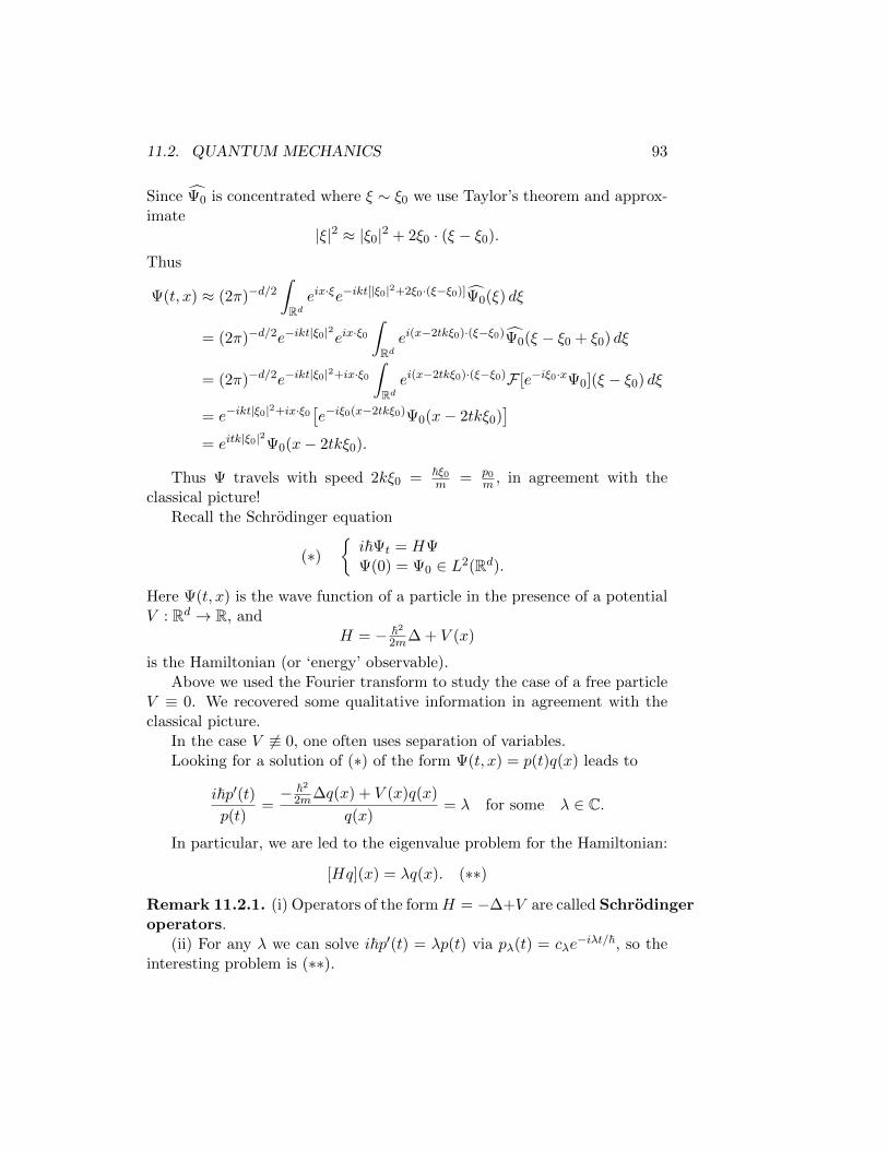
11.2. QUANTUM MECHANICS 93
Since Ψ0 is concentrated where ξ ∼ ξ0 we use Taylor’s theorem and approx-imate
|ξ|2 ≈ |ξ0|2 + 2ξ0 · (ξ − ξ0).
Thus
Ψ(t, x) ≈ (2π)−d/2∫Rdeix·ξe−ikt[|ξ0|
2+2ξ0·(ξ−ξ0)]Ψ0(ξ) dξ
= (2π)−d/2e−ikt|ξ0|2eix·ξ0
∫Rdei(x−2tkξ0)·(ξ−ξ0)Ψ0(ξ − ξ0 + ξ0) dξ
= (2π)−d/2e−ikt|ξ0|2+ix·ξ0
∫Rdei(x−2tkξ0)·(ξ−ξ0)F [e−iξ0·xΨ0](ξ − ξ0) dξ
= e−ikt|ξ0|2+ix·ξ0[e−iξ0(x−2tkξ0)Ψ0(x− 2tkξ0)
]= eitk|ξ0|
2Ψ0(x− 2tkξ0).
Thus Ψ travels with speed 2kξ0 = ~ξ0m = p0
m , in agreement with theclassical picture!
Recall the Schrodinger equation
(∗)i~Ψt = HΨΨ(0) = Ψ0 ∈ L2(Rd).
Here Ψ(t, x) is the wave function of a particle in the presence of a potentialV : Rd → R, and
H = − ~22m∆ + V (x)
is the Hamiltonian (or ‘energy’ observable).Above we used the Fourier transform to study the case of a free particle
V ≡ 0. We recovered some qualitative information in agreement with theclassical picture.
In the case V 6≡ 0, one often uses separation of variables.Looking for a solution of (∗) of the form Ψ(t, x) = p(t)q(x) leads to
i~p′(t)p(t)
=− ~2
2m∆q(x) + V (x)q(x)
q(x)= λ for some λ ∈ C.
In particular, we are led to the eigenvalue problem for the Hamiltonian:
[Hq](x) = λq(x). (∗∗)
Remark 11.2.1. (i) Operators of the formH = −∆+V are called Schrodingeroperators.
(ii) For any λ we can solve i~p′(t) = λp(t) via pλ(t) = cλe−iλt/~, so the
interesting problem is (∗∗).

94 CHAPTER 11. TOPICS FROM PHYSICS
Thus, we have the following
Possible strategy:
• Find the eigenvalues λn and (orthogonal) eigenfunctions qn for (∗∗).
• Show that any Ψ0 ∈ L2 can be written as Ψ0(x) =∑
n cnqn(x).
• Solve (∗) via Ψ(t, x) =∑
n cnpn(t)qn(x).
In some cases, this strategy works beautifully (e.g. infinite well, har-monic oscillator, Coulomb potential, ...). We will do an example in detail inwhat follows.
Note that (L2-)eigenfunctions qn are steady-state solutions to (∗). Ifa particle has state qn then measurement of the energy will yield λn (seebelow). We call such states determinate states for the energy.
Possible issues:
• What if the ‘eigenvalues’ are no longer discrete?
• What if the ‘eigenfunctions’ do not belong to L2?
These issues are really ‘two sides of the same coin’. They are connectedto the “spectral theory” of Schrodinger operators.
To make a long story short, the solution to both issues is to replacethe sums by integrals. The “eigenfunctions” are still useful in building upstates Ψ(t, x) mathematically, but they no longer represent possible statesthemselves.
Before moving on to examples, we discuss some general principles of thequantum mechanics model.
Recall that observables are modelled by hermitian operators Q on L2. IfP is in state Ψ then the expected value of Q is
IE(Q) = 〈Ψ, QΨ〉 =
∫Rd
Ψ(x)[QΨ](x) dx.
(In fact, this definition makes sense for any operator Q.)
If Q is hermitian then
IE(Q) = 〈Ψ, QΨ〉 = 〈QΨ,Ψ〉 = 〈Ψ, QΨ〉 = IE(Q)
Thus IE(Q) ∈ R, as one would expect.
For λ ∈ R we define Q− λ by (Q− λ)Ψ = QΨ− λΨ. If Q is hermitian,so is Q− λ. (check!)

11.2. QUANTUM MECHANICS 95
The variance of Q, defined by σ2Q = IE
((Q− IE(Q))2
), is computed by
σ2Q = 〈Ψ, (Q−IE(Q))2Ψ〉 = 〈(Q−IE(Q))Ψ, (Q−IE(Q))Ψ〉 = ‖(Q−IE(Q))Ψ‖2.
The commutator of two observables Q,Q′ is the operator defined by[Q,Q′] = QQ′ −Q′Q. (Remark: IE([Q,Q′]) is pure imaginary. Check!)
For any state Ψ and any two observables Q,Q′, the uncertainty prin-ciple holds:
σ2Qσ
2Q′ ≥
(− i
2 IE([Q,Q′]))2.
A determinate state for an observable Q is a state Ψ ∈ L2 such thatσ2Q = 0. Equivalently:
(Q− IE(Q))Ψ = 0, or QΨ = IE(Q)Ψ.
That is, determinate states are L2-eigenvectors; the expected values are theeigenvalues.
The set of λ such that Q− λ is not (boundedly) invertible is called thespectrum of Q, denoted σ(Q). The set of λ ∈ σ(Q) with L2-eigenvectorsis the discrete spectrum; the set of λ ∈ σ(Q) without L2-eigenvectors isthe continuous spectrum.
Eigenvalue problem
Consider the eigenvalue problem Hq = λq in three dimensions, where
H = − ~22m∆ + V (x), V : R3 → R.
Let us only consider radial potentials, i.e. V = V (|x|), and let κ = ~22m .
We introduce spherical coordinates:
(x1, x2, x3) = (r sin θ cosφ, r sin θ sinφ, r cos θ)
Then∆ = r−2[∂r(r
2∂r) + (sin θ)−1∂θ(sin θ∂θ) + (sin θ)−2∂φφ].
We use separation of variables and look for a solution of the form
q(r, θ, φ) = a(r)b(θ, φ).
Then Hq = λq becomes
−κr−2[b∂r(r
2ar) + a(sin θ)−1∂θ(sin θbθ) + (sin θ)−2bφφ]
+ V (r)ab = λab.

96 CHAPTER 11. TOPICS FROM PHYSICS
Rearranging and multiplying by r2
κab :
1a∂r(r
2ar)− r2
κ [V (r)− λ]︸ ︷︷ ︸radial equation
= −1b [(sin θ)
−1∂θ(sin θbθ) + (sin θ)−2bφφ]︸ ︷︷ ︸angular equation
= µκ
for some µ ∈ C.We now study the angular equation, which does not depend on V
(since V is radial).We use separation of variables (again) and look for a solution of the form
b(θ, φ) = f(θ)g(φ).
Multiplying by − sin2 θ and rearranging yields
1f sin θ∂θ(sin θf
′(θ)) + µ sin2 θ = −1gg′′(φ) = α
for some α ∈ C.We solve g′′ = −αg via g(φ) = e±i
√αφ.
Since we want g(φ+ 2π) = g(φ), we need e2πi√α = 1, and hence
√α = m for some m ∈ 0 ∪ N.
Rearranging the f equation gives
∂θ(sin θf ′)sin θ + [µ− m2
sin2 θ]f = 0.
If we define z = cos θ and suppose f(θ) = h(z), this becomes(1− z2)h′′ − 2zh′ + [µ− m2
1−z2 ]h = 0 (∗)m (check!)
h(z) finite at z = ±1.
The case m = 0 is Legendre’s equation; the others are associated Leg-endre equations.
We first solve (∗)0. We will generate solutions to (∗)m below.We employ the power series method and write
h(z) =∞∑k=0
ckzk, h′(z) =
∞∑k=0
kckzk−1, h′′(z) =
∞∑k=0
k(k − 1)ckzk−2.
Then (∗)0 becomes (after rearranging)
∞∑k=0
(k + 2)(k + 1)ck+2 − [k(k + 1)− µ]ck zk = 0.

11.2. QUANTUM MECHANICS 97
Thus h is a solution provided
ck+2 = k(k+1)−µ(k+2)(k+1)ck, c0, c1 arbitrary.
Note that if µ = `(`+1) for some ` ∈ 0∪N then c`+2 = c`+4 = · · · = 0.Thus for µ = `(`+1) we can (by choosing c0 = 0 or c1 = 0) find a degree
` polynomial solution h`0, where h`0 is odd for ` odd and even for ` even.(These are the Legendre polynomials.)
If µ is not of this form then solutions exist but are badly behaved atz = 1 or z = −1.
We turn to (∗)m for m > 0. Recall µ = `(`+ 1), ` ∈ 0 ∪ N.As h`0 solves (∗)0 then the function h`m = ∂m
∂zmh`0 solves
(1− z2)h′′m − 2(m+ 1)zh′m + [`(`+ 1)−m(m+ 1)]hm = 0,
and it follows that the associated Legendre function
H`m := (1− z2)m/2h`m
satisfies (∗)m. (Check these!)Note that we should restrict to m ≤ ` to guarantee h`m 6= 0 (recall h`0 is
a degree ` polynomial).Conclusion. For ` ∈ 0 ∪ N and m ∈ 0, . . . , ` we can solve the
angular equation with µ = `(`+ 1) with
b`±m(θ, φ) = e±imφH`m(cos(θ)).
These functions (after normalization) are called spherical harmonics.The number ` is called the azimuthal quantum number, while m is
called the magnetic quantum number.(The spherical harmonics are determinate states for angular momentum.)We return to the eigenvalue problem Hq = λq, where
H = −κ∆ + V (x),
with κ = ~22m and V : R3 → R radial.
Employing spherical coordinates and looking for solutions of the form
q(r, θ, φ) = a(r)b(θ, φ)
led to the “angular equation” for b, which we solved via spherical harmonicsb`±m, and the radial equation r2a′′ + 2ra′ − r2
κ [V (r)− λ]a = `(`+ 1)a
` ∈ 0 ∪ N, limr→∞ a(r) = 0,

98 CHAPTER 11. TOPICS FROM PHYSICS
to which we turn now.Introducing the function u(r) = r a(r) and rearranging yields
u′′ − 1κ [V (r)− λ]u = `(`+1)
r2u
− κu′′ + [V (r) + κ `(`+1)r2
]u = λu (∗∗)
This is the eigenvalue problem for a one-dimensional Schrodinger oper-ator on (0,∞) with potential
V (r) = V (r) + κ `(`+1)r2
.
Example. QM models an electron in orbit around a proton with theCoulomb potential:
V (x) = − e2
4πε01|x| , i.e. V (r) = − e2
4πε01r .
where e is the charge of the electron and ε0 is the permittivity of vacuum(in SI units).
We are interested in the discrete spectrum, corresponding to “boundstates”. Eigenvalues are real (they are expected values of the Hamiltonian),and because limr→∞ V (r) = 0 one can show they are contained in (−∞, 0).(Beyond the scope of this course.)
With the Coulomb potential, (∗) becomes
u′′ = c2[1− e2
4cπκε01cr + `(`+1)
(cr)2
]u,
where c2 = −λκ . We define
ρ = cr, ddρ = 1
cddr , u(r) = w(ρ), ρ0 = e2
4cπκε0.
Then
w′′ = [1− ρ0ρ + `(`+1)
ρ2]w, ′ = d
dρ (∗∗)
We revisit the power series method, but with a twist.First, as ρ→∞ this ODE resembles w′′ = w, whose (decaying) solution
is like e−ρ.Next, as ρ→ 0 this ODE resembles w′′ = `(`+1)
ρ2w, whose (well-behaved)
solution is like ρ`+1.Thus we look for w of the form
w(ρ) = ρ`+1e−ρv(ρ).

11.2. QUANTUM MECHANICS 99
We compute
w′ = ρ`e−ρ[ρv′ + (`+ 1− ρ)v],
w′′ = ρ`e−ρρv′′ + 2[`+ 1− ρ]v′ + [−2`− 2 + ρ+ `(`+1)
ρ ]v.
Then (∗∗) becomes
ρv′′ + 2(`+ 1− ρ)v′ + [ρ0 − 2(`+ 1)]v = 0.
Now we try to write
v(ρ) =∞∑k=0
ckρk, v′(ρ) =
∞∑k=0
kckρk−1, v′′(ρ) =
∞∑k=0
k(k − 1)ckρk−2.
Inserting this into the ODE yields∑k(k + 1)ck+1 + 2(`+ 1)(k + 1)ck+1 − 2kck + [ρ0 − 2(`+ 1)]ck
ρk = 0.
Thus we should take
ck+1 = 2(k+`+1)−ρ0(k+1)(k+2`+2)ck, c0 arbitrary.
Now if ρ0 = 2(k∗ + `+ 1) for some k∗ ∈ 0 ∪ N, then ck∗+1 = ck∗+2 =· · · = 0.
(If ρ0 is not of this form it turns out that the solution is badly behaved.)In this case we call n := k∗ + `+ 1 the principle quantum number.We denote the degree n − ` − 1 polynomial solution by v`n(ρ) (called a
Laguerre polynomial).Then
u`n(r) = w`n(ρ) = ρ`+1e−ρv`n(ρ), ρ = cnr =
√|λn|κ r
a`n(r) = r`e−cnrv`n(cnr),
where we can unravel the constants in
2n = ρ0 = e2
4cnπκε0, c2
n = −λnκ , κ = ~2
2me
to compute λn. In particular:Conclusion. The determinate energies of the hydrogen atom are
λn = −[(
e2
4πε0
)2 me2~2]
1n2 for n ∈ N,
and for each n there are 2n2 (orthogonal) eigenvectors
q`n,±m(r, θ, φ) = a`n(r)b`±m(θ, φ),
where ` ∈ 0, 1, . . . , n− 1, m ∈ 0, . . . , `.

100 CHAPTER 11. TOPICS FROM PHYSICS
11.3 Electromagnetism
In classical electromagnetism, the electric field E(t, x) ∈ R3 and mag-netic field B(t, x) ∈ R3 have the following interpretation: the force on aparticle with charge q and velocity v is
F = q(E + v ×B),
while the behavior of E,B is determined by Maxwell’s equations:∇ · E = 1
ε0ρ (Gauss’s law)
∇ ·B = 0∇× E + ∂tB = 0 (Faraday’s law)∇×B − µ0ε0∂tE = µ0J, (Ampere’s law, with Maxwell’s correction)
where ρ = ρ(t, x) ∈ R is the charge density, J = J(t, x) ∈ R3 is the currentdensity, ε0 is the permittivity of vacuum, and µ0 is the permeability ofvacuum.
Using Gauss’s law and Ampere’s law we can also deduce the continuityequation for ρ and J :
∂tρ+∇ · J = 0.
Consider a region of space in which there is no charge or current (ρ, J =0). Note
∇× (∇× E) = ∇× (−∂tB) = −∂t(∇×B) = −∂t(µ0ε0∂E∂t ) = −µ0ε0∂ttE
and
∇× (∇× E) = −∆E +∇(∇ · E) = −∆E.
Rearranging yields
µ0ε0∂ttE −∆E = 0.
Similarly (computing ∇× (∇×B) we find
µ0ε0∂ttB −∆B = 0.
Conclusion. In regions of spacetime with no charge or current, the com-ponents of E and B satisfy the wave equation, with speed of propagationequal to c = 1√
µ0ε0(which happens to be the speed of light in vacuum).
One can also study Maxwell’s equations using the potential formula-tion.

11.3. ELECTROMAGNETISM 101
Lemma 11.3.1 (Helmholtz Theorem). If G is a (sufficiently nice, decaying)vector field then
G = −∇g +∇×H
for some scalar field g and vector field H.
Corollary. If ∇ · G = 0 then G = ∇ × H and if ∇ × G = 0 thenG = −∇g.
We apply these results to E and B. In particular, ∇ ·B = 0 implies
B = ∇×A for some magnetic potential A.
Combining this with Faraday’s law yields ∇× (E + ∂tA) = 0, so that
E + ∂tA = −∇V for some electric potential V.
Plugging this into Gauss’s law yields
−∆V = ∇ · E + ∂t∇ ·A = 1ε0ρ+ ∂t∇ ·A.
(Note if ∂tB = 0 then ∂tA = 0 and this reduces to Coulomb’s law fromelectrostatics.)
Using Ampere’s law and B = ∇×A yields
∇× (∇×A) + µ0ε0∂t[∂tA+∇V ] = µ0J
=⇒ µ0ε0∂ttA−∆A+∇[∇ ·A+ µ0ε0∂tV ] = µ0J.
Thus, given ρ and J the equations for A and V are:
(∗)
−∆V − ∂t∇ ·A = 1
ε0ρ
µ0ε0∂ttA−∆A+∇(∇ ·A+ µ0ε0∂tV ) = µ0J.
This looks horrible.Key observation. (gauge invariance) Let λ(t, x) be a scalar function.
If we defineA = A+∇λ, V = V − ∂tλ,
then A and V yield the same fields E,B. Indeed,
∇× A = ∇×A+ 0 = B,
∂tA+∇V = ∂tA+ ∂t∇λ+∇V − ∂t∇λ = ∂tA+∇V = −E.
Thus we have some freedom in how we choose A, V , which may simplify (∗).

102 CHAPTER 11. TOPICS FROM PHYSICS
Example 1. If we choose A to satisfy the Coulomb gauge condition
∇ ·A = 0,
then (∗) becomes −∆V = 1
ε0ρ,
µ0ε0∂ttA−∆A = µ0J − µ0ε0∂t∇V.
Example 2. If we choose A to satisfy the Lorentz gauge condition
∇ ·A = −µ0ε0∂tV,
then (∗) becomes µ0ε0∂ttV −∆V = 1
ε0ρ,
µ0ε0∂ttA−∆A = µ0J.
Once again we get the (inhomogeneous) wave equation, with speed of prop-agation equal to c.
It is generally accepted that the laws of physics should be invariant underspace translation, space rotation, and time translation.
The laws of Newtonian physics (and its descendants) are also invariantunder Galilean transformations, such as
(t, x1, x2, x3) 7→ (t, x1 − vt, x2, x3) for v ∈ R.
The laws of electromagnetism are not. Instead, they are invariant underLorentz transformations, such as
(t, x1, x2, x3) 7→(t− (vx1/c
2)√1− (v/c)2
,x1 − vt√1− (v/c)2
, x2, x3
), v ∈ R, |v| < c.
(These arise when one takes as an axiom that the speed of light is thesame for any inertial observer.)
Einstein’s insight was that the laws of mechanics should be modifiedto be invariant under Lorentz transformations. (This led to the theory ofrelativity.)
11.4 Elementary Particles
The QM model improves the classical model at microscopic length scales.

11.4. ELEMENTARY PARTICLES 103
Relativity substitutes Galilean invariance with Lorentz invariance, whichimproves the classical mechanics model at high velocities.
The QM model still respects Galilean invariance.
The modification of QM to a model that respects Lorentz invariance isknown as relativistic quantum mechanics.
Classical mechanics: (Lagrangian version) If P is a particle of (rest)mass m in the presence of a potential V , we define the Lagrangian by
L(x, v) = 12mv · v − V (x).
The momentum is given by p = ∇vL(x, x) and p = −∇V (x) is the Euler–Lagrange equation for the functional
∫L(x(t), x(t)) dt. The energy is given
by
H = p · x− L(x, x) = 12m |p|
2 + V (x).
Relativistic mechanics: (for free particle, i.e. V ≡ 0) Define theLagrangian by
L(x, v) = −mc2√
1− |v|2/c2.
• analogue of arc length integral, but with Lorentz invariance
• constant mc2 chosen to recover classical mechanics if |v| c (cf.Taylor expansion)
The momentum is
p = ∇vL(x, x) = mx√1−|x|2/c2
,
and p = 0 is the Euler–Lagrange equation for the functional∫L(x(t), x(t)) dt.
The energy is given by
H = p · x− L(x, x) = c√|p|2 +m2c2.
Quantisation: To get the “quantum version” we make the followingreplacements:
i~∂t = H, p = −i~∇.
Formally this becomes
i~∂t = c√
(−i~∇) · (−i~∇) +m2c2 = c√−~2∆ +m2c2.
Squaring both sides:
−~2∂tt = c2(−~2∆ +m2c2).

104 CHAPTER 11. TOPICS FROM PHYSICS
Thus we derive the Klein–Gordon equation
1c2∂ttΨ−∆Ψ + m2c2
~2 Ψ = 0. (KG)
Evidently squaring loses something vital, because KG does not accuratelymodel the electron.
(However, it can be used to accurately model “spinless pions”.)Dirac equation. The idea of Dirac was to use an equation of the form
i~∂tΨ = HΨ,
where H was a first order differential operator satisfying
H2 = c2[− ~2∆ +m2c2
]. (∗)
WritingH = −ic~(α1∂1 + α2∂2 + α3∂3) +mc2β
one finds
H2 = −c2~2[3∑j=1
α2j∂
2j + (α1α2 + α2α1)∂1∂2 + (α1α3 + α3α1)∂1∂3 + (α2α3 + α3α2)∂2∂3)]
− ic3~m[(α1β + βα1)∂1 + (α2β + βα2)∂2 + (α3β + βα3)∂3] +m2c4β2.
Imposing (∗), one finds the following conditions need to be satisfied:
αjαk + αkαj = 0 (j 6= k),
αkβ + βαk = 0,
α2j = 1, β2 = 1.
While this is impossible to achieve if αj , β ∈ C, it is possible if they arematrices!
This is now a purely algebraic problem, a solution to which is given bythe following 4× 4 matrices:
αj =
(0 σjσj 0
), β =
(I2 00 −I2
),
where I2 is the 2× 2 identity matrix and σj are the 2× 2 Pauli matricesare defined by
σ1 =
(0 11 0
), σ2 =
(0 −ii 0
), σ3 =
(1 00 −1
).
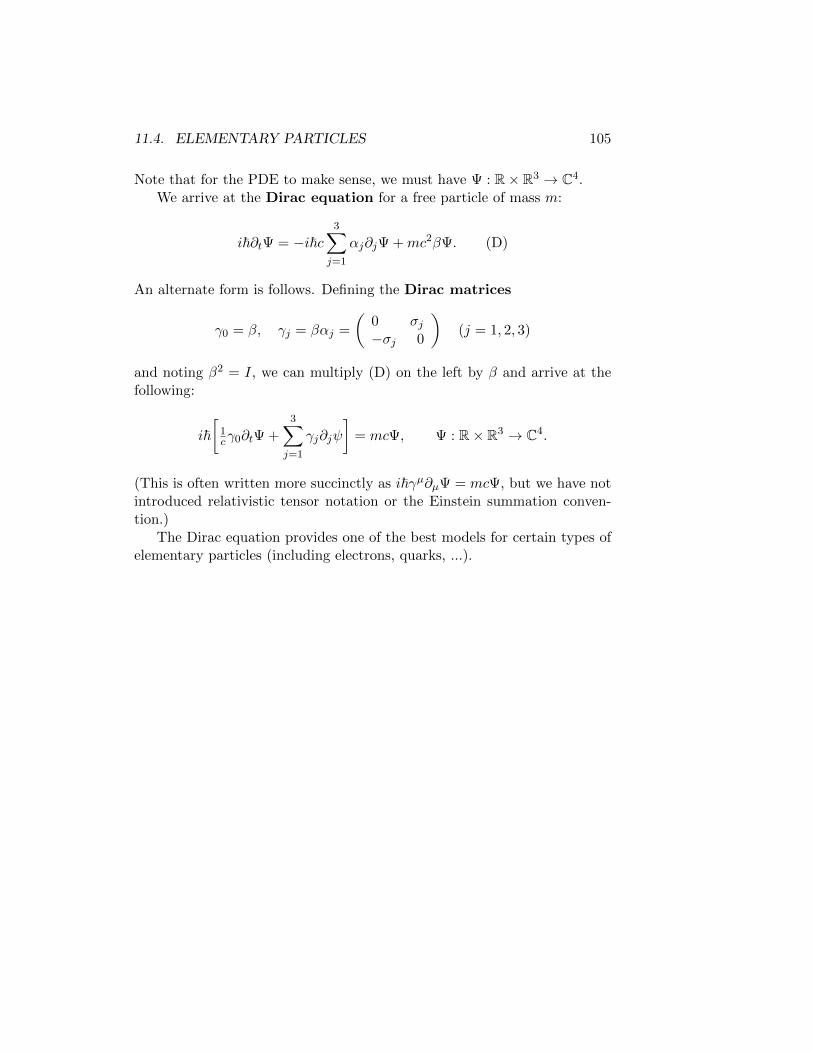
11.4. ELEMENTARY PARTICLES 105
Note that for the PDE to make sense, we must have Ψ : R× R3 → C4.We arrive at the Dirac equation for a free particle of mass m:
i~∂tΨ = −i~c3∑j=1
αj∂jΨ +mc2βΨ. (D)
An alternate form is follows. Defining the Dirac matrices
γ0 = β, γj = βαj =
(0 σj−σj 0
)(j = 1, 2, 3)
and noting β2 = I, we can multiply (D) on the left by β and arrive at thefollowing:
i~[
1cγ0∂tΨ +
3∑j=1
γj∂jψ
]= mcΨ, Ψ : R× R3 → C4.
(This is often written more succinctly as i~γµ∂µΨ = mcΨ, but we have notintroduced relativistic tensor notation or the Einstein summation conven-tion.)
The Dirac equation provides one of the best models for certain types ofelementary particles (including electrons, quarks, ...).