jan ubøe introductory statistics for business and economics
TRANSCRIPT

Springer Texts in Business and Economics
Introductory Statistics forBusiness and EconomicsTheory, Exercises and Solutions
Jan Ubøe

Springer Texts in Business and Economics

More information about this series at http://www.springer.com/series/10099

Jan Ubøe
Introductory Statisticsfor Businessand EconomicsTheory, Exercises and Solutions
123

Jan UbøeDepartment of Businessand Management ScienceNorwegian School of EconomicsBergen, Norway
ISSN 2192-4333 ISSN 2192-4341 (electronic)Springer Texts in Business and EconomicsISBN 978-3-319-70935-2 ISBN 978-3-319-70936-9 (eBook)https://doi.org/10.1007/978-3-319-70936-9
Library of Congress Control Number: 2017960422
© Springer International Publishing AG 2017Revised translation from the Norwegian language edition: Statistikk for økonomifag, c� GyldendalNorsk Forlag AS 2004, 2007, 2008, 2012, 2015, All Rights Reserved.This work is subject to copyright. All are reserved by the Publisher, whether the whole or part of thematerial is concerned, specifically the rights of translation, reprinting, reuse of illustrations, recitation,broadcasting, reproduction on microfilms or in any other physical way, and transmission or informationstorage and retrieval, electronic adaptation, computer software, or by similar or dissimilar methodologynow known or hereafter developed.The use of general descriptive names, registered names, trademarks, service marks, etc. in this publicationdoes not imply, even in the absence of a specific statement, that such names are exempt from the relevantprotective laws and regulations and therefore free for general use.The publisher, the authors and the editors are safe to assume that the advice and information in this bookare believed to be true and accurate at the date of publication. Neither the publisher nor the authors orthe editors give a warranty, express or implied, with respect to the material contained herein or for anyerrors or omissions that may have been made. The publisher remains neutral with regard to jurisdictionalclaims in published maps and institutional affiliations.
Printed on acid-free paper
This Springer imprint is published by Springer NatureThe registered company is Springer International Publishing AGThe registered company address is: Gewerbestrasse 11, 6330 Cham, Switzerland

Electronic Supplementary Material The online version of this book (https://doi.org/10.1007/978-3-319-70936-9) contains supplementary material, which isavailable to authorized users.

To Bernt Øksendal who taught me everythingI know about probability theory, and JosteinLillestøl who taught me all I know aboutstatistics.

Preface
This book has a traditional yet modern approach to teaching statistics. Whencombined with my newly developed system for collaborate learning, it is well suitedfor modern teaching formats like flipped classrooms, but it also serves well if thelecturer prefers a more traditional approach.
My system for collaborative learning can be downloaded from the book’swebsite. The files are available for lecturers only and contain supplementaryproblems with separate solution files for each chapter. The system is particularlytargeted at the average student, and my own students like it a lot. Many of themreport back that it is great fun!
I strongly believe that the best way to learn statistics is by doing. As aconsequence of this, the main body of each chapter is shorter than what has beencommon. The idea is to let students work with exercises as soon as possible, andmost of my efforts have been invested in developing interesting, relevant, and tosome extent challenging exercises. The exercises are divided into two parts. Theexercises in the first part of each chapter are straightforward. From my experienceeven excellent students struggle a lot when they study new material, and to quicklygain momentum it is necessary that the first few exercises are very simple. Onlywhen the basic framework is in place is it time to move on to more interestingproblems.
As a motivation for further studies, students need to see interesting applicationsfrom the start. Throughout the book I have picked bits and pieces of theory thatare usually taught on a much higher level and organized them such that they aresuitable for beginners. These exercises are all equipped with a short label providinglecturers with hints of what type of theory/issues they discuss. My approach ismuch appreciated by students, who at an early stage see that statistics is essential toany serious study of economics. In the beginning of the book there are only a fewsuch problems, but as we learn more there is more room for relevant applications.Some of these exercises are challenging, but complexity was never a goal. Nontrivialproblems tend to have nontrivial solutions, but my intent is to present theory in thesimplest possible way. The labeled exercises are not always difficult. Indeed, someof the exercises that have given me the most pleasure have a very simple solution.
My book is one of the very few that makes some use of nonlinear theory, inparticular theory related to logarithms and exponential functions. I have often heard
ix

x Preface
that such theory should be avoided since it is too difficult for students, but from myexperience this is not true. Why at all do we teach beginner courses in mathematics,if none of this theory is to be used later? To keep things simple, however, I havemainly included computations that would have been considered straightforwardwhen encountered in a beginner course in mathematics.
Many textbooks now focus on software applications. Statistical software is anindispensable tool once the theory is understood. Very often, however, the users donot properly understand the limitations of the theory, and misinterpretations are alltoo common. The problem is increasing at all levels in science. I refer to and usesoftware applications only sparingly throughout the book. To hedge various formsof malpractice, I discuss several pitfalls I have come across, in the exercises.
A lot of people have contributed to this book, and I will mention only a few. Firstof all I wish to thank all my former students at Norwegian School of Economics.These students have been my fortune in life, and few of the exercises in this bookwould ever materialized had it not been for such abundance of ability and talent.Second I should thank Per Oscar Andersen for his never ending encouragement forthe Norwegian edition and Arve Michaelsen for endless hours of typesetting andpreparation of figures. Bernt Øksendal deserves a special thanks for teaching meprobability theory and for being a constant source of inspiration. Jostein Lillestøldeserves a special thanks for teaching me statistics, and Jostein’s brilliant textbookin statistics has no doubt served as a template for my own presentation. JonasAndersson deserves a special thanks for the many times he clarified points I didnot fully understand.
Last I wish to thank the editorial staff at Springer for a very positive, swift, andprofessional handling of my manuscript.
Bergen, Norway Jan UbøeOctober 2017

Contents
1 Descriptive Statistics . . . . . . . . . . . . . . . . . . . . . . . . . . . . . . . . . . . . . . . . . . . . . . . . . . . . . . . 11.1 Population and Samples . . . . . . . . . . . . . . . . . . . . . . . . . . . . . . . . . . . . . . . . . . . . 11.2 The Median.. . . . . . . . . . . . . . . . . . . . . . . . . . . . . . . . . . . . . . . . . . . . . . . . . . . . . . . . . 41.3 Quartiles and Mode . . . . . . . . . . . . . . . . . . . . . . . . . . . . . . . . . . . . . . . . . . . . . . . . . 61.4 Relative Frequency and Histograms . . . . . . . . . . . . . . . . . . . . . . . . . . . . . . . 71.5 The Mean .. . . . . . . . . . . . . . . . . . . . . . . . . . . . . . . . . . . . . . . . . . . . . . . . . . . . . . . . . . . 81.6 Sample Variance and Sample Standard Deviation.. . . . . . . . . . . . . . . . 101.7 Sample Covariance and Coefficient of Variation . . . . . . . . . . . . . . . . . . 121.8 Using Excel . . . . . . . . . . . . . . . . . . . . . . . . . . . . . . . . . . . . . . . . . . . . . . . . . . . . . . . . . 171.9 Summary of Chap. 1 . . . . . . . . . . . . . . . . . . . . . . . . . . . . . . . . . . . . . . . . . . . . . . . . 181.10 Problems for Chap. 1 . . . . . . . . . . . . . . . . . . . . . . . . . . . . . . . . . . . . . . . . . . . . . . . 20
2 Probability . . . . . . . . . . . . . . . . . . . . . . . . . . . . . . . . . . . . . . . . . . . . . . . . . . . . . . . . . . . . . . . . . . . 272.1 Sample Space . . . . . . . . . . . . . . . . . . . . . . . . . . . . . . . . . . . . . . . . . . . . . . . . . . . . . . . 272.2 Probability .. . . . . . . . . . . . . . . . . . . . . . . . . . . . . . . . . . . . . . . . . . . . . . . . . . . . . . . . . . 29
2.2.1 Events . . . . . . . . . . . . . . . . . . . . . . . . . . . . . . . . . . . . . . . . . . . . . . . . . . . . 302.2.2 Uniform Probability . . . . . . . . . . . . . . . . . . . . . . . . . . . . . . . . . . . . . 302.2.3 Set Theory .. . . . . . . . . . . . . . . . . . . . . . . . . . . . . . . . . . . . . . . . . . . . . . . 312.2.4 Computing Probabilities . . . . . . . . . . . . . . . . . . . . . . . . . . . . . . . . . 332.2.5 The Negation Principle . . . . . . . . . . . . . . . . . . . . . . . . . . . . . . . . . . 35
2.3 Summary of Chap. 2 . . . . . . . . . . . . . . . . . . . . . . . . . . . . . . . . . . . . . . . . . . . . . . . . 352.4 Problems for Chap. 2 . . . . . . . . . . . . . . . . . . . . . . . . . . . . . . . . . . . . . . . . . . . . . . . 36
3 Combinatorics . . . . . . . . . . . . . . . . . . . . . . . . . . . . . . . . . . . . . . . . . . . . . . . . . . . . . . . . . . . . . . 413.1 Counting Combinations . . . . . . . . . . . . . . . . . . . . . . . . . . . . . . . . . . . . . . . . . . . . 41
3.1.1 Ordered Selections . . . . . . . . . . . . . . . . . . . . . . . . . . . . . . . . . . . . . . . 423.1.2 Unordered Choices Without Replacement . . . . . . . . . . . . . . 443.1.3 Combinatorial Probabilities . . . . . . . . . . . . . . . . . . . . . . . . . . . . . 47
3.2 Summary of Chap. 3 . . . . . . . . . . . . . . . . . . . . . . . . . . . . . . . . . . . . . . . . . . . . . . . . 493.3 Problems for Chap. 3 . . . . . . . . . . . . . . . . . . . . . . . . . . . . . . . . . . . . . . . . . . . . . . . 49
xi

xii Contents
4 Conditional Probability . . . . . . . . . . . . . . . . . . . . . . . . . . . . . . . . . . . . . . . . . . . . . . . . . . . . 554.1 Conditional Probability . . . . . . . . . . . . . . . . . . . . . . . . . . . . . . . . . . . . . . . . . . . . . 55
4.1.1 Computing Conditional Probabilities . . . . . . . . . . . . . . . . . . . 574.1.2 Splitting the Sample Space . . . . . . . . . . . . . . . . . . . . . . . . . . . . . . 594.1.3 Probability Trees . . . . . . . . . . . . . . . . . . . . . . . . . . . . . . . . . . . . . . . . . 60
4.2 Subjective Probabilities . . . . . . . . . . . . . . . . . . . . . . . . . . . . . . . . . . . . . . . . . . . . . 644.3 Independence.. . . . . . . . . . . . . . . . . . . . . . . . . . . . . . . . . . . . . . . . . . . . . . . . . . . . . . . 654.4 Summary of Chap. 4 . . . . . . . . . . . . . . . . . . . . . . . . . . . . . . . . . . . . . . . . . . . . . . . . 664.5 Problems for Chap. 4 . . . . . . . . . . . . . . . . . . . . . . . . . . . . . . . . . . . . . . . . . . . . . . . 67
5 Random Variables, Mean, and Variance . . . . . . . . . . . . . . . . . . . . . . . . . . . . . . . . . 755.1 Random Variables. . . . . . . . . . . . . . . . . . . . . . . . . . . . . . . . . . . . . . . . . . . . . . . . . . . 755.2 Expectation .. . . . . . . . . . . . . . . . . . . . . . . . . . . . . . . . . . . . . . . . . . . . . . . . . . . . . . . . . 80
5.2.1 Computing Expectations . . . . . . . . . . . . . . . . . . . . . . . . . . . . . . . . 825.2.2 General Expectations and Variance . . . . . . . . . . . . . . . . . . . . . 83
5.3 Some Simple Facts About Option Pricing . . . . . . . . . . . . . . . . . . . . . . . . . 855.3.1 Hedging Portfolios . . . . . . . . . . . . . . . . . . . . . . . . . . . . . . . . . . . . . . . 86
5.4 Summary of Chap. 5 . . . . . . . . . . . . . . . . . . . . . . . . . . . . . . . . . . . . . . . . . . . . . . . . 885.5 Problems for Chap. 5 . . . . . . . . . . . . . . . . . . . . . . . . . . . . . . . . . . . . . . . . . . . . . . . 89
6 Joint Distributions . . . . . . . . . . . . . . . . . . . . . . . . . . . . . . . . . . . . . . . . . . . . . . . . . . . . . . . . . . 976.1 Simultaneous Distributions . . . . . . . . . . . . . . . . . . . . . . . . . . . . . . . . . . . . . . . . . 976.2 Covariance . . . . . . . . . . . . . . . . . . . . . . . . . . . . . . . . . . . . . . . . . . . . . . . . . . . . . . . . . . 103
6.2.1 An Alternative Formula for the Covariance . . . . . . . . . . . . 1046.2.2 Sums of Random Variables . . . . . . . . . . . . . . . . . . . . . . . . . . . . . . 105
6.3 Summary of Chap. 6 . . . . . . . . . . . . . . . . . . . . . . . . . . . . . . . . . . . . . . . . . . . . . . . . 1066.4 Problems for Chap. 6 . . . . . . . . . . . . . . . . . . . . . . . . . . . . . . . . . . . . . . . . . . . . . . . 106
7 Basic Probability Distributions . . . . . . . . . . . . . . . . . . . . . . . . . . . . . . . . . . . . . . . . . . . 1137.1 The Indicator Distribution . . . . . . . . . . . . . . . . . . . . . . . . . . . . . . . . . . . . . . . . . . 1137.2 The Binomial Distribution . . . . . . . . . . . . . . . . . . . . . . . . . . . . . . . . . . . . . . . . . . 1147.3 The Hypergeometric Distribution . . . . . . . . . . . . . . . . . . . . . . . . . . . . . . . . . . 1187.4 The Poisson Distribution . . . . . . . . . . . . . . . . . . . . . . . . . . . . . . . . . . . . . . . . . . . 1227.5 The Normal Distribution . . . . . . . . . . . . . . . . . . . . . . . . . . . . . . . . . . . . . . . . . . . 124
7.5.1 The General Normal Distribution . . . . . . . . . . . . . . . . . . . . . . . 1277.5.2 Standardizing Random Variables . . . . . . . . . . . . . . . . . . . . . . . 1287.5.3 The Central Limit Theorem . . . . . . . . . . . . . . . . . . . . . . . . . . . . . 1297.5.4 Integer Correction. . . . . . . . . . . . . . . . . . . . . . . . . . . . . . . . . . . . . . . . 1357.5.5 Normal Approximation of Hypergeometric
and Poisson Distributions . . . . . . . . . . . . . . . . . . . . . . . . . . . . . . . 1367.5.6 Summing Normal Distributions . . . . . . . . . . . . . . . . . . . . . . . . . 1377.5.7 Applications to Option Pricing . . . . . . . . . . . . . . . . . . . . . . . . . . 138
7.6 Summary of Chap. 7 . . . . . . . . . . . . . . . . . . . . . . . . . . . . . . . . . . . . . . . . . . . . . . . . 1407.7 Problems for Chap. 7 . . . . . . . . . . . . . . . . . . . . . . . . . . . . . . . . . . . . . . . . . . . . . . . 142

Contents xiii
8 Estimation . . . . . . . . . . . . . . . . . . . . . . . . . . . . . . . . . . . . . . . . . . . . . . . . . . . . . . . . . . . . . . . . . . . 1598.1 Estimation .. . . . . . . . . . . . . . . . . . . . . . . . . . . . . . . . . . . . . . . . . . . . . . . . . . . . . . . . . . 159
8.1.1 Estimators . . . . . . . . . . . . . . . . . . . . . . . . . . . . . . . . . . . . . . . . . . . . . . . . 1608.1.2 Reporting Estimates . . . . . . . . . . . . . . . . . . . . . . . . . . . . . . . . . . . . . 1628.1.3 The Measurement Model . . . . . . . . . . . . . . . . . . . . . . . . . . . . . . . . 162
8.2 Confidence Intervals . . . . . . . . . . . . . . . . . . . . . . . . . . . . . . . . . . . . . . . . . . . . . . . . 1648.2.1 Constructing Confidence Intervals . . . . . . . . . . . . . . . . . . . . . . 1648.2.2 The t-Distribution . . . . . . . . . . . . . . . . . . . . . . . . . . . . . . . . . . . . . . . . 166
8.3 The Lottery Model . . . . . . . . . . . . . . . . . . . . . . . . . . . . . . . . . . . . . . . . . . . . . . . . . . 1698.4 Summary of Chap. 8 . . . . . . . . . . . . . . . . . . . . . . . . . . . . . . . . . . . . . . . . . . . . . . . . 1718.5 Problems for Chap. 8 . . . . . . . . . . . . . . . . . . . . . . . . . . . . . . . . . . . . . . . . . . . . . . . 172
9 Hypothesis Testing . . . . . . . . . . . . . . . . . . . . . . . . . . . . . . . . . . . . . . . . . . . . . . . . . . . . . . . . . . 1779.1 Basic Ideas . . . . . . . . . . . . . . . . . . . . . . . . . . . . . . . . . . . . . . . . . . . . . . . . . . . . . . . . . . 1779.2 Motivation .. . . . . . . . . . . . . . . . . . . . . . . . . . . . . . . . . . . . . . . . . . . . . . . . . . . . . . . . . . 1799.3 General Principles for Hypothesis Testing. . . . . . . . . . . . . . . . . . . . . . . . . 1819.4 Designing Statistical Tests. . . . . . . . . . . . . . . . . . . . . . . . . . . . . . . . . . . . . . . . . . 183
9.4.1 One-Sided and Two-Sided Tests . . . . . . . . . . . . . . . . . . . . . . . . 1879.4.2 Confidence Intervals and Hypothesis Testing . . . . . . . . . . 1889.4.3 P-Value . . . . . . . . . . . . . . . . . . . . . . . . . . . . . . . . . . . . . . . . . . . . . . . . . . . 189
9.5 Summary of Chap. 9 . . . . . . . . . . . . . . . . . . . . . . . . . . . . . . . . . . . . . . . . . . . . . . . . 1929.6 Problems for Chap. 9 . . . . . . . . . . . . . . . . . . . . . . . . . . . . . . . . . . . . . . . . . . . . . . . 192
10 Commonly Used Tests . . . . . . . . . . . . . . . . . . . . . . . . . . . . . . . . . . . . . . . . . . . . . . . . . . . . . . 20110.1 Testing Binomial Distributions . . . . . . . . . . . . . . . . . . . . . . . . . . . . . . . . . . . . . 20110.2 t-Test for Expected Value . . . . . . . . . . . . . . . . . . . . . . . . . . . . . . . . . . . . . . . . . . . 20310.3 Comparing Two Groups . . . . . . . . . . . . . . . . . . . . . . . . . . . . . . . . . . . . . . . . . . . . 206
10.3.1 t-Test for Comparison of Expectationin Two Groups . . . . . . . . . . . . . . . . . . . . . . . . . . . . . . . . . . . . . . . . . . . 206
10.3.2 t-Test Executed in Excel . . . . . . . . . . . . . . . . . . . . . . . . . . . . . . . . . 21010.3.3 t-Test for Comparison of Expectation in Two
Groups, Paired Observations . . . . . . . . . . . . . . . . . . . . . . . . . . . . 21010.3.4 t-Test with Paired Observations Executed in Excel . . . . 214
10.4 Wilcoxon’s Distribution Free Tests . . . . . . . . . . . . . . . . . . . . . . . . . . . . . . . . 21510.4.1 The Wilcoxon Signed-Rank Test . . . . . . . . . . . . . . . . . . . . . . . . 21810.4.2 Comparison of t-Tests and Wilcoxon Test . . . . . . . . . . . . . . 221
10.5 The U-Test for Comparison of Success Probabilities . . . . . . . . . . . . . 22110.6 Chi-Square Test for Goodness-of-Fit . . . . . . . . . . . . . . . . . . . . . . . . . . . . . . 224
10.6.1 The Chi-Square Test Executed in Excel . . . . . . . . . . . . . . . . 22610.7 The Chi-Square Test for Independence . . . . . . . . . . . . . . . . . . . . . . . . . . . . 227
10.7.1 The Chi-Square Test for Independence Executedin Excel . . . . . . . . . . . . . . . . . . . . . . . . . . . . . . . . . . . . . . . . . . . . . . . . . . . 230
10.8 Summary of Chap. 10. . . . . . . . . . . . . . . . . . . . . . . . . . . . . . . . . . . . . . . . . . . . . . . 23010.9 Problems for Chap. 10 . . . . . . . . . . . . . . . . . . . . . . . . . . . . . . . . . . . . . . . . . . . . . . 231

xiv Contents
11 Linear Regression . . . . . . . . . . . . . . . . . . . . . . . . . . . . . . . . . . . . . . . . . . . . . . . . . . . . . . . . . . 24511.1 Linear Correspondence . . . . . . . . . . . . . . . . . . . . . . . . . . . . . . . . . . . . . . . . . . . . . 24511.2 Linear Regression . . . . . . . . . . . . . . . . . . . . . . . . . . . . . . . . . . . . . . . . . . . . . . . . . . . 24811.3 Residuals and Explanatory Power. . . . . . . . . . . . . . . . . . . . . . . . . . . . . . . . . . 251
11.3.1 Naming Variables . . . . . . . . . . . . . . . . . . . . . . . . . . . . . . . . . . . . . . . . 25311.4 Hypothesis Testing in the Regression Model . . . . . . . . . . . . . . . . . . . . . . 25411.5 Prediction/Estimation .. . . . . . . . . . . . . . . . . . . . . . . . . . . . . . . . . . . . . . . . . . . . . . 25711.6 Regression Using Excel . . . . . . . . . . . . . . . . . . . . . . . . . . . . . . . . . . . . . . . . . . . . 26111.7 Multiple Regression . . . . . . . . . . . . . . . . . . . . . . . . . . . . . . . . . . . . . . . . . . . . . . . . 263
11.7.1 Explanatory Power . . . . . . . . . . . . . . . . . . . . . . . . . . . . . . . . . . . . . . . 26311.8 Causality . . . . . . . . . . . . . . . . . . . . . . . . . . . . . . . . . . . . . . . . . . . . . . . . . . . . . . . . . . . . 26511.9 Multicollinearity . . . . . . . . . . . . . . . . . . . . . . . . . . . . . . . . . . . . . . . . . . . . . . . . . . . . 26611.10 Dummy Variables . . . . . . . . . . . . . . . . . . . . . . . . . . . . . . . . . . . . . . . . . . . . . . . . . . . 26711.11 Analyzing Residuals . . . . . . . . . . . . . . . . . . . . . . . . . . . . . . . . . . . . . . . . . . . . . . . . 269
11.11.1 Histogram . . . . . . . . . . . . . . . . . . . . . . . . . . . . . . . . . . . . . . . . . . . . . . . . 26911.11.2 Normal Score Plot . . . . . . . . . . . . . . . . . . . . . . . . . . . . . . . . . . . . . . . 26911.11.3 Residuals in Observed Order . . . . . . . . . . . . . . . . . . . . . . . . . . . . 27011.11.4 Residuals Sorted with Respect to Size . . . . . . . . . . . . . . . . . . 270
11.12 Summary of Chap. 11 . . . . . . . . . . . . . . . . . . . . . . . . . . . . . . . . . . . . . . . . . . . . . . . 27111.13 Problems for Chap. 11 . . . . . . . . . . . . . . . . . . . . . . . . . . . . . . . . . . . . . . . . . . . . . . 274
Solutions . . . . . . . . . . . . . . . . . . . . . . . . . . . . . . . . . . . . . . . . . . . . . . . . . . . . . . . . . . . . . . . . . . . . . . . . . . . 315
Index . . . . . . . . . . . . . . . . . . . . . . . . . . . . . . . . . . . . . . . . . . . . . . . . . . . . . . . . . . . . . . . . . . . . . . . . . . . . . . . 465

1Descriptive Statistics
Abstract
In this chapter we will look at very basic statistical concepts. The material isfacilitated to make it available to a wide audience and does not require anyprerequisites. For some readers this will mean that they are already familiarwith the contents and it may be sufficient to browse quickly through the chapterbefore continuing to the next chapters. Otherwise it can be necessary to study thematerial in detail, and it might be wise to invest some time on the exercises.
1.1 Population and Samples
Most statistical surveys start out with a collection of numbers in some form. Wecan imagine that we collect data for a poll, or that we collect data to examine theearnings of a company, the possibilities are endless. Such collection of data can,however, be done in two principally different ways.
One option is that we collect all the relevant information. In a poll this meansthat we ask everybody, or that we examine every single earning of a company. Thetask for a statistician is then to find a good way to present the numbers to make thecontents easy to interpret for everyone.
In many cases it may not be practical or even possible to collect all theinformation. In such cases we must settle with a sample. In a poll this means thatwe only ask a part of the population, and in accounting we might only check somerandomly selected earnings. This puts the statistician in a different position. He orshe must examine the results, but in addition judge if the effects within the samplecan be generalized to the rest of the population. How much confidence can we havein the effects seen in the sample? The problem is that elements in the sample maydiffer from the rest of the population in a systematic way. We call such differencesselection bias.
© Springer International Publishing AG 2017J. Ubøe, Introductory Statistics for Business and Economics, Springer Textsin Business and Economics, https://doi.org/10.1007/978-3-319-70936-9_1
1

2 1 Descriptive Statistics
A B C D E
Fractions
Fig. 1.1 A bar chart
Fractions
A B C D E Others
Fig. 1.2 A pie chart
Example 1.1 During an election a total of 2;521;879 votes were cast. Party Areceived 612;632 votes, party B received 534;852 votes, party C received 369;236
votes, party D received 316;456 votes, and party E received 312;839 votes. Thesenumbers are facts. How can we present them in a transparent fashion?
A common solution is to transfer the numbers into percentages, i.e.
A 24:3% B 21:3% C 14:6% D 12:5% E 12:4%
A graphical display in terms of a bar chart gives a better overview, see Fig. 1.1.When we have sorted the numbers such that the biggest number comes first with
the other numbers following in descending order, it is usual to call the graph a Paretochart. This makes the information easy to read and is often a good idea. Alternativelywe may display the numbers in terms of a pie chart, see Fig. 1.2.

1.1 Population and Samples 3
In a pie chart the size of the numbers is represented by the area of the pie. Thatgives a visual impression of the numbers. We can, e.g., see that parties A and B didnot receive a majority of the votes together.
We have seen that it is possible to display the same information in severaldifferent ways. There is, however, no reason to question the numbers. The factsare undisputed and give the exact outcome of the election. In this case there is noselection bias.
Example 1.2 In a poll we have asked 1000 randomly chosen people what party theywould prefer if there was an election today. 203 would have voted A, 201 B, 160 C,134 D, and 120 E.
It is of course possible to display these numbers as in Example 1.1, but there isa principal difference. What would have happened if we asked somebody else? Towhat extent does the poll generalize to the whole population? These are importantquestions for a statistician. In a poll we run the risk of selection bias, and astatistician must be able to judge the size of this bias. The answers to these questionswill have to wait, but we will return to them later in the book.
In a statistical survey we use the word population to denote all possiblealternatives that could have been examined, while the word sample is used tosignify only those alternatives that were in fact examined. In a poll the populationis typically all the people with the right to vote, while the sample is those peoplewho were in fact asked about their opinion. Since it is quite important to distinguishthe two notions, we will throughout the book use the uppercase letter N when wetalk about the whole population, while the lowercase letter n refers to the number ofobservations in a sample.
In most applications we only have information on the sample, but wish to makedecisions based on the properties of the population. In the book we will see howproperties of the sample can be used to compute what properties we are likely tofind in the population. This is a central topic in statistics and has a special name:statistical inference. Statistical inference is central to any decision process. We haveto ask if the probability is sufficiently large to make a decision. The process prior toa decision can be displayed as shown in Fig. 1.3.
It is important to keep in mind that the sample should represent the population.The selection needs to be random, and we should seek to avoid that the membersof the sample influence each other. We should, for example, not ask members ofa protest march as those people may have opinions that are not typical for thepopulation.
When we ask questions, it is important that formulations are neutral. In manysituations it may be important that the members of the sample are anonymous. If weforget to take such matters into account, chances are that the answers are affectedby the way we carried out the survey.
When we have collected all the data, we need to analyze them. We can rarely besure of what the population means. Sometimes the tendency is so weak that we areunable to draw any conclusions. In other cases tendencies are so strong that theyprobably apply to the population.

4 1 Descriptive Statistics
PopulationN people
Samplen people
Selection
Samplen people
What is theopinion in
the sample?
Question
What is theopinion in
the sample?
The populationprobably means
Inference
The populationprobably means
Is the basissufficiently
strong?
Decision
Fig. 1.3 The process prior to a decision
When the statistical analysis is ready, we have to determine if the basis is strongenough to make a decision. This is something that should be discussed prior to thesurvey. When we are planning a survey, we should think through if we are likely toend up with a clear conclusion. If it later becomes clear that our data are insufficient,we are not free to simply repeat the survey. If we repeat a survey sufficiently manytimes, we are likely to obtain results supporting quite divergent views. In such casesit is necessary to consider all examinations in conjunction, and we are not free topick out a single observation set supporting a particular point of view. Violations ofthis principle are considered to be scientific fraud, but mistakes are common amongpeople with insufficient knowledge of statistics. It is a serious problem that peopleunintentionally misinterpret statistical findings, and later in the book we will discussseveral common pitfalls.
1.2 TheMedian
When we have collected data, it is important to present the findings in a transparentfashion. Let us assume that we have collected data on the return of 7 different stocks.The numbers we collected were as follows:

1.2 The Median 5
2:7%; 9:2%; 11:4%; 4:6%; 5:2%; 5:6%; �2:4%:
This gives a rather messy picture of the data. The picture becomes more clear if wesort the numbers in ascending order:
�2:4%; 2:7%; 3:6%; 5:2%; 5:6%; 9:2%; 11:4%:
We are now able to conclude that the returns varied from �2:4% to 11:4%. Wecan proceed in this way to describe the extremes in the data. The extremes do notnecessarily give a good picture of the entire dataset. It can very well happen that theextremes are somewhat special and not really typical for the data. We need otherconcepts which offer more precise information. The median is an example of thiskind and is roughly defined as a number such that half of the observations are smallerwhile the second half are larger. The median for the dataset above is hence 5:2%.This number tells us that half of the unit trusts performed at 5.2% or better, and thatthe other half performed at 5.2% or worse. The precise definition of the median isas follows:
Definition 1.1 The median of a collection of n numbers/observations orderedin ascending order is:
• Observation number nC12
if n is an odd number.• The midpoint between observation n
2and observation n
2C 1 if n is even.
Example 1.3 Find the median of the numbers
1:5%; 2:3%; �3:4%; �5:6%; 0:3%; �3:4%; 3:2% 2:2%:
Solution: We first write these numbers in ascending order
�5:6%; �3:4%; �3:4%; 0:3%; 1:5%; 2:2%; 2:3%; 3:2%:
In this case we have n D 8 observations. Since n is even, the median is themidpoint between observation 4 and 5, i.e.
Median D 0:3% C 1:5%
2D 0:9%:
Strictly speaking there is no need to process the numbers when we have just afew observations. The situation is quite different if we have a huge number of data.We can for example imagine that we have collected data from 1451 different unittrusts. It serves no purpose to print out all these numbers. If it turns out that thereturns vary from �11:9% to 7:7% with a median of �10:5%, we can quickly form

6 1 Descriptive Statistics
an image of the data. We can conclude that at least half of these trusts performedquite badly, i.e., not better than �10:5%. We do not, however, possess a clear pictureof how many trusts had a good performance. Was the trust with 7:7% return a rareexception or did many trusts perform at that level? To answer such questions, weneed information beyond the median.
1.3 Quartiles andMode
Quartiles provide additional information about the data. Roughly speaking we findthe quartiles when we divide the numbers (sorted in ascending order) into fourequally large groups. We call the transition between the first two groups as the firstquartile, the transition between the two groups in the middle is the median, and thetransition between the last two groups is the third quartile.
If nC1 is divisible by 4, the first quartile is observation number nC14
and the third
quartile is observation number 3.nC1/
4. The general definition is a bit cumbersome,
see Exercise 1.15, but the computations are fully automated in computer programsand there is no reason to study this in detail. The concept provides only a roughpicture of the data anyway, and the roughness does not change if we focus thedetails.
We return to the example above where we observed the return of 1451 unit trusts.If we sort the returns in ascending order, we get
1451 C 1
4D 363 and
3.1451 C 1/
4D 1089:
The first quartile is hence observation number 363 and the third quartile isobservation 1089. As an example let us assume that the first quartile is �10:7%and that the third quartile is �9:8%. We then know that about half of the trusts areperforming between these two levels. This improves the picture compared with thecase where we only knew the median. We are also able to conclude that at most onequarter of the funds (those above the third quartile) are performing well. This showsus that information on the quartiles clarifies the major trends in our data.
The distance between the first and third quartile is called the interquartile range.If the interquartile range is small, we know that about half of the data are close toeach other. The interquartile range is one of several examples of how to measurethe spread in our data. We have seen that the quartiles make it possible to get abetter overview of the data, but certainly not a full solution. We can always proceedto present more details. The challenge is to focus the main features of the datasetwithout entering into too much detail.
In some connections we are likely to observe the same number multiple times.It can then be useful to know which observation is the most frequent. The mostfrequent observation is called the mode.

1.4 Relative Frequency and Histograms 7
Table 1.1 The length of stay at an hotel
Days 1 2 3 4 5 6 7 8 9 10
Frequency 419 609 305 204 177 156 103 105 62 35
Example 1.4 We have collected data from n D 2175 visitors at an hotel. Table 1.1shows the number of days people stayed.
Find the mode, median, and first and third quartiles for this observation set.
Solution: The most frequent observation is 2 days, which is registered 609 times.The mode is hence 2 days. The median is observation number 1088. We see that thesum of the two first categories is 1028, hence the median must be in category 3, i.e.,the median is 3 days. To find the first and third quartiles we compute
2175 C 1
4D 544 3 � 544 D 1632:
We see that observation number 544 must be in category 2, the first quartile ishence 2 days. If we compute the sum of the first 4 categories, we see that they sumto 1537. That means that the third quartile must be in category 5. Third quartile ishence 5 days.
1.4 Relative Frequency and Histograms
Instead of frequencies we can compute how many percent of the observations wefind in each category. We call these numbers relative frequencies. In general wedefine relative frequency as follows:
Relative frequency D Number of observations within a group
Number of observations in total:
In Example 1.4 we had 2175 observations in total. We find the relative frequen-cies if we divide the numbers in Table 1.1 by 2175. The results are displayed inTable 1.2.
In cases where there are lots of different outcomes, it may be beneficial toaggregate data in groups. It is then possible to make a new frequency table withthe relative frequencies of each group. If we use the data from Example 1.4, we getTable 1.3.
Table 1.2 The length of stay at an hotel
Days 1 2 3 4 5 6 7 8 9 10
Relative frequency 0.19 0.28 0.14 0.09 0.08 0.07 0.05 0.05 0.03 0.02

8 1 Descriptive Statistics
Table 1.3 The length of stayat an hotel
Days 1–2 3–4 5–6 7 or more
Relative frequency 0.47 0.23 0.15 0.15
1 2 3 4 5 6 7 8 9 10Days
0.1
0.2
1 2 3 4 5 6 7 8 9 10Days
0.1
0.2
Fig. 1.4 Histograms
Tables of relative frequencies are often displayed by histograms. When we makehistograms, we divide the sorted data into a number of nonoverlapping intervals andfind relative frequencies within each interval. The result is displayed in a bar chartwhere:
• Each bar has a width equal to the width of the corresponding data.• Each bar has a height defined by
Height of bar D Relative frequency
Width of interval:
• All bars are adjacent.
It is possible to make several different histograms from the same dataset. Mostcommon is to divide the range of the data into 5–15 equally spaced intervals.Figure 1.4 shows two different histograms using the data from Example 1.4.
From the expressions above we see that
Area of bar D Width of interval � Relative frequency
Width of intervalD Relative frequency:
The area of each bar shows how big fraction of the observations that are relatedto the bar. In particular we note that the sum of the areas is 1, i.e., 100%. That is aproperty common to all probability densities, a concept we will study in detail later.
1.5 TheMean
The mean is probably the single most important concept in statistics, and we willreturn to this concept several times throughout this book. We first consider a simpleexample.

1.5 The Mean 9
Example 1.5 What is the mean of the numbers
0; 1; 2; 3; 4; 5; 6; 7; 8; 9; 10; 11; 12; 13; 14; 15; 16; 17; 17; 18; 19; 20‹
Solution: The mean is the middle value of the numbers, and even though wehave not yet formulated a precise definition, it is clear that the answer must be 10.
One reason why the mean is so central to statistics is that it is suited to describelarge datasets. If we compute the mean of the numbers
0; 100; 200; 300; : : : ; 1800; 1900; 2000;
the answer is 1000. Even if we did not know the numbers behind the computations,it is easy to understand that numbers with mean 10 must be very different fromnumbers with mean 1000; in the latter case most of the numbers need to beconsiderably larger. In many statistical surveys there are enormous amounts of databehind the computations. The purpose of using means is to present basic findings inthe simplest possible way. It is, however, important to understand that the usefulnessis limited. The use of means is a crude simplification that by far does not sayeverything about the data in question.
We find the arithmetic mean of a series of numbers/observations when we addthe numbers and divide the result by the number of observations. We can imaginethat we observe the values X of a stock on 5 consecutive days. If we find
X1 D 2; X2 D 3; X3 D 2; X4 D 1; X5 D 2;
the mean is
X D 1
5.2 C 3 C 2 C 1 C 2/ D 2:
This principle is true in general as the mean is defined as follows:
Definition 1.2 Given n observations of a variable X, the mean X is definedby
X D 1
n.X1 C X2 C � � � C Xn/ D 1
n
nX
iD1
Xi:
In this definition we have made use of the mathematical symbolP
. That doesnot present any complications since it simply means we should sum all the numbersindicated by the indices marked out at the top/bottom of the symbol. If we use thisdefinition on the numbers we considered in Example 1.5, we have 21 numbers in

10 1 Descriptive Statistics
total. If we sum all these numbers, we find
X1 C X2 C � � � C X21 D 0 C 1 C � � � C 21 D 210:
The mean is hence
X D 1
21� 210 D 10:
This corresponds well with the more intuitive approach above. As we alreadymentioned, the mean is far from containing all the relevant information. If weconsider the two sequences:
1:8 2 2:2 (1.1)
1 2 3; (1.2)
both have mean 2. As the spread of the sequences are quite different, it is clear thatwe need more information to separate them.
1.6 Sample Variance and Sample Standard Deviation
In statistics we usually make use of the sample variance and the sample standarddeviation to quantify the spread in a dataset. When it is clear from context that wespeak about a sample, we sometimes drop the prefix sample and talk about varianceand standard deviation. The purpose of these quantities is to measure how much thenumbers deviate from the mean. Using these measures we will see that the spreadsin (1.1) and (1.2) are quite different.
Definition 1.3 The sample variance S2X of a series of numbers/observations
is defined by the formula
S2X D 1
n � 1
�.X1 � X/2 C � � � C .Xn � X/2
� D 1
n � 1
nX
iD1
.Xi � X/2:
The formula is a bit complicated but this is of no consequence in practicalapplications. Computations of this sort are almost exclusively carried out bycomputer software, see the section on Excel at the end of this chapter. The formula isabstract, and it is definitely possible to misinterpret it. It is important to understandthat the order of the operations is crucial, and that only one order provides the correctanswer.

1.6 Sample Variance and Sample Standard Deviation 11
Table 1.4 Sum of squarederrors
i Xi .Xi � X/ .Xi � X/2
1 1 �6 36
2 8 1 1
3 10 3 9
4 4 �3 9
5 7 0 0
6 12 5 25
Sum 0 80
Example 1.6 Assume that X1 D 1; X2 D 8; X3 D 10; X4 D 4; X5 D 7; X6 D 12. Itis easy to see that X D 7. The sample variance can then be computed as in Table 1.4.
In the third column in Table 1.4 we see how much the observations deviate fromthe mean. We see that the sum of the deviations is zero. This is in fact true for anydataset, which explains why the sum of the deviations is useless as a measure ofspread. When we square the deviations, we make sure that all the terms contributeto the sum. When we have computed the sum of squares, we use the formula fromthe definition to see that
S2X D 1
5
nX
iD1
.Xi � X/2 D 1
5� 80 D 16:
From the definition we see that the sample variance is small when all thedeviations from the mean value are small, and that the sample variance is large whenseveral terms are positioned far from the mean. Small sample variance is hence thesame as small spread in the data, while the sample variance will be large if theobserved values are far apart.
The size of the sample variance is often difficult to interpret. We often report thespread in terms of the sample standard deviation SX which is defined as follows:
SX Dq
S2X:
The advantage of the standard deviation is that it usually has a more transparentinterpretation. We often think of the standard deviation as the typical spread aroundthe mean value, see the exercises where we elaborate further on this interpretation.For the dataset reported in Example 1.6, we get
SX D p16 D 4;
and we interpret that the deviation from the mean 7 is typically 4. From the tableabove we see that some deviations are smaller than 4 and some are bigger, but 4 isroughly the right size of the deviations.
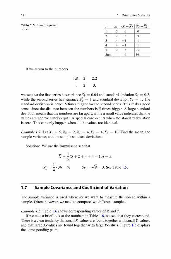
12 1 Descriptive Statistics
Table 1.5 Sum of squarederrors
i Xi .Xi � X/ .Xi � X/2
1 5 0 0
2 2 �3 9
3 4 �1 1
4 4 �1 1
5 10 5 25
Sum 0 36
If we return to the numbers
1:8 2 2:2
1 2 3;
we see that the first series has variance S2X D 0:04 and standard deviation SX D 0:2,
while the second series has variance S2X D 1 and standard deviation SX D 1. The
standard deviation is hence 5 times bigger for the second series. This makes goodsense since the distance between the numbers is 5 times bigger. A large standarddeviation means that the numbers are far apart, while a small value indicates that thevalues are approximately equal. A special case occurs when the standard deviationis zero. This can only happen when all the values are identical.
Example 1.7 Let X1 D 5; X2 D 2; X3 D 4; X4 D 4; X5 D 10. Find the mean, thesample variance, and the sample standard deviation.
Solution: We use the formulas to see that
X D 1
5.5 C 2 C 4 C 4 C 10/ D 5;
S2X D 1
4� 36 D 9; SX D p
9 D 3: See Table 1.5:
1.7 Sample Covariance and Coefficient of Variation
The sample variance is used whenever we want to measure the spread within asample. Often, however, we need to compare two different samples.
Example 1.8 Table 1.6 shows corresponding values of X and Y.If we take a brief look at the numbers in Table 1.6, we see that they correspond.
There is a clear tendency that small X-values are found together with small Y-values,and that large X-values are found together with large Y-values. Figure 1.5 displaysthe corresponding pairs.

1.7 Sample Covariance and Coefficient of Variation 13
Table 1.6 The data forExample 1.8
X1 X2 X3 X4 X5 X6 X7 X8 X9 X10
2 12 1 1 10 25 3 9 27 2
Y1 Y2 Y3 Y4 Y5 Y6 Y7 Y8 Y9 Y10
3 11 3 1 12 21 6 4 31 2
Fig. 1.5 Correspondingvalues
5 10 15 20 25 X
5
10
15
20
25
30
Y
There are some exceptions that do not have a clear interpretation, but the maintendency appears to be clear. The question is then if we can find a method to measurehow strongly the values correspond to each other. The sample covariance turns outto be useful in this respect, and we can use this quantity to judge if two samples pullin the same direction.
Definition 1.4 If our two samples are X1; : : : ; Xn and Y1; : : : ; Yn, the samplecovariance SXY is defined by
SXY D 1
n � 1
�.X1 � X/. Y1 � Y/ C � � � C .Xn � X/. Yn � Y/
�
D 1
n � 1
nX
iD1
.Xi � X/.Xi � X/:
It is interesting to note that if the two samples happen to be equal, then the samplecovariance equals the variance. When it is clear from context that we speak aboutsamples, we sometimes drop the prefix sample and speak about covariance.
Example 1.9 Let X1 D 242; X2 D 266; X3 D 218; X4 D 234 and Y1 D 363; Y2 D399; Y3 D 327; Y4 D 351. Find SXY .

14 1 Descriptive Statistics
Solution: We first compute X D 240 and Y D 360. We then use the formula tosee that
SXY D 1
3
�.X1 � X/. Y1 � Y/ C .X2 � X/. Y2 � Y/
C.X3 � X/. Y3 � Y/ C .X4 � X/. Y4 � Y/�
D 1
3
�.242 � 240/.363 � 360/ C .266 � 240/.399 � 360/
C.218 � 240/.327 � 360/ C .234 � 240/.351 � 360/�
D 600:
The main purpose of the covariance is to measure how two variables correspond.If it is mainly the case that a large value of X (large here means bigger than themean) is found together with a large value of Y, while small values (smaller than themean) of X largely are found together with small values of Y, most of the terms inthe covariance will be positive. A positive covariance indicates that the terms pullin the same direction. We call this positive covariation. The opposite will happen ifsmall X is usually found together with large Y and large X usually are together withsmall Y. When this happens most terms in the covariance will be negative, oftenleading to a negative total value. With negative covariance the terms pull in oppositedirections, and we call this negative covariation. A borderline case happens if thecovariance is zero. There is then no tendency in any direction, and we say that theresults are uncorrelated.
Even though the sign of the covariance is quite informative, the size is moredifficult to interpret. What is big depends to a great extent on the context. In somecases a covariance of 1;000;000 may be big, but not always. If we, e.g., considerdistances in space measured in km, a covariance of 1;000;000 may be approximatelyzero. There is, however, a simple way to measure the impact of the covariance; thecoefficient of variation.
Maximum linear covariation is obtained whenever the observation pairs are on aline with nonzero slope. When the slope is positive, an increase in one variable willalways lead to an increase in the other variable, this is positive covariation. If theslope is negative, an increase in one variable will always lead to a decrease in theother variable, this is negative covariation. The coefficient of variation measures theamount of linear covariation.
Definition 1.5 The coefficient of variation RXY is defined by
RXY D SXY
SX � SY:

1.7 Sample Covariance and Coefficient of Variation 15
In this formula we must compute the standard deviations SX and SY separately. Itis possible to prove that for any pair of samples, then
�1 � RXY � 1:
If we return to Example 1.9 and compute SX and SY , we get
RXY D 600
20 � 30D 1:
This means that in this case the linear covariation is maximal. If we look closer atthe numbers, it is easy to see why. For any i, we have
Yi D 3
2� Xi:
Even in cases with few observations, a relation of this sort is by no means easy todetect. This shows that the coefficient of variation is an efficient tool to reveal suchrelations, in particular if the number of observations is large.
The values �1 and 1 are extremes, and such values can only be obtained in specialcases. It is possible to show that RXY D 1 if and only if there is a constant k > 0 andanother constant K such that
Xi D k � Yi C K; for all i D 1; 2; : : : ; n;
and that RXY D �1 if and only if there is a constant k < 0 and another constant Ksuch that
Xi D k � Yi C K; for all i D 1; 2; : : : ; n:
In both cases the observations .Xi; Yi/ are confined to a straight line, and this is theonly way we can obtain maximum linear covariation. If we return to Example 1.8,we can compute
RXY D 0:96:
We see that this value is close to maximum positive covariation, and we have thusconfirmed the tendency that we saw in the dataset.
Example 1.10 Assume that we have observed the values of 4 different stocks, A, B,C, and D at 100 different point in time. We wonder if there is a connection betweenthe stock price of A and any of the other stock prices. To see if there is a connectionbetween A and B, we plot the numbers .A1; B1/; .A2; B2/; : : : ; .A100; B100/ in thesame figure. We do the same with A and C and with A and D. The results are shownin Fig. 1.6.

16 1 Descriptive Statistics
Fig. 1.6 Correspondingstock prices
20 40 60 80 100 120 140A
50
100
150
200
B
20 40 60 80 100 120 140A
20
40
60
80
100
120
140
C
20 40 60 80 100 120 140A
50
100
150
D
From Fig. 1.6 we see that there is clearly positive covariation between A and B;when the price on A is low, so is the price on B, and a high price on A typicallyis seen together with a high price on B. The coefficient of variation confirms this,RAB D 0:98. We can’t see much connection between A and C. For the numbers
1.8 Using Excel 17
reported in the figure we have RAC D �0:01. There seems to be a clear connectionbetween A and D. The tendency is that the stock price of D is high when the stockprice of A is low and the reverse is also true. This is negative covariation and for thenumbers reported in the figure RAD D �0:62.
1.8 Using Excel
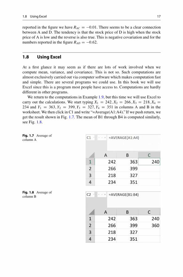
At a first glance it may seem as if there are lots of work involved when wecompute mean, variance, and covariance. This is not so. Such computations arealmost exclusively carried out via computer software which makes computation fastand simple. There are several programs we could use. In this book we will useExcel since this is a program most people have access to. Computations are hardlydifferent in other programs.
We return to the computations in Example 1.9, but this time we will use Excel tocarry out the calculations. We start typing X1 D 242; X2 D 266; X3 D 218; X4 D234 and Y1 D 363; Y2 D 399; Y3 D 327; Y4 D 351 in columns A and B in theworksheet. We then click in C1 and write “=Average(A1:A4).” If we push return, weget the result shown in Fig. 1.7. The mean of B1 through B4 is computed similarly,see Fig. 1.8.
Fig. 1.7 Average ofcolumn A
Fig. 1.8 Average ofcolumn B

18 1 Descriptive Statistics
Fig. 1.9 The sample variance of column A and B, the sample covariance of A and B, and thecoefficient of variation
The sample variances, covariance, and coefficient of variation are computed inthe same way, see Fig. 1.9. To compute the sample standard deviation we may usethe command STDEV.S. Instead of writing the commands in full it is possible toclick and drag the corresponding menus. This is simple, but is not something wewill discuss here.
1.9 Summary of Chap. 1
• The median of n observations in ascending order
Median D Observation numbern C 1
2:
Interpretation: Roughly one half of the observations are below the median, andthe other half above.
• The first and third quartiles of n observations in ascending order
First quartile D Observation numbern C 1
4;

1.9 Summary of Chap. 1 19
First quartile D Observation number3.n C 1/
4:
Interpretation: Roughly half of the observations are found between the 1. and 3.quartiles.
• The mode of a set of observations: The most frequent observation.• The mean of a set of observations
X D 1
n.X1 C X2 C � � � C Xn/ D 1
n
nX
iD1
Xi:
• The sample variance of a set of observations
S2X D 1
n � 1
�.X1 � X/2 C � � � C .Xn � X/2
� D 1
n � 1
nX
iD1
.Xi � X/2:
Interpretation: A large value means that the observations are far apart.• The sample standard deviation of a set of observations
Sx Dq
S2X:
Interpretation: The typical deviation from the mean.• The sample covariance
SXY D 1
n � 1
�.X1 � X/. Y1 � Y/ C � � � C .Xn � X/. Yn � Y/
�
D 1
n � 1
nX
iD1
.Xi � X/.Xi � X/:
Interpretation: When SXY > 0, the quantities pull in the same direction. WhenSXY < 0, the quantities pull in opposite directions.
• Coefficient of variation
RXY D SXY
SX � SY:
Interpretation: Strong positive covariation when RXY is close to 1, strong negativecovariation when RXY is close to �1, uncorrelated when RXY is close to zero.
• Excel commandsMean: AVERAGE(A1:AN)Sample variance: VAR.S(A1:AN)Sample standard deviation STDEV.S(A1:AN)

20 1 Descriptive Statistics
Sample covariance: COVAR.S(A1:AN;B1:BN)Coefficient of variation: CORREL(A1:AN;B1:BN).
1.10 Problems for Chap. 1
1.1 Table 1.7 gives a survey of the willingness to pay for n D 675 customers. Thecustomers were asked about the maximum price they would be willing to pay for aspecific good. Find the mode, median, and 1. and 3. quartiles for the numbers in thetable.
1.2 Table 1.8 shows how frequent people visit their local food store. We have accessto n D 1275 observations in total.
(a) Find the mode, median, and 1. and 3. quartiles for the numbers in the table.(b) Find the mean of the observations.
1.3 Table 1.9 shows the stock price for 5 different companies.
(a) Find the mean of the 5 prices in the table.(b) Company A has a total of 140;000 stocks, company B 50;000 stocks, company
C 20;000 stocks, company D 10;000 stocks, and company E 30;000 stocks. Findthe total market value of the five companies. How many stocks are there in total?What is the mean value of each stock in total? Compare with the result in (a).
1.4 (a) Find the mean of the numbersi) 1; 3; 4; 2; 7; 9; 2
ii) 2; 6; 8; 4; 14; 18; 4
iii) 10; 30; 40; 20; 70; 90; 20.(b) How do the results in (a) connect?
Table 1.7 Data forProblem 1.1
Price in USD 100 110 120 130 140 150
Frequency 90 115 121 162 109 78
Table 1.8 Data forProblem 1.2
Number of days per week 0 1 2 3 4 5 6 7
Frequency 257 241 459 103 84 62 47 22
Table 1.9 Data forProblem 1.3
Company A B C D E
Stock price in USD 100 200 400 300 500

1.10 Problems for Chap. 1 21
Table 1.10 Data forProblem 1.8
Day 1 2 3 4 5
Stock price in USD 99 101 97 101 102
1.5 (a) Find the mean of the numbersi) 1; 2; 3; 4; 5; 6; �21
ii) �2; 4; 32; �4; 1
2.
(b) Do you see any connections between the numbers in (a)?
1.6 (a) Find the sample variance for the numbersi) 8; 3; 7; 1; 11
ii) 2; �3; 1; �5; 5.(b) Are there any connection between the numbers in (a)?
1.7 Let X1 D 12; X2 D 1; X3 D 7; X4 D 5; X5 D 5. Find the mean, samplevariance, and sample standard deviation.
1.8 Table 1.10 shows the stock price of a company through 5 consecutive days. Findthe mean, sample variance, and sample standard deviation for these stock prices.
1.9 Let X1 D 1; X2 D 4; X3 D 5; X4 D 7; X5 D 13.
(a) Use the formula
S2 D 1
5
�.X1 � X/2 C .X2 � X/2 C .X3 � X/2 C .X4 � X/2 C .X5 � X/2
�;
to compute S2 and S.(b) Use the formula
S2 D 1
4
�.X1 � X/2 C .X2 � X/2 C .X3 � X/2 C .X4 � X/2 C .X5 � X/2
�;
to compute S2X and SX .
(c) Use your calculator to compute the standard deviation. Does the answer coincidewith (a) or (b)?
1.10 Assume that
S2 D 1
n
nX
iD1
.Xi � X/2 and that S2X D 1
n � 1
nX
iD1
.Xi � X/2:

22 1 Descriptive Statistics
Table 1.11 Data forProblem 1.13
Price X1 D 71 X2 D 47 X3 D 23 X4 D 27
Demand Y1 D 58 Y2 D 106 Y3 D 154 Y4 D 146
Table 1.12 Data for Problem 1.14
Portfolio 1 X1 D 18 X2 D 22 X3 D 14 X4 D 10 X5 D 11
Portfolio 2 Y1 D 36 Y2 D 44 Y3 D 28 Y4 D 20 Y5 D 22
Show that
S Dr
n � 1
n:
Is S greater or smaller than SX?
1.11 Let .X1; : : : X5/ D .140; 126; 133; 144; 152/ and .Y1; : : : ; Y5/ D.248; 252; 254; 244/. Find SXY .
1.12 Let .X1; : : : X5/ D .140; 126; 133; 144; 152/ and .Y1; : : : ; Y5/ D.253; 221; 239; 229; 233/. Find SX; SY ; SXY and RXY .
1.13 Table 1.11 shows 4 matching values of price (in USD) and demand (in units)of a good.
Find SX; SY ; SXY and RXY . What is the relation between demand and price?
1.14 Table 1.12 shows 5 matching values of the returns (in % per year) of twoportfolios of stocks.
Find SX; SY ; SXY and RXY . What is the relation between Yi and Xi? How can youput together two portfolios that behave like this?
1.15 This Exercise Provides the Rigorous Definitions of Quartiles: If n is thenumber of observations, we find the position of the quartiles computing k1 D nC1
4
and k3 D 3.nC1/
4. Depending on n we get two reminders which are 0; 1
4; 1
2, or 3
4.
i) If the remainder is zero, we use observation k.ii) If the reminder is 1
4we start at observation k � 1
4(an integer) and increase this
value by 25% of the distance to the next observation.iii) If the reminder is 1
2we start at observation k � 1
2(an integer) and increase this
value by 50% of the distance to the next observation.iv) If the reminder is 3
4we start at observation k � 3
4(an integer) and increase this
value by 75% of the distance to the next observation.

1.10 Problems for Chap. 1 23
Find the 1. and 3. quartiles for the observations
(a) 2; 6; 10; 14; 18; 22
(b) 2; 6; 10; 12; 14; 18; 22
(c) 2; 6; 10; 11; 13; 14; 18; 22
(d) 2; 6; 10; 11; 12; 13; 14; 18; 22.
1.16 You have made 25 observations of the price of a good. The results are shownbelow.
123 156 132 141 127 136 129 144 136 142 126 133 141
154 143 121 138 125 137 123 133 141 127 126 149
Type these observations in Excel, and use Excel commands to answer thequestions.
(a) Find the mean of the observations.(b) Find the sample variance and the sample standard deviation.(c) Use the command QUARTILE.A1 W A25I 1/ to find the 1. quartile, and figure out
how you can modify the command to find the 2. and the 3. quartiles. What is adifferent name for the 2. quartile?
1.17 Portfolio Optimization: Table 1.13 shows the development of the stocks inthe two companies ALPHA and BETA. The price on the stocks (in USD) has beenobserved monthly over a period of 20 consecutive months. The stock prices onALPHA are quoted by a1; : : : ; a20 and the stock prices for BETA are quoted byb1; : : : ; b20.
(a) Compute the mean stock price for the stocks in ALPHA and BETA (separately).(b) Make a plot of the time development of the two stock prices in the same figure.
Which stock do you consider to be the most unsure?
Table 1.13 Stock prices forcompany ALPHA and BETA
a1 a2 a3 a4 a5 a6 a7 a8 a9 a10
92 86 90 86 95 92 96 102 106 96
a11 a12 a13 a14 a15 a16 a17 a18 a19 a20
95 102 101 107 106 110 103 107 116 112
b1 b2 b3 b4 b5 b6 b7 b8 b9 b10
127 114 141 113 128 115 84 101 96 119
b11 b12 b13 b14 b15 b16 b17 b18 b19 b20
93 88 79 103 63 60 116 82 82 96
24 1 Descriptive Statistics
(c) Compute the sample variances S2a and S2
b, you might prefer to use Excel to dothis. Do the values on S2
a and S2b coincide with the conclusions you could draw
in (b)?(d) Can a large sample variation be an advantage? Which of the stocks ALPHA and
BETA do you consider the best?(e) Compute the covariance Sab, you may prefer to use Excel.(f) You want to invest 1;000;000 USD in these stocks. We assume that you buy
each stock at their mean value, and that you invest x% of the money in ALPHAand y% D 100% � x% in BETA. Let an and bn denote the price on the stocks atany time n. Show that the value cn of your investment is given by
cn D 100xan C 100ybn:
(g) We cannot say anything for sure about the future, but it may sometimes bereasonable to assume that the mean and the sample variance will remainconstant. What would the mean value of cn be based on the data above?
(h) Show that S2c D 10;000.x2S2
a C 2xySab C y2S2b, and use this to find a value for
x such that S2c is as small as possible. How much must you buy of each stock if
you prefer low risk?
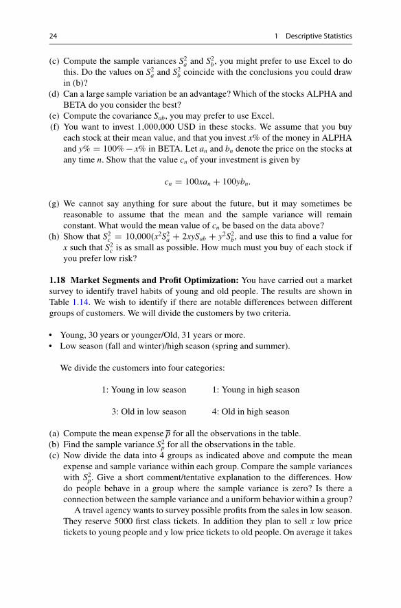
1.18 Market Segments and Profit Optimization: You have carried out a marketsurvey to identify travel habits of young and old people. The results are shown inTable 1.14. We wish to identify if there are notable differences between differentgroups of customers. We will divide the customers by two criteria.
• Young, 30 years or younger/Old, 31 years or more.• Low season (fall and winter)/high season (spring and summer).
We divide the customers into four categories:
1: Young in low season 1: Young in high season
3: Old in low season 4: Old in high season
(a) Compute the mean expense p for all the observations in the table.(b) Find the sample variance S2
p for all the observations in the table.(c) Now divide the data into 4 groups as indicated above and compute the mean
expense and sample variance within each group. Compare the sample varianceswith S2
p. Give a short comment/tentative explanation to the differences. Howdo people behave in a group where the sample variance is zero? Is there aconnection between the sample variance and a uniform behavior within a group?
A travel agency wants to survey possible profits from the sales in low season.They reserve 5000 first class tickets. In addition they plan to sell x low pricetickets to young people and y low price tickets to old people. On average it takes

1.10 Problems for Chap. 1 25
Table 1.14 Survey on total expenditure (USD) for travelers
Number Season Age Expense Number Season Age Expense
1 Winter 22 3018 21 Summer 23 1687
2 Winter 66 4086 22 Summer 45 7011
3 Winter 19 3034 23 Summer 75 6643
4 Winter 51 3730 24 Summer 15 1915
5 Winter 17 2623 25 Summer 16 2006
6 Winter 15 2757 26 Summer 36 7678
7 Winter 29 2927 26 Summer 17 1796
8 Winter 50 3844 28 Summer 71 7159
9 Winter 15 3569 29 Summer 49 7403
10 Winter 76 4102 30 Summer 65 7325
11 Spring 64 6949 31 Fall 22 3029
12 Spring 38 6885 32 Fall 72 4240
13 Spring 76 6839 33 Fall 27 3242
14 Spring 16 1577 34 Fall 16 3390
15 Spring 34 6746 35 Fall 24 3204
16 Spring 24 1965 36 Fall 58 4146
17 Spring 57 7387 37 Fall 50 3854
18 Spring 21 2077 38 Fall 71 4089
19 Spring 18 2091 39 Fall 15 2959
20 Spring 68 6985 40 Fall 37 3817
20 min to process a low price ticket for young people, while the correspondingnumber for old people is 35 min. To process the tickets the company has 3 peopleeach of whom works 37.5 hours per week. The managers have decided that lowprice tickets for young people should not exceed 20% of the total number oftickets.
(e) The price per ticket for first class is 7500 USD. To calculate the price on theother tickets, we use that mean values we computed above. The price for youngpeople should be 10% lower than the average expense reported from the data,while the price for old people should be 5% below the reported mean for thiscategory. How many tickets should you sell to each customer group to maximizetotal profit? Note: This is a linear programming problem and requires knowledgeon how to solve such problems. If you don’t have this knowledge, proceed to (g).
(f) Assume that the price on tickets for young people is fixed. How much must youraise the price on tickets for old people so that it is most profitable to sell all lowprice tickets to old people?
(g) The young people can be subdivided into two new categories A and B. We havecarried out a supplementary survey indicating that the two subgroups have asimilar mean expenditure over time. The two subgroups have different samplevariances S2
A D 20;000 and S2B D 40;000. In addition we have computed that
the sample covariance is SAB D �20;000. We will sell ˛% to group A and

26 1 Descriptive Statistics
ˇ% D 100% � ˛% to group B. This gives a combined sample variance
S2˛ˇ D 1
10;000.˛2S2
A C 2˛ˇSAB C ˇ2S2B/:
(you may take this for granted). Compute values for ˛ and ˇ to minimize thesample variance for the combination.

2Probability
Abstract
In this short chapter we will go through the basic definitions of probability. Toease the exposition, we will only discuss very simple examples. It is important tonotice that the concepts we develop in this chapter are central to all thinking aboutstatistics. Regardless of level and purpose these concepts provide tools that can beused to describe statistical methods. From this point of view the theory providesus with a framework that can be used to study any statistical phenomenon.
2.1 Sample Space
When we carry out an experiment, we get a result. This result is called the outcome.If we test 10 goods and find 3 defective items, the outcome is 3 defective items. Anexperiment can have several possible outcomes, and the collection of all of these iscalled the sample space. If we test 10 goods if they are defective or not, the outcomecan be anything from 0 to 10 defectives. The sample space is the set of all theindividual outcomes, i.e.
f0 defective; 1 defective; : : : ; 10 defectivesg:
We usually use the letter ˝ to denote a sample space. If an experiment can havethe outcomes !1; !2; : : : ; !m, the sample space is the set ˝ D f!1; !2; : : : ; !mg.We use the following definition:
© Springer International Publishing AG 2017J. Ubøe, Introductory Statistics for Business and Economics, Springer Textsin Business and Economics, https://doi.org/10.1007/978-3-319-70936-9_2
27

28 2 Probability
Definition 2.1 A sample space is a list of the outcomes of an experiment.
• The list must cover any possible outcome.• The outcomes must be mutually exclusive.
When these two conditions are satisfied, we say that the sample space iscomplete and distinguishing.
Example 2.1 Assume that we toss a dice once and look at the result. The samplespace is ˝ D f1; 2; 3; 4; 5; 6g.
Example 2.2 Assume that we watch a soccer match and consider the number ofpoints for the home team. The sample space is ˝ D f0; 1; 3g.
Example 2.3 Assume that we watch a soccer match and consider the goals made byboth teams separately. The sample space is
˝ D f.0; 0/; .0; 1/; .1; 0/; .2; 0/; .1; 1/; .0; 2/; .3; 0/; : : :g:
By the notation j˝j we mean the number of elements in the sample space. InExamples 2.1 and 2.2 we have j˝j D 6 and j˝j D 3, respectively. In Example 2.3,however, there is no limit to how many goals can be scored. In practice it might bedifficult to imagine cases with millions of goals, but no matter how many goals arescored, it is in theory possible to score once more. In this case it is natural to definej˝j D 1.
Example 2.4 We measure the temperature in a room in ıC. In that case ˝ DŒ�273; 1/, i.e., an interval. In this case, too, j˝j D 1.
Even though j˝j D 1 in Example 2.3 and in Example 2.4, there is an importantdifference between the two cases. In Example 2.3 it is possible to sort all outcomesin a sequence where each outcome is given a specific number, while no suchenumeration is possible in Example 2.4.
A sample space ˝ where all outcomes can be enumerated in a sequence iscalled discrete. In this case we may write ˝ D f!1; !2; : : : ; !ng, where n D1 signifies a case with infinitely many outcomes.

2.2 Probability 29
2.2 Probability
One of the most important concepts in statistics is the probability for the differentoutcomes in the sample space. Somewhat simplified these numbers express howoften we can expect to observe the different outcomes.
The probability for an outcome is an idealized quantity which defines the relativefrequency we will observe in the long run, i.e., in the course of infinitely many trials.It is of course impossible to carry out an experiment infinitely many times, but theidea is that the more repetitions we make, the closer will the relative frequency be tothe probability of the outcome. Imagine that we have repeated an experiment a largenumber of times, and observed that the relative frequency of one of the outcomes is10%. We then have a clear impression that this outcome will occur in 10% of thecases no matter how many times we repeat the experiment. We then say that theprobability of the outcome is 10%.
Definition 2.2 By a probability on a discrete sample space ˝ , we mean a setof real numbers
p1; p2; : : : ; pn
with the properties
• 0 � pi � 1, for all i D 1; 2; : : : ; n.• p1 C p2 C � � � C pn D 1.
Here p1 is the probability of outcome !1, p2 is the probability of outcome !2,and so on, so we write
pi D p.!i/; i D 1; : : : ; n:
The last expression makes it clear that a probability is a function defined on thesample space. Verbally we can express the conditions as follows: A probability isa number between 0 and 1, and the probability of all the outcomes must sum to1. In some cases we speak about subjective probabilities, which are more or lesswell-founded suggestions of how often an outcome will occur. We will return tosubjective probabilities in Chap. 4.

30 2 Probability
2.2.1 Events
By an event in statistics we mean a subset of the sample space. The use of the wordmay seem strange at a first glance, but quickly makes more sense if we consider anexample.
Example 2.5 We toss a dice twice. The sample space is ˝ D f.1; 1/; .1; 2/; : : : ;
.6; 6/g. Consider the subset A D f.1; 6/; .2; 6/; .3; 6/; .4; 6/; .5; 6/; .6; 6/g. Since Ais a subset of the sample space, it is an event. Verbally we can see that A expressesthat something very explicit has happened: “The second toss was a 6.”
The probability P.A/ of an event A is defined as the sum of the probabilitiesof all outcomes which are elements in A, i.e.
P.A/ DX
!2A
p.!/:
Example 2.6 We toss a fair dice twice. The sample space is
˝ D f.1; 1/; .1; 2/; : : : ; .6; 6/g:
The dice is fair when all these outcomes are equally probable, i.e., when p.!/ D 136
.The probability of the event
A D f.1; 6/; .2; 6/; .3; 6/; .4; 6/; .5; 6/; .6; 6/g
is hence
P.A/ D 1
36C 1
36C 1
36C 1
36C 1
36C 1
36D 1
6:
2.2.2 Uniform Probability
We will often study cases where all outcomes are equally probable. If there aren different outcomes, the probability of each outcome is hence 1
n . We call this auniform probability. When the probabilities are uniform, it is particularly easy tofigure out the probability of an event. We can simply count the number of elementsin the subset. If A has a elements, then
P.A/ D a
n:

2.2 Probability 31
Example 2.7 In a market segment of 1000 persons we know that 862 persons areworthy of credit. What is the probability that a randomly selected person is worthyof credit?
Solution: When we choose a randomly selected person, we are tacitly assuminga uniform probability. The subset of persons worthy of credit has 862 elements,while there are 1000 outcomes in total. The probability p that a randomly selectedperson is worthy of credit is hence p D 862
1000D 82:6%.
Example 2.8 We toss a dice once. A uniform probability on the sample space is
p.1/ D p.2/ D p.3/ D p.4/ D p.5/ D p.6/ D 1
6:
2.2.3 Set Theory
Since sample spaces are formulated as sets and events as subsets, set theoryis a natural tool in this context. The classical set operations have very specificinterpretations in statistics, and we will now briefly consider how this is done. Whenwe carry out an experiment and get an outcome ! which is an element of a subset A,we say that the event A has occurred. Each set operation has a similar interpretation(Figs. 2.1, 2.2, 2.3, 2.4, 2.5, and 2.6).
• Intersection
A \ B D The event that A and B both occurs:
• Union
A [ B D The event that either A or B or both occurs:
• Complement
Ac D The event that A does not occur:
Fig. 2.1 A \ B
A
B

32 2 Probability
Fig. 2.2 A [ B
A
B
Fig. 2.3 Ac is here the blueshaded area
A
Fig. 2.4 B � A
A
B
Fig. 2.5 B 6� A
A
B
Fig. 2.6 A \ B D ;A
B
The notation A, too, is often used with exactly the same meaning, i.e., when Ais a set, A D Ac.
• SubsetWhen B � A it means that when B occurs, A will always occur.
• Not subsetWhen B 6� A it means that when B occurs, A will not always occur.
• Empty intersection
A \ B D ;; when A and B never occurs simultaneously:
2.2 Probability 33
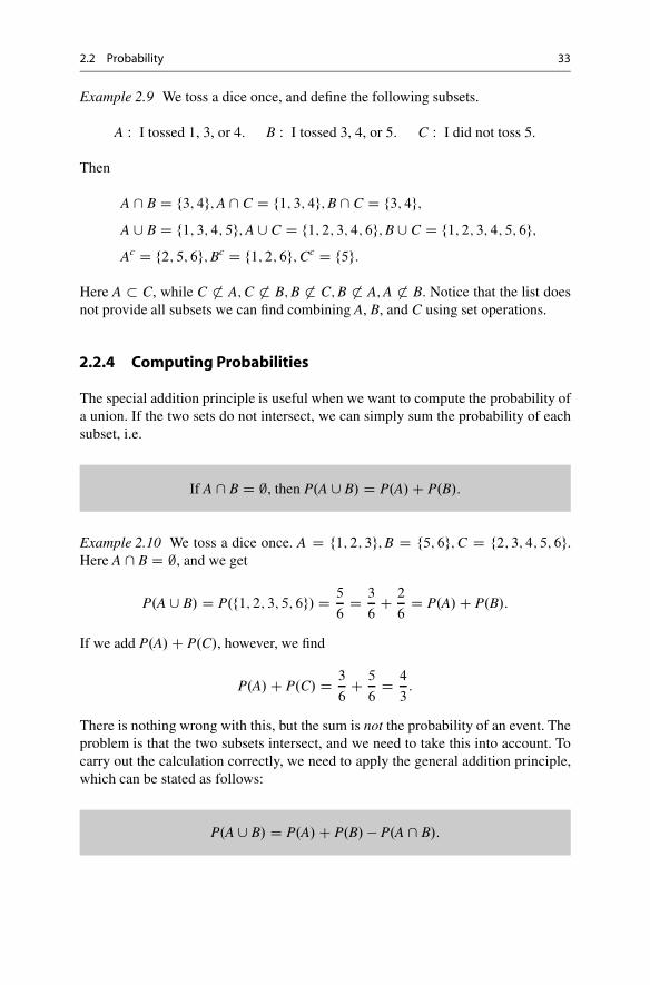
Example 2.9 We toss a dice once, and define the following subsets.
A W I tossed 1, 3, or 4: B W I tossed 3, 4, or 5: C W I did not toss 5:
Then
A \ B D f3; 4g; A \ C D f1; 3; 4g; B \ C D f3; 4g;A [ B D f1; 3; 4; 5g; A [ C D f1; 2; 3; 4; 6g; B [ C D f1; 2; 3; 4; 5; 6g;Ac D f2; 5; 6g; Bc D f1; 2; 6g; Cc D f5g:
Here A � C, while C 6� A; C 6� B; B 6� C; B 6� A; A 6� B. Notice that the list doesnot provide all subsets we can find combining A, B, and C using set operations.
2.2.4 Computing Probabilities
The special addition principle is useful when we want to compute the probability ofa union. If the two sets do not intersect, we can simply sum the probability of eachsubset, i.e.
If A \ B D ;, then P.A [ B/ D P.A/ C P.B/:
Example 2.10 We toss a dice once. A D f1; 2; 3g; B D f5; 6g; C D f2; 3; 4; 5; 6g.Here A \ B D ;, and we get
P.A [ B/ D P.f1; 2; 3; 5; 6g/ D 5
6D 3
6C 2
6D P.A/ C P.B/:
If we add P.A/ C P.C/, however, we find
P.A/ C P.C/ D 3
6C 5
6D 4
3:
There is nothing wrong with this, but the sum is not the probability of an event. Theproblem is that the two subsets intersect, and we need to take this into account. Tocarry out the calculation correctly, we need to apply the general addition principle,which can be stated as follows:
P.A [ B/ D P.A/ C P.B/ � P.A \ B/:

34 2 Probability
If we use this rule, we find
P.A [ C/ D P.f1; 2; 3; 4; 5; 6g/ D 1 D 3
6C 5
6� 2
6D P.A/ C P.C/ � P.A \ C/:
The general addition principle can be extended to cover unions of more than twosubsets. If we have three subsets A, B, and C, the result can be stated as follows:
P.A [ B [ C/ D P.A/ C P.B/ C P.C/
�P.A \ B/ � P.A \ C/ � P.B \ C/
CP.A \ B \ C/:
Example 2.11 In a customer survey all the people who participated used at leastone of the three products A, B, or C. All three products were used by 60% of thecustomers. 95% of the customers used at least one of the products A and B, 85%used at least one of the products B and C, and 30% used both A and C. How bigshare of the customers used all the three products?
Solution: In this example there are lots of information, and we need to find asystematic way of dealing with this. Since all the customers used at least one of theproducts A; B or C, we know that
P.A [ B [ C/ D 1 D 100%:
Since all three products were used by 60% of the customers, we know that
P.A/ D P.B/ D P.C/ D 60%:
From the text we have
P.A [ B/ D 95%; P.B [ C/ D 85%; P.A \ C/ D 30%:
If we use the general addition principle for two subsets, we get
95% D 60% C 60% � P.A \ B/ ) P.A \ B/ D 25%:
85% D 60% C 60% � P.B \ C/ ) P.B \ C/ D 35%:
If we plug all the above into the general addition formula for 3 subsets, we get theequation
100% D 60% C 60% C 60% � 25% � 30% � 35% C P.A \ B \ C/:

2.3 Summary of Chap. 2 35
Solving this equation, we get P.A\B\C/ D 10%. It is hence 10% of the customerswho use all the three products.
2.2.5 The Negation Principle
Since A and Ac never intersect and A [ Ac D ˝ , it follows from the special additionprinciple that
P.A/ C P.Ac/ D P.A [ Ac/ D P.˝/ D 1:
If we view this as an equation, we can solve for P.A/ or P.Ac/ to see that
P.A/ D 1 � P.Ac/ P.Ac/ D 1 � P.A/:
Hence to find the probability that A occurs, we can instead find the probabilitythat A does not occur. At a first glance this not appear to be very useful, but wewill throughout this book see many cases where this angle of approach simplifiescalculations.
2.3 Summary of Chap. 2
• Sample space:
˝ D The set of all outcomes:
• Event: A subset of a sample space.• General addition principles:
P.A [ B/ D P.A/ C P.B/ � P.A \ B/:
P.A [ B [ C/ D P.A/ C P.B/ C P.C/
�P.A \ B/ � P.A \ C/ � P.B \ C/
CP.A \ B \ C/:
• The negation principle:
P.A/ C P.Ac/ D 1:

36 2 Probability
2.4 Problems for Chap. 2
2.1 A bank serves three customers in succession. The customers are either worthyof credit or not worthy of credit. Suggest a suitable sample space for this situation.Write down the events:
A: At least one customer is worthy of credit.B: Customer number 2 is worthy of credit.C: All the customers have the same credit rating.
2.2 We observe the Dow Jones Index over two consecutive days and will considera sample space with four different outcomes:
!1: The index rises both days.!2: The index rises the first day and does not rise the second day.!3: The index does not rise the first day and rises the second day.!4: The index does not rise the first day and does not rise the second day.
Define two events A and B by:
A: The Dow Jones rises the first day.B: The Dow Jones rises the second day.
(a) Find the events A [ B, A \ B, Ac, and Bc.(b) Show that .A \ B/ [ .Ac \ B/ D B.(c) Show that A [ .Ac \ B/ D A [ B.
2.3 An auditing firm regularly inspects the accounting done by a large company. Inmany such inspections the firm reveals one or more errors, see Table 2.1.
Let A denote the event “There is at least one error,” and let B denote the event“There are less than 10 errors.”
(a) Find the probabilities for A and Ac.(b) Find the probabilities for B and Bc.(c) Find the probability for A [ B.(d) Find the probability for A \ B. How would you express this event in words?
Table 2.1 Data for Problem 2.3
Number or errors 0 1 to 3 4 to 6 7 to 9 10 to 12 More than 12
Probability in % 10 30 25 20 10 5

2.4 Problems for Chap. 2 37
Table 2.2 Data for Problem 2.4
Processing time in days 1 2 3 4 5 6 or more
Probability in % 10 40 30 10 5 5
Table 2.3 Data for Problem 2.5
Warehouse/Type Regular Superior Superior extra
Warehouse 1 12 9 10
Warehouse 2 25 16 5
Warehouse 3 9 9 3
2.4 A company uses at least one day to process a particular type of order. A surveyof the processing time is shown in Table 2.2.
(a) Define a suitable sample space for this situation and explain why the numbersin the table define a probability on this sample space.
(b) Find the probability of the events:
A: Processing time shorter than 3 days.B: Processing time at least 3 days.
(c) What is the connection between A and B?
2.5 A company produces a good in three different types: Regular, Superior, andSuperior Extra. The goods are stored in three different warehouses. The distributionof the production is shown in Table 2.3.
(a) We choose a good randomly. How many outcomes are there in the sample space?Explain why the table defines a probability.
(b) We choose a good randomly, and let A, B, and C denote the events
A W The good is of type Regular
B W The good is of type Superior
C W The good is stored at warehouse 3
Express the following events in words, and find the probability for each event.
(i) A \ C(ii) A [ C
(iii) A \ B(iv) A [ B

38 2 Probability
2.6 In a customer survey 70% of the customers used at least one of the productsA and B. 60% used product A and 40% used product B. 50% used product B. Howmany % of the customers used both products?
2.7 In a customer survey 70% of the customers used at least one of the productsA and B, while 40% used both products. 50% used product B. How many % of thecustomers used product A?
2.8 In a customer survey 30% of the customers used both products A and B. 60%used product A and 40% used product B. 50% used product B. How many % of thecustomers used none of the products?
2.9 In this exercise we will consider the stocks in 5 companies. Company A has140;000 stocks, company B has 50;000 stocks, company C has 20;000 stocks,company D has 10;000, and company E has 30;000 stocks. In total there are 250;000
stocks. We choose a stock randomly among the 250;000 stocks. Suggest a suitablesample space, and define a probability which describes this situation.
2.10 Unions of 3 Subsets: In a customer survey 89% of the customers used at leastone of the products A, B, and C. 60% used product A, 50% used product B and 45%used product C. 82% of the customers used at least one of the products A and B,73% used at least one of the products A and C, and 74% used at least one of theproducts B and C.
(a) How big share of the customers used(i) Both A and B?
(ii) Both A and C?(iii) Both B and C?(b) How big share of the customers used all the three products?
2.11 A Practical Illustration: In a customer survey we asked 80 customers if theyliked the products A or B. The customers liking product A were numbers
1; 2; 3; 4; 5; 7; 8; 9; 10; 11; 13; 15; 16; 17; 18; 19; 20; 22; 23; 24; 27; 28; 30; 31; 33; 34;
35; 36; 37; 39; 40; 42; 43; 47; 48; 49; 50; 51; 52; 53; 56; 57; 58; 59; 60; 61; 62; 65; 67;
70; 71; 72; 73; 74; 75; 76; 77; 78; 79; 80:
while the customers liking product B were numbers
3; 6; 7; 11; 12; 18; 19; 20; 25; 27; 32; 33; 34; 38; 39; 41; 42; 43; 44; 45; 49; 53; 54; 55;
56; 57; 60; 61; 62; 65; 67; 68; 69; 71; 72; 73; 74; 76; 78; 80:

2.4 Problems for Chap. 2 39
(a) Which customers liked both A and B?(b) Which customers liked at least one of the two products?(c) How big share of the customers liked(i) Product A?
(ii) Product B?(iii) Both A and B?(iv) At least one of the two products?(d) How do the numbers in (c) connect?

3Combinatorics
Abstract
In this chapter we will study certain types of random selection within a uniformmodel. Such samples can occur when we select a representative from anaudience, when we sample for errors, play lotteries, or generally when we choosebetween alternatives which are equally probable. The main problem is then tofigure out how many combinations there are of a particular type. When we knowthe number of combinations, it is easy to figure out the probabilities, since in auniform model all alternatives are equally probable. We then find the probabilityas the fraction between the number of combinations of the type we are lookingfor and the number of combinations in total.
3.1 Counting Combinations
The simplest basic principle in combinatorics takes its starting point in a sequenceof choices where there are no connections between each choice. When choicesare connected, certain outcomes may influence the other choices. When there areno connections, we find the total number of combinations when we multiply thenumber of possible outcomes of each choice.
Example 3.1 We want to select one girl and one boy from a class consisting of 15girls and 12 boys. Since there are no connections, we have a total of 15 � 12 D 180
different combinations.This principle applies in general: If we have c1 possibilities in choice number 1,
c2 possibilities in choice number 2,. . . , cm possibilities in choice number m, and thechoices do not connect, there is a total of c1 � c2 � � � cm different combinations.
In combinatorics it is hence crucial to identify if there are connections or not.When the choices connect, the situation quickly becomes rather complex. In thefollowing we will consider some standard connections which are not too complex,
© Springer International Publishing AG 2017J. Ubøe, Introductory Statistics for Business and Economics, Springer Textsin Business and Economics, https://doi.org/10.1007/978-3-319-70936-9_3
41

42 3 Combinatorics
and in these cases we can compute the number of different combinations by explicitformulas.
3.1.1 Ordered Selections
In some selections the order of choices may be crucial. If we select a team, thefirst one selected may be the leader, while the next few members may take onpredefined positions. Each sequence will then define a unique outcome. Sometimesthe same person can be selected multiple times, and that may influence the numberof different combinations. If no object can be selected more than once, we say thatthe choice is without replacement. When the same object can be selected again everytime we make a new choice, we say that the choices are with replacement.
Example 3.2 We want to elect CEO and board leader for a company. There are 4candidates, and all candidates are eligible for both positions. We first elect the CEO,and there are 4 possible outcomes. Next we should select the board leader, and thenthe situation is not clear. We have two different options:
• If the CEO can become board leader, the selection is with replacement, and wehave a total of 4 � 4 D 16 different outcomes.
• If the CEO cannot become board leader, the selection is without replacement,and we have a total of 4 � 3 D 12 different outcomes (Fig. 3.1).
These simple principles apply in general:
If we have n different elements in our choice set, and want to choose s ofthese elements with replacement, there are n � n � n D ns different orderedcombinations.
Fig. 3.1 12 different outcomes

3.1 Counting Combinations 43
If we have n different elements in our choice set, and want to choose s of theseelements without replacement, there are
n.n � 1/ � � � .n � s C 1/
different ordered combinations.
Example 3.3 In how many ways can we make an ordered selection of 5 personsfrom a group of 20 people?
Solution: If the choice is with replacement, there are
20 � 20 � 20 � 20 � 20 D 3;200;000
different ordered combinations.If the choice is without replacement, there are
20 � 19 � 18 � 17 � 16 D 1;860;480
different ordered combinations.Since we often need to compute the number of ordered combinations in a
sequence of choices without replacements, there is a special symbol for this:
.n/s D n.n � 1/ � � � .n � s C 1/:
The symbol .n/s can be expressed in terms of the factorial function. This functionis defined as follows:
nŠ D n.n � 1/ � � �3 � 2 � 1;
where we in addition define
1Š D 1 0Š D 1:
Example 3.4 5Š D 5 � 4 � 3 � 2 � 1 D 120.We hence compute the factorial of a positive integer n multiplying all the integers
from 1 up to n. The definition 0Š D 1 is an exception and may appear a bit strangeat a first glance, but several relevant formulas simplify with this convention. If we

44 3 Combinatorics
look at Example 3.3 again, we see that
20 � 19 � 18 � 17 � 16 D 20 � 19 � 18 � 17 � 16 � 15 � 14 � � �3 � 2 � 1
15 � 14 � � �3 � 2 � 1(3.1)
D 20 � 19 � 18 � � �3 � 2 � 1
15 � 14 � � �3 � 2 � 1D 20Š
15Š
This principle applies in general and
.n/s D n.n � 1/ � � � .n � s C 1/ D nŠ
.n � s/Š
In the example above, we used n D 20 and s D 5. Then the calculation endedwith the factor .n � s C 1/ D 16, and the nominator was .n � s/Š D 15Š. Notice thatwhen we use a calculator to carry out the computations, it is often better to use theoriginal definition as the factorials may become so large that the calculator cannothandle them. Using the definition we see that
.1000/3 D 100 � 999 � 998 D 997;002;000
while
1000Š
997Š
may lead to trouble as 1000Š � 4:0 � 102567, which is a number that is too large formost calculators to handle.
3.1.2 Unordered ChoicesWithout Replacement
In some types of choices the order does not matter. If we are to select two boardmembers instead of CEO and board leader, the order makes no difference. If Smithand Johnson are selected, it does not matter who is selected first. The orderedchoices fSmith; Johnsong and fJohnson; Smithg both lead to the same result. Whenthe order does not count, we will in general end up with fewer combinations. Tofigure out how many unordered combinations that are genuinely different, we needto be able to compute how many ordered combinations lead to the same unorderedresult (Fig. 3.2).
It is easy to understand that n different objects can be sorted in nŠ different ways.In the first position we have n different options, in the second position .n�1/ optionsremains, and we may continue like this until we reach the last position where thereis only one object left.

3.1 Counting Combinations 45
Fig. 3.2 Outcomes come in two versions
Example 3.5 In the Lotto lottery (England) the players select 6 out of 59 numberswithout replacement. 6 out of 59 numbers are then drawn randomly withoutreplacement, and any player who selected the same 6 numbers wins the Jackpot.What is the probability of winning the Jackpot?
Solution: The number of unique ordered outcomes is .59/6 D 32;441;381;280,but each time we select 6 numbers they can be sorted in 6Š D 720 different waysthat all lead to the same result. This means that the number of unordered outcomesis reduced by a factor 720, and the number of unique unordered outcomes is
32;441;381;280
720D 45;057;474:
As each such combination has the same probability of winning, the probability ofwinning the Jackpot is hence
1
45;057;474:
The same line of reasoning can be used in general. Whenever we pick s elementsfrom n unique objects, there are .n/s different ordered combinations. Each suchcombination can be sorted into sŠ different ordered combinations, all of which areleading to the same unordered outcome. The number of ordered combinations isreduced by a factor sŠ, and the number of unique unordered combinations is hence
.n/s
sŠD nŠ
sŠ.n � s/Š:
The number of unique unordered combinations coincides with the binomial coeffi-cient
� ns
�used in mathematics, and we use the same notation, i.e.
�n
s
�D .n/s
sŠD nŠ
sŠ.n � s/Š:
46 3 Combinatorics
Example 3.6
�10
3
�D 10 � 9 � 8
1 � 2 � 3D 120:
Note that s D 3 and there are three terms both in the nominator and the denominator.The principles above can be summarized as follows: When we select s elements
from a set with n unique elements, we get the following number of uniquecombinations
Ordered with replacement:
ns D n � n � n � � � n„ ƒ‚ …s terms
:
Ordered without replacement:
.n/s D n.n � 1/ � � � .n � s C 1/ D nŠ
.n � s/Š:
Unordered without replacement:
�n
s
�D .n/s
sŠD nŠ
sŠ.n � s/Š:
If we make efficient use of these principles we are able to solve many differentproblems related to combinatorics. One question remains, however: What aboutunordered selections with replacement? Curiously, this case becomes much morecomplex than any of the others. We will illustrate the problem with an example.
Example 3.7 How many unique unordered combinations exist when we select 3elements out of 5 with replacement?
Solutions: Obviously there are 5 � 5 � 5 D 125 ordered combinations. In thecase without replacement, any ordered combination could be sorted into sŠ differentvariants, but this is no longer true. The ordered combination .1; 1; 1/ only existsonce, the ordered combination .1; 1; 2/ can be sorted in 3 different versions, and theordered combination .1; 2; 3/ can be sorted in 6 different versions. We hence haveto treat all such cases separately. There are 5 different ordered cases where all theelements are equal, and they are also different as unordered combinations. If wecount carefully, we can figure out 60 ordered combinations where two elementsare equal while the third is different. All such combinations can be sorted in 3different ordered combinations which all lead to the same unordered outcome. Thisgives 60=3 D 20 different unordered combinations. Finally there are 60 ordered

3.1 Counting Combinations 47
combinations where all the three elements are different. These cases can be sortedin 6 different ordered versions, all leading to the same unordered outcome. Thisleads to 60=6 D 10 unique unordered combinations. To summarize we end up with5 C 20 C 10 D 35 unique unordered combinations.
As we can see from the example, computation of the number of such unorderedcombinations is possible but quite cumbersome. It is possible to make a systematictreatment of this topic, but since we rarely will encounter such cases in practice, wewill not enter more deeply into this.
3.1.3 Combinatorial Probabilities
In many connections it is reasonable to assume that all the different combinations areequally probable. This corresponds to a uniform probability as defined in Chap. 2.In particular it applies to situations where you guess possible outcomes without anyprior information. In such cases we can compute probabilities simply by countingthe number of cases with a specified outcome.
Example 3.8 A group of 300 students were given a list of 10 imaginary companiesand asked to pick 4 different companies from the list. After all the students had madetheir choice, the stock price was simulated on a computer and the values of certaincall options were calculated from this. The worth of 10;000 such call options aredisplayed in Table 3.1.
It turned out that 1 student had picked all the four best, i.e., NoWonder,DataFriends, UnitedMath, and SlowFix. 8 students had picked all the 3 best, 42students had picked the two best, and 120 students had picked the best. The questionis now if this was a good or bad achievement.
Since the students had no prior information about the companies, it may bereasonable to assume that the choices are purely random. Since the order makes nodifference, the choices are unordered. The students should pick different companies,
which means that the selection is without replacement. There is hence�
104
�D 210
Table 3.1 Values of 10;000
optionsGroggy USD 6700
Phrazebook USD 0
Externet USD 9500
NoWonder USD 191; 700
McHeaven USD 0
DataFriends USD 241; 900
UnitedMath USD 17; 100
AllStats USD 0
LowTech USD 0
SlowFix USD 147; 000

48 3 Combinatorics
unique outcomes, all of which are equally probable. We can then ask the followingquestions:
• What is the probability of picking all the four best?• What is the probability of picking the three best?• What is the probability of picking the two best?• What is the probability of picking the best?
Solution: What is the probability of picking all the four best? As there is just onesuch combination, the probability is 1
210.
What is the probability of picking the three best? If we are to pick the three best,the last company can be picked arbitrarily among the 7 companies that are left, and
this can be done in�
7
1
�D 7 different ways. The probability is hence 7
210D 1
30.
What is the probability of picking the two best? If we are to pick the two best, thelast two companies can be picked arbitrarily among the 8 companies that are left,
and this can be done in�
82
�D 28 different ways. The probability is hence 28
210D 2
15.
What is the probability of picking the best company? If we are to pick the bestcompany, the last three companies can be picked arbitrarily among the 9 companies
that are left, and this can be done in�
93
�D 84 different ways. The probability is
hence 84210
D 25.
If 300 students pick 4 out of 10 companies at random, we expect that about300210
� 1 pick all the four best, that about 300 � 130
D 10 pick the three best, that about300 � 2
15D 40 pick the two best, while 300 � 2
5pick the best. We see that the reported
numbers do not differ much from what we would expect.
Example 3.9 We now consider a modified version of Example 3.8. Assume that thelist contains 6 technology companies and 4 other, and assume that the students mustpick exactly two technology companies and two other. How many combinations arethere now, and what is the probability that the students pick the best company fromboth groups?
Solution: We can view this as two independent choices, where both areunordered without replacement. Since the choices do not connect, we can usethe principle in the start of this chapter to compute the number of combinationswithin each choice, and then simply multiply them. This gives
�6
2
��4
2
�D 15 � 6 D 90
different combinations. The best technology company can be realized in 5 differentways, and the best other company in 3 different ways. The probability is hence
5 � 3
90D 1
6:

3.3 Problems for Chap. 3 49
Proceeding as in Example 3.9, we can break down many problems in combi-natorics into unconnected parts. The number of combinations within each part canoften be found from the simple formulas we have been through, and when there areno connections we can just multiply the number of combinations within each partto find the total number of unique combinations.
3.2 Summary of Chap. 3
When we select s elements from a set with n unique elements, the number of uniquecombinations can be found as follows:
• Ordered with replacement:
ns D n � n � n � � � n„ ƒ‚ …s terms
:
• Ordered without replacement:
.n/s D n.n � 1/ � � � .n � s C 1/ D nŠ
.n � s/Š:
• Unordered without replacement:
�n
s
�D .n/s
sŠD nŠ
sŠ.n � s/Š:
• If the choices are unordered with replacement, the problem can be broken downinto separate cases as in Example 3.7.
3.3 Problems for Chap. 3
3.1 You should put together a portfolio consisting of one mutual fund, one bondfund, and one money market fund. There is in all 103 different mutual funds, 43bond funds, and 39 money market funds. In how many different ways can you puttogether your portfolio?
3.2 You are to invest in 3 different out of 10 different mutual funds. In the first fundyou should invest 10%, in the second 30%, and in the third 60%. In how many wayscan this be done?
3.3 You want to rank 5 out of 20 different products. In how many ways can this bedone?

50 3 Combinatorics
3.4 You are to invest in 4 different out of 10 different mutual funds. In all the fundsyou should invest 25%. In how many different ways can this be done?
3.5 You should choose 4 different out of 15 different products. In how many wayscan this be done?
3.6 You should answer 5 different questions. Every question has the alternativesYes and No, and only one of these answers is correct. How many combinations endup with exactly 3 correct answers?
3.7 You should answer 20 different questions. Every question has the alternativesYes and No, and only one of these answers is correct. How many combinations endup with exactly 5 correct answers?
3.8 You invest in 6 out of 30 different mutual funds, and do not have any priorinformation about the funds. We hence assume that they are selected randomly.
(a) How many different combinations of funds are there?(b) At the end of the year you examine your investment. Compute the probability
that you have(i) the best fund.
(ii) the two best funds.
3.9 In the area where you live, there are 10;000 different households. A companysends a questionnaire to 1000 randomly selected households.
(a) What is the probability that you receive the questionnaire?(b) What is the probability that you and your nearest neighbor receive the question-
naire?
3.10 In the area where you live there are N households. A company sends aquestionnaire to n randomly selected households. What is the probability that youreceive the questionnaire?
3.11 In a collection of 8 companies, all companies have a cooperation agreementwith each of the other companies.
(a) How many cooperation documents are there?(b) In each company there is an executive officer who has the responsibility of each
cooperation document. We assume that no one has the responsibility of morethan one document. How many executive officers are there?
3.12 A warehouse contains 105 crates. 14 of these crates contains goods witherrors. We pick 2 crates randomly from the warehouse.

3.3 Problems for Chap. 3 51
(a) What is the probability that none of the two crates contains errors?(b) What is the probability that at least one of the crates contains errors?
3.13 A warehouse contains 13 crates with the product Regular, 7 crates with theproduct Superior, and 6 crates with the product Superior Extra. All the goods arestored in equally looking crates. We pick three crates at random.
(a) What is the probability that all the three crates contain the product Regular?(b) What is the probability that all the crates contain different products?
3.14 8 persons buy one of the three products A, B, and C.
(a) How many different outcomes are there?(b) How many different outcomes are there where exactly one person buys
product A?(c) How many cases are there where exactly 5 persons buy product A?(d) How many cases are there where exactly 2 persons buy A, 3 persons buy B, and
3 persons buy C?(e) How many cases are there where product A is bought by more persons than the
number sold of products B and C in total?
3.15 A fund company offers investments in 30 different mutual funds. 18 of theseinvest in the USA, while 12 invest in China. A customer wants to invest in 4 fundsfrom the USA and 3 funds from China.
(a) How many different combination of funds can the customer choose between?(b) Assume that two of the US funds will give bad returns the next few years. What
is the probability that the customer has these two funds in her portfolio?(c) Assume that the customer evaluates her investment after one year. What is the
probability that she has invested in the two best US funds and in the best Chinafund?
3.16 Nonuniform Combinations: In a customer survey the customers may selectproducts from 4 different product groups. They must select 2 products, but can onlyselect at most one product from each group.
(a) A customer selects two products, and we register which products have beenselected. How many different combinations of 2 product groups are there?Group 1 has 4 different products.Group 2 has 2 different products.Group 3 has 3 different products.Group 4 has 6 different products.

52 3 Combinatorics
All the products in the survey are considered to be different, hence there are15 different products that can be selected.
A customer selected products from groups 1 and 4. In how many ways canthis be done?
(b) How many different combinations of products can the customer end up with?(c) Assume that the first product is selected randomly among the 15 products, and
that the second product is selected among the remaining products the customercan select. Explain why not all the different combinations are equally probable.
(d) What is the probability that the customer selects products from groups 1 and 4?
3.17 Passing a Multiple Choice Test: You participate in a test where there are 20questions, and each question has 3 alternatives. Each question has one and only onecorrect answer.
(a) How many different answer combinations are there in all? How many of thesehave 19 correct answers and 1 wrong answer?
(b) Assume that you are guessing (picking the answers randomly) on all thequestions. What is the probability that you get exactly 14 correct answers?
(c) Assume that you know the answers to 10 of the questions, but have to guess therest. What is the probability that you get at least 13 correct answers?
3.18 Random Investments: A finance company plans to focus a portfolio of 10different mutual funds. In the market that that company wishes to focus, there are inall 75 different mutual funds.
(a) Assume that the company picks all the 10 funds randomly. How many differentcombinations of funds are possible?
The 75 funds have different historical performance. Table 3.2 shows howmany funds performed, very bad, bad, average, good, and very good in relationto the reference index.
What is the probability that the company has focused 4 average, 3 good, and3 very good funds?
(b) What is the probability that all the 10 funds performed average or worse? Whatis the probability that the company has focused at least one of the very goodfunds?
3.19 Finding the Most Probable Outcome in Terms of Entropy: In a marketwith only one good we assume there are 10 potential buyers and 5 potential sellers.We assume for simplicity that each buyer can buy 0 or 1 unit of the good, and that
Table 3.2 Data forProblem 3.18
Very bad Bad Average Good Very good
25 20 15 10 5
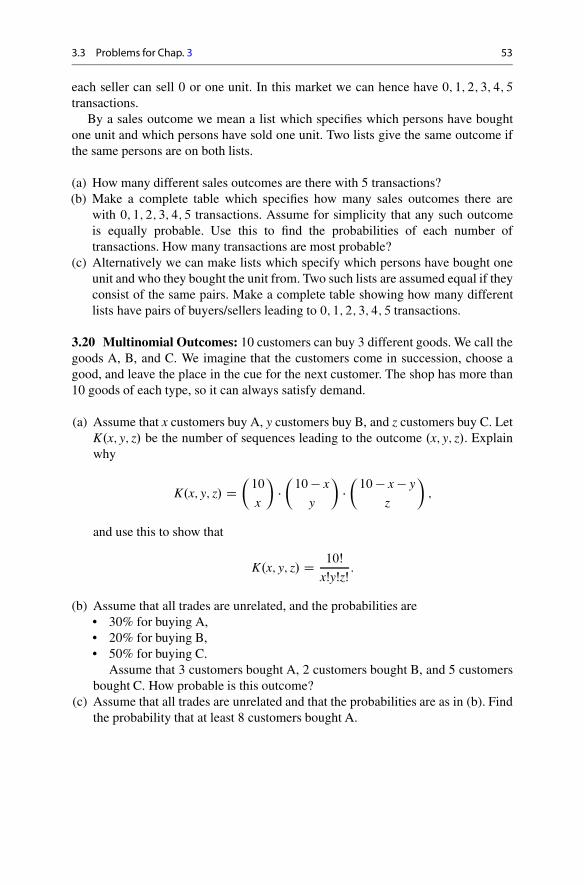
3.3 Problems for Chap. 3 53
each seller can sell 0 or one unit. In this market we can hence have 0; 1; 2; 3; 4; 5
transactions.By a sales outcome we mean a list which specifies which persons have bought
one unit and which persons have sold one unit. Two lists give the same outcome ifthe same persons are on both lists.
(a) How many different sales outcomes are there with 5 transactions?(b) Make a complete table which specifies how many sales outcomes there are
with 0; 1; 2; 3; 4; 5 transactions. Assume for simplicity that any such outcomeis equally probable. Use this to find the probabilities of each number oftransactions. How many transactions are most probable?
(c) Alternatively we can make lists which specify which persons have bought oneunit and who they bought the unit from. Two such lists are assumed equal if theyconsist of the same pairs. Make a complete table showing how many differentlists have pairs of buyers/sellers leading to 0; 1; 2; 3; 4; 5 transactions.
3.20 Multinomial Outcomes: 10 customers can buy 3 different goods. We call thegoods A, B, and C. We imagine that the customers come in succession, choose agood, and leave the place in the cue for the next customer. The shop has more than10 goods of each type, so it can always satisfy demand.
(a) Assume that x customers buy A, y customers buy B, and z customers buy C. LetK.x; y; z/ be the number of sequences leading to the outcome .x; y; z/. Explainwhy
K.x; y; z/ D�
10
x
���
10 � x
y
���
10 � x � y
z
�;
and use this to show that
K.x; y; z/ D 10Š
xŠyŠzŠ:
(b) Assume that all trades are unrelated, and the probabilities are• 30% for buying A,• 20% for buying B,• 50% for buying C.
Assume that 3 customers bought A, 2 customers bought B, and 5 customersbought C. How probable is this outcome?
(c) Assume that all trades are unrelated and that the probabilities are as in (b). Findthe probability that at least 8 customers bought A.

4Conditional Probability
Abstract
In most cases where we study probabilities, we have some additional informationabout what has happened. Information of this sort will often pose a restriction onthe sample space. In this chapter we will show how to compute probabilitiesunder such restrictions.
4.1 Conditional Probability
Before we consider the definition of conditional probability, we take a look at asimple example.
Example 4.1 During the years 2016 and 2017 a total of 100 students participated inthe exam for the course STAT000. The results are depicted in Fig. 4.1. Each squarerepresents the result of one student.
From Fig. 4.1 we see that 20% of the students received the grad A, 30% got B,30% got C, and 20% got D. Half of the students took the exam in 2017. The resultsof these students are indicated by the shaded squares in Fig. 4.2.
We see that 18 students got the grade A in 2017. This corresponds to 18% ofthe total number of students in 2016 and 2017. If we want to find the fraction ofthe students that got A in 2017, we must take into account that 50 students took theexam that year. The fraction is hence 36%.
Example 4.1 shows the underlying principle behind conditional probabilities;when we condition the probabilities, we must take into account that we change theoutcomes under consideration.
© Springer International Publishing AG 2017J. Ubøe, Introductory Statistics for Business and Economics, Springer Textsin Business and Economics, https://doi.org/10.1007/978-3-319-70936-9_4
55
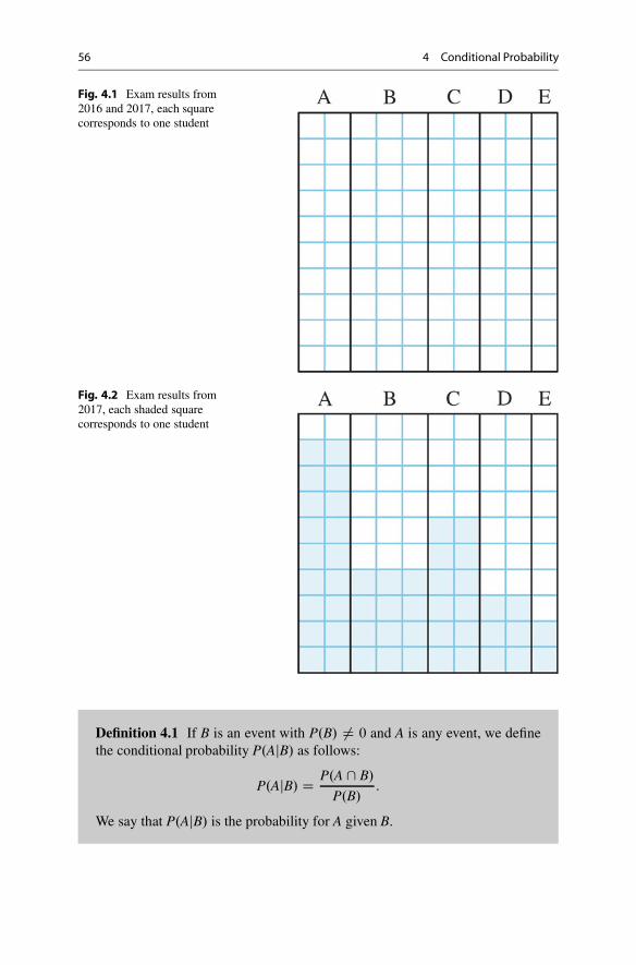
56 4 Conditional Probability
Fig. 4.1 Exam results from2016 and 2017, each squarecorresponds to one student
Fig. 4.2 Exam results from2017, each shaded squarecorresponds to one student
Definition 4.1 If B is an event with P.B/ 6D 0 and A is any event, we definethe conditional probability P.AjB/ as follows:
P.AjB/ D P.A \ B/
P.B/:
We say that P.AjB/ is the probability for A given B.

4.1 Conditional Probability 57
If we use this definition in Example 4.1, the computation is as follows:
P.Aj2017/ D P.A \ 2017/
P.2017/D 0:18
0:5D 0:36 D 36%:
We see that this is exactly what we want to know when we restrict attention to onlythose who took the exam in 2017. Note that the order of the events is important. Ifwe change the order, we get
P.2017jA/ D P.2017 \ A/
P.A/D 0:18
0:20D 0:90 D 90%:
This number tells us that 90% of the students who obtained an A took the exam in2017.
Example 4.2 In a customer survey we found that 60% of the customers used thebrand Favorite, while 30% used the brand Super. 15% of the customers used bothbrands. How many percent of the Favorite users use Super, and how many percentof the Super users use Favorite?
Solution: We use the formulas for conditional probabilities to see that
P.Sj F/ D P.S \ F/
P. F/D 15%
60%D 25%:
P. FjS/ D P. F \ S/
P.S/D 15%
30%D 50%:
This means that 25% of the Favorite users use Super, and that 50% of the Superusers use Favorite.
4.1.1 Computing Conditional Probabilities
When we compute conditional probabilities, we can work with complements just asbefore. This can be seen as follows:
P.AjB/ C P.AcjB/ D P.A \ B/ C P.Ac \ B/
P.B/D P.B/
P.B/D 1:
From this we see that
P.AcjB/ D 1 � P.AjB/:

58 4 Conditional Probability
The formula for conditional probability also provides us with some usefulrearrangements which help in special situations. If we multiply the definition ofP.AjB/ with P.B/ on both sides, we get
P.A \ B/ D P.AjB/ � P.B/:
Correspondingly
P.B \ A/ D P.BjA/ � P.A/
Since P.A \ B/ D P.B \ A/, we get
P.AjB/ � P.B/ D P.BjA/ � P.A/:
If we divide by P.A/ on both sides, we have proved Bayes’ rule which is animportant tool in statistics.
Bayes’ rule:
P.BjA/ D P.AjB/ � P.B/
P.A/:
Returning to Example 4.2, we now have an alternative way of finding the secondanswer:
P.FjS/ D P.SjF/ � P.F/
P.S/D 25% � 60%
15%D 50%
This way of rearranging the probabilities turns out to be useful in many connections.We will return to this later in this chapter.
Example 4.3 A car dealer wanted to try some new incentives to increase sales.All visitors would be offered a scratch card if they were willing to participate ina meeting with a customer advisor. The new incentives were examined after oneyear. 10% of the visitors ended up buying a car. 30% of the visitors who bought acar received a scratch card, and 10% of the customers who did not buy a car receiveda scratch card.
The car dealer wanted to find the answer to the following question: Havecustomers receiving scratch cards, a higher probability of buying a car?
Solution: We define the events B W The customer bought a car, S W The customerreceived a scratch card. From the information in the text, we know that
P.B/ D 0:1; P.Bc/ D 0:9; P.SjB/ D 0:3; P.SjBc/ D 0:1:
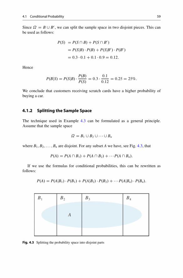
4.1 Conditional Probability 59
Since ˝ D B [ Bc, we can split the sample space in two disjoint pieces. This canbe used as follows:
P.S/ D P.S \ B/ C P.S \ Bc/
D P.SjB/ � P.B/ C P.SjBc/ � P.Bc/
D 0:3 � 0:1 C 0:1 � 0:9 D 0:12:
Hence
P.BjS/ D P.SjB/ � P.B/
P.S/D 0:3 � 0:1
0:12D 0:25 D 25%:
We conclude that customers receiving scratch cards have a higher probability ofbuying a car.
4.1.2 Splitting the Sample Space
The technique used in Example 4.3 can be formulated as a general principle.Assume that the sample space
˝ D B1 [ B2 [ � � � [ Bn
where B1; B2; : : : ; Bn are disjoint. For any subset A we have, see Fig. 4.3, that
P.A/ D P.A \ B1/ C P.A \ B2/ C � � � P.A \ Bn/:
If we use the formulas for conditional probabilities, this can be rewritten asfollows:
P.A/ D P.AjB1/ � P.B1/ C P.AjB2/ � P.B2/ C � � � P.AjBn/ � P.Bn/:
Fig. 4.3 Splitting the probability space into disjoint parts

60 4 Conditional Probability
The case where we split ˝ into two pieces B and Bc is particularly important. Theformula then reads as:
P.A/ D P.AjB/ � P.B/ C P.AjBc/ � P.Bc/:
At a first glance this may not appear very useful. Quite the contrary in fact,as the expression for A seems more complicated than where we started. Ournotation, however, is playing us a trick here; A may be a complicated set, whilethe intersections may be more simple to handle. When this happens, the splittingprinciple is very useful, and that is just what we could see happen in Example 4.3.
4.1.3 Probability Trees
In many cases complex situations with several conditional probabilities can be mademore manageable if we draw a tree showing the different cases.
Example 4.4 We want to study the investments made by a mutual fund. The fundinvests in the USA, and the investments have been placed with 75% on NASDAQ(National Association of Securities Dealers Automated Quotations System) and25% on NYSE (New York Stock Exchange). Of the funds invested on NASDAQ100% are invested in technology, while 40% of the money invested on NYSE areinvested in tech firms.
The text is relatively complex, and the information becomes more transparent ifwe draw a tree as in Fig. 4.4.
To illustrate how to use the figure, we try to answer an explicit question: Howmany percent of the US stocks are invested in technology?
Solution: The problem can be solved in several different ways. We define ˝ DUSA; A D Technology; B1 D NASDAQ and B2 D NYSE. Then B1 and B2 aredisjoint and ˝ D B1 [ B2. The splitting principle gives
P.A/ D P.AjB1/ � P.B1/ C P.AjB2/ � P.B2/ (4.1)
D 1 � 0:75 C 0:4 � 0:25 D 0:85 D 85%:
Fig. 4.4 The tree ofconditional probabilities fromExample 4.4
USA
NASDAQ NYSE
75 25
Technology Other
100 0
Technology Other
40 60

4.1 Conditional Probability 61
Fig. 4.5 Total investmentsusing the rules fromExample 4.4
USA
NASDAQ NYSE
75 M $ 25 M $
Technology Other
75 M $ 0
Technology Other
10 M $ 15 M $
There is, however, an alternative approach which most people find to be simpler.Let us imagine that we invest 100 M USD in the fund. It is then very simple to writedown a tree displaying how much money we are investing, see Fig. 4.5.
From the information in Fig. 4.5, the question above has an almost trivial answer.We have invested 100 M USD and 85 M USD have been invested in technology.Hence the share of investments in technology is
85
100D 0:85 D 85%:
Example 4.5 We consider a new question based on the same information as inExample 4.4: How many percent of the technology funds are invested on NYSE?
Solution: Again the solution is straightforward from Fig. 4.5. 85 M USD havebeen invested in technology, and 10 M USD of these have been invested on NYSE.The share is hence
10
85� 11:76%:
Strictly speaking we have until now looked at shares and not probabilities. Thepoint is now that we can reason with probabilities in exactly the same way.
Example 4.6 A firm has two main machines, Machine 1 and Machine 2. 60% ofthe goods are produced using machine 1, while the rest is produced on machine 2.The goods that are produced on machine 1 is in the next step finished on machine3 or machine 4. 75% of these goods continue to machine 3, while the rest continueto machine 4. The goods that have been produced on machine 3 is in the next stepfinished on machine 5 or 6. 50% of these goods continue to machine 5, while the restis treated on machine 6. All the goods produced on machine 3 are without errors. Ofthe goods produced on machine 4, 40% are OK. Of the goods treated by machine5, 60% are OK, while only 10% of the goods treated on machine 6 are OK. A treedepicting all this information is shown in Fig. 4.6.

62 4 Conditional Probability
Production
Machine 1 Machine 2
60 40
Machine 3 Machine 4
75 25
Machine 5 Machine 6
50 50
OK Error
100 0
OK Error
40 60
OK Error
60 40
OK Error
10 90
Fig. 4.6 Conditional probabilities
Just as in the examples above, it will in most cases help if we convert the condi-tional probabilities in Fig. 4.6 to absolute probabilities. When 60% of the goods areproduced on machine 1 and 75% of these are fished on machine 3, there is in total0:6 � 0:75 D 0:45 D 45% of the total that are produced on machines 1 and 3. If wetranslate all the numbers in this way, we end up with the tree in Fig. 4.7.
From the tree in Fig. 4.7 it is easy to answer several relevant questions.
Example 4.7 What is P.OKjProduced on machines 1 and 3/?
Solution:
P.OKjProduced on machines 1 and 3/ D P.OK \ machine 1 \ machine 3/
P.machine 1 \ machine 3/(4.2)
D 45%
45%D 1 D 100%:
What is P.Produced on machines 1 and 3jOK/?
Solution:
P.Produced on machines 1 and 3jOK/ D P.OK \ machine 1 \ machine 3/
P.OK/(4.3)
D 45%
45% C 6% C 12% C 2%� 69:23%:

4.1 Conditional Probability 63
Production
Machine 1 Machine 2
60 40
Machine 3 Machine 4
45 15
Machine 5 Machine 6
20 20
OK Error
45 0
OK Error
6 9
OK Error
12 8
OK Error
2 18
Fig. 4.7 Absolute probabilities
We can also find the answer to the last question using Bayes’ rule:
P.Produced on machines 1 and 3jOK/
D P.OKjmachine 1 \ machine 3/ � P.machine 1 \ machine 3/
P.OK/
D 100% � 45%
45% C 6% C 12% C 2%� 69:23%:
From the examples above, we see that it is often a good idea to convert a tree withconditional probabilities to a tree of absolute probabilities. We now look at how wecan do this quickly.
Example 4.8 To the left in Fig. 4.8 we show a part of a tree with conditionalprobabilities. We wish to compute the absolute probability of reaching the nodesshown to the right.
The node in the bottom of the tree represents 100%, and since 20% of this istransferred to A, P.A/ D 20%. The probability of reaching node B is
P.A \ B/ D P.BjA/ � P.A/ D 50% � 20% D 10%:
Furthermore
P.A \ B \ C/ D P.CjA \ B/ � P.A \ B/ D P.CjA \ B/ � P.BjA/ � P.A/ (4.4)
D 50% � 50% � 20% D 5%:

64 4 Conditional Probability
20
50
50
20
A
B
C
D
?
?
?
?
Fig. 4.8 A part of a probability tree
20
10
5
1
Fig. 4.9 Multiplying probabilities along branches
We can continue like this until we reach the end of the branch. Even though thederivation is somewhat complicated, we end up with a simple and transparentprinciple:
We find the absolute probabilities multiplying the conditional probabilities insuccession along each branch.
The end result is hence as shown in Fig. 4.9.
4.2 Subjective Probabilities
We often hear people make more of less wild guesses on the probabilities ofsomething happening. Such probabilities are often based on wishful thinking; theperson feels that a probability is large, or claims to have reason to believe that aprobability is small. When a person speaks in public on such matters, it is easy tomake contradictory statements.
Example 4.9 Two teams A and B are playing the final, and a supporter of teamA claims that the chance of A winning the final is P.A/ D 80%. One of the bestplayers on team B is injured however, and it is not clear that he will recover to playin the final. The supporter believes that the chance of recovery is P.B/ D 0:1. Ifhe recovers, the supporter claims that the chance of winning falls to 60%, while thechance of team A winning is 90% if he does not recover.

4.3 Independence 65
We let B denote the event that the best player on team B recovers, and thesupporter has made the statements
P.A/ D 0:8; P.B/ D 0:1; P.AjB/ D 0:6; P.AjBc/ D 0:9:
What are the consequences of these subjective statements?We know that
P.AjB/ D P.A \ B/
P.B/D 0:6 ) P.A \ B/ D 0:6 P.B/ D 0:06:
P.AjBc/ D P.A \ Bc/
P.Bc/D 0:9 ) P.A \ Bc/ D 0:9 P.Bc/ D 0:81:
Hence
P.A/ D P.A \ B/ C P.A \ Bc/ D 0:06 C 0:81 D 0:87;
which is quite disturbing as the supporter already claimed that P.A/ D 0:8. Thenumbers do not add up, and there must be something wrong with the subjectiveassessments. The reader is encouraged to check that only the value P.B/ D 1=3 isconsistent with the three other values.
4.3 Independence
Independence is one of the most central concepts in statistics. Broadly speakingwe can say that two events are independent when there are no connectionsbetween them. Independence is particularly important when we conduct scientificexperiments. It is important to carry out the experiments in a way such that theoutcome of a new experiment does not depend on what has happened in the previouscases. Technically the definition of independence is surprisingly simple:
Two events A and B are independent if and only if P.A \ B/ D P.A/ � P.B/.
Independence is intimately related to conditional probability. If P.B/ 6D 0, and Aand B are independent events, then
P.AjB/ D P.A \ B/
P.B/D P.A/ � P.B/
P.B/D P.A/:

66 4 Conditional Probability
Hence if A and B are independent the probability of A does not change whenwe condition on B. The multiplicative rule makes it simple to compute independentevents, and the definition is easily extended to cases with more than two events.
A collection of events are mutually independent if and only if the probabilityof any intersection is equal to the product of the probabilities of the eventsincluded in the intersection.
Example 4.10 Assume that the events A; B; C; D are mutually independent.Then, e.g.
P.A \ B \ C \ D/ D P.A/ � P.B/ � P.C/ � P.D/
and
P.B \ D/ D P.B/ � P.D/:
Example 4.11 Assume that an experiment has the outcome r with probability 0.2,s with probability 0.5, and t with probability 0.3. Assume that we repeat theexperiment 4 times, and that the outcomes of each repetition are independent. Whatis the probability of the sequence rrts?
Solution: Since each repetition is independent from the rest, we get
P.rrts/ D P.r/ � P.r/ � P.t/ � P.s/ D 0:2 � 0:2 � 0:3 � 0:5 D 0:006:
We notice that independence leads to the same simplicity we exploit in combina-torics when the choices are unconnected.
4.4 Summary of Chap. 4
• Definition of conditional probability
P.AjB/ D P.A \ B/
P.B/:
• Bayes’ rule:
P.BjA/ D P.AjB/ � P.B/
P.A/:

4.5 Problems for Chap. 4 67
• The splitting principle
P.A/ D P.AjB1/ � P.B1/ C P.AjB2/ � P.B2/ C � � � C P.AjBn/ � P.Bn/:
• Two events are independent when P.A \ B/ D P.A/ � P.B/.
4.5 Problems for Chap. 4
4.1 In a customer survey we have found that 35% of the customers use the brandFavorite, while 56% use Super. 14% of the customers use both brands. How manypercent of the Favorite users use Super, and how many percent of the Super usersuse Favorite?
4.2 In a customer survey we have found that 50% of the Favorite users use Super,while 25% of the Super users use Favorite. 20% of the customers use both brands.How many percent of the customers use Favorite, and how many percent of thecustomers use Super?
4.3 In a survey 160 men and 240 women were asked if they liked a particularproduct. 40% of the men and 20% of the women liked the product. How manypercent of the participants liked the product?
4.4 You want to invest some money. 60% should be invested in mutual funds and40% in money market funds. Of the money invested in mutual funds, 30% shouldbe invested in China and 70% in other countries. Of the money invested in moneymarket funds, 80% should be invested in Chinese funds and 20% in other countries.
(a) Make a tree displaying the information.(b) How many percent of the money is invested in China?(c) How many percent of the money invested in China are in mutual funds?
4.5 A company has 3 departments. 20% of the reports are from department A, 45%from department B, and 35% from department C. An examination revealed that 3%of the reports for A contained errors, 6% of the reports from B contained errors, and2% of the reports from C contained errors.
(a) Make a tree displaying the information.(b) How many percent of the reports contained errors?(c) A report contained errors. What is the probability that the report came from
department A?

68 4 Conditional Probability
4.6 We look at the stock price in two companies, and define the following events:
A: The stock price in company 1 increases.B: The stock price in company 2 increases.C: The stock price in company 2 does not increase.
We assume that there is 60% probability of an increase in the stock price ofcompany 1, 40% probability of an increase in the stock price of company 2, and24% probability of an increase in the stock price of both companies?
(a) Are A and B independent?(b) Are A and C independent?(c) Are B and C independent?
4.7 Show that if A and B are independent, then A and C D Bc are independent.
4.8 We consider two events:
A: The stock price in company 1 increases.B: The interest rate falls.
Assume that there is 60% probability for an increase in stock price, and that thisprobability does not change if the interest rate falls.
(a) Show that A and B are independent events.(b) Try to formulate a general version of this result.
4.9 A shop has three goods on offer, A, B, and C. Each customer buys at most oneof these goods. If a customer buys one of the goods on offer, then there is
• 50% probability for buying A.• 20% probability for buying B.• 30% probability for buying C.
4 customers buy goods on offer, and we assume that buys are independent.
(a) What is the probability that customer 1 buys A, customer 2 buys A, customer 3buys B, and customer 4 buys C?
(b) What is the probability that at least 3 customers buy A?(c) What is the probability that 2 customers buy C?
4.10 A company has two departments, department A with 60 employees anddepartment B with 90 employees. Each department is divided into groups of 30people, A1 and A2 at department A and B1; B2; B3 at department B. During the last

4.5 Problems for Chap. 4 69
Table 4.1 Performance at departments A and B in Problem 4.10
Group Good Average Bad
A1 50% 25% 25%
A2 10% 70% 20%
B1 40% 50% 10%
B2 20% 60% 20%
B3 30% 60% 10%
Table 4.2 Fractions liking the product in Problem 4.11
Fractions liking the product
Women Younger than 25 years 25–40 years Older than 40 years
60% 30% 80%
Fractions liking the product
Men Younger than 25 years 25–40 years Older than 40 years
20% 40% 60%
Fractions of the participants
Women Younger than 25 years 25–40 years Older than 40 years
15% 30% 15%
Fractions of the participants
Men Younger than 25 years 25–40 years Older than 40 years
20% 10% 10%
year the performance of each group has been examined, and the results are shownin Table 4.1.
We assume that the observed fractions represent the probabilities for the respec-tive performances, and the probability that a project is carried out at a department isproportional to the number of workers at the department.
(a) Make a tree displaying the information.(b) What is the probability that a project done at department A is good?(c) A project is good. What is the probability that it has been done at department B?(d) Is the probability of good performance independent of department?
4.11 Structuring Complex Information: In a customer survey a large number ofpeople were asked if they liked a product. The question was posed to 6 differentgroups of the population. The fractions liking the product are shown in Table 4.2.The table also shows how large fractions of the participants belonged to each group.
(a) How large fraction of the participants liked the product?(b) How large fraction of the women were in the group Younger than 25 years old?(c) How large fraction of the women and how large fraction of the men liked the
product?

70 4 Conditional Probability
Table 4.3 Investingstrategies in Problem 4.12
Fund USA Europe China
Global A 50% 30% 20%
Global B 20% 70% 10%
Aggressive C 30% 50% 20%
4.12 Extracting Information from Trees: A broker sells shares from three differ-ent global funds: Global A, Global B, and Aggressive C. 30% of the investments areplaced in Global A, 60% in Global B, and 10% in Aggressive C. The funds diversifytheir investments and invest in the USA, Europe, and China. The fractions investedin these markets are shown in Table 4.3.
(a) Draw a tree displaying the information given above.(b) How large share of the two funds Global A and B in total is invested in the USA?(c) How large fraction of the US investments is invested in Global A?(d) From the information provided above, is it possible to determine how many
percent of the customers who invest more than 40% of their investments in theUSA?
4.13 Untangling Conditional Information: In surveys focusing private/sensitiveinformation it is important that the participants feel they are anonymous. A simplestrategy taking this into account can be outlined as follows:
Split the participants into two categories:
• Category 1: Persons with date of birth from January 1 to August 31.• Category 2: Persons with date of birth from September 1 to December 31.
The participants in Category 1 answer Yes/No to the question: Is your year ofbirth an even number?
The participants in Category 2 answer Yes/No to the question: Have you everused illegal drugs?
The participants should not reveal their category, and the people conducting thesurvey hence do not know which question has been answered.
(a) We assume that all relevant dates/year of birth are equally probable, and weignore leap years. How large fraction does each category make up? What is theprobability of answering Yes, given that the person is in Category 1?
(b) We ask the questions to a large number of people, and find that in total 60% ofthe participants answered Yes. Assume that the answers were honest. How largefraction of Category 2 admitted using illegal drugs?
(c) Alternatively we could swap the questions for Category 1 and 2. Discuss if therecan be advantages/disadvantages in swapping.

4.5 Problems for Chap. 4 71
4.14 True/False Positives: A medical test gives a true positive in 77% of the caseswhere the patient has the illness, and a false positive in 2% of the cases wherethe patient does not have the illness. We assume that at any given time 2% of thepopulation has the illness.
(a) The test is used on a randomly chosen patient. In how many percent of the caseswill the test return a positive result? Given that the test returns a positive value,how large is the probability that the person has the illness?
(b) A person is tested and the test returns a positive value. Discuss circumstancesthat can influence the probability that the person has the illness.
(c) Can there exist circumstances where a positive value implies more than 77%chance that the person has the illness?
4.15 The Chance of True Positives Can Be Strongly Misleading: An auditingfirm has developed a diagnostic tool to predict which firms will go bankrupt the nextyear. The model has been tested on old data and returned the following results:
• Of the companies that went bankrupt, 80% were flagged by the tool.• Of the companies that did not go bankrupt, 95% were not flagged by the tool.
We assume that 10% of the firms will go bankrupt the next year, and that theperformance of the diagnostic tool will stay in line with the performance on the olddata.
(a) What is the probability that the firm is flagged given that it will not go bankrupt?How large percent of bankruptcies will the model predict?
(b) A firm has been flagged by the tool. What is the probability that the firm will infact go bankrupt?
4.16 Markov Chains: A bank has some good and some bad customers.
• The probability that a good customer is downgraded to a bad customer duringone time period is 30%.
• The probability that a bad customer is upgraded to a good customer during onetime period is 20%.
We assume for simplicity that the development during any time period isindependent of what has happened in the previous time periods, and that the timedevelopment of different customers is independent.
(a) A customer is rated as good. How probable is it that:(i) The customer is rated as good in the next two time periods?
(ii) The customer is rated as good two time periods from now?(b) A customer is rated as good. How probable is it that the customer is rated as
good in exactly 9 of the 10 next time periods?

72 4 Conditional Probability
(c) Point to circumstances that can make the assumptions of independence ques-tionable.
4.17 Simpson’s Paradox: During the first six months of the year auditing firmA inspected 2000 documents and detected 120 errors. In the next 6 months theyinspected 8000 documents and detected 240 errors. In the first six months auditingfirm B inspected 4000 documents and detected 200 errors. In the next six monthsthey inspected 1000 documents and detected 20 errors. We assume that the numbersare representative in that they reflect the probabilities of finding errors in the twoperiods.
(a) Which firm had the largest probability of finding errors in the first six months?Which firm had the largest probability of finding errors in the next six months?Which firm had the largest probability of finding errors during the whole year?
(b) Try to explain the connection between the results in (a).
4.18 Combining Splitting and Bayes’ Rule: We classify firms into three differentgroups: Gr 1: Solvent, Gr 2: Worrisome, Gr 3: Bankrupt.
A bank gives the firms rating A, B, or C (A is the best rating.) Figures fromprevious years:
• 2:5% of the firms that went bankrupt had rating A.• 15% that ended up as worrisome had rating A.• 30% that ended up as solvent had rating A.
We assume that these numbers are stable from year to year. The numbers forrating B and C are omitted since they are not needed to answer the questions.
(a) How many percent of the firms get rating A?(b) A firm has rating A. How large is the probability that it will go bankrupt?
4.19 Few False Positives Might Still Be Bad: An auditing firm has developed atool to predict bankruptcy. The tool is very conservative. Among companies that donot go bankrupt, 5% are flagged for bankruptcy. We assume in this problem that arandomly selected firm has 0:1% probability of bankruptcy.
(a) Explain why
P.The firm is flagged for bankruptcy/ � 1 � 0:001 C 0:05 � 0:999
(b) A firm has been flagged for bankruptcy with this tool. Show that the probabilitythat the firm does not go bankrupt is larger than 98%.
4.20 Polls May Be Misleading: Assume that 60% of the viewers of TV programthink that the level of taxation should be decreased, while 40% would like to see

4.5 Problems for Chap. 4 73
an increase. Assume further that 2% of those in favor of a reduction participate in apoll, while 7% of the viewers in favor of a tax raise participate in the poll.
(a) How large fraction of the viewers participate in the poll?(b) How large fraction of the participants in the poll would like to see an increase
in the tax level? Comment the result.
4.21 Combining Splitting and Bayes’ Rule: There is often a connection betweeneconomic growth in a country and a strengthening of the currency. Assume that theprobabilities for economic growth are as follows:
P.High growth/ D 0:3 P.Medium growth/ D 0:5 P.Low growth/ D 0:2:
• When growth is high, there is a 70% chance of strengthening the currency.• When growth is medium, there is a 50% chance of strengthening the currency.• When growth is low, there is a 20% chance of strengthening the currency.
(a) How large is the probability that the currency will strengthen?(b) The currency is strengthening. What is the probability of high economic growth?(c) Are the events “High economic growth” and “The currency is strengthening”
independent in this case. Justify the answer.
4.22 Spam Filtering: The frequency of special words is very different in e-mailspam than in ordinary e-mail. In e-mail spam the frequency of the word “debt”is 30.9%, while the frequency of the word is 0.447% in ordinary e-mail. In thisproblem we will assume that e-mail spam make up 50% of the e-mail that youreceive.
(a) How large is the frequency of the word “debt” in all e-mail?(b) An e-mail contains the word “debt.” What is the probability that the e-mail is
spam?
4.23 Untangling Conditional Probabilities: Assume that a special group ofworkers makes up 5% of the tax payers within a city. The taxation authorities haveestimated that about 10% of the workers commit tax fraud. Previous data suggestthat 1% of the workers who do not commit tax fraud belong to the special group.
(a) Use the information in the text to suggest how big share the special group makesup of those committing tax fraud.
(b) Use the answer in (a) to find the probability that a person in the special groupcommits tax fraud.
4.24 A Simpson’s Paradox fromReal Life: In a statistical survey from the period1972–1974, 1316 women were interviewed regarding their smoking habits. The

74 4 Conditional Probability
Table 4.4 Mortality rates in age groups
Age 18–24 25–34 35–44 45–54 55–64 65–74 75+
Mortality in % smokers 3:6 2:4 12:8 20:8 44:3 80:6 100
Mortality in % nonsmokers 1:6 3:2 5:7 15:4 33:1 78:3 100
Table 4.5 Number of participants in each age group
Age 18–24 25–34 35–44 45–54 55–64 65–74 75+
Number of participants smokers 55 124 109 130 115 36 13
Number of participants nonsmokers 62 157 123 78 121 129 64
sample was drawn randomly and there were 582 smokers and 734 nonsmokers inthe sample. 20 years later, the scientists recorded how many of the participants thatwere still alive. The results are shown in Tables 4.4 and 4.5. Age refers to the age atthe start of the survey.
(a) What was (according to the tables) the probability of death given that theparticipant was a smoker in the age group 18–24? How big share of the smokersdid this group make up? Use the splitting principle to compute the probabilityfor death among smokers.
(b) What was (according to the tables) the probability of death given that theparticipant was a nonsmoker in the age group 18–24? How big share of thesmokers did this group make up? Use the splitting principle to compute theprobability for death among nonsmokers.
(c) The survey shows that the probability for death was considerably lower forsmokers than for nonsmokers. Explain, using the tables above, that this doesnot show that smoking is healthy.

5RandomVariables, Mean, and Variance
Abstract
In this chapter we will introduce a general framework we will use to studystatistical distributions. A statistical distribution specifies the probability of thedifferent outcomes that can occur. We can, e.g., ask about the probability forexactly x defective items in a sample of 10 items. We let x run from 0 to10, and compute 11 probabilities. The set of these probabilities we call thedistribution. When the distribution is known, we are usually able to computeall the probabilities we may need. The distribution is hence the key to ourcalculations.
5.1 Random Variables
In many cases we wish to study a number which comes as a result of a randomoutcome. We call any such number a random variable. We first consider a fewexamples.
Example 5.1 Let ˝ be the set of outcomes from one roll of a dice, and define afunction X by
X.!/ D(
1 if ! D 1; 3; 5
�1 if ! D 2; 4; 6:
Hence if the outcome is odd, the result is 1, and the result is �1 when the outcomeis even. In any case X will be a real number.
© Springer International Publishing AG 2017J. Ubøe, Introductory Statistics for Business and Economics, Springer Textsin Business and Economics, https://doi.org/10.1007/978-3-319-70936-9_5
75

76 5 Random Variables, Mean, and Variance
Example 5.2 Let ˝ be the set of outcomes from two rolls of a dice, and define afunction
X.!1; !2/ D !1 C !2;
where !1 is the result of the first roll and !2 is the result of the second roll. Anyoutcome of the two tosses leads to a real number.
Example 5.3 Let v1; v2; v3 denote the stock price for three different companies, andlet the sample space ˝ be all possible combinations of values that the stock pricescan have tomorrow. We can then define a function
X.v1; v2; v3/ D 1
3.v1 C v2 C v3/:
Whatever stock prices will occur tomorrow, the resulting value of X will be a realnumber.
All the three examples above have that in common that they define a functionon the sample space leading to a real number. We call any such function a randomvariable.
Definition 5.1 By a random variable we mean a function defined on thesample space which returns a well-defined real number from any outcome.
In this chapter we will only consider random variables defined on a discretesample space. When the sample space is discrete, we can define a random variablespecifying the values X.!1/; X.!2/; : : : . The same value can occur multiple times,and this is something we need to take into account.
Definition 5.2 The probability distribution of a random variable X is definedby
P.x/ D P.X D x/;
where x is any value that X can have.
The probability distribution hence specifies the probability of the differentvalues that X can have. The probability distribution P.x/ is also called the pointprobabilities of X. In statistics it is common to use capital letters to define randomvariables, and use lowercase letters about constants. In the definition above X is arandom variable, while x is used about all the constant values that X can have.

5.1 Random Variables 77
Example 5.4 Let ˝ D f!1; !2; !3g with uniform probabilities, and define a randomvariable by
X.!1/1; X.!2/ D �2; X.!3/ D 1:
Then P.X D �2/ D 13
and P.X D 1/ D 23. For any other values of x, P.X D x/ D 0.
Example 5.5 Let X be the number of heads in two tosses of a fair coin. There arethree possible values for X: 0; 1; 2. The value 1 can be realized in two different ways,and the probability distribution is hence:
P.X D 0/ D 1
4; P.X D 1/ D 1
2; P.X D 2/ D 1
4:
For any other values of x, P.X D x/ D 0.To get an overview of the distribution, we can display these values as bars in a
histogram. The histogram in Fig. 5.1 shows the relative frequencies we would expectto find if we did a large number (ideally infinitely many) of independent tosses.
Example 5.6 Assume that ˝ D f!1; !2; !3; !4; !5g,
p.!1/ D 0:2; p.!2/ D 0:3; p.!3/ D 0:1; p.!4/ D 0:1; p.!5/ D 0:3;
and that
X.!1/ D 1; X.!2/ D 2; X.!3/ D 1; X.!4/ D 2; X.!5/ D 3:
Fig. 5.1 The distribution inExample 5.5
0 1 2
0.25
0.50
P(x)
x

78 5 Random Variables, Mean, and Variance
Fig. 5.2 The distribution inExample 5.6
1 2 3
0.1
0.2
0.3
0.4
0.5P(x)
x
Fig. 5.3 The distribution ofthe sum of two dice tosses
2 3 4 5 6 7 8 9 10 11 12
0.025
0.05
0.075
0.1
0.125
0.15
P(x)
x
Then
P.X D 1/ D p.!1/ C p.!3/ D 0:3;
P.X D 2/ D p.!2/ C p.!4/ D 0:4;
P.X D 3/ D p.!5/ D 0:3:
The histogram is displayed in Fig. 5.2.
Example 5.7 Let ˝ be the set of all outcomes of two tosses of a dice with uniformprobability, and let S denote the sum of the two tosses. Here there are lots of differentcases, and it is tedious to go through them all. The end result is displayed in Fig. 5.3,and looking at the figure we quickly get an overview of the distribution. We can, e.g.,see that the result S D 7 is the most probable, and that the value is about 0.17.

5.1 Random Variables 79
Sometimes it may be convenient to organize the information a bit differently.Instead of giving the probability for each possible value of X, we might give theprobability that X is below a threshold x. The probability that the random variableis less than or equal to a constant x, we call the cumulative distribution.
Definition 5.3 The cumulative distribution of a random variable X is definedby
F.x/ D P.X � x/;
which is defined for any real number x.
When the distribution of X is known, we see that
F.x/ DX
xi�x
P.X D xi/:
That means that we find the value of the cumulative distribution adding theprobability of all cases where xi � x. Figure 5.4 shows the principle behind thefunction. It is piecewise constant and increases in jumps at x1; x2; x3 : : : : The sizesof the jumps are equal to the corresponding values of P.X D xi/.
Example 5.8 Assume that ˝ D f!1; : : : ; !5g, and
p.!1/ D 0:2; p.!2/ D 0:3; p.!4/ D 0:1; p.!4/ D 0:1; p.!5/ D 0:3;
Fig. 5.4 A cumulativedistribution
x1 x2 x3 x4x
0.2
0.4
0.6
0.8
1.0F

80 5 Random Variables, Mean, and Variance
Fig. 5.5 The cumulativedistribution of Example 5.8
1 2 3 4x
0.2
0.4
0.6
0.8
1.0F
and that
X.!1/ D 1; X.!2/ D 2; X.!3/ D 1; X.!4/ D 2; X.!1/ D 3:
Find the cumulative distribution.
Solution: If x < 1, then F.x/ D P.X � x/ D 0.
If 1 � x < 2, then F.x/ D P.X � x/ D p.!1/ C p.!3/ D 0:3:
If 2 � x < 3, then F.x/ D P.X � x/ D p.!1/ C p.!2/ C p.!3/ C p.!4/ D 0:7:
If 3 � x, then F.x/ D P.X � x/ D p.!1/ C p.!2/ C p.!3/ C p.!4/ C p.!5/ D 1:
We see that the function is piecewise constant, and that it increases everywhere. Thegraph is shown in Fig. 5.5.
5.2 Expectation
In Chap. 1 we computed the mean of a sequence of numbers. The mean isone of the major practical concepts in statistics, and we will now look at thecorresponding theoretical concept. The expectation EŒX� of a random variable Xis a theoretical quantity with the following property: If we make a large number ofindependent observations of X, the mean of these observations will approach EŒX�.The expectation is hence an idealized quantity which we intuitively may think of as

5.2 Expectation 81
the mean of infinitely many observations. The rigorous definition reads as follows:
Definition 5.4 If X is a random variable with possible values x1; x2; : : : ; xm,then
EŒX� D x1 � P.X D x1/ C x2 � P.X D x2/ C � � � C xm � P.X D xm/:
We call EŒX� the expectation of X, or the expected value when it is clear formcontext which random variable we are considering.
It is sometimes cumbersome to write the terms like this, and as an alternative wemay use the summing symbol instead. Then the expression is
EŒX� DmX
iD1
xi � P.X D xi/:
Verbally we may express this as follows: We consider all the values that X canachieve, and multiply each such value by the probability that X has this particularvalue. The expected value is the sum of all such terms.
Example 5.9 Let X be the result from one toss of a dice. Find EŒX�.
Solution: Using the formula above, we find
EŒX� D 1 � 1
6C 2 � 1
6C 3 � 1
6C 4 � 1
6C 5 � 1
6C 6 � 1
6D 3:5:
Example 5.10 X is the number of items that a randomly selected customer buys ina special shop. We assume the following distribution:
P.X D 0/ D 0:3; P.X D 1/ D 0:2; P.X D 0/ D 0:4; P.X D 0/ D 0:1:
Find EŒX�.
Solution:
EŒX� D 0 � P.X D 0/ C 1 � P.X D 1/ C 2 � P.X D 2/ C 3 � P.X D 3/
D 0 � 0:3 C 1 � 0:2 C 2 � 0:4 C 3 � 0:1 D 1:3:

82 5 Random Variables, Mean, and Variance
Example 5.11 Let ˝ be the outcome of two tosses of a fair dice, and let S be thesum of the two rolls. S has the values 2; 3; 4; 5; 6; 7; 8; 9; 10; 11; 12, and
p.2/ D 1
36; p.3/ D 2
36; p.4/ D 3
36; p.5/ D 4
36; p.6/ D 5
36; p.7/ D 6
36; (5.1)
p.8/ D 5
36; p.9/ D 4
36; p.10/ D 3
36; p.11/ D 2
36; p.12/ D 1
36:
Using the definition, we find
EŒS� D 2 � 1
36C 3 � 2
36C 4 � 3
36C � � � C 12 � 1
36D 7:
We will, however, soon see that this was not an efficient way of computing theexpectation. Using some general principles, we can avoid most of the work.
5.2.1 Computing Expectations
If X and Y are two random variables, and a and b are two constants, then thefollowing rules may be used:
EŒX C Y� D EŒX� C EŒ Y�; EŒa� D a; EŒb � X� D b � EŒX�:
The proofs of these rules are straightforward and we omit them. We see thatthe expectation of a sum is the sum of the expectations, and that the expectationof a constant is equal to the constant itself. The last rule says that constants maybe moved outside the expectation. To see how to apply these rules, we return toExample 5.11. This time we define
X D Result of the first toss; Y D Result of the second toss:
It is easy to see (Example 5.9), that
EŒX� D EŒ Y� D 3:5:
Since S D X C Y, we get
EŒS� D EŒX C Y� D EŒX� C EŒ Y� D 3:5 C 3:5 D 7:
Comparing the two methods, we see that the second method is much simpler.

5.2 Expectation 83
5.2.2 General Expectations and Variance
Sometimes we need to compute the expectation of a function of a random variable.We may, e.g., consider the quantity Q we could sell of a certain good. Frommicroeconomic theory it is well known that the price P is a function P.Q/. If Qis a random variable, we would like to find the expected price; EŒ P.Q/�.
If X is a random variable and h is a function, then Y D h.X/ is a new randomvariable. The expectation of Y can be found as follows:
EŒh.X/� D h.x1/ � P.X D x1/ C h.x2/ � P.X D x2/ C � � � C h.xm/ � P.X D xm/:
This can be expressed as follows: We find the expectation of a function of arandom variable when we compute the function value for any value that X can haveand multiply the function value by the probability that X has this particular value.The expectation is the sum of all such terms.
Example 5.12 Let X be the result of one toss of a dice, and let h.x/ D x2. Then
EŒX2� D 12 � 1
6C 22 � 1
6C 32 � 1
6C 42 � 1
6C 52 � 1
6C 62 � 1
6D 91
6:
In Chap. 1 we introduced the sample variance, which is very useful in practicalapplications. We will now consider its theoretical analogue. Intuitively the theoreti-cal variance is the sample variance we would have obtained if we could do infinitelymany independent observations. The rigorous definition reads as follows:
Definition 5.5 The variance VarŒX� of a random variable is defined via
VarŒX� D EŒ.X � EŒX�/2�:
We see that the variance is a measure of the deviation from the expected value; ifall the values of the random variable are close to EŒX�, then all the values .X�EŒX�/2
are small positive numbers, and the variance will be small. Once the variance isdefined, we can define the standard deviation just as in Chap. 1.

84 5 Random Variables, Mean, and Variance
Definition 5.6 The standard deviation �ŒX� of a random variable is definedvia
�ŒX� Dp
VarŒX�:
Example 5.13 We assume that X is a random variable with the values 2; 4; 6; 8 andthat the distribution is p.2/ D p.4/ D p.6/ D p.8/ D 1
4. Then
EŒX� D 2 � 1
4C 4 � 1
4C 6 � 1
4C 8 � 1
4D 5:
If we define Y D X � EŒX� D X � 5, Y becomes a new random variable with thevalues �3; �1; 1; 3. We find the variance of X by
VarŒX� D EŒ Y2� D .�3/2 � 1
4C .�1/2 � 1
4C 12 � 1
4C 32 � 1
4D 5:
When we want to compute the variance, it may be convenient to rearrange theterms. If we do that properly, we can find the relation
VarŒX� D EŒX2� � .EŒX�/2
We are generally not very concerned with proofs, but this time we make anexception. The reason is that the proof makes use of some central techniques, and itis valuable to see how they are applied. The proof goes as follows:
VarŒX� D EŒ.X � EŒX�/2� D EŒX2 � 2X � EŒX� C .EŒX�/2�
D EŒX2� � 2EŒX � EŒX�� C EŒ.EŒX�/2�
D EŒX2� � 2EŒX� � EjX� � .EŒX�/2 EŒ1�
D EŒX2� � 2.EŒX�/2 � .EŒX�/2 D EŒX2� � .EŒX�/2 :
In the first line we used that .a � b/2 D a2 � 2ab C b2, in the second line we usedEŒU C V C W� D EŒU� C EŒV� C EŒW�, and in the third line k D EŒX� is a constant,which gives EŒk � U� D k � EŒU�. In addition we used EŒ1� D 1.
We return to Example 5.13 to see how the computation looks like when we usethis new technique. We have
EŒX2� D 22 � 1
4C 42 � 1
4C 62 � 1
4C 82 � 1
4D 30:

5.3 Some Simple Facts About Option Pricing 85
This gives
VarŒX� D EŒX2� � .EŒX�/2 D 30 � 52 D 5:
We see that the computation becomes a bit simpler since we need not consider theY � s.
The variance has some basic properties which we list below:
• If X D k is a constant, then VarŒX� D 0.• If Y D X C k where k is a constant, then VarŒ Y� D VarŒX�.• If k is a constant, then VarŒk � X� D k2VarŒX�.• VarŒX� � 0.• VarŒX� D VarŒ�X�.
We omit the proofs of the first two properties, but take a brief look at the third.The reason why we want to highlight this is that students often make errors whenthey apply this principle. It is possible to move constants outside the variance, butthen the constant needs to be squared.
VarŒk � X� D EŒ.k � X � EŒk � X�/2� D EŒ.k � X � k � EŒX�/2� (5.2)
D EŒ.k � .X � EŒX�//2� D EŒk2 � .X � EŒX�/2�
D k2 � EŒ.X � EŒX�/2� D k2 � VarŒX�:
Example 5.14
VarŒ10X� D 102VarŒX� D 100VarŒX�:
5.3 Some Simple Facts About Option Pricing
Most people have heard about options, but some definitions may be appropriate.There are many different kinds of options, and we will only discuss a special case:a European call option. A European call option gives the right but not the obligationto buy a stock for a certain price at some specific point in time.
Example 5.15 Assume that we own a European call option which gives us the rightto buy a stock for 100 USD one year from now. If the stock price is above 100USD one year from now, we use the option to buy the stock. Afterwards we can sellthe stock and make a profit. If the stock price is less than 100 USD, the option isworthless and we do not buy the stock.
Clearly it is possible to profit from an option, so a right of this sort can’t be free.We consider a strongly simplified example.

86 5 Random Variables, Mean, and Variance
Example 5.16 A stock costs today 100 USD. Tomorrow only two cases can occur.Either the stock rises to 140 USD or it will fall to 90 USD. The probability that theprice rises is p D 0:6 and the probability that it falls is q D 0:4. A customer comesto a bank and wants to purchase 100 call options which gives the right to buy 100stocks for 100 USD each tomorrow. The bank demands 800 USD for the options.
Initially we disregard transaction costs, and wish to answer the followingquestions:
• The customer buys 8 stocks for 800 USD. What is the expected value of the stocktomorrow?
• The customer uses 800 USD to buy 100 call options. What is the expected valueof the call options tomorrow?
Solution: We let X be the stock price. The expected value of 8 stocks tomorrowis
EŒ8X� D 8 � EŒX� D 8 � .140 � 0:6 C 90 � 0:4/ D 960:
We see that the expected value of the stock increases from 800 USD to 960 USD,which is an increase of 20%.
We let Z denote the value of the options. If the stock price rises to 140 USD, weuse the options to buy the stock for 100 USD each. This leaves us with a profit of 40USD for each option. If the stock price falls, the options are worthless. The expectedvalue of the options is
EŒZ� D 40 � 100 � 0:6 C 0 � 100 � 0:4 D 2400:
We see that the expected value of the investment increases from 800 USD to 2400
USD, which is an increase of 200%.
5.3.1 Hedging Portfolios
At a first glance the example above might appear speculative, and one could questionif banks should be involved in such businesses. Is the bank gambling with oursavings? The rather surprising answer is no, the bank has no risk writing thiscontract. The reason is that the bank can eliminate all risk if it make specialinvestments. The strategy the bank applies is the following: Receive 800 USD fromthe customer, take up a loan of 7200 USD from a bank account, and use the 8000
USD to buy 80 stocks. What happens if the bank employs this strategy?If the stock rises to 140 USD, the bank owns 80 stock with a total worth of 11;200
USD. It has a debt of 7200 USD and need to pay the customer 4000 USD for the100 options the customer redeems. When all is settled, the bank breaks even. If thestock falls to 90 USD, the bank owns 80 stocks with a total worth of 7200 USD

5.3 Some Simple Facts About Option Pricing 87
which just matches the debt. The options are worthless in this case, so the bank donot need to pay anything to the customer. We see that the bank breaks even in thiscase as well.
Note that p and q have no influence on the strategy, and the bank will breakeven no matter what values p and q have. To set up a strategy of this kind is calledhedging, where the idea is that the bank protects (hedges) itself from risk.
The numbers above may appear as pure magic, but there is a simple mathematicalexplanation: The strategy has three unknowns, the price x that the customer need topay for the option, then number y of stock the bank should buy, and z the amount ofmoney the bank should lend from the bank account. To decide these three unknowns,we need three equations:
y � 100 D x C z
y � 140 � z � .140 � 100/ � 100 D 0
y � 90 � z D 0:
The first equation says that we use x C z USD to buy y stocks, and the other twoequations say that the bank breaks even when the contract is settled. In this case thesolution of the system of equations is x D 800; y D 80; z D 7200. In the examplewe ignored interests on the bank account, but it poses no problem to take this intoaccount. If the per day interest rate is r%, we can modify the equations as follows:
y � 100 D x C z
y � 140 � z � .1 C r=100/ � .140 � 100/ � 100 D 0
y � 90 � z � .1 C r=100/ D 0:
Regardless of the value we put on r, it is straightforward to solve these equations.
Example 5.17 Here is a slightly more advanced example: A customer wants to buy60 call options which gives the right to buy a stock for 100 USD two days from now.The time development of the stock is shown in Fig. 5.6. The following strategy turnsout to solve the problem: The price of the options is 840 USD. The bank initiallybuys 54 stocks and lends 4560 USD on a bank account. If the stock price rises to140 USD, the bank sells 4 stocks. If the stock price falls to 90 USD, the bank sells39 stocks. If you take the time to check all the outcomes, you will see that the bankbreaks even in all the four cases. We omit the computations, but the main point isthat the system is described by 5 unknowns which are settled from 5 equations, seeProblem 5.19.

88 5 Random Variables, Mean, and Variance
Fig. 5.6 Price evolution
100 USD
Today Day 1
140 USD
90 USD
Day 2
200 USD
80 USD
110 USD
70 USD
Even though the examples above are simplified to the extreme, they stillcapture the main essence of the theory. In a real world stock market there isan unlimited number of possibilities for the stock price. Nevertheless it is oftenpossible to construct trading strategies that eliminate all risk. R. C. Merton andM. S. Scholes were in 1997 awarded The Sveriges Riksbank Prize in EconomicSciences in Memory of Alfred Nobel (often wrongly referred to as the Nobel Prizein Economics) for the development of such models. Even though this theory iscomplicated beyond our imagination, what comes out of the theory is a quite simpleprocedure we will study closely in Chap. 7.
5.4 Summary of Chap. 5
• Random variable: Any function defined on the sample space which to eachpossible outcome defines a unique real number.
• The probability distribution of a random variable X:
P.x/ D P.X D x/:
• The cumulative distribution of a random variable X:
F.x/ D P.X � x/ DX
xi�x
P.X D xi/:
• The expectation of a discrete random variable X:
EŒX� DX
x
x � P.X D x/:
• The expectation of a function of a discrete random variable X:
EŒh.X/� DX
x
h.x/ � P.X D x/:
• The variance of a discrete random variable X:
VarŒX� D EŒ.X � EŒX�/2� D EŒX2� � EŒX�2:

5.5 Problems for Chap. 5 89
• Computational rules for expectation and variance (a and b are constants):
EŒX C Y� D EŒX� C EŒ Y�; EŒa� D a; EŒb � X� D b � EŒX�:
VarŒb � X� D b2VarŒX�:
5.5 Problems for Chap. 5
5.1 Which of the following quantities are random variables?
(i) The price of a stock in USD.(ii) The number of units sold of a good.
(iii) The fraction of “Yes” in a poll.(iv) The result of a soccer match.(v) The fraction of stocks rising.
(vi) The number of defective items.
5.2 Assume that the stock price X in USD is a random variable with probabilitydistribution
P.X D 95/ D 20%; P.X D 100/ D 70%; P.X D 110/ D 10%:
(a) Which values can the stock price have?(b) We let F.x/ denote the cumulative distribution of X. Compute the following
values:
F.90/; F.95/; F.100/; F.105/; F.110/; F.115/:
5.3 The stock prices in the companies A; B, and C were all 100 USD. We used 200USD to buy 2 stocks. The stocks were selected randomly.
(a) How many different outcomes are there? Find the probability of each suchoutcome.
(b) After we bought the stocks, the stock price of A was unchanged, the stock priceon B rose to 104 USD, and the stock price of C rose to 102 USD. Let X denotethe total value of our two stocks. Which values can X have? Find the probabilitydistribution of X.
(c) Find the cumulative function F.x/ of X. How can we interpret F.x/ in this case?
5.4 A company has at most 6 days of delivery of a good. The fastest delivery timeis 1 day, and the probabilities for the different delivery times are shown in Table 5.1.Let X be the number of days of delivery.

90 5 Random Variables, Mean, and Variance
Table 5.1 Delivery times Delivery time in days 1 2 3 4 5 6
Probability in % 55 20 10 5 5 5
Table 5.2 Stock prices Company A B C D E
Stock price in USD 100 200 400 300 500
Table 5.3 Number of unitssold
Number of units sold 0 1 2 3
Probability 2.5% 5% 82.5% 10%
(a) Explain why X is a random variable.(b) Find the cumulative distribution F.x/ of X. How can we interpret F.x/ in this
case?(c) Find the expected days of delivery EŒX�.
5.5 The number of defective items X in a random shipment of 100 items has thefollowing distribution:
P.X D 0/ D 65%; P.X D 1/ D 25%; P.X D 1/ D 5%; P.X D 3/ D 5%:
(a) What is the probability of 4 or more defective items?(b) Find the expected number of defectives EŒX�.
5.6 Table 5.2 shows the stock price in 5 different companies. Company A has inall 140;000 stocks, company B has 50;000 stocks, company C has 20;000 stocks,company D has 10;000, and company E has 30;000. We pick a stock randomlyfrom the 250;000 stocks, and let X be the price of the stock. Find the probabilitydistribution of X and use it to compute the expected value EŒX�.
5.7 A customer comes to a shop, and we let X denote the number of items thecustomer buys of a certain good. The distribution of X is as follows:
P.X D 0/ D 0:2; P.X D 0/ D 0:2; P.X D 0/ D 0:6:
Find the expected value EŒX�, the variance VarŒX�, and the standard deviation �ŒX�.
5.8 Table 5.3 shows the number of units sold at a warehouse during a randomlyselected week. Find the expected value EŒX�, the variance VarŒX�, and the standarddeviation �ŒX�.
5.9 Table 5.4 shows the number of days for delivery of an order.Find the expected value EŒX�, the variance VarŒX�, and the standard deviation
�ŒX�.

5.5 Problems for Chap. 5 91
Table 5.4 Delivery times Number of days for delivery 1 2 3 4 5
Probability 10% 10% 60% 10% 10%
5.10 Let X1; X2; X3 be random variable with EŒX1� D EŒX2� D EŒX2� D 25:
(a) What is
EŒX1 C X2 C X3�‹
(b) Assume that p; q; r are constants such that p C q C r D 1. What is EŒ pX1 CqX2 C rX3�?
5.11 X is a random variable with EŒX� D 100 and VarŒX� D 100. Assume that pand q are constants such that p C q D 1. Define a new random variable Y by
Y D pX C q � 100:
Find EŒ Y� and VarŒ Y�. How should you choose p and q if you want that VarŒ Y� is assmall as possible?
5.12 A stock cost today 100 USD. The company negotiates a new contract. If thecontract is accepted, the stock price tomorrow will rise to 130 USD, if it fails theprice tomorrow will fall to 90 USD. The probability that the contract is acceptedis p.
(a) Assume that p D 60%. What is the expected stock price tomorrow?(b) How large must p be if the expected stock price tomorrow is at least 120 USD?
5.13 Queueing Theory: You wait in line outside an office that has just opened, andthere are three people before you in the queue. Let X denote the processing time ofa randomly selected client (in minutes), and assume that X has the distribution
P.X D 1/ D 0:5; P.X D 2/ D 0:3; P.X D 3/ D 0:2:
We assume for simplicity that the processing time is an entire number of minutesand that the officials do not take breaks between clients. Let X1; X2; X3 denote theprocessing time of the three first clients, and assume that these processing times areall independent.
(a) We first assume that the office only has one counter, and that you must wait untilthe three people before you have finished their business. The time you need to

92 5 Random Variables, Mean, and Variance
wait before you reach the counter Z is hence given by
Z D X1 C X2 C X3:
Find the expected waiting time EŒZ�.(b) Assume that the office only has one counter. What is the probability that the
waiting time is less than or equal to 7 min.(c) Assume instead the office has two counters, and that the clients draw queue
tickets. Find the expected waiting time until you reach a counter.
5.14 Conditional Expectation: A bank make credit ratings of their customers.Previous data show that the bank has 75% good customers and 25% customers withpayment difficulties. In a survey of the good customers it turned out that 10% ofthose were unmarried men with low income, while it was 50% unmarried men withlow income among the customers with payment difficulties. We will assume thatthese numbers apply for new customers.
(a) How large percentage of the customer group were unmarried men with lowincome? What is the probability that an unmarried man with low income willhave payment difficulties?
(b) Assume that the bank makes a profit of 6000 USD on good customers, but makesa 4000 USD loss on customers with payment difficulties. Is it profitable to offernew loans to young men with low income? Compute the expected profit on loansto this group.
5.15 Option Pricing: A stock cost today 100 USD. Tomorrow the price either risesto 120 USD or falls to 80 USD. A customer wants to buy 100 call options whichgives the right to buy the stock for 100 USD tomorrow.
(a) What is the price for these call options, and how can the bank hedge againstlosses? We ignore interests and transaction costs.
(b) Let p denote the probability that the stock price rises. How large must p be suchthat the expected value of the options is as least as big as the price for them?
5.16 Option Pricing: A stock cost today 100 USD. Tomorrow the price either risesto 110 USD or falls to 70 USD. A customer wants to buy 100 call options whichgives the right to buy the stock for 100 USD tomorrow.
(a) What is the price for these call options, and how can the bank hedge againstlosses? We ignore interests and transaction costs.
(b) Let p denote the probability that the stock price rises. How large must p be suchthat the expected value of the options is as least as big as the price for them?

5.5 Problems for Chap. 5 93
5.17 Option Pricing: A stock costs today 300 USD. In a year the price can eitherrise to 330 USD or fall to 280 USD. A customer wants to buy 100 call options whichgives the right to buy the stock for 100 USD one year from now. The bank interestrate is 5%. What must the customer pay for the options, and how can the bank hedgeagainst losses? We ignore transaction costs.
5.18 Conditional Expectation: A stock has today the value X0 D 100 (USD).Tomorrow it is 50% probable that the stock rises to X1 D 110 (USD), while it is50% probable that it falls to X1 D 95 (USD). If X1 D 110 (USD), there is 60%probability that X2 D 120 (USD), and 40% probability that X2 D 100 (USD).If X1 D 95, there is 20% probability that X2 D 100 (USD), and 80% probabilitythat X2 D 80 (USD). X2 is the price the day after tomorrow.
(a) Draw a tree showing the price development for the stock, and use the results tocompute EŒX2�. Is this stock a good investment?
(b) A stock holder which has all his wealth in this stock owns 1000 stocks at timet D 0. She has decided to use the following trading strategy:• If the stock rises to 110 USD at time t D 1, she keeps all the stocks.• If the stock falls to 95 USD at time t D 1, she will sell half of the stocks and
put the money in a bank account.
Let V denote the total wealth of the stock holder at t D 2, i.e., the value ofthe stocks plus any bank deposits. Since money is only deposited one day in thebank, we ignore interests. Find the expected wealth EŒV�. Can you find an alternativetrading strategy which provides even larger expected wealth? Justify our answer.
5.19 Option Pricing, Two Time Periods: The time development of a stock isdisplayed in Fig. 5.7. A customer wants to buy 60 call options which gives theright to buy the stock for 100 USD in two days. We ignore interests and transactionscosts. We let x denote the price the customer needs to pay for the 60 options, y thenumber of stocks the bank needs to purchase to set up a perfect hedge, and z theamount of money the bank needs to lend from a bank account to set up the hedge.Furthermore, u is the number of stocks the bank sells at day 1 if the stock rises thefirst day, and v is the number of stocks the bank sells if the stock falls the first day.
(a) Explain that x; y; z; u; v satisfy the equations
100y D x C z
200. y � u/ C 140u � z � 6000 D 0
80. y � u/ C 140u � z D 0
110. y � v/ C 90v � z � 600 D 0
70. y � v/ C 90v � z D 0:

94 5 Random Variables, Mean, and Variance
Fig. 5.7 Price evolution
100 USD
Today Day 1
140 USD
90 USD
Day 2
200 USD
80 USD
110 USD
70 USD
(b) Solve the system in (a).(c) Assume that there is 60% probability that the stock rises the first day, 50%
probability that the stock rises on day 2 if it rose on day 1, and that there is 25%probability that the price rises on day 2 if it fell on day 1. Find the expectedvalue of the 60 options.
5.20 Bounded Rationality:A buyer with limited information about the market canchoose between 5 different, but equally useful objects. That they are equally usefulmeans that the buyer has the same utility of any of the objects. Assume that the costsof buying the objects are
c1 D 20; c2 D 25; c3 D 22; c4 D 18; c5 D 30:
A fully rational buyer will of course always buy object number 4, but our buyer isnot fully informed about the costs. A commonly used model for limited informationis the multinomial logit model. This model can be formulated as follows:
The probability of buying object i D e�ˇci
P5jD1 e�ˇcj
:
Here ˇ � 0 is a parameter measuring the amount of information about the market.
(a) Assume that ˇ D 0. What kind of distribution does this lead to? What is theexpected cost in this case?
(b) Assume that ˇ D 0:5, and compute the probabilities for buying the differentgoods. What is the expected cost? Assume that 4 buyers are trading indepen-dently. What is the probability that at least one of them does not buy the cheapestgood? What happens to this probability when ˇ increases?
(c) Assume that ˇ ! C1. What kind of distribution do we get in the limit? Whatis the expected cost if we use this distribution?
5.21 Bounded Rationality/Discrete Choice: We want to study a group of n agentswhere each agent can make four different choices. Assume that the four choiceshave utility values u1 D 3; u2 D 8; u3 D 2, and u4 D 4. The agents are not fullyinformed and do not always choose the best alternative (number 2). Let p1; p2; p3; p4
be the probabilities for the four different choices.

5.5 Problems for Chap. 5 95
(a) Assume that n D 5, that
p1 D 0:1; p2 D 0:4; p3 D 0:2; p4 D 0:3;
and that each agent makes his or her choice independent of the rest. Find theprobability that agent 1 chooses alternative 1, agent 2 chooses 3, agent 3 chooses2, agent 4 chooses 1, and agent 5 chooses 2. We call a specification of this sorta specific outcome.
When the n agents have made their choices, we can count the frequencies ofeach different outcome. Let f1 be how many chose alternative 1, f2 how manychose alternative 2, and so on. Explain that we, regardless of the value of n, canfind the probability P of a specific outcome by
P D p f11 � p f2
2 � p f33 � p f4
4 :
(b) We find the total utility U of a specific outcome from U D f1u1 C f2u2 C f3u3 Cf4u4. A group of agents are called boundedly rational if the probability of aspecific outcome with lower total utility is always smaller than the probabilityof a specific outcome with higher total utility. Find a counterexample provingthat the agents in (a) are not boundedly rational.
5.22 Bounded Rationality/Discrete Choice: We want to study a group of n agentswhere each agent can make four different choices. Assume that the four choiceshave utility values u1 D �1; u2 D 1; u3 D 1, and u4 D �1. The agents are notfully informed and do not always choose the best alternatives (number 2 and 3). Letp1; p2; p3; p4 be the probabilities for the four different choices.
(a) Assume that n D 5, and that
p1 D 0:1; p2 D 0:4; p3 D 0:4; p4 D 0:1:
Show that for i D 1; : : : ; 4, then pi D 2ui
5.
(b) When the n agents have made their choices, we can count the frequencies ofeach different outcome. Let f1 be how many chose alternative 1, f2 how manychose alternative 2, and so on. Regardless of the value of n, we can find theprobability P of a specific outcome by
P D p f11 � p f2
2 � p f33 � p f4
4 :
Show that
P D 2 f1u1Cf2u2Cf3u3Cf4u4
5n:

96 5 Random Variables, Mean, and Variance
(c) We find the total utility U of a specific outcome from U D f1u1 C f2u2 C f3u3 Cf4u4. A group of agents are called boundedly rational if the probability of aspecific outcome with lower total utility is always smaller than the probabilityof a specific outcome with higher total utility. Use the result in (b) to prove thatthe agents in (a) are boundedly rational.
5.23 Adjusting Independent Orders Is a Bad Idea: You want to sell a good, andthe demand for the good is a random variable D. We assume that D can have thevalues 10; 20; 30; 40; 50, and that the distribution is uniform. If you order X units,while the customers demand D units, you have a deviation
� D jD � Xj:
If, e.g., you have ordered 10 units too much or 10 units too little, the deviation� D 10 in both cases.
(a) Show that the expected deviation is 20 if you order X D 10 units of the good.(b) Repeat the calculation in (a) for the cases where you order 20; 30; 40; 50 units.
Which order minimizes the expected deviation?(c) You are about to sell the goods in two periods, and adjust the orders for the
second period from the observed demand in the first period. If, e.g., the demandin the first period turned out to be D1 D 20, you order X2 D 20 units for periodnumber two. Assume that D1 and D2 are independent. Use the splitting principleto compute P.�2 D 10/.
(d) Use similar expressions to compute the probability distribution of �2, and usethis to find the expected deviation in period 2. Is this a strategy reducing thedeviation? What assumption must be changed for this to be a good idea?

6Joint Distributions
Abstract
In this chapter we will look at situations that occur when we study two discreterandom variables at the same time. One example of that sort could be that X isthe price of a stock, while Y is the number of that stock that is sold each day. Inmany cases there can be more or less strong relations between the two variables,and it is important to be able to decide to what extent such relations are present.The theory has much in common with the theory in Chap. 1. In this case we needto take into account that different outcomes are not in general equally probable.
6.1 Simultaneous Distributions
When we study two random variables X and Y, we first make a list of all the possiblevalues X and Y can have. The next step is to consider all the possible combinationsthat can occur, and to figure out the probability of each such combination.
Example 6.1 Let X be the price in USD on a good and let Y be the number of unitswe sell of the good. We assume that the price is 10 USD, 11 USD, and 12 USD, andthat we can sell between 0 and 10 units of the good. Here there are in all 33 possiblecombinations. To make an overview of the interaction between the two variables, wehave to make a table defining the probability of all these 33 different combinations.
© Springer International Publishing AG 2017J. Ubøe, Introductory Statistics for Business and Economics, Springer Textsin Business and Economics, https://doi.org/10.1007/978-3-319-70936-9_6
97

98 6 Joint Distributions
A table providing explicit values for each of the 33 combinations in Example 6.1,we call a joint distribution. The mathematical definition reads as follows:
Definition 6.1 By the joint distribution of two random variables X and Y, wemean the function
P.x; y/ D P.X D x; Y D y/:
The only thing this means is that we need to specify the possibility of all possiblepairs of x and y. In Example 6.1 it would be possible to get arbitrary many differenttables depending on the situation we want to model. We can, e.g., assume that allcombinations are equally probable, i.e., a uniform distribution. In the real world it isusually reasonable to assume that the distribution of demand will change when wechange the price, and a uniform distribution is not realistic in this case.
Example 6.2 In a town there are two different firms with about the same numberof customers. We refer to these firms as Firm 1 and Firm 2. We let X denote whichfirm is chosen by a randomly selected customer, and let Y denote the number ofdays it takes to process an order. Based on a large number of previously recordedobservations, the joint distribution is provided in Table 6.1.
From the numbers in Table 6.1 we can easily find the distribution of X and Yseparately. For any value of x, we must have
P.X D x/ D P.X D x; Y D 1/ C P.X D x; Y D 2/ C P.X D x; Y D 3/:
The different values are hence found adding the numbers in each row. The end resultis:
PX.1/ D 50%; PX.2/ D 50%:
Here we add X as a subscript to emphasize that it is the probability distribution of Xwe talk about. If we instead add the numbers in each column, we get the distributionof Y, i.e.:
PY.1/ D 30%; PY.2/ D 20%; PY.3/ D 50%:
Table 6.1 Number of daysfor delivery
Firm/Number of days for delivery Y D 1 Y D 2 Y D 3
X D 1 10% 10% 30%
X D 2 20% 10% 20%

6.1 Simultaneous Distributions 99
Table 6.2 Marginal distributions
Firm/Number of days for delivery Y D 1 Y D 2 Y D 3 P.X D x/
X D 1 10% 10% 30% 50%
X D 2 20% 10% 20% 50%
P.Y D y/ 30% 20% 50%
We often call these distributions the marginal distributions of X and Y, respectively.It is often convenient to include the marginals in the table of the joint distribution,see Table 6.2.
When we discussed combinatorics in Chap. 3, it was crucial to identify if thechoices were connected or not. Equally central in the theory of joint distributionsis the independence of random variables. For each value of x, the statement X D xdefines an event, namely
f!jX.!/ D xg:
Correspondingly the statement Y D y defines an event for each value of y.
Definition 6.2 We say that two random variables X and Y are independent ifand only if the events implied by X D x and Y D y are independent for any xand y. When this happens
P.X D x; Y D y/ D P.X D x/ � P.Y D y/:
If the probability distributions of X and Y are known, the joint distribution isgiven by the product, i.e.
P.x; y/ D PX.x/ � PY.y/;
when X and Y are independent.
Looking at the marginal distributions of X and Y in Example 6.2, we easily seethat these random variables are not independent. For example, we see that
P.1; 1/ D 0:1 6D 0:15 D 0:5 � 0:3 D PX.1/ � PY.1/:
In general we find the marginal distributions as follows: When X has the differentvalues x1; : : : ; xL and Y has the different values y1; : : : ; yM , then
pX.x/ D p.x; y1/ C p.x; y2/ C � � � C p.x; yM/;

100 6 Joint Distributions
Fig. 6.1 The jointdistribution in Example 6.2
0.00.51.01.52.0
2
4
6 0
2
4
6
Table 6.3 The jointdistribution in Example 6.3
X=Y Y D 2 Y D 4 Y D 6 P.X D x/
X D 1 10% 5% 15% 30%
X D 2 4% 7% 22% 33%
X D 4 11% 17% 9% 37%
P.Y D y/ 25% 29% 46%
and
pY.y/ D p.x1; y/ C p.x2; y/ C � � � C p.xL; y/:
This may seem complicated, but the content is simple; we find the marginaldistributions when we sum the rows or the columns in the joint distribution(Fig. 6.1).
Example 6.3 We have two random variables X and Y where X can have the values1; 2; 4, while Y can have the values 2; 4; 6. Assume that the joint distribution is asin Table 6.3.
The marginal distribution of X we find when we add the numbers in the rows, i.e.
PX.1/ D 30%; PX.2/ D 33%; PX.4/ D 37%:
The marginal distribution of Y we find when we add the numbers in the columns,i.e.
PY.1/ D 25%; PY.2/ D 29%; PY.4/ D 46%:
When the joint distribution is known, we can in principle compute the expectationof any function of the two random variables. The expression below may seem verycomplicated, but the main principle is no different from what we have been usingbefore. We compute all the values that can occur and multiply these values by theprobability that they occur.

6.1 Simultaneous Distributions 101
Definition 6.3 The expectation of a function of two random variables X andY we find by
EŒh.X; Y/�
D h.x1; y1/P.x1; y1/ C h.x1; y2/P.x1; y2/ C � � � C h.x1; yM/P.x1; yM/
C h.x2; y1/P.x2; y1/ C h.x2; y2/P.x2; y2/ C � � � C h.x2; yM/P.x1; yM/
:::
C h.xL; y1/P.xL; y1/ C h.xL; y2/P.xL; y2/ C � � � C h.xL; yM/P.xL; yM/:
Example 6.4 Assume that X can have the values 0 and 1, that Y can have the values1 and 2, and that the joint distribution is
P.0; 1/ D 0:3; P.0; 2/ D 0:1;
P.1; 1/ D 0:2; P.1; 2/ D 0:4:
Compute EŒh.X; Y/� when h.x; y/ D .x C 1/.y C 5y2/:
Solution: We compute the four different values that can occur to get
EŒh.X; Y/� D .0 C 1/.1 C 5 � 12/ � 0:3 C .0 C 1/.2 C 5 � 22/ � 0:1 (6.1)
C.1 C 1/.1 C 5 � 12/ � 0:2 C .1 C 1/.2 C 5 � 22/ � 0:4
D 24:
An important case occurs when X and Y are independent. In that case
EŒX � Y� D EŒX� � EŒY�:
The proof for this is not terribly important, but is sufficiently short to be included:
EŒX � Y�
DLX
iD1
MX
jD1
xi � yj � P.xi; yj/ DLX
iD1
MX
jD1
xi � yj � PX.xi/ � PY.yj/
DLX
iD1
xi � PX.xi/ �MX
jD1
yj � PY.yj/ D EŒX� � EŒY�:

102 6 Joint Distributions
As these definitions are hard to digest for most people, we will look at atransparent example to see how they are used in practice.
Example 6.5 We let
X D The number of stocks in a firm traded during a day;
Y D The stock price in USD:
The daily trading volume we find when we multiply X and Y. If, e.g., one day wehave X D 80;000 and Y D 100, the daily trading volume is 8;000;000 (USD). Thedaily trading volume is simply the total value of the stocks traded during a day. If Xand Y are independent with EŒX� D 100;000, EŒY� D 100, then the expected tradingvolume is
EŒX � Y� D EŒX� � EŒY� D 10;000;000:
In most cases, however, it is not reasonable to assume that these quantities areindependent. We will consider an example of this sort, and assume that the jointdistribution is as in Table 6.4.
We first compute the marginal distributions of X and Y, and find
P.X D 80;000/ D 1
12C 1
6C 3
12D 1
2;
P.X D 120;000/ D 3
12C 1
6C 1
12D 1
2;
P.Y D 70/ D 1
12C 3
12D 1
3;
P.Y D 100/ D 1
6C 1
6D 1
3;
P.Y D 130/ D 3
12C 1
12D 1
3:
From these we find
EjX� D 80;000 � 12
C 120;000 � 12
D 100;000:
EjY� D 70 � 13
C 100 � 13
C 130;000 � 13
D 100:
Table 6.4 A jointdistribution of tradesand prices
Number of stocks traded/Stock price in USD 70 100 130
80,000 112
16
312
120,000 312
16
112

6.2 Covariance 103
If we want to compute the expected trading volume, however, we need to take allthe six cases into account.
EŒX � Y� D 80;000 � 70 � 1
12C 80;000 � 100 � 1
6C 80;000 � 130 � 3
12
C 100;000 � 70 � 3
12C 100;000 � 100 � 1
6C 100;000 � 130 � 1
12
D 9;800;000:
We see that EŒX � Y� D 9;800;000 6D 10;000;000 D EŒX� � EŒY�. We are henceable to conclude that X and Y are not independent. Where did the 200;000 USD“disappear”? Of course nothing has disappeared here, but it is nevertheless possibleto explain the difference in more detail, see the next section.
6.2 Covariance
To measure the amount of covariation, we need a new definition:
By the covariance between two random variables X and Y we mean
CovŒX; Y� D EŒ.X � EŒX�/.Y � EŒY�/�:
The purpose of the covariance is to provide a measure of the tendency that X andY move in the same direction. To compute the covariance we need to compute all thevalues that .X �EŒX�/.Y �EŒY�/ can have, multiply with the respective probabilities,and add all those values. Using the values from Example 6.5, we get
EŒ.X � EŒX�/ � .Y � EŒY�/�
D .�20;000/ � .�30/ � 1
12C .�20;000/ � 0 � 1
6C .�20;000/ � 30 � 3
12
C 20;000 � .�30/ � 3
12C 20;000 � 0 � 1
6C 20;000 � 30 � 1
12
D �200;000:
The covariance between two random variables is interpreted in the same way asthe covariance between two samples. If the covariance is positive, it is mostly thecase that small values of X are found together with small values of Y, and whenX is large, Y is usually large as well. Broadly speaking, the two variables pull inthe same directions. The opposite happens when the covariance is negative, then the

104 6 Joint Distributions
variables pull in the opposite direction. To getter a better understanding of the degreeof covariation, we use the coefficient of variation, which is defined as follows:
Definition 6.4 The coefficient of variation �ŒX; Y� between two randomvariables X and Y is defined by
�ŒX; Y� D CovŒX; Y�pVarŒX� �pVarŒY�
:
The coefficient of variation is always a real number between �1 and 1, andthe extremes define the maximum amount of negative and positive covariation. IfCovŒX; Y� D 0, we say that X and Y are uncorrelated.
If we compute the coefficient of variation using the values in Example 6.5, weget CovŒX; Y� � �0:41. In this case we have a clear, but not extreme amount ofnegative covariation.
6.2.1 An Alternative Formula for the Covariance
When we worked with the variance, we showed that terms could be rearrangedto simplify computations. In fact, the same argument can be used to rewrite theexpression for the covariance. We omit the details, but the end result reads asfollows:
CovŒX; Y� D EŒX � Y� � EŒX� � EŒY�:
Using the formula above, we can see in detail how the results in Example 6.5are related. In that example we found EŒX � Y� D 9;800;000, and EŒX� � EŒY� D10;000;000. The difference between the two quantities is precisely the covariance,which is �200;000.
When X and Y are independent, we know that EŒX � Y� D EŒX� � EŒY�.From the formula above, we see that such random variables are uncorrelated, i.e.,CovŒX; Y� D 0. It is of some importance to notice that two random variables can beuncorrelated even in cases where they are not independent. Students often tend tothink that CovŒX; Y� D 0 implies independence, but this is not true in general.

6.2 Covariance 105
6.2.2 Sums of RandomVariables
The principles we just discussed are also useful when we want to consider sumsof random variables. When we add such variables, the covariance pops up in theformula for the variance:
VarŒX C Y� D VarŒX� C VarŒY� C 2CovŒX; Y�:
A quick look at the proof is of some value here, since it makes it easier toremember why we need to add the covariance in the formula.
VarŒX C Y� D EŒ.X C Y � EŒX C Y�/2�
D EŒ.X � EŒX� C Y � EŒY�/2�
D EŒ.X � EŒX�/2 C 2.X � EŒX�/.Y � EŒY�/ C .Y � EŒY�/2�
D VarŒX� C 2CovŒX; Y� C VarŒY�:
From the proof we see that this principle follows directly from the common ruleswe use to square binomials. A particular feature of this addition rule is that it canbe generalized to sums of more than two variables. We omit the proof, but the finalresult reads as follows:
Var� nX
iD1
Xi D
nX
iD1
VarŒXi� CnX
i 6Dji;jD1
CovŒXi; Xj�:
Of particular importance is the case where X1; X2; : : : ; Xn are all independent.Then all the covariances equal zero, and we get the following result:
When X1; X2; : : : ; Xn are all independent, then
Var� nX
iD1
Xi D
nX
iD1
VarŒXi�:
When the variables are independent, it is hence the case that the variance of thesum equals the sum of the variances. This is a central result in statistics which wewill use repeatedly throughout the book.

106 6 Joint Distributions
6.3 Summary of Chap. 6
• The joint distribution of two random variables
P.x; y/ D P.X D x; Y D y/:
• The marginal distribution of X: PX.x/ D P.X D x/ D Py P.x; y/:
• The marginal distribution of Y: PY.y/ D P.Y D y/ D Px P.x; y/:
• The expectation of a function of two random variables
EŒh.X; Y/� DX
x;y
h.x; y/P.x; y/:
• The covariance of X and Y:
CovŒX; Y� D EŒ.X � EŒX�/.Y � EŒY�/� D EŒX � Y� � EŒX� � EŒY�:
• When X and Y are independent, then
P.x; y/ D PX.x/ � PY.y/; CovŒX; Y� D 0; VarŒX C Y� D VarŒX� C VarŒY�:
• For all random variables X and Y
VarŒX C Y� D VarŒX� C VarŒY� C 2CovŒX; Y�:
• The coefficient of variation
�ŒX; Y� D CovŒX; Y�pVarŒX� �pVarŒY�
2 Œ�1; 1�:
6.4 Problems for Chap. 6
6.1 Table 6.5 shows the probability that a randomly selected person has a givennumber of credit cards, and use the cards a given number of times per week.
We let X denote the number of credits cards (1–3) and Y the number of uses perweek (0–4).
Table 6.5 Joint distribution of uses and number of credit cards
Number of credit cards/Number of uses per week 0 1 2 3 4
1 3% 7% 6% 9% 3%
2 2% 6% 5% 15% 9%
3 2% 3% 8% 10% 12%

6.4 Problems for Chap. 6 107
(a) Find the marginal distributions of X and Y.(b) What is the probability that a randomly selected person has more than one credit
card?(c) What is the probability that a randomly selected person uses her cards at least
twice per week?
6.2 Table 6.6 shows how often two stores sell a good for the prices 9.0 USD, 9.1USD, or 9.2 USD.
We let X denote the price at store A, and Y denote the price at store B.
(a) Find the marginal distributions of X and Y.(b) What is the probability that the stores sell the goods for the same price?(c) Find EŒX� and EŒY�.
6.3 We consider the stock price for two different companies A and B, and let Xdenote the stock price for company A and Y the stock price for company B. Thejoint distribution is shown in Table 6.7.
(a) Find the marginal distributions of X and Y.(b) Are X and Y independent?(c) Find EŒX� and EŒY�.
6.4 A shop sells a good. We let X denote the number of units bought by a randomlyselected customer, and let Y denote the price of the good. The joint distribution isshown in Table 6.8.
Table 6.6 The jointdistribution in Problem 6.2
Store A/Store B 9 USD 9.1 USD 9.2 USD
9.0 USD 27% 4% 2%
9.1 USD 5% 22% 6%
9.2 USD 3% 8% 23%
Table 6.7 The jointdistribution in Problem 6.3
Stock prices for company B Stock prices for company A
80 USD 120 USD
80 USD 10% 20%
120 USD 30% 40%
Table 6.8 The jointdistribution in Problem 6.4
Number of units bought/Price 100 USD 240 USD
0 5% 35%
1 10% 20%
2 20% 10%

108 6 Joint Distributions
Table 6.9 The jointdistribution in Problem 6.5
Price for A Price for B
34 USD 24 USD
20 USD 25% 15%
30 USD 45% 15%
Table 6.10 The jointdistribution in Problem 6.6
Price/Number of units bought 100 80 50
20 USD 20% 0% 0%
24 USD 0% 50% 0%
30 USD 0% 0% 30%
(a) Find the marginal distributions of X and Y.(b) Find EŒX� and EŒY�.(c) Find EŒX � Y� and CovŒX; Y�.
6.5 We consider the price of two goods, let X denote the price of good A, and let Ydenote the price of good B. The joint distribution is shown in Table 6.9.
(a) Find the marginal distributions of X and Y.(b) Find EŒX�; VarŒX�; EŒY�; VarŒY�.(c) Find EŒX � Y�; CovŒX; Y�, and �ŒX; Y�.
6.6 Table 6.10 shows the relationship between price X and demand Y for a good.
(a) Find the marginal distributions of X and Y.(b) Find EŒX� and EŒY�.(c) Find EŒX � Y� and CovŒX; Y�.(d) Find the coefficient of variation �ŒX; Y�. How are X and Y related?
6.7 Let X1; X2; X3, and X4 be independent, random variables with
EŒX1� D 100; EŒX2� D 120; EŒX3� D 90; EŒX4� D 115:
VarŒX1� D 230; VarŒX2� D 170; VarŒX3� D 260; VarŒX4� D 240:
We define Y D X1 C X2 C X3 C X4.
(a) Find EŒY�; VarŒY� and �ŒY�.(b) Compute EŒX1 � Y� and CovŒX1; Y�. Are X1 and Y independent?
6.8 Conditional Expectations: We let X denote the number of units we sell of agood, and Y the price of the good. The joint distribution is shown in Table 6.11.

6.4 Problems for Chap. 6 109
Table 6.11 The jointdistribution in Problem 6.8
Number of units bought/Price 10 USD 15 USD 20 USD
90 5% 10% 15%
150 10% 20% 10%
210 15% 10% 5%
Table 6.12 The jointdistribution in Problem 6.9
Number of units bought/Price Y D 100 Y D 120 Y D 140
X D 110;000 10% 25% 15%
X D 150;000 15% 25% 10%
(a) Find the marginal distributions of X and Y and use these to compute EŒX� andEŒY�.
(b) Find the expected trading volume EŒX � Y�. Are X and Y independent randomvariables?
(c) The price is fixed at Y D 10 (USD). What is the expected trading volumeconditional on this fixation? Also find the expected trading volumes conditionalon Y D 15 and Y D 20. Is it possible to change the values in the jointdistribution such that the expected trading volume conditional on Y D 20 issmaller than the corresponding value conditional on Y D 15?
6.9 Conditional Expectations: In this problem X denotes the number of stocks thatis traded per day in a particular company, and Y is the price of the stock. We assumethat X only can have the values 110;000 (low turnover) or 150;000 (high turnover),and that the stock price only can have the values 100 (low), 120 (medium), and 140(high). In a particular market X and Y have the joint distribution given in Table 6.12.
(a) Find the marginal distributions of X and Y, and compute the values EŒX� andEŒY�.
(b) Compute the conditional probabilities P.X D xjY D y/ and P.Y D yjX D x/
for all possible pairs of .x; y/.(c) The condition expectation EŒUjV D v� of a random variable U given the value
of another random variable V is found from the expression
EŒUjV D v� DX
u
u � P.U D ujV D v/:
Find the three conditional expectations EŒXjY D 100�; EŒXjY D 120�;
EŒXjY D 140�, and the conditional expectations EŒYjX D 110;000�; EŒYjX D150;000�.
(d) Are X and Y independent random variables? Try to offer a short verbalinterpretation of this market based on the results from (c).

110 6 Joint Distributions
6.10 Dummy Variables: A company has three types of workers, A, B, and C. 30%are of type A, 40% are of type B, and 30% are of type C. A worker is selectedrandomly, and we define three random variables as follows:
X D(
1 if the worker is of type A
0 otherwise
Y D(
1 if the worker is of type B
0 otherwise
Z D(
1 if the worker is of type C
0 otherwise:
(a) Find EŒX�; EŒY�; EŒZ�; VarŒX�; VarŒY�; VarŒZ�.(b) Find EŒX �Y�, and use this value to compute CovŒX; Y�. Are X and Y independent?
Justify your answer. Find the joint distribution of X and Y.
6.11 PortfolioManagement:The stocks in companies A and B both cost 100 USDtoday. We let X and Y denote the stock price in the two companies one year fromnow. We assume that X and Y are independent random variables with
EŒX� D 110; EŒY� D 110; VarŒX� D 100; VarŒY� D 400:
We want to invest 10 million USD in the two stocks. Let p denote the fractioninvested in company A.
(a) Show that the total value Z of the stocks one year from now is
Z D 105 � p � X C 105 � .1 � p/ � Y:
(b) Find EŒZ� and VarŒZ�. How should you choose p if you want as little variation aspossible in your investment?
6.12 Portfolio Management: We want to invest 10 million USD in three differentcompanies, A, B, and C. All the stocks cost 100 USD each today. The stock price (inUSD) one year from now is X in company A, Y in company B, and Z in company C.All the stocks have an expected price of 120 USD each one year from now. Assumethat we invest x% in company A, y% in company B, and z% in company C. Short-selling is not allowed, hence x � 0; y � 0; z � 0.
(a) Explain why the total value V of the stocks one year from now is given by theexpression
V D 1000x � X C 1000y � Y C 1000z � Z:
and use this to find the expected total value of the stocks one year from now.

6.4 Problems for Chap. 6 111
(b) Assume VarŒX� D 100; VarŒY� D 200, and VarŒZ� D 600. In which stock shouldyou place most of your funds if you want that the variance in the total value isas small as possible?
(c) Assume that the variances are as in (b) and that the stock prices are independent.Compute how much you should invest in each of the stocks if you want thatthe variance in the total value is as small as possible. Compare the final resultwith (b).
(d) Assume that the stock prices are dependent, and that
X D 120 C 10�; Y D 120 C 10p
2 � �; Z D 120 C 10p
6 � �;
where � is a distribution with EŒ�� D 0; VarŒ�� D 1. Find EŒX�; EŒY�; EŒZ�, andVarŒX�; VarŒY�; VarŒZ�.
(e) Assume that stock prices are as in (d). Show that
V D 12;000;000 C 10;000.x C p2y C p
6z/�:
Compute how much you should invest in each of the stocks if you want that thevariance in the total value is as small as possible. Compare the result with theanswers from (b) and (c).

7Basic Probability Distributions
Abstract
In this chapter we will discuss some of the most commonly used probabilitydistributions. We will discuss basic properties of these distributions; in particular,we will provide explicit formulas for the mean and variance. We focus thebinomial distribution, the hyper geometric distribution, the Poisson distribution,and the normal distribution. The literature making use of these distributions isreally huge. The normal distribution alone is applied in thousands of scientificpapers yearly. A full treatment is hence impossible, so we limit our ambitions toa basic survival kit.
7.1 The Indicator Distribution
To be able to discuss properties of the other distributions, we start out with adescription of the indicator distribution. This distribution is defined as follows:
I D(
1 with probability p
0 with probability 1 � p:
All computer programming rely on series of 0 and 1, so we should not underestimatethe usefulness of this simple distribution. As there are only two outcomes, we seethat
EŒI� D 0 � .1 � p/ C 1 � p D p;
and
VarŒI� D EŒI2� � EŒI�2 D 02 � .1 � p/ C 12 � p � p2 D p.1 � p/:
© Springer International Publishing AG 2017J. Ubøe, Introductory Statistics for Business and Economics, Springer Textsin Business and Economics, https://doi.org/10.1007/978-3-319-70936-9_7
113

114 7 Basic Probability Distributions
In applications it is sometimes useful to think about the outcome 1 as “YES” and 0as “NO.” The indicator is typically triggered by an event. i.e., the set of outcomeswhere the value is 1.
7.2 The Binomial Distribution
As we could see in Chap. 4, it is easy to compute probabilities when we haveindependent trials. These computations are particularly simple if there are only twopossible outcomes. Such situations arise in several different contexts. We can checkif an item is defective or not, we can check if a computation is correct or not, or if astudent passed an exam or not. The possibilities are endless. In all these cases thereare only two possible outcomes.
An experiment where a trial with 2 possible outcomes is repeated a certainnumber of times, where the trials are independent and the probability of the eachoutcome is constant, is called binomial trials. The criteria for binomial trials can beemphasized as follows:
• Each trial has two outcomes, s (success) or f (failure).• The probability of success is a constant p in all trials.• All trials are independent.• The number of trials is a constant n.
Since the trials are independent, it is easy to compute the probability of anysequence of outcomes. Using the principles from Chap. 4, we see that, e.g.
P.ssfsff / D p � p � .1 � p/ � p � .1 � p/ � .1 � p/ D p3.1 � p/3:
A central question is the following: What is the probability of exactly x successes inn trials? To answer this, we must first figure out how many sequences there are withx successes. We first consider a simple example.
Example 7.1 We do 5 trials. How many outcomes have exactly 3 successes?
Solution: In this case the situation is so simple that we can write down all 10possibilities:
sssff ; ssfsf ; ssffs; sfssf ; sfsfs; sffss; fsssf ; fssfs; fsfss; ffsss
To understand it better, we think about this as a combinatorial problem where weselect the positions of each success. Each position can only be selected once, sothe selection is without replacement. We choose 3 of the 5 positions. The selectionof the positions is unordered. If we choose the numbers 4, 3, and 2, we have s inposition 2, 3, and 4, i.e., the outcome fsssf . The order of the numbers 2, 3, and 4 doesnot matter. The number of different combinations is hence equal to the number of

7.2 The Binomial Distribution 115
different outcomes when we select 3 out of 5 different elements, unordered without
replacement. From the theory in Chap. 3, we know that there are�
53
�D 10 different
outcomes. We see that this coincides with the number of combinations we wrotedown.
The advantage with the combinatorial reasoning above is that it applies ingeneral. The number of different sequences with x successes in n trials is
� nx
�.
Each of these specific sequences has the same probability: px.1 � p/n�x. Since theoutcomes are disjoint, we can simply add the probabilities (we are using the additionprinciple from Chap. 2), and adding
� nx
�equal numbers with value px.1�p/n�x gives
the result� n
x
�px.1 � p/n�x. The argument can be summarized as follows:
P.x successes in n independent trials/ D�n
x
�px.1 � p/n�x:
The expression above is often called a binomial probability.
Example 7.2 We want to produce 100 watches. The probability that a watch isdefective is 5%. We assume that the outcomes of the production are independent.What is the probability of exactly 5 defective watches?
Solution: This is a binomial trial, where “success” means that a watch isdefective. The probability P of exactly 5 defectives is hence:
P D�
100
5
�� 0:055 � 0:9595 � 18%:
If we move one step further, we may ask about the probability of at most 5defective watches. The calculation is more elaborate, but the principle is simple; wecompute the probabilities for exactly 0, 1, 2, 3, 4, and 5 defective watches separately.If we let X denote the number of defective watches, we get:
P.X � 5/ D P.X D 0/ C P.X D 1/ C P.X D 2/
C P.X D 3/ C P.X D 4/ C P.X D 5/
D�
100
0
�0:050 � 0:95100 C
�100
1
�0:051 � 0:9599
C�
100
2
�0:052 � 0:9598 C
�100
3
�0:053 � 0:9597
C�
100
5
�0:055 � 0:9595
� 61:6%:

116 7 Basic Probability Distributions
Binomial trials are applied in just about every possible connection where wecount the number of successes in a series of independent trials. Here are someexamples:
• The number of successes in n independent trials.• The number of Yes in a poll.• The number of defect items in a consignment.• The number of students attending a lecture.
With a binomial distribution we mean a random variable X defined by
X D The number of outcomes s in n binomial trials:
It is usual to think about the outcome s as success and the outcome f as failure,X is then simply counting the number of successes in n trials. A distribution of thiskind is also called binomial .n:p/, and we sometimes write
X D BinŒn; p�:
The probability distribution is given by
P.X D x/ D�n
x
�px.1 � p/n�x:
We now wish to compute the expectation and variance for the binomial distribu-tions. Using the definition, we see that
EŒX� DnX
xD0
x � P.X D x/ DnX
xD0
x ��n
x
�px.1 � p/n�x:
This expression can be simplified by brute force using recursive formulas for thebinomial coefficients. It is quite a challenge to get through along this route, but it isnot necessary to resort to such excesses. We can instead proceed as follows: If weadd n independent indicator distributions, the sum provides us with the total numberof 1-s in n trials using the indicator distribution. If we interpret 1 as a success, thesum equals the number of successes. Hence if X is a binomial distribution:
X D I1 C I2 C � � � C In;
where I1; I2; : : : ; In are independent indicator distributions. From Chap. 6 we knowthat the expected value of a sum is the sum of the expected values of each term.Hence
EŒX� D EŒI1� C EŒI2� C � � � C EŒIn� D p C p C � � � C p D n � p:

7.2 The Binomial Distribution 117
Moreover, the theory from Chap. 6 says that the variance of a sum of independentdistributions equals the sum of the variances of each term. This can be applied hereto see that
VarŒX� D VarŒI1� C VarŒI2� C � � � C VarŒIn�
D p.1 � p/ C p.1 � p/ C � � � C p.1 � p/ D n � p.1 � p/: (7.1)
The results can be summarized as follows:
If X is BinŒn; p�, then
EŒX� D n � p; VarŒX� D n � p.1 � p/:
See Fig. 7.1 for a display of a binomial distribution with n D 6; p D 0:4.
Example 7.3 Let X denote the number of defective items in a shipment of 7600
items, and assume that the probability of an item being defective is p D 5%. Whatis the distribution of X, and what is the expectation, variance, and standard deviationfor this distribution?
Solution: If we interpret the outcome “defective” as a success s, this is a binomialdistribution with n D 7600; p D 0:05. The formulas above give
EŒX� D n � p D 7600 � 0:05 D 380;
VarŒX� D n � p.1 � p/ D 7600 � 0:05 � 0:95 D 361;
Fig. 7.1 Binomialdistribution with n D 6 andp D 0:4
0 1 2 3 4 5 6
0.1
0.2
0.3

118 7 Basic Probability Distributions
and
�ŒX� Dp
VarŒX� D p361 D 19:
7.3 The Hypergeometric Distribution
Assume that we have 25 items and that 10 of these items are defective. Ifwe randomly select an item, the probability of the item being defective is 10
25.
If, however, we select two items, the outcomes of the two selections are notindependent. The probability of a defective second item depends on the first itemwe selected. If the first item was defective, the probability of the second item beingdefective is 9
24, while this probability is 10
24if the first item was not defective. The
conditions for binomial trials are not satisfied in this case.Strictly speaking, the dilemma above arises in many different contexts. In general
we can describe the context as follows: Assume that we have N elements in thepopulation and that M of these elements is special, while the rest, i.e., N�S elementsare ordinary. From the population we randomly select a sample with n objects. Theselection is unordered without replacement. We define a random variable X by
X D The number of special elements in the sample:
This random variable is called hypergeometric, and we will now derive itsprobability distribution. The foundations for this theory were established in Chap. 3,
and the argument goes as follows: There is in total�
Nn
�different unordered
outcomes. A random selection means these outcomes are equally probable. Theprobability of each different outcome is hence 1
. Nn /
. How many of these outcomes
gives X D x? To clarify this we consider a simple example.
Example 7.4 How many different combinations end up with X D 3 if N D 30; M D20, and n D 10?
Solution: In total there are 20 special elements and we must select 3 of these.
Since the order does not matter, we can do this in�
203
�different ways. In addition
we need to pick 7 of the 10 ordinary elements, and this can be done in�
107
�different
ways. All these choices can be combined with each other, and hence there are in all�203
���
107
�different combinations where X D 3.
Exactly the same argument goes through in general. Hence there is a total of�Mx
���
N�Mn�x
�different combinations where X D x. Since all these combinations are

7.3 The Hypergeometric Distribution 119
equally probable with probability 1
. Nn /
, the distribution of X is as follows:
P.X D x/ D�
Mx
���
N�Mn�x
�
�Nn
� :
Any random variable with this probability distribution is called hypergeometric.N; M; n/. For the example above we get
P.X D 3/ D�
203
���
107
�
�3010
� :
Example 7.5 We receive a shipment of 25 items where 10 items are defective. Wesample 10 of the items, and let
X D Number of defective items in the sample:
Then X is hypergeometric .25; 10; 10/, and the distribution is
P.X D x/ D�
10x
���
1510�x
�
�25
10
� :
For example we have
P.X D 1/ D�
101
���
159
�
�2510
� � 1:5%;
and
P.X D 3/ D�
103
���
157
�
�2510
� � 23:6%:

120 7 Basic Probability Distributions
Fig. 7.2 A hypergeometricdistribution withN D 30; M D 20; n D 6
0 1 2 3 4 5 6
0.1
0.2
0.3
0.4
We now know the formula for the hypergeometric distribution. An example of ahypergeometric distribution is shown in Fig. 7.2. From this formula it is possible toderive the formulas for the expected value and variance for this distribution. Sincethe details are tedious, we state the final results without proof:
If X is hypergeometric .N; M; n/, then
EŒX� D n � M
N; VarŒX� D
�N � n
N � 1
�� n � M
N��
1 � M
N
�:
When we conduct a survey where the answers are Yes/No, we do not ask thesame person multiple times. The distribution is then hypergeometric. The populationis all the people in the town/country, and the special elements are the people whowill answer Yes to the question. In total we sample n observations. The selectionis without replacement since we only ask each person once. In most such cases thesample is only a tiny fraction of the total population, and it is hence of interest tosee what happens to the distribution when n is relatively small and N very big.
We define p D MN equal to the probability of selecting a special element the first
time we select an element. If, e.g., N D 100;000; M D 5000, and n D 10, we find
EŒX� D n � p;
VarŒX� D�
100;000 � 10
100;000 � 1
�� n � p � .1 � p/ D 0:9999 � n � p � .1 � p/ :
We see that these values are almost exactly the same as we get in a binomialdistribution with the same n and p. This makes good sense. When N is very big,the odds of choosing a special element hardly change if we remove a moderatenumber of elements. In such cases we can use the binomial distribution, even if,

7.3 The Hypergeometric Distribution 121
strictly speaking, the true distribution is hypergeometric. The binomial distributionis simpler to handle, and we only use the hypergeometric distribution when n andN have the same order of magnitude. In general approximating a hypergeometricdistribution by a binomial distribution is acceptable if N � 20n. Another advantageof using the binomial approximation is that we need not know the values on N andM. We only need to know the fraction between them.
Example 7.6 We receive a shipment of 100;000 items where a fraction p isdefective. We inspect 10 items and have decided to accept the shipment if thenumber of defective items is less than or equal to two. What is the probability thatwe accept the shipment?
Solution: There are two issues of interest here. First, the answer will depend onthe actual value of p, second, strictly speaking we are dealing with a hypergeometricdistribution. Since we only inspect 10 items, the probability of choosing a defectiveitem does not change much. A binomial approximation is legitimate in this case. Toget an overview of the situation, we try out a few different values for p.
• p D 0:05. We put X D BinŒ10; 0:05�, and wish to find
P.X � 2/ D P.X D 0/ C P.X D 1/ C P.X D 2/:
Here we can of course use the binomial distribution function to compute thesevalues, but it is more efficient to use a table. Tables for the binomial distributioncan be found at the end of the book. If we use the table (Table A (continued)),we find
P.X � 2/ D 0:5987 C 0:3151 C 0:0746 D 98:8%:
• p D 0:2. We put X D BinŒ10; 0:2� and use the table to get
P.X � 2/ D 0:1074 C 0:2684 C 0:3020 D 67:8%:
We have provided a survey which can be used to make an opinion of theusefulness of our inspection. The next question is if the inspection is sufficient forour purposes. Questions of this type are intimately related to hypothesis testing thatis something we study in detail later on.
The use of tables for the binomial distribution is not important for applications.Quite soon, however, we will enter situations where statistical tables are crucialfor computation. Some practice using tables for the binomial distribution serves asa gentle introduction to the more advanced tables, and they hardly have any usebeyond that.

122 7 Basic Probability Distributions
7.4 The Poisson Distribution
Example 7.7 We receive a shipment of 1;000;000 items where 0:1% are defective.We inspect 1000 items and have decided to accept the shipment if the number ofdefective items is less than or equal to 4. What is the probability that we accept theshipment?
Solution: This is clearly an approximate binomial distribution with n D 1000
and p D 0:001, where
P.X D x/ D�
1000
x
�px.1 � p/1000�x:
There are no tables that can be used here, and it may also happen that calculatorshave trouble with the large factorials involved here. There is, however, anotherdistribution, the Poisson distribution, which is well suited to deal with this situation.The Poisson distribution arise as the limit of a sequence of binomial distributionswhen p ! 0C; n ! 1 in such a way that n � p D � is constant.
A Poisson distribution X with parameter � has the distribution
P.X D x/ D �x
xŠe��:
To see how this works, let us compare the values of the Poisson distribution withthe binomial distribution in Example 7.7. If we use the formulas for the binomialdistribution, we see that
P.X D 0/ D 0:3677 P.X D 1/ D 0:3681
P.X D 2/ D 0:1840 P.X D 3/ D 0:0:0613:
If we instead compute the values from the Poisson distribution using � D n � p D1000 � 0:001 D 1, we get
P.X D 0/ D 0:3679 P.X D 1/ D 0:3679
P.X D 2/ D 0:1839 P.X D 3/ D 0:0:0613:
We see that there is a difference, but the difference is so small that it is of nopractical consequence. The numbers we found for the Poisson distribution can becomputed directly from the definition, but it is also possible to find these values inthe tables at the end of the book (Table B).

7.4 The Poisson Distribution 123
The conditions p ! 0C; n ! 1 can be interpreted as follows: In practice itmeans that p is very small while n is very large. A small p means that success is arare event. Roughly speaking the Poisson distribution arises when we try to achievea rare outcome a large number of times. The Poisson distribution is sometimes calledthe law of rare events.
Approximating a BinŒn; p� distribution with a Poisson distribution with parameter� D n � p is passable when n � 50 and p � 0:05. The approximation improves if weincrease n or decrease p.
The Poisson distribution admits explicit formulas for expectation and variance.We state the final results without proofs:
If X is a Poisson distribution with parameter �, then
EŒX� D �; VarŒX� D �:
An example of a Poisson distribution with � D 2:5 is shown in Fig. 7.3. In thisbook we will only consider cases where the Poisson distribution is related to thebinomial distribution. The Poisson distribution may, however, also arise in contextsthat have nothing to do with the binomial distribution. It is hence a distribution ofindependent interest.
Example 7.8 Every day a large and relatively constant number of customers visit ashopping center. In the center there is a shop that sells a very special product. Fewcustomers buy this product, but since many people are visiting, the shop sells onesuch product per day on average. What is the probability that the shop sells 2 ormore such products during a day?
Solution: This is clearly a situation where we can apply the law of rare events.If X is the number of items sold of the special product, it is reasonable to assumethat X has Poisson distribution. Since the shop sells one such product per day onaverage, we assume EŒX� D 1. As the expectation equals the parameter � in thiscase, we use � D 1. Hence
P.X D x/ D 1x
xŠe�1 D 1
xŠe�1:
Moreover
P.X � 2/ D 1 � P.X � 1/ D 1 � P.X D 0/ � P.X D 0/:
Using the table for the Poisson distribution at the end of the book (Table B), we get
P.X � 2/ D 1 � 0:3678 � 0:3679 D 26:42%:
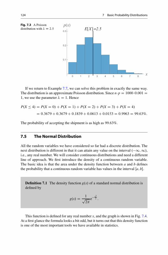
124 7 Basic Probability Distributions
Fig. 7.3 A Poissondistribution with � D 2:5
0 1 2 3 4 5 6 7 8
0.1
0.2
0.3
If we return to Example 7.7, we can solve this problem in exactly the same way.The distribution is an approximate Poisson distribution. Since n �p D 1000 �0:001 D1, we use the parameter � D 1. Hence
P.X � 4/ D P.X D 0/ C P.X D 1/ C P.X D 2/ C P.X D 3/ C P.X D 4/
D 0:3679 C 0:3679 C 0:1839 C 0:0613 C 0:0153 D 0:9963 D 99:63%:
The probability of accepting the shipment is as high as 99:63%.
7.5 The Normal Distribution
All the random variables we have considered so far had a discrete distribution. Thenext distribution is different in that it can attain any value on the interval .�1; 1/,i.e., any real number. We will consider continuous distributions and need a differentline of approach. We first introduce the density of a continuous random variable.The basic idea is that the area under the density function between a and b definesthe probability that a continuous random variable has values in the interval Œa; b�.
Definition 7.1 The density function g.x/ of a standard normal distribution isdefined by
g.x/ D 1p2�
e� x2
2 :
This function is defined for any real number x, and the graph is shown in Fig. 7.4.At a first glance the formula looks a bit odd, but it turns out that this density functionis one of the most important tools we have available in statistics.

7.5 The Normal Distribution 125
Fig. 7.4 The densityfunction of a standard normaldistribution
4 2 2 4
0.1
0.2
0.3
0.4
When the density function fX.x/ of a random variable X is known, we define
P.a � X � b/ DZ b
afX.x/dx:
The probability that X is between a and b is hence equal to the area under thedensity function between a and b. For this to be a sensible definition, we need torequire that the area under the full graph is 1, i.e., that
lima!�1;b!1 P.a � X � b/ D
Z 1
�1fX.x/dx D 1:
It may seem cumbersome that we need integration to compute probabilities, butthis is not much of a complication. The reason is that all the values we will need areavailable through statistical tables. The table for the standard normal distribution isavailable at the end of the book (Tables C and D). The table shows the values of theintegral
G.z/ DZ z
�11p2�
e� x2
2 dx:
G.z/ is hence the area under the graph of the density function to the left of z, seeFig. 7.5. The table only contains the values for G.z/ when z � 0. The reason is thatwhen z is negative, the value can be found by a simple symmetry argument. Thedensity function is symmetric about zero, and hence the area to the right of z must

126 7 Basic Probability Distributions
Fig. 7.5 The area to the left of z. The area to the left of �z equals the area to the right of z
be equal to G.�z/, see Fig. 7.5. Hence
G.z/ C G.�z/ D Area under the full graph D 1:
and from this relation it follows that
G.�z/ D 1 � G.z/:
Example 7.9 How do we find G.�1/ from the table?
Solution: We use the formula G.�1/ D 1�G.1/. From the table we find G.1/ D0:8413. Hence
G.�1/ D 1 � 0:8413 D 0:1587:
Example 7.10 Find the probability that a standard normal distribution has valuesbetween �2 and 1.
Solution: It follows from the definitions that
P.�2 � X � 1/ D G.1/ � G.�2/:
From the table we get G.1/ D 0:8413. To find the value of G.�2/, we use therelation G.�2/ D 1 � G.2/. From the table we get G.2/ D 0:9772, which gives
P.�2 � X � 1/ D 0:8413 � .1 � 0:9772/ D 0:8185:

7.5 The Normal Distribution 127
7.5.1 The General Normal Distribution
The expectation of a continuous random variable X with density fX.x/ is defined by
EŒX� DZ 1
�1x � fX.x/dx;
and the variance is defined by
VarŒX� DZ 1
�1.x � EŒX�/2 � fX.x/dx:
From these definitions it is possible to prove that a standard normal distributionX has
EŒX� D 0; VarŒX� D 1:
This, however, is a special case, and the general normal distribution X has a densityfunction
fX.x/ D 1p2��2
e� .x�/2
2�2 :
With this density it is possible to show that
EŒX� D ; VarŒX� D �2;
and we say that X is an N.; �2/ random variable (Figs. 7.6 and 7.7).
Fig. 7.6 Density functionsof normal distributions with D 2, � D 0:6 and � D 1:4
2 2 4 6
0.1
0.2
0.3
0.4
0.5
0.6

128 7 Basic Probability Distributions
Fig. 7.7 Density functionsof normal distributions with� D 0:6, D 2 and D 5
2 2 4 6 8 10
0.1
0.2
0.3
7.5.2 Standardizing RandomVariables
It turns out that we do not need new tables to compute probabilities related to thegeneral normal distributions. A useful technical procedure solves the problem. If Xis any random variable with
EŒX� D VarŒX� D �2;
we can define a new random variable Z by
Z D X �
�:
Then EŒZ� D 0; VarŒZ� D 1.
Proof We use the general rules for expectation and variance to see that
EŒZ� D E
X �
�
�D 1
�EŒX � � D 1
�.EŒX� � EŒ�/ D 0;
VarŒZ� D Var
X �
�
�D 1
�2VarŒX � � D 1
�2VarŒX� D 1
�2� �2 D 1:
The usefulness of this procedure will be clear from the following example.

7.5 The Normal Distribution 129
Example 7.11 Assume that X is a normal distribution with EŒX� D 20 and �2 D 16.Find P.X � 28/ and P.24 � X � 28/.
Solution: Z D X�204
is a standard normal distribution. Hence
P.X � 28/ D P
�X � 20
4� 28 � 20
4
�D P.Z � 2/ D G.2/ D 0:9972:
Correspondingly (Note that P.X D 24/ D 0 since X is a continuous distribution)
P.24 � X � 28/ D P.X � 28/ � P.X � 24/
D P
�X � 20
4� 28 � 20
4
�� P
�X � 20
4� 24 � 20
4
�
D P.Z � 2/ � P.Z � 1/ D G.2/ � G.1/
D 0:9772 � 0:8413 D 0:1359:
The method we used in the previous example is very useful in applications. It canalso be used in cases where X is approximately normal, meaning that the distributionis very close to a normal distribution. The final result can be stated as follows:
If X is approximately normal with EŒX� D and VarŒX� D �2, then
P.X � z/ � G� z �
�
�:
If X is a normal distribution, we get the same result but with equality insteadof approximation.
7.5.3 The Central Limit Theorem
We will now consider one of the most important results in statistics. The resultsexplain clearly why a standard normal distribution has such a prominent place. Arigorous proof is too difficult, so we omit the details. We will instead focus themeaning of the statement and explain how it can be applied in practical cases.
Example 7.12 Assume that we toss a coin 10 times. If we do this only once theresult will be quite random. If we repeat this multiple times, it might happen that wesee a pattern. The table below shows the result of a computer simulation where wehave repeated the 10 coin tosses 1000 times.

130 7 Basic Probability Distributions
10 tails W once
9 tails; 1 heads W 8 times
8 tails; 2 heads W 56 times
7 tails; 3 heads W 115 times
6 tails; 4 heads W 206 times
5 tails; 5 heads W 247 times
4 tails; 6 heads W 190 times
3 tails; 7 heads W 117 times
2 tails; 8 heads W 51 times
1 tails; 9 heads W 8 times
10 heads W once
The frequencies have been plotted to the left in Fig. 7.8. We see that the plotforms a curve resembling the density of a normal distribution. The effect is evenmore pronounced in the graph to the right in Fig. 7.8. Here the results are based on100 coin tosses in 100;000 repeated experiments.
The results in Fig. 7.8 are typical when we add the results from several repeatedexperiments. Regardless of what distribution we start out with, the sum of the resultsfrom many independent experiments will be close to a normal distribution. Moreprecisely the following theorem holds:
2 4 6 8 10
50
100
150
200
250
40 50 60 70
2000
4000
6000
8000
Fig. 7.8 Frequencies of heads in repeated coin tosses

7.5 The Normal Distribution 131
Theorem 7.1 Let X1; : : : ; Xn be independent random variables with the samedistribution, and assume that EŒXi� D ; VarŒXi� D �2 for all i D 1; : : : ; n.Put
Sn D X1 C X2 C � � � C Xn:
Then for all z
P
�Sn � EŒSn�
�ŒSn�� z
�� G.z/; when n is sufficiently big.
Theorem 7.1 is often called the central limit theorem and is one of the mostimportant results in statistics. How big n needs to be depends on the distribution,but a crude rule of thumb says n > 30. In some special cases we can give a moreprecise answer. The proof of the central limit theorem is too difficult to be includedhere, so we will focus on applications.
Example 7.13 Assume that we know that S D X1 CX2 C� � �CXn, where X1; : : : ; Xn
all are independent with the same distribution. We don’t know the precise value ofn, but we know that the value is large. Find an approximate value for P.S � 8/ whenEŒS� D 2; VarŒS� D 9.
Solution: We want to use the central limit theorem. First we find
�ŒS� Dp
VarŒS� D 3:
Next we subtract EŒS� and then divide by �ŒS� on both sides of the inequality to seethat
P.S � 8/ D P
�S � EŒS�
�ŒS�� 8 � 2
3
�� G.2/ D 0:9772:
The principle we used in this example is useful, and we formulate a generalversion of it:
Assume that n is big, and that S D X1 C X2 C � � � C Xn, where X1; : : : ; Xn allare independent with the same distribution. Then
P.S � s/ � G
�s � EŒS�
�ŒS�
�

132 7 Basic Probability Distributions
The central limit theorem also applies to the mean and can be stated as follows:
Theorem 7.2 Let X1; : : : ; Xn be independent random variables with the samedistribution, and assume that EŒXi� D ; VarŒXi� D �2 for all i D 1; : : : ; n. Ifn is big and we put
S D X1 C X2 C � � � C Xn
X D 1
n.X1 C X2 C � � � C Xn/;
then
S � NŒn; n�2� and X � N
;
�2
n
�:
When the conditions in Theorem 7.2 hold, we can show that
EŒS� D n; VarŒS� D n�2;
and
EŒX� D n; VarŒX� D �2
n:
The last relation is particularly useful in applications.
Example 7.14 Assume that 400 customers come to a shop every day and that theirpurchases are independent. They often buy milk, and we assume that the number ofliters bought by each customer is a random variable X with distribution
P.X D 0/ D 0:3; P.X D 1/ D 0:5; P.X D 2/ D 0:2:
Find an approximate value for the probability that the shop sells between 341and 390 liters.
Solution: We call the total number of liters sold S, and have
S D X1 C X2 C � � � C X400:
To solve the problem, we need to compute
P.341 � S � 390/ D P.S � 390/ � P.S � 340/:

7.5 The Normal Distribution 133
We can find approximate values for these probabilities from the central limittheorem, but we need to know EŒS� and VarŒS�. To find these values we first need tocompute EŒX� and VarŒX�. We get
EŒX� D 0 � 0:3 C 1 � 0:5 C 2 � 0:2 D 0:9
EŒX2� D 02 � 0:3 C 12 � 0:5 C 22 � 0:2 D 1:3
VarŒX� D EŒX2� � EŒX�2 D 1:3 � 0:92 D 0:49:
We use these values to see that
EŒS� D EŒX1� C EŒX2� C � � � C EŒX400�
D 0:9 C 0:9 C � � � C 0:9 D 400 � 0:9 D 360:
Since X1; X2; : : : ; X400 all are independent
VarŒS� D VarŒX1� C VarŒX2� C � � � C VarŒX400�
D 0:49 C 0:49 C � � � C 0:49 D 400 � 0:49 D 196:
Hence
�ŒS� Dp
VarŒS� D p196 D 14:
Now we have all the information we need to use the central limit theorem, and weget
P.341 � S � 390/ D P.S � 390/ � P.S � 340/
� G
�390 � 360
14
�� G
�340 � 360
14
�
� G.2:14/ � G.�1:43/ D G.2:14/ � .1 � G.1:43//
D 0:9838 � .1 � 0:9236/ D 0:9074:
The probability that the customers buy between 341 and 390 liters of milk is henceabout 90%.
In the previous calculation we tacitly assumed that n D 400 is sufficient toapply the central limit theorem. A general problem in applications of the centrallimit theorem is the following: How many terms are sufficient? There is no simpleanswer to this question. In many cases our random variables come from a binomialdistribution, and in that particular case it is possible to give a fairly precise rule forhow many terms are needed. Note that a binomial distribution can always be viewed
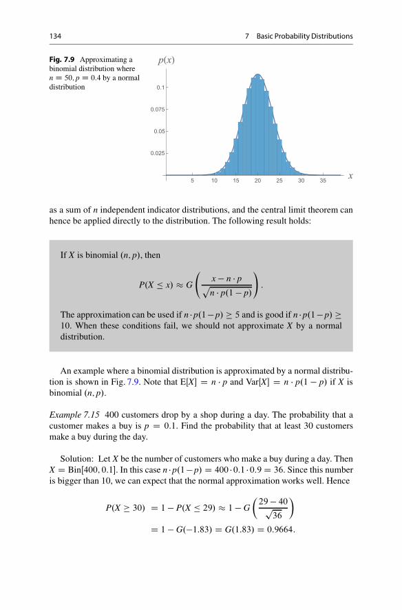
134 7 Basic Probability Distributions
Fig. 7.9 Approximating abinomial distribution wheren D 50; p D 0:4 by a normaldistribution
5 10 15 20 25 30 35
0.025
0.05
0.075
0.1
as a sum of n independent indicator distributions, and the central limit theorem canhence be applied directly to the distribution. The following result holds:
If X is binomial .n; p/, then
P.X � x/ � G
x � n � ppn � p.1 � p/
!:
The approximation can be used if n � p.1 � p/ � 5 and is good if n � p.1 � p/ �10. When these conditions fail, we should not approximate X by a normaldistribution.
An example where a binomial distribution is approximated by a normal distribu-tion is shown in Fig. 7.9. Note that EŒX� D n � p and VarŒX� D n � p.1 � p/ if X isbinomial .n; p/.
Example 7.15 400 customers drop by a shop during a day. The probability that acustomer makes a buy is p D 0:1. Find the probability that at least 30 customersmake a buy during the day.
Solution: Let X be the number of customers who make a buy during a day. ThenX D BinŒ400; 0:1�. In this case n � p.1 � p/ D 400 � 0:1 � 0:9 D 36. Since this numberis bigger than 10, we can expect that the normal approximation works well. Hence
P.X � 30/ D 1 � P.X � 29/ � 1 � G
�29 � 40p
36
�
D 1 � G.�1:83/ D G.1:83/ D 0:9664:

7.5 The Normal Distribution 135
7.5.4 Integer Correction
When a random variable has a continuous distribution, the probability for anyspecific value is zero. The probability that X D 2, e.g., is smaller than the probabilitythat 1:9999 � X � 2:0001. The last probability is given by
Z 2:0001
1:9999
fX.x/dx � 0;
since in all but exceptional cases the area under the graph is small. When we usethe normal distribution to approximate a random variable with integer values, wesometimes need to handle inequalities with care. If X only has integer values, then
P.X � 30/ D 1 � P.X � 29/
while
P.X � 30/ D 1 � P.X � 30/
if X has a continuous distribution. If X is integer valued, then
P.X � 10/ D P.X � 10:9999/
but the normal approximation will give different answers for left- and the right-hand side. We can hope that the difference is small, but in general it is difficultto judge which of the approximations provides the best approximation to the exactprobability. In some cases the approximation
P.X � 10/ � G
�10 � EŒX�
�ŒX�
�
is best, while it may also happen that
P.X � 10/ � G
�10:9999 � EŒX�
�ŒX�
�
is closer to the exact answer. It is sometimes seen that a good option is to meethalfway, i.e.
P.X � 10/ � G
�10:5 � EŒX�
�ŒX�
�
This method is called integer correction. Integer correction must be handled withcare, and it frequently happens that the “correction” provides a worse result.

136 7 Basic Probability Distributions
Definition 7.2 If X is integer valued with an approximate normal distribution,the integer correction is defined via
P.X � x/ � G
x C 1
2� EŒX�
�ŒX�
!:
If X is binomial .n; p/ where 20 � n � 50, then integer correction alwaysimproves the result in comparison with the standard approximation. In other casesit happens frequently that the “correction” leads to a larger error. Integer correctionis somewhat obsolete. The reason why we still include some material on this topicis that it focuses an important difference between continuous and discrete variables.This difference can also be illustrated as follows: Assume that we quote stock pricesand that the smallest unit is 1 USD. Then
P.X � 10/ D 1 � P.X � 9/:
If, however, the smallest unit is 1 cent, then
P.X � 10/ D 1 � P.X � 9:99/:
We see that the resolution matters. A continuous distribution has a resolution whichis arbitrarily fine. Then
P.X � 10/ D 1 � P.X � 10/:
In computations we often need to reverse inequalities as above. In doing so we needto focus on the resolution of the variable.
7.5.5 Normal Approximation of Hypergeometric and PoissonDistributions
We mentioned above that a hypergeometric distribution is approximately binomialwhen N � 20n. Moreover a binomial distribution is approximately Poisson whenn � 50 and p � 0:05. If we in addition assume that np.1 � p/ � 10, we knowthat the binomial distribution is approximately normal (Figs. 7.10 and 7.11). Thismeans that there cannot be much difference between the normal distribution andthe hypergeometric distribution or between the normal distribution and the Poissondistribution in such cases. The final results can be summarized as follows:

7.5 The Normal Distribution 137
5 10 15 20 25 30 35 40 45
0.025
0.05
0.075
0.1
Fig. 7.10 Approximating a hypergeometric distribution where N D 1000; M D 600; n D 50
with a normal distribution
5 10 15 20 25 30 35
0.025
0.05
0.075
Fig. 7.11 Approximating a Poisson distribution where � D 20 with a normal distribution
A hypergeometric distribution is approximatively normal if
N � 20n; n � M
N
�1 � M
N
�� 10:
A Poisson distribution is approximatively normal if � � 10.
7.5.6 Summing Normal Distributions
As we have seen in Chap. 6, the sum of two random variables X and Y can be quitecomplicated. If X and Y are normally distributed, it is possible to prove that thesum Z D X C Y also has normal distribution. The situation is particularly simple

138 7 Basic Probability Distributions
if X and Y are independent. In that case Z is normally distributed with expectationEŒX� C EŒY� and variance VarŒX� C VarŒY�. The result can be generalized to sums ofarbitrary length, and the main result can be formulated as follows:
If X1; X2; : : : ; Xn all are independent and normally distributed, then the sum isa normal distribution with expected value equal to the sum of the expectationsand variance equal to the sum of the variances.
7.5.7 Applications to Option Pricing
As we mentioned in Chap. 5, there are explicit formulas to price options in realworld markets. We now have tools to take a brief look at this. To avoid too highlevels of abstraction we will consider some special cases where most numbers aregiven. The principles we use, however, are true in general, and it is not very difficultto figure out what to do when we change some of these numbers.
Let us consider a stock with the following technical data:
• Stock price today: K0 D 100 (USD).• Volatility: ˇ D 10%.• Expected annual return: ˛ D 5%.• Bank interest rate: r D 5% (annually, continuously compounded).
The volatility, ˇ, is a technical parameter often used in finance. It can betranslated to the more common concept of standard deviation by the followingformula
Standard deviation of the stock price Kt at time t D K0e˛tp
eˇ2 t � 1
We see that the standard deviation changes with time t. That makes good sense. Weknow the stock price at time t D 0. If we put t D 0 in the formula we get:
K0e˛�0peˇ2�0 � 1 D K0e0p
e0 � 1 D 0:
As time passes, the standard deviation increases. At time t D 1 (years), we get
100e0:1�0pe0:12�0 � 1 D 11:08 (USD):
The standard deviation in the stock price one year into the future is hence 11.08USD.

7.5 The Normal Distribution 139
A commonly used model for the time development of stock prices can beformulated as follows:
Kt D K0e.˛� 12 ˇ2/tCˇXt ;
where Xt is normally distributed with EŒXt� D 0 and VarŒXt� D t.
Now assume that we want to consider the distribution of possible stock pricesone year into the future. We put t D 1 and get
K1 D e0:095C0:1X1 ;
where X1 is NŒ0; 1�. This is an example of a lognormal distribution. The distributionof K1 follows easily from the distribution of X1 if we use logarithms.
P.K1 � k/ D P.100 e0:095C0;1X1 � k/
D P.e0:095C0;1X1 � k=100/
D P.0:095 C 0; 1X1 � lnŒk=100�/
D P.X1 � 10 � lnŒk=100� � 0:95/: (7.2)
Since X1 is a standard normal distribution, we get
P.K1 � k/ D G.10 � lnŒk=100� � 0:95/:
Instead of buying the stock, we could buy a call option to be redeemed one yearfrom the start. If the strike of the option is, e.g., 110 USD, we have the right to buythe stock for 110 USD at time t D 1. Hence if the stock price raises by more than10 USD, the option will pay out money. The price of a call option can be computedby the procedure below, which is often referred to as the Black and Scholes pricingformula.
The price V of a call option with strike K at time T is calculated as follows:
1: Compute R D ln
K
K0
�C �1
2ˇ2 � r
�T: 2: Compute S D ˇ
pT:
3: V D K0 � .1 � G.R=S � S// � K � e�rT.1 � G.R=S//:

140 7 Basic Probability Distributions
We now want to use the Black and Scholes formula to compute the price of10;000 call options with strike K D 110 (USD) at time T D 1. When we insert thegiven quantities into the formulas, we get
R D lnŒ110=100� C 0:005 � 0:05 D 0:0503; S D 0:1:
The price on one call option is
V D 100 � .1 � G.0:0503=0:1 � 0:1// � 110 � e�0:05.1 � G.0:0503=0:1//
D 100 � .1 � G.0:40// � 110 � e�0:05.1 � G.0:50//
D 100 � .1 � 0:6554/ � 110 � e�0;05.1 � 0:6915/
D 2:18:
The price on 10;000 call options is hence 21;800 USD.A question of interest is to figure out the probability that the investment is
profitable. We make a profit when the value of the options exceeds 21;800 USD.The limiting stock price K1 is determined by the equation
10;000 � .K1 � 110/ D 21;800;
and we see that the stock price must be at least 112.18 USD before we begin tomake a profit. The probability that we make a profit is
P.K1 � 112:18/ D 1 � P.K1 � 112:18/
D 1 � G.10 � lnŒ112:18=100� � 0:95/ D 1 � G.0:20/
D 42:1%:
Note that the calculations critically depend on the given parameters. If theeconomy enters a recession, the parameters will most certainly change and this inturn will change the stock prices. Questions of this type will be discussed in theexercises.
7.6 Summary of Chap. 7
• X D Binomial.n; p/: Total number of successes in n independent trials when theprobability of success is p.
P.X D x/ D�n
x
�px.1 � p/n�x; EŒX� D n p; VarŒX� D n p.1 � p/:

7.6 Summary of Chap. 7 141
• X D Hypergeometric.N; M; n/: Total number of special elements when wesample n elements from a population of N elements, where M elements arespecial.
P.X D x/ D�
Mx
� �N�Mn�x
�
�Nn
� ; EŒX� D n � M
N:
VarŒX� D N � n
n � 1� n � M
N��
1 � M
N
�:
• X D Poisson �: Total number of successes when an experiment where success isa rare outcome is repeated many times.
P.X D x/ D �x
xŠe��; EŒX� D �; VarŒX� D �:
• X D NŒ0; 1� D Standard normaldistribution: A continuous distribution where
P.X 2 Œa; b�/ DZ b
a
1p2�
e�x2=2dx; EŒX� D 0; VarŒX� D 1:
The cumulative distribution for the standard normal distribution is listed in tablesand is defined by
G.z/ DZ z
�11p2�
e�x2=2dx:
The following relations are useful in applications:
G.�z/ D 1 � G.z/; P.a � X � b/ D G.b/ � G.a/
• The central limit theorem: Let Sn D X1 C � � � C Xn, where X1; : : : ; Xn areindependent variables with the same distribution. Then
limn!1 P
�Sn � EŒSn�
�ŒSn�
�D G.z/:
• Any random variable S which (roughly speaking) appears as a sum of many inde-pendent effects will according to the central limit theorem lead to an approximatenormal distribution. How many terms are needed for a satisfactory approximationdepend on the situation. Some guidelines are provided in Table 7.1.
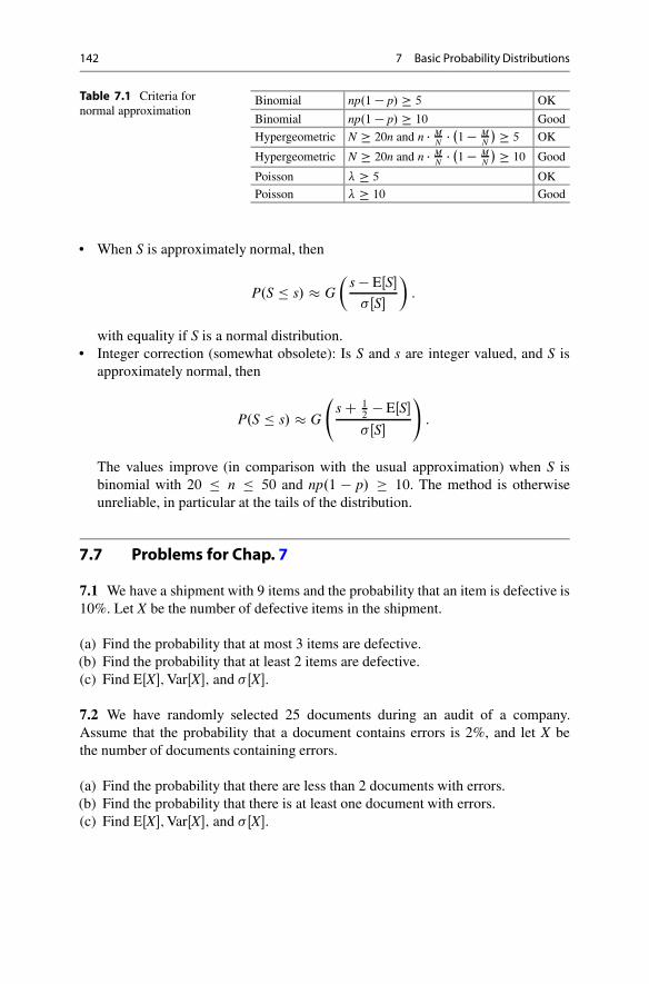
142 7 Basic Probability Distributions
Table 7.1 Criteria fornormal approximation
Binomial np.1 � p/ � 5 OK
Binomial np.1 � p/ � 10 Good
Hypergeometric N � 20n and n � MN � �1 � M
N
� � 5 OK
Hypergeometric N � 20n and n � MN � �1 � M
N
� � 10 Good
Poisson � � 5 OK
Poisson � � 10 Good
• When S is approximately normal, then
P.S � s/ � G
�s � EŒS�
�ŒS�
�:
with equality if S is a normal distribution.• Integer correction (somewhat obsolete): Is S and s are integer valued, and S is
approximately normal, then
P.S � s/ � G
s C 1
2� EŒS�
�ŒS�
!:
The values improve (in comparison with the usual approximation) when S isbinomial with 20 � n � 50 and np.1 � p/ � 10. The method is otherwiseunreliable, in particular at the tails of the distribution.
7.7 Problems for Chap. 7
7.1 We have a shipment with 9 items and the probability that an item is defective is10%. Let X be the number of defective items in the shipment.
(a) Find the probability that at most 3 items are defective.(b) Find the probability that at least 2 items are defective.(c) Find EŒX�; VarŒX�; and �ŒX�.
7.2 We have randomly selected 25 documents during an audit of a company.Assume that the probability that a document contains errors is 2%, and let X bethe number of documents containing errors.
(a) Find the probability that there are less than 2 documents with errors.(b) Find the probability that there is at least one document with errors.(c) Find EŒX�; VarŒX�; and �ŒX�.

7.7 Problems for Chap. 7 143
7.3 We ask a sample of 16 persons if they like a good. The probability that arandomly selected person likes the good is 20%. X is the number of people in thesample that like the good.
(a) Find the probability that 3 persons like the good.(b) Find EŒX�; VarŒX�; and �ŒX�.
7.4 We have a shipment with 26 items and know that half of the items, i.e., 13items are defective. We randomly select 8 items from the shipment. X is the numberof defective items in the sample.
(a) Find the probability that 4 items are defective.(b) Find EŒX�; VarŒX�; and �ŒX�.
7.5 A political party has 65 representatives, and we know that 20% of therepresentatives are negative to a proposal. We select 20 people randomly, and letX denote the number of representatives that are negative to the proposal.
(a) Find the probability that at least 2 representatives in the sample are negative tothe proposal.
(b) Find EŒX�; VarŒX�; and �ŒX�.
7.6 A company handles every day a large and relatively constant number oforders. On average the company receives 4 complaints per day. X is the numberof complaints the company receives a randomly selected day.
(a) Find the probability that the company receives at most 3 complaints.(b) Find EŒX�; VarŒX�; and �ŒX�.
7.7 We receive a consignment of 2;000;000 items where the probability of an itembeing defective is 0:05%. We sample 500 items, and accept the consignment if thenumber of defective items in the sample is at most one.
(a) What is the probability that we accept the consignment?(b) Find EŒX�; VarŒX�; and �ŒX�.
7.8 Assume that X is a standard normal distribution.
(a) Find the probability that X � 1:64.(b) Find the probability that X D 1:64.(c) Find the probability that X < 1:64.

144 7 Basic Probability Distributions
7.9 Assume that X is a standard normal distribution.
(a) Find the probability that 0 � X � 0:44.(b) Find the probability that �1:96 � X � 1:96.(c) Find the probability that X > �2:33.
7.10 Assume that X is a random variable with EŒX� D 5 and VarŒX� D 16. Define anew random variable Y D X�5
4. Prove that
EŒY� D 0; VarŒY� D 1:
7.11 Assume that S D X1 C X2 C � � � C Xn where X1; : : : ; Xn are independent withthe same distribution and n is very large. EŒS� D 3 and VarŒS� D 16.
(a) Find the probability that S � 7.(b) Find the probability that �1 � S � 11.(c) Find the probability that S � 5.(d) Is there a good reason to use integer correction in this problem?
7.12 Assume that S is normally distributed with EŒS� D 10 and VarŒS� D 25. Howlarge must z be if
P.S � z/ D 95%‹
7.13 We have a consignment with 225 items and the probability that an item isdefective is 20%. Let X be the number of defective items in the consignment.
(a) Find EŒX�; VarŒX�; and �ŒX�.(b) Find the probability that at most 50 items are defective.(c) Find the probability that at least 35 items are defective.
7.14 We ask a sample of 48 persons if they like a good. Assume that the probabilitythat a randomly selected person likes the good is 25%. X is the number of people inthe sample who like the good.
(a) Find EŒX�; VarŒX�; and �ŒX�.(b) Why could integer correction be a good idea in this problem?(c) Use integer correction to find the probability that at least 15 persons like the
good.(d) Find the probability that at least 15 persons likes the good using a normal
approximation without integer correction. The exact answer is P.X � 15/ D87:68%. Comment the answers in (c) and (d).

7.7 Problems for Chap. 7 145
7.15 Assume that X1; X2; X3; X4 are independent and normally distributed with
EŒX1� D 100 EŒX2� D 90 EŒX3� D 95 EŒX4� D 105
VarŒX1� D 30 VarŒX2� D 20 VarŒX3� D 25 VarŒX4� D 15:
(a) What is the distribution of S D X1 C X � 2 C X3 C X4? Can we use the centrallimit theorem in this case?
(b) Find EŒS�; VarŒS�; and �ŒS�.(c) Compute P.S � 390/. Is the answer different from P.S < 390/?
7.16 Option Pricing Theory: A stock has today a price K0 D 100 USD, and it hasan expected annual return ˛ D 15% and a volatility ˇ D 20%. The bank interestrate is r D 5%.
(a) Find the standard deviation in the stock price 6 months from now.(b) What is the price of a call option that gives the right to buy the stock for 112
USD 6 months from now?
7.17 Option Pricing Theory: A stock has today a price K0 D 200 USD, it has anexpected annual return ˛ D 9% and a volatility ˇ D 2%. The bank interest rate isr D 5%.
(a) What is the price of a call option that gives the right to buy the stock for 205USD 3 months from now?
(b) What is the probability that the option will be worthless?(c) A short time after the option was bought, the company met serious problems.
The stock price fell instantly to 198 USD and the expected annual return wentdown to 5%. What is the probability that the option will be worthless?
7.18 Option Pricing Theory: A stock has today a price K0 D 98 USD, and it hasan expected annual return ˛ D 12% and a volatility ˇ D 12%. The bank interestrate is r D 5%.
(a) What is the price of a call option that gives the right to buy the stock for 109USD 1 year from now?
(b) You spend 10;000 USD to buy options like in (a). Instead of buying the optionsyou could have made a safe investment putting your money in the bank. Whatmust the stock be worth one year from now so that you get at least as muchprofit as you would have gotten from a bank deposit?
(c) What is the probability that the options give at least as much profit from theoptions as you would get from a bank deposit?

146 7 Basic Probability Distributions
7.19 Option Pricing Theory: The price of a stock at time t (in years) is given bythe formula
Kt D 100e0:08tC0:2Xt ;
where Xt is normally distributed with expected value zero and standard deviationp
t.
(a) Find the probability that the stock price is above 115 USD when t D 4.(b) What is the volatility of the stock? Assume that the bank interest rate is r D 3%.
Use the Black and Scholes pricing formula to find the price on a call option thatgives the right to buy the stock for 115 USD 4 years from now.
7.20 Applications of the Central Limit Theorem: Every day about 10;000 peoplewalk past an ice cream store. We let X1; X2; : : : ; X10;000 denote the number of icecream bought by each person. Assume that X1; X2; : : : ; X10;000 are independent withthe same distribution, and that the distribution is given by
P.X D 0/ D 86% P.X D 1/ D 8% P.X D 2/ D 2% P.X D 3/ D 4%
(a) Find EŒX� and VarŒX�.(b) Put S D X1 C X2 C � � � C X10;000. Find EŒS�; VarŒS�, and �ŒS�.(c) Find the probability that the store sells more than 2450 ice cream.(d) How many ice cream must the store have in stock to be 99% sure that they can
meet the demand?
7.21 Applications of the Central Limit Theorem: A building plot area is plannedfor 900 houses. Let X be the number of cars per household, and assume that
P.X D 0/ D 0:1 P.X D 1/ D 0:6 P.X D 2/ D 0:3:
(a) Find EŒX� and VarŒX�.(b) Is it reasonable to assume that the number of cars in each household are
independent random variables? Point (shortly) to issues for and against thisassumption.
(c) Assume that the number of cars in each household are independent randomvariables, and define Y D P900
iD1. Find EŒY� and VarŒY�. How many parkinglots are needed if we require 90% probability that all the cars can parksimultaneously? Approximate Y by a normal distribution in your calculations.
7.22 Applications of the Central Limit Theorem: The probability that a ran-domly selected customer in a bookstore buys a textbook in statistics is p D 0:001.During a day the store has about 10;000 customers. We assume that the customersshop independently and let X denote the number of textbooks in statistics boughtduring a day.

7.7 Problems for Chap. 7 147
(a) What is the exact distribution of X? Find EŒX� and VarŒX�.(b) Use a normal approximation with and without integer correction to compute an
approximate value for P.X � 3/.(c) The exact answer in (b) is P.X � 3/ D 0:0103. Let Y be a Poisson random
variable with � D 10. Compute the probability P.Y � 3/ and compare theresults in (b) and (c).
7.23 Portfolio Computations: You want to invest 400;000 USD in two stocks, Aand B. The two stocks cost today
A W 100 USD per stock B W 200 USD per stock
(a) Let a be the number of A stocks and b be the number of b stocks. Find a and bwhen you want to invest the same total amount in the two stocks.
(b) We assume that the prices on the two stocks one year from now are independentrandom variables XA and XB. The total value V of your portfolio one year fromnow is given by
V D a XA C b XB;
where a and b are the values you found in (a). Find EŒV� and VarŒV� if we assumethat EŒXA� D 200; EŒXB� D 300; VarŒXA� D 1500, and VarŒXB� D 400. Also findthe standard deviation �ŒV�.
(c) Assume that XA and XB are normally distributed. What is the probability that thevalue of the portfolio exceeds 800;000 USD after one year?
7.24 Poisson Versus Normal Approximation: A shop sells a good. We let X bea random variable showing how many units each customer buys of the good. Theprobability distribution of X is given by
P.X D 0/ D 0:905 P.X D 1/ D 0:090 P.X D 2/ D 0:005:
(a) Find EŒX� and VarŒX�.(b) During one day 100 customers visit the shop. We can compute the total number
of units the customers buy of the good, and denote this number by Y. We assumethat the customers shop independently. Find EŒY� and VarŒY� and use normalapproximation to compute the probability that the shop sells at most 5 units ofthe good during a day.
(c) Since the distribution of X is special, we don’t have any simple criteria to decideif the normal approximation is good or not. The distribution of X is, however,quite close to a Poisson random variable Z with parameter �. Suggest a valuefor � and compute P.Z � 3/.
(d) A sum of 100 independent Poisson random variables, all with parameter �, isa Poisson random variable with parameter 100�. Use this result to compute theprobability that the shop sells at most 5 units of the good during a day, without

148 7 Basic Probability Distributions
the use of normal approximation. Compare with the exact answer P.Y � 5/ D6:72% and give a comment.
7.25 Extreme Values: A company has 5 relatively equal production units, and eachunit produces 10 items. We assume that the probability that an item is defective is10% and that the number of defective items at each unit are independent randomvariables.
(a) We assume that outcomes (defective/not defective) of each item are independentrandom variables, and let X denote the number of defective items at randomlyselected unit. What is the distribution of X? What is P.X � 4/?
(b) Let Y be the number of defective items at the unit with the worst result, i.e., theunit with the most defective items. What is P.Y � 4/?
7.26 Stochastic Game Theory:
(a) Assume that X is a normal distribution with expectation and variance �2, andthat C is a constant. What is P.X � / and P.X D C/?
A simplified model for a wage negotiation can be formulated as follows: Theemployer presents an offer o and the workers (simultaneously) present a demandd. The outcome is decided by a mediator who thinks that a fair outcome of thenegotiations is X. The value of X is a random variable which is unknown to theparties. The party which comes closest to X gets full acceptance for their claim.If the parties are equally close to X, X will be the outcome of the negotiations.The expected result EŒR� from the negotiations is given by the formula
EŒR� D o �P�
X <o C d
2
�Cd �P
�X >
o C d
2
�C 1
2.oCd/ �P
�X D o C d
2
�:
(b) Explain the terms in the formula for EŒR� (o and d are constants). How canyou simplify this expression if you know that X is a normal distribution withexpected value and variance �2?
(c) If the employer wishes to minimize the expected result while the workers wantto maximize it, it is possible to prove that equilibrium is obtained if and only if
.d � o/ � fX
�o C d
2
�D 2 � P
�X � o C d
2
�;
.d � o/ � fX
�o C d
2
�D 2 � P
�X >
o C d
2
�:
where fX is the density of X. Explain why this leads to P.X � oCd2
/ D 12. How
would you interpret this result?
7.7 Problems for Chap. 7 149
(d) If X is normally distributed with expected value and variance �2, the densityis given by
fX.x/ D 1p2��2
e� .x�/2
2�2 :
Show that the solution to the system of equations in (c) is
o D �r
�
2� �; d D C
r�
2� �:
What happens to the distance between the parties when � increases?
7.27 Stochastic Game Theory: A simplified model for a wage negotiation canbe formulated as follows: The employer presents an offer o and the workers(simultaneously) present a demand d. The outcome is decided by a mediator whothinks that a fair outcome of the negotiations is X. The value of X is a randomvariable which is unknown to the parties. The party which comes more close to Xgets full acceptance for their view. If the parties are equally close to X, X will be theoutcome of the negotiations. The expected result EŒR� from the negotiations is givenby the formula
EŒR� D o � P
�X <
o C d
2
�C d � P
�X >
o C d
2
�C 1
2.o C d/ � P
�X D o C d
2
�:
(a) Assume that the employer offers o D 3% while the workers demand d D6%. Compute the expected outcome of the negotiations when X is a normaldistribution with D 5% and standard deviation � D 0:5%.
(b) Assume that the employer offers o D 3% while the workers demand d D6%. Compute the expected outcome of the negotiations when X is a normaldistribution with D 5% and standard deviation � D 2%. Compare the answerwith (a) and comment the results.
7.28 Poisson Versus Normal Distribution: In this problem X denotes the totalquantity of a good that is sold during a day.
(a) We first assume that X is a normal distribution with expected value D 1 andstandard deviation � D 1. What is the probability that X � 3?
(b) We now assume that the good is sold at a shopping center where there are a hugenumber of customers every day. The customers either buy one unit or nothingof the good, and all customers have the same probability of buying one unit.What distribution do you assume for X in this case? We assume as above thatexpected value is D 1 and standard deviation � D 1. Find P.X � 3/ underthese new assumptions.

150 7 Basic Probability Distributions
(c) Compare the results from (a) and (b) and try to explain the difference. Why dowe in (b) need to assume that all customers have the same probability of buyingone unit?
7.29 Stocks That Fail in the Long Run: In a standard model for stock prices thestock price Kt (in USD) at time t (in years) is given by
Kt D K0e.˛� 12 ˇ2/tCˇXt ;
where Xt is normally distributed with EŒXt� D 0; VarŒXt� D t; and X0 D 0. K0 isthe stock price at t D 0 and ˛; ˇ are constants. We will in this problem assume thatK0 D 100; ˛ D 0:03; ˇ D 0:5. In addition we will assume that the bank interest rateis r D 2:5% annually. We disregard transaction costs.
(a) Find the price of a call option that gives the right to buy a stock of this sort for100 USD after 9 years.
(b) Find the probability that the stock price exceeds 1 USD after 100 years.(c) It is possible to prove that
EŒeˇXt � D e12 ˇ2
:
Use this to compute the expected stock price after 100 years. This result is insharp contrast to the result in (b). Try to explain how this is possible.
7.30 Expected Utility: A game has 6 different outcomes all of which are equallyprobable. The first 5 outcomes give a reward equal to one unit, while the lastoutcome results in a loss of 4 units.
(a) Compute the expected result of the game.(b) The players participating in the game have a utility function
u.x/ Dp
x C a2 � a:
We interpret u.x/ as the utility of winning x units (a negative x is a loss), and2 � a � 4 is a constant that can differ from player to player. Compute theexpected utility of the game in the two cases (i) a D 2 and (ii) a D 4. Alsofind the expected utility of not playing for arbitrary a (this we may interpret asa game that pays 0 units on all the 6 outcomes).
(c) It is possible to prove (you can take that for granted) that expected utility is anincreasing function of a. Assume that a player participates in the game only ifhe or she has greater expected utility from playing than for not playing. Explainthat there exists a constant a0 such that a player participates in the game ifand only if a > a0. Compare the result with (a) and try to explain this from abehavioral point of view.

7.7 Problems for Chap. 7 151
7.31 Life Insurance: When insurance companies price life insurances, they use adeath rate function
x D ˛ C ˇcx:
Here x is the probability that a man of age x dies in the course of one year giventhat he is x years today, ˛; ˇ; and c are constants. Commonly used values are
˛ D 9:0 � 10�4; ˇ D 4:4 � 10�5; c D 1:10154:
(a) Explain that the death rate increases with x. Compute the value 50.(b) Let Tx be the remaining lifetime of a man with age x (this is a random variable
which varies between individuals). It is possible to show that Tx has a cumulativedistribution Fx given by
Fx.t/ D P.Tx � t/ D 1 � e� R t0 xCsds:
You can take this for granted. Use the result to compute the value
P.T40 > 10/:
(c) Compute the conditional probability
P.10 < T40 � 11jT40 > 10/:
Compare the result with (a), and try to interpret these results.
7.32 Binomial Distribution Conditional on Events: A company has 6 maincollaborating companies. The probability that a collaborating company takes contactduring one week is 70%. We assume that the collaborating companies act indepen-dently.
(a) Let X be the number of collaborating companies that takes contact during oneweek. What is the distribution of X? Find the probability that X D 4.
(b) The probability that a collaborating company taking contact writes a contract is60%. Find the probability that the company writes 4 contracts with collaboratorsduring one week.
7.33 The Distribution of a Sum: 10 men and 10 women apply for admission toa study. The admission is divided into two rounds. In the first round 4 men and 6women apply, while the rest apply in the second round. In the first round 3 studentswill be admitted, while 7 will be admitted in the second round. We assume that allapplicants have the same chance to be admitted in each round.

152 7 Basic Probability Distributions
(a) Find the probability that 2 men are admitted in the first round. Find theprobability that at least 5 men are admitted in the second round.
(b) Find the probability that at least 5 men are admitted in total. Is this procedurediscriminating with regards to gender? Explain your answer and try to suggestwhat causes the difference.
7.34 Put Options: A stock has today a price K0 D 400 USD, it has an expectedannual return ˛ D 15% and a volatility ˇ D 12%. The bank interest rate is r D 5%(continuously compounded).
(a) Find the price of a call option that gives the right to buy the stock for 390 USDone year from now.A (European) put option is a right (but not a duty) to sell a stock for a certainprice (strike) after a time T. An option of this sort makes it possible to profitwhen prices are falling.
(b) We will compare two contracts. Contract A consists of one put option and onestock. Contract B consists of one call option and a bank deposit B. Both optionshave strike 390 USD and the size of the bank deposit B is given by
B D strike � e�rT :
Disregard any transaction costs and explain why the two contracts pay out thesame amount regardless of the stock price KT at time T. Take into account thatyou get interest on the bank deposit.
(c) Since the two contracts in (b) pays out the same amount of money, they musthave the same price at t D 0. Use this to find the price of a put option with strike390 USD at time T D 1.
(d) Expected annual return is adjusted down to ˛ D �5%. What happens to theprice of the options after the adjustment? Find the probability that the value ofthe put option is at least 8 USD.
7.35 Basic Properties of Brownian Motion: Most models for financial marketsuse a Brownian motion Bt where 0 � t < 1. At each point in time Brownianmotion is a random variable with the properties
• For every t 2 Œ0; 1/, Bt is a normal distribution.• B0 D 0; EŒBt� D 0 and VarŒBt� D t.• If t1 � t2 � t3 � t4, then the two differences Bt2 �Bt1 and Bt4 �Bt3 are independent
random variables.
(a) Explain why VarŒBt� D EŒB2t � for all values of t.
(b) Let t D 100 and find P.B100 � 10/.(c) Assume t � s. Use the two last bullet points above to compute EŒBs.Bt � Bs/�.
Hint: Put t1 D 0; t2 D s; t3 D s; t4 D t.

7.7 Problems for Chap. 7 153
(d) Assume t � s. Show that EŒBtBs� D s, and use this expression to find anexpression for EŒ.Bt � Bs/
2�.
7.36 Basic Properties of Brownian Motion: Most models for financial marketsuse a Brownian motion Bt where 0 � t < 1. At each point in time Brownianmotion is a random variable with the properties
• For every t 2 Œ0; 1/, Bt is a normal distribution.• B0 D 0; EŒBt� D 0 and VarŒBt� D t.• If t � s, then EŒ.Bt � Bs/
2 D t � s.• If t1 � t2 � t3 � t4, then the two differences Bt2 �Bt1 and Bt4 �Bt3 are independent
random variables.
(a) Let Xt D 2Bt C 6. Find EŒXt�, and explain why VarŒXt� D 4t for any t.(b) Let Xt D 2Bt C 6. Find P.X25 � 16/.(c) Assume t � s. Use the last 3 bullet points above to compute
EŒB2s B2
t � 2BtB3s C B4
s �:
7.37 Basic Properties of Brownian Motion: Most models for financial marketsuse a Brownian motion Bt where 0 � t < 1. At each point in time Brownianmotion is a random variable with the properties
• For every t 2 Œ0; 1/, Bt is a normal distribution.• B0 D 0; EŒBt� D 0 and VarŒBt� D t.• If t � s, then EŒ.Bt � Bs/
2 D t � s.• If t1 � t2 � t3 � t4, then the two differences Bt2 �Bt1 and Bt4 �Bt3 are independent
random variables.
(a) Find the probability P.100eB9 � 2000/.(b) Assume t � s, and find an expression for EŒB2
s .Bt � Bs/2�.
(c) Assume 0 D t0 < t1 < � � � < tnC1 D T. Find the value for
EŒBti Btj.BtiC1� Bti/.BtjC1
� Btj/�
for each of the cases (i) i < j, (ii) i D j, and (iii) i > j. The answers must bejustified in detail.
7.38 Bayesian Priors: In this problem X is a binomial .n; p/ variable.
(a) We first assume that p D 13
and that n D 6. Compute P.X D 2/.(b) We now assume that p is unknown, but we know that p can only have the
values 0; 13; 2
3; 1. We assume a priori that these four values are equally probable.

154 7 Basic Probability Distributions
Assume n > 2 and prove that
P.X D 2/ D�n
2
� �1
3
�2 �2
3
�n�2
� 1
4C�
2
3
�2 �1
3
�n�2
� 1
4
!:
Explain why this formula is wrong if n D 2.(c) Now assume that n D 6. We observe X D 2. Compute the conditional
probability
P
�p D 1
3
ˇˇX D 2
�:
7.39 Lognormal Distribution and Expected Stock Prices: A random variable Yis called lognormal if it can be written on the form
Y D eX;
where X is a normal distribution N.; �2/.
(a) Assume that Y D eX , where X is N.2; 22/, i.e., D 4 and � D 2. Compute theprobability
P. Y � 403:43/:
(b) If Y is lognormal, it is possible to prove that
EŒY� D eC 12 �2
:
You can take this formula for granted. Use the formula to find the expectedvalue of Y D eX , where X is N.2; 22/. Compare the answer with (a) and give acomment.
(c) Assume that Kt is given by
Kt D K0e.˛� 12 ˇ2/tCˇZt :
where Zt is N.0; t/, and where ˛ and ˇ are two constants. Explain why Kt has alognormal distribution for each t, and find EŒKt�.
7.40 Distributions Conditional on Events: A newspaper has two types of buyers,regular buyers and special buyers. We assume throughout this exercise that thenewspaper is printed in more than 16;000 copies. The regular buyers have a totaldemand D1 which is normally distributed with expectation 1 and variance �2
1
where
1 D 10;000; �21 D 30002:
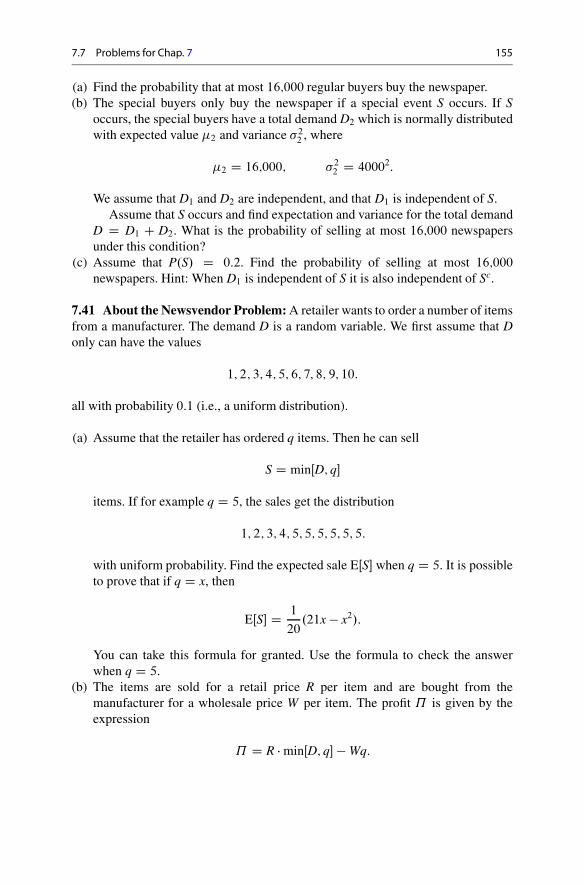
7.7 Problems for Chap. 7 155
(a) Find the probability that at most 16;000 regular buyers buy the newspaper.(b) The special buyers only buy the newspaper if a special event S occurs. If S
occurs, the special buyers have a total demand D2 which is normally distributedwith expected value 2 and variance �2
2 , where
2 D 16;000; �22 D 40002:
We assume that D1 and D2 are independent, and that D1 is independent of S.Assume that S occurs and find expectation and variance for the total demand
D D D1 C D2. What is the probability of selling at most 16;000 newspapersunder this condition?
(c) Assume that P.S/ D 0:2. Find the probability of selling at most 16;000
newspapers. Hint: When D1 is independent of S it is also independent of Sc.
7.41 About the Newsvendor Problem:A retailer wants to order a number of itemsfrom a manufacturer. The demand D is a random variable. We first assume that Donly can have the values
1; 2; 3; 4; 5; 6; 7; 8; 9; 10:
all with probability 0:1 (i.e., a uniform distribution).
(a) Assume that the retailer has ordered q items. Then he can sell
S D minŒD; q�
items. If for example q D 5, the sales get the distribution
1; 2; 3; 4; 5; 5; 5; 5; 5; 5:
with uniform probability. Find the expected sale EŒS� when q D 5. It is possibleto prove that if q D x, then
EŒS� D 1
20.21x � x2/:
You can take this formula for granted. Use the formula to check the answerwhen q D 5.
(b) The items are sold for a retail price R per item and are bought from themanufacturer for a wholesale price W per item. The profit ˘ is given by theexpression
˘ D R � minŒD; q� � Wq:

156 7 Basic Probability Distributions
Find an expression for the expected profit when the retailer orders q D x items.Assume that R D 20 and W D 5, and find x such that the profit is maximal.Hint: R; W; q are constants with respect to the expectation.
(c) It is possible to prove that if D has a continuous distribution with cumulativedistribution FD, then maximal expected profit is obtained when
FD.x/ D 1 � W
R:
You can take this for granted. Assume that D is a normal distribution withexpected value D 5:5 and variance �2 D 1, and that R D 20; W D 5.Find x such that expected profit is maximal. Why is the optimal order less thanin (b)?
7.42 Hinting at Significance: You want to sell a good and assume that a randomlyselected person demands D units of the good, where D is normally distributed withexpectation D 10 and variance �2 D 10.
(a) In all there are 1000 people demanding the good. We assume that the demandsare all independent with the distribution above. Let Z denote the total demandfrom 1000 people. Compute EŒZ� and VarŒZ�.
(b) First assume that the market is as in (a). How many units do you need to order ifyou want at least 95% probability of satisfying the total demand? Now assumethat a large number of people demand the good, and that the market is otherwiseas above. How many units do you need to order if you want at least 95%probability of satisfying the demand?
7.43 Adjusting Random Fluctuations Is a Bad Idea: Assume that the weeklysurplus from a branch of a company is a random variable. Let Xi denote the surplusin week i, where i D 1; 2; : : : . We assume that X1; X2; : : : are independent randomvariables all with the same expectation and variance �2.
(a) Assume that Xi is normally distributed with D 45; �2 D 900. Find theprobability that Xi � 0.
(b) The managers of the company want to reduce bad results for this particularbranch and suggest the following strategy: If the result is below the expectedvalue, the management injects extra amounts of cash the next week. If theresult is above the expected value, the management withdraws a correspondingamount of cash. We assume that the injections/withdrawals are proportional tothe deviation from the expected result, i.e.
Adjusted surplus in the next period D YiC1 D XiC1 � ˛. � Xi/;
where ˛ is the constant of proportionality.

7.7 Problems for Chap. 7 157
Assume that Xi and XiC1 are normally distributed with D 45; �2 D 900,and that ˛ D 0:75. Find the probability that YiC1 � 0.
(c) Assume that ; � , and ˛ are arbitrary numbers. Is it possible to find acombination of these numbers such that the branch gets higher adjusted surplusafter adjustment? What value on ˛ should the company use if they want tominimize the probability of deficit?
7.44 Adjusting Random Fluctuations Can Be Very Costly: A producer ofmachine parts has a lathe. The lathe produces sleeves with diameter 100 mm. Sincethe material may vary, the sleeves differ slightly in diameter. We assume that thediameter is a random variable which is normally distributed with expected value D 100 and standard deviation � D 0:1, measured in mm.
(a) The sleeves are discarded if the deviation is more than 0.2 mm. Find theprobability that a sleeve is discarded. Hint: P.jX � 100j � 0:2/ D 2 � P.X �100:2/.
(b) The management wants to improve quality by letting the worker adjust themachine after every sleeve they produce. Assume that the first sleeve has adiameter X1, where
X1 D 1 C �1;
1 D 100 and �1 is normally distributed with expected value zero and standarddeviation �1 D 0:1. The value after the first adjustment is
X2 D 2 C �2;
where �2 is normally distributed with expected value zero and standard deviation�1 D 0:1 and independent of �1. The adjusted expectation is
2 D 1 � .X1 � 1/:
Show that X2 D 1 � �1 C �2, and use this to find expectation and variance forX2. How probable is it that X2 must be discarded? Comment the result.
(c) Correspondingly
X3 D 3 C �3;
with adjusted expectation 3 D 2 � .X2 � 1/. Find a simple expression forX3 and use it to show that X3 has the same distribution as X2.

8Estimation
Abstract
In this chapter we will try to find the values of unknown parameters in our modelsfrom observations. We know for example that there is a probability p of errors ina shipment of goods, but we do not know the exact value. This requires a line ofapproach which is different from what we have been using so far. In the previouschapters the distribution was known, and the purpose of the distribution was tocompute the probabilities of special events. Now we will assume that only partsof the distribution are known, and we need to develop strategies to fill the gaps.
8.1 Estimation
Imagine that we toss a coin 10 times and get 7 heads and 3 tails. Is this a fair coin?Obviously we cannot be sure about this. The observation is slightly skewed, but thatmight be a coincidence. If the coin is fair, then the probability of coins is p D 1=2.From the information we have so far, we cannot decide if the coin is fair or not. Wehence hold the opportunity open that p might have another value.
Since we got 70% coins in our 10 tosses, we have estimated p to have the valueOp D 0:7. This does not mean that we know that p D 0:7, it only means that thevalue 0.7 is our best shot given the information we have available. To examine ourcoin in more detail we carried out several series of n coin tosses, each series with anincreasing value on n. Assume that we see the results below:
n D 100 Op D 0:53
n D 1000 Op D 0:507
n D 10;000 Op D 0:4915
© Springer International Publishing AG 2017J. Ubøe, Introductory Statistics for Business and Economics, Springer Textsin Business and Economics, https://doi.org/10.1007/978-3-319-70936-9_8
159

160 8 Estimation
n D 100;000 Op D 0:50104
n D 1;000;000 Op D 0:499127:
For each new series we get a new suggestion Op, and since each new series isbased on more tosses, we imagine that our suggestions improve. With one millioncoin tosses we get Op D 0:499127. Note that we still do not know for sure that thecoin is fair, but it now seems likely that the true value for p is very close to 1=2.
When we make observations to find the value of one or more unknown constants,we say that we estimate the unknowns. Typically our estimates will improve whenwe make more observations. Nonetheless there will always be room for errors, weusually never obtain certainly about the value.
8.1.1 Estimators
Expected values and variances are examples of numbers that we often would liketo know. Constants in our models are usually called parameters. If the constants D EŒX� and �2 D VarŒX� are unknowns, we wish to estimate their values fromobservations. An estimator O is a random variable we use to estimate the value ofan unknown constant . In this chapter we will use the symbols and O when wediscuss general properties of estimators, while symbols like O and O�2 are used inspecific contexts.
Example 8.1 The most widely used estimator is the mean
X D 1
n.X1 C X2 C � � � C Xn/:
The mean is used to estimate the expected value D EŒX�, and we writeO D X when we use the mean to estimate the expected value. If we assumethat X1; X2; : : : ; Xn are random variables which all have the same expected value D EŒXi�, then
EŒ O� D E�1
n.X1 C X2 C � � � C Xn/
D 1
n.EŒX1� C � � � C EŒXn�/ D 1
n. C � � � C / D :
If the expectation of an estimator equals the unknown constant under consideration,we say that the estimator is unbiased. We have hence seen that the mean is often anunbiased estimator for the expected value.

8.1 Estimation 161
Definition 8.1 An estimator O for a constant is called unbiased if EŒ O� D .A biased estimator is an estimator where EŒ O� 6D .
When we want to estimate a constant, we can often choose between severalunbiased estimators. If X1; X2; : : : ; Xn are independent random variables which allhave the same expected value D EŒXi� and variance �2 D VarŒXi�, then
VarŒX� D Var
1
n.X1 C X2 C � � � C Xn/
�
D 1
n2VarŒX1 C X2 C � � � C Xn�
D 1
n2.VarŒX1� C � � � VarŒXn�/
D 1
n2.�2 C � � � C �2/ D 1
n2� n�2 D �2
n:
In this case the mean is an unbiased estimator for the expected value regardlessof the value of n, but larger n leads to smaller variance. This makes perfect sensefrom a practical point of view; the more observations we have, the better is theperformance of the estimator.
If we are to choose between two unbiased estimators, we will usually prefer theone with the smallest variance. In some special cases we might even prefer a biasedestimator over an unbiased one. This might happen when the variance of the biasedestimator is much smaller than the variance of the unbiased one.
Example 8.2 Assume that X and Y are two random variables with EŒX� D andEŒ Y� D 2, and that a is a constant. Show that for any value of a, then
Z D .1 � 2a/X C aY;
is an unbiased estimator of . We further assume that X and Y are independent andthat VarŒX� D 1; VarŒ Y� D 4. Find a value for a such that the variance of Z is assmall as possible.
Solution:
EŒZ� D EŒ.1 � 2a/X C aY� D .1 � 2a/ C a � 2 D :

162 8 Estimation
Hence Z is an unbiased estimator for . Since X and Y are independent, we get
VarŒZ� D VarŒ.1 � 2a/X C aY� D VarŒ.1 � 2a/X� C VarŒaY�
D .1 � 2a/2VarŒX� C a2VarŒ Y� D .1 � 2a/2 C 4a2
D 1 � 4a C 4a2 C 4a2 D 1 � 4a C 8a2:
We have to find minimum for the function f .a/ D 1 � 4a C 8a2: The derivativeis zero when a D 1
4, and since f 00.a/ D 16 > 0, this is a global minimum for the
function. The preferred estimator is hence Z D 12X C 1
4Y.
8.1.2 Reporting Estimates
The standard deviation of an estimator is important to discuss the amount ofuncertainty related to an estimate. In a scientific survey the authors often report
estimated value ˙ standard deviation of the estimator:
It is important to notice that this does not mean that the true value is between theseextremes. The notation focuses the estimated value, and the last term just quotes thestandard deviation. We will later in this chapter be able to form an opinion on wherewe expect to find the true value we have estimated.
8.1.3 TheMeasurement Model
We have already seen that the mean is usually an unbiased estimator for the expectedvalue. In most cases we also face an unknown variance, and we might need toestimate this quantity as well. The sample variance S2
X which we studied in Chap. 1is a natural candidate. We recall
S2X D 1
n � 1
�.X1 � X/2 C .Xs � X/2 C � � � C .Xn � X/2
�:
By tedious verification, we omit the details, and it is possible to prove thefollowing result:
If X1; X2; : : : ; Xn are independent random variables which all have the sameexpected value D EŒXi� and variance �2 D VarŒXi�, then
EŒS2X� D �2:

8.1 Estimation 163
The conclusion of the above result is hence that the sample variance is anunbiased estimator of the (theoretical) variance �2. We sometimes write O�2 D S2
Xto emphasize that S2
X is an estimator of �2. The results above can be summarized asfollows:
Assume that X1; : : : ; Xn are independent random variables with EŒXi� D
and VarŒXi� D �2 for all i D 1; : : : ; n. When we carry out a survey where and �2 are unknowns, we make n independent observations/measurementsand compute
O D X D 1
n.X1 C X2 C � � � C Xn/;
and
O�2 D S2X D 1
n � 1
�.X1 � X/2 C .Xs � X/2 C � � � C .Xn � X/2
�:
These estimators are unbiased estimators for and �2.
In many scientific surveys we want to compute O and O�2. To estimate the standarddeviation � we use
O� D SX Dp
O�:
Curiously, O� is not in general an unbiased estimator for � , and that is one reasonwhy we prefer to work with the variance instead.
Example 8.3 Let X be the production at a department a randomly selected day. Weobserve
X1 D 210; X2 D 220; X3 D 210; X4 D 225; X5 D 220; X6 D 217:
Find unbiased estimates for D EŒX� and VarŒX� D �2:
Solution: We know that X and S2X are unbiased estimates for D EŒX� and
VarŒX� D �2: Inserting the observations into the formulas we get O D 217 andO�2 D 36.

164 8 Estimation
8.2 Confidence Intervals
For obvious reasons, any given interval either contains an unknown parameter or itdoes not. A confidence interval is an interval where the limits are random variables,and prior to the observations there is a certain probability that the interval covers theunknown parameter. Once observations have been made, the interval either coversthe unknown parameter, or it does not.
A 95% confidence interval hence has 95% chance of covering the unknownparameter, prior to the observations. When observations have been made, the limitsof the confidence interval can be computed, and we are quite confident that a 95%confidence interval does indeed contain the unknown parameter. In most cases wehave no way of finding the true value for the unknown parameter, and a confidenceinterval is then our best shot of where the parameter is likely to be.
Correspondingly, a .1 � ˛/100% confidence interval has .1 � ˛/100% chance ofcovering the unknown parameter, prior to the observations. The smaller the valueof ˛, the better is the chance that the confidence interval does indeed cover theunknown parameter. Hence when we decrease ˛ we get more confidence, since itrarely happens that the interval does not cover the unknown value.
8.2.1 Constructing Confidence Intervals
Assume that O is an estimator for an unknown parameter . Even though intervalsneed not be symmetric about the estimated value, symmetry is our preferred choice.To find a .1 � ˛/100% confidence interval we hence seek a number d such that
P.j O � j � d/ D .1 � ˛/:
If such a value of d can be found, the interval Œ O � d; O C d� has probability 1 � ˛
of covering . Here ˛ is the probability that the interval does not contain , and wewant that this probability is rather small. Most commonly used is the case where˛ D 0:05, which yields a 95% confidence interval.
Example 8.4 Assume for the sake of discussion that we know that D 0 and thata 95% confidence interval has limits O ˙ 0:1. If we observe O D 0:12, a commonmisconception is that we are 95% sure that is in the interval Œ0:01; 0:22�. Thismakes no sense since we know for sure that is not in this interval. Occasionallyit might even happen that another researcher carries out the same experiment andfind O D �0:12, leading to a 95% confidence interval from Œ�0:22; �0:02�. Clearlythey cannot both be 95% sure that the unknown value is covered by their intervals.The randomness of confidence intervals makes such cases possible. A good way ofthinking about this case is that each repetition of the experiment will lead to a newconfidence interval, and that 5% of these intervals will not contain zero.

8.2 Confidence Intervals 165
To construct formulas for confidence intervals we will now assume that the esti-mator O is unbiased, with known standard deviation �Œ O � and that O is approximatelynormal. If we put d D z � �Œ O�, we get
P.j O � j � d/ D P
ˇˇˇ
O �
�Œ O�
ˇˇˇ � z
!� G.z/ � G.�z/
D G.z/ � .1 � G.z// D 2G.z/ � 1:
To find a .1 � ˛/100% confidence interval, we need to solve the equation
2G.z/ � 1 D 1 � ˛:
We find a 95% confidence interval as follows:
2G.z/ � 1 D 0:95 , G.z/ D 0:975 , z D 1:96:
Figure 8.1 illustrates this result and also shows the corresponding result for a 99%confidence interval. We conclude that the interval with limits O ˙ 1:96 � �Œ O� has a95% chance of covering , prior to observations.
Example 8.5 Assume that O is unbiased, approximately normal, and that �Œ O� D25. Find a 95% confidence interval for when we have observed O D 210.
Solution: From the discussion above, we know that the limits are O ˙1:96 ��Œ O�.If we insert the given values, we get
O � 1:96 � �Œ O� D 210 � 1:96 � 25 D 161;
Fig. 8.1 Standard normal distribution with confidence limits

166 8 Estimation
and
O C 1:96 � �Œ O� D 210 C 1:96 � 25 D 259:
A 95% confidence interval is hence Œ161; 259�.The argumentation above requires that �Œ O� is known and that approximation
by a normal distribution can be used. In cases where we have a large number ofindependent observations, it follows from the central limit theorem that the meanX satisfies these conditions. Strictly speaking the standard deviation is not known,but when we have a large number of observations, then �ŒX� � SXp
n. The following
result is very useful in applications:
Assume that X1; : : : ; Xn are independent random variables with EŒXi� D
and VarŒXi� D �2 for all i D 1; : : : ; n, and that and � are both unknown. Ifn is large, an approximate 95% confidence interval is given by the limits
X ˙ 1:96 � SXpn
:
In cases with many observations, we estimate � by SX and assume that theapproximation is sufficiently good to treat SX as a constant. Often, however, we willencounter cases with relatively few observations, and then the formulas above donot apply. Since this is a common situation in statistical surveys, statisticians havedeveloped methods to deal with this. Surprisingly, cases with few observations canbe dealt with using more or less the same line of approach. The solution is to replacethe normal distribution with a new distribution which is called the t-distribution.
8.2.2 The t-Distribution
To find confidence intervals for the expected value in cases with few observations,we consider a new random variable T defined by
T D X �
SŒX�;
where
SŒX� D SXpn
:

8.2 Confidence Intervals 167
ν=5ν=2
−5 −4 −3 −2 −1 0 1 2 3 4 5
0.1
0.2
0.3
0.4
Fig. 8.2 t-distributions
In these expressions, X is the mean and SX is the sample standard deviation. In caseswith many observations, we could appeal to the central limit theorem and treat SX
as a constant, but these principles no longer apply. To deal with this case, we needto assume that each Xi; i D 1; : : : ; n is approximately normal. The reader shouldnotice that this is a much stronger restriction than what we have been using so far.Since linear combinations of normal distributions are normal, it follows that X �
is approximately normal, but that does not make T approximately normal. When nis small, the nominator SŒX� can change considerably if we repeat the experiment,and hence T is a fraction between two random variables. These fractions are wellbehaved, however, and their statistical distributions can be found directly from tablesfor the t-distribution.
The t-distribution is a statistical distribution with a parameter �. The parameterreally means that we are talking about a family of distributions, one for each valueof the parameter. Once the parameter is known, we can look up the distribution ina statistical table. The shape of t-distributions are all quite similar to the standardnormal distribution, see Fig. 8.2. In fact as � ! 1, the t-distributions converge tothe standard normal distribution. The convergence is quite fast, and the differencefrom the standard normal distribution is hardly noticeable when � � 100. It is alsouseful to note that the t- distributions are always symmetric about zero, since this issomething we need to make confidence intervals.
The t-distributions have several uses in statistics, and they are hence an objectof independent interest. They let us deal with confidence intervals via the followingresult:
Assume that X1; : : : ; Xn are independent, approximately normal, with expec-
tation EŒXi� D and variance VarŒX� D �2. Then T D X�
SŒX�is t-distributed
with parameter � D n � 1.

168 8 Estimation
To see how this can be used to construct confidence intervals, we consider thefollowing example.
Example 8.6 Assume that X1; : : : ; Xn are independent, approximately normal, withexpectation EŒXi� D and variance VarŒX� D �2. We make n D 9 independentexperiments and observe
43; 11; 16; 34; 40; 25; 35; 22; 44:
Find a 95% confidence interval for .
Solution: From the result above we know that T is t-distributed with parameter� D 9�1 D 8, and write T.8/ to emphasize that we are talking about a t-distributionwith this parameter. We look up the 2.5% level in this table to find
P.T.8/ � 2:306/ D 2:5%:
Hence by symmetry, with 95% probability jT.8/j � 2:306 (prior to observations).Now
ˇˇX �
SŒX�
ˇˇ � 2:306 , �2:306 � X �
SŒX�� 2:306
, �2:306 SŒX� � X � � 2:306 SŒX�
, X � 2:306 SŒX� � � X C 2:306 SŒX�: (8.1)
We conclude that the limits in a 95% confidence interval is
X ˙ 2:306 SŒX�:
Using Excel or a direct approach, we find X D 30 and SX D 12. Using thisinformation in the formulas above, we get
SŒX� D SXpn
D 12p9
D 4:
The limits in a 95% confidence interval are hence 30 ˙ 2:306 � 4 which gives theinterval Œ20:8; 39:2�.
The line of approach used in Example 8.6 can of course be used in general:
To construct a .1 � ˛/100% confidence interval, we first look up a numbert.n�1/
˛=2 such that
P.T.n�1/ � t.n�1/
˛=2 / D ˛=2:
(continued)

8.3 The Lottery Model 169
The limits in a .1 � ˛/100% confidence interval are then
X ˙ t.n�1/
˛=2 � SŒX� D X ˙ t.n�1/
˛=2 � SXpn
:
Example 8.7 Assume that X1; : : : ; Xn are independent, approximately normal, withexpectation EŒXi� D and variance VarŒX� D �2. We make n D 100 independentexperiments and observe X D 30 and SX D 12. Find a 95% confidence intervalfor .
Solution: Here the parameter in the t-distribution is 99. We don’t have a table forthis case, but see that there is hardly any difference between the numbers for � D 90
and � D 100. We hence use the table for � D 100 to see that t.99/0:025 D 1:984. From
the observations we find
SŒX� D 12p100
D 1:2:
The limits in a 95% confidence interval is 30 ˙ 1:984 � 1:2, which gives the intervalŒ27:6; 32:4�.
For the sake of comparison let us assume that we know that � D 12 inthe previous example. If we use the corresponding framework for cases withmany observations, the limits in a 95% confidence interval are 30 ˙ 1:96 � 1:2,which (rounded to one decimal) gives the interval Œ27:6; 32:4�, i.e., the same as inExample 8.7. The reason is that 100 observations is enough to invoke the centrallimit theorem, and t-tables are no different from the standard normal distribution inthis case.
8.3 The LotteryModel
So far in this chapter we have assumed independent observations. In some cases thisassumption may not be appropriate. In particular this happens when the populationis small. Sampling without replacement may then put new restrictions on the nextoutcomes. An extreme case happens when we sample the entire population, in thatcase there is no randomness left. The effect originates from the same core that leadsto hyper-geometric distributions in Chap. 7. This context is typical for a lotterywhere each ticket can be drawn only once. The word lottery model is a collectivename for such kind of models, though we should note that applications go beyondpure lotteries.
In general the lottery model can be described as follows: Assume that we havea population with N elements, v1; : : : ; vN . Here N is a constant. The population has

170 8 Estimation
an (unknown) mean
D v D 1
N.v1 C � � � C vN/;
and an (unknown) variance
�2 D 1
N..v1 � v/2 C � � � .vN � v/2/:
From the population we draw (without replacement) random elements Y1; : : : ; Yn.A natural estimator for is then
O D Y D 1
n. Y1 C � � � C Yn/:
It is then possible to prove (we omit the details) that
EŒ O� D ; VarŒ O� D N � n
N � 1� �2
n:
We see that the sample mean is an unbiased estimator for the population mean.Since the factor N�n
N�1< 1 when n > 1, the variance is smaller than what we would
get when we sample random elements with replacement. As already noted above,all randomness disappear when N D n, and we see that VarŒ O� D 0 in that case.
Example 8.8 A company has 50 production units of the same type and wants tocheck 10 of these units. As it would be quite unnatural to check the same unit twice,the 10 units are drawn randomly without replacement. Previous work with theseunits suggested � D 0:4: The results are shown in Table 8.1.
This is a lottery model, and we find Y D 2:067. If we use the formulas abovewith � D 0:4, we find
VarŒY� D 40
49� 0:42
10D 0:013;
which gives �ŒY � D 0:11: In comparison an assumption of independence would
have given VarŒY � Dq
�2
n D 0:13: We see that the effect of dependence is moderate,but the direction is clear; we get less variance when we take into account that thepopulation is small.
Table 8.1 Data for Example 8.8
Y1 Y2 Y3 Y4 Y5 Y6 Y7 Y8 Y9 Y10
2.11 1.99 2.35 1.64 1.32 2.84 2.21 2.28 1.92 2.01

8.4 Summary of Chap. 8 171
In most cases the population variance �2 will be unknown, and it is possible toprove that
S2 D N
N � 1� 1
n � 1.. Y1 � Y/2 C � � � C . Yn � Y/2/;
is an unbiased estimator for �2. We see that when N is large, there is hardly anydifference from the expression
1
n � 1.. Y1 � Y/2 C � � � C . Yn � Y/2/;
which we use to estimate the variance when observations are independent. If we usethe unbiased estimator in the example above, we get
S Dr
50
49� 1
9.. Y1 � Y/2 C � � � C . Y10 � Y/2/ D 0:41:
In other words there is no reason to believe that the variance has changed.
8.4 Summary of Chap. 8
• An unbiased estimator for a number : A random variable O with EŒ O� D .When we choose between several unbiased estimators we usually prefer the onewith the smallest variance.
• A biased estimator for a number : A random variable O with EŒ O� 6D .• A .1�˛/100% confidence interval for : A random interval that with probability
.1 � ˛/100% covers prior to observations.• When we have a large number of independent variables with the same distribu-
tion, the limits of a 95% confidence interval for the mean is given by
X ˙ 1:96SXp
n:
• If we have a small or moderate number of independent variables with the samedistribution, and that distribution is approximately normal, we find confidenceintervals from the t-distribution: First we find t.n�1/
˛=2 such that
P.T.n�1/ � t.n�1/
˛=2 / D ˛
2:

172 8 Estimation
A .1 � ˛/100% confidence interval for the mean is given by
X ˙ t.n�1/
˛=2
SXpn
:
8.5 Problems for Chap. 8
8.1 Let X denote the income (in USD) of a randomly selected person. We observe
X1 D 30;000; X1 D 40;000; X1 D 28;000; X1 D 20;000; X1 D 60;000:
Find unbiased estimates for EŒX� D and VarŒX� D �2 based on these observations.
8.2 Let X denote the income (in USD) of a randomly selected person. We havemade 10;000 independent observations and found
X D 35;600; S2X D 441;000;000:
Find a 95% confidence interval for EŒX� D .
8.3 Let X denote the wealth (in USD) of a randomly selected person. We have made2500 independent observations and found the values
X D 120;000; S2X D 90;000;000;000:
Find a 95% confidence interval for EŒX� D .
8.4 Let p be the probability that a randomly selected person wants to buy a specificgood.
(a) Let X be the number of people in a random selection of 40;000 persons whowant to buy the good. What is the distribution of X?
(b) Define
O D X
40;000:
Show that EŒ O� D p and VarŒ O� D p.1�p/
40;000.
(c) We asked 40;000 people, and 14;400 of them wanted to buy the good. Find a99% confidence interval for p. Hint: Assume that �Œ O� is constant.
(d) What values will �Œ O � get if p is at the endpoint of the confidence interval. Canthis affect the answers in this problem?

8.5 Problems for Chap. 8 173
8.5 The probability that a certain document has errors is p. 5 consecutive days wecheck 10 randomly selected documents per day, and note how many documents haveerrors.
(a) Let
X D 1
5.X1 C X2 C X3 C X4 C X5/
S2X D 1
4..X1 � X/2 C .X2 � X�/2 C .X3 � X�/2 C .X4 � X/2 C .X5 � X/2/:
What is EŒX� and VarŒS2X� in this case?
(b) We observe
X1 D 2; X2 D 1; X3 D 2; X4 D 2; X5 D 3:
Compute X and S2X . Are these values in conflict with the results from (a)?
(c) Define O D X10
. Show that O is an unbiased estimator for p. What is VarŒ O�?
8.6 Assume that X1; X2; X3; X4 are independent variables, all with the same distri-bution. Let EŒXi� D and VarŒXi� D �2. Define
V D X1 C X2 C X3 C X4:
(a) Compute EŒV� and VarŒV�. Can V be used as an estimator for ?(b) Define W D V � 3. Show that W is an unbiased estimator for . What is the
problem using W as an estimator?
8.7 Let X denote the income (in USD) of a randomly selected person. We havemade 25 independent observations and found
X D 35;600; S2X D 441;000;000:
Assume that X is approximately normal and find a 95% confidence interval forEŒX� D .
8.8 Let X denote the wealth (in USD) of a randomly selected person. We have made9 independent observations and found the values
X D 120;000; S2X D 90;000;000;000:
Assume that X is approximately normal and find a 90% confidence interval forEŒX� D .

174 8 Estimation
8.9 A producer of a good claims that the net contents of a pack is more than 100gram in average. Let X be the net contents of a randomly drawn pack. We bought 4such packs and weighed the net contents. The results were as follows:
X1 D 96; X2 D 93; X3 D 96; X4 D 94:
Assume that X is approximately normal. Find a 99% confidence interval for EŒX�.Comment the result.
8.10 In a special group of workers there are 1014 persons in total. We make calls togather information about their income, and manage to get replies from 312 people.We assume that our sample is representative in that it is purely random whether aperson can be reached on the phone or not. Computations show that
Y D 1
312
312X
iD1
Yi D 678;995;
S2 D 1014
1013� 1
311
312X
iD1
. Yi � Y/2 D 1:04814 � 1010:
Assume that Y has normal distribution, and find a 95% confidence interval for themean income of this group of workers. Hint: Regard S as a constant and put
VarŒY� D N � n
N � 1� S2
n:
8.11 In a special industry a total of 522 firms are registered. We manage to getinformation about the net return after tax from 478 firms. We assume that oursample is representative in that it is purely random if results are missing or not.Our computations show that
Y D 1
478
478X
iD1
Yi D 2;133;190;
S2 D 522
521� 1
477
478X
iD1
. Yi � Y/2 D 6:7123 � 1011:
(a) Assume that Y is approximatively normal, and find a 95% confidence intervalfor the mean net return after tax for these firms. Hint: Regard S as a constant andput
VarŒY� D N � n
N � 1� S2
n:

8.5 Problems for Chap. 8 175
(b) Assume that Y D 2;133;190 and that S2Y D 6:7123 � 1011: What would the
confidence interval be if the 478 firms instead were a random sample from alarge number of firms?
8.12 Merging Two Observation Sets: Two researchers make independent obser-vations of a random variable X with mean EŒX� D and VarŒX� D �2. The firstresearcher makes 100 independent observations, while the second researcher makes400 new and independent observations. They use
O1 D 1
100
100X
iD1
Xi;
O2 D 1
400
400X
iD1
X0i :
as estimators for the mean.
(a) What are EŒ O1�; EŒ O2�; VarŒ O1� and VarŒ O2� in this case?(b) To extract as much information as possible from the observations, we would like
to use a combination of the two estimators. We let c be any constant and define
Oc D c O1 C .1 � c/ O2:
Show that Oc is an unbiased estimator for regardless of the value on c, andshow that
VarŒ Oc� D .4c2 C .1 � c/2/ � �2
400:
(c) Find a value c D c� such that VarŒ Oc� � is as small as possible. Give a verbaldescription of the optimal estimator Oc� and comment the result.

9Hypothesis Testing
Abstract
In this chapter we will study statistical testing of a hypothesis. Hypothesis testinghas found widespread applications in many different fields. We can, e.g., askif a poll confirms that voters have changed their opinion, or if a manager ofmutual funds is performing systematically better than another. To test differenthypotheses against each after, we need to make observations. From observationswe can determine which hypothesis is more likely, but we can seldom drawa certain conclusion. The best we can achieve is to say that a hypothesis ismost likely false. We sometimes have to settle with a conclusion stating thatthe observed difference is too small to decide which hypothesis is the better, i.e.,we can’t say anything for sure.
9.1 Basic Ideas
Hypothesis testing is often viewed as technically demanding, but the theory restson very simple ideas which we can understand without the use of mathematicalformulas. In many cases it may be difficult, or simply not possible, to offer a directproof that a hypothesis is true. To prove that a hypothesis is wrong, however, all weneed to do is to come up with a convincing counter example. In statistical hypothesistesting the basic line of approach is to provide strong evidence against a hypothesis.
All hypothesis testing originates from a null hypothesis and an alternativehypothesis. The two hypotheses should be mutually exclusive; if one of them iswrong the other should be true. We aim to find strong evidence against the nullhypothesis. If we succeed, we can claim that the alternative hypothesis probably istrue. The direction is crucial and should be taken into account when we designa hypothesis test. Designing a test of this sort, we usually take the alternativehypothesis as our starting point, it is this hypothesis we hope to prove.
© Springer International Publishing AG 2017J. Ubøe, Introductory Statistics for Business and Economics, Springer Textsin Business and Economics, https://doi.org/10.1007/978-3-319-70936-9_9
177

178 9 Hypothesis Testing
When we execute a test of this sort, the test sometimes succeeds, sometimes not.If we fail to find strong evidence against the null hypothesis, this does not mean thatthe null hypothesis is true. It does not exclude the possibility that we later may findsuch evidence. From that point of view, failure to reject a null hypothesis makesus unable to progress. Our alternative hypothesis may still be true, but we have notfound sufficient evidence to support it. It is only when we are able to reject the nullhypothesis that we have something interesting to say, i.e., the alternative hypothesisis then probably true.
All hypothesis tests have a test static and a rejection region. The test static isa random variable we can evaluate from empirical data. If the value of the teststatic falls in the rejection region, it means that we believe we have found sufficientevidence to reject the null hypothesis. In all but exceptional cases we are unable tobe 100% certain about the conclusion. No matter how we organize the test, there isalways a chance that we reject a true null hypothesis. This type of mistake is calleda false positive or type 1 error.
The probability of a false positive is called the significance level and should,for obvious reasons, be small. In practice statisticians very often use a significancelevel of 5%. While there is little or no scientific support for this convention, it is afruitful rule of thumb. If the significance level is too low, it leads to paralysis. If itis too high, conclusions are drawn from weak evidence. A significance level of 5%provides a proper balance between the two effects. It is a guideline supporting thecorrect result in 19 out of 20 cases, and most decision makers will be comfortablewith that level of precision. It is certainly not sufficient to convict a person for aserious offense, in such cases the significance level should be much, much smaller.
A false negative or type 2 error occurs when the test fails to reject a false nullhypothesis. No matter how we organize a test, errors of this kind cannot completelybe avoided. The probability of a type 2 error should of course be small, but contraryto the type 1 errors, there are no simple guidelines on how to proceed. The alternativehypothesis is usually a collection of many different outcomes, and to be able tocompute the probability of a type 2 error, we usually need to specify a proper subsetof those outcomes. If we specify an alternative too close (measured in terms of thetest static) to the null hypothesis, the test will often fail to detect the difference.The probability of a type 2 error is then large. If we specify an alternative far fromthe null hypothesis, however, we can expect that the probability of a type 2 erroris very small. Hence the probability of a type 2 error will usually depend on whichalternative we believe to be true.
The strength of a statistical test is the complement of the probability of a type2 error. The strength hence depends on which alternative we believe is true. Thestrength is high when the probability of a type 2 error is low. Conversely, highstrength means low probability of a type 2 error.
When we execute a statistical test, we use the test static to measure how muchthe observed value deviates from the null hypothesis. We reject the null hypothesiswhen the deviation is too large. In this connection it may be valuable to know howprobable the deviation is. We measure this probability in terms of P-value. TheP-value is the probability of a deviation which is larger than or equal to the observed

9.2 Motivation 179
deviation, given that the null hypothesis is true. We should reject the null hypothesiswhen the P-value is less than or equal to the significance level, but the P-value offersinformation beyond rejection/non-rejection. The lower the P-value, the less likelyit seems that the null hypothesis can be true. Hence if the P-value is very smallwe are quite confident that the null hypothesis is false. The reader should note theresemblance in logic with confidence intervals. The P-value is not the probabilitythat the null hypothesis is true; this probability is either 0 or 1.
Some of the material in this chapter is quite technical. If you are to use hypothesistesting in practice, it is of some importance to notice that computations of this sortare often fully automated in statistical software. Hence in applications the hardshipof mathematical computation can often be avoided. The reader should hence focusthe rather nonmathematical concepts we have just been through.
9.2 Motivation
To motivate the discussion later in this chapter, we consider an example. Theexample is not a hypothesis test. Nevertheless it contains much of the logic behindsuch tests.
Example 9.1 Assume that the stock price K of a stock in a collection of someparticular companies is a random variable which is normally distributed with meanzero and variance �2. The mean and variance are both unknown.
We start to assume that D 100 and �2 D 100. We pick a random stock andobserve K D 131. Since this value is rather high, we wonder if we can really believeour assumptions. We hence ask the following question: If our assumptions are true,what is the probability of observing K � 131? As K is normally distributed
P.K � 131/ D 1 � P.K � 131/ D 1 � G
�131 � 100p
100
�D 0:001:
Since an observation as large as 131 or more only occurs in 1 out of 1000 cases, it isdifficult to believe in our assumptions. We hence reject these assumptions. Readingthrough some old surveys of these stocks, we find some results suggesting that D 127 and �2 D 85 might be reasonable. Assuming that these new assumptionsare true, what is then the probability of observing 131 or more? Here we get
P.K � 131/ D 1 � P.K � 131/ D 1 � G
�131 � 127p
85
�D 0:332:
With these new parameters we then expect to observe 131 or more in 1 out of 3 cases.As this is very common, we no longer have a just cause for rejection. A frequentmisconception is to interpret P.K � 131/ as the probability that our assumptions(our hypothesis) are true. That interpretation is wrong. The basic idea in hypothesis

180 9 Hypothesis Testing
testing is to reject when our observation would be rare if the assumptions were true.Something that happens in 1 out of 3 cases is not rare in any meaningful sense.
Believing that D 127 and �2 D 85 might be sensible values, we make 100independent observations. We call these K1; : : : ; K100. As mentioned in Chap. 7, asum of normally distributed variables is normally distributed. K hence has normaldistribution. If our assumptions are true, then
EŒK� D D 127;
and
VarŒK� D �2
nD 85
100D 0:85:
We carry out the observations, and find, e.g., K D 128:6. How should we interpretthat? Ideally the mean and the expected value should match, and we should ask if itis common to see a difference of 1.6 when our assumptions are true. We computethe probability
P.K � 128:6/ D 1 � P.K � 128:6/ D 1 � G
�128:6 � 127p
0:85
�D 0:04:
This case is more awkward to interpret. A deviation of this magnitude is slightlyuncommon, but not very rare. In statistics it is common to draw a line at probabilitiesless than 5%, and the rule of thumb is to reject our assumptions in such cases.Even though rejection appears to be the right decision, we should proceed withcare. Rejection is the correct decision in 19 out of 20 cases, but we keep in mindthat in 1 out of 20 cases rejection would be wrong.
Since the basis for rejection was slightly fragile, we decide to make a closerexamination. This time we make 10;000 observations. Assume that we, e.g., observeK D 127:05. This time too, the mean deviates somewhat from the expected value.We should examine how common the deviation could be. The computations aresimilar to the previous case, the only difference is that the variance is reduced to
VarŒK� D �2
nD 85
10;000D 0:0085:
Hence
P.K � 127:05/ D 1 � P.K � 127:05/ D 1 � G
�127:05 � 127p
0:0085
�D 0:293:
Assuming that we make 10;000 observations and that our assumptions are true, wewould expect a deviation of C0:05 or more in about 1 out of 3 cases. By symmetrywe would expect a deviation of �0:05 or more in roughly 1 out of 3 cases.
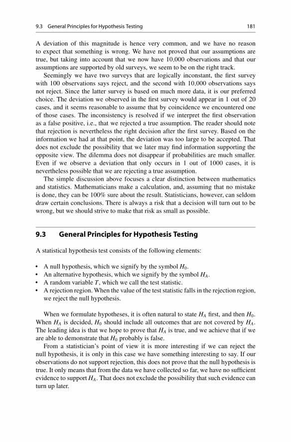
9.3 General Principles for Hypothesis Testing 181
A deviation of this magnitude is hence very common, and we have no reasonto expect that something is wrong. We have not proved that our assumptions aretrue, but taking into account that we now have 10;000 observations and that ourassumptions are supported by old surveys, we seem to be on the right track.
Seemingly we have two surveys that are logically inconstant, the first surveywith 100 observations says reject, and the second with 10;000 observations saysnot reject. Since the latter survey is based on much more data, it is our preferredchoice. The deviation we observed in the first survey would appear in 1 out of 20cases, and it seems reasonable to assume that by coincidence we encountered oneof those cases. The inconsistency is resolved if we interpret the first observationas a false positive, i.e., that we rejected a true assumption. The reader should notethat rejection is nevertheless the right decision after the first survey. Based on theinformation we had at that point, the deviation was too large to be accepted. Thatdoes not exclude the possibility that we later may find information supporting theopposite view. The dilemma does not disappear if probabilities are much smaller.Even if we observe a deviation that only occurs in 1 out of 1000 cases, it isnevertheless possible that we are rejecting a true assumption.
The simple discussion above focuses a clear distinction between mathematicsand statistics. Mathematicians make a calculation, and, assuming that no mistakeis done, they can be 100% sure about the result. Statisticians, however, can seldomdraw certain conclusions. There is always a risk that a decision will turn out to bewrong, but we should strive to make that risk as small as possible.
9.3 General Principles for Hypothesis Testing
A statistical hypothesis test consists of the following elements:
• A null hypothesis, which we signify by the symbol H0.• An alternative hypothesis, which we signify by the symbol HA.• A random variable T, which we call the test statistic.• A rejection region. When the value of the test statistic falls in the rejection region,
we reject the null hypothesis.
When we formulate hypotheses, it is often natural to state HA first, and then H0.When HA is decided, H0 should include all outcomes that are not covered by HA.The leading idea is that we hope to prove that HA is true, and we achieve that if weare able to demonstrate that H0 probably is false.
From a statistician’s point of view it is more interesting if we can reject thenull hypothesis, it is only in this case we have something interesting to say. If ourobservations do not support rejection, this does not prove that the null hypothesis istrue. It only means that from the data we have collected so far, we have no sufficientevidence to support HA. That does not exclude the possibility that such evidence canturn up later.

182 9 Hypothesis Testing
Fig. 9.1 A typical rejectionregion
2.5 %2.5 %
T
The distribution of T
Rejection Rejection
The example we discussed in the motivation section has much in common witha hypothesis test. The context there could have been formulated as follows:
• H0: The parameters in the normal distribution are D 100 and �2 D 100.• HA: 6D 100 or �2 6D 100.• T D K.• Reject H0 if T � 80:3 or T � 119:7.
If we formulate a test as above, what is then the probability of a false positive? Toanswer that, we should assume that H0 is true, and find the probability that the teststatic T falls in the rejection region see Fig. 9.1, i.e.
P.T � 80:2/ C P.T � 119:7/ D G
�80:3 � 100p
100
�C 1 � G
�80:3 � 100p
100
�
D G.�1:97/ C 1 � G.1:97/
D 1 � G.1:97/ C 1 � G.1:97/
D 2:5% C 2:5% D 5%:
From this computation we see that the rejection region was designed in such a waythat the probability of a false positive is 5%. The probability of a false positive, giventhat the null hypothesis is true, is called the significance level. The significance levelis here 5%, which, as we have already remarked, is a typical choice.
The probability of a false negative will depend on which alternative that is true.In this context we could, e.g., ask about the probability of a false negative if D 127
and �2 D 85, i.e., the values we decided to use after rejecting our initial choice. Wedo not reject the null hypothesis when 80:3 < T < 119:7, and, conditional on our

9.4 Designing Statistical Tests 183
specific alternative, the probability is computed as follows:
P.80:3 < T � 119:7/ D P.T < 119:7/ � P.T � 80:3/
D G
�119:7 � 127p
85
�� G
�80:3 � 127p
85
�
D G.�0:79/ � G.�5:07/
D 1 � G.0:79/ � .1 � G.5:07//
D G.5:07/ � G.0:79/ D 1:000 � 0:7852 D 21:48%:
We see that the probability of making a false negative is more than 20% in thiscase. The strength is the complement of this quantity, and we conclude that thestrength is 78:52% when we consider this particular alternative.
The significance level of a hypothesis test is ˛ when the maximum probabilityfor a false positive is ˛. The strength of a specific alternative is the probabilitythat we reject the null hypothesis when the alternative is true.
9.4 Designing Statistical Tests
When we are in the process of designing a test to analyze a given set of observations,there are several pitfalls we could walk into. The conditions for most statistical testare violated if we inspect the data first and then decide which test to use. Whileseemingly innocent, this sequence of events is actually a serious mistake. To explainwhy this is a mistake, we consider an example.
Example 9.2 Assume that we have collected data from 10 different departments.We inspect the data and observe, e.g., that department number 3 performed quitebadly. It could then be tempting to try to test if department 3 is performing worsethan average. A reasonable null hypothesis is that all departments are equally good.When H0 is true, any department will be the worst in 1 out of 10 cases. Inspecting thedata and selecting the worst department, we have tacitly increased the probability oftesting the worst department to 100%. If H0 is true, the probability of a bad resultwill be much higher than for a randomly selected department, and most statisticaltests do not take this into account.
Unusual events will always pop up randomly when we inspect sufficiently manycases, and, moreover, unusual events will become common when we do so. Raritymust always be seen in comparison with how many cases we have inspected, andmost statistical tests are tacitly assuming that we are inspecting only one case.A legitimate line of action in Example 9.2 would be to state an alternative hypothesisthat department 3 is performing worse than average. To examine this hypothesis,

184 9 Hypothesis Testing
What is the alternative hypothesis?
What is the nullhypothesis?
Which test static should we use?
When should we reject the nullhypothesis?
Fig. 9.2 The line of events in hypothesis testing
however, we then need to collect an entirely new set of observations, and use thisnew set to determine the performance. If the performance of department 3 continuesto be bad, we then have legitimate evidence in favor of the alternative.
When we design statistical tests, it is important to find a proper balance betweenhigh strength and a sufficiently low level of significance. In most cases goodstrength comes at the expense of unsatisfactory significance levels, and vice versa.The only way we can increase both is by collecting more observations, but thatoption is frequently too costly or time consuming. As mentioned above all suchconsiderations should be done prior to the collection of data.
The proper line of events in hypothesis testing is outlined in Fig. 9.2.Only when all of these questions have been answered, should we begin to collect
data. In practice we often need to analyze data that already has been collected. Thatis perfectly OK as long as we do not inspect the data before we decide which teststo use.
Example 9.3 We are flipping coins with a friend, and after loosing 50 times in arow, we get a sneaking feeling that something is wrong. To examine this in detailwe formulate our problem in terms of a hypothesis test. The test is made as follows:
H0 W The probability of heads is p D 1=2:
HA W The probability of heads is p > 1=2:
The test is executed by flipping the coin 1000 times, and we let
Xi D(
1 if the result is heads in flip number i
0 if the result is tails in flip number i:
Each Xi is hence an indicator distribution with EŒXi� D p and VarŒXi� D p.1 � p/
where p is unknown. As test static we use the mean
Op D 1
1000.X1 C X2 C � � � C X1000/:

9.4 Designing Statistical Tests 185
Here:
EŒ Op� D p; VarŒ Op� D p.1 � p/
1000:
We should reject the null hypothesis if we observe too many heads, but where shouldwe draw the line? The rejection region should be an interval Πplimit; 1/, where plimit
is the exact place where we draw the line.With a 5% significance level, we should design the test such that the probability
of a false positive is 5%. Hence when H0 is true, i.e., p D 1=2, the probability ofending up in the rejection region should be 5%. We are then in the fortunate situationthat p is known, and we can consider the statement
P. Op � limit/ D 0:05:
From the central limit theorem we know that Op is approximately normal. Hence
P. Op � plimit/ D 1 � P. Op < plimit/ � 1 � G
0
B@plimit � pq
p.1�p/
1000
1
CA D 0:05:
Since we know that p D 0:5, we can view this as an equation with a single unknown,plimit. From the table for the standard normal distribution, we see that G.z/ D 0:95
if and only if z D 1:6449. Hence
plimit � 0:5q0:5.1�0:5/
1000
D 1:6449 , plimit D 0:5 C 1:6449 �r
0:5.1 � 0:5/
1000D 0:526:
In other words, we reject the null hypothesis if we carry out the test and observe atleast 526 heads.
Example 9.4 In Example 9.3 we were fortunate that H0 identified a single value forp. This will not always be the case. To examine this in detail, we modify the exampleas follows:
H0 W The probability of heads is p � 1=2:
HA W The probability of heads is p > 1=2:
We use the same test static Op and the same rejection region as before. What is thesignificance level of the new test?

186 9 Hypothesis Testing
Solution: We assume that H0 is true, and want to compute P. Op � 0:526/: Theproblem now is that p is unknown. The only information we have is that p � 1=2.The smaller the true value of p, the smaller is the probability P. Op � 0:526/: Hencefor any p < 1=2, then
P. Op � 0:526/ � P pD1=2. Op � 0:526/ D 5%:
We see that p D 1=2 is an extreme case, and that all other cases lead to lowerrisk of type 1 error. The maximum probability of a false positive is hence 5%. Inaccordance with the general definition of significance level, the significance levelremains at 5% in this extended case.
Example 9.4 demonstrates why we need to consider the maximum probabilityof false positives in the general definition of significance level, and also explainshow we might compute the significance level in such extended cases. The basic ideais to consider the most extreme case, and, with luck, that makes the computationsufficiently explicit to be carried out.
To proceed, we continue to consider the test in Example 9.4, but now we wantto figure out the strength of alternatives. As we remarked above, the strength willdepend on which alternative that is true. We hence look at some explicit cases.
Case 1 Assume that the true value of p D 0:58. What is the probability of a falsenegative?
Solution: A false negative occurs when the outcome of the test leads to non-rejection of the null hypothesis. In our case we do not reject when Op < 0:526. Ifp D 0:58, then
P. Op < 0:526/ � G
0
B@0:526 � 0:58q
0:58�0:421000
1
CA D G.�3:46/ D 1 � G.3:46/ D 0:03%:
We see that test is really strong in that case, i.e., we will nearly always reject H0 ifthe true value of p is 0.58.
Case 2 Assume that the true value of p D 0:51. What is the probability of a falsenegative?
Solution: We still do not reject when Op < 0:526. If p D 0:51, then
P. Op < 0:526/ � G
0B@
0:526 � 0:51q0:51�0:49
1000
1CA D G.1:01/ D 84%:

9.4 Designing Statistical Tests 187
Fig. 9.3 The strengthfunction of Example 9.4
0.46 0.48
0.2
0.4
0.6
0.8
1.0
0.52 0.54 0.56 0.58 0.60
We see that test is not at all strong when the true value of p is 0.51. In a majority ofoutcomes, we will not detect the difference.
Note that as long as we keep the number of observations fixed at 1000, we reducethe probability of false positives if we increase plimit. This, however, will come at theexpense of less strength of any alternative. The only way of improving both strengthand significance level is to increase the number of observations.
In a test with one unknown parameter , the strength function � is defined asfollows:
�./ D Probability of a false negative given that the true value is :
The graph of the strength function for the test in Example 9.4 is shown in Fig. 9.3.From Fig. 9.3 we see that the strength is nearly zero when p is less than 0:47 and
nearly 100% when p is larger than 0.6.
9.4.1 One-Sided and Two-Sided Tests
A test involving one unknown parameter is called one-sided if the hypotheses areon one of the forms
H0 W � 0; HA W > 0;
H0 W D 0; HA W > 0;
H0 W � 0; HA W < 0;
H0 W D 0; HA W < 0:
In theory other versions are possible, but are generally avoided.The test is called two-sided when it is on the form
H0 W D 0; HA W 6D 0:

188 9 Hypothesis Testing
For computational simplicity we have only considered one-sided tests so far.One-sided tests should, however, only be used in special situations. Typically thereshould be some kind of information available that excludes certain outcomes.
Example 9.5 Imagine you wish to examine if some special form of training leads toimproved production. We measure production in terms of an unknown parameter ,which increases when production improves. It may be unreasonable to assume thatthis special form of training can lead to lower production. Hence the alternative
after training < before training
is excluded by common sense. In that case it is legitimate to consider
H0 W after training D before training; HA W after training > before training:
Example 9.6 Imagine that you wish to examine if some form of new securitymeasure affects production. In this case there is nothing to exclude that productioncan go up or down, and hence a two-sided test is then appropriate.
9.4.2 Confidence Intervals and Hypothesis Testing
We should notice that symmetric confidence intervals are closely connected to two-sided tests. To see how this works, we consider the following example.
Example 9.7 Assume that we have made several independent observations of a ran-dom variable with unknown and variance �2. The observations are approximatelynormal, and we have used the t-distribution to find a 95% confidence interval for theunknown expectation. The resulting interval was Œ6:2�1:4; 6:2C1:4�. Next assumethat we want to test the null hypothesis H0 W D 4 against the two-sided alternativeHA W 6D 4. What conclusion can we draw from this if we use 5% significancelevel?
Solution: From the confidence interval we can see that X D 6:2. We don’t known; t.n�1/
0:025 or SŒX�, but we know that t.n�1/0:025 � SŒX� D 1:4. In a two-sided test we use the
test static X and should reject H0 if X > 4 C 1:4 or if X < 4 � 1:4. In conclusion wereject H0.
If we look more closely on the previous example, we see that we keep H0 if andonly if the expected value defined by H0 is an element of the confidence interval. Ifthe expectation defined by H0 is outside the confidence interval, it always leads torejection.

9.4 Designing Statistical Tests 189
9.4.3 P-Value
The single most important concept in applications of hypothesis testing is the P-value. The reason for this is that most statistical software reports the outcomes ofstatistical tests in terms of P-values. The definition reads as follows:
Definition 9.1 Assuming that the null hypothesis is true, the P-value is theprobability of a deviation (from the null hypothesis) which is greater than orequal to the observed deviation.
The somewhat awkward part of this definition is to understand what we mean bya deviation from the null hypothesis. To examine this more closely, we first considera one-sided test where we reject when T � Tlimit. The larger the value of T, the largeris the deviation from the null hypothesis. This means that the P-value is defined by
P-value D PH0 .T � Tobserved/:
The notation PH0 means that when we compute the probability, we assume that H0
is true.If the level of significance is ˛ and the P-value is less than ˛, this combination
of values can only occur if Tobserved � Tlimit, which means that the observed valueleads to rejection. One advantage of this approach is that we need not find an explicitvalue for Tlimit, it suffices to see that the P-value is less than the confidence level.Another advantage of P-values is that they offer information about the quality ofrejection. The smaller the P-value, the less we believe in the null hypothesis.
When the P-value is smaller than the confidence level, but rather close to thislevel, the rejection is weak. We are much more confident if the test returns a verysmall P-value. In that case the rejection is strong.
Example 9.8 Assume that the test static is T D 131, and that the conditions in thenull hypothesis imply that PH0 .T � 131/ D 0:001: This means that our observationis very rare given that the null hypothesis is true. The P-value is 0.001, and we willreject the null hypothesis at any reasonable significance level. See Fig. 9.4.
Example 9.9 Assume that the test static is T D 131, and that the conditions in thenull hypothesis imply that PH0 .T � 131/ D 0:332: This means that our observationis very common given that the null hypothesis is true. This gives no reason to reject,and we keep the null hypothesis at any reasonable significance level. See Fig. 9.5.
If we instead consider one-sided tests where we reject when T � Tlimit, weproceed in the same way. The only difference is that smaller observed values areinterpreted as larger deviations. The P-value is hence defined via
P-value D PH0 .T � Tobserved/:

190 9 Hypothesis Testing
fT (x)
T 131
0.1 %
x
Fig. 9.4 P-value equal to 0.001
fT (x)
xT 131
33.2 %
Fig. 9.5 P-value equal to 0.332
Considering two-sided tests with symmetric distribution, deviation can work in twodirections. We reject if the value is too large, but also when it is too small. Undersymmetry, we reject when T � Tlimit and also when T � �Tlimit. When that happens,we need to modify the computation of P-value accordingly, i.e.
P-value D PH0 .T � jTobservedj/ C PH0 .T � �jTobservedj/:
Example 9.10 We want to test if the expected value is 4, and use a two-sided testwith test static
T D 1
1000.X1 C X2 C � � � C X1000/ � 4:
We observe the value T D �0:1. The P-value we then find as
P-value D PH0.T � �0:1/ C PH0 .T � 0:1/:

9.4 Designing Statistical Tests 191
We should reject the null hypothesis when the P-value is less than or equal tothe significance level. The smaller the P-value, the more confident we are thatrejection is the right thing to do. Conversely, we keep the null hypothesis whenthe P-value is greater than the significance level. The greater the P-value, theless reason we have for rejection.
Example 9.11 We carry out a survey, and find that the P-value is 0:1%. This meansthat if H0 is true, then we would only expect to see a deviation as large as the onewe have observed in 1 out of 1000 cases. This makes it hard to believe in H0, andwe will almost always reject it.
Example 9.12 We carry out a survey and find that the P-value is 40%. This meansthat if H0 is true, then we would expect to see a deviation as large as the one wehave observed in 4 out of 10 cases. As this is very common, there is no indicationthat something is wrong with the null hypothesis, and we will never reject H0 basedon this information.
Example 9.13 We carry out a survey and find that the P-value is 4%. This meansthat if H0 is true, then we would expect to see a deviation as large as the one we haveobserved in 1 out of 20 cases. This is quite rare, but there is a nonzero chance thatwe observed a large deviation by coincidence. We will reject H0 if the significancelevel is 5%, but will not reject H0 if the significance level is 1%.
Example 9.14 A firm with many customers considers to introduce a new product.The firm think they will be able to make a profit if more than 20% of their customerswill buy the product. The firm asks 40 randomly selected customers, and 10 of thoseconfirm that they want to buy the product.
Question: Based on this survey, is it likely that more than 20% of the customerswill buy the product?
Solution: We let p be the fraction of the customers who want to buy the product,and formulate our question as a hypothesis test. The null hypothesis is that p � 20%,and the alternative is p > 20%. We ask 40 randomly selected customers, and let X bethe number of these customers who want to buy the product. Since the firm has manycustomers, it is reasonable to assume that X has binomial distribution with n D 40.With this information we can compute the P-value of the observation X D 10.
P-value D P pD0:2.X � 10/ D40X
iD10
�40
i
�0:2i0:840�i D 26:82%:
Since the P-value is quite large, we keep the null hypothesis. There is a considerablerisk that the project will not make a profit.

192 9 Hypothesis Testing
If, for the sake of argument, we instead had observed, e.g., X D 17, theconclusion would be different. Then
P-value D P pD0:2.X � 17/ D40X
iD17
�40
i
�0:2i0:840�i D 0:01%:
Here the P-value is so small that it seems very unlikely that the null hypothesis canbe true, and we are hence confident that the project will profit.
9.5 Summary of Chap. 9
• A hypothesis test has the following elements:(i) A null hypothesis H0.
(ii) An alternative hypothesis HA.(iii) A test static T.(iv) A rejection region.
The test is executed by an observation of OT . If OT falls in the rejectionregion, we reject H0 and claim that HA is probably true. If OT is outside therejection region, we keep H0, but that does not mean that we have foundproof that H0 is true.
• A false positive or type 1 error occurs when we reject a true null hypothesis.• A test has significance level ˛ if the probability of a false positive is at most ˛.• A false negative or type 2 error occurs if we keep a false null hypothesis. The
probability will depend on which alternative is true.• The strength of an alternative is the probability of not getting a false negative
when the alternative that is true.• The P-value is the probability of a deviation (from the null hypothesis) that is at
least as large as the observed value, given that the null hypothesis is true.• We reject the null hypothesis if the P-value is at least as small as that of the
significance level, and are more confident about rejection the smaller the P-valueis.
• We keep the null hypothesis when the P-value is larger than the significance level,and are more confident about keeping it the larger the P-value is.
9.6 Problems for Chap. 9
9.1 In this problem we want to study the power consumption in a small city.We assume that the power consumption X (in kWh) of a randomly selected con-sumer in the first quarter of the year has expectation and variance �2 D 4;000;000.Last year the average power consumption was 8000 kWh. To test if the expected

9.6 Problems for Chap. 9 193
power consumption has decreased, we checked the power consumption for 100randomly selected customers.
(a) What is the natural null hypothesis and alternative hypothesis?(b) As test static we use
T D X D 1
100.X1 C X2 C � � � C X100/:
What is EŒT� and �ŒT�?(c) What is the rejection region if we use a significance level of 5%?(d) We observe T D 7800 (kWh). Which conclusion can we draw from this?
9.2 In this problem we study the fee usage in a bank. We assume that the total feeX (in USD) of a randomly selected customer has expectation and variance �2 D1600. Last year the average fee was 120 USD. To test if the fees have increased, wechecked 400 randomly selected customers.
(a) What is the natural null hypothesis and alternative hypothesis?(b) As test static we use
T D X D 1
400.X1 C X2 C � � � C X400/:
What is EŒT� and �ŒT�?(c) What is the rejection region if we use a significance level of 5%?(d) We observe T D 130 (USD). Which conclusion can we draw from this?
9.3 A company claims that firms buying their new Internet package improve theirsales by 10% on average. We doubt that this can be true, and check the sales at 25randomly selected firms. Let X be the sales improvement (in percent of previoussales volumes) of a randomly selected customer that bought the new Internetpackage. Assume that X is normally distributed with expectation and variance�2. We assume that trade volumes at different firms are roughly equal.
(a) What is the natural null hypothesis and alternative hypothesis?(b) As test static we use
T D X � 0:1
SŒX�:
What is the distribution of T when H0 is true?(c) What is the rejection region if we use a significance level of 5%?(d) We observe X D 0:09 and SX D 0:05. Which conclusion can we draw from
this?

194 9 Hypothesis Testing
9.4 A small company has introduced flextime as a means to reduce absence due toillness. Before the introduction of flextime, the average absence due to illness was11 days per year. Let X be the total number of days a randomly selected workeris absent due to illness during a whole year. Assume that X is normally distributedwith expectation and variance �2. The company has 36 workers.
(a) What is the natural null hypothesis and alternative hypothesis?(b) As test static we use
T D X � 11
SŒX�:
What is the distribution of T when H0 is true?(c) What is the rejection region if we use a significance level of 5%?(d) We observe X D 10 and SX D 3. Which conclusion can we draw from this?
9.5 A firm claims that more than 50% of the population prefer their new product.We ask 5 randomly selected people if they prefer the new product. Let X be thenumber of people in the sample who answer yes.
(a) We believe that the company may be right, and wish to execute a test where itwill be possible to conclude that the firm probably is right. What is the naturalnull hypothesis and alternative hypothesis in this test?
(b) We use X as a test static. What is the distribution of X when H0 is true?(c) 5 out of 5 people say that they prefer the new product. Which conclusion can
we draw from this? Use 5% significance level.
9.6 A firm claims that at most 10% of the customers are dissatisfied with the itemsthey have bought from the firm. We ask 400 randomly selected customers if they aredissatisfied. Let X be the number of customers who are dissatisfied.
(a) We believe the firm is mistaken and want to execute a test where it is possible toconclude that the firm probably is mistaken. What is the natural null hypothesisand alternative hypothesis in this test?
(b) We use X as a test static. What is the distribution of X when H0 is true?(c) 53 persons answer that they are dissatisfied. Find the P-value of this observation
by normal approximation. What is the conclusion if the significance level is 5%?
9.7 An accountant checks 400 randomly selected documents from a firm. Theaccounting is approved if at most 3 documents contain errors. Let X be the numberof documents with errors, and let p be the true fraction of documents with errors.
(a) Find the strength of the alternative p D 1% by(i) The Poisson distribution. (ii) The binomial distribution.

9.6 Problems for Chap. 9 195
(b) What result would normal approximation give in this case? Try with and withoutinteger correction.
9.8 A finance institution offers a special type of contracts. It takes very long timeto find the exact price for a contract of this type, but the company has developeda system for approximate prices, and offer to sell the contracts at the approximateprice. We assume that the error has expectation and variance �2 D 100;000;000,and wish to examine the hypothesis H0 W D 0 against HA W 6D 0.
(a) The company tests their method on 400 randomly chosen contracts, andcompute X. Find the rejection region. Use 5% significance level.
(b) What is the strength of the alternative D 2000?
9.9 Simultaneous Strength and Significance: A company believes that less than2.5% of the items they produce contain errors. We want to design a test where wetest n items. Let p be the fraction of the tested items that contain errors. The testshould have 5% significance level, and the produce is approved if there is no reasonto reject the null hypothesis H0 W p � 2:5%.
How large must n be if we want that the strength of the alternative p D 5% isat least 95%? Hint: Use normal approximation. Formulate two equations that n andTlimit must satisfy, and eliminate Tlimit from these equations.
9.10 Logarithmic Transformation: Table 9.1 shows daily observations of thestock price in a company.
(a) Discuss shortly if it is reasonable to assume that Xi are independent?(b) We define new data
Yi D ln
Xi
Xi�1
�; i D 1; : : : ; 10;
and the values of these transformed data are shown in Table 9.2.Assume that all Yi have the same distribution with expectation . Use the
values in the table to find an estimate for .
Table 9.1 Data for Problem 9.10
X0 X1 X2 X3 X4 X5 X6 X7 X8 X9 X10
100 92 96 117 120 126 149 152 176 196 184
Table 9.2 Logarithmic transformed data
Y1 Y2 Y3 Y4 Y5 Y6 Y7 Y8 Y9 Y10
�0:083 0.043 0.198 0.025 0.049 0.168 0.020 0.147 0.108 �0:063

196 9 Hypothesis Testing
(b) The company claims that the numbers clearly demonstrate considerable poten-tial for growth. Technically this is equivalent to the claim > 0. Assume thatall Yi are independent, normally distributed with expectation and variance�2 D 0:01. We want to test H0 W � 0 against HA W > 0. Execute this test.
(c) Find the P-value for the test in (b).
9.11 Strength and t-Distribution: A mutual fund has invested in 10 differentstocks. The fund achieved a return of 20.3% last year. The fund is compared witha reference index showing that stocks of this type had a mean return of 15%. Thefund manager claims that this clearly demonstrates outstanding abilities in findinggood investment opportunities.
For simplicity we assume that the fund has invested equally much in each stock.The return is hence decided from X D 1
10
P10iD1 Xi, where X1; : : : ; X10 is the return
of each of the individual stocks.
(a) Assume that X1; : : : ; X10 are independent random variables with expectation
and variance �2. Find EŒX� and VarŒX�.(b) Assume that X1; : : : ; X10 are independent, normally distributed with expectation
and variance �2. Let S2X be the sample variance. What is the distribution of
Y D X�
SX=p
10?
(c) We want to formulate a hypothesis test which is able to support the managerspoint of view, i.e., where rejection of the null hypothesis implies that themanager probably performs above average. We let H0 W � 15%; HA W >
15%. Find the rejection region using a 5% significance level.(d) We execute the test and observe the results in Table 9.3.
If we process these observations, we find
X D 0:203; SX D 0:099:
Use the results to compute the test static Y. What can you conclude fromthis?
(e) If we want to consider the strength of the alternative A W D 0:023, we need tocompute
PA. Y � Ylimit/ D PA
X �
SX=p
10> Ylimit � 0:053
SX=p
10
!:
When A is true, we know that X�
SX=p
10is t-distributed. Why can’t we use the
t-table to compute this probability?
Table 9.3 Data forProblem 9.11
X1 X2 X3 X4 X5 X6 X7 X8 X9 X10
17.8 4.3 13.9 21.7 25.7 38.9 12.2 14.3 28.2 26.2

9.6 Problems for Chap. 9 197
9.12 Using Poisson Distribution in Accounting: An auditing firm checks samplesfrom the accounting of a large company. There are 100;000 documents, and 1000
randomly selected documents are inspected. We assume that a share p of thedocuments contains errors, and the accountant approves the accounting, if there isno valid reason to reject the claim p � 1 at 5% significance level.
(a) Let X be the total number of checked documents containing errors. What is theexact distribution of X? What distributions can be used as approximations to theexact distribution?
(b) Formulate a hypothesis test where you specify the null hypothesis, alternativehypothesis, test static, and rejection region. Use normal approximation tocompute the rejection region.
(c) The auditing firm finds 11 documents with errors. Find the P-value for thisobservation. What is your conclusion?
(d) In reality 2% of the 100;000 documents contained errors. Find the probabilitythat the auditing firm approves the accounting.
(e) In auditing it is usual to work with Poisson approximations. Use this to find therejection region. Comment the finding.
9.13 Variable “Constants”: We want to test if the transaction volumes for a stockare different on Mondays than on Wednesdays. We have data for the 10 last years,and select randomly 16 Mondays and 16 Fridays. We let X1; : : : ; X16 denote thetransaction volumes on Mondays, and Y1; : : : ; Y16 denote the transaction volumeson Wednesdays. We estimate mean and variance for these data, and find
X D 1200; Y D 1020;
and
S2X D 75;000; S2
Y D 85;000:
(a) Assume that X1; : : : ; X16; Y1; : : : ; Y16 are independent, normally distributed anddefine new variables S2; T; and U by
S2 D S2X C S2
Y
2; T D X � Yp
S2=8; U D X � Yp
80;000=8:
What kind of distribution has U? Are T and U different random variables?Justify the answer.
(b) We want to test the hypotheses
H0 W Trade volumes on Mondays and Wednesdays have the same expectation;
HA W Trade volumes on Mondays and Wednesdays have different expectations.

198 9 Hypothesis Testing
Table 9.4 Data forProblem 9.14
1 2 3 4 5 6 7 8
149 150 134 155 104 147 147 123
You can take for granted that when H0 is true, then T is t-distributed withparameter � D 30. Find the rejection region. What conclusion can you draw?Use 5% significance level.
(c) What is the problem using U as a test static?
9.14 One-Sided Test Versus Two-Sided Confidence Interval: The production ata department was observed 8 consecutive working days. The results are shown inTable 9.4.
Processing these numbers we get
X D 138:625; SX D 17:3612:
(a) Assume that the observations are approximately normal and find a 95%confidence interval for expected production.
(b) A few years before, the company carried out an extensive survey at the samedepartment. This survey found a mean production 125 (units/day). Use a one-sided test. Can we claim that production has increased? Compare with the resultfrom (a) and comment the answer.
9.15 Testing Extremes: In this problem we will study a food chain with 100branches. We assume that the branches are equally large. Previous surveys con-cluded that yields were approximately normal with expectation 5% and standarddeviation 2%.
(a) Let X denote the yield of a randomly selected branch. Compute the probabilitiesi) P.X < 2%/ ii) P.X < �1%/.
(b) The management decided at the start of the year to follow a certain department.At the end of the year the department had a yield equal to 2%. From thisinformation, can you reject a null hypothesis saying that the branch had thesame expected yield as the others? Use a two-sided test and find the P-value.Use 5% significance level.
(c) The management collected numbers from all the branches, and it turned outthe worst department had a yield of �1%. From this number can you reject ahypothesis claiming that all the departments have the same expected yield asbefore? Use a two-sided test with 5% significance level. Use a two-sided testand find the P-value. Use 5% significance level.
(d) The branch with the worst result in (c) reported a yield of �1% also thefollowing year. From this number can you reject a hypothesis claiming that allthe departments have the same expected yield as before?

9.6 Problems for Chap. 9 199
9.16 Testing Extremes: A company has 10 different production units. When theproduction equipment functions properly, all the units have an expected productionof 100 items per day. The standard deviation is 5 items. All produced units arechecked, and only approved items are included in the production numbers. We letX1; : : : ; X10 denote the number of produced items at the 10 different units, and weassume that these values are approximately normal. Throughout the problem wewill use 5% level of significance.
(a) Unusual production numbers indicate that the equipment does not functionproperly. Why is it natural to use one-sided tests to examine this?
(b) Assume that Z is a normal distribution with expectation and standarddeviation � . Explain why
P.Z � z/ D 0:05 , z D � 1:645 �:
(c) How low must the value of X1 be before you would reject the null hypothesis1 D 100 against < 100?
(d) Assume that the production equipment functions properly, and that all units havean expected production of 100 items with a standard deviation of 5 items. Whatis the probability that at least one of the units produces less than 92 items?
(e) Let Xmin be the number of items produced at the worst unit. How low must thevalue of Xmin be before you would reject the null hypothesis
H0 W 1 D 2 D � � � D 10 D 100;
against the alternative that at least one of the expectations is less than 100?
9.17 Misinterpreting Randomness: In this problem we will assume that theprobability of bankruptcy (during one year) for a certain type of company is 5%.We also assume that bankruptcy or not are independent events among the differentcompanies.
(a) Assume that there are in total 120 companies of this type, and that X is thenumber of companies going bankrupt during one year. What is the distributionof X?
(b) i) Find the probability that exactly 2 of 120 companies go bankrupt. ii) Find theprobability that at most 2 of such companies go bankrupt.
(c) Assume that 2 of the 120 companies went bankrupt the last year. A journalistpoints out that only 1:7% of the companies went bankrupt, and this shows thatthe probability of bankruptcy is not 5%. Comment this claim.
(d) Point at circumstances that would make the assumption of independence amongcompanies unreasonable. How would that affect the distribution of X?

200 9 Hypothesis Testing
9.18 P-Values in Repeated Samples: You want to examine if a new training haseffect, and carry out a statistical test of the effect. The null hypothesis is that thetraining has no effect, and the alternative hypothesis is that it has effect. We use 5%significance level.
(a) A randomly selected school has completed this training, and after completionthe statistical test returns a P-value equal to 25%. How would you interpret thisresult, and what conclusion would you draw?
(b) 25 different schools have completed this training. At one of the schools thetest returned a P-value of 4%. How would you interpret that result, and whatconclusion would you draw?

10Commonly Used Tests
Abstract
In this chapter we will look at some special hypothesis tests. These tests havefound widespread applications and are used by almost everyone that need toprocess statistical data. The tests we consider are: A test for binomial variables,the t-test for expected value, the t-test for comparison of two populations,Wilcoxons’ distribution free tests, the U test, and the chi-square tests. The testsare presented in terms of recipes, i.e., step by step explanations on how to executethe test and how to interpret the outcomes. As we focus applications, we make noattempt to explain in detail why these tests work. They are based on quite lengthymathematical derivations, but these details are omitted.
10.1 Testing Binomial Distributions
In many cases we need to test the probability for success in a binomial distribution.This can be carried out if we make n independent trials and observe the total numberof successes X. To test H0 W p D p0 against HA W p 6D p0, we compute thestandardized test static
Z D X � np0pnp0.1 � p0/
:
If we have reasonably many observations, then Z is an approximate standard normaldistribution. The test can be summarized as follows:
© Springer International Publishing AG 2017J. Ubøe, Introductory Statistics for Business and Economics, Springer Textsin Business and Economics, https://doi.org/10.1007/978-3-319-70936-9_10
201

202 10 Commonly Used Tests
Two-sided test for binomial trials where np0.1 � p0/ is at least 5.
H0 W p D p0 against HA W p 6D p0:
Significance level ˛.
1. Compute
Z D X � np0pnp0.1 � p0/
:
2. Find z˛=2 from the table of the standard normal distribution such that
P.Z � z˛=2/ D z˛=2:
3. Reject H0 if Z � z˛=2 or if Z � �z˛=2.
If we can use one-sided tests instead, we proceed similarly.
One-sided test for binomial trials where np0.1 � p0/ is at least 5.
H0 W p � p0 against HA W p > p0:
Significance level ˛.
1. Compute
Z D X � np0pnp0.1 � p0/
:
2. Find z˛ from the table of the standard normal distribution such that
P.Z � z˛/ D z˛:
3. Reject H0 if Z � z˛ .

10.2 t-Test for Expected Value 203
One-sided test for binomial trials where np0.1 � p0/ is at least 5.
H0 W p � p0 against HA W p < p0:
Significance level ˛.
1. Compute
Z D X � np0pnp0.1 � p0/
:
2. Find z˛ from the table of the standard normal distribution such that
P.Z � z˛/ D z˛:
3. Reject H0 if Z � �z˛ .
Example 10.1 We have carried out 100 binomial trials and observed a total of 56successes. We want to test H0 W p D 0:5 against HA W p 6D 0:5. What is theconclusion from the test?
Solution: We use the recipe above:
Z D 56 � 100 � 0:5p100 � 0:5.1 � 0:5/
D 1:2:
When no significance level is stated, we tacitly assume that the significance level is5%, i.e., ˛ D 5%. Since the test is two-sided, we need to look up the 2.5% level. Wefind z0:025 D 1:96. Since the observed test static is smaller than the rejection limit,we keep H0. There is no sufficient evidence to claim that p is different from 0.5.
10.2 t-Test for Expected Value
It happens frequently that we want to test an unknown expected value, and the mostcommon situation is that the variance, too, is unknown. If we assume that we haven independent and approximately normal observations, we know that
T D X �
SŒX�

204 10 Commonly Used Tests
is t-distributed with parameter � D n �1. A test for H0 W D 0 against HA W 6D0 can then be executed as follows:
Two-sided t-test for expected value. Independent and approximately normalobservations with unknown expectation and variance.
H0 W D 0 against HA W 6D 0:
Significance level ˛.
1. Find X.2. Find SX .3. Compute SŒX� D SX=
pn.
4. Compute T D X�0
SŒX�.
5. Use the t-table with parameter � D n � 1 to find t.n�1/
˛=2 such that
P.T.n�1/ � t.n�1/
˛=2 / D ˛=2:
6. Reject H0 if T � t.n�1/
˛=2 or if T � �t.n�1/
˛=2 .
The one-sided versions read as follows:
One-sided t-test for expected value. Independent and approximately normalobservations with unknown expectation and variance.
H0 W � 0 against HA W > 0:
Significance level ˛.
1. Find X.2. Find SX .3. Compute SŒX� D SX=
pn.
4. Compute T D X�0
SŒX�.
5. Use the t-table with parameter � D n � 1 to find t.n�1/˛ such that
P.T.n�1/ � t.n�1/˛ / D ˛:
6. Reject H0 if T � t.n�1/˛ .

10.2 t-Test for Expected Value 205
One-sided t-test for expected value. Independent and approximately normalobservations with unknown expectation and variance.
H0 W � 0 against HA W < 0:
Significance level ˛.
1. Find X.2. Find SX .3. Compute SŒX� D SX=
pn.
4. Compute T D X�0
SŒX�.
5. Use the t-table with parameter � D n � 1 to find t.n�1/˛ such that
P.T.n�1/ � t.n�1/˛ / D ˛:
6. Reject H0 if T � �t.n�1/˛ .
Example 10.2 We have 9 independent observations and have found X D �11:2 andSX D 9:6. We assume that observations are approximately normal and want to testH0 W � 0 against HA W < 0. What is the conclusion from the test?
Solution: We follow the recipe above. The first two steps follow from the text,so we proceed to step 3.
SŒX� D 9:6p9
D 3:2:
Since 0 D 0, we get
T D �11:2 � 0
3:2D �3:5:
The rejection limit we find from a t-table with parameter 8. If we use 5%significance, we must find the 5% level in this table. This gives t.8/
0:05 D 1:86. Weshould hence reject H0 if T < �1:86. As this is certainly true, we reject H0 andclaim that the expected value is probably negative.

206 10 Commonly Used Tests
10.3 Comparing Two Groups
In statistics we often need to compare properties of two different groups. We willnow consider some special techniques that can be used to decide if the groups aredifferent.
10.3.1 t-Test for Comparison of Expectation in Two Groups
Assume that we have two groups. In the first group we observe X and in the secondgroup we observe Y. Expectations and variances are unknown, and we want to testif EŒX� D EŒ Y� or not. As in the previous t-test we need to assume that observationsare approximately normal.
We let X1; : : : ; Xn1 denote the observations from the first group, while Y1; : : : ; Yn2
denote observations from the second group. We assume that
EŒXi� D X ; VarŒXi� D �2X ; i D 1; : : : ; n1;
and
EŒ Yi� D Y ; VarŒXi� D �2Y ; i D 1; : : : ; n2:
Two- and one-sided tests can then be executed as follows:
Two-sided test for comparison of expectations in two groups. Independent andapproximately normal observations with unknown expectation and variance.Equal variances in the two groups.
H0 W X D Y against HA W X 6D Y :
Significance level ˛.
1. Find X and Y.2. Find S defined via
S2 D 1
n1 C n2 � 2
n1X
iD1
.Xi � X/2 Cn2X
iD1
. Yi � Y/2
!:
(continued)

10.3 Comparing Two Groups 207
3. Compute
SŒ Oı� D S �s
1
n1
C 1
n2
:
4. Compute
T D X � Y
SŒ Oı�:
5. Use the t-table with parameter � D n1 C n2 � 2 to find t.�/
˛=2 such that
P.T.�/ � t.�/
˛=2/ D ˛=2:
6. Reject H0 if T � t.�/
˛=2 or if T � �t.�/
˛=2.
Extra: The limits for a .1 � ˛/100% confidence interval for the differenceX � Y are given by
X � Y ˙ t.�/
˛=2 � SŒ Oı�:
One-sided test for comparison of expectations in two groups. Independent andapproximately normal observations with unknown expectation and variance.Equal variances in the two groups.
H0 W X � Y against HA W X > Y :
Significance level ˛.
1. Find X and Y.2. Find S defined via
S2 D 1
n1 C n2 � 2
n1X
iD1
.Xi � X/2 Cn2X
iD1
. Yi � Y/2
!:
(continued)

208 10 Commonly Used Tests
3. Compute
SŒ Oı� D S �s
1
n1
C 1
n2
:
4. Compute
T D X � Y
SŒ Oı�:
5. Use the t-table with parameter � D n1 C n2 � 2 to find t.�/˛ such that
P.T.�/ � t.�/˛ / D ˛:
6. Reject H0 if T � t.�/˛ .
One-sided test for comparison of expectations in two groups. Independent andapproximately normal observations with unknown expectation and variance.Equal variances in the two groups.
H0 W X � Y against HA W X < Y :
Significance level ˛.
1. Find X and Y.2. Find S defined via
S2 D 1
n1 C n2 � 2
n1X
iD1
.Xi � X/2 Cn2X
iD1
. Yi � Y/2
!:
3. Compute
SŒ Oı� D S �s
1
n1
C 1
n2
:
(continued)

10.3 Comparing Two Groups 209
4. Compute
T D X � Y
SŒ Oı�:
5. Use the t-table with parameter � D n1 C n2 � 2 to find t.�/˛ such that
P.T.�/ � t.�/˛ / D ˛:
6. Reject H0 if T � �t.�/˛ .
Remark In these tests we had to assume that the variances are equal in the twogroups. Modern statistical software can easily handle situations where the variancesare different.
Example 10.3 Assume that a factory can use two different methods in production.We make 10 independent observations of the production, 5 using method 1 and 5using method 2. Method 1 gave the results:
4:7; 3:5; 3:3; 4:2; 3:6;
while the corresponding numbers for method 2 was
3:2; 4:2; 3:3; 3:9; 3:0:
Assuming that we have normally distributed observations with equal variances, wecompute
X D 3:86; Y D 3:52; S D 0:543; SŒ Oı� D 0:344:
We insert these quantities into the formula, and get
T D X � Y
SŒ Oı�D 0:34
0:344D 0:99:
In this case we should refer to a t-table with parameter
� D n1 C n2 � 2 D 5 C 5 � 2 D 8:
From this table we find t.8/0:025 D 2:306. Since the observed T value is well within
the non-rejection region, there is no reason to reject H0. We hence keep the null

210 10 Commonly Used Tests
Fig. 10.1 t-test executed inExcel
hypothesis saying there is no difference in expectation. The limits for a 95%confidence interval for the difference X � Y are given by
X � Y ˙ t.�/
˛=2 � SŒ Oı� D 0:34 ˙ 2:306 � 0:344:
The confidence interval is hence Œ�0:45; 1:13�. We notice that the value zero iscontained in this interval, which is consistent with our null hypothesis.
10.3.2 t-Test Executed in Excel
Using the Excel command TTEST.A1 W AnI B1 W BnI 2; 2/, we can easily executethe two-sided test we examined in Example 10.3. We write the observations frommethod 1 in the first column, and the corresponding results for method 2 in thesecond column. The final result is displayed in Fig. 10.1.
The result displayed in C1 is the P-value for this test, and we see that the P-valueis as large as 35%. There is hence no reason to suspect that the null hypothesis iswrong, and we keep the hypothesis about equal expectations.
10.3.3 t-Test for Comparison of Expectation in Two Groups, PairedObservations
It sometimes happens that we want to compare observations from two differentgroups where the observations are paired in a natural way. Let .X1; Y1/; : : : ; .Xn; Yn/
denote the observed pairs. In the previous t-test we assumed that all observationswere independent. In our new case X1 and Y1 may be dependent, and the sameapplies for any pair. The different pairs, however, are independent of each other.With a structure like this, we need to modify the procedure to take the pairing intoaccount. This is done as follows:

10.3 Comparing Two Groups 211
Two-sided test for comparison of expectations in two groups, paired obser-vations. Independent pairs and approximately normal observations withunknown expectation and variance.
H0 W X D Y against HA W X 6D Y :
Significance level ˛.
1. Find X and Y.2. Find S defined via
S2 D 1
n � 1
n1X
iD1
.Xi � Yi � X C Y/2:
3. Compute
SŒ Oı� D S=p
n:
4. Compute
T D X � Y
SŒ Oı�:
5. Use the t-table with parameter � D n � 1 to find t.�/
˛=2 such that
P.T.�/ � t.�/
˛=2/ D ˛=2:
6. Reject H0 if T � t.�/
˛=2 or if T � �t.�/
˛=2.
Extra: The limits for a .1 � ˛/100% confidence interval for the differenceX � Y are given by
X � Y ˙ t.�/
˛=2 � SŒ Oı�:

212 10 Commonly Used Tests
Two-sided test for comparison of expectations in two groups, paired obser-vations. Independent pairs and approximately normal observations withunknown expectation and variance.
H0 W X � Y against HA W X > Y :
Significance level ˛.
1. Find X and Y.2. Find S defined via
S2 D 1
n � 1
n1X
iD1
.Xi � Yi � X C Y/2:
3. Compute
SŒ Oı� D S=p
n:
4. Compute
T D X � Y
SŒ Oı�:
5. Use the t-table with parameter � D n � 1 to find t.�/˛ such that
P.T.�/ � t.�/˛ / D ˛:
6. Reject H0 if T � t.�/˛ .
Two-sided test for comparison of expectations in two groups, paired obser-vations. Independent pairs and approximately normal observations withunknown expectation and variance.
H0 W X � Y against HA W X < Y :
Significance level ˛.
1. Find X and Y.
(continued)

10.3 Comparing Two Groups 213
2. Find S defined via
S2 D 1
n � 1
n1X
iD1
.Xi � Yi � X C Y/2:
3. Compute
SŒ Oı� D S=p
n:
4. Compute
T D X � Y
SŒ Oı�:
5. Use the t-table with parameter � D n � 1 to find t.�/˛ such that
P.T.�/ � t.�/˛ / D ˛:
6. Reject H0 if T � �t.�/˛ .
Example 10.4 We now return to the numbers used in Example 10.3, but this timewe assume that the same workers first used method 1 and then method 2. X1 and Y1
are hence the results of the same worker using two different methods. If we orderthe results in the same order as the workers, it turned out that the workers obtainedthe following results:
4:7; 3:5; 3:3; 4:2; 3:6
with method 1, and
4:2; 3:2; 3:0; 3:9; 3:3
with method 2. By inspection we notice that all the workers reported larger numbersby method 1 than by method 2. The unpaired test we used in the previous sectiondid not take this into account. Our new test does, and it makes a lot of difference. Ifwe carry out a two-sided test using the recipe above, we get
n D 5; X D 3:86; Y D 3:52; S D 0:089:

214 10 Commonly Used Tests
With
T D X � Y
S=p
n;
we get T D 8:5. Using a t-table with parameter � D n � 1 D 4, we see thatt.4/0:025 D 2:775 which is the rejection limit with 5% significance level. The observed
T falls deep into the rejection region, and there is good reason to claim that the twomethods lead to different expected production.
We should notice that this does not mean that the analysis from the unpaired testwas wrong. The information regarding the pairs provides new evidence, and it isnot surprising that more evidence can alter the conclusion. When we fail to rejecta null hypothesis, it does not mean that we have proved that the null hypothesis istrue. Furthermore it does not exclude the possibility that we later may come up withmore convincing evidence. Statistical data can often be analyzed using differenttests, and it is not uncommon that different tests provide different conclusions. Insuch situations we should put more weight on the test that best makes use of theavailable information.
10.3.4 t-Test with Paired Observations Executed in Excel
Using the Excel command TTEST.A1 W AnI B1 W BnI 2; 1/, we can easily execute thetwo-sided test we examined in Example 10.4. The only difference is that we changethe last digit in the command from 2 to 1. This makes Excel understand that wewant to use a paired test (Fig. 10.2).
We see that the P-value for the paired test is as small as 0:1% meaning that weare very confident in rejecting the null hypothesis. It seems very probable that thetwo methods lead to different expected production.
Fig. 10.2 Paired t-testexecuted in Excel

10.4 Wilcoxon’s Distribution Free Tests 215
10.4 Wilcoxon’s Distribution Free Tests
A general weakness with the t-tests we have discussed so far is that they assumeapproximately normal observations. This assumption may not be true, and we canthen not trust the results. In cases where the assumption may be questionable, wecan use what is called distribution free tests, i.e., tests that do not assume thatthe observations have a particular distribution. The price for doing so is that wewithdraw invalid evidence, and with less evidence the chances of rejection arereduced.
We will now consider Wilcoxon’s tests for the comparison of two differentgroups. The basis for these tests is exactly the same as for the t-test for comparisonof expected values in two different groups. The only difference is that we no longerassume that observations are normally distributed.
The Wilcoxon rank-sum test takes its starting point in the so-called rank-sum ofthe observations. A simplistic procedure for finding the rank-sum can be describedas follows: First write all the observations from the two groups in ascending order.The next step is to underline the observations from the first group. The rank-sum isdefined as the sum of the positions of the underlined numbers. The basic idea is thatW will be small if the numbers from group 1 are largely smaller than the numbersfrom group 2, and large if the differences go in the opposite direction.
Example 10.5 We have observed working times (measured in seconds) for workersin two different groups. In group 1 the working times were:
47; 59; 43; 50; 45; 45; 49; 41; 47; 95; 50;
while the working times for group 2 were
45; 48; 61; 52; 48; 63; 52; 54; 50; 58:
To compute the rank-sum of these observations, we sort all the observations inascending order and underline the observations from group 1:
41; 43; 45; 45; 45; 47; 47; 48; 48; 49; 50; 50; 50; 52; 52; 54; 58; 59; 61; 63; 95:
The rank-sum W is found from the sum of the positions of the underlined numbers,i.e.
W D 1 C 2 C 3 C 5 C 6 C 7 C 10 C 11 C 13 C 18 C 21 D 97:
Remark When we write the observations in ascending order, it may happen thatsome observations are equal. It is then not clear which one to write first. It iscommon practice to swap the order every second time, i.e., the first time we haveequality, we write down the value from group 1 first, and the next time we have

216 10 Commonly Used Tests
equality, we write down the observation from group 2 first. Modern computersoftware uses a more refined version where the program computes the rank-sumfor any possible permutation of equal numbers, and takes the mean over all theserank-sums. The difference is often negligible.
The Wilcoxon rank-sum two-sided test for comparison of expectations in twogroups. Independent observations with any distribution.
H0 W X D Y against HA W X 6D Y :
Significance level ˛.
1. Compute EŒW� D 12n1.n1 C n2 C 1/.
2. Compute VarŒW� D 112
n1n2.n1 C n2 C 1/.3. Compute
Z D W � EŒW�p
VarŒW�:
4. Find z˛=2 from the table of the standard normal distribution such that
P.Z � z˛=2/ D ˛=2:
5. Reject H0 if Z � z˛=2 or if Z � �z˛=2:
The Wilcoxon rank-sum one-sided test for comparison of expectations in twogroups. Independent observations with any distribution.
H0 W X � Y against HA W X > Y :
Significance level ˛.
1. Compute EŒW� D 12n1.n1 C n2 C 1/.
2. Compute VarŒW� D 112
n1n2.n1 C n2 C 1/.3. Compute
Z D W � EŒW�pVarŒW�
:
(continued)

10.4 Wilcoxon’s Distribution Free Tests 217
4. Find z˛ from the table of the standard normal distribution such that
P.Z � z˛/ D ˛:
5. Reject H0 if Z � z˛ .
The Wilcoxon rank-sum one-sided test for comparison of expectations in twogroups. Independent observations with any distribution.
H0 W X � Y against HA W X < Y :
Significance level ˛.
1. Compute EŒW� D 12n1.n1 C n2 C 1/.
2. Compute VarŒW� D 112
n1n2.n1 C n2 C 1/.3. Compute
Z D W � EŒW�pVarŒW�
:
4. Find z˛ from the table of the standard normal distribution such that
P.Z � z˛/ D ˛:
5. Reject H0 if Z � �z˛ .
Remark Even though these tests rest on the central limit theorem, the number ofobservations need not be very large. As stated above, there should be at least 8–10observations in each group. Modern statistical software, however, can handle caseswith fewer observations.
Example 10.6 We want to carry out a two-sided test for the observations inExample 10.5. We use the values n1 D 11 and n2 D 10 to get:
1. EŒW� D 12
� 11 � 22 D 121:
2. VarŒW� D 112
� 11 � 10 � 22 D 201:667:
3. Z D 97�121p201:667
D �1:69:

218 10 Commonly Used Tests
Using 5% significance level, we get z0:025 D 1:96, and we conclude that we haveto keep our null hypothesis of no difference in expected values.
10.4.1 TheWilcoxon Signed-Rank Test
When we studied t-test previously in this chapter, we could see that it made a lotof difference if the observations were paired. There is a Wilcoxon test dealing withthis situation, and it is called the Wilcoxon signed-rank test. A simplistic version ofthe procedure can be described as follows:
Compute the differences between each pair of number, i.e.
difference D value from group 2 � value from group 1;
and write all these differences in ascending order with respect to absolute value. Therank V is the sum of the positions of the negative terms. The idea behind the test isthat V is small if the numbers from group 1 is largely smaller than the numbers fromgroup 2, and V will be large if the effect goes in the opposite direction.
Example 10.7 10 workers performed the same working operation twice, the firsttime without training and the second time after training. The required working timeswere as follows:
Without training:
48; 53; 52; 57; 43; 83:59; 71; 40; 61;
while the working times after training were
45; 42; 58; 50; 41; 47; 53; 66; 45; 53:
If we compute the differences between each such pair, we get:
�3; �11; 6; �7; �2; �36; �6; �5; 5; �8:
We sort these numbers in ascending order with respect to absolute value andunderline the negative numbers. We get:
�2; �3; �5; 5; 6; �6; �7; �8; �11; �36:
We find the rank V when we compute the sum of the positions of the underlinednumbers, i.e.
V D 1 C 2 C 3 C 6 C 7 C 8 C 9 C 10 D 46:

10.4 Wilcoxon’s Distribution Free Tests 219
Once the rank is computed, the tests are carried out using the recipes below:
The Wilcoxon signed-rank two-sided test for comparison of expectations intwo groups, paired observations. Independent pairs with any distribution.
H0 W X D Y against HA W X 6D Y :
Significance level ˛.
1. Compute EŒV� D 14n.n C 1/.
2. Compute VarŒV� D 124
n.n C 1/.2n C 1/.3. Compute
Z D V � EŒV�pVarŒV�
:
4. Find z˛=2 from the table of the standard normal distribution such that
P.Z � z˛=2/ D ˛=2:
5. Reject H0 if Z � z˛=2 or if Z � �z˛=2:
The Wilcoxon signed-rank one-sided test for comparison of expectations intwo groups, paired observations. Independent pairs with any distribution.
H0 W X � Y against HA W X > Y :
Significance level ˛.
1. Compute EŒV� D 14n.n C 1/.
2. Compute VarŒV� D 124
n.n C 1/.2n C 1/.3. Compute
Z D V � EŒV�p
VarŒV�:
4. Find z˛ from the table of the standard normal distribution such that
P.Z � z˛/ D ˛:
5. Reject H0 if Z � z˛ .
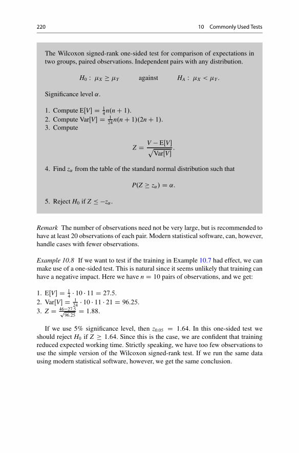
220 10 Commonly Used Tests
The Wilcoxon signed-rank one-sided test for comparison of expectations intwo groups, paired observations. Independent pairs with any distribution.
H0 W X � Y against HA W X < Y :
Significance level ˛.
1. Compute EŒV� D 14n.n C 1/.
2. Compute VarŒV� D 124
n.n C 1/.2n C 1/.3. Compute
Z D V � EŒV�pVarŒV�
:
4. Find z˛ from the table of the standard normal distribution such that
P.Z � z˛/ D ˛:
5. Reject H0 if Z � �z˛ .
Remark The number of observations need not be very large, but is recommended tohave at least 20 observations of each pair. Modern statistical software, can, however,handle cases with fewer observations.
Example 10.8 If we want to test if the training in Example 10.7 had effect, we canmake use of a one-sided test. This is natural since it seems unlikely that training canhave a negative impact. Here we have n D 10 pairs of observations, and we get:
1. EŒV� D 14
� 10 � 11 D 27:5:
2. VarŒV� D 124
� 10 � 11 � 21 D 96:25:
3. Z D 46�27:5p96:25
D 1:88:
If we use 5% significance level, then z0:05 D 1:64. In this one-sided test weshould reject H0 if Z � 1:64. Since this is the case, we are confident that trainingreduced expected working time. Strictly speaking, we have too few observations touse the simple version of the Wilcoxon signed-rank test. If we run the same datausing modern statistical software, however, we get the same conclusion.

10.5 The U-Test for Comparison of Success Probabilities 221
10.4.2 Comparison of t-Tests andWilcoxon Test
In cases where the observations are approximately normal, we can use both t-testsand the Wilcoxon tests. In such cases it might happen that the tests lead to oppositeconclusions. When this occurs, we put more weight on the results from the t-tests.In general the Wilcoxon tests are weaker, i.e., the deviation from the null hypothesisneeds to be larger before we can confidently reject it. In other words, the deviationfrom the null hypothesis needs to be stronger before the Wilcoxon tests lead torejection.
It might happen that we have run both tests, and only later understand that theassumption of normally distributed observations may be questionable. In such caseswe should disregard the results from the t-tests and only rely on the results from theWilcoxon tests.
10.5 TheU-Test for Comparison of Success Probabilities
Instead of comparing expected values, we might want to compare success probabil-ities in two groups. To study this in detail, we proceed as follows:
• We make n1 binomial trials in the first group, and n2 in the second group.• We let p1 denote the probability of success in the first group, and p2 the
probability of success in the second group.• X1 is the total number of successes in the first group, and X2 is the total number
of successes in the second group.
We want to test if the success probabilities are different, and can use the followingtest:
Two-sided U-test for comparison of success probabilities. Binomial trials.
H0 W p1 D p2 against HA W p1 6D p2:
Significance level ˛.
1. Find
Op1 D X1
n1
; Op2 D X2
n2
:
(continued)

222 10 Commonly Used Tests
2. Find Op defined by
Op D X1 C X2
n1 C n2
:
3. Compute
U D Op1 � Op2r�1n1
C 1n2
�Op.1 � Op/
:
4. When the numbers of observations are sufficiently large, see note below, Uis approximately normal. Use the table for the standard normal distributionto find z˛=2 such that
P.Z � z˛=2/ D ˛=2:
5. Reject H0 if U � z˛=2 or if U � �z˛=2.
Extra: The limits for a .1 � ˛/100% significance interval for p1 � p2 are
Op1 � Op2 ˙ z˛=2
sOp1.1 � Op1
n1
C Op2.1 � Op2/
n2
:
One-sided U-test for comparison of success probabilities. Binomial trials.
H0 W p1 � p2 against HA W p1 > p2:
Significance level ˛.
1. Find
Op1 D X1
n1
; Op2 D X2
n2
:
2. Find Op defined by
Op D X1 C X2
n1 C n2
:
(continued)
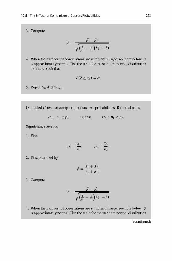
10.5 The U-Test for Comparison of Success Probabilities 223
3. Compute
U D Op1 � Op2r�1n1
C 1n2
�Op.1 � Op/
:
4. When the numbers of observations are sufficiently large, see note below, Uis approximately normal. Use the table for the standard normal distributionto find z˛ such that
P.Z � z˛/ D ˛:
5. Reject H0 if U � z˛.
One-sided U-test for comparison of success probabilities. Binomial trials.
H0 W p1 � p2 against HA W p1 < p2:
Significance level ˛.
1. Find
Op1 D X1
n1
; Op2 D X2
n2
:
2. Find Op defined by
Op D X1 C X2
n1 C n2
:
3. Compute
U D Op1 � Op2r�1n1
C 1n2
�Op.1 � Op/
:
4. When the numbers of observations are sufficiently large, see note below, Uis approximately normal. Use the table for the standard normal distribution
(continued)

224 10 Commonly Used Tests
to find z˛ such that
P.Z � z˛/ D ˛:
5. Reject H0 if U � �z˛ .
Note: These tests all require that the numbers of observations are sufficientlylarge. More precisely it is usual to require that n1 Op1; n1.1 � Op1/; n2 Op2; n2.1 � Op2/ areall greater than 5.
Example 10.9 40 men and 60 women have been asked if they think statistics isan interesting subject. 11 men and 14 women answered No, the rest Yes. Whatconclusion can we draw from this?
Solution: We use a two-sided U-test to answer this. We have
Op1 D 11
40; Op2 D 14
60:
Op1 D 11 C 14
40 C 60D 25
100:
We insert these quantities in the formula below and get
U D Op1 � Op2r�1n1
C 1n2
�Op.1 � Op/
D 0:47:
At 5% significance level, z0:025 D 1:96. The observed U is well within the non-rejection region. We keep the null hypothesis saying there is no difference in opinionbetween men and women.
10.6 Chi-Square Test for Goodness-of-Fit
The chi-square test for probabilities is a useful test when we want to examine a givenset of probabilities. The starting point is a sample space with m different outcomes.We want to test if the different outcomes occur with frequencies that are compatiblewith a given set of probabilities. To settle this, we make n independent observationsand record how many times we got each outcome. Here
Xi D Number of times we observed outcome i; i D 1; : : : ; m:

10.6 Chi-Square Test for Goodness-of-Fit 225
The test is executed as follows:
Chi-square test for a given set of probabilities p1; p2; : : : ; pm (goodness-of-fit).
H0 W The probability distribution of the outcomes equals p1; p2; : : : ; pm:
HA W The probability of at least one outcome differs from the given distribution:
Requires n independent observations where npi > 5 for i D 1; : : : ; m.Significance level ˛.
1. Compute
Q D .X1 � np1/2
np1
C .X2 � np2/2
np2
C � � � C .Xm � npm/2
npm:
2. Use a chi-square table with parameter � D m � 1 to find q.�/˛ such that
P.Q.�/ � q.�/˛ / D ˛:
3. Reject H0 if Q � q.�/˛ .
Notice that this test does not have a two-sided version. The chi-square distribu-tion is always positive, and a two-sided test makes no sense. We should also noticethat the distribution is not approximately normal, so we cannot use the standardnormal distribution in this case.
Example 10.10 A country has 5 political parties, A,B,C,D,E. In the previouselection votes were distributed as follows:
A W 20%; B W 30%; C W 20%; D W 2%; E W 28%:
In our model we hence have p1 D 0:2; p2 D 0:3; p3 D 0:2; p4 D 0:02; p5 D0:28. To see if the distribution has changed, we asked n D 1000 randomly selectedpersons. The results of the poll were:
X1 D 220; X2 D 280; X3 D 225; X1 D 25; X1 D 250:
Has the distribution of votes changed?

226 10 Commonly Used Tests
Solution: We compute
Q D .220 � 200/2
200C .280 � 300/2
300C .225 � 200/2
200C .25 � 20/2
20C .250 � 280/2
280
D 10:92:
Since we have m D 5 different outcomes, we should use a chi-square table withparameter � D m � 1 D 4. Using 5% significance level we find q.4/
0:05 D 9:49. Sincethe observed Q > 9:49, we reject the null hypothesis. We are confident that thedistribution of votes has changed (Fig. 10.3).
10.6.1 The Chi-Square Test Executed in Excel
Using the Excel command CHITEST, we can easily carry out the test in Exam-ple 10.10. We write the observed frequencies in the first column. In the secondcolumn we write the corresponding probabilities multiplied by n, i.e., we multiplythe given probabilities with the total number of observations (Fig. 10.4).
The test reports the P-value 2:7448%. Since the P-value is less than 5%, wereject the null hypothesis at 5% significance level. In Example 10.10 we computed
Fig. 10.3 Chi-squaredistribution with parameter� D 4
fQ(x)
x9.49
5 %0.05
0.10
0.15
0.20
Fig. 10.4 Chi-square testexecuted in Excel

10.7 The Chi-Square Test for Independence 227
Q D 10:92. The P-value is then
P.Q.4/ � 10:92/ � P.Q.4/ � 11:0/ D 0:027:
where we could find the last probability in the chi-square table. We see that ourcalculations coincide with those made by Excel.
10.7 The Chi-Square Test for Independence
Assume that you have a population of 10;000 persons, half of which are men andthe other half women. Furthermore, assume that 20% of those people have problemspaying their bills. If the distribution of people with payment problem is independentof gender, we would expect the distribution displayed in Table 10.1.
If the observed distribution is very different from this, we would think thatgender makes a difference. This simple idea is the basis for the chi-square test forindependence. In general we proceed as follows:
Assume that we have a sample with a total of n objects, and where each objecthas two factors. The first factor has I different versions, while the second factor hasJ different versions. We can then write a table with elements Xij where
Xij D Number of objects where the first factor is version i, and the second j:
To assess these numbers, we need all the marginals, i.e.
Ai DJX
jD1
Xij; i D 1; : : : ; I; Bj DIX
iD1
Xij; j D 1; : : : ; J:
Here Ai is the total number of object where the first factor is version i, and Bj is thetotal number of objects where the second factor is version j. To see what this meansin practice, we consider an explicit example.
Example 10.11 A traveling agency has asked n D 10;000 customers if they weresatisfied with their holiday. The holidays took place in 4 different towns, and thecustomers could choose the alternatives: Satisfied, Not satisfied, Don’t know. Theresults are shown in Table 10.2 which also shows the marginals.
In this example factor 1 is the town the customer stayed in, and factor 2 is thereply to the question. Is there a connection between these factors?
Table 10.1 Distribution ofcustomer under independence
Payment problems No payment problems Total
Women 1000 4000 5000
Men 1000 4000 5000
Total 2000 5000 10;000

228 10 Commonly Used Tests
Table 10.2 Observedsatisfaction levels
Town 1 Town 2 Town 3 Town 4 Total
Satisfied 1100 800 400 1400 3700
Not satisfied 1700 1000 800 2100 5600
Don’t know 200 100 100 300 700
Total 3000 1900 1300 3800 10;000
Table 10.3 Expectedsatisfaction levels underindependence
Town 1 Town 2 Town 3 Town 4 Total
Satisfied 1110 703 481 1406 3700
Not satisfied 1680 1064 728 2128 5600
Don’t know 210 133 91 266 700
Total 3000 1900 1300 3800 10;000
Solution: From the table we see that the choice of town has the distribution:
Town 1:30%; Town 2:19%; Town 3:13%; Town 4:38%;
while the answers had the distribution:
Satisfied:37%; Not satisfied:56%; Don’t know:7%:
If the distribution of replies is independent of the locations, it would have beenpossible to calculate the expected number in each entry multiplying the total numberof observations by the corresponding probabilities, e.g., in the first entry we wouldexpect:
10;000 � 0:3 � 0:37 D 1110:
If we carry out similar computations for all the other entries, we end up with theexpected values shown in Table 10.3.
We see that the numbers in Tables 10.2 and 10.3 are somewhat different, butis the difference significant in the sense that we can reject a null hypothesis ofindependence? We can answer this question by a chi-square test for independence,and the recipe for this test reads as follows:
Chi-squared test for independence of two factors. We have n independentobservations, and the test requires that all expected values are at least 5.Significance level ˛.
H0 W The factors are independent;
(continued)

10.7 The Chi-Square Test for Independence 229
against
HA W The factors are dependent:
I D Number of different versions of factor 1:
J D Number of different versions of factor 2:
Xij D Number of observations with ith version of factor 1, jth of factor 2:
1. Find all marginals
Ai DJX
jD1
Xij; i D 1; : : : ; I; Bj DIX
iD1
Xij; j D 1; : : : ; J:
2. Compute the table of expectations:
Eij D AiBj
n; i D 1; : : : ; I; j D 1; : : : ; J:
3. Compute Q by
Q DIX
iD1
JX
jD1
.Xij � Eij/2
Eij:
4. Use a chi-square table with parameter � D .I � 1/. J � 1/ to find q.�/˛ such
that
P.Q.�/ � q.�/˛ / D ˛:
5. Reject H0 if Q � q.�/˛ .
If we use this test in Example 10.11, we see that we already did most of thework. The observations Xij are shown in Table 10.2 and the expected values Eij areshown in Table 10.3. We see that the smallest expected value is 100, so we meet therequirements for the test. All what remains is to use these numbers to compute Q.
Q D .1100 � 1110/2
1110C .800 � 703/2
703C � � � C .300 � 266/2
266D 52:62:
In this case we should refer to a chi-square table with parameter � D 3�2 D 6: Using5% significance level, we see that q.6/
0:05 D 12:6: The observed value Q D 52:62 is

230 10 Commonly Used Tests
Fig. 10.5 Chi-square test for independence
much larger than the rejection limit. We should hence reject the null hypothesis,and we are confident that there is a connection between the towns and the answersthat have been given. If we look a bit closer on the numbers, we see, e.g., that thereare far more satisfied customers than we expected in town 2, and far less satisfiedcustomers than we expected in town 3. The differences are so huge that they areprobably not due to chance. The value
.800 � 703/2
703D 13:38;
is alone sufficient to bring Q above the rejection limit.
10.7.1 The Chi-Square Test for Independence Executed in Excel
Using the Excel command CHISQ.TEST, we can easily carry out the test inExample 10.11. We write the observed values from Table 10.2 in the first 4 columns,and the expected values from Table 10.3 below.
The test reports the P-value 1:4 � 10�9 (Fig. 10.5), which is very small indeed. Itis hence clear that we should reject the null hypothesis of independence.
10.8 Summary of Chap. 10
• Test for probability in binomial trials.– Keywords: Is the probability of success different from before?– Model assumptions: H0 W p D p0 or p � p0 or p � p0.– Alternatives: HA W p 6D p0 or p > p0 or p < p0.

10.9 Problems for Chap. 10 231
• t-test for expected value.– Keywords: Is the expectation different from before?– Approximately normal observations.– Model assumptions: H0 W D 0 or � 0 or � 0.– Alternatives: HA W 6D 0 or > 0 or < 0.
• t-test for comparison of expectations in two groups.– Keywords: Are the expectations in two groups equal?– Approximately normal observations.– Model assumptions: H0 W X D Y or X � Y or X � Y .– Alternatives: HA W X 6D Y or X > Y or X < Y .
• The Wilcoxon tests for comparison of expectations in two groups.– Keywords: Are the expectations in two groups equal?– Observations may have any distribution.– Model assumptions: H0 W X D Y or X � Y or X � Y .– Alternatives: HA W X 6D Y or X > Y or X < Y .
• The U test for comparison of probabilities.– Keywords: Are the probabilities in two groups equal?– Model assumptions: H0 W p1 D p2 or p1 � p2 or p1 � p2.– Alternatives: HA W p1 6D p2 or p1 > p2 or p1 < p2.
• The chi-square test for goodness-of-fit.– Keywords: Are the probabilities the same as before?– Model assumption: H0 W The outcomes have the given probabilities.– Alternative: HA W The outcomes do not have the given probabilities.
• The chi-square test for independence.– Keywords: Are two factors independent?– Model assumption: H0 W The factors are independent.– Alternative: HA W The factors are dependent.
10.9 Problems for Chap. 10
10.1 We have made 200 independent binomial trials and have observed 132successes. We want to test H0 W p D 0:5 against HA W p 6D 0:5. What conclusioncan we draw?
10.2 We have made 50 independent binomial trials and have observed 25 successes.We want to test H0 W p D 0:6 against HA W p 6D 0:6. What conclusion can we draw?
10.3 We have made 120 independent binomial trials and have observed 70 suc-cesses. We want to test H0 W p D 0:5 against HA W p � 0:5. What conclusion canwe draw?

232 10 Commonly Used Tests
Table 10.4 Data forProblem 10.7
Women 200 210 185 290 225
Men 205 190 180 220 195 160
Table 10.5 Data forProblem 10.8
Department 1 Department 2
123 113
129 124
125 132
126 128
133 127
139 131
143 119
130 118
10.4 We have made 12 independent observations and have found the values X D106:3 and SX D 13:6. We assume that observations are approximately normal andwant to test H0 W D 100 against HA W 6D 100. What conclusion can we draw?
10.5 We have made 20 independent observations and have found the values X D16:9 and SX D 22:1. We assume that observations are approximately normal andwant to test H0 W D 0 against HA W 6D 0. What conclusion can we draw?
10.6 We have made 11 independent observations and have found the values X D12:96 and SX D 3:22. We assume that observations are approximately normal andwant to test H0 W D 10 against HA W < 10. What conclusion can we draw?
10.7 In a small survey in a shop we have asked 6 men and 5 women how muchmoney they have spent on food the last week. The answers (in USD) are shown inTable 10.4.
Use a t-test for comparison of expected values to decide if gender makes asignificant difference. Use 5% significance level, and assume that variances in thetwo groups are equal.
10.8 A company wants to compare the production at two departments. Thecompany has observed how many units were produced during one hour at somerandomly selected points in time. They have made 8 observations for each depart-ment, and the results are reported in Table 10.5.
Department 1 has gotten some new production equipment, and hence thecompany wants to test if department 1 is doing significantly better than department2. Assume that observations are approximately normal and use Excel to execute aone-sided t-test to see if the effect is significant.
Hint: A one-sided test can either be executed by TTEST(A1:A8;B1:B8;1,2) oryou can divide the P-value for TTEST(A1:A8;B1:B8;2,2) by 2. Excel do not take

10.9 Problems for Chap. 10 233
Table 10.6 Data forProblem 10.9
Month Department 1 Department 2
January 125 126
February 122 128
March 131 129
April 142 145
May 139 135
June 145 151
July 152 160
August 147 145
September 142 148
October 138 137
November 129 130
December 130 134
into account which mean is the largest, so to reject the null hypothesis you need toverify that the mean for department 1 is greater than the mean for department 2.
10.9 A company has two sales departments. We have observed the sales from eachdepartment every month during one year. The results are shown in Table 10.6.
(a) A two-sided t-test for two groups reported a P-value of 60%, while a two-sidedt-test for paired observations reported a P-value of 8%. Which of the two testsdo you trust? What conclusion could you draw from the test?
(b) Data from previous years indicate that the departments has had the sameexpected sales volumes for a number of years. Prior to the survey above,department 2 ran a comprehensive advertising campaign for their products. Maythis information be of importance here?
10.10 In a survey the participants were asked if they believed that the annualinflation would surpass 2.5%. 250 people in group 1 were asked this question, while225 people in group 2 got the same question. In group 1, 60 people answered YES,while 78 of the people in group 2 gave the same answer. Examine if the two groupsare different using the U-test. What is the P-value?
10.11 In a survey people in two different working groups were asked if the wagelevel was decisive for their choice of profession. The question was posed to 120persons in group 1 and to 140 persons in group 2. In group 1 there were 68 peopleanswering YES, while 65 people answered YES in group 2. Examine if the twogroups are different using the U-test. What is the P-value?
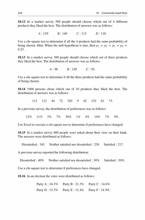
234 10 Commonly Used Tests
10.12 In a market survey 500 people should choose which out of 4 differentproducts they liked the best. The distribution of answers was as follows:
A W 129 B W 140 C W 113 D W 118:
Use a chi-square test to determine if all the 4 products had the same probability ofbeing chosen. Hint: When the null hypothesis is true, then p1 D p2 D p3 D p4 D0:25.
10.13 In a market survey 300 people should choose which out of three productsthey liked the best. The distribution of answers was as follows:
A W 98 B W 120 C W 92:
Use a chi-square test to determine if all the three products had the same probabilityof being chosen.
10.14 1000 persons chose which out of 10 products they liked the best. Thedistribution of answers was as follows:
115 112 44 72 320 9 42 152 61 73:
In a previous survey, the distribution of preferences was as follows:
12% 11% 5% 7% 30% 1% 4% 14% 7% 9%:
Use Excel to execute a chi-square test to determine if preferences have changed.
10.15 In a market survey 800 people were asked about their view on their bank.The answers were distributed as follows:
Dissatisfied W 345 Neither satisfied nor dissatisfied W 238 Satisfied W 217:
A previous survey reported the following distribution:
Dissatisfied W 40% Neither satisfied nor dissatisfied W 30% Satisfied W 30%:
Use a chi-square test to determine if preferences have changed.
10.16 In an election the votes were distributed as follows:
Party A W 24:3% Party B W 21:3% Party C W 14:6%
Party D W 12:5% Party E W 12:4% Party F W 14:9%:
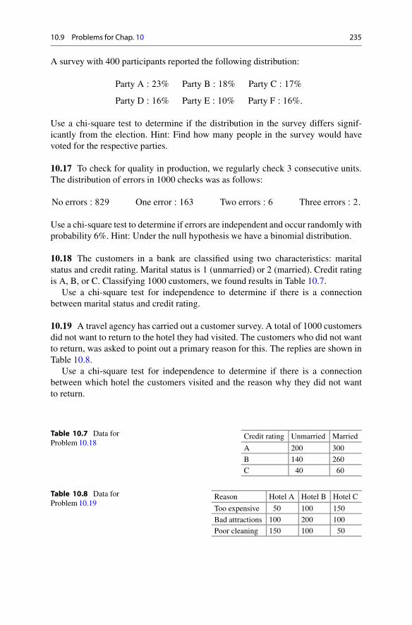
10.9 Problems for Chap. 10 235
A survey with 400 participants reported the following distribution:
Party A W 23% Party B W 18% Party C W 17%
Party D W 16% Party E W 10% Party F W 16%:
Use a chi-square test to determine if the distribution in the survey differs signif-icantly from the election. Hint: Find how many people in the survey would havevoted for the respective parties.
10.17 To check for quality in production, we regularly check 3 consecutive units.The distribution of errors in 1000 checks was as follows:
No errors W 829 One error W 163 Two errors W 6 Three errors W 2:
Use a chi-square test to determine if errors are independent and occur randomly withprobability 6%. Hint: Under the null hypothesis we have a binomial distribution.
10.18 The customers in a bank are classified using two characteristics: maritalstatus and credit rating. Marital status is 1 (unmarried) or 2 (married). Credit ratingis A, B, or C. Classifying 1000 customers, we found results in Table 10.7.
Use a chi-square test for independence to determine if there is a connectionbetween marital status and credit rating.
10.19 A travel agency has carried out a customer survey. A total of 1000 customersdid not want to return to the hotel they had visited. The customers who did not wantto return, was asked to point out a primary reason for this. The replies are shown inTable 10.8.
Use a chi-square test for independence to determine if there is a connectionbetween which hotel the customers visited and the reason why they did not wantto return.
Table 10.7 Data forProblem 10.18
Credit rating Unmarried Married
A 200 300
B 140 260
C 40 60
Table 10.8 Data forProblem 10.19
Reason Hotel A Hotel B Hotel C
Too expensive 50 100 150
Bad attractions 100 200 100
Poor cleaning 150 100 50

236 10 Commonly Used Tests
10.20 Merging Observations: A travel agency has changed their primary collab-orator. A survey carried out before the change reported the following distribution:
Very satisfied W 20% Quite satisfied W 10% Somewhat satisfied W 50%
Somewhat dissatisfied W 15% Very dissatisfied W 5%:
After the change they carried out a similar survey with n D 740 customers. Theanswers were as follows:
Very satisfied W 188 Quite satisfied W 80 Somewhat satisfied W 330
Somewhat dissatisfied W 92 Very dissatisfied W 50:
(a) Use a chi-square test with 5% significance level to determine if the customershave changed opinions.
(b) Carried out a similar test using the merged data, i.e.
Satisfied W 80% Dissatisfied W 20%:
Satisfied W 598 Dissatisfied W 142:
How would you interpret this?(c) Let X5 denote the number of very dissatisfied customers in a survey with
n participants where the probability of being very dissatisfied is p5. Whatapproximative distribution has
X5 � n p5pn p5.1 � p5/
;
if n is large? Use this to approximate P.X5 � 50/ under the condition that thecustomers have the same opinions as before the change. Comment the answer.
10.21 Testing Binomial Distribution: A questionnaire has 6 questions. Eachquestion has two alternatives, and only one alternative is correct.
(a) Let R be the number of correct answers from a person guessing the answer on allquestions. What is the distribution of R? Write a table showing the probabilityfor each possible value of R.
(b) 300 persons answered the questionnaire. The number of correct answerswere distributed as shown in Table 10.9. We assume that the answers wereindependent, and want to test if the observed distribution is consistent with pureguessing. Find a test suitable for this purpose, and execute the test on theseobservations. Use 5% significance level. What do you conclude?

10.9 Problems for Chap. 10 237
Table 10.9 Data forProblem 10.21
Number of correct answers Number of persons
0 7
1 34
2 54
3 85
4 79
5 34
6 7
Table 10.10 Data for Problem 10.23
Product 1 2 3 4 5 6
Number of people choosing the product 28 42 25 52 25 28
Table 10.11 Previousobservations
Product 1 2 3 4 5 6
Percentages choosing the product 10 20 15 30 10 15
10.22 Is One Manager Significantly Better Than Another? Two finance compa-nies sell mutual funds. Company A offers a total of n1 D 100 different funds, whilecompany B offers n2 D 110 different funds. We assume that all funds within thesame company have a constant probability of beating the reference index during agiven year. We call these probabilities pA and pB. Let XA be the number of fundsfrom company A that beat the reference index, and XB be the corresponding numberat company B.
(a) Assume that the results for each fund are different random variables. What isthe distribution of XA and XB?
(b) Last year 30 of the funds in A and 23 of the funds in B beat their reference index.Find a suitable test for this situation, execute the test and find the P-value. Whatis your conclusion? Use 5% significance level.
(c) The analysis above assumes that the results for each fund are independent. Pointat circumstances where this assumption may be unrealistic.
10.23 Did Preferences Change? 200 persons should choose which product theyliked the best among 6 different products. Each person could only choose oneproduct. The answers were distributed as shown in Table 10.10.
In a previous survey the distribution was as in Table 10.11.
(a) We want to examine if the customers have changed their opinion. Find a suitabletest for this. State the null hypothesis, alternative hypothesis, test static, andrejection region. Use 5% significance level.
(b) Execute the test in (a). How large (approximately) is the P-value? What is yourconclusion?

238 10 Commonly Used Tests
10.24 Checking Normality: We have observed the production at two differentdepartments. At department 1 the production numbers were:
101; 103; 105; 102; 101; 100; 117; 100; 102; 104:
At department 2 we recorded:
107; 106; 108; 125; 112; 108; 107; 106; 104; 105:
In the tests below we will use 5% significance level.
(a) We have used a two-sided t-test to compare the two sets of observations. Withdata as above, the P-value for this test is 4.8% (you can take this for granted).What is the null hypothesis and the alternative hypothesis in this test? Whatconclusion can you draw from the test?
(b) If we join the two observation sets, the mean value is 106:15 and the samplevariance is S2
X D 36:87. Imagine that we make 20 independent draws from anormally distributed random variable with expectation D 106:15 and variance�2 D 36:87. What is the probability that the largest value is greater than or equalto 125?
(c) A Shapiro test can be used to determine if data are normally distributed. Thehypotheses in this test are:
H0 W Data are normally distributed
HA W Data are not normally distributed:
A Shapiro test based on the numbers from department 1 and 2 returns the P-value 0:14%. What conclusion can you draw from this? Does this conclusionhave any consequences for the analysis in (a)?
10.25 Can Different Tests Lead to Different Conclusions? We have observedproduction before and after training at a department. The observation was not paired.Before training the production numbers were:
113; 124; 132; 128; 127; 131; 119; 118:
After training the results were as follows:
123; 129; 125; 126; 133; 139; 140; 130:
(a) Use a one-sided t-test with 5% significance level to determine if the trainingaffected expected production. You can make use of the results X D 124; Y D130:63, and S2 D 42:71.

10.9 Problems for Chap. 10 239
(b) Use a one-sided Wilcoxon test with 5% significance level to determine if thetraining affected expected production. You can make use of the result W D 53.
(c) Compare the results from the two tests above. Assume that you have informationindicating that production numbers are not normally distributed. What conclu-sion would you draw?
10.26 Unpaired/Paired Observations: We have examined working times (inseconds) before and after training at a department. Before training we got the results:
239; 237; 235; 224; 259; 227; 220; 268; 228; 252;
238; 288; 283; 248; 285; 279; 245; 210; 251; 286:
After training the results were as follows:
218; 240; 241; 206; 247; 211; 212; 263; 214; 253;
219; 264; 276; 246; 260; 275; 232; 195; 229; 296:
(a) Use a one-sided Wilcoxon test with 5% significance level to determine iftraining has had effect.
(b) Used a one-sided Wilcoxon test for paired observations with 5% significancelevel to determine if training has had effect.
(c) The observations were done in pairs. The order of the results corresponds tothe same workers in both observation sets. What conclusion can you draw fromthis?
10.27 When Can We Use One-Sided Tests? The workers at a factory have gottentraining with the intention of reducing the number of defective items. To examinethe effect of training, we observed the number of defective units before and aftertraining. The results before training were:
Among 100 items, we found 10 defective items.
After training the results were as follows:
Among 120 items, we found 8 defective items.
(a) Use a one-sided U-test to examine the effect of training. Why can we use a one-sided test in this situation? What is the P-value for the test. What conclusion canyou draw from the results? Use 5% significance level.
(b) Alternatively we can imagine a different scenario where the workers havereceived training to improve the security at the department. What kind of testis appropriate in this situation?

240 10 Commonly Used Tests
10.28 Outliers: We have examined the effect of training, and observed theproduction of each worker before and after training. X is the results before training,while Y is the result after training. The results are listed such that the production ofworker 1 is listed first, then the result for worker 2, and so on.
X W 12; 11; 15; 17; 12; 14; 15; 11; 12; 14; 11; 11; 15; 12; 56
Y W 20; 21; 20; 19; 18; 22; 20; 18; 18; 17; 19; 22; 17; 19; 19:
To examine if training has had effect, we first executed a one-sided t-test for pairedobservations, then a one-sided Wilcoxon test for paired observations.
(a) Why can we use one-sided test in this situation? What is the null hypothesis andthe alternative hypothesis for these tests?
(b) The P-value for the t-test was 13.53% and the P-value for the Wilcoxon test was0.57%. What conclusion can you draw from the two tests? Use 5% significancelevel.
(c) The two tests give conflicting conclusions. What conclusion would you draw intotal? Hint: Inspect the observed pairs. Do you notice a pattern?
10.29 Sorting Paired Observations: You want to consider production numbersbefore and after training, and have collected 50 production numbers from 50workers before and after training. The observations are paired, i.e., productionnumbers from the same worker occur in the same position in the two sequences.
(a) We have no information indicating that data has normal distribution, and we willfirst use a Wilcoxon rank-sum test with rank-sum W to examine the data. We letX be the expected production before training, and Y the expected productionafter training. What is the null hypothesis and the alternative hypothesis in thiscase? Find the values for EŒW� and VarŒW� under the null hypothesis.
(b) We observe W D 2455 in the test from (a). What is your conclusion? Use 5%significance level.
(c) Since the observations are paired, we will also use a one-sided Wilcoxon signed-rank test with rank V . Find EŒV� and VarŒV� under the null hypothesis.
(d) We observe V D 604 in the test from (c). What is your conclusion? Use 5%significance level.
(e) It is suggested that you alternatively might proceed as follows:• Sort the data prior to training in ascending order.• Sort the data after training in ascending order.• Compute the signed-rank for the sorted data.
After sorting we observed V D 364. What conclusion do you draw from this?(f) The tests in (d) and (e) give conflicting answers. Which answer is the right one?

10.9 Problems for Chap. 10 241
10.30 Equivalence Testing: We have examined average wages in two differentregions, and have collected data from 5000 persons in region 1 and 7000 persons inregion 2. In region 1 we found X D 31;200 (USD), while Y D 31;000 (USD) inregion 2. Estimated standard deviation was S D 4300 (USD), where
S D 1
n1 C n2 � 2
n1X
iD1
.Xi � X/2 Cn2X
iD1
. Yi � Y/2
!:
(a) Use a two-sided t-test with 5% significance level to determine if there is asignificant difference between the regions.
(b) Equivalence tests have been suggested in situations where we want to comparethe expectations of two random variables X and Y, and where we want toexamine if the difference is so small that it is of no practical relevance. In thistest we define X D EŒX� and Y D EŒ Y�, and define
ı D X � Y :
In a test of this kind we need to specify how small ı need to be before we cansay the difference is of no practical relevance. We call this quantity �, and wesay that the two expected values are equivalent when
�� < ı < �:
An equivalence test can then be formulated as follows:
H0 W ı � �� or ı � �; HA W �� < ı < �:
The test is executed via
T1 DOı C �
SŒ Oı�; T2 D � � Oı
SŒ Oı�:
where Oı and SŒ Oı� are computed in exactly the same way as we do in a t-test forthe comparison of two expectations. We reject H0 at significance level ˛ if
min.T1; T2/ � t.n1Cn2�2/˛ :
Choose � D 500 (USD) and carry out an equivalence test for the two regions.Compare the results from (a) and (b).
10.31 Strength Considerations:
(a) Assume that Q is chi-square distributed with parameter 20. Find q such thatP.Q � q/ D 5%:

242 10 Commonly Used Tests
Let X denote the time it takes to serve one randomly selected customer. Wewill assume that X is exponentially distributed with expectation > 0, i.e., it isa continuous distribution with density
fx.x/ D 1
e� x
:
To estimate we will make 10 independent observations and observe X.(b) We want to test if expected service time is larger than 10 (minutes), and
formulate the hypotheses
H0 W D 10 HA W > 10:
For simplicity we assume that a one-sided test can be used here. It is possible toshow (you can take this for granted) that if we make n observations, then
Q D 2nX
is chi-square distributed with parameter 2n. How large must X be before we canreject H0? Use 5% significance level and n D 10. We observe X D 15. Whatconclusion can we draw from this?
(c) What do we mean by the strength of the alternative D 20? What (approxi-mately) is the strength of this alternative when n D 10? How large must n be ifthe strength of the alternative D 12:5 is at least 50%? Hint: Examine differentvalues of n using trial and error.
10.32 Confidence Intervals Provides More Information: We have collected datafor wages from two different regions. In region 1 we collected n1 D 15;000
observations and found X D 32;378 (USD). In region 2 we collected n2 D 10;000
observations and found Y D 32;209 (USD). For the spread (as defined in the t-test)we computed S D 2900 (USD).
(a) We want to test if expected wages are significantly different in the two regions.Execute a two-sided t-test with 5% significance level. What is your conclusion?
(b) Find a 95% confidence interval for the difference in expected wages. Commentthe result.
10.33 Misinterpreting Unscaled Variables: A travel agency has collected data onthe level of satisfaction among their customers. The answered were ranked 1 to 5:
Very dissatisfied D 1
Somewhat dissatisfied D 2
Neither satisfied nor dissatisfied D 3

10.9 Problems for Chap. 10 243
Table 10.12 Data forProblem 10.33
Answer 1 2 3 4 5 Number of respondents
Before 160 240 160 240 160 960
After 264 310 230 115 460 1379
Somewhat satisfied D 4
Very satisfied D 5:
The agency has carried out a new arrangement where the customers have receivedmore support than before, and wants to examine the effect of the new arrangement.They collected the data shown in Table 10.12.
(a) Let X denote the reply from a customer. We want to use data to computethe average value before and after the new arrangement. Compute X DAverage before, and Y D Average after:
(b) Use a one-sided t-test to examine if the expected answer has increased signifi-cantly under the new arrangement.
(c) Point to problems related to the test in (b).(d) As an alternative to the test in (b) we can use one-sided U-tests. Use U-tests
with 5% significance level to answer the following:• Is the fraction of very satisfied customers significantly higher than before?• Is the fraction of satisfied customers significantly higher than before?• Is the fraction of very dissatisfied customers significantly higher than before?
(e) Are the tests in (d) more credible than the test in (b)?
10.34 Extreme Values: 100 randomly selected pupils participate in a standardizedtest at a school. We assume that the skill of a randomly selected pupil is normallydistributed with mean 489 and standard deviation 90, and that the skill of differentpupils are independent random variables.
(a) Let X be the average score at the school. Explain why EŒX� D 489 and VarŒX� D81.
(b) How probable is it that the average score for the school is 463 or below?(c) The test is executed at 500 different schools. Assume that the pupils at all
these schools have skills with the distribution above. How probable is it thatthe average score at all schools are 463 or better?
(d) How probable is it that the worst of the 500 schools have a score that is 463 orbelow? Compare with (b) and comment the answer.
10.35 Interpreting Random Fluctuation: A large industrial company has 100relatively similar production units.

244 10 Commonly Used Tests
(a) A t-test of the production numbers from the worst department against theproduction numbers from all the other departments leads to a P-value of 4%.Is that normal? What should the management do?
(b) A t-test of the production numbers from the worst department against theproduction numbers from all the other departments leads to a P-value of 0.01%.Is that normal? What should the management do?
(c) Assume that the production numbers Zi; i D 1; : : : ; 100, all are independent andlog normally distributed with
Zi D eXi ; where EŒXi� D 10; VarŒXi� D 9; Xi are normally distributed:
How probable is it that the result at the worst department is less than or equal to10?
10.36 Strength Is a Strong Issue: In this problem we will use t-tests for thecomparison of expected values in two groups. We assume for simplicity that theissue is such that we can ignore the case X < Y , i.e., that we are allowedto use one-sided tests. We assume that data are normally distributed and use 5%significance level.
(a) A researcher has collected data from two different groups. There were 40observations from each group, but the observations were not paired. For group 1she found X D 101:75 and for group 2 Y D 112:12. The S-value was S D 23:23.Use a one-sided t-test to determine if we have significant support for the claimX < Y . Suggest an approximate P-value for the test. What conclusion wouldyou draw from this?
(b) To confirm the finding, the researcher was advised to repeat the study with 10observations in each group. The observed values turned out as follows:
X D 103:62; Y D 110:88; S D 19:91:
What conclusion would you draw if you see these results in isolation from thefirst study?
(c) It is possible to show that if the true values equal the observed values in (a), i.e.
X D 101:75; Y D 112:12; �X D 23:23; �Y D 23:23;
then the strength of the test in (b) is about 25%. What does that mean in practice?Is it a good idea to try to confirm the finding in this way?
(d) If we see the two studies in conjunction, i.e., we merge the datasets into twodatasets with 50 observations in each, we get
X D 102:12; Y D 111:88; S D 22:42:
What conclusion can you draw from the two studies seen in conjunction?Compare the result with (a) and (b).
11Linear Regression
Abstract
When we make observations, we often encounter cases where the size ofobservations appears to change in some systematic way. One possible cause forthis is that we have done the observations over a period of time, and as timepasses the distribution of values may change. To determine if such changes arerandom or systematic, we can use linear regression. Linear regression is a widelyused technique that has a lot to offer, in particular since we are often able toquantify systematic changes.
11.1 Linear Correspondence
In this section we take a new look on the relation between two variables. Previouslywe used the covariance or the coefficient of variation to determine a relationship. Wenow proceed a step further; we want to see if there is a linear relationship betweenthe two variables. Before we try to write down any expressions, we take a look atsome figures.
In Fig. 11.1 we have observed the values of two different stocks at 100 differentpoints in time. We let X be the stock price of company A and Y the stock priceof company B. From the figure we see there is strong covariation between the twostock prices. The coefficient of variation confirms this. We have �ŒX; Y� D 0:98.If we look at the numbers, we see that Y is largely twice as big as X. That we canexpress mathematically by
Y D 2 � X:
This function is a straight line through the origin with slope 2. In Fig. 11.2 we haveincluded this line.
© Springer International Publishing AG 2017J. Ubøe, Introductory Statistics for Business and Economics, Springer Textsin Business and Economics, https://doi.org/10.1007/978-3-319-70936-9_11
245

246 11 Linear Regression
Fig. 11.1 Pairs of stockprices
20 40 60 80 100 120 140A
50
100
150
200
250
300
B
Fig. 11.2 A regression linethrough the data
20 40 60 80 100 120 140A
50
100
150
200
250
300
B
The figure confirms that the expression Y D 2 � X provides a good assessment,but it is not 100% correct. We hence write
Y D 2 � X C “error”;
where the term “error” is a random variable which explains the deviations from thestraight line. This example is particularly simple, but it tells us what we are after.When we have data which are distributed as a band around a straight line, we wantthe formula for the line, and we want to use the formula to study the connectionbetween the two quantities.
Example 11.1 In Fig. 11.3 we have again studied the values of two stocks at 100different points in time. We see that the observations are located in a band around astraight line, and this line is included in Fig. 11.4.

11.1 Linear Correspondence 247
Fig. 11.3 Pairs of stockprices
20 40 60 80 100 120 140A
100
200
300
400
500
B
Fig. 11.4 A regression linethrough the data
20 40 60 80 100 120 140A
100
200
300
400
500
B
Since we need to find a formula for the straight line, we read the values at twodifferent points on the line. We choose X D 20 and read Y D 160, and whenX D 140 we read Y D 520. We can now use a two-point formula for a straight line,i.e.
y D y1 � y0
x1 � x0
.x � x0/ C y0:
If we insert the values into the formula, we get
Y D 520 � 160
140 � 20.X � 20/ C 160 D 3 � .X � 20/ C 160 D 3 � X C 100:
We conclude that
Y D 3 � X C 100 C “random errors”:

248 11 Linear Regression
A relation of that sort might be useful when we want to make predictions. If thestock price of company A rises to 200 (USD), what can we expect the price forstocks in company B to be? The formula offers an answer to this question.
Y D 3 � 200 C 100 C “random error” D 700 C “random error”:
11.2 Linear Regression
An important field within statistics is centered around phenomena which areconnected via a systematic coupling. The key word is trend. The typical frameworkis two quantities x and y related through a fully or partially known function, i.e.,y D f .x/. Here we will focus the linear case
y D ˛ C ˇx:
In this case the graph is a straight line, ˛ is the intercept with the y-axis and ˇ isthe slope. A common problem is that ˛ and ˇ are unknowns, and we need to makeobservations to settle the values. In many cases the observations are not prefect butsubject to errors. Instead of points on a perfect straight line, we might have a bandof observations as in Fig. 11.5.
Clearly it is not possible to draw a straight line through all these points, so wemust settle for less. The best we can achieve is to draw a line with the best possiblefit. What we mean by the best possible fit is not clear, but it is usual to construct aline with the property that the sum of all squared errors is as small as possible. The
700
600
500
400
300
200
0 10 20 40 50 x
y
60 70 80 90 10030
y = 201.085 + 4.95027 x
Regression Plot
S = 18.7623 R − Sq = 98.3 % R − Sq(adj) = 98.3 %
Fig. 11.5 Corresponding values of x and y

11.2 Linear Regression 249
method is commonly called the ordinary least squares method or OLS for short.Since our primary concern is to study properties of the optimal line, we will notexplain in detail why the construction below works. Some details are provided inExercises 11.23 and 11.18.
Construction of the OLS line:Assume we have n observation pairs .X1; Y1/; : : : ; .Xn; Yn/.
1. Compute
X D 1
n.X1 C � � � C Xn/:
2. Compute
Y D 1
n. Y1 C � � � C Yn/:
3. Compute the sum of squares
M D .X1 � X/2 C � � � C .Xn � X/2:
4. Compute
O D 1
M
�.X1 � X/. Y1 � Y/ C � � � C .Xn � X/. Yn � Y/
�:
5. Compute
O D Y � OX:
6. The OLS line is
OY D O C O � X:
Technically we assume that all X and Y are related through
Y D ˛ C ˇ � X C �

250 11 Linear Regression
where � are independent random variables (one variable for every X) with EŒ�� D 0
and VarŒ�� D �2 (the same variance regardless of X). Under these assumptions it ispossible to prove that O is an unbiased estimator for the (unknown) constant ˛, andthat O is an unbiased estimator for the (unknown) constant ˇ. We will often need toestimate the unknown constant �2, and the following expression is useful:
An unbiased estimator for �2 is
S2 D 1
n � 2
�. Y1 � OY1/
2 C � � � C . Y1 � OY1/2�
:
where OYi D O C O � Xi; i D 1; : : : ; n.
In this context X is often called an explanatory variable, and Y a dependentvariable. The idea is that when we know X, we can suggest a reasonable value forY. We say that X explains Y since the value of Y depends on X.
The formulas above require considerably manual labor to compute, but we willhardly ever need to carry them out. Computations of this sort are fully automated instatistical software, and we only need a broad view of how the expressions work.
Example 11.2 Find the OLS line when we have the observations (1,1), (2,3), (3.3).
Solution: Here n D 3 and X1 D 1; X2 D 2; X3 D 3 and Y1 D 1; Y2 D 3; Y3 D 3.If we use these numbers in the formulas above, we find
X D 2;
Y D 7
3
M D .1 � 2/2 C .2 � 2/2 C .3 � 2/2 D 2;
O D 1
2
�.1 � 2/
�1 � 7
3
�C .2 � 2/�3 � 7
3
�C .3 � 2/�3 � 7
3
�� D 1;
O D 7
3� 1 � 2 D 1
3:
The regression line is hence OY D 13
C X; see the straight line in Fig. 11.6.

11.3 Residuals and Explanatory Power 251
Fig. 11.6 The regressionline in Example 11.2
1 2 3X
1
2
3
Y
11.3 Residuals and Explanatory Power
The regression line will usually not go through all the points. For each Xi wewill usually see a difference between the observed value Yi and the point on theregression line OYi D O C O � Xi. This difference we call the i-th residual, and we usethe symbol Ri. That is,
Ri D Yi � OYi; i D 1; : : : ; n:
The residuals hence measure the errors we make when we replace the observedvalues by the corresponding values on the regression line. To quantify the overallerror, statisticians use the quantity SSE (sum squared errors) which is the sum of thesquares of all residuals, i.e.
SSE DnX
iD1
. Yi � OYi/2:
A measure for the total variation in Y is the SST (sum squares total) which is definedby
SST DnX
iD1
. Yi � Y/2;
see Fig. 11.7.The idea is now that if the total squared error is much smaller than the total
squared variation, then the regression line captures most of the variation in Y.Phrased differently, we can say that the explanatory variable X explains most of

252 11 Linear Regression
Y
Xi
Yi
Yi
Ri Yi Yi
Yi Y Total variation
Fig. 11.7 Residuals and total variation
200
100
100
200
300
400
20 40 60 80 100
Y
X
Fig. 11.8 Small explanatory power
the variation in Y. We define the explanatory power R2 of the model as follows:
R2 D 1 � SSE
SST:
It is possible to show mathematically that R2 D 100% if and only if all the observedpoints lie on the regression line. In practice that means that if the explanatorypower is nearly 100%, then nearly all the observation points must be very closeto the regression line. The explanatory power R2 is relatively easy to interpret, andthe value gives a good impression of how close the observations are to a linearrelationship. Consider the plots in Figs. 11.8, 11.9, and 11.10.
In Fig. 11.8 there hardly seems to be a relationship between X and Y. Theexplanatory power R2 D 2:3% for this dataset. In Fig. 11.9 there seems to be arelation between the variables, and an explanatory power R2 D 30:7% confirms

11.3 Residuals and Explanatory Power 253
Fig. 11.9 Some explanatorypower
50
50
100
150
250
200
20 40 60 80 100
Y
X
Fig. 11.10 Largeexplanatory power
25
50
75
100
125
150
175
20 40 60 80 100
Y
X
that there is some relationship. In Fig. 11.10 the relationship is quite strong, hereR2 D 98:3%.
11.3.1 Naming Variables
In the general exposition of the theory we have used the notation X for theexplanatory variable and Y for the dependent variable. In practical cases it is usefulto equip the variables with more descriptive names. Some examples:
• If we want to examine if there is a linear relationship between a stock priceand time, then S (short for stock) and t are natural names, i.e., we consider the

254 11 Linear Regression
regression line
OS D O C O � t:
• Sometimes it may be appropriate to write some variable names in full. If we wantto examine a relation between quantity Q and price, P is not a good variablename, since it can be confused with probability. In such cases we might write
OQ D O C O � price:
Full names on variables are quite common when we use statistical software. Laterin this chapter we will use convenient variable names when we study regressions,and that does not affect the mathematical formulas we will use.
11.4 Hypothesis Testing in the RegressionModel
One of the most important questions in statistics is the following: Does X affect Y?If the answer is yes, the distribution of Y changes when we change X. When X andY have a linear relation
Y D ˛ C ˇ � X C �;
we want to know if ˇ D 0 or not. If ˇ D 0, then Y never changes when we changeX. In most cases ˛ and ˇ are unknown constants, and we make observations toestimate those constants. Even in cases where ˇ D 0, we will usually find O 6D 0. IfO is small, it appears quite likely that the true value for ˇ may be zero. This problem
is well suited for hypothesis testing, where
H0 W ˇ D 0; HA W ˇ 6D 0:
If we can reject H0, we are able to conclude that ˇ is probably not zero, which inturn means that X probably affects Y.
Formally the test is executed as follows:
Two-sided hypothesis test for the slope ˇ in a linear regression:
H0 W The explanatory variable has no impact, i.e., ˇ D 0:
HA W The explanatory variable has impact, i.e., ˇ 6D 0:
(continued)

11.4 Hypothesis Testing in the Regression Model 255
The test requires either many independent observations or that the residualsare independent and normally distributed. Significance level � .
1. Find the values for O; S; and M using the formulas from the OLSregression.
2. Compute
SŒ O� D S=p
M:
3. The test static is
T D O=SŒ O�:
4. Use the t-table with parameter � D n � 2, and find t.�/
�=2 such that
P�
T.�/ � t.�/
�=2
�D �=2:
5. Reject H0 if T � t.�/
�=2 or if T � �t.�/� :
Extra: The limits for a .1 � �/100% confidence interval for ˇ are given by
O ˙ t.�/
�=2 � SŒ O�:
Note that we here use � to denote the significance level. This is to avoid confusionwith the intercept ˛ in the OLS regression.
One-sided hypothesis test for the slope ˇ in a linear regression:
H0 W The explanatory variable has no impact, i.e., ˇ � 0:
HA W The explanatory variable has impact, i.e., ˇ > 0:
The test requires either many independent observations or that the residualsare independent and normally distributed. Significance level � .
1. Find the values for O; S; and M using the formulas from the OLSregression.
(continued)

256 11 Linear Regression
2. Compute
SŒ O� D S=p
M:
3. The test static is
T D O=SŒ O�:
4. Use the t-table with parameter � D n � 2, and find t.�/˛ such that
P�
T.�/ � t.�/�
�D �:
5. Reject H0 if T � t.�/� :
One-sided hypothesis test for the slope ˇ in a linear regression:
H0 W The explanatory variable has no impact, i.e., ˇ � 0:
HA W The explanatory variable has impact, i.e., ˇ < 0:
The test requires either many independent observations or that the residualsare independent and normally distributed. Significance level � .
1. Find the values for O; S; and M using the formulas from the OLSregression.
2. Compute
SŒ O� D S=p
M:
3. The test static is
T D O=SŒ O�:
4. Use the t-table with parameter � D n � 2, and find t.�/� such that
P�
T.�/ � t.�/�
�D �:
5. Reject H0 if T � �t.�/� :

11.5 Prediction/Estimation 257
If H0 can be rejected at 5% significance level, we say that the explanatory variableis significant. If the explanatory variable can be rejected at any sensible significancelevel, we say that the explanatory variable is strongly significant. The wording iscommonly used when the P-value is less than 0.1%, but values other than 0.1%are used sometimes. We should note that statistical software reports the P-values ofsuch tests.
The value of M is usually not reported in printouts. As we sometimes need thisvalue to do calculations, it may help to note that:
• M D .n � 1/VarŒX�.• M D S2
SŒ O� . The values of S and SŒ O� are often reported.
Example 11.3 In a regression with n D 10 independent and normally distributedobservations we have found the regression line
OY D 104:28 C 4:409 � X:
Furthermore we have computed S D 25:53 and M D 110. What is the conclusionof a two-sided test for zero slope? We use 5% significance level.
Solution: We compute
SŒ O� D 25:53p110
D 2:43:
From the regression line we see that O D 4:409. That gives
T D 4:409
2:43D 1:81:
Using a t-table with parameter � D 10 � 2 D 8, we find t.8/0:025 D 2:306 (the test is
two-sided). The test static is well within the non-rejection region. The effect of X isnot significant, and we keep the null hypothesis saying that X has no impact on Y.
11.5 Prediction/Estimation
An important application of linear regression is to suggest the value of the dependentvariable Y when we know the value of the explanatory variable X. We have, e.g.,observed the time development over the last 12 months, and want to predict the valueat some specific point in the future. We should note that there are two somewhat

258 11 Linear Regression
different angles of approach:
• We can predict the value of Y itself when X D x.• We can estimate the expectation EŒ Y� when X D x.
The reader should notice the exact wording here. Statisticians use the wordpredict when they talk about random variables, and the word estimate when they talkabout constants. The two versions have much in common, but there is a principaldifference. The uncertainty in Y itself is larger than the uncertainty in the expectationEŒY�. Confidence intervals are hence smaller in the latter case.
By definition we have
Y D ˛ C ˇ � x C �;
and hence
EŒY� D EŒ˛ C ˇ � x C �� D ˛ C ˇ � x;
since we always assume EŒ�� D 0. The principal difference is that Y contains theterm � causing it to vary a lot more. In both cases our best shot is the value on theregression line, i.e., OY D O C ˇ � x: There is some uncertainty in EŒY� as well.This uncertainty is caused by a finite number of observations. If we repeat theexperiment with a similar number of observations, we will probably end up witha slightly different regression line. The uncertainty in the regression line is depictedin Fig. 11.11.
If we want to predict the value of Y itself, we should imagine what would happenif we made several new observations of Y when X D x. In Fig. 11.12, we see thatY varies with a certain bandwidth in the interval Œ0; 10� (it is here we have ourobservations). There is no reason to expect that Y will vary less at X D 20. Henceif changing X from 10 to 20 does not change the behavior of Y, we would expect
Fig. 11.11 Uncertainty inthe line of regression
5 10 15 20 25X
75
100
125
150
175
200
225
Y

11.5 Prediction/Estimation 259
Fig. 11.12 Uncertainty inthe line of regression plus thenatural variation
5 10 15 20 25X
75
100
125
150
175
200
225
Y
to see a variation in Y like in Fig. 11.12. The uncertainty in Fig. 11.12 is caused bytwo effects, uncertainty in the regression line plus the fluctuations in Y.
If we assume that we have independent observations with normal distribution,it is possible to show that the uncertainty follows a t-distribution with parameter� D n � 2. Explicit formulas for the confidence intervals can then be found asfollows:
Estimated value EŒ Y� when X D x, we find by
OY D O C ˇ � x:
We compute
SŒ OY� D S �s
1
nC .x � X/2
M;
and the limits for a .1 � �/100% confidence interval is found from
OY ˙ t.n�2/
�=2 � SŒ OY�:
Predicted value of Y when X D x, we find by
OY D O C ˇ � x:
We compute
(continued)

260 11 Linear Regression
SŒ Y � OY� D S �s
1 C 1
nC .x � X/2
M;
and the limits for a .1 � �/100% confidence interval is found from
OY ˙ t.n�2/
�=2 � SŒ Y � OY�:
Example 11.4 We have made n D 401 observations of the price of a goodat different times t, and notice that the prices grow over time. The regressionequation is
Oprice D 101:773 C 4:733 � t:
Furthermore we have computed
S D 25:85; t D 5; M D 3358:38:
Use this information to predict the price at time t D 20, and find a 95% confidenceinterval for the price. Then estimate the expected price at time t D 20, and find a95% confidence interval for the expected price.
Solution: When t D 20, then
bprice D 101:773 C 4:733 � 20 D 196:43:
We have
SŒprice � bprice� D 25:85 �r
1 C 1
20C .20 � 5/2
3358:58D 26:73;
and
SŒbprice� D 25:85 �r
1
20C .20 � 5/2
3358:58D 6:81:
To find the confidence intervals we should use tables for a t-distribution withparameter � D 399, but with so many observations we can just as well use thetable for the standard normal distribution. We get t.399/
0:025 D z0:025 D 1:96: The limitsfor the confidence intervals are
196:43 ˙ 1:96 � 26:73;

11.6 Regression Using Excel 261
and
196:43 ˙ 1:96 � 6:81:
A 95% confidence interval for the price itself at t D 20 is then Œ144; 249�, and a95% confidence interval for the expected price at t D 20 becomes Œ183; 210�. Wenotice that the latter interval is much smaller.
11.6 Regression Using Excel
As we already mentioned, calculation of the regression line is fully automated instatistical software. If we use Excel, we first enter the x-coordinates in column Aand the y-coordinates in column B. Using the values from Example 11.2, we get thedisplay in Fig. 11.13.
We then click Data and choose Data Analysis. If you don’t see this option, youmust load the Data Analysis package, see Options in the File tab. In the DataAnalysis package choose Regression and a dialog box will open. Mark the inputY-range and the input X-range, and click OK. We then get a detailed summary ofthe results as shown in Figs. 11.14 and 11.15
There are lots of details in the output, and we only comment the most relevantinformation.
• R Square: The value is 0.75, which means that the explanatory power R2 D 75%.• Standard Error. This is the value of S in the regression model, and S D 0:81645.• The numbers under Coefficients are the regression coefficients, i.e., O D 0:3333
and O D 1.• The numbers to the right of X variable offer important information about O.
Under Standard Error we find SŒ O� D 0:57735. The value under t Stat is thetest static for a hypothesis test of ˇ D 0, i.e., T D 1:732051, and the twofollowing numbers are the limits for a 95% confidence interval for ˇ, i.e., theinterval Œ�6:33593; 8:335931�.
Fig. 11.13 Input data forlinear regression

262 11 Linear Regression
Fig. 11.14 Dialogue box in Excel
Fig. 11.15 Final results reported by Excel

11.7 Multiple Regression 263
11.7 Multiple Regression
In the linear regression model above we used one explanatory variable X to explainthe development of a dependent variable Y. In many situations it makes good senseto use more than one explanatory variable. We then get a model on the form
Y D ˛ C ˇ1X1 C ˇ"X2 C � � � C ˇrXr C �:
Here ˛ is the intercept, X1; : : : ; Xr are called explanatory variables, and ˇ1; : : : ; ˇr
called regression coefficients. The major part of the theory works just as before. Weneed to collect n observations of .X1; X2; : : : ; Xr; Y/ and find the coefficients suchthat the total squared error is as small as possible. The construction is more or lessthe same as we used in the case with one explanatory variable. In practice we willalways use statistical software to compute the coefficients, and we omit the detailsof the construction.
11.7.1 Explanatory Power
The explanatory power R2 works just as before and shows the fraction of thevariation in Y that can be explained by the explanatory variables. We illustrate thisby a few examples.
Example 11.5 During 9 consecutive days we sold
1 3 2 4 2 2 3 5 2;
units of a good, respectively. The total prices we obtained were
12 39 31 55 34 38 50 76 45:
How big fraction of the variation in total prices can be explained by changes in soldquantities and time?
Solution: We let Q denote the quantities we sold each day. A regression with Qas explanatory variable gives
3total price D 6:296 C 13:472 � Q;
with explanatory power R2 D 86:9%. The P-value from a test of ˇ D 0 is 0:025%.This shows, not surprisingly, that Q explains much of the variation in total prices.To see if time also matters, we carry out a new regression using time as explanatoryvariable. This gives
3total price D 20:22 C 4:40 � time;

264 11 Linear Regression
Table 11.1 Data for Example 11.6
Crop size in kg per area unit 70 60 80 80 90 60 70 50
Rainfall in centimeters 10 20 25 20 18 15 30 25
Mean temperature in degrees Celsius 25 18 22 22 25 18 16 16
with explanatory power R2 D 46:3%. The P-value from a test of ˇ D 0 is 4.36%.We conclude that time probably matters and that the variation in time explains alarge portion of the variation in total prices. Even though the two models aboveprovide some relevant information, it is better to use a joint model which makes useof both explanatory variables. We then get the following
3total price D �0:6541 C 11:3871 Q C 2:5022 � time:
The explanatory power is now R2 D 99:8%. The P-value from a test of ˇ1 D 0
is as small as 2:9 � 10�8, and P-value from a test of ˇ2 D 0 is only 2:0 � 10�6.The conclusion is that both variables are strongly significant and that they togetherexplain almost all the variation in total prices.
Example 11.6 We want to see if there is a connection between the size of crops,rainfall, and temperature. We have observations from 8 different years, and thenumbers are shown in Table 11.1.
We first want to see if there is a connection between crop size and rainfall. Aregression gives the result
3crop size D 72:93 � 0:1439 � rainfall:
The explanatory power R2 D 0:5%, and the P-value for ˇ D 0 is 87%. We noticethat the regression coefficient is negative, but it is strongly insignificant and themodel explains nothing. That seems rather strange. A regression against temperatureworks better. In that case
3crop size D 16:00 C 2:667 � temperature;
with explanatory power R2 D 57%. The P-value for ˇ D 0 is 2.86%. Temperaturehence seems to explain a good deal of the crop size. A multiple regression usingboth variables yields a surprising result
3crop size D �38:35 C 1:3159 � rainfall C 4:0265 � temperature:
Here the explanatory power increases to R2 D 82:8%. The P-value for thecoefficient ˇ1 D 0 is 4.2%, and the P-value for ˇ2 D 0 is 0.44%. In conclusionboth variables are significant, and together they explain a lot more than a modelonly using temperature.
11.8 Causality 265
At first sight the result above may seem surprising, but there is a simpleexplanation. Temperature is the primary cause here. If we compare years with thesame amount of rainfall, crops are larger when there is more rainfall. A lot of rainis hence good for crops, but lots of rain lead to lower temperature, which is bad.Seen in isolation the effect of rainfall is negligible since the benefit of more waterbalances the loss due to lower temperature.
11.8 Causality
From the examples above we have seen that regression can be used to measure theextent that one variable explains another. High explanatory power, however, does notin general imply causality. There exist lots of cases where one can find a systematicrelation between two variables and where changes in one of the variables do notcause changes in the other.
Example 11.7 In a survey of several small towns it turned out that there were morenewborn children in towns with many storks. The explanatory power was nearly100%. Does that mean that the number of storks causes more newborn children?
Solution: For obvious reasons the answer is no. A more likely explanation isthe number of houses in each town. When a town has more houses, there are morefamilies living there and hence more children are born. Storks build their nests onroofs, and with more houses there are more places to nest. Hence in larger townsthere are more storks. Both variables increase more or less in proportion to the sizeof the towns. When a town is twice as big as another, we expect twice as manynewborns and twice as many storks. If planners want more newborns, they shouldnot try to increase the number of storks!
Example 11.8 In a survey of car ownership we found that older people had moresport cars. Does that mean that the interest for sport cars increases with age?
Solution: The answer is probably no. A more reasonable explanation is that olderpeople tend to have more wealth. As wages/wealth often increases with age, theopportunities for owning sport cars increases with age. If we compare car ownerswith the same wages/wealth, it may happen that the covariation changes direction,i.e., that the interest for owning sport cars decreases with age.
The examples above show that we must not jump to conclusions when we havedemonstrated significant covariation between variables. To prove that changes inone variables causes variation in another variable, we must be able to argue that thereare no other relationships that can explain the connection. A statistical regression isnever sufficient evidence of causality.

266 11 Linear Regression
11.9 Multicollinearity
In a regression with several explanatory variables it is undesirable if some of thevariables have the same cause. When this happens, numerical results are unstable,and sometimes the coefficients may have signs that appear to make no sense.
Example 11.9 We have made observations in a group of people between 6 and 18years old. Our explanatory variables are X1 D age and X2 D months of education.Assuming that holidays are counted as education, we largely have
X2 D 12.X1 � 6/:
Is it possible to see a difference between the regressions
Y D 100 C 10X1 C X2 and Y D 28 C 22X1‹
Solution: If X2 D 12.X1 � 6/, then
100 C 10X1 C X2 D 100 C 10X1 C 12X1 � 72 D 28 C 22X1:
Due to rounding and a small number of people dropping out from school, therelation X2 D 12.X1 � 6/ is only approximatively true. For some data the best fitmay be Y D 100 C 10X1 C X2. If we change one single observation in that dataset,it may happen that Y D 28 C 22X1 provides the best fit.
Ideally all explanatory variables should be independent. Deviations from thisrequirement is called multicollinearity. If we suspect that one of the explanatoryvariables, e.g., Xj, may be expressed by the others, we can check the explanatorypower R2 of the regression
Xj D ˛ C ˇ1X1 C � � � C ˇj�1Xj�1 C ˇjC1XjC1 C � � � C ˇrXr:
If R2 of this regression exceeds 90%, it means that problems with multicollinearityprobably are so severe that it may be better to remove the variable Xj from theregression.
If the primary use of the regression is prediction, multicollinearity need notbe a problem. Admittedly marginally different datasets may lead to very differentcoefficients, but if we use these to predict a new value for the dependent variable,we will get approximately the same answer. The predicted value is only slightlyaffected by those differences.
Example 11.10 We have made 10 observations of monthly allowances (USD), ageand months of education. The results are shown in Table 11.2.

11.10 Dummy Variables 267
Table 11.2 Monthly allowances
Pocket money 50 70 75 55 60 75 35 50 60 65
Age in years 12 17 18 13 15 18 8 12 15 16
Months of education 72 120 144 84 108 144 24 72 108 120
A regression of this dataset gave the result
6pocket money D 1:032 C 4:222 � age � 0:235 � education;
with explanatory power R2 D 99:1%. The P-value for ˇ1 D 0 was 2.2%, and theP-value for ˇ2 D 0 was 85.4%. We conclude that months of education appear tohave no impact. To check for multicollinearity, we regress education against age.The result of this regression is
3education D �86:23 C 11:655 � age;
with explanatory power R2 D 99:0%. Since the explanatory power of this regressionexceeds 90%, we conclude, as expected, that there are multicollinearity between ageand months of education. If we remove education as explanatory variable, we get
6pocket money D 2:6327 C 3:9491 � age;
with explanatory power R2 D 99:1%. The P-value for a test of ˇ D 0 is 1:71 �10�9: We see that explanatory power remains at the same level when we use lessparameters. Less parameters imply a simpler explanation, which is something weusually prefer. The reduced model is hence better than the first one.
11.10 Dummy Variables
In a regression explanatory variables should be quantities that can be measured on ascale in a meaningful way. We call such variables as scale variables. Variables thatdo not possess a clear size and direction should not be used.
Example 11.11 We want to study if there is a connection between wages Y andcountry X. We have coded X such that X D 0 means a person living in Norway,X D 1 means a person from Denmark, while X D 2 denotes a person from Sweden.We have 12 observations, shown in Table 11.3.
Notice that country is not a scale variable. It makes no sense to say that Swedesare twice as good as Danes. As mentioned above, such variables cannot be used inregressions, at least not directly. What happens if we try this anyway? With data asabove, we get
1wages D 33;2727 C 181:8 � country;

268 11 Linear Regression
Table 11.3 Observation forExample 11.11
Salary in USD Country Salary in USD Country
30,000 0 32,000 2
31,000 0 32,500 2
29,000 0 31,500 2
40,500 1 32,000 2
40,000 1 32,500 2
39,500 1 31,500 2
with explanatory power R2 D 0:15%. P-value for a test of ˇ D 0 is 90.5%. Theconclusion is that country does not matter, and that country does not explain any ofthe variation. Mathematically that is correct, but nevertheless entirely wrong. Thereason is that such explanatory variables cannot be used in regressions.
What happens if we try to change the coding? We may instead use the codingX D 0 is Norwegian, X D 1 is Swedish, and X D 2 is Danish. Then
1wages D 28;500 C 5000 � country;
with explanatory power R2 D 83:1%. P-value for a test of ˇ D 0 is 3:7 � 10�5. Nowcountry appears to be significant and country seems to explain the major part of thevariation. This analysis is just as bad as the first one. There is, however, a legitimateway of coding this using dummy variables. We proceed as follows:
X1 D(
1 if Norwegian
0 otherwise; X2 D
(1 if Danish
0 otherwise; X3 D
(1 if Swedish
0 otherwise:
Such variables may be used in regressions, but some care must be taken. Notice thatthe three variables exhibit multicollinearity, e.g.
X3 D 1 � X1 � X2:
To avoid this problem, we have to delete one of these variables, e.g., we can deleteX3. Using X1 and X2 as explanatory variables, a multiple regression returns
1wages D 32;000 � 2000 X1 C 8000 X2;
with explanatory power R2 D 98%. P-value for a test of ˇ1 D 0 is 0:14%, andP-value for a test of ˇ2 D 0 is 2:14 � 10�8. The correct conclusion is that countryis significant and explains almost everything. If we take a closer look at our data,we see that the new model makes good sense. In our dataset all Norwegians earnaround 30;000 USD, all the Danes around 40;000 USD, and all the Swedes around32;000 USD. If a person is Norwegian, then X1 D 0; X2 D 0 and our model predicts
1wages D 32;000 � 2000 � 1 C 8000 � 0 D 30;000:

11.11 Analyzing Residuals 269
If the person is Danish, then X1 D 0; X2 D 1 and our model predicts
1wages D 32;000 � 2000 � 0 C 8000 � 1 D 40;000:
The person is Swedish if and only if X1 D 0; X2 D 0, and then we get the value
1wages D 32;000 � 2000 � 0 C 8000 � 0 D 32;000:
We see that the model returns values that make sense in all cases, and that willalways be the case when we make use of dummy variables for such cases.
11.11 Analyzing Residuals
Regression analysis using t-tests takes for granted that the residuals are
• Independent.• Normally distributed with expectation zero.• Same variance for all values of the explanatory variables.
We can use diagnostic plots of the residuals to examine these assumptions. Wewill inspect four different plots here; histogram, normal score, residuals in observedorder, and residuals sorted with respect to the size of the dependent variable. Weassess these plots by visual inspection. In practice it takes years of experience toanalyze such plots with confidence, so we start out with some particularly easycases.
11.11.1 Histogram
The histogram of the residuals should resemble the density of a normal distribution.Frequently we only have a relatively small number of observations, and cannotexpect a perfect fit. We are content if we see a fairly symmetric distribution centeredat zero. The plot in Fig. 11.16 is acceptable.
In Fig. 11.17, however, the distribution appears to be skewed, suggesting that theresiduals are not normally distributed.
11.11.2 Normal Score Plot
The normal score plot also tests for normal distribution. Ideally, this plot should bea straight line. We are content with the shape we see in Fig. 11.18.
In Fig. 11.19, however, the plot has a profound banana shape, suggesting that theresiduals are not normally distributed.
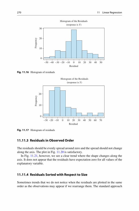
270 11 Linear Regression
−50 −40 −30 −20 −10 0 10 20 30 40 50
30
20
10
0
Residual
Freq
uenc
y
Histogram of the Residuals
(response is Y)
Fig. 11.16 Histogram of residuals
−30 −20 −10 0 10 20 30 40 50 60 70
Residual
20
10
0
Freq
uenc
y
Histogram of the Residuals
(response is Y)
Fig. 11.17 Histogram of residuals
11.11.3 Residuals in Observed Order
The residuals should be evenly spread around zero and the spread should not changealong the axis. The plot in Fig. 11.20 is satisfactory.
In Fig. 11.21, however, we see a clear trend where the shape changes along theaxis. It does not appear that the residuals have expectation zero for all values of theexplanatory variable.
11.11.4 Residuals Sorted with Respect to Size
Sometimes trends that we do not notice when the residuals are plotted in the sameorder as the observations may appear if we rearrange them. The standard approach

11.12 Summary of Chap. 11 271
−50
3
Normal Probability Plot of the Residuals(response is Y)
0
1
2
−3
−2
−1
−40 −20 −10 0 10 20 30 40 50−30
Residual
Nor
mal
Sco
re
Fig. 11.18 Normal score plot of residuals
Normal Probability Plot of the Residuals
(response is Y)
40 800Residual
3
0
1
2
−3
−2
−1
Nor
mal
Sco
re
Fig. 11.19 Normal score plot of residuals
is to sort the residuals according to the size of the observed values. Again we hopeto see an even spread around zero which do not change along the axis. The plot inFig. 11.22 is satisfactory.
In Fig. 11.23, however, we see a clear trend where the shape changes along theaxis. It does not appear that the residuals have expectation zero for all values of theexplanatory variable.
11.12 Summary of Chap. 11
• Ordinary least squares (OLS) is a method to find the best line through a set ofobservation pairs.

272 11 Linear Regression
Fig. 11.20 Residuals sortedin observed order
Residuals Versus the Order of the Data(response is Y)
60 70 8010 20 30 40 50 90 100
Observation Order
50
010203040
−50
−30−40
−20−10R
esid
uals
Fig. 11.21 Residuals sortedin observed order
400
200
200
400
20 40 60 80 100
• The intercept O and the slope O are unbiased estimators of a relationship
Y D ˛ C ˇ � X C �:
Y is called the dependent variable and X the explanatory variable.• The explanatory power R2 is interpreted as the fraction of the variation of the
dependent variable that can be explained by the explanatory variable.• To check if an explanatory variable matters, we can perform a statistical test
with null hypothesis ˇ D 0. If this hypothesis is rejected, then the value of theexplanatory variable matters.
• The regression line can be used to predict values for the dependent variableoutside the observation set. Such predictions should in general be used closeto the set where we have observations.

11.12 Summary of Chap. 11 273
Residuals Versus the Fitted values
(response is Y)
700600500400300200
Fitted Value
50
010203040
−50
−30−40
−20−10R
esid
uals
Fig. 11.22 Residuals sorted with respect to the size of the dependent variable
200
100
100
200
20 40 60 80 100
Fig. 11.23 Residuals sorted with respect to the size of the dependent variable
• In multiple regression we have more than one explanatory variables and use amodel on the form
Y D ˛ C ˇ1X1 C ˇ"X2 C � � � C ˇrXr C �:
• A significant linear relationship does not in general prove that a change in anexplanatory variable will cause a change in the dependent variable.
• Explanatory variables with a common cause may lead to collinearity and shouldbe avoided.
• Explanatory should be scalable, but non-scale variables can sometimes be codedin terms of dummy variables.
• Diagnostic plots are tools for visual inspection. They can be used to assess theassumptions in the OLS model.

274 11 Linear Regression
11.13 Problems for Chap. 11
11.1 Figure 11.24 displays four different sets of data. Which of these are suitablefor linear regression?
11.2 Choose two points and draw a line that fits reasonably well with theobservations in Fig. 11.25. Use the two-point formula to find the formula for thisline.
a) 5 10 15 20 25 30t
20
40
60
80
100x
b) 5 10 15 20 25 30t
20
40
60
80
100x
c) 5 10 15 20 25 30t
20
40
60
80
100x
d) 5 10 15 20 25 30t
20
40
60
80
100x
Fig. 11.24 Data sets for Problem 11.1
5 10 15 20t
2
4
6
8
10x
Fig. 11.25 Data set for Problem 11.2
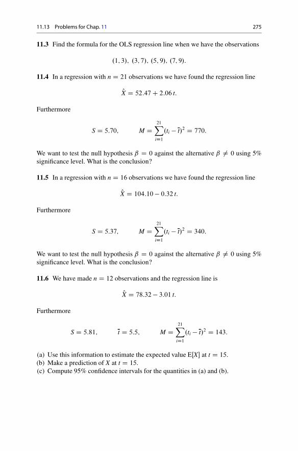
11.13 Problems for Chap. 11 275
11.3 Find the formula for the OLS regression line when we have the observations
.1; 3/; .3; 7/; .5; 9/; .7; 9/:
11.4 In a regression with n D 21 observations we have found the regression line
OX D 52:47 C 2:06 t:
Furthermore
S D 5:70; M D21X
iD1
.ti � t/2 D 770:
We want to test the null hypothesis ˇ D 0 against the alternative ˇ 6D 0 using 5%significance level. What is the conclusion?
11.5 In a regression with n D 16 observations we have found the regression line
OX D 104:10 � 0:32 t:
Furthermore
S D 5:37; M D21X
iD1
.ti � t/2 D 340:
We want to test the null hypothesis ˇ D 0 against the alternative ˇ 6D 0 using 5%significance level. What is the conclusion?
11.6 We have made n D 12 observations and the regression line is
OX D 78:32 � 3:01 t:
Furthermore
S D 5:81; t D 5:5; M D21X
iD1
.ti � t/2 D 143:
(a) Use this information to estimate the expected value EŒX� at t D 15.(b) Make a prediction of X at t D 15.(c) Compute 95% confidence intervals for the quantities in (a) and (b).
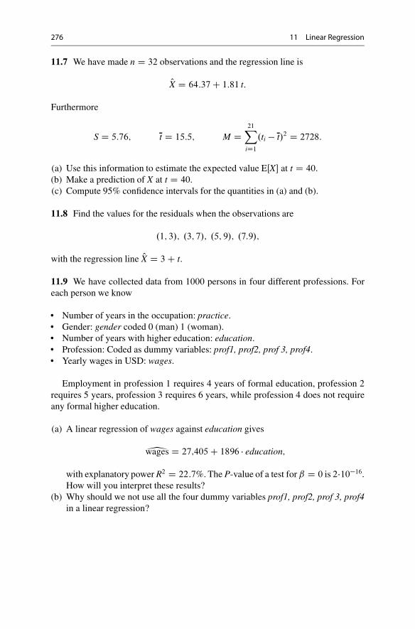
276 11 Linear Regression
11.7 We have made n D 32 observations and the regression line is
OX D 64:37 C 1:81 t:
Furthermore
S D 5:76; t D 15:5; M D21X
iD1
.ti � t/2 D 2728:
(a) Use this information to estimate the expected value EŒX� at t D 40.(b) Make a prediction of X at t D 40.(c) Compute 95% confidence intervals for the quantities in (a) and (b).
11.8 Find the values for the residuals when the observations are
.1; 3/; .3; 7/; .5; 9/; .7:9/;
with the regression line OX D 3 C t:
11.9 We have collected data from 1000 persons in four different professions. Foreach person we know
• Number of years in the occupation: practice.• Gender: gender coded 0 (man) 1 (woman).• Number of years with higher education: education.• Profession: Coded as dummy variables: prof1, prof2, prof 3, prof4.• Yearly wages in USD: wages.
Employment in profession 1 requires 4 years of formal education, profession 2requires 5 years, profession 3 requires 6 years, while profession 4 does not requireany formal higher education.
(a) A linear regression of wages against education gives
1wages D 27;405 C 1896 � education;
with explanatory power R2 D 22:7%. The P-value of a test for ˇ D 0 is 2�10�16.How will you interpret these results?
(b) Why should we not use all the four dummy variables prof1, prof2, prof 3, prof4in a linear regression?

11.13 Problems for Chap. 11 277
(c) We have carried out a multiple regression of wages against practice, gender,education, prof1, prof2, prof3. The results read as follows
1wages D 14;970 C 506 � practice C 5171 � gender � 98 � education
C2705 � prof 1 C 15;380 � prof 2 C 10;658 � prof 3:
R2 D 95:7%, and the P-values for the explanatory variables were
practice W P -value 2 � 10�16;
gender W P -value 2 � 10�16;
education W P -value 43:5%;
prof 1 W P -value 4 � 10�7;
prof 2 W P -value 2 � 10�16;
prof 3 W P -value 2 � 10�16:
How will you interpret these results? Compare the answers with the conclu-sion in (a) and try to explain the difference.
(d) To examine if there is collinearity between education and professions, we havemade a new regression. The results read as follows:
3education D 0:496 C 4:03 � prof 1 C 5:04 � prof 2 C 6:00 � prof 3:
R2 D 95:6%, and the P-values for the explanatory variables were
prof 1 W P -value 2 � 10�16;
prof 2 W P -value 2 � 10�16;
prof 3 W P -value 2 � 10�16:
What conclusion can you draw from this analysis?(e) We have made a new regression where we have deleted education as explanatory
variable. The results read as follows
1wages D 14;924 C 506 � practice C 5167 � gender
C2312 � prof 1 C 14;889 � prof 2 C 10;721 � prof 3:
R2 D 95:7%, and the P-values for the explanatory variables were
practice W P -value 2 � 10�16;
gender W P -value 2 � 10�16;

278 11 Linear Regression
prof 1 W P -value 2 � 10�7;
prof 2 W P -value 2 � 10�16;
prof 3 W P -value 2 � 10�16:
How will you interpret these results? Compare with the conclusions in(a) and (c).
(f) Use one of the regressions above to predict the salary of a woman with 12 yearspractice, 6 years of higher education, and working in profession 3.
11.10 We have used three different production methods, and the production (inunits) was registered on nine consecutive days. The 27 results are shown inTable 11.4.
Table 11.4 Data forProblem 11.10
Method Day Production
1 1 1 162
2 2 1 208
3 3 1 172
4 1 2 168
5 2 2 221
6 3 2 180
7 1 3 181
8 2 3 232
9 3 3 189
10 1 4 192
11 2 4 242
12 3 4 201
13 1 5 198
14 2 5 249
15 5 5 208
16 1 6 210
17 2 6 208
18 3 6 221
19 1 7 222
20 2 7 268
21 3 7 230
22 1 8 231
23 2 8 279
24 3 8 238
25 1 9 240
26 2 9 291
27 3 9 252

11.13 Problems for Chap. 11 279
(a) To examine if there is a connection between production, method, and time, wecarried out a linear regression. The results read as follows
4production D 106:2 C 4:83 � method C 9:67 � time:
R2 D 59:9%. The P-value for ˇ1 D 0 was 35.9%, and the P-value for ˇ2 D 0
was 4:2 � 10�6. Comment these results.(b) We have introduced two new variables
X1 D(
1 if we use method 1
0 otherwise; X2 D
(1 if we use method 3
0 otherwise:
A regression of production against time, X1, and X2 gave the result
4production D 195:9 C 9:67 � time � 43:77 � X1 � 34:11 � X2:
R2 D 91:5%, and P-values for all explanatory variables were less than 10�6.Comment these results.
(c) Compare the results in (a) and (b). Which method is best?
11.11 Figure 11.26 displays diagnostic plots from a regression. To what extent arethe assumptions on normality and independence satisfied in this case?
11.12 Figure 11.27 displays diagnostic plots from a regression. To what extent arethe assumptions on normality and independence satisfied in this case?
11.13 Double Logarithmic Transformation: In this exercise we will study theconnection between sold quantity Q and the price p for a good. We have observedQ3; Q4; : : : ; Q100 for p D 3; 4; : : : ; 100, respectively. The results are shown below.
(a) We have carried out a regression of Q against p, and got the following results:Regression line
OQ D 775 � 8:55 � p; S D 198:1; R2 D 59:9%:
Figure 11.28 displays diagnostic plots for the residuals. Comment to what extentyou think the assumptions for the regression model are satisfied in this case.
(b) Alternatively we have carried out a new regression where we observe ln.Q/ asa function of ln.p/.

280 11 Linear Regression
Histogram of the Residuals
(response is C3)
−10 −8 −6 −4 −2 0 2 4 6 8 10
Residual
20
10
0
Freq
uenc
yNormal Probability Plot of the Residuals
(response is C3)
−3
−2
−1
0
1
2
3
−10 0 10
Residual
Nor
mal
Sco
re10
0
−10
Res
idua
l
Residuals Versus the Order of the Data
(response is C3)
10 20 30 40 50 60 70 80 90 100
Observation Order
10
0
−10
Res
idua
l
Residuals Versus the Fitted Values
(response is C3)
20 30 40 50 60 70 80 90 100
Fitted Value
Fig. 11.26 Residual plots for Problem 11.11
Regression line
Oln.Q/ D 8:91 � 0:914 � ln. p/; S D 0:2162; R2 D 91:3%:
Diagnostic plots for the residuals are shown in Fig. 11.29. Comment to whatextent you think the assumptions for the regression model is satisfied in thiscase.
(c) Use the results from (b) to suggest a value for OQ D e Oln.Q/ for the expected valueof Q when p D 110. You need not consider the uncertainty in this value.
(d) Assume that Q D K � pˇ � U, where K and ˇ are (unknown) constants and U > 0
is a random variable. Show that ln.Q/ can be written in the form
ln.Q/ D � C ˇ � ln. p/ C �;
where � is a constant and � is a random variable with EŒ�� D 0.(e) If � in (d) is normally distributed N.0; �2/, then EŒln.U/� D ln.EŒU�/ � 1
2�2.
You can take that relation for granted. Show that
EŒQ� D e�Cˇ ln. p/C 12 �2
;
and use this to estimate EŒQ� again when p D 110.

11.13 Problems for Chap. 11 281
10
5
0
Freq
uenc
yHistogram of the Residuals
(response is C3)
−5 0 5 10
Residual
0
1
2
3
−2
−1
−3
Nor
mal
Sco
re
Normal Probability Plot of the Residuals
(response is C3)
−5 0 5 10
Residual
10
5
0Freq
uenc
y
10 20 30 40 50 60 70 80 90 100−5
Residuals Versus the Order of the Data
(response is C3)
Observation Order
10
5
0Freq
uenc
y
−80 −70 −60−5
Residuals Versus the Fitted Values
(response is C3)
Fitted Value
Fig. 11.27 Residual plots for Problem 11.12
11.14 Logarithmic Transformation:We have observed the price of a stock on 100consecutive days. The price is increasing and there is a clear tendency of increasinggrowth. The plot has a convex profile.
(a) Why is it futile to use linear regression on these observations? Why is itreasonable to assume that the prices on stocks, bonds, and bank deposits growexponentially?
(b) As an alternative to linear regression we have plotted ln.X/ against t for t D0; 1; : : : ; 100 and carried out a linear regression on the transformed data.
Regression line
Oln.X/ D 4:23 C 0:0175 � t; S D 0:3025; R2 D 74:4%:
Diagnostic plots for the regression are displayed in Fig. 11.30. To what extentare the assumptions on normality and independence satisfied in this case?
(c) Assume that ln.X/ D � C ˇ � t C � where � and ˇ are constants and � isnormally distributed with expectation zero and variance �2. It is possible toshow that EŒe�� D e
12 �2
(you can take that for granted). Use this formula tofind an expression for EŒX�, and write down a general estimator for the expectedvalue. Estimate the expectation of X when t D 110.

282 11 Linear Regression
2000
1000
00 10 20 30 40 50 60 70 80 90 100
Pri
20
30
10
0
Freq
uenc
y
Histogram of the Residuals
(response is Q)
0 500 1000
Residual
1
2
3
0
−3
−2
−1
Nor
mal
Sco
re
Normal Probability Plot of the Residuals
(response is Q)
0 500 1000
Residual
1000
500
0
Res
idua
ls
(response is C3)
10 20 30 40 50 60 70 80 90Observation Order
1000
0
500
Res
idua
l
Residuals Versus the Fitted Values
(response is Q)
100 200 3000−100 400 500 600 700 800Fitted Value
Fig. 11.28 Observation and residual plots for Problem 11.13
(d) Why is it reasonable to assume that the variance of a stock price changes whenthere is a considerable change in the price? How and in what direction can thisinfluence a prediction of expected value into the future?
11.15 Cyclic Behavior: We have made weekly observations of the daily powerconsumption in a small city. Data were obtained each Monday starting in week 10and ending in week 26. The results of the survey are displayed in Fig. 11.31.
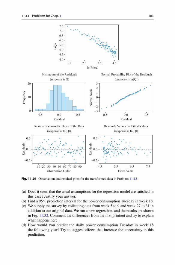
11.13 Problems for Chap. 11 283
4.0
4.5
5.0
5.5
6.0
6.5
7.0
7.5
ln( Q
)
1.5 2.5 3.5 4.5
ln( )
20
10
0
Freq
uenc
y
Histogram of the Residuals
(response is Q)
0.5 0.0 0.5
Residual
1
23
0
−3
−2
−1
Nor
mal
Sco
re
Normal Probability Plot of the Residuals
(response is ln(Q))
−0.5 0.0 0.5
Residual
Residuals Versus the Order of the Data
(response is ln(Q))
Observation Order
0.5
0.0
−0.5
Res
idua
ls
10 20 30 40 50 60 70 80 90
0.5
0.0
−0.5
Res
idua
ls
Residuals Versus the Fitted Values
(response is ln(Q))
5.54.5 6.5 7.5
Fitted Value
Fig. 11.29 Observation and residual plots for the transformed data in Problem 11.13
(a) Does it seem that the usual assumptions for the regression model are satisfied inthis case? Justify your answer.
(b) Find a 95% prediction interval for the power consumption Tuesday in week 18.(c) We supply the survey by collecting data from week 5 to 9 and week 27 to 31 in
addition to our original data. We run a new regression, and the results are shownin Fig. 11.32. Comment the differences from the first printout and try to explainwhat happens here.
(d) How would you predict the daily power consumption Tuesday in week 18the following year? Try to suggest effects that increase the uncertainty in thisprediction.

284 11 Linear Regression
4
5
6
7
Ln(
X)
0 50 100
t
5
10
15
0
Freq
uenc
y
Histogram of the Residuals
(response is Ln(X))
−0.5 0.0 0.5 1.0
Residual
1
23
0
−3
−2
−1
Nor
mal
Sco
re
Normal Probability Plot of the Residuals
(response is Ln(X))
−0.5 0.0 0.5
Residual
0.5
0
−0.5
Res
idua
l
Residuals Versus the Order of the Data
(response is Ln(X))
60 80 10020 40
Observation Order
0.5
0
−0.5
Res
idua
l
Residuals Versus the Fitted Values
(response is Ln(X))
4 5 6
Fitted Value
Fig. 11.30 Observation and residual plots for the transformed data in Problem 11.14
11.16 Autocorrelation: In an analysis of productivity we have made daily observa-tions of the production over a period of 100 days. A regression of production againsttime gave the result:
Regression line
4production D 1:07 C 2:09 � t; S D 6:802; R2 D 98:8%:
Diagnostic plots are displayed in Fig. 11.33.

11.13 Problems for Chap. 11 285
50
100
150
Ene
rgy
10 15 20 25
Ti
Regression Plot
Energy = 242.029 − 7.82843 T
S = 3.18072 R − Sq = 99.4 % R − Sq(adj) = 99.4 %
2
1
4
3
5
0
Freq
uenc
y
Histogram of the Residuals
(response is Energy)
−6 −4 −2 0 2 4 6
Residual
Normal Probability Plot of the Residuals
(response is Energy)
−1
0
1
2
−2
Nor
mal
Sco
re
−5 0 5
Residual
Residuals Versus the Order of the Data
(response is ))
0
5
−5
Res
idua
l
8 102 4 6 12 14 16
Observation Order
Residuals Versus the Fitted Values
(response is Energy)
0
5
−5
Res
idua
l
50 100 150
Fitted Value
Fig. 11.31 Observation and residual plots for Problem 11.15
(a) Does it seem that the usual assumptions for the regression model are satisfied inthis case? Justify your answer.
(b) Offer a prediction of the productivity at time t D 110 based on the linearregression of productivity as a function of time. What kinds of uncertainty dowe have in this prediction? You need not quantify the uncertainty.
(c) A precise study of the residuals in the previous regression reveals that they areautocorrelated, i.e., dependent. In normal cases the degree of autocorrelationmust be estimated. We will here, however, look at a simplified version where

286 11 Linear Regression
0
100
200
Ene
rgy
10 20 30
Ti
Regression Plot
Energy = 214.617 − 6.36142 Ti
S = 8.46808 R − Sq = 97.4 % R − Sq(adj) = 97.3 %
Histogram of the Residuals
(response is Energy)
21
34
65
0
Freq
uenc
y
−15−12 −9 −6 −303691215
Residual
Normal Probability Plot of the Residuals
(response is Energy)
0
−1
1
2
−2
Nor
mal
Sco
re
−15 −10 −5510 01 5
Residual
Residuals Versus the Order of the Data
(response is Energy)
−5
510
0
15
−15−10
Res
idua
l
255101520
Observation Order
Residuals Versus the Fitted Values
(response is Energy)
−5−10
510
0
15
−15
Res
idua
l
1000 200
Fitted Value
Fig. 11.32 Observation and residual plots for the extended data in Problem 11.15
the degree of autocorrelation is known. In a model of that kind we assume that
Xi D � C ˇ � t C Rt;
where
Rt D � � Rt�1 C �t;

11.13 Problems for Chap. 11 287
0
100
200
prod
u cti
on
0 20 40
ti
60 80 100
Histogram of the Residuals
(response is production)
5
10
15
0
Freq
uenc
y
−20 −10 0 10 20
Residual
Normal Probability Plot of the Residuals
(response is production)
1
23
0
−3
−2
−1
Nor
mal
Sco
re
−20 0 10
Residual
−10
Residuals Versus the Order of the Data
(response is production)
10
0
−20
Res
idua
l
−10
70 80 10010 40
Observation Order
20 30 50 60 90
Residuals Versus the Fitted Values
(response is production)
10
0
−20
Res
idua
l
−10
−10 0 10
Fitted Value
Fig. 11.33 Observation and residuals plots for Problem 11.16
where � is a known constant and where �1; �2; : : : are independent, normallydistributed, with expectation zero and constant variance �2. We define a new setof observations Y1; Y2; : : : ; Y100 by
Yt D Xt � � � Xt�1:
Show that
Yt D �.1 � �/ C � � ˇ C .1 � �/ˇ � t C �t:
Explain why Yt satisfies the usual conditions in a linear regression model.

288 11 Linear Regression
0
10
20
Y
0 20 40
time
60 80 100
5
10
15
0
Freq
uenc
y
−10 0 10
Residual
Histogram of the Residuals
(response is Y)
1
23
0
−3
−2
−1
Nor
mal
Sco
re
−10 0 10
Residual
Normal Probability Plot of the Residuals
(response is Y)
10
0
−10
Res
idua
l
60 8010 40
Observation Order
20 30 50 70 90
Residuals Versus the Order of the Data
(response is Y)
Residuals Versus the Fitted Values
(response is Y)10
0
−10
Res
idua
l
0 10 20
Fitted Value
Fig. 11.34 Observation and residual plots for the transformed data in Problem 11.16
(d) The results from a linear regression of Y against t were:Regression line
OY D 2:30 C 0:201 � t; S D 3:252; R2 D 71:6%:
Diagnostic plots are displayed in Fig. 11.34. Does it seem that the usualassumptions for the regression model are satisfied in this case? Justify youranswer.

11.13 Problems for Chap. 11 289
Table 11.5 Data for Problem 11.17
Location Number of mobile phones sold Number of cars sold
City 1 33,739 20; 664
City 2 28,646 17; 168
City 3 12,624 7890
City 4 17,885 11; 067
City 5 20,518 12; 349
City 6 14,035 8513
City 7 28,067 16; 990
City 8 16,697 9870
City 9 14,713 9197
City 10 27,202 16; 130
(e) In our calculations of Y1; Y2; : : : ; Y100 we have used � D 0:9. Use the formulafor Yt in (c) together with the printout to estimate values for the constants � andˇ. Use this to make a new prediction of the productivity X110 at time t D 110.
11.17 Causality: We want to see if there is a connection between sales of mobilephones and cars. We have collected data from 10 relatively small cities. Theobservations are shown in Table 11.5.
We have carried out a linear regression of car sales against sales of mobilephones, and the results were as follows:
2carsales D 201:8 C 0:59694 � mobilesales; S D 231:0; R2 D 99:8%:
The P-value for a test of ˇ D 0 was 0.000.
(a) Do the results give reason to claim that there is a connection between sales ofcars and sale of mobile phones? Justify your answer.
(b) Diagnostic plots for the residuals are displayed in Fig. 11.35. Does it seem thatthe usual assumptions for the regression model are satisfied in this case? Justifyyour answer.
(c) How large share of the variation in car sales can be explained by the variationin sales of mobile phones?
(d) Predict the number of care sales in a city where sales of mobile phones are150;000. What kind of uncertainties are attached to this prediction?
(e) A consultant for the car industry claims there is a clear connection between caresales and sales of mobile phones. He suggests to raise the car sales by givingaway a large number of mobile phones. Is this a good idea?

290 11 Linear Regression
300 100 100 300Residual
Histogram of the Residuals
Freq
uenc
yResidual Plots for Carsales
Normal Probability Plot of the Residuals
Nor
mal
Sco
re 1
3
2
1
0
0
1
300 200 100 0 100 200 300Residual
300
300200100
0100200300
200100
0100200300
1 2 3 4 5 6 7 8 9 10Observation Order
Residuals Versus the Order of the Data
Res
idua
l
Residuals Versus the Order of the Data
Res
idua
l
10000 15000 20000Fitted Value
Fig. 11.35 Diagnostic plots of the residuals in Problem 11.17
11.18 Nonlinear Regression: A monopolist wishes to optimize his profit. Theprofit has a random fluctuation which may be due to, e.g., varying prices on rawmaterials. The profit is simulated selling 1 to 100 units of the good, and the result isshown in Fig. 11.36.
(a) Discuss statistical and economical issues which speak against using linearregression in this case.
(b) This case is well suited for quadric regression. In quadratic regression we use amodel where the profit X and the production q is given by
X D a C b � q C c � q2 C �;
and where � denotes independent, normally distributed random variables withconstant variance. Having observed .X1; q1/; : : : ; .Xn; Qn/, we want to fit aquadratic curve such that
errorŒa; b; c� DnX
iD1
.Xi � a � b � qi � c � q2i /2;

11.13 Problems for Chap. 11 291
06 08 001
SR-SqR-Sq(adj)
1774 8731 2%30 5%
Fitted Line PlotProfit 956 7 40 98
Prof
it
0 02 044000
2000
0
2000
4000
6000
500040003000Fitted ValueResidual
Observation OrderResidual
Residuals Versus the Order of the DataHistogram of the Residuals
Residuals Versus the Fitted Values
Residual Plots for Profit
Normal Probability Plot of the Residuals
Freq
uenc
yPe
rcen
t
Res
idua
lR
esid
ual
20001000
10070 80 9050 6030 401 020130000 0051150030004500
500040003000200010006000
4000
2000
0
2000
6000
4000
2000
0
2000
0
4
8
12
16
Fig. 11.36 Observation and residual plots for Problem 11.18
is as small as possible. Explain that we achieve optimal fit when a; b; c aresolutions of the 3 linear equations
nX
iD1
.Xi � a � b � qi � c � q2i / D 0
nX
iD1
.Xi � a � b � qi � c � q2i /qi D 0
nX
iD1
.Xi � a � b � qi � c � q2i /q2
i D 0

292 11 Linear Regression
Residual
Histogram of the Residuals
Freq
uenc
y
20000 00012000 100030000
6
12
18
24
Observation Order
Residuals Versus the Order of the Data
Res
idua
l
10070 80 9050 6030 401 0201
3000
4000
0
1500
3000
500040003000Fitted ValueResidual
Residuals Versus the Fitted Values
Residual Plots for Residuals
Normal Probability Plot of the Residuals
Perc
ent
Res
idua
l
2000100030001500015003000
3000
1500
0
1500
3000
Fig. 11.37 Residual plots for the quadratic regression in Problem 11.18
(c) For the data above the solution of the system was
Oa D �2482:2; Ob D 243:275; Oc D �2:003:
Figure 11.37 displays diagnostic plots of the residuals from the quadraticregression. Does it seem that the statistical assumptions are valid? How manyunits should we produce to obtain maximum expected profit?
11.19 Disaggregation: In this problem we want to discuss what happens when wedisaggregate data into subgroups. Here income denotes annual wages in USD andeduc denotes number of years of education. We have collected data from 700 women(W) and 1221 men (M). Aggregating the data for men and women, we get
2income D 10;241 C 1114 � educ;
with
S D 10;072; R2 D 8:8%; P-value of ˇ D 0 D 0:000:

11.13 Problems for Chap. 11 293
If we consider the data for men and women separately, we get
2incomeM D 9974 C 1371 � educM;
with
S D 10;969; R2 D 11:2%; P-value of ˇ D 0 D 0:000:
2incomeW D 11;223 C 621 � educW;
with
S D 5368; R2 D 9:3%; P-value of ˇ D 0 D 0:000:
(a) How do you interpret the P-values? Are there differences between men andwomen, and how does this turn out?
(b) The explanatory power is relatively low in all three cases. Is this something wewould expect?
(c) Predict income for a woman with 17 years of education. Find a 95% confidenceinterval for this income. Here educW D 11:86361 and SŒ O� D 73:26. Hint: Theformula M D S2
SŒ O�2 will be useful.
11.20 Explains Everything—Predicts Nothing: In a survey we asked 500 hotelguests how satisfied they were with their stay. There were 6 alternatives as shown inTable 11.6.
The guests also answered the question “How likely is it that you will visit thesame hotel again?” Alternatives: 0%,5%,10%,. . . ,95%,100%. As it appears there isa connection between the two questions, we have carried out a linear regression ofthe satisfaction level SL against the probability of returning PR.
cPR D 14:4 C 14:8 � SL;
with
S D 7:50500; R2 D 91:5%; P-value (of ˇ D 0/ D 0:000:
Table 11.6 Satisfactionlevels n Problem 11.20
Very dissatisfied 0
Dissatisfied 1
Somewhat dissatisfied 2
Neutral 3
Somewhat satisfied 4
Satisfied 5

294 11 Linear Regression
Fitted Line Plot PR 14 40 14 76
SR-SqR-Sq(adj)
7 5050091 5%91 5%
PR
0
20
40
60
80
100
Residual
Histogram of the Residuals
Freq
uenc
y
0
25
50
75
100
Observation Order
Residuals Versus the Order of the Data
Res
idua
l
500350 400 450250 300150 2000 00105
10
20
0
10
20
8060Fitted ValueResidual
Re iduals Versus the Fitted Values
Residual Plots for PR
Normal Probability Plot of the Residuals
Perc
ent
Res
idua
l
40200 01 02102020
10
0
10
20
0 6 21 8112 618
0 1 2 3 4 5
Fig. 11.38 Observation and residual plots for Problem 11.20
Diagnostic plots are displayed in Fig. 11.38.
(a) Does it seem that the usual assumptions for the regression model are satisfied inthis case? Justify your answer.
(b) We can imagine that we introduced a new alternative: 6—very satisfied. Is itreasonable to use the regression model to predict the number of very satisfiedguest?
(c) As an alternative we have used polynomial regression with a third degreepolynomial:
cPR D 5:710 C 40:06 � SL � 11:66 � SL2 C 1:389 � SL3;

11.13 Problems for Chap. 11 295
SL
SR-SqR-Sq(adj)
5.1266296.1%96.0%
Fitted Line PlotPR 5.710 40.06 SL
11.66 SL**2 1.389 SL**3
PR
3 4 50 1 2
0
20
40
60
80
100
Scatterplot of RESI1 vs Fit
908060 70
Fit
RE
SI1
5030 4010 2020
10
0
10
20
Scatterplot of RESI1 vs Nr
500300 400
Nr
RE
SI1
100 200020
10
0
10
20
Fig. 11.39 Observation and residual plots for the cubic regression in Problem 11.20
with
S D 5:12662; R2 D 96:1%:
Some diagnostic plots are displayed in Fig. 11.39. Does this model appear tofunction better?
(d) Alternatively we could use the third degree polynomial from (c) to predict theoutcome of the alternate SL D 6. Would that solve the problem in (b)?
11.21 Logistic Regression: A large number of people between 15 and 75 years oldhave been asked if they ever used a certain product. The answers were distributed asshown in Table 11.7.
(a) It seems reasonable to assume that the fraction that has ever used the productincreases with age. To examine this further we have carried out a linearregression of fractions against age. Comment the results in this regression.
2fraction D �8:12 C 1:78 � age;

296 11 Linear Regression
Table 11.7 Data forProblem 11.21
Age group Fraction in % that has used the product
15–20 Y15 D 10:0
20–25 Y20 D 11:0
25–30 Y25 D 31:2
30–35 Y30 D 52:2
35–40 Y35 D 61:3
40–45 Y40 D 77:0
45–50 Y45 D 86:7
50–55 Y50 D 92:2
55–60 Y55 D 93:5
60–65 Y60 D 97:3
65–70 Y65 D 98:7
70–75 Y70 D 99:6
with
S D 11:7844; R2 D 89:1%; P-value (of ˇ D 0/ D 0:000:
Diagnostic plots are displayed in Fig. 11.40.(b) Use the model from (a) to predict the fraction of 80 years old that has ever used
the product. There are several problems connected to this prediction. Point outsome of these problems.
(c) We define f .x/ as the expected fraction (in %) of persons of age x that has everused the product. We assume that f .x/ can be written in the form
f .x/ D 100 e�Cˇ x
1 C e�Cˇ x;
where � and ˇ are unknown constants. Use this expression to show that
ln
�f .x/
100 � f .x/
�D � C ˇ x:
(d) To estimate the values for � and ˇ, we have replaced Y15; : : : ; Y70 in the tableabove with the transformed values
Z15 D ln
�Y15
100 � Y15
�; : : : ; Z70 D ln
�Y70
100 � Y70
�:
We have then carried out a linear regression of Zx against x. The results areshown below. Comment the results in this new regression.
1values D �4:31 C 0:135 � age;

11.13 Problems for Chap. 11 297
7050 6040a
SR-SqR-Sq(adj)
11 784489 1%88 0%
Fitted Line Plotfraction 8.124 1 781
frac
tion
01 02 030
20
40
80
60
100
100
90 120Fitted ValueResidual
Re i uals Versus the Fitted Values
Residual Plots for fraction
Normal Probability Plot of the Residuals
Perc
ent
Res
idua
l
60300 01 02102020
10
0
10
1
10
50
90
99
Residual
Histogram of the Residuals
Freq
uenc
y
0
1
2
3
Observation Order
Residuals Versus the Order of the Data
Res
idua
l
11 128 9 106 74 52 31
10
20
10
0
0 5 01 5110 515
Fig. 11.40 Observation and residual plots for Problem 11.21
with
S D 0:2853; R2 D 98:8%; P-value (of ˇ D 0/ D 0:000:
Diagnostic plots are displayed in Fig. 11.41.(e) Use the model from (c) and (d) to predict the fraction of 80 years old that has
ever used the product. Comment the answer.
11.22 Outliers: We have collected data for the value of sales and sales costs. Datawere observed on a weekly basis and we have data for 30 weeks. The observationsare plotted in Fig. 11.42.
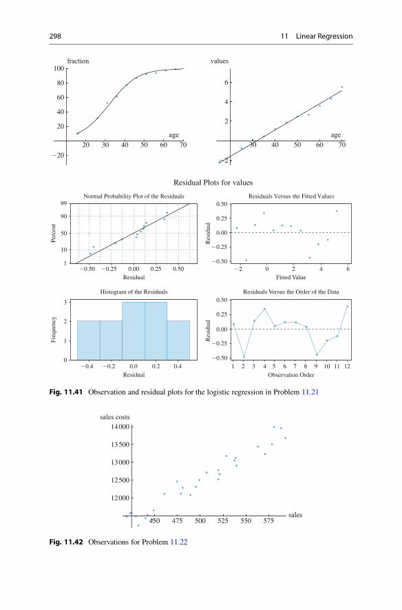
298 11 Linear Regression
20 30 40 50 60 70
values
03 04 05 06 07
20
40
60
80
100
6
4
2
220
Residual
Histogram of the Residuals
Freq
uenc
y
0
1
2
3
Observation Order
Residuals Versus the Order of the Data
Res
idua
l
11 128 9 106 74 52 310.0 2.0 4.00.20.4
4 6Fitted ValueResidual
Residuals Versus the Fitted Values
Residual Plots for values
Normal Probability Plot of the Residuals
Perc
ent
Res
idua
l
2020.500.250.000.250.500.50
0.25
0.00
0.50
0.25
1
10
50
90
99
0.50
0.25
0.00
0.50
0.25
Fig. 11.41 Observation and residual plots for the logistic regression in Problem 11.21
sales
sales costs
450 475 500 525 550 575
12000
12500
13000
13500
14000
Fig. 11.42 Observations for Problem 11.22

11.13 Problems for Chap. 11 299
(a) The figure indicates that there is a linear relationship between sales costs andthe value of the sales. Is this something we could expect, and what could be thereason for that?
(b) We have carried out a linear regression, and the results were as follows:
4sales costs D 5212:6 C 0:0145 � sale;
with
S D 193:985; R2 D 94:6%; P-value (of ˇ D 0/ D 0:000:
Diagnostic plots are displayed in Fig. 11.43.What kind of information can we draw from the printouts? Comment the
results and the plots in detail.(c) The week after the survey we observed a sales of 500;000 USD, while the
reported sales costs were 14;500 USD. Find a 95% prediction interval for thesales costs, and discuss if the reported number seems reasonable. To computethe prediction interval you need to know that mean value of the sales were499;110 USD and that SŒ O� D 0:0006543. Use the formula M D S2
SŒ O�2 :
Residual
Histogram of the Residuals
Freq
uenc
y
0
2
4
8
6
Observation Order
Residuals Versus the Order of the Data
Res
idua
l
22 24 62 038202816112 148 104 62300 4000 001 002200 100300
Residual Plots for sales costs
13000 13500Fitted ValueResidual
Residuals Versus the Fitted ValuesNormal Probability Plot of the Residuals
Perc
ent
Res
idua
l
1250012000115005002500250500400
200
0
400
200
400
200
0
400
200
1
10
50
90
99
Fig. 11.43 Residual plots for Problem 11.22

300 11 Linear Regression
11.23 Solving the OLS Equations: In this problem the aim is to find the bestpossible linear fit to the points .1; 1/; .2; 3/; .3; 3/: A straight line has the formula
x D ˛ C ˇ � t:
The errors we make at the three given values of t are
error1 D ˛ C ˇ � 1 � 1;
error2 D ˛ C ˇ � 2 � 3;
error3 D ˛ C ˇ � 3 � 3:
(a) Show that
error21 C error2
2 C error23 D 3˛2 C 12˛ˇ C 14ˇ2 � 14˛ � 32ˇ C 19:
(b) Find ˛ and ˇ such that
F.˛; ˇ/ D error21 C error2
2 C error23;
is as small as possible. Hint: compute @F@˛
and @F@ˇ
, and solve the first order
conditions @F@ˇ
D 0, @F@ˇ
D 0.
11.24 Bid Auctions: Many special items are today traded via bid auctions. Thebidders often have different valuations of the item. A high bid has a good chanceof winning the auction, but gives less profit. We will consider a simplified settingwhere the bidders only can place one bid (the bids are secret), and where the highestbid wins. We will let x denote the size of the bid, while y is the valuation of theitem. The profit is defined as y � x. Expected profit F.x; y/ placing the bid x can becomputed by the expression
F.x; y/ D . y � x/ � probability of winning the auction:
For the rest of this problem we will assume that y D 10;000 USD, and we imaginethat we have carried out many auctions and registered how often we have won theauction bidding x (USD). The results are shown in Fig. 11.44.
(a) A regression of winning probability against bid gives
bwinning probability D �0:164 C 0:000138 � bid;

11.13 Problems for Chap. 11 301
2 4 5 108Bid
0.2
0.4
0.6
0.8
1P
Fig. 11.44 Observed winning probability in Problem 11.24
Perc
ent
Res
idua
l
0.00.2 0.2 0.4 0.2 0.4 0.4 0.4 0.40.41
10
0.00
0.15
0.30
0.15
0.30
2.4
1.2
0.0
3.6
4.8
50
90
99
Residual Plots for winningprobability
Normal Probability Plot Versus fits
Residual Fitted value
2 40.00.3 0.2 0.1 0.1 0.2 0.3 6 8 10 12 14 16 18 20
Res
idua
l
Freq
uenc
y
0.00
0.15
0.30
0.15
0.30
Versus orderHistogram
Observation orderResidual
Fig. 11.45 Residual plots for Problem 11.24
with
S D 0:168797; R2 D 86:1%; P-value (of ˇ D 0/ D 0:000:
Diagnostic plots are displayed in Fig. 11.45.Comment this information in detail.
(b) Alternatively we have carried out a new regression where we only consider bidsin the interval Œ3000; 7000�. Why is that a good idea here?
bwinning probability D �0:164 C 0:000138 � bid;
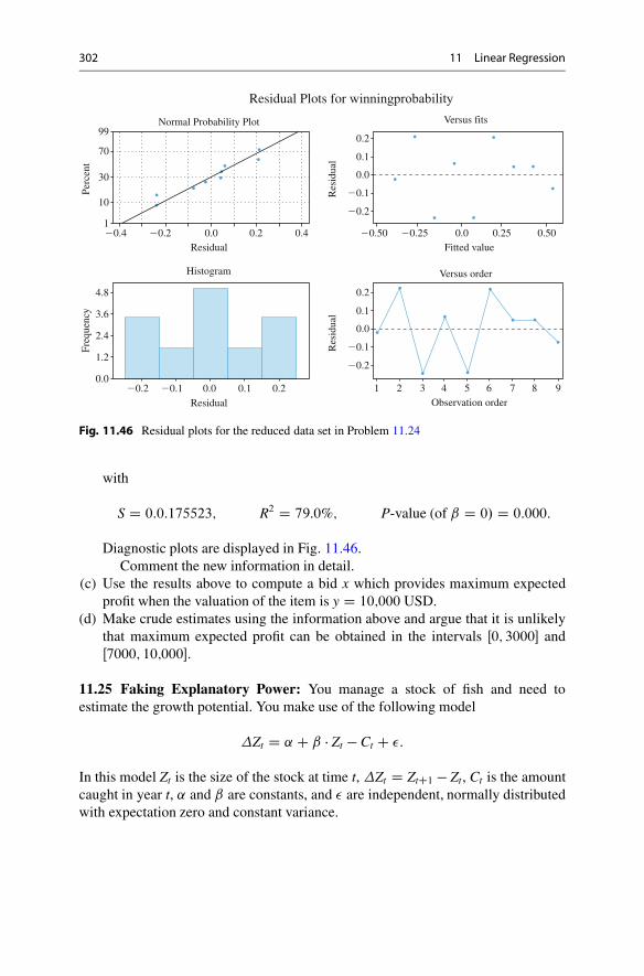
302 11 Linear Regression
Res
idua
l
0.50 0.25 0.0 0.25 0.50
0.0
0.1
0.2
0.1
0.2
Versus fits
Fitted value
Res
idua
l
1
0.0
0.1
0.2
0.1
0.2
Versus order
Observation order2 3 4 5 6 7 8 9
2.4
1.2
0.0
3.6
4.8
0.00.2 0.1 0.1 0.2
Freq
uenc
y
Histogram
Residual
Perc
ent
0.00.2 0.2 0.40.41
10
30
70
99
Residual Plots for winningprobability
Normal Probability Plot
Residual
Fig. 11.46 Residual plots for the reduced data set in Problem 11.24
with
S D 0:0:175523; R2 D 79:0%; P-value (of ˇ D 0/ D 0:000:
Diagnostic plots are displayed in Fig. 11.46.Comment the new information in detail.
(c) Use the results above to compute a bid x which provides maximum expectedprofit when the valuation of the item is y D 10;000 USD.
(d) Make crude estimates using the information above and argue that it is unlikelythat maximum expected profit can be obtained in the intervals Œ0; 3000� andŒ7000; 10;000�.
11.25 Faking Explanatory Power: You manage a stock of fish and need toestimate the growth potential. You make use of the following model
�Zt D ˛ C ˇ � Zt � Ct C �:
In this model Zt is the size of the stock at time t, �Zt D ZtC1 � Zt, Ct is the amountcaught in year t, ˛ and ˇ are constants, and � are independent, normally distributedwith expectation zero and constant variance.

11.13 Problems for Chap. 11 303
SR-SqR-Sq(adj)
2655.3168.3%64.3%
10000090000
Fitted Line Plotgross growth 438 0.2623
gro
ss g
row
th
800007000060000
15000
17500
20000
22500
25000
27500
2.4
1.2
0.0
3.6
4.8
Freq
uenc
y
Versus orderHistogram
1Observation order
2 3 4 5 6 7 8 10904000 2000 2000 4000Residual
Perc
ent
Res
idua
l
1
10
5000
0
2500
2500
5000
Res
idua
l
5000
0
2500
2500
5000
50
90
99Versus fits
Residual Plots for gross growth
Normal Probability Plot
02500 2500Residual Fitted value
5000 15000 17500 20000 22500 250005000
Fig. 11.47 Observation and residual plots for Problem 11.25
(a) We have carried out a linear regression of gross growth, i.e., �Zt C Ct againststock, i.e., Zt. The results read as follows:
5gross growth D �438 C 0:262 � stock;
with
S D 2655:31; R2 D 68:3%; P-value (of ˇ D 0/ D 0:0032:
Diagnostic plots are displayed in Fig. 11.47.Comment the information in detail.

304 11 Linear Regression
(b) The P-value of a test of H0 W ˛ D 0 against HA W ˛ 6D 0 is 93.8%. Is thissomething we would expect in this case? How would you interpret the number0.262?
(c) We have also made a regression where the dependent variable is ZtC1 C Ct, i.e.,how large the stock would have been in the next period if we did not fish. Theresults read as follows:
1catch adjusted stock D �437 C 1:262 � stock;
with
S D 2655:31; R2 D 98%; P-value (of ˇ D 0/ D 0:0032:
Diagnostic plots are displayed in Fig. 11.48.Comment the new information in detail.
11.26 Price Versus Demand for Substitute Goods: A company sells a good intwo different versions; Superior and Extra. The price for Superior is x1 per unit, andthe price for Extra is x2 per unit.
(a) Suppose that the price for Extra is fixed at x2 D 50 USD. We observe thedemand for Superior for different values of x1. The results were as follows:
8Demand Superior D 155:1 C 2:102 � Price Superior;
with
S D 0:9956; R2 D 99:4%; P-value (of ˇ D 0/ D 0:0000:
Diagnostic plots are displayed in Fig. 11.49.Comment the information in detail. How will you explain this connection
from an economic point of view?(b) Assume that the price for Superior is fixed at x1 D 40 USD. We observed the
demand Superior for different values of the price for Extra. The results were asfollows:
8Demand Superior D 66 C 0:1 � Price Superior;
with
S D 0:9090; R2 D 30:0%; P-value (of ˇ D 0/ D 0:0000:
Diagnostic plots are displayed in Fig. 11.50.

11.13 Problems for Chap. 11 305
SR-SqR-Sq(adj)
2655.4798.0%97.8%
10000090000stock
Fitted Line Plotcatch adjusted stock 437 1.262 stock
catc
h a
dju
sted
sto
ck
80000700006000070000
80000
90000
100000
110000
120000
130000
2.4
1.2
0.0
3.6
4.8
Freq
uenc
y
Versus orderHistogram
1Observation order
2 3 4 5 6 7 8 10904000 2000 2000 4000Residual
Perc
ent
Res
idua
l
1
10
5000
0
2500
2500
5000
Res
idua
l
5000
0
2500
2500
5000
50
90
99Versus fits
Residual Plots for catch adjusted stock
Normal Probability Plot
02500 2500Residual Fitted value
5000 70000 80000 100000 110000 1200005000
Fig. 11.48 Observation and residual plots for the adjusted data in Problem 11.25
Comment the information in detail. How will you explain this connectionfrom an economic point of view?
(c) Assume that the connection is such that
Expected demand Superior D ˛ � 2:1x1 C 0:1x2:
What value must ˛ have for this to be consistent with the results from (a) and(b)?

306 11 Linear Regression
SR-SqR-Sq(adj)
0.99560299.4%99.4%
45 50Pri Superior
Fitted Line PlotDemand Superior-1 155.1 2.102 Pri Superior
403530
50
60
70
80
90D
eman
d S
uper
ior
10
5
0
15
20
Freq
uenc
y
Histogram
02 1 1 2Residual
Res
idua
l
2
0
1
1
2
Versus fits
Fitted value50 60 70 08 09
Perc
ent
0.1
10
1
50
9099
99.9
Residual Plots for Demand Superior-1
Normal Probability Plot
0.01.5 1.5Residual
3.03.0
Versus order
1Observation order
08 09 00107060504030201
Res
idua
l
2
0
1
1
2
Fig. 11.49 Observation and residual plots for Problem 11.26
(d) The corresponding numbers for the demand of Extra is
Expected demand Extra D 216 C 0 � 2x1 � 1:9x2:
Find an expression for total expected sales value as a function of x1 and x2, anduse this expression to determine values for x1 and x2 giving maximum expectedsales value.

11.13 Problems for Chap. 11 307
SR-SqR-Sq(adj)
0.90902830.0%29.3%
65 70Pri Extra
Fitted Line PlotDemand Superior-2 66.00 0.1010 Pri Extra
605550
69
70
71
72
75D
eman
d S
uper
ior-
2
10
5
0
15
20
Freq
uenc
y
Histogram
02 1 1 2Residual
Res
idua
l
3.0
0
1.5
1.5
3.0
Versus fits
Fitted value71.0 71.5 72.0 73.072.5
Perc
ent
0.1
10
1
50
9099
99.9
Residual Plots for Demand Superior-2
Normal Probability Plot
0.01.5 1.5Residual
3.03.0
Versus order
1Observation order
08 09 00107060504030201
Res
idua
l
3.0
0
1.5
1.5
3.0
Fig. 11.50 Observation and residual plots for Problem 11.26
11.27 Non-existing Trends: Figure 11.51 shows the price of a stock over a periodof 100 days.
In the period t D 30 to t D 60 there appears to be a linearly decreasing trend,and we have carried out a linear regression using data in that time span. The resultswere as follows:
4Stock price D 121 � 0:37 � time;

308 11 Linear Regression
t
stock
price
20 40 60 80 100
100
102
104
106
108
110
Fig. 11.51 Stock prices in Problem 11.27
20
10
0
30
40
Freq
uenc
y
Histogram
0.001.502.25 0.75 0.75 1.50 2.25
Residual
Res
idua
l
2
0
2
Versus fits
Fitted value100.0 102.5 105.0 107.5 110.0
Perc
ent
0.1
10
1
50
90
9999.9
Residual Plots for stock price
Normal Probability Plot
0.01.5 1.5Residual
3.03.0
Versus order
Observation order
20 40 60 80100
120140
160180
200220
240260
280300
Res
idua
l
2
0
2
Fig. 11.52 Residual plots for Problem 11.27
with
S D 0:9302; R2 D 92:3%; P-value (of ˇ D 0/ D 0:0000:
Diagnostic plots are displayed in Fig. 11.52.
(a) Comment the information above in detail. Is this a model we can haveconfidence in?

11.13 Problems for Chap. 11 309
(b) Use the regression model above to predict the stock price at time t D 80, andcompare with the observed value. Is this a result we should trust?
11.28 Multiplicative Models: We have data for 100 different companies within aspecial industry and have observed
• Production Y (measured in million units).• Capital K (measured in million USD).• Labor L (measured in number of workers).
Data were analyzed by linear regression, and the results are shown below.
(a) Comment the following results in detail
bY D �1:63913 C 0:0197683 � K C 0:0126971 � L;
with
S D 0:119558; R2 D 99:32%; P-value (of ˇ D 0/ D 0:000:
Diagnostic plots are displayed in Fig. 11.53.
0
0.05
0.1
0.15
0.2
0.25
0.3
0.35
0.4
0.45
-0.5 -0.4 -0.3 -0.2 -0.1 0 0.1 0.2
Rel
ativ
e fr
eque
ncy
uhat1
-0.5
-0.4
-0.3
-0.2
-0.1
0
0.1
0.2
0 20 40 60 80 100
resi
dual
Regression residuals (= observed - fitted Y)
-0.5
-0.4
-0.3
-0.2
-0.1
0
0.1
0.2
0.3
0.4
-0.4 -0.3 -0.2 -0.1 0 0.1 0.2 0.3 0.4
Normal quantiles
Q-Q plot for uhat1
y = x
-0.5
-0.4
-0.3
-0.2
-0.1
0
0.1
0.2
4 5 6 7 8 9 10
resi
dual
Y
Regression residuals (= observed - fitted Y)
Fig. 11.53 Residual plots for Problem 11.28

310 11 Linear Regression
(b) An alternative to the linear regression model is
Y D ˛Kˇ1 Lˇ2 � �;
where ˛; ˇŠ; ˇ2 are constants and � a random variable. Explain how we can uselogarithms to transform this model into a model suitable for linear regression.What kind of distribution must � have for this to work?
(c) We have used multiple regression to study the relation between the variables
• log Y D ln.Y/.• log K D ln.K/.• log L D ln.L/.
Comment the printout in detail and try to explain why the regression in (c)works better.
1log Y D �5:06822 C 0:299762 � log K C 0:900619 � log L;
with
S D 0:001023; R2 D 99:99%; P-value (of ˇ D 0/ D 0:000:
Diagnostic plots are displayed in Fig. 11.54.
0
0.05
0.1
0.15
0.2
0.25
0.3
20 40 60 80 100 120 140 160 180
Rel
ativ
e fr
eque
ncy
K
-0.003
-0.002
-0.001
0
0.001
0.002
0.003
-0.003 -0.002 -0.001 0 0.001 0.002 0.003Normal quantiles
Q-Q plot for uhat2
y = x
-0.003
-0.002
-0.001
0
0.001
0.002
0.003
0 20 40 60 80 100
resi
dual
Regression residuals (= observed - fitted logY)
-0.003
-0.002
-0.001
0
0.001
0.002
0.003
1.4 1.5 1.6 1.7 1.8 1.9 2 2.1 2.2 2.3
resi
dual
logY
Regression residuals (= observed - fitted logY)
Fig. 11.54 Residual plots for the log-transformed model in Problem 11.28

11.13 Problems for Chap. 11 311
(d) Use the printout in (c) to estimate the values for the constants ˛; ˇ1; ˇ2 in (b).Hint: When you compute ˛, you need to take into account that the numbers forK and Y are given in millions, as this affects the original value for ˛.
11.29 Multicollinearity: We have studied the relation between grades on a stan-dardized test and the fraction of the population that has higher education. We havedata from 19 different regions. In each region we know the fraction that has shorthigher education (EdSh, defined as � 4 years) and long higher education (EdL,defined as > 4 years). The sum of these two fractions gives the fraction with eithershort or long higher education, Ed for short.
(a) We have used multiple regression to study the average result in each region as afunction of EdSh and EdL (each measured in %). The results were as follows:
1result D 1:65345 C 0:0650691 � EdSh � 0:0150208 � EdL;
with
S D 0:121993; R2 D 52:97%;
P-value (of ˇ1 D 0/ D 13:47%; and P-value (of ˇ2 D 0/ D 64:87%:
We have also made a regression of EdSh as a function of EdL. The resultswere as follows:
1EdSh D �16:3735 C 0:754853 � EdL;
with
S D 2:604113; R2 D 92:85%; P-value (of ˇ D 0/ D 0:000:
Comment the two regressions in detail. What type of problem do we havehere, and how can we deal with that problem?
(b) We merge the two variables EdSh and EdL into Ed. Using Ed as the onlyexplanatory variable we get
1result D 2:38286 C 0:0200711 � Ed;
with
S D 0:121724; R2 D 49:43%;
P-value (of ˇ D 0/ D 0:000:
Diagnostic plots are displayed in Fig. 11.55.Comment the new results in detail.

312 11 Linear Regression
0
0.1
0.2
0.3
0.4
0.5
-0.4 -0.3 -0.2 -0.1 0 0.1 0.2 0.3
Rel
ativ
e fr
eque
ncy
uhat3
-0.3
-0.2
-0.1
0
0.1
0.2
2 4 6 8 10 12 14 16 18
resi
dual
Regression residuals (= observed - fitted Kar2014)
-0.3
-0.2
-0.1
0
0.1
0.2
2.6 2.7 2.8 2.9 3 3.1 3.2 3.3
resi
dual
Kar2014
Regression residuals (= observed - fitted Kar2014)
Theoretical Quantiles
Normal Q-Q Plot
Sam
ple
Qua
ntile
s
-2
-1
0
1
0 1 2-2 -1
Fig. 11.55 Residual plots for Problem 11.29
(c) Use the model from (b) to predict the average result in a region where 47.5%of the population have higher education, and compute a 95% prediction intervalfor this value. To compute this interval we need the values Ed D 27:86; SŒ O� D0:00492369. Use one decimal to specify the limits for the prediction interval.In the central region where 47.5% of the population had higher education, theresult was 3.3. Do we have sufficient reason to claim that this result was weakerthan expected?
11.30 Polynomial Regression: We want to study the relation between demand andprice. Data are shown in Fig. 11.56 together with the best line fit.
(a) A linear regression of demand against price produced the results reported below.Comment these results in detail.
2Demand D 911:713 � 112:057 � Price;
with
S D 120:1707; R2 D 85:73%; P-value (of ˇ D 0/ D 0:000:
Diagnostic plots are displayed in Fig. 11.57.

11.13 Problems for Chap. 11 313
-1
0
1
2
3
4
5
6
7
8
0 200 400 600 800 1000
Pric
e
Demand
Price versus Demand (with least squares fit)
Y = 7,64 - 0,00771X
Fig. 11.56 Observed demand as a function of price in Problem 11.30
(b) We try to improve our model using polynomial regression, where we use secondorder and third order polynomials. The results were as follows:
2Demand D 1281:78 � 356:953 � Price C 27:2106 � Price2;
with
S D 80:752; R2 D 94:17%;
P-value (of ˇ1 D 0/ D 0:000; and P-value (of ˇ2 D 0/ D 0:000:
and
2Demand D 1513:62 � 581:236 � Price C 84:7985 � Price2 � 4:26577 � Price3;
with
S D 74:295; R2 D 95:33%;
P-value (of ˇ1 D 0/ D 0:000; P-value (of ˇ2 D 0/ D 0:68%; and
P -value (of ˇ3 D 0/ D 4:9%:
Which of the three models is the best?(c) Use the three models to estimate expected demand when Price D 10. Compare
the estimated values with the plot above. Which of the three models is the best?What kind of problems do we face here, and what causes these problems?

314 11 Linear Regression
-250
-200
-150
-100-50 0 50
100
150
200
250 -2
50-2
00-1
50-1
00-5
0 0
50
100
150
200
250
Nor
mal
qua
ntile
s
Q-Q
plo
t fo
r uh
at1
y =
x
-250
-200
-150
-100-50 0 50
100
150
200
0 2
00 4
00 6
00 8
00 1
000
residual
Dem
and
Reg
ress
ion
resi
dual
s (=
obs
erve
d -
fitte
d D
eman
d)
0
0,0
5
0,1
0,1
5
0,2
0,2
5
0,3
0,3
5
-300
-200
-100
0 1
00 2
00
Relative frequency
uhat
1-2
50
-200
-150
-100-50 0 50
100
150
200
5 1
0 1
5 2
0
residual
Reg
ress
ion
resi
dual
s (=
obs
erve
d -
fitte
d D
eman
d)
Fig.11.57
Res
idua
lplo
tsfo
rPr
oble
m11
.30

Solutions
Problems of Chap. 1
1.1 The most frequent observation is 130, and the mode is hence 130 USD. Themedian is observation 338. By a little trial and error we see that 90 C 115 C 121 D326. Then observation 338 must belong to category number 4. The median is hence130 USD. To find the 1. and 3. quartile we compute
675 C 1
4D 169; 169 � 3 D 507:
We see that observation 169 must belong to category 2, i.e., the 1. quartile is 110USD. Furthermore we see that 90 C 115 C 121 C 162 D 488. This means thatobservation 507 must belong to category 5, i.e., the 3. quartile is 140 USD.
1.2
(a) The most frequent observation is 2, which we recorded 459 times. The median isobservation 638. There is in total 257 C 241 D 498 observations in the two firstcategories. Then observation 638 must be in category 3. The median is hence 2.To find the 1. and 3. quartile we compute
1275 C 1
4D 319; 319 � 3 D 957:
We see that observation 319 must be in category 2, i.e., the 1. quartile is 1.Furthermore we see that in total 257 C 241 C 459 D 957 observations are incategories 1,2,3. The 3. quartile must then be in category 3, and the 3. quartileis hence 2.
(b) To compute the mean, we have to remember that the same observation is listedmultiple times.
X D 1
1275.0 C � � � C 0 C 1 C � � � C 1 C 2 C � � � C 2
© Springer International Publishing AG 2017J. Ubøe, Introductory Statistics for Business and Economics, Springer Textsin Business and Economics, https://doi.org/10.1007/978-3-319-70936-9
315

316 Solutions
C3 C � � � C 3 C 4 C � � � C 4 C 5 C � � � C 5 C 6 C � � � C 6 C 7 C � � � C 7/
D 1
1275.0 � 257 C 1 � 241 C 2 � 459
C3 � 103 C 4 � 84 C 5 � 62 C 6 � 47 C 7 � 22/ D 2:
1.3
(a) The mean value of the 5 stock prices is
1
5.100 C 200 C 400 C 300 C 500/ D 300:
(b) The total market value is
100 � 140;000 C 200 � 50;000 C 400 � 20;000 C 300 � 10;000 C 500 � 30;000 D 50;000;000:
(c) In total there are
140;000 C 50;000 C 20;000 C 10;000 C 30;000 D 250;000;
stocks in the companies. The mean value of a stock in these companies is hence
50;000;000
250;000D 200:
The average in (a) is mathematically feasible, but does not make much senseeconomically as it does not reflect the total market value of the companies.
1.4
(a) i) X D 4 ii) X D 8 iii) X D 40.(b) In case ii) all the numbers are twice as big as in case i), and the mean is also
twice as big. In case iii) all the numbers are 10 times as big as in case i), andcorrespondingly the mean becomes 10 times as big.
1.5
(a) i) X D 0 ii) X D 0.(b) The two sequences both have mean zero. Apart from that there are hardly any
resemblances between them.
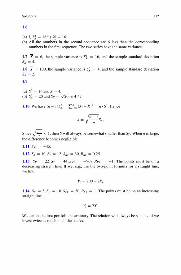
Solutions 317
1.6
(a) i) S2X D 16 ii) S2
X D 16.(b) All the numbers in the second sequence are 6 less than the corresponding
numbers in the first sequence. The two series have the same variance.
1.7 X D 6, the sample variance is S2X D 16, and the sample standard deviation
SX D 4.
1.8 X D 100, the sample variance is S2X D 4, and the sample standard deviation
SX D 2.
1.9
(a) S2 D 16 and S D 4.(b) S2
X D 20 and SX D p20 � 4:47:
1.10 We have .n � 1/S2X D Pn
iD1.Xi � X/2 D n � S2. Hence
S Dr
n � 1
nSX:
Sinceq
n�1n < 1, then S will always be somewhat smaller than SX . When n is large,
the difference becomes negligible.
1.11 SXY D �45.
1.12 SX D 10; SY D 12; SXY D 30; RXY D 0:25.
1.13 SX D 22; SY D 44; SXY D �968; RXY D �1. The points must be on adecreasing straight line. If we, e.g., use the two-point formula for a straight line,we find
Yi D 200 � 2Xi:
1.14 SX D 5; SY D 10; SXY D 50; RXY D 1. The points must be on an increasingstraight line.
Yi D 2Xi:
We can let the first portfolio be arbitrary. The relation will always be satisfied if weinvest twice as much in all the stocks.

318 Solutions
1.15
(a) nC14
D 1 C 34. The reminder is 3
4. We then start at observation number 1, i.e., 2
and move 75% of the distance to 6. The 1. quartile is hence
2 C 0:75 � .6 � 2/ D 5:
Furthermore 3.nC1/
4D 5C 1
4. and the reminder is 1
4. We then start at observation
number 5, i.e., 18 and move 25% of the distance to 22. The 3. quartile is hence
5 C 0:25 � .22 � 18/ D 19:
(b) Here nC14
D 2 and 3.nC1/
4D 6. Both reminders are zero and the 1. quartile is 6
and the 3.quartile is 18.(c) Here nC1
4D 2:25 and 3.nC1/
4D 6:75. The 1. quartile is hence
6 C 0:25 � .10 � 6/ D 7;
and the 3. quartile is
14 C 0:75 � .18 � 14/ D 17:
(d) Here nC14
D 2:5 and 3.nC1/
4D 7:5. The 1. quartile is hence
6 C 0:5 � .10 � 6/ D 8;
and the 3. quartile is
14 C 0:5 � .18 � 14/ D 16:
1.16
(a) X D 135:32. Write the data in column A from A1 to A25. Click in any entryoutside column A and write the command “=Average(A1:A25)” in the entry.Remember to write “=” in front of the command. If you press the return button,the answer 135.32 should be displayed in the entry.
(b) The sample variance is 93.31 and the sample standard deviation is 9.65971.(c) The quartiles are 127, 136, and 141. The 2. quartile is called the median.
Remark Excel does not use the definitions in Problem 1.15 to compute thequartiles. Instead it, e.g., computes the 1. quartile as the median of theobservations to the left of the median of the data. The difference is of nopractical significance but is part of the reason why we never entered into detailsabout quartiles in Chap. 1. As a rough thumb of rule a division by 4 will workfine to find the entry of the first quartile.

Solutions 319
Fig. 1 Prices as functions oftime
5 10 15 20
50
100
150
1.17
(a) a D 100; b D 100.(b) The result is shown in Fig. 1. The solid line shows the stock prices for ALPHA,
while the dashed line shows the stock prices for BETA. From the figure we seethat the values of BETA vary considerably more than the values of ALPHA, andBETA is hence the most insecure stock.
(c) S2a D 73:16; S2
b D 471:05. We see that S2b is considerably bigger than S2
a,reflecting the larger spread we see in the plot.
(d) A risk seeking investor will prefer a stock with a larger spread as it provides abigger chance of high returns. A risk averse investor will prefer a low spread.Which of the stocks ALPHA or BETA that is better is hence a matter of opinion.
(e) Sab D �122:26.(f)
Value of stocks D Number of stocks in ALPHA � Price per stock ALPHA
CNumber of stocks in BETA � Price per stock BETA
D Money used to buy ALPHA
Selling price ALPHA� an C Money used to buy BETA
Selling price BETA� bn
D 1;000;000 � x100
100� an C 1;000;000 � y
100
100� bn
D 100x � an C 100y � bn:
(g) c D 1;000;000.

320 Solutions
(h) Note that c D 100xa C 100yb and that y D 100 � x.
S2c D 1
19
20X
nD1
.cn � c/2 D 1
19
20X
nD1
.100 x an C 100 y bn � c/2
D 1
19
20X
nD1
.100 x .an � a/ C 100 y .bn � b//2
D 1
19
20X
nD1
1002 x2 .an � a/2 C 2 � 1002 x y .an � a/.bn � b/
C1002 y2 .bn � b/2
D 104�
x2 1
19
20X
nD1
.an � a/2 C 2 x y1
19
20X
nD1
.an � a/.bn � b/
Cy2 1
19
20X
nD1
.bn � b/2�
D 104.x2 S2a C 2x y Sab C y2 S2
b/
D 10;000.x273:16 C 2x .100 � x/.�122:26/ C .100 � x/2471:05/
D 1;000;000.7:8873 x2 � 1186:62 x C 47105/:
The minimum for this function is obtained at x � 75, i.e., if we want tominimize the variance of the investment we should buy 7500 stock in ALPHAand 2500 stocks in BETA.
1.18
(a) p D 4244:60 .USD/.(b) S2
p D 4;082;771:73.(c) Young people in low season: Mean category 1 D 3068:36 .USD/; S2
1 D74;256:62.
Young people in high season: Mean category 2 D 1889:25 .USD/; S22 D
33;761:88.Old people in low season: Mean category 3 D 3989:78 .USD/; S2
3 D31;572:53.Old people in high season: Mean category 4 D 7084:17 .USD/; S2
4 D97;390:52.
(d) The variance within each category is considerably smaller than the variance forthe whole sample. This means that the behavior within the categories is moreuniform than for the group seen as a whole. If the variance within a subgroup is

Solutions 321
Fig. 2 Constrained linearoptimization
500 1000 1500 2000 2500 3000
4000
2000
2000
4000
6000
zero, all people must spend the same amount. The variance is small only if allthe members of a category spend approximately the same amount of money.
(e) Optimization constraints
x � 0 y � 0 20x C 35y � 175;500
x � 20
100.5000 C x C y/ ) 4x � y � 5000:
See Fig. 2. The prices: Young people 2761:52 USD, Old people 3790:29
USD. We should then find the maximum of the function
f .x; y/ D 2761:52x C 3790:29;
under the constraints shown in the figure. LP-theory says that the maximumis obtained at the corners which are .0; 0/; .1250; 0/; .2191; 3763/; .0; 5014/. Ifwe insert these points into f .x; y/, we see that the biggest value is obtained using.2191; 3763/. With these prices maximum profit is hence obtained selling 2191
tickets to young people and 3763 tickets to old.(f) Call the unknown price for old people w, and find a value for w resulting in the
same profit in the two last corners reported in (e).
2191 � 2761:52 C 3763 � w D 0 � 2761:52 C 5014 � w:
We hence obtain equal profit in the two corners if w D 4836:52 (USD). If theprice on tickets to old people goes above this value, it will be more profitable tosell all the low price tickets to old people.
(g) Note that ˇ D 100�˛. The variance is hence a function of ˛. Using the numbersgiven in the text we obtain V.˛/ D 2˛2 � 4˛.100 � ˛/ C 4.100 � ˛/2. ThenV 0.˛/ D 20˛ � 1200. If we solve V 0.˛/ D 0, we find ˛ D 60; ˇ D 40. Thesevalues give the smallest possible variance.

322 Solutions
Problems of Chap. 2
2.1
˝ D fKKK; KKI; KIK; IKK; KII; IKI; IIK; IIIgA D fKKK; KKI; KIK; IKK; KII; IKI; IIKgB D fKKK; KKI; IKK; IKIgC D fKKK; IIIg:
2.2
(a) A [ B D f!1; !2; !3g; A \ B D f!1g; Ac D f!3; !4g; Bc D f!2; !4g.(b) .A \ B/ [ .Ac \ B/ D f!1g [ f!3g D f!1; !3g D B.(c) A [ .Ac \ B/ D f!1; !2g [ f!3g D f!1; !2; !3g D A [ B.
2.3
(a) P.A/ D 90%; P.Ac/ D 10%.(b) P.B/ D 85%; P.Bc/ D 15%.(c) P.A [ B/ D 1.(d) P.A \ B/ D 75%, A \ B D “There are between 1 and 9 errors”.
2.4
!1: Processing time is 1 day.!2: Processing time is 2 days.!3: Processing time is 3 days.!4: Processing time is 4 days.!5: Processing time is 5 days.!6: Processing time is 6 or more days.
We have
p1 D 0:1; p2 D 0:4; p3 D 0:3; p4 D 0:1; p5 D 0:05; p6 D 0:05:
These are all numbers between 0 and 1. In addition we see that
p1 C p2 C p3 C p4 C p5 C p6 D 0:1 C 0:4 C 0:3 C 0:1 C 0:05 C 0:05 D 1
This means that both conditions in the definition of a probability are satisfied.

Solutions 323
(b)
P.A/ D 0:1 C 0:4 D 0:5 D 50%:
P.B/ D 0:3 C 0:1 C 0:05 C 0:05 D 0:5 D 50%
(c) A D Bc.
2.5
(a) We have a sample space with 9 possible outcomes. For this to define aprobability p, we must have
0 � pi � 1; i D 1; : : : ; 9
and
p1 C p2 C � � � p9 D 1 D 100%:
The first requirement is clear. For the second we see that
9X
iD1
pi D 12%C9%C10%C25%C16%C5%C11%C9%C3% D 100% D 1:
Since the probabilities sum to 1, both conditions are satisfied.(b) (i) The good is of type Regular and is stored in warehouse 3.
P.A \ C/ D 11%:
(ii) The good is either of type Regular or it is stored in warehouse 3 (or both).
P.A [ C/ D 12% C 25% C 11% C 9% C 3% D 60%:
(iii) The good is of type Regular and Superior. This is impossible.
P.A \ B/ D 0:
(iv) The good is of type Regular or Superior.
P.A [ B/ D 12% C 25% C 11% C 9% C 16% C 9% D 82%:
Alternatively we use complements to see that
P.A [ B/ D 1 � 11% � 9% � 3% D 82%;
which is slightly more efficient.
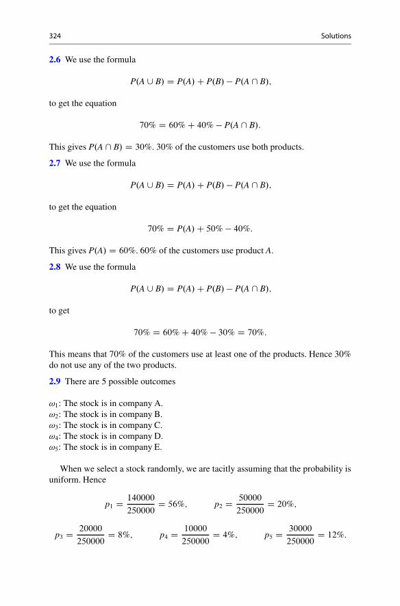
324 Solutions
2.6 We use the formula
P.A [ B/ D P.A/ C P.B/ � P.A \ B/;
to get the equation
70% D 60% C 40% � P.A \ B/:
This gives P.A \ B/ D 30%. 30% of the customers use both products.
2.7 We use the formula
P.A [ B/ D P.A/ C P.B/ � P.A \ B/;
to get the equation
70% D P.A/ C 50% � 40%:
This gives P.A/ D 60%. 60% of the customers use product A.
2.8 We use the formula
P.A [ B/ D P.A/ C P.B/ � P.A \ B/;
to get
70% D 60% C 40% � 30% D 70%:
This means that 70% of the customers use at least one of the products. Hence 30%do not use any of the two products.
2.9 There are 5 possible outcomes
!1: The stock is in company A.!2: The stock is in company B.!3: The stock is in company C.!4: The stock is in company D.!5: The stock is in company E.
When we select a stock randomly, we are tacitly assuming that the probability isuniform. Hence
p1 D 140000
250000D 56%; p2 D 50000
250000D 20%;
p3 D 20000
250000D 8%; p4 D 10000
250000D 4%; p5 D 30000
250000D 12%:

Solutions 325
2.10
(a) (i)
P.A \ B/ D P.A/ C P.B/ � P.A [ B/ D 60% C 50% � 82% D 28%:
(ii)
P.A \ C/ D P.A/ C P.C/ � P.A [ C/ D 60% C 45% � 73% D 32%:
iii)
P.B \ C/ D P.B/ C P.C/ � P.B [ C/ D 50% C 45% � 74% D 21%:
(b)
P.A \ B \ C/
D P.A [ B [ C/
� . P.A/ C P.B/ C P.C/ � P.A \ B/ � P.A \ C/ � P.B \ C//
D 89% � 60% � 50% � 45% C 28% C 32% C 21% D 15%:
2.11
(a) The customers liking both A and B were numbers
3; 7; 11; 18; 19; 20; 27; 33; 34; 39; 42; 43; 49; 53; 56; 57; 60; 61; 62; 65; 67; 71;
72; 73; 74; 76; 78; 80:
(b) The customers liking at least one of the two products were
1; 2; 3; 4; 5; 6; 7; 8; 9; 10; 11; 12; 13; 15; 16; 17; 18; 19; 20; 22; 23;
24; 25; 27; 28; 30; 31; 32; 33; 34; 35; 36; 37; 38; 39; 40; 41; 42; 43; 44;
45; 47; 48; 49; 50; 51; 52; 53; 54; 55; 56; 57; 58; 59; 60; 61; 62; 65; 67;
68; 69; 70; 71; 72; 73; 74; 75; 76; 77; 78; 79; 80:
(c) (i) A total of 60 customers liked A, i.e., 60%.(ii) A total of 40 customer liked B, i.e., 40%.
(iii) A total of 28 customers liked both A and B, i.e., 35%.(iv) A total of 72 customers liked at least one of the two products, i.e., 90%.

326 Solutions
(d)
90% D 75% C 50% � 35%;
which illustrates the general addition principle.
Problems of Chap. 3
3.1 As there are no connections between the choices, there are in all
103 � 43 � 39 D 172731;
different ways of making the portfolio.
3.2 The order makes a difference for how the money is invested, and since the fundsmust be different, the choices are without replacements. The number of differentcombinations is hence
.10/3 D 10 � 9 � 8 D 720:
3.3 This is an ordered choice, since the order of the ranking makes a difference.For example will the ranking 7; 2; 11; 19; 15 (where product 7 is best) be differentfrom the ranking 2; 7; 11; 19; 15 (where product 2 is best). A product can only beranked once, and hence the choice is without replacement. The number of differentcombinations is
.20/5 D 20 � 19 � 18 � 17 � 16 D 1;860;480:
3.4 In this problem the order makes no difference for how the money are invested,and the choices are without replacements. The number of different combinations is
�10
4
�D 210:
3.5 This is an unordered choice, since the order makes no difference for the result.For example will the sequence 2; 5; 11; 12 provide the same result as the sequence5; 2; 11; 12 since the same goods have been chosen in both cases. The number ofdifferent combinations is
�15
4
�D 1365:
3.6 We choose 3 of the numbers 1–5, unordered without replacement. We interpretthe 3 numbers as the position of our correct answers. The choices are unordered

Solutions 327
since the order makes no difference. For example will the sequence 1; 3; 5 lead tothe same result as the sequence 5; 1; 3 since they both have the same interpretation:Answers 1, 3, and 5 are correct, while answers 2 and 4 are wrong. The choiceis without replacements since the positions must be different. Any such choicecorresponds to a combination of answers with exactly 3 correct answers. Thenumber of different combinations is
�5
3
�D 10:
3.7 We choose 5 of the numbers 1–20, unordered without replacement. These5 numbers we interpret as the position of our correct answers. Any such choicecorresponds to an answer combination with exactly 5 correct answers, hence thenumber of different combinations is
�20
5
�D 15;504:
3.8 In this problem the order of the funds makes no difference, so we use theformulas for unordered choices without replacements.
(a) There is in all�
30
6
�D 593;775 different combinations of funds.
(b) (i) The probability that you have selected the best fund is
�295
�
�60
6
� D 20%:
(ii) The probability that you have selected the two best funds is
�284
�
�606
� D 1
29� 3:4%:
3.9
(a) The probability that you receive the questionnaire is
�11
� �9999999
�
�100001000
� D 1
10:
You hence have 10% probability of receiving the questionnaire.

328 Solutions
(b) The probability that you and your nearest neighbor receive the questionnaire is
�22
� �9998998
�
�100001000
� D 111
11;110� 0:009991:
Note that the answer is slightly different from the seemingly obvious (andwrong) answer 1
100.
3.10 The probability that you do not receive the questionnaire is
�N�1
n
�
�Nn
� D.N�1/Š
nŠ.N�n�1/Š
NŠnŠ.N�n/Š
D nŠ.N � n/Š.N � 1/Š
nŠ.N � n � 1/ŠNŠD N � n
ND 1 � n
N:
The probability that you receive the questionnaire is hence nN .
3.11
(a) There are�
82
�D 28 different cooperation documents.
(b) There are .8/2 D 56 different executive officers.
3.12
(a) The probability that none of the crates contain errors is
�912
�
�1052
� D 75%:
(b) The probability that at least one of the crates contain errors is
�141
� �911
�
�1052
� C�
142
�
�1052
� D 25%:
Notice that a much simpler solution is to take the complement of the answerfrom (a).
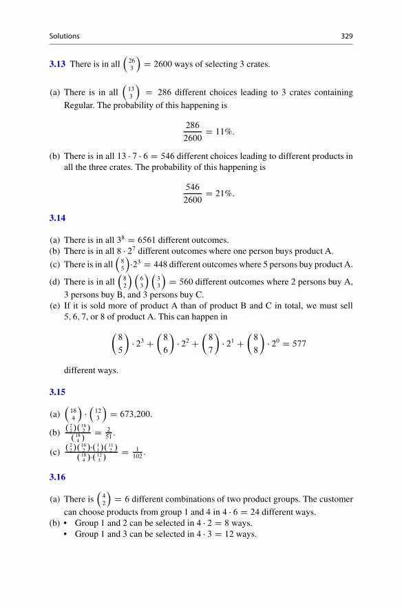
Solutions 329
3.13 There is in all�
263
�D 2600 ways of selecting 3 crates.
(a) There is in all�
133
�D 286 different choices leading to 3 crates containing
Regular. The probability of this happening is
286
2600D 11%:
(b) There is in all 13 � 7 � 6 D 546 different choices leading to different products inall the three crates. The probability of this happening is
546
2600D 21%:
3.14
(a) There is in all 38 D 6561 different outcomes.(b) There is in all 8 � 27 different outcomes where one person buys product A.
(c) There is in all�
85
��23 D 448 different outcomes where 5 persons buy product A.
(d) There is in all�
82
� �63
� �33
�D 560 different outcomes where 2 persons buy A,
3 persons buy B, and 3 persons buy C.(e) If it is sold more of product A than of product B and C in total, we must sell
5; 6; 7, or 8 of product A. This can happen in
�8
5
�� 23 C
�8
6
�� 22 C
�8
7
�� 21 C
�8
8
�� 20 D 577
different ways.
3.15
(a)�
184
���
123
�D 673;200.
(b) . 22 /. 16
2 /. 18
4 /D 2
51.
(c) . 22 /. 16
2 /�. 11 /. 11
2 /. 18
4 /�. 123 /
D 1102
.
3.16
(a) There is�
4
2
�D 6 different combinations of two product groups. The customer
can choose products from group 1 and 4 in 4 � 6 D 24 different ways.(b) • Group 1 and 2 can be selected in 4 � 2 D 8 ways.
• Group 1 and 3 can be selected in 4 � 3 D 12 ways.

330 Solutions
• Group 1 and 4 can be selected in 4 � 6 D 24 ways.• Group 2 and 3 can be selected in 2 � 3 D 6 ways.• Group 2 and 4 can be selected in 2 � 6 D 12 ways.• Group 3 and 4 can be selected in 3 � 6 D 18 ways.
There is hence a total of 80 different combinations.(c) When we choose the second product, the number of products we can choose
between will depend on which group we selected first. If we order the productsfrom number 1 to number 15, is, e.g., the probability of the combination .1; 5/
equal to 1=15 � 1=11 C 1=15 � 1=13 and the probability of the combination .5; 7/
equal to 1=15 � 1=13 C 1=15 � 1=12. Those probabilities are not equal.(d) The probability of this is 4=15 � 6=11 C 6=15 � 4=9 D 32=99.
3.17
(a) There are 320 different combinations.�
2019
�� 2 D
�201
�� 2 D 40 of these contain
19 correct and one wrong answer.(b) X D BinŒ20; p� with p D 1
3.
P.X D 14/ D�
20
14
�p14.1 � p/6 D
�20
14
�26
320:
(c)
P.X D 14/ D�
10
4
�p4.1 � p/6 D 22:8%:
P.X � 13/ D 1 � P.X � 12/
D 1 � P.X D 10/ � P.X D 11/ � P.X D 12/
D 1 ��
10
0
�210
310��
10
1
�29
310��
10
2
�28
310D 70:1%:
3.18
(a) There are�
7510
�D 828931106355 different portfolios. The probability that
the company has 4 average, 3 good, and 3 very good funds is given by theexpression:
�154
� �103
� �53
�
�7510
� � 2:0 � 10�6:

Solutions 331
(b) If none of the funds are good or very good, the selection must be made from theremaining 60 funds. The probability is hence
�6010
�
�7510
� � 9:1%:
To find the probability of at least one very good fund, we first find the probabilityof none very good funds and consider the complement. Hence the probability is
1 ��
70
10
�
�7510
� � 52:1%:
3.19
(a) If there are 5 transactions, the list needs to contain all the 5 sellers. In additionwe need to select 5 buyers from the 10 potential buyers. The order makes nodifference, hence the selection is unordered without replacement. There is
�10
5
��5
5
�D 252:
different combinations with 5 transactions.(b) With x transactions, the number of different combinations is given by
�10
x
��5
x
�:
This leads to Table 1.There are in all 3003 different combinations. If all of these are equally
probable, we find the probabilities dividing the numbers in the previous tableby 3003, Table 2.
The most probable number of transactions is hence 3 units.
Table 1 Number of combinations as a function of the number of transactions
Number of transactions 0 1 2 3 4 5
Number of combinations 1 50 450 1200 1050 252
Table 2 Probability as a function of the number of transactions
Number of transactions 0 1 2 3 4 5
Probability 0.0003 0.0167 0.1499 0.3996 0.3497 0.0839

332 Solutions
Table 3 Number of different lists as a function of the number of transactions
Number of transactions 0 1 2 3 4 5
Number of different lists 1 50 900 7200 25;200 30;240
(c) When the number of transactions is x, any choice of x buyers can be combinedwith any choice of x sellers in xŠ different ways. The number of unique lists ishence given by the expression
�10
x
��5
x
�xŠ:
This leads to Table 3.
3.20
(a) We can, e.g., reason as follows: First we select which customers buy A. Thiscan be done in
�10x
�different ways. After selection of these customers, there are
10 � x customers left. Among these we choose y customers buying B. This canbe done in
�10�x
y
�different ways. Finally we are left with 10 � x � y customers
and z of these buy C. Note that z D 10�x�y, and the last factor is always equalto 1.
Using the definition of the binomial coefficients, we get
10
x
! 10 � x
y
! 10 � x � y
z
!D 10Š
xŠ.10 � x/Š
.10 � x/Š
yŠ.10 � x � y/Š
.10 � x � y/Š
zŠ.10 � x � y � z/Š
D 10Š
xŠyŠzŠ0ŠD 10Š
xŠyŠzŠ
since 0Š D 1.(b) The probability of each combination leading to 3 customers buying A, 2
customers buying B, and 5 customers buying C is 0:33 � 0:22 � 0:55. There are10Š
3Š2Š5Šdifferent such combinations, and since these are all disjoint, the probability
becomes
10Š
3Š2Š5Š0:33 � 0:22 � 0:55 D 8:5%:
(c) There are 6 different outcomes leading to at least 8 customers buying A:
.8; 0; 2/; .8; 1; 1/; .8; 2; 0/; .9; 0; 1/; .9; 1; 0/; .10; 0; 0/:

Solutions 333
The probability P for these outcomes is computed as follows:
P D 10Š
8Š0Š2Š0:38 � 0:20 � 0:52 C 10Š
8Š1Š1Š0:38 � 0:21 � 0:51
C 10Š
8Š2Š0Š0:38 � 0:22 � 0:50 C 10Š
9Š0Š1Š0:39 � 0:20 � 0:51
C 10Š
9Š1Š0Š0:39 � 0:21 � 0:50 C 10Š
10Š0Š0Š0:310 � 0:20 � 0:50 D 0:16%:
Problems of Chap. 4
4.1 We use the definition of conditional probability to get
P.Sj F/ D P.S \ F/
P.F/D 14%
35%D 40%:
P.FjS/ D P.F \ S/
P.S/D 14%
56%D 25%:
Hence 40% of the Favorite users use Super, and 25% of the Super users use Favorite.
4.2 We use the definition of conditional probability to get
P.Sj F/ D P.S \ F/
P.F/) 0:50 D 0:20
P.F/:
P.FjS/ D P.F \ S/
P.S/) 0:25 D 0:20
P.S/:
This gives P.F/ D 0:4 and P.S/ D 0:8. Hence 40% use Favorite and 80% useSuper.
4.3 We use the formulas for splitting to see that
P.L/ D P.LjM/ � P.M/ C P.LjK/ � P.K/ D 40% � 160
400C 20% � 240
400D 28%:
Hence 28% like the product.
4.4
(a) The result is displayed in Fig. 3.(b) The fraction invested in China is 18% C 32% D 50%:

334 Solutions
Fig. 3 Solution toProblem 4.4 (a)
Investments
30 70 80 20
Mutual funds Money market
60 40
China Other
18 42
China Other
32 8
Fig. 4 Solution toProblem 4.5 (a)
Company
3 97 6 94 2 98
A B C
20 45 35
Error OK Error OK
0.6 19.4
Error OK
2.7 42.3 0.7 34.3
(c) The fraction of mutual funds among the investments in China is
P.MjCh/ D P.M \ Ch/
P.Ch/D 0:18
0:5D 36%:
4.5
(a) The result is displayed in Fig. 4.(b) The fraction of reports with errors is
0:6% C 2:7% C 0:7% D 4%:
(c) The probability that a report with errors has been made at department A is
P.AjErr/ D P.A \ Err/
P.Err/D 0:006
0:04D 15%:
4.6
(a) Here we have
P.A/ � P.B/ D 0:6 � 0:4 D 0:24 D P.A \ B/;
which means that A and B are independent events.

Solutions 335
(b) We have
P.A/ D P.A \ B/ C P.A \ Bc/ D P.A \ B/ C P.A \ C/:
This gives
P.A \ B/ D P.A/ � P.A \ B/ D 0:6 � 0:24 D 0:36:
Hence
P.A/ � P.C/ D 0:6 � 0:6 D 0:36 D P.A \ C/;
which means that A and B are independent events.(c) Here
P.B/ � P.C/ D 0:4 � 0:6 6D 0 D P.B \ C/:
This means that B and C are not independent events.
4.7 We have
P.A/ D P.A \ B/ C P.A \ Bc/ D P.A \ B/ C P.A \ C/:
That gives
P.A \ C/ D P.A/ � P.A \ B/:
Furthermore
P.A/ � P.C/ D P.A/.1 � P.B// D P.A/ � P.A/ � P.B/
D P.A/ � P.A \ B/ D P.A \ C/:
Hence A and C are independent.
4.8
(a) We have
P.AjB/ D 60% D P.A \ B/
P.B/;
which gives
P.A \ B/ D 60% � P.B/ D P.A/ � P.B/:
This shows that A and B are independent.

336 Solutions
(b) In general, when P.B/ 6D 0, then A and B are independent if and only if P.A/ DP.AjB/. This can be seen as follows:(i) Assume that A and B are independent, then
P.AjB/ D P.A \ B/
P.B/D P.A/ � P.B/
P.B/D P.A/:
(ii) Assume P.A/ D P.AjB/, then
P.A/ D P.AjB/ D P.A \ B/
P.B/:
If we multiply with P.B/ on both sides, we find
P.A/ � P.B/ D P.A \ B/;
proving that A and B are independent.
4.9
(a)
P.AABC/ D 0:5 � 0:5 � 0:2 � 0:3 D 1:5%:
(b) The following combinations provide the required result:
AAAA; AAAB; AABA; ABAA; BAAA; AAAC; AACA; ACAA; CAAA:
The probability is hence
P.At least 4 customers buy A/ D 0:5 � 0:5 � 0:5 � 0:5
C4 � 0:5 � 0:5 � 0:5 � 0:2 C 4 � 0:5 � 0:5 � 0:5 � 0:3 D 31:25%:
(c) The following combinations provide the required result:
CCAA; CACA; CAAC; ACCA; ACAC; AACC;
CCAB; CACB; CABC; ACCB; ACBC; ABCC;
CCBA; CBCA; CBAC; BCCA; BCAC; BACC;
CCBB; CBCB; CBBC; BCCB; BCBC; BBCC:

Solutions 337
Fig. 5 Solution toProblem 4.10 (a)
Company
0.4
0.6
A
B
0.5
0.5
1 3
1 3
1 3
A1
A2
B1
B2
B3
0.25
0.5
0.25
0.1
0.7
0.2
0.4
0.5
0.1
0.2
0.6
0.2
0.3
0.6
0.1
Good
Average
Bad
Good
Average
Bad
Good
Average
Bad
Good
Average
Bad
Good
Average
Bad
0.10
0.05
0.05
0.02
0.14
0.04
0.08
0.10
0.02
0.04
0.12
0.04
0.06
0.12
0.02
The probability is hence
P.2 customers buy C/ D 6 � 0:3 � 0:3 � 0:5 � 0:5
C12 � 0:3 � 0:3 � 0:5 � 0:2 C 6 � 0:3 � 0:3 � 0:2 � 0:2 D 26:46%:
4.10
(a) The result is displayed in Fig. 5.(b)
P.GjB/ D P.G \ B/
P.B/D 0:08 C 0:04 C 0:06
0:6D 0:3:
(c)
P.AjG/ D P.A \ G/
P.G/D 0:1 C 0:02
0:1 C 0:02 C 0:08 C 0:04 C 0:06D 0:4:

338 Solutions
(d) We compute
P.G \ B/ � P.G/ � P.B/
D .0:08 C 0:04 C 0:06/
�.0:1 C 0:02 C 0:08 C 0:04 C 0:06/ � .0:6/ D 0:
This means that P.G \B/ D P.G/ � P.B/ which means that the event G D Goodis independent of the event B D Executed at department B.
4.11
(a) We use the formulas for splitting to see that
P.L/ D P.LjK25�/P.K25�/ C P.LjK25 � 40/P.K25 � 40/
CP.LjK40C/P.K40C/ C P.LjM25�/P.M25�/
CP.LjM25 � 40/P.M25 � 40/ C P.LjM40C/P.M40C/
D 0:6 � 0:15 C 0:3 � 0:3 C 0:8 � 0:15
C0:2 � 0:2 C 0:4 � 0:1 C 0:6 � 0:1 D 44%:
(b) The women made up 60% of the participants, hence
P.K25�jK/ D P.K25�/
P.K/D 0:15
0:60D 25%:
(c) The fraction of the women liking the product, we find from
P.LjK/ D P.LjK25�/P.K25�jK/ C P.LjK25 � 40/P.K25 � 40jK/
CP.Lj40C/P.40CjK/
D 0:6 � 0:15
0:60C 0:3 � 0:3
0:60C 0:8 � 0:15
0:60D 50%:
The fraction of the men liking the product, we find from
P.LjM/ D P.LjM25�/P.M25�jM/ C P.LjM25 � 40/P.M25 � 40jM/
CP.Lj40C/P.40CjM/
D 0:2 � 0:20
0:40C 0:4 � 0:1
0:40C 0:6 � 0:1
0:40D 35%:

Solutions 339
Fig. 6 Solution toProblem 4.12 (a)
Funds
0.3
0.6
0.1
A
B
C
0.5
0.3
0.2
0.2
0.7
0.1
0.3
0.5
0.2
USA
Europe
China
USA
Europe
China
USA
Europe
China
0.15
0.09
0.06
0.12
0.42
0.06
0.03
0.05
0.02
4.12
(a) The result is displayed in Fig. 6.
(b) P.USAjGlobal/ D P.USA\Global/P.Global/ D 0:15C0:12
0:3C0:6D 30%.
(c) P.Global AjUSA/ D P.USA\Global A/
P.USA/D 0:15
0:15C0:12C0:03D 50%:
(d) No. The customers may invest amounts of unequal size. If, e.g., 99 customershave invested a small amount in Global A, and one large investor the rest,the answer will be different from the case where everybody invested the sameamount in all the different funds.
4.13
(a) Ignoring leap years, there are 243 possible days of birth from January 1 toAugust 31. This gives P.Category 1/ D 243
365� 66:6% and P.Category 2/ D
122365
� 33:4%. (An answer based on months is sufficient). P.YesjCategory 1/ D0:5.
(b) We get the equation
P.Yes/ D P.YesjCategory 1/ � P.Category 1/
CP.YesjCategory 2/ � P.Category 2/:
Inserting the information provided in the text, we get
0:60 D 0:5 � 0:666 C P.YesjCategory 2/ � 0:334
If we solve this equation, we find P.YesjCategory 2/ � 80%.

340 Solutions
(c) The advantage of swapping is that twice as many will answer the relevantquestion. A disadvantage can be less feeling of anonymity. After swapping amajority will answer the sensitive question, and more might answer No hidingthe true answer to the person who carries out the survey.
4.14
(a) We let I mean that the person has the illness, and C denote that the test ispositive. The information in the text says P.CjI/ D 0:77; P.CjIc/ D 0:02 andthat P.I/ D 0:02. Hence P.Ic/ D 0:98, and we find
P.C/ D P.CjI/ � P.I/ C P.CjIc/ � P.Ic/ D 0:77 � 0:02 C 0:02 � 0:98 D 3:5%:
We use the result above to find
P.IjC/ D P.CjI/ � P.I/
P.C/D 0:77 � 0:02
0:035D 44%:
(b,c) If the person is not randomly selected, the analysis in (a) does not apply. If theperson is tested because he or she has symptoms, the test is executed withina subpopulation where the probability of P.I/ can be much larger than 2%.In the most extreme case the symptoms can be so strong that we know forsure that the person has the illness, i.e., P.I/ D 1, in which case P.IjC/ D 1
as well. The probability that the person has the illness can hence be arbitrarylarge.
4.15 Let B denote the event “The company goes bankrupt,” and let F denote theevent “The company is flagged for bankruptcy.” The information given in the textcan be formulated as follows:
P.FjB/ D 0:8; P.FcjBc/ D 0:95:
(a) P.FjBc/ D 1 � P.FcjBc/ D 0:05 D 5%, i.e., 5% of the firms that do not gobankrupt are flagged for bankruptcy.
P.F/ D P.FjB/ � P.B/ C P.FjBc/ � P.Bc/ D 0:8 � 0:1 C 0:05 � 0:9 D 0:125 D 12:5%:
The model will hence predict that 12.5% of the firms will go bankrupt.(b) We use Bayes’ formula to get
P.Bj F/ D P.B/
P.F/� P.FjB/ D 0:1
0:125� 0:8 D 0:64 D 64%:
There is hence 64% probability a firm flagged for bankruptcy will in fact gobankrupt.

Solutions 341
4.16
(a) (i) We have a time development Good-Good-Good. The probability of remain-ing good after one time step is 0.7, and the probability of this happeningtwice is 0:7 � 0:7 D 49%.
(ii) There are two possibilities: GGG with probability 0:7 � 0:7 D 0:49, andGBG with probability t 0:3 � 0:2 D 0:06. The total probability is 55%.
(b) There are 10 different variants. The first is GGGGGGGGGGD with probability0:79 � 0:3. All the 9 other variants have probability 0:78 � 0:3 � 0:2. In total theprobability becomes
0:79 � 0:3 C 9 � 0:78 � 0:3 � 0:2 D 4:32%:
(c) Several different issues can be discussed here. Causes for things going bad areimportant for independence. If, e.g., the person has lost his or her job, it is likelythat payments will continue to be bad. If the economy goes bad in general, it islikely that many customers will be affected, leading to dependence.
4.17
(a) In the first six months company A found 6% errors, while company B found 5%errors. Company A had hence the best results in the first six months. In the nextsix months company A found 3% errors, while company B found 2% errors.Company A had hence the largest probability of finding errors in the secondhalf of the year.
The year seen as a whole, company A found 3.6% errors, while company Bfound 4.4% errors. Company B hence have the best results for the year seen asa whole.
(b) The explanation is that there were a lot more errors in the first six months, andcompany B comes out as the overall winner since they focused their activityto the most important time period. Remark: The phenomenon is well known instatistics and is commonly referred to as the Yule-Simpson paradox.
4.18
(a) We use splitting to see that
P.A/ D P.AjB/P.B/ C P.AjW/P.W/ C P.AjS/P.S/
D 0:025 � 0:1 C 0:15 � 0:15 C 0:30 � 0:75
D 0:25 D 25%:

342 Solutions
(b) Here we use Bayes’ law
P.BjA/ D P.AjB/ � P.B/
P.A/D 0:025 � 0:1
0:25D 0:01 D 1%:
4.19 F D The company is flagged for bankruptcy. B D The company does in factgo bankrupt.
(a)
P.F/ D P.FjB/P.B/ C P.FjBc/P.Bc/ D P.FjB/ � 0:001 C 0:05 � 0:999
� 1 � 0:001 C 0:05 � 0:999 D 0:05095:
(b)
P.Bcj F/ D P.FjBc/ � P.Bc/
P.F/D 0:05 � 0:999
P.F/� 0:05 � 0:999
0:05095D 0:9804:
This means that a huge majority of the firms that are flagged for bankruptcy willin fact not go bankrupt.
Remark The tool flags 5% of the companies that do not go bankrupt. As we can seefrom the calculations, this does not mean that 95% of the flags are correct. Quite thecontrary, at least 98% of the flagged companies will not go bankrupt. Regrettably,this confusion of terms is a common misconception.
4.20
(a) Let p denote participation in the poll, and let up mean that the person would liketo see an increase in taxes. Then
P. p/ D P. pjup/P.up/ C P. pjupc/P.upc/ D 0:02 � 0:6 C 0:07 � 0:4 D 4%:
(b) We use Bayes’ law:
P.upj p/ D P. pjup/ � P.up/
P. p/D 0:07 � 0:4
0:04D 70%:
We see that 70% of the participants in the poll would like to see an increase intaxes, while a majority of the viewers do not want that.
4.21 We let S denote the event that the currency is strengthening, H denotes higheconomic growth, A denotes average economic growth, and L denotes low economicgrowth.

Solutions 343
(a) From the splitting principle we get
P.S/ D P.SjH/P.H/ C P.SjA/P.A/ C P.SjL/P.L/
D 0:7 � 0:3 C 0:5 � 0:5 C 0:2 � 0:2 D 0:5 D 50%:
The probability of strengthening of the currency is hence 50%.(b) We use Bayes’ law and find
P.HjS/ D P.SjH/ � P.H/
P.S/D 0:7 � 0:3
0:5D 0:42 D 42%:
If the currency is strengthening, it is hence 42% probability of high economicgrowth.
(c) We have
P.S \ H/ D P.SjH/P.H/ D 0:7 � 0:3 D 0:21
P.S/ � P.H/ D 0:5 � 0:3 D 0:15:
Since the two values do not match, the events S and H are dependent.
4.22
(a)
P.debt/ D P.debtjspam/P.spam/ C P.debtjspamc/P.spamc/
D 0:309 � 0:5 C 0:00447 � 0:5 D 15:67%:
(b)
P.spamjdebt/ D P.debtjspam/ � P.spam/
P.debt/D 0:309 � 0:5
0:1567D 98:6%:
4.23
(a) We define S: a tax payer is in the special group, F: the tax payer commits taxfraud. With this notation the information in the text can be stated as follows:
P.S/ D 0:05; P.F/ D 0:1; P.Sj Fc/ D 0:01:
(b)
P.S/ D P.Sj F/P.F/ C P.Sj Fc/P.Sc/:

344 Solutions
This leads us to the equation
0:05 D P.Sj F/ � 0:1 C 0:01 � 0:9:
Solving this equation, we find P.Sj F/ D 0:41 D 41%:
(c) Bayes’ rule gives
P.FjS/ D P.Sj F/ � P.F/
P.S/D 0:41 � 0:1
0:05D 82%:
4.24
(a) P.DjS18 � 24/ D 3:6%, P.S18 � 24/ D 55=582 D 9:45%.
P.DjS/ D P.DjS18 � 24/ � P.S18 � 24/ C P.DjS25 � 34/ � P.S25 � 34/
CP.DjS35 � 44/ � P.S35 � 44/ C P.DjS45 � 54/ � P.S45 � 54/
C � � � C P.DjS75C/ � P.S75C/
D 0:036 � 55
582C 0:024 � 124
582C 0:128 � 109
582C 0:208 � 130
582
C0:443 � 115
582C 0:806 � 36
582C 1:0 � 13
582D 23:87%:
(b) P.DjNS18 � 24/ D 1:6%, P.NS18 � 24/ D 62=734 D 8:45%.
P.DjNS/ D P.DjNS18 � 24/ � P.NS18 � 24/ C P.DjNS25 � 34/ � P.NS25 � 34/
CP.DjNS35 � 44/ � P.NS35 � 44/ C P.DjNS45 � 54/ � P.NS45 � 54/
C � � � C P.DjNS75C/ � P.NS75C/
D 0:16 � 62
734C 0:032 � 157
734C 0:057 � 123
734C 0:154 � 78
734
C0:331 � 121
734C 0:783 � 129
734C 1:0 � 64
734D 31:35%:
(c) We see that the death rate for smokers (23.87%) is considerably lower thanfor nonsmokers (31.35%). If we compare the numbers in the tables, we see(with a marginal exception for the group 25–34) that the death rate for smokersis considerably higher than for nonsmokers. The reason why we come to theopposite conclusion for the groups seen as a whole is that there are relativelyfewer elderly smokers among the participants. Regrettably, the elderly smokerswere already dead when the sample was drawn.

Solutions 345
Problems of Chap. 5
5.1 (i), (ii), (iii), (v), and (vi) all give out a real number as the result, and hencedefine random variables. The outcome of a soccer match, e.g., 2–2, is a pair ofnumbers and does not define a random variable (but the results for each team arerandom variables).
5.2
(a) The stock price can only have the values 95;100, and 110.(b) The definition of the cumulative distribution is F.x/ D P.X � x/. F.90/ is
hence the probability that the stock price is at most 90 USD. Since the stockprice is never less than 95 USD, F.90/ D 0. Furthermore,
F.95/ D 20%; F.100/ D 20% C 70% D 90%; F.105/ D 90%;
F.110/ D 20% C 70% C 10% D 100%; F.115/ D 100%:
5.3
(a) There are 6 different outcomes: AA; BB; CC; AB; AC; BC. Note that AB and BAgive the same outcome here. The probabilities of AA; BB; CC are all 1
9, while
the probabilities of AB; AC; BC are all 29.
(b) AA gives X D 200, BB gives X D 208, CC gives X D 204, AB gives X D 204,AC gives X D 202, and BC gives X D 206. X can hence achieve 5 differentvalues; 200; 202; 204; 206; 208. The distribution of X is as follows:
P.X D 200/ D 1
9; P.X D 202/ D 2
9; P.X D 204/ D 3
9;
P.X D 206/ D 2
9; P.X D 208/ D 1
9:
(c) We find the cumulative distribution when we progressively add the values in theprobability distribution, i.e.
F.200/ D 1
9; F.202/ D 1
9C 2
9D 3
9; F.204/ D 1
9C 2
9C 3
9D 6
9;
F.206/ D 1
9C 2
9C 3
9C 2
9D 8
9; F.208/ D 1
9C 2
9C 3
9C 2
9C 1
9D 1:
The interpretation is that F.x/ is the probability that the value of the stocks is atmost x USD.

346 Solutions
5.4
(a) Regardless of outcome, X becomes an integer between 1 and 6 and is hence arandom variable.
(b) We find the cumulative distribution when we progressively add the probabilitiesin the table, i.e.
F.1/ D 55%; F.2/ D 55% C 20% D 75%;
F.3/ D 55% C 20% C 10% D 85%
F.4/ D 55% C 20% C 10% C 5% D 90%;
F.5/ D 55% C 20% C 10% C 5% C 5% D 95%;
F.6/ D 55% C 20% C 10% C 5% C 5% C 5% D 1:
When x is an integer, we can interpret F.x/ as the probability that the deliverytime is at most x days.
EŒX� D 1 � 0:55 C 2 � 0:2 C 3 � 0:1 C 4 � 0:05 C 5 � 0:05 C 6 � 0:05 D 2:
The expected delivery time is hence 2 days.
5.5
(a) We have
P.4 or more errors/
D 1 � P.X D 0/ � P.X D 1/ � P.X D 2/ � P.X D 3/
D 1 � 0:65 � 0:25 � 0:05 � 0:05 D 0:
(b)
EŒX� D 0 � 0:65 C 1 � 0:25 C 2 � 0:05 C 3 � 0:05 D 0:5:
5.6
p.100/ D 140000
400000D 56%; p.200/ D 50000
400000D 20%;
p.300/ D 10000
400000D 4%; p.400/ D 20000
400000D 8%;
p.500/ D 30000
400000D 12%:
EŒX� D 100 � 0:56 C 200 � 0:2 C 300 � 0:04 C 400 � 0:08 C 500 � 0:12 D 200:

Solutions 347
5.7
EjX� D 0 � 0:2 C 1 � 0:2 C 2 � 0:6 D 1:4:
VarŒX� D EŒX2� � EŒX�2
D 02 � 0:2 C 12 � 0:2 C 22 � 0:6 � 1:42 D 0:64:
�ŒX� D pVarŒX� D p
0:64 D 0:8:
5.8
EjX� D 0 � 0:025 C 1 � 0:05 C 2 � 0:825 C 3 � 0:1 D 2:
VarŒX� D EŒX2� � EŒX�2
D 02 � 0:025 C 12 � 0:05 C 22 � 0:825 C 32 � 0:1 � 22 D 0:25:
�ŒX� D pVarŒX� D p
0:25 D 0:5:
5.9
EjX� D 1 � 0:1 C 2 � 0:1 C 3 � 0:6 C 4 � 0:1 C 5 � 0:1 D 3:
VarŒX� D EŒX2� � EŒX�2
D 12 � 0:1 C 22 � 0:1 C 32 � 0:6 C 42 � 0:1 C 52 � 0:1 � 92 D 1:
�ŒX� D pVarŒX� D p
1 D 1:
5.10
(a)
EŒX1 C X2 C X3� D EŒX1� C EŒX2� C EŒX3� D 25 C 25 C 25 D 75:
(b)
EŒ pX1 C qX2 C rX3� D pEŒX1� C qEŒX2� C rEŒX3� D 25. p C q C r/ D 25:

348 Solutions
5.11
EŒ Y� D EŒ pX Cq �100� D pEŒX�Cq �100 D p �100Cq �100 D 100. p Cq/ D 100:
VarŒ Y� D VarŒ pX C q � 100� D VarŒ pX� D p2VarŒX� D 100p2:
The variance becomes as small as possible when we choose p D 0 and q D 1.
5.12
(a)
EŒX� D 30 � 0:6 C 90 � 0:4 D 114:
(b) We need to solve
130 � p C 90 � .1 � p/ D 120:
This implies
130p C 90 � 90p D 120 ) 30p D 40;
which gives p D 75%. The probability that the contract is accepted must be at least75%.
5.13
(a) We first find EŒX� D 1 � 0:5 C 2 � 0:3 C 3 � 0:2 D 1:7: That gives
EŒZ� D EŒX1� C EŒX2� C EŒX3� D 1:7 C 1:7 C 1:7 D 5:1:
The expected waiting time is 5.1 min in this case.(b)
P.Z � 7/ D 1 � P.Z D 8/ � P.Z D 9/:
Z D 8 in the three cases .X1; X2; X3/ D .3; 3; 2/; .3; 2; 3/; .2; 3; 3/. That gives
P.Z D 8/ D 0:2 � 0:2 � 0:3 C 0:2 � 0:3 � 0:2 C 0:3 � 0:2 � 0:2 D 0:036:
Z D 9 only in the case .X1; X2; X3/ D .3; 3; 3/, giving
P.Z D 9/ D 0:2 � 0:2 � 0:2 D 0:008:
In total we get
P.Z � 7/ D 1 � 0:036 � 0:008 D 95:6%:

Solutions 349
(c) Let W denote the new waiting time. W D 1 only occur if X1 D X2 D 1, and theprobability for this is
P.W D 1/ D 0:5 � 0:5 D 0:25:
If .X1; X2/ D .1; 2/; .2; 1/; .2; 2/, then W D 2. The probability for this is
0:5 � 0:3 C 0:3 � 0:5 C 0:3 � 0:3 D 0:39:
In addition W D 2 if .X1; X2; X3/ D .1; 3; 1/; .3; 1; 1/, and the probability forthis is
0:5 � 0:2 � 0:5 C 0:2 � 0:5 � 0:5 D 0:1:
In total we get
P.W D 2/ D 0:39 C 0:1 D 0:49:
W D 3 in all other cases. Hence
P.W D 3/ D 1 � P.W D 1/ � P.W D 2/ D 1 � 0:25 � 0:49 D 0:26:
Hence
EŒW� D 1 � 0:25 C 2 � 0:49 C 3 � 0:26 D 2:10:
5.14
(a) We use the following abbreviations U D unmarried; L D low income; G Dgood; B D payment difficulties.
P.UL/ D P.ULjG/P.G/ C P.ULjB/P.B/ D 0:1 � 0:75 C 0:50 � 0:25 D 0:2:
Unmarried men with low income hence make up 20% of the customers.
P.BjUL/ D P.ULjB/ � P.B/
P.UL/D 0:50 � 0:25
0:2D 0:625:
The probability that an unmarried man with low income has payment difficultiesis hence 62.5%.
(b) First observe that P.GjUL/ D 1 � P.BjUL/ D 0:375: The expected profit byapproving a loan is hence
EŒprofitjUL� D 6000 � 0:375 � 4000 � 0:625 D �250:

350 Solutions
It is hence not profitable to approve a loan. Remark: It is nevertheless notobvious that a decision to reject such customers is optimal. A policy of thiskind can lead to a loss of goodwill that can be very costly, and such additionalissues must be taken into account.
5.15
(a) We let x be the price for 100 options, y the number of stocks that the bank buystoday, and z the number of USD that the bank lends from a bank account. Wesolve the system of equations:
y � 100 D x C z
y � 120 � z � 20 � 100 D 0
y � 80 � z D 0:
This system of equations has the solution x D 1000; y D 50; z D 4000. Thecustomer hence needs to pay 1000 USD, the bank buys 50 stocks and lends4000 USD (free of charge) from a bank account. The bank then breaks even inboth cases.
(b) We let Y be the value of the options tomorrow. The customer paid 1000 USDfor the options, and the expected value for Y is
EŒ Y� D p � 2000 C q � 0 D 2000p:
We solve the equation
2000p D 1000;
and find p D 50%. The probability of a rise must then be at least 50% if theexpected value of the stock is to exceed the price paid by the customer.
5.16
(a) We let x be the price for 100 options, y the number of stocks that the bank buystoday, and z the number of USD that the bank lends from a bank account. Wesolve the system of equations:
y � 100 D x C z
y � 110 � z � 10 � 100 D 0
y � 70 � z D 0:
This system of equations has the solution x D 750; y D 25; z D 1750. Thecustomer hence needs to pay 750 USD, the bank buys 25 stocks and lends 1750

Solutions 351
USD (free of charge) from a bank account. The bank then breaks even in bothcases.
(b) We let Y be the value of the options tomorrow. The customer paid 750 USD forthe options, and the expected value for Y is
EŒ Y� D p � 1000 C q � 0 D 1000p:
We solve the equation
1000p D 750;
and find p D 75%. The probability of a rise must then be at least 75% if theexpected value of the stock is to exceed the price paid by the customer.
5.17
(a) We let x be the price for 100 options, y the number of stocks that the bank buystoday, and z the number of USD that the bank lends from a bank account. Wesolve the system of equations:
y � 300 D x C z
y � 330 � z � 1:05 � 30 � 100 D 0
y � 280 � z � 1:05 D 0:
This system of equations has the solution x D 2000; y D 60; z D 16;000. Thecustomer hence needs to pay 2000 USD, the bank buys 60 stocks and lends16;000 USD (5% interest per day) from a bank account. The bank then breakseven in both cases.
5.18
(a) The result is displayed in Fig. 7.
EŒX2� D 120 � 0:3 C 100 � 0:2 C 100 � 0:1 C 80 � 0:4 D 98:
Fig. 7 Solution toProblem 5.18 (a)
100 USD
Today Day 1
110 USD
95 USD
Day 2
120 USD 30
100 USD 20
100 USD 10
80 USD 40
50
50
60
40
20
80

352 Solutions
Even though it might seem as if this is a bad investment, it will be clear from(b) that this is not the case. The investment is bad if the buyer stays inactive, butthere is nothing preventing an active approach.
(b)
EŒV� D 1000 � 120 � 0:3 C 1000 � 100 � 0:2
C.500 � 95 C 500 � 100/ � 0:1 C .500 � 95 C 500 � 80/ � 0:4
D 100;750:
An even better strategy is to sell all the stocks if they fall the first day. Then
EŒV� D 1000 � 120 � 0:3 C 1000 � 100 � 0:2
C1000 � 95 � 0:1 C 1000 � 95 � 0:4
D 103;500:
5.19
(a) The equation 100y D x C z expresses that the bank uses x C z USD to buy ystocks. The other four equations express that the bank must break even in all thefour cases.
(b) The solution of the system is x D 840; y D 54; z D 4560; u D 4; v D 39.(c) The probabilities for the four end states is
P.X2 D 200/ D 0:6 � 0:5 D 0:3;
P.X2 D 80/ D 0:6 � 0:5 D 0:3;
P.X2 D 110/ D 0:4 � 0:25 D 0:1;
P.X2 D 70/ D 0:4 � 0:75 D 0:3:
The expected value of the 60 options is hence
60 � 100 � 0:3 C 60 � 0 � 0:3 C 60 � 10 � 0:1 C 60 � 0 � 0:3 D 1860:
5.20
(a) If ˇ D 0, then
Probability of buying object number i D expŒ�ˇci�P5jD1 expŒ�ˇcj�
D 1
1 C 1 C 1 C 1 C 1D 1
5;

Solutions 353
which is a uniform distribution corresponding to the case where the buyer hasno information. The expected cost is
20 � 1
5C 25 � 1
5C 22 � 1
5C 18 � 1
5C 30 � 1
5D 23:
(b) We insert ˇ D 0:5 in the formula, and find
p1 D 0:2395; p2 D 0:01966; p3 D 0:08812; p4 D 0:6511; p5 D 0:00161:
The expected cost becomes
20 � 0:2395 C 25 � 0:01966 C 22 � 0:08812 C 18 � 0:6511 C 30 � 0:00161 D 18:99:
At least one buyer does not buy the cheapest item
D 1 � Probability that they all buy the cheapest item D 1 � 0:6510884
D 82:03%:
When ˇ increases (more information), the probability of buying the cheapestitem increases, and the probability that at least one does not buy the cheapestitem decreases.
(c) To find the limit we can multiply by e18ˇ both in the nominator and thedenominator:
The probability of buying item number 4
D expŒ�18ˇ�
expŒ�20ˇ� C expŒ�25ˇ� C expŒ�22ˇ� C expŒ�18ˇ�� C expŒ�30ˇ�
D 1
expŒ�2ˇ� C expŒ�7ˇ� C expŒ�4ˇ� C 1 C expŒ�12ˇ�! 1:
The same computation gives that the other probabilities approach zero. In thelimit the buyer is fully informed and always buys the cheapest alternative. Theexpected cost is then 18.
5.21
(a)
P D 0:1 � 0:2 � 0:4 � 0:1 � 0:4 D 0:032%:
Since the value of the product does not change when we rearrange the terms, wecan (after completion of all choices) put the ones choosing 1 first, then the ones

354 Solutions
choosing 2, and so on, i.e.
P D 0:1 � � �0:1„ ƒ‚ …f1
� 0:4 � � �0:4„ ƒ‚ …f2
� 0:2 � � �0:2„ ƒ‚ …f3
� 0:1 � � �0:1„ ƒ‚ …f4
:
The frequencies are just how many such terms we have of each type, and hence
P D 0:1f10:4 f20:2 f30:1 f4 :
If we change the choice probabilities, we can use the same argument to see thatin general
P D p f11 � p f2
2 � p f33 � p f4
4 :
(b) We notice that alternative number 3 has less utility than number 1, but largerprobability. If . f1; f2; f3; f4/ D .5; 0; 0; 0/, total utility is 15 while the probabilityis 0:15. If . f1; f2; f3; f4/ D .0; 0; 5; 0/, total utility is 10 while the probability is0:25. This contradicts our definition of bounded rationality. These agents are notboundedly rational, they are irrational.
5.22
(a)
p1 D 2�1
5D 0:1; p2 D 21
5D 0:4; p3 D 21
5D 0:4; p4 D 2�1
5D 0:1:
(b)
P D p f11 � p f2
2 � p f33 � p f4
4
D�
2u1
5
�f1 �2u2
5
�f2 �2u3
5
�f3 �2u4
5
�f4
D 2f1u1Cf2u2Cf3u3Cf4u4
5f1Cf2Cf3Cf4D 2f1u1Cf2u2Cf3u3Cf4u4
5n:
since f1 C f2 C f3 C f4 D n.(c) Assume that U1 < U2 where
U1 D f .1/1 u1 C f .1/
2 u2 C f .1/3 u3 C f .1/
4 u4
U2 D f .2/1 u1 C f .2/
2 u2 C f .2/3 u3 C f .2/
4 u4:

Solutions 355
Then
P.1/ D 2U1
5n<
2U2
5nD P.2/:
This means that all outcomes with frequencies . f .1/1 ; f .1/
2 ; f .1/3 ; f .1/
4 / are less
probable that outcomes with frequencies . f .2/1 ; f .2/
2 ; f .2/3 ; f .2/
4 /. Smaller total utilityimplies smaller probability for those outcomes. The agents are hence boundedlyrational according to our definition.
5.23
(a) If the order B D 10, the deviations become 0; 10; 20; 30; 40, each withprobability 1/5. This gives
EŒAjB D 10� D 0 � 1
5C 10 � 1
5C 20 � 1
5C 30 � 1
5C 40 � 1
5D 20:
(b) If B D 20, we get deviations 10; 0; 10; 20; 30 in the 5 cases. This gives
EŒAjB D 20� D 10 � 1
5C 0 � 1
5C 10 � 1
5C 20 � 1
5C 30 � 1
5D 14:
If B D 30, we get deviations 20; 10; 0; 10; 20 in the 5 cases. This gives
EŒAjB D 30� D 20 � 1
5C 10 � 1
5C 0 � 1
5C 10 � 1
5C 20 � 1
5D 12:
If B D 40, we get deviations 30; 20; 10; 0; 10 in the 5 cases. This gives
EŒAjB D 40� D 30 � 1
5C 20 � 1
5C 10 � 1
5C 0 � 1
5C 10 � 1
5D 14:
If B D 50, we get deviations 40; 30; 20; 10; 0 in the 5 cases. This gives
EŒAjB D 50� D 40 � 1
5C 30 � 1
5C 20 � 1
5C 10 � 1
5C 0 � 1
5D 20:
We see, not surprisingly, that we get the smallest expected deviation if we order30 units of the good.
(c) Here we need to consider all the variants that can occur. The formula for splittinggives
P.A2 D 10/ D P.A2 D 10jD1 D 10/P.D1 D 10/ C P.A2 D 10jD1 D 20/P.D1 D 20/
CP.A2 D 10jD1 D 30/P.D1 D 30/ C P.A2 D 10jD1 D 40/P.D1 D 40/

356 Solutions
CP.A2 D 10jD1 D 50/P.D1 D 50/
D 1
5� 1
5C 2
5� 1
5C 2
5� 1
5C 2
5� 1
5C 1
5� 1
5D 8
25:
(d) The principle is the same as in (c), but requires more work. The answersbecome:
P.A2 D 0/ D 1
5� 1
5C 1
5� 1
5C 1
5� 1
5C 1
5� 1
5C 1
5� 1
5D 5
25:
P.A2 D 20/ D 1
5� 1
5C 1
5� 1
5C 2
5� 1
5C 1
5� 1
5C 1
5� 1
5D 6
25:
P.A2 D 30/ D 1
5� 1
5C 1
5� 1
5C 0
5� 1
5C 1
5� 1
5C 1
5� 1
5D 4
25:
P.A2 D 40/ D 1
5� 1
5C 0
5� 1
5C 0
5� 1
5C 0
5� 1
5C 1
5� 1
5D 2
25:
This gives
EŒA2� D 0 � 5
25C 10 � 8
25C 20 � 6
25C 30 � 4
25C 40 � 2
25D 16:
We see that this strategy is relatively bad. It is not the worst strategy, but isinferior to the second best strategy in (b). A strategy of this kind can be agood idea if there is strong positive correlation between the demands in thetwo periods, but that is not the case here.
Problems of Chap. 6
6.1
(a)
PX.1/ D 3% C 7% C 6% C 9% C 3% D 28%;
PX.2/ D 2% C 6% C 5% C 15% C 9% D 37%;
PX.3/ D 2% C 3% C 8% C 10% C 12% D 35%;
PY.0/ D 3% C 2% C 2% D 7%;
PY.1/ D 7% C 6% C 3% D 16%;

Solutions 357
PY.2/ D 6% C 5% C 8% D 19%;
PY.3/ D 9% C 15% C 10% D 34%;
PY.4/ D 3% C 9% C 12% D 24%:
(b)
P.X � 1/ D 1 � PX.1/ D 1 � 28% D 72%:
(c)
P. Y � 2/ D PY.2/ C PY.3/ C PY.4/ D 19% C 34% C 24% D 77%:
6.2
(a)
PX.9; 00/ D 27% C 4% C 2% D 33%;
PX.9; 10/ D 5% C 22% C 6% D 33%;
PX.9; 20/ D 3% C 8% C 23% D 34%;
PY.9; 00/ D 27% C 5% C 3% D 35%;
PY.9; 10/ D 4% C 22% C 8% D 34%;
PY.9; 20/ D 2% C 6% C 23% D 31%:
(b)
P.X D Y/ D 27% C 22% C 23% D 72%:
(c)
EŒX� D 9:00 � 0:33 C 9:10 � 0:33 C 9:20 � 0:34 D 9:101:
EŒ Y� D 9:00 � 0:35 C 9:10 � 0:34 C 9:20 � 0:31 D 9:096:

358 Solutions
6.3
(a)
PX.80/ D 10% C 30% D 40%;
PX.120/ D 20% C 40% D 60%;
PY.80/ D 10% C 20% D 30%;
PY.120/ D 30% C 40% D 70%:
(b) X and Y are not independent. For example
PX.80/ � PY.80/ D 0:4 � 0:3 D 0:12 6D 0:1 D P.80; 80/:
(c)
EŒX� D 80 � 0:4 C 120 � 0:6 D 104:
EŒ Y� D 80 � 0:3 C 120 � 0:7 D 108:
6.4
(a)
PX.0/ D 5% C 35% D 40%;
PX.1/ D 10% C 20% D 30%;
PX.2/ D 20% C 10% D 30%;
PY.100/ D 5% C 10% C 20% D 35%;
PY.240/ D 35% C 20% C 10% D 65%:
(b)
EŒX� D 0 � 0:4 C 1 � 0:3 C 2 � 0:3 D 0:9:
EŒ Y� D 100 � 0:35 C 240 � 0:65 D 191:

Solutions 359
(c)
EŒX � Y� D 0 � 100 � 0:05 C 0 � 240 � 0:35
C1 � 100 � 0:10 C 1 � 240 � 0:20
C2 � 100 � 0:20 C 2 � 240 � 0:10 D 146:
CovŒX; Y� D EŒX � Y� � EŒX� � EŒ Y� D 146 � 191 � 0:9 D �25:9:
6.5
(a)
PX.20/ D 25% C 15% D 40%;
PX.30/ D 45% C 15% D 60%;
PY.34/ D 25% C 45% D 70%;
PY.24/ D 15% C 15% D 30%:
(b)
EŒX� D 20 � 0:4 C 30 � 0:6 D 26:
VarŒX� D 202 � 0:4 C 302 � 0:6 � 262 D 24:
EŒ Y� D 34 � 0:7 C 24 � 0:3 D 31:
VarŒ Y� D 342 � 0:7 C 242 � 0:3 � 312 D 21:
(c)
EŒX � Y� D 20 � 34 � 0:25 C 20 � 24 � 0:15
C30 � 34 � 0:45 C 30 � 24 � 0:15 D 809:
CovŒX; Y� D EŒX � Y� � EŒX� � EŒ Y� D 809 � 26 � 31 D 3:
�ŒX; Y� D CovŒX; Y�pVarŒX� � VarŒ Y�
D 3p24 � 21
D 0:134:

360 Solutions
6.6
(a)
PX.10/ D 20%;
PX.12/ D 50%;
PX.15/ D 30%;
PY.50/ D 20%;
PY.40/ D 50%;
PY.25/ D 30%:
(b)
EŒX� D 20 � 0:2 C 24 � 0:5 C 30 � 0:3 D 25:
EŒ Y� D 100 � 0:2 C 80 � 0:5 C 50 � 0:3 D 75:
(c)
EŒX � Y� D 20 � 100 � 0:2 C 24 � 80 � 0:5 C 30 � 50 � 0:30 D 1810:
CovŒX; Y� D EŒX � Y� � EŒX� � EŒ Y� D 1810 � 25 � 75 D �65:
(d)
VarŒX� D 202 � 0:2 C 242 � 0:5 C 302 � 0:3 � 252 D 13
VarŒ Y� D 1002 � 0:2 C 802 � 0:5 C 502 � 0:3 � 752 D 325:
�ŒX; Y� D CovŒX; Y�p
VarŒX� � VarŒ Y�D �65p
13 � 325D �1:
Y is a linear function of X. Using the two-point formula for a straight line, wefind
Y D 200 � 10X:

Solutions 361
6.7
(a)
EŒ Y� D 100 C 120 C 90 C 115 D 425:
Since X1; X2; X3; X4 all are independent, we get
VarŒ Y� D VarŒX1 C X2 C X3 C X4�
D VarŒX1� C VarŒX2� C VarŒX3� C VarŒX4�
D 230 C 170 C 260 C 240 D 900:
(b) Note that VarŒX1� D EŒX21 � � EŒX1�2 gives
EŒX21 � D VarŒX1� C EŒX1�
2 D 10;230:
EŒX1 � Y� D EŒX21 C X1X2 C X1X3 C X1X4�
D EŒX21� C EŒX1� � EŒX2� C EŒX1� � EŒX3� C EŒX1� � EŒX4�
D 10230 C 100 � 120 C 100 � 90 C 100 � 115
D 42;730:
CovŒX1; Y� D EŒX1 � Y� � EŒX1� � EŒ Y� D 42;730 � 100 � 425 D 230:
Since CovŒX1; Y� 6D 0, X1 and Y are not independent.
6.8
(a)
P.X D 90/ D 0:3; P.X D 150/ D 0:4; P.X D 210/ D 0:3;
P. Y D 10/ D 0:3; P. Y D 12/ D 0:4; P. Y D 20/ D 0:3:
This gives EŒX� D 150 and EŒ Y� D 15.(b) EŒX � Y� D 2190. Since EŒX� � EŒ Y� D 150 � 15 D 2250 6D 2190 D EŒX � Y�, X
and Y cannot be independent.(c) If Y D 10, the expected trade volume is 1700, Y D 15 gives expected trade
volume 2250, and Y D 20 gives expected trade volume 2600. The largestexpected trade volume occurs when Y D 20. It is not necessarily so that thehighest price implies the largest trade volume. If, e.g., the joint distribution isas in Table 4, then expected trade volume is 1800 when Y D 20. As the otherexpected trade volumes do not change, maximum is obtained at Y D 15.

362 Solutions
Table 4 Example of a jointdistribution
Number of units bought/Price 10 USD 15 USD 20USD
90 5% 10% 30%
150 10% 20% 0%
210 15% 10% 0%
6.9
(a)
P.X D 110;000/ D 10% C 25% C 15% D 50%;
P.X D 150;000/ D 15% C 25% C 10% D 50%;
EŒX� D 110;000 � 0:5 C 150;000 � 0:5 D 130;000:
P. Y D 100/ D 10% C 15% D 25%;
P. Y D 120/ D 25% C 25% D 50%;
P. Y D 140/ D 15% C 10% D 25%;
EŒ Y� D 100 � 0:25 C 120 � 0:5 C 140 � 0:25 D 120:
(b)
P.X D 110;000j Y D 100/ D 0:1
0:25D 0:4;
P.X D 150;000j Y D 100/ D 0:15
0:25D 0:6;
P.X D 110;000j Y D 120/ D 0:25
0:5D 0:5;
P.X D 150;000j Y D 120/ D 0:25
0:5D 0:5;
P.X D 110;000j Y D 140/ D 0:15
0:25D 0:6;
P.X D 150;000j Y D 140/ D 0:10
0:25D 0:4;

Solutions 363
P. Y D 100jX D 110;000/ D 0:10
0:5D 0:2;
P. Y D 120jX D 110;000/ D 0:25
0:5D 0:5;
P. Y D 140jX D 110;000/ D 0:15
0:5D 0:3;
P. Y D 100jX D 150;000/ D 0:15
0:5D 0:3;
P. Y D 120jX D 150;000/ D 0:25
0:5D 0:5;
P. Y D 140jX D 150;000/ D 0:10
0:5D 0:2:
(c)
EŒXj Y D 100� D 110;000 � 0:4 C 150;000 � 0:6 D 134;000;
EŒXj Y D 120� D 110;000 � 0:5 C 150;000 � 0:5 D 130;000;
EŒXj Y D 140� D 110;000 � 0:6 C 150;000 � 0:4 D 126;000;
EŒ YjX D 110;000� D 100 � 0:2 C 120 � 0:5 C 140 � 0:3 D 122;
EŒ YjX D 150;000� D 100 � 0:3 C 120 � 0:5 C 140 � 0:2 D 118:
(d) No. If X and Y are independent, then, e.g., the conditional expectation EŒXj Y Dy� will not change with y, and here we see that the value changes. In this marketthere is a clear tendency of high turnover when the price is low, and low turnoverwhen the price is high.
6.10
(a)
EŒX� D 1 � 0:3 C 0 � 0:4 C 0 � 0:3 D 0:3;
EŒ Y� D 0 � 0:3 C 1 � 0:4 C 0 � 0:3 D 0:4;
EŒZ� D 0 � 0:3 C 0 � 0:4 C 1 � 0:3 D 0:3:

364 Solutions
EŒX2� D 12 � 0:3 C 02 � 0:4 C 02 � 0:3 D 0:3;
EŒ Y2� D 02 � 0:3 C 12 � 0:4 C 02 � 0:3 D 0:4;
EŒZ2� D 02 � 0:3 C 02 � 0:4 C 12 � 0:3 D 0:3:
That gives
VarŒX� D EŒX2� � EŒX�2 D 0:21;
VarŒ Y� D EŒ Y2� � EŒ Y�2 D 0:24;
VarŒZ� D EŒZ2� � EŒZ�2 D 0:21:
(b)
EŒX � Y� D 1 � 0 � 0:3 C 0 � 1 � 0:4 C 0 � 0 � 0:3 D 0:
CovŒX; Y� D EŒX � Y� � EŒX� � EŒ Y� D �0:12:
When two variables are independent, the covariance is always zero. Since this isnot the case here, X and Y are not independent. The joint distribution is shownin Table 5.
6.11
(a) When we invest p � 10;000;000 USD in company A, we get in all
p � 10;000;000
100D 105 � p
stocks in the company. The value of those stocks one year from now is
105 � p � X:
Correspondingly the values of the stocks in company B becomes
105 � .1 � p/ � Y:
Table 5 The jointdistribution in Problem 6.10
Y D 0 Y D 1
X D 0 0.3 0.4
X D 1 0.3 0

Solutions 365
(b)
EŒZ� D EŒ105 � p � X C 105 � .1 � p/ � Y�
D 105 � p � EŒX� C 105 � .1 � p/ � EŒ Y�
D 107p C 107.1 � p/ D 107:
Since X and Y are independent, pX and .1 � p/Y are independent. Then
VarŒZ� D 1010VarŒ p � X C .1 � p/Y� D 1010. p2VarŒX� C .1 � p/2VarŒ Y�/
D 1012. p2 C 4.1 � p/2/:
(c) We need to find the minimum of
f . p/ D p2 C 4.1 � p/2:
Since this function is a parabola, we find the minimum where f 0.p/ D 0.
f 0. p/ D 2p � 8.1 � p/ D 10p � 8 D 0:
This gives p D 80%. We should invest 8 million in company A and 2 million incompany B.
6.12
(a) Since each stock costs 100 USD, we are to buy 100;000 stocks. For each percentwe invest, we get 1000 stocks. We hence buy 1000x stocks in company A,1000y stocks in company B, and 1000z stocks in company C. The total valueV becomes
V D number of stocks in A � price per stock A
Cnumber of stocks in B � price per stock B
Cnumber of stocks in C � price per stock C
D 1000x � X C 1000y � Y C 1000z � Z:
EŒV� D EŒ1000x � X C 1000y � Y C 1000z � Z�
D 1000xEŒX� C 1000yEŒ Y� C 1000zEŒZ�
D 1000 � 120 � .x C y C z/ D 12;000;000:
since x C y C z D 100.

366 Solutions
(b) Since the stocks in A have the smallest variance, we should buy more of thesestocks than the others.
(c) We first compute the variance of V:
VarŒV� D VarŒ1000x � X C 1000y � Y C 1000z � Z�
D 1;000;000x2VarŒX� C 1;000;000y2VarŒ Y� C 1;000;000z2VarŒZ�
D 100;000;000.x2 C 2y2 C 6z2/:
We have to find x; y; z such that x2 C 2y2 C 6z2 is as small as possible. Sincez D 100 � x � y, we can find the minimum for the function
f .x; y/ D x2C2y2C6.100�x�y/2 D 60000�1200xC7x2�1200yC12xyC8y2:
We compute the partial derivatives to get the system
14x C 12y D 1200
12x C 16y D 1200:
This system of equations has the solution x D 60; y D 30, which gives theminimum of the function. If we want that the variance is as small as possible,we should invest 60% in company A, 30% in company B, and 10% in companyC. We see that we invest most of the money in A (as indicated by (b)), but wealso need to invest some of the money in the other companies.
(d) Since EŒ�� D 0, then EŒX� D EŒ Y� D EŒZ� D 120 as before. If we use the rule
VarŒa C b�� D b2VarŒ��;
we get
VarŒX� D 100; VarŒ Y� D 200; VarŒZ� D 600;
as in (b) and (c).(e) We insert the expressions for X; Y, and Z into the formula to get:
V D 1000x � X C 1000y � Y C 1000z � Z
D 1000x.120 C 10�/ C 1000y.120 C 10p
2�/ C 1000z.120 C 10p
6�//
D 120;000.x C y C z/ C 10;000.x C p2 � y C p
6 � z/�
D 12;000;000 C 10;000.x C p2 � y C p
6 � z/�:
In this case
VarŒV� D 100;000;000.x C p2 � y C p
6 � z/2:

Solutions 367
This function has its minimum in x D 100; y D 0; z D 0. In this particular casewe get minimum variance when we invest all the money in A. This agrees with theresult from (b). Here the stock prices are 100% correlated and there is nothing togain by diversifying the investments as we did in (c).
Remark � can be viewed as a market indicator. “Things are going well” when thisindicator is positive, but correspondingly bad when it is negative. Company A isthe company where the indicator has least influence, and we get minimum variancewhen we invest all the money there. If short-sale had been permitted, we could haveeliminated almost all variation if we, e.g., bought about 169;000 stocks in companyA, while at the same time shorting about 69;000 stocks in company C.
Problems of Chap. 7
7.1 This is a binomial distribution with p D 10% and n D 9.
(a) We use the table and find
P.X � 3/ D P.X D 0/ C P.X D 1/ C P.X D 2/ C P.X D 3/
D 0:3874 C 0:3874 C 0:1722 C 0:0446 D 99:16%:
(b) We use the table and find
P.X � 2/ D 1 � P.X D 0/ � P.X D 1/ D 1 � 0:3874 � 0:3874 D 22:52%:
(c)
EŒX� D n � p D 9 � 0:1 D 0:9;
VarŒX� D n � p.1 � p/ D 9 � 0:1 � 0:9 D 0:81;
�ŒX� Dp
VarŒX� D p0:81 D 0:9:
7.2 This is a binomial distribution with p D 2% and n D 25.
(a)
P.X � 1/ D P.X D 0/ C P.X D 1/
D�
25
0
�p0.1 � p/25 C
�25
1
�p1.1 � p/24
D 0:6035 C 0:3079 D 91:14%:

368 Solutions
(b)
P.X � 1/ D 1 � P.X D 0/ D 1 � 0:6035 D 39:65%:
(c)
EŒX� D n � p D 25 � 0:02 D 0:5;
VarŒX� D n � p.1 � p/ D 25 � 0:02 � 0:98 D 0:49;
�ŒX� D pVarŒX� D p
0:49 D 0:7:
7.3 This is a binomial distribution with p D 20% and n D 16.
(a)
P.X D 3/ D�
16
3
�p3.1 � p/13 D 24:63%:
(b)
EŒX� D n � p D 16 � 0:2 D 3:2;
VarŒX� D n � p.1 � p/ D 16 � 0:2 � 0:8 D 2:56;
�ŒX� D pVarŒX� D p
2:56 D 1:6:
7.4 This is a hypergeometric distribution with n D 8; M D 13, and N D 26.
(a)
P.X D 4/ D�
134
� �26�138�4
�
�26
8
� D 32:72%:
(b)
P.X � 2/ D 1 � P.X D 0/ � P.X D 1/
D 1 ��
130
� �26�138�0
�
�26
8
� ��
131
� �26�138�1
�
�26
8
� D 98:49%:

Solutions 369
(c)
EŒX� D n � M
ND 8 � 13
26D 4;
VarŒX� D N � n
N � 1� n � M
N� �1 � M
N
�
D 26 � 8
26 � 1� 8 � 13
26� �1 � 13
26
� D 1:44;
�ŒX� D pVarŒX� D p
1:44 D 1:2:
7.5 This is a hypergeometric distribution with n D 20; M D 13, and N D 65.
(a)
P.X � 2/ D 1 � P.X D 0/ � P.X D 1/
D 1 ��
130
� �65�1320�0
�
�6520
� ��
131
� �65�1320�1
�
�6520
� D 96:05%:
(b)
EŒX� D n � M
ND 20 � 13
65D 4;
VarŒX� D N � n
N � 1� n � M
N� �1 � M
N
�
D 65 � 20
65 � 1� 20 � 13
65� �1 � 13
65
� D 2:25;
�ŒX� D pVarŒX� D p
2:25 D 1:5:
7.6 This is a Poisson distribution with parameter � D 4.
(a)
P.X � 3/ D P.X D 0/ C P.X D 1/ C P.X D 2/ C P.X D 3/
D 40
0Še�4 C 41
1Še�4 C 42
2Še�4 C 43
3Še�4 D 43:35%:

370 Solutions
(b)
EŒX� D � D 4;
VarŒX� D � D 4;
�ŒX� D pVarŒX� D p
4 D 2:
7.7 This is a Poisson distribution with parameter � D 500 � 0:0005 D 0:25.
(a)
P.X � 1/ D P.X D 0/ C P.X D 1/
D 0:250
0Še�0:25 C 0:251
1Še�0:25 D 97:35%:
(b)
EŒX� D � D 0:25;
VarŒX� D � D 0:25;
�ŒX� D pVarŒX� D p
0:25 D 0:5:
7.8
(a) We find the answer from the table of the standard normal distribution.
P.X � 1:64/ DZ 1:64
�11p2�
e�x2=2dx D G.1:64/ D 0:9495:
(b)
P.X D 1:64/ DZ 1:64
1:64
1p2�
e�x2=2dx D G.1:64/ � G.1:64/ D 0:
Remark For any continuous random variable the probability of a point value iszero.
(c)
P.X < 1:64/ D P.X � 1:64/ � P.X D 1:64/ D 0:9495:
Remark For continuous random variables it does not matter if inequalities are strictor not.

Solutions 371
7.9
(a)
P.0 � X � 0:44/ D G.0:44/ � G.0/ D 0:6700 � 0:5000 D 17%:
(b)
P.�1:96 � X � 1:96/ D G.1:96/ � G.�1:96/
D G.1:96/ � .1 � G.1:96//
D 0:9750 � .1 � 0:9750/ D 95%:
(c)
P.X > �2:33/ D 1 � P.X � �2:33/
D 1 � .1 � G.2:33//
D 1 � .1 � 0:9901/ D 99:01%:
7.10
EŒ Y� D E
X �
�
�D 1
�EŒX � � D 1
�.EŒX� � / D 1
�. � / D 0;
VarŒ Y� D Var
X �
�
�D 1
�2VarŒX � � D 1
�2VarŒX� D 1
�2�2 D 1:
7.11 Here we apply the central limit theorem.
(a)
P.S � 7/ � G
�7 � 3
4
�D G.1/ D 84:13%:
(b)
P.�1 � S � 11/ D P.S � 11/ � P.S < �1/
� G
�11 � 3
4
�� G
��1 � 3
4
�
D G.2/ � G.�1/ D G.2/ � .1 � G.1//
D 0:9772 � .1 � 0:8413/ D 81:85%:
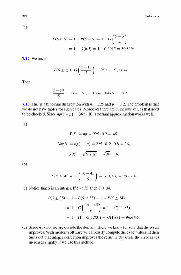
372 Solutions
(c)
P.S � 5/ D 1 � P.S < 5/ � 1 � G
�5 � 3
4
�
D 1 � G.0:5/ D 1 � 0:6915 D 30:85%:
7.12 We have
P.S � z/ � G
�z � 10
5
�D 95% D G.1:64/:
Then
z � 10
5D 1:64 ) z D 10 C 1:64 � 5 D 18:2:
7.13 This is a binomial distribution with n D 225 and p D 0:2. The problem is thatwe do not have tables for such cases. Moreover there are numerous values that needto be checked. Since np.1 � p/ D 36 > 10, a normal approximation works well.
(a)
EŒX� D np D 225 � 0:2 D 45;
VarŒX� D np.1 � p/ D 225 � 0; 2 � 0:8 D 36;
�ŒX� Dp
VarŒX� D p36 D 6:
(b)
P.S � 50/ � G
�50 � 45
6
�D G.0; 83/ D 79:67%:
(c) Notice that S is an integer. If S < 35, then S � 34.
P.S � 35/ D 1 � P.S < 35/ D 1 � P.S � 34/
D 1 � G
�34 � 45
6
�D 1 � G.�1:83/
D 1 � .1 � G.1:83// D G.1:83/ D 96:64%:
(d) Since n > 50, we are outside the domain where we know for sure that the resultimproves. With modern software we can easily compute the exact values. It thenturns out that integer correction improves the result in (b) while the error in (c)increases slightly if we use this method.

Solutions 373
7.14 This is a binomial distribution with n D 48 and p D 0:25. The problem is thatwe do not have tables for such cases. Moreover there are numerous values that needto be checked. Since np.1 � p/ D 9 > 5, a normal approximation works well.
(a)
EŒX� D np D 48 � 0:25 D 12;
VarŒX� D np.1 � p/ D 48 � 0:25 � 0:75 D 9;
�ŒX� Dp
VarŒX� D p9 D 3:
(b) Since 20 � n � 50, integer correction will improve the result.(c)
P.S � 15/ � G
�15:5 � 12
3
�D G.1:17/ D 87:90%;
(d)
P.S � 15/ � G
�15 � 12
3
�D G.1/ D 84:13%:
Since the exact answer is 87.68%, we see that integer correction improves theresult in this case.
7.15
(a) S is a normal distribution since it is a sum of normal distributions. The centrallimit theorem can’t be used since the conditions fail.
(b)
EŒS� D 100 C 90 C 95 C 105 D 400:
Since X1; X2; X3; X4 are independent, then
VarŒS� D VarŒX1 C X2 C X3 C X4�
D VarŒX1� C VarŒX2� C VarŒX3� C VarŒX4�
D 30 C 20 C 25 C 15 D 100;
�ŒS� D p100 D 10:

374 Solutions
(c)
P.S � 390/ D G
�390 � 400
10
�D G.�1/
D 1 � G.1/ D 1 � 0:8413 D 15:87%:
Since S is a normal distribution P.S D 390/ D 0, and there is no differencebetween P.S � 390/ and P.S < 390/.
7.16
(a)
�ŒK0;5� D 100e0:15�0:5p
e0:22�0:5 � 1 D 15:32 (USD):
(b) We compute
R D lnŒ112=100� C �1
20:22 � 0:05
� � 0:5 D 0:0983;
S D 0:2 � p0:5 D 0:1424:
The price of the option is then
V D 100 � .1 � G.R=S � S// � 112 � e�0:05�0:5.1 � G.R=S//
D 100 � .1 � G.0:55// � 112 � e�0:05�0:5.1 � G.0:70//
D 100 � .1 � 0:7088/ � 112 � e�0:05�0:5.1 � 0:7580/
D 2:69:
Remark The answer is somewhat inaccurate since 2 decimal accuracy is too littlehere.
7.17
(a) We compute
R D lnŒ205=200� C �1
20:022 � 0:05
� � 0:25 D 0:01224;
S D 0:02 � p0:25 D 0:01:

Solutions 375
The price of the option is
V D 200 � .1 � G.R=S � S// � 205 � e�0:05�0:25.1 � G.R=S//
D 200 � .1 � G.1; 21// � 205 � e�0;05�0:25.1 � G.1:22//
D 200 � .1 � 0:8869/ � 205 � e�0:05�0:25.1 � 0:8888/
D 0:107:
(b) The options are worthless when
K0:25 � 205:
This gives
200e�0:09� 1
2 0:022�
�0:25C0:02X0:25 � 205
�0:09 � 1
20:022
� � 0:25 C 0:02X0:25 � lnŒ1:025�
0:02245 C 0:02X0:25 � 0:02469
X0:25 � 0:02469 � 0:02245
0:02D 0:112:
We know that EŒX0:25� D 0 and that VarŒX0:25� D 0:25. This gives �ŒX0:25� D0:5. Since X0:25 is a normal distribution, we find
P.K0;25 � 205/ D P.X0:25 � 0:112/ � G
�0:112
0:5
�
D G.0:22/ D 58:71%:
(c) The same computation as above gives
K0:25 � 205;
if and only if
198e�0:05� 1
2 0:022�
�0:25C0:02X0:25 � 205
�0:05 � 1
20:022
� � 0:25 C 0:02X0:25 � lnŒ1:035�
0:01245 C 0:02X0:25 � 0:03440
X0:25 � 0:03440 � 0:01245
0:02D 1:10:
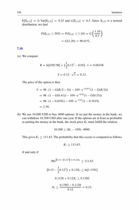
376 Solutions
EŒX0:25� D 0; VarŒX0:25� D 0:25 and �ŒX0:25� D 0:5. Since X0:25 is a normaldistribution, we find
P.K0:25 � 205/ D P.X0:25 � 1:10/ � G
�1:10
0:5
�
D G.2:20/ D 98:61%:
7.18
(a) We compute
R D lnŒ109=98� C �1
20:122 � 0:05
� � 1 D 0:06358:
S D 0:12 � p1 D 0:12:
The price of the option is then
V D 98 � .1 � G.R=S � S// � 109 � e�0:05�1.1 � G.R=S//
D 98 � .1 � G.0:41// � 109 � e�0:05.1 � G.0:53//
D 98 � .1 � 0:6591/ � 109 � e�0:05.1 � 0:7019/
D 2:50:
(b) We use 10;000 USD to buy 4000 options. If we put the money in the bank, wecan withdraw 10;500 USD after one year. If the options are at least as profitableas putting the money in the bank, the stock price K1 must fulfill the relation
10;500 � .K1 � 109/ � 4000:
This gives K1 � 111:63. The probability that this occurs is computed as follows
K1 � 111:63;
if and only if
98e�0:12� 1
2 0:122�
�1C0:12X1 � 111:63
�0:12 � 1
20:122
�C 0:12X1 � lnŒ1:1391�
0:1128 C 0:12X1 � 0:1302
X1 � 0:1302 � 0:1128
0:12D 0:15:

Solutions 377
EŒX1� D 0; VarŒX1� D 1, and �ŒX1� D 1. Since X1 is a standard normaldistribution, we find
P.K1 � 111:63/ D P.X1 � 0:15/ D 1 � G.0:15/
D 1 � 0:5596 D 44:04%:
7.19
(a)
P.K4 � 115/ D P.100 e0:32C0:2X4 � 115/ D P
�X4 � lnŒ1:15� � 0:32
0:2
�
D P.X4 � �0:90/ D 1 � P.X4 � �0:90/
D 1 � G
�0:90 � 0
2
�D 1 � GŒ�0:45� D GŒ0:45� D 67:36%:
(b) The volatility ˇ D 0:2. We compute
R D ln
115
100
�C�
1
20:22 � 0:03
�� 4 D 0:1; S D 0:2 � p
4 D 0:4:
The Black-Scholes pricing formula gives
V D 100 ��
1 � G
0:1
0:4� 0:4
��� 115 � e�0:12 �
�1 � G
0:1
0:4
��
D 100 � .1 � G Œ�0:15�/ � 115 � e�0:12 � .1 � G Œ0:25�/
D 100 � G Œ0:15� � 115 � e�0:12 � .1 � G Œ0:25�/
D 100 � 0:5596 � 115 � e�0:12 � .1 � 0:5987/ D 15:03:
The price of this option is hence 15.03 USD.
7.20
(a)
EŒX� D 0 � 0:86 C 1 � 0:08 C 2 � 0:02 C 3 � 0:04 D 0:24;
VarŒX� D 02 � 0:86 C 12 � 0:08 C 22 � 0:02 C 32 � 0:04 D �0; 242 D 0:4624:

378 Solutions
(b)
EŒS� D EŒX1� C EŒX2� C � � � C EŒX10;000�
D 0:24 C 0:24 C � � � C 0:24 D 10;000 � 0:24 D 2400:
Since X1; : : : ; X10;000 are independent, then
VarŒS� D VarŒX1� C VarŒX2� C � � � C VarŒX10;000�
D 0:4624 C 0:4624 C � � � C 0:4624 D 10;000 � 0:4624 D 4624:
�ŒS� D pVarŒS� D p
4624 D 68:
(c)
P.S > 2450/ D 1 � P.S � 2450/ � 1 � G�
2450�240068
�
D 1 � G.0:74/ D 1 � 0:7704 D 22:96%:
(d)
P.S � s0/ � G
�s0 � 2400
68
�D 99% D G.2; 33/:
Then
s0 � 2400
68D 2:33 ) s0 D 2400 C 2:33 � 68 D 2558:44:
The ice cream shop must order at least 2559 ice cream to be 99% sure that theysatisfy the demand.
7.21
(a) EŒX� D 0 � 0:1 C 1 � 0:6 C 2 � 0:3 D 1:2.VarŒX� D EŒX2� � EŒX�2 D 02 � 0:1 C 12 � 0:6 C 22 � 0:3 � 1:22 D 0:36.
(b) A condition that speaks against independence is that a household can beinfluenced by the actions of their neighbors. Here we are in the planning phase,so people moving in are hardly aware of any such circumstances. In any case itdoes not seem as if any particular choice will influence many other decisions.
(c) EŒ Y� D 900 � EŒX� D 1080. By independence VarŒ Y� D 900 � VarŒX� D 324.That gives �Œ Y� D 18. We call the unknown capacity Z0. We use the central

Solutions 379
limit theorem to see that
P. Y � Z0/ D P
�Y � 1080
18� Z0 � 1080
18
�� G
�Z0 � 1080
18
�
D 0:9 � G.1:28/:
This gives the equation
Z0 � 1080
18D 1:28 ) Z0 D 1080 C 1:28 � 18 � 1103:
7.22
(a) X D BinŒ10;000; p�. EŒX� D np D 10, and VarŒX� D np.1 � p/ D 9:99.
(b) Without integer correction
P.X � 3/ � G
�3 � 10p
9:99
�D G.�2:21/ D 1 � G.2:21/ D 0:0136:
With integer correction
P.X � 3/ � G
�3:5 � 10p
9:99
�D G.�2:06/ D 1 � G.2:06/ D 0:0197:
(c) We use the table for the Poisson distribution, and get
P. Y � 3/ D P. Y D 0/ C P. Y D 1/ C P. Y D 2/ C P. Y D 3/
D 0:0000 C 0:0005 C 0:0023 C 0:0076 D 0:0104:
We see that the Poisson distribution gives the best result, and that integercorrection increases the error.
7.23
(a) a D 2000 and b D 1000.(b)
EŒV� D aEŒX1� C bEŒX2� D 2000 � 200 C 1000 � 300 D 700;000:
Since X1 and X2 are independent,
VarŒV� D VarŒaX1� C VarŒbX2� D a2VarŒX1� C b2VarŒX2� D 6;400;000;000:
That gives �ŒV� D 80;000.

380 Solutions
(c) When X1 and X2 are normally distributed, then V has normal distribution. Hence
P.V > 800;000/ D 1 � P.V � 800;000/ D 1 � P
�V � eŒV�
�ŒV�� 800;000 � 700;000
80;000
�
D 1 � G
�800;000 � 700;000
80;000
�D 1 � G.1:25/ � 10:56%:
7.24
(a) EŒX� D 0:1; VarŒX� D 0:1.(b) EŒ Y� D 10; VarŒ Y� D 10.
P. Y � 5/ � G
�5 � 10p
10
�D G.�1:58/ D 1 � G.1:58/ D 5:71%:
With integer correction we get the answer 7:78%, which can also be approvedas an answer to the problem.
(c) � D 0:1. That gives
P.Z � 3/ D 1 � P.Z D 0/ � P.Z D 1/ � P.Z D 2/
D 1 � 0:9048 � 0:0905 � 0:0045 D 0:0002 D 0:02%:
(d) The distribution of Y can be approximated by a Poisson distribution W withparameter � D 10. That gives
P. Y � 5/ � P.W � 5/
D P.W D 0/ C P.W D 1/ C P.W D 2/ C P.W D 3/ C P.W D 4/
CP.W D 5/
D 0:000 C 0:0005 C 0:0023 C 0:0076 C 0:0189 C 0:0378 D 6:71%:
We see that the approximation is very close to the exact answer, and consid-erably closer than the normal approximation. This is what we expect since thedistribution of X is very close to a Poisson distribution with parameter � D 0:1.It follows from (c) that outcomes where Z � 3 are very rare, and have littleimpact on the final results.
7.25
(a) X is binomial with n D 10 and p D 0:1. We use the table for the binomialdistribution to find
P.X � 4/ D 1 � P.X � 3/ D 1 � 0:3487 � 0:3874 � 0:1937 � 0:0574
D 1 � 0:9872 D 1:28%:

Solutions 381
(b) We let Xi be the number of defective items produced at unit i. These variables areassumed to be independent with binomial distribution. We note that the resultby the worst unit has at most 3 defective items if and only if all the all units haveat most 3 defective items, and that
P.Xi � 3/ D 0:9872:
This gives
P. Y � 4/ D 1 � P. Y � 3/
D 1 � P.X1 � 3/ � P.X2 � 3/ � P.X3 � 3/ � P.X4 � 3/ � P.X5 � 3/
D 1 � 0:98725 D 6:24%:
7.26
(a) P.X � / D G�
�
�
� D G.0/ D 50% and P.X D C/ D 0 since X has acontinuous distribution.
(b) The result R can have the values o, d, and 12.o C d/. R gets the value o if and
only if o is closer to X than d. This happens if and only if the midpoint betweeno and d is to the left of X, i.e., X < oCd
2. The first term is hence the value of
R multiplied with the probability that this value occurs. This applies to all theterms, and the sum gives us the expected value. If X is a normal distribution, thelast term vanishes. Then
EŒR� D o � G
oCd
2�
�
!C d �
1 � G
oCd
2�
�
!!
D o � G
�o C d � 2
2�
�C d �
�1 � G
�o C d � 2
2�
��:
Alternatively one can use the distribution of X. Then the expression is asfollows:
EŒR� D o � FX
�o C d
2
�C d �
�1 � FX
�o C d
2
��:
Remark The last expression can easily be used to derive the equations forequilibrium. Nash equilibrium is obtained if and only if
@EŒR�
@oD 0;
@EŒR�
@dD 0:
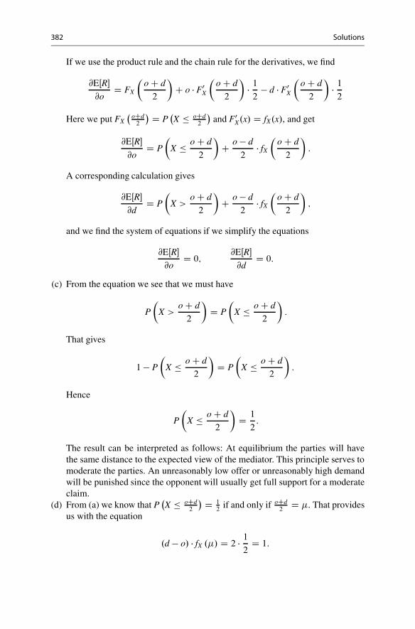
382 Solutions
If we use the product rule and the chain rule for the derivatives, we find
@EŒR�
@oD FX
�o C d
2
�C o � F0
X
�o C d
2
�� 1
2� d � F0
X
�o C d
2
�� 1
2
Here we put FX�
oCd2
� D P�X � oCd
2
�and F0
X.x/ D fX.x/, and get
@EŒR�
@oD P
�X � o C d
2
�C o � d
2� fX
�o C d
2
�:
A corresponding calculation gives
@EŒR�
@dD P
�X >
o C d
2
�C o � d
2� fX
�o C d
2
�;
and we find the system of equations if we simplify the equations
@EŒR�
@oD 0;
@EŒR�
@dD 0:
(c) From the equation we see that we must have
P
�X >
o C d
2
�D P
�X � o C d
2
�:
That gives
1 � P
�X � o C d
2
�D P
�X � o C d
2
�:
Hence
P
�X � o C d
2
�D 1
2:
The result can be interpreted as follows: At equilibrium the parties will havethe same distance to the expected view of the mediator. This principle serves tomoderate the parties. An unreasonably low offer or unreasonably high demandwill be punished since the opponent will usually get full support for a moderateclaim.
(d) From (a) we know that P�X � oCd
2
� D 12
if and only if oCd2
D . That providesus with the equation
.d � o/ � fX ./ D 2 � 1
2D 1:

Solutions 383
If we insert x D in the expression for fX.x/, we find fX ./ D 1p2��2
. We musthence solve the system
d � o Dp
2��2d C t D 2:
If we add the two equations, we get
2d D 2 Cp
2��2 ) d D Cr
�
2� � ) o D �
r�
2� �:
When � increases, the distance between the parties gets bigger. When theuncertainty in X is large, it will not pay to be close to the expected view. Ifthe opponent is less moderate, he or she might still get full support in almost50% of the cases, and profit from this strategy in the long run.
7.27
(a) We compute
P
�X <
o C d
2
�D P.X < 0:045/ D G
0:045 � 0:05
0:005
�
D GŒ�1� D 1 � GŒ1� D 1 � 0:8413 D 0:1587:
That gives P�X > oCd
2
� D 0:8413. Since X is continuous, P�X D oCd
2
� D 0. Ifwe insert this in the given formula, then
EŒR� D 0:03 � 0:1587 C 0:06 � 0:8413 D 5:52%:
(b) We compute
P
�X <
o C d
2
�D P.X < 0:045/ D G
0:045 � 0:05
0:02
�
D GŒ�0:25� D 1 � GŒ0:25� D 1 � 0:5987 D 0:4013:
This gives P�X > oCd
2
� D 0:5987. If we insert this in the given formula, then
EŒR� D 0:03 � 0:4013 C 0:06 � 0:5987 D 4:80%:
Remark We see that when the insecurity in the view of the mediator is low(0.5%), it pays to be close to the expected view. When the insecurity is high(2%), however, the probability increases to get full support for a bold claim. Itthen pays to present a claim further from the expected view of the mediator.

384 Solutions
7.28
(a) If we assume that the good is sold in continuous quantities, we get
P.X � 3/ D 1 � P.X < 3/ � 1 � G
�3 � 1
1
�D 1 � 0:9772 D 0:0228:
The probability of selling at least 3 units during a randomly selected day ishence about 2:3%. If the good is only sold in integer units, then
P.X � 3/ D 1 � P.X � 2/ � 1 � G
�2 � 1
1
�D 1 � 0:8413 D 0:1587:
From the text we used to formulate the problem, it is natural to use the firstinterpretation, but the second interpretation, too, is considered a full solution tothe problem.
(b) The distribution arise as a limit of a binomial .n; p/ variable where n is largeand p is small, and a distribution of this sort will be Poisson distributed. For thePoisson distribution we have EŒX� D � and �2ŒX� D �, and from the numbersgiven in the problem we can conclude that � D 1. This gives
P.� 3/ D 1 � P.X D 0/ � P.X D 1/ � P.X D 2/
D 1 � 0:3679 � 0:3679 � 0:1839 D 0:0803:
The probability of selling at least 3 units during a randomly selected day is about8% in this case.
(c) The answers are quite different. The reason is that the Poisson distribution isapproximately normal only when � is sufficiently large, and this is not the casehere. If the customers do not have the same probability of buying the good,the resulting distribution need not be of Poisson type. It might, e.g., happenthat there is a small but devoted group of customers that buy the good relativelyoften, while that rest never buy it. In this case we cannot appeal to the law of rareevents, and it may be more natural to use a binomial distribution where p is notsmall. The information D 1; � D 1, however, speak against an interpretationwhere p is not small.
7.29
(a) We use the Black and Scholes pricing formula. We compute
R D ln.110=100/ C�
1
20:52 � 0:025
�� 9 D 0:9; S D 0:5 � p
9 D 1:5:

Solutions 385
This gives R=S D 0:6. The price of the option is then
V D 100.1 � GŒ�0:9�/ � 100e�0:225.1 � GŒ0:6�/
D 100GŒ0:9� � 100e�0:025�9.1 � GŒ0:6�/
D 100 � 0:8159 � 100e�0:225.1 � 0:7257/
D 59:69 (USD):
(b)
100e�0:03� 1
2 0:52�
100C0:5X100 � 1
m�0:03 � 1
20:52
�100 C 0:5X100 � lnŒ0:01�
m
X100 � 9:79:
This gives
P.K100 � 1/ D P.X � 9:79/ D 1 � P.X100 � 9:79/
D 1 � G
9:79 � 0p
100
�D 1 � GŒ0:98� D 1 � 0:8365
D 16:35%:
It is hence only 16:35% probability that the stock price exceeds 1 USD after 100years.
(c)
EŒKt� D EŒK0e.˛� 12 ˇ2/tCˇXt � D K0e.˛� 1
2 ˇ2/tEŒeˇXt �
D K0e�
˛� 12 ˇ2�
te12 ˇ2t D K0e˛ t:
This gives
EŒK100� D 100e0:03�100 D 2008:55 (USD):
From (b) we see that the stock price will usually be less than 1 USD after 100years. This seems to contradict an expected value of 2000 USD. The reason why

386 Solutions
this is possible is that while most outcomes lead to small values this is balancedby some outcomes leading to extremely large values.
7.30 We call the outcome of the game X.
(a)
EŒX� D 5=6 � 1 C 1=6 � �4 D 1=6:
(b) a D 2
EŒU.X/� D 5=6�.p
1 C 22�2/C1=6�.p
�4 C 22�2/ D 5p
5=6�2 � �0:137:
a D 4
EŒU.X/� D 5=6�.p
1 C 42 �4/C1=6�.p
�4 C 42 �4/ D 5p
17=6Cp3=3�5 � 0:013:
The expected utility of not playing, we find as
EŒU.X/� D 5=6 � .p
a2 � a/ C 1=6 � .p
a2 � a/ D 0:
(c) Since the expected utility of not playing is zero, a rational player chooses toparticipate if and only if he has strictly positive expected utility of playing.Expected utility is an increasing function of a. We call this function e.a/. From(b) we know that e.2/ < 0 and that e.4/ > 0. Since the function is increasing,it has exactly one point a0 2 .2; 4/ where it is zero. When a > a0, expectedutility is strictly positive proving the claim. From (a) we know that the gamehas positive expected outcome. Players who are sufficiently risk averse willnevertheless choose not to play. We can divide the population into two parts:those with high risk aversion (a � a0) do not play, and those with low riskaversion (a > a0) choose to play.
7.31
(a) We see that the base c D 1:10154 in the exponential function is bigger than 1.Then the value increases with x. We put x D 50, and find
50 D 9:0 � 10�4 C 4:4 � 10�5 � 1:1015450 D 0:644%:
(b)
P.T40 > 10/ D 1 � P.T40 � 10/ D 1 � .1 � e� R 100 ˛Cˇc40Csds/
D e� R 100 ˛Cˇc40Csds D e�10˛� ˇ
ln.c/ .c50�c40/ D 95:65%:

Solutions 387
(c)
P.T40 > 11/ D 1 � P.T40 � 11/ D 1 � .1 � e� R 100 ˛Cˇc40Csds/
D e� R 110 ˛Cˇc40Csds D e�10˛� ˇ
ln.c/ .c51�c40/ D 95:01%:
The conditional probability is computed as follows:
P.10 < T40 � 11jT40 > 10/ D P.10 < T40 � 11 \ T40 > 10/
P.T40 > 10/
D P.10 < T40 � 11/
P.T40 > 10/
D P.T40 > 10/ � P.T40 > 11/
P.T40 > 10/
D 95:65% � 95:01%
95:65%D 0:669%:
We can interpret this quantity as the probability that the man dies in the courseof the year of insurance given that he was 50 years old and alive when the year ofinsurance started. This probability is approximately equal to the death rate in (a).There is a slight difference which is caused by the rate in (a) being an instant rate,while the rate in (c) is an average rate.
Remark Insurance companies do not always use the same tables for men andwomen. The death rates of women are lower than for men, and for some types oflife insurance, women pay the same amount as a man who is 3 years younger.
7.32
(a) X er Bin[6,0.7].
P.N D 4/ D
6
4
!0:740:32 D 32:41%:
(b) Let Y be the number of contracts that are signed. The simplest way to solvethe problem is to see that the probability for a collaborator writing a contract is0:7 � 0:6 D 0:42. Y is hence Bin[6,0.42], and
P. Y D 4/ D
6
4
!0:4240:582 D 15:70%:

388 Solutions
Alternatively, the conditional probabilities can be computed as follows: If thecollaborators sign 4 contracts, then X D 4; 5, or 6.
P. Y D 4/
D P. Y D 4jX D 4//P.X D 4/ C P. Y D 4jX D 5/P.X D 5/
C P. Y D 4jX D 6/P.X D 6/
D
4
4
!0:640:40 �
6
4
!0:740:32
C
5
4
!0:640:41 �
6
5
!0:750:31
C
6
4
!0:640:42 �
6
6
!0:760:30 D 15:70%:
7.33 We let X denote the number of men admitted in the first round and Y thenumber of men admitted in the second round. In general
P.X D x/ D�
4
x
��6
3�x
��
103
� ; P. Y D y/ D�
6y
��4
7�y
��
107
� :
(a)
P.X D 2/ D�
4
2
��6
1
��
10
3
� D 0:3:
P. Y � 5/ D P. Y D 5/ C P. Y D 6/ D 1=3:
(b) In the second round at least 3 men are admitted, hence P.Y � 3/ D P.Y �2/ D P.Y � 1/ D 1.
P.X C Y � 5/ D P.X D 0/P. Y � 5/ C P.X D 1/P. Y � 4/
CP.X D 2/P. Y � 3/ C P.X D 3/P. Y � 2/
CP.X D 4/P. Y � 1/ D 80:56%:
The men have a larger chance of being admitted. This scheme is in favor of men.The majority of the men are allowed to apply in the second round where the chanceof being admitted in higher than in the first round.

Solutions 389
7.34
(a) We use the Black and Scholes formula and find
R D lnŒ390=400� C .1=2 � 0:122 � 0:05/ � 1 D �0:06812;
S D 0:12 � p1 D 0:12:
This gives
V D 400.1 � GŒ�0:69�/ � 390e�0:05 � .1 � GŒ�0:57�/
D 400 � GŒ0:69� � 390e�0:05 � GŒ0:57�
D 400 � 0:7549 � 390e�0:05 � 0:7157 D 36:45:
(b) After T years of continuous interest r, the value of a bank deposit of 390e�rT
USD is equal to 390 USD.If KT � 390, then the put option is worthless and the value of contract A is
0 C KT D KT :
The value of the call option is KT � 390 in this case, and the total value ofcontract B is
.KT � 390/ C 390 D KT :
If KT � 390, the value of the put option is 390 � KT , and the total value ofcontract A is
.390 � KT/ C KT D 390:
The call option is worthless in this case, and hence the value of contract B is
0 C 390 D 390:
We see that the values of contract A and B are equal no matter what happens.(c) We call the price of the put option W. Since we can buy the stock for 400 USD,
the price of contract A is W C400. The call option costs 36.45 USD, and a bankdeposit of 390e�0:05 D 370:98 USD costs exactly this amount. Since the twocontracts must have the same price, we get the equation
W C 400 D 36:45 C 370:98: (*)
If we solve this equation, we get W D 7:43 (USD).
Remark The equation (*) is referred to as put/call parity in the literature.

390 Solutions
(d) The prices on the options do not depend on the expected return, so they donot change. If we are to profit at least 8 USD on the put options, the price ofthe stock must be at most 382 USD after one year. We must hence find whichvalues of XT lead to
400e.˛�1=2ˇ2/TCˇXT � 382:
A standard rewriting of this expression gives
XT � 0:09:
Since XT is normally distributed with D 0 and variance �2 D T D 1, then
P.KT � 382/ D P.XT � 0:09/ D GŒ0:09� D 53:59%:
7.35
(a) In general
VarŒX� D EŒX2� � EŒX�2:
but in this case EŒBt� D 0 and the second term is zero.(b) B100 is a normal distribution with expectation zero and variance �2 D 100.
Hence
P.B100 � 10/ D G
�10 � 0
10
�D G.1/ D 84:13%:
(c) It follows from the third bullet point that Bs and Bt �Bs are independent randomvariables. Hence
EŒBs.Bt � Bs/� D EŒBs� � EŒBt � Bs� D 0 � .0 � 0/ D 0:
(d) From (c) we have
EŒBs.Bt � Bs/� D 0:
If we expand the left-hand side, we see that
EŒBsBt� � EŒB2s � D 0:
This gives
EŒBsBt� D EŒBtBs� D EŒB2s � D s:

Solutions 391
Furthermore
EŒ.Bt � Bs/2� D EŒB2
t � 2BtBs C B2s � D t � 2s C s D t � s:
7.36
(a) EŒXt� D EŒ2Bt C 6� D 2EŒBt� C 6 D 6.
VarŒXt� D VarŒ2Bt C 6� D VarŒ2Bt� D 22VarŒBt� D 4t:
(b) X25 is a normal distribution with EŒX25� D 6 and VarŒX25� D 4 � 25 D 100. Thisgives
P.X25 � 16/ D G
�16 � 6p
100
�D G.1/ D 84:13%:
(c)
EŒB2s B2
t � 2BtB3s C B4
s � D EŒB2s .B2
t � 2BtBs C B2s /� D EŒB2
s .Bt � Bs/2�
D EŒB2s � � EŒ.Bt � Bs/
2� D s.t � s/:
7.37
(a)
P.100eB9 � 2000/ D P.B9 � lnŒ20�/ D G
lnŒ20� � 0p
9
�D GŒ1:00� D 84:13%:
(b) Here the terms B2s and .Bt � Bs/
2 are independent, and we get
EŒB2s .Bt � Bs/
2� D EŒB2s � � EŒ.Bt � Bs/
2� D s.t � s/:
(c) i) Assume i < j. Then the term .BtjC1� Btj/ is independent of the three other
terms Bti ; Btj , and .BtiC1� Bti/. That gives
EŒBti Btj.BtiC1�Bti/.BtjC1
�Btj/� D EŒBti Btj.BtiC1�Bti/��EŒ.BtjC1
�Btj/� D 0:
ii) If i D j, we get
EŒBti Btj.BtiC1� Bti/.BtjC1
� Btj/� D EŒB2ti.BtiC1
� Bti/2� D ti.tiC1 � ti/:
(the last equality follows from (b)).

392 Solutions
iii) Assume i > j. Then the term .BtiC1� Bti/ is independent of the three other
terms Bti ; Btj and .BtjC1� Btj/. This gives
EŒBti Btj.BtiC1�Bti/.BtjC1
�Btj/� D EŒBti Btj.BtjC1�Btj/��EŒ.BtiC1
�Bti/� D 0:
Remark The calculations above are central to the construction of a stochasticintegral which plays an important part of mathematical finance.
7.38
(a)
P.X D 2/ D�
6
2
��1
3
�2 �2
3
�4
D 32:92%:
(b)
P.X D 2/ D P.X D 2j p D 0/P. p D 0/ C P.X D 2j p D 1=3/P. p D 1=3/
CP.X D 2j p D 2=3/P. p D 2=3/ C P.X D 2j p D 1/P. p D 1/:
If n > 2, the first and the last term are both zero. Then we get
P.X D 2/ D�n
2
��1
3
�2 �2
3
�n�2
� 1
4C�n
2
��2
3
�2 �1
3
�n�2
� 1
4:
If we put� n
2
�outside as a common factor, we have proved the claim. If n D 2,
then P.X D 2j p D 1/ D 1, and this term comes in addition.(c) We use Bayes’ formula to get
P
�p D 1
3
ˇˇX D 2
�D P
�X D 2
ˇˇ p D 1
3
�� P�
p D 13
�
P.X D 2/:
If we insert n D 6 in the formula from (b), we get P.X D 2/ D 10:29%. Thistogether with the answer for (a) gives
P
�p D 1
3
ˇˇX D 2
�D 0:3292 �
14
0:1029D 0:800 D 80%:
Remark This problem is a simple example of Bayesian statistics. Prior to theexamination we have what we call an a priori distribution:
P. p D 0/ D 1=4 P. p D 1=3/ D 1=4 P. p D 2=3/ D 1=4 P. p D 1/ D 1=4:

Solutions 393
After we have done 6 trials and observed X D 2 successes, we modify thedistribution to what we call an a posteriori distribution:
P. p D 0jX D 2/ D 0 P. p D 1=3jX D 2/ D 80%
P. p D 2=3jX D 2/ D 20% P. p D 1jX D 2/ D 0:
We now believe there is a large probability (80%) that p D 13, but we still hold it
possible (20%) that p can be 23.
7.39
(a)
P. Y � 403:43/ D P.eX � 403:43/ D P.X � lnŒ403:43�/
D Gh
lnŒ403:43��4
2
iD GŒ1� D 84:13%:
(b) If we put D 4; � D 2 in the formula, we find
EŒ Y� D e4C 12 22 D e6 D 403:43:
We see that the answer is the same as in (a). The explanation is that thedistribution is skewed, it is much more likely (84.13%) that the value of Y isbelow EŒ Y� than above the same value (15.87%).
(c) We can rewrite the expression as follows:
Kt D elnŒK0�C.r� 12 ˇ2/tCˇZt :
If we put X D lnŒK0�C .r � 12ˇ2/t CˇZt , then X is a normal distribution with
D lnŒK0� C .r � 12ˇ2/t and � D ˇ
pt. The formula from (b) gives
EŒKt� D eC 12 �2 D elnŒK0�C.r� 1
2 ˇ2/tC 12 ˇ2 t D elnŒK0�Crt D K0ert:
7.40
(a)
P.D1 � 16;000/ D G
16;000 � 10;000
3000
�D GŒ2� D 97:72%:
(b)
EŒD� D EŒD1� C EŒD2� D 10;000 C 16;000 D 26;000:

394 Solutions
Since D1 and D2 are independent, then
VarŒD� D VarŒD1� C VarŒD2� D 30002 C 40002 D 25;000;000 D 50002:
which gives
P.D � 16;000jS/ D G
16;000 � 26;000
5000
�D GŒ�2� D 1 � 0:9772% D 2:28%:
(c)
P.Sell at most 16,000 newspapers/ D P.D � 16;000jS/P.S/
CP.D1 � 16;000jSc/P.Sc/
D 0:0228 � 0:2 C 0:9772 � 0:8 D 78:63%:
7.41
(a) The expected sale is given by
EŒS� D 1 � 0:1 C 2 � 0:1 C 3 � 0:1 C 4 � 0:1 C 5 � 0:6 D 4:
If we instead put x D 5 in the formula, we get
EŒS� D 1
20.21 � 5 � 52/ D 4:
The two answers are in agreement.(b)
EŒ˘� D EŒR minŒD; q� � W q� D R EŒS� � W q D R � 1
20.21x � x2/ � Wx:
If R D 20; W D 5, then
EŒ˘� D .21x � x2/ � 5x D 16x � x2:
If we compute the derivative of this function and set it equal to zero, we findthat maximum is achieved when x D 8.
(c) Maximum is achieved when x is such that
FD.x/ D P.D � x/ D 1 � 5
20D 0:75:

Solutions 395
If D is normally distributed N.; �2/, then
P.D � x/ D G�x �
�
�:
From the table of the normal distribution we find
G�x �
�
�D 0:75 , x �
�D 0:6745:
This gives
x D C 0:6745 � D 5:5 C 0:6745 � 1:0 D 6:1745:
When the sales distribution is normal, it is not probable (2.5%) that the valueis larger than 5:5 C 1:96 � 1:0 D 7:46. In comparison this probability is morethan 25% for the uniform distribution. We order less since high demand is lessprobable.
7.42
(a) We have
EŒZ� D E
"1000X
iD1
Di
#D
1000X
iD1
EŒDi� D 1000 � 10 D 10;000:
Since the variance of a sum of independent variables is equal to the sum of thevariances, we get
VarŒZ� D Var
"1000X
iD1
Di
#D
1000X
iD1
VarŒDi� D 1000 � 10 D 10;000:
(b)
P.D � z/ D 0:95 , G
z � 10;000
100
�D 0:95 , z � 10;000
100D 1:6449:
If we order 10;165 units, we have at least 95% probability of satisfying thedemand. If the number of people in the market is very large, we need to ordermore than 10 units for each person. The variance will in this case be very smallin comparison to the expected value. Hence if we order just slightly more thanexpected, we can be quite sure to satisfy the demand.

396 Solutions
7.43
(a)
P.Xi � 0/ D G
�0 � 45
30
�D G.�1:5/ D 1 � G.1:5/ D 1 � 0:9332 D 6:68%:
(b) We first need to find expectation and variance for YiC1. We have
EŒ YiC1� D EŒXiC1� C ˛. � EŒXi�/ D C ˛. � / D D 45:
Since XiC1 and Xi are independent, we find
VarŒ YiC1� D VarŒXiC1� C VarŒ˛ � ˛Xi� D VarŒXiC1� C VarŒ�˛Xi�
D VarŒXiC1� C .�˛/2VarŒXi� D .1 C ˛2/�2 D 1406:25:
That leads to a standard deviation
�Œ YiC1� D p1406:25 D 37:5:
A linear combination of normal distributions is normal, and hence
P. YiC1 � 0/ D G
�0 � 45
37:5
�D G.�1:2/ D 1 � G.1:2/ D 1 � 0:8849 D 11:51%:
(c) No, all values of ˛ give the same expected surplus. The larger the value of ˛, thelarger will the standard deviation be. This in turn leads to a larger probability ofdeficit. Even though the intention is good, the best strategy is to do nothing, i.e.,˛ D 0. Any other strategy will be worse.
7.44
(a)
P.jX � 100j � 0:2/ D 2 � P.X � 100:2// D 2.1 � P.X � 100:2//
D 2
�1 � G
�100:2 � 100
0:1
��D 2.1 � G.2// D 2.1 � 0:9772/
D 4:56%:

Solutions 397
(b)
X2 D 2 C�2 D 1 � .X1 �1/C�2 D 1 �1 � �1 C1 C�2 D 1 � �1 C�2:
EŒX2� D EŒ1� � EŒ�1� C EŒ�2� D 1 � 0 C 0 D 100:
Since �1 and �2 are independent, then
VarŒX2� D VarŒ��1 C �2� D VarŒ��1� C VarŒ�2� D VarŒ�1� C VarŒ�2� D �21
C�22 D 2 � 0:12 D 0:02:
P.jX2 � 100j � 0:2/ D 2 � P.X2 � 100:2// D 2.1 � P.X2 � 100:2//
D 2
�1 � G
�100:2 � 100p
0:02
��
D 2.1 � G.1:41// D 2.1 � 0:9207/ D 15:86%:
We see that this attempt to improve quality is a disaster as the parts that need tobe discarded are more than tripled.
(c) Since X2 D 2 C �2, we get
X3 D 3 C �3 D 2 � .X2 � 1/ C �3 D 2 � 2 � �2 C 1 C �3 D 1 � �2 C �3;
leading to the same distribution as before.
Remark By induction it is possible to prove that
Xn D 1 � �n�1 C �n;
which shows that the distribution does not change when we carry on with theprocedure. Note that it is the adjustment, not the measurement that creates theproblem. A basic idea in the control of processes is to measure continuously, butto adjust only if the deviation is statistically significant.
Problems of Chap. 8
8.1 We know that X and S2 are unbiased estimators for and �2. If we computethe values, we find
X D 35;600; S2 D 236;800;000:

398 Solutions
8.2 Since we have lots of observations, we can appeal to the central limit theorem.We can also assume that S2
X is a quite accurate estimate for �2. We can hence assume
that X is approximately normal with EŒX� D and VarŒX� D �2
10;000. We have to find
z such that
P
X �
�ŒX�� z
!D 2:5%:
That gives z D 1:96. A 95% confidence interval is then
X ˙ 1:96 � �ŒX� D 35;600 ˙ 1:96 � 210:
This gives the interval Œ35;188; 36;012�.
8.3 Since we have lots of observations, we can appeal to the central limit theorem.We can also assume that S2
X is a quite accurate estimate for �2. We can hence assume
that X is approximately normal with EŒX� D and VarŒX� D �2
2500. We have to find
z such that
P
X �
�ŒX�� z
!D 2:5%:
That gives z D 1:96. A 95% confidence interval is then
X ˙ 1:96 � �ŒX� D 120;000 ˙ 1:96 � 6000:
This gives the interval Œ108;240; 131;760�.
8.4
(a) X is a binomial distribution with n D 40;000 and p D p.(b)
EŒ O� D 1
40;000EŒX� D 1
40;000� 40;000 � p D p:
VarŒ O� D 1
40;0002VarŒX� D 1
40;0002� 40;000 � p.1 � p/ D p.1 � p/
40;000:
(c) We have observed O D 0:36. Since we have lots of observations, we can assumethat O is approximately normal and that
�Œ O � Ds
p.1 � p/
40;000�s
0:36.1 � 0:36/
40;000D 0:0024:

Solutions 399
We must find z such that
P
O �
�Œ O �� z
!D 0:5%:
That gives z D 2:5758. A 99% confidence interval is then
O ˙ 2:5758 � �Œ O� D 0:36 ˙ 2:5758 � 0:0024:
That gives the interval Œ0:354; 0:366�.(d) If p D 0:354, then �Œ O� D 0:00239, and if p D 0:366, then �Œ O� D 0:00241. If
we use these values instead, the confidence interval still becomes Œ0:354; 0:366�.The error we make when we use the constant �Œ O� D 0:0024 can hence beignored.
8.5 In this problem X is a binomial distribution with n D 10 and p D p.
(a) We know that X and S2 are unbiased estimators for EŒX� and VarŒX�. Then
EŒX� D EŒX� D n � p D 10p:
EŒS2� D VarŒX� D n � p.1 � p/ D 10p.1 � p/:
(b) We insert the values to find
X D 1
5.2 C 1 C 2 C 2 C 3/ D 2:
S2 D 1
4..2 � 2/2 C .1 � 2/2 C .2 � 2/2 C .2 � 2/2 C .3 � 2/2/ D 1
2:
There is no conflict between these results. The result in (b) is the consequenceof one single execution of the experiment, while the result in (a) tells us what toexpect when we repeat it several times.
(c)
EŒ O� D 1
10EŒX� D 1
10� 10p D p:
VarŒ O� D 1
102VarŒX�
D 1
102� 1
52VarŒX1 C X2 C X3 C X4 C X5�

400 Solutions
D 1
102� 1
52.VarŒX1� C VarŒX2� C VarŒX3� C VarŒX4� C VarŒX5�/
D 1
102� 1
52� 5 � 10p.1 � p/ D p.1 � p/
50:
Remark The results in this problem coincide with what we would have gotten froma single binomial variable with n D 50.
8.6
(a)
EŒV� D EŒX1 C X2 C X3 C X4�
D EŒX1� C EŒX2� C EŒX3� C EŒX4�
D C C C D 4:
VarŒV� D VarŒX1 C X2 C X3 C X4�
D VarŒX1� C VarŒX2� C VarŒX3� C VarŒX4�
D �2 C �2 C �2 C �2 D 4�2:
From a formal point of view, V is an estimator, but there is no reason to expectthat the value is close to .
(b) We have
EŒW� D EŒV � 3� D EŒV� � 3 D 4 � 3 D :
W is hence unbiased. The problem is that W contains the unknown number thatwe want to find. This is not useful, and in more advanced textbooks we can finddefinitions excluding constructions of this type.
8.7 Since we have few, but normally distributed observations, we can use the t-distribution. We know that
T D X �
SŒX�
is t-distributed with parameter � D 24. We must find z such that
P�T.24/ � z
� D 2:5%:

Solutions 401
That gives z D 2:064. A 95% confidence interval is hence given by
X ˙ 2:064 � SŒX� D 35;600 ˙ 2:064 � 4200
That gives the interval Œ26;931; 44;269�.
8.8 Since we have few, but normally distributed observations, we can use the t-distribution. We know that
T D X �
SŒX�
is t-distributed with parameter � D 8. We must find z such that
P�T.8/ � z
� D 5%:
That gives z D 1:86. A 90% confidence interval is hence given by
X ˙ 1; 86 � SŒX� D 120;000 ˙ 1; 86 � 100;000:
That gives the interval Œ�66;000; 306;000�.
8.9 We compute
X D 94:75; S2 D 1
3
4X
iD1
.Xi � X/2 D 2:25:
That gives
SŒX� Dr
S2
4D 0:75:
We know that
T D X �
SŒX�
is t-distributed with parameter � D 3. We must find z such that
P�T.3/ � z
� D 0:5%:
That gives z D 5:841. A 99% confidence interval is hence given by
X ˙ 5:841 � SŒX� D 94:75 ˙ 5:841 � 0:75:

402 Solutions
That gives the interval Œ90:37; 99:13�. The value 100 is outside the confidenceinterval. If the claim was true, that would only happen in 1 out of 100 suchexperiments. It hence seems unlikely that the claim is true.
8.10 We use the formula and find
VarŒY� D N � n
N � 1� S2
nD 1014 � 312
1014 � 1� 1:04814 � 1010
312D 2:32805 � 107:
That gives
�ŒY� D 4825:
For the normal distribution a 95% confidence interval is given by
Y ˙ 1:96�ŒY� D 678;995 ˙ 1:96 � 4825:
That gives the interval Œ669;498; 688;412�.
8.11
(a) We use the formula and find
VarŒY� D N � n
N � 1� S2
nD 522 � 478
522 � 1� 6:7123 � 1011
478D 1:18593 � 108:
That gives
�ŒY � D 10;890:
For the normal distribution a 95% confidence interval is given by
Y ˙ 1:96�ŒY� D 2;133;190 ˙ 1:96 � 10;890:
That gives the interval Œ2;111;846; 2;154;534�.(b) If N is very large, we can use the formula
VarŒY � D S2
nD 6:7123 � 1011
478D 1:40425 � 109:
That gives
�ŒY � D 37;473:

Solutions 403
For the normal distribution a 95% confidence interval is then given by
Y ˙ 1:96�ŒY� D 2;133;190 ˙ 1:96 � 37;473:
That gives the interval Œ2;059;743; 2;206;637�. We see that the confidenceinterval is much wider when we ignore the previous information.
8.12
(a) EŒ O1� D EŒ O2� D , VarŒ O1� D �2
100and VarŒ O2� D �2
400.
(b)
EŒ Oc� D EŒc O1 C .1 � c/ O2� D cEŒ O1� C .1 � c/EŒ O2� D c C .1 � c/ D :
VarŒ Oc� D VarŒc O1 C .1 � c/ O2� D c2VarŒ O1� C .1 � c/2VarŒ O2�
D c2 � �2
100C .1 � c/2 � �2
400D .4c2 C .1 � c/2/ � �2
400:
(c) We define
f .c/ D .4c2 C .1 � c/2/ � �2
400:
This is a parabola, and minimum is found where f 0.c/ D 0. That gives
f 0.c/ D .8c C 2.1 � c/ � �1/ � �2
400D 0:
10c � 2 D 0 ) c D 1
5:
When c� D 15, then
c� D 1
5� 1
100
100X
iD1
Xi C 4
5� 1
400
400X
iD1
X0i D 1
500
� 100X
iD1
Xi C400X
iD1
X0i
�:
This is just the mean of all the 500 observations, and we see that it is not possibleto improve the estimator by combining the observations in a particularly cleverway.

404 Solutions
Problems of Chap. 9
9.1
(a) We have H0 W D 8000 and HA W < 8000.(b) EŒX� D and VarŒX� D �2
n D 4;000;000100
D 40;000. That gives �ŒX� D 200.(c) We reject H0 when X � xlimit where
PH0.X � xlimit/ D 5%:
Since we have many observations, we can use the central limit theorem. WhenH0 is true, then
PH0 .X � xlimit/ � G
�xlimit � 8000
200
�D G.�1:6449/:
That gives
xlimit D 8000 � 1:6449 � 200 D 7671:
The rejection region is hence the interval .�1; 7671�.(d) Since the observed value of X is outside the rejection region, we must keep H0.
There is not sufficient evidence to conclude that the power consumption hasdecreased.
9.2
(a) We have H0 W D 1200 and HA W > 1200.(b) EŒX� D and VarŒX� D �2
n D 160;000400
D 400. That gives �ŒX� D 20.(c) We reject H0 when X � xlimit where
PH0.X � xlimit/ D 5%:
Since we have many observations, we can use the central limit theorem. WhenH0 is true, then
PH0.X � xlimit/ � 1 � G
�xlimit � 1200
20
�D 5%:
Hence
G
�xlimit � 1200
20
�D 0:95 D G.1:6449/:

Solutions 405
That gives
xlimit D 1200 C 1:6449 � 20 D 1232:90:
The rejection region is hence the interval Œ1232:90; 1/.(d) Since the observed value of X is inside the rejection region, we reject H0.
There is hence sufficient evidence to conclude that the fee usage probably hasincreased.
9.3
(a) We have H0 W D 0:1 and HA W 6D 0:1.(b) T is t-distributed with parameter � D 24.(c) We reject H0 when jT.24/j � tlimit where
PH0 .jT.24/j � tlimit/ D 5%:
Hence
PH0 .T.24/ � tlimit/ D 2:5%:
That gives tlimit D 2:064. The rejection region is hence the interval.�1; �2:064� [ Œ2:064; 1/.
(d) Here we have
S2ŒX� D S2
nD 0:052
25D 0:0001:
That gives SŒX� D 0:01. If we insert this, we find that the observed value for Tis
T D 0:09 � 0:1
0:1D �1:
Since this value is outside the rejection region, we keep H0. There is notsufficient evidence to claim that 6D 0:1.
9.4
(a) We have H0 W D 11 and HA W < 11.(b) T is t-distributed with parameter � D 35.(c) We reject H0 when T.35/ � tlimit where
PH0 .T.35/ � tlimit/ D 5%:

406 Solutions
That gives tlimit D �1:69. The rejection region is hence the interval.�1; �1; 69�.
(d) Here we have
S2ŒX� D S2
nD 32
36D 0:25:
That gives SŒX� D 0:5. If we insert this, we find that the observed value for T is
T D 10 � 11
0:5D �2:
Since the observed value of X is inside the rejection region, we reject H0. There ishence sufficient evidence to conclude that the absence due to illness probably hasdecreased.
9.5
(a) Let p denote the probability that a randomly selected person prefers the newproduct. We have H0 W p � 50% and HA W p > 50%.
(b) X is a binomial distribution with parameters n D 5 and p D p.(c) P-value of the observed result is
PH0 .X � 5/ D PH0 .X D 5/ D�
5
5
�p5 � .1 � p/0 �
�5
5
�0:55 D 3:1%:
Since the P-value is smaller than the significance level, we reject H0. There is hencesufficient evidence to conclude that more than 50% of the population probably preferthe new product.
Remark When the tendency in the data is strong, it is sometimes possible to drawconclusions based on very few observations.
9.6
(a) Let p denote the probability that a randomly selected person is dissatisfied. Wehave H0 W p � 10% and HA W p > 10%.
(b) X is a binomial distribution with parameters n D 400 and p D p.(c) P-value for the observations is
PH0 .X � 53/ � PpD10%.X � 53/ D 1 � PpD10%.X � 52/
� 1 � G
�52 � 40
6
�D 1 � G.2/ D 1 � 0:997
D 2:28%:

Solutions 407
Since the P-value is less than the significance level, we reject the null hypothe-sis. There is sufficient evidence to conclude that more than 10% of the customersprobably are dissatisfied.
9.7
(a) We assume that p D 1%, and find the probability that the accounting is notrejected, i.e.
P.X � 3/ D P.X D 0/ C P.X D 1/ C P.X D 2/ C P.X D 3/:
i) Using the table for the Poisson distribution with parameter � D n � p D 4,we find
P.X � 4/ D 0:0183 C 0:0733 C 0:1465 C 0:1954 D 43:35%:
ii) Exact computation gives
P.X � 4/ D�
400
0
�0:010 � 0:99400 C
�400
1
�0:011 � 0:99399
C�
400
2
�0:012 � 0:99398 C
�400
3
�0:013 � 0:99397
D 43:25%:
This is the probability that the accountant approves an accounting with too manyerrors. The strength of this alternative is the probability that the accounting isnot approved, i.e.
Strength D 1 � 43:25% D 56:75%:
(b) Using normal approximation, we find n � p.1 � p/ D 3:96 and get
P.X � 3/ � G
�3 � 4p
3:96
�D G.�0:50/
D 1 � G.0:50/ D 1 � 0:6915 D 30:85%:
and
P.X � 3/ � G
�3:5 � 4p
3:96
�D G.�0:25/
D 1 � G.0:25/ D 1 � 0:5987 D 40:13%:
We see that integer correction gives a better result, but that both answers aresomewhat wrong. The reason is that n � p.1 � p/ D 3:96 < 5, and we are henceconsidering a case where normal approximation is not recommended.

408 Solutions
9.8
(a) We have H0 W D 0 and HA W 6D 0.(b) We have VarŒX� D �2
n D 100;000;000400
D 250;000. Which gives �ŒX� D 500. Wereject H0 when jXj � xlimit, where
PH0 .X � xlimit/ D 2:5%:
Since we have lots of observations, we can use the central limit theorem. WhenH0 is true, then
PH0 .X � xlimit/ � G�xlimit
500
�D G.1:96/:
That gives
xlimit D 1:96 � 500 D 980:
(c) The strength of the alternative D 2000, we find as follows:
P.X � 980/ � G
�980 � 2000
500
�D G.�2:04/
D 1 � G.2:04/ D 1 � 0:9793 D 2:07%:
This is the probability of a false negative. The strength is the complement, andhence the strength is 97:93%.
9.9 The following conditions must be satisfied
PpD2:5%.X � xlimit/ D 95%; PpD5%.X � xlimit/ D 5%:
X is a binomial distribution, and we have EŒX� D n� ; �ŒX� D pn � p.1 � p/: If
p D 2:5%, then EŒX� D n � 0:025; �ŒX� D pn � 0:025 � 0:975: Using normal
approximation, we find
PpD2:5%.X � xlimit/ D 95% D G
�xlimit � EŒX�
�ŒX�
�D G.1:6449/:
This gives
xliimit D EŒX� C 1:6449 � �ŒX�;

Solutions 409
which gives rise to the equation
xlimit D n � 0:025 C 1:6449 �p
n � 0; 025 � 0:975:
Similarly we can use p D 5% to find a new equation
xlimit D n � 0:05 � 1:6449 � pn � 0:05 � 0:95:
If we equate the two expressions for xlimit and collect terms, we find
0:025n D 1:6449 � .p
0:025 � 0:975 C p0:05 � 0:95/
pn;
i.e.,
pn D 1:6449 � .
p0:025 � 0:975 C p
0:05 � 0:95/
0:025� 24:61;
which implies n D 606. Note: Since 606�0:025�0:975 D 14:77 > 10, approximationwith the normal distribution works fine.
9.10
(a) It is not reasonable to assume that Xi are independent. If, e.g., the stock price is120 today, it is more likely that the price is 125 tomorrow than if the pricehad been 80 today. There is hence reason to believe that the stock price inthe near future depends quite strongly on previous prices. The logarithmictransformation below removes this problem.
(b) O D Y D 110
P10iD1 Yi D 0:0612:
(c) VarŒY� D 1100
P10iD1 VarŒ Yi� D 0:001 ) �ŒY� � 0:0316.
0:05 D P.Y � Ylimit/ ) P.Y � Ylimit/ D 0:95:
G.1:645/ � 0:95 D P
Y �
�ŒY�� Ylimit �
�ŒY �
!D G
�Ylimit �
�ŒY �
�:
Hence
Ylimit D C 1:645�ŒY� D 0:052:
Since O D 0:0612 > 0:052 D Ylimit, we reject the null hypothesis at 5%significance level. There is hence reason to believe that the stock price increases.
(d) The P-value is found via P.Y � O/ assuming that the null hypothesis is true.Here

410 Solutions
P.Y � O/
D P
Y �
�ŒY �� O �
�ŒY �
!D G
� O �
�ŒY�
�D G.
0:0612
0:0316/ D G.1:94/ � 0:974;
i.e.
P-value D P.Y � O/ D 1 � P.Y � O/ D 2:6%:
In other words we would reject H0 at 5% significance level, but we would notbe able to reject at 1% significance level.
9.11
(a) EŒX� D and VarŒX� D �2
10:
(b) Y is t-distributed with parameter 9.(c) H0 W D 0:15; HA W > 0:15. We reject H0 when Y � Ylimit where
P. Y � Ylimit/ D 5%;
which using the 5% level in the t-table gives Ylimit D 1:833.(d) We compute the observed value for Y assuming that H0 is true.
Y D 0:203 � 0:150:099p
10
D 1:19:
Since Y < Ylimit, we keep H0 at 5% significance level. There is reason to assumethat the result may be due to pure chance.
(e) The expression at the right side of the inequality, i.e., Ylimit � 0:053
SX=p
10is not a
constant. If we repeat the experiment, the value of the right-hand side wouldprobably change. This problem can be solved using theory of asymmetric t-distribution.
9.12
(a) X is hypergeometric with parameters N D 100;000, M D 100;000 � p, and n D1000. This distribution is very close to a binomial distribution with parametersn D 1000 and p D p. When p is relatively small, we can approximate by anormal distribution with parameters D 1000 � p, �2 D 100;000�1000
100;000�1� 1000 � p �
.1 � p/ (the first factor can be skipped). When p is relatively small, we can alsoapproximate by a Poisson distribution with parameter � D 1000 � p.
(b) H0 W p � 1%; Ha W p > 1%. Rejection limit: Find x such that
P.X � x/ D 5%:

Solutions 411
Put p D 0:01, � D 3:13
P.X � x/ � G
�x � 10
3:13
�D 5%;
i.e.
x � 10
3:13D 1:645 ) x D 10 C 3:13 � 1:645 D 15:15:
Since the rejection limit must be an integer, we keep H0 if X � 15 and reject ifX � 16.
(c) To find the P-value we compute
P.X � 11/ D 1 � P.X � 10/ � 1 � G
�10 � 10
3:13
�D 50%:
Since the P-value is very large, there is no reason to reject H0.(d) We need to compute P.X � 15/ assuming that p D 0:02. Then we get
P.X � 15/ � G
�15 � 20
4:43
�D G.�1:13/ D 1 � G.1:13/ D 1 � 0:8708 D 12:9%:
(e) When p D 1%, we can use the Poisson distribution with parameter � D 10.Then we get
P.X � 15/ D 0:9513:
This corresponds well with 16 as rejection limit.
9.13
(a) Since X and Y both have normal distribution and the denominator is constant,then U has normal distribution. The variables T and U are different; if we repeatthe experiment we will probably observe S2
X 6D 80;000.(b) This is a two-sided test, and we use T as a test static. We reject if T � �z and
T � z, where P.T � z/ D 2:5%. Using the t-table with parameter 30, we findz D 2:042. The rejection region is hence .�1; �2:042� [ Œ2:042; 1/. Whenwe compute T for our particular observation, we find T D 1:8. Since this valueis outside the rejection region, we cannot reject H0 at 5% significance level.
(c) U has normal distribution, but we have problems computing probabilities on theform
P
�U � EŒU�
�ŒU�� z
�:

412 Solutions
When the null hypothesis is true, EŒU� D 0, but we do not know �ŒU�. Tocircumvent this problem we might use an estimated variance, but then we revertto the original T static.
9.14
(a) We first compute SŒX� D SXp8
D 6:13811: To find a 95% confidence interval, weuse the t-table with parameter � D 8 � 1 D 7. The 2.5% level in that table ist D 2:365, and the limits for the confidence interval are
138:625 C ˙2:365 � 6:13811:
This provides us with the interval Œ124; 153�.(b) Here we can try a one-sided test of H0 W � 125 against HA W > 125. As test
static we use T D X�125
SŒX�. We insert the numbers from (a) and get T D 2:22. We
know that if H0 is true, then T is t-distributed with parameter 7. The rejectionlimit for a one-sided alternative in that table is 1.895. Since T is in the rejectionregion, we reject the null hypothesis.
If we compare with the confidence interval from (a), we see that the observedvalue falls inside a 95% confidence interval. There is hence not sufficient evidenceto reject H0 in a two-sided test. This may seem as a contradiction, but one-sidedtests should only be used if we have additional information excluding alternativesin the opposite direction. The conclusion in (b) is only valid if we can argue thatexpected production cannot decline. If we have no such arguments, we should use atwo-sided test and keep a null hypothesis of no change.
9.15
(a)(i)
P.X < 2%/ D G
�2% � 5%
2%
�D G.�1:5/ D 1 � G.1:5/ D 1 � 0:9332 D 6:68%:
(ii)
P.X > �1%/ D 1 � P.X < �1%/ D 1 � G
��1% � 5%
2%
�
D 1 � G.�3/ D G.3/ D 0:9987:
(b) We do not have reason to assume that this department are worse than theothers, hence the alternative hypothesis is that department has an expected yielddifferent from 5%. We let X denote the result for this department. From (a)
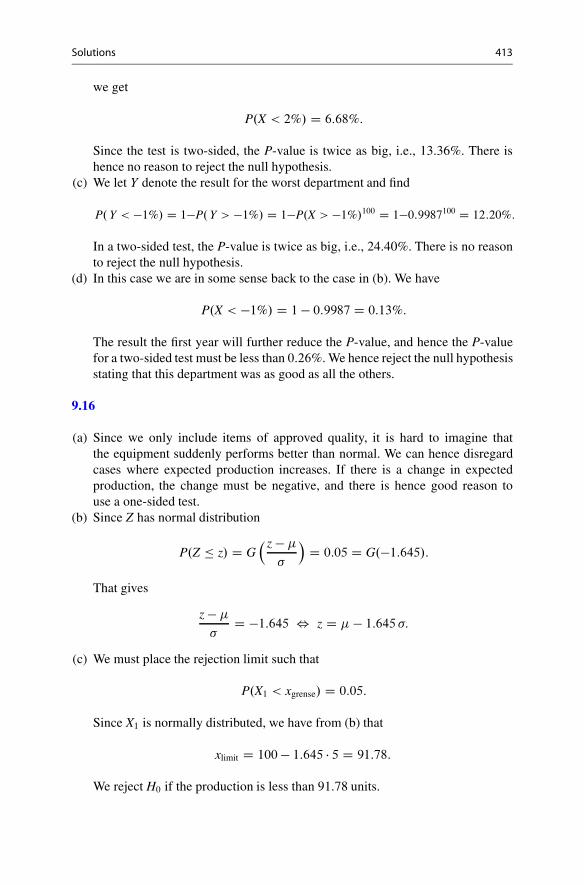
Solutions 413
we get
P.X < 2%/ D 6:68%:
Since the test is two-sided, the P-value is twice as big, i.e., 13.36%. There ishence no reason to reject the null hypothesis.
(c) We let Y denote the result for the worst department and find
P. Y < �1%/ D 1�P. Y > �1%/ D 1�P.X > �1%/100 D 1�0:9987100 D 12:20%:
In a two-sided test, the P-value is twice as big, i.e., 24.40%. There is no reasonto reject the null hypothesis.
(d) In this case we are in some sense back to the case in (b). We have
P.X < �1%/ D 1 � 0:9987 D 0:13%:
The result the first year will further reduce the P-value, and hence the P-valuefor a two-sided test must be less than 0:26%. We hence reject the null hypothesisstating that this department was as good as all the others.
9.16
(a) Since we only include items of approved quality, it is hard to imagine thatthe equipment suddenly performs better than normal. We can hence disregardcases where expected production increases. If there is a change in expectedproduction, the change must be negative, and there is hence good reason touse a one-sided test.
(b) Since Z has normal distribution
P.Z � z/ D G� z �
�
�D 0:05 D G.�1:645/:
That gives
z �
�D �1:645 , z D � 1:645 �:
(c) We must place the rejection limit such that
P.X1 < xgrense/ D 0:05:
Since X1 is normally distributed, we have from (b) that
xlimit D 100 � 1:645 � 5 D 91:78:
We reject H0 if the production is less than 91.78 units.

414 Solutions
(d) Let
Y D miniD1;:::;10
Xi:
Then
P. Y � 92/ D 1 � P. Y � 92/ D 1 � P.X � 92/10:
We compute
P.X � 92/ D 1�P.X � 92/ D 1�G
�92 � 100
5
�D 1�G.�1:6/ D G.1:6/ D 0:9452:
That gives P.Y � 92/ D 1 � 0:945210 D 0:4308. The probability of thishappening is hence 43.08%.
(e) We should reject H0 when
P. Y � ygrense/ D 0:05:
That gives
P.X � ylimit/10 D 0:95 ) P.X � ylimit/ D 1 � 0:951=10 D 0:0051:
Which implies
ylimit � 100
5D �2:57 ) ylimit D 87:15:
We reject H0 when production is not more than 87.15 units.
9.17
(a) X is Bin[120,0.05].(b)
P.X D 2/ D
120
2
!0:0520:95118 D 4:2%:
P.X � 2/ D P.X D 0/ C P.X D 1/ C P.X D 2/
D
120
0
!0:0500:95120 C
120
1
!0:0510:95119
C
120
2
!0:0520:95118 D 5:8%:

Solutions 415
(c) We cannot say anything sure about the probability for bankruptcy from onlyone observation. A statistician would interpret this statement in terms of ahypothesis test. With a null hypothesis stating p D 5%, we see that anobservation where X D 2 is not very rare (occurs in 4.2% of the cases). Fromthe computation in (b) we see that the P-value for a one-sided test is 5.8%.In normal cases we would keep a null hypothesis stating p D 5%. We cannotclaim that the journalist is wrong, but can point out that 2 or less bankruptcieswill occur quite often even when p is as large as 5%.
(d) If the firms are relatively similar, the probability of bankruptcy will largelydepend on the market for such firms. Even when firms are quite different,market prospects may depend on the general economic development. When theeconomy is growing, we will see less bankruptcies than when it falls. If theprobability of bankruptcy depends on such external circumstances, we will seemore extreme distributions. In some years very few, while in other years theymay appear in large numbers. We cannot assume that X is binomial, and in anycase it will be much harder to reject p D 5% since the distribution is not clear.
9.18
(a) Since the P-value is very large, we cannot reject the null hypothesis. There is noindication that the training has effect.
(b) If the school had been selected randomly, then a P-value of 4% would leadto rejection when it is seen in isolation. Here, however, we have repeated theexperiment 25 times. If training has no effect, we expect to observe a P-valueof 4% in 1 out of 25 cases. The result is hence not surprising, and there is noreason to assume that the training has effect when we see all the 25 cases inconjunction.
Problems of Chap. 10
10.1 This is a binomial test and we compute
Z D 132 � 200 � 0:5p
200 � 0:5 � .1 � 0:5/D 4:53:
Since the test is two-sided, we look up z0:025 D 1:96 in the table over the standardnormal distribution. The observed value is greater than the rejection limit, and wereject the null hypothesis. The conclusion is that p is probably not equal to 0.5.
10.2 This is a binomial test and we compute
Z D 25 � 50 � 0:6p
50 � 0:6 � .1 � 0:6/D �1:44:

416 Solutions
Since the test is two-sided, we look up z0:025 D 1:96 in the table over the standardnormal distribution. The observed value is well within the non-rejection region, andwe keep the null hypothesis that p D 0:6.
10.3 This is a binomial test and we compute
Z D 70 � 120 � 0:5p120 � 0:5 � .1 � 0:5/
D 1:83:
Since the test is one-sided, we look up z0:05 D 1:65 in the table over the standardnormal distribution. The observed value is greater than the rejection limit, and wereject the null hypothesis. The conclusion is that p is probably greater than 0.5.
10.4 We compute
SŒX� D 13:6p12
D 3:93:
Since 0 D 100, we find
T D 106:3 � 100
3:93D 1:6:
The rejection limits we find from the t-table with parameter 11. We have a two-sided test. Using 5% significance level, we look up the 2.5% level in the table.This gives t.19�
0:025 D 2:201. The non-rejection region is hence .�2:201; 2:201/. Sincethe observed value 1:6 is well within this region, we must keep the null hypothesis.There is not sufficient evidence to support a claim that the expected value is differentfrom 100.
10.5 We compute
SŒX� D 22:1p20
D 4:94:
Since 0 D 0, we find
T D 16:9 � 0
4:94D 3:42:
The rejection limits we find from the t-table with parameter 19. We have a two-sidedtest. Using 5% significance level, we look up the 2.5% level in the table. This givest.19�0:025 D 2:093. Since the observed value 1:6 is greater than the rejection limit, we
reject the null hypothesis. We have sufficient evidence to claim that the expectedvalue is probably different from zero.

Solutions 417
10.6 We compute
SŒX� D 3:22p11
D 0:97:
Since 0 D 10, we find
T D 12:96 � 10
0:97D 3:05:
The rejection limits we find from the t-table with parameter 10. We have a one-sidedtest. Using 5% significance level, we look up the 5% level in the table. This givest.19�0:05 D 1:812. In this case we should reject H0 only if T � �1:812. This is not
the case here, so we have not sufficient evidence to claim that the expected value issmaller than 10.
10.7 We compute X D 222 and Y D 192. We then calculate
S Dvuut 1
5 C 6 � 2
5X
iD1
.Xi � X/2 C6X
iD1
. Yi � Y/2
!D 30:98;
which gives
SŒ Oı� D S �r
1
5C 1
6D 18:76:
The value of the test static is then
T D 222 � 192
18:76D 1:60:
When the null hypothesis is true, T is t-distributed with parameter � D 5C6�2 D 9.The rejection limit for a two-sided test is then 2.26 (using 5% significance level).We keep the null hypothesis that there is no difference w.r.t. gender.
10.8 The mean value for department 1 is 131, and the mean value for department 2is 124. A one-sided t-test in Excel returns a P-value equal to 3.06%. The differenceis hence significant, and we conclude that the expected production at department 1is probably greater than the expected production at department 2.
10.9
(a) In this case the observations are paired, and the paired test is the one that makesbest use of the information. As the P-value from both tests fails to be significant,we have no sufficient evidence to claim that the expectations are different.

418 Solutions
(b) It is hard to imagine that advertising might have a negative effect. We havehence good reason to use a one-sided test for paired observations. H0 W 1 D2 against HA W 2 > 1. The P-value for this test is half the value for atwo-sided test, i.e., 4%. At 5% significance level we have sufficient evidence toclaim that the expected sales volume is probably greater at department 2 than atdepartment 1.
10.10
(a) We have
Op1 D 190
250; Op2 D 147
225; Op D 337
475:
We insert these quantities into the formula for U to get
U D Op1 � Op2r�1n1
C 1n2
�Op.1 � Op/
D 2:56:
Since we have a two-sided test, we use the table of the standard normaldistribution to look up z0:025 D 1:96. Since the observed value is greater thanthe rejection limit, we conclude that the two groups probably have differentexpectations. The P-value equals
2 � P.U � 2:56/ D 2 � .1 � 0:9948/ D 1:04%:
10.11
(a) We have
Op1 D 52
120; Op2 D 75
140; Op D 127
260:
We insert these quantities into the formula for U to get
U D Op1 � Op2r�1n1
C 1n2
�Op.1 � Op/
D �1:65:
Since we have a two-sided test, we use the table of the standard normaldistribution to look up z0:025 D 1:96. Since the observed value is within thenon-rejection region, we do not have sufficient evidence to claim that the twogroups have different expectations.

Solutions 419
10.12 In the chi-square test we have n D 500 and p1 D p2 D p3 D p4 D 0:25. Wethen get
Q D .129 � 125/2
125C .140 � 125/2
125C .113 � 125/2
125C .118 � 125/2
125D 3:472:
When H0 is true, then Q is chi-square distributed with parameter 3. At 5%significance level we should reject if Q � 7:81. As this is not the case here, wekeep the null hypothesis. There is no sufficient evidence to claim that any of theproducts are more liked than the others.
10.13 In the chi-square test we have n D 300 and p1 D p2 D p3 D 1=3. We thenget
Q D .98 � 100/2
100C .120 � 100/2
100C .92 � 100/2
100D 4:68:
When H0 is true, then Q is chi-square distributed with parameter 2. At 5%significance level we should reject if Q � 3:89. As this is the case here, we rejectthe null hypothesis. There is sufficient evidence to claim that some of the productsare probably more liked than the others.
10.14 We first write the observed numbers in the first column. Then we multiplythe percentages with 1000 and write these numbers in the second column. Thecommand =CHITEST(A1:A10;B1:B10) returns the P-value 53.90%. There is henceno reason to reject the null hypothesis.
10.15 In the chi-square test n D 800; p1 D 0:4; p2 D 0:3; p3 D 0:3. Then
Q D .345 � 320/2
320C .238 � 240/2
240C .217 � 240/2
240D 4:174:
When H0 is true, then Q is chi-square distributed with parameter 2. At 5% level ofsignificance we should reject H0 if Q � 5:99. This is not the case here, so the testdoes not provide sufficient evidence that opinions have changed.
10.16 In the chi-square test n D 400 and
p1 D 0:243; p2 D 0:213; p3 D 0:146; p4 D 0:125; p5 D 0:124; p6 D 0:149:
In the poll 92 people answered party A, 72 B, 68 C, 40 D, and 64 E. Then we get
Q D .92 � 0:234 � 400/2
0:234 � 400C .72 � 0:213 � 400/2
0:213 � 400C .68 � 0:146 � 400/2
0:146 � 400
C .64 � 0:125 � 400/2
0:125 � 400C .40 � 0:124 � 400/2
0:124 � 400C .64 � 0:149 � 400/2
0:149 � 400
D 10:00:

420 Solutions
When H0 is true, then Q is chi-square distributed with parameter 5. At 5% level ofsignificance we should reject H0 if Q � 11:11. This is not the case here, so the testdoes not provide sufficient evidence that opinions have changed.
10.17 In the chi-square test n D 1000. The probability of X errors in 3 independenttrials in a binomial distribution. Hence
P.X D 0/ D�
3
0
�0:0600:943 D 0:8306;
P.X D 1/ D�
3
1
�0:0610:942 D 0:1590;
P.X D 2/ D�
3
2
�0:0620:941 D 0:0102;
P.X D 3/ D�
3
3
�0:0630:940 D 0:0002:
Then
Q D .829 � 830:6/2
830:6C .163 � 159/2
159C .6 � 10:2/2
10:2C .2 � 0:2/2
0:2D 18:03:
When H0 is true, then Q is chi-square distributed with parameter 3. At 5%significance level we should reject if Q � 7:81. As this is the case here, we reject thenull hypothesis. There is sufficient evidence to claim that some of the distribution isprobably not binomial.
10.18 We first need to find the marginals. The results are shown in Table 6.
Table 6 Marginal totals Credit rating Unmarried Married Total
A 200 300 500
B 140 260 400
C 40 60 100
Total 380 620 1000
To execute the test, we also need to make a table over the expected values in eachentry. Formally we use the formula Eij D AiBj
n , but we might just as well multiplythe fractions and multiply these answers with n D 1000. In both cases we end upwith Table 7.
Now we can compute the Q-value:
Q D .200 � 190/2
190C .300 � 310/2
310C .140 � 152/2
152

Solutions 421
Table 7 Expected ratingsunder independence
Credit rating Unmarried Married Total
A 190 310 500
B 152 248 400
C 38 62 100
Total 380 620 1000
C .260 � 248/2
248C .40 � 38/2
38C .60 � 62/2
62
D 2:55:
To find the rejection limit we must use a chi-square table with parameter � D.2 � 1/.3 � 1/ D 2. Using 5% significance level, the rejection limit in that table is5.99. Our observed Q is smaller than the rejection limit, and we are unable to rejectthe null hypothesis stating independence. In other words we do not have sufficientevidence to claim that there is a connection between marital status and credit rating,
10.19 We first need to find the marginals. The results are shown in Table 8.
Table 8 Marginal totals Reason Hotel A Hotel B Hotel C Total
Too expensive 50 100 150 300
Bad attractions 100 200 100 400
Bad cleaning 150 100 50 300
Total 300 400 300 1000
To execute the test, we also need to make a table over the expected values in eachentry. Formally we use the formula Eij D AiBj
n , but we might just as well multiplythe fractions and multiply these answers with n D 1000. In both cases we end upwith Table 9.
Table 9 Expected resultsunder independence
Reason Hotel A Hotel B Hotel C Total
Too expensive 90 120 90 300
Bad attractions 120 160 120 400
Bad cleaning 90 120 90 300
Total 300 400 300 1000

422 Solutions
Now we can compute the Q-value:
Q D .50 � 90/2
90C .100 � 120/2
120C .150 � 90/2
90
C .100 � 120/2
120C .200 � 160/2
160C .100 � 120/2
120
C .150 � 90/2
90C .100 � 120/2
120C .50 � 90/2
90
D 138:89:
To find the rejection limit we must use a chi-square table with parameter � D .3 �1/.3 � 1/ D 4. Using 5% significance level, the rejection limit in that table is 9.49.Our observed Q is far above the rejection limit, and we reject the null hypothesisstating independence. In other words there is probably a connection between thehotel that was used and the answer that was given.
10.20
(a) The null hypothesis is that there is no change in the distribution of answers,while the alternative hypothesis is that there has been a change. We should makeuse of a chi-square table with parameter 4, and at 5% significance level weshould reject the null hypothesis if Q � 9:49:
Q D .188 � 148/2
148C .80 � 74/2
74C .330 � 370/2
370
C .92 � 111/2
111C .50 � 37/2
37D 23:44:
Since Q � 9:49 we reject the null hypothesis, and we have sufficient evidenceto claim that the customers probably have changed opinions.
(b) We should make use of a chi-square table with parameter 1, and at 5%significance level we should reject the null hypothesis if Q � 3:84:
Q D .598 � 592/2
592C .142 � 148/2
148D 0:304:
Since Q < 3:84, we keep the null hypothesis. We do not have evidence thatthe distribution of satisfied/dissatisfied has been altered. This suggests thatthe changes reported in (a) is due to internal changes within the two groupssatisfied/dissatisfied.
(c) X5�np5pnp5.1�p5
is approximately standard normal under these assumptions. That gives
P.X5 � 50/ D 1�P.X5 � 49/ D 1�G
�49 � 37p37 � 0:95
�D 1�G.2:02/ D 0:0217:

Solutions 423
If the customers have the same opinions as before, there is only 2% probabilityof finding as many very dissatisfied customers as we observed. There is hencereason to believe that the fraction of very dissatisfied customers has increased.
10.21 R is Bin[6,0.5]. We can find the values from a table or directly from thedefinition of binomial probabilities. We get
p0 D 0:015625; p1 D 0:09375; p2 D 0:234375; p3 D 0:3125;
p4 D 0:234375; p4 D 0:09375 p6 D 0:015625:
(b) A chi-square test can be formulated as follows:
H0 W The probabilities are equal to the probabilities from (a).
HA W The probabilities are not equal to the probabilities from (a).
Let Xi be the number of persons with exactly i correct answers. As test static weuse
Q D6X
iD0
.Xi � 300 � pi/2
300 � pi:
When the null hypothesis is correct, Q is approximately chi-square distributed withparameter 6. Using 5% significance level, we should reject H0 if Q � 12:6. If weinsert the observed numbers, we get Q D 10:41. We keep the null hypothesis, andcannot be reasonably sure that the distribution of answers are different from whatwe would expect if all participants were guessing the answers.
10.22
(a) X1 D BinŒn1; p1� and X2 D BinŒn2; p2�.(b) H0 W p1 � p2 against HA W p1 > p2. We insert the values and find U D 1:51.
Since U is approximately standard normal, the P-value is given by
P D P.U � 1:51/ D 1 � P.U � 1:51/ D 1 � G.1:51/ D 1 � 0:9345 D 6:5%:
At 5% significance level we would keep the null hypothesis, which means thatthe results may be coincidental.
(c) It may happen that a company focuses funds within a particular branch, i.e.,information technology. If information technology companies are doing well,all the funds will be doing well, and if the market for such companies declines,the majority of the funds will perform badly. The result of each different fund ishence strongly dependent on how the other funds are doing.

424 Solutions
10.23
(a) A chi-square test is well suited for this situation. The null hypothesis is thatthe probability that a randomly chosen customer prefers product number i isgiven by
p1 D 0:1; p2 D 0:2; p3 D 0:15; p4 D 0:3; p5 D 0:1; p6 D 0:15:
The alternative hypothesis is that the probabilities are not like that. As test staticwe use
Q D6X
iD1
.Xi � n pi/2
n pi:
When H0 is true, this test static is approximately chi-square distributed withparameter 5. Using 5% significance level, we should reject H0 if Q � 11:1. Therejection region is Œ11:1; 1/.
(b) We find
Q D .28 � 20/2
20C .42 � 40/2
40C .25 � 30/2
30
C .52 � 60/2
60C .25 � 20/2
20C .28 � 30/2
30
D 6:58:
Since the value of Q is below the rejection limit, we keep the null hypothesis.The tendency in our data material is not sufficient strong to support a claim thatopinions have changed. From the table we see that the P-value is slightly largerthan 25%. (25% gives Q D 6:63).
10.24
(a) Any t-test takes the t-distribution as a starting point, which requires data to beapproximately normal. Since the P-value is lower than the significance level,we should reject the null hypothesis. If all the requirements are satisfied, weconclude that the two departments probably have different expected production.
(b)
P.X � 125/ D G
�125 � 106:15p
36:87
�D G.3:1/ D 0:999:
P.Largest � 125/ D 1 � P.All � 125/ D 1 � P.X � 125/20
D 1 � 0:99920 D 1:98%:

Solutions 425
(c) Since the P-value is far less than the significance level, we confidently rejectthe null hypothesis. Our data are probably not normally distributed. This meansthat we cannot trust the test in (a). We hence do not have sufficient evidence toclaim that the two departments have different expected production.
10.25
(a) We first find
SŒ Oı� Ds
42:71 ��
1
8C 1
8
�D 3:27:
That gives
T D 124 � 130:63
3:27D �2:03:
This is a one-sided test with 5% significance level. The parameter is � D 8 C8 � 1 D 14, and from this t-table we find t.14/
0:025 D 1:761. The training has effectif X < Y , and we use the hypotheses H0 W X � Y and HA W X < Y . Wecan reject H0 if T � �1:761. Since this is the case, we reject the null hypothesisand claim that the training probably had effect.
(b) To compute W we sort the values in ascending order and underline the valuesfrom the first group. That gives
113; 118; 119; 123; 124; 125; 126; 127; 128; 129; 130; 131; 132; 133; 139; 140:
To compute W we sum the positions of the underlined numbers, i.e.
W D 1 C 2 C 3 C 5 C 8 C 9 C 12 C 13 D 53:
We compute
EŒW� D 1
2� 8.8 C 8 C 1/ D 68:
VarŒW� D 1
12.8 � 8.8 C 8 C 1/ D 90:67:
That gives
Z D 53 � 68p90:67
D �1:58:

426 Solutions
This is a one-sided test with 5% significance level. From the table of the standardnormal distribution we get z0:05 D 1:6449: The hypotheses are the same as in(a), and we should reject H0 if Z � �1:6449. This is not the case, so we keepH0 as we are not sufficiently sure there is an effect.
(c) We see that the two tests give opposite conclusions. If we have information thatimplies that data are not normally distributed, the assumptions for the t-test failsand we must disregard that result. The only valid conclusion is the one from (b).
10.26
(a)
EŒW� D 1
2� 20 � .20 C 20 C 1/ D 410:
VarŒW� D 1
12� 20 � 20 � .20 C 20 C 1/ D 1366:67:
We sort the observations in ascending order and underline the observations fromgroup 1:
195; 206; 210; 211; 212; 214; 218; 219; 220; 224;
227; 228; 229; 232; 235; 237; 238; 239; 240; 241;
245; 246; 247; 248; 251; 252; 253; 259; 260; 263;
264; 268; 275; 276; 279; 283; 285; 286; 288; 296:
W is the sum of the positions of the underlined numbers, i.e.
W D 3 C 9 C 10 C 11 C 12 C 15 C 16 C 17 C 18 C 21
C24 C 25 C 26 C 28 C 32 C 35 C 36 C 37 C 38 C 39
D 452:
This gives
Z D 452 � 410p1366:67
D 1:14:
Since this is a one-sided test with 5% significance level, we find z0:05 D 1:6449:
We should hence reject H0 if Z � 1:6449. As this is not the case, we keep thenull hypothesis and do not have sufficient evidence to claim that the expectedworking time has been reduced.

Solutions 427
(b)
EŒW� D 1
4� 20 � .20 C 1/ D 105:
VarŒW� D 1
24� 20 � .20 C 1/ � .2 � 20 C 1/ D 717:5:
We take the numbers from group 2 and subtract the corresponding numbersfrom group 1. That gives
�21; 3; 6; �18; �12; �16; �8; �5; �14; 1;
�19; �24; �7; �2; �25; �4; �13; 15; �22; 10:
The next step is to sort the observation in ascending order with respect toabsolute value, and then underline the negative numbers.
1; �2; 3; �4; �5; 6; �7; �8; 10; �12; �13�14;
�15; �16; �18; �19; �21; �22; �24; �25:
V is the sum of the positions of the underlined items:
V D 2C4C5C7C8C10C11C12C13C14C15C16C17C18C19C20 D 191:
That gives
Z D 191 � 105p717:5
D 3:21:
Since this is a one-sided test with 5% significance level, we find z0:05 D 1:6449:
We should hence reject H0 if Z � 1:6449. This is true, and we hence rejectthe null hypothesis and claim that the expected working time has probably beenreduced.
(c) The test in (b) is the one that best makes use of the given information. Theobservations are paired, and the test in (a) does not take this into account. Thereis no contradiction here. The conclusion in (a) is that we do not have sufficientevidence to reject the null hypothesis. When more precise information is given,we can execute a more refined test. We conclude that the expected working timehas probably been reduced.

428 Solutions
10.27
(a)
Op1 D 10
100Op2 D 8
120Op D 18
220:
That gives
U D Op1 � Op2q�1
100C 1
120
� Op.1 � Op/D 0:90:
We let p1 be the probability for error before training and p2 be the probabilityfor error after training, In this case H0 W p1 D p2 and HA W p1 > p2. It is notreasonable that training of this sort will increase the probability for errors. Wecan hence disregard cases where p1 < p2. That means that it is legitimate to usea one-sided test in this case.
P-value D P.U � 0:90/ D 1 � P.U � 0:90/ D 1 � G.0:90/ D 1 � 0:8159 D 18:41%:
Since the P-value is large, there is no reason to reject the null hypothesis sayingthat training had no effect.
(b) It is easy to realize that training of this kind might reduce the efficiency ofproduction, and hence a two-sided test is appropriate here.
10.28
(a) It is unreasonable that training should lead to lower production, and we can thenuse one-sided tests.
H0 W Expected production is the same before and after training:
HA W Expected production is larger after training:
(b) t-test: The P-value is large and we must keep the null hypothesis that expectedproduction is the same as before. Training does not appear to have had effect.
The Wilcoxon test: The P-value is very small, and we reject the hullhypothesis and claim that expected production probably has increased.
(c) If we inspect to observed pairs, we see that in all cases except the last pair,production has increased after training. The last pair is very different from allthe others and pulls the conclusion in the opposite direction. Either the last pairis a mistyping, or data are probably not normally distributed. In either case weshould rely on the result from the Wilcoxon test. A general advantage of theWilcoxon test over t-tests is that it is less sensitive with respect to outliers, i.e.,observations that are very different from the rest.

Solutions 429
10.29
(a) Here we have H0 W X � Y and HA W X < Y . Using the formulas for theWilcoxon test, we get
EŒW� D 1
2� 50 � .50 C 50 C 1/ D 2525:
VarŒW� D 1
12� 50 � 50 � .50 C 50 C 1/ D 21;041:67:
(b) We find
Z D 2455 � 2525p21;041:67
D �0:48:
In this case we should reject H0 if Z � �1:6449. This is not the case here, sowe keep the null hypothesis saying that training has no effect.
(c) EŒV� D 1450 � 51 D 637:5, VarŒV� D 1
2450 � 51 � 101 D 10;731:25:
(d) We get Z D 604�637:5p10;731:25
D �0:32: In this case, too, we should reject H0 if Z ��1:6449: This is not the case here, so we keep the null hypothesis saying thattraining has no effect.
(e) After sorting we find Z D 664�637:5p10;731:25
D �2:64: If this value had made sense, itwould have lead to rejection. The problem is that the sorting breaks the pairingof the data, and we are not allowed to use a paired test on the sorted data.
(f) As mentioned under (e), a paired test cannot be used on the sorted data. Theonly valid conclusion comes from (d), which do not find sufficient evidence toclaim that training had effect.
Remark The sorting in (e) will in general create strong effects. We typically getvalues for Z in the interval Œ�25; 25� even when there is no effect present, and Z willnot be approximately normal (under H0) in this case. Such creative processing ofdata is a very serious mistake.
10.30
(a) We compute
SŒ Oı� D S �s
1
n1
C 1
n2
D 43;000 �r
1
5000C 1
7000D 796:21:
T D 312;000 � 310;000
796:21D 2:51:

430 Solutions
Since we have a two-sided test with 5% significance level, we findt.11;998/0:025 D 1:96 (with so many observations there is no difference between
the t-distributions and the standard normal distribution). Since T D 2:51 >
1:96 D t.11;998/0:025 , we reject the null hypothesis stating equal expected wages, and
conclude that expected wages probably are different in the two regions.(b) We compute
T1 D 2000 C 5000
796:21D 8:79; T2 D 5000 � 2000
796:21D 3:77:
In this case we find t.11;998/0:05 D 1:645. Since minŒT1; T2� D 3:77,
minŒT1; T2� > 1:645 D t.11;998/0:05 ;
and we reject the null hypothesis stating that expected wages are not equivalent,and conclude that the difference in expected wages is probably so small that itis unimportant.
Remark The exercise illustrates a general weakness of classical hypothesis testing.If we have many observations, even the slightest difference will lead to rejection ofa null hypothesis stating equality. In such cases an equivalence test may be moresuited to shed light on the situation. It should be noted, however, that an equivalencetest is to some extent in conflict with basic principles of classical hypothesis testingwhere one nearly always starts out with a null hypothesis stating equality.
10.31
(a) The answer q D 31:4 we find from the chi-square table with parameter � D 20.(b) The rejection limit follows from (a). We reject if
2 � 10 � X
10� 31:4 , X � 15:7:
Since the observed value X D 15 is below the rejection limit, we keep H0.We note that even though the observed value appears to be quite far from theexpected value D 10, this is not sufficient for rejection.
(c) By the strength of the alternative D 20, we mean the probability of rejectingH0 when the true value of is 20. We reject when X � 15:7, and that gives
P.X � 15:7/ D P
2 � 10 � X
20� 2 � 10 � 15:7
20
!D P.Q20 � 15:7/ � 75%;
(the closest number we find in the table is 15.5, and the strength is hence slightlysmaller that 75%). To answer the last question, we must try out different values

Solutions 431
of n. If n D 50, we should use the chi-square table with parameter 100. Wereject when Q � 12:4, and the strength of the alternative D 12:5 becomes
P.X � 12:4/ D P
�Q100 � 2 � 50 � 12:4
12:5
�D P.Q100 � 99:2/ � 50%;
(the closest number we find in the table is 99.3, and the strength is hence slightlyabove 50%).
10.32
(a) We compute
SŒ Oı� D S �s
1
n1
C 1
n2
D 2900 �s
1
15;000C 1
10;000D 37:44:
That gives
T D 32;378 � 32;209
37:44D 4:51:
Here we have lots of observations, and there is no difference between the t-distributions and the standard normal distribution. Hence t.�/
2:5% D 1:96. Since Tis far above the rejection limit, we reject H0 and conclude that the differencein expected wages is strongly significant. The wording strongly significantis sometimes used when the P-value is less than 1%, but note that stronglysignificant does not in any way mean the same as very important.
(b) A 95% confidence interval we find by
X � Y ˙ t.�/
˛=2 � SŒ Oı� D 32;378 � 32;209 ˙ 1:96 � 37:44:
which gives the interval Œ95; 242�. We see that the difference in expected wagesis quite modest even though the difference is strongly significant. In cases withmany observations, confidence intervals are often more informative as theyprovide a clear indication of how large the difference can be expected to be.
10.33
(a)
Xbefore D 1 � 160
960C 2 � 160
960C 3 � 160
960C 4 � 160
960C 5 � 160
960D 3:
Xafter D 1 � 264
1379C 2 � 310
1379C 3 � 230
1379C 4 � 115
1379C 5 � 460
1379D 3:14:

432 Solutions
(b)
SŒ Oı� D 1:47 �r
1
960C 1
1379D 0:062; T D 3 � 3:14
0:062D �2:25:
From the table of the standard normal distribution, the rejection limit at 5%significance level is �1:65. Since the observed value is less than this, we rejectthe null hypothesis and claim that the expected answer (whatever that might be)has increased significantly.
(c) The test in (b) is problematic. Data are not scaled; we probably do not mean that5 (very satisfied) is 5 times better than 1 (very dissatisfied) or 25% better than 4(somewhat satisfied). It is not even clear that the mean value has any meaningfulinterpretation. Overall the whole analysis is questionable.
(d) (i) Here we have Op1 D 160960
; Op2 D 4601379
, and Op D 160C460960C1379
. Inserting thesevalues, we find
U D Op1 � Op2q�1
960C 1
1379
� Op.1 � Op/
D �9:00:
The effect is strongly significant, and we conclude that there are probablymore very satisfied customers than before.
(ii) Here we merge the data from answers 4 and 5. That gives
Op1 D 240 C 160
960; Op2 D 115 C 460
1379; Op D 240 C 160 C 115 C 460
960 C 1379:
Inserting these values, we find
U D Op1 � Op2q�1
960C 1
1379
� Op.1 � Op/
D �0:015:
This value is well inside the non-rejection region, and there is no reason toclaim that there are more satisfied customers than before.
(iii) Here we have Op1 D 160960
; Op2 D 2641379
, and Op D 160C264960C1379
. Inserting thesevalues, we find
U D Op1 � Op2q�1
960C 1
1379
� Op.1 � Op/
D �1:53:
Here we notice a tendency that the fraction of very dissatisfied customershas increased, but the effect is not sufficient for rejection. The resultmay be due to chance, and we must keep the null hypothesis stating nodifference. Note that when we use one-sided tests here, we tacitly assumethat more support cannot lead to more dissatisfaction. That strengthens the

Solutions 433
impression that the increase is due to chance. Strictly speaking the test in(iii) does not make sense under these assumptions.
(e) The serious problems that we pointed out with the test in (b) are not presenthere. Quite the contrary, these tests are credible and are clearly the right toolsfor handling these data.
10.34
(a)
EŒX� D E
"1
100
100X
iD1
Xi
#D 1
100
100X
iD1
EŒXi� D 1
100
100X
iD1
489 D 489:
VarŒX� D Var
"1
100
100X
iD1
Xi
#D 1
1002
100X
iD1
VarŒXi� D 1
1002
100X
iD1
902 D 81:
It is not necessary to show these calculations. Alternatively we can just refer towell-known principles from the book.
(b) From (a) we have EŒX� D 489 and �ŒX� D 9. That gives
P.X � 463/ D G
�463 � 489
9
�D G.�2:89/ D 1 � G.2:89/ D 1 � 0:9981 D 0:0019:
(c) From (b) we see that
P.X � 463/ D 0:9981:
The probability that all the 500 schools have a mean score above 463 is hence
0:9981500 D 0:386392:
(d) We use the equivalence
The worst school has a result � 463 , Not all schools have a score > 463
The score has normal distribution, and hence the probability of a mean scoreequal to 463 is zero. That gives
P.The worst school has a result � 463/ D 1 � 0:9981500 D 61:36%:
Even though a randomly selected school has very little probability of scoring463 or less, it is very likely that at least one of the schools performs at such lowlevel.

434 Solutions
10.35
(a) This result is perfectly normal. If all the departments are equally good, a P-valueof 4% will occur in one out of 25 cases. Since the company has 100 productiondepartments, there is nothing strange with this value. The management shouldnot take any action.
(b) This result is not normal. If all departments are equally good, a P-value of 0.01%will only occur in 1 out of 10;000 cases. Even when we take into account thatthe company has 100 production departments, this result is unusually bad. Themanagement should take swift action and see if they are able to identify a causefor this.
(c) Independence gives
P
�min
1�i�100Z1 � 10
�D 1 � P.Zi � 10/100:
We need to compute
P.Zi � 10/ D 1 � P.Zi � 10/ D 1 � P.Xi � lnŒ10�/ D 1 � G
�lnŒ10� � 10
3
�
D 1 � G.�2:57/ D G.2:57/ D 0:9949:
That gives
P
�min
1�i�100Z1 � 10
�D 1 � 0:9949100 D 40:03%:
10.36
(a) We compute SŒ Oı� D 23:23 �q
140
C 140
D 5:19. That gives
T D 101:75 � 112:12
5:19D �2:00:
Rejection is decided from a t-table with parameter 78, the table with parameter80 suggests rejection when T � �1:664. We see from the table that the P-valueis about 2.5%. We are able to reject the null hypothesis, and draw the conclusionthat the expected value is probably greater in group 2.
(b) If we repeat the computations from (a) using new values, we get
SŒ Oı� D 19:91 �r
1
10C 1
10D 8:90:

Solutions 435
That gives
T D 103:62 � 110:88
8:90D �0:82:
Rejection is decided from a t-table with parameter 18, and the table suggestsrejection when T � �1:734. Seen in isolation, this result does not give causefor rejection.
(c) That the strength is as low as 25% means that we in 3 out of 4 cases will do a typeII error, i.e., keep a wrong null hypothesis. We should hence not be surprisedwhen the new test does not confirm the result from (a). Quite the contrary, thisis something that will happen in a majority of cases. It is hence not a good ideato try to confirm the result in this way. To avoid seemingly contradictory resultsas this, it is important that the confirmation has sufficient strength. In our casea confirmation should build on more than 100 observations in each group. If wesimply repeat the data collection in (a) with 40 observations in each group, thestrength is still no more than about 65%, meaning that 1 out of 3 samples doesnot confirm a significant effect.
(d) If we merge the data from (a) and (b), we find
SŒ Oı� D 22:42 �r
1
50C 1
50D 4:48:
This gives
T D 102:12 � 111:88
4:48D �2:18:
Rejection is decided from a t-table with parameter 98, the table with parameter100 suggests rejection when T � �1:660. We see that the two datasets intotal gives a clear rejection, and that the rejection is even clearer than in (a).It may appear contradictory that (b) in fact supports the finding in (a), but theexplanation is that (b) too gives a result in the same direction as (a), i.e., X < Y .
Problems of Chap. 11
11.1 (a) Suitable. (b) Nonlinear, unsuitable. (c) Suitable. (d) No particular pairing,partly unsuitable.
11.2 We choose the points t D 0; x D 10 and t D 20; x D 0. The two point formulagives
x D 10 � 0
0 � 20� .t � 0/ C 10 D �1
2� t C 10:

436 Solutions
11.3 Here we have t1 D 1; t2 D 3; t3 D 5; t4 D 7 and X1 D 3; X2 D 7; X3 D9; X4 D 9. We insert those values into the formulas
t D 1
4.1 C 3 C 5 C 7/ D 4;
X D 1
4.3 C 7 C 9 C 9/ D 7;
O D 1
.1 � 4/2 C .3 � 4/2 C .3 � 4/2 C .7 � 4/2
�..3 � 7/.1 � 4/ C .7 � 7/.3 � 4/ C .9 � 7/.5 � 4/ C .9 � 7/.7 � 4//
D 1
20� 20 D 1:
O D X � O t D 7 � 1 � 4 D 3:
The regression line is
OX D 3 C t:
11.4 We compute
SŒ O� Dr
5:702
770D 0:205:
If ˇ D 0, then
T DO � ˇ
SŒ O� D 2:06
2:43D 10:05:
Under H0, T is t-distributed with parameter � D 19. In a two-sided test with 5%significance level, we should reject H0 when
jTj � 2:093:
The rejection criterion is satisfied, and we claim that the effect of time t isstatistically significant.
11.5 We compute
SŒ O� Dr
5:372
340D 0:291:

Solutions 437
If ˇ D 0, then
T DO � ˇ
SŒ O� D �0:32
0:291D 1:10:
Under H0, T is t-distributed with parameter � D 14. In a two-sided test with 5%significance level, we should reject H0 when
jTj � 2:145:
The rejection criterion is not satisfied, and we are unable to claim that time t hassignificant effect.
11.6
(a) When t D 15, then
OX D 78:31 � 3:01 � 15 D 33:16:
We have
SŒ OX� D 5:81 �r
1
12C .15 � 5:5/2
143D 4:91:
We hence estimate
EŒX� D 33:16 ˙ 4:91:
(b) Here we compute
SŒ OX � X� D 5:81 �r
1 C 1
12C .15 � 5:5/2
143D 7:61:
The predicted value is
X D 33:16 ˙ 7:61:
(c) Since the variance is unknown, we use the t-distribution with parameter � D 10.The two 95% confidence intervals hence have the limits
33:16 ˙ 2:228 � 4:91 ! Œ22:22; 44:10�;
and
33:16 ˙ 2:228 � 7:61 ! Œ16:20; 50:12�:

438 Solutions
11.7
(a) When t D 40, then
OX D 64:37 C 1:81 � 40 D 136:77:
We have
SŒ OX� D 5:76 �r
1
32C .40 � 15:5/2
2728D 2:89:
We hence estimate
EŒX� D 136:77 ˙ 2:89:
(b) Here we compute
SŒ OX � X� D 5:76 �r
1 C 1
32C .40 � 15:5/2
2728D 6:44:
The predicted value is
X D 136:77 ˙ 6:44:
(c) Since the variance is unknown, we use the t-distribution with parameter � D 30.The two 95% confidence intervals hence have the limits
136:77 ˙ 2:042 � 2:89 D Œ130:87; 142:67�;
and
136:77 ˙ 2:042 � 6:44 D Œ123:61; 149:92�:
11.8 The residual is the difference between the point on the regression line and thecorresponding observed value. We have t1 D 1 and X1 D 3.
OX1 D 3 C t1 D 3 C 1 D 4:
The first residual is hence
OR1 D X1 � OX1 D 3 � 4 D �1:

Solutions 439
Similarly we find
OR2 D X2 � OX2 D 7 � 6 D 1;
OR3 D X3 � OX3 D 9 � 8 D 1;
OR4 D X4 � OX4 D 9 � 10 D �1:
11.9
(a) We see that education is strongly significant. The explanatory power is about23%, and one year of extra education offers an increase of 1896 USD inexpected wages.
(b) The four variables exhibit multicollinearity. For example is
prof 4 D 1 � prof 1 � prof 2 � prof 3:
When dummy variables are used in regression, one of the dummies must bedeleted.
(c) We see that the variables practice, gender, and profession are strongly signif-icant. Education is clearly nonsignificant, even the sign makes no sense. Theexplanation is multicollinearity between education and profession. This is laterconfirmed by the findings in (d). The reason why education is significant in (a)is not that extra education is good in itself, but it is likely that long education isneeded to get work in the professions that pay more. The profession is probablythe primary cause for high salary, and education fails to be significant whenprofession is included as explanatory variable.
(d) Since R2 > 90%, we interpret this as multicollinearity between education andprofession. This suggest that we may delete education as explanatory variable.
(e) Now all explanatory variables are strongly significant. The explanatory poweris 96% and has not been reduced by deleting the variable education. This is abetter model.
(f) We use the model from (e), and find
1wages D 14;924 C 506 � 12 C 10;072 � 1 D 31;063:
All the other terms are zero.
11.10
(a) Method is not a scale variable and cannot be used directly in a regression. Theresults here are all without meaning.
(b) Using X1 and X2 we have coded method via dummy variables. Contrary to (a)this is a valid construction, and the results show that time and method are both

440 Solutions
strongly significant. In addition we see that the model has explanatory power91.5%, which is great.
(c) As mentioned above (a) is pointless and only the model in (b) carries weight.From the regression
4production D 195:9 C 9:67 � time � 43:77 � X1 � 34:11 � X2;
we see that the coefficients in front of X1 and X2 are both negative. That meansthat maximum expected/predicted value is obtained when X1 and X2 are bothzero. This case occurs when we use method 2. Method 2 is hence the one withthe best expected/predicted value.
11.11 The histogram resembles the normal distribution, normal score is approxi-mately a straight line, and the residuals are fairly symmetric and do not change alongthe axes. In total the assumptions of independent, normally distributed residualsappear to be satisfied.
11.12 The histogram does not resemble the normal distribution, the normal scoreis not a straight line, and the residuals exhibit noticeable trends. Everything goeswrong here, and the assumption of independent, normally distributed residuals doesnot appear to be satisfied.
11.13
(a) The observations do not lie in the vicinity of a straight line, the normal scoreis not a straight line, the histogram does not resemble the normal distribution,and the residuals have obvious trends. Conclusion: None of the standard criteriaappears to be satisfied, and linear regression serves no purpose in this case.
(b) The observations lie in the vicinity of straight line, the normal score is a fairlystraight line, and the residuals are fairly symmetric without noticeable trends.Residual versus fitted values is maybe not fully symmetric at the right side, butthat is due to a low number of observations, and does not indicate that somethingis wrong. Conclusion: All the standard criteria appears to be satisfied, and alinear regression appears to make good sense.
(c) If we insert p D 110, we find
blnŒQ� D 8:91 � 0:914 lnŒ110� D 4:61:
That gives
OQ D e4:61 D 100:
An estimate for the expectation of Q hence 100.

Solutions 441
(d) The trick is to add and subtract EŒln.U/� at the right place. Using standard rulesfor logarithms we get
lnŒQ� D ln.K � pˇ � U/
D ln.K/ C ln. pˇ/ C ln.U/ D ln.K/ C ˇ ln. p/ C ln.U/
D .ln.K/ C EŒln.U/�/ C ˇ ln. p/ C .ln.U/ � EŒln.U/�/;
i.e., � D lnŒK� C EŒln.U/� and � D ln.U/ � EŒln.U/�. Strictly speaking we alsoneed to assume that EŒln.U/� < 1.
(e) Since
� D ln.K/ C EŒln.U/� ) K D e��EŒln.U/� D e��lnŒEŒU��C 12 �2 D e�C 1
2 �2
EŒU�:
The expected value is hence given by
EŒQ� D K � pˇ � EŒU� D e�C 12 �2
EŒU�� eˇ ln. p/ � EŒU� D e�Cˇ ln. p/C 1
2 �2
:
If we use this formula to estimate EŒQ�, we find
EŒQ� � e O�C O ln.110/C 12 S2 D e8:91�0:914 ln.110/C 1
2 �0:21622 D 103:
11.14
(a) When data form a strictly convex profile, the data cannot be described by astraight line. Linear regression is unsuitable in such situations.
Stock prices, mutual bonds, and bank deposits usually exhibit exponentialgrowth. When the value doubles, a percentage increase typically doubles theincrease. For example, 5% growth will increase the price by 6 USD when theprice is 120 USD, while the increase will be 12 USD when the price is 240USD. This in turn will lead to exponential growth.
(b) The transformed data are fairly linear. The histogram is slightly skewed, butstill acceptable. The normal score is fairly straight, and the residuals are fairysymmetric and homogeneous. There is a tendency that the residuals increase atthe right side, but all in all we conclude that the standard assumptions for linearregression are satisfied.
(c) We have
X D e�Cˇ tC� D e�Cˇ t � e�:

442 Solutions
Since e�Cˇ t is a constant, we have
EŒX� D EŒe�Cˇ t � e�� D e�Cˇ t � EŒe�� D e�Cˇ t � e1=2 �2 D e�Cˇ tC1=2 �2
:
An estimator for this is
OX D e O�C O tC1=2 S2
:
An estimate for expected value at t D 110 is hence
OX D e4:2332C0:017524�110C1=2�0:30252 D 496:
(d) The standard deviation is usually a fraction of the price. If the price falls by 5%,we expect that the change depends on the price level. If, e.g., the price is 10USD, the price falls to 9.5 USD, while a price of 100 USD will fall to 95 USD.The change in price is 10 times larger in the latter case. If we try to predict pricesfar into the future, the price can be much higher than what we observe today. Insuch cases we expect that S, too, can be much larger. The estimate in (c) will thengive a too low estimate. This only works if the underlying growth conditionsare fixed. If we try to make a prediction far into the future, this assumptionis probably not reasonable. In general we should seek to avoid predictions faroutside where we have data.
11.15
(a) The observations are fairly linear, the histogram resembles the normal distribu-tion, and the normal score is approximatively a straight line. The residuals arefairly homogeneous with no apparent trends. In total the standard assumptionsappear to be satisfied.
(b) We have n D 17 observations and want to make a prediction at time t D 18 C17
D 18:14. That gives the value
Energy D 242 � 7:83 � 18:14 D 99:96:
Since we want to predict the value of X itself, we need to compute
SŒ OX � X� D S �s
1 C 1
nC .t � t/2
P17iD1.ti � t/2
:
Here S D 3:181; n D 17; t D 18; t D 18:14 andP17
iD1.ti � t/2 D 408. Thatgives
SŒ OX � X� D 3:273:

Solutions 443
We know that
T D OX � X
SŒ OX � X�
is t-distributed with parameter � D n � 2 D 15. We find the 2.5% level in thatt-table, and find the value 2:131. The limits for a 95% confidence interval arehence
99:96 ˙ 2:131 � 3:273:
This gives the interval Œ93; 107�.(c) We see that the observations begin to exhibit an S-profile. The histogram no
longer resembles the normal distribution, the normal score is somewhat shaky.The residuals have crystal clear trends. There is no support for independenceand normal distribution here. The explanation is very simple, the powerconsumption is stabilizing to reach a minimum in late summer, after which itwill begin to increase since the temperature falls as winter is approaching.
(d) Regression serves no purpose here. It is reasonable to assume that powerconsumption is largely periodic with a cycle of one year. Systematic deviationsfrom this pattern can occur if the consumers change their habits. If we assumethat the underlying conditions are fixed, we might suggest the same interval asin (b). If consumption changes, the interval could be different, but there is noway to tell how large it could be unless we have more information.
11.16
(a) The observations are approximatively linear, the histogram resembles thenormal distribution, and the normal score is approximatively a straight line. Theresiduals, however, have crystal clear trends, which is not OK. The assumptionsabout constant variance appears to be violated here.
(b) Since the observations are relatively linear, we use the regression line to make aprediction. We predict
OX110 D 1:07 C 2:09 � 110 D 230:97:
The standard assumptions are not satisfied here, so we cannot trust errorestimates relying on the t-distribution. On the other hand, it seems as if thedeviations from the regression line are relatively small. On the positive side wemake a prediction in the near future, and have some reason to believe that theprediction error is moderate.

444 Solutions
(c)
Yt D Xt � � � Xt�1
D � C ˇ � t C Rt � �.� C ˇ.t � 1/ C Rt�1/
D � C ˇ � t � �� � �ˇ � t C �ˇ C Rt � � � Rt�1
D �.1 � �/ C �ˇ C .1 � �/ˇ � t C �t
D a C b � t C �t;
where a and b are constants given by
a D �.1 � �/ C �ˇ; b D .1 � �/ˇ:
Since a and b are constants, and �t are independent, normally distributed withconstant variance, Yt satisfy all the standard requirements.
(d) The observations are fairy linear even though the spread around the regressionline is relatively large. The histogram resembles the normal distribution, and thenormal score is a straight line. The residuals are fairly symmetric and do notchange much along the axes. The standard assumptions in the regression modelappear to be satisfied here.
(e) From the printout and the equation above, we get the equations
2:30 D �.1 � �/ C �ˇ; 0:201 D .1 � �/ˇ:
The value of � D 0:9 by assumption. That gives
2:30 D � � 0:1 C 0:9 � ˇ; 0:201 D 0:1 � ˇ:
If we multiply both equations by 10 on each side, we get
23:0 D � C 9 � ˇ; 2:01 D ˇ:
Hence � D 4:91 and ˇ D 2:01. Using these as estimators, we get
OX D 4:91 C 2:01 � t:
Note that EŒRt� D 0 for all t (a formal proof can be made by induction) andthat � and ˇ are unbiased since � is a known constant. An unbiased predictor ofX110 is
OX D 4:91 C 2:01 � 110 D 226:01:

Solutions 445
11.17
(a) From the printout we see that the P-value (for ˇ D 0) is very small. We henceconclude that the sales of mobile phones probably relates to the sales of cars.
(b) The histogram somewhat resembles the normal distribution. The normal scoreis somewhat shaky, but still acceptable. The residuals are fairly symmetric anddo not change much along the axes. With only 10 observations, we cannotexpect more than this, and conclude that there is no indication of violation ofthe standard assumptions.
(c) From the printout we see that the explanatory power is 99.8%. Nearly all thevariation in the number of car sales can be explained by the variation in thesales of mobile phones.
(d) The formula for the regression line is
y D 0:59694 � x C 201:8:
If we insert x D 150;000, we find y D 89;743. In a town where the dealers sold150;000 mobile phones, we predict 89,743 car sales. There is uncertainty in thisprediction since the coefficients are uncertain. In addition we cannot be surethat the pattern of demand is the same in this town as in the others. This town issubstantially larger than the towns in our dataset, and that could mean that thepopulation has a different socioeconomic distribution. That in turn could lead toa different relation between sales of mobile phones and car sales.
(e) From a statistical point of view this is an unusually bad idea. The regressionshows that there is a relation between the two quantities. That does not meanthat the one causes the other. In this case there is a third variable, the number ofpeople living in the towns, that governs the sales. The towns differ in populationsize and this is what causes the relation. If the car dealers want to increase carsales, they could seek to increase the population. Giving away mobile phonescould have a slight goodwill effect, but is unlikely to affect the sales of cars.
11.18
(a) We see from the printout that data are nonlinear. The normal score is not toobad, but bends at the right side. The histogram is right skewed. The residualshave crystal clear trends breaking the assumption of independence and constantvariance. From an economic point of view it is unreasonable to assume that theprofit is linear. It is more natural to assume that it is strictly concave. In thisconnection we should seek to maximize profit, and a linear model is unsuitablefor that purpose.

446 Solutions
(b) If we differentiate with respect to a; b, and c, we get
@error
@aD
nX
iD1
2.Xi � a � bxi � cx2i / � �1
@error
@bD
nX
iD1
2.Xi � a � bxi � cx2i / � �xi
@error
@cD
nX
iD1
2.Xi � a � bxi � cx2i / � �x2
i :
The suggested set of equations is nothing but the first order conditions for thisproblem.
(c) The normal score is reasonably straight. The histogram is slightly skewed, butstill acceptable. The residuals are evenly distributed around zero and do notchange along the axes. All in all the standard assumptions appear to be satisfied.Expected profit is estimated by the function
˘Œx� D �2482:2 C 243:275 x � 2:003 x2:
We differentiate to find
˘ 0Œx� D 243:275 � 4:006 x:
This function has a maximum at x D 243:2754:006
D 60:73. Since we can onlyproduce an integer number of items, maximum expected profit is obtained atx D 61.
11.19
(a) All the three P-values are very small, and we conclude that the number of yearsof education is strongly significant for wages. The numbers for men and womenare quite different. From the printout we see that one year of extra educationincreases expected income by 1371 USD for men, but only 621 USD for women.The gender difference is somewhat reduced since the constant term is higher forwomen. The difference 1249 USD is balanced by two years of education, andmen are clearly ahead when they have more than two years of education.
(b) The model tries to explain differences in wages by the number of years ofeducation. Many other aspects contribute to explain such differences. Twopersons with the same years of education can have very different salaries. Inaddition to purely individual differences, the type of education clearly matters.For example, there are huge differences between financial analysts and school

Solutions 447
teachers. The majority of the variation is hence caused by effects not includedin the model, and this explains the relatively moderate explanatory power.
(c) We predict the value
2income D 11;223 C 621 � 17 D 21;780:
To measure the variation we need to compute
M D S2
SŒ O�2 D 53682
73:262D 5368:97:
This we insert into the formula
SŒ OX � X� D 5368 �p
1 C 1=700 C .17 � 11:86361/2=5368:97 D 5385:
We should use a t-table with parameter � D 698. When the parameter is solarge, there is hardly any difference between the t-distribution and the normaldistribution. The limits for a 95% prediction interval are hence given by
21;780 ˙ 1:96 � 5385 D(
11;225:4
32;334:6:
11.20
(a) The plot shows that data to some extent can be approximated by a straight line,but there seems to be systematic deviations. The histogram seems strange, butthat might be due to the resolution, and need not be a problem. The normal scorecould have been better, but may be acceptable. The residuals versus fitted valuesshow tendencies of trends, while the residuals versus order of the data are OK.All in all it is somewhat shaky, maybe not totally unacceptable, but we shouldnot have too much faith in the conclusions.
(b) This question is awkward. The problem is that there is no linear correspondencebetween the degrees of satisfaction. “Satisfied (5)” is, e.g., not 5 times betterthan “Dissatisfied (1).” The explanatory variable is not a scale variable, whichmakes it questionable to use linear regression in this case. If we insert the valueSL D 6, in the regression line, we get
OPR D 14:40 C 14:8 � 6 D 103:2:
That value is meaningless. Customers who are satisfied (5) appear to haveabout 90% probability of returning. It seems reasonable that customers whoare very satisfied (6) should have an even larger probability of returning, but itis impossible to say how much larger.

448 Solutions
(c) The residuals versus observations are OK. Residuals versus fitted values stillhave slight trends, but less than the first model. The curve appears to fit wellwith the observations, the explanatory power has increased, and all in all weseem to have a better model.
(d) No. The problem from (b) is still present. The reason is that we have no controlon how much a one unit increase will affect the result. It may well happen thata third degree polynomial only makes matters worse. If we insert SL D 6 intothe regression, we get
OPR D 5:710 C 40:06 � 6 � 11:66 � 62 C 1:389 � 63 D 126:334;
which is even more meaningless than before.
Remark This exercise illustrates a common paradox in econometrics. When weincrease the number of parameters, the explanatory power will always increase. Theability to predict, however, do not always increase. In some cases the ability topredict can be reduced. A model with lots of parameters often explains everything,but predicts nothing.
11.21
(a) The points are not well adapted to a straight line. It is not reasonable to assumea linear relationship here. A fraction (measured in percent) is always a numberbetween 0 and 100. Sooner or later the increase must flatten out, which violates alinear model. From the diagnostic plots we see the following: The normal scoreis OK, but the histogram does not resemble the normal distribution, and theresiduals have crystal clear trends. This suggests clear violations of the standardassumptions.
(b) If we use the model from (a) to predict the fraction of 80-year olds who haveused the product, we find
fraction in percent D �8:12 C 1:78 � 80 D 134:
This result makes no sense. In addition it may well happen that 80-year oldsmight have a completely different way of behavior than younger generations,which focuses that it might be problems using a model of this kind outsidewhere we have observations.
(c)
ln
f .x/
100 � f .x/
�D ln
2
4100e�Cˇx
1Ce�Cˇx
100 � 100e�Cˇx
1Ce�Cˇx
3
5
D ln
100e�Cˇx
100.1 C e�Cˇx/ � 100e�Cˇx
�
D lnŒe�Cˇx� D � C ˇx:

Solutions 449
(d) These printouts look much better. We see that the curve fits well with data, andthat it flattens out in a convincing way. The diagnostic plots are also easier toaccept as we cannot expect too much regularity with only 12 observations. Allin all this looks like a good model.
(e) With this model we get a fraction (in percent)
f .80/ D 100e�4:31C0:135�80
1 C e�4:31C0:135�80D 99:85:
It might still be a problem that 80-year olds may have a completely differentbehavioral pattern, but the fraction is in line with what we see in our data. Inconclusion this a kind of product that everyone get to use sooner or later. Wedon’t have much confidence in 99.8%, but that the true answer is close to 100%seems right.
11.22
(a) Yes, this is something we could expect. The intercept can be interpreted as fixedcosts connected with the sales (e.g., wages for vendors), while the slope can beinterpreted as marginal costs. From the plot we see that the number does notchange much from week to week. It is then reasonable to assume that the fixedcosts are fairly constant. The marginal costs, which, e.g., might be determinedfrom a fixed amount per unit, also seems to be constant. If we some weeks sellvery much or very little, we could see deviations from a linear relationship, butthat does not seem to be the case.
(b) From the printout we see that fixed costs are
5212:6 C 0:0145 � 500;000 D 12;477:6:
We find M D 193:9852
0:00065432 D 8:79 � 1010. In the formulas we need the term
.500;000 � 499;110/2
M
but the value is so small that we can comfortably ignore it. We find
SŒ OX � X� D 193:985 �p1 C 1=30 C 0 D 197:2:
We should make use of the t-table with parameter 28. From that table we findt D 2:048. The limits for the prediction interval are hence
12;477:6 ˙ 2:048 � 197:2 D(
12;073:7
12;881:5:

450 Solutions
We see that the observed value is far outside a 95% prediction interval. It henceseems very likely that there is something special behind these costs.
(d) From the analysis in (c) we conclude that expenses are much higher than normal.The deviation is more than 10 standard deviations, and it seems very unlikelythat this happened by coincidence. We should first check if the high reportedcosts are due to a typo. If that is not the case, we need to go through all the postsin search of a plausible explanation.
11.23
(a)
FŒ˛; ˇ� D error12 C error2
2 C error32
D .˛ C ˇ � 1/2 C .˛ C 2ˇ � 3/2 C .˛ C 3ˇ � 3/2
D ˛2 C ˛ˇ � ˛ C ˇ˛ C ˇ2 � ˇ � ˛ � ˇ C 1
C˛2 C 2˛ˇ � 3˛ C 2ˇ˛ C 4ˇ2 � 6ˇ � 3˛ � 6ˇ C 9
C˛2 C 3�ˇ � 3� C 3ˇ� C 9ˇ2 � 9ˇ � 3� � 9ˇ C 9
D 3˛2 C 12˛ˇ C 14ˇ2 � 32ˇ � 14˛ C 19:
(b) We compute
@F
@˛D 6˛ C 12ˇ � 14 D 0;
and
@F
@D 12˛ C 28ˇ � 32 D 0:
Solving this system, we find ˇ D 1 and ˛ D 13.
11.24
(a) We see that the plot is not linear. The normal score is acceptable, and so is alsothe histogram. The residuals, however, have crystal clear trends which are dueto a nonlinear relationship. This case is unsuitable for linear regression.
(b) From the plot we see that data are fairly linear in the interval Œ3000; 7000�. Thediagnostic plots are all acceptable. This case is suitable for linear regression.
(c) We use the regression from (b) and need to find maximum for the function
f .x/ D .10;000 � x/.0:000232x � 0:587/:
This function has a maximum for x D 6265 with value equal to 3236.

Solutions 451
(d) From the plot we see that in the interval Œ0; 3000� the probability of winning thebidding is less than 10%. Since the profit is bounded by 10;000, the expectedprofit cannot exceed 1000 USD. In the interval Œ7000; 10;000�, the profit cannotexceed 3000 USD. We hence conclude that in both these intervals, the best valueis less than the value we found in (c).
11.25
(a) Data have a relatively large spread around the regression line, but that initself need not be a problem. The histogram is not much different from thenormal distribution. The normal score is fairly straight, and the residuals arefairly homogeneous with no apparent trends. As the number of observationsare modest, we cannot expect anything better than this. We conclude that thestandard conditions appear to be satisfied.
(b) Since the P-value is very high, we cannot reject a null hypothesis saying ˛ D 0.This makes sense in this situation. If the stock is close to zero and we do notfish, the change in the stock must be small. That corresponds to ˛ D 0. Thenumber 0:262 is the percentage natural growth rate. If we do not fish, we expectthat the stock grows by about 26% per year.
(c) We see that data seemingly have a smaller spread around the regression lineand that the explanatory power has increased for 68.3% to 98.0%. This effectis purely cosmetic and do not provide any new insights. It is hardly surprisingthat the size of the stock affects the size of the stock the year after. A prioriwe expect that the explanatory power of this relation is very close to 100%.The number 98% is hence without practical value. The number 68.3% is muchmore informative since it says that other effects explain about one-third of thevariation in our data. This information would have been lost if we only carriedout the second regression. If we look at the residual plots, we see that thespread is exactly the same as before. In the first model we study the growthpotential directly, while this quantity is only implicit in the second model. Inthe second model we only achieve to disguise the spread in the data, and thesecond regression is not in any way better than the first.
11.26
(a) We see that the observations are fairly linear, normal score is a straight line,the histogram is acceptable, and the residuals are homogeneous with no cleartrends. The standard assumptions appear to be satisfied. The explanatory poweris very high, 99.4%. P-value for the slope is very small, which means that priceis strongly significant for demand. This is classic economic theory, demand isfalling when the price increases.
(b) The spread around the regression line is larger than in (a), but that is not aproblem in itself. The increased spread is reflected in the explanatory power,which is 30%, considerably less than in (a). Normal score is a straight line,the histogram is acceptable, and the residuals are homogeneous with no clear

452 Solutions
trends. The standard conditions appear to be satisfied. Increasing the price onExtra appears to increase the demand for Superior, but the model only explains apart of the variation. This is classical economic theory, the goods are substitutes,and the demand for the one good is expected to grow when the price on thesubstitute increases.
(c) We assume that expected demand after Superior is ˛ � 2:1x1 C 0:1x2. Whenx2 D 50, this gives
˛ � 2:1x1 C 0:1 � 50 D .˛ C 5/ � 2:1x1:
This result is consistent with (a) if ˛ D 150. When x1 D 40, the model gives
˛ � 2:1 � 40 C 0:1 � x2 D .˛ � 84/ C 0:1x2:
That is consistent with (b) if ˛ D 150. The value ˛ D 150 is hence the onlyvalue which makes the results consistent.
(d)
Expected sales value D EŒx1 � Demand Superior C x2 � Demand Extra�
D x1 � EŒDemand Superior� C x2 � EŒDemand Extra�
D x1.150 � 2:1x1 C 0:1x2/ C x2.216 C 0:2x1 � 1:9x2/:
If we define
f Œx1; x2� D x1.150 � 2:1x1 C 0:1x2/ C x2.216 C 0:2x1 � 1:9x2/;
then
@f
@x1
D 150 � 4:2x1 C 0:3x2;
and
@f
@x2
D 216 C 0:3x1 � 3:8x2:
Using first order conditions, we find x1 D 40 and x2 D 60, which gives themaximum for the function.
11.27
(a) The normal score is fairly straight. The histogram is slightly skewed, but stillacceptable. The residuals have obvious trends, which is a clear violation of thestandard assumptions. If we consider the price development outside the intervalŒ30; 60�, the price function is not at all linear. Even though the P-value for theslope is small and the explanatory power is good, we should seriously doubt iflinear regression is the right tool here.
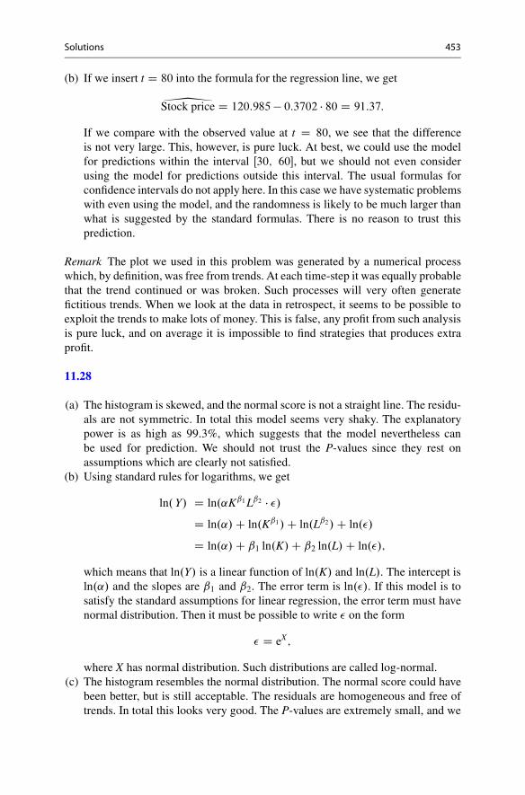
Solutions 453
(b) If we insert t D 80 into the formula for the regression line, we get
4Stock price D 120:985 � 0:3702 � 80 D 91:37:
If we compare with the observed value at t D 80, we see that the differenceis not very large. This, however, is pure luck. At best, we could use the modelfor predictions within the interval Œ30; 60�, but we should not even considerusing the model for predictions outside this interval. The usual formulas forconfidence intervals do not apply here. In this case we have systematic problemswith even using the model, and the randomness is likely to be much larger thanwhat is suggested by the standard formulas. There is no reason to trust thisprediction.
Remark The plot we used in this problem was generated by a numerical processwhich, by definition, was free from trends. At each time-step it was equally probablethat the trend continued or was broken. Such processes will very often generatefictitious trends. When we look at the data in retrospect, it seems to be possible toexploit the trends to make lots of money. This is false, any profit from such analysisis pure luck, and on average it is impossible to find strategies that produces extraprofit.
11.28
(a) The histogram is skewed, and the normal score is not a straight line. The residu-als are not symmetric. In total this model seems very shaky. The explanatorypower is as high as 99.3%, which suggests that the model nevertheless canbe used for prediction. We should not trust the P-values since they rest onassumptions which are clearly not satisfied.
(b) Using standard rules for logarithms, we get
ln. Y/ D ln.˛Kˇ1 Lˇ2 � �/
D ln.˛/ C ln.Kˇ1/ C ln.Lˇ2/ C ln.�/
D ln.˛/ C ˇ1 ln.K/ C ˇ2 ln.L/ C ln.�/;
which means that ln.Y/ is a linear function of ln.K/ and ln.L/. The intercept isln.˛/ and the slopes are ˇ1 and ˇ2. The error term is ln.�/. If this model is tosatisfy the standard assumptions for linear regression, the error term must havenormal distribution. Then it must be possible to write � on the form
� D eX;
where X has normal distribution. Such distributions are called log-normal.(c) The histogram resembles the normal distribution. The normal score could have
been better, but is still acceptable. The residuals are homogeneous and free oftrends. In total this looks very good. The P-values are extremely small, and we

454 Solutions
conclude that ln.K/ and ln.L/ are strongly significant. This means that changesin K and L probably affects the value of Y. The relation is nonlinear (concave),which explains why we get problems in (a).
(d) From the computation in (b) we see that
ln. Y=106/ D ln. Y/ � ln.106/ D ln.˛/ C ˇ1 ln.K/ C ˇ2 ln.L/ C ln.�/ � ln.106/
D ln.˛/ C ˇ1.ln.K=106/ C ln.106// C ˇ2 ln.L/ C ln.�/ � ln.106/
D ln.˛/ C .ˇ1 � 1/ ln.106/ C ˇ1 ln.K=106/ C ˇ2 ln.L/ C ln.�/:
From the printout we see directly that ˇ1 D 0:30 and ˇ2 D 0:90. Furthermorethe intercept leads to the equation
ln.˛/ C .ˇ1 � 1/ ln.106/ D �5:06822:
Here everything is known except ln.˛/, and we can solve to get
ln.˛/ D �.0:30 � 1/ ln.106/ � 5:06822 D 4:60264:
Hence
˛ D e4:60264 D 99:75:
11.29
(a) We see that the coefficient for EdSh is positive, which means that the largerfraction that has short higher education, the better are the scores. The coefficientfor EdL is negative, however, which is rather weird. None of the coefficients aresignificant, so we cannot claim they are important for the results. On the positiveside the model explains about 50% of the variation.
The problem with this regression is multicollinearity between EdSh and EdL.This is confirmed by the second printout where EdL explains more than 90% ofthe variation in EdSh. That suggests that we should not use both EdSh and EdLas explanatory variables in the same model. Common practice is to delete one ofthe variables, but in this context we may also merge the results as we do below.
(b) This regression is much better. We have removed the problem with collinearity,and Ed is strongly significant. It seems quite clear that the fraction of thepopulation with higher education affects the results. If we increase Ed by 10,we expect that results improve by 0.2. We see that the explanatory power isabout 49%, almost the same as in (a). Taking into account that we only have19 observations, the diagnostic plots are all OK. The normal score has a slightbend, but not more than we can accept. The residuals versus order are OK. Theresiduals versus fitted values are not uniform, but the plot is partly misleadingsince many observations have the same value. To the extent that we can seetrends, those are caused by two outliers, which happen to be skewed. This isnormal when we have few observations.

Solutions 455
(c) The predicted value we find from the regression line
predicted value D 2:38286 C 0:0200711 � 47:5 D 3:34:
The variation we find using the formula
SŒ OY � Y� D S �s
1 C 1
nC .X � X/2
M:
In our case we have S D 0:122724; n D 19; X D 47:5; X D 27:86. The valuefor M we find by
M D S2
SŒ O�2 D 0:1227242
0:004923692D 621:266:
Inserting these number into the formula, we get SŒ OY�Y� D 0:158761. The limitsfor the prediction interval we find using a t-table with parameter � D n�2 D 17,giving t.17/
2:5% D 2:11. The limits for a 95% prediction interval are hence
3:34 ˙ 2:11 � 0:158761;
which rounded gives Œ3:0; 3:7�. The observed value, 3.3, is slightly lower thanthe predicted value 3.34. The value is safely near the center of the predictioninterval, so we have no reason to claim that the result is significantly weakerthan expected.
11.30
(a) We see that the P-value for the coefficient of Price is very low, hence Price (notunexpected) is strongly significant for demand. The explanatory power is good,about 86%. We see that the regression coefficient is negative. This means thatdemand falls when the price increases, which seems logical. The normal scoreis supposed to be a straight line; it could have been better, but is still acceptable.The histogram resembles the normal distribution and is OK. The residualsshould be homogeneous and free of trends; they could have been better, butdeviations probably appear as a consequence of very few observations. In totalthe model can be accepted.
(b) In both models we see that all the regression coefficients are significant.The explanatory power increases from 86% with linear regression, to 94%for quadratic regression, and further to 95% for cubical regression. Cubicalregression is best in the sense that it offers the best fit to data, but is only slightlybetter than quadratic regression.
(c) Model 1: Demand D 911:713 � 112:057 � 10 � �209.Model 2: Demand D 1281:78 � 356:953 � 10 C 27:2106 � 102 � 433.Model 3: Demand D 1513:62�581:236 �10C84:7985 �102�4:26577 �103 �
�85.

456 Solutions
Models 1 and 3 produce negative values, which must be wrong. Model2 produces a positive value, but the value is much higher than the observedvalues at the right side of the plot. That, too, must be wrong. It is reasonableto assume that expected demand is a positive and monotonically decreasingfunction of price, but no polynomial has those properties over the whole realaxis. Even though polynomial regression gives better fit to data, it is unsuitablefor prediction outside the set where we have observations.
Table of the Binomial Distribution
Table A gives the probability P.X D x/ when X is a binomial distribution withparameters .n; p/. Example: n D 8; p D 0:1 gives P.X D 2/ D 0:1488.
Table A Binomialdistribution
n x p D 0:05 p D 0:1 p D 0:2 p D 0:3 p D 0:4 p D 0:5
2 0 0:9025 0:8100 0:6400 0:4900 0:3600 0:2500
1 0:0950 0:1800 0:3200 0:4200 0:4800 0:5000
2 0:0025 0:0100 0:0400 0:0900 0:1600 0:2500
3 0 0:8574 0:7290 0:5120 0:3430 0:2160 0:1250
1 0:1354 0:2430 0:3840 0:4410 0:4320 0:3750
2 0:0071 0:0270 0:0960 0:1890 0:2880 0:3750
3 0:0001 0:0010 0:0080 0:0270 0:0640 0:1250
4 0 0:8145 0:6561 0:4096 0:2401 0:1296 0:0625
1 0:1715 0:2916 0:4096 0:4116 0:3456 0:2500
2 0:0135 0:0486 0:1536 0:2646 0:3456 0:3750
3 0:0005 0:0036 0:0256 0:0756 0:1536 0:2500
4 0:0000 0:0001 0:0016 0:0081 0:0256 0:0650
5 0 0:7738 0:5905 0:3277 0:1681 0:0778 0:0312
1 0:2036 0:3280 0:4096 0:3602 0:2592 0:1562
2 0:0214 0:0729 0:2048 0:3087 0:3456 0:3125
3 0:0011 0:0081 0:0512 0:1323 0:2304 0:3125
4 0:0000 0:0005 0:0064 0:0284 0:0768 0:1562
5 0:0000 0:0000 0:0003 0:0024 0:0102 0:0312
6 0 0:7351 0:5314 0:2621 0:1176 0:0467 0:0156
1 0:2321 0:3543 0:3932 0:3025 0:1866 0:0938
2 0:0305 0:0984 0:2458 0:3241 0:3110 0:2344
3 0:0021 0:0146 0:0819 0:1852 0:2765 0:3125
4 0:0001 0:0012 0:0154 0:0595 0:1382 0:2344
5 0:0000 0:0001 0:0015 0:0102 0:0369 0:0938
6 0:0000 0:0000 0:0001 0:0007 0:0041 0:0156
(continued)

Solutions 457
Table A (continued) n x p D 0:05 p D 0:1 p D 0:2 p D 0:3 p D 0:4 p D 0:5
7 0 0:6983 0:4783 0:2097 0:0824 0:0280 0:0078
1 0:2573 0:3720 0:3670 0:2471 0:1306 0:0547
2 0:0406 0:1240 0:2753 0:3176 0:2613 0:1641
3 0:0036 0:0230 0:1147 0:2269 0:2903 0:2734
4 0:0002 0:0026 0:0287 0:0972 0:1935 0:2734
5 0:0000 0:0002 0:0043 0:0250 0:0774 0:1641
6 0:0000 0:0000 0:0004 0:0036 0:0172 0:0547
7 0:0000 0:0000 0:0000 0:0002 0:0016 0:0078
8 0 0:6634 0:4305 0:1678 0:0576 0:0168 0:0039
1 0:2793 0:3826 0:3355 0:1977 0:0896 0:0312
2 0:0515 0:1488 0:2936 0:2965 0:2090 0:1094
3 0:0054 0:0331 0:1468 0:2541 0:2787 0:2188
4 0:0004 0:0046 0:0459 0:1361 0:2322 0:2734
5 0:0000 0:0004 0:0092 0:0467 0:1239 0:2188
6 0:0000 0:0000 0:0011 0:0100 0:0413 0:1094
7 0:0000 0:0000 0:0001 0:0012 0:0079 0:0312
8 0:0000 0:0000 0:0000 0:0001 0:0007 0:0039
9 0 0:6302 0:3874 0:1342 0:0404 0:0101 0:0020
1 0:2985 0:3874 0:3020 0:1556 0:0605 0:0176
2 0:0629 0:1722 0:3020 0:2668 0:1612 0:0703
3 0:0077 0:0446 0:1762 0:2668 0:2508 0:1641
4 0:0006 0:0074 0:0661 0:1715 0:2508 0:2461
5 0:0000 0:0008 0:0165 0:0735 0:1672 0:2461
6 0:0000 0:0001 0:0028 0:0210 0:0743 0:1641
7 0:0000 0:0000 0:0003 0:0039 0:0212 0:0703
8 0:0000 0:0000 0:0000 0:0004 0:0035 0:0176
9 0:0000 0:0000 0:0000 0:0000 0:0003 0:0020
10 0 0:5987 0:3487 0:1074 0:0282 0:0060 0:0010
1 0:3151 0:3874 0:2684 0:1211 0:0403 0:0098
2 0:0746 0:1937 0:3020 0:2335 0:1209 0:0439
3 0:0105 0:0574 0:2013 0:2668 0:2150 0:1172
4 0:0010 0:0112 0:0881 0:2001 0:2508 0:2051
5 0:0001 0:0015 0:0264 0:1029 0:2007 0:2461
6 0:0000 0:0001 0:0055 0:0368 0:1115 0:2051
7 0:0000 0:0000 0:0008 0:0090 0:0425 0:1172
8 0:0000 0:0000 0:0001 0:0014 0:0106 0:0439
9 0:0000 0:0000 0:0000 0:0001 0:0016 0:0098
10 0:0000 0:0000 0:0000 0:0000 0:0001 0:0010

458 Solutions
Table of the Poisson Distribution
Table B gives the probability P.X D x/ when X is a Poisson distribution withparameter �. Example: � D 5 gives P.X D 4/ D 0:1755.
Table B Poisson distribution
�
x 0:1 0:2 0:3 0:4 0:5 0:6 0:7 0:8 0:9 1:0
0 0:9048 0:8187 0:7408 0:6703 0:6065 0:5488 0:4966 0:4493 0:4066 0:3679
1 0:0905 0:1637 0:2222 0:2681 0:3033 0:3293 0:3476 0:3595 0:3659 0:3679
2 0:0045 0:0164 0:0333 0:0536 0:0758 0:0988 0:1217 0:1438 0:1647 0:1839
3 0:0002 0:0011 0:0033 0:0072 0:0126 0:0198 0:0284 0:0383 0:0494 0:0613
4 0:0000 0:0001 0:0003 0:0007 0:0016 0:0030 0:0050 0:0077 0:0111 0:0153
5 0:0000 0:0000 0:0000 0:0001 0:0002 0:0004 0:0007 0:0012 0:0020 0:0031
6 0:0000 0:0000 0:0000 0:0000 0:0000 0:0000 0:0001 0:0002 0:0003 0:0005
7 0:0000 0:0000 0:0000 0:0000 0:0000 0:0000 0:0000 0:0000 0:0000 0:0001
�
x 1 2 3 4 5 6 7 8 9 10
0 0:3679 0:1353 0:0498 0:0183 0:0067 0:0025 0:0009 0:0003 0:0001 0:0000
1 0:3679 0:2707 0:1494 0:0733 0:0337 0:0149 0:0064 0:0027 0:0011 0:0005
2 0:1839 0:2707 0:2240 0:1465 0:0842 0:0446 0:0223 0:0107 0:0050 0:0023
3 0:0613 0:1804 0:2240 0:1954 0:1404 0:0892 0:0521 0:0286 0:0150 0:0076
4 0:0153 0:0902 0:1680 0:1954 0:1755 0:1339 0:0912 0:0572 0:0337 0:0189
5 0:0031 0:0361 0:1008 0:1563 0:1755 0:1606 0:1277 0:0916 0:0607 0:0378
6 0:0005 0:0120 0:0504 0:1042 0:1462 0:1606 0:1490 0:1221 0:0911 0:0631
7 0:0001 0:0034 0:0216 0:0595 0:1044 0:1377 0:1490 0:1396 0:1171 0:0901
8 0:0000 0:0009 0:0081 0:0298 0:0653 0:1033 0:1304 0:1396 0:1318 0:1126
9 0:0000 0:0002 0:0027 0:0132 0:0363 0:0688 0:1014 0:1241 0:1318 0:1251
10 0:0000 0:0000 0:0008 0:0053 0:0181 0:0413 0:0710 0:0993 0:1186 0:1251
11 0:0000 0:0000 0:0002 0:0019 0:0082 0:0225 0:0452 0:0722 0:0970 0:1137
12 0:0000 0:0000 0:0001 0:0006 0:0034 0:0113 0:0264 0:0481 0:0728 0:0948
13 0:0000 0:0000 0:0000 0:0002 0:0013 0:0052 0:0142 0:0296 0:0504 0:0729
14 0:0000 0:0000 0:0000 0:0001 0:0005 0:0022 0:0071 0:0169 0:0324 0:0521
15 0:0000 0:0000 0:0000 0:0000 0:0002 0:0009 0:0033 0:0090 0:0194 0:0347
16 0:0000 0:0000 0:0000 0:0000 0:0000 0:0003 0:0014 0:0045 0:0109 0:0217
17 0:0000 0:0000 0:0000 0:0000 0:0000 0:0001 0:0006 0:0021 0:0058 0:0128
18 0:0000 0:0000 0:0000 0:0000 0:0000 0:0000 0:0002 0:0009 0:0029 0:0071
19 0:0000 0:0000 0:0000 0:0000 0:0000 0:0000 0:0001 0:0004 0:0014 0:0037
20 0:0000 0:0000 0:0000 0:0000 0:0000 0:0000 0:0000 0:0002 0:0006 0:0019
21 0:0000 0:0000 0:0000 0:0000 0:0000 0:0000 0:0000 0:0001 0:0003 0:0009
22 0:0000 0:0000 0:0000 0:0000 0:0000 0:0000 0:0000 0:0000 0:0001 0:0004
23 0:0000 0:0000 0:0000 0:0000 0:0000 0:0000 0:0000 0:0000 0:0000 0:0002
24 0:0000 0:0000 0:0000 0:0000 0:0000 0:0000 0:0000 0:0000 0:0000 0:0001

Solutions 459
Table of the Normal Distribution—Area Table
Table C gives the area G.z/ under the standard normal density to the left of z.Example: z D 1:54 gives G.z/ D 0:9382.
Table C Normal distribution
z 0:00 0:01 0:02 0:03 0:04 0:05 0:06 0:07 0:08 0:09
0 0:5000 0:5040 0:5080 0:5120 0:5160 0:5199 0:5239 0:5279 0:5319 0:5359
0:1 0:5398 0:5438 0:5478 0:5517 0:5557 0:5596 0:5636 0:5675 0:5714 0:5753
0:2 0:5793 0:5832 0:5871 0:5910 0:5948 0:5987 0:6026 0:6064 0:6103 0:6141
0:3 0:6179 0:6217 0:6255 0:6293 0:6331 0:6368 0:6406 0:6443 0:6480 0:6517
0:4 0:6554 0:6591 0:6628 0:6664 0:6700 0:6736 0:6772 0:6808 0:6844 0:6879
0:5 0:6915 0:6950 0:6985 0:7019 0:7054 0:7088 0:7123 0:7157 0:7190 0:7224
0:6 0:7257 0:7291 0:7324 0:7357 0:7389 0:7422 0:7454 0:7486 0:7517 0:7549
0:7 0:7580 0:7611 0:7642 0:7673 0:7704 0:7734 0:7764 0:7794 0:7823 0:7852
0:8 0:7881 0:7910 0:7939 0:7967 0:7995 0:8023 0:8051 0:8078 0:8106 0:8133
0:9 0:8159 0:8186 0:8212 0:8238 0:8264 0:8289 0:8315 0:8340 0:8365 0:8389
1:0 0:8413 0:8438 0:8461 0:8485 0:8508 0:8531 0:8554 0:8577 0:8599 0:8621
1:1 0:8643 0:8665 0:8686 0:8708 0:8729 0:8749 0:8770 0:8790 0:8810 0:8830
1:2 0:8849 0:8869 0:8888 0:8907 0:8925 0:8944 0:8962 0:8980 0:8997 0:9015
1:3 0:9032 0:9049 0:9066 0:9082 0:9099 0:9115 0:9131 0:9147 0:9162 0:9177
1:4 0:9192 0:9207 0:9222 0:9236 0:9251 0:9265 0:9279 0:9292 0:9306 0:9319
1:5 0:9332 0:9345 0:9357 0:9370 0:9382 0:9394 0:9406 0:9418 0:9429 0:9441
1:6 0:9452 0:9463 0:9474 0:9484 0:9495 0:9505 0:9515 0:9525 0:9535 0:9545
1:7 0:9554 0:9564 0:9573 0:9582 0:9591 0:9599 0:9608 0:9616 0:9625 0:9633
1:8 0:9641 0:9649 0:9656 0:9664 0:9671 0:9678 0:9686 0:9693 0:9699 0:9706
1:9 0:9713 0:9719 0:9726 0:9732 0:9738 0:9744 0:9750 0:9756 0:9761 0:9767
2:0 0:9772 0:9778 0:9783 0:9788 0:9793 0:9798 0:9803 0:9808 0:9812 0:9817
2:1 0:9821 0:9826 0:9830 0:9834 0:9838 0:9842 0:9846 0:9850 0:9854 0:9857
2:2 0:9861 0:9864 0:9868 0:9871 0:9875 0:9878 0:9881 0:9884 0:9887 0:9890
2:3 0:9893 0:9896 0:9898 0:9901 0:9904 0:9906 0:9909 0:9911 0:9913 0:9916
2:4 0:9918 0:9920 0:9922 0:9925 0:9927 0:9929 0:9931 0:9932 0:9934 0:9936
2:5 0:9938 0:9940 0:9941 0:9943 0:9945 0:9946 0:9948 0:9949 0:9951 0:9952
2:6 0:9953 0:9955 0:9956 0:9957 0:9959 0:9960 0:9961 0:9962 0:9963 0:9964
2:7 0:9965 0:9966 0:9967 0:9968 0:9969 0:9970 0:9971 0:9972 0:9973 0:9974
2:8 0:9974 0:9975 0:9976 0:9977 0:9977 0:9978 0:9979 0:9979 0:9980 0:9981
2:9 0:9981 0:9982 0:9982 0:9983 0:9984 0:9984 0:9985 0:9985 0:9986 0:9986
3:0 0:9987 0:9987 0:9987 0:9988 0:9988 0:9989 0:9989 0:9989 0:9990 0:9990
(continued)

460 Solutions
Table C (continued)
z 0:00 0:01 0:02 0:03 0:04 0:05 0:06 0:07 0:08 0:09
3:1 0:9990 0:9991 0:9991 0:9991 0:9992 0:9992 0:9992 0:9992 0:9993 0:9993
3:2 0:9993 0:9993 0:9994 0:9994 0:9994 0:9994 0:9994 0:9995 0:9995 0:9995
3:3 0:9995 0:9995 0:9995 0:9996 0:9996 0:9996 0:9996 0:9996 0:9996 0:9997
3:4 0:9997 0:9997 0:9997 0:9997 0:9997 0:9997 0:9997 0:9997 0:9997 0:9998
3:5 0:9998 0:9998 0:9998 0:9998 0:9998 0:9998 0:9998 0:9998 0:9998 0:9998
3:6 0:9998 0:9998 0:9999 0:9999 0:9999 0:9999 0:9999 0:9999 0:9999 0:9999
3:7 0:9999 0:9999 0:9999 0:9999 0:9999 0:9999 0:9999 0:9999 0:9999 0:9999
3:8 0:9999 0:9999 0:9999 0:9999 0:9999 0:9999 0:9999 0:9999 0:9999 0:9999
3:9 1:0000 – – – – – – – – –
Table of the Normal Distribution—Percentage Points
Table D gives z such that P.X � z/ D a, when X is a standard normal distribution.Example: P.X � 1:6449/ D 5%.
Table D Normal distribution a z a z a z
0:50 0:0000 0:30 0:5244 0:10 1:2816
0:49 0:0251 0:29 0:5534 0:09 1:3408
0:48 0:0502 0:28 0:5828 0:08 1:4051
0:47 0:0753 0:27 0:6128 0:07 1:4758
0:46 0:1004 0:26 0:6434 0:06 1:5548
0:45 0:1257 0:25 0:6745 0:050 1:6449
0:44 0:1510 0:24 0:7063 0:045 1:6954
0:43 0:1764 0:23 0:7389 0:040 1:7507
0:42 0:2019 0:22 0:7722 0:035 1:8119
0:41 0:2275 0:21 0:8064 0:030 1:8808
0:40 0:2534 0:20 0:8416 0:025 1:9600
0:39 0:2793 0:19 0:8779 0:020 2:0538
0:38 0:3055 0:18 0:9154 0:015 2:1701
0:37 0:3319 0:17 0:9542 0:010 2:3264
0:36 0:3585 0:16 0:9945 0:005 2:5758
0:35 0:3853 0:15 1:0364 0:0010 3:0902
0:34 0:4125 0:14 1:0803 0:0005 3:2905
0:33 0:4399 0:13 1:1264 0:0001 3:7190
0:32 0:4677 0:12 1:1750
0:31 0:4959 0:11 1:2265

Solutions 461
Table of the Chi-Square Distribution—Percentage Points
Table E gives q such that P.X � q/ D a, when X is a chi-square distribution withparameter �. Example: � D 10 gives P.X � 9:342/ D 50%.
Table E Chi-square distribution
a
� 99:9% 99:5% 99:0% 97:5% 95:0% 90:0% 87:5% 80:0% 75:0% 66:6% 50:0%
1 0:000 0:000 0:000 0:001 0:004 0:016 0:025 0:064 0:102 0:186 0:455
2 0:002 0:010 0:020 0:051 0:103 0:211 0:267 0:446 0:575 0:811 1:386
3 0:024 0:072 0:115 0:216 0:352 0:584 0:692 1:005 1:213 1:568 2:366
4 0:091 0:207 0:297 0:484 0:711 1:064 1:219 1:649 1:923 2:378 3:357
5 0:210 0:412 0:554 0:831 1:145 1:610 1:808 2:343 2:675 3:216 4:351
6 0:381 0:676 0:872 1:237 1:635 2:204 2:441 3:070 3:455 4:074 5:348
7 0:598 0:989 1:239 1:690 2:167 2:833 3:106 3:822 4:255 4:945 6:346
8 0:857 1:344 1:646 2:180 2:733 3:490 3:797 4:594 5:071 5:826 7:344
9 1:152 1:735 2:088 2:700 3:325 4:168 4:507 5:380 5:899 6:716 8:343
10 1:479 2:156 2:558 3:247 3:940 4:865 5:234 6:179 6:737 7:612 9:342
11 1:834 2:603 3:053 3:816 4:575 5:578 5:975 6:989 7:584 8:514 10:341
12 2:214 3:074 3:571 4:404 5:226 6:304 6:729 7:807 8:438 9:420 11:340
13 2:617 3:565 4:107 5:009 5:892 7:042 7:493 8:634 9:299 10:331 12:340
14 3:041 4:075 4:660 5:629 6:571 7:790 8:266 9:467 10:165 11:245 13:339
15 3:483 4:601 5:229 6:262 7:261 8:547 9:048 10:307 11:037 12:163 14:339
16 3:942 5:142 5:812 6:908 7:962 9:312 9:837 11:152 11:912 13:083 15:338
17 4:416 5:697 6:408 7:564 8:672 10:085 10:633 12:002 12:792 14:006 16:338
18 4:905 6:265 7:015 8:231 9:390 10:865 11:435 12:857 13:675 14:931 17:338
19 5:407 6:844 7:633 8:907 10:117 11:651 12:242 13:716 14:562 15:859 18:338
20 5:921 7:434 8:260 9:591 10:851 12:443 13:055 14:578 15:452 16:788 19:337
21 6:447 8:034 8:897 10:283 11:591 13:240 13:873 15:445 16:344 17:720 20:337
22 6:983 8:643 9:542 10:982 12:338 14:041 14:695 16:314 17:240 18:653 21:337
23 7:529 9:260 10:196 11:689 13:091 14:848 15:521 17:187 18:137 19:587 22:337
24 8:085 9:886 10:856 12:401 13:848 15:659 16:351 18:062 19:037 20:523 23:337
25 8:649 10:520 11:524 13:120 14:611 16:473 17:184 18:940 19:939 21:461 24:337
26 9:222 11:160 12:198 13:844 15:379 17:292 18:021 19:820 20:843 22:399 25:336
27 9:803 11:808 12:879 14:573 16:151 18:114 18:861 20:703 21:749 23:339 26:336
28 10:391 12:461 13:565 15:308 16:928 18:939 19:704 21:588 22:657 24:280 27:336
29 10:986 13:121 14:256 16:047 17:708 19:768 20:550 22:475 23:567 25:222 28:336
30 11:588 13:787 14:953 16:791 18:493 20:599 21:399 23:364 24:478 26:165 29:336
35 14:688 17:192 18:509 20:569 22:465 24:797 25:678 27:836 29:054 30:894 34:336
40 17:916 20:707 22:164 24:433 26:509 29:051 30:008 32:345 33:660 35:643 39:335
45 21:251 24:311 25:901 28:366 30:612 33:350 34:379 36:884 38:291 40:407 44:335
50 24:674 27:991 29:707 32:357 34:764 37:689 38:785 41:449 42:942 45:184 49:335
55 28:173 31:735 33:570 36:398 38:958 42:060 43:220 46:036 47:610 49:972 54:335
60 31:738 35:534 37:485 40:482 43:188 46:459 47:680 50:641 52:294 54:770 59:335

462 Solutions
Table of the Chi-square Distribution—Continued
Table F gives q such that P.X � q/ D a, when X is a chi-square distribution withparameter �. Example: � D 10 gives P.X � 18:307/ D 5%.
Table F Chi-square distribution
a
� 40.0% 33.3% 25.0% 20.0% 12.5% 10.0% 5.0% 2.5% 1.0% 0.5% 0.1%
1 0:708 0:936 1:323 1:642 2:354 2:706 3:841 5:024 6:635 7:879 10:828
2 1:833 2:197 2:773 3:219 4:159 4:605 5:991 7:378 9:210 10:597 13:816
3 2:946 3:405 4:108 4:642 5:739 6:251 7:815 9:348 11:345 12:838 16:266
4 4:045 4:579 5:385 5:989 7:214 7:779 9:488 11:143 13:277 14:860 18:467
5 5:132 5:730 6:626 7:289 8:625 9:236 11:070 12:833 15:086 16:750 20:515
6 6:211 6:867 7:841 8:558 9:992 10:645 12:592 14:449 16:812 18:548 22:458
7 7:283 7:992 9:037 9:803 11:326 12:017 14:067 16:013 18:475 20:278 24:322
8 8:351 9:107 10:219 11:030 12:636 13:362 15:507 17:535 20:090 21:955 26:125
9 9:414 10:215 11:389 12:242 13:926 14:684 16:919 19:023 21:666 23:589 27:877
10 10:473 11:317 12:549 13:442 15:198 15:987 18:307 20:483 23:209 25:188 29:588
11 11:530 12:414 13:701 14:631 16:457 17:275 19:675 21:920 24:725 26:757 31:264
12 12:584 13:506 14:845 15:812 17:703 18:549 21:026 23:337 26:217 28:300 32:910
13 13:636 14:595 15:984 16:985 18:939 19:812 22:362 24:736 27:688 29:819 34:528
14 14:685 15:680 17:117 18:151 20:166 21:064 23:685 26:119 29:141 31:319 36:123
15 15:733 16:761 18:245 19:311 21:384 22:307 24:996 27:488 30:578 32:801 37:697
16 16:780 17:840 19:369 20:465 22:595 23:542 26:296 28:845 32:000 34:267 39:252
17 17:824 18:917 20:489 21:615 23:799 24:769 27:587 30:191 33:409 35:718 40:790
18 18:868 19:991 21:605 22:760 24:997 25:989 28:869 31:526 34:805 37:156 42:312
19 19:910 21:063 22:718 23:900 26:189 27:204 30:144 32:852 36:191 38:582 43:820
20 20:951 22:133 23:828 25:038 27:376 28:412 31:410 34:170 37:566 39:997 45:315
21 21:991 23:201 24:935 26:171 28:559 29:615 32:671 35:479 38:932 41:401 46:797
22 23:031 24:268 26:039 27:301 29:737 30:813 33:924 36:781 40:289 42:796 48:268
23 24:069 25:333 27:141 28:429 30:911 32:007 35:172 38:076 41:638 44:181 49:728
24 25:106 26:397 28:241 29:553 32:081 33:196 36:415 39:364 42:980 45:559 51:179
25 26:143 27:459 29:339 30:675 33:247 34:382 37:652 40:646 44:314 46:928 52:620
26 27:179 28:520 30:435 31:795 34:410 35:563 38:885 41:923 45:642 48:290 54:052
27 28:214 29:580 31:528 32:912 35:570 36:741 40:113 43:195 46:963 49:645 55:476
28 29:249 30:639 32:620 34:027 36:727 37:916 41:337 44:461 48:278 50:993 56:892
29 30:283 31:697 33:711 35:139 37:881 39:087 42:557 45:722 49:588 52:336 58:301
30 31:316 32:754 34:800 36:250 39:033 40:256 43:773 46:979 50:892 53:672 59:703
35 36:475 38:024 40:223 41:778 44:753 46:059 49:802 53:203 57:342 60:275 66:619
40 41:622 43:275 45:616 47:269 50:424 51:805 55:758 59:342 63:691 66:766 73:402
45 46:761 48:510 50:985 52:729 56:052 57:505 61:656 65:410 69:957 73:166 80:077
50 51:892 53:733 56:334 58:164 61:647 63:167 67:505 71:420 76:154 79:490 86:661
55 57:016 58:945 61:665 63:577 67:211 68:796 73:311 77:380 82:292 85:749 93:168
60 62:135 64:147 66:981 68:972 72:751 74:397 79:082 83:298 88:379 91:952 99:607

Solutions 463
Table of the t-Distribution—Percentage Points
Table G gives t such that P.X � t/ D a, when X is a t-distribution with parameter�. Example: � D 10 gives P.X � 3:169/ D 5%.
Table G t-distribution
a
� 40.0% 33.3% 25.0% 20.0% 12.5% 10.0% 5.0% 2.5% 1.0% 0.5% 0.1%
1 0:325 0:577 1:000 1:376 2:414 3:078 6:314 12:706 31:821 63:657 318:31
2 0:289 0:500 0:816 1:061 1:604 1:886 2:920 4:303 6:965 9:925 22:327
3 0:277 0:476 0:765 0:978 1:423 1:638 2:353 3:182 4:541 5:841 10:215
4 0:271 0:464 0:741 0:941 1:344 1:533 2:132 2:776 3:747 4:604 7:173
5 0:267 0:457 0:727 0:920 1:301 1:476 2:015 2:571 3:365 4:032 5:893
6 0:265 0:453 0:718 0:906 1:273 1:440 1:943 2:447 3:143 3:707 5:208
7 0:263 0:449 0:711 0:896 1:254 1:415 1:895 2:365 2:998 3:499 4:785
8 0:262 0:447 0:706 0:889 1:240 1:397 1:860 2:306 2:896 3:355 4:501
9 0:261 0:445 0:703 0:883 1:230 1:383 1:833 2:262 2:821 3:250 4:297
10 0:260 0:444 0:700 0:879 1:221 1:372 1:812 2:228 2:764 3:169 4:144
11 0:260 0:443 0:697 0:876 1:214 1:363 1:796 2:201 2:718 3:106 4:025
12 0:259 0:442 0:695 0:873 1:209 1:356 1:782 2:179 2:681 3:055 3:930
13 0:259 0:441 0:694 0:870 1:204 1:350 1:771 2:160 2:650 3:012 3:852
14 0:258 0:440 0:692 0:868 1:200 1:345 1:761 2:145 2:624 2:977 3:787
15 0:258 0:439 0:691 0:866 1:197 1:341 1:753 2:131 2:602 2:947 3:733
16 0:258 0:439 0:690 0:865 1:194 1:337 1:746 2:120 2:583 2:921 3:686
17 0:257 0:438 0:689 0:863 1:191 1:333 1:740 2:110 2:567 2:898 3:646
18 0:257 0:438 0:688 0:862 1:189 1:330 1:734 2:101 2:552 2:878 3:610
19 0:257 0:438 0:688 0:861 1:187 1:328 1:729 2:093 2:539 2:861 3:579
20 0:257 0:437 0:687 0:860 1:185 1:325 1:725 2:086 2:528 2:845 3:552
21 0:257 0:437 0:686 0:859 1:183 1:323 1:721 2:080 2:518 2:831 3:527
22 0:256 0:437 0:686 0:858 1:182 1:321 1:717 2:074 2:508 2:819 3:505
23 0:256 0:436 0:685 0:858 1:180 1:319 1:714 2:069 2:500 2:807 3:485
24 0:256 0:436 0:685 0:857 1:179 1:318 1:711 2:064 2:492 2:797 3:467
(continued)

464 Solutions
Table G (continued)
a
� 40.0% 33.3% 25.0% 20.0% 12.5% 10.0% 5.0% 2.5% 1.0% 0.5% 0.1%
25 0:256 0:436 0:684 0:856 1:178 1:316 1:708 2:060 2:485 2:787 3:450
26 0:256 0:436 0:684 0:856 1:177 1:315 1:706 2:056 2:479 2:779 3:435
27 0:256 0:435 0:684 0:855 1:176 1:314 1:703 2:052 2:473 2:771 3:421
28 0:256 0:435 0:683 0:855 1:175 1:313 1:701 2:048 2:467 2:763 3:408
29 0:256 0:435 0:683 0:854 1:174 1:311 1:699 2:045 2:462 2:756 3:396
30 0:256 0:435 0:683 0:854 1:173 1:310 1:697 2:042 2:457 2:750 3:385
35 0:255 0:434 0:682 0:852 1:170 1:306 1:690 2:030 2:438 2:724 3:340
40 0:255 0:434 0:681 0:851 1:167 1:303 1:684 2:021 2:423 2:704 3:307
45 0:255 0:434 0:680 0:850 1:165 1:301 1:679 2:014 2:412 2:690 3:281
50 0:255 0:433 0:679 0:849 1:164 1:299 1:676 2:009 2:403 2:678 3:261
55 0:255 0:433 0:679 0:848 1:163 1:297 1:673 2:004 2:396 2:668 3:245
60 0:254 0:433 0:679 0:848 1:162 1:296 1:671 2:000 2:390 2:660 3:232
1 0:253 0:431 0:674 0:842 1:150 1:282 1:645 1:960 2:326 2:576 3:090

Index
addition principle, general, 33addition principle, special, 33alternative hypothesis, 177
bar chart, 2Bayes’ rule, 58biased, 161binomial distribution, 114Black and Scholes formula, 140
call option, 85causality, 265central limit theorem, 129Chi-square test, goodness-of-fit, 224Chi-square test, independence, 227coefficient of variation, 14, 104conditional probability, 56confidence intervals, 164covariance, 13covariance of random variables, 103cumulative distribution, 79cumulative standard normal distribution, 125
density of normal distribution, 127density of standard normal distribution, 124dependent variable, 250diagnostic plots, 269discrete sample space, 28dummy variables, 268
estimation, 257estimator, 160event, 30Excel, 17expectation, 81
expectation of a function of two randomvariables, 101
explanatory power, 252explanatory variable, 250
fair dice, 30false negative, 178false positive, 178
histogram, 8, 77histogram, residuals, 269hypergeometric distribution, 118hypothesis testing, 177
independence, 65independence of random variables, 99indicator distribution, 113inference, 3integer correction, 135intercept, 248interquartile range, 6
joint distribution, 98
lottery model, 169
marginal distribution, 99mean, 9median, 5mode, 6multicollinearity, 266multiple regression, 263
© Springer International Publishing AG 2017J. Ubøe, Introductory Statistics for Business and Economics, Springer Textsin Business and Economics, https://doi.org/10.1007/978-3-319-70936-9
465

466 Index
negation principle, 35normal approximation, 142normal distribution, 124normal score, 269null hypothesis, 177
OLS, 249option pricing, 138options, 85ordered, 42ordinary least squares, 249outcome, 27
P-value, 178pie chart, 2Poisson distribution, 122population, 3prediction, 257probability, 29probability distribution, 76probability tree, 60
quartile, 6
random selection, 31random variable, 76regression, 248regression, Excel, 261rejection region, 178relative frequency, 7residuals, 251residuals, plot, 270
sample, 3sample space, 27scale variable, 267slope, 248splitting principle, 60standard deviation, 10, 84standardized random variables, 128strength, of a test, 178subjective probability, 64
t-distribution, 166t-test, comparison of two groups, 206t-test, expected value, 203t-test, paired observations, 210test of binomial probability, 201test static, 178type 1 error, 178type 2 error, 178
U-test of success probabilities, 222unbiased, 160uniform probability, 30unordered, 44
variance, 10, 83variance, sum of random variables, 105volatility, 138
Wilcoxon’s rank-sum test, 216Wilcoxon’s signed-rank test, 218with replacement, 42without replacement, 42