j&>-:*q ^ ,- >,' '-••.--r-> ^ -p' ''-'/...
TRANSCRIPT

• x v /•• w" V->; -x • • •" - - "• ' ' • ' - •./;" • - ••••< >• '' • : ,^ • • • ' • ' > - - -V . - • . . . . • - ' > . • < • - , - r : :v'-. , - v ,< .^v*- ' .(, • • ->• -i x :' k- .- - - ' • ; • ; - . • ' " - - , - - ' / , : < • . -i ,
( ' ' - V
.
.v ~ .-:.; ;^<IPL PUBLICATION 85-5?;; .,'-~£%^.? r- • , ; ?y " , . ; » ' ' • •• : " ' . .'"V -\ v,-" >,' '-••".--r->1^ -p': -'"^^ -"^^^f^, :• "v^ •:>-•->:!-• V•'.- '"^ ':I ' / - . - . • , MI ' .^ -J \' • • .' ' ^" '• j&>-:*Q ^ : ' ' - ' / . ' • • • f " ' •v ' ': '- -- '*
• :?-'A • > ' \ • ' . ' • ' - - • " : . V - . . . • . ' . ' - ' ' • - - . - • •"^>.,"-jtt^iV^/.^'•'•-.- • • - . - • - ' . - ' ' • » • . ' • . ^ : -v : , • / • ' . • - "Tv> , -0 - . - . - - - ^Jtitm&:"~
•^ftca^
/j/^--^:-^:.:-;1^^^^^:'^-;!-.^?-,-^-VA- ::,^V^>:v"--U-, -," '- ' ;•• '• - ; - : - \; gfl£
. ••. - / . " • • " - . ' v ' ' - • ' - { -'/ ' V-'-V - :
.'
> , . • • . • , . . . . , .
Mo
" ' '• . H . /^ s ..
Che-Hang, Chiles Ih
' •
. sVv* V;»,- : •. -^ ' • , ' „ ' • ' > ; •-'•' i c. . - ' " ' . - : '• •. ,'v-: '/1 '\N.- '^ ' ' /• '"* '/;.;•; "• ' " ''*'• ..- V< ; i
'-\ "- <• vNati'onal Aeronautics and ,. , . ( i ' (- • ' • / ; . /-.:^ - . - - - ' / • " - , ' • • • • . - / . . >-;-:;(-'^.:: !.. -S-A-- . - '.-• > " ( • > /' Space Administration; \ :". " ":.v :-J\ ' > ' - t - '')-•' - / " v - ,v:^ / - • • • ' ' - . " ' . • :V '••'";, -, ^ "t;' \ -—,;Ss
V l v ""^ -.:,-.. v i-^0 A - . - ' V ' - . ' - ;--vv,-. :• ;. ^'V : ' ' ^ '-• ' - ' ^ '' -' ; ^:? ^ ' - :,. • ' • ' . , et Poulsion^Laboratory ' -.. '.'-, ' !" ' ;-'-s , -"k?. '.-•/'','" v- -,' ' ? : y ^ '.'-••' ."•/- ' M
. ;!" vh,California Institute^ of Technology;;'. ' <r -V, ."^•rf->'::,';. i \ > " • ."; f'v ^;; .^''. V''Rasadena^California -1. ' • ' . . ,-x " . - V :'.%f •-../ - ;!';'y / \ - ; ; . - ; . . v . - ; . - . • • : . - , , N" ., ;'.
rr-; '--^:1. >':./.=,-i. ->.-c - » v . ' . - : ; . . i':;' ,-.:-^> -v4 'V. 'V'^fV • x ' "-r"Y- : ' \X7v->>^-v , - . ' -y - ' • - • : • . ' • - / . r v ' r ^ .?"- - ^-•.-•.v.'v' - v : 3 • • • ^ .V - - " - '^ 7
• ;^i^;^:;:^^o--^^^^vw^ ;:-^:^w^^ ' '
https://ntrs.nasa.gov/search.jsp?R=19860006781 2020-03-16T16:24:58+00:00Z

JPL PUBLICATION 85-57
Dynamic Modeling and AdaptiveControl for Space StationsChe-Hang Charles IhShyh Jong Wang
July 15, 1985
NASANational Aeronautics andSpace Administration
Jet Propulsion LaboratoryCalifornia Institute of TechnologyPasadena, California

The research described in this publication was carried out by the Jet PropulsionLaboratory, California Institute of Technology, under a contract with the NationalAeronautics and Space Administration.
Reference herein to any specific commercial product, process, or service by tradename, trademark, manufacturer, or otherwise, does not constitute or imply itsendorsement by the United States Government or the Jet Propulsion Laboratory,California Institute of Technology.

ABSTRACT
Of all large space structural systems, space stations present a
unique challenge and requirement to advanced control technology. Their
operations require control system stability over an extremely broad range
of parameter changes and high level of disturbances. During shuttle
docking the system mass may suddenly increase by more than 100% and during
station assembly the mass may vary even more drastically. These coupled
with the inherent dynamic model uncertainties associated with large space
structural systems require highly sophisticated control systems that can
grow as the stations evolve and cope with the-uncertainties and time-
varying elements to maintain the stability and pointing of the space
stations.
This report first deals with the aspects of space station operational
properties including configurations, dynamic models, shuttle docking
contact dynamics, solar panel interaction and load reduction to yield a
set of system models and conditions. A model reference adaptive control
algorithm along with the inner-loop plant augmentation design for
controlling the space stations under severe operational conditions of
shuttle docking, excessive model parameter errors, and model truncation
are then investigated. The instability problem caused by the zero-
frequency rigid body modes and a proposed solution using plant augmentation
are addressed. Two sets of sufficient conditions which guarantee the
globally asymptotic stability for the space station systems are obtained.
The performance of this adaptive control system on space stations
is analyzed through extensive simulations. Asymptotic stability, high
iii

rate of convergence, and robustness of the system are observed under the
above-mentioned severe conditions and constraints induced by control hard-
ware saturation. It is also found that further actuation level reductions
can be achieved by using model switching and disturbance modeling
techniques.
iv

TABLE OF CONTENTS
CHAPTER I INTRODUCTION 1
1.1 Adaptive Control and Large Space Structures 1
1.2 Objectives and-Motivations 3
1.3 Literature Review 4
1.4 Outline of this Report 10
CHAPTER II CONFIGURATIONS AND MASS PROPERTIES OF SPACE STATIONS 12
2.1 Two-Panel Baseline Configuration 12
2.2 Four-Panel Planar Configuration 14
CHAPTER III DYNAMIC MODELS FOR SPACE STATIONS 23
3.1 Finite-Element Model for the Two-Panel StationConfiguration 23
3.1.1 Dynamic Variables, Coordinates, andParameters * • 23
3.1.2 The Stiffness Matrix 253.1.3 The Consistent-Mass Matrix 313.1.4 The Lumped-Mass Matrix and System-Mass
Matrix 333.1.5 Equations of Motion 333.1.6 Modal Coordinates and Modal Properties 34
3.2 Finite-Element Model for the Four-Panel StationConfiguration 36
3.2.1 Dynamic Variables, Coordinates, andParameters 36
3.2.2 The Stiffness Matrix 39
3.2.3 The Consistent-Mass Matrix 473.2.4 The Lumped-Mass Matrix and System Mass
Matrix 523.2.5 Payload Dynamics and Hinge Torque Model .... 523.2.6 Equations of Motion 543.2.7 Modal Coordinates and Modal Properties 57
3.3 Frequency Characterization of Space StationDynamical Systems 62

CHAPTER IV PROBLEM FORMULATION 65
CHAPTER V CONTROL ARCHITECTURE 67
5.1 Control Architecture for the Two-PanelConfiguration 67
5.2 Control Architecture for the Four-PanelConfiguration ..................................... 69
CHAPTER VI ADAPTIVE CONTROL ALGORITHM 73
6.1 The Command Generator Tracker Theory ..*•• 74
6.2 Direct Model Reference Adaptive Control 78
6.3 Instability Problem Caused by Rigid Body Modes .... 83
6.4 Plant Augmentation 87
6.5 Sufficient Conditions for Global AsymptoticStability 90
CHAPTER VII PERFORMANCE ANALYSIS AND PRACTICAL CONSIDERATIONS . 108
7.1 Shuttle Reaction Control Subsystem Residual Rates . 109
7.2 Design of Shuttle Docking Devices
7.3 Performance of Adaptive Control on the Two-PanelSpace Station7.3.1 Augmented Plant Modal Properties7.3.2 The Selection of the Reference Model 116
7.3.3 Adaptive Regulator Control 117
7.3.4 Adaptive Control During Shuttle Docking .... 12°
7.4 Performance of Adaptive Control on the Four-PanelSpace Station 127
7.4.1 Augmented Plant Modal Properties 128
7.4.2 The Selection of the Reference Model 128
7.4.3 Adaptive Regulator Control with High InitialTransient .. 130
7.4.4 Adaptive Control During Shuttle Hard Docking 133
CHAPTER VIII CONCLUSIONS 138
vi

APPENDICES A. DEVELOPMENT OF HINGED PAYLOAD DYNAMICS USINGLAGRANGIAN APPROACH FOR FOUR-PANELCONFIGURATION 226
B. DEFINITION OF POSITIVE REALNESS AND STRICTLYPOSITIVE REALNESS OF MATRICES 237
C. DERIVATION OF FORMULAS FOR CALCULATING THESPRING CONSTANTS AND DAMPING FACTORS OFDOCKING DEVICE . . . ? 238
D. PROGRAM LISTING FOR THE SIMULATION OF ADAPTIVECONTROL DURING SHUTTLE HARD DOCKING TO FOUR-PANEL SPACE STATION 241
E. NUMERICAL OUTPUTS FOR THE SIMULATION OF ADAPTIVECONTROL DURING SHUTTLE HARD DOCKING TO FOUR-PANEL SPACE STATION 261
BIBLIOGRAPHY 280
vii

LIST OF TABLES
Table 1 Component Dimension and Mass for Four-PanelConfiguration 20
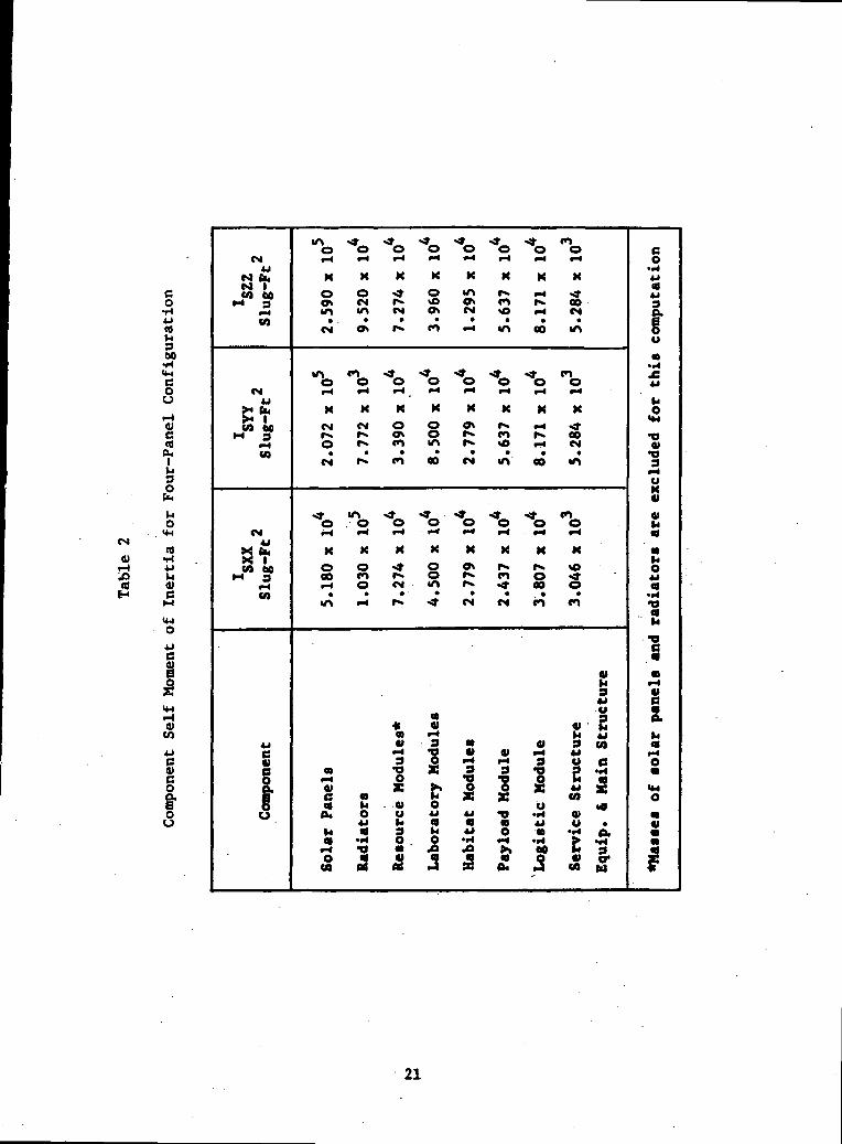
Table 2 Component Self Moment of Inertia for Four-PanelConfiguration 21
Table 3 Component Moment of Inertia w.r.t. the Center ofReference Frame for the Four-Panel Configuration 22
viii

LIST OF FIGURES
Page
Figure 1 Adaptive Control Problems for Space Stations 5
Figure 2 Two-Panel IOC Baseline Configuration 13
Figure 3 IOC Baseline Configuration with Payloads 15
Figure 4 IOC Baseline Configuration Closest to the 6-DOFDynamic Model • 16
Figure 5 Four-Panel CDG Split-Module Planar Configuration .... 17
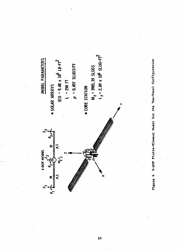
Figure 6 6-DOF Finite-Element Model for the Two-PanelConfiguration 24
Figure 7 Uniform Ream Elements 28
Figure 8 . Combined Uniform Beam Elements 30
Figure 9 Modal Properties for the 6-DOF Two-Panel ConfigurationModel 37
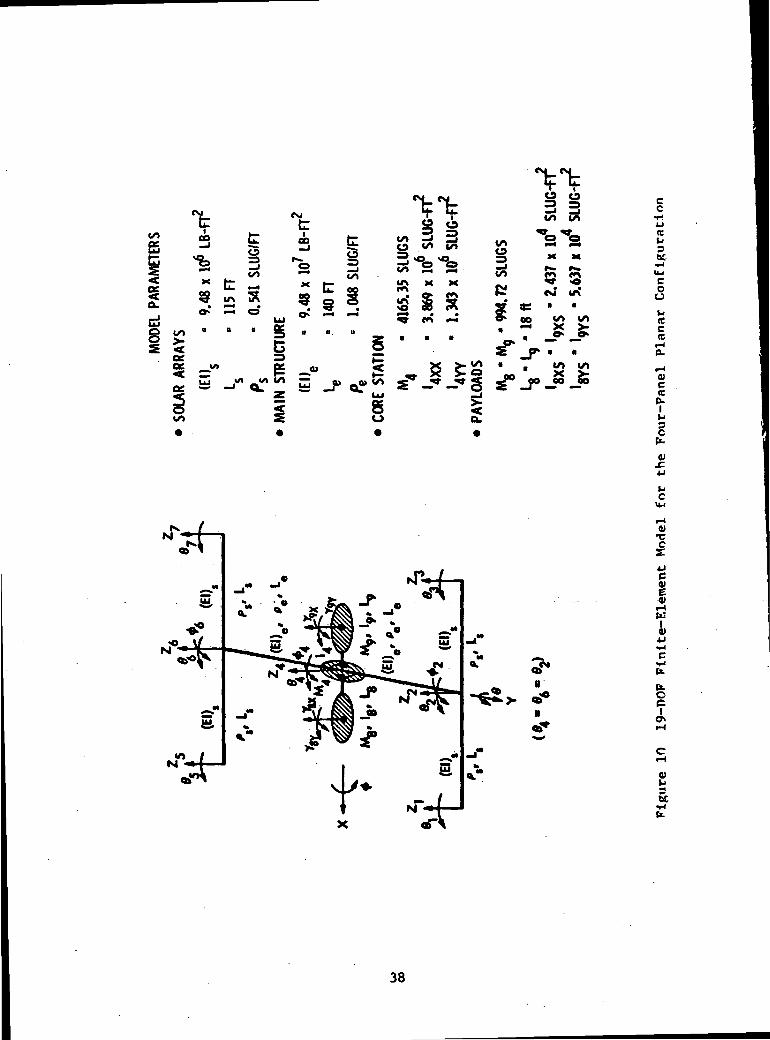
Figure 10 19-DOF Finite-Element Model for the Four-Panel PlanarConfiguration 38
Figure 11 Elastic Model for Solar Panels — South 41
Figure 12 Elastic Model for Solar Panels — North 41
Figure 13 Elastic Model for the Main Structure 42
Figure 14 Distributed Mass Model for Solar Panels — South .... 48
Figure 15 Distributed Mass Model for Solar Panels — North .... 48
Figure 16 Distributed Mass Model for the Main Structure 49
Figure 17 Payload Dynamics and Hinge Model 53
Figure 18 Modal Properties for the Four-Panel ConfigurationModel 59
Figure 19
Figure 20 Space Station Adaptive Control System Block Diagram .
Frequency Characteristics of Space Station DynamicalSystems 63
ix

Figure 21 Shuttle Reaction Control Subsystem (RCS) ResidualRates 110
Figure 22 Concept and Design of Shuttle Docking Device 112
Figure 23 Augmented Plant Modal Properties for the 6-DOF Two-Panel Configuration Model 115
Figure 24 Adaptive Regulator Control for Two-Panel Configuration— Plant and Model Outputs 141
Figure 25 Adaptive Regulator Control for Two-Panel Configuration— Plant and Model Translational State Responses .... 142
Figure 26 Adaptive Regulator Control for Two-Panel Configuration— Plant and Model Rotational State Responses 143
Figure 27 Adaptive Regulator Control for Two-Panel Configuration— Plant and Model Modal Responses 144
Figure 28 Adaptive Regulator Control for Two-Panel Configuration— High Frequency Plant Modal Responses 145
Figure 29 Adaptive Regulator Control for Two-Panel Configuration— Adaptive Control Inputs 146
Figure 30 Adaptive Regulator Control with Measurement Noise forTwo-Panel Configuration — Plant and Model Outputs .. 147
Figure 31 Adaptive Regulator Control with Measurement Noise forTwo-Panel Configuration — Adaptive Control Inputs .. 148
Figure 32 Adaptive Control During Shuttle Hard Docking for Two-Panel Configuration — Plant and Model Outputs 149
Figure 33 Adaptive Control During Shuttle Hard Docking for Two-Panel Configuration— Plant and Model TranslationalState Responses 130
Figure 34 Adaptive Control During Shuttle Hard Docking for Two-Panel Configuration —Plant and Model RotationalState Responses . 151
Figure 35 Adaptive Control During Shuttle Hard Docking for Two-Panel Configuration — Plant and Model ModalResponses 152
Figure 36 Adaptive Control During Shuttle Hard Docking for Two-Panel Configuration — High Frequency Plant ModalResponses 153
x
Figure 37 Adaptive Control During Shuttle Hard Docking for Two-Panel Configuration — Shuttle Angular Position andRate 154
Figure 38 Adaptive Control During Shuttle Hard Docking for Two-Panel Configuration —Docking Force and Torque 155
Figure 39 Adaptive Control During Shuttle Hard Docking for Two-Panel Configuration — Adaptive Control Inputs 156
Figure 40 Adaptive Control During Shuttle Soft Docking for Two-Panel Configuration — Plant and Model Outputs 157
Figure 41 Adaptive Control During Shuttle Soft Docking for Two-Panel Configuration — Plant and Model TranslationalState Responses 158
Figure 42 Adaptive Control During Shuttle Soft Docking for Two-Panel Configuration — Plant and Model RotationalState Responses 159
Figure 43 Adaptive Control During Shuttle Soft Docking for Two-Panel Configuration — Plant and Model Modal Responses 160
Figure 44 Adaptive Control During Shuttle Soft Docking for Two-Panel Configuration — High Frequency Plant ModalResponses 161
Figure 45 Adaptive Control During Shuttle Soft Docking for Two-Panel Configuration — Shuttle Angular Position andRate 162
Figure 46 Adaptive Control During Shuttle Soft Docking for Two-Panel Configuration — Docking Force and Torque 163
Figure 47 Adaptive Control During Shuttle Soft Docking for Two-Panel Configuration — Adaptive Control Inputs 164
Figure 48 Comparative Shuttle Soft Docking Responses —Relative Panel Tip Displacements 165
Figure 49 Comparative Shuttle Soft Docking Responses —Relative Panel Tip Acceleration 166
Figure 50 Adaptive Control During Shuttle Hard Docking withActuator Saturation for Two-Panel Configuration —Plant and Model Outputs 167
xi

Figure 51 Adaptive Control During Shuttle Hard Docking withActuator Saturation for Two-Panel Configuration —Plant and Model Translational State Responses 168
Figure 52 Adaptive Control During Shuttle Hard Docking withActuator Saturation for Two-Panel Configuration —Plant and Model Rotational State Responses 169
Figure 53 Adaptive Control During Shuttle Hard Docking withActuator Saturation for Two-Panel Configuration —Plant and Model Modal Responses 170
Figure 54 Adaptive Control During Shuttle Hard Docking withActuator Saturation for Two-Panel Configuration —High Frequency Plant Modal Responses 171
Figure 55 Adaptive Control During Shuttle Hard Docking withActuator Saturation for Two-Panel Configuration —Shuttle Angular Position and Rate 172
Figure 56 Adaptive Control During Shuttle Hard-Docking withActuator Saturation for Two-Panel Configuration —Docking Force and Torque .. • 173
Figure 57 Adaptive Control During Shuttle Hard Docking withActuator Saturation for Two-Panel Configuration—Adaptive Control Inputs 174
Figure 58 Adaptive Control During Shuttle Hard Docking with MoreSevere Actuator Saturation for Two-Panel Configuration— Plant and Model Outputs 175
Figure 59 Adaptive Control During Shuttle Hard Docking with MoreSevere Actuator Saturation for Two-Panel Configuration— Adaptive Control Inputs .................. ••• 176
Figure 60 Adaptive Control During Shuttle Hard Docking withModel Switching and Disturbance Modeling for Two-Panel Configuration — Plant and Model Outputs
Figure 61 Adaptive Control During Shuttle Hard Docking withModel Switching and Disturbance Modeling for Two-Panel Configuration — Plant and Model TranslationalState Responses 178
Figure 62 Adaptive Control During Shuttle Hard Docking withModel Switching and Disturbance Modeling for Two-Panel Configuration — Plant and Model RotationalState Responses • 179
xii

Figure 63 Adaptive Control During Shuttle Hard Docking withModel Switching and Disturbance Modeling for Two-Panel Configuration — Plant and Model ModalResponses 180
Figure 64 Adaptive Control During Shuttle Hard Docking withModel Switching and Disturbance Modeling for Two-Panel Configuration — High Frequency Plant ModalResponses 181
Figure 65 Adaptive Control During Shuttle Hard Docking withModel Switching and Disturbance Modeling for Two-Panel Configuration — Adaptive Control Inputs ...... 182
Figure 66 Augmented Plant Modal Properties for the Four-PanelConfiguration Model 183
Figure 67 Adaptive Regulator Control for Four-Panel Configuration— Plant and Model Outputs 186
Figure 68 Adaptive Regulator Control for Four-Panel Configuration— Plant and Model Physical State Responses 189
Figure 69 Adaptive Regulator Control for Four-Panel Configuration— Plant and Model Physical State Rate Responses .... 193
Figure 70 Adaptive Regulator Control for Four-Panel Configuration— Plant and Model Rigid Body Modal Responses 197
Figure 71 Adaptive Regulator Control for Four-Panel Configuration— Plant and Model First Bending Group Modal Responses 198
Figure 72 Adaptive Regulator Control for Four-Panel Configuration— Plant Second Bending Group Modal Responses 200
Figure 73 Adaptive Regulator Control for Four-Panel Configuration— Adaptive Control Inputs 202
Figure 74 Adaptive Control During Shuttle Hard Docking for Four-Panel Configuration — Plant and Model Outputs 205
Figure 75 Adaptive Control During Shuttle Hard Docking for Four-Panel Configuration — Plant and Model Physical StateResponses 208
Figure 76 Adaptive Control During Shuttle Hard Docking for Four-Panel Configuration — Plant and Model Physical StateRate Responses 212
xiii

Figure 77 Adaptive Control During Shuttle Hard Docking for Four-Panel Configuration — Plant and Model Rigid bodyModal Responses 216
Figure 78 Adaptive Control During Shuttle Hard Docking for Four-Panel Configuration — Plant and Model First BendingGroup Modal Responses 217
Figure 79 Adaptive Control During Shuttle Hard Docking for Four-Panel Configuration — Plant Second Bending GroupModal Responses 219
Figure 80 Adaptive Control During Shuttle Hard Docking for Four-Panel Configuration — Adaptive Control Inputs ...... 221
Figure 81 Adaptive Control During Shuttle Hard Docking for Four-Panel Configuration — Shuttle Linear and AngularPosition 224
Figure 82 Adaptive Control During Shuttle Hard Docking for Four-Panel Configuration — Docking Force .and Torque 225
xiv

CHAPTER I
INTRODUCTION
1.1 Adaptive Control and Large Space Structures
Most of the well-developed control theory, either in the
frequency domain or in the time domain, deals with systems whose
mathematical representations are completely known. However, in many
practical situations, the parameters of the systems are .either poorly
known or time-varying. In such situations the usual fixed-gain
controller will be inadequate to achieve satisfactory performance in
the entire range over which the characteristics of the system may
vary. Hence, some type of monitoring of the system's behavior,
followed by the adjustment of the control input, is needed and is
referred to as adaptive control. In other words, while a
conventional control system is oriented toward the elimination of the
effects of state perturbations, the adaptive control system is
oriented toward the elimination of the effects of structural
perturbations upon the performance of the control system.
Model Reference Adaptive Control (MRAC) and Self Tuning
Regulators (STR) are two principal approaches to the adaptive control
problems. In MRAC, the objective is to make the output of an unknown
plant asymptotically approach that of a given reference model which
specifies the desired performance of the plant. With STR, a controller
for a plant with assumed parameters is first chosen and the control
gains are then updated with the recursively estimated parameters of the
unknown plant.

MRAC can be classified into the following two types based on the
adaptation method used:
(i) Indirect Control, in which the plant parameters are
estimated and these in turn are used to adjust the
controller parameters to meet the performance requirement
dictated by the reference model.
(ii) Direct Control, in which no effort is made to identify the
plant parameters, the control parameters are adjusted
directly so that, the error between the plant outputs and
the model outputs approaches zero asymptotically.
Since the adaptive control systems are highly nonlinear closed-
loop feedback systems, there is a distinct possibility that such
systems can become unstable. In fact, the proof of global stability
of adaptive control schemes had been a long standing problem for two
decades and was not resolved until around 1979-1980. One ideal
application area for adaptive control is in large space structures
(LSS). The purposes of applying adaptive control to LSS are to
reduce the structural and parameter sensitivities of the controller.
This is due to the fundamental difficulties of obtaining an accurate
model for a distributed parameter system. One often has to
deal with linearized reduced-order models; hence, a great deal
of uncertainties in the mathematical model describing the dynamics of
LSS exist. In addition, time variation in the parameter values are
quite common in LSS environments. Slow time-varying effects may be

caused by structural settling, thermal distortions, or reorientations of,
system or subsystems. Spontaneous changes can also happen,
especially for space stations.
1.2 Objectives and Motivations
After the space shuttle, the next major space endeavor will be a
permanent manned space station. The launching of an initial space
station is planned for the early 1990's. By virtue of its mission and
function, the space station is a large space structure with a very unique
operational environment. As such, it suffers the same drawbacks as other
large space structures. These are related to its large size, flexibility,
and the way it is built and deployed. The size and flexibility prevent it
from comprehensive ground measurement and test, which implies that pre-flight
knwoledge of the spacecraft dynamics will be far from precise. In-flight
system identification will enhance out knowledge on flight
dynamics but it cannot totally eliminate the model parameter
uncertainites. Structural flexibility implies infinite dimensionality;
hence, model truncation is inevitable. With current technology,
only a relatively small number of states can be handled in
control design and state estimation. Previous studies of control
of large space antennas, for instance, have concluded that
destabllization can occur when the parameters of a design model
deviate from those of the actual plant by a significant amount
[1,2]. In addition to model errors, dynamic disturbances of many
3

orders of magnitude greater than those of the conventional
spacecraft will be routine for space stations. Shuttle docking can
cause an instantaneous change of mass of more than 100% accompanied
by a high intensity shock load. Station assembly, payload
articulation, crew motion, launching and retrieving of satellites,
etc., will all contribute to disturbance and model parameter
variations. The adaptive control problems for space stations are
summarized in Fig. 1. Although fixed-gain robust control designs can
desensitize the system performance, it Is only effective to a limited
extent, i.e., for cases where parameter values deviate slightly from
their nominal values [3]. All these have motivated us to investigate
the feasibility of applying adaptive control techniques to space
stations to maintain the stability and pointing.
1.3 Literature Review
Indirect adaptive control was first proposed by Kalman [4] in
1958. The control task may be divided into two parts: a
prestructured controller and a recursive plant identification
scheme. The parameter estimates are used by the controller to
compute appropriate control actions. Feldbaum [5] called this dual
control because of the two steps Involved in finding the control. In
Ref. 6 Iserman et al. compared six on-line identification and
parameter estimation methods that can be used for indirect control.
Ljung [7,8] has proposed a general technique for analyzing the
convergence of discrete-time stochastic adaptive algorithms, yet the
problem of boundedness has not been resolved. More recently, Landau
[9] and Martin-Sanchez [10] have proven the stability of certain

ORIGINAL PAGE ISOF POOR QUALITY
II =15 i1Ml
2 5«'ill
_ a «• o _Si 551"I sss;s 1
issssi
iiiiiiifiill
0)
o
en0)uaaen
0)iHXIO
&
I
01
acd
0)»-c
bo

types of Indirect adaptive controllers. These results had been
extended by Johnstone [11] in 1979. Narendra and Valavani [12]
derived, in 1979, some indirect adaptive control laws by employing a
specific controller structure and the concept of positive realness
and showed that these laws are identical to those obtained in the case
of direct control. Goodwin [13] has utilized a projection algorithm to
obtain a class of globally convergent adaptive algorithms in 1980 and
established global convergence of a stochastic adaptive control
algorithm for discrete-time linear systems [14] in 1981.
Direct adaptive control was first designed using the performance
index minimization method proposed by Whitaker [15] of the MIT
Instrumentation Laboratory in 1961 and has since then been referred
to as the MIT design rule. The performance index used is the
integral square of the response error. An improved design rule with
respect to the speed of response had been proposed in 1963 by
Donalson et al. [16], who used a more general performance index than
that of Whitaker. Winsor [17] had also modified the MIT rule in 1968
to reduce the response sensitivity to the loop gain, at the expense
of additional instrumentation. Although some progress was made then,
none of the design rules mentioned so far are globally stable. From
then on, stability has become a major concern for subsequent studies.
The most common application of stability theory to direct MRAC
had been Lyapunov's second method. The adaptive rule is obtained by
selecting the design equations to satisfy conditions derived from
Lyapunov's second method. Butchart and Shackcloth [18] first
suggested the use of a quadratic Lyapunov function, which was

employed later in 1966 by Parks [19] to redesign *a system formerly
designed by the MIT rule. The use of a different Lyapunov function
by Phillipson [20] and Gilbart et al. [21] has resulted in the
introduction of feedforward loops that would improve the damping of
adaptive response. Unfortunately, all these algorithms are difficult
to realize in practice because of the requirement of measuring the
entire state vector, which is often Impossible.
Landau [22] was the first one to apply Popov's hyperstability
criterion [23] to multi-input multi-output continuous MRAC systems
subject to perfect model following conditions. He also used the same
technique to treat the discrete-time MRAC problems [24,25], as did
Bethoux et al. [26]. Anderson has given a lucid proof of Popov's
hyperstability criterion in Ref. 27. An important contribution was
made by Monopoli [28] (1974), who proposed an ingenious control
scheme for continuous single-input single-output systems involving an
auxiliary signal fed into the reference model and a corresponding
augmented error between the model and the plant outputs, so that the
use of pure differentiators in the algorithm can be avoided.
However, as pointed out in Ref. 29 (1978), the arguments given in Ref.
28 concerning stability are incomplete. Following the augmented
error signal concept, Narendra [30] (1978) and [31] (1980) and Morse [32]
(1978) and [33] (1980) succeeded in designing globally stable, asymptotic
output tracking algorithms for continuous single-input single-output
systems. Both Narendra and Morse have assumed that the relative
degrees of the plant transfer function are known. Besides, Morse's
algorithm is much too complex for use in practical applications. The

application of augmented error technique to discrete-time single-
input single-output systems was made by lonescu [34], Narendra [35]
and Suzuki [36]. Johnstone et al. [37] have extended Suzuki's
technique to solve some simple non-minimum phase problems by
optimizing an augmented optimization criterion. Goodwin [13] took a
different approach. Instead of relying upon the use of augmented
errors or auxiliary inputs, he used the projection theorem to
establish the global convergence of a class of adaptive control
algorithms for discrete-time deterministic linear multi-input multi-
output systems.
Narendra and Valavani have proved that the direct and indirect
control would arrive at the same result [38]. Using a typical error
model, they also found that when all the signals in the plant are
uniformly bounded, hyperstability and asymptotic hyperstability are
achieved under exactly the same conditions as stability and
asymptotic stability in the sense of Lyapunov [39].
Most stability proofs for direct model reference adaptive
control systems have been restricted to single-input single-output or
at best, multi-input single-output systems [40] (1975). Results
pertaining to direct MRAC for multi-input multi-output continuous
systems which do not satisfy the perfect model following conditions
are limited. Also, the assumption made by the above algorithms that
the relative degrees (difference between the number of poles and
zeros) of the plant are known is too restrictive from the engineering
point of view.

One particular adaptive control algorithm applied to multi-input
multi-output (MIMO) systems was proposed by Sobel et al. [41] (1979) and
[42] (1982). Using the Command Generator Tracker (CGT) law developed
by Broussard [43] and a direct Lyapunov stability approach, they
designed a direct MRAC algorithm that, without the need for parameter
identification, forced the error between the outputs of plant and
model (which need not be of the same order as the plant) to approach
zero. Like all other MIMO adaptive control algorithms, this one also
requires that the number of controls equals the number of outputs and
the plant input-output transfer function matrix is strictly positive
real for some feedback gain matrix.
As far as applications of adaptive control to large space
structures is concerned, direct control is superior to indirect
control. Since large space structures are infinite dimensional,
the identification of all or a large number of parameters of the
plant is clearly impossible or unfeasible* As described in Ref. 44,
the adaptive controller must then be based on a reduced-order model
(ROM) whose order is substantially lower than that of the plant.
However, when the adaptive controller operates in closed-loop with
the plant, it interacts with the unmodeled residual subsystems, this
may cause great difficulties or disastrous problems [45].
The literature which deals with the application of adaptive
control to large space structures is very limited. This is due t'o
the difficulties associated with LSS in both the model truncations
and parameter uncertainties.
Rohrs et al. [46] (1982) developed a method of analyzing
stability and robustness properties of a wide class of adaptive
control algorithms for systems that have unmodeled dynamics and
output disturbances. According to their investigation, none of the
algorithms they tested including those of the widely recognized
researchers are stable under these conditions.
Bar-Kana et al. [47] (1983) applied and extended the algorithm
proposed by Sobel et al. [42] to the control of large space
structural systems, in which they have treated the problems of
unmodeled dynamics and other model uncertainties. This work also
suffers from some drawbacks, e.g., it cannot handle rigid body modes
which always play an important role in large space sructural systems;
the design and analysis are specific to the control of a simply
supported beam while LSS are usually much more complex; the
sufficient conditions for stability are too restrictive, etc. All
these necessitate further investigation for the application of
adaptive control to large space structures in general, and to space
stations in particular.
1.4 Outline of This Report
In Chapter II, two space station configurations and their mass
properties are described. Finite-element, dynamic models for both the
two-panel and four-panel station configurations are developed in Chapter
III. In Chapter IV, the adaptive control problem is formulated. The
control structure is addressed in Chapter V. In Chapter VI, a direct
model reference adaptive control algorithm together with the plant
augmentation design is presented and two sets of sufficient
10

conditions for asymptotic stability of the system are derived. In
Chapter VII, extensive performance analyses through simulation are
discussed, and conclusions are summarized in Chapter VIII.
11

CHAPTER II
CONFIGURATIONS AND MASS PROPERTIES OF SPACE STATIONS
During the last few years, many space station configurations have
been proposed and studied. The configuration development is indeed an
evolutionary process, since there are so many factors that need to be
considered and assessed against various configuration concepts [48,49].
Two configurations have drawn particular attention — the NASA
Space Station Task Force Initial Operation Center (IOC) Baseline Configu-
ration and the Concept Development Group (CDG) Split-Module Planar Configu-
ration [49]. They are also referred to as the two-panel baseline
configuration (or 6 degree-of-freedom model) and four-panel planar
configuration (or 19 degree-of-freedom model), respectively, hereafter.
2.1 Two-Panel Baseline Configuration
Figure 2 shows the Task Force IOC Baseline Configuration which
was developed by the Space Station Task Force with the Jet Propulsion
Laboratory. The system dynamics of this configuration is dominated
by the two very large solar panels measuring 250 ft x 40 ft and
weighing 4000 Ibs each on the ground. It also has a 50 ft x 10 ft
radiator panel, a central bus structure consisting of a resource
module, habitat module, logistics module, laboratory module, berthing
truss, payloads, etc. The entire station weighs 134,000 Ibs. Note
that the lighter weight of this configuration compared with that of
the four-panel configuration is due to the fact that fewer modules
12

(M (Mt t
O O
( / > ( / > ( / )
(M (M
«F ?3 §
o
u
I fc
O u
t ten Ocsl IAB 0
> M
< <—t I—< I—4 I—I I-H -1
^ x x x x
| 1C R S IX— od i-4 od o*
a B B BX i
X
&MM
M>
O
I0)
01cc
Ir-l
2tc
13

were considered for this configuration rather than the structural
differences between the two concepts.
The moments of inertia for this configuration are Ixx «
8.75xl06 slug-ft2, Iyy - 1.58xl06 slug-ft2, and IZ2 - 8.60xl06
slug-ft2. Due to the asymmetric design, the products of inertia are
quite high, Ixy - -9.57X101* slug-ft2, Iyz - -4.89x10*' slug-ft
2, and
IX2 = 5.18x10** slug-ft2. With the selection of the reference
coordinates as shown in Fig. 2, the center of mass has a high bias of
X - 27 ft, Y - -2.3 ft, and Z - 5 ft.
Figure 3 shows a similar configuration with additional modules
and payloads attached. The 6 degree-of-freedom (DOF) dynamic model
that is developed in Chapter III and used extensively for feasibility
analysis is based on the mass properties of the configuration shown
In Fig. 2. As far as dynamic properties are concerned, the 6-DOF
model is closer to that illustrated in Fig. 4.
2.2 Four-Panel Planar Configuration [48,49]
Figure 5 shows a version of the CDG Split-Module Planar
Configuration. The basic difference between this configuration and
that of Fig. 2 is that this configuration consists of 4 smaller solar
panels (100 ft x 50 ft) and 4 larger radiator panels (70 ft x 20 ft)
and, in addition, this configuration is a dynamically balanced design
with structural symmetry. Since the solar panels are of much smaller
size and a more reasonable aspect ratio, the structural strength
improves and the fundamental modal frequencies increase.
The main structure of this configuration measures 280 ft in
length and it supports two resource modules, several pressurized
14

ORIGINAL PAGE CSOF POOR QUALITY
CO•c
CCo
COOu
u
*o
\bC
I0)c
0)co
01»-
15

V•c
(0c5s
h.OC
£4-1
O
GO0)(0O
O
00
I
0)00CO
PC
«»tu
16

ORIGINAL PAGE ESOF POOR QUALITY
oSt. I/OO CO»
£ §O <si
fc f o o'
g o o n
X .>- M
X I X i X i
i^3 "\ 3 °.vt pr? l/> «-J
Hco
be
I
nre
|
V
I
inQ>
be-
17

modules, a 30-ft service truss, and payloads. The pressurized
modules are sized 22 ft x 14 ft diameter determined by the space
shuttle payload bay size. The solar panels are hinged to rotate
about the axes parallel to roll (X) and pitch (Y) axes, respectively,
for solar inertial pointing. The radiators are also hinged for
articulation, and the core or the bus of the station is pointed to
the nadir direction. Again due to its large size and flexibility,
the .solar panels are the dominant factor for the flexible body
dynamics.
Referring to Fig. 5, Table 1 lists the dimensions and masses of
the major components. Using the body coordinates with origin placed
at the geometric center of the station, the center of mass is,
X - - 1.235 ftcm
Y - 0
Z - •= 0cm
The self moments of inertia of each component are computed using
the mass and dimension data shown in Table 1. Each of the components
falls in one of the three basic structures — a rectangular plate, a
rectangular cube, or a right cylinder. For simplicity, all the
component masses are assumed uniformly distributed throughout the
18

respective component structure. Table 2 shows the self moments of
Inertia for each component and Table 3 shows the component moments of
inertia with respect to the center of the reference frame which is
also the center of mass if we Ignore the small offset along the X-axis.
19

co•r4JCOM
00•H»nQ
O
iH
BR)
^p
o(Xu
«-< 0Iw
cu•-I COJ3 CO«5 5H S
•o(J
C -o•HCOJ3
§sa•HQ
4JJJOJB
cS
4J4=00 CO
• ft•« «oV i-J»
4Jj=00
•H4) CO
*34J*v4BO
B'O
•HCO 4JB 012 ,*.S"*Q
4JB
S
I
U
0 0 0 0 0 0 0 5 3 0o o o o o o o o . *o m o o o o o o ^c o r ^ o ^ r ^ f M o o o s
\o w» t-i en «r»
4Jt*t
o > n o o o o o o c oo f ^ - o o o o o o o aO O O o O O O O O n J
< N I - I O > O » ^ * N O « » > Oen CM in en m •«•
eg CD co co aQ Q Q O Q
O O ,» ^ ^ •» ^•r\ CM i-< t-i <-4 »-i F^
K K K K X K K
O O CM CM CM CM CM O ^0O f ^ C M C M C M C M C M C n c n*H CM
« 4Jh JS3 00«J -H
? */-N (4CM 4J •
/-*>-* M U
s^ CO ^s C•H 01 00 4J^s CO t-l B CO•* . a> 3 a* ••«-w * i-i-o a> a > f - 4 . c « e
*-» g O r+ ** 3 *•« - * - o X 3 3 - | j ; ._ , S * r O - O - O O W O i«> as >» o o ac so -He c o h a c z < ^ sco *< V O u oreu o u ^ ' w ' o ^ a i M
4J |4 eg eg «9 «j uV l C 0 3 t 4 t j O C O - H hCO ' 0 0 -H «^ >H > Vr - l - 0 C 9 U > A > > O O M J B
S , S £ ^ 2 2 ^ < S S
o •
^«k
enCMCM
CO
5(ft
4J•s>•H
£f4•4J£
«0^fc»
A
«o
CO00
r-tCO
«coCO
2rHCO4J
£
«
rii:osM
V
4J
B•H
•o•ot-lO
•H
2CO
CDh04J«
*(^•osM
•OB
COX
|4M
h
t-4O
IMO •
CO*J V
' fB t-l00 3"* "2
l«
20
CM
0)i-l,0
•2M
o•H^J(0V4
60•Hti__j**H
g3iH«en)f\
°li,w
fe
o- . *W
n)•H4JM<U
M
<M
4J
ai£<Mf-l0)
CO
4J\Bou
CM4J
N toN T
MW £t-4CO
CM4j
^ toCO 60
M g1-4CO
CM4j
M |
(O 60M 3
t-4CO
4JC41B
so
*Ao»~4
MOOxin• .
CM
inOrH
K
CMr«O•
CM
"*0••4
KO00t-4•
m
0)1-4V
(804
t4
01flo
CO
"*0• ^
K
OCMmOx
4V\
0t^
KCMfxrx
r«»
l/\•••, O
f^^
K
Oc*>O•
P4
0ItO4J«
•H
i
A
^0_^
K«»fxCM
fx
^*
*0^^
K
OOxcnn
_.*
^0• ^
K
r*.CM
rx
*0V•H
19)UU
.
J
^•^
^0_^
M0vOOx
ro
_•*
^0••H
K
OOm00
^*^0. _j
K
sin••»
««
t-4• '3ifrOu2J3
^f*0
^4
KmOxCM
1-4
.
*0_^
K
Oxfxr»CM
.<S1*4
KOXr^rxCM
«
Mod
ule
«j«4J•Hi
*J* «J
^0 "*0•"^ _^
K K
r<- 1-4m rx«O 1-4
m oo
*J* •.•*
^0 **0^^ t^
K K
r» r-tm rs.<0 f-4
m QO
•* •*^0 ^0^J ^J^^ • •"*
K MI** r»m o-* 00• •CM <o
«0) f-l
" 1u•o •*
I 1t-« «H
-& 1
*y\Mo_J
K
sCM
m
ff\
"o••H
K
-*00CM
m
tn"of^
MxO •
§
«n
£P4-
4JU« s
Wl 4J9 M4J
2 -£ 2CO
«0«u ••H a.> .?it 3W C7*
CO H
BO
•H4J04J31§U
0•HJ54J
Lj
0«M
•oa>1•uK«
cu|4•)
i4Ja)
•H
"Ss• •o
••"•4
«B
a|4
41t-4O•
*MO
'0«0
1
21

en
<dPM
01goi01
u-i C0 5U 4-1OI (0
C 30) 60O -H
01 C•5 S
gCOa-
3o
01 0)C JS
o o«M
4-1
NN
M
£M
SM
44
1M9i-t
44
fM9
M
4J
*
M9
M
4Je4)
fe
O
X
001-1
VO
O
X
vO•ACM
i-l
O
X
CMOX
**
0)t-l
£
»*•t-4Q
M
0
K
Oeo
SO
O
X01-4oI-l
o
XoOxr*.
"•
wo44
•H•o
"
o
X|S
f^>H
CM
O
XoOxen
en
O
X
f^T-t
CM
*CO«
t-49
X01u9OaX
O
X
ovO
en
o
K
r*.
eo
o
K
f^M>
00
-
CO41i-t9
X
O44
hOM
4
0
X
•AOxCM
tH
O
K
Ox£
CM
O
X
1f»CM
(0
t-49
w
44•T»f\
9
*
O
Xf^ao
en
o
Xr>»00
en
O
X
CO«*CM
t-l9•o
•Osf^j>t0)
o
K
CM•A00
U>
O
K
CM
00
•A
O
K
O00
en
QJ)
•O
X
u•rt44
•*4MoJ
0
X
00^DoI-l
o
K00
O
t-4
O
X
^*oen
o>|4
944U
44M
41U
^4t)|
M
O
X
sOOxO
SO
O
X
00IA
Ox
O
K
xO
O
sO
M
. U
24J
M
e
&•*o.
•H90-a
o
X
sOCM
X
00
enen
o
X
Ox
t-4
§440)
CO
,_««MoH
22

CHAPTER III
DYNAMIC MODELS FOR SPACE STATIONS
The development of space station control technology requires
results of the following nature:
(1) First - order assessment of problems that will have
significant effects on the space station designs. In order
to guide the concept formulation and design, these types of
results must be generated at a high rate of return.
(2) Analysis of problems that involve multiple interactive
elements which require somewhat complex implementation.
Because of the complexity of the problem, more time will be
required for development and Implementation.
For the first purpose stated above, a 6-DOF finite-element
dynamic model is developed for the two-panel space station. Because
of its tractability and reasonable simulation turnaround time and
cost, it is used extensively to evaluate adaptive control problems
and performance. For the second purpose, a 19-DOF finite-element
dynamic model is developed for the four-panel space station.
However, the analysis in this report is, in general,
configuration Independent.
3.1 Finite-Element Model for the Two-Panel Station Configuration
3.1.1 Dynamic Variables, Coordinates, and Parameters
The 6-DOF finite-element model is shown in Fig. 6, in which only
plane motions are considered. The motions of interest are the
rotations about the X-axis which are tightly coupled with the
displacements along the Z-axls. Hence, this model has six degrees of
23
N
o
aJ-i
coo
0)
§PL.
9)
01
1
o>
o\C
NO
0)H
be
24

freedom — three linear displacements Zj, Z^ Z$ and three bending
angles 6j, 82, 63 of the central bus and the two outer tips of the
solar panels. The solar panels are-modeled as two uniform beams with
length L, linear mass density p, and flexural rigidity El. The bus
and modules are modeled as a rigid core body with mass M2 and moment
of inertia I2 located at the center of the structure.
3.1.2 The Stiffness Matrix
A finite-element technique is used to derive the stiffness and
mass matrices for the model [50]. To obtain the stiffness matrix by
using this technique, one starts by dividing the structure into a
finite number of elements, the properties of each element are then
determined. The properties of the entire structure are obtained by
superimposing those of the elements at the associated nodes. There
are two nodal points associated with each element, and two degrees of
freedom at each node if only transverse plane displacements are
considered. The deflected shape of the beam element may be described
by a set of cubic Hermitian polynomials, as follows, when unit
displacement is applied at the left end,
****(f)3(3.2)
25

The shape functions for unit displacement at the right end are,
(x).3(f)2-2/r3 (3.3)
(3.4)
The general shape expression is the superposition of these functions,
v (x) - * (x) (x) v + * (x) (x) 9 (3.5)
The stiffness coefficient associated with the beam flexure is
(L' JLEl (x) *£ (x) *V (x) dx « k^ (3.6)
For a uniform beam segment, the stiffness matrix becomes
"F "a
Fb
Ta
\
2EI
L3
"6 -6 3L 3L "
-6 6 -3L -3L
3L -3L 2L2 L2
3L -3L L2 2L2
V a
Vea
.6b.
(3.7)
where Ffl, Fb, Tfl, and Tfe are the nodal forces and torques at nodes a
and b, respectively, and vfl, vfe, 9fl, and 6^ are the corresponding
nodal displacements — translation and rotation. The stiffness of
the complete structure is obtained by adding the element stiffness
26

appropriately. For instance, the structural stiffness of node i at
which elements 1, m, and n are attached is
= k(l) + k(m) * k(n)ii ii Kii ii (3.8)
where the hat implies that all the variables are expressed in a
common global coordinate system, or they have been transformed to a
common system from their local systems.
Now we shall use Eqs. (3.7) and (3.8) to derive the stiffness
matrix for the 6-DOF model. Consider the uniform beam element in Fig. 7.
If the two nodal points taken are located at its ends, there will be
a total of four DOF — one translation and one rotation at each node.
Through the finite-element method the stiffness matrix K. is£\
~F1TlF2
_T2_
' KA
"Zj"
•l
z2_92_
. 2EIA
L3
6 3L -6 3L~"
3L 2L2 -3L L2
-6 -3L 6 -3L
3L L2 -3L 2L2
~zl"
el
Z2
_62_
(3.9)
where F^ and F2 are the forces, Tj and T2 are the torques applied at
the nodes. For a similar beam element (see Fig. 7), the stiffness
matrix K_ is
27

Z2 Z2
El, L 2 7 02>T El, L
Figure 7 Uniform Bean Elements
28

F2
T2
F3
T3_
•» V* KB
" Z2~
02
z3e3
0 2EIoL3
6 3L -6 3L
3L 2L2 -3L L2
-6 -3L 6 -3L
3L L2 -3L 2L2
Z2
62
Z3
.93
(3.10)
By using Eq. (3.8) to combine Eqs. (3.9) and (3.10), i.e., adding the
element stiffness at the joining point, the stiffness matrix K for
the combined uniform beam elements (Fig. 8) is obtained as
•F
K
2EI,3L
6
3L
-6
3L
0
0
3L -6 3L |1
2L2 -3L L2 1_ l_
r-3L | 12 0 ]
' |L2 ! 0 4L2 1- •*- JT0 I -6 -3L
1
0 | 3L L2
0
0
-6
-3L
6
-3L
0
0
3L
L2
-3L
2L2
(3.11)
29

Z3
El, L 2 £1. L
Figure 8 Conbined Uniform Beam Elements
30

3.1.3 The Consistent-Mass Matrix
The consistent-mass matrix is the mass matrix for the
distributed mass of the flexible structure. For a beam element of
length L, mass density p(x), the mass influence coefficient m^ can
be expressed as
CLm. . • IXJ Jn
p(x) *.(x) <|» .(x) dx • m.. (3.12)
where (x) and 'l'j(x) are the shape functions. The term "consistent"
signifies that this mass matrix is obtained using the same shape
functions t|>.(x) as those used for deriving the stiffness matrix. The
cubic Hermitian polynomials are generally used for straight beams.
Therefore, for the straight uniformly distributed beam element shown in
Fig. 7, the consistent-mass matrix M. is
FlTIF2
T2
MA
Zl
'9'l
z292
L
420
156 22L 54 -13L
22L 4L2 13L -3L2
54 -13L 156 -22L
-13L -3L2 -22L 4L2
Zl
'6*1
Z2
V2_
(3.13)
Similarly, the consistent-mass matrix Mg for the adjoining beam
element Is
31

» "
F2
T2
F3
* *
Z2
92
z3
PL420
156 22L
22L 4L'
54 -13L
13L -3L2
54 -13L 156 -22L
-13L -3L2 -22L 4L2
(3.14)
Hence, the combined consistent-mass matrix MQ for the 6-DOF model can
be obtained by using an approach similar to that for obtaining the
stiffness matrix as,
PL420
156
22L
54
-13L
0
0
22L
4L2
13L
-3L2
0
0
54
13L
r~ ~ •1 31211 0j_
i 54
i, -13L
-13L
-SL2
0
8L2
13L
-3L2
1 011
1 541
1 13LJ
156
-22L
0
0
-13L
-3L2
-22L
4L2
Zl
e'i
Z2
*e*2
*3
. \
(3.15)
32

3.1.4 The Lumped-Mass Matrix and System Mass Matrix
The consistent-mass matrix accounts for the effect of
distributed mass only, the effect of concentrated mass is accounted
for by the lumped-mass matrix Mp,
MD = diag (0, 0, M2, I2, 0, 0) (3.16)
The total system mass matrix is, then
M - Mc + MD (3.17)
3.1.5 Equations of Motion
The equations of motion for the 6-DOF model can then be written
as
M *Z*+ K Z - F « B u (3.18)
yp - C(a Zp + Zp) (3.19)
where
ZP ™ ^Zpl 6pl Zp2 9p2 Zp3 6p3^
9» Zo 80 Z-» 8->]
F - [FJ TJ F2 T2 F3 T3]T
u • M-dimensional plant control input vector
y_ - M-dimensional plant output vector
33

B « 6 x M control influence matrix
C » M x 6 measurement distribution matrix
a is the weighting factor of the position vs. rate measurement
3.1.6 Modal Coordinates and Modal Properties
To carry out the analysis of this dissertation, modal
coordinates are used. The modal model is obtained by setting F = 0
in Eq. (3.18) and solving the eigenvalue problem. Let <j> be the
normalized eigenvector matrix which is selected such that
*TM«J> - I (3.20)
*TK$ - A (3.21)
where A is the diagonal eigenvalue matrix. Let ti be the modal
amplitude vector, and Z • 4>n. Substitute this into Eq. (3.18) and
premultiply both sides by <J>T, one has the following dynamical
equation in modal form,
'n* + An - 4>TBup (3.22)
After adding damping terms, Eq. (3.22) becomes
n + diag (2C!»!»...2C6u6)n + diag(u>J o)|)na«|»TBup (3.23)
The corresponding damped dynamical equation in physical coordinates
can be obtained through transformation. Let D be the damping factor
matrix, one has
34

diag.-I (3.24)
Hence, the system equations of motion in physical and modal
coordinates are, respectively
and
MZp + DZp + KZp - Bup
yp - C (aZp + Zp)
diag-(2C1«o1,...,
C(a<|»n
diag
(3.25a)
(3.25b)
«J.TBup (3.26a)
(3.26b)
The modal properties of the 6-DOF model are obtained by using
the parameters given in Fig. 6. The modal frequencies are,
w2 -
to)_ s3
We -
0
0
0.04 Hz
0.0637 Hz
0.3885 Hz
- 0.3947 Hz
(3.27a)
and the mode shape matrix (eigenvector matrix) <fr is
35

.872E-1 .194E-1 -.127 -.961E-1 .178 .178
-.352E-3 -.157E-4 .720E-3 .719E-3 -.545E-2 -.549E-2
-.693E-3 .155E-1 .301E-2 -.360E-7 .151E-2 -.174E-5
* - -.352E-3 -.157E-4 .727E-8 -.450E-3 .126E-6 -.117E-3
-.886E-1 .116E-1 -.127 .961E-1 .179 -.117
-.352E-3 -.157E-4 -.720E-3 .719E-3 .546E-2 -.548E-2
(3.27b)
Figure 9 shows the mode shapes corresponding to the above mode
shape matrix. Of the six modes, there are two zero-frequency rigid
body rotational and translational modes, two first bending modes —
symmetric and antisymmetric, and two second bending modes.
3.2 Finite-Element Model for the Four-Panel Station Configuration
3.2.1 Dynamic Variables, Coordinates, and Parameters
Referring to Fig. 10, the main or backbone structure is modeled
as two flexible beams rigidly attached to the core body (the bus);
and the solar panels are also modeled as flexible beams with two
beams jointed together and attached to the ends of the main
structure. The two payloads, assumed rigid here, are hinge connected
to the core body to form a balanced structure. To keep the model to
a tractable size, the beams are assumed torsionally stiff, and hence,
only bending angles and the associated deflections are modeled here*
This model consists of 19 dynamic variables, 7 translations and
12 rotations, as indicated In Fig. 10. Since the beams are assumed
torsionally stiff, $2 (*6 represents the roll angles for the entire
length of the beams associated with the south (north) panels. For
36

CD
CO
O
4f\
Csl
Crt %
i3<oCM
O
5:•rtUi
§
O
2CD
O
•* DC OLU ^_ •go ~« O -a2 CO O
O
O
S
Wl
CM < Oiu B: •
o5
a-
Io
V
4J
c<*-!
a4)•H4J
0)
oa.r-l
CC
1
stic•Hb.
37
«V_ c«gt t
£ 3 t iuj o
§1
5a.d§
* 5ir\ iA
1/t§IA X X
"
">(<r> f« OO
irt
o
c
at
ou
cCC
(U
<eP.
t»-£
v
I
Io>
V
u.c
Ibe
38

the same reason, 6^ is the pitch angle for the entire main structure,
therefore, the following constraints apply:
(3.28)
The payload motions are modeled by the hinge angles, Ygx, Ygy»
Ygy, where in Fig. 10, Ygx, Y8y, Ygx, Yg are the corresponding
inertial attitude angles. The translations at the c.m. of the
payloads can be computed using the hinge angles.. Therefore, the
translation variables are Zj, Z2, Z3, Z4, Z5, Z6, Z7, and the
rotation variables are 8lt <f>2, 93» 8A» *4» e5» *6» 67» Y8x» Y8y' Y9x»
iand Ygy.
The model parameters are basically the flexural rigidity (El),
the length, and the mass density for the beam elements in the model;
the mass, moment of Inertia and length for the payloads and the core
station. The values for the mass- related parameters are computed
based on information discussed in Chapter II.
3.2.2 The Stiffness Matrix
First, the 19-DOF model is divided into three parts, the solar
panels — south, the solar panels — north, and the main structure.
The payloads will not be considered until later. The finite-element
technique used is the same as that for the 6-DOF model.
Consider Fig. 11, the two "south" panels are modeled as two
uniform beams, each 115 ft in length. Referring to Eq. (3.11),
one has . .
39
16
26
2(EI)
" 6
3Ls
-6
3Ls
0
0—
3Ls
2L2s
-3Ls
I2s
0
0
-6
-3Ls
12
0
.
-6
3Ls
3Ls
L28
0
/T24Ls
-3Ls
L28
0
0
-6
-3Ls
6
-3Ls
0
0
3Ls
L28
-3Ls
2L28_
(3.29)
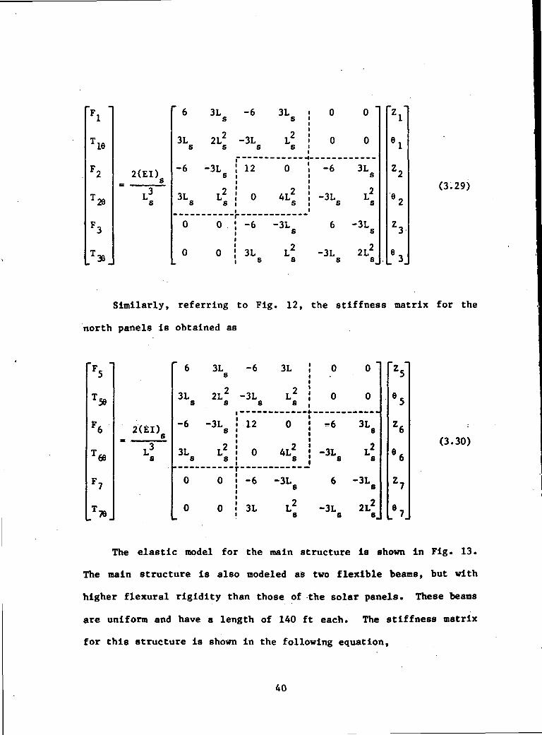
Similarly, referring to Fig. 12, the stiffness matrix for the
north panels is obtained as
'56
66
2(EI)
6
3L' 8
-6
3L8
0
0„
3Ls
2L2s
-3Ls
L2s
0
0
-6
-3L8
12
0
-6
3L
3L
L28
0
24IT8
-3L8
L28
0-
0
6
-3L8
6
-3L8
0 "
0
3L8
L28
-3L8
2L28_
(3.30)
78
The elastic model for the main structure is shown in Fig. 13.
The main structure is also modeled as two flexible beams, but with
higher flexural rigidity than those of the solar panels. These beams
are uniform and have a length of 140 ft each. The stiffness matrix
for this structure is shown in the following equation,
40

«i»(El> (ED
Figure 11 Elastic Model for Solar Panels — South
(El) (ED '4Ls ; 4
Figure 12 Elastic Model for Solar Panels — North

Figure 13 Elastic Model for the Main Structure
42

"F2 "
T2*
F4
T4»
F6
.V
2(EI)g
Le
6 3L -6 3L 0 0 "e e
3L 2L2 -3L L2 0 0e e e e
-6 -3L 12 0 -6 3Le e
2 2 23L IT 0 4IT -3L L
e e e e e
0 0 -6 -3L 6 -3Le e
0 0 3L L2 -3L 2L2
e e e e
Z2
*2
Z4
*4
Z6
.V
(3.31)
Applying the same principle of Eq. (3.8), the stiffness matrices
of Eqs. (3.29), (3.30) and (3.31) can be combined to yield the system
stiffness matrix. Reorder the force and displacement vectors and the
corresponding rows and columns of Eq. (3.29) as follows,
T28
F.1
Tie
F3
TJ> **»38
F,2
2(EI)8
L3
4L2 3L L2 -3L L2 08 S 8 8 8
3L 6 3L 0 0 -6S S
2 2L 3L 2L 0 0 -3L8 8 8 8
-3L 0 0 6 -3L -68 8
2 7L 0 0 -3L 2L -3L
8 8 8 8
0 -6 -3L -6 3L 128 8
"e "
2
Z.19123
g3
z. 2_
(3.32)
The purpose of this reordering process is to move ^2% an^ ®2 to tlie
top for later use and F2 and Z2 to the bottom so that the "south"
panels can be combined with the main structure.
43

Reorder the rows and columns of Eq. (3.31) so that ?2 and T. , are
placed on the top and Fg and Zg are on the bottom,
F2
F4
.F6.
2(El)e
Le
6 3L -6 3L 0 0e e
T"""2 2 "*3L 2L -3L L 0 0
e e e e
-6 -3L 12 0 3L -6e e
3L L2 0 4L2 L2 -3Le e e e e
0 0 3L L2 2L2 -3Le e e e
0 0-6 -3L -3L 6e e
Z2
*2
ZA
.Z6.
(3.33)
Reorder Eq. (3.30) so that Fg and Zg sit on the top and Tgg and
8g at the bottom,
F6
F5
T50
F7
T7B
T t t_
2(EI)
L3
8
12 -6 -3L -6 3L 08 8
-6 6 3L 0 0 3L8 8
- 3 L 3 L 2 L 2 0 0 L 2
S 8 8 8
- 6 0 0 6 - 3 L - 3 L8 8
3L 0 0 -3L 2L2 L2
8 8 8 8
0 3L L2 -3L L2 4L2
8 6 8 8 8 _
>6
Z5
S
Z7
•7
_••_
(3.34)
44

Let
ORIGINAL PAGE 13Of POOR QUALITY
and 6 (3.35)
combine Eqs. (3.32), (3.33) and (3.34) one has
ILiJi 6n 3t^i 0 Q
Lg«i 3L i 2*-2<i ^ 0
3Lg» 0 0 f t i ' t-^1
L|» 0 0 3L£i 2l|n
0 -6n -3Lcn -6n 31. 1
0
3L,0 60 3L^ 0 0
2L^fl -3L,;) tjd 0 0 II
3L/ I2« 0 3L^ -eO I
tjd 0 4tJ( tj( -31,0 '
0 3LJ) uJ0 2Lj( -31,0
0 •«« -31 1 -3L.0 I 6flt|2n I
0
-3Lgi -to
0
0
L|O
Now we shall use the constraints of Eq. (3.28) and
Ls"
(3.36)
T26 (3.37)
to combine T6? and T2Q and rename it as T4e, and e& and &2 and rename
it as 64 and rearrange the rows and columns so that they appear
between F^ and T^ and between Z^ and , respectively. In addition,
we also exchange the orders of Tg^ and Fg, and ^g, and Zg. Thus if
we let F8, Z8, and Kg be the force vector, displacement vector, and
45

the stiffness matrix, respectively, Eq. (3.36) becomes
where
(3.38)
Fg = T19 F3 T39 F2
Z3 63 Z2 <fr2
TA9 TA(J F6
Z6 *6 Z5 65 Z?
F7 T79)J
(3.39)
(3.40)
and K_ is shown in Eq. (3.41).
60
31,0
0
0
-60
0
0
3Lso
0
0
0
0
0
0
0
3LS0
2L?0
0
0
-3LS0
0
0
4-.0
0
0
0
0
0
0
0
0
60
-31,0
-60
0
0
-3lso
0
0
0
0
0
0
0
0
0
-3LS0
21JO
31^0
0
0
ll.0
0
0
0
0
0
0
-60 0
. -3l$u 0
•60 0
31,0 0
120 «60 3le0
31.0 *4*
-60 -31^/J
0 0
3w* 400 0
0 0
0 0
0 0
0 0
0 0
0
0
0
0
-60
-3L.0
120
0
0
-60
31*0
0
0
0
D
31,0
&
-3L$0
4.a
0
0
2
a
0
0
3Lsa
L?o
-31,0
4.
0 0 0
0 0 0
0 0 0
0 0 0
3Le0 0 . 0
&S 0 ' 0
0 -60 3le0
0 0 0
«l|0 ~3l«0 40
-31^0 12O*60 -3Lj0
2 21^0 "31^0 2le0
0 -60 0
0 -3lsa 0
0 -60 0
0 31)0 0
0
0
0
0
0
0
0
3l,a
0-
-6a
0
60
3l,a
0
0
0
0
0
0
0
0
0
&
0
-3L,a
0
3Lsa
2^0
0
0
u
0
0
0
0
0
0
31,0
0
-60
0
0
0
. 6a
-3lsa
0
0
0
0
0
0
0
4--0
3lsa
0
0
0
3L,0
2
(3.41)
46

where a and 6 <•
A quick check of symmetry, Kg Is symmetric as it is supposed to be.
3.2.3 The Consistent-Mass Matrix
Consider Figs. 14, 15, and 16 which show the distributed mass
models for the south and north solar panels and the main structure,
respectively. By using the same finite-element technique, the
consistent-mass matrices for the component structures are,
Solar Panel South
16
'29
P Lm B 8
420
156 22L 54 -13L 0 0s s
2 222L 4L 13L -3L 0 08 8 8 8
54 13L 312 0 54 -13L8 8
-13L -3L2 0 8L2 13L -3L26 8 8 8 8
0 0 54 13L 156 -22L8 8
2 20 0 -13L -3IT -22L 4IT
8 8 8 8 _
2.1
• *
9.1
• •
Z,2~ »*
6,2»*
Z,3• •
e,3_
(3.42)
47

's -4
Figure 14 Distributed Mass Model for Solar Panels — South
.. z,e.
Figure 15 Distributed Mass Model for Solar Panels — North

for

b. Solar Panel — North
F5
T56
F,0
T69
F,7
T/78_
P Ls 8 8
420
156 22L 54 -13L 0 08 8
2 122L 4L 13L -3L 0 0
8 8 .8 8
54 13L 312 0 54 -13L8 8
-13L -3L2 0 8L2 13L -3L2
8 8 8 8 8
0 0 54 13L 156 -22L6 6
2 "J0 0 -13L -3I/ -22L 4IT
8 8 8 8_
'5..6 5
26
e6
Z,7
..8 7.
(3.43)
Main Structure
F02
T&
F4
T4*
F6
T,.6*_
P L« e e420
156 22L 54 -13L 0 0e e
2 222L 4L 13L -3I/ 0 0
e e e e
54 13L 312 0 54 -13L- C = - =-- -- -=- - - C
-13L -3L2 0 8L2 13L -3L2e e e e e
0 0 54 13L 156 -22Le e
2 20 0 -13L -3I/ -22L 4IT
e e e e_
Z.2
..
^2
V
*4
6••
•. 6_
(3.44)
Employing a similar approach for obtaining the stiffness matrix,
the following equation can be obtained:
F8 - M8C Z8(3.45)
50

whereORIGINAL PAGE 53OF POOR QUALITY
F T1Q F3 T38 F2 F4 T4Q
Z3 63 Z2 V2 Z4 84 *4 *Z6 *6 'Z5 *e*5 Z7 97)T
and the consistent-mass matrix Msc is shown in Eqs. (3.46) and
(3.47).
M5C=
l*s
.**0
0
5fe
0
0-
-13Lsa
0
0
0
0
0
0
0
as,44.
0
0
13Lsa
0
0
-34,
0
0
0
0
0
0
0
0
0
156a
-22lsa
Ma
0
0
13Lsa
0
0
0
0
0
0
0
0 Ml 0
0 Ulsa 0
-22M Ma 0
4 -»* o
-13l,a 312a.l566 Hl,J>
0 22let> 4L^b
0 Mb l3L«b
-3tja 0 0
0 -13leb 3l|b
0 0 0
0 0 0
0 0 . 0
0 0 0-
0 0 0
0 0 0
0
0
0
0
Mb
ULjb
3l2b
0
0
Mb
•BV
0
0
0
0
-Ulsa
-34,
13L,a
-34.
0
0
• o
IMJa
0
0
0
-IV
•-ilii
13Lsa
-34.
o o . o o
0 0 0 0
0 0 0 0
0 0 0 q
-Ul b 0 0 0
-3l/b 0 0 0
0 Mt> -I3L«b 0
0 0 0 -13lsa
ajb UM) -3l|b 0
UL,b lS6b»3IZ9 -22l«b S4a
-3i|i) -za^b ojo "
0 Ma 0 I56»
0 13L,a 0 22lsa
0 Ma 0 0
0 -LRsa 0 0
0
0
0
0
0
0
0
-34.
0
13Lsa
0
^<4«0
0
0
0
0
0
0
0
. 0
l3Lsa
0
Ma
0
0
0
156a
-221
0
0
0
0
0
0
0
0
-13Lsa
0
0
0
-22lsa
•Si
(3.46)
where a 420 and b
peLe420"
(3.47)
51

3.2.4 The Lumped-Mass Matrix and System Mass Matrix
Mgc accounts for the distributed mass for the flexible structure
but not the lumped mass associated with the rigid bodies. Let MSD be
the lumped-mass matrix for the station excluding the payloads, then
MSD = diag (0,0,0,0,0,0,M4,I4yy,I4xx,0,0,0,0,0,0) (3.48) '
where M4, I4xx, and I4yy are the mass and moments of inertia of the
core station defined in Fig. 10.
The total mass matrix, excluding payloads is,
Ms - Msc
The corresponding dynamic equation due to mass and inertia is
FS - Ms*z's (3.50)
3.2.5 Payload Dynamics and Hinge Torque Model
The dynamic model for the payloads (identified as bodies 8 and 9)
and the hinge coordinates are shown in Fig. 17.
To include the pay load dynamics and the dynamic interactions
between the payloads and the station, the following expressions are
obtained using the Lagrangian approach:
52

7
9X
PAYLOAD CONFIGURATION
m8' 'sxs' 'BYS
m9' *9XS' !9YS
78X " 78XHINGE ANGLE FOR "PAYLOAO 8" ABOUT X-AXIS
T8Y ** V " 64 " HINGE ANGLE FOR "PAYLOAD 8" ABOUT Y-AXIS
9XHINGE ANGLE FOR "PAYLOAD 9" ABOUT X-AXIS
9Y * 79Y " ^4 " HINGE ANGLE FOR "PAYLOAD 9" ABOUT Y-AXIS
Figure 17 Payload Dynamics and Hinge Model
53

FA - (M8+M9)Z4 + (M8L8-M9L9)e4 + M8L8bY8y-M9L9bY9y (3.51)
T49 + (M8L8-M9L9)Z4 - (I8y8+M8L§ + ys L )' (3.52)
+ M8L8aL8b + M8L8b 8
- (I8xs + I9xs>*4 - '
F.qs. (3.51), (3.52) and (3.53) are used to replace F4, 149, and
in Eq. (3.50).
The torques applied at the payload hinges are,
T9x - xs** + xs' x (3.55)
T8y = ~ M8L8bz*4 + (l8ys+M8L8aL8b+M8L8b)'6A + Sys S b Sy <
T9y - MgLgb' -K (igyg+MgLgaL L ) + ( I9yB+ lb 9y (3'57)
I t Iwhere Y8x, Y8y, Y9x» and Y9y are the hinge angles for payloads 8 and
9 about the X- and Y-axes.
The above equations are derived using the Lagranglan approach
with more general assumptions and then linearized for small angles.
The detailed derivation is shown in Appendix A.
3.2.6 . Equations of Motion
Let Fp " <T8x. T9x» T8y» T9y> and Zp " <Y8x, Yg,, Y8y. ) be
the payload forcing and displacement vectors, the corresponding
vectors for the system can be partitioned as follows,
54

F_ _8_
FP
and Z »Z
_ JL _Z
P
The system mass matrix becomes,
(3.58)
M = Mc + MD (3.59)
where
' C
MSC 15x4
°4xl5 °4x4
and
MSD+MSD ' MPSD
"PSD ! "PD
(3.60)
(3.61)
MSC is defined in Eq. (3.46) and MgD in Eq. (3.48), and Mgn, MpD,
MpSD are,
6x6
°3x6
, ,6x6
6x3 6x6
I8yS'fI9yS
6x3 °6x6
(3.62)
55

"PD
I8xS0
0
0
0
T9xS
0
0
0
0
2I8yS'hn8L8b
0
0
0
0
2I9yS4l°9L9b
(3.63)
MPSD °/ *4x6
0 0
0 0
"Vsb I8yS4m8L8aL8b4m8L8b2
°9L9b I9yS4m9L9aL9b4in9L9b
X8xSI9xS
0
0
°4x6(3.64)
The system stiffness matrix is
I 0,s I "15x41
04xl5| °4x4
where Kg is defined in Eq. (3.41),
The equation of motion is
(3.65)
MZ + KZ - F (3.66)
56

3.2.7 Modal Coordinates and Modal Properties
Let n(t), A, and 4> be the modal amplitude vector, eigenvalue
matrix, and normalized eigenvector matrix, respectively. Let Z(t) =
4>n(t), substitute this into Eq. (3.66) and premultlply Eq. (3.66) by
$ » then <|iTMi|» = I and <J> K<J> = A, one has the following dynamical
equation in modal form,
n + An = 4>TF (3.67)
where A = diag (o»| ..... (t>\g) . Adding damping terms, Eq. (3.67)
becomes,
"n* + diag (2C1a)1,...,2c19to19)f| + diag(u> ,... ,o) g)n - <t»TF (3.68)
The corresponding damped dynamical equation in physical coordinates
can be obtained through transformation. Let D be the damping factor
matrix, one has
D = (TT diag (2C1o)1,...,2i:iga)19)<|)~1 (3.69)
and the equation of motion becomes,
MZ + DZ + KZ - F . (3.70)
For the purpose of control, let B and C be the control influence
matrix and measurement distribution matrix, respectively, the system
equation in physical and modal coordinates are, respectively,
57

MZ + DZ + KZ " Bur
I yp - C (aZp + Zp)
(3.71)
(3.72)
and
n + diag
. y
+ diag (uj ..... u\9)r\ = <J>TBup (3.73)
(3.74)
To obtain the modal properties, i.e., to determine the
eigenvalues and eigenvectors, for the open-loop system, one can
either free the hinges for the payloads or clamp them. For the
latter case, a 15-DOF system results with 12 flexible modes and 3
rigid body modes. For the former case, however, a 19-DOF system
results since the payloads are considered rigid bodies and the hinges
are freed, it ends up with 4 additional rigid or zero frequency
modes. Since this does not yield additional information, only the
clamped-hinge case is considered in this dissertation.
The modal frequencies and mode shapes for the four-panel
configuration with clamped-hinge case are shown in Fig. 18. These
modes are divided into three groups. The first bending group
consists of 6 modes with frequencies ranging from 0.115 Hz to 0.302
Hz. These modes are formed with the first symmetric or antisymmetric
bending of the three major structures, i.e., the two solar panel
pairs and the main structure. The second bending group is caused by
58

c:•co
§
o
N§•o(-1
00
•H•o
ICOM•rlfc
(1)
«P.I(J
Ob-
01
OU-
03O>•HAJP0)&ouo.
\I
'
^~>
£^sUJ 2
ss
i°'^^B
•
^
3
CO•cc
g&
•T-l
d.
59

lf\
2o00.50)
CQ
oo&
•o0)3
eo
00
00
£8
S3
60

UJ „
5 3
CO<U1.
•o
•o•H00
01
C
I
00tH
(II
3
61

the second symmetric or the. antisymmetric bending of the three major
structures. The frequencies for this group are much higher than
those of the first group, ranging from 1.67 Hz to 2.34 Hz. The third
group consists of three rigid body modes with zero frequency.
The structural and mass parameters used for generating these
modes are shown in Fig. 10. The flexural rigidity (EI)g « 9.48xl06
lb-ft2 has been used for the solar panels and a value of an order of
magnitude higher has been used for the main structure.
3.3 Frequency Characterization of Space Station Dynamical Systems
With the availability of these space station models, the
frequency characteristics of the various dynamical systems in the
space station environment are identified as shown in Fig. 19.
For a nominal orbital altitude of 400 km, the orbital period is
92.61 minutes or 1.8x10"** Hz rate. For an altitude close to 400 km, the
orbital rate will be inside the shaded narrow region in Fig. 19. The
solar panel libration frequency for quasi-solar-inertial pointing
[51] will be twice the orbital rate, as shown in Fig. 19. A low
bandwidth attitude control system for the space station will have a
bandwidth in the range of 0.001 Hz to 0.005 Hz. The two-panel low
DOF model and the four-panel finite-element model are shown in Fig.
19 with their modeled frequencies identified by vertical lines. The
dashed regions extending the modeled modes represent the modal
spectra that are not Included in the models. The payload attitude
control systems for a range of applications will have bandwidth in a
range centered at 1 Hz. The core body Including the pressurized
modules should have structural frequencies above 9 Hz. The figure
62

tMo
IOz
o
fc•v.5
O
ejio
II
V.
reot-i
TO
O
e/:
QJuna
tnuJJCO
uTO
TO
5u<U£?cr2t
0)t-.
be
SW31SAS IVDIWVNAa
63

indicates that the spectral separations of the orbital rate, the
attitude controllers, and the low frequency modes of the station
structure are reasonable. However, the same cannot be said about the
structural modes and the payload controls. For instance, the payload
controller bandwidth falls between the modes of the first and the second
bending groups. This result strongly suggests that decoupling control
for the payload is required.
64

.CHAPTER IV
PROBLEM FORMULATION
The space station, or the controlled plant can be represented by
the following state space model:
xp(t) - Ap xp(t) + Bp up(t) (4.1)
yp(t) = Cp xp(t) (4.2)
where xp(t) is the Np-dimensional plant states, up(t) is the M-
dinensional plant control inputs, and y0(t) is the M-dimensional
plant outputs. Here it has been implicitly assumed that the number
of inputs equals the number of outputs. Physically, control inputs
are the forces and torques generated by actuators, such as thrusters,
proof masses, Control Moment Gyros, and momentum wheels. The outputs
are measurements such as linear and angular displacements and rates
measured by accelerometers, rate and integration gyros, etc. A , B ,
C are the state, control influence, and measurement distribution
matrices of appropriate dimensions. (Ap,Bp) is controllable and (Ap,
Cp) is observable.
A reference model that serves as a performance measure is
required. This model is chosen to be asymptotically
stable and can be represented by the following equations:
Bm
65

where (t) is the ^-dimensional model states, u^t) is the M-
dimensional model commands, and ym(t) is the M-dimensional model
outputs. Afg, Bm, Cm are matrices of appropriate dimensions.
Since the space station is infinitely dimensional while the
dimension of the reference model has to be reasonably small for
practical implementation, the following condition will be necessary
for any adaptive algorithms for LSS (large space structures) or space
stations:
Np » Nm (4.5)
Define the output error between the plant and the model as
ey(t) - ym(t) - yp(t) (4.6)
Since the reference model specifies the desired performance of the
plant (space station), the objective is then, without assuming the
complete knowledge of the plant, to design an adaptation mechanism to
generate a suitable plant control input u_(t), so that the plant
output tracks the model output asymptotically, i.e.,
lira ey(t) - 0 (4.7)
66

CHAPTER V
CONTROL ARCHITECTURE
5.1 Control Architecture for the Two-Panel Configuration
Referring to Fig. 6, the most rigid location on the station is
its core on which inertial sensors, accelerometers and actuators are
located. Control Moment Gyros (CMC's) are assumed and they are
effective only for antisymmetric modes; the symmetric modes are
controlled by the thrusters or proof masses. To gain controllability
and compensate for vibrations of the large flexible panel structure,
reaction wheels at the tips of the panels are postulated.
Accelerometers and a target set of vibration sensors for relative attitude
and rate measurements are also placed at the panel tips. Although the
panel tips are far from ideal for locating hardware components, the choice
is nil. For translational control, force actuators are required at
the bus.
With the above control architectural design, the control input
and output vectors are defined as follows:
u.
and
VVUP3
.Up4."ypl"yP2yP3
yP4_
a
S3
Tl
F2
T2
T3
a
com
cont
com
com
" aepl + *pl
azp2 + Zp2
06P2 * ®P2
a6P3
+ 9p3
control torque at left panel tip
control force at central bus
control torque at central bus
control torque at right panel tip
(5.1)
(5.2)
67

In order to apply adaptive control techniques to this 6-DOF
model, Eqs. (3.26a) and (3.26b), i.e., the plant equations, are
written in state space form. Let np be the modal amplitude vector,
and define the plant state vector x as,
P_
we have
0
aC<J>
(5.3)
_p_•
n_
the corresponding Ap, B_, and C matrices are
(5.4)
(5.5)
6x6 6x6
-co 0 1 -2? ,o), PI
B0
T(5.7)
68
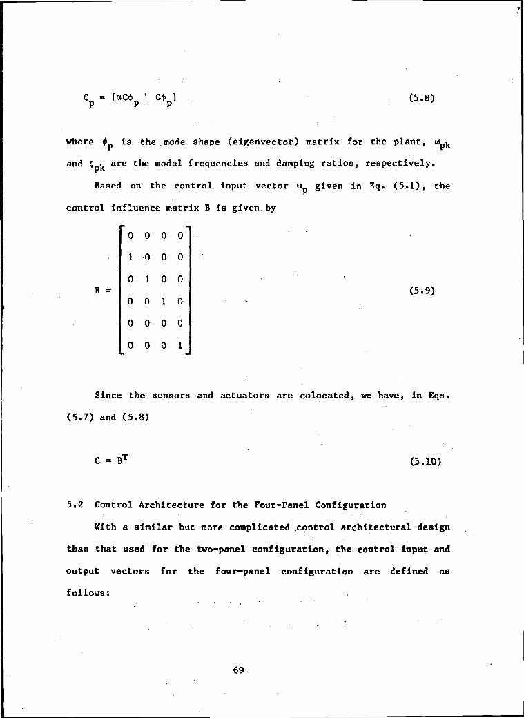
j C*p] (5.8)
where <fr is the mode shape (eigenvector) matrix for the plant, u-^
and C k are the modal frequencies and damping ratios, respectively.
Rased on the control input vector u given in Eq. (5.1), the
control influence matrix B is given by
0 0 0 0
1 0 0 0
0 1 0 0(5.9)
0 0 1 0
0 0 0 0
0 0 0 1
Since the sensors and actuators are colocated, we have, in Eqs.
(5.7) and (5.8)
C - B1 (5.10)
5.2 Control Architecture for the Four-Panel Configuration
With a similar but more complicated control architectural design
than that used for the two-panel configuration, the control input and
output vectors for the four-panel configuration are defined as
follows:
69

u.
and
"v~UP2
UP3
V
UP5
UP6
Up7
UP8
UP9
Upl0
.""'I
~ypl~
yp2
yP3yP4p5
po
yp7
Po
yp9
ypioypii
S9
"
"T16
T36
F2
T2*
F4
T46
T4*
F6
T6<J>
T59_T79_
-
"Y-t
Y-t
Z-f
X-t
Z-f
Y-t
X-t
Z-f
X-t
Y-t
Y-t
aepl * 9pl"
°6p3 * 6p3•
aZp2 * Zp2
a*p2 * *p2•
°zp4 + 4*
00p4 + 9P4
°*p4 + *p4•
azp6 * Zp6
a*p6 * *p6
°9p5 + 9p5
aep7 * 9p7
Y-torque at left south panel tip
Y-torque at right south panel tip
Z-force at the root of south panel
X-torque (bending) at the root of south panel
Z-force at central bus
Y-torque (twisting) at central bus
X-torque (bending) at central bus
Z-force at the root of north panel
X-torque (bending) at the root of north panel
Y-torque at left north panel tip
Y-torque at right north panel tip
(5.11)
(5.12)
11 sets of sensors and actuators are used at 7 locations. The
problem becomes more involved now because of the more complicated
70

structure and the three-dimensional motion instead of plane motion
only.
Again, for the application of adaptive control, state-space
representations of Eqs. (3.73) and (3.74) are obtained. Let YJ
be the modal amplitude vector', and define the plant state vector x_
as,
n•
n(5.13)
we have
m
X **p
*
0
i •
I" '
> yp"
NN
N
0 -a) ,.p!5
iaC^ i Cd>
P , Pj
2
the corresponding Ap,
A •
P
-
o15x15
•t-u * 0
Pi
0
nP_• -n P _
NX
X
"^plS^plS
• " tp ~
V o+ u
n , Tn PP 9 0
p
(5~.14)
(5.15)
B_, and C matrices are
111
i
1 ?Pl0 * * - ( ! } . - *
p!5 |
•
I15x15
u , 0Plx
° V-2Cpl5Upl5
/C 1 £L\
71

B,
B
S- <V
(5.17)
(5.18)
where A , u ^, and C-^ are the eigenvector matrix, modal frequencies
and damping ratios, respectively, and the control influence matrix B
is
0 0 0 0 0 0 0 0 0 0 0
1 0 0 0 0 0 0 0 0 0 0
o o o o o o o o o o o
0 1 0 0 0 0 0 0 0 0 0
0 0 1 0 0 0 0 0 0 0 0
0 0 0 1 0 0 0 0 0 0 0
0 0 0 0 1 0 0 0 0 0 0
B - 0 0 0 0 0 1 0 0 0 0 0 (5.19)
0 0 0 0 0 0 1 0 0 0 0
0 0 0 0 0 0 0 1 0 0 0
0 0 0 0 0 0 0 0 1 0 0
o o o o o o o o o o o
0 0 0 0 0 0 0 0 0 1 0
o o o o o o o o o o o
0 0 0 0 0 0 0 0 0 0 1
Again, the sensors and actuators are colocated, hence
B
in Eqs. (5.17) and (5.18).
(5.20)
72

CHAPTER VI
ADAPTIVE CONTROL ALGORITHM
The equations of the plant (space station) and the reference
model are described in Eqs. (4.1)-(4.4), and are repeated below for
convenience:
plant ( xp(t) = Ap xp(t) + Bp up(t) (6.1)
( yp(t) = Cp xp(t) (6.2)
model ra • ui ui • iii ui • ~ '
(6.4)
The output error is
ev(t) - y_(t) - y-(t) (6.5)
The objective is to find up such that
lira ey(t) = 0 (6.6)
with the requirement that dimension N. » N,,, and A_, Bp, C_ are not
completely known.
The adaptive control algorithm under consideration here is an
extension of that developed in Ref. 42. Since the Command Generator
Tracker theory [43] formed the basis of that algorithm, it is
introduced first in the following.
73

6.1 The Command Generator Tracker Theory
The Command Generator Tracker (CGT) concept developed by
Broussard is a type of model reference control. What makes it
attractive is that it allows perfect model output tracking even
though the plant and the model are not of the same order. The basic
idea of CGT is to generate a plant input u (t) as a linear
combination of the model states x t), model inputs
output tracking error ey(t), i.e.,
, an(* the
up(t) » S2ixm(t) ey(t) (6.7)
so that the output tracking error asymptotically approaches zero.
The gain matrices Soi and Soo are referred to as the CGT gains, and
Ke is selected to stabilize (Ap-B KfiC ).
When yp(t) » ym(t) (i.e., perfect tracking occurs), the
corresponding plant state and control trajectories are called "ideal
trajectories" and are denoted as x*(t) and u£(t), respectively. When
um(t) is constant, xp(t) and up(t) are assumed to be linearly related
to the model command um and model state
following equations:
as shown in the
(t) sll S12
S21 S22
(6.8)
where Sjj, Sj2t $21 an(' ^22 are matrices with appropriate
dimensions. By definition, the ideal trajectory xp(t) is such that
"'Tor the more general case, refer to Ref . 54.
74

y*(t) = Cp XpXt) - Cm xm(t) = yn(t) (6.9)
and
xj(t) - Ap xj(t) + Bp uj(t) (6.10)
To find the CGT gains S21 and S22, we first substitute Eq. (6.8) into
Eq. (6.9). Thus,
Cp xj(t) ' Cp(SH *n(t> + S12 "m> = Cm xm (6-U)
Hence,
Cp sll ™ Cm (6.12)
Cp S12 • 0 (6.13)
Differentiating Eq. (6.8),
* k v * • *
(6.1A)
and substituting Eq. (6.8) into Eq. (6.10)
xp(t) " V8!! **<*) + S12 %> * Bp(s21 xm(t) + S22 %)
= (Ap Sn + Bp S21) ^(t) + (Ap S12 + Bp S22) um (6,15)
and comparing Eqs. (6.14) and (6.15), we have
75

Ap Sll + Bp S21
Bra 12 + Bp S22
(6.16)
(6.17)
Rewriting Eqs. (6.12), (6.13), (6.16) and (6.17) in matrix form, we
obtain
\ BP~Cp 0
sll S12
s12 s22^sa
SllAm
and then define
"ll n!2~
02i «22-\ BP~
.°P °.
-1
The resulting CGT equations become
12 "
521 -
522 -
(6.18)
(6.19)
(6.20a)
(6.20b)
(6.20c)
(6.20d)
The so-called perfect model following (PMF) conditions are a
special case of the CGT when the state vector is available and it is
assumed that x£(O - (t). Since x£(t) - S11xra(t) + S , the PMF
conditions imply that Sjj » I and S}2 - 0. Also, since
(6.21)
76

i.e.,
Bp(S21 x^t) + S22 um)
Bp S21> *m<t) + Bp S22 v^
A, Vt) + Bm u, (6'22)
From Eq. (6.22), It is found that
Bp S21 = A* - Ap (6.23.)
Bp S22 = B^ (6-23b)
If the CGT gains S2J and S22 which satisfy the PMF conditions
(Eq. (6.23)) exist, a valid PMF controller then becomes
up(t) = u*(t) + K(xm(t) - Xp(t)) (6.24)
where K is a stabilizing feedback gain.
Back to the general CGT, we define the state error as ex(t) =
x_(t) - xp(t) and seek a controller which guarantees that ex(t) •»• 0
as t * «. Because when xp(t-) - x*(t), we have Cp xp(t) - Cp x*(t),
hence
yp(t) A Cp xp(t) - Cp xp1 (t) A 0 (1) A ym(t) (6.25)
and that is exactly the desired result we require.
77

With the error defined as ex(t) » xp(t) - xp(t), the error
dynamics becomes
ex(t) - ApXp(t) + Vp(t) ' AP XP(t) ~ BP uP(t)
= Ap ex(t) + Bp[u* (t) - up(t)l (6.26)
Note that
ey(t) - ym(t) - yp(t) = Cp(xJ(t) - xp(t)) - Cp ex(t) (6.27)
Equation (6.26) will be used in the subsequent stability analysis.
The CGT concept stated above is, however, non-adaptive. The
purpose of adaptive control is to eliminate the need for a priori
knowledge of the plant that is required in CGT.
6.2 Direct Model Reference Adaptive Control
Based on the CGT concept, Sobel et al. [42] developed the
following adaptive control law:
" Ke(t) "y(t) + K»(t) **(t> + M*) Vt) (6.28)
or, let r ( t ) b e a 2 M + N m vector defined as
rT(t) - [eyT(t) (t) un
T(t)] (6.29)
78

and K(t) be the M x (2M+Nm) adaptive gain matrix defined as
K(t ) = [Ke(t) ^(t) Kjt)] (6.30)
Then
up(t) = K(t) r(t) (6.31)
where K( t ) is a combination of two types of gains, i.e.,
K(t) = Kp(t) + Kx(t) (6.32)
and K_(t) is the direct gain, Kj(t) is the integral gain defined as
follows:
Kp(t) - ey(t) rT(t)T (6.33)
KT(t) = ey(t) rT(t)T (6.34)
with
Kx(0) - KIO (6.35)
where T and T are the (2M+Nm) x (ZM+J ,) gain weighting matrices. KIO
is the initial integral gain. Note that u_(t) is highly nonlinear
and its values are, in part, proportional to the cube of the output
error ey(t) eyT(t) ey(t).
The stability conditions of the adaptive controller are
established via the Lyapunov direct method by considering a positive
definite function given by
V(ex»KI> = e x ( t ) P ex^> * TrfSCKj-T-kKj-c)^ 1 ] (6.36)
79 '

where
P is a N x Np positive definite symmetric matrix
K is a MX (aM+N, dummy gain matrix
S is a M x M nonsingular matrix
t**
Note that dummy gain matrix K does not appear in the control*-w *v ** ***
algorithm. It can be partitioned as K = [K , K, K ] so that
• K r(t) - Ke Cp ex(t) + x t) + um (6.37)
where K , K and K are, like K, dummy gains.
Introducing the control algorithm into the error equation given
by Eq. (6.26), using Eqs. (6.31) to (6.33) and recalling from Eq. (6.8)
that u*(t) = S01 x (t) + S_9 u , gives:p 21 m // m
ex(t) - Ap ex(t) + Bp[S2i
- Kx(t)r(t) - Cp ex(t) rT(t) 7r(t)J (6.38)
The time dependence of the variables is omitted in the sequel for
brevity. Thus the adaptive system is described by
S22um ~ KIr
and
K! - CpexrTT (6.40)
80
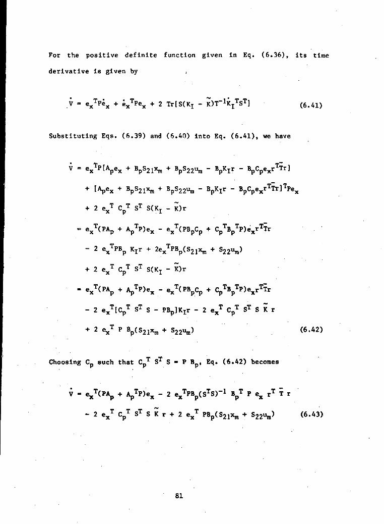
For the positive definite function given in Eq. (6.36), its time
derivative is given by ,
Substituting Eqs. (6.39) and (6.40) into Eq. (6.41), we have
V = exTP[Apex + BpS21xm + BpS22Ura - BpKTr - BpCpexr
TTr]
BPS22um ~ BpKIr "
2 exT Cp
T ST S(KZ - K)r
CpTBp
TP)exrTTr
- 2 e
T T T2 ex Cp S S(KT - K)r
- 2 exT[Cp
T ST S - PBpll^r - 2 exT Cp
T ST S K r
+ 2 P
Choosing C such that CpT ST S - P B , Eq. (6.42) becomes
V - exT(PAp + Ap
TP)ex - 2 exTPBp(S
TS)-1 BpT P ex r
T T r
- 2 exT Cp
T ST S K r + 2 exT PBp(S2ixm + 823%) (6.43)
81

Substituting -Eq. (6.37) into Eq. (6.43), we obtain
V = exT[P(Ap - BpKeCp) + (Ap - BpKeCp)
TP]ex
- 2 exTPBp(S
TS)~1BpT P ex r
T T r
+ 2 exT PBp[(S21-Kx)xm + (S22 - K^uJ (6.44)
f*+ f*4
with the choice 1^=8^ and KU = S22, Eq. (6.44) reduces to
V - exTlP(Ap - BpKeCp) + (Ap - BpKeCp)
TP]ex
- 2 exTPBp(S
TS)~1BpT P ex r
T T r (6.45)
Let Q - - P(Ap - BpKeCp) - (Ap - BpKeCp) P (6.46)
Eq. (6.45) becomes
Q ex - 2 exT P Bp(s
TS)-1 BpT P ex r
T T r (6.47)
If T is chosen to be positive semidefinite, the second term in
Eq. (6.47) will be negative semidefinite in ex. Then we choose P~
such that for some K£, Q is positive definite. Consequently, V is
negative definite in ex, and V is a Lyapunov function for establish-
ing the asymptotic stability of the zero state of Eqs. (6.39) and
(6.40).
82

To summarize, a sufficient condition for asymptotic stability is
(1) T is positive definite
(2) T is positive semidefinite
(3) P Bp = CpT(STS)
(4) P is chosen such that P(Ap-Bp KC Cp) + (Ap-Bp Kg Cp)TP
^
is negative definite for some K .
Under the above conditions, the plant output will asymptotically
track the model output. Furthermore, since the derivative of V is
negative semidefinite in the augmented state [ex(t), Kj(t)], the
adaptive gains will be bounded.
It should be noted that conditions (3) and (4) together are
equivalent to requiring that the plant transfer matrix
~ • iZ(s) = Cp(sI-Ap + Bp Ke Cp)""
1 Bp be strictly positive real for someX*
feedback gain matrix Kg. For the definition of positive realness and
strictly positive realness of matrices, see Appendix B.
6.3 Instability Problem Caused by Rigid Body Modes
It is well-known that the zero frequency rigid body modes are
unstable modes. Simulation results show that this adaptive control
algorithm fails to stabilize these modes and yield stable states or
outputs. These problems may be verified analytically. They are
treated as critical cases of stability problems for autonomous
differential equations developed in Ref. 52. Let
x = Ax + g(x) (6.48)
83
be the given differential equation, where Ax represents the linear
part and g(x) the nonlinear part. The real parts of the eigenvalues
of A are assumed to be nonpositive. The critical case refers to the
situation where some of the eigenvalues have zero real parts. If the
matrix A has a double zero eigenvalue and if the reduced equation can
be written in the form
(6.49)
(6.50)
(where g is at least of second order, Y and 6 are positive integers),
then we have the following sufficient conditions for instability due
to Lyapunov [53],
The equilibrium is unstable, if one of the following conditions
is satisfied:
(1) y even;
(2) Y odd, a>0;
(3) Y odd, a<0, 6 even, Y > 5 + 1. b>0;
(A) Y odd, a<0, 5 odd, Y > 26 + 2;
(5) Y odd, a<0, 6 odd, Y - 26 + 1, b2+4(6+l)Y > 0;
(6) the equation for 012 contains only the term MCOJ,^)*

To apply the above criteria to our case, the system equations
are rewritten in the form of Eqs. (6.49) and (6.50) by defining
-<vAx
m
(6.51)
(6.52)
Then
ey ' cm*m ~ CPXP " Jx
since
(6.53)
m (6.54)
ey
xm
urn
(6.55)
Hence
rT Tr - e,,T Ty ey *y xm itn um iB
ey Txm x, + C (constant) (6-56)
Therefore the system equations (6.1) and (6.3) can be rewritten as,
85

AX
•xm
•X
P
s
A 0ro
0 AP
AX +
B um m
B Jx (xTJT ¥ Jx + x T T X + C)p ey m xtn m
0
B K_ rP I
(6.57)
TKI- ey r T (6.58)
As stated in Chapter VII, in the present study, we concentrate
on the space station attitude hold only, i.e., u,,, • 0. In this
special case, the corresponding coj's are xpi (modal amplitudes) and
i»2*8 are Xpi (nodal amplitude rates), respectively. For a certain
mode, its corresponding block in matrix A is
0 1
[i 0Hence for rigid body modes, it becomes \ n n \ which is exactly the
form represented by Eqs. (6.49) and (6.50). Taking the 6-DOF model
as an example, it is found through tedious expansion that Y • 3, and
a < 0; hence, the possibilities of satisfying condition 1 or 2 are
excluded. One of the remaining conditions may still be satisfied
although the expansion will be extremely tedious and is not done
here. Note that the above conditions are sufficient conditions;
86

therefore, the equilibrium state of the system may still be unstable
even though none of them are satisfied.
If um is equal to some constant instead of zero, the analysis of
stability will be different. Since the term B_JxC in Eq. (6.57) is
linear in x_, it should be added to A . This changes the
corresponding matrix A in Eq. (6.48) and its eigenvalues. The zero
frequency modes would disappear, and the stability of the system will
be entirely determined by the eigenvalues of matrix A. If any of
them has a positive real part, instability of the system can be
concluded immediately.
6.4 Plant Augmentation
To solve this unstable rigid body modes problem, a method
referred to as plant augmentation is proposed. The plant
augmentation is accomplished by Introducing an inner control loop in
the plant.
Consider the equation of motion (Eq. (3.18) or (3.66)) before
the damping term is added, ,
MZp + KZp - Bup (6.59)
After the inner loop is introduced, the above equation becomes
MZp + KZp - Bup - KIL Zp (6.60)
where KIL is the inner loop control gain matrix. By rewriting Eq,
(6.60) as follows,
87
MZp + (K + KIL)Zp - Bup (6.61)
one can see that the modal characteristics of the plant have been
altered due to Kj . By choosing the values and structure of KJL» the
rigid body modes will no longer have zero frequencies. As a result
of this plant characteristic change, a stable adaptive control system
can be realized. It Is important to note that to design such an
Inner loop, one does not require accurate knowledge of the plant.
This is because the Inner loop controller can be made very robust by
choosing the loop only at the location where the controllability.is
the highest for the rigid body modes. Furthermore, the exact values
of the augmented rigid mode frequencies are not important and what is
important is that they are different from zero. Looking from another
point of view, the stability of the adaptive system has been improved
by the highly robust inner control loop.
Taking the two-panel configuration as an example, the inner loop
gain KJL is chosen to have the following form:
KIL - diag(0, 0, KZ2, K92, 0, 0) (6.62)
This selection is based on the fact that the rigid body modes are
largely determined by the core body of the space station. To
determine KZ2» we refer to the following block diagram:
88

Since the transfer function H can be written as
H (6.63)
Z2
the natural frequency <oz2 for the rigid body translational mode can
then be estimated as,
~ KZ2Z2 (6.64)
Similarly, the natural frequency 0)92 or t*le rigid body rotational
mode is
(6.65)
Hence, the selection of 2 an^ (092 determines the values of KZ2 and
K62.
Extending the above approach to the four-panel configuration is
straightforward. KIL is now of the form:
KIL » diag(0, 0, 0, 0, 0, 0, KZ4, , 0, 0, 0, 0, 0, 0)
(6.66)
89

Including the effects of payloads, the natural frequencies of
the rigid body modes are estimated as follows,
r K
^ V
24 - (6.67)
r K94V ^yy+W+V '9 +I8ys"'"I9ys
(6.68)
~ / *= J i7~Ti\ 4xx 8xs 9xs
(6.69)
Again the selection of (*>24f U04 an^ u*4 determines the values of
K04,-and.K^4, respectively.
With the inner loop introduced, the space station adaptive
control system block diagram is shown in Fig. 20.
6.5 Sufficient Conditions for Global Asymptotic Stability
After solving the problem of zero frequency rigid body modes via
plant augmentation, we need to find sufficient conditions that will
make the space station adaptive control system globally
asymptotically stable. Referring to Section 6.2, we have to select a
positive definite P satisfying PBp - CpT(STS), and for which
~ ~ T ~Q - - P(Ap-Bp Ke Cp)-(Ap-Bp KeCp)
TP is positive definite for some Kfi.
90

O 1^~
8>§ i
tc(t
Uo
01U05S*V.
o14U
o
G-n
g•H4Ja4Jv.0)u«a
CO
oCM
60
_l
91

Before deriving the sufficient conditions for globally
asymptotic stability, we consider first the characteristic equation
of a symmetric matrix for determining its eigenvalues.
Let W be a symmetric matrix having the following partitioned
form:
Let A be an eigenvalue of W. Then
(6.70)
(6.71)
where [Vj V2^ *8 an eigenvector of W corresponding to X, i.e.,
A1V1 * A3V2 " X vi (6>72)
A3V1 * A2V2 " X V2 (6.73)
From Eq. (6.73)
A3 Vl " (X X " A2} V2
Hence
(XI - A2)v2 (6.75)
92

Substituting Eq. (6.75) into Eq. (6.72), we have
(XI
(XI (XI - A2)v2 (6.76)
i.e.,
[A3 - (XI - (XI - A2)]v2 - 0 (6.77)
Define the matrix inside the brackets in Eq. (6.77) as Afi.e.,
A = A - (XI - (XI - A2) (6.78)
Since A is a diagonal matrix, in order to have a nontrivial solution
v?, at least one element of A must be zero.
Expanding Eq. (6.78), we have
A - X2A~X - (AL+A2) + (A3"1A1A2 - (6.79)
To find the first set of sufficient conditions, let
I al
ol I
TS*S
K - K, K,e 1 1
(6.80)
(6.81)
(6.82)
93
then
PB" I al"
al I- P -
:s
" I al"
al I
0
* TrT9 CL p J
T TC
T T»V(6.83)
and the condition PB - C T(STS) Is satisfied.
Since P is required to be positive definite, all of its
eigenvalues must be positive. Referring to Eqs. (6.70) and (6.80),
the corresponding A., A» and A_ here are
A2 - I
A, - ol
(6.84)
(6.85)
(6.86)
In view of Eq. (6.79), we have
or
A - X2I - 2X1 -»• (I - o2!)
(6.87)
(6.88)
94

Hence a typical pair of eigenvalues are found by
A2 - 2X + (1 - a2) « 0 (6.89)
The roots of Eq. (6.89) are given by
(6.90)
Note that a > 0, hence
A, - 1 + a > 0 (6.91)
For X 2 - l - a > 0 , w e require
o < 1 (6.92)
Referring to Eq. (5.6) or (5.16), we define
A -
».* 0. *\
0 Np
(6.93)
and assume the sane damping for all nodes,
(6.94)
95

Then the matrix Ap can be written as
0 I
-A -2?A1/2(6.95)
Substituting P, A , Bp, C_ and K into the equation for Q,
*«* /s*
Q * -P(Ap-BpKeCp)-(Ap-BpKeCp)TP
I al
al I
0 I
0 I
-A -25A1/2 T T ] j
-A -2CA1/2
L PT TC
1
', [•=*, %])I al
al I
I al
al I
0 I
-A -2CA1/2 T T Tc Ki
T T Tc Ki Kic*P.
o i
-A -2?A1/2
0
*c\\ctf +pIcTk,ti
TI al
al I
I al
al I
T TK, K,C«J>
T T TC K
I al
al I
96

9 T T T<fr AC Kj KjC*
1 / 2 T T T1/^-a* XC Kj KjC*
T T T 1 / 2 T T T•A-a<J> *C K/K.C* OI-2CA ' -* C K. K.C*
p l l p P 1 1 P „
0 T T T-aA-cr<)> XC K, K.C<J>
P I I P
1 / 2 T T TI-2aU -«<(> C K, K,C4>
P l i p
fr TCTK1TK.C(J)
P l i p
1 / 2 T T T1' -+ C K. K.C(|)
T T T 1 / 7 T T T*C K, K.C+ -I+2acAi/ *+a* C K. K.C*
p l l p p l l p
T T T 1 / 2 T T TA+a<J) C K. K.C* -OI+2CA ' +4> C K, K.C*
p l l p p l l p .
9 T T T<|> XC K/K.C*P I I P
1/2 T T T1' C K. K.C+P I I P
A+a* TCTK.TK.C+p l l p
1 / 2 T T T*7*** C K. K.C*
P I I P .
1/22oA A-I+2o£A
A-H-2a?A1/2 -2aI+4?A1/2T T T
* PC K i K i c * p
2aA 1/2 T TT 0
T^T
OK.
0
(6.96)
0P.
97

The second term in Eq. (6.96) is apparently positive semidefinite.
Hence in order to make Q positive definite, the first term must be
positive definite. Let
1/22aA , A-I+2a?A
A-I+2acA1/2 -2aI+4cA1/2(6.97)
referring to Eq. (6.70), the corresponding Aj, A2 and Aj here are
2aA
1/2
- A-I+20CA1/2
(6.98)
(6.99)
(6.100)
Substituting them into Eq. (6.79), we have
1/2 —1 1/7 —11/<4) - X(A-I+2o?A 7 )
(A-H-2acA1/2)"1(2aA) (- - (A-H-2ocA1/2) (6.101)
In order that (A-n-latA1/2)"1 exists,
|A-H-2ocA1/2| * 0 (6.102)
i.e., w -l+2aea) * 0 , for i -.1, ... N (6.103)
98

I.e., a * for i « 1, ..., N (6.104)
Expanding Eq. (6.101), we have
A.» 2 - X
~2au -20+4CU, 0
(6.105)
I.e., the characteristic equations are,
X2-2 " 2 ~to -H-2acu ID -H-2acu-0
for 1-1, ..., N. (6.106)
or
X -(
for 1-1, ..., Np (6.107)
Note that for the quadratic equation:
aX + bX + C = 0 (6.108)
99

the roots are,
(6.uo)
Hence, in order to have A > o and X > 0 we must have
b < 0 (6.111)
ac > 0 (6.112)
Referring to Eq. (6.107), the conditions for positive Xj's are then,
- o(l-wj) > 0 , for 1 - 1,..., N ' (6.113)
l-4oCa)1-(2-4a2-4a2c2)u)1
2-4a(;u)13-m)1
4<0 , for i - 1, .... N (6.114)
To summarize, the first set of sufficient conditions for
globally asymptotic stability is given by
T is positive definite
T is positive semideflnlte
a < 1 (6.115)
- o(l-Wl2) > 0 (6.117)
l-4ocw1-(2-4a2-4a2c2)a»1
2-4a5(1»13+(oi* < 0 (6.118)
for i » 1, ..., U.
100
To find the second set of sufficient conditions, we select
P *BI ctl
al I
STS - I
(6.119)
(6.120)
(6.121)
Then
PB -
BI ol
ol I, — I
0
T T4> C
I P -
a
T T"d<{> C
P
T T* C
. P
(6.122)
and the condition PBp = CpT(STS) is satisfied.
Since P is required to be positive definite, we have, first of
all,
B > 0 (6.123)
and the eigenvalues of P must be positive. Referring to Eq. (6.70),
the corresponding Aj, A£ and A.J here are
A, « 61
A2 *
ctl
(6.124)
(6.125)
(6.126)
101

Substituting them into Eq. (6.79), It becomes
^ " — A (6.127)
or
A - X2I - (8+1)1 + (6-a2)I
Hence, a typical pair of eigenvalues are determined by
(6.128)
X2 - (8+l)X + (B-a2) - 0 (6.129)
Referring to Eqs. (6.111) and (6.112), the conditions for positive
A's are
and
B > -1 (automatically satisfied)
8 >
(6.130)
(6.131)
Substituting P, A^, B_, C_ and Kg into the equation for Q, we have
Q - - P(Ap-BpKeCp) - (Ap-BpKeCp)TP
61 al
al I
0
T T T* 1/2 T T T'
102

T T T0 -A-a<fr C K, K,C<{.p l l p
1/2 T T T*' *• i f> v v
61 al
al I
2 T T T 1/2 TTT-aA-ct <fr C K. K.C* Bl-2acA ' -a* C K . 'K .C*p l l p p l l p
TTT 1 /2 T T T-A-o* XC K j K j C * OI-25A1' -* ^C^ jKjC*
T T T. C K. K.C«J)p l i p
T T T** C K, K,C<t>P l i p
TCTK.TK.C* aI-2;A1/2-4>p " "1 ^l^pj
T T T 1 / 2 T T ' T* *C K. K.C* -BH-2acA1/<£+o<|. LC K. K. C*p l l p p l l p
T T T 1 / 2 T T TVK/K.afr -OI+2CA ' +* ^/K.C*p l l p p l l p
2 T T T
Vc VT T T
C K. K,C4>P I I P
T T TLC K. K.C*p l i p
TCTK,TK1C«|»p l i p
1/2 T T T1/z+* ^V/K.C*p 1 1 p j
A-BI+2acA1/2-l-2o<fr
T T TC K. K,C*
P l i pT TC^
P I rp J
103
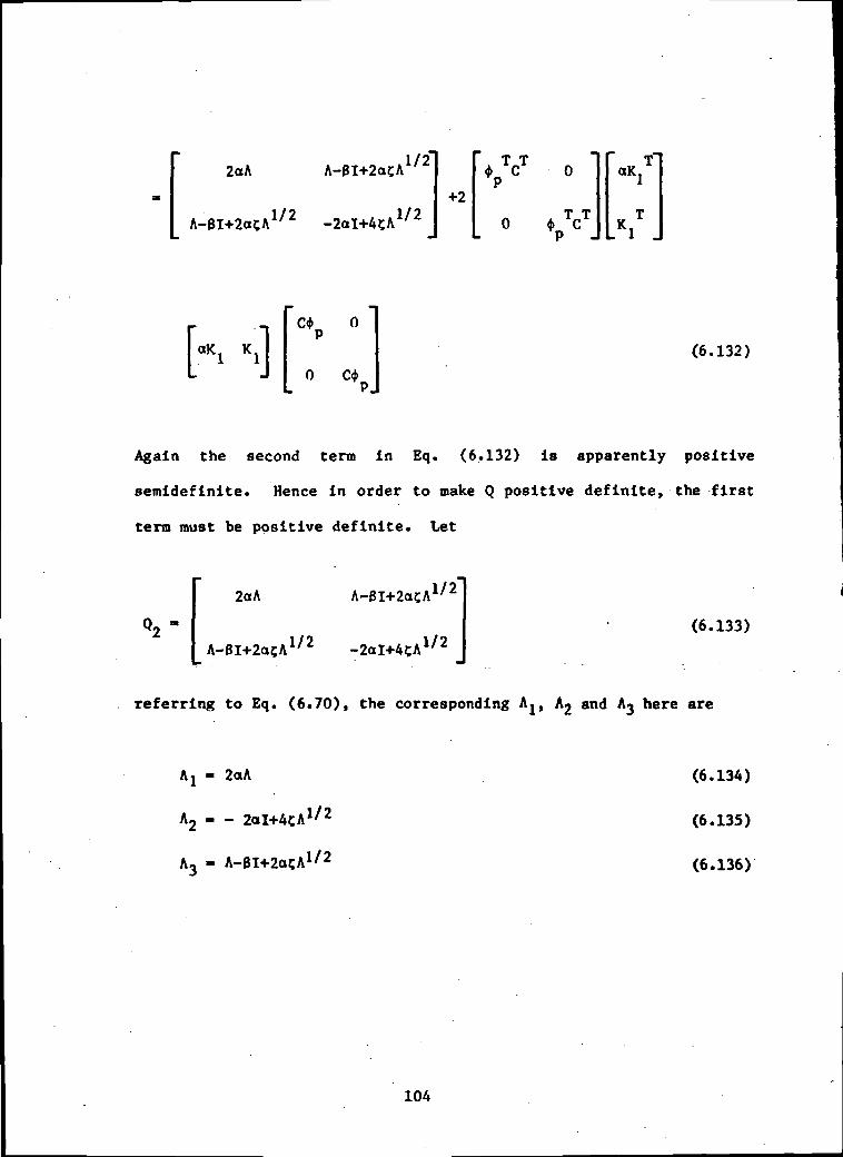
2aA A-BI+2acA1/2
-2oI+4cA1/2+2
T T4 V 0
P
o 4. TcTL p J
T"1
K T
. 1
C* 0p
0 C<f>p_
(6.132)
Again the second term in Eq. (6.132) is apparently positive
semidefinite. Hence in order to make Q positive definite, the first
term must be positive definite. Let
2aA
A-8l+2acA
1/2
1/2
referring to Eq. (6.70), the corresponding
(6.133)
and A here are
- 2oA
- - 2aI+4cA1/2
(6.134)
(6.135)
(6.136)
104

Substituting them into Eq. (6.79), we have
A - X2(A-0H-2ocA1/2)"1-X(A-BH-2acA1/2)~1(2aA-2aI+4cA1/2)
-1 1/71(2aA)(-2oH-4?A ' )1/7' (6.137)
In order that (A-8H-2OCA1' 2)-1 exists, we must have
|A-BH-2ocA1/z| * o
i.e., u> -8 + 2a£<o * 0 for i - 1, ..., N1 i p (6.138)
i.e., a8-o)
2Coi, for i - 1, ..., N (6.139)
Expanding Eq. (6.137), we have
A - * *
r i o iu ™B+2oC(i)
•v
o x i2u ~8+2a(uNp • Hj^
-
r i o i2 °
X
*2ou 2-2a+4;w 0
X>.
Xv
2
2ouHp2 ^
(6.140)
105
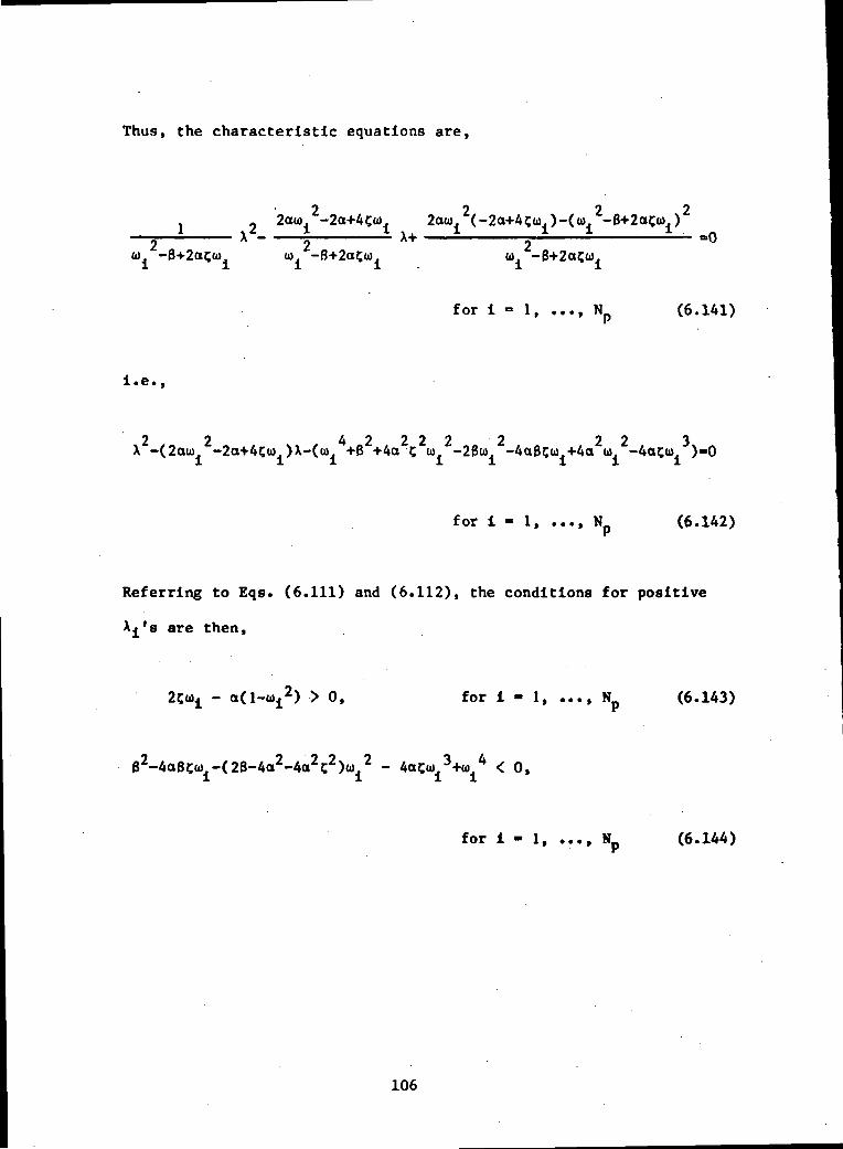
Thus, the characteristic equations are,
2 2 2 2- 2au> -2a+4eu 2au> (-2a+4cu).)-(w. -B+2acw )1 % f c 1 X * 1 X X X r tx - . x+ • . =o
2 2 2to -8+2aeu) u -8+2aC<j) u
for 1 - 1, .... Np (6.141)
i.e.,
for i - 1 Np (6.142)
Referring to Eqs. (6.111) and (6.112), the conditions for positive
A^'s are then,
L-to ) > 0, for 1-1, ..., Np (6.143)
e2-4aBCa>1-(2S-4a2-4a2C2)a)1
2 - totu^+u^ < 0,
for 1-1, ..., Np (6.144)
106

In summary, the second set of sufficient conditions for globally
asymptotic stability is given by
T is positive definite
T is positive semidefinite
6 > a2 (6.145)
B-OJ 2
" * 253- <6-146)
2C<o1'- ad-uj2) > 0 (6.147)
B2 - 4a8Ca>1 - (28-4o2-4o2c2)a)i
2 - 4ac<oi3+<o1
4 < 0 (6.148)
for i = 1 Np
As we compare the above two sets of sufficient conditions, it is
apparent that the second set gives us more freedom for selecting the
system parameters.
107

CHAPTER VII
PERFORMANCE ANALYSIS AND PRACTICAL CONSIDERATIONS
The purpose of this chapter is to investigate the dynamic
responses of the space stations under the severe disturbances as the
adaptive controller described above is applied without assuming the
complete knowledge of the system parameters. In addition, from the
point of view of practical implementation, means of reducing the
control efforts and their effects on the performance of the system
are studied.
Crew motion, reboost, and vehicle docking are the major
disturbance sources. They will also cause changes of mass
property. Crew motion will shift the center of mass, reboost
will result in gradual mass reduction, and vehicle docking will
spontaneously increase mass and inertia of the system. From the
point of view of time-varying effect and the level of disturbances,
space shuttle docking is by far the most significant source of
disturbance. Since most of the cases studied here are
related to shuttle docking, the docking characteristics and
devices are described first in the following sections.
The simulation programs are written In Advanced Continuous
Simulation Language (ACSL). The program and numerical results of the
simulation of adaptive control during shuttle docking for the 19-DOF
four-panel space station are listed in Appendices D and E,
respectively.
108

7.1 Shuttle Reaction Control Subsystem Residual Rates
The shuttle Reaction Control Subsystem (RCS) consists of two
major parts, the primary (PRCS) and the vernier (VRCS) subsystems.
There are a total of 44 thrusters, 38 of them are associated with the
PRCS, each has a nominal thrust level of 870 Ibs; and the other 6 are
associated with the VRCS with a thrust level of 24 Ibs each. Phase
plane control laws are employed to determine when actuations are
needed and jet select logics are used to determine what thrusters are
to turn on. The states of the system are estimated by a two-stage
state estimator with a dual cycle time of 80 ms and 160 ins.
PRCS is normally employed for AV change, attitude maneuvers, and
coarse attitude control; and the VRCS is for fine attitude control.
Since shuttle docking requires maneuvers, PRCS roust be used. Due to
the high thrust level of the PRCS, and with more than one jet used at
the same time to maintain attitude and approach rate while
maneuvering, large residual rates result. The best achievable
(minimum) residual rates, i.e., rates obtained under ideal
conditions, are AV « 0.05 ft/sec and Au = 0.20 deg/sec. However,
these minimum rates are difficult to realize under nominal
operational conditions and much higher rates are expected. These
expected rates are on the order of AV - 0.50 ft/sec and Au - 1.00
deg/sec. Figure 21 shows the shuttle control system block diagram
and residual rates.
For the purpose of performance analysis, the following
assumptions are made regarding the shuttle and space station docking:
109

o °5o: —'o oLL. r>-
oo O
-> 00§§fc r: ot SR 8 3
•O
e u "
5> 3
1aCD
1
o^ «jjt o
8 5o n
5 I
0)4JCO>>CO
•§v:
I
§•rt4JO
V.
<M
V
9bC
0.•
UJ
110

(1) Throughout the docking period, the space station attitude
control system will maintain operational on attitude hold
mode*
(2) Just prior to the contact, the shuttle RCS is set at
passive mode, i.e., no thrusters are allowed to fire.
(3) Once contact is made, latching is assumed, i.e., no
separation is allowed.
7.2 Design of Shuttle Docking Devices
Shuttle hard docking is a rather idealized condition. Under
this condition, the shuttle momentum is transferred to the space
station for a short period of time, At. At the end of At, the
station and the shuttle are latched together as one integrated body.
The initial momentum of the shuttle is determined by the shuttle
mass, ML » 7.81 x 10³ slugs (2.52 x 10⁵ Ibs) and inertia, I_ » 7.54 xO D
106 slug-ft2, and the shuttle residual rate AV and Au> (see Fig. 21).
The final velocities are, of course, determined by the combined system
mass and inertia.
The concept and design of a shuttle docking device which can
simulate both hard and soft docking is shown In Fig. 22. The space
station and shuttle are considered as two separate bodies coupled by
a set of angular and rectilinear springs and dampers. Let Mg and Ig
be the shuttle mass and inertia, and M2 and 12 the mass and inertia
of the station. The values of the spring constants and damping
factors can be computed using the following equations:
111
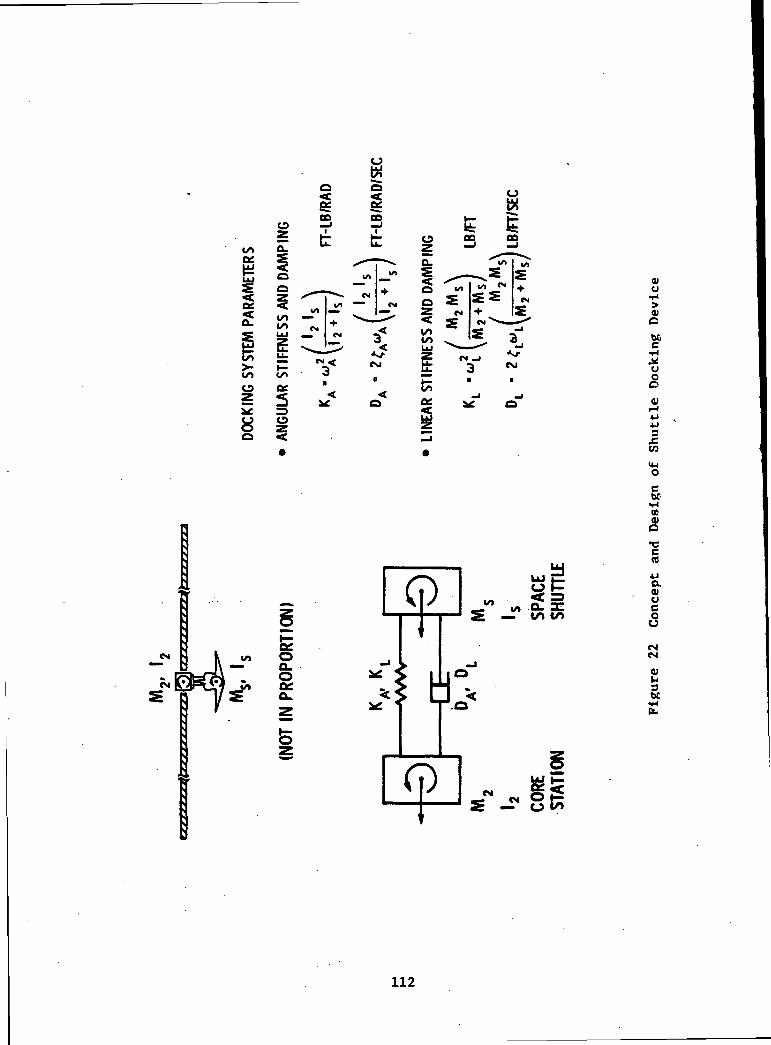
oW
CO
o
01o1-1
0)o60
o
(U
s
(j,p, t/>
S Jf1
LU
gCO
OQ.O > n\°"
$ CL*
bf-
03
•c
c.01U
ItMCvl
01I-s•HPL.
112

DA" 2cAMi + i ) . 0 - 2 )A A A\12 + lg/
n I M., M \
M M
DL
where K , D , to , £ are the spring constant, damping factor, naturalA A A A
frequency and damping ratio for the set of rotational spring and damper,
respectively. Similarly, VL , D , ID , £ are for the set of rectilinearLi Li Li Li
spring and damper. The detailed derivation of Eqs. (7.1) - (7.4) is
given in Appendix C.
With this design, shuttle hard docking can be simulated by using
extremely stiff springs and dampers while for soft docking, much
weaker springs and dampers are employed*
7.3 Performance of Adaptive Control on the Two-Panel Space Station
As stated in Chapter III, the 6-DOP two-panel space station is
used extensively to evaluate adaptive control problems and
performance because of the associated reasonable simulation
turnaround time and cost. These results provide valuable guidance to
the understanding of the performance of space station adaptive
control systems. .
113

7.3.1 Augmented Plant Modal Properties
Following the approach described in Section 6.4, the following inner-
loop control gains are chosen:
K_ 0
wz 45662 ft-lb/rad
K = 4464 Ib/ftLtZ.
This plant augmentation has caused changes of modal properties from
those shown in Eq. (3.27) of the unaugmented plant. The modal frequencies
and mode shape matrix for this augmented plant are,
V 0.01163 Hz
and
to 2 = 0.039 Hz
a) 3 - 0.0656 Hz
iop4 - 0.1684 Hz
u)p5 - 0.3892 Hz
(»>„<; - 0.3947 Hz
-.921E-1 .128
(7.5)
-.922E-1 .144E-1 .178 .178
.382E-3 -.704E-3 .705E-3 -.264E-3 -.544E-2 -.549E-2
.382E-9 .177E-3 .641E-8 -.158E-1 .185E-2 .226E-5
.332E-3 -.745E-8 -.465E-3 -.959E-9 .135E-6 -.117E-3
.921E-1 .128 .922E-1 .144E-1 .178 -.177
.382E-3 .704E-3 .705E-3 .264E-3 .546E-2 -.548E-2
(7.6)
The corresponding mode shapes are plotted in Fig. 23. As can be
seen, the four lower frequency modes have changed substantially, and
most importantly, the two evolved rigid body modes no longer have
zero frequencies.
114

o >; 5 °S o t "
S I 3"
._ LUC CO
LU p ~
8iS
o
o
IS
9)cCM
-8fi«/» LU
"• ^ °°
I S 1 3S o Lu *
al3'
vO
b0>ao
cd
S P S S*• 2 g
ill?
4J
CO^H&,t)
0!l-i
6C
115

With the nodal dampings assumed to be ? k • 0.5% for all modes,
the A_, B , and C matrices in Eqs. (5.6), (5.7) and (5.8) can be
readily determined.
7.3.2 The Selection of the Reference Model
To evaluate the performance of the adaptive controller, the
reference model is selected to have lower order, significantly
different model parameters, and high damping. It consists of 4 modes
(corresponding to the 4 low frequency modes of the plant) or 8 states
x,,,, 4 inputs um, and 4 outputs yn which are defined as follows,
mm
m
(7.7)
um
umlum2u'm3
(7.8)
m
" yml"ym2ym3
.ym4.
"a6mlQZm2O9m2
.°9m3
*!-!+ *«2
* %2
*6m3.
(7.9)
the corresponding system matrices A^, and C^ are
»
°4x4
-2,mK.
^
X4x4
(0
"-2? .tom4 m4
(7.10)
116

B -m
0
T,
C*m]
(7.11)
(7.12)
where B and C are shown in Eqs. (5.9) and (5.10), respectively. The
modal frequencies for the reference model are,
Um2
Um3
"mA
0.02 Hz
0.03 Hz
0.04 Hz
0.06 Hz
(7.13)
The modal dampings are t, , = 0.707 for all modes. The position to ratelUK.
measurement weighting factor a - 0.2 and the gain weighting matrices
T - T - diag (2.5 x 10⁹, 2.5 x 10⁹, 2.5 x 10¹¹, 2.5 x 10⁹, 1000,
1000, 1000, 1000, 1000, 1000, 1000, 1000, 400, 400, 400, 400) are
used.
7.3.3 Adaptive Regulator Control
7.3.3.1 Controller Performance with High Initial Transient
The purpose here is to evaluate the convergence property of the
adaptive controller for the attitude hold and vibration suppression
under very large Initial transient conditions. The initial conditions
for the plant are:
117

Zpl - - 3.699 ft Zpl = - 0.877 ft/sec
8 j o 0.860 deg 6 j = 0.336 deg/sec
0.035 ft/sec(7.14)
Zp2 - 0.345 ft Zp2 = 0.035 ft/sec
6p2 » 0.937 deg 9p2 - 0.037 deg/sec
Zp3 = 4.071 ft Zp3 - 1.045 ft/sec
8p3 = 0.723 deg 6p3 = 0.387 deg/sec
These conditions were taken 10 seconds after the shuttle docked to
the space station with the shuttle initial approaching rates of 0.2
deg/sec and 0.05 ft/sec. The corresponding values in the modal
coordinates are obtained through the following transformation,
(7.15)
(7.16)
The initial conditions for the reference model are
• 0.9 npi
• 0.9 v
for i-1, ...,4.
The simulation results for this case are shown in Figs. 24-29.
Figure 24 shows the outputs of the plant and the model. The model
outputs damp out quickly because of its high damping, and the plant
The remaining figures are at the end of this report.
118

outputs track them asymptotically and converge within 100 seconds
from the transient starts. The same behavior is observed in Figs. 25
and 26 for the plant and model physical states. In Fig. 25, Z^
follows Z2m better than Zj_ to Zjra or Zj- to Z m because a force
actuator is employed at the central bus; thus, at this position,
linear displacement can be controlled more effectively. Figure 27
indicates that the four lower frequency modes of the plant also
closely follow the corresponding modes of the model although mode 2
damps out at a slower pace. Mode 1, the rigid body rotational mode,
is apparently the dominant mode of the system. The two high
frequency modes shown in Fig. 28 also converge to zero within 100
seconds. The required adaptive control inputs, u ., are plotted in
Fig. 29. The demand on bus control torque is quite high, almost
3,000 ft-lb under these high initial transient conditions.
7.3.3.2 Controller Performance with High Initial Transient andMeasurement Noise
The measurement noises of the sensors are assumed to be zero-
mean gaussian white processes. The level of the noises are taken to
be two orders of magnitude lower than those of the peak outputs. Under
these assumptions, the measurement uncertainties for the
accelerometers are 0.012 inch and for the gyros are 20.63 sec. The
qualities for the sensors in existence today are much better than
these. For Instance, the accuracy of the gyro used on High Energy
Astronomy Observatory - 1 (HEAO-1) is 0.5 sec".
The plant and model outputs are shown in Fig. 30. Apparently,
the measurement noises have no significant effects on the high rate
119

of convergence and stability of the system although y 3 has some
noticeable fluctuations throughout the time history. Figure 31 shows
the adaptive control inputs. The bus control force u 2 fluctuates
highly during the first 25 seconds which is quite different from that
of the case without measurement noises. After the initial transient,
all the control Inputs are associated with sustaining or even
increasing fluctuations. Control energy is wasted by reacting to
noises after the steady state is reached. One way to solve this
problem is to employ a threshold at the actuator input. Control is
applied to the system only when the input exceeds the threshold
levels. Nevertheless, controller robustness is observed even with a
high degree of measurement noises applied to the system.
7.3.A Adaptive Control During Shuttle Docking
The following simulations are designed to test the controller
performance and stability using shuttle docking dynamics. To
simulate these cases, a docking disturbance term B u is added to the
right-hand side of Eq. (3.18), where
B d-• o
0100
.0
0'00100
•••m (7.17)
and Fj is the docking force, T^ is the docking torque applied to the
space station. F<j and T<j are determined by the following equations:
120

Pd - DL (^shuttle - Zp2> + KL ^shuttle ~ Zp2> (7.18)
Td " DA (^shuttle - V> + KA shuttle ' 8p2) (7-19)
and the equations of motion of the shuttle are characterized by
'shuttle • - Fd/Ms (7.20)
Shuttle = - Td/][s (7-21)
where Mg is the mass and Ig is the moment of inertia of the shuttle*
The shuttle residual rates (rates prior to docking) are:
shuttle <°> " °'05 ft/sec (7.22)
Shuttle (0) " °'2 de8/8ec (7.23)
7.3.4.1 Shuttle Hard Docking
The control objective here is to stabilize the space station so that
it returns to its prior docking condition after docking occurs. Thus
all of the initial conditions for the plant and the model are set to
zero. For regulator control, the input command u to the model is
zero. Since there are no model disturbances employed under the
"unscheduled event," the reference model stays at its quiescent state
throughout the simulation period. Thus the plant, while under the
influence of the docking disturbances, is commanded to follow the zero
output.
121

The following docking parameters are used in this case:
DL - 2.313 x 10³ Ib/ft/sec
KL - 1.028 x 10³ Ib/ft
_ (7.24)DA - 1.86 x 10' ft-lb/rad/sec
KA - 8.25 x 107 ft-lb/rad
the corresponding damping ratios and natural frequencies are
linear: £L - 0.707(7.25)
(D = 0.1 Hz
angular: £A - 0.707(7.26)
u>A - 1.0 Hz
This case is termed "simulated hard docking" because the springs
and dampers used are extremely stiff. The simulation results are
plotted in Figs. 32-39. Figure 32 shows that all of the plant
outputs converge to zero within 100 seconds after docking begins.
The results here are surprisingly good since, in addition to the high
docking disturbances and the parameter and truncation errors, we also
deal with a sudden increase of plant mass and inertia by more than
100Z. The same performance is observed for the plant and model
physical states in Figs. 33 and 34. In Fig. 35, all but mode 2 are
well damped. Mode 2 shows a very lightly damped oscillation,
however, since the amplitude of this mode is very small and it
122

presents no noticeable effects on any of the physical outputs. At
higher amplitude, the damping is also higher, the oscillation will be
decayed at a faster rate and it will pose no real problem to the
system. The two high frequency modes in Fig. 36 also show good
convergence rates. Figure 37 illustrates the time history of shuttle
angular position and rate. It is not surprising to note that they
appear almost exactly the same as the central bus angular position
and rate (Figs. 34(b) and (d)) because after the hard docking, the
shuttle and the station are supposed to combine and become one
body. Figure 38 indicates that the peak of the docking torque is
63,158 ft-lb.
To achieve the above performance, a peak torque as high as 7500
ft-lb has to be generated by the bus torque actuator (0 3) as shown
In Fig. 39. This is extremely high and presents an implementation
problem. Of course, hard docking will not be a realistic docking
option due to its high transient loads to the space station* Under
soft docking conditions, the torque should be much less.
7.3.4.2 Shuttle Soft Docking
The conditions for the shuttle soft docking simulation are the
same as those of shuttle hard docking except that much weaker springs
and dampers are employed here. Specifically, the following docking
Interface parameters are used:
123

DL = 693.8 Ib/ft/sec
KL - 92.49 Ib/ft
DA - 5.57 x 10A ft-lb/rad/sec
KA - 742 ft-lb/rad
the corresponding damping ratios and natural frequencies are
linear: £L = 0.707(7.28)
I). B- »» «•> "
Lt
angular: CA = 0.707(7.29)
0. m- n nnt »i_
Because of the very low system natural frequencies yielded under
soft docking, it will take a much longer time for the space station
to reach its quiescent state. Hence, the simulation time of 400
seconds is used in this case. The simulation results are shown in
Figs. 40-49. Referring to Fig. 40, all plant outputs except y 2
converge slower than those of the hard docking case, especially Vp3- In
Figs. 41 and 42, Zpl, Zp3 and 0p2 also show a significantly slower
convergence rate. The same behavior is observed for modes 1, 2, 3
and 6 in Figs. 43 and 44. In contrast to the hard docking case as
expected, the shuttle angular position and rate as shown in Fig. 45
have experienced high excursions. However, with the adaptive control
system on the space station, the angular position and rate of the central
bus have deviated very little from their nominal values (Figs. 42 (b) and
(d)). Figure 46 indicates that the peak of the docking torque is 190 ft-lb,
124

substantially lower than the 63,158 ft-lb of the hard docking — a
factor of 332.
What makes the soft docking a desirable* docking option is, in
addition to the reduced shock load, that the demand of control
efforts drops drastically. For instance, the peak of u 3 drops to 300
ft-lb from 7,500 ft-lb of hard docking (Fig. 47). The comparison of
relative panel tip displacement and acceleration by employing
adaptive control vs. low gain bus control are shown in Figs. 48 and
49, respectively. The dynamic load and panel deflection are markedly
reduced by using adaptive control. For example, with the adaptive
control, tne peak panel deflection drops to 0.41 ft. from 6.6 ft.
7.3.4.3 Shuttle Hard Docking with Actuator Saturation
One way to relieve the high actuation demand on the control
hardware is to employ actuator saturation through gain limiting. - To
study the effect of actuator saturation, shuttle hard docking is
again employed here (for soft docking will take too long to
simulate). The following limits for the control inputs are used:
max I u , - 50 ft-lbPi
max I u j - 12 Ibs(7.30)
.b
max I u , I - 50 ft-lb
max I u , I - 1000 ft-lbP3
125

Figures 50-54 indicate that the system performance has degraded
compared with those without saturation (Figs. 32-36), as expected.
The peaks of the responses are higher and it takes longer time
periods for them to converge. It is also seen that the responses are
more jittering due to the bang-bang effect. Larger angular excursion
of the shuttle is also observed in Fig. 55. The docking force and
torque remain unchanged (Fig. 56). Figure 57 shows that the control
inputs Upi and u_^ have not yet totally stayed within their linear
operation region at the end of 150 sec.
As the gain limit becomes more severe (one half the values shown
in Eq. (7.30)), the system performance degrades further as indicated in
Fig. 58. Though it is believed that the outputs will still converge,
it will take a much longer time than the above cases. Moreover, only
u 2 stayed within the linear operation during the simulation period
(Fig. 59).
Regardless of the severe actuation saturations applied, the
results show no sign of threatening the system stability.
7.3.4.4 Shuttle Hard Docking with Model Switching and DisturbanceModeling
Intuitively it is true that the control effort can be reduced if
after the shuttle docking contact is made with the space station, one
uses a new reference model In which the shuttle mass and inertia are
Incorporated and a simulated disturbance similar to the docking
disturbance is Injected. The plant outputs will now follow the new
model transient instead of the zero model outputs. The reason for
the control inputs to be smaller is because of the expected smaller output
126

errors. This has motivated us to study the effect of model switching
and disturbance modeling.
Since the plant is assumed to be poorly known, after
incorporating the shuttle mass properties, the mode shapes and modal
frequencies of the A modes of the model are deliberately selected
with an error up to 20%. The disturbance force and torque inputs to
the reference model are taken to be 2.25 sec-pulse of 173.78 Ibs and
0.225 sec-pulse of 116953 ft-lb amplitude, respectively.
The simulation results are shown in Figs. 60-65. The plant
outputs follow the reference model outputs reasonably well. By
comparing Figs. 60-6A with Figs. 32-36, it is found that the
convergence rates are about the same for the two cases. As far as
the peak control inputs are concerned, u 3 drops significantly from
7500 ft-lb to 2880 ft-lb, and up2 drops from 120 Ibs to 75 Ibs as
shown in Fig. 65. However, upl and up rise from 230 ft-lb to about
800 ft-lb. These results indicate that the concept of model
switching is more involved than one may think. More study in the
area of peak control effort reduction will be required. In general,
one should not expect to reduce all the control efforts, but only the
critical ones.
7.4 Performance of Adaptive Control on the Four-Panel Space Station
The purpose of this section is to demonstrate the performance of
adaptive control on the much more complex 19-DOF four-panel space
station model.
127

7.4.1 Augmented Plant Modal Properties
Plant augmentation has altered the modal properties from those
of the original plant. The new modal frequencies and mode shapes are
shown in Fig. 66. The three evolved rigid body modes no longer have
zero frequencies, and the evolved modes 1 and 2 become pure rotation
about the X and Y axes, respectively. Note that the frequencies .of the
modes in the first bending group are also pushed higher while those
of the modes in the. second bending group remain unchanged due to the
fact that the inner-loop controller is a low-bandwidth system.
With the modal dampings assumed to be Cp^ - 0.5% for all modes,
the Ap, Bp and Cp matrices in Eqs. (5.16), (5.17) and (5.18) can be
readily determined.
7.4.2 The Selection of the Reference Model
Again, to evaluate the performance of the adaptive controller on
the four-panel space station, the reference model is selected to be a
lower order system with high damping and significantly different
parameters from those of the plant. It consists of 9 modes
(corresponding to the rigid body modes and the modes in the first
bending group of the plant) or 18 states *„,, 11 inputs u,,, and 11
outputs ym which are defined as follows
x (7-31)nm
128
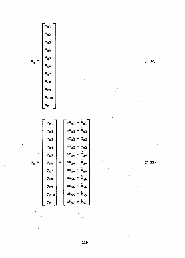
u.ra
"ml
Um2
"ra3
Utn4
Um5
Ura6
Ura7
An8
"m9
"mlO
"rail
(7.32)
a6ml
aera3
azm2
°*m2
azm4
a8tn4
Zm6
a9m5
a8m7
m2
m4
*m6
(7.33)
129

The corresponding system matrices Am, Bm and Cm are,
m
°9x9
""m9
, .ml ml (7.34)
Bm
m
C - I act C<J>m l m m l
(7.35)
(7.36)
where B and C are shown in Eqs. (5.19) and (5.20), respectively. To
show the breadth of the controller performance, the modal frequencies
are selected to have a 40% error and mode shapes a 30% error. The
high modal damping ratios C^ • 0.707 for all modes and position to
rate measurement weighting factor a = 0.2 are employed.
7.4.3 Adaptive Regulator Control with High Initial Transient
The purpose here is to evaluate the convergence property of the
adaptive controller for the attitude hold and vibration suppression
under very large initial transient conditions.
130

The initial conditions for the plant are:
Zpl - - 1.649 ft Zpl - 0.283 ft/sec
9pl o 0.845 deg 6pl - - 0.179 deg/sec
Zp3 m 1.617 ft Zp3 - - 0.284 ft/sec
ep3 * 0.830 deg 83 = - 0.180 deg/sec
Zp2 - - 0.004 ft Zp2 - 0.002 ft/sec•
<frp2 " ~ 0.004 deg $ 2 " 0.017 deg/sec
Zp4 - - 0.001 ft Z 4 = 0.0002 ft/sec(7.37)
6p4 B 0.722 deg 6p4 - - 0.029 deg/sec
<frp4 = 0.012 deg £p4 = - 0.035 deg/sec
Zp6 - 0.004 ft Zp6 - - 0.001 ft/sec
*p6 " ~ O'003 de8 *p6 " 0.017 deg/sec
Zp5 -- 1.618 ft Zp5 - 0.283 ft/sec
6p5 » 0.830 deg 6p5 - - 0.180 deg/sec
Zp7 - 1.649 ft Zp7 » - 0.284 ft/sec
6p7 = 0.846 deg 6p7 - - 0.179 deg/sec
These dynamical conditions were taken 10 seconds after the shuttle
docked to the space station with the following Initial approaching
rates:
^shuttle - 0.05 ft/sec
Shuttle - °-2 deg/sec (7.38)
^shuttle " °'2 deg/sec
131

The corresponding initial values in the modal coordinates are
obtained through the following transformation,
_ _ A—I rjip - 4>P zp(7.39)
_ , 1 nn =s m I*p 9p P
The initial conditions for the reference model are,
"mi " °'8 V(7.40)
°*8 ipi
for i = 1, ..., 9.
The gain weighting matrices T = T •= diag (2.5 x 10⁸, 2.5 x 10⁸,
2.5 x 10⁶, 2.5 x 10⁶, 2.5 x 10⁶, 2.5 x 10⁹, 2.5 x 10⁸, 2.5 x 10⁶,
2.5 x 10⁶, 2,5 x 10⁸, 2.5 x 10⁸, 100, 100, 100, 100, 100, 100, 100,
100, 100, 100, 100, 100, 100, 100, 100, 100, 100, 100, 400, 400, 400,
400, 400, 400, 400, 400, 400, 400, 400) are used.
The adaptive system simulation for the four-panel configuration
is Implemented in a fashion similar to that for the two-panel
configuration except that the dimension and complexity are much
greater and the execution time and cost are high. Because of this,
relatively fewer cases have been studied here. However, the results
are very encouraging as shown in Figs. 67-73. The simulation period
is 75 seconds. Figure 67 indicates that the plant outputs closely
track the model outputs; and with the exception of yp4, ypy and
132

all outputs converge within 75 seconds. Figures 68 and 69 also show
excellent physical state responses. The three bending angles $2» $4»• . .
*6 and their rates $2. "!>4» 4>6 converge slower than other states and
rates. The modal responses are shown in Figs. 70-72. All except
mode 5 show relatively high damping rates. Mode 2, the rigid Y-.
rotational mode, strongly dominates the system dynamics and has a
very high rate of damping. This mode is excited due to the fact that
the simulation assumes a huge shuttle angular momentum about the
pitch axis. The demand for control efforts shown in Fig. 73 is
substantially lower than that required for the two-panel
configuration. The peak of control torque is 400 ft-lb at the
central bus and 350 ft-lb at the panel tips as compared with 3,000
ft-lb and 1,000 ft-lb, respectively, for the two-panel configuration.
This is because the four-panel configuration is much more stiff and
massive.
7.4.4 Adaptive Control During Shuttle Hard Docking
Unlike the hard docking case for the two-panel configuration, it
is assumed-here that the residual angular momenta of the shuttle are,
about its roll and pitch axes. The docking disturbance term B u is
then defined as
133

~0
0
0
0
0
0
1
0
0
0
0
0
0
0
0
0
0
0
0
0
0
0
1
0
0
0
0
0
0
0
0~
0
0
0
0
0
0
0
1
0
0
0
0
0
0_
l~Fd~ud = Td
l_pd_(7.41)
where Fj is the docking force, T<j is the docking torque about the
pitch axis (Y-axis), and P<j is the docking torque about the roll axis
(X-axis). Again the shuttle is assumed to dock with the space station
at the central bus (the core). Fd, Td and Pj are determined by the
following equations:
Fd " DF (zshuttle ~
Td - DT (Oghuttle ~
Pd - Dp (4>8nuttle ~
KF <zshuttle
KT <8shuttle
Kp (*shuttle
(7.42)
(7.43)
(7.44)
134

and the equations of motion of the shuttle are characterized by
'"'shuttle '- VMs (7-45)
'"shuttle - - Vie (7.46)
Shuttle " - V1* (7-47)
where Mg = 7820 slugs is the mass; Ie - 7.54 x 10⁶ slug-ft2 is the
ft 2moment of Inertia about the pitch axis; and IA ° 1*0 x 10° slug-ft
is the moment of inertia about the roll axis of the shuttle.
The shuttle residual rates (rates prior to docking) are:
'shuttle (°> " °-05 ft/sec (7.48)
^shuttle (°> - °-2 deg/sec (7.49)
^shuttle (°> = °'2 deg/sec (7.50)
Again all of the initial conditions for the plant and the model
are set to zero, and since there are no reference model disturbances,
the reference model stays at its quiescent state throughout the1
simulation period. Thus the plant is commanded to follow the zero
output at the presence of docking disturbances.
The docking parameters used and the corresponding damping ratios
and natural frequencies are listed as follows:
135

linear: Dp = 3.06 x 10³ Ib/ft/sec
KF = 1.36 x 10³ Ib/ft
(7.51)- 0.707
= 0.1 Hz
angular: DT - 1.46 x 107 ft-lb/rad/sec
(pitch) KT - 6.48 x 107 ft-lb/rad(7.52)
CT - 0.707
<OT = 1.0 Hz
angular:. Dp - 7.08 x 106 ft-lb/rad/sec
(roll) Kp - 3.15 x 107 ft-lb/rad
(7.53)CP - 0.707
o)p - 1.0 Hz
The gain weighting matrices are T - T - diag (2.5 x 10⁶, 2.5 x 10⁶,
2.5 x 10⁶, 2.5 x 10⁶, 2.5 x 10⁶, 2.5 x 10⁸, 2.5 x 10⁸, 2.5 x 10⁶,
2.5 x 10⁶, 2.5 x 10⁶, 2.5 x 10⁶, 1000, 1000, 1000, 1000, 1000, 1000,
1000, 1000, 1000, 1000, 1000, 1000, 1000, 1000, 1000, 1000, 1000,
1000, 400, 400, 400, 400, 400, 400, 400, 400, 400, 400, 400).
The simulation results are shown in Figs. 74-82.
Figure 74 shows that all of the plant outputs converge to
equilibrium state within 300 seconds after docking begins.
The same performance is observed for the plant states and their
rates in Figs. 75 and 76. In Figs. 77-79, all but mode 5 are well damped.
However, the amplitude of mode 5 is very small and it is believed
136

that it will converge after some longer period of time. Mode 2
strongly dominates the system dynamics due to the huge shuttle
angular momentum applied about the pitch axis. Due to the higher
structural stiffness, the required control efforts (Fig. 80) drop
drastically compared with those in the hard docking case for the two-
panel configuration while the docking force and torque maintain
unchanged (see Figs. 38 and 82). The linear and angular positions of
the shuttle shown in Fig. 81 are practically the same as those of the
station central hus (Figs. 75(d), (j) and (n)), as expected.
137

CHAPTER VIII
CONCLUSIONS
The feature of a large space deployable structure Is its complex
flexible dynamics. Flexible dynamics are characterized by extremely
high system dimensions and parameter uncertainties. Model truncation
plays an important role in spacecraft control due to the limited
computer capability and related hardware available today or in the
near future. Control systems that can adequately deal with truncated
dynamics and model parameter errors are necessary for large space
structural systems. Space stations, among all large space structural
systems, have stringent operational requirements and present a unique
challenge for control engineers and researchers. For space
stations, in addition to the parameter uncertainties and
truncation errors, the control system has also to deal with
the growth, time-varying dynamics, and high-intensity environmental
disturbances. Adaptive control provides a potential solution to
these problems. A direct model reference adaptive control
algorithm for the control of space stations is investigated.
This algorithm along with the proposed inner-loop plant
augmentation technique (for the unstable rigid body dynamics)
form a potentially robust control system for space stations. Two
sufficient conditions have been derived to assure the globally
asymptotic stability. Extensive control simulations and analyses
have been conducted for two space station configurations with
emphasis on generic properties and practical implementation issues.
138

The adaptive system developed here has exhibited high
performance and robustness. . However, in common with all other
adaptive control algorithms, this one is also nonlinear, complex, and
high gain. The demand on control effort, especially during stringent
high disturbance operations, is so high that it has exceeded the
capability of the realistic hardware. To cope with this problem, a
number of solutions have been proposed and investigated. These
solutions are gain limiting, reference model switching, disturbance
modeling, and disturbance load reduction (e.g., soft space shuttle
docking). With these methods integrated into the controller, the
required hardware capability has been drastically reduced yet
stability and robust performance of the system are still observed.
Further research in this area is required and fruitful results are
expected.
Specific conclusions are summarized as follows:
(1) The study results show promising potential applica-
tion of adaptive control techniques to space
stations.
(2) The proposed inner-loop plant augmentation method as
part of the adaptive system has improved the system
convergence significantly and stabilized the rigid
body modes.
(3) High rates of convergence and robustness have been
observed throughout the simulated cases.
139

Specifically,
(i) The system is robust a) in the presence of unmodeled
dynamics — model truncation, b) with poorly known
plant dynamics, and c) in the event of instant change
of system mass property by more than 100%.
(ii) It shows a good convergence property even under severe
dynamic conditions including a) high initial elastic
deformation and initial attitude errors, b) strong
shuttle docking disturbances and dynamic interactions.
(4) Shuttle hard docking is an example of the harsh space
station operational environment. The high gain requirement
associated with the adaptive controller will far exceed
hardware limitations. Two methods of reducing the control
demand have been investigated. Gain limitation can be
applied to set a practical limit to the control effort and
maintain stability of the system at the expense of higher
transient and longer settling time. Model switching
together with disturbance modeling provides a means for
output error reduction and hence, the reduced control
demand. However, since our knowledge about the plant is
incomplete, tuning through simulation is required to
achieve good results.
(5) It is believed that a combination of load reduction (e.g.,
shuttle soft docking), gain limiting, model switching, and
disturbance modeling will result in satisfactory system
performance with realistic hardware implementation.
140

ORIGINAL PAGE 5SQF. POOR QUALSTY
CM
01'0"idA
B
II"
T3(0(-1
CM
B
IICM
• E
00 I
"ooT
tol-c
en coo. e
8 8
it n
00 I
•T"
osoIMA
Ot'O- "5V
.•»..co
• CD
C. ECD CD
B B
II II
sr src. E
•oR
CNiC
CO
CM• CD
'+
B
II
CO
as'o-
00
BJ'"l
Cc
«c{-I5c
o
(U
rep-o
i-l 0?C *J
1J p
C 4->
8 <§cn
be£
an
1-1bt
1
cre
141
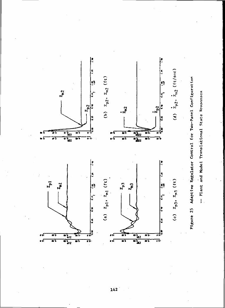
«MCME
CMaK
CM
"Jbz"»*
» -
a -'a tii tan orbdZZ
c
3 tttt C
1-1 V,U- C§ I
pu1
rcc
o-oi 00%
toi
0 TO
(0
Ml- fO r
o •-'k> CE4J Cc no wC H
oa
Ie;
•o
CM
<u9
<D
O
• II 031
«oo.dC2
142

ORIGINAL P&QS ISOF POOR QUALITY
be01•c
ts
00 r-
*>'<• *ro
o01(A
a>•c
"ifcloro-
01 b-
c/tccc
C
t>c
co
0>
reo-Io
o ^«•- re
c—I Co -•W JJ*j rec uc o
•si
OB'I
•01
M'f-
8*
bCrn
007 •01 «o r 00 I-
bC01•o
cnD.
00 I
•oi
I
a•a£"C
ec
> e1-1 re4J i-Ha a,
I !
«M
0>
5c•H(L
143

oo •§-
01_ T:
8'or
O'OI
o.X
OJ
r 1
c
c
0)c(Cao
a-at at-"VdX
KOV.
ccr.
«- 1«* r
031 031
» 7.X^
H'I
*?
eoi- att-
mt- «-oi-
4J ItC -cO Oc r
$
.*
c.n
01i-be
•ctC
cc
144

vC
0.'
O
cc
C
CJ
cr.0)
re Ki cc e.
0 <-~U-l (t
•c
1 *
ot;
c(C
1
4-1 Ure c1-1 a>be 5-<I> Q)
Of Up-
1-1 bC
a xn•c i
oc
4)t-lsbe
I'D Bfl
145
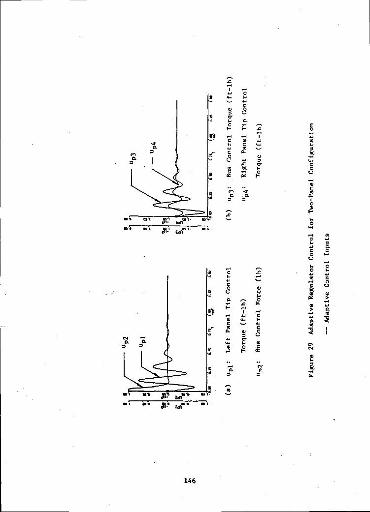
R^
K—'
B*-« "
e"b
9
JC
14-114-
^-^
0)
5-cH
i— iCWi4-1Co
t_*(0
c
i—icIJ4-1Cs
\^r
C.•rJt-
iH01c(C0-
4-1£.be•H0!
^-\Xi™H1
4-1U_
^^>
0>3a-u
5
o4J<e
t>c
cc
01
(00-
o
t-o
i-H O)C 4JU 34J ac cO M
^
n
8%^ •
«rb
9b
1C'b
'Bo •
4-'CccC. /-s
c ^B- r-(
i-< 4J0) «-C v--«P- 0)
3J 1 BV** W^
U-> t->01 C*5 H
*•
^^
C.3
<I"S
(0
i— i****
ai04^
Cft.
i— 1Cb4-1
g
C
2PC
• •es'a=
o4V
bCV
0)
a(0
a>
I
O>->4-1C
0)
C-03
I
146

cc
CMD.
«M6
oooWA
+8* CM-.' C-
CMC.
N: ..oiiCM.a
wo oo 'b
Ot'O-
orb
eiiCME
9 -0- to
8
reu
• O • CD
CD CD
(0
be
Cc
a)cc_
Ic
a/a
z
ev
3tr.(0
J!
•01 as't o-'o . at a-' TMA
i • <]^
8 8
cS
C.
0)O•<->CO O-i rbe -c0) C
tf ccOJ 4-1
•H «4J i-la a.C0
5 !
0)
be
147
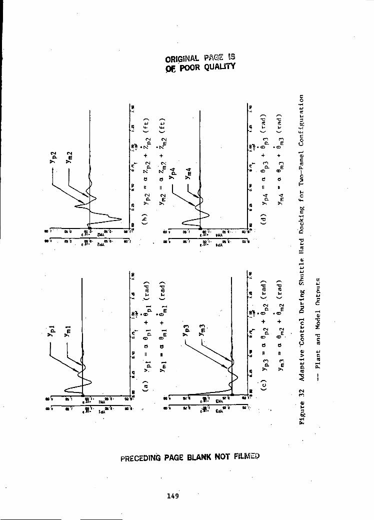
ORIGINAL PA©E SSPOOR QUAUTY
•cIt
_~8s • • o
•- {*•» n« Q. E'O . CD CD
e eii ii
flji-
"oPi
cO
nrij
0)c0-
§
u. c
T3Pre
tc•HIt
C4J
«
c -co cp re<L 4J
•H re& are5 !
01p5c
PRECEDING PAGE BLANK NOT FSUlip
149

co
CM
Oo-(0 c
o
0.c«&o
«0 I,*?
•g•ct-l
tcoKCcCA
dOZZ
71 o
*ot oat-
f.
3j:w:
C•rlP
C
c
ce5
co
09
CD
H
n
•H «
•t"III
001 001
150

ttO
CD
cc
3be
OCJ
0)c<ca-o
bC
(JC
0)
co
a;4-1
a
o»-o
« 0
CC
tc reC 4J•H O
ou4-1
O
0)
or
<B
Vp
bC
151

co
Co
a;cfC0-
I
o
ttGCO
O
0)(D
•C
c
u to •*•
3
V.
3
O
•H (C4J fHc. o-n
•5 !inen
a£
be
152
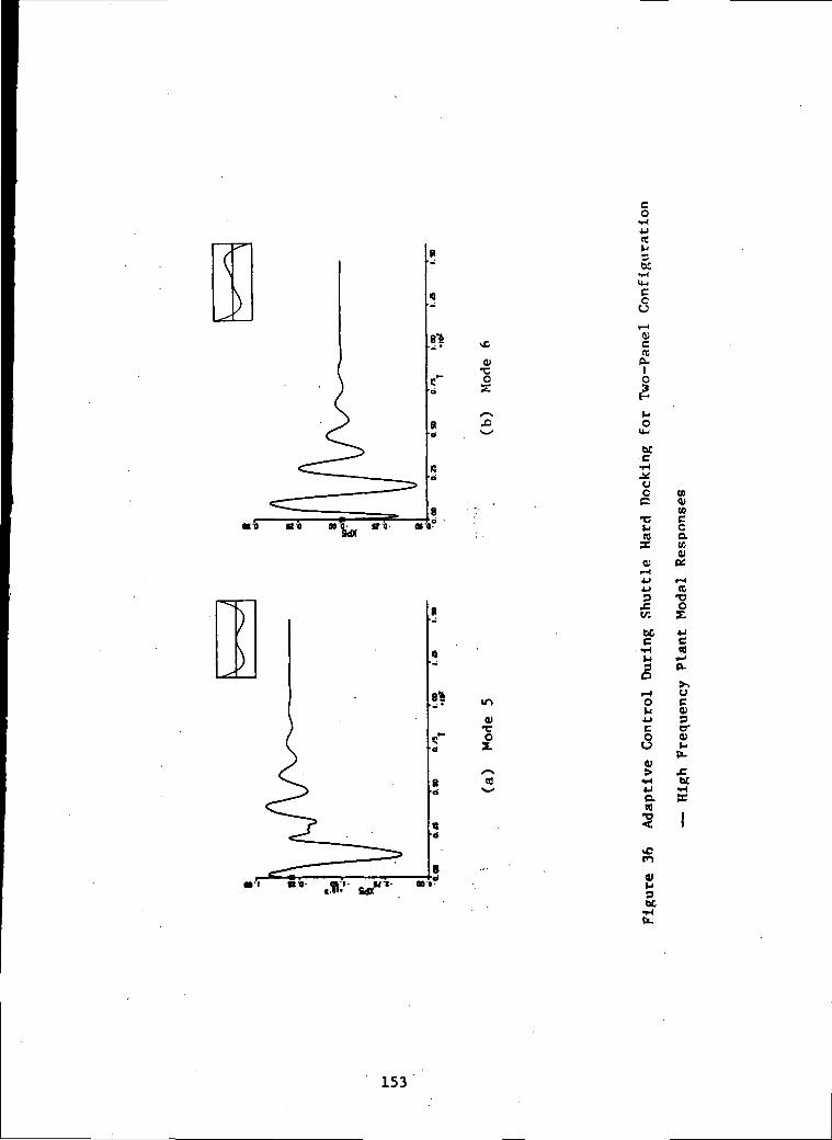
o
be
c
•co
n't
o.Io
bC•c
u
c•cl-l5a;
09a>to§aceQJ
C*
1
c/:
ff
oM
O
id
vP3bC
(CT3O
CO
Ue3er0)
be
153
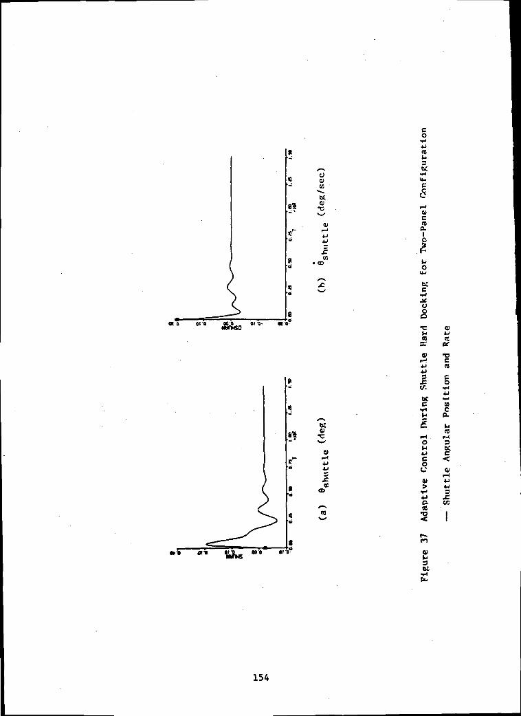
o
bl01•o
.ctc
i O
t-.3bC
IQ)
I
c
t-O
.o
£
bC0)
ce<D
SC
0)
jj
V.
co0>
•ocCO
§be -H
r IW 0-
o
V
<e*3
bC1-1fe.
154

o
JC.«HI
«eu3bC
oCJ
0)0)
«0-
c
be
u&
a!
0)O
bC
I
3
V,
c
§81
•cCC
a;u
bec
uai
>OM4001
be
155

o
co''
o>o
£B*
C07
Ou(0
ec
fNC.
Cc
- c.•HE-
8* ^-• oi
C(C
-- 0-
be
01
H
3 >
<c
5:
c
<U
CM
I
O
oU-i
?&•ct-l<0
5 24J
CB C
8%
C-•H
c- 2l-b
« 2
at3cr
•5 «
0>8 S•- v
(-1c
8« H
•-* tHOt-i
*- £'* O
a:
ff
0)
bC
a4-1
a
Ot*
o a>o >•H
0) 4J
> §•'•H 034-1 "QC. <«c
156
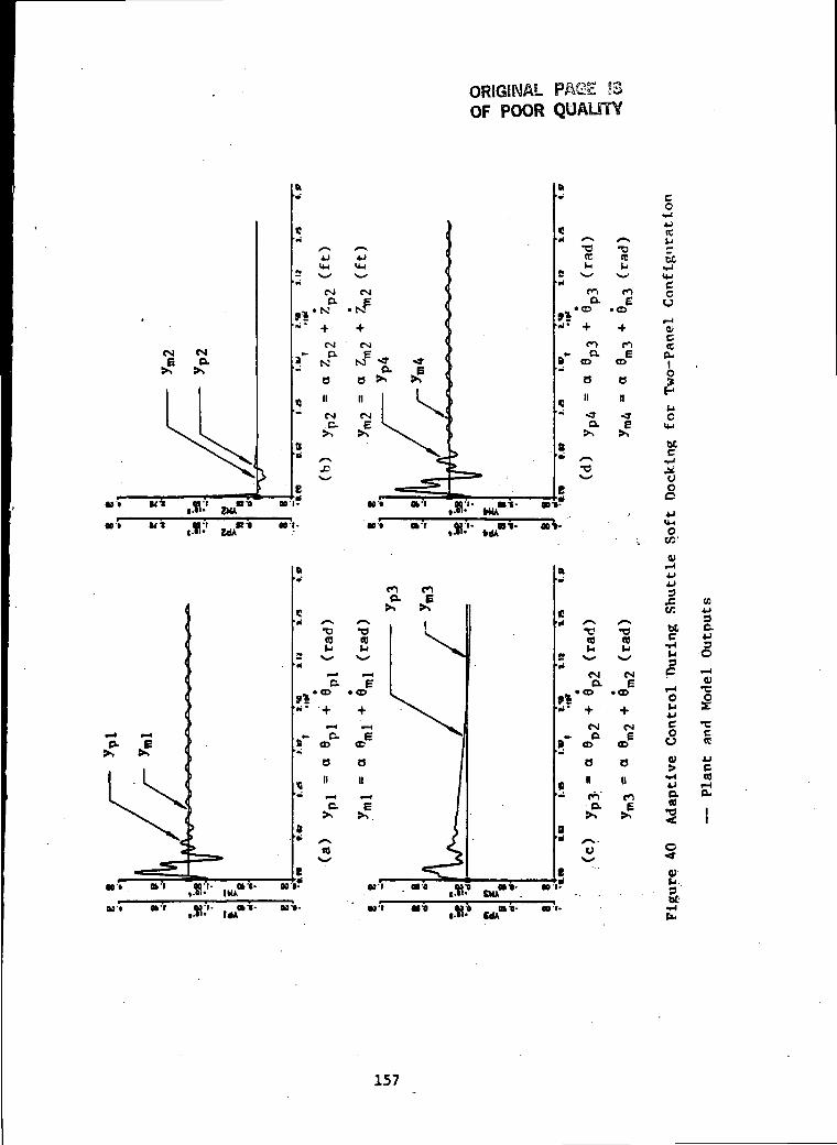
ORIGINAL PAGE S3OF POOR QUAUTY
CM CMe a
cO
iJttp
cu
•*
S>
E-5b
3
4J
> e*H CO
157

tea*9
u0)
CMC.
C • N
"To
aN:
c
6C•HU-iCoc
a,ctcG.
C
o
&oV.
be
oI*u
j0)
aa
•»
0)
bC
KC
c.IT
cx
<U4-1CO4Jw:
re
C
tcc
t-i E-
2 -
•cC(C
et-o BO. «•«-
158

ORIGINAL PAGE S3OF POOR QUALITY
a;•c
tMe.
O0)
be
•*• •£. {VI
s .«
t .tviC.
MOZl
MV1 «-.. at o- ,*? dOZi'
aii-
097-
«9'0
0)•c
1C
et-e M-O
•S 'sc01
rtro
<D
§<t
bC
c
0)crea.o
oc
ow:
I
ce
oav,
a;4->it4J
fl) V.
(0
c
C 4J•H C
'
01•oc
•cctc
4) 4J
5 SCD
B
011dd
159

ORIGINAL PAGE SSOf POOR QUALITY
1
CMO. ^=
K
ei-o
V 01•c
ot-e tit- OfO- rio-
01•c
o
(0
5t
cc
acID0-
c
uǤOV.
0)
V.0!
0) Cr-1 C4J C.4-1 09s aX OiCO
s ITJ.. . .*
01
£ 1coU n
c•H tC4J f-lC. D-CO
< I
PI
01
be
160
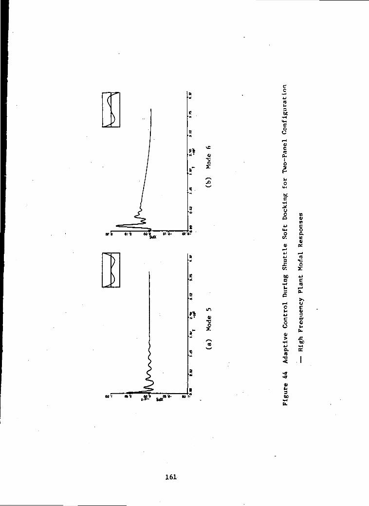
0)•cc
W0 Oil •''*" 8*'°"
0)•c
cc
tol-lbC
o
crea.
I
bC
Ow.
3
c/:
IN£
I>
•H4-1aca<
sf
0)3be
0)0)tn
Oc.tc01a:
C
».
u
^^1-tsc
161

o
(Ck-3
U0)ce O
4)•c
£1C
a;c1Ca.
I
wo a; ~a
c•H
*uǤ
oV.
0)4-1C6
•C**s
01
9
CC
3
w:
P
O
•c
ct
o
COoa.
tc<
0) 4->> 4J•^ 34J fc. cr.cc
a>P
oo t - on -
162

c
I4-1
14-1CO
V3
no-o
uc1=
uo
•H
uo
o
01
ut-io
oc
uǤ
CO
oc
c
C0
te0)yi*O
btC
•H U
a ca
sbt
163

a;o
p% C
-T i:C *
05
(C
aw-
CV.iJCct;a•HH
a1
creo-
o
c.3
I
£
I
CD- 0 - 0 1
! « &
&B 9•*
5 £i
•*-•
0>
te
! 9&
cc
e
o>c<00-
o
ttc
oo
OW
0)t-J4J4J9
w:
P
c
501
c.c
t-to
o
a;
c«c
fr <tC8•C I< I
be
164

Cocj
(C
c•H(Cc
CMa
CMa
CO
oaa
be4J
Ia1
CJ
f-l
"In
C-ce
f-4C
c.H
O
I-4J
g
a<e
'III
CM
at- »-o
Irt
2
5
!
CMO.
N
COO.
N
•H4JCOh«a
oc•a-cuM
bC
C(Ca.
a)f-4
165

ICO
eec•H
«
I
uVV.
o01CO
CC(UwoD-09
•HA!U
Cc
top01
0)u
a•HH
0)>
CL(0
U0)<eu0)CO
CM
4J 0)
J Scr. e.4) O> >
a)a
be
166

O>CCOa.i
<•»• o
O
(Cw;i-o4Jtc34JU
bo
00 t
UA
u eno «C =•O 4Jp =CB C
.e -oe« cCC
beC 4J•H e
ovt.4JCC
I-
4-1
OC_J
814J tH0. <4-t
CO C
cin
2S•rtb-
167

CNc.
• N
u<uce
8* ^.7 4J
<N
JP
CMc.
CUcCCCL
ic
ccV.
CC3
<
X
btC
ycO
cc.K
o;ucc4Jv.
CCCO
ac«
e-oi
a-01
o-fli
00?
C.M
ouiJ
o
0)>
«e5
O
•cce
CO
Cc
CO
tic•H
C
be•Hb.
168

0!
COOuIo
000 WO-HZ1
be<U•c
o;
CD
CMa
CD
ooo
00 I CB'I-
be
e" «>b
Vic
c
tfi
ce4Jy
K<u
9cn
oaK
t-i ce^ co oO -JC *J
ce•c wI- C
or
1
i-l CU CO
«i fi
2 '4J Ce o9 *"*
CO
•H beC^ tt»4
CO C
dIJ oo-o eo-i-dCi
be
169

-a-o.
X(
8%
fl
"id. OJ'O- wi-
00 »•
oo V
<rc«aio
c
<tw:
c4-1ce
be
a,'CB
§c.Ka<
•c T;t- oCTJ SL
0)
«:be
a1
1"C
4JCCD
S '4J CC O
0) £
•H bC
01w.be
«f->(>.
170

Oic«
OuIo
co
V.
(09*J V.(J u< aJ= c4J C.
bC
II-0- 0»'0r
w
C
ore 01 o-
0)
1
TO
0)
4J9
(A
be
cCD
CJ
01
cro>
t- bC
<? £
2 !
? §,5 S«O> I-> 9•H bC4-1 <H
« e
ino>b
be
171

OJ
<cc.o
tt'o oi'0 oo -o ore
yVV,
tc<v
w
«o->
W
•OSM'
VI-<4J
. JJS
05
/•seg
co
(0tr.-
O4J
2uu
•e
oa(0
0)f-lJ_l
Ibe•HId
*J Cc oa r*ft) lj
> 3
C-CD
cc«£
*
oca Of-0. 00 I-§
•n
bC•Hpu
172

0)cB)O.
O
o
3cr
CO
(-!
o
8'0
bO
uoc
bC
U
80)3cr
'«ttT-
B?
0)U
u£
(0
0)
4J
cr.beCI-1
Co
«•p<\cin
bC
•cc
U
£
o
tc
ec
173

001 000 001
a/crea-
io
tev.
cJJ
re
o
t:c
tdH
00 :
c.•c cl-> Mreff -sa; i-
r-l J-l4J C
ti 9
co at
C.(C
4J Cc oo **C Wrew t*5 &
(0•c<
Co
o>14
be
174

ORIGINAL PAGE ISPOOR QUALITY
co
«eI*3
tCc/:
O
uo0)to
I-O
2ua
3c.
uT5C
•cc
MCOX
0)
?
oIrf
o
a<o•o
ocm
c(C
c
U-ic
0)
(0CL,
i
bC
175

V• a•- o
cl-lco
(0
sm
o
0)CCCfl-
O'Qi 0*8 a or
c£
f- jo
ee s^0-
VI j M
£ o-bc P
IN -°
Oft- 00»! ?
5
a1
9-a-wo
<s
. _wn
2 £c r
c c
«
P«
c.(C
9 C£ CCO -rt
c »-*- =Vi KS -HO u-
CO
CO
U-l
£
0!C
1
176

c1-1•Ho>
COl-i
tN
CN
8II
u00'I
u
I94-109i-lO
ff•H
U
a>•O
Uo
cc
aCB
ca4J
g.
01•O5 I•O
(0
(jCOX
0)1-14J1J
f.inb£C•HVi
s
cCOiHeu
1co
•»i4nJ
CO
3
•H<4-l
I
01
COfr,
ih
3 o^C ^4
01
bt
177

btc
(M
CM
•N
CM
N
00 f.
"flpl.
oo •«.*? wzz00'"
ufljw
CMC.
2 9.
•»?
oot~
"Sri-
T3O
a>uc
•c«c
a;•cr
be
aiCAC
c-te
i- c/;UU i—•H (t» CC/i C
encK
0;•CO
CM Ml
•oN
ott-
sV
1C
cre
H tscS -Ho «*.
; Oo c;
c o>o cc «
> i5 *I £
>C
V
be
178

ORIGINAL PAGE ISOF POOR QUALITY be
m•oo
be
ca i-
CO'l-
or 0-
O<u
CME
• ^•d O-• CD
.2 £
m
bCcu
o
UCTO
t-;
If.1-1O
•cCO
O
5c/:
•cO
bC
O
&-E
0)
sw;be
ci-HO
CO
C.CO
u:l«:CC.K
S
re4-1tr.
ccc
ces:
0.'•co
•cc
cre
CO
bC1-<<4-i
c
I
P
I-o
UJ
2bC
179

01•co
00 I
81
O2:o
D.X
001
oo i
0)oc
U
•X•*-<
c
tc•I—
f.o4-1•rJ
3cr
C
4J
C'tccc.ff.a
rec
:* 1-10,
be "cc o
vC
dl
£•Hfe
•t
ax
•J'l
-co
I- •
ri-
I
"lao-ai- ooj-
• •I-
(-1
3:
01
c1-1w
c
O
01
(0
c(0
eo
co
0)
(0CuIo
180

be
00 I
0)
I
Oi
I<uucCO
(0
Cre
I- 001-
0)•c
btc
soccaso
•co
cCC
oe
V
i
oa•ctice
.3
CO
tc
I
d-£
§
P ^C t.r-l Oo u
TOd.
U 2(-CC
14-1
0)l-l
181

t:c
<D
£f I
CMC.
Ic.f'H
I-cH
8 -CD V-'
ZdP
Q)•CO
01CJCref!l-l34Jcei->C
•cCO
bei-jo
a;•co
occ
a
ct-l4-1
J
01>
00 :
£4J
O
a x-s•H rf)H
"" 0) *4-<c ^
.f * s° 4J O-
9 "
0)« s
CJj4JcO
e r,«* a
i- c.CO CO3: -c
1-1 I4J I4J
J §CA 1-1
4J
C U•H ri- beC £
O
Cdn
I
«-c
inso01
be
182

N
~
O "> 3
01
c
cO
(Cw
EC
c
a/reo-i
! oo
Ol-cbet-i•c0)ec
•c0)
w
cu-
er.
t-41aot-c0-
CO•c
<c
•c0)u
0)
i
0»M
tic•Hfr.
183

c.
uc
•c c
1 «* i•cooa'cr.•o<v
1-1c
vCvC
3
184

I?
C\J
/ tjj
/ I/ er >t
O2;
NDCi— iI-H
&
0II
3~
KOi•cOIT
>,•cO(C
•Hbt•K•c0)
t-J0>b:
£c•H^J
§
vCvC
flj(j9bC
•<-!b.
O ••«3
185

CMQ.
CM
oai
aa-a «•«-«•«• OU
ZdA
co
CClJ3
C
0)C(C&.t-cb.
^ CCO iJ1-1 -4-1 C.C Uo =O C
CM
8% • N . N!
•- CM* D.* N
O
" a
CM
N
8
n
e§-f-
ai
a«c
vC
01
bC
a-cC
SCtt
tit
186

3C
u
<re.
euin&
>\
.oft-
•c -o<c <e
DC
8».-e- .-e-•d*
4 +
eti
187

oat
0)
£
§a
\cai
Etc».
188

CMa
N
vrJF
Cc
c
Vcd-I
ou.
•TO 01V
av.cctfica
V.
teu
aN)
"III "•'•••d.l
I
oCOf-i
bea>
«
•co
CD
'c. e-ce•c i
oc\cVi->be
•1
189
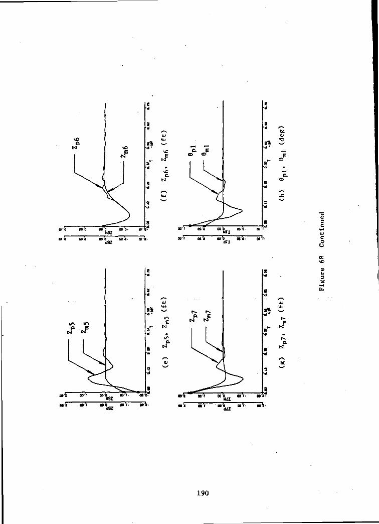
ocOJ
"111WO-
"°d9Z "'dli
a> t
"art
•co;
o
in
00 t
inE
ocsC
01P3
be
190

ORIGINAL PADS 53Cf. POOR QUAUTV
oso
t>0V
"O
•OOi
§
•ibC
OB'I Oit 'tsi
s0.'
be•H(fc
bea>
^ «>
ma
o
"'•
191

a/•c
CM
,- -e-
tsiC.
-6-
dZd*"'
alb'
bt
CO t.
00'»•
•cOi
OCJ
ocvC
OC01•o
a•e-
.1?
192

n't
ooi
CNJ
fIN:c.
8
o•<uK
dozz
00 t-
00 t-
HdtZ.00 T-
UOJ(ft
8%
«c
Jiii
Kd
U0)03
cn.sf
aca-
oo -a- «•••"Jiu
oo r
"Jri
Co
c[*.
c(-14JCo
o4J
*be
0)>
e.te
a-vC
ac,w
cc.
a;4-CC
<co
a.
-ccw
cCO
193

8 «ecu
•a *" **~s
HG9Z
«0 . 00 t-1.01- dQ9Z
00 t.
(n't-u
a»b'
o01tc
0•c
.CD
tffl-
•ca,
ot;
B-8 OyO- Oii-
81d'
O.• N:
B O•d 0)
(0
4JHi >n•d' ^^
^3
e>C
a\c<D»-
bCi-id.
09-1 01'0 •O7!-
194

ORIGINAL PASS S3OF POOR QUALJ7Y
01 0MOV1
tr o-
8%<*•
01ccbe
Ot 0-
wt-"Jba CfO-
CJ<L
tc<uX
"Jba
o» .
»•»•
0)5C
C0
\£
<U
"fci
be
bC
ITlC.
0»'0
195

CJG,IT.
41•c
tM
• •e-
fs!c.
.-e-
001
t:i
vCE
•-e-
HQZd
00't
ouCO
bo0)•c
a;3CTJ4JCo
avC
bei->EL
MOWOB»-
I.
196

cf-f
t
oo
SBa,i
cu-i
I
3be
oV>
Cc.<t.0)
rec
oPC
ai•cc
•oe
01 4-1> ci-t (0
o. a<u
TJ i<( i
«
bo
•*•
197

oo -atMX
os-o-
001 00 t
a1
6
001-
o
r 1ao-g oo i-
rl •' .»? sat"19-
cC
be
Ccc.teOetu-
c —U K
i-< C<U £
«C C.D- rI C
§
IOu(0-1
bb
c.(C
r»
0)
be
bf
1-1-cCa'
CC
<D
i•cce
<e
198

ORIGINAL PAGE 53OF POOR QUALITY
O.K
(V•CO
or-a
era"
8*•d '
Cl•oo
wo- or a-
too- irt-
Oft so-a
or a no
oro
01 iRl
•c<D
C
I
0)
OC
V
O
tfO- M-0-
f>H-
199

«t Oft Ml) OS'l-«•"• OtdX
>- "Cft O•«* r
al
cc
I(-1
I
C.1
v.coc.K
re
1
o
K4
a*
8%*•
_*•ft4
nd
i-lr-t
01•aor
x^.c
4-1Couho±J
ecr-l3beO
OK
0)>•H4JO.to5CM
U
tcc
•H•cea;
cc
•cco00)w:
^e<oi-H0-
!
be
200

or o •YU 01•«. oz o-
•c01
o
CM
0!
K•fHb.
O>t- "O
201

.=
~ O.•d =
o ot
QC
£ f•C 4J
0) OCO to
Q) O
§B:
c <fcM £ iH4J 4J O)e cc AJ «o
O (0 ft«
a at• -C• -w
I"I- . «•*•tcfl
" - o 7ld' K gCO
C 3O O
s a•d S
• (0d ^x
4JOO
pe:
at at
"!C ft-
ft C 3•d H O
4J CO
O U-it) O
•d
• O
* ^
U-cOu
cRa.
O <U
4J C.C Co •--o
o4Jto
»-lsbe0)
0)
'enr-
be
I01
o.
II
202

ORIGINAL PAGE ISOF POOR QUALITY
Oo
OS'Z
TJ -0
e » Vd -H '
o•
\ca
3
00 f
« gu 5t a-
s4J *
oca •c
OJ
e
c
i-« 2' o>u
0)u
^H XI•- O 1-1
C toO 3O ee
tm-
£cC•
be
203

x^be-c
y<£-j*
•He -c* c
<U«^x
B•d 0)
^5*8» S'-r£
r^I," C5 ^d 4J
c0
« u•4
• •
o^
5 7
\•5 y^ r% \^o ^^
z — ^ Jjg-i ^0 /-s ^
* <~-_•U ^4 ^0 1 Si
! * i!•^ "*j• . ^— wre a
" |S5- .i- "?
«»^ ^d- ^ «_. c-c
ft" ^1 1 ' 'k-i 4J *•*«* c *
3 5n•^
^*
5 *O-•d 3
X"N
• ^O u »> «'r JQ'I- .,_«*• »'••B; i , #•• rr«n
^X
(Uj: 1-14J (U
e ^_S S « 2K ^ U-. rH
ad =
^s
8«_J^
ode o'di MO o'o'i- o <n°09
\;x
« ,3 i4 M-t
iJ ^X
B 0) i-l* 9 H
crH «H
_ C DHi H Cd- eo
^ a.c
^ ^ ft 4_> *J- e p
0 0o z
nd ..
•co
co
f!f-0)p5
a
^^
for-T*-
204

ORIGINAL PAGE SSOF POOR QUAUTY
•CD
+
OCD
O
II
Ct:
a;c«0a-ila3
be
O«§•O
0!
•ri
•W
8%«4*
•T
a
•*
•
"N
AJ
M-lx^
CMa
• N:+Cs|c.
s:8
nCOOu
>>.
^^0y~s
S-*4JM-l
•**
CM
+
CME
B
n
*E>>
«£
occ•H
D
1-1O
JJcO
CJ
a>-i
4J
•<
l~-
CO4J
D-*J
C
1•Cc(C
4J
cei-4Ou
11
9•Hb.
205

\co.
• N:\c
vDC.
N:
oca
T:ai
oCJ
in
OfO
i-t(X.
206
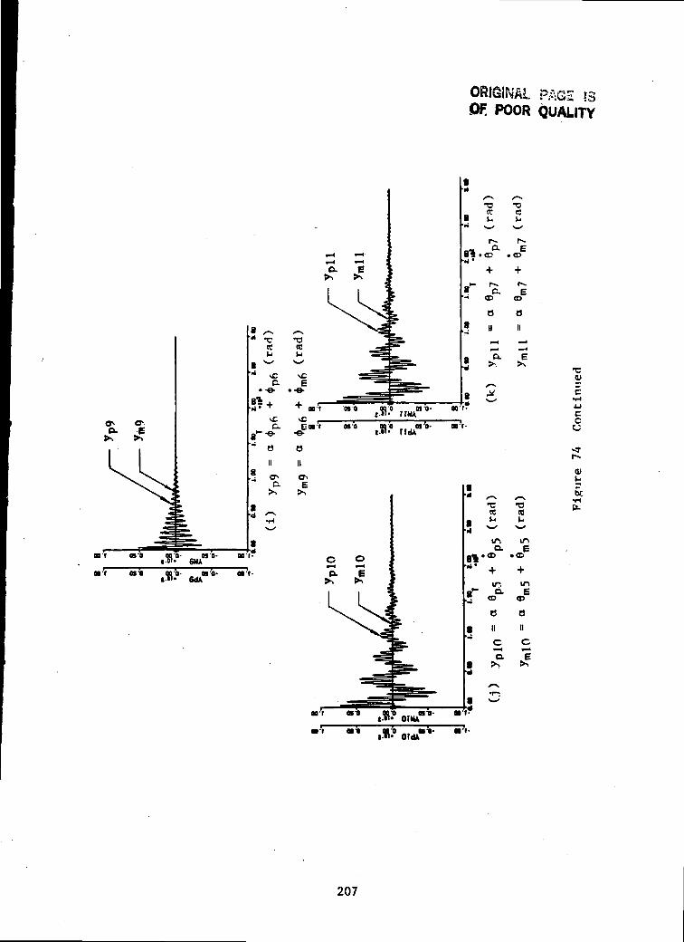
ORIGINAL PAGE ?3OF. POOR QUALITY
•c<U
cCJ
207

oat
CM
^F
CS'o.
00 I-
oat ao r
8%•ri'
K
o
CCI-3tt
c
cto
3O(*.
&c•H
CJ
£•c(C
1Ca< t->
(Ca05ca
001-
AJ3
be
3 .HC 0)
r-t O
2 *
I «
cto
4J D.a« i
5 '
01P3
208

Nl
o
c.<D
00 I-
d9ZB'O
•Ca;
N!
0)
ec
"da ort-
209

ORIGINAL PAGE !3Of POOR QUALITY
CD
•oOl3C.
o
••r
be0)•o
incx
o>
210

be
-8
•e-
esc.
-e-
•ca>001 Oft
W9doft. aoV
dMBfl- 0§>-
oo» ocr «rr. art.!•"• dU
DOS
IVM~-be
211

CMO.
> N
•3 £CO
*» so01If.
t- E* »N
(0
l-l-
c
c
cCJ
01c
I3
beC
oo
•ca
I
ff•H(-
I
a03
vO
be
oc.
014-1K
0) *J1-1 tr.
ccu
CO
Qu
O
•cK
212

oa;
O.• NJ
dQ9Za»'t
T!0)
cu
00 I-
2?
u01m
i~^
f .J
bt•Hb-
fl-
213
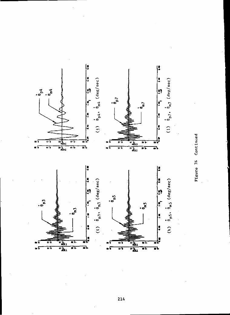
01'0-
•cflj
co
u0)<nbCII)
•O
o»t "Jfci "'
o0)(0
0)•c
aiP
214
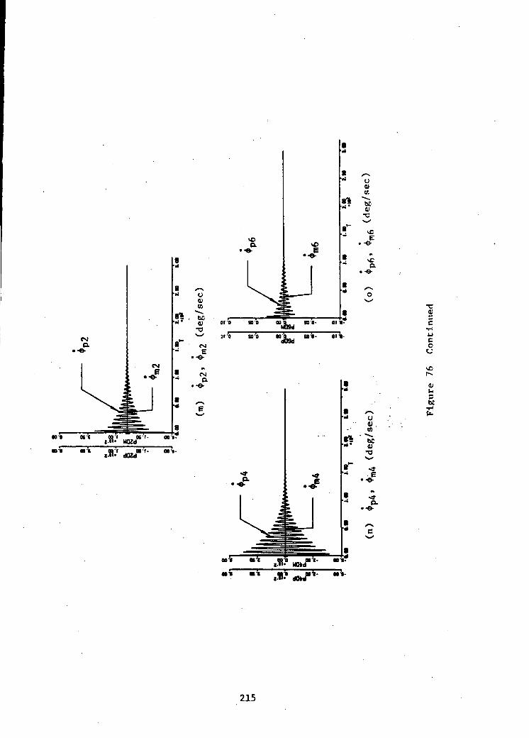
CMa
a• •e-
•c
c
o
be1-1b-
•1?
215

ax
aK
8*•*'
o•- s:
'°- .I?"
81•!*• r"
0*_•- -c,. °
ao>-
eo V
IdX rt.
iti o«
"i*o-*r- •*
c
3U
o
0)
rec-bcb.
bo
3
W
bO
1-114
£
I
are
(CuK
OC.ce
re
1
TJ
(C
•o•HbC1-1c*
O
•o
bC1-1b.
216

ORIGSNAIOF POOR QUALITY
Oi
o
T3O
co
9bC
O<J
0)c
QMI
bCc
rtI
9
V.
be
co
aa)
4)
9bC
a;ff.ccc.
•c
a9O
C
bC•H•c0)ec
a>•ao
•c. c
0) 4J> c
•H «0
G,
I
217

r*.c.
X
"''MX 8r'8'
81
r^01
o
oca
ait 8-0-
ooa
xCO
0)
o
'it
ft
2?
ro
•c
c
ou
ocr^
<uJj5:•t-ib.
218

B°-
ri • c
o
-co
" - 81'
r «- o
co
c
§o
0!c
3Od.
3
V.
W
O
I0)
ft
aTO
Cfio
o.c.tB01
o1
•ca'ee•coo01ce
cC8
<3C
219
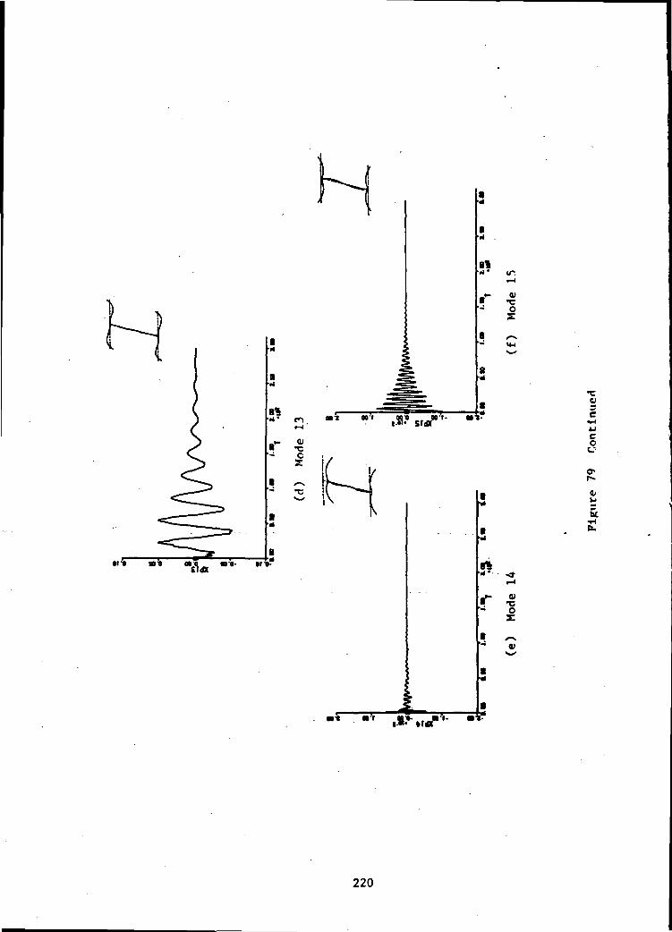
01'• SD'O
8%••*•
81
«f -go
0)1
X
~t
oc
r-
0>w
5c•HPL.
rt
r v•co
220

ORIGINAL°F
001
£be I
4-1U-l
H
4J 4-1C 3C Oo w:
CM
8 _P-•d 3 .
bC
»!««s3 C ^
: S g fH 5 «
C -Q)»-• f. <->4J 4J 0"C CC JJ «c « e-
a
§
TO1-
bt
cc0
01c1C
Ou
lJo
PL.
U
a•g(0
* eeCA 4-1
3abp
4J U
0 OiCJ >
•H01 4-1> a
•H CO4J 5
a <a
coc
3be
221

bo
-r* ^/
0, §
c
2 afr
9dn 001- oat oai
•cc
cc
ooc
I •*-*•i c
a• «•i cd
- £_r oS'<• p ^^
4Jc v
• u *•4
ina
! 3?|i
i •^•^••* tn
bC
°
222

ORIG5WAI PAGE ISOF POOR QUALITY
a ... i*d* § o^
* S-81 O § 1*• H o J-
o a;». .e IHAJ 4J Q>C CO •*-> «U « P-
oo,
•3 SB
C I-C Ct: z
n*"" "*
<*4 7"
• JSi• VM
* « 2 S
^ 4J 4JC k>o oo z
I O.* 9
#? or*00"
T!0)
O
C00
bC•H(*.
223

co
o
8*••*•
C
CJ
a/
Iijo
3oo c0 5
•c uU i-1
5 gCO
N!
ara so'a ,nHEZ «•'•• I' "f
aDCC t1-1 e
CCi-l 0)o cu ^•u ,-:o a,
a«
ec
ai£5c
•rH
(x.
224

o
rt
JC
T
a.
iuoH
U-l
I
01creo-u
«•*"'"
a -< 2o1
oc
boc•H
*oo
MY 81••!•
C•H
*u
ooc
01I—I4J4J
w:
^•HP
OU
a)
art
ecQ)MSbe
•c(C
a>u
be
ucc
225

APPENDIX A
DEVELOPMENT OF HINGED PAYLOAD DYNAMICS USINGLAGRANGIAN APPROACH FOR FOUR-PANEL CONFIGURATION
PAPER)
Lagrange's equation:
dt (A.I)
Starting from taking position vectors for points A, B and C
PA " z/ «A—A 4 —A
- 2 8a
8a B 8bthen
V. - Z. e—A 4 —A
V_ - Z, e. + L_—B 4 —A 8a
226

Similarly,
Z4 *A * L9a
—c
Z4 + L8a 8b 2 Z L 8a
2 2 4 L f i -A
- 2 Z4 L8b
Similarly,
C°8 Y8Y * 2 L8a6 V CO8
v;: - v • v-E -E
Z4 9b Y' 2 Z4 L9a
2 24 L9b Y9Y COS Y9Y * 2 L9a L9b 64 Y9Y Cos Y9
227

Hence,
T - £ "4 'Zl + I "8 VC + I "9 VE + I '4YY 6'J I 'SYS
1 * 2 ' 1 * 2 1 * 2 1 * 2* " X Y * 2 XAXX *4 * T X8XS Y8X * 2 J9XS Y 9X"2 9YS
»*2 2 *2 2 *2 2 * * 9
4 + L 8 b ( e 4 ^ 8 Y >
- 2 - 2 y cos y
. 2 L 8 a L 8 b 6 4 C08 8Y*2 2 *2
L9b ( e*4+SY )2 + 2 Z 4 L 9 a e *
2 Z 4 L 9 b
C 0 8 Y 9YJ * 2 X4YY 6
«J
228

V V - 0
.'. L » T - V - T
There are 7 independent variables: Z,, 6., TTgy» *ov» *A»i i
Y8X' Y9X' one e<Juati°n *or each of them. The generalized forces are:
o m If
similarly
36
" T8X8X
9X
t8Y
Shv If3Y9yk
-9Y 19Y
229

Equation for Z,:
i.e.
ddt
•
m . Z . <4 4
*
" m8Z4 ~ ffl8
• •
Lfio6/. C08 6A ~ BfiLfiK ^i«oa 4 4 o oo or
•« 64) cos <84
* »9Z4 + »9L9aeA cos 64 + n>9L9b (yjy + 64> cos (64
Expand it, we have,
»8Z4 * tt8L8a64 CO8 64 e 8in
B8L8b C0fl (64 * T8Y) * °8L8b
cos
cos
" ffl9L9b 8in (Y9Y * e4} " F4 (A'2)
230
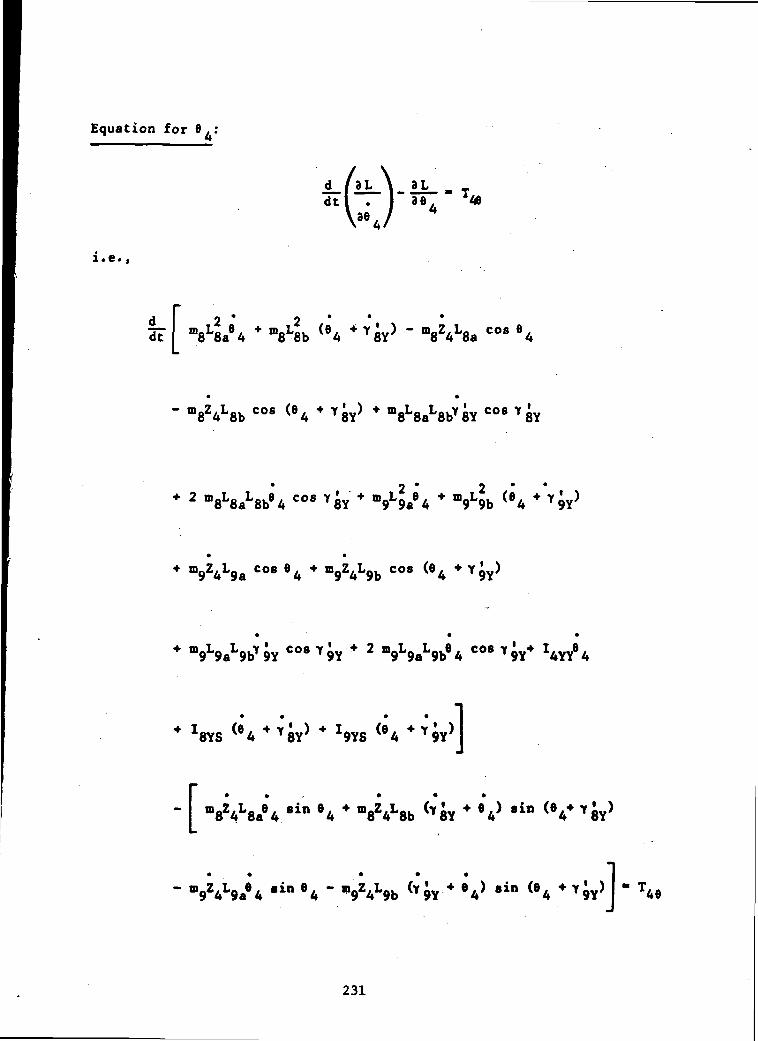
Equation for 6,:
i.e.,
__
dt m8L8aB*4 + ffl8L8b (6*4 CO8
- m8Z4L8b COS (64 m8L8aL8bY8Yc°81f8Y
C08 Y 8Y B9L9b
n9Z4L9a C08 94 * B9Z4L9b COS (64
m9L9aV9Y C°8 Y9Y '* 2 n9L9aL9b64 COS
8Y8
B8Z4L8a64 8in
B9Z4L9a64- ine4
»8Z4L8b in (V
8in ( f l 4 4 Y 9Y ) J 146
231

Expand it, we have,
m L2 e' + m L2 6 * n. L2 y1 C0*
Cos
m8L83L8bY8Y sin Y8Y + 2 COS
2 m8L8aL8bV8Y sin Y8Y * m
m9Z4L9a cos COS
COS Y •9Y
COS Y9Y ' 2 m9L9aV AY9Y sin Y 9Y
(A'3)
Equation for Y
i.e.,
^dt
3L \ 3L<M rt«t
01
18Y
cos
8YS
m8L8aL8b\ <Y8Y + V sinY8Yj 18Y
232

Expand it, we have,
+ m8L8bY8Y ~m8ZAL8b COS Cos Y 8Y
I8YS64 B8L8.L8b84 8Y (A.4)
Equa t ion f o r Y I
i.e.
9Y'
d f 3L \ 3Ldt I . / 3Y 9Y
'9Y
d_dt m9L9b
• •
9Y} + m 9 Z A L 9 b C O S
9YS
Sin
- m9L9aL9b»4 (SY + %) 8 i n Y9YJ 19Y
Expand it, we have,
COS COS
9Y6A sin Y 9Y
(A.5)
233

After linearization, Eqs. (A.2), (A.3), (A.4), and (A.5) become:
Equation for Z,:
9Y
Equation for 8,:
SL9 ' -eV Z4 * (m8L8 + m9L9 + J4YY * *8YS + J9Ys) °4
( 2 \ "m8L8b * m8L8aL8b * ^YSVSY
+ fm«L' t + m^L« Lni + I,99b + m9L9aL9b + X9YS )7 9Y
Equation for Y J,v:
" m8L8bZ4 * (m8L8b * m8L8aL8b * J8Ys) 64 * (m8L8b * I8Ys) Y8Y " T8Y
Equation for YQV:
** y 9 \ **°9L9bZ4 * (ID9L9b * n9L9aL9b * X9YS/ 64 * KL9b * 19Ys)Y9Y * T9Y
234

The equations for $4, t8X» Y 9X are:
Equation for $ ,:
i.e.,
riL.
dt
i.e.,
(14XX * X8XS * I9XS) I8XSY8X + I9YSY 9X
Equation for
i.e.
- T8X
i.e. ,
+ T v* « TX8XST8X 8X
235

Equation f o r Y « :
d 3L 9L19X
_dt 9XS (*4 *-»' 9X
X9XS*4 * X9XSY9X * T9X
236

APPENDIX B
DEFINITION OF POSITIVE REALNESS AND STRICTLY POSITIVE
REALNESS OF MATRICES [55]
Definition B.I
An m x m matrix H(s) of real rational functions is positive
real if
(1) All elements of H(s) are analytic in the open right half
plane Re[s] > 0 (i.e., they do not have poles with positive
real parts).
(2) The eventual poles of any element of H(s) on the axis Re[s]
« 0 are distinct, and the associated residual matrix of
H(s) is positive semidefinite Hermltian.
(3) The matrix H(jo))+HT(-ju>) is a positive semidefinite
Hermitian for all real values of u> which are. not a pole of
any element of H(s).
Definition B.2
An m x m matrix H(s) of real rational functions is strictly
positive real if
(1) All elements of H(s) are analytic in the closed right half
plane Re[s] > 0 (i.e., they do not have poles with non-
negative real parts).
(2) The matrix H(ju)+HT(-j<«>) is a positive definite Hermitian
for all real <i>.
237

APPENDIX C
DERIVATION OF FORMULAS FOR CALCULATING THE
SPRING CONSTANTS AND DAMPING FACTORS OF DOCKING DEVICE
Consider the angular springs and dampers first. Referring to
the following figure, the moment of inertia I2 of the core body of
the space station is used to represent the space station and I
represents the shuttle
*A fa
the equations of motion can be written as
I262 T2
I2e8> DA(e8-e2) + .KA.(e8-e2) - TS
(C.I)
(C.2)
Assume that docking occurs at time t - 0, and 02(0) » 8g(0) - 0 (this
will not affect the values of KA and DA). Take Laplace Transforms,
Eqs. (C.I) and (C.2) become
(I2sz + DAs ••• KA)82(8) - (DA8+KA)68(8) - T2(s)
(Iss2 * DA8 + KA)6s(s> ~ (I>A8+KA>e2<8> - Tg(s)
(C.3)
(C.4)
238

From Eq. (C.4)
(D.s + K.)9 (s)6 (s) - —A? —- + Tsv _ 2 . _ ... _ 2
Tg(8)
I S + D.8 + K. I 8 + D.S + K.s A A s A A
(C.5)
Substituting Eq. (C.5) into Eq. (C.3), we have,
(D .
- - 62(s) = T2(s)<DAS+KA)
(I882+DA8-HCA)
TS(S) (C.6)
i.e.,
(I,s2+D.s+K.) (I s2+DAs+K.)e (s) - (D.s+KA)26,(8)Z A A s A A Z A A 2
T2(s) Ts(8) (C.7)
For the purpose of obtaining the characteristics of the system, the
right-hand side of Eq. (C.7) is set to zero. Then we have
[I2I8sZ + (I2+I8)DAs + (I2+I8)KA]8
2 = 0 (C.8)
for s 4 0 ('.' s2 - 0 Implies two rigid modes at the origin)
I2I8s2 + (I2+I8)DAs (C.9)
239

or
Vs' " ' s
Hence >
and
For the linear springs and dampers, K^ and DL are obtained as follows
by using the same approach
where M2 is the mass of the core body of the space station and Ms is
the mass of the shuttle.
240

ORIGINAL PAGE ISOf POOR QUALITY
APPENDIX D
PROGRAM LISTING FOR THE SIMULATION OF ADAPTIVE CONTROL DURINGSHUTTLE HARD DOCKING TO FOUR-PANEL SPACE STATION
INITIAL
1 PROGRAM23 '4 :
5:
6 :
7:
8 :
9 =
10:
11 :
12:
13:
14:
IS:
16:
17 =
IS:
19:
20:
21:
22 =
23:
24:
25 =26:
27:
28:
29 =30 :3132:
33:
34:
35:
36:
37:
38:
39 =
40:
41:
42:
43:
44:
45:
46:
47:
48:
49.SO:
Si >
52:
53<
54:
55:
56:
57:
58:
59
APPLICATION OF ADAPTIVE CONTROL ON SPACE STATION (IS DOF)
CREATED OCT 1984 —BY C.H.C.IH
== INITIAL ==
TYPE AND DIMENSION OF VARIABLES
,ZPDO(15),ZPDD(1S>
AM ( 1 8 , 1 8 ) , BM ( 18 , 1 1 ) ,CM ( 1 1 , 18 )XP<30) ,XPD(30>,XPO(30>,XM<18>,XMD(i8>,XMO<18)B(15,ii>,C(ii,i5),BPF(i5,ii),CPF(il,lS),BMF(7,H>,CMF(U,7>YP(ll) ,YM(ii),UP(il),UM(il)ETA(15),ETAO(iS),ETAD(iS> ,ETADO( IS) ,ETADD( 15)ETAS<9) >ETASD<9)>ETASO<9),ETASDO(9)EVAL(iS),EVEC(i5>lS),EyECT(15,15),EVECI(iS,iS)EVECS (15,9), EVECST (9,15), EVECSB (15,9)TA(40,40),TB(40,40),TAS(40),TBS(40),R(40>,RT(1DAMPFC(15),DAMP(15,15),ZETA(9),DAM(9]KI(11,40),KP(11,40),KID(11,40),KIO(15DUMY4(1,40) .DIJMY5(i .40) .DUMY6(il) . MT i
INTEGERARRAYARRAYARRAYARRAYARRAYARRAYARRAYARRAYARRAYARRAYARRAYARRAYARRAYARRAYARRAYARRAYARRAYARRAY
CONSTANT N=1S
CONSTANT N2=30CONSTANT M=il
CONSTANT L=9
CONSTANT L2=18CONSTANT UhCONSTANT TFINAL»100.0CINTERVAL CINT°0.2
CONSTANTCONSTANTCONSTANTCONSTANTCONSTANTCONSTANTCONSTANTCONSTANTCONSTANT
»'NUMBER OF PHYSICAL COORDINATES''(ALSO NUMBER OF MODAL COORDINATES)'
$'NUMBER OF PLANT STATES'*'NUMBER OF PLANT INPUTS AND MODEL INPUTS''(ALSO NUMBER OF PLANT OUTPUTS AND MODEL'' OUTPUTS)
t'NUMBER OF THE MODES RETAINED(TO FORM'THE MODEL)
*'NUMBER OF MODEL STATES'S'MODEL INPUT'f'TIME TO STOP'«'COMMUNICATION INTERVAL'
* DEFINE THE PHYSICAL PARAMETERS OF THE SPACE STATION »'.*<**«**************«*«***************«*«****«******«**«'
G=32.174ZETA=9*0.707EIS-9475776.LS-115.LE-140.RHOS-.541RHOE-1.048M4-4165.35M8=994.72
'GRAVITATIONAL ACCELERATION''DAMPING RATIOS OF THE REFERENCE MODEL'
241

60 CONSTANT6.1 CONSTANT62 CONSTANT63 CONSTANT64 : CONSTANT65 . CONSTANT66 CONSTANT67: CONSTANT60= CONSTANT69; CONSTANT70: CONSTANT71= CONSTANT72 .CONSTANT73:
74:
7576: CONST ANT77= CONSTANT7D -CONSTANT79: CONSTANT80 : CONSTANT81: CONSTANT82. CONSTANT83:
84:
85:
86:
87:
88: 30.89: 40.90:
91 :
92:
93-94:
VS :
96: 50.97: 60.98 .99:
100:
101:
102= 61.103: 62.104:
105:
106:
107:
108:
109:
110: 63.
ill- 65.112:
113 =
114:
115:
116.117 =
118:
M9«994.72I4XX«3 .B69C+6I4YY-1 .343E+6I8XS=2.437E+419X5=2. 437E+4I8YS=S . 637E+4I9YS=5.637E+4L8A=7.L8P==li.L9A=7.L9B=ii.FAC=10 .PI«3. 14159265LB=LBA+L8BL9-L9A+L9BEIE=FAC*EISTAS=5*2.5E*6,2«2TBrJ=S*2.5E+6,2*2DAKPrC=15*O.OOE»ALPMA-0.2NSTPl=i200NSTP2=SOTSU=5.0DTRCC=PI/180.0Q=M-»-L2+MDO 40 II-i.NDO 30 J=1,NK1(II,J)-0.
.CONTINUE.CONTINUEKi(7,7)«28184.K 1(8,8) "339324.Ki<9,9)=244308.DO 60 JI-1,MDO 50 J-i,QKIO<II,J>-0.
.CONTINUE
.CONTINUE
DO 62 11=1, NDO 61 J=l,3Bi(II,J)«0 .
.CONTINUE
.CONTINUEB1(7,1>-1.Bl(8,2)=l.B1<9,3)«1 .DO 65 11=1, NDO 63 J-l.HB(II,J)-0.
.CONTINUE
.CONTINUEB(2,1>«1.6(4,2)*!.B(5,3)«l-B(6,4)*l.B(7,S)»i.B(8,6>»1 .B<9,7)«1
.5E+8,4«2.5E-*6, 18*1000., 11*400.. SE+0,4*2.5E+6,1Q*1000. ,11*400.'MODAL DAMPING RATIOS OF THE PLANT
•
242
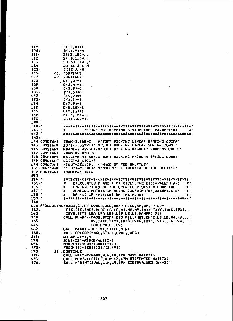
119 =120 =
123:
123:
124:
125.126. 66.127: 68.128:
129 =130 =131 =
132.133:
134:
135.136:
137.133 =139.140 = '141.'142.'143 =144= CONSTANT145 . CONSTANT146 .CONSTANT147 . CONSTANT148 . CONSTANT149: CONSTANT150 CONSTANT151. CONSTANT152= CONSTANT153.154:
155.156.157.158.1S9.160.
B< 10 ,8)«i .B(ii,9)-l.
B(15,'ll)-i.DO 68 II~1,MDO 66 J=1,NC(II,J)=0.
.CONTINUE
. CONTINUECd^)**!.C(2,4)=l .C<3,5)=1.C(4,6)ol.C(5,7>»1.C(6,8)oi.C (7,9)«1 .C(8, 10)«1 .C(9,il)»l .C( 10 ,13)«1 .C( 11 ,15)™1 .
#X4ttA4yX$X44&X($&X4444X44444X).X4XXV4#44&'4¥KXc444iV $4V#&4* DEFINE THE DOCKING DISTURBANCE PARAMETERS
ZDAM=3.06E+3 S'SOFT DOCKING LINEAR DAMPING COEFF'ZSTI-1 .3S97E+3 f'SOFT DOCKING LINEAR SPRING CONST'RDAMT=1 .4S93E+7*'SOFT DOCKING ANGULAR DAMPING COEFF'RDAMP-7.078E+6RSTIT=6.4845E£+7$'SOFT DOCKING ANGULAR SPRING CONST'RGTIP=3 . 14SE+7MSI!UT=251600. $'MASS OF THE SHUTTLE'ISNUTT=7.54E+6 S'MOHENT OF INERTIA OF THE SHUTTLE'ISHUTP-i.OE+6
* CALCULATES M AND K MATRICES, THE EIGENVALUES AND* EIGENVECTORS OF THE OPEN LOOP SYSTEM, FORM THE* DAMPING MATRIX IN MODAL COORDINATES, ASSEMBLE AP* BP AND CP MATRICES OF THE PLANT
****
KA '
*'*'*'t '
K& '
161 = PROCEDURAL (MASS, STIFF, EVAL.EWEC, DAMP, FREQ, AP ,BP ,CP,BD=. . .162.163.1*4.165=166.167.168 <169.170.171.172.173= 69.174.175.176 =
EIS,EIE,RHOS,RHOE,LS,LE,M4,M8,M9,I4XX,I4YY,I8XS,I9XSI8YS,I9YS,L8A,L9A,L8B,L9B,L8,L9,DAMPFC,B1)
CALL READMK (MASS, STIFF, EIS, FIE, RHOS.RHDE.LS ,LE,M4 , MS,M9,T4XX,T4Yt,r8XS,I9XS,inYS>I9YS,LBA,L?A,L8B,L9B,LB,L9>
CALL MADD(STIFF,K1, STIFF, N,N)CALL OPLOOP( MASS, STIFF, EVAL.EVEC)DO 69 XX-l.NSCR1(II)-ABS(EVAL(ID)SCR2(II>-SQRT(SCR1(ID)FREQ(II)=SCR2(II)/(2.*PI)
.CONTINUE:CALL MPRINT(HASS,N,N,12,1SH MASS MATRIX)CALL MPRINT(STIFF,N,N,17,17H STIFFNESS MATRIX)CALL MPRINT(EVAL,i,N,19,19H EIGENVALUES (U**3) >
* • •
243
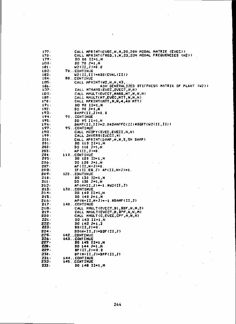
177: CALL nPRINT(EVEC,N,N,20,20H MODAL MATRIX (EVEO)173: CALL MPRINT(FREQ,1,N,23,23H MODAL FREQUENCIES (HZ))179: DO 80 II=1,N100: DO 70 J-l.N181= W2<II,J>«0.0182: 70..CONTINUE183: U2(II,n>«ABS(EVAL(II»184: 80..CONTINUE105: CALL MPRINT(U2,N,N,43,. . .186: 43H GENERALIZED STIFFNESS MATRIX OF PLANT <U2))107: CALL MTRANS(EVEC,EVECT,N,N>1B!3: CALL MMULT<EVECT,HASS,MT,N,N,N>189: CALL MMULT(MT,EVEC,HTT,N,N,N)1^0: CALL MPRINT<HTT,N,N,4,4H MTT)191: DO 90 XI-i-.N192. DO 90 J«i,N193. DAMP(II,J>eO.O194: 90..CONTINUE195= DO 95 11=1,N196.- DAMP (11,11) -2 . OfcDAMPFC (II) *SQRT < U2 (11,11))197= 93..CONTINUE190: CALL MCOPY(EVEC,EVECI,N,N>199: CALL JNVERS(EVECI,N)200: CALL «PRINT(DAMP,N,N,S,5H DAMP)201: DO 110 11=1,N202: DO 110 J=1,N203. A P ( I I , J > « 0 .204: 110 . .CONTINUE205: DO 120 11=1,N206: DO 120 J-i,N207: A P ( I I , N > J ) = 0 .208= I F ( I I . E Q . J ) A P ( Z I , N + J > « 1 .209> 120..CONTINUE210; DO 130 II»i,N211: DO 130 J«=1,N212- AP(N*II , J )»-1 .*U2<II , J )213: 130. .CONTINUE214: DO 140 II-l.N215: DO 140 J=l ,N216- AP(N-«- I I ,N-»-J )« - l .»DAMP(I I , J )217: 1 4 0 . . C O N T I N U E218: CALL MMULT(EVECT,Bi,BDF,N,N,3)219= CALL MMULT(EVECT,B,BPF,N,N,M)220: CALL MMULT(C,EVEC,CPF,M,N,N>221: DO 143 11=1,N222: DO 142 J-1,3223: B D ( I I , J ) = 0 .224. BD(N-HI , J ) -BDF(I I , J )2SS: 142..CONTINUE226. 143..CONTINUE227< 00 145 II-i,N228. DO 144 J-l.M229: B P ( I I , J ) - = 0 . 0230: BP(N-HI , J ) -BPF(I I , J )231' 144. .CONTINUE232: 145..CONTINUE233: DO 148 II-1,M
244

234. BO 147 J = = i , N235: CPUI,J)=ALPHA*CPF<II,J>236; C P < I I , N + J > « C P F ( I I , J )237: 147..CONTINUE239: 148..CONTINUE237:
24tl :END * 'END OF PROCEDURAL'241:
242: ' *«)(-.»:243;' * ASSEMBLE AM.BM.CM MATRICES OF THE REFERENCE MODEL *'244 : ' #X*******************»******#****#************#******* '245:
2-16 : PROCEDURAL. < AM, DM ,CM,EVECS,EVECST, DAM, U2M=7ETA,EVEC,U2 ,6,0, ALPHA)247: DO ISO II=i,L24f!. DO ISO J-1,L249: U 2 M ( I I , J ) « 0 .250.- 150. .CONTINUE251: DO 152 I I= i ,6252: W 2 M ( I I , I I ) = W 2 < 6 + I I , 6 + I I ) * 0 . 6253. 1 5 2 . . C O N T I N U E254; DO 153 11=1,3255: U 2 M < 6+II ,6- i 11 > = U 2 < 12+11, i2+I I )* l , 4256: 153 . .CONTINUE257: DO 160 11=1,L250: DO 155 J=i ,L259: D A M ( I I , J > = 0 . 0260: 155 . .CONTINUE261: D A M ( I I , I I > = 2 . 0*ZETA< II > * S ( 3 R T < U 2 M < II ,11) >£62= 160..CONTINUE263: DO 170 11 = 1,L264: DO 170 J=1,L265: A M ( I I , J ) « 0 .266: 170..CONTINUE267: DO ISO II«1,L268: BO 180 J=i ,L269: A M < I I , L * J > = 0 .270- I F < I I . E Q . J ) A M ( I I , L * J ) = 1 .271: 1 8 0 . . C O N T I N U E272= DO 190 11=1,L273; DO 190 J»1,L274: A M ( L - H I , J ) = - 1 . * W 2 M < I I , J )275: 1 9 0 . . C O N T I N U E276: DO 200 11=1,L277: DO 200 J=1,L278= A M ( L + I I , L - « J > = - 1 . * D A M U I , J >279: 200..CONTINUE280: 00 205 11=1,N281: DO 205 J«l,9282: EVECSBai , J>=EVEC(I I ,6«J )203: 205..CONTINUE284: 00 212 J-l.L285: EVECS(1,J)=EVECSD(1,J)*0.7286: EVECS<2,J)=EVECSB(2,J)*0.7287. EVECS(3,J>-EVECSB<3>J)*1.3288: EVnCS<4,J ) -EVECSB(4 ,J )*1 .3289: EVECS(S,J)=EVECSB(5,J)*1.0290= EVECS(6,J)=EVECSB(6,J)*0.7291= EVECS(7 ,J )=EVECSB(7 ,J>*1 .0292 EVECSC8,J)=EVECSB(8,J>*1.0
245

?93:
294.295:
296 =277 =298:
£99:
300: 212.301 =302:
303 =304:
305:
306:
307.308: 215.309 =310.311:
312 =
313: 220.314:
315:END316 =
317:'
310: '
319:'
320:
321=CONSTANT322:CONSTANT323:CONSTANT324 = CONSTANT325:CONSTANT326:CONSTANT327.CONSTANT328:CONSTANT329:CONSTANT330.CONSTANT331:CONSTANT332.CONSTANT333:CONSTANT334=CONSTANT335iCONSTANT336-CONSTANT337:CONSTANT338:CONSTANT339.CONSTANT340:CONSTANT341.CONSTANT342.CONSTANT343.CONSTANT344:CONSTANT345 > CONSTANT346=CONSTANT347.CONSTANT348.CONSTANT349:CONSTANT
EVECS<9, J>«=EVECSB<9,J>*1 . 0EVECS<10,J>=EVECSB<10,J>*1.0EVECCC 1 1 , J)=EVECSB(i 1 , J)*l .3EVECS<12 , J>=EVECSB<i2 , J>*0 .7EVECS(13,J>=EVECS8U3,J>»0.7EVECS<14 , J>=EVECSB( i4 , J>*1 .3EVECS(15,J)=EVECSB(15,J)*1.3
.CONTINUECALL MTRANS<EVECS,EVECST,N,L>CALL MHULT<EVECST,B,BMF,L,N,M>CALL MMULT(C,EVECS,CMF,H,N,L)DO 215 II»1,LDO 215 J=1,HBM(II,J>-0.BM<L+II,J)«BMFUI,J>.CONTINUEDO 220 II-i.MDO 220 J«i,LC«(II,J)=ALPHA*CMFCII,J>CM<II,L+J)»CMF(II,J>.CONTINUE
»'END OP PROCEDURAL'
SET THE INITIAL CONDITIONS IN PHYSICAL COORDINATES
Z10«0.T i O « 0 .230=0.T30-0.Z20=0.P20=0.240«0.T40«0.P40-0.260«0P60-0.ZSO=0.T50-0.270=0.T70-0.Z1DO-0.T1DO-0.Z3DO-0.T3DO-0.Z2DO-0.P2DO«0.Z4DO=0.T4DO-0.P4DO-0.26DO=0.P6DO*0.Z5DO=0 .TSDO-0.Z7DO-0.
246

350: CONSTANT351 =352 =353.354:
353 =356'
357:
356:
359 =360:
361:
362:
363.364:
367-366:
369:
370:
371 =372:
373:
374:
375 =376:
377:
378:
379:
330:
381 .-CONSTANT382: CONSTANT383 : CONSTANT384; CONSTANT38S. CONSTANT386 'CONSTANT307.308 >389:
390 =371:
392='393.'394. '
T7DO-0.ZPO(i)=Z10ZPO<2)*T10»DTRCCZPO<3)*Z30ZPO(4)«T30*DTRCCZPO<5)=Z20ZPO<6)»P20*DTRCCZPO<7>"Z40ZPO(8)»T40*DTRCCZPO<9)=P40*DTRCCZP<K10)-Z60ZPO(l l)eP60*DTRCCZPOU2)=Z50ZPO(13)=T50*OTRCCZPOU4)«Z70ZPO(1S)«T70«TRCCZPDO(i)-ZiDOZPOO(2>»TiDO*DTRCCZPDO<3)»Z3DOZPDO<4)*T3DO»OTRCCZPDO(5)«=Z2DOZPDO(6)«P2DO*DTRCCZPDO(7)=Z4DOZPDO<B)sT4DO*DTRCCZPDO(9)=P4DO*DTRCCZ P D O ( i O ) = Z 6 D OZPDO ( i 1)"P6DO*DTRCCZPDO<12)-Z5DOZPDO(13)«TSDO*DTRCCZPDO(14)«Z7DOZPPO(15)«T7DO*DTRCCDGHUi-0.2SHUi»0.DSHU2-0.2SHU2=0.ZOSHUOcO.05ZSHUO-0.DSHUTO«DSHUi*DTRCCSHUTO«SHU1*DTRCCDSHUPO-DGHU2*DTRCCSHUPO«SHU2*DTRCC
* FIND THE INITIAL CONDITIONS IN MODAL COORDINATES *'
**:»*******************************«**#***«»#***«*****'395.396:PROCC»URAL(XPO,XMO»£yECI,ZPO,ZPDO)397: CALL MWMULT(EVECI,ZPO,ETAO,N,N>398. CALL MVMULT(EVECI,ZPDO,ETADO,N,N>399. DO 250 II»1,N400. XPO(II)-ETAO(II)401. XPO(N+II) -ETADO<II)402. 250..CONTINUE403. DO 258 II-1,L404. ETASO<II)«0.9*ETAO(6-fII)405. ETASDO(II)-0.9*ETADO(6*II)406: 258..CONTINUE407. DO 280 II-i.L
247

408: XMO(II)-ETASO(II>407: XMO<L+II>=ETASDO<II>410; 200..CONTINUE411. CALL MPRINTCXPO,1,N2,4,4H X P O )413: CALL MPRINT(XMO,1,L2,4,4H XMO)413;414:END f'END OF PROCEDURAL'415:
416 '417.' * DEFINE THE SCALING MATRICES TA AND TB418: '419 =420:PROCCDURAL<TA,TB»TAS,TBS>421: DO 270 11=1,Q422: DO 270 J-i,Q423: T A ( I I , J > - 0 . 0424: 270..CONTINUE425: DO 300 II»1,Q426: . T A ( I I , I I ) = T A S ( I I )427= 3 0 0 . . C O N T I N U E420: DO 310 11-1,0429: DO 310 J-i,Q430= T B ( I I , J ) = 0 . 0431. 310..CONTINUE432: DO 320 11=1,Q433= TB(II , I I )»TBS(II)434.- 320. .CONTINUE435 =436:END t'CND OF PROCEDURAL'437:
438:
439:END440:
441:'«»3.*.:=o«.»=...>=»»» END OF INITIAL442 =443.444:
445:
446.447: •mmmmaemmmmmm*m*mmmmmama~mmmm DYNAMIC ••448.449:DYNAMIC450= TERMT(T.CT.TFINAL)451: T E R M T ( X P ( 1 ) . C T . 1 . 0 E - H O >452: T E R M T ( X P ( 2 ) . C T . i . O E * 1 0 >453.PROCEDURAL < NSTP-T,TSU,NSTP1,NSTP2)454. JF(T.GT.TSU) CO TO 325455: NSTP-NSTPi456< CO TO 327457 . 325.. NSTP«NSTP2458 > 327..CONTINUE459>END t'END OF PROCEDURAL'460:
461 : •mmmmmm*mmmm*mmmmmmmmm,mm*,m DERIVATIVE m462:
4t3=DERIVATIVE464.
248

465 : ' ****x**X*XXX>**XXX*X*****XXXX**XXX**Xt«X***X**XX*:**«»**** -464;' * CALCULATE THE SOFT DOCKING DISTURBANCE FORCE & TOROUC *'467: ' ' .**x*X*««**«x**X«****XX**X>M««**XXX«*ttX*X****««xXX«***X««4'468 :469 PROCEDURAL (FDOCK ,TQ0CKT,TQDCKP,FDDOCK ,DDSHUT,DI>EHUP ,ZDDSHU= . . .470 : RPAMT,RDAMP,ZDAM,DSHUT,DSHUP,ZDSHU,ZPD,RSTIT, . . .471 = R STIP , ZSTI , SHUT , SHIIP ,ZSHU , ZP , ISHUTT , I5HUTP , MSHUT ,C)472 : TQDCKT=RDAMT* ( DSHUT-ZPD < 8 >> +RSTIT* < SHUT-ZP <8 > )473: TRDCKP=RDAMP*<DSHUP-ZPD<9>>+R3TIP*<SHUP-ZP<9>>474. FDOCK=ZDAM*<ZDSHU-ZPD<7> >+ZDTI*<ZSHU-ZP <7) >475^ DDSMUT=-(TQDCKT/ISHUTT>476= DDSHUP«-<TQDCKP/ISHUTP>477= ZDD3HUo-< FDOCK/ <HSHUT/G>>^78: FDDOCKU>»FDOCK479: FDDOCK(2)«TQDCKT400: FDDOCK(3>-TQDCKP481:
4B2:£ND *'END OF PROCEDURAL'483:
484: ' **X***»*X***»********S********««************xyx***»*xy'485:' *DEFINE THE INTEGRAL CAIN KI AND PROPORTIONAL GAIN KP*'486 : ' **XX***X*XX*»*XX*X***XXXXX*#*X*X*****X**XXXX**XX****X* '487.
489: DO 330 II-1,«490: EYS<II)-491= 330. .CONTINUE492= DO 340 II-i.M493:494: 340. .CONTINUE495: DO 350 11=1, L2496=497: 350. .CONTINUE498: DO 360 II-1,M499= R(M+L2-HI>-UM(II)500: 360.. CONTINUE501. DO 365 11=1, M502: EY(II,1)=EYS(1I>503: 365. .CONTINUE504: CALL VTRANSCR,RT,Q)505= CALL MMULT(RT,TA,DUMY4,i,Q,Q)506: CALL MMULT<RT,TB,DUMY5,i,Q,Q>507= CALL MHULT<EY,DUMY4,KID,M,i,Q)508= CALL MMULT(EY,DUMYS,KP,M,i,Q)509. KI«INTVC(KID,KIO)510.511. END «'END OF PROCEDURAL'512:
513 >'514.' * FIND THE CONTROL UP FOR THE PLANT *'515 > ' . ******«******«**********************«»«******:!(***$****'516.517 : PROCEDURAL (UP-KI ,KP,R )518. CALL MVHULT(KI,R,DUMY6,H,Q>519. CALL MUMULT(KP,R,DUMY7,H,Q>520. CALL VADD(DUNY6,DUHY7,Uf ,M>521:
SS2 END t'tHD OF PROCEDURAL'
249

523:
534:' »*«*«**«*************««************«**************X***'525 i ' * INTEGRATE THE EQUATIONS OF THE PLANT AND THE MODEL *'526 ' XX*XXXXX*«XX*XX****X****X*S*XX«X*XX**XXXXXX*X*XX*X*XXX'527 =52O: CALL MVMULT<AP,XP,»UMY8,N2,N2>529= CALL MVMULT<BP,UP,DUMY9)N2,M>530.- CALL MVMULT(BD,FDDOCK,DUMY12,N2,3>531: CALL VADD<DUMY8,DUMY9,DUMY13,N2>532= CALL VADD<DUMY13,DUMY12,XPD,N2)533: XP«INTYC(XPD,XPO>534= CALL MVMULT(CP,XP,YP,M,N2>535= CALL MVMULT<AM,XM,DUMY10,L2,L2>536: CALL MVMULT<BM,UM,DUMYii,L2,H>537: CALL VADD<DUHY10,DU«Yii,XMD,L2>538: XM*=INTVC<XHD,XMO>539= CALL MVMULT<CM,XM,YH,M,L2>540: DSIIUT«INTEG<D1)SHUT,DSHUTO)541: DSHUP«INTEG<DDSHUP,DSHUPO>542: SHUT=INTEC(DSHUT,SHUTO>543: SHUP»INTEG(DSHUP,SHUPO)544• ZDSHU=INTEG(ZDDSHU>ZDSHUO>545: ZSHU=INTEG<ZDSHU,ZSHUO>
547: ' x**XX**X«***X**X8X*'xx*S*X*XXXXXXXX«*XXX:i:XX**X**«*x***X'548:' * OBTAIN RESULTS IN PHYSICAL COORDINATES *'
549:' *»*»*#**»******»#*****»***x***»***********«»:s:»:!i;ar*****'550 :
551=PROCEDURAL<ZP,ZPD,ZPDD,ZM,ZMD=XP,XPD,XM.EVEC)552: DO 370 I I - i ,N553: E T A < I I > « X P ( I I )554: ETAD(II)=XP(N«II)5E5: ETADD(II)-XPD<N+II)556: 370..CONTINUE557= CALL MUMULTCEVEC.ETA.ZP.N.N)558: CALL MVMULT<EVEC,ETAD,ZPD,N,N)559. CALL HVMULTCEVEC^TADD.ZPDD.N.N)560: DO 300 II-l.L561. ETAS(XI)»Xn(IZ>562: ETASD(II)-Xh(L+II)S63: 380..CONTINUE564= CALL. MVMULT(FyECS,ETAS,ZM,N,L)565: CALL MVMULKEWECSjETASO.ZMD.N.L)566:
567:END *'END OF PROCEDURAL'56S:
569:
570 =END571:
572.573. '»«««m«««««o«»««»»=««= END OF DERIVATIVE «•«•»•»••«—••«««•»••»•574 <575 > ' «*t****»«**S«**«S*X****»***********«S****X«*«**«***«S*'576.' * CHANGE RADIANS TO DEGREES *'577 > ' o**X*************X*****«****t*****S**************iM*«'578 =579. Z1P-ZPU)580. T1P-ZP(2)/I>TRCC581= Z3P-ZP(3)
250

581? = T3P=ZP<4)/BTRCC583: Z2P=ZP(S>584: P2P=ZPC6>/DTRCC585: Z4P=ZP<7>586: T4P=ZP(8>/BTRCC507: P4P=ZP(9>/BTRCC588: Z6P=ZP<10)589: P6P=ZPC11>/BTRCC590: ZSP=ZP(12>591= T5P=ZPU3>/BTRCC592: Z7P=ZP<14>593 T7P=ZP(1S)/DTRCC594: Z1DP»ZPD<1>595: TiI)P»ZPD(2)/DTRCC596: Z3DP*ZPD<3>597= T3BP-ZPD<4)/DTRCC590: Z2I)P«ZPD(S)599: P2DP=ZPD(6)/BTRCC6 0 0 = Z4DP=ZPD<7>601; T4DP=ZPD(8)/DTRCC602- P4DP=ZP»(9)/DTRCC603: Z60P=ZPD(10)604: P6DP»ZPD(ii)/DTRCC6 0 5 = ZSDP=ZrB(12)606 T5DP=ZPD(13)/DTRCC607= Z7DP»ZPD(14)608= T7DP-ZPD(15)/DTRCC609; Z1M-ZMC1)6 1 0 = T1«=ZM(2)/DTRCC611= Z3M=ZM(3>612 T3M=-ZM<4)/DTRCC613= Z2M=Z«(S)614= P2M=ZM(6)/DTRCC615. Z4rt=ZM(7)616 < T4M=ZH(8)/DTRCC617. P4M«ZM(9)/DTRCC618= Z6M>ZH(10>619= P6M»ZM(li>/I>TRCC620= Z5M=ZM(12)621= TSH=ZM(13)/DTRCC622= Z7M=ZH<14)623= T7H=ZM<15)/DTRCC624= Z1DM«ZMD<1>625= T1DM"=ZMD(2)/BTRCC626= Z3DM=ZHD<3>627: T3DH-ZMD(4)/»TRCC
629: P2DM-ZMD<6)/DTRCC630 > Z4DH=ZMD(7)631> T4DM=ZMD(Q)/DTRCC632= P4DM-ZMD<9)/BTRCC633 > Z6DM=ZMD(10)634: P6DM«ZHD(il>/BTRCC635. Z5DM«ZMD<12)636: T5DM«ZHD(13>/BTRCC637; Z7BM>ZHB(14>638; T7DM«ZND(1S)/BTRCC639:
251

640;641= BSHANT=DSHUT/DTRCC642: SHANT=SHUT/DTRCC643= DSHANP-DSHUP/DTRCC644. SHANP=SHUP/DTRCC645= XP15=XP(1)646: XP14«XP(2>647: XP13=XP(3)64Q. XP12=XP<4>649= XPil=XP(5)650: XPlfl«XP(6>651: XP9=XP<7)632: XP8»XP(S)653= XP7»XP<9>654: XP6-XP(10)655: XP5*XP(11>656= XP4«XP<12>657= XP3«XP(13)658: XP2-XPU4)659: XP1=XP(15>660: • XH9«XM(1)661. XHB=XH<2)662: XM7«XM(3>663: XM6«=XM(4)664: XHS»XM(5)665. XM4=XM(6)666: XM3"XM(7)667: XM2*XM(B>668: XM1«XM(9)669 YPi«YP(i)670= YP2-YP<2>671: YP3=YP(3)672= YP4«YP(4)673= YPS=YP(S)674: YP6«YP(6>675= YP7=YP(7)676= YP8«YP(8)677= YP9»YP(9)678= YPIO-YP(IO)679: YPil«YP(ll)680: YMl-YMU)681= YM2*YM(2)682• YM3-YM(3)6B3. Y«4=YH(4)684: YMS«YM(5)685. YM6-YH(6)686= YM7«YM(7)687= YMB=YM(8)688: YM9-YM(9)689. YM10=YHC10>690> YMii»YM(l l )691. UPl-UP(l)692. UP2-UP(2)693> UP3=UP(3>694= UP4«UP<4>695. UPS-UP(S)696.- UP6»UP(6)
252

697;698697:
700.701 =702 =7 0 3 = E N D704 =70S:'—==-«706 =707 =70S:
709= '««««.«710:
7 l i ; T E R M I N A L712:
713='714: '
715:'
716 =717 =718:
719:
720:
721 =
722 =723 =724:
725:
726 =727 =728.
729 =730 >
UP7«UP<7>UP8«UP(8)UP9«=UP<9)UP10-UPUO)U P i i * U P ( i l )
END OF DYNAMIC
TERMINAL ==
#!M*****»*>M***»i************#*»********»*************'* PRINT SYSTEM PARAMETERS *'
CALL MPRINTCEVECT,N,N,34, . . .34H TRANSPOSE OF MODAL MATRIX (EVECT) )
CALL MPRINT(EVCCI,N,N,32,. . .32H INVERSE OF MODAL MATRIX <EVECI»
CALL MPRINT(EVECS,N,L,3i, . . .31H TRUNCATED MODAL MATRIX <EVECS>>
CALL MPRINT(DAMP,N,N,3S, . . .3SH DAMPING MATRIX OF THE PLANT (DAMP))
CALL MPRINT(DAM,L,L,34, . . .34H DAMPING MATRIX OF THE MODEL (DAM))
CALL MPRINT(U2,N,N,43, . . .43H GENERALIZED STIFFNESS MATRIX OF PLANT (U.'.'M
CALL MPRINT<U2M,L,L,44, . . .44H GENERALIZED STIFFNESS MATRIX OF HOUCL (U2tt»
,N2,N2,10,iOH MATRIX AP>,N2,M,10,10H MATRIX BP ),M,N2,10,10H MATRIX CP ),L2>L2>10,10H MATRIX AM),L2,M,10,10H MATRIX BM>,M,L2,10,10H MATRIX CM),Q,Q,iO,iOH MATRIX TA)
,1.0, iOH MATRIX TB)
731:
732 =733:734:
735:736.737:
738 =739.740:
741:
742:743:
744 = END745.
747.740:749 =750: END
CALL MPRINT<APCALL MPRINTCBPCALL MPRINT(CPCALL MPRINT(AMCALL MPRINT(BMCALL MPRINT<CMCALL MPRINTCTACALL MPRINT(TB
«'END OF PROCRi
END OF TERMINAL
253

1: SUBROUTINE READMK(MASS,STIFF,EIS,EIE,RHOS,RHOE,LS,LE,M4,2 *M8,M7,I4XX, I4YY,IQXS,I9XS,IBYS,19YS,LBA,L9A,LBB,L9B,3: $L8,L9>4; REAL MASS(i5,iS),STIFF<i5,lS),MC(15,iS),MD(15,i5)5; REAL I4XX.I4YY,IQXS,I9XS,IBYS,I9YS,L8A,LBB,L9A,L9B,L8,L9(,-• REAL ALPHA, BETA, A, B,EIS,EIE,RHOS,RHOE,LS,LE,M4,M8,M97 ALPHA-2.*EIS/(LS**3>8= BETA*2.*EIE/(LE**3>9: A=RHOS*LS/420.
10: B«RHOE*LE/420.11: DO 10 1=1,1512: DO 10 J=i,1513: STIFF(I,J>=0.14= 10 CONTINUE15= STIFF(i,i)=6.*ALPHA16= STIFF(1,2)«3.*LS»ALPHA17 STIFF(i,S>=-6.*ALPHA18: STIFr<i,8)=3.«LS*ALPHA19= STIFF(2,2)=2.*<LS**2)*ALPHA20: STIFF<2,5>— 3.*LS*ALPHA21= STIFF<2,8)»(LS**2>*ALPHA22= STIFF(3,3)=6.*ALPHA23= STIFF(3,4)=-3.»LS«ALPHA24: STIFF<3,5)=-6.*ALPHA25= STIFF<3,8>— 3.*US*ALPHA26= STIFF(4,4)=2.*<LS**2)*ALPHA27. STIFF(4,5)=3.*LS*ALPHA28: STIFF(4,8)=(LS**2)*ALPHA29.- STIFFS,5>-12.*ALPHA+6.*BETA30= STIFF(S,6)=3.*LE*BETA31: STIFF(S,7>«-6.«£CTA32: STIFF(S,9)=3.*LE*BETA33- STIFF<6>6>"2.*(LE**2)*E<ETA34= CTIFF(6,7)«=-3.»LE*BETA35. STIFF(6,9)=<LE**2)*BETA36= STIFF<7,7)-12.*BETA37. STIFF(7,10)»-6.»BETA38= STIFF<7,il)«3.*LE*BETA39: STIFF(8,8)=0.*(LS**2)*ALPHA40: STIFF( 8,i2)-3.*l.S*ALPHA41-- STIFF(8,13)«<LS**2)*ALPHA42= STIFF (8,14 >— 3 . *LS*ALPHA43= STIFF(8,15)=(LS**2)*ALPHA44- STIFF(9,9)=4.»(LE**2)*BETA45. STIFF(9,10)«-3.*LEfBETA46: STIFF(9,1J)-(LE**2)*BETA47 = STIFF <10,10 >»12.*ALPHA*6. »BETA48- STIFF(10,11)«-3.»LE*BETA49= STIFF(10,12>«-6.tALPHASO- STIFF<10,13)—3.*LS*ALPHA51: STIFF(10,14)«-6.*ALPHA52: STIFF(10,15>«3.»LS*ALPHA531 STIFF(11,11)-2.*(LE**2)*BETA54: STIFF(12,12>*6.(ALPHA55: STIFF(12,13>=3.*LS*ALPHA56> STIFF(13,13)«2.*(LS**2)*ALPHA57 > STIFF(14,14)*6.(ALPHA58 STIFF(14,15)»-3.*LS*ALPHA59: STZFF(15,1S)«2.«(|.S**2>«ALPHA
254

OKJGiMAl PAGE ISOF POOR QUALITY
60:61 ••62:63.64:65:
66:67:68:69:7 0 =71:72=73:7 4 =75:76:77:78:79:80:81:82:83:84.85:86=87:88:89:90 <91=92=93:94:95:96.97=9B<99:
100=101:102=103=104:105=106.107=103=109:110=ill.112.113=114:115=116.117=118=
DO 20 1-1,14K-I+iDO 20 J»K,15STIFF<J,I)«STIFF(I ,J)
20 CONTINUE
DO 30 I»i,15DO 30 J«1,1SH C ( I , J > = 0 .
30 CONTINUEMC<1 > 1>-156 .«AMC<i ,2>=22.«LS*AMC<1,5>=54.»AMC(i,8>»-13.*LS*AMC(2,2)«4.*(LS**2)*AMC(2,S)-13.*LS*AMC<2,B>«-3.»<LS**2>*AMCC3,3>»1S6.*AMC(3,4)«-22.*LS*AMC(3,5)=S4.*AMC(3,0>«13.*LS*AMC<4,4)«4.*aS«2>*A
MC(4,8)»-3.*(LS<*2)*AMC(S,S>-312.*A+156*BMC<S,6)-22.*LE*BMC(5,7)«54.»BM C < 5 , 9 > — 13.*LE*B
MC<6,7)»13.*LE*BMC(6,9)=-3 *(LE**2)*BMC(7,7)«312.*BMC(7,10)«S4.*BH C ( 7 , l i > — 13.»LE*BMC(8,8>»16.*(LS*X2)*AMC(8>12)«-13.*LS*AMC(B,13)=-3.*(LS**2)»AMC(8,14)«13.*LS*AMC(8>15)«-3.t(LS*«2)*AHC(9>9)-8.*(LE**2)*BMC(9,10)«=13.»LE*BMC<9 ,11>— 3.*(LE**2>*BMC(10, 105=156. *B+312.*AMC(10,U)«- 22.*LE*BMC(10 , 12)^54. *AMC(10,13)=13.*LS*AMC<10,14>-S4.»AMC(10,15) — 13.»LS*AMC(l l , i i ) -4 *<LE**2)*BMC(12,12)-156.»AMC(12,13)-22.«LS*AHC(13,13>-4.*<LS**2>*AMC(14,14)-1S6.«AMC(14,15)«-22.*LS*AHC(15,15>-4.*<LS**2>*ADO 40 1-1,14K-I+1DO 40 J-K,15MC(J , I ) -MC(I , J )
255

120:121:122=123'124=125=126=127120=
130 :131=13£:133:134:135;136;137:13ft:
40 CONTINUEDO 50 1-1,15DO 50 J-1,15MD<I,J)«0.
SO CONTINUEHD<7,7)*Mt+M8+M9MD<7,8)=M9*L9-HQ*L8
DO 60 1 = 1 ,14
DO 60 J=K,15M D < J , I ) * M O ( I , J )
6o CONTINUE:DO 70 1-1,15DO 70 J=1,1SM A S S ( I , J ) » M C ( I , J ) + M D ( I , J )
70 CONTINUER E T U R NEND
256
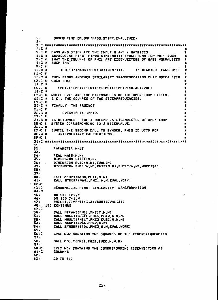
1:
23:
A56789,1011131314IS161718192021222324232627.
SUBROUTINE: OP LOOP <MASS, STIFF, EVAL,EVEC>
28 ;C29.C30;C31 :32:
33:
34:
35:
36:
37.38:
39:
40:
41:
42=C
43 :C
44 :C
45 =
46 <47.48:
49. CS0>51:
52.S3.54.55.56 :C
57:
58:57:
60 :C
61:C
62:
63:
MASS AND STIFF ARE THE INPUT H AND K MATRICES.SUBROUTINE FIRST FINDS SIMILARITY TRANSFORMATION PHI1 SUCHTHAT THE COLUMNS OF PHI1 ARE EIGENVECTORS OF MASS NORMALIZEDSUCH THAT
(PHI!)'(MASS)<PHI1>=<IDENTITY) (' DENOTES TRANSPOSE)
THEN FINDS ANOTHER SIMILARITY TRANSFORMATION PHIS NORMALIZEDGUCH THAT
(PHI2)'<PHI1>'(STIFF) <PHI1XPHI2)«DIAG(EVAL)
WHERE EVAL ARE THE EIGENVALUES OF THE OPEN-LOOP SYSTEM,I.E., THE SQUARES OF THE EIGENFREQUGNCIES.
FINALLY, THE PRODUCT
EVEC=<PHI1MPHI2>
IS RETURNED - THE J COLUMN IS EIGENVECTOR OF OPEN-LCDPSYSTEM CORRESPONDING TO J EIGENVALUE.
(UNTIL THE SECOND CALL TO SYMQRR, PHI2 1C UDPD FORINTERMEDIARY CALCULATIONS)
PARAMETER N-15
REAL MASS(N,N)DIMENSION STIFF(N,N>DIMENSION EVEC<N,N>,EVAL(N>DIMENSION PHIi<N,N),PHI2<N,N),PHIiT(N,N>,WORK<500>
CALL MCOPY(MASS,PIIIi,N,N>CALL SYMQRR (*601, PHI I, N,N,EVAL,UORK >
RENORMALIZE FIRST SIMILARITY TRANSFORMATION
DO 100 1=1, NDO 100 J«=i,NPHI1(I,J)=PHI1(I,J)/SQRT(EVAL(J))
100 CONTINUE
CALL MTRANS(PHI1 ,PHI1T,N,N)CALL MMULT<STIFF,PHI1,PHI2,N,N,N)CALL MMULT<PHI1T,PKI2,EVEC,N,N,N)CALL MCOPY(EVEC,PHI2,N,N)CALL SYMQRR(»701,PHI2,N,N,EVAL,HORI{)
CVAL NOW CONTAINS THE SQUARES OF THE EIGENFREQUENCIES
CALL MMULT<PHI1,PHI2,EVEC,N,N,N)
EVEC NOU CONTAINS THE CORRESPONDING EIGENVECTORS ASCOLUMNS
CO TO 900
257

64:
65:
66:
67:
68:
69:
70 :
71'72 =73:
74:
75 =
601 CONTINUEWRITE(6,602>
602 FORMAT(IX,'CLUTCHED ON FIRST CALL TO SYMQRR')GO TO 900
701 CONTINUEWRITE(6 ,702)
702 FORMAT(IX,'CLUTCHED ON SECOND CALL TO SYMQRR')900 CONTINUE
RETURNEND
1:
Z
3 =4 .
6'C7:
8:
9 =
10'
12 =
13'C14: 100
15:
16: lOOd
17 =18:
19:
SUBROUTINE INVERS(A,N>
DIMENSION A<N,N>,UORK(1000>
THIS SUBROUTINE WILL CALL AINU FOR AN ACSL PROGRAMAND IT WILL HANDLE THE ERROR TRAPPING
CALL AINVR(A,N,N,*100,UORK>
RETURN
HANDLE ERROR BOMB OUTSCONTINUEWRITE(6,1000>FORMATdX,' ****»«*»***«* INVERSION PROBLEM *«*********«««»»*'>
RETURN 0END
258

1 SUBROUTINE MADD<A,B,C,L,N>2:C THIS SUBROUTINE CALCULATES THE SUM A+B AND STORES THE RESULT IN C3-C L " ROUS OF A AND B , N » COLS OF A AND B4-- DIMENSION A(L ,N> ,B<L ,N > ,C(L ,N)5: DO 100 I-l.Lb. DO 100 J=1,N7. C(I,J) -8:100 CONTINUE9: RETURN
10: END
1 :2 C
3-CA5 =
6:
7
Q.
10:
11 i
12
13:
SUBROUTINE MhULT<A,B,C,L,M,M>THIS SUBROUTINE CALCULATES THE PRODUCT AB AND STORES THE RESULT IN C
100
" ROUS OF A , M - COLS OF A AND ROUS OF B,DIMENSION A(L,M)>B(M,N)>C(L,N)DO 100 I=1,LDO 100 J=i,NCCI.J) =0.0DO 100 K~1,MCC " A(I,K)*B(K,J)C(I,J) - C(I,J) * CCCONTINUERETURNEND
N = COLS OF B
1: SUBROUTINE MVMULT<A,B,C,M,N)2=C THIS SUBROUTINE CALCULATES THE PRODUCT OP HATRIX A AND3:C VECTOR B AND STORES THE RESULT IN VECTOR C4: DIMENSION A(M,N>,B(N),C<«)5: DO 100 I»1,N6: C<I>-0 07: DO 100 J=1,NB< CC*A(I,J)*£<(J)?= C<I)=C<I)+CC10 100 CONTINUE11= RETURN12: END
1: SUBROUTINE MTRANSCA,AT,M,N)2=C THIS SUBROUTINE CALCULATES A TRANSPOSE AND STORES RESULT IN AT3:C M - ROWS OF A , N • COLUMNS OF A4: DIMENSION A<M,N>,AT<N,H>Si DO 100 J«1,H6> 00 100 1=1,N7. AT(I,J) •8:100 CONTINUE9. RETURN10: END
259

1: SUBROUTINE VADD<A,B,C,M>P.C THIS SUBROUTINE CALCULATES THE SUM OF VECTORS A AND ft AND3:C STORES THE RESULT IN VECTOR C4> DIMENSION A(M),B(M),C(M)5 = DO 100 I-l.M6 C(X>*A(X>+B(I>?: 100 CONTINUE3 RETURN9: END
1 SUBROUTINE VTRANS(A,AT,M>2:C THIS SUBROUTINE CALCULATES THE TRANSPOSE Or VECT0.7 A AND3:C STORES THE RESULT IN MATRIX AT4; DIMENSION A(M),AT(i,H>S-. DO 100 1=1,M6; AT(1,I)-A(I>7i 100 CONTINUE8: RETUHN9= END
1: SUBROUTINE M C O P Y < A 1 , B 1 , M , N >2-C THIS SUBROUTINE COPIES A INTO B3 C (BOTH ARE M ROWS BY N COLUMNS)4.- DIMENSION Al ( M , N ) ,Bl (M, N)S> DO SOO I»1,M6. DO 200 J-i.N7' B 1 ( I , J > « A K I , J >B. 200 CONTINUE9< 500 CONTINUE10• RETURN11; END
ii SUBROUTINE MPRINT(A,M,N,NCHAR,TEXT)2=C THIS SUBROUTINE PRINTS A HATRIX WITH TEXT AS A HEADING3=C M - ROWS OF A , N - COLUMNS QF A4; DIMENSION A(M,N),TEXT(SO)5< IREH-MOD(NCHAR,6)6< IF(IREM.EQ.O) NUORDS-NCHAR/67> I F ( I R E M . N E . O ) NUORDS-NCHAR/6 •»• 18> URITE(6 ,10) (TEXT(I ) , I= i ,NUORDS>9.10 FORMAT(//iX,SOA6//>
10. DO 100 I-i,Hi i > U R I T E < 6 , 2 0 ) < A ( I , J > , J - 1 , N >12-100 CONTINUE13.20 FORMAT(SX,11C11.S)14. URXTE (6,31)15.30 FORMAT ( / />16. RETURN17 •. END
260

gWWL PAQs £**• POOR ouAin*,
APPENDIX E
NUMERICAL OUTPUTS FOR THE SIMULATION OF ADAPTIVE CONTROL DURINGSHUTTLE HARD DOCKING TO FOUR-PANEL SPACE STATION
o e e e e e8 S S S S §8 S S 8 S 2
o o e o§ e e e
S S S
e p p p « •
1 1 1 1 2 se p p c r> e• • • • « «•
• i
• •• • ». o o- • » • - • » • o c«• • •» • e eM «n • •> • •
S o o oe e e
S o e ee o c
I
« ••
i
i»M•••
i
ixol*a iz=.'-.1.
• K « x «• M'M MOW
iLik"^ >v»-oao, >zZ c . •• ooeaik
— f 1^»».zz xo& — t M *i»m £«TiL«s-.rs-.-.sss^-.s-.isi-.gsss.»= M X •.»-•.»*>-• •«»bX%^^MO
t .«•— •> »eo<
11 1** p » » S?2 "21*15 4
t •• ••* »W• •MMILZh » • *Z^
• ••••&» X «.••••>•->«W ••• X »»W«O •
-» ••««• ••»xx«- •»>•••&.• •
% S S Ss s s g
9 m f • «• •» • » • • tn
?ggo/grg*.ogo• • • • ni «M •#» •-• •
M»c»e••OOKO O O O
ooc• «c •oopoo^ooc£ •5«po5eo»ooo,«*<c»eepee «ece
Is
261

• o •» • o o o o» 0 * t f * O O O O O
• o w o » * * « » * « »o o m o o « n t • • «
I •
o0 O •> » • O O O O
O O »• • • O 0 0 0
O •• O O O • •« •o n a o o • » > f »
• • t
O a • • O O 0 0
*
S o* >oeo«occococ« -o .>0»»OOO 'OOOOOOO 'O-O
o o»»ooo->oooeeoo*oi»
o o ••••o o o* o o o o o o o *o«O O W M O O O «oe co eoo»> o>-
'
S o • »ooo«ooo*o «oooooi^»oo<9 »oao «o«oooo
o o*»-^ooo«ooo« omoooo» a«« OOOMOO oi> o«o a o a
• 0
oo • •« oo* o o o— olooooO O W W O O O •OOO»O».OOOO
o o o o o e • o » . « « o o e oo o o o o o o o « o o o o o o
O O O O « O O M O • * • *O O O O O • * O * 4 * V M t f M
o o§ 0 0 0 • o o « * * * » o o o o
O O O O * O O « I » — O O O O
t
0 0 0 0 0
0 0 0 0 0 0 0 ^ 0 0 0 0 0 0 0• o • • 0 0 0 * ^ 0 0 0 • • • •
• •
2 O O O M » O O M » O O O Oo o o • • » o o « e o o o o
t •
oo o o o > * o i ? o o a a o oo o o o o 0 0 * 1 0 0 0 0 0 0e o o o * « i » o » o o o o o o
s ° . 5 ° . ; ^ s § . - § s § § s §* • • J " . t - S . ' S o § § S S § §
s ss s• * • •
eooe«ooo«oooooooeoo«eooceeo«eooooo«o >o«aoooa • »ooo« oo aoooo«o •oooo «o*o «oaooo**ooo «ooooooo *o*
t • • • • •
S So S• * * *
• 0*00000 *ooooo««ooo *ooo «o*oooo;|s|||g|£|||||::||g£|||:|S||||
J. • t • . . .•
• o«ooooo*oooeooia>ooe*ooo«e*iOooe
* *
262

PAGE 13OF POOR QUALITY
« « « *
» » »
o o o o o o
«t « * *f 1*1 -• »-» « « o * o •PI £ «? £ $ £ .«
o o « o * t * n o o M * t v t
M « * M * * « « « l « » « y ^ M
1 S
o e o o o o o o o o o
5 i s 13 f- i I i- i:-r s ^ f s r s s r s ?
e c e co o o eo o o oo o o oo o o c
o o o oS o o o0 0 0
o e e co o o o
o o o ee e o eo e o eo e o oo e o c
i i
S o e ee e o
o o o oS o o o0 0 0
o o o o o o o o
i i i * i i i i i i* «M C O »» »• ***» * * l « * * M 0 t v « V t
? o o o c o o o e• t • • • t • • •^ ^ •* O ^ •• Irt • O *^ • 9
OOO OOOOOOO00OOOOOO00 OOO OOO• •• ••••••*•••»•••••• • • • •••o*»** vw^MfMvtvvpb•*o««iMir»o* • •*»»«.* ••* *«yfi«».
e-*. wri c*fc»i*»*-*i« (vr-*> «». •H«V>'«-I^*I^* ••*»•*• w*viin«-in«^tfi**o««mm««*«« *^n««»m«w*««o««iwMO««^••—o^. •—••»*»»•.«» «^.p«»o^«*«***«i«o*m«
S S 5 .O C O Co o c o
S g g g0 0 0 0s g s s
>ooo» e•• oooooo •«w oooooo**c•OOOOOOMO
oco o c e c o c o o o
_ __ > « 9<w«»IV^f^ •••«»Pt«*^«l«iPt»IW«fVt«*«OWM»««n«MI
OOO QOOOOOOOOOOOOOOOO OOO OOO• » • • • • • • • • • t t » t t » » a « • • • • i •
»*.*«i»*.«vtr»««io» r- «r>. e »
???«*««ie»»**oo»««i 0*0 o^^
- I f f«
7S
is:
M
«*oov^oo
263

o o o o o o o oS o o o o o « o o o o
O O O O O M O Oe o a a
s I o o «• oo o • o o a
S o a o oe e o *
o a o o f>0 0 0 0 0
8 § g
o oo oo oo oa o
-> o o
« o o o o o o o• o o - - -
S S 6 og go o
O O O O O O O O O - -o o o o o o o o a o oss-. s s s s s s s s
o o o o o o a o o o ao o o o o o o o o o o- ( 0 0 0 0 0 0 0 0 0S o o o o o o o o o
o o o e o o o o o§
o o o
o o o o o o o d o o o«• 0 0 0 0 0 0 0 0 0 0
o o o o e e o o o- o o » o ~ - ~ -0 0 0 0
lOoooaoooooooooooooooM> oooooooeccooooooooooo> oaoooooooooaooooooooniI O O O O O O O O O O O O O O O O O O O O < MI OOOOO 000 O 00 000000000<U
ieoooeooooeoooeeooe«eo100900303000000090000'ooooooeooooooeoooo^o> ooooooooooooooooooooloooooooeo
o ooooooooooooooao«oooo
tooooooooooSooooantoooooooooooooeooeeoo»oeeoaoaooooooooaooo0*0000
oi•J
a o o o e e e e
• • • •
o o o o o
o o o o• • I t
« • • »°. °.o «
r s• • t • • •? ? ? ? ? ? ?s s s s s z t zs s s s s z z :
• • • • • • • •3 S S S 2 K S'S S 5 C0 0 • . • » « . • > • — » « «O O o o m m m o f f i o
o o o o o- » t » » —
* * • •
o o o o o o e
oaoooo oooooooooooooooooaoooo•••••• ••••••••§••••••••>••>•W*k«*»OAIfltOOOM«OO«««*O««Mfl»fft«toO^t«o«**«
Mmnn MMnmvn* • •m«m*n*M «n« •! « n?o o o e eooeecooe e ec o ee ooo c e o• • • • t « i t « i > i i < t > t t
MOM«O»««»««>»inMi>•§»«!•• ••>•••«§»••» ••*
• • * • ! • •
oooa• i • •«<•
S oooooooeoooooowooeooooooooaooooooooMaooaoaooooooooooooooo«ooooooO OOOOOO90 OOOOOOoOOOOOOooooooooooooooo»oooooo
ooooeoooooooooooooo oo oooeeo• • • • • • • • • • • • • • • • • • • • • • • • • • •
» • OM«I —>••« <nn o •»»••• o —•>•"•« o«o« — •»•«••» «•«•••«««« m iw •»» o»» ». oa«*«o«w <• o»wo<i» •»O>«M M«l«*fli«»fli««W«*o •»*»••• •••no «*••• ««»»M^«<||
264

ORIGINAL PAGE IS
POOR QUALITY
o o o o o o o o o o o o o o oS o o o o o o o o o — o o o oO O O O O O O O O O O O O O O
ot
iiililiii.iiiii
0
o
i e i s 3 S S ? S S 3 S S 3 3
o
o o o o o o o o o o o o o o oe o o o e o M o o o o o o o o
O O O O O « » O O O O O O O O O
S e o o o w o o c e o c o o oo o o o o — o o o o o o o o o
f o o o o o o o o o o o o o oo o o v i a o o o o o o o o oo o o o o o o o o o o o o o o
w0
f eoo o o— c e o o o o o c o c o o o o e o o e o o e c o0000000000000000000000000000»
so o o o M O O o o o o o o o o o o o c o o o o c e o e m c eO O O O 0 9 O O O O O O O O O O O O O O O O O O O O O O O O
SSS 0-8 00 000 000 000009000000 S3 00e c o o — o o c o o o o o o o o o o o o o o o o e o e — o e
M
eeoooooeooooooeoooooooooo»ooooOO«OO90<BOOOOOOOOOOOOOOOOO«»OOOOo o o o o o c e o o o e e o e o o o o o o c e e o o o e o oO O « O O 9 O 0 O O O a O O O O O O O O O O 9 O O t » O O O O
o«ooooooeoooooooooeoooeo<neooooo» OOO OO OOOO O O O O 3 O O O O O O O O O O 9 OOOO«ooooooeoooooooeoeooooo».oocooo• 9 0 O O O O O O O O O 9 0 O O 9 O O O O O 9 O O O O 9 0 O• •ooooooooeooooeeeooooooxeooooo
ssss0 0
00ooo o
iiO 0o c
ooooooSSSooo
000
000
o o oe o eooo
g o oo e
000o e e
oooSSSooo
o o o000
ill
ooo
in
iiigooo e
oo0oo
0
0
oe
oooa
00
o oe o
0 9
000 0
sso o§3
eoO 9
SS
ii
S Cf0
\\
ooS3So
o e e o o oo ooooo
o o oo o c
0 OOOO 0e oo o o o000000
o ooooo0 0000 0
x =». r a.r
S e oo o e9 9 09 O
O OOOO 0e o ooo ce ooooo
265

g oeeeoooooooooooooooooeO Q O G O O O O O O O O O O G O O O G G O G — — — — — — — — — — — —
O O O O O O 0 O O O O O O O O O O O O O O O O O O O O O O O O G O O O
S o o o e o p o o o o o o o o o o o o e o o o o o o o o o o o o o o oeoaoeeooeoceeeeoeoeeoeooeooeoeeeoe>ooooooooeooooooooo«<o
iza .z f tz f tz f tza .za .x f t r t . r i . z f t ;>>-ft c ft z ft S •• —» »»— — »>•>•»• »«»«».cioooooce>ooix»KM>«ic>*f t f t .3 soft iw»«^ ft »«ft »•»•-•- — •< *> m » « a<nnp><a«
«• » 3 MM^ftMftMM^^OX
Sooooooooooooooooooooooooooooooeooooooeooooaeeooooaooeoeeeoeeeeeeeeaeooooooooooooooooooooooooooooooooooooooooooooooooooooooooooooooooooooooaoeeoooeooooaoeooooooeooooooooooooe
O •• fli »l V « • » « I V » » « » f t Z f t f f lS —n-za -c* . = —.a.fti — — • > « «
• • •S M Of- o.» e» o <0 ^ #« ^> •sr
» o*ooo*e»o«or-o*«S« • • • • • • • • • • • • • • • •.• O Q0 O ««Otfl O MO •• O •• O VKM ^
• • I • *— • ••!».«« —*»»•> «•_• <••<«•X Z ft Z ft Z --X Zft Z ft Z - — ft
?o eo o e o o o oeoe* » • • • • • • ••••
ooooooaoooooooeoooooooooeoooeoeoooop* o«emcine«>e«cineei««»39000390000 ooooooooaoaooooooo?3ooooo« o»3aooo»oao«o*»««eooeooaeoooeoooooeooooooooGoeoeoooooo o«a«ten>eMo«a«o — — •»•O O O O O O <» O O O O O O O O O O O O O O O O O O O O O O OOOOOO O». O T C O * O M 3 V < O « O — O —«••<«ooooooooooooooooooooooooaooooooooooe* e — e * a»e«e«o —e ««>«•>
S .».
—
x&ca.c».et.Ck.rxxk.^a.*».•. eee oooooooa*»MM*. — «t MM* •«»»»« « k>
T T O
266
ORIGINAL PAGE ISOF POOR QUALITY
oo o o o o o o o o o oooo o o o o o o eooooo e o oo'« e«ooo*-o»o»o«o«o«o«o«£>«o o» o£ o • o«'o« a*-oXt «« ••oo»o»o».eo*»o»o<uoAio«o«o t»>o«>o<wo«o<»MMw o**e^o<vo*«OfAO* t o««*«* iA i * *e*o«c^c• <^o«o»o»o<HO»o«io«ono«omo»-> o««o«io*o*o*ic«*oo»«»*»Of>o«>o»o• *vo«ov*oi*o**o«o«*c*oooMO»«iMio O « O * » O V > O W O « C < * O M « > V » » V V O « * O « C ~ O•»*o»o»o«iooocooe«ooo<*o«w«» o»o*>o«>o«>o»aooo >»• vo»owooo«o
• • • ( • • • • • •
aa.MM^^Mfc«^^-f,«».,*w«r«-g ^^^^^^j«-..-- tSaaaSMM^XM tM
>oo o o o o o o o o o ooo o o o o o o o oooooo o o omjijt J>oJ> J» * * * •• • ••• f . t _ ? _ J _ « _ •_ J_iJ-.« i^J • • •>MOOOO«O~O —otTowo mo^oaoM — <•OMOooo«o~o~o^>owe«o«a«ToM«« _o oivoo o «o i o« e»««>-<ii^e>e«iv-amom o»ooo«o*o«o •aoovomv* »»o»ooo»o>"ot»o».o»«»>o«jo»io»«•••-• o • « o o *»o -»o-* o« e «o a o « o o*t « •» e mo » o«e «o *»c A«O •••* • •«p*o — o»"««»om omooo«o«o»Oi^o«on9i»>'i>t » ono « o»»ooo«< o»> o——ji «»>wo«oo
• • • • • « • •oniomn »«« —OKioxi
• ! * • • <
S§Sr?32?i>JS£22SgS|SSSS5||
•«O««M • t « B M > « » M M I » l * l » «•••«• flB • •• • 9 V *• ••••••^••••At • *•ooeo o o o o o o o o o ooo oo o o o o o oooooooo o o•••• • • • • • • • • • ••• • • • • • • • • • • » • • • • • ••»Mwoa>OMOoofteo*o*o**owa»>c9«i* o^eae«iooo^eoo«*MO»«M««fteoe*«o»Mcoa »onomoi>9«io«ooa«o «o «-— onoSaoa? §3 o—So «•««•-» JJO — OMO
»o« MO»• • • • • • • • • • • • • • • • •-• o - O <• O • O — O O —- — •
n»*.c&c*.z*.z«.z*.za.z*.ca.cft.zi.>-a.——•••«<•• • «ai»»>oaooooaoeoz >»%»- MM*. «- & •.•••«»««><««•• •««»•>««»a »Mw«.to«.«.M»»c x o
267
• » < • •e a o• • •OTOI* ce e« e» CM e« o»- e»ow o» ooo
» o«o
&x ».x a.z•• ooo oo
> «• «•• «• MO OO O O• 11 • •
O £ O " M • So wo iv* m no e o «*• •• «o» o»* * «
SSfCSJS
? ? SI
>»o-»eao«<*o ft o «*o MO •?<
«IOO<MO»IO»O — OO 0*>OO OooMooo«io4e 'O«o4ro«ooo«o«o«e» o^o —o
—««. •>«to»e« o—o «o« o «i o«y o
o o o o o o o o o o o o o o o o o o o o o o o o o o o o o
• S 2 SS• • »CrxciSS—o
t • • • • f
o o o o o o o o o e• • • ' » » • • • i • ooo eooooooo o o o o o o
S »5wo-oaooaoo«m««i.»i»«o~o393io-o»ooof c O » e M o » o * > o » o « » o o O««MOM o f » e « > c « 2 « o « c
o 9 ov^a* a«*o«otna<u»^ooMft«*W9A 04* 9«*o «•• o*' o«»o5Sio«>o«o«o»o«o*!««ooo»»e*e«o«e»o«<o»o
«•.»>
7-7 -^—«.7«^.• ». ^-«. ^w>»M««»M.i * * m »«».c«.r — !:lil --——-ft'
268

• «-«•<>»-«!•.;s
oaoceT 2 x• « x*i *.««u•.MM I-.-OXO
o o o
o -• o » oo e o vo « e «o «of t>
o e o e o e o o o o o o o o o o oooor«* AI«OA1O««O«lG«»O«OMOMOMO*or-*»M*»~ ~ OM O »*O *«O — O « M
O«UO*O«O«<O» — A><
« *) « «MO O OOO
oa oni oo AIMO«0« 00^ —
§ »OX Of OAI••on o» • AI
OWOM am*-*
X 30. »aoaoa xz uV4«X«ktf l«C
o o o e o o o oooooo o o o o o o o o o ooo• •• • • • • • • • » • • • • • • •• • i • • • •
• O M O « O « 0 « O M 9 « O « « « * r » » * O « O » - O M O M O O O « 0 0 ^ * * ~ "~
>»o<r oin o«i>>
? O M O ^ O ^ O V O O V 9 ••••MO •• O <AO • O •• O At a **O M O V O •• O M 4 ••• • • • • • I I • • •
:i.r-» —a.ra. = a. x>«»a, x a. •—»» *i •• * «nf»eaaaaoooaa x xu• ^ ^ * . X M M M K M K O k a 3 a 9 « « « » ^ l « f M ^ N a . ^ M « « * * M < U « « « « I A # » « « e
»• >- »» N^.k>MM^ NO,>- M M Z a
• I •V.OOO«*O^C«f^OMOMOM «<MO»O«O»9 IMOOO *O «O<
S O O O O OI • • f » O O O O O O O O O O O O O O O O O O O O O
• • • • * t t « 4 _ J • _ • _ . ? • * _ J • _ • • £ •
gr:
»*«.r»« <4*r •. »•. x •.«_ a •.« _..m«v*iv * ««»^ftoooeooooooo ** «
^»»M*4(L *-^ & MM^vwrnnfU 9* « » ^> f-« « k>S ' ^ M f ^ A ^ & & M f M ^ X X O
269

o o o o o eoeoco o o o o o o o o o eooe• • •• • • • • - • • • * • • » • • . • • • • • • • • • • »» o »o »• o»> ee owoo « «ni<u»o*>o*> e «io • o*» o»> < "
o o o o o o• t • III
- — _- — > o « o o o — o<nr>»jo* O*-OI»OKO<WO»»-*«» — o^o««o»-o— o»o»io*>o»o»»o —•>.»«ooofc .o^r ~ - _ - _ _ _ ^
i«»o •
•«• • • « « • » « • «l«»OM*0«t • « • * « • • % • - • « • • •«« —oo o o o o o oooooooo o o o o o o o o o ooo•II I I I » lll*ll*l * I « I I I I • • III
O O O M C i*c^o«ooo««e»»«'f |»ooo — o « o — o t f *e«o9o«o«o— o**«^V v O O O t f l O — O ^ o •O0M9*^OV l m «*O f% C t t l O A O W O - O ^ O t f l O ^ O W O * * ^ V
«• «0«iO — 0*>>0«0»<>«••«<•• — «W«o"»To—0« O — O —0«0* — 0*«IO— 0-^— —• • • • • • • • • • • • • • « • •
•»•»•»•» MM M M M « L £ 333&t-MM*.>-a.l. MM»- ..M <U Jl • « «£££«££
270

O O 09 9 O O O O O O O O O O O O O O 9 9 O O O O
Of0«0«0
•• I* * -»\
& * & :
• • >l • • •
«-ooccaoacco :
O O
• • • • • • V»-9.>O>.9.>OI»tftO«teOI*Ol*O««»ome9enio^
name W9«ool*QtfO99*.9«
« 9 -*O* D«»O—O«WO «9 * .I • • • t • • •
s •?»•M 7 O
oo o e o o e 0990000 0 o o o o o oco
9«9t>.o«o«ovoni9-*«-o»ininnii«i909« o mow o -
• • • • • :• IV Mtft«O*«*«a«t* «»»V «*V«& X « . X ? Z - Z « . Z & C K - - I ^?i
271

•» o *»O • * tf»
c o o o o o o o o o o e o o
O « ••
« « « * » » O* 4 n M •* * •**t O «- M m • M *. (U •* •• M^ • * « f r » * - M « M O O « »
O » W*M IV »»
• •
0 0 0 0 0 0
s s =
o •• ••
O O O O O p O O A O 0 0 0 0 0 0 0 0 0 0 0 0 0 0 0 0 0 0 0 0
• • ! • • ¥ • • • • § • • • • • • • • • » • • • • • • • • •in oiro«**ti»i« *n* 0*1 *n • r> * o« *M*»*^O«O«OIA(V*>
i • • • t • • »
» O O O Q f t * A I - « M m i * « « * «
i • I • • •
O O O O « h — — • I * ^ — » ' W » I••••••M«««*«*«*»k».»-.t^* I
• • • • t •
oooo ooooeooo• • • • ••••••••• *» * ^ Wt w»P* •* O *»W 4 O 9 •.••
te M •
t • • »
'
•e o e• • •
s -s
)*««e«*«t««««>«r«>—•w«to*^*o^«»«bO«««*pi »»•>*•*•|MMM«OOM««^««90>fr«*» OO«««««Minirt*<U •*«•»»»» MOM O«^-*»
I • • • • • • * • • • • • • • • »•• M •• •• (V I* •• ••
• • • • • • t 0 » • 0 t
• • t •
• • » •
272

•to3
m
•>
*VK•••
D
•O
t
•k
•
A «fC-
•1
•>MV*•nV.
•
••
i
«•«.
r — «-• *»•* « to c
• •
* •*<•• ••!
* »
• •
r> «•v » •O O «
«IT0>•
«
•
4>
O»
*
_o•
w
«w
0• •
• «• M
»A,n.
m
*0
•r-.«P-,IWc••
»•
•*• -
•
VM0»
M •• •• •
•**• m «F **r- »b•* — s o
*
» • « m•- « * IA* ** « «• * n «i
t ft ft
O ftri«V»MMt» >- — O J» » « «
M« MVt
> *M*I
oeooocooooooeoo
» • t I
• • o •
eo o o o o o o o o o o otS.U^SSJm^**»-•<••».—— nj»i — —r>««o«
— «• «••«««« ««»IH W00 C O O O O C O C C C O
• ••• • ••• I •
oo e e ? c e o o e o e i
u • • • • • • t • .*>•••( w««ntft»bfn**pt«*Mi w«• oo oooooooooo o• • • • • • • • • » » • •M « % * « t f l ^ M M « t f » » ^ « O M«• *W» » « W V « « M •<U*«M»»»M
• • • ft • • •
« • • • t • •
s s g g o o — o c c
gi
o oo co o
0 0 0 0 0 0 * 0c o e o o o
S o c o o o eo o o o o c
ooc o o o- c e e o c c
O O O O O O M l O O O O O O Oo o o o e e * o o o o o o oe e o e o o M i o o c o o o o
§ s0 0 * ^ 0 0 0 c o e c co o o o o o o o o o oo e t n o o o e o o o eo o o o o o o o o o o
oooooo^oooooooooooooooooooo
gooooooooooooooooooooooooooo o o o c — o o o o o o o o o e o o o c o o o o c o
O O O O O O « " O O O O O O O O O O O O O O O O O O O 9
o o o o c c c o o o o o e c e c oOOOOOOOO 9OO00009 3_ _ ^ _ .oooooocoooccooooo
O O O O « « O O O O O O O O O O O O O i 9 O O O O O O 9 Ooooo«*oocec ec o c o e c o o o o c o c o o c
oooooooocooooooooooooooooo -oO O ^ O O O O O O O O O O O O O O O O O O O d O O — Ooo*oooeccocoo* -ooooooooooooooo»oooooao«.o
Soooooooo<»oooocooecec-oo — oec
273

O O 9 O O O O O
iiiiliii
oooooooooO 9 9 9 O O 9 4 *O O C O O O O C A I
§o
o o o o o aO 3 9 O O O
ooooooooo
|
I
000000*00oooooo«»oo
0 0 0 0 0 0 0 0 0 0 0 0 0 0 00 0
O O O O 3<% 309
O O O O O « O O O0 0 0 0 0 — 0 0 0oc o o o «oo o
o o o o o « oo o o o o • o
0 9 9 9 9 9
S o o o o eo e o o
0000*0000OOOO 90 O 90oooon ioooo0000^*9900OOOO *OOOO
O O O OO O O O9 9 9 9
O O O O O 3 O 3 0S S a S S S S S So o o o o o o o o
o oosss O O C C O O O O COOOOOO«tOO9OOOOOOOOOOOOOOOOOOO»ooeoooMoooooooooooooceooeoooee
« % O O O O O O «OOO OO OO OO 9O O O O O OO O O O O <p«Win oo oooo«ooooooooooo oooo oo oooo om* O O O O O O < M O O O O O O O O O « O O O O » O O O 0 9 0 0 / W
— o o*l 39m oo
3O9o o o o o o o o oOQ<P 9 O 9 9 O Ooo • o o o o o o
ooooo3oaooO . O O O O »O OOOO OO O O O O O O OOO9 OO .aOf l tOOOOO 3 9 O O 9 O O O O 9 9 O O O 9 O O O
o o o o w e o o o o o o o o o o o a o o o e o o o o o x o o
o ooo ooo oo X O400300OO•- ooooooooo
O *O 3 3O9 O 9
• OOOT O O O O O 00 O O O O3000v>Oooooco00 •0oot f iooooocooo
9O-*9 l>9OOO9OO
O O O O O O O O O O O « O O O OO-3O000094OO«l09OOoooooooeooo^oeeoOOO3OO3 33 O9«99O3
«9O000VOOOOOOOOWOO99OOOO«00 GOOO 0 0
W » 9 O O O O O O O 9 9 9 O O O 9 O 3 9 O O O O i < I O O 9 9 ' 9 9fit * O O O O O O O O O O O O O O O O O O O O O O « O O O O C OM 4 t O 9 0 0 9 O O O O O a < > O , 0 9 9 O 9 O O 0 3 * » O 9 9 O 0 3_i — o oo oooooooo oe oooo oo oe o > o o o e o o
274

c
o o *c c ooooooc9O9OOOOO**
O OOOOOO*Oc* 000000*0C- O9OOO99Oocoocoovo
C 000 00» 00o o o o o o * ooc ooooc*oo
OOOOOttOOO0 0 000* 000ocooo»-cooc o o o o e oooc 0000*000
o oco— oooc
^ oootAaooooooo » o o oo o
c cooooccc0 9 9 OO OOOOe cmoooooooo «o c o o c> c
0*0000000C foOOOOOOOo «aooooooS — oooccc'C•99OOOOO
— oooooooo•*» oooooooo** ooooeooof^ OOOOOOOO• oooccooo
§0 00 00 00 00 00 00 00 00 00 00 00 00 00 OCo oo oo oo oo oo oo oo oo oo oo oo oo oo oo
oc oo oo e e oo o o o o oo oo oo oo oo oo cc c c
OO OC OC OO OO OO OC OO OO OO OO OO OO CO COOO OO OO OO OO CO OO OO OO OO OO OO OO OO OO
0000000000000000000000000000000000 D COOOC00090
oooeoooooooooooooooooooooooooooooooooooooooocOOOCOCO • 0 C OC C 0 0 OO O 000 OOOOOOOOOOO 0 O 0 OO 0 C C C -COO
S0900000000000OO9900OOOOOOOOOOOOOOOOO09O900O9ooooocooooocoocooooooooooooooooooooooooooeoo
oooo •oooooooc-ooooooooooooooooooocooocc *oooooo
coococ c oooooooooooooooooocoooooooo oo eeoc-oeoecOOOOOOO 9OOOOOOOOOOOOOOOOOOOOOOOOOO OOOOOOOOOOOo o o c o o ooooooooeeooooooooooooooocco oooooooeeocOOOOO 00 00 OOOOO OOOO 0000000000000000 OOOOOOOO OOO
OOOOO OOOO OOOOOO 000 OOOOOOOOOOOOOOOOOOOOOO 09000ooooooooooooooooooooooooooooooooooooooooooooooooooooooooooooooooooooooooooooo *oooooooooooo
SSSS§SSoSSSeo§ooSSoSeeSSSeSSSSSSS§oSSS§eoeSSSOOOOOOOO9OOOOOOOOOOOOOOOOOOOOOOO99OOOOoooooeooooocoooeooeooe *ooe coo coocoococ
voooooooooooooooooooooooooeoooooooooeeoooooooOOOOO OOOOOOOO OOOOOOOOOOOOOOOOOOOOOOO9OOOOOOOOoccooooooooocooocooooooeoeooooooocococooococoOOO900OOOOOOOOOOOOOOOOOOOO •99OOOOOCOO09OOO009
SooooooooooooooooooooooooooooooooooooooooooooOOOOO OO9O 9OOOOOOOOOO OOO OOOOOOOOOOO9OOOOOOOOOftOOOCOOOOOOOOOOOOOOOOOOOOOOOOOOOOOOOOOOOOOOOOC4OOOOOOOO-9OOOOOOOOOOOOOOOOOOOOOOOOOOOOOOO9O9O9
at
275

o o c*o o oo o c
CO Co o o
o o o99 0
O O O
OOOO0 C C 0O O 9 O
OOOO
Sc* c oOOO
OOOO
o o oo o oo o c
o o oo a o
0 00O 9 O
0 00
OOOOOOOOo o c oOOOO
o o o«ooo-S.OOO —
0 0
o o00c o
o o
o es*00
OOOO
C 0 — 0o o —o
*
9000OOOOOOOOOOOO
eo0 0o oo o
o oo o0 0
O Mss
0 000o o
sso o00
e oo oooo o
e*>0*o o
o o0 0
90 OOO O COOOOO
900000 00
OC 00
o «-0 •
O —O ta
'o oo o00
o o??
OOO000OOO
* oo* oo• oo
04
o <S3
e0o
o9o
«• «
*
o <c c
a 00
> e o> 00: co
COo o
oo« om o
o o o oo o e o
> 9000
> O O 9 O»aooo
00 ft 0o o woo o • o
*
* o e owo o o
e o o ogo o o0 00
OOOO
o o o o co oo o o
o o o o o00000
00 00o o o oo o o o
o e oo o o o
o o o oo o o o00 00
O C C 9 O O
o o o o c oOOOOOO
00 OO OOO O OOOOssssss
o o00o oc o
eoo oe e
o o9 Ooo
OOOO
OOOO0 000
M0•
OOOO
000=
00o oo oC 0
c oss
sso o
oooio eo§ 00-0*o o *•
*
ssssss
OOCOCCCC COOOOO3OOCOOOOOO 9OCoooooooooocccococr
oooooooocoo o o o o o c coooooooooooccccoc cooooooooc
oooooooccoooooooc.^eococcocc,O O O O O O O O 2
ooooooooc
foooooc c coooococcooococcc
ooooooooc
eeoooocccSooooooocoooooooc
OOOC^OCOOOOOOOO* 00 O CO <> e o c o e o o o o c c o o o o o ~ o c o o o o
o oo&«oooooooooooooooooeoooceoooooo oooo«-eeoeoo
OOOOO 3O93-oooocccccooec e c c eeeooecooc?coooocooc
S * o o o e c c o o o o » o o o e o e c o o o o o c o o o e o o o o o t f t o o o o e j o o o o_ V O O O O O O O O O O « y o O 9 O O O O O 9 p O O O p p 9 O O 9 O O O « O O O O O O O O O
SOO9OOOOOOOOo—ooooooooo
» * O O O O O O O O O O n i O 9 9 O O O O O ' 3 Oo « o e o o o o c o o o •eeoeooooooOVOOOOOOO9OOOOOOOOO9OOOOOOOOOOOOOOOO9OOOOOO
>ecoccoc> o o o o o o ;»c c cc o c c
000000000<AOOOOOOOOOOOOOOOOOO>OOOOOO OOOOOO OO O-»9c . e c c o c o c c f » o o o o o o o o e o o o o o c e e o c e c c * o o o > e e e o e > e e c eO O O 9 O O O O O * O O O O O O O O O O O O O O O O O O O O O O - * O O O O O O O O O O W O
S O O O O O O O O M O O O O O O O O O O O O O O O O O C O O O O M O O O O O O O O O O W Ooooooooowoooooooooooooooooooooo«»oooooooooowo
ooooooooo~>c o c o c c c c» O O O O 00 O C.^ o o e o o c c)O 9 99 9 O Csst
e cgoeoKi eeooeeeeeoeooeeeooeeee»oeoeeooeoe«eeoe
S ooooo • e o o c o o o c o c o o o o o o o o o o e o « o e o c o o o o o o » « o o c oooooo<vaooooooooooooooooooooo t *oooaooooooooooo
e o o o o o « i c o o o o o e o o o o o o o o o o o o o o o * o o o o o c o o Q O * - c e o o
ecececcecOO 3033333
SeoocoeceOO O O 30 O Cooeoooooc
00 *00 90000 0000 00000000009*000 000 0000«WO 000 000oo««ecoocococoooooooooooeo»>ecooeoooee»90ooooo
ooo ooeo e cooooaooooooecoeoccOOOO 30C O
oooooooc cSOO 30 3 J O Cooooooc cm000000003oeeeeoc ec
276

• • I
t t • t • »
o ococoo^r«»^^«** — o
c cccecfr>«-0'**C' — ««*v<
• • • • • •
S r c c cee»*~»£»£ei£
»• » • »
c c c c oc c oe c
OAOOOOOO9O
ft • • • t
0000000000
O O»OOO*»OfW — *—(/»»—«
Pt • « • •*ir* o» — •
» •
sUs;• t •
a
i
s 5JJ
t • • f
t • • •
0 0 0 00
o o o oo• • • * •
oooeo
ORIGINAL PAGE J3Of POOFt uAfclfT
oo oo oo oo oo oo oo oo oo oo ooII •• t* II • I * » » t It It • 1 II
*£ *« M* »£ M* MM 0»- VO 0 * W 2 * ** . » o — o —• — fr r> « c r« c— • •* »»t »r
• ft t i l l * »ft •! • • •
Ofc**O(W«****IAO«'V*'V«*«IO«***V*«ft*OIMOO*'1«»G«>"*»
ooooooooooooooeeooooooooooooooooo
ooooooooooooooooooooooooooooooooo
M • vt rT« 10 m «*••«*« *««»»»» ««^» ««w«*«vo**i*«*in
ooccooc cooooooooooooc ooeocooocoec
zS«ss%SSHs8:§S22?2&§H;S*sss:-s«:OOOOOOOOOOO9O9OOOOOOOOOOOOO90O99O
ooeooooooooooooooooc oooooooooooe o• • • • • • • • t i « » * f t i • • • • • t t « t » t t t * t t i t
c -V277

o o o o oo o o o oo • o o o s s
000t t t
OOCCCOOO69MCOOOOOOOOO—*^OOOOOOOOO9 9 •*
OOOOOO3O-OJ1F-
o o o o oo o o o oo o o a oo o o o o• 3 o o a
0 0 0 1 * 0 0o o o « o oo o o £ o oo o o • o o
o o o o o
o o o o oO O O O C O O O O - * « I V
g o o o o 0 0 3- O O O
o a o 3 o 3o o o
t t to o o o o o o o o » t » n iOOOOOOOOOOMK
e o o o o o o e e « » > -
3 O
S oo o —
§OOOOOO003 O
IOOOOOOOOOOOOCOOOOOOOOCVOOOOO
• ooooooooo<SOOOOOOoooooooooni—inoooocoooomv*
OOOOOOOOOOOOOOCOOOCOOOOOOOOOf^OCOC^OOoooooooooooooooooooooooooooo^oooonooOOOOOOOOOOOOOOO •OOOOOOOOOOOO«OOOO«10O
_
eoooooeoovvm
gOOOOOOOOOOOOOOO*ooooooapppppaa.p<00 00 OOOO^OOO
OOaOOOOOOOOOOOOOOOOO^OOOOV^OOOOMOOOOOOoo 'ocoooocoooooooocoocooo.«*oooo«-coocoooooaoooooooiaoooooooaoooo<»oooo«oooao3oooooooooooooooooooooooo<*oc ~ ~ ~ ~ ~ ~ ~OOOOOOOOOOO »O OO O 00 OOOOO O »OC
oooaoooooxotfie c c o o c c c c o . * * .
oooaoooooeoooo*oooo«ocoooooo8oooooooOO3O33OOOOaOO9O3O03OooaooooooooooooooooooSOoooOOOO
nioooontooooooooasoooAtooooodSOOOOO >OOOO »OOOOOOOO
oO
oooooOO3OO
Soo oo oooooooo ooo oooo — oooo»ooeooooooooooaoo »o a a oo o oo o oo o * O 3 O 3 «o3oo3oaaoo
oooooooooooO M 9 O O O O O O O O Oo»ooeoooooo
ooooooccc«*cOOO 3OOOOO9 /» —OOOOOOCOCK—•"g oaaoooo 3 Ji *• •»•oooooooo—««
• itMMM333
>oo eoo» nt —
SO O O O* J* •*a a •» o * * M8
oopoopoooooooppopoSioeopooppoooooooeo• oeoooo OOP
ooo* • •
OOOOOOOCO"——
I , ft • ft
278

ORIGINAL PAGE ISOf- POOR QUALITY
• • • •
O O O O 00• ff • • • •«• o «*« » •
O O O O 00
e •* i
ooooo
• • • • •
• • • •
o o c o o o o o o o
— ni o ni T
o o o e o
• • • I
O O O O O O O O O O O O I
• •
o o oo
• • • I tit t • t ••
oooooooooooooooooooooo
« — — •>•I I • •
« *«»!«•e c a e oo»«• •» 9- +• •» o
—If O * ••
O O O O O O
•> m » iwn vi» -u -• m /< tfi
A t • •0»«I
— «>•. O-* 9 J* l/t
o o o o c c c o o c o o e o c o o c o c o oW» — « V«U •> KIT r-9 » « p» — W 0« » <!« «
• • • • • • • • t • t
OOOOOOOOO030OOOOOOOOOO• I•«•> I
l o c o c e o o o o e o o o o e o
• m«««4«<**«^i4a«<vo««»«*nfv«<«
• Mnmiv —•»n>ma «•»<«« •» •ooooooooaoooooocooo• • • • • • > • • • • > • • ( • • • •
> —«v—4>>un>»«t.r-i
279

BIBLIOGRAPHY
1. Wang, S.J. and J.M. Cameron, "Dynamics and control of a large
space antenna," Journal of Guidance, Control and Dynamics, Vol.7,
No. 1, Jan.-Feb. 1984, pp. 69-76.
2. Cameron, J.M., M. Hamidi, Y.H. Lin, and S.J. Wang, "Distributed
control of large space antennas," paper presented at the
Workshop on Applications of Distributed System Theory to the
Control of Large Space Structures, July 14-16, 1982, Pasadena,
Ca., pp. 225-247.
3. Landau, I.D., Adaptive Control: The Model Reference Approach,
Marcel Dekker, Inc., New York, 1979.
4. Kalraan, R.E., "Design of self-optimizing control," Trans. ASME,
Vol. 80, No. 2, 1958, pp. 468-478.
5. Feldbaura, A.A., "Dual control theory," collected in Optimal and
Self-Optimizing, R. Oldenburger, Ed., MIT Press, Cambridge,
Mass., 1966, pp. 458-496.
6. Iserman, R., II. Baur, W. Bamberger, P. Kneppo, and H. Sibert,
"Comparison of six on-line identification and parameter
estimation methods," Automatica, Vol. 10, 1974, pp. 81-103.
7. Ljung, L., "Analysis of recursive stochastic algorithms," IEEE
Trans, on Automatic Control, Vol. AC-22, 1977, pp. 551-575.
8. Ljung, L., "On positive real transfer functions and the
convergence of some recursive schemes," IEEE Trans, on Automatic
Control, Vol. AC-22, 1977, pp. 539-551.
280

9. Landau, I.D., "Elimination of the real positivity condition in
the design of parallel MRAS," IEEE Trans, on Automatic Control,
Vol. AC-23, No. 6, Dec. 1978, pp. 1015-1020.
10. Martin-Sanchez, J.M., "A new solution to adaptive control,"
Proc. IEEE, Vol. 64, 1976, pp. 1209-1218.
11. Johnstone, R.M., D.G. Fisher, and S.L. Shah, "Hyperstable
adaptive control — an indirect, input-output approach with
explicit model identification," Joint Automatic Control
Conference, 1979, pp. 487-494.
12. Narendra, K.S., and L.S. Valavani, "Direct and indirect adaptive
control," Automatica, Vol. 15, No. 6, Nov. 1979, pp. 653-654.
13. Goodwin, G.C., P.J. Ramadge and P.E. Caines, "Discrete time
multivariable adaptive control," IEEE Trans, on Automatic
Control, Vol. AC-25, No. 3, June 1980, pp. 449-456.
14. Goodwin, G.C., P.J. Ramadge, and P.E. Caines, "Discrete time
stochastic adaptive control," SIAM Journal of Control and
Optimization, Vol. 19, 1981, pp. 282-285.
15. Whitaker, H.P., P.V. Osburn, and A. Keezer, "New developments in
the design of adaptive control systems," Institute of
Aeronautical Sciences, Paper 61-39, 1961.
16. Donalson, D.D., and C.T. Leondes, "A model referenced parameter
tracking technique for adaptive control systems," IEEE Trans.
Appl. Ind., Sept. 1963, pp. 241-262.
17. Winsor, C.A., "Model reference adaptive design," NASA-CR-98453,
Nov. 1968.
281

18. Butchart, R.L. and B. Shackcloth, "Synthesis of model reference
adaptive control systems by Lyapunov's second method," Proc,
1965 IFAC Symp. Adaptive Control (Teddington, England), ISA,
1966, pp. 145-152.
19. Parks, P.C. "Lyapunov redesign of model reference adaptive
control systems," IEEE Trans, on Automatic Control., Vol. AC-11,
July 1966, pp. 362-367.
20. Phillipson, P.H., "Design methods for model reference adaptive
systems," Proc. Inst. Mechanical Engineers, Vol. 183, Part I,
'1968-1969, pp. 695-706.
21. Gilbart, J.W., R.V. Monopoli and C.F. Price, "Improved
convergence and increased flexibility in the design of model
reference adaptive control systems," Proc. 9th IEEE Symp.
Adaptive Processes Design and Control, Dec. 1970, pp. IV.3.1-
3.10.
22. Landau, I.D. and B. Courtiol, "Adaptive model following systems
for flight control and simulation," AIAA 10th Aerospace Sciences
Meeting, No. 72-95, January 1972.
23. Popov, V.M., "The solution of a new stability problem for
controlled systems," Automation and Remote Control, 24, 1963,
pp. 1-23.
24. Landau, I.D.,. "Synthesis of discrete model reference adaptive
control," IEEE Trans, on Automatic Control, Vol. AC-16, 1971,
pp. 507 508.
282

25. Landau, I.D. and H.M. Silveira, "A stability theorem with
applications to adaptive control system," Proc. 3rd IFAC Symp.
on Sensitivity, Adaptivity, and Optimality, Ischia, Italy, June
1973, pp. 282-286.
26. Bethoux, B. and B. Courtiol, "A hyperstable discrete model
reference adaptive control system," Proc. 3rd IFAC Symp. on
Sensitivity, Adaptivity, and Optimality, Ischia, Italy, June
1973, pp. 287-289.
27. Anderson, B.D.O., "A simplified view of hyperstability," IEEE
Trans, on Automatic Control, Vol. AC-13, 1968, pp. 292-294.
28. Monopoli, R.V., "Model reference adaptive control with an
augmented error signal," IEEE Trans, on Automatic Control, Vol.
AC-19, Oct. 1974, pp. 474-485.
29. Morse, A.S., A. Feuer, and B.R. Bartnish, "An unstable dynamical
system associated with model reference adaptive control," IEEE
Trans, on Automatic Control, Vol. AC-23, June 1978, pp. 499-500.
30. Narendra, K.S. and L.S. Valavani, "Stable adaptive controller
design - direct control," IEEE Trans, on Automatic Control, Vol.
AC-23, Aug. 1978, pp. 570-583.
31. Narendra, K.S., Y.H. Lin and L.S. Valavani, "Stable adaptive
controller design - part II: proof of stability," IEEE Trans, on
Automatic Control, Vol. AC-25, No. 3,, June 1980, pp. 440-448.
32. Morse, S. and A. Feuer, "Adaptive control of single-input
single-output linear systems," IEEE Trans, on Automatic Control,
Vol. AC-23, August 1978, pp. 557-570.
283

33. Morse, A.S., "Global stability of parameter-adaptive control
systems," IEEE Trans, on Automatic Control, Vol. AC-25, No. 3,
June 1980, pp. 433-439.
34. lonescu, T. and R.V. Monopoli, "Discrete model reference
adaptive control with an augmented error signal," Automatica,
Vol. 13, 1977, pp. 507-517.
35. Narendra, K.S. and Y.H. Lin, "Stable discrete adaptive control,"
IEEE Trans, on Automatic Control, Vol. AC-25, No. 3, June 1980,
pp. 456-461.
36. Suzuki, T. and S. Takashima, "A hyperstable scheme for discrete
model reference adaptive control system," International Journal
of Control, Vol. 28, 1978, pp. 245-252.
37. Johnstone, R.M., S.L. Shah, and D.G. Fisher, "An extension of
hyperstable adaptive control to nonminimum phase systems,"
International Journal of Control, Vol. 31, 1980, pp. 539-545.
38. Narendra, K.S. and L.S. Valavani, "Direct and indirect model
reference adaptive control," Automatica, Vol. 15, 1979, pp. 653-
664.
39. Narendra, K.S. and L.S. Valavani, "A comparison of Lyapunov and
hyperstability approaches to adaptive control of continuous
systems," IEEE Trans, on Automatic Control, Vol. AC-25, No. 2,
April 1980, pp. 243-247.
40. Monopoli, R.V. and C.C. Hsing, "Parameter adaptive control of
multivariable systems," International Journal of Control, 22,
No. 3, 1975, pp. 313-327.
284

41. Sobel, K., H. Kaufman, and L. Mabius, "Model reference output
adaptive control systems without parameter identification," 18th
IEEE Conference on Decision and Control, Ft. Lauderdale, FL,
Dec. 1979, pp. 347-351.
42. Sobel, K., H. Kaufman, and L. Mabius, "Implicit adaptive control
systems for a class of multi-input multi-output systems," IEEE
Trans, on Aerospace and Electronics Systems, Sept. 1982, pp.
576-590.
43. Broussard, J.R. and M.J. O'Brien, "Feedforward control to track
the output of a forced model," Proc. 17th IEEE Conference on
Decision and Control, Jan. 1979, pp. 1149-1154.
44. Balas, M.J. and C.R. Johnson, "Toward adaptive control of large
structures in space," Applications of Adaptive Control, Academic
Press, 1980, pp. 313-344.
45. Johnson, C.R., "Adaptive modal control of large flexible
spacecraft," AIAA Journal of Guidance and Control, Vol. 3, No.
4, July-August 1980, pp. 369-375.
46. Rohrs, C.E., L. Valavanl, M. Athens, and 6. Stein, "Robustness
of adaptive control algorithms in the presence of unmodeled
dynamics," Proc. 21st IEEE Conference on Decision and Control,
Dec. 1982, pp. 3-11.
47. Bar-Kana, I., H. Kaufman, and M. Balas, "Model reference
adaptive control of large structural systems," AIAA Journal of
Guidance and Control, Vol. 6, No. 2, March-April 1983,
pp. 112-118.
285

48. Workshop Briefing Charts, Study Task No. 9 - Berthing, NASA
Space Station Task Force Concept Development Group, Dec. 5-9,
1983.
49. Craig, M., Study Task No. 11 - Configuration and Controllability
Studies, NASA Space Station Task Force Concept Development
Group, Dec. 16, 1983.
50. Clough, R.W. and J. Penzien, Dynamics of Structures, McGraw-
Hill, N.Y., N.Y., 1975.
51. Juang, J.N. and S.J. Wang, "An investigation of quasi-inertial
attitude control for a solar power satellite," Space Solar Power
Review, Vol. 3, 1982, pp. 337-352.
52. Hahn, W., Theory and Application of Lyapunov's Direct Method,
Prentice-Hall, Inc., New Jersey, 1963.
53. Lyapunov, M.A., "Investigation of a singular case of the problem
of stability of motion," Mat. Sbornik 17, 1893, pp. 252-333
54. Bar-Kana, I., ."Direct multivariable model reference adaptive
control with application to large structural systems," Ph.D.
Dissertation, Rensselaer Polytechnic Institute, Troy, New York,
May, 1983.
55. Landau, I.D., "Design of discrete model reference adaptive
systems using the positivity concepts," in Proc. 3rd Symp. on
Sensitivity, Adaptlvity and Optimality, Ischia, Italy, 1973,
pp. 307-314.
286 NASA-JPL-ComL. LA.. CaB.

TECHNICAL REPORT STANDARD TITLE PAGE
1. Report No. JRL 85_5? 2. Government Accession No.
4. 'Tit le and SubtitleDynamic Modeling and Adaptive Control for
Space Stations
7. Author(s) che_Hang charles In and Snyh John Wang
9. Performing Organization Name ar
JET PROPULSION LAB(California Institul4800 Oak Grove DriiPasadena, Calif orn:
id Address
3RATORY:e of Technology/eLa 91109
12. Sponsoring Agency Name and Address
NATIONAL AERONAUTICS AND SPACE ADMINISTRATIONWashington, D.C. 20546
3. Recipient's Catalog No.
5. Report DateJuly 15, 1985
6. Performing Organization Code
8. Performing Organization Report No.
10. Work Unit No.
11. Contract or Grant No.NAS7-918
13. Type of Report and Period Covered
JPL Publication
14. Sponsoring Agency Code
15. Supplementary Notes
16. Abstract of all large space structural systems, space stations present a uniquechallenge and requirement to advanced control technology. Their .operations requirecontrol system stability over an extremely broad range of parameter changes and highlevel of disturbances. During shuttle docking the system mass may suddenly increase bymore than 100% and during station assembly the mass may vary even more drastically.These coupled with the inherent dynamic model uncertainties associated with large spacestructural systems require highly sophisticated control systems that can grow as thestations evolve and cope with the uncertainties and time-varying elements to maintainthe stability and pointing of the space stations.
This report first deals with the aspects of space station operational propertiesincluding configurations, dynamic models, shuttle docking contact dynamics, solar panelinteraction and load reduction to yield a set of system models and conditions. A modelreference adaptive control algorithm along with the inner-loop plant augmentation designfor controlling the space stations under severe operational conditions of shuttledocking, excessive model parameter errors, and model truncation are then investigated.The instability problem caused by the zero-frequency rigid body modes and a proposedsolution using plant augmentation are addressed. Two sets of sufficient conditionswhich guarantee the globablly asymptotic stability for the space station systems areobtained.
The performance of this adaptive control system on space stations is analyzed throughextensive simulations. Asymptotic stability, high rate of convergence, and robustness ofthe system are observed under the above-mentioned severe conditions and constraintsinduced by control hardware saturation.
17. Key Words (Selected by Author(s))
Astronautics (General),Engineering (General)"Computer Programming and SoftwareSystems Analysis
18. Distribution Statement
Unlimited/Unclassified
19. Security Clossif. (of this report)
Unclassified
20. Security Clossif. (of this page)
Unclassified21. No. of Pages 22. Price
JPL 0184 R9/83