j. fluid mech. (2014), . 747, pp. …berndnoack.com/publications/2014_jfm_osth.pdf · on the need...

J. Fluid Mech. (2014), vol. 747, pp. 518–544. c© Cambridge University Press 2014doi:10.1017/jfm.2014.168

518

On the need for a nonlinear subscale turbulenceterm in POD models as exemplified for a

high-Reynolds-number flow over an Ahmed body

Jan Östh1,†, Bernd R. Noack2, Siniša Krajnović1, Diogo Barros2,3 andJacques Borée2

1Division of Fluid Dynamics, Department of Applied Mechanics, Chalmers University of Technology,SE-412 96 Göteborg, Sweden

2Institut PPRIME, CNRS – Université de Poitiers – ENSMA, UPR 3346, Départment Fluides,Thermique, Combustion, CEAT, 43 rue de l’Aérodrome, F-86036 Poitiers CEDEX, France

3PSA Peugeot Citroën, Centre Technique de Velizy, 78943 Vélizy-Villacoublay CEDEX, France

(Received 22 October 2013; revised 18 February 2014; accepted 22 March 2014)

We investigate a hierarchy of eddy-viscosity terms in proper orthogonal decomposition(POD) Galerkin models to account for a large fraction of unresolved fluctuationenergy. These Galerkin methods are applied to large eddy simulation (LES) data fora flow around a vehicle-like bluff body called an Ahmed body. This flow has threechallenges for any reduced-order model: a high Reynolds number, coherent structureswith broadband frequency dynamics, and meta-stable asymmetric base flow states.The Galerkin models are found to be most accurate with modal eddy viscosities asproposed by Rempfer & Fasel (J. Fluid Mech., vol. 260, 1994a, pp. 351–375; J.Fluid Mech. vol. 275, 1994b, pp. 257–283). Robustness of the model solution withrespect to initial conditions, eddy-viscosity values and model order is achieved onlyfor state-dependent eddy viscosities as proposed by Noack, Morzynski & Tadmor(Reduced-Order Modelling for Flow Control, CISM Courses and Lectures, vol. 528,2011). Only the POD system with state-dependent modal eddy viscosities can addressall challenges of the flow characteristics. All parameters are analytically derivedfrom the Navier–Stokes-based balance equations with the available data. We arrive atsimple general guidelines for robust and accurate POD models which can be expectedto hold for a large class of turbulent flows.

Key words: low-dimensional models, turbulence simulation, wakes

1. IntroductionIn this work, we address important enablers for low-dimensional proper orthogonal

decomposition (POD) models for complex high-Reynolds-number flows. Reducedorder models (ROMs) are widely used in fluid mechanics. The purposes range fromunderstanding of the physical mechanisms, to computational inexpensive surrogatemodels for optimization, to low-dimensional plants for control design. In this study,

† Email address for correspondence: [email protected]

mailto:[email protected]

On the need for a nonlinear subscale turbulence term 519

we focus on reduced-order Galerkin models, as they have a convenient mathematicalstructure for the above-mentioned purposes. The Galerkin expansions may arise frommathematical completeness considerations (Busse 1991; Noack & Eckelmann 1994),from eigenfunctions of Navier–Stokes related equations (Joseph 1976; Boberg &Brosa 1988) or empirical data (Holmes et al. 2012). The majority of low-dimensionalGalerkin models in engineering applications are of an empirical nature and utilizeone or another variant of POD. The first dynamical POD model was presented in thepioneering work of Aubry et al. (1988). Their ROM describes the coherent structuresin the turbulent boundary layer, particularly sweeps or ejections. Other examples arethe vortex shedding flow behind a circular cylinder at low Reynolds number (Deaneet al. 1991; Noack et al. 2003), transitional and turbulent boundary layers (Aubryet al. 1988; Rempfer & Fasel 1994b), a turbulent jet and the mixing layer (Rajaee,Karlsson & Sirovich 1994; Ukeiley et al. 2001) and lid-driven cavity flow (Cazemier,Verstappen & Veldman 1998).

POD models have been presented for myriad flow configurations, ranging fromlaminar, to transitional and turbulent states. However, the construction of PODmodels for broadband turbulence still constitutes a challenge. A rich set of subscaleturbulence representations in POD models have been proposed. Aubry et al. (1988)and Podvin (2009) employ a single eddy-viscosity term, thus effectively modelling aNavier–Stokes equation (NSE) at lower Reynolds number. Rempfer & Fasel (1994a,b)have proposed mode-dependent refinement of eddy viscosities, inspired by spectraleddy viscosities of homogeneous isotropic turbulence. All these subscale turbulencerepresentations constitute linear terms in the mode coefficients. Galletti et al. (2004)add an additional linear term to the Galerkin system, calibrating the parameterswith a solution matching technique. Several authors have also proposed nonlinearterms. Noack, Morzynski & Tadmor (2011) derive a nonlinear eddy-viscosity model,based on a finite-time thermodynamics (FTT) closure (Noack et al. 2008). Nonlinearmodels based on the Galerkin projection of filtered NSE have been pursued byWang et al. (2011, 2012). An approach of a completely different nature is suggestedby Balajewicz, Dowell & Noack (2013). Here, no auxiliary subscale turbulenceterms have been introduced in the Galerkin system, but the dissipative effects areincorporated in a generalized POD.

In the present work, we present for the first time a ROM for the highly turbulentflow around a three-dimensional vehicle bluff body, the so-called Ahmed body. TheAhmed model is used in vehicle aerodynamics as a generic test case that reproducesthe important flow structures around passenger vehicles (Ahmed, Ramm & Faltin1984; Duell & George 1999; Spohn & Gillieron 2002; Lienhart & Becker 2003).Recently, the model has been subjected to intensive research for the pursuit of flowcontrol methods capable of reducing the aerodynamic drag on the model, both passivecontrol (Beaudoin & Aider 2008; Krajnovic 2013) and active control (Brunn et al.2008; Pastoor et al. 2008; Aider, Beaudoin & Wesfreid 2010; Krajnovic & Fernandes2011). In the present study, we focus on the square-back variant of the Ahmed body,which is essentially a bluff body with curved front edges placed in proximity to theground. This flow poses a severe challenge for the ROM, due to the bi-modal statesof the wake that were discovered in the recent study by Grandemange, Gohlke &Cadot (2013), i.e. the flow switches from one semi-stable asymmetric state to anotherover time scales, TS, which is of the order of TS ≈ 100H/U∞, where H is the heightof the body and U∞ is the velocity of the oncoming flow.

In the proposed POD models, we employ the modal eddy-viscosity refinementby Rempfer & Fasel (1994b) and the nonlinear eddy-viscosity scaling based on the

520 J. Östh, B. R. Noack, S. Krajnović, D. Barros and J. Borée

FTT framework proposed by Noack et al. (2011) to stabilize the long-term solutionbehaviour. The POD model utilizes a dataset of time-resolved flow fields of theflow around the bluff body. The dataset has been produced by numerical simulationsemploying the large eddy simulation (LES) technique. The LES data capture thesemi-stable asymmetric states and departures from these states. The flow around asimilar bluff body was simulated with a LES by Krajnovic & Davidson (2003) overone decade ago. The standard Smagorinsky (1963) subgrid stress model was usedboth in that study and is used in the present study. Although there have been manymore intricate subgrid-stress models developed since the days of Smagorinsky half acentury ago, his nonlinear model has proved to be robust, highly applicable and verycapable of producing unsteady solutions to complex bluff-body flow cases with highaccuracy that are able to yield further physical understanding of the flow dynamics.For instance, the same LES technique was used to simulate the flow around anAhmed body with a 25 angle of the rear slanted surface by Krajnovic & Davidson(2005a,b), the flow around high-speed trains at low Reynolds numbers by Hemida &Krajnovic (2008, 2010), the flow around freight trains by Hemida, Gil & Baker (2010)and Östh & Krajnovic (2014), and the flow around a finite tall circular cylinder byKrajnovic (2011).

This paper is organized as follows. First, the flow configuration with a car modeland the LES that was used to produce the dataset of time-resolved flow are presented(§ 2). Next, the employed Galerkin models with a hierarchy of subscale turbulencerepresentations are outlined (§ 3). Then, the performance of these POD Galerkinmodels is studied (§ 4) and conclusions and future directions are provided (§ 5).

2. ConfigurationThis section presents the LES that produced the dataset of flow snapshots serving as

input to the empirical Galerkin models. It begins with the description of the geometryof the vehicle model (§ 2.1), followed by the set-up and a brief outline of the LEStechnique and numerical details of the simulation (§ 2.2). The main features of theflow are lastly presented (§ 2.4).

2.1. The Ahmed body model

The employed LES reproduces a companion experiment at Institute PPRIME (Östhet al. 2013). A description of these experiments and a comparison of the LES andparticle image velocimetry (PIV) data are included in appendix A. The vehicle modelhas a square-back geometry. The model length, L, is 0.893 m, the width, W, is0.35 m and the height of the body, H, is 0.297 m. All four front edges are roundedwith a radius of r= 0.285H. The model is placed on four cylindrical supports with anoval-shaped cross-section and the ground clearance, h, is 0.168H (0.05 m). Similarsquare-back models with curved fronts were used in the numerical investigation usingLES reported in Krajnovic & Davidson (2003) and in the joint experimental andnumerical study by Verzicco et al. (2002). In the present study the Reynolds numberbased on the height of the model, the free-stream velocity, U∞, and the kinematicviscosity of air at room temperature, ν, is ReH = 3× 105.

2.2. Flow configurationWe consider an incompressible flow of the Ahmed body in a steady finite domain,Ω ∈ R3. The flow is described in a Cartesian coordinate system x = (x, y, z) with


unit vectors ex, ey, ez, respectively. The unit vectors are oriented such that thex-direction corresponds to the streamwise direction. The y-direction correspondsto the wall-normal direction in which the lift force is acting on the bluff body andthe z-direction is aligned with the axis of action of the side force on the body. Theorigin is located at the midpoint of the base face of the Ahmed body. The planez = 0 thus corresponds to the only symmetry plane of the configuration. The timeis represented by t. The velocity vector u = (u, v, w), has u, v and w as its x-, y-and z-components, respectively. The pressure field is denoted by p. In the following,all quantities are normalized with respect to the oncoming velocity U∞, the Ahmedbody height H and the constant density ρ of the fluid. The flow is described by theincompressible NSE with corresponding initial and boundary conditions, uIC and uBC,respectively:

∂tu+ u · ∇u+∇p− ν∇2u = 0, (2.1a)∇ · u = 0, (2.1b)

u(x, 0) = uIC(x) ∀x ∈Ω, (2.1c)u(x, t) = uBC(x) ∀x ∈ ∂Ω, t ∈ [0, T]. (2.1d)

Here, ν = 1/ReH represents the non-dimensionalized kinematic viscosity, or,equivalently, the reciprocal Reynolds number. The length of the investigated timeinterval [0, T] is T = 500 time units, after the flow has converged to its post-transienttime. For later reference, we define the residual of the momentum equation,

R(u)= ∂tu+ u · ∇u+∇p− ν∇2u. (2.2)

This residual is considered as function of the velocity field, since the pressure canbe computed from the velocity field by the pressure Poisson equation.

2.3. Large eddy simulation (LES)The database of the time-resolved flow around the Ahmed model that servesas the input to the empirical ROMs was produced using numerical simulationsemploying the LES technique. The governing filtered incompressible NSEs areclosed using the nonlinear subgrid-stress model originally proposed by Smagorinsky(1963). The method has already been used in numerous scientific investigationsof vehicle aerodynamics bluff-body flows (see e.g. Krajnovic 2002; Hemida 2008;Krajnovic 2009; Wassen & Thiele 2009; Östh & Krajnovic 2012). The LES equationsare discretized by means of a commercial finite-volume code (AVL Fire 2013)using a co-located grid arrangement and the discretized equations are solved forthe velocities. The pressure is obtained by a pressure-correction procedure. Theemployed computational grid consists of 34 million grid points and the obtainedspatial resolution was fine enough to be considered a well-resolved LES accordingto the common conventions in the field (Davidson 2010). The spatial resolution isdetailed in appendix B. The convective fluxes are approximated by a blend of 95 %linear interpolation of second-order accuracy (Central Differencing Scheme) and of5 % upwind differences of first-order accuracy (Upwind Scheme). The diffusive termscontaining viscous plus subgrid terms are approximated by a central differencinginterpolation of second-order accuracy. The time-marching procedure is done usingthe implicit second-order accurate three-time level scheme. The computational domainis shown in figure 1. On the inlet a uniform velocity profile in the streamwise


Inlet

Outlet

Ground

5.35

H

y

x

z

SidesTop

8H

20H8.05H

FIGURE 1. The computational domain used in the LES.

direction (x direction) is applied with the free-stream velocity U∞. On the outlet thehomogeneous Neumann condition is used and on the sides the symmetry conditionis used. On the ground a slip condition is set on the first part from the inlet to thebody in order to prevent the boundary layer development here. On the rest of theground the no-slip condition is enforced. This no-slip condition on the ground is setin order to match the experimental set-up, where the model is mounted on a plateabove the ground (see appendix A).

2.4. Flow characteristicsFigure 2(a) presents the time history of the normalized drag force signal, CD, fromthe simulation. A spectral analysis of the signal reveals several low-frequency peaksat Strouhal numbers St= f H/U∞ = 0.036, 0.054, 0.085, 0.12, 0.17 and 0.21, but nodominant peak is found, indicating a broadband spectrum of the flow structures in thewake. Figure 2(b) shows the side force signal, CS. The aerodynamic coefficients aredefined as

CD = Fx12ρU2∞Ax

; CS = Fz12ρU2∞Ax

. (2.3a,b)

Here, Fx and Fz are the total force (pressure and viscous) integrated over the bodyin the streamwise and transverse direction, respectively, and Ax = HW is the cross-sectional area of the Ahmed body.

The switch between one bi-modal state to the other is clearly indicated infigure 2(b). The time interval used to plot the forces in figure 2 corresponds tothe time-domain that is covered by the snapshots used for the POD and the Galerkinmodels.

Figure 3 shows a small selection of the flow results in the wake in the plane y= 0(indicated in figure 3(e)) to help give an appreciation of the flow behaviour in thewake. In the POD we have used the method described by Sirovich (1987b) to splitthe original data into two sets: one set that is symmetric with respect to the symmetryplane (z= 0), and one which is anti-symmetric. This procedure will be described indetail in § 3.1.


(a) (b)

0 100 200 300 400 5000.31

0.32

0.33

0.34

0.35

0.36

0.37

0.38

t

CD

0 100 200 300 400 500−0.06

−0.04

−0.02

0

0.02

0.04

0.06

t

CS

FIGURE 2. Time history of the force signals from the LES of the natural flow: (a) dragforce; (b) side force.

(a) (b)

(d)

(e)

(c)

y

z x

2.4H

1.1

0

–0.4

0.2

0

–0.2

1.7H

FIGURE 3. (Colour online) Visualizations of the wake flow: (a) time-averagedsymmetrized flow; (b) one instantaneous realization; (c) the symmetric part of theinstantaneous realization; (d) the anti-symmetric part of the instantaneous realization; (e)the Ahmed model and the plane used to visualize the flow.


Figure 3(a) shows the symmetrized mean flow, u(x). Figure 3(b) shows oneinstantaneous realization of the flow and figures 3(c) and 3(d) show the correspondingsymmetric and anti-symmetric decomposition of that snapshot, respectively. Here, themean flow has been subtracted from the symmetric snapshot (the anti-symmetricmean is zero) so that it corresponds to the input of the POD.

3. Reduced order modelling

In this section, the path to the POD model is outlined. In § 3.1, the employed LESdata and its symmetrization is outlined. In § 3.2, the POD expansion is described.Finally in § 3.3, the refined subscale turbulence representations are discussed.

3.1. LES snapshotsThe POD is based on M= 1000 snapshots of the LES. The sampling frequency is two,i.e. 500 convective time units are covered. The convective time unit is based on H andU∞. Statistical symmetry with respect to the z=0 plane is enforced following Sirovich(1987b). This symmetrization increases the accuracy of the POD decomposition.

Each velocity field is decomposed into a symmetric and antisymmetric contributionwith respect to the plane z= 0,

u(x, y, z)= us(x, y, z)+ uas(x, y, z). (3.1)

Here, the symmetric part us is defined by

us(x, y, z) = 12(u(x, y, z)+ u(x, y,−z)), (3.2a)

vs(x, y, z) = 12(v(x, y, z)+ v(x, y,−z)), (3.2b)

ws(x, y, z) = 12(w(x, y, z)−w(x, y,−z)) (3.2c)

while the anti-symmetric component uas reads

uas(x, y, z) = 12(u(x, y, z)− u(x, y,−z)), (3.3a)

vas(x, y, z) = 12(v(x, y, z)− v(x, y,−z)), (3.3b)

was(x, y, z) = 12(w(x, y, z)+w(x, y,−z)). (3.3c)

Thus, M = 1000 snapshots create equal numbers of symmetric and anti-symmetricsnapshots. The POD is performed on each of the symmetrized sets separately. Theresulting two PODs are combined in a single POD and sorted according to theirenergy level. Thus, we have in total 2000 POD modes. This procedure has alreadybeen recommended by Sirovich (1987b) and guarantees the expected statisticalsymmetries of the snapshot ensemble. In addition, the POD modes are eithersymmetric or anti-symmetric, as derivable from theory.

In principle, the same results can be achieved by a simpler method: the morecommonly employed inclusion of M mirror-symmetric snapshots in the snapshotensemble. However, in practice, pure symmetric and anti-symmetric POD modes areguaranteed only in their corresponding subspace. We observed that some symmetricand anti-symmetric POD modes with very similar energy levels in the first approachyield two non-symmetric (mixed) modes in the second approach due to numericalerrors.


3.2. Proper orthogonal decompositionWe perform a POD expansion (Lumley 1970) of M temporally equidistantly sampledvelocity snapshots um := u(x, tm) at times tm = m1t, m = 1, . . . , M with the timestep 1t. The averaging operation of any velocity-dependent function F(u) over thisensemble is denoted by angular brackets,

〈F(u)〉 := 1M

M∑m=1

F (um) . (3.4)

The colon in front of the sign emphasizes that the left-hand side is defined by theright-hand side of the equation. The observation region ΩROM ⊂Ω is a wake-centredsubset of the computational domain

ΩROM = (x, y, z) ∈Ω : 0 6 x 6 5 H,−0.67 H 6 y 6 1.12 H, |z|6 1.21 H . (3.5)

This domain is large enough to resolve the recirculation region and the absolutelyunstable wake dynamics, but small enough to keep the model dimension affordable.The corresponding inner product for two velocity fields v,w ∈L 2(ΩROM) reads

(v,w)ROM :=∫ΩROM

dxv ·w. (3.6)

This inner product defines the energy norm ‖v‖ROM :=√(v, v).

The averaging operation and inner product uniquely define the employed snapshotPOD (Sirovich 1987a; Holmes et al. 2012). First, the velocity field is decomposedinto a mean field, u0= 〈u〉, and a fluctuating contribution, u′, following the Reynoldsdecomposition. Then, the fluctuating part is approximated by a Galerkin expansionwith space-dependent modes ui, i= 1, 2, . . . and the corresponding mode coefficientsai(t):

u(x, t) = u0(x)+ u′(x, t), (3.7a)

u′(x, t) =∞∑

i=1

ai(t)ui(x)≈N∑

i=1

ai(t)ui(x)+ ures(x, t). (3.7b)

POD yields the minimal average squared residual⟨‖ures‖2

⟩as compared to any

other Galerkin expansions with N modes (Lumley 1970). Note that the snapshot PODmethod limits the number of POD to N 6M− 1. When summing up over i= 1, 2, . . . ,without bound, we consider the original formulation of POD with an accountableinfinity of modes.

We re-write the POD expansion more compactly, following the convention ofRempfer & Fasel (1994a,b):

u(x, t)= u0(x)+N∑

i=1

ai(t)ui(x)=N∑

i=0

ai(t)ui(x), (3.8)

where a0≡ 1, For later reference, we recapitulate the first and second moments of thePOD mode coefficients:

〈ai〉 = 0, 〈aiaj〉 = λiδij. (3.9)


The energy content in each mode is given by Ki(t) = (1/2)ai(t)2. The totalturbulence kinetic energy (TKE) resolved by the Galerkin expansion KΣ(t) reads

KΣ(t)=N∑

i=1

Ki(t). (3.10)

The limit limN→∞ KΣ for POD yields the TKE K of the velocity field. From hereonwards in the paper, the time-averaged value of the quantity K,Ki and KΣ is impliedwhen the t dependence is dropped, e.g. K = 〈K(t)〉, Ki = 〈Ki(t)〉 and KΣ = 〈KΣ(t)〉.Note that by (3.9), the modal energy and POD eigenvalues are synonymous:Ki = λi/2.

The Galerkin expansion (3.8) satisfies the incompressibility condition by construction.The evolution equation for the mode coefficients ai is derived by a Galerkinprojection onto the NSE (2.1), i.e. from (ui, R(u))ΩROM

= 0. Details are providedin the textbooks of Noack et al. (2011) and Holmes et al. (2012). For large domainsand three-dimensional fluctuations, the pressure term can generally be neglected asin Deane et al. (1991), Ma & Karniadakis (2002) and Noack, Papas & Monkewitz(2005). Here, the Galerkin projection of the pressure term was found to be negligibleand it is thus omitted from the model. Thus, the Galerkin system describing thetemporal evolution of the modal coefficients, ai(t), reads

dai

dt= ν

N∑j=0

lνijaj +N∑

j,k=0

qcijkajak. (3.11)

The coefficients lνij and qcijk are the Galerkin system coefficients describing the viscous

and convective Navier–Stokes terms, respectively.

3.3. Hierarchy of low-dimensional Galerkin systemsIn this section, subscale turbulence representations for truncated Galerkin systems arerevisited. We have to account for the dynamic effect of ures in (3.7). First, the exactform of the Galerkin system (propagator) residual is detailed (§ 3.3.1). Then, foureddy-viscosity terms for this residual are outlined based on a single constant eddyviscosity (§ 3.3.2), a modal constant eddy viscosity (§ 3.3.3), a single nonlinear eddyviscosity (§ 3.3.4), and a combination of the last two models (§ 3.3.5).

3.3.1. Exact representation of the propagator residualThe dynamical system (3.11) predicts the evolution of all modal coefficients. By

integrating the Galerkin system in time we can obtain further long-term informationabout the dynamical behaviour of the original system. However, the aim is tosimulate the dynamical behaviour of the ‘large’ scales that presumably govern theglobal physics of the flow in the wake of the Ahmed body. This is desirable sincethe time to compute the convective term, qc

ijk, and the integration time of the systemscales as ∼N3, so that the computational effort soon exceeds that of the originalLES. Thus, we want to build a ROM that contains the important physics, but witha computational effort to build and to integrate in time that is much less than thetime to perform the original LES. We therefore choose a small number of modes N,accounting for the unresolved POD modes at i = N + 1, N + 2, . . . with a subscale


turbulence representation. Let a= (a1, a2, . . .,) represent the mode coefficients. Thenthe accurate dynamical system takes the following form:

dai

dt= fi(a)+ gi(a), (3.12a)

fi(a) = ν

N∑j=0

lνijaj +N∑

j,k=0

qcijkajak, (3.12b)

gi(a) = ν

∞∑j=N+1

lνijaj +∞∑

j,k=0maxj,k>N

qcijkajak. (3.12c)

Here, the propagator fi represents the resolved part of the dynamics while gi representsthe residual of the truncated Galerkin system. This residual contains the viscous andconvective terms, with at minimum one unresolved mode i>N.

In the Kolmogorov description of the turbulence cascade (Kolmogorov 1941a,b;Pope 2000), the large, energy-carrying scales transfer energy to successively smallerscales where most of the dissipation of the kinetic energy to internal energy (heat)of the molecules takes place. Therefore, any attempt to solve the reduced system in(3.12b) not accounting for the residual, gi(a), will lead to excessive energy levels, oreven divergence of the system.

3.3.2. Single constant eddy viscosity (Galerkin system A)In the ground-breaking work by Aubry et al. (1988) on the dynamics of coherent

structures in the turbulent boundary layer, the residual was modelled by a constant‘eddy viscosity’ term, resulting in a linear subscale turbulence representation gi(a)= νT

0∑Nj=1 lνijaj. Here νT

0 is generally obtained by solution matching techniques. In this study,the eddy viscosity is derived from the TKE power balance. The resulting model (3.12)will be called Galerkin system A and abbreviated as GS-A.

3.3.3. Modal constant eddy viscosity (Galerkin system B)Rempfer & Fasel (1994a) refined the linear model by reasoning that the eddy

viscosity should be scale-dependent, resulting in modal eddy viscosities νTi ,

i= 1, . . . , N. The resulting linear subscale turbulence representation reads gi(a)= νTi∑N

j=1 lνijaj. Here νTi can be obtained by solution matching. In this study, νT

i is derivedfrom the modal power balance (Noack et al. 2005). We refer to the resulting modelas Galerkin system B, or GS-B.

3.3.4. Single nonlinear eddy viscosity (Galerkin system C)Noack et al. (2011) remark that the subscale turbulence representations of GS-A and

GS-B are linear while the energy transfer is caused by nonlinear mechanisms. We startwith a single eddy-viscosity ansatz

gi(a)= νT0 (a)

N∑j=1

lνijaj, (3.13)

but allow the eddy viscosity to be state-dependent. On the other hand (3.13) is writtenas

gi(a)= ν∞∑

j=N+1

lνijaj +∞∑

j,k=0maxj,k>N

qcijkajak. (3.14)


Evidently, both terms cannot be exactly matched. However, the energy transfer rateeffect should be similar. In the modal power balance, this energy loss is quantified by〈aigi〉. Equality of the energy transfer rate yields

νT lνiiλi =∞∑

j,k=0maxj,k>N

Tijk, where Tijk = qcijk〈aiajak〉, (3.15)

exploiting 〈aiaj〉 = λiδij (3.9). The triadic power terms on the right-hand side may beapproximated with a FTT closure (Noack et al. 2008)

Tijk = αχijk

√KiKjKk

(1− 3Ki

Ki +Kj +Kk

), (3.16)

where α and χijk are determined from the Galerkin system (see Noack et al. 2008).In the next step, we introduce relative modal energy contents κi via Ki= κiKΣ , with∑Ni=1 κi = 1. Then, (3.15) becomes

2νT lνiiκi =√

KΣ

∞∑j,k=0

maxj,k>N

αχijk√κiκjκk

(1− 3κi

κi + κj + κk

). (3.17)

This closure relation suggests that νT scales with√

KΣ , assuming that the κi remainapproximately constant with KΣ . The resulting nonlinear eddy-viscosity model usedin the present work thus takes the form:

gi(a)= νT0

√KΣ(t)

KΣ

N∑j=1

lνijaj. (3.18)

Thus, large (small) fluctuation levels KΣ(t) > KΣ (KΣ(t) < KΣ) lead to a higher(smaller) damping than predicted by the corresponding linear subscale turbulencerepresentation. In particular, boundedness of the new Galerkin system C (GS-C) canbe proved, if the energy preservation of the quadratic term is enforced (Cordier et al.2013).

3.3.5. Modal nonlinear eddy viscosity (Galerkin system D)Combining the nonlinear eddy viscosity of GS-C (3.18) and the modal eddy

viscosities of GS-B yields the following nonlinear subscale turbulence representation:

gi(a)= νTi

√KΣ(t)

KΣ

N∑j=1

lνijaj. (3.19)

The resulting dynamical system is referred to as Galerkin system D, or GS-D.

4. ResultsIn this section, we present results of the four Galerkin systems A–D from §§3.3.2–

3.3.5, respectively. First, the POD is presented (§ 4.1). Then, the solutions of Galerkinsystems A–D are compared (§ 4.2). Finally, the robustness of the Galerkin systems interms of model parameters is investigated (§ 4.3).


20

(a) (b)

40 60 80 1000

0.010

0.020

0.030

0.040

i100 500 1000 1500 20000

0.2

0.4

0.6

0.8

1.0

i

FIGURE 4. Spectrum from the POD: (a) Normalized spectrum; (b) Normalized cumulativespectrum. The first mode has by far the largest energy level. It resolves asymmetric base-flow variations between positive and negative side forces.

4.1. PODFigure 4 presents the cumulative spectrum from the POD eigenvalues of the datasetof flow snapshots during the considered time interval. The convergence rate is quiteslow, and the first 100 modes contain some 35 % of the total kinetic energy in thesystem. The first 500 modes resolve 60 % of the kinetic energy. We will not visualizethe POD modes here, as their structure contributes little to the understanding of thesubscale turbulence representations. It is only important to note that the first PODmode u1 describes a slow base-flow change between positive and negative side forces.This mode is called the shift mode (Noack et al. 2003), reflecting the analogous rolein resolving base flow changes.

4.2. Comparative study of the Galerkin systemsThe key parameters of the subscale turbulence representation are the total andmodal eddy viscosities of Galerkin systems A and B, respectively. These parametershave been determined by the total and modal power balance for GS-A and GS-B,respectively. In other words, no solution matching is performed. Figure 5 showstheir values. The total eddy viscosity νT

0 lies between the extremal modal values,as expected. The modal eddy viscosities νT

i are all positive and follow a nearlymonotonous trend with the mode index i. Such a nearly monotonous behaviourindicates a good quality of the LES data. For other flow data, the authors frequentlyobserve a large scatter of these values with i.

Galerkin system C (GS-C) assumes the νT0 of GS-A and rescales the value according

to the square-root law (3.18). Similarly, GS-D applies the same scaling to the modaleddy viscosities νT

i of GS-B.We start the comparison of the four Galerkin systems with the modal energy

spectrum Ki of their respective long-term solutions. From figure 6, the most simpleGS-A is seen to deviate farthest from the CFD values. Better spectra might beobtained with solution matching techniques for νT

0 (see below), but such a procedureindicates that the total power balance as a consistency condition is violated.

GS-B indicates an increased performance on replacing the total eddy viscosity bythe modal analogues. The increase in employed knowledge from the NSE, namely theuse of N modal power balances, pays off.


20 40 60 80 1000

0.002

0.004

0.006

0.008

0.010

0.012

0.014

i

GS−AGS−B

FIGURE 5. (Colour online) Total and modal eddy viscosities of Galerkin systems A andB.

100 101 10210−3

10−2

10−1

100

i

Ki

LESGS−AGS−BGS−CGS−D

FIGURE 6. (Colour online) Comparison of the modal kinetic energies Ki between the LESand the four Galerkin system solutions (GS-A. . .D).

GS-C tends to outperform both Galerkin systems, particularly for large modeindices. This indicates that the nonlinearity of the eddy-viscosity ansatz is a crucialphysical enabler and should not be ignored. The correct TKE-dependent scaling ofthe eddy viscosity appears to be more important than the modal refinement of theirvalues. However, one should note that the deviation of the modal eddy-viscosityvalues from the total analogue is less than a factor two for this particular flow. Theenergy levels in mode one (the shift mode) and the oscillatory modes i= 2, . . . , 11are over-predicted by GS-C as compared to the levels of the LES. One reasonfor this over-prediction is a shortcoming of the total eddy viscosity: the physically


correct modal values for these modes are almost two times larger. Similarly, the next(large-scale) oscillatory POD modes i= 2, . . . , 7 are over-predicted.

Galerkin system D has larger eddy viscosities for the most dominant first PODmodes and cures the over-prediction of the corresponding modal amplitudes of GS-C.The modal energies of the higher-order modes of GS-B and GS-D are comparable.The modal refinement of the nonlinear eddy-viscosity term has a price: the higher-order (less energetic) modes of GS-D tend to be more energetic than the those ofGS-C. We hypothesize that the cause is a broadband frequency time-variation of theeddy viscosity due to KΣ(t). The modal eddy viscosities of the higher-order modes aresmaller than the total eddy viscosity (see figure 5). Hence, the higher-order modesof GS-D are less damped and more energized by the unsteady subscale turbulenceterm as compared to GS-C. A low-pass filter on KΣ(t) could cure this problem, ifthe low-energy tail of the POD decomposition is of sufficient interest. We will notincorporate this additional refinement here.

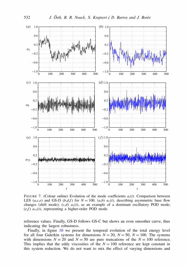
The temporal dynamics of the GS-D and the POD (from LES data) are presentedfor selected modes in figure 7. The first coefficient a1 of the shift mode is the mostinteresting one. This coefficient is depicted in figure 7(a) and describes the changefrom one asymmetric base-flow state to the other. Its value follows exactly the side-force signal from the LES in figure 2(b). Only Galerkin system D was found capableof predicting the sudden switches from one side force state to the other with realisticamplitudes at realistic time scales. Also GS-C exhibits such base-flow changes, but theamplitude is over-predicted by a factor two and these time scales were over-predictedby three orders of magnitudes. GS-A predicts a purely periodic solution for N = 100,and GS-B does not predict the amplitude in a physical correct way. Summarizing,both the modal refinement of the eddy viscosity (GS-B and GS-D) and their energy-dependent scaling in (GS-C and GS-D) emerge as crucial enablers for the accurateGalerkin systems.

4.3. Robustness study of the Galerkin systemsIn this section, the robustness of the Galerkin systems with respect to their dimensionand the eddy-viscosity parameters is investigated.

In figure 8, the time-averaged total energy of all Galerkin systems is depicted fordifferent dimensions N of the ROM. GS-D has, on average, the best agreement withthe LES values for all four dimensions, i.e. N = 10, 20, 50 and 100. In contrast, themost simple GS-A shows even the wrong trend with respect to N. We emphasize thatall eddy-viscosity values are derived from TKE power balances. The performance ofeach Galerkin system could easily be improved with solution matching techniques forthese parameters. However, the price of such techniques is a potentially large residualin the TKE power balance, i.e. the predicted modal energy distribution and energyflows may be significantly distorted.

Finally, the role of the eddy-viscosity parameter is investigated in figure 9 for N =100. For the simulations in this figure, we have varied the total viscosities νT

i in therange 25, 50, 75, 150, 200, 250 and 300 % of the reference value νT

0 for GS-A and GS-C. The modal eddy viscosities νT

i of GS-B and GS-D have been changed by the samefactor depicted on the abscissa. GS-A does not show monotonous behaviour in termsof the parameter change. GS-B has a more monotonous physical behaviour but itsdeviations are stronger than for GS-A. One may speculate that modal eddy viscositiesare ‘over-fitted’ for the physical reference level. GS-C is seen to be far less affectedby these changes, the nonlinear eddy viscosity compensates for too small or too large


(a) (b)

(c) (d )

(e) ( f )

0 100 200 300 400 500−1.0

−0.6

−0.2

0.2

0.6

1.0

a1

0 100 200 300 400 500−1.0

−0.6

−0.2

0.2

0.6

1.0

0 100 200 300 400 500−1.0

−0.6

−0.2

0.2

0.6

1.0

a5

0 100 200 300 400 500−1.0

−0.6

−0.2

0.2

0.6

1.0

0 100 200t t

300 400 500−1.0

−0.6

−0.2

0.2

0.6

1.0

a75

0 100 200 300 400 500−1.0

−0.6

−0.2

0.2

0.6

1.0

FIGURE 7. (Colour online) Evolution of the mode coefficients ai(t). Comparison betweenLES (a,c,e) and GS-D (b,d,f ) for N = 100. (a,b) a1(t), describing asymmetric base flowchanges (shift mode); (c,d) a5(t), as an example of a dominant oscillatory POD mode;(e,f ) a75(t), representing a higher-order POD mode.

reference values. Finally, GS-D follows GS-C but shows an even smoother curve, thusindicating the largest robustness.

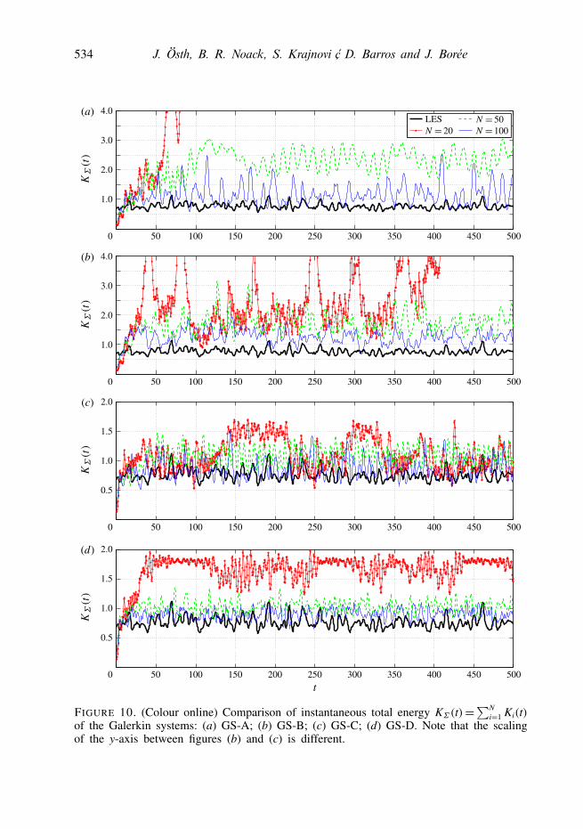
Finally, in figure 10 we present the temporal evolution of the total energy levelfor all four Galerkin systems for dimensions N = 20, N = 50, N = 100. The systemswith dimensions N = 20 and N = 50 are pure truncations of the N = 100 reference.This implies that the eddy viscosities of the N = 100 reference are kept constant inthis system reduction. We do not want to mix the effect of varying dimensions and


0 10 20 50 10010−1

100

101

N


FIGURE 8. (Colour online) Comparison of the total energy, KΣ , in the ROM for differentdimensions N of the ROM. The eddy viscosity is kept constant to the value of that forN = 100.

0 1 2 3

10−1

100

101


FIGURE 9. (Colour online) Comparison of the total energy, KΣ , in the ROM for differentvalues of νT

i and νT0 .

varying eddy viscosity. Again, GS-C and GS-D with the nonlinear subscale turbulencerepresentation outperform GS-A and GS-B in terms of robustness.

Mean values and the variances of the signals from the N = 100 ROMs (seefigure 10) and LES are presented in table 1. GS-C predicts the mean value slightlycloser to LES than GS-D, but the variance of GS-C (0.0304) is overpredicted by afactor of three compared to the LES (0.0095), while the variance of GS-D (0.0091)is close to that of the LES. GS-A and GS-B overpredict the mean and variancesignificantly.


(a)

50 100 150 200 250 300 350 400 450 5000

1.0

2.0

3.0

4.0

(b)

50 100 150 200 250 300 350 400 450 5000

1.0

2.0

3.0

4.0

(c)

50 100 150 200 250 300 350 400 450 5000

0.5

1.0

1.5

2.0

(d)

50 100 150 200 250 300 350 400 450 5000

0.5

1.0

1.5

2.0

t

LES

FIGURE 10. (Colour online) Comparison of instantaneous total energy KΣ(t)=∑Ni=1 Ki(t)

of the Galerkin systems: (a) GS-A; (b) GS-B; (c) GS-C; (d) GS-D. Note that the scalingof the y-axis between figures (b) and (c) is different.


GS-A GS-B GS-C GS-D LES

Mean 1.1693 1.2535 0.8740 0.9010 0.7671Variance 0.1264 0.0606 0.0304 0.0091 0.0095

TABLE 1. Mean values and variances of KΣ(t) for the N = 100 ROMs and LES.

In summary, the accuracy and robustness of the Galerkin system is found toimprove by modal refinement of the eddy viscosities and by an energy-dependentscaling. A similar observation for the energy-dependent scaling has been made forthe POD models of a mixing layer by Cordier et al. (2013).

5. ConclusionsWe have investigated a hierarchy of linear and nonlinear eddy-viscosity terms for a

POD Galerkin model accounting for the unresolved velocity fluctuations. The chosenconfiguration is a high-Reynolds-number flow over a square-back Ahmed body. Thisflow exhibits three challenging features for reduced-order models. Firstly, the highReynolds number implies that a subscale turbulence representation is mandatory forrealistic fluctuation levels, or even boundedness, of the Galerkin system solution.Secondly, the coherent structures of the Ahmed body have a broadband frequencysignature. The resulting frequency cross-talk implies that many modal interactionsexist and need to be correctly resolved. Thirdly, the base flow has two meta-stablestates with nearly constant non-vanishing side forces. Experiments on a similarAhmed body configuration (Grandemange et al. 2013) exhibit these asymmetricquasi-attractors. Such quasi-attractors imply a complex interaction from small tovery large time scales and constitute a significant modelling challenge – even forNavier–Stokes simulations.

The solutions of a POD Galerkin model with 100 modes or less converge to infinity,underlining the need for a subscale turbulence presentation. Four correspondingauxiliary models have been tested, using a single or modally refined eddy viscositieswith constant or energy-dependent values. These parameters are determined from thetotal or modal TKE power balance. Solution matching techniques are excluded asa parameter identification method, to avoid any inconsistency with the TKE powerbalances. A single constant eddy viscosity, as used by Aubry et al. (1988) and others,is already sufficient to stabilize the Galerkin solution. Modally refined viscosities,as suggested by Rempfer & Fasel (1994b), are found to significantly improve theaccuracy of the modal fluctuation energies. However, both approaches rely on constanteddy viscosities, leading to linear subscale turbulence representations for nonlinearenergy flow cascade. The resulting Galerkin solutions converge to infinity if the initialconditions are far from the attractor. In addition, neither Galerkin system exhibits themeta-stable asymmetric base flow states.

We corroborate the need for eddy viscosities which scale with the square rootof the resolved fluctuation energy. The single nonlinear eddy-viscosity model leadsto an accurate prediction for the fluctuation levels of higher-order modes, whilethe amplitudes of the first seven modes are over-predicted. Arguably, the first sevenmodes define the large-scale coherent structures and are the most important part of thespectrum. The modally refined eddy viscosity cures this over-prediction at the expenseof a less accurate tail of the modal energy spectrum. These nonlinear eddy-viscositymodels are capable of resolving the flipping between asymmetric base flow states.


Constant eddy viscosity (GS-A)− blow up in finite time for certain initial conditions− significant overprediction of fluctuation levels (with NSE inferred eddy viscosity)

Modal eddy viscosities (GS-B)− blow up in finite time for certain initial conditions+ more accurate prediction of fluctuation levels+ reduced dependency on ROM dimension N

Nonlinear constant eddy viscosity (GS-C)− significant overprediction of fluctuation levels+ guaranteed boundedness of solution, independent of the initial condition+ reduced dependency on ROM dimension N+ reduced dependency on νT variation

Nonlinear modal eddy viscosity (GS-D)+ guaranteed boundedness of solution, independent of the initial condition+ more accurate prediction of fluctuation levels+ reduced dependency on ROM dimension (N)+ reduced dependency on νT variation

TABLE 2. Performance of the Galerkin systems A–D: ‘−’ refers to challenges, ‘+’ toimprovements with respect to the benchmark Galerkin system A.

In addition, the resulting Galerkin systems converge to their respective attractorsfor initial conditions – even if these are far away from them. Global convergencecan be strictly ensured by enforcing energy preservation on the quadratic term. Thisenergy preservation is derivable from the NSE (Kraichnan & Chen 1989; Schlegel& Noack 2013). In addition, Galerkin systems with nonlinear subscale turbulencerepresentations are shown to be much more robust with respect to changes of theeddy-viscosity parameters and the dimension of the model.

The modally refined, nonlinear eddy-viscosity terms have significantly increasedaccuracy and robustness of the Galerkin system as compared to traditional linearsubscale turbulence representations. The accuracy has been achieved with a parameteridentification, based purely on NSE-based constraints and without solution matchingtechniques. The robustness is a key enabler for three ROM-based applications. Firstly,the ROM may serve as a test-bed for understanding of the nonlinear dynamics.One key question is the mechanism for the amplitude selection, i.e. what drivesthe transients towards the attractor. Secondly, the ROM may be employed as acomputationally inexpensive surrogate model for multiple purposes, e.g. for the inletconditions of the flow around a following car model. In this case, it is desirable tohave a ROM which works over a certain range of operating conditions, e.g. slowlyvarying oncoming velocity. This variability implies that the ROM employs a physicallycorrect robust amplitude selection mechanism, e.g. does not diverge for a small changeof the Reynolds number. Finally, model-based control design requires a ROM whichworks robustly for a range of natural and forced transients. Moreover, the controldesign is often based on a hierarchy of ROMs with different dimensions – rangingfrom robust least-order models to more accurate higher-order models, which posegreater challenges to state estimation. The nonlinear eddy-viscosity term serves allthree mentioned applications. Table 2 summarizes the benefits achieved from themodal and nonlinear eddy-viscosity refinements.


To conclude, the proposed nonlinear subscale turbulence term with modal eddyviscosity of Rempfer & Fasel (1994b) and energy-dependent scaling of Noacket al. (2011) is a recipe for accurate and robust POD models for a large classof complex flows, comprising the flow over an Ahmed body as shown here, amixing layer (Cordier et al. 2013), and subsonic jet noise (Schlegel et al. 2009). Thestudy emphasizes the decisive role of a good structure identification of the Galerkinsystem propagator – here in form of a nonlinear stabilizing term – before parameteridentification methods are to be applied.

Acknowledgements

The thesis of J. Östh is supported financially by Trafikverket (Swedish TransportAdministration). The thesis of D. Barros is supported financially by PSA PeugeotCitroën and ANRT in the context of the OpenLab Fluidics between PSA and InstitutePPRIME. The work by S. Krajnovic in this paper was partially funded by theChalmers Sustainable Transport Initiative. The authors acknowledge the fundingand excellent working conditions of the Senior Chair of Excellence ‘Closed-loopcontrol of turbulent shear flows using reduced-order models’ (TUCOROM), supportedby the French Agence Nationale de la Recherche (ANR) and hosted by InstitutePPRIME. We thank the Ambrosys Ltd. Society for Complex Systems Management,the Bernd Noack Cybernetics Foundation and OpenLab PPRIME/PSA for additionalsupport. We appreciate valuable stimulating discussions with our collaborators MarkusAbel, Jean-Paul Bonnet, Steven Brunton, Laurent Cordier, Joël Delville, ThomasDuriez, Fabien Harambat, Eurika Kaiser, Robert Niven, Tamir Shaqarin, VladimirParezanovic, Bartek Protas, Tony Ruiz, Michael Schlegel, Marc Segond and AndreasSpohn. Special thanks are due to Nadia Maamar for a wonderful job in hosting theTUCOROM visitors.

Software licenses for AVL Fire were provided by AVL List GmbH. Computationswere performed at SNIC (Swedish National Infrastructure for Computing) at theCenter for Scientific Computing at Chalmers (C3SE), Center for High PerformanceComputing at KTH (PDC) and National Supercomputer Center (NSC) at LiU.

Last but not least, we thank the referees for their constructive suggestions.

Appendix A. Comparison between experimental data and LES dataThis appendix describes the companion experiment at Institute PPRIME, which

serves as a reference for the LES. PIV and hot-wire data are used only to validatethe data obtained from the LES.

A.1. Description of the experimental set-upThe experiments were conducted in a closed-loop wind tunnel with a test sectionof 6.24 m2. The model was mounted over an elliptical leading-edge flat plate, asillustrated in figure 11. At the end of the flat plate, an inclined flap was adjustedin order to obtain an upstream flow aligned perpendicularly to its leading edge.This procedure was done without the bluff body in the wind tunnel. Consideringthe upper area above the plate, the blockage ratio is approximately 2 % and noblockage corrections were performed. The upstream velocity, measured on the uppersurface of the wind tunnel (above the model), was kept constant at U∞ = 15 m s−1.Particle image velocimetry (PIV) was performed on the near-wake (see detail infigure 11). Streamwise and transverse (respectively x and y directions) components of


0.28H

11.6H

1.67H

PIV plane

2.42H

6.4H

0.33H

CentralsupportFairing

Profiledsupports0.67H

2H

y

x

FIGURE 11. Experimental set-up.

the velocity field were measured using two LaVision Imager pro X 4M (resolution2000× 2000 pixels) cameras. A laser sheet was pulsed (with time delays of 120 µs)in the symmetry plane of the configuration and image pairs were acquired at asampling frequency of 3 Hz. Velocity vector calculations are processed with aninterrogation window of 32×32 pixels (an overlap of 50 %) giving a spatial resolutionof approximately 1 % of the model height. Starting with an absolute displacementerror of 0.1 pixels, the maximum uncertainty on instantaneous velocity fields isestimated to be 0.2 m s−1. The mean flow was computed using 500 independentvelocity fields and the estimated statistical error for time-averaged velocity is 0.09σrms

with 95 % of confidence level and σrms is the local root mean square of the velocity.

A.2. Velocity profilesFigure 12 presents a comparison between the LES results and the experimental datafor the time-averaged streamwise velocity component, u, at different locations in thesymmetry plane of the wake. The shear layer profile slightly downstream (0.03 H) ofthe top trailing edge of the PIV data and the LES data are presented in figure 12(a).The two profiles are in good agreement. The slow recovery of the shear layer is due tomomentum loss in the separation on the front edges of the body. Such slow recoveryof the shear layer profile at the trailing edge was also found in the experimental studyby Grandemange et al. (2013). Figures 12(b)–(f ) present profiles along lines extendingfrom the ground to a position above the wake at five different streamwise locationsin the wake. None of the profiles shows any significant discrepancy between the LESand the PIV data.

A.3. Streamlines of time-averaged velocity in the symmetry planeFigures 13(a) and 13(b) present the time-averaged flow in the symmetry planefrom the PIV data and the LES. The upper centre of the time-averaged toroïdalvortical structure in the wake is located closer to the base than the lower centre. Theorganization of the flow in the wake is very sensitive to the set-up, in particular the


0.2 0.4 0.6 0.8 1.00

0.02

0.04

0.06

0.08

0.10

0.12(a) (b)

(c) (d)

(e) ( f )

LES

Exp

−0.4 0 0.4 0.8 1.2−0.6

−0.4

−0.2

0

0.2

0.4

0.6

0.8

1.0

−0.4 0 0.4 0.8 1.2−0.6

−0.4

−0.2

0

0.2

0.4

0.6

0.8

1.0

−0.4 0 0.4 0.8 1.2−0.6

−0.4

−0.2

0

0.2

0.4

0.6

0.8

1.0

−0.4 0 0.4 0.8 1.2−0.6

−0.4

−0.2

0

0.2

0.4

0.6

0.8

1.0

−0.4 0 0.4 0.8 1.2−0.6

−0.4

−0.2

0

0.2

0.4

0.6

0.8

1.0

FIGURE 12. Profiles showing comparison of the time-averaged streamwise velocitycomponent, u, for different locations in the wake. (a) Shear layer profile 0.03Hdownstream of the top trailing edge. Here y∗= y+0.5H. (b) 0.17H downstream; (c) 0.34Hdownstream; (d) 0.5H downstream; (e) 0.67H downstream; (f ) 0.84H downstream.

gap clearance between the body and the ground. Therefore, similar studies of thegeometry show different organization of the wake. In the study by Grandemange et al.(2013), the location of the upper vortical centre is located further downstream, at thesame distance from the base as the lower centre. However, both the gap width andthe Reynolds number were less in that study than presented here. Figures 13(c) and13(d) show one instantaneous realization from the PIV and LES data, respectively.


(a) (b)

(c) (d)

1.0

0

–0.3

FIGURE 13. (Colour online) Comparison between experimental PIV data and LES data inthe symmetry plane. (a) time-averaged PIV; (b) time-averaged LES; (c) one instantaneousrealization of PIV data; (d) one instantaneous realization of LES data. The length of theplanes is 1.7H and the height is 1.5H.

mean(1n+) mean(1x+) mean(1s+)

0.55 80 20

TABLE 3. Spatial resolution in the LES.

A.4. Spectra of the transverse velocity component

Spectra of velocity are presented in figure 14 at a point located downstream of theseparation region. Both the hot-wire data and the LES data show a signature at St≈0.2, corresponding to the global shedding of the wake. This peak was also found inthe study by Lahaye, Leroy & Kourta (2014).

Appendix B. Spatial resolution in the LES

The time-averaged spatial resolution on the body expressed in viscous wall units,1n+=1n/λ+, 1x+=1x/λ+ and 1s+=1s/λ+, is presented in table 3. Here 1n, 1xand 1s refer to the sizes of the cells in the wall-normal direction, streamwise directionand spanwise direction, respectively. Here λ+ is the viscous length scale, defined asλ+ = ν/u∗, where u∗ is the wall friction velocity. The size of the cells in the normaldirection on the body, n+, is everywhere less than 1. The spatial- and time-average ofthe viscous length scale on the body, λ+, was computed to be 0.0002 H. The valuespresented in table 3 refer to the mean values on the body.


10−2 10−1 100

10−2

St

PSD

Exp

LES

FIGURE 14. Power spectral density (PSD) of the transverse velocity component, v, at thepoint x= 2.25H, y= 0.34H, of LES data and the velocity magnitude of the hot-wire data.

0.25

0.22

0.18

0.14

0.10y

x

z

FIGURE 15. A plane cut from the LES in the fifth cell layer away from the roof atapproximately y/λ+ ≈ 5, showing regions of low- and high-speed streamwise velocities.The length of the plane is approximately 13 000λ+ (2.7H).

Figure 15 shows the streamwise velocity component in a plane cut in the innerboundary layer on the roof. The figure reveals low- and high-speed streaks in thestreamwise direction, indicating the high spatial resolution in the LES.

REFERENCES

AHMED, S., RAMM, G. & FALTIN, G. 1984 Some salient features of the time-averaged groundvehicle wake. SAE Tech. Rep. 840300.

AIDER, J.-L., BEAUDOIN, J.-F. & WESFREID, J. E. 2010 Drag and lift reduction of a 3D bluff-bodyusing active vortex generators. Exp. Fluids 48, 771–789.

AUBRY, N., HOLMES, P., LUMLEY, J. L. & STONE, E. 1988 The dynamics of coherent structures inthe wall region of a turbulent boundary layer. J. Fluid Mech. 192, 115–173.

AVL Fire 2013 CFD Solver. FIRE CFD Solver Users Guide, v2013.BALAJEWICZ, M. J., DOWELL, E. H. & NOACK, B. R. 2013 Low-dimensional modelling of

high-Reynolds-number shear flows incorporating constraints from the Navier–Stokes equation.J. Fluid Mech. 729, 285–308.


BEAUDOIN, J.-F. & AIDER, J.-L. 2008 Drag and lift reduction of a 3D bluff body using flaps.Exp. Fluids 44, 491–501.

BOBERG, L. & BROSA, U. 1988 Onset of turbulence in a pipe. Z. Naturforsch. 43a, 697–726.BRUNN, A., NITSCHE, W., HENNING, L. & KING, R. 2008 Application of slope-seeking to a generic

car model for active drag control. AIAA Paper 2008-6734.BUSSE, F. H. 1991 Numerical analysis of secondary and tertiary states of fluid flow and their stability

properties. Appl. Sci. Res. 48, 341–351.CAZEMIER, W., VERSTAPPEN, R. W. C. P. & VELDMAN, A. E. P. 1998 Proper orthogonal

decomposition and low-dimensional models for driven cavity flows. Phys. Fluids 10, 1685–1699.CORDIER, L., NOACK, B. R., TISSOT, G., LEHNASCH, G., DELVILLE, J., BALAJEWICZ, M.,

DAVILLER, G. & NIVEN, R. K. 2013 Identification strategies for model-based control.Exp. Fluids 54 (8), 1–21.

DAVIDSON, L. 2010 How to estimate the resolution of an LES of recirculating flow. In Qualityand Reliability of Large-Eddy Simulations II (ed. M. V. Salvetti, B. Geurts, J. Meyers &P. Sagaut), Ercoftac Series, vol. 16, pp. 269–286. Springer.

DEANE, A. E., KEVREKIDIS, I. G., KARNIADAKIS, G. E. & ORSZAG, S. A. 1991 Low-dimensionalmodels for complex geometry flows: application to grooved channels and circular cylinders.Phys. Fluids A 3, 2337–2354.

DUELL, E. G. & GEORGE, A. R. 1999 Experimental study of a ground vehicle body unsteady nearwake. SAE Paper 1999-01-0812.

GALLETTI, G., BRUNEAU, C. H., ZANNETTI, L. & IOLLO, A. 2004 Low-order modelling of laminarflow regimes past a confined square cylinder. J. Fluid Mech. 503, 161–170.

GRANDEMANGE, M., GOHLKE, M. & CADOT, O. 2013 Turbulent wake past a three-dimensionalblunt body. Part 1. Global modes and bi-stability. J. Fluid Mech. 722, 51–84.

HEMIDA, H. 2008 Numerical simulations of flows around trains and buses in cross winds. PhD thesis,Chalmers University of Technology, Gothenburg, Sweden, ISBN/ISSN 978-91-7385-187-9.

HEMIDA, H., GIL, N. & BAKER, C. 2010 LES of the slipstream of a rotating train. Trans. ASME J.Fluids Engng 132 (5), 051103–051103-9.

HEMIDA, H. & KRAJNOVIC, S. 2008 LES study of the influence of a train-nose shape on the flowstructures under cross-wind conditions. Trans. ASME J. Fluids Engng 130 (9), 091101–091101-12.

HEMIDA, H. & KRAJNOVIC, S. 2010 LES study of the influence of the nose shape and yaw angleson flow structures around trains. J. Wind Engng Ind. Aerodyn. 98, 34–46.

HOLMES, P., LUMLEY, J. L., BERKOOZ, G. & ROWLEY, C. W. 2012 Turbulence, Coherent Structures,Dynamical Systems and Symmetry, 2nd edn. Cambridge University Press.

JOSEPH, D. D. 1976 Stability of Fluid Motions I & II. Springer-Verlag.KOLMOGOROV, A. N. 1941a Dissipation of energy in locally isotropic turbulence. Dokl. Akad. Nauk

SSSR 32, 16–18 (translated and reprinted 1991 in Proc. R. Soc. Lond. A 434, 15–17).KOLMOGOROV, A. N. 1941b The local structure of turbulence in incompressible viscous fluid for

very large Reynolds number. Dokl. Akad. Nauk SSSR 30, 9–13 (translated and reprinted 1991in Proc. R. Soc. Lond. A 434, 9–13).

KRAICHNAN, R. H. & CHEN, S. 1989 Is there a statistical mechanics of turbulence? Physica D 37,160–172.

KRAJNOVIC, S. 2002 Large-Eddy Simulation for computing the flow around vehicles. PhD thesis,Chalmers University of Technology, Gothenburg, Sweden, ISBN/ISSN 91-7291-188-3.

KRAJNOVIC, S. 2009 LES of flows around ground vehicles and other bluff bodies. Phil. Trans. R.Soc. A 367 (1899), 2917–2930.

KRAJNOVIC, S. 2011 Flow around a tall finite cylinder explored by large eddy simulation. J. FluidMech. 676, 294–317.

KRAJNOVIC, S. 2013 LES investigation of passive flow control around an Ahmed body. In ASME2013 International Mechanical Engineering Congress & Exposition, San Diego, CA, USA,vol. 1, pp. 305–315, Paper IMECE2013-62373.

KRAJNOVIC, S. & DAVIDSON, L. 2003 Numerical study of the flow around the bus-shaped body.Trans. ASME J. Fluids Engng 125, 500–509.


KRAJNOVIC, S. & DAVIDSON, L. 2005a Flow around a simplified car. Part 1. Large Eddy Simulation.Trans. ASME J. Fluids Engng 127, 907–918.

KRAJNOVIC, S. & DAVIDSON, L. 2005b Flow around a simplified car. Part 2. Understanding theflow. Trans. ASME J. Fluids Engng 127, 919–928.

KRAJNOVIC, S. & FERNANDES, J. 2011 Numerical simulation of the flow around a simplified vehiclemodel with active flow control. Intl J. Heat Fluid Flow 32 (5), 192–200.

LAHAYE, A., LEROY, A. & KOURTA, A. 2014 Aerodynamic characterisation of a square back bluffbody flow. Intl J. Aerodyn. 4 (1–2), 43–60.

LIENHART, H. & BECKER, S. 2003 Flow and turbulent structure in the wake of a simplified carmodel. SAE Paper No. 2003-01-0656.

LUMLEY, J. L. 1970 Stochastic Tools in Turbulence. Academic Press.MA, X. & KARNIADAKIS, G. E. 2002 A low-dimensional model for simulating three-dimensional

cylinder flow. J. Fluid Mech. 458, 181–190.NOACK, B. R., AFANASIEV, K., MORZYNSKI, M., TADMOR, G. & THIELE, F. 2003 A hierarchy

of low-dimensional models for the transient and post-transient cylinder wake. J. Fluid Mech.497, 335–363.

NOACK, B. R. & ECKELMANN, H. 1994 A global stability analysis of the steady and periodiccylinder wake. J. Fluid Mech. 270, 297–330.

NOACK, B. R., MORZYNSKI, M. & TADMOR, G. 2011 Reduced-Order Modelling for Flow Control.(CISM Courses and Lectures), vol. 528. Springer.

NOACK, B. R., PAPAS, P. & MONKEWITZ, P. A. 2005 The need for a pressure-term representationin empirical Galerkin models of incompressible shear flows. J. Fluid Mech. 523, 339–365.

NOACK, B. R., SCHLEGEL, M., AHLBORN, B., MUTSCHKE, G., MORZYNSKI, M., COMTE, P. &TADMOR, G. 2008 A finite-time thermodynamics of unsteady fluid flows. J. Non-Equilib.Thermodyn. 33, 103–148.

ÖSTH, J. & KRAJNOVIC, S. 2012 The flow around a simplified tractor-trailer model studied by LargeEddy Simulation. J. Wind Engng Ind. Aerodyn. 102, 36–47.

ÖSTH, J. & KRAJNOVIC, S. 2014 A study of the aerodynamics of a generic container freight wagonusing Large-Eddy Simulation. J. Fluid. Struct. 44, 31–51.

ÖSTH, J., KRAJNOVIC, S., BARROS, D., CORDIER, L., NOACK, B. R., BORÉE, J. & RUIZ, T. 2013Active flow control for drag reduction of vehicles using Large Eddy Simulation, experimentalinvestigations and reduced order modelling. Proceedings of the 8th International Symposiumon Turbulent and Shear Flow Phenomena (TSFP-8), Poitiers, France.

PASTOOR, M., HENNING, L., NOACK, B. R., KING, R. & TADMOR, G. 2008 Feedback shear layercontrol for bluff body drag reduction. J. Fluid Mech. 608, 161–196.

PODVIN, B. 2009 A proper-orthogonal-decomposition-based model for the wall layer of a turbulentchannel flow. Phys. Fluids 21, 015111 1. . .18.

POPE, S. B. 2000 Turbulent Flows. 1st edn. Cambridge University Press.RAJAEE, M., KARLSSON, S. K. F. & SIROVICH, L. 1994 Low-dimensional description of free-shear-

flow coherent structures and their dynamical behaviour. J. Fluid Mech. 258, 1–29.REMPFER, D. & FASEL, F. H. 1994a Evolution of three-dimensional coherent structures in a flat-plate

boundary-layer. J. Fluid Mech. 260, 351–375.REMPFER, D. & FASEL, F. H. 1994b Dynamics of three-dimensional coherent structures in a flat-plate

boundary-layer. J. Fluid Mech. 275, 257–283.SCHLEGEL, M. & NOACK, B. R. 2013 On long-term boundedness of Galerkin models. J. Fluid

Mech. (submitted).SCHLEGEL, M., NOACK, B. R., COMTE, P., KOLOMENSKIY, D., SCHNEIDER, K., FARGE, M.,

SCOUTEN, J., LUCHTENBURG, D. M. & TADMOR, G. 2009 Reduced-order modelling ofturbulent jets for noise control. In Numerical Simulation of Turbulent Flows and NoiseGeneration: Results of the DFG/CNRS Research Groups FOR 507 and FOR 508, Notes onNumerical Fluid Mechanics and Multidisciplinary Design (NNFM), vol. 1, pp. 3–27. Springer.

SIROVICH, L. 1987a Turbulence and the dynamics of coherent structures, part I: coherent structures.Q. Appl. Math. 45, 561–571.


SIROVICH, L. 1987b Turbulence and the dynamics of coherent structures, part II: symmetries andtransformations. Q. Appl. Math. 45, 573–582.

SMAGORINSKY, J. 1963 General circulation experiments with the primitive equations. Mon. Weath.Rev. 91 (3), 99–165.

SPOHN, A. & GILLIERON, P. 2002 Flow separations generated by a simplified geometry of anautomotive vehicle. IUTAM Symposium: Unsteady Separated Flows, Toulouse, France.

UKEILEY, L., CORDIER, L., MANCEAU, R., DELVILLE, J., BONNET, J. P. & GLAUSER, M. 2001Examination of large-scale structures in a turbulent plane mixing layer. Part 2. Dynamicalsystems model. J. Fluid Mech. 441, 61–108.

VERZICCO, R., FATICA, M., LACCARINO, G. & MOIN, P. 2002 Large Eddy Simulation of a roadvehicle with drag-reduction devices. AIAA J. 40, 2447–2455.

WANG, Z., AKHTAR, I., BORGGAARD, J. & ILIESCU, T. 2011 Two-level discretizations of nonlinearclosure models for proper orthogonal decomposition. J. Comput. Phys. 230, 126–146.

WANG, Z., AKHTAR, I., BORGGAARD, J. & ILIESCU, T. 2012 Proper orthogonal decompositionclosure models for turbulent flows: a numerical comparison. Comput. Meth. Appl. Mech.Engng 237–240, 10–26.

WASSEN, E. & THIELE, F. 2009 Road vehicle drag reduction by combined steady blowing andsuction. AIAA Paper 2009-4174.

j. fluid mech. (2014), . 747, pp. …berndnoack.com/publications/2014_jfm_osth.pdf · on the need...

Documents