iterative regularization methods for ill-posed problems · regularization of ill-posed problems in...
TRANSCRIPT
Alma Mater Studiorum
Universita di Bologna
Dottorato di Ricerca in
MATEMATICA
Ciclo XXV
Settore Concorsuale di afferenza: 01/A5
Settore Scientifico disciplinare: MAT/08
Iterative regularization methods
for ill-posed problems
Tesi di Dottorato presentata da: Ivan Tomba
Coordinatore Dottorato:
Chiar.mo Prof.
Alberto Parmeggiani
Relatore:
Chiar.ma Prof.ssa
Elena Loli Piccolomini
Esame Finale anno 2013

Contents
Introduction vii
1 Regularization of ill-posed problems in Hilbert spaces 1
1.1 Fundamental notations . . . . . . . . . . . . . . . . . . . . . . 2
1.2 Differentiation as an inverse problem . . . . . . . . . . . . . . 2
1.3 Abel integral equations . . . . . . . . . . . . . . . . . . . . . . 6
1.4 Radon inversion (X-ray tomography) . . . . . . . . . . . . . . 7
1.5 Integral equations of the first kind . . . . . . . . . . . . . . . . 9
1.6 Hadamard’s definition of ill-posed problems . . . . . . . . . . 11
1.7 Fundamental tools in the Hilbert space setting . . . . . . . . . 12
1.7.1 Basic definitions and notations . . . . . . . . . . . . . 12
1.7.2 The Moore-Penrose generalized inverse . . . . . . . . . 13
1.8 Compact operators: SVD and the Picard criterion . . . . . . . 17
1.9 Regularization and Bakushinskii’s Theorem . . . . . . . . . . 20
1.10 Construction and convergence of regularization methods . . . 22
1.11 Order optimality . . . . . . . . . . . . . . . . . . . . . . . . . 24
1.12 Regularization by projection . . . . . . . . . . . . . . . . . . . 28
1.12.1 The Seidman example (revisited) . . . . . . . . . . . . 29
1.13 Linear regularization: basic results . . . . . . . . . . . . . . . 32
1.14 The Discrepancy Principle . . . . . . . . . . . . . . . . . . . . 36
1.15 The finite dimensional case: discrete ill-posed problems . . . . 38
1.16 Tikhonov regularization . . . . . . . . . . . . . . . . . . . . . 41
1.17 The Landweber iteration . . . . . . . . . . . . . . . . . . . . . 44
i
ii CONTENTS
2 Conjugate gradient type methods 51
2.1 Finite dimensional introduction . . . . . . . . . . . . . . . . . 52
2.2 General definition in Hilbert spaces . . . . . . . . . . . . . . . 59
2.3 The algorithms . . . . . . . . . . . . . . . . . . . . . . . . . . 61
2.3.1 The minimal residual method (MR) and the conjugate
gradient method (CG) . . . . . . . . . . . . . . . . . . 66
2.3.2 CGNE and CGME . . . . . . . . . . . . . . . . . . . . 67
2.3.3 Cheap Implementations . . . . . . . . . . . . . . . . . 69
2.4 Regularization theory for the conjugate gradient type methods 72
2.4.1 Regularizing properties of MR and CGNE . . . . . . . 74
2.4.2 Regularizing properties of CG and CGME . . . . . . . 78
2.5 Filter factors . . . . . . . . . . . . . . . . . . . . . . . . . . . 80
2.6 CGNE, CGME and the Discrepancy Principle . . . . . . . . . 81
2.6.1 Test 0 . . . . . . . . . . . . . . . . . . . . . . . . . . . 82
2.6.2 Test 1 . . . . . . . . . . . . . . . . . . . . . . . . . . . 85
2.6.3 Test 2 . . . . . . . . . . . . . . . . . . . . . . . . . . . 86
2.7 CGNE vs. CGME . . . . . . . . . . . . . . . . . . . . . . . . . 88
2.8 Conjugate gradient type methods with parameter n=2 . . . . 92
2.8.1 Numerical results . . . . . . . . . . . . . . . . . . . . . 93
3 New stopping rules for CGNE 97
3.1 Residual norms and regularizing properties of CGNE . . . . . 98
3.2 SR1: Approximated Residual L-Curve Criterion . . . . . . . . 102
3.3 SR1: numerical experiments . . . . . . . . . . . . . . . . . . . 107
3.3.1 Test 1 . . . . . . . . . . . . . . . . . . . . . . . . . . . 108
3.3.2 Test 2 . . . . . . . . . . . . . . . . . . . . . . . . . . . 108
3.4 SR2: Projected Data Norm Criterion . . . . . . . . . . . . . . 110
3.4.1 Computation of the index p of the SR2 . . . . . . . . . 113
3.5 SR2: numerical experiments . . . . . . . . . . . . . . . . . . . 114
3.6 Image deblurring . . . . . . . . . . . . . . . . . . . . . . . . . 116
3.7 SR3: Projected Noise Norm Criterion . . . . . . . . . . . . . . 121
3.8 Image deblurring: numerical experiments . . . . . . . . . . . . 124
CONTENTS iii
3.8.1 Test 1 (gimp test problem) . . . . . . . . . . . . . . . . 125
3.8.2 Test 2 (pirate test problem) . . . . . . . . . . . . . . . 127
3.8.3 Test 3 (satellite test problem) . . . . . . . . . . . . . . 128
3.8.4 The new stopping rules in the Projected Restarted CGNE129
4 Tomography 133
4.1 The classical Radon Transform . . . . . . . . . . . . . . . . . 133
4.1.1 The inversion formula . . . . . . . . . . . . . . . . . . 136
4.1.2 Filtered backprojection . . . . . . . . . . . . . . . . . . 139
4.2 The Radon Transform over straight lines . . . . . . . . . . . . 141
4.2.1 The Cone Beam Transform . . . . . . . . . . . . . . . 143
4.2.2 Katsevich’s inversion formula . . . . . . . . . . . . . . 145
4.3 Spectral properties of the integral operator . . . . . . . . . . . 149
4.4 Parallel, fan beam and helical scanning . . . . . . . . . . . . . 151
4.4.1 2D scanning geometry . . . . . . . . . . . . . . . . . . 152
4.4.2 3D scanning geometry . . . . . . . . . . . . . . . . . . 154
4.5 Relations between Fourier and singular functions . . . . . . . 154
4.5.1 The case of the compact operator . . . . . . . . . . . . 155
4.5.2 Discrete ill-posed problems . . . . . . . . . . . . . . . . 156
4.6 Numerical experiments . . . . . . . . . . . . . . . . . . . . . . 158
4.6.1 Fanbeamtomo . . . . . . . . . . . . . . . . . . . . . . . 159
4.6.2 Seismictomo . . . . . . . . . . . . . . . . . . . . . . . . 160
4.6.3 Paralleltomo . . . . . . . . . . . . . . . . . . . . . . . . 161
5 Regularization in Banach spaces 163
5.1 A parameter identification problem for an elliptic PDE . . . . 164
5.2 Basic tools in the Banach space setting . . . . . . . . . . . . . 167
5.2.1 Basic mathematical tools . . . . . . . . . . . . . . . . . 167
5.2.2 Geometry of Banach space norms . . . . . . . . . . . . 168
5.2.3 The Bregman distance . . . . . . . . . . . . . . . . . . 174
5.3 Regularization in Banach spaces . . . . . . . . . . . . . . . . . 176
5.3.1 Minimum norm solutions . . . . . . . . . . . . . . . . . 176
iv CONTENTS
5.3.2 Regularization methods . . . . . . . . . . . . . . . . . 178
5.3.3 Source conditions and variational inequalities . . . . . 180
5.4 Iterative regularization methods . . . . . . . . . . . . . . . . . 181
5.4.1 The Landweber iteration: linear case . . . . . . . . . . 182
5.4.2 The Landweber iteration: nonlinear case . . . . . . . . 185
5.4.3 The Iteratively Regularized Landweber method . . . . 186
5.4.4 The Iteratively Regularized Gauss-Newton method . . 189
6 A new Iteratively Regularized Newton-Landweber iteration193
6.1 Introduction . . . . . . . . . . . . . . . . . . . . . . . . . . . . 194
6.2 Error estimates . . . . . . . . . . . . . . . . . . . . . . . . . . 199
6.3 Parameter selection for the method . . . . . . . . . . . . . . . 202
6.4 Weak convergence . . . . . . . . . . . . . . . . . . . . . . . . . 207
6.5 Convergence rates with an a-priori stopping rule . . . . . . . . 211
6.6 Numerical experiments . . . . . . . . . . . . . . . . . . . . . . 213
6.7 A new proposal for the choice of the parameters . . . . . . . . 219
6.7.1 Convergence rates in case ν > 0 . . . . . . . . . . . . . 224
6.7.2 Convergence as n → ∞ for exact data δ = 0 . . . . . . 224
6.7.3 Convergence with noisy data as δ → 0 . . . . . . . . . 225
6.7.4 Newton-Iteratively Regularized Landweber algorithm . 227
Conclusions 229
A Spectral theory in Hilbert spaces 231
B Approximation of a finite set of data with cubic B-splines 235
B.1 B-splines . . . . . . . . . . . . . . . . . . . . . . . . . . . . . . 235
B.2 Data approximation . . . . . . . . . . . . . . . . . . . . . . . 236
C The algorithms 239
C.1 Test problems from P. C. Hansen’s Regularization Tools . . . 239
C.2 Conjugate gradient type methods algorithms . . . . . . . . . . 241
C.3 The routine data−approx . . . . . . . . . . . . . . . . . . . . . 242
CONTENTS v
C.4 The routine mod−min−max . . . . . . . . . . . . . . . . . . . . 243
C.5 Data and files for image deblurring . . . . . . . . . . . . . . . 244
C.6 Data and files for the tomographic problems . . . . . . . . . . 245
D CGNE and rounding errors 247
Bibliography 249
Acknowledgements i

Introduction
Inverse and ill-posed problems are nowadays a very important field of re-
search in applied mathematics and numerical analysis. The main reason for
this large interest is the wide number of applications, ranging from medi-
cal imaging, via material testing, seismology, inverse scattering and financial
mathematics, to weather forecasting, just to cite some of the most famous.
Typically, in these problems some fundamental information is not available
and the solution does not depend continuously on the data. As a consequence
of this lack of stability, even very small errors in the data can cause very large
errors in the results. Thus, the problems have to be regularized by inserting
some additional information in the data to obtain reasonable approximations
of the sought for solution. On the other hand, it is important to keep the
computational cost of the corresponding algorithms as low as possible, since
in practical applications the total amount of data to be processed is usually
very high.
The main topic of this Ph.D thesis is the regularization of ill-posed problems
by means of iterative regularization techniques. The principal advantage of
the iterative methods is that the regularized solutions are obtained by ar-
resting the methods at an early stage, which often allows to spare time in
the computations. On the other side, the main difficulty in their use is the
choice of the stopping index of the iteration: an early stopping produces an
over-regularized solution, whereas a late stopping computes a noisy solution.
In particular, we shall focus on the conjugate gradient type methods for
regularizing linear ill-posed problems from the classical Hilbert space set-
vii

viii Introduction
ting point of view, and on a new inner-outer Newton-Iteratively Regularized
Landweber method for solving nonlinear ill-posed problems in the Banach
space framework.
Regarding the conjugate gradient type methods, we propose three new au-
tomatic1 stopping rules for the Conjugate Gradient method applied to the
Normal Equation in the discrete setting, based on the regularizing properties
of the method in the continuous setting. These stopping rules are tested in
a series of numerical simulations, including some problems of tomographic
images reconstruction.
Regarding the Newton-Iteratively Regularized Landweber method, we define
both the iteration and the stopping rules showing convergence and conver-
gence rates results.
In detail, the thesis is constituted by six chapters.
• In Chapter 1 we recall the basic notions of the regularization theory in
the Hilbert space framework. Revisiting the regularization theory, we
mainly follow the famous book of Engl, Hanke and Neubauer [17]. Some
examples are added, some others corrected and some proofs completed.
• Chapter 2 is dedicated to the definition of the conjugate gradient type
methods and the analysis of their regularizing properties. A comparison
of these methods is made by means of numerical simulations.
• In Chapter 3 we motivate, define and analyze the new stopping rules
for the Conjugate Gradient applied to the Normal Equation. The stop-
ping rules are tested in many different examples, including some image
deblurring test problems.
• In Chapter 4 we consider some applications in tomographic problems.
Some theoretical properties of the Radon Transform are studied and
then used in the numerical tests to implement the stopping rules defined
in Chapter 3.
1i.e. that can be defined precisely by a software

Introduction ix
• Chapter 5 is a survey of the regularization theory in the Banach space
framework. The main advantages of working in a Banach space setting
instead of a Hilbert space setting are explained in the introduction.
Then, the fundamental tools and results of this framework are sum-
marized following [82]. The regularizing properties of some important
iterative regularization methods in the Banach space framework, such
as the Landweber and Iteratively Regularized Landweber methods and
the Iteratively Regularized Gauss-Newton method, are described in the
last section.
• The main results about the new inner-outer Newton-Iteratively Regu-
larized Landweber iteration are presented in the conclusive part of the
thesis, in Chapter 6.

x Introduction

Chapter 1
Regularization of ill-posed
problems in Hilbert spaces
The fundamental background of this thesis is the regularization theory for
(linear) ill-posed problems in the Hilbert space setting. In this introductory
chapter we are going to revisit and summarize the basic concepts of this
theory, which is nowadays well-established. To this end, we will mainly
follow the famous book of Engl, Hanke and Neubauer [17].
Starting from some very famous examples of inverse problems (differentia-
tion and integral equations of the first kind) we will review the notions of
regularization method, stopping rule and order optimality. Then we will
consider a class of finite dimensional problems arising from the discretization
of ill-posed problems, the so called discrete ill-posed problems. Finally, in
the last two sections of the chapter we will recall the basic properties of the
Tikhonov and the Landweber methods.
Apart from [17], general references for this chapter are [20], [21], [22], [61],
[62], [90] and [91] and, concerning the part about finite dimensional problems,
[36] and the references therein.
1
2 1. Regularization of ill-posed problems in Hilbert spaces
1.1 Fundamental notations
In this section, we fix some important notations that will we used throughout
the thesis.
First of all, we shall denote by Z, R, C, the sets of the integer, real and
complex numbers respectively. In C, the imaginary unit will be denoted by
the symbol ı. The set of strictly positive integers will be denoted by N or
Z+, the set of positive real numbers by R+.
If not stated explicitly, we shall denote by 〈·, ·〉 and by ‖ · ‖ the standard
euclidean scalar product and euclidean norm on the cartesian product RD,
D ∈ N respectively. Moreover, SD−1 := x ∈ RD | ‖x‖ = 1 will be the unit
sphere in RD.
For i and j ∈ N, we will denote by Mi,j(R) (respectively, Mi,j(C)) the space
of all matrices with i rows and j columns with entries in R (respectively,
C) and by GLj(R) (respectively, GLj(C)) the space of all square invertible
matrices on R (C).
For an appropriate subset Ω ⊆ RD, D ∈ N, C(Ω) will be the set of conti-
nuous functions on Ω. Analogously, Ck(Ω) will denote the set of differentiable
functions with k continuous derivatives on Ω, k = 1, 2, ...,∞, and Ck0 (Ω)
will be the corresponding sets of functions with compact support. For p
∈ [1,∞], we will write Lp(Ω) for the Lebesgue spaces with index p on Ω,
and Wp,k(Ω) for the corresponding Sobolev spaces, with the special cases
Hk(Ω) = W2,k(Ω). The space of rapidly decreasing functions on RD will be
denoted by S(RD).
1.2 Differentiation as an inverse problem
In this section we present a fundamental example for the study of ill-posed
problems: the computation of the derivative of a given differentiable function.
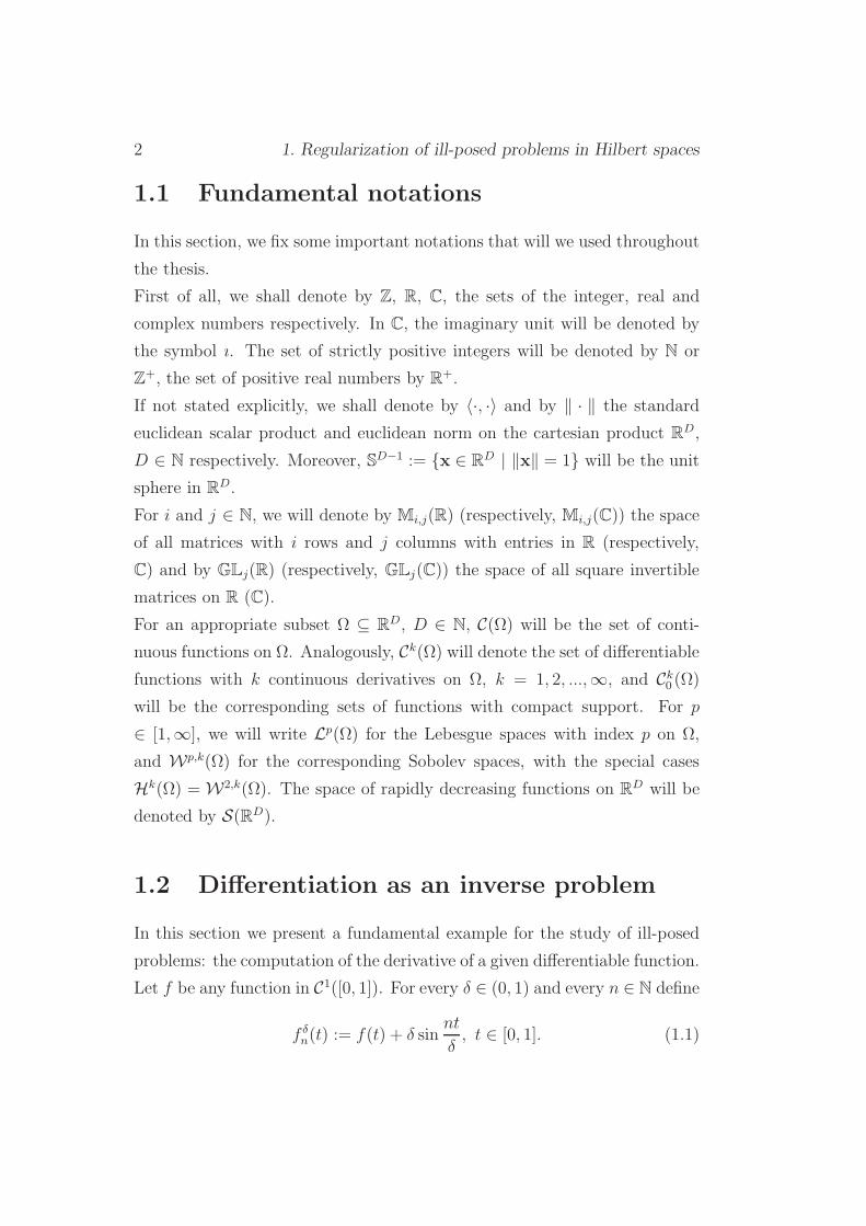
Let f be any function in C1([0, 1]). For every δ ∈ (0, 1) and every n ∈ N define
f δn(t) := f(t) + δ sin
nt
δ, t ∈ [0, 1]. (1.1)

1.2 Differentiation as an inverse problem 3
Thend
dtf δn(t) =
d
dtf(t) + n cos
nt
δ, t ∈ [0, 1],
hence, in the uniform norm,
‖f − f δn‖C([0,1]) = δ
and
‖ ddtf − d
dtf δn‖C([0,1]) = n.
Thus, if we consider f and f δn the exact and perturbed data, respectively, of
the problem compute the derivative dfdt
of the data f , for an arbitrary small
perturbation of the data δ we can obtain an arbitrary large error n in the
result. Equivalently, the operator
d
dt: (C1([0, 1]), ‖ ‖C([0,1])) −→ (C([0, 1]), ‖ ‖C([0,1]))
is not continuous. Of course, it is possible to enforce continuity by measuring
the data in the C1-norm, but this would be like cheating, since to calculate
the error in the data one should calculate the derivative, namely the result.
It is important to notice that dfdt
solves the integral equation
K[x](s) :=
∫ s
0
x(t)dt = f(s)− f(0), (1.2)
i.e. the result can be obtained by inverting the operator K. More precisely,
we have:
Proposition 1.2.1. The linear operator K : C([0, 1]) −→ C([0, 1]) defined
by (1.2) is continuous, injective and surjective onto the linear subspace of
C([0, 1]) denoted by W := x ∈ C1([0, 1]) | x(0) = 0. The inverse of K
d
dt: W −→ C([0, 1])
is unbounded.
If K is restricted to
Sγ := x ∈ C1([0, 1]) | ‖x‖C([0,1]) + ‖dxdt
‖C([0,1]) ≤ γ, γ > 0,
then (K|Sγ)−1 is bounded.

4 1. Regularization of ill-posed problems in Hilbert spaces
Proof. The first part is obvious. For the second part, it is enough to observe
that ‖x‖C([0,1]) + ‖dxdt‖C([0,1]) ≤ γ ensures that Sγ is bounded and equicontinu-
ous in C([0, 1]), thus, according to the Ascoli-Arzela Theorem, Sγ is relatively
compact. Hence (K|Sγ )−1 is bounded because it is the inverse of a bijective
and continuous operator defined on a relatively compact set.
The last statement says that we can restore stability by assuming a-priori
bounds for f ′ and f ′′.
Suppose now we want to calculate the derivative of f via central difference
quotients with step size σ and let f δ be its noisy version with
‖f δ − f‖C([0,1]) ≤ δ. (1.3)
If f ∈ C2[0, 1], a Taylor expansion gives
f(t+ σ)− f(t− σ)
2σ= f ′(t) +O(σ),
but if f ∈ C3[0, 1] the second derivative can be eliminated, thus
f(t+ σ)− f(t− σ)
2σ= f ′(t) +O(σ2).
Remembering that we are dealing with perturbed data
f δ(t+ σ)− f δ(t− σ)
2σ∼ f(t+ σ)− f(t− σ)
2σ+δ
σ,
the total error behaves like
O(σν) +δ
σ, (1.4)
where ν = 1, 2 if f ∈ C2[0, 1] or f ∈ C3[0, 1] respectively.
A remarkable consequence of this is that for fixed δ, when σ is too small,
the total error is large, because of the term δσ, the propagated data error.
Moreover, there exists an optimal discretization parameter σ♯, which cannot
be computed explicitly, since it depends on unavailable information about
the exact data, i.e. the smoothness.
However, if σ ∼ δµ one can search the power µ that minimizes the total error
with respect to δ, obtaining µ = 12if f ∈ C2[0, 1] and µ = 1
3if f ∈ C3[0, 1],

1.2 Differentiation as an inverse problem 5
0 0.2 0.4 0.6 0.8 10
0.2
0.4
0.6
0.8
1
1.2
1.4The behavior of the Total Error in ill−posed problems
Approximation ErrorPropagated Data ErrorTotal Error
Figure 1.1: The typical behavior of the total error in ill-posed problems
with a resulting total error of the order of O(√δ) and O(δ
23 ) respectively.
Thus, in the best case, the total error O(δ23 ) tends to 0 slower than the
data error δ and it can be shown that this result cannot be improved unless
f is a quadratic polynomial: this means that there is an intrinsic loss of
information.
Summing up, in this simple example we have seen some important features
concerning ill-posed problems:
• amplification of high-frequency errors;
• restoration of stability by a-priori assumptions;
• two error terms of different nature, adding up to a total error as in
Figure 1.1;
• appearance of an optimal discretization parameter, depending on a-
priori information;
6 1. Regularization of ill-posed problems in Hilbert spaces
• loss of information even under optimal circumstances.
1.3 Abel integral equations
When dealing with inverse problems, one has often to solve an integral equa-
tion. In this section we present an example which can be described mathe-
matically by means of the Abel Integral Equation. The name is in honor of
the famous Norwegian mathematician N. H. Abel, who studied this problem
for the first time.1
Let a mass element move on the plane R2x1,x2
along a curve Γ from a point
P1 on level h > 0 to a point P0 on level 0. The only force acting on the mass
element is the gravitational force mg.
The direct problem is to determine the time τ in which the element moves
from P1 to P0 when the curve Γ is given. In the inverse problem, one mea-
sures the time τ = τ(h) for several values of h and tries to determine the
curve Γ. Let the curve be parametrized by x1 = ψ(x2). Then Γ = Γ(x2) and
Γ(x2) =
(
ψ(x2)
x2
)
, dΓ(x2) =√
1 + ψ′(x2)2.
According to the conservation of energy,
m
2v2 +mgx2 = mgh,
thus the velocity verifies
v(x2) =√
2g(h− x2).
The total time τ from P1 to P0 is
τ = τ(h) =
∫ P0
P1
dΓ(x2)
v(x2)=
∫ h
0
√
1 + ψ′(x2)2
2g(h− x2)dx2, h > 0.
1This example is taken from [61].
1.4 Radon inversion (X-ray tomography) 7
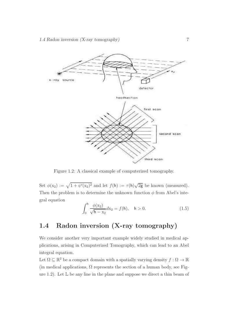
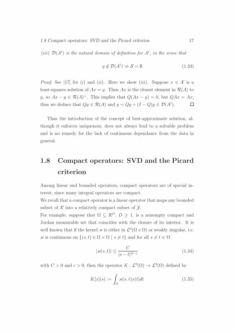
Figure 1.2: A classical example of computerized tomography.
Set φ(x2) :=√
1 + ψ′(x2)2 and let f(h) := τ(h)√2g be known (measured).
Then the problem is to determine the unknown function φ from Abel’s inte-
gral equation∫ h
0
φ(x2)√h− x2
dx2 = f(h), h > 0. (1.5)
1.4 Radon inversion (X-ray tomography)
We consider another very important example widely studied in medical ap-
plications, arising in Computerized Tomography, which can lead to an Abel
integral equation.
Let Ω ⊆ R2 be a compact domain with a spatially varying density f : Ω → R
(in medical applications, Ω represents the section of a human body, see Fig-
ure 1.2). Let L be any line in the plane and suppose we direct a thin beam of
8 1. Regularization of ill-posed problems in Hilbert spaces
X-rays into the body along L and measure how much intensity is attenuated
by going through the body. Let L be parametrized by its normal versor θ ∈S1 and its distance s > 0 from the origin. If we assume that the decay −∆I
of an X-ray beam along a distance ∆t is proportional to the intensity I, the
density f and to ∆t, we obtain
∆I(sθ + tθ⊥) = −I(sθ + tθ⊥)f(sθ + tθ⊥)∆t,
where θ⊥ is a unit vector orthogonal to θ. In the limit for t→ 0, we have
d
dtI(sθ + tθ⊥) = −I(sθ + tθ⊥)f(sθ + tθ⊥).
Thus, if IL(s, θ) and I0(s, θ) denote the intensity of the X-ray beam measured
at the detector and the emitter, respectively, where the detector and the
emitter are connected by the line parametrized by s and θ and are located
outside of Ω, an integration along the line yields
R[f ](s, θ) :=
∫
f(sθ + tθ⊥)dt = − logIL(s, θ)
I0(s, θ), θ ∈ S1, s > 0, (1.6)
where the integration can be made over R, since obviously f = 0 outside of
Ω.
The inverse problem of determining the density distribution f from the X-
ray measurements is then equivalent to solve the integral equation of the first
kind (1.6). The operator R is called the Radon Transform in honor of the
Austrian mathematician J. Radon, who studied the problem of reconstructing
a function of two variables from its line integrals already in 1917 (cf. [75]).
The problem simplifies in the following special case (which is of interest, e.g.
in material testing), where Ω is a circle of radius R, f is radially symmetric,
i.e. f(r, θ) = ψ(r), 0 < r ≤ R, ‖θ‖ = 1 for a suitable function ψ, and we
choose only horizontal lines. If
g(s) := − logIL(s, θ0)
I0(s, θ0)(1.7)
1.5 Integral equations of the first kind 9
denotes the measurements in this situation, with θ0 = (0,±1), for 0 < s ≤ R
we have
R[f ](s, θ0) =
∫
R
f(sθ0 + tθ⊥0 )dt =
∫
R
ψ(√s2 + t2)dt
=
∫ √R2−s2
−√R2−s2
ψ(√s2 + t2)dt = 2
∫ √R2−s2
0
ψ(√s2 + t2)dt
= 2
∫ R
s
rψ(r)√r2 − s2
dr.
(1.8)
Thus we obtain another Abel integral equation of the first kind:
∫ R
s
rψ(r)√r2 − s2
dr =g(s)
2, 0 < s ≤ R. (1.9)
In the case g(R) = 0, the Radon Transform can be explicitly inverted and
ψ(r) = −1
π
∫ R
r
g′(s)√s2 − r2
ds. (1.10)
We observe from the last equation that the inversion formula involves the
derivative of the data g, which can be considered as an indicator of the ill-
posedness of the problem. However, here the data is integrated and thus
smoothed again, but the kernel of this integral operator has a singularity for
s = r, so we expect the regularization effect of integration to be only partial.
This heuristic statement can be made more precise, as we shall see later in
Chapter 4.
1.5 Integral equations of the first kind
In Section 1.3, starting from a physical problem, we have constructed a very
simple mathematical model based on the integral equation (1.5), where we
have to recover the unknown function φ from the data f . Similarly, in Sec-
tion 1.4 we have seen that an analogous equation is obtained to recover the
function ψ from the measured data g.
As a matter of fact, very often ill-posed problems lead to integral equations.
In particular, Abel integral equations such as (1.5) and (1.10) fall into the

10 1. Regularization of ill-posed problems in Hilbert spaces
class of the Fredholm equations of the first kind whose definition is recalled
below.
Definition 1.5.1. Let s1 < s2 be real numbers and let κ, f and φ be real va-
lued functions defined respectively on [s1, s2]2, [s1, s2] and [s1, s2]. A Fredholm
equation of the first kind is an equation of the form
∫ s2
s1
κ(s, t)φ(t)dt = f(s) s ∈ [s1, s2]. (1.11)
Fredholm integral equations of the first kind must be treated accurately
(see [22] as a general reference): if κ is continuous and φ is integrable, then
it is easy to see that f is also continuous, thus if the data is not continuous
while the kernel is, then (1.11) has no integrable solution. This means that
the question of existence is not trivial and requires investigation. Concerning
the uniqueness of the solutions, take for example κ(s, t) = s sin t, f(s) = s
and [s1, s2] = [0, π]: then φ(t) = 1/2 is a solution of (1.11), but so is each of
the functions φn(t) = 1/2 + sinnt, n ∈ N.
Moreover, we also observe that if κ is square integrable, as a consequence of
the Riemann-Lebesgue lemma, there holds
∫ π
0
κ(s, t) sin(nt)dt→ 0 as n→ +∞. (1.12)
Thus if φ is a solution of (1.11) and C is arbitrarily large
∫ π
0
κ(s, t)(φ(t) + C sin(nt))dt→ f(s) as n→ +∞ (1.13)
and for large values of n the slightly perturbed data
f(s) := f(s) + C
∫ π
0
κ(s, t) sin(nt)dt (1.14)
corresponds to a solution φ(t) = φ(t) +C sin(nt) which is arbitrarily distant
from φ. In other words, as in the example considered in Section 1.2, the
solution doesn’t depend continuously on the data.
1.6 Hadamard’s definition of ill-posed problems 11
1.6 Hadamard’s definition of ill-posed pro-
blems
Integral equations of the first kind are the most famous example of ill-posed
problems. The definition of ill-posedness goes back to the beginning of the
20-th century and was stated by J. Hadamard as follows:
Definition 1.6.1. Let F be a mapping from a topological space X to another
topological space Y and consider the abstract equation
F (x) = y.
The equation is said to be well-posed if
(i) for each y ∈ Y, a solution x ∈ X of F (x) = y exists;
(ii) the solution x is unique in X ;
(iii) the dependence of x upon y is continuous.
The equation is said to be ill-posed if it is not well-posed.
Of course, the definition of well-posedness above is equivalent to the re-
quest that F is surjective and injective and that the inverse mapping F−1 is
continuous.
For example, due to the considerations made in the previous sections, inte-
gral equations of the first kind are examples ill-posed equations. If X = Y is
a Hilbert space and F = A is a linear, self-adjoint operator with its spectrum
contained in [0,+∞[, the equation of the second kind
y = Ax+ tx
is well-posed for every t > 0, since the operator A + t is invertible and its
inverse (A+ t)−1 is also continuous.
12 1. Regularization of ill-posed problems in Hilbert spaces
1.7 Fundamental tools in the Hilbert space
setting
So far, we have seen several examples of ill-posed problems. It is obvious
from Hadamard’s definition of ill-posedness that an exhaustive mathematical
treatment of such problems should be based on a different notion of solution
of the abstract equation F (x) = y to achieve existence and uniqueness. For
linear problems in the Hilbert space setting, this is done with the Moore-
Penrose Generalized Inverse.
At first, we fix some standard definitions and notations. General references
for this section are [17] and [21].
1.7.1 Basic definitions and notations
Let A be a linear bounded (continuous) operator between two Hilbert Spaces
X and Y . To simplify the notations, the scalar products in X and Y and
their induced norms will be denoted by the same symbols 〈·, ·〉 and ‖ · ‖respectively. For x ∈ X and δ > 0,
Bδ(x) := x ∈ X | ‖x− x‖ < δ (1.15)
is the open ball centered in x with radius δ and Bδ(x) or Bδ(x) is its closure
with respect to the topology of X .
We denote by R(A) the range of A:
R(A) := y ∈ Y | ∃ x ∈ X : y = Ax (1.16)
and by ker(A) the null-space of A:
ker(A) := x ∈ X | Ax = 0. (1.17)
We recall that R(A) and ker(A) are subspaces of Y and X respectively and
that ker(A) is closed.
We also recall the following basic definitions.
1.7 Fundamental tools in the Hilbert space setting 13
Definition 1.7.1 (Orthogonal space). Let M ⊆ X . The orthogonal space
of M is the closed vector space M⊥ defined by:
M⊥ := x ∈ X | 〈x, z〉 = 0, ∀z ∈ M. (1.18)
Definition 1.7.2 (Adjoint operator). The bounded operator A∗ : Y → X ,
defined as
〈A∗y, x〉 = 〈y, Ax〉, ∀x ∈ X , y ∈ Y , (1.19)
is called the adjoint operator of A.
If A : X → X and A = A∗, then A is called self-adjoint.
Definition 1.7.3 (Orthogonal projector). Let W be a subspace of X .
For every x ∈ X , there exist a unique element in W, called the projection of
x onto W, that minimizes the distance ‖x− w‖, w ∈ W.
The map P : X → X , that associates to an element x ∈ X its projection
onto W, is called the orthogonal projector onto W.
This is the unique linear and self-adjoint operator satisfying the relation P =
P 2 that maps X onto W.
Definition 1.7.4. Let xnn∈N be a sequence in X and let x ∈ X . The
sequence xn is said to converge weakly to x if, for every z ∈ X , 〈xn, z〉converges to 〈x, z〉. In this case, we shall write
xn x.
1.7.2 The Moore-Penrose generalized inverse
We are interested in solving the equation
Ax = y, (1.20)
for x ∈ X , but we suppose we are only given an approximation of the exact
data y ∈ Y , which are assumed to exist and to be fixed, but unknown.

14 1. Regularization of ill-posed problems in Hilbert spaces
Definition 1.7.5. (i) A least-squares solution of the equation Ax = y is
an element x ∈ X such that
‖Ax− y‖ = infz∈X
‖Az − y‖. (1.21)
(ii) An element x ∈ X is a best-approximate solution of Ax = y if it is a
least-squares solution of Ax = y and
‖x‖ = inf‖z‖ | z is a least-squares solution of ‖Ax− y‖ (1.22)
holds.
(iii) The Moore-Penrose (generalized) inverse A† of A is the unique linear
extension of A−1 to
D(A†) := R(A) +R(A)⊥ (1.23)
with
ker(A†) = R(A)⊥, (1.24)
where
A := A|ker(A)⊥ : ker(A)⊥ → R(A). (1.25)
A† is well defined: in fact, it is trivial to see that ker(A) = 0 and
R(A) = R(A), so R(A)−1 exists. Moreover, since R(A)⋂R(A)⊥ = 0,
every y ∈ D(A†) can be written in a unique way as y = y1 + y2, with y1 ∈R(A) and y2 ∈ R(A)⊥, so using (1.24) and the requirement that A† is linear,
one can easily verify that A†y = A−1y1.
The Moore Penrose generalized inverse can be characterized as follows.
Proposition 1.7.1. Let now and below P and Q be the orthogonal projectors
onto ker(A) and R(A), respectively. Then R(A†) = ker(A)⊥ and the four
Moore-Penrose equations hold:
AA†A = A, (1.26)
A†AA† = A†, (1.27)
1.7 Fundamental tools in the Hilbert space setting 15
A†A = I − P, (1.28)
AA† = Q|D(A†). (1.29)
Here and below, the symbol I denotes the identity map.
If a linear operator A : D(A†) → X verifies (1.28) and (1.29), then A = A†.
Proof. For the first part, see [17]. We show the second part.
Since AAA = AQ|D(A†) = A and AAA = A(I − P ) = A − AP = A, all
Moore-Penrose equations hold for A. Then, keeping in mind that I − P is
the orthogonal projector onto ker(A)⊥, for every y ∈ D(A†) we have: Ay =
AAAy = (I − P )Ay = A−1A(I − P )Ay = A−1AAy = A−1Qy = A†y.
An application of the Closed Graph Theorem leads to the following im-
portant fact.
Proposition 1.7.2. The Moore-Penrose generalized inverse A† has a closed
graph gr(A†). Furthermore, A† is continuous if and only if R(A) is closed.
We use this to give another characterization of the Moore-Penrose pseu-
doinverse:
Proposition 1.7.3. There can be only one linear bounded operator
A : Y → X that verifies (1.26) and (1.27) and such that AA and AA are self-
adjoint. If such an A exists, then A† is also bounded and A = A†. Moreover,
in this case, the Moore-Penrose generalized inverse of the adjoint of A, (A∗)†,
is bounded too and
(A∗)† = (A†)∗. (1.30)
Proof. Suppose A, B : Y → X are linear bounded operators that verify (1.26)
and (1.27) and such that AA, BA, AA and AB are self-adjoint.
Then
AA = A∗A∗ = (A∗B∗A∗)A∗ = (A∗B∗)(A∗A∗) = (BA)(AA) = B(AAA) = BA
16 1. Regularization of ill-posed problems in Hilbert spaces
and in a similar way AB = AA. Thus we obtain
A = A(AA) = A(AB) = (AA)B = (BA)B = B.
Suppose now that such an operator A exists. For every z ∈ Y and every y ∈R(A), y = limn→+∞Axn, xn ∈ X , we have
〈y, z〉 = limn→+∞
〈Axn, z〉 = limn→+∞
〈xn, A∗z〉 =
= limn→+∞
〈xn, A∗A∗A∗z〉 = 〈AAy, z〉,
so y = AAy and y lies in R(A). This means that R(A) is closed, thus
according to Proposition 1.7.2 A† is bounded and for the first part of the
proof A† = A.
Finally, to prove the last statement it is enough to verify that for the linear
bounded operator (A†)∗ conditions (1.26) and (1.27) hold with A replaced
by A∗, together with the the correspondent self-adjointity conditions, which
consists just of straightforward calculations.
The definitions of least-squares solution and best-approximate solution
make sense too: if y ∈ D(A†), the set S of the least-squares solutions of
Ax = y is non-empty and its best-approximate solution turns out to be
unique and strictly linked to the operator A†. More precisely, we have:
Proposition 1.7.4. Let y ∈ D(A†). Then:
(i) Ax = y has a unique best-approximate solution, which is given by
x† := A†y. (1.31)
(ii) The set S of the least-squares solutions of Ax = y is equal to x†+
ker(A) and every x ∈ X lies in S if and only if the normal equation
A∗Ax = A∗y (1.32)
holds.
1.8 Compact operators: SVD and the Picard criterion 17
(iii) D(A†) is the natural domain of definition for A†, in the sense that
y /∈ D(A†) ⇒ S = ∅. (1.33)
Proof. See [17] for (i) and (ii). Here we show (iii). Suppose x ∈ X is a
least-squares solution of Ax = y. Then Ax is the closest element in R(A) to
y, so Ax − y ∈ R(A)⊥. This implies that Q(Ax − y) = 0, but QAx = Ax,
thus we deduce that Qy ∈ R(A) and y = Qy + (I −Q)y ∈ D(A†).
Thus the introduction of the concept of best-approximate solution, al-
though it enforces uniqueness, does not always lead to a solvable problem
and is no remedy for the lack of continuous dependance from the data in
general.
1.8 Compact operators: SVD and the Picard
criterion
Among linear and bounded operators, compact operators are of special in-
terest, since many integral operators are compact.
We recall that a compact operator is a linear operator that maps any bounded
subset of X into a relatively compact subset of Y .
For example, suppose that Ω ⊆ RD, D ≥ 1, is a nonempty compact and
Jordan measurable set that coincides with the closure of its interior. It is
well known that if the kernel κ is either in L2(Ω×Ω) or weakly singular, i.e.
κ is continuous on (s, t) ∈ Ω× Ω | s 6= t and for all s 6= t ∈ Ω
|κ(s, t)| ≤ C
|s− t|D−ǫ(1.34)
with C > 0 and ǫ > 0, then the operator K : L2(Ω) → L2(Ω) defined by
K[x](s) :=
∫
Ω
κ(s, t)x(t)dt (1.35)

18 1. Regularization of ill-posed problems in Hilbert spaces
is compact (see e.g. [20]).2
If a compact linear operator K is also self-adjoint, the notion of eigensystem
is well-defined (a proof of the existence of an eigensystem and a more exhaus-
tive treatment of the argument can be found e.g. in [62]): an eigensystem
(λj; vj)j∈N of the operator K consists of all nonzero eigenvalues λj ∈ R of
K and a corresponding complete orthonormal set of eigenvectors vj . Then
K can be diagonalized by means of the formula
Kx =
∞∑
j=1
λj〈x, vj〉vj , ∀x ∈ X (1.36)
and the nonzero eigenvalues of K converge to 0.
If K : X → Y is not self-adjoint, then observing that the operators K∗K : X→ X and KK∗ : Y → Y are positive semi-definite and self-adjoint compact
operators with the same set of nonzero eigenvalues written in nondecreasing
order with multiplicity
λ21 ≥ λ22 ≥ λ23..., λj > 0 ∀j ∈ N,
we define a singular system λj ; vj, ujj∈N. The vectors vj form a complete
orthonormal system of eigenvectors of K∗K and uj, defined as
uj :=Kvj
‖Kvj‖, (1.37)
form a complete orthonormal system of eigenvectors of KK∗. Thus vjj∈Nspan R(K∗) = R(K∗K), ujj∈N span R(K) = R(KK∗) and the following
formulas hold:
Kvj = λjuj, (1.38)
K∗uj = λjvj, (1.39)
Kx =∞∑
j=1
λj〈x, vj〉uj, ∀x ∈ X , (1.40)
2Here and below, we shall denote with the symbol K a linear and bounded operator
which is also compact.
1.8 Compact operators: SVD and the Picard criterion 19
K∗y =
∞∑
j=1
λj〈y, uj〉vj, ∀y ∈ Y . (1.41)
All the series above converge in the Hilbert space norms of X and Y .
Equations (1.40) and (1.41) are the natural infinite-dimensional extension of
the well known singular value decomposition (SVD) of a matrix.
For compact operators, the condition for the existence of the best-approximate
solution K†y of the equation Kx = y can be written down in terms of the
singular value expansion of K. It is called the Picard Criterion and can be
given by means of the following theorem (see [17] for the proof).
Theorem 1.8.1. Let λj; vj , ujj∈N be a singular system for the compact
linear operator K an let y ∈ Y. Then
y ∈ D(K†) ⇐⇒∞∑
j=1
|〈y, uj〉|2λ2j
< +∞ (1.42)
and whenever y ∈ D(K†),
K†y =∞∑
j=1
〈y, uj〉λj
vj . (1.43)
Thus the Picard Criterion states that the best-approximate solution x†
of Kx = y exists only if the SVD coefficients |〈y, uj〉| decay fast-enough with
respect to the singular values λj.
In the finite dimensional case, of course the sum in (1.42) is always finite, the
best-approximate solution always exists and the Picard Criterion is always
satisfied.
From (1.43) we can see that in the case of perturbed data, the error compo-
nents with respect to the the basis uj corresponding to the small values of
λj are amplified by the large factors λ−1j . For example, if dim(R(K)) = +∞
and the perturbed data is defined by yδj := y + δuj, then ‖y − yδj‖ = δ, but
K†y −K†yδj = λ−1j 〈δuj, uj〉vj
and hence
‖K†y −K†yδj‖ = λ−1j δ → +∞ as j → +∞.
20 1. Regularization of ill-posed problems in Hilbert spaces
In the finite dimensional case there are only finitely many eigenvalues, so
these amplification factors stay bounded. However, they might be still very
large: this is the case of the discrete ill-posed problems, for which also a
Discrete Picard Condition can be defined, as we shall see later on.
1.9 Regularization and Bakushinskii’s Theo-
rem
In the previous sections, we started discussing the problem of solving the
equation Ax = y. In practice, the exact data y is not known precisely, but
only approximations yδ with
‖yδ − y‖ ≤ δ (1.44)
is available. In literature, yδ ∈ Y is called the noisy data and δ > 0 the noise
level.
Our purpose is to approximate the best-approximate solution x† = A†y of
(1.20) from the knowledge of δ, yδ and A.
According to Proposition 1.7.2, in general the operator A† is not continuous,
so in the ill-posed case A†yδ is in general a very bad approximation of x†
even if it exists. Roughly speaking, regularizing Ax = y means essentially to
construct of a family of continuous operators Rσ, depending on a certain
regularization parameter σ, that approximate A† (in some sense) and such
that xδσ := Rσyδ satisfies the conditions above. We state this more precisely
in the following fundamental definition.
Definition 1.9.1. Let σ0 ∈ (0,+∞]. For every σ ∈ (0, σ0), let Rσ : Y → Xbe a continuous (not necessarily linear) operator.
The family Rσ is called a regularization operator for A† if, for every y ∈D(A†), there exists a function
α : (0,+∞)× Y → (0, σ0),
1.9 Regularization and Bakushinskii’s Theorem 21
called parameter choice rule for y, that allows to associate to each cou-
ple (δ, yδ) a specific operator Rα(δ,yδ) and a regularized solution xδα(δ,yδ) :=
Rα(δ,yδ)yδ, and such that
limδ→0
supyδ∈Bδ(y)
α(δ, yδ) = 0. (1.45)
If the parameter choice rule (below, p.c.r.) α satisfies in addition
limδ→0
supyδ∈Bδ(y)
‖Rα(δ,yδ)yδ −A†y‖ = 0. (1.46)
then it is said to be convergent.
For a specific y ∈ D(A†), a pair (Rσ, α) is called a (convergent) regularization
method for solving Ax = y if Rσ is a regularization for A† and α is a
(convergent) parameter choice rule for y.
Remark 1.9.1. • In the definition above all possible noisy data with
noise level ≤ δ are considered, so the convergence is intended in a
worst-case sense.
However, in a specific problem, a sequence of approximate solutions
xδnα(δn,yδn )
can converge fast to x† also when (1.46) fails!
• A p.c.r. α = α(δ, yδ) depends explicitly on the noise level and on the
perturbed data yδ.
According to the definition above it should also depend on the exact data
y, which is unknown, so this dependance can only be on some a priori
knowledge about y like smoothness properties.
We distinguish between two types of parameter choice rules:
Definition 1.9.2. Let α be a parameter choice rule according to Definition
1.9.1. If α does not depend on yδ, but only on δ, then we call α an a-
priori parameter choice rule and write α = α(δ). Otherwise, we call α an
a-posteriori parameter choice rule. If α does not depend on the noise level δ,
then it is said to be an heuristic parameter choice rule.
22 1. Regularization of ill-posed problems in Hilbert spaces
If α does not depend on yδ it can be defined before the actual calculations
once and for all: this justifies the terminology a-priori and a-posteriori in the
definition above.
For the choice of the parameter, one can also construct a p.c.r. that depends
explicitly only on the perturbed data yδ and not on the noise level. However,
a famous result due to Bakushinskii shows that such a p.c.r. cannot be
convergent:
Theorem 1.9.1 (Bakushinskii). Suppose Rσ is a regularization operator
for A† such that for every y ∈ D(A†) there exists a convergent p.c.r. α which
depends only on yδ. Then A† is bounded.
Proof. If α = α(yδ), then it follows from (1.46) that for every y ∈ D(A†) we
have
limδ→0
supyδ∈Bδ(y)
‖Rα(yδ)yδ − A†y‖ = 0, (1.47)
so that Rα(y)y = A†y. Thus, if ynn∈N is a sequence in D(A†) converging to
y, then A†yn = Rα(yn)yn converges to A†y. This means that A† is sequentially
continuous, hence it is bounded.
Thus, in the ill-posed case, no heuristic parameter choice rule can yield a
convergent regularization method. However, this doesn’t mean that such a
p.c.r. cannot give good approximations of x† for a fixed positive δ!
1.10 Construction and convergence of regu-
larization methods
In general terms, regularizing an ill-posed problem leads to three questions:
1. How to construct a regularization operator?
2. How to choose a parameter choice rule to give rise to convergent regu-
larization methods?
1.10 Construction and convergence of regularization methods 23
3. How can these steps be performed in some optimal way?
This and the following sections will deal with the answers of these problems,
at least in the linear case. The following result provides a characterization
of the regularization operators. Once again, we refer to [17] for more details
and for the proofs.
Proposition 1.10.1. Let Rσσ>0 be a family of continuous operators con-
verging pointwise on D(A†) to A† as σ → 0.
Then Rσ is a regularization for A† and for every y ∈ D(A†) there exists
an a-priori p.c.r. α such that (Rσ, α) is a convergent regularization method
for solving Ax = y.
Conversely, if (Rσ, α) is a convergent regularization method for solving Ax =
y with y ∈ D(A†) and α is continuous with respect to δ, then Rσy converges
to A†y as σ → 0.
Thus the correct approach to understand the meaning of regularization
is pointwise convergence. Furthermore, if Rσ is linear and uniformly
bounded, in the ill-posed case we can’t expect convergence in the opera-
tor norm, since then A† would have to be bounded.
We consider an example of a regularization operator which fits the definitions
above. Although very similar examples can be found in literature, cf. e.g.
[61], this is slightly different.
Example 1.10.1. Consider the operator K : X := L2[0, 1] → Y := L2[0, 1]
defined by
K[x](s) :=
∫ s
0
x(t)dt.
Then K is linear, bounded and compact and it is easily seen that
R(K) = y ∈ H1[0, 1] | y ∈ C([0, 1]), y(0) = 0 (1.48)
and that the distributional derivative from R(K) to X is the inverse of K.
Since R(K) ⊇ C∞0 [0, 1], R(K) is dense in Y and R(K)⊥ = 0.
24 1. Regularization of ill-posed problems in Hilbert spaces
For y ∈ C([0, 1]) and for σ > 0, define
(Rσy)(t) :=
1σ(y(t+ σ)− y(t)), if 0 ≤ t ≤ 1
2,
1σ(y(t)− y(t− σ)), if 1
2< t ≤ 1.
(1.49)
Then Rσ is a family of linear and bounded operators with
‖Rσy‖L2[0,1] ≤√6
σ‖y‖L2[0,1] (1.50)
defined on a dense linear subspace of L2[0, 1], thus it can be extended to the
whole Y and (1.50) is still true.
Since the measure of [0, 1] is finite, for y ∈ R(K) the distributional derivative
of y lies in L1[0, 1], so y is a function of bounded variation. Thus, according
to Lebesgue’s Theorem, the ordinary derivative y′ exists almost everywhere
in [0, 1] and it is equal to the distributional derivative of y as an L2-function.
Consequently, we can apply the Dominate Convergence Theorem to show that
‖Rσy −K†y‖L2[0,1] → 0, as σ → 0
so that, according to Proposition 1.10.1, Rσ is a regularization for the distri-
butional derivative K†.
1.11 Order optimality
We concentrate now on how to construct optimal regularization methods. To
this aim, we shall make use of some analytical tools from the spectral theory
of linear and bounded operators. For the reader who is not accustomed with
the spectral theory, we refer to Appendix A or to the second chapter of [17],
where the basic ideas and results we will need are gathered in a few pages;
for a more comprehensive treatment, classical references are e.g. [2] and [44].
In principle, a (convergent) regularization method (Rσ, α) for solving Ax = y
should be optimal if the quantity
ε1 = ε1(δ, Rσ, α) := supyδ∈Bδ(y)
‖Rα(δ,yδ)yδ − A†y‖ (1.51)
1.11 Order optimality 25
converges to 0 as quickly as
ε2 = ε2(δ) := inf(Rσ ,α)
supyδ∈Bδ(y)
‖Rα(δ,yδ)yδ −A†y‖, (1.52)
i.e. if there are no regularization methods for which the approximate solu-
tions converge to 0 (in the usual worst-case sense) quicker than the approxi-
mate solutions of (Rσ, α).
Once again, it is not advisable to look for some uniformity in y, as we can
see from the following result.
Proposition 1.11.1. Let Rσ be a regularization for A† with Rσ(0) = 0,
let α = α(δ, yδ) be a p.c.r. and suppose that R(A) is non closed. Then there
can be no function f : (0,+∞) → (0,+∞) with limδ→0 f(δ) = 0 such that
ε1(δ, Rσ, α) ≤ f(δ) (1.53)
holds for every y ∈ D(A†) with ‖y‖ ≤ 1 and all δ > 0.
Thus convergence can be arbitrarily slow: in order to study convergence
rates of the approximate solutions to x† it is necessary to restrict on subsets
of D(A†) (or of X ), i.e. to formulate some a-priori assumption on the exact
data (or equivalently, on the exact solution). This can be done by introducing
the so called source sets, which are defined as follows.
Definition 1.11.1. Let µ, ρ > 0. An element x ∈ X is said to have a source
representation if it belongs to the source set
Xµ,ρ := x ∈ X | x = (A∗A)µw, ‖w‖ ≤ ρ. (1.54)
The union with respect to ρ of all source sets is denoted by
Xµ :=⋃
ρ>0
Xµ,ρ = x ∈ X | x = (A∗A)µw = R((A∗A)µ). (1.55)
Here and below, we use spectral theory to define
(A∗A)µ :=
∫
λµdEλ, (1.56)

26 1. Regularization of ill-posed problems in Hilbert spaces
where Eλ is the spectral family associated to the self-adjoint A∗A (cf. Ap-
pendix A) and since A∗A ≥ 0 the integration can be restricted to the compact
set [0, ‖A∗A‖] = [0, ‖A‖2].
Since A is usually a smoothing operator, the requirement for an element
to be in Xµ,ρ can be considered as a smoothness condition.
The notion of optimality is based on the following result about the source
sets, which is stated for compact operators, but can be extended to the non
compact case (see [17] and the references therein).
Proposition 1.11.2. Let A be compact with R(A) being non closed and let
Rσ be a regularization operator for A†. Define also
∆(δ,Xµ,ρ, Rσ, α) := sup‖Rα(δ,yδ)yδ − x‖ | x ∈ Xµ,ρ, y
δ ∈ Bδ(Ax) (1.57)
for any fixed µ, ρ and δ in (0,+∞) (and α a p.c.r. relative to Ax). Then
there exists a sequence δk converging to 0 such that
∆(δk,Xµ,ρ, Rσ, α) ≥ δ2µ
2µ+1
k ρ1
2µ+1 . (1.58)
This justifies the following definition.
Definition 1.11.2. Let R(A) be non closed, let Rσ be a regularization for
A† and let µ, ρ > 0.
Let α be a p.c.r. which is convergent for every y ∈ AXµ,ρ.
We call (Rσ, α) optimal in Xµ,ρ if
∆(δ,Xµ,ρ, Rσ, α) = δ2µ
2µ+1ρ1
2µ+1 (1.59)
holds for every δ > 0.
We call (Rσ, α) of optimal order in Xµ,ρ if there exists a constant C ≥ 1 such
that
∆(δ,Xµ,ρ, Rσ, α) ≤ Cδ2µ
2µ+1ρ1
2µ+1 (1.60)
holds for every δ > 0.
1.11 Order optimality 27
The term optimality refers to the fact that if R(A) is non closed, then
a regularization algorithm cannot converge to 0 faster than δ2µ
2µ+1ρ1
2µ+1 as
δ → 0, under the a-priori assumption x ∈ Xµ,ρ, or (if we are concerned with
the rate only), not faster than O(δ2µ
2µ+1 ) under the a-priori assumption x ∈Xµ. In other words, we prove the following fact:
Proposition 1.11.3. With the assumption of Definition 1.11.2, (Rσ, α) is
of optimal order in Xµ,ρ if and only if there exists a constant C ≥ 1 such that
for every y ∈ AXµ,ρ
supyδ∈Bδ(y)
‖Rα(δ,yδ)yδ − x†‖ ≤ Cδ
2µ2µ+1ρ
12µ+1 (1.61)
holds for every δ > 0. For the optimal case an analogous result is true.
Proof. First, we show that y ∈ AXµ,ρ if and only if y ∈ R(A) and x† ∈ Xµ,ρ.
The sufficiency is obvious because of (1.29). For the necessity, we observe
that if x = (A∗A)µw, with ‖w‖ ≤ ρ, then x lies in (kerA)⊥, since for every
z ∈ kerA we have:
〈x, z〉 = 〈(A∗A)µw, z〉 = limǫ→0
∫ ‖A‖2
ǫ
λµd〈w,Eλz〉
= limǫ→0
∫ ‖A‖2
ǫ
λµd〈w, z〉 = 0.
(1.62)
We obtain that x† = A†y = A†Ax = (I − P )x = x is the only element in
Xµ,ρ
⋂A−1(y), thus the entire result follows immediately and the proof is
complete.
The following result due to R. Plato assures that, under very weak as-
sumptions, the order-optimality in a source set implies convergence in R(A).
More precisely:
Theorem 1.11.1. Let Rσ a regularization for A†. For s > 0, let αs be the
family of parameter choice rules defined by
αs(δ, yδ) := α(sδ, yδ), (1.63)

28 1. Regularization of ill-posed problems in Hilbert spaces
where α is a parameter choice rule for Ax = y, y ∈ R(A).
Suppose that for every τ > τ0, τ0 ≥ 1, (Rσ, ατ) is a regularization method of
optimal order in Xµ,ρ, for some µ, ρ > 0.
Then, for every τ > τ0, (Rσ, ατ ) is convergent for every y ∈ R(A) and it is
of optimal order in every Xν,ρ, with 0 < ν ≤ µ.
It is worth mentioning that the source sets Xµ,ρ are not the only possible
choice one can make. They are well-suited for operators A whose spectrum
decays to 0 as a power of λ, but they don’t work very well in the case of
exponentially ill-posed problems in which the spectrum of A decays to 0 ex-
ponentially fast. In this case, different source conditions such as logarithmic
source conditions should be used, for which analogous results and definitions
can be stated. In this work logarithmic and other different source conditions
shall not be considered. A deeper treatment of this argument can be found,
e.g., in [47].
1.12 Regularization by projection
In practice, regularization methods must be implemented in finite-dimensional
spaces, thus it is important to see what happens when the data and the
solutions are approximated in finite-dimensional spaces. It turns out that
this important passage from infinite to finite dimensions can be seen as a
regularization method itself. One approach to deal with this problem is
regularization by projection, where the approximation is the projection onto
finite-dimensional spaces alone: many important regularization methods are
included in this category, such as discretization, collocation, Galerkin or Ritz
approximation.
The finite-dimensional approximations can be made both in the spaces Xand Y : here we consider only the first one.
We approximate x† as follows: given a sequence of subspaces of X
X1 ⊆ X2 ⊆ X3... (1.64)
1.12 Regularization by projection 29
such that⋃
n∈NXn = X , (1.65)
the n-th approximation of x† is
xn := A†ny, (1.66)
where An = APn and Pn is the orthogonal projector onto Xn. Note that since
An has finite-dimensional range, R(An) is closed and thus A†n is bounded (i.e.
xn is a stable approximation of x†). Moreover, it is an easy exercise to show
that xn is the minimum norm solution of Ax = y in Xn: for this reason, this
method is called least-squares projection.
Note that the iterates xn may not converge to x† in X , as the following
example due to Seidman shows. We reconsider it entirely in order to correct
a small inaccuracy which can be found in the presentation of this example
in [17].
1.12.1 The Seidman example (revisited)
Suppose X is infinite-dimensional, let en be an orthonormal basis for Xand let Xn := spane1, ...en, for every n ∈ N. Then of course Xn satisfies
(1.64) and (1.65). Define an operator A : X → Y as follows:
A(x) = A
( ∞∑
j=1
xjej
)
:=∞∑
j=1
(xjaj + bjx1) ej , (1.67)
with
|bj| :=
0 if j = 1,
j−1 if j > 1,(1.68)
|aj| :=
j−1 if j is odd,
j−52 if j is even.
(1.69)
Then:
• A is well defined, since |ajxj + bjx1|2 ≤ 2 (|xj |2 + |x1|j−2) for every j
and linear.
30 1. Regularization of ill-posed problems in Hilbert spaces
• A is injective: Ax = 0 implies
(a1x1, a2x2 + b2x1, a3x3 + b3x1, ...) = 0,
thus xj = 0 for every j, i.e. x = 0.
• A is compact: in fact, suppose xkk∈N is a bounded sequence in X .
Then also the first components of xk, denoted by xk,1, form a bounded
sequence in C, which has a convergent subsequence xkl,1 and, in cor-
respondence,∑∞
j=1 bjxkl,1ej is a subsequence of∑∞
j=1 bjxk,1ej conver-
ging in X to∑∞
j=1 bj liml→∞ xkl,1ej . Consequently, the application x 7→∑∞
j=1 bjx1ej is compact. Moreover, the application x 7→ ∑∞j=1 ajxjej
is also compact, because it is the limit of the sequence of operators
defined by Anx :=∑n
j=1 ajxjej . Thus, being the sum of two compact
operators, A is compact (see, e.g., [62] for the properties of the compact
operators used here).
Let y := Ax† with
x† :=∞∑
j=1
j−1ej (1.70)
and let xn :=∑∞
j=1 xn,jej be the best-approximate solution of Ax = y in Xn.
Then it is readily seen that xn := (xn,1, xn,2, ..., xn,n) is the vector minimizing
n∑
j=1
(aj(xj − j−1) + bj(x1 − 1)
)2+
∞∑
j=n+1
j−2(1 + aj − x1)2 (1.71)
among all x = (x1, ..., xn) ∈ Cn.
Imposing that the gradient of (1.71) with respect to x is equal to 0 for x =
xn, we obtain
2a21(xn,1 − 1)− 2
∞∑
j=n+1
j−2(1 + aj − xn,1) = 0,
2n∑
j=1
(aj(xn,j − j−1) + bj(xn,1 − 1)
)ajδj,k, k = 2, ..., n.

1.12 Regularization by projection 31
Here, δj,k is the Kronecker delta, which is equal to 1 if k = j and equal to 0
otherwise.
Consequently, for the first variable xn,1 we have
xn,1 =
(
1 +∞∑
j=n+1
(1 + aj)j−2
)(
1 +∞∑
j=n+1
j−2
)−1
= 1 +
( ∞∑
j=n+1
ajj−2
)(
1 +
∞∑
j=n+1
j−2
)−1(1.72)
and for every k = 2, ..., n there holds
xn,k = (ak)−1(k−1ak − bk(xn,1 − 1)
)= k−1 − (akk)
−1(xn,1 − 1). (1.73)
We use this to calculate
‖xn − Pnx†‖2 = ‖
n∑
j=1
(xn,j − j−1)ej‖2
= (xn,1 − 1)2 +n∑
j=2
(j−1 − (ajj)
−1(xn,1 − 1)− j−1)2
= (xn,1 − 1)2
(
1 +n∑
j=2
(ajj)−2
)
=
(n∑
j=1
(ajj)−2
)( ∞∑
j=n+1
ajj−2
)2(
1 +∞∑
j=n+1
j−2
)−2
.
(1.74)
Of these three factors, the third one is clearly convergent to 1.
The first one behaves like n4, since, applying Cesaro’s rule to
sn :=
∑nj=1 j
3
n4,
we obtain
limn→∞
sn = limn→∞
(n+ 1)3
(n+ 1)4 − n4=
1
4.
Similarly,∞∑
j=n+1
ajj−2 ∼
∞∑
j=n+1
j−3 ∼ n−2,
32 1. Regularization of ill-posed problems in Hilbert spaces
because∑∞
j=n+1 j−3
n−2∼ −(n + 1)−3
(n+ 1)−2 − n−2=
n2(n+ 1)−1
(n+ 1)2 − n2→ 1
2.
These calculations show that
||xn − Pnx†|| → λ > 0, (1.75)
so xn doesn’t converge to x†, which was what we wanted to prove.
The following result gives sufficient (and necessary) conditions for con-
vergence.
Theorem 1.12.1. For y ∈ D(A†), let xn be defined as above. Then
(i) xn x† ⇐⇒ ‖xn‖ is bounded;
(ii) xn → x† ⇐⇒ lim supn→+∞
‖xn‖ ≤ ‖x†‖;
(iii) if
lim supn→+∞
‖(A†n)
∗xn‖ = lim supn→+∞
‖(A∗n)
†xn‖ <∞, (1.76)
then
xn → x†.
For the proof of this theorem and for further results about the least-
squares projection method see [17].
1.13 Linear regularization: basic results
In this section we consider a class of regularization methods based on the
spectral theory for linear self-adjoint operators.
The basic idea is the following one: let Eλ be the spectral family associated
to A∗A. If A∗A is continuously invertible, then (A∗A)−1 =∫
1λdEλ. Since
the best-approximate solution x† = A†y can be characterized by the normal
equation (1.32), then
x† =
∫1
λdEλA
∗y. (1.77)

1.13 Linear regularization: basic results 33
In the ill-posed case the integral in (1.77) does not exist, since the integrand1λhas a pole in 0. The idea is to replace 1
λby a parameter-dependent family
of functions gσ(λ) which are at least piecewise continuous on [0, ‖A‖2] and,for convenience, continuous from the right in the points of discontinuity and
to replace (1.77) by
xσ :=
∫
gσ(λ)dEλA∗y. (1.78)
By construction, the operator on the right-hand side of (1.78) acting on y is
continuous, so the approximate solutions
xδσ :=
∫
gσ(λ)dEλA∗yδ, (1.79)
can be computed in a stable way.
Of course, in order to obtain convergence as σ → 0, it is necessary to require
that limσ→0 gσ(λ) =1λfor every λ ∈ (0, ‖A‖2].
First, we study the question under which condition the family Rσ with
Rσ :=
∫
gσ(λ)dEλA∗ (1.80)
is a regularization operator for A†.
Using the normal equation we have
x† − xσ = x† − gσ(A∗A)A∗y = (I − gσ(A
∗A)A∗A)x† =
∫
(1− λgσ(λ))dEλx†.
(1.81)
Hence if we set, for all (σ, λ) for which gσ(λ) is defined,
rσ(λ) := 1− λgσ(λ), (1.82)
so that rσ(0) = 1, then
x† − xσ = rσ(A∗A)x†. (1.83)
In these notations, we have the following results.
Theorem 1.13.1. Let, for all σ > 0, gσ : [0, ‖A‖2] → R fulfill the following
assumptions:
34 1. Regularization of ill-posed problems in Hilbert spaces
• gσ is piecewise continuous;
• there exists a constant C > 0 such that
|λgσ(λ)| ≤ C (1.84)
for all λ ∈ (0, ‖A‖2];
•limσ→0
gσ(λ) =1
λ(1.85)
for all λ ∈ (0, ‖A‖2].
Then, for all y ∈ D(A†),
limσ→0
gσ(A∗A)A∗y = x† (1.86)
and if y /∈ D(A†), then
limσ→0
‖gσ(A∗A)A∗y‖ = +∞. (1.87)
Remark 1.13.1. (i) It is interesting to note that for every y ∈ D(A†) the
integral∫gσ(λ)dEλA
∗y is converging in X , even if∫
1λdEλA
∗y does not
exist and gσ(λ) is converging pointwise to 1λ.
(ii) According to Proposition 1.10.1, in the assumptions of Theorem 1.13.1,
Rσ is a regularization operator for A†.
Another important result concerns the so called propagation data error
‖xσ − xδσ‖:
Theorem 1.13.2. Let gσ and C be as in Theorem 1.13.1, xσ and xδσ be
defined by (1.78) and (1.79) respectively. For σ > 0, let
Gσ := sup|gσ(λ)| | λ ∈ [0, ‖A‖2]. (1.88)
Then,
‖Axσ −Axδσ‖ ≤ Cδ (1.89)
and
‖xσ − xδσ‖ ≤ δ√
CGσ (1.90)
hold.
1.13 Linear regularization: basic results 35
Thus the total error ‖x† − xδσ‖ can be estimated by
‖x† − xδσ‖ ≤ ‖x† − xσ‖+ δ√
CGσ. (1.91)
Since gσ(λ) → 1λas σ → 0, and it can be proved that the estimate (1.90)
is sharp in the usual worst-case sense, the propagated data error generally
explodes for fixed δ > 0 as σ → 0 (cf. [22]).
We now concentrate on the first term in (1.91), the approximation error.
While the propagation data error can be studied by estimating gσ(λ), for the
approximation error one has to look at rσ(λ):
Theorem 1.13.3. Let gσ fulfill the assumptions of Theorem 1.13.1. Let
µ, ρ, σ0 be fixed positive numbers. Suppose there exists a function ωµ : (0, σ0) →R such that for every σ ∈ (0, σ0) and every λ ∈ [0, ‖A‖2] the estimate
λµ|rσ(λ)| ≤ ωµ(σ) (1.92)
is true. Then, for x† ∈ Xµ,ρ,
‖xσ − x†‖ ≤ ρ ωµ(σ) (1.93)
and
‖Axσ − Ax†‖ ≤ ρ ωµ+ 12(σ) (1.94)
hold.
A straightforward calculation leads immediately to an important conse-
quence:
Corollary 1.13.1. Let the assumptions of Theorem 1.13.3 hold with
ωµ(σ) = cσµ (1.95)
for some constant c > 0 and assume that
Gσ = O
(1
σ
)
, as σ → 0. (1.96)
Then, with the parameter choice rule
α ∼(δ
ρ
) 22µ+1
, (1.97)
the regularization method (Rσ, α) is of optimal order in Xµ,ρ.

36 1. Regularization of ill-posed problems in Hilbert spaces
1.14 The Discrepancy Principle
So far, we have considered only a-priori choices for the parameter α = α(δ).
Such a-priori choices should be based on some a-priori knowledge of the true
solution, namely its smoothness, but unfortunately in practice this infor-
mation is often not available. This motivates the necessity of looking for
a-posteriori parameter choice rules. In this section we will discuss the most
famous a-posteriori choice, the discrepancy principle (introduced for the first
time by Morozov, cf. [67]) and some other important improved choices de-
pending both on the noise level and on the noisy data.
Definition 1.14.1. Let gσ be as in Theorem 1.13.1 and such that, for every
λ > 0, σ 7→ gσ(λ) is continuous from the left, and let rσ be defined by (1.82).
Fix a positive number τ such that
τ > sup|rσ(λ)| | σ > 0, λ ∈ [0, ‖A‖2]. (1.98)
For y ∈ R(A), the regularization parameter defined via the Discrepancy Prin-
ciple is
α(δ, yδ) := supσ > 0 | ‖Axδσ − yδ‖ ≤ τδ. (1.99)
Remark 1.14.1. • The idea of the Discrepancy Principle is to choose
the biggest parameter for which the corresponding residual has the same
order of the noise level, in order to reduce the propagated data error as
much as possible.
• It is fundamental that y ∈ R(A). Otherwise, ‖Axδσ−yδ‖ can be bounded
from below in the following way:
‖y −Qy‖ − 2δ ≤ ‖y − yδ‖+ ‖Q(yδ − y)‖+ ‖yδ −Qyδ‖ − 2δ
≤ δ + δ + ‖Axδσ − yδ‖ − 2δ = ‖Axδσ − yδ‖.(1.100)
Thus, if δ is small enough, the set
σ > 0 | ‖Axδσ − yδ‖ ≤ τδ
is empty.
1.14 The Discrepancy Principle 37
• The assumed continuity from the left for gσ assures that the functional
σ 7→ ‖Axδσ − yδ‖ is also continuous from the left. Therefore, if α(δ, yδ)
satisfies the Discrepancy Principle (1.99), we have
‖Axδα(δ,yδ) − yδ‖ ≤ τδ. (1.101)
• If ‖Axδσ − yδ‖ ≤ τδ holds for every σ > 0, then α(δ, yδ) = +∞ and
xδα(δ,yδ)
has to be understood in the sense of a limit as α→ +∞.
The main convergence properties of the Discrepancy Principle are de-
scribed in the following important theorem (see [17] for the long proof). A
full understanding of the statement of the theorem requires the notions of
saturation and qualification of a regularization method.
The term saturation is used to describe the behavior of some regularization
operators for which
‖xδσ − x†‖ = O(δ2µ
2µ+1 ) (1.102)
does not hold for every µ, but only up to a finite value µ0, called the qualifi-
cation of the method.
More precisely, the qualification µ0 is defined as the largest value such that
λµ|rσ(λ)| = O(σµ) (1.103)
holds for every µ ∈ (0, µ0].
Theorem 1.14.1. In addition to the assumptions made for gσ in Definition
1.14.1, suppose that there exists a constant c such that Gσ satisfies
Gσ ≤ c
σ, (1.104)
for every σ > 0. Assume also that the regularization method (Rσ, α) corre-
sponding to the Discrepancy Principle has qualification µ0 >12and that, with
ωµ defined as in Theorem 1.13.3,
ωµ(α) ∼ αµ, for 0 < µ ≤ µ0. (1.105)
Then (Rσ, α) is convergent for every y ∈ R(A) and of optimal order in Xµ,ρ,
for µ ∈ (0, µ0 − 12] and for ρ > 0.

38 1. Regularization of ill-posed problems in Hilbert spaces
Thus, in general, a regularization method (Rσ, α) with α defined via the
Discrepancy Principle need not be of optimal order in Xµ,ρ for µ > µ0 − 12,
as the following result for the Tikhonov method in the compact case implies:
Theorem 1.14.2 (Groetsch). Let K = A be compact, define Rσ := (K∗K+
σ)−1K∗ and choose the Discrepancy Principle (1.99) as a parameter choice
rule for Rσ. If
‖xδα(δ,yδ) − x†‖ = o(δ12 ) (1.106)
holds for every y ∈ R(K) and yδ ∈ Y fulfilling ‖yδ − y‖ ≤ δ, then R(K) is
finite-dimensional.
Consequently, since
• µ0 = 1 for (Rσ, α) as in Theorem 1.14.2 (cf. the results in Section 1.16)
and
• in the ill-posed case ‖xδα(δ,yδ)−x†‖ does not converge faster than O(δ12 ),
(Rσ, α) cannot be of optimal order in Xµ,ρ for µ > µ0 − 12.
This result is the motivation and the starting point for the introduction
of other (improved) a-posteriori parameter choice rules defined to overcome
the problem of saturation. However, we are interested mainly in iterative
methods, where these rules are not needed, so we address the interested
reader to [17] for more details about such rules. There, also a coverage of
some of the most important heuristic parameter choices rules can be found.
1.15 The finite dimensional case: discrete ill-
posed problems
In practice, ill-posed problems like integral equations of the first kind have
to be approximated by a finite dimensional problem whose solution can be
found by a software.
In the finite dimensional setting, the linear operator A is simply a matrix A
1.15 The finite dimensional case: discrete ill-posed problems 39
∈ Mm,N(R), the Moore Penrose Generalized Inverse A† is defined for every
data b ∈ Y = Rm and being a linear map from Rm to ker(A)⊥ ⊆ X = RN is
continuous. Thus, according to Hadamard’s definition, the equation Ax = b
cannot be ill-posed. However, from a practical point of view, a theoretically
well-posed problem can be very similar to an ill-posed one. To explain this,
recall that a linear operator A is bounded if and only if there exists a con-
stant C > 0 such that ‖Ax‖ ≤ C‖x‖ for every x ∈ X : if the constant C is
too big, then this estimate is virtually useless and little perturbations in the
data can generate very huge errors in the results. This concern should be
even more serious if one takes into account also rounding errors due to finite
arithmetics calculations. Such finite dimensional problems occur very often
in practice and they are characterized by very ill-conditioned matrices.
In his book [36], P.C. Hansen distinguishes between two classes of problems
where the matrix of the system Ax = b is highly ill-conditioned: rank defi-
cient and discrete ill-posed problems.
In a rank deficient problem, the matrix A has a cluster of small eigenva-
lues and a well determined gap between its large and small singular values.
Discrete ill-posed problems arise from the discretization of ill-posed problems
such as integral equations of the first kind and their singular values typically
decay gradually to zero. Although of course we shall be more interested
in discrete ill-posed problems, we should keep in mind that regularization
methods can also be applied with success on rank deficient problems and
therefore should be considered also from this point of view.
As we have seen in Example 1.10.1, the process of discretization of an ill-
posed problem is indeed a regularization itself, since it can be considered as
a projection method. However, as a matter of fact, usually the regularizing
process of discretization is not enough to obtain a good approximation of the
exact solution and it is necessary to apply other regularization methods.
Here, we will give a very brief survey about the discretization of integral
equations of the first kind. More details can be found for example in [61]
(Chapter 3), in [3] and [14].
40 1. Regularization of ill-posed problems in Hilbert spaces
There are essentially two classes of methods for discretizing integral equa-
tions such as (1.11): quadrature methods and Galerkin methods.
In a quadrature method, one choosesm samples f(si), i = 1, ..., m of the func-
tion f(s) and uses a quadrature rule with abscissas t1, t2, ..., tN and weights
ω1, ω2, ...ωN to calculate the integrals
∫ s2
s1
κ(si, t)φ(t)dt ∼N∑
j=1
ωjκ(si, tj)φ(tj), i = 1, ..., m.
The result is a linear system of the type Ax = b, where the components of
the vector b are the samples of f , the elements of the matrix A ∈ Mm,N(R)
are defined by ai,j = ωjκ(si, tj) and the unknowns xj forming the vector x
correspond to the values of φ at the abscissas tj .
In a Galerkin method, it is necessary to fix two finite dimensional sub-
spaces XN ⊆ X and Ym ⊆ Y , dim(XN )= N , dim(Ym)= m and define two
corresponding sets of orthonormal basis functions φj , j = 1, ..., N and ψi,
i = 1, ..., m. Then the matrix and the right-hand side elements of the system
Ax = b are given by
ai,j =
∫ ∫
[s1,s2]2κ(s, t)ψi(s)φj(t)dsdt and bi =
∫ s2
s1
f(s)ψi(s)ds (1.107)
and the unknown function φ depends on the solutions of the system via the
formula φ(t) =∑N
j=1 xjφj(t).
If κ is symmetric, X = Y , m = N , XN = YN and φi = ψi for every i,
then the matrix A is also symmetric and the Galerkin method is called the
Rayleigh-Ritz method.
A special case of the Galerkin method is the least-squares collocation or
moment discretization: it is defined for integral operators K with continuous
kernel and the delta functions δ(s− si) as the basis functions ψi. In [17] it is
shown that least-squares collocation is a particular projection method of the
type described in Section 1.12 in which the projection is made on the space
Y and therefore a regularization method itself.
For discrete ill-posed problems, we have already noticed that the Picard
1.16 Tikhonov regularization 41
Criterion is always satisfied. However, it is possible to state a Discrete Picard
Criterion as follows (cf. [32] and [36]).
Definition 1.15.1 (Discrete Picard condition). Fix a singular value de-
composition of the matrix A = UΛV∗ where U and V are constituted by the
singular vectors of A thought as column vectors. The unperturbed right-hand
side b in a discrete ill-posed problem satisfies the discrete Picard condition
if the SVD coefficients |〈uj,b〉| on the average decay to zero faster than the
singular values λj.
Unfortunately, the SVD coefficients may have a non-monotonic behavior,
thus it is difficult to give a precise definition.
For many discrete ill-posed problems arising from integral equations of the
first kind the Discrete Picard Criterion is satisfied for exact data. In general,
it is not satisfied when the data is perturbed by the noise.
We shall return to this argument later on and we will see how the plot of the
SVD coefficients may help to understand the regularizing properties of some
regularization methods.
1.16 Tikhonov regularization
The most famous regularization method was introduced by A.N. Tikhonov
in 1963 (cf. [90], [91]).
In the linear case, it fits the general framework of Section 1.13 and fulfills
the assumptions of Theorem 1.13.1 with
gσ(λ) :=1
λ+ σ. (1.108)
The regularization parameter σ stabilizes the computation of the approxi-
mate solutions
xδσ = (A∗A + σ)−1A∗yδ, (1.109)
which can therefore be defined by the following regularized version of the
normal equation:
A∗Axδσ + σxδσ = A∗yδ. (1.110)
42 1. Regularization of ill-posed problems in Hilbert spaces
Tikhonov regularization can be studied from a variational point of view,
which is the key to extend it to nonlinear problems:
Theorem 1.16.1. Let xσ be as in (1.109). Then xδσ is the unique minimizer
of the Tikhonov functional
x 7→ ‖Ax− yδ‖2 + σ‖x‖2. (1.111)
As an illustrative example, we calculate the functions defined in the pre-
vious chapter in the case of Tikhonov regularization.
• Remembering that gσ(λ) =1
λ+ σ, we obtain immediately that
Gσ =1
σand rσ(λ) = 1− gσ(λ) =
σ
σ + λ. (1.112)
• The computation of ωµ(σ) requires an estimate for the function
hµ(σ) := λµσ
λ+ σ. (1.113)
Calculating the derivative of hµ brings to
h′µ(λ) = rσ(λ)λµ−1(µ− λ
λ+ σ), (1.114)
thus if µ < 1 hµ has a maximum for λ = σµ1−µ
and we obtain
hµ(σ) ≤ µµ(1− µ)1−µσµ, (1.115)
whereas h′µ(λ) > 0 for µ ≥ 1, so hµ assumes its maximum for λ = ‖A‖2.Putting this together, we conclude that for ωµ we can take
ωµ(σ) =
σµ, µ ≤ 1
cσ, µ > 1(1.116)
with c=‖A‖2µ−2.
1.16 Tikhonov regularization 43
The results of Section 1.13 can thus be applied to Tikhonov regularization:
in particular, according to Corollary 1.13.1, as long as µ ≤ 1 Tikhonov
regularization with the parameter choice rule (1.97) is of optimal order in Xµ,ρ
and the best possible convergence rate, obtained when µ = 1 and α ∼(
δρ
) 23,
is given by
‖xδα − x†‖ = O(δ23 ) (1.117)
for x† ∈ X1,ρ.
Due to the particular form of the function ωµ found in (1.116), the Tikhonov
method saturates, since (1.103) holds only for µ ≤ 1. Thus Tikhonov regula-
rization has finite qualification µ0 = 1. A result similar to Theorem 1.14.2
can be proved (see [17] or [22]).
Theorem 1.16.2. Let K be compact with infinite-dimensional range, xδσ be
defined by (1.109) with K instead of A. Let α = α(δ, yδ) be any parameter
choice rule. Then
sup‖xδα − x†‖ : ‖Q(y − yδ)‖ ≤ δ = o(δ23 ) (1.118)
implies x† = 0.
The Tikhonov regularization method was also studied on convex subsets
of the Hilbert space X . This can be of particular interest in certain appli-
cations such as image deblurring where we can take X = L2([0, 1]2) and the
solution lies in the convex set C := x ∈ X | x ≥ 0. A quick treatment of
the argument can be found in [17] and for details we suggest [71].
The Tikhonov method is now well understood, but has some drawbacks:
1. It is quite expensive from a computational point of view, since it re-
quires an inversion of the operator A∗A+ σ.
2. For every choice of the regularization parameter the operator to be
inverted in the formula (1.109) changes, thus if α is chosen in the wrong
way the computations should be restarted.
44 1. Regularization of ill-posed problems in Hilbert spaces
3. As a matter of fact, Tikhonov regularization calculates a smooth solu-
tion.
4. It has finite qualification.
The third drawback implies that Tikhonov regularization may not work very
well if one looks for irregular solutions. For this reason, in certain problems
such as image processing nowadays many researchers prefer to rely on other
methods based on the minimization of a different functional. More precisely,
in the objective function (1.111), ‖x‖2 is replaced by a term that takes into
account the nature of the sought solution x†. For example, one can choose a
version of the total variation of x, which often provides very good practical
results in imaging (cf. e.g. [96]).
The fourth problem can be overcome by using a variant of the algorithm
known as iterative Tikhonov regularization (cf. e.g. [17]).
The points 1 and 2 are the main reasons why we prefer iterative methods
to Tikhonov regularization. Nevertheless, the Tikhonov method is still very
popular. In fact, it can be combined with different methods, works well in
certain applications (e.g. when the sought solution is smooth) and it remains
one of the most powerful weapon against ill posed problems in the nonlinear
case.
1.17 The Landweber iteration
A different way of regularizing an ill-posed problem is the approach of the
iterative methods: consider the direct operator equation (1.20), i.e. the
problem of calculating y from x and A. If the computation of y is easy and
reasonably cheap, the iterative methods form a sequence of iterates xkbased on the direct solution of (1.20) that xk converges to x†.
It turns out that for many iterative methods the iteration index k plays the
role of the regularization parameter σ and that these methods can be studied
from the point of view of the regularization theory developed in the previous
1.17 The Landweber iteration 45
sections.
When dealing with perturbed data yδ, in order to use regularization tech-
niques, one has to write the iterates xδk in terms of an operator Rk (and of
course of yδ). Now, Rk may depend or not on yδ itself. If it doesn’t, then the
resulting method fits completely the general theory of linear regularization:
this is the case of the Landweber iteration, the subject of the present section.
Otherwise, some of the basic assumptions of the regularization theory may
fail to be true (e.g. the operator mapping yδ to xδk may be not continuous):
conjugate gradient type methods, which will we discussed in detail in the
next chapter, fit into this category.
In spite of the difficulties arising from this problem, in practice the conjugate
gradient type methods are known as a very powerful weapon against ill-posed
problems, whereas the Landweber iteration has the drawback of being a very
slow method and is mainly used in nonlinear problems. For this reason, in
this section we give only an outline of the main properties of the Landweber
iteration and skip most of the proofs.
The idea of the Landweber method is to approximate A†y with a sequence
of iterates xkk∈N transforming the normal equation (1.32) into equivalent
fixed point equations like
x = x+ A∗(y − Ax) = (I − A∗A)x. (1.119)
In practice, one is given the perturbed data yδ instead of y and defines the
Landweber iterates as follows:
Definition 1.17.1 (Landweber Iteration). Fix an initial guess xδ0 ∈ Xand for k = 1, 2, 3, ... compute the Landweber approximations recursively via
the formula
xδk = xδk−1 + A∗(yδ −Axδk−1). (1.120)
We observe that in the definition of the Landweber iterations we can
suppose without loss of generality ‖A‖ ≤ 1. If this were not the case, then
we would introduce a relaxation parameter ω with 0 < ω ≤ ‖A‖−2 in front
46 1. Regularization of ill-posed problems in Hilbert spaces
of A∗, i.e. we would iterate
xδk = xδk−1 + ωA∗(yδ −Axδk−1), k ∈ N. (1.121)
In other words, we would multiply the equation Ax = yδ by ω12 and iterate
with (1.120).
Moreover, if zδk is the sequence of the Landweber iterates with initial guess
zδ0 = 0 and data yδ −Axδ0, then xδk = xδ0 + zδk, so that supposing xδ0 = 0 is no
restriction too.
Since we have assumed ‖A‖2 = 1 < 2, then I−A∗A is nonexpansive and one
may apply the method of successive approximations. It is important to note
that in the ill-posed case I −A∗A is no contraction, because the spectrum of
A∗A clusters at the origin. For example, if A is compact, then there exists a
sequence λn of eigenvalues of A∗A such that |λn| → 0 as n→ +∞ and for
a corresponding sequence of eigenvectors vn one has
‖(I − A∗A)vn‖‖vn‖
=‖(1− λn)vn‖
‖vn‖= |1− λn| −→ 1 as n→ +∞,
i.e. ‖(I −A∗A)‖ ≥ 1.
Despite this, already in 1956 in his work [63], Landweber was able to prove
the following strong convergence result in the case of compact operators (our
proof, taken from [17] makes use of the regularization theory and is valid in
the general case of linear and bounded operators).
Theorem 1.17.1. If y ∈ D(A†), then the Landweber approximations xk
corresponding to the exact data y converge to A†y as k → +∞. If y /∈D(A†), then ‖xk‖ → +∞ as k → +∞.
Proof. By induction, the iterates xk may be expressed in the form
xk =
k−1∑
j=0
(I −A∗A)jA∗y. (1.122)
Suppose now y ∈ D(A†). Then since A∗y = A∗Ax†, we have
x†−xk = x†−k−1∑
j=0
(I−A∗A)jA∗Ax† = x†−A∗Ak−1∑
j=0
(I−A∗A)jx† = (I−A∗A)kx†.
1.17 The Landweber iteration 47
Thus we have found the functions g and r of Section 1.13:
gk(λ) =k−1∑
j=0
(1− λ)j,
rk(λ) = (1− λ)k.
(1.123)
Since ‖A‖ ≤ 1 we consider λ ∈ (0, 1]: in this interval λgk(λ) = 1 − rk(λ)
is uniformly bounded and gk(λ) converges to 1λas k → +∞ because rk(λ)
converges to 0. We can therefore apply Theorem 1.13.1 to prove the assertion,
with k−1 playing the role of σ.
The theorem above states that the approximation error of the Landweber
iterates converges to zero. Next we examine the behavior of the propagated
data error: on the one hand, according to the same theorem, if yδ /∈ D(A†)
the iterates xk must diverge; on the other hand, the operator Rk defined by
Rkyδ := xδk (1.124)
is equal tok−1∑
j=0
(I −A∗A)jA∗. Therefore, for fixed k, xδk depends continuously
on the data so that the propagation error cannot be arbitrarily large.
This leads to the following result.
Proposition 1.17.1. Let y, yδ be a pair of right-hand side data with ‖y −yδ‖ ≤ δ and let xk and xδk be the corresponding two iteration sequences.
Then we have
‖xk − xδk‖ ≤√kδ, k ≥ 0. (1.125)
Remark 1.17.1. According to the previous results, the total error has two
components, an approximation error converging (slowly) to 0 and the propa-
gated data error of the order at most√kδ. For small values of k the data
error is negligible and the total error seems to converge to the exact solution
A†y, but when√kδ reaches the order of magnitude of the approximation
error, the data error is no longer hidden in xδk and the total error begins to
increase and eventually diverges.

48 1. Regularization of ill-posed problems in Hilbert spaces
The phenomenon described in Remark 1.17.1 is called semi-convergence
and is very typical of iterative methods for solving inverse problems. Thus the
regularizing properties of iterative methods for ill-posed problems ultimately
depend on a reliable stopping rule for detecting the transient from conver-
gence to divergence: the iteration index k plays the part of the regularization
parameter σ and the stopping rule is the counterpart of the parameter choice
rule for continuous regularization methods.
As an a-posteriori stopping rule, a discrete version of the Discrepancy Prin-
ciple can be considered:
Definition 1.17.2. Fix τ > 1. For k = 0, 1, 2, ... let xδk be the k-th iterate
of an iterative method for solving Ax = y with perturbed data yδ such that
‖y− yδ‖ ≤ δ, δ > 0. The stopping index kD = kD(δ, yδ) corresponding to the
Discrepancy Principle is the biggest k such that
‖yδ −Axδk‖ ≤ τδ. (1.126)
Of course, one should prove that the stopping index kD is well defined,
i.e. there is a finite index such that the residual ‖yδ − Axδk‖ is smaller than
the tolerance τδ.
In the case of the Landweber iteration, we observe that the residual can be
written in the form
yδ − Axδk = y −Axδk−1 −AA∗(yδ − Axδk−1) = (I − AA∗)(yδ −Axδk−1),
hence the non-expansivity of I−AA∗ implies that the residual norm is mono-
tonically decreasing. However, this is not enough to show that the discre-
pancy principle is well defined. For this, a more precise estimate of the
residual norm is needed. This estimate can be found (cf. [17], Proposition
6.4) and leads to the following result.
Proposition 1.17.2. The Discrepancy Principle defines a finite stopping
index kD(δ, yδ) with kD(δ, y
δ) = O(δ−2).
The regularization theory can be used to prove the order optimality of
the Landweber iteration with the Discrepancy Principle as a stopping rule:
1.17 The Landweber iteration 49
Theorem 1.17.2. For fixed τ > 1, the Landweber iteration with the discre-
pancy principle is convergent for every y ∈ R(A) and of optimal order in
Xµ, for every µ > 0.
Moreover, if A†y ∈ Xµ, then kD(δ, yδ) = O(δ−
22µ+1 ) and the Landweber
method has qualification µ0 = +∞.
As mentioned earlier, the main problem of the Landweber iteration is
that in practice it requires too many iterations until the stopping criterion
is met. Another stopping rule has been proposed in [15], but it requires a
similar number of iterations. In fact, it can be shown that the exponent 22µ+1
cannot be improved in general. However, it is possible to reduce it to 12µ+1
if
more sophisticated methods are used. Such accelerated Landweber methods
are the so called semi-iterative methods (with the ν-methods as significant
examples): they will not be treated here, since we will focus our attention
in greater detail on the conjugate gradient type methods, which are conside-
red quicker (or at least not slower) and more flexible than the accelerated
Landweber methods. For a complete coverage of the semi-iterative methods,
see [17].

50 1. Regularization of ill-posed problems in Hilbert spaces
Chapter 2
Conjugate gradient type
methods
This chapter is entirely dedicated to the conjugate gradient type methods.
These methods are mostly known for being fast and robust solvers of large
systems of linear equations: for example, the classical Conjugate Gradient
method (CG), introduced for the first time by Hestenes and Stiefel in 1952
(see [45]), finds the exact solution of a linear system with a positive definite
N×N matrix in at most N iterative steps, cf. Theorem 2.1.1 below. For this
reason, the importance of these methods goes far beyond the regularization
of ill-posed problems, although here they will be studied mainly from this
particular point of view.
One can approach the conjugate gradient type methods in many different
ways: it is possible to see them as optimization methods or as projection
methods. Alternatively, one can study them from the point of view of the
orthogonal polynomials. In each case, the Krylov spaces are fundamental in
the definition of the conjugate gradient type methods, so that they are often
regarded as Krylov methods.
Definition 2.0.3. Let V be a vector space and let A be a linear map from
V to itself. For a given vector x0 ∈ V and for k ∈ N, the k-th Krylov space
51

52 2. Conjugate gradient type methods
(based on x0) is the linear subspace of V defined by
Kk−1(A; x0) := spanx0, Ax0, A2x0, ..., Ak−1x0. (2.1)
A Krylov method selects the k-th iterative approximate solution xk of x†
as an element of a certain Krylov space depending on A and x0 satisfying
certain conditions.
In particular, a conjugate gradient type method chooses the minimizer of a
particular function in the shifted space x0 + Kk−1(A; y − Ax0) with respect
to a particular measure.
We will introduce the subject in a finite dimensional setting with an opti-
mization approach, but in order to understand the regularizing properties
of the algorithms in the general framework of Chapter 1 the main analysis
will be developed in Hilbert spaces using orthogonal polynomials. The main
reference for this chapter is the book of M. Hanke [27]. For the finite dimen-
sional introduction, we will follow [59].
2.1 Finite dimensional introduction
For N ∈ N we denote by
〈·, ·〉 : RN × RN −→ R (2.2)
the standard scalar product on RN inducing the euclidean norm ‖ · ‖.For a matrix A ∈ Mm,N(R), m ∈ N, ‖A‖ denotes the norm of A as a linear
operator from RN to Rm.
For notational convenience, here and below a vector x ∈ RN will be thought
as a column vector x ∈ MN,1(R), thus x∗ will be the row vector transposed
of x.
We consider the linear system
Ax = b, (2.3)
with A ∈ GLN(R) symmetric and positive definite, b ∈ RN , N >> 1.
2.1 Finite dimensional introduction 53
Definition 2.1.1. The conjugate gradient method for solving (2.3) generates
a sequence xkk∈N in RN such that for each k the k-th iterate xk minimizes
φ(x) :=1
2x∗Ax− x∗b (2.4)
on x0 +Kk−1(A; r0), with r0 := b−Ax0.
Of course, when the minimization is made on the whole space, then the
minimizer is the exact solution x†.
Due to the assumptions made on the matrix A, there are an orthogonal
matrix U ∈ ON (R) and a diagonal matrix Λ = diagλ1, ..., λN, with λi > 0
for every i = 1, ..., N , such that
A = UΛU∗ (2.5)
and (2.5) can be used to define on RN the so called A-norm
‖x‖A :=√x∗Ax. (2.6)
It turns out that the minimization property of xk can be read in terms of
this norm:
Proposition 2.1.1. If Ω ⊆ RN and xk minimizes the function φ on Ω, then
it minimizes also ‖x† − x‖A = ‖r‖A−1 on Ω, with r = b−Ax.
Proof. Since Ax† = b and A is symmetric, we have
‖x† − x‖2A = (x† − x)∗A(x† − x) = x∗Ax− x∗Ax† − (x†)∗Ax+ (x†)∗Ax†
= x∗Ax− 2x∗b+ (x†)∗Ax† = 2φ(x) + (x†)∗Ax†.
(2.7)
Thus the minimization of φ is equivalent to the minimization of ‖x† − x‖2A(and consequently of ‖x† − x‖A).Moreover, using again the symmetry of A,
‖x− x†‖2A = (A(x− x†))∗A−1(A(x− x†)) = (Ax− b)∗A−1(Ax− b)
= ‖Ax− b‖2A−1
(2.8)
and the proof is complete.
54 2. Conjugate gradient type methods
Remark 2.1.1. Proposition 2.1.1 has the following consequences:
1. The k-th iterate of CG minimizes the the approximation error
εk := xk − x†
in the A-norm in the shifted Krylov space x0 +Kk−1(A; r0).
Since a generic element x of x0 + Kk−1(A; r0) can be written in the
form
x = x0 +
k−1∑
j=0
γjAjr0 = x0 +
k−1∑
j=0
γjAj+1(x† − x0)
for some coefficients γ0, ..., γk−1, if we define the polynomials
qk−1(λ) :=k−1∑
j=0
γjλj,
pk(λ) := 1− λqk−1(λ),
(2.9)
we obtain that
x† − x = x† − x0 − qk−1(A)r0 = x† − x0 − qk−1(A)A(x† − x0)
= pk(A)(x† − x0).
(2.10)
Hence the minimization property of xk can also be written in the form
‖x† − xk‖A = minp∈Π0
k
‖p(A)(x† − x0)‖A, (2.11)
where Π0k is the the set of all polynomials p of degree equal to k such
that p(0) = 1.
2. For every p ∈ Πk := polynomials of degree k one has
p(A) = Up(Λ)U∗.
Moreover, the square root of A is well defined by A12 := UΛ
12U∗, with
Λ12 := diagλ
121 , ..., λ
12N and immediately there follows
‖x‖2A = ‖A 12x‖2, x ∈ RN . (2.12)
2.1 Finite dimensional introduction 55
Consequently, since the norm of a symmetric, positive definite matrix
is equal to its largest eigenvalue, we easily get:
‖p(A)x‖A = ‖p(A)A12x‖ ≤ ‖p(A)‖‖x‖A, ∀x ∈ RN , ∀p ∈ Πk, (2.13)
‖x† − xk‖A ≤ ‖(x† − x0)‖A minp∈Π0
k
maxλ∈spec(A)
|p(λ)|, (2.14)
where spec(A) denotes the spectrum of the matrix A.
The last inequality can be reinterpreted in terms of the relative error:
Corollary 2.1.1. Let A be symmetric and positive definite and let xkk∈Nbe the sequence of iterates of the CG method. If k ≥ 0 is fixed and p is any
polynomial in Π0k, then the relative error is bounded as follows:
‖x† − xk‖A‖x† − x0‖A
≤ maxλ∈spec(A)
|p(λ)|. (2.15)
This leads to the most important result about the Conjugate Gradient
method in RN .
Theorem 2.1.1. If A ∈ GLN (R) is a symmetric and positive definite matrix
and b is any vector in RN , then CG will find the solution x† of (2.3) in at
most N iterative steps.
Proof. It is enough to define the polynomial
p(λ) =N∏
j=1
λj − λ
λj,
observe that p belongs to Π0N and use Corollary 2.1.1: since p vanishes on
the spectrum of A, ‖x† − xN‖A must be equal to 0.
This result is of course very pleasant, but not so good as it seems: first,
if N is very large, N iterations can be too many. Then, we should remember
that we usually have to deal with perturbed data and if A is ill-conditioned
finding the exact solution of the perturbed system can lead to very bad
results. The first problem will be considered immediately, whereas for the

56 2. Conjugate gradient type methods
second one see the next sections.
A-priori information about the data b and the spectrum of A can be very
useful to improve the result stated in Theorem 2.1.1: we consider two different
situations in which the same improved result can be shown.
Proposition 2.1.2. Let uj ∈ RN , j = 1, ..., N , be the columns of a matrix
U for which (2.5) holds. Suppose that b is a linear combination of k of these
N eigenvectors of A:
b =k∑
l=1
γluil , γl ∈ R, 1 ≤ i1 < ... < ik ≤ N. (2.16)
Then, if we set x0 := 0, CG will converge in at most k iteration steps.
Proof. For every l = 1, ..., k, let λil be the eigenvalue corresponding to the
eigenvector uil. Then obviously
x† =k∑
l=1
γlλil
uil
and we proceed as in the proof of Theorem 2.1.1 defining
p(λ) =
k∏
l=1
λil − λ
λil.
Now p belongs to Π0k and vanishes on λil for every l, so
p(A)x† =
k∑
l=1
p(λil)γlλil
uil = 0
and we use the minimization property
‖x† − xk‖A ≤ ‖p(A)x†‖A = 0
to conclude.
In a similar way it is possible to prove the following statement.
2.1 Finite dimensional introduction 57
Proposition 2.1.3. Suppose that the spectrum of A consists of exactly k
distinct eigenvalues. Then CG will find the solution of (2.3) in at most k
iterations.
One can also study the behavior of the relative error measured in the
euclidean norm in terms of the condition number of the matrix A:
Proposition 2.1.4. 1. Let λ1 ≥ λ2 ≥ ... ≥ λN be the eigenvalues of A.
Then for every x ∈ RN we have
‖x‖Aλ12N ≤ ‖Ax‖ ≤ ‖x‖Aλ
121 . (2.17)
2. If κ2(A) := ‖A‖‖A−1‖ is the condition number of A, then
‖b−Axk‖‖b‖ ≤
√
κ2(A)‖r0‖‖b‖
‖xk − x†‖A‖x0 − x†‖A
. (2.18)
Proof. Let uj ∈ RN (j = 1, ..., N) be the columns of a matrix U as in the
proof of Proposition 2.1.2. Then
Ax =N∑
j=1
λj(u∗jx)uj ,
so
λN‖x‖2A = λN‖A12x‖2A = λN
N∑
j=1
λj(u∗jx)
2
≤ ‖Ax‖2 ≤ λ1
N∑
j=1
λj(u∗jx)
2 = λ1‖A12x‖2A = λ1‖x‖2A,
(2.19)
which proves the first part.
For the second statement, recalling that ‖A−1‖ = λ−1N and using the previous
inequalities, we obtain
‖b−Axk‖‖r0‖
=‖A(x† − xk)‖‖A(x† − x0)‖
≤√
λ1λN
‖x† − xk‖A‖x† − x0‖A
=√
κ2(A)‖xk − x†‖A‖x0 − x†‖A
.
58 2. Conjugate gradient type methods
At last, we mention a result of J.W. Daniel (cf. [8]) that provides a bound
for the relative error, which is, in some sense, as sharp as possible:
‖xk − x†‖A‖x0 − x†‖A
≤ 2
(√
κ2(A)− 1√
κ2(A) + 1
)k
. (2.20)
We conclude the section with a couple of examples that show clearly the
efficiency of this method.
Example 2.1.1. Suppose we know that the spectrum of the matrix A is
contained in the interval I1 :=]9, 11[. Then, if we put x0 := 0 and
pk(λ) :=(10− λ)k
10k,
since pk lies in Π0k the minimization property (2.11) gives
‖xk − x†‖A ≤ ‖x†‖ max9≤λ≤11
|pk(λ)| = pk(9) = 10−k. (2.21)
Thus after k iteration steps, the relative error in the A-norm will be reduced
of a factor 10−3 when 10−k ≤ 10−3, i.e. when k ≥ 3.
Observing that κ2(A) ≤ 119, the estimate (2.18) can be used to deduce that
‖Axk − b‖‖b‖ ≤
√11
310−k, (2.22)
so the norm of the residual will be reduced of 10−3 when 10−k ≤ 3√1110−3, i.e.
when k ≥ 4. Moreover, since the function λ 7→√λ−1√λ+1
is strictly increasing in
]0,+∞[,
√κ2(A)−1√κ2(A)+1
is bounded by√11−3√11+1
and Daniel’s inequality provides an
improved version of (2.21).
Even Daniel’s estimate can be very pessimistic if we have more precise
information about the spectrum of A. For instance, if all the eigenvalues
cluster in a small number of intervals, the condition number of A can be
very huge, but CG can perform very well, as the following second example
shows.
2.2 General definition in Hilbert spaces 59
Example 2.1.2. Suppose that the spectrum of A is contained in the intervals
I1 := (1, 1.50) and I2 := (399, 400) and put x0 := 0.
The best we can say about the condition number of A is that κ2(A) ≤ 400,
which inserted in Daniel’s formula gives
‖xk − x†‖‖x†‖ ≤ 2
(19
21
)k
≈ 2(0.91)k, (2.23)
predicting a slow convergence.
However, if we take
p3k(λ) :=(1.25− λ)k(400− λ)2k
(1.25)k(400)2k
we easily see that
maxλ∈spec(A)
|p3k(λ)| ≤(0.25
1.25
)k
= (0.2)k, (2.24)
providing a much sharper estimate. More precisely, in order to reduce the
relative error in the A-norm of the factor 10−3 Daniel predicts 83 iteration
steps, since 2(0.91)k < 10−3 when k > − log10(2000)log10(0.91)
≈ 82.5. Instead, according
to the estimate based on p3k the relative error will be reduced of the factor 10−3
after k = 3i iterations when (0.2)i < 10−3, i.e. when i > − 3log10(0.2)
≈ 4.3,
hence it predicts only 15 iterations!
In conclusion, in the finite dimensional case we have seen that the Con-
jugate Gradient method combines certain minimization properties in a very
efficient way and that a-priori information can be used to predict the strength
of its performance. Moreover, the polynomials qk and pk can be used to un-
derstand its behavior and can prove to be very useful in particular cases.
2.2 General definition in Hilbert spaces
In this section we define the conjugate gradient type methods in the usual
Hilbert space framework. As a general reference and for the skipped proofs,
we refer to [27].
60 2. Conjugate gradient type methods
If not said otherwise, here the operator A acting between the Hilbert spaces
X and Y will be self-adjoint and positive semi-definite with its spectrum
contained in [0, 1].1
For n ∈ N0 := N ∪ 0 , fix an initial guess x0 ∈ X of the solution A†y of
Ax = y and consider the bilinear form defined on the space of all polynomials
Π∞ by
[φ, ψ]n : = 〈φ(A)(y −Ax0), Anψ(A)(y − Ax0)〉
=
∫ ∞
0
φ(λ)ψ(λ)λnd‖Eλ(y − Ax0)‖2,(2.25)
where Eλ denotes the spectral family associated to A.
Then from the theory of orthogonal polynomials (see, e.g., [88] Chapter II)
we know that there is a well defined sequence of orthogonal polynomials
p[n]k such that p[n]k ∈ Πk and
[p[n]k , p
[n]j ]n = 0, k 6= j. (2.26)
Moreover, if we force these polynomials to belong to Π0k, the sequence is uni-
vocally determined and satisfies a well known three-term recurrence formula,
given by
p[n]0 = 1, p
[n]1 = 1− α
[n]0 λ,
p[n]k+1 = −α[n]
k λp[n]k + p
[n]k − α
[n]k
β[n]k
α[n]k−1
(
p[n]k−1 − p
[n]k
)
, k ≥ 1,(2.27)
where the numbers α[n]k 6= 0 and β
[n]k , k ≥ 0 can be computed explicitly (see
below).
The k-th iterate of a conjugate gradient type method is given by
x[n]k := x0 + q
[n]k−1(A)(y −Ax0), (2.28)
where the iteration polynomials q[n]k−1 are related to the residual polyno-
mials p[n]k via
q[n]k−1(λ) =
1− p[n]k
λ∈ Πk−1. (2.29)
1Of course, if this is not the case, the equation Ax = y can always be rescaled to
guarantee ‖A‖ ≤ 1.
2.3 The algorithms 61
The expression residual polynomial for p[n]k is justified by the fact that
y − Ax[n]k = y − A
(
x0 + q[n]k−1(A)(y − Ax0)
)
= y − Ax0 −Aq[n]k−1(A)(y −Ax0)
=(
I − Aq[n]k−1(A)
)
(y − Ax0)
= p[n]k (A)(y − Ax0).
(2.30)
Moreover, if y ∈ R(A) and x ∈ X is such that Ax = y, then
x− x[n]k = x− x0 − q
[n]k−1(A)A(x− x0) = p
[n]k (A)(x− x0). (2.31)
In the following sections, in order to simplify the notations, we will omit
the superscript n and the dependance of pk and qk from y unless strictly
necessary.
2.3 The algorithms
In this section we describe how the algorithms of the conjugate gradient type
methods can be derived from the general framework of the previous section.
We refer basically to [27], adding a few details.
Let n ∈ Z, n ≥ 0.
Proposition 2.3.1. Due to the recurrence formula (2.27), the iteration poly-
nomials satisfy
q−1 = 0, q0 = α0,
qk = qk−1 + αk
(
pk +βkαk−1
(qk−1 − qk−2)
)
, k ≥ 1.(2.32)
Proof. By the definition of the iteration polynomials, we have
λq−1(λ) = 1− 1 = 0, q0(λ) =1− p1(λ)
λ= α0 (2.33)

62 2. Conjugate gradient type methods
and for k ≥ 1 the recurrence formula for the pk gives
qk(λ) =1− pk+1(λ)
λ=
1 + αkλpk(λ)− pk(λ) + αkα−1k−1βk(pk−1(λ)− pk(λ))
λ
=αkλ− λ2αkqk−1(λ) + λqk−1(λ) + αkα
−1k−1βk(λqk−1(λ)− λqk−2(λ))
λ
= αkpk(λ) + qk−1(λ) +αk
αk−1βk (qk−1(λ)− qk−2(λ)) .
(2.34)
Proposition 2.3.2. The iterates xk of the conjugate gradient type methods
can be computed with the following recursion:
∆x0 = y − Ax0, x1 = x0 + α0∆x0,
∆xk = y − Axk + βk∆xk−1, xk+1 = xk + αk∆xk, k ≥ 1.(2.35)
Proof. Since q0 = α0, the relation between x1 and x0 is obvious.
We proceed by induction on k. From the definitions of xk and xk+1 there
follows
xk+1 = xk + (qk − qk−1)(A)(∆x0) (2.36)
and now using Proposition 2.3.1 and the induction we have:
(qk − qk−1)(A)(∆x0) = αkpk(A)(∆x0) +αk
αk−1βk(qk−1 − qk−2)(A)(∆x0)
= αk(y −Axk) + αkβk(qk−1 − qk−2)(A)(∆x0)
αk−1
= αk(y −Axk + βk∆xk−1).
(2.37)
Proposition 2.3.3. Define
s0 := 1, sk := pk + βksk−1, k ≥ 1. (2.38)
Then for every k ≥ 0 the following relations hold:
∆xk = sk(A)(y − Ax0), (2.39)
pk+1 = pk − αkλsk. (2.40)
2.3 The algorithms 63
Proof. For k = 0, the first relation is obviously satisfied. For k ≥ 1, using
induction again we obtain:
∆xk = y − Axk + βk∆xk−1 = pk(A)(∆x0) + βksk−1(A)(∆x0) = sk(A)(∆x0),
which proves (2.39).
To see (2.40), it is enough to consider the relations
xk+1 − xkαk
= ∆xk = sk(A)(∆x0),
xk+1 − xk = (qk(A)− qk−1(A)) (∆x0),
λ (qk(λ)− qk−1(λ)) = pk(λ)− pk+1(λ)
and link them together.
Proposition 2.3.4. The sequence sk = s[n]k k∈N is orthogonal with respect
to the inner product [·, ·]n+1. More precisely, if ℓ denotes the number of the
nonzero points of increase of the function α(λ) = ‖Eλ(∆x0)‖2, then 2
p[n+1]k =
1
πk,n
p[n]k − p
[n]k+1
λ, with πk,n := (p
[n]k )′(0)− (p
[n]k+1)
′(0) > 0 (2.41)
for every 0 ≤ k < ℓ.
Proof. A well known fact from the theory of orthogonal polynomials is that
p[n]k has k simple zeros λ
[n]j,k, j = 1, ..., k, with
0 < λ[n]1,k < λ
[n]2,k < ... < λ
[n]k,k ≤ ‖A‖ ≤ 1.
As a consequence, we obtain
p[n]k (λ) =
k∏
j=1
(
1− λ
λ[n]j,k
)
, (p[n]k )′(0) = −
k∑
j=1
1
λ[n]j,k
. (2.42)
Thus (p[n]k )′(0) ≤ −k. Moreover, the zeros of two consecutive orthogonal
polynomials interlace, i.e.
0 < λ[n]1,k+1 < λ
[n]1,k < λ
[n]2,k+1 < λ
[n]2,k < ... < λ
[n]k,k < λ
[n]k+1,k+1,
2of course, ℓ can be finite or infinity: in the ill-posed case, since the spectrum of A∗A
clusters at 0, it is infinity.
64 2. Conjugate gradient type methods
so πk,n > 0 holds true.
Now observe that by the definition of πk,n the right-hand side of (2.41) lies
in Π0k. Denote this polynomial by p. For any other polynomial q ∈ Πk−1 we
have
[p, q]n+1 =1
πk,n[p
[n]k − p
[n]k+1, q]n =
1
πk,n([p
[n]k , q]n − [p
[n]k+1, q]n) = 0
and since p[n+1]k is the only polynomial in Π0
k satisfying this equation for
every q ∈ Π0k−1, p = p
[n+1]k . The orthogonality of the sequence sk follows
immediately from Proposition 2.3.3.
Proposition 2.3.5. If the function α(λ) defined in Proposition 2.3.4 has
ℓ = ∞ points of increase, the coefficients αk and βk appearing in the formulas
(2.35) of Proposition 2.3.2 can be computed as follows:
αk =[pk, pk]n[sk, sk]n+1
, k ≥ 0, (2.43)
βk =1
αk−1
[pk, pk]n[sk−1, sk−1]n+1
=[pk, pk]n
[pk−1, pk−1]n, k ≥ 1. (2.44)
Otherwise, the formulas above remain valid, but the iteration must be stopped
in the course of the (ℓ + 1)-th step since [sℓ, sℓ]n+1 = 0 and αk is undefined.
In this case, we distinguish between the following possibilities:
• if y belongs to R(A), for every n ∈ N0 x[n]ℓ = A†y;
• if y has a non-trivial component along R(A)⊥ and n ≥ 1, then (I −E0)xℓ = A†y;
• if y has a non-trivial component along R(A)⊥ and n = 0, then the
conclusion (I − E0)xℓ = A†y does not hold any more.
Proof. Note that in the ill-posed case (2.43) and (2.44) are well defined, since
all inner products are nonzero. By the orthogonality of pk and Proposition
2.3.3, for every k ≥ 0 we have
0 = [pk+1, sk]n = [pk, sk]n − αk[λsk, sk]n = [pk, pk]− αk[sk, sk]n+1,
2.3 The algorithms 65
which gives (2.43).
For every k ≥ 1, the orthogonality of sk with respect to [·, ·]n+1 yields
0 = [sk, sk−1]n+1 = [pk, λsk−1]n + βk[sk−1, sk−1]n+1
=1
αk−1[pk, pk−1 − pk]n + βk[sk−1, sk−1]n+1
= − 1
αk−1[pk, pk]n + βk[sk−1, sk−1]n+1,
(2.45)
which leads to (2.44).
Now suppose that ℓ <∞. Then the bilinear form (2.25) turns out to be
[φ, ψ]n =
∫ +∞
0
λnφ(λ)ψ(λ)dα(λ) =ℓ∑
j=1
λnj φ(λj)ψ(λj) (2.46)
if y ∈ R(A) or if n ≥ 1, whereas if neither of these two conditions is satisfied
λ0 := 0 is the (ℓ+ 1)-th point of increase of α(λ) and
[φ, ψ]n =
ℓ∑
j=0
λnj φ(λj)ψ(λj).
If y ∈ R(A), since there exists a unique polynomial p[n]k ∈ Π0
k perpendicular
to Πk−1 such that p[n]k (λj) = 0 for j = 1, ..., k and consequently satisfying
[pk, pk]n = 0, then ‖x[n]ℓ −x†‖2 = ‖pℓ(A)(x0 −x†)‖2 = 0. If y does not belong
to R(A) and n ≥ 1, since (2.46) is still valid, due to the same considerations
we obtain (I−E0)x[n]ℓ = x†. Finally, in the case n = 0 it is impossible to find
p[n]k as before, thus the same conclusions cannot be deduced.
From the orthogonal polynomial point of view, the minimization property
of the conjugate gradient type methods turns out to be an easy consequence
of the previous results.
Proposition 2.3.6. Suppose n ≥ 1, let xk be the k-th iterate of the corre-
sponding conjugate gradient type method and let x be any other element in
the Krylov shifted subspace x0 +Kk−1(A; y − Ax0). Then
‖An−12 (y − Axk)‖ ≤ ‖An−1
2 (y −Ax)‖ (2.47)

66 2. Conjugate gradient type methods
and the equality holds if and only if x = xk.
If n = 0 and y ∈ R(A12 ), then ‖An−1
2 (y−Axk)‖ is well defined and the same
result obtained in the case n ≥ 1 remains valid.
Proof. Consider the case n = 1. In terms of the residual polynomials pk,
(2.47) reads as follows:
[pk, pk]n−1 ≤ [p, p], for every p ∈ Π0k.
Since for every p ∈ Π0k there exists s ∈ Πk−1 such that p − pk = λs, by
orthogonality we have
[p, p]n−1 − [pk, pk]n−1 = [p− pk, p+ pk]n−1 = [s, λs+ 2pk]n = [s, s]n+1 ≥ 0,
and the equality holds if and only if s = 0, i.e. if and only if p = pk.
If n = 0 and y ∈ R(A12 ), then [pk, pk]−1 is well defined by
[pk, pk]−1 :=
∫ ∞
0+
p2k(λ)λ−1d‖Eλ(y −Ax0)‖2
and the proof is the same as above.
Note that in the case n = 0 this is the same result obtained in the discrete
case in Proposition 2.1.1.
The computation of the coefficients αk and βk allows a very easy and cheap
computation of the iterates of the conjugate gradient type-methods.
We focus our attention on the cases n = 1 and n = 0, corresponding respec-
tively to the minimal residual method and the classical conjugate gradient
method.
2.3.1 The minimal residual method (MR) and the con-
jugate gradient method (CG)
• In the case n = 1, from Proposition 2.3.6 we see that the corresponding
method minimizes, in the shifted Krylov space x0 +Kk−1(A; y −Ax0),
the residual norm. For this reason, this method is called minimal resi-
dual method (MR). Propositions 2.3.1-2.3.5 lead to Algorithm 1.
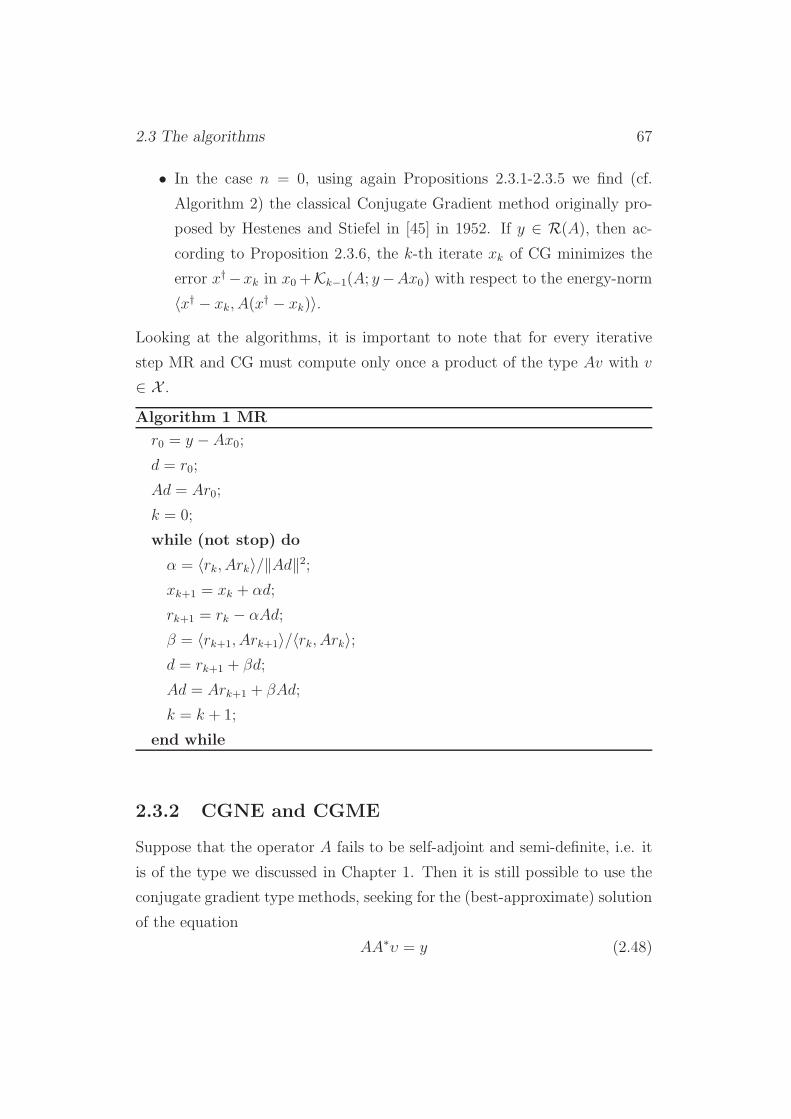
2.3 The algorithms 67
• In the case n = 0, using again Propositions 2.3.1-2.3.5 we find (cf.
Algorithm 2) the classical Conjugate Gradient method originally pro-
posed by Hestenes and Stiefel in [45] in 1952. If y ∈ R(A), then ac-
cording to Proposition 2.3.6, the k-th iterate xk of CG minimizes the
error x†−xk in x0+Kk−1(A; y−Ax0) with respect to the energy-norm
〈x† − xk, A(x† − xk)〉.
Looking at the algorithms, it is important to note that for every iterative
step MR and CG must compute only once a product of the type Av with v
∈ X .
Algorithm 1 MR
r0 = y −Ax0;
d = r0;
Ad = Ar0;
k = 0;
while (not stop) do
α = 〈rk, Ark〉/‖Ad‖2;xk+1 = xk + αd;
rk+1 = rk − αAd;
β = 〈rk+1, Ark+1〉/〈rk, Ark〉;d = rk+1 + βd;
Ad = Ark+1 + βAd;
k = k + 1;
end while
2.3.2 CGNE and CGME
Suppose that the operator A fails to be self-adjoint and semi-definite, i.e. it
is of the type we discussed in Chapter 1. Then it is still possible to use the
conjugate gradient type methods, seeking for the (best-approximate) solution
of the equation
AA∗υ = y (2.48)
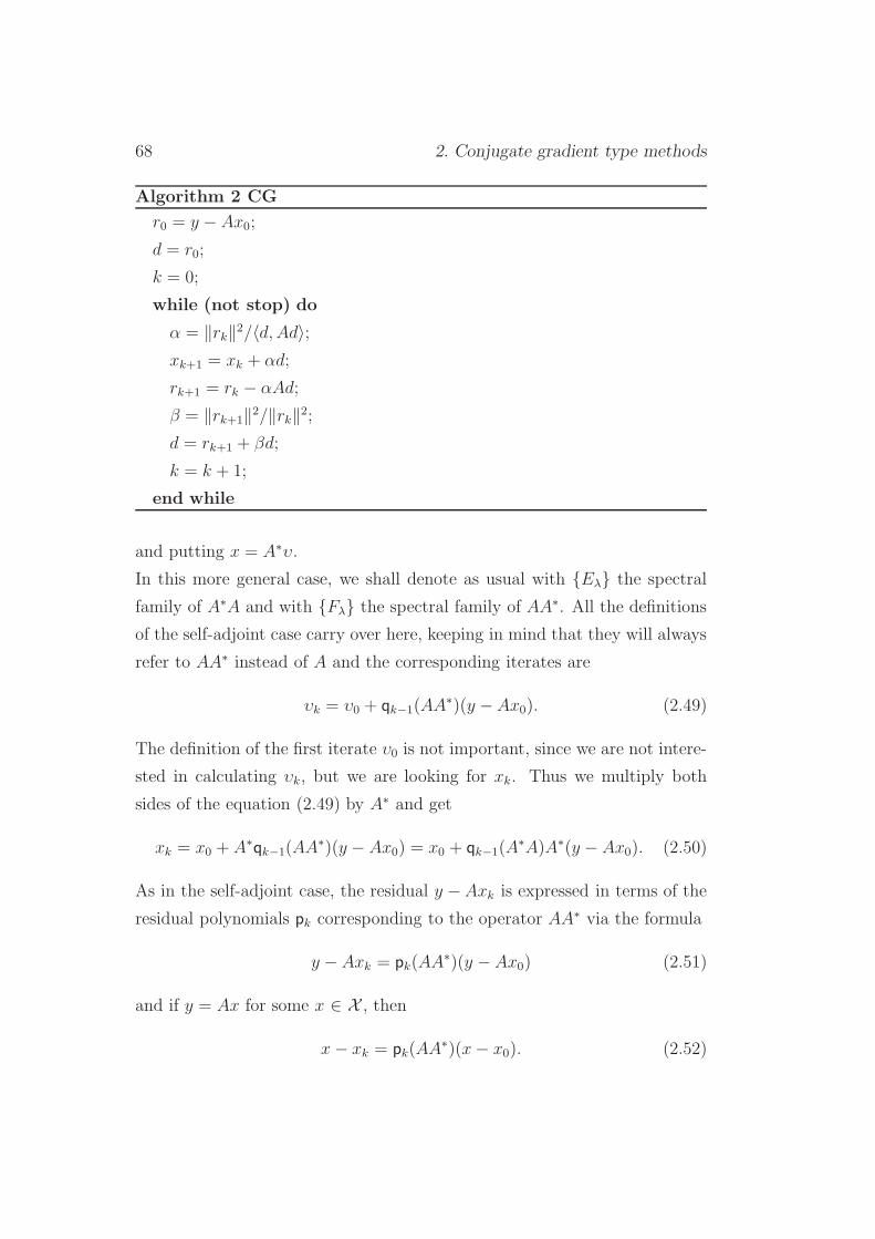
68 2. Conjugate gradient type methods
Algorithm 2 CG
r0 = y − Ax0;
d = r0;
k = 0;
while (not stop) do
α = ‖rk‖2/〈d, Ad〉;xk+1 = xk + αd;
rk+1 = rk − αAd;
β = ‖rk+1‖2/‖rk‖2;d = rk+1 + βd;
k = k + 1;
end while
and putting x = A∗υ.
In this more general case, we shall denote as usual with Eλ the spectral
family of A∗A and with Fλ the spectral family of AA∗. All the definitions
of the self-adjoint case carry over here, keeping in mind that they will always
refer to AA∗ instead of A and the corresponding iterates are
υk = υ0 + qk−1(AA∗)(y −Ax0). (2.49)
The definition of the first iterate υ0 is not important, since we are not intere-
sted in calculating υk, but we are looking for xk. Thus we multiply both
sides of the equation (2.49) by A∗ and get
xk = x0 + A∗qk−1(AA∗)(y − Ax0) = x0 + qk−1(A
∗A)A∗(y − Ax0). (2.50)
As in the self-adjoint case, the residual y −Axk is expressed in terms of the
residual polynomials pk corresponding to the operator AA∗ via the formula
y − Axk = pk(AA∗)(y −Ax0) (2.51)
and if y = Ax for some x ∈ X , then
x− xk = pk(AA∗)(x− x0). (2.52)
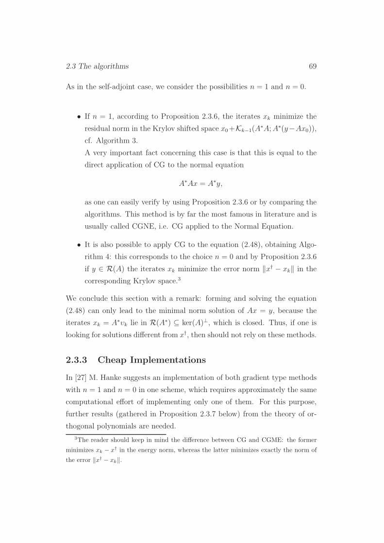
2.3 The algorithms 69
As in the self-adjoint case, we consider the possibilities n = 1 and n = 0.
• If n = 1, according to Proposition 2.3.6, the iterates xk minimize the
residual norm in the Krylov shifted space x0+Kk−1(A∗A;A∗(y−Ax0)),
cf. Algorithm 3.
A very important fact concerning this case is that this is equal to the
direct application of CG to the normal equation
A∗Ax = A∗y,
as one can easily verify by using Proposition 2.3.6 or by comparing the
algorithms. This method is by far the most famous in literature and is
usually called CGNE, i.e. CG applied to the Normal Equation.
• It is also possible to apply CG to the equation (2.48), obtaining Algo-
rithm 4: this corresponds to the choice n = 0 and by Proposition 2.3.6
if y ∈ R(A) the iterates xk minimize the error norm ‖x† − xk‖ in the
corresponding Krylov space.3
We conclude this section with a remark: forming and solving the equation
(2.48) can only lead to the minimal norm solution of Ax = y, because the
iterates xk = A∗υk lie in R(A∗) ⊆ ker(A)⊥, which is closed. Thus, if one is
looking for solutions different from x†, then should not rely on these methods.
2.3.3 Cheap Implementations
In [27] M. Hanke suggests an implementation of both gradient type methods
with n = 1 and n = 0 in one scheme, which requires approximately the same
computational effort of implementing only one of them. For this purpose,
further results (gathered in Proposition 2.3.7 below) from the theory of or-
thogonal polynomials are needed.
3The reader should keep in mind the difference between CG and CGME: the former
minimizes xk − x† in the energy norm, whereas the latter minimizes exactly the norm of
the error ‖x† − xk‖.
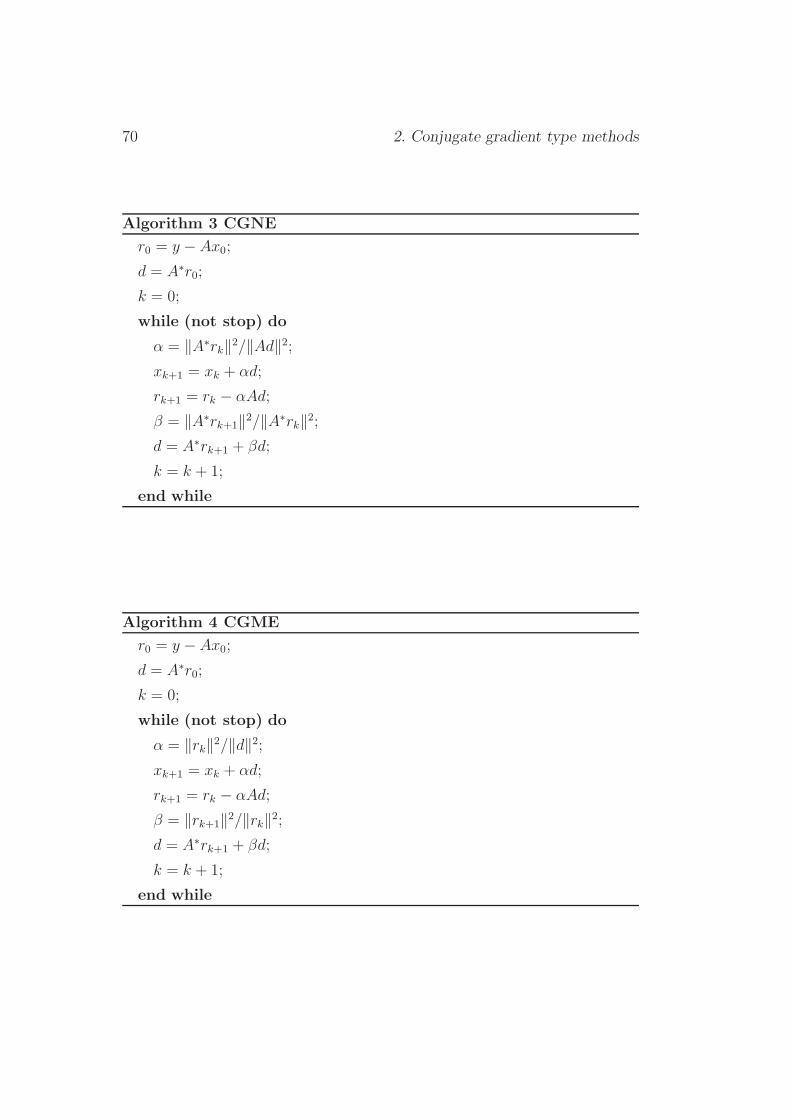
70 2. Conjugate gradient type methods
Algorithm 3 CGNE
r0 = y − Ax0;
d = A∗r0;
k = 0;
while (not stop) do
α = ‖A∗rk‖2/‖Ad‖2;xk+1 = xk + αd;
rk+1 = rk − αAd;
β = ‖A∗rk+1‖2/‖A∗rk‖2;d = A∗rk+1 + βd;
k = k + 1;
end while
Algorithm 4 CGME
r0 = y − Ax0;
d = A∗r0;
k = 0;
while (not stop) do
α = ‖rk‖2/‖d‖2;xk+1 = xk + αd;
rk+1 = rk − αAd;
β = ‖rk+1‖2/‖rk‖2;d = A∗rk+1 + βd;
k = k + 1;
end while

2.3 The algorithms 71
For simplicity, in the remainder we will restrict to the case in which A is a
semi-definite, self-adjoint operator and the initial guess is the origin: x0 = 0.
For the proof of the following facts and for a more exhaustive coverage of
the argument, see [27]. The second statement has already been proved in
Proposition 2.3.4.
Proposition 2.3.7. Fix k ∈ N0, k < ℓ. Then:
1. For n ∈ N, the corresponding residual polynomial p[n]k can be written in
the form
p[n]k = [p
[n]k , p
[n]k ]n−1
k∑
j=0
[p[n−1]j , p
[n−1]j ]−1
n−1p[n−1]j (2.53)
and
‖An−12 (y − Ax
[n]k )‖2 = [p
[n]k , p
[n]k ]n−1 =
(k∑
j=0
[p[n−1]j , p
[n−1]j ]−1
n−1
)−1
.
(2.54)
The same is true for n = 0 if and only if E0y = 0, i.e. if and only if
the data y has no component along R(A)⊥.
2. For n ∈ N0 there holds:
p[n+1]k =
1
πk,n
p[n]k − p
[n]k+1
λ. (2.55)
3. For n ∈ N, πk,n = (p[n]k )′(0)− (p
[n]k+1)
′(0) is also equal to
πk,n =[p
[n]k , p
[n]k ]n−1 − [p
[n]k+1, p
[n]k+1]n−1
[p[n+1]k , p
[n+1]k ]n
=[p
[n+1]k , p
[n+1]k ]n
[p[n+1]k , p
[n+1]k ]n+1
. (2.56)
Starting from Algorithm 1 and using Proposition 2.3.7, it is not difficult to
construct an algorithm which implements both MR and CG without further
computational effort. The same can be done starting from CGNE. The
results are summarized in Algorithm 5 (6), where xk and zk are the iterates
corresponding respectively to CG (CGME) and MR (CGNE).
Once again, we address the reader to [27] for further details.

72 2. Conjugate gradient type methods
Algorithm 5 MR+CGx0 = z0;
r0 = y − Az0;
d = r0;
p1 = Ar0;
p2 = Ad;
k = 0;
while (not stop) do
α = 〈rk, p1〉/‖p2‖2;zk+1 = zk + αd;
π = ‖rk‖2/〈rk, p1〉xk+1 = xk + πrk;
rk+1 = rk − αp2;
t = Ark+1;
β = 〈rk+1, t〉/〈rk, p1〉;d = rk+1 + βd;
p1 = t;
p2 = t+ βp2;
k = k + 1;
end while
2.4 Regularization theory for the conjugate
gradient type methods
This section is entirely devoted to the study of the conjugate gradient me-
thods for ill-posed problems. Although such methods are not regularization
methods in the strict sense of Definition 1.9.1, as we will see they preserve the
most important regularization properties and for this reason they are usually
included in the class of regularization methods. Since the results we are going
to state can nowadays be considered classic and are treated in great detail
both in [27] and in [17], most of the proofs will be omitted. The non-omitted
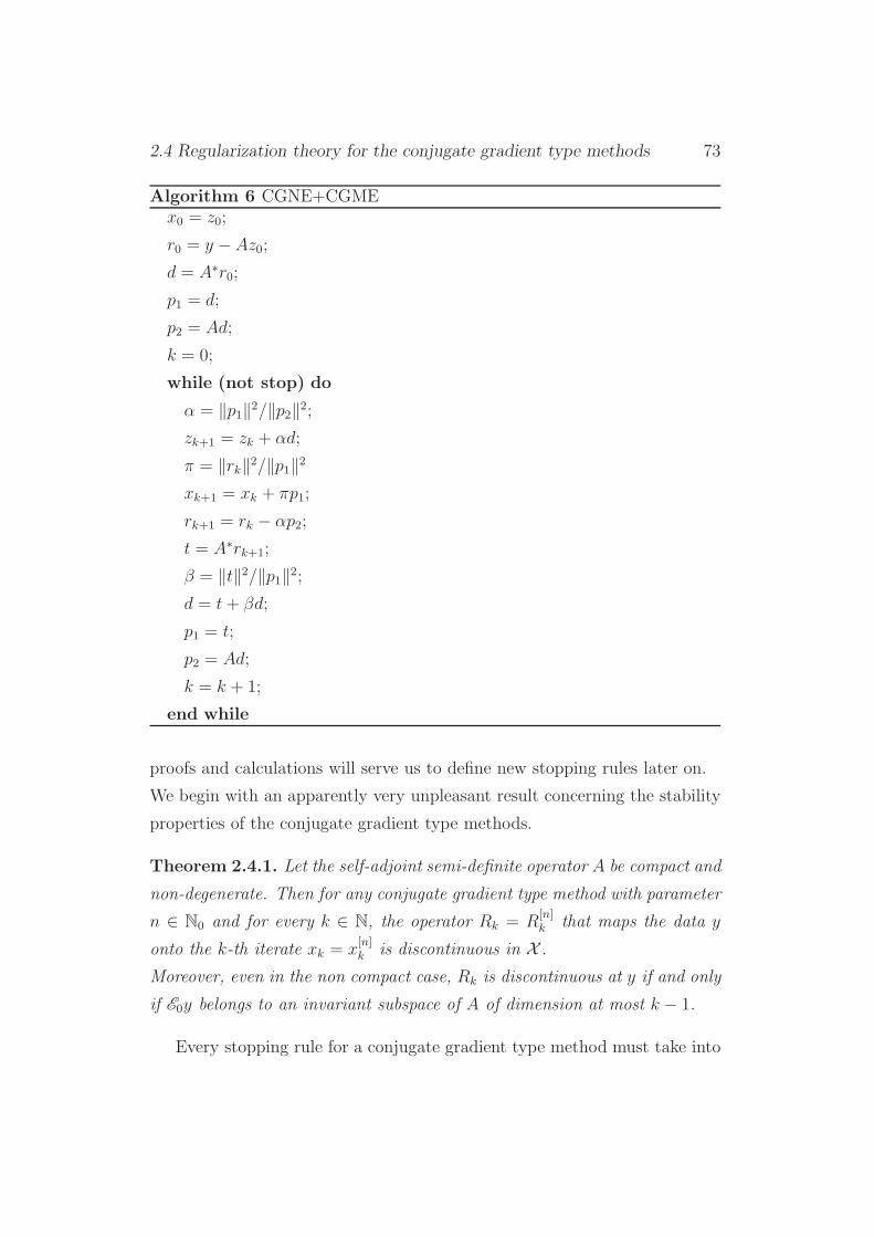
2.4 Regularization theory for the conjugate gradient type methods 73
Algorithm 6 CGNE+CGMEx0 = z0;
r0 = y −Az0;
d = A∗r0;
p1 = d;
p2 = Ad;
k = 0;
while (not stop) do
α = ‖p1‖2/‖p2‖2;zk+1 = zk + αd;
π = ‖rk‖2/‖p1‖2xk+1 = xk + πp1;
rk+1 = rk − αp2;
t = A∗rk+1;
β = ‖t‖2/‖p1‖2;d = t+ βd;
p1 = t;
p2 = Ad;
k = k + 1;
end while
proofs and calculations will serve us to define new stopping rules later on.
We begin with an apparently very unpleasant result concerning the stability
properties of the conjugate gradient type methods.
Theorem 2.4.1. Let the self-adjoint semi-definite operator A be compact and
non-degenerate. Then for any conjugate gradient type method with parameter
n ∈ N0 and for every k ∈ N, the operator Rk = R[n]k that maps the data y
onto the k-th iterate xk = x[n]k is discontinuous in X .
Moreover, even in the non compact case, Rk is discontinuous at y if and only
if E0y belongs to an invariant subspace of A of dimension at most k − 1.
Every stopping rule for a conjugate gradient type method must take into
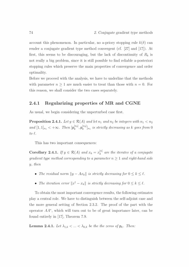
74 2. Conjugate gradient type methods
account this phenomenon. In particular, no a-priory stopping rule k(δ) can
render a conjugate gradient type method convergent (cf. [27] and [17]). At
first, this seems to be discouraging, but the lack of discontinuity of Rk is
not really a big problem, since it is still possible to find reliable a-posteriori
stopping rules which preserve the main properties of convergence and order
optimality.
Before we proceed with the analysis, we have to underline that the methods
with parameter n ≥ 1 are much easier to treat than those with n = 0. For
this reason, we shall consider the two cases separately.
2.4.1 Regularizing properties of MR and CGNE
As usual, we begin considering the unperturbed case first.
Proposition 2.4.1. Let y ∈ R(A) and let n1 and n2 be integers with n1 < n2
and [1, 1]n1 < +∞. Then [p[n2]k , p
[n2]k ]n1 is strictly decreasing as k goes from 0
to ℓ.
This has two important consequences:
Corollary 2.4.1. If y ∈ R(A) and xk = x[n]k are the iterates of a conjugate
gradient type method corresponding to a parameter n ≥ 1 and right-hand side
y, then
• The residual norm ‖y − Axk‖ is strictly decreasing for 0 ≤ k ≤ ℓ.
• The iteration error ‖x† − xk‖ is strictly decreasing for 0 ≤ k ≤ ℓ.
To obtain the most important convergence results, the following estimates
play a central role. We have to distinguish between the self-adjoint case and
the more general setting of Section 2.3.2. The proof of the part with the
operator AA∗, which will turn out to be of great importance later, can be
found entirely in [17], Theorem 7.9.
Lemma 2.4.1. Let λ1,k < ... < λk,k be the the zeros of pk. Then:
2.4 Regularization theory for the conjugate gradient type methods 75
• In the self-adjoint case, for y ∈ X ,
‖y −Axk‖ ≤ ‖Eλ1,kϕk(A)y‖, (2.57)
with the function ϕ(λ) := pk(λ)λ1,k
λ1,k−λsatisfying
0 ≤ ϕk(λ) ≤ 1, λ2ϕ2k(λ) ≤ 4|p′k(0)|−1, 0 ≤ λ ≤ λ1,k. (2.58)
• In the general case with AA∗, for y ∈ Y,
‖y −Axk‖ ≤ ‖Fλ1,kϕk(AA
∗)y‖, (2.59)
with the function ϕ(λ) := pk(λ)(
λ1,k
λ1,k−λ
) 12satisfying
0 ≤ ϕk(λ) ≤ 1, λϕ2k(λ) ≤ |p′k(0)|−1, 0 ≤ λ ≤ λ1,k. (2.60)
This leads to the following convergence theorem.
Theorem 2.4.2. • Suppose that A is self-adjoint and semi-definite. If
y ∈ R(A), then the iterates xk of a conjugate gradient type method
with parameter n ≥ 1 converge to A†y as k → +∞. If y /∈ R(A) and
ℓ = ∞, then ‖xk‖ → +∞ as k → +∞. If y /∈ R(A) and ℓ < ∞ then
the iteration terminates after ℓ steps, Axℓ = E0y and xℓ = A†y if and
only if ℓ = 0.
• Let A satisfy the assumptions of Section 2.3.2 and let xk be the itera-
tes of a conjugate gradient type method with parameter n ≥ 1 applied
with AA∗. If y ∈ D(A†), then xk converges to A†y as k → +∞, but if
y /∈ D(A†), then ‖xk‖ → +∞ as k → +∞.
Theorem 2.4.2 implies that the iteration must be terminated appropria-
tely when dealing with perturbed data yδ /∈ D(A†), due to numerical insta-
bilities.
Another consequence of Lemma 2.4.1 is the following one:

76 2. Conjugate gradient type methods
Lemma 2.4.2. Let xδk be the iterates of a conjugate gradient type method
with parameter n ≥ 1 corresponding to the perturbed right-hand side yδ and
the self-adjoint semi-definite operator A. If the exact right-hand side belongs
to R(A) and ℓ = ∞, then
lim supk→+∞
‖yδ − Axδk‖ ≤ ‖y − yδ‖. (2.61)
Moreover, if the exact data satisfy the source condition
A†y ∈ Xµ2,ρ, µ > 0, ρ > 0, (2.62)
then there exists a constant C > 0 such that
‖yδ − Axδk‖ ≤ ‖y − yδ‖+ C|p′k(0)|−µ−1ρ, 1 ≤ k ≤ ℓ. (2.63)
The same estimate is obtained for the gradient type methods working with
AA∗ instead of A, but the exponent −µ− 1 must be replaced by −µ+12.
Assuming the source condition (2.62), it is also possible to give an esti-
mate for the error:
Lemma 2.4.3. Let xδk be the iterates of a conjugate gradient type method
with parameter n ≥ 1 corresponding to yδ and the self-adjoint semi-definite
operator A. If (2.62) holds, then for 0 ≤ k ≤ ℓ,
‖A†y − xδk‖ ≤ C(
‖Fλ1,k(y − yδ)‖|p′k(0)|+ ρ
1µ+1M
µµ+1
k
)
, (2.64)
where C is a positive constant depending only on µ, and
Mk := max‖yδ − Axδk‖, ‖yδ − y‖. (2.65)
In the cases with AA∗ instead of A, the same is true, but in (2.64) |p′k(0)|must be replaced by |p′k(0)|
12 .
We underline that in Hanke’s statement of Lemma 2.4.3 (cf. Lemma
3.8 in [27]) the term ‖Fλ1,k(y − yδ)‖ in the inequality (2.64) is replaced by
‖y−yδ‖. This sharper estimate follows directly from the proof of the Lemma
3.8 in [27].
Combining Lemma 2.4.2 and Lemma 2.4.3 we obtain:
2.4 Regularization theory for the conjugate gradient type methods 77
Theorem 2.4.3. If y satisfies the source condition (2.62) and ‖yδ − y‖ ≤ δ,
then the iteration error of a conjugate gradient type method with parameter
n ≥ 1 associated to a self-adjoint semi-definite operator A is bounded by
‖A†y − xδk‖ ≤ C(|p′k(0)|−µρ+ |p′k(0)|δ
), 1 ≤ k ≤ ℓ. (2.66)
In the cases with AA∗ instead of A, the same estimate holds, but |p′k(0)| must
be replaced by |p′k(0)|12 .
Theorem 2.4.3 can be seen as the theoretical justification of the well
known phenomenon of the semi-convergence, which is experimented in prac-
tical examples: from (2.66), we observe that for small values of k the right-
hand side is dominated by |p′k(0)|−µρ, but as k increases towards +∞, this
term converges to 0, while |p′k(0)|δ diverges. Thus, as usual, there is a pre-
cise value of k that minimizes the error ‖A†y − xδk‖ and it is necessary to
define appropriate stopping rules to obtain satisfying results. In the case of
the conjugate gradient type methods with parameter n ≥ 1, the Discrepancy
Principle proves to be an efficient one.
Definition 2.4.1 (Discrepancy Principle for MR and CGNE). Assume
‖yδ − y‖ ≤ δ. Fix a number τ > 1 and terminate the iteration when, for the
first time, ‖yδ − Axδk‖ ≤ τδ. Denote the corresponding stopping index with
kD = kD(δ, yδ).
A few remarks are necessary:
(i) The Discrepancy Principle is well defined. In fact, due to Lemma 2.4.2,
for every δ and every yδ such that ‖yδ − y‖ ≤ δ there is always a finite
stopping index such that the corresponding residual norm is smaller
than τδ.
(ii) Since the residual must be computed anyway in the course of the itera-
tion, the Discrepancy Principle requires very little additional compu-
tational effort.
78 2. Conjugate gradient type methods
The following result is fundamental for the regularization theory of conjugate
gradient type methods. For MR and CGNE it was proved for the first time by
Nemirovsky in [70], our statement is taken as usual from [27], where a detailed
proof using the orthogonal polynomial and spectral theory framework is also
given.
Theorem 2.4.4. Any conjugate gradient type method with parameter n ≥ 1
with the Discrepancy Principle as a stopping rule is of optimal order, in
the sense that it satisfies the conditions of Definition 1.11.2, except for the
continuity of the operators Rk.
It is not difficult to see from the proof of Plato’s Theorem 1.11.1 that
the discontinuity of Rk does not influence the result. Thus we obtain also a
convergence result for y ∈ R(A):
Corollary 2.4.2. Let y ∈ R(A) and ‖yδ − y‖ ≤ δ. If the stopping index for
a conjugate gradient type method with parameter n ≥ 1 is chosen according
to the Discrepancy Principle and denoted by kD = kD(δ, yδ), then
limδ→0
supyδ∈Bδ(y)
‖xδkD − A†y‖ = 0. (2.67)
2.4.2 Regularizing properties of CG and CGME
The case of conjugate gradient type methods with parameter n = 0 is much
harder to study. The first difficulties arise from the fact that the residual
norm is not necessarily decreasing during the iteration, as the following exam-
ple shows:
Example 2.4.1. Let A ∈ M2(R) be defined by
A =
(
τ 0
0 1
)
, (2.68)
τ > 0, and let x0 = 0 and y =
(
2
1
)
. Then according to Algorithm 2 we
have: r0 = y, Ar0 =
(
2τ
1
)
, α = 54τ+1
and x1 = 54τ+1
y. Therefore, if τ is
2.4 Regularization theory for the conjugate gradient type methods 79
sufficiently small, we have
‖y −Ax1‖ =
∥∥∥∥∥
(
2− 10τ4τ+1
1− 54τ+1
)∥∥∥∥∥>
√5 = ‖y‖ = ‖y −Ax0‖.
Moreover, in the ill-posed case it is necessary to restrict to the case where
the data y belongs to R(A) (and not to D(A†)):
Theorem 2.4.5. If y /∈ R(A) and xk are the iterates of CG (CGME)
then either the iteration breaks down in the course of the (ℓ + 1)-th step or
ℓ = +∞ and ‖xk‖ → +∞ as k → +∞.
However, the main problem is that there are examples showing that the
Discrepancy Principle does not regularize these methods (see [27], Section
4.2). More precisely, CG and CGME with the Discrepancy Principle as a
stopping rule may give rise to a sequence of iterates diverging in norm as δ
goes to 0. Thus, other stopping criteria have to be formulated: one of the
most important is the following.
Definition 2.4.2. Fix τ > 1 and assume ‖y − yδ‖ ≤ δ. Terminate the CG
(CGME) iteration as soon as ‖yδ −Axδk‖ = 0, or when for the first time
k∑
j=0
‖yδ − Axδj‖−2 ≥ (τδ)−2. (2.69)
According to Proposition 2.3.7, the index corresponding to this stopping
rule is the smallest integer k such that [p[1]k , p
[1]k ]
120 ≤ τδ, i.e. it is exactly the
same stopping index defined for MR (CGNE) by the Discrepancy Principle,
thus we denote it again by kD. The importance of this stopping criterion lies
in the following result.
Theorem 2.4.6. Let y satisfy (2.62) and let ‖y− yδ‖ ≤ δ. If CG or CGME
is applied to yδ and terminated after kD steps according to Definition 2.4.2,
then there exists some uniform constant C > 0 such that
‖A†y − xδkD‖ ≤ Cρ1
µ+1 δµ
µ+1 . (2.70)
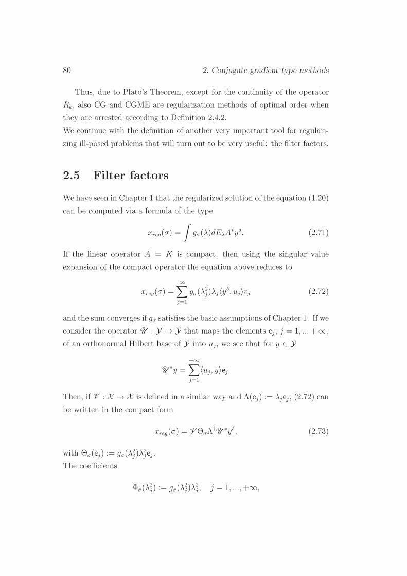
80 2. Conjugate gradient type methods
Thus, due to Plato’s Theorem, except for the continuity of the operator
Rk, also CG and CGME are regularization methods of optimal order when
they are arrested according to Definition 2.4.2.
We continue with the definition of another very important tool for regulari-
zing ill-posed problems that will turn out to be very useful: the filter factors.
2.5 Filter factors
We have seen in Chapter 1 that the regularized solution of the equation (1.20)
can be computed via a formula of the type
xreg(σ) =
∫
gσ(λ)dEλA∗yδ. (2.71)
If the linear operator A = K is compact, then using the singular value
expansion of the compact operator the equation above reduces to
xreg(σ) =
∞∑
j=1
gσ(λ2j )λj〈yδ, uj〉vj (2.72)
and the sum converges if gσ satisfies the basic assumptions of Chapter 1. If we
consider the operator U : Y → Y that maps the elements ej , j = 1, ...+∞,
of an orthonormal Hilbert base of Y into uj, we see that for y ∈ Y
U∗y =
+∞∑
j=1
〈uj, y〉ej.
Then, if V : X → X is defined in a similar way and Λ(ej) := λjej , (2.72) can
be written in the compact form
xreg(σ) = V ΘσΛ†U
∗yδ, (2.73)
with Θσ(ej) := gσ(λ2j)λ
2jej .
The coefficients
Φσ(λ2j) := gσ(λ
2j)λ
2j , j = 1, ...,+∞,
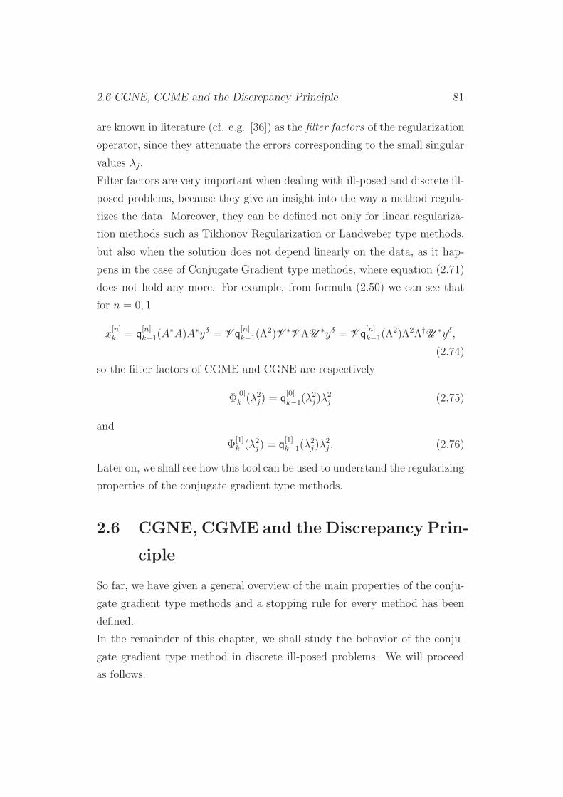
2.6 CGNE, CGME and the Discrepancy Principle 81
are known in literature (cf. e.g. [36]) as the filter factors of the regularization
operator, since they attenuate the errors corresponding to the small singular
values λj.
Filter factors are very important when dealing with ill-posed and discrete ill-
posed problems, because they give an insight into the way a method regula-
rizes the data. Moreover, they can be defined not only for linear regulariza-
tion methods such as Tikhonov Regularization or Landweber type methods,
but also when the solution does not depend linearly on the data, as it hap-
pens in the case of Conjugate Gradient type methods, where equation (2.71)
does not hold any more. For example, from formula (2.50) we can see that
for n = 0, 1
x[n]k = q
[n]k−1(A
∗A)A∗yδ = V q[n]k−1(Λ
2)V ∗V ΛU
∗yδ = V q[n]k−1(Λ
2)Λ2Λ†U
∗yδ,
(2.74)
so the filter factors of CGME and CGNE are respectively
Φ[0]k (λ2j) = q
[0]k−1(λ
2j )λ
2j (2.75)
and
Φ[1]k (λ2j) = q
[1]k−1(λ
2j)λ
2j . (2.76)
Later on, we shall see how this tool can be used to understand the regularizing
properties of the conjugate gradient type methods.
2.6 CGNE, CGME and the Discrepancy Prin-
ciple
So far, we have given a general overview of the main properties of the conju-
gate gradient type methods and a stopping rule for every method has been
defined.
In the remainder of this chapter, we shall study the behavior of the conju-
gate gradient type method in discrete ill-posed problems. We will proceed
as follows.
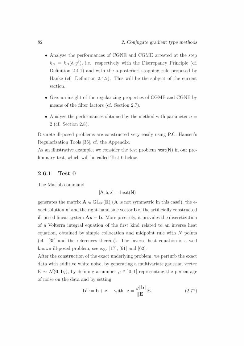
82 2. Conjugate gradient type methods
• Analyze the performances of CGNE and CGME arrested at the step
kD = kD(δ, yδ), i.e. respectively with the Discrepancy Principle (cf.
Definition 2.4.1) and with the a-posteriori stopping rule proposed by
Hanke (cf. Definition 2.4.2). This will be the subject of the current
section.
• Give an insight of the regularizing properties of CGME and CGNE by
means of the filter factors (cf. Section 2.7).
• Analyze the performances obtained by the method with parameter n =
2 (cf. Section 2.8).
Discrete ill-posed problems are constructed very easily using P.C. Hansen’s
Regularization Tools [35], cf. the Appendix.
As an illustrative example, we consider the test problem heat(N) in our pre-
liminary test, which will be called Test 0 below.
2.6.1 Test 0
The Matlab command
[A, b, x] = heat(N)
generates the matrix A ∈ GLN (R) (A is not symmetric in this case!), the e-
xact solution x† and the right-hand side vector b of the artificially constructed
ill-posed linear system Ax = b. More precisely, it provides the discretization
of a Volterra integral equation of the first kind related to an inverse heat
equation, obtained by simple collocation and midpoint rule with N points
(cf. [35] and the references therein). The inverse heat equation is a well
known ill-posed problem, see e.g. [17], [61] and [62].
After the construction of the exact underlying problem, we perturb the exact
data with additive white noise, by generating a multivariate gaussian vector
E ∼ N (0, IN), by defining a number ∈ ]0, 1[ representing the percentage
of noise on the data and by setting
bδ := b+ e, with e =‖b‖‖E‖ E. (2.77)

2.6 CGNE, CGME and the Discrepancy Principle 83
0 20 40 60 80 10010
−2
10−1
100
101
102
103
Relative error history
Iteration number
Rel
ativ
e er
rors
CGNECGME
(a) Relative errors history
0 200 400 600 800 1000−0.2
0
0.2
0.4
0.6
0.8
1
1.2Comparison of the optimal solutions
j
x(j)
Exact solution
(CGNE,kz#)
(CGME,kx#)
(b) Optimal Solutions
Figure 2.1: Test 0: relative errors (on the left) and optimal solutions (on the
right)
Here and below, 0 is the constant column vector whose components are equal
to 0 and IN is the identity matrix of dimension N ×N .
Of course, from the equation above there follows immediately that δ = ‖b‖and e ∼ N (0, δIN). In this case, since ‖b‖ = 1.4775 and is chosen equal
to 1%, δ = 1.4775× 10⁻².
Next, we solve the linear system with the noisy data bδ performing kMAX =
40 iteration steps of algorithm 6, by means of the routine cgne−cgme defined
in the Appendix. The parameter τ > 1 of the Discrepancy Principle is fixed
equal to 1.001. Looking at Figure 2.1 we can compare the relative errors of
CGME (red stars) and CGNE (blue circles) in the first 30 iteration steps.
Denoting with xδk the CGME iterates and with zδk the CGNE iterates we
observe:
1. The well known phenomenon of semi-convergence is present in both al-
gorithms, but appears with stronger evidence in CGME than in CGNE.
2. If k♯x(δ) and k♯z(δ) are defined as the iteration indices at which, respec-
tively, CGME and CGNE attain their best approximation of x†, the
numerical results show that k♯x(δ) = 8 and k♯z(δ) = 24. The correspon-
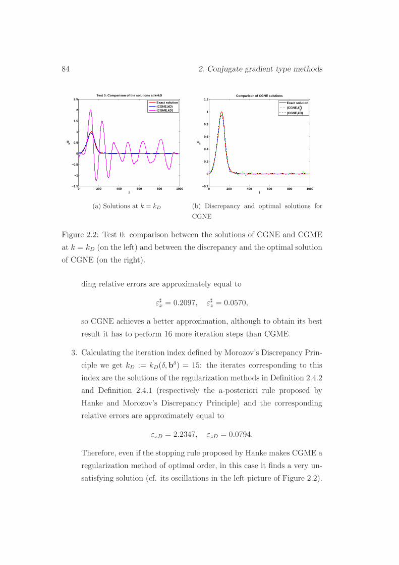
84 2. Conjugate gradient type methods
0 200 400 600 800 1000−1.5
−1
−0.5
0
0.5
1
1.5
2
2.5Test 0: Comparison of the solutions at k=kD
j
x(j)
Exact solution(CGNE,kD)(CGME,kD)
(a) Solutions at k = kD
0 200 400 600 800 1000−0.2
0
0.2
0.4
0.6
0.8
1
1.2Comparison of CGNE solutions
j
x(j)
Exact solution
(CGNE,kz#)
(CGNE,kD)
(b) Discrepancy and optimal solutions for
CGNE
Figure 2.2: Test 0: comparison between the solutions of CGNE and CGME
at k = kD (on the left) and between the discrepancy and the optimal solution
of CGNE (on the right).
ding relative errors are approximately equal to
ε♯x = 0.2097, ε♯z = 0.0570,
so CGNE achieves a better approximation, although to obtain its best
result it has to perform 16 more iteration steps than CGME.
3. Calculating the iteration index defined by Morozov’s Discrepancy Prin-
ciple we get kD := kD(δ,bδ) = 15: the iterates corresponding to this
index are the solutions of the regularization methods in Definition 2.4.2
and Definition 2.4.1 (respectively the a-posteriori rule proposed by
Hanke and Morozov’s Discrepancy Principle) and the corresponding
relative errors are approximately equal to
εxD = 2.2347, εzD = 0.0794.
Therefore, even if the stopping rule proposed by Hanke makes CGME a
regularization method of optimal order, in this case it finds a very un-
satisfying solution (cf. its oscillations in the left picture of Figure 2.2).
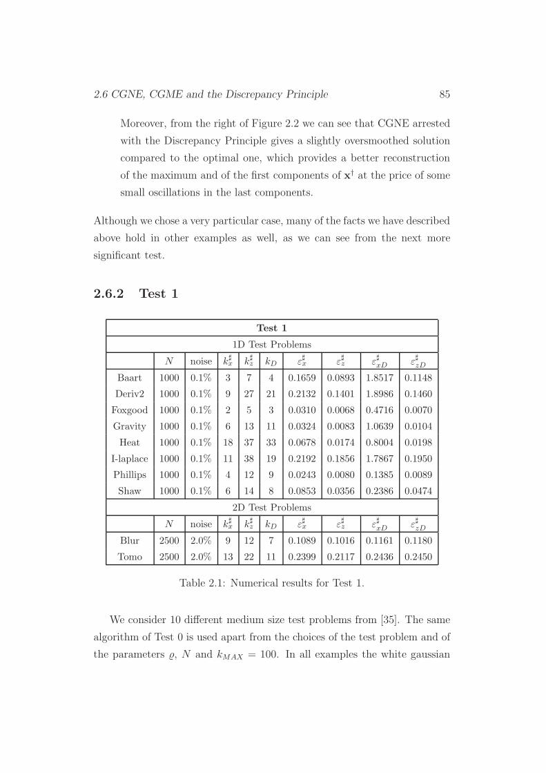
2.6 CGNE, CGME and the Discrepancy Principle 85
Moreover, from the right of Figure 2.2 we can see that CGNE arrested
with the Discrepancy Principle gives a slightly oversmoothed solution
compared to the optimal one, which provides a better reconstruction
of the maximum and of the first components of x† at the price of some
small oscillations in the last components.
Although we chose a very particular case, many of the facts we have described
above hold in other examples as well, as we can see from the next more
significant test.
2.6.2 Test 1
Test 1
1D Test Problems
N noise k♯x k
♯z kD ε
♯x ε
♯z ε
♯xD ε
♯zD
Baart 1000 0.1% 3 7 4 0.1659 0.0893 1.8517 0.1148
Deriv2 1000 0.1% 9 27 21 0.2132 0.1401 1.8986 0.1460
Foxgood 1000 0.1% 2 5 3 0.0310 0.0068 0.4716 0.0070
Gravity 1000 0.1% 6 13 11 0.0324 0.0083 1.0639 0.0104
Heat 1000 0.1% 18 37 33 0.0678 0.0174 0.8004 0.0198
I-laplace 1000 0.1% 11 38 19 0.2192 0.1856 1.7867 0.1950
Phillips 1000 0.1% 4 12 9 0.0243 0.0080 0.1385 0.0089
Shaw 1000 0.1% 6 14 8 0.0853 0.0356 0.2386 0.0474
2D Test Problems
N noise k♯x k
♯z kD ε
♯x ε
♯z ε
♯xD ε
♯zD
Blur 2500 2.0% 9 12 7 0.1089 0.1016 0.1161 0.1180
Tomo 2500 2.0% 13 22 11 0.2399 0.2117 0.2436 0.2450
Table 2.1: Numerical results for Test 1.
We consider 10 different medium size test problems from [35]. The same
algorithm of Test 0 is used apart from the choices of the test problem and of
the parameters , N and kMAX = 100. In all examples the white gaussian
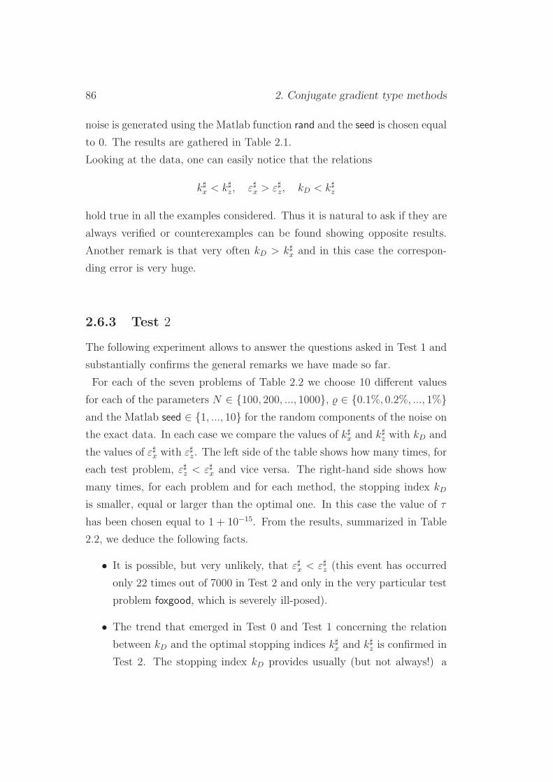
86 2. Conjugate gradient type methods
noise is generated using the Matlab function rand and the seed is chosen equal
to 0. The results are gathered in Table 2.1.
Looking at the data, one can easily notice that the relations
k♯x < k♯z, ε♯x > ε♯z, kD < k♯z
hold true in all the examples considered. Thus it is natural to ask if they are
always verified or counterexamples can be found showing opposite results.
Another remark is that very often kD > k♯x and in this case the correspon-
ding error is very huge.
2.6.3 Test 2
The following experiment allows to answer the questions asked in Test 1 and
substantially confirms the general remarks we have made so far.
For each of the seven problems of Table 2.2 we choose 10 different values
for each of the parameters N ∈ 100, 200, ..., 1000, ∈ 0.1%, 0.2%, ..., 1%and the Matlab seed ∈ 1, ..., 10 for the random components of the noise on
the exact data. In each case we compare the values of k♯x and k♯z with kD and
the values of ε♯x with ε♯z. The left side of the table shows how many times, for
each test problem, ε♯z < ε♯x and vice versa. The right-hand side shows how
many times, for each problem and for each method, the stopping index kD
is smaller, equal or larger than the optimal one. In this case the value of τ
has been chosen equal to 1 + 10−15. From the results, summarized in Table
2.2, we deduce the following facts.
• It is possible, but very unlikely, that ε♯x < ε♯z (this event has occurred
only 22 times out of 7000 in Test 2 and only in the very particular test
problem foxgood, which is severely ill-posed).
• The trend that emerged in Test 0 and Test 1 concerning the relation
between kD and the optimal stopping indices k♯x and k♯z is confirmed in
Test 2. The stopping index kD provides usually (but not always!) a
2.6 CGNE, CGME and the Discrepancy Principle 87
Test 2
Best err. perf. Stopping
CGNE CGME kD < k♯ kD = k♯ kD > k♯
Baart 1000 0 CGNE 564 372 64
CGME 0 545 455
Deriv2 1000 0 CGNE 882 112 6
CGME 0 0 1000
Foxgood 978 22 CGNE 483 426 91
CGME 0 532 468
Gravity 1000 0 CGNE 861 118 21
CGME 0 1 999
Heat 1000 0 CGNE 991 9 0
CGME 0 1 999
Phillips 1000 0 CGNE 751 207 42
CGME 0 48 952
Shaw 1000 0 CGNE 806 185 9
CGME 0 4 996
Total 6978 22 CGNE 5338 1429 233
CGME 0 1031 5869
Table 2.2: Numerical results for Test 2.
slightly oversmoothed solution for CGNE and often a noise dominated
solution for CGME.
In the problems with a symmetric and positive definite matrix A, it is also
possible to compare the results of CGNE and CGME with those obtained
by MR and CG. This was done for phillips, shaw, deriv2 and gravity and the
outcome was that CGNE attained the best performance 3939 times out of
4000, with 61 successes of MR in the remaining cases.
In conclusion, the numerical tests described above lead us to ask the following
questions:
1. The relations k♯x < k♯z and ε♯x > ε♯z hold very often in the cases consi-
88 2. Conjugate gradient type methods
dered above. Is there a theoretical justification of this fact?
2. The conjugate gradient methods with parameter n = 1 seem to provide
better results than those with parameter n = 0. What can we say about
other conjugate gradient methods with parameter n > 1?
3. To improve the performance of CGME one can choose a larger τ . This
is not in contrast with the regularization theory above. On the other
hand, arresting CGNE later means stopping the iteration when the
residual norm has become smaller than δ, while the Discrepancy Prin-
ciple states that τ must be chosen larger than 1. How can this be
justified and implemented in practice by means of a reasonable stop-
ping rule?
We will answer the questions above in detail.
2.7 CGNE vs. CGME
In the finite dimensional setting described in Section 2.6, both iterates of
CGME and CGNE will eventually converge to the vector x := A†bδ as de-
scribed in Section 2.1, which can be very distant from the exact solution
x† = A†b we are looking for, since A† is ill-conditioned. The problem is to
understand how the iterates converge to x and how they reach an approxi-
mation of x† in their first steps.
First of all, we recall that xδk minimizes the norm of the error ‖x − x‖ in
Kk−1(A∗A;A∗bδ), whereas zδk minimizes the residual norm ‖Ax−bδ‖ in the
same Krylov space. Thus the iterates of CGME, converging to x as fast as
possible, will be the better approximations of the exact underlying solution
x† in the very first steps, when the noise on the data still plays a secondary
role. However, being the greediest approximations of the noisy solution x,
they will also be influenced by the noise at an earlier stage than the iterates
of CGNE. This explains the relation k♯x < k♯z, which is often verified in the
numerical experiments.
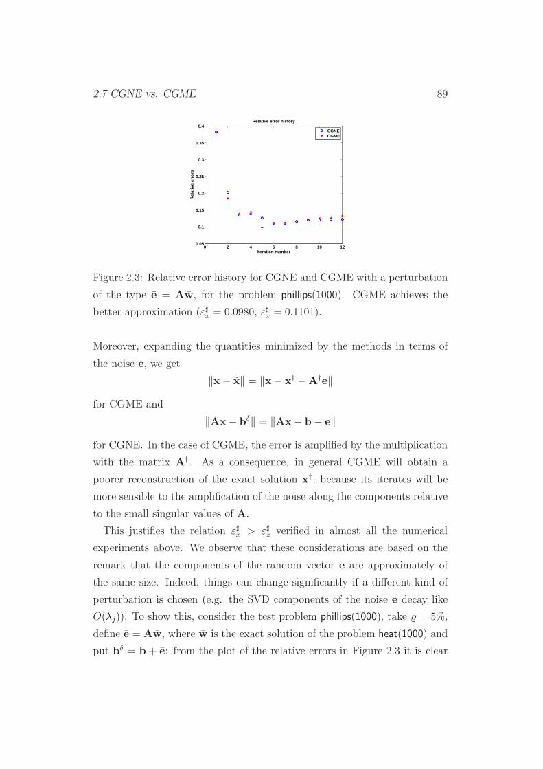
2.7 CGNE vs. CGME 89
0 2 4 6 8 10 120.05
0.1
0.15
0.2
0.25
0.3
0.35
0.4Relative error history
Iteration number
Rel
ativ
e er
rors
CGNECGME
Figure 2.3: Relative error history for CGNE and CGME with a perturbation
of the type e = Aw, for the problem phillips(1000). CGME achieves the
better approximation (ε♯x = 0.0980, ε♯x = 0.1101).
Moreover, expanding the quantities minimized by the methods in terms of
the noise e, we get
‖x− x‖ = ‖x− x† −A†e‖
for CGME and
‖Ax− bδ‖ = ‖Ax− b− e‖
for CGNE. In the case of CGME, the error is amplified by the multiplication
with the matrix A†. As a consequence, in general CGME will obtain a
poorer reconstruction of the exact solution x†, because its iterates will be
more sensible to the amplification of the noise along the components relative
to the small singular values of A.
This justifies the relation ε♯x > ε♯z verified in almost all the numerical
experiments above. We observe that these considerations are based on the
remark that the components of the random vector e are approximately of
the same size. Indeed, things can change significantly if a different kind of
perturbation is chosen (e.g. the SVD components of the noise e decay like
O(λj)). To show this, consider the test problem phillips(1000), take = 5%,
define e = Aw, where w is the exact solution of the problem heat(1000) and
put bδ = b + e: from the plot of the relative errors in Figure 2.3 it is clear
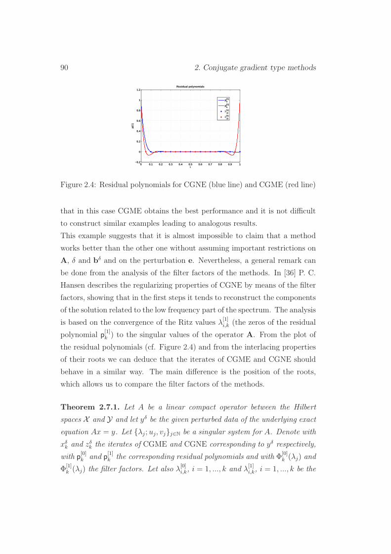
90 2. Conjugate gradient type methods
0 0.1 0.2 0.3 0.4 0.5 0.6 0.7 0.8 0.9 1−0.2
0
0.2
0.4
0.6
0.8
1
1.2Residual polynomials
λ
p(λ)
pk[1]
pk[0]
λi,k[1]
λi,k[0]
Figure 2.4: Residual polynomials for CGNE (blue line) and CGME (red line)
that in this case CGME obtains the best performance and it is not difficult
to construct similar examples leading to analogous results.
This example suggests that it is almost impossible to claim that a method
works better than the other one without assuming important restrictions on
A, δ and bδ and on the perturbation e. Nevertheless, a general remark can
be done from the analysis of the filter factors of the methods. In [36] P. C.
Hansen describes the regularizing properties of CGNE by means of the filter
factors, showing that in the first steps it tends to reconstruct the components
of the solution related to the low frequency part of the spectrum. The analysis
is based on the convergence of the Ritz values λ[1]i,k (the zeros of the residual
polynomial p[1]k ) to the singular values of the operator A. From the plot of
the residual polynomials (cf. Figure 2.4) and from the interlacing properties
of their roots we can deduce that the iterates of CGME and CGNE should
behave in a similar way. The main difference is the position of the roots,
which allows us to compare the filter factors of the methods.
Theorem 2.7.1. Let A be a linear compact operator between the Hilbert
spaces X and Y and let yδ be the given perturbed data of the underlying exact
equation Ax = y. Let λj ; uj, vjj∈N be a singular system for A. Denote with
xδk and zδk the iterates of CGME and CGNE corresponding to yδ respectively,
with p[0]k and p
[1]k the corresponding residual polynomials and with Φ
[0]k (λj) and
Φ[1]k (λj) the filter factors. Let also λ
[0]i,k, i = 1, ..., k and λ
[1]i,k, i = 1, ..., k be the

2.7 CGNE vs. CGME 91
zeros of p[0]k and p
[1]k respectively.
Then, for every j such that λ2j < λ[0]1,k,
Φ[0]k (λj) > Φ
[1]k (λj). (2.78)
Proof. The filter factors of the conjugate gradient type methods are:
Φ[n]k (λj) = q
[n]k (λ2j)λ
2j , n = 0, 1.
We recall from the theory of orthogonal polynomials that the zeros of p[0]k
and of p[1]k interlace as follows:
λ[0]1,k < λ
[1]1,k < λ
[0]2,k < λ
[1]2,k < ... < λ
[0]k,k < λ
[1]k,k. (2.79)
Thus, writing down the residual polynomials in the form
p[n]k (λ) =
k∏
j=1
(
1− λ
λ[n]j,k
)
, n = 0, 1, (2.80)
it is very easy to see that p[0]k < p
[1]k on ]0, λ
[0]1,k] (cf. Figure 2.4) and conse-
quently
q[0]k > q
[1]k on ]0, λ
[0]1,k].
This result is a theoretical justification of the heuristic considerations of
the beginning of this section: the iterates of CGNE filter the high frequencies
of the spectrum slightly more than the iterates of CGME. Summing up:
• Thanks to its minimization properties, CGNE works better than CGME
along the high frequency components, keeping the error small for a few
more iteration and usually achieving the better results.
• Anyway this is not a general rule (see the counterexample of this section
and the results of Test 2), because the performances of the two methods
strongly depend on the matrix A and on the vectors x†, b, e and x0.
• Finding a particular class of problems (or data) in which CGNE always
gets the better results is maybe possible, but rather difficult.
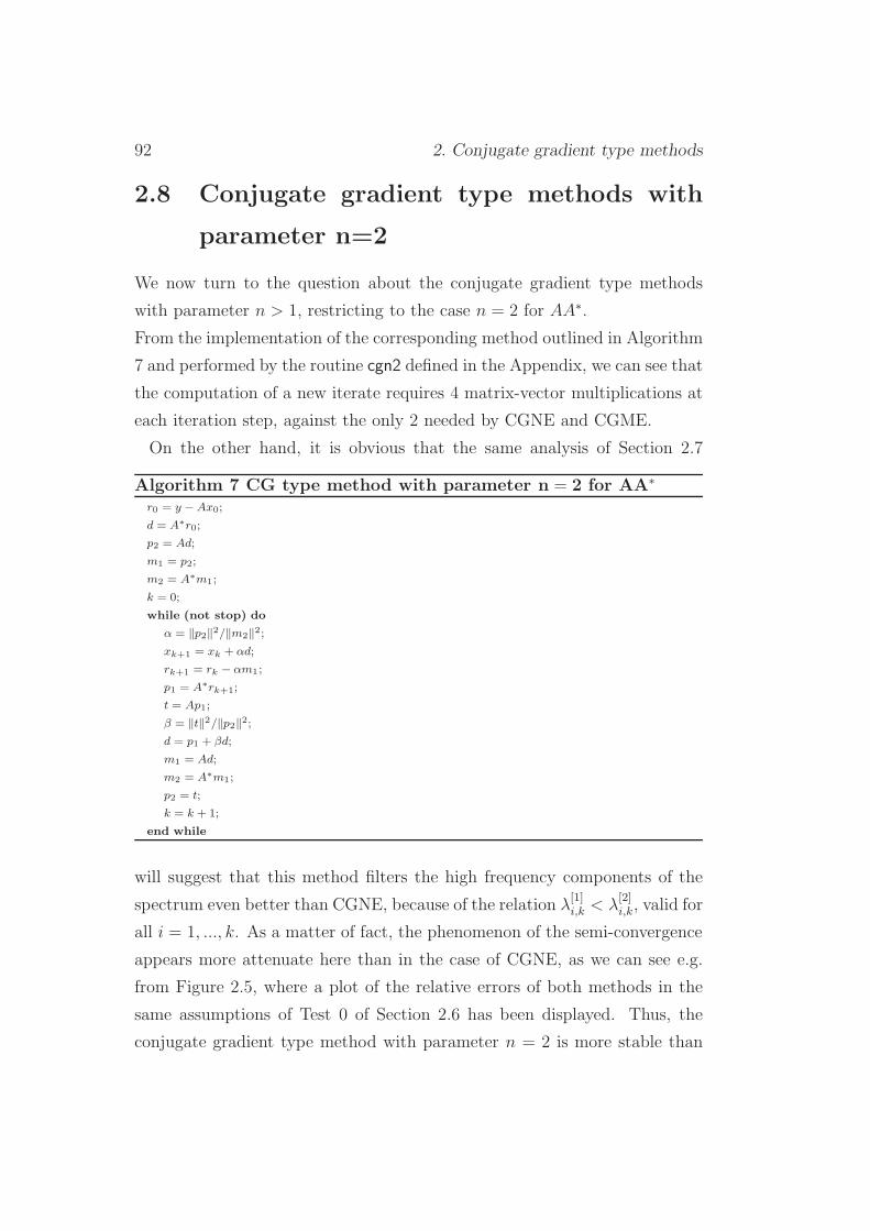
92 2. Conjugate gradient type methods
2.8 Conjugate gradient type methods with
parameter n=2
We now turn to the question about the conjugate gradient type methods
with parameter n > 1, restricting to the case n = 2 for AA∗.
From the implementation of the corresponding method outlined in Algorithm
7 and performed by the routine cgn2 defined in the Appendix, we can see that
the computation of a new iterate requires 4 matrix-vector multiplications at
each iteration step, against the only 2 needed by CGNE and CGME.
On the other hand, it is obvious that the same analysis of Section 2.7
Algorithm 7 CG type method with parameter n = 2 for AA∗
r0 = y − Ax0;
d = A∗r0;
p2 = Ad;
m1 = p2;
m2 = A∗m1;
k = 0;
while (not stop) do
α = ‖p2‖2/‖m2‖2;xk+1 = xk + αd;
rk+1 = rk − αm1;
p1 = A∗rk+1;
t = Ap1;
β = ‖t‖2/‖p2‖2;d = p1 + βd;
m1 = Ad;
m2 = A∗m1;
p2 = t;
k = k + 1;
end while
will suggest that this method filters the high frequency components of the
spectrum even better than CGNE, because of the relation λ[1]i,k < λ
[2]i,k, valid for
all i = 1, ..., k. As a matter of fact, the phenomenon of the semi-convergence
appears more attenuate here than in the case of CGNE, as we can see e.g.
from Figure 2.5, where a plot of the relative errors of both methods in the
same assumptions of Test 0 of Section 2.6 has been displayed. Thus, the
conjugate gradient type method with parameter n = 2 is more stable than

2.8 Conjugate gradient type methods with parameter n=2 93
0 20 40 60 80 10010
−2
10−1
100
Relative error history
Iteration number
Rela
tive
erro
rs
CGNECGN2
Figure 2.5: Relative error history for CGNE and the conjugate gradient type
method with parameter n = 2 in the assumptions of Test 0 of Section 2.6.
CGNE with respect to the iteration index k (exactly for the same reasons
why we have seen that CGNE is more stable than CGME). This could be an
advantage especially when the data are largely contaminated by the noise.
For example, if we consider the test problem blur(500), with = 10%, we can
see from Figure 2.6 that the optimal reconstructed solutions of both methods
are similar, but the conjugate gradient type method with parameter n = 2
attenuates the oscillations caused by the noise in the background better than
CGNE.
2.8.1 Numerical results
We compare the conjugate gradient type methods for the matrix AA∗ with
parameters 1 and 2 in the same examples of Test 2 of Section 2.6, by adding
the test problem i−laplace. From the results of Table 2.3, we can see that the
methods obtain quite similar results. The conjugate gradient type method
with parameter n = 2 usually performs a little bit better, but this advantage
is minimal: the average improvement of the results obtained by the method
with n = 2, namely the difference of the total sums of the relative errors

94 2. Conjugate gradient type methods
blur500 CGN2 kN2=2 sigma=10 −1 errN2=0.122231
100 200 300 400 500
50
100
150
200
250
300
350
400
450
500
blur500 CGNE kZBEST=1 sigma=10 −1 errZBEST=0.128101
100 200 300 400 500
50
100
150
200
250
300
350
400
450
500
Figure 2.6: Comparison between the conjugate gradient type method with
parameter n = 2 and CGNE for the test problem blur(500), with = 10%.
divided by the total sum of the relative errors of CGNE, is equal to
|683.74− 686.74|686.74
∼= 0.4%.
Concerning the stopping index, we observe that in both cases the Discre-
pancy Principle stops the iteration earlier than the optimal stopping index
in the large majority of the considered cases. We shall return to this impor-
tant topic later.
Our numerical experiments confirm the trend also for a larger noise. Per-
forming the same test with ∈ 10−2, 2 × 10⁻², ..., 10−1 instead of ∈10−3, 2× 10⁻³, ..., 10−2, we obtain that the method with parameter n = 2
achieves the better relative error in 4763 cases (59.5% of the times) and the
overall sums of the relative errors are 1101.8 for n = 2 and 1115.5 for n = 1.
Thus the average improvement obtained by the method with n = 2 is 1% in
this case.
In conclusion, the conjugate gradient type method with parameter n = 2 has
nice regularizing properties: in particular, it filters the high frequency compo-
nents of the noise even better than CGNE. Consequently, it often achieves

2.8 Conjugate gradient type methods with parameter n=2 95
Comparison of CG type methods: n = 1 and n = 2
Best err. perf. Average rel. err. n Discrepancy Stopping
kD < k♯ kD = k♯ kD > k♯
Baart 598 0.13404 n = 1 564 372 64
402 0.13482 n = 2 616 321 63
Deriv2 197 0.19916 n = 1 882 112 6
803 0.19792 n = 2 965 33 2
Foxgood 565 0.01862 n = 1 483 426 91
435 0.01876 n = 2 547 362 91
Gravity 386 0.02179 n = 1 861 118 21
614 0.02151 n = 2 838 147 15
Heat 294 0.05709 n = 1 991 9 0
706 0.05657 n = 2 996 4 0
I-laplace 447 0.18091 n = 1 957 30 13
553 0.18036 n = 2 971 18 11
Phillips 441 0.01774 n = 1 751 207 42
559 0.01731 n = 2 775 204 21
Shaw 548 0.05739 n = 1 806 185 9
452 0.05649 n = 2 837 156 7
Total 3476 0.08584 n = 1 6285 1459 256
4524 0.08546 n = 2 6545 1245 210
Table 2.3: Comparison between the CG type methods for AA∗ with para-
meters 1 and 2. We emphasize that kD is not the same stopping index here
for n = 1 and n = 2.
the better results and keeps the phenomenon of the semi-convergence less
pronounced, especially for large errors in the data. On the other hand, it is
more expensive than CGNE from a computational point of view, because it
usually performs more steps to reach the optimal solution and in each step
it requires 4 matrix-vector multiplications (against the only 2 required by
CGNE). Despite the possible advantages described above, in our numerical
tests the improvements were minimal, even in the case of a large δ. For this
reason, we believe that it should be rarely worth it, to prefer the method
with parameter n = 2 to CGNE.

96 2. Conjugate gradient type methods
Chapter 3
New stopping rules for CGNE
In the last sections of Chapter 2 we have seen that CGNE, being both efficient
and precise, is one of the most promising conjugate gradient type methods
when dealing with (discrete) ill-posed problems.
The general theory suggests the Discrepancy Principle as a very reliable stop-
ping rule, which makes CGNE a regularization method of optimal order1. Of
course, the stopping index of the Discrepancy Principle is not necessarily
the best possible for a given noise level δ > 0 and a given perturbed data
yδ. Indeed, as we have seen in the numerical tests of Chapter 2, it usually
provides a slightly oversmoothed solution. Moreover, in practice the noise
level is often unknown: in this case it is necessary to define heuristic stopping
rules. Due to Bakushinskii’s Theorem a method arrested with an heuristic
stopping rule cannot be convergent, but in some cases it can give more sa-
tisfactory results than other methods arrested with a sophisticated stopping
rule of optimal order based on the knowledge of the noise level.
When dealing with discrete ill-posed problems (e.g. arising from the discre-
tization of ill-posed problems defined in a Hilbert space setting), it is very
important to rely on many different stopping rules, in order to choose the best
one depending on the particular problem and data: among the most famous
1except for the continuity of the operator that maps the data into the k-th iterate of
CGNE, cf. Chapter 2.
97

98 3. New stopping rules for CGNE
stopping rules that can be found in literature, apart from the Discrepancy
Principle, we mention the Monotone Error Rule (cf. [24], [23], [25], [36])
and, as heuristic stopping rules, the L-curve ([35], [36]), the Generalized
Cross Validation ([17] and the references therein) and the Hanke-Raus Cri-
terion ([27], [24]).
In this chapter, three new stopping rules for CGNE will be proposed, ana-
lyzed and tested. All these rules rely on a general analysis of the residual
norm of the CGNE iterates.
The first one, called the Approximated Residual L-Curve Criterion, is an
heuristic stopping rule based on the global behavior of the residual norms
with respect to the iteration index.
The second one, called the Projected Data Norm Criterion, is another heuri-
stic stopping rule that relates the residual norms of the CGNE iterates to
the residual norms of the truncated singular value decomposition.
The third one, called the Projected Noise Norm Criterion, is an a-posteriori
stopping rule based on a statistical approach, intended to overcome the over-
smoothing effect of the Discrepancy Principle and mainly bound to large
scale problems.
3.1 Residual norms and regularizing proper-
ties of CGNE
This section is dedicated to a general analysis of the regularizing properties
of CGNE, by linking the relative error with the residual norm in the case of
perturbed data.
In their paper [60] Kilmer and Stewart related the residual norm of the
minimal residual method to the norm of the relative error.
Theorem 3.1.1 (Kilmer, Stewart). Let the following assumptions hold:
• The matrix A ∈ GLN(R) is symmetric and positive definite, and in
the coordinate system of its eigenvectors the exact linear system can be
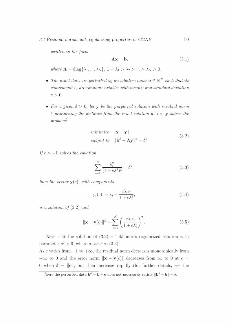
3.1 Residual norms and regularizing properties of CGNE 99
written in the form
Λx = b, (3.1)
where Λ = diagλ1, ..., λN, 1 = λ1 > λ2 > ... > λN > 0.
• The exact data are perturbed by an additive noise e ∈ RN such that its
components ei are random variables with mean 0 and standard deviation
ν > 0.
• For a given δ > 0, let y be the purported solution with residual norm
δ minimizing the distance from the exact solution x, i.e. y solves the
problem2
minimize ‖x− y‖subject to ‖bδ −Λy‖2 = δ2.
(3.2)
If c > −1 solves the equation
N∑
i=1
e2i(1 + cλ2i )
2= δ2, (3.3)
then the vector y(c), with components
yi(c) := xi +cλiei
1 + cλ2i, (3.4)
is a solution of (3.2) and
‖x− y(c)‖2 =N∑
i=1
(cλiei
1 + cλ2i
)2
. (3.5)
Note that the solution of (3.2) is Tikhonov’s regularized solution with
parameter δ2 > 0, where δ satisfies (3.3).
As c varies from −1 to +∞, the residual norm decreases monotonically from
+∞ to 0 and the error norm ‖x − y(c)‖ decreases from ∞ to 0 at c =
0 when δ = ‖e‖, but then increases rapidly (for further details, see the
2here the perturbed data bδ = b+ e does not necessarily satisfy ‖bδ − b‖ = δ.
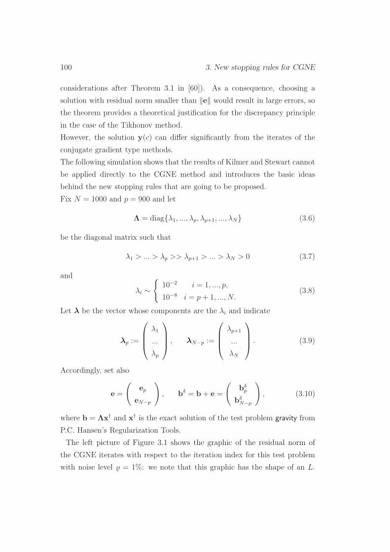
100 3. New stopping rules for CGNE
considerations after Theorem 3.1 in [60]). As a consequence, choosing a
solution with residual norm smaller than ‖e‖ would result in large errors, so
the theorem provides a theoretical justification for the discrepancy principle
in the case of the Tikhonov method.
However, the solution y(c) can differ significantly from the iterates of the
conjugate gradient type methods.
The following simulation shows that the results of Kilmer and Stewart cannot
be applied directly to the CGNE method and introduces the basic ideas
behind the new stopping rules that are going to be proposed.
Fix N = 1000 and p = 900 and let
Λ = diagλ1, ..., λp, λp+1, ..., λN (3.6)
be the diagonal matrix such that
λ1 > ... > λp >> λp+1 > ... > λN > 0 (3.7)
and
λi ∼
10−2 i = 1, ..., p,
10−8 i = p+ 1, ..., N.(3.8)
Let λ be the vector whose components are the λi and indicate
λp :=
λ1
...
λp
, λN−p :=
λp+1
...
λN
. (3.9)
Accordingly, set also
e =
(
ep
eN−p
)
, bδ = b+ e =
(
bδp
bδN−p
)
, (3.10)
where b = Λx† and x† is the exact solution of the test problem gravity from
P.C. Hansen’s Regularization Tools.
The left picture of Figure 3.1 shows the graphic of the residual norm of
the CGNE iterates with respect to the iteration index for this test problem
with noise level = 1%: we note that this graphic has the shape of an L.
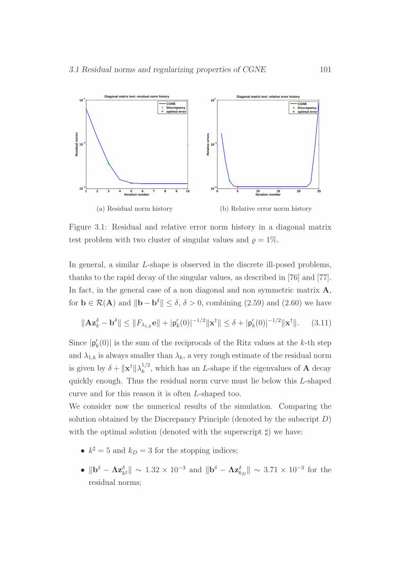
3.1 Residual norms and regularizing properties of CGNE 101
1 2 3 4 5 6 7 8 9 1010
−3
10−2
10−1
Diagonal matrix test: residual norm history
Iteration number
Res
idua
l nor
ms
CGNEDiscrepancyoptimal error
(a) Residual norm history
0 5 10 15 20 2510
−2
10−1
100
Diagonal matrix test: relative error history
Iteration number
Rel
ativ
e er
rors
CGNEDiscrepancyoptimal error
(b) Relative error norm history
Figure 3.1: Residual and relative error norm history in a diagonal matrix
test problem with two cluster of singular values and = 1%.
In general, a similar L-shape is observed in the discrete ill-posed problems,
thanks to the rapid decay of the singular values, as described in [76] and [77].
In fact, in the general case of a non diagonal and non symmetric matrix A,
for b ∈ R(A) and ‖b−bδ‖ ≤ δ, δ > 0, combining (2.59) and (2.60) we have
‖Azδk − bδ‖ ≤ ‖Fλ1,ke‖+ |p′k(0)|−1/2‖x†‖ ≤ δ + |p′k(0)|−1/2‖x†‖. (3.11)
Since |p′k(0)| is the sum of the reciprocals of the Ritz values at the k-th step
and λ1,k is always smaller than λk, a very rough estimate of the residual norm
is given by δ + ‖x†‖λ1/2k , which has an L-shape if the eigenvalues of A decay
quickly enough. Thus the residual norm curve must lie below this L-shaped
curve and for this reason it is often L-shaped too.
We consider now the numerical results of the simulation. Comparing the
solution obtained by the Discrepancy Principle (denoted by the subscript D)
with the optimal solution (denoted with the superscript ♯) we have:
• k♯ = 5 and kD = 3 for the stopping indices;
• ‖bδ − Λzδk♯‖ ∼ 1.32 × 10⁻³ and ‖bδ − ΛzδkD‖ ∼ 3.71 × 10⁻³ for the
residual norms;
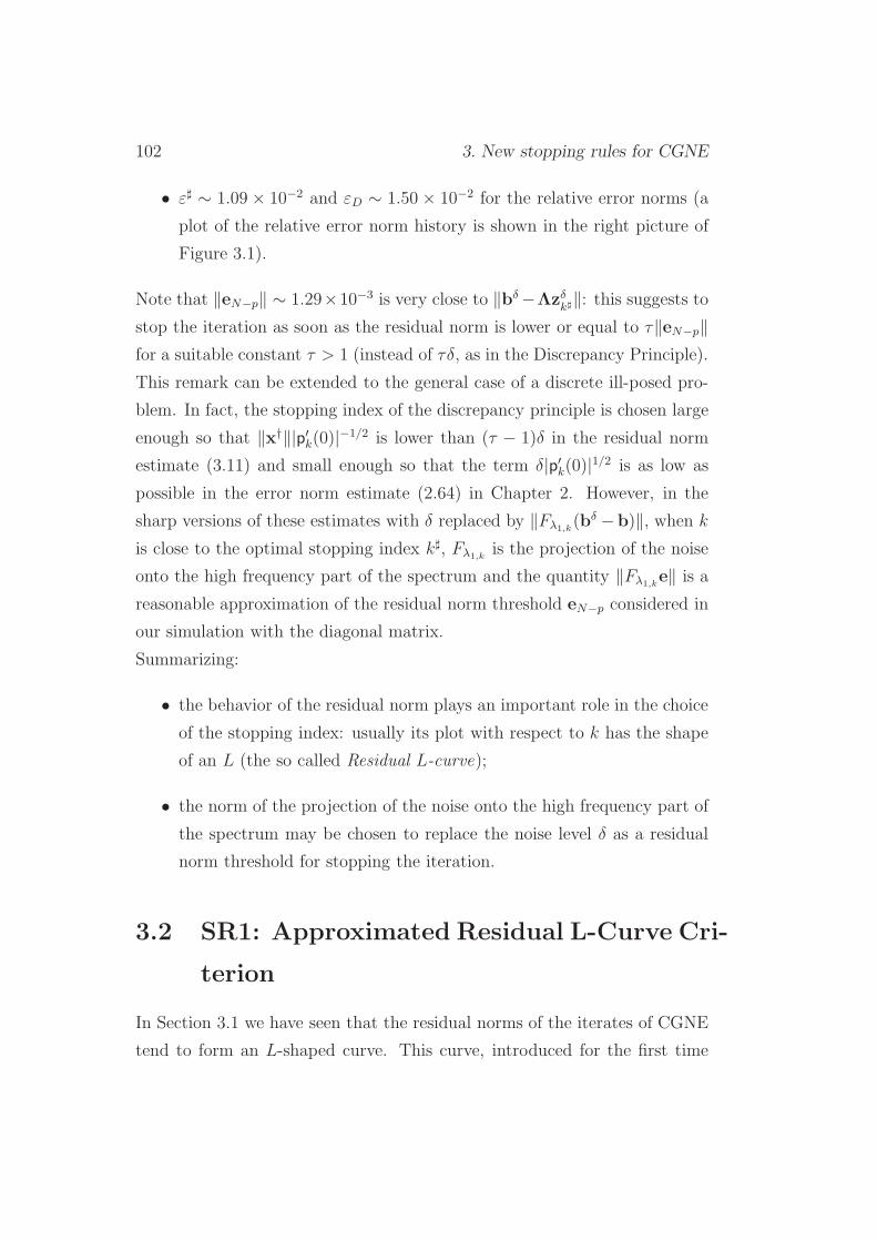
102 3. New stopping rules for CGNE
• ε♯ ∼ 1.09 × 10⁻² and εD ∼ 1.50 × 10⁻² for the relative error norms (a
plot of the relative error norm history is shown in the right picture of
Figure 3.1).
Note that ‖eN−p‖ ∼ 1.29×10⁻³ is very close to ‖bδ−Λzδk♯‖: this suggests to
stop the iteration as soon as the residual norm is lower or equal to τ‖eN−p‖for a suitable constant τ > 1 (instead of τδ, as in the Discrepancy Principle).
This remark can be extended to the general case of a discrete ill-posed pro-
blem. In fact, the stopping index of the discrepancy principle is chosen large
enough so that ‖x†‖|p′k(0)|−1/2 is lower than (τ − 1)δ in the residual norm
estimate (3.11) and small enough so that the term δ|p′k(0)|1/2 is as low as
possible in the error norm estimate (2.64) in Chapter 2. However, in the
sharp versions of these estimates with δ replaced by ‖Fλ1,k(bδ −b)‖, when k
is close to the optimal stopping index k♯, Fλ1,kis the projection of the noise
onto the high frequency part of the spectrum and the quantity ‖Fλ1,ke‖ is a
reasonable approximation of the residual norm threshold eN−p considered in
our simulation with the diagonal matrix.
Summarizing:
• the behavior of the residual norm plays an important role in the choice
of the stopping index: usually its plot with respect to k has the shape
of an L (the so called Residual L-curve);
• the norm of the projection of the noise onto the high frequency part of
the spectrum may be chosen to replace the noise level δ as a residual
norm threshold for stopping the iteration.
3.2 SR1: Approximated Residual L-Curve Cri-
terion
In Section 3.1 we have seen that the residual norms of the iterates of CGNE
tend to form an L-shaped curve. This curve, introduced for the first time
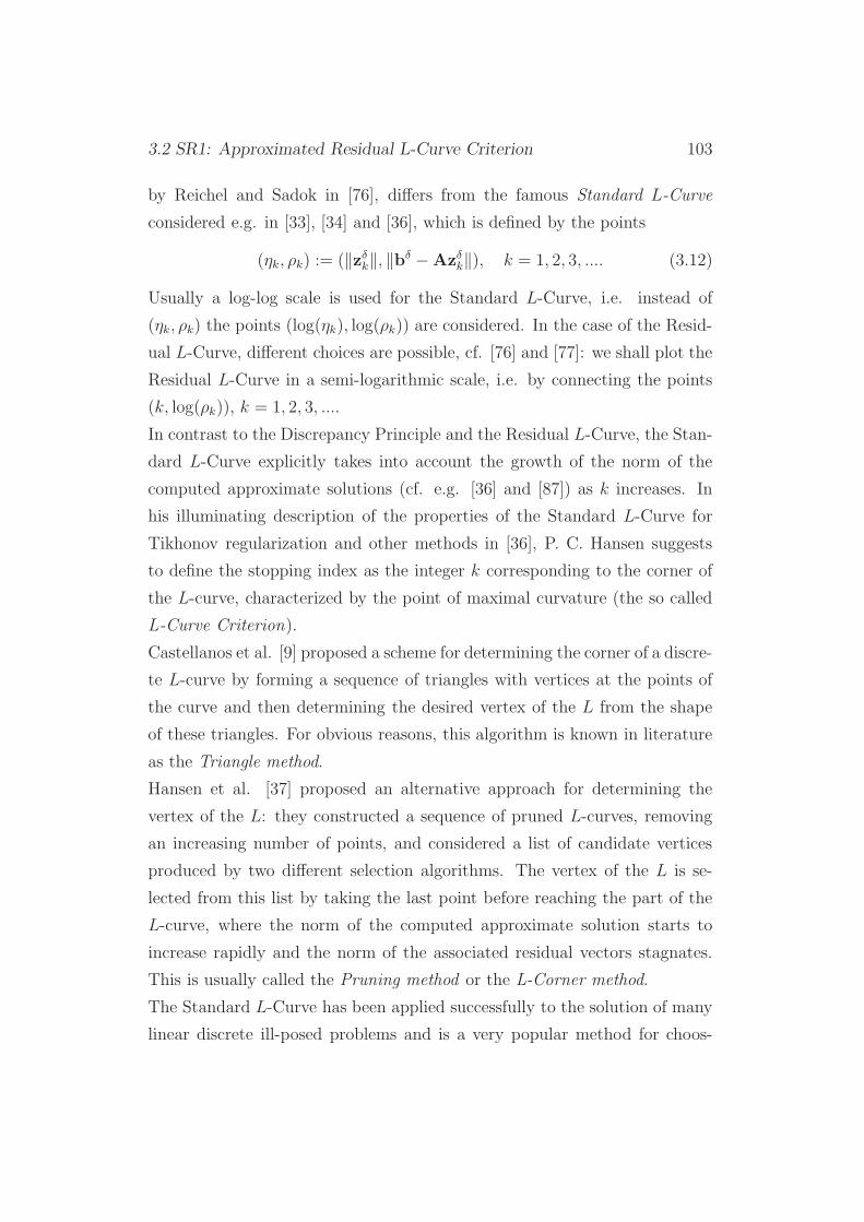
3.2 SR1: Approximated Residual L-Curve Criterion 103
by Reichel and Sadok in [76], differs from the famous Standard L-Curve
considered e.g. in [33], [34] and [36], which is defined by the points
(ηk, ρk) := (‖zδk‖, ‖bδ −Azδk‖), k = 1, 2, 3, .... (3.12)
Usually a log-log scale is used for the Standard L-Curve, i.e. instead of
(ηk, ρk) the points (log(ηk), log(ρk)) are considered. In the case of the Resid-
ual L-Curve, different choices are possible, cf. [76] and [77]: we shall plot the
Residual L-Curve in a semi-logarithmic scale, i.e. by connecting the points
(k, log(ρk)), k = 1, 2, 3, ....
In contrast to the Discrepancy Principle and the Residual L-Curve, the Stan-
dard L-Curve explicitly takes into account the growth of the norm of the
computed approximate solutions (cf. e.g. [36] and [87]) as k increases. In
his illuminating description of the properties of the Standard L-Curve for
Tikhonov regularization and other methods in [36], P. C. Hansen suggests
to define the stopping index as the integer k corresponding to the corner of
the L-curve, characterized by the point of maximal curvature (the so called
L-Curve Criterion).
Castellanos et al. [9] proposed a scheme for determining the corner of a discre-
te L-curve by forming a sequence of triangles with vertices at the points of
the curve and then determining the desired vertex of the L from the shape
of these triangles. For obvious reasons, this algorithm is known in literature
as the Triangle method.
Hansen et al. [37] proposed an alternative approach for determining the
vertex of the L: they constructed a sequence of pruned L-curves, removing
an increasing number of points, and considered a list of candidate vertices
produced by two different selection algorithms. The vertex of the L is se-
lected from this list by taking the last point before reaching the part of the
L-curve, where the norm of the computed approximate solution starts to
increase rapidly and the norm of the associated residual vectors stagnates.
This is usually called the Pruning method or the L-Corner method.
The Standard L-Curve has been applied successfully to the solution of many
linear discrete ill-posed problems and is a very popular method for choos-
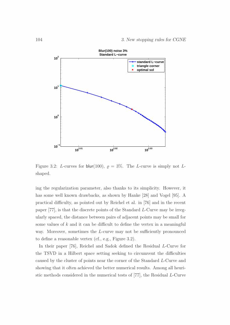
104 3. New stopping rules for CGNE
102.01
102.02
102.03
10−1
100
101
102
Blur(100) noise 3%Standard L−curve
standard L−curvetriangle corneroptimal sol
Figure 3.2: L-curves for blur(100), = 3%. The L-curve is simply not L-
shaped.
ing the regularization parameter, also thanks to its simplicity. However, it
has some well known drawbacks, as shown by Hanke [28] and Vogel [95]. A
practical difficulty, as pointed out by Reichel et al. in [76] and in the recent
paper [77], is that the discrete points of the Standard L-Curve may be irreg-
ularly spaced, the distance between pairs of adjacent points may be small for
some values of k and it can be difficult to define the vertex in a meaningful
way. Moreover, sometimes the L-curve may not be sufficiently pronounced
to define a reasonable vertex (cf., e.g., Figure 3.2).
In their paper [76], Reichel and Sadok defined the Residual L-Curve for
the TSVD in a Hilbert space setting seeking to circumvent the difficulties
caused by the cluster of points near the corner of the Standard L-Curve and
showing that it often achieved the better numerical results. Among all heuri-
stic methods considered in the numerical tests of [77], the Residual L-Curve
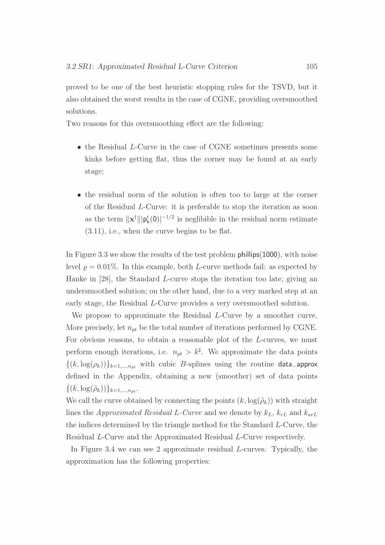
3.2 SR1: Approximated Residual L-Curve Criterion 105
proved to be one of the best heuristic stopping rules for the TSVD, but it
also obtained the worst results in the case of CGNE, providing oversmoothed
solutions.
Two reasons for this oversmoothing effect are the following:
• the Residual L-Curve in the case of CGNE sometimes presents some
kinks before getting flat, thus the corner may be found at an early
stage;
• the residual norm of the solution is often too to large at the corner
of the Residual L-Curve: it is preferable to stop the iteration as soon
as the term ‖x†‖|p′k(0)|−1/2 is neglibible in the residual norm estimate
(3.11), i.e., when the curve begins to be flat.
In Figure 3.3 we show the results of the test problem phillips(1000), with noise
level = 0.01%. In this example, both L-curve methods fail: as expected by
Hanke in [28], the Standard L-curve stops the iteration too late, giving an
undersmoothed solution; on the other hand, due to a very marked step at an
early stage, the Residual L-Curve provides a very oversmoothed solution.
We propose to approximate the Residual L-Curve by a smoother curve.
More precisely, let npt be the total number of iterations performed by CGNE.
For obvious reasons, to obtain a reasonable plot of the L-curves, we must
perform enough iterations, i.e. npt > k♯. We approximate the data points
(k, log(ρk))k=1,...,npt with cubic B-splines using the routine data−approx
defined in the Appendix, obtaining a new (smoother) set of data points
(k, log(ρk))k=1,...,npt.
We call the curve obtained by connecting the points (k, log(ρk)) with straight
lines the Approximated Residual L-Curve and we denote by kL, krL and karL
the indices determined by the triangle method for the Standard L-Curve, the
Residual L-Curve and the Approximated Residual L-Curve respectively.
In Figure 3.4 we can see 2 approximate residual L-curves. Typically, the
approximation has the following properties:
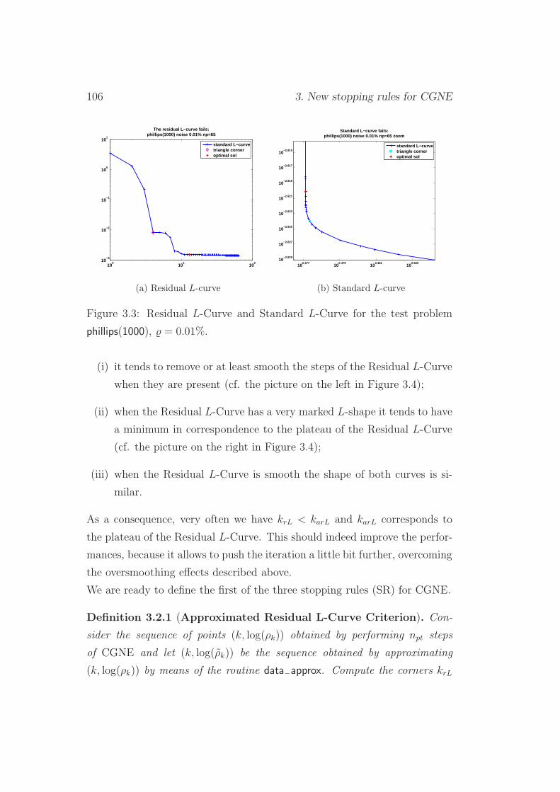
106 3. New stopping rules for CGNE
100
101
102
10−3
10−2
10−1
100
101
The residual L−curve fails:phillips(1000) noise 0.01% np=65
standard L−curvetriangle corneroptimal sol
(a) Residual L-curve
100.477
100.479
100.481
100.483
10−2.829
10−2.827
10−2.825
10−2.823
10−2.821
10−2.819
10−2.817
10−2.815
Standard L−curve fails:phillips(1000) noise 0.01% np=65 zoom
standard L−curvetriangle corneroptimal sol
(b) Standard L-curve
Figure 3.3: Residual L-Curve and Standard L-Curve for the test problem
phillips(1000), = 0.01%.
(i) it tends to remove or at least smooth the steps of the Residual L-Curve
when they are present (cf. the picture on the left in Figure 3.4);
(ii) when the Residual L-Curve has a very marked L-shape it tends to have
a minimum in correspondence to the plateau of the Residual L-Curve
(cf. the picture on the right in Figure 3.4);
(iii) when the Residual L-Curve is smooth the shape of both curves is si-
milar.
As a consequence, very often we have krL < karL and karL corresponds to
the plateau of the Residual L-Curve. This should indeed improve the perfor-
mances, because it allows to push the iteration a little bit further, overcoming
the oversmoothing effects described above.
We are ready to define the first of the three stopping rules (SR) for CGNE.
Definition 3.2.1 (Approximated Residual L-Curve Criterion). Con-
sider the sequence of points (k, log(ρk)) obtained by performing npt steps
of CGNE and let (k, log(ρk)) be the sequence obtained by approximating
(k, log(ρk)) by means of the routine data−approx. Compute the corners krL
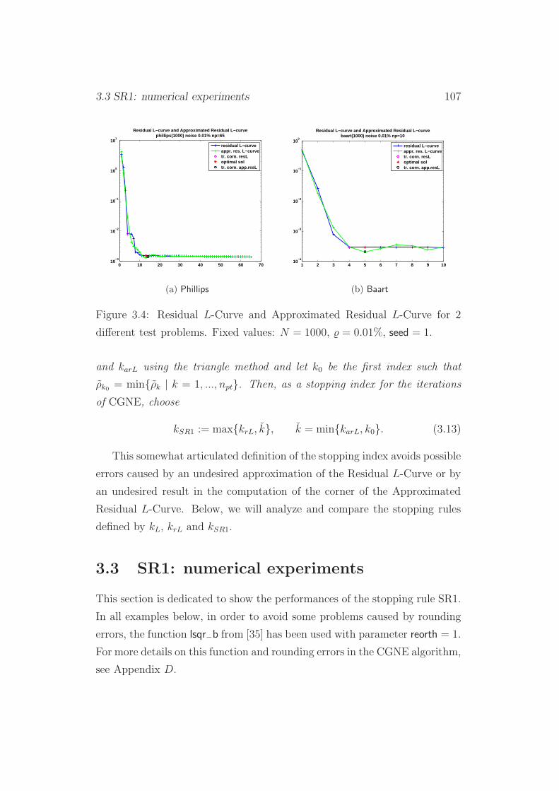
3.3 SR1: numerical experiments 107
0 10 20 30 40 50 60 7010
−3
10−2
10−1
100
101
Residual L−curve and Approximated Residual L−curvephillips(1000) noise 0.01% np=65
residual L−curveappr. res. L−curvetr. corn. resLoptimal soltr. corn. app.resL
(a) Phillips
1 2 3 4 5 6 7 8 9 1010
−4
10−3
10−2
10−1
100
Residual L−curve and Approximated Residual L−curvebaart(1000) noise 0.01% np=10
residual L−curveappr. res. L−curvetr. corn. resLoptimal soltr. corn. app.resL
(b) Baart
Figure 3.4: Residual L-Curve and Approximated Residual L-Curve for 2
different test problems. Fixed values: N = 1000, = 0.01%, seed = 1.
and karL using the triangle method and let k0 be the first index such that
ρk0 = minρk | k = 1, ..., npt. Then, as a stopping index for the iterations
of CGNE, choose
kSR1 := maxkrL, k, k = minkarL, k0. (3.13)
This somewhat articulated definition of the stopping index avoids possible
errors caused by an undesired approximation of the Residual L-Curve or by
an undesired result in the computation of the corner of the Approximated
Residual L-Curve. Below, we will analyze and compare the stopping rules
defined by kL, krL and kSR1.
3.3 SR1: numerical experiments
This section is dedicated to show the performances of the stopping rule SR1.
In all examples below, in order to avoid some problems caused by rounding
errors, the function lsqr−b from [35] has been used with parameter reorth = 1.
For more details on this function and rounding errors in the CGNE algorithm,
see Appendix D.
108 3. New stopping rules for CGNE
3.3.1 Test 1
In order to test the stopping rule of Definition 3.2.1, we consider 10 different
test problems from P.C. Hansen’s Regularization Tools [35]. For each test
problem, we fix the number npt in such a way that both the standard and the
residual L-curves can be visualized appropriately and take 2 different values
for the dimension and the noise level. In each of the possible cases, we run
the algorithm with 25 different Matlab seeds, for a total of 1000 different
examples.
In Table 3.1, for each test problem and for each couple (Ni, j), i,j ∈ 1, 2,we show the average relative errors obtained respectively by the stopping
indices kL (Standard L-Curve), krL (Residual L-Curve) and kSR1 for all pos-
sible seeds. In round brackets we collect the number of failures, i.e. how
many times the relative error obtained by the stopping rule is at least 5
times larger than the relative error obtained by the optimal stopping index
k♯. We can see that stopping rule associated to the index kSR1 improves the
results of the Residual L-Curve in almost all the cases.
This stopping rule proves to be reliable also when the noise level is smaller
and the Standard L-Curve fails, as we will see below.
3.3.2 Test 2
In this example we test the robustness of the method when the noise level is
small and with respect to the number of points npt. As we have seen, this
is a typical case in which the Standard L-Curve method may fail to obtain
acceptable results.
We consider the test problems gravity, heat and phillips, with N = 1000, ∈1 × 10⁻⁵, 5 × 10⁻⁵, 1 × 10⁻⁴, 5 × 10⁻⁴, seed ∈ 1, 2, ..., 25. For each case,
we also take 3 different values of npt (the smallest one is only a little bit
larger than the optimal index k♯), in order to analyze the dependence of the
methods on this particular parameter.
The results of Table 3.2 clearly show that the Approximated Residual L-
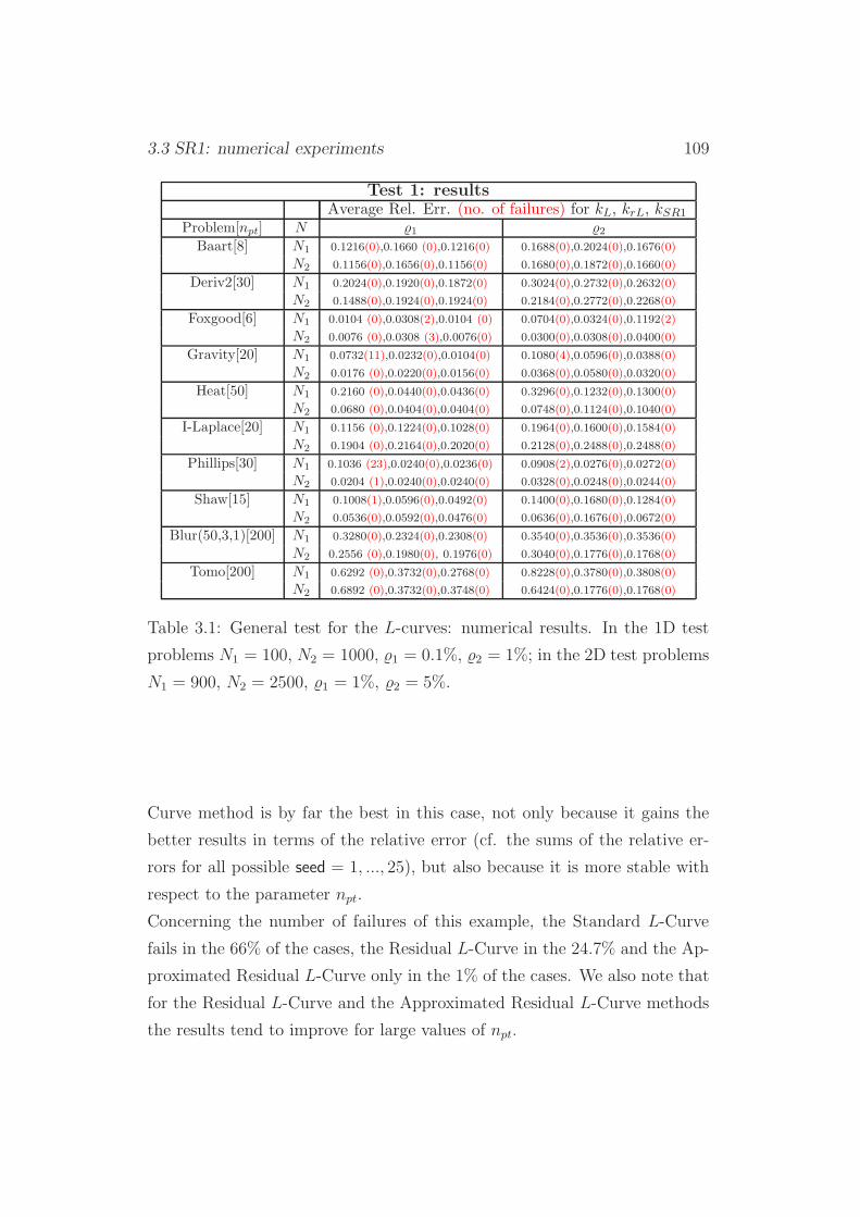
3.3 SR1: numerical experiments 109
Test 1: resultsAverage Rel. Err. (no. of failures) for kL, krL, kSR1
Problem[npt] N 1 2Baart[8] N1 0.1216(0),0.1660 (0),0.1216(0) 0.1688(0),0.2024(0),0.1676(0)
N2 0.1156(0),0.1656(0),0.1156(0) 0.1680(0),0.1872(0),0.1660(0)
Deriv2[30] N1 0.2024(0),0.1920(0),0.1872(0) 0.3024(0),0.2732(0),0.2632(0)
N2 0.1488(0),0.1924(0),0.1924(0) 0.2184(0),0.2772(0),0.2268(0)
Foxgood[6] N1 0.0104 (0),0.0308(2),0.0104 (0) 0.0704(0),0.0324(0),0.1192(2)
N2 0.0076 (0),0.0308 (3),0.0076(0) 0.0300(0),0.0308(0),0.0400(0)
Gravity[20] N1 0.0732(11),0.0232(0),0.0104(0) 0.1080(4),0.0596(0),0.0388(0)
N2 0.0176 (0),0.0220(0),0.0156(0) 0.0368(0),0.0580(0),0.0320(0)
Heat[50] N1 0.2160 (0),0.0440(0),0.0436(0) 0.3296(0),0.1232(0),0.1300(0)
N2 0.0680 (0),0.0404(0),0.0404(0) 0.0748(0),0.1124(0),0.1040(0)
I-Laplace[20] N1 0.1156 (0),0.1224(0),0.1028(0) 0.1964(0),0.1600(0),0.1584(0)
N2 0.1904 (0),0.2164(0),0.2020(0) 0.2128(0),0.2488(0),0.2488(0)
Phillips[30] N1 0.1036 (23),0.0240(0),0.0236(0) 0.0908(2),0.0276(0),0.0272(0)
N2 0.0204 (1),0.0240(0),0.0240(0) 0.0328(0),0.0248(0),0.0244(0)
Shaw[15] N1 0.1008(1),0.0596(0),0.0492(0) 0.1400(0),0.1680(0),0.1284(0)
N2 0.0536(0),0.0592(0),0.0476(0) 0.0636(0),0.1676(0),0.0672(0)
Blur(50,3,1)[200] N1 0.3280(0),0.2324(0),0.2308(0) 0.3540(0),0.3536(0),0.3536(0)
N2 0.2556 (0),0.1980(0), 0.1976(0) 0.3040(0),0.1776(0),0.1768(0)
Tomo[200] N1 0.6292 (0),0.3732(0),0.2768(0) 0.8228(0),0.3780(0),0.3808(0)
N2 0.6892 (0),0.3732(0),0.3748(0) 0.6424(0),0.1776(0),0.1768(0)
Table 3.1: General test for the L-curves: numerical results. In the 1D test
problems N1 = 100, N2 = 1000, 1 = 0.1%, 2 = 1%; in the 2D test problems
N1 = 900, N2 = 2500, 1 = 1%, 2 = 5%.
Curve method is by far the best in this case, not only because it gains the
better results in terms of the relative error (cf. the sums of the relative er-
rors for all possible seed = 1, ..., 25), but also because it is more stable with
respect to the parameter npt.
Concerning the number of failures of this example, the Standard L-Curve
fails in the 66% of the cases, the Residual L-Curve in the 24.7% and the Ap-
proximated Residual L-Curve only in the 1% of the cases. We also note that
for the Residual L-Curve and the Approximated Residual L-Curve methods
the results tend to improve for large values of npt.
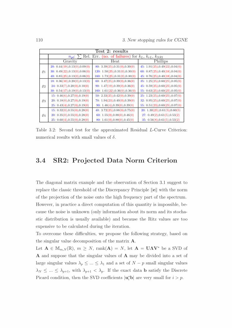
110 3. New stopping rules for CGNE
Test 2: resultsnpt:
∑Rel. Err. (no. of failures) for kL, krL, kSR1
Gravity Heat Phillips20: 0.44(19),0.13(0),0.09(0) 80: 3.39(25),0.31(0),0.30(0) 45: 1.91(25),0.49(22),0.04(0)
1 30: 0.49(22),0.13(0),0.06(0) 120: 1.50(25),0.31(0),0.30(0) 60: 0.87(25),0.40(18),0.04(0)
40: 0.85(25),0.13(0),0.06(0) 160: 1.73(25),0.31(0),0.30(0) 45: 0.76(25),0.40(18),0.04(0)
18: 0.36(10),0.20(0),0.13(0) 60: 3.47(25),0.39(0),0.36(0) 35: 1.25(25),0.60(25),0.05(0)
2 24: 0.33(7),0.20(0),0.10(0) 90: 1.47(19),0.39(0),0.36(0) 45: 0.59(25),0.60(25),0.05(0)
30: 0.54(17),0.19(0),0.13(0) 160: 1.61(22),0.36(0),0.36(0) 55: 0.63(25),0.60(25),0.05(0)
15: 0.46(6),0.27(0),0.19(0) 50: 2.33(25),0.42(0),0.39(0) 25: 1.23(25),0.60(25),0.07(0)
3 20: 0.18(0),0.27(0),0.19(0) 70: 1.94(23),0.40(0),0.39(0) 32: 0.95(25),0.60(25),0.07(0)
25: 0.43(4),0.27(0),0.19(0) 90: 1.46(4),0.39(0),0.39(0) 55: 0.51(23),0.60(25),0.07(0)
15: 0.32(0),0.55(0),0.28(0) 40: 3.72(25),0.88(0),0.75(0) 20: 1.30(25),0.61(5),0.60(5)
4 20: 0.35(0),0.55(0),0.28(0) 60: 1.55(0),0.88(0),0.46(0) 27: 0.49(2),0.61(5),0.53(2)
25: 0.60(4),0.55(0),0.28(0) 80: 1.61(0),0.88(0),0.45(0) 35: 0.56(8),0.61(5),0.53(2)
Table 3.2: Second test for the approximated Residual L-Curve Criterion:
numerical results with small values of δ.
3.4 SR2: Projected Data Norm Criterion
The diagonal matrix example and the observation of Section 3.1 suggest to
replace the classic threshold of the Discrepancy Principle ‖e‖ with the norm
of the projection of the noise onto the high frequency part of the spectrum.
However, in practice a direct computation of this quantity is impossible, be-
cause the noise is unknown (only information about its norm and its stocha-
stic distribution is usually available) and because the Ritz values are too
expensive to be calculated during the iteration.
To overcome these difficulties, we propose the following strategy, based on
the singular value decomposition of the matrix A.
Let A ∈ Mm,N(R), m ≥ N , rank(A) = N , let A = UΛV∗ be a SVD of
A and suppose that the singular values of A may be divided into a set of
large singular values λp ≤ ... ≤ λ1 and a set of N − p small singular values
λN ≤ ... ≤ λp+1, with λp+1 < λp. If the exact data b satisfy the Discrete
Picard condition, then the SVD coefficients |u∗ib| are very small for i > p.
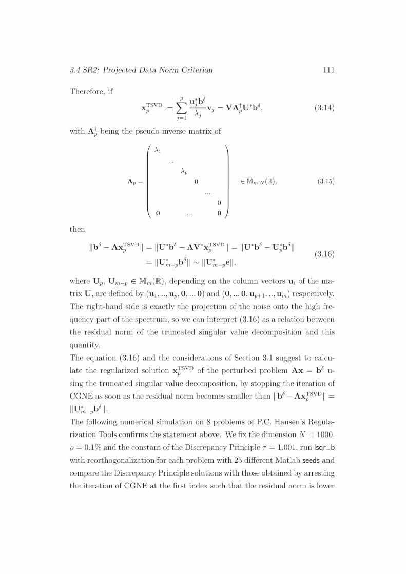
3.4 SR2: Projected Data Norm Criterion 111
Therefore, if
xTSVDp :=
p∑
j=1
u∗jb
δ
λjvj = VΛ†
pU∗bδ, (3.14)
with Λ†p being the pseudo inverse matrix of
Λp =
λ1
...
λp
0
...
0
0 ... 0
∈ Mm,N (R), (3.15)
then
‖bδ −AxTSVDp ‖ = ‖U∗bδ −ΛV∗xTSVD
p ‖ = ‖U∗bδ −U∗pb
δ‖= ‖U∗
m−pbδ‖ ∼ ‖U∗
m−pe‖,(3.16)
where Up, Um−p ∈ Mm(R), depending on the column vectors ui of the ma-
trix U, are defined by (u1, ..,up, 0, .., 0) and (0, .., 0,up+1, ..,um) respectively.
The right-hand side is exactly the projection of the noise onto the high fre-
quency part of the spectrum, so we can interpret (3.16) as a relation between
the residual norm of the truncated singular value decomposition and this
quantity.
The equation (3.16) and the considerations of Section 3.1 suggest to calcu-
late the regularized solution xTSVDp of the perturbed problem Ax = bδ u-
sing the truncated singular value decomposition, by stopping the iteration of
CGNE as soon as the residual norm becomes smaller than ‖bδ −AxTSVDp ‖ =
‖U∗m−pb
δ‖.The following numerical simulation on 8 problems of P.C. Hansen’s Regula-
rization Tools confirms the statement above. We fix the dimension N = 1000,
= 0.1% and the constant of the Discrepancy Principle τ = 1.001, run lsqr−b
with reorthogonalization for each problem with 25 different Matlab seeds and
compare the Discrepancy Principle solutions with those obtained by arresting
the iteration of CGNE at the first index such that the residual norm is lower
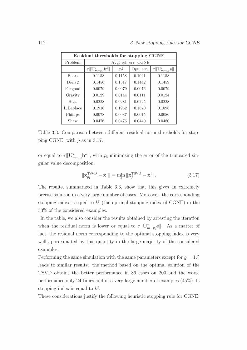
112 3. New stopping rules for CGNE
Residual thresholds for stopping CGNE
Problem Avg. rel. err. CGNE
τ‖U∗m−p♯
bδ‖ τδ Opt. err. τ‖U∗m−p♯
e‖Baart 0.1158 0.1158 0.1041 0.1158
Deriv2 0.1456 0.1517 0.1442 0.1459
Foxgood 0.0079 0.0079 0.0076 0.0079
Gravity 0.0129 0.0144 0.0111 0.0124
Heat 0.0228 0.0281 0.0225 0.0228
I−Laplace 0.1916 0.1952 0.1870 0.1898
Phillips 0.0078 0.0087 0.0075 0.0086
Shaw 0.0476 0.0476 0.0440 0.0480
Table 3.3: Comparison between different residual norm thresholds for stop-
ping CGNE, with p as in 3.17.
or equal to τ‖U∗m−p♯
bδ‖, with p♯ minimizing the error of the truncated sin-
gular value decomposition:
‖xTSVDp♯
− x†‖ = minj
‖xTSVDj − x†‖. (3.17)
The results, summarized in Table 3.3, show that this gives an extremely
precise solution in a very large number of cases. Moreover, the corresponding
stopping index is equal to k♯ (the optimal stopping index of CGNE) in the
53% of the considered examples.
In the table, we also consider the results obtained by arresting the iteration
when the residual norm is lower or equal to τ‖U∗m−p♯
e‖. As a matter of
fact, the residual norm corresponding to the optimal stopping index is very
well approximated by this quantity in the large majority of the considered
examples.
Performing the same simulation with the same parameters except for = 1%
leads to similar results: the method based on the optimal solution of the
TSVD obtains the better performance in 86 cases on 200 and the worse
performance only 24 times and in a very large number of examples (45%) its
stopping index is equal to k♯.
These considerations justify the following heuristic stopping rule for CGNE.
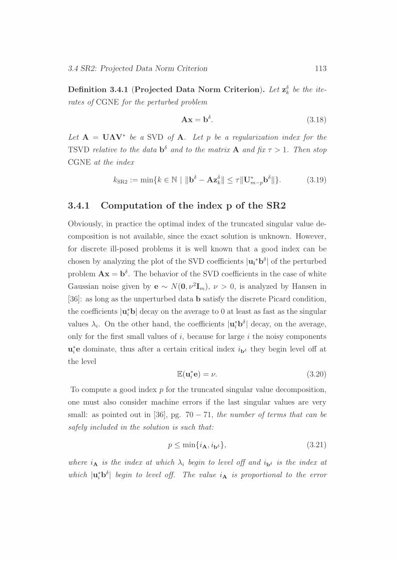
3.4 SR2: Projected Data Norm Criterion 113
Definition 3.4.1 (Projected Data Norm Criterion). Let zδk be the ite-
rates of CGNE for the perturbed problem
Ax = bδ. (3.18)
Let A = UΛV∗ be a SVD of A. Let p be a regularization index for the
TSVD relative to the data bδ and to the matrix A and fix τ > 1. Then stop
CGNE at the index
kSR2 := mink ∈ N | ‖bδ −Azδk‖ ≤ τ‖U∗m−pb
δ‖. (3.19)
3.4.1 Computation of the index p of the SR2
Obviously, in practice the optimal index of the truncated singular value de-
composition is not available, since the exact solution is unknown. However,
for discrete ill-posed problems it is well known that a good index can be
chosen by analyzing the plot of the SVD coefficients |ui∗bδ| of the perturbed
problem Ax = bδ. The behavior of the SVD coefficients in the case of white
Gaussian noise given by e ∼ N(0, ν2Im), ν > 0, is analyzed by Hansen in
[36]: as long as the unperturbed data b satisfy the discrete Picard condition,
the coefficients |u∗ib| decay on the average to 0 at least as fast as the singular
values λi. On the other hand, the coefficients |u∗ib
δ| decay, on the average,
only for the first small values of i, because for large i the noisy components
u∗i e dominate, thus after a certain critical index ibδ they begin level off at
the level
E(u∗i e) = ν. (3.20)
To compute a good index p for the truncated singular value decomposition,
one must also consider machine errors if the last singular values are very
small: as pointed out in [36], pg. 70 − 71, the number of terms that can be
safely included in the solution is such that:
p ≤ miniA, ibδ, (3.21)
where iA is the index at which λi begin to level off and ibδ is the index at
which |u∗ib
δ| begin to level off. The value iA is proportional to the error
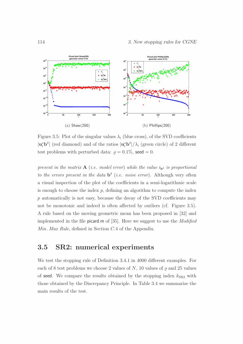
114 3. New stopping rules for CGNE
0 50 100 150 20010
−20
10−15
10−10
10−5
100
105
1010
1015
i
Picard plot Shaw(200)gaussian noise 0.1%
σi
|uiTb|
|uiTb|/σ
i
(a) Shaw(200)
0 50 100 150 20010
−8
10−6
10−4
10−2
100
102
104
i
Picard plot Phillips(200)gaussian noise 0.1%
σ
i
|uiTb|
|uiTb|/σ
i
(b) Phillips(200)
Figure 3.5: Plot of the singular values λi (blue cross), of the SVD coefficients
|u∗ib
δ| (red diamond) and of the ratios |u∗ib
δ|/λi (green circle) of 2 different
test problems with perturbed data: = 0.1%, seed = 0.
present in the matrix A (i.e. model error) while the value ibδ is proportional
to the errors present in the data bδ (i.e. noise error). Although very often
a visual inspection of the plot of the coefficients in a semi-logarithmic scale
is enough to choose the index p, defining an algorithm to compute the index
p automatically is not easy, because the decay of the SVD coefficients may
not be monotonic and indeed is often affected by outliers (cf. Figure 3.5).
A rule based on the moving geometric mean has been proposed in [32] and
implemented in the file picard.m of [35]. Here we suggest to use the Modified
Min−Max Rule, defined in Section C.4 of the Appendix.
3.5 SR2: numerical experiments
We test the stopping rule of Definition 3.4.1 in 4000 different examples. For
each of 8 test problems we choose 2 values of N , 10 values of and 25 values
of seed. We compare the results obtained by the stopping index kSR2 with
those obtained by the Discrepancy Principle. In Table 3.4 we summarize the
main results of the test.
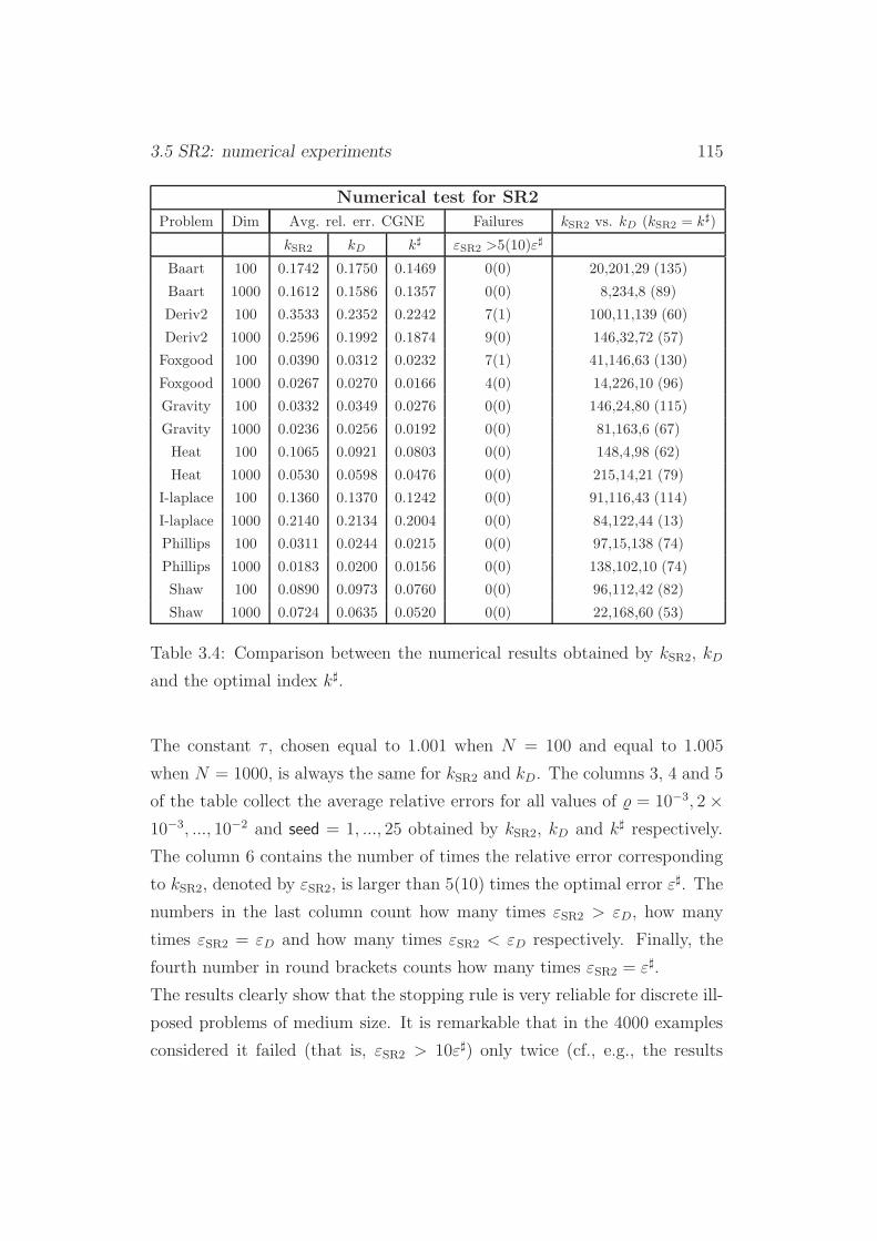
3.5 SR2: numerical experiments 115
Numerical test for SR2
Problem Dim Avg. rel. err. CGNE Failures kSR2 vs. kD (kSR2 = k♯)
kSR2 kD k♯ εSR2 >5(10)ε♯
Baart 100 0.1742 0.1750 0.1469 0(0) 20,201,29 (135)
Baart 1000 0.1612 0.1586 0.1357 0(0) 8,234,8 (89)
Deriv2 100 0.3533 0.2352 0.2242 7(1) 100,11,139 (60)
Deriv2 1000 0.2596 0.1992 0.1874 9(0) 146,32,72 (57)
Foxgood 100 0.0390 0.0312 0.0232 7(1) 41,146,63 (130)
Foxgood 1000 0.0267 0.0270 0.0166 4(0) 14,226,10 (96)
Gravity 100 0.0332 0.0349 0.0276 0(0) 146,24,80 (115)
Gravity 1000 0.0236 0.0256 0.0192 0(0) 81,163,6 (67)
Heat 100 0.1065 0.0921 0.0803 0(0) 148,4,98 (62)
Heat 1000 0.0530 0.0598 0.0476 0(0) 215,14,21 (79)
I-laplace 100 0.1360 0.1370 0.1242 0(0) 91,116,43 (114)
I-laplace 1000 0.2140 0.2134 0.2004 0(0) 84,122,44 (13)
Phillips 100 0.0311 0.0244 0.0215 0(0) 97,15,138 (74)
Phillips 1000 0.0183 0.0200 0.0156 0(0) 138,102,10 (74)
Shaw 100 0.0890 0.0973 0.0760 0(0) 96,112,42 (82)
Shaw 1000 0.0724 0.0635 0.0520 0(0) 22,168,60 (53)
Table 3.4: Comparison between the numerical results obtained by kSR2, kD
and the optimal index k♯.
The constant τ , chosen equal to 1.001 when N = 100 and equal to 1.005
when N = 1000, is always the same for kSR2 and kD. The columns 3, 4 and 5
of the table collect the average relative errors for all values of = 10−3, 2×10⁻³, ..., 10−2 and seed = 1, ..., 25 obtained by kSR2, kD and k♯ respectively.
The column 6 contains the number of times the relative error corresponding
to kSR2, denoted by εSR2, is larger than 5(10) times the optimal error ε♯. The
numbers in the last column count how many times εSR2 > εD, how many
times εSR2 = εD and how many times εSR2 < εD respectively. Finally, the
fourth number in round brackets counts how many times εSR2 = ε♯.
The results clearly show that the stopping rule is very reliable for discrete ill-
posed problems of medium size. It is remarkable that in the 4000 examples
considered it failed (that is, εSR2 > 10ε♯) only twice (cf., e.g., the results
116 3. New stopping rules for CGNE
obtained by the heuristic stopping rules in [77], Table 2). Moreover, in many
cases it even improves the results of the Discrepancy Principle, which is based
on the knowledge of the noise level.
3.6 Image deblurring
One of the most famous applications of the theory of ill-posed problems is
to recover a sharp image from its blurry observation, i.e. image deblurring.
It frequently arises in imaging sciences and technologies, including optical,
medical, and astronomical applications and is crucial for allowing to detect
important features and patterns such as those of a distant planet or some
microscopic tissue.
Due to its importance, this subject has been widely studied in literature:
without any claim to be exhaustive, we point out at some books [10], [38],
[48], [100], or chapters of books [4], [96] dedicated to this problem.
In most applications, blurs are introduced by three different types of physical
factors: optical, mechanical, or medium-induced, which could lead to familiar
out-of-focus blurs, motion blurs, or atmospheric blurs respectively. We refer
the reader to [10] for a more detailed account on the associated physical
processes.
Mathematically, a continuous (analog) image is described by a nonnegative
function f = f(x) on R2 supported on a (rectangular) 2D domain Ω and the
blurring process is either a linear or nonlinear operator K acting on the some
functional space. Since we shall focus only on linear deblurring problems, K
is assumed to be linear.
Among all linear blurs, the most frequently encountered type is the shift
invariant blur, i.e. a linear blur K = K[f ] such that for any shift vector y ∈R2,
g(x) = K [f(x)] =⇒ g(x− y) = K [f(x− y)] ,x ∈ Ω. (3.22)
3.6 Image deblurring 117
It is well known in signal processing as well as system theory [72] that a
shift-invariant linear operator must be in the form of convolution:
g(x) = K[f ](x) = κ ∗ f(x) =∫
Ω
κ(x− y)f(y)dy, (3.23)
for some suitable kernel function κ(x), or the point spread function (PSF).
The function g(x) is the blurred analog image that is converted into a digital
image through a digitalization process (or sampling).
A digital image is typically recorded by means of a CCD (charge-coupled
device), which is an array of tiny detectors (potential wells), arranged in a
rectangular grid, able to record the amount, or intensity, of the light that
hits each detector.
Thus, a digital grayscale image
G = (gj,l), j = 1, ..., J, l = 1, ..., L (3.24)
is a rectangular array, whose entries represent the (nonnegative) light inten-
sities captured by each detector.
The PSF is described by a matrix H = (hj,l) of the same size of the image,
whose entries are all zero except for a very small set of pixels (j, l) distributed
around a certain pixel (jc, lc) which is the center of the blur. Since we are
assuming spatial invariant PSFs, the center of the PSF corresponds to the
center of the 2D array.
In some cases the PSF can be described analytically and H can be con-
structed from a function, rather than through experimentation (e.g. the
horizontal and vertical motion blurs are constructed in this way).
In other cases, the knowledge of the physical process that causes the blur
provides an explicit formulation of the PSF. In this case, the elements of
the PSF array are given by a precise mathematical expression: e.g. the
out-of-focus blur is given by the formula
hj,l =
1
πr2if (j − jc)
2 + (l − lc)2 ≤ r2,
0 otherwise,(3.25)
118 3. New stopping rules for CGNE
where r > 0 is the radius of the blur.
For other examples, such as the blur caused by atmospheric turbulence or
the PSF associated to an astronomical telescope, we refer to [38] and the
references therein.
As a consequence of the digitalization process, the continuous model de-
scribed by (3.23) has to be adapted to the discrete setting as well. To do
this, we consider first the 1D case
g(t) =
∫
κ(t− s)f(s)ds. (3.26)
To fix the ideas, we assume that J is even and that the function f(s) is
defined in the interval [−J−12, J−1
2]. Let
sj = −J − 1
2+ j − 1, j = 1, ..., J (3.27)
be the J points in which the interval is subdivided and discretize κ and f
in such a way that κ(s) = κ(sj) = hj if |s − sj | < 12or s = sj +
12and
analogously for κ. Approximating (3.26) with the trapezoidal rule
g(t) ∼=J∑
j′=1
κ(t− sj′)f(sj′) (3.28)
and recomputing in the points sj, we obtain the components of the discretized
version g of the function g:
gj =
J∑
j′=1
κ(sj − sj′)f(sj′), j = 1, ...J. (3.29)
As a consequence of the assumptions we have made, (3.29) can be rewritten
into
gj =J∑
j′=1
hj−j′+J2fj′, j = 1, ...J, (3.30)
which is the componentwise expression of the discrete convolution between
the column vectors h = (hj) and f = (fj). We observe that some terms in
the sum in the right-hand side of (3.30) may be not defined: this happens

3.6 Image deblurring 119
because the support of the convolution between κ and f is larger than the
supports of κ and f . The problem is solved by extending the vector h to the
larger vector
h =
h−J2+1
...
h0
h
hJ+1
...
hJ+J2
, hj = hj+J , j = −J2+ 1, ...,
J
2(3.31)
and substituting h with h in (3.30), which is equivalent to extend κ periodi-
cally on the real line. The convolution (3.30) may also be expressed in the
form
g = Af , A = (ai,j), ai,j = hi−j+J2, i, j = 1, ..., J. (3.32)
In the 2D case, proceeding in an analogous way, we get
gj,l =J∑
j′=1
L∑
l′=1
hj−j′+J2,l−l′+L
2fj′,l′. (3.33)
The equation above (3.33) is usually written in the form
G = H ∗ F, (3.34)
where G, H and F are here matrices in MJ,L(R). If g and f are the column
vectors obtained by concatenating the columns of G and F respectively, then
(3.34) can be rewritten in the form
g = Af . (3.35)
In the case of an image f with 1024 × 1024 pixels, the system (3.35) has
then more than one million unknowns. For generic problems of this size,
the computation of the singular value decomposition is not usually possible.
120 3. New stopping rules for CGNE
However, if we set N := JL, then A ∈ MN(R) is a circulant matrix with
circulant blocks (BCCB). It is well known (cf. e.g. [4] or [38]) that BCCB
matrices are normal (that is, A∗A = AA∗) and that may be diagonalized by
A = Φ∗ΛΦ, (3.36)
where Φ is the two-dimensional unitary matrix unitary Discrete Fourier
Transform (DFT) matrix.
We recall that the DFT of a vector z ∈ CN is the vector z whose components
are defined by
zj =1√N
N∑
j′=1
zj′e−2πı(j′−1)(j−1)/N (3.37)
and the inverse DFT of a vector w ∈ CN is the vector w, whose components
are calculated via the formula
wj =1√N
N∑
j′=1
wj′e2πı(j′−1)(j−1)/N . (3.38)
The two-dimensional DFT of a 2D array can be obtained by computing the
DFT of its columns, followed by a DFT of its rows. A similar approach is
used for the inverse two-dimensional DFT. The DFT and inverse DFT com-
putations can be written as matrix-vector multiplication operations, which
may be computed by means of the FFT algorithm, see e.g. [12], [94] and
Matlab’s documentation on the routines fft, ifft, fft2 and ifft2. In general, the
speed of the algorithms depends on the size of the vector x: they are most
efficient if the dimensions have only small prime factors. In particular, if N
is a power of 2, the cost is N log2(N).
Thus, matrix-vector multiplications withΦ andΦ∗ may be performed quickly
without constructing the matrices explicitly and since the first column of Φ
is the vector of all ones scaled by the square root of the dimension, denoting
with a1 and φ1 the first column of A and Φ respectively, it follows that
Φa1 = Λφ1 =1√Nλ, (3.39)
3.7 SR3: Projected Noise Norm Criterion 121
where λ is the column vector of the eigenvalues of A.
As a consequence, even in the 2D case, the spectral decomposition of the
matrix A can be calculated with a reasonable computational effort, so it is
possible to apply the techniques we have seen in Chapter 3 for this particular
problem. In particular, we shall be able to compute the SVD coefficients
(Fourier coefficients) |φ∗jg| and the ratios |φ∗
jg|/λj, and arrest the CGNE
method according to the stopping rule of Definition 3.4.1.
Moreover, when the spectral decomposition of A is known, matrix-vector
multiplications can be performed very efficiently in Matlab using the DFT.
For example, as shown in [38], given the PSF matrix H and an image F:
• to compute the eigenvalues of A, use
S = fft2(fftshift(H)); (3.40)
• to compute the blurred image G = H ∗ F, use3
G = real(ifft2(H⊚ fft2(F))). (3.41)
3.7 SR3: Projected Noise Norm Criterion
In this section we define an a-posteriori stopping rule, based on a statistical
approach, suited mainly for large scale problems. The aim is again to ap-
proximate the norm of the projection of the noise onto the high frequency
components
‖U∗m−pe‖, (3.42)
where p ≥ 0 is the number of the low frequency components of the problem.
We assume that p can be determined by means of an algorithm: for example,
in the case of image deblurring, the algorithm of Section 3.4 can be applied.
We simply consider a modified version of the Discrepancy Principle with δ
replaced by the expected value of ‖U∗m−pe‖:
3the operation ⊚ is the componentwise multiplication of two matrices.
122 3. New stopping rules for CGNE
Definition 3.7.1 (Projected Noise Norm Criterion). Suppose the ma-
trix A ∈ Mm,N (R) has m − p noise-dominated SVD coefficients. Fix τ > 1
and stop the iteration of CGNE as soon as the norm of the residual is lower
or equal to τ δ with δ := δ√
(m− p)/m:
kSR3 := mink ∈ N | ‖Azδk − bδ‖ ≤ τ δ. (3.43)
Note that the definition does not require a SVD of the matrix A, but
only a knowledge about p.
The following result provides a theoretical justification for the definition
above: if m is big, with high probability δ is not smaller than ‖U∗m−pe‖.
Theorem 3.7.1. Let ǫ1 > 0 and ǫ2 > 0 be small positive numbers and let α
∈ (0, 1/2). Then there exists a positive integer m = m(ǫ1, ǫ2, α) such that for
every m > m the estimate
P(‖U∗
m−pe‖2 − ǫ1 > δ2)≤ ǫ2 (3.44)
holds whenever the following conditions are satisfied:
(i) p ≤ αm;
(ii) e ∼ N (0, ν2Im), ν > 0;
(iii) δ2 = ‖e‖2.
Before proving the theorem, a few remarks:
• The theorem is based on the simple idea that if e ∼ N (0, ν2Im), then
U∗e has the same distribution: this argument fails if the perturbation
has a different distribution!
• In principle it is possible, but maybe hard, to calculate m in terms of
ǫ1, ǫ2 and α. For this reason we do not recommend this stopping rule
for the small and medium size problems of Section 3.4.
3.7 SR3: Projected Noise Norm Criterion 123
• The assumption on p restricts the validity of the statement: luckily
enough, in most cases p is small with respect to m. When this does
not happen (p >> m/2), the choice p = m/2 should improve the
performances anyway.
Proof. Fix ǫ1 > 0, ǫ2 > 0 and α ∈ (0, 1/2). Let A = UΛV∗ be an SVD of
A and let p ∈ 1, ..., m − 1. We observe that if e ∼ N (0, ν2Im), ν > 0,
then U∗e ∼ N (0, ν2Im), so U∗m−pe ∼ (0, ..., 0, ep+1, ..., em). Thus, if p, e and
δ satisfy (i), (ii) and (iii) respectively, there holds:
P
(
‖U∗m−pe‖2 −
δ2(m− p)
m> ǫ1
)
= P
(m∑
i=p+1
e2i −δ2(m− p)
m> ǫ1
)
.
(3.45)
For 0 < t < min1/(2pν2), Markov’s inequality and our assumptions (ii)
and (iii) yield
P
(m∑
i=p+1
e2i −δ2(m− p)
m> ǫ1
)
= P
(
p
m∑
i=p+1
e2i − (m− p)
p∑
i=1
e2i > mǫ1
)
= P
(
exp
[
t
(
pm∑
i=p+1
e2i − (m− p)
p∑
i=1
e2i
)]
> exp[tmǫ1]
)
≤ exp[−tmǫ1]E(
exp
[
t
(
pm∑
i=p+1
e2i −p∑
i=1
e2i
)])
= exp[−tmǫ1](1− 2tsν2)−m−p
2 (1 + 2t(m− p)ν2)−p2 ,
(3.46)
where in the last equality we have used the assumption (ii) and the fact that
if X is a random variable with gaussian distribution X ∼ N (0, ν2), then, for
every a < 1/(2ν2),
E(exp[aX2]) = (1− 2aν2)−12 . (3.47)
Putting w := 2tν2 the right-hand side of (3.46) can be rewritten as
exp
[−mǫ1w2ν2
]
(1− sw)−m−p
2 (1 + (m− p)w)−p2 . (3.48)
124 3. New stopping rules for CGNE
If p ≤ √m, the expression above can be made < ǫ2 choosing w close enough
to 1/p for all m sufficiently large. On the other hand, if√m < p ≤ αm and
w = o( 1m), a Taylor expansion of the second and the third factor gives
exp
[
−mǫ1w2ν2
+m− p
2(sw +
p2w2
2+O(p3w3))
−p2
(
(m− p)w +(m− p)2w2
2+O((m− p)3w3)
)]
= exp
[
−mǫ1w2ν2
− p(m− p)(m− 2p)w2
4(1 + o(1))
]
,
(3.49)
thus it is possible to choose w (e.g., w ≈ 1/(mp1/4)) in such a way that the
last expression can be made arbitrarily small for all m sufficiently large.
Summing up, we have proved that there exists m ∈ N such that for allm > m
and for all p < αm there holds
inft > 0 | exp[−tmǫ1](1− 2tsν2)−m−p
2 (1 + 2t(m− p)ν2)−p2 ≤ ǫ2 (3.50)
and according to (3.45) and (3.46) this completes the proof.
3.8 Image deblurring: numerical experiments
This section is dedicated to show the performances of the stopping rules SR2
and SR3 (with p as in the SR2) for the case of image deblurring.
In all examples below, we are given an exact image F and a PSF H. Assu-
ming periodic boundary conditions on the matrix A corresponding to H and
perturbing G := H∗F with white gaussian noise, we get a blurred and noisy
image Gδ = G + E, where E ∈ MJ(R) is the noise matrix. The problem
fits the framework of Section 3.6: as a consequence, the singular values and
the Fourier coefficients are computed by means of the 2D Discrete Fourier
Transform fft2 using the routine fou−coeff from the Appendix. The stopping
rules SR2 and SR3 can be applied with δ = ‖e‖ = ‖gδ − Af‖, where the
vectors e, gδ and f are the columnwise stacked versions of the matrices E,
Gδ and F respectively.
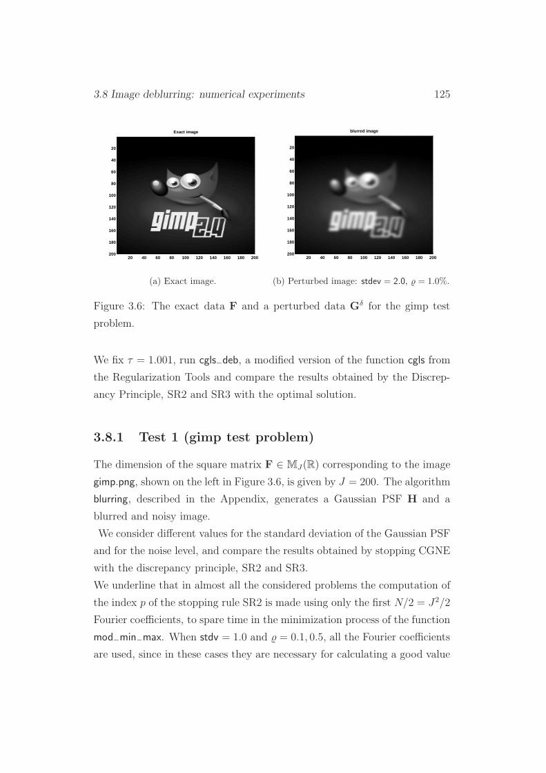
3.8 Image deblurring: numerical experiments 125
Exact image
20 40 60 80 100 120 140 160 180 200
20
40
60
80
100
120
140
160
180
200
(a) Exact image.
blurred image
20 40 60 80 100 120 140 160 180 200
20
40
60
80
100
120
140
160
180
200
(b) Perturbed image: stdev = 2.0, = 1.0%.
Figure 3.6: The exact data F and a perturbed data Gδ for the gimp test
problem.
We fix τ = 1.001, run cgls−deb, a modified version of the function cgls from
the Regularization Tools and compare the results obtained by the Discrep-
ancy Principle, SR2 and SR3 with the optimal solution.
3.8.1 Test 1 (gimp test problem)
The dimension of the square matrix F ∈ MJ(R) corresponding to the image
gimp.png, shown on the left in Figure 3.6, is given by J = 200. The algorithm
blurring, described in the Appendix, generates a Gaussian PSF H and a
blurred and noisy image.
We consider different values for the standard deviation of the Gaussian PSF
and for the noise level, and compare the results obtained by stopping CGNE
with the discrepancy principle, SR2 and SR3.
We underline that in almost all the considered problems the computation of
the index p of the stopping rule SR2 is made using only the first N/2 = J2/2
Fourier coefficients, to spare time in the minimization process of the function
mod−min−max. When stdv = 1.0 and = 0.1, 0.5, all the Fourier coefficients
are used, since in these cases they are necessary for calculating a good value

126 3. New stopping rules for CGNE
CGNE results for the gimp test problem
stdev Relative error (stopping index)
Discr. Princ. SR2 SR3 Opt. Sol.
3.0 0.1% 0.2104(154) 0.2082(196) 0.2053(313) 0.2048(348)
3.0 0.5% 0.2257(49) 0.2259(48) 0.2194(86) 0.2182(112)
3.0 1.0% 0.2331(34) 0.2286(45) 0.2264(61) 0.2261(68)
3.0 5.0% 0.2733(13) 0.3079(7) 0.2613(17) 0.2583(22)
2.0 0.1% 0.1265(144) 0.1703(61) 0.1196(213) 0.1167(310)
2.0 0.5% 0.1846(36) 0.1762(54) 0.1612(96) 0.1599(109)
2.0 1.0% 0.1962(20) 0.1962(20) 0.1878(36) 0.1849(53)
2.0 5.0% 0.2199(7) 0.2228(6) 0.2160(9) 0.2149(11)
1.0 0.1% 0.0442(45) 0.0419(50) 0.0350(68) 0.0344(92)
1.0 0.5% 0.0725(15) 0.0652(22) 0.0636(28) 0.0636(28)
1.0 1.0% 0.0865(9) 0.0797(13) 0.0781(15) 0.0780(16)
1.0 5.0% 0.1244(4) 0.1435(3) 0.1194(5) 0.1194(5)
Table 3.5: Comparison between different stopping rules of CGNE for the
gimp problem.
of p.
The numerical results of Table 3.5 show that the a-posteriori stopping rule
SR3 always finds a relative error lower than that obtained by the Discrepancy
Principle. The heuristic stopping rule SR2 gives very good results apart
from some cases where it provides an over-regularized solution. Since the
performance of SR3 is excellent here and changing the Matlab seed does
not make things significantly different (i.e. the statistical approximation of
‖U∗m−pe‖ seems to be very solid in such a large-size problem), we deduce
that the approximation of the residual norm of the TSVD solution with the
norm of the projection of the noise onto the high frequency components
‖gδ −AfTSVDp ‖ ∼ ‖U∗
m−pe‖
is not very appropriate in these cases.

3.8 Image deblurring: numerical experiments 127
exact image
50 100 150 200 250 300 350 400 450 500
50
100
150
200
250
300
350
400
450
500
(a) Exact image.
blurred image
50 100 150 200 250 300 350 400 450 500
50
100
150
200
250
300
350
400
450
500
(b) Perturbed image: stdev = 2.0, = 1.0%.
Figure 3.7: The exact data F and a perturbed data Gδ for the pirate test
problem.
3.8.2 Test 2 (pirate test problem)
The image pirate.tif, shown on the left in Figure 3.7, has a higher resolution
than gimp.png: J = 512.
We proceed as in the gimp test problem, but with a few variations:
• instead of the values 1.0, 2.0, 3.0 for the stdev we consider the values
3.0, 4.0, 5.0;
• To compute the index p of the stopping rules SR2 and SR3, instead of
considering the first N/2 ratios ϕi = |φ∗ig
δ|/λi, we take only the first
N/4. Moreover, in the computation of the curve that approximates
the ϕi, we use the function data−approx with only ⌊N/200⌋ inner knots(instead of ⌊N/50⌋).
The results, summarized in Table 3.6, show that both SR2 and SR3 give
excellent results, finding a relative error lower than the Discrepancy Principle
in almost all cases. The phenomenon observed in the gimp test problem
concerning SR2 appears to be much more attenuate here.
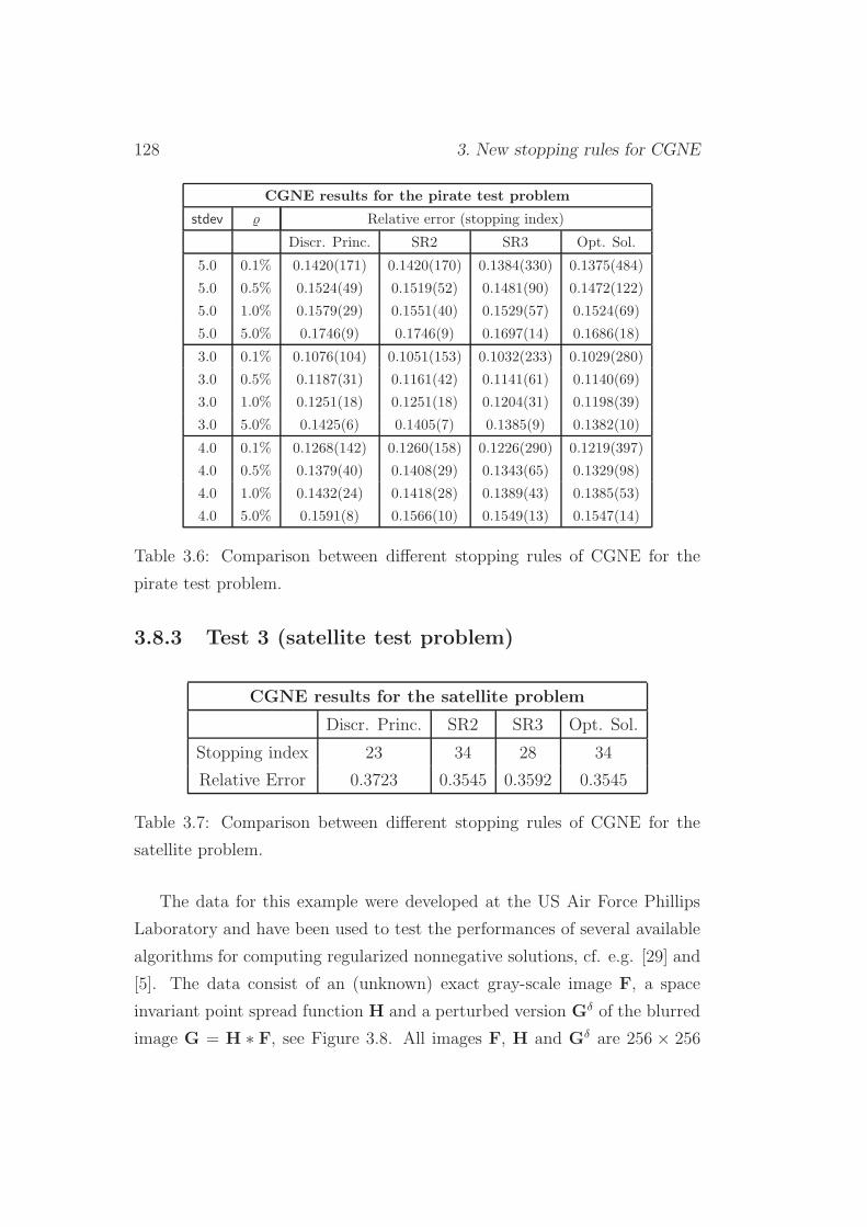
128 3. New stopping rules for CGNE
CGNE results for the pirate test problem
stdev Relative error (stopping index)
Discr. Princ. SR2 SR3 Opt. Sol.
5.0 0.1% 0.1420(171) 0.1420(170) 0.1384(330) 0.1375(484)
5.0 0.5% 0.1524(49) 0.1519(52) 0.1481(90) 0.1472(122)
5.0 1.0% 0.1579(29) 0.1551(40) 0.1529(57) 0.1524(69)
5.0 5.0% 0.1746(9) 0.1746(9) 0.1697(14) 0.1686(18)
3.0 0.1% 0.1076(104) 0.1051(153) 0.1032(233) 0.1029(280)
3.0 0.5% 0.1187(31) 0.1161(42) 0.1141(61) 0.1140(69)
3.0 1.0% 0.1251(18) 0.1251(18) 0.1204(31) 0.1198(39)
3.0 5.0% 0.1425(6) 0.1405(7) 0.1385(9) 0.1382(10)
4.0 0.1% 0.1268(142) 0.1260(158) 0.1226(290) 0.1219(397)
4.0 0.5% 0.1379(40) 0.1408(29) 0.1343(65) 0.1329(98)
4.0 1.0% 0.1432(24) 0.1418(28) 0.1389(43) 0.1385(53)
4.0 5.0% 0.1591(8) 0.1566(10) 0.1549(13) 0.1547(14)
Table 3.6: Comparison between different stopping rules of CGNE for the
pirate test problem.
3.8.3 Test 3 (satellite test problem)
CGNE results for the satellite problem
Discr. Princ. SR2 SR3 Opt. Sol.
Stopping index 23 34 28 34
Relative Error 0.3723 0.3545 0.3592 0.3545
Table 3.7: Comparison between different stopping rules of CGNE for the
satellite problem.
The data for this example were developed at the US Air Force Phillips
Laboratory and have been used to test the performances of several available
algorithms for computing regularized nonnegative solutions, cf. e.g. [29] and
[5]. The data consist of an (unknown) exact gray-scale image F, a space
invariant point spread function H and a perturbed version Gδ of the blurred
image G = H ∗ F, see Figure 3.8. All images F, H and Gδ are 256 × 256
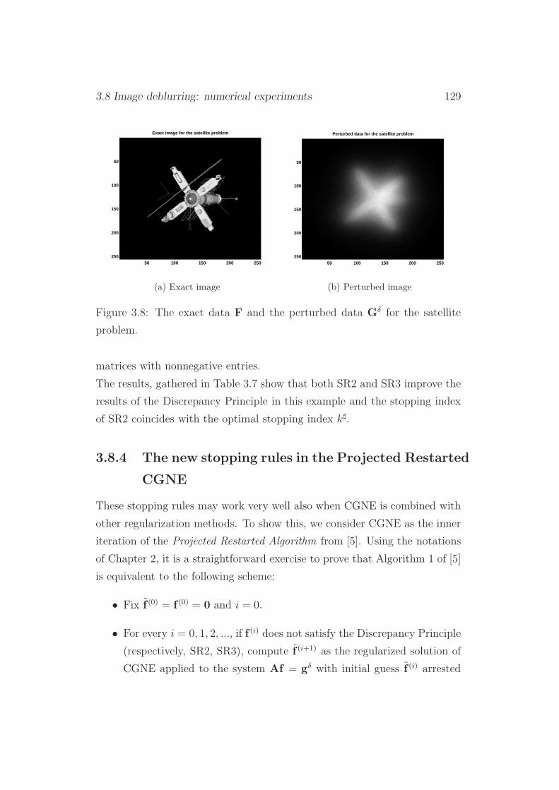
3.8 Image deblurring: numerical experiments 129
Exact image for the satellite problem
50 100 150 200 250
50
100
150
200
250
(a) Exact image
Perturbed data for the satellite problem
50 100 150 200 250
50
100
150
200
250
(b) Perturbed image
Figure 3.8: The exact data F and the perturbed data Gδ for the satellite
problem.
matrices with nonnegative entries.
The results, gathered in Table 3.7 show that both SR2 and SR3 improve the
results of the Discrepancy Principle in this example and the stopping index
of SR2 coincides with the optimal stopping index k♯.
3.8.4 The new stopping rules in the Projected Restarted
CGNE
These stopping rules may work very well also when CGNE is combined with
other regularization methods. To show this, we consider CGNE as the inner
iteration of the Projected Restarted Algorithm from [5]. Using the notations
of Chapter 2, it is a straightforward exercise to prove that Algorithm 1 of [5]
is equivalent to the following scheme:
• Fix f (0) = f (0) = 0 and i = 0.
• For every i = 0, 1, 2, ..., if f (i) does not satisfy the Discrepancy Principle
(respectively, SR2, SR3), compute f (i+1) as the regularized solution of
CGNE applied to the system Af = gδ with initial guess f (i) arrested
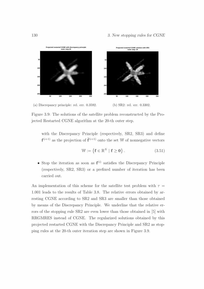
130 3. New stopping rules for CGNE
Projected restarted CGNE with discrepancy principleouter step:20
50 100 150 200 250
50
100
150
200
250
(a) Discrepancy principle: rel. err. 0.3592.
Projected restarted CGNE solution with SR2outer step: 20
50 100 150 200 250
50
100
150
200
250
(b) SR2: rel. err. 0.3302.
Figure 3.9: The solutions of the satellite problem reconstructed by the Pro-
jected Restarted CGNE algorithm at the 20-th outer step.
with the Discrepancy Principle (respectively, SR2, SR3) and define
f (i+1) as the projection of f (i+1) onto the set W of nonnegative vectors
W :=f ∈ RN | f ≥ 0
. (3.51)
• Stop the iteration as soon as f (i) satisfies the Discrepancy Principle
(respectively, SR2, SR3) or a prefixed number of iteration has been
carried out.
An implementation of this scheme for the satellite test problem with τ =
1.001 leads to the results of Table 3.8. The relative errors obtained by ar-
resting CGNE according to SR2 and SR3 are smaller than those obtained
by means of the Discrepancy Principle. We underline that the relative er-
rors of the stopping rule SR2 are even lower than those obtained in [5] with
RRGMRES instead of CGNE. The regularized solutions obtained by this
projected restarted CGNE with the Discrepancy Principle and SR2 as stop-
ping rules at the 20-th outer iteration step are shown in Figure 3.9.
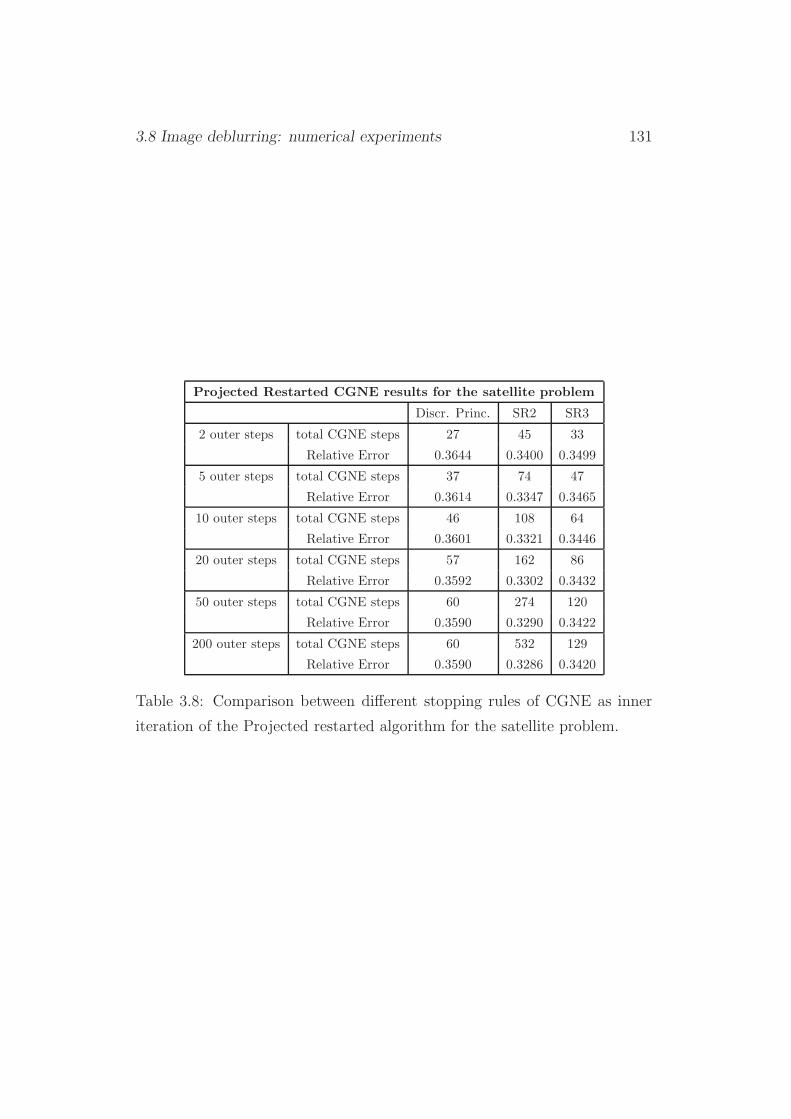
3.8 Image deblurring: numerical experiments 131
Projected Restarted CGNE results for the satellite problem
Discr. Princ. SR2 SR3
2 outer steps total CGNE steps 27 45 33
Relative Error 0.3644 0.3400 0.3499
5 outer steps total CGNE steps 37 74 47
Relative Error 0.3614 0.3347 0.3465
10 outer steps total CGNE steps 46 108 64
Relative Error 0.3601 0.3321 0.3446
20 outer steps total CGNE steps 57 162 86
Relative Error 0.3592 0.3302 0.3432
50 outer steps total CGNE steps 60 274 120
Relative Error 0.3590 0.3290 0.3422
200 outer steps total CGNE steps 60 532 129
Relative Error 0.3590 0.3286 0.3420
Table 3.8: Comparison between different stopping rules of CGNE as inner
iteration of the Projected restarted algorithm for the satellite problem.

132 3. New stopping rules for CGNE
Chapter 4
Tomography
The term tomography is derived from the Greek word τoµos, slice. It stands
for a variety of different techniques for imaging two-dimensional cross sections
of three-dimensional objects. The impact of these techniques in diagnostic
medicine has been revolutionary, since it has enabled doctors to view internal
organs with unprecedented precision and safety to the patient. We have
already seen in the first Chapter that these problems can be mathematically
described by means of the Radon Transform. The aim of this chapter is to
analyze the main properties of the Radon Transform and to give an overview
of the most important algorithms.
General references for this chapter are [19], [68], [69] and [43].
4.1 The classical Radon Transform
In this section we provide an outline of the main properties of the Radon
Transform over hyperplanes of RD. An hyperplane H of RD can be repre-
sented by an element of the unit cylinder
CD := (θ, s) | θ ∈ SD−1, s ∈ R, (4.1)
via the formula
H(θ, s) = x ∈ RD | 〈x, θ〉 = s, (4.2)
133
134 4. Tomography
where 〈·, ·〉 denotes the usual euclidean inner product of RD and where we
identify H(−θ,−s) with H(θ, s). We denote the set of all hyperplanes of RD
with
ΞD := CD/Z2, (4.3)
and define the Radon Transform of a rapidly decreasing function f ∈ S(RD)
as its integral on H(θ, s):
R[f ](θ, s) :=
∫
H(θ,s)
f(x)dµH(x), (4.4)
where µH(x) is the Lebesgue measure on H(θ, s).
Much of the theory of the Radon Transform is based on its behavior under
the Fourier Transform and convolution. We recall that the Fourier Transform
of a function f ∈ L1(RD) is given by
f(y) = F (f)(y) = (2π)−D/2
∫
RD
f(x)e−ı〈x,y〉dx, y ∈ RD. (4.5)
Observing that the exponential e−ı〈x,y〉 is constant on hyperplanes orthogonal
to y, an important relation between the Fourier and the Radon Transform
is obtained integrating (4.5) along such hyperplanes. Explicitly, we write
y = ξθ for ξ ∈ R and θ ∈ SD−1 to get the famous Projection-Slice Theorem:
f(ξθ) = (2π)−D/2
∫
R
∫
H(θ,s)
f(x)e−ıξ〈x,θ〉dµH(x)ds
= (2π)−D/2
∫
R
(∫
H(θ,s)
f(x)dµH(x)
)
e−ısξds
= (2π)−D/2
∫
R
R[f ](θ, s)e−ısξds.
(4.6)
This immediately implies that the operator R is injective on S(RD) (but also
on larger spaces, e.g. on L1(RD)).
Moreover, let us introduce the space of Schwartz-class functions on ΞD. We
say that a function f ∈ C∞(CD) belongs to S(CD) if for every k1,k2 ∈ N0 we
have
sup(θ,s)
(1 + |s|)k1∣∣∣∣
∂k2
∂sk2f(θ, s)
∣∣∣∣< +∞.
4.1 The classical Radon Transform 135
The space S(ΞD) is the space of the even functions in S(CD), i.e. f(θ, s) =
f(−θ,−s). The Partial Fourier Transform of a function f ∈ S(ΞD) is its
Fourier Transform in the s variable:
f(θ, s) 7→ f(θ, ξ) = F (s 7→ f(θ, s)) (ξ) =
∫
R
f(θ, s)e−ıξsds. (4.7)
On ΞD, we understand the convolution as acting on the second variable as
well:
(g ∗ h)(θ, s) =∫
R
g(θ, s− t)h(t)dt. (4.8)
The Partial Fourier Transform maps S(CD) into itself and S(ΞD) into itself
and the Projection-Slice Theorem states that the Fourier Transform of f
∈ S(RD) is the Partial Fourier Transform of its Radon Transform. For f ∈S(RD), if we change to polar coordinates (θ, s) 7→ sθ in RD, a straightforward
application of the chain rule shows that its Fourier Transform lies in S(CD).
By the Projection-Slice Theorem then
R : S(RD) −→ S(ΞD). (4.9)
Another consequence of the Projection-Slice Theorem is that the Radon
Transform preserves convolutions, in the sense that for every f and g ∈S(RD) the following formula holds:
R(f ∗ g)(θ, s) =∫
R
R[f ](θ, s− t)R[g](θ, t)dt. (4.10)
We now introduce the backprojection operator R∗ by
R∗[g](x) =
∫
SD−1
g(θ, 〈x, θ〉)dθ, g ∈ S(ΞD). (4.11)
For g = Rf , R∗[g](x) is the average of all hyperplane integrals of f through
x. Mathematically speaking, R∗ is simply the adjoint of R: for φ ∈ S(R)and f ∈ S(RD), there holds
∫
R
φ(s)R[f ](θ, s)ds =
∫
RD
φ(〈x, θ〉)f(x)dx (4.12)
136 4. Tomography
and consequently for g ∈ S(ΞD) and f ∈ S(RD)
∫
SD−1
∫
R
g(Rf)dθds =
∫
RD
(R∗g)fdx. (4.13)
A more general approach for studying the Radon Transform leading to the
same result can be found in the first chapters of [19].
The following result is the starting point for the Filtered Backprojection
algorithm, which will be discussed later.
Theorem 4.1.1. Let f ∈ S(RD) and υ ∈ S(ΞD). Then1
R∗(υ ∗ Rf) = (R∗υ) ∗ f. (4.14)
Proof. For any x ∈ RD, we have
R∗(υ ∗ Rf)(x) =
∫
SD−1
(∫
R
υ(θ, 〈θ,x〉 − s)R[f ](θ, s)ds
)
dθ
=
∫
SD−1
(∫
R
υ(θ, 〈θ,x〉 − s)
(∫
H(θ,s)
f(y)dµH(y)
)
ds
)
dθ
=
∫
SD−1
(∫
RD
υ(θ, 〈θ,x− y〉)f(y)dy)
dθ
=
∫
RD
(∫
SD−1
υ(θ, 〈θ,x− y〉)dθ)
f(y)dy
=
∫
RD
R∗υ(x− y)f(y)dy
= ((R∗υ) ∗ f)(x).(4.15)
4.1.1 The inversion formula
We are now ready to derive the inversion formula for the Radon Transform.
The proof is basically taken from [19], but here, apart from the different
notations and definitions, some small errors in the resulting constants have
1Note the different meaning of the symbol ∗ in the formula!
4.1 The classical Radon Transform 137
been corrected. We state the general theorem exactly as in [69].
We start from the inversion formula of the classical Fourier Transform in RD
(2π)D/2f(x) =
∫
RD
f(y)eı〈x,y〉dy (4.16)
and switch to polar coordinates y = ξθ, obtaining
(2π)D/2f(x) =
∫
SD−1
∫ +∞
0
f(ξθ)eıξ〈x,θ〉ξD−1dξdθ
=1
2
∫
SD−1
∫ +∞
0
f(ξθ)eıξ〈x,θ〉ξD−1dξdθ
+1
2
∫
SD−1
∫ +∞
0
f(ξ(−θ))eıξ〈x,−θ〉ξD−1dξdθ
=1
2
∫
SD−1
∫ +∞
0
f(ξθ)eıξ〈x,θ〉ξD−1dξdθ
+1
2
∫
SD−1
∫ 0
−∞f(ξθ)eıξ〈x,θ〉(−ξ)D−1dξdθ
=1
2
∫
SD−1
∫ +∞
−∞f(ξθ)eıξ〈x,θ〉|ξ|D−1dξdθ.
(4.17)
If D is odd, |ξ|D−1 = ξD−1, thus the Projection-Slice Theorem and the pro-
perties of the Fourier Transform in one variable imply
f(x) =1
2(2π)D
∫
SD−1
∫ +∞
−∞eıξ〈x,θ〉ξD−1
(∫
R
R[f ](θ, s)e−ısξds
)
dξdθ
= cD
∫
SD−1
F−1
(
ξ 7→ F
(
s 7→ ∂D−1
∂sD−1R[f ](θ, s)
)
(ξ)
)
(〈x, θ〉)dθ
= cDR∗(∂D−1
∂sD−1Rf
)
(x),
(4.18)
where
cD :=2π
2(ı)D−1(2π)D=
1
2(2π)1−D(−1)
D−12 . (4.19)
Suppose now D is even. To obtain a complete inversion formula, we recall a
few facts from the theory of distributions (cf. [19] and, as a general reference
for the theory of distributions, [80]).
138 4. Tomography
1. The linear mapping p.v.[1/t] from S(R) to C defined by
p.v.[1/t]h = limǫ→0+
∫
|t|>ǫ
h(t)
tdt (4.20)
is well defined (although 1/t is not locally integrable) and belongs to
the dual space of S(R); that is to say, it is a tempered distribution on
R.
2. The signum function on R defined by
sgn(ξ) =
1 if ξ ≥ 0,
−1 if ξ < 0(4.21)
is a tempered distribution on R as well, whose (distributional) Fourier
Transform is related to p.v.[1/t] via the formula
F (p.v.[1/t])(ξ) = −√π
2ısgn(ξ). (4.22)
The Hilbert Transform of a function φ ∈ S(R) is the convolution H φ :=
φ ∗ 1πp.v.[1/t], i.e.
H [φ](p) = limǫ→0+
∫
|t|>ǫ
φ(p− t)
πtdt, p ∈ R. (4.23)
As a consequence, the Fourier Transform of H φ is the function
F [H φ](ξ) = −ıφ(ξ)sgn(ξ). (4.24)
Now we return to the right-hand side of (4.17), which, for D even, is equal
to1
2
∫
SD−1
∫ +∞
−∞f(ξθ)eıξ〈x,θ〉ξD−1sgn(ξ)dξdθ.
We proceed similarly to the odd case and using (4.24) we have
f(x) =1
2(2π)D
∫
SD−1
∫ +∞
−∞eıξ〈x,θ〉ξD−1sgn(ξ)
(∫
R
R[f ](θ, s)e−ısξds
)
dξdθ
= cD
∫
SD−1
F−1
(
ξ 7→ F
(
H (s 7→ ∂D−1
∂sD−1R[f ])(θ, s)
)
(ξ)
)
(〈x, θ〉)dθ
= cDR∗(
H
(∂D−1
∂sD−1R[f ]
))
(x),
(4.25)

4.1 The classical Radon Transform 139
where
cD :=2π
2(ı)D−2(2π)D=
1
2(2π)1−D(−1)
D−22 . (4.26)
Altogether, we have proved the following theorem.
Theorem 4.1.2. Let f ∈ S(RD) and let g = Rf . Then
f = cD
R∗H g(D−1) n even,
R∗g(D−1) n odd,(4.27)
with
cD =1
2(2π)1−D
(−1)D−2
2 n even,
(−1)D−1
2 n odd,(4.28)
where the derivatives in ΞD are intended in the second variable.
We conclude the section with a remark on the inversion formula from [69].
For D odd, the equation (4.18) says that f(x) is simply an average of g(D−1)
over all hyperplanes through x. Thus, in order to reconstruct f at some
point x, one needs only the integrals of f through x. This is not true for
D even. In fact, inserting the definition of the Hilbert Transform into (4.25)
and changing the order of integration, we obtain2
f(x) = limǫ→0+
cD
∫
|t|>ǫ
1
t
∫
SD−1
g(D−1)(θ, 〈x, θ〉 − t)dθdt, (4.29)
from which we can see that the computation of f at some point x requires
integrals of f also over hyperplanes far away from x.
4.1.2 Filtered backprojection
Rather than using the inversion formula described above, the most common
method for reconstructing X-ray images is the method of the Filtered Back-
projection. Its main advantage is the ability to cancel out high frequency
noise.
2the equality with the right-hand side of formula (4.25) is guaranteed because g is a
rapidly decreasing function.
140 4. Tomography
Let υ ∈ S(ΞD). There is a constant C such that |υ(ξ)| ≤ C for all ξ ∈ ΞD and
so the definition of R∗ implies that also |R∗υ(x)| ≤ C for all x. Thus R∗υ
is a tempered distribution. Moreover, in [19] it is shown that the following
relation between R∗υ and υ holds for all y 6= 0 in RD:
F (R∗υ)(y) = 2(2π)(D−1)/2‖y‖1−Dυ
(y
‖y‖ , ‖y‖)
. (4.30)
The starting point of the Filtered Backprojection algorithm is Theorem 4.1.1:
we put in formula (4.14) g = Rf and V = R∗υ obtaining
V ∗ f = R∗(υ ∗ g). (4.31)
The idea is to choose V as an approximation of the Dirac δ-function and to
determine υ from V = R∗υ. Then V ∗ f is an approximation of the sought
function f that is calculated in the right-hand side by backprojecting the
convolution of υ with the data g.
Usually only radially symmetric functions V are chosen, i.e. V (y) = V (‖y‖).Then υ = υ(θ, s) can be assumed to be only an even function of s and formula
(4.30) reads now
F (R∗υ)(y) = 2(2π)(D−1)/2‖y‖1−Dυ(‖y‖). (4.32)
Now we choose V as a band limited function by allowing a filter factor φ(y)
which is close to 1 for ‖y‖ ≤ 1 and which vanishes for ‖y‖ > 1 putting
VΥ(y) := (2π)−D/2φ(‖y‖/Υ), Υ > 0. (4.33)
Then the corresponding function υΥ such that R∗υΥ = VΥ satisfies
υΥ(ξ) =1
2(2π)1/2−DξD−1φ(ξ/Υ), ξ > 0 (4.34)
(note that υΥ is an even function being the Fourier Transform of an even
function).
Many choices of φ can be found in literature. We mention the choice proposed
by Shepp and Logan in [84], where
φ(ξ) :=
sinc(ξπ/2), 0 ≤ ξ ≤ 1,
0, ξ > 1,(4.35)

4.2 The Radon Transform over straight lines 141
where sinc(t) is equal to sin(t)/t if t 6= 0, and 1 otherwise.
Once υ has been chosen, the right-hand side of equation (4.14) has to be
calculated to obtain the approximation V ∗ f of f . This has to be done in
a discrete setting, and the discretization of (4.14) depends on the way the
function g is sampled: different samplings lead to different algorithms. Since
we are going to concentrate on iterative methods, we will not proceed in the
description of these algorithms and for a detailed treatment of this argument
we refer to [69].
4.2 The Radon Transform over straight lines
In the previous section we studied the Radon Transform, which integrates
functions on RD over hyperplanes. One can also consider an integration
over d-planes, with d = 1, ..., D − 1. In this case, ΞD is replaced by the
set of unoriented affine d-planes in RD, the affine Grassmannian G(d,D).
For simplicity, here we will consider only the case d = 1: the corresponding
transform is the so called X-Ray Transform or just the Ray Transform.
We identify a straight line L of G(1, D) with a direction θ ∈ SD−1 and a
point s ∈ θ⊥ as s+ tθ, t ∈ R and define the X-Ray Transform P by
P[f ](θ, s) =
∫
R
f(s+ tθ)dt. (4.36)
Similarly to the case d = D−1 we have a Projection Slice Theorem as follows.
For f ∈ L1(RD) and y ∈ RD let L = L(θ, s) ∈ G(1, D) be a straight line
such that y lies in θ⊥. Then
f(y) = (2π)−D/2
∫
RD
f(x)e−ı〈x,y〉dx
= (2π)−D/2
∫
θ⊥
(∫
R
f(s+ tθ)e−ı〈s+tθ,y〉dt
)
dµθ⊥(s)
= (2π)−D/2
∫
θ⊥
Pf(θ, s)e−ı〈s,y〉dµθ⊥(s).
(4.37)
142 4. Tomography
Thus Pf is a function on TD := (θ, s) θ ∈ SD−1, s ∈ θ⊥ and f ∈ S(RD)
implies Pf ∈ S(TD), where
S(TD) =
g ∈ C∞ : sup(θ,s)
(1 + |s|)k1∣∣∣∣
∂k2
∂sk2g(θ, s)
∣∣∣∣< +∞
. (4.38)
On TD, the convolution and the Partial Fourier Transform are defined by
(g ∗ h)(θ, s) =∫
θ⊥
g(θ, s− t)h(θ, t)dµθ⊥(t), s ∈ θ⊥, (4.39)
g(θ, ξ) = (2π)(1−D)/2
∫
θ⊥
e−ı〈s,ξ〉g(θ, s)dµθ⊥(s), ξ ∈ θ⊥. (4.40)
Theorem 4.2.1. For f, g ∈ S(RD), we have
Pf ∗ Pg = P(f ∗ g). (4.41)
As in the case d = D− 1, the convolution on RD and on TD are denoted
by the same symbol in the theorem.
The backprojection operator P∗ is now
P∗[g](x) =
∫
SD−1
g(θ, Eθx)dθ, (4.42)
where Eθ is the orthogonal projector onto θ⊥, i.e. Eθx = x−〈x, θ〉θ. Againit is the adjoint of P:
∫
SD−1
∫
θ⊥
gPfdθdµθ⊥(s) =
∫
RD
fP∗gdx. (4.43)
There is also an analogous version of Theorem 4.1.1:
Theorem 4.2.2. Let f ∈ S(RD) and g ∈ S(TD). Then
P∗(g ∗ Pf) = (P∗g) ∗ f. (4.44)
From (4.37) and (4.40) follows immediately that for f ∈ S(RD), θ ∈ SD−1
and ξ ⊥ θ there holds
(Pf)(θ, ξ) = (2π)1/2f(ξ). (4.45)
This is already enough to state the following uniqueness result in R3.

4.2 The Radon Transform over straight lines 143
Theorem 4.2.3. Let S20 be a subset of S2 that meets every equatorial circle
of S2 (Orlov’s condition, 1976). Then the knowledge of Pf for θ ∈ S20
determines f uniquely.
Proof. For every ξ ∈ R3, since S20 satisfies Orlov’s condition, there exists an
element θ ∈ S20 such that θ ⊥ ξ. Hence f(ξ) is determined by (4.45).
An explicit inversion formula on S20 was found by the same Orlov in 1976
(see Natterer [69] for a proof).
In spherical coordinates,
x =
cosχ cosϑ
sinχ cosϑ
sinϑ
, 0 ≤ χ < 2π, |ϑ| ≤ π
2, (4.46)
S20 is given by ϑ−(χ) ≤ ϑ ≤ ϑ+(χ), 0 ≤ χ < 2π, where ϑ± are functions such
that −π2< ϑ−(χ) < 0 < ϑ+(χ) <
π2, 0 ≤ χ < 2π.
Now, let l(x,y) be the length of the intersection of S20 with the plane spanned
by x and y ∈ R3. According to the assumption made on ϑ±, l(x,y) > 0 if x
and y are linearly independent.
Theorem 4.2.4 (Orlov’s inversion formula). Let f ∈ S(R3) and g(θ, s) =
P[f ](θ, s) for θ ∈ S20 and s ⊥ θ. Then
f(x) = ∫
S20
h(θ, Eθx)dθ, (4.47)
where
h(θ, s) = − 1
4π2
∫
θ⊥
g(θ, s− t)
‖t‖l(θ, t) dµθ⊥(t) (4.48)
and is the Laplace operator on R3.
4.2.1 The Cone Beam Transform
We define the Cone Beam Transform of a density function f ∈ S(R3) by
D [f ](x, θ) =
∫ +∞
0
f(x+ tθ)dt, x ∈ R3, θ ∈ S2. (4.49)
144 4. Tomography
When x is the location of an X-ray source traveling along a curve Γ, the
operator D is usually called the Cone Beam Transform of f along the source
curve Γ. We want to invert D in this particular case, which is of interest in
the applications.
We start by considering the case where Γ is the unit circle in the x1-x2
plane. A point x on Γ is expressed as x = (cos φ, sinφ, 0)∗, with x⊥ =
(− sinφ, cosφ, 0)∗. An element θ ∈ S2 \ x corresponds to a couple (y2,y3)∗
∈ R2 by taking the intersection of the beam through θ and x with the plane
spanned by x⊥ and e3 := (0, 0, 1)∗ passing through −x 3. Thus, if f vanishes
outside the unit ball of R3, we have
D [f ](φ, y2, y3) =
∫ +∞
0
f((1− t)x+ t(y2x⊥ + y3e3))dt. (4.50)
We also define the Mellin Transform of a function h ∈ R by
M [h](s) =
∫ +∞
0
ts−1h(t)dt. (4.51)
Then in [69] it is shown that performing a Mellin Transform of g and f with
respect to y3 and x3 respectively and then expanding the results in Fourier
series with respect to φ one obtains the equations
gl(y2, s) =
∫ +∞
0
fl
(√
(1− t)2 + t2y22, s
)
e−ılα(t,y2)dt, l ∈ Z, (4.52)
where α(t, y2) is the argument of the point (1 − t, ty2) in the x1-x2 plane.
Unfortunately an explicit solution to this equation does not exist and the
entire procedure seems rather expensive from a computational point of view.
This is a reason why usually nowadays different paths are used.
An explicit inversion formula was found by Tuy in 1983 (cf. [93]). It applies
to paths satisfying the following condition:
Definition 4.2.1 (Tuy’s condition). Let Γ = Γ(t), t ∈ [0, 1] be a para-
metric curve on R3. Γ is said to satisfy Tuy’s condition if it intersects each
3in other words, y2 and y3 are just the coordinates of the stereographic projection of
θ from the projection point x.
4.2 The Radon Transform over straight lines 145
plane hitting supp(f) transversally, i.e. if for each x ∈ supp(f) and each θ
∈ S2 there exists t = t(x, θ) ∈ [0, 1] such that
〈Γ(t), θ〉 = 〈x, θ〉, 〈Γ′(t), θ〉 6= 0. (4.53)
Theorem 4.2.5. Suppose that the source curve satisfies Tuy’s condition.
Then
f(x) = (2π)−3/2ı−1
∫
S2(〈Γ′(t), θ〉)−1 d
dt(Df)(Γ(t), θ)dθ, (4.54)
where t = t(x, θ) and where the Fourier Transform is performed only with
respect to the first variable.
Of course, Tuy’s condition doesn’t hold for the circular path described
above since it lies entirely on a plane. In the pursuit of the data sufficiency
condition, various scanning trajectories have been proposed, such as circle
and line, circle plus arc, double orthogonal circles, dual ellipses and helix
(see [50] and the references therein). Of particular interest is the helical
trajectory, for which in a series of papers from 2002 to 2004 ([56], [57] and
[58]) the Russian mathematician A. Katsevich found an inversion formula
strictly related to the Filtered Backprojection algorithm. Although we won’t
investigate the implementation of these algorithms, we dedicate the follo-
wing section to the basic concepts developed in those papers since they are
considered a breakthrough by many experts in the field.
4.2.2 Katsevich’s inversion formula
In the description of Katsevich’s inversion formula we follow [97] and [98].
First of all, the source lies on an helical trajectory defined by
Γ(t) =
(
R cos(t),R sin(t),Pt
2π
)∗, t ∈ I, (4.55)
where R > 0 is the radius of the helix, P > 0 is the helical pitch and I := [a, b],
b > a. In medical applications, the helical path is obtained by translating the
platform where the patient lies through the rotating source-detector gantry.
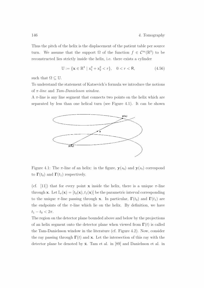
146 4. Tomography
Thus the pitch of the helix is the displacement of the patient table per source
turn. We assume that the support Ω of the function f ∈ C∞(R3) to be
reconstructed lies strictly inside the helix, i.e. there exists a cylinder
U := x ∈ R3 | x21 + x22 < r, 0 < r < R, (4.56)
such that Ω ⊆ U.
To understand the statement of Katsevich’s formula we introduce the notions
of π-line and Tam-Danielsson window.
A π-line is any line segment that connects two points on the helix which are
separated by less than one helical turn (see Figure 4.1). It can be shown
Figure 4.1: The π-line of an helix: in the figure, y(sb) and y(st) correspond
to Γ(t0) and Γ(t1) respectively.
(cf. [11]) that for every point x inside the helix, there is a unique π-line
through x. Let Iπ(x) = [t0(x), t1(x)] be the parametric interval corresponding
to the unique π-line passing through x. In particular, Γ(t0) and Γ(t1) are
the endpoints of the π-line which lie on the helix. By definition, we have
t1 − t0 < 2π.
The region on the detector plane bounded above and below by the projections
of an helix segment onto the detector plane when viewed from Γ(t) is called
the Tam-Danielsson window in the literature (cf. Figure 4.2). Now, consider
the ray passing through Γ(t) and x. Let the intersection of this ray with the
detector plane be denoted by x. Tam et al. in [89] and Danielsson et al. in
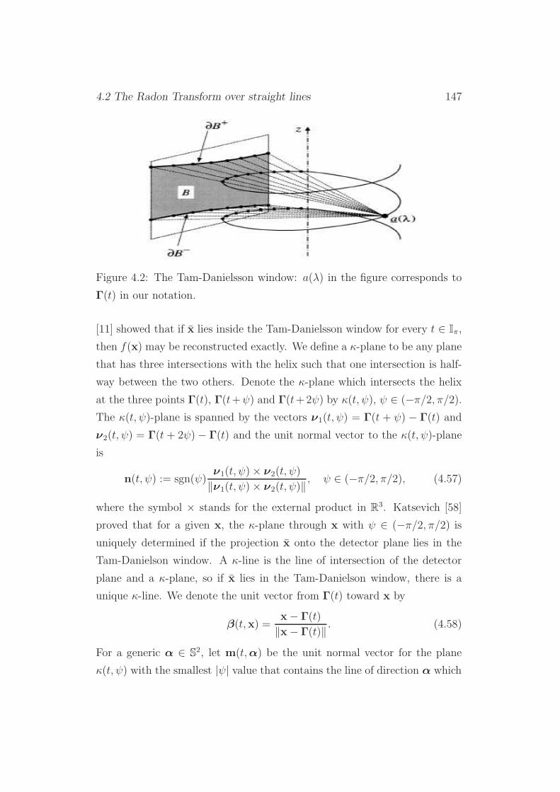
4.2 The Radon Transform over straight lines 147
Figure 4.2: The Tam-Danielsson window: a(λ) in the figure corresponds to
Γ(t) in our notation.
[11] showed that if x lies inside the Tam-Danielsson window for every t ∈ Iπ,
then f(x) may be reconstructed exactly. We define a κ-plane to be any plane
that has three intersections with the helix such that one intersection is half-
way between the two others. Denote the κ-plane which intersects the helix
at the three points Γ(t), Γ(t+ψ) and Γ(t+2ψ) by κ(t, ψ), ψ ∈ (−π/2, π/2).The κ(t, ψ)-plane is spanned by the vectors ν1(t, ψ) = Γ(t + ψ) − Γ(t) and
ν2(t, ψ) = Γ(t + 2ψ)− Γ(t) and the unit normal vector to the κ(t, ψ)-plane
is
n(t, ψ) := sgn(ψ)ν1(t, ψ)× ν2(t, ψ)
‖ν1(t, ψ)× ν2(t, ψ)‖, ψ ∈ (−π/2, π/2), (4.57)
where the symbol × stands for the external product in R3. Katsevich [58]
proved that for a given x, the κ-plane through x with ψ ∈ (−π/2, π/2) is
uniquely determined if the projection x onto the detector plane lies in the
Tam-Danielson window. A κ-line is the line of intersection of the detector
plane and a κ-plane, so if x lies in the Tam-Danielson window, there is a
unique κ-line. We denote the unit vector from Γ(t) toward x by
β(t,x) =x− Γ(t)
‖x− Γ(t)‖ . (4.58)
For a generic α ∈ S2, let m(t,α) be the unit normal vector for the plane
κ(t, ψ) with the smallest |ψ| value that contains the line of direction α which

148 4. Tomography
passes through Γ(t), and put e(t,x) := β(t,x) × m(t,β). Then β(t,x) and
e(t,x) span the κ-plane that we will want to use for the reconstruction of f
in x. Any direction in the plane may be expressed as
θ(t,x, γ) = cos(γ)β(t,x) + sin(γ)e(t,x), γ ∈ [0, 2π). (4.59)
We can now state Katsevich’s result as follows.
Theorem 4.2.6 (Katsevich). For f ∈ C∞0 (U),
f(x) = − 1
2π2
∫
Iπ(x)
1
‖x− Γ(t)‖p.v.∫ 2π
0
∂
∂qDf(Γ(q), θ(t,x, γ))|q=t
dγdt
sin γ,
(4.60)
where p.v. stands for the principal value integral and where all the objects
appearing in the formula are defined as above.
Proof. See [56], [57], [58].
For a fixed x, consider the κ-plane with unit normal m(t,β(t,x)). We
consider a generic line in this plane with direction θ0(t,x) = cos(γ0)β(t,x)+
sin(γ0)e(t,x), γ0 ∈ [0, 2π) and define
g′(t, θ0(t,x)) :=∂
∂qDf(Γ(q), θ(t,x, γ)|q=t (4.61)
and
gF (t, θ0(t,x)) := p.v.
∫ 2π
0
1
π sin γg′(t, cos(γ0−γ)β(t,x)−sin(γ0−γ)e(s,x))dγ.
(4.62)
Thus Katsevich’s formula can be rewritten as
f(x) = − 1
2π
∫
Iπ(x)
1
‖x− Γ(t)‖gF (t,β(t,x))dt. (4.63)
Therefore, we see that Katsevich’s formula may be implemented as a deriva-
tive, followed by a 1D convolution, and then a back-projection: for this reason
it is usually described as a Filtered Backprojection-type formula. Further de-
tails for the implementation of Katsevich’s formula can be found, e.g., in [97]
and [98].
4.3 Spectral properties of the integral operator 149
4.3 Spectral properties of the integral ope-
rator
In this section we study the spectral properties of the operator R defined by
(4.4).
We consider the polynomials of degree k orthogonal with respect to the weight
function tl in [0, 1] and denote them by Pk,l = Pk,l(t). Similarly to what we
have already seen in Chapter 2, the polynomials Pk,l are well defined for every
k and l ∈ N0 and the orthogonality property means that∫ 1
0
tlPk1,l(t)Pk2,l(t) = δk1,k2, (4.64)
where δk1,k2 = 1 if k1=k2 and 0 otherwise. In fact, up to a normalization, they
are the Jacobi polynomials Gk(l+(D−2)/2, l+(D−2)/2, t) (cf. Abramowitz
and Stegun [1], formula 22.2.2).
We shall also need the Gegenbauer polynomials Cµm, which are defined as
the orthogonal polynomials on [−1, 1] with weight function (1 − t2)µ−1/2,
µ > −1/2. Moreover, we recall that a spherical harmonic of degree l is the
restriction to SD−1 of an harmonic polynomial homogeneous of degree l on
RD (cf. e.g. [66], [83] and [85]). There exist exactly
n(D, l) :=(2l +D − 2)(D + l − 3)!
l!(D − 2)!(4.65)
linearly independent spherical harmonics of degree l and spherical harmonics
of different degree are orthogonal in L2(SD−1).
Now let Yl,k, k = 1, ..., n(D, l) be an orthonormal basis for the spherical
harmonics of degree l. We define, for i ≥ 0, 0 ≤ l ≤ i, 1 ≤ k ≤ n(D, l),
filk(x) =√2P(i−l)/2,l+(D−2)/2(‖x‖2)‖x‖lYl,k(x/‖x‖) (4.66)
and
gilk(θ, s) = c(i)w(s)D−1CD/2i (s)Yl,k(θ). (4.67)
Here w(s) := (1− s2)1/2 and
c(i) =π21−D/2Γ(i+D)
i!(i+D/2)(Γ(D/2))2, (4.68)

150 4. Tomography
where Γ stands for Euler’s Gamma function.
Theorem 4.3.1 (Davison(1983) and Louis (1984)). The functions filk
and gilk, i ≥ 0, 0 ≤ l ≤ i, 1 ≤ k ≤ n(D, l), are complete orthonormal families
in the spaces L2(‖x‖ < 1) and L2(ΞD, w1−D), respectively. The singular
value decomposition of R as an operator between these spaces is given by
Rf =
∞∑
i=0
λi∑
0≤l≤i,l+i even
n(D,l)∑
k=1
〈f, filk〉L2(‖x‖<1)gilk, (4.69)
where
λi =
(2DπD−1
(i+ 1) · · · (i+D − 1)
)1/2
(4.70)
are the singular values of R, each being of multiplicity n(D, l)⌊ i+22⌋.
Proof. See [13] and [64]. For a proof in a simplified case with D = 2, cf.
[4].
We observe that in the case D = 2 the singular values decay to zero
rather slowly, namely λi = O(i−1/2). This is in accordance with the remark
we have made in the introductory example of Chapter 1, where we have seen
that to compute an inversion of R the data are differentiated and smoothed
again. A more precise statement to explain this can be made by means of
the following theorem (see [69] for the details not specified below).
Theorem 4.3.2. Let Ω be a bounded and sufficiently regular domain in RD
and let α ∈ R. Then there are positive constants c(α,Ω) and C(α,Ω) such
that for all f ∈ Hα0 (Ω)
c(α,Ω)‖f‖Hα0 (Ω) ≤ ‖Rf‖Hα+(D−1)/2(ΞD) ≤ C(α,Ω)‖f‖Hα
0 (Ω). (4.71)
Here, Hα0 (Ω) is the closure of C∞
0 (Ω) with respect to the norm of the Sobolev
space Hα(RD) and Hβ(ΞD) is the space of even functions g on the cylinder
CD such that
‖g‖Hβ(CD) :=
∫
SD−1
∫
R
(1 + ξ2)β/2g(θ, ξ)2dξdθ, β ∈ R. (4.72)
4.4 Parallel, fan beam and helical scanning 151
Thus, roughly speaking, in the general case we can say that Rf is smoother
than f by an order of (D − 1)/2.
Similar results can be found for the operator P.
Theorem 4.3.3 (Maass (1987)). With the functions filk defined above
and a certain complete orthonormal system gilk on L2(TD, w), where w(ξ) =
(1− ‖ξ‖2)1/2, there are positive numbers λil such that
Pf(θ, s) =
∞∑
i=0
∑
0≤l≤i,l+i even
λil
n(D,l)∑
k=1
〈f, filk〉gilk. (4.73)
The singular values λil, each of multiplicity n(D, l), satisfy
λil = O(i−1/2) (4.74)
as i → +∞, uniformly in l.
Proof. See [65].
Theorem 4.3.4. Let Ω be a bounded and sufficiently regular domain in RD
and let α ∈ R. Then there are positive constants c(α,Ω) and C(α,Ω) such
that for all f ∈ Hα0 (Ω)
c(α,Ω)‖f‖Hα0 (Ω) ≤ ‖Pf‖Hα+1/2(TD) ≤ C(α,Ω)‖f‖Hα
0 (Ω), (4.75)
where
‖g‖Hβ(TD) :=
∫
SD−1
∫
θ⊥
(1 + ‖ξ‖2)β/2g(θ, ξ)2dξdθ, β ∈ R. (4.76)
4.4 Parallel, fan beam and helical scanning
In this section we give a very brief survey of the different scanning geometries
in computerized tomography. We distinguish between the 2D and the 3D
cases.

152 4. Tomography
(a) First generation: parallel, dual mo-
tion scanner.
(b) Second generation: narrow fan beam
(∼ 10), dual motion scanner.
Figure 4.3: First and second generation scanners.
4.4.1 2D scanning geometry
In 2D geometry, only one slice of the object is scanned at a time, the recon-
struction is made slice by slice by means of the classical 2D Radon Transform.
In parallel scanning, the X-rays are emitted along a two-parameter family
of straight lines Ljl, j = 0, ..., j − 1, l = −l, ..., l, where Ljl is the straight
line making an angle φj = j∆φ with the x2-axis and having signed distance
sl = l∆s from the origin, i.e., 〈x, θj〉 = sl, θj = (cosφj, sinφj)∗. The mea-
sured values gPARjl are simply
gPARjl = R[f ](θj, sl), j = 0, ..., j − 1, l = −l, ..., l. (4.77)
In the first CT scanners (first generation scanners) the source moves along a
straight line. The X-ray is fired at each position sl and the intensity is mea-
sured by a detector behind the object which translates simultaneously with
the source. Then the same process is repeated with a new angular direction.
A first improvement on this invasive and rather slow technique came with
the second generation scanners, where more than one detector is used, but

4.4 Parallel, fan beam and helical scanning 153
the number of detectors is still small (cf. Figure 4.3).
Fan beam scanning geometry is characterized by the use of many detectors.
In a third generation scanner, the X-ray source and the detectors are mounted
(a) Third generation: fan beam, rotating
detectors.
(b) Fourth generation: fan beam, sta-
tionary detectors.
Figure 4.4: Fan beam geometry: third and fourth generation scanners.
on a common rotating frame (cf. Figure 4.4). During the rotation the detec-
tors are read out in small time intervals which is equivalent to assume that
the X-rays are fired from a number of discrete source positions. Let rθ(βj),
θ(β) := (cos β, sin β)∗ be the j-th source position and let αl be the angle
the l-th ray in the fan emanating from the source at rθ(βj) makes with the
central ray. Then the measured valued gjl correspond to the 2D Cone Beam
Transform:
gFANjl = D [f ](rθ(βj), θ(αl + βj + π)), j = 0, ..., j − 1, l = −l, ..., l. (4.78)
In a fourth generation scanner, the detectors are at rθ(βj), the source is
rotating continuously on a circle around the origin (cf. Figure 4.4) and the
detectors are read out at discrete time intervals.
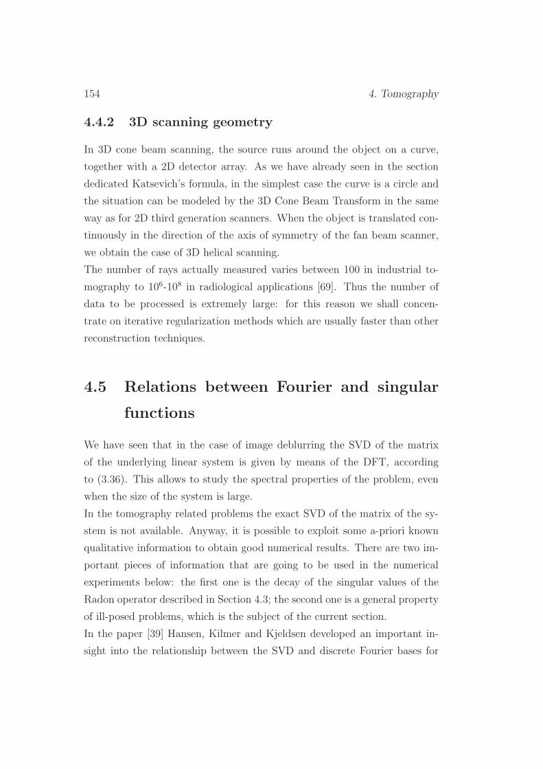
154 4. Tomography
4.4.2 3D scanning geometry
In 3D cone beam scanning, the source runs around the object on a curve,
together with a 2D detector array. As we have already seen in the section
dedicated Katsevich’s formula, in the simplest case the curve is a circle and
the situation can be modeled by the 3D Cone Beam Transform in the same
way as for 2D third generation scanners. When the object is translated con-
tinuously in the direction of the axis of symmetry of the fan beam scanner,
we obtain the case of 3D helical scanning.
The number of rays actually measured varies between 100 in industrial to-
mography to 106-108 in radiological applications [69]. Thus the number of
data to be processed is extremely large: for this reason we shall concen-
trate on iterative regularization methods which are usually faster than other
reconstruction techniques.
4.5 Relations between Fourier and singular
functions
We have seen that in the case of image deblurring the SVD of the matrix
of the underlying linear system is given by means of the DFT, according
to (3.36). This allows to study the spectral properties of the problem, even
when the size of the system is large.
In the tomography related problems the exact SVD of the matrix of the sy-
stem is not available. Anyway, it is possible to exploit some a-priori known
qualitative information to obtain good numerical results. There are two im-
portant pieces of information that are going to be used in the numerical
experiments below: the first one is the decay of the singular values of the
Radon operator described in Section 4.3; the second one is a general property
of ill-posed problems, which is the subject of the current section.
In the paper [39] Hansen, Kilmer and Kjeldsen developed an important in-
sight into the relationship between the SVD and discrete Fourier bases for

4.5 Relations between Fourier and singular functions 155
discrete ill-posed problems arising from the discretization of Fredholm inte-
gral equations of the first kind. We reconsider their analysis and relate it to
the considerations we have made in Chapter 3 and in particular in Section
3.1 and Section 3.4.
4.5.1 The case of the compact operator
Although we intend to study large scale discrete ill-posed problems, we return
first to the continuous setting of Section 1.8, because the basic ideas draw
upon certain properties of the underlying continuous problem involving a
compact integral operator. As stated already in [39], this material is not
intended as a rigorous analysis but rather as a tool to gain some insight into
non-asymptotic relations between the Fourier and singular functions of the
integral operator.
Consider the Hilbert space X = L2([−π, π]) with the usual inner product
〈·, ·〉 and denote with ‖ · ‖ the norm induced by the scalar product. Define
K[f ](s) :=
∫
I
κ(s, t)f(t)dt, I = [−π, π]. (4.79)
Assume that the kernel κ is real, (piecewise) C1(I × I) and non-degenerate.
Moreover, assume for simplicity also that ‖κ(π, ·) − κ(−π, ·)‖ = 0. Then,
as we have seen in Section 1.8, K is a compact operator from X to itself
and there exist a singular system λj; vj , uj for K such that (1.38), (1.39),
(1.40) and (1.41) hold.
Define the infinite matrix B whose rows indexed by k = −∞, ...,+∞ and
columns indexed by j = 1, ...,+∞, with entries
Bk,j = |〈uj, eıks/√2π〉|.
Then the following phenomenon, observed in the discrete setting, can be
shown:
The largest entries in the matrix B form a V -shape, with the V lying on the
side and the tip of the V located at k = 0, j = 1.
This means that the function uj is well represented only by a small number

156 4. Tomography
of the eıks/√2π for some |k| in a band of contiguous integers depending on j.
Therefore, the singular functions are similar to the Fourier series functions
in the sense that large singular values (small j) and their corresponding
singular functions correspond to low frequencies, and small singular values
(larger j) correspond to high frequencies. The important consequence is
that it is possible to obtain at least some qualitative information about the
spectral properties of an ill-posed problem without calculating the SVD of
the operator but only performing a Fourier Transform.
4.5.2 Discrete ill-posed problems
As a matter of fact, the properties of the integral operator described in
Section 4.5.1 are observed in practice. As already shown in the paper [39],
the Fourier and the SVD coefficients of a discrete ill-posed problem Ax = b
with perturbed data bδ have a similar behavior if they are ordered in the
correct way.
As a consequence of the phenomenon described in Section 4.5.1 and of the
properties of the Discrete Fourier Transform, we can reorder the Fourier
coefficients as follows:
ϕi :=
(Φ∗bδ)(i+1)/2 if i is odd,
(Φ∗bδ)(2m−i+2)/2 if i is even.(4.80)
In Figure 4.5 we compare the SVD and the Fourier coefficients of the test
problem phillips(200) with = 0.1% and Matlab seed = 1. It is evident from
the graphic that the Fourier coefficients, reordered according to the formula
(4.80), decay very similarly to the SVD coefficients in this example.
In [39], only the case of the 1D ill-posed problems was considered in detail.
Here we consider the case of a 2D tomographic test problem, where:
• the matrix A of the system is the discretization of a 2D integral ope-
rator acting on a function of two space variables. For example, in the
case of parallel X-rays modeled by the Radon Transform, R[f ](θ, s) is

4.6 Numerical experiments 157
0 20 40 60 80 10010
−8
10−6
10−4
10−2
100
102
Phillips(200) noise 0.1%SVD and Fourier coefficients
|u
i*bδ|
|F bδ|
Figure 4.5: SVD(blue full circles) and Fourier (red circles) coefficients of
phillips(200), noise 0.1%
simply the integral of the density function f multiplied by the Dirac
δ-function supported on the straight line corresponding to (θ, s).
• The exact data, denoted by the vector g, is the columnwise stacked
version of the matrix G with entries given by a formula of the type
(4.77) or (4.78) (the sinogram).
• The exact solution f is the columnwise stacked version of the image
F obtained by computing the density function f on the discretization
points of the domain.
To calculate the Fourier coefficients of the perturbed problem Af = gδ,
‖gδ − g‖ ≤ δ, we suggest the following strategy:
(i) compute the two-dimensional Discrete Fourier Transform of the (per-
turbed) sinogram Gδ corresponding to gδ.
(ii) Consider the matrix of the Fourier coefficients obtained at the step
(i) and reorder its columnwise stacked version as in the 1D case (cf.
formula (4.80)).
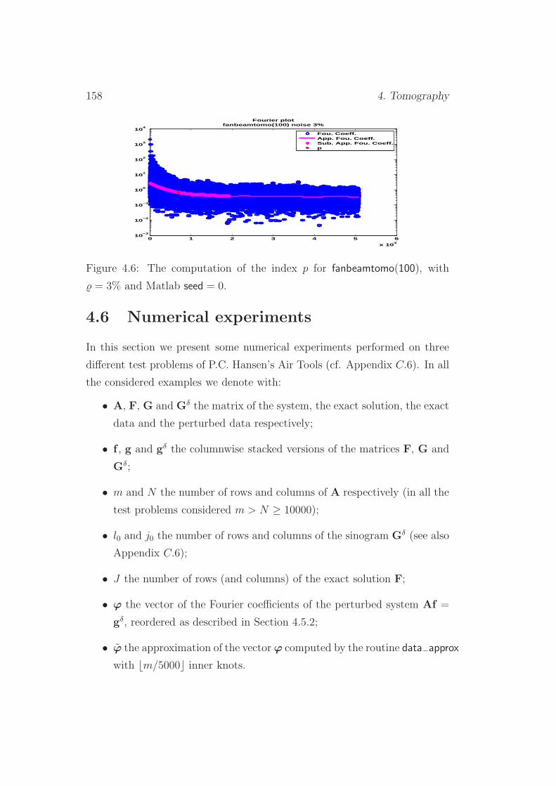
158 4. Tomography
0 1 2 3 4 5 6
x 104
10−3
10−2
10−1
100
101
102
103
104
Fourier plotfanbeamtomo(100) noise 3%
Fou. Coeff.App. Fou. Coeff.Sub. App. Fou. Coeff.p
Figure 4.6: The computation of the index p for fanbeamtomo(100), with
= 3% and Matlab seed = 0.
4.6 Numerical experiments
In this section we present some numerical experiments performed on three
different test problems of P.C. Hansen’s Air Tools (cf. Appendix C.6). In all
the considered examples we denote with:
• A, F, G and Gδ the matrix of the system, the exact solution, the exact
data and the perturbed data respectively;
• f , g and gδ the columnwise stacked versions of the matrices F, G and
Gδ;
• m and N the number of rows and columns of A respectively (in all the
test problems considered m > N ≥ 10000);
• l0 and j0 the number of rows and columns of the sinogram Gδ (see also
Appendix C.6);
• J the number of rows (and columns) of the exact solution F;
• ϕ the vector of the Fourier coefficients of the perturbed system Af =
gδ, reordered as described in Section 4.5.2;
• ϕ the approximation of the vector ϕ computed by the routine data−approx
with ⌊m/5000⌋ inner knots.

4.6 Numerical experiments 159
CGNE results for the fanbeamtomo problem
J Average relative error
Discr. Princ. SR1(np) SR3 Opt. Sol.
100 1% 0.0750 0.0817(100) 0.0568 0.0427
100 3% 0.1437 0.1347(75) 0.1232 0.1132
100 5% 0.1943 0.1847(50) 0.1715 0.1696
100 7% 0.2273 0.2273(25) 0.2139 0.2127
200 1% 0.1085 0.1049(80) 0.0947 0.0886
200 3% 0.1747 0.1669(60) 0.1693 0.1668
200 5% 0.2226 0.2143(40) 0.2127 0.2123
200 7% 0.2550 0.2550(20) 0.2495 0.2477
Table 4.1: Comparison between different stopping rules of CGNE for the
fanbeamtomo test problem.
Using the algorithm cgls, we compute the regularized solutions of CGNE
stopped according to the Discrepancy Principle and to SR1 and SR3.
The index p of SR3 is calculated as follows (see Figure 4.6):
(i) determine a subsequence of the approximated Fourier coefficients by
choosing the elements ϕ1, ϕ1+J , ϕ1+2J , ....
(ii) Discard all the elements after the first relative minimum of this subse-
quence.
(iii) The index p is defined by p := 1 + (i+ 1)J where i is the corner of the
discrete curve obtained at the step (ii) determined by the algorithm
triangle.
4.6.1 Fanbeamtomo
We consider the function fanbeamtomo, that generates a tomographic test
problem with fan beam X-rays. We choose two different values for the di-
mension J , four different percentages of noise on the data, and 16 different
Matlab seeds, for a total of 128 simulations.
For fixed values of J and , the average relative errors over all Matlab seeds
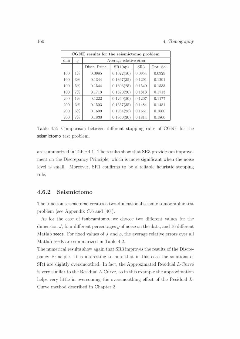
160 4. Tomography
CGNE results for the seismictomo problem
dim Average relative error
Discr. Princ. SR1(np) SR3 Opt. Sol.
100 1% 0.0985 0.1022(50) 0.0954 0.0929
100 3% 0.1344 0.1367(35) 0.1291 0.1291
100 5% 0.1544 0.1603(25) 0.1549 0.1533
100 7% 0.1713 0.1820(20) 0.1813 0.1713
200 1% 0.1222 0.1260(50) 0.1207 0.1177
200 3% 0.1503 0.1637(35) 0.1484 0.1481
200 5% 0.1699 0.1934(25) 0.1661 0.1660
200 7% 0.1830 0.1960(20) 0.1814 0.1800
Table 4.2: Comparison between different stopping rules of CGNE for the
seismictomo test problem.
are summarized in Table 4.1. The results show that SR3 provides an improve-
ment on the Discrepancy Principle, which is more significant when the noise
level is small. Moreover, SR1 confirms to be a reliable heuristic stopping
rule.
4.6.2 Seismictomo
The function seismictomo creates a two-dimensional seismic tomographic test
problem (see Appendix C.6 and [40]).
As for the case of fanbeamtomo, we choose two different values for the
dimension J , four different percentages of noise on the data, and 16 different
Matlab seeds. For fixed values of J and , the average relative errors over all
Matlab seeds are summarized in Table 4.2.
The numerical results show again that SR3 improves the results of the Discre-
pancy Principle. It is interesting to note that in this case the solutions of
SR1 are slightly oversmoothed. In fact, the Approximated Residual L-Curve
is very similar to the Residual L-Curve, so in this example the approximation
helps very little in overcoming the oversmoothing effect of the Residual L-
Curve method described in Chapter 3.
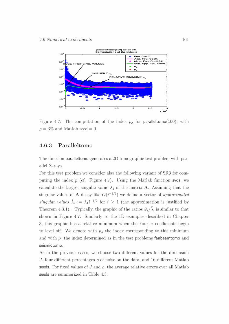
4.6 Numerical experiments 161
0 0.5 1 1.5 2 2.5 3
x 104
10−3
10−2
10−1
100
101
102
103
104
paralleltomo(100) noise 3%Computations of the index p
Fou. Coeff.App. Fou. Coeff.(App. Fou. Coeff.)./ λSub. App. Fou. Coeff.p
c
pλ
HUGE FIRST SING. VALUES
RELATIVE MINIMUM ∼ pλ
CORNER ∼ pc
Figure 4.7: The computation of the index pλ for paralleltomo(100), with
= 3% and Matlab seed = 0.
4.6.3 Paralleltomo
The function paralleltomo generates a 2D tomographic test problem with par-
allel X-rays.
For this test problem we consider also the following variant of SR3 for com-
puting the index p (cf. Figure 4.7). Using the Matlab function svds, we
calculate the largest singular value λ1 of the matrix A. Assuming that the
singular values of A decay like O(i−1/2) we define a vector of approximated
singular values λi := λ1i−1/2 for i ≥ 1 (the approximation is justified by
Theorem 4.3.1). Typically, the graphic of the ratios ϕi/λi is similar to that
shown in Figure 4.7. Similarly to the 1D examples described in Chapter
3, this graphic has a relative minimum when the Fourier coefficients begin
to level off. We denote with pλ the index corresponding to this minimum
and with pc the index determined as in the test problems fanbeamtomo and
seismictomo.
As in the previous cases, we choose two different values for the dimension
J , four different percentages of noise on the data, and 16 different Matlab
seeds. For fixed values of J and , the average relative errors over all Matlab
seeds are summarized in Table 4.3.
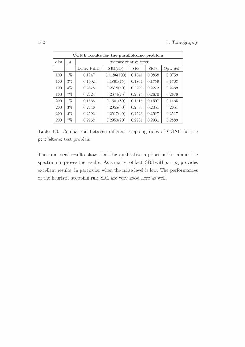
162 4. Tomography
CGNE results for the paralleltomo problem
dim Average relative error
Discr. Princ. SR1(np) SR3c SR3λ Opt. Sol.
100 1% 0.1247 0.1186(100) 0.1041 0.0868 0.0759
100 3% 0.1992 0.1861(75) 0.1861 0.1759 0.1703
100 5% 0.2378 0.2378(50) 0.2299 0.2272 0.2269
100 7% 0.2724 0.2674(25) 0.2674 0.2670 0.2670
200 1% 0.1568 0.1501(80) 0.1516 0.1507 0.1465
200 3% 0.2140 0.2055(60) 0.2055 0.2051 0.2051
200 5% 0.2593 0.2517(40) 0.2523 0.2517 0.2517
200 7% 0.2962 0.2950(20) 0.2931 0.2931 0.2889
Table 4.3: Comparison between different stopping rules of CGNE for the
paralleltomo test problem.
The numerical results show that the qualitative a-priori notion about the
spectrum improves the results. As a matter of fact, SR3 with p = pλ provides
excellent results, in particular when the noise level is low. The performances
of the heuristic stopping rule SR1 are very good here as well.
Chapter 5
Regularization in Banach
spaces
So far, we have considered only linear ill-posed problems in a Hilbert space
setting. We have seen that this theory is well established since the nineties,
so we focused mainly on the applications in the discrete setting.
In the past decade of research, in the area of inverse and ill-posed problems, a
great deal of attention has been devoted to the regularization in the Banach
space setting. The research on regularization methods in Banach spaces was
driven by different mathematical viewpoints. On the one hand, there are
various practical applications where models that use Hilbert spaces are not
realistic or appropriate. Usually, in such applications sparse solutions1 of
linear and nonlinear operator equations are to be determined, and models
working in Lp spaces, non-Hilbertian Sobolev spaces or continuous function
spaces are preferable. On the other hand, mathematical tools and techniques
typical of Banach spaces can help to overcome the limitations of Hilbert
models. In the monograph [82], a series of different applications ranging from
non-destructive testing, such as X-ray diffractometry, via phase retrieval, to
an inverse problem in finance are presented. All these applications can be
1Sparsity means that the searched-for solution has only a few nonzero coefficients with
respect to a specific, given, basis.
163

164 5. Regularization in Banach spaces
modeled by operator equations
F (x) = y, (5.1)
where the so-called forward operator F : D(F ) ⊆ X → Y denotes a conti-
nuous linear or nonlinear mapping between Banach spaces X and Y .
In the opening section of this chapter we shall describe another important
example, the problem of identifying coefficients or source terms in partial
differential equations (PDEs) from data obtained from the PDE solutions.
Then we will introduce the fundamental notions and tools that are peculiar
of the Banach space setting and discuss the problem of regularization in this
new framework.
At the end of the chapter we shall focus on the properties of some of the most
important regularization methods in Banach spaces for solving nonlinear ill-
posed problems, such as the Landweber-type methods and the Iteratively
Regularized Gauss-Newton method.
We point out that the aim of this chapter is the introduction of the Newton-
Landweber type iteration that will be discussed in the final chapter of this
thesis. Thus, methods using only Tikhonov-type penalization terms shall not
be considered here.
5.1 A parameter identification problem for
an elliptic PDE
The problem of identifying coefficients or source terms in partial differential
equations from data obtained from the PDE solution arises in a variety of
applications ranging from medical imaging, via nondestructive testing, to
material characterization, as well as model calibration.
The following example has been studied repeatedly in the literature (see,
e.g. [7], [16], [31], [52], [78] and [82]) to illustrate theoretical conditions and
numerically test the convergence of regularization methods.
Consider the identification of the space-dependent coefficient c in the elliptic
5.1 A parameter identification problem for an elliptic PDE 165
boundary value problem
−u+ cu = f in Ω
u = 0 on ∂Ω(5.2)
from measurements of u in Ω. Here, Ω ⊆ RD, D ∈ N is a smooth, bounded
domain and is the Laplace operator on Ω.
The forward operator F : D(F ) ⊆ X → Y , where X and Y are to be specified
below, and its derivative can be formally written as
F (c) = A (c)−1f, F ′(c)h = −A (c)−1(hF (c)), (5.3)
where A (c) : H2(Ω) ∩H10(Ω) → L2(Ω) is defined by A (c)u = −u+ cu.
In order to preserve ellipticity, a straightforward choice of the domain D(F )
is
D(F ) := c ∈ X | c ≥ 0 a.e., ‖c‖X ≤ γ, (5.4)
for some sufficiently small γ > 0. For the situation in which the theory
requires a nonempty interior of D(F ) in X , the choice
D(F ) := c ∈ X | ∃ ϑ ∈ L∞(Ω), ϑ ≥ 0 a.e. : ‖c− ϑ‖X ≤ γ, (5.5)
for some sufficiently small γ > 0, has been devised in [30].
The preimage and image spaces X and Y are usually both set to L2(Ω),
in order to fit into the Hilbert space theory. However, as observed in [82],
the choice Y = L∞(Ω) is the natural topology for the measured data and
in the situation of impulsive noise the choice Y = L1(Ω) provides a more
robust option than the choice Y = L2(Ω) (cf. also [6] and [49]). Concerning
the preimage space, one often aims at actually reconstructing a uniformly
bounded coefficient, or a coefficient that is sparse in some sense, suggesting
the use of the L∞(Ω) or the L1(Ω)-norm.
This motivates to study the use of
X = Lp(Ω), Y = Lr(Ω),
with general exponents p, r ∈ [1,+∞] within the context of this example.
Restricting to the choice (5.4) of the domain, it is possible to show the
following results (cf. [82]).
166 5. Regularization in Banach spaces
Proposition 5.1.1. Let p, r, s ∈ [1,+∞] and denote by (W2,s ∩H10)(Ω) the
closure of the space C∞0 (Ω) with respect to the norm
‖v‖W2,s∩H10:= ‖v‖Ls + ‖∇v‖L2,
invoking Friedrichs’ inequality.
Let also X = Lp(Ω), Y = Lr(Ω).
(i) If
s ≥ D/2 and s = 1 or s > max1, D/2 or r < +∞
or
s < D/2 and r ≤ Ds
D − 2s,
then (W2,s∩H10)(Ω) ⊆ Lr(Ω) and there exists a constant Cr
(a) > 0 such
that
∀v ∈ (W2,s ∩ H10)(Ω) : ‖v‖Lr ≤ Cr
(a)‖v‖W2,s∩H10.
(ii) Assume c ∈ D(F ) with a sufficiently small γ > 0 and let
1 = s ≥ D
2or s > max1, D
2. (5.6)
Then the operator A (c)−1 : Ls(Ω) → (W2,s ∩ H10)(Ω) is well defined
and bounded by some constant Cs(d).
(iii) For any f ∈ Lmax1,D/2(Ω), the operator F : D(F ) ⊆ X → Y, F (c) =
A (c)−1f is well defined and bounded on D(F ) as in (5.4) with γ > 0
sufficiently small.
(iv) For any
p, r ∈ [1,+∞], f ∈ L1(Ω), D ∈ 1, 2
or
p ∈ (D/2,∞], p ≥ 1, r ∈ [1,+∞], f ∈ LD/2+ǫ(Ω), ǫ > 0
and c ∈ D(F ), the operator F ′(c) : X → Y, F ′(c) = −A (c)−1(hF (c)),
is well defined and bounded.
5.2 Basic tools in the Banach space setting 167
5.2 Basic tools in the Banach space setting
The aim of this section is to introduce the basic tools and fix the classical
notations used in the Banach space setting for regularizing ill-posed problems.
For details and proofs, cf. [82] and the references therein.
5.2.1 Basic mathematical tools
Definition 5.2.1 (Conjugate exponents, dual spaces and dual pai-
rings). For p > 1 we denote by p∗ > 1 the conjugate exponent of p, satisfying
the equation1
p+
1
p∗= 1. (5.7)
We denote by X ∗ the dual space of a Banach space X , which is the Banach
space of all bounded (continuous) linear functionals x∗ : X → R, equipped
with the norm
‖x∗‖X ∗ := sup‖x‖=1
|x∗(x)|. (5.8)
For x∗ ∈ X ∗ and x ∈ X we denote by 〈x∗, x〉X ∗×X and 〈x, x∗〉X×X ∗ the duality
pairing (duality product) defined as
〈x∗, x〉X ∗×X := 〈x, x∗〉X×X ∗ := x∗(x). (5.9)
In norms and dual pairings, when clear from the context, we will omit the
indices indicating the spaces.
Definition 5.2.2. Let xnn∈N be a sequence in X and let x ∈ X . The
sequence xn is said to converge weakly to x if, for every x∗ ∈ X ∗, 〈x∗, xn〉converges to 〈x∗, x〉.
As in the Hilbert space case, we shall denote by the symbol the weak
convergence in X and by → the strong convergence in X .
Definition 5.2.3 (Adjoint operator). Let A be a bounded (continuous)
linear operator between two Banach spaces X and Y. Then the bounded
linear operator A∗ : Y∗ → X ∗, defined as
〈A∗y∗, x〉X ∗×X = 〈y∗, Ax〉Y∗×Y , ∀x ∈ X , y∗ ∈ Y∗,
168 5. Regularization in Banach spaces
is called the adjoint operator of A.
As in the Hilbert space setting, we denote by ker(A) the null-space of A
and by R(A) the range of A.
We recall three important inequalities that are going to be used later.
Theorem 5.2.1 (Cauchy’s inequality). For x ∈ X and x∗ ∈ X ∗ we have:
|〈x∗, x〉X ∗×X | ≤ ‖x∗‖X ∗‖x‖X .
Theorem 5.2.2 (Holder’s inequality). For functions f ∈ Lp(Ω), g ∈Lp∗(Ω), Ω ⊆ RD as in Section 5.1:
∣∣∣∣
∫
Ω
f(x)g(x)dx
∣∣∣∣≤(∫
Ω
|f(x)|pdx)1/p(∫
Ω
|g(x)|p∗dx)1/p∗
.
Theorem 5.2.3 (Young’s inequality). Let a and b denote real numbers
and p, p∗ > 1 conjugate exponents. Then
ab ≤ 1
p|a|p + 1
p∗|b|p∗.
5.2.2 Geometry of Banach space norms
Definition 5.2.4 (Subdifferential of a convex functional). A functional
f : X → R ∪ ∞ is called convex if
f(tx+ (1− t)y) ≤ tf(x) + (1− t)f(y), ∀x, y ∈ X , ∀t ∈ [0, 1].
In this case, an element x∗ ∈ X ∗ is a subgradient of f in x if
f(y) ≥ f(x) + 〈x∗, y − x〉, ∀y ∈ X .
The set ∂f(x) of all subgradients of f in x is called the subdifferential of f
in x.
Theorem 5.2.4 (Optimality conditions). Let f : X → R ∪ ∞ be a convex
functional and let z be such that f(z) <∞. Then
f(z) = minx∈X
f(x) ⇐⇒ 0 ∈ ∂f(z).
5.2 Basic tools in the Banach space setting 169
This result generalizes the classical optimality condition f ′(z) = 0, where
f ′ is the Frechet derivative of f . The subdifferential also is a generaliza-
tion of the differential in the sense that if f is Gateaux-differentiable, then
∂f(x) = ∇f(x).In general the subdifferential of a function may also be the empty set. How-
ever, if the function is Lipschitz-continuous, its sudifferential is not empty.
Among the various properties of the subdifferential of a convex functional,
we recall the following one.
Theorem 5.2.5 (Monotonicity of the subgradient). Assume that the
convex functional f : X → R ∪ ∞ is proper, i.e. the set of all x ∈ Xsuch that f(x) <∞ is non-empty. Then the following monotonicity property
holds:
〈x∗ − y∗, x− y〉 ≥ 0, ∀x∗ ∈ ∂f(x), y∗ ∈ ∂f(y), x, y ∈ X .
To understand the geometry of the Banach spaces, it is important to
study the properties of the proper convex functional x 7→ 1p‖x‖p. We start
introducing the so-called duality mapping JXp .
Definition 5.2.5 (Duality mapping). The set valued mapping JXp : X →
2X∗
, with p ≥ 1 defined by
JXp (x) := x∗ ∈ X ∗ | 〈x∗, x〉 = ‖x‖‖x∗‖, ‖x∗‖ = ‖x‖p−1, (5.10)
is called the duality mapping of X with gauge function t 7→ tp−1.
By jXp we denote a single-valued selection of JXp , i.e. jXp : X → X ∗ is a
mapping with jXp ∈ JXp for all x ∈ X .
The duality mapping is the subgradient of the functional above:
Theorem 5.2.6 (Asplund). Let X be a normed space and p ≥ 1. Then
JXp = ∂
(1
p‖ · ‖pX
)
.
170 5. Regularization in Banach spaces
Example 5.2.1. For every p ∈ (1,+∞), Jp : Lp(Ω) → Lp∗(Ω) is given by
JXp (f) = |f |p−1sgn(f), f ∈ Lp(Ω). (5.11)
From the monotonicity property of the subgradient and the Asplund
Theorem, we know that for all x, z ∈ X we have
1
p‖z‖p − 1
p‖x‖p − 〈JX
p (x), z − x〉 ≥ 0,
and setting y = −(z − x) yields
1
p‖x− y‖p − 1
p‖x‖p + 〈JX
p (x), y〉 ≥ 0.
We are interested in the upper and lower bounds of the left-hand side of the
above inequality in terms of the norm of y.
Definition 5.2.6 (p-convexity and p-smoothness). • A Banach space
X is said to be convex of power type p or p-convex if there exists a con-
stant cp > 0 such that
1
p‖x− y‖p ≥ 1
p‖x‖p − 〈jXp (x), y〉+
cpp‖y‖p
for all x, y ∈ X and all jXp ∈ JXp .
• A Banach space X is said to be smooth of power type p or p-smooth if
there exists a constant Gp > 0 such that
1
p‖x− y‖p ≤ 1
p‖x‖p − 〈jXp (x), y〉+
Gp
p‖y‖p
for all x, y ∈ X and all jXp ∈ JXp .
The p-convexity and p-smoothness properties can be regarded as an ex-
tension of the polarization identity
1
2‖x− y‖2 = 1
2‖x‖2 − 〈x, y〉+ 1
2‖y‖2, (5.12)
which ensures that Hilbert spaces are 2-convex and 2-smooth.
The p-convexity and p-smoothness are related to other famous properties of
convexity and smoothness.
5.2 Basic tools in the Banach space setting 171
Definition 5.2.7. • A Banach space X is said to be strictly convex if
‖12(x+ y)‖ < 1 for all x, y of the unit ball of X satisfying the condition
x 6= y.
• A Banach space X is said to be uniformly convex if, for the modulus of
convexity δX : [0, 2] → [0, 1], defined by
δX (ǫ) := inf
1− ‖12(x+ y)‖ : ‖x‖ = ‖y‖ = 1, ‖x− y‖ ≥ ǫ
,
we have
δX (ǫ) > 0, 0 < ǫ ≤ 2.
• A Banach space X is said to be smooth if, for every x ∈ X with x 6= 0,
there is a unique x∗ ∈ X ∗ such that ‖x∗‖ = 1 and 〈x∗, x〉 = ‖x‖.
• A Banach space X is said to be uniformly smooth if, for the modulus
of smoothness ρX : [0,+∞) → [0,+∞), defined by
ρX (τ) :=1
2sup‖x+ y‖+ ‖x− y‖ − 2 | ‖x‖ = 1, ‖y‖ ≤ τ,
there holds:
limτ→0
ρX (τ)
τ= 0.
If a Banach space is p-smooth for some p > 1, then x 7→ ‖x‖p is Frechet-
differentiable, hence Gateaux-differentiable and therefore JXp is single-valued.
In the famous paper [99], Xu and Roach proved a series of important inequa-
lities, some of which will be very useful in the proofs of the following chapter.
Here we recall only the results about uniformly smooth and s-smooth Banach
spaces and refer to [82] and to [99] for the analogous results about uniformly
convex and s-convex Banach spaces.
Theorem 5.2.7 (Xu-Roach inequalities I). Let X be uniformly smooth,
1 < p <∞, and jXp ∈ JXp . Then, for all x, y ∈ X , we have
‖x− y‖p − ‖x‖p + p〈jXp (x), y〉
≤ +pGp
∫ 1
0
(‖x− ty‖ ∨ ‖x‖)pt
ρX
(t‖y‖
‖x− ty‖ ∨ ‖x‖
)
dt,(5.13)
172 5. Regularization in Banach spaces
where a ∨ b = maxa, b, a, b ∈ R, and where Gp > 0 is a constant that can
be written explicitly (cf. its expression in [82]).
Theorem 5.2.8 (Xu-Roach inequalities II). The following statements
are equivalent:
(i) X is s-smooth.
(ii) For some 1 < p < ∞ the duality mapping JXp is single-valued and for
all x, y ∈ X we have
‖JXp (x)− JX
p (y)‖ ≤ C(‖x‖ ∨ ‖y‖)p−s‖x− y‖s−1.
(iii) The statement (ii) holds for all p ∈ (1,∞).
(iv) For some 1 < p < ∞, some jXp ∈ JXp and for all x, y, the inequality
(5.13) holds. Moreover, the right-hand side of (5.13) can be estimated
by
C
∫ 1
0
ts−1 (‖x− ty‖ ∨ ‖x‖)p−s ‖y‖sdt.
(v) The statement (iv) holds for all p ∈ (1,∞) and all jXp ∈ JXp .
The generic constant C can be chosen independently of x and y.
An important consequence of the Xu-Roach inequalities is the following
result.
Corollary 5.2.1. If X be p-smooth, then for all 1 < q < p the space X is
also q-smooth. If on the other hand X is p-convex, then for all q such that
p < q <∞ the space X is also q-convex.
If X is s-smooth and p > 1, then the duality mapping JXp is single-valued.
The spaces that are convex or smooth of power type share many intere-
sting properties, summarized in the following theorems.
Theorem 5.2.9. If X is p-convex, then:
5.2 Basic tools in the Banach space setting 173
• p ≥ 2;
• X is uniformly convex and the modulus of convexity satisfies δX (ǫ) ≥Cǫp;
• X is strictly convex;
• X is reflexive (i.e. X ∗∗ = X ).
If X is p-smooth, then:
• p ≤ 2;
• X is uniformly smooth and the modulus of smoothness satisfies ρX (τ) ≤Cτ p;
• X is smooth;
• X is reflexive.
Theorem 5.2.10. There hold:
• X is p-smooth if and only if X ∗ is p∗ convex.
• X is p-convex if and only if X ∗ is p∗ smooth.
• X is uniformly convex (respectively uniformly smooth) if and only if X ∗
is uniformly smooth (respectively uniformly convex).
• X is uniformly convex if and only if X is uniformly smooth.
Theorem 5.2.11. The duality mappings satisfy the following assertions:
• For every x ∈ X the set JXp (x) is empty and convex.
• X is smooth if and only if the duality mapping JXp is single-valued.
• If X is uniformly smooth, then JXp is single-valued and uniformly con-
tinuous on bounded sets.
174 5. Regularization in Banach spaces
• If X is convex of power type and smooth, then JXp is single-valued,
bijective, and the duality mapping JX ∗
p∗ is single-valued with
JX ∗
p∗ (JXp (x)) = x.
An important consequence of the last statement is that for spaces being
smooth of power type and convex of power type the duality mappings on the
primal and dual spaces can be used to transport all elements from the primal
to the dual space and vice versa. This is crucial to extend the regularization
methods defined in the Hilbert space setting to the Banach space setting, as
we shall see later.
The smoothness and convexity of power type properties have been studied for
some important function spaces. We summarize the results in the theorem
below.
Theorem 5.2.12. Let Ω ⊆ RD be a domain. Then for 1 < r <∞ the spaces
ℓr of infinite real sequences, the Lebesgue spaces Lr(Ω) and the Sobolev spaces
Wm,r(Ω), equipped with the usual norms, are
max2, r-convex and min2, r-smooth.
Moreover, it is possible to show that ℓ1 cannot be p-convex or p-smooth for
any p.
5.2.3 The Bregman distance
Due to the geometrical properties of the Banach spaces, it is often more
appropriate to exploit the Bregman distance instead of functionals like ‖x−y‖pX or ‖jXp (x)− jXp (y)‖pX ∗ to prove convergence of the algorithms.
Definition 5.2.8. Let jXp be a single-valued selection of the duality mapping
JXp . Then, the functional
Dp(x, y) :=1
p‖x‖p − 1
p‖y‖p − 〈jXp (y), x− y〉X ∗×X , x, y ∈ X (5.14)
is called the Bregman distance (with respect to the functional 1p‖ · ‖p).
5.2 Basic tools in the Banach space setting 175
The Bregman distance is not a distance in the classical sense, but has
many useful properties.
Theorem 5.2.13. Let X be a Banach space and jXp be a single-valued selec-
tion of the duality mapping JXp . Then:
• Dp(x, y) ≥ 0 ∀ x, y ∈ X .
• Dp(x, y) = 0 if and only if jXp (y) ∈ JXp (x).
• If X is smooth and uniformly convex, then a sequence xn ⊆ X re-
mains bounded in X if Dp(y, xn) is bounded in R. In particular, this is
true if X is convex of power type.
• Dp(x, y) is continuous in the first argument. If X is smooth and uni-
formly convex, then JXp is continuous on bounded subsets and Dp(x, y)
is continuous in its second argument. In particular, this is true if X is
convex of power type.
• If X is smooth and uniformly convex, then the following statements are
equivalent:
limn→∞ ‖xn − x‖ = 0;
limn→∞ ‖xn‖ = ‖x‖ and limn→∞〈JXp (xn), x〉 = 〈JX
p (x), x〉;
limn→∞Dp(x, xn) = 0.
In particular, this is true if X is convex of power type.
• The sequence xn is a Cauchy sequence in X if it is bounded and for all
ǫ > 0 there is an N(ǫ) ∈ N such that Dp(xk, xl) < ǫ for all k, l ≥ N(ǫ).
• X is p-convex if and only if Dp(x, y) ≥ cp‖x− y‖p.
• X is p-smooth if and only if Dp(x, y) ≤ Gp‖x− y‖p.
The following property of the Bregman distance replaces the classical
triangle inequality.
176 5. Regularization in Banach spaces
Proposition 5.2.1 (Three-point identity). Let jXp be a single-valued se-
lection of the duality mapping JXp . Then:
Dp(x, y) = Dp(x, z) +Dp(z, y) + 〈jXp (z)− jXp (y), x− z〉. (5.15)
There is a close relationship between the primal Bregman distances and
the related Bregman distances in the dual space.
Proposition 5.2.2. Let jXp be a single-valued selection of the duality map-
ping JXp . If there exists a single-valued selection jX
∗
p∗ of JX ∗
p∗ such that for
fixed y ∈ X we have jX∗
p∗ (jXp (y)) = y, then
Dp(y, x) = Dp∗(jXp (x), j
Xp (y)) (5.16)
for all x ∈ X .
5.3 Regularization in Banach spaces
In this section we extend the fundamental concepts of the regularization
theory for linear ill-posed operator equations in Hilbert spaces discussed in
Chapter 1 to the more general framework of the present chapter.
5.3.1 Minimum norm solutions
In Section 1.6 we have seen Hadamard’s definition of ill-posed problems. We
recall that an abstract operator equation F (x) = y is well posed (in the sense
of Hadamard) if for all right-hand sides y a solution of the equation exists,
is unique and the solution depends continuously on the data.
For linear problems in the Hilbert space setting, we have defined the Moore-
Penrose generalized inverse, that allows to overcome the problems of existence
and uniqueness of the solution by defining the minimum norm (or best-
approximate) solution. For general ill-posed problems in Banach spaces,
it is also possible to define a minimum norm solution.
In the linear case, the definition is similar to the Hilbert space setting.
5.3 Regularization in Banach spaces 177
Definition 5.3.1 (Minimum norm solution). Let A be a linear operator
between Banach spaces X and Y An element x† ∈ X is called a minimum
norm solution of the operator equation Ax = y if
Ax† = y and ‖x†‖ = inf‖x‖ | x ∈ X , Ax = y.
The following result gives a characterization of the minimum norm solu-
tion (see [82] for the proof).
Proposition 5.3.1. Let X be smooth and uniformly convex and let Y be an
arbitrary Banach space. Then, if y ∈ R(A), the minimum norm solution of
Ax = y is unique. Furthermore, it satisfies the condition JXp (x†) ∈ R(A∗)
for 1 < p <∞. If additionally there is some x ∈ X such that JXp (x) ∈ R(A∗)
and x− x† ∈ ker(A), then x = x†.
In the nonlinear case, one has to face nonlinear operator equations of the
type
F (x) = y, x ∈ D(F ) ⊆ X , y ∈ F (D(F )) ⊆ Y , (5.17)
where F : D(F ) ⊆ X → Y is a nonlinear mapping with domain D(F ) and
range F (D(F )).
According to the local character of the solutions in nonlinear equations we
have to focus on some neighborhood of a reference element x0 ∈ X which can
be interpreted as an initial guess for the solution to be determined. Then,
one typically shifts the coordinate system from the zero to x0 and searches
for x0-minimum norm solutions.
Definition 5.3.2 (x0-minimum norm solution). An element x† ∈ D(F )
⊆ X is called a x0-minimum norm solution of the operator equation F (x) = y
if
F (x†) = y and ‖x† − x0‖ = inf‖x− x0‖ | x ∈ D(F ), F (x) = y.
To ensure that x0-minimum norm solutions to the nonlinear operator
equation (5.17) exist, some assumptions have to be made on the Banach
spaces X and Y , on the domain D(F ) and on the operator F .
178 5. Regularization in Banach spaces
Proposition 5.3.2. Assume the following conditions hold:
(i) X and Y are infinite dimensional reflexive Banach spaces.
(ii) D(F ) ⊆ X is a convex and closed subset of X .
(iii) F : D(F ) ⊆ X → Y is weak-to-weak sequentially continuous, i.e. xn
x in X with xn ∈ D(F ), n ∈ N, and x ∈ D(F ) implies F (xn)
F (x) in Y.
Then the nonlinear operator equation (5.17) admits an x0-minimum norm
solution.
Proof. See [82], Proposition 3.14.
5.3.2 Regularization methods
As usual, we shall assume that the data y of an ill-posed (linear or nonlinear)
operator equation are not given exactly, but only elements yδ ∈ Y satisfying
the inequality ‖y − yδ‖ ≤ δ, with noise level δ > 0 are available.
Consequently, regularization approaches are required for detecting good ap-
proximate solutions. Here we give a definition of regularization methods
which is analogous to that given in Chapter 1, but a little more general.
Definition 5.3.3. Let σ0 ∈ (0,+∞]. For every σ ∈ (0, σ0), let Rσ : Y → Xbe a continuous operator.
The family Rσ is called a regularization operator for A† if, for every y ∈D(A†), there exists a function
α : (0,+∞)× Y → (0, σ0),
called parameter choice rule for y, that allows to associate to each cou-
ple (δ, yδ) a specific operator Rα(δ,yδ) and a regularized solution xδα(δ,yδ)
:=
Rα(δ,yδ)yδ, and such that
limδ→0
supyδ∈Bδ(y)
α(δ, yδ) = 0. (5.18)

5.3 Regularization in Banach spaces 179
If, in addition, for every sequence yδnn∈N ⊆ Y with ‖yδn − y‖ ≤ δn and δn
→ 0 as n → ∞ the regularized solutions xδnα(yδn,δn)
converge in a well-defined
sense to a well-defined solution x† of (5.17), then α is said to be convergent.
Convergent regularization methods are defined accordingly, analogously to
Definition 1.9.1. If the solution of equation (5.17) is not unique, convergence
to solutions possessing desired properties, e.g. x0-minimum norm solutions,
is required.
In the linear case, similar definitions hold.
The distinction between a-priori, a-posteriori and heuristic parameter
choice rules is still valid in this context.
We have seen that in the case of linear operator equations in a Hilbert space
setting the construction of regularization methods is based in general on
the approximation of the Moore-Penrose approximated inverse of the linear
operator A by a σ-dependent family of bounded operators with regularized
solutions
xδσ = gσ(A∗A)A∗yδ, σ > 0.
However, in the Banach space setting neither A† nor A∗A is available, since
the adjoint operator A∗ : Y∗ →X ∗ maps between the dual spaces. In the case
of nonlinear operator equations, a comparable phenomenon occurs, because
the adjoint operator
F ′(x†)∗ : Y∗ → X ∗
of a bounded linear derivative operator
F ′(x†) : X → Y
of F at the solution point x† ∈ D(F ) also maps between the dual spaces.
Nevertheless, two large and powerful classes of regularization methods with
prominent applications, for example in imaging, were recently promoted: the
class of Tikhonov-type regularization methods in Banach spaces and the class
of iterative regularization methods in Banach spaces.
Once again, we shall focus our attention on iterative regularization methods:

180 5. Regularization in Banach spaces
since Tikhonov-type regularization methods require the computation of a
global minimizer, often the amount of work required for carrying out iterative
regularization methods is much smaller than the comparable amount for a
Tikhonov-type regularization.
For a detailed coverage of the most recent results about Tikhonov-type regu-
larization methods, see [82].
5.3.3 Source conditions and variational inequalities
We have seen in Chapter 1 that the convergence of the regularized solutions
of a regularization method to the minimum norm solution of the ill-posed
operator equation Ax = y can be arbitrarily slow. To obtain convergence
rates
ε(xδα, x†) = O(ϕ(δ)) as δ → 0 (5.19)
for an error measure ε and an index function ϕ, some smoothness of the
solution element x† with respect to A : X → Y is required. In Chapter 1,
we have seen a classical tool for expressing the smoothness of x†, the source
conditions. In the Hilbert space setting, this allows to define the concept of
(order) optimality of a regularization method.
In the Banach space setting, things are more complicated. The issue of
the order optimality of a regularization method is, at least to the author’s
knowledge, still an open question in the field. The rates depend on the
interplay of intrinsic smoothness of x† and the smoothing properties of the
operator A with non-closed range, but very often proving rates is a difficult
task and it is not easy to find the correct smoothness assumptions on x† to
obtain convergence rates that, at least in the special case of Hilbert spaces,
can be considered optimal.
In this presentation, the extension of the concept of source conditions to the
Banach space setting is omitted. We only say that a wide variety of choices
has been proposed and analyzed, where either x† itself or an element ξ† from
the subdifferential of functionals of the form 1p‖·‖pX in x† belongs to the range
of a linear operator that interacts with A in an appropriate manner. The
5.4 Iterative regularization methods 181
source conditions defined in Chapter 1 are only one of these choices.
We will focus our attention on a different strategy for proving convergence
rates, the use of variational inequalities. As many authors pointed out (cf.
e.g. [46], [82] and the references therein), estimating from above a term of
the form
|〈JXp (x†), x† − x〉X ∗×X |
is a very powerful tool for proving convergence rates in regularization. The
main advantage of this approach is that this term is contained in the Bregman
distance with respect to the functional 1p‖ · ‖pX .
In the literature, many similar variational inequalities have been proposed.
Essentially, the right-hand side of these inequalities contain a term with the
Bregman distance between x and x† and a term that depends on the operator
A or, in the nonlinear case, on the forward operator F , for example:
|〈JXp (x†), x† − x〉X ∗×X | ≤ β1Dp(x, x
†) + β2‖F (x)− F (x†)‖, (5.20)
for constants 0 ≤ β1 < 1 and β2 ≥ 0. The inequalities must hold for all x ∈M, with some set M which contains all regularized solutions of interest.
We shall not discuss these assumptions here, but we limit ourselves to state a
particular variational inequality in each examined case. For a more detailed
treatment of the argument, we refer to [82], where some important results
that link the variational inequalities with the source conditions can also be
found.
5.4 Iterative regularization methods
In this section we consider iterative regularization methods for nonlinear ill-
posed operator equations (5.17). We will assume that the noise level δ is
known to provide convergence and convergence rates results.
In the following, x0 is some initial guess. We will assume that a solution
to (5.17) exists: according to Proposition 5.3.2, this implies the existence
of an x0-minimum norm solution x†, provided that the assumptions of that
182 5. Regularization in Banach spaces
proposition are satisfied.
The iterative methods discussed in this section will be either of gradient
(Landweber and Iteratively Regularized Landweber) or of Newton-type (Ite-
ratively Regularized Gauss-Newton method).
5.4.1 The Landweber iteration: linear case
Before turning to the nonlinear case, we consider the Landweber iteration
for linear ill-posed problems in Banach spaces with noisy data.
In Chapter 1, we have seen that the Landweber iteration for solving linear
ill-posed problems in Hilbert spaces can be expressed in the form
xk+1 = xk − ωA∗(Axk − y),
where ω > 0 is the step size of the method. Here, we shall consider a variable
step size ωk > 0 (k ∈ N) in the course of the iteration, since an appropriate
choice of the step size helps to prove convergence.
The generalization of the Landweber iteration to the Banach space setting
requires the help of the duality mappings. As a consequence, the space X is
assumed to be smooth and uniformly convex, whereas Y can be an arbitrary
Banach space. Note that this implies that jXp = JXp is single-valued, X is
reflexive and X ∗ is strictly convex and uniformly smooth.
The Landweber algorithm
Assume that instead of the exact data y ∈ R(A) and the exact linear and
bounded operator A : X → Y , only some approximations yjj in Y and
All in the space L (X ,Y) of linear and bounded operators between X and
Y , are available. Assume also that estimates for the deviations
‖yj − y‖ ≤ δj , δj > δj+1 > 0, limj→∞
δj = 0, (5.21)
and
‖Al − A‖ ≤ ηl, ηl > ηl+1 > 0, liml→∞
ηl = 0, (5.22)
5.4 Iterative regularization methods 183
are known. Moreover, to properly include the second case (5.22), we need an
a-priori estimate for the norm of x†, i.e. there is a constant R > 0 such that
‖x†‖ ≤ R. (5.23)
Further, set
S := supl∈N
‖Al‖. (5.24)
(i) Fix p, r ∈ (1,∞). Choose constants C, C ∈ (0, 1) and an initial vector
x0 such that
jXp (x0) ∈ R(A∗) and Dp(x†, x0) ≤
1
p‖x†‖p. (5.25)
Set j−1 := 0 and l−1 := 0. For k = 0, 1, 2, ... repeat
(ii) If for all j > jk−1 and all l > lk−1,
‖Alxk − yj‖ ≤ 1
C(δj + ηlR), (5.26)
stop iterating.
Else, find jk > jk−1 and lk > lk−1 with
δjk + ηlkR ≤ CRk
where
Rk := ‖Alkxk − yjk‖.
Choose ωk according to:
(a) In case x0 = 0 set
ω0 := C(1− C)p−1p∗p−1
SpRp−r0 .
(b) For all k ≥ 0 (respectively k ≥ 1 if x0 = 0), set
γk := min
ρX ∗(1),
(
C(1− C)Rk
2p∗Gp∗S‖xk‖
)
,
184 5. Regularization in Banach spaces
whereGp∗ is the constant from the Xu-Roach inequalities (cf. The-
orem 5.2.7), and choose τk ∈ (0, 1], with
ρX ∗(τk)
τk= γk
and set
ωk :=τkS
‖xk‖p−1
Rr−1k
. (5.27)
Iterate
xk+1 := JX ∗
p∗
(JXp (xk)− ωkA
∗lkjYr (Alkxk − yjk)
). (5.28)
Theorem 5.4.1. The Landweber algorithm either stops after a finite number
of iterations with the minimum norm solution of Ax = y or the sequence of
iterates xk converges strongly to x†.
Proof. See [82], Theorem 6.6.
Let us consider now the case of noisy data yδ and a perturbed operator
Aη, with noise level
‖y − yδ‖ and ‖A− Aη‖ ≤ η. (5.29)
We apply the Landweber algorithm with δj = δ and ηl = η for all j, l ∈ N
and use the Discrepancy Principle. To that end, condition (5.26) provides us
with a stopping rule: we terminate the iteration at kD = kD(δ), where
kD(δ) := mink ∈ N | Rk <1
C(δ + ηR). (5.30)
The proof of Theorem 5.4.1 shows that, as long as Rk ≥ 1C(δ + ηR), xk+1
is a better approximation of x† than xk. A consequence of this fact and of
Theorem 5.4.1 is the stability of this method with respect to the noise.
Corollary 5.4.1. Together with the Discrepancy Principle (5.30) as a stop-
ping rule, the Landweber algorithm is a regularization method for Ax = y.
We observe that since the selection jYr needs not to be continuous, the
method is another example of regularization with non-continuous mapping,
exactly like the the conjugate gradient type methods.

5.4 Iterative regularization methods 185
5.4.2 The Landweber iteration: nonlinear case
Analogous to the Landweber method in Hilbert spaces (cf. [30]), we study a
generalization of the Landweber iteration described in Section 5.4.1 to solve
nonlinear problems of the form (5.17):
JXp (xδk+1) = JX
p (xδk)− ωkA∗kj
Yr (F (x
δk)− yδ),
xδk+1 = JX ∗
p∗ (JXp (xδk+1)), k = 0, 1, ...
(5.31)
where we abbreviate Ak = F ′(xδk).
Of course, some assumptions are required on the spaces and on the forward
operator F (see the results below). A typical assumption on the forward
operator is the so-called η-condition (or tangential cone condition):
‖F (x)− F (x)− F ′(x)(x− x)‖ ≤ ‖F (x)− F (x)‖, ∀x, x ∈ BD
ρ (x†) (5.32)
for some 0 < η < 1, where BD
ρ (x†) := x ∈ X | Dp(x
†, x) ≤ ρ2, ρ > 0.A key point for proving convergence of the Landweber iteration is showing
the monotonicity of the Bregman distances.
Proposition 5.4.1. Assume that X is smooth and p-convex, that the ini-
tial guess x0 is sufficiently close to x†, i.e. x0 ∈ BD
ρ (x†), that F satisfies
the tangential cone condition with a sufficiently small η, that F and F ′ are
continuous, and that
BD
ρ (x†) ⊆ D(F ). (5.33)
Let τ be chosen sufficiently large, so that
c(η, τ) := η +1 + η
τ< 1. (5.34)
Then, with the choice
ωk :=p∗(1− c(η, τ))p−1
Gp−1p∗
‖F (xδk − yδ‖p − r
‖Ak‖p≥ 0, (5.35)
with Gp∗ being the constant from the Xu-Roach inequalities (cf. Theorem
5.2.7), monotonicity of the Bregman distances
Dp(x†, xδk+1)−Dp(x
†, xδk) ≤ −p∗(1− c(η, τ))p
p(Gp∗p∗)p−1
‖F (xδk − yδ‖p‖Ak‖p
(5.36)
186 5. Regularization in Banach spaces
as well as xδk+1 ∈ D(F ) holds for all k ≤ kD(δ)− 1, with kD(δ) satisfying the
Discrepancy Principle:
kD(δ) := mink ∈ N | ‖F (xδk)− yδ‖ ≤ τδ. (5.37)
This allows to show the following convergence results for the Landweber
iteration. For a proof of this theorem, as well as of Proposition 5.4.1, we
refer as usual to [82].
Theorem 5.4.2. Let the assumptions of Proposition 5.4.1 hold, with ad-
ditionally Y being uniformly smooth and let kD(δ) be chosen according to
the Discrepancy Principle (5.37), with (5.34). Then, according to (5.31),
the Landweber iterates xδkD(δ) converge to a solution of (5.17) as δ → 0. If
R(F ′(x)) ⊆ R(F ′(x†)) for all x ∈ Bρ(x0) and JXp (x0) ∈ R(F ′(x†)), then
xδkD(δ) converge to x† as δ → 0.
5.4.3 The Iteratively Regularized Landweber method
In the Hilbert space setting, the proof of convergence rates for the Landweber
iteration under source conditions
x† − x0 ∈ R((F ′(x†)∗F ′(x†))
ν2
)(5.38)
relies on the fact that the iteration errors xδk − x† remain in
R((F ′(x†)∗F ′(x†))
ν2
)
and their preimages under((F ′(x†)∗F ′(x†))
ν2
)form a bounded sequence (cf.
Proposition 2.11 in [53]). In [82] is stated that this approach can hardly be
carried over to the Banach space setting, unless more restrictive assumptions
are made on the structure of the spaces than in the proof of convergence
only, even in the case ν = 1.
Therefore, an alternative version of the Landweber iteration is considered,
namely the Iteratively Regularized Landweber method.

5.4 Iterative regularization methods 187
The iterates are now defined by
JXp (xδk+1 − x0) = (1− αk)J
Xp (xδk − x0)− ωkA
∗kj
Yr (F (x
δk)− yδ),
xδk+1 = x0 + Jp∗X ∗(JXp (xδk+1 − x0)), k = 0, 1, ...
(5.39)
An appropriate choice of the sequence αkk∈N ∈ [0, 1], has been shown to
be convergent in a Hilbert space setting (with rates under a source condition
of the form ξ† = (F ′(x†))∗v, v ∈ Y∗) in [81].
In place of the Hilbert space condition (5.38) we consider the variational
inequality
∃ β > 0 : ∀x ∈ BDρ (x
†)
|〈JXp (x† − x0), x− x†〉X ∗×X | ≤ βDx0
p (x†, x)1−ν2 ‖F ′(x†)(x− x†)‖ν
(5.40)
where
Dx0p (x†, x) := Dp(x
† − x0, x− x0). (5.41)
According to (5.40), due to the presence of additional regularity, the tangen-
tial cone condition can be relaxed to a more general condition on the degree
of nonlinearity of the operator F :
∥∥(F ′(x† + v)− F ′(x†))v
∥∥ ≤ K
∥∥F ′(x†)v
∥∥c1Dx0
p (x†, v + x†)c2 ,
v ∈ X, x† + v ∈ BDρ (x
†) , (5.42)
with
c1 = 1 or c1 + rc2 > 1 or (c1 + rc2 ≥ 1 and K > 0 sufficiently small)
(5.43)
and
c1 + c22ν
ν + 1≥ 1. (5.44)
For further details on the degree of nonlinearity conditions, see [82] and the
references therein.
The step size ωk > 0 is chosen such that
ωk1− 3C(c1)K
3(1− C(c1)K)‖F (xδk)− yδ‖r − 2p
∗+p−2Gp∗ωp∗
k ‖A∗kj
Yr (F (x
δk)− yδ)‖p∗ ≥ 0,
(5.45)

188 5. Regularization in Banach spaces
where C(c1) = cc11 (1 − c1)1−c1 , c1 and K as in (5.42). This is possible, e.g.
by a choice
0 < ωk ≤ Cω‖F (xδk)− yδ‖ p−r
p−1
‖Ak‖p∗=: ωk,
with Cω := 22−p∗−p
31−3C(c1)K
(1−C(c1)K)Gp∗.
If r ≥ p, F and F ′ are bounded on BD
ρ (x†), it is possible to bound ωk from
above and below, i.e. there exist ω, ω > 0, independent of k and δ, such that
0 < ω ≤ ωk ≤ ω, (5.46)
cf. [82].
To prove convergence rates, the following a-priori stopping rule has been
proposed:
k∗(δ) := mink ∈ N | αν+1
r(ν+1)−2ν
k ≤ τδ, (5.47)
where ν < 1 is the exponent of the variational inequality (5.40).
Theorem 5.4.3. Assume that X is smooth and p-convex, that x0 ∈ BD
ρ (x†),
that the variational inequality (5.40) holds with ν ∈ (0, 1] and β sufficiently
small, that F satisfies (5.42), with (5.43) and (5.44), that F and F ′ are
continuous and uniformly bounded in BD
ρ (x†), that BD
ρ (x†) ⊆ D(F ) and that
p∗ ≥ 2ν
p(ν + 1)− 2ν+ 1. (5.48)
Let k∗(δ) be chosen according to (5.47), with τ sufficiently large. Moreover,
assume that r ≥ p and that the sequence ωkk∈N is chosen such that (5.46)
holds. Finally, assume that the sequence αkk∈N ⊆ [0, 1] is chosen such that
(αk+1
αk
) 2νp(ν+1)−2ν
+1
3αk − 1 ≥ cαk (5.49)
for some c ∈ (0, 13) independent of k and αmax = maxk∈N αk is sufficiently
small.
Then, the iterates xδk+1 remain in BD
ρ (x†) for all k ≤ k∗(δ) − 1, with k∗(δ)
according to (5.47). Moreover, we obtain optimal rates
Dx0p (x†, xk∗) = O(δ
2νν+1 ), δ → 0 (5.50)
5.4 Iterative regularization methods 189
as well as in the noise free case δ = 0
Dx0p (x†, xk∗) = O(α
2νr(ν+1)−2ν
k ), k → ∞. (5.51)
A possible choice of the parameters αkk∈N, satisfying (5.49), and small-
ness of αmax is given by
αk =α0
(k + 1)t(5.52)
with t ∈ (0, 1] such that 3tθ < α0 sufficiently small, cf. [82].
We emphasize that in the Banach space setting an analogous of Plato’s The-
orem 1.11.1 is not available. Consequently, convergence rate results under
source conditions or variational inequalities like (5.40) cannot be used to
prove (strong) convergence results.
5.4.4 The Iteratively Regularized Gauss-Newton method
Among the iterative methods, the Iteratively Regularized Gauss-Newton
(IRGN) method is one of the most important for solving nonlinear ill-posed
problems.
In the Banach space setting, the (n+ 1)-th iterate of the IRGN method, de-
noted by xδn+1 = xδn+1(αn), is a minimizer xδn+1(α) of the Tikhonov functional
‖An(x−xδn)+F (xδn)−yδ‖r+α‖x−x0‖p, x ∈ D(F ), n = 0, 1, 2, ...., (5.53)
where p, r ∈ (1,∞), αn is a sequence of regularization parameters, and
An = F ′(xδn).
The regularizing properties of the IRGN method are now well understood.
If one of the assumptions
F ′(x) : X → Y is weakly closed ∀x ∈ D(F ), and Y is reflexive, (5.54)
D(F ) is weakly closed (5.55)
holds, then the method is well defined (cf. Lemma 7.9 in [82]). Moreover,
assuming variational inequalities similar to (5.40) and the a-priori choice
(5.47) for αn, it is possible to obtain optimal convergence rates, see [82] and
190 5. Regularization in Banach spaces
the references therein.
Here we concentrate on the a-posteriori choice given by the Discrepancy
Principle. More precisely, we have the following two theorems (see, as usual,
[82] for the proofs).
Theorem 5.4.4. Assume that X is smooth and uniformly convex and that F
satisfies the tangential cone condition (5.32) with BD
ρ (x†) replaced by D(F )∩
Bρ(x0) and with η sufficiently small. Assume also that
(xn x ∧ F (xn) → f) ⇒ (x ∈ D(F ) ∧ F (x) = f) (5.56)
or
(JXp (xn−x0) x∗∧F (xn) → f) ⇒ (x := JX ∗
p∗ (x∗)+x0 ∈ D(F )∧F (x) = f)
(5.57)
for all xnn∈N ⊆ X , holds, as well as (5.54) or (5.55). Let
η < σ < σ < 1, (5.58)
and let τ be chosen sufficiently large, so that
η +1 + η
τ≤ σ and η <
1− σ
2. (5.59)
Choose the regularization parameters αn such that
σ‖F (xδn)−yδ‖ ≤ ‖An(xδn+1(αn)−xδn)+F (xδn)−yδ‖ ≤ σ‖F (xδn)−yδ‖, (5.60)
if
‖An(x0 − xδn) + F (xδn)− yδ‖ ≥ σ‖F (xδn)− yδ‖ (5.61)
holds. Moreover, assume that
δ <‖F (x0)− yδ‖
τ(5.62)
and stop the iteration at the iterate nD = nD(δ) according to the Discrepancy
Principle (5.37). Then, for all n ≤ nD(δ)− 1, the iterates
xδn+1 :=
xδn+1 = xδn+1(αn), with αn as in (5.60), if (5.61) holds
x0, else
(5.63)

5.4 Iterative regularization methods 191
are well defined.
Furthermore, there exists a weakly convergent subsequence of
xδnD(δ), if (5.56) holds
JXp (xδnD(δ) − x0), if (5.56) holds
(5.64)
and along every weakly convergent subsequence xnD(δ) converges strongly to
a solution of F (x) = y as δ → 0. If the solution is unique, then xnD(δ)
converges strongly to this solution as δ → 0.
The theorem above provides us with a convergence result. The following
theorem gives convergence rates.
Theorem 5.4.5. Let the assumptions of Theorem 5.4.4 be satisfied. Then
under the variational inequality
∃ β > 0 : ∀x ∈ BDρ (x
†)
|〈JXp (x† − x0), x− x†〉X ∗×X | ≤ βDx0
p (x, x†)1−ν2 ‖F ′(x†)(x− x†)‖ν
(5.65)
with 0 < ν < 1, we obtain optimal convergence rates
Dx0p (xnD
, x†) = O(δ2νν+1 ), as δ → 0. (5.66)

192 5. Regularization in Banach spaces
Chapter 6
A new Iteratively Regularized
Newton-Landweber iteration
The final chapter of this thesis is entirely dedicated to a new inner-outer
Newton-Iteratively Regularized Landweber iteration for solving nonlinear
equations of the type (5.17) in Banach spaces.
The reasons for choosing a Banach space framework have already been ex-
plained in the previous chapter. We will see the advantages of working in
Banach spaces also in the numerical experiments presented later.
Concerning the method, a combination of inner and outer iterations in a
Newton type framework has already been shown to be highly efficient and
flexible in the Hilbert space context, see, e.g., [78] and [79].
In the recent paper [49], a Newton-Landweber iteration in Banach spaces
has been considered and a weak convergence result for noisy data has been
proved. However, neither convergence rates nor strong convergence results
have been found. The reason for this is that the convergence rates proof
in Hilbert spaces relies on the fact that the iteration errors remain in the
range of the adjoint of the linearized forward operator and their preimages
under this operator form a bounded sequence. Carrying over this proof to
the Banach space setting would require quite restrictive assumptions on the
structure of the spaces, though, which we would like to avoid, to work with
193
194 6. A new Iteratively Regularized Newton-Landweber iteration
as general Banach spaces as possible.
Therefore, we study here a combination of the outer Newton loop with an
Iteratively Regularized Landweber iteration, which indeed allows to prove
convergence rates and strong convergence.
From Section 6.1 to Section 6.5 we will study the inner-outer Newton-Iteratively
Regularized Landweber method following [54]. We will see that a strategy
for the stopping indices similar to that proposed in [49] leads to a weak con-
vergence result. Moreover, always following [54], we will show a convergence
rate result based on an a-priori choice of the outer stopping index.
Section 6.6 is dedicated to some numerical experiments for the elliptic PDE
problem presented in Section 5.1.
In Section 6.7 we will consider a different choice of the parameters of the
method that allows to show both strong convergence and convergence rates.
6.1 Introduction
In order to formulate and later on analyze the method, we recall some basic
notations and concepts. For more details about the concepts appearing be-
low, we refer to Chapter 5.
Consider, for some p ∈ (1,∞), the duality mapping JXp (x) := ∂
1p‖x‖p
from X to its dual X ∗. To analyze convergence rates we employ the Breg-
man distance
Dp(x, x) =1
p‖x‖p − 1
p‖x‖p − 〈jXp (x), x− x〉X ∗×X
(where jXp (x) denotes a single-valued selection of JXp (x)) or its shifted version
Dx0p (x, x) := Dp(x− x0, x− x0) .
Throughout this paper we will assume that X is smooth (which implies that
the duality mapping is single-valued, cf. Chapter 5) and moreover, that Xis s-convex for some s ∈ [p,∞), which implies
Dp(x, y) ≥ cp,s‖x− y‖s(‖x‖+ ‖y‖)p−s (6.1)
6.1 Introduction 195
for some constant cp,s > 0, cf. Chapter 5. As a consequence, X is reflexive
and we also have
Dp∗(x∗, y∗) ≤ Cp∗,s∗‖x∗ − y∗‖s∗((pDp∗(J
X ∗
p∗ (x∗), 0))1−s∗
p∗ + ‖x∗ − y∗‖p∗−s∗) ,
(6.2)
for some Cp∗,s∗, where s∗ denotes the dual index s∗ = s
s−1. The latter can be
concluded from estimate (2.2) in [49], which is the first line in
Dp∗(x∗, y∗) ≤ Cp∗,s∗‖x∗ − y∗‖s∗(‖y∗‖p∗−s∗ + ‖x∗ − y∗‖p∗−s∗)
≤ Cp∗,s∗‖x∗ − y∗‖s∗(‖x∗‖p∗−s∗ + ‖x∗ − y∗‖p∗−s∗)
= Cp∗,s∗‖x∗ − y∗‖s∗(‖JX ∗
p∗ (x∗)‖(p∗−s∗)(p−1) + ‖x∗ − y∗‖p∗−s∗)
= Cp∗,s∗‖x∗ − y∗‖s∗((pDp∗(JX ∗
p∗ (x∗), 0))(p∗−s∗)p−1
p + ‖x∗ − y∗‖p∗−s∗),
where Cs∗,p∗ is equal to Cs∗,p∗(1+2p∗−s∗−1) if p∗−s∗ > 1 and is simply 2Cs∗,p∗
otherwise.
Note that the duality mapping is bijective and (JXp )−1 = JX ∗
p∗ , the latter de-
noting the (by s-convexity also single-valued) duality mapping on the dual
X ∗ of X .
We will also make use of the Three-point identity (5.15) and the relation
(5.16), which connects elements of the primal space with the corresponding
elements of the dual space.
We here consider a combination of the Iteratively Regularized Gauss-Newton
method with an Iteratively Regularized Landweber method for approximating
the Newton step, using some initial guess x0 and starting from some xδ0 (that
196 6. A new Iteratively Regularized Newton-Landweber iteration
need not necessarily coincide with x0)
For n = 0, 1, 2 . . . do
un,0 = 0
zn,0 = xδn
For k = 0, 1, 2 . . . , kn − 1 do
un,k+1 = un,k − αn,kJXp (zn,k − x0)
−ωn,kA∗nj
Yr (An(zn,k − xδn)− bn)
JXp (zn,k+1 − x0) = JX
p (xδn − x0) + un,k+1
xδn+1 = zn,kn ,
(6.3)
where we abbreviate
An = F ′(xδn) , bn = yδ − F (xδn) .
For obtaining convergence rates we impose a variational inequality
∃ β > 0 : ∀x ∈ BD
ρ (x†)
|〈JXp (x† − x0), x− x†〉X ∗×X | ≤ βDx0
p (x†, x)12−ν‖F (x)− F (x†)‖2ν , (6.4)
with ν ∈ (0, 12], corresponding to a source condition in the special case of
Hilbert spaces, cf., e.g., [42].
Here
BD
ρ (x†) = x ∈ X |Dx0
p (x†, x) ≤ ρ2
with ρ > 0 such that x0 ∈ BD
ρ (x†).
By distinction between the cases ‖x − x0‖ < 2‖x† − x0‖ and ‖x − x0‖ ≥2‖x† − x0‖ and the second triangle inequality we obtain from (6.1) that
BD
ρ (x†) ⊆ Bρ(x0) = B‖·‖
ρ (x0) = x ∈ X | ‖x− x0‖ ≤ ρ (6.5)
with ρ = max2‖x† − x0‖ ,(
2p3s−pρcp,s
)1/p
.The assumptions on the forward operator besides a condition on the domain
BD
ρ (x†) ⊆ D(F ) (6.6)
6.1 Introduction 197
include a structural condition on its degree of nonlinearity. For simplicity of
exposition we restrict ourselves to the tangential cone condition
‖F (x)− F (x)− F ′(x)(x− x)‖ ≤ η ‖F (x)− F (x)‖ , x, x ∈ BD
ρ (x†) , (6.7)
and mention in passing that most of the results shown here remain valid under
a more general condition on the degree of nonlinearity already encountered
in Chapter 5 (cf. [42])
∥∥(F ′(x† + v)− F ′(x†))v
∥∥ ≤ K
∥∥F ′(x†)v
∥∥c1Dx0
p (x†, v + x†)c2 ,
v ∈ X , x† + v ∈ BD
ρ (x†) , (6.8)
with conditions on c1, c2 depending on the smoothness index ν in (6.4). Here
F ′ is not necessarily the Frechet derivative of F , but just a linearization of
F satisfying the Taylor remainder estimate (6.7). Additionally, we assume
that F ′ and F are uniformly bounded on BD
ρ (x†).
The method contains a number of parameters that have to be chosen appro-
priately. At this point we only state that at first the inner iteration will be
stopped in the spirit of an inexact Newton method according to
∀0 ≤ k ≤ kn − 1 : µ‖F (xδn)− yδ‖ ≤ ‖An(zn,k − xδn) + F (xδn)− yδ‖ (6.9)
for some µ ∈ (η, 1).
Since zn,0 = xδn and µ < 1, at least one Landweber step can be carried out in
each Newton iteration. By doing several Landweber steps, if allowed by (6.9),
we can improve the numerical performance as compared to the Iteratively
Regularized Landweber iteration from [55].
Concerning the remaining parameters ωn,k, αn,k and the overall stopping
index n∗, we refer to the sections below for details.
Under the condition (6.9), we shall distinguish between the two cases:
(a) (6.4) holds with some ν > 0;
(b) a condition like (6.4) cannot be made use of, since the exponent ν is
unknown or (6.4) just fails to hold.
198 6. A new Iteratively Regularized Newton-Landweber iteration
The results we will obtain with the choice (6.9) by distinction between a
priori and a posteriori parameter choice are weaker than what one might
expect at a first glance. While the Discrepancy Principle for other methods
can usually be shown to yield (optimal) convergence rates if (6.4) happens
to hold (even if ν > 0 is not available for tuning the method but only for
the convergence analysis) we here only obtain weak convergence. On the
other hand, the a priori choice will only give convergence with rates if (6.4)
holds with ν > 0, otherwise no convergence can be shown. Still there is an
improvement over, e.g, the results in [55] and [81] in the sense that there no
convergence at all can be shown unless (6.4) holds with ν > 0. Of course from
the analysis in [49] it follows that there always exists a choice of αn,k such
that weak convergence without rates holds, namely αn,k = 0 corresponding
to the Newton-Landweber iteration analyzed in [49]. What we are going to
show here is that a choice of positive αn,k is admissible, which we expect to
provide improved speed of convergence for the inner iteration, as compared
to pure Landweber iteration.
Later on, we will analyze a different choice of the stopping indices that leads
to strong convergence.
6.2 Error estimates 199
6.2 Error estimates
For any n ∈ IN we have
Dx0p (x†, zn,k+1)−Dx0
p (x†, zn,k)
= Dx0p (zn,k, zn,k+1) + 〈JX
p (zn,k+1 − x0)− JXp (zn,k − x0)
︸ ︷︷ ︸
=un,k+1−un,k
, zn,k − x†〉X ∗×X
= Dx0p (zn,k, zn,k+1)
︸ ︷︷ ︸
(I)
−ωn,k〈jYr (An(zn,k − xδn) + F (xδn)− yδ), An(zn,k − x†)〉Y∗×Y︸ ︷︷ ︸
(II)
−αn,k〈JXp (x† − x0), zn,k − x†〉X ∗×X
︸ ︷︷ ︸
(III)
−αn,k〈JXp (zn,k − x0)− JX
p (x† − x0), zn,k − x†〉X ∗×X︸ ︷︷ ︸
(IV )
. (6.10)
Assuming that zn,k ∈ BD
ρ (x†), we now estimate each of the terms on the
right-hand side separately, depending on whether in (6.4) ν > 0 is known
(case a) or is not made use of (case b).
By (6.2) and (5.16) we have for the term (I)
Dx0p (zn,k, zn,k+1) ≤ Cp∗,s∗‖ JX
p (zn,k+1 − x0)− JXp (zn,k − x0)
︸ ︷︷ ︸
=un,k+1−un,k
‖s∗
·(
(pρ2)1−s∗
p∗ + ‖JXp (zn,k+1 − x0)− JX
p (zn,k − x0)‖p∗−s∗)
= Cp∗,s∗(pρ2)1−
s∗
p∗ ‖αn,kJXp (zn,k − x0)
+ωn,kA∗nj
Yr (An(zn,k − xδn) + F (xδn)− yδ)‖s∗
+Cp∗,s∗‖αn,kJXp (zn,k − x0) + ωn,kA
∗nj
Yr (An(zn,k − xδn) + F (xδn)− yδ)‖p∗
≤ 2s∗−1Cp∗,s∗(pρ
2)1−s∗
p∗αs∗
n,k‖zn,k − x0‖(p−1)s∗
+2s∗−1Cp∗,s∗(pρ
2)1−s∗
p∗ωs∗
n,k‖A∗nj
Yr (An(zn,k − xδn) + F (xδn)− yδ)‖s∗
)
+2p∗−1Cp∗,s∗α
p∗
n,k‖zn,k − x0‖(p−1)p∗
+2p∗−1Cp∗,s∗ω
p∗
n,k‖A∗nj
Yr (An(zn,k − xδn) + F (xδn)− yδ)‖p∗
)
≤ Cp∗,s∗
(
(pρ2)1−s∗
p∗ ρ(p−1)s∗2s∗−1αs∗
n,k + ρp2p∗−1αp∗
n,k
)
+ ϕ(ωn,ktn,k),(6.11)
200 6. A new Iteratively Regularized Newton-Landweber iteration
where we have used the triangle inequality in X ∗ and X , the Young’s ine-
quality
(a+ b)λ ≤ 2λ−1(aλ + bλ) for a, b ≥ 0 , λ ≥ 1 , (6.12)
and (6.5), as well as the abbreviations
dn,k = Dx0p (x†, zn,k)
1/2,
tn,k = ‖An(zn,k − xδn) + F (xδn)− yδ‖,tn,k = ‖A∗
njYr (An(zn,k − xδn) + F (xδn)− yδ)‖,
≤ ‖An‖tr−1n,k . (6.13)
Here
ϕ(λ) = 2s∗−1Cp∗,s∗(pρ
2)1−s∗
p∗ λs∗
+ 2p∗−1Cp∗,s∗λ
p∗ , (6.14)
which by p∗ ≥ s∗ > 1 defines a strictly monotonically increasing and convex
function on R+.
For the term (II) in (6.10) we get, using (6.7) and (1.44),
ωn,k〈jYr (An(zn,k − xδn) + F (xδn)− yδ), An(zn,k − x†)〉Y∗×Y
= ωn,ktrn,k
+ωn,k〈jYr (An(zn,k − xδn) + F (xδn)− yδ),
An(xδn − x†)− F (xδn) + yδ〉Y∗×Y
≥ ωn,ktrn,k − ωn,kt
r−1n,k (η‖F (xδn)− yδ‖+ (1 + η)δ). (6.15)
Together with (6.9) this yields
ωn,k〈jYr (An(zn,k − xδn) + F (xδn)− yδ), An(zn,k − x†)〉Y∗×Y
≥ (1− η
µ)ωn,kt
rn,k − (1 + η)ωn,kt
r−1n,k δ (6.16)
≥ (1− η
µ− C( r−1
r)ǫ)ωn,kt
rn,k − C( r−1
r)(1 + η)r
ǫr−1ωn,kδ
r , (6.17)
where we have used the elementary estimate
a1−λbλ ≤ C(λ)(a+ b) for a, b ≥ 0 , λ ∈ (0, 1) (6.18)
with C(λ) = λλ(1− λ)1−λ.
6.2 Error estimates 201
To make use of the variational inequality (6.4) for estimating (III) in case
a) with ν > 0, we first of all use (6.7) to conclude
‖F (zn,k)− F (x†)‖= ‖(An(zn,k − xδn) + F (xδn)− yδ)
+(F (zn,k)− F (xδn)− An((zn,k − xδn) + (yδ − y)‖≤ tn,k + η‖F (zn,k)− F (xδn)‖+ δ
≤ tn,k + η(‖F (zn,k)− F (x†)‖+ ‖F (xδn)− yδ‖) + (1 + η)δ ,
hence by (6.9)
‖F (zn,k)− F (x†)‖ ≤ 1
1− η
(
(1 +η
µ)tn,k + (1 + η)δ
)
. (6.19)
This together with (6.4) implies
|αn,k〈JXp (x† − x0), zn,k − x†〉X ∗×X |
≤ β
(1− η)2ναn,kd
1−2νn,k
(
(1 +η
µ)tn,k + (1 + η)δ
)2ν
≤ C(2νr)
β
(1− η)2ν
ωn,k
(
(1 +η
µ)tn,k + (1 + η)δ
)r
+(
ω− 2ν
rn,k αn,kd
1−2νn,k
) rr−2ν
≤ C(2νr)
β
(1− η)2ν
2r−1ωn,k
(
(1 +η
µ)rtrn,k + (1 + η)rδr
)
+C( (1−2ν)r2(r−2ν)
)[
αn,kd2n,k + ω
− 4νr(1+2ν)−4ν
n,k αr(1+2ν)
r(1+2ν)−4ν
n,k
]
, (6.20)
where we have used (6.18) twice. In the case b) we simply estimate
|αn,k〈JXp (x† − x0), zn,k − x†〉X ∗×X | ≤ ‖x† − x0‖p−1αn,k(pd
2n,k)
1p . (6.21)
Finally, for the term (IV) we have that
αn,k〈JXp (x† − x0)− JX
p (zn,k − x0), x† − zn,k〉X ∗×X
= αn,k(Dx0p (x†, zn,k) +Dx0
p (zn,k, x†)) ≥ αn,kd
2n,k . (6.22)
202 6. A new Iteratively Regularized Newton-Landweber iteration
Altogether in case a) we arrive at the estimate
d2n,k+1 ≤
(
1− (1− c0)αn,k
)
d2n,k + c1α
s∗
n,k + c2αp∗
n,k + c3ω−θn,kα
1+θn,k
−(1 − c4)ωn,ktrn,k + C5ωn,kδ
r + ϕ(ωn,ktn,k) , (6.23)
where
c0 =β
(1− η)2νC(2ν
r)C( (1−2ν)r
2(r−2ν)) (6.24)
c1 = Cp∗,s∗(pρ2)1−
s∗
p∗ ρ(p−1)s∗2s∗−1 (6.25)
c2 = Cp∗,s∗ρp2p
∗−1 (6.26)
c3 = c0 (6.27)
c4 =η
µ+ C( r−1
r)ǫ+
β
(1− η)2νC(2ν
r)2r−1(1 +
η
µ)r (6.28)
C5 = C( r−1r)(1 + η)r
ǫr−1+
β
(1− η)2νC(2ν
r)2r−1(1 + η)r (6.29)
θ =4ν
r(1 + 2ν)− 4ν, (6.30)
(small c denoting constants that can be made small by assuming x0 to be
sufficiently close to x† and therewith β, η, ‖x0 − x†‖ small).
In case b) we use (6.16), (6.21) instead of (6.17), (6.20), which yields
d2n,k+1 ≤
(
1− αn,k
)
d2n,k + c0αn,kd
2p
n,k + c1αs∗
n,k + c2αp∗
n,k
−(
1− η
µ
)
ωn,ktrn,k + (1 + η)ωn,kt
r−1n,k δ + ϕ(ωn,ktn,k), (6.31)
where
c0 = ‖x† − x0‖p−1p1p . (6.32)
6.3 Parameter selection for the method
To obtain convergence and convergence rates we will have to appropriately
choose
• the step sizes ωn,k,
6.3 Parameter selection for the method 203
• the regularization parameters αn,k,
• the stopping indices kn of the inner iteration,
• the outer stopping index n.
We will now discuss these choices in detail.
In view of estimates (6.23), (6.31) it makes sense to balance the terms
ωn,ktrn,k and ϕ(ωn,ktn,k). Thus for establishing convergence in case b), we will
assume that in each inner Landweber iteration the step size ωn,k > 0 in (6.3)
is chosen such that
cω ≤ϕ(
ωn,ktn,k
)
ωn,ktrn,k≤ cω (6.33)
with sufficiently small constants 0 < cω < cω. In case a) of (6.4) holding true
it will turn out that we do not need the lower bound in (6.33) but have to
make sure that ωn,k stays bounded away from zero and infinity
ω ≤ ωn,k ≤ ω andϕ(
ωn,ktn,k
)
ωn,ktrn,k≤ cω (6.34)
for some ω > ω > 0.
To see that we can indeed satisfy (6.33), we rewrite it as
cω ≤ ϕ(ωn,ktn,k)1
ωn,ktrn,k= ψ(ωn,ktn,k)
tn,ktrn,k
≤ cω ,
with sufficiently small constants 0 < cω < cω, and ψ(λ) = ϕ(λ)λ
, which by
(6.14) and p∗ > 1, s∗ > 1 defines a continuous strictly monotonically increas-
ing function on R+ with ψ(0) = 0, limλ→+∞ ψ(λ) = +∞, so that, after fixing
tn,k and tn,k, ωn,k is well-defined by (6.33). An easy to implement choice of
ωn,k such that (6.33) holds is given by
ωn,k = ϑmintr
s∗−1
n,k t−sn,k , t
rp∗−1
n,k t−pn,k (6.35)
with ϑ sufficiently small, which is similar to the choice proposed in [49] but
avoids estimating the norm of An. Indeed, by (6.14), with this choice, the
204 6. A new Iteratively Regularized Newton-Landweber iteration
quantity to be estimated from below and above in (6.33) becomes
min 2s∗−1Cp∗,s∗(pρ
2)1−s∗
p∗ ϑs∗−1 + 2p
∗−1Cp∗,s∗ϑp∗−1T−(p∗−1) ,
2s∗−1Cp∗,s∗(pρ
2)1−s∗
p∗ ϑs∗−1T (s∗−1) + 2p
∗−1Cp∗,s∗ϑp∗−1 ,
where
T =
[
tr( 1
p∗−1− 1
s∗−1)
n,k ts−pn,k
]
.
This immediately implies the lower bound with
cω = min2s∗−1Cp∗,s∗(pρ2)1−
s∗
p∗ ϑs∗−1 , 2p
∗−1Cp∗,s∗ϑp∗−1. (6.36)
The upper bound with
cω = 2s∗−1Cp∗,s∗(pρ
2)1−s∗
p∗ ϑs∗−1 + 2p
∗−1Cp∗,s∗ϑp∗−1 (6.37)
follows by distinction between the cases T ≥ 1 and T < 1.
For (6.34) in case a) we will need the step sizes ωn,k to be bounded away
from zero and infinity. For this purpose, we will assume that
F ′ and F are uniformly bounded on BD
ρ (x†) (6.38)
and that
r ≥ s ≥ p , (6.39)
i.e., r∗ ≤ s∗ ≤ p∗. To satisfy (6.34), the choice (6.35) from case b) is modified
to
ωn,k = minϑtr
s∗−1
n,k t−sn,k , ϑt
rp∗−1
n,k t−pn,k , ω (6.40)
which, due to the fact that ψ is strictly monotonically increasing, obviously
still satisfies the upper bound in (6.33) with (6.37). Using (6.13) we get
tr
ξ∗−1
n,k t−ξn,k ≥
(
supx∈BD
ρ (x†)‖F ′(x)‖
)−ξ
t−rξ( 1
r∗− 1
ξ∗)
n,k
≥
supx∈BD
ρ (x†)
‖F ′(x)‖
−ξ
(2 + 3η) supx∈BD
ρ (x†)
‖F (x)− F (x†))‖+ δ
−rξ( 1r∗
− 1ξ∗
)
︸ ︷︷ ︸
=:S(ξ)
6.3 Parameter selection for the method 205
by (6.7), provided zn,k, xδn ∈ BD
ρ (x†) (a fact which we will prove by induction
below). Hence, we also have that ωn,k according to (6.40) satisfies ωn,k ≥ ω
with ω ≥ ϑminS(s) , S(p), thus altogether (6.34).
The regularization parameters αn,kn∈IN will also be chosen differently
depending on whether the smoothness information ν in (6.4) is known or not.
In the former case we choose αn,kn∈IN a priori such that
d20,0
αθ0,0
≤ γ , (6.41)
αθn,k ≤
ρ2
γ, (6.42)
max0≤k≤kn
αn,k → 0 as n→ ∞ , (6.43)(
αn,k
αn,k−1
)θ
− 1 + (1− c0)αn,k−1
γ
≥ c1αs∗−θn,k−1 + c2α
p∗−θn,k−1 + (c3ω
−θ +C5ω
τ r)αn,k−1 (6.44)
for some γ > 0 independent of n, k, where c0, C1, c2, c3, C5, θ, ω, ω are as
in (6.24)–(6.30), (6.34), and ν ∈ (0, 12] is the exponent in the variational
inequality (6.4). Moreover, when using (6.4) with ν > 0, we are going to
impose the following condition on the exponents p, r, s
1 + θ =r(1 + 2ν)
r(1 + 2ν)− 4ν≤ s∗ ≤ p∗ . (6.45)
Well definedness in case k = 0 is guaranteed by setting αn,−1 = αn−1,kn−1 ,
ωn,−1 = ωn−1,kn−1, which corresponds to the last line in (6.3). To satisfy
(6.41)–(6.44) for instance, we just set
γ :=d20,0
αθ0,0
, αn,k =α0,0
(n + 1)σ(6.46)
with αθ0,0 ≤ ρ2
γand σ ∈ (0, 1] sufficiently small. Indeed, with this choice we
have
1−(
αn,k
αn,k−1
)θ
=
1− nσθ
(n+1)σθ if k = 0
0 else.

206 6. A new Iteratively Regularized Newton-Landweber iteration
In the first case by the Mean Value Theorem we have for some t ∈ [0, 1]
1−(
αn,k
αn,k−1
)θ
≤ (n+ 1)σθ − nσθ
(n + 1)σθ=σθ(n + t)σθ−1
(n+ 1)σθ
≤ σθ
n= σθ
(αn,k−1
α0,0
) 1σ
≤ σθ
α0,0αn,k−1 .
Hence, provided (6.45) holds, a sufficient condition for (6.44) is
1 ≥ σθ
α0,0+ c0 +
1
γ
(
c1αs∗−θ−10,0 + c2α
p∗−θ−10,0 + c3ω
−θ +C5ω
τ r
)
,
which can be achieved by making c0, c3, α0,0,σθα0,0
sufficiently small and τ
sufficiently large.
If ν is unknown or just zero, then in order to obtain weak convergence
only, we choose αn,k a posteriori such that
αn,k ≤ min1 , cωn,ktrn,k (6.47)
for some sufficiently small constant c > 0.
Also the number kn of interior Landweber iterations in the n-th Newton
step acts as a regularization parameter. We will choose it such that (6.9)
holds. In case b), i.e., when we cannot make use of a ν > 0 in (6.4), we also
require that on the other hand
µ‖F (xδn)− yδ‖ ≥ ‖An(zn,kn − xδn) + F (xδn)− yδ‖ = tn,kn. (6.48)
While by zn,0 = xδn and µ < 1, obviously any kn ≥ 1 that is sufficiently small
will satisfy (6.9), existence of a finite kn such that (6.48) holds will have to
be proven below.
The stopping index n∗ of the outer iteration in case a) ν > 0 is known
will be chosen according to
n∗(δ) = minn ∈ IN : ∃k ∈ 0, . . . , kn : α1+θr
n,k ≤ τδ . (6.49)
with some fixed τ > 0 independent of δ, and we define our regularized solution
as zn∗,k∗n∗with the index
k∗n∗= mink ∈ 0, . . . , kn∗
: α1+θr
n∗,k≤ τδ . (6.50)

6.4 Weak convergence 207
Otherwise, in case b) we use a Discrepancy Principle
n∗(δ) = minn ∈ IN : ‖F (xδn)− yδ‖ ≤ τδ (6.51)
and consider xδn∗= znn∗−1,kn∗−1 as our regularized solution.
6.4 Weak convergence
We now consider the case in which the parameter ν in (6.4) is unknown or
ν = 0.
Using the notations of the previous sections, we recall that ωn,k, αn,k, kn and
n∗(δ) are chosen as follows. For fixed Newton step n, and Landweber step k
we choose the step size ωn,k > 0 in (6.3) is such that
cω ≤ϕ(
ωn,ktn,k
)
ωn,ktrn,k
≤ cω (6.52)
i.e., (6.33) holds. We refer to Section 6.3 for well-definedness of such a step
size.
Next, we select αn,k such that
αn,k ≤ min1, γ0ωn,kt
rn,k
, (6.53)
where γ0 > 0 satisfies
γ0 <1− η+ 1+η
τ
µ− cω
c0Dx0p (x†, x0)
1p + c1 + c2
. (6.54)
The stopping index of the inner Landweber iteration is chosen such that
∀0 ≤ k ≤ kn − 1 : µ‖bn‖ ≤ tn,k (6.55)
i.e., (6.9) holds for some µ ∈ (η, 1) and on the other hand kn is maximal with
this property, i.e.
µ‖bn‖ ≥ tn,kn. (6.56)
208 6. A new Iteratively Regularized Newton-Landweber iteration
The stopping index of the Newton iteration is chosen according to the
discrepancy principle (6.51)
n∗(δ) = minn ∈ IN : ‖bn‖ ≤ τδ . (6.57)
In order to show weak convergence, besides the tangential cone condition
(6.7) we also assume that there is a constant γ1 > 0 such that
‖F ′(x)‖ ≤ γ1 (6.58)
for all x ∈ BD
ρ (x†).
We will now prove monotone decay of the Bergman distances between
the iterates and the exact solution, cf. [30, 49]. Since n∗ is chosen according
to the Discrepancy Principle (6.51), and by (6.9), estimate (6.31) yields
d2n,k+1 ≤
(
1− αn,k
)
d2n,k + c0αn,kd
2p
n,k + c1αs∗
n,k + c2αp∗
n,k
−(
1− η + 1+ητ
µ
)
ωn,ktrn,k + ϕ(ωn,ktn,k), (6.59)
from (6.59) and the definitions of ωn,k and αn,k according to (6.52), (6.53),
we infer
d2n,k+1 − d2
n,k ≤ (c0Dx0p (x†, x0)
1p + c1 + c2)αn,k (6.60)
−(1 − η + 1+ητ
µ− cω)ωn,kt
rn,k. (6.61)
Thus, since αn,k is chosen smaller than γ0ωn,ktrn,k, we obtain
d2n,k+1 − d2
n,k ≤ −γ2ωn,ktrn,k, (6.62)
with γ2 := 1− η+ 1+ητ
µ− cω − (c0D
x0p (x†, x0)
1p + c1 + c2)γ0 > 0 by(6.54).
Summing over k = 0, ..., kn − 1 we obtain
Dx0p (x†, xn)−Dx0
p (x†, xn+1) =
kn−1∑
k=0
(d2n,k − d2
n,k+1) ≥ γ2
kn−1∑
k=0
ωn,ktrn,k. (6.63)
6.4 Weak convergence 209
Now, we use the definition of ωn,k to observe that
ωn,ktrn,k ≥ Φ
(trn,k
tn,k
)
≥ Φ
(µ‖bn‖‖An‖
)
, (6.64)
for k ≤ kn − 1, where the strictly positive and strictly monotonically increa-
sing function Φ : R+ → R is defined by Φ(λ) = λψ−1(cωλ), which yields
Dx0p (x†, xn)−Dx0
p (x†, xn+1) ≥ γ2knΦ
(µ‖bn‖‖An‖
)
. (6.65)
Consequently, for every Newton step n with bn 6= 0, the stopping index kn
is finite. Moreover, summing now over n = 0, ..., n∗(δ) − 1 and using the
assumed bound on F ′ (6.58) as well as (6.51) and kn ≥ 1, we deduce
Dx0p (x†, x0) ≥ Dx0
p (x†, x0)−Dx0p (x†, xn∗(δ)) ≥ γ2n∗(δ)Φ
(µτδ
γ1
)
. (6.66)
Thus, for δ > 0, n∗(δ) is also finite, the method is well defined and we can
directly follow the lines of the proof of Theorem 3.2 in [49] to show the weak
convergence in the noisy case as stated in Theorem 6.4.1.
Besides the error estimates from Section 6.2, the key step of the proof of
strong convergence as n → ∞ in the noiseless case δ = 0 of Theorem 6.4.1
is a Cauchy sequence argument going back to the seminal paper [30]. Since
some additional terms appear in this proof due to the regularization term
in the Landweber iteration, we provide this part of the proof explicitly here.
By the identity
Dx0p (xl, xm) = Dx0
p (x†, xm)−Dx0p (x†, xl)
+〈JXp (xl − x0)− JX
p (xm − x0), xl − x†〉X ∗×X (6.67)
and the fact that the monotone decrease (6.63) and boundedness from below
of the sequence Dx0p (x†, xm) implies its convergence, it suffices to prove that
the last term in (6.67) tends to zero as m < l → ∞. This term can be
rewritten as
〈JXp (xl−x0)−JX
p (xm−x0), xl−x†〉X ∗×X =
l−1∑
n=m
kn−1∑
k=0
〈un,k+1−un,k, xl−x†〉X ∗×X
210 6. A new Iteratively Regularized Newton-Landweber iteration
where
|〈un,k+1 − un,k, xl − x†〉X ∗×X |= |αn,k〈JX
p (zn,k − x0), xl − x†〉X ∗×X
+ωn,k〈jYr (An(zn,k − xδn)− bn), An(xl − x†)〉X ∗×X |≤ ωn,kt
r−1n,k
((2ρpγ0tn,k + ‖An(xl − x†)‖
)
by our choice (6.53) of αn,k. Using (6.7), (6.48), it can be shown that
‖F (xn+1)− y‖ ≤ µ+ η
1− η‖F (xn)− y‖ (6.68)
with a factor µ+η1−η
< 1 by our assumption µ < 1−2η, (which by continuity of
F implies that a limit of xn – if it exists – has to solve (5.17)). Hence, using
again (6.7), as well as (6.68), we get
‖An(xl − x†)‖ ≤ 2(1 + η)‖F (xn)− y‖+ (1 + η)‖F (xl)− y‖ ≤ 3(1 + η)
µtn,k ,
so that altogether we arrive at an estimate of the form
||〈JXp (xl − x0)− JX
p (xm − x0), xl − x†〉X ∗×X |
≤ Cl−1∑
n=m
kn−1∑
k=0
ωn,ktrn,k ≤
C
γ2(Dx0
p (x†, xm)−Dx0p (x†, xl))
by (6.63) with l ≥ n, where the right-hand side goes to zero as l, m→ ∞ by
the already mentioned convergence of the monotone and bounded sequence
Dx0p (x†, xm).
Altogether we have proven the following result.
Theorem 6.4.1. Assume that X is smooth and s-convex with s ≥ p, that x0
is sufficiently close to x†, i.e., x0 ∈ BD
ρ (x†), and that F satisfies (6.7) with
(6.6), that F and F ′ are continuous and uniformly bounded in BD
ρ (x†). Let
ωn,k, αn,k, kn, n∗ be chosen according to (6.9), (6.33), (6.47), (6.48), (6.51)
with η < 13, η < µ < 1− 2η, τ sufficiently large.
Then, the iterates zn,k remain in BD
ρ (x†) for all n ≤ n∗ − 1, k ≤ kn, hence

6.5 Convergence rates with an a-priori stopping rule 211
any subsequence of xδn∗= zn∗−1,kn∗−1 has a weakly convergent subsequence as
δ → 0. Moreover, the weak limit of any weakly convergent subsequence solves
(5.17). If the solution x† to (5.17) is unique, then xδn∗converges weakly to x†
as δ → 0.
In the noise free case δ = 0, xn converges strongly to a solution of (5.17) in
BD
ρ (x†).
6.5 Convergence rates with an a-priori stop-
ping rule
We now consider the situation that ν > 0 in (6.4) is known and recall that
the parameters appearing in the methods are then chosen as follows, using
the notation of Section 6.2.
First of all, for fixed Newton step n and Landweber step k we again choose
the step size ωn,k > 0 in (6.3) such that (6.34) holds with a sufficiently small
constant cω > 0 (see (6.69) below) which is possible as explained in Section
6.3. In order to make sure that ωn,k stays bounded away from zero we assume
that (6.38), (6.39) hold.
Next, we assume (6.45) and select αn,k such that (6.41)–(6.44) holds.
Concerning the number kn of interior Landweber iterations, we only have to
make sure that (6.9) holds for some fixed µ ∈ (0, 1) independent of n and k.
The overall stopping index n∗ of the Newton iteration is chosen such that
(6.49) holds.
With this n∗, our regularized solution is zn∗,k∗n∗with the index according to
(6.50).
The constants µ ∈ (0, 1), τ > 0 appearing in these parameter choices are a
priori fixed, τ will have to be sufficiently large.
Moreover we assume that cω, β and η are small enough (the latter can be
achieved by smallness of the radius ρ of the ball around x† in which we will

212 6. A new Iteratively Regularized Newton-Landweber iteration
show the iterates to remain), so that we can choose ǫ > 0 such that
c4 + cω ≤ 1 (6.69)
with c4 as in (6.28).
By the choice (6.34) of ωn,k, estimate (6.23) implies
d2n,k+1 ≤
(
1− (1− c0)αn,k
)
d2n,k + c1α
s∗
n,k + c2αp∗
n,k + c3ω−θn,kα
1+θn,k
−(1 − c4 − cω)ωn,ktrn,k + C5ωn,kδ
r . (6.70)
Multiplying (6.70) with α−θn,k+1, using (6.49), and abbreviating
γn,k := d2n,kα
−θn,k ,
we get
γn,k+1 ≤(
αn,k
αn,k+1
)θ (
1− (1− c0)αn,k γn,k
+(c1αs∗−θn,k + c2α
p∗−θn,k + (c3ω
−θ +C5ω
τ r)αn,k
)
.
Using (6.44), this enables to inductively show
γn,k+1 ≤ γ ,
hence by (6.42) also
d2n,k+1 ≤ γαθ
n,k ≤ ρ2 (6.71)
for all n ≤ n∗ − 1 and k ≤ kn − 1 as well as for n = n∗ and k ≤ k∗n∗− 1
according to (6.50). Inserting the upper estimate defining k∗n∗we therewith
get
d2n∗,k∗n∗
≤ γαθn∗,k∗n∗
≤ γ(τδ)rθ1+θ ,
which is the desired rate. Indeed, by (6.43), there exists a finite k∗n∗≤ kn∗
such that
α1+θr
n∗,k∗n∗≤ τδ
and
∀0 ≤ k ≤ k∗n∗− 1 : µ‖F (xδn∗
)− yδ‖ ≤ ‖An(zn∗,k − xδn∗) + F (xδn∗
)− yδ‖ .
Summarizing, we arrive at
6.6 Numerical experiments 213
Theorem 6.5.1. Assume that X is smooth and s-convex with s ≥ p, that
x0 is sufficiently close to x†, i.e., x0 ∈ BD
ρ (x†), that a variational inequality
(6.4) with ν ∈ (0, 1] and β sufficiently small is satisfied, that F satisfies (6.7)
with (6.6), that F and F ′ are continuous and uniformly bounded in BD
ρ (x†),
and that (6.45), (6.39) hold. Let ωn,k, αn,k, kn, n∗, k∗n∗
be chosen according to
(6.9), (6.34), (6.41)–(6.44), (6.49), (6.50) with τ sufficiently large.
Then, the iterates zn,k remain in BD
ρ (x†) for all n ≤ n∗ − 1, k ≤ kn and
n = n∗, k ≤ k∗n∗. Moreover, we obtain optimal convergence rates
Dx0p (x†, zn∗,k∗n∗
) = O(δ4ν
2ν+1 ) , as δ → 0 (6.72)
as well as in the noise free case δ = 0
Dx0p (x†, zn,k) = O
(
α4ν
r(2ν+1)−4ν
n,k
)
(6.73)
for all n ∈ IN.
6.6 Numerical experiments
In this section we present some numerical experiments to test the method
defined in Section 6.4. We consider the estimation of the coefficient c in the
1D boundary value problem
−u′′ + cu = f in (0, 1)
u(0) = g0 u(1) = g1(6.74)
from the measurement of u, where g0, g1 and f ∈ H−1[0, 1] are given.
Here and below, H−1([0, 1]) is the dual space of the closure of C∞0 ([0, 1])
in H1([0, 1]), denoted by H10([0, 1]), cf. e.g. [92]. We briefly recall some
important facts about this problem (cf. Section 5.1):
1. For 1 ≤ p ≤ +∞ there exists a positive number γp such that for every
c in the domain
D := c ∈ Lp[0, 1] : ‖c− ϑ‖Lp ≤ γp, ϑ ≥ 0 a.e.
(6.74) has a unique solution u = u(c) ∈ H1([0, 1]).
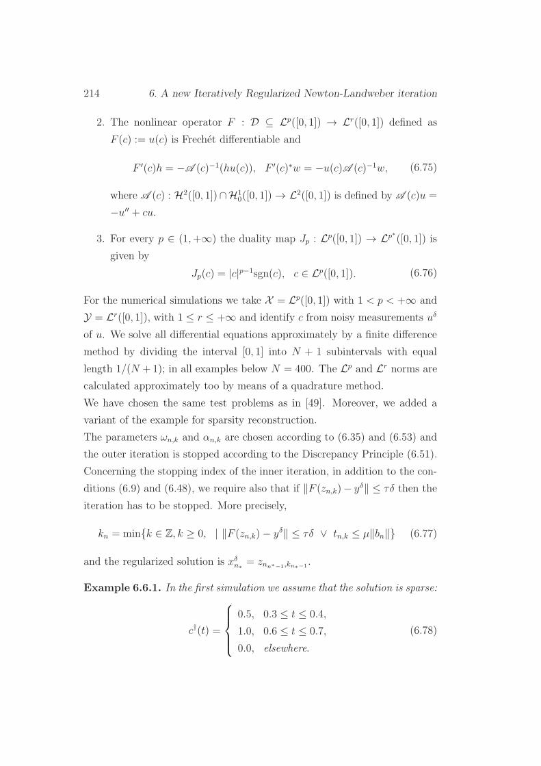
214 6. A new Iteratively Regularized Newton-Landweber iteration
2. The nonlinear operator F : D ⊆ Lp([0, 1]) → Lr([0, 1]) defined as
F (c) := u(c) is Frechet differentiable and
F ′(c)h = −A (c)−1(hu(c)), F ′(c)∗w = −u(c)A (c)−1w, (6.75)
where A (c) : H2([0, 1])∩H10([0, 1]) → L2([0, 1]) is defined by A (c)u =
−u′′ + cu.
3. For every p ∈ (1,+∞) the duality map Jp : Lp([0, 1]) → Lp∗([0, 1]) is
given by
Jp(c) = |c|p−1sgn(c), c ∈ Lp([0, 1]). (6.76)
For the numerical simulations we take X = Lp([0, 1]) with 1 < p < +∞ and
Y = Lr([0, 1]), with 1 ≤ r ≤ +∞ and identify c from noisy measurements uδ
of u. We solve all differential equations approximately by a finite difference
method by dividing the interval [0, 1] into N + 1 subintervals with equal
length 1/(N +1); in all examples below N = 400. The Lp and Lr norms are
calculated approximately too by means of a quadrature method.
We have chosen the same test problems as in [49]. Moreover, we added a
variant of the example for sparsity reconstruction.
The parameters ωn,k and αn,k are chosen according to (6.35) and (6.53) and
the outer iteration is stopped according to the Discrepancy Principle (6.51).
Concerning the stopping index of the inner iteration, in addition to the con-
ditions (6.9) and (6.48), we require also that if ‖F (zn,k)− yδ‖ ≤ τδ then the
iteration has to be stopped. More precisely,
kn = mink ∈ Z, k ≥ 0, | ‖F (zn,k)− yδ‖ ≤ τδ ∨ tn,k ≤ µ‖bn‖ (6.77)
and the regularized solution is xδn∗= znn∗−1,kn∗−1.
Example 6.6.1. In the first simulation we assume that the solution is sparse:
c†(t) =
0.5, 0.3 ≤ t ≤ 0.4,
1.0, 0.6 ≤ t ≤ 0.7,
0.0, elsewhere.
(6.78)
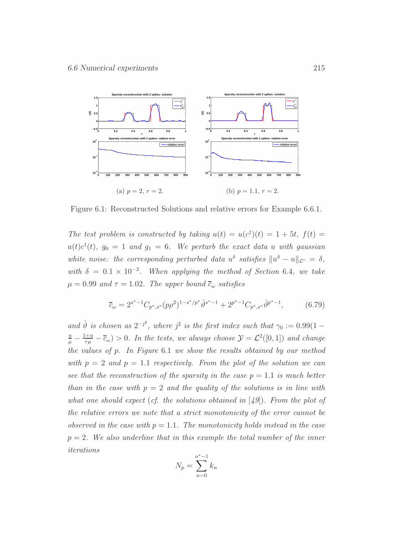
6.6 Numerical experiments 215
0 0.2 0.4 0.6 0.8 1−0.5
0
0.5
1
1.5
t
c(t)
Sparsity reconstruction with 2 spikes: solution
c+
cn*δ
0 100 200 300 400 500 600 700 800 90010
−2
10−1
100
Sparsity reconstruction with 2 spikes: relative error
relative error
(a) p = 2, r = 2.
0 0.2 0.4 0.6 0.8 1−0.5
0
0.5
1
1.5
t
c(t)
Sparsity reconstruction with 2 spikes: solution
c+
cn*δ
0 100 200 300 400 500 600 700 800 90010
−2
10−1
100
Sparsity reconstruction with 2 spikes: relative error
relative error
(b) p = 1.1, r = 2.
Figure 6.1: Reconstructed Solutions and relative errors for Example 6.6.1.
The test problem is constructed by taking u(t) = u(c†)(t) = 1 + 5t, f(t) =
u(t)c†(t), g0 = 1 and g1 = 6. We perturb the exact data u with gaussian
white noise: the corresponding perturbed data uδ satisfies ‖uδ − u‖Lr = δ,
with δ = 0.1 × 10⁻³. When applying the method of Section 6.4, we take
µ = 0.99 and τ = 1.02. The upper bound cω satisfies
cω = 2s∗−1Cp∗,s∗(pρ
2)1−s∗/p∗ϑs∗−1 + 2p
∗−1Cp∗,s∗ϑp∗−1, (6.79)
and ϑ is chosen as 2−j♯, where j♯ is the first index such that γ0 := 0.99(1−ηµ− 1+η
τµ− cω) > 0. In the tests, we always choose Y = L2([0, 1]) and change
the values of p. In Figure 6.1 we show the results obtained by our method
with p = 2 and p = 1.1 respectively. From the plot of the solution we can
see that the reconstruction of the sparsity in the case p = 1.1 is much better
than in the case with p = 2 and the quality of the solutions is in line with
what one should expect (cf. the solutions obtained in [49]). From the plot of
the relative errors we note that a strict monotonicity of the error cannot be
observed in the case with p = 1.1. The monotonicity holds instead in the case
p = 2. We also underline that in this example the total number of the inner
iterations
Np =
n∗−1∑
n=0
kn
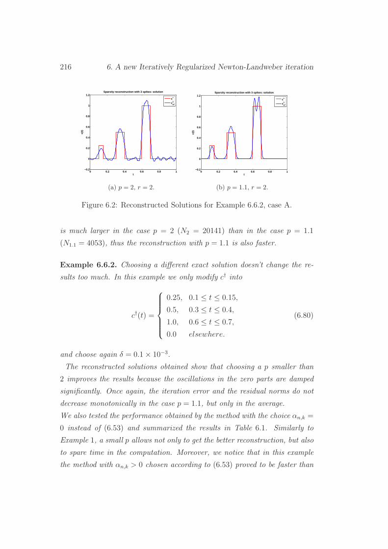
216 6. A new Iteratively Regularized Newton-Landweber iteration
0 0.2 0.4 0.6 0.8 1−0.2
0
0.2
0.4
0.6
0.8
1
1.2
t
c(t)
Sparsity reconstruction with 3 spikes: solution
c+
cn*δ
(a) p = 2, r = 2.
0 0.2 0.4 0.6 0.8 1−0.2
0
0.2
0.4
0.6
0.8
1
1.2
t
c(t)
Sparsity reconstruction with 3 spikes: solution
c+
cn*δ
(b) p = 1.1, r = 2.
Figure 6.2: Reconstructed Solutions for Example 6.6.2, case A.
is much larger in the case p = 2 (N2 = 20141) than in the case p = 1.1
(N1.1 = 4053), thus the reconstruction with p = 1.1 is also faster.
Example 6.6.2. Choosing a different exact solution doesn’t change the re-
sults too much. In this example we only modify c† into
c†(t) =
0.25, 0.1 ≤ t ≤ 0.15,
0.5, 0.3 ≤ t ≤ 0.4,
1.0, 0.6 ≤ t ≤ 0.7,
0.0 elsewhere.
(6.80)
and choose again δ = 0.1× 10⁻³.
The reconstructed solutions obtained show that choosing a p smaller than
2 improves the results because the oscillations in the zero parts are damped
significantly. Once again, the iteration error and the residual norms do not
decrease monotonically in the case p = 1.1, but only in the average.
We also tested the performance obtained by the method with the choice αn,k =
0 instead of (6.53) and summarized the results in Table 6.1. Similarly to
Example 1, a small p allows not only to get the better reconstruction, but also
to spare time in the computation. Moreover, we notice that in this example
the method with αn,k > 0 chosen according to (6.53) proved to be faster than
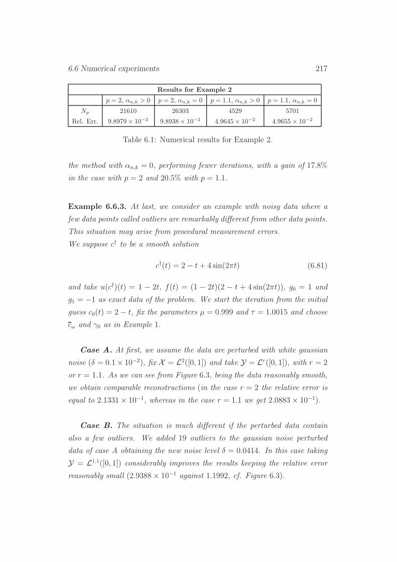
6.6 Numerical experiments 217
Results for Example 2
p = 2, αn,k > 0 p = 2, αn,k = 0 p = 1.1, αn,k > 0 p = 1.1, αn,k = 0
Np 21610 26303 4529 5701
Rel. Err. 9.8979× 10⁻² 9.8938× 10⁻² 4.9645× 10⁻² 4.9655× 10⁻²
Table 6.1: Numerical results for Example 2.
the method with αn,k = 0, performing fewer iterations, with a gain of 17.8%
in the case with p = 2 and 20.5% with p = 1.1.
Example 6.6.3. At last, we consider an example with noisy data where a
few data points called outliers are remarkably different from other data points.
This situation may arise from procedural measurement errors.
We suppose c† to be a smooth solution
c†(t) = 2− t+ 4 sin(2πt) (6.81)
and take u(c†)(t) = 1 − 2t, f(t) = (1 − 2t)(2 − t + 4 sin(2πt)), g0 = 1 and
g1 = −1 as exact data of the problem. We start the iteration from the initial
guess c0(t) = 2− t, fix the parameters µ = 0.999 and τ = 1.0015 and choose
cω and γ0 as in Example 1.
Case A. At first, we assume the data are perturbed with white gaussian
noise (δ = 0.1× 10⁻²), fix X = L2([0, 1]) and take Y = Lr([0, 1]), with r = 2
or r = 1.1. As we can see from Figure 6.3, being the data reasonably smooth,
we obtain comparable reconstructions (in the case r = 2 the relative error is
equal to 2.1331× 10⁻¹, whereas in the case r = 1.1 we get 2.0883× 10⁻¹).
Case B. The situation is much different if the perturbed data contain
also a few outliers. We added 19 outliers to the gaussian noise perturbed
data of case A obtaining the new noise level δ = 0.0414. In this case taking
Y = L1.1([0, 1]) considerably improves the results keeping the relative error
reasonably small (2.9388× 10⁻¹ against 1.1992, cf. Figure 6.3).
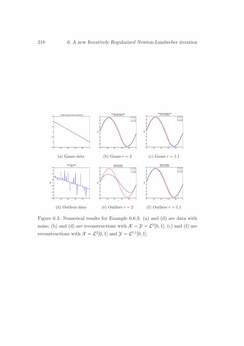
218 6. A new Iteratively Regularized Newton-Landweber iteration
0 0.2 0.4 0.6 0.8 1−1.5
−1
−0.5
0
0.5
1
1.5Example 3 gaussian noise: perturbed data
(a) Gauss data
0 0.2 0.4 0.6 0.8 1−3
−2
−1
0
1
2
3
4
5
6
t
c(t)
Example 3 gaussian data:p=2 r=2 solution
c+
cn*δ
(b) Gauss r = 2
0 0.2 0.4 0.6 0.8 1−3
−2
−1
0
1
2
3
4
5
6
t
c(t)
Example 3 gaussian datap=2 r=1.1 solution
c+
cn*δ
(c) Gauss r = 1.1
0 0.2 0.4 0.6 0.8 1−2.5
−2
−1.5
−1
−0.5
0
0.5
1
1.5
2
2.5
Data with ouliers:plot
t
uδ (t
)
(d) Outliers data
0 0.2 0.4 0.6 0.8 1−3
−2
−1
0
1
2
3
4
5
6
t
c(t)
Data with outliers:p=2 r=2 solution
c+
cn*δ
(e) Outliers r = 2
0 0.2 0.4 0.6 0.8 1−3
−2
−1
0
1
2
3
4
5
6
t
c(t)
Data with outliers:p=2 r=1.1 solution
c+
cn*δ
(f) Outliers r = 1.1
Figure 6.3: Numerical results for Example 6.6.3: (a) and (d) are data with
noise; (b) and (d) are reconstructions with X = Y = L2[0, 1]; (c) and (f) are
reconstructions with X = L2[0, 1] and Y = L1.1[0, 1].
6.7 A new proposal for the choice of the parameters 219
Concerning the total number of iterations N , in this example it is not sub-
jected to remarkable variations.
To summarize, in all examples above the method obtained reasonable
results, proving to be reliable, both in the sparsity reconstruction examples
and when the data are affected with outliers. Concerning the total number
of iterations, the introduction of the parameters αn,k has accelerated the
method in Example 2, but the issue of the speed of the algorithms requires
further investigation.
6.7 A new proposal for the choice of the pa-
rameters
With the parameter choices proposed in Section 6.3, it is rather difficult to
prove strong convergence and convergence rates for the Discrepancy Princi-
ple. Moreover, the numerical experiments show that the method still requires
many iterations to obtain good regularized solutions.
Indeed, the choices that have been made for ωn,k and αn,k seem to make the
method not flexible enough. For this reason, we propose here a different way
to select these parameters. To do this, we return to the estimates of Section
6.2. Using the same notations, we estimate the term d2n,k+1 as in (6.10) and
proceed exactly as in Section 6.2 for estimating the terms (I), (II) and (IV).
For the term (III), if ν = 0 instead of using (6.9), we reconsider the estimate
‖F (zn,k)− F (x†)‖= ‖(An(zn,k − xδn) + F (xδn)− yδ)
+(F (zn,k)− F (xδn)− An((zn,k − xδn) + (yδ − y)‖≤ tn,k + η‖F (zn,k)− F (xδn)‖+ δ
≤ tn,k + η(‖F (zn,k)− F (x†)‖+ ‖F (xδn)− yδ‖) + (1 + η)δ ,
to conclude
‖F (zn,k)− F (x†)‖ ≤ 1
1− η(tn,k + ηrn + (1 + η)δ) . (6.82)
220 6. A new Iteratively Regularized Newton-Landweber iteration
This together with (6.4) implies
|αn,k〈JXp (x† − x0), zn,k − x†〉X ∗×X |
≤ β
(1− η)2ναn,kd
1−2νn,k (tn,k + ηrn + (1 + η)δ)2ν
≤ C(12+ ν)
β
(1− η)2ναn,k
d2n,k + (tn,k + ηrn + (1 + η)δ)
4ν1+2ν
(6.83)
where we have used (6.18) with C(λ) = λλ(1− λ)1−λ.
In the case ν = 0, we simply use (6.21) as in Section 6.2.
Altogether, we obtain
d2n,k+1 ≤
(
1− (1− c0)αn,k
)
d2n,k + c0αn,k + c1α
s∗
n,k + c2αp∗
n,k
+c3αn,k (tn,k + ηrn + (1 + η)δ)4ν
1+2ν
−ωn,ktrn,k + ωn,kt
r−1n,k (ηrn + (1 + η)δ) + ϕ(ωn,ktn,k) , (6.84)
where
c0 =
0 if ν = 0β
(1−η)2νC(1
2+ ν) if ν > 0
(6.85)
c0 =
‖x† − x0‖p−1(pρ2)1p if ν = 0
0 if ν > 0
c1 = Cp∗,s∗(pρ2)1−
s∗
p∗ ρ(p−1)s∗2s∗−1 (6.86)
c2 = Cp∗,s∗ ρp2p
∗−1 (6.87)
c3 =
c0 in case (a) ν, θ > 0
‖x† − x0‖p−1(pρ2)1p in case (b) ν, θ = 0
(6.88)
θ =4ν
r(1 + 2ν)− 4ν. (6.89)
Multiplying (6.84) with α−θn,k+1 and abbreviating
γn,k := d2n,kα
−θn,k ,
6.7 A new proposal for the choice of the parameters 221
we get
γn,k+1 − γn,k ≤(
αn,k
αn,k+1
)θ (
1− (1− c0)αn,k −(αn,k+1
αn,k
)θ)
γn,k
+(c0α1−θn,k + c1α
s∗−θn,k + c2α
p∗−θn,k + c3α
1−θn,k (tn,k + ηrn + (1 + η)δ)
4ν1+2ν
−α−θn,k
(ωn,kt
rn,k − ωn,kt
r−1n,k (ηrn + (1 + η)δ)− ϕ(ωn,ktn,k)
)
.
To obtain monotone decay of the sequence γn,k with increasing k we
choose
• ωn,k ≥ 0 such that
ω ≤ ωn,k ≤ ω andϕ(
ωn,ktn,k
)
ωn,ktrn,k
≤ cω (6.90)
for some 0 < ω < ω, cω > 0. We will do so by setting
ωn,k = ϑmintr
s∗−1
n,k t−sn,k , t
rp∗−1
n,k t−pn,k , ω (6.91)
with ϑ sufficiently small, and assuming that
r ≥ s ≥ p , (6.92)
• αn,k ≥ 0 such that
αn,k ≥ αn,k := τ (tn,k + ηrn + (1 + η)δ)r
1+θ (6.93)
and
c0+c0γ0,0
+c1γ0,0
αs∗−θ−1n,k +
c2γ0,0
αp∗−θ−1n,k +
c3τ θγ0,0
+1
τ 1+θγ0,0≤ q < 1 (6.94)
(note that in case θ = 0 we have c0 = 0 and vice versa, in case θ > 0
we have c0 = 0). The latter can be achieved by
αn,k ≤ 1 and (6.95)
s∗ ≥ θ + 1 , p∗ ≥ θ + 1 , (6.96)
c0, c0, c1, c2, c3, τ1 sufficiently small.
222 6. A new Iteratively Regularized Newton-Landweber iteration
In case (a) we additionally require
αn,k+1 ≥ αn,k+1 := αn,k
(
1− (1− q)αn,k
)1/θ
(6.97)
with an upper bound γ0,0 for γ0,0. Note that this just means αn,k+1 ≥ 0
in case (b) corresponding to ν = 0, i.e., θ = 0, thus an empty condition
in case (b).
To meet conditions (6.93), (6.97) with a minimal αn,k+1 we set
αn,k+1 = maxαn,k+1 , αn,k+1 for k ≥ 0 (6.98)
αn,0 =
αn−1,kn−1 if n ≥ 1
α0,0 if n = 0.
It remains to choose
• the inner stopping index kn
• the outer stopping index n∗,
see below.
Indeed with these choices of ωn,k and αn,k+1 we can inductively conclude from
(6.90) that
γn,k+1 − γn,k ≤(
αn,k
αn,k+1
)θ (
1− (1− q)αn,k −(αn,k+1
αn,k
)θ)
γ0,0
−α−θn,k+1(1− cω)ωn,kt
rn,k ,
≤ −α−θn,k+1(1− cω)ωn,kt
rn,k ≤ 0 . (6.99)
This monotonicity result holds for all n ∈ IN and for all k ∈ IN.
By (6.99) and αn,k ≤ 1 (cf. (6.95)) it can be shown inductively that all
iterates remain in BD
ρ (x†) provided
γ0,0 ≤ ρ2 . (6.100)
Moreover, (6.99) implies that
∞∑
n=0
∞∑
k=0
α−θn,k+1ωn,kt
rn,k ≤
γ0,01− cω
<∞, (6.101)

6.7 A new proposal for the choice of the parameters 223
hence by αn,k+1 ≤ 1, ωn,k ≥ ω
tn,k → 0 as k → ∞ for all n ∈ IN (6.102)
and
supk∈IN0
tn,k → 0 as n→ ∞ . (6.103)
Especially, since tn,0 = rn,
rn → 0 as n→ ∞ . (6.104)
To quantify the behavior of the sequence αn,k according to (6.93), (6.97),
(6.98) for fixed n we distinguish between two cases.
(i) There exists a k such that for all k ≥ k we have αn,k = αn,k. Con-
sidering an arbitrary accumulation point αn of αn,k (which exists since
0 ≤ αn,k ≤ 1) we therefore have αn = αn
(
1 − (1 − q)αn
) 1θ, hence
αn = 0.
(ii) Consider the situation that (i) does not hold, i.e., there exists a sub-
sequence kj such that for all j ∈ IN we have αn,kj = αn,kj . Then by
(6.93), (6.97), and (6.102) we have αn,kj → τ (ηrn + (1 + η)δ)r
1+θ .
Altogether we have shown that
lim supk→∞
αn,kj ≤ τ (ηrn + (1 + η)δ)r
1+θ for all n ∈ IN. (6.105)
Since η and δ can be assumed to be sufficiently small, this especially implies
the bound αn,k ≤ 1 in (6.95).
We consider zn∗,kn∗∗
as our regularized solution, where n∗, kn∗∗ (and also
kn for all n ≤ n∗ − 1; note that kn∗∗ is to be distinguished from kn∗ - actually
the latter is not defined, since we only define kn for n ≤ n∗ − 1!) are still to
be chosen appropriately, according to the requirements from the proofs of
• convergence rates in case ν, θ > 0,
• convergence for exact data δ = 0,
• convergence for noisy data as δ → 0.
224 6. A new Iteratively Regularized Newton-Landweber iteration
6.7.1 Convergence rates in case ν > 0
From (6.99) we get
d2n,k ≤ γ0,0α
θn,k for all n, k ∈ IN , (6.106)
hence in order to get the desired rate
d2n∗,k
n∗∗
= O(δrθ1+θ )
in view of (6.105) (which is a sharp bound in case (ii) above) we need to have
a bound
rn∗ ≤ τδ (6.107)
for some constant τ > 0, and we should choose kn∗∗ large enough so that
αn∗,kn∗∗
≤ Cα(rn∗+ δ)
r1+θ (6.108)
which is possible with a finite kn∗∗ by (6.105) for Cα > (τ(1 + η))
r1+θ . Note
that this holds without any requirements on kn.
6.7.2 Convergence as n → ∞ for exact data δ = 0
To show that (xn)n∈IN is a Cauchy sequence (following the seminal paper
[30]), for arbitrary m < j, we choose the index l ∈ m, . . . , j such that rl is
minimal and use the identity
Dx0p (xl, xm) = Dx0
p (x†, xm)−Dx0p (x†, xl)
+〈JXp (xl − x0)− JX
p (xm − x0), xl − x†〉X ∗×X (6.109)
and the fact that the monotone decrease and boundedness from below of the
sequence Dx0p (x†, xm) implies its convergence, hence it suffices to prove that
the last term in (6.109) tends to zero as m < l → ∞ (analogously it can
be shown that Dx0p (xl, xj) tends to zero as l < j → ∞). This term can be
rewritten as
〈JXp (xl − x0)− JX
p (xm − x0), xl − x†〉X ∗×X
=
l−1∑
n=m
kn−1∑
k=0
〈un,k+1 − un,k, xl − x†〉X ∗×X ,
6.7 A new proposal for the choice of the parameters 225
where
|〈un,k+1 − un,k, xl − x†〉X ∗×X |= |αn,k〈JX
p (zn,k − x0), xl − x†〉X ∗×X
+ωn,k〈jYr (An(zn,k − xδn)− bn), An(xl − x†)〉X ∗×X |≤ 2ρpαn,k + ωn,kt
r−1n,k ‖An(xl − x†)‖
≤ 2ρpτ (tn,k + ηrn)r + ωn,kt
r−1n,k (1 + η)(2rn + rl)
≤ 2ρpτ (tn,k + ηrn)r + 3(1 + η)ωn,kt
r−1n,k rn
by our choice of αn,k = αn,k (note that αn,k = 0 in case θ = 0), condition
(6.7) and the minimality of rl.
Thus we have by ωn,k ≤ ω and Young’s inequality that there exists C > 0
such that
〈JXp (xl − x0)− JX
p (xm − x0), xl − x†〉X ∗×X ≤ Cl−1∑
n=m
(kn−1∑
k=0
trn,k
)
+ knrrn
)
for which we can conclude convergence as m, l → ∞ from (6.101) provided
that∞∑
n=m
knrrn → 0 as m→ ∞ ,
which we guarantee by choosing, for an a priori fixed summable sequence
(an)n∈IN,
kn := anr−rn . (6.110)
6.7.3 Convergence with noisy data as δ → 0
In case (a) ν, θ > 0 convergence follows from the convergence rates results in
Subsection 6.7.1. Therefore it only remains to show convergence as δ → 0 in
case θ = 0.
In this section we explicitly emphasize dependence of the computed quan-
tities on the noisy data and on the noise level by a superscript δ.
226 6. A new Iteratively Regularized Newton-Landweber iteration
Let ‖yδj − y‖ ≤ δj with δj a zero sequence and n∗j the corresponding
stopping index. As usual [30] we distinguish between the two cases that (i)
n∗j has a finite accumulation point and (ii) n∗j tends to infinity.
(i) There exists an N ∈ IN and a subsequence nji such that for all i ∈ IN
we have nji = N . Provided
n∗(δ) = N for all δ ⇒ The mapping δ 7→ xδN is continuous at δ = 0 ,
(6.111)
we can conclude that xδjiN → x0N as i → ∞, and by taking the limit as
i → ∞ also in (6.107), x0N is a solution to (5.17). Thus we may set
x† = x0N in (6.99) (with θ = 0) to obtain
Dx0p (x0N , z
δji
n∗ji,k
n∗ji∗ji
) = Dx0p (x0N , z
δji
N,kn∗ji∗ji
) ≤ Dx0p (x0N , x
δjiN ) → 0 as i→ ∞
where we have again used the continuous dependence (6.111) in the
last step.
(ii) Let n∗j → ∞ as j → ∞, and let x† be a solution to (5.17). For
arbitrary ǫ > 0, by convergence for δ = 0 (see the previous subsection)
we can find n such that Dx0p (x†, x0n) <
ǫ2and, by Theorem 2.60 (d) in
[82] there exists j0 such that for all j ≥ j0 we have n∗,j ≥ n + 1 and
|Dx0p (x†, x
δjn )−Dx0
p (x†, x0n)| < ǫ2, provided
n ≤ n∗(δ)−1 for all δ ⇒ The mapping δ 7→ xδn is continuous at δ = 0 .
(6.112)
Hence, by monotonicity of the errors we have
Dx0p (x†, z
δj
n∗j ,kn∗j∗j
) ≤ Dx0p (x†, xδjn )
≤ Dx0p (x†, x0n) + |Dx0
p (x†, xδjn )−Dx0p (x†, x0n)| < ǫ .
(6.113)
Indeed, (6.111), (6.112) can be concluded from continuity of F , F ′, the defi-
nition of the method (6.3), as well as stable dependence of all parameters
ωn,k, αn,k, kn according to (6.91), (6.93), (6.97), (6.98), (6.110) on the data
yδ.
Altogether we have derived the following algorithm.
6.7 A new proposal for the choice of the parameters 227
6.7.4 Newton-Iteratively Regularized Landweber algo-
rithm
Choose τ, τ , Cα sufficiently large, x0 sufficiently close to x†,
α00 ≤ 1, ω > 0, (an)n∈IN0 such that∑∞
n=0 an <∞.
If (6.4) with ν ∈ (0, 1] holds, set θ = 4νr(1+2ν)−4ν
, otherwise θ = 0.
For n = 0, 1, 2 . . . until rn ≤ τδ do
un,0 = 0
zn,0 = xδn
αn,0 = αn−1,kn−1 if n > 0
For k = 0, 1, 2 . . . until
k = kn − 1 = anr−rn if rn > τδ
αn∗,kn∗∗
≤ Cα(rn∗+ δ)
r1+θ if rn ≤ τδ
do
ωn,k = ϑmintr
s∗−1
n,k t−sn,k , t
rp∗−1
n,k t−pn,k , ω
un,k+1 = un,k − αn,kJXp (zn,k − x0)
−ωn,kF′(xδn)
∗jYr (F′(xδn)(zn,k − xδn) + F (xδn)− yδ)
JXp (zn,k+1 − x0) = JX
p (xδn − x0) + un,k+1
αn,k+1 = maxαn,k+1 , αn,k+1 with αn,k+1 , αn,k+1 as in (6.93), (6.97)
xδn+1 = zn,kn .
Note that we here deal with an a priori parameter choice: θ and therefore
ν has to be known, otherwise θ must be set to zero.
The analysis above yields the following convergence result.
Theorem 6.7.1. Assume that X is smooth and s-convex with s ≥ p, that
x0 is sufficiently close to x†, i.e., x0 ∈ BD
ρ (x†), that F satisfies (6.7) with
(6.6), that F and F ′ are continuous and uniformly bounded in BD
ρ (x†), and
that (6.92), (6.96) hold.
Then, the iterates zn,k defined by Algorithm 6.7.4 remain in BDρ (x
†) and con-
verge to a solution x† of (5.17) subsequentially as δ → 0 (i.e., there exists
a convergent subsequence and the limit of every convergent subsequence is a
solution).
In case of exact data δ = 0, we have subsequential convergence of xn to a so-
lution of (5.17) as n→ ∞. If additionally a variational inequality (6.4) with
228 6. A new Iteratively Regularized Newton-Landweber iteration
ν ∈ (0, 1] and β sufficiently small is satisfied, we obtain optimal convergence
rates
Dx0p (x†, zn∗,k
n∗∗) = O(δ
4ν2ν+1 ) , as δ → 0 . (6.114)
Conclusions
In this short conclusive chapter, we point out the main contributions of the
thesis in the area of the regularization of ill-posed problems and present some
possible further developments of this work.
The three stopping rules for the Conjugate Gradient method applied to
the Normal Equation presented in Chapter 3 produced very promising nu-
merical results in the numerical experiments. In particular, SR2 provided an
important insight into the regularizing properties of this method, connecting
the well-known theoretical estimates of Chapter 2 with the properties of the
Truncated Singular Value Decomposition method.
In the numerical experiments presented in Chapter 4, the new stopping
rules defined in Chapter 3 also produced very good numerical results. Of
course, these results can be considered only the starting point of a possible
future work. Some further developments can be the following:
• applications of the new stopping rules in combination with more so-
phisticated regularization methods that make use of CGNE (e.g., the
Restarted Projected CGNE described in Chapter 3);
• extension of the underlying ideas of the new stopping rules to other
regularization methods (e.g., SART, Kaczmarz,...);
• analysis of the speed of the algorithms presented for computing the
indices of the new stopping rules, to get improvements.
The theoretical results of Chapter 6, and in particular of Section 6.7, en-
hanced the regularization theory of Banach spaces. However, they have to
229
230 Conclusions
be tested in more serious practical examples. We believe that the new ways
to arrest the iteration can indeed improve the performances significantly.
Besides the repetition of the numerical tests of Section 6.6, also two di-
mensional examples should be considered, as well as a comparison of the
inner-outer Newton-Landweber iteration proposed here with the classical Ite-
ratively regularized Gauss-Newton method.
Possible extensions to the case of non-reflexive Banach spaces and further
simulations in different ill-posed problems should also be a subject of future
research.
Appendix A
Spectral theory in Hilbert
spaces
We recall briefly some fundamental results of functional calculus for self-
adjoint operators in Hilbert spaces. Details and proofs can be found, e.g. in
[2], [17] and [44].
Throughout this section, X will always denote a Hilbert space. The scalar
product in X will be denoted by 〈·, ·〉X and the norm induced by this scalar
product will be denoted by ‖ · ‖X .
Definition A.0.1 (Spectral family). A family Eλλ∈R of orthogonal pro-
jectors in X is called a spectral family or resolution of the identity if it satisfies
the following conditions:
(i) EλEµ = Eminλ,µ, λ, µ ∈ R;
(ii) E−∞ = 0, E+∞ = I, where E±∞x := limλ→±∞ Eλx, ∀ x ∈ X , and where
I is the identity map on X .
(iii) Eλ−0 = Eλ, where Eλ−0x := limǫ→0+ Eλ−ǫx, ∀ x ∈ X .
Proposition A.0.1. Let f : R → R be a continuous function. Then the
limit of the Riemann sumn∑
i=1
f(ξi)(Eλi
− Eλi−1
)x
231

232 A. Spectral theory in Hilbert spaces
exists in X for |λi − λi−1| → 0, where −∞ < a = λ0 < ... < λn = b < +∞,
ξi ∈ (λi−1, λi], and is denoted by
∫ b
a
f(λ)dEλx.
Definition A.0.2. For any given x ∈ X and any continuous function f :
R → R, the integral∫ +∞−∞ f(λ)dEλx is defined as the limit, if it exists, of
∫ b
af(λ)dEλx when a → −∞ and b → +∞.
Since condition (i) in the definition of the spectral family is equivalent to
〈Eλx, x〉 ≤ 〈Eµx, x〉, for all x ∈ Xandλ ≤ µ,
the function λ 7→ 〈Eλx, x〉 = ‖Eλx‖2 is monotonically increasing and due to
the condition (ii) in the definition of the spectral family also continuous from
the left. Hence it defines a measure on R, denoted by d‖Eλx‖2. Then the
following connection holds:
Proposition A.0.2. For any given x ∈ X and any continuous function f :
R → R:
∫ +∞
−∞f(λ)dEλx exists ⇐⇒
∫ +∞
−∞f 2(λ)d‖Eλx‖2 < +∞.
Proposition A.0.3. Let A be a self-adjoint operator in X . Then there
exist a unique spectral family Eλλ∈R, called spectral decomposition of A or
spectral family of A, such that
D(A) = x ∈ X |∫ +∞
−∞λ2d‖Eλx‖2 < +∞
and
Ax =
∫ +∞
−∞λdEλx, x ∈ D(A).
We write:
A =
∫ +∞
−∞λdEλ.
233
Definition A.0.3. Let A be a self-adjoint operator in X with spectral family
Eλλ∈R and let f be a measurable function on R with respect to the measure
d‖Eλx‖2 for all x ∈ X . Then f(A) is the operator defined by the formula
f(A)x =
∫ +∞
−∞f(λ)dEλx, x ∈ D(f(A)),
where
D(f(A)) = x ∈ X |∫ +∞
−∞f 2(λ)d‖Eλx‖2 < +∞.
Proposition A.0.4. Let M0 be the set of all measurable functions on R
with respect to the measure d‖Eλx‖2 for all x ∈ X (in particular, piecewise
continuous functions lie in M0). Let A be a self-adjoint operator in X with
spectral family Eλλ∈R and let f , g ∈ M0.
(i) If x ∈ D(f(A)) and z ∈ D(g(A)), then
〈f(A)x, g(A)z〉 =∫ +∞
−∞f(λ)g(λ)d〈Eλx, z〉.
(ii) If x ∈ D(f(A)), then f(A)x ∈ D(g(A)) if and only if x ∈ D((gf)(A)).
Furthermore,
g(A)f(A)x = (gf)(A)x.
(iii) If D(f(A)) is dense in X , then f(A) is self-adjoint.
(iv) f(A) commutes with Eλ for all λ ∈ R.
Proposition A.0.5. Let A be a self-adjoint operator in X with spectral fam-
ily Eλλ∈R.
(i) λ0 lies in the spectrum of A if and only if Eλ0 6= Eλ0+ǫ for all ǫ > 0.
(ii) λ0 is an eigenvalue of A if and only if Eλ0 6= Eλ0+0 = limǫ→0 Eλ0+ǫ. The
corresponding eigenspace is given by (Eλ0+0 − Eλ0)(X ).

234 A. Spectral theory in Hilbert spaces
At last, we observe that if A is a linear bounded operator, then the
operator A∗A is a linear, bounded, self-adjoint and semi-positive definite
operator. Let Eλ be the spectral family of A∗A and let M be the set of
all measurable functions on R with respect to the measure d‖Eλx‖2 for all x∈ X . Then, for all f ∈ M,
∫ +∞
−∞f(λ)dEλx =
∫ ‖A‖2
0
f(λ)dEλx = limǫ→0+
∫ ‖A‖2+ǫ
0
f(λ)dEλx.
Hence, the function f can be restricted to the interval [0, ‖A‖2 + ǫ] for some
ǫ > 0.

Appendix B
Approximation of a finite set of
data with cubic B-splines
B.1 B-splines
Let [a, b] be a compact interval of R, let
∆ = a = t0 < t1 < ... < tk < tk+1 = b (B.1)
be a partition of [a, b] and let m be an integer, m > 1. Then the space
Sm(∆) of polynomial splines with simple knots of order m on ∆ is the space
of all function s = s(t) for which there exist k+1 polynomials s0, s1, ..., sk of
degree ≤ m− 1 such that
(i) s(t) = sj(t) for tj ≤ t ≤ tj+1, j = 0, ..., k;
(ii) di
dtisj−1(tj) =
di
dtisj(tj), for i = 0, ..., m− 2, j = 1, ..., k.
The points tj are called the knots of the spline and t1, ..., tk are the inner
knots.
It is well known (cf. e.g. [86]) that Sm(∆) is a vector space of dimension
m+k. A base of Sm(∆) with good computational properties is given by the
normalized B-splines.
An extended partition of [a, b] associated to Sm(∆) is a sequence of points
235
236 B. Approximation of a finite set of data with cubic B-splines
∆∗ = t−m+1 ≤ ... ≤ tk+m such that ti = ti for every i = 0, ..., k + 1. There
are different possible choices of the extended partition ∆∗. Here, we shall
consider the choice
t−m+1 = ... = t0 = a, tk+1 = tk+2 = ... = tk+m. (B.2)
The normalized B-splines on ∆∗ are the functions Nj,mj=−m+1,...,k defined
recursively in the following way:
Nj,1(t) =
1, for tj ≤ t ≤ tj+1,
0, elsewhere;(B.3)
Nj,h(t) =
t−tj
tj+h−1−tjNj,h−1(t) +
tj−t
tj+h−tj+1Nj+1,h−1(t), for tj 6= tj+h,
0, elsewhere
(B.4)
for h = 2, ..., m. The cases 0/0 must be interpreted as 0.
The functions Nj,h have the following well known properties:
(1) Local support: Nj,m(t) = 0, ∀ t /∈ [tj , tj+m) if tj < tj+m;
(2) Non negativity: Nj,m(t) > 0, ∀ t ∈ (tj , tj+m), tj < tj+m;
(3) Partition of unity:∑k
j=−m+1 Nj,m(t) = 1, ∀ t ∈ [a, b].
B.2 Data approximation
Let now (λ1, µ1), ..., (λn, µn), n ∈ N, n ≥ m+ k, λj and µj ∈ R such that
a = λ1 < ... < λn = b (B.5)
be a given set of data. We want to find a spline s(t) ∈ Sm(∆),
s(t) =k∑
j=−m+1
cjNj,m(t),
that minimizes the least-squares functional
n∑
l=1
|s(λl)− µl|2 (B.6)

B.2 Data approximation 237
on Sm(∆). Simple calculations show that the solutions of this minimization
problem are the solutions of the overdetermined linear system
k∑
j=−m+1
cj
n∑
l=1
Ni,m(λl)Nj,m(λl) =
n∑
l=1
µlNi,m(λl), i = −m+ 1, ..., k. (B.7)
Denoting with H the matrix of the normalized B-splines on the approxima-
tion points:
H = hl,j = Nj,m(λl), l = 1, ..., n; j = −m+ 1, ..., k, (B.8)
we can rewrite (B.7) in the form
H∗Hc = H∗µ, (B.9)
where c and µ are the column vectors of the cj and of the µl respectively.
It can be shown that the system has a unique solution if ∆∗ satisfies the so
called Schonberg-Whitney conditions :
Theorem B.2.1. The matrix H has maximal rank if there exists a sequence
of indices 1 ≤ j1 ≤ ... ≤ jm+k ≤ n such that
ti < λji < ti+m, i = −m+ 1, ..., k, (B.10)
where the ti are the knots of the extended partition ∆∗.
With equidistant inner knots ti = a + i (b−a)k+1
and the particular choice
(B.2), it is easy to see that the Schonberg-Whitney conditions are satisfied
for every k ≤ n−m: for example, if k = n−m, ji = i for every i = 1, ..., n.
238 B. Approximation of a finite set of data with cubic B-splines
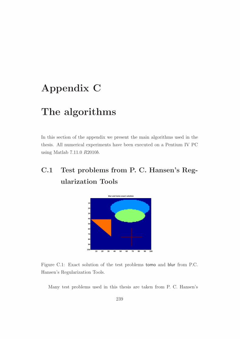
Appendix C
The algorithms
In this section of the appendix we present the main algorithms used in the
thesis. All numerical experiments have been executed on a Pentium IV PC
using Matlab 7.11.0 R2010b.
C.1 Test problems from P. C. Hansen’s Reg-
ularization Tools
blur and tomo exact solution
10 20 30 40 50 60 70 80 90 100
10
20
30
40
50
60
70
80
90
100
Figure C.1: Exact solution of the test problems tomo and blur from P.C.
Hansen’s Regularization Tools.
Many test problems used in this thesis are taken from P. C. Hansen’s
239
240 C. The algorithms
Regularization Tools. This is a software package that consists of a collection
of documented Matlab functions for analysis and solution of discrete ill-posed
problems. The package and the underlying theory is published in [35] and the
most recent version of the package, which is updated regularly, is described
in [41]. The package can be downloaded directly from the page
http : //www2.imm.dtu.dk/ pch/Regutools/, (C.1)
where a complete manual is also available.
All the algorithms of the thesis referring to [35] or [41] are taken from the
version 4.1 (for Matlab version 7.3). Below, we describe briefly the files that
have been used in the thesis.
More details on these functions such as the synopsis, the input and output
arguments, the underlying integral equation and the references can be found
in the manual of the Regularization Tools [35] in a pdf format at the web
page (C.1).
We consider 10 different very famous test problems:
• baart, deriv2, foxgood, gravity, heat, i−laplace, phillips, shaw generate the
square matrix A, the exact solution x and the exact right-hand side b
of a discrete ill-posed problem, typically arising from a discretization of
an integral equation of the first kind. The dimension N of the problem
is the main input argument of these functions. In some cases it is
possible to choose between 2 or 3 different exact solutions. Of course,
A is always very ill-conditioned, but in some problems the eigenvalues
decrease more quickly than in others.
• blur and tomo generate the square matrix A, the exact solution f and
the exact right-hand side g a 2D image reconstruction problem. In
both cases, the vector f is a columnwise stacked version of a simple
test image (cf. Figure C.1) with J ×J pixels and J is the fundamental
input argument of the function. In the blur problem, the matrix A is
a symmetric J2 × J2 doubly Toeplitz matrix, stored in sparse format
associated to an atmospheric turbulence blur and g := Af is the blurred
C.2 Conjugate gradient type methods algorithms 241
image. By modifying the third input argument of the function which
is set by default equal to 0.7, it is possible to control the shape of the
Gaussian point spread function associated to A. In the tomo problem,
the matrix A arises from the discretization of a simple 2D tomography
model. If no additional input arguments are used, A is a square matrix
of dimension J2 × J2 as in the case of blur.
C.2 Conjugate gradient type methods algo-
rithms
Two different functions for the implementation of CGNE can be found in
the Regularization tools: cgls and lsqr−b. cgls is a direct implementation of
algorithm 3, lsqr−b is an equivalent implementation of the same algorithm
based on Lanczos bidiagonalization (cf. [73] and [36]).
Both routines require the matrix of the system A, a data vector b and an
integer kMAX corresponding to the number of CGNE steps to be performed
and return all kMAX solutions, stored as columns of the matrix X. The
corresponding solution norms and residual norms are returned in η and ρ,
respectively. If the additional parameter reorth is set equal to 1, then the
routines perform a reorthogonalization of the normal equation residual vec-
tors.
To compare CGNE and CGME, a new routine cgne−cgme has been gene-
rated based on Algorithm 6. This function is similar to cgls and lsqr−b, but
returns also the solutions, the residual norms and the solution norms of the
CGME iterates.
A modified version of cgls, cgls−deb has been used for the image deblur-
ring problems to avoid forming the matrix A. In the cgls−deb algorithm,
the matrix A is replaced by the PSF, the data vector g is replaced by its
corresponding image and all matrix-vectors multiplications are replaced by
the corresponding 2D convolutions as in Section 3.6, formula (3.41). As a
242 C. The algorithms
consequence, the synopsis of this function is different from the others:
[f, rho, eta] = cgls−deb(h, g, k); (C.2)
here the input arguments are the matrices of the PSF h and of the blurred
image g and the number of iterations kMAX . The output is a 3D matrix f
such that for every k = 1, ..., kMAX the Matlab command
f(:, :, k)
gives the k-th iterate of the algorithm in the form of an image.
At last, a new routine cgn2 similar to cgls and lsqr−b has been created to
implement the conjugate gradient type method with parameter n = 2 (cf.
Algorithm 7 from Chapter 2).
We emphasize that in the tests where a visualization of the reconstructed
solutions was not necessary, all these functions were used without generating
the matrix of the reconstructed solutions, but instead overwriting at each
step the new iterate of CGNE on the old one, in order to spare memory and
time.
C.3 The routine data−approx
In the notations of Appendix B, the routine data−approx generates an approx-
imation (λ1, µ1), ..., (λn, µn) of the data set (λ1, µ1), ..., (λn, µn) accordingto the following scheme (valid for n ≥ 5):
Step 1: Fix m = 4 and the number of inner knots k according to the dimension
of the problem: if n ≤ 5000 then k = ⌊n/4⌋, if n > 5000 then k =
⌊n/50⌋. Construct the partition ∆ = t0 < t1 < ... < tk < tk+1 such
that t0 = λ1, tk+1 = λn and ti = λ1 + iλn−λ1
k+1, then choose the extended
partition ∆∗ according to (B.2).
Step 2: Construct the matrix H of the normalized B-splines of order m on the
approximation points λ1, ..., λn relative to the extended partition ∆∗
according to (B.3), (B.4) and (B.8).
C.4 The routine mod−min−max 243
Step 3: Find the unique solution c of the linear system (B.9).
Step 4: Evaluate the spline s(t) =∑k
i=−m+1 ciNi,m(t) on the approximation
points λj denoting with µj = s(λj) the corresponding results.
C.4 The routine mod−min−max
This section describes the Matlab function implemented for the computation
of the index p that divides the vector of the SVD (Fourier) coefficients |u∗ib
δ|,i = 1, ..., m, associated to the (perturbed) linear system Ax = bδ, into a
vector of low frequency components, constituted by its first p entries and a
vector of high frequency components, constituted by its last m− p entries.
The routine, denoted with the name mod−min−max, is a variation of the
Min−Max Rule proposed in [101] and requires the singular values λ1, ..., λN
of A.
Suppose for simplicity m = N and let ϕi denote the ratios |u∗ib
δ|/λi for
i = 1, ..., N . Separate the set Ψ = ϕ1, ..., ϕN into 2 sets
Ψ1 := ϕi | ϕi > λi Ψ2 := ϕi | ϕi ≤ λi (C.3)
and let N1 and N2 be the number of elements in Ψ1 and Ψ2 respectively.
Then:
(i) If N2 = 0 or λN < 10−13, calculate an approximation Ψ of Ψ by means
of cubic B-splines with the routine data−approx of the Section C.3 of
the Appendix and choose p as the index corresponding to the minimal
value in Ψ.
(ii) Otherwise, consider the first of the last 5 elements in Ψ2 such that ϕij+1
/∈ Ψ2 and choose p as the corresponding index.
When the smallest singular value is close to the machine epsilon or the set
Ψ2 is empty, then Ψ can be used to determine the regularization index. In
this case the data noise is assumed to be predominant with respect to the

244 C. The algorithms
model errors, so the minimum of the sequence ϕi should correspond to the
index ibδ . Moreover, the data approximation is used to avoid the presence
of possible outliers. A typical case is shown in Figure 3.5 with the shaw test
problem.
In the second case of the modified Min−Max Rule the model errors are pre-
dominant and the greatest indices in Ψ2 are included in the TSVD provided
that they are contiguous (i.e. the successive element does not belong to Ψ1).
This situation is shown in the picture on the right of Figure 3.5 obtained
with the phillips test problem.
C.5 Data and files for image deblurring
The experiments on image deblurring performed in Section 3.6 make use of
the following files.
• The file psfgauss is taken the HNO Functions, a small Matlab package
that implements the image deblurring algorithms presented in [38]. The
package is available at the web page
http : //www2.imm.dtu.dk/ pch/HNO/.
For a given integer J and a fixed number stdev, representing the devi-
ations of the Gaussian along the vertical and horizontal directions, the
Matlab command
[h, center] = psfGauss(J, stdev); (C.4)
generates the PSF matrix h of dimension J × J and the center of the
PSF.
• The file im−blurring generates a test problem for image deblurring. A
gray-scale image is read with the Matlab function im−read. Then a
Gaussian PSF is generated by means of the function psfgauss and the
image is blurred according to the forumla (3.41) from Section 3.6. At
C.6 Data and files for the tomographic problems 245
last, Gaussian white noise is added to the blurred image to obtain the
perturbed data of the problem.
• The function fou−coeff plots the Fourier coefficients of an image de-
blurring test problem. Given the (perturbed) image g and the PSF h,
it returns the Fourier coefficients, the singular values of the BCCB ma-
trix A corresponding to h and the index p computed by the function
mod−min−max of Section C.4 of the Appendix.
C.6 Data and files for the tomographic prob-
lems
The numerical experiments on the tomographic problems described in Sec-
tion 4.6 make use of the files paralleltomo, fanbeamtomo and seismictomo from
P.C. Hansen’s Air Tools. This is a Matlab software package for tomographic
reconstruction (and other imaging problems) consisting of a number of alge-
braic iterative reconstruction methods. The package, described in the paper
[40], can be downloaded at the web page
http : //www2.imm.dtu.dk/ pcha/AIRtools/.
For a fixed integer J > 0, the Matlab command
[A, g, f] = paralleltomo(J) (C.5)
generates the exact solution f , the matrix A and the exact data g = Af of a
two dimensional tomographic test problem with parallel X-rays. The input
argument J is the size of the exact solution f of the system. Therefore, the
matrix A has N := J2 columns. The number of rows of A is given by the
number of total rays for each angle l0 multiplied by the number of angles j0.
Consequently, the sinogram G corresponding to the exact data g is a matrix
with l0 rows and j0 columns.
The functions fanbeamtomo and seismictomo generate the test problem in
246 C. The algorithms
a similar way. We emphasize that for each problem the dimensions of the
sinogram are different. If these values are not specified, they are set by
default. In particular:
• paralleltomo: l0 = round(√2J), j0 = 180;
• fanbeamtomo: l0 = round(√2J), j0 = 360;
• seismictomo: l0 = 2J, j0 = J .
Appendix D
CGNE and rounding errors
In literature, there are a number of mathematically equivalent implementa-
tions of CGNE and of the other methods discussed above. Many authors
suggest LSQR (cf. [73] and [36]), which is an equivalent implementation of
CGNE based on Lanczos bidiagonalization.
The principal problem with any of these methods is the loss of orthogonality
in the residuals due to finite precision arithmetic. The orthogonality can
be maintained by reorthogonalization techniques that are significantly more
expensive and require a larger number of intermediate vectors (cf. e.g., [18]).
In the literature the influence of round-off errors on conjugate gradient type
methods has been studied mainly for well-posed problems.
In [27] Hanke comments on the ill-posed case that the reorthogonalization
techniques did not improve the optimal accuracy in the case he considered.
Our numerical experiments confirm that the sequence of the relative errors
‖x† − zδk‖ does not change significantly for k smaller than the optimal stop-
ping index.
However, even small differences in the computation of the residual norms
and of the norm of the solutions ‖zδk‖ may affect seriously the results pre-
sented in the following sections of Chapter 3, especially in the 1D examples.
Therefore, in these sections the routine lsqr−b from [35], with the parameter
reorth = 1 was preferred to the other routines in the implementation of the
247
248 D. CGNE and rounding errors
CGNE algorithm.
In the other cases we proceeded as follows:
• In the tests of Chapter 2, to compare the results obtained by CGNE
and CGME we implemented Algorithm 6, generating a new routine
cgne−cgme specific for this case;
• In the numerical experiments of Chapter 3 on image deblurring we used
the routine cgls−deb;
• In the numerical experiments of Chapter 4 we simply used cgls without
reorthogonalization.
Bibliography
[1] M. ABRAMOWITZ & I. A. STEGUN, Handbook of Mathematical Func-
tions, Dover, New York, 1970.
[2] N.I. AKHIEZER & I.M. GLAZMAN Theory of linear operators in
Hilbert spaces, Pitman, 1981.
[3] C. T. H. BAKER, The Numerical Treatment of Integral Equations,
Clarendon Press, Oxford, UK, 1977.
[4] M. BERTERO & P. BOCCACCI, Introduction to Inverse Problems in
Imaging, IOP Publishing, Bristol, 1998.
[5] D. CALVETTI, G. LANDI, L. REICHEL & F. SGALLARI: Nonnega-
tivity and iterative methods for ill-posed problems, Inverse Problems 20
(2004), 1747-1758.
[6] C. CLASON, B. JIN, K. KUNISCH, A semismooth Newton method for
L1 data fitting with automatic choice of regularization parameters and
noise calibration, SIAM J. Imaging Sci., 3 (2010), 199-231.
[7] F. COLONIUS & K. KUNISCH Output least squares stability in elliptic
systems, Appl. Math. Opt. 19 (1989), 33-63.
[8] J. W. DANIEL, The Conjugate Gradient Method for Linear and Non-
linear Operator Equations, SIAM J. Numer. Anal., 4 (1967), 10-26.
249
250 BIBLIOGRAPHY
[9] J. L. CASTELLANOS, S. GOMEZ & V. GUERRA The triangle method
for finding the corner of the L-curve Appl. Numer. Math. 43 (2002) 359-
373.
[10] T. F. CHAN & J. SHEN, Image Processing and Analysis: variational,
PDE, wavelet, and stochastic methods, SIAM, Philadelphia, 2005.
[11] P. E. DANIELSSON, P. EDHOLM & M. SEGER, Towards exact 3D-
reconstruction for helical cone-beam scanning of long objects. A new de-
tector arrangement and a new completeness condition, in Proceedings
of the 1997 International Meeting on Fully Three-Dimensional Image
Reconstruction in Radiology and Nuclear Medicine, edited by D. W.
Townsend & P. E. Kinahan, Pittsburgh, 1997.
[12] P. J. DAVIS, Circulant matrices, Wiley, New York, 1979.
[13] M. K. DAVISON The ill-conditioned nature of the limited angle tomogra-
phy problem, SIAM J. Appl. Math. 43, 428-448.
[14] L. M. DELVES & J. L. MOHAMED, Computational Methods for Inte-
gral Equations, Cambridge University Press, Cambridge, UK, 1985.
[15] H. W. ENGL & H. GFRERER, A Posteriori Parameter Choice for Gen-
eral Regularization Methods for Solving Linear Ill-posed Problems, Appl.
Numer. Math. 7 (1988) 395-417.
[16] H. W. ENGL, K. KUNISCH & A. NEUBAUER, Convergence rates for
Tikhonov regularization of non-linear ill-posed problems, Inverse Prob-
lems, 5 (1989), 523-540.
[17] H. W. ENGL, M. HANKE & A. NEUBAUER, Regularization of Inverse
Problems, Kluwer Academic Publishers, 1996.
[18] G. H. GOLUB & C. F. VAN LOAN, Matrix Computations, The John
Hopkins University Press, Baltimore, London, 1989.
BIBLIOGRAPHY 251
[19] F. GONZALES, Notes on Integral Geometry and Harmonic Analysis,
COE Lecture Note Vol. 24, Kyushu University 2010.
[20] C. W. GROETSCH, Elements of Applicable and Functional Analysis,
Dekker, New York, 1980.
[21] C. W. GROETSCH, Generalized Inverses of Linear Operators: Repre-
sentation and Approximation, Dekker, New York, 1977.
[22] C. W. GROETSCH, The Theory of Tikhonov Regularization for Fred-
holm Equations of the First Kind, Pitman, Boston, 1984.
[23] U. HAEMARIK & U. TAUTENHAHN, On the Monotone Error Rule for
Parameter Choice in Iterative and Continuous Regularization Methods,
BIT Numer. Math. 41,5 (2001), 1029-1038.
[24] U. HAEMARIK & R. PALM, On Rules for Stopping the Conjugate
Gradient Type Methods in Ill-posed Problems, Math. Model. Anal. 12,1
(2007) 61-70.
[25] U. HAEMARIK & R. PALM, Comparison of Stopping Rules in Con-
jugate Gradient Type Methods for Solving Ill-posed problems, in Pro-
ceedings of the 10-th International Conference MMA 2005 & CMAM 2,
Trakai. Technika (2005) 285-291.
[26] U. HAEMARIK, R. PALM & T. RAUS Comparison of Parameter
Choices in Regularization Algorithms in Case of Different Information
about Noise Level, Calcolo 48,1 (2011) 47-59.
[27] M. HANKE, Conjugate Gradient Type Methods for Ill-Posed Problems,
Longman House, Harlow, 1995.
[28] M. HANKE, Limitations of the L-curve method in ill-posed problems,
BIT 36 (1996), 287-301.
252 BIBLIOGRAPHY
[29] M. HANKE & J. G. NAGY, Restoration of Atmospherically Blurred
Images by Symmetric Indefinite Conjugate Gradient Techniques, Inverse
Problems, 12 (1996), 157-173.
[30] M. HANKE, A. NEUBAUER, & O. SCHERZER, A convergence anal-
ysis of the Landweber iteration for nonlinear ill-posed problems, Numer.
Math., 72 (1995) 21-37.
[31] M. HANKE, A regularization Levenberg-Marquardt scheme, with appli-
cations to inverse groundwater filtration problems, Inverse Problems, 13
(1997), 79-95.
[32] P. C. HANSEN, The discrete Picard condition for discrete ill-posed prob-
lems, BIT 30 (1990), 658-672.
[33] P. C. HANSEN, Analysis of the discrete ill-posed problems by means of
the L-curve, SIAM Review, 34 (1992), 561-580.
[34] P. C. HANSEN & D. P. O’LEARY, The use of the L-curve in the regular-
ization of discrete ill-posed problems, SIAM J. Sci. Comput., 14 (1993),
1487-1503.
[35] P. C. HANSEN, Regularization Tools: A Matlab Package for Analy-
sis and Solution of Discrete Ill-posed Problems (version 4.1), Numerical
Algorithms, 6 (1994) 1-35.
[36] P.C. HANSEN, Rank Deficient and Discrete Ill-posed Problems: Numer-
ical Aspects of Linear Inversion, SIAM, Philadelphia, 1998.
[37] P. C. HANSEN, T. K. JENSEN & G. RODRIGUEZ, An adaptive prun-
ing algorithm for the discrete L-curve criterion, J. Comput. Appl. Math.
198 (2006), 483-492.
[38] P. C. HANSEN, J. G. NAGY, D. P. O’LEARY, Deblurring Images,
Matrices, Spectra and Filtering, SIAM, Philadelphia, 2006.
BIBLIOGRAPHY 253
[39] P. C. HANSEN, M. KILMER, R. H. KJELDSEN, Exploiting residual
information in the parameter choice for discrete ill-posed problems, BIT
Numerical Mathematics, 46,1 (2006), 41-59.
[40] P. C. HANSEN & M. SAXILD-HANSEN, AIR Tools - A MATLAB
Package of Algebraic Iterative Reconstruction Methods, Journal of Com-
putational and Applied Mathematics, 236 (2012), 2167-2178.
[41] P. C. HANSEN, Regularization Tools Version 4.0 for Matlab 7.3, Nu-
merical Algorithms, 46 (2007), 189-194.
[42] T. HEIN & B. HOFMANN, Approximate source conditions for nonlin-
ear ill-posed problems – chances and limitations, Inverse Problems, 25
(2009), 035003 (16pp).
[43] S. HELGASON, The Radon Transform, 2nd. Ed., Birkhauser Progress
in Math., 1999.
[44] G. HELMBERG, Introduction to Spectral Theory in Hilbert Spaces,
North Holland, Amsterdam, 1969.
[45] M. R. HESTENES & E. STIEFEL, Methods of Conjugate Gradients
for Solving Linear Systems, J. Research Nat. Bur. Standards 49 (1952),
409-436.
[46] B. HOFMANN, B. KALTENBACHER, C. POSCHL & O. SCHERZER,
A convergence rates result for Tikhonov regularization in Banach spaces
with non-smooth operators, Inverse Problems, 23,3 (2007), 987-1010.
[47] T. HOHAGE, Iterative methods in inverse obstacle scattering: regular-
ization theory of linear and nonlinear exponentially ill-posed problems,
PhD Thesis University of Linz, Austria, 1999.
[48] P. A. JANSSON Deconvolution of Images and Spectra, San Diego, Aca-
demic 1997.
254 BIBLIOGRAPHY
[49] Q. JIN, Inexact Newton-Landweber iteration for solving nonlinear in-
verse problems in Banach spaces, Inverse Problems 28 (2012) 065002,
14pp.
[50] H. HU & J. ZHANG, Exact Weighted-FBP Algorithm for Three-
Orthogonal-Circular Scanning Reconstruction, Sensors, 9 (2009), 4606-
4614.
[51] B. KALTENBACHER & B. HOFMANN, Convergence rates for the iter-
atively regularized gauss-newton method in Banach spaces, Inverse Prob-
lems, 26,3 (2010) 035007 21pp.
[52] B. KALTENBACHER & A. NEUBAUER, Convergence of projected it-
erative regularization methods for nonlinear problems with smooth solu-
tions, Inverse Problems, 22 (2006), 1105-1119.
[53] B. KALTENBACHER, A. NEUBAUER, & O. SCHERZER, Iterative
Regularization Methods for Nonlinear Ill-posed Problems, de Gruyter,
2007.
[54] B. KALTENBACHER & I. TOMBA, Convergence rates for an itera-
tively regularized Newton-Landweber iteration in Banach space, Inverse
Problems 29 (2013) 025010.
[55] B. KALTENBACHER, Convergence rates for the iteratively regularized
Landweber iteration in Banach space, Proceedings of the 25th IFIP TC7
Conference on System Modeling and Optimization, Springer, 2013, to
appear.
[56] A. KATSEVICH, Analysis of an exact inversion formula for spiral cone-
beam CT, Physics in Medicine and Biology, 47 (2002) 2583-2598.
[57] A. KATSEVICH, Theoretically exact filtered backprojection-type inver-
sion algorithm for spiral CT, SIAM Journal of Applied Mathemathics,
62 (2002), 2012-2026.
BIBLIOGRAPHY 255
[58] A. KATSEVICH, An improved exact filtered backprojection algorithm
for spiral computed tomography. Advances in Applied Mathematics, 32
(2004), 681-697.
[59] C. T. KELLEY, Iterative Methods for Linear and Nonlinear Equations,
Society for Industrial and Applied Mathematics, Philadelphia 1995.
[60] M. KILMER & G. W. STEWART, Iterative Regularization and MIN-
RES, SIAM J. Matrix Anal. Appl., 21,2 (1999) 613-628.
[61] A. KIRSCH, An Introduction to the Mathematical Theory of Inverse
Problems, Springer-Verlag, New York, 1996.
[62] R. KRESS, Linear Integral Equations, Applied Mathematical Sciences
vol. 82, Second Edition, Springer-Verlag, New York, 1999.
[63] L. LANDWEBER, An Iteration Formula for Fredholm Integral Equation
of the First Kind, Amer. J. Math. 73 (1951), 615-624.
[64] A. K. LOUIS, Orthogonal Function Series Expansion and the Null Space
of the Radon Transform, SIAM J. Math. Anal. 15 (1984), 621-633.
[65] P. MAASS, The X-Ray Transform: Singular Value Decomposition and
Resolution, Inverse Problems 3 (1987), 729-741.
[66] T. M. MACROBERT, Spherical Harmonics: An Elementary Treatise
on Harmonic Functions with Applications, Pergamon Press, 1967.
[67] V. A. MOROZOV, On the Solution of Functional Equations by the
Method of Regularization, Soviet Math. Dokl., 7 (1966) 414-417.
[68] F. NATTERER, The Mathematics of Computerized Tomography, J. Wi-
ley, B.G. Teubner, New York, Leipzig, 1986.
[69] F. NATTERER, and F. WUBBELING Mathematical Methods in Image
Reconstruction, Cambridge University Press, SIAM 2001.

256 BIBLIOGRAPHY
[70] A. S. NEMIROVSKII, The Regularization Properties of the Adjoint Gra-
dient Method in Ill-posed Problems, USSR Comput. Math. and Math.
Phys., 26,2 (1986) 7-16.
[71] A. NEUBAUER, Tikhonov-Regularization of Ill-Posed Linear Operator
Equations on Closed Convex Sets, PhD thesis, Johannes Kepler Univer-
sitat Linz November 1985, appeared in Verlag der Wissenschaftlichen
Gesellschaften Osterreich, Wien, 1986.
[72] A. V. OPPENHEIM & R. W. SCHAFER, Discrete-Time Signal Pro-
cessing, Prentice Hall Inc., New Jersey, 1989.
[73] C. C. PAIGE & M. A. SAUNDERS, LSQR: an algorithm for sparse
linear equations and sparse least squares, ACM trans. Math. Software,
8 (1982), 43-71.
[74] R. PLATO, Optimal algorithms for linear ill-posed problems yield regu-
larization methods, Numer. Funct. Anal. Optim., 11 (1990), 111-118.
[75] J. RADON, Uber die Bestimmung von Funktionen durch ihre Integral-
werte langs gewisser Mannigfaltigkeiten, Berichte Sachsische Akademie
der Wissenschaften, Math.-Phys., Kl, 69 (1917), 262-267.
[76] L. REICHEL & H. SADOK, A New L-Curve for Ill-Posed Problems, J.
Comput. Appl. Math., 219 (2008) 493-508.
[77] L. REICHEL & G. RODRIGUEZ, Old and new parameter choice rules
for discrete ill-posed problems, Num. Alg., 2012, DOI 10.1007/s11075-
012-9612-8.
[78] A. RIEDER, On convergence rates of inexact Newton regularizations,
Numer. Math. 88 (2001), 347-365.
[79] A. RIEDER, Inexact Newton regularization using conjugate gradients as
inner iteration, SIAM J. Numer. Anal. 43 (2005) 604-622.

BIBLIOGRAPHY 257
[80] W. RUDIN, Functional Analysis, Mc Graw-Hill Book Company, 1973.
[81] O. SCHERZER, A modified Landweber iteration for solving parameter
estimation problems, Appl. Math. Opt., 68 (1998), 38-45.
[82] T. SCHUSTER, B. KALTENBACHER, B. HOFMANN, & K. KAZ-
IMIERSKI, Regularization Methods in Banach Spaces De Gruyter,
Berlin, New York, 2012.
[83] R. T. SEELEY, Spherical Harmonics, Amer. Math. Monthly 73 (1966),
115-121.
[84] L. A. SHEPP & B.F. LOGAN The Fourier Reconstruction of a Head
Section, IEEE Trans. Nuclear Sci. NS-21 (1974), 21-43.
[85] M. A. SHUBIN, Pseudodifferential Operators and Spectral Theory, Sec-
ond Edition, Springer-Verlag 2001.
[86] L. L. SHUMAKER, Spline functions basic theory, John Wiley and Sons
1981.
[87] T. STEIHAUG, The conjugate gradient method and trust regions in large
scale optimization, SIAM J. Num. Anal., 20 (1983), 626-637.
[88] G. SZEGO, Orthogonal Polynomials, Amer. Math. Soc. Colloq. Publ.,
Vol. 23, Amer. Math. Soc., Providence, Rhode Island, 1975.
[89] K. C. TAM, S. SAMARASEKERA & F. SAUER, Exact cone-beam CT
with a spiral scan, Physics in Medicine and Biology, 43 (1998), 1015-
1024.
[90] A. N. TIKHONOV, Regularization of Incorrectly Posed Problems, Soviet
Math. Dokl., 4 (1963) 1624-1627.
[91] A. N. TIKHONOV, Solution of Incorrectly Formulated Problems and the
Regularization Method, Soviet Math. Dokl., 4 (1963), 1035-1038.
258 BIBLIOGRAPHY
[92] F. TREVES, Basic Linear Partial Differential Equations, Dover, New
York, 2006.
[93] H. K. TUY, An inversion formula for cone-beam reconstruction, SIAM
J. Appl. Math., 43 (1983), 546-552.
[94] C. F. VAN LOAN, Computational frameworks for the fast Fourier
Transform, SIAM, Philadelphia, 1992.
[95] C. R. VOGEL, Non Convergence of the L-curve Regularization Param-
eter Selection Method, Inverse Problems, 12 (1996), 535-547.
[96] C. R. VOGEL, Computational Methods for Inverse Problems, SIAM
Frontiers in Applied Mathematics, 2002.
[97] A. J. WUNDERLICH, The Katsevich Inversion Formula for Cone-Beam
Computed Tomography, Master Thesis, 2006.
[98] J. YANG, Q. KONG, T. ZHOU & M. JIANG, Cone-beam cover method:
an approach to performing backprojection in Katsevich’s exact algorithm
for spiral cone-beam CT, Journal of X-Ray Science and Technology, 12
(2004), 199-214.
[99] Z. B. XU & G. F. ROACH, Characteristic inequalities of uniformly con-
vex and uniformly smooth Banach spaces, Journal of Mathematical Anal-
ysis and Applications, 157,1 (1991), 189-210.
[100] S. S. YOUNG, R. G. DRIGGERS & E. L. JACOBS, Image Deblurring,
Boston, Artech House Publishers, 2008.
[101] F. ZAMA, Computation of Regularization Parameters using the
Fourier Coefficients, AMS acta, 2009, www.amsacta.unibo.it.
Acknowledgements
First of all, I would like to thank my supervisor Elena Loli Piccolomini, espe-
cially for the support and for the patience she showed in the difficult moments
and during the numerous discussions we have made about this thesis. Then
I would like to thank Professor Germana Landi, whose suggestions and re-
marks were crucial in the central chapters of the thesis and allowed Elena
and me to improve the level of this part significantly. A special thank to
Professor Barbara Kaltenbacher, for the very kind hospitality in Klagenfurt
and for her illuminating guide in the final part of the thesis. Without her
advices, that part would not have been possible.
I am very grateful also to Professor Alberto Parmeggiani, whose support was
very important for me during these three years.
I would also like to thank the Department of Mathematics of the University
of Bologna, that awarded me with 3 fellowships for the Ph.D and that gave
me the opportunity of studying and carrying out my research in such a beau-
tiful environment. I also thank the Alpen Adria Universitat of Klagenfurt
for the hospitality in April 2012 and October-November 2012 respectively.
In particular a special greeting is dedicated to the secretary Anita Wachter,
who provided me with a beautiful apartment during my second period in
Klagenfurt.
And now, let’s turn to italian!
Alla fine, sono arrivato in fondo anche a questa fatica ed ancora non ci credo.
Sebbene non sia un amante dei ringraziamenti, questa volta vorrei ringraziare
le persone a me piu vicine, per la pazienza che mi hanno dedicato in questi
i
ii Acknowledgements
anni di ricerca pieni di alti e bassi.
Innanzitutto, la mia famiglia, mia sorella, mio padre e mia madre, che hanno
sempre creduto in me, anche quando tornavo a casa arrabbiato, triste o sfidu-
ciato. Inutile dire che il supporto di tutti, compresi i miei nonni e mia zia
Carla, e stato e sara sempre fondamentale per me.
Grazie anche ad Anna e Marco, che posso definire membri onorari della
famiglia, ai miei cugini Daniele ed Irene e ai miei zii, Lidia e Davide.
Voglio poi ringraziare i miei tre compagni di viaggio in quest’avventura:
Gabriele Barbieri, Luca Ferrari e Giulio Tralli. In particolare Giulio, col
quale ho condiviso in pieno quest’esperienza, con discussioni infinite, dalla
matematica ai massimi sistemi alle stupidaggini, oltre ad un viaggio memo-
rabile insieme, e tantissime altre esperienze.
Un immenso grazie anche a tutti i miei amici, in particolare quelli piu stretti,
Luca Fabbri, Barbara Galletti, Laura Melega, Andrea Biondi, Roberto e
Laura Costantini, Emanuele Salomoni, Elena Campieri, Anna Cavrini, Luca
Cioni e tutti gli altri.
Infine, l’ultimo ringraziamento va a Silvia, che semplicemente mi ha dato
quella felicita che cercavo da tanto tempo e che spero di avere finalmente
trovato.