iterative methods for large scale convex optimization

Iterative Methods for Large Scale Convex

Optimization

By

Thomas Katsekpor

10014581

A thesis submitted to the Department of Mathematics, University

of Ghana, Legon, in partial fulfillment of the requirements for the

Degree of Doctor of Philosophy

University of Ghana

Legon

July 2017

University of Ghana http://ugspace.ug.edu.gh

Declaration

This thesis was written under the supervision of Professor Alvaro Rodolfo De

Pierro, Institute of Mathematical Sciences and Computer Sciences (ICMC), Uni-

versity of Sao Paulo at Sao Carlos, Brazil.

I hereby declare that except where due acknowledgment is made, this work has

never been presented wholly or in part for an award of a degree in any university.

Student: Thomas Katsekpor.................................................................................

Supervisor: Professor Alvaro Rodolfo De Pierro.....................................................

Supervisor: Dr. Margaret Mclntyre.......................................................................

Supervisor: Dr. Douglas Adu-Gyamfi....................................................................

i


Abstract

This thesis presents a detailed description and analysis of Bregman’s iterative

method for convex programming with linear constraints. Row and block action

methods for large scale problems are adopted for convex feasibility problems. This

motivates Bregman type methods for optimization.

A new simultaneous version of the Bregman’s method for the optimization of

Bregman function subject to linear constraints is presented and an extension of

the method and its application to solving convex optimization problems is also

made.

Closed-form formulae are known for Bregman’s method for the particular cases of

entropy maximization like Shannon and Burg’s entropies. The algorithms such as

the Multiplicative Algebraic Reconstruction Technique (MART) and the related

methods use closed-form formulae in their iterations. We present a generalization

of these closed-form formulae of Bregman’s method when the objective function

variables are separated and analyze its convergence.

We also analyze the algorithm MART when the problem is inconsistent and give

some convergence results.

ii


Acknowledgments

First and foremost, I want to thank the almighty God for his continuous protec-

tion and guidance throughout the period of the thesis. I also want to thank my

mum for her prayers during the period of the thesis.

I thank Professor Alvaro Rodolfo De-Pierro for introducing me to convex opti-

mization and making me like it. In fact, I am indebted to him for being my advisor

and for his support, concern, insight and encouragement. His patience has sus-

tained my research no matter how slow my research would seem to progress.

I am also grateful to Dr. Margaret Mclntyre for creating the needed atmosphere

for this work to begin. In fact, I owe her a debt of gratitude for her advice, sup-

port and concern and for the urgent manner she has addressed issues concerning

the thesis.

I also want to thank Dr. Adu-Gyamfi for his advice and encouragement through-

out the period of the thesis.

I am also grateful to Daniel Reem of Technion for the explanations of some key

concepts of my thesis and making some important materials available to me for

use. I thank him for his concern and support.

The financial support granted by the University of Ghana, Office of Research,

Innovation and Development, during my studies is gratefully acknowledged .

Finally, I thank all my colleagues in the department of mathematics who have

encouraged and assisted me to get this work done.

iii


Contents

Declaration i

Abstract ii

Acknowledgments iii

List of Notations vii

1 Introduction 1

1.1 The convex optimization problem . . . . . . . . . . . . . . . . . . 4

1.2 Optimality conditions . . . . . . . . . . . . . . . . . . . . . . . . . 5

1.2.1 Existence of an optimal solution . . . . . . . . . . . . . . . 5

1.2.2 Least-squares problems . . . . . . . . . . . . . . . . . . . . 7

1.3 Lagrangian duality . . . . . . . . . . . . . . . . . . . . . . . . . . 7

1.3.1 The Lagrange dual function . . . . . . . . . . . . . . . . . 7

1.3.2 Weak duality . . . . . . . . . . . . . . . . . . . . . . . . . 8

1.3.3 Complementary slackness . . . . . . . . . . . . . . . . . . 9

1.3.4 KKT optimality conditions . . . . . . . . . . . . . . . . . . 10

1.4 The Convex Feasibility Problem (CFP) . . . . . . . . . . . . . . . 11

1.5 Projections onto Convex Sets (POCS) . . . . . . . . . . . . . . . 14

1.5.1 ART and Cimino . . . . . . . . . . . . . . . . . . . . . . . 16

1.6 Bregman measures and generalized projections . . . . . . . . . . . 18

1.6.1 A generalized Pythagoras theorem . . . . . . . . . . . . . . 21

1.6.2 Generalized projections onto hyperplanes . . . . . . . . . . 23

1.7 Bregman’s method for linear constraints . . . . . . . . . . . . . . 25

1.7.1 Bregman’s method for linear inequality constraints . . . . 28

1.7.2 On relaxation . . . . . . . . . . . . . . . . . . . . . . . . . 29

1.8 Entropy maximization and closed formulas: MART, SMART and

related methods . . . . . . . . . . . . . . . . . . . . . . . . . . . . 30

iv


2 The convex feasibility problem and block Bregman methods

for equality constraints 34

2.1 An extension of relaxation . . . . . . . . . . . . . . . . . . . . . . 39

2.1.1 Relaxed Bregman projections onto closed convex sets . . . 39

2.1.2 The relationship with the Censor-Herman definition . . . . 41

2.1.3 The relationship with the Aharoni-Berman-Censor definition 43

2.2 A general Bregman projection method . . . . . . . . . . . . . . . 44

2.2.1 A convergence theorem . . . . . . . . . . . . . . . . . . . . 45

2.2.2 A general underrelaxed entropy projection method . . . . 50

2.3 An application for general convex sets . . . . . . . . . . . . . . . . 51

2.4 Linear equality constraints . . . . . . . . . . . . . . . . . . . . . . 54

2.5 A Conjecture for the strongly underrelaxed case . . . . . . . . . . 54

3 Block Bregman methods for inequality constraints 56

3.1 The problem . . . . . . . . . . . . . . . . . . . . . . . . . . . . . . 56

3.1.1 Simultaneous under-relaxed Bregman’s algorithm for linear

inequality constraints . . . . . . . . . . . . . . . . . . . . . 57

3.1.2 Preliminary results . . . . . . . . . . . . . . . . . . . . . . 58

3.2 Convergence results . . . . . . . . . . . . . . . . . . . . . . . . . . 61

4 Closed form formulas for separated variables optimization 70

4.1 Analysis of Bregman’s algorithm for optimization of variable sepa-

rable functions . . . . . . . . . . . . . . . . . . . . . . . . . . . . 71

4.1.1 Bregman’s algorithm for linear equalities using closed-form

formula . . . . . . . . . . . . . . . . . . . . . . . . . . . . 73

4.1.2 General underrelaxed Bregman’s algorithm for linear in-

equalities . . . . . . . . . . . . . . . . . . . . . . . . . . . 74

4.1.3 The half-squared Euclidean norm . . . . . . . . . . . . . . 75

4.1.4 The negative Shannon entropy . . . . . . . . . . . . . . . . 75

4.1.5 The negative Burg’s entropy . . . . . . . . . . . . . . . . . 77

5 Analysis of inconsistent problems 80

v


5.1 Introduction . . . . . . . . . . . . . . . . . . . . . . . . . . . . . . 80

5.2 Convergence results . . . . . . . . . . . . . . . . . . . . . . . . . 83

5.2.1 Boundedness . . . . . . . . . . . . . . . . . . . . . . . . . 83

5.2.2 Change of variables . . . . . . . . . . . . . . . . . . . . . . 84

5.2.3 Limit points . . . . . . . . . . . . . . . . . . . . . . . . . . 89

5.2.4 Convergence of the whole sequence . . . . . . . . . . . . . 91

5.3 On SMART . . . . . . . . . . . . . . . . . . . . . . . . . . . . . . 92

6 New results, conclusion and future work 94

6.1 New results and conclusion . . . . . . . . . . . . . . . . . . . . . . 94

6.2 Future work . . . . . . . . . . . . . . . . . . . . . . . . . . . . . . 95

Bibliography 97

vi


List of Notations

The following is a list of frequently used symbols in the thesis. The symbols

are used for the same purpose throughout the thesis. The meanings of those

symbols that have multiple meanings will be clear from the context.

N or Z+ the set of natural numbers or positive integers.

R the set of real numbers.

Rn the n-dimensional Euclidean plane.

Rn+ the non-negative orthant of the n-dimensional

Euclidean plane.

Rn++ the positive orthant of the n-dimensional

Euclidean plane.

Rn− the extended n-dimensional vector space,

adding −∞ coordinates.

Rm×n the space of all real m× n matrices.

S or clS the closure of the set S.

bdS or ∂S the boundary of the set S.

B(S) the family of Bregman functions with zone S.

C the closure of a convex hull.

A a real m× n matrix.

ai the ith row of the matrix A.

aij the entry on ith row and jth column of the matrix A.

Df (x, y) generalized distance between the vectors x and y.

♦ denotes the end of definition, algorithm, remark and assumption.

vii


denotes the end of proof.

b a real m-dimensional vector.

bi the i element of the vector b.

AT , xT the transpose of the matrix A or the vector x.

Im(AT ) or R(AT ) the row space of the matrix A.

ei the ith standard basis vector in Rm or Rn.

IntS the interior of the set S.

epi(f) the epigraph of the function f .

f−1 the inverse of the function f .

‖ · ‖ the 2-norm.

PC(x) Bregman projection of the point x

onto the closed convex set C.

Hi the ith hyperplane.

〈·, ·〉 inner product, i.e., 〈x, y〉 = xTy.

PH(x) Bregman projection of the point x onto

the hyperplane H.

πH(x) the parameter associated with the projection of x

onto the hyperplane H.

argminC f(x) a minimizer of the function f over the closed convex set C.

f ′(x) or ∇f(x) the derivative of the function f with respect to x.

∇xf(x, y) the derivative of the function f with respect to x.

X \ Y the set difference containing all elements in the set X

and not in Y .

1 the vector of ones in Rn or Rm

viii


Chapter 1

Introduction

This thesis is about iterative methods for solving optimization problems with lin-

ear constraints, where the objective function to be optimized belongs to a wide

family of functions known as Bregman functions.

The main feature of this kind of iterative method is its capability of dealing with

the constraints by blocks [21], making them especially suited for solving large-scale

problems arising in various fields of applications such as image reconstruction from

projections and image restoration [55, 50]. Usually, when the constraints are lin-

ear, the matrix describing the constraints is sparse, but all too often, no special

structure pattern is detectable in it. In such cases, row or block-action methods

are the main option.

One important example is the so called Algebraic Reconstruction Technique (ART)

[67] method that computes the projection of the starting point onto the solu-

tion set of a linear system of equations. An extension of ART is the Hildreth’s

quadratic programming algorithm [58] that computes the projection of a given

point onto a polyhedron, that is, the solution set of a system of linear inequali-

ties.

Lev Bregman, in a famous paper [14] extended all the previous methods to a large

family of functions that are optimized over linear constraints. The main feature

of these Bregman’s methods is that they essentially consist of a sequence of pro-

1


jections that generalizes the sequence of the standard orthogonal projections in

Euclidean spaces.

In image reconstruction from projections, systems of equations are not only very

large but sometimes underdetermined, i.e., when the system has fewer equations

than unknowns. In the case of incomplete data [21], they are overdetermined, and

the system has more equations than unknowns, and possibly inconsistent [49, 25].

In the underdetermined systems of equations, where we usually have more than

one solution, a particular solution is chosen based on some criteria. A common

approach, based on some physical considerations, is to choose a maximum entropy

solution [65, 68].

For the overdetermined systems of equations, where usually the equations are

inconsistent with no solution, algorithms are developed that converge to the

weighted least squares solutions of the systems.

The chapters of the thesis are organized in the following manner:

Chapter 2: We study the block Bregman methods, which involve a sequence of

Bregman projections onto separating hyperplanes, for solving the convex feasibil-

ity problem. Issues of convergence associated with the methods are discussed and

addressed. We also extend or generalize the concept of relaxation for Bregman

projections, first proposed in [41] and further extended to general convex set in

[29].

Chapter 3: This chapter deals with the optimization of Bregman functions subject

to linear inequality constraints using the simultaneous method.

Chapter 4: We develop a general closed-form formula for the iterative step in

Bregman’s algorithm for linearly constrained convex optimization of any Breg-

man function whose variables are separated. That is, we replace the computa-

tional burden involved in an inner loop calculation of the projection parameter

by a closed form formula. We derive specific closed-form formulae for Burg’s and

Shannon’s entropies and compare the results with the existing ones in the litera-

ture. General underrelaxed Bregman’s algorithm for linear inequality constraints

2


is also proposed.

Chapter 5: We analyze the behaviour of MART algorithm. Here, all problems are

assumed to be inconsistent. Strongly underrelaxed parameters, with some specific

conditions, are therefore incorporated into the methods to enable them converge

to the desired solutions.

Chapter 6: This chapter contains the conclusion and suggestions for future work.

In this introductory chapter, we describe not only the basic and the detailed in-

formation needed to understand the remaining chapters of the thesis, but also

give its historical framework. The results in this chapter are not new.

In the following two sections, we describe the optimization problem to be solved,

the optimality conditions and some basic results on convex duality theory. Sec-

tions 1.4 and 1.5 present the convex feasibility problem and the detailed descrip-

tion of the available iterative algorithms in the literature for solving it. The

general and the popular one, in its sequential form, is known as Projections onto

Convex Sets (POCS) and its particular cases for linear systems of equations are

ART and Cimmino.

Section 1.6 is dedicated to the definitions of Bregman measures and the corre-

sponding generalized projections. The generalization of the Pythagoras theorem

for Bregman measures and the main properties of Bregman projections onto hy-

perplanes or half-spaces are also presented in this section.

Section 1.7 describes the known versions of the sequential Bregman’s method for

linear equality constraints as well as its relaxed version introduced in [41].

Section 1.7 also describes the sequential Bregman’s method for linear inequality

constraints and its particular case for the quadratic optimization problem known

as the Hildreth’s method.

When using Bregman’s method to maximize entropy functions with linear con-

straints, it is possible to obtain simpler closed form formulae for the iterations.

3


The Multiplicative Algebraic Reconstruction Techniques (MART) and the Simul-

taneous MART (SMART) are two of these well known methods for Shannon’s

entropy maximization [23] that are generated as relaxed Bregman’s methods us-

ing appropriate relaxation parameters. This is described in Section 1.8.

1.1 The convex optimization problem

We are concerned with iterative methods for solving the Convex Optimization

Problem (COP) defined by

minimize f(x)

subject to x ∈ C =m⋂

i=1

Ci,(1.1)

where f : D ⊆ Rn → R is a real valued convex function and C is the constraint set,

nonempty, closed and convex. In most practical situations, C is the intersection

of other closed convex sets Ci; that is, C = ∩mi=1 Ci, as in (1.1). The function f is

called the objective function or cost function.

Usually the set C is specified by a set of inequality constraints fi : Rn → R

for i = 1, . . . ,m, or equality constraints hj : Rn → R for j = 1, . . . , p, or, a

combination of both, i.e.,

C := x ∈ Rn | fi(x) ≤ 0, ∀i = 1, . . . ,m and hj(x) = 0, ∀j = 1, . . . , p . (1.2)

In this case, the set of points for which the objective function and all the constraint

functions are defined

D = D ∩m⋂

i=1

domfi ∩

p⋂

j=1

domhj

is called the domain of the optimization problem (1.1). A point x ∈ Rn is called

feasible if it satisfies the constraints fi(x) ≤ 0, i = 1, . . . ,m, and hj(x) = 0, j =

1, . . . , p. The problem (1.1) is said to be feasible if there exists at least one feasible

point, and infeasible otherwise. The set of all feasible points is called the feasible

set or the constraint set C.

4


The problem is convex if f and the fi’s are convex and the hi’s are affine. It is

referred to as a nonlinear convex optimization problem, if in addition, f is either

nonlinear or the fi’s are nonlinear. It is a linear programming problem if f is

linear and C is a polyhedron.

In this work, we assume that all of the functions are continuously differentiable

on C and the optimization problems we discuss and analyze consist of linear and

nonlinear constraints. In this regard, we restate problem (1.1) with the convex

set C decomposed into linear and nonlinear constraints as stated on page 373 of

[11] as follows.

minimize f(x)

subject to x ∈ X, fi(x) ≤ 0, i = 1, . . . , m,

〈cj, x〉 = dj, j = 1, . . . , p, 〈ai, x〉 ≤ bi, i = m+ 1, . . . ,m,

(1.3)

where X is a nonempty subset of Rn, fi : Rn → R are nonlinear functions, cj, ai

are nonzero vectors in Rn and dj, bi are real numbers.

In the next section, we present the general material on convex optimization

problem which will be used in the sequel.

1.2 Optimality conditions

Here, we first look at the conditions for the existence of optimal solution as de-

scribed in [11] and then examine some basic results of convex analysis needed for

the solution of the convex optimization problem stated in Section 1.1.

1.2.1 Existence of an optimal solution

For the function f : D ⊆ Rn → R, i.e., the set f(x) ∈ R | x ∈ D, there are two

possibilities:

(i) The set f(x) | x ∈ D is bounded below. In this case, infx∈D f(x) ∈ R.

(ii) The set f(x) | x ∈ D is unbounded below. In this case, infx∈D f(x) = −∞.

5


Existence of at least one global minimum is guaranteed if f is a continuous func-

tion and D is a nonempty compact subset of Rn. This is the Weierstrass theorem.

We consider the following definitions.

Definition 1.2.1. Let f : D ⊆ Rn → R be a function. Then

(i) x∗ ∈ D is a minimum of f over D if f(x∗) = infx∈D f(x). We call x∗ a

minimizing point or a minimizer or a minimum of f over D. We denote this

by x∗ = argminx∈D

f(x).

(ii) A subset D of Rn is called convex if αx+(1−α)y ∈ D, ∀x, y ∈ D, ∀α ∈ [0, 1].

(iii) Let D be a convex subset of Rn. A function f : D → R is called convex if

f(αx+ (1− α)y) ≤ αf(x) + (1− α)f(y), ∀x, y ∈ D, ∀α ∈ [0, 1]

and strictly convex if

f(αx+ (1− α)y) < αf(x) + (1− α)f(y), ∀x, y ∈ D, x 6= y, ∀α ∈ (0, 1).

(iv) A vector x is said to be a relative interior point of the nonempty convex

set D if x ∈ D and there exists an open sphere S centered at x such that

S ∩ affD ⊂ D, i.e., x is an interior point of D relative to affD, where affD is

the notation for the affine hull of D, defined as the intersection of all affine

sets containing D. The set of all relative interior points of D is called the

relative interior of D.

♦

Proposition 1.2.2. Let f : D ⊆ Rn → R be a convex function over the convex

set D.

(i) A local minimum of f over D is also a global minimum over D. If in addition

f is strictly convex, then there exists at most one global minimum of f .

(ii) If f is convex and the set D is open then ∇f(x∗) = 0 is a necessary and

sufficient condition for a vector x∗ ∈ D to be a global minimum of f over

D.

The proof of this proposition can be found on page 14 of [10].

6


1.2.2 Least-squares problems

A least-squares problem is problem (1.1) with the objective function f given by

f(x) = ‖Ax− b‖2 =m∑

i=1

(〈ai, x〉 − bi)2,

and with no constraints. A ∈ Rm×n with m ≥ n, ai is the ith row of the matrix

A and x ∈ Rn is the optimization variable.

For overdetermined linear system of equations Ax = b, A ∈ Rm×n with m > n

and b ∈ Rm, we cannot solve for x for most b. Therefore, we find x = x∗

ls that

minimizes ‖Ax−b‖2 and x∗ls is the least-squares (approximate) solution of Ax = b.

It must be noted that if the objective function of an optimization problem is

quadratic and the associated quadratic form is positive semidefinite then it is a

least-squares problem. While the basic least-squares problem has a simple fixed

form, several standard techniques are used to increase its flexibility in applications.

In a weighted least-squares, the weighted least-squares cost

m∑

i=1

wi(〈ai, x〉 − bi)

2,

where the wi’s are positive is minimized. The wi’s are the weights and are chosen

to reflect differing levels of concern about the sizes of the terms 〈ai, x〉 − bi, or

simply to influence the solution.

1.3 Lagrangian duality

In this section, we define the Lagrange dual function and the duality gap and then

state the Karush-Kuhn-Tucker conditions for the optimization problem (1.1).

1.3.1 The Lagrange dual function

The Lagrangian L : D × Rm × R

p → R associated with problem (1.1) with the

convex set C specified by (1.2) is given by

L(x, λ, ν) = f(x) +m∑

i=1

λifi(x) +

p∑

j=1

νjhj(x) (1.4)

7


where λi and νj are the Lagrange multipliers associated with the ith inequality

constraint fi(x) ≤ 0 and the jth equality constraint hj(x) = 0 respectively; the

vectors (λ, ν) ∈ Rm×R

p are the dual variables or the Lagrange multiplier vectors.

fi(x) and hj(x) are assumed to be convex for all i and j.

We define the (Lagrange) dual function as

g(λ, ν) = infxL(x, λ, ν).

When L is unbounded below in x, we have g(λ, ν) = −∞. Since the dual function

is the pointwise infimum of a family of affine functions of (λ, ν), it is always

concave, even if problem (1.1) is not convex.

If the optimal value of problem (1.1) is p∗ then for any λi ≥ 0 for all i and any

ν, we have

g(λ, ν) ≤ p∗. (1.5)

This inequality is justified in Subsection 1.3.3 under complementary slackness.

The (Lagrange) dual problem associated with problem (1.1) is given by

maximize g(λ, ν)

subject to λi ≥ 0 for i = 1, . . . ,m.(1.6)

In this context, the original problem (1.1) is sometimes called the primal problem.

1.3.2 Weak duality

Suppose the optimal value of the dual problem is d∗. Then, by (1.5), it is the

best lower bound on p∗ that can be obtained from the Lagrange dual function. In

particular, we have

d∗ ≤ p∗.

This is the weak duality and it holds even when d∗ and p∗ are infinite. For

example, if the primal problem is unbounded below, so that p∗ = −∞, then we

have d∗ = −∞, i.e., the Lagrange dual problem is infeasible. Conversely, if the

dual problem is unbounded above, so that d∗ = ∞, then we must have p∗ = ∞, i.e.,

the primal problem is infeasible. The difference p∗− d∗ is the optimal duality gap

8


of the original problem. We have strong duality if p∗ = d∗. It was demonstrated

on page 226 of [12] that the strong duality holds for convex problems where the

feasible set has nonempty interior, i.e., the Slater’s condition holds.

The following result, the strong duality theorem for linear and nonlinear con-

straints stated and proved on page 373 of [11], shows that, under suitable convexity

assumptions and under a constraint qualification, there is no duality gap between

the primal and the dual optimal objective function values. We repeat this the-

orem and Assumption 6.4.3 therein as Assumption 1.3.1 for the purpose of easy

reference.

Assumption 1.3.1. (Linear and nonlinear constraints) The optimal value

p∗ of problem (1.3) is finite, and the following hold:

(i) The set X is the intersection of a polyhedral set and a convex set D.

(ii) The functions f : Rn → R and fi : Rn → R are convex over D.

(iii) There exists a feasible vector x such that fi(x) < 0 for all i = 1, . . . , m, i.e.,

the Slater’s condition holds.

(iv) There exists a vector that satisfies the linear constraints (but not necessarily

the constraints fi(x) ≤ 0, i = 1, . . . , m), and belongs to X and to the relative

interior of D. ♦

Theorem 1.3.2. Strong duality theorem for linear and nonlinear con-

straints Let Assumption 1.3.1 hold for problem (1.3). Then there is no duality

gap and there exists at least one geometric multiplier.

Note: A vector (λ∗, ν∗) is said to be a geometric multiplier for problem (1.3)

if λ∗ ≥ 0 and p∗ = infx∈X

L(x, λ∗, ν∗).

1.3.3 Complementary slackness

Suppose that the primal and the dual optimal values are attained and equal (so,

in particular, strong duality holds). Let x∗ be a primal optimal and (λ∗, ν∗) be a

9


dual optimal point. This means that

f(x∗) = g(λ∗, ν∗),

= infx

(f(x) +

m∑

i=1

λ∗i fi(x) +

p∑

j=1

ν∗j hj(x)

), by the definition of g

≤ f(x∗) +m∑

i=1

λ∗i fi(x

∗) +

p∑

j=1

ν∗j hj(x

∗)

≤ f(x∗).

(1.7)

The last inequality follows from λ∗i ≥ 0 and fi(x

∗) ≤ 0 for i = 1, . . . ,m, and

hj(x∗) = 0 for j = 1, . . . , p. We conclude that the two inequalities in this chain

hold with equality. This means that∑m

i=1 λ∗i fi(x

∗) = 0 and since each term in

this sum is nonpositive, we have

λ∗i fi(x

∗) = 0 for i = 1, . . . ,m.

This condition is known as complementary slackness; it holds for any primal

optimal x∗ and any dual optimal (λ∗, ν∗) (when strong duality holds). We can

express the complementary slackness condition as

λ∗i > 0 ⇒ fi(x

∗) = 0

or equivalently,

fi(x∗) < 0 ⇒ λ∗

i = 0.

1.3.4 KKT optimality conditions

Suppose the functions f0, . . . , fm, h1, . . . , hp are differentiable and therefore have

open domains. Let x∗ and (λ∗, ν∗) be any primal and dual optimal points with

zero duality gap. Now since x∗ minimizes L(x, λ∗, ν∗) over x, ∇L(x∗, λ∗, ν∗) = 0.

Therefore we have

10


∇f(x∗) +m∑

i=1

λ∗i∇fi(x

∗) +

p∑

j=1

ν∗j∇hj(x

∗) = 0,

λ∗i fi(x

∗) = 0, for i = 1, . . . ,m,

λ∗i ≥ 0, for i = 1, . . . ,m,

fi(x∗) ≤ 0, for i = 1, . . . ,m,

hj(x∗) = 0, for j = 1, . . . , p,

(1.8)

which are called the Karush-Kuhn-Tucker (KKT) conditions. Thus, for any opti-

mization problem with differentiable objective and constraint functions for which

strong duality holds, any pair of primal and dual optimal points must satisfy the

KKT conditions (1.8). When the primal problem is convex, the KKT conditions

are also sufficient for the points to be primal and dual optimal [[12], page 244].

In other words, if fi are convex and hj are affine, and x, λ, ν are any points that

satisfy the KKT conditions then x, λ, ν are primal and dual optimal, with zero

duality gap.

1.4 The Convex Feasibility Problem (CFP)

When there is no objective function to be minimized, the problem of convex

optimization (1.1) reduces to just finding a point in the intersection of the closed

convex sets (1.9) and this is called the convex feasibility problem. That is, we

find

x ∈ C =m⋂

i=1

Ci. (1.9)

A common feature of all the algorithms used to solve (1.9) and (1.1) in the thesis

is their row-action nature in the sense of [21]. These algorithms obey a specific

control sequence. In this section therefore, we would want to define a control

sequence of an algorithm and to describe two different types of this sequence used

in the thesis, and then give the definition of a row action method.

Definition 1.4.1. A control sequence A control sequence i(k) is a sequence

11


of indices according to which individual sets Ci or blocks that are groups of the

sets Ci in the convex feasibility problem (1.9) may be chosen for the execution of

an iterative algorithm.

(i) Cyclic control : A control sequence i(k) is cyclic if i(k) = k mod m + 1,

where m is the total number of sets in problem (1.9).

(ii) Almost cyclic control : A control sequence i(k) is almost cyclic on I :=

1, 2, . . . ,m if i(k) ∈ I for all k ≥ 0, and there exists a fixed integer

r ≥ m (called almost cyclicality constant) such that, for all k ≥ 0, I ⊂

i(k), . . . , i(k + r). ♦

Definition 1.4.2. A row-action method is an iterative procedure which requires,

in each iterative step, only the current iterate and one row of the matrix or a

group of rows, and performs no transformation on the matrix elements. ♦

The matrix mentioned in the last definition is either the matrix A ∈ Rm×n if

the constraints in (1.9) are linear or the Jacobian matrix of first partial derivatives

if the constraints are nonlinear. Row-action method is frequently used in areas

where the matrix describing the constraints is huge and sparse as observed in the

field of image reconstruction from projections.

A row-action iteration has the functional form

xk+1 = Pri(x

k, Ci), (1.10)

where k is the iteration index, and i = i(k) for 1 ≤ i ≤ m is the control index,

specifying the row that is acted upon by the algorithmic operator Pri. The

algorithmic operator generates, in some specified manner, the new iterate xk+1

from the current iterate xk and from information contained in Ci for 1 ≤ i ≤ m.

Pri may depend on additional parameters that vary from iteration to iteration,

such as relaxation parameters, weights, etc.

The constraints in (1.9) may be decomposed into M groups of constraints

called blocks by choosing a sequence of integers mtMt=0 such that

0 = m0 < m1 < . . . < mM−1 < mM = m

12


and defining for each t, 1 ≤ t ≤ M, the subset

It = mt−1 + 1,mt−1 + 2, . . . ,mt.

This yields a partition of the set:

I = 1, 2, . . . ,m = I1 ∪ I2 ∪ · · · ∪ IM . (1.11)

A block-action iteration then has the functional form

xk+1 = Pbt(x

k, Cii∈It), (1.12)

where t = t(k) is the control index, 1 ≤ t ≤ M , specifying the block that is used

when the algorithmic operator Pbi generates x

k+1 from xk and from information

contained in all constraints in (1.9) whose indices belong to It. Pbi may also

depend on additional parameters that vary from iteration to iteration.

The iterative methods we consider may therefore be classified as having one

of the following four basic structures.

(i) Sequential algorithms. For this class of algorithms we define a control se-

quence i(k) and the algorithm performs, in a strictly sequential manner,

row-action iterations according to (1.10), from an appropriate initial point

until a stopping rule is applied.

(ii) Simultaneous algorithms. Algorithms in this class first execute simultane-

ously row-action iterations on all rows or constraints

xk+1,i = Pri(x

k, Ci), i = 1, 2, . . . ,m

and the next iterate xk+1 is a convex combination of the iterates xk+1,i.

(iii) Sequential block-iterative algorithms. Here, the constraints in (1.9) are de-

composed into fixed blocks in a form (1.11), and a control sequence t(k)

over the set 1, 2, . . . ,M is defined. The algorithm performs sequentially,

according to the control sequence, block iterations of the form (1.12).

13


(iv) Simultaneous block-iterative algorithms. In this case, block iterations are first

performed using the same current iterate xk, on all blocks simultaneously

xk+1,t = Pbt(x

k, Cii∈It), t = 1, 2, . . . ,M.

The next iterate xk+1 is then the convex combination of the iterates xk+1,t.

1.5 Projections onto Convex Sets (POCS)

When we are dealing with a problem with a huge number of constraint sets Ci for

i = 1, . . . ,m, it is important to develop methods that deal with a few constraints

at a time. The most popular of these methods for the CFP consists of orthogonal

projection in a sequential manner onto the convex sets, that is, given an initial

point x0 ∈ Rn, the algorithm is defined by the sequence

xk+1 = PCi(k)(xk) (1.13)

where PCi(k)denotes the orthogonal projection onto the convex set Ci(k) and i(k)

is a control sequence, usually cyclic along the set of integers I := 1, 2, . . . ,m.

The control sequence i(k) can also be ‘almost cyclic’.

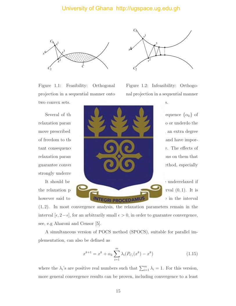
Figure 1.1 illustrates the case of feasibility of the CFP where orthogonal pro-

jections are used in a sequential manner onto the intersection of two convex sets.

Figure 1.2 illustrates the case of infeasibility of the CFP where orthogonal pro-

jections are used in a sequential manner onto two non-intersecting convex sets.

In this case, the sequence generated may not converge to the projection of the

starting point.

It is also possible to define a relaxed version of POCS method as

xk+1 = xk + αk(PCi(k)(xk)− xk) (1.14)

where the αk’s are positive relaxation parameters. It can be proven (see [54]) that

the above sequence converges if the constraint set is nonempty, control sequence

is cyclic and αk ∈ (0, 2).

14


2C

2x

C

1C

3x

1x

0x

Figure 1.1: Feasibility: Orthogonal

projection in a sequential manner onto

two convex sets.

0x

1x

2C

1C

3x

2x

Figure 1.2: Infeasibility: Orthogo-

nal projection in a sequential manner

onto two convex sets.

Several of the methods we discuss in this thesis employ a sequence αk of

relaxation parameters. Loosely speaking, these parameters overdo or underdo the

move prescribed in an iterative step. Relaxation parameters add an extra degree

of freedom to the way a method might actually be implemented and have impor-

tant consequences on the performance of the method in practice. The effects of

relaxation parameters on the iterations and the technical conditions on them that

guarantee convergence of an algorithm are discussed for each method, especially

strongly underrelaxed methods in Chapter 5.

It should be noted that an iterative algorithm is said to be underrelaxed if

the relaxation parameters incorporated are confined to the interval (0, 1). It is

however said to be overrelaxed if the relaxation parameters lie in the interval

(1, 2). In most convergence analysis, the relaxation parameters remain in the

interval [ǫ, 2− ǫ], for an arbitrarily small ǫ > 0, in order to guarantee convergence,

see, e.g Aharoni and Censor [5].

A simultaneous version of POCS method (SPOCS), suitable for parallel im-

plementation, can also be defined as

xk+1 = xk + αk

m∑

i=1

λi(PCi(xk)− xk) (1.15)

where the λi’s are positive real numbers such that∑m

i=1 λi = 1. For this version,

more general convergence results can be proven, including convergence to a least

15


3H

2H

1H

• 5x

4x

3x

2x

1x

0x

Figure 1.3: The iterative step of the algorithm ART with three equations and

unity relaxation parameter.

squares solution in the infeasible case (see [40] for details) for system of linear

equations.

1.5.1 ART and Cimino

When the problem is linear and the constraints are equalities, POCS method and

its simultaneous version SPOCS method give rise to two well known algorithms

in the literature: ART [67] and Cimmino [34]. Figure 1.3 illustrates the algorithm

for ART with a system of three equations as in (1.16) with unity relaxation pa-

rameter. ART is very popular in image and signal processing [53], especially in

Computerized Tomography [60, 55]. In this case, for a given matrix A ∈ Rm×n

with rows ai 6= 0 for i = 1, . . . ,m and b ∈ Rm, problem (1.9) reduces to finding a

solution of the linear system of equalities

Ax = b (1.16)

and (1.13) becomes the algorithm ART or Kaczmarz’s algorithm given by

xk+1 = xk +bi − 〈ai, xk〉

‖ai‖2ai, (1.17)

and from (1.14), its relaxed version is

xk+1 = xk + αk

bi − 〈ai, xk〉

‖ai‖2ai, (1.18)

16


and with a cyclic control sequence along the set of integers I := 1, 2, . . . ,m.

〈·, ·〉 stands for the standard inner product in Rn and ‖ ·‖ for the Euclidean norm.

Similarly, from (1.15), the simultaneous version known as Cimmino’s algo-

rithm, is given by

xk+1 = xk + αk

m∑

i=1

λi

bi − 〈ai, xk〉

‖ai‖2ai. (1.19)

As noted earlier, Cimmino’s algorithm converges to a least squares solution in

the case of infeasibility. This behaves like a gradient method applied to a square

objective function [10, 11, 40].

If the equalities (1.16) are replaced with the inequalities

Ax ≤ b, (1.20)

then we have the relaxed method of Agmon, Motzkin, and Schoenberg (AMS) (

see [1]) and its relaxed Cimmino’s method respectively as

xk+1 = xk + αkcki a

i, (1.21)

and

xk+1 = xk + αk

m∑

i=1

λicki a

i, (1.22)

where

cki = min

0,

bi − 〈ai, xk〉

‖ai‖2

and with a cyclic control sequence.

Figure 1.4 illustrates the iterative step in Cimmino’s algorithm using a system

of three inequalities with unity relaxation parameter.

It is worth noting that, in general, a sequence of orthogonal projections onto

closed convex sets does not converge to the orthogonal projection of the initial

point onto the intersection. A simple counterexample is shown next.

Consider the half-spaces C1 = x ∈ R2 | x2 ≤ 0 and C2 = x ∈ R

2 | x1+x2 ≤ 0

and let C = C1 ∩ C2. If x0 = (2, 1) is the initial point of projection then, by

simple calculation, the projection of x0 onto C, i.e., the minimizer of the function

12‖x − x0‖

2 over C is (12,−1

2), i.e., (1

2,−1

2) = 1

2argmin‖x − x0‖

2 | x ∈ C. But

17


•

3C

2C

1C

1kx

+

kx

Figure 1.4: The iterative step of the simultaneous Cimmino’s algorithm

with three inequalities and unity relaxation parameter.

using Algorithm 1.13, with initial projection of x0 onto C1, the algorithm does

not converge to (12,−1

2).

This counterexample motivates the development of Bregman measures and meth-

ods [14], where the objective function defines the measure to be used for the

projections, and a clever duality scheme allows the preservation of information

about the starting point and the function to be minimized. This is the subject of

the next section.

1.6 Bregman measures and generalized projec-

tions

Let S be a nonempty, open, convex set, such that S ⊆ D with the function

f : D ⊆ Rn → R. Then S is called the zone of f and is sometimes defined as

S := Int(domf).

Definition 1.6.1. Bregman Functions A function f : D ⊆ Rn → R with zone

S is called a Bregman function if there exists a nonempty, open, convex set S,

such that S ⊆ D and the following conditions hold:

(i) f(x) has continuous first partial derivatives at every x ∈ S,

18


(ii) f is strictly convex on S,

(iii) f is continuous on S,

(iv) for every α ∈ R, the partial level sets Lf1(y, α) and Lf

2(x, α) are bounded for

every y ∈ S and for every x ∈ S, respectively, where

Lf1(y, α) :=

x ∈ S | Df (x, y) ≤ α

and Lf

2(x, α) := y ∈ S | Df (x, y) ≤ α .

(v) If yk ∈ S for all k ≥ 0 and limk→∞

yk = y∗ then limk→∞

Df (y∗, yk) = 0,

(vi) If yk ∈ S and xk ∈ S for all k ≥ 0 and if limk→∞

Df (xk, yk) = 0 and

limk→∞

yk = y∗, andxkis bounded, then lim

k→∞xk = y∗.

We denote the collection of all Bregman functions with zone S by B(S). ♦

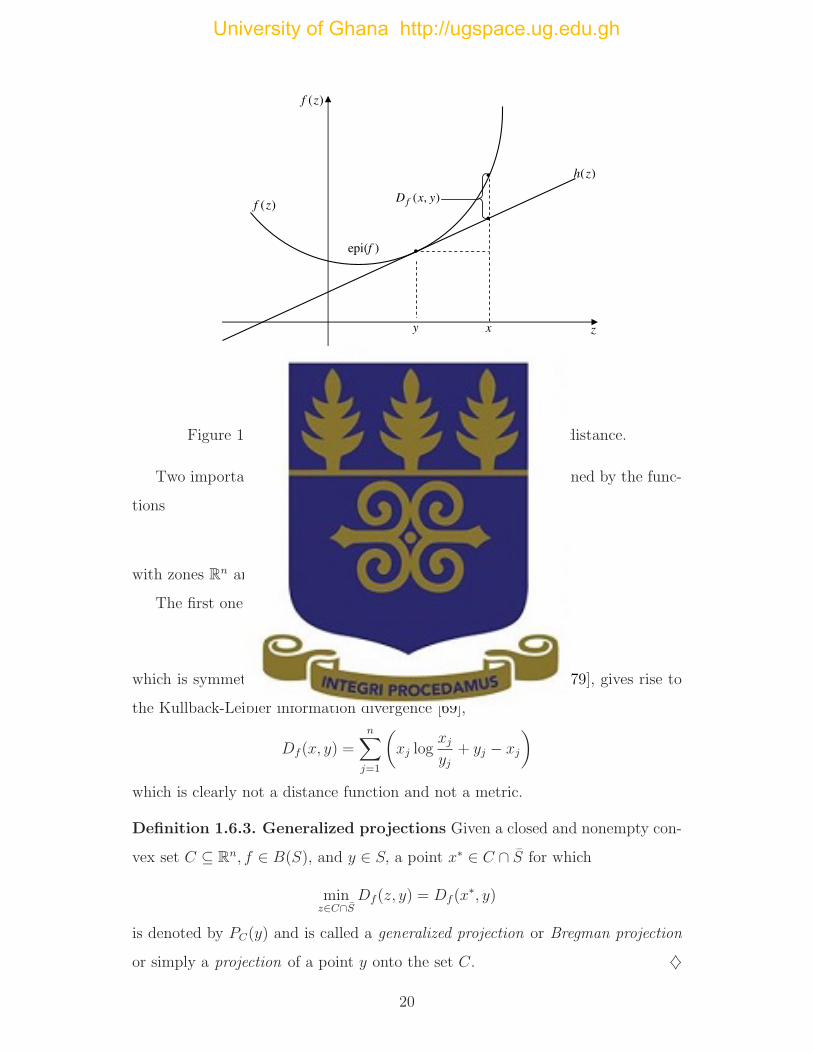
The function Df , where Df : S × S ⊆ R2n → R, is constructed from f(x) in

Definition 1.6.1 by

Df (x, y) := f(x)− f(y)− 〈∇f(y), x− y〉. (1.23)

This function is called the generalized distance function or the D-function.

Df (x, y) may be interpreted as the difference f(x)−h(x), where h(z) represents

the hyperplane H given by

H = (z, h(z)) | h(z) = f(y) + 〈∇f(y), z − y〉 (1.24)

which is tangent to the epigraph of f at the point (y, f(y)) in Rn+1.

Figure 1.5 shows the geometric interpretation of the generalized distance Df (x, y).

Remark 1.6.2. It is worth noting that the D-function is not necessarily sym-

metric, i.e., Df (x, y) 6= Df (y, x), and in general, does not satisfy the triangle

inequality. Therefore we will prefer to call Df a Bregman measure instead of a

distance or generalized distance function. However, the phrases ‘Bregman dis-

tance’ and ‘Bregman divergence’ are very common in the literature to denote Df .

♦

19


epi( )f

( )h z

( )f z

z y x

•

•

( , )fD x y ( )f z

•

Figure 1.5: Geometric interpretation of the generalized distance.

Two important examples of Bregman measures are those defined by the func-

tions

f(x) =1

2‖x‖2 and f(x) = −

n∑

j=1

(xj log xj)

with zones Rn and Rn+ respectively.

The first one gives rise to the standard 2-norm,

Df (x, y) =1

2‖x− y‖2

which is symmetric. The second one, the Shannon entropy [68, 79], gives rise to

the Kullback-Leibler information divergence [69],

Df (x, y) =n∑

j=1

(xj log

xj

yj+ yj − xj

)

which is clearly not a distance function and not a metric.

Definition 1.6.3. Generalized projections Given a closed and nonempty con-

vex set C ⊆ Rn, f ∈ B(S), and y ∈ S, a point x∗ ∈ C ∩ S for which

minz∈C∩S

Df (z, y) = Df (x∗, y)

is denoted by PC(y) and is called a generalized projection or Bregman projection

or simply a projection of a point y onto the set C. ♦

20


The next lemma shows the nonnegativity associated with the Bregman mea-

sure which is justified in the literature. This lemma is followed by Lemma 1.6.5

which guarantees the existence and uniqueness of generalized projections. Its

proof can be found on page 32 of [32].

Lemma 1.6.4. For every f ∈ B(S), we have Df (x, y) ≥ 0 for all x ∈ S and for

all y ∈ S, and Df (x, y) = 0 if and only if y = x.

Proof. This is an immediate consequence of the strict convexity of f and the

definition of Df (x, y).

Lemma 1.6.5. If f ∈ B(S), then for any closed convex set C ⊆ Rn, such that

C ∩ S 6= ∅, and for any y ∈ S, there exists a unique generalized projection x∗ =

PC(y).

An important geometrical property about the Bregman measure and its pro-

jection, which is the basis for all the main convergence proofs, is briefly described

next. Details of this description will be given in the next chapter.

1.6.1 A generalized Pythagoras theorem

First, we will prove the following.

Lemma 1.6.6. If f ∈ B(S) and Df is a Bregman measure then for a given point

x ∈ S and its Bregman projection PC(x) onto a closed convex set C, the function

defined by

G(z) = Df (z, x)−Df (z, PC(x))

is convex (as a matter of fact linear) for z ∈ S ∩ C.

Proof. Using the definition of Df , we have

G(z) = Df (z, x)−Df (z, PC(x))

= f(z)− f(x)− 〈∇f(x), z − x〉 − f(z) + f(PC(x))

+〈∇f(PC(x)), z − PC(x)〉

= f(PC(x))− f(x)− 〈∇f(x), z − x〉+ 〈∇f(PC(x)), z − PC(x)〉

21


which is linear in z.

The most important property that underlines the application of Bregman pro-

jections in Bregman’s method or algorithm for solving convex optimization prob-

lem is presented next. The property describes the geometry behind Bregman’s

method and makes it possible for the method to converge.

Theorem 1.6.7. For a given f ∈ B(S) and a closed convex set C, define PC(x)

as the Bregman projection of x onto C. Then the following inequality holds for

every y ∈ C ∩ S.

Df (PCx, x) ≤ Df (y, x)−Df (y, PCx) (1.25)

Proof. The proof of this theorem could be found in [14] as Lemma 1 on page 201.

But because of its importance in the sequel, we will present the proof in detail in

Chapter 2.

y ( )CP x

C

x

Figure 1.6: Geometric description of

Theorem 1.6.7 when orthogonal pro-

jections are used.

y ( )CP x

C

x

Figure 1.7: Geometric description of

Theorem 1.6.7 when generalized pro-

jections are used.

Remark 1.6.8. It is worth nothing that when the function f is the half-squared

2-norm and the set C is a hyperplane, the inequality (2.3) becomes equality and

the result becomes the old and well known Pythagoras theorem. A deeper analysis

of this fact, together with the proof, will appear in Chapter 2. ♦

22


1.6.2 Generalized projections onto hyperplanes

A key role in the iterative projection methods for linear feasibility problems and

for linearly constrained optimization problems is played by generalized projections

onto hyperplanes. A hyperplane in Rn is a set of the form

H = x ∈ Rn | 〈a, x〉 = b,

where a ∈ Rn, a 6= 0, and b ∈ R are given. We will need the following definition.

Definition 1.6.9. Zone consistency

(i) A function f ∈ B(S) is said to be zone consistent with respect to the

convex set C if for every y ∈ S we have PC(y) ∈ S. That is, the generalized

projection PC(y) of any point y ∈ S onto the convex set C remains in S.

(ii) f ∈ B(S) is said to be strongly zone consistent with respect to the hyper-

plane H and the point y ∈ S, if it is zone consistent with respect to H, and

with respect to every other hyperplane H ′ which is parallel to H and lies

between y and H. ♦

Two examples of strongly zone consistent Bregman functions with respect to the

hyperplane H = x ∈ Rn | 〈a, x〉 = b are the functions f : R

n → R and

g : Rn+ → R given by

f(x) =1

2‖x‖2 and g(x) = −

n∑

j=1

(xj log xj)

with zones Rn and Rn+ respectively

The following lemma characterizes generalized projections onto hyperplanes

and its proof can be found on page 35 of [32].

Lemma 1.6.10. Let f ∈ B(S), H = x ∈ Rn | 〈a, x〉 = b with a ∈ R

n \ 0,

b ∈ R, and assume that f is zone consistent with respect to H. Then, for any

given y ∈ S, the system

∇f(z) = ∇f(y) + λa, (1.26)

〈a, z〉 = b, (1.27)

23


determines uniquely the point z, which is the generalized projection of y onto H.

For a fixed representation of H, i.e., for a fixed a ∈ Rn \ 0 and b ∈ R, the

system also determines uniquely the real number λ. In this case, the vector z and

λ are the unknowns.

For a fixed representation of the hyperplane H, λ obtained from the system

(1.26)-(1.27) is called the generalized projection parameter associated with the

generalized projection of y onto H. We denote this by πH(y), i.e., λ = πH(y).

The next two results, Lemmas 1.6.11 and 1.6.12 whose proofs can be found

on pages 36 and 37 of [32], give statements about the signs of the parameters

associated with the generalized projections onto hyperplanes and the relationship

between two such parameters if a point is projected onto two parallel hyperplanes.

Lemma 1.6.11. Let H = x ∈ Rn | 〈a, x〉 = b and y ∈ S. For any f ∈ B(S)

which is zone consistent with respect to H, the parameter λ associated with the

generalized projection of y onto some particular representation of H, i.e., a 6= 0

and b ∈ R given, satisfies

λ(b− 〈a, y〉) > 0, if y 6∈ H, (1.28)

λ = 0, if y ∈ H. (1.29)

Lemma 1.6.12. Let Hr = x ∈ Rn | 〈a, x〉 = br for r = 1, 2 be two parallel

hyperplanes in Rn with a ∈ R

n \ 0, br ∈ R, and let x ∈ S. Then for any

f ∈ B(S) which is zone consistent with respect to both hyperplanes,

πH1(x) ≤ πH2(x) if and only if b1 ≤ b2.

Lemma 1.6.13. Let H = x ∈ Rn | 〈a, x〉 = b with a 6= 0 be a hyperplane in

Rn and let y ∈ S and PH(y) be the Bregman projection of y onto H, y /∈ H.

If b < 〈a, y〉 then for any f ∈ B(S) which is zone consistent with respect to the

hyperplane, the projection parameter λ is negative.

Proof. The proof follows from Lemma 1.6.11. If b < 〈a, y〉 then from (1.28),

λ < 0.

24


1.7 Bregman’s method for linear constraints

Another common feature of our algorithms is their primal-dual nature. In view of

Theorem 1.3.2, the primal-dual approach for constrained optimization problems

aims at solving the dual unconstrained problem. This is done by an iterative

scheme which alternates between the minimization of the Lagrangian and the

application of a steepest ascent iteration [11] to the dual problem.

For simplicity, we first develop a primal-dual algorithm for the following linear

equality constrained problem and then extend it to linear inequality constraints.

min f(x) (1.30)

subject to Ax = b, (1.31)

x ∈ Rn+, (1.32)

where Rn+ is the non-negative orthant of the n-dimensional Euclidean plane, A is

anm×nmatrix, b ∈ Rm, C = x ∈ R

n+ | Ax = b 6= ∅ and f is a Bregman function

zone consistent with respect to the hyperplane Hi := x ∈ Rn+ | 〈ai, x〉 = bi,

ai 6= 0, for i = 1, . . . ,m.

The Lagrangian of (1.30)-(1.32) with respect to the equality constraints is

L(x, z) = f(x) + 〈z, Ax− b〉,

where z ∈ Rm+ is the dual vector of the Lagrange multipliers. The dual function

g : Rm+ → R is given by

g(z) = minx∈Rn

+

L(x, z)

and a necessary condition for the minimization of L(x, z) is

∇xL(x, z) = 0 for x ∈ Rn++.

This implies that

∇f(x) = −AT z. (1.33)

From (1.33), for xk ∈ Rn++ and zk ∈ R

m+ , k ≥ 0, we generate an iterative primal-

dual algorithm as follows:

∇f(xk) = −AT zk. (1.34)

25


To do this, the corrections to the dual vectors have to be prescribed. But from

the Lagrange Duality Theorem 1.3.2,

minx∈Rn

+∩Hf(x) = max

z∈Rm+

g(z).

Therefore the dual corrections should at least entail dual ascent, i.e., guarantee

that the sequenceg(zk)

is increasing. This dual correction can be represented

by

zk+1 = zk + yk (1.35)

where yk ∈ Rm is a dual correction vector. Therefore, using (1.34) and (1.35), we

have

∇f(xk+1) = −AT zk+1 = −AT zk − ATyk = ∇f(xk)− ATyk. (1.36)

If a decision is made to change only one component of zk, i.e., the i(k)th compo-

nent at each iteration, then we can write yk = θkei(k). This enables us to write

(1.35) in component form as

zk+1i =

zki , i 6= i(k),

zki + θk, i = i(k),(1.37)

and (1.36) in the form

∇f(xk+1) = ∇f(xk)− θkai (1.38)

for i ∈ I := 1, 2, . . . ,m.

Now if the projection parameter θk is calculated so that xk+1 satisfies

〈ai, xk+1〉 = bi, (1.39)

i.e., the next iterate xk+1 lies on the i(k)th hyperplane, we obtain Bregman’s

method for convex programming with linear equality constraints and with the

almost cyclic control sequence i(k).

The solution xk+1 of the system (1.38)-(1.39) is the generalized projection of

the current primal iterate xk onto the i(k)th hyperplane Hi(k), as described in

Subsection 1.6.2, and θk is the generalized projection parameter.

26


The primal-dual algorithm for linear inequality constraints also follows the

same format and also calculates the parameter θk. However, before proceeding,

it compares θk with the i(k)th component of the current dual vector zk and uses

the smaller of these two in the iterative step.

Figure 1.8 illustrates the geometric interpretation of all the possible cases in an

iterative step of Bregman’s primal-dual algorithm for linear inequality constraints.

We state this linear inequality constrained problem and its Bregman’s algorithm

for solving it in the next subsection.

1k kx x

+=

( )i kH

( )i kH 1k

x+

1kx

+

kx

1kx

+

( )i kC

kx

Figure 1.8: Geometric interpretation of all the possible cases of Bregman’s algo-

rithm for linear inequality constraints.

Since Bregman’s algorithm is a row-action method, it takes at each iteration, a

hyperplane Hi and projects onto it the current iterate according to the generalized

distance constructed from the objective function f(x), and computes the next

iterate. That is, in the kth iterative step, only one row of the system of equalities

or inequalities is used; i(k) denotes the index of this row. The sequence i(k) is

the control sequence of the algorithm.

Next, we state Bregman’s method for solving the linear equality constrained

problem (1.30)-(1.32).

27


Algorithm 1.7.1. Bregman’s algorithm for linear equalities

(i) Initialization x0 ∈ Intdomf (Rn++) is such that for an arbitrary z0 ∈ R

m+ ,

∇f(x0) = −AT z0. (1.40)

(ii) Iterative Step Given xk calculate xk+1 from the system

∇f(xk+1) = ∇f(xk) + ckai(k), (1.41)

〈ai(k), xk+1〉 = bi(k), (1.42)

where ck = πHi(k)(xk). We assume that f is zone consistent with respect to

the hyperplane Hi := x ∈ Rn+ | 〈ai, x〉 = bi for i = 1, . . . ,m and that

the representation of every hyperplane is fixed during the whole iteration

process, so that the values of ck are well defined.

(iii) Control The control sequence i(k) is almost cyclic on the index set I. ♦

1.7.1 Bregman’s method for linear inequality constraints

This subsection describes Bregman’s method for linear inequality constraints and

emphasizes its relationship with the application of Gauss-Seidel type methods to

a dual problem.

Let f ∈ B(S) and consider the problem

min f(x), (1.43)

subject to 〈ai, x〉 ≤ bi, i ∈ I := 1, 2, . . . ,m, (1.44)

x ∈ S. (1.45)

Let Hi := x ∈ Rn | 〈ai, x〉 = bi and Ci := x ∈ R

n | 〈ai, x〉 ≤ bi; denote also

C = ∩mi=1Ci 6= ∅, and assume that C ∩ S 6= ∅. A is an m×n matrix whose ith row

is ai, and b ∈ Rm. Assume that ai 6= 0 for all i ∈ I and that f ∈ B(S) is strongly

zone consistent with respect to every Hi.

Below is the Bregman’s algorithm for solving the linear inequality constraints

problem (1.43)-(1.45).

28


Algorithm 1.7.2. Bregman’s algorithm for linear inequalities

(i) Initialization x0 ∈ S is such that for an arbitrary z0 ∈ Rm+ ,

∇f(x0) = −AT z0. (1.46)

(ii) Iterative Step Given xk and zk, calculate xk+1 and zk+1 from

∇f(xk+1) = ∇f(xk) + ckai(k), (1.47)

zk+1 = zk − ckei(k), (1.48)

ck = min(zki(k), θk

), (1.49)

where θk = πHi(k)(xk).

(iii) Control The control sequence i(k) is almost cyclic on the index set I. ♦

1.7.2 On relaxation

In [41], an important modification of Bregman’s method was made by incorpo-

rating into the method a relaxation parameter. The underlying idea behind the

relaxation strategy is to relax the constraints before computing the Bregman pro-

jections. More precisely, if at iteration k, the ith constraint

〈ai, x〉 ≤ bi

is to be used, we substitute it for the relaxed constraint

〈ai, x〉 ≤ αbi + (1− α)〈ai, x〉.

This simply means that instead of projecting onto the hyperplane

Hi = x ∈ Rn | 〈ai, x〉 = bi,

we project onto the relaxed hyperplane

Hi(α) = x ∈ Rn | 〈ai, x〉 = αbi + (1− α)〈ai, xk〉,

where the so called relaxation parameter (possibly also depending on k), α, lies

in the interval (0, 1]. In Chapter 2, we elaborate further on this concept and its

consequences to developing closed-form formulas in Chapter 4. Clearly, relaxation

can also be applied to the last algorithm for inequality constraints.

29


1.8 Entropy maximization and closed formulas:

MART, SMART and related methods

In this section, we describe existing results that simplify the application of Breg-

man’s method to entropy maximization and its related problems.

The x log x entropy function, ent x, which maps the nonnegative orthant Rn+

into R according to

−ent(x) =n∑

j=1

(xj log xj),

where, by convention, 0 log 0 = 0, is a Bregman function with zone Rn++ (see

page 33 of [32]). This function, known as Shannon’s entropy, has its origins in

information theory.

We now consider the following entropy optimization problem over linear equal-

ity constraints.

min f(x), (1.50)

subject to Ax = b, (1.51)

x ∈ Rn+, (1.52)

where f(x) =∑n

j=1(xj log xj).

Using Algorithm 1.7.2 with f(x) =∑n

j=1(xj log xj), we have the algorithm for

solving (1.50)-(1.52) as

Algorithm 1.8.1. Bregman’s method for equality constrained entropy

optimization

(i) Initialization x0 ∈ Rn++ is such that for an arbitrary z0 ∈ R

m+

x0j = exp

((−AT z0

)j− 1), j = 1, 2, . . . , n.

(ii) Iterative Step Given xk choose a control index i(k) and solve the system

xk+1j = xk

j exp(cka

ij

), j = 1, 2, . . . , n, (1.53)

bi = 〈ai, xk+1〉. (1.54)

30


(iii) Control The sequence i(k) is almost cyclic on I = 1, 2, . . . ,m. ♦

We discuss Algorithm 1.8.1 and its relationship with the algorithm MART.

From Lemma 1.6.10, there exists a unique choice of xk+1 and ck that satisfies

the system (1.53)-(1.54). To proceed with the iteration, this system with n + 1

equations needs to be solved for xk+1 and ck.

An alternative algorithm for solving this same problem is MART which em-

ploys a closed-form formula for the iterative updates instead of solving a system

of n + 1 nonlinear equations. However, for the proof of convergence for MART,

the following assumptions are made.

Assumption 1.8.2.

(i) Feasibility: x ∈ Rn | Ax = b ∩ R

n+ 6= ∅.

(ii) Non-negativity: aij ≥ 0, and bi > 0 for all i ∈ I and j = 1, 2, . . . , n.

(iii) Normalization: Ax = b is scaled so that for all i ∈ I and j = 1, 2, . . . , n,

aij ≤ 1. ♦

With this assumption, we state the algorithm for MART:

Algorithm 1.8.3. Multiplicative Algebraic Reconstruction Technique

(i) Initialization z0 ∈ Rm+ is arbitrary, and x0 ∈ R

n++ is given by

1 + log x0j =

(−AT z0

)j, j = 1, 2, . . . , n.

(ii) Iterative Step

xk+1j = xk

j

(bi

〈ai, xk〉

)aij

, j = 1, 2, . . . , n. (1.55)

(iii) Control: The sequence i(k) is almost cyclic on I. ♦

The question we want to address briefly here, and in more detail in Chapter

4, is whether it is possible to replace the iterative step of the system (1.53)-(1.54)

31


in the Algorithm 1.8.1 with a closed-form formula as it is the case for orthogonal

projections onto hyperplanes using Assumption 1.8.2?

The answer to this question will motivate the development of general closed-

form formula for the iterative steps in Bregman’s algorithm for linear constraints

in Chapter 4.

To answer this question, observe that in order to use Algorithm 1.8.1, the

system (1.53)-(1.54) has to be solved for ck and xk+1 in each iterate. Doing this

for the kth iterate, by eliminating xk+1 from this system, we have

n∑

j=1

aijxkj exp

(cka

ij

)− bi = 0.

Let exp ck = yk and define the function fk : R+ → R by

fk(yk) =n∑

j=1

aijxkj exp

(cka

ij

)− bi.

Then we need a positive root of fk to determine ck. Now, if the conditions or

Assumption 1.8.2 that enable the convergence of MART are imposed on Algorithm

1.8.1 then fk(0) = −bi < 0, limyk→∞

fk(yk) = +∞, and for yk ≥ 0, we have the

derivatives f ′k(yk) > 0 and f ′′

k (yk) ≤ 0. Now, since fk(0) < 0 and limyk→∞

fk(yk) =

+∞, there exists yk > 0 such that fk(yk) > 0. Also since fk is continuous, the

intermediate value theorem ensures that for some y∗ ∈ (0, yk) we have fk(y∗k) = 0.

Since f ′k(yk) > 0 for all yk > 0, it follows that fk is strictly increasing on (0,∞).

Hence it is one-to-one there, and therefore if fk(yk) = 0 for some yk > 0 then

y∗k = yk and so y∗k > 0 is unique and fk(y∗k) = 0.

Now consider the line through the points (0,−bi) and (1, fk(1)) in the plane of

the graph of fk(yk). This line or the secant line to the graph intersects the yk−axis

at the point yk given by

yk =bi

〈ai, xk〉.

yk is therefore considered as a secant approximation to the root y∗k of fk and

exp ck = yk. Hence

ck = logbi

〈ai, xk〉.

32


When this approximate value ck is substituted into (1.53) of Algorithm 1.8.1,

we obtain the closed-form formula (1.55) of Algorithm 1.8.3 which is MART’s

iterative step. Therefore MART’s iterative step is a secant approximation to

Bregman’s iterative step if the conditions that enable the convergence of MART

hold. Details of these can be found in [23].

The question of whether the algorithms MART and SMART will converge

when x ∈ Rn | Ax = b = ∅ will be addressed in Chapter 5.

33


Chapter 2

The convex feasibility problem

and block Bregman methods for

equality constraints

Now, let us go back to the CFP (1.9) and its solution using a sequence of Bregman

projections. In this chapter, we show how to generalize the method of relaxed

Bregman projections onto closed convex sets, itself a generalization of POCS. As

a consequence, we derive an application to convex but nonlinear sets of constraints

and to linear equality constraints as well.

Before presenting the algorithm, we need to define a separating hyperplane.

Definition 2.0.4. Separating hyperplanes For a given point x and a closed,

nonempty convex set C, define for s ∈ Rn\0 and d ∈ R, Hs = x ∈ R

n | 〈s, x〉 =

d. We say that Hs separates x and C, that is, it is a separating hyperplane for

x and C, if 〈s, x〉 ≤ d ∀x ∈ C and 〈s, x〉 ≥ d. ♦

Definition 2.0.5. Supporting hyperplanes For a given closed and nonempty

convex set C and a given point x ∈ ∂C, the boundary of C, define for s ∈ Rn\0

the hyperplane, Hs = x ∈ Rn | 〈s, x − x〉 = 0. We say that Hs supports C at

x if either 〈s, x− x〉 ≥ 0 for all x ∈ C, or 〈s, x− x〉 ≤ 0 for all x ∈ C. ♦

It is clear from Proposition 11 in [24] that, for a given closed and nonempty

34


convex set C and a point x, if PC(x) is the orthogonal projection of x onto C,

then H = y ∈ Rn | 〈y − PC(x), x− PC(x)〉 = 0 defines a tangent hyperplane at

PC(x) which is a supporting and a separating hyperplane of x /∈ C and C.

The following result extends this concept to Bregman projections. If we con-

sider PC(x) as a Bregman projection of x onto C then there exists a tangent

hyperplane to C at the point PC(x), see [24] . This hyperplane will be related to

our generalization of relaxation.

Our new general method for solving (1.9) will be defined as follows.

xk+1 = P sCi(k)

(xk) (2.1)

where P sCi(k)

denotes the Bregman projection onto a separating hyperplane for the

point xk and the closed convex set Ci for i = 1, . . . ,m.

Next, we state a well-known result, the three-point lemma by Chen and

Teboulle 1993, which is widely used in the analysis of generalized Bregman pro-

jection methods.

Lemma 2.0.6. Let f be a Bregman function with zone S. Then for any x, z ∈ S

and y ∈ S,

Df (y, x) = Df (z, x) +Df (y, z) + 〈∇f(x)−∇f(z), z − y〉. (2.2)

The next theorem is Lemma 1 in [14]. We repeat the statement and its proof

here because of its important to the work in this chapter.

Theorem 2.0.7. Let f be a Bregman function with zone S and let C be a closed

and nonempty convex set such that C ∩ S 6= ∅. Define PC(x) as the Bregman

projection of x onto C and assume that for any x ∈ S, PC(x) ∈ S. Then the

following inequality is true

Df (PC(x), x) ≤ Df (y, x)−Df (y, PC(x)) (2.3)

for every y ∈ C ∩ S.

35


Proof. Using the convexity of the function G in Lemma 1.6.6 and the fact that

Df (x, x) = 0 for all x ∈ S, we have, for any α ∈ (0, 1],

Df (αy + (1− α)PC(x), x)−Df (αy + (1− α)PC(x), PC(x)) ≤ (2.4)

αDf (y, x) + (1− α)Df (PC(x), x)− αDf (y, PC(x)). (2.5)

This implies that

Df (y, x)−Df (PC(x), x)−Df (y, PC(x)) ≥ (2.6)

Df (αy + (1− α)PC(x), x)−Df (PC(x), x)

α−

Df (αy + (1− α)PC(x), PC(x))

α.

(2.7)

The first term on the right-hand side of (2.7) is non-negative ∀α ∈ (0, 1] because

PC(x) is a minimizer, and the second term tends to zero as α tends to zero because

of the definition of the Bregman measure. That is,

limα→0

Df (αy + (1− α)PC(x), PC(x))

α

= limα→0

Df (PC(x) + α(y − PC(x)), PC(x))−Df (PC(x), PC(x))

α

= 〈∇zDf (z, PC(x))|z=PC(x), y − PC(x)〉 = 0,

since Df (x, y) = f(x)−f(y)−〈∇f(y), x−y〉 implies∇xDf (x, y) = ∇f(x)−∇f(y)

and so ∇xDf (y, y) = 0. This completes the proof.

A deeper analysis of this result (Theorem 2.0.7) for inequalities, not considered

by Bregman, gives us a better geometrical view of Bregman projections. In (2.4),

the difference is not only convex but linear in the first variable and so

Df (y, x)−Df (PC(x), x)−Df (y, PC(x)) = (2.8)

Df (αy + (1− α)PC(x), x)−Df (PC(x), x)

α(2.9)

−Df (αy + (1− α)PC(x), PC(x))

α. (2.10)

Using the definition of the Bregman measure to expand (2.9), we have

f(αy + (1− α)PC(x))− f(x)− 〈∇f(x), αy + (1− α)PC(x)− x〉

α

36


−[f(PC(x))− f(x)− 〈∇f(x), PC(x)− x〉]

α

=f(αy + (1− α)PC(x))− f(PC(x))− α〈∇f(x), y − PC(x)〉

α(2.11)

and also for the expansion of (2.10), we have

f(αy + (1− α)PC(x))− f(PC(x))− α〈∇f(PC(x)), y − PC(x)〉

α. (2.12)

Therefore using (2.8), (2.9), (2.10), (2.11) and (2.12) , we have

Df (y, x)−Df (PC(x), x)−Df (y, PC(x)) = 〈∇f(PC(x))−∇f(x), y−PC(x)〉 (2.13)

for every y ∈ C, which, if PC(x) = z, is the result of Lemma 2.0.6.

If f is 12‖ ·‖2 then (2.13) gives, as expected, the cosine of the angle determined

by the points x, PC(x) and y. When this is zero, the Pythagoras theorem for

equalities is retrieved.

In the general case, if f is a Bregman function with zone S and C is a closed

and nonempty convex set such that C ∩ S 6= ∅, and if f is zone consistent with

respect to C then, for x /∈ C, the equation

〈∇f(x)−∇f(PC(x)), y − PC(x)〉 = 0 (2.14)

defines a hyperplane that is tangent to C at PC(x), where PC(x) is the Bregman

projection of x onto C.

Remark 2.0.8. It should be noted that if x /∈ C then x 6= PC(x) and since f is

a Bregman function assumed to be strictly convex on S, ∇f is strictly monotone

on S (see page 10 of [77]) and so ∇f(x) 6= ∇f(PC(x)).

Alternatively, if f satisfies Assumption 2.2.2 so that ∇f is invertible from S

onto Rn then ∇f is one-to-one and therefore ∇f(x) = ∇f(PC(x)) implies x =

PC(x), a contradiction to the assumption that x /∈ C. Thus ∇f(x) 6= ∇f(PC(x))

for all x ∈ S. ♦

Again, the next theorem which is Theorem 2.4.2 on page 43 of [32] is repeated

here with its proof because of its important to the work of this section.

37


Theorem 2.0.9. Under the assumption of Theorem 2.0.7, for any x ∈ S,

v ∈ C ∩ S is PC(x) if and only if

〈∇f(x)−∇f(v), y − v〉 ≤ 0 (2.15)

for all y ∈ C ∩ S.

Proof. If z = PC(x) in Lemma 2.0.6 then (2.15) follows from (2.2) and (2.3).

Conversely, if (2.15) holds then with v = PC(x) in Lemma 2.0.6, (2.2) reduces to

the inequality

Df (v, x) ≤ Df (y, x) for all y ∈ C ∩ S

since Df is nonnegative. Therefore v = PC(x).

This theorem says that a hyperplane H through the point PC(x), x /∈ C, and

which is perpendicular to ∇f(x) −∇f(PC(x)) supports the convex set C at the

point PC(x). That is, the set C lies entirely on one side of H.

Definition 2.0.10. Generalized tangent hyperplane For a given closed and

nonempty convex set C, and a given Bregman function f with zone S such that

C ∩ S 6= ∅, define PC(x) as the Bregman projection of x onto C. If f is zone

consistent with respect to C, then the generalized tangent hyperplane at PC(x) is

the set

y ∈ S | 〈y − PC(x),∇f(x)−∇f(PC(x))〉 = 0 (2.16)

if x /∈ C. ♦

Now consider the minimization problem for a given y ∈ S, where S is a zone

of the Bregman function f , and a closed and nonempty convex set C.

minx∈C∩S

G(x) := f(x)− f(y)− 〈∇f(y), x− y〉. (2.17)

The condition for the minimum PC(y), that is, the Bregman projection of y onto

C, is given by

〈−∇G(PC(y)), x− PC(y)〉 = 〈∇f(y)−∇f(PC(y)), x− PC(y)〉 ≤ 0 (2.18)

38


for all x ∈ C ∩ S, which describes the hyperplane from the Pythagorean equality.

We note that, with G(x) = f(x)−f(y)−〈∇f(y), x−y〉, ∇G(x) = ∇f(x)−∇f(y)

and so ∇G(PC(y)) = ∇f(PC(y))−∇f(y).

Thus 〈∇G(PC(y)), x−PC(y)〉 = 〈∇f(PC(y))−∇f(y), x−PC(y)〉 and (2.18) follows

from Theorem 2.0.9.

2.1 An extension of relaxation

In this section, we extend the concept of relaxation for Bregman projections, first

proposed in [41] and further extended in [29] to, not necessarily the linear case.

As described in Subsection 1.7.2, for a given hyperplane

H = x ∈ Rn | 〈a, x〉 = b,

a relaxed Bregman projection onto H with relaxation parameter α ∈ (0, 1] is

defined as the Bregman projection onto the parallel hyperplane defined by

H = x ∈ Rn | 〈a, x〉 = αb+ (1− α)〈a, xk〉. (2.19)

We generalize this concept to a general closed convex sets in a natural way in the

next subsection.

2.1.1 Relaxed Bregman projections onto closed convex sets

For a given closed and nonempty convex set C ⊆ Rn, a point x ∈ R

n and its

Bregman projection PC(x) onto C, we define a relaxed Bregman projection onto

C with parameter α ∈ (0, 1], PH(α,x)(x), as the Bregman projection onto the

hyperplane defined by

H(α, x) = y ∈ Rn | 〈∇f(x)−∇f(PC(x)), y〉 = (2.20)

α〈∇f(x)−∇f(PC(x)), PC(x)〉+ (1− α)〈∇f(x)−∇f(PC(x)), x〉

if x 6∈ C. If x ∈ C then the hyperplane is the entire space Rn and so x, PH(α,x)(x) ∈

Rn, since in this case, the normal vector ∇f(x)−∇f(PC(x)) = 0 . We show that

39


H(α, x) is a separating hyperplane for the point x 6∈ C and C in the following

proposition.

Proposition 2.1.1. Suppose f is a Bregman function with zone S and let C be

a closed and nonempty convex set such that C ∩ S 6= ∅. Define PC(x) as the

Bregman projection of x onto C and assume that for any x ∈ S, PC(x) ∈ S.

Then, for α ∈ (0, 1] and x ∈ S, the hyperplane

H(α, x) = y ∈ Rn | 〈∇f(x)−∇f(PC(x)), y〉 =

α〈∇f(x)−∇f(PC(x)), PC(x)〉+ (1− α)〈∇f(x)−∇f(PC(x)), x〉

separates the point x /∈ C from C ∩ S for x ∈ S.

Proof. We first show that H(1, x) is a separating and supporting hyperplane of

C at the point PC(x) of C and then deduce that H(α, x) separates x from C ∩ S

for α ∈ (0, 1), since H(α, x) is parallel to H(1, x) and lies between x and H(1, x)

for α ∈ (0, 1) and x ∈ S.

Now by definition,

H(1, x) = y ∈ Rn | 〈∇f(x)−∇f(PC(x)), y〉 = 〈∇f(x)−∇f(PC(x)), PC(x)〉

= y ∈ Rn | 〈∇f(x)−∇f(PC(x)), y − PC(x)〉 = 0

is the generalized tangent hyperplane in (2.16).

By Theorem 2.0.9,

〈∇f(x)−∇f(PC(x)), y − PC(x)〉 ≤ 0

for all y ∈ C and so C ⊆ y ∈ Rn | 〈∇f(x)−∇f(PC(x)), y − PC(x)〉 ≤ 0. Thus

C ∩ S lies on one side of H(1, x), and since by definition, H(α, x) is parallel to

H(1, x) and lies between x and H(1, x) for α ∈ (0, 1), C ∩ S lies on one side of

H(α, x).

On the other hand, if x ∈ S but x /∈ C then

〈∇f(x)−∇f(PC(x)), x〉 = α〈∇f(x)−∇f(PC(x)), PC(x)〉

+(1− α)〈∇f(x)−∇f(PC(x)), x〉

40


implies

〈∇f(x)−∇f(PC(x)), α(x− PC(x))〉 = 0.

But, by the definition of Df ,

Df (x, y) +Df (y, x) = f(x)− f(y)− 〈∇f(y), x− y〉

+f(y)− f(x)− 〈∇f(x), y − x〉

= 〈∇f(x)−∇f(y), x− y〉. (2.21)

Therefore

α〈∇f(x)−∇f(PC(x)), x− PC(x)〉 = α(Df (x, PC(x)) +Df (PC(x), x)) > 0.

Hence, for α ∈ (0, 1] and x ∈ S, H(α, x) separates x from C ∩ S.

2.1.2 The relationship with the Censor-Herman definition

A definition of underrelaxation of the Bregman projection onto a general closed

convex set (not necessarily linear or half space) was given by Yair Censor and Ga-

bor T. Herman in [29]. This definition includes as special cases the underrelaxed

orthogonal projections and the underrelaxed Bregman projections onto linear con-

straints, i.e., hyperplanes and half-spaces, as given in [41]. Censor-Herman in [29]

defines the underrelaxed Bregman projection of a point x ∈ S onto a general

closed convex set C, with respect to a Bregman function f and with a relaxation

parameter λ ∈ [0, 1], as a point PC,λ(x) that satisfies the equation

∇f(PC,λ(x)) = (1− λ)∇f(x) + λ∇f(PC(x)), (2.22)

where PC(x) is the Bregman projection of x onto C and S is the zone of f . In

Proposition 1 in [29], it was shown that f is zone consistent with respect to C.

This proposition also guarantees the invertibility of ∇f and hence the uniqueness

of PC,λ. In particular, for every z ∈ S, PC,λ(z) ∈ S.

We prove in the following proposition that our new extended definition of

underrelaxed Bregman projections onto a general closed convex sets contains that

of Censor-Herman.

41


Proposition 2.1.2. Let f be a Bregman function with zone S = Int(domf), and

C be a general closed and nonempty convex set. Assume that f is strongly zone

consistent with respect to the separating hyperplane H(α, x) for x ∈ S, 0 < α ≤ 1,

of C defined in (2.20). Then there exists λ ∈ [0, 1] such that, for x ∈ S, PC,λ(x)

of (2.22) is the underrelaxed Bregman projection PH(α,x)(x), i.e., the Bregman

projection of x onto the separating hyperplane H(α, x).

Proof. We observe that if x ∈ C ∩S then there is nothing to prove. Since, in this

case, ∇f(x) −∇f(PC(x)) = 0 and the hyperplanes H(1, x) and H(α, x) for α ∈

(0, 1) and x ∈ S are the entire Rn and so, PC(x) = PH(1,x)(x) = PH(α,x)(x) = x.

Thus

∇f(PH(α,x)(x)) = (1− λ)∇f(x) + λ∇f(PH(1,x)(x)),

holds for all λ ∈ R and in particular for λ ∈ [0, 1]. Therefore suppose that

x /∈ C. Then PH(α,x)(x) is the relaxed Bregman projection of x onto H(1, x) and

by Lemma 1.6.10, it is uniquely determined with its projection parameter θ by

the system

∇f(PH(α,x)(x)) = ∇f(x) + θ(∇f(x)−∇f(PC(x)))(2.23)

〈PH(α,x)(x),∇f(x)−∇f(PC(x))〉 = α〈∇f(x)−∇f(PC(x)), PC(x)〉

+(1− α)〈∇f(x)−∇f(PC(x)), x〉.

Similarly, the Bregman projection of x onto H(1, x), PH(1,x)(x), is also uniquely

determined with its projection parameter θ∗ by the system

∇f(PH(1,x)(x)) = ∇f(x) + θ∗(∇f(x)−∇f(PC(x)))(2.24)

〈PH(1,x)(x),∇f(x)−∇f(PC(x))〉 = 〈∇f(x)−∇f(PC(x)), PC(x)〉.

Now, by Lemma 1.6.12, θ∗ ≤ θ, and since α ∈ (0, 1], i.e., α 6= 0, x /∈ H(α, x) and

so by Lemma 1.6.11, θ∗ 6= 0. This means that θ∗ ≤ θ and θ/θ∗ is well defined.

Therefore, from (2.23) and (2.24),

∇f(PH(α,x)(x)) = ∇f(x) + θ(∇f(x)−∇f(PC(x)))

= ∇f(x) +θ

θ∗(∇f(PH(1)(x))−∇f(x))

=

(1−

θ

θ∗

)∇f(x) +

θ

θ∗∇f(PH(1,x)(x)).

42


Now since x /∈ C and the hyperplane H(α, x) separates C from x, ∇f(x) −

∇f(PC(x)) is the outward normal to the hyperplane H(α, x) and so by Lemma

1.6.13 , the projection parameters of x onto H(α, x) for α ∈ (0, 1] are negative.

Thus θ∗ ≤ θ implies 1 ≥ θθ∗

and so if we define λ = θθ∗

then 0 ≤ λ ≤ 1 and

∇f(PH(α,x)(x)) = (1− λ)∇f(x) + λ∇f(PH(1,x)(x)),

which completes the proof.

2.1.3 The relationship with the Aharoni-Berman-Censor

definition

In [3], Aharoni, Berman and Censor associate the set AQ(x) with the closed convex

set Q and a point x ∈ Rn as follows

AQ(x) =

x if x ∈ Q,

x+ λ(PH(x)− x) | H ∈ Hx,Q, η ≤ λ ≤ 2− η if x /∈ Q,(2.25)

where 0 ≤ η ≤ 1 and λ is a relaxation parameter. Here PH(x) is the orthogonal

projection of x /∈ Q onto a hyperplane H that separates the ball B(x, δd(x,Q))

with center x and radius δd(x,Q) for 0 ≤ δ ≤ 1, from Q; d(x,Q) is the Euclidean

distance between x and Q. Hx,Q is the collection of all hyperplanes that separate

B(x, δd(x,Q)) from Q. The set AQ(x) is then used to describe the iterative step

in their (δ, η)-algorithm.

Next, we show that in the special case when f = 12‖·‖2, method (2.1) coincides

with the method by Aharoni-Berman-Censor in [3].

Proposition 2.1.3. If f = 12‖ · ‖2 then H(α, x) ∈ Hx,C for a closed convex set C,

α ∈ (0, 1], and PH(α,x)(x) ∈ AC(x), where AC(x) is as defined by (2.25) with Q

replaced by C and H(α, x) is the separating hyperplane of C.

Proof. Since, by the definition in [3], Hx,C is a collection of all hyperplanes that

separate the ball B(x, δd(x,C)) from the closed convex set C for 0 ≤ δ ≤ 1 if x /∈

C, by Proposition 2.1.1, H(α, x) ∈ Hx,C for α ∈ (0, 1]. Therefore PH(α,x)(x) ∈

AC(x). If x ∈ C then, as observed in the beginning of the proof of Proposition

2.1.2, PH(α,x)(x) = x and so PH(α,x)(x) ∈ AC(x).

43


2.2 A general Bregman projection method

In this subsection, we propose a block-iterative algorithm with underrelaxed Breg-

man projections as defined in Subsection 2.1.1 for solving (1.9). By block-iterative,

we mean that, at the kth iteration, the next iterate xk+1 is generated from the

current iterate xk by using a subset or a block of the family of the closed convex

sets Cimi=1 in the convex feasibility problem (1.9). Such a block-iterative scheme

for a convex feasibility problem was first proposed in [5] by Aharoni and Censor.

We partition the integer interval [1,m] into p disjoint blocks or intervals Ωl,

that is, [1,m] = ∪pl=1Ωl and let Ql = ∩i∈Ωl

Ci. Let f be a Bregman function

with zone S = Int(domf), and assume that f is essentially smooth and strongly

zone consistent with respect to the separating hyperplane Hi(α, x) of Ci such that

Hi(α, x) ∩ S 6= ∅. Then, our new general method for solving (1.9) will be defined

as follows.

∇f(xk+1) =∑

i∈Ωl(k)

λi∇f(PHi(α,xk)(xk)), (2.26)

where PHi(α,xk)(xk) denotes the Bregman projection of the current iterate xk onto

the hyperplane Hi(α, xk) that separates xk from the closed convex set Ci ∩ S, as

defined in Subsection 2.1.1. λi’s are positive numbers which are bounded away

from zero, i.e., there exists ǫ > 0 such that λi ≥ ǫ for each i, and

∑

i∈Ωl(k)

λi = 1. (2.27)

l(k) is a cyclic control sequence over the index set 1, . . . , p.

Remark 2.2.1. It must be noted that the applicability of the algorithm defined by

(2.26) depends on the ability to invert the gradient ∇f explicitly. If the Bregman

function f is essentially smooth then ∇f is one-to-one mapping with continuous

inverse (∇f)−1, see [[78], Theorem 26.5]. We must also assume zone consistency;

that is, all the gradients that appear in the iterative step are defined. ♦

Based on Remark 2.2.1, the Bregman function f used in the algorithm defined

by (2.26) and the iterates produced by the algorithm must satisfy the following

assumption.

44


Assumption 2.2.2. f ∈ B(S) is essentially smooth and zone consistent or

strongly zone consistent with respect to every hyperplane and the iterate xk ∈ S

for all k ≥ 0. ♦

2.2.1 A convergence theorem

We will establish the convergence of the sequence generated by (2.26) for p = 1.

It however remains a conjecture that the sequence generated by the general block-

iterative Bregman projection method (2.26) for p > 1 converges to the solution of

(1.9).

To do this, we will use Propositions 2.2.4-2.2.6 below. The method of proof

is closely related to the previous proofs given by Aharoni, Berman and Censor in

[3], and Censor and Herman in [29].

The properties of the Bregman function f in relation to a closed and nonempty

convex set C with zone S = Int(domf) such that C∩S 6= ∅ will be used repeatedly

in the analysis leading to the proof of Theorem 2.2.9.

Properties 2.2.3.

(i) 〈∇f(x)−∇f(PC(x)), y − PC(x)〉 ≤ 0 for y ∈ C ∩ S and x ∈ S.

(ii) 〈∇f(x) − ∇f(y), x − y〉 ≥ 0, ∀x, y ∈ S, i.e.,∇f is a monotone operator on

S.

(iii) 〈∇f(x)−∇f(y), x− y〉 = Df (x, y) +Df (y, x) for all x, y ∈ S.

(iv) For every α ∈ R, the partial level sets L1(y, α) and L2(x, α) are bounded for

every y ∈ S and for every x ∈ S, respectively.

(v) If yk ∈ S for all k ≥ 0, and limk→∞

yk = y∗ then limk→∞

Df (y∗, yk) = 0.

(vi) If yk ∈ S and xk ∈ S for all k ≥ 0 and if limk→∞

Df (xk, yk) = 0, and lim

k→∞yk =

y∗, andxkis bounded, then lim

k→∞xk = y∗. ♦

45


Proof. The proof of (i) is the proof of Theorem 2.0.9. The proofs of (ii) and (iii)

are part of the proof of Proposition 2.1.1, precisely (2.21). (iv) to (vi) are part of

the definition of a Bregman function.

Next, we prove the general Bregman measure descendant property for the algo-

rithm defined by (2.26). This is known in the literature as the Fejer monotonicity.

Proposition 2.2.4. Let f be a Bregman function with zone S = Int(domf), and

assume that f is strongly zone consistent with respect to the separating hyperplane

Hi(α, x) of Ci such that Hi(α, x) ∩ S 6= ∅ for α ∈ (0, 1] and x ∈ S. Then the

Bregman measure for the algorithm defined by (2.26) decreases towards C∩ S with

respect to the second variable; that is,

Df (x, xk+1) ≤ Df (x, x

k) (2.28)

for every x ∈ C ∩ S. Moreover, the sequence xk is bounded.

Proof. By the definition of Df , for every x ∈ C,

Df (x, xk+1) = f(x)− f(xk+1)− 〈∇f(xk+1), x− xk+1〉.

Using the definition of the algorithm in (2.26) and condition (2.27), the last equal-

ity becomes

Df (x, xk+1) =

m∑

i=1

λi

(f(x)− f(xk+1)− 〈∇f(PHi(α,xk)(x

k)), x− xk+1〉)

=m∑

i=1

λi

(f(x)− f(PHi(α,xk)(x

k)) + f(PHi(α,xk)(xk))− f(xk+1)

− 〈∇f(PHi(α,xk)(xk)), x− PHi(α,xk)(x

k) + PHi(α,xk)(xk)− xk+1〉

).

Thus, using the definition of Df again, we have

Df (x, xk+1) =

m∑

i=1

λi

(Df (x, PHi(α,xk)(x

k))−Df (xk+1, PHi(α,xk)(x

k))).

46


Therefore, using (2.27), we have

Df (x, xk)−Df (x, x

k+1) =m∑

i=1

λiDf (xk+1, PHi(α,xk)(x

k)) (2.29)

+m∑

i=1

λi

(Df (x, x

k)−Df (x, PHi(α,xk)(xk))).

(2.30)

But, by Theorem 2.0.7,

Df (PHi(α,xk)(xk), xk) ≤ Df (x, x

k)−Df (x, PHi(α,xk)(xk))

for every x ∈ C ∩ S and so (2.29) becomes


k+1) ≥m∑

i=1

λi(Df (xk+1, PHi(α,xk)(x

k)) +Df (PHi(α,xk)(xk), xk)).

Hence, since the weights λi are positive,


k+1) ≥m∑

i=1

λiDf (PHi(α,xk)(xk), xk) (2.31)

and (2.28) follows since Df is nonnegative. In the literature, this means that

the sequence xk is Df -Fejer monotone with respect to C ∩ S and implies that

xk is bounded. This is because a repeated use of (2.28) gives xk ∈ L(x, α0) for

all k ≥ 0 with α0 = Df (x, x0) and so xk is bounded by the definition of the

Bregman function (see Properties 2.2.3(iv)).

Several important consequences can be deduced from Proposition 2.2.4. We

begin with the next corrollary.

Corollary 2.2.5. The sequence generated by the algorithm defined by (2.26) is

such that for every y ∈ C

limk→∞

Df (y, xk) = θ,

for some nonnegative θ and for i ∈ I := 1, . . . ,m,

limk→∞

Df (PHi(α,xk)(xk), xk) = 0. (2.32)

47


Proof. By (2.28), for every y ∈ C ∩ S, the sequence Df (y, xk) is monotonically

decreasing, bounded below by zero and therefore convergent. Hence, there exists

a nonnegative θ such that limk→∞ Df (y, xk) = θ. Also, as observed in the proof

of Proposition 2.2.4, the sequence xk is bounded and so the left hand side of

(2.31) tends to zero. Therefore limk→∞Df (PHi(α,xk)(xk), xk) = 0 since the λi’s are

positive and bounded away from zero.

Since the sequence generated by the algorithm defined by (2.26) is bounded,

it has a limit point. In the next proposition, we show that if a limit point exists

and it belongs to C then it is the limit of the sequence.

Proposition 2.2.6. Any limit point x∗ ∈ C of the bounded sequence xk of the

algorithm defined by (2.26) is the limit of the entire sequence.

Proof. Suppose x∗ ∈ C is a limit point of xk and that x∗∗ is another limit point

of xk. That is

limk∈N1;k→∞

xk = x∗ and limk∈N2;k→∞

xk = x∗∗,

where N1 and N2 are two different infinite subsets of N = 0, 1, 2, . . . , . Then,

since f is zone consistent with respect to the Ci’s and xk ∈ S for all k ≥ 0,

x∗ ∈ S. Therefore, from (2.28), limk→∞

Df (x∗, xk) exists. Applying Properties 2.2.3

(v) in the definition of Bregman function to the sequence xkk≥0,k∈N1 , we have

limk∈N1;k→∞

Df (x∗, xk) = 0 and so by (2.28) lim

k→∞Df (x

∗, xk) = 0 for all k ≥ 0 which

also holds for the sequence xkk≥0,k∈N2 . Therefore using Properties 2.2.3 (vi), we

have x∗ = x∗∗.

Before the next step for the convergence proof, we need a condition that must

be satisfied by the separating hyperplanes in order to guarantee convergence. This

condition induces the following definition.

Definition 2.2.7. For a given closed convex set C and a point x /∈ C we say that

H is a δ separating hyperplane for C and x if H lies between C and B(x, δd(x, PCx)),

where d(·, ·) stands for the Euclidean distance and δ ∈ (0, 1) and B(x, r) is the

ball with center at x and radius r. ♦

48


It is clear that this definition is equivalent to saying that for every x ∈ Rn,

‖PH(x)− x‖ ≥ δ‖PC(x)− x‖, (2.33)

where PC(x) and PH(x) are the Bregman projections of x onto C and the separat-

ing hyperplane H respectively. In other words, if the Euclidean distance between

x and its projection onto the hyperplane tends to zero, the same is valid for the

Euclidean distance between x and its projection onto the associated convex set.

Therefore our assumption for the separating hyperplanes Hi(α, x) in (2.26) for

i = 1, . . . ,m will be

Assumption 2.2.8. For the algorithm defined by (2.26), and for i ∈ I :=

1, . . . ,m and for all x ∈ S which are not in Ci, the inequality (2.33) holds with

Hi(α, x) defined in (2.20) with respect to Ci for α ∈ (0, 1). ♦

Given that the algorithm defined by (2.26) satisfies Assumption 2.2.8, we can

prove that every limit point of the sequence xk generated by (2.26) belong to

C. The following theorem justifies this statement.

Theorem 2.2.9. The whole sequence of the algorithm defined by (2.26) converges

to a point in C.

Proof. Using (2.32) and (2.33), we have

limk→∞

Df (PCi(xk), xk) = 0, ∀i ∈ I := 1, . . . ,m. (2.34)

Suppose x∗ is a limit point of the sequence xk. The limit point x∗ exists because

xk is bounded by Proposition 2.2.4. This means that there exists a subsequence

xkl such that liml→∞ xkl = x∗, and using (2.34)

liml→∞

Df (PCi(xkl), xkl) = 0 for all i ∈ I. (2.35)

Now, by Theorem 2.0.7,

Df (x, PHi(α,xk)(xk)) ≤ Df (x, x

k)−Df (PHi(α,xk)(xk), xk)

for every x ∈ C ∩ S. But by (2.32) and (2.28), Df (PHi(α,xk)(xk), xk) and

Df (x, xk) are bounded for any x ∈ C ∩ S and so Df (x, PHi(α,xk)(x

k)) is

49


bounded. Therefore by Properties 2.2.3 (iv), PHi(α,xk)(xk) is bounded. The

boundedness of PCi(xk) follows from Assumption 2.2.8. Therefore, using Prop-

erties 2.2.3 (vi), liml→∞ PCi(xkl) = x∗ for each i ∈ I. Hence x∗ ∈ C.

2.2.2 A general underrelaxed entropy projection method

In this section, we derive a general block iterative algorithm with underrelaxed

entropy projections using projections onto separating hyperplanes. We derive this

algorithm for the solution of a linear system of equations Ax = b.

The x log x entropy function is a Bregman function with zone S = IntRn+, see

page 33 of [32]. Therefore, by Lemma 1.6.10, the Bregman projection PHi(α,x)(x)

of x onto H(α, x) satisfies the equation

∇f(PHi(α,x)(x)) = ∇f(x) + θ(∇f(x)−∇f(PCi(x))), (2.36)

where θ is the parameter associated with the projection of x onto H(α, x). For

f(x) =∑n

j=1(xj log xj), the gradient of the jth component is ∇f(x)j = 1+log xj.

Thus using (2.36), we have

1 + log(PHi(α,xk)(xk))j = 1 + log xk

j + θki (log xkj − log(PCi

(xk))j)

which simplifies to

log(PHi(α,xk)(xk))j = log xk

j + θki log

(xkj

(PCi(xk))j

)(2.37)

and by the definition of the general Bregman method given in (2.26) for p = 1,

∇f(xk+1)j =m∑

i=1

λi∇f(PHi(α,xk)(xk))j

1 + log(xk+1)j =m∑

i=1

λi(1 + log(PHi(α,xk)(xk))j

log(xk+1)j =m∑

i=1

λi log(PHi(α,xk)(xk))j for j = 1, . . . , n, k ≥ 0.

50



log xk+1j =

m∑

i=1

λi

(log xk

j + θki log

(xkj

(PCi(xk))j

))

= log xkj +

m∑

i=1

log

(xkj

(PCi(xk))j

)λiθki

.

Therefore, the iterative step becomes

xk+1j = xk

j

m∏

i=1

(xkj

(PCi(xk))j

)λiθki

. (2.38)

But Hi = x | 〈ai, x〉 = bi, ai 6= 0, for i = 1, 2, . . . ,m, and the jth component

of the normal aij is

aij = ∇f(xk)j −∇f(PCi(xk))j = 1 + log xk

j − (1 + log(PCi(xk))j)

= log

(xkj

(PCi(xk))j

).

This implies that

exp aij =xkj

(PCi(xk))j

.

Therefore, using (2.38), the iterative method becomes

xk+1j = xk

j

m∏

i=1

(exp aij)λiθ

ki = xk

j

m∏

i=1

exp(aijλiθ

ki

)for j = 1, . . . , n, k ≥ 0

and if we replace the θki ’s with dki = log bi〈ai,xk〉

for all i and k ≥ 0 then the

resulting formula resembles the iterative step formula of the block-iterative MART

algorithm of Censor and Segman [31]. However if one replaces the θki ’s with

ck = α log bi〈ai,xk〉

, 0 < α ≤ 1, for all i and k ≥ 0, then the resulting formula

resembles the iterative step formula of the underrelaxed MART algorithm in [23].

2.3 An application for general convex sets

When an exact Bregman projection onto a closed convex set is too costly to

compute, we can use the algorithm defined by (2.26)when p = 1 and the separating

51


hyperplane defined by the approximation of the function that defines the convex

set. That is, suppose that the convex set Ci is defined by

Ci = x ∈ Rn | gi(x) ≤ 0, (2.39)

where gi : Rn → R is a differentiable convex function. We follow closely the

definition of the approximating hyperplane on page 151 of [61], i.e., a separating

hyperplane, Hi(α, xk) for α ∈ (0, 1) and xk ∈ S = Int(domg), between the current

iterate xk and the current constraint Ci if xk /∈ Ci as

Hi(α, xk) = x ∈ R

n | αgi(xk) +∇gi(x

k)T (x− xk) = 0, (2.40)

and Hi(α, xk) = R

n if xk ∈ Ci. We assume C = ∩mi=1Ci 6= ∅.

For the algorithm defined by (2.26), PHi(α,xk)(xk) is the Bregman projection of

xk onto Hi(α, xk). This means that for a function f ∈ B(S) with S = Int(domf)

which is strongly zone consistent with respect to the hyperplane Hi, the projection

solves the equations given by

∇f(PHi(α,xk)(xk)) = ∇f(xk) + θki ∇gi(x

k), (2.41)

αgi(xk) +∇gi(x

k)T (PHi(α,xk)(xk)− xk) = 0 (2.42)

for the projection parameter θki and PHi(α,xk)(xk).

Now from (2.41), we have

〈∇f(PHi(α,xk)(xk))−∇f(xk), PHi(α,xk)(x

k)−xk〉 = θki 〈∇gi(xk), PHi(α,xk)(x

k)−xk〉.



k)− xk〉 = −αθki gi(xk).

Thus if xk /∈ Ci or gi(xk) > 0 then

θki =〈∇f(PHi(α,xk)(x

k))−∇f(xk), PHi(α,xk)(xk)− xk〉

−αgi(xk)

and (2.41) becomes

∇f(PHi(α,xk)(xk)) = ∇f(xk)−


k)− xk〉

αgi(xk)∇gi(x

k)

(2.43)

52


and if xk ∈ Ci or gi(xk) ≤ 0 then ∇f(PHi(α,xk)(x

k)) = ∇f(xk).

Observe that if ∇gi(xk) = 0 then gi takes its minimal value at xk, implying

by the non-emptyness of C that gi(xk) ≤ 0, so that PHi(α,xk)(x

k) = xk and so

∇f(PHi(α,xk)(xk)) = ∇f(xk).

In order that the algorithm defined by (2.26) converges to x∗ ∈ C for the gen-

eral convex set, we make the following assumption on the gradient of the function

gi for i = 1, . . . ,m. With this assumption, i.e., Assumption 2.3.1, Proposition

2.3.2 guarantees that x∗ ∈ C and ensures that Assumption 2.2.8 is satisfied.

Assumption 2.3.1. For each of the functions gi used in (2.39), there exists

ǫ > 0 such that ‖∇gi(xk)‖ ≥ ǫ.

Proposition 2.3.2. On the basis of Assumption 2.3.1, limk→∞ gi(xk) = 0 and

limk→∞ xk ∈ Ci for each i ∈ 1, . . . ,m.

Proof. If ‖∇gi(xk)‖ is bounded away from zero as in Assumption 2.3.1 then (2.32)

implies that PHi(α,xk)(xk)−xk tends to zero as k → ∞, and so (2.42) implies that

α limk→∞ gi(xk) = 0. Therefore, limk→∞ xk ∈ Ci for each i since the gi’s are

continuous and α ∈ (0, 1). This further implies that limk→∞(PCi(xk) − xk) = 0

which satisfies condition (2.33).

Remark 2.3.3. It must be noted that, for the general convex sets, Assump-

tion 2.3.1 is sufficient for the proof of Theorem 2.2.9. Assumption 2.2.8 is thus

redundant.

The proof of Theorem 2.2.9 may therefore take the following simple form:

Proof. By Proposition 2.2.4, xk is bounded and so there exists a subsequence

xkl such that liml→∞ xkl = x∗. Therefore, by Proposition 2.3.2, x∗ ∈ Ci for each

i ∈ 1, . . . ,m. Thus x∗ ∈ C and hence by Proposition 2.2.6, x∗ is the limit of

the entire sequence.

53


2.4 Linear equality constraints

In the case of linear equality constraints, given by a linear system of equations

Ax = b,

where A ∈ Rm×n, x ∈ R

n and b ∈ Rm, if for some function f ∈ B(S) which is

strongly zone consistent with respect to the hyperplane Hi := x ∈ Rn | 〈ai, x〉 =

bi, ai 6= 0, for each i ∈ 1, . . . ,m, the starting point of the algorithm defined by

(2.26) is given by

∇f(x0) = −AT z0

for a given z0 ∈ Rm+ (observe that the obvious choice is z0 = 0 and x0 would be

the unconstrained minimum of f) then we have the iterative formula given by

∇f(xk+1) =m∑

i=1

λi∇f(PHi(α,xk)(xk))

where, from (1.34), ∇f(xk) = −AT zk for k ≥ 0 and so, in the limit, say x∗,

∇f(x∗) = −AT z∗, for some z∗. Therefore the Kuhn-Tucker conditions are satisfied

for the optimization problem

min f(x) subject to Ax = b. (2.44)

In this case, algorithm (2.26) solves (2.44) when p = 1.

2.5 A Conjecture for the strongly underrelaxed

case

In the general case, where the constraints are not linear equalities, just the se-

quence of Bregman projections defined by algorithm (2.26) does not guarantee

convergence to the solution of a minimization problem, say

min f(x) subject to 〈ai, x〉 ≤ bi

for the function f ∈ B(S) with S = Intdomf and i = 1, . . . ,m, but converges

to the solution of only the convex feasibility problem, unless dual variables are

54


updated as in Chapter 3 for linear inequalities. So, what happens in the general

case? Our conjecture is that in the purely sequential Bregman algorithm, when

the relaxation parameters tend to zero, the sequence generated by algorithm (2.26)

tends to the solution of the optimization problem limx∈Rn Df (Ax, b) in the general

case.

55


Chapter 3

Block Bregman methods for

inequality constraints

In this chapter, we present a new simultaneous version of the Bregman method

for linear constraints with corresponding convergence results.

3.1 The problem

We recall the problem of Subsection 1.7.1,

min f(x),

subject to 〈ai, x〉 ≤ bi, i ∈ I := 1, 2, . . . ,m,

x ∈ S,

where Hi := x ∈ Rn | 〈ai, x〉 = bi, Ci := x ∈ R

n | 〈ai, x〉 ≤ bi; C = ∩mi=1Ci

and C ∩ S 6= ∅.

A is an m × n matrix whose ith row is ai, and b ∈ Rm, ai 6= 0 for all i ∈ I.

S = Int(domf) and f ∈ B(S) is essentially smooth and strongly zone consistent

with respect to every Hi.

56


3.1.1 Simultaneous under-relaxed Bregman’s algorithm for

linear inequality constraints

We present the simultaneous version of Algorithm 1.7.2 for solving problem (1.43)-

(1.45).

Algorithm 3.1.1. Simultaneous under-relaxed Bregman’s algorithm for

linear inequalities

(i) Initialization x0 ∈ S is such that for an arbitrary z0 ∈ Rm+ ,

∇f(x0) = −AT z0. (3.1)


∇f(xk+1) = ∇f(xk) +∑

i∈It(k)

λki c

ki a

i, (3.2)

zk+1 = zk −∑

i∈It(k)

λki c

ki e

i (3.3)

with

cki =

min

(zkiλki

, θki

)if i ∈ It(k),

0 if i 6∈ It(k),

(3.4)

where θki = πH(k)i(xk), and there exists ǫ > 0 such that, for the positive

weights λki with

∑i∈It(k)

λki = 1 for all k ≥ 0, λk

i ≥ ǫ for i ∈ It(k) and λki = 0

for i /∈ It(k).

(iii) H(k)i is parallel to Hi = x ∈ Rn | 〈ai, x〉 = bi for all i ∈ It(k) and k ≥ 0.

H(k)i := x ∈ Rn | 〈ai, x〉 = αkbi + (1− αk)〈ai, xk〉, where αk such that

ǫ ≤ αk ≤ 1 for ǫ > 0 is a sequence of relaxation parameters. We adopt

the concept of relaxation highlighted in Subsection 1.7.2 and implemented

in [41].

(iv) The sequence t(k)∞k=0 is almost cyclic on the index set 1, 2, . . . ,M, where

M is the number of blocks. The index set I := 1, 2, . . . ,m of the m

constraints has been partitioned into M nonempty disjoint blocks such that

I = I1 ∪ . . . ∪ IM . ♦

57


In order to justify the proof of Lemma 3.1.4 and the proofs of the propositions

leading to the proof of the convergence theorem, Theorem 3.2.1, let Pi and Qi be

Bregman projections onto

C(k)i = x ∈ Rn | 〈ai, x〉 ≤ αkbi + (1− αk)〈ai, xk〉 (3.5)

and H(k)i respectively so that for any function f ∈ B(S) which is strongly

zone consistent with respect to Hi for i ∈ It(k) and xk ∈ S with θki = πH(k)i(xk),

∇f(Pixk) = ∇f(xk) + min0, θki a

i, (3.6)

∇f(Qixk) = ∇f(xk) + θki a

i. (3.7)

Define

∇f(wki ) = ∇f(xk) + cki a

i for i ∈ It(k). (3.8)

The wki ’s are ‘modified relaxed Bregman projections’ onto the Hi’s (see page

233 of [62]) such that the next iterate xk+1 satisfies the equation ∇f(xk+1) =∑

i∈It(k)λki∇f(wk

i ).

This is because, multiplying (3.8) by λki for i ∈ It(k) with

∑i∈It(k)

λki = 1 and

summing over i ∈ It(k), we have

∑

i∈It(k)

λki∇f(wk

i ) = ∇f(xk) +∑

i∈It(k)

λki c

ki a

i.

Therefore, from iterative step (3.2),

∇f(xk+1) =∑

i∈It(k)

λki∇f(wk

i ). (3.9)

Since the applicability of Algorithm 3.1.1 depends on the ability to invert the

gradient ∇f explicitly, we assume that the Bregman function f used in Algorithm

3.1.1 satisfies Assumption 2.2.2.

3.1.2 Preliminary results

The following lemma establishes the non-negativity of the dual variables.

Lemma 3.1.2. For any k ≥ 0, zki ≥ 0 for i ∈ It(k).

58


Proof. By initialization, z0 ∈ Rm+ . By induction, assume zk ∈ R

m+ . If i /∈ It(k) then

zk+1i = zki ≥ 0 and if i ∈ It(k) then using (3.4), zk+1

i = zki − λki c

ki ≥ zki − zki = 0.

Hence zk+1 ∈ Rm+ .

Lemma 3.1.3. ∇f(xk) = −AT zk for any k ≥ 0.

Proof. We proceed by induction. By (3.1), the result is true when k = 0. Assume

that the result is true for any k ≥ 0. Then by (3.2) and (3.3),

∇f(xk+1) = ∇f(xk) +∑

i∈It(k)

λki c

ki a

i (3.10)

= −AT (zk −∑

i∈It(k)

λki c

ki e

i) = −AT zk+1. (3.11)

The next lemma shows that the wki is a Bregman projection of xk onto H(k)i

if xk /∈ C(k)i or a point in the segment between xk and its projection onto H(k)i

if xk ∈ C(k)i.

Lemma 3.1.4. Let the function f ∈ B(S) be strongly zone consistent with respect

to the hyperplane Hi for all i ∈ It(k) and k ≥ 0, and let wki satisfy (3.8). Then for

the closed and nonempty convex set C with C ∩ S 6= ∅, the following statements

hold if f satifies Assumption 2.2.2.

(a) If xk /∈ C(k)i then wki = Pix

k = Qixk and θki = cki < 0; Pi and Qi are as

defined in (3.6) and (3.7).

(b) If xk ∈ C(k)i then 0 ≤ cki ≤ θki .

(c) wki ∈ C(k)i.

(d) Df (wki , x

k) ≤ Df (y, xk)−Df (y, w

ki ) for all y ∈ C ∩ S.

Proof. (a) If xk /∈ C(k)i then by Lemma 1.6.11 θki < 0, and since zki ≥ 0 by

Lemma 3.1.2, cki = θki by (3.4). Therefore, from the definitions of wki , Pi and

Qi, we have wki = Pix

k = Qixk.

59


(b) If xk ∈ C(k)i then θki ≥ 0 and since zki ≥ 0, 0 ≤ cki ≤ θki .

(c) Clearly wki ∈ C(k)i if cki = θki . Thus, suppose cki 6= θki or cki = zki /λ

ki ,

i.e., cki < θki , and recall that θki , the parameter associated with the Bregman

projection of xk onto H(k)i (in what follows we denote this projection by

xk+1) is obtained by solving the system

∇f(xk+1) = ∇f(xk) + θki ai, (3.12)

〈ai, xk+1〉 = αkbi + (1− αk)〈ai, xk〉. (3.13)

Now, using (3.8) and (3.12), we have

∇f(wki )−∇f(xk+1) = (cki − θki )a

i

and so

〈∇f(wki )−∇f(xk+1), wk

i − xk+1〉 = 〈(cki − θki )ai, wk

i − xk+1〉.

But, by Properties 2.2.3 (iii),

〈∇f(wki )−∇f(xk+1), wk

i − xk+1〉 = Df (wki , x

k+1) +Df (xk+1, wk

i ) ≥ 0

and since cki < θki , we have

〈ai, wki − xk+1〉 ≤ 0.

Therefore

〈ai, wki 〉 ≤ αkbi + (1− αk)〈ai, xk〉

since

〈ai, xk+1〉 = αkbi + (1− αk)〈ai, xk〉.

This means that wki ∈ C(k)i.

(d) The result follows from Theorem 2.0.7.

60


3.2 Convergence results

Next, is the convergence theorem for Algorithm 3.1.1.

Theorem 3.2.1. Assume the following:

(i) f ∈ B(S),

(ii) f is strongly zone consistent with respect to each Hi, i ∈ It(k),

(iii) t(k)∞k=0 is almost cyclic on 1, 2, . . . ,M with a constant of almost cycli-

cality r,

(iv) C ∩ S 6= ∅.

Then any sequence xk produced by Algorithm 3.1.1 converges to the point x∗,

which is the solution of (1.43)-(1.45).

To prove Theorem 3.2.1, we use Propositions 3.2.2 to 3.2.7.

Proposition 3.2.2. If the assumptions of Theorem 3.2.1 hold and wki satisfies

(3.8), then

wki = PH(k)i(x

k) and cki = πH(k)i(xk) where

H(k)i = x ∈ Rn | 〈ai, x〉 = γkbi + (1− γk)〈ai, xk〉 (3.14)

for some γk ∈ R such that 0 ≤ γk ≤ αk for all k ≥ 0.

Proof. Note that wki is the Bregman projection of xk onto the hyperplane

H(k)i = 〈ai, x〉 = 〈ai, wki 〉, which is parallel to H(k)i and passes through wk

i .

It remains to demonstrate that the right-hand side 〈ai, wki 〉 has the desired form

as in (3.14). It is clear that if cki = θki for i ∈ It(k) then H(k)i = H(k)i. This is

because, by definition, H(k)i is parallel to H(k)i and lies between xk and H(k)i,

and θki is the parameter associated with the Bregman projection of xk onto H(k)i.

Therefore H(k)i and H(k)i coincide if cki = θki . Hence γk = αk.

61


On the other hand, if cki 6= θki for i ∈ It(k) then, by the definition of cki ,

0 ≤zkiλki

= cki < θki .

Now consider the following which is possible by Properties 2.2.3 (iii) and (3.8):

0 ≤ Df

(wk

i , xk)+Df

(xk, wk

i

)= 〈∇f

(wk

i

)−∇f

(xk), wk

i − xk〉,

= 〈cki ai, wk

i − xk〉. (3.15)

Therefore if cki = 0 for i ∈ It(k) then Df

(xk, wk

i

)= 0 and Df

(wk

i , xk)= 0 imply

wki = xk, i.e.,〈ai, wk

i 〉 = 〈ai, xk〉 and so we may take γk = 0.

Finally if 0 < cki < θki then 0 < πH(k)i(xk) < πH(k)i(x

k). Hence, by Lemma

1.6.12,

〈ai, xk〉 < 〈ai, wki 〉 < αkbi + (1− αk)〈ai, xk〉 (3.16)

for i ∈ It(k) and so there is γk ∈ (0, αk) as desired. For more insight, see page 427

of [41]

Proposition 3.2.3. If the assumptions of Theorem 3.2.1 hold, λki and cki are as

defined in Algorithm 3.1.1 and wki satisfies (3.8) then for xk ∈ S,

∑

i∈It(k)

λki

Df (x

k, wki )−Df (x

k, xk+1)

and

Df

(xk+1, xk

)+∑

i∈It(k)

λki c

ki

(bi − 〈ai, xk+1〉

)

are non-negative.

Proof. Using Lemma 2.0.6 with y = xk, x = wki and z = xk+1, we have

Df (xk, wk

i ) = Df (xk, xk+1) +Df (x

k+1, wki )− 〈∇f(wk

i )−∇f(xk+1), xk − xk+1〉.

Now, multiplying the last equation by λki for i ∈ It(k),

∑i∈It(k)

λki = 1, and sum-

ming over i ∈ It(k), we have

∑

i∈It(k)

λkiDf (x

k, wki ) = Df (x

k, xk+1) +∑

i∈It(k)

λkiDf (x

k+1, wki )

62


since, by (3.9),

∑

i∈It(k)

λki 〈∇f(wk

i )−∇f(xk+1), xk − xk+1〉 = 〈∇f(xk+1)−∇f(xk+1), xk − xk+1〉

= 0.

Thus

∑

i∈It(k)

λki

Df (x

k, wki )−Df (x

k, xk+1)=∑

i∈It(k)

λkiDf (x

k+1, wki ) ≥ 0. (3.17)

Now let

dk = Df

(xk+1, xk

)+∑

i∈It(k)

λki c

ki

(bi − 〈ai, xk+1〉

). (3.18)

Then, using Properties 2.2.3 and (3.2), we have

dk +Df

(xk, xk+1

)= Df

(xk, xk+1

)+Df

(xk+1, xk

)

+∑

i∈It(k)

λki c

ki

(bi − 〈ai, xk+1〉

)

= 〈∇f(xk+1

)−∇f

(xk), xk+1 − xk〉

+∑

i∈It(k)

λki c

ki

(bi − 〈ai, xk+1〉

)

= 〈∑

i∈It(k)

λki c

ki a

i, xk+1 − xk〉+∑

i∈It(k)

λki c

ki

(bi − 〈ai, xk+1〉

)

=∑

i∈It(k)

λki c

ki

(bi − 〈ai, xk〉

).

But, by Proposition 3.2.2, 〈ai, wki 〉 = γkbi + (1− γk)〈ai, xk〉 implies

〈ai, wki − xk〉 = γk


). (3.19)

Therefore, from (3.15),

0 ≤ Df

(wk

i , xk)+Df

(xk, wk

i

)= cki γ

k(bi − 〈ai, xk〉

). (3.20)

Therefore, using (3.20), if γk = 0 then wki = xk, and by (3.8), wk

i = xk implies

cki = 0. Therefore by (3.2), ∇f(xk+1) = ∇f(xk) implies xk+1 = xk if f satisfies

Assumption 2.2.2. Hence

dk = −Df

(xk, xk+1

)+∑

i∈It(k)

λki c

ki


)= 0 if γk = 0.

63


Next we consider when γk > 0 for k ≥ 0. Using (3.20), we have

dk =∑

i∈It(k)

λki

−Df

(xk, xk+1

)+

Df

(wk

i , xk)+Df

(xk, wk

i

)

γk

and since γk is less or equal to one, we have

dk ≥∑

i∈It(k)

λki

Df

(wk

i , xk)+Df

(xk, wk

i

)−Df

(xk, xk+1

).

Therefore, using (3.17),

dk ≥∑

i∈It(k)

λki

Df

(wk

i , xk)+Df

(xk+1, wk

i

). (3.21)

Thus

dk ≥ 0 for all k ≥ 0.

Proposition 3.2.4. If the Lagrangian of the minimization problem in (1.43)-

(1.45) is L(x, z) = f(x) + 〈z, Ax − b〉 then, for any sequences xk and zk

produced by Algorithm 3.1.1,

(i) the sequenceL(xk, zk

)is nondecreasing and lim

k→∞L(xk, zk

)exists,

(ii) limk→∞

Df

(wk

i , xk)= 0 and lim

k→∞Df

(xk+1, wk

i

)= 0 for each i ∈ It(k),

(iii) xk is bounded.

Proof. (i) Define

dk = L(xk+1, zk+1

)− L

(xk, zk

). (3.22)

Then, from the definition of L,

dk = f(xk+1) + 〈zk+1, Axk+1 − b〉 −(f(xk) + 〈zk, Axk − b〉

)

= f(xk+1)− f(xk) + 〈zk+1, Axk+1〉 − 〈zk+1, b〉 − 〈zk, Axk〉+ 〈zk, b〉.

64


But 〈zk, Axk〉 = 〈AT zk, xk〉 = −〈∇f(xk), xk〉.

Therefore

dk = f(xk+1)− f(xk)− 〈∇f(xk), xk+1 − xk〉+ 〈∇f(xk), xk+1 − xk〉

−〈zk+1 − zk, b〉 − 〈∇f(xk+1), xk+1〉+ 〈∇f(xk), xk〉

= Df

(xk+1, xk

)− 〈zk+1 − zk, b〉+ 〈∇f(xk)−∇f(xk+1), xk+1〉

= Df

(xk+1, xk

)− 〈

∑

i∈It(k)

λki c

ki a

i, xk+1〉+ 〈∑

i∈It(k)

λki c

ki e

i, b〉

= Df

(xk+1, xk

)− 〈

∑

i∈It(k)

λki c

ki a

i, xk+1〉+∑

i∈It(k)

λki c

ki bi

= Df

(xk+1, xk

)+∑

i∈It(k)

λki c

ki

(bi − 〈ai, xk+1〉

).

Hence, by Proposition 3.2.3 and (3.18), dk = dk ≥ 0 and soL(xk, zk)

is

non-decreasing.

We now prove the existence of limk→∞

L(xk, zk

)by showing that

L(xk, zk

)

is bounded from above on C ∩ S for all k ≥ 0.

To do this, we choose z ∈ C ∩ S and consider:

Df (z, xk) = f(z)− f(xk)− 〈∇f(xk), z − xk〉

= f(z)− f(xk) + 〈AT zk, z − xk〉

= f(z)− f(xk) + 〈zk, Az〉 − 〈zk, Axk〉

≤ f(z)− f(xk) + 〈zk, b− Axk〉 = f(z)− L(xk, zk

).

Therefore

L(xk, zk

)≤ f(z)−Df (z, x

k) ≤ f(z).

HenceL(xk, zk

)is bounded from above and so the limit exists.

(ii) Since limk→∞

L(xk, zk

)exists, by (3.22), lim

k→∞dk = lim

k→∞dk = 0. Therefore, from

(3.21),

limk→∞

∑

i∈It(k)

λki

Df

(wk

i , xk)+Df

(xk+1, wk

i

)= 0 (3.23)

and since λki ≥ ǫ > 0 for i ∈ It(k) and k ≥ 0, we have

limk→∞

Df

(wk

i , xk)= 0 and lim

k→∞Df

(xk+1, wk

i

)= 0

65


for each i ∈ It(k) and k ≥ 0.

(iii) Applying dk = L(xk+1, zk+1

)− L

(xk, zk

)≥ 0 for all k ≥ 0 recursively to

the expression Df (z, xk) ≤ f(z)− L

(xk, zk

), we have

Df (z, xk) ≤ f(z)− L

(x0, z0

)= α,

where α ∈ R. Therefore, from the boundedness of the partial level set

Lf2(z, α), Properties 2.2.3 (iv), we have that

xkis bounded.

Proposition 3.2.5. Assume that limj→∞

xkj = x∗. Fix q, a positive integer, and

take a sequence lj with lj ∈ 1, 2, . . . , q. Then limj→∞

wkj+l

i = x∗ for i ∈ It(kj)

and limj→∞

xkj+lj = x∗.

Proof. Consider first the q sequencesxkj+l

∞j=0

with 1 ≤ l ≤ q. Sincexkj+l

∞j=0

are sub-sequences of the bounded sequence xk∞k=0, they are bounded, and from

Proposition 3.2.4 (ii), for all s ∈ 0, 1, . . . , q, i ∈ It(kj) and j ≥ 0,

limj→∞

Df

(w

kj+s

i , xkj+s)= 0 and lim

j→∞Df

(xkj+s+1, w

kj+s

i

)= 0. (3.24)

From Proposition 3.2.4 (ii) and (iii), Df (wki , x

k) is bounded and Df (x, xk)

for each x ∈ C ∩ S is bounded . Therefore by Lemma 3.1.4 (d), Df (x, wki )

is bounded for x ∈ C ∩ S. This means that, by Properties 2.2.3 (iv), wki is

bounded. Therefore, using the first equation on the left hand side of (3.24) and

applying recursively Properties 2.2.3 (vi), we have, for all l such that 0 ≤ l ≤ q

and i ∈ It(kj),

limj→∞

wkj+l

i = x∗. (3.25)

Hence, using the second equation on the right hand side of (3.24) and applying

recursively Properties 2.2.3 (vi), we have that, for all l such that 0 ≤ l ≤ q,

limj→∞

xkj+l = x∗.

Thus, interlacing these q + 1 sequences, we can form the sequences

wk1

i , wk1+1i , . . . , wk1+q

i , wk2i , wk2+1

i , . . . , wk2+qi , . . . , w

kji , w

kj+1i . . . , w

kj+q

i , . . .

66


and

xk1 , xk1+1, . . . , xk1+q, xk2 , xk2+1, . . . , xk2+q, . . . , xkj , xkj+1 . . . , xkj+q, . . .

both converging to x∗ with wkj+lji and xkj+lj as their respective sub-sequences.

Proposition 3.2.6. All limit points of the sequence xk produced by Algorithm

3.1.1 belong to C ∩ S.

Proof. Let p ∈ 1, 2, . . . ,M and lj ∈ 1, 2, . . . , r, where r is the constant of

almost cyclicality of t(kj)∞j=0, such that t(kj + lj) = p. Then, with q = r as in

Proposition 3.2.5 and with i ∈ It(kj+lj) = Ip,

limj→∞

wkj+lji = x∗ and lim

j→∞xkj+lj = x∗

hold and so we can extract sub-sequences xsj∞j=0 ofxkj+lj

∞j=0

such that xsj →

x∗, γsj → γ, αsj → α ≥ ǫ, and by Lemma 3.1.4 (c) and Proposition 3.2.2,

x∗ ∈ C(sj)i as j → ∞. Therefore, it follows that for i ∈ It(sj),

〈ai, x∗〉 = γbi + (1− γ)〈ai, x∗〉 or γ(〈ai, x∗〉 − bi

)= 0. (3.26)

Therefore if γ 6= 0 then 〈ai, x∗〉 = bi and if γsj → γ = 0 then (3.26) is inconclusive,

and moreover γ 6= α since αsj → α ≥ ǫ > 0, and so by Proposition 3.2.2, precisely

(3.16), we have

〈ai, x∗〉 ≤ αbi + (1− α)〈ai, x∗〉 or 0 ≤ α(bi − 〈ai, x∗〉

)

for i ∈ Ip. Therefore 〈ai, x∗〉 ≤ bi for i ∈ Ip. Hence, since p is an arbitrary index,

we have Ax∗ ≤ b and so x∗ ∈ C.

Proposition 3.2.7. For x ∈ C, define It(k)1 (x) := i ∈ It(k) : 〈a

i, x〉 < bi and

It(k)2 (x) := i ∈ It(k) : 〈a

i, x〉 = bi for all k ≥ 0 and assume that limj→∞

xkj = x∗.

Then zkj+r+1i = 0 for all i ∈ I

t(kj)1 (x∗) and j ≥ 0, where r is the constant of almost

cyclicality.

67


Proof. Let

δ =ǫ

4min

i∈It(kj)

1 (x∗)

(bi − 〈ai, x∗〉)

‖ai‖

> 0.

By Proposition 3.2.5, there exists a natural number J such that

‖wkj+l

i − x∗‖ < δ for all l ∈ 0, . . . , r + 1, and i ∈ I(t(kj)+l)1 (x∗) for all j ≥ J.

(3.27)

Define lj = max0≤l≤r

l : t(kj + l) = p. The existence of lj is guaranteed by almost

cyclicality of the control sequence. Let sj = kj + lj and assume that csji = θ

sji .

Then

〈ai, wsji 〉 = αsjbi + (1− αsj)〈ai, xsj〉

i.e.,

〈ai, wsji − xsj〉 = αsj

(bi − 〈ai, xsj〉

).

Therefore

αsji

(bi − 〈ai, x∗〉

)= 〈ai, w

sji − xsj〉+ αsj〈ai, xsj − x∗〉.

Thus, using (3.27) and the fact that 0 < ǫ ≤ αsj ≤ 1, we have the following

inequalities for all j ≥ J and i ∈ It(sj)1 (x∗):

ǫ(bi − 〈ai, x∗〉

)≤ 〈ai, w

sji − xsj〉+ αsj〈ai, xsj − x∗〉

≤ ‖ai‖(‖w

sji − xsj‖+ αsj‖xsj − x∗‖

)

≤ ‖ai‖(‖w

sji − x∗‖+ ‖xsj − x∗‖+ αsj‖xsj − x∗‖

)

< ‖ai‖(2 + αsj)δ ≤ 3δ‖ai‖.

Hence we have the contradiction 3δ > ǫ (bi − 〈ai, x∗〉)/‖ai‖ ≥ 4δ for all i ∈

It(sj)1 (x∗). It therefore follows that c

sji 6= θ

sji and so c

sji =

zsji

λsji

implies zsj+1i = 0 for

i ∈ It(sj)1 (x∗) = Ip1 (x

∗). By the definition of lj, the index p is not used in iteration

kj + l for lj < l ≤ r and so zsj+l

i for i ∈ Ip1 (x∗) remains unaffected. We conclude

that zsj+r+1i = 0 for i ∈ Ip1 (x

∗) with p ∈ 1, . . . ,M.

Now the proof of Theorem 3.2.1 follows:

68


Proof. Since zkji = 0 for i ∈ I

t(kj)1 (x∗) whiles 〈ai, x∗〉 = bi for i ∈ I

t(kj)2 (x∗), and

It(kj) = It(kj)1 ∪ I

t(kj)2 for all j ≥ 0, we have

〈zkj , Axkj − b〉 = 〈zkj , Axkj − Ax∗〉

= 〈AT zkj , xkj − x∗〉

But AT zkj = −∇f(xkj) and so

〈zkj , Axkj − b〉 = −〈∇f(xkj), xkj − x∗〉

= Df (x∗, xkj)− f(x∗) + f(xkj) → 0 as j → ∞.

Therefore by the continuity of f on S, we have

limj→∞

L(xkj , zkj) = limj→∞

(f(xkj) + 〈zkj , Axkj − b〉

)= f(x∗).

But L(xkj , zkj) ≤ f(z) −Df (z, xkj) ≤ f(z) for all z ∈ C ∩ S. Therefore f(x∗) ≤

f(z) for any z ∈ C ∩ S. This shows that x∗ is a solution for (1.43)-(1.45), since by

Proposition 3.2.6, x∗ ∈ C. This solution is unique because of the strict convexity

of f .

69


Chapter 4

Closed form formulas for

separated variables optimization

From the computational point of view, the difficult part of any Bregman’s algo-

rithm lies in the projection operation at each iterative step. For n-dimensional

iterates, the system of equations to solve at each iterative step usually consists of

n+ 1 equations, n of which are usually nonlinear. This means that if the system

has to be solved numerically in each iteration, then the computational burden

might reduce the efficiency of the algorithm. Numerical errors in the calculation

of the projections may also cause the practical algorithm to deviate from the con-

ceptual one.

To reduce the computational burden, we develop a closed-form formula for the it-

erative step in Bregman’s algorithm for the optimization of any Bregman function

over linear constraints. That is, we replace the computational burden involved in

an inner loop calculation of the projection parameter by a closed-form formula.

In [23] and [22], closed-form formulas were derived for the iterative steps for the

maximization of Burg’s and Shannon’s entropy. It was also established in [23]

that MART step is indeed a secant approximation to Bregman’s iterative step for

entropy maximization and this is the motivation for the work in this chapter.

70


4.1 Analysis of Bregman’s algorithm for opti-

mization of variable separable functions

We consider the minimization of the Bregman function f : Rn → R given by

f(x) =n∑

j=1

gj(xj) with zone S = Int(domf). We assume that g′′j > 0 everywhere

and that f is essentially smooth, twice continuously differentiable and zone consis-

tent with respect to the hyperplane Hi = x ∈ Rn | 〈ai, x〉 = bi for i = 1, . . . ,m

and ∩mi=1Hi 6= ∅.

We begin with the problem

min f(x) subject to Ax = b, (4.1)

where A is an m × n real matrix; x and b are n and m dimensional vectors

respectively. ai 6= 0 for i = 1, . . . ,m is the transpose of the ith row of A and bi

the ith component of b.

If xk is the current iterate then, according to Lemma 1.6.10, the following

equations determine uniquely the next iterate xk+1 and the projection parameter

ck in the Bregman’s algorithm for solving (4.1) at kth iterative step.

∇f(xk+1) = ∇f(xk) + ckai,

〈ai, xk+1〉 = bi.

This implies

g′j(xk+1j ) = g′j(x

kj ) + cka

ij, (4.2)

〈ai, xk+1〉 = bi. (4.3)

We assume that the function f ∈ B(S) satisfies Assumption 2.2.2 since the ap-

plicability of the algorithm defined by (4.2) and (4.3) depends on the ability to

invert the gradient ∇f explicitly.

Now eliminating xk+1 from these two equations, we have

n∑

j=1

aijG−1j

(Gj(x

kj ) + caij

)= bi, where ck = c, g′j = Gj (4.4)

71


and the inverse G−1j exists based on the assumption that f is essentially smooth

and zone consistent with respect to the hyperplane Hi = x ∈ Rn | 〈ai, x〉 = bi.

We define the function h : R → R by

h(c) =n∑

j=1

aijG−1j

(Gj(x

kj ) + caij

)− bi. (4.5)

We find the approximate root of (4.5) using the root of a secant line to h(c).

To verify whether h(c) really has a root, we consider the following features:

h′(c) =n∑

j=1

(aij)2(G−1

j )′(Gj(x

kj ) + caij

)

and

(G−1j )′

(Gj(x

kj ) + caij

)=

1

G′j

(G−1

j

(Gj(xk

j ) + caij)) =

1

g′′(G−1

j (Gj

(xkj ) + caij

))

which is positive since gj is a strictly convex and twice continuously differentiable

function. Therefore h′(c) > 0 for all c ∈ R. This means that h is monotonically

increasing on its domain, and by Lemma 1.6.10, the system (4.2)-(4.3) also deter-

mines uniquely the parameter c. Thus h(c) has unique real root.

Interestingly, these features of h(c) remain unchanged with relaxation, i.e., if we

substitute bi in (4.5) for αki bi + (1 − αk

i )〈ai, xk〉, where the relaxation parameter

αki is such that 0 < αk

i < 1 for all k ≥ 0 and i = 1, . . . ,m.

To find an approximate value for the root of h(c) = 0, we first find a secant

line to the curve h(c) as follows.

The linear approximation of G−1j

(Gj(x

kj ) + caij

)is given by

G−1j

(Gj(x

kj ) + caij

)≈ G−1

j (Gj(xkj )) + caij(G

−1j )′(Gj(x

kj )) = xk

j + caij

g′′j (xkj ). (4.6)

We substitute (4.6) into (4.5) and the resulting expression becomes the secant line

f(c) to the curve h(c). That is

f(c) =n∑

j=1

aij

(xkj + c

aijg′′j (x

kj )

)− bi = 〈ai, xk〉 − bi + c

n∑

j=1

(aij)2

g′′j (xkj )

and for the c-intercept, c, we have

c =bi − 〈ai, xk〉∑n

j=1

(aij)2

g′′j (xkj )

72


and with underrelaxation (i.e., replacing bi with αki bi + (1− αk

i )〈ai, xk〉), we have

c = αki

bi − 〈ai, xk〉∑n

j=1

(aij)2

g′′j (xkj )

. (4.7)

Therefore using the last equation and (4.2), the closed-form formula in the itera-

tive step in underrelaxed Bregman’s algorithm for solving (4.1) is

xk+1j = G−1

j

g′j(x

kj ) + aijα

ki


j=1

(aij)2

g′′j (xkj )

(4.8)

for k ≥ 0, j = 1, . . . , n and the control sequence i(k) is almost cyclic on

1, 2, . . . ,m.

We therefore propose the following Bregman’s algorithm which employs closed-

form formula for the iterative updates for solving (4.1).

4.1.1 Bregman’s algorithm for linear equalities using closed-

form formula

Algorithm 4.1.1. Bregman’s algorithm for linear equalities using closed-

form formula

(i) Initialization x0 ∈ Intdomf is such that for an arbitrary z0 ∈ Rm+ ,

∇f(x0) = −AT z0.

(ii) Iterative Step

xk+1j = G−1

j

g′j(x

kj ) + aijα

ki


j=1

(aij)2

g′′j (xkj )

The sequence i(k) is almost cyclic on the index set 1, 2, . . . ,m and αki

is a sequence of relaxation parameters such that ǫ ≤ αki ≤ 1 for a fixed ǫ > 0.

♦

73


4.1.2 General underrelaxed Bregman’s algorithm for lin-

ear inequalities

The algorithm for linear inequality constraints also calculates the projection pa-

rameter c in (4.7). However, before proceeding, it compares it with the ith com-

ponent of the current dual vector zk and uses the smaller of the two in the it-

eration. We therefore propose the following general Bregman algorithm for the

minimization of any Bregman function over inequality constraints with the pro-

jection parameter given in a closed-form in (4.7). That is, a general underrelaxed

Bregman’s algorithm for solving the problem

min f(x) subject to Ax ≤ b, x ∈ S (4.9)

where A and b are as defined in (4.1).

Algorithm 4.1.2. General underrelaxed Bregman’s algorithm for linear

inequalities

(i) Initialization x0 ∈ Intdomf is such that for an arbitrary z0 ∈ Rm+ ,

∇f(x0) = −AT z0.


∇f(xk+1) = ∇f(xk) + cki ai,

zk+1 = zk − cki ei

with

cki = min(zki , θ

ki

)

where

θki = αki


j=1(aij)

2/g′′j (xkj ).

(iii) H(k)i = x ∈ Rn | 〈ai, x〉 = αk

i bi + (1− αki )〈a

i, xk〉.

(iv) The sequence i(k) is almost cyclic on the index set 1, 2, . . . ,m

74


and αki is a sequence of relaxation parameters such that ǫ ≤ αk

i ≤ 1 for a fixed

ǫ > 0. We assume that the problem is feasible and f is strongly zone consistent

with respect to every Hi. ♦

Note: By analyzing Lemma 4 and its proof in [23] and the proof of Theorem

1 which is the main result of [82], we conjecture that algorithms 4.1.1 and 4.1.2

converge to the desired solutions of problems (4.1) and (4.9).

We will now use (4.8) to derive estimates for closed-form formulas for the

iterative steps in Bregman’s algorithm for the following functions:

4.1.3 The half-squared Euclidean norm

As noted in Chapter 1, the function f = 12‖ · ‖2, which leads to orthogonal pro-

jections onto hyperplanes, always leads to a closed-form formula for the iterative

step. That is the Kaczmarz’s algorithm for solving the system Ax = b. When

gj(xkj ) = 1

2(xk

j )2 in (4.8), we recover exactly the closed-form formula for Kacz-

marz’s algorithm.

Thus, for gj(xkj ) =

12(xk

j )2, we have

g′j(xkj ) = xk

j , g′′j (xkj ) = 1 and G−1

j (xkj ) = xk

j (4.10)

and the substitution of (4.10) into (4.8) gives

xk+1j = xk

j + aijαki


j=1(aij)

2= xk

j + αki

bi − 〈ai, xk〉

‖ai‖2aij

or

xk+1 = xk + αki

bi − 〈ai, xk〉

‖ai‖2ai

for all k ≥ 0.

4.1.4 The negative Shannon entropy

We use (4.8) to derive a closed-form formula for the case when gj(xkj ) = xk

j ln xkj for

xkj > 0 for each j and establish its relation with MART. Now, for gj(x

kj ) = xk

j ln xkj ,

75


we have

g′j(xkj ) = 1 + ln xk

j , g′′j (xkj ) =

1

xkj

and G−1j (xk

j ) = exp(xkj − 1) (4.11)

and the substitution of (4.11) into (4.8) gives

xk+1j = G−1

j

(1 + ln xk

j + aijαki


j=1(aij)

2xkj

)

= exp

(ln xk

j + aijαki


j=1(aij)

2xkj

)(4.12)

= xkj exp

(aijα

ki


j=1(aij)

2xkj

)

= xkj exp

aijαki 〈a

i, xk〉∑n

j=1(aij)

2xkj

(bi

〈ai, xk〉− 1

).

For the convergence of MART or Bregman’s algorithm for entropy maximization

over equality constraints, the following assumptions are made:

(i) aij > 0 for i = 1, . . . ,m, and j = 1, . . . , n.

(ii) Ax = b is scaled so that aij ≤ 1 for i = 1, . . . ,m and j = 1, . . . , n.

Using these assumptions, 0 < aij ≤ 1 implies 0 < (aij)2xk

j ≤ aijxkj and so

0 ≤n∑

j=1

(aij)2xk

j ≤ 〈ai, xk〉 or1∑n

j=1(aij)

2xkj

≥1

〈ai, xk〉. (4.13)

Therefore, for the case bi〈ai,xk〉

> 1, multiplying the last inequality by

αki (bi − 〈ai, xk〉), we have

aijαki


j=1(aij)

2xkj

≥ aijαki

bi − 〈ai, xk〉

〈ai, xk〉= aijα

ki

(bi

〈ai, xk〉− 1

).

Now, using the inequality ln y ≤ y − 1 for y > 1, we have

aijαki

(bi

〈ai, xk〉− 1

)≥ aijα

ki ln

(bi

〈ai, xk〉

)= ln

(bi

〈ai, xk〉

)aijαki

.

Using the last inequality and (4.12), we have

xk+1j ≥ exp

(ln xk

j + ln

(bi

〈ai, xk〉

)aijαki

)

= xkj

(bi

〈ai, xk〉

)aijαki

.

76


This means that for the case bi〈ai,xk〉

> 1, our formula produces iterates that ma-

jorize those generated by MART.

Now for the case 0 < bi〈ai,xk〉

< 1, multiplying (4.13) by αki (bi − 〈ai, xk〉), we have

aijαki


j=1(aij)

2xkj

≤ aijαki

bi − 〈ai, xk〉

〈ai, xk〉=

aijbiαki

〈ai, xk〉

(1−

〈ai, xk〉

bi

)

and using the inequality 1− 1y≤ ln y for 0 < y ≤ 1, we have

aijαki


j=1(aij)

2xkj

≤aijbiα

ki

〈ai, xk〉ln

(bi

〈ai, xk〉

)= αk

i

bi〈ai, xk〉

ln

(bi

〈ai, xk〉

)aij

.

If we define a sequence of relaxation λki such that λk

i = αki

bi〈ai,xk〉

then (4.12)

becomes

xk+1j ≤ exp

(ln xk

j + λki ln

(bi

〈ai, xk〉

)aij)

= xkj

(bi

〈ai, xk〉

)aijλki

.

This means that for the case 0 < bi〈ai,xk〉

< 1, our formula produces iterates that

are majorized by those of MART.

However, in order to compare the efficiency of the two algorithms, we ought

to do some numerical experimentation on both MART and Algorithm 4.1.2.

4.1.5 The negative Burg’s entropy

The Burg’s entropy, B(x), also known as ‘log x-entropy’ is defined on Rn++ by

B(x) =n∑

j=1

log xj.

Burg’s entropy was first proposed in [17] and has since then provoked a controversy

regarding the question of which entropy functional should be used in different

situations. This question was discussed in [46] and recently also in [66]. It must

be noted that the negative Burg’s entropy is not a Bregman function because it

becomes singular on the boundary of its zone, i.e., when xkj tends to zero for even

only one j, then B(x) tends to ∞, demonstrating an essential discontinuity.

77


In this subsection, we use (4.8) to derive a closed-form formula for the mini-

mization of the negative Burg’s entropy, i.e., f(x) = −B(x) with zone S = IntRn+

and gj(xkj ) = − ln xk

j for xkj > 0 and for each j. We will compare our method with

the method in [22].

Now for gj(xkj ) = − ln xk

j , we have

g′j(xkj ) = −

1

xkj

, g′′j (xkj ) =

1

(xkj )

2and G−1

j (xkj ) = −

1

xkj

. (4.14)

The substitution of (4.14) into (4.8) gives

xk+1j = G−1

j

(−

1

xkj

+ aijαki


j=1(aijx

kj )

2

)

=xkj

∑n

j=1(aijx

kj )

2

∑n

j=1(aijx

kj )

2 + (aijαki x

kj )(〈a

i, xk〉 − bi)

=xkj

1− ukj

, where ukj =

aijαki x

kj (bi − 〈ai, xk〉)∑n

j=1(aijx

kj )

26= 1. (4.15)

In [22], using underrelaxation and with the condition aijbi ≥ 0 imposed on the

elements of the matrix A and the vector b, the following expression was derived

for the projection parameter ck.

ϕ(ai, xk, bi) =

λk

(1− 〈ai,xk〉

bi

)tk if bi > 0,

λk

(1− 〈ai,xk〉

bi

)rk if bi < 0,

(4.16)

where 0 < λk < 1, and

rk = max

1

aijxkj

| 1 ≤ j ≤ n, aij < 0

and if aij ≥ 0 for all j then rk = −∞;

tk = min

1

aijxkj

| 1 ≤ j ≤ n, aij > 0

and if aij ≤ 0 for all j then tk = ∞.

But our projection parameter ck with relaxation is estimated here as

ck = αki


j=1(aijx

kj )

2=

biαki∑n

j=1(aijx

kj )

2

(1−

〈ai, xk〉

bi

). (4.17)

78


We compare (4.17) with (4.16) in [22] and derive any relation between the two

estimates.

By the definition of tk in [22], aijxkj ≤ 1

tkif ai > 0, and tk = ∞ if aij ≤ 0 for all j.

This means that, (aijxkj )

2 ≤aijx

kj

tkor∑n

j=1(aijx

kj )

2 ≤ 〈ai,xk〉tk

.

Thereforebi∑n

j=1(aijx

kj )

2≥

tkbi〈ai, xk〉

for bi > 0 and aij 6= 0

since aijbi > 0. Thus, using (4.17) for bi〈ai,xk〉

< 1, we have

ck ≤bi

〈ai, xk〉αki

(1−

〈ai, xk〉

bi

)tk (4.18)

and for bi〈ai,xk〉

> 1, we have

ck ≥bi

〈ai, xk〉αki

(1−

〈ai, xk〉

bi

)tk. (4.19)

Similarly, by the definition of rk in [22], aijxkj ≥ 1

rkif ai < 0, and rk = −∞ if

aij ≥ 0 for all j. This means that, (aijxkj )

2 ≤aijx

kj

rkor∑n

j=1(aijx

kj )

2 ≤ 〈ai,xk〉rk

.

Thereforebi∑n

j=1(aijx

kj )

2≤

rkbi〈ai, xk〉

for bi < 0

since aijbi ≥ 0. Thus, using (4.17) for bi〈ai,xk〉

< 1, we have

ck ≥bi

〈ai, xk〉αki

(1−

〈ai, xk〉

bi

)rk (4.20)

and for bi〈ai,xk〉

> 1, we have

ck ≤bi

〈ai, xk〉αki

(1−

〈ai, xk〉

bi

)rk. (4.21)

79


Chapter 5

Analysis of inconsistent problems

5.1 Introduction

As stated in the introduction, ART is a very well known iterative algo-

rithm for image processing and reconstruction [51] that aims at solving a linear

system of equations

Ax = b, (5.1)

where A = (aij) is the m×n nonnegative projection matrix, x is the image vector

with components xj and b is the m-dimensional vector of projection data with ith

element bi (bi ≥ 0). For a given starting point x0, ART’s iteration is defined by

xk+1 = xk + λk

bi − 〈ai, xk〉

‖ai‖2ai. (5.2)

ai 6= 0 is the ith column of the transpose AT and λk is a positive relaxation

parameter that lies in the open interval (0, 2). The sequence i(k) determines

the ordering (usually cyclic) in which the matrix rows are selected [21].

In the consistent case, when the system (5.1) has solutions, (5.2) converges to

the solution for which ‖x− x0‖ is minimized. If the system (5.1) has no solution,

ordering is cyclic and the relaxation parameter is fixed, it has been proven [25]

that (5.2) generates m fixed points, that, when λ tends to zero, (5.2) approaches

a weighted least squares solution, that is, the limit solves the problem

minx≥0

m∑

i=1

(bi − 〈ai, x〉

‖ai‖

)2

. (5.3)

80


In [24, 81], it was also proven that the sequence (5.2) itself converges to the

solution of (5.3) provided that the relaxation parameters satisfy the conditions

λk −→k→∞

0 (5.4)

and∞∑

k=0

λk = +∞. (5.5)

Block versions of ART share the same properties mentioned above and the fully

parallel version (a single block), known as Cimmino’s method can be shown to

converge to the solution in the feasible case and to a least squares solution in the

infeasible case for a fixed relaxation parameter in (0, 2) (see [40]).

The question that follows is that, is it true that for other Bregman meth-

ods or algorithms, the under-relaxed version of the sequences generated by the

algorithms in the inconsistent case converges to the solution of an optimization

problem, as it is the case in ART, if the relaxation parameters satisfy certain

condition? Also can the fully simultaneous version of the sequences generated by

other Bregman methods in the inconsistent case converge to the solution of an

optimization problem? In this chapter, we give an answer for the particular case

of MART and its simultaneous version SMART, already analyzed in [18].

One of the first iterative algorithms in image reconstruction for underdeter-

mined problems (limited number of views) is MART [51]. This is also a very

well known nonlinear iterative algorithm for transmission computed tomography

(CT) with very attractive properties. It converges to a maximum entropy solution

of the linear CT equations [35, 71, 37] and it confines the reconstruction to the

convex hull of the object [8, 33].

Both ART and MART were introduced by Gordon, Bender and Herman. But

MART is limited to non-negative systems for which non-negative solutions are

sought. That is, MART finds non-negative solutions to the system (5.1) provided

(5.1) is non-negative, i.e., aij’s are non-negative and bi’s are positive.

In the under-determined case, both algorithms find the solution closest to the

81


starting point, in the two-norm or weighted two-norm sense for ART, and in the

cross-entropy sense for MART. Thus, both algorithms can be viewed as solving

optimization problem.

MART (now we consider the cyclic version, i(k) = k(mod m)) is defined by the

following sequence: given a positive starting point x0, and, in general, xk = x(k,0),

and xk+1 = x(k,m), then, for all i = 1, . . . ,m and, j = 1, . . . , n such that aij > 0

and xkj > 0,

x(k,i)j = x

(k,i−1)j

(bi

〈ai, x(k,i−1)〉

)λkaij

. (5.6)

Like ART, in the consistent case, when the system (5.1) has solutions, (5.6) con-

verges to the solution for which K(x, x0) is minimized, where the function K is

as defined in (5.8) below.

Next, we prove that the properties of MART are similar to those of ART

when the problem is inconsistent. We prove that, when properly underrelaxed as

in (5.4) and (5.5), the algorithm converges to a solution of the problem

minx≥0

L(x) :=m∑

i=1

(〈ai, x〉 ln〈ai, x〉 − 〈ai, x〉(ln bi + 1)

)(5.7)

which is the projection of the data vector b onto the range of A with respect to the

Kullback-Leibler distance [69]. The Kullback-Leibler distance, or relative entropy

of the vector x in Rn+ with respect to the vector y also in R

n++ is defined as

K(x, y) =n∑

j=1

(xj ln

xj

yj+ yj − xj

). (5.8)

So, (5.7) is equivalent to

minx≥0

K(Ax, b), (5.9)

since, using (5.8) with the assumption that aij ≥ 0 and bi > 0, we have Ax ∈ Rm+

and b ∈ Rm++ and so

K(Ax, b) =m∑

i=1

(〈ai, x〉 ln〈ai, x〉 − 〈ai, x〉(ln bi + 1) + bi), (5.10)

which has the same minimizer as (5.7) since bi is a positive constant for each i.

The solution of (5.9) is not necessarily unique. We will prove that MART chooses

82


the one minimizing K(x, x0), where x0 is the (positive) starting point. It gives

the maximum entropy if x0 = 1. We will confine our results to row action MART

described above, for the sake of simplicity. Proofs for more general block versions,

like those in [18], are similar.

5.2 Convergence results

5.2.1 Boundedness

Taking into account (5.4) for k large enough, we have that ∀ i, j

λkaij ≤ 1. (5.11)

Define

c = minaij 6=0aij (5.12)

and

b = maxi bi. (5.13)

Then, using (5.11) and the fact that xkj > 0 for each j and k ≥ 0, we obtain the

following inequalities for aij > 0 (when aij = 0 the iteration remains unmodified)

and bi〈ai,xk〉

> 1.

0 < xk+1j = xk

j

(bi

〈ai, xk〉

)λkaij

≤ xkj

bi〈ai, xk〉

≤xkja

ijbi

c∑

l ailx

kl

≤bi

c(1 +

∑l 6=j

ailxkl

aijxkj

) ≤b

c. (5.14)

The inequalities in (5.14) are as a result of (5.12) and (5.13).

Now suppose that, for some k, xkj > b

c, then the inequality (5.14) is valid if

bi〈ai,xk〉

> 1, and so bc< xk

j < xkj

bi〈ai,xk〉

≤ bcwhich is a contradiction. Hence xk

j ≤ bc.

Also if bi〈ai,xk〉

≤ 1, then from (5.6), xk+1j ≤ xk

j . Using induction on k, it can be

easily proved that xkj ≤ xk0

j for some given k0. So, the sequence generated by

(5.6) is uniformly bounded (independently of λ).

83


5.2.2 Change of variables

Now, let us change variables in (5.6). Taking logarithms and using the notation

ey = (ey1 , . . . , eyn)T for y = (y1, . . . , yn)T and y

(k,i)j = ln

(x(k,i)j

), we obtain the

iteration

y(k,i)j = y

(k,i−1)j + λka

ij ln

(bi

〈ai, ey(k,i−1)〉

)for j = 1, . . . , n. (5.15)

Alternatively, we may consider K(x(k,i)j , 1) and use ∇K(x

(k,i)j , 1) for y

(k,i)j since

K(x(k,i)j , 1) = x

(k,i)j ln x

(k,i)j + 1 − x

(k,i)j and ∇K(x

(k,i)j , 1) = ln x

(k,i)j = y

(k,i)j . (5.15)

therefore takes the form

∇K(x(k,i)j , 1) = ∇K(x

(k,i−1)j , 1) + λka

ij ln

(bi

〈ai, x(k,i−1)〉

)for j = 1, . . . , n. (5.16)

Now, summing (5.15) over i for j = 1, . . . , n, we have

y(k,m)j − y

(k,0)j = λk

m∑

i=1

aij ln

(bi


). (5.17)

(5.15) and (5.17) motivate the definition of the following objective function

L(y) :=m∑

i=1

(〈ai, ey〉 ln〈ai, ey〉 − 〈ai, ey〉(ln bi + 1)). (5.18)

Equivalently, we write

L(y) =m∑

i=1

Li(y), (5.19)

where

Li(y) = 〈ai, ey〉 ln〈ai, ey〉 − 〈ai, ey〉(ln bi + 1). (5.20)

In order to simplify our notation, we will consider the extended n-dimensional

vector space, adding possibly −∞ coordinates, that we will denote by Rn−. There

is a one-to-one correspondence between this set and Rn+ via the logarithm of the

coordinates.

A trivial observation using (5.7) and (5.19) is that,

minx≥0

L(x) = miny∈Rn

L(y) (5.21)

84


and for x = ey,

e−yj∇L(y)j = ∇L(x)j. (5.22)

It is easy to show that, if y∗ ∈ Rn− is a minimum, and x∗ = ey

∗

, then, for

i = 1, . . . ,m, using (5.22),

∇L(y∗)j = x∗j∇L(x∗)j = 0. (5.23)

Iteration (5.15) becomes

y(k,i)j = y

(k,i−1)j − λke

−yj(k,i−1)

∇Li(y(k,i−1))j, (5.24)

for j = 1, . . . , n. This is because, from (5.20), we have

∇Li(y)j = 〈ai, ey〉aije

yj

〈ai, ey〉+ aije

yj ln〈ai, ey〉 − aijeyj ln(bi + 1)

= aijeyj ln〈ai, ey〉 − aije

yj ln bi = −aijeyj ln

(bi

〈ai, ey〉

).

(5.24) means that, for k large enough, Li is decreased at each iteration (see Section

1.2 of [10]).

To simplify notation, we define the diagonal matrix

D(y) = diag(e−y1 , . . . , e−yn), (5.25)

and substitute Dk for D(yk), and in general, we substitute D for D(y), whenever

this is clear. Using this notation, (5.24) becomes

y(k,i) = y(k,i−1) − λkD(y(k,i−1))∇Li(y(k,i−1)) (5.26)

and since in Subsection 5.2.1, x(k,i) is bounded, y(k,i) is bounded from above.

Lemma 5.2.1. The differences between sub-iterates in (5.24) and major iterates

in (5.26) tend to zero, that is, for i = 1, . . . ,m,

y(k,i) − y(k,i−1) −→k→∞

0 (5.27)

and

yk+1 − yk −→k→∞

0. (5.28)

85


Also, for i = 1, . . . ,m,

x(k,i)j

x(k,i−1)j

−→k→∞

1. (5.29)

Proof. The sequence xk is bounded and so 〈ai, ey(k,i−1)

〉 is bounded and

bi


(5.30)

is bounded away from zero for each i. If 〈ai, ey(k,i−1)

〉 is bounded away from zero

then the factors multiplying the relaxation parameter in (5.15) and (5.17) are

bounded and (5.27) and (5.28) hold. If not, then 〈ai, ey(k,i−1)

〉 > 0 for i = 1, . . . ,m

and for all k ≥ 0. This means that (5.30) is not bounded from above and so

bi

〈ai,ey(k,i−1)

〉may tend to +∞ as k → ∞. But, from (5.17), for j = 1, . . . , n, we

have

yk+1j = y0j +

k∑

l=0

λl

m∑

i=1

aij ln

(bi

〈ai, ey(l,i−1)〉

)(5.31)

since yk+1j = y

(k,m)j and ykj = y

(k,0)j .

Thus the series on the right hand side of (5.31) may diverge to +∞ due to (5.5)

and the fact that (5.30) is not bounded from above. This is a contradiction since

yk+1j is bounded from above for each j and so 〈ai, ey

(k,i−1)〉 must be bounded

away from zero. Therefore 〈ai, ey(k,i−1)

〉 is bounded and bounded away from zero.

Hence (5.29) follows, since y(k,i)j − y

(k,i−1)j −→ 0 implies ln x

(k,i)j − ln x

(k,i−1)j −→ 0

and sox(k,i)j

x(k,i−1)j

−→ 1, bearing in mind that ln is continuous.

Another immediate consequence of the rationale in the last lemma is the fol-

lowing corollary. Now, let the set C be the closure of the convex hull of the iterates

(y(k,i)) in Rn−.

Corollary 5.2.2. ‖D(y)∇Ll(y)‖ is bounded in C.

Proof. Considering only the jth component of D(y)∇Ll(y), we have

D(y)j∇Ll(y)j = e−yj∇Ll(y)j

= e−yj

(−aije

yj ln

(bi

〈ai, ey(k,i)〉

))

= −aij ln

(bi

〈ai, ey(k,i)〉

)(5.32)

86


and from the last lemma, 〈ai, ey(k,i)

〉 is bounded and bounded away from zero

and so ln(

bi

〈ai,ey(k,i)

〉

)is bounded since ln is continuous and C, being the closure

of the convex hull of the bounded iterates (y(k,i)) in Rn−, is bounded.

The next lemma shows that the sequence is essentially asymptotically decreas-

ing.

Lemma 5.2.3. If there is an accumulation point y∗ ∈ Rn−, and a positive number

γ such that

‖∇L(y)‖ > γ (5.33)

for y in an open set Ω in Rn− containing y∗, then for k large enough and yk ∈ Ω,

L(yk+1) ≤ L(yk). In particular, if (5.33) is valid for every y, then the whole

sequence decreases for k large enough.

Proof. Using (5.26) for a complete iteration, we have

yk+1 = yk − λk

m∑

i=1

(D(k,i−1)∇Li(y(k,i−1))) (5.34)

and using (5.20), we have

Dk∇L(yk) =m∑

i=1

Dk∇Li(yk). (5.35)

Define the algorithm’s direction as

dk =m∑

i=1

D(k,i−1)∇Li(y(k,i−1))

so that

yk+1 = yk − λkdk.

Now, using (5.34) and (5.35), for k large enough, we have

yk+1 = yk − λkDk∇L(yk)− λk

m∑

i=1

(D(k,i−1)∇Li(y(k,i−1))−Dk∇Li(y

k))

= yk − λkDk∇L(yk) +O(λk

2), (5.36)

87


where the last equality is obtained by Lipschitz continuity and boundedness of

D(y)∇Li(y) on C by Corollary 5.2.2. That is, for some positive W ∈ R, we have

∥∥∥∥∥

m∑

i=1

λk(D(k,i−1)∇Li(y

(k,i−1))−Dk∇Li(yk))

∥∥∥∥∥ ≤ λkW

m∑

i=1

∥∥y(k,i−1) − yk∥∥

= λkW

m∑

i=1

∥∥y(k,i−1) − y(k,0)∥∥ = λkW

m∑

i=2

∥∥∥∥∥

i−1∑

l=1

(y(k,l) − y(k,l−1))

∥∥∥∥∥

≤ (λk)2W

m∑

i=2

i−1∑

l=1

∥∥∥D(k,l−1)∇Ll(y(k,l−1))

∥∥∥ ≤ (λk)2W

m∑

i=2

i−1∑

l=1

M

where

M = maxy(k,l)∈C

‖D(k,l−1)∇Ll(y

(k,l−1))‖.

Therefore∥∥∥∥∥

m∑

i=1

λk(D(k,i−1)∇Li(y

(k,i−1))−Dk∇Li(yk))

∥∥∥∥∥ ≤ (λk)2m2WM

and so for k large enough,

−λk

m∑

i=1

(D(k,i−1)∇Li(y(k,i−1))−Dk∇Li(y

k)) = O(λk2).

Now consider the objective function L(yk). Since ∇Li(y) is Lipschitz continuous

on C, for some L0 > 0, we have from [[77], precisely (15) on p.6],

∥∥∥L(yk+1)− L(yk)− (yk+1 − yk)T∇L(yk)∥∥∥ ≤

L0

2‖yk+1 − yk‖2.

Therefore, from (5.28), for k large enough, we have

L(yk+1) = L(yk) + (yk+1 − yk)T∇L(yk) +O(‖yk+1 − yk‖2). (5.37)

Now, using (5.36) for k large enough and the fact that Dk∇L(yk) is bounded , we

have

(yk+1 − yk)T∇L(yk) = (−λkDk∇L(yk) +O(λk

2))T∇L(yk)

= −λk(∇L(yk))TDk∇L(yk) +O(λk2)∇L(yk)

= −λk(∇L(yk))TDk∇L(yk) +O(λk2)

88


and

‖yk+1 − yk‖2 = (−λkDk∇L(yk) +O(λk

2))T (−λkDk∇L(yk) +O(λk

2))

= λk2(Dk∇L(yk))TDk∇L(yk) +O(λk

2)λkDk∇L(yk)

+O(λk2)O(λk

2)

= O(λk2) +O(λk

2) +O(λk2) = O(λk

2),

due to (5.4). Therefore from (5.37), for k large enough, we have

L(yk+1) = L(yk)− λk(∇L(yk))TDk∇L(yk) +O(λk2) (5.38)

and the result holds since the factor multiplying λk is bounded away from zero.

This is because Dk is bounded away from zero, since in the proof of Lemma 5.2.1,

xk or eyk

is bounded away from zero. Thus, using (5.33), (∇L(yk))TDk∇L(yk) is

bounded away from zero.

5.2.3 Limit points

In the next proposition, we further assume that in addition to conditions (5.4)

and (5.5), the relaxation parameter λk is chosen such that∑∞

k=1(λk)2 < ∞. In

this case,∑∞

k=1O(λk)2 < ∞.

Proposition 5.2.4. If∑∞

k=1(λk)2 < ∞ then there is a limit point x∗ of the

sequence (5.6) such that

x∗j∇L(x∗)j = 0. (5.39)

Equivalently

∇L(y∗) = 0, (5.40)

where y∗ ∈ Rn− and y∗j = ln x∗

j for j = 1, . . . , n.

Proof. If there is no such a limit point then using (5.22),

D−1(yk)D(yk)∇L(xk) = D(yk)∇L(yk)

is bounded away from zero and there exists a real positive number η such that

(∇L(yk))TDk∇L(yk) > η > 0.

89


Thus, by Lemma 5.2.3, L(yk+1) ≤ L(yk) for every k ≥ k0, and, for every integer

l > k0, we have

L(yl+1)− L(yk0) =l∑

k=k0

(L(yk+1)− L(yk)) ≤ −ηl∑

k=k0

λk +l∑

k=k0

O(λk2). (5.41)

But, since by hypothesis, liml→∞

∑l

k=k0O(λk

2) is finite, the right hand side of

(5.41) tends to −∞ as l tends to infinity due to (5.5) whiles the left hand side is

bounded which is a contradiction.

Theorem 5.2.5. Every limit point of the sequence generated by (5.6) satisfies

(5.39).

Proof. From Proposition 5.2.4, we know that such a limit point, say x∗ or y∗,

exists. Suppose that there is another limit point x∗∗ = limj→∞ xkj (y∗∗ =

limj→∞ ykj = limj→∞ ln xkj , such that x∗∗∇L(x∗∗) 6= 0 or ∇L(y∗∗) 6= 0). Then, it

is clear from (5.23) that, limj→∞∇L(ykj) 6= 0, that is, ‖∇L(ykj)‖ > γ for some

positive γ.

Now let LP be the set of limit points of the sequence yk such that∇L(y) = 0

or x∇L(x) = 0. Then LP is closed and bounded since the sequence is bounded.

For a given positive ǫ, define the set LPǫ := y | distance(y, LP ) ≤ ǫ, and

assume that the limit point y∗∗ /∈ LPǫ and that distance(y∗∗, LPǫ) = δ > 0. Then

‖∇L(ykj)‖ > γ for ykj ∈ Ω, where Ω is some open neighbourhood of y∗∗ in Rn−

and a complement of LPǫ in Rn−.

Now considering the whole sequence yk, by Lemma 5.2.3, L(yk) decreases

for k large enough and yk ∈ Ω, i.e., there exists a constant k0 such that L(yk+1) ≤

L(yk) for k ≥ k0 if yk /∈ LPǫ or yk ∈ Ω. But, since there is a subsequence

converging to y∗ ∈ LP , there exists k1 > k0 such that yk1 ∈ LPǫ and L(y∗) <

L(yk). This is because if L(y∗) ≤ L(yk) for k large enough and yk ∈ LPǫ then

(i) there could not exist a subsequence converging to y∗∗ this is because the

distance between iterates tends to zero, i.e., yk+1 − yk −→ 0,

(ii) the sequence L(yk) decreases outside LPǫ and the distance between y∗∗

and LPǫ is positive.

90


Thus, since yk1 ∈ LPǫ, if by continuity LPǫ −→ LP as ǫ −→ 0 then yk1 tends

to say y as ǫ tends to zero (or a convergent subsequence for ǫ tending to zero).

Therefore y ∈ LP , ∇L(y) = 0 and L(y) ≥ L(y∗) which is a contradiction.

5.2.4 Convergence of the whole sequence

The next proposition is trivial, reflecting the fact that the solution set is the

intersection of a linear system with the nonnegative orthant. The proof can be

found in [19].

Proposition 5.2.6. If x∗ solves (5.7) then every other solution x (nonnegative)

solves the linear system Ax = Ax∗.

Theorem 5.2.7. The whole sequence generated by (5.6) converges to a maximum

entropy (relative to the starting point) solution of (5.7).

Proof. From (5.16), it is clear that

∇K(xk,1) = ∇K(xk−1,1) + AT zk−1 (5.42)

for some vector zk−1 ∈ Rm with zk−1

i = λk ln(

bi〈ai,x(k,i−1)〉

)and 1 stands for the

vector of ones. Therefore iterating, we have

∇K(xk,1)−∇K(x0,1) = ∇K(xk, x0) = AT

k∑

s=1

zk−s (5.43)

and taking limits, we have

∇K(x∗, x0) = 0 ∈ Im(AT ) (5.44)

since, in this case, for j = 1, . . . , n,

limk→∞

k∑

s=1

m∑

i=1

aijzk−si = lim

k→∞

k∑

s=1

λs

m∑

i=1

aij ln

(bi

〈ai, x(s,i−1)〉

)= 0

in view of (5.5) and the fact that x∗ is a maximum entropy solution of (5.7). We

must therefore have

91


lims→∞

m∑

i=1

aij ln

(bi

〈ai, x(s,i−1)〉

)=

m∑

i=1

aij ln

(bi

〈ai, x∗〉

)= 0.

But, considering Proposition 5.2.6, (5.44) completes the Kuhn-Tucker conditions

for the problem

minx≥0

K(x, x0) subject to x = argminx≥0

L(x). (5.45)

The problem (5.45) has a unique solution (entropy is a strictly convex function

with linear constraints); so, the whole sequence converges.

5.3 On SMART

In this section, we deduce the Simultaneous Multiplicative Algebraic Reconstruc-

tion Technique, better known as SMART (see [18]), as a particular case of the

majorizing functions technique, introduced by De Pierro in [15, 39], applied to the

function defined by (5.7). Writing 〈ai, x〉 =∑n

j=1

(aijx

kj

〈ai,xk〉(xj

xkj

)〈ai, xk〉)and noting

that∑n

j=1

aijxkj

〈ai,xk〉= 1, and using convexity of the x ln x functional, we have the

following inequality,

L(x) ≤m∑

i=1

n∑

j=1

(aijx

kj

〈ai, xk〉·xj

xkj

〈ai, xk〉 lnxj

xkj

〈ai, xk〉 − (1 + ln bi)〈ai, x〉

), (5.46)

i.e.,

L(x) ≤ ϕ(x, xk) =m∑

i=1

n∑

j=1

(aijxj ln

xj

xkj

〈ai, xk〉 − (1 + ln bi)〈ai, x〉

). (5.47)

The function ϕ(x, xk) is strictly convex with separated variables and has the

following properties:

(i) ϕ(xk, xk) = L(xk),

(ii) ∇xϕ(xk, xk) = ∇L(xk).

Essentially this means that the new function majorizes the one that we want to

minimize and coincides with its gradient at the current iterate xk.

The majorizing algorithm is then defined iteratively as:

xk+1 = argminx≥0

ϕ(x, xk). (5.48)

92


In order to compute the next iterate, we differentiate the variable separable func-

tion ϕ(x, xk) and have

∂ϕ(x, xk)

∂xj

=m∑

i=1

aij

(− ln bi + ln xj

〈ai, xk〉

xkj

)= ln

m∏

i=1

(xj

xkj

〈ai, xk〉

bi

)aij

= 0.

(5.49)

From this equation, we have

(xk+1)∑

i aij = (xk)

∑i a

ij

m∏

i=1

(bi

〈ai, xk〉

)aij

. (5.50)

When the row sums,∑

i aij, are one, we recover SMART. Following this approach,

a convergence proof of SMART can be obtained, but this has been done in a more

general setting by C. Byrne in [18].

93


Chapter 6

New results, conclusion and

future work

6.1 New results and conclusion

We presented new results on Bregman iterative methods. In Chapter 2, a new

approach to Bregman projection methods for the convex feasibility problem that

generalizes the concept of relaxation introduced in [41, 29] was presented. This

generalization allowed us to define approximate Bregman’s projection method for

general not necessarily linear convex feasibility problems. As a consequence, we

derived an application to convex but nonlinear sets of constraints and to linear

equality constraints as well.

In Chapter 3, we discussed block type methods for linear inequality constrained

problems and the corresponding convergence proofs emphasizing on the dual ap-

proach. To the best of our knowledge, the simultaneous version of the Breg-

man’s algorithmic scheme for solving linearly constrained optimization problem

formulated in Chapter 3 does not exist anywhere in the literature. Therefore our

simultaneous algorithmic scheme is a new method for minimizing any Bregman

function over linear constraints. A convergence proof of this algorithm was also

given.

Again, for the first time, a general closed-form formula for the iterative step in

94


Bregman’s algorithm for the optimization of any Bregman function with separated

variables was presented in Chapter 4. The secant approximation approach used

in [23] to establish the relationship between MART and Entropy maximization

over linear equalities was the motivation.

In Chapter 5, we analyzed the behaviour of Bregman type algorithm when the

problem is inconsistent. We have proven that adequately underrelaxed MART for

equalities converges to a minimum solution of Kullback Leibler distance.

6.2 Future work

In future, we will illustrate the conjecture outlined at the end of Chapter 2 by some

numerical examples and prove it. This will enable us construct an algorithm using

a sequence of Bregman projections in the general case, i.e., where the constraints

are not only linear equalities, to minimize the Bregman function involved. We

will then examine the specific case where the Bregman function is quadratic for

norm minimization.

In Chapter 3, we produced a simultaneous Bregman’s algorithm that min-

imizes Bregman function over polyhedron. As part of our future work, we will

consider the case where the polyhedron is empty and find an approximate solution

for the minimization problem. This will be a generalization of the result in [40],

i.e., the simultaneous Hildreth method where the function 12‖ · ‖2 was minimized

over the empty polyhedron.

We will also consider a generalization of the work in [73], as a consequence of

a result in [2]. We will do this by proving the following statements:

(i) Any sequence of orthogonal projections onto a finite family of polyhedral

convex sets is bounded.

(ii) Any sequence of Bregman projections (including the orthogonal projections)

onto a finite family of affine sets is bounded.

(iii) Any sequence of Bregman projections onto a finite family of polyhedral

95


convex sets is bounded.

The Algorithmic schemes 4.1.1 and 4.1.2 proposed in Chapter 4 are without

convergence results. To establish the practicability of these algorithmic schemes,

we shall first prove the convergence results of the schemes and demonstrate numer-

ically the capabilities of these schemes for a particular Bregman function, i.e., the

negative Shannon entropy as defined by the iterative steps (4.12) for solving large

scale problems in image reconstruction from projections. We will go ahead and

compare numerically the performance of the algorithm MART and the algorithm

for entropy maximization over linear equalities as defined in (4.12). It will also

enable us to compare the efficiencies of our proposed algorithms for maximization

of Shannon entropy with that of the existing similar algorithms in the literature

[22].

Finally, we will work on a MATLAB package with implementation of MART

and SMART algorithms for discretization of inverse problems. In this regard, we

shall provide a few simplified 2D and 3D tomography test problems from x-ray

CT and then undertake a series of experiments to determine the importance of

these algorithms with underrelaxation to image quality.

96


Bibliography

[1] Agmon S. 1954, The Relaxation Method for Linear Inequalities, Canad. J.

Math, Vol. 6, pp. 382-392.

[2] Aharoni R., Duchet P. and Wajnryb B. 1984, Successive Projections on Hy-

perplanes, Journal of Mathematical Analysis and Applications, Vol. 103, pp.

134-138.

[3] Aharoni R., Breman A. and Censor Y 1983, An Interior Points Algorithm

for the Convex Feasibility Problem, Advances in Applied Mathematics, Vol.

4, pp. 479-489.

[4] Aharoni R., Censor Y., De Pierro A. R. and Zaknoon M. 2004, On the

convergence of sequential projection algorithms for the inconsistent convex

feasibility problem, submitted.

[5] Aharoni R. and Censor Y. 1989, Block-iterative projection methods for par-

allel computation of solutions to convex feasibility problems, Linear Algebra

and its Applications, Vol. 120, pp. 165-175.

[6] Avriel M. 1976, Nonlinear Programming: Analysis and Methods, Prentice

Hall, Englewood Cliffs, NJ.

[7] Bauschke H. H. and Combettes P. L. 2011, Convex Analysis and Mono-

tone Operator Theory in Hilbert Spaces, Canadian Mathematical Society,

Address: Halifax, Nova Scotia, Canada.

[8] Beyer W. A. and Ulam S. M. 1968, Note on the visual hull of a set, J. Comb.

97


Theory, Vol. 4, 240-245.

[9] Bertsekas D. P. and Tsitsiklis J. N. 1996, Neuro-Dynamic Programming,

Athena Scientific, Bel-mont, MA., address: Athena Scientific, Belmont Mass.

U.S.A

[10] Bertsekas D. P. 2003, Nonlinear Programming Athena Scientific, Belmont,

Massachusetts, address: Athena Scientific, Belmont Mass. U.S.A

[11] Bertsekas D. P. 2003, Convex Analysis and Optimization, Athena Scientific,

Belmont, Massachusetts., address: Athena Scientific, Belmont Mass. U.S.A

[12] Boyd S. and Vandenberghe L. 2009, Convex Optimization, Cambridge Uni-

versity Press, Address: The Edinburgh Building, Cambridge, UK.

[13] Bregman L. M., Censor Y. and Reich S. 1999, Dykstra’s Algorithim as the

Nonlinear Extension of Bregman’s Optimization Method, J. Convex Analysis,

Vol. 6, pp. 319-333.

[14] Bregman L.M. 1967, The Relaxation method of finding the common point

of convex sets and its application to the solution of problems in convex pro-

gramming, U.S.S.R. ‘Com-put.’ Math. and Math. Phys,, Vol. 7, pp. 200-217.

[15] Browne J. A. and De Pierro A. R. 1996, A row-action alternative to the EM

algorithm for maximizing likelihoods in emission tomography, IEEE Trans-

actions on Medical Imaging, Vol. 15, pp. 687-699.

[16] Burg J. P. 1967, Maximum Entropy Spectral Analysis, Proceedings 37th An-

nual Meeting of the Society of Exploration Geophysicists, Oklahoma City,

OK.

[17] Burg J. P. 1967, Maximum Entropy Spectral Analysis, Proceedings 37th An-

nual Meeting of the Society of Exploration Geophysicists, Vol. 3

[18] Byrne C. 1996, Block iterative methods for image reconstruction from pro-

jections, IEEE Trans. Image Process. IP-5, 792-794.

98


[19] Byrne C. 1994, Iterative Reconstruction Algorithms Based on Cross-Entropy

Minimization, in Image Models (and their Speech Model Cousins), S. E.

Levinson and L. Shepp, Editors, IMA Volumes in Mathematics and its Ap-

plications, Vol. 80, pp. 1-11 New York: Springer-Verlag.

[20] Censor Y. 1979, Row-action methods for huge and sparse systems and their

applications, Tech. Rep. MIPG 28, Medical Image Processing Group, Dept.

of Computer Science, State Univ. of New York.

[21] Censor Y. 1981, “Row-action methods for huge and sparse systems and their

applications”, SIAM Rev., Vol. 23, pp. 444-466.

[22] Censor Y., De Pierro A. R. and Iusem A. N. 1991, Optimization of Burg’s

Entropy over Linear Constraints, Applied Numerical Mathematics, Vol. 7, pp.

151-165.

[23] Censor Y., De Pierro A. R., Elfving T., Herman G.T, and Iusem A. N. 1990,

On Iterative Methods for Linearly Constrained Entropy Maximization, Nu-

merical Analysis and Mathematical Modelling, Banach Center Publications,

Vol. 24, pp. 145-163.

[24] Censor Y., De Pierro A. R. and Zaknoon M. 2004, Steered Sequential Projec-

tions for the Inconsistent Convex Feasibility Problem, Transportation Res.,

Vol. 59, pp. 385-405.

[25] Censor Y., Eggermont P. P. B. and Gordon D. 1983, Strong underrelaxation

in Kaczmarz’s method for inconsistent systems, Numer. Math. Vol. 41, pp.

83-92.

[26] Censor Y., Elfving T. and Herman G.T. 1977, Maximum-Entropy and

Bayesian Spectral Analysis and Estimation Problems, Special-purpose algo-

rithms for linearly constrained entropy maximization, in: C.R. Smith and

G.J. Erickson, eds. , pp.241-254.

[27] Censor Y., Elfving T. and Herman G.T. 1983, Methods for Entropy Maxi-

99


mization with Applications in Image Processing, in: P. Johansen and P.W.

Becker, eds., Proceedings Third Scandinavian Conference on Image Analysis

, pp. 296-300.

[28] Censor Y. and Herman G.T. 1979, Row-generation methods for feasibility

and optimization problems involving sparse matrices and their applications,

Sparse Matrix Proceedings 1978, I.S. Duff and G. W. Stewart, eds., Society

for Industrial and Applied Mathematics, Philadelphia, Vol. 4, pp. 197-219.

[29] Censor Y. and Herman G. T. 2002, Block-Iterative Algorithms with Under-

relaxed Bregman Projections, SIAM Journal on Optimization, Vol. 13, pp.

283-297.

[30] Censor Y. and Lent A. 1981, An Iterative Row-action Method for interval

convex programming, Journal of optimization Theory and Applications, Vol.

34, pp. 321-353.

[31] Censor Y. and Segmen J. 1987, On block-iterative Entropy Maximization

Journal of Information and Optimization Sciences, Vol. 8, pp. 275-291.

[32] Censor Y. and Zenios S. A. 1997, Parallel Optimization; Theory, Algorithms,

and Applications, Oxford University Press, Inc., address: New York, USA.

[33] Chaudhuri B. B. and Rosenfeld A. 1998, On the computation of the digital

convex hull and circular hull of a digital region, Pattern Recognition, Vol. 31,

2007-16.

[34] Cimmino G. 1938, Calcoho approssimato per le soluzioni dei sistemi di

equazioni lineari, La Ricerca Scientifica, Roma, Vol. XVI, Ser. II. Anno IX,

pp. 326-333.

[35] Csiszar I. and Tusnady G. 1984, Information geometry and alternating min-

imization procedures’, in Statistics and Decisions, Supplement Issue No. 1,

R. Oldenbourg Verlag, pp. 205-237.

[36] Daniel J. W. 1971, The Approximate Minimization of Functionals, Prentice-

100


Hall, Address:Englewood Cliffs, NJ.

[37] Darroch J. N. and Ratcliff D. 1972, Generalized iterative scaling for log-linear

models, Annals of Mathematical Statistics, Vol. 43, 1470-80.

[38] Dempster A. P., Laird N. M. and Rubin D. D. 1977, Maximum likelihood

from incomplete data via the EM algorithm, J. Roy. Stat. Soc., Series B, Vol.

39, pp. 1-38.

[39] De Pierro A. R. 1995, A modified expectation maximization algorithm for

penalized likelihood estimation in emission tomography, IEEE Trans. Med.

Imaging, Vol. 14, 1, pp. 132-137.

[40] De Pierro A. R. and Iusem A. N. 1985, “A simultaneous projection method

for linear inequalities”, Linear Algebra and its Applications, Vol. 64, 243-253.

[41] De Pierro A. R. and Iusem A. N. 1986, A Relaxed Version of Bregman’s

Method for Convex Programming, Optimization Theory and its Applications,

Vol. 5, pp. 421-440.

[42] De Pierro A. R. and Iusem A. N. 1988, A Finitely Convergent ”‘Row-Action”’

Method for the Convex Feasibility Problem, Applied Mathematics and Opti-

mization, Vol. 17, pp. 225-235.

[43] De Pierro A. R. and Iusem A. N. 1989, On the Asymptotic Behavior of Some

Alternate Smoothing Series Expansion Iterative Methods, Applied Numerical

Mathematics, Vol. 29, pp. 421-440.

[44] De Pierro A. R. and Iusem A. N. 1990, A Finitely Convergent ”‘Row-

Action”’Method for the Convex Feasibility Problem, Mathematical Program-

ming, Vol. 47, pp. 37-51.

[45] De Pierro A. R. and Iusem A. N. 1991, On The Convergence of Han’s Method

for Convex Programming with Quadratic Objective, Mathematical Program-

ming, Vol. 52, pp. 265-284.

101


[46] D’Addario L. R. 1977, Maximum-Entropy Imaging, Theory and philosophy,

in: R. Shaw, ed.,Image Analysis and Evaluation (Society of Photographic

Scientists and Engineers(SPSE)), pp. 221-225.

[47] Elfving T. 1980, One Some Methods for Entropy Maximization and Matrix

Scaling, Linear Algebra and its Applications, Vol. 34, pp. 329-343.

[48] Erlander S. 1981, Entropy in Linear Programmes, Mathematical Program-

ming, Vol. 21, pp. 137-151.

[49] Eggermont P.P.B., Herman G.T. and Lent A. 1981, Iterative Algorithms for

Large Partitioned Linear Systems, with Applications to Image Reconstruc-

tion, Linear Algebra Appl., Vol. 40, pp. 37-67.

[50] Frieden B.R. 1980, Statistical Models for the Image Restoration Problem,

Comput. Graph Image Process, Vol. 12, pp. 40-59.

[51] Gordon R., Bender R. and Herman G. T. 1970, Algebraic Reconstruction

Techniques (ART) for three-dimensional electron microscopy and x-ray pho-

tography, J. Theor. Biol., Vol. 29, 471-81.

[52] Gordon R. and Herman G. T. 1974, Three dimensional reconstruction from

projections: a review of algorithms, Int. Rev. Cytol., Vol. 38, 111-51.

[53] Gordon R, Bender R. and Herman G. T. 1970, Algebraic reconstruction tech-

niques (ART) for three dimensional electron microscopy and x-ray photog-

raphy, Journal of Theoretical Biology, Vol. 29, pp. 471-481.

[54] Gubin L., Polyak B. and Raik E. 1967, The Method of Projections for Finding

the Common Point of Convex Sets, USSR Computational Mathematics and

Mathematical Physics, Vol. 7, pp. 1-24.

[55] Herman G. T. 1980, Image Reconstruction from Projections: The Funda-

mentals of Computerized Tomography, Academic Press, New York .

[56] Herman G.T. and Lent A. 1978, A Family of Iterative Quadratic Optimiza-

102


tion Algorithms for Pairs of Inequalities, with Applications in Diagnostic

Radiology, Mathematical Programming Study, Vol. 9, pp. 15-29.

[57] Herman G. T. and Lent A. 1976, Iterative Reconstruction Algorithms, Com-

puters in Biology and Medicine, Vol. 6, pp. 273-294.

[58] Hildreth C. 1957, Quadratic Programming Procedure, Michigan Agricultural

Experiment Station, Issue No. 361, Vol. 4, pp. 79-85.

[59] Hoffman A. J. 1952, Convex Analysis and Monotone Operator Theory in

Hilbert Spaces, J. Res. Nat. Bur. Standards, A Vol. 49, pp. 263-265.

[60] Hounsfield G. N. 1973, Computerized transverse axial scanning tomography,

Part I: Description of the system, British Journal of Radiology, Vol. 46, pp.

1016-1022.

[61] Iusem A. N. and Svaiter B. F. 1994, A Row-Action Method for Convex

Programming Mathematical Programming, Vol. 64, pp. 149-171.

[62] Iusem A. N. and De Pierro A. R. 1987, A Simultaneous Iterative Method

for Computing Projections on Polyhedra, Siam J. Control and Optimization,

Vol. 25, pp. 231-242.

[63] Iusem A. N. and De Pierro A. R. 1990, On The Convergence Properties of

Hildreth’s Quadratic Programming Algorithm, Discrete Mathematics, Vol.

47, pp. 37-51.

[64] Iusem A. N. and De Pierro A. R. 1991, Optimization of Burg’s Entropy over

Linear Constraints, Applied Numerical Mathematics, Vol. 46, pp. 265-284.

[65] Jaynes E. T. 1982, On the rational of maximum entropy methods, Proceedings

of the IEEE, Vol. 70, pp. 939-952.

[66] Johnson R. and Shore J. E. 1984, Which is the better Entropy Expression for

Speech Processing:-SlogS or logS, IEEE Trans. Acoust. Speech Signal Process,

Vol. 32, pp. 129-136.

103


[67] Kaczmarz S. 1937, Angenaherte Auflosung von Systemen linearer Gleichun-

gen, Bull. Acad. Polon. Sci. Lett., Vol. 35, pp. 355-357.

[68] Kapur J. N. 1983, A Comparative Assessment of Various Measures of En-

tropy, J. Information Optimization Sciences, Vol. 4, pp. 207-232.

[69] Kullback S. and Leibler R., 1951, “On information and sufficiency”, Ann.

Math. Stat. Vol. 22, 1, pp. 79-86.

[70] Lamond B. and Stewart N. P. 1981, Statistical Models for the Image Restora-

tion Problem, Transportation Res., Vol. 15B, pp. 239-248.

[71] Lent A. 1977, A convergent algorithm for maximum entropy image restora-

tion with a medical x-ray application”, In: Shaw, Image Analysis and Evalu-

ation, pp. 249-257, Washington, D.C., Society of Photographic Scientists and

Engineers.

[72] Lent A. and Censor Y. 1980, Extensions of Hildreth’s Row-Action Method

For Quadratic Programming, Siam J. Control and Optimization, Vol. 18, pp.

444-454.

[73] Meshulam R. 1996, On Products of Projections, Discrete Mathematics, Vol.

154, pp. 307-310.

[74] Nashed M. Z. 1981, Continuous and semicontinuous analogues of iterative

methods of Cimmino and Kaczmarz with applications to inverse Radon trans-

form, Mathematical Aspects of Computerized Tomography, Lectures Notes

in Medical Informatics, Springer Verlag Berlin, Editors:Herman G. T. and

Natterer F. Vol. 8, 160-178.

[75] Nowak R. D. 2003, Distributed EM algorithms for density estimation and

clustering in sensor networks, IEEE Trans. Signal Process., Vol. 51, pp. 2245-

2253.

[76] Ostrowski A. M. 1973, Solution of Equations in Euclidean and Banach

Spaces, New York, Academic Press.

104


[77] Polyak B. T. 1987, Introduction to Optimization, New York: Optimization

Software.

[78] Rockafellar R. T. 1970, Convex Analysis, Princeton University Press., ad-

dress: Princeton, New Jersey, USA

[79] Shannon C. E. 1948, A Mathematical Theory of Communication, Bell System

Technical Journal, Vol. 27, pp. 379-423.

[80] Solodov M. V. 2003, Incremental gradient algorithms with stepsizes bounded

away from zero, ”‘Com-put.”’ Optim. Appl., Vol. 11, pp. 23-35.

[81] Trummer M. R. 1984, Short Communications / Kurze Mitteilungen, A Note

on the ART of Relaxation, Computing by Springer-Verlag, Vol. 33, pp. 349-

352.

[82] -,-. 1986, A relaxed version of Bregman’s method for convex programming,

J. Optim. Theory and Application, Vol. 51, 421–440.

105


iterative methods for large scale convex optimization

Documents