Issues in Integrated Health Management of Life Support Systems

David Kortenkamp,NASA Johnson Space Center/Metrica Inc.

Gautam Biswas and Eric-Jan Manders,Vanderbilt University, Institute for Software Integrated Systems

Abstract

The Environmental Control and Life Support (ECLS) system of a space vehicle or habitat is respon-sible for maintaining a livable environment for human crew members. Depending on the duration of themission, ECLS systems can vary from a set of simple subsystems to a set of complex interacting systems.The high importance of ECLS systems on manned space vehicles and surface habitats being planned onthe Moon and Mars along with the need to operate them continuously in a safe, reliable, and possibly au-tonomous manner while ensuring very efficient utilization of all resources will require careful monitoringand integrated control of the system. As NASA begins to work toward longer and more distant missions,the complexity of this task will escalate. This paper adopts an integrated system health managementfocus and uses this to establish the unique requirements of life support systems with respect to monitor-ing and control. The different components of a life support systems are discussed, including AdvancedLife Support Systems (ALSS) that are designed to operate in a closed loop by regenerating and recyclingconsumables to reduce launch mass. We present a high-level ISHM architecture for life support and somerecent results in implementing the architecture. Finally, the life support monitoring and control issuesfor the Crew Exploration Vehicle (CEV) and for lunar and martian habitats are discussed and compared.

1 Introduction

Environmental Control and Life Support (ECLS) systems are among the most vital of all manned spacecraftsystems. They are designed to sustain life under the harshest environmental conditions in space and onlunar and planetary surfaces that are very different from what we experience on Earth. Thus, the reliability,dependability, and efficient operation of ECLS systems is vital to the health and survival of the crew, andto the overall success of the mission. Depending on the duration and the distance (from Earth) of themission, ECLS systems can vary greatly in complexity depending on the length of the manned missions.Some of the complexity can be attributed to the highly nonlinear behavior of the individual subsystemsthat make up the ECLS. The complexity is further magnified by the number of interacting subsystems thatmake up the system, and the fact that these systems have to operate with limited resources in unpredictableenvironments. The simpler ECLS systems that are currently used for the shorter missions that operate closeto the Earth are open loop, i.e., all of the essential consumables, such as oxygen, water, and food, are storedand then released into the astronaut working and living areas to ensure these spaces are habitable, and all ofthe by-products and waste generated, such as carbon dioxide, urine, and solid waste, are removed from theastronaut living areas and either dumped or stored for later disposal. As the duration of the missions (e.g.,Space Station) and distance from Earth increase (e.g., lunar and Mars missions), the corresponding ECLSsystems (often called Advanced Life Support (ALS) systems) are designed to be closed loop and regenerative,i.e., the goal is to reclaim or regenerate the essential consumables from the waste products continually sothat the total amount of resources required for the duration of the mission is greatly reduced. In additionto conserving resources, this approach has the big advantage that it can significantly reduce launch weight,a very important factor in determining the feasibility and cost of the overall mission. To further elaborate,two reasons why closed loop systems are essential for extended human space flight are:

1

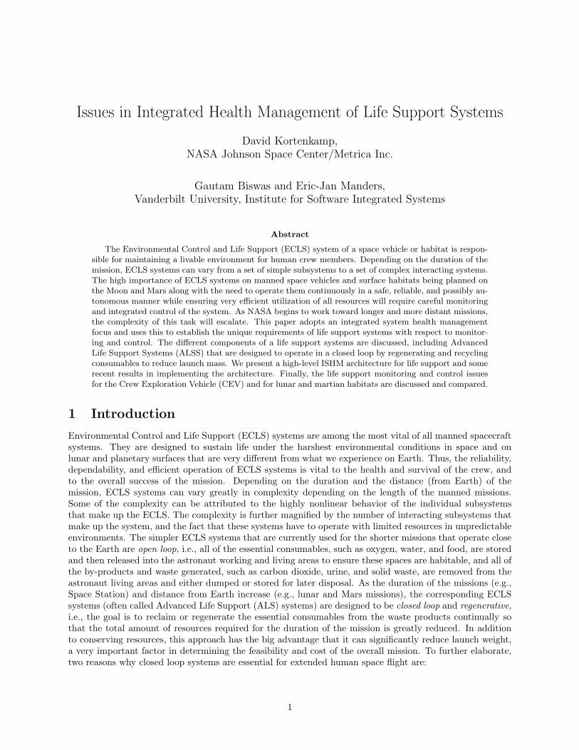
Figure 1: A proposed ISHM architecture for life support systems.

1. the amount of consumable resources required for a long mission (air, water, and food) would far exceedthe payload that current propulsion technology is capable of launching; and

2. resupply of resources during the mission is not a feasible alternative.

Autonomy (or at least human-supported autonomy) for ECLS (and ALS) systems, which have to operatecontinuously at high efficiency to ensure safety, keep energy consumption low, and prevent loses in con-sumables is also an important consideration in such systems. There is no doubt that as mission durationsand distances increase, managing of complex ECLS systems in a safe and reliable manner using currenttechnology and methodologies will become very hard to achieve.

Integrated Systems Health Management (ISHM) refers to a collection of techniques that provide thefunctionality for maintaining system health and performance over the life of a system. This is illustratedin Figure 1. ISHM requires an integrated approach to monitoring, control, fault diagnosis, adaptation, andmaintenance. In all systems that operate for long periods, components in the system are bound to sufferdegradations in performance, and sometimes fail. Therefore, for autonomous and human-in-the-loop systems,ISHM schemes must have the ability to detect these degradations from deviations in system behavior, analyzeperformance and resource usage, and use this information to determine when maintenance is necessary topreserve system functionality and minimize downtime.

The two interacting loops in Figure 1 illustrate this concept. The lower loop includes the traditionalmonitoring, diagnosis, and feedback control systems. The introduction of a supervisory controller in thisloop enables a choice between autonomous fault-adaptive control approaches to mitigate or compensate forthe effects of degradations and faults, and the activation of the second loop, where monitors inform thehuman operators or crew about the status of the system as a whole, and the humans make decisions on whento schedule maintenance operations, and, in some cases, to alter the goals of the mission, because the lossof functionality and/or resources will not allow for previous goals to be accomplished in a safe manner.

Comprehensive ISHM must involve interacting multiple control strategies. At the fast time scales, robustcontrol can be employed to make the functionality of the system independent of the disturbance to thesystem [32]. At this level, the degradations and fault magnitudes are small, and a robust controller cancompensate for discrepancies without noticeable changes in system behavior. The field of robust control iswell developed, and capabilities and limitations of these approaches are well understood [32]. At the nextlevel, Fault Adaptive Control (FAC) [9] goes beyond disturbance handling by changing the system controlstrategy to adapt the system structure and/or functionality to mitigate the fault effects. Examples of theFAC approach are:

2

1. model-predictive control techniques, where diagnosis schemes are applied to compute parameter valuechanges due to faults and degradations, and update the system models used for online control [1]; and

2. supervisory schemes for reconfiguring system structure to nullify fault effects [11].

ISHM for ECLS systems, but especially for ALS systems, poses several significant and unique issues thatinclude:

• Interacting subsystems: Life support systems contain many interacting subsystems. As describedin the next section, air, water, food, and waste systems all generate and consume shared resources,such as electrical power, water, and oxygen. Life support systems also cover a variety of domains, fromphysiological and biological processes to physical processes that include fluid, mechanical, thermal,electrical, and pneumatic systems.

• Sensing: Sensing for life support systems is particularly challenging because of the wide variety ofsensors required. Moreover, current state of the art sensors in these domains, often produce noisyoutput []. Biological elements that include humans, are difficult to monitor. In-line sensing of waterand air quality is difficult, and the current state-of-the-art often requires that samples be analyzedoffline in a laboratory to get reliable estimates. Besides, the different subsystems operate at verydifferent rates, so monitoring and data analysis schemes have to accommodate multi-rate analysis.

• Decision-making: There are several decision-making loops in integrated health management for lifesupport systems (see Figure 1). There are short-term loops that operate in continuous time that areinvolved in regulating and feedback control of the life support processes. Intermediate loops respond toevents (typically fault events) and deal with fault-adaptive control and reconfiguration decisions. Thelong-duration upper loop usually includes humans as decision makers aided by software tools that areinvolved in monitoring and making duration of mission predictions on scarce, consumable resources.To build effective ISHM systems, these loops must be integrated.

• Human involvement: Humans are not only a part of the system in that they produce and consumelife support resources, but they may need to be a part of the decision-making process at all levels, i.e.,in both the lower and upper loops in Figure 1. This places significant requirements on an integratedhealth management system – requirements that may not be necessary in other domains.

This paper presents an overview of integrated health management schemes for ECLS systems. We beginby describing the unique attributes of an ECLS system. We do this by looking at the various modulesthat comprise an ECLS system and the connections between these modules. Next we discuss modeling oflife support systems, which is at the core of our ISHM approach. Then we present a high-level integratedhealth management architecture for ECLS systems and describe some recent results using the architecture.Some of this work is futuristic, however, the diagnostic techniques that we present have already been appliedto a number of real-life applications [19, 7]. We demonstrate the effectiveness of the diagnostic techniquesby showing results we have obtained for degradation and fault analysis in aircraft fuel transfer systems.Finally, we look at future integrated health management needs for life support systems including the CrewExploration Vehicle (CEV) and Lunar and Martian habitats.

1.1 Life support systems

Figure 2 shows a complete and connected ECLS system. Simpler ECLS systems for short missions will nothave several of these components, and they may not operate in a completely connected closed loop form.For example, there may be no biomass or food processor module in a two week manned mission of the CEV,only a food store with sufficient food to last the astronauts for the duration of the mission. A more complete,regenerative system shown in the figure is essential for long duration human missions, such as trip to thesurface of Mars, which would last 15-18 months and have limited resupply opportunities. Typically, mostmissions allocate thin margins for mass, energy and buffers for each system of the spacecraft, and this requiresoptimization during the design phase, and tight control during operations to keep the systems within theirdesired range of behavior, i.e., providing the necessary output while ensuring resource consumption does notexceed pre-specified limits. Since advanced life support systems have many interconnected subsystems all of

3

Figure 2: The various subsystems and recovery systems (RS) and their connections that comprise an envi-ronmental control and life support system.

which share resources and interact in predictable and unpredictable ways, the design and control optimizationtasks become quite difficult, especially if one has to consider the dynamic behavior of the system. In otherwork [1] we have shown that using dynamic models (as opposed to static models) during the design phase andintegrating controller and system design, leads to much smaller buffer sizes (therefore, Equivalent SystemsMass) for the ECLS system.

In this section, we briefly review the different components of an environmental control and life supportsystem. We briefly describe the various, interacting subsystems of ALS using Figure 2 as a reference config-uration. While each subsystem can be self-contained subsystems also interact in terms of sharing differentresources. This section provides sufficient background for readers to become aware of issues that are uniqueto ISHM design of ECLS systems. For detailed documentation on advanced life support systems see [31] orgo to: http://advlifesupport.jsc.nasa.gov.

One of the key issues that one has to take into account is that the human crew are very much a part ofthe physical and biological processes that define the life support systems, and at the same time they playan important role in controlling the operations and managing the working of the system. When developingautonomy by automating the ISHM, control, and resource management functions, interesting issues arisein the interactions between the humans in the control loop and autonomous systems. These issues arediscussed in other papers [1, 5], However, we do take into account biological models of the crew and crewactivity models as part of the overall ECLSS system.

1.1.1 Crew

The crew as a subsystem places demands on the life support system for various resources necessary to sustainlife. Equations that capture human consumption models are available in many papers (e.g., [15]). Thesemodels are parameterized by the number, gender, age and weight of the crew and their typical activity

4

profiles for the particular mission. An integrated monitoring and control system for the ECLS system wouldtrack crew resource use(oxygen, water, food, etc.) over time. This would require a variety of sensors, such asthose that monitor air flow in and out of the crew living and working chambers, its contents (percentage ofoxygen and carbon dioxide, water vapor, and trace contaminants), and its pressure and temperature, while atthe same time monitoring the stores of the consumable resources associated with the air, such as the amountof oxygen, and the amount of chemical filters for available for carbon dioxide removal. In a closed loopsystem, there will be additional subsystems, which replenish the consumable resources, and these processeshave to be monitored so that the control system can maintain the proper balance between consumption andreplenishment, while ensuring that other resource constraints, such as available power, are not violated. Amore advanced life support controller may take into account the biological crew models and their activities,and provide a tool for scheduling crew activities and accommodating crew requests in a way that resourceconstraints are not violated [5].

1.1.2 Water

The water recovery subsystem converts dirty and waste water into potable and grey water (i.e., waterthat can be used for washing but not drinking). An example water recovery system from a recent NASAJSC test consists of four subsystems that process the water[10]. The biological water processing (BWP)subsystem removes organic compounds. Then the water passes to a reverse osmosis (RO) subsystem, whichremoves inorganic and particulate matter by pushing the water through a membrane. About 85% of thedirty water passing through the RO subsystem is converted into grey water. The 15% of water remainingfrom the RO (called brine) is passed to the air evaporation subsystem (AES), which recovers the rest byan evaporation/condensation process. These two streams of grey water (from the RO and the AES) arecombined and passed through a post-processing subsystem (PPS) to remove bacterial traces and generatepotable water. This system can run in various configurations. For example, the BWP can operate withthe pump running at various speeds. The RO is more sophisticated in that it has four modes of operation:(i) a primary mode, where the water circulates on a longer path, (ii) a secondary mode where the waterpath is shortened so it speeds up and pushes harder against the membrane, (iii) a purge mode, where thebrine is transferred to the AES system, and (iv) a clean mode, where the membrane is cleaned of particulatematter by creating a reverse flow through the membrane. The different modes of operation help the systemmaintain desired levels of throughput without exceeding energy consumption constraints. The WRS has anexternal controller that can turn on or off various subsystems (e.g., if needed all the water can be passedthrough the AES, but then the purification process has a high energy cost). In other work, we have designedsophisticated model-predictive controllers that have fault-adaptive properties, and they operate to maintaina tradeoff between energy consumption, throughput, and water quality.

1.1.3 Air

The air subsystem takes in exhalant carbon dioxide CO2 and produces oxygen O2 as long as there is sufficientenergy being provided to the system. An example Air Revitalization System (ARS) from a test at NASAJSC [22] consists of three interacting air subsystems: the Carbon Dioxide Removal System (CRS) in whichCO2 is removed from the air stream; the Carbon Dioxide Reduction Assembly (CDRA), which uses waterto break CO2 down into methane (CH4) and water (H2O); and the Oxygen Generation System (OGS) inwhich O2 is added to the air stream by breaking water down into hydrogen and oxygen. It is important tonote that both the removal of CO2 and the addition of O2 are required for human survival.

1.1.4 Biomass

The biomass subsystem is where crops are grown. It consumes water, energy (light) and CO2 and producesbiomass, which can be turned into food, and O2. Models of crop growth and crop resource consumption canbe found in [17]. This subsystem is optional for all but the longest missions as food can be carried on-boardfairly cheaply if it is dehydrated. However, many mid-term missions could benefit from salad crops (lettuce,tomatoes, carrots) to provide the psychological benefits of eating fresh food. Crops can also be viewed asredundant air and water processors. When one considers the entire ALS configuration, one notes that thetime constants involved in the biomass system vary greatly from the air and water systems.

5

1.1.5 Food processing

Before biomass can be consumed by the crew it must be converted to food. The input to the food processingsubsystem is biomass, energy, and crew time, and the output is food and solid waste. Unless significantautomation is provided, this is a labor intensive process.

1.1.6 Waste

The waste subsystem consumes energy, O2 and solid waste and produces CO2. Some tests have used anincinerator to burn solid waste [28]. There are many other forms of waste recycling besides incineration thatmight be used. Most short duration missions will simply dispose of waste by leaving it behind or packagingit for return back to earth.

1.1.7 Power

While not just a part of the life support system, power is a common thread that enables all of the life supportsubsystems. It also one of the factors that defines the interactions among these subsystems. An integratedmonitoring and control system for ECLS will need to monitor and control power consumption to both staywithin power budgets and react to reductions in available power.

2 Modeling

We adopt a model-based approach to ISHM The basic idea is that well-constructed models capture therelationships between the variables in the system, and between variables and components. These relation-ships form the basis for designing powerful to diagnosis, fault-adaptive control, and prognosis in a commonframework [6].

In its basic form, a model is an executable software representation of a system that can be used tosimulate system behavior. A number of different modeling forms for physical processes have been proposedby design engineers, operations specialists, and maintenance personnel. Integrated health managementsystems for most complex systems, such as the ALS, requires models for analysis of dynamic system behaviorat different levels of detail. Attempting to build a comprehensive detailed first-principles model of thesystem is very difficult and time consuming, and analysis with that kind of a model will most likely becomputationally intractable. Therefore, is important to build models at the right level of detail to supportthe tasks for which they are to be used for. For example, a model for diagnosis should have an explicitrepresentation for the components that are under diagnostic scrutiny. Models for diagnosis and control alsoneed to capture the dynamic behaviors that influence system functionality and performance. On the otherhand, tracking the interactions between subsystems and tracking of system performance may be accomplishedby higher level functional models that focus on interactions that are governed by material balance, energytransfer, and resource consumption, but these models do not need to include details of individual componentdynamics. To develop ISHM applications for the ALS, we build the two kinds of models: (i) those thatmodel subsystem behavior by composing component dynamic behaviors using principles of enegy transferand energy conservation [18, 24], and (ii) higher level models that define subsystem interactions in terms ofmaterial and energy balance and resource consumption [21].

From another perspective, these models correspond to ones that apply to the control loop, and the onesthat apply to the decision-making loop in Figure 1. Our approach to building models for diagnosis and controlis to develop physics-based component models using the bond graph [18] and hybrid bond graphs [24] forcontinuous and hybrid system behaviors, respectively. The decision-making loop models are resource-basedand operate as discrete-time and discrete-event models using very coarse time scales [21]. We discuss ourapproach to the two modeling paradigms next.

2.1 Physics-based modeling

We develop our physics-based component models and compose them into subsystem and system models us-ing well-defined component interfaces defined by our modeling environment toolset [19, 23, 30], The toolset

6

includes component-oriented model libraries of physical processes. Each component has well-designed inter-faces to allow for construction of subsystem and system-level models by composition. The toolset also allowsfor designing sensor and actuator interfaces for plant models, and software-based controllers for managingplant behavior.

Modeling physical system dynamics is based on bond graphs, a methodology that captures multi-domainsystem dynamics into an integrated, homogeneous, energy-based compositional modeling framework [18].The Hybrid Bond Graph (HBG) paradigm is an extension that allows discrete switching between modes ofbehavior to capture both continuous and discrete behaviors of a system [24]. The discrete changes may beattributed to control actions that turn system components on and off or change system parameter settings,and autonomous changes that flip on-off switches when state variables of the system cross pre-specifiedthreshold values. In a HBG, mode changes are implemented by switching bond graph junctions off andon using signals that are computed by parameterized decision functions. Nonlinear systems are modeledby components that have time-varying parameters, i.e., the parameter values are defined by modulationfunctions, whose arguments are again system variables. Parameters for both the decision and modulationfunctions can be system variables and external signals.

The FACT toolset includes translators that can generate simulation test beds for diagnosis and controlapplications [23, 4]. Convenient user interfaces allow the user to enter faults with pre-defined profiles atspecific times into the simulation, and the fault data generated can be used for testing diagnosis and healthmanagement routines.

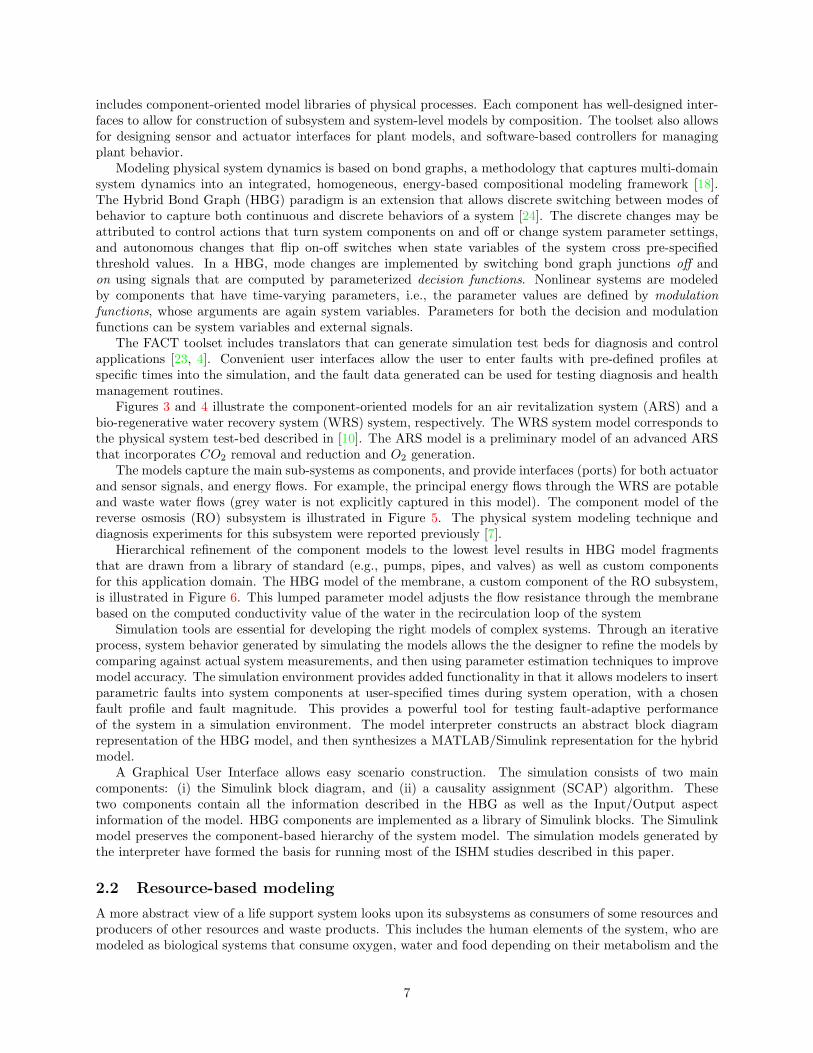
Figures 3 and 4 illustrate the component-oriented models for an air revitalization system (ARS) and abio-regenerative water recovery system (WRS) system, respectively. The WRS system model corresponds tothe physical system test-bed described in [10]. The ARS model is a preliminary model of an advanced ARSthat incorporates CO2 removal and reduction and O2 generation.

The models capture the main sub-systems as components, and provide interfaces (ports) for both actuatorand sensor signals, and energy flows. For example, the principal energy flows through the WRS are potableand waste water flows (grey water is not explicitly captured in this model). The component model of thereverse osmosis (RO) subsystem is illustrated in Figure 5. The physical system modeling technique anddiagnosis experiments for this subsystem were reported previously [7].

Hierarchical refinement of the component models to the lowest level results in HBG model fragmentsthat are drawn from a library of standard (e.g., pumps, pipes, and valves) as well as custom componentsfor this application domain. The HBG model of the membrane, a custom component of the RO subsystem,is illustrated in Figure 6. This lumped parameter model adjusts the flow resistance through the membranebased on the computed conductivity value of the water in the recirculation loop of the system

Simulation tools are essential for developing the right models of complex systems. Through an iterativeprocess, system behavior generated by simulating the models allows the the designer to refine the models bycomparing against actual system measurements, and then using parameter estimation techniques to improvemodel accuracy. The simulation environment provides added functionality in that it allows modelers to insertparametric faults into system components at user-specified times during system operation, with a chosenfault profile and fault magnitude. This provides a powerful tool for testing fault-adaptive performanceof the system in a simulation environment. The model interpreter constructs an abstract block diagramrepresentation of the HBG model, and then synthesizes a MATLAB/Simulink representation for the hybridmodel.

A Graphical User Interface allows easy scenario construction. The simulation consists of two maincomponents: (i) the Simulink block diagram, and (ii) a causality assignment (SCAP) algorithm. Thesetwo components contain all the information described in the HBG as well as the Input/Output aspectinformation of the model. HBG components are implemented as a library of Simulink blocks. The Simulinkmodel preserves the component-based hierarchy of the system model. The simulation models generated bythe interpreter have formed the basis for running most of the ISHM studies described in this paper.

2.2 Resource-based modeling

A more abstract view of a life support system looks upon its subsystems as consumers of some resources andproducers of other resources and waste products. This includes the human elements of the system, who aremodeled as biological systems that consume oxygen, water and food depending on their metabolism and the

7

ARS Concept model

In PresOut

CO2_tank

InSwi Out

H2_Compressor

Air_O2Setp

Air_O2_c

Regulator

O2_Compressor_sw

CO2_Compressor_sw

In CO2Out

Pipe

In PresOut

H2_tank

InSwi Out

O2_Compressor

InSwi Out

CO2_Compressor

CO2H2HeatBlow

CH4H2OT_2F_1

CRS

H2OSetp

O2H2

Pres

OGS

In PresOut

O2_tank

H2_Compressor_sw

HeatHeatBlowPrecAirSValvValvValvValvValvValvAIR_

T_1P_1CO2AIR_

CDRS

CRS_heater

CDRS_HeaterA

Air_in

P_cdrs1

F_CRS1

T_cdrs1

H2O_out

CH4

H2O_in

Air_out

CDRS_Valve3

CRS_blower

Regulator_sp

OGS_sp

P_O2

P_OGS

P_CO2

CDRS_Valve1

T_CRS1

CDRS_AirSavePump

CDRS_HeaterB

CDRS_Valve5

P_H2

CDRS_Precooler

CDRS_Valve4

CDRS_Valve6

CDRS_Valve2

O2_conc

CDRS_Blower

CO2_conc

Figure 3: Component-oriented model of an Air Revitalization System.BioRegenerative WRS with reject valve

P_steam

P_loop

P_condensate

T_air2

RecyclePump_ctl

F_perm

P_GLSNitrifierPump1_ctl

FeedReciValvIn

P_meK

P_puF_peP_loOut_Out_

ReverseOsmosis

P_Nit1

NitrifierAirSlough2

T_coolant

P_pump

Conductivity

T_air1

T_air3

P_wres

FeedPump_ctl

Out_potable

MultiWayValve_ctl

P_OCOR

P_Nit4

FeedPump_ctl

NitrifierPump4_ctl

PosiIn

PresOut1Out2

RejectValve

RejectValve_ctl

P_memb

Heater_ctl

NitrNitrNitrNitrNitrNitrNitrNitrRecyFeedIn

P_NiP_NiP_NiP_Ni

P_OCP_GLP_Re

OutF_ReF_GLP_tmF_FeP_Fe

BioWaterProcessor

BlowHeatCoolCondIn

T_aiT_aiT_ai

T_coV_aiP_st

P_wrP_co

Out

AirEvaporation

P_Nit3

P_RecPump

V_air

RecyclePump_ctl

CoolantPump_ctl

NitrifierAirSlough4

In FlowOut

PostProcessor

NitrifierAirSlough1

NitrifierAirSlough3

CondensatePump_ctl

NitrifierPump3_ctl

Out_reject

P_Nit2

In

Blower_ctl

NitrifierPump2_ctl

Figure 4: Component-oriented model of a Water Recovery System.

8

RO subsystem: Conductivity calculation decoupled from system

BrineFlFlowInMode

K

Conductivity

In

RecircPump_ctl

Out_brine

FeedPump_ctl

P_pump

K

P_loop

P_memb

Out_perm

Valve_ctl

F_perm

PreIn

PreOut

RecirculationPump

PosIn

PreOutOutOut

ThreeWayValve

In FlowOut

InterConnectPipe1

In FlowOut

PermeateOutpipe

In1In2

PresOut

PrimaryMerge

In FlowOut

InterConnectPipe2

KFlowIn

MembPreout_perout_bri

Membrane

In1In2

PresOut

SecondaryMerge

Pum Ene

TubularReservoir

SpeInF

FloOut

FeedPump

Figure 5: Component-oriented model of the Reverse Osmosis system.Membrane

RmembMembPressure

MembPress

Cmemb

K

out_brine

out_permPermeatedFlow

Rdrain

FlowIn

Figure 6: Component HBG model of the Reverse Osmosis system membrane.

activities (see Section 1.1.1). Subsystems of the ALS are modeled as producers and consumers of resources.The underlying technologies, the individual component dynamics and the particular configuration of valves,pumps, blowers, and other components within the subsystem is unimportant for these kinds of analyses,and, therefore, not included in the models.

Over the last several years NASA JSC has been developing a resource-based model of life support systemscalled BioSim [20, 21]. BioSim consists of all of the life support components described in Section 1.1 andshown in Figure 2. Readers interested in experimenting with monitoring or controlling life support systemscan obtain the simulation from http://www.traclabs.com/biosim.

BioSim is a discrete event simulation with a variable time step that is currently set to one hour. Insimulation, each time step is mapped onto a simulation “tick.” Each module has a local counter thatadvances that module’s state from t to t + 1, i.e., advances its state one hour in the default setting. Whileeach module is run sequentially, data is cached so that all modules use data generated from the previoustick, which effectively makes all modules run in parallel.

When modeling life support systems we need to consider nominal and off-nominal situations. BioSimmodels malfunctions in each module and has an application programmer’s interface (API) to introducethose malfunctions at any time in the simulation. Each module can have malfunctions of varying degrees ofseverity and temporal length. For simplicity, the malfunctions have been divided into two categories: length(permanent and temporary) and severity (low, medium and high). These malfunctions are interpreteddifferently by each module. For example, a temporary but severe malfunction in the potable water storewould be a large water leak. A permanent but low severity malfunction in the power production modulewould be the loss of a small part of a solar array.

BioSim also models stochastic processes. Because real life support systems are not deterministic, neitheris the simulation. For example, the exact amount of air that is breathed in by a crew member is differentwith every breath. This is modeled using a Gaussian function with adjustable parameters. The Gaussiancan be set to zero to produce a deterministic simulation.

9

3 System architecture

An ISHM architecture for life support systems will require many interacting components. Figure 1 shows apotential architecture for an ISHM system for life support. Parts of this architecture have been implementedin various life support systems over the past ten years. We will describe each component of the architecturein turn and discuss experimental results.

3.1 Behavior monitors and diagnoser

Model-based approaches to fault detection, isolation and identification (FDII) include many different ap-proaches that have been developed over the past decades [12]. Our focus in this area has been on physicalsystem component faults, rather than sensor or actuator faults. These faults result in transient behavior inthe system response, and analysis of the transient is at the core of the fault isolation algorithms[19, 26, 27].

Our approach to diagnosis explicitly separates the fault detection task from the fault isolation and identi-fication tasks. A numeric observer is realized using an extended Kalman filter-based [14] state estimator [19].Fault detection is realized through a sliding window hypothesis testing scheme in the time domain using abank of Z-test detectors [8], and in the time-frequency domain [23] using an energy-based scheme. Theenergy-based scheme explicitly utilizes the properties of the energy in a fault transient response to designa statistical test that is tuned to trade sensitivity to faults versus likely false alarms. For faults that donot manifest with distinctive transient behaviors, i.e., incipient or degradation faults, our work exploits theresults in the literature on change detection to design fault detection filters that are based on likelihood ratioderived techniques [16].

Fault isolation and identification is implemented as a two-stage process. The first stage uses an qualitativefault isolation engine that operates on a symbolic transformation of the residual [25, 26]. This generatesa potential candidate list and fault signatures that predict measurement fault dynamics after the faultoccurrence. As time progresses and additional measurement deviations are observed, the fault isolationscheme removes spurious candidates from that initial candidate set. Qualitative symbolic analysis is fastbut the loss of information in the transformation can result in multiple candidates. At an appropriate time,the system switches from fault isolation to fault identification [8, 26]. Fault identification uses a searchmethod to perform quantitative parameter estimation with multiple candidate hypotheses. Once reliableestimates are obtained, a minimum square error technique is employed to determine the unique candidateand its estimated parameter value [8]. The fault isolation and identification scheme, initially developed forcontinuous systems, has been extended to diagnosis of hybrid systems [26]. We illustrate the application ofour fault diagnosis scheme for two realistic applications: (i) detection, isolation, and identification of faultsand degradation in fuel transfer systems of fighter aircraft (an aerospace application), and (ii) detection,isolation, and identification of faults in the RO system of the water system described in Section 1.1.2 [7].The two projects used actual data provided by Boeing and a NASA JSC RO system test, respectively.

3.1.1 Diagnosis of component faults in the Fuel Transfer System

The generic fuel transfer system for fighter aircraft is illustrated in Figure 7. The system is designed toprovide an uninterrupted supply of fuel at a constant rate to the aircraft engines while maintaining thecenter of gravity of the aircraft. The system is symmetrically divided into left and right parts (top andbottom in the schematic). The four supply tanks (Left Wing (LWT), Right Wing (RWT), Left Transfer(LTT), and Right Transfer (RTT)) are full initially, and so are the two receiving tanks (Left Feed (LFT)and Right Feed (RFT)) that directly feed the engine. During engine operation, fuel is transferred from thesupply tanks through a common manifold to the two feed tanks in a sequence determined by the fuel systemcontroller. The controller generates on/off signals for the pumps in the supply tanks and the valves in thepipes to achieve different flow configurations.

Table 1 illustrates the results of a set of diagnosis experiments that we ran for a set of faults using theHBG scheme. In the experiments, we varied the fault size and amount of measurement noise in the signal.In designing the experiments, we had to set parameters for the Kalman filter, fault detector, and symbolgenerator. A high fidelity simulator (from Boeing PhantomWorks in St. Louis, MO) was used to generatethe data for the experimental runs, and measurement noise was added to the simulated data. Ten runswere conducted for each noise level and fault size, and the mean values of the detection and isolation times,

10

PP

PP

PP

P PLV

LV

IV IV

BP

BP

FM

FM

P Transfer PumpLV Level Control ValveIV Interconnect ValveBP Boost PumpFM Flow Meter

Fuel Quantity Sensor

Left Transfer Tank

Right Transfer Tank

Left Wing Tank

Right Wing Tank

Left FeedTank

Right FeedTank

Left Engine

Right Engine

Typical Fuel System Configuration

FEED

INTER-CONNECT

TRANSFER

Figure 7: Fuel Transfer System of fighter aircraft.

Faults Performance Parameters

FaultType

FaultSize

Fault Detection Fault Isolation Final Candidate Parameter Estimation

Time (seconds) Time (seconds) Set (number) Error (percent)

2% 3% 2% 3% 2% 3% 2% 3%

LTT-PumpEfficiency Drop

33% 422 555 225 398 3 4 2.19% 5.43%

60% 182 183 144 240 4 4 1.28% 1.79%

80% 134 134 124 197 4 5 0.88% 1.49%

RWT-PumpEfficiency Drop

33% 117 285 170 211 4 4 2.15% 6.11%

60% 83 93 139 183 4 4 1.52% 1.67%

80% 5 5 55 106 3 4 0.68% 0.68%

RLCV ValveBlock

× 1.5 63 65 97 103 2 2 0.62% 0.5%

× 1.75 51 58 86 398 2 1 0.28% 0.46%

× 2.0 51 52 46 79 1 2 0.2% 0.2%

Leg 21 PipeBlock

× 1.5 99 100 136 150 3 3 1.58% 1.65%

× 1.75 95 95 90 303 2 3 0.78% 1.57%

× 2.0 93 93 76 202 2 2 0.19% 0.34%

Table 1: Fuel System Experiments with different fault magnitudes and noise levels.

the candidates generated by qualitative fault isolation, and the parameter value error after least squaresestimation are reported in the table. Note that the results of the qualitative fault isolation are ambiguousand they produce multiple fault candidates. The quantitative parameter estimation procedure reduces thefault hypotheses to a single candidate, and also estimates the magnitude of change in the parameter as aresult of the fault or degradation in the particular component. The results indicate that as the noise levelsin the measurements increase and the fault magnitudes become smaller the time to detection, isolation, andidentification (i.e., parameter estimation) increase, and the parameter estimation error increases. Furtherdetails of the fuel system models and diagnosis experiments can be found in [26].

11

3.1.2 Diagnosis of component faults in the Reverse Osmosis system

Similar health monitoring studies were conducted on the Reverse Osmosis (RO) subsystem mentioned earlier.The WRS and RO system models illustrated in Figure 4 and Figure 5 capture the physical flow thourgh thesystem. Input water from the previous subsystem, a Biological Waste Processor (BWP) is pushed at highpressure through the membrane. Clean water (permeate) leaves the system, and the remaining water (witha larger concentration of brine) is recirculated in a feedback loop.

As a result, the concentration of impurities in the recirculating water increases with time. The systemcycles through three operating modes, which are set by the 4-way multi-position valve. The feed pump,which is on in all modes, pulls effluent from the BWP and creates a flow into the system through a coiledpipe, which acts as a tubular reservoir. In the primary mode (valve setting 1), the input flow is mixedwith the water in the primary recirculation loop. The recirculation pump boosts the liquid pressure as itflows into the membrane. The flow through causes dirt to accumulate in the membrane, which increasesthe resistance to the flow through it, thus causing the outflow from the system to decrease with time. Ata predetermined fluid pressure value at the membrane, the system switches to the secondary mode (valvesetting 2), and the recirculating fluid is routed back to the membrane in a smaller secondary loop. Thiscauses the liquid velocity (and, therefore, flowrate) to increase, and as a result the outflow from the systemdoes not keep decreasing as sharply as it does in the primary loop.

As clean water leaves the system, the concentration of brine in the residual water in the RO loop keepsincreasing. At some point the increasing concentration plus the collection of impurities in the membranedecreases the output flow significantly, and again at a predetermined pressure value the RO switches to thepurge mode (valve setting 3), where the recirculation pump is turned off, and concentrated brine is pushedout to the next subsystem, the Air Evaporation System (AES). Following the purge operation, the systemgoes back to primary mode.

For the health monitoring experiments, we used five of the measurements (see Figure 5): (i) the pressureimmediately after the recirculation pump, Ppump, (ii) the pressure of the permeate at the membrane, Pmemb

(iii) the pressure of the liquid in the return path of the recirculation loop, Pback, (iv) the flow rate of theeffluent, Fperm, and the conductivity of liquid in the return path of the recirculation loop, K.

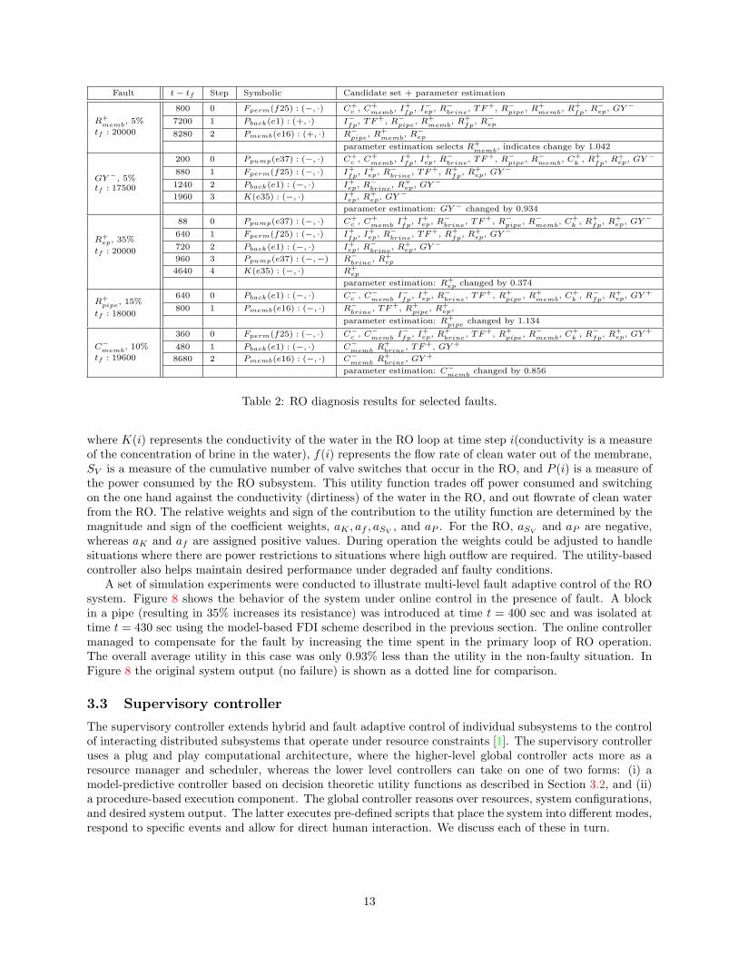
Simulation experiments were run on a number of fault scenarios. Empirical information on sensor noisewas not available, so we simulated measurement noise as Gaussian white noise with a noise power level setat 2% of the average signal power for each measurement. Fault scenarios were created that correspond toabrupt faults in the pump (loss of efficiency and increased friction in the bearings), membrane (clogging),and the connecting pipes (blocks). Table 2 presents the comprehensive results for selected faults in the ROsystem. For each scenario, the qualitative fault isolation scheme reduces the initial candidate set considerably,and parameter estimation converges to the correct fault candidate. The estimated parameter values werealso quite acceptable for all scenarios. This demonstrated the effectiveness of the health monitoring, faultsisolation, and fault identification methodology.

3.2 Fault-adaptive controller

The Fault Adaptive Control scheme is designed as a hierarchical limited look-ahead control scheme [2, 3],where the overall control scheme tries to satisfy given specifications (e.g., throughput for the WRS system)by continuously monitoring the system state and selecting input from a finite control set that will best meetthe given specifications. In addition, the controller is required to keep the system stable within the domainthat satisfies the specifications.

In this setting, the controller is simply an agent that generates a sequence of events to achieve a givenobjective. This objective is typically expressed as a multi-attribute utility function that takes the form∑

i Vi(Pi), where each Vi corresponds to a value function associated with performance parameter, Pi. Theparameters, Pi, can be continuous or discrete-valued, and they are derived from the system state variables,x(t), i.e., Pi(t) = pi(x(t)). The value functions employed have been simple weighted functions of the formVi(Pi) = wi · Pi, where the weights, wi ∈ [−1, 1] represent the importance of the parameter in the overalloperation of the system. For example, the utility function for the RO system is given by

V (k) =k+N∑i=k

aK(K(i)

KMAX) + af (

f(i)fMAX

) + aSV.SV + aP (

P (i)PMAX

),

12

Fault t − tf Step Symbolic Candidate set + parameter estimation

R+memb

, 5%

tf : 20000

800 0 Fperm(f25) : (−, ·) C+c , C+

memb, I+

fp, I−ep, R−

brine, TF+, R−

pipe, R+

memb, R+

fp, R−ep, GY −

7200 1 Pback(e1) : (+, ·) I−fp

, TF+, R−pipe

, R+memb

, R+fp

, R−ep

8280 2 Pmemb(e16) : (+, ·) R−pipe

, R+memb

, R−ep

parameter estimation selects R+memb

, indicates change by 1.042

GY −, 5%tf : 17500

200 0 Ppump(e37) : (−, ·) C+c , C+

memb, I+

fp, I+

ep, R−brine

, TF+, R−pipe

, R−memb

, C+k

, R+fp

, R+ep, GY −

880 1 Fperm(f25) : (−, ·) I+fp

, I+ep, R−

brine, TF+, R+

fp, R+

ep, GY −

1240 2 Pback(e1) : (−, ·) I+ep, R−

brine, R+

ep, GY −

1960 3 K(e35) : (−, ·) I+ep, R+

ep, GY −

parameter estimation: GY − changed by 0.934

R+ep, 35%

tf : 20000

88 0 Ppump(e37) : (−, ·) C+c , C+

membI+

fp, I+

ep, R−brine

, TF+, R−pipe

, R−memb

, C+k

, R+fp

, R+ep, GY −

640 1 Fperm(f25) : (−, ·) I+fp

, I+ep, R−

brine, TF+, R+

fp, R+

ep, GY −

720 2 Pback(e1) : (−, ·) I+ep, R−

brine, R+

ep, GY −

960 3 Ppump(e37) : (−,−) R−brine

, R+ep

4640 4 K(e35) : (−, ·) R+ep

parameter estimation: R+ep changed by 0.374

R+pipe

, 15%

tf : 18000

640 0 Pback(e1) : (−, ·) C−c , C−memb

I−fp

, I+ep, R−

brine, TF+, R+

pipe, R+

memb, C+

k, R−

fp, R+

ep, GY +

800 1 Pmemb(e16) : (−, ·) R−brine

, TF+, R+pipe

, R+ep,

parameter estimation: R+pipe

changed by 1.134

C−memb

, 10%

tf : 19600

360 0 Fperm(f25) : (−, ·) C−c , C−memb

I−fp

, I+ep, R+

brine, TF+, R+

pipe, R−

memb, C+

k, R−

fp, R+

ep, GY +

480 1 Pback(e1) : (−, ·) C−memb

R+brine

, TF+, GY +

8680 2 Pmemb(e16) : (−, ·) C−memb

R+brine

, GY +

parameter estimation: C−memb

changed by 0.856

Table 2: RO diagnosis results for selected faults.

where K(i) represents the conductivity of the water in the RO loop at time step i(conductivity is a measureof the concentration of brine in the water), f(i) represents the flow rate of clean water out of the membrane,SV is a measure of the cumulative number of valve switches that occur in the RO, and P (i) is a measure ofthe power consumed by the RO subsystem. This utility function trades off power consumed and switchingon the one hand against the conductivity (dirtiness) of the water in the RO, and out flowrate of clean waterfrom the RO. The relative weights and sign of the contribution to the utility function are determined by themagnitude and sign of the coefficient weights, aK , af , aSV

, and aP . For the RO, aSVand aP are negative,

whereas aK and af are assigned positive values. During operation the weights could be adjusted to handlesituations where there are power restrictions to situations where high outflow are required. The utility-basedcontroller also helps maintain desired performance under degraded anf faulty conditions.

A set of simulation experiments were conducted to illustrate multi-level fault adaptive control of the ROsystem. Figure 8 shows the behavior of the system under online control in the presence of fault. A blockin a pipe (resulting in 35% increases its resistance) was introduced at time t = 400 sec and was isolated attime t = 430 sec using the model-based FDI scheme described in the previous section. The online controllermanaged to compensate for the fault by increasing the time spent in the primary loop of RO operation.The overall average utility in this case was only 0.93% less than the utility in the non-faulty situation. InFigure 8 the original system output (no failure) is shown as a dotted line for comparison.

3.3 Supervisory controller

The supervisory controller extends hybrid and fault adaptive control of individual subsystems to the controlof interacting distributed subsystems that operate under resource constraints [1]. The supervisory controlleruses a plug and play computational architecture, where the higher-level global controller acts more as aresource manager and scheduler, whereas the lower level controllers can take on one of two forms: (i) amodel-predictive controller based on decision theoretic utility functions as described in Section 3.2, and (ii)a procedure-based execution component. The global controller reasons over resources, system configurations,and desired system output. The latter executes pre-defined scripts that place the system into different modes,respond to specific events and allow for direct human interaction. We discuss each of these in turn.

13

Figure 8: System Performance with Utility-based controller under fault conditions.

3.3.1 Supervisory Controller

Since a detailed behavioral model of the underlying distributed system may be very complex, reasoning atthis level uses an abstract (simplified) model to describe the composite behavior of the system componentsthat is relevant to the overall requirements and operational constraints. The abstract model uses a set ofglobal variables that are related by the input-output interactions between the individual systems. Moreover,the global controller’s decisions are based on aggregate behaviors, which are determined over longer timeframes compared to the individual systems. The global model is represented by y(k+1) = g(y(k), v(k), µ(k)),where y(k) is the global state vector, v(k) ∈ V and V is the set of global control inputs which represent aset of local control settings for the local modules, and µ(k) are the global environmental inputs. The mapg defines how the global state variables respond to relevant changes in environment inputs with respect tothe global control inputs. The objective of the model-based reasoner is to minimize a given cost functionover the operation span of the system. We assume here also that the cost function takes the form of theset point specification. The global specifications are communicated to the procedure-based executor forimplementation.

3.3.2 Procedure-based execution

Procedures are standardized methods for operating a system. They are pre-defined by system engineers.They typically involve a sequence of commands given to the system to move it from one configuration toanother. They can be initiated by automation or by a human. In previous life support applications wehave used the Reactive Action Packages (RAP) system [13] for procedure representation and procedureexecution [10]. Each procedure in the RAP system consists of a set of preconditions (conditions that mustbe true before the procedure can be executed), a set of commands to be executed and a set of succeedconditions (conditions that are true after executing the procedure). The set of commands can be ordered invarious ways (e.g., parallel, sequential) and controlled via timing relationships between the steps. Procedurescannot be created on-the-fly but are all pre-defined and available for execution. Automation or humans canrequest that a procedure be executed. In addition, procedures can be triggered automatically by specificexternal events.

14

Figure 9: Drawing of the proposed Northrop Grumman/Boeing CEV.

3.4 Resource monitors

Resources are vital to the success of any space mission and to life support systems specifically. The ability tomanage resources directly affects the mass of a space vehicle which directly affects its cost. For life supportsystems, resources include gases (such as oxygen, nitrogen and carbon dioxide), water, food, waste (liquidand solid), power, storage tanks and any spare parts such as filters. Resource monitors are responsible forpredicting the need for a particular resource over the length of the mission and for allocating and optimizingresource usage. Resource monitors provide an absolute constraint on the supervisory controller describedabove.

3.5 Planner and scheduler

Life support activities, including crew activities that impact life support systems such as exercise, need to bescheduled so as to balance system and crew activities. In current space mission operations this is primarilya manual process done by ground controllers. In ground tests we have begun experimenting with automatedplanning and scheduling of life support activities. For example, in a space habitat test in 1998 an automatedplanner was used to schedule solid waste incineration [29].

4 Future NASA life support applications

NASA is embarking on a new exploration vision that will take it to the Moon and beyond. A new set ofvehicles and spacecraft is currently being designed to achieve this mission. Each vehicle or spacecraft willrequire different kinds of life support systems and, therefore, different kinds of health management systemsfor life support.

4.1 Crew exploration vehicle

The Crew Exploration Vehicle (CEV) will be NASA’s successor to the Space Shuttle and will carry humansto the International Space Station by 2012 and back to the Moon by 2018. Because it will primarily beused for short-duration flights it will not have complex, regenerative life support systems. However, therewill still be a need for integrated system health management for both the CEV and the ECLS system ofthe CEV. Most of this will focus on the air subsystem, i.e., those components that create oxygen, remove

15

carbon dioxide and detect trace contaminants. System health management for CEV will encompass morethan just fault detection. It will need to be proactive in allocating resources (especially power), schedulingECLS activities and assessing the life support system’s state and capabilities.

The current NASA lunar exploration architecture states that the CEV will be uncrewed in lunar orbitwhile astronauts explore the lunar surface. Some scenarios envision uncrewed operation for nearly six months.Such uncrewed activities will pose significant system health management requirements – the crew on thesurface needs to know that they are returning to a habitable spacecraft. The life support systems will eitherneed to shut down and be restarted or will need to operate during the uncrewed periods. These systems willneed to be checked out or restarted before the crew returns.

4.2 Lunar habitats

A long-term lunar habitat will require significantly more complex life support systems because of the cost ofresupplying resources. In particular, regenerative life support systems will be required especially for air andwater. Such life support systems will need even more complicated and integrated system health managers.Planning and scheduling will become more prominent with long-duration missions. Resource monitoring andmanagement will extend mission life at lower costs.

4.3 Mars habitats

Mars habitats will require significant regeneration of resources, possibly including food. Because of thesignificant time delays these life support systems will have to be almost entirely autonomous. Adding cropsinto a life support systems adds redundancy (crops can produce oxygen, consume carbon dioxide and cleanwater) in addition to providing food. However, being entirely biological, crops pose significant problems tointegrated health management. They are difficult to model and almost impossible to control. Crop plantingand harvesting must be planned and scheduled and is driven by a variety of constraints.

5 Conclusions

Integrated health management for life support systems poses several interesting challenges mostly becauseof the human’s impact on the life support system. In most other vehicle systems (propulsion, guidance,navigation and control, power, etc.) the human impact is minimal. In life support systems the humanimpact is substantial. Humans are producers and consumers of life support system resources. This leads tomodeling challenges, human-interaction challenges and control challenges. In this paper, we have outlined apotential approach to building an integrated health management system for life support systems for long-duration missions. Pieces of this approach have already been tested in simulation and in hardware tests. Wehave briefly described some of our previous work in applying diagnosis and fault-adaptive control techniquesto aircraft and ALSS subsystems. For NASA to realize its human exploration vision, additional developmentand testing of health management for life support systems needs to be done. An important decision thatneeds to be made is that for economic and practical reasons, it is best that the ISHM design be incorporatedinto the early design phase of the CEV and future mission spacecraft systems.

References

[1] S. Abdelwahed, J. Wu, G. Biswas, and E.-J. Manders. Hierarchical online control design for autonomousresource management in advanced life support systems. In Proc. of the 35th Intl. Conf. on EnvironmentalSystems, Rome, Italy, July 2005.

[2] S. Abdelwahed, J. Wu, G. Biswas, J. Ramirez, and E.-J. Manders. On-line hierarchical fault adaptivecontrol for advanced life support systems. In Proc. of the 34nd Intl. Conf. on Environmental Systems,Colorado Springs, CO, July 2004.

16

[3] S. Abdelwahed, J. Wu, G. Biswas, J. Ramirez, and E.-J. Manders. Online adaptive control for effectiveresource management in advanced life support systems. Habitation - An International Journal forHuman Support Research, 10(2):105–115, February 2005.

[4] C. D. Beers, E.-J. Manders, G. Biswas, and P. J. Mosterman. Building efficient simulations from hybridbond graph models. In IFAC Conference on analysis and design of hybrid systems, Alghero, Italy, June2006. To Appear.

[5] G. Biswas, P. Bonasso, S. Abdelwahed, E.-J. Manders, J. Wu, D. Kortenkamp, and S. Bell. Requirementsfor an autonomous control architecture for advanced life support systems. In Proc. of the 35th Intl.Conf. on Environmental Systems, Rome, Italy, July 2005.

[6] G. Biswas and E.-J. Manders. Integrated systems health management to achieve autonomy in complexsystems. In Proc. of 6th IFAC Symposium On Fault Detection Supervision and Safety for TechnicalProcesses. Beijing, PR China, August 2006. To Appear.

[7] G. Biswas, E.-J. Manders, J. Ramirez, N. Mahadevan, and S. Abdelwahed. Online model-based diagnosisto support autonomous operation of an advanced life support system. Habitation: An InternationalJournal for Human Support Research, 10(1):21–38, January 2004.

[8] G. Biswas, G. Simon, N. Mahadevan, S. Narasimhan, J. Ramirez, and G. Karsai. A robust method forhybrid diagnosis of complex systems. In Proc. of 5th IFAC Symposium On Fault Detection Supervisionand Safety for Technical Processes, pages 1125–1131, Washington, DC, June 2003.

[9] M. Blanke, R. Izadi-Zamanabadi, S.A. Bogh, and C.P. Lunau. Fault-tolerant control systems - a holisticview. Control Engineering Practice, 5(5):693–702, 1997.

[10] R. Peter Bonasso, David Kortenkamp, and Carroll Thronesbery. Intelligent control of a water recoverysystem. AI Magazine, 24(1), 2003.

[11] C. G. Cassandras and S. Lafortune. Introduction to Discrete Event Systems. Kluwer, Norwell, MA,1999.

[12] J. Chen and R. J. Patton. Robust Model-Based Fault Diagnosis for Dynamic Systems. Kluwer Academicpublishers, Boston, MA USA, 1998.

[13] R. James Firby. An investigation into reactive planning in complex domains. In Proceedings of theNational Conference on Artificial Intelligence (AAAI), 1987.

[14] A. Gelb. Applied optimal Estimation. MIT Press, Cambridge, MA, 1994.

[15] Sara Goudarzi and K.C. Ting. Top-level modeling of crew component of alss. In Proceedings Interna-tional Conference on Environmental Systems, 1999.

[16] F. Gustafsson. Adaptive filtering and change detection. John Wiley & Sons, Ltd, United Kingdom,2000.

[17] Harry Jones and James Cavazzoni. Top-level crop models for advanced life support analysis. In Pro-ceedings International Conference on Environmental Systems, SAE paper 2000-01-2261, 2000.

[18] D. C. Karnopp, D. L. Margolis, and R. C. Rosenberg. Systems Dynamics: Modeling and Simulation ofMechatronic Systems. John Wiley & Sons, Inc., New York, third edition, 2000.

[19] G. Karsai, G. Biswas, T. Pasternak, S. Narasimhan, G. Peceli, G. Simon, and T. Kovacshazy. Towardsfault-adaptive control of complex dynamical systems. In T. Samad and G. Balas, editors, Software-Enabled Control – Information Technology for Dynamical Systems, chapter 17, pages 347–368. Wiley-IEEE press, Piscataway, NJ, 2003.

[20] David Kortenkamp and Scott Bell. Simulating advanced life support systems for integrated controlsresearch. In Proceedings International Conference on Environmental Systems, 2003.

17

[21] David Kortenkamp, Scott Bell, and Luis Rodriguez. Simulating lunar habitats and activities to derivesystem requirements. In Proceedings 1st AIAA Space Exploration Conference, 2005.

[22] Jane Malin, Joseph Nieten, Debra Schreckenghost, Matt MacMahon, Jeffrey Graham, Carroll Thrones-bery, R. Peter Bonasso, Jeffrey Kowing, and Land Fleming. Multi-agent diagnosis and control of an airrevitalization system for life support in space. In Proceedings of the IEEE Aerospace Conference, 2000.

[23] E-.J. Manders, G. Biswas, J. Ramirez, N. Mahadevan, J. Wu, and S. Abdelwahed. A model-integratedcomputing tool-suite for fault adaptive control. In Working Papers of the Fifteenth Intl. Workshop onPrinciples of Diagnosis, Carcassonne, France, June 2004.

[24] P. J. Mosterman and G. Biswas. A theory of discontinuities in physical system models. Journal of theFranklin Institute, 335B(3):401–439, 1998.

[25] P. J. Mosterman and G. Biswas. Diagnosis of continuous valued systems in transient operating regions.IEEE Trans. on Systems, Man and Cybernetics – part A, 29(6):554–565, 1999.

[26] S. Narasimhan and G. Biswas. Model based diagnosis of hybrid systems. IEEE Trans. on Systems,Man and Cybernetics – part B, 2006.

[27] I. Roychoudhoury, G. Biswas, X. Koutsoukos, and S. Abdelwahed. Distributed diagnosis. In WorkingPapers Fifteenth Int Workshop Principles Diagnosis, Monterey, CA, June 2005.

[28] Debra Schreckenghost, Cheryl Martin, Pete Bonasso, David Kortenkamp, Tod Milam, and CarrollThronesbery. Supporting group interaction among humans and autonomous agents. In AAAI 2002Workshop on Autonomy, Delegation, and Control: From Inter-Agent to Groups, 2002.

[29] Debra Schreckenghost, Daniel Ryan, Carroll Thronesbery, R. Peter Bonasso, and Daniel Poirot. Intelli-gent control of life support systems for space habitats. In Proceedings of the Conference on InnovativeApplications of Artificial Intelligence, 1998.

[30] G. Simon, G. Karsai, G. Biswas, S. Abdelwahed, N Mahadevan, T Szemethy, G. Peceli, and T. Ko-vacshazy. Model-based fault adaptive control of complex dynamic systems. In Proc. of the 20th IEEEInstrumentation and Measurement Technology Conf., Vail, CO, May 2003.

[31] T. O. Tri. Bioregenerative planetary life support systems test complex (bio-plex): Test mission objectivesand facility development. In Proc. of the 29th Intl. Conf. on Environmental Systems, 1999.

[32] K. Zhou and J. Doyle. Essentials of Robust Control. Prentice Hall, Inc, 1998.

18