1

FAO Regional Office for Europe and Central Asia

Policy Studies on Rural Transition No. 2012-3

Issues Affecting the Future of Agriculture and Food Security for

Europe and Central Asia

William H. Meyers, Jadwiga R. Ziolkowska,

Monika Tothova and Kateryna Goychuk

July 2012

2

The Regional Office for Europe and Central Asia of the Food and Agriculture Organization distributes this policy study to disseminate findings of work in progress and to encourage the exchange of ideas within FAO and all others interested in development issues. This paper carries the name of the authors and should be used and cited accordingly. The findings, interpretations and conclusions are the authors’ own and should not be attributed to the Food and Agriculture Organization of the UN, its management, or any member countries.

Author’s affiliations at the time of writing are Howard Cowden Professor of Agricultural and Applied Economics and FAPRI, University of Missouri; Postdoctoral Researcher, Department of Agricultural Economics, Humboldt University of Berlin; Policy Analyst, European Commission; and PhD graduate research assistant, Department of Agricultural and Applied Economics and FAPRI, University of Missouri. The views expressed in this paper are those of the authors and should not be attributed to their affiliated institutions.

3

Contents Introduction ............................................................................................................................................................. 5

Theme 1. Agricultural Technologies .................................................................................................................... 10

1.1 Setting the stage: High prices, volatility, new market environment ........................................................... 10

1.2 Why the current interest in technology? ..................................................................................................... 11

1.3 Evidence of decreasing yield growth in various countries?........................................................................ 13

1.4 What can be done ........................................................................................................................................ 18

1.5 Differences within the region and different policy priorities ...................................................................... 21

1.6 Management of agricultural research .......................................................................................................... 22

1.7 Public and private investment, research in particular ................................................................................. 24

1.8 Diffusion of information to support technology adoption .......................................................................... 26

1.9 Concluding thoughts ................................................................................................................................... 30

Theme 2. Investment in agriculture ..................................................................................................................... 32

2.1 Introduction ................................................................................................................................................. 32

2.2 Historic trends and current conditions of agricultural investment in Europe and Central Asia ................. 33

2.2.1 State of investment in agriculture ........................................................................................................ 33

2.2.2 Investment climate ............................................................................................................................... 36

2.3 Benefits and risks of investment in agriculture........................................................................................... 42

2.4 The investment challenge for investors and policy makers ........................................................................ 45

References for Themes 1 and 2 ............................................................................................................................. 47

Theme 3. Climate change ..................................................................................................................................... 52

3.1 Agriculture in the climate change discussion – problems and challenges .................................................. 52

3.1.1 Impacts of climate change in Europe and Central Asia – current developments and long-term projections ..................................................................................................................................................... 53

3.1.2 Climate change and biodiversity loss ............................................................................................. 57

3.1.3 Climate change impacts on food security ....................................................................................... 58

3.2 Mitigation options in the agricultural and forestry sectors .................................................................... 59

3.3 Adaptation of agriculture to climate change .......................................................................................... 62

3.4 Need for action, recommendations and synergies between mitigation and adaptation in the agricultural sector ................................................................................................................................................................. 66

Theme 4.Bioenergy ............................................................................................................................................... 68

4.1 Bioenergy production technologies ........................................................................................................ 68

4.2 Current situation and projections for the biofuels markets .................................................................... 69

4.3 Impacts of bioenergy production on food security................................................................................. 71

4.4 Effects and implications of biofuels production .................................................................................... 72

4.4.1 Environmental effects of biofuels production ................................................................................. 73

4.4.2 Socio-economic effects of biofuels production .............................................................................. 75

4.4.3 Technical and sustainability aspects ............................................................................................... 75

4.5 Bioenergy in Europe and Central Asia ................................................................................................... 77

4.6 Recommendations for policy making .................................................................................................... 79

Theme 5. Environmental sustainability ................................................................................................................ 82

5.1 Land degradation, soil health and soil loss ................................................................................................. 82

5.2 Water pollution and conservation ............................................................................................................... 85

5.3 Biodiversity ................................................................................................................................................. 87

5.3.1 Plant genetic resources ......................................................................................................................... 89

5.3.2 Animal genetic resources ..................................................................................................................... 94

5.3.3 Forest genetic resources ....................................................................................................................... 95

5.3.4 Aquatic genetic resources .................................................................................................................... 96

5.3.5 Microorganisms and invertebrates ....................................................................................................... 97

4

5.4 Recommendations ....................................................................................................................................... 97

References for Themes 3, 4 and 5 ......................................................................................................................... 99

Theme 6. Institutional and policy changes ......................................................................................................... 105

6.1 Economic and Market Context for the policy agenda .............................................................................. 105

6.1.1 Outlook for economic recovery ......................................................................................................... 105

6.1.2 Outlook for agricultural markets and trade ........................................................................................ 106

6.2 Policy agenda for an uncertain future ....................................................................................................... 106

6.2.1 Technology and investment in agriculture ......................................................................................... 107

6.2.2 Climate change................................................................................................................................... 110

6.2.3 Bioenergy ........................................................................................................................................... 112

6.2.4 Environmental sustainability ............................................................................................................. 113

6.3 Policy Priorities ......................................................................................................................................... 113

References for Theme 6 ...................................................................................................................................... 116

ANNEXES .......................................................................................................................................................... 117

FAO Regional Office for Europe and Central Asia Policy Studies on Rural Transition ................................... 172

5

Introduction

The purpose of this paper is to suggest how the thematic issues in each section are related to the future of agriculture and food security in Europe (West and East) and Central Asia. These sections of the paper state the basic issues under each theme, outline the latest literature on the subtopics, discuss the main issues that are important for this region, and suggest how FAO and member countries can address these issues through policy and institutional actions and reforms. Public goods provision is a cross-cutting issue. Although the scope of this paper covers all of the region, there will be considerably more emphasis on the transition countries of the region, including the EU-12, and less on the EU-15 or old member states (OMS) of the EU.

It is well understood that the Central and Eastern Europe and Central Asia regions encompass a great deal of diversity. All countries have been through a transition of institutions and governance during the last twenty years but the initial conditions, transition policies and the pace and direction of reforms and restructuring varied greatly as did the consequences for the social and economic well-being of the populations and the business environment. To highlight some of these differences and anticipate some of the implications for policy responses, this large and diverse group of countries is divided into three subgroups: the European Union New Member States (NMS), Other European (OEUR), and Southern Caucasus/Central Asia (SCCA). As is clear from data, there is still much diversity within each group, so any generalizations about these sub-regions are likely to be misleading (Table 1). (Kosovo, which declared its independence from Serbia in February 2008 and is recognized by many countries, including most EU member states, is included but there is very limited data as of yet.)

The greatest degree of commonality is found in the European Union NMS that have adopted common policies and regulations of the European Union and have undertaken harmonization of reforms and institutions to apply the regulations of and to be competitive within the European Union. The OEUR group includes European Union candidate countries at various stages of the accession process, potential candidate countries, at various stages of negotiating pre-accession, and other countries at differing stages of reform.

Economic development as measured by per capita Gross Domestic Product measured in purchasing power parity (GDP/PPP) in 2010 varies widely in each of the groups and there is overlap in GDP levels between the groups. These levels also reflect differing impacts of the 2009 recession which hit some countries much more than others and will be discussed below. The income class designations of the World Bank indicate which are in the high income (HI), upper middle income (UMI), lower middle income (LMI), and low income (LI) classification as of July 2011. Again, there is some overlapping, with a few UMI countries among the EU-15 and a wide range from LI to UMI countries in the SCCA group.

From 1989 to 2008, just before the global economic crisis, many economies had recovered from the initial transition declines and posted substantial increases (index well over 100), some have recovered to nearly where they were in 1989 (index near 100) and some are still below their 1989 level (index below 100). Real GDP growth rates were mostly very strong (4 per cent or more) over the ten years before the economic crisis and in most countries adding the two years after 2008 reduced this growth rate.

6

Table 1. Comparison of selected economic, institutional and food security measures by country

Countries 2010 2011 2008 Real 1998-2008 1998-2010 2006-08 2010

USD/cap Income GDP GDP % GDP % % score

European Union NMS GDP(PPP) class 1989=100 Per year Per year FAO* TI**

Slovenia 28 072 HI 156 4.3 3.5 <5 46

Czech Republic 24 950 HI 142 4.1 3.6 <5 na

Slovak Republic 22 195 HI 164 5.3 4.9 <5 50

Poland 18 981 HI 178 4.0 4.1 <5 54

Hungary 18 841 HI 136 3.9 2.6 <5 54

Estonia 18 527 HI 147 7.3 5.2 <5 53

Lithuania 17 235 UMI 120 7.0 5.3 <5 49

Latvia 14 504 UMI 118 7.8 5.4 <5 49

Bulgaria 12 934 UMI 114 5.4 4.8 <5 48

Romania 11 895 UMI 128 5.5 4.7 <5 49

Other European

Croatia 17 819 HI 111 4.1 3.4 <5 48

Russian Federation 15 612 UMI 108 6.8 5.8 <5 42

Belarus 13 874 UMI 161 7.7 7.5 <5 26

Turkey 13 577 UMI 221 4.7 4.2 <5 44

Montenegro 10 775 UMI 92 5.1*** 4.4*** <5 38

Serbia 10 252 UMI 72 4.5 3.8 <5 39

FYR of Macedonia 9 868 UMI 102 2.7 3.0 <5 44

Bosnia and Herzegovina 7 816 UMI 84 5.3 4.5 <5 39

Albania 7 468 UMI 163 6.1 5.9 <5 40

Ukraine 6 698 LMI 70 6.9 5.2 <5 40

Republic of Moldova 3 092 LMI 55 5.6 5.0 <5 40

Kosovo 2 445 LMI n/a 5.1*** 4.9*** <5 n/a

Southern Caucasus/Central Asia

Kazakhstan 12 015 UMI 141 9.5 8.6 <5 40

Azerbaijan 10 063 UMI 177 14.2 15.0 <5 34

Turkmenistan 6 805 LMI 226 15.1 14.1 7 19

Armenia 5 100 LMI 153 11.3 9.3 21 42

Georgia 5 074 LMI 61 7.1 6.5 6 42

Uzbekistan 3 048 LMI 163 6.0 6.5 11 29

Kyrgyz Republic 2 200 LI 102 4.4 4.3 11 36

Tajikistan 1 924 LI 61 8.6 8.1 26 31

* % undernourished

** sum of transition scores

*** from 2000 only

Sources: FAO, The State of Food Insecurity in the World (SOFI), 2011; GDP index and Transition Indicator, EBRD (2010); GDP(PPP) per capita and growth rates, International Monetary Fund (IMF), 2010.

7

Only Poland, TFYR Macedonia, Azerbaijan and Uzbekistan managed to have higher growth rates when the last two years are included. In some cases, such as Estonia, Latvia, Lithuania, Russia, Ukraine, and Armenia, the last two years took one percentage point or more off of the average rate of growth from 1989. So this economic crisis is an important part of the context for the issues we will discuss and more attention will be given to this shortly.

The percentage of undernourished in the population, one FAO indicator of food insecurity, shows the main problems of food insecurity are in the SCCA group, though it is well known that food insecurity (whether permanent or temporary) is not a problem to be ignored in any country.

The Transition Indicator (TI) scores give a crude measure of transition progress, because it is the simple sum of the European Bank for Reconstruction and Development (EBRD) scores given for eight transition reform indicators and five infrastructure reform indicators. European Union Members and Croatia are all at TI scores of 46 or more and the others range from 44 to 19, indicating a wide range of progress in transition reforms. Such measures and similar indices related to foreign investment conditions will be given more attention in the investment section.

Diversity also becomes very apparent when analysing the impacts of the economic crisis that hit the region with severe declines in capital flows, in exports and in remittances (World Bank, 2009). Real GDP growth was very robust in the middle of the last decade (Figure 1), but in 2009, this region, including the European Union experienced the largest decline in real GDP among all the regions in the world. Though the recovery in 2010 was reasonably good, the IMF now expects declines in growth in 2011 and 2012, which means a long and slow recovery and many years before returning to the growth path that existed in many countries of the region prior to the 2009 financial crisis.

Figure 1. Growth in real Gross Domestic Product year over year, percent

Source: International Monetary Fund (IMF) world economic outlook projections (Sept., 2011)

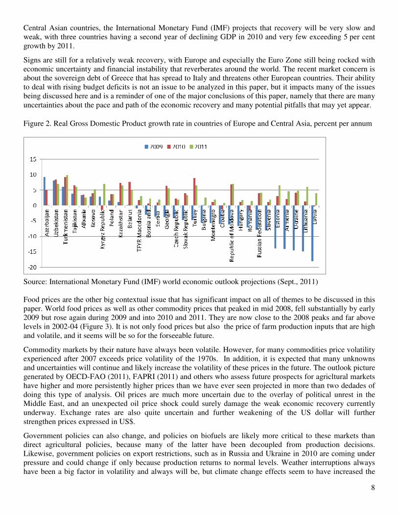
It is even more instructive to look at the individual country data for this region. Although ten of the 30 countries seem to have avoided negative growth in 2009, the economies that were estimated to decline by 6 per cent or more, including the Russian Federation, were in every subregion except Central Asia (Figure 2). Seven of the 11 countries with declines of more than 6 per cent in 2009 are NMS of the European Union. Except for two

8

Central Asian countries, the International Monetary Fund (IMF) projects that recovery will be very slow and weak, with three countries having a second year of declining GDP in 2010 and very few exceeding 5 per cent growth by 2011.

Signs are still for a relatively weak recovery, with Europe and especially the Euro Zone still being rocked with economic uncertainty and financial instability that reverberates around the world. The recent market concern is about the sovereign debt of Greece that has spread to Italy and threatens other European countries. Their ability to deal with rising budget deficits is not an issue to be analyzed in this paper, but it impacts many of the issues being discussed here and is a reminder of one of the major conclusions of this paper, namely that there are many uncertainties about the pace and path of the economic recovery and many potential pitfalls that may yet appear.

Figure 2. Real Gross Domestic Product growth rate in countries of Europe and Central Asia, percent per annum

Source: International Monetary Fund (IMF) world economic outlook projections (Sept., 2011) Food prices are the other big contextual issue that has significant impact on all of themes to be discussed in this paper. World food prices as well as other commodity prices that peaked in mid 2008, fell substantially by early 2009 but rose again during 2009 and into 2010 and 2011. They are now close to the 2008 peaks and far above levels in 2002-04 (Figure 3). It is not only food prices but also the price of farm production inputs that are high and volatile, and it seems will be so for the forseeable future.

Commodity markets by their nature have always been volatile. However, for many commodities price volatility experienced after 2007 exceeds price volatility of the 1970s. In addition, it is expected that many unknowns and uncertainties will continue and likely increase the volatility of these prices in the future. The outlook picture generated by OECD-FAO (2011), FAPRI (2011) and others who assess future prospects for agricltural markets have higher and more persistently higher prices than we have ever seen projected in more than two dedades of doing this type of analysis. Oil prices are much more uncertain due to the overlay of political unrest in the Middle East, and an unexpected oil price shock could surely damage the weak economic recovery currently underway. Exchange rates are also quite uncertain and further weakening of the US dollar will further strengthen prices expressed in US$.

Government policies can also change, and policies on biofuels are likely more critical to these markets than direct agricultural policies, because many of the latter have been decoupled from production decisions. Likewise, government policies on export restrictions, such as in Russia and Ukraine in 2010 are coming under pressure and could change if only because production returns to normal levels. Weather interruptions always have been a big factor in volatility and always will be, but climate change effects seem to have increased the

9

frequency and severity of weather damage to crops. In short, there are a wide range of possible outcomes and increasing difficulty for producers and policy makers to make decisions in view of increased uncertainty of future developments.

High prices are beneficial to some economic interests and harmful to others, as was carefully documented in the 2011 SOFI report (FAO, 2011); and we will pay attention to how high and volatile prices may impact the themes we are discussing. In particular, higher prices could stimulate more production, more rapid adoption of improved technologies, increased input use, more investment in R&D and agricultural infrastructure, but they can also put more pressure on constrained water supplies and fragile environments. Figure 3. World Bank food, energy, metals price indices, 6/08 to 9/11, 2000=100

Source: World Bank, Food, energy, metals and minerals price indices, pink data (Sept., 2011)

10

Theme 1. Agricultural Technologies This chapter is divided in 9 parts. After setting the stage of the new market environment we explore why discussions on agricultural technology and yield increases are fashionable again. Focusing on Europe and Central Asia, we review evidence on decreasing yield growth and yield gaps. The rest of the chapter is policy driven, and discusses possible steps to be taken, differences within the region covered, various aspects of agricultural research management and knowledge diffusion and derives some generalizable policy conclusions.

1.1 Setting the stage: High prices, volatility, new market environment

Not least due to various G20 and other international initiatives launched following the first "food crises" of 2007-2008, high prices in general and their consequences on food security in particular remain firmly on the international agenda. Despite the political attention bestowed on ensuring food security, due to multiple uses of agricultural commodities (food, feed, fibre, fuel – bioenergy, etc.), agriculture produces far more than “just” food, and considerations beyond food security deserve to be considered. Steadily growing demand (for food or otherwise), low stock levels and at times supply shocks lead to a persistent market uncertainty and volatility. A variety of justifications is on offer by various analysts, many of whom agree on the main contributors to current situation, such as bioefuel policies, increasing demand from emerging countries, or lagging investment into agriculture resulting in slower yield growth. Although population growth is slowing, analysts also tend to agree on the presence of a “new market environment”. “New market environment” (or some other synonym used to describe it) is characterised by oil scarcity resulting in higher input and energy costs as well as higher transport prices, increased interdependence of energy and agricultural markets due to the growing biofuels industry; land scarcity and competition among the crops for land allocation, exploitation of depletable resources such as water and phosphorus, uncertain effects of climate change pointing to sustainability considerations, etc. At the same time many societies today are imposing higher requirements on agricultural production based on sustainability, ethical or other considerations. While international trade is generally considered to be beneficial and allowing countries to benefit from their comparative advantage and specialisation, in the shorter term increased utilisation of export bans and trade restriction during the recent bouts of “food crisis” were adding to the tightness of the markets and reducing trust in the global trading system, as well as fuelling concerns about price volatility. The key word remains uncertainty: uncertainty about the impacts of climate change, energy prices, trade restrictive policies, etc. Agriculture paradigms valid earlier were mostly based on (relatively) increasing agricultural productivity and saturated demand for agricultural commodities. Although biofuels were introduced and supported for different reasons on different sides of Atlantic (energy security in the United States, environmental considerations in the EU), they nevertheless resulted in a softening of the saturation assumption on the demand side. In the previous paradigm, energy prices influenced agriculture as an input, for example via cost of fertiliser or transport. Currently, although biofuels are small (rather negligible) in the overall energy basket, the amount of agricultural products used in the biofuels production (vegetable oil, grains, sugar) compared to the overall production is increasing and clearly has price effects. Available medium term projections (e.g., OECD/FAO 2011) do not foresee any long lasting respite in prices and project prices at structurally higher levels, albeit possibly below the current peaks. International initiatives, such as G20, attempt to reduce the effect of this uncertainty on the market players by introducing more transparency in the market and improved market information systems (e.g., AMIS – Agricultural Market Information System).

11

Although many commentators, including the report by international organisations on price volatility prepared at the request of G-20 in June 2011 (FAO et al, 2011) proposed eliminating or limiting biofuels policies, suggestions to limit demand, in particular use of grains and vegetable oils in biofuels seem to be lacking political backing. Nevertheless, there is a general support for increased production. Limited resources (water, land) and high input costs are constraints to a successful response to increased and more diversified demands for food and non-food use of agricultural products. Production can be increased either by bringing in more land or raising productivity by intensifying production or increasing yields on land already in the production or land that can be brought in the production without imposing undue environmental cost. High food prices present incentives for increased long-term investment in the agriculture sector, which can contribute to improved food security in the longer term. Despite higher fertilizer prices, this has led to a strong supply response in many countries (FAO, 2011). While high prices in their own right support increased production, incentives to produce more based on higher prices can put more pressure on the environment and sustainable development. Climate change is possibly adding to the slowing of supply response to high prices because of the added burden of adaptation. At the same time, as agriculture is both a contributor to and a victim of climate change, it is both a challenge and an opportunity with adaptation, mitigation and carbon sequestration. This chapter focuses on increasing productivity by discussing various aspects of agricultural technology including investment, research management, and policy considerations.

1.2 Why the current interest in technology?

Where would the increases in supply come from? Opportunities for land expansion are not yet fully exploited across the globe and additional land remains available although at varying costs, with the most land available in Brazil, DRC, Angola, Sudan, Argentina, Columbia and Bolivia (Bruinsma, 2009). However, not least owing to high prices of many crops, land use in many countries faces strong competition for allocation among crops. In addition, parts of land not cultivated are on marginal holdings with high potential for environmental degradation and possibly small production potential. As such, land expansion would raise environmental and sustainability concerns if marginal lands are brought into production. In addition, land expansion also depends on appropriate investment and infrastructure which might be lacking. Many lands currently cultivated – but perhaps not cultivated for a long time – lack conditions or technical infrastructure making their eventual exploitation more expensive. For example, previously cultivated land in parts of former Soviet Union and abandoned in the early 1990s may remain too costly to be brought back into production even at current elevated prices without the assurance of continuing high prices, and future price developments are indeed uncertain. As land is a finite resource, policy prescriptions have focused on increasing productivity by increasing yields. Given the environmental considerations, the projections (OECD-FAO, 2011) indicate that most gains in production will be achieved by increasing yield growth and cropping intensity on existing farmlands rather than by increasing the amount of land brought under agricultural production. Globally, 90 percent of required production increases are projected to come from augmenting yields and cropping intensity, and only 10 percent by expanding arable land. For developing countries, FAO estimates that ratio at 80/20. But in land-scarce countries, almost all growth would need to be achieved by improving yields. A necessary step is to push the agricultural technology frontier, albeit not all countries face the same conditions (FAO, 2009). In the 1980s, for the first time in history the increase in yields due to increases in productivity exceeded increases due to land expansion. Work on advancing and fine tuning agricultural technology to increase

12

production or employ more environmentally sensitive methods is called for on the grounds of the need for increasing productivity. Whether it is because of competitiveness, food security or other considerations, the need is to close the gap between linearly growing supply and exponentially growing demand while ensuring sustainable resource management and environment preservation and taking into account resource constraints (land, water), climate change adaptation and mitigation. Policy considerations, such as applications of agro-environmental measures in the EU and other developed countries, can also contribute to the need to innovate and invest in technology development. It is expected that the new price environment would bring additional investment into technology development. Many technologies being developed have the potential not only to increase farm productivity but also to reduce the environmental and resource costs sometimes associated with agricultural production. These include technologies that conserve land and water by increasing yields with the same or fewer inputs and technologies that protect environmental quality, such as pest- and disease-resistant crops that require fewer chemicals (Anderson et al., 1997). Two forces guide technological development. The first is “demand-pull,” where the needs of the marketplace create the demand for a product. Both public and private-sector scientists, inventors, and entrepreneurs often seek to meet this demand. The second force is “supply-push.” Here the impetus for development comes from scientists and inventors who find a new and valuable technology. This technology can then be introduced into the marketplace. Both forces (singly and together) produce important and useful technologies, and governments can use both to encourage innovations that foster environmental quality and resource conservation. Policies such as environmental regulation can boost the demand-pull forces for environmentally benign technologies. Other government policies can foster supply-push forces for the desirable technologies. These policies include funding research and development, technology transfer activities, and efforts to understand and facilitate technology adoption (Anderson et al., 1997) However, increasing productivity by increasing yields will not materialize without increased investment on the macroeconomic, sectorial and farm levels. There is a rare agreement among commentators – and a great variety of publications on the topic – that investment in agricultural technology and productivity was neglected following the success of Green Revolution (for example rice, maize and wheat). Consequently, as a result of low investment over the last three decades, slower growth of cereal yields (and production), especially those of rice and wheat, during the past 20 years are often noted. This issue is treated in more detail below. Productivity can be increased by a range of interventions with varying degrees of investment needed. Developing new seed varieties is a longer term process and is likely to be costlier than to substitute primary production through adoption and improved management of existing technology, reduction of post-harvest losses, and reduction of losses in the whole supply chain. Nevertheless, the latter still calls for some investment into adaptation research and innovation and possibly a large investment in extension and other agricultural knowledge systems. The often cited goal justifying investment in technology is increased competitiveness. Different concepts of competitiveness exist across the countries (OECD, 2011a). While competitiveness is a relative concept, productivity is an absolute concept. Productivity represents the ability to turn production inputs into outputs which can be measured at the farm, industry or national level. While total factor productivity can be used to measure the efficiency of all inputs being converted into all outputs, there are also partial indicators of productivity such as output per worker, per hectare (e.g. crop yield) or per animal (e.g. milk yield). Total factor productivity growth can be decomposed into three elements: 1) technological change, which indicates a change in the technology available (innovation creation); 2) technical efficiency, which represents the ability of farms to use best technologies available, and 3) scale efficiency. These components of total factor productivity are often used to measure innovation, creation and diffusion. It is, however, also possible to measure the adoption of a specific form of innovation.

13

In developed countries, total factor productivity grew strongly from the 1960s to the mid-1990s, but not thereafter. Some studies indicate that productivity growth has slowed since the mid-1990s (e.g. Alston et al., 2010). Over the same time period, the situation is diverse in other countries. On the one hand, agricultural productivity growth resumed in some transition economies after a temporary slowdown in the 1990s and is high in some large producing countries of Central and Eastern Europe. Moreover, productivity growth has been particularly strong in some emerging economies like Brazil and China. On the other hand, agricultural productivity growth is still low in most least developed countries. Overall, there is no clear evidence that total factor productivity growth is decreasing at the global level (Alston et al., 2010). Alston and Pardey (2009) provide evidence of a significant slowdown in agricultural productivity since 1990 or so, with China being an exception. Productivity grew in China, following institutional changes. While multifactor measures might not be readily available for all countries, this slowdown in productivity can be measured using various measures, such as production per unit or crop yields. Decreases in productivity are a challenge to all, but this paper does not look at total factor productivity but rather focuses on yields and the impact of technology. Among the possible determinants of productivity growth, research and development (R&D) has been the subject of many studies. R&D is the main source of new technologies and agricultural productivity growth in the long run. Agricultural R&D activities take place in private and public domains but also within farmers' organisations, as well as on farms. Expenditure on R&D is often used as an indicator of efforts in this area, while the number of patents is considered as a measure of achievements. There are many conceptual models of how R&D leads to innovation and there have been many attempts to measure the impact of R&D expenditures on productivity growth in agriculture. While technology and investment are two distinct issues, it is generally understood that research, development, and, of course, investment are necessary for successful development of technology. In addition, as it will be treated later, successful innovation and development of new technologies is conditional on their adaption which has links to farmers’ access to technology as well as other attributes. In short, there is a need to increase agricultural productivity globally to satisfy the demand of increasing population and incomes while taking account of competing demands for land, water, fuel, climate change mitigation and adaption as well as changing environmental conditions influencing pests and diseases. The next part will explore crop yields in detail.

1.3 Evidence of decreasing yield growth in various countries?

This part analyses yields of a variety of commodities over the last 50 years in the countries in the region and compares them with world averages. However, geopolitical changes in Europe and Central Asia do not lend themselves well to time series analysis. For example, average yield data in FAOSTAT for the Soviet Union stop in 1992 after which data for individual states are reported. Thus, the data tables report yield growth and average yields for USSR until 1992, followed by calculations for individual states. While a certain trend could be observed, one cannot really compare average yield growth in the Former Soviet Union – an average of a variety of natural conditions – with an average yield, for example, in Kazakhstan or Ukraine. Yield data for the analysis were taken from FAOSTAT. Time series were limited by the data availability as of January 2012 to 1961 – 2010. In all cases the end points were three-year averages except for the 1961 being only two years because of data availability. Some other limitations described in the Annex applied depending on data availability. However, those do not alter the results.

14

Two different time periods were studied. In the first case we examined the whole available data set from 1961 to 2009, and focused on four equal 11-year time periods corresponding broadly to different economic periods:

• 1961-1972 capturing the green revolution,

• 1973-1984 the aftermath of the two energy shocks and stagflation,

• 1985-1996 the recovery of agricultural prices until their mid-1990s spike, and finally

• 1997-2008 representing the parallel boom in agricultural and other markets and agricultural price spike of 2007-2008.

In the second case we focused on the 1985 – 2009 period, and studied 5 year intervals. In the interest of comprehensiveness we look at:

1. Yield growth rates. 2. Average yields, comparing countries in the region with the world. 3. Yield gaps between the actual yields in the region and the world average – this measure is biased as it

does not account for the differences in natural conditions. A more appropriate measure would be to calculate a yield gap between the actual and potential yield but it is beyond the scope of this paper.

4. And finally variability of actual yields in selected countries. A frequently cited argument in medium term projections (e.g., OECD-FAO, 2011) is that production is moving to countries where yield variability is higher, thus creating conditions for greater price volatility in the future. In addition, some of these countries, such as Russia, Kazakhstan, Ukraine are or aim to be important players on the world market but have proven to be rather unreliable trading partners, due to their variability in production and general unpreparedness to deal with weather related events as well as willingness to react with trade restrictive policies.

Results for points 1 – 3 are presented in the Annex. Annex 1 presents growth rates, annex 2 -average yields in the same period as well as deviations between national average yields and world yields. Although in many cases we do observe slowing yield growth rates (particularly on the world level), it is impossible to say with certainty whether decreasing yield growth on the country level was due technology, weather related events, or for example disinvestment following structural changes in Eastern Europe and former Soviet Union. Yield analyses also fail to account for climatic, soil and other conditions. Yields are in most cases continuing to increase, and no straightforward conclusions can be drawn regarding the slowdown of yield growth for many commodities on the world level. While yield growth rates for wheat declined systematically from 3.2% in 1961 – 1972 to 1.0 % in 1997- 2008 (calculated as averages), other commodities experienced both upward and downward changes over the years. Table 1.1 summarises the developments for the main grains, oilseeds and potatoes on the world level for two time frames analyses, 1961 – 2008 and 1985 – 2008. While declining wheat yield growth in the 11 year time period is apparent, a similar pattern does not appear to hold when focusing on the time period starting from 1985. Annex 1 provides country level information on the rates of growth for selected commodities and countries in the region. While yield growth rates of many commodities on the world level declined over the time periods studied compared to the period of 1961 – 1972 during the green revolution (for example barley, maize, oats and rice), the developments did not follow a steady decline like in case of wheat and soybeans. Yield growth rate developments on the country level remain rather heterogeneous and are listed in the annex. Generalised conclusions of declining growth rates across countries and commodities cannot be drawn, in particular as the analysis fails to account for climatic conditions and institutional changes. Institutional changes are particularly remarkable in countries of the former Soviet Union and other transition economies. While data for the former Soviet Union do not allow for detailed analysis, consecutive data for transition economies show bottoming yield growth rates in the 1985 – 1996 period, followed by a recovery in 1997 – 2008. The decline in yield growth is noticeable in economies transitioning from a planned to market economies in the analysis,

15

focusing on 1985 – 2008 data in 5 year growth increments. Growth rates in many transition economies during the 1991 – 1996 and 1997 – 2002 were in fact negative. With the entry to the EU many former transition economies reversed their declining growth rates. Nevertheless, in many cases the growth rates in the period 1997 – 2008 were lower than in 1961 – 1972. Table 1.1 Rates of world yield growth for selected crops and periods from 1961-2009 World Yield growth rates

11 year periods 5 year periods

avg61/62-

avg08/10

avg61/62-

avg71/73

avg72/74-

avg83/85

avg84/86-

avg95/97

avg96/98-

avg07/09

avg84/86-

avg08/10

avg84/86-

avg89/91

avg90/92-

avg95/97

avg96/98-

avg01/03

avg02/04-

avg07/09

Barley 1.3% 2.6% 1.0% 0.4% 0.9% 0.9% 0.9% -0.1% 0.8% 0.9% Maize 2.0% 2.9% 2.2% 1.0% 1.6% 1.5% 0.2% 1.5% 0.8% 2.0% Oats 1.0% 2.0% 0.8% 0.0% 1.2% 0.8% -0.7% 0.8% 1.3% 0.8% Potatoes 0.9% 1.6% 0.5% 0.3% 0.8% 0.6% -0.7% 1.5% 0.0% 1.1% Rapeseed 2.5% 3.3% 3.7% 1.1% 2.4% 1.6% 1.2% 1.1% 1.7% 2.5% Rice, paddy 1.7% 2.1% 2.6% 1.3% 1.1% 1.2% 1.6% 1.1% 0.5% 1.8% Rye 1.7% 3.2% 1.2% 1.1% 1.7% 1.2% 1.5% 0.8% 1.1% 2.1% Sorghum 0.9% 2.8% 1.4% -0.6% -0.1% -0.2% -2.1% -0.3% -1.4% 1.0% Soybeans 1.6% 2.7% 1.4% 1.4% 0.7% 1.2% 0.6% 1.7% 1.1% 0.7% Sunflower seed 0.6% 1.2% 0.3% -0.3% 0.9% 0.3% 1.4% -0.9% -0.5% 2.0% Wheat 2.1% 3.2% 2.6% 1.4% 1.0% 1.3% 1.9% 0.7% 0.4% 1.5%

Source: Calculated by the author from FAOSTAT data (accessed January 2012) However, while growth rates tell the story of progression, they omit the starting point. Although some countries experience two digit growth rates, their average yields still lag behind even the world average. Annex 2 presents average yields in selected countries and on the world level for two time frames: 1961 – 2008 (divided into 11 year intervals as before), and 1985 – 2008 (divided into 5 year intervals) together with the perceptual deviation from the world average. Although possibly with some room for improvement, in terms of yields the EU15 countries are generally faring rather well compared to the world average, often producing on average more than double the world average (clearly depending on the climatic and geographical conditions). However, many countries in the region with presumably large potential for grain production are producing well below the world average, for example Russia and Kazakhstan in case of wheat. When sorting the results of % deviation from world average in 2003 – 2008, the countries with the largest deviation from the world average are often the same countries in Central Asia. In addition, as the world average remains relatively stable, large differences in countries' deviations from the world average point to a large yield variability within many countries. Although the analysis does not differentiate between varieties and qualities of commodities produced and does not account for different geographical and climatic conditions, it does provide an indication of the potential should improvements in technologies (both seed and management) be adopted. However, although many crops experienced bumper harvests (e.g., wheat in 2008) it is more likely that it was due to positive weather developments positively limiting the difference between the actual and real yields, rather than changes in the seeds or production practices. While the supply response following the price hikes was rather positive and production increased, it is highly unlikely this was due to investment technology, which takes longer to be realized.

16

Finally, we examined yield variability in major producing countries and compared it with yield variability in major producing countries in Europe and Central Asia. Medium term outlooks (e.g., OECD-FAO, 2011) indicate that the production is shifting from "traditional" countries to countries with higher yield variability which is likely to influence price volatility in the future. Yield variability was calculated as a coefficient of variation (a ratio of standard deviation to the mean) for wheat, barley, maize and rapeseed on the world level as well as for France, Germany, Netherlands, Poland, USSR up to 1991, and Kazakhstan, Russian Federation and Ukraine after 1992 (graphed on figures 1 – 4). As expected, yield variability on the world level is lower than yield variability in individual countries. While no generalisations can be made, in many countries yield variability has a decreasing trend over the years. However, in countries that aim to play an increasingly important role on the world market (Kazakhstan Russia, Ukraine), yield variability is often higher than in other countries studied, perhaps with the exception of maize. Figure 1.1 Wheat yield variability in selected ECA countries over several periods 1965 to 2009.

Wheat yield variability (CV)

0%

5%

10%

15%

20%

25%

30%

35%

World France Germany Netherlands Poland USSR Kazakhstan Russian Fed. Ukraine

65-73 74-82 83-91 92-00 01-09

Source: Calculated by the authors from FAOSTAT data (accessed Oct 2011)

17

Figure 1.2: Barley yield variability in selected ECA countries over several periods 1965 to 2009.

Barley yield variability (CV)

0%

5%

10%

15%

20%

25%

30%

35%

World France Germany Netherlands Poland USSR Kazakhstan Russian Fed. Ukraine

65-73 74-82 83-91 92-00 01-09

Source: Calculated by the authors from FAOSTAT data (accessed Oct 2011) Figure 1.3: Maize yield variability in selected ECA countries over several periods 1965 to 2009.

Maize yield variability (CV)

0%

5%

10%

15%

20%

25%

30%

35%

40%

45%

World France Germany Netherlands Poland USSR Kazakhstan Russian Fed. Ukraine

65-73 74-82 83-91 92-00 01-09

Source: Calculated by the authors from FAOSTAT data (accessed Oct 2011)

18

Figure 1.4: Rapeseed yield variability in selected ECA countries over several periods 1965 to 2009.

Rapeseed yield variability (CV)

0%

10%

20%

30%

40%

50%

60%

World France Germany Netherlands Poland USSR Kazakhstan Russian Fed. Ukraine

65-73 74-82 83-91 92-00 01-09

Source: Calculated by the authors from FAOSTAT data (accessed Oct 2011)

1.4 What can be done

While recognising some increases in land use are still possible, this paper focuses on technology and related topics of research, development and extension. On the macroeconomic level, a frequent policy prescription to the challenge of enhancing farm productivity while taking into account social and environmental resource constraints and considerations is to demand increased funding for research and development. Various steps that can be taken on a practical level to increase yields require various costs in terms of investment:

1. Seeds: a. advancements in seeds: often one of the few possibilities in mature agricultural production

systems. b. adoption of existing seeds.

2. Changes in the environment: advance in environment management systems, irrigation and other environmental aspects, interaction between seed and environmental conditions

a. changes with significant investment, e.g., irrigation, precision agriculture, etc. b. changes possible without significant investment, e.g., conservation agriculture, no till or low

tillage practices, adoption of good agricultural practice, etc.

While innovation is a significant contributor to technological progress and innovation, significant gains in closing gaps between actual yields lie in management and good agricultural practices adjusted to particular environmental and geographical locations. In addition, while new advances in seeds are often necessary but often take a long time and financial resources, an immediate solution of harvesting the low hanging fruit is employment of better management, conservation techniques and facilitation of technology transfer and potential. For example, Saskatchewan has climate and agronomic conditions quite similar to Kazakhstan but

19

better management practices lead to less production variability. Nevertheless, in the light of changing environmental conditions and climate change effects, what are considered best agricultural practices are also likely to change over time. At the farm level, farm characteristics often play a significant role in determining the degree of technology adaption, and consequently in determining actual increases in yield and productivity. For example, in the sector of field crops, small farmers might be less likely to invest in machinery than big farms because of their lack of access to capital and perhaps because they might not have the necessary collateral to secure the capital. At times countries with atomised farm structure might be also lacking a well-functioning credit market. In addition, some productivity increasing enhancements might not necessarily call for high investment in capital but farmers farming on rented land might be less likely to adopt these measures (for example, to install irrigation systems). Good weather and ideal conditions for seed and crop development help to achieve strong yields. In the simplest agronomic terms, yields can be influenced by the attributes of the seed itself (gene), the environment itself (e.g., by irrigation), or the interaction between gene and environment. While in Western Europe and other mature agricultural systems, influencing the environment is unlikely to bring large increases in yields, elsewhere in Europe (and the rest of the world) bringing actual yields on par with potential yields by influencing the production environment and the interaction between the seed and environment remain an option. As only 30% of crops in developing countries are under improved varieties, seed systems are essential. However, public research is unlikely to deliver enough on its own, and sound public private partnerships coupled with scientifically sound participatory approaches should be considered. Climate change mitigation and adaptation calls for more climate resilient varieties, and fighting specific diseases. More advancement is needed, however, and the combination of “old” (shuttle breeding) and “new” (biotechnology) should be also considered. Genetic variability is of crucial importance: higher genetic variability leads to higher potential genetic improvement. Many tasks previously done by the public sector are now done privately, and shared multilateral access to preserved germoplasm remains an important element. Many advances, such as nitrogen fixation, photosynthesis manipulation or exploitation of metabolic pathways in gene development are possible. However, these advances are likely to have rather long delivery periods and not materialise in the near future. However, changes in the environment, both natural and “social” (e.g., management) are more easily attainable than some of the more significant advances in seed. Among possible changes in the environment are resource management, conservation tillage, no till systems, judicious use of inputs etc. In its report, FAO talks about conservation agriculture and concludes that conservation agriculture delivers benefits for climate change (FAO, 2001a). Nevertheless, the report indicates that currently only 1% of land is under conservation agriculture. While precision agriculture has been around for a while, it is rather investment intensive. Likewise, site specific nutrient management has a potential to deliver higher yields. It would also allow pesticide management and better targeting of nutrients and pesticides. However, it remains little used because of its high cost and its information management and knowledge intensity. The report State of Food Insecurity in the World 2011 (FAO, 2011) stresses that investment in agriculture remains critical to sustainable, long-term food security. Key areas where such investments should be directed are cost-effective irrigation, improved land-management practices and better seeds developed through agricultural research. That would help reduce the production risks facing farmers, especially smallholders, and mitigate price volatility. The FAO (2009) identified the following priority areas for action where enhanced farming techniques and new technologies could be tapped to boost production:

20

• Improving efficiency in farmers' use of agricultural inputs. This will become increasingly important as natural resources get scarcer and prices of resources such as fossil fuels, nitrogen and phosphorus increase. One technique that offers promise in this regard is conservation agriculture using zero tillage - farms employing this technique reduce their fuel use by an average of two-thirds while simultaneously raising levels of soil carbon sequestration. Fertilizers will need to be used more efficiently through greater on-farm use of nitrogen and increasing supplies of biologically-fixed nitrogen. Water must be used more efficiently through practices such as water harvesting and conservation of soil moisture. • Developing improved crop varieties. Plant breeding techniques can lead to improved crop varieties that increase yields, decrease losses, and make agriculture more resistant to climate-associated stresses and water scarcity. However, FAO's discussion paper also notes the need to evaluate new technologies carefully to avoid possible negative environmental and human-health impacts. • Heavily investing in agricultural research and development. Noting that investment in R&D is the most productive way to support agriculture, the paper argues that "massive public and private investments in R&D are required if agriculture is to benefit from the use of new technologies and techniques". The need for substantially higher levels of investment in agriculture R&D will further increase due to climate change and greater water scarcity. • Closing existing "yield gaps". Even as new technologies are explored, one area where progress is needed is promoting greater adoption of existing technologies. Many farms today produce less food than they are capable of simply because they do not make use of enhanced seeds and cropping techniques that are currently available. Reasons for this include a lack of financial incentives or resources, poor access to information, weak extension services, and insufficient opportunities for acquiring the necessary technical skills. On the interaction between gene and “environment”, the Green revolution resulted in plants being able to take higher pesticide doses. Hybrid seeds developed currently are not necessarily delivering higher yields per seed but are able to stand higher planting densities. The Green revolution delivered a major change in the past. Although a lot of effort is now put into biotechnology, due to policy restrictions it remains unclear whether biotechnology will deliver the boost the Green Revolution once delivered and on the scale it delivered. Biotechnology might have not been well received, in particular in Europe due to its association with genetic modification. However, new plant breeding techniques which make use of biotechnology but which are not necessarily generating GMOs became available, creating additional challenges for the EU GMO legislation and approval. These new techniques offer advantages over older techniques of genetic modification or mutagenesis (exempted from the GMO legislation) and even conventional breeding techniques, as they are more specific and better targeted. In most cases, the genome of the final commercialised crop does not contain an inserted transgene, i.e. the natural borders of reproduction are respected. It is a faster breeding process but presents new challenges with respect to detection and identification (Lusser et al, 2011). Land is a constraint but water use is too. Production efficiencies in water use are needed and are likely to originate from production practices, such as strip tillage, irrigation timing, drip irrigation, etc. Conservation tillage increases soil moisture, increases root growth and changes plant’s water use pattern. Primed acclimation involves holding off water early and allowing the plant to develop root growth to become more tolerant later in the season (Smit, 2010)

21

1.5 Differences within the region and different policy priorities

Analysing Europe as a geographical setting is a tall order. The variety of geographical conditions, coupled with a diversity of different social, institutional and political backgrounds gave rise to a variety of agricultural systems. The introduction already highlighted a variety of economic conditions across studied countries. It is worth pointing out different political, social and economic institutions across Europe and Central Asia (also discussed under policy priorities in the last section). This part describes additional differences and when possible, supports the description with analysis. However, lack of comparable statistics and changes in political structures do not lend themselves very well to analysis. Policy goals across European countries lack homogeneity, as do availability of public finances to support these policy goals in the current economic environment. Among the most frequent policy goals are maintaining production potential, ensuring food security, and ensuring sustainable use of environmental resources. Even countries in the European Union sharing a Common Agricultural Policy do not necessarily subscribe to the same policy goals but agree on general principles described above.. Like the policy goals, country coffers and agricultural support budgets differ across countries, even as some (developed in particular) countries continue to fight structural imbalances in their budgets and face uncertainty in their budgetary outlays. The OECD numbers for Producer Support Estimate (PSE) in the region are only available for EU, Iceland, Norway, Switzerland, Turkey, Russia and Ukraine but the date show substantial differences, using average data for 2008 – 2010 (Table 1.2). Table 1.2: Support to agriculture for selected countries in ECA, 2008-2010 average

Country PSE as % of receipts

Potentially most distorting support

as % of PSE

Ratio of producer price to border

price (NPC)

Total Support Estimate (TSE) as % of GDP

EU 22% 29% 1.07 0.8%

Iceland 48% 65% 1.67 1.1%

Norway 60% 53% 1.91 1.0%

Switzerland 56% 49% 1.51 1.2%

Turkey 27% 90% 1.26 3.2%

Russia 22% 81% 1.16 1.6%

Ukraine 7% 84% 1.01 2.1%

Source: OECD (2011b) The OECD also calculates a General Services Support Estimate (GSSE) indicator which includes research and development, financing for agricultural schools, inspection services, infrastructure, marketing and promotion and public stockholding (OECD, 2011c). In the EU the share of research and development in 2010 represented approximately 21% of the GSSE, while in Norway it accounted for over 40% and only 10.7 and 8% in Russia and Ukraine. Table 1.3 summarises the composition of GSSE in the same sample of European countries in 2010.

22

Table1.3: Composition of GSSE for selected countries in ECA, 2010 Country Research and

Development Agricultural

schools Inspection Services

Infrastructure Marketing and

promotion

Public Stockholding

Misc

EU 20.97 11.86 8.27 28.88 29.54 0.06 0.43

Iceland 10.81 0 43.14 5.16 6.20 34.69 0

Norway 40.30 0 13.14 14.09 3.28 0.02 29.18

Switzerland 20.57 4.23 2.26 17.28 11.79 8.31 35.57

Turkey 2.0 0 4.66 0 93.34 0 0

Russia 10.69 21.96 22.12 31.06 0.67 6.98 6.52

Ukraine 8.02 27.26 12.27 16.20 1.11 34.90 0.25

Source: OECD (2011b) While some countries in the region aim to increase their productivity for domestic self-sufficiency reasons, some – especially geographically large economies of former Soviet Union such as Russia, Kazakhstan and Ukraine – aim to produce to become or maintain and enhance their positions among the leading world exporters. However, despite their efforts to be active exporters, these countries in particular have been inclined to use export taxes, quotas and bans in reaction to domestic production shortfalls or world price spikes. To allow farmers to react to increased prices by increasing their production, it is important to assure complete price transmission. At times the prices from international markets are not fully transmitted to farmers because of a variety of border protection, weak infrastructure, agricultural policies, structure of the supply chain, etc. Above all, assuring a stable macroeconomic and policy environment is of the utmost importance. In addition to ensuring a stable macroeconomic and policy environment and efficiently functioning markets, policy options for research include:

- Status quo: possibly the worst scenario both from the perspective of food security as well as sustainability and natural resources.

- Re-invest in public agricultural research: enhancing commitment to agriculture, shift priorities within agricultural support budgets from subsidies to research (the new CAP proposal does that partly, although the amount of money allocated to research is small).

- Encourage private investment in agricultural R&D – need to enhance IPR, strengthen co-financing arrangements and institutions. However, reinvesting in agricultural R&D and encouraging private investment are not mutually exclusive.

1.6 Management of agricultural research

Management of agricultural research within a country – but also internationally – impacts its productivity as well as technology adoption. Successfully managed agricultural research in a country responds to the society as a driver of innovation, in addition to markets, politics, regulation, ethical or social commitments, stress or crisis, and incentives. It also encompasses a range of actors: researchers, farmers, market agents, civil society, and the government. A linear approach to innovation includes four stages:

1. production of knowledge for example via education and research. 2. transfer of knowledge using public or extension or advisory services, agribusiness networks, etc. 3. adoption by producers. 4. feedback on problems and constraints from producers to research and extension.

23

Another line to draw is between public and private research. Fundamental research is usually done with public funds, while applied research is best left to the private sector which is more likely to assure its marketability (Anderson et al. 1997) However, increasing fundamental research without technology adaptation by the producers is unlikely to deliver good results. Also there can be “market failure” in private research if important crops, for example, are neglected because of lack of market incentive to conduct private research on them. In this case there may be needed a kind of public-private partnership or incentive structure where the public sector supports private commercialization of a technology. This approach was successfully used in incentivizing drug companies to produce HIV-AIDS drugs for Africa at affordable prices. In addition to new varieties, two types of research are distinguished -

1. adaptive research to adopt to different locations and 2. maintenance research to adopt to evolving pests and diseases.

Innovation can follow an established or a radical path. In the established path, innovations are adopted as they become available. In the radical path, a technology is being used and replaced not by the technology that became available immediately, but later (skipping a technology). The research agenda and policy agenda do not always follow the same timeline. Differences in the time horizons are often in the midst of problems in the research area in terms of setting and financing research priorities within the public research agenda. Despite their rhetoric, policy makers tend to operate in a short time span, and thus at times are unable to allocate research budgets to fight long term issues, such as sustainability or other environmental considerations and environmental monitoring. Policy led research might not always correspond to long term research needs (not least due to different time schemes). Likewise, despite many advantages, decentralised research management is unlikely to work sufficiently for research needed to address long term challenges. Thus, strategic public research priorities based on sound science should be identified. While agricultural research is not funded solely by governments, centrally and strategically led priorities are to be set. Policies should have the capacity to deliver on multiple objectives, including environmental ones, in an environment of increased uncertainty. Increased uncertainty and new challenges might imply less the need for more fixed research agendas, and more work on foresight and scenario analysis to allow for adjustment to climate change mitigation and adaptation. Widening the scope of research will imply more transdisciplinary work (within economics, with other social sciences and with other sciences e.g. agronomy) so as to help better grasp complexity. It remains clear that as public investment in research is decreasing, most of the investment would have to come from the private sector – and, as will be discussed in later parts, a policy environment facilitating private investment in research has to play a key role. In part, this is because although the immediate return to agricultural R&D investment is small, long term social returns to R&D investments are between 20 and 80% with a mean of 65% (Alston 2010).

It would make an interesting exercise to compare agricultural R&D figures across countries across the studied region. However, data sets often exclude former Soviet Union and Eastern Europe due to lack of data (e.g., Pardey, 2011). Despite high rates of return on agricultural investment, agriculture appears to be under persistent underinvestment. Studies (e.g., Alston, 2010) list high internal rates of return from research but recognise possible attribution issues: long time lags in knowledge creation and adoption, spatial spillovers among states and countries, as well as absence of a relevant counterfactual alternative. Nevertheless, although the rates of return might be overstated, the true returns still remain very high.

24

Some numbers to support the claims (Alston, 2011):

• Long lags in technology development are illustrated in Alston (2010): it took 59 years for hybrid corn from when the first controlled crosses/hybrid vigor were conducted in 1877 to developing hybrid corn in 1936 (and another 36 years when vastly improved in-breds led to a shift to single cross hybrids). 96 years passed between the discovery of Bt (Bacillus thuringiensis) to the commercialisation of Bt corn in the US (and over 10 more years to receive regulatory approval in 20 countries). Finally, roundup ready soybean only took only 26 years from the research on glyphosphate in 1970 to commercialisation of roundup ready soybeans in 1996.

• It took 19 years for hybrid corn and 13 years for GE corn in the US to reach 80% adoption in the share of acreage

Market failure to deliver agricultural research served as a rationale for public intervention. Nevertheless, governments have gradually withdrawn themselves from research and research funding. However, agricultural research is a public good where research results should stay in the public domain. Two challenges occur: first, with withdrawal of public funding, what new structures and partnerships can assure sufficient levels of funding to continue research? Second, how to ensure relevant agricultural research remains in a public domain despite being done by private entities? While the term "funding" of public research is often used, due to its production of a public good, public agricultural research could be more appropriately described as “being invested in”. Increased research investment is needed to reverse a decline in public agricultural research, particularly in developed countries. The public good nature of agricultural knowledge and technology is possibly underestimated, while ability of the private sector is possibly overestimated. Setting up research consultation and liaison between public and private research could be of service in rebuilding public agricultural research. Agricultural knowledge systems will be discussed in the next section; however, they can contribute in setting up bottom-up research agenda. Private research tends to focus on marketable products which can lead to underinvestment in research. DEFRA (2002) studied the balance in funding between public and private sectors in plant breeding activities in the UK where until the mid-1980s plant breeding was funded mostly by a substantial public sector investment. The report recommended that more money is spent on applied research as opposed to basic research: in the time frame covered by the study, 89% of UK government spending on plant genetic improvement research was basic science and 11% applied science. In line with recommendations of DEFRA, one of the new instruments announced by the European Commission together with legislative proposals for the post 2013 CAP is the European Innovation Partnership “Agricultural productivity and sustainability” (EIP-A) which will aim at improving the links between research on the one hand and implementation of research results and innovation in the agriculture sector and rural economy on the other, or in other words, to “rebuild broken links in the chain between research and bringing innovation to the market” (Matthews, 2011). From publicly available materials on the EIP-A it is not immediately clear how the instrument would operate on practical level (e.g., House of Lords, 2011). However, it seems quite likely that ECA countries lacking EU’s institutions, budget and structure might be unlikely to replicate the experiment. However, innovation partnerships based on cooperation between the industry and research community might be worth trying, as might be partnerships on international level involving multiple stakeholders.

1.7 Public and private investment, research in particular

25

Traditionally agricultural research in developed countries was funded with public funds, and results of research done with public funds remained in the public domains. With decreased availability of public funding, a lot of attention and hope is being put into private research funded with private resources. While private research is no doubt important, private research is more likely to deliver in the area of applied research while public funding should be directed to fundamental research on which private or applied research can be built. Developed countries in particular saw a slowdown in spending growth, with a diminishing share for enhancing on-farm productivity – naturally resulting in a slowdown in high income countries. Different patterns occur in Brazil and China, where the countries in this region could probably look for helpful examples. Following shifts in public support R&D, productivity patterns are shifting too (Alston, 2011). China is often cited as a success story in increasing agricultural productivity, and it is clearly targeted public investment to stimulate productivity growth (Hu et al., 2010). Three levels of research occur in China: national, provincial, and prefectural. National level research centres account for 10% of total research staff and 15% of total budget, provincial for 41% of staff, 51% of budget and finally agricultural research centres on the level of prefectures account for 32% of staff and 34% of budget. In the Chinese research system, the central government established agricultural research institutes that cover most of agricultural products at the national level, while local governments established agricultural research institutes that covered nearly all agricultural products in their region. Some figures:

• There are 1237 agricultural research institutes and 88 agricultural universities or technological academies that are located in every province or prefecture.

• The research fields cover nearly all agricultural products (Nominally 109 products) in China.

• 50 innovation product industries have been specially invested by MOA (Ministry of Agriculture) since 2008.

• Annual growth in government fiscal investment in agricultural research is 15.9%, which is more development than basic research.

• Investment in agri biotech research has doubled in every 4 years before the mid-2000s (clearly from a low base) and in 2003 was 1.65 Billion yuan (200 million USD or 950 million in USD PPP).

• Government investment in agricultural research started picking up after 1985.

• China also has the largest agricultural extension system in the world.

• Commercialisation helps, as did a move from a formula-based allocation to competitive grants. Changing economic conditions call for sound and flexible institutions and policies which enable countries to deal with the challenges of new market realities based on generally tight markets impacted by climate change. Even as increased investment in technology and innovation is often called upon and encouraged, it remains clear that public coffers tightened by fiscal restraint in the aftermath of the economic and financial crisis are and will be less likely to finance long term public research. Instead public spending is likely to focus on short term policy priorities, even in the area of research and development. The gap in research funding is likely to be picked up by private entities, ideally in the framework of public-private partnerships. While private research does produce marketable goods by funding technology and innovation in response to market signals, time horizons and policy priorities of private funders are likely to differ from public needs. A question of identifying robust policy approaches in national and international settings remains a relevant one. The economic, financial and environmental situation across the world remains an uncertain one, with at times limited confidence given to existing international structures. Since public funds are used for funding, agricultural research needs to support a broad range of stakeholders, including producer groups, environmental groups, etc. A broad based constituency prevents the funding from being too narrowly targeted. However, since agricultural research creates a pubic good, some form of public support remains necessary. Division between fundamental public and applied private research should be maintained.

26

There is less data in countries of Former Soviet Union and Eastern Europe, but anecdotal evidence indicates that research budgets have decreased and limited funding is more likely to be used for farm subsidies than for research and extension services that have a broader benefit to the industry as well as to society as a whole. There is also little long-term vision for agricultural research needs. There needs to be a coherent policy set to facilitate access to private funding and enable tapping into private investment both foreign and domestic.

1.8 Diffusion of information to support technology adoption

This part discusses three possible ways to diffuse information to support technology adoption: - extension services and broader agriculture knowledge systems (AKS); - learning and innovation networks; - supply chain pushed innovation. How should the development and adoption of innovation at the national and global level be fostered in order to meet global food security and climate change challenges? Market forces themselves are unlikely to ensure that higher prices will force farmers to adjust their technology given the uncertainty of price developments. A functioning agricultural knowledge system (AKS) could help to support technology adoption. Many technologies are information intensive. New systems of extension should take into account specificities of location, networking, exchange experience, and bottom-up innovation. Agricultural extension operates within a broader knowledge system that includes research and agricultural education. FAO and the World Bank refer to this larger system as AKIS/RD (Agricultural Knowledge and Information Systems for Rural Development). The OECD countries refer to it simply as the Agricultural Knowledge System (AKS) (FAO, 2001b) The dissemination and use of improved agricultural technology and management practices can be traced back thousands of years in different parts of the world, including China, Mesopotamia, Egypt, and even in the Americas. The origins of public- or government-funded extension and advisory systems can be traced back to Ireland and the United Kingdom during the middle of the nineteenth century. During the potato famine in Ireland (1845–1851), agricultural advisors helped Irish potato farmers diversify into different food crops Swanson and Rajalahti (2010). FAO (1997) provides a fascinating history of agricultural extension, as well as overview of various aspects surrounding agricultural extension. Agricultural knowledge systems are formally defined as “a set of agricultural organizations and/or persons, and the links and interactions between them, engaged in the generation, transformation, transmission, storage, retrieval, integration, diffusion and utilization of knowledge and information, with the purpose of working synergistically to support decision making, problem solving and innovation in agriculture” (Röling and Engel, 1991). The AKS concept is broader but agricultural extension and farm advisory services are an integral part of AKS. Figure 1.5 summaries the principles of the AKS concept in the centre of which are agricultural producers. While not graphically represented in the figure, agricultural producers also interact among themselves and influence each other. On the poles of the concept are research, extension, education and support services with mutual links among themselves but also between themselves and agricultural producers.

27

Figure 1.5 Summary of the AKS concept.

Source: Poppe, 2011 Literature on agricultural extension is rather rich. Many publications have been written on agricultural extension and strengthening, transforming, assessing, etc. of agricultural extension and advisory systems both in developed and developing countries. Swanson and Rajalahti (2010) focused on small scale farm households and transforming and strengthening pluralistic agricultural extension and advisory systems towards a broader goal of increasing farm income and improving rural livelihoods. Literature (e.g, Swanson and Rajalahti, 2010) identify four major paradignms of agricultural extension depending how and why the delivery takes place:

1. Technology transfer of the training and visit type delivering top down specific recommendations from research to all types of farmers. The goal of this extension model is to increase (food) production. As illustrated by North American and European countries, with increased commercialisation, both technology development and transfer will increasingly be privatised.

2. Advisory services delivered both by public extension workers and private sector firms. Farmers are “advised” to use a specific practice or technology to solve an identified problem or production constraint. Public extension organizations should have validated information available from research about the effectiveness of different inputs or methods in solving specific problems so that inquiring farmers receive objective and validated information. Although most firms use persuasive methods to sell more products and increase their profit, an alternative private-sector model is to support outgrower schemes where export firms have field agents who both advise and supervise contract growers to ensure that specific production inputs and practices are followed to generate a specific quality product.

3. Nonformal Education (NFE) continues to be used in most extension systems, but the focus is shifting more toward training farmers how to utilize specific management skills or technical knowledge to increase their production efficiency or to utilize specific management practices, such as integrated pest management (IPM), as taught through Farmer Field Schools (FFS).

4. Facilitation Extension has evolved over time from participatory extension methods used 20–30 years ago and now focuses on getting farmers with common interests to work more closely together to achieve both individual and common objectives. An important difference is that front-line extension agents primarily work as “knowledge brokers” in facilitating the teaching–learning process among all types of farmers. Under this extension model, the field staff first identifies specific needs and interests of farmers. Once their specific needs and interests have been determined, then the next step is to identify

28

the best sources of expertise (e.g., innovative farmers who are already producing and marketing specific products, researchers, rural bank representatives, etc.) that can help these different groups address specific issues and/or opportunities.

While increasing farm incomes is a noteworthy cause of agricultural extension, agricultural extension also has to take into account environmental and sustainable development considerations. Perhaps the best known is the U.S. agricultural extension service which roots go back to 1810, though extension was formalized with the Smith-Lever Act in 1914. The role of the extension service as set in the act was to (1) develop practical applications of research knowledge, and (2) give instructions and practical demonstrations of existing or improved practices or technologies in agriculture. Today U.S. extension covers both rural and urban areas in six major streams: youth development, agriculture, leadership development, natural resources, family and consumer sciences, and finally community and economic development (USDA, 2011). Traditionally agricultural research, extension and education were provided under the auspices of governments as public goods owing to market failures in their provision. Nevertheless, following budgetary issues, many services where liberalised and privatized. Many extension organisations were multiplied, and producers were asked to contribute to the costs. Following a more detailed public scrutiny of using public resources, organisations were obliged to use competitive bidding and evaluation. Extension systems are lagging behind even in Western Europe, but decreasing interest in tackling productivity issues over the last several decades was partly fuelled by surpluses of production. With declining interest in agricultural productivity over the last several decades, development aid originating from many donors also neglected aid to agriculture. Although producers are increasingly faced with increasing numbers of societal demands, requirements and government regulation, agricultural knowledge systems are lagging behind, not least due to decreasing availability of public funding. In addition, a growing disconnection between farmers’ knowledge and research and extension systems exists. An AKS should be able to propose and develop practical ideas to support innovation, knowledge transfer and information exchange. Policy needs to reflect the manner in which innovation actually occurs today: often through diffuse networks of actors who are not necessarily focused on traditional research and development. The "science" of the AKS concept originated in 1960s, driven by an interventionist agricultural policy that sought to coordinate knowledge and innovation transfer in order to accelerate agricultural modernization. In many countries the movement resulted in a strong integration of public research, education and extension bodies, often under the control of the Ministry of Agriculture. In the EU the AKIS are quite different between countries and regions (Laurent et al, 2006):

• Mainly privatized systems for extension (e.g.: NL, some states in Germany) where the funding mainly comes from direct payments from farmers, but coupled with high state funding for research.

• Co-management between farmer organizations and the state (e.g. France, Finland and some states in Germany), with public funding, partial payments by farmers and farmer organizations.

• Semi-state management (e.g. Teagasc in Ireland which has a board with representatives from the state, industry and farmer organizations).

• Management by the state through regional organizations (e.g. Switzerland, Italy and Finland).

• Uncoordinated individual innovation nucleuses. Some countries have restructured their AKIS considerably:

29

• NL: Privatising of state extension service, leading to competition; merge of applied research and university into Wageningen UR (a „third generation university” with innovation in its mission), learning networks to address systemic coordination issues.

• FR: Pole de competitive – regional clustering with special projects to support consortia

• DK: merged applied research into regional universities.

• Hungary: Farm Advisory System in addition to Farm Information Service (chambers of agriculture) and Network of Village Agronomists (and agri-business).

AKIS components are governed by quite different incentives:

• interaction between the elements is crucial

• but elements are driven by different incentives, e.g. o research: publications, citations, ”excellence” o education: funding based on student numbers o extension: payments by farmers / vouchers / subsidized o need for multi- / transdisciplinary approach often mentioned o competition impedes cooperation between actors

AKIS are governed by public policy but consistent AKIS policies do not exist:

• Policies for education and for research.

• Some countries (e.g. NL) see research / innovation programs as a policy instrument to reach certain public goals (e.g. environment) and combine them with other types of regulation.

• Interaction with innovation in the private sector is often weak.

• Questions on relations between agricultural innovation instruments and general innovation policy (e.g. Flanders).

• Monitoring of AKIS (input, system, and output) is fragmented.

• The high level of attention to “innovation” in the policy domain and the lack of research for evidence-based policy are inconsistent.

• Data mainly on R&D food industry, patents, publications of research system

• No monitoring reports for parliament / public.

• Sometimes ex-post policy analysis of certain innovation programs

• The high level of attention to “innovation” in the policy domain and the lack of research for evidence-based policy are inconsistent.

• Lack of knowledge infrastructure interaction, coordination and synergy. Deficient connections of education and practice, practice and policy, practice and science. Change towards demand driven research is desired, but needs a different institutional background.

A successful AKIS requires adequate infrastructure: roads, communication, R&D, funding, etc., a well-trained human resource base, linkages between heterogeneous actors (farmers, researchers, etc.) and a conducive institutional framework. This means investment in public goods to provide this good infrastructure. Failures in AKS occur primarily because of lack of infrastructure, capacity, network (limited linkage formation, lock in), institutional failures (laws, regulations, etc. – and different values, habits, etc.). Recent trends in agricultural knowledge systems have included a reduction of resources, privatization of service, farmers' participation in costs, and a "knowledge market" approach; and these lead to fragmentation and short time horizon thinking. For a successful dissemination of innovation and R&D, results need social and organisational restructuring. While the standard organization of agricultural extension might be costly and require setting up formal structures, demand driven research and advisory services, learning and innovation networks might be a more

30

attractive solution. These do not have to be limited to players formally involved in AKS but can involve other stakeholders. Innovation and adaptation is supported by interaction among the participants.1 Supply chain approach to innovation adoption, new systems: Pushed innovation and technology application does not appear to be sufficient. However, demand driven innovations running through the supply chains could contribute to technology adoption as well to supplement their requirements by offering farm advisory type services. This could be and is sometimes done via production contracting with specified quality and quantity requirements. We should not talk only about a productivity in terms of yield growth but productivity across food chain. The increased use of contracts over time, characterized by a wide variety of arrangements, differing a lot among the agricultural sectors and within sectors adds to the integrated nature of productivity in modern marketing systems. Development of contractual relations is one of the outcomes of the process of concentration in processing and retailing, and embodies an imbalance in power relations within the agro-food market. However, potential advantages for farmers are: - Reduction of price risk; - Reduction of uncertainty of the market outlet; - Reduction of uncertainty on the return on investment; - Better return for quality attributes of products. Which type of extension and knowledge dissemination would work the best in the ECA countries? The answer depends on the institutions already in place. While privately offered advisory services are attractive due to their low public costs, it is unlikely that without public intervention public goods of agricultural extension would be delivered.

1.9 Concluding thoughts

While the need to reinvest in development, adaptation and adoption of agricultural technology is generally accepted, the earlier mentioned price uncertainty, fuelled by increased concerns about supply variations arising from possibly higher occurrence of extreme weather events is likely to slow down technological investment. The price environment is important. Current high, albeit volatile, prices are incentives for additional investment, from investment on the farm level to investment into seed advancement. However, even current high prices do not seem to be sufficient; and with volatile prices even less so. However, high prices represent an opportunity to spur long-term investment in agriculture, which will contribute to sustainable food security in the longer run. Price volatility is likely to present an obstacle for additional investment in technology, in particular development of new seed varieties due to an uncertain return on investment. “Low hanging fruit” in terms of closing the gaps between actual and potential yields would be the introduction of management practices, record keeping, conservation agriculture. In addition to the decreasing rates of productivity increases for more traditional reasons of yield stagnation and lack of investment, the uncertainty associated with climate change is likely to make resilience and boosting of crop yields a moving target.

1 The SOLINSA project (http://www.solinsa.net/) aims to identify barriers to the development of Learning and Innovation Networks for sustainable agriculture (LINSA). The project will explore how policy instruments, financial arrangements, research, education and advisory services might support LINSA's in cost-efficient and effective ways.

31

Water scarcity and still prevalent post-harvest losses further amplify the moving target nature of the task. As tackled elsewhere in this report, the impact of climate change is likely to differ depending on geographical location and actual increase in global temperatures and changes in precipitation and flooding. In the absence of effective adaptation measures, including investments into technology, global food production is expected to be significantly affected by climate change.

32

Theme 2. Investment in agriculture

2.1 Introduction

Investment in agriculture has been at the forefront of FAO’s priorities for combating food insecurity at least since the World Food Summit Five Years Later in 2002, when the first estimations of investments needed as part of a “twin track” approach to combat hunger and food insecurity in the world were released by FAO (FAO 2002). This led to launching of the Anti-Hunger Programme in 2003 and many subsequent efforts to promote the concept (FAO 2003). It was clear then and is still clear today that there is far too little investment in agriculture by governments, by international agencies and institutions, and by the private sector, despite the clear evidence of research that growth of agriculture is the most effective means to reducing poverty and food insecurity when a large share of the population is living and working in agriculture and rural areas (World Bank 2008). A very recent estimate of the investment resources required to eliminate food insecurity, updates and expands the FAO Anti-Hunger Programme (Schmidhuber and Bruinsma, 2011). The authors focus on two categories of investment that parallel the “twin-track” approach. The first is a set of investments in agriculture and rural areas “designed to create new income opportunities for the rural poor” and include “investments in rural infrastructure and institutions, research, development and extension as well as natural resource conservation.” The second set of investments is on “productive safety nets for poor farmers as well as food safety nets for rural and urban people without access to productive assets”. This study and others that preceded it rightfully focused on the developing countries of the world where hunger and poverty are the greatest concerns, but many of the same priorities and concern can apply as well to our region of emphasis. Our focus is on the Europe and Central Asia region, where there are only two countries in the “low income” category as denoted by the World Bank classification and also few countries with severe food insecurity problems as defined by FAO prevalence of undernourishment indicator. However, this region does play a role and can play a greater role in the global food security picture, because of the large and as yet unrealized potential for production and trade of food and feed. Therefore, investments in agriculture and rural areas and in productive safety nets for lower income groups in the population are still a high priority for this region. Investment in agriculture is of particular interest in this region, and especially in the transition countries of this region, because of the massive disinvestment that occurred in the years following the radical government and institutional changes that took place since 1990. In a study of investment that was part of the FAO Expert meeting on How to Feed the World in 2050, Cramon-Taubadel et al (2009) identified the transition countries of this region as the area where agricultural capital stock (ACS) shrank most dramatically since 1990 and Western Europe as the area with a smaller but persistent decline in ACS during the same period. Most developing country regions, by contrast, had rates of growth in ACS that were well over one percent annually. We begin this analysis by looking at the country data for Europe and Central Asia from the same data set they used so as to better understand what happened to agricultural investment in the region in the last two decades as a basis for looking ahead at the needs for the future. Then we will explore the differences in the investment climate, especially in the transition countries, where the need for investment growth is more acute. Finally, we will look at the investment challenge in the region, including issues related to private and public investment, large and small investors and the question of responsible agricultural investment.

33

2.2 Historic trends and current conditions of agricultural investment in Europe and Central

Asia

2.2.1 State of investment in agriculture

Data on ACS is very problematic; but for all its shortcomings, the FAOSTAT data on capital assets is better than other sources and was updated by Cramon-Taubadel et al to 2007 for their study (2009), and that is the source of our country data for this region. Despite its shortcomings, it provides a picture of what has happened during the large restructuring and adjustment that occurred during the last 15 years. Unfortunately, there is still no similar indicator to show how this picture may have changed in response to the significant price increases that occurred since 2007. The individual country data for 1992 to 2007 indicate that very few countries in this region had a positive growth in ACS (Table 2.1)2. Turkey, Turkmenistan, Greece and Spain are the only countries that had positive ACS growth in every period. Only two countries among the new member states of the EU (Estonia data is not available) had positive average growth in ACS for the whole period: Poland and Slovenia. Among other transition countries, Turkmenistan and Uzbekistan, had overall positive growth. Among the EU-15, Italy and Ireland as well as Greece and Spain achieved positive average growth. All other countries in this region lost ACS during these 15 years. The sub-regional averages reveal some additional stories. For the transitional economies the last period, 2004-07, was better than any other period, which is indeed an encouraging indicator for the future. In the transition countries, the impact of the transition from state to market economy is clear in that larger adjustments occurred in earlier periods. For the EU new member states (NMS) this was in the 92-96 period, while for other transition countries where the economic transformations were slower and later, the larger decline occurred in the 1996-2000 period. Similarly, the NMS countries saw a positive growth in ACS in the 2004-07 period, while other transition countries were not quite in positive territory by then. The more rapid recovery in ACS among NMS countries is surely also related to EU accession and its effects. Meanwhile, the average ACS in EU-15 countries was slowly but persistently declining throughout this period. It is well known that much of the adjustment that occurred from about 1990 onward in transition economies was that under state control or partial state control, there was very likely over-investment in agriculture for many of these countries, so the rapid decline was necessary to rationalize production with market conditions reflected in product and input prices. Not only was investment often too high, but also not in the most efficient places.

2 Bulgaria was omitted from calculations because data indicated extreme declines

34

Table 2.1. Average annual growth in agricultural capital stock in ECA, percent per annum3

Country 1992-96 1996-00 2000-04 2004-07 1992-2007

Czech Republic -2.77 -1.61 -1.60 -1.22 -1.84

Hungary -1.85 0.69 -0.01 -0.92 -0.50

Latvia -7.92 -3.10 0.38 0.95 -2.71

Lithuania -4.80 -0.98 -3.09 0.94 -2.20

Poland -0.35 -0.26 0.09 1.33 0.12

Romania -1.14 -0.88 0.28 0.88 -0.29

Slovak Republic -6.76 -2.82 -1.20 -1.95 -3.29

Slovenia 1.71 3.46 -1.03 -0.99 0.88

Turkey 0.37 0.83 0.67 1.42 0.78

Belarus -4.58 -2.64 -2.54 -0.75 -2.77

Georgia -0.94 0.22 0.19 0.57 -0.03

Kazakhstan -2.37 -3.50 0.51 0.53 -1.34

Kyrgyzstan -1.90 0.03 -0.52 -0.18 -0.68

Russian Federation -4.34 -3.58 -1.24 -1.53 -2.76

Tajikistan -0.75 -0.16 0.45 0.61 0.00

Turkmenistan 4.34 0.37 1.28 0.62 1.71

Ukraine -3.80 -4.83 -2.37 -1.89 -3.32

Uzbekistan 0.12 -0.02 0.31 0.33 0.17

Average for the region -2.09 -1.85 -0.35 0.06 -1.16

EU New Member States -1.53 -0.62 -0.10 0.63 -0.48

Other European -2.71 -2.76 -0.67 -0.65 -1.77

Austria -0.24 -1.20 -0.10 0.17 -0.38

Belgium-Luxembourg 0.68 -2.17 -0.91 -0.17 -0.68

Denmark -0.26 -1.35 -0.20 -0.64 -0.61

Finland -1.26 -1.25 -0.62 -0.37 -0.90

France 0.07 -0.59 -0.64 -0.28 -0.37

Germany -1.74 -2.47 -1.07 -0.48 -1.51

Greece 1.37 0.55 0.21 0.25 0.62

Ireland 0.99 0.82 0.72 -0.77 0.52

Italy -0.50 3.41 -0.10 -0.02 0.73

Netherlands -1.15 -1.83 -1.90 0.32 -1.24

Portugal -0.41 -0.88 -1.46 -1.10 -0.95

Spain 1.11 1.56 0.90 0.61 1.07

Sweden 0.37 -1.25 -0.25 -0.42 -0.39

United Kingdom -0.33 -0.93 -1.51 -1.09 -0.96

EU-15 average -0.16 -0.04 -0.34 -0.09 -0.17

Source: Cramon-Taubadel, S. et al. (2009) One area where overinvestment was greatest was in the livestock industry, so it is the sector that saw the greatest disinvestment during transition. This is seen in Figures 2.1 and 2.2, which are shown on the same scale so as to demonstrate the much larger declines in ACS for livestock as compared with all other investments. In

3 Annual growth rates for a given period were calculated using the following formula: r = ((Xt – X0)

(1/t)-1)*100, where r is the growth rate for a given period, X0 is the ACS in the first year of the period, Xt is the ACS in the last year of the period, t is the number of years between X0 and Xt.

35

the EU-15 and Turkey, the differences are not so great, but for the transition economies the decline in livestock ACS was far greater in every period. Figure 2.1 Growth rates in ACS for livestock investment, % per annum

Source: Cramon-Taubadel, S. et al. (2009) Figure 2.2 Growth rates for ACS in non-livestock investment, % per annum

Source: Cramon-Taubadel, S. et al. (2009) Again, the faster adjusting EU NMS saw a larger difference in the 1992-96 period, while in other transition countries it came in the next period. It can also be noted that one reason for the strong growth of grain exports from places like Russia, Ukraine and Kazakhstan in recent years, is the decline of domestic feed use related to this liquidation of livestock. A more positive picture of recent agricultural investment in countries of this region is in the inward FDI flows and FDI stock in agriculture, forestry and fishing (Table 2.2). Although data is not available for all countries, there was clearly a large growth in FDI in agriculture to this region in the 2002 to 2007 period. Although it was

36

less than one percent of total FDI for most countries, the FDI stock increased by 6 times or more during this 5 year period in the Russian Federation, Turkey, Czech Republic, Bulgaria, Estonia, FYR Macedonia and Slovenia and more than doubled in many other countries. The slowing of the disinvestment in agriculture in the recent period and the indicated turnaround to positive growth in ACS at least in the EU NMS, and the FDI data for 2002 to 2007 shows that the region is in a position to and apparently has already started to reinvest in agriculture, and hopefully this time investment is being driven by market forces and comparative advantage rather than by state plans. The admonition by FAO and others that investment in agriculture is critical in the future does not mean that it should be driven by arbitrary or centrally directed decisions. It means that governments and international institutions and NGOs and private business should all play their role in this, and the government’s primary role is to create and preserve a business environment where public goods are provided, investors are encouraged by sound governance and the rule of law, and policies are stable and predictable.

2.2.2 Investment climate

It is clear that in a market economy it is the private sector investment that dominates investment activity in any sector, and all of the countries in this region have opted for the market economy model but are at different stages of developing and perfecting the market institutions and infrastructure that allow the market to function effectively and efficiently. There are various ways of measuring the progress of transition countries in creating a good investment climate that will attract both domestic and foreign private investment. One of these is to observe the general investment climate, and this is the first indicator we employ. With respect to the general investment conditions, there is a wide range of factors that could affect the quality of the investment climate. Among them are levels of taxation, quality of legislation, extent of corruption, and the duration and complexity of the procedures needed to start, close and maintain a business. Creating a reliable investment climate is one of the major prerequisites for the investment inflow in a country as well as for domestic investment. An extensive data collection was conducted by several world organizations (World Bank, World Economic Forum, OECD-EBRD) to track and assess the investment climate across the globe. Table 2.3 includes the results of the Cost of Doing Business (CODB) survey conducted by the World Bank and International Finance Corporation in 2010. The analysis of the table suggests

37

Table 2.2 Inward FDI in agriculture, forestry and fishing (including hunting), various years

Millions of dollars Percentage share in total

Country/Economy Flows Stock Flows Stock

Transition and NMS 2002-04 2005-07 2002b 2007c 2002-04 2005-07 2002b 2007c

Russian Federation 7.3 187.7 87.0 953.0 0.1 1 0.4 0.9

Ukraine .. 57.3 113.6 557.6 .. 4 2.1 1.9

Hungary 26.6 13.6 387.3 493.9 0.8 0.2 1.1 0.5

Poland 43.6 73.9 185.7 446.3 0.6 0.4 0.4 0.4

Romania 16.8 67.7 108.2 412.8 0.3 0.7 0.9 0.7

Turkey 2.3 7.0 27.0 289.0 0.3 0.0 0.2 0.2

Czech Republic 27.8 29.0 20.3 196.5 0.5 0.3 0.1 0.2

Latvia 10.3 14.1 47.0 159.3 2.6 0.9 1.7 1.5

Bulgaria 4.9 34.6 16.4 158.1 0.2 0.5 0.4 0.4

Estonia 0.5 21.1 16.6 102.7 0.1 0.9 0.4 0.6

Lithuania 6.6 11.3 18.4 81.5 1.2 0.7 0.5 0.5

Slovak Republic 6.3 1.7 23.0 65.7 0.3 0.1 0.3 0.2

Croatia 2.7 1.3 17.9 64.2 0.2 0.1 0.3 0.2

Macedonia, FYR 2.7 2.7 3.9 27.1 2.3 1.3 0.3 1.3

Kazakhstan 0.1 3.1 16.6 22.1 0.0 0.0 0.1 0.0

Slovenia .. .. 1.2 10.5 .. .. 0.0 0.1

Bosnia and Herzegovina

-0.7 -0.4 6.9 6.7 -0.1 -0.0 0.4 0.1

Moldova 0.8 0.8 3.4 3.8 0.6 0.6 0.9 0.7

Albania 1.0 .. 1.5 3.7 0.3 .. 0.4 0.2

Armenia 1.1 .. 3.6 3.6 0.8 .. 0.5 0.2

Kyrgyz Republic .. -0.0 .. .. .. -0.0 .. ..

Serbia 10.8 14.7 .. .. 0.4 0.4 .. ..

EU-15

Italy 83.0 28.6 264.3 624.3 0.5 0.1 0.2 0.2

France 25.4 61.5 351.3 616.4 0.1 0.1 0.1 0.1

United Kingdom -2.0 84.7 243.4 490.8 -0.0 0.0 0.0 0.0

Germany 5.6 -6.7 194.0 225.2 0.0 -0.0 0.1 0.0

Portugal 14.3 .. 130.4 158.1 0.4 .. 0.3 0.3

Austria 2.0 -4.6 40.9 25.0 0.1 -0.0 0.1 0.0

Greece 9.1 24.6 2.6 5.9 0.7 0.9 0.0 0.0

Denmark .. -0.1 .. 0.4 .. -0.0 .. 0.0

Belgium -2.1 -326.3 .. .. -0.0 -0.9 .. ..

Netherlands 21.2 .. 349.2 .. 0.1 .. 0.1 ..

Spain -13.9 -44.2 .. .. -0.0 -0.2 .. ..

Sweden 0.5 .. .. .. 0.0 .. .. ..

b Or closest year available

c Or latest year available

Source: UNCTAD World Investment Report 2009

38

Table 2.3 Selected investment climate indicators by country

Starting a business

Registering property

Protecting investors

Enforcing contracts

Paying taxes

Nu

mb

er o

f

pro

ced

ure

s

Tim

e (d

ays)

Co

st (

%o

f in

com

e p

er

cap

ita)

Pro

ced

ure

s (n

um

ber

)

Tim

e (d

ays)

Co

st (

% o

f p

rop

erty

val

ue)

D

iscl

osu

re

ind

ex

(0-1

0)

Str

eng

th o

f

inv

esto

r p

rote

ctio

n

ind

ex

(0-1

0)

Nu

mb

er o

f

pro

ced

ure

s

Tim

e (d

ays)

Co

st (

% o

f

deb

t)

To

tal

tax r

ate

(% p

rofi

t)

EU NMS

Bulgaria 4.0 18.0 1.6 8.0 15.0 3.0 10.0 6.0 39.0 564 23.8 29.0

Czech Republic 9.0 20.0 9.3 4.0 43.0 3.0 2.0 5.0 27.0 611 33.0 48.8

Estonia 5.0 7.0 1.9 3.0 18.0 0.5 8.0 5.7 36.0 425 26.3 49.6

Hungary 4.0 4.0 8.2 4.0 17.0 5.0 2.0 4.3 35.0 395 15.0 53.3

Latvia 5.0 16.0 1.5 6.0 42.0 2.0 5.0 5.7 27.0 309 23.1 38.5

Lithuania 6.0 22.0 2.8 3.0 3.0 0.8 5.0 5.0 30.0 275 23.6 38.7

Poland 6.0 32.0 17.5 6.0 152.0 0.4 7.0 6.0 38.0 830 12.0 42.3

Romania 6.0 10.0 2.6 8.0 48.0 1.3 9.0 6.0 31.0 512 28.9 44.9

Slovak Republic 6.0 16.0 1.9 3.0 17.0 0.0 3.0 4.7 31.0 565 30.0 48.7

Slovenia 2.0 6.0 0.0 6.0 113.0 2.1 3.0 6.7 32.0 1290 12.7 35.4

EU NMS average 5.3 15.1 4.7 5.1 46.8 1.8 5.4 5.5 32.6 578 22.8 42.9

Other European (OE) Albania 5.0 5.0 16.8 6.0 42.0 3.4 8.0 7.3 39.0 390 35.7 40.6

Belarus 5.0 5.0 1.6 3.0 15.0 0.0 5.0 4.7 28.0 225 23.4 80.4

Bosnia and Herzegovina

12.0 55.0 17.7 7.0 33.0 5.3 3.0 5.0 37.0 595 40.4 23.0

Croatia 6.0 7.0 8.6 5.0 104.0 5.0 1.0 4.0 38.0 561 13.8 32.5

FYR of Macedonia 3.0 3.0 2.5 5.0 58.0 3.2 9.0 6.7 37.0 370 33.1 10.6

Montenegro 7.0 10.0 1.9 7.0 71.0 3.3 5.0 6.3 49.0 545 25.7 26.6

Republic of Moldova 8.0 10.0 10.9 5.0 5.0 0.9 7.0 4.7 31.0 365 20.9 30.9

Russian Federation 9.0 30.0 3.6 6.0 43.0 0.1 6.0 5.0 37.0 281 13.4 46.5

Serbia 7.0 13.0 7.9 6.0 91.0 2.7 7.0 5.3 36.0 635 28.9 34.0

Turkey 6.0 6.0 17.2 6.0 6.0 3.0 9.0 5.7 35.0 420 18.8 44.5

Ukraine 10.0 27.0 6.1 10.0 117.0 4.1 5.0 4.7 30.0 345 41.5 55.5

OT average 7.1 15.5 8.6 6.0 53.2 2.8 5.9 5.4 36.1 430 26.9 38.6

Southern Caucasus/Central Asia

Armenia 6.0 15.0 3.1 3.0 7.0 0.3 5.0 5.0 49.0 285 19.0 40.7

Azerbaijan 6.0 8.0 3.1 4.0 11.0 0.2 7.0 6.7 39.0 237 18.5 40.9

Georgia 3.0 3.0 5.0 1.0 2.0 0.1 8.0 6.7 36.0 285 29.9 15.3

Kazakhstan 6.0 19.0 1.0 4.0 40.0 0.1 8.0 6.0 38.0 390 22.0 29.6

Kyrgyz Republic 2.0 10.0 3.7 4.0 5.0 2.3 8.0 7.7 39.0 260 29.0 57.2

Tajikistan 8.0 27.0 36.9 6.0 37.0 5.5 8.0 5.7 34.0 430 25.5 86.0

Uzbekistan 7.0 15.0 11.9 12.0 78.0 1.2 4.0 4.0 42.0 195 22.2 95.6

SCCA average 5.4 13.9 9.2 4.9 25.7 1.4 6.9 6.0 39.6 297 23.7 54.1

Source: Cost of Doing Business Report, World Bank-International Finance Corporation (2010)

39

that the majority of the indicators are of similar magnitude across the sub-regions. However, it is significantly more costly for investors in the Other Transition countries to start a business, register property or enforce a contract, compared to the EU New Member States. For example, it takes on average 17% of the economy’s income per capita to start a business in Albania, Bosnia & Herzegovina, and Turkey, compared to 4.7% for the EU NMS. Other Transition and Caucasus/Central Asian countries, however, do better than EU NMS when it comes to the time it takes to enforce a contract.

Taxation is another critical barrier for investment inflow. The Business Environment and Enterprise Performance Survey (BEEPS) At-a-Glance 2008 Cross Country Report (World Bank, 2010) suggests that the tax rate is one of the top three problems faced by the investors in the region. According to Table 2.3, the tax rate, as the percentage of total income, is the highest for the Southern Caucasus/Central Asian countries. It averages at 54.1 percent compared to 42.9 percent for the EU NMS and 38.9 percent for Other Transition economies. The highest tax rates for businesses are observed in Tajikistan (86 percent) and Uzbekistan (95.6 percent). Several studies that assessed the investment climate in the CIS countries (Dubrovskiy et al., Pinto, Kudina et al.) consistently pointed out that one of the major impediments to the investment inflow to the countries of the region is the corruption of governmental officials. The Corruption Perception Index compiled by the Transparency International in 2010 supports such claims. The indicator ranges from 0 (very corrupt) to 10 (very clean). According to this index, Other Transition countries are 1.5 points lower than EU NMS states, while Southern Caucasus/Central Asian economies are 2.3 points lower than the EU NMS average at 4.8 (Table 2.4). Further division by the sub-region suggests that Balkan countries’ (Croatia, FYR of Macedonia, and Montenegro) index results along with those for Turkey are close to the results for the EU NMS. At the same time the CIS countries in the Other Transition region provide consistently low results and are more consistent with those from the Caucasus/Central Asian countries. Among all the analyzed countries, the ones that scored the highest (best) are Estonia (6.5), Slovenia (6.4), Poland (5.3) and Lithuania (5.0). The countries with the lowest scores are Uzbekistan (1.6), the Kyrgyz Republic (2.0) and Tajikistan (2.1). Another type of measure of the investment climate is the Global Competitiveness Index (GCI) compiled by the World Economic Forum and combines numerous measures of economic, market efficiency, infrastructure, education and similar conditions that influence competitiveness. It is instructive to see where countries in this region are ranked relative to some of these measures that could impact agriculture. Agriculture and the whole marketing chain to which it is linked has many of the same needs in terms of business climate as any other business, and this index and it’s very detailed subcomponents use statistics as well as expert knowledge to measure the relative status of countries on a wide range of factors including public and private institutions, health and education, infrastructure, market efficiency (which includes agricultural policy and trade barriers), and innovation and sophistication factors (Table 2.5). For brevity we use only the overall index, two of the three main sub-indices (basic requirements and efficiency enhancers), and three of the 12 pillars of the index (institutions, infrastructure and goods market efficiency) that are deemed to be especially important in agriculture.

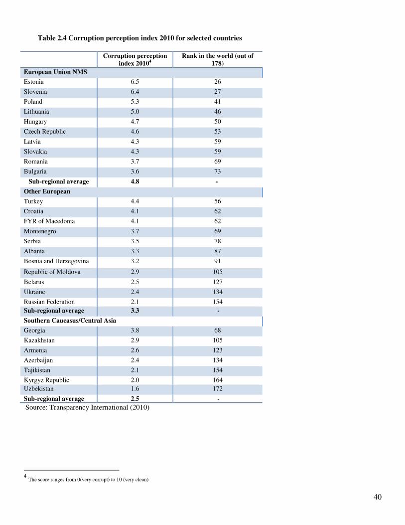
40

Corruption perception

index 20104

Rank in the world (out of

178)

European Union NMS

Estonia 6.5 26

Slovenia 6.4 27

Poland 5.3 41

Lithuania 5.0 46

Hungary 4.7 50

Czech Republic 4.6 53

Latvia 4.3 59

Slovakia 4.3 59

Romania 3.7 69

Bulgaria 3.6 73

Sub-regional average 4.8 -

Other European

Turkey 4.4 56

Croatia 4.1 62

FYR of Macedonia 4.1 62

Montenegro 3.7 69

Serbia 3.5 78

Albania 3.3 87

Bosnia and Herzegovina 3.2 91

Republic of Moldova 2.9 105

Belarus 2.5 127

Ukraine 2.4 134

Russian Federation 2.1 154

Sub-regional average 3.3 -

Southern Caucasus/Central Asia

Georgia 3.8 68

Kazakhstan 2.9 105

Armenia 2.6 123

Azerbaijan 2.4 134

Tajikistan 2.1 154

Kyrgyz Republic 2.0 164

Uzbekistan 1.6 172

Sub-regional average 2.5 -

Source: Transparency International (2010)

4 The score ranges from 0(very corrupt) to 10 (very clean)

Table 2.4 Corruption perception index 2010 for selected countries

41

Table 2.5 Scores in different indicators of the global competitiveness index, low 1 to high 7 Country/Economy Overall

Index

Basic

requirements

Efficiency

Enhancers

Institutions Infrastructure

Goods market

efficiency

European Union NMS

Estonia 4.62 5.41 4.52 4.99 4.71

4.74

Czech Republic 4.52 4.90 4.63 3.65 4.87

4.58

Poland 4.46 4.70 4.61 4.17 3.87

4.36

Lithuania 4.41 4.82 4.31 3.94 4.64

4.25

Hungary 4.36 4.72 4.39 3.79 4.52

4.32

Slovenia 4.30 5.12 4.23 4.08 4.81

4.37

Latvia 4.24 4.60 4.20 3.87 4.12

4.28

Slovak Republic 4.19 4.66 4.38 3.46 4.23

4.36

Bulgaria 4.16 4.46 4.10 3.32 3.62

4.08

Romania 4.08 4.28 4.09 3.49 3.37

3.96

Other European

Turkey 4.28 4.61 4.22 3.69 4.39

4.38

Montenegro 4.27 4.69 4.07 4.53 4.01

4.50

Russian Federation 4.21 4.61 4.19 3.08 4.52

3.60

Croatia 4.08 4.76 4.01 3.59 4.73

3.81

Albania 4.06 4.53 3.87 4.01 3.87

4.46

Macedonia, FYR 4.05 4.55 3.83 3.68 3.66

4.26

Ukraine 4.00 4.18 4.00 2.98 3.87

3.58

Moldova 3.89 4.13 3.62 3.38 3.32

3.94

Serbia 3.88 4.28 3.73 3.15 3.67

3.49

Bosnia and Herzegovina 3.83 4.25 3.63 3.32 3.24

3.81

Southern Caucasus/Central Asia

Azerbaijan 4.31 6.68 3.99 3.84 3.87

4.12

Kazakhstan 4.18 4.64 4.00 3.54 3.70

4.07

Georgia 3.95 4.32 3.74 3.97 3.95

4.16

Armenia 3.89 4.24 3.73 3.65 3.75

3.88

Tajikistan 3.77 4.03 3.42 3.93 2.84

3.78

Kyrgyz Republic 3.45 3.52 3.44 2.91 2.77

3.74

EU-15

Sweden 5.61 6.06 5.33 6.06 5.74

5.21

Finland 5.47 6.02 5.19 5.98 5.62

4.89

Germany 5.41 5.83 5.18 5.27 6.35

4.79

Netherlands 5.41 5.88 5.29 5.61 6.02

5.17

Ireland 4.77 5.20 4.67 5.19 5.12

5.10

Spain 4.54 5.18 4.58 4.27 5.83

4.23

Italy 4.43 4.84 4.41 3.61 5.01

4.30

Portugal 4.40 5.00 4.42 4.20 5.48

4.27

Greece 3.92 4.36 4.06 3.52 4.54

3.88

Source: World Economic Forum: global competitiveness index 2011-12 rankings Note: only the five lowest and four highest of the EU-15 were included in this summary

42

The countries in each group are ranked according to the overall index, but not all scores follow the same ranking. In the case of NMS the newest members, Bulgaria and Romania, are lowest in all six reported categories; and in SCCA Tajikistan and Kyrgyz Republic are lowest in all but one category. But if we look for the lowest two or three (marked in red) for institutions and goods market efficiency in Other European, they are Russian Federation and Ukraine. Ukraine is also in the lowest two for Basic requirements, but otherwise most of the lowest were also in the lowest three of the overall index. Another observation is that Greece is not noticeably different from Romania and Bulgaria in these scores and is sometimes even lower. As a point of reference, the top four ranked countries in the EU-15 are also in the top 7 countries of the world by the GCI ranking, while the lowest overall score, Kyrgyz Republic, was ranked 126th in the world. Finally, it is useful to do another comparison that includes the “old member states” of the EU, because there are also some lessons there. Guy Dinmore pointed out in the Financial Times (FT weekend, Nov 12/13) just before Berlusconi stepped down that Italy had dropped below Zambia and Mongolia in the World Bank’s “Ease of Doing Business Survey” (World Bank 2011b). In fact Italy was below most of the countries in ECA in the ranking and had the very worst rating for the ranking of “enforcing contracts” (Table 2.6). Part of the general ranking was due to the financial crisis and Greece was even lower. But as regards enforcing contracts, Dinmore argues that is was evidence of rising corruption and disintegration of the rule of law during the last 10 years. It means that even relatively advanced countries of the region are not immune to problems that can damage the business climate and stifle investment. Again, there is great diversity in the countries of this region and the most competitive by the GCI indicator are almost always also ranking high in the corruption perception index (Table 2.4). If the engine of growth for the food and agriculture industry needs to be private sector investment, both domestic and foreign, then many of these countries need to give priority to removing the barriers (corruption, unstable policies, lack of transparency, etc.) to a good business environment and investing in public goods (infrastructure, information systems, etc.) that enhance the confidence of investors and stimulate the needed inflow of capital and expertise that often comes with it.

2.3 Benefits and risks of investment in agriculture

Are all investments good investments? Clearly, the standard for evaluating any investment, whether public or private, is the rate of return on investment; but research on returns to investment in agriculture have invariably confirmed it as a high payoff investment (World Bank 2008). However, we also know from seeing the waste and dismal failure of public investment in parts of this region that were under a command economy system for so long that some investment can also be wasteful of resources. The concern in current times in this region and others is the rise of large investments from both private sources and foreign sovereign wealth funds or state funds that may not be adequately vetted with respect to their externalities. Of particular concern are the social consequences of displaced farmers or workers or the sustainability of the investments from an environmental standpoint. One of these new forms of investment is the agriholdings in places like Russia, Ukraine and Kazakhstan. As the role the ECA region plays in satisfying the growing need for global food production increases, the emergence of these new farm structures, agriholdings, has been invoking interest among the experts.

43

Table 2.6. Rankings of ECA countries in Ease of Doing Business Survey

Economy Ease of Doing

Business Rank

Enforcing

Contracts

Georgia 16 41

Germany 19 8

Latvia 21 17

Macedonia, FYR 22 60

Estonia 24 29

Lithuania 27 15

Portugal 30 22

Netherlands 31 28

Austria 32 9

Slovenia 37 58

Cyprus 40 105

Spain 44 54

Kazakhstan 47 27

Slovak Republic 48 71

Luxembourg 50 1

Hungary 51 19

Armenia 55 91

Montenegro 56 133

Bulgaria 59 87

Poland 62 68

Czech Republic 64 78

Azerbaijan 66 25

Belarus 69 14

Kyrgyz Republic 70 48

Turkey 71 51

Romania 72 56

Croatia 80 48

Moldova 81 26

Albania 82 85

Italy 87 158

Serbia 92 104

Greece 100 90

Kosovo 117 157

Russian Federation 120 13

Bosnia and Herzegovina 125 125

Tajikistan 147 42

Ukraine 152 44

Uzbekistan 166 43

Source: World Bank, Ease of Doing Business Survey, June 2011.

44

Agriholdings are the large farms (sometimes larger than 100,000 ha) that are sometimes vertically integrated with processors or exporters. The majority of them have been formed in the grain sector, while some of them function in the oilseed, sugar and dairy sectors. According to FAO-EBRD (2009), “some of these farms have managed to attract financing though the placement of stocks on leading European stock exchange, and borrowing from private investors or EBRD.” For example, between 2006 and 2008 Ukrainian agriholdings attracted through IPO more than 800 billion U.S. dollars (Sadovnik, 2008).

Unfortunately, there are no official statistics sources on the number of agriholdings in Kazhakstan, Russia and Ukraine, or the amount of land in their use. A growing number of the studies, however, provide a useful approximation. For example, according to Akimbekova (2006), the agriholdings in Kazakhstan control about 30 percent of the farmland used for grain production, and produce close to 70 percent of all the grain sold in the country and abroad. An FAO-EBRD study on grain markets in Ukraine, Russia and Kazakhstan (2009) states that there are 196 agriholdings in Russia that operate on 11.5 million ha, and 33 agriholdings in Ukraine that use almost 5 million hectares. The reasons for the investors’ interest in the agriholdings are quite numerous. Among them are vast availability of relatively cheap fertile land, sufficient level of infrastructure development, world market access, productive and relatively cheap labor, and finally, increasing commodity prices as a promise of higher profits. However, Demyanenko (2008) also points out that the major reason for the agriholdings to be a post-USSR (rather than a Western) phenomenon is the underdeveloped institutional and legislative conditions of the transition economies that allow for large capital accumulation. For example, in Ukraine, there is a moratorium on the sale of land. This allows the owners of the agriholdings to rent a large amount of land at a relatively cheap rental rate. Moreover, there are cases where land contracts are secured and allowed to remain idle as the agriholding company uses the land holdings to attract investments in exchange markets. This is clearly not in the interests of the nation nor the small land holders and workers in rural areas. The leasing law should prevent this practice from continuing, but routinely such laws are not enforced. The major benefit of the agriholdings is that they allow attracting a large amount of investment in the agribusiness sector both from domestic and international investors, which as was mentioned earlier in our study is crucial for increasing the food production. Additionally, the economies of scale of the agriholdings should allow them to decrease the cost and increase the efficiency of production, while the extent of their integration allows for the fast and smooth product movement from a farm to an exporter or domestic user. However, massive land holdings that are usually widely scattered geographically and not always well managed as farming enterprises are very likely to be more inefficient than holdings in the 10-20,000 hectare scale as shown in research by Demyanenko (2011). In addition, the agriholding farming system is much more likely to engage in monoculture practices that lead to deterioration of land quality and other environmental externalities. At the same time, there are a number of risks associated with the creation of such large farms. The main one is the disconnect between the agriholdings and the rural areas where they operate. Usually, the major offices of such holdings are located in the larger cities and not in the areas where the production takes place. Therefore, the agriholdings pay taxes to the cities, which decreases the stream of financing to the rural territories. In turn, this results in lower levels of financing of infrastructure and public goods provision in the rural areas of Kazakhstan, Russia and Ukraine. Additionally, some experts (Visser et al.) fear that the emergence of agriholdings might be an example of “land grabbing” practices, where a big share of land is owned or under long-term lease by foreign or domestic investors. As a result, this might cause even further loss of revenues on the part of the local population. Whether the benefits that agriholdings provide outweigh the risks or vice versa is yet to be determined. However, at this point it is already clear that they are major players in the grain sector of Kazakhstan, Russia and Ukraine, and shape their production and exports. As an example, 62 agriholdings in Ukraine control 5.1 million hectares of land, which is more than 25 percent of sown area.

45

A study commissioned by OECD on private financial sector investment in farmland and agricultural infrastructure showed a wide use of this type of investment, mostly FDI, for agricultural investments (HighQuest Partners, 2010). Twenty four international companies were interviewed with about USD 7.4 billion in agricultural assets around the world. They were quite varied in their business profiles, but most felt that international protocols to regulate or certify investment in farmland did not pose a problem, and they have developed working relationships with organizations like FAO and World Bank who are working on such protocols and many are following such existing schemes or certifications. One interesting result of the study with regard to this region is that Eastern Europe locations ranked fourth in investors who preferred North America and Oceana, Brazil and Africa in that order. The main reasons given for ranking such a productive area so low was the “legal and political challenges”, which only reinforces the importance of those factors already noted that provide a good investment climate.

2.4 The investment challenge for investors and policy makers

The FAO challenge for more investment in agriculture has become more nuanced and sophisticated over the nearly 10 years since the 2002 Summit and it has been supported by a growing body of research and experience and joined by many other international agencies as well as national governments and multinational organizations and NGOs that are striving to achieve the food security and anti-poverty objectives that have been so widely supported but also seemingly intractable. The G-8 Summit in L’Aguila in July 2009 highlighted the importance of agriculture and committed $20 billion in resources to the effort, and the G-20 Ministers of Agriculture in June 2011 adopted the “Action Plan on food price volatility and agriculture” that included priorities for investment in agriculture and market information systems. So some momentum has been gained. However, the lingering financial crisis that is severely constraining national budgets in many of these same countries and slowing the global economic recovery has cast doubt on how and when these commitments can be realized. The size of the challenge and the constrained resources put a high priority on smart policies that leverage limited government resources and stimulate private investment as well as public-private partnerships. The new SOFI 2011 summarized the challenge well in a key message “Investment in agriculture will improve the competitiveness of domestic production, increase farmers’ profits and make food more affordable for the poor. Private investment will form the bulk of this investment, but public investment has a catalytic role to play in supplying public goods that the private sector will not provide. These investments should consider the rights of existing users of land and related natural resources, benefit local communities, promote food security and not cause undue harm to the environment.” (FAO, 2011). There are indeed signs of growing investments in agriculture by private foreign and domestic investors, by states and by sovereign wealth funds; and the drivers of these investments include rising commodity prices and the food crisis, increased demand for animal protein and processed food, competition for land and water resources for food, feed and biofuels as well as non-agricultural uses, climate change and climate commitments, and investment diversification interests (High Quest Partners, 2010, GTZ, 2009). Although ECA has not been the favorite region for many of these investments, it has still attracted substantial amounts of investment capital and these investment activities often bring with them significant know-how transfers that can also be valuable for agricultural development. A good example of growing investment and its impact on food security of local populations is in a recent study of the North-Kazakh Grain Region (Petrick, 2011). Since 2000 investment in agricultural fixed assets, cropland expansion as well as growing input use in this region of Kazakhstan has contributed to growing production but also to rising wages, and rising consumption expenditures that well exceeded cost of living increases. During

46

the same period the share of households below the poverty line in this region fell from over 35 percent in 2001 to about 5 percent in 2010. Although increased investment is one of the main vehicles for improving agricultural technologies, production, farm and rural incomes, and food security more generally, it also can entail risks and have negative consequences. As with any economic activity, there are costs and benefits, winners and losers, so it is important that policy makers be well aware of both the costs and benefits of such investments and have appropriate policies, laws, and institutions to manage these risks and provide transparent mechanisms for balancing the costs and benefits if needed. Guidance for public and private entities involved in such investment activities have been developed jointly by FAO, IFAD, World Bank, and UNCTAD in consultation with other stakeholders and provided in the form of guidelines and voluntary principles for responsible agricultural investment (RAI, 2011). The goal of such guidance is at the same time to encourage increased investment, which is mostly private investment, and minimize the negative consequences. The principles are as follows:

1. Land and Resource Rights: Existing rights to land and natural resources are recognized and respected.

2. Food Security: Investments do not jeopardize food security, but rather strengthen it.

3. Transparency, Good Governance and Enabling Environment: Processes for accessing land and making associated investments are transparent, monitored, and ensure accountability.

4. Consultation and Participation: Those materially affected are consulted and agreements from consultations are recorded and enforced.

5. Economic viability and responsible agro-enterprise investing: Projects are viable in every sense, respect the rule of law, reflect industry best practice, and result in durable shared value.

6. Social Sustainability: Investments generate desirable social and distributional impacts and do not increase vulnerability.

7. Environmental Sustainability: Environmental impacts are quantified and measures taken to encourage sustainable resource use, while minimizing and mitigating them negative impact.

These principles are designed to be comprehensive and inclusive of many differing situations, so they would apply differently to different countries and types of investment. As mentioned in the previous section, the types of large agricultural investment most prominent in this region are buying or leasing large tracks of land for extensive crop production or to a lesser extent establishing large scale animal or dairy production facilities. In some cases fallow or abandoned land is brought back into production, while in other cases cropland is aggregated into larger production units. There are also, however, cases where land use contracts are merely used to raise capital in financial markets, while the land stands idle. This is obviously not desirable for either the country or for the communities where the idle land resides. Land tenure and ownership differ greatly across this region (USAID 2007), but in most cases land is leased from a large number of residents who own or have land use rights on small plots and in either case have little if any alternative leasing opportunities and very low bargaining leverage. So as large and more capital intensive production practices are introduced in such conditions, labor displacement is almost inevitable. Some of the lease contracts in Ukraine, for example, also include the first option to buy the land, should the moratorium on the sale of agricultural land be lifted. So even in cases where land is not purchased, many of the principles listed above could apply, since the potential impacts on land use rights, transparency of contracts, social sustainability and environmental sustainability could all be important. The fact that data on agriholdings, for example, is not routinely collected and reported by the government of the region is one indication that these principles are not being applied.

47

References for Themes 1 and 2 Akimbekova, G. 2006. “Formirovanie effektovnoy sistemy proizvodstva, pererabotki I sbyta

sel’skokhozyaystvennoy produkcii,” Almaty, Kazakhstan. Alston, J. 2010. “The benefits from Agricultural Research and Development, Innovation, and Productivity

Growth,” OECD Food, Agriculture and Fisheries Working Papers. Available online at http://www.oecd-ilibrary.org/docserver/download/fulltext/5km91nfsnkwg.pdf?expires=1320468918&id=id&accname=guest&checksum=345BC83A559D515D7C241537765611F1. Accessed 4 November 2011.

Alston, J. 2011. “Global and U.S. Trends in Agricultural E&D in a Global Food Security Setting,” OECD

Conference on Agricultural Knowledge Systems: Responding to Global Food Security and Climate Change Challenges, OECD, Paris. Available at http://www.oecd.org/dataoecd/17/22/48165448.pdf, accessed November 4, 2011.

Alston, J.M., Andersen, M.A., James, J.S. and Pardey, P.G. 2010. “Persistence Pays: U.S. Agricultural

Productivity and the Benefits from Public R&D Spending”. New York: Springer.

Alston, J. and Pardey, P. 2009. "Theme Overview: Agricultural Productivity and Global Food Security in the Long Run,” Choices. Available at http://www.choicesmagazine.org/magazine/pdf/article_90.pdf. Accessed November 4, 2011.

Anderson, M. and Magleby, R. 1997. "Agricultural Resources and Environmental Indicators," Agriculture

Handbook No. AH712. Available at http://www.ers.usda.gov/Publications/AREI/AH712/. Accessed November 4, 2011.

Bruinsma, J. 2009. "The Resource Outlook to 2050: By how much do land, water and crop yields need to

increase by 2050?". Prepared for the expert meeting on How to Feed the World in 2050. Available at ftp://ftp.fao.org/docrep/fao/012/ak971e/ak971e00.pdf. Accessed November 4, 2011.

DEFRA. 2002. “The role of future public research investment in the genetic improvement of UK grown crops”,

Available at http://sciencesearch.defra.gov.uk/Default.aspx?Menu=Menu&Module=More&Location=None&Completed=0&ProjectID=10412. Accessed 22 November 2011.

Demyanenko, S. 2008. “Agriholdings in Ukraine: good or bad?” The Institute for Economic Research and

Policy Consulting. Kiev, Ukraine. Available online at http://www.ier.com.ua/en/publications/consultancy_work/?pid=1497. Accessed 28 October 2011

Dubrovskiy, V. & Ustenko, O. 2005. “Business Climate in CIS Countries,” Center for Social and Economic Research, Warsaw, Poland.

EBRD. 2010. “Forecasts, Macro Data, Transition Indicators.” Available online at http://www.ebrd.com/pages/research/economics/data/macro.shtml. Accessed 16 October 2011.

FAO. 1997. “Improving agricultural extension. A reference manual”. Edited by Swanson, B., Bentz, R., and

Sofranko, A. Rome, Italy. Available online at http://www.fao.org/docrep/W5830E/w5830e00.htm. Accessed 25 November 2011.

48

FAO. 2001a. "The Economics of Conservation Agriculture,” Rome, Italy. Available at http://www.fao.org/DOCREP/004/Y2781E/Y2781E00.HTM. Accessed November 4, 2011.

FAO. 2001b. “Agricultural and Rural Extension Worldwide: Options for Institutional Reform in the

Developing Countries”. Rome, Italy. Available online at ftp://ftp.fao.org/docrep/fao/004/y2709e/y2709e.pdf. Accessed 23 November 2011.

FAO. 2002. “The World Food Summit: Five Years Later. Mobilizing the political will and resources to banish

world hunger,” Technical Background Documents, Rome, Italy. Available online at http://www.fao.org/DOCREP/004/Y1780e/Y1780e00.HTM. Accessed 14 October 2011.

FAO. 2003. “Anti-Hunger Programme. A twin-track approach to hunger reduction: priorities for national and

international action,” Rome, Italy. Available online at ftp://ftp.fao.org/docrep/fao/006/j0563e/j0563e00.pdf. Accessed 14 October 2011.

FAO. 2009. "The Technology Challenge,” Rome, Italy. Available at

http://www.fao.org/fileadmin/templates/wsfs/docs/Issues_papers/HLEF2050_Technology.pdf. Accessed November 4, 2011.

FAO. 2010. “Policy Response to Challenges in Agriculture and Rural Development in the Europe and Central

Asia Region: Sharing Experience and Enhancing Cooperation in the Region,” Document ERC/10/7, Agenda Item 12, Twenty-Seventh FAO Regional Conference for Europe, Yerevan, Armenia, 13-14 May 2010. Available online at http://www.fao.org/docrep/meeting/018/k7854e.pdf. Accessed 9 September 2011.

FAO. 2011. “The State of Food Insecurity in the World: How does international price volatility affect domestic

economies and food security?” Rome, Italy. Available online at http://reliefweb.int/sites/reliefweb.int/files/resources/Full%20Report_266.pdf.

FAO-EBRD. 2009. “Grain markets in Kazakhstan, the Russian Federation and Ukraine”, prepared by D.

Pryhodko. Rome, Italy. Available online at http://www.eastagri.org/files/Grain-Markets-KZ_RU_UA.pdf. Accessed 28 October 2011.

FAO, IFAD, IMF, OECD, UNCTAD, WFP, the World Bank, the WTO, IFPRI and the UN HLTF. 2011.

“Price Volatility in Food and Agricultural Markets: Policy Responses,” Policy Report prepared for the G-20. Available online at http://www.fao.org/fileadmin/templates/est/Volatility/Interagency_Report_to_the_G20_on_Food_Price_Volatility.pdf. Accessed November 4, 2011.

FAOSTAT. 2011. Available online at http://faostat.fao.org/default.aspx. Accessed 4 November 2011. Financial Times. 2011. "Italians fear 'Berlusconismo' is down but not out", FT Weekend, Nov 12/13, p.2. Food and Agricultural Policy Research Institute. 2011. “FAPRI 2011 U.S.Baseline Briefing Book,” FAPRI

MU Report 02-11, Ames, Iowa. Available at http://www.fapri.missouri.edu/outreach/publications/2011/FAPRI_MU_Report_02_11.pdf Accessed 16 October 2011

HighQuest Partners, United States. 2010. “Private Financial Sector Investment in Farmland and Agricultural

Infrastructure,” OESD Food, Agriculture and Fisheries Working Papers, No.33, OECD Publishing. Available online at http://farmlandgrab.org/wp-content/uploads/2010/10/private-financial-sector-investment-in-farmland-and-agricultural-infrastructure_5km7nzpjlr8v.pdf. Accessed 1 December 2011.

49

House of Lords. 2011. “Innovation in EU Agriculture”. Available at http://www.publications.parliament.uk/pa/ld201012/ldselect/ldeucom/171/171.pdf. Accessed 22 November 2011.

Hu, R. and Huang, J. 2010. “China’s Agricultural Innovation System: Issues and Reform,” OECD, Paris. Available online at http://www.oecd.org/dataoecd/58/2/48218753.pdf. Accessed 4 November 2011.

IMF. 2010. “World Economic Outlook Database.” Available online at

http://www.imf.org/external/pubs/ft/weo/2008/02/weodata/index.aspx. Accessed 16 October 2011. Kudina, A. & Jakubiak, M. 2008. “The Motives and Impediments to FDI in the CIS,” Background Paper

prepared for the OECD’s 2008 Global Forum on International Investment. Available online at http://www.oecd.org/dataoecd/24/52/40401047.pdf. Accessed 9 September 2011.

Laurent, C., Cerf, M. and Labarthe, P. 2006. “Agricultural extension services and market regulation:

learning from a comparison of six EU countries”. Journal of Agricultural Education and Extension, vol. 12, n° 1, 5-16.

Lusser, M., Parisi, C., Plan, D., and Rodriguez-Cerezo, E. 2011. "New plant breeding techniques: State-of-

the-art and prospects for commercial development”. Institute for Prospective Technological Studies, Seville. Available online at http://ftp.jrc.es/EURdoc/JRC63971.pdf. Accessed 22 November 2011.

Matthews, A. 2011. “The future role for the European Innovation Partnership for agricultural productivity and

sustainability”. Available at http://capreform.eu/the-future-role-for-the-european-innovation-partnership-for-agricultural-productivity-and-sustainability/. Accessed 22 November 2011.

Meyers, W. 2010. “The Global Economic Crisis and Food Security in Europe and Central Asia: Impacts and

Policy Priorities” in I. Ferto, C. Forgacs, A. Jambor (Eds.), Changing Landscape of European Agriculture:

Essays in Honor of Professor Csaba Csaki. Publisher: Agroinfor Kiado, Budapest, Hungary. OECD. 2011a. "Productivity and Competitiveness in Agriculture: The Role of Research and Development".

TAD/CA/APM/WP(2011)18/FINAL. Unclassified. Paris, France. OECD. 2011b. “Agricultural Policy Monitoring and Evaluation 2011: OECD Countries and Emerging

Economies”. OECD Publishing, Paris. OECD. 2011c. “Producer and Consumer Support Estimates database.” Available online at

http://www.oecd.org/document/59/0,3746,en_2649_37401_39551355_1_1_1_37401,00.html. Accessed 4 November 2011.

OECD-FAO. 2011. “Agricultural Outlook 2011-2020,” OECD Publishing. Available online at

http://www.agri-outlook.org/pages/0,2987,en_36774715_36775671_1_1_1_1_1,00.html. Accessed 20 September 2011.

Pardey, P.G. 2011. “A Strategic Look at Global Wheat Production, Productivity and R&D Developments”,

Czech J. Genet. Plant Breed., 47, 2011 (Special Issue): S6–S19, available at http://www.agriculturejournals.cz/publicFiles/48940.pdf. Accessed 22 November 2011.

Petrick, M., Wandel, J., and Karsten, K. 2011. “Farm Restructuring and Agricultural Recovery in Kazakhstan’s Grain Region: An Update”, Leibniz Institute of Agricultural Development in Central and

50

Eastern Europe, Leibniz, Germany. Available online at http://www.iamo.de/dok/_3903.pdf. Accessed 25 November 2011.

Pinto, R. 2005. “Challenges for Public Policy in Promoting Entrepreneurship in South Eastern Europe”, Local

Economy 20 (1), pp. 111-117. Available online at http://pintoconsulting.blog385.com/eng/wp-content/uploads/2009/03/7_entrepreneurship_see_local_economy_2005.pdf. Accessed 20 September 2011.

Poppe, K. J. 2011. “AKIS – Agricultural Knowledge and Innovation Systems in Transition”. Presentation

prepared for an OECD Conference on Agricultural Knowledge Systems: Responding to Global Food

Security and Climate Change Challenges, OECD, Paris, France. Available at http://www.oecd.org/dataoecd/58/9/48218517.pdf. Accessed 4 November 2011.

RAI. 2011. Responsible Agro Investment Knowledge Exchange Platform.

http://www.responsibleagroinvestment.org/rai/node/232. Accessed 3 November 2011. Roling, N. and Engel, P. 1991. “The development of the concept of agricultural knowledge information

systems (AKIS): Implications for extension”, in Agricultural extension: Worldwide institutional evolution

and forces for change, edited by W. Rivera and D. Gustafson, Amsterdam: Elsevier Science. Sadovnik, O. 2009. “Suchasni tendencii rozvytku agroholdyngiv v Ukraini”. Visnyk SNAU 4, pp. 10-15.

Available online at http://www.nbuv.gov.ua/portal/Chem_Biol/Vsna/ekon/2009_4/Sadovnik.pdf. Accessed 2 November 2011.

Schmidhuber, J. & Bruinsma, J. 2011. “Investing towards a world free of hunger: lowering vulnerability and

enhancing resilience” in A. Prakash (Eds.), Safeguarding food security in volatile global markets (pp. 523-549). FAO, Rome. Available online at http://www.fao.org/docrep/013/i2107e/i2107e27.pdf. Accessed 14 October 2011.

Smith, R. 2010. “Production practices may improve water efficiency”, Southwest Farm Press, February 22,

2010. Available at http://southwestfarmpress.com/irrigation/production-practices-may-improve-water-efficiency. Accessed 4 November 2011

Swanson, B. and Rajalahti, R. 2010. “Strengthening Agricultural Extension and Advisory Systems:

Procedures for Assessing, Transforming, and Evaluating Extension Systems.” World Bank, Agriculture and Rural Development Discussion Paper 45. Available at http://siteresources.worldbank.org/INTARD/Resources/Stren_combined_web.pdf. Accessed 23 November 2011.

Transparency International. 2010. “Corruption Perception Index 2010.” Available online at

http://www.transparency.org/policy_research/surveys_indices/cpi/2010. Accessed 16 October 2011. UNCTAD. 2009. “World Investment Report 2009: Transnational Corporations, Agricultural Production and

Development,” United Nations, New York, Geneva. Available online at http://www.unctad.org/en/docs/wir2009overview_en.pdf. Accessed 14 October 2011.

USAID. 2007. “Land Tenure and Property Rights Regional Report,” prepared by ARD, Inc. Available online at

http://prrgp.com/tools.htm. Accessed 4 November 2011. USDA. 2011. Available online at http://www.csrees.usda.gov/qlinks/extension.html. Accessed 4 November

2011.

51

Visser, O. and Spoor, M. 2011. “Land grabbing in post-Soviet Eurasia: the world’s largest agricultural land reserves at stake”. The Journal of Peasant Studies, Volume 38(2), pp. 299-323.

von Cramon-Taubadel, S., Anriquez, G., de Haen, H. & Nivyevskiy, O. 2009. “Investment in Developing Countries’ Food and Agriculture: Assessing Agricultural Capital Stocks and their Impact on Productivity,” Paper prepared for FAO’s Expert Meeting on “How to Feed the World in 2050,” 24-26 June 2009, Rome, Italy. Available online at ftp://ftp.fao.org/docrep/fao/012/ak975e/ak975e00.pdf. Accessed 9 September 2011. Accessed 14 October 2011.

World Bank – International Finance Corporation. 2010. “Cost of Doing Business Survey.” Available online

at http://www.doingbusiness.org/rankings. Accessed 16 October 2011. World Bank. 2008. “World Development Report 2008: Agriculture for Development,” World Bank

Publications, Washington, D.C.

World Bank. 2009. “The Crisis Hits Home: Stress Testing Households in Europe and Central Asia”, World Bank Report No. 50158-ECA, Washington, D.C.

World Bank. 2010. “The Business Environment and Enterprise Performance Survey At-a-Glance 2008 Cross

Country Report,” World Bank Publications, Washington, D.C. Available online at http://siteresources.worldbank.org/INTECA/Resources/BEEPS_Cross_Country_Report_2010.pdf. Accessed 14 October 2011.

World Bank. 2011a. “Commodity Price Data (Pink Sheet),” World Bank Publications, Washington, D.C. World Bank. 2011b. “Ease of Doing Business Survey”, World Bank Publications, Washington, D.C. World Economic Forum. 2011. “The Global Competitiveness Report 2011-2012.” Available online at

http://www3.weforum.org/docs/WEF_GCR_Report_2011-12.pdf. Accessed 14 October 2011.

52

Theme 3. Climate change Climate change is defined as a change in the state of the climate that can be identified by changes in the mean and/or the variability of its properties, and that persists for an extended period, typically decades or longer, whether due to natural variability or as a result of human activity (FAO, 2008b). According to scientific studies, climate change and increasing demand for water resources will impact growing conditions and thus food production in many countries of the world. Integrated assessment models have shown that climate change effects on temperature and rainfall will induce an increase in crop yield in cooler climates, while a decrease in low latitude regions (most developing countries) (Easterling et al., 2007). According to Cline (2007), developing countries will have a 9-21% decrease in agricultural productivity due to global warming, while industrialized countries will face a 6% decline to an 8% increase, depending on the offsetting effects of atmospheric carbon emissions. Thus, as a result of the direct effects of global warming, some regions will benefit with increased production yields while other regions will have to rely more on food imports to meet the national demand. Fischer et al. (2005) estimated that cereal imports will increase in developing countries by 10-40% by 2080. In this chapter, we will present implications of climate change on the agricultural sector and food security in Europe and Central Asia. Also, policy measures are discussed that can contribute to mitigation climate change effects on agriculture and adaptation of the agricultural sector to climate change.

3.1 Agriculture in the climate change discussion – problems and challenges

According to OECD (2009: 26), the world greenhouse gas (GHG) emissions have doubled since 1970 and are expected to double again in 2008-2050, if no action is taken. In such a case, the average global temperature would increase to 4-6°C (39.6-43.2 F) by 2100. The Intergovernmental Panel on Climate Change (IPCC) informed that the total cost of reducing global greenhouse gas emissions by 50% by 2050 could be achieved at a cost of 1-3% of global GDP, assuming relatively stable economic conditions. This change range is said to be necessary to reach the goals of limiting global warming by around 36F (2°C) above preindustrial temperatures (World Bank, 2010: 259). Regardless of mitigation efforts, the overall temperature increase of 1.6-2.6ºC is expected to occur in ECA by 2050. Considering ‘business-as-usual’ scenario, worldwide projections suggest a temperature increase of 5ºC (Sokolov et al., 2009). Climate change impacts the overall development in countries/regions. It diminishes the pace of development and slows down the progress of achieving the Millennium Development Goals (MDGs), especially the goals of reducing hunger and poverty, and ensuring environmental sustainability. Agriculture, forestry and fisheries sectors are faced with ‘twin challenges’ in regard to climate change. On the one hand, they contribute to greenhouse gas (GHG) emissions, but on the other, they offer sustainable mitigation options for development and food security. Thus, adaptation and mitigation actions can be integrated directly into sustainable development policies. (FAO, n.d. a). Agriculture accounts for 13.5% of global greenhouse gas (GHG) emissions (about 6.6 Gt of CO2 eqv./yr) (IPCC 2007b,c), released mainly as methane (CH4) from animals and animal waste and nitrous oxide (N2O) from fertilized soils, enteric fermentation, biomass burning, rice production, and manure and fertilizer production. The emissions do not include overall carbon capture through photosynthesis in terrestrial ecosystems. On the other hand, agriculture has a potential to mitigate between 5.5-6 Gt of CO2 eqv./yr by 2030 (IPCC, 2007c),

53

mainly through soil carbon sequestration in developing countries, which equals about 83-91% of the total sectors’ emissions. Climate change, and rising temperatures, can also impact animal production and cause heat stress and nutritional changes. For instance, the availability of livestock feeds and the quantity and quality of pastures and forage crops can be affected and further influence health, growth and reproduction of livestock. Climate change may also trigger zoonoses (diseases and infections naturally transmitted between vertebrate animals and man) (Jaykus et al., n.d.). In addition to the direct and indirect impacts of global warming and climate change on the agricultural food and feed production and food security, agriculture has to cope with demographic changes. In the last 50 years, the world population increased from 3 billion in 1959 to 6.7 billion in 2009, while it is predicted to increase by another 50% up to 9.1 billion by 2050. Meeting the food and feed demand of the growing population and production livestock will be very challenging for the agricultural sector, forestry and fisheries sectors. Therefore, according to the FAO (n.d. a) report, agricultural production in the European and Central Asia economies should be increased to meet increased demands and secure global food security. Simultaneously, natural resources should be maintained and adaptation and mitigation measures should be prepared for the long-term. As other economy sectors are also influenced by climatic changes, direct interactions are expected. In addition, as climate change occurs on a global scale with different effects in different regions/countries, the patterns of production and trade will need to adjust to satisfy the national food and feed demand in many countries of Europe and Central Asia (ECA).

3.1.1 Impacts of climate change in Europe and Central Asia – current developments and long-term

projections

The World Bank (2010) report states that Europe and Central Asia (ECA) are already experiencing a number of consequences of climatic changes, such as increasing variability, higher temperatures, changing hydrology, and extreme events, e.g., droughts, floods, heat waves, windstorms, and forest fires. Due to climate-related natural disasters, many regions in ECA are experiencing more frequent and larger economic losses in GDP (Dilley et al. 2005). The droughts in 2000-2001 have cost Georgia and Tajikistan approximately 6% and 5% percent of their respective GDPs (World Bank, 2006). Climate change induces many challenges for the agricultural sector, especially in the Central Asia countries that are facing the problem of environmental mismanagement and under-investment in infrastructure and housing. As a result, the region is already vulnerable to the current climate conditions because of its ‘adaptation deficit,’ which can only increase with the projected climate changes. In addition, the region’s vulnerability is influenced by socio-economic and environmental factors such as the legacy of the former Soviet system. While Turkey does not carry the same legacy issues, it is under demographic pressure on fragile natural resources and inadequate and vulnerable infrastructure. The socio-economic conditions exacerbate climate risks and hamper the ability of sectors to adjust to changes imposed by global warming and climate change. Furthermore, climate change creates an additional uncertainty for farmers as the limited ability to predict local impacts and the timing of particular weather events, negatively impacts farmers’ decisions about their production practices and inputs. This, in turn, can significantly impact food production and distribution. In the situation of limited data availability and unsatisfactory information exchange on those highly relevant issues, policymakers on the national and local levels as well as international organizations should invest not only in potential impact assessment measures, but mainly in reducing vulnerability of private businesses to

54

current climate changes. In this way, a relatively steady level of food and feed supply could be secured and unexpected spikes in price levels for agricultural products could be moderated (table 3.1). Europe and Central Asia face a substantial threat from climate change, with an average temperature increase of 0.5ºC in the south to 1.6ºC in the north (Siberia). An overall temperature increase of 1.6-2.6ºC is expected by the middle of the century, regardless of all mitigation efforts. The temperature changes are expected to induce a rapid melting of the region’s glaciers (Kyrgyzstan and Tajikistan) and a decrease in winter snows (World Bank, 2009). At the same time, many countries are already suffering from winter floods and summer droughts, while Southeastern Europe and Central Asia are at risk of severe water shortages. In ECA, the number of frost days is projected to decline by 14-30 days over the next 20-40 years with the number of hot days increasing by 22-37 days over the same time period. By midcentury, Poland and Hungary are expected to experience the same number of hot days (>30oC) as Spain and Sicily today. Water availability is projected to decrease in the entire ECA region, expect Russia, as increased precipitation in many regions, except Southeastern Europe, will be evaporated due to higher temperatures. Southeastern Europe is supposed to experience the most dramatic water decreases (-25%). In Russia, most of the precipitation is projected for the winter time, thus, it is possible that higher summer temperatures could offset precipitation and lead to drought. According to the World Bank (2010) study, the economic effects of climate change on agriculture include direct yield impacts. The following changes in the agricultural economies are expected: a) Net losses in Southeastern Europe and Turkey, the North and South Caucasus, and Central Asia; b) Gains in the Baltics and Siberia, Urals, Far East, and Baltic & Western Arctic regions of Russia; c) Mixed or uncertain outcomes in Central and Eastern Europe, Kazakhstan, and the Central and Volga regions of Russia. Still uncertainties remain in the projected scenarios, but they can be helpful in identifying problems and possible responses both by farmers and policymakers. A detailed overview of climate change impacts on the agricultural sector in ECA till 2050 is presented in table 3.1. Climate change will also affect the sea level of the ECA’s four basins (the Baltic Sea, the East Adriatic and Mediterranean coast of Turkey, the Black Sea, and the Caspian) and the Russian Arctic Ocean. On the Baltic, Poland with its strongly populated low-lying coast is especially vulnerable to sea level rise. Along the Adriatic and the Mediterranean, storm surge and saltwater intrusion into aquifers can be a threat to parts of the Croatian, Albanian, and Turkish coasts. The high sea levels in the Black Sea can threaten the ports and towns at the coast of Russia, Ukraine, and Georgia. In the Caspian Sea, water levels may drop by about six meters by the end of the 21st century which will be induced by the increased surface evaporation. This again can imperil fish stock and affect coastal infrastructure. According to an index of Baettig et al. (2007) (measuring the strength of future climate change relative to today’s natural variability), among the ECA countries, Russia, Albania, Turkey and Armenia would be exposed to the highest extent to climate changes, while Lithuania and Turkmenistan will not experience drastic changes (figure 3.1). In many ECA countries, dangerous facilities or dump sites were located close to weather sensitive sites. This can aggravate the problems of floods or extreme events and cause greater damage in those countries than in other parts of the world. For instance, in Estonia the leaching of radioactive waste at the Sillamae industrial center (dumping site for the radioactive wastes of a former uranium enrichment plant) is separated from the sea only by a narrow dam that can be potentially damaged by coastal surges. Also, some coastal landfills along the Black Sea, mostly in Georgia, have been identified as pollution hotspots. The coastal erosion could increase the amount of pollutants flushed to the sea, thus threatening the fish population and fishing industry.

55

Also, the power sector across ECA is under pressure of adjusting to growing electricity demands due to rising summer temperatures. Thus, technical upgrading and expansion are needed to insure its proper functioning, especially in unexpected critical situations of demand spikes. Warmer summers and periods of intense heat have already exposed the transmission networks of Turkey, Azerbaijan, Kazakhstan, and other Southeastern Europe countries to new challenges. The ECA’s transport infrastructure that is poorly maintained in many countries is at stake in the context of climatic changes. In the long-term, the World Bank (2010) expects the intense precipitation to weaken the road pavements and retaining walls. Long periods of droughts are expected to cause earth settling underneath the roads and transportation lines or extreme road deterioration through high temperatures. Those changes will require societies and economies to adjust in a practical manner (e.g., in Kazakhstan truck travel is limited on hot summer days due to the softening asphalt). This is just one example of necessary adaptation.

56

Table 3.1 Estimated agronomic impacts of climate change in ECA to 2050 – a summary

Source: World Bank (2009)

57

Figure 3.1 Climate change index for ECA countries by the end of the 21st century

Source: Baettig et al. (2007) Some authors claim that warmer climate and abundant precipitation in the northeastern part of ECA (Kazakhstan, Russia and Ukraine) will create benefits and new development chances for the agricultural sector. However, the region is characterized by low agricultural performance, with very low efficiency and productivity levels. These limiting economic indicators will play a decisive role in the development of the regions and do not provide an optimistic perspective on seizing new opportunities. Olesen and Bindi (2002) concluded that the current yield gap for the former Soviet countries in Europe (including Ukraine and European Russia) is 4.5 times higher than the potential increase in production from climate change by 2050. While some impacts of climate change have already been experienced in Europe and Central Asia, they are said to be manageable over the next decade, which provides an opportunity to increase the countries’ resilience to climate change by focusing on actions that have numerous co-benefits (World Bank, 2010). A future-oriented approach is to focus on strategies that could be effective even in the unpredictable future (‘robust strategies’) (Lempert and Schlesinger, 2000). With this approach the question should be answered: ‘What actions should we take, given that we cannot predict the future?’ Climate change policy is defined in these terms as a contingency (what if?) problem rather than an optimization problem (‘What is the best strategy

given the most likely outcome?’). The question of uncertainties should also be considered in policy making. The capacity to manage climate change will depend on the region’s ability to respond to environmental and national resource problems. The institutional and economic conditions of the respective countries and regions will have decisive impacts on the ways countries respond to climate changes. Stakeholders and policymakers involved in adaptation assessments and planning will have to understand the diversity of agricultural practices, the land use practices, and the vulnerability of different population groups to climate change. Research and policy debates and models should emphasize the importance of energy efficiency and biologically based production practices to address GHG and climate change issues in the food and agricultural sector.

3.1.2 Climate change and biodiversity loss

Crop wild relatives as a source of genetic diversity can be used to adapt crops to future needs. Currently, they are under threat from the impacts of climate change. Distribution models for wild relatives of three major food

58

security crops (peanuts, cowpea and potato) show that by 2050: 16-22% of wild species will be threatened by extinction; the potential genetic range size will be reduced for 97% of species with most of them losing more than 50% of their range size; and for one species, more than 50% of wild relatives are predicted to become extinct (FAO, 2008c). An adaptation strategy in this case could be to enable the natural systems to adapt on their own to climate change. This could be supported by additional measures, such as the establishment of networks of protected areas, shielded by buffer zones and connected through vegetation corridors that would allow species’ migration along altitude and latitude gradients (Price and Neville 2003), similar to the Natura 2000 Network (with 26,000 protected areas with a total area of 850,000 km2 or more than 20% of the EU territory) or the UNESCO World Network of Biosphere Reserves. To insure the effectiveness of this approach, interregional collaborations addressing specific needs in different regions would be necessary. The IPCC asserts that 20-30%, varying from 1-80% of regional biotas of species assessed to date, are likely to be at increasingly high risk of extinction with the global temperature increase. Loss of biodiversity will affect both food production and other branches of the agricultural sector, and may also lead to significant losses of genetic diversity within the species relevant for food and agriculture. Therefore, sustainable use of genetic resources for food and agriculture should be a major topic in adaptation strategies. Plants and animals important for food production and security will be exposed to the adjustment to abiotic changes: heat, drought, floods and salinity. Also animal breeds, fish breeds and crop and forest varieties will need to become resilient and resistant to pest and diseases resulting from climate change. This may lead to an increased demand for genetically modified crops that are currently rejected by citizens of most EU countries. Also, interdependence among countries will increase as a result of climate change due to a growing import of food and genetic diversity from other countries that are not as directly affected by climatic changes (FAO, 2008c). The following actions can be taken to protect genetic resources, species or genotypes relevant for food production and the agricultural sector: A) Improve biodiversity national inventories to include relevant spatial information assessing threats caused by climate change to species, populations or genotypes relevant to food production and the agricultural sector in general, B) Improve knowledge on the genetic processes (geneflow, introgression, local populations and extinctions) that promote or undermine species adaptation to climate change, C) Undertake predictive modeling of future distribution of genetic resources under different climate change scenarios to inform policymakers and analysts, D) Develop biodiversity monitoring plans to analyze changes in delivery of ecosystem services due to climate change in specific farming systems, E) Strengthen characterization and evaluation of genetic resources and enable sustainable use of these resources, F) Develop or strengthen information systems on genetic resources, including early warning systems (FAO, 2008c). In terms of the institutional support for biodiversity protection due to the climate change, the following actions are recommended: A) Improve cooperation between the United Nations Framework Convention on Climate Change and relevant biodiversity forums, such as the Commission on Genetic Resources for Food and Agriculture, the International Treaty on Plant Genetic Resources for Food and Agriculture and the Convention on Biological Diversity, B) Integrate climate change dimensions into future global assessments on biodiversity for food production and the agricultural sector, C) Develop integrated strategies for climate change adaptation and mitigation, food security and rural development, and the sustainable management of biodiversity. For this purpose, opportunities for how to deliver these benefits should be identified, and also approaches should be found to resolve existing tradeoffs (FAO, 2008c).

3.1.3 Climate change impacts on food security

FAO defines food security in four dimensions: food availability, access to food, stability of food supply and utilization of food, which goes far beyond food production. In the short term, socio-economic factors may

59

dominate food security, while in the long-term of providing a stable and sustainable food production and food supply, environmental factors may become crucial. Climate change is expected to negatively impact food availability. Food production will drop and become more volatile as a result of extreme climatic events, changes in the suitability or availability of arable land and water, and the unavailability or lack of access to crops, crop varieties and animal breeds that can be productive. It will also lead to changes in pest and disease occurrence. Also, access to food will be limited by climate change as a result of damages in infrastructure and losses of livelihood assets as well as loss of income and employment opportunities. Stability of food supply may be influenced by fluctuations of food prices and a higher dependency on imports and food aid from unaffected or less affected countries/ regions. Utilization of food may be affected indirectly by food safety hazards associated with pests and animal diseases as well as an increase of human diseases, e.g., malaria, diarrhoea. The price of food is also critical to food security. According to Msangi and Rosegrant (2009), the global market price for maize in 2050 could more than double due to climate change, which will imply strong effects for the livestock industry, relying on maize for feed, as well as for maize consumers. The increases in rice and wheat prices have a stronger implication for food consumers than for feed use purposes. The presented increases do not necessarily display sudden spikes in prices to occur in 2050, but a gradual accumulation of price pressures building over time in response to the constant tightening of supplies. Small-scale, rainfed farming systems, pastoralist systems, inland and coastal fishing and aquaculture communities, and forest-based systems are particularly vulnerable to climate change. Also, the urban areas, particularly in coastal cities and floodplain settlements are under risk. The impacts of climate change on smallholder and subsistence farmers, pastoralists, artesanal fisherfolk and forest dwellers, including indigenous people, are complex and highly localized. Vulnerability is estimated to vary within communities, dependent on different factors, e.g., land ownership, gender, age and health. On the global scale, the IPCC estimated only a marginal increase in the number of people facing hunger due to climate change. However, considering that many of the 82 low income, food deficit countries have limited financial capacity and rely on their own production, climate change can have severe impacts on existence of many family farms as well as the local food supply that they provide. Global studies on effects of climate change should include comprehensive national assessments of climate change impacts on agriculture and food security. Current studies are mostly focused on the effect of climate change scenarios on major crops. The future studies should consider a wider range of crops and also take into account supply chains of the food production system, such as food delivery, international connectivity, food prices and price relations on agricultural markets, agricultural policy implications and possible development scenarios. Studies should also consider the factor of competing land use for agricultural production and biofuels feedstock production under the climate change scenarios. This tradeoff in the land use would further impact food prices on top of the decreased supply as a direct result of climatic events and climate change in the long run. Also, the impact of climate change and CO2 fertilization on pests, weeds and diseases should be investigated as well as the role of land tenure and rights systems in use of natural resources.

3.2 Mitigation options in the agricultural and forestry sectors

According to IPCC (FAO, 2008b,e), mitigation of climate change is a human intervention aimed at reducing the sources or enhancing the sinks of greenhouse gases.

60

Agriculture and land-use change (deforestation) are major contributors to climate change, thus, they also provide a significant potential for GHG mitigation. According to the IPCC Fourth Assessment Report, agriculture (including cropland, pasture and livestock production) and forestry account for 13% and 17% of total anthropogenic GHG emissions, respectively. This percentage does not include other emissions associated with the production of fertilizers for agricultural production, food supply (transport and industry), packaging (waste), and cooling and heating (energy supply). Mitigation in the area of natural resources should focus on its five major sectors: livestock, forestry, rangeland, agriculture and fisheries. The classical mitigation options in the forestry sector comprise reducing deforestation and forest degradation and increasing afforestation and reforestation. The most relevant mitigation measures in agriculture include: improving crop and grazing land management in order to increase soil carbon storage, improving nitrogen fertilizer application techniques in order to reduce N2O emission and investing in energy crops in order to limit fossil fuel use. Possible mitigation strategies for the agricultural and forestry sector are summarized in table 3.2. Soil carbon sequestration is one of the most promising climate change mitigation strategies and can benefit biodiversity, soil fertility and productivity, and soil water storage capacity. Through better management practices, it can also help to stabilize and increase food production. In addition, it can limit the use of synthetic fertilizers, reverse land degradation and restore ecological processes. As fertilizers, pesticides and monoculture production are not effective in optimizing soil carbon sequestration or in limiting GHGs, other natural production approaches are recommended, such as: integrated crop and animal production, use of intermediate, catch and cover crops, compost application, crop rotation and diversification, zero or reduced tillage. Also, livestock is a significant source of GHG emissions. Mitigation strategies in this case comprise: improving livestock waste management through covered lagoons, improving ruminant livestock management through improved diet, nutrients and increased feed digestibility, improving animal genetics, and increasing reproduction efficiency. Despite the wide range of possible mitigation options for the livestock production, the implementation of these strategies may be hindered by the fragmented structure of agriculture in some countries. In countries with intensive livestock production systems, investment in agro-ecological research and capacity building is needed to support the introduction and implementation of mitigation strategies.

61

Table 3.2 Mitigation technologies, policy measures, constraints and opportunities for agriculture and

forestry

Source: FAO (2008b) Preventing activities that contribute to global warming and climate change is the most cost-effective strategy to avoid negative impacts of human activities on the climate and food production. Evaluation standards and guidelines should be developed to ensure that mitigation strategies have no negative impacts on food security (FAO, 2008b). Mitigation has a different importance for the countries that are obliged with international agreements to reduce their emissions than for other countries that are not a part of GHG emission obligations, but that suffer from climate changes in a direct way. International collaboration mechanisms should be supported to provide international funding for the most vulnerable CEA countries/regions. Many mitigation practices are especially relevant in lower income countries which could ideally realize about 70% of the global technical mitigation potential of agriculture (IPCC, 2007c). Many mitigation options may also appear to be cost neutral, as they require low investments and technical inputs, and may even be profitable, since they can increase agricultural productivity over time and improve resilience and ecosystem services (Smith et al., 2007; McKinsey, 2009). IPCC has estimated that the global mitigation potential for agriculture (excluding forestry and fossil fuel offsets from biomass) will amount to 5,500-6,000 Mt CO2-equivalent per year by 2030, 89% of which are assumed to be from carbon sequestration in soils.

62

Financial support for mitigation activities will only be feasible when it is possible to measure, report and verify (MRV) the reduction of emissions or the sequestration of carbon in soils and biomass. Sustainable and organic agriculture that apply zero or low tillage and provide permanent soil cover are promising adaptation options promoted by FAO to increase soil organic carbon, reduce mineral fertilizers use and reduce on-farm energy costs. Land and water management techniques have also been developed under the FAO partnership of the World Overview of Conservation Approaches and Techniques (WOCAT). The framework identifies the methods that have proven to be viable under specific biophysical and socio-economic conditions. Also, land use planning approaches have been developed defining participatory approaches as relevant methodologies for identifying where investments are most needed under changing climatic conditions. Land cover assessment and monitoring of its dynamics are necessary for sustainable management of natural resources, assessing the vulnerability of ecosystems and insuring food security. Currently, reliable or comparable baseline data is still missing, even though the Global Land Cover Network (GLCN) led by FAO and UNEP is an approach established with the purpose to define land coverage, standardize land cover baseline datasets, facilitate data acquisition and build capacity at the national and regional levels. Also, the Global Terrestrial Observing System (GTOS) is hosted by FAO and cosponsored by ICSU, UNEP, UNESCO and WMO (FAO, 2007a). In terms of improving farming systems and their efficiency when facing climate change, the following actions are recommended: A) Identify which agro-ecosystems5, components or properties of agricultural biodiversity are most or least sensitive to climatic variability. B) Downscale climate change data to provide farmers and rural communities with necessary information for their decision making. C) Establish long-term monitoring of functional agricultural biodiversity in production systems and identify key biodiversity indicators to facilitate such monitoring. D) Promote local institutions to manage agricultural biodiversity and strengthen community capacity to access genetic resources and information about climate changes. E) Strengthen the dissemination of knowledge, technologies and tools to improve management practices related to agricultural biodiversity and ecosystem services (FAO, 2008c).

3.3 Adaptation of agriculture to climate change

Adaptation is defined by IPCC as an adjustment in natural or human systems in response to actual or expected climatic stimuli or their effects, which moderates harm or exploits beneficial opportunities. Various types of adaptation can be distinguished, including anticipatory (proactive), autonomous (spontaneous) and planned adaptation (FAO, 2008b). Anticipatory and planned adaptation is an immediate concern, while vulnerabilities are mostly local and, thus, adaptation should be region specific. Several practical problems may appear in the process of creating an adaptation strategy. Although adaptation is urgent, it requires substantial resources. This can be a significant impediment for Central Asia countries that do not have the necessary financial resources and technical knowledge for anticipatory and planned mitigation intervention. Financial and technical assistance will be needed for those countries, in addition to designing and implementing intervention measures. Anticipatory adaptation and technology innovation should attempt to improve resilience6 to future and uncertain climate change impacts. As these actions bring about immediate and future costs as well as tradeoffs between

5 Agro-ecosystem – ecosystems in which humans have deliberately selected the composition of living organisms.

63

optimization in current conditions and minimizing vulnerability to anticipated shocks, a challenge for national governments and international organizations is to increase sponsoring of necessary anticipatory adaptation and technological development. The current cost of such measures would be offset by the benefits of mitigated climate changes and would, in the long-term, reduce the total costs of mitigation and adaptation actions. Practical examples of such adaptation actions are, for instance, the diversification of agricultural production, which may reduce profitability in the short-term, but will reduce the risk of crop failure and future vulnerability. The diversification would allow for the agricultural sector to enhance food security under the conditions of rapid and unexpected climate changes. Diverse and flexible livelihood and food production on the local, national, regional and global levels in combination with flexible and robust institutions, risk reduction initiatives for food and feed, and planned food security adaptation and transformation have been acknowledged as sustainable and effective approaches (FAO, 2008b). In February 2011, FAO presented the Framework Program on Climate Change Adaptation (FAO-Adapt) - a tool for achieving FAO objectives on cross-cutting issues, such as climate change, with its main purpose to systematize the current adaptation activities. The UN Framework Convention on Climate Change (UNFCCC) underlined that the most effective adaptation approaches in lower income countries are those addressing a combination of environmental stresses and factors. Political measures should be sustainable and thus linked with coordinated efforts of alleviating poverty, enhancing food security and water availability, combating land degradation and soil erosion, reducing loss of biological diversity and ecosystem services as well as improving adaptive capacity and improving the food production chain within the framework of sustainable development. Adaptation strategies should address social inequalities, e.g., differences in land tenure and lack of access to resources (credit, education and decision making) that affect people’s ability to adapt. This could be reached by integrating adaptation strategies into development policies. An overview of possible adaptation strategies is presented in table 3.3. Adaptation to climate change must also occur through the prevention or removal of maladaptive practices. Maladaptation refers to adaptation measures that increase vulnerability instead of reducing it. Risk transfer mechanisms should be included in adaptation strategies from the national to the household level. This can include crop insurance or diversified livelihoods such as integrated aquaculture-agriculture systems, which would allow activities to shift in response to changes in the suitability of land and availability of water for food production. Safety nets will be required in cases where benefits of diversification are limited, such as changes that affect all aspects of the food production systems (FAO, 2008b). Climate change is local and region specific. Methodologies used to assess adaptation need to focus on local impacts, but also recognize that during the implementation phase, interventions should be undertaken on a larger scale, according to coherent adaptation programs. Climate change impacts will change over time, and individual elements of adaptation must change with them. Production systems of many farms are characterized by low productivity on the one hand and high production volatility on the other. This makes them vulnerable to climate changes and they are said to have ‘adaptation deficits’. Therefore, adaptation processes should be location- and context-specific, integrated and flexible. Climate monitoring and location and context-specific impact and vulnerability assessments as well as collaborations with stakeholders are instruments that can be used to reach the adaptation goal.

6 Resilience refers to situations in which extreme climate events will disturb agro-ecosystems, which, however, can be buffered by sustainable use of agricultural biodiversity.

64

The farm adaptation capacity to climate change depends on several factors: timely climate information and weather forecasts, skills needed for information interpretation; locally relevant agricultural research in techniques and crop varieties, training in new technologies and knowledge-based farming practices, including seeds and machinery, affordable finance for such inputs; infrastructure for water storage and irrigation; physical infrastructure and logistical support for storing, transporting, and distributing farm outputs; strong linkages with local, national, and international markets for agricultural goods. Knowledge systems and information dissemination systems are very important to facilitate farm adaptation. Table 3.3 Typology of possible adaptation strategies

Source: UKCIP (2003) Smaller private farms seem to be more flexible in responding to changing climate conditions, however, larger farms generally would have superior climate information and expanded access to credit; while government-owned farms would have better access to state sources of information and finance. Corporate farms in Bulgaria, Romania, Russia, and northern Kazakhstan represent the largest type of farm and have the greatest physical and human capital resources. The cooperative or group farms can use economies of scale, however, their managers may lack the technological know-how (also about financing these farms), which makes them more vulnerable to

65

changing climatic conditions. The largest and fastest growing farm group is small family farms producing for commercial market at a small scale, which have a high share in the Balkan countries, Turkey, Caucasus, and Central Asia, as well as in Central and Eastern Europe and Russia. These farms may be highly vulnerable to climate change due to their size, the farmers’ limited technical knowledge, and poor access to public and private information and financial services, poor environmental management, ill-defined property rights, as well as increasing demand for standardized and safe products (Easterling et al., 2007). The following strategies can be applied to foster the adaptation process to climate change:

− Mainstream and integrate adaptation into agriculture, forestry, fisheries, food security, biodiversity and natural and genetic resource policies, as well as strategies and programs at the subnational, national, subregional and regional levels. In this way, synergies among food security, sustainable development, adaptation and mitigation by raising awareness of links, screening existing development and sectoral policies, strategies and plans could be established and potential maladaptation detected in advance (UNDP, 2010).

− Climate proof all future development plans and interventions by determining whether they are climate sensitive and apply climate risk assessment.

− Enhance adaptation by investing in piloting tools and methods, facilitating information exchanges and communication, advocating and contributing to global, regional and national processes, preparing manuals and guidelines, and establishing networks and partnerships.

− Promote adaptation through prevention or removal of maladaptive practices (e.g., monoculture at the cost of biodiversity).

− Include adaptation as a component of larger programs and multidisciplinary research programs or institutional capacity development programs.

− Build institutional capacities, e.g., Internet knowledge systems for implementing adaptation instruments (FAO, 2011a,b).

Specific priorities in terms of adapting to climate change in Europe and Central Asia have been defined by FAO regional conferences and regional government bodies as follows:

− Assess and monitor impacts of climate change on agricultural sectors and conduct climate change vulnerability assessments.

− Communicate information and promote equitable access to information related to impacts of climate variability and climate change.

− Establish a climate change data management system.

− Strengthen institutional capacities and coordination for adaptation and access of financial resources.

− Breed and conserve crops, trees, livestock and fish adapted to changing climate conditions.

− Establish an interface between climate change, agriculture and rural development.

− Fully involve ministries of agriculture in work on adaptation and mitigation and on National Communications Reports to UNFCCC, incorporating climate change-related policies into rural development and agriculture.

− Disseminate policies on good agriculture practices for adaptation to climate change impacts and their mitigation, based on solid scientific foundations, for sustainable management of land and water and protection of biodiversity (FAO, 2011b).

Managing uncertainty in the adaptation process means reducing the vulnerability of the human, social, ecological system, to climate changes (IPCC, 2007a). To identify and define vulnerabilities, many analysts recommend relying on past extreme events as an indicator of the range of risks to expect to occur in the future and of the major vulnerabilities of existing systems (EEA, 2005).

66

3.4 Need for action, recommendations and synergies between mitigation and adaptation in

the agricultural sector

In the process of implementing adaptation measures, linkages between adaptation and mitigation need to be considered (Swart and Raes, 2007), since some adaptation options can be applied in synergy with mitigation (e.g., land and water management systems). Also negative tradeoffs between adaptation and mitigation should be analyzed in order to avoid mal-adaptation. Adaptation measures in one sector can negatively affect livelihoods in other sectors. For example, river fisheries can be negatively affected from adaptations in other livelihood sectors upstream. Mitigation measures, e.g., reduced emissions from deforestation, can threaten the land rights and livelihoods of rural people and undermine efforts to improve food security and sustainable development. The challenge for policy making is to create effective national adaptation strategies that are complementary with the strategies of the other ECA countries as well as with international strategies. This refers particularly to the overlapping areas in the agricultural sector. As different EU Member States and other ECA countries are at different stages of developing and implementing national adaptation strategies, the establishment of synergies and linkages between the respective climate change strategies at the ECA level is challenging (FAO, 2008b). Due to the global nature of climate change and its impact on food security and the agricultural sector, the availability of statistical data is a challenging issue. Different sources of national data and coarse grids at the global and regional scales, local data for local impact assessments, policymaking and other interventions as well as local data on climate, agriculture, natural resources and markets are required to develop reliable global climate models. This approach will be much more difficult for the developing countries (e.g., Central Asia) that do not have well-established adaptation strategies and therefore do not collect this kind of data on a regular basis. Also, due to differing regional conditions (water resources, land fertility, rain fall), a global climate model may not cover all aspects of climatic changes in the respective countries. Thus, regional models are recommended that can be further incorporated in the big picture of climate change and the global climate model. It is crucial for international organizations, such as FAO, to emphasize and communicate the need of reliable and coherent data sources on major changes in the enumerated areas. This would allow developing robust indicators that could be further integrated into the methodology of climate change investigations and that would allow comparisons among countries with little or no methodological biases. Technical help should be provided to lower income countries on using the available (collected) data for analyses purposes and establishing viable regulations and policies. The added value of this approach, reflected with extending knowledge and skills, would increase the information flow and availability both to national agencies, ministries as well as consumers. This would contribute to growing awareness of consumers and their crucial rule in mitigating global warming on the household level. Policymakers and agricultural research and extension services need to be sensitized to the problem of climate change and food security related to agricultural activities and production. They should be communicating with farmers and customers to increase the awareness and understanding of the climate change issue. With the population’s understanding of political actions on climate change (both on the production and consumption side), not only policy makers, but the society would be involved and participate in a direct way in facing the global problem of climate change. In this way, the regional and national policies of different

67

countries could be consistent in climate change mitigation, according to the premise: ‘Think globally, act regionally’. Even if modeling of future climate impacts on complex food security systems is still in a research stage, climate-proof research is possible and can be used as a bridge to address temporary and local impacts of climate change on local communities and agricultural markets. Climate-proof research can cover such issues as: climate change impacts on crops, livestock, fisheries, forests, pests and diseases; evolving ‘adverse climate tolerant’ genotypes and land-use systems, value-added weather management services (e.g., contingency plans, climate predictions for reducing production risks, and pest forecasting systems); compiling traditional knowledge for adaptation; water management; measures to counter the impacts of saltwater intrusion, and decision-support systems. Also social aspects should be included, such as: migration and changing household composition, land tenure security, access to credit and technologies, and household activities (FAO, 2008b). Disaster Risk Management (DRM) system can be used for managing and reducing the likelihood of negative outcomes resulting from disasters. In terms of food security, it can be helpful with monitoring and insuring a constant food supply in changing climate conditions. DRM comprises three steps: risk identification, risk reduction and risk transfer. Risk reduction provides measures to prevent losses, e.g., early warning systems based on observations and research, operational emergency planning, training of response staff, and the development of contingency plans. Risk transfer is provided by using financial mechanisms to share risks and transfer them among different actors. Risk transfer is possible with such tools as weather derivatives, catastrophe bonds and different types of insurance. A stronger support should be given to extension specialists who can communicate needs and problems on the producer’s (farmer) level to policymakers and vice versa. A direct knowledge and information exchange between scientists, economists, stakeholders, practitioners and policymakers is necessary in order to consider the existing preferences of different groups and to allow a direct and undisturbed information exchange and a subsequent efficient implementation of policy measures (compare: FAO, 2008b).

68

Theme 4. Bioenergy

4.1 Bioenergy production technologies

Bioenergy is defined as energy derived from various biofuels feedstocks and other biological material. More than 85% of biomass energy is used as solid fuels (fuelwood and charcoal) for cooking, heating and lighting, often with low efficiency. Woodfuels dominate bioenergy consumption; in developing countries up to 95% of national energy consumption relies on woodfuels. For power (heat and electricity) generation, biomass resources are utilized through combustion, to generate bioenergy. The biomass sources include residues from agro-industries (bagasse), residues left on the fields (corn stalks), animal manure, wood wastes from forestry and industry, residues from food and paper industries, municipal solid wastes (MSW), sewage sludge, dedicated energy crops such as short-rotation perennials (eucalyptus, poplar, willow) and grasses (miscanthus and switchgrass), and biogas from the digestion of agricultural and other organic wastes. UCE-UU (2001) estimated that the cumulative residue and organic waste could provide 40-170EJ7 of energy per year, globally. Also, biogas can be used for heating or electricity generation or, after treatment, as a transport fuel. Biogas can be produced through anaerobic digestion of food or animal waste by bacteria, in an oxygen-starved environment. Biofuels include solid, gas or liquid fuels. Liquid biofuels amount to less than 2% of road transport fuels worldwide, and future potential of biofuels development is expected to remain low (4 % in 2030). Current liquid biofuels include ethanol (from fermentation of sugar and starch crops) and biodiesel (from transesterification of plant oils and animal fats). The derived ethyl or methyl esters can be used as a pure biodiesel or be blended with conventional diesel. Pure vegetable oil can be also used as fuel for diesel engines. Biofuels have been divided into four groups, representing different biofuels production generations that specify the degree of their sustainability. First generation biofuels refer to fuels produced from sugar, starch, vegetable oil, or animal fats using conventional technologies. Second-generation biofuels are produced from lignocellulosic biomass feedstocks using advanced technical processes and are expected to be produced on a commercial scale in the next 5-10 years. Third generation biofuels refer to biodiesel from algae with its current production in a pilot stage only. The fourth generation biofuels (the so called ‘drop-in’ biofuels) are produced in advanced biochemical processes (or with implementation of genetically modified organisms) and are expected to emerge on the market in the future. Algae (the 3rd generation biofuels) are acknowledged to be a promising alternative for biofuels production. In lower income countries, biodiesel production from algae can generate several socio-economic benefits, e.g., generating new employment forms and new jobs, independence from (foreign) energy sources, energy availability and access for the poor, which all can foster the economic development. Also, income and other products such as food, feed, fertilizer, and base chemicals, can be generated, both for maintaining self-reliance, while in the long-term for export purposes. The risks of algae production refer to the problem of food security (similar as for other biofuels feedstocks) and loss of agrobiodiversity (Rossi and Lambrou, 2008). If cultivated on land, the biggest threat evolves from the large area necessary to accommodate algae production. This could potentially lead to a forced displacement of weaker social groups (small farmers and fishermen) and their economic activities in the regions.

7 EJ = Exajoule is equal to 1,018 joules

69

In order to avoid those problems, non-arable land or sea can be used. Algae technologies have been acknowledged to have potential to supply fuel, food and feed in lower income countries, but commercial viability as well as a stimulus for the development of these concepts is lacking. Nevertheless, the high requirements of production capital and high production potential in developing countries is likely to attract foreign investments, which will provide an economic stimulus, but will simultaneously result in an export of the revenues. Although the algae technology has a tremendous potential both for biofuels production and for food, feed, renewable chemicals and other products, technical knowledge and commercial experiences are still missing. Thus, more information is needed on the economic factors of the process: cost-effectiveness of the production, environmental safety and social acceptance (FAO, 2009).

4.2 Current situation and projections for the biofuels markets

The main feedstocks for production of conventional biofuels (produced from eatable crops and thus competing with feed and food production) are corn for ethanol and soybean for biodiesel in the US and wheat and sugar beet for ethanol and rapeseed for biodiesel in Europe. Ethanol production is concentrated in Brazil (based on cane sugar) and the United States, which accounted for almost 88% of global ethanol production in 2010 (Lichts, 2001). Biodiesel production is concentrated in the European Union countries and accounted for 55-60% of the global biodiesel production in 2009 (Biofuels Platform, 2010). The fast development of the biofuels sector is driven by strong financial support from the German and French governments. According to OECD (2011), world ethanol prices increased by more than 30% in 2010 in the context of the commodity price spike of ethanol feedstocks, mainly sugar and maize, and firm energy prices. The current situation is contrary to the market situation in 2007/08 when ethanol price changes did not follow the commodity price increases. World biodiesel prices have increased in 2010 due to rising rapeseed and other vegetable oil prices and high crude oil prices (figure 4.1). The ethanol and biodiesel prices are expected to remain stable till 2020 and crude oil prices are projected to remain high. The global ethanol production is projected to grow from 99,423.16 million liter in 2010 up to 154,961.86 million liter in 2020. A similar trend is expected for the biodiesel production with 19,825.723 million liter in 2010 and 41,917.169 million liter in 2020 (OECD, 2011).

70

Figure 4.1 Ethanol and biodiesel prices (past and projected levels) (in nominal terms – left; in real terms - right)

Source: OECD (2011) The US is expected to remain the largest ethanol producer and consumer. Raw sugar prices are projected to fall, and thus sugar cane based ethanol will be more competitive than in 2010. Exports from Brazil should recover in the next years. The European Union is expected to be the main producer and user of biodiesel. Biofuels production projections in other countries are uncertain due to a low or no production increase in recent years. Biofuel use will have an important share of global cereal, sugar and vegetable oil production in 2011-2020. By 2020, 12% of the global production of coarse grains will be used to produce ethanol as compared to 11% in the time period 2008-2010. Sixteen percent of the global production of vegetable oil will be used to produce biodiesel as compared to 11% in 2008-2010, while 33% of the global production of sugar is projected to be used for biofuels as compared to 21% in 2008-2010. In developed countries, the share of corn based ethanol in the total ethanol production is projected to decrease from 89% in 2008-2010 to 78% in 2020. Wheat based ethanol will amount to 6% of the ethanol production in developed countries as compared to 3% in 2008-2010. Sugar beet based ethanol will account for about 4% of the total ethanol production, while the relevance of cellulosic ethanol production is expected to grow in developed countries from 2017 on and cellulosic ethanol is expected to amount to 8% of the total ethanol production by 2020 (OECD, 2011). In lower income countries, more than 80% of the ethanol production in 2020 is expected to be based on sugar cane due to the dominating role of the Brazilian ethanol production. Ethanol based on roots and tubers such as cassava is projected to account for only about 4%. In developed countries, the share of vegetable oil based biodiesel in total biodiesel production is projected to decrease from 85% in 2008-2010 to 75% in 2020. Biodiesel from non-agricultural sources (fat and tallow, waste oils and by-products of ethanol production) are expected to amount to 15% of the total biodiesel production in 2011-2020. Also, second generation biodiesel production is expected to increase in developed countries from 2018 on and could represent 10% of the total biodiesel production in 2020. Figure 4.2 and 4.3 display global ethanol and biodiesel production from various feedstocks without differentiating between developing and developed countries.

71

Figure 4.2 Global ethanol production by feedstocks used (billion liters)

Source: OECD (2011) Figure 4.3 Global biodiesel production by feedstocks used (billion liters)

Source: OECD (2011)

4.3 Impacts of bioenergy production on food security

The development strategies of agro-industrial sectors can determine the ways in which bioenergy production and consumption may affect food security. Agricultural production of bioenergy feedstocks constitutes an input into the agro-industrial sector. In turn, the agro-industrial sector triggered by profit maximization can strongly support bioenergy production, and thus affect the agricultural sector in terms of the crop selection, type of agricultural management system or the scale of operation used for the bioenergy production. Also, private investors could favor large scale production in order to minimize the production costs. Bioenergy growth is determined by fossil fuel prices, agricultural feedstock prices and national policies. The spike of oil and gas prices created beneficial conditions for bioenergy production that competes with fossil fuels for power and heat generation and transport purposes. Demand for biofuels (ethanol and biodiesel) is expected to grow rapidly over the next 10-20 years due to the high fossil fuel prices and policies promoting biofuels to address global warming and energy security. In general, the biomass energy use (per capita) is projected to remain stable due to the growing population in lower income countries.

72

Referring to the definition of food security by FAO, the following relations may apply in terms of bioenergy production: Availability of food can be threatened by displacing the use of natural resources (land, water and other production resources) from food and feed production to biofuels production. The competition for natural resources occurs regardless of the feedstocks (edible or non-edible crops) used for the biofuels production and is called the ‘food vs. fuel conflict’. The extent and degree of biomass use, either for food, feed or fuel production will be determined by several factors, such as crop selection, farming practices, agricultural yields and the pace at which the next-generation biofuels technologies will develop. The competition for resource use can be diminished by cultivating non-edible perennial crops on marginal lands that cannot be used for agricultural production purposes, but the fact remains that even switchgrass and miscanthus are more competitive on good soils.

Access to food will be determined by consumers’ economic ability to purchase food as well as their ability to overcome barriers resulting from, e.g., physical remoteness or social marginalization. Bioenergy production can impact food security through changes in farmers’ and consumers’ incomes, food prices, employment and rural development. Income is a decisive factor for the quantity and quality of food consumption. High food prices limit the net food consumption, while farmers who are net food producers can benefit from higher prices. Thus, bioenergy interventions can influence the welfare shifts in the societies, depending on the direction and extent of the bioenergy production and consumption and whether the household is a producer as well as a consumer.

Stability of food supplies is determined by the degree of consumers’ vulnerability and exposition to losing access to resources due to extreme weather events, economic or market failure, civil conflict or environmental degradation. The further growth of the biofuels production could create additional pressure on the stability of food supplies. As the price movements on oil markets affect directly the agricultural production, the vulnerability to food insecurity may also increase.

Utilization of food is closely related to health aspects, such as access to clean water, sanitation and medical services. Some scientists express concern that if biofuels feedstock production competes for water supply, it may decrease water availability for household use and thus diminish the health and food security status of societies. However, such dramatic scenarios and fears are not solely related to biofuels, as water use is increasing globally, regardless of the use, production and cultivation patterns. Several studies showed that the increased biofuels demand in 2000-2007 accounted for 30% of the increase in wheat (22%), rice (21%) and corn (39%) prices (Rosegrant, 2008). According to Meyers and Meyer (2008), with low petroleum prices, supporting policies can increase or decrease maize prices by 5-15% by stimulating maize use for ethanol production. The high impact on the corn prices is determined by the high US ethanol production. The cereal-based bioethanol industry in Europe consumes only about 1.4% of the total cereal end-use (UNIDO, 2009; Elobio, 2008). Thus, bioethanol production has been acknowledged as not likely to influence any price changes, though the increased corn production puts pressure on land use for wheat production. Based on those trends, it is difficult to estimate direct changes in food prices.

4.4 Effects and implications of biofuels production

Biofuels have emerged as a means to mitigate climate change, alleviate global energy concerns and support rural development. However, some scientists stress that the rapid growth of biofuels production may negatively impact sustainability of agricultural production and food security (FAO, 2008a,f). The implications of bioenergy production have been discussed in several studies in terms of energy provision for the poor, agro-industrial developments and job creation, health and gender implications, structure of

73

agriculture, food security, government budget, trade, foreign exchange balances and energy security, impacts on biodiversity and natural resource management, and implications for climate change. In the context of the discussed topic, biofuels production and its implications refer mainly to the European Union countries as well as Ukraine and Kazakhstan cultivating rapeseed for biodiesel production on a commercial scale. Other countries in Central Asia do not have a commercial biofuels feedstock or biofuels production, even if the necessary potential exists in these countries. The main strategies for bioenergy production include: a) Minimizing the environmental costs of biofuels production and use, b) Ensuring that energy crop production generates income and improves the quality of life of poor and small-scale farmers, without compromising food security and local food availability, c) Fostering national energy security in rural areas of developing countries (SARD, 2007).

4.4.1 Environmental effects of biofuels production

Despite the enumerated benefits of bioenergy, some concerns exist about recent developments and their potential negative impact on food prices, food production, natural resource competition and intensive agriculture production. The interventions in bioenergy production and their effects on the use of natural and agricultural resources have a significant impact on food security, as bioenergy production can and does compete with food production. Land displacement and degradation and water resource management are the major concerns related to the bioenergy production8. Bioenergy can threaten and displace food production due to changes in land use. Reductions in food output could cause higher prices and reduced availability of staple food crops. Also, shortfalls in domestic production could bring about increases in food imports. In regions where bioenergy feedstocks are grown for export purposes, small farmers would be under pressure of selling their lands or losing land use access. In addition, bioenergy feedstock production is resource-intensive, which could affect soil quality in the long-term and therefore land productivity. If land displacement occurs, and the bioenergy production covers an increasing area of agricultural land at the expense of agricultural land use for food production, farmers might be forced to move to lower soil quality lands, e.g., former pastures and meadows used for livestock grazing. Biomass use amounted to around 10% of the 470 EJ world primary energy demand in 2007 and was used mainly in the form of non-commercial solid biomass for heating and cooking. In 2004, about 14 million ha of land were used for the production of biofuels which makes about 1% of the global arable land (FAO, 2008d), while 34.5 million ha are expected to be required in 2030 (2.5% of the global arable land) if current production trends remain unchanged (FAO, n.d. c). The potential for energy from biomass depends among other things on land availability. Currently, the amount of land devoted to growing energy crops for biofuels is only 0.19% of the world’s total land area and only 0.5% of the global agricultural land (Ladanai and Vinterbäck, 2009). Thus, the negative impact on the global land resources remains low, though it is higher in some places such as Brazil and the US. Currently, agriculture uses more than 50% of available water resources in many lower income countries. Bioenergy production can compete for the same water resources used for the agricultural production. The bioenergy industry is likely to establish an intensive system of agricultural management, with high usage of agrochemicals and fertilizers to boost feedstocks yields. Thus, depending on the bioenergy feedstock, the water use can be excessive and thus reduce the overall water availability in the region, with increasing water prices or

8 Both US and EU biofuels policy count indirect land use effects as a factor in determining the GHG effects.

74

access constraints for other production and consumption purposes. Also, an excessive use of fertilizers and agrochemicals can negatively impact water quality, which again affects food security (World Bank, 2010). Bioenergy is acknowledged to contribute to GHG emission reductions, however the range of this potential depends on several factors, such as: land use changes, feedstock type (figure 4.4), agricultural practices, type of energy being replaced, conversion practices and end use. According to IEA (2007) and FAO/GBEP (2007), the highest level of GHG emission reductions can be achieved by using fiber-based feedstocks (switchgrass, miscanthus or poplar) for biofuels production. Figure 4.4 Potential Reductions in GHG Emissions, by Feedstock Type

Source: IEA (2007), FAO/GBEP (2007) Most studies confirm positive environmental effects of biofuels and their high potential in reducing GHG emissions. However, in those analyses, only carbon sequestration from the production process of energy crops were considered, while the loss of carbon sequestration on forest and grasslands that are converted to energy crop production was not included. In addition, biofuels can be energy inefficient due to high energy inputs for the cultivation of biofuels feedstock, transportation to refineries, conversion to ethanol and transportation to market for sale. The energy gain ratio for biofuels is positive only if the energy content of the biofuels is higher than the energy inputs for feedstock production, farm mechanization, crop processing and fuel distribution. In some countries and regions, the growing biofuels production causes shifts in land tenure systems. Individual rights to the land acquired through a commercial real estate market may replace communal lands rights. Thus, those farmers who can afford market prices will secure their control over the land, but the majority of land owners are at risk of losing their access to the land. The increasing biofuels production may drive up land prices and land rents. Low-income farmers may not be able to afford buying land and feel excluded from the rental market, which again would diminish their security in their production. By implementing sustainable biofuels certification, the biofuels industry could support the process of implementing land tenure policies and safeguarding the rights of local farmers. Governments are encouraged to integrate land policies into the climate change adaptation strategies (FAO, n.d. c).

75

4.4.2 Socio-economic effects of biofuels production

Bioenergy offers many socio-economic benefits, especially for poor countries. Establishing bioenergy as a renewable energy source allows for enhancing energy security and reducing the dependence on fossil fuels and oil exporting countries. The provision of power generated from biomass sources can improve the energy access of rural communities and thus positively impact rural development. Further, improved energy access can enhance agricultural productivity, food preparation and education, which in turn, have direct impacts on food security (World Bank, 2010). Also, the bioenergy sector can create a new market for producers and new forms of employment that can positively affect agricultural and rural incomes, poverty reduction and economic growth. Therefore, bioenergy has been defined as an important policy objective in developing countries. Developing countries need to meet a number of formal requirements of the bioenergy agro-industrial sector to be suitable for production of bioenergy crops, e.g., high productivity in the agricultural sector. High agricultural productivity might contribute to poverty reduction and also increase food security, either because poorer farmers would benefit from productivity gains through growing incomes or because agricultural productivity might increase food productivity and thus induce a reduction of food prices. Current concerns about the productivity gains from the bioenergy production emphasize that only large-scale farms would benefit, while the positive effects for small and poor farmers would be indiscernible. Another concern is that an increased demand for biofuels feedstocks may cause an increase of food prices, if the feedstock production competes with food production. Bioenergy production and investments in bioenergy infrastructure can potentially create new forms of employment, e.g., directly in the biofuels production, processing, transportation, trade and distribution processes. Also, positive employment spillovers on the geographical and sector level could occur (World Bank, 2010). Current trade barriers (e.g., US and EU tariffs) for biofuels and certain biofuels feedstocks may disturb a free biofuels trade exchange. This could affect especially developing countries whose exporting potential of biofuels (faced with the increasing global demand for bioenergy) could be diminished.

4.4.3 Technical and sustainability aspects

A significant knowledge, technology and capacity gap exist among the richest and the poorest nations in terms of bioenergy production. Thus, international cooperation is necessary in early stages of a sustainable bioenergy production and infrastructure development to foster capacity building and technical development. FAO has established a set of criteria to assess bioenergy/food security tradeoffs that are supported, e.g., by the Global Bioenergy Partnership (GBEP), addressing the issues of sustainability of biofuels production and by the Roundtable for Sustainable Biofuels focusing on principles for cooperation with global stakeholders. To meet policy requirements for establishing sustainable bioenergy policies, FAO (n.d. b) has developed a sustainable bioenergy toolkit (table 4.1). The Integrated Food Energy Systems (IFES) is a tool that can be used to develop a sustainable bioenergy production, thus enhancing food security. The goal of this approach is to either combine the production of food and biomass for energy generation on the same plot or to make multiple uses of each agricultural product and its residues. A main challenge is to provide an integrated food-energy

76

system for both small-scale farmers and rural communities in a climate-friendly way (Bogdanski et al., 2010). An optimal use of biomass means that nothing is considered as ‘waste’. By-products and leftovers from one process are the feedstocks for another process. Such an integrated approach has some practical requirements, i.e. the cultivation of crops that are easily fractionated into food/feed components (the nutritional part of plants) and fuel energy components (the fibrous structural elements of plants); and the means for converting the fibrous elements into usable or saleable energy. Table 4.1 Four elements of FAO’s Sustainable Bioenergy Toolkit

Source: FAO (n.d. b) Currently, regulation and production standards to guarantee sustainable biofuels production are lacking. Thus, at the current stage of biofuels production, sustainability cannot be ensured and the biofuels investments are triggered by economic and revenue benefits with little or no regard to environmental and social issues. To balance those objectives, a common reference framework of sustainability principles for the bioenergy production and consumption could be established on the international level. In May 2011, GEBP (2011) created a set of economic, environmental and social indicators that should be considered in the process of creating a sustainable bioenergy policy (table 4.2). Monitoring activities would be necessary to insure the compliance with those rules.

77

Table 4.2 GBEP Sustainability Indicators for

Bioenergy Source: GEBP (2011)

4.5 Bioenergy in Europe and Central Asia

The World Bank/FAO (n.d.) scenarios for bioenergy production and consumption in Europe and Central Asia (table 4.3) show that bioenergy consumption is expected to decline in the future due to reductions in the use of primary solid biomass. Currently, only a few of the Eastern Europe and Central Asia countries have liquid biofuels targets. Therefore, consumption of liquid biofuels is expected to increase only insignificantly. However, due to the high demand in the developed European countries (particularly Western Europe), CA is expected to become a net exporter of biodiesel feedstocks and wood pellets to other high-demand regions.

78

Table 4.3 Scenarios for bioenergy production and consumption in Europe and Central Asia (in MTOE)

Source: IEA (2006b); World Bank/FAO (n.d.) The total primary solid biomass use in Europe and Central Asia amounts currently to 115 million m3, with 95 million m3 used as traditional woodfuel, the rest used in modern production of bioenergy and a small amount of wood pellet (500,000 MT) for exports. Traditional woodfuel is expected to decline to 65 million m3 by 2030. Also, the production of woodfuel for new ways and fields of consumption are expected to increase up to 30 million m3. In addition, due to high demand in Western Europe, wood pellet exports are expected to increase to 20-25 million MT. These exports could regard both biofuels (most likely to be produced from rapeseed) and biofuels feedstocks. The annual production of 4.2 million MT of rapeseed would be required by 2030 to meet the projected needs of the Western Europe countries, while currently inputs of rapeseed from the Ukraine and Kazakhstan are rising rapidly. Therefore, the presented scenario for ECA presumes that liquid biofuels production and consumption will remain negligible in this region. Due to the low level of the projected bioenergy production, the socio-economic impacts will be small and limited to slight income and employment generation in the production process of wood pellets and biodiesel (or biodiesel feedstocks) for export. Rapeseed production in Central Asia is projected to influence income and employment generation only slightly due to the large scale of production. However, the increase of the rapeseed production may trigger an increase of food prices. The exact implications are uncertain, as there is an expectation that the food industry could create a demand for less expensive substitute oils, e.g., palm oil. The 4.2 million MT of the estimated rapeseed-based biodiesel production in 2030 is much higher than the current production of 0.7 million MT. Simultaneously, current yields (1.4 MT/ha) are far below the yields achieved in developed countries with similar growing conditions (i.e. Western Europe). Thus, if yields do not improve, the feedstock production would require 3 million ha of land for rapeseed production (for bioenergy purposes only). Moreover, with or without yield gains, the area of land required for this production is very small compared to the total agricultural area in CA countries. Therefore, even if there may be crop substitution, land resources are not expected to be affected to a large extent (and also the current agricultural production is unlikely to be replaced by bioenergy production). In addition, the amount of primary solid biomass in CA expected to be used in the future for bioenergy production is far below the amount that could be produced from the currently available forest industry residues and forest and agricultural residues. Thus, bioenergy production is not expected to impact forests in Central Asia either. As the World Bank/FAO study is focused on the rapeseed production only, some global impacts on the region may be underestimated. The environmental impacts of bioenergy developments in CA are likely to be modest and will be related mostly to expanded and/or intensified production of feedstocks for biodiesel production.

79

The impact on climate change is also estimated as modest. The reduction in traditional uses of woodfuel combined with an extended modern uses (i.e. wood pellets) may contribute to decreasing energy intensity of heat and power production (also in importing countries) and result in net GHG emission reductions. Transport costs of biomass can be minimized by densifying it into compact wood pellets, charcoal briquettes, and logs. An increasing trend in biomass trade can be observed on the internal bioenergy market. International trade of wood pellets has occurred in several EU countries, e.g, Sweden, Netherlands and Baltic countries. The major trade flows have occurred from Estonia, Latvia, Lithuania and Poland to Sweden, Denmark, Germany and Netherlands, with Austria as the strongest trader in Central Europe.

4.6 Recommendations for policy making

In order to facilitate and improve investments in bioenergy, the following actions are recommended to be taken by policymakers: a) evaluation of costs and benefits of bioenergy, b) analysis of a country’s potential to establish a sustainable biofuels development program, including environmental impacts, current agricultural production and estimated future expansion of energy crop cultivation, land availability and utilization, production potential in marginal and degraded lands, current uses of agricultural and forestry byproducts, availability of water and other natural resources. This requires a clear and unified definition of sustainability criteria that could be applied in all countries producing bioenergy. Thus, country specific recommendations would be possible and detailed programs could be worked out for each region, depending on the existing problems and adjustment necessities. International collaborations should be intensified between countries and financial support should be provided to establish a collaboration network. Rural development and food security should be fostered, while the synergies between bioenergy and food security and potential risks should be evaluated. Based on those assessments, future-oriented strategies could be formulated for the four dimensions of food security, as defined by FAO: availability, access, stability and utilization. For instance: crops for energy production can be incorporated into rotations with food crops to improve productivity and diversify income opportunities for producers. Local processing and use of the energy should be promoted. Also, biofuels conversion in producing rather than importing countries is recommended, to increase the likelihood of revenues for lower income countries. Farmers’ organizations should be strengthened (to provide the chance of gaining economies of scale by organizing independent growers into farmer cooperatives), while small and medium-sized enterprises should be protected by linking them to the bioenergy value chain and market. Cooperation in bioenergy production and investments should be extended to public institutions and private stakeholders, e.g., forest owners, farmers, agro-industries and nongovernmental organizations (NGOs). Environment-friendly farming technologies and practices should be promoted and investments initiated for energy crops that are energy efficient and most suitable for local environments and climates. This can be achieved by applying the good agricultural practice, avoiding mono-crop cultivations and applying crop rotations or associations, as well as reducing energy inputs for bioenergy production. In the cultivation process, sufficient biomass should be retained on the field to maintain and improve soil fertility through the buildup of soil organic matter. Strong financial support should be provided for research projects to evaluate bioenergy production technologies that are cost-effective and energy-efficient; especially research on second generation biofuels from lignocellulosic biomass that are acknowledged to be more cost-effective and environment friendly than the conventional (1st generation) bioenergy feedstocks.

80

Also, extension activities should be disseminated in order to maintain good agricultural production practices, facilitate farmers’ participatory learning and provide technical assistance. If necessary, incentives for farmers could be considered in the form of cost-sharing purchased equipment for bioenergy production, processing, transportation, storage, distribution and bioenergy use. When developing a sustainable bioenergy policy, relationships among various sectors should be considered, such as: agriculture, transport, heat & power, and traditional biomass (household and institutional use of biomass for cooking, heating and lighting). It can happen that policy developments are focused on the areas attracting foreign investors, i.e. transport fuels and heat & power provision, while the traditional biomass sector and the agricultural sector receive less attention due to their domestic and regional scale. A sustainable bioenergy policy should provide a stronger support to poverty reduction goals, agricultural use of the bioenergy and opportunities to improve energy services in the household and small commercial sectors (FAO, 2010a,b). As bioenergy is an interdisciplinary subject, several groups of stakeholders should be included in decision-making processes, such as: a) Central government authorities responsible for energy, science and research, agriculture, rural development, poverty and food insecurity, environment, forests, water, finance, planning, trade, donor liaison b) Representatives of regions/local government, agricultural extension providers/organizations, energy related stakeholders, e.g., energy utilities, regulatory bodies c) Non-governmental organizations (NGOs for environment and development, labor organizations, trade organizations, farmers’ organizations, community-based organizations) d) Private sector (producers, distributors and users of biomass, providers of bioenergy facilities, producers of bioenergy technologies, research agencies, providers of advisory services, private utilities) e) Financing institutions (banks and finance institutions, small-scale finance providers) f) Bilateral and multilateral organizations in development cooperation. The choice of an appropriate feedstock for bioenergy production is necessary to insure sustainability of the bioenergy policy. The following aspects need to be taken into account when selecting the feedstock and its risks in the process of generating bioenergy:

− Location determining the distance between the feedstock cultivation area and the processing facilities that will further determine the production costs of bioenergy

− Homogeneity determining the quality of the feedstock (e.g., a specific variety of tree) or heterogeneity (e.g., collection of different residues)

− Alternative buyers – this aspect will determine future supply possibilities and markets in case of a low demand.

− Climate factor – influencing the availability of the feedstock depending on the climatic, seasonal or other (non-price) fluctuations

− Pre-processing – determining the energy input in the feedstock preprocessing and economic benefits of this stage

− Measurement ability and cost-efficiency of the feedstocks production

− Procurement and possible non-price limitations or conditions that can be used to obtain the feedstock from the supplier

− Experience of the facility manager/operator which would determine the need for education and knowledge management (FAO, 2010b).

Labeling and certification of biofuels and their feedstocks (e.g., to indicate net GHG effects) constitute a useful instrument in securing sustainability of bioenergy production and compliance with environmental norms. This should not distort current trade relationships, especially with developing countries.

81

In order to provide a comprehensive picture of occurring climate changes and its impact on the agricultural sector, food and feed production and food security, FAO and international organizations could launch an international research framework focused on providing answers and information on certain pre-defined questions organized in a survey form. National governments and researchers should be approached to accomplish this task and thus provide a unified data for all European and Central Asia countries (and other countries of interest). First steps in this regard have been undertaken by FAO, e.g., with the Bioenergy and Food Security Criteria and Indicators (BEFSCI) project and the Bioenergy and Food Security (BEFS) project.

82

Theme 5. Environmental sustainability

Sustainable agriculture integrates three spheres and their corresponding goals: 1) economic (increasing profitability, economic growth, research and development), 2) environmental (responsible use of natural resources, environmental management, protection of natural habitats: air, water, soil, biodiversity), and 3) social (improving life standards of rural communities and education, providing equal opportunities). In order to achieve all these sustainability goals, a balance between farming activities (food production), the use of natural resources and maintaining natural ecosystems (conservation policies) and wider rural development (diversification of rural areas) needs to be established. This section will focus on environmental sustainability, the second of these three spheres of sustainability. There are different aspects of environmental sustainability that will be discussed in this section, but the main focus will be on biodiversity, because that is the area for which there is extensive country-specific information for this region. The other issues are also very important, but can be treated at a more general level of principles to be applied in any and all countries. Due to the massive upheaval of agricultural production systems in Central and Eastern Europe and Central Asia during the transition and the still evolving structures of ownership and management of farming systems, there remains a large potential for improvement of land, soil and water management as well as for preservation of genetic resources.

5.1 Land degradation, soil health and soil loss

Land degradation in the agricultural sector is influencing agricultural production and food security. It comprises the following components: biodiversity loss, salinization, sand dune erosion, encroachment, rangeland degradation, and outmigration. In 2006, FAO launched a ‘land degradation assessment in drylands’ project with the purpose of creating the basis for policy advice on land degradation at the global, national and local level. The project provides an assessment of global trends in land degradation by means of several indicators, such as: Net Primary Productivity (NPP), Rainfall Use Efficiency (RUE), Aridity Index, rainfall variability, and erosion risk. These indicators denote factors influencing land degradation, e.g., land cover, urban and protected areas, livestock pressure, irrigation crops, temperature and thermal regime, rainfall regime, dominant soils and terrain slope, population density, and poverty. Local assessment requires each partner country to initiate detailed assessments for two to six local areas selected from its national land degradation assessment pool. Areas are chosen based on national policy priorities and local opportunities for monitoring or promoting sustainable land and ecosystem management. The ultimate goal of these efforts is to slow the process of land degradation and preserve its productivity. A closely related but separate issue is the preservation of soil quality. The composition and diversity of a given soil as well as the number of microorganism species in it depend on a number of factors, including aeration, temperature, acidity, moisture, nutrient content and organic substrate. The number and types of organisms are mostly influenced by land management practices, which vary greatly across countries and even within countries. Agricultural practices (including forestry) have significant impacts (both positive and negative) on soil biota. With an integrated management approach for agricultural production, the biological efficiency of soil processes can be enhanced with the purpose of optimizing soil productivity and crop production and protection. Globally, soil is being lost 13-80 times faster than it is being formed. It takes about 500 years to form 25 mm of soil under agricultural conditions and about 1,000 years in forest habitats. The value of soil biota to soil formation on agricultural land worldwide has been estimated at US$ 50,000 million annually.

83

Some micro-organisms fix atmospheric nitrogen and make it available to the ecosystem. This natural process of biological nitrogen fixation is both economically attractive and improves the quality and quantity of internal resources. Recent studies have shown that the global terrestrial biological N2 fixation varies between 100 and 290 million tons of N per year, of which 40-48 million tones/ year is estimated to be fixed in agricultural crops and fields (FAO, n.d. d). Asia and Europe have the highest usage of mineral fertilizers per hectare in the world. They are also exposed to the greatest problems of environmental pollution resulting from excessive fertilizer use, soil and water acidification, contamination of surface and groundwater resources, and increased emissions of greenhouse gases. Although purchased inputs, including fertilizers and chemicals, declined substantially during the harsh economic times of transition and again after the 2009 financial crisis, high commodity prices are increasing the economic incentives to apply more purchased inputs at a time when environmentally sound and sustainable management practices to maintain soil health are still not widely adopted. Soil health is defined as the capacity of soil to function as a living system. Healthy soils maintain a diversity of soil organisms that help to control plant disease, insect and weed pests, form beneficial symbiotic associations with plant roots, recycle essential plant nutrients, improve soil structure with positive repercussions for soil water and nutrient holding capacity, and finally to improve crop production (FAO, 2008e). Considering a sustainable ecosystem perspective, a healthy soil does not pollute the environment, but it contributes to mitigating climate change by maintaining or increasing its carbon content. Interactions of soil biota with organic and inorganic components as well as with air and water determine the potential to store and release nutrients and water to plants and to sustain plant growth. The reserves of stored nutrients do not guarantee high soil fertility or high crop production. However, a shortage of any of the 15 nutrients required for plant growth can limit crop yield. Also, a balanced water and nutrient content needs to be guaranteed to maintain soil health. As nutrients are transported to plant roots through free-flowing water, the soil structure should be maintained in a balance and other chemical problems such as soil acidity, salinity, sodality or toxic substances should be avoided. The following strategies are recommended in the process of maintaining healthy soil resources:

− Establishing national regulations for land husbandry: Farmers should be encouraged to adopt sustainable farming systems based on healthy soils. Farming practices causing soil degradation or posing threats to the environment should be legally regulated.

− Monitoring soil health: Efforts have been undertaken to monitor farming practices and soil health on the global, regional and national scales (Sachs et al., 2010; Steiner et al., 2000). Monitoring the impact of agricultural production on soil health conditions has advanced in developed countries, but it is in the beginning stage in many developing and transition countries. Indicators have been developed, with the key message of monitoring soil organic matter content, nutrient balance, yield gap, land use intensity and diversity, and land cover. Other indicators need to be developed measuring soil quality, land degradation and agro-biodiversity.

− Building capacity: Soil health management requires knowledge for its adoption. Thus, training programs for extension workers and farmers will be necessary.

− Disseminating information and communicating benefits: The benefits of maintain healthy soils, for production and the environment, should be disseminated to encourage farmers and the following farmer generation to be aware of the existing risks, on the one hand, and benefits of soil health, on the other.

One of major problems with maintaining soil health is soil salinization that significantly limits crop production and eventually has negative effects on food security. The consequences of soil salinization are damaging in both

84

socio-economic and environmental terms. The global cost of irrigation-induced salinity is equivalent to about US$11 billion per year. Primary salinization occurs naturally where the soil parent material is rich in soluble salts, or in the presence of a shallow saline groundwater table. In arid and semiarid regions with insufficient precipitation to leach soluble salts from the soil, or where drainage is restricted, soils with high salt concentrations (‘salt-affected soils’) may be formed. Secondary salinization occurs when large amounts of water are provided by irrigation, with no adequate provision of drainage for the leaching and removal of salts, which makes the soils salty and unproductive. Salt-affected soils reduce the ability of crops to take up water and the availability of micronutrients. Also the concentrate of toxic ions is accelerated which can degrade the soil structure. The salt balance of soils can be significantly affected through improper soil and water management, such as: 1. Improper irrigation schemes management, including:

a. insufficient water application; insufficient drainage; irrigation at low efficiency (where most of the water leaks into the groundwater) and/or over-irrigation contribute to a high water table, increasing drainage requirements and can cause waterlogging and salinity build-up in many irrigation projects of the world;

b. irrigation with saline or marginal quality water, which may be caused by intrusion of saline water into fresh water aquifers in coastal zones due to overpumping.

2. Poor land levelling - small differences in elevation may result in salinization of the lower parts, as the water table is closer to the surface and is subject to greater evaporation;

3. Dry season fallow practices in the presence of a shallow water table; 4. Misuse of heavy machinery leading to soil compaction and poor drainage; 5. Excessive leaching during reclamation techniques on land with insufficient drainage; 6. Use of improper cropping patterns and rotations; 7. Chemical contamination, e.g., as a result of intensive farming, where large amounts of mineral fertilizers

have been applied over a long period of time. Irrigation-induced salinity can be controlled by implementing good farming practices, water-use efficiency measures and drainage facilities, such as: 1. Good soil management:

− Maintenance of satisfactory fertility levels, pH and structure of soils to encourage growth of high yielding crops;

− Maximization of soil surface cover, e.g., use of multiple crop species;

− Mulching exposed ground to help retain soil moisture and reduce erosion;

− Crop selection, e.g., use of deep-rooted plants to maximize water extraction;

− Using crop rotation, minimum tillage, minimum fallow periods. 2. Good water management:

− Efficient irrigation of crops, soil moisture monitoring and accurate determination of water requirements;

− Choice of appropriate drainage according to the situation: a. surface drainage systems to collect and control water entering and/or leaving the irrigation site; b. subsurface drainage systems to control a shallow water table below the crop root zone; c. bio-drainage: the use of vegetation to control water fluxes in the landscape through evapotranspiration.

− Adequate disposal of drainage waters to avoid contamination of receiving waters and the environment. Prevention and reclamation of salt-affected soils require an integrated management approach, including consideration of socioeconomic aspects, monitoring & maintenance of irrigation schemes and reuse and/or safe disposal of drainage water. Implementation of efficient irrigation and drainage systems and good farming practices can prevent or even reverse salinization. If necessary actions are not taken in time, it may be necessary to take the land out of production (CISEAU, 2005).

85

5.2 Water pollution and conservation

The average amount of water necessary to produce food for one person amounts to 1,000 m3 per year, varying, depending among others on the produced food and availability of natural resources. With the world population of 6 billion, 6,000 km3 water are needed to produce food (excluding conveyance losses associated with irrigation systems). Agriculture uses mostly rainfall water stored in the soil and only about 15% is provided through irrigation. Irrigation requires 900 km3 of water per year for food crops (excluding water use for nonfood crops). Only about 40% of water from rivers, lakes and aquifers withdrawn for agricultural production effectively contribute to crop cultivation, while the rest is lost through evaporation, transpiration, deep infiltration or the growth of weeds. The global water withdrawals for irrigation are estimated to amount to 2,000-2,500 km3 per year (FAO, 2003). The irrigation activities in agriculture are projected to increase in developing countries, among others, in the Central Asia countries, as the region has a limited or no potential for expanding non-irrigated agriculture. Agriculture is the largest user of freshwater resources, with around 70% of all surface water supplies and up to 95% in developing countries. Agriculture is both a cause and a victim of water pollution. It is a major cause of degradation of surface and groundwater resources through erosion and chemical runoffs and also through net loss of soil by poor agricultural practices, salinization and waterlogging of irrigated land (table 5.1). It is a victim due to the use of wastewater and polluted surface and groundwater for agricultural production, which contaminate crops and can cause diseases to consumers and farm workers. Also, the agrofood-processing industry is a significant source of organic pollution in most countries, while aquaculture can have negative impacts on freshwater resources, estuarine and coastal environments, leading to eutrophication and ecosystem damage. Thus, water quality is a relevant issue in the discussion of environmental sustainability in the agricultural, forestry and aquaculture sector. Table 5.1 Agricultural impacts on water quality

Agricultural activity

Impacts

Surface water Groundwater

Tillage/ploughing Sediment/turbidity: sediments carry phosphorus and pesticides adsorbed to sediment particles; siltation of river beds and loss of habitat, spawning ground, etc.

Fertilizing Runoff of nutrients, especially phosphorus, leading to eutrophication causing taste and odour in public water supply, excess algae growth leading to deoxygenation of water and fish kills.

Leaching of nitrate to groundwater; excessive levels are a threat to public health.

Manure spreading Carried out as a fertilizer activity; spreading on frozen ground results in high levels of contamination of receiving waters by pathogens, metals, phosphorus and nitrogen leading to eutrophication and potential contamination.

Contamination of ground-water, especially by nitrogen

Pesticides Runoff of pesticides leads to contamination of surface water and biota; dysfunction of ecological system in surface waters by loss of top predators due to growth inhibition and reproductive failure; public health impacts from eating contaminated fish. Pesticides are carried as dust by wind over very long distances and contaminate aquatic systems 1000s of miles away (e.g. tropical/subtropical pesticides found in Arctic mammals).

Some pesticides may leach into groundwater causing human health problems from contaminated wells.

Feedlots/animal Contamination of surface water with many pathogens Potential leaching of nitrogen,

86

corrals (bacteria, viruses, etc.) leading to chronic public health problems. Also contamination by metals contained in urine and faeces.

metals, etc. to groundwater.

Irrigation Runoff of salts leading to salinization of surface waters; runoff of fertilizers and pesticides to surface waters with ecological damage, bioaccumulation in edible fish species, etc. High levels of trace elements such as selenium can occur with serious ecological damage and potential human health impacts.

Enrichment of groundwater with salts, nutrients (especially nitrate).

Clear cutting Erosion of land, leading to high levels of turbidity in rivers, siltation of bottom habitat, etc. Disruption and change of hydrologic regime, often with loss of perennial streams; causes public health problems due to loss of potable water.

Disruption of hydrologic regime, often with increased surface runoff and decreased groundwater recharge; affects surface water by decreasing flow in dry periods and concentrating nutrients and contaminants in surface water.

Silviculture Broad range of effects: pesticide runoff and contamination of surface water and fish; erosion and sedimentation problems.

Aquaculture Release of pesticides (e.g. TBT1) and high levels of nutrients to surface water and groundwater through feed and faeces, leading to serious eutrophication.

Source: Ongley (1996) Some studies predict that in many countries pollution can no longer be remedied by dilution, which will diminish the quality of freshwater sources and thus sustainable development in these countries. Agricultural pollution has a direct and indirect impact on human health. The WHO reports that nitrogen levels in groundwater have increased in many countries of the world due to intensified farming (WHO, 1993). In some European countries, the nitrate levels are above the approved 10 mg/l norm for drinking water, and more than 10% of the population is exposed to this contamination. Ground water can also be polluted by excessive fertilization. The following measures have been proposed by FAO/ECE (1991) to control fertilizer usage:

− Taxes on fertilizer

− Requirement of preparing fertilization plans by farmers

− Preventing leaching of nutrients into the ground water after the growing season by increasing the area under autumn/winter green cover, and by sowing crops with high level of nitrogen

− Promoting and subsidizing or cost-sharing better application methods, developing new, environment friendly fertilizers, and promoting soil testing

− Limiting the fertilizer use in, e.g., water extraction areas and nature protection areas. Global water strategies are mostly focused on improving water use efficiency for agricultural purposes, reducing wastage and redistributing large amounts of water for more productive uses as well as sustaining environmental constellations of rivers and lakes. Although strategy plans can be clearly defined, the anticipated improvements and developments can be limited by several factors. For instance, water use efficiency is usually estimated at the level of the farm or irrigation scheme; however, most of the water that is not used by the crops returns to the hydrological system. Thus, any improvement in water use efficiency at the field level does not bring about any direct improvements in overall efficiency at the level of the river basin. In addition, different

87

crop systems have a different potential for improvements in water use efficiency. Tree crops and vegetables are normally well adapted to the use of localized, highly efficient irrigation technologies, while these techniques cannot be used for the production of cereals or other crops (FAO, 2003).

5.3 Biodiversity

Providing environmental sustainability and protecting biodiversity for food and agriculture are relevant aspects of achieving and maintaining global food security. In order to protect biodiversity, the intergovernmental Commission on Genetic Resources for Food and Agriculture was established by FAO in 1983. Global food security is faced with multiple challenges and threats, e.g., population growth, high and volatile food prices, diseases, natural disasters, climate variability. In its Multi-Year Program of Work, the FAO Commission on Genetic Resources for Food and Agriculture identified main areas where preserving biodiversity is crucial for ensuring food security for future generations, including plant genetic resources, animal genetic resources, forest genetic resources, aquatic genetic resources, and microorganisms and invertebrates. These issues are discussed in the following sections. In order to support the defined objectives of biodiversity protection, FAO has established the Priority Area for Interdisciplinary Action (PAIA) for the ‘Integrated Management of Biological Diversity for Food and Agriculture’ that brings together multidisciplinary expertise to address biodiversity issues globally and on the ecosystems levels. In recent decades, specialist committees of several international organizations have proposed indicator approaches for genetic diversity, incorporated in the broad context of agro-ecosystem. Twenty six indicators have been defined by OECD in 2001, out of which the most important for agricultural biodiversity are: a) At the gene level:

− The total number of crop varieties or breeds registered and certified for marketing

− The share of crop varieties in the total marketed production

− The share of livestock breeds in total numbers of animals

− The number of national crop varieties that are endangered b) At the species level:

− Trends in population distributions and numbers of wild species related to agricultural species

− Trends in population distributions and numbers of non-native species threatening agricultural production or agro-ecosystems

These indicators do not address issues related to the nature of intra-specific genetic diversity, its erosion or its deployment to render agricultural production less vulnerable to changes, such as climate change. Indicators of genetic diversity of plant genetic resources for the in situ and ex situ production are displayed in table 5.2.

88

Table 5.2 Indicators of genetic diversity in four categories of plant genetic resources for food and agriculture, managed in a particular region or country for conservation and use

Source: Brown (2008) after Brown and Brubaker (2002) Genetic erosion is a major aspect of diversity dynamics in time, while genetic vulnerability results from patterns of deployment or impoverishment of genetic diversity in space. Populations of a crop species are said to be genetically vulnerable if they lack the diversity necessary to adapt to a biotic challenge or to an abiotic stress that is likely to intensify. Indicators of genetic vulnerability are presented in table 5.3 and they can be built upon different kinds of genetic vulnerability: genetic homogeneity, mutational vulnerability, migrational and environmental vulnerability (Brown, 2008).

89

Table 5.3 Indicators of genetic vulnerability

Source: Brown (2008)

5.3.1 Plant genetic resources

Throughout history, over 7,000 species of plants have been cultivated or collected worldwide, but, despite this genetic diversity, nowadays only about thirty crops cover 95% of human food energy needs. The major crops: rice, wheat, maize and potatoes provide 60% of human food energy needs globally. Due to climate change, soil erosion, and crop diseases, a new approach is necessary to conserve plant genetic biodiversity. This can be achieved through increased financial support for conservation and use of traditional and underutilized crop species, especially in poor regions and for farmers cultivating on marginal lands. It has been shown that more than 90% of potential crop insect pests can be controlled by natural enemies living in natural and semi-natural areas adjacent to farmlands. Thus, many methods of pest control, both traditional and modern, rely on biodiversity (FAO, n.d. d). Plant genetic diversity may provide valuable traits needed for meeting challenges of the future. A variety of Turkish wheat, collected and stored in 1948 was ignored until 1980s when it was found to carry genes resistant to many disease-causing fungi. Nowadays, plant breeders use those genes to breed wheat varieties resistant to a range of diseases. Wild botanical relative plants of food crops, often growing on the periphery of cultivated lands, may contain genes that allow them to survive under stressful climatic conditions. Thus, the major research incentive of the current studies worldwide is to explore the valuable characteristics of plan genetics, to use them in human food production systems, and thus safeguard food security. Plant genetic diversity is at risk of ‘genetic erosion’ associated with the loss of individual and/or combinations of genes that are found in locally adapted landraces. According to FAO’s State of the World’s Plant Genetic Resources for Food and Agriculture (1996), the main reason for genetic erosion is the replacement of local varieties by modern varieties. Also, the sheer number of varieties is reduced when commercial varieties are

90

introduced into traditional farming systems. Other reasons for genetic erosion include the emergence of new pests, weeds and diseases, environmental degradation, urbanization and land clearing through deforestation and bush fires. Current efforts to reduce genetic plant erosion are focused on conservation of seeds in crop gene banks (ex situ). The most sustainable strategy is the combination of ex situ conservation with on-the-ground (in situ) conservation by farmers in their agro-ecosystems and of crop wild relatives on nature protected areas. The maintenance of gene banks will face new challenges in the context of climate change that will threaten wild relatives of cultivated crops and potentially landraces. Thus, gene banks will have to ensure that important gene pools are adequately conserved and can stimulate greater use of germplasm holdings. In order to explore the full scope of benefits of genetic plant resources and their conservation, collaborations and networks among relevant stakeholders (farmers, researchers, gene bank managers) are necessary. In 2004, two international initiatives were launched: a) The International Treaty on Plant Genetic Resources for Food and Agriculture ratified by more than 120 countries. The countries agree to facilitate access to genetic resources of 64 of the most important crops and forages, and to share information, access to and the transfer of technology, and capacity-building with other treaty members. Also funding strategies are envisaged to be made available to small farmers in developing countries. b) The Global Crop Diversity Trust with the aim of endowing the world’s most important collections of crop diversity. The following issues have been addressed by the initiatives:

− There is an increased need for consolidating collections of wild species, including crop wild relatives, due to the threat of extinction of narrowly adapted and endemic species. The collections need to emphasize the stress-adapted genetic material that can contribute to adaptation to climate change.

− Gene banks need to be adjusted to and prepared for a growing demand for germplasm that is needed for adapting agriculture to climate change.

− Breeding strategies and priorities need to be reviewed on a crop-by-crop and region-by-region basis in order to make crop improvement programs relevant to the challenges at the end of the crop-improvement cycle (5-10 years).

− There is a need to review and strengthen policies for promoting dynamic seed systems, including the promotion of longer-distance exchange of seed between farmers, and review of priorities and procedures in seed relief after disasters.

− There is a growing demand to facilitate access to more genetic resource materials through increased interdependency initiated by global shifts in climate zones (Jarvis et al., n.d.).

Different needs and priorities exist in different countries of Europe and Central Asia in terms of genetic erosion and environmental protection and sustainability. For instance, genetic erosion is very critical in Albania, especially in regard to medical and/or aroma plants. The main factors of genetic erosion are:

− Limited actions protecting biodiversity;

− Rapid economic and social changes resulting in massive population migrations from rural areas to towns and cities;

− Collection of aroma/medical plants for human livelihood and unmonitored sales by the collectors;

− Missing regulatory framework for exploring collected plants;

− Replacing traditional agricultural plants with modern varieties;

− Frequent fires set purposely for fighting plant diseases;

− Destroying natural habitat through structural work.

91

Since 1995, Albania has intensified cultivation of foreign cultivars and hybrids due to their higher productivity and good resistance against diseases, pests and environment conditions. These developments trigger genetic erosion in the country (MAFCPA, 2007). A similar situation can be found in Armenia where the threat of erosion for ex situ collections increased as a result of low seed germination, small seed samples, untimely and inadequate regeneration practices (e.g., agro-ecological conditions, isolation of cross-pollinated plants, etc.). Also, a gene bank is missing that would allow for a proper maintenance collection of genetically diverse plants. A coherent and adequately funded conservation policy with necessary regeneration and preservation measures for genetic integrity of existing collections is necessary (MARA, 2008). Croatia is one the countries that has no organized and established specification mechanisms for plant genetic resources in all institutions involved in plant breeding. Therefore, a recording mechanism for initial materials for breeders and a documented system of germplasm origin are required. The Croatian Plant Genetic Resources Database - CPGRD is one of the first projects to meet the goals of plant genetic material protection in the country. Similarly, Georgia does not have a coordinated research agenda for protecting genetic plant material. A target-oriented collection and research of biodiversity are necessary as well as technical capacities for an assessment of genetic erosion. For this purpose, public awareness of nature conservation and genetic erosion should be strengthened, scientific collaboration, information exchange between the government and science as well as technology transfer should be improved (TBGIB, 2008). Greece has experienced a dramatic loss of its cultivated germplasm that was displaced by superior modern varieties produced by the local breeding institutes or imported from abroad. The genetic erosion was particularly severe and rapid in cultivated cereals. Traditional varieties are still used in tree cultivation (olive, apples, cherry, apricots, pears, nuts) and in grapevine production. However the number of varieties used on a large scale has been substantially reduced. The main reason for the genetic erosion is associated with the benefits of the modern varieties over the traditional plants, their better suitability for intensive farming systems and their conformity to the demands of the market (HRMRDF, 2006). In Romania, in the 20 years since decollectivization, there has been an increase in biodiversity due to the twin forces of land restitution (creating land parcels too small to be mechanized) and poverty problem (preventing the use of chemical inputs and high stocking densities). Both factors forced the extensification of agriculture. However, since the accession to the European Union in 2007, negative impacts on the countryside biodiversity have been identified. In some areas, soil erosion increased due to abandoning agricultural land and unsuitable farming practices (e.g., stubble burning, plowing against the slope) resulting from lack of knowledge or limited financial resources. Decreasing animal livestock due to a post accession crash in milk and meat prices have hastened the abandonment of large areas of traditional grassland and thus led to degradation of pastures and meadows. Furthermore, changes in the structure of subsidy policy, combined with an ageing farming population, have induced changes in farming patterns and thus negatively affected traditional rural landscapes and biodiversity. Several areas have been defined and specified to protect biological diversity in Romania and establish action for sustainable development: a) Protection of natural ecosystems b) Preservation and improving the state of natural resources and habitats c) Improving the environment and countryside d) Rescuing rare plant varieties Some countries in Europe have positive experiences with nature protection and plant conservation. The nature conservation system of Estonia is well developed at administrative and legal level, although it requires

92

improvements in system management. Also, Nordic cooperation in ex situ conservation has been very successful in Finland. Still, the future needs have been specified as follows:

− Complementing cultivar information in the Nordic Sesto information system for Finnish cultivars;

− Clarification of procedures and sharing tasks and possible adjustment of database structure and user interface of Sesto documentation system to better serve national uses of the system;

− Adding options in the Sesto documentation system to allow for better consolidation of different views and practices on plant taxonomy and nomenclature;

− Strategic plan for germplasm collections including gap analysis in existing ex situ collections and collection of the material;

− Diminishing the multiplication gap of collected seed material of Finnish origin;

− Improvement of the health status of Finnish onions in in vitro collections and other species in national field collections;

− Cryopreservation method development for the species which do not yet have functioning procedures;

− Improving the security of the national field collections through duplication of the material in another site and cryopreservation;

− Extension of the national conservation network to material in botanical gardens, agricultural and horticultural colleges and other actors;

− Enhancement of the use of germplasm collections through characterization, evaluation, pre-breeding and research through strategic approach;

− Establishment of a germplasm distribution system for national collections;

− Stable funding for national conservation activities and field gene banks (Vetelainen, 2008). In Germany, the diversity of crop genetic resources (and protection of agro-biodiversity) has been acknowledged as a means of increasing both global and local food security. In the long-term, the improvement of sustainable conservation and sustainable utilization of plant genetic resources is supported. To reach these goals, risk management for effective food safety and security is conducted at the national level, in order to improve food quality, sustainable consumption and production (FAAF, 2008). Plant genetic resources in Iceland are not at risk of genetic erosion or extinction through human activities, except species that have always been rare in the country. Preservation of land races and bred grass varieties is provided with the program of the Nordic Gene Bank (NordGen). Numerous plants varieties have been successfully introduced, which indicates the prospects of implementing this system for other regions. This applies both to new species as well as new genetic material of already acquired species. Sweden has a long tradition and a high standard in plant genetics, taxonomy and plant breeding research, though a need for action has been also defined. The Swedish gene pool was estimated to be insufficient in terms of information availability. Particular studies on the gene pool of the indigenous Swedish gene resources and their wild relatives should be conducted. Sweden uses over 800 documented foreign species, of which about 450 are landscape plants and/or ornamentals, in cultivation and breeding. Also, a survey of landraces and old varieties in Sweden should be performed in collaboration with different organizations. A survey of germplasm collections outside the Nordic Gene Bank should be conducted in order to confirm the current availability of the plant genetic resources in the country (SUAS, 1996). The main challenge in Norway is to increase the value of the conserved germplasm, and to ensure its availability and value for different users. The current breeding projects use conserved material only to a limited extent. The national programs define the identification of relevant germplasm and accommodating production and marketing as a priority.

93

The current system of protecting genetic plant resources and maintaining gene banks in Poland requires stable financing programs. In the country, the awareness of breeders’ rights to profits from their cultivars is missing. For instance, a big share of the seed market remains uncontrolled and does not bring revenues to breeders. The governmental regulations are often ignored by illegal seed producers, while penalty measures do not exist. Thus, an effective prosecution system and control of the seed market is a fundamental factor for creating demand for genetic resources. Also, it is important to extend the awareness among breeders for the appropriate use of genetic resources and institutions (PBAI, 2008). In Cyprus, local genetic material is in danger of erosion, especially in landraces cultivated for non-commercial purposes. The threat of genetic erosion is high for wild crop relatives and wild edible plants due to external factors influencing their production, such as drought, overgrazing, fire, habitat fragmentation and urbanization. Climate change, associated with extended drought periods and the increase of the average temperature, can accelerate the loss of genetic diversity. In addition, frequent forest fires and difficulties with restoring the natural eco systems may be another factor causing genetic erosion. Also, the expansion of the touristic and urban areas, the construction of a dense road network and the development of recreation activities influence the extent of deterioration of ecosystems and habitat fragmentation. The construction of dams has significantly reduced genetic diversity along torrent banks and around the dams; however, on the other hand, by establishing permanent water reserves, new species were domiciled around dams, thus extending genetic diversity. In Cyprus, genetically modified crops have been officially recognized as invasive alien species that may negatively impact local biodiversity. Moreover, agricultural activities are associated with the potential biodiversity loss. The diversity within species is unexplored. Thus, the state of diversity of genetic material within species and especially of the native genetic material should be recorded on a regular basis, while the outcomes should be used for assessing potential genetic erosion and undertaking in situ and ex situ conservation initiatives in advance. Furthermore, the impact of climate change and pollution on genetic erosion should be thoroughly investigated. To achieve these goals, linkages between policymakers, agricultural and environmental scientists and other stakeholders should be strengthened, and integrated approaches should developed to insure effectiveness of the implemented strategies and policy measures (MANRE, 2009). Due to its geographical location and geophysical conditions, Portugal has rich natural biodiversity. Also, Portuguese agriculture has preserved several landraces. However, in recent years, severe genetic erosion occurred in various Portuguese habitats due urbanization pressure, tourism resorts and establishing golf greens. Also, the introduction of invasive species has triggered genetic erosion. Also Turkey has very rich flora with broad genetic diversity. However, due to social, economic and environmental problems, natural resources in Turkey are in danger of extinction and require urgent conservation and sustainability instruments. Environmental destruction, over exploitation, replacement of traditional cultivars, and modernization of agriculture are the main factors contributing to genetic erosion. As of 2008, ex

situ and in situ biodiversity conservation is conducted within the framework of the National Program on Conservation of Genetic Resource/Diversity, existing since 1960s (Tan, 2008). In Azerbaijan, financial support is needed for creating an institution combining human potential with systematic knowledge, staff training, analytical laboratory studies, and investments in modern laboratory equipment to conduct a complete evaluation of the current state of genetic resources as well as to create a favorable political, social and economic environment protecting genetic resources. Also other urgent measures supporting biodiversity conservation are urgently needed, especially measures for in situ conservation of wild plants and wild crop relatives. Breeding activities and selection of the material should be accomplished according to international standards. In the past, limited amounts of sample seeds of wild plant diversity, low rates of germination, a changing agro-ecological environment, lack of proper facilities for isolation of cross-pollinated plants, and poor professionalism of staff members increased the danger of genetic erosion. The necessary

94

support from international and regional organization should target staff training as well as technical and methodical assistance. Genetic diversity in Kazakhstan is at risk of erosion. In 2007, the Ministry of Agriculture of Kazakhstan Republic expressed a need for mechanisms and approaches to assess genetic erosion in both in situ and ex situ reserves in the country. Currently, the process of monitoring genetic erosion is faced with the following problems:

− The need for genetic erosion assessment is not recognized;

− Skilled and experienced personnel is lacking;

− Appropriate technology and financial resources are missing (MAKR, 2007). In Kyrgyzstan, plant gene pools are in danger of extinction due to the limited number and area of natural habitats and ecosystems to maintain the existing plant genetic resources exposed to changing environment and anthropogenic impacts and negative practices, such as: overgrazing that leads to degradation of pastures or chemical pollution of cultivated lands. The major objective is to improve awareness of farmers and stakeholders of nature conservation and protection of genetic material as well as to establish a direct support from the government and international organizations. For this purpose, training of specialists should be provided and fostered, and new biotechnological methods should be implemented, among others in the agricultural sector. Also, a National Gene Bank with medium-term conservation facilities needs to be established. Furthermore, the process of collecting genetic materials and organizing expeditions to the origins of cultural plants should be monitored and conducted according to unified national standards. The establishment of a National Botanical Garden has been defined as urgent by the government. At the same time, the country is lacking adequate facilities for proper organization of field trials, registration of germplasm, varieties and planting materials (Dzunusova et al., 2008). Tajikistan has limited land resources, but a huge diversity of plant species, and also good quality soils and climatic conditions for growing almost all plant species. The government of Tajikistan is supporting conservation of germplasm, while minimizing genetic erosion, with two research programs in 2008. Many local crop breeding programs have limited access to plant genetic resources and rely only on a limited breeding stock and subsequently produce also narrowly adapted plant varieties. Conservation of the genetic resources is a strategic priority of the Tajikistan government. However, the national gene bank of Tajikistan has not been established yet. Also, local breeding programs need to be supported to provide adequate access to the international and foreign germplasm banks and germplasm exchange networks (Muminjanov, 2008).

5.3.2 Animal genetic resources

Livestock is a substantial element in 70% of the world’s poor households. Out of the 8,000 breeds in the world, more than 1,700 are in danger of extinction due to climate change and new diseases. Currently, the knowledge about genetic animal resources and the ways of their protection are missing. Therefore, the main preservation actions are focused on harnessing local and traditional knowledge about livestock. Similarly as with plant genetic resources, animal genes are maintained in gene banks. The main scientific approach is however, to maintain the breeds in the production systems in which they were developed, while considering gene banks only as a backup for critical situations of animal gene loss. Therefore, sustainable strategies for livestock breeding should be incorporated in sustainable development plans. Future predictions about the effects of climate changes on the livestock production are very pessimistic and include the following: a) Heat stress caused by rising temperatures will impair reproduction.

95

b) Reduced water, feed and fodder availability as well as the increased demand for fuel crops will reduce the amount of land and water available for feed crops.

c) With increasing temperatures, vectors carrying animal diseases will expand to higher elevations and latitudes, thus threatening traditional breeds and leading to further genetic erosion.

Climate change might create a pressure for using breeds which are more resistant or tolerant to diseases and more resilient to temperature changes. In the Global Plan of Action for Animal Genetic Resources, an international framework for the improved management of breed diversity was launched in 2007. The following priorities for the sustainable use, development and conservation of animal genetic resources have been defined: a) National governments should assess the capability of existing institutions to manage necessary breeding and

conservation programs, and adapt policies to improve their capacities. b) On the global level, the implementation of the Global Plan of Action will be assessed by the Commission

and a funding strategy will be developed for supporting these goals. FAO also developed the Domestic Animal Diversity Information System (DAD-IS) - a multilingual, dynamic database communication and information tool. DAD-IS has been recognized by the Convention on Biological Diversity as an early warning tool for animal genetic resources for food and agriculture. Regional country specific systems of thirteen countries (Austria, Cyprus, Georgia, Estonia, Iceland, Ireland, Italy, Netherlands, Poland, Slovakia, Slovenia, Switzerland and the United Kingdom) have been linked to DAD-IS. Also, ‘in vivo conservation’ is possible that encompasses in situ and ex situ in vivo conservation methods. In the United Kingdom, the Traditional Breeds Incentive scheme covers livestock kept at, or adjacent to, sites of special scientific interest (English Nature, 2004) with the aim of grazing the herbage at these sites. Incentive payments to the farmers can be incorporated in the payment system for environmental services. In Croatia, registered breeders of locally adapted endangered breeds are supported with state subsidies of around US$650,000 per annum (CR Croatia, 2003). Similarly, in Serbia and Montenegro, the Department for Animal and Plant Genetic Resources of the Ministry of Agriculture runs a payment scheme for on-farm conservation of locally adapted breeds of horses, cattle, pigs and sheep (Marczin, 2005; FAO, 2007b).

5.3.3 Forest genetic resources

Forests cover about 31% of the world land area and generate biomes (defined as "the world's major communities, classified according to the predominant vegetation and characterized by adaptations of organisms to that particular environment" (Campbell, 1996)) for 80% of terrestrial biodiversity. Currently, 1.6 billion people in the world are dependent on forests for their subsistence needs. At the same time, forest resources are at risk due to the world’s increasing population and pressure on forest resources and lands. As forests capture more carbon than the atmosphere, they will play a dual role as both producers and absorbers of carbon. The majority of forest genetic diversity is unknown, especially in tropical forests. Though estimates of the number of tree species vary between 80,000-100,000. However, forest loss and degradation are two major risk factors for forest diversity and land. With 13 million ha of forests lost annually (mainly through conversion to other land uses), new forest restoration and afforestation of 5.7 million ha annually are not able to offset the negative effects of diversity loss (FAO, n.d. e). In addition, changing weather patterns are influencing the growing conditions for forest trees and the dynamic of the pests and diseases. To maintain genetic diversity of forest tree populations, a “dynamic gene conservation” approach has been proposed (both in ‘in situ’ and ‘ex situ’ conditions). Also, several countries have established forest gene conservation areas. The sustainable use of forest genetic resources includes the appropriate selection of forest seed and germplasm management.

96

5.3.4 Aquatic genetic resources

Fisheries and aquaculture are promising sources for safeguarding food security, reducing poverty and improving human well-being. Capture fisheries mostly rely on hunting, gathering and trapping aquatic genetic resources. About 5,000 fish species are harvested for food and other purposes (out of 32,000 species available in the world), while 236 species of fish and aquatic invertebrates and plants are farmed around the world. Due to the vulnerability of aquatic genetic resources and their contributions to meeting the challenges of climate change and their importance in satisfying food demand (40 million tons of fish per year will be required to meet global demand by 2030) (FAO, 2006), an ecosystem approach for food and agriculture and a road map for preserving genetic aquatic resources are necessary. According to FAO (2011a), the production of marine capture fisheries has grown so far that no room for further expansion exists. Currently, more than 50% of the world’s marine fish stocks are fully exploited, 17% are overexploited, while 8% percent depleted or recovering from overuse. Also production of inland water fisheries is affected by heavy fishing and the effects of environmental degradation and modification of river basins. The Millennium Ecosystem Assessment has listed 20% more of the world’s freshwater fish species as threatened, endangered or extinct, in the last few decades. Rising temperatures associated with climate change will negatively impact low-lying coastal areas of island and mainland countries by creating conditions that are conducive to the spread of invasive alien species, which will result in loses of aquatic biodiversity, and further the type and size of catches, thus threatening food security. In addition, marine and coastal areas comprise aquatic biological diversity that contributes to the economic, cultural, nutritional, social, recreational and spiritual betterment of human populations. In 2005, about 84 million tons of seafood were produced in marine waters on a global scale, with catch data reported for over 1,300 marine taxa; farming of over 260 taxa of fish, 18.8 million tons of molluscs and crustaceans, while the production of kelp, seaweed and other aquatic plants amounted to 14.7 million tons. Many marine and coastal species are very high valued, e.g., tuna, lobster, crab, shrimp, abalone, and other specialty products (Fugu, surimi). Another component of the biodiversity includes marine mammals that can be either harvested sustainably or as emblematic species be preserved for non-consumptive purposes (e.g., for tourism). Also, coral reefs are highly important sources of biodiversity, as well as soft-bottom and upwelling continental shelves. There is a potential for a sustainable farming system combining agriculture and aquaculture, in which nutrients are exchanged between production components, fish ponds can provide a source of water for irrigation, and irrigation systems can be fished. Aquaculture can also be used to support culture-based fisheries. Conserving fish genetic resources is challenging, complicated and expensive. Currently, gene banking of fish genetic resources is at an early stage of development. Information about the available fish resources, dangers and need for action in the affected areas are required. Currently, FAO is collaborating with the Convention on International Trade in Endangered Species of Wild Fauna and Flora (CITES) that provides recommendations and advice on costs and implications of listing commercially exploited aquatic species. According to the FAO Code of Conduct for Responsible Fisheries, the genetic diversity of both farmed and natural populations must be managed responsibly. In recent years, genetically modified organisms have been advertised as a more efficient solution. While natural genetic biodiversity offers raw ingredients to improve the

97

production, efficiency and marketability of animal and plant species in aquaculture, the genetically modified plants and animals are supposed to grow faster and use food more efficiently. Genetic modifications can improve breeding in diverse salinities or temperatures or under low oxygen conditions. Animals are resistant to diseases and thus require less pharmaceutical treatments. However, genetic modification can also have negative effects in the long-term and cause imbalances in protein utilization cycle and thus be carcinogenic both for livestock and for humans. As many negative effects of the genetically modified organisms are not known yet, a cautious use of this technology is recommended.

5.3.5 Microorganisms and invertebrates

Microorganisms and invertebrates are called ‘hidden’ biodiversity and their importance and contribution to enhancing food production is increasing. Changes in land-use and the resulting habitat loss, the use of pesticides and fertilizers, climate change and upsurges of invasive alien species, have disturbed ecosystem balances, and caused loss of many micro-organisms and invertebrates. Micro-organisms and invertebrates have positive effects on the following bio-system elements:

− They enrich soil biodiversity and by interacting with each other or with plants, they contribute to decomposition of organic matter, enhancing nutrient acquisition by vegetation, and soil carbon sequestration.

− They can be used for biological pest control in agriculture. This would help farmers to produce food with less fertilizers or chemical plant protection.

− They can be used on a large scale by agroindustry for fermentation and food preservation. However, in this area, genetic erosion can occur meaning that with the standardization of food products, a reduced number of selected cultures are concentrated in most commercial products, without considering the aspect of maintaining genetic diversity.

Currently, collections of the genetic diversity of micro-organisms (both the helpful ones and the harmful ones to agriculture and food processing) are available. As these collections have been established independently by soil scientists, botanists, animal geneticists and other agricultural or food specialists, no data base or a system-wide frameworks or approaches for collaborative collecting, cataloguing and storing the genetic material exist at this point of time.

5.4 Recommendations

To adopt sustainable strategies, countries will be required to measure the extent and distribution of the diversity of crop species and their wild relatives. Technologies for mapping diversity and locating diversity threatened by climate change have been developed and several projects launched. A project supported by the Global Environment Facility, among others, in Armenia and Uzbekistan has established and tested ways of improving the conservation and use of crop wild relatives. An agroforestry system is a possible solution for sustainable land and forest use and is based on combined cultivation of woody perennials and annual crops. Also, conservation agriculture can be easily integrated with agroforestry and tree crop systems, and it can be implemented both in Central Asia and high-income European regions. In addition, crop associations (including legumes) and livestock breeding could be incorporated in those systems. Alley cropping is another innovation that offers productivity, economic and environmental benefits. Also, the so called ‘fertilizer trees’ can be used to enhance biological nitrogen fixation, conserve moisture and increase production of biomass for use as surface residues.

98

An ecosystem approach, considering biodiversity protection and sustainability of agricultural production, is anticipated to become a main instrument in formulating robust adaptation strategies to climate change and linking biodiversity objectives with climate change adaptation and mitigation policies.

99

References for Themes 3, 4 and 5

Baettig, M.B., Wild, M. & Imboden, D.M. 2007. “A climate change index: Where climate change may be most prominent in the 21st century.” Geophysical Research Letters 34.

Biofuels Platform. 2010. “Production of biodiesel in the EU”. Available online at http://www.biofuels-platform.ch/en/infos/eu-biodiesel.php. Accessed 8 October 2011.

Bogdanski, A., Dubois, O., Jamieson, C. & Krel, R. 2010. “Making Integrated Food-Energy Systems Work for People and Climate An Overview”. Envrironmental and Natural Resource Management Working Paper 45. FAO, Rom.

Brown, A.H.D. & Brubaker C.L. 2002. “Indicators for sustainable management of plant genetic resources: How well are we doing?”. In: Engels, JM.M., Ramanatha Rao, V., Brown, A.H.D. & Jackson, M.T. (eds.): Managing Plant Genetic Diversity, pp. 249-262. CABI Publishing, Wallingford, UK.

Brown, A.H.D. 2008. “Indicators of Genetic Diversity, Genetic Erosion and Genetic Vulnerability for Plant Genetic Resources for Food and Agriculture”. FAO, Rome.

Campbell, N.A. 1996. “Biology, 4th Edition”. The Benjamin/Cummings Publishing Company, Inc., Menlo Park, California.

CISEAU. 2005. “Management of irrigation-induced salt-affected soils”. CISEAU, IPTRID, AGLL, FAO, Rome.

Cline, W. 2007. “Global Warming and Agriculture: Impact Estimates by Country”. Center for Global Development. Washington DC, USA.

CR Croatia. 2003. “Country report on the state of animal genetic resources”. FAO, Rome. Available online at www.fao.org/dad-is/. Accessed 23 September 2011.

Dilley, M., Chen, R.S. , Deichmann, U., Lerner‐‐‐‐Lam, A.L. & Arnold, M. 2005. “Natural Disaster Hotspots: A Global Risk Analysis”. Washington, DC, World Bank.

Dzunusova, M, Apasov, R. & Mammadov, A. 2008. “National Report on the State of Plant Genetic Resources for Food and Agriculture in Kyrgyzstan”. Bishkek.

Easterling, W.E., Aggarwal, P.K., Batima, P., Brander, K.M., Erda, L., Howden S.M., Kirilenko, A.,

Morton, J., Soussana, J.-F., Schmidhuber, J. & Tubiello, F.N. 2007. “Food, fibre and forest products. Climate Change 2007: Impacts, Adaptation and Vulnerability”. Contribution of Working Group II to the Fourth Assessment Report of the Intergovernmental Panel on Climate Change, In: Parry, M.L., Canziani, O.F., Palutikof, J.P., van der Linden, P.J. & Hanson, C.E. (eds.). Cambridge University Press, Cambridge, UK, pp. 273-313.

EEA (European Environment Agency). 2005. “Vulnerability and adaptation to climate change in Europe.” EEA

technical report 7/2005. Copenhagen.

Elobio. 2008. “Policy Paper 1”. Available online at www.elobio.eu/fileadmin/elobio/user/docs/Elobio_PolicyPaper_200809.pdf. Accessed 24 September 2011.

100

English Nature. 2004. “Traditional breeds incentive for sites of special scientific interest. Taunton, UK, English Nature. Available online at www.english-nature.org.uk/pubs/publication/PDF/TradbreedsIn04.pdf. Accessed 25 September 2011.

FAAF (Federal Agency for Agriculture and Food). 2008. “State of Plant Genetic Resources for Food and Agriculture in Germany”. Second German National Report on Conservation and Sustainable Utilisation of

Plant Genetic Resources for Food and Agriculture. Bonn.

FAO (Food and Agricultural Organization of the United Nations). 2003. “Agriculture, food and water. A contribution to the World Water Development Report”. FAO, Rome.

FAO. 2006. “State of world aquaculture 2006”. FAO Fisheries Technical Paper 500. FAO, Rome.

FAO. 2007a. “Adaptation to climate change in agriculture, forestry and fisheries: Perspective, framework and priorities”. FAO, Rome.

FAO. 2007b. “The State of the World’s Animal Genetic Resources for Food and Agriculture, edited by Barbara Rischkowsky & Dafydd Pilling. Rome.

FAO. 2008a. “The State of Food and Agriculture. Biofuels: prospects, risks and opportunities”. FAO, Rome.

FAO. 2008b. “Climate change adaptation and mitigation in the food and agriculture sector”. Technical

background document from the expert consultation ‘Climate change, energy, food’ held on 5-7 March 2008, FAO, Rome.

FAO. 2008c. “Climate change and biodiversity for food and agriculture”. Technical background document from

the expert consultation hlc/08/bak/3 held on 13-14 February 2008, FAO, Rome.

FAO. 2008d. “High-level conference on world food security: The challenges of climate change and bioenergy”. Technical background document from the expert consultation hlc/08/inf/3 ‘Bioenergy, food security and sustainability – Towards an international framework’ held on 3 -5 June 2008, FAO, Rome.

FAO. 2008e. “An international technical workshop investing in sustainable crop intensification: The case for improving soil health”, FAO, Rome.

FAO. 2008f. “Soaring Food Prices: Facts, Perspectives, Impacts and Actions Required”. Paper prepared for the

High-level Conference on World Food Security ‘The Challenges of Climate change and Bioenergy’. HLC/08/INF/1. FAO, Rome.

FAO. 2009. “Algae-Based Biofuels: A Review of Challenges and Opportunities for Developing Countries”. FAO, Rome.

FAO. 2010a. “Bioenergy and Food Security The BEFS Analytical Framework”. Environment and Natural

Resources Management Series 16. FAO, Rome.

FAO. 2010b. “A Decision Support Tool for Sustainable Bioenergy”, An Overview Prepared by FAO and UNEP as a UN Energy publication. FAO, Rome.

FAO. 2011a. “Safeguarding biodiversity The Commission on Genetic Resources for Food and Agriculture’. In: Natural Resources and Environment issues in the spotlight, FA, Rome.

FAO. 2011b. “FAO-ADAPT Framework Programme on Climate Change Adaptation Food and Agriculture Organization of The United Nations . FAO, Rome.

101

FAO. n.d. a. “Profile for Climate Change”. FAO, Rome.

FAO. n.d. b. “Introducing the FAO Sustainable Bioenergy Toolkit Making Bioenergy Work for Climate, Energy and Food Security”. FAO, Rome.

FAO. n.d. c. “Climate change, biofuels and land. FAO, Rome.

FAO. n.d. d. “Agricultural biodiversity in FAO”. FAO, Rome.

FAO. n.d. e. “Forest genetic resources. Bringing solutions to sustainable forest management. Commission on Genetic Resources for Food and Agriculture. FAO, Rome.

FAO/ECE. 1991. “Legislation and Measures for the Solving of Environmental Problems Resulting from Agricultural Practices (With Particular Reference to Soil, Air and Water), Their Economic Consequences and Impact on Agrarian Structures and Farm Rationalization. United Nations Economic Commission for Europe (UNECE) and FAO, Agri/Agrarian Structures and Farm Rationalization Report 7. United Nations, Geneva.

FAO/GBEP. 2007. “A Review of the Current State of Bioenergy Development in G8 +5 Countries”. FAO, Rome.

Fischer, G., Shah, M., Tubiello, F.N. & van Velhuizen, H. 2005. „Socio-economic and climate change impacts on agriculture: an integrated assessment, 1990–2080”. Phil. Trans. R. Soc. B 360: p. 2067-2083.

GEBP. 2011. “GBEP Sustainability Indicators for Bioenergy”. FAO, Rome.

HRMRDF (Hellenic Republic Ministry of Rural Development and Food). 2006. “Greece Second Country Report Concerning the State on Plant Genetic Resources for Food and Agriculture. HRMRDF, Greece.

IEA. 2007. “Renewables information. Good Practice Guidelines, Bioenergy Project Development and Biomass Supply”. IEA.

IPCC (Intergovernmental Panel on Climate Change). 2007a. “Appendix I: Glossary.” In Climate Change 2007: Impacts, Adaptation and Vulnerability. Contribution of Working Group II to the Fourth Assessment Report of the Intergovernmental Panel on Climate Change, In: Parry, M.L., Canziani, O.F., Palutikof, J.P., van der Linden, P.J. & Hanson, C.E. Cambridge, UK, Cambridge University Press.

IPCC. 2007b. “Technical Summary in Climate Change 2007: Mitigation”. Contribution of Working Group III

to the Fourth Assessment Report of the Intergovernmental Panel on Climate Change. Cambridge, United Kingdom and New York, NY, USA, Cambridge University Press.

IPCC. 2007c. “Agriculture in Climate Change 2007: Mitigation”. Contribution of Working Group III to the

Fourth Assessment Report of the Intergovernmental Panel on Climate Change. Cambridge, United Kingdom and New York, NY, USA, Cambridge University Press.

Jarvis, A., Upadhyaya, H., Gowda, CLL, Aggarwal, PK, Fujisaka, S. & Anderson, B. (n.d.). “Climate Change and its Effect on Conservation and Use of Plant Genetic Resources for Food and Agriculture and Associated Biodiversity for Food Security”. Thematic background story. FAO, Rome.

Jaykus, L.A., Woolridge, M., Frank, J.M., Miraglia, M., McQuatters-Gollop, A., Tirado, C., Clarke, R. &

Friel, M. n.d. “Implications for food safety”. FAO, Rome.

102

Ladanai, S. & Vinterbäck, J. 2009. “Global Potential of Sustainable Biomass for Energy”. SLU, Institutionen

för energi och teknik Report 013. Swedish University of Agricultural Sciences Department of Energy and Technology. SLU, Uppsala.

Lempert, R.J. & Schlesinger, M.E. 2000. “Robust Strategies for Abating Climate Change”. Climatic Change 45 (3-4): p. 387-401.

Lichts, F.O. 2011. “Industry Statistics: 2010 World Fuel Ethanol Production”. Renewable Fuels Association.

MAFCPA (Ministry of Agriculture, Food and Consumer Protection of Albania). 2007. “Country Report on the State of Plant Genetic Resources for Food and Agriculture - Albania”. MAFCPA, Tirana.

MAKR (Ministry of Agriculture of Kazakhstan Republic). 2007. “Country Report on the State of Plant Genetic Resources for Food and Agriculture in the Kazakhstan Republic”. MAKR, Almaty.

MANRE (Ministry of Agriculture, Natural Resources and Environment). 2009. “State of Plant Genetic Resources for Food and Agriculture in Cyprus”. Second National Report. MANRE, Lefkosia.

MARA (Ministry Of Agriculture Of The Republic Of Armenia). 2008. “Country Report on the State of Plant Genetic Resources for Food and Agriculture - Armenia”. National report on the State of Plant Genetic

Resources in Armenia. MARA, Yerevan.

Marczin, O. 2005. “Environmental integration in agriculture in south eastern Europe”. Background document

to the SEE Senior Officials meeting on agriculture and environment policy integration, Durres, Albania, April 15-16, 2005. Szentendre, Hungary. The Regional Environmental Center for Central and Eastern Europe.

McKinsey & Company. 2009. “Pathways to a low-carbon economy”. Version 2 of the Global Greenhouse GasAbatement Cost Curve. Available online at http://www.mckinsey.com/clientservice/ccsi/pathways_low_carbon_economy.asp. Accessed 25 September 2011.

Meyers, W.H., Meyer, S. 2008. “Causes & Implications of the Food Price Surge”. Fapri-MU Report #12-08, December 2008. FAPRI, Missouri-Columbia.

Msangi, S. & Rosegrant, M. 2009. “World agriculture in a dynamically-changing environment: IFPRI’s long-term outlook for food and agriculture under additional demand and constraints”. FAO Expert Meeting on

How to feed the World in 2050, 24-26 June 2009. FAO and Social Development Department, Rome.

Muminjanov, H. 2008. “State of Plant Genetic Resources for Food and Agriculture in the Republic of Tajikistan Country Report, Dushanbe.

OECD. 2009. “The economics of climate change mitigation. Policy and options for a global action beyond 2012”, OECD, Paris.

OECD. 2011. “OECD-FAO Agricultural Outlook 2011-2020”, OECD/FAO, Paris, Rome.

Olesen, J., Bindi, M. 2002. “Consequences of climate change for European agricultural productivity, land use and policy.” European Journal of Agronomy 16 (2002): p. 239-262.

Ongley, E.D. 1996. “Control of water pollution from agriculture”. FAO irrigation and drainage paper 55. FAO, Rome.

103

PBAI (Plant Breeding and Acclimatization Institute). 2008. “Plant Genetic Resources for Food and Agriculture in Poland Second National Report. Country Report on the State of Plant Genetic Resources for Food and Agriculture. PBAI, Warsaw.

Price, M.F. &Neville, G.R. 2003. “Designing strategies to increase the resilience of alpine/montane systems to climate change.” In: Hansen, L.J., Biringer, J.L. & Hoffman, J.R. A user's manual for building resistance and resilience to climate change in natural systems. WWF, Berlin.

Rosegrant, M.W. 2008. “Biofuels and grain prices: impacts and policy responses”. International Food Policy Research Institute (IFPRI), Washington DC.

Rossi, A. & Lambrou, Y. 2008. “Gender and equity issues in liquid biofuels production: minimizing the risks to maximize the opportunities:. FAO, Rome.

Sachs, J., Remans, R., Smukler, S., Winowiecki, L., Sandy, J., Andelman, S.J., Cassman, K.G., Castle,

L.D., DeFries, R., Denning, G., Fanzo, J., Jackson, L.E., Leemans, R., Lehmann, J., Milder, J.C.,

Naeem, S., Nziguheba, G., Palm, C.A., Pingali, P.L., Reganold, J.P., Richter, D.D., Scherr, S.J.,

Sircely, J., Sullivan, C., Tomich, T.P. & Sanchez, P.A. 2010. “Monitoring the world’s agriculture”. Nature 466, p. 558-560.

SARD (Sustainable Agriculture and Rural Development). 2007. “SARD and Bioenergy”. Policy Brief 10. FAO, UNEP, IFAD.

Smith, P., Martino, D., Cai, Z., Gwary, D., Janzen, H.H., Kumar, P., McCarl, B.A., Ogle, S.M., Mara, F.

O., Rice, C., Scholes, R.J., Sirotenko, O., Howden, M., McAllister, T., Pan, G., Romanenkov, V.,

Schneider, U.A., & Towprayoon, S. 2007. “Policy and technological constraints to implementation of greenhouse gas mitigation options in agriculture”. Agriculture, Ecosystems and Environment 118, p. 6-28.

Sokolov, A.P., Stone, P.H., Forest, C.E., Prinn, R., Sarofim, M.C., Webster, M., Paltsev, S., Schlosser,

C.A., Kicklighter, D., Dutkiewicz, S., Reilly, J., Wang, C., Felzer, B. & Jacoby, H.D. 2009. “Probabilistic Forecast for 21st Century Climate Based on Uncertainties in Emissions (without Policy) and Climate Parameters.” MIT Joint Program on the Science and Policy of Global Change. Report 169.

Steiner, K., Herweg, K. & Dumanski, J. 2000. “Practical and cost-effective indicators and procedures for monitoring the impacts of rural development projects on land quality and sustainable land management”. Agriculture, Ecosystems and Environment 81, p. 147-154.

SUAS (Swedish University of Agricultural Sciences). 1996. “Sweden: Country Report to the FAO International Technical Conference on Plant Genetic Resources”. SUAS, Leipzig.

Swart, R. & Raes F. 2007. “Making integration of adaptation and mitigation work: mainstreaming into sustainable development policies?” Climate Policy 7(4), p. 288-303.

Tan, A. 2008. “Second National Report of Turkey on Conservation and Sustainable Utilisation of Plant Genetic Resources for Food and Agriculture”.

TBGIB (Tbilisi Botanical Garden and Institute of Botany), International Center for Agricultural Research in the Dryland Areas (ICARDA). 2008. “Country Report on the State of Plant Genetic Resources for Food and Agriculture Georgia”. National Report on the State of Plant Genetic Resources for Food and Agriculture in Georgia. TBGIB, Tbilisi.

104

UKCIP (United Kingdom Climate Impacts Programme). 2003. “Climate Adaptation: Risk, Uncertainty and Decision‐making”. In: Willows, R. & Connel, R. (eds.): UKCIP Technical Report. UKCIP, Oxford.

UNDP. 2010. “Screening Tool and Guidelines to Support the Mainstreaming of Climate Change Adaptation into Development Assistance”. A Stocktaking Report, UNDP, New York.

UNIDO (UN Industrial Development Organization). 2009. “Navigating Bioenergy Contributing to informed decision making on bioenergy issues”. UNIDO, Vienna.

Vetelainen, M., Hulden, M. & Pehu, T. 2008. “Country Report on the State of Plant Genetic Resources for Food and Agriculture Finland. State of Plant Genetic Resources for Food and Agriculture in Finland Second Finnish National Report.

WHO (World Health Organization). 1993. “Guidelines for Drinking-Water Quality, Volume 1: Recommendations. WHO, Geneva.

World Bank. 2006. “Drought Management and Mitigation Assessment for Central Asia and the Caucasus: Regional and Country Profiles and Strategies”. World Bank, Washington DC.

World Bank. 2009. “Adapting to Climate Change in Europe and Central Asia”. World Bank, Washington DC.

World Bank. 2010. “World Development Report: Development and climate change”. World Bank, Washington DC.

World Bank/FAO. n.d. “Bioenergy Development: Issues and impacts for poverty and natural resource management”. World Bank, FAO, Washington DC, Rome.

105

Theme 6. Institutional and policy changes In this section we will seek to address a broad range of policy and institutional issues, including those that were raised in the previous chapters as well as more general ones that have not yet been specifically discussed. There are four principles that we try to maintain throughout this discussion of institutions and policy. The first is to remember the great diversity of the ECA region and to emphasize there are few “one size fits all” solutions. So it is important in discussion of these priorities to think carefully of how and where they fit individual country circumstances while at the same time avoiding the “it doesn’t apply here” response. The second principle is to recognize that policy makers in every country make decisions based on perceptions of what is best for themselves. Whether those perceptions are narrowly or broadly based depends on the form of government and how wide is the range of stakeholder’s views that contribute to those perceptions. The point is that domestic food security is usually a priority for any country, but “global food security” in many cases would not be a high priority except in the higher income countries of the region, where the benefits of reducing poverty and food insecurity in the world are generally given a higher policy weight than in lower income countries. The third principle is that agricultural development is generally seen as a means to achieve broader goals such as economic development and food security rather than being a goal in itself. So, in discussing policy and institutional issues, it is useful to focus on benefits to the domestic economy and broad social and economic goals of a government or society at large. For many of the lower and lower-middle income countries in this region, there is still a large portion of the population working in agriculture and an even larger share living and working in rural areas, so developing agriculture and rural economies more generally is one of the best ways to stimulate broader economic development for the country. Finally, greater agricultural supply is not the only means to improve incomes and food security in rural areas, so attention must also be given to non-farm rural development and employment. As agriculture develops, it is natural that employees leaving agriculture will be seeking jobs in other sectors and some of those jobs need to be in rural areas as well as in cities. In some cases structural reforms going beyond agriculture will be needed.

6.1 Economic and Market Context for the policy agenda

As Bruinsma (2011) has pointed out, the demand growth in this region will not be very strong, given that population growth is low or declining and average consumption levels are already relatively high, so the main stimulus for growth in agricultural production will be through the strong export demand and strong prices that are expected in the future. Likewise, under normal conditions the main constraint to achieving food security goals in this region is not production but income and income distribution. So, the contribution of agriculture to food security is more through its role in increasing incomes of the rural population, which is often the lowest of income groups, than through increased agricultural production. As a corollary, economic development of rural areas does not depend only on agriculture, so a broad perspective of how to improve rural incomes needs to be included in any food security strategy.

6.1.1 Outlook for economic recovery

Although economic forecasts are as unreliable as weather forecasts, it is useful to compare different countries of this region with respect to where the higher or lower future growth rates are likely to be. Just like the picture of the 2009 recession discussed in the introduction, the ranking of future growth rates does not follow a tidy formula (Table 6.1). The top 4 growth prospects for the 7 years 2010-16 are actually countries that averaged above zero growth in 2009-10 rather than ones that declined the most during recession. And the lowest are a

106

mixture of those who did well and poorly during the recession. And the pre-recession growth is also not a good predictor of future growth. So there is not a clear story here, except that there is again great diversity in future prospects. Of course countries which had a larger downturn or slower recovery or both, will have more constrained resources. Actual growth rates in a country depend on growth rates in their trading partners and their level of integration into the world economy. A continuing slow recovery in the EU is likely to have a negative impact on the countries in the region, depending on the composition of their trade. In addition, many former Soviet republics remain largely dependent on remittances from Russia and thus growth rates in the Russian Federation have spillover effects on the countries in the region. Finally, those that are fortunate to have large energy exports tend to fare better than others.

6.1.2 Outlook for agricultural markets and trade

As was mentioned at the beginning of this paper, the outlook picture generated by the annual OECD-FAO market analysis (2011) projects higher and more persistently higher prices than we have ever seen projected since such analyses have been conducted, even if the usual story includes prices declining from their current peaks. Prices are also expected to continue the kind of volatility that we have seen in recent years. Of course, commodity markets have always been volatile, but it is expected that many unknowns and uncertainties will continue to generate volatility in the future. Oil prices are much more uncertain due to the overlay of political unrest in the Middle East, and an unexpected oil price shock could surely damage the weak economic recovery currently underway. Exchange rates are also quite uncertain and often add to price volatility in unexpected ways. Weather interruptions always have been a big factor in volatility and always will be, but climate change effects seem to have increased the frequency and severity of weather damage to crops. In addition, emergence of commodity derivatives and associated financialisation of commodity derivaties is introducing additional uncertainty to the markets where futures markets might no longer serve their orignial purpose of risk hedging and price discovery. In short, there are a wide range of possible outcomes and increasing difficulty for producers and policy makers to make decisions in view of increased uncertainty of future developments. It puts a high premium on risk management tools for farms that will be discussed later.

6.2 Policy agenda for an uncertain future

Two general points are important in discussion of policy priorities. The main challenge is to devise policy strategies and principles that are sustainable in the unpredictable environment in the coming years and, secondly, to take advantage of opportunities that may emerge. This section elaborates on specific policy recommendations, those that relate to national policy and those in the purview of international agencies or trade agreements dealing with food and development assistance.

107

Table 6.1 Average projected GDP growth 2010 to 2016 relative to recent past, IMF

Ave 02-08 2009 Ave 10-16

Turkmenistan 13.91 6.09 7.63

Uzbekistan 6.94 8.10 6.79

Kazakhstan 8.74 1.18 6.30

Tajikistan 8.47 3.90 5.50

Georgia 8.03 -3.80 5.31

Republic of Moldova 6.41 -6.00 5.27

Turkey 5.92 -4.83 4.76

Kyrgyz Republic 4.72 2.90 4.64

Belarus 8.84 0.16 4.53

Kosovo 3.97 2.90 4.48

Ukraine 6.69 -14.46 4.34

Estonia 6.37 -13.90 4.16

Russian Federation 6.78 -7.80 4.02

Slovak Republic 6.56 -4.78 3.94

Armenia 12.21 -14.15 3.89

Albania 5.76 3.32 3.67

Serbia 4.90 -3.50 3.64

Lithuania 7.55 -14.74 3.64

Former Yugoslav Republic of

Macedonia 4.11 -0.90 3.53

Poland 4.63 1.61 3.52

Bosnia and Herzegovina 5.27 -2.95 3.34

Latvia 7.27 -17.96 3.24

Montenegro 5.60 -5.70 3.07

Azerbaijan 17.93 9.30 3.06

Bulgaria 6.06 -5.48 3.01

Romania 6.36 -7.08 2.84

Czech Republic 4.53 -4.15 2.56

Hungary 3.01 -6.69 2.46

Slovenia 4.50 -8.08 2.00

Croatia 4.40 -5.99 1.79

Source: International Monetary Fund (IMF) world economic outlook projections (Sept., 2011)

6.2.1 Technology and investment in agriculture

So much of what is needed in terms of promoting and accelerating productivity growth and increased investment is directly related to development of well-functioning markets. One could almost say that “letting markets do their job” is the most important imperative, but such a statement already presumes that markets are functioning properly. In fact, market failure is almost endemic in this region, not only in the traditional sense of market failure but also in the sense that many market institutions are lacking or functioning very poorly. Think of a market as water flowing down a stream or through a field. When it reaches an obstacle, it flows around it or over it. The larger the obstacle, the more it diverts or slows the flow of water, but sooner or later, faster or slower, the water finds its way downstream to its destination, whether that be a river or sea or ocean.

108

In a mature and well-functioning market, goods flow smoothly and efficiently from the source to the destination (farm to port, farm to fork, etc.). But in many ECA countries the market economy is barely 20 years old and is not yet a well-oiled machine, so there are relatively more obstacles and inefficiencies in the marketing channels. Some of these are due to lack of experience of market agents (farmers, traders, etc.), some to poorly developed or lacking market institutions, some to lack of infrastructure, some to government policies. The status of marketing channels differs greatly among countries and we will not attempt to classify or rank them, but we will discuss the factors that can improve or worsen market performance. Before that discussion, however, it is important to return to the water analogy and give a few examples of how the market finds a way around obstacles and deficiencies. The first and obvious example is that an inefficient market raises the cost of obtaining farm inputs and reduces the prices farmer receive for products at the farm gate. The best example is the gap between the farm price and the export price (for an exporting country), which is essentially transport and handling costs. The gap is higher if market infrastructure is bad, if inspections, grades and standards are poorly developed or administered, or if the government introduces excessive fees or barriers (such as export quotas, duties or bans). Secondly, if the farm credit market is not well developed or if it serves only a favored group of farmers, then it impedes production growth and sometimes leads to credit provided by input suppliers, produce buyers or others. Swinnen (2011), for example, developed an analytical framework to show how contracting by upstream or downstream firms can emerge endogenously to provide such credit when the credit market fails. Either way, the cost of credit very likely increases. Petrick et al (2011) also provide numerous examples of the interdependencies across different types and sizes of farms in Kazakhstan for obtaining inputs or machinery services in the face of market imperfections. Finally, when land sales are not permitted, leasing becomes more important as a means to adjust land use patterns and farm operating units. The rise of agro-holdings in Russia, Ukraine and Kazakhstan is itself an example of market agents developing farming systems that would rarely if ever be seen in a well-functioning market. The emergence of these mega-farm operations can be seen as a way to overcome the deficiencies in land and commodity market institutions in these countries, and their rapid growth may also reflect lack of transparency and poor enforcement of existing laws. Whether market inefficiencies are due to government action or inaction, lack of functioning institutions or to the “learning by doing” of market agents, improved institutions and government policy are the means to improving market performance. Improving market efficiency is one of the most effective and low-cost means to increase farm production and income and stimulate more investment in agriculture. In some cases improving market efficiency means the government doing less and in some case it means doing more. We provide short lists of means for 1) correcting deficiencies, 2) removing barriers, and 3) supporting policies.

6.2.1.1 Correcting deficiencies

In this category are actions primarily by national governments to improve the functioning of markets by improving the rule of law (fair and clear enforcement), transparency, the regulatory system, grades and standards, property rights (legally and clearly defined with protection of rights by a fair and just legal system). International agencies and organizations can assist these actions with technical support and financial means. For those countries in the region who are EU new member states, candidate countries or potential candidate countries, many of these issues are being supported or even required by EU accession and pre-accession programs and requirements such as adoption of the acquis, so the situation for that group is quite different from the other countries. One of the clearest examples of benefit from clarifying rights to agricultural land is that private investment in farms is the dominant source of agricultural investment, and such investment is stifled as long as land rights are not clear. Whether it be ownership or clear and long term leasing contracts, lack of clarity only delays needed

109

private investment. In Western Europe and North America there is also a large amount of land leased by owners to other users, but the property rights are well defined and well protected, so investment is not impaired.

6.2.1.2 Removing barriers and policy bias

The most obvious barriers recently have been export bans, quotas and taxes, and these are also the easiest to remove. Good production in 2011 has already resulted in reduction of export barriers that were introduced by some countries in 2010, but the longer term issue is policy stability and predictability. Ukraine, for example, moved from quotas to export duties for wheat, barley and corn in May 2011 then removed the duties for wheat and corn in October. Quotas remain on buckwheat and rye, and VAT export refunds remain unavailable to all agricultural exporters. In some ways an unpredictable and erratic policy is more disruptive to investment and production than a stable but unfavorable policy. Another type of business environment that is unfavorable to investment and agricultural development is policy bias, such as when certain types of farms are favored based on size, ownership structure or management system. The best way to foster the conditions that encourage competitiveness and increased productivity is to let farms of different types, sizes, ownership and locations compete on a level playing field. It is the best way to know which type of farm is best in different conditions or locations. Even the case of foreign vs domestic ownership of land or ownership by legal persons falls into this category of policy bias. Again, the EU accession process requires acceding countries to eliminate such ownership constraints over an agreed time period, but removing such barriers would also be advantageous to other countries in the region.

6.2.1.3 Supporting policies

When governments (and farmers) think about supporting policies, they often think of subsidies and tariffs and other such market interventions. In fact, it is well established that the most cost effective ways to support agricultural development are through public goods that enhance the ability of farmers and investors to access markets, market information, technology, risk management tools and credit. Such public goods include data collection, market information systems, extension and advisory services, agricultural R&D, roads, as well as education and health services in rural areas.

A decade or so ago in countries concerned about farm income, policies were aimed at dealing with low and decreasing commodity prices. Current prices – often labelled high and/or volatile – present another challenge. Consumers are concerned about transposing high commodity prices into high food prices (despite the low share of raw commodity in many processed products), while producers are concerned about uncertainty of net returns in the environment of volatile prices. Volatile prices could also slow investment and the adoption of more efficient technologies. With increasing input prices, high but uncertain commodity prices do not necessarily translate into higher incomes.

Public policies should address uncertainty of returns by putting efficient risk management mechanisms and safety nets in place. Risk management tools help to manage price, weather and other risks to better manage production and marketing in the new market environment. To achieve this goal, market agents also need access to market information systems to allow for efficient price discovery for the players in the food chain. Government can assist the private sector in offering such tools and use prudent incentive measures to encourage adoption. In designing and implementing such risk management tools, it is important to consider the decision-making roles of both women and men in farm households.

Agricultural research has long been considered to be an engine of growth, a provider of food security, and an assurance of continued competitiveness and income while taking into account sustainability and environmental considerations. The availability of public research funding differs across countries, as does a history and tradition of agricultural research and extension systems. Investment in agriculture remains critical to sustainable long-term food security. For example, cost-effective irrigation and improved practices and seeds developed through agricultural research can reduce the production risks facing farmers and reduce price volatility. Private

110

investment forms the bulk of the needed investment, but public investment has a catalytic role to play in supplying public goods that the private sector will not provide. While it is not necessary for each country to have primary research facilities, which benefit greatly from economies of scale, functioning technology transfer is conditional on well defined intellectual property rights and efficient extension systems supporting technology adoption. So, in addition to research funding on the macroeconomic level, an innovation friendly environment, policies supporting market based functioning of the food and agricultural system allowing for price transmission and well as functioning extension and advisory systems often create the best conditions for increasing productivity. Agricultural knowledge and information systems (AKIS) take many forms, as discussed in chapter 1, but they all have similar means and objectives to enhance agricultural growth and farm incomes. A successful AKIS requires adequate infrastructure: roads, communication, R&D, funding, a well-trained human resource base, linkages between heterogeneous actors (farmers, researchers, etc) and a conducive institutional framework. This means investment in public goods to provide this good infrastructure. Failures in AKIS occur primarily because of lack of infrastructure, capacity, networks (limited linkage formation), and institutional failures (laws, regulations, different values, habits, etc). While the standard organization of agricultural extension might be costly and require setting up formal structures, demand driven research and advisory services, learning and innovation networks might be a more attractive solution. These do not have to be limited to players formally involved in AKIS but can involve other stakeholders. Innovation and adaptation is supported by interaction among the participants. It is increasingly clear that increased production and reduction of “field to market” waste are both means to achieve greater agricultural supply, given that there are substantial farm to market loses in many countries. Recent estimates say that about a third of edible food is lost globally, mostly between production and retail, before it is consumed (FAO, 2011). It may sometimes be the case that reducing waste in the field to market chain is more cost effective than increasing production, so cost and returns analysis also needs to be applied in this choice of strategy. In an era of scarce water, energy and environmental goods the externalities associated with waste also needs to be taken into account in such calculations. Some of the solutions to post-harvest waste also involve investment, such as in infrastructure, transportation, and food processing technologies. Given the importance of the non-farm rural economy in most countries and the high share of population living in rural areas in this region, it should be clear that infrastructure investments and extension services should not be only for the agricultural industry. Rural development must also be a priority which can be enhanced with investment aid and rural business development as well as knowledge transfers. The rural and the agricultural economies are interrelated in many ways but they are not the same, and rural policy needs to recognize that.

Finally, “risk management” for consumers in a volatile price enviroment must rely primarily on social protection rather than market or price interventions. Aside from general income safety nets, this may include targeted food access programmes to protect vulnerable populations in the medium and long term as well as targeted cash transfer schemes, school feeding programmes and employment schemes. Social protection is to cushion the main impacts of market and financial shocks in order to limit the long-term consequences. For example, when unemployment increases and incomes decline or when food prices or shortages threaten households, they may dispose of valuable assets, interrupt the education of their children or suffer malnutrition. Safety net measures are temporary and targeted to mitigate the worst consequences of a financial or food crisis.

6.2.2 Climate change

The challenge for policy making is to create effective national adaptation strategies that are complementary with the strategies of the other ECA countries as well as with international strategies. This refers particularly to

111

overlapping areas in the agricultural sector. Since different EU Member States and other ECA countries are at different stages of developing and implementing national adaptation strategies, also the establishment of synergies and linkages between the respective climate change strategies and the ECA level is challenging (FAO, 2008). Due to the global nature of climate change and its impact on food security and the agricultural sector, the availability of statistical data is a challenging issue. Different sources of national data and coarse grids at the global and regional scales, local data for local impact assessments, policymaking and other interventions as well as local data on climate, agriculture, natural resources and markets are required to develop reliable global climate models. This approach will be much more difficult for lower income countries (e.g., Central Asia) that do not have well-established adaptation strategies and therefore do not collect this kind of data on a regular basis. Also, due to differing regional conditions (water resources, land fertility, rain fall), a global climate model may not cover all aspects of climatic changes in the respective countries. Thus, regional models are recommended that can be further incorporated in the big picture of climate change and the global climate model. Organizations, such as FAO, need to emphasize and communicate the need for reliable and coherent data sources on major changes in the enumerated areas and develop indicators that would allow comparisons among countries with little or no methodological biases. Technical help should be provided to lower income countries with using the available (collected) data for analyses purposes and establishing viable regulations and policies. The added value of this approach, reflected with extending knowledge and skills, would increase the information flow and availability both to national agencies and ministries as well as consumers. This would contribute to growing awareness of consumers and their crucial rule in mitigating global warming at the household level. The growing emphasis on climate-smart agriculture provides the opportunity for mainstreaming agriculture in national and international climate change policy (GSCSA, 2011). Even if modeling of future climate impacts on complex food security systems is still in a research stage, climate-proof research is possible and can be used as a bridge to address temporary and local impacts of climate change on local communities and agricultural markets. The climate-proof research can cover such issues as: climate change impacts on crops, livestock, fisheries, forests, pests and diseases; evolving ‘adverse climate tolerant’ genotypes and land-use systems, value-added weather management services (e.g., contingency plans, climate predictions for reducing production risks, and pest forecasting systems); compiling traditional knowledge for adaptation; water management; measures to counter the impacts of saltwater intrusion, and decision-support systems. A stronger support should be given to extension specialists who can communicate needs and problems on the producer’s (farmer) level to policymakers and vice versa. A direct knowledge and information exchange between scientists, economists, stakeholders, practitioners and policymakers is necessary in order to consider the existing preferences of different groups and to allow a direct and undisturbed information exchange and a subsequent efficient implementation of policy measures (FAO, 2008). Last but not least, adaptation skills of farmers, in particular, will be extremely important in keeping pace with changing climate conditions. The danger is that regions that are now lagging behind in terms of technology and productivity are also those with fewer adaptation skills and thus will be more jeopardized by climate change. Policymakers and agricultural research and extension services need to be sensitized to this problem and should be communicating with farmers and customers to increase the awareness and understanding of the climate change issue and how to adapt to it.

112

6.2.3 Bioenergy

In order to facilitate and improve investments in bioenergy, the following actions are recommended to be taken by policymakers: a) evaluation of costs and benefits of bioenergy, b) analysis of a country’s potential to establish a sustainable biofuels development program, including environmental impacts, current agricultural production and estimated future expansion of energy crop cultivation, land availability and utilization, production potential in marginal and degraded lands, current uses of agricultural and forestry byproducts, availability of water and other natural resources. This requires a clear and unified definition of sustainability criteria that could be applied in all countries producing bioenergy. Thus, country specific recommendations would be possible and detailed programs could be worked out for each region, depending on the existing problems and adjustment necessities. International collaborations should be intensified between countries and financial support should be provided to establish a collaboration network. Rural development and food security should be fostered, while the synergies between bioenergy and food security and potential risks should be evaluated. Farmers’ organizations should be strengthened (to provide the chance of gaining economies of scale by organizing independent growers into farmer cooperatives), while small and medium-sized enterprises should be protected by linking them to the bioenergy value chain and market. Cooperation in bioenergy production and investments should be extended to public institutions and private stakeholders, e.g., forest owners, farmers, agro-industries and nongovernmental organizations (NGOs). Environment-friendly farming technologies and practices should be promoted and investments initiated for energy crops that are energy efficient and most suitable for local environments and climates. This can be achieved by applying good agricultural practices, avoiding mono-crop cultivations and applying crop rotations or intercropping, as well as reducing energy inputs for bioenergy production. In the cultivation process, sufficient biomass should be retained on the field to maintain and improve soil fertility through the buildup of soil organic matter. Strong financial support should be provided for research projects to evaluate bioenergy production technologies that are cost-effective and energy-efficient; especially research on the second generation biofuels from lignocellulosic biomass that are acknowledged to be more cost-effective and environment friendly than the conventional (1st generation) bioenergy feedstocks. Also, extension activities should be disseminated in order to maintain good agricultural production practices, facilitate farmers’ participatory learning and provide technical assistance. When developing a sustainable bioenergy policy, relationships among various sectors should be considered, such as: agriculture, transport, heat & power, and traditional biomass (household and institutional use of biomass for cooking, heating and lighting). It can happen that policy developments are focused on the areas attracting foreign investors, i.e. transport fuels and heat & power provision, while the traditional biomass sector and the agricultural sector receive less attention due to their domestic and regional scale. A sustainable bioenergy policy should provide a stronger support to poverty reduction goals, agricultural use of the bioenergy and opportunities to improve energy services in the household and small commercial sectors especially in rural areas (FAO, 2010a,b). As bioenergy is an interdisciplinary subject, several groups of stakeholders should be included in decision-making processes, as outlined in chapter 4. The choice of an appropriate feedstock for bioenergy production is necessary to insure sustainability of the bioenergy policy. The criteria for selecting the feedstock and its risks in the process of generating bioenergy is also elaborated in chapter 4. Labeling and certification of biofuels and their feedstocks (e.g., to indicate net GHG effects) constitute a useful instrument in securing sustainability of

113

bioenergy production and compliance with environmental norms. This should not distort current trade relationships, especially with developing countries. In order to provide a comprehensive picture of occurring climate changes and its impact on the agricultural sector, food and feed production and food security, FAO and international organizations could launch an international research framework focused on providing answers and information on certain pre-defined questions organized in a survey form. National governments and researchers should be approached to accomplish this task and thus provide a unified data for all European and Central Asia countries (and other countries of interest). First steps in this regard have been undertaken by FAO, e.g., with the Bioenergy and Food Security Criteria and Indicators (BEFSCI) project and the Bioenergy and Food Security (BEFS) project.

6.2.4 Environmental sustainability

To adopt sustainable strategies, countries should measure the extent and distribution of the diversity of crop species and their wild relatives. Technologies for mapping diversity and locating diversity threatened by climate change have been developed and several projects launched. An agroforestry system is a possible solution for sustainable land and forest use and is based on combined cultivation of woody perennials and annual crops. Also, conservation agriculture can be easily integrated with agroforestry and tree crop systems, and it can be implemented both in Central Asia and high-income European regions. In addition, crop associations (including legumes) and livestock breeding could be incorporated in those systems. Alley cropping is another innovation that offers productivity, economic and environmental benefits. Also, the so called ‘fertilizer trees’ can be used to enhance biological nitrogen fixation, conserve moisture and increase production of biomass for use as surface residues. An ecosystems approach, considering biodiversity protection and sustainability of agricultural production, is anticipated to become a main instrument in formulating robust adaptation strategies to climate change and linking biodiversity objectives with climate change adaptation and mitigation policies.

6.3 Policy Priorities

In setting priorities, a guiding principle should be to give priority to policies that contribute to long-term development goals and avoid policies that conflict with long-term development. The list of policy recommendations provided in this paper may seem very long, but one way to focus priorities is to emphasize good governance and provision of public goods (Meyers, 2010). The government’s role is research and development, infrastructure investment and improvement of the business environment for the private sector to invest. A favorable institutional and regulatory environment for foreign investors is important, since FDI has proven to be an engine of growth for productivity and competitiveness in the agriculture and food industries of the transition economies (FAO 2009). Surveys indicate that the volatility of the political and economic environment, ambiguities in the legal system and corruption, are the most important constraints for FDI in the region.

Investments in public goods, such as irrigation and roads, contribute more to agricultural growth than other public spending (e.g. farm subsidies). Investments in rural infrastructure have two important effects. First, they connect farmers to markets by reducing transport costs and integrate smaller farmers into modern supply chains. The investments in rural infrastructure also reduce constraints on farmers in delivering the quality demanded by modern supply chains. Second, investments in rural infrastructure improve the access of rural labourers to urban areas and attract more off-farm employment, including foreign investors.

114

Farmers, consumers and the national economy gain from improvements in market efficiency, improved transport infrastructure and market information systems, and increased competition, efficiency and transparency in the marketing chain. The government’s role is to create this enabling environment.

The governments should support the development of modern supply chains by stimulating foreign investments but also through policies that facilitate the integration of farmers. The bargaining power of (small) farmers is enhanced through farmer associations that also serve to reduce transaction costs.

The governments should certify quality and safety standards for modern supply chains. Investing in public certification and standards enhances the bargaining power of the farmers and guarantees correct payment for quality. The governments should also facilitate access to rural credit for farmers for necessary investments.

It is likely that the future will most likely see a continuation of the kind of price and market volatility that we have seen in recent years. Risks associated with yield and price variability can be mitigated with good risk management tools such as yield, price and/or revenue insurance, market information systems and contract facilitation. Government can provide assistance to the private sector in developing and offering such tools and use prudent incentive measures to encourage adoption.

The rural and the agricultural economies are interrelated in many ways but they are not the same, and rural policy needs to recognize that. Rural development needs targeted attention, including social infrastructure such as schools and child care facilities, hospitals and clinics, community centres with libraries, internet connections and adult learning facilities. These support measures are territorial not sectoral and they improve the rural business environment as well as the capacity of rural residents to enhance human capital, increase economic opportunities and enhance the quality of life.

Safety nets include targeted food distribution programmes to protect vulnerable populations in the medium and long term as well as targeted cash transfer schemes, feeding programmes and employment schemes. Social protection is to cushion the main impacts of market and financial shocks in order to limit the long-term consequences. For example, when unemployment increases, incomes decline and food prices or shortages threaten households, they may dispose of valuable assets, interrupt the education of their children or suffer malnutrition. Safety net measures are temporary and targeted to mitigate the worst consequences of a financial or food crisis.

Given the probable climate change impacts and necessary mitigation and adaptation measures, there is need for coordination of national strategies with neighboring countries and developing climate-smart agriculture methods. Adaptation skills are especially critical for farmers in keeping pace with changing climate conditions. The danger is that regions that are now lagging behind in terms of technology and productivity are also those with fewer adaptation skills and thus will be more jeopardized by climate change. Policymakers and agricultural research and extension services need to be sensitized to this problem and should be communicating with farmers and customers to increase the awareness and understanding of the climate change issue and how to adapt to it. Policies to enhance environmental sustainability are closely related to climate change and bioenergy policies. An ecosystems approach, considering biodiversity protection and sustainability of agricultural production, should be a key instrument in formulating robust adaptation strategies to climate change and linking biodiversity objectives with climate change adaptation and mitigation policies. Bioenergy policies need to be integrated with other food, agricultural, environmental and development policies, and careful cost-benefit assessments are needed to avoid wasteful spending, environmental degradation and counterproductive policies. Environment-friendly farming technologies and practices should be promoted and investments initiated for energy crops if they are energy efficient and suitable for local environments and climates. This can be achieved by applying good agricultural practices, avoiding mono-crop cultivations and applying crop rotations or intercropping, as well as reducing energy inputs for bioenergy production.

115

Relationships among various sectors should be considered, such as: agriculture, transport, heat & power, and traditional biomass (household and institutional use of biomass for cooking, heating and lighting). It can be that the areas attracting foreign investors are quite different from those that may be of interest to domestic or local investors. The policies to address agriculture and food security in such a risky economic environment are not simple formulas or quick remedies, because adverse economic conditions and the consequences for poverty and food insecurity in some parts of the region are likely to persist for some time. This paper has stressed the diversity of conditions in Central and Eastern Europe and Central Asia and explored food security policy approaches and policy principles that could be sustainable in the unpredictable and unstable future that most analysts anticipate. Discussion of the suggested policy priorities for the Europe and Central Asia countries refers to a wide spectrum of countries, from high-income to low-income economies and countries integrated into the European Union and those at the early stages of market reforms and restructuring. Some policies and countries have clearly been more successful than others and much can be learned from their successes as well as from the failures of others. This creates an opportunity for lessons to be learned through the exchange of experiences and the sharing of successes and failures among countries that have progressed along different paths during the last twenty years. It should be a high priority for FAO and other international agencies and institutions to foster such sharing and learning not only with government officials but especially with practitioners and scholars who are needed to assist and advise policy makers with analysis of policy alternatives.

116

References for Theme 6

Bruinsma, J. 2011. “European agriculture: towards 2030 and 2050”, manuscript prepared for FAO.

FAO. 2008. “Climate change adaptation and mitigation in the food and agriculture sector”. Technical background document from the expert consultation ‘Climate change, energy, food’ held on 5-7 March 2008, FAO, Rome.

FAO. 2009. Swinnen, J.F.M. & Van Herck, K. “Policy Response to Challenges in Agriculture and Rural Development in the Europe and Central Asia Region: Sharing Experience and Enhancing Cooperation in the Region”, Technical Paper for FAO 27th Regional Conference for Europe.

FAO. 2010a. “Bioenergy and Food Security The BEFS Analytical Framework”. Environment and Natural Resources Management Series 16. FAO, Rome.

FAO. 2010b. “A Decision Support Tool for Sustainable Bioenergy”, An Overview Prepared by FAO and UNEP as a UN Energy publication. FAO, Rome.

FAO. 2011. “Global food losses and Food Waste”. Study prepared by Gustavsson, J., Cederberg, C., Sonesson,

U., van Otterdijk, R., and Meybeck, A. for the International Congress at Interpack 2011, Dusseldorf, Germany. Available online at http://www.imf.org/external/pubs/ft/weo/2008/02/weodata/index.aspx. Accessed 25 Novermber 2011.

GSCSA. 2011. “The Wageningen Statement: Climate-Smart Agriculture – Science for Action”, Wageningen,

the Netherlands. Available online at http://climatechange.worldbank.org/sites/default/files/documents/Wageningen_Statement_final.pdf. Accessed 25 November 2011.

IMF. 2011. “World Economic Outlook Database.” Available online at http://www.imf.org/external/pubs/ft/weo/2008/02/weodata/index.aspx. Accessed 16 October 2011.

Meyers W. H., “The Global Economic Crisis and Food Security in Europe and Central Asia: Impacts and

Policy Priorities” in Imre Ferto, Csaba Forgacs, Attila Jambor (ed.) Changing Landscape of European Agriculture: Essays in Honor of Professor Csaba Csaki. Agroinfor Kiado. Budapest. 2010

OECD-FAO. 2011. “Agricultural Outlook 2011-2020,” OECD Publishing. Available online at

http://www.agri-outlook.org/pages/0,2987,en_36774715_36775671_1_1_1_1_1,00.html. Accessed 20 September 2011.

Petrick, M., Wandel, J., and Karsten, K. 2011. “Farm Restructuring and Agricultural Recovery in

Kazakhstan’s Grain Region: An Update”, Leibniz Institute of Agricultural Development in Central and

Eastern Europe, Leibniz, Germany. Available online at http://www.iamo.de/dok/_3903.pdf. Accessed 25

November 2011.

Swinnen, J., Vandemoortele, T., and Vandeplas, A. 2011. “Food Market Instability and Market Failures: A Theoretical Analysis with Endogenous Institutions “ paper prepared for presentation at the EAAE 2011 Congress, August 30 to September 2, 2011, ETH Zurich, Zurich, Switzerland.

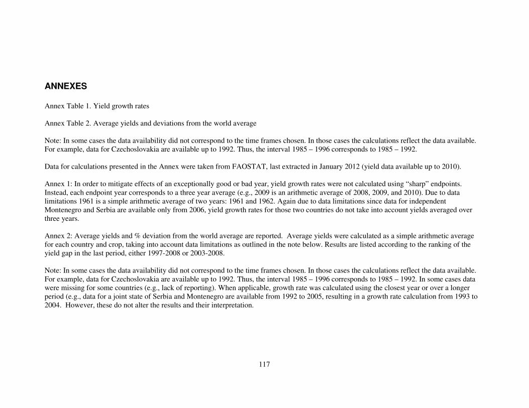
117

ANNEXES Annex Table 1. Yield growth rates Annex Table 2. Average yields and deviations from the world average Note: In some cases the data availability did not correspond to the time frames chosen. In those cases the calculations reflect the data available. For example, data for Czechoslovakia are available up to 1992. Thus, the interval 1985 – 1996 corresponds to 1985 – 1992. Data for calculations presented in the Annex were taken from FAOSTAT, last extracted in January 2012 (yield data available up to 2010). Annex 1: In order to mitigate effects of an exceptionally good or bad year, yield growth rates were not calculated using “sharp” endpoints. Instead, each endpoint year corresponds to a three year average (e.g., 2009 is an arithmetic average of 2008, 2009, and 2010). Due to data limitations 1961 is a simple arithmetic average of two years: 1961 and 1962. Again due to data limitations since data for independent Montenegro and Serbia are available only from 2006, yield growth rates for those two countries do not take into account yields averaged over three years. Annex 2: Average yields and % deviation from the world average are reported. Average yields were calculated as a simple arithmetic average for each country and crop, taking into account data limitations as outlined in the note below. Results are listed according to the ranking of the yield gap in the last period, either 1997-2008 or 2003-2008. Note: In some cases the data availability did not correspond to the time frames chosen. In those cases the calculations reflect the data available. For example, data for Czechoslovakia are available up to 1992. Thus, the interval 1985 – 1996 corresponds to 1985 – 1992. In some cases data were missing for some countries (e.g., lack of reporting). When applicable, growth rate was calculated using the closest year or over a longer period (e.g., data for a joint state of Serbia and Montenegro are available from 1992 to 2005, resulting in a growth rate calculation from 1993 to 2004. However, these do not alter the results and their interpretation.

118

Annex 1: Yield growth rates for selected countries: barley

Barley

11 year intervals, average 1961/62 – average 2007/09 5 year intervals, average 1984/6 – average 2007/08 avg1961/2-avg2008/10

avg1961/2-avg1971/3

avg1972/4-avg1983/5

avg1984/6-avg1995/7

avg1996/8-avg2007/9

avg1984/6-avg2008/10

avg1984/6-avg1989/91

avg1990/2-avg1995/7

avg1996/8-avg2001/3

avg2002/4-avg2007/9

Albania 2.2% -0.1% 7.9% -3.5% 4.5% 0.4% -8.0% 8.5% 13.2% -3.3%

Austria 0.7% 1.7% 2.2% 0.4% 0.3% -0.3% 2.6% -1.7% -0.7% 0.4%

Belarus 3.3% -2.9% 1.0% 3.6%

Belgium-Luxembourg 1.6% 1.5% 1.9% 1.4% 1.0% 1.1% -0.5% 3.5% 1.5% 0.0%

Bosnia and Herzegovina 1.9% 1.0% -3.0% 5.5%

Bulgaria 1.2% 3.8% 0.7% -3.3% 2.8% 0.0% 2.5% -7.4% 3.2% 1.9%

Croatia 2.3% -1.1% -0.8% 5.3%

Czech Republic 1.2% 0.3% 0.7%

Czechoslovakia 2.9% 2.1% 2.1%

Denmark 0.7% 0.4% 1.0% 0.9% -0.3% 0.3% 1.6% 2.6% -0.4% -0.1%

Estonia 3.0% 11.3% 0.7% 5.0%

Finland 1.7% 3.9% 2.7% 1.4% 1.9% 0.8% 2.5% 1.3% 1.4% 2.8%

France 2.0% 3.4% 2.2% 1.3% 0.2% 1.1% 2.2% 0.2% -0.7% 0.1%

Germany 1.7% 3.0% 1.4% 1.3% 0.5% 1.1% 2.3% 1.0% -0.1% 1.0%

Greece 1.6% 4.9% -0.6% 0.8% 0.0% 0.5% 1.1% 0.9% -0.3% 0.0%

Hungary 1.2% 3.1% 2.5% -1.4% 0.2% -0.5% 3.2% -4.5% -2.6% 1.5%

Ireland 1.3% 0.8% 2.5% 1.2% 0.9% 0.9% 1.5% 0.4% 1.0% 0.7%

Italy 2.1% 4.2% 3.9% 0.3% -0.1% 0.1% 0.8% -0.8% -1.4% 0.3%

Kazakhstan 4.4% -13.5% 9.0% 3.2%

Kyrgyzstan 0.6% -9.4% 4.5% -3.7%

Latvia 1.8% 7.7% -0.7% 3.3%

Lithuania 1.6% 6.5% 1.0% 1.0%

Malta 2.3% 1.9% 6.9% -2.3% 2.5% 0.5% -2.1% 0.0% 4.0% 0.3%

Montenegro 6.2%

Netherlands 1.0% 0.0% 1.8% 0.9% 0.2% 0.5% -1.0% 1.8% -0.9% 1.1%

Norway 0.9% 2.1% 0.8% 0.1% -0.2% 0.3% 1.1% 0.4% -1.8% 0.1%

Poland 1.0% 3.1% 0.8% -0.6% 0.3% -0.2% 0.8% -0.2% -0.5% 0.4%

Portugal 3.2% 4.5% 1.2% 1.1% 5.2% 3.1% 6.7% -2.9% 3.1% 5.5%

Republic of Moldova -0.4% -9.9% -1.9% 1.8%

Romania 1.0% 3.4% 2.3% -1.2% -0.7% -0.7% 2.8% -2.0% -2.1% -0.7%

Russian Federation 3.5% -5.7% 5.6% 3.0%

Serbia 2.4%

Serbia and Montenegro 1.9% 1.4%

Slovakia 0.4% -0.9% 0.2%

Slovenia 0.3% 1.0% -1.0% 0.9%

Spain 1.5% 2.5% 2.9% -0.2% 1.0% 0.9% -1.4% 3.2% -2.2% 1.3%

119

Sweden 0.9% 1.2% 0.7% 1.2% 0.5% 0.6% 2.4% 2.0% -0.3% 1.1%

Switzerland 1.3% 1.8% 2.2% 1.6% -0.7% 0.7% 3.2% 1.0% -2.6% -0.2%

Tajikistan 5.3% -1.2% 9.0% -0.3%

The former Yugoslav Republic of Macedonia 2.0% 0.7% -2.1% 2.2%

Turkmenistan 5.3% -14.4% 3.0% 5.1%

Ukraine 2.3% -8.3% 4.2% 1.3%

United Kingdom 1.1% 1.2% 2.0% 1.0% 0.1% 0.4% -0.3% 1.5% -0.4% 0.2%

USSR 3.4% -0.7% 3.2%

Uzbekistan 7.6% 1.9% 13.0% 4.5%

Yugoslav SFR 2.0% 2.2% 1.6%

World + (Total) 1.3% 2.6% 1.0% 0.4% 0.9% 0.9% 0.9% -0.1% 0.8% 0.9%

120

Annex 1: Yield growth rates for selected countries: maize

Maize

11 year intervals, average 1961/62 – average 2007/09 5 year intervals, average 1984/6 – average 2007/08 avg1961/2-avg2008/10

avg1961/2-avg1971/3

avg1972/4-avg1983/5

avg1984/6-avg1995/7

avg1996/8-avg2007/9

avg1984/6-avg2008/10

avg1984/6-avg1989/91

avg1990/2-avg1995/7

avg1996/8-avg2001/3

avg2002/4-avg2007/9

Albania 3.8% 6.8% 5.6% -1.9% 4.0% 1.6% -0.6% 1.1% 4.1% 3.4%

Austria 2.3% 4.3% 2.2% 1.1% 1.1% 1.5% 0.4% 3.0% 0.4% 0.8%

Belarus 6.4% -5.6% 7.7% 4.7%

Belgium-Luxembourg 2.1% 1.8% 2.9% 1.4% 2.7% 2.1% 0.9% 1.4% 3.6% 1.8%

Bosnia and Herzegovina 1.0% 0.1% -1.2% 1.2%

Bulgaria 1.3% 5.2% 1.7% -3.2% 1.8% -0.2% -2.7% -2.1% 2.3% -4.0%

Croatia 2.0% 5.0% -1.2% 5.6%

Czech Republic 2.1% 2.9% 2.2%

Czechoslovakia 4.9% 1.5% -1.5%

France 2.8% 7.1% 2.4% 2.7% 0.7% 1.6% 1.4% 3.4% -1.0% 2.3%

Germany 2.3% 4.5% 1.7% 1.9% 1.5% 1.6% 1.9% 2.7% 0.8% 2.3%

Greece 4.5% 9.6% 8.3% 1.0% 0.3% 0.7% 1.8% 0.4% 1.0% -0.2%

Hungary 2.3% 4.8% 3.4% -1.0% -0.3% 0.4% -1.5% 2.8% -3.4% 1.9%

Italy 2.3% 4.8% 2.0% 2.4% -0.3% 1.1% 1.3% 3.4% -1.3% 0.8%

Kazakhstan 8.0% -11.0% 13.6% 2.8%

Kyrgyzstan 2.8% -5.7% 6.0% 0.0%

Lithuania 5.5% 16.0%

Montenegro 4.7%

Netherlands 2.4% 0.3% 4.8% -1.4% 3.8% 1.8% 0.7% -2.1% 6.9% -0.2%

Poland 1.8% 2.0% 1.3% 1.4% 1.2% 1.2% 1.9% 2.8% 1.5% 1.7%

Portugal 3.6% 1.1% 3.0% 6.5% 1.8% 4.6% 6.3% 7.4% 1.7% 2.3%

Republic of Moldova -3.1% 5.9% -5.5% -3.1%

Romania 1.7% 4.6% 2.4% -0.5% -1.5% 0.0% -3.1% 3.0% -1.4% -4.9%

Russian Federation 4.1% -1.0% 3.7% 0.4%

Serbia 1.0%

Serbia and Montenegro 4.5% 7.6% 0.1%

Slovakia -13.6% -2.9% 4.3%

Slovenia 1.6% 17.4% -2.5% 1.5%

Spain 3.1% 4.6% 3.7% 2.6% 0.9% 1.9% 0.7% 4.3% 0.8% 1.0%

Switzerland 1.5% 2.0% 2.5% 1.8% 0.8% 1.1% 3.1% 1.2% -3.7% 5.1%

Tajikistan 8.2% -1.0% 1.5% 13.3% The former Yugoslav Republic of Macedonia 0.8% 4.5% 0.0% 0.3%

Turkmenistan 6.5% -18.0% 14.6% -0.4%

Ukraine 4.2% 3.4% 3.6% 4.6%

USSR 1.4% 1.5% 1.7%

121

Uzbekistan 7.0% -2.6% 4.4% 9.3%

Yugoslav SFR 4.6% 2.5% -2.7%

World + (Total) 2.0% 2.9% 2.2% 1.0% 1.6% 1.5% 0.2% 1.5% 0.8% 2.0%

122

Annex 1: Yield growth rates for selected countries: oats

Oats

11 year intervals, average 1961/62 – average 2007/09 5 year intervals, average 1984/6 – average 2007/08 avg1961/2-avg2008/10

avg1961/2-avg1971/3

avg1972/4-avg1983/5

avg1984/6-avg1995/7

avg1996/8-avg2007/9

avg1984/6-avg2008/10

avg1984/6-avg1989/91

avg1990/2-avg1995/7

avg1996/8-avg2001/3

avg2002/4-avg2007/9

Albania 2.0% 3.6% 3.0% -2.1% 2.3% 0.8% -11.8% 7.7% 2.8% 0.6%

Austria 1.2% 2.5% 2.0% 0.5% -0.5% 0.2% 0.2% 1.5% -0.9% -1.0%

Belarus 3.6% 0.1% 0.3% 4.5%

Belgium-Luxembourg 0.8% 1.0% 0.1% 1.3% 2.2% 1.1% -3.7% 5.2% 4.3% -0.1%

Bosnia and Herzegovina 1.2% 0.0% -1.8% 2.2%

Bulgaria 1.2% 1.6% -0.9% -0.3% 1.8% 1.4% 8.8% -6.3% 4.0% -2.0%

Croatia 0.8% -0.8% -2.7% 5.4%

Czech Republic -0.4% -2.1% -1.0%

Czechoslovakia 2.0% 2.6% 0.7%

Denmark 0.4% 0.3% 0.3% 1.8% -1.4% 0.2% 2.3% 3.7% -0.5% -2.7%

Estonia 1.7% 16.4% -2.5% 5.7%

Finland 1.4% 3.5% 2.9% 1.0% 1.1% 0.3% 2.6% 0.0% 0.4% 1.9%

France 1.9% 4.8% 1.8% 0.8% 0.2% 0.8% 0.2% 1.1% 0.2% -0.7%

Germany 1.1% 2.5% 0.9% 0.9% -1.1% 0.1% -0.9% 2.8% -1.9% -0.8%

Greece 1.3% 3.3% -0.1% 1.7% 0.0% 0.9% 1.8% 2.3% 0.7% -1.0%

Hungary 1.3% 2.0% 5.0% -2.2% -0.5% -1.1% -0.5% -3.1% -4.2% 1.2%

Ireland 2.1% 2.1% 3.2% 2.8% 1.2% 1.7% 5.8% -0.4% 2.0% 0.0%

Italy 1.1% 0.8% 1.7% 0.5% 0.1% 0.5% -0.9% 0.3% -1.6% 1.7%

Kazakhstan 5.0% -14.8% 10.2% 3.3%

Kyrgyzstan 0.7% -12.5% 8.7% -7.5%

Latvia 1.4% 14.9% -3.2% 4.7%

Lithuania 0.5% 15.5% 0.0% -0.4%

Montenegro 5.6%

Netherlands 0.1% -1.3% 0.6% 0.2% -0.7% -0.1% -2.4% 1.5% 0.6% -2.1%

Norway 1.0% 2.9% 1.5% -0.2% -0.4% -0.1% 0.5% 0.1% -1.1% -0.4%

Poland 0.7% 2.8% 0.1% -0.6% -0.3% -0.4% 0.3% 0.6% -1.6% 0.1%

Portugal 3.1% 6.0% 1.8% -1.4% 6.5% 1.8% 0.8% -0.2% 3.5% 7.2%

Republic of Moldova -4.8% -14.9% -3.1% -9.4%

Romania 1.0% 0.0% 2.3% 1.0% 0.5% 1.0% 2.2% -0.5% 0.9% -2.4%

Russian Federation 2.2% -0.4% 4.2% 1.5%

Serbia 1.6%

Serbia and Montenegro 2.4% 0.6% 2.2%

Slovakia -1.8% -4.2% -0.9%

Slovenia -0.1% -0.1% -0.4% -0.6%

Spain 1.6% 1.3% 2.9% -1.4% 2.8% 1.4% -0.5% -0.4% 2.3% 1.4%

Sweden 0.8% 1.6% 1.6% 0.2% 0.1% -0.1% 0.9% 1.7% -1.1% 0.3%

123

Switzerland 1.0% 2.0% 1.4% 1.3% -1.1% 0.3% 2.1% 1.4% -1.9% -0.6%

Tajikistan 7.1% -14.3% 9.2% 1.1% The former Yugoslav Republic of Macedonia 3.6% -2.3% 2.0% 3.0%

Ukraine 1.0% -6.7% 2.8% -0.5%

United Kingdom 1.5% 3.0% 1.6% 1.6% -0.4% 0.6% -0.2% 2.9% -0.3% -0.9%

USSR 5.2% 1.2% -0.7%

Yugoslav SFR 0.0% 2.6% 3.0%

World + (Total) 1.0% 2.0% 0.8% 0.0% 1.2% 0.8% -0.7% 0.8% 1.3% 0.8%

124

Annex 1: Yield growth rates for selected countries: potatoes

Potatoes

11 year intervals, average 1961/62 – average 2007/09 5 year intervals, average 1984/6 – average 2007/08 avg1961/2-avg2008/10

avg1961/2-avg1971/3

avg1972/4-avg1983/5

avg1984/6-avg1995/7

avg1996/8-avg2007/9

avg1984/6-avg2008/10

avg1984/6-avg1989/91

avg1990/2-avg1995/7

avg1996/8-avg2001/3

avg2002/4-avg2007/9

Albania 2.5% -0.6% 1.2% 4.6% 5.1% 4.9% 4.8% 7.3% 5.6% 5.6%

Austria 1.0% 2.2% 0.9% 0.2% 0.9% 0.6% -2.2% 3.6% 0.1% 1.5%

Belarus 4.9% 2.0% 3.2% 4.5%

Belgium-Luxembourg 1.0% 2.4% 0.8% 0.7% -0.1% 0.1% -2.9% 2.4% -1.2% -0.1%

Bosnia and Herzegovina 1.7% 0.5% -0.5% 3.1%

Bulgaria 1.2% 2.8% -1.0% -1.1% 4.6% 1.7% 1.1% -2.5% 7.1% 0.1%

Croatia 5.2% 5.0% -1.8% 10.0%

Czech Republic 2.2% 0.8% 3.1%

Czechoslovakia 3.9% 1.2% -3.1%

Denmark 1.5% 2.1% 2.3% 0.1% 0.4% 0.4% -0.2% 1.2% 0.4% 0.6%

Estonia 2.3% -1.1% 3.5% 4.2%

Finland 1.5% 1.2% 2.5% 1.7% 2.3% 1.6% 2.2% 2.4% 2.8% 2.7%

France 2.0% 3.8% 2.0% 1.4% 1.3% 1.1% -0.9% 2.3% 1.4% 0.2%

Germany 1.5% 0.8% 0.5% 2.7% 0.8% 1.8% 0.1% 5.0% -0.4% 1.8%

Greece 2.6% 5.7% 2.5% 0.8% 1.6% 1.4% 1.8% 0.0% 0.3% 3.1%

Hungary 2.4% 3.5% 4.0% -0.6% 1.8% 1.0% -3.1% 2.5% 1.5% 2.3%

Iceland 0.0% -5.9% 1.7% -3.8% 2.4% 0.0% -11.5% 1.6% -2.1% 6.3%

Ireland 0.3% 0.6% -1.9% 2.2% 1.1% 1.1% 2.8% 0.5% 4.2% -3.3%

Italy 1.9% 3.7% 1.0% 2.1% 0.6% 1.2% 1.7% 1.9% 0.5% 0.7%

Kazakhstan 5.6% -4.2% 10.0% 2.3%

Kyrgyzstan 2.4% -3.6% 8.3% -3.1%

Latvia 2.5% 1.4% -0.1% 4.6%

Lithuania -1.1% 8.8% -1.8% -1.8%

Malta 1.5% 0.7% -1.9% 11.5% -1.5% 3.4% 12.5% 9.1% -4.5% -1.0%

Montenegro 4.9%

Netherlands 0.9% 2.2% 0.0% 0.3% 0.4% 0.3% -0.8% 1.5% -0.1% 0.7%

Norway 0.4% 0.9% 0.1% -0.2% -0.1% 0.2% -0.2% -1.0% 0.1% -1.0%

Poland 0.6% 1.7% -0.9% -0.3% 0.6% 0.2% 0.3% 1.0% -1.0% 1.2%

Portugal 1.0% 0.7% -1.4% 3.1% 0.6% 1.6% 2.7% 2.4% 0.9% -0.4%

Republic of Moldova 2.5% 2.1% 5.9% -0.6%

Romania 0.9% 1.8% 5.3% -3.5% 0.8% -1.2% -11.8% 4.6% 1.8% -0.9%

Russian Federation 2.2% 0.4% 0.3% 4.1%

Serbia 1.4%

Serbia and Montenegro 3.9% 3.0% 2.6%

Slovakia 0.6% -1.1% 0.9%

Slovenia 1.3% 9.6% -1.0% 1.8%

125

Spain 2.0% 1.6% 1.9% 1.5% 2.2% 2.0% 2.2% 0.9% 3.8% 0.7%

Sweden 1.1% 2.4% 1.7% 0.1% -1.0% -0.1% 0.5% 0.1% -3.6% 0.8%

Switzerland 1.2% 3.6% 0.2% 1.2% -0.3% 0.4% -0.3% 1.9% -4.0% 3.1%

Tajikistan 7.1% 4.6% 8.3% 5.4% The former Yugoslav Republic of Macedonia 1.4% 1.0% 1.3% 1.2%

Turkmenistan 2.4% -17.4% 5.4% 0.6%

Ukraine 2.1% -2.1% 0.1% 2.9%

United Kingdom 1.4% 2.3% 1.3% 1.0% 0.3% 0.7% -0.2% 1.0% 0.4% -0.2%

USSR 2.6% 0.6% -2.1%

Uzbekistan 5.9% 5.3% 5.4% 6.5%

Yugoslav SFR 0.5% 0.0% -2.0%

World + (Total) 0.9% 1.6% 0.5% 0.3% 0.8% 0.6% -0.7% 1.5% 0.0% 1.1%

126

Annex 1: Yield growth rates for selected countries: rapeseed

Rapeseed

11 year intervals, average 1961/62 – average 2007/09 5 year intervals, average 1984/6 – average 2007/08 avg1961/2-avg2008/10

avg1961/2-avg1971/3

avg1972/4-avg1983/5

avg1984/6-avg1995/7

avg1996/8-avg2007/9

avg1984/6-avg2008/10

avg1984/6-avg1989/91

avg1990/2-avg1995/7

avg1996/8-avg2001/3

avg2002/4-avg2007/9

Austria 0.9% 0.1% 2.0% -0.6% 2.4% 0.8% 0.2% -1.7% -0.8% 3.8%

Belarus 7.9% -12.2% 3.9% 10.9%

Belgium-Luxembourg 1.1% 2.3% -0.8% 1.8% 1.0% 1.4% 1.8% 3.9% 0.3% 1.0%

Bosnia and Herzegovina 6.0% -11.8% 12.1% 0.9%

Bulgaria 2.6% 0.9% 8.0% 3.3% 9.6%

Croatia 3.2% 0.8% -0.3% 8.6%

Czech Republic 2.0% -2.0% 4.3%

Czechoslovakia 2.8% 2.1% 1.9%

Denmark 1.0% -1.8% 1.3% -0.6% 2.5% 1.5% 1.6% -1.8% 0.9% 2.1%

Estonia 3.3% 8.7% 7.4% 0.4%

Finland 0.5% 2.6% 0.5% -0.2% 0.9% -0.3% 1.9% -2.9% 0.9% 2.5%

France 1.5% 2.1% 2.5% 1.2% -0.1% 0.7% 0.3% 2.7% -2.4% 0.3%

Germany 1.7% 1.9% 1.2% 0.2% 2.4% 1.4% 1.8% 0.0% 1.5% 2.9%

Hungary 1.6% 1.9% 2.4% -0.3% 4.1% 1.2% 0.4% 1.3% 2.2% 3.5%

Ireland -1.4% 2.0% -0.1% 0.9% -3.6% 1.3% 3.1%

Italy 1.0% 2.9% 0.1% -3.6% 6.9% 0.4% 3.4% -10.7% 4.0% 7.7%

Kazakhstan 6.8% -20.2% 16.0% -2.3%

Kyrgyzstan 1.4% -3.0% 3.8% -0.1%

Latvia 4.0% 2.5% 2.4% 5.0%

Lithuania 0.9% 2.5% -2.4% 1.4%

Netherlands 1.1% 1.5% -0.2% 0.8% 1.7% 1.4% 1.2% 1.5% -0.1% 1.5%

Norway 0.8% 1.6% 1.0% 0.0% -0.4% -0.1% -1.0% 2.3% -2.2% 1.1%

Poland 1.3% 0.6% 2.5% -2.0% 3.4% 0.7% 0.8% -2.4% 2.0% 3.7%

Romania 2.4% 15.0% -8.7% 4.8% 1.3% 3.3% 3.6% 7.9% -8.4% 5.6%

Russian Federation 3.2% -8.7% 2.8% 2.8%

Serbia 7.4%

Serbia and Montenegro 1.7% 3.0% -0.5%

Slovakia 1.3% -2.4% 3.2%

Slovenia 0.4% -2.8% -0.9% 2.1%

Spain -6.6% -1.3% 2.2% 1.6% 2.8% -5.6% 4.8% 3.1%

Sweden 0.4% -1.1% 0.4% -1.2% 3.0% 1.0% -1.1% -2.2% 2.2% 3.3%

Switzerland 1.0% 2.0% 0.7% 1.1% -0.4% 0.4% 1.0% 2.6% -0.9% -0.8%

Tajikistan 14.5% -1.3% -1.3% 31.7% The former Yugoslav Republic of Macedonia 5.4% -0.8% 8.9% 6.3%

Ukraine 5.3% -15.2% 0.9% 9.9%

127

United Kingdom 0.6% -1.8% 2.9% -0.2% 0.2% 0.2% -1.0% 0.8% -0.7% 0.4%

USSR 2.4% -5.0% 9.5%

Uzbekistan 1.7% 3.7% 5.0% -1.5%

Yugoslav SFR 5.0% 1.7% 0.1%

World + (Total) 2.5% 3.3% 3.7% 1.1% 2.4% 1.6% 1.2% 1.1% 1.7% 2.5%

128

Annex 1: Yield growth rates for selected countries: rice

Rice paddy

11 year intervals, average 1961/62 – average 2007/09 5 year intervals, average 1984/6 – average 2007/08 avg1961/2-avg2008/10

avg1961/2-avg1971/3

avg1972/4-avg1983/5

avg1984/6-avg1995/7

avg1996/8-avg2007/9

avg1984/6-avg2008/10

avg1984/6-avg1989/91

avg1990/2-avg1995/7

avg1996/8-avg2001/3

avg2002/4-avg2007/9

Albania 6.0% 1.8% -5.9%

Bulgaria 1.1% 1.3% 1.1% -2.2% 5.6% 1.3% -9.2% 4.1% 6.7% 5.4%

France 0.6% -1.5% 3.5% 0.9% -0.2% 0.5% 3.6% -0.7% -0.4% -0.5%

Greece 1.3% 2.6% 1.8% 1.5% -0.1% 0.3% -1.2% 3.6% -0.2% -0.8%

Hungary 1.7% 2.7% 3.3% -1.1% 3.4% 1.0% -3.9% -0.1% 7.9% -0.6%

Italy 0.3% -1.3% 1.3% 0.0% 0.4% 0.3% 0.6% -0.5% 0.3% -0.2%

Kazakhstan 1.3% -8.3% 0.6% 0.7%

Kyrgyzstan 4.3% 2.9% 9.7% -0.4%

Portugal 0.4% -1.6% 1.1% 2.2% -0.3% 0.9% 0.3% 3.3% -0.5% -0.2%

Romania 1.1% -3.3% 4.5% -1.1% 4.5% 1.6% -16.8% 10.5% -10.9% 11.8%

Russian Federation 5.4% -1.2% 5.6% 5.7%

Spain 0.3% -0.4% -0.2% 0.6% 0.3% 0.7% -0.2% 0.9% 1.1% -0.1%

Tajikistan 5.5% 0.6% 5.2% 4.9% The former Yugoslav Republic of Macedonia 1.6% 0.1% -1.2% 4.7%

Turkmenistan 7.7% -7.0% 14.0% -0.5%

Ukraine 4.9% -2.3% 3.7% 7.0%

USSR 5.0% 0.2% -1.6%

Uzbekistan 3.9% -6.6% 1.3% 4.7%

Yugoslav SFR 1.5% -0.7% -1.8%

World + (Total) 1.7% 2.1% 2.6% 1.3% 1.1% 1.2% 1.6% 1.1% 0.5% 1.8%

129

Annex 1: Yield growth rates for selected countries: rye

Rye

11 year intervals, average 1961/62 – average 2007/09 5 year intervals, average1984/6 – average 2007/08 avg1961/2-avg2008/10

avg1961/2-avg1971/3

avg1972/4-avg1983/5

avg1984/6-avg1995/7

avg1996/8-avg2007/9

avg1984/6-avg2008/10

avg1984/6-avg1989/91

avg1990/2-avg1995/7

avg1996/8-avg2001/3

avg2002/4-avg2007/9

Albania 2.7% 2.9% 1.0% 1.8% 6.1% 3.4% -11.4% 10.6% 5.9% 8.9%

Austria 1.1% 2.8% 1.9% -0.5% 1.1% 0.1% 2.1% -2.9% 0.9% 0.5%

Belarus 2.5% -7.3% 0.4% 2.9%

Belgium-Luxembourg 0.8% 1.7% 0.9% 0.0% 1.1% 0.3% -2.2% 4.3% 1.4% -0.2%

Bosnia and Herzegovina 1.7% 0.2% -1.7% 3.9%

Bulgaria 1.5% 3.1% 0.6% -1.7% 3.1% 0.6% 4.6% -6.9% 3.0% 3.8%

Croatia 0.6% -0.5% -1.3% 1.6%

Czech Republic 2.9% 1.2% 2.6%

Czechoslovakia 2.6% 1.8% 2.6%

Denmark 1.2% 1.8% 2.2% 0.8% -0.1% 0.4% 1.1% 2.5% -0.2% 0.5%

Estonia 4.7% -4.5% 1.4% 8.4%

Finland 1.5% 4.5% 0.9% 0.3% 2.6% 0.4% 3.9% -2.4% 3.4% 2.0%

France 2.6% 5.4% 1.6% 2.7% 0.5% 1.8% 2.5% 3.1% -1.0% 0.5%

Germany 1.7% 3.1% 1.1% 2.9% -0.6% 1.2% 1.4% 5.0% -0.4% -0.9%

Greece 1.9% 3.5% 2.8% 0.3% 0.3% 0.4% 1.3% -0.1% -0.3% 0.9%

Hungary 1.6% 3.4% 2.7% -0.4% 0.6% 0.1% 3.4% -2.0% -0.7% 0.8%

Ireland 0.9% 5.2% 0.9% -1.5% 0.8% -0.3% -3.4% -0.1% 1.2% 0.0%

Italy 0.9% 2.0% 1.6% -0.1% 1.3% -0.1% -0.4% -0.2% 4.1% -1.0%

Kazakhstan 7.6% -8.7% 16.1% 2.7%

Kyrgyzstan 7.5% 7.4% 1.5% 27.8%

Latvia 4.0% -2.6% 1.1% 6.9%

Lithuania 2.1% -1.4% 2.3% 1.0%

Montenegro 10.5%

Netherlands 1.0% 1.1% 2.2% 1.8% -1.0% 0.1% 0.9% 2.3% -1.8% -0.7%

Norway 1.2% 2.7% 0.4% -1.2% 3.5% 1.1% -3.4% 2.8% 1.6% 1.6%

Poland 1.0% 3.4% 0.6% -0.6% 0.5% -0.1% 0.5% 0.2% -0.3% 0.4%

Portugal 1.4% 3.6% 0.9% -1.8% 3.1% 0.3% 2.8% -5.7% 2.8% 1.7%

Republic of Moldova -2.4% -0.9% -6.1% 0.3%

Romania 1.6% 1.9% 5.2% -2.7% 2.0% 0.0% -3.8% 1.4% 3.0% 0.7%

Russian Federation 3.0% -3.5% 5.0% 2.8%

Serbia 2.9%

Serbia and Montenegro 2.5% 0.3% 0.6%

Slovakia 0.5% -0.5% -0.6%

Slovenia 0.0% 1.8% -0.3% -0.1%

Spain 1.8% 1.1% 2.5% 1.4% 2.2% 1.9% 2.2% 2.6% -0.7% 2.5%

Sweden 1.8% 3.4% 0.3% 2.4% 1.9% 1.7% 3.3% 3.0% 1.2% 2.7%

130

Switzerland 1.2% 1.5% 1.7% 2.1% -0.8% 0.8% 0.8% 3.7% -1.8% -0.7%

Tajikistan 1.6% -6.0% 7.9% -8.8% The former Yugoslav Republic of Macedonia 2.6% -0.7% -0.2% 3.9%

Ukraine 1.2% -4.1% 1.4% 0.7%

United Kingdom 2.0% 1.9% 2.3% 2.2% 1.3% 1.4% 2.9% 2.7% -0.4% 2.4%

USSR 2.7% 1.2% 4.4%

Uzbekistan 8.1% 3.4% 3.4% 12.4%

Yugoslav SFR 1.6% 2.8% 2.8%

World + (Total) 1.7% 3.2% 1.2% 1.1% 1.7% 1.2% 1.5% 0.8% 1.1% 2.1%

131

Annex 1: Yield growth rates for selected countries: sorghum

Sorghum

11 year intervals, average 1961/62 – average 2007/09 5 year intervals, average 1984/6 – average 2007/08 avg1961/2-avg2008/10

avg1961/2-avg1971/3

avg1972/4-avg1983/5

avg1984/6-avg1995/7

avg1996/8-avg2007/9

avg1984/6-avg2008/10

avg1984/6-avg1989/91

avg1990/2-avg1995/7

avg1996/8-avg2001/3

avg2002/4-avg2007/9

Albania 5.4% 2.0% -3.9%

Bulgaria 1.4% 2.5% -1.0% 0.0% -1.2% -1.2%

Croatia -3.0% -1.9% -3.3% -0.5%

Czechoslovakia 11.9% -1.1% 0.1%

France 1.8% 4.2% 1.5% 3.2% -0.5% 1.2% 1.3% 3.9% -2.8% 2.3%

Greece 1.7% 5.4% 1.6% -0.8% -2.3% -1.0% -1.8% -3.1% -2.5% -2.1%

Hungary 2.0% 6.8% 0.8% -5.7% 2.9% -1.6% -5.1% -4.2% -2.5% 9.3%

Italy 1.5% 0.6% 1.5% 1.8% 0.2% 1.0% 2.7% 1.8% 0.6% -0.2%

Kazakhstan -2.0% -17.9% 22.2% -20.1%

Kyrgyzstan 0.4% -9.9% 2.4% 0.9%

Republic of Moldova -4.7% -3.6% 7.0% -16.4%

Romania 1.2% 2.3% -4.2% -4.3% 6.6% 2.8% -3.8% -4.5% 2.0% 2.0%

Russian Federation 2.1% 3.2% 2.7% -2.9%

Serbia -8.8%

Serbia and Montenegro 3.8% 3.0% 2.4%

Slovakia 0.4% -6.0% 4.0%

Spain 3.6% 15.6% 0.9% -0.5% -2.1% -0.8% 2.7% -3.6% -4.9% 1.1%

Tajikistan -0.3% 0.1% 1.7% -4.3%

Ukraine 8.7% -0.8% 10.0% 5.0%

USSR 4.6% -1.3% -0.4%

Uzbekistan 7.6% 2.0% 1.5% 19.7%

Yugoslav SFR -1.3% 1.8% -3.3%

World + (Total) 0.9% 2.8% 1.4% -0.6% -0.1% -0.2% -2.1% -0.3% -1.4% 1.0%

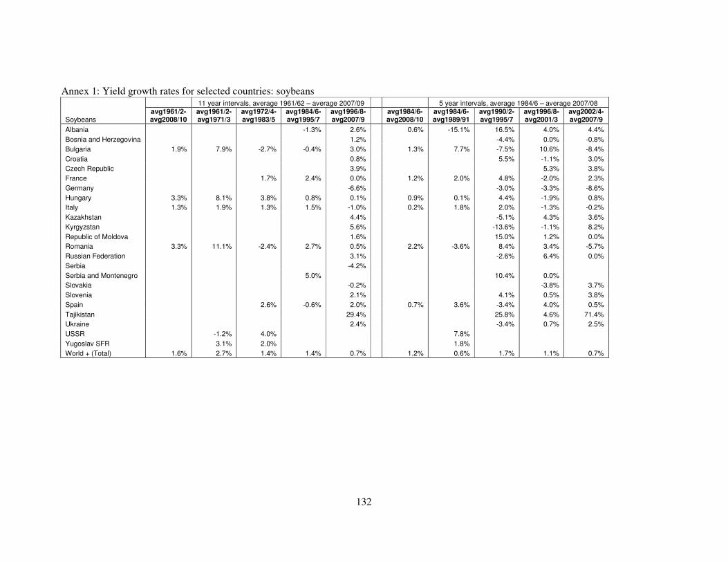
132

Annex 1: Yield growth rates for selected countries: soybeans

Soybeans

11 year intervals, average 1961/62 – average 2007/09 5 year intervals, average 1984/6 – average 2007/08 avg1961/2-avg2008/10

avg1961/2-avg1971/3

avg1972/4-avg1983/5

avg1984/6-avg1995/7

avg1996/8-avg2007/9

avg1984/6-avg2008/10

avg1984/6-avg1989/91

avg1990/2-avg1995/7

avg1996/8-avg2001/3

avg2002/4-avg2007/9

Albania -1.3% 2.6% 0.6% -15.1% 16.5% 4.0% 4.4%

Bosnia and Herzegovina 1.2% -4.4% 0.0% -0.8%

Bulgaria 1.9% 7.9% -2.7% -0.4% 3.0% 1.3% 7.7% -7.5% 10.6% -8.4%

Croatia 0.8% 5.5% -1.1% 3.0%

Czech Republic 3.9% 5.3% 3.8%

France 1.7% 2.4% 0.0% 1.2% 2.0% 4.8% -2.0% 2.3%

Germany -6.6% -3.0% -3.3% -8.6%

Hungary 3.3% 8.1% 3.8% 0.8% 0.1% 0.9% 0.1% 4.4% -1.9% 0.8%

Italy 1.3% 1.9% 1.3% 1.5% -1.0% 0.2% 1.8% 2.0% -1.3% -0.2%

Kazakhstan 4.4% -5.1% 4.3% 3.6%

Kyrgyzstan 5.6% -13.6% -1.1% 8.2%

Republic of Moldova 1.6% 15.0% 1.2% 0.0%

Romania 3.3% 11.1% -2.4% 2.7% 0.5% 2.2% -3.6% 8.4% 3.4% -5.7%

Russian Federation 3.1% -2.6% 6.4% 0.0%

Serbia -4.2%

Serbia and Montenegro 5.0% 10.4% 0.0%

Slovakia -0.2% -3.8% 3.7%

Slovenia 2.1% 4.1% 0.5% 3.8%

Spain 2.6% -0.6% 2.0% 0.7% 3.6% -3.4% 4.0% 0.5%

Tajikistan 29.4% 25.8% 4.6% 71.4%

Ukraine 2.4% -3.4% 0.7% 2.5%

USSR -1.2% 4.0% 7.8%

Yugoslav SFR 3.1% 2.0% 1.8%

World + (Total) 1.6% 2.7% 1.4% 1.4% 0.7% 1.2% 0.6% 1.7% 1.1% 0.7%

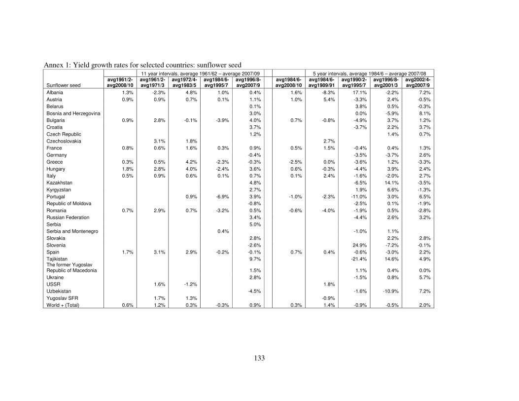
133

Annex 1: Yield growth rates for selected countries: sunflower seed

Sunflower seed

11 year intervals, average 1961/62 – average 2007/09 5 year intervals, average 1984/6 – average 2007/08 avg1961/2-avg2008/10

avg1961/2-avg1971/3

avg1972/4-avg1983/5

avg1984/6-avg1995/7

avg1996/8-avg2007/9

avg1984/6-avg2008/10

avg1984/6-avg1989/91

avg1990/2-avg1995/7

avg1996/8-avg2001/3

avg2002/4-avg2007/9

Albania 1.3% -2.3% 4.8% 1.0% 0.4% 1.6% -8.3% 17.1% -2.2% 7.2%

Austria 0.9% 0.9% 0.7% 0.1% 1.1% 1.0% 5.4% -3.3% 2.4% -0.5%

Belarus 0.1% 3.8% 0.5% -0.3%

Bosnia and Herzegovina 3.0% 0.0% -5.9% 8.1%

Bulgaria 0.9% 2.8% -0.1% -3.9% 4.0% 0.7% -0.8% -4.9% 3.7% 1.2%

Croatia 3.7% -3.7% 2.2% 3.7%

Czech Republic 1.2% 1.4% 0.7%

Czechoslovakia 3.1% 1.8% 2.7%

France 0.8% 0.6% 1.6% 0.3% 0.9% 0.5% 1.5% -0.4% 0.4% 1.3%

Germany -0.4% -3.5% -3.7% 2.6%

Greece 0.3% 0.5% 4.2% -2.3% -0.3% -2.5% 0.0% -3.6% 1.2% -3.3%

Hungary 1.8% 2.8% 4.0% -2.4% 3.6% 0.6% -0.3% -4.4% 3.9% 2.4%

Italy 0.5% 0.9% 0.6% 0.1% 0.7% 0.1% 2.4% -1.6% -2.0% 2.7%

Kazakhstan 4.8% -6.5% 14.1% -3.5%

Kyrgyzstan 2.7% 1.9% 6.6% -1.3%

Portugal 0.9% -6.9% 3.9% -1.0% -2.3% -11.0% 3.0% 6.5%

Republic of Moldova -0.8% -2.5% 0.1% -1.9%

Romania 0.7% 2.9% 0.7% -3.2% 0.5% -0.6% -4.0% -1.9% 0.5% -2.8%

Russian Federation 3.4% -4.4% 2.6% 3.2%

Serbia 5.0%

Serbia and Montenegro 0.4% -1.0% 1.1%

Slovakia 2.8% 2.2% 2.8%

Slovenia -2.6% 24.9% -7.2% -0.1%

Spain 1.7% 3.1% 2.9% -0.2% -0.1% 0.7% 0.4% -0.6% -3.0% 2.2%

Tajikistan 9.7% -21.4% 14.6% 4.9% The former Yugoslav Republic of Macedonia 1.5% 1.1% 0.4% 0.0%

Ukraine 2.8% -1.5% 0.8% 5.7%

USSR 1.6% -1.2% 1.8%

Uzbekistan -4.5% -1.6% -10.9% 7.2%

Yugoslav SFR 1.7% 1.3% -0.9%

World + (Total) 0.6% 1.2% 0.3% -0.3% 0.9% 0.3% 1.4% -0.9% -0.5% 2.0%

134

Annex 1: Yield growth rates for selected countries: wheat

Wheat

11 year intervals, average 1961/62 – average 2007/09 5 year intervals, average 1984/6 – average 2007/08 avg1961/2-avg2008/10

avg1961/2-avg1971/3

avg1972/4-avg1983/5

avg1984/6-avg1995/7

avg1996/8-avg2007/9

avg1984/6-avg2008/10

avg1984/6-avg1989/91

avg1990/2-avg1995/7

avg1996/8-avg2001/3

avg2002/4-avg2007/9

Albania 3.1% 6.8% 4.1% -1.4% 3.6% 1.1% -2.7% 1.0% 2.4% 4.8%

Austria 1.5% 2.5% 2.5% 0.8% 0.1% 0.5% 1.4% -0.3% -0.9% 0.2%

Belarus 4.1% -3.1% 1.4% 4.8%

Belgium-Luxembourg 1.7% 1.4% 1.9% 1.7% 0.4% 1.3% -0.4% 4.3% -0.2% 0.2%

Bosnia and Herzegovina 1.6% -1.5% -3.7% 4.1%

Bulgaria 1.7% 6.9% -0.2% -3.2% 2.0% 0.0% 3.4% -7.8% 1.9% 0.7%

Croatia 2.3% -0.2% -1.2% 6.3%

Czech Republic 1.6% 0.3% 1.9%

Czechoslovakia 3.1% 2.7% 1.6%

Denmark 1.2% 0.8% 2.9% 1.1% 0.4% 0.6% 2.4% 1.0% 0.0% 1.1%

Estonia 4.1% 2.5% 1.6% 6.7%

Finland 1.6% 3.6% 1.9% 2.0% 0.8% 0.8% 2.4% 3.9% -1.0% 2.5%

France 2.0% 4.1% 2.3% 1.1% -0.2% 0.8% 1.7% 0.7% -1.0% -0.4%

Germany 1.9% 2.8% 2.4% 1.7% 0.4% 1.1% 1.0% 2.4% -0.4% 1.2%

Greece 1.6% 3.4% 0.7% 0.1% 0.7% 0.7% 1.9% -0.1% -1.2% 2.7%

Hungary 1.7% 5.1% 3.2% -2.1% 0.6% -0.6% 1.2% -4.1% -2.1% 1.9%

Ireland 1.9% 1.5% 4.8% 2.2% 0.3% 1.1% 3.9% 0.6% 0.8% -0.7%

Italy 1.3% 2.0% 1.2% 0.6% 0.9% 1.0% 0.4% -1.3% -2.3% 2.5%

Kazakhstan 4.8% -12.9% 9.5% 3.1%

Kyrgyzstan -0.3% -5.7% 1.0% -1.6%

Latvia 3.5% -1.5% 3.3% 3.9%

Lithuania 3.4% -1.6% 3.6% 2.0%

Malta 2.6% 4.4% 5.2% -0.6% 1.2% 1.0% -0.1% -0.7% 1.5% 0.1%

Montenegro 5.1%

Netherlands 1.6% 1.2% 3.1% 1.1% 0.3% 0.7% 0.3% 1.6% 0.1% -0.3%

Norway 1.1% 3.5% 1.5% 0.1% -0.6% -0.4% -0.7% 1.1% -1.1% -1.2%

Poland 1.5% 2.9% 1.6% -0.3% 1.5% 0.6% 1.7% -1.1% 1.0% 1.1%

Portugal 2.0% 5.0% 0.9% -0.9% 4.4% 1.1% 3.5% -3.1% -2.3% 8.2%

Republic of Moldova -1.9% -2.8% -6.7% 2.5%

Romania 1.6% 5.0% 1.1% -0.2% 0.2% 0.3% 2.8% -0.4% -1.3% 0.5%

Russian Federation 3.3% -3.5% 4.1% 3.5%

Serbia 1.6%

Serbia and Montenegro 0.1% 0.7% -1.7%

Slovakia -0.1% -2.9% 1.8%

Slovenia -0.2% -0.5% 0.1% -0.3%

Spain 2.2% 2.6% 5.0% -0.8% 1.4% 0.8% -0.3% -0.2% -0.1% 1.0%

135

Sweden 1.3% 2.7% 1.0% 1.0% 0.4% 0.4% 2.9% 0.4% -0.1% 0.9%

Switzerland 1.2% 1.8% 2.6% 1.0% -0.6% 0.2% 1.5% 1.8% -3.0% 1.2%

Tajikistan 6.9% 2.0% 8.8% 3.8%

The former Yugoslav Republic of Macedonia 1.2% -0.6% -2.3% 1.3%

Turkmenistan 6.2% -8.3% 12.2% 0.0%

Ukraine 1.4% -2.7% -0.4% 3.4%

United Kingdom 1.4% 0.9% 3.7% 0.9% -0.2% 0.4% -0.1% 2.0% -0.2% -0.9%

USSR 3.7% -0.3% 4.0%

Uzbekistan 6.3% 5.8% 9.1% 3.7%

Yugoslav SFR 4.7% 2.0% 2.3%

World + (Total) 2.0% 3.2% 2.6% 1.4% 1.0% 1.3% 1.9% 0.7% 0.4% 1.5%

136

Annex 2: Average yields (MT/ha), % deviation from world average, 1961 – 2008, barley, ranked by gap in 1997-2008

Barley

Average yield per period % deviation from world average

1961-2009 1961-1972 1973-1984 1985-1996 1997-2008 1961-2009 1961-1972 1973-1984 1985-1996 1997-2008

Belgium-Luxembourg 5.40 3.70 4.71 5.86 7.06 156.08% 123.23% 139.07% 161.59% 182.36%

Ireland 5.17 3.65 4.58 5.84 6.51 145.23% 120.55% 132.53% 160.33% 160.11%

France 4.75 3.08 3.98 5.51 6.24 125.19% 85.80% 101.78% 146.00% 149.41%

Switzerland 4.99 3.53 4.55 5.62 6.13 136.71% 113.14% 130.64% 150.92% 145.19%

Netherlands 5.08 3.85 4.70 5.60 6.00 140.97% 132.68% 138.30% 150.03% 139.85%

Germany 4.68 3.30 4.19 5.19 5.87 122.01% 99.29% 112.74% 131.75% 134.64%

United Kingdom 4.76 3.61 4.33 5.29 5.70 125.70% 118.01% 119.52% 136.15% 127.74%

Denmark 4.48 3.85 3.94 4.87 5.14 112.42% 132.61% 100.15% 117.09% 105.39%

Austria 4.00 3.02 3.81 4.55 4.56 89.66% 82.56% 93.19% 102.85% 82.23%

Sweden 3.60 2.94 3.47 3.83 4.09 70.98% 77.40% 75.89% 70.88% 63.49%

Czech Republic 3.80 3.94 69.39% 57.61%

Malta 2.77 1.39 2.79 2.87 3.93 31.29% -15.94% 41.74% 27.94% 57.04%

Slovenia 3.27 3.67 45.96% 46.71%

Norway 3.31 2.74 3.35 3.49 3.67 57.10% 65.64% 70.21% 55.57% 46.51%

Italy 2.92 1.57 2.77 3.67 3.62 38.47% -5.32% 40.76% 63.82% 44.52%

Slovakia 3.39 3.37 51.45% 34.64%

Hungary 3.16 2.11 3.34 3.80 3.36 49.77% 27.62% 69.32% 69.37% 34.45%

Croatia 3.13 3.34 39.84% 33.53%

Finland 2.77 1.99 2.65 3.08 3.28 31.60% 20.22% 34.26% 37.51% 31.21%

Serbia 3.14 25.65%

Poland 2.83 2.22 2.89 3.11 3.05 34.29% 34.00% 46.84% 38.60% 21.85%

Bulgaria 2.97 2.38 3.36 3.30 2.83 41.13% 43.76% 70.37% 47.19% 13.07%

Spain 2.12 1.57 1.91 2.21 2.75 0.45% -4.98% -2.96% -1.61% 9.95%

Serbia and Montenegro 2.28 2.72 1.53% 8.89%

Bosnia and Herzegovina 2.56 2.66 14.24% 6.36%

Belarus 2.43 2.56 8.20% 2.29%

The former Yugoslav Republic of Macedonia 2.28 2.55 1.82% 1.93%

Lithuania 1.90 2.48 -15.25% -0.94%

Romania 2.59 1.94 2.85 3.14 2.46 23.09% 17.28% 44.85% 40.16% -1.63%

Albania 1.80 0.95 1.72 2.06 2.40 -14.54% -42.60% -12.59% -8.23% -3.98%

Greece 2.21 1.69 2.31 2.42 2.40 4.70% 1.88% 17.12% 7.91% -4.07%

Montenegro 2.12 -15.31%

Ukraine 2.57 2.09 14.82% -16.36%

Estonia 1.69 2.07 -24.80% -17.08%

Latvia 1.65 2.07 -26.22% -17.17%

137

Kyrgyzstan 1.72 2.01 -23.21% -19.50%

Russian Federation 1.53 1.83 -31.62% -26.81%

Republic of Moldova 2.56 1.80 14.01% -28.01%

Portugal 1.01 0.57 0.71 1.25 1.46 -51.86% -65.48% -64.09% -44.36% -41.59%

Uzbekistan 1.07 1.37 -52.28% -45.10%

Tajikistan 0.68 1.17 -69.78% -53.09%

Kazakhstan 0.98 1.09 -56.22% -56.52%

Turkmenistan 1.94 0.71 -13.66% -71.73%

Czechoslovakia 2.66 3.76 4.54 60.88% 90.87% 102.59%

USSR 1.22 1.42 1.63 -26.22% -28.14% -27.21%

Yugoslav SFR 1.57 2.28 2.74 -5.20% 15.55% 22.14%

World + (Total) 2.11 1.66 1.97 2.24 2.50

138

Annex 2: Average yields (MT/ha), % deviation from world average, 1985 – 2008, barley ranked by gap in 2003-2008

Barley

Average yield per period % deviation from world average

1985-2009 1985-1990 1991-1996 1997-2002 2003-2008 1985-2009 1985-1990 1991-1996 1997-2002 2003-2008

Belgium-Luxembourg 6.54 5.60 6.13 6.92 7.21 173.75% 149.45% 173.78% 181.53% 183.15%

Ireland 6.18 5.71 5.96 6.28 6.74 158.47% 154.37% 166.30% 155.53% 164.53%

France 5.92 5.26 5.77 6.25 6.23 147.57% 134.06% 157.98% 154.30% 144.70%

Switzerland 5.90 5.33 5.92 6.12 6.14 146.95% 137.20% 164.69% 149.22% 141.30%

Netherlands 5.85 5.30 5.91 5.94 6.07 144.78% 136.11% 163.99% 141.52% 138.24%

United Kingdom 5.51 4.99 5.60 5.55 5.85 130.71% 122.31% 150.04% 125.81% 129.60%

Germany 5.57 5.03 5.36 5.91 5.84 133.24% 124.01% 139.52% 140.28% 129.19%

Denmark 5.03 4.89 4.84 5.22 5.05 110.56% 117.96% 116.23% 112.56% 98.46%

Austria 4.55 4.54 4.56 4.48 4.64 90.63% 102.09% 103.62% 82.25% 82.21%

Malta 3.41 3.42 2.32 3.69 4.17 42.87% 52.34% 3.46% 50.26% 63.59%

Czech Republic 3.80 3.72 4.16 69.69% 51.49% 63.52%

Sweden 3.99 3.76 3.90 4.03 4.15 66.90% 67.29% 74.49% 63.99% 63.01%

Norway 3.56 3.53 3.45 3.54 3.79 49.07% 57.15% 53.98% 44.13% 48.80%

Italy 3.64 3.54 3.80 3.55 3.68 52.13% 57.75% 69.91% 44.63% 44.42%

Slovenia 3.27 3.67 3.67 46.21% 49.40% 44.11%

Slovakia 3.39 3.15 3.59 51.71% 28.08% 40.97%

Hungary 3.57 4.14 3.45 3.23 3.50 49.39% 84.50% 54.18% 31.47% 37.34%

Croatia 3.13 3.20 3.49 40.09% 30.03% 36.92%

Finland 3.21 2.78 3.38 3.09 3.47 34.34% 24.01% 51.05% 25.83% 36.42%

Serbia 3.14 23.47%

Poland 3.09 3.32 2.89 3.04 3.06 29.42% 47.90% 29.27% 23.52% 20.23%

Belarus 2.43 2.11 3.01 8.39% -14.08% 18.09%

Bulgaria 3.07 3.73 2.87 2.80 2.86 28.67% 66.24% 28.08% 13.92% 12.25%

Spain 2.48 2.27 2.14 2.66 2.84 3.61% 1.20% -4.42% 8.21% 11.63%

Serbia and Montenegro 2.28 2.68 2.81 1.71% 9.17% 10.25%

Bosnia and Herzegovina 2.56 2.52 2.80 14.44% 2.63% 9.96%

The former Yugoslav Republic of Macedonia 2.28 2.38 2.72 2.00% -3.32% 7.00%

Lithuania 1.90 2.28 2.68 -15.11% -7.41% 5.31%

Albania 2.25 2.52 1.60 2.32 2.48 -5.98% 12.13% -28.66% -5.53% -2.48%

Romania 2.78 3.62 2.67 2.51 2.41 16.40% 61.11% 19.15% 2.16% -5.28%

Greece 2.41 2.28 2.56 2.40 2.40 0.71% 1.34% 14.51% -2.27% -5.80%

Estonia 2.00 1.69 1.79 2.36 -16.29% -24.66% -27.02% -7.48%

Latvia 1.65 1.91 2.23 -26.09% -22.28% -12.23%

Montenegro 2.12 -16.79%

Ukraine 2.57 2.08 2.11 15.02% -15.55% -17.14%

139

Kyrgyzstan 1.72 2.02 2.00 -23.08% -17.62% -21.32%

Russian Federation 1.53 1.70 1.96 -31.50% -30.71% -23.04%

Republic of Moldova 2.56 1.92 1.68 14.21% -21.96% -33.84%

Portugal 1.37 1.05 1.44 1.27 1.66 -42.49% -53.12% -35.57% -48.49% -34.93%

Uzbekistan 1.07 1.19 1.55 -52.20% -51.43% -38.99%

Tajikistan 0.68 0.91 1.44 -69.73% -63.08% -43.44%

Kazakhstan 0.98 1.08 1.09 -56.14% -56.01% -57.01%

Turkmenistan 1.94 0.43 0.99 -13.51% -82.56% -61.28%

Czechoslovakia 4.59 4.40 104.40% 96.44%

USSR 1.66 1.45 -26.00% -35.12%

Yugoslav SFR 2.69 3.00 19.96% 34.24%

World + (Total) 2.39 2.25 2.24 2.46 2.55

140

Annex 2: Average yields (MT/ha), % deviation from world average, 1961 – 2008, maize ranked by gap in 1997-2008

Maize

Average yield per period % deviation from world average

1961-2009 1961-1972 1973-1984 1985-1996 1997-2008 1961-2009 1961-1972 1973-1984 1985-1996 1997-2008

Belgium-Luxembourg 7.69 5.04 6.27 7.79 11.27 122.37% 123.18% 102.30% 109.86% 144.35%

Netherlands 7.11 4.00 4.88 8.70 10.37 105.71% 76.88% 57.55% 134.19% 124.88%

Greece 7.04 2.23 6.06 9.63 10.00 103.63% -1.50% 95.84% 159.22% 116.88%

Austria 7.48 4.76 6.83 8.15 9.94 116.51% 110.50% 120.62% 119.38% 115.43%

Spain 6.02 2.77 4.61 6.77 9.58 74.12% 22.60% 48.94% 82.27% 107.66%

Italy 6.95 3.93 6.45 8.01 9.27 101.04% 74.19% 108.26% 115.53% 100.90%

Switzerland 7.46 5.10 6.92 8.52 9.04 115.75% 125.84% 123.39% 129.28% 96.09%

Germany 6.52 4.14 5.64 7.19 8.83 88.57% 83.13% 82.14% 93.52% 91.53%

France 6.41 4.05 5.32 7.27 8.76 85.40% 79.40% 71.87% 95.72% 89.96%

Slovenia 5.16 7.01 38.89% 51.98%

Czech Republic 4.41 6.78 18.74% 47.00%

Hungary 4.87 3.07 5.16 5.23 5.91 40.99% 35.76% 66.75% 40.68% 28.11%

Kyrgyzstan 4.06 5.72 9.34% 24.03%

Poland 4.27 2.41 4.08 4.70 5.71 23.42% 6.64% 31.80% 26.46% 23.82%

Croatia 4.66 5.64 25.50% 22.36%

Portugal 2.97 1.26 1.45 3.27 5.59 -13.94% -44.05% -53.02% -11.83% 21.13%

Slovakia 4.85 5.48 30.58% 18.81%

Serbia and Montenegro 3.45 4.46 -7.17% -3.20%

Serbia 4.41 -4.41%

Uzbekistan 3.58 4.41 -3.65% -4.41%

Albania 3.13 1.53 3.25 3.36 4.17 -9.51% -32.46% 4.83% -9.43% -9.58%

Bosnia and Herzegovina 4.00 4.12 7.63% -10.77%

The former Yugoslav Republic of Macedonia 3.13 4.07 -15.75% -11.80%

Tajikistan 2.70 3.95 -27.33% -14.38%

Kazakhstan 2.45 3.86 -33.95% -16.21%

Bulgaria 3.65 3.27 4.35 3.36 3.53 5.58% 44.58% 40.52% -9.54% -23.46%

Ukraine 2.67 3.50 -28.00% -24.03%

Belarus 1.89 3.40 -49.09% -26.33%

Romania 2.88 2.13 3.11 3.03 3.20 -16.71% -5.71% 0.43% -18.40% -30.65%

Montenegro 3.11 -32.61%

Russian Federation 2.40 2.92 -35.39% -36.59%

Lithuania 2.92 -36.68%

Republic of Moldova 2.88 2.78 -22.41% -39.78%

Turkmenistan 3.12 0.91 -16.02% -80.18%

Czechoslovakia 3.28 4.55 4.91 45.36% 46.88% 32.33%

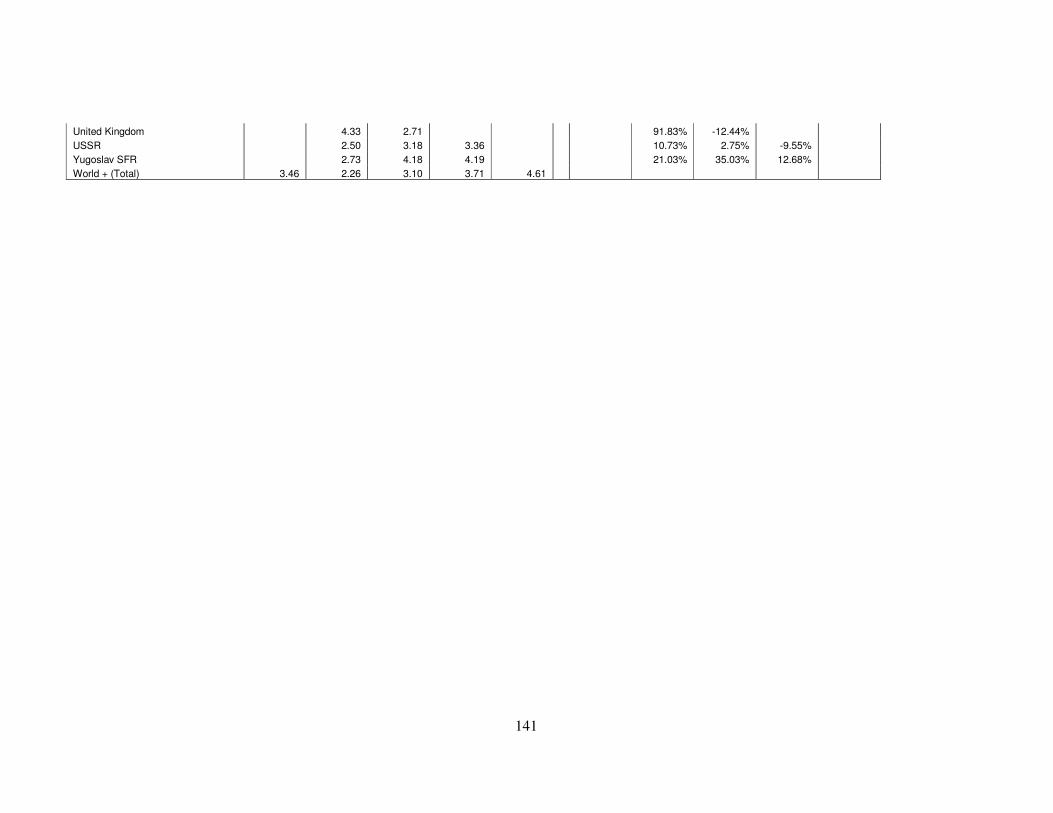
141

United Kingdom 4.33 2.71 91.83% -12.44%

USSR 2.50 3.18 3.36 10.73% 2.75% -9.55%

Yugoslav SFR 2.73 4.18 4.19 21.03% 35.03% 12.68%

World + (Total) 3.46 2.26 3.10 3.71 4.61

142

Annex 2: Average yields (MT/ha), % deviation from world average, 1985 – 2008, maize ranked by gap in 2003-2008

Maize

Average yield per period % deviation from world average

1985-2009 1985-1990 1991-1996 1997-2002 2003-2008 1985-2009 1985-1990 1991-1996 1997-2002 2003-2008

Belgium-Luxembourg 9.64 7.51 8.08 10.93 11.61 129.25% 112.07% 107.86% 150.07% 139.20%

Netherlands 9.67 8.96 8.43 9.38 11.37 130.18% 153.26% 116.84% 114.60% 134.13%

Austria 9.10 8.14 8.16 9.60 10.27 116.60% 129.87% 109.84% 119.76% 111.55%

Greece 9.81 9.30 9.96 9.80 10.20 133.51% 162.76% 156.00% 124.35% 110.16%

Spain 8.25 6.46 7.08 9.43 9.73 96.32% 82.47% 82.09% 115.73% 100.39%

Italy 8.63 7.49 8.52 9.54 8.99 105.42% 111.66% 119.05% 118.30% 85.24%

Germany 8.08 6.98 7.40 8.83 8.84 92.24% 97.23% 90.14% 102.15% 81.98%

France 8.06 6.68 7.86 8.85 8.68 91.73% 88.64% 102.16% 102.48% 78.69%

Switzerland 8.85 8.28 8.75 9.44 8.65 110.45% 133.88% 125.09% 116.07% 78.11%

Slovenia 5.16 6.86 7.16 32.64% 57.11% 47.38%

Czech Republic 4.41 6.90 6.66 13.39% 57.86% 37.22%

Hungary 5.60 5.80 4.65 5.73 6.09 33.23% 63.77% 19.67% 31.11% 25.41%

Kyrgyzstan 4.06 5.38 6.06 4.41% 23.24% 24.73%

Croatia 4.66 5.36 5.92 19.85% 22.74% 22.02%

Slovakia 4.85 5.20 5.76 24.70% 19.10% 18.55%

Uzbekistan 3.58 3.24 5.58 -7.99% -25.90% 14.92%

Poland 5.24 4.79 4.60 5.88 5.54 24.78% 35.49% 18.24% 34.53% 14.19%

Portugal 4.52 2.66 3.89 5.68 5.49 7.64% -24.77% -0.06% 30.01% 13.13%

Tajikistan 2.70 2.95 4.95 -30.60% -32.46% 1.89%

Serbia and Montenegro 3.45 4.29 4.82 -11.35% -1.89% -0.70%

Albania 3.84 3.93 2.80 3.65 4.69 -8.66% 11.05% -28.06% -16.41% -3.44%

Kazakhstan 2.45 3.12 4.61 -36.92% -28.70% -4.97%

Serbia 4.41 -9.19%

Bosnia and Herzegovina 4.00 3.86 4.37 2.78% -11.69% -9.94%

The former Yugoslav Republic of Macedonia 3.13 3.89 4.24 -19.55% -10.91% -12.59%

Belarus 1.89 2.59 4.21 -51.38% -40.82% -13.29%

Ukraine 2.67 3.01 3.99 -31.25% -31.00% -17.76%

Bulgaria 3.50 3.65 3.07 3.09 3.97 -16.84% 3.04% -20.99% -29.18% -18.31%

Russian Federation 2.40 2.26 3.59 -38.30% -48.26% -26.09%

Romania 3.13 3.06 3.00 3.05 3.35 -25.61% -13.41% -22.94% -30.29% -30.97%

Montenegro 3.11 -35.98%

Lithuania 2.86 2.93 -34.49% -39.65%

Republic of Moldova 2.88 2.89 2.67 -25.90% -33.93% -45.04%

Turkmenistan 3.12 0.76 1.07 -19.80% -82.56% -78.04%

Czechoslovakia 4.97 4.75 40.48% 22.00%

143

United Kingdom

USSR 3.37 3.29 -4.76% -15.32%

Yugoslav SFR 3.99 5.34 12.84% 37.18%

World + (Total) 4.20 3.54 3.89 4.37 4.85

144

Annex 2: Average yields (MT/ha), % deviation from world average, 1961 – 2008, oats ranked by gap in 1997-2008

Oats

Average yield per period % deviation from world average

1961-2009 1961-1972 1973-1984 1985-1996 1997-2008 1961-2009 1961-1972 1973-1984 1985-1996 1997-2008

Ireland 5.06 3.00 3.92 6.03 7.09 180.96% 88.42% 132.42% 236.94% 239.33%

United Kingdom 4.56 3.19 4.02 5.06 5.85 153.13% 100.57% 137.96% 182.85% 179.94%

Netherlands 4.97 4.37 4.93 5.21 5.29 176.08% 174.33% 191.71% 190.80% 153.30%

Switzerland 4.59 3.45 4.48 5.18 5.18 155.00% 116.79% 165.04% 189.30% 147.82%

Belgium-Luxembourg 4.42 3.87 4.15 4.43 5.08 145.55% 142.70% 146.02% 147.72% 143.07%

Denmark 4.19 3.73 3.69 4.46 4.82 132.53% 134.31% 118.47% 149.03% 130.73%

Germany 4.03 3.11 3.80 4.43 4.69 123.83% 95.23% 124.79% 147.71% 124.48%

France 3.58 2.48 3.30 4.02 4.42 99.16% 55.92% 95.47% 124.59% 111.84%

Austria 3.36 2.50 3.27 3.70 3.95 86.79% 56.87% 93.49% 106.64% 89.34%

Norway 3.47 2.76 3.63 3.65 3.89 92.96% 73.44% 114.99% 103.62% 86.33%

Sweden 3.41 2.91 3.35 3.58 3.77 89.63% 82.50% 98.17% 99.98% 80.58%

Finland 2.75 2.09 2.64 3.09 3.11 52.56% 30.93% 56.12% 72.66% 49.00%

Czech Republic 3.22 3.03 79.74% 44.90%

Slovenia 2.38 2.53 32.82% 21.36%

Croatia 2.42 2.41 35.27% 15.61%

Kyrgyzstan 2.03 2.40 13.47% 15.01%

Hungary 2.26 1.32 2.56 2.77 2.40 25.38% -17.27% 51.41% 54.46% 14.85%

Poland 2.33 1.97 2.40 2.53 2.39 29.40% 23.38% 42.06% 41.26% 14.58%

Bosnia and Herzegovina 2.27 2.32 26.56% 11.25%

Italy 1.95 1.47 1.80 2.22 2.30 8.57% -7.74% 6.65% 23.79% 10.00%

Belarus 2.21 2.29 23.51% 9.87%

Serbia 2.11 1.07%

Slovakia 2.49 2.04 39.20% -2.10%

Estonia 1.87 2.00 4.49% -4.29%

Greece 1.62 1.23 1.54 1.74 1.96 -10.07% -22.92% -8.63% -3.07% -6.00%

Serbia and Montenegro 1.66 1.92 -7.32% -8.10%

Lithuania 1.45 1.85 -18.83% -11.20%

Montenegro 1.85 -11.49%

Spain 1.31 0.94 1.17 1.30 1.82 -27.02% -40.98% -30.84% -27.59% -12.70%

Latvia 1.51 1.78 -15.91% -14.99%

Ukraine 2.25 1.76 25.56% -15.72%

Bulgaria 1.42 1.15 1.27 1.65 1.62 -20.98% -27.79% -25.05% -8.08% -22.51%

Romania 1.30 1.04 1.08 1.47 1.60 -27.67% -34.66% -35.92% -18.05% -23.18%

Albania 1.27 0.86 1.37 1.23 1.55 -29.61% -46.06% -18.72% -31.02% -25.95%

Russian Federation 1.26 1.51 -29.76% -27.85%

145

The former Yugoslav Republic of Macedonia 1.13 1.39 -36.91% -33.55%

Republic of Moldova 1.90 1.21 6.16% -42.09%

Kazakhstan 1.18 1.05 -34.17% -49.78%

Portugal 0.72 0.41 0.52 0.88 1.02 -59.97% -74.21% -69.05% -50.94% -51.06%

Tajikistan 0.60 0.75 -66.37% -64.21%

Czechoslovakia 2.10 3.05 3.69 31.67% 80.41% 106.39%

Turkmenistan 2.19 22.31%

USSR 1.03 1.23 1.36 -35.05% -27.26% -24.03%

Uzbekistan 1.15 -35.56%

Yugoslav SFR 1.11 1.43 1.83 -30.58% -15.19% 1.94%

World + (Total) 1.80 1.59 1.69 1.79 2.09

146

Annex 2: Average yields (MT/ha), % deviation from world average, 1985 – 2008, oats ranked by gap in 2003-2008

Oats

Average yield per period % deviation from world average

1985-2009 1985-1990 1991-1996 1997-2002 2003-2008 1985-2009 1985-1990 1991-1996 1997-2002 2003-2008

Ireland 6.59 5.45 6.62 6.83 7.34 237.34% 201.24% 273.37% 237.38% 241.15%

United Kingdom 5.47 4.72 5.41 5.84 5.86 180.00% 160.96% 205.17% 188.15% 172.22%

Belgium-Luxembourg 4.81 4.09 4.78 4.75 5.40 146.48% 126.03% 169.85% 134.44% 151.20%

Netherlands 5.28 4.98 5.43 5.34 5.24 170.28% 175.55% 206.36% 163.75% 143.46%

Switzerland 5.19 5.06 5.30 5.38 4.97 165.78% 179.99% 198.79% 165.60% 131.07%

Germany 4.58 4.28 4.59 4.81 4.57 134.63% 136.50% 159.16% 137.29% 112.42%

Denmark 4.64 4.30 4.61 5.08 4.56 137.67% 137.93% 160.37% 150.69% 111.94%

France 4.25 3.87 4.17 4.46 4.38 117.62% 114.05% 135.35% 120.40% 103.78%

Austria 3.82 3.77 3.63 3.98 3.92 95.73% 108.23% 105.03% 96.63% 82.48%

Norway 3.74 3.66 3.63 3.90 3.89 91.46% 102.37% 104.91% 92.39% 80.63%

Sweden 3.69 3.60 3.56 3.73 3.81 88.88% 99.22% 100.76% 84.04% 77.32%

Finland 3.12 2.83 3.36 3.04 3.18 59.56% 56.25% 89.42% 50.25% 47.83%

Czech Republic 3.22 2.99 3.06 81.57% 47.47% 42.48%

Belarus 2.21 1.87 2.72 24.77% -7.58% 26.30%

Slovenia 2.38 2.56 2.51 34.18% 26.21% 16.79%

Hungary 2.56 3.10 2.43 2.34 2.46 31.28% 71.67% 36.89% 15.58% 14.17%

Bosnia and Herzegovina 2.27 2.26 2.39 27.85% 11.33% 11.19%

Poland 2.47 2.73 2.33 2.42 2.36 26.50% 51.12% 31.21% 19.63% 9.83%

Italy 2.26 2.02 2.42 2.25 2.34 15.76% 11.46% 36.38% 11.29% 8.78%

Croatia 2.42 2.49 2.34 36.65% 23.05% 8.60%

Kyrgyzstan 2.03 2.50 2.31 14.62% 23.20% 7.30%

Estonia 1.87 1.79 2.20 5.55% -11.41% 2.42%

Serbia 2.11 -1.87%

Serbia and Montenegro 1.66 1.84 2.08 -6.37% -9.22% -3.32%

Slovakia 2.49 2.07 2.02 40.62% 1.97% -5.94%

Greece 1.84 1.62 1.85 1.92 2.01 -5.63% -10.25% 4.25% -5.22% -6.73%

Spain 1.56 1.40 1.19 1.68 1.97 -19.97% -22.32% -32.96% -17.19% -8.47%

Lithuania 1.45 1.78 1.93 -18.00% -12.25% -10.21%

Latvia 1.51 1.67 1.88 -15.05% -17.40% -12.73%

Montenegro 1.85 -14.07%

Ukraine 2.25 1.74 1.78 26.84% -14.03% -17.32%

Bulgaria 1.63 1.83 1.46 1.50 1.74 -16.63% 1.16% -17.50% -26.16% -19.08%

Romania 1.53 1.46 1.47 1.48 1.73 -21.50% -19.23% -16.86% -27.16% -19.42%

Albania 1.41 1.29 1.18 1.44 1.65 -27.70% -28.57% -33.52% -28.91% -23.16%

Russian Federation 1.26 1.44 1.57 -29.04% -28.78% -26.97%

147

The former Yugoslav Republic of Macedonia 1.13 1.22 1.55 -36.27% -39.54% -27.91%

Republic of Moldova 1.90 1.27 1.15 7.25% -37.32% -46.58%

Portugal 0.96 0.93 0.83 0.90 1.14 -50.62% -48.56% -53.36% -55.52% -46.85%

Kazakhstan 1.18 1.02 1.08 -33.50% -49.78% -49.78%

Tajikistan 0.60 0.50 1.00 -66.03% -75.56% -53.53%

Czechoslovakia 3.78 3.45 108.84% 94.69%

Turkmenistan 2.19 23.56%

USSR 1.36 1.39 1.21 -30.35% -23.40% -31.77%

Uzbekistan 1.15 -34.91%

Yugoslav SFR 1.81 1.91 0.09% 8.05%

World + (Total) 1.95 1.81 1.77 2.03 2.15

148

Annex 2: Average yields (MT/ha), % deviation from world average, 1961 – 2008, potatoes ranked by gap in 1997-2008

Potatoes

Average yield per period % deviation from world average

1961-2009 1961-1972 1973-1984 1985-1996 1997-2008 1961-2009 1961-1972 1973-1984 1985-1996 1997-2008

Belgium-Luxembourg 39.30 32.08 37.88 42.04 44.73 162.38% 143.74% 161.54% 171.74% 170.03%

Netherlands 38.92 32.50 36.79 42.01 43.75 159.86% 146.94% 154.01% 171.56% 164.12%

United Kingdom 34.04 24.84 30.96 38.21 41.41 127.31% 88.79% 113.75% 146.97% 149.94%

France 30.30 20.05 26.05 33.28 40.83 102.31% 52.35% 79.86% 115.11% 146.49%

Germany 29.29 22.05 22.12 31.00 40.76 95.58% 67.57% 52.71% 100.37% 146.05%

Denmark 31.62 23.22 27.07 35.66 39.70 111.14% 76.43% 86.92% 130.49% 139.66%

Switzerland 36.02 28.43 36.07 39.61 39.13 140.51% 116.05% 149.02% 156.04% 136.18%

Ireland 26.90 25.08 24.05 25.59 32.81 79.65% 90.58% 66.04% 65.41% 98.05%

Sweden 28.17 23.22 26.34 32.46 30.35 88.09% 76.47% 81.84% 109.81% 83.20%

Austria 26.04 22.60 24.69 26.11 30.22 73.87% 71.71% 70.49% 68.78% 82.42%

Spain 18.26 12.02 15.07 18.87 26.18 21.94% -8.65% 4.06% 21.96% 58.06%

Norway 24.18 22.49 24.68 24.13 25.41 61.44% 70.87% 70.39% 55.95% 53.41%

Italy 18.54 11.85 17.05 20.57 24.17 23.79% -9.96% 17.69% 32.97% 45.89%

Finland 18.64 14.90 15.69 19.58 23.54 24.44% 13.22% 8.32% 26.59% 42.10%

Czech Republic 19.33 22.60 24.94% 36.43%

Hungary 16.18 9.62 14.93 16.90 22.54 8.06% -26.91% 3.06% 9.26% 36.06%

Malta 13.25 7.44 8.18 15.65 21.66 -11.50% -43.47% -43.53% 1.13% 30.73%

Slovenia 15.11 21.00 -2.35% 26.79%

Greece 16.68 10.32 15.70 19.51 20.46 11.36% -21.59% 8.41% 26.10% 23.52%

Poland 17.55 16.53 17.54 17.78 18.17 17.20% 25.59% 21.08% 14.94% 9.68%

Uzbekistan 10.20 16.63 -34.06% 0.37%

Tajikistan 14.95 16.23 -3.35% -2.04%

Faroe Islands 14.55 14.00 13.75 14.12 16.21 -2.86% 6.41% -5.08% -8.71% -2.14%

Kyrgyzstan 11.05 15.72 -28.55% -5.09%

Belarus 13.43 15.60 -13.20% -5.82%

Slovakia 14.55 15.42 -5.97% -6.91%

Albania 9.60 6.75 7.07 8.18 15.37 -35.89% -48.69% -51.17% -47.14% -7.23%

Iceland 12.59 12.12 11.51 11.93 14.74 -15.93% -7.88% -20.56% -22.91% -11.00%

Portugal 11.66 10.00 9.01 12.89 14.50 -22.17% -24.04% -37.79% -16.71% -12.47%

Latvia 12.95 14.02 -16.28% -15.35%

Romania 12.76 9.21 14.63 13.09 13.87 -14.83% -30.02% 1.01% -15.37% -16.26%

Estonia 13.95 13.63 -9.84% -17.75%

Lithuania 12.51 13.24 -19.13% -20.05%

The former Yugoslav Republic of Macedonia 10.24 13.23 -33.80% -20.12%

Bulgaria 11.62 11.30 10.90 10.75 13.13 -22.38% -14.11% -24.72% -30.52% -20.73%

149

Kazakhstan 9.42 12.70 -39.14% -23.31%

Croatia 8.96 12.25 -42.07% -26.05%

Montenegro 12.22 -26.24%

Ukraine 11.53 11.71 -25.49% -29.31%

Russian Federation 11.09 11.42 -28.32% -31.05%

Serbia 0.00 10.18 -38.54%

Serbia and Montenegro 7.41 9.36 -52.09% -43.49%

Bosnia and Herzegovina 7.82 9.14 -49.48% -44.83%

Republic of Moldova 7.16 7.62 -53.70% -54.00%

Turkmenistan 6.51 5.72 -57.90% -65.49%

Czechoslovakia 14.25 17.06 17.77 8.26% 17.78% 14.88%

USSR 10.53 11.68 11.56 -19.96% -19.34% -25.29%

Yugoslav SFR 8.55 9.08 8.18 -35.06% -37.31% -47.11%

World + (Total) 14.98 13.16 14.48 15.47 16.57

150

Annex 2: Average yields (MT/ha), % deviation from world average, 1985 – 2008, potatoes ranked by gap in 2003-2008

Potatoes

Average yield per period % deviation from world average

1985-2009 1985-1990 1991-1996 1997-2002 2003-2008 1985-2009 1985-1990 1991-1996 1997-2002 2003-2008

Belgium-Luxembourg 43.44 39.38 44.70 45.25 44.22 170.07% 156.68% 186.55% 182.60% 158.28%

Netherlands 43.02 42.00 42.02 44.29 43.22 167.45% 173.78% 169.38% 176.60% 152.44%

France 37.26 32.10 34.46 39.11 42.56 131.63% 109.26% 120.85% 144.24% 148.60%

United Kingdom 39.94 36.66 39.76 41.10 41.71 148.31% 138.95% 154.86% 156.70% 143.62%

Germany 36.21 27.80 34.20 40.96 40.56 125.10% 81.21% 119.22% 155.83% 136.90%

Denmark 37.84 36.18 35.14 40.40 39.01 135.24% 135.81% 125.26% 152.30% 127.84%

Switzerland 39.64 37.53 41.69 40.11 38.14 146.44% 144.65% 167.24% 150.49% 122.80%

Ireland 29.15 22.68 28.50 30.79 34.83 81.24% 47.84% 82.68% 92.30% 103.43%

Austria 28.34 27.15 25.07 29.59 30.85 76.18% 76.98% 60.71% 84.79% 80.19%

Sweden 31.42 32.33 32.59 31.16 29.54 95.36% 110.74% 108.89% 94.59% 72.55%

Spain 22.79 18.17 19.57 24.95 27.41 41.68% 18.42% 25.43% 55.85% 60.13%

Norway 24.75 24.23 24.02 25.13 25.70 53.87% 57.93% 54.00% 56.96% 50.09%

Czech Republic 19.33 20.93 24.27 23.90% 30.73% 41.75%

Italy 22.47 18.77 22.38 24.17 24.16 39.69% 22.34% 43.43% 50.98% 41.12%

Hungary 19.94 18.08 15.73 21.10 23.98 23.95% 17.84% 0.83% 31.81% 40.04%

Finland 21.84 18.64 20.53 23.37 23.71 35.81% 21.49% 31.61% 45.94% 38.51%

Malta 18.48 9.16 22.13 20.89 22.43 14.90% -40.29% 41.86% 30.45% 31.00%

Slovenia 15.11 20.78 21.23 -3.16% 29.76% 24.01%

Greece 20.20 18.78 20.23 20.01 20.92 25.58% 22.44% 29.70% 24.94% 22.18%

Tajikistan 14.95 12.20 20.25 -4.16% -23.80% 18.31%

Uzbekistan 10.20 13.80 19.46 -34.60% -13.84% 13.66%

Belarus 13.43 11.84 19.36 -13.92% -26.05% 13.10%

Poland 18.05 18.75 16.81 17.76 18.57 12.23% 22.23% 7.78% 10.94% 8.50%

Albania 12.18 7.05 9.30 13.72 17.02 -24.27% -54.02% -40.38% -14.33% -0.58%

Iceland 13.34 12.53 11.33 12.97 16.51 -17.09% -18.34% -27.40% -18.98% -3.55%

Faroe Islands 15.19 13.56 14.68 16.25 16.18 -5.55% -11.58% -5.88% 1.47% -5.51%

Bulgaria 12.12 11.03 10.47 10.45 15.81 -24.62% -28.13% -32.87% -34.72% -7.65%

Slovakia 14.55 15.10 15.75 -6.75% -5.72% -8.02%

Kyrgyzstan 11.05 15.81 15.64 -29.14% -1.28% -8.66%

Portugal 13.72 11.39 14.38 14.01 14.99 -14.69% -25.78% -7.79% -12.47% -12.47%

Kazakhstan 9.42 10.78 14.63 -39.64% -32.68% -14.56%

Latvia 12.95 13.56 14.49 -16.98% -15.33% -15.36%

Croatia 8.96 10.19 14.32 -42.55% -36.38% -16.38%

Romania 13.56 14.03 12.16 13.48 14.27 -15.70% -8.55% -22.08% -15.84% -16.65%

Estonia 13.95 13.18 14.07 -10.59% -17.70% -17.79%

151

The former Yugoslav Republic of Macedonia 10.24 12.74 13.73 -34.35% -20.44% -19.82%

Ukraine 11.53 10.40 13.02 -26.11% -35.07% -23.93%

Russian Federation 11.09 10.37 12.47 -28.92% -35.22% -27.15%

Lithuania 12.51 14.15 12.34 -19.80% -11.64% -27.92%

Montenegro 12.22 -28.63%

Serbia and Montenegro 7.41 8.93 10.23 -52.49% -44.25% -40.25%

Serbia 10.18 -40.53%

Bosnia and Herzegovina 7.82 8.51 9.76 -49.90% -46.83% -42.97%

Republic of Moldova 7.16 6.43 8.81 -54.09% -59.84% -48.54%

Turkmenistan 6.51 5.39 6.04 -58.25% -66.32% -64.72%

Czechoslovakia 17.77 18.30 16.20 10.50% 19.27% 3.85%

USSR 11.69 10.78 -23.81% -30.90%

Yugoslav SFR 8.07 8.88 -47.41% -43.10%

World + (Total) 16.08 15.34 15.60 16.01 17.12

152

Annex 2: Average yields (MT/ha), % deviation from world average, 1961 – 2008, rapeseed ranked by gap in 1997-2008

Rapeseed

Average yield per period % deviation from world average

1961-2009 1961-1972 1973-1984 1985-1996 1997-2008 1961-2009 1961-1972 1973-1984 1985-1996 1997-2008

Belgium-Luxembourg 3.30 2.59 3.73 3.14 3.65 179.36% 269.77% 283.80% 133.29% 122.79%

Netherlands 3.16 2.68 2.91 3.35 3.56 167.37% 282.42% 199.48% 149.04% 117.65%

Germany 2.73 1.95 2.46 2.90 3.47 131.28% 179.13% 153.10% 115.52% 112.33%

France 2.58 1.85 2.19 2.98 3.20 118.58% 164.91% 125.39% 121.26% 95.34%

Ireland 1.54 3.11 3.16 58.47% 130.83% 92.80%

Denmark 2.42 1.88 2.07 2.49 3.12 105.17% 169.18% 112.96% 85.04% 90.60%

United Kingdom 2.77 2.30 2.60 3.00 3.11 134.27% 229.11% 167.27% 123.14% 89.80%

Switzerland 2.63 2.09 2.47 2.84 3.09 122.85% 198.15% 153.55% 110.84% 88.87%

Austria 2.38 1.97 2.20 2.56 2.74 101.67% 181.56% 126.66% 89.94% 67.35%

Czech Republic 2.39 2.71 77.42% 65.29%

Slovenia 2.37 2.44 76.22% 49.28%

Sweden 2.20 2.23 2.07 2.02 2.42 86.52% 218.66% 112.61% 50.06% 47.73%

Poland 2.05 1.56 1.95 2.22 2.39 73.73% 123.46% 100.52% 64.58% 45.90%

Serbia 2.38 45.66%

Croatia 1.97 2.24 46.60% 36.87%

The former Yugoslav Republic of Macedonia 1.54 2.13 14.43% 30.01%

Bosnia and Herzegovina 1.49 2.10 10.89% 28.60%

Slovakia 1.94 2.08 44.37% 27.19%

Hungary 1.62 1.24 1.49 1.72 1.97 36.95% 76.97% 52.88% 27.74% 20.46%

Serbia and Montenegro 1.55 1.70 15.29% 4.10%

Norway 1.55 1.24 1.68 1.56 1.70 30.98% 77.59% 72.35% 15.87% 4.02%

Lithuania 1.48 1.67 9.72% 2.05%

Latvia 1.16 1.66 -13.76% 1.15%

Greece 1.63 -0.20%

Spain 1.48 2.06 1.36 1.30 1.58 25.26% 193.66% 40.25% -3.60% -3.54%

Italy 1.87 1.68 2.08 2.21 1.48 58.17% 140.28% 113.96% 64.30% -9.48%

Bulgaria 1.07 0.75 0.72 1.10 1.47 -9.32% 6.54% -26.08% -18.65% -10.12%

Estonia 0.93 1.46 -31.14% -10.96%

Romania 1.22 1.26 1.37 0.87 1.36 3.24% 79.73% 41.40% -35.14% -17.16%

Finland 1.44 1.32 1.49 1.58 1.33 21.56% 88.30% 52.81% 17.50% -18.74%

Ukraine 1.12 1.21 -17.16% -26.16%

Republic of Moldova 1.14 -30.48%

Uzbekistan 0.83 1.12 -38.39% -31.68%

Russian Federation 0.78 1.03 -41.84% -36.84%

Belarus 0.77 0.95 -43.16% -41.82%

153

Kyrgyzstan 0.73 0.82 -45.80% -49.98%

Kazakhstan 0.44 0.57 -67.62% -64.92%

Tajikistan 0.07 0.11 -94.46% -93.57%

Czechoslovakia 1.54 2.15 2.69 119.54% 121.59% 99.71%

USSR 0.83 0.72 0.83 18.54% -26.07% -38.50%

Yugoslav SFR 1.30 2.06 2.25 86.03% 112.03% 67.18%

World + (Total) 1.18 0.70 0.97 1.35 1.64

154

Annex 2: Average yields (MT/ha), % deviation from world average, 1985 – 2008, rapeseed ranked by gap in 2003-2008

Rapeseed

Average yield per period % deviation from world average

1985-2009 1985-1990 1991-1996 1997-2002 2003-2008 1985-2009 1985-1990 1991-1996 1997-2002 2003-2008

Belgium-Luxembourg 3.43 3.27 3.01 3.44 3.85 127.01% 146.11% 120.80% 127.57% 118.69%

Netherlands 3.50 3.32 3.38 3.33 3.80 131.88% 150.03% 148.08% 120.26% 115.42%

Germany 3.23 3.00 2.80 3.34 3.61 113.90% 126.03% 105.28% 120.84% 105.03%

Ireland 3.14 3.20 3.02 2.83 3.48 107.91% 140.90% 121.01% 87.01% 97.77%

Denmark 2.85 2.63 2.35 2.80 3.44 88.53% 97.88% 72.53% 85.22% 95.22%

France 3.12 2.97 2.99 3.14 3.25 106.17% 123.73% 118.86% 107.95% 84.52%

United Kingdom 3.07 3.14 2.87 3.04 3.17 102.99% 136.52% 110.11% 101.05% 80.14%

Switzerland 2.97 2.82 2.86 3.05 3.13 96.63% 112.40% 109.33% 101.77% 77.80%

Austria 2.66 2.53 2.59 2.57 2.91 76.19% 90.34% 89.55% 69.78% 65.27%

Czech Republic 2.39 2.57 2.84 75.10% 70.08% 61.19%

Poland 2.33 2.49 1.94 2.18 2.60 54.40% 87.40% 42.36% 44.16% 47.39%

Sweden 2.25 2.04 2.01 2.26 2.57 49.08% 53.22% 46.99% 49.64% 46.09%

Serbia 2.38 35.30%

Slovenia 2.37 2.56 2.32 73.91% 69.65% 31.80%

Croatia 1.97 2.16 2.32 44.69% 43.05% 31.57%

Hungary 1.86 1.90 1.54 1.64 2.30 23.14% 42.70% 13.18% 8.75% 30.50%

Slovakia 1.94 2.01 2.15 42.49% 33.07% 22.15%

Bosnia and Herzegovina 1.49 2.07 2.14 9.44% 37.09% 21.32%

The former Yugoslav Republic of Macedonia 1.54 2.19 2.07 12.93% 44.66% 17.44%

Italy 1.85 2.31 2.11 1.08 1.88 22.68% 73.83% 55.02% -28.63% 6.94%

Latvia 1.16 1.44 1.87 -14.89% -4.79% 6.24%

Bulgaria 1.10 1.10 1.84 -19.71% -26.89% 4.27%

Serbia and Montenegro 1.55 1.64 1.83 13.78% 8.42% 4.10%

Lithuania 1.48 1.57 1.77 8.28% 3.85% 0.51%

Norway 1.63 1.63 1.49 1.73 1.67 7.84% 22.41% 9.50% 14.56% -5.01%

Greece 1.63 -7.29%

Spain 1.44 1.48 1.12 1.62 1.54 -4.60% 11.14% -17.95% 6.91% -12.51%

Estonia 0.93 1.38 1.54 -32.04% -8.92% -12.71%

Romania 1.12 0.77 0.98 1.18 1.54 -25.56% -42.35% -28.12% -22.21% -12.83%

Ukraine 1.12 0.96 1.46 -18.24% -36.51% -17.27%

Finland 1.47 1.53 1.63 1.36 1.30 -2.93% 15.50% 19.43% -9.75% -26.46%

Belarus 0.77 0.67 1.23 -43.90% -55.66% -29.94%

Uzbekistan 0.83 1.05 1.19 -39.20% -30.75% -32.48%

Republic of Moldova 1.07 1.19 -29.49% -32.69%

Russian Federation 0.78 0.89 1.17 -42.60% -40.95% -33.31%

155

Kyrgyzstan 0.73 0.78 0.86 -46.51% -48.69% -51.09%

Kazakhstan 0.44 0.49 0.66 -68.04% -67.88% -62.39%

Tajikistan 0.07 0.06 0.15 -94.53% -95.73% -91.71%

Czechoslovakia 2.71 2.63 103.88% 92.75%

USSR 0.79 1.06 -40.61% -22.19%

Yugoslav SFR 2.22 2.41 67.47% 76.40%

World + (Total) 1.51 1.33 1.36 1.51 1.76

156

Annex 2: Average yields (MT/ha), % deviation from world average, 1961 – 2008, rice, ranked by gap in 1997-2008

Rice, paddy

Average yield per period % deviation from world average

1961-2009 1961-1972 1973-1984 1985-1996 1997-2008 1961-2009 1961-1972 1973-1984 1985-1996 1997-2008

Greece 5.92 4.54 5.09 6.68 7.29 89.98% 111.38% 86.72% 91.13% 82.12%

Spain 6.43 6.14 6.05 6.32 7.13 106.43% 186.01% 122.32% 80.83% 78.17%

Italy 5.58 4.87 5.31 5.82 6.26 79.04% 126.97% 95.11% 66.51% 56.36%

Portugal 4.86 4.42 4.15 4.97 5.82 55.81% 105.94% 52.28% 42.16% 45.42%

France 4.69 3.79 3.96 5.25 5.68 50.53% 76.49% 45.43% 50.38% 41.88% The former Yugoslav Republic of Macedonia 4.48 5.11 28.26% 27.63%

Bulgaria 3.93 3.57 3.96 3.45 4.61 25.97% 66.49% 45.46% -1.32% 15.26%

Ukraine 3.50 3.92 0.24% -2.13%

Russian Federation 2.78 3.62 -20.56% -9.52%

Hungary 2.75 2.00 2.25 3.03 3.59 -11.76% -6.86% -17.40% -13.26% -10.29%

Tajikistan 1.78 3.23 -48.97% -19.25%

Kazakhstan 3.04 3.19 -12.99% -20.31%

Romania 2.75 2.66 2.49 2.69 2.95 -11.70% 23.69% -8.51% -22.99% -26.35%

Kyrgyzstan 1.39 2.76 -60.35% -30.93%

Uzbekistan 2.67 2.64 -23.50% -34.08%

Turkmenistan 2.21 1.66 -36.89% -58.53%

Yugoslav SFR 4.12 4.32 4.32 91.73% 58.62% 23.68%

USSR 2.80 3.65 3.61 30.53% 33.95% 3.40%

Albania 2.62 3.42 3.35 22.24% 25.53% -4.18%

World + (Total) 3.12 2.15 2.72 3.49 4.00

157

Annex 2: Average yields (MT/ha), % deviation from world average, 1985 – 2008, rice ranked by gap in 2003-2008

Rice, paddy

Average yield per period % deviation from world average

1985-2009 1985-1990 1991-1996 1997-2002 2003-2008 1985-2009 1985-1990 1991-1996 1997-2002 2003-2008

Greece 6.99 6.33 7.02 7.19 7.38 85.26% 89.28% 92.82% 85.96% 78.52%

Spain 6.76 6.23 6.41 7.22 7.04 79.17% 86.04% 76.04% 86.55% 70.32%

Italy 6.05 5.86 5.77 6.10 6.41 60.37% 75.23% 58.50% 57.76% 55.04%

Portugal 5.40 4.47 5.47 5.89 5.74 43.34% 33.43% 50.19% 52.30% 38.97%

France 5.48 5.47 5.04 5.78 5.57 45.20% 63.42% 38.40% 49.49% 34.75%

The former Yugoslav Republic of Macedonia 4.48 4.78 5.43 23.06% 23.57% 31.43%

Bulgaria 4.08 3.57 3.32 4.15 5.07 8.14% 6.77% -8.74% 7.22% 22.79%

Ukraine 3.50 3.34 4.49 -3.82% -13.72% 8.72%

Russian Federation 2.78 3.14 4.10 -23.78% -18.72% -0.91%

Hungary 3.35 3.29 2.77 3.46 3.71 -11.15% -1.71% -23.87% -10.46% -10.12%

Romania 2.92 2.59 2.79 2.19 3.71 -22.48% -22.62% -23.32% -43.51% -10.29%

Tajikistan 1.78 2.82 3.64 -51.04% -27.15% -11.85%

Kazakhstan 3.04 3.00 3.38 -16.52% -22.53% -18.23%

Uzbekistan 2.67 2.08 3.19 -26.60% -46.16% -22.77%

Kyrgyzstan 1.39 2.59 2.93 -61.96% -32.98% -29.01%

Turkmenistan 2.21 1.01 2.31 -39.45% -73.96% -44.10%

Albania 3.18 3.68 -4.87% 0.98%

USSR 3.66 3.31 9.46% -9.01%

Yugoslav SFR 4.32 4.31 29.17% 18.47%

World + (Total) 3.77 3.35 3.64 3.87 4.13

158

Annex 2: Average yields (MT/ha), % deviation from world average, 1961 – 2008, rye, ranked by gap in 1997-2008

Rye

Average yield per period % deviation from world average

1961-2009 1961-1972 1973-1984 1985-1996 1997-2008 1961-2009 1961-1972 1973-1984 1985-1996 1997-2008

Switzerland 4.97 3.73 4.53 5.44 6.04 167.32% 185.69% 163.14% 167.00% 164.07%

United Kingdom 4.39 2.77 3.61 5.14 5.81 136.49% 112.65% 109.66% 152.35% 153.78%

Sweden 4.01 2.80 3.58 4.31 5.17 115.79% 115.03% 107.85% 111.49% 126.07%

Germany 3.87 2.71 3.24 4.23 5.16 108.59% 107.72% 88.13% 107.55% 125.70%

Denmark 4.14 3.14 3.79 4.58 4.97 123.07% 140.72% 119.75% 124.57% 117.11%

Netherlands 4.13 3.02 3.78 4.84 4.84 122.62% 131.64% 119.13% 137.70% 111.40%

France 3.32 1.89 2.94 3.72 4.56 78.59% 44.74% 70.68% 82.63% 99.40%

Norway 3.53 2.92 3.43 3.40 4.35 90.06% 124.08% 98.96% 66.81% 90.30%

Belgium-Luxembourg 3.83 3.36 3.77 4.12 3.99 106.34% 157.81% 118.65% 102.30% 74.29%

Czech Republic 3.46 3.95 69.71% 72.77%

Austria 3.42 2.55 3.36 3.89 3.85 84.10% 95.28% 94.76% 91.06% 68.28%

Uzbekistan 1.67 2.89 -18.09% 26.36%

Slovenia 2.72 2.89 33.44% 26.22%

Slovakia 2.87 2.73 41.00% 19.18%

Italy 2.35 1.78 2.28 2.64 2.69 26.51% 36.17% 32.45% 29.48% 17.37%

Croatia 2.60 2.62 27.39% 14.59%

Bosnia and Herzegovina 2.43 2.53 19.13% 10.52%

Poland 2.23 1.81 2.32 2.43 2.33 20.16% 38.59% 34.58% 19.33% 1.98%

Latvia 1.93 2.31 -5.44% 0.90%

Estonia 2.04 2.27 -0.14% -0.89%

Serbia 2.26 -1.42%

Finland 2.16 1.68 2.12 2.54 2.25 16.12% 28.67% 23.08% 24.84% -1.60%

Lithuania 1.83 2.24 -10.03% -2.26%

Hungary 1.82 1.16 1.72 2.15 2.22 -2.24% -10.67% 0.09% 5.54% -2.84%

Greece 1.77 1.07 1.70 2.06 2.22 -4.94% -17.74% -1.16% 1.18% -3.10%

Ireland 2.30 2.09 2.86 2.07 2.21 23.95% 60.16% 65.78% 1.67% -3.50%

Belarus 2.48 2.08 21.59% -9.07%

Montenegro 2.08 -9.10%

Romania 1.71 1.13 1.81 1.87 2.02 -7.82% -13.67% 4.85% -8.49% -11.91%

Serbia and Montenegro 1.55 1.86 -24.06% -18.61%

The former Yugoslav Republic of Macedonia 1.49 1.84 -26.91% -19.67%

Ukraine 2.08 1.81 1.99% -20.81%

Spain 1.28 0.89 1.05 1.38 1.78 -31.09% -31.61% -38.88% -32.10% -22.12%

Albania 1.14 0.73 0.93 1.00 1.75 -38.71% -44.24% -46.00% -50.85% -23.65%

Russian Federation 1.52 1.71 -25.30% -25.40%

159

Bulgaria 1.44 1.13 1.33 1.64 1.64 -22.20% -13.36% -22.94% -19.36% -28.28%

Republic of Moldova 1.97 1.57 -3.58% -31.24%

Kyrgyzstan 1.47 1.57 -28.04% -31.40%

Tajikistan 0.81 1.02 -60.43% -55.49%

Kazakhstan 0.81 0.94 -60.02% -58.71%

Portugal 0.81 0.65 0.72 0.93 0.91 -56.62% -50.37% -58.18% -54.54% -60.10%

Czechoslovakia 2.24 3.21 3.74 71.39% 86.04% 83.64%

Turkmenistan 1.98 -2.71%

USSR 0.96 1.29 1.70 -26.46% -25.06% -16.47%

Yugoslav SFR 1.11 1.40 1.86 -14.84% -18.96% -8.58%

World + (Total) 1.86 1.30 1.72 2.04 2.29

160

Annex 2: Average yields (MT/ha), % deviation from world average, 1985 – 2008, rye, ranked by gap in 2003-2008

Rye

Average yield per period % deviation from world average

1985-2009 1985-1990 1991-1996 1997-2002 2003-2008 1985-2009 1985-1990 1991-1996 1997-2002 2003-2008

United Kingdom 5.54 4.77 5.52 5.48 6.13 153.46% 136.38% 167.99% 148.75% 158.47%

Switzerland 5.77 4.98 5.90 6.27 5.81 163.64% 147.06% 186.52% 184.55% 145.04%

Sweden 4.79 4.00 4.62 4.98 5.37 119.00% 98.43% 124.27% 125.77% 126.35%

Norway 3.87 3.31 3.49 3.64 5.07 76.96% 64.00% 69.56% 65.21% 113.63%

Germany 4.74 3.73 4.73 5.41 4.92 116.57% 85.15% 129.49% 145.37% 107.42%

Denmark 4.80 4.55 4.61 5.10 4.84 119.28% 125.45% 123.72% 131.28% 103.95%

Netherlands 4.84 4.46 5.23 4.99 4.68 121.36% 121.37% 153.69% 126.41% 97.44%

France 4.18 3.44 4.01 4.53 4.59 91.27% 70.54% 94.47% 105.58% 93.66%

Belgium-Luxembourg 4.09 4.19 4.06 3.58 4.39 86.95% 107.84% 96.87% 62.57% 85.20%

Czech Republic 3.46 3.54 4.36 67.93% 60.65% 84.04%

Austria 3.87 3.89 3.90 3.79 3.91 76.87% 93.06% 89.11% 72.02% 64.80%

Uzbekistan 1.67 2.25 3.54 -18.95% 1.86% 49.13%

Slovakia 2.87 2.57 2.88 39.52% 16.73% 21.47%

Slovenia 2.72 2.92 2.86 32.05% 32.23% 20.63%

Italy 2.66 2.57 2.71 2.62 2.75 21.49% 27.28% 31.64% 18.69% 16.14%

Croatia 2.60 2.61 2.64 26.05% 18.31% 11.13%

Estonia 2.04 1.93 2.61 -1.18% -12.51% 9.91%

Bosnia and Herzegovina 2.43 2.46 2.60 17.88% 11.40% 9.69%

Latvia 1.93 2.03 2.59 -6.43% -7.98% 9.15%

Finland 2.40 2.45 2.63 2.07 2.44 9.89% 21.68% 27.92% -6.32% 2.79%

Poland 2.39 2.55 2.31 2.31 2.36 9.44% 26.57% 12.24% 4.72% -0.58%

Lithuania 1.83 2.14 2.33 -10.98% -3.03% -1.55%

Hungary 2.17 2.30 2.01 2.12 2.32 -0.70% 13.90% -2.65% -3.71% -2.04%

Belarus 2.48 1.85 2.31 20.31% -16.13% -2.50%

Ireland 2.14 2.14 2.00 2.13 2.28 -2.24% 6.28% -2.84% -3.28% -3.70%

Greece 2.13 2.05 2.08 2.17 2.26 -2.71% 1.45% 0.92% -1.36% -4.72%

Serbia 2.26 -4.88%

Romania 1.95 2.15 1.58 1.91 2.12 -10.94% 6.44% -23.10% -13.32% -10.60%

Montenegro 2.08 -12.29%

Serbia and Montenegro 1.55 1.78 2.02 -24.85% -19.12% -14.81%

The former Yugoslav Republic of Macedonia 1.49 1.67 2.01 -27.68% -24.40% -15.28%

Albania 1.44 0.89 1.12 1.53 1.96 -34.37% -56.07% -45.74% -30.50% -17.28%

Spain 1.58 1.36 1.41 1.61 1.95 -27.99% -32.67% -31.54% -26.82% -17.74%

Ukraine 2.08 1.77 1.85 0.92% -19.66% -21.87%

Russian Federation 1.52 1.63 1.79 -26.08% -26.14% -24.70%

161

Bulgaria 1.65 1.83 1.46 1.59 1.69 -24.46% -9.31% -29.19% -27.80% -28.72%

Kyrgyzstan 1.47 1.58 1.55 -28.79% -28.12% -34.76%

Republic of Moldova 1.97 1.67 1.47 -4.59% -24.08% -37.90%

Tajikistan 0.81 0.84 1.19 -60.85% -61.78% -49.64%

Portugal 0.92 0.98 0.87 0.86 0.96 -57.82% -51.18% -57.82% -60.81% -59.43%

Kazakhstan 0.81 1.03 0.86 -60.44% -53.17% -63.86%

Czechoslovakia 3.76 3.68 86.61% 78.75%

Turkmenistan 1.98 -3.73%

USSR 1.70 1.71 -15.67% -16.77%

Yugoslav SFR 1.84 2.03 -8.96% -1.59%

World + (Total) 2.19 2.02 2.06 2.20 2.37

162

Annex 2: Average yields (MT/ha), % deviation from world average, 1961 – 2008, sorghum, ranked by gap in 1997-2008

Sorghum

Average yield per period % deviation from world average

1961-2009 1961-1972 1973-1984 1985-1996 1997-2008 1961-2009 1961-1972 1973-1984 1985-1996 1997-2008

Italy 4.87 3.42 4.48 5.55 5.93 272.37% 223.82% 220.04% 298.16% 331.57%

France 4.56 3.03 4.18 5.23 5.74 248.85% 186.26% 198.97% 275.31% 317.97%

Spain 3.96 2.41 4.43 5.01 3.96 202.74% 127.89% 217.00% 259.30% 188.57%

Serbia and Montenegro 2.40 3.62 72.34% 163.95%

Croatia 4.18 3.47 199.87% 152.42%

Serbia 2.93 113.35%

Uzbekistan 1.61 2.77 15.39% 102.06%

Hungary 2.25 1.41 2.52 2.67 2.36 71.87% 33.55% 80.03% 91.17% 71.63%

Slovakia 2.56 2.30 83.40% 67.19%

Kazakhstan 0.91 2.10 -35.06% 52.91%

Bulgaria 1.86 1.78 0.82 1.65 2.08 41.83% 68.47% -41.41% 18.41% 51.62%

Greece 1.64 0.92 1.78 2.13 1.74 25.44% -12.57% 27.36% 52.53% 26.91%

Romania 1.42 1.31 1.71 0.94 1.65 8.65% 23.45% 22.12% -32.71% 20.35%

Ukraine 0.76 1.41 -45.79% 2.39%

Tajikistan 1.32 1.39 -5.29% 1.23%

The former Yugoslav Republic of Macedonia 1.08 1.26 -22.84% -8.40%

Russian Federation 1.04 1.18 -25.60% -14.34%

Republic of Moldova 0.80 1.06 -42.88% -22.61%

Kyrgyzstan 1.05 0.85 -24.48% -38.06%

Albania 0.91 1.18 1.13 -13.55% -15.78% -18.64%

Czechoslovakia 1.51 2.56 2.14 43.02% 82.67% 53.68%

Turkmenistan 0.76 -45.55%

USSR 1.12 1.19 1.12 5.56% -14.77% -19.59%

Yugoslav SFR 2.18 2.36 2.21 106.43% 69.05% 58.38%

World + (Total) 1.31 1.06 1.40 1.39 1.37

163

Annex 2: Average yields (MT/ha), % deviation from world average, 1985 – 2008, sorghum, ranked by gap in 2003-2008

Sorghum

Average yield per period % deviation from world average

1985-2009 1985-1990 1991-1996 1997-2002 2003-2008 1985-2009 1985-1990 1991-1996 1997-2002 2003-2008

Italy 5.75 5.19 5.91 6.10 5.75 315.54% 270.31% 326.33% 344.67% 318.51%

France 5.48 4.71 5.76 6.17 5.31 295.98% 236.05% 315.03% 349.76% 286.27%

Spain 4.48 5.26 4.76 4.44 3.48 223.26% 275.17% 243.26% 224.10% 153.13%

Serbia and Montenegro 2.40 3.77 3.34 73.32% 174.82% 142.62%

Uzbekistan 1.61 2.55 3.00 16.05% 86.16% 117.92%

Serbia 2.93 113.08%

Croatia 4.18 4.06 2.87 201.57% 196.23% 108.73%

Hungary 2.52 3.29 2.04 1.99 2.72 81.96% 134.54% 47.32% 45.34% 97.84%

Slovakia 2.56 2.17 2.42 84.44% 58.14% 76.23%

Romania 1.34 0.98 0.90 1.20 2.10 -3.32% -30.33% -35.12% -12.45% 53.07%

Ukraine 0.76 0.94 1.87 -45.49% -31.44% 36.13%

Bulgaria 1.95 1.78 1.63 2.31 1.85 40.92% 26.76% 17.56% 68.50% 34.77%

Greece 1.92 2.09 2.17 1.93 1.55 38.44% 48.87% 56.24% 40.99% 12.86%

Tajikistan 1.32 1.35 1.42 -4.75% -1.19% 3.65%

Russian Federation 1.04 1.00 1.35 -25.18% -26.94% -1.77%

Kazakhstan 0.91 2.93 1.26 -34.70% 113.95% -7.99%

The former Yugoslav Republic of Macedonia 1.08 1.27 1.25 -22.40% -7.73% -9.08%

Kyrgyzstan 1.05 0.81 0.89 -24.05% -40.90% -35.23%

Republic of Moldova 0.80 1.32 0.80 -42.55% -3.62% -41.56%

Albania 1.28 0.70 -8.73% -49.63%

Czechoslovakia 2.18 2.05 55.09% 47.64%

Turkmenistan 0.76 -45.25%

USSR 1.12 1.12 -20.05% -19.08%

Yugoslav SFR 2.22 2.13 58.39% 53.85%

World + (Total) 1.38 1.40 1.39 1.37 1.37

164

Annex 2: Average yields (MT/ha), % deviation from world average, 1961 – 2008, soybeans, ranked by gap in 1997-2008

Soybeans

Average yield per period % deviation from world average

1961-2009 1961-1972 1973-1984 1985-1996 1997-2008 1961-2009 1961-1972 1973-1984 1985-1996 1997-2008

Italy 2.90 1.93 2.79 3.38 3.44 60.23% 45.76% 69.08% 74.62% 50.45%

Switzerland 2.50 2.88 29.16% 25.98%

France 1.88 2.34 2.58 14.15% 20.53% 12.91%

Spain 2.07 1.34 1.76 2.15 2.47 14.41% 1.29% 7.05% 10.72% 8.03%

Serbia 2.42 5.88%

Slovenia 1.96 2.41 1.26% 5.43%

Croatia 2.14 2.30 10.38% 0.53%

Serbia and Montenegro 1.71 2.27 -11.91% -0.61%

Hungary 1.63 0.68 1.58 1.87 2.11 -48.24% -4.30% -3.68% -7.54%

Greece 2.59 2.00 33.68% -12.40%

Bosnia and Herzegovina 1.65 1.83 -14.86% -20.01%

Romania 1.25 0.83 1.23 1.11 1.79 -30.72% -36.96% -25.38% -42.53% -21.63%

Germany 2.27 1.70 17.34% -25.63%

Czech Republic 1.21 1.66 -37.39% -27.33%

The former Yugoslav Republic of Macedonia 1.64 -28.22%

Slovakia 1.44 1.57 -25.78% -31.29%

Kazakhstan 1.00 1.45 -48.27% -36.51%

Poland 1.26 -44.83%

Ukraine 0.93 1.25 -100.00% -52.16% -45.43%

Republic of Moldova 0.81 1.22 -58.45% -46.71%

Bulgaria 1.10 0.89 1.43 0.91 1.18 -39.19% -32.63% -13.21% -53.28% -48.35%

Latvia 1.03 1.11 -46.81% -51.24%

Russian Federation 0.70 0.97 -64.06% -57.64%

Kyrgyzstan 0.97 0.74 -50.00% -67.66%

Tajikistan 0.01 0.04 -99.40% -98.03%

Czechoslovakia 1.53 -21.17%

USSR 0.54 0.64 0.98 -59.54% -61.43% -49.38%

Yugoslav SFR 1.23 1.92 2.09 -7.41% 16.63% 7.59%

World + (Total) 1.81 1.32 1.65 1.94 2.28

165

Annex 2: Average yields (MT/ha), % deviation from world average, 1985 – 2008, soybeans, ranked by gap in 2003-2008

Soybeans

Average yield per period % deviation from world average

1985-2009 1985-1990 1991-1996 1997-2002 2003-2008 1985-2009 1985-1990 1991-1996 1997-2002 2003-2008

Italy 3.41 3.31 3.46 3.68 3.19 61.27% 79.44% 70.24% 64.93% 36.60%

Switzerland 2.72 2.41 2.55 3.10 2.66 28.36% 30.66% 25.47% 38.68% 13.84%

Spain 2.30 2.33 1.96 2.35 2.58 8.73% 26.48% -3.57% 5.21% 10.73%

France 2.46 2.26 2.41 2.65 2.51 16.22% 22.56% 18.69% 18.60% 7.47%

Serbia 2.42 3.57%

Serbia and Montenegro 1.71 2.20 2.41 -16.02% -1.57% 3.40%

Slovenia 1.96 2.41 2.40 -3.46% 8.00% 2.98%

Croatia 2.14 2.25 2.34 5.24% 0.99% 0.10%

Hungary 2.00 1.85 1.88 2.06 2.16 -5.47% 0.31% -7.31% -7.72% -7.35%

Romania 1.46 0.87 1.35 1.57 2.01 -30.84% -52.54% -33.45% -29.60% -14.01%

Greece 2.26 2.58 2.60 2.00 2.00 6.66% 40.11% 27.71% -10.40% -14.32%

Bosnia and Herzegovina 1.65 1.73 1.92 -18.83% -22.38% -17.75%

Czech Republic 1.21 1.52 1.80 -40.31% -31.94% -22.91%

The former Yugoslav Republic of Macedonia 1.00 1.77 -55.20% -24.32%

Kazakhstan 1.00 1.23 1.67 -50.68% -44.72% -28.66%

Slovakia 1.44 1.52 1.62 -29.24% -31.90% -30.71%

Bulgaria 1.04 0.85 0.96 0.91 1.45 -50.88% -54.00% -52.62% -59.36% -37.81%

Republic of Moldova 0.81 1.03 1.40 -60.39% -53.81% -39.93%

Ukraine 0.93 1.14 1.35 -54.39% -48.75% -42.25%

Poland 1.26 -46.04%

Germany 1.92 2.22 2.29 2.05 1.00 -9.48% 20.56% 12.72% -8.29% -57.16%

Russian Federation 0.70 0.94 1.00 -65.74% -58.07% -57.22%

Kyrgyzstan 0.97 0.53 0.91 -52.33% -76.11% -61.05%

Tajikistan 0.01 0.04 0.06 -99.42% -98.40% -97.60%

Czechoslovakia 1.59 1.40 -13.63% -31.18%

Latvia 1.03 1.11 -49.29% -50.12%

USSR 0.98 1.01 -47.02% -50.45%

Yugoslav SFR 2.00 2.58 8.67% 26.80%

World + (Total) 2.12 1.84 2.03 2.23 2.33

166

Annex 2: Average yields (MT/ha), % deviation from world average, 1961 – 2008, sunflower seed, ranked by gap in 1997-2008

Sunflower seed

Average yield per period % deviation from world average

1961-2009 1961-1972 1973-1984 1985-1996 1997-2008 1961-2009 1961-1972 1973-1984 1985-1996 1997-2008

Switzerland 1.88 2.88 46.92% 129.62%

Austria 2.35 1.91 2.31 2.55 2.57 93.47% 69.06% 96.63% 99.87% 105.31%

France 2.05 1.62 1.96 2.25 2.35 69.19% 43.49% 67.02% 76.02% 87.09%

Germany 2.66 2.28 108.08% 81.78%

Croatia 1.91 2.23 49.72% 77.50%

Czech Republic 2.01 2.21 57.22% 76.02%

Serbia 2.13 69.78%

Italy 2.03 1.87 1.84 2.32 2.09 67.83% 65.34% 56.76% 81.41% 66.77%

Hungary 1.66 1.11 1.62 1.90 1.95 36.74% -2.24% 37.71% 48.71% 55.61%

Slovakia 1.84 1.90 43.83% 51.66%

Serbia and Montenegro 1.85 1.86 44.78% 48.06%

Belarus 1.35 1.79 5.95% 43.08%

Poland 1.62 29.11%

Greece 1.37 0.95 1.45 1.66 1.44 13.10% -15.74% 23.56% 29.59% 14.82%

Albania 1.16 0.99 1.24 0.92 1.44 -4.29% -12.77% 5.41% -28.32% 14.72%

Slovenia 1.23 1.43 -3.98% 13.68%

Uzbekistan 1.67 1.32 30.50% 4.89%

Bulgaria 1.50 1.55 1.73 1.42 1.25 23.47% 37.39% 46.91% 11.18% -0.11%

The former Yugoslav Republic of Macedonia 1.12 1.25 -12.71% -0.37%

Romania 1.37 1.30 1.56 1.41 1.22 13.21% 14.66% 32.98% 10.30% -2.96%

Republic of Moldova 1.39 1.16 8.70% -7.20%

Ukraine 1.19 1.15 -6.70% -8.05%

Kyrgyzstan 0.54 1.07 -57.67% -14.30%

Spain 0.86 0.73 0.76 0.91 1.05 -28.69% -35.87% -35.26% -28.72% -16.39%

Russian Federation 0.91 0.99 -28.49% -21.02%

Tajikistan 1.33 0.84 3.71% -32.88%

Bosnia and Herzegovina 0.62 0.67 -51.16% -46.73%

Portugal 0.60 0.76 0.64 0.59 0.54 -50.49% -32.54% -45.09% -54.14% -56.68%

Kazakhstan 0.31 0.52 -75.42% -58.24%

Czechoslovakia 1.33 1.49 2.11 17.18% 26.79% 64.90%

USSR 1.22 1.24 1.39 7.91% 5.58% 9.08%

Yugoslav SFR 1.69 1.81 2.07 49.00% 53.93% 61.74%

World + (Total) 1.21 1.13 1.17 1.28 1.25

167

Annex 2: Average yields (MT/ha), % deviation from world average, 1985 – 2008, sunflower seed, ranked by gap in 2003-2008

Sunflower seed

Average yield per period % deviation from world average

1985-2009 1985-1990 1991-1996 1997-2002 2003-2008 1985-2009 1985-1990 1991-1996 1997-2002 2003-2008

Switzerland 1.88 2.96 2.80 55.12% 142.02% 117.84%

Austria 2.57 2.60 2.51 2.52 2.63 102.50% 93.46% 107.00% 105.90% 104.75%

Croatia 1.91 2.03 2.42 58.08% 65.95% 88.48%

France 2.30 2.32 2.18 2.33 2.36 81.14% 72.36% 80.09% 90.81% 83.56%

Czech Republic 2.01 2.13 2.28 66.00% 74.67% 77.31%

Hungary 1.94 2.03 1.77 1.65 2.25 52.98% 50.60% 46.62% 34.80% 75.40%

Germany 2.45 3.12 2.35 2.36 2.20 92.94% 131.95% 94.25% 92.97% 71.14%

Slovakia 1.84 1.64 2.16 51.85% 34.32% 68.15%

Serbia 2.13 65.60%

Italy 2.21 2.33 2.31 2.08 2.10 73.80% 73.15% 90.60% 69.95% 63.75%

Serbia and Montenegro 1.85 1.81 1.95 52.86% 47.88% 52.06%

Belarus 1.35 1.86 1.73 11.86% 52.25% 34.37%

Poland 1.62 25.93%

Greece 1.53 1.79 1.52 1.34 1.54 20.80% 33.36% 25.40% 9.67% 19.72%

Bulgaria 1.36 1.62 1.23 1.03 1.47 7.12% 20.06% 1.31% -15.36% 14.38%

Slovenia 1.23 1.43 1.42 1.38% 17.19% 10.35%

Romania 1.32 1.56 1.26 1.08 1.35 3.82% 16.15% 3.80% -11.64% 5.30%

Albania 1.21 0.96 0.88 1.56 1.32 -4.97% -28.89% -27.69% 27.25% 2.82%

The former Yugoslav Republic of Macedonia 1.12 1.19 1.31 -7.84% -2.75% 1.88%

Ukraine 1.19 1.07 1.23 -1.49% -12.14% -4.16%

Republic of Moldova 1.39 1.18 1.15 14.76% -3.30% -10.91%

Kyrgyzstan 0.54 1.01 1.14 -55.31% -17.62% -11.14%

Tajikistan 1.33 0.55 1.13 9.50% -55.11% -11.75%

Russian Federation 0.91 0.86 1.12 -24.50% -29.37% -13.07%

Spain 0.98 1.02 0.80 1.05 1.05 -22.70% -24.25% -33.68% -14.05% -18.62%

Uzbekistan 1.67 1.62 1.01 37.79% 32.63% -21.49%

Bosnia and Herzegovina 0.62 0.57 0.76 -48.43% -52.98% -40.80%

Kazakhstan 0.31 0.46 0.58 -74.05% -62.00% -54.66%

Portugal 0.57 0.73 0.44 0.51 0.57 -55.43% -45.63% -63.61% -58.15% -55.29%

Czechoslovakia 2.11 2.10 56.90% 73.15%

USSR 1.42 1.23 5.70% 1.25%

Yugoslav SFR 2.06 2.10 53.21% 73.53%

World + (Total) 1.27 1.35 1.21 1.22 1.29

168

Annex 2: Average yields (MT/ha), % deviation from world average, 1961 – 2008, wheat, ranked by gap in 1997-2008

Wheat

Average yield per period % deviation from world average

1961-2009 1961-1972 1973-1984 1985-1996 1997-2008 1961-2009 1961-1972 1973-1984 1985-1996 1997-2008

Ireland 6.37 3.73 5.36 7.53 8.73 200.17% 176.13% 189.60% 210.69% 212.66%

Belgium-Luxembourg 6.11 3.99 5.08 6.81 8.27 187.58% 195.16% 174.55% 180.98% 196.10%

Netherlands 6.72 4.44 6.19 7.85 8.19 216.50% 228.27% 234.76% 223.87% 193.30%

United Kingdom 6.09 4.04 5.41 6.98 7.76 186.70% 199.15% 192.46% 188.29% 177.81%

Germany 5.58 3.66 4.77 6.35 7.37 162.93% 170.62% 157.90% 161.97% 163.91%

Denmark 5.98 4.37 5.49 6.70 7.18 181.57% 223.54% 196.60% 176.61% 157.15%

France 5.40 3.34 4.82 6.32 6.96 154.45% 147.26% 160.37% 160.89% 149.29%

Sweden 5.02 3.70 4.73 5.62 5.94 136.32% 173.44% 155.63% 131.96% 112.60%

Switzerland 4.98 3.56 4.59 5.86 5.84 134.63% 163.20% 147.92% 141.83% 109.07%

Austria 4.26 2.94 4.02 4.92 5.09 100.51% 117.56% 117.34% 103.19% 82.26%

Czech Republic 4.52 4.75 86.62% 69.96%

Norway 3.92 2.91 4.08 4.28 4.49 84.58% 114.90% 120.73% 76.56% 60.90%

Slovenia 4.10 4.34 69.21% 55.19%

Malta 3.12 1.55 3.12 3.47 4.23 47.05% 14.86% 68.68% 43.30% 51.33%

Croatia 3.88 4.16 60.30% 48.82%

Slovakia 4.32 4.05 78.19% 44.97%

Hungary 3.73 2.30 4.08 4.49 4.02 75.43% 70.24% 120.53% 85.15% 44.04%

Serbia 3.70 32.52%

Poland 3.14 2.22 3.04 3.55 3.65 47.70% 63.97% 64.39% 46.48% 30.79%

Uzbekistan 1.66 3.44 -31.53% 23.14%

Finland 2.87 2.04 2.68 3.25 3.41 35.10% 50.64% 44.87% 34.08% 21.99%

Serbia and Montenegro 3.22 3.41 32.85% 21.97%

Lithuania 2.50 3.37 3.08% 20.50%

Italy 2.84 2.21 2.63 3.13 3.32 33.61% 63.46% 42.07% 29.16% 18.98%

Bosnia and Herzegovina 3.32 3.08 36.95% 10.30%

Albania 2.45 1.30 2.49 2.78 3.08 15.16% -3.90% 34.87% 14.60% 10.25%

Bulgaria 3.18 2.47 3.77 3.43 3.04 49.72% 82.60% 104.03% 41.78% 8.79%

Montenegro 2.99 7.21%

Latvia 2.26 2.99 -6.61% 7.17%

The former Yugoslav Republic of Macedonia 2.56 2.76 5.57% -1.07%

Turkmenistan 1.76 2.76 -27.23% -1.15%

Spain 2.01 1.18 1.68 2.36 2.76 -5.42% -12.91% -8.98% -2.55% -1.33%

Belarus 2.49 2.71 2.65% -3.06%

Ukraine 3.05 2.66 25.77% -4.81%

Romania 2.40 1.69 2.54 2.69 2.65 12.80% 25.25% 37.19% 11.23% -5.05%

169

Greece 2.29 1.67 2.46 2.56 2.43 7.66% 23.17% 33.12% 5.54% -12.92%

Estonia 1.97 2.39 -18.66% -14.27%

Republic of Moldova 2.96 2.34 22.25% -16.38%

Kyrgyzstan 2.17 2.26 -10.28% -19.00%

Russian Federation 1.61 1.89 -33.45% -32.51%

Tajikistan 0.87 1.68 -64.14% -40.04%

Portugal 1.31 0.96 1.11 1.61 1.50 -38.39% -29.03% -39.75% -33.56% -46.17%

Kazakhstan 0.85 1.00 -64.85% -64.08%

Czechoslovakia 2.79 4.16 5.01 106.47% 124.70% 106.65%

USSR 1.14 1.42 1.72 -15.60% -23.05% -28.99%

Yugoslav SFR 2.18 3.25 3.89 61.23% 75.85% 60.43%

World + (Total) 2.12 1.35 1.85 2.42 2.79

170

Annex 2: Average yields (MT/ha), % deviation from world average, 1985 – 2008, wheat, ranked by gap in 2003-2008

Wheat

Average yield per period % deviation from world average

1985-2009 1985-1990 1991-1996 1997-2002 2003-2008 1985-2009 1985-1990 1991-1996 1997-2002 2003-2008

Ireland 8.13 7.14 7.92 8.58 8.89 209.68% 205.72% 215.32% 215.48% 209.97%

Belgium-Luxembourg 7.62 6.35 7.27 8.09 8.46 190.12% 171.76% 189.55% 197.39% 194.88%

Netherlands 8.07 7.34 8.35 7.98 8.41 207.42% 214.46% 232.62% 193.42% 193.20%

United Kingdom 7.39 6.53 7.43 7.68 7.84 181.67% 179.86% 196.12% 182.37% 173.49%

Germany 6.90 5.98 6.71 7.35 7.40 162.73% 156.09% 167.45% 170.18% 157.96%

Denmark 6.99 6.53 6.87 7.22 7.15 166.11% 179.55% 173.88% 165.56% 149.17%

France 6.67 6.00 6.64 7.11 6.82 154.23% 156.85% 164.66% 161.40% 137.80%

Sweden 5.79 5.50 5.74 5.94 5.94 120.62% 135.59% 128.59% 118.45% 107.06%

Switzerland 5.86 5.64 6.08 5.90 5.78 123.08% 141.55% 142.09% 116.95% 101.59%

Austria 5.00 4.84 5.00 5.07 5.12 90.61% 107.48% 99.21% 86.26% 78.48%

Czech Republic 4.52 4.48 5.01 80.11% 64.78% 74.86%

Norway 4.33 4.06 4.49 4.37 4.62 64.86% 73.95% 78.98% 60.81% 61.00%

Malta 3.88 3.75 3.19 4.14 4.32 47.70% 60.66% 27.16% 52.12% 50.58%

Croatia 3.88 4.02 4.29 54.71% 47.98% 49.61%

Slovenia 4.10 4.41 4.26 63.31% 62.04% 48.70%

Hungary 4.24 4.91 4.06 3.90 4.15 61.45% 110.23% 61.81% 43.32% 44.72%

Slovakia 4.32 3.99 4.11 71.97% 46.70% 43.33%

Uzbekistan 1.66 2.78 4.10 -33.92% 2.05% 43.14%

Poland 3.62 3.69 3.41 3.49 3.82 38.04% 58.09% 35.68% 28.39% 33.06%

Serbia 3.70 29.09%

Lithuania 2.50 3.08 3.65 -0.52% 13.44% 27.20%

Finland 3.36 2.94 3.55 3.17 3.65 27.95% 26.02% 41.57% 16.51% 27.19%

Italy 3.24 2.82 3.44 3.14 3.51 23.36% 20.90% 36.85% 15.35% 22.43%

Serbia and Montenegro 3.22 3.42 3.39 28.22% 25.58% 18.26%

Albania 2.97 3.05 2.50 2.86 3.30 13.20% 30.54% -0.24% 5.29% 14.96%

Latvia 2.26 2.73 3.26 -9.86% 0.21% 13.78%

Bosnia and Herzegovina 3.32 2.93 3.23 32.17% 7.89% 12.58%

Belarus 2.49 2.22 3.19 -0.93% -18.28% 11.39%

Bulgaria 3.23 3.98 2.89 2.89 3.19 23.22% 70.37% 15.19% 6.36% 11.11%

Turkmenistan 1.76 2.42 3.10 -29.77% -10.89% 8.09%

Montenegro 2.99 4.44%

Spain 2.56 2.47 2.25 2.57 2.94 -2.37% 5.76% -10.28% -5.46% 2.58%

The former Yugoslav Republic of Macedonia 2.56 2.59 2.93 1.89% -4.63% 2.30%

Estonia 1.97 1.99 2.80 -21.50% -26.96% -2.23%

Romania 2.66 2.98 2.41 2.63 2.67 1.47% 27.57% -3.97% -3.22% -6.78%

171

Ukraine 3.05 2.65 2.67 21.38% -2.62% -6.89%

Greece 2.50 2.51 2.61 2.47 2.40 -4.78% 7.35% 3.86% -9.23% -16.43%

Kyrgyzstan 2.17 2.35 2.17 -13.41% -13.56% -24.17%

Republic of Moldova 2.96 2.58 2.09 17.98% -5.22% -26.96%

Tajikistan 0.87 1.31 2.04 -65.39% -51.92% -28.77%

Russian Federation 1.61 1.75 2.02 -35.77% -35.58% -29.59%

Portugal 1.57 1.56 1.66 1.35 1.66 -40.25% -33.33% -33.78% -50.39% -42.16%

Kazakhstan 0.85 0.97 1.04 -66.07% -64.33% -63.84%

Czechoslovakia 5.05 4.88 116.26% 94.24%

USSR 1.75 1.57 -25.25% -37.48%

Yugoslav SFR 3.82 4.27 63.74% 69.95%

World + (Total) 2.63 2.34 2.51 2.72 2.87

172

FAO Regional Office for Europe and Central Asia Policy Studies on Rural Transition

2012-3 Issues Affecting the Future of Agriculture and Food Security for Europe and

Central Asia

William H. Meyers; Jadwiga R. Ziolkowska, Monika Tothova and Kateryna Goychuk

2012-2 Агрохолдинги России и их роль в производстве зерна

Узун В.Я. , д.э.н., проф., Шагайда Н.И., д.э.н., Сарайкин В.А., к.э.н.

2012-1 Europe and Central Asian Agriculture Towards 2030 and 2050

Jelle Bruinsma

2011-1 Потенциал роста доходов сельского населения Туркменистана на основе

альтернативных сельскохозяйственных культур

Иван Станчин, Цви Лерман и Дэвид Седик

2010-2 The Diversity of Agriculture in Former Soviet and Western Balkan Countries

Tamas Mizik

2010-1 The Feed-Livestock Nexus in Tajikistan: Livestock Development Policy in

Transition (revised version). David Sedik

2009-5 Sources of Agricultural Productivity Growth in Central Asia: The Case of

Tajikistan and Uzbekistan Zvi Lerman and David Sedik

2009-4 The Diversity of Effects of EU Membership on Agriculture in New Member States

Csaba Csaki and Attila Jambor

2009-3 Agricultural Recovery and Individual Land Tenure: Lessons from Central Asia. Zvi Lerman and David Sedik

2009-2 The Feed-Livestock Nexus in Tajikistan: Livestock Development Policy in

Transition. David Sedik

2009-1 Agrarian Reform in Kyrgyzstan: Achievements and the Unfinished Agenda. Zvi Lerman and David Sedik

2008-2 Farm Debt in Transition: the Problem and Possible Solutions

Zvi Lerman

2008-1 The Economic Effects of Land Reform in Tajikistan.

Zvi Lerman and David Sedik

173

Regional Office for Europe and Central Asia Food and Agriculture Organization of the United Nations

34 Benczur ut. 1068 Budapest, Hungary

Telephone: +36 1 461 2000

Fax: +36 1 351 7029 http://www.fao.org/world/Regional/REU