issn 1725-3209 (online) issn 1725-3195 (print)...
TRANSCRIPT

EUROPEAN ECONOMY
Occasional Papers 200 | September 2014
Assessing Public Debt Sustainability in EU Member States A Guide
Economic and Financial Affairs
ISSN 1725-3209 (online) ISSN 1725-3195 (print)
Occasional Papers are written by the staff of the Directorate-General for Economic and Financial Affairs or by experts working in association with them The Papers are intended to increase awareness of the technical work being done by staff and cover a wide spectrum of subjects Views expressed in unofficial documents do not necessarily reflect the official views of the European Commission Comments and enquiries should be addressed to European Commission Directorate-General for Economic and Financial Affairs Unit Communication and inter-institutional relations B-1049 Brussels Belgium E-mail ecfin-infoeceuropaeu
LEGAL NOTICE Neither the European Commission nor any person acting on its behalf may be held responsible for the use which may be made of the information contained in this publication or for any errors which despite careful preparation and checking may appear This paper exists in English only and can be downloaded from httpeceuropaeueconomy_financepublications More information on the European Union is available on httpeuropaeu
KC-AH-14-200-EN-N (online) KC-AH-14-200-EN-C (print) ISBN 978-92-79-38812-5 (online) ISBN 978-92-79-38813-2 (print) doi10276588866 (online) doi10276588909 (print) copy European Union 2014 Reproduction is authorised provided the source is acknowledged
European Commission Directorate-General for Economic and Financial Affairs
Assessing Public Debt Sustainability in EU Member States A Guide
EUROPEAN ECONOMY Occasional Papers 200
2
AKNOWLEDGEMENTS This paper was prepared in the Directorate-General for Economic and Financial Affairs under the direction of Marco Buti Director-General Servaas Deroose Deputy Director-General and Lucio Pench Director for Fiscal Policy The paper was prepared by Giuseppe Carone and Katia Berti with the statistical assistance of Etienne Sail and Eugeniu Colesnic The Debt Sustainability Monitor model used in the public debt sustainability analysis framework presented in the paper is the product of joint work in ECFINC2 (Giuseppe Carone Per Eckefeldt Katia Berti Veli Laine Etienne Sail) SYMBOL simulations used in the analysis of governments contingent liability risks from the banking sector are provided by the European Commissions Joint Research Centre (Institute for the Protection and Security of the Citizen Scientific Support to Financial Analysis) Comments on the paper would be gratefully received and should be sent to Giuseppe Carone European Commission Directorate-General for Economic and Financial Affairs Directorate for Fiscal Policy Unit C2 Sustainability of Public Finances Office CHAR 12048 B-1049 Brussels e-mail giuseppecaroneeceuropaeu or Katia Berti European Commission Directorate-General for Economic and Financial Affairs Directorate for Fiscal Policy Unit C2 Sustainability of Public Finances Office CHAR 12129 B-1049 Brussels e-mail katiabertieceuropaeu
3
TABLE OF CONTENTS 1 Introduction 6 2 Criteria used to identify vulnerable countries for enhanced
DSA 7 3 The European Commissions DSA framework toolkit used 9
31 Deterministic public debt projections 9
32 Sensitivity analysis around deterministic public debt projections 15
33 Stochastic public debt projections 16
34 The analysis of risks related to the structure of public debt financing 19
35 Financial market information 20 36 The analysis of risks related to governments contingent
liabilities 21 37 Forecast accuracy analysis 24
Annex 1 Sample country fiche for DSA 27 Annex 2 Interest rates on public debt in the European Commission -
DG ECFINs debt projection model 31 Annex 3 The signals approach for threshold determination
variables of public debt structure banking sector vulnerabilities and yield spreads 34
Annex 4 SYMBOL 36 Annex 5 Stochastic public debt projections based on the historical
variance-covariance matrix approach 39
4
LIST OF TABLES 1 Gross public debt projections ( of GDP) and underlying macro-fiscal
assumptions sample country ndash Baseline no-fiscal policy change scenario 13 2 Gross public debt ( of GDP) from stochastic debt projections sample
country ndash Distribution percentiles 19 3 Heat map of risks related to the structure of public debt
financing sample country 20 4 Financial market indicators sample country 20 5 Sovereign ratings sample country 20 6 Governments contingent liabilities sample country 22 7 Heat map on governments contingent liability risks from the
banking sector sample country 23 A31 Possible cases based on type of signal sent by the variable at t-1
and states of the world at t 34 A32 Thresholds signalling power type I and type II errors obtained
from signals approach 35 LIST OF GRAPHS 1 European Commissions (DG ECFIN) DSA framework 8 2 Gross public debt projections ( of GDP) sample country ndash
Baseline no-fiscal policy change and historical scenarios 12 3 Structural primary balance (average and forecasted reference
values) for sample country against probability distribution (all EU countries 1998-2012) of 3-year average structural primary balance 12
4 Change in structural primary balance (average and forecasted
reference values) for sample country against probability distribution (all EU countries 1998-2012) of 3-year cumulative change in structural primary balance 12
5 Determinants of changes in gross public debt ( of GDP) sample
country ndash Baseline no-fiscal policy change scenario 13 6 Evolution of the maturity structure of gross public debt ( of GDP)
sample country ndash Baseline no-fiscal policy change scenario 13 7 Gross public debt projections ( of GDP) sample country ndash Baseline
no-fiscal policy change SGP institutional and SCP scenarios 14
5
8 Gross public debt projections ( of GDP) sample country ndash Sensitivity
tests on interest rates real GDP growth inflation primary balance and nominal exchange rate around baseline no-fiscal policy change scenario 17
9 Gross public debt ( of GDP) from stochastic debt projections sample
country ndash Fan chart 18 10 Criteria to assess the countrys vulnerability to banking contingent
liability risks for the government 24 11 Forecast errors on primary balance ( of GDP) for sample country
against EU distribution of forecast errors on primary balance ( of GDP) 25 12 Forecast errors on real GDP growth for sample country against EU distribution
of forecast errors on real GDP growth 25 13 Forecast errors on inflation rate for sample country against EU
distribution of forecast errors on inflation rate 26 A21 A graphical representation of interest rates applied in the
European Commission ndash DG ECFINs debt projection model under the simplifying assumption of no change in debt 33
LIST OF BOXES 1 Debt projection scenarios 11
6
1 INTRODUCTION The aim of this paper is to illustrate the methodological approach used by the Commission services (DG ECFINC2) to carry out in a systematic and harmonised way public debt sustainability analysis (henceforth DSA) for EU Member States
Analysing recent and prospective public debt developments and risks to debt sustainability is crucial for EA countries and the EU as a whole to be able to formulate appropriate policy responses To this aim the Commission services (DG ECFIN) prepare on a regular basis (twice a year following autumn and spring Commission forecasts) an internal Debt Sustainability Monitor report (DSM) presenting for each Member State a detailed public debt sustainability analysis accompanied by the analysis of fiscal sustainability indicators1 The DSM provides key information for regular budgetary surveillance The assessment of Member States debt developments is indeed a key component of fiscal surveillance under the Stability and Growth Pact (SGP) the European semester and the Europe 2020 strategy
The Commission services (DG ECFIN) approach to DSA results from the continuous effort to develop a DSA framework that is in line with most recent methodological developments and practice in other international organisations (IMF ECB OECD)2
Main features of the Commissions DSA framework are the following
1) Criteria are used to identify vulnerable countries from the point of view of public debt sustainability For the latter the DSA is enhanced with a detailed write-up in which the macro-fiscal assumptions used in the projections are illustrated and debt projection results and risks to debt sustainability more broadly are discussed
2) The framework is designed in a way to allow for a comprehensive assessment of risks to public debt sustainability Sensitivity analysis around baseline public debt projections for instance is extensive covering downside and upside risks to the main macro-fiscal determinants of debt dynamics (possibly emerging from fiscal fatigue tighteningrelaxing of governments financing conditions on the markets shocks to GDP growth inflation and the exchange rate bank-related contingent liability shocks)
3) Variables capturing risks potentially arising from the structure of public debt (public debt by maturity holder currency of denomination) are integrated in the DSA through heat maps thus usefully complementing the analysis of risks related to the projected public debt dynamics
4) The analysis of governments contingent liabilities features prominently in the DSA framework An overview of overall contingent liabilities for the public sector is provided based on most recent (Eurostat) data on state guarantees Contingent liability risks arising from the banking sector are captured indirectly through heat maps of variables that measure banking sector vulnerabilities as well as through model estimates of the theoretical probability of significant bank losses hitting public finances in a simulated bank crisis3 Public debt projections are additionally run under a specific banking contingent liability
1 The fiscal sustainability analysis is based on the S0 S1 and S2 indicators respectively capturing short- medium- and
long-term fiscal sustainability challenges For more details see European Commission (2012) Fiscal Sustainability Report 2012 European Economy 82012
2 Recent improvements to the Commission services (DG ECFIN) DSA framework have been partly inspired by important methodological changes recently introduced by the IMF in its own DSA framework For a presentation of the latter see IMF (2013) Staff Guidance Note for public debt sustainability analysis in market-access countries 9 May 2013
3 Simulation results are obtained from SYMBOL (SYstemic Model of Banking Originated Losses) a model that has been developed jointly by the European Commission ndash DG JRC DG MARKT and academic experts The model allows estimating aggregate banking losses that derive from bank defaults accounting for banks capital and the existence of banking safety net tools For further methodological details see De Lisa R S Zedda F Vallascas F Campolongo and M Marchesi (2011) Modeling deposit insurance scheme losses in a Basel II framework Journal of Financial Services Research 40(3) For an application of the model to the analysis of governments contingent liabilities from the banking sector see European Commission (2012) Fiscal Sustainability Report 2012 European Economy 82012 Section 551 A short explanation on the SYMBOL model is also provided in Annex 4
7
shock scenario if banking contingent liability risks are highlighted by the aforementioned tools4
5) Commission forecast accuracy analysis on the main macro-fiscal determinants of public debt dynamics (real GDP growth primary balance and inflation) is included in the DSA5 This analysis aims at providing some indication on whether forecasts incorporated in baseline public debt projections tend to be systematically biased in one direction or the other in a sign of persistent optimism or pessimism
The paper is structured as follows Section 2 describes the criteria used to identify vulnerable countries for which a detailed DSA write-up is required by the European Commissions (DG ECFIN) framework Section 3 provides an accurate description of the framework and all the analytical and reporting tools it encompasses
2 CRITERIA USED TO IDENTIFY VULNERABLE COUNTRIES FOR ENHANCED DSA
In the European Commissions (DG ECFIN) DSA framework a set of objective criteria based on selected variablesindicators is systematically applied to all EU countries to establish the degree of vulnerability of the country under examination from the point of view of risks to public debt sustainability When through this first screening a country is found to be vulnerable its DSA (labelled at this point as enhanced DSA) is integrated with a detailed write-up where macro-fiscal assumptions used in the projections are discussed as are the risks to public debt sustainability emerging from the analysis Additional ad-hoc sensitivity tests around baseline public debt projections may be run for vulnerable countries as part of this enhanced DSA on top of the wide range of sensitivity tests already included by default in the standard DSA EU countries are subject to an enhanced DSA requiring a DSA write-up and in case including additional customized sensitivity tests as explained above whenever one or more of the following conditions hold true (see also Graph 1)
1) the country has a value of the composite indicator of short-term fiscal stress risk S0 above the critical threshold andor a value of the S0 fiscal sub-index above threshold 6
2) the countrys current andor forecasted gross public debt7 is at or higher than 90 of GDP8
3) the countrys current andor forecasted change in gross public debt over GDP is at or higher than 5 pp
4) the countrys gross financing needs are at or higher than 15 of GDP
4 For more details see Benczur P K Berti G Cannas J Cariboni S Langedijk A Pagano and M Petracco (2014) A
banking contingent liability stress-test scenario for public debt projections using the SYMBOL model European Economy Economic Paper forthcoming
5 For details see Gonzalez Cabanillas L and A Terzi (2012) The accuracy of the European Commissions forecasts re-examined European Economy Economic Paper No 476
6 The S0 indicator of short-term fiscal stress risk is a composite indicator constructed using 14 fiscal variables and 14 macro-financial variables that are found to be good predictors of fiscal stress Thresholds of fiscal risk for the S0 indicator its sub-indexes gathering groups of homogeneous variables (fiscal and macro-financial variables respectively) and the individual variables incorporated in the composite indicator are calculated using the non-parametric signals approach Values of the S0 indicator above the threshold signal risks of fiscal stress in the year ahead For more details on S0 see Berti K M Salto and M Lequien (2012) An early-detection index of fiscal stress for EU countries European Economy Economic Paper No 475 On the signals approach see Kaminsky GL S Lizondo and CM Reinhart (1998) Leading indicators of currency crises IMF Staff Papers Vol 45 No 1 and Kaminsky GL and CM Reinhart (1999) The twin crises the causes of banking and balance-of-payments problems American Economic Review vol 89(3) pp 473-500 A short explanation on the signals approach is also provided in Annex 3
7 Here the reference is to general government consolidated gross debt (Maastricht debt) 8 Despite the threshold for enhanced DSA being set at 90 of GDP consideration is clearly also given in the DSA to
whether public debt is below or above the Treaty reference value of 60 of GDP
8
5) the country is under a macroeconomic adjustment programme under post-programme surveillance or enhanced surveillance as from the Two-Pack regulation9
The thresholds indicated above for the change in gross public debt and gross financing needs have been obtained by lowering for prudential reasons the critical thresholds of fiscal risk derived with the signals approach10 11
For gross public debt both the level and the change are considered as useful criteria to establish the need for an enhanced DSA In the context of the latest economic and financial crisis this would have allowed singling out some critical cases where public debt evolution displayed worrying trends though starting from relatively low levels While individual variables included in the set of criteria above focus exclusively on public finances the inclusion of the S0 indicator ensures that also fiscal risks stemming from the competitiveness and financial sides of the economy (and that are such to put the country at overall short-term risk of fiscal stress as indicated by a value of the S0 indicator above the threshold) lead to the requirement of an enhanced DSA with detailed write-up of risks
Graph 1 European Commissions (DG ECFIN) DSA framework
9 Regulation (EU) No 4722013 of the European Parliament and the Council of 21 May 2013 on the strengthening of
economic and budgetary surveillance of Member States in the euro area experiencing or threatened with serious difficulties with respect to their financial stability
10 The logic behind the calculation of thresholds based on the signals approach rests on the observation that economies behave in a systematically different way in periods preceding fiscal stress According to this time series of the variables for which thresholds are to be determined and the series of fiscal-stress episodes recorded in the past are used together to determine an optimal fiscal risk threshold for the variable in question based on its past behaviour ahead of fiscal stress episodes Such optimal threshold is determined by maximising the signalling power of the model ie its ability to correctly predict past fiscal stress By first distinguishing between the two types of errors that can be made in such a prediction (ie predicting fiscal stress for a variable value beyond the threshold ahead of no fiscal stress episode and predicting no fiscal stress for a variable value on the safe side of the threshold ahead of a fiscal stress episode) the optimal threshold is then determined in a way to minimise the share of missed (in the sense of not signalled) stress episodes plus the share of non-fiscal-stress episodes wrongly signalled as upcoming fiscal stress A short explanation on the signals approach is also provided in Annex 3
11 Critical thresholds of fiscal risk as obtained through the signals approach are 65 pp for the change in gross public debt over GDP and 1683 of GDP for gross financing needs See Berti et al (2012)
Are S0 indicator andor S0 fiscal sub-index above threshold Is the current andor forecasted gross public debt athigher than 90 of GDP Is the current andor forecasted change in gross public debt over GDP athigher than 5 pp Are gross financing needs athigher than 15 of GDP Is the country under a macroeconomic adjustment programme under post-programme
surveillance or enhanced surveillance
None of the above holds
Any of the above holds
DSA relying on following tools
1 Deterministic public debt projections 2 Sensitivity analysis around baseline
public debt projections (on interest rates GDP growth inflation primary balance exchange rate)
3 Stochastic public debt projections 4 Analysis of risks related to the
structure of public debt financing 5 Analysis of risks related to
governments contingent liabilities 6 Financial market information 7 Forecast accuracy analysis
Enhanced DSA integrating the standard DSA with
1 Customized sensitivity tests around baseline public debt projections
2 DSA write-up
9
3 THE EUROPEAN COMMISSIONS DSA FRAMEWORK TOOLKIT USED
This section describes in detail the way the DSA is conducted by the European Commission services (DG ECFIN) Apart for providing an overview of what are the tools used the different scenarios sensitivity and stress tests run the objective is to provide a clear picture of how all these different elements fit together in the DSA (see Annex 1 for the format of a sample DSA country fiche displaying results for all tools) 31 DETERMINISTIC PUBLIC DEBT PROJECTIONS The Commissions DSA relies on both deterministic and stochastic public debt projections Traditional deterministic projections comprise a whole set of scenarios respectively based on Commissions and Member Statesrsquo (Stability and Convergence Programmes) forecasts no-fiscal policy change and fiscal consolidation assumptions beyond forecasts As will become clearer from the explanations that follow these debt projection scenarios are designed so as to complement each other in terms of information they convey on possible future debt trajectories They are therefore conceived to be used in an integrated way to make assessments on public debt sustainability Debt projections run by the European Commission are presented over a 10-year horizon (2014-2024 at the time of writing this paper) This is deemed to be a good compromise between the need to keep public debt projections referred to a time interval that is not too long (as uncertainty naturally rises the further projections move into the future) nor too short (thus allowing for a meaningful analysis of the impact of projected age-related implicit liabilities) The deterministic debt projection scenarios used in the Commissions framework are as follows (see Box 1 for a summary view)
1) A baseline no-fiscal policy change scenario relying on Commission forecasts the Economic Policy Committee (EPC) agreed long-run convergence assumptions of underlying macroeconomic variables (real interest rate real GDP growth inflation rate)12 and the assumption of constant fiscal policy (ie constant structural primary balance SPB at last forecast value) beyond the forecast horizon The cyclical component of the balance is calculated using standard country-specific semi-elasticity parameters13 and the stock-flow adjustment is set to zero beyond forecasts This scenario incorporates implicit liabilities related to ageing (projected pensions healthcare and long-term care expenditure)14
2) A no-fiscal policy change scenario without ageing costs which differs from the baseline no-fiscal policy change scenario above only for the exclusion of age-related implicit liabilities
3) Historical scenarios (which incorporate age-related costs) consisting of i A historical SPB scenario relying on Commission forecasts and the assumption of
gradual (3-year) convergence of the SPB to last 10-year historical average beyond the forecast horizon while all other macroeconomic assumptions remain as in baseline scenario (1)
12 For GDP growth projections agreed with the Economic Policy Committee-Output Gap Working Group are used For the
inflation rate (GDP deflator) and the real long-term interest rate the long-run convergence assumptions agreed with the Economic Policy Committee are used The inflation rate (GDP deflator) is therefore assumed to converge linearly to 2 in the year of output gap closure (T+5) and remain constant at that value thereafter The real long-term interest rate is assumed to converge linearly to 3 by the end of the projection horizon (10 years time) Annex 2 provides a more detailed analysis of how interest rates enter the debt projection model
13 Estimated semi-elasticity parameters are those endorsed by the Economic Policy Committee ndash Output Gap Working Group
14 These are based on European Commission-Economic Policy Committee long-run projections of age-related costs See European Commission (2012) The 2012 Ageing Report Economic and budgetary projections for the 27 EU Member States (2010-2060) European Economy 22012
10
ii A combined historical scenario relying on Commission forecasts and the assumption of gradual (3-year) convergence of the main underlying macroeconomic variables (SPB interest rate real GDP growth) to last 10-year historical averages beyond the forecast horizon
4) A Stability and Growth Pact (SGP) institutional scenario where for countries under excessive deficit procedure (EDP) a structural adjustment path in compliance with the fiscal effort recommended by the Council is maintained until the excessive deficit is corrected and thereafter an annual structural consolidation effort of 05 pp of GDP (or 06 pp if public debt exceeds 60 of GDP) is maintained until the medium-term objective (MTO) is reached For the other countries the consolidation effort to reach the MTO is centred on an annual improvement in the SPB by 0506 pp of GDP as of 2014 This scenario accounts for a feedback effect of fiscal consolidation on GDP growth (a 1 pp consolidation effort reducing baseline GDP growth by 05 pp in the same year)15 Age-related costs are incorporated in this SGP institutional scenario
5) A Stability and Convergence Programme (SCP) scenario relying on SCPs macro-fiscal assumptions over the programme horizon and constant fiscal policy assumption (constant SPB at last programme year) beyond the programme horizon
The scenarios listed above usefully complement each other in the context of country-specific DSAs The comparison between debt projection results obtained under the baseline no-fiscal policy change scenario (1) and those obtained under the no-fiscal policy change scenario without ageing costs (2) makes it possible for instance to assess the impact of projected governments implicit liabilities related to ageing on public debt dynamics Historical scenarios (3) provide a stress test on the long-run convergence assumptions of macroeconomic variables (structural primary balance interest rate and real GDP growth) made under the baseline no-fiscal policy change scenario The comparison between the baseline no-fiscal policy change and the historical SPB scenarios for instance shows the difference in debt dynamics if the structural primary balance gradually reverted to historical average after the forecasts rather than remaining constant at last forecast year (based on the definition of no-fiscal policy change) The SGP institutional scenario (4) shows the evolution of the debt-to-GDP ratio under the assumption of fiscal policy changes over the projection horizon in a way to fully reflect compliance with fiscal rules (EDP recommendations MTO convergence) The comparison with the baseline no-fiscal policy change scenario allows capturing the effect of fiscal consolidation (during and beyond the forecast horizon) in line with fiscal rules relative to a baseline scenario that prudentially assumes fiscal policy constant at last forecast year Finally the comparison between the SCP scenario (5) and the baseline no-fiscal policy change scenario (1) is illustrative of the differences arising by using Member States versus Commissions forecasts (in both cases under a scenario based on the no-fiscal policy change assumption) Debt projection results for the baseline no-fiscal policy change scenario are presented graphically together with those obtained for the no-fiscal policy change scenario without ageing costs the historical SPB scenario and the combined historical scenario (see sample country in Graph 2) As anticipated above the historical SPB scenario importantly allows singling out the role played by the no-fiscal policy change assumption in the baseline scenario In the latter the SPB is set constant at last forecast year beyond the forecast horizon as the standard and simplest way to deal with the fact that fiscal policy developments are unknown thereafter On the other hand for countries for which the SPB is forecasted to take an unusually lowhigh value (by historical standards) in the last forecast year the assumption that the SPB remains constant at such value also in following years till the end of the projection horizon might turn out too restrictive Debt projection results under no-fiscal policy change and historical SPB scenarios are therefore looked at jointly in the DSA to be able to gauge the impact on projected debt dynamics were the SPB to revert to historical mean beyond forecasts Clearly the joint analysis of results obtained for the baseline no-fiscal policy change scenario and the
15 Over the forecast years (2014-15 at the time of writing this paper) the feedback effect of fiscal consolidation on GDP
growth applies to the difference between the forecasted fiscal effort (change in the structural balance) and the assumed fiscal effort (EDP structural adjustment path or benchmark fiscal effort of 0506 pp of GDP) This is done to avoid any double-counting as feedback effects of fiscal consolidation on growth are already featured in the forecasts over the two forecast years
11
historical SPB scenario is the more important for countries for which the last forecast year SPB lies in the tails of the distribution of the (3-year) average SPB over all EU countries in the last 15 years (highlighting an exceptionally lowhigh last forecast year SPB for the country under examination) For this reason the aforementioned distribution is provided as complementary information to debt projection results together with the distribution of the 3-year SPB change from which it can be seen whether the cumulated structural fiscal effort for the country under examination appears to be atypical or not (see sample country in Graphs 3-4)
Projection results for the baseline no-fiscal policy change scenario are also presented in more detail in a standard table (see Table 1) To facilitate the reading of results the determinants of changes in the debt ratio under the baseline is also represented graphically (as illustrated in Graph 5) as it is the evolution of the debt maturity structure over the projection horizon (Graph 6)
Box 1 DEBT PROJECTION SCENARIOS The debt projection scenarios included in the European Commissions (DG ECFIN) Debt Sustainability Monitor report are the following 1 Baseline no-fiscal policy change scenario (European Commission forecasts assumption of unchanged
fiscal policy after forecasts Economic Policy Committee-agreed long-run convergence assumptions of underlying macroeconomic variables)
2 No-fiscal policy change scenario without age-related costs (same as scenario (1) but without ageing
costs)
3 Historical scenarios (European Commission forecasts assumption of gradual convergence of structural primary balance interest rate real GDP growth ndash one at the time and then all together ndash to historical average(s) after forecasts)
4 Stability and Growth Pact (SGP) institutional scenario (full compliance with excessive deficit
procedure EDP recommendations and convergence to the medium-term objective MTO)
5 Stability and Convergence Programme (SCP) scenario (SCP assumptions for main macro-fiscal variables assumption of unchanged fiscal policy after programme horizon)
Sensitivity test scenarios run around the baseline no-fiscal policy change scenario are the following 1 Standard sensitivity tests on short- and long-term interest rates (-1pp+1pp on short- and long-
term interest rates on new and rolled over debt over whole 10-year projection period)
2 Enhanced sensitivity tests on short- and long-term interest rates (-1pp+2pp on short- and long-term interest rates on new and rolled over debt for first 3 projection years followed by -1pp+1pp over remaining of projection period)
3 Standard sensitivity tests on real GDP growth (-05+05 pp on real GDP growth over whole 10-year projection period)
4 Enhanced sensitivity tests on real GDP growth (-1 standard deviation+1 standard deviation on real GDP growth for first 2 projection years followed by -05+05 pp over remaining of projection period)
5 Sensitivity tests on inflation (-05+05 pp on inflation rate over whole projection period)
6 Sensitivity test on primary balance (negative shock to primary balance equal to 50 of forecasted cumulative change over the 2 forecast year primary balance kept constant at lower last forecast year level over remaining of projection period)
7 Sensitivity test on nominal exchange rate (shock equal to maximum historical change in the exchange rate over last 10 years applied for first 2 projection years)
12
Graph 2 Gross public debt projections ( of GDP) sample country ndash Baseline no-fiscal policy change and historical scenarios
Source Commission services
Graph 3 Structural primary balance (average and forecasted reference values) for sample country against probability distribution (all EU countries 1998-2012) of 3-year average structural primary balance
Source Commission services Graph 4 Change in structural primary balance (average and forecasted reference values) for sample country against probability distribution (all EU countries 1998-2012) of 3-year cumulative change in structural primary balance
Source Commission services
13
Table 1 Gross public debt projections ( of GDP) and underlying macro-fiscal assumptions sample country ndash Baseline no-fiscal policy change scenario
Source Commission services
Graph 5 Determinants of changes in gross public debt ( of GDP) sample country ndash Baseline no-fiscal policy change scenario
Source Commission services
Graph 6 Evolution of the maturity structure of gross public debt ( of GDP) sample country ndash Baseline no-fiscal policy change scenario
Source Commission services Notes Short-term and long-term public debt are defined as general govt debt with maturity below and above the year respectively
2011 2012 2013 2014 2015 2016 2017 2018 2019 2020 2021 2022 2023 2024Gross debt ratio 657 713 735 738 734 729 718 703 692 683 677 672 671 672
Changes in the ratio 23 55 22 03 -04 -05 -11 -15 -11 -09 -06 -04 -02 01of which
Outstanding debt 589 532 562 548 555 561 574 570 570 543 596Rolled-over short-term debt 120 118 115 108 98 90 84 79 76 75 75Rolled-over long-term debt 26 83 52 62 50 40 25 28 26 53 00
New short-term debt 00 00 00 00 00 00 00 00 00 00 00New long-term debt 02 00 00 00 00 00 00 00 00 00 01
(1) Primary balance (+ = deficit) 23 22 14 10 02 -01 -04 -07 -06 -05 -02 00 01 03Primary balance in structural terms 17 08 -05 -04 -09 -09 -09 -09 -09 -09 -09 -09 -09 -09Cyclical component 06 14 19 15 10 07 03 00 00 00 00 00 00 00Cost of ageing 00 01 02 03 04 05 07 08 10 11Property incomes 00 00 -01 -01 -02 -01 00 00 01 02
(2) Snowball effect 08 19 14 00 -01 -04 -07 -09 -04 -04 -04 -04 -03 -02Interest expenditure 21 19 18 17 17 16 17 17 17 17 18 19 20 20Growth effect -06 08 06 -08 -10 -10 -12 -12 -08 -08 -09 -09 -10 -09Inflation effect -07 -09 -10 -09 -08 -10 -12 -14 -14 -13 -13 -13 -13 -13
(3) Stock flow adjustment and one-off measures -07 15 -05 -08 -04 00 00 00 00 00 00 00 00 00
Key macroeconomic assumptionsActual GDP grow th (real) 09 -12 -08 12 14 14 16 17 12 12 13 14 15 14Potential GDP grow th (real) 05 02 01 04 05 08 10 11 12 12 13 14 15 14Implicit interest rate (nominal) 33 29 25 24 23 23 23 24 25 26 27 28 31 31Inflation (GDP deflator) 11 13 14 12 11 14 17 20 20 20 20 20 20 20
14
For our sample country Graph 2 for instance shows that gross public debt over GDP in the no-fiscal policy change scenario leads to a lower projected debt trajectory compared to the scenario in which reversion to the historical average SPB is assumed (due to a higher last forecast year SPB compared to the last 10-year historical average) This is to say that for the country under examination if fiscal fatigue were to set in and reduce projected fiscal consolidation by gradually realigning the projected fiscal stance to what observed on average for the country over the last 10 years the projected debt ratio would increase as shown in Graph 2 If also the interest rate and real GDP growth converged to historical averages debt dynamics under the combined historical scenario would further worsen Implicit liabilities related to ageing do have a significant negative impact on the projected evolution of this sample countrys debt ratio (a debt ratio that is around 5 pp higher in 2024 in the baseline scenario with ageing costs relative to the scenario without ndash see Graph 2 and Table 1) In terms of assessing the degree of realism of the baseline no-fiscal policy change assumption from the plot of the distribution of the 3-year average SPB over all EU countries in the last 15 years in Graph 2 it can be seen that the 2015 forecasted SPB for the sample country is broadly in line with the average 2003-12 SPB for the country (percentile ranks of 34 and 39 respectively as from Graph 2) and is not ldquoatypicalrdquo relative to 3-year average SPBs recorded in the EU (in Graph 2 the white circle and the red rhombus indicate respectively the positions of the average 2003-12 SPB and 2015 forecasted SPB for the country which are close to each other and do not lie in the tail of the distribution) This points to a possibly high degree of realism of the no-fiscal policy change assumption beyond forecasts for the country under examination Projection results under the baseline no-fiscal policy change scenario are also plotted against the SGP institutional scenario in a separate chart (Graph 7) This makes it possible to assess how debt dynamics would change by lifting the no-fiscal policy change assumption after forecast horizon and assuming fiscal efforts put in place by the Member State according to EDP recommendations and convergence to the MTO (taking account of feedback effects from additional fiscal consolidation on growth) The significance of the fiscal effort required to put the debt ratio on the more decisive downward path of the institutional SGP scenario displayed in Graph 7 can be grasped by looking at where the implied fiscal adjustment lies in the overall distribution of cumulative SPB changes over all EU countries (the triangle in Graph 4) The percentile rank tells us that in less than one third of the cases over all EU countries in the last 15 years cumulative (3-year) fiscal adjustments have been greater than that implied by the SGP scenario for the sample country The fiscal adjustment (cumulative change in the SPB) forecasted for the country is even more ambitious than what implied by the SGP scenario (Graph 4) though the level of the SPB forecasted for 2015 (last forecast year) remains significantly below the average SPB required by the SGP scenario over the projection period (percentile ranks of 34 and 25 respectively in Graph 3) In the plot displayed as Graph 7 debt dynamics under the SCP scenario is also shown in order to allow comparing the impact of Member Statesrsquo versus Commission forecasts (in both cases relying on the no-fiscal policy change assumption) Graph 7 Gross public debt projections ( of GDP) sample country ndash Baseline no-fiscal policy change SGP institutional and SCP scenarios
Source Commission services
15
32 SENSITIVITY ANALYSIS AROUND DETERMINISTIC PUBLIC DEBT PROJECTIONS Sensitivity tests are run around the baseline no-fiscal policy change scenario to assess the possible impact of downward and upward risks on public debt dynamics Risks can be related to fiscal fatigue the tighteningrelaxing of governments financing conditions on the markets shocks to real GDP growth and inflation shocks to the nominal exchange rate Standard sensitivity tests described in this section aim at covering the broad nature of shocks that can affect the future evolution of public debt Sensitivity tests on macro-fiscal assumptions used in the standard Commission services DSA are designed as follows (see also Box 1)
1) Standard sensitivity tests on short- and long-term interest rates consisting of (permanent) negative and positive shocks (-1 pp +1 pp) to the short- and long-term interest rates on newly issued and rolled over debt applied starting from the year following the one of last historical data available (currently 2014) till the end of the projection horizon (currently 2024)16
2) Standard sensitivity tests on real GDP growth consisting of (permanent) negative and positive shocks (-05 pp +05 pp) on real GDP growth applied from the year following the one of last historical data available till the end of the projection horizon17
3) Sensitivity tests on inflation consisting in standard negative and positive (permanent) shocks
to the inflation rate (-05 pp +05 pp) applied from the year following the one of last historical data available till the end of the projection horizon
4) Sensitivity test on the primary balance consisting of a standard (permanent) negative shock to the primary balance equal to 50 of the forecasted cumulative change over the two forecast years18 (the structural primary balance is then kept constant for the remaining of the projection horizon at the lower level obtained for the last forecast year after applying the shock of the indicated size)
5) Sensitivity test on the nominal exchange rate (for non-EA countries) consisting of a shock (for two years from the year following the one of last historical data available) identical to the maximum historical change occurred in the exchange rate over the last 10 years This sensitivity test should receive relatively more attention in the DSA of countries for which the share of public debt in foreign currency is beyond the upper threshold of risk (calculated using the signalsrsquo approach) based on last available data as reported in the heat map on public debt structure (see Section 34)
For countries that are identified as vulnerable according to the criteria presented in Section 2 and are therefore subject to the enhanced DSA standard sensitivity tests are integrated by more customised scenarios designed as follows
1) An enhanced sensitivity test on short- and long-term interest rates on newly issued and rolled over debt aimed at capturing instances of a (temporarily) more extreme worsening of governments financing conditions on the markets This is done by applying a greater positive shock (+2 pp) on short- and long-term interest rates on newly issued and rolled over debt for three years starting from the year following the one of last historical data available
16 In the European Commissions (DG ECFIN) debt projection model these shocks feed into changes in the overall implicit
interest rate (IIR) with the size of the change in the IIR depending on the structure of public debt in terms of short- and long-term debt maturing and non-maturing debt In this sense pronounced differences in average public debt maturity across EU countries is one of the factors behind the differential impact of an interest rate shock on public debt dynamics As the increase in interest rates only affects debt that is newly issued or rolled over countries with shorter average debt maturities are clearly more exposed to interest rate shocks than those with longer maturities
17 The shock is symmetrically applied to actual and potential GDP growth so that the output gap remains unchanged The cyclical component of the balance (calculated using standard semi-elasticity parameters endorsed by the Economic Policy Committee ndash Output Gap Working Group) is therefore not affected by these shocks to growth
18 The usual feedback effect on growth applies in this case (-1 pp fiscal consolidation leading to +05 pp in GDP growth in the same year)
16
(currently 2014) After the first three projection years the usual +1 pp permanent shock till the end of the projection horizon would be applied also in this case
2) Enhanced sensitivity tests on real GDP growth aimed at capturing the country-specific
historical variability of real GDP growth that can differ (also substantially) from the 05 used in the standard sensitivity tests These enhanced sensitivity tests are designed based on a reductionincrease in real GDP growth by one standard deviation19 for two years from the year following the one of last historical data available After the first two projection years the usual -05 pp+05 pp permanent shocks on GDP growth would be applied till the end of the projection horizon
3) Fully customized sensitivity tests on individual macro-fiscal assumptions when needed capturing country-specific risks that require a more tailored approach
4) A customized combined macro-fiscal shock scenario in which shocks to interest rates real
GDP growth inflation primary balance and exchange rate are combined based on a country-tailored approach
Results from sensitivity analysis around the baseline no-fiscal policy change scenario are reported in charts as displayed in Graph 8 for a sample country A summary table reporting the underlying macroeconomic assumptions (real and potential GDP growth inflation implicit interest rate and structural primary balance) for each of the sensitivity scenarios is always presented below the chart 33 STOCHASTIC PUBLIC DEBT PROJECTIONS The European Commissions (DG ECFIN) DSA includes stochastic projections as the way to feature the impact of uncertainty in macroeconomic conditions on public debt dynamics in a more comprehensive way20 This methodology allows gauging the possible impact of downside and upside risks to growth on public debt dynamics (also accounting for the impact on the cyclical component of the budget balance through the functioning of the automatic stabilizers) as well as the effects of positivenegative developments on financial markets translating into lowerhigher borrowing costs for governments Stochastic debt projections produce a ldquoconerdquo (a distribution) of debt paths corresponding to a wide set of possible underlying macroeconomic conditions The latter are obtained by applying random shocks to short- and long-term interest rates on government bonds growth rate and exchange rate assumed in the central scenario The size and correlation of the shocks are based on variablesrsquo historical behaviour21 The methodology allows accounting for a very large number of simulated macroeconomic conditions beyond what is conceivable in the context of sensitivity analysis for deterministic projections (2000 simulations lie for instance behind the results regularly presented in the Debt Sustainability Monitor DSM report)
19 The standard deviation is calculated over the last three years of historical data 20 For methodological details on stochastic public debt projections see Berti K (2013) ldquoStochastic public debt projections
using the historical variance-covariance matrix approach for EU countriesrdquo European Economy Economic Paper No 480 Stochastic debt projections were presented in the European Commissionrsquos Fiscal Sustainability Report 2012 and results are regularly updated in ECFINC2 internal Debt Sustainability Monitor Stochastic debt projections for the EA have also been used in the assessment of the 2014 Draft Budgetary Plans (DBPs) of the EA (see Annex 2 to the Commission Communication COM(2013) 900 final of 15112013) to the aim of assessing risks to public finance sustainability in the event of adverse economic financial or budgetary developments (as required by Art 7 of Regulation (EU) No 4732013)
21 Shocks are additionally assumed to follow a joint normal distribution
17
Graph 8 Gross public debt projections ( of GDP) sample country ndash Sensitivity tests on interest rates real GDP growth inflation primary balance and nominal exchange rate around baseline no-fiscal policy change scenario
Source Commission services
The baseline no-fiscal policy change scenario from deterministic debt projections presented before is taken as the central scenario for stochastic projections which are run over a 5-year horizon (the
18
standard projection horizon to obtain meaningful results from the methodology based on the relevant literature) The implicit interest rate and the growth rate in the central scenario therefore correspond to Commission forecasts over the forecast horizon and to macroeconomic assumptions agreed with the Economic Policy Committee beyond the forecast horizon The structural primary balance corresponds to forecasts and is set constant at last forecast value thereafter based on the standard assumption made in deterministic projections under the no-fiscal policy change scenario (the government budget cyclical component on the contrary changes under the effects of stochastic shocks to the growth rate22 thus changing the primary balance) Stochastic debt projections therefore provide a significantly reinforced sensitivity analysis around the baseline scenario The debt ratio distribution obtained through stochastic projections allows attaching probabilities to debt paths It is possible for instance to attach a probability to the debt ratio of a certain country being higher than a specified value in a given projection year or to the debt ratio being on a stable or declining path over the projection horizon DG ECFINrsquos DSA includes the fan chart from stochastic projections representing the cone of the debt-to-GDP ratio distribution over the 5-year horizon In the fan chart the projected debt path under the central scenario (around which shocks apply) and the median of the debt ratio distribution are reported respectively as a dashed and a solid black line at the centre of the cone The cone covers 80 of all possible debt paths obtained by simulating the 2000 shocks to growth interest rates and exchange rates (the lower and upper lines delimiting the cone represent respectively the 10th and the 90th distribution percentiles) thus excluding from the shaded area simulated debt paths (20 of the whole) that result from more extreme shocks or ldquotail eventsrdquo The differently shaded areas within the cone represent different portions of the distribution of possible debt paths The dark blue area (delimited by the 40th and the 60th percentiles) includes the 20 of all possible debt paths that are closer to the central scenario Graph 9 reports the fan chart for the a sample country and Table 2 reports for each of the five years the values of the debt-to-GDP ratio at the distribution percentiles displayed in the chart By looking at the chart it is possible to conclude for instance that the 2018 debt ratio for this country can be expected to lie roughly between 65 (the 10th percentile) and 78 (the 90th percentile) with an 80 probability In particular the 2018 debt ratio is projected to be higher than 75 (the 80th percentile) with a probability of around 20 In terms of debt dynamics the chart shows that in the presence of temporary shocks to interest rates and growth the debt ratio for the country is projected to continue rising till 2016 with a 50 probability Graph 9 Gross public debt ( of GDP) from stochastic debt projections sample country ndash Fan chart
Source Commission services
22 Country-specific semi-elasticity parameters (endorsed by the Economic Policy Committee ndash Output Gap Working Group)
are used to translate shocks to the growth rate into changes in the budget balance-to-GDP ratio
19
Table 2 Gross public debt ( of GDP) from stochastic debt projections sample country ndash Distribution percentiles
Source Commission services 34 THE ANALYSIS OF RISKS RELATED TO THE STRUCTURE OF PUBLIC DEBT FINANCING The analysis of risks related to the structure of public debt financing (by maturity creditor base currency of denomination) is integral part of the Commissions (DG ECFIN) DSA Three variables are considered to the purpose the change in short-term public debt (at original maturity) over total public debt the share of public debt held by non-residents and the share of public debt denominated in a foreign currency (for all three variables data for the last available year are used in risk assessment) Clearly changes in the share of short-term public debt provide an indication of increaseddecreased vulnerability of the country under examination in terms of governmentrsquos reliance on short-term market financing The share of public debt by non-residents captures the degree of vulnerability related to capital holdings by non-residents being more volatile while the share of debt in a foreign currency provides an indication of risks related to exchange rate fluctuations For the three variables critical thresholds of fiscal risk have been calculated using the signalsrsquo approach23 The application of the methodology shows that based on historical events the three variables appear to be very good leading indicators of fiscal stress which further highlights the importance of including an analysis of these variables in the DSA24 Values taken by the variables are examined in relation to the calculated critical thresholds to establish whether fiscal risks related to the structure of public debt financing seem to emerge under one dimension or the other Results of this analysis are presented in the DSA in the form of a heat map in which values of the three variables (change in the share of short-term public debt share of public debt by non-residents and share of public debt in foreign currency) are reported i) in red if they are at or above the critical threshold of fiscal risk from the signals approach ii) in yellow if they are below the threshold as obtained from the signals approach but at or above a benchmark of around 80 of the same threshold highlighting an intermediate level of fiscal risk iii) in green otherwise An example of this heat map relying on upper and lower thresholds of risk calculated as indicated is provided for a sample country in Table 3
23 The definition of fiscal stress used in the application of the methodology is borrowed from Baldacci E I Petrova N
Belhocine G Dobrescu and S Mazraani (2011) Assessing fiscal stress IMF Working Paper No 11100 24 Results obtained by applying the signalsrsquo approach on the three variables display an excellent in-sample performance of
these variables in anticipating fiscal stress (signalling powers of 035 029 and 024 are obtained respectively for the share of public debt by non-residents the change in the share of short-term public debt and the share of public debt in foreign currency) Among fiscal variables the three public debt structure variables appear to be among the strongest leading indicators of fiscal stress They also appear to be among the best-performing fiscal variables also in terms of relatively low type-II errors (ie error made when predicting no fiscal stress ahead of a fiscal stress event) Type-II errors of 035 054 and 058 are obtained for the share of public debt by non-residents the share of public debt in foreign currency and the change in the share of short-term public debt respectively More details on the results are provided in Annex 3
Distribution percentiles 2014 2015 2016 2017 2018
p10 710 697 686 667 647p20 719 709 701 686 668p30 727 719 712 699 683p40 733 727 722 712 696p50 738 736 732 723 708p60 745 743 742 735 721p70 751 752 753 747 736p80 757 763 767 763 754p90 768 778 785 785 776
20
Table 3 Heat map of risks related to the structure of public debt financing sample country
Source Commission services Notes (1) Critical upper and lower thresholds
i Change (yearly) in the share of short-term public debt upper threshold 276 pp lower threshold 22 pp ii Share of public debt by non-residents upper threshold 4902 lower threshold 40 iii Share of public debt in foreign currency upper threshold 2982 lower threshold 24
(2) Data on the change in the share of short-term public debt over total debt come from ESTAT data on the share of public debt by non-residents come from ECB and OECD data on the share of public debt in foreign currency come from ESTAT ECB and OECD
35 FINANCIAL MARKET INFORMATION A brief overview of financial market information accompanies the presentation of results in DG ECFINs DSA The overview consists of two tables (see Tables 4 and 5 for a sample country) reporting respectively government bond yield spreads (2-year and 10-year benchmarks) and CDS spreads and sovereign ratings by Moodyrsquos SampPs and Fitch For yield spreads (2-year and 10-year benchmarks separately)25 critical thresholds of fiscal risk have been calculated using the signalsrsquo approach (see Annex 3 for more details) Also in this case we use an upper threshold corresponding to the threshold obtained directly from the application of the signals approach and a lower threshold set at about 80 of the original signals approach threshold The corresponding cells in the table are highlighted in redyellowgreen depending on where values lie relative to these upper and lower thresholds (see Table 4) Table 4 Financial market indicators sample country
Source Commission services Notes (1) Critical upper and lower thresholds
i Govt bond yield spreads 2-year benchmark upper threshold 2766 bp lower threshold 220 bp
ii Govt bond yield spreads 10-year benchmark upper threshold 231 bp lower threshold 185 bp
(2) Data come from Bloomberg
Table 5 Sovereign ratings sample country
Source Commission services
25 For the calculation of the thresholds using the signals approach government bond yield spreads have been defined
relative to German and US bonds of similar maturity for EU and extra-EU countries respectively
-15 (2012) 529 25
Public debt structure (2013)
Change in share of short-term public debt (pp)
Share of public debt by non-residents ()
Share of public debt in foreign currency ()
10-year 285-year 29CDS (bp)
Financial market information as of May 2014
Sovereign yield spreads(bp)
2-year 7
long term short term long term short termAaa Aaa P-1AA+ A-1+ AA+ A-1+AAA AAA
Sovereign Ratings as of May 2014
Local currency Foreign currency
MoodysSampPFitch
21
36 THE ANALYSIS OF RISKS RELATED TO GOVERNMENTS CONTINGENT LIABILITIES The latest economic and financial crisis has clearly shown the importance of taking into due account governments contingent liabilities and in particular those arising from vulnerabilities in the banking sector as these can lead to rapid and substantial increases in gross public debt over GDP once they materialise (the Irish case being an extreme example of the risks involved) The integration of the analysis of governments contingent liability risks in the DSA indeed allows a more comprehensive assessment of risks to public debt sustainability For this reason a new module on contingent liabilities has been introduced in DG ECFINrsquos DSA This should make it possible to broadly assess related risks in terms of the probability of materialization of the events triggering the liabilities for the government and the size of the potential liabilities involved Data availability on governments contingent liabilities is unfortunately still limited The new contingent liability module in DG ECFINs DSA therefore relies on both direct and indirect information from available statistical sources including the following
1) Latest data on state guarantees as percentage of GDP for the country under examination based on data published by Eurostat26 providing a measure of the size of overall contingent liabilities for the government (including guarantees on EFSF borrowing)27
2) Latest data on governmentrsquos contingent liabilities in percentage of GDP directly related to public support to financial institutions (activities related to financial sector support that may contribute to government liabilities in the future but are considered as contingent on future events at the moment of the reporting) based on data that is regularly collected by Eurostat together with the Excessive Deficit Procedure notifications The disaggregation of the data into individual items (liabilities and assets of financial institutions guaranteed by the government securities issued by the government under liquidity schemes liabilities of special purpose entities including those to which certain impaired assets of financial institutions were transferred) is also reported28 29
3) A heat map reporting values of variables that indirectly capture short-term risks to public finances from vulnerabilities in the financial sector (private sector credit flow in percentage of GDP30 bank loan-to-deposit ratio the level and change in the share of banksrsquo non-performing loans the change in the nominal house price index31) as well as the (country-specific) estimated theoretical probability of governments contingent liabilities due to
26 Eurostat data on state guarantees refer to explicit guarantees granted at all levels of government to any non-government
units (public and private corporations non-profit institutions households and non-resident entities) State guarantees provided to financial institutions in the context of the economic and financial crisis are also included as are guarantees on EFSF borrowing The data are available at httpeppeurostateceuropaeuportalpageportalstatisticssearch_database
27 Unfortunately time series on overall governments contingent liabilities are too short to make it possible to calculate a critical threshold using the signals approach
28 These data are taken from Eurostat supplementary tables for the financial crisis (data collection started with the October 2009 EDP notification) Data provided by Member States in these tables are an indication of the potential maximum impact that could (theoretically) arise for government finances from such contingent liabilities (see Eurostat (2013) ldquoEurostat supplementary table for the financial crisis Background noterdquo October 2013) General government guarantees on bank deposits are not included in these data on contingent liabilities related to financial sector support
29 It should be noted that Eurostat has already decided to introduce a new questionnaire to the EDP related questionnaires (the so called ldquoSupplement on contingent liabilities and potential obligations to the EDP related questionnairerdquo) including tables on government guarantees total outstanding liabilities related to public-private partnerships recorded off balance sheet of the government and non-performing loans of the general government (see Eurostat (2013) ldquoDecision of Eurostat on government deficit and debt Supplement on contingent liabilities and potential obligations to the EDP related questionnairerdquo 22 July 2013) These data will be transmitted annually and the first transmission will take place in December 2014 (the data will be released by Eurostat in January 2015) This additional information will be included in DG ECFINrsquos DSA once available
30 This variable is common to the scoreboard of the macroeconomic imbalance procedure but it is used here in a narrower way to capture risks of fiscal stress from vulnerabilities in the financial sector
31 The variable change in house prices has been found in the literature to be a good leading indicator of banking crises (see IMF 2013) Results related to the change in the nominal house price index are nonetheless to be interpreted with caution Only relatively high values of the variable are indicated in the heat map as flashing red in terms of signalling risks of building up of bubbles in the context of an early-warning system of possible fiscal stress But in an already set in crisis context a negative value of the variable could also pose risks (due to the loss in value of properties repossessed by banks) and this consideration need to inform the interpretation of the data in the risk assessment
22
banking losses exceeding 3 of GDP32 obtained from SYMBOL simulations (under assumptions reflecting the current banking safety net design)33 This estimated probability is presented in the heat map for two possible scenarios based on the assumptions of bank recapitalization needs up to 45 and 8 of risk-weighted assets respectively aimed at capturing the two extremes of the interval where the probability of governments banking contingent liabilities is likely to fall For the first five variables included in the heat map (see Table 7) critical thresholds of fiscal risk have been calculated using the signalsrsquo approach34 and for them the heat map relies on upper thresholds of risk corresponding to the original signals approach thresholds and lower threshold of risk set at about 80 of the original thresholds For the last variable in the heat map (the probability of governments contingent liabilities from banking losses based on SYMBOL) relatively high and intermediate values are highlighted in the heat map based on two critical values that reflect major clusters in the cross-country distribution of the estimated theoretical probability values35
Latest statistics on overall contingent liabilities and contingent liabilities related to support to financial institutions are reported in the DSA as shown for a sample country in Table 6 In Table 7 the heat map for governmentrsquos contingent liability risks from the banking sector is reported in the format used for DG ECFINs DSA Table 6 Governments contingent liabilities sample country
Source Commission services Notes (1) State guarantees (first line) include guarantees on EFSF borrowing (2) The item liabilities and assets outside gen govt under guarantee does not include guarantees on bank deposits (3) Data are taken from ESTAT (4) EU averages are calculated using sub-groups of countries for which data are available
32 The expression theoretical probability indicates a probability based on the Basel risk assessment models The Basel II
criteria are such that an institution is expected to suffer losses exceeding its capital on average once in a thousand years (a confidence level of 999) The regulation acknowledges that ldquothe high confidence level was also chosen to protect against estimation errors that might inevitably occur from banksrsquo internal Probability of Default Loss Given Default and Exposure At Default estimation as well as other model uncertaintiesrdquo (See Basel Committee on Banking Supervision 2005) In other words the confidence level cannot be directly interpreted as a frequency Laeven and Valencia (2013) identify 17 systemic banking crisis episodes worldwide in the period 2008-11 and 147 episodes since 1970 Based on this it is safe to say that the Basel models tend to under-predict the actual frequency of bank defaults which then carries over to these model estimates While theoretical probabilities cannot be taken literally as frequencies their relative magnitudes can provide information on whether a country is at higher risk than another
33 See Annex 4 for more details 34 See Annex 3 for more details 35 See Annex 4 for more details
Sample country
EU1 123 (2012) 141 (2012)
0 27 71
0 Contingent liabilities of gen govt related to support to f inancial institutions ( GDP)
State guarantees ( GDP) 2
Special purpose entity
Total
Liabilities and assets outside gen govt under guarantee 3 27
Securities issued under liquidity schemes
Governments contingent liabilities - 2013
23
Table 7 Heat map on governments contingent liability risks from the banking sector sample country
Source Commission services Notes (1) Critical upper and lower thresholds
i Private sector credit flow ( of GDP) upper threshold 109 lower threshold 87 ii Bank loans-to-deposits ratio upper threshold 14209 lower threshold 110 iii Share of non-performing loans upper threshold 23 lower threshold 18 iv Change in share of non-performing loans upper threshold 03 pp lower threshold 02 pp v Change in nominal house price index (YoY growth) upper threshold 1259 lower threshold 10 vi Theoretical probability of govt contingent liabilities linked to banking losses exceeding 3 of GDP (SYMBOL) upper
threshold 02 lower threshold 005 (2) Statistical sources used ESTAT for private sector credit flow ESTAT and WBs GFDD for bank loans-to-deposits ratio ECB IMFs FSI and WBs GFDD for share of non-performing loans ESTAT ECB BIS and OECD for change in nominal house price index (3) SYMBOL estimated probabilities of governments contingent liabilities linked to possible bank losses are provided by the European Commissions Joint Research Centre For countries that are identified as vulnerable from the point of view of contingent liability risks the new DSA framework further requires additional tools to be deployed In particular a country should have its DSA integrated with contingent liability stress-test scenarios around baseline public debt projections when significant bank-related risks are identified The latter are deemed to arise when one or both of the following criteria hold true (see also Graph 10)
1) at least one of a set of three variables aimed at indirectly capturing banking contingent liability risks and included in the heat map (private sector credit flow in percentage of GDP bank loan-to-deposit ratio and change in the share of non-performing loans36) is above the respective critical threshold of fiscal risk calculated using the signals approach37
2) the theoretical probability of governments contingent liabilities linked to bank losses exceeding 3 of GDP in the country under examination38 is estimated to be high (ie greater than the upper threshold) under at least one of the two bank recapitalisation assumptions39
Whenever any of the conditions mentioned above holds true the countryrsquos DSA is complemented with an additional stress-test scenario for bank-related contingent liability risks Based on the two criteria for our sample country for instance this contingent liability shock scenario is not required as the three variables in question do not signal high risks (bank loan-to-deposit ratio is the only variable signaling medium risks among those concerned) and the estimated theoretical probability of governmentrsquos contingent liabilities related to bank losses exceeding 3 of GDP reaches only intermediate values under both bank recapitalization assumptions (see Table 7) For countries for which either of the two aforementioned criteria on the contrary highlight contingent liability risks from the banking sector SYMBOL estimates on the size of the possible impact of a severe banking crisis on the countrys public finances (under the current regulatory scenario) are used to design the banking contingent liability shock scenario40 A banking contingent liability shock of the size indicated by SYMBOL simulation results for the country is assumed in t+1 and the impact on the projected path of the debt-to-GDP ratio is presented as a banking contingent liability shock scenario This is displayed in the DSA in an additional plot together with the path of the debt-to-GDP ratio under the baseline no-fiscal policy change scenario
36 The change in the share of non-performing loans rather than the share itself is inserted here among the criteria to be used
to select countries for which a contingent liability shock scenario is to be run This is because the change in the share of non-performing loans is found to be a better leading indicator of fiscal stress than the share itself (a signalling power of 028 for the former against one of 016 for the latter ndash see Annex 3 for more details)
37 See Annex 3 for more details on results from threshold determination based on the signals approach for these variables 38 See Annex 4 for more details 39 This type of analysis was presented for the first time in the European Commissions Fiscal Sustainability Report 2012 40 See Benczur P K Berti G Cannas J Cariboni S Langedijk A Pagano and M Petracco (2014) A banking contingent
liability stress-test scenario for public debt projections using the SYMBOL model European Economy Economic Paper forthcoming
bank recap at 45 bank recap at 802 (2012) 1244 (2012) 27 (2012) 0 (2012) -57 008 014
Governments contingent liability risks from banking sector (2013)
Change in share of non-performing loans (pp)
Private sector credit f low ( GDP)
Share of non-performing loans ()
Bank loans-to-deposits ratio ()
Change in nominal house price index
Theoetical probab of govt cont liabilities due to banking losses gt3 of GDP
24
Graph 10 Criteria to assess the countrys vulnerability to banking contingent liability risks for the government 37 FORECAST ACCURACY ANALYSIS European Commissionrsquos (DG ECFIN) forecasts lie behind deterministic and stochastic public debt projections It is therefore important to accompany DSA results with a brief assessment of Commissionrsquos forecast accuracy based on the forecast track record for the country under examination with regard to the main macro-fiscal variables underlying public debt dynamics (real GDP growth inflation primary balance) This analysis is meant to show whether forecasts on the aforementioned variables for the country under examination are systematically biased in one direction or the other in a sign of persistent optimism or pessimism European Commissions forecast accuracy analysis is regularly conducted in DG ECFIN41 Latest data elaborations resulting from the analysis are presented also in DG ECFINrsquos DSA The specification of forecast error used to this purpose is one of the two options used in broader forecast accuracy analysis (the specification based on the so called year-ahead forecast)42 according to which the forecast error for variable X in year t is defined as the difference between the forecasted value of variable X in year t according to the Autumn vintage of year t-1 and the historical value taken by variable X in year t according to the Autumn vintage of year t+1 Results of forecast accuracy analysis are presented in the DSA in the form of plots where Commission forecast errors for the country under examination are reported against the distribution of forecast errors over the whole sample of EU countries for real GDP growth inflation and the primary balance respectively Plots for a sample country are reported in Graphs 11 to 13 where the dots represent forecast errors for the sample country in a given year while the continuous line for the median and the band for the interquartile range refer to the distribution of forecast errors over the sample of EU countries The plots allow to easily visualizing where forecast errors for the sample country lie relative to the distribution of forecast errors over all countries No systematic biases appear for any of the three variables from the plots Reported in the graphs are also the value of the median forecast error for the country under examination over the time span displayed (1999-2012) and its percentile rank in the distribution of median forecast errors over all EU countries For this sample country on average forecast errors over the considered time span appear not to be anomalous compared to the overall distribution (percentile ranks between 42 and 56 for the three variables)
41 For latest results on European Commissions (DG ECFIN) forecast accuracy analysis see Gonzalez Cabanillas L and A
Terzi (2012) ldquoThe accuracy of the European Commissionrsquos forecasts re-examinedrdquo European Economy Economic Paper 476
42 The second option used in DG ECFIN relies on the current-year forecast rather than the year-ahead forecast See Gonzalez Cabanillas and Terzi (2012) for more details
Is at least one of the 3 variables capturing banking contingent liability risks (private sector credit flow over GDP bank loan-to-deposit ratio and change in share of non-performing loans) above threshold of fiscal risk
Is the theoretical probability of govt contingent liabilities linked to bank losses greater than 3 of GDP estimated to be relatively high
None of the above holds
Any of the above holds
Bank-related contingent liability stress test NOT required
Additional bank-related contingent liability stress test (using SYMBOL estimates) required
25
Graph 11 Forecast errors on primary balance ( of GDP) for sample country against EU distribution of forecast errors on primary balance ( of GDP)
Source Commission services Notes (1) Forecast error for the variable at year t is defined as forecast of the variable from Autumn vintage of year t-1 minus historical realization from Autumn vintage of year t+1 Graph 12 Forecast errors on real GDP growth for sample country against EU distribution of forecast errors on real GDP growth
Source Commission services Notes (1) Forecast error for the variable at year t is defined as forecast of the variable from Autumn vintage of year t-1 minus historical realization from Autumn vintage of year t+1
26
Graph 13 Forecast errors on inflation rate for sample country against EU distribution of forecast errors on inflation rate
Source Commission services Notes (1) Forecast error for the variable at year t is defined as forecast of the variable from Autumn vintage of year t-1 minus historical realization from Autumn vintage of year t+1
27
ANNEX 1 ndash SAMPLE COUNTRY FICHE FOR DSA
Sample Country
Public debt projections ( GDP) under baseline and alternative scenarios and sensitivity tests Table A11
Notes for primary balance and structural primary balance a positive sign indicates a deficit in the table above Graph A11
2011 2012 2013 2014 2015 2016 2017 2018 2019 2020 2021 2022 2023 2024Gross debt ratio 657 713 735 738 734 729 718 703 692 683 677 672 671 672
Changes in the ratio 23 55 22 03 -04 -05 -11 -15 -11 -09 -06 -04 -02 01of which
(1) Primary balance 23 22 14 10 02 -01 -04 -07 -06 -05 -02 00 01 03Structural primary balance (kept constant at 2015 lvl) 17 08 -05 -04 -09 -09 -09 -09 -09 -09 -09 -09 -09 -09Cyclical component 06 14 19 15 10 07 03 00 00 00 00 00 00 00Cost of ageing 00 00 00 00 00 01 02 03 04 05 07 08 10 11Others (taxes and property incomes) 00 00 00 00 00 -01 -01 -01 -02 -01 00 00 00 01
(2) Snowball effect 08 19 14 00 -01 -04 -07 -09 -04 -04 -04 -04 -03 -02Interest expenditure 21 19 18 17 17 16 17 17 17 17 18 19 20 20Growth effect -06 08 06 -08 -10 -10 -12 -12 -08 -08 -09 -09 -10 -09Inflation effect -07 -09 -10 -09 -08 -10 -12 -14 -14 -13 -13 -13 -13 -13
(3) Stock flow adjustment and one-off measures -07 15 -05 -08 -04 00 00 00 00 00 00 00 00 00
Debt projections baseline scenario
28
Graph A12 Determinants of changes in public debt ( GDP) ndash Baseline
Graph A13 Maturity structure of public debt ( GDP) - Baseline
Risks related to the structure of public debt financing Table A12
Risks related to governments contingent liabilities Table A13
Table A14
-15 (2012) 529 25
Public debt structure (2013)
Change in share of short-term public debt (pp)
Share of public debt by non-residents ()
Share of public debt in foreign currency ()
Sample country
EU1 123 (2012) 141 (2012)
0 27 71
0 Contingent liabilities of gen govt related to support to f inancial institutions ( GDP)
State guarantees ( GDP) 2
Special purpose entity
Total
Liabilities and assets outside gen govt under guarantee 3 27
Securities issued under liquidity schemes
Governments contingent liabilities - 2013
bank recap at 45 bank recap at 802 (2012) 1244 (2012) 27 (2012) 0 (2012) -57 008 014
Governments contingent liability risks from banking sector (2013)
Change in share of non-performing loans (pp)
Private sector credit f low ( GDP)
Share of non-performing loans ()
Bank loans-to-deposits ratio ()
Change in nominal house price index
Theoetical probab of govt cont liabilities due to banking losses gt3 of GDP
29
Financial market information Table A15 Table A16
Underlying macro-fiscal assumptions Table A17
long term short term long term short termAaa Aaa P-1AA+ A-1+ AA+ A-1+AAA AAA
Sovereign Ratings as of May 2014
Local currency Foreign currency
MoodysSampPFitch
10-year 285-year 29CDS (bp)
Financial market information as of May 2014
Sovereign yield spreads(bp)
2-year 7
Macro-fiscal assumptions2013 2014 2015 2016 2017 2018 2019 2020 2021 2022 2023 2024
Primary balance -14 -10 -02 01 04 07 06 05 02 00 -01 -03Structural primary balance 05 04 09 09 09 09 09 09 09 09 09 09Real GDP grow th -08 12 14 14 16 17 12 12 13 14 15 14Potential GDP grow th 01 04 05 08 10 11 12 12 13 14 15 14Inflation rate 14 12 11 14 17 20 20 20 20 20 20 20Implicit interest rate (nominal) 25 24 23 23 23 24 25 26 27 28 31 31
2013 2014 2015 2016 2017 2018 2019 2020 2021 2022 2023 2024Primary balance -14 -02 01 05 08 12 12 12 12 12 13 13Structural primary balance 05 12 12 12 13 14 14 16 19 21 23 25Real GDP grow th -08 08 16 14 16 16 11 11 12 13 14 14Potential GDP grow th 01 00 08 08 10 10 11 11 12 13 14 14Inflation rate 14 12 11 14 17 20 20 20 20 20 20 20Implicit interest rate (nominal) 25 24 23 23 24 24 25 26 27 28 30 31
2013 2014 2015 2016 2017 2018 2019 2020 2021 2022 2023 2024Primary balance -15 -11 -03 02 07 09 08 07 04 02 01 -01Structural primary balance 04 04 08 08 09 09 09 09 09 09 09 09Real GDP grow th -08 12 14 16 16 17 12 12 13 14 15 14Potential GDP grow th 03 04 05 08 09 11 12 12 13 14 15 14Inflation rate 18 12 11 09 09 20 20 20 20 20 20 20Implicit interest rate (nominal) 20 23 25 33 35 38 40 41 42 43 44 44
2013 2014 2015 2016 2017 2018 2019 2020 2021 2022 2023 2024Primary balance -14 -10 -02 00 01 02 02 00 -02 -04 -06 -08Structural primary balance 05 04 09 07 05 04 04 04 04 04 04 04Real GDP grow th -08 12 14 15 17 18 12 12 13 14 15 14
2013 2014 2015 2016 2017 2018 2019 2020 2021 2022 2023 2024Primary balance -14 -10 -02 00 01 02 02 00 -02 -04 -06 -08Structural primary balance 05 04 09 07 05 04 04 04 04 04 04 04Real GDP grow th -08 12 14 13 12 11 10 10 10 10 10 10Implicit interest rate (nominal) 25 24 23 24 26 29 30 31 32 34 35 36
2013 2014 2015 2016 2017 2018 2019 2020 2021 2022 2023 2024Implicit interest rate (nominal) 25 26 26 27 28 29 30 31 33 34 37 38
2013 2014 2015 2016 2017 2018 2019 2020 2021 2022 2023 2024Implicit interest rate (nominal) 25 22 20 20 19 20 20 21 22 23 25 25
2013 2014 2015 2016 2017 2018 2019 2020 2021 2022 2023 2024Implicit interest rate (nominal) 25 28 29 30 29 30 32 33 34 36 39 40
2013 2014 2015 2016 2017 2018 2019 2020 2021 2022 2023 2024Real GDP grow th -08 17 19 19 21 22 17 17 18 19 20 19Potential GDP grow th 01 09 10 13 15 16 17 17 18 19 20 19
2013 2014 2015 2016 2017 2018 2019 2020 2021 2022 2023 2024Real GDP grow th -08 07 09 09 11 12 07 07 08 09 10 09Potential GDP grow th 01 -01 00 03 05 06 07 07 08 09 10 09
2013 2014 2015 2016 2017 2018 2019 2020 2021 2022 2023 2024Real GDP grow th -08 23 25 19 21 22 17 17 18 19 20 19Potential GDP grow th 01 16 17 13 15 16 17 17 18 19 20 19
2013 2014 2015 2016 2017 2018 2019 2020 2021 2022 2023 2024Real GDP grow th -08 00 02 09 11 12 07 07 08 09 10 09Potential GDP grow th 01 -08 -06 03 05 06 07 07 08 09 10 09
2013 2014 2015 2016 2017 2018 2019 2020 2021 2022 2023 2024Inf lation rate 14 17 16 19 22 25 25 25 25 25 25 25
2013 2014 2015 2016 2017 2018 2019 2020 2021 2022 2023 2024Inf lation rate 14 07 06 09 12 15 15 15 15 15 15 15
2013 2014 2015 2016 2017 2018 2019 2020 2021 2022 2023 2024Primary balance 14 08 03 00 -02 -05 -05 -03 -01 01 03 05Structural primary balance 05 06 07 07 07 07 07 07 07 07 07 07Real GDP grow th -08 11 15 14 16 17 12 12 13 14 15 14Potential GDP grow th 01 03 07 08 10 11 12 12 13 14 15 14
2013 2014 2015 2016 2017 2018 2019 2020 2021 2022 2023 2024Exchange rate depreciation 00 00 00 00 00 00 00 00 00 00 00 00Implicit interest rate (nominal) 25 24 23 23 23 24 25 26 27 28 31 31
12 Lower growth scenario (enhanced DSA)
13 Higher inflation scenario
14 Lower inflation scenario
15 Lower SPB scenario
16 Exchange rate depreciation scenario
11 Higher growth scenario (enhanced DSA)
1 Baseline no-policy change scenario
2 SGP institutional scenario
3 SCP scenario
4 Historical SPB scenario
5 Combined historical scenario
6 Higher IR scenario (standard DSA)
7 Lower IR scenario
8 Higher IR scenario (enhanced DSA)
9 Higher growth scenario (standard DSA)
10 Lower growth scenario (standard DSA)
30
Realism of baseline assumptions
Graph A14 Forecast errors on primary balance ( GDP) Graph A15 Forecast errors on real GDP growth Graph A16 Forecast errors on inflation (deflator)
Notes the distribution of forecast errors against which country-specific forecast errors are displayed refers to the sample of EU countries
Graph A17 Prob distrib (EU 1998-2012) of 3-year avg struct primary balance (SPB) Graph A18 Prob distrib (EU 1998-2012) of 3-year cum change in struct primary balance (SPB)
31
ANNEX 2 ndash INTEREST RATES ON PUBLIC DEBT IN THE EUROPEAN COMMISSION ndash DG ECFINS DEBT PROJECTION MODEL A21 ACCOUNTING FOR THE DISTINCTION BETWEEN SHORT- AND LONG-TERM DEBT
MATURING AND NON-MATURING DEBT The distinction between short- and long-term debt is accounted for in European Commission ndash DG ECFINs public debt projections based on Eurostat data on general government debt with maturity respectively below and above the year and on the assumption that the shares of short- and long-term debt remain constant over the projection horizon In the projection model short- and long-term interest rates are therefore applied separately to the corresponding shares of total public debt The distinction between debt maturing within the year and debt with longer residual maturity is also integrated in the debt projection model (relying on Bloomberg data) This allows a differential treatment in terms of interest rates applied to different debt vintages (debt that is rolled over or newly issued in the current year versus debt that has been issued in the past and is not maturing in the current year) For newly issuedrolled over debt the applicable interest rate is clearly the rate projected for the year in which debt is issuedrenewed Integrating the distinction between maturing and non-maturing debt with that between short- and long-term debt produces different shares of debt to be considered in terms of applicable interest rates i) maturing short-term debt ii) maturing long-term debt and iii) non-maturing long-term debt43 Graph A21 allows a quick visualization of this under the simplifying assumption of no change in debt A22 THE DIFFERENT INTEREST RATES APPLIED The short- and long-term interest rates are projected separately based on assumptions on the long-run values to which the two rates converge As agreed with the Economic Policy Committee ndash Working Group on Ageing Populations and Sustainability the long-term interest rate is assumed to linearly converge to 3 in real terms by the end of the 10-year projection horizon The long-run convergence value for the short-term interest rate is derived from the convergence value assumed for the long-run rate based on the relationship between the two rates from the EA yield curve In each projection year t the short- and long-term interest rates at t apply to new and to maturing and rolled over short- and long-term debt respectively (under the assumption of debt rollover at unchanged maturity) For the long-term non-maturing debt a third interest rate concept is used which allows dealing with the coexistence of different debt vintages (issuedrolled over at different points in time thus at different interest rate conditions) within the stock of long-term debt (see Graph A21) This is implemented by using a long-term implicit interest rate that year after year along the projection period incorporates the new interest rate conditions applied to debt rolled over within the year through a weighted average of new and past interest rate conditions In the long-run when all past debt (outstanding debt in the first year of projection) has been rolled over this long-term implicit interest rate simply converges to the same long-run value assumed for the long-term interest rate as better explained below Formally the long-term implicit interest rate at time t ( L
ti~ ) is defined as the weighted average of the
long-term interest rate at t-1 ( Lti 1minus ) and the long-term implicit interest rate at t-2 ( L
ti 2~minus )
43 The definitions used for short-term debt (maturity below 1 year) and maturing debt (residual maturity up to 1 year) allow
to simplify by excluding the case of non-maturing short-term debt
32
( ) Ltt
Ltt
Lt iii 2111
~1~minusminusminusminus minus+= γγ (1)
with the weight 1minustγ defined as maturing and rolled over plus newly issued long-term debt at t-1 over total long-term debt at t-1 (ie the share of total long-term debt to which the long-term interest rate
Lti 1minus applies)
( )( ) Ltt
Ltstmtt DD
DDα
αααγ
11
1111
minusminus
minusminusminusminus ∆+
∆+minus=
where 1minustD = public debt at time t-1 (beginning of the year) 1minus∆ tD = change in public debt at t-1
(end of the year) 1 minustmα = share of total public debt at t-1 with residual maturity up to 1 year44 Sα =
share of total public debt that is short-term Lα = share of total public debt that is long-term By looking at equation (1) it is straightforward to see that in the long-run the long-term implicit interest rate ( L
ti~ ) simply converges to the same long-run value assumed for the long-term interest rate
( Lti )45
The three interest rates short- and long-term interest rates at year t and long-term implicit interest rate at t are then summarized in a single value for the implicit interest rate that is applied to public debt at year t (as the weighted average of the three rates applied to different shares of the stock of debt as detailed above)
44 Given that for ease of treatment non-maturing short-term debt is ruled out the share of maturing short-term debt (
Stmα )
corresponds to the share of short-term debt over total debt ( SS
tm αα = tforall ) The share of maturing total debt at t is
therefore given by L
tmStm ααα +=
45 By definition in the long run all interest rates are constant (implying LLt
Lt iii ~~~
2 == minus in equation (1)) while Lti 1minus is
assumed to converge to a long-run value Li (3 in real terms as agreed with the Economic Policy Committee) Thus from equation (1) the long-term implicit interest rate and the long-term interest rate converge to the same long-run value (
LL ii =~ ie 3 in real terms)
33
Graph A21 A graphical representation of interest rates applied in the European Commission ndash DG ECFINs debt projection model under the simplifying assumption of no change in debt
Short-term debt
at t1 ( )
Long-term debt
at t1 ( )
debt maturing amp rolled over within year t1
debt maturing amp rolled over within year t1
debt non-maturing within year t1
short-term interest
rate at t1 ( )
long-term interest
rate at t1 ( )
long-term implicit interest rate at t1
( )
debt maturing amp rolled over within year t2
Short-term debt at
t2 ( = )
Long-term debt at
t2 ( = )
debt maturing amp rolled over within year t2
debt non-maturing within year t2
short-term interest
rate at t2 ( )
long-term interest
rate at t2 ( )
long-termimplicit interest rate at t2
( )
Year t2 Year t1
34
ANNEX 3 ndash THE SIGNALS APPROACH FOR THRESHOLD DETERMINATION VARIABLES OF PUBLIC DEBT STRUCTURE BANKING SECTOR VULNERABILITIES AND YIELD SPREADS A31 THE SIGNALS APPROACH FOR THE CALCULATION OF THE THRESHOLDS For a given variable the signals approach applied to fiscal stress events as done here46 provides an optimal threshold that is chosen in a way to minimise based on historical data the sum of the number of fiscal stress signals sent ahead of no-fiscal-stress episodes (false positive signals ndash type-I error) and the number of no-fiscal-stress signals sent ahead of fiscal stress episodes (false negative signals ndash type-II error) with different weights attached to the two components The table below reports the four possible combinations of events Table A31 Possible cases based on type of signal sent by the variable at t-1 and state of the world at t
Fiscal stress episode No-fiscal stress episode
Fiscal stress signal
True Positive signal
False Positive signal
(Type I error)
No-fiscal stress signal
False Negative signal
(Type II error)
True Negative signal
Formally for each variable i the optimal threshold (
it ) is such as to minimise the sum of type I and type II errors for variable i (respectively fiscal stress signals followed by no-fiscal stress episodes - False Positive signals - and no-fiscal-stress signals followed by fiscal stress episodes ndash False Negative signals) as from the following total misclassification error for variable i ( iTME ) 47
( )( ) ==isin
iiTt
i tTMEtii
minarg
( ) ( )
+=
isin NfstFP
FstFN iiii
Tt ii
minarg i = 1hellip n (1)
where iT = set of all values taken by variable i over all countries and years in the panel ( )ii tFN = total number of false negative signals sent by variable i (over all countries and years) based on threshold it ( )ii tFP = total number of false positive signals sent by variable i (over all countries and
years) based on threshold it Fs = total number of fiscal stress episodes recorded in the data Nfs = total number of no-fiscal-stress episodes recorded in the data n = total number of variables used
46 For more details see Berti K M Salto and M Lequien (2012) An early-detection index of fiscal stress for EU countries
European Economy Economic Paper No 475 47 Following this methodological approach the optimal threshold is such as to balance between type I and type II errors For
variables for which values above the threshold would signal fiscal stress a relatively low threshold would produce relatively more false positive signals and fewer false negative signals meaning higher type I error and lower type II error the opposite would be true if a relatively high threshold was chosen
35
It is straightforward to see from (1) that in the minimisation problem False Negative signals are weighted more than False Positive signals as
NfsFs11
gt
This is due to the fact that the total number of fiscal stress episodes recorded over a (large enough) panel of countries will be typically much smaller than the total number of non-fiscal-stress episodes This is a positive feature of the model as we might reasonably want to weigh the type II error more than the type I given the more serious consequences deriving from failing to correctly predict a fiscal stress episode relative to predicting a fiscal stress episode when there will be none The threshold for variable i (with i = 1hellip n) obtained from (1) is common to all countries in the panel We define it as a common absolute threshold (a critical value for the level of public debt to GDP or general government balance over GDP for instance) A32 RESULTS FROM THE SIGNALS APPROACH FOR VARIABLES OF PUBLIC DEBT STRUCTURE
BANKING SECTOR VULNERABILITIES AND YIELD SPREADS Table A32 reports results on optimal thresholds type I and type II errors signalling power - defined as 1-(type I error + type II error) - obtained by applying the signals approach (as described in the previous section) to individual variables describing the structure of public debt financing sovereign yield spreads and variables capturing banking sector vulnerabilities In all these cases optimal thresholds of fiscal stress are determined (by relating the historical behaviour of the variables to the time series of fiscal stress events as explained above)48
Table A32 Thresholds signalling power type I and type II errors obtained from signals approach
Source Commission services Notes (1) Variables preceded by L1 are taken with one-year lag
48 The definition of fiscal stress used in the application of the methodology is borrowed from Baldacci E I Petrova N
Belhocine G Dobrescu and S Mazraani (2011) Assessing fiscal stress IMF Working Paper No 11100
Variables safety thresholdsignaling
powertype I error
type II error
Public debt by non-residents of total lt 4902 035 030 035Public debt in foreign currency of total lt 2982 024 023 054Change (yearkly) in share of short-term public debt over total debt pp
lt 276 029 012 058
Govt bond yield spreads relative to GermanyUS 10-year benchmark bp
lt 23100 038 009 053
Govt bond yield spreads relative to GermanyUS 2-year benchmark bp
lt 27660 035 015 050
Variables of banking sector vulnerabilitiesL1Private sector credit flow GDP lt 109 044 042 014L1Bank loan to deposit ratio lt 14209 022 015 063Non-performing loans to total gross loans lt 230 016 053 031Change in non-performing loans to total gross loans pp
lt 030 028 019 053
L1change (YoY growth) in nominal house price index
lt 1259 029 026 044
Public debt structure variables
Government bond yield spreads
36
ANNEX 4 ndash SYMBOL This annex briefly presents the methodology used for the estimation of the direct impact of possible banking losses on public finances based on the SYMBOL model (SYstemic Model of Banking Originated Losses) developed by a joint team of Commission services (DG JRC and DG MARKT) and academic experts The model has been used in many impact assessment exercises related to recent changes in banking regulation and resolution49 and it is being continuously refined by the JRC team More details on the methodology can be found in De Lisa Zedda Vallascas Campolongo and Marchesi (2011) and in the European Commissions Fiscal Sustainability Report 2012 Benczur Berti Cannas Cariboni Langedijk Pagano and Petracco (2014) specifically focusses on the use of the model in the context of public debt sustainability analysis The model first estimates an average implied default probability of bank obligors from risk-weighted assets reported by the bank itself to the countrys banking system regulator These estimates are then used to evaluate each individual banks unexpected losses and potential default risk The distribution of losses for the countrys banking system as a whole is then obtained by aggregating simulated individual banks losses All this is derived country by country under specific assumptions with regard to the regulatory and resolution regime in place All these steps are described in more detail below A41 ESTIMATION OF DEFAULT PROBABILITIES OF INDIVIDUAL BANKS OBLIGORS SYMBOL approximates the probability distributions of individual banks losses using two main sources of information 1) publicly available information from banks financial statements 2) publicly available capital requirements set by national regulators from which it is possible to derive an average implied default probability of the individual banks assetloan portfolios The main data source on banks financial statements is Bankscope a commercial database produced by the private company Bureau van Dijk50 When needed and when possible data were integrated with public information on banks financial statements released by supervisory authorities andor central banks In addition ECB data were used to complete or correct the input dataset for SYMBOL The Basel regulatory framework imposes minimum capital requirements for credit risk allowing banks to absorb all unexpected losses with an ex-ante theoretical probability of 99951 Unexpected losses are computed by regulators for various categories of loans according to a standard statistical model of credit risk and an assessment made by each bank (and not made public) of the underlying default probability of each loan class The model adopted by the regulators is public as are all relevant parameters used for its computation the only exception being the default probabilities of banks obligors assessed by the banks themselves and validated by the regulators52 Using publicly available data on capital requirements53 and the regulatory values for the other parameters of the
49 Examples include European Commission (2012c 2014a and 2014b) 50 The Bankscope database builds on publicly available balance sheet information Its main value added is the collection and
harmonization of balance sheet entries allowing reliable comparisons across banks Institutions are listed in Bankscope under various categories according to their main activities There are both unconsolidated (bank-level) and consolidated (group-level) balance sheets listed To the purpose of our analysis the focus is generally restricted to commercial cooperative and savings banks (unconsolidated data) But in order to have more data for some countries the input dataset also includes some banks from different categories from commercial cooperative and savings (ie bank holdings and holding companies finance companies - credit card factoring and leasing investment banks real estate and mortgage banks specialised governmental credit institutions) The database is fully documented in Pagano Cariboni and Petracco (2012)
51 See footnote 32 for a discussion on the notion of theoretical probability 52 In SYMBOL unexpected losses are computed according to the Basel Foundation Internal Ratings Based (FIRB) formula
which is a calibrated version of the Vasicek model for portfolio losses explained in more detail in OA Vasicek (1991 Limiting loan loss probability distributions KMV Corporation) The Basel FIRB approach is discussed in more detail in Basel Committee on Banking Supervision (2005)
53 As capital requirements are often missing in banks financial statements reported in Bankscope missing values were imputed relying on the strong observed correlation between capital requirements and common equity (see Pagano Cariboni and Petracco 2012)
37
credit risk model54 SYMBOL estimates the underlying average default probability of individual banks obligors reflecting the assessments done by the banks based on the assumption that banks assets entirely consist of loans55 The average probability of default of the credit portfolio of each bank is therefore estimated consistently with minimum capital requirements for credit risk A42 COMPUTATION OF AGGREGATE BANKING LOSSES AND ESTIMATED IMPACT ON PUBLIC
FINANCES Starting from the estimated average probability of default of each individual banks obligors SYMBOL generates realizations for each individual banks credit losses via a Monte Carlo simulation using the Basel FIRB (Foundation Internal Ratings Based) loss distribution function Each banks simulated losses are then compared with loss provisions and the banks total capital56 whenever unexpected losses are greater than the total capital the bank is assumed to default Individual banks losses exceeding banksrsquo total capital are then added up to obtain estimated aggregate banking losses for a given country Losses are then multiplied by the ratio of total banking assets of the country to total assets in the sample in order to obtain the aggregate loss distribution for the entire population of banks in a country Besides obtaining estimates for aggregate bank losses the main strength of the model is its ability to assess the potential impact on public finances from losses in the banking sector by allowing simulations of the loss cascade after a default In this exercise as detailed above banking losses are first covered by banks capital if any In case this is not sufficient to fully cover losses so that the bank defaults the tools in place in the regulatory financial safety net assumed for the scenario under examination are called upon Losses that are not absorbed by these regulatory instruments (eg bail-in or the Resolution Fund) are assumed to be covered by the government as experienced in the current financial crisis The model therefore allows estimating the probability distribution of the amount of public funds needed to cover losses after exhausting the protection provided by the financial safety net To obtain the model results used as input in the heat map on governments contingent liability risks (Table 7) the minimum size of governments contingent liabilities is fixed (at 3 of GDP) and the theoretical probability of the materialization of the event is then assessed A43 A SIMULATION SCENARIO REPRESENTING THE CURRENT INSTITUTIONAL SETTING SYMBOL simulation results on the estimated theoretical probability of public finances being hit in case of bank losses are obtained under a safety net scenario that resembles as much as possible the current setting (as of 2014 at the time of writing this paper) in terms of stage of implementation of the EU legislation on the banking sector Assumptions made are also in line with the ones used in European Commission (2014a) When assessing potential risks for 2014 tools that will become part of the safety net in the future like bail-in and the Resolution Fund are not taken into account When these additional tools will indeed become operational along the way of implementing the relevant EU legislation (for instance the bail-in tool will enter into force starting from 2016 the Resolution Fund is to be collected over a period of 8 years starting from 2015) the estimated impact of banking crises on public finances is expected to decrease significantly relative to estimates for the year 2014 As far as bank capital and risk-weighted assets (RWA) are concerned values obtained from banks balance sheets (as reported in Bankscope) have been corrected using results of the end-2012 EBA 54 These are the Loss Given Default (LGD) the correlation between banks assets maturity and other correction parameters 55 This means that all capital requirements considered in the model are as if they were for credit risk But in fact banks
assets are not entirely made up of loans and there are also capital requirements for market risk counterparty risk operational risk etc These are not explicitly accounted for in the model However except for vary large banks with extensive and complex trading agreements the simplifying assumption that banks assets are made only of loans and as a consequence that capital requirements only derive from these is likely to be reasonable
56 Total capital can be higher than the minimum capital requirement the difference being labelled as excess capital
38
Quantitative Impact Study which determines the EU-wide average impact of introducing Capital Requirement Directives IV rules57 These corrections decrease the level of total capital and increase the RWA in each banks balance sheet Finally estimated probabilities of public finances being hit are obtained under two different assumptions on bank recapitalization needs (45 and 8 of RWA) The most favourable scenario (from the perspective of public finances) of bank recapitalization needs up to 45 of RWA is thought of as reflecting the fact that banks can partly raise their level of capital also by issuing equity on the markets and cutting dividend earnings The least favourable scenario represents on the contrary a case where all recapitalization needs to maintain the bank viable are covered by public finances where needed The probability of governments contingent liabilities greater than 3 of GDP (used in the heat map in Section 36 Graph 11) is calculated as number of cases in the simulations when excess losses plus bank recapitalization needs exceed 3 of GDP The two cutting points used in the contingent liability risk heat map to highlight relatively high intermediate and low probabilities (005 and 02) have been identified as reflecting major clusters in the cross-country distribution of the estimated theoretical probability values
57 This legislation increases the quality and quantity of minimum capital requirements that banks should set aside
39
ANNEX 5 ndash STOCHASTIC PUBLIC DEBT PROJECTIONS BASED ON THE HISTORICAL VARIANCE-COVARIANCE MATRIX APPROACH This Annex provides a short description of the methodology used for stochastic public debt projections based on the historical variance-covariance matrix approach and the data used to implement it More details are available in the original paper by Berti (2013)58 A51 THE METHOD TO OBTAIN (ANNUAL) STOCHASTIC SHOCKS TO MACROECONOMIC
VARIABLES Stochastic shocks are simulated for four macroeconomic variables entering the debt evolution equation nominal short-term interest rate nominal long-term interest rate nominal growth rate and the exchange rate First the methodology requires transforming the time series of quarterly data for each macroeconomic variable x into series of historical quarterly shocks x
qδ as follows
1minusminus= qqxq xxδ
A Monte Carlo simulation is then run by extracting random vectors of quarterly shocks over the projection period (2014-18) from a joint normal distribution with zero mean and variance-covariance matrix identical to that of historical (quarterly) shocks The quarterly shocks ( qε ) obtained in this way are aggregated into annual shocks to nominal short-term interest rate nominal long-term interest rate nominal growth and exchange rate for non-EA countries as follows minus the shock to nominal growth g in year t is given by the sum of the quarterly shocks to growth
sum=
=4
1q
gq
gt εε
minus the shock in year t to the nominal exchange rate e is given by the sum of the quarterly shocks to
the exchange rate
sum=
=4
1q
eq
et εε
minus the shock in year t to the nominal short-term interest rate iS is given by the sum of the quarterly
shocks to the short-term interest rate
sum=
=4
1q
iq
it
SS
εε
The calculation of the shock to the nominal short-term interest rate in annual terms is justified based on the fact that the short-term interest rate is defined here as the interest rate on government bonds with maturity below the year With the equation above we rule out persistence of short-term interest 58 Berti K (2013) Stochastic debt projections based on the historical variance-covariance matrix approach for EU
countries European Economy Economic Paper No 480 The paper follows the methodology used in di Giovanni J and E Gardner (2008) A simple stochastic approach to debt sustainability applied to Lebanon IMF Working Paper No 0897 and in Beynet P and E Paviot (2012) Assessing the sensitivity of Hungarian debt sustainability to macroeconomic shocks under two fiscal policy reactions OECD Economics Department Working Paper No 946
40
rate shocks over time In other words unlike the case of the long-term interest rate (see below) a shock to the short-term interest rate occurring in any of the quarters of year t is not carried over beyond year t minus the aggregation of the quarterly shocks to the nominal long-term interest rate iL into annual shocks
takes account of the persistence of these shocks over time This is due to the fact that long-term debt issuedrolled over at the moment where the shock takes place will remain in the debt stock for all years to maturity at the interest rate conditions holding in the market at the time of issuance59 A shock to the long-term interest rate in year t is therefore carried over to the following years in proportion to the share of maturing debt that is progressively rolled over (Bloomberg data on weighted average maturity is used to implement this) For countries where average weighted maturity of debt T is equal or greater than the number of projection years (5 years from 2014 to 2018) the annual shock to long-term interest rate in year t is defined as
sum=
=4
1
1q
iq
it
LL
Tεε if t = 2014
summinus=
=4
4
2q
iq
it
LL
Tεε if t = 2015
summinus=
=4
8
3q
iq
it
LL
Tεε if t = 2016
summinus=
=4
12
4q
iq
it
LL
Tεε if t = 2017
summinus=
=4
16
5q
iq
it
LL
Tεε if t = 2018
where q = -4 -8 -12 -16 respectively indicate the first quarter of years t-1 t-2 t-3 and t-4 The set of equations above clearly allows for shocks to the long-term interest rate in a certain year to carry over to the following years till when on average debt issued at those interest rate conditions will remain part of the stock For countries where the average weighted maturity of debt is smaller than the number of projection years the equations above are adjusted accordingly to reflect a shorter carryover of past shocks For instance countries with average weighted maturity T = 3 years will have the annual shock to the long-term interest rate defined as follows60
sum=
=4
131
q
iq
it
LL
εε if t = 2014
summinus=
=4
432
q
iq
it
LL
εε if t = 2015
summinus=
=4
8q
iq
it
LL
εε if t ge 2016
Finally the weighted average of annual shocks to short- and long-term interest rates (with weights given by the shares of short-term debt Sα and long-term debt Lα over total) gives us the annual shock to the implicit interest rate i
59 The implicit assumption is made here that long-term government bonds are issued at fixed interest rates only 60 Annual shocks to the long-term interest rate for countries with weighted average maturities of 2 and 4 years is defined in a
fully analogous way
41
LS it
Lit
Sit εαεαε +=
A52 APPLYING STOCHASTIC SHOCKS TO THE CENTRAL SCENARIO Stochastic projections presented in DG ECFINs DSA refer to a scenario in which shocks are assumed to be temporary In this case annual shocks ( tε ) are applied to the baseline value of the variables
(implicit interest rate ti nominal growth rate tg and exchange rate te ) each year as follows
gttt gg ε+= with tg = baseline (from standard deterministic projections) nominal GDP growth
at year t
ittt ii ε+= with ti = baseline (from standard deterministic projections) implicit interest rate at
year t
ettt ee ε+= with te = nominal exchange rate as in DG ECFIN forecasts if t within forecast
horizon nominal exchange rate identical to last forecasted value if t beyond forecast horizon In other words if the shock in year t were equal to zero the value of the variable would be the same as in the standard deterministic baseline projections The temporary shock to GDP growth translates into a shock to the balance (as a ratio to GDP) through the budget cyclical component 61 The impact on the balance is calculated by using the standard estimated semi-elasticity parameters (s) that are used also in deterministic projections Thus the shock to the balance b linked to the shock in GDP growth is given by the following
gt
bt s εε sdot=
A53 THE DEBT EVOLUTION EQUATION Through the steps described above we obtain series over the whole projection period of simulated nominal growth rate implicit interest rate nominal exchange rate and changes in the budget cyclical component that can be used in the debt evolution equation to calculate debt ratios over a 5-year horizon starting from the last historical value The debt evolution equation takes the following form
tttt
t
t
tt
f
t
tt
nt fcb
ee
gi
dgi
dd ++minus++
+++
=minus
minusminus1
11 11
11
αα
where dt = debt-to-GDP ratio in year t nα = share of total debt denominated in national currency62 fα = share of total debt denominated in foreign currency it = nominal implicit interest rate at year t gt = nominal GDP growth rate at year t et = nominal exchange rate at year t bt = structural primary balance over GDP in year t
61 The budget cyclical component is calculated as the output gap multiplied by the coefficient of budget sensitivity to the
cycle 62 Shares of public debt denominated in national and foreign currency are kept constant over the projection period at the
latest available data
42
ct = change in age-related costs over GDP in year t relative to base year (2012)63 ft = stock-flow adjustment over GDP in year t All the steps above (extraction of random vectors of quarterly shocks over the projection horizon aggregation of quarterly shocks into annual shocks calculation of the corresponding simulated series of implicit interest rate nominal growth rate exchange rate and change in the budget cyclical component calculation of the corresponding path for the debt ratio) are repeated 2000 times This allows us to obtain yearly distributions of the debt-to-GDP ratio over 2014-18 from which we extract the percentiles to construct the fan charts A54 THE DATA USED For the calculation of the historical variance-covariance matrix quarterly data on nominal short-term and long-term interest rates are taken from IMFs IFS and OECD quarterly data on nominal growth rate come from ESTAT and IFS quarterly data on nominal exchange rate for non-EA countries come from ESTAT Results using the methodology described above are derived for all EU countries by using both short- and long-term interest rates whenever possible based on data availability to keep in line with standard deterministic projections In general data starting from the late 70s-early 80s till the last available quarter are used to calculate the historical variance-covariance matrix for old Member States whereas for the Member States that joined more recently the data used generally cover the period from the late 90s-early 2000 till the last available quarter
63 Figures on age-related costs from the 2012 Ageing Report (updated to account for major peer-reviewed pension reforms
introduced after the publication of the report) are used
43
REFERENCES Baldacci E I Petrova N Belhocine G Dobrescu and S Mazraani (2011) Assessing fiscal stress IMF Working Paper No 11100 Basel Committee on Banking Supervision (2005) An explanatory note on the Basel II IRB risk weight functions available at httpwwwbisorgbcbsirbriskweightpdf Benczur P K Berti G Cannas J Cariboni S Langedijk A Pagano and M Petracco (2014) A banking contingent liability stress-test scenario for public debt projections using the SYMBOL model European Economy Economic Paper forthcoming Berti K (2013) ldquoStochastic public debt projections using the historical variance-covariance matrix approach for EU countriesrdquo European Economy Economic Paper No 480 Berti K M Salto and M Lequien (2012) An early-detection index of fiscal stress for EU countries European Economy Economic Paper No 475 Beynet P and E Paviot (2012) Assessing the sensitivity of Hungarian debt sustainability to macroeconomic shocks under two fiscal policy reactions OECD Economics Department Working Paper No 946 De Lisa R S Zedda F Vallascas F Campolongo and M Marchesi (2011) Modeling deposit insurance scheme losses in a Basel II framework Journal of Financial Services Research 40(3) Di Giovanni J and E Gardner (2008) A simple stochastic approach to debt sustainability applied to Lebanon IMF Working Paper No 0897 European Commission (2012a) Fiscal Sustainability Report 2012 European Economy 82012 European Commission (2012b) The 2012 Ageing Report Economic and budgetary projections for the 27 EU Member States (2010-2060) European Economy 22012 European Commission (2012c) Impact assessment accompanying the document proposal for a directive of the European Parliament and of the Council establishing a framework for the recovery and resolution of credit institutions and investment firms Commission Staff Working Document SWD(2012) 166 final 662012 European Commission (2014a) Economic Review of the Financial Regulation Agenda accompanying the document Communication from the Commission to the European Parliament the Council the European Economic and Social Committee and the Committee of the Regions A Reformed Financial Sector for Europe Commission Staff Working Document SWD(2014) 158 final 1552014 European Commission (2014b) Impact assessment annexes 5-14 accompanying the document Proposal for a Regulation of the European Parliament and of the Council on structural measures improving the resilience of EU credit institutions and the Proposal for a Regulation of the European Parliament and of the Council on reporting and transparency of securities financing transactions Commission Staff Working Document SWD(2014) 30 final 2912014 part 33 European Commission - Eurostat (2013) ldquoEurostat supplementary table for the financial crisis Background noterdquo October 2013
44
European Commission - Eurostat (2013) ldquoDecision of Eurostat on government deficit and debt Supplement on contingent liabilities and potential obligations to the EDP related questionnairerdquo 22 July 2013 Gonzalez Cabanillas L and A Terzi (2012) The accuracy of the European Commissions forecasts re-examined European Economy Economic Paper No 476 IMF (2013) Staff Guidance Note for public debt sustainability analysis in market-access countries 9 May 2013 Kaminsky GL S Lizondo and CM Reinhart (1998) Leading indicators of currency crises IMF Staff Papers Vol 45 No 1 Kaminsky GL and CM Reinhart (1999) The twin crises the causes of banking and balance-of-payments problems American Economic Review vol 89(3) pp 473-500 Laeven L and F Valencia (2013) ldquoSystemic Banking Crises Database An Updaterdquo IMF Economic Review Vol 61 pp 225ndash270 Pagano A J Cariboni and M Petracco Giudici (2012) ldquoSYMBOL model database and analyses for public finance sustainabilityrdquo JRC Technical Reports 2012 Vasicek OA (1991) Limiting loan loss probability distributions KMV Corporation
OCCASIONAL PAPERS
Occasional Papers can be accessed and downloaded free of charge at the following address httpeceuropaeueconomy_financepublicationsoccasional_paperindex_enhtm Alternatively hard copies may be ordered via the ldquoPrint-on-demandrdquo service offered by the EU Bookshop httpbookshopeuropaeu
HOW TO OBTAIN EU PUBLICATIONS Free publications bull one copy
via EU Bookshop (httpbookshopeuropaeu) bull more than one copy or postersmaps
from the European Unionrsquos representations (httpeceuropaeurepresent_enhtm) from the delegations in non-EU countries (httpeeaseuropaeudelegationsindex_enhtm) by contacting the Europe Direct service (httpeuropaeueuropedirectindex_enhtm) or calling 00 800 6 7 8 9 10 11 (freephone number from anywhere in the EU) () () The information given is free as are most calls (though some operators phone boxes or hotels may charge you)
Priced publications bull via EU Bookshop (httpbookshopeuropaeu) Priced subscriptions bull via one of the sales agents of the Publications Office of the European Union
(httppublicationseuropaeuothersagentsindex_enhtm)
KC-AH-14-200-EN
-N

4
LIST OF TABLES 1 Gross public debt projections ( of GDP) and underlying macro-fiscal
assumptions sample country ndash Baseline no-fiscal policy change scenario 13 2 Gross public debt ( of GDP) from stochastic debt projections sample
country ndash Distribution percentiles 19 3 Heat map of risks related to the structure of public debt
financing sample country 20 4 Financial market indicators sample country 20 5 Sovereign ratings sample country 20 6 Governments contingent liabilities sample country 22 7 Heat map on governments contingent liability risks from the
banking sector sample country 23 A31 Possible cases based on type of signal sent by the variable at t-1
and states of the world at t 34 A32 Thresholds signalling power type I and type II errors obtained
from signals approach 35 LIST OF GRAPHS 1 European Commissions (DG ECFIN) DSA framework 8 2 Gross public debt projections ( of GDP) sample country ndash
Baseline no-fiscal policy change and historical scenarios 12 3 Structural primary balance (average and forecasted reference
values) for sample country against probability distribution (all EU countries 1998-2012) of 3-year average structural primary balance 12
4 Change in structural primary balance (average and forecasted
reference values) for sample country against probability distribution (all EU countries 1998-2012) of 3-year cumulative change in structural primary balance 12
5 Determinants of changes in gross public debt ( of GDP) sample
country ndash Baseline no-fiscal policy change scenario 13 6 Evolution of the maturity structure of gross public debt ( of GDP)
sample country ndash Baseline no-fiscal policy change scenario 13 7 Gross public debt projections ( of GDP) sample country ndash Baseline
no-fiscal policy change SGP institutional and SCP scenarios 14
5
8 Gross public debt projections ( of GDP) sample country ndash Sensitivity
tests on interest rates real GDP growth inflation primary balance and nominal exchange rate around baseline no-fiscal policy change scenario 17
9 Gross public debt ( of GDP) from stochastic debt projections sample
country ndash Fan chart 18 10 Criteria to assess the countrys vulnerability to banking contingent
liability risks for the government 24 11 Forecast errors on primary balance ( of GDP) for sample country
against EU distribution of forecast errors on primary balance ( of GDP) 25 12 Forecast errors on real GDP growth for sample country against EU distribution
of forecast errors on real GDP growth 25 13 Forecast errors on inflation rate for sample country against EU
distribution of forecast errors on inflation rate 26 A21 A graphical representation of interest rates applied in the
European Commission ndash DG ECFINs debt projection model under the simplifying assumption of no change in debt 33
LIST OF BOXES 1 Debt projection scenarios 11
6
1 INTRODUCTION The aim of this paper is to illustrate the methodological approach used by the Commission services (DG ECFINC2) to carry out in a systematic and harmonised way public debt sustainability analysis (henceforth DSA) for EU Member States
Analysing recent and prospective public debt developments and risks to debt sustainability is crucial for EA countries and the EU as a whole to be able to formulate appropriate policy responses To this aim the Commission services (DG ECFIN) prepare on a regular basis (twice a year following autumn and spring Commission forecasts) an internal Debt Sustainability Monitor report (DSM) presenting for each Member State a detailed public debt sustainability analysis accompanied by the analysis of fiscal sustainability indicators1 The DSM provides key information for regular budgetary surveillance The assessment of Member States debt developments is indeed a key component of fiscal surveillance under the Stability and Growth Pact (SGP) the European semester and the Europe 2020 strategy
The Commission services (DG ECFIN) approach to DSA results from the continuous effort to develop a DSA framework that is in line with most recent methodological developments and practice in other international organisations (IMF ECB OECD)2
Main features of the Commissions DSA framework are the following
1) Criteria are used to identify vulnerable countries from the point of view of public debt sustainability For the latter the DSA is enhanced with a detailed write-up in which the macro-fiscal assumptions used in the projections are illustrated and debt projection results and risks to debt sustainability more broadly are discussed
2) The framework is designed in a way to allow for a comprehensive assessment of risks to public debt sustainability Sensitivity analysis around baseline public debt projections for instance is extensive covering downside and upside risks to the main macro-fiscal determinants of debt dynamics (possibly emerging from fiscal fatigue tighteningrelaxing of governments financing conditions on the markets shocks to GDP growth inflation and the exchange rate bank-related contingent liability shocks)
3) Variables capturing risks potentially arising from the structure of public debt (public debt by maturity holder currency of denomination) are integrated in the DSA through heat maps thus usefully complementing the analysis of risks related to the projected public debt dynamics
4) The analysis of governments contingent liabilities features prominently in the DSA framework An overview of overall contingent liabilities for the public sector is provided based on most recent (Eurostat) data on state guarantees Contingent liability risks arising from the banking sector are captured indirectly through heat maps of variables that measure banking sector vulnerabilities as well as through model estimates of the theoretical probability of significant bank losses hitting public finances in a simulated bank crisis3 Public debt projections are additionally run under a specific banking contingent liability
1 The fiscal sustainability analysis is based on the S0 S1 and S2 indicators respectively capturing short- medium- and
long-term fiscal sustainability challenges For more details see European Commission (2012) Fiscal Sustainability Report 2012 European Economy 82012
2 Recent improvements to the Commission services (DG ECFIN) DSA framework have been partly inspired by important methodological changes recently introduced by the IMF in its own DSA framework For a presentation of the latter see IMF (2013) Staff Guidance Note for public debt sustainability analysis in market-access countries 9 May 2013
3 Simulation results are obtained from SYMBOL (SYstemic Model of Banking Originated Losses) a model that has been developed jointly by the European Commission ndash DG JRC DG MARKT and academic experts The model allows estimating aggregate banking losses that derive from bank defaults accounting for banks capital and the existence of banking safety net tools For further methodological details see De Lisa R S Zedda F Vallascas F Campolongo and M Marchesi (2011) Modeling deposit insurance scheme losses in a Basel II framework Journal of Financial Services Research 40(3) For an application of the model to the analysis of governments contingent liabilities from the banking sector see European Commission (2012) Fiscal Sustainability Report 2012 European Economy 82012 Section 551 A short explanation on the SYMBOL model is also provided in Annex 4
7
shock scenario if banking contingent liability risks are highlighted by the aforementioned tools4
5) Commission forecast accuracy analysis on the main macro-fiscal determinants of public debt dynamics (real GDP growth primary balance and inflation) is included in the DSA5 This analysis aims at providing some indication on whether forecasts incorporated in baseline public debt projections tend to be systematically biased in one direction or the other in a sign of persistent optimism or pessimism
The paper is structured as follows Section 2 describes the criteria used to identify vulnerable countries for which a detailed DSA write-up is required by the European Commissions (DG ECFIN) framework Section 3 provides an accurate description of the framework and all the analytical and reporting tools it encompasses
2 CRITERIA USED TO IDENTIFY VULNERABLE COUNTRIES FOR ENHANCED DSA
In the European Commissions (DG ECFIN) DSA framework a set of objective criteria based on selected variablesindicators is systematically applied to all EU countries to establish the degree of vulnerability of the country under examination from the point of view of risks to public debt sustainability When through this first screening a country is found to be vulnerable its DSA (labelled at this point as enhanced DSA) is integrated with a detailed write-up where macro-fiscal assumptions used in the projections are discussed as are the risks to public debt sustainability emerging from the analysis Additional ad-hoc sensitivity tests around baseline public debt projections may be run for vulnerable countries as part of this enhanced DSA on top of the wide range of sensitivity tests already included by default in the standard DSA EU countries are subject to an enhanced DSA requiring a DSA write-up and in case including additional customized sensitivity tests as explained above whenever one or more of the following conditions hold true (see also Graph 1)
1) the country has a value of the composite indicator of short-term fiscal stress risk S0 above the critical threshold andor a value of the S0 fiscal sub-index above threshold 6
2) the countrys current andor forecasted gross public debt7 is at or higher than 90 of GDP8
3) the countrys current andor forecasted change in gross public debt over GDP is at or higher than 5 pp
4) the countrys gross financing needs are at or higher than 15 of GDP
4 For more details see Benczur P K Berti G Cannas J Cariboni S Langedijk A Pagano and M Petracco (2014) A
banking contingent liability stress-test scenario for public debt projections using the SYMBOL model European Economy Economic Paper forthcoming
5 For details see Gonzalez Cabanillas L and A Terzi (2012) The accuracy of the European Commissions forecasts re-examined European Economy Economic Paper No 476
6 The S0 indicator of short-term fiscal stress risk is a composite indicator constructed using 14 fiscal variables and 14 macro-financial variables that are found to be good predictors of fiscal stress Thresholds of fiscal risk for the S0 indicator its sub-indexes gathering groups of homogeneous variables (fiscal and macro-financial variables respectively) and the individual variables incorporated in the composite indicator are calculated using the non-parametric signals approach Values of the S0 indicator above the threshold signal risks of fiscal stress in the year ahead For more details on S0 see Berti K M Salto and M Lequien (2012) An early-detection index of fiscal stress for EU countries European Economy Economic Paper No 475 On the signals approach see Kaminsky GL S Lizondo and CM Reinhart (1998) Leading indicators of currency crises IMF Staff Papers Vol 45 No 1 and Kaminsky GL and CM Reinhart (1999) The twin crises the causes of banking and balance-of-payments problems American Economic Review vol 89(3) pp 473-500 A short explanation on the signals approach is also provided in Annex 3
7 Here the reference is to general government consolidated gross debt (Maastricht debt) 8 Despite the threshold for enhanced DSA being set at 90 of GDP consideration is clearly also given in the DSA to
whether public debt is below or above the Treaty reference value of 60 of GDP
8
5) the country is under a macroeconomic adjustment programme under post-programme surveillance or enhanced surveillance as from the Two-Pack regulation9
The thresholds indicated above for the change in gross public debt and gross financing needs have been obtained by lowering for prudential reasons the critical thresholds of fiscal risk derived with the signals approach10 11
For gross public debt both the level and the change are considered as useful criteria to establish the need for an enhanced DSA In the context of the latest economic and financial crisis this would have allowed singling out some critical cases where public debt evolution displayed worrying trends though starting from relatively low levels While individual variables included in the set of criteria above focus exclusively on public finances the inclusion of the S0 indicator ensures that also fiscal risks stemming from the competitiveness and financial sides of the economy (and that are such to put the country at overall short-term risk of fiscal stress as indicated by a value of the S0 indicator above the threshold) lead to the requirement of an enhanced DSA with detailed write-up of risks
Graph 1 European Commissions (DG ECFIN) DSA framework
9 Regulation (EU) No 4722013 of the European Parliament and the Council of 21 May 2013 on the strengthening of
economic and budgetary surveillance of Member States in the euro area experiencing or threatened with serious difficulties with respect to their financial stability
10 The logic behind the calculation of thresholds based on the signals approach rests on the observation that economies behave in a systematically different way in periods preceding fiscal stress According to this time series of the variables for which thresholds are to be determined and the series of fiscal-stress episodes recorded in the past are used together to determine an optimal fiscal risk threshold for the variable in question based on its past behaviour ahead of fiscal stress episodes Such optimal threshold is determined by maximising the signalling power of the model ie its ability to correctly predict past fiscal stress By first distinguishing between the two types of errors that can be made in such a prediction (ie predicting fiscal stress for a variable value beyond the threshold ahead of no fiscal stress episode and predicting no fiscal stress for a variable value on the safe side of the threshold ahead of a fiscal stress episode) the optimal threshold is then determined in a way to minimise the share of missed (in the sense of not signalled) stress episodes plus the share of non-fiscal-stress episodes wrongly signalled as upcoming fiscal stress A short explanation on the signals approach is also provided in Annex 3
11 Critical thresholds of fiscal risk as obtained through the signals approach are 65 pp for the change in gross public debt over GDP and 1683 of GDP for gross financing needs See Berti et al (2012)
Are S0 indicator andor S0 fiscal sub-index above threshold Is the current andor forecasted gross public debt athigher than 90 of GDP Is the current andor forecasted change in gross public debt over GDP athigher than 5 pp Are gross financing needs athigher than 15 of GDP Is the country under a macroeconomic adjustment programme under post-programme
surveillance or enhanced surveillance
None of the above holds
Any of the above holds
DSA relying on following tools
1 Deterministic public debt projections 2 Sensitivity analysis around baseline
public debt projections (on interest rates GDP growth inflation primary balance exchange rate)
3 Stochastic public debt projections 4 Analysis of risks related to the
structure of public debt financing 5 Analysis of risks related to
governments contingent liabilities 6 Financial market information 7 Forecast accuracy analysis
Enhanced DSA integrating the standard DSA with
1 Customized sensitivity tests around baseline public debt projections
2 DSA write-up
9
3 THE EUROPEAN COMMISSIONS DSA FRAMEWORK TOOLKIT USED
This section describes in detail the way the DSA is conducted by the European Commission services (DG ECFIN) Apart for providing an overview of what are the tools used the different scenarios sensitivity and stress tests run the objective is to provide a clear picture of how all these different elements fit together in the DSA (see Annex 1 for the format of a sample DSA country fiche displaying results for all tools) 31 DETERMINISTIC PUBLIC DEBT PROJECTIONS The Commissions DSA relies on both deterministic and stochastic public debt projections Traditional deterministic projections comprise a whole set of scenarios respectively based on Commissions and Member Statesrsquo (Stability and Convergence Programmes) forecasts no-fiscal policy change and fiscal consolidation assumptions beyond forecasts As will become clearer from the explanations that follow these debt projection scenarios are designed so as to complement each other in terms of information they convey on possible future debt trajectories They are therefore conceived to be used in an integrated way to make assessments on public debt sustainability Debt projections run by the European Commission are presented over a 10-year horizon (2014-2024 at the time of writing this paper) This is deemed to be a good compromise between the need to keep public debt projections referred to a time interval that is not too long (as uncertainty naturally rises the further projections move into the future) nor too short (thus allowing for a meaningful analysis of the impact of projected age-related implicit liabilities) The deterministic debt projection scenarios used in the Commissions framework are as follows (see Box 1 for a summary view)
1) A baseline no-fiscal policy change scenario relying on Commission forecasts the Economic Policy Committee (EPC) agreed long-run convergence assumptions of underlying macroeconomic variables (real interest rate real GDP growth inflation rate)12 and the assumption of constant fiscal policy (ie constant structural primary balance SPB at last forecast value) beyond the forecast horizon The cyclical component of the balance is calculated using standard country-specific semi-elasticity parameters13 and the stock-flow adjustment is set to zero beyond forecasts This scenario incorporates implicit liabilities related to ageing (projected pensions healthcare and long-term care expenditure)14
2) A no-fiscal policy change scenario without ageing costs which differs from the baseline no-fiscal policy change scenario above only for the exclusion of age-related implicit liabilities
3) Historical scenarios (which incorporate age-related costs) consisting of i A historical SPB scenario relying on Commission forecasts and the assumption of
gradual (3-year) convergence of the SPB to last 10-year historical average beyond the forecast horizon while all other macroeconomic assumptions remain as in baseline scenario (1)
12 For GDP growth projections agreed with the Economic Policy Committee-Output Gap Working Group are used For the
inflation rate (GDP deflator) and the real long-term interest rate the long-run convergence assumptions agreed with the Economic Policy Committee are used The inflation rate (GDP deflator) is therefore assumed to converge linearly to 2 in the year of output gap closure (T+5) and remain constant at that value thereafter The real long-term interest rate is assumed to converge linearly to 3 by the end of the projection horizon (10 years time) Annex 2 provides a more detailed analysis of how interest rates enter the debt projection model
13 Estimated semi-elasticity parameters are those endorsed by the Economic Policy Committee ndash Output Gap Working Group
14 These are based on European Commission-Economic Policy Committee long-run projections of age-related costs See European Commission (2012) The 2012 Ageing Report Economic and budgetary projections for the 27 EU Member States (2010-2060) European Economy 22012
10
ii A combined historical scenario relying on Commission forecasts and the assumption of gradual (3-year) convergence of the main underlying macroeconomic variables (SPB interest rate real GDP growth) to last 10-year historical averages beyond the forecast horizon
4) A Stability and Growth Pact (SGP) institutional scenario where for countries under excessive deficit procedure (EDP) a structural adjustment path in compliance with the fiscal effort recommended by the Council is maintained until the excessive deficit is corrected and thereafter an annual structural consolidation effort of 05 pp of GDP (or 06 pp if public debt exceeds 60 of GDP) is maintained until the medium-term objective (MTO) is reached For the other countries the consolidation effort to reach the MTO is centred on an annual improvement in the SPB by 0506 pp of GDP as of 2014 This scenario accounts for a feedback effect of fiscal consolidation on GDP growth (a 1 pp consolidation effort reducing baseline GDP growth by 05 pp in the same year)15 Age-related costs are incorporated in this SGP institutional scenario
5) A Stability and Convergence Programme (SCP) scenario relying on SCPs macro-fiscal assumptions over the programme horizon and constant fiscal policy assumption (constant SPB at last programme year) beyond the programme horizon
The scenarios listed above usefully complement each other in the context of country-specific DSAs The comparison between debt projection results obtained under the baseline no-fiscal policy change scenario (1) and those obtained under the no-fiscal policy change scenario without ageing costs (2) makes it possible for instance to assess the impact of projected governments implicit liabilities related to ageing on public debt dynamics Historical scenarios (3) provide a stress test on the long-run convergence assumptions of macroeconomic variables (structural primary balance interest rate and real GDP growth) made under the baseline no-fiscal policy change scenario The comparison between the baseline no-fiscal policy change and the historical SPB scenarios for instance shows the difference in debt dynamics if the structural primary balance gradually reverted to historical average after the forecasts rather than remaining constant at last forecast year (based on the definition of no-fiscal policy change) The SGP institutional scenario (4) shows the evolution of the debt-to-GDP ratio under the assumption of fiscal policy changes over the projection horizon in a way to fully reflect compliance with fiscal rules (EDP recommendations MTO convergence) The comparison with the baseline no-fiscal policy change scenario allows capturing the effect of fiscal consolidation (during and beyond the forecast horizon) in line with fiscal rules relative to a baseline scenario that prudentially assumes fiscal policy constant at last forecast year Finally the comparison between the SCP scenario (5) and the baseline no-fiscal policy change scenario (1) is illustrative of the differences arising by using Member States versus Commissions forecasts (in both cases under a scenario based on the no-fiscal policy change assumption) Debt projection results for the baseline no-fiscal policy change scenario are presented graphically together with those obtained for the no-fiscal policy change scenario without ageing costs the historical SPB scenario and the combined historical scenario (see sample country in Graph 2) As anticipated above the historical SPB scenario importantly allows singling out the role played by the no-fiscal policy change assumption in the baseline scenario In the latter the SPB is set constant at last forecast year beyond the forecast horizon as the standard and simplest way to deal with the fact that fiscal policy developments are unknown thereafter On the other hand for countries for which the SPB is forecasted to take an unusually lowhigh value (by historical standards) in the last forecast year the assumption that the SPB remains constant at such value also in following years till the end of the projection horizon might turn out too restrictive Debt projection results under no-fiscal policy change and historical SPB scenarios are therefore looked at jointly in the DSA to be able to gauge the impact on projected debt dynamics were the SPB to revert to historical mean beyond forecasts Clearly the joint analysis of results obtained for the baseline no-fiscal policy change scenario and the
15 Over the forecast years (2014-15 at the time of writing this paper) the feedback effect of fiscal consolidation on GDP
growth applies to the difference between the forecasted fiscal effort (change in the structural balance) and the assumed fiscal effort (EDP structural adjustment path or benchmark fiscal effort of 0506 pp of GDP) This is done to avoid any double-counting as feedback effects of fiscal consolidation on growth are already featured in the forecasts over the two forecast years
11
historical SPB scenario is the more important for countries for which the last forecast year SPB lies in the tails of the distribution of the (3-year) average SPB over all EU countries in the last 15 years (highlighting an exceptionally lowhigh last forecast year SPB for the country under examination) For this reason the aforementioned distribution is provided as complementary information to debt projection results together with the distribution of the 3-year SPB change from which it can be seen whether the cumulated structural fiscal effort for the country under examination appears to be atypical or not (see sample country in Graphs 3-4)
Projection results for the baseline no-fiscal policy change scenario are also presented in more detail in a standard table (see Table 1) To facilitate the reading of results the determinants of changes in the debt ratio under the baseline is also represented graphically (as illustrated in Graph 5) as it is the evolution of the debt maturity structure over the projection horizon (Graph 6)
Box 1 DEBT PROJECTION SCENARIOS The debt projection scenarios included in the European Commissions (DG ECFIN) Debt Sustainability Monitor report are the following 1 Baseline no-fiscal policy change scenario (European Commission forecasts assumption of unchanged
fiscal policy after forecasts Economic Policy Committee-agreed long-run convergence assumptions of underlying macroeconomic variables)
2 No-fiscal policy change scenario without age-related costs (same as scenario (1) but without ageing
costs)
3 Historical scenarios (European Commission forecasts assumption of gradual convergence of structural primary balance interest rate real GDP growth ndash one at the time and then all together ndash to historical average(s) after forecasts)
4 Stability and Growth Pact (SGP) institutional scenario (full compliance with excessive deficit
procedure EDP recommendations and convergence to the medium-term objective MTO)
5 Stability and Convergence Programme (SCP) scenario (SCP assumptions for main macro-fiscal variables assumption of unchanged fiscal policy after programme horizon)
Sensitivity test scenarios run around the baseline no-fiscal policy change scenario are the following 1 Standard sensitivity tests on short- and long-term interest rates (-1pp+1pp on short- and long-
term interest rates on new and rolled over debt over whole 10-year projection period)
2 Enhanced sensitivity tests on short- and long-term interest rates (-1pp+2pp on short- and long-term interest rates on new and rolled over debt for first 3 projection years followed by -1pp+1pp over remaining of projection period)
3 Standard sensitivity tests on real GDP growth (-05+05 pp on real GDP growth over whole 10-year projection period)
4 Enhanced sensitivity tests on real GDP growth (-1 standard deviation+1 standard deviation on real GDP growth for first 2 projection years followed by -05+05 pp over remaining of projection period)
5 Sensitivity tests on inflation (-05+05 pp on inflation rate over whole projection period)
6 Sensitivity test on primary balance (negative shock to primary balance equal to 50 of forecasted cumulative change over the 2 forecast year primary balance kept constant at lower last forecast year level over remaining of projection period)
7 Sensitivity test on nominal exchange rate (shock equal to maximum historical change in the exchange rate over last 10 years applied for first 2 projection years)
12
Graph 2 Gross public debt projections ( of GDP) sample country ndash Baseline no-fiscal policy change and historical scenarios
Source Commission services
Graph 3 Structural primary balance (average and forecasted reference values) for sample country against probability distribution (all EU countries 1998-2012) of 3-year average structural primary balance
Source Commission services Graph 4 Change in structural primary balance (average and forecasted reference values) for sample country against probability distribution (all EU countries 1998-2012) of 3-year cumulative change in structural primary balance
Source Commission services
13
Table 1 Gross public debt projections ( of GDP) and underlying macro-fiscal assumptions sample country ndash Baseline no-fiscal policy change scenario
Source Commission services
Graph 5 Determinants of changes in gross public debt ( of GDP) sample country ndash Baseline no-fiscal policy change scenario
Source Commission services
Graph 6 Evolution of the maturity structure of gross public debt ( of GDP) sample country ndash Baseline no-fiscal policy change scenario
Source Commission services Notes Short-term and long-term public debt are defined as general govt debt with maturity below and above the year respectively
2011 2012 2013 2014 2015 2016 2017 2018 2019 2020 2021 2022 2023 2024Gross debt ratio 657 713 735 738 734 729 718 703 692 683 677 672 671 672
Changes in the ratio 23 55 22 03 -04 -05 -11 -15 -11 -09 -06 -04 -02 01of which
Outstanding debt 589 532 562 548 555 561 574 570 570 543 596Rolled-over short-term debt 120 118 115 108 98 90 84 79 76 75 75Rolled-over long-term debt 26 83 52 62 50 40 25 28 26 53 00
New short-term debt 00 00 00 00 00 00 00 00 00 00 00New long-term debt 02 00 00 00 00 00 00 00 00 00 01
(1) Primary balance (+ = deficit) 23 22 14 10 02 -01 -04 -07 -06 -05 -02 00 01 03Primary balance in structural terms 17 08 -05 -04 -09 -09 -09 -09 -09 -09 -09 -09 -09 -09Cyclical component 06 14 19 15 10 07 03 00 00 00 00 00 00 00Cost of ageing 00 01 02 03 04 05 07 08 10 11Property incomes 00 00 -01 -01 -02 -01 00 00 01 02
(2) Snowball effect 08 19 14 00 -01 -04 -07 -09 -04 -04 -04 -04 -03 -02Interest expenditure 21 19 18 17 17 16 17 17 17 17 18 19 20 20Growth effect -06 08 06 -08 -10 -10 -12 -12 -08 -08 -09 -09 -10 -09Inflation effect -07 -09 -10 -09 -08 -10 -12 -14 -14 -13 -13 -13 -13 -13
(3) Stock flow adjustment and one-off measures -07 15 -05 -08 -04 00 00 00 00 00 00 00 00 00
Key macroeconomic assumptionsActual GDP grow th (real) 09 -12 -08 12 14 14 16 17 12 12 13 14 15 14Potential GDP grow th (real) 05 02 01 04 05 08 10 11 12 12 13 14 15 14Implicit interest rate (nominal) 33 29 25 24 23 23 23 24 25 26 27 28 31 31Inflation (GDP deflator) 11 13 14 12 11 14 17 20 20 20 20 20 20 20
14
For our sample country Graph 2 for instance shows that gross public debt over GDP in the no-fiscal policy change scenario leads to a lower projected debt trajectory compared to the scenario in which reversion to the historical average SPB is assumed (due to a higher last forecast year SPB compared to the last 10-year historical average) This is to say that for the country under examination if fiscal fatigue were to set in and reduce projected fiscal consolidation by gradually realigning the projected fiscal stance to what observed on average for the country over the last 10 years the projected debt ratio would increase as shown in Graph 2 If also the interest rate and real GDP growth converged to historical averages debt dynamics under the combined historical scenario would further worsen Implicit liabilities related to ageing do have a significant negative impact on the projected evolution of this sample countrys debt ratio (a debt ratio that is around 5 pp higher in 2024 in the baseline scenario with ageing costs relative to the scenario without ndash see Graph 2 and Table 1) In terms of assessing the degree of realism of the baseline no-fiscal policy change assumption from the plot of the distribution of the 3-year average SPB over all EU countries in the last 15 years in Graph 2 it can be seen that the 2015 forecasted SPB for the sample country is broadly in line with the average 2003-12 SPB for the country (percentile ranks of 34 and 39 respectively as from Graph 2) and is not ldquoatypicalrdquo relative to 3-year average SPBs recorded in the EU (in Graph 2 the white circle and the red rhombus indicate respectively the positions of the average 2003-12 SPB and 2015 forecasted SPB for the country which are close to each other and do not lie in the tail of the distribution) This points to a possibly high degree of realism of the no-fiscal policy change assumption beyond forecasts for the country under examination Projection results under the baseline no-fiscal policy change scenario are also plotted against the SGP institutional scenario in a separate chart (Graph 7) This makes it possible to assess how debt dynamics would change by lifting the no-fiscal policy change assumption after forecast horizon and assuming fiscal efforts put in place by the Member State according to EDP recommendations and convergence to the MTO (taking account of feedback effects from additional fiscal consolidation on growth) The significance of the fiscal effort required to put the debt ratio on the more decisive downward path of the institutional SGP scenario displayed in Graph 7 can be grasped by looking at where the implied fiscal adjustment lies in the overall distribution of cumulative SPB changes over all EU countries (the triangle in Graph 4) The percentile rank tells us that in less than one third of the cases over all EU countries in the last 15 years cumulative (3-year) fiscal adjustments have been greater than that implied by the SGP scenario for the sample country The fiscal adjustment (cumulative change in the SPB) forecasted for the country is even more ambitious than what implied by the SGP scenario (Graph 4) though the level of the SPB forecasted for 2015 (last forecast year) remains significantly below the average SPB required by the SGP scenario over the projection period (percentile ranks of 34 and 25 respectively in Graph 3) In the plot displayed as Graph 7 debt dynamics under the SCP scenario is also shown in order to allow comparing the impact of Member Statesrsquo versus Commission forecasts (in both cases relying on the no-fiscal policy change assumption) Graph 7 Gross public debt projections ( of GDP) sample country ndash Baseline no-fiscal policy change SGP institutional and SCP scenarios
Source Commission services
15
32 SENSITIVITY ANALYSIS AROUND DETERMINISTIC PUBLIC DEBT PROJECTIONS Sensitivity tests are run around the baseline no-fiscal policy change scenario to assess the possible impact of downward and upward risks on public debt dynamics Risks can be related to fiscal fatigue the tighteningrelaxing of governments financing conditions on the markets shocks to real GDP growth and inflation shocks to the nominal exchange rate Standard sensitivity tests described in this section aim at covering the broad nature of shocks that can affect the future evolution of public debt Sensitivity tests on macro-fiscal assumptions used in the standard Commission services DSA are designed as follows (see also Box 1)
1) Standard sensitivity tests on short- and long-term interest rates consisting of (permanent) negative and positive shocks (-1 pp +1 pp) to the short- and long-term interest rates on newly issued and rolled over debt applied starting from the year following the one of last historical data available (currently 2014) till the end of the projection horizon (currently 2024)16
2) Standard sensitivity tests on real GDP growth consisting of (permanent) negative and positive shocks (-05 pp +05 pp) on real GDP growth applied from the year following the one of last historical data available till the end of the projection horizon17
3) Sensitivity tests on inflation consisting in standard negative and positive (permanent) shocks
to the inflation rate (-05 pp +05 pp) applied from the year following the one of last historical data available till the end of the projection horizon
4) Sensitivity test on the primary balance consisting of a standard (permanent) negative shock to the primary balance equal to 50 of the forecasted cumulative change over the two forecast years18 (the structural primary balance is then kept constant for the remaining of the projection horizon at the lower level obtained for the last forecast year after applying the shock of the indicated size)
5) Sensitivity test on the nominal exchange rate (for non-EA countries) consisting of a shock (for two years from the year following the one of last historical data available) identical to the maximum historical change occurred in the exchange rate over the last 10 years This sensitivity test should receive relatively more attention in the DSA of countries for which the share of public debt in foreign currency is beyond the upper threshold of risk (calculated using the signalsrsquo approach) based on last available data as reported in the heat map on public debt structure (see Section 34)
For countries that are identified as vulnerable according to the criteria presented in Section 2 and are therefore subject to the enhanced DSA standard sensitivity tests are integrated by more customised scenarios designed as follows
1) An enhanced sensitivity test on short- and long-term interest rates on newly issued and rolled over debt aimed at capturing instances of a (temporarily) more extreme worsening of governments financing conditions on the markets This is done by applying a greater positive shock (+2 pp) on short- and long-term interest rates on newly issued and rolled over debt for three years starting from the year following the one of last historical data available
16 In the European Commissions (DG ECFIN) debt projection model these shocks feed into changes in the overall implicit
interest rate (IIR) with the size of the change in the IIR depending on the structure of public debt in terms of short- and long-term debt maturing and non-maturing debt In this sense pronounced differences in average public debt maturity across EU countries is one of the factors behind the differential impact of an interest rate shock on public debt dynamics As the increase in interest rates only affects debt that is newly issued or rolled over countries with shorter average debt maturities are clearly more exposed to interest rate shocks than those with longer maturities
17 The shock is symmetrically applied to actual and potential GDP growth so that the output gap remains unchanged The cyclical component of the balance (calculated using standard semi-elasticity parameters endorsed by the Economic Policy Committee ndash Output Gap Working Group) is therefore not affected by these shocks to growth
18 The usual feedback effect on growth applies in this case (-1 pp fiscal consolidation leading to +05 pp in GDP growth in the same year)
16
(currently 2014) After the first three projection years the usual +1 pp permanent shock till the end of the projection horizon would be applied also in this case
2) Enhanced sensitivity tests on real GDP growth aimed at capturing the country-specific
historical variability of real GDP growth that can differ (also substantially) from the 05 used in the standard sensitivity tests These enhanced sensitivity tests are designed based on a reductionincrease in real GDP growth by one standard deviation19 for two years from the year following the one of last historical data available After the first two projection years the usual -05 pp+05 pp permanent shocks on GDP growth would be applied till the end of the projection horizon
3) Fully customized sensitivity tests on individual macro-fiscal assumptions when needed capturing country-specific risks that require a more tailored approach
4) A customized combined macro-fiscal shock scenario in which shocks to interest rates real
GDP growth inflation primary balance and exchange rate are combined based on a country-tailored approach
Results from sensitivity analysis around the baseline no-fiscal policy change scenario are reported in charts as displayed in Graph 8 for a sample country A summary table reporting the underlying macroeconomic assumptions (real and potential GDP growth inflation implicit interest rate and structural primary balance) for each of the sensitivity scenarios is always presented below the chart 33 STOCHASTIC PUBLIC DEBT PROJECTIONS The European Commissions (DG ECFIN) DSA includes stochastic projections as the way to feature the impact of uncertainty in macroeconomic conditions on public debt dynamics in a more comprehensive way20 This methodology allows gauging the possible impact of downside and upside risks to growth on public debt dynamics (also accounting for the impact on the cyclical component of the budget balance through the functioning of the automatic stabilizers) as well as the effects of positivenegative developments on financial markets translating into lowerhigher borrowing costs for governments Stochastic debt projections produce a ldquoconerdquo (a distribution) of debt paths corresponding to a wide set of possible underlying macroeconomic conditions The latter are obtained by applying random shocks to short- and long-term interest rates on government bonds growth rate and exchange rate assumed in the central scenario The size and correlation of the shocks are based on variablesrsquo historical behaviour21 The methodology allows accounting for a very large number of simulated macroeconomic conditions beyond what is conceivable in the context of sensitivity analysis for deterministic projections (2000 simulations lie for instance behind the results regularly presented in the Debt Sustainability Monitor DSM report)
19 The standard deviation is calculated over the last three years of historical data 20 For methodological details on stochastic public debt projections see Berti K (2013) ldquoStochastic public debt projections
using the historical variance-covariance matrix approach for EU countriesrdquo European Economy Economic Paper No 480 Stochastic debt projections were presented in the European Commissionrsquos Fiscal Sustainability Report 2012 and results are regularly updated in ECFINC2 internal Debt Sustainability Monitor Stochastic debt projections for the EA have also been used in the assessment of the 2014 Draft Budgetary Plans (DBPs) of the EA (see Annex 2 to the Commission Communication COM(2013) 900 final of 15112013) to the aim of assessing risks to public finance sustainability in the event of adverse economic financial or budgetary developments (as required by Art 7 of Regulation (EU) No 4732013)
21 Shocks are additionally assumed to follow a joint normal distribution
17
Graph 8 Gross public debt projections ( of GDP) sample country ndash Sensitivity tests on interest rates real GDP growth inflation primary balance and nominal exchange rate around baseline no-fiscal policy change scenario
Source Commission services
The baseline no-fiscal policy change scenario from deterministic debt projections presented before is taken as the central scenario for stochastic projections which are run over a 5-year horizon (the
18
standard projection horizon to obtain meaningful results from the methodology based on the relevant literature) The implicit interest rate and the growth rate in the central scenario therefore correspond to Commission forecasts over the forecast horizon and to macroeconomic assumptions agreed with the Economic Policy Committee beyond the forecast horizon The structural primary balance corresponds to forecasts and is set constant at last forecast value thereafter based on the standard assumption made in deterministic projections under the no-fiscal policy change scenario (the government budget cyclical component on the contrary changes under the effects of stochastic shocks to the growth rate22 thus changing the primary balance) Stochastic debt projections therefore provide a significantly reinforced sensitivity analysis around the baseline scenario The debt ratio distribution obtained through stochastic projections allows attaching probabilities to debt paths It is possible for instance to attach a probability to the debt ratio of a certain country being higher than a specified value in a given projection year or to the debt ratio being on a stable or declining path over the projection horizon DG ECFINrsquos DSA includes the fan chart from stochastic projections representing the cone of the debt-to-GDP ratio distribution over the 5-year horizon In the fan chart the projected debt path under the central scenario (around which shocks apply) and the median of the debt ratio distribution are reported respectively as a dashed and a solid black line at the centre of the cone The cone covers 80 of all possible debt paths obtained by simulating the 2000 shocks to growth interest rates and exchange rates (the lower and upper lines delimiting the cone represent respectively the 10th and the 90th distribution percentiles) thus excluding from the shaded area simulated debt paths (20 of the whole) that result from more extreme shocks or ldquotail eventsrdquo The differently shaded areas within the cone represent different portions of the distribution of possible debt paths The dark blue area (delimited by the 40th and the 60th percentiles) includes the 20 of all possible debt paths that are closer to the central scenario Graph 9 reports the fan chart for the a sample country and Table 2 reports for each of the five years the values of the debt-to-GDP ratio at the distribution percentiles displayed in the chart By looking at the chart it is possible to conclude for instance that the 2018 debt ratio for this country can be expected to lie roughly between 65 (the 10th percentile) and 78 (the 90th percentile) with an 80 probability In particular the 2018 debt ratio is projected to be higher than 75 (the 80th percentile) with a probability of around 20 In terms of debt dynamics the chart shows that in the presence of temporary shocks to interest rates and growth the debt ratio for the country is projected to continue rising till 2016 with a 50 probability Graph 9 Gross public debt ( of GDP) from stochastic debt projections sample country ndash Fan chart
Source Commission services
22 Country-specific semi-elasticity parameters (endorsed by the Economic Policy Committee ndash Output Gap Working Group)
are used to translate shocks to the growth rate into changes in the budget balance-to-GDP ratio
19
Table 2 Gross public debt ( of GDP) from stochastic debt projections sample country ndash Distribution percentiles
Source Commission services 34 THE ANALYSIS OF RISKS RELATED TO THE STRUCTURE OF PUBLIC DEBT FINANCING The analysis of risks related to the structure of public debt financing (by maturity creditor base currency of denomination) is integral part of the Commissions (DG ECFIN) DSA Three variables are considered to the purpose the change in short-term public debt (at original maturity) over total public debt the share of public debt held by non-residents and the share of public debt denominated in a foreign currency (for all three variables data for the last available year are used in risk assessment) Clearly changes in the share of short-term public debt provide an indication of increaseddecreased vulnerability of the country under examination in terms of governmentrsquos reliance on short-term market financing The share of public debt by non-residents captures the degree of vulnerability related to capital holdings by non-residents being more volatile while the share of debt in a foreign currency provides an indication of risks related to exchange rate fluctuations For the three variables critical thresholds of fiscal risk have been calculated using the signalsrsquo approach23 The application of the methodology shows that based on historical events the three variables appear to be very good leading indicators of fiscal stress which further highlights the importance of including an analysis of these variables in the DSA24 Values taken by the variables are examined in relation to the calculated critical thresholds to establish whether fiscal risks related to the structure of public debt financing seem to emerge under one dimension or the other Results of this analysis are presented in the DSA in the form of a heat map in which values of the three variables (change in the share of short-term public debt share of public debt by non-residents and share of public debt in foreign currency) are reported i) in red if they are at or above the critical threshold of fiscal risk from the signals approach ii) in yellow if they are below the threshold as obtained from the signals approach but at or above a benchmark of around 80 of the same threshold highlighting an intermediate level of fiscal risk iii) in green otherwise An example of this heat map relying on upper and lower thresholds of risk calculated as indicated is provided for a sample country in Table 3
23 The definition of fiscal stress used in the application of the methodology is borrowed from Baldacci E I Petrova N
Belhocine G Dobrescu and S Mazraani (2011) Assessing fiscal stress IMF Working Paper No 11100 24 Results obtained by applying the signalsrsquo approach on the three variables display an excellent in-sample performance of
these variables in anticipating fiscal stress (signalling powers of 035 029 and 024 are obtained respectively for the share of public debt by non-residents the change in the share of short-term public debt and the share of public debt in foreign currency) Among fiscal variables the three public debt structure variables appear to be among the strongest leading indicators of fiscal stress They also appear to be among the best-performing fiscal variables also in terms of relatively low type-II errors (ie error made when predicting no fiscal stress ahead of a fiscal stress event) Type-II errors of 035 054 and 058 are obtained for the share of public debt by non-residents the share of public debt in foreign currency and the change in the share of short-term public debt respectively More details on the results are provided in Annex 3
Distribution percentiles 2014 2015 2016 2017 2018
p10 710 697 686 667 647p20 719 709 701 686 668p30 727 719 712 699 683p40 733 727 722 712 696p50 738 736 732 723 708p60 745 743 742 735 721p70 751 752 753 747 736p80 757 763 767 763 754p90 768 778 785 785 776
20
Table 3 Heat map of risks related to the structure of public debt financing sample country
Source Commission services Notes (1) Critical upper and lower thresholds
i Change (yearly) in the share of short-term public debt upper threshold 276 pp lower threshold 22 pp ii Share of public debt by non-residents upper threshold 4902 lower threshold 40 iii Share of public debt in foreign currency upper threshold 2982 lower threshold 24
(2) Data on the change in the share of short-term public debt over total debt come from ESTAT data on the share of public debt by non-residents come from ECB and OECD data on the share of public debt in foreign currency come from ESTAT ECB and OECD
35 FINANCIAL MARKET INFORMATION A brief overview of financial market information accompanies the presentation of results in DG ECFINs DSA The overview consists of two tables (see Tables 4 and 5 for a sample country) reporting respectively government bond yield spreads (2-year and 10-year benchmarks) and CDS spreads and sovereign ratings by Moodyrsquos SampPs and Fitch For yield spreads (2-year and 10-year benchmarks separately)25 critical thresholds of fiscal risk have been calculated using the signalsrsquo approach (see Annex 3 for more details) Also in this case we use an upper threshold corresponding to the threshold obtained directly from the application of the signals approach and a lower threshold set at about 80 of the original signals approach threshold The corresponding cells in the table are highlighted in redyellowgreen depending on where values lie relative to these upper and lower thresholds (see Table 4) Table 4 Financial market indicators sample country
Source Commission services Notes (1) Critical upper and lower thresholds
i Govt bond yield spreads 2-year benchmark upper threshold 2766 bp lower threshold 220 bp
ii Govt bond yield spreads 10-year benchmark upper threshold 231 bp lower threshold 185 bp
(2) Data come from Bloomberg
Table 5 Sovereign ratings sample country
Source Commission services
25 For the calculation of the thresholds using the signals approach government bond yield spreads have been defined
relative to German and US bonds of similar maturity for EU and extra-EU countries respectively
-15 (2012) 529 25
Public debt structure (2013)
Change in share of short-term public debt (pp)
Share of public debt by non-residents ()
Share of public debt in foreign currency ()
10-year 285-year 29CDS (bp)
Financial market information as of May 2014
Sovereign yield spreads(bp)
2-year 7
long term short term long term short termAaa Aaa P-1AA+ A-1+ AA+ A-1+AAA AAA
Sovereign Ratings as of May 2014
Local currency Foreign currency
MoodysSampPFitch
21
36 THE ANALYSIS OF RISKS RELATED TO GOVERNMENTS CONTINGENT LIABILITIES The latest economic and financial crisis has clearly shown the importance of taking into due account governments contingent liabilities and in particular those arising from vulnerabilities in the banking sector as these can lead to rapid and substantial increases in gross public debt over GDP once they materialise (the Irish case being an extreme example of the risks involved) The integration of the analysis of governments contingent liability risks in the DSA indeed allows a more comprehensive assessment of risks to public debt sustainability For this reason a new module on contingent liabilities has been introduced in DG ECFINrsquos DSA This should make it possible to broadly assess related risks in terms of the probability of materialization of the events triggering the liabilities for the government and the size of the potential liabilities involved Data availability on governments contingent liabilities is unfortunately still limited The new contingent liability module in DG ECFINs DSA therefore relies on both direct and indirect information from available statistical sources including the following
1) Latest data on state guarantees as percentage of GDP for the country under examination based on data published by Eurostat26 providing a measure of the size of overall contingent liabilities for the government (including guarantees on EFSF borrowing)27
2) Latest data on governmentrsquos contingent liabilities in percentage of GDP directly related to public support to financial institutions (activities related to financial sector support that may contribute to government liabilities in the future but are considered as contingent on future events at the moment of the reporting) based on data that is regularly collected by Eurostat together with the Excessive Deficit Procedure notifications The disaggregation of the data into individual items (liabilities and assets of financial institutions guaranteed by the government securities issued by the government under liquidity schemes liabilities of special purpose entities including those to which certain impaired assets of financial institutions were transferred) is also reported28 29
3) A heat map reporting values of variables that indirectly capture short-term risks to public finances from vulnerabilities in the financial sector (private sector credit flow in percentage of GDP30 bank loan-to-deposit ratio the level and change in the share of banksrsquo non-performing loans the change in the nominal house price index31) as well as the (country-specific) estimated theoretical probability of governments contingent liabilities due to
26 Eurostat data on state guarantees refer to explicit guarantees granted at all levels of government to any non-government
units (public and private corporations non-profit institutions households and non-resident entities) State guarantees provided to financial institutions in the context of the economic and financial crisis are also included as are guarantees on EFSF borrowing The data are available at httpeppeurostateceuropaeuportalpageportalstatisticssearch_database
27 Unfortunately time series on overall governments contingent liabilities are too short to make it possible to calculate a critical threshold using the signals approach
28 These data are taken from Eurostat supplementary tables for the financial crisis (data collection started with the October 2009 EDP notification) Data provided by Member States in these tables are an indication of the potential maximum impact that could (theoretically) arise for government finances from such contingent liabilities (see Eurostat (2013) ldquoEurostat supplementary table for the financial crisis Background noterdquo October 2013) General government guarantees on bank deposits are not included in these data on contingent liabilities related to financial sector support
29 It should be noted that Eurostat has already decided to introduce a new questionnaire to the EDP related questionnaires (the so called ldquoSupplement on contingent liabilities and potential obligations to the EDP related questionnairerdquo) including tables on government guarantees total outstanding liabilities related to public-private partnerships recorded off balance sheet of the government and non-performing loans of the general government (see Eurostat (2013) ldquoDecision of Eurostat on government deficit and debt Supplement on contingent liabilities and potential obligations to the EDP related questionnairerdquo 22 July 2013) These data will be transmitted annually and the first transmission will take place in December 2014 (the data will be released by Eurostat in January 2015) This additional information will be included in DG ECFINrsquos DSA once available
30 This variable is common to the scoreboard of the macroeconomic imbalance procedure but it is used here in a narrower way to capture risks of fiscal stress from vulnerabilities in the financial sector
31 The variable change in house prices has been found in the literature to be a good leading indicator of banking crises (see IMF 2013) Results related to the change in the nominal house price index are nonetheless to be interpreted with caution Only relatively high values of the variable are indicated in the heat map as flashing red in terms of signalling risks of building up of bubbles in the context of an early-warning system of possible fiscal stress But in an already set in crisis context a negative value of the variable could also pose risks (due to the loss in value of properties repossessed by banks) and this consideration need to inform the interpretation of the data in the risk assessment
22
banking losses exceeding 3 of GDP32 obtained from SYMBOL simulations (under assumptions reflecting the current banking safety net design)33 This estimated probability is presented in the heat map for two possible scenarios based on the assumptions of bank recapitalization needs up to 45 and 8 of risk-weighted assets respectively aimed at capturing the two extremes of the interval where the probability of governments banking contingent liabilities is likely to fall For the first five variables included in the heat map (see Table 7) critical thresholds of fiscal risk have been calculated using the signalsrsquo approach34 and for them the heat map relies on upper thresholds of risk corresponding to the original signals approach thresholds and lower threshold of risk set at about 80 of the original thresholds For the last variable in the heat map (the probability of governments contingent liabilities from banking losses based on SYMBOL) relatively high and intermediate values are highlighted in the heat map based on two critical values that reflect major clusters in the cross-country distribution of the estimated theoretical probability values35
Latest statistics on overall contingent liabilities and contingent liabilities related to support to financial institutions are reported in the DSA as shown for a sample country in Table 6 In Table 7 the heat map for governmentrsquos contingent liability risks from the banking sector is reported in the format used for DG ECFINs DSA Table 6 Governments contingent liabilities sample country
Source Commission services Notes (1) State guarantees (first line) include guarantees on EFSF borrowing (2) The item liabilities and assets outside gen govt under guarantee does not include guarantees on bank deposits (3) Data are taken from ESTAT (4) EU averages are calculated using sub-groups of countries for which data are available
32 The expression theoretical probability indicates a probability based on the Basel risk assessment models The Basel II
criteria are such that an institution is expected to suffer losses exceeding its capital on average once in a thousand years (a confidence level of 999) The regulation acknowledges that ldquothe high confidence level was also chosen to protect against estimation errors that might inevitably occur from banksrsquo internal Probability of Default Loss Given Default and Exposure At Default estimation as well as other model uncertaintiesrdquo (See Basel Committee on Banking Supervision 2005) In other words the confidence level cannot be directly interpreted as a frequency Laeven and Valencia (2013) identify 17 systemic banking crisis episodes worldwide in the period 2008-11 and 147 episodes since 1970 Based on this it is safe to say that the Basel models tend to under-predict the actual frequency of bank defaults which then carries over to these model estimates While theoretical probabilities cannot be taken literally as frequencies their relative magnitudes can provide information on whether a country is at higher risk than another
33 See Annex 4 for more details 34 See Annex 3 for more details 35 See Annex 4 for more details
Sample country
EU1 123 (2012) 141 (2012)
0 27 71
0 Contingent liabilities of gen govt related to support to f inancial institutions ( GDP)
State guarantees ( GDP) 2
Special purpose entity
Total
Liabilities and assets outside gen govt under guarantee 3 27
Securities issued under liquidity schemes
Governments contingent liabilities - 2013
23
Table 7 Heat map on governments contingent liability risks from the banking sector sample country
Source Commission services Notes (1) Critical upper and lower thresholds
i Private sector credit flow ( of GDP) upper threshold 109 lower threshold 87 ii Bank loans-to-deposits ratio upper threshold 14209 lower threshold 110 iii Share of non-performing loans upper threshold 23 lower threshold 18 iv Change in share of non-performing loans upper threshold 03 pp lower threshold 02 pp v Change in nominal house price index (YoY growth) upper threshold 1259 lower threshold 10 vi Theoretical probability of govt contingent liabilities linked to banking losses exceeding 3 of GDP (SYMBOL) upper
threshold 02 lower threshold 005 (2) Statistical sources used ESTAT for private sector credit flow ESTAT and WBs GFDD for bank loans-to-deposits ratio ECB IMFs FSI and WBs GFDD for share of non-performing loans ESTAT ECB BIS and OECD for change in nominal house price index (3) SYMBOL estimated probabilities of governments contingent liabilities linked to possible bank losses are provided by the European Commissions Joint Research Centre For countries that are identified as vulnerable from the point of view of contingent liability risks the new DSA framework further requires additional tools to be deployed In particular a country should have its DSA integrated with contingent liability stress-test scenarios around baseline public debt projections when significant bank-related risks are identified The latter are deemed to arise when one or both of the following criteria hold true (see also Graph 10)
1) at least one of a set of three variables aimed at indirectly capturing banking contingent liability risks and included in the heat map (private sector credit flow in percentage of GDP bank loan-to-deposit ratio and change in the share of non-performing loans36) is above the respective critical threshold of fiscal risk calculated using the signals approach37
2) the theoretical probability of governments contingent liabilities linked to bank losses exceeding 3 of GDP in the country under examination38 is estimated to be high (ie greater than the upper threshold) under at least one of the two bank recapitalisation assumptions39
Whenever any of the conditions mentioned above holds true the countryrsquos DSA is complemented with an additional stress-test scenario for bank-related contingent liability risks Based on the two criteria for our sample country for instance this contingent liability shock scenario is not required as the three variables in question do not signal high risks (bank loan-to-deposit ratio is the only variable signaling medium risks among those concerned) and the estimated theoretical probability of governmentrsquos contingent liabilities related to bank losses exceeding 3 of GDP reaches only intermediate values under both bank recapitalization assumptions (see Table 7) For countries for which either of the two aforementioned criteria on the contrary highlight contingent liability risks from the banking sector SYMBOL estimates on the size of the possible impact of a severe banking crisis on the countrys public finances (under the current regulatory scenario) are used to design the banking contingent liability shock scenario40 A banking contingent liability shock of the size indicated by SYMBOL simulation results for the country is assumed in t+1 and the impact on the projected path of the debt-to-GDP ratio is presented as a banking contingent liability shock scenario This is displayed in the DSA in an additional plot together with the path of the debt-to-GDP ratio under the baseline no-fiscal policy change scenario
36 The change in the share of non-performing loans rather than the share itself is inserted here among the criteria to be used
to select countries for which a contingent liability shock scenario is to be run This is because the change in the share of non-performing loans is found to be a better leading indicator of fiscal stress than the share itself (a signalling power of 028 for the former against one of 016 for the latter ndash see Annex 3 for more details)
37 See Annex 3 for more details on results from threshold determination based on the signals approach for these variables 38 See Annex 4 for more details 39 This type of analysis was presented for the first time in the European Commissions Fiscal Sustainability Report 2012 40 See Benczur P K Berti G Cannas J Cariboni S Langedijk A Pagano and M Petracco (2014) A banking contingent
liability stress-test scenario for public debt projections using the SYMBOL model European Economy Economic Paper forthcoming
bank recap at 45 bank recap at 802 (2012) 1244 (2012) 27 (2012) 0 (2012) -57 008 014
Governments contingent liability risks from banking sector (2013)
Change in share of non-performing loans (pp)
Private sector credit f low ( GDP)
Share of non-performing loans ()
Bank loans-to-deposits ratio ()
Change in nominal house price index
Theoetical probab of govt cont liabilities due to banking losses gt3 of GDP
24
Graph 10 Criteria to assess the countrys vulnerability to banking contingent liability risks for the government 37 FORECAST ACCURACY ANALYSIS European Commissionrsquos (DG ECFIN) forecasts lie behind deterministic and stochastic public debt projections It is therefore important to accompany DSA results with a brief assessment of Commissionrsquos forecast accuracy based on the forecast track record for the country under examination with regard to the main macro-fiscal variables underlying public debt dynamics (real GDP growth inflation primary balance) This analysis is meant to show whether forecasts on the aforementioned variables for the country under examination are systematically biased in one direction or the other in a sign of persistent optimism or pessimism European Commissions forecast accuracy analysis is regularly conducted in DG ECFIN41 Latest data elaborations resulting from the analysis are presented also in DG ECFINrsquos DSA The specification of forecast error used to this purpose is one of the two options used in broader forecast accuracy analysis (the specification based on the so called year-ahead forecast)42 according to which the forecast error for variable X in year t is defined as the difference between the forecasted value of variable X in year t according to the Autumn vintage of year t-1 and the historical value taken by variable X in year t according to the Autumn vintage of year t+1 Results of forecast accuracy analysis are presented in the DSA in the form of plots where Commission forecast errors for the country under examination are reported against the distribution of forecast errors over the whole sample of EU countries for real GDP growth inflation and the primary balance respectively Plots for a sample country are reported in Graphs 11 to 13 where the dots represent forecast errors for the sample country in a given year while the continuous line for the median and the band for the interquartile range refer to the distribution of forecast errors over the sample of EU countries The plots allow to easily visualizing where forecast errors for the sample country lie relative to the distribution of forecast errors over all countries No systematic biases appear for any of the three variables from the plots Reported in the graphs are also the value of the median forecast error for the country under examination over the time span displayed (1999-2012) and its percentile rank in the distribution of median forecast errors over all EU countries For this sample country on average forecast errors over the considered time span appear not to be anomalous compared to the overall distribution (percentile ranks between 42 and 56 for the three variables)
41 For latest results on European Commissions (DG ECFIN) forecast accuracy analysis see Gonzalez Cabanillas L and A
Terzi (2012) ldquoThe accuracy of the European Commissionrsquos forecasts re-examinedrdquo European Economy Economic Paper 476
42 The second option used in DG ECFIN relies on the current-year forecast rather than the year-ahead forecast See Gonzalez Cabanillas and Terzi (2012) for more details
Is at least one of the 3 variables capturing banking contingent liability risks (private sector credit flow over GDP bank loan-to-deposit ratio and change in share of non-performing loans) above threshold of fiscal risk
Is the theoretical probability of govt contingent liabilities linked to bank losses greater than 3 of GDP estimated to be relatively high
None of the above holds
Any of the above holds
Bank-related contingent liability stress test NOT required
Additional bank-related contingent liability stress test (using SYMBOL estimates) required
25
Graph 11 Forecast errors on primary balance ( of GDP) for sample country against EU distribution of forecast errors on primary balance ( of GDP)
Source Commission services Notes (1) Forecast error for the variable at year t is defined as forecast of the variable from Autumn vintage of year t-1 minus historical realization from Autumn vintage of year t+1 Graph 12 Forecast errors on real GDP growth for sample country against EU distribution of forecast errors on real GDP growth
Source Commission services Notes (1) Forecast error for the variable at year t is defined as forecast of the variable from Autumn vintage of year t-1 minus historical realization from Autumn vintage of year t+1
26
Graph 13 Forecast errors on inflation rate for sample country against EU distribution of forecast errors on inflation rate
Source Commission services Notes (1) Forecast error for the variable at year t is defined as forecast of the variable from Autumn vintage of year t-1 minus historical realization from Autumn vintage of year t+1
27
ANNEX 1 ndash SAMPLE COUNTRY FICHE FOR DSA
Sample Country
Public debt projections ( GDP) under baseline and alternative scenarios and sensitivity tests Table A11
Notes for primary balance and structural primary balance a positive sign indicates a deficit in the table above Graph A11
2011 2012 2013 2014 2015 2016 2017 2018 2019 2020 2021 2022 2023 2024Gross debt ratio 657 713 735 738 734 729 718 703 692 683 677 672 671 672
Changes in the ratio 23 55 22 03 -04 -05 -11 -15 -11 -09 -06 -04 -02 01of which
(1) Primary balance 23 22 14 10 02 -01 -04 -07 -06 -05 -02 00 01 03Structural primary balance (kept constant at 2015 lvl) 17 08 -05 -04 -09 -09 -09 -09 -09 -09 -09 -09 -09 -09Cyclical component 06 14 19 15 10 07 03 00 00 00 00 00 00 00Cost of ageing 00 00 00 00 00 01 02 03 04 05 07 08 10 11Others (taxes and property incomes) 00 00 00 00 00 -01 -01 -01 -02 -01 00 00 00 01
(2) Snowball effect 08 19 14 00 -01 -04 -07 -09 -04 -04 -04 -04 -03 -02Interest expenditure 21 19 18 17 17 16 17 17 17 17 18 19 20 20Growth effect -06 08 06 -08 -10 -10 -12 -12 -08 -08 -09 -09 -10 -09Inflation effect -07 -09 -10 -09 -08 -10 -12 -14 -14 -13 -13 -13 -13 -13
(3) Stock flow adjustment and one-off measures -07 15 -05 -08 -04 00 00 00 00 00 00 00 00 00
Debt projections baseline scenario
28
Graph A12 Determinants of changes in public debt ( GDP) ndash Baseline
Graph A13 Maturity structure of public debt ( GDP) - Baseline
Risks related to the structure of public debt financing Table A12
Risks related to governments contingent liabilities Table A13
Table A14
-15 (2012) 529 25
Public debt structure (2013)
Change in share of short-term public debt (pp)
Share of public debt by non-residents ()
Share of public debt in foreign currency ()
Sample country
EU1 123 (2012) 141 (2012)
0 27 71
0 Contingent liabilities of gen govt related to support to f inancial institutions ( GDP)
State guarantees ( GDP) 2
Special purpose entity
Total
Liabilities and assets outside gen govt under guarantee 3 27
Securities issued under liquidity schemes
Governments contingent liabilities - 2013
bank recap at 45 bank recap at 802 (2012) 1244 (2012) 27 (2012) 0 (2012) -57 008 014
Governments contingent liability risks from banking sector (2013)
Change in share of non-performing loans (pp)
Private sector credit f low ( GDP)
Share of non-performing loans ()
Bank loans-to-deposits ratio ()
Change in nominal house price index
Theoetical probab of govt cont liabilities due to banking losses gt3 of GDP
29
Financial market information Table A15 Table A16
Underlying macro-fiscal assumptions Table A17
long term short term long term short termAaa Aaa P-1AA+ A-1+ AA+ A-1+AAA AAA
Sovereign Ratings as of May 2014
Local currency Foreign currency
MoodysSampPFitch
10-year 285-year 29CDS (bp)
Financial market information as of May 2014
Sovereign yield spreads(bp)
2-year 7
Macro-fiscal assumptions2013 2014 2015 2016 2017 2018 2019 2020 2021 2022 2023 2024
Primary balance -14 -10 -02 01 04 07 06 05 02 00 -01 -03Structural primary balance 05 04 09 09 09 09 09 09 09 09 09 09Real GDP grow th -08 12 14 14 16 17 12 12 13 14 15 14Potential GDP grow th 01 04 05 08 10 11 12 12 13 14 15 14Inflation rate 14 12 11 14 17 20 20 20 20 20 20 20Implicit interest rate (nominal) 25 24 23 23 23 24 25 26 27 28 31 31
2013 2014 2015 2016 2017 2018 2019 2020 2021 2022 2023 2024Primary balance -14 -02 01 05 08 12 12 12 12 12 13 13Structural primary balance 05 12 12 12 13 14 14 16 19 21 23 25Real GDP grow th -08 08 16 14 16 16 11 11 12 13 14 14Potential GDP grow th 01 00 08 08 10 10 11 11 12 13 14 14Inflation rate 14 12 11 14 17 20 20 20 20 20 20 20Implicit interest rate (nominal) 25 24 23 23 24 24 25 26 27 28 30 31
2013 2014 2015 2016 2017 2018 2019 2020 2021 2022 2023 2024Primary balance -15 -11 -03 02 07 09 08 07 04 02 01 -01Structural primary balance 04 04 08 08 09 09 09 09 09 09 09 09Real GDP grow th -08 12 14 16 16 17 12 12 13 14 15 14Potential GDP grow th 03 04 05 08 09 11 12 12 13 14 15 14Inflation rate 18 12 11 09 09 20 20 20 20 20 20 20Implicit interest rate (nominal) 20 23 25 33 35 38 40 41 42 43 44 44
2013 2014 2015 2016 2017 2018 2019 2020 2021 2022 2023 2024Primary balance -14 -10 -02 00 01 02 02 00 -02 -04 -06 -08Structural primary balance 05 04 09 07 05 04 04 04 04 04 04 04Real GDP grow th -08 12 14 15 17 18 12 12 13 14 15 14
2013 2014 2015 2016 2017 2018 2019 2020 2021 2022 2023 2024Primary balance -14 -10 -02 00 01 02 02 00 -02 -04 -06 -08Structural primary balance 05 04 09 07 05 04 04 04 04 04 04 04Real GDP grow th -08 12 14 13 12 11 10 10 10 10 10 10Implicit interest rate (nominal) 25 24 23 24 26 29 30 31 32 34 35 36
2013 2014 2015 2016 2017 2018 2019 2020 2021 2022 2023 2024Implicit interest rate (nominal) 25 26 26 27 28 29 30 31 33 34 37 38
2013 2014 2015 2016 2017 2018 2019 2020 2021 2022 2023 2024Implicit interest rate (nominal) 25 22 20 20 19 20 20 21 22 23 25 25
2013 2014 2015 2016 2017 2018 2019 2020 2021 2022 2023 2024Implicit interest rate (nominal) 25 28 29 30 29 30 32 33 34 36 39 40
2013 2014 2015 2016 2017 2018 2019 2020 2021 2022 2023 2024Real GDP grow th -08 17 19 19 21 22 17 17 18 19 20 19Potential GDP grow th 01 09 10 13 15 16 17 17 18 19 20 19
2013 2014 2015 2016 2017 2018 2019 2020 2021 2022 2023 2024Real GDP grow th -08 07 09 09 11 12 07 07 08 09 10 09Potential GDP grow th 01 -01 00 03 05 06 07 07 08 09 10 09
2013 2014 2015 2016 2017 2018 2019 2020 2021 2022 2023 2024Real GDP grow th -08 23 25 19 21 22 17 17 18 19 20 19Potential GDP grow th 01 16 17 13 15 16 17 17 18 19 20 19
2013 2014 2015 2016 2017 2018 2019 2020 2021 2022 2023 2024Real GDP grow th -08 00 02 09 11 12 07 07 08 09 10 09Potential GDP grow th 01 -08 -06 03 05 06 07 07 08 09 10 09
2013 2014 2015 2016 2017 2018 2019 2020 2021 2022 2023 2024Inf lation rate 14 17 16 19 22 25 25 25 25 25 25 25
2013 2014 2015 2016 2017 2018 2019 2020 2021 2022 2023 2024Inf lation rate 14 07 06 09 12 15 15 15 15 15 15 15
2013 2014 2015 2016 2017 2018 2019 2020 2021 2022 2023 2024Primary balance 14 08 03 00 -02 -05 -05 -03 -01 01 03 05Structural primary balance 05 06 07 07 07 07 07 07 07 07 07 07Real GDP grow th -08 11 15 14 16 17 12 12 13 14 15 14Potential GDP grow th 01 03 07 08 10 11 12 12 13 14 15 14
2013 2014 2015 2016 2017 2018 2019 2020 2021 2022 2023 2024Exchange rate depreciation 00 00 00 00 00 00 00 00 00 00 00 00Implicit interest rate (nominal) 25 24 23 23 23 24 25 26 27 28 31 31
12 Lower growth scenario (enhanced DSA)
13 Higher inflation scenario
14 Lower inflation scenario
15 Lower SPB scenario
16 Exchange rate depreciation scenario
11 Higher growth scenario (enhanced DSA)
1 Baseline no-policy change scenario
2 SGP institutional scenario
3 SCP scenario
4 Historical SPB scenario
5 Combined historical scenario
6 Higher IR scenario (standard DSA)
7 Lower IR scenario
8 Higher IR scenario (enhanced DSA)
9 Higher growth scenario (standard DSA)
10 Lower growth scenario (standard DSA)
30
Realism of baseline assumptions
Graph A14 Forecast errors on primary balance ( GDP) Graph A15 Forecast errors on real GDP growth Graph A16 Forecast errors on inflation (deflator)
Notes the distribution of forecast errors against which country-specific forecast errors are displayed refers to the sample of EU countries
Graph A17 Prob distrib (EU 1998-2012) of 3-year avg struct primary balance (SPB) Graph A18 Prob distrib (EU 1998-2012) of 3-year cum change in struct primary balance (SPB)
31
ANNEX 2 ndash INTEREST RATES ON PUBLIC DEBT IN THE EUROPEAN COMMISSION ndash DG ECFINS DEBT PROJECTION MODEL A21 ACCOUNTING FOR THE DISTINCTION BETWEEN SHORT- AND LONG-TERM DEBT
MATURING AND NON-MATURING DEBT The distinction between short- and long-term debt is accounted for in European Commission ndash DG ECFINs public debt projections based on Eurostat data on general government debt with maturity respectively below and above the year and on the assumption that the shares of short- and long-term debt remain constant over the projection horizon In the projection model short- and long-term interest rates are therefore applied separately to the corresponding shares of total public debt The distinction between debt maturing within the year and debt with longer residual maturity is also integrated in the debt projection model (relying on Bloomberg data) This allows a differential treatment in terms of interest rates applied to different debt vintages (debt that is rolled over or newly issued in the current year versus debt that has been issued in the past and is not maturing in the current year) For newly issuedrolled over debt the applicable interest rate is clearly the rate projected for the year in which debt is issuedrenewed Integrating the distinction between maturing and non-maturing debt with that between short- and long-term debt produces different shares of debt to be considered in terms of applicable interest rates i) maturing short-term debt ii) maturing long-term debt and iii) non-maturing long-term debt43 Graph A21 allows a quick visualization of this under the simplifying assumption of no change in debt A22 THE DIFFERENT INTEREST RATES APPLIED The short- and long-term interest rates are projected separately based on assumptions on the long-run values to which the two rates converge As agreed with the Economic Policy Committee ndash Working Group on Ageing Populations and Sustainability the long-term interest rate is assumed to linearly converge to 3 in real terms by the end of the 10-year projection horizon The long-run convergence value for the short-term interest rate is derived from the convergence value assumed for the long-run rate based on the relationship between the two rates from the EA yield curve In each projection year t the short- and long-term interest rates at t apply to new and to maturing and rolled over short- and long-term debt respectively (under the assumption of debt rollover at unchanged maturity) For the long-term non-maturing debt a third interest rate concept is used which allows dealing with the coexistence of different debt vintages (issuedrolled over at different points in time thus at different interest rate conditions) within the stock of long-term debt (see Graph A21) This is implemented by using a long-term implicit interest rate that year after year along the projection period incorporates the new interest rate conditions applied to debt rolled over within the year through a weighted average of new and past interest rate conditions In the long-run when all past debt (outstanding debt in the first year of projection) has been rolled over this long-term implicit interest rate simply converges to the same long-run value assumed for the long-term interest rate as better explained below Formally the long-term implicit interest rate at time t ( L
ti~ ) is defined as the weighted average of the
long-term interest rate at t-1 ( Lti 1minus ) and the long-term implicit interest rate at t-2 ( L
ti 2~minus )
43 The definitions used for short-term debt (maturity below 1 year) and maturing debt (residual maturity up to 1 year) allow
to simplify by excluding the case of non-maturing short-term debt
32
( ) Ltt
Ltt
Lt iii 2111
~1~minusminusminusminus minus+= γγ (1)
with the weight 1minustγ defined as maturing and rolled over plus newly issued long-term debt at t-1 over total long-term debt at t-1 (ie the share of total long-term debt to which the long-term interest rate
Lti 1minus applies)
( )( ) Ltt
Ltstmtt DD
DDα
αααγ
11
1111
minusminus
minusminusminusminus ∆+
∆+minus=
where 1minustD = public debt at time t-1 (beginning of the year) 1minus∆ tD = change in public debt at t-1
(end of the year) 1 minustmα = share of total public debt at t-1 with residual maturity up to 1 year44 Sα =
share of total public debt that is short-term Lα = share of total public debt that is long-term By looking at equation (1) it is straightforward to see that in the long-run the long-term implicit interest rate ( L
ti~ ) simply converges to the same long-run value assumed for the long-term interest rate
( Lti )45
The three interest rates short- and long-term interest rates at year t and long-term implicit interest rate at t are then summarized in a single value for the implicit interest rate that is applied to public debt at year t (as the weighted average of the three rates applied to different shares of the stock of debt as detailed above)
44 Given that for ease of treatment non-maturing short-term debt is ruled out the share of maturing short-term debt (
Stmα )
corresponds to the share of short-term debt over total debt ( SS
tm αα = tforall ) The share of maturing total debt at t is
therefore given by L
tmStm ααα +=
45 By definition in the long run all interest rates are constant (implying LLt
Lt iii ~~~
2 == minus in equation (1)) while Lti 1minus is
assumed to converge to a long-run value Li (3 in real terms as agreed with the Economic Policy Committee) Thus from equation (1) the long-term implicit interest rate and the long-term interest rate converge to the same long-run value (
LL ii =~ ie 3 in real terms)
33
Graph A21 A graphical representation of interest rates applied in the European Commission ndash DG ECFINs debt projection model under the simplifying assumption of no change in debt
Short-term debt
at t1 ( )
Long-term debt
at t1 ( )
debt maturing amp rolled over within year t1
debt maturing amp rolled over within year t1
debt non-maturing within year t1
short-term interest
rate at t1 ( )
long-term interest
rate at t1 ( )
long-term implicit interest rate at t1
( )
debt maturing amp rolled over within year t2
Short-term debt at
t2 ( = )
Long-term debt at
t2 ( = )
debt maturing amp rolled over within year t2
debt non-maturing within year t2
short-term interest
rate at t2 ( )
long-term interest
rate at t2 ( )
long-termimplicit interest rate at t2
( )
Year t2 Year t1
34
ANNEX 3 ndash THE SIGNALS APPROACH FOR THRESHOLD DETERMINATION VARIABLES OF PUBLIC DEBT STRUCTURE BANKING SECTOR VULNERABILITIES AND YIELD SPREADS A31 THE SIGNALS APPROACH FOR THE CALCULATION OF THE THRESHOLDS For a given variable the signals approach applied to fiscal stress events as done here46 provides an optimal threshold that is chosen in a way to minimise based on historical data the sum of the number of fiscal stress signals sent ahead of no-fiscal-stress episodes (false positive signals ndash type-I error) and the number of no-fiscal-stress signals sent ahead of fiscal stress episodes (false negative signals ndash type-II error) with different weights attached to the two components The table below reports the four possible combinations of events Table A31 Possible cases based on type of signal sent by the variable at t-1 and state of the world at t
Fiscal stress episode No-fiscal stress episode
Fiscal stress signal
True Positive signal
False Positive signal
(Type I error)
No-fiscal stress signal
False Negative signal
(Type II error)
True Negative signal
Formally for each variable i the optimal threshold (
it ) is such as to minimise the sum of type I and type II errors for variable i (respectively fiscal stress signals followed by no-fiscal stress episodes - False Positive signals - and no-fiscal-stress signals followed by fiscal stress episodes ndash False Negative signals) as from the following total misclassification error for variable i ( iTME ) 47
( )( ) ==isin
iiTt
i tTMEtii
minarg
( ) ( )
+=
isin NfstFP
FstFN iiii
Tt ii
minarg i = 1hellip n (1)
where iT = set of all values taken by variable i over all countries and years in the panel ( )ii tFN = total number of false negative signals sent by variable i (over all countries and years) based on threshold it ( )ii tFP = total number of false positive signals sent by variable i (over all countries and
years) based on threshold it Fs = total number of fiscal stress episodes recorded in the data Nfs = total number of no-fiscal-stress episodes recorded in the data n = total number of variables used
46 For more details see Berti K M Salto and M Lequien (2012) An early-detection index of fiscal stress for EU countries
European Economy Economic Paper No 475 47 Following this methodological approach the optimal threshold is such as to balance between type I and type II errors For
variables for which values above the threshold would signal fiscal stress a relatively low threshold would produce relatively more false positive signals and fewer false negative signals meaning higher type I error and lower type II error the opposite would be true if a relatively high threshold was chosen
35
It is straightforward to see from (1) that in the minimisation problem False Negative signals are weighted more than False Positive signals as
NfsFs11
gt
This is due to the fact that the total number of fiscal stress episodes recorded over a (large enough) panel of countries will be typically much smaller than the total number of non-fiscal-stress episodes This is a positive feature of the model as we might reasonably want to weigh the type II error more than the type I given the more serious consequences deriving from failing to correctly predict a fiscal stress episode relative to predicting a fiscal stress episode when there will be none The threshold for variable i (with i = 1hellip n) obtained from (1) is common to all countries in the panel We define it as a common absolute threshold (a critical value for the level of public debt to GDP or general government balance over GDP for instance) A32 RESULTS FROM THE SIGNALS APPROACH FOR VARIABLES OF PUBLIC DEBT STRUCTURE
BANKING SECTOR VULNERABILITIES AND YIELD SPREADS Table A32 reports results on optimal thresholds type I and type II errors signalling power - defined as 1-(type I error + type II error) - obtained by applying the signals approach (as described in the previous section) to individual variables describing the structure of public debt financing sovereign yield spreads and variables capturing banking sector vulnerabilities In all these cases optimal thresholds of fiscal stress are determined (by relating the historical behaviour of the variables to the time series of fiscal stress events as explained above)48
Table A32 Thresholds signalling power type I and type II errors obtained from signals approach
Source Commission services Notes (1) Variables preceded by L1 are taken with one-year lag
48 The definition of fiscal stress used in the application of the methodology is borrowed from Baldacci E I Petrova N
Belhocine G Dobrescu and S Mazraani (2011) Assessing fiscal stress IMF Working Paper No 11100
Variables safety thresholdsignaling
powertype I error
type II error
Public debt by non-residents of total lt 4902 035 030 035Public debt in foreign currency of total lt 2982 024 023 054Change (yearkly) in share of short-term public debt over total debt pp
lt 276 029 012 058
Govt bond yield spreads relative to GermanyUS 10-year benchmark bp
lt 23100 038 009 053
Govt bond yield spreads relative to GermanyUS 2-year benchmark bp
lt 27660 035 015 050
Variables of banking sector vulnerabilitiesL1Private sector credit flow GDP lt 109 044 042 014L1Bank loan to deposit ratio lt 14209 022 015 063Non-performing loans to total gross loans lt 230 016 053 031Change in non-performing loans to total gross loans pp
lt 030 028 019 053
L1change (YoY growth) in nominal house price index
lt 1259 029 026 044
Public debt structure variables
Government bond yield spreads
36
ANNEX 4 ndash SYMBOL This annex briefly presents the methodology used for the estimation of the direct impact of possible banking losses on public finances based on the SYMBOL model (SYstemic Model of Banking Originated Losses) developed by a joint team of Commission services (DG JRC and DG MARKT) and academic experts The model has been used in many impact assessment exercises related to recent changes in banking regulation and resolution49 and it is being continuously refined by the JRC team More details on the methodology can be found in De Lisa Zedda Vallascas Campolongo and Marchesi (2011) and in the European Commissions Fiscal Sustainability Report 2012 Benczur Berti Cannas Cariboni Langedijk Pagano and Petracco (2014) specifically focusses on the use of the model in the context of public debt sustainability analysis The model first estimates an average implied default probability of bank obligors from risk-weighted assets reported by the bank itself to the countrys banking system regulator These estimates are then used to evaluate each individual banks unexpected losses and potential default risk The distribution of losses for the countrys banking system as a whole is then obtained by aggregating simulated individual banks losses All this is derived country by country under specific assumptions with regard to the regulatory and resolution regime in place All these steps are described in more detail below A41 ESTIMATION OF DEFAULT PROBABILITIES OF INDIVIDUAL BANKS OBLIGORS SYMBOL approximates the probability distributions of individual banks losses using two main sources of information 1) publicly available information from banks financial statements 2) publicly available capital requirements set by national regulators from which it is possible to derive an average implied default probability of the individual banks assetloan portfolios The main data source on banks financial statements is Bankscope a commercial database produced by the private company Bureau van Dijk50 When needed and when possible data were integrated with public information on banks financial statements released by supervisory authorities andor central banks In addition ECB data were used to complete or correct the input dataset for SYMBOL The Basel regulatory framework imposes minimum capital requirements for credit risk allowing banks to absorb all unexpected losses with an ex-ante theoretical probability of 99951 Unexpected losses are computed by regulators for various categories of loans according to a standard statistical model of credit risk and an assessment made by each bank (and not made public) of the underlying default probability of each loan class The model adopted by the regulators is public as are all relevant parameters used for its computation the only exception being the default probabilities of banks obligors assessed by the banks themselves and validated by the regulators52 Using publicly available data on capital requirements53 and the regulatory values for the other parameters of the
49 Examples include European Commission (2012c 2014a and 2014b) 50 The Bankscope database builds on publicly available balance sheet information Its main value added is the collection and
harmonization of balance sheet entries allowing reliable comparisons across banks Institutions are listed in Bankscope under various categories according to their main activities There are both unconsolidated (bank-level) and consolidated (group-level) balance sheets listed To the purpose of our analysis the focus is generally restricted to commercial cooperative and savings banks (unconsolidated data) But in order to have more data for some countries the input dataset also includes some banks from different categories from commercial cooperative and savings (ie bank holdings and holding companies finance companies - credit card factoring and leasing investment banks real estate and mortgage banks specialised governmental credit institutions) The database is fully documented in Pagano Cariboni and Petracco (2012)
51 See footnote 32 for a discussion on the notion of theoretical probability 52 In SYMBOL unexpected losses are computed according to the Basel Foundation Internal Ratings Based (FIRB) formula
which is a calibrated version of the Vasicek model for portfolio losses explained in more detail in OA Vasicek (1991 Limiting loan loss probability distributions KMV Corporation) The Basel FIRB approach is discussed in more detail in Basel Committee on Banking Supervision (2005)
53 As capital requirements are often missing in banks financial statements reported in Bankscope missing values were imputed relying on the strong observed correlation between capital requirements and common equity (see Pagano Cariboni and Petracco 2012)
37
credit risk model54 SYMBOL estimates the underlying average default probability of individual banks obligors reflecting the assessments done by the banks based on the assumption that banks assets entirely consist of loans55 The average probability of default of the credit portfolio of each bank is therefore estimated consistently with minimum capital requirements for credit risk A42 COMPUTATION OF AGGREGATE BANKING LOSSES AND ESTIMATED IMPACT ON PUBLIC
FINANCES Starting from the estimated average probability of default of each individual banks obligors SYMBOL generates realizations for each individual banks credit losses via a Monte Carlo simulation using the Basel FIRB (Foundation Internal Ratings Based) loss distribution function Each banks simulated losses are then compared with loss provisions and the banks total capital56 whenever unexpected losses are greater than the total capital the bank is assumed to default Individual banks losses exceeding banksrsquo total capital are then added up to obtain estimated aggregate banking losses for a given country Losses are then multiplied by the ratio of total banking assets of the country to total assets in the sample in order to obtain the aggregate loss distribution for the entire population of banks in a country Besides obtaining estimates for aggregate bank losses the main strength of the model is its ability to assess the potential impact on public finances from losses in the banking sector by allowing simulations of the loss cascade after a default In this exercise as detailed above banking losses are first covered by banks capital if any In case this is not sufficient to fully cover losses so that the bank defaults the tools in place in the regulatory financial safety net assumed for the scenario under examination are called upon Losses that are not absorbed by these regulatory instruments (eg bail-in or the Resolution Fund) are assumed to be covered by the government as experienced in the current financial crisis The model therefore allows estimating the probability distribution of the amount of public funds needed to cover losses after exhausting the protection provided by the financial safety net To obtain the model results used as input in the heat map on governments contingent liability risks (Table 7) the minimum size of governments contingent liabilities is fixed (at 3 of GDP) and the theoretical probability of the materialization of the event is then assessed A43 A SIMULATION SCENARIO REPRESENTING THE CURRENT INSTITUTIONAL SETTING SYMBOL simulation results on the estimated theoretical probability of public finances being hit in case of bank losses are obtained under a safety net scenario that resembles as much as possible the current setting (as of 2014 at the time of writing this paper) in terms of stage of implementation of the EU legislation on the banking sector Assumptions made are also in line with the ones used in European Commission (2014a) When assessing potential risks for 2014 tools that will become part of the safety net in the future like bail-in and the Resolution Fund are not taken into account When these additional tools will indeed become operational along the way of implementing the relevant EU legislation (for instance the bail-in tool will enter into force starting from 2016 the Resolution Fund is to be collected over a period of 8 years starting from 2015) the estimated impact of banking crises on public finances is expected to decrease significantly relative to estimates for the year 2014 As far as bank capital and risk-weighted assets (RWA) are concerned values obtained from banks balance sheets (as reported in Bankscope) have been corrected using results of the end-2012 EBA 54 These are the Loss Given Default (LGD) the correlation between banks assets maturity and other correction parameters 55 This means that all capital requirements considered in the model are as if they were for credit risk But in fact banks
assets are not entirely made up of loans and there are also capital requirements for market risk counterparty risk operational risk etc These are not explicitly accounted for in the model However except for vary large banks with extensive and complex trading agreements the simplifying assumption that banks assets are made only of loans and as a consequence that capital requirements only derive from these is likely to be reasonable
56 Total capital can be higher than the minimum capital requirement the difference being labelled as excess capital
38
Quantitative Impact Study which determines the EU-wide average impact of introducing Capital Requirement Directives IV rules57 These corrections decrease the level of total capital and increase the RWA in each banks balance sheet Finally estimated probabilities of public finances being hit are obtained under two different assumptions on bank recapitalization needs (45 and 8 of RWA) The most favourable scenario (from the perspective of public finances) of bank recapitalization needs up to 45 of RWA is thought of as reflecting the fact that banks can partly raise their level of capital also by issuing equity on the markets and cutting dividend earnings The least favourable scenario represents on the contrary a case where all recapitalization needs to maintain the bank viable are covered by public finances where needed The probability of governments contingent liabilities greater than 3 of GDP (used in the heat map in Section 36 Graph 11) is calculated as number of cases in the simulations when excess losses plus bank recapitalization needs exceed 3 of GDP The two cutting points used in the contingent liability risk heat map to highlight relatively high intermediate and low probabilities (005 and 02) have been identified as reflecting major clusters in the cross-country distribution of the estimated theoretical probability values
57 This legislation increases the quality and quantity of minimum capital requirements that banks should set aside
39
ANNEX 5 ndash STOCHASTIC PUBLIC DEBT PROJECTIONS BASED ON THE HISTORICAL VARIANCE-COVARIANCE MATRIX APPROACH This Annex provides a short description of the methodology used for stochastic public debt projections based on the historical variance-covariance matrix approach and the data used to implement it More details are available in the original paper by Berti (2013)58 A51 THE METHOD TO OBTAIN (ANNUAL) STOCHASTIC SHOCKS TO MACROECONOMIC
VARIABLES Stochastic shocks are simulated for four macroeconomic variables entering the debt evolution equation nominal short-term interest rate nominal long-term interest rate nominal growth rate and the exchange rate First the methodology requires transforming the time series of quarterly data for each macroeconomic variable x into series of historical quarterly shocks x
qδ as follows
1minusminus= qqxq xxδ
A Monte Carlo simulation is then run by extracting random vectors of quarterly shocks over the projection period (2014-18) from a joint normal distribution with zero mean and variance-covariance matrix identical to that of historical (quarterly) shocks The quarterly shocks ( qε ) obtained in this way are aggregated into annual shocks to nominal short-term interest rate nominal long-term interest rate nominal growth and exchange rate for non-EA countries as follows minus the shock to nominal growth g in year t is given by the sum of the quarterly shocks to growth
sum=
=4
1q
gq
gt εε
minus the shock in year t to the nominal exchange rate e is given by the sum of the quarterly shocks to
the exchange rate
sum=
=4
1q
eq
et εε
minus the shock in year t to the nominal short-term interest rate iS is given by the sum of the quarterly
shocks to the short-term interest rate
sum=
=4
1q
iq
it
SS
εε
The calculation of the shock to the nominal short-term interest rate in annual terms is justified based on the fact that the short-term interest rate is defined here as the interest rate on government bonds with maturity below the year With the equation above we rule out persistence of short-term interest 58 Berti K (2013) Stochastic debt projections based on the historical variance-covariance matrix approach for EU
countries European Economy Economic Paper No 480 The paper follows the methodology used in di Giovanni J and E Gardner (2008) A simple stochastic approach to debt sustainability applied to Lebanon IMF Working Paper No 0897 and in Beynet P and E Paviot (2012) Assessing the sensitivity of Hungarian debt sustainability to macroeconomic shocks under two fiscal policy reactions OECD Economics Department Working Paper No 946
40
rate shocks over time In other words unlike the case of the long-term interest rate (see below) a shock to the short-term interest rate occurring in any of the quarters of year t is not carried over beyond year t minus the aggregation of the quarterly shocks to the nominal long-term interest rate iL into annual shocks
takes account of the persistence of these shocks over time This is due to the fact that long-term debt issuedrolled over at the moment where the shock takes place will remain in the debt stock for all years to maturity at the interest rate conditions holding in the market at the time of issuance59 A shock to the long-term interest rate in year t is therefore carried over to the following years in proportion to the share of maturing debt that is progressively rolled over (Bloomberg data on weighted average maturity is used to implement this) For countries where average weighted maturity of debt T is equal or greater than the number of projection years (5 years from 2014 to 2018) the annual shock to long-term interest rate in year t is defined as
sum=
=4
1
1q
iq
it
LL
Tεε if t = 2014
summinus=
=4
4
2q
iq
it
LL
Tεε if t = 2015
summinus=
=4
8
3q
iq
it
LL
Tεε if t = 2016
summinus=
=4
12
4q
iq
it
LL
Tεε if t = 2017
summinus=
=4
16
5q
iq
it
LL
Tεε if t = 2018
where q = -4 -8 -12 -16 respectively indicate the first quarter of years t-1 t-2 t-3 and t-4 The set of equations above clearly allows for shocks to the long-term interest rate in a certain year to carry over to the following years till when on average debt issued at those interest rate conditions will remain part of the stock For countries where the average weighted maturity of debt is smaller than the number of projection years the equations above are adjusted accordingly to reflect a shorter carryover of past shocks For instance countries with average weighted maturity T = 3 years will have the annual shock to the long-term interest rate defined as follows60
sum=
=4
131
q
iq
it
LL
εε if t = 2014
summinus=
=4
432
q
iq
it
LL
εε if t = 2015
summinus=
=4
8q
iq
it
LL
εε if t ge 2016
Finally the weighted average of annual shocks to short- and long-term interest rates (with weights given by the shares of short-term debt Sα and long-term debt Lα over total) gives us the annual shock to the implicit interest rate i
59 The implicit assumption is made here that long-term government bonds are issued at fixed interest rates only 60 Annual shocks to the long-term interest rate for countries with weighted average maturities of 2 and 4 years is defined in a
fully analogous way
41
LS it
Lit
Sit εαεαε +=
A52 APPLYING STOCHASTIC SHOCKS TO THE CENTRAL SCENARIO Stochastic projections presented in DG ECFINs DSA refer to a scenario in which shocks are assumed to be temporary In this case annual shocks ( tε ) are applied to the baseline value of the variables
(implicit interest rate ti nominal growth rate tg and exchange rate te ) each year as follows
gttt gg ε+= with tg = baseline (from standard deterministic projections) nominal GDP growth
at year t
ittt ii ε+= with ti = baseline (from standard deterministic projections) implicit interest rate at
year t
ettt ee ε+= with te = nominal exchange rate as in DG ECFIN forecasts if t within forecast
horizon nominal exchange rate identical to last forecasted value if t beyond forecast horizon In other words if the shock in year t were equal to zero the value of the variable would be the same as in the standard deterministic baseline projections The temporary shock to GDP growth translates into a shock to the balance (as a ratio to GDP) through the budget cyclical component 61 The impact on the balance is calculated by using the standard estimated semi-elasticity parameters (s) that are used also in deterministic projections Thus the shock to the balance b linked to the shock in GDP growth is given by the following
gt
bt s εε sdot=
A53 THE DEBT EVOLUTION EQUATION Through the steps described above we obtain series over the whole projection period of simulated nominal growth rate implicit interest rate nominal exchange rate and changes in the budget cyclical component that can be used in the debt evolution equation to calculate debt ratios over a 5-year horizon starting from the last historical value The debt evolution equation takes the following form
tttt
t
t
tt
f
t
tt
nt fcb
ee
gi
dgi
dd ++minus++
+++
=minus
minusminus1
11 11
11
αα
where dt = debt-to-GDP ratio in year t nα = share of total debt denominated in national currency62 fα = share of total debt denominated in foreign currency it = nominal implicit interest rate at year t gt = nominal GDP growth rate at year t et = nominal exchange rate at year t bt = structural primary balance over GDP in year t
61 The budget cyclical component is calculated as the output gap multiplied by the coefficient of budget sensitivity to the
cycle 62 Shares of public debt denominated in national and foreign currency are kept constant over the projection period at the
latest available data
42
ct = change in age-related costs over GDP in year t relative to base year (2012)63 ft = stock-flow adjustment over GDP in year t All the steps above (extraction of random vectors of quarterly shocks over the projection horizon aggregation of quarterly shocks into annual shocks calculation of the corresponding simulated series of implicit interest rate nominal growth rate exchange rate and change in the budget cyclical component calculation of the corresponding path for the debt ratio) are repeated 2000 times This allows us to obtain yearly distributions of the debt-to-GDP ratio over 2014-18 from which we extract the percentiles to construct the fan charts A54 THE DATA USED For the calculation of the historical variance-covariance matrix quarterly data on nominal short-term and long-term interest rates are taken from IMFs IFS and OECD quarterly data on nominal growth rate come from ESTAT and IFS quarterly data on nominal exchange rate for non-EA countries come from ESTAT Results using the methodology described above are derived for all EU countries by using both short- and long-term interest rates whenever possible based on data availability to keep in line with standard deterministic projections In general data starting from the late 70s-early 80s till the last available quarter are used to calculate the historical variance-covariance matrix for old Member States whereas for the Member States that joined more recently the data used generally cover the period from the late 90s-early 2000 till the last available quarter
63 Figures on age-related costs from the 2012 Ageing Report (updated to account for major peer-reviewed pension reforms
introduced after the publication of the report) are used
43
REFERENCES Baldacci E I Petrova N Belhocine G Dobrescu and S Mazraani (2011) Assessing fiscal stress IMF Working Paper No 11100 Basel Committee on Banking Supervision (2005) An explanatory note on the Basel II IRB risk weight functions available at httpwwwbisorgbcbsirbriskweightpdf Benczur P K Berti G Cannas J Cariboni S Langedijk A Pagano and M Petracco (2014) A banking contingent liability stress-test scenario for public debt projections using the SYMBOL model European Economy Economic Paper forthcoming Berti K (2013) ldquoStochastic public debt projections using the historical variance-covariance matrix approach for EU countriesrdquo European Economy Economic Paper No 480 Berti K M Salto and M Lequien (2012) An early-detection index of fiscal stress for EU countries European Economy Economic Paper No 475 Beynet P and E Paviot (2012) Assessing the sensitivity of Hungarian debt sustainability to macroeconomic shocks under two fiscal policy reactions OECD Economics Department Working Paper No 946 De Lisa R S Zedda F Vallascas F Campolongo and M Marchesi (2011) Modeling deposit insurance scheme losses in a Basel II framework Journal of Financial Services Research 40(3) Di Giovanni J and E Gardner (2008) A simple stochastic approach to debt sustainability applied to Lebanon IMF Working Paper No 0897 European Commission (2012a) Fiscal Sustainability Report 2012 European Economy 82012 European Commission (2012b) The 2012 Ageing Report Economic and budgetary projections for the 27 EU Member States (2010-2060) European Economy 22012 European Commission (2012c) Impact assessment accompanying the document proposal for a directive of the European Parliament and of the Council establishing a framework for the recovery and resolution of credit institutions and investment firms Commission Staff Working Document SWD(2012) 166 final 662012 European Commission (2014a) Economic Review of the Financial Regulation Agenda accompanying the document Communication from the Commission to the European Parliament the Council the European Economic and Social Committee and the Committee of the Regions A Reformed Financial Sector for Europe Commission Staff Working Document SWD(2014) 158 final 1552014 European Commission (2014b) Impact assessment annexes 5-14 accompanying the document Proposal for a Regulation of the European Parliament and of the Council on structural measures improving the resilience of EU credit institutions and the Proposal for a Regulation of the European Parliament and of the Council on reporting and transparency of securities financing transactions Commission Staff Working Document SWD(2014) 30 final 2912014 part 33 European Commission - Eurostat (2013) ldquoEurostat supplementary table for the financial crisis Background noterdquo October 2013
44
European Commission - Eurostat (2013) ldquoDecision of Eurostat on government deficit and debt Supplement on contingent liabilities and potential obligations to the EDP related questionnairerdquo 22 July 2013 Gonzalez Cabanillas L and A Terzi (2012) The accuracy of the European Commissions forecasts re-examined European Economy Economic Paper No 476 IMF (2013) Staff Guidance Note for public debt sustainability analysis in market-access countries 9 May 2013 Kaminsky GL S Lizondo and CM Reinhart (1998) Leading indicators of currency crises IMF Staff Papers Vol 45 No 1 Kaminsky GL and CM Reinhart (1999) The twin crises the causes of banking and balance-of-payments problems American Economic Review vol 89(3) pp 473-500 Laeven L and F Valencia (2013) ldquoSystemic Banking Crises Database An Updaterdquo IMF Economic Review Vol 61 pp 225ndash270 Pagano A J Cariboni and M Petracco Giudici (2012) ldquoSYMBOL model database and analyses for public finance sustainabilityrdquo JRC Technical Reports 2012 Vasicek OA (1991) Limiting loan loss probability distributions KMV Corporation
OCCASIONAL PAPERS
Occasional Papers can be accessed and downloaded free of charge at the following address httpeceuropaeueconomy_financepublicationsoccasional_paperindex_enhtm Alternatively hard copies may be ordered via the ldquoPrint-on-demandrdquo service offered by the EU Bookshop httpbookshopeuropaeu
HOW TO OBTAIN EU PUBLICATIONS Free publications bull one copy
via EU Bookshop (httpbookshopeuropaeu) bull more than one copy or postersmaps
from the European Unionrsquos representations (httpeceuropaeurepresent_enhtm) from the delegations in non-EU countries (httpeeaseuropaeudelegationsindex_enhtm) by contacting the Europe Direct service (httpeuropaeueuropedirectindex_enhtm) or calling 00 800 6 7 8 9 10 11 (freephone number from anywhere in the EU) () () The information given is free as are most calls (though some operators phone boxes or hotels may charge you)
Priced publications bull via EU Bookshop (httpbookshopeuropaeu) Priced subscriptions bull via one of the sales agents of the Publications Office of the European Union
(httppublicationseuropaeuothersagentsindex_enhtm)
KC-AH-14-200-EN
-N

8
5) the country is under a macroeconomic adjustment programme under post-programme surveillance or enhanced surveillance as from the Two-Pack regulation9
The thresholds indicated above for the change in gross public debt and gross financing needs have been obtained by lowering for prudential reasons the critical thresholds of fiscal risk derived with the signals approach10 11
For gross public debt both the level and the change are considered as useful criteria to establish the need for an enhanced DSA In the context of the latest economic and financial crisis this would have allowed singling out some critical cases where public debt evolution displayed worrying trends though starting from relatively low levels While individual variables included in the set of criteria above focus exclusively on public finances the inclusion of the S0 indicator ensures that also fiscal risks stemming from the competitiveness and financial sides of the economy (and that are such to put the country at overall short-term risk of fiscal stress as indicated by a value of the S0 indicator above the threshold) lead to the requirement of an enhanced DSA with detailed write-up of risks
Graph 1 European Commissions (DG ECFIN) DSA framework
9 Regulation (EU) No 4722013 of the European Parliament and the Council of 21 May 2013 on the strengthening of
economic and budgetary surveillance of Member States in the euro area experiencing or threatened with serious difficulties with respect to their financial stability
10 The logic behind the calculation of thresholds based on the signals approach rests on the observation that economies behave in a systematically different way in periods preceding fiscal stress According to this time series of the variables for which thresholds are to be determined and the series of fiscal-stress episodes recorded in the past are used together to determine an optimal fiscal risk threshold for the variable in question based on its past behaviour ahead of fiscal stress episodes Such optimal threshold is determined by maximising the signalling power of the model ie its ability to correctly predict past fiscal stress By first distinguishing between the two types of errors that can be made in such a prediction (ie predicting fiscal stress for a variable value beyond the threshold ahead of no fiscal stress episode and predicting no fiscal stress for a variable value on the safe side of the threshold ahead of a fiscal stress episode) the optimal threshold is then determined in a way to minimise the share of missed (in the sense of not signalled) stress episodes plus the share of non-fiscal-stress episodes wrongly signalled as upcoming fiscal stress A short explanation on the signals approach is also provided in Annex 3
11 Critical thresholds of fiscal risk as obtained through the signals approach are 65 pp for the change in gross public debt over GDP and 1683 of GDP for gross financing needs See Berti et al (2012)
Are S0 indicator andor S0 fiscal sub-index above threshold Is the current andor forecasted gross public debt athigher than 90 of GDP Is the current andor forecasted change in gross public debt over GDP athigher than 5 pp Are gross financing needs athigher than 15 of GDP Is the country under a macroeconomic adjustment programme under post-programme
surveillance or enhanced surveillance
None of the above holds
Any of the above holds
DSA relying on following tools
1 Deterministic public debt projections 2 Sensitivity analysis around baseline
public debt projections (on interest rates GDP growth inflation primary balance exchange rate)
3 Stochastic public debt projections 4 Analysis of risks related to the
structure of public debt financing 5 Analysis of risks related to
governments contingent liabilities 6 Financial market information 7 Forecast accuracy analysis
Enhanced DSA integrating the standard DSA with
1 Customized sensitivity tests around baseline public debt projections
2 DSA write-up
9
3 THE EUROPEAN COMMISSIONS DSA FRAMEWORK TOOLKIT USED
This section describes in detail the way the DSA is conducted by the European Commission services (DG ECFIN) Apart for providing an overview of what are the tools used the different scenarios sensitivity and stress tests run the objective is to provide a clear picture of how all these different elements fit together in the DSA (see Annex 1 for the format of a sample DSA country fiche displaying results for all tools) 31 DETERMINISTIC PUBLIC DEBT PROJECTIONS The Commissions DSA relies on both deterministic and stochastic public debt projections Traditional deterministic projections comprise a whole set of scenarios respectively based on Commissions and Member Statesrsquo (Stability and Convergence Programmes) forecasts no-fiscal policy change and fiscal consolidation assumptions beyond forecasts As will become clearer from the explanations that follow these debt projection scenarios are designed so as to complement each other in terms of information they convey on possible future debt trajectories They are therefore conceived to be used in an integrated way to make assessments on public debt sustainability Debt projections run by the European Commission are presented over a 10-year horizon (2014-2024 at the time of writing this paper) This is deemed to be a good compromise between the need to keep public debt projections referred to a time interval that is not too long (as uncertainty naturally rises the further projections move into the future) nor too short (thus allowing for a meaningful analysis of the impact of projected age-related implicit liabilities) The deterministic debt projection scenarios used in the Commissions framework are as follows (see Box 1 for a summary view)
1) A baseline no-fiscal policy change scenario relying on Commission forecasts the Economic Policy Committee (EPC) agreed long-run convergence assumptions of underlying macroeconomic variables (real interest rate real GDP growth inflation rate)12 and the assumption of constant fiscal policy (ie constant structural primary balance SPB at last forecast value) beyond the forecast horizon The cyclical component of the balance is calculated using standard country-specific semi-elasticity parameters13 and the stock-flow adjustment is set to zero beyond forecasts This scenario incorporates implicit liabilities related to ageing (projected pensions healthcare and long-term care expenditure)14
2) A no-fiscal policy change scenario without ageing costs which differs from the baseline no-fiscal policy change scenario above only for the exclusion of age-related implicit liabilities
3) Historical scenarios (which incorporate age-related costs) consisting of i A historical SPB scenario relying on Commission forecasts and the assumption of
gradual (3-year) convergence of the SPB to last 10-year historical average beyond the forecast horizon while all other macroeconomic assumptions remain as in baseline scenario (1)
12 For GDP growth projections agreed with the Economic Policy Committee-Output Gap Working Group are used For the
inflation rate (GDP deflator) and the real long-term interest rate the long-run convergence assumptions agreed with the Economic Policy Committee are used The inflation rate (GDP deflator) is therefore assumed to converge linearly to 2 in the year of output gap closure (T+5) and remain constant at that value thereafter The real long-term interest rate is assumed to converge linearly to 3 by the end of the projection horizon (10 years time) Annex 2 provides a more detailed analysis of how interest rates enter the debt projection model
13 Estimated semi-elasticity parameters are those endorsed by the Economic Policy Committee ndash Output Gap Working Group
14 These are based on European Commission-Economic Policy Committee long-run projections of age-related costs See European Commission (2012) The 2012 Ageing Report Economic and budgetary projections for the 27 EU Member States (2010-2060) European Economy 22012
10
ii A combined historical scenario relying on Commission forecasts and the assumption of gradual (3-year) convergence of the main underlying macroeconomic variables (SPB interest rate real GDP growth) to last 10-year historical averages beyond the forecast horizon
4) A Stability and Growth Pact (SGP) institutional scenario where for countries under excessive deficit procedure (EDP) a structural adjustment path in compliance with the fiscal effort recommended by the Council is maintained until the excessive deficit is corrected and thereafter an annual structural consolidation effort of 05 pp of GDP (or 06 pp if public debt exceeds 60 of GDP) is maintained until the medium-term objective (MTO) is reached For the other countries the consolidation effort to reach the MTO is centred on an annual improvement in the SPB by 0506 pp of GDP as of 2014 This scenario accounts for a feedback effect of fiscal consolidation on GDP growth (a 1 pp consolidation effort reducing baseline GDP growth by 05 pp in the same year)15 Age-related costs are incorporated in this SGP institutional scenario
5) A Stability and Convergence Programme (SCP) scenario relying on SCPs macro-fiscal assumptions over the programme horizon and constant fiscal policy assumption (constant SPB at last programme year) beyond the programme horizon
The scenarios listed above usefully complement each other in the context of country-specific DSAs The comparison between debt projection results obtained under the baseline no-fiscal policy change scenario (1) and those obtained under the no-fiscal policy change scenario without ageing costs (2) makes it possible for instance to assess the impact of projected governments implicit liabilities related to ageing on public debt dynamics Historical scenarios (3) provide a stress test on the long-run convergence assumptions of macroeconomic variables (structural primary balance interest rate and real GDP growth) made under the baseline no-fiscal policy change scenario The comparison between the baseline no-fiscal policy change and the historical SPB scenarios for instance shows the difference in debt dynamics if the structural primary balance gradually reverted to historical average after the forecasts rather than remaining constant at last forecast year (based on the definition of no-fiscal policy change) The SGP institutional scenario (4) shows the evolution of the debt-to-GDP ratio under the assumption of fiscal policy changes over the projection horizon in a way to fully reflect compliance with fiscal rules (EDP recommendations MTO convergence) The comparison with the baseline no-fiscal policy change scenario allows capturing the effect of fiscal consolidation (during and beyond the forecast horizon) in line with fiscal rules relative to a baseline scenario that prudentially assumes fiscal policy constant at last forecast year Finally the comparison between the SCP scenario (5) and the baseline no-fiscal policy change scenario (1) is illustrative of the differences arising by using Member States versus Commissions forecasts (in both cases under a scenario based on the no-fiscal policy change assumption) Debt projection results for the baseline no-fiscal policy change scenario are presented graphically together with those obtained for the no-fiscal policy change scenario without ageing costs the historical SPB scenario and the combined historical scenario (see sample country in Graph 2) As anticipated above the historical SPB scenario importantly allows singling out the role played by the no-fiscal policy change assumption in the baseline scenario In the latter the SPB is set constant at last forecast year beyond the forecast horizon as the standard and simplest way to deal with the fact that fiscal policy developments are unknown thereafter On the other hand for countries for which the SPB is forecasted to take an unusually lowhigh value (by historical standards) in the last forecast year the assumption that the SPB remains constant at such value also in following years till the end of the projection horizon might turn out too restrictive Debt projection results under no-fiscal policy change and historical SPB scenarios are therefore looked at jointly in the DSA to be able to gauge the impact on projected debt dynamics were the SPB to revert to historical mean beyond forecasts Clearly the joint analysis of results obtained for the baseline no-fiscal policy change scenario and the
15 Over the forecast years (2014-15 at the time of writing this paper) the feedback effect of fiscal consolidation on GDP
growth applies to the difference between the forecasted fiscal effort (change in the structural balance) and the assumed fiscal effort (EDP structural adjustment path or benchmark fiscal effort of 0506 pp of GDP) This is done to avoid any double-counting as feedback effects of fiscal consolidation on growth are already featured in the forecasts over the two forecast years
11
historical SPB scenario is the more important for countries for which the last forecast year SPB lies in the tails of the distribution of the (3-year) average SPB over all EU countries in the last 15 years (highlighting an exceptionally lowhigh last forecast year SPB for the country under examination) For this reason the aforementioned distribution is provided as complementary information to debt projection results together with the distribution of the 3-year SPB change from which it can be seen whether the cumulated structural fiscal effort for the country under examination appears to be atypical or not (see sample country in Graphs 3-4)
Projection results for the baseline no-fiscal policy change scenario are also presented in more detail in a standard table (see Table 1) To facilitate the reading of results the determinants of changes in the debt ratio under the baseline is also represented graphically (as illustrated in Graph 5) as it is the evolution of the debt maturity structure over the projection horizon (Graph 6)
Box 1 DEBT PROJECTION SCENARIOS The debt projection scenarios included in the European Commissions (DG ECFIN) Debt Sustainability Monitor report are the following 1 Baseline no-fiscal policy change scenario (European Commission forecasts assumption of unchanged
fiscal policy after forecasts Economic Policy Committee-agreed long-run convergence assumptions of underlying macroeconomic variables)
2 No-fiscal policy change scenario without age-related costs (same as scenario (1) but without ageing
costs)
3 Historical scenarios (European Commission forecasts assumption of gradual convergence of structural primary balance interest rate real GDP growth ndash one at the time and then all together ndash to historical average(s) after forecasts)
4 Stability and Growth Pact (SGP) institutional scenario (full compliance with excessive deficit
procedure EDP recommendations and convergence to the medium-term objective MTO)
5 Stability and Convergence Programme (SCP) scenario (SCP assumptions for main macro-fiscal variables assumption of unchanged fiscal policy after programme horizon)
Sensitivity test scenarios run around the baseline no-fiscal policy change scenario are the following 1 Standard sensitivity tests on short- and long-term interest rates (-1pp+1pp on short- and long-
term interest rates on new and rolled over debt over whole 10-year projection period)
2 Enhanced sensitivity tests on short- and long-term interest rates (-1pp+2pp on short- and long-term interest rates on new and rolled over debt for first 3 projection years followed by -1pp+1pp over remaining of projection period)
3 Standard sensitivity tests on real GDP growth (-05+05 pp on real GDP growth over whole 10-year projection period)
4 Enhanced sensitivity tests on real GDP growth (-1 standard deviation+1 standard deviation on real GDP growth for first 2 projection years followed by -05+05 pp over remaining of projection period)
5 Sensitivity tests on inflation (-05+05 pp on inflation rate over whole projection period)
6 Sensitivity test on primary balance (negative shock to primary balance equal to 50 of forecasted cumulative change over the 2 forecast year primary balance kept constant at lower last forecast year level over remaining of projection period)
7 Sensitivity test on nominal exchange rate (shock equal to maximum historical change in the exchange rate over last 10 years applied for first 2 projection years)
12
Graph 2 Gross public debt projections ( of GDP) sample country ndash Baseline no-fiscal policy change and historical scenarios
Source Commission services
Graph 3 Structural primary balance (average and forecasted reference values) for sample country against probability distribution (all EU countries 1998-2012) of 3-year average structural primary balance
Source Commission services Graph 4 Change in structural primary balance (average and forecasted reference values) for sample country against probability distribution (all EU countries 1998-2012) of 3-year cumulative change in structural primary balance
Source Commission services
13
Table 1 Gross public debt projections ( of GDP) and underlying macro-fiscal assumptions sample country ndash Baseline no-fiscal policy change scenario
Source Commission services
Graph 5 Determinants of changes in gross public debt ( of GDP) sample country ndash Baseline no-fiscal policy change scenario
Source Commission services
Graph 6 Evolution of the maturity structure of gross public debt ( of GDP) sample country ndash Baseline no-fiscal policy change scenario
Source Commission services Notes Short-term and long-term public debt are defined as general govt debt with maturity below and above the year respectively
2011 2012 2013 2014 2015 2016 2017 2018 2019 2020 2021 2022 2023 2024Gross debt ratio 657 713 735 738 734 729 718 703 692 683 677 672 671 672
Changes in the ratio 23 55 22 03 -04 -05 -11 -15 -11 -09 -06 -04 -02 01of which
Outstanding debt 589 532 562 548 555 561 574 570 570 543 596Rolled-over short-term debt 120 118 115 108 98 90 84 79 76 75 75Rolled-over long-term debt 26 83 52 62 50 40 25 28 26 53 00
New short-term debt 00 00 00 00 00 00 00 00 00 00 00New long-term debt 02 00 00 00 00 00 00 00 00 00 01
(1) Primary balance (+ = deficit) 23 22 14 10 02 -01 -04 -07 -06 -05 -02 00 01 03Primary balance in structural terms 17 08 -05 -04 -09 -09 -09 -09 -09 -09 -09 -09 -09 -09Cyclical component 06 14 19 15 10 07 03 00 00 00 00 00 00 00Cost of ageing 00 01 02 03 04 05 07 08 10 11Property incomes 00 00 -01 -01 -02 -01 00 00 01 02
(2) Snowball effect 08 19 14 00 -01 -04 -07 -09 -04 -04 -04 -04 -03 -02Interest expenditure 21 19 18 17 17 16 17 17 17 17 18 19 20 20Growth effect -06 08 06 -08 -10 -10 -12 -12 -08 -08 -09 -09 -10 -09Inflation effect -07 -09 -10 -09 -08 -10 -12 -14 -14 -13 -13 -13 -13 -13
(3) Stock flow adjustment and one-off measures -07 15 -05 -08 -04 00 00 00 00 00 00 00 00 00
Key macroeconomic assumptionsActual GDP grow th (real) 09 -12 -08 12 14 14 16 17 12 12 13 14 15 14Potential GDP grow th (real) 05 02 01 04 05 08 10 11 12 12 13 14 15 14Implicit interest rate (nominal) 33 29 25 24 23 23 23 24 25 26 27 28 31 31Inflation (GDP deflator) 11 13 14 12 11 14 17 20 20 20 20 20 20 20
14
For our sample country Graph 2 for instance shows that gross public debt over GDP in the no-fiscal policy change scenario leads to a lower projected debt trajectory compared to the scenario in which reversion to the historical average SPB is assumed (due to a higher last forecast year SPB compared to the last 10-year historical average) This is to say that for the country under examination if fiscal fatigue were to set in and reduce projected fiscal consolidation by gradually realigning the projected fiscal stance to what observed on average for the country over the last 10 years the projected debt ratio would increase as shown in Graph 2 If also the interest rate and real GDP growth converged to historical averages debt dynamics under the combined historical scenario would further worsen Implicit liabilities related to ageing do have a significant negative impact on the projected evolution of this sample countrys debt ratio (a debt ratio that is around 5 pp higher in 2024 in the baseline scenario with ageing costs relative to the scenario without ndash see Graph 2 and Table 1) In terms of assessing the degree of realism of the baseline no-fiscal policy change assumption from the plot of the distribution of the 3-year average SPB over all EU countries in the last 15 years in Graph 2 it can be seen that the 2015 forecasted SPB for the sample country is broadly in line with the average 2003-12 SPB for the country (percentile ranks of 34 and 39 respectively as from Graph 2) and is not ldquoatypicalrdquo relative to 3-year average SPBs recorded in the EU (in Graph 2 the white circle and the red rhombus indicate respectively the positions of the average 2003-12 SPB and 2015 forecasted SPB for the country which are close to each other and do not lie in the tail of the distribution) This points to a possibly high degree of realism of the no-fiscal policy change assumption beyond forecasts for the country under examination Projection results under the baseline no-fiscal policy change scenario are also plotted against the SGP institutional scenario in a separate chart (Graph 7) This makes it possible to assess how debt dynamics would change by lifting the no-fiscal policy change assumption after forecast horizon and assuming fiscal efforts put in place by the Member State according to EDP recommendations and convergence to the MTO (taking account of feedback effects from additional fiscal consolidation on growth) The significance of the fiscal effort required to put the debt ratio on the more decisive downward path of the institutional SGP scenario displayed in Graph 7 can be grasped by looking at where the implied fiscal adjustment lies in the overall distribution of cumulative SPB changes over all EU countries (the triangle in Graph 4) The percentile rank tells us that in less than one third of the cases over all EU countries in the last 15 years cumulative (3-year) fiscal adjustments have been greater than that implied by the SGP scenario for the sample country The fiscal adjustment (cumulative change in the SPB) forecasted for the country is even more ambitious than what implied by the SGP scenario (Graph 4) though the level of the SPB forecasted for 2015 (last forecast year) remains significantly below the average SPB required by the SGP scenario over the projection period (percentile ranks of 34 and 25 respectively in Graph 3) In the plot displayed as Graph 7 debt dynamics under the SCP scenario is also shown in order to allow comparing the impact of Member Statesrsquo versus Commission forecasts (in both cases relying on the no-fiscal policy change assumption) Graph 7 Gross public debt projections ( of GDP) sample country ndash Baseline no-fiscal policy change SGP institutional and SCP scenarios
Source Commission services
15
32 SENSITIVITY ANALYSIS AROUND DETERMINISTIC PUBLIC DEBT PROJECTIONS Sensitivity tests are run around the baseline no-fiscal policy change scenario to assess the possible impact of downward and upward risks on public debt dynamics Risks can be related to fiscal fatigue the tighteningrelaxing of governments financing conditions on the markets shocks to real GDP growth and inflation shocks to the nominal exchange rate Standard sensitivity tests described in this section aim at covering the broad nature of shocks that can affect the future evolution of public debt Sensitivity tests on macro-fiscal assumptions used in the standard Commission services DSA are designed as follows (see also Box 1)
1) Standard sensitivity tests on short- and long-term interest rates consisting of (permanent) negative and positive shocks (-1 pp +1 pp) to the short- and long-term interest rates on newly issued and rolled over debt applied starting from the year following the one of last historical data available (currently 2014) till the end of the projection horizon (currently 2024)16
2) Standard sensitivity tests on real GDP growth consisting of (permanent) negative and positive shocks (-05 pp +05 pp) on real GDP growth applied from the year following the one of last historical data available till the end of the projection horizon17
3) Sensitivity tests on inflation consisting in standard negative and positive (permanent) shocks
to the inflation rate (-05 pp +05 pp) applied from the year following the one of last historical data available till the end of the projection horizon
4) Sensitivity test on the primary balance consisting of a standard (permanent) negative shock to the primary balance equal to 50 of the forecasted cumulative change over the two forecast years18 (the structural primary balance is then kept constant for the remaining of the projection horizon at the lower level obtained for the last forecast year after applying the shock of the indicated size)
5) Sensitivity test on the nominal exchange rate (for non-EA countries) consisting of a shock (for two years from the year following the one of last historical data available) identical to the maximum historical change occurred in the exchange rate over the last 10 years This sensitivity test should receive relatively more attention in the DSA of countries for which the share of public debt in foreign currency is beyond the upper threshold of risk (calculated using the signalsrsquo approach) based on last available data as reported in the heat map on public debt structure (see Section 34)
For countries that are identified as vulnerable according to the criteria presented in Section 2 and are therefore subject to the enhanced DSA standard sensitivity tests are integrated by more customised scenarios designed as follows
1) An enhanced sensitivity test on short- and long-term interest rates on newly issued and rolled over debt aimed at capturing instances of a (temporarily) more extreme worsening of governments financing conditions on the markets This is done by applying a greater positive shock (+2 pp) on short- and long-term interest rates on newly issued and rolled over debt for three years starting from the year following the one of last historical data available
16 In the European Commissions (DG ECFIN) debt projection model these shocks feed into changes in the overall implicit
interest rate (IIR) with the size of the change in the IIR depending on the structure of public debt in terms of short- and long-term debt maturing and non-maturing debt In this sense pronounced differences in average public debt maturity across EU countries is one of the factors behind the differential impact of an interest rate shock on public debt dynamics As the increase in interest rates only affects debt that is newly issued or rolled over countries with shorter average debt maturities are clearly more exposed to interest rate shocks than those with longer maturities
17 The shock is symmetrically applied to actual and potential GDP growth so that the output gap remains unchanged The cyclical component of the balance (calculated using standard semi-elasticity parameters endorsed by the Economic Policy Committee ndash Output Gap Working Group) is therefore not affected by these shocks to growth
18 The usual feedback effect on growth applies in this case (-1 pp fiscal consolidation leading to +05 pp in GDP growth in the same year)
16
(currently 2014) After the first three projection years the usual +1 pp permanent shock till the end of the projection horizon would be applied also in this case
2) Enhanced sensitivity tests on real GDP growth aimed at capturing the country-specific
historical variability of real GDP growth that can differ (also substantially) from the 05 used in the standard sensitivity tests These enhanced sensitivity tests are designed based on a reductionincrease in real GDP growth by one standard deviation19 for two years from the year following the one of last historical data available After the first two projection years the usual -05 pp+05 pp permanent shocks on GDP growth would be applied till the end of the projection horizon
3) Fully customized sensitivity tests on individual macro-fiscal assumptions when needed capturing country-specific risks that require a more tailored approach
4) A customized combined macro-fiscal shock scenario in which shocks to interest rates real
GDP growth inflation primary balance and exchange rate are combined based on a country-tailored approach
Results from sensitivity analysis around the baseline no-fiscal policy change scenario are reported in charts as displayed in Graph 8 for a sample country A summary table reporting the underlying macroeconomic assumptions (real and potential GDP growth inflation implicit interest rate and structural primary balance) for each of the sensitivity scenarios is always presented below the chart 33 STOCHASTIC PUBLIC DEBT PROJECTIONS The European Commissions (DG ECFIN) DSA includes stochastic projections as the way to feature the impact of uncertainty in macroeconomic conditions on public debt dynamics in a more comprehensive way20 This methodology allows gauging the possible impact of downside and upside risks to growth on public debt dynamics (also accounting for the impact on the cyclical component of the budget balance through the functioning of the automatic stabilizers) as well as the effects of positivenegative developments on financial markets translating into lowerhigher borrowing costs for governments Stochastic debt projections produce a ldquoconerdquo (a distribution) of debt paths corresponding to a wide set of possible underlying macroeconomic conditions The latter are obtained by applying random shocks to short- and long-term interest rates on government bonds growth rate and exchange rate assumed in the central scenario The size and correlation of the shocks are based on variablesrsquo historical behaviour21 The methodology allows accounting for a very large number of simulated macroeconomic conditions beyond what is conceivable in the context of sensitivity analysis for deterministic projections (2000 simulations lie for instance behind the results regularly presented in the Debt Sustainability Monitor DSM report)
19 The standard deviation is calculated over the last three years of historical data 20 For methodological details on stochastic public debt projections see Berti K (2013) ldquoStochastic public debt projections
using the historical variance-covariance matrix approach for EU countriesrdquo European Economy Economic Paper No 480 Stochastic debt projections were presented in the European Commissionrsquos Fiscal Sustainability Report 2012 and results are regularly updated in ECFINC2 internal Debt Sustainability Monitor Stochastic debt projections for the EA have also been used in the assessment of the 2014 Draft Budgetary Plans (DBPs) of the EA (see Annex 2 to the Commission Communication COM(2013) 900 final of 15112013) to the aim of assessing risks to public finance sustainability in the event of adverse economic financial or budgetary developments (as required by Art 7 of Regulation (EU) No 4732013)
21 Shocks are additionally assumed to follow a joint normal distribution
17
Graph 8 Gross public debt projections ( of GDP) sample country ndash Sensitivity tests on interest rates real GDP growth inflation primary balance and nominal exchange rate around baseline no-fiscal policy change scenario
Source Commission services
The baseline no-fiscal policy change scenario from deterministic debt projections presented before is taken as the central scenario for stochastic projections which are run over a 5-year horizon (the
18
standard projection horizon to obtain meaningful results from the methodology based on the relevant literature) The implicit interest rate and the growth rate in the central scenario therefore correspond to Commission forecasts over the forecast horizon and to macroeconomic assumptions agreed with the Economic Policy Committee beyond the forecast horizon The structural primary balance corresponds to forecasts and is set constant at last forecast value thereafter based on the standard assumption made in deterministic projections under the no-fiscal policy change scenario (the government budget cyclical component on the contrary changes under the effects of stochastic shocks to the growth rate22 thus changing the primary balance) Stochastic debt projections therefore provide a significantly reinforced sensitivity analysis around the baseline scenario The debt ratio distribution obtained through stochastic projections allows attaching probabilities to debt paths It is possible for instance to attach a probability to the debt ratio of a certain country being higher than a specified value in a given projection year or to the debt ratio being on a stable or declining path over the projection horizon DG ECFINrsquos DSA includes the fan chart from stochastic projections representing the cone of the debt-to-GDP ratio distribution over the 5-year horizon In the fan chart the projected debt path under the central scenario (around which shocks apply) and the median of the debt ratio distribution are reported respectively as a dashed and a solid black line at the centre of the cone The cone covers 80 of all possible debt paths obtained by simulating the 2000 shocks to growth interest rates and exchange rates (the lower and upper lines delimiting the cone represent respectively the 10th and the 90th distribution percentiles) thus excluding from the shaded area simulated debt paths (20 of the whole) that result from more extreme shocks or ldquotail eventsrdquo The differently shaded areas within the cone represent different portions of the distribution of possible debt paths The dark blue area (delimited by the 40th and the 60th percentiles) includes the 20 of all possible debt paths that are closer to the central scenario Graph 9 reports the fan chart for the a sample country and Table 2 reports for each of the five years the values of the debt-to-GDP ratio at the distribution percentiles displayed in the chart By looking at the chart it is possible to conclude for instance that the 2018 debt ratio for this country can be expected to lie roughly between 65 (the 10th percentile) and 78 (the 90th percentile) with an 80 probability In particular the 2018 debt ratio is projected to be higher than 75 (the 80th percentile) with a probability of around 20 In terms of debt dynamics the chart shows that in the presence of temporary shocks to interest rates and growth the debt ratio for the country is projected to continue rising till 2016 with a 50 probability Graph 9 Gross public debt ( of GDP) from stochastic debt projections sample country ndash Fan chart
Source Commission services
22 Country-specific semi-elasticity parameters (endorsed by the Economic Policy Committee ndash Output Gap Working Group)
are used to translate shocks to the growth rate into changes in the budget balance-to-GDP ratio
19
Table 2 Gross public debt ( of GDP) from stochastic debt projections sample country ndash Distribution percentiles
Source Commission services 34 THE ANALYSIS OF RISKS RELATED TO THE STRUCTURE OF PUBLIC DEBT FINANCING The analysis of risks related to the structure of public debt financing (by maturity creditor base currency of denomination) is integral part of the Commissions (DG ECFIN) DSA Three variables are considered to the purpose the change in short-term public debt (at original maturity) over total public debt the share of public debt held by non-residents and the share of public debt denominated in a foreign currency (for all three variables data for the last available year are used in risk assessment) Clearly changes in the share of short-term public debt provide an indication of increaseddecreased vulnerability of the country under examination in terms of governmentrsquos reliance on short-term market financing The share of public debt by non-residents captures the degree of vulnerability related to capital holdings by non-residents being more volatile while the share of debt in a foreign currency provides an indication of risks related to exchange rate fluctuations For the three variables critical thresholds of fiscal risk have been calculated using the signalsrsquo approach23 The application of the methodology shows that based on historical events the three variables appear to be very good leading indicators of fiscal stress which further highlights the importance of including an analysis of these variables in the DSA24 Values taken by the variables are examined in relation to the calculated critical thresholds to establish whether fiscal risks related to the structure of public debt financing seem to emerge under one dimension or the other Results of this analysis are presented in the DSA in the form of a heat map in which values of the three variables (change in the share of short-term public debt share of public debt by non-residents and share of public debt in foreign currency) are reported i) in red if they are at or above the critical threshold of fiscal risk from the signals approach ii) in yellow if they are below the threshold as obtained from the signals approach but at or above a benchmark of around 80 of the same threshold highlighting an intermediate level of fiscal risk iii) in green otherwise An example of this heat map relying on upper and lower thresholds of risk calculated as indicated is provided for a sample country in Table 3
23 The definition of fiscal stress used in the application of the methodology is borrowed from Baldacci E I Petrova N
Belhocine G Dobrescu and S Mazraani (2011) Assessing fiscal stress IMF Working Paper No 11100 24 Results obtained by applying the signalsrsquo approach on the three variables display an excellent in-sample performance of
these variables in anticipating fiscal stress (signalling powers of 035 029 and 024 are obtained respectively for the share of public debt by non-residents the change in the share of short-term public debt and the share of public debt in foreign currency) Among fiscal variables the three public debt structure variables appear to be among the strongest leading indicators of fiscal stress They also appear to be among the best-performing fiscal variables also in terms of relatively low type-II errors (ie error made when predicting no fiscal stress ahead of a fiscal stress event) Type-II errors of 035 054 and 058 are obtained for the share of public debt by non-residents the share of public debt in foreign currency and the change in the share of short-term public debt respectively More details on the results are provided in Annex 3
Distribution percentiles 2014 2015 2016 2017 2018
p10 710 697 686 667 647p20 719 709 701 686 668p30 727 719 712 699 683p40 733 727 722 712 696p50 738 736 732 723 708p60 745 743 742 735 721p70 751 752 753 747 736p80 757 763 767 763 754p90 768 778 785 785 776
20
Table 3 Heat map of risks related to the structure of public debt financing sample country
Source Commission services Notes (1) Critical upper and lower thresholds
i Change (yearly) in the share of short-term public debt upper threshold 276 pp lower threshold 22 pp ii Share of public debt by non-residents upper threshold 4902 lower threshold 40 iii Share of public debt in foreign currency upper threshold 2982 lower threshold 24
(2) Data on the change in the share of short-term public debt over total debt come from ESTAT data on the share of public debt by non-residents come from ECB and OECD data on the share of public debt in foreign currency come from ESTAT ECB and OECD
35 FINANCIAL MARKET INFORMATION A brief overview of financial market information accompanies the presentation of results in DG ECFINs DSA The overview consists of two tables (see Tables 4 and 5 for a sample country) reporting respectively government bond yield spreads (2-year and 10-year benchmarks) and CDS spreads and sovereign ratings by Moodyrsquos SampPs and Fitch For yield spreads (2-year and 10-year benchmarks separately)25 critical thresholds of fiscal risk have been calculated using the signalsrsquo approach (see Annex 3 for more details) Also in this case we use an upper threshold corresponding to the threshold obtained directly from the application of the signals approach and a lower threshold set at about 80 of the original signals approach threshold The corresponding cells in the table are highlighted in redyellowgreen depending on where values lie relative to these upper and lower thresholds (see Table 4) Table 4 Financial market indicators sample country
Source Commission services Notes (1) Critical upper and lower thresholds
i Govt bond yield spreads 2-year benchmark upper threshold 2766 bp lower threshold 220 bp
ii Govt bond yield spreads 10-year benchmark upper threshold 231 bp lower threshold 185 bp
(2) Data come from Bloomberg
Table 5 Sovereign ratings sample country
Source Commission services
25 For the calculation of the thresholds using the signals approach government bond yield spreads have been defined
relative to German and US bonds of similar maturity for EU and extra-EU countries respectively
-15 (2012) 529 25
Public debt structure (2013)
Change in share of short-term public debt (pp)
Share of public debt by non-residents ()
Share of public debt in foreign currency ()
10-year 285-year 29CDS (bp)
Financial market information as of May 2014
Sovereign yield spreads(bp)
2-year 7
long term short term long term short termAaa Aaa P-1AA+ A-1+ AA+ A-1+AAA AAA
Sovereign Ratings as of May 2014
Local currency Foreign currency
MoodysSampPFitch
21
36 THE ANALYSIS OF RISKS RELATED TO GOVERNMENTS CONTINGENT LIABILITIES The latest economic and financial crisis has clearly shown the importance of taking into due account governments contingent liabilities and in particular those arising from vulnerabilities in the banking sector as these can lead to rapid and substantial increases in gross public debt over GDP once they materialise (the Irish case being an extreme example of the risks involved) The integration of the analysis of governments contingent liability risks in the DSA indeed allows a more comprehensive assessment of risks to public debt sustainability For this reason a new module on contingent liabilities has been introduced in DG ECFINrsquos DSA This should make it possible to broadly assess related risks in terms of the probability of materialization of the events triggering the liabilities for the government and the size of the potential liabilities involved Data availability on governments contingent liabilities is unfortunately still limited The new contingent liability module in DG ECFINs DSA therefore relies on both direct and indirect information from available statistical sources including the following
1) Latest data on state guarantees as percentage of GDP for the country under examination based on data published by Eurostat26 providing a measure of the size of overall contingent liabilities for the government (including guarantees on EFSF borrowing)27
2) Latest data on governmentrsquos contingent liabilities in percentage of GDP directly related to public support to financial institutions (activities related to financial sector support that may contribute to government liabilities in the future but are considered as contingent on future events at the moment of the reporting) based on data that is regularly collected by Eurostat together with the Excessive Deficit Procedure notifications The disaggregation of the data into individual items (liabilities and assets of financial institutions guaranteed by the government securities issued by the government under liquidity schemes liabilities of special purpose entities including those to which certain impaired assets of financial institutions were transferred) is also reported28 29
3) A heat map reporting values of variables that indirectly capture short-term risks to public finances from vulnerabilities in the financial sector (private sector credit flow in percentage of GDP30 bank loan-to-deposit ratio the level and change in the share of banksrsquo non-performing loans the change in the nominal house price index31) as well as the (country-specific) estimated theoretical probability of governments contingent liabilities due to
26 Eurostat data on state guarantees refer to explicit guarantees granted at all levels of government to any non-government
units (public and private corporations non-profit institutions households and non-resident entities) State guarantees provided to financial institutions in the context of the economic and financial crisis are also included as are guarantees on EFSF borrowing The data are available at httpeppeurostateceuropaeuportalpageportalstatisticssearch_database
27 Unfortunately time series on overall governments contingent liabilities are too short to make it possible to calculate a critical threshold using the signals approach
28 These data are taken from Eurostat supplementary tables for the financial crisis (data collection started with the October 2009 EDP notification) Data provided by Member States in these tables are an indication of the potential maximum impact that could (theoretically) arise for government finances from such contingent liabilities (see Eurostat (2013) ldquoEurostat supplementary table for the financial crisis Background noterdquo October 2013) General government guarantees on bank deposits are not included in these data on contingent liabilities related to financial sector support
29 It should be noted that Eurostat has already decided to introduce a new questionnaire to the EDP related questionnaires (the so called ldquoSupplement on contingent liabilities and potential obligations to the EDP related questionnairerdquo) including tables on government guarantees total outstanding liabilities related to public-private partnerships recorded off balance sheet of the government and non-performing loans of the general government (see Eurostat (2013) ldquoDecision of Eurostat on government deficit and debt Supplement on contingent liabilities and potential obligations to the EDP related questionnairerdquo 22 July 2013) These data will be transmitted annually and the first transmission will take place in December 2014 (the data will be released by Eurostat in January 2015) This additional information will be included in DG ECFINrsquos DSA once available
30 This variable is common to the scoreboard of the macroeconomic imbalance procedure but it is used here in a narrower way to capture risks of fiscal stress from vulnerabilities in the financial sector
31 The variable change in house prices has been found in the literature to be a good leading indicator of banking crises (see IMF 2013) Results related to the change in the nominal house price index are nonetheless to be interpreted with caution Only relatively high values of the variable are indicated in the heat map as flashing red in terms of signalling risks of building up of bubbles in the context of an early-warning system of possible fiscal stress But in an already set in crisis context a negative value of the variable could also pose risks (due to the loss in value of properties repossessed by banks) and this consideration need to inform the interpretation of the data in the risk assessment
22
banking losses exceeding 3 of GDP32 obtained from SYMBOL simulations (under assumptions reflecting the current banking safety net design)33 This estimated probability is presented in the heat map for two possible scenarios based on the assumptions of bank recapitalization needs up to 45 and 8 of risk-weighted assets respectively aimed at capturing the two extremes of the interval where the probability of governments banking contingent liabilities is likely to fall For the first five variables included in the heat map (see Table 7) critical thresholds of fiscal risk have been calculated using the signalsrsquo approach34 and for them the heat map relies on upper thresholds of risk corresponding to the original signals approach thresholds and lower threshold of risk set at about 80 of the original thresholds For the last variable in the heat map (the probability of governments contingent liabilities from banking losses based on SYMBOL) relatively high and intermediate values are highlighted in the heat map based on two critical values that reflect major clusters in the cross-country distribution of the estimated theoretical probability values35
Latest statistics on overall contingent liabilities and contingent liabilities related to support to financial institutions are reported in the DSA as shown for a sample country in Table 6 In Table 7 the heat map for governmentrsquos contingent liability risks from the banking sector is reported in the format used for DG ECFINs DSA Table 6 Governments contingent liabilities sample country
Source Commission services Notes (1) State guarantees (first line) include guarantees on EFSF borrowing (2) The item liabilities and assets outside gen govt under guarantee does not include guarantees on bank deposits (3) Data are taken from ESTAT (4) EU averages are calculated using sub-groups of countries for which data are available
32 The expression theoretical probability indicates a probability based on the Basel risk assessment models The Basel II
criteria are such that an institution is expected to suffer losses exceeding its capital on average once in a thousand years (a confidence level of 999) The regulation acknowledges that ldquothe high confidence level was also chosen to protect against estimation errors that might inevitably occur from banksrsquo internal Probability of Default Loss Given Default and Exposure At Default estimation as well as other model uncertaintiesrdquo (See Basel Committee on Banking Supervision 2005) In other words the confidence level cannot be directly interpreted as a frequency Laeven and Valencia (2013) identify 17 systemic banking crisis episodes worldwide in the period 2008-11 and 147 episodes since 1970 Based on this it is safe to say that the Basel models tend to under-predict the actual frequency of bank defaults which then carries over to these model estimates While theoretical probabilities cannot be taken literally as frequencies their relative magnitudes can provide information on whether a country is at higher risk than another
33 See Annex 4 for more details 34 See Annex 3 for more details 35 See Annex 4 for more details
Sample country
EU1 123 (2012) 141 (2012)
0 27 71
0 Contingent liabilities of gen govt related to support to f inancial institutions ( GDP)
State guarantees ( GDP) 2
Special purpose entity
Total
Liabilities and assets outside gen govt under guarantee 3 27
Securities issued under liquidity schemes
Governments contingent liabilities - 2013
23
Table 7 Heat map on governments contingent liability risks from the banking sector sample country
Source Commission services Notes (1) Critical upper and lower thresholds
i Private sector credit flow ( of GDP) upper threshold 109 lower threshold 87 ii Bank loans-to-deposits ratio upper threshold 14209 lower threshold 110 iii Share of non-performing loans upper threshold 23 lower threshold 18 iv Change in share of non-performing loans upper threshold 03 pp lower threshold 02 pp v Change in nominal house price index (YoY growth) upper threshold 1259 lower threshold 10 vi Theoretical probability of govt contingent liabilities linked to banking losses exceeding 3 of GDP (SYMBOL) upper
threshold 02 lower threshold 005 (2) Statistical sources used ESTAT for private sector credit flow ESTAT and WBs GFDD for bank loans-to-deposits ratio ECB IMFs FSI and WBs GFDD for share of non-performing loans ESTAT ECB BIS and OECD for change in nominal house price index (3) SYMBOL estimated probabilities of governments contingent liabilities linked to possible bank losses are provided by the European Commissions Joint Research Centre For countries that are identified as vulnerable from the point of view of contingent liability risks the new DSA framework further requires additional tools to be deployed In particular a country should have its DSA integrated with contingent liability stress-test scenarios around baseline public debt projections when significant bank-related risks are identified The latter are deemed to arise when one or both of the following criteria hold true (see also Graph 10)
1) at least one of a set of three variables aimed at indirectly capturing banking contingent liability risks and included in the heat map (private sector credit flow in percentage of GDP bank loan-to-deposit ratio and change in the share of non-performing loans36) is above the respective critical threshold of fiscal risk calculated using the signals approach37
2) the theoretical probability of governments contingent liabilities linked to bank losses exceeding 3 of GDP in the country under examination38 is estimated to be high (ie greater than the upper threshold) under at least one of the two bank recapitalisation assumptions39
Whenever any of the conditions mentioned above holds true the countryrsquos DSA is complemented with an additional stress-test scenario for bank-related contingent liability risks Based on the two criteria for our sample country for instance this contingent liability shock scenario is not required as the three variables in question do not signal high risks (bank loan-to-deposit ratio is the only variable signaling medium risks among those concerned) and the estimated theoretical probability of governmentrsquos contingent liabilities related to bank losses exceeding 3 of GDP reaches only intermediate values under both bank recapitalization assumptions (see Table 7) For countries for which either of the two aforementioned criteria on the contrary highlight contingent liability risks from the banking sector SYMBOL estimates on the size of the possible impact of a severe banking crisis on the countrys public finances (under the current regulatory scenario) are used to design the banking contingent liability shock scenario40 A banking contingent liability shock of the size indicated by SYMBOL simulation results for the country is assumed in t+1 and the impact on the projected path of the debt-to-GDP ratio is presented as a banking contingent liability shock scenario This is displayed in the DSA in an additional plot together with the path of the debt-to-GDP ratio under the baseline no-fiscal policy change scenario
36 The change in the share of non-performing loans rather than the share itself is inserted here among the criteria to be used
to select countries for which a contingent liability shock scenario is to be run This is because the change in the share of non-performing loans is found to be a better leading indicator of fiscal stress than the share itself (a signalling power of 028 for the former against one of 016 for the latter ndash see Annex 3 for more details)
37 See Annex 3 for more details on results from threshold determination based on the signals approach for these variables 38 See Annex 4 for more details 39 This type of analysis was presented for the first time in the European Commissions Fiscal Sustainability Report 2012 40 See Benczur P K Berti G Cannas J Cariboni S Langedijk A Pagano and M Petracco (2014) A banking contingent
liability stress-test scenario for public debt projections using the SYMBOL model European Economy Economic Paper forthcoming
bank recap at 45 bank recap at 802 (2012) 1244 (2012) 27 (2012) 0 (2012) -57 008 014
Governments contingent liability risks from banking sector (2013)
Change in share of non-performing loans (pp)
Private sector credit f low ( GDP)
Share of non-performing loans ()
Bank loans-to-deposits ratio ()
Change in nominal house price index
Theoetical probab of govt cont liabilities due to banking losses gt3 of GDP
24
Graph 10 Criteria to assess the countrys vulnerability to banking contingent liability risks for the government 37 FORECAST ACCURACY ANALYSIS European Commissionrsquos (DG ECFIN) forecasts lie behind deterministic and stochastic public debt projections It is therefore important to accompany DSA results with a brief assessment of Commissionrsquos forecast accuracy based on the forecast track record for the country under examination with regard to the main macro-fiscal variables underlying public debt dynamics (real GDP growth inflation primary balance) This analysis is meant to show whether forecasts on the aforementioned variables for the country under examination are systematically biased in one direction or the other in a sign of persistent optimism or pessimism European Commissions forecast accuracy analysis is regularly conducted in DG ECFIN41 Latest data elaborations resulting from the analysis are presented also in DG ECFINrsquos DSA The specification of forecast error used to this purpose is one of the two options used in broader forecast accuracy analysis (the specification based on the so called year-ahead forecast)42 according to which the forecast error for variable X in year t is defined as the difference between the forecasted value of variable X in year t according to the Autumn vintage of year t-1 and the historical value taken by variable X in year t according to the Autumn vintage of year t+1 Results of forecast accuracy analysis are presented in the DSA in the form of plots where Commission forecast errors for the country under examination are reported against the distribution of forecast errors over the whole sample of EU countries for real GDP growth inflation and the primary balance respectively Plots for a sample country are reported in Graphs 11 to 13 where the dots represent forecast errors for the sample country in a given year while the continuous line for the median and the band for the interquartile range refer to the distribution of forecast errors over the sample of EU countries The plots allow to easily visualizing where forecast errors for the sample country lie relative to the distribution of forecast errors over all countries No systematic biases appear for any of the three variables from the plots Reported in the graphs are also the value of the median forecast error for the country under examination over the time span displayed (1999-2012) and its percentile rank in the distribution of median forecast errors over all EU countries For this sample country on average forecast errors over the considered time span appear not to be anomalous compared to the overall distribution (percentile ranks between 42 and 56 for the three variables)
41 For latest results on European Commissions (DG ECFIN) forecast accuracy analysis see Gonzalez Cabanillas L and A
Terzi (2012) ldquoThe accuracy of the European Commissionrsquos forecasts re-examinedrdquo European Economy Economic Paper 476
42 The second option used in DG ECFIN relies on the current-year forecast rather than the year-ahead forecast See Gonzalez Cabanillas and Terzi (2012) for more details
Is at least one of the 3 variables capturing banking contingent liability risks (private sector credit flow over GDP bank loan-to-deposit ratio and change in share of non-performing loans) above threshold of fiscal risk
Is the theoretical probability of govt contingent liabilities linked to bank losses greater than 3 of GDP estimated to be relatively high
None of the above holds
Any of the above holds
Bank-related contingent liability stress test NOT required
Additional bank-related contingent liability stress test (using SYMBOL estimates) required
25
Graph 11 Forecast errors on primary balance ( of GDP) for sample country against EU distribution of forecast errors on primary balance ( of GDP)
Source Commission services Notes (1) Forecast error for the variable at year t is defined as forecast of the variable from Autumn vintage of year t-1 minus historical realization from Autumn vintage of year t+1 Graph 12 Forecast errors on real GDP growth for sample country against EU distribution of forecast errors on real GDP growth
Source Commission services Notes (1) Forecast error for the variable at year t is defined as forecast of the variable from Autumn vintage of year t-1 minus historical realization from Autumn vintage of year t+1
26
Graph 13 Forecast errors on inflation rate for sample country against EU distribution of forecast errors on inflation rate
Source Commission services Notes (1) Forecast error for the variable at year t is defined as forecast of the variable from Autumn vintage of year t-1 minus historical realization from Autumn vintage of year t+1
27
ANNEX 1 ndash SAMPLE COUNTRY FICHE FOR DSA
Sample Country
Public debt projections ( GDP) under baseline and alternative scenarios and sensitivity tests Table A11
Notes for primary balance and structural primary balance a positive sign indicates a deficit in the table above Graph A11
2011 2012 2013 2014 2015 2016 2017 2018 2019 2020 2021 2022 2023 2024Gross debt ratio 657 713 735 738 734 729 718 703 692 683 677 672 671 672
Changes in the ratio 23 55 22 03 -04 -05 -11 -15 -11 -09 -06 -04 -02 01of which
(1) Primary balance 23 22 14 10 02 -01 -04 -07 -06 -05 -02 00 01 03Structural primary balance (kept constant at 2015 lvl) 17 08 -05 -04 -09 -09 -09 -09 -09 -09 -09 -09 -09 -09Cyclical component 06 14 19 15 10 07 03 00 00 00 00 00 00 00Cost of ageing 00 00 00 00 00 01 02 03 04 05 07 08 10 11Others (taxes and property incomes) 00 00 00 00 00 -01 -01 -01 -02 -01 00 00 00 01
(2) Snowball effect 08 19 14 00 -01 -04 -07 -09 -04 -04 -04 -04 -03 -02Interest expenditure 21 19 18 17 17 16 17 17 17 17 18 19 20 20Growth effect -06 08 06 -08 -10 -10 -12 -12 -08 -08 -09 -09 -10 -09Inflation effect -07 -09 -10 -09 -08 -10 -12 -14 -14 -13 -13 -13 -13 -13
(3) Stock flow adjustment and one-off measures -07 15 -05 -08 -04 00 00 00 00 00 00 00 00 00
Debt projections baseline scenario
28
Graph A12 Determinants of changes in public debt ( GDP) ndash Baseline
Graph A13 Maturity structure of public debt ( GDP) - Baseline
Risks related to the structure of public debt financing Table A12
Risks related to governments contingent liabilities Table A13
Table A14
-15 (2012) 529 25
Public debt structure (2013)
Change in share of short-term public debt (pp)
Share of public debt by non-residents ()
Share of public debt in foreign currency ()
Sample country
EU1 123 (2012) 141 (2012)
0 27 71
0 Contingent liabilities of gen govt related to support to f inancial institutions ( GDP)
State guarantees ( GDP) 2
Special purpose entity
Total
Liabilities and assets outside gen govt under guarantee 3 27
Securities issued under liquidity schemes
Governments contingent liabilities - 2013
bank recap at 45 bank recap at 802 (2012) 1244 (2012) 27 (2012) 0 (2012) -57 008 014
Governments contingent liability risks from banking sector (2013)
Change in share of non-performing loans (pp)
Private sector credit f low ( GDP)
Share of non-performing loans ()
Bank loans-to-deposits ratio ()
Change in nominal house price index
Theoetical probab of govt cont liabilities due to banking losses gt3 of GDP
29
Financial market information Table A15 Table A16
Underlying macro-fiscal assumptions Table A17
long term short term long term short termAaa Aaa P-1AA+ A-1+ AA+ A-1+AAA AAA
Sovereign Ratings as of May 2014
Local currency Foreign currency
MoodysSampPFitch
10-year 285-year 29CDS (bp)
Financial market information as of May 2014
Sovereign yield spreads(bp)
2-year 7
Macro-fiscal assumptions2013 2014 2015 2016 2017 2018 2019 2020 2021 2022 2023 2024
Primary balance -14 -10 -02 01 04 07 06 05 02 00 -01 -03Structural primary balance 05 04 09 09 09 09 09 09 09 09 09 09Real GDP grow th -08 12 14 14 16 17 12 12 13 14 15 14Potential GDP grow th 01 04 05 08 10 11 12 12 13 14 15 14Inflation rate 14 12 11 14 17 20 20 20 20 20 20 20Implicit interest rate (nominal) 25 24 23 23 23 24 25 26 27 28 31 31
2013 2014 2015 2016 2017 2018 2019 2020 2021 2022 2023 2024Primary balance -14 -02 01 05 08 12 12 12 12 12 13 13Structural primary balance 05 12 12 12 13 14 14 16 19 21 23 25Real GDP grow th -08 08 16 14 16 16 11 11 12 13 14 14Potential GDP grow th 01 00 08 08 10 10 11 11 12 13 14 14Inflation rate 14 12 11 14 17 20 20 20 20 20 20 20Implicit interest rate (nominal) 25 24 23 23 24 24 25 26 27 28 30 31
2013 2014 2015 2016 2017 2018 2019 2020 2021 2022 2023 2024Primary balance -15 -11 -03 02 07 09 08 07 04 02 01 -01Structural primary balance 04 04 08 08 09 09 09 09 09 09 09 09Real GDP grow th -08 12 14 16 16 17 12 12 13 14 15 14Potential GDP grow th 03 04 05 08 09 11 12 12 13 14 15 14Inflation rate 18 12 11 09 09 20 20 20 20 20 20 20Implicit interest rate (nominal) 20 23 25 33 35 38 40 41 42 43 44 44
2013 2014 2015 2016 2017 2018 2019 2020 2021 2022 2023 2024Primary balance -14 -10 -02 00 01 02 02 00 -02 -04 -06 -08Structural primary balance 05 04 09 07 05 04 04 04 04 04 04 04Real GDP grow th -08 12 14 15 17 18 12 12 13 14 15 14
2013 2014 2015 2016 2017 2018 2019 2020 2021 2022 2023 2024Primary balance -14 -10 -02 00 01 02 02 00 -02 -04 -06 -08Structural primary balance 05 04 09 07 05 04 04 04 04 04 04 04Real GDP grow th -08 12 14 13 12 11 10 10 10 10 10 10Implicit interest rate (nominal) 25 24 23 24 26 29 30 31 32 34 35 36
2013 2014 2015 2016 2017 2018 2019 2020 2021 2022 2023 2024Implicit interest rate (nominal) 25 26 26 27 28 29 30 31 33 34 37 38
2013 2014 2015 2016 2017 2018 2019 2020 2021 2022 2023 2024Implicit interest rate (nominal) 25 22 20 20 19 20 20 21 22 23 25 25
2013 2014 2015 2016 2017 2018 2019 2020 2021 2022 2023 2024Implicit interest rate (nominal) 25 28 29 30 29 30 32 33 34 36 39 40
2013 2014 2015 2016 2017 2018 2019 2020 2021 2022 2023 2024Real GDP grow th -08 17 19 19 21 22 17 17 18 19 20 19Potential GDP grow th 01 09 10 13 15 16 17 17 18 19 20 19
2013 2014 2015 2016 2017 2018 2019 2020 2021 2022 2023 2024Real GDP grow th -08 07 09 09 11 12 07 07 08 09 10 09Potential GDP grow th 01 -01 00 03 05 06 07 07 08 09 10 09
2013 2014 2015 2016 2017 2018 2019 2020 2021 2022 2023 2024Real GDP grow th -08 23 25 19 21 22 17 17 18 19 20 19Potential GDP grow th 01 16 17 13 15 16 17 17 18 19 20 19
2013 2014 2015 2016 2017 2018 2019 2020 2021 2022 2023 2024Real GDP grow th -08 00 02 09 11 12 07 07 08 09 10 09Potential GDP grow th 01 -08 -06 03 05 06 07 07 08 09 10 09
2013 2014 2015 2016 2017 2018 2019 2020 2021 2022 2023 2024Inf lation rate 14 17 16 19 22 25 25 25 25 25 25 25
2013 2014 2015 2016 2017 2018 2019 2020 2021 2022 2023 2024Inf lation rate 14 07 06 09 12 15 15 15 15 15 15 15
2013 2014 2015 2016 2017 2018 2019 2020 2021 2022 2023 2024Primary balance 14 08 03 00 -02 -05 -05 -03 -01 01 03 05Structural primary balance 05 06 07 07 07 07 07 07 07 07 07 07Real GDP grow th -08 11 15 14 16 17 12 12 13 14 15 14Potential GDP grow th 01 03 07 08 10 11 12 12 13 14 15 14
2013 2014 2015 2016 2017 2018 2019 2020 2021 2022 2023 2024Exchange rate depreciation 00 00 00 00 00 00 00 00 00 00 00 00Implicit interest rate (nominal) 25 24 23 23 23 24 25 26 27 28 31 31
12 Lower growth scenario (enhanced DSA)
13 Higher inflation scenario
14 Lower inflation scenario
15 Lower SPB scenario
16 Exchange rate depreciation scenario
11 Higher growth scenario (enhanced DSA)
1 Baseline no-policy change scenario
2 SGP institutional scenario
3 SCP scenario
4 Historical SPB scenario
5 Combined historical scenario
6 Higher IR scenario (standard DSA)
7 Lower IR scenario
8 Higher IR scenario (enhanced DSA)
9 Higher growth scenario (standard DSA)
10 Lower growth scenario (standard DSA)
30
Realism of baseline assumptions
Graph A14 Forecast errors on primary balance ( GDP) Graph A15 Forecast errors on real GDP growth Graph A16 Forecast errors on inflation (deflator)
Notes the distribution of forecast errors against which country-specific forecast errors are displayed refers to the sample of EU countries
Graph A17 Prob distrib (EU 1998-2012) of 3-year avg struct primary balance (SPB) Graph A18 Prob distrib (EU 1998-2012) of 3-year cum change in struct primary balance (SPB)
31
ANNEX 2 ndash INTEREST RATES ON PUBLIC DEBT IN THE EUROPEAN COMMISSION ndash DG ECFINS DEBT PROJECTION MODEL A21 ACCOUNTING FOR THE DISTINCTION BETWEEN SHORT- AND LONG-TERM DEBT
MATURING AND NON-MATURING DEBT The distinction between short- and long-term debt is accounted for in European Commission ndash DG ECFINs public debt projections based on Eurostat data on general government debt with maturity respectively below and above the year and on the assumption that the shares of short- and long-term debt remain constant over the projection horizon In the projection model short- and long-term interest rates are therefore applied separately to the corresponding shares of total public debt The distinction between debt maturing within the year and debt with longer residual maturity is also integrated in the debt projection model (relying on Bloomberg data) This allows a differential treatment in terms of interest rates applied to different debt vintages (debt that is rolled over or newly issued in the current year versus debt that has been issued in the past and is not maturing in the current year) For newly issuedrolled over debt the applicable interest rate is clearly the rate projected for the year in which debt is issuedrenewed Integrating the distinction between maturing and non-maturing debt with that between short- and long-term debt produces different shares of debt to be considered in terms of applicable interest rates i) maturing short-term debt ii) maturing long-term debt and iii) non-maturing long-term debt43 Graph A21 allows a quick visualization of this under the simplifying assumption of no change in debt A22 THE DIFFERENT INTEREST RATES APPLIED The short- and long-term interest rates are projected separately based on assumptions on the long-run values to which the two rates converge As agreed with the Economic Policy Committee ndash Working Group on Ageing Populations and Sustainability the long-term interest rate is assumed to linearly converge to 3 in real terms by the end of the 10-year projection horizon The long-run convergence value for the short-term interest rate is derived from the convergence value assumed for the long-run rate based on the relationship between the two rates from the EA yield curve In each projection year t the short- and long-term interest rates at t apply to new and to maturing and rolled over short- and long-term debt respectively (under the assumption of debt rollover at unchanged maturity) For the long-term non-maturing debt a third interest rate concept is used which allows dealing with the coexistence of different debt vintages (issuedrolled over at different points in time thus at different interest rate conditions) within the stock of long-term debt (see Graph A21) This is implemented by using a long-term implicit interest rate that year after year along the projection period incorporates the new interest rate conditions applied to debt rolled over within the year through a weighted average of new and past interest rate conditions In the long-run when all past debt (outstanding debt in the first year of projection) has been rolled over this long-term implicit interest rate simply converges to the same long-run value assumed for the long-term interest rate as better explained below Formally the long-term implicit interest rate at time t ( L
ti~ ) is defined as the weighted average of the
long-term interest rate at t-1 ( Lti 1minus ) and the long-term implicit interest rate at t-2 ( L
ti 2~minus )
43 The definitions used for short-term debt (maturity below 1 year) and maturing debt (residual maturity up to 1 year) allow
to simplify by excluding the case of non-maturing short-term debt
32
( ) Ltt
Ltt
Lt iii 2111
~1~minusminusminusminus minus+= γγ (1)
with the weight 1minustγ defined as maturing and rolled over plus newly issued long-term debt at t-1 over total long-term debt at t-1 (ie the share of total long-term debt to which the long-term interest rate
Lti 1minus applies)
( )( ) Ltt
Ltstmtt DD
DDα
αααγ
11
1111
minusminus
minusminusminusminus ∆+
∆+minus=
where 1minustD = public debt at time t-1 (beginning of the year) 1minus∆ tD = change in public debt at t-1
(end of the year) 1 minustmα = share of total public debt at t-1 with residual maturity up to 1 year44 Sα =
share of total public debt that is short-term Lα = share of total public debt that is long-term By looking at equation (1) it is straightforward to see that in the long-run the long-term implicit interest rate ( L
ti~ ) simply converges to the same long-run value assumed for the long-term interest rate
( Lti )45
The three interest rates short- and long-term interest rates at year t and long-term implicit interest rate at t are then summarized in a single value for the implicit interest rate that is applied to public debt at year t (as the weighted average of the three rates applied to different shares of the stock of debt as detailed above)
44 Given that for ease of treatment non-maturing short-term debt is ruled out the share of maturing short-term debt (
Stmα )
corresponds to the share of short-term debt over total debt ( SS
tm αα = tforall ) The share of maturing total debt at t is
therefore given by L
tmStm ααα +=
45 By definition in the long run all interest rates are constant (implying LLt
Lt iii ~~~
2 == minus in equation (1)) while Lti 1minus is
assumed to converge to a long-run value Li (3 in real terms as agreed with the Economic Policy Committee) Thus from equation (1) the long-term implicit interest rate and the long-term interest rate converge to the same long-run value (
LL ii =~ ie 3 in real terms)
33
Graph A21 A graphical representation of interest rates applied in the European Commission ndash DG ECFINs debt projection model under the simplifying assumption of no change in debt
Short-term debt
at t1 ( )
Long-term debt
at t1 ( )
debt maturing amp rolled over within year t1
debt maturing amp rolled over within year t1
debt non-maturing within year t1
short-term interest
rate at t1 ( )
long-term interest
rate at t1 ( )
long-term implicit interest rate at t1
( )
debt maturing amp rolled over within year t2
Short-term debt at
t2 ( = )
Long-term debt at
t2 ( = )
debt maturing amp rolled over within year t2
debt non-maturing within year t2
short-term interest
rate at t2 ( )
long-term interest
rate at t2 ( )
long-termimplicit interest rate at t2
( )
Year t2 Year t1
34
ANNEX 3 ndash THE SIGNALS APPROACH FOR THRESHOLD DETERMINATION VARIABLES OF PUBLIC DEBT STRUCTURE BANKING SECTOR VULNERABILITIES AND YIELD SPREADS A31 THE SIGNALS APPROACH FOR THE CALCULATION OF THE THRESHOLDS For a given variable the signals approach applied to fiscal stress events as done here46 provides an optimal threshold that is chosen in a way to minimise based on historical data the sum of the number of fiscal stress signals sent ahead of no-fiscal-stress episodes (false positive signals ndash type-I error) and the number of no-fiscal-stress signals sent ahead of fiscal stress episodes (false negative signals ndash type-II error) with different weights attached to the two components The table below reports the four possible combinations of events Table A31 Possible cases based on type of signal sent by the variable at t-1 and state of the world at t
Fiscal stress episode No-fiscal stress episode
Fiscal stress signal
True Positive signal
False Positive signal
(Type I error)
No-fiscal stress signal
False Negative signal
(Type II error)
True Negative signal
Formally for each variable i the optimal threshold (
it ) is such as to minimise the sum of type I and type II errors for variable i (respectively fiscal stress signals followed by no-fiscal stress episodes - False Positive signals - and no-fiscal-stress signals followed by fiscal stress episodes ndash False Negative signals) as from the following total misclassification error for variable i ( iTME ) 47
( )( ) ==isin
iiTt
i tTMEtii
minarg
( ) ( )
+=
isin NfstFP
FstFN iiii
Tt ii
minarg i = 1hellip n (1)
where iT = set of all values taken by variable i over all countries and years in the panel ( )ii tFN = total number of false negative signals sent by variable i (over all countries and years) based on threshold it ( )ii tFP = total number of false positive signals sent by variable i (over all countries and
years) based on threshold it Fs = total number of fiscal stress episodes recorded in the data Nfs = total number of no-fiscal-stress episodes recorded in the data n = total number of variables used
46 For more details see Berti K M Salto and M Lequien (2012) An early-detection index of fiscal stress for EU countries
European Economy Economic Paper No 475 47 Following this methodological approach the optimal threshold is such as to balance between type I and type II errors For
variables for which values above the threshold would signal fiscal stress a relatively low threshold would produce relatively more false positive signals and fewer false negative signals meaning higher type I error and lower type II error the opposite would be true if a relatively high threshold was chosen
35
It is straightforward to see from (1) that in the minimisation problem False Negative signals are weighted more than False Positive signals as
NfsFs11
gt
This is due to the fact that the total number of fiscal stress episodes recorded over a (large enough) panel of countries will be typically much smaller than the total number of non-fiscal-stress episodes This is a positive feature of the model as we might reasonably want to weigh the type II error more than the type I given the more serious consequences deriving from failing to correctly predict a fiscal stress episode relative to predicting a fiscal stress episode when there will be none The threshold for variable i (with i = 1hellip n) obtained from (1) is common to all countries in the panel We define it as a common absolute threshold (a critical value for the level of public debt to GDP or general government balance over GDP for instance) A32 RESULTS FROM THE SIGNALS APPROACH FOR VARIABLES OF PUBLIC DEBT STRUCTURE
BANKING SECTOR VULNERABILITIES AND YIELD SPREADS Table A32 reports results on optimal thresholds type I and type II errors signalling power - defined as 1-(type I error + type II error) - obtained by applying the signals approach (as described in the previous section) to individual variables describing the structure of public debt financing sovereign yield spreads and variables capturing banking sector vulnerabilities In all these cases optimal thresholds of fiscal stress are determined (by relating the historical behaviour of the variables to the time series of fiscal stress events as explained above)48
Table A32 Thresholds signalling power type I and type II errors obtained from signals approach
Source Commission services Notes (1) Variables preceded by L1 are taken with one-year lag
48 The definition of fiscal stress used in the application of the methodology is borrowed from Baldacci E I Petrova N
Belhocine G Dobrescu and S Mazraani (2011) Assessing fiscal stress IMF Working Paper No 11100
Variables safety thresholdsignaling
powertype I error
type II error
Public debt by non-residents of total lt 4902 035 030 035Public debt in foreign currency of total lt 2982 024 023 054Change (yearkly) in share of short-term public debt over total debt pp
lt 276 029 012 058
Govt bond yield spreads relative to GermanyUS 10-year benchmark bp
lt 23100 038 009 053
Govt bond yield spreads relative to GermanyUS 2-year benchmark bp
lt 27660 035 015 050
Variables of banking sector vulnerabilitiesL1Private sector credit flow GDP lt 109 044 042 014L1Bank loan to deposit ratio lt 14209 022 015 063Non-performing loans to total gross loans lt 230 016 053 031Change in non-performing loans to total gross loans pp
lt 030 028 019 053
L1change (YoY growth) in nominal house price index
lt 1259 029 026 044
Public debt structure variables
Government bond yield spreads
36
ANNEX 4 ndash SYMBOL This annex briefly presents the methodology used for the estimation of the direct impact of possible banking losses on public finances based on the SYMBOL model (SYstemic Model of Banking Originated Losses) developed by a joint team of Commission services (DG JRC and DG MARKT) and academic experts The model has been used in many impact assessment exercises related to recent changes in banking regulation and resolution49 and it is being continuously refined by the JRC team More details on the methodology can be found in De Lisa Zedda Vallascas Campolongo and Marchesi (2011) and in the European Commissions Fiscal Sustainability Report 2012 Benczur Berti Cannas Cariboni Langedijk Pagano and Petracco (2014) specifically focusses on the use of the model in the context of public debt sustainability analysis The model first estimates an average implied default probability of bank obligors from risk-weighted assets reported by the bank itself to the countrys banking system regulator These estimates are then used to evaluate each individual banks unexpected losses and potential default risk The distribution of losses for the countrys banking system as a whole is then obtained by aggregating simulated individual banks losses All this is derived country by country under specific assumptions with regard to the regulatory and resolution regime in place All these steps are described in more detail below A41 ESTIMATION OF DEFAULT PROBABILITIES OF INDIVIDUAL BANKS OBLIGORS SYMBOL approximates the probability distributions of individual banks losses using two main sources of information 1) publicly available information from banks financial statements 2) publicly available capital requirements set by national regulators from which it is possible to derive an average implied default probability of the individual banks assetloan portfolios The main data source on banks financial statements is Bankscope a commercial database produced by the private company Bureau van Dijk50 When needed and when possible data were integrated with public information on banks financial statements released by supervisory authorities andor central banks In addition ECB data were used to complete or correct the input dataset for SYMBOL The Basel regulatory framework imposes minimum capital requirements for credit risk allowing banks to absorb all unexpected losses with an ex-ante theoretical probability of 99951 Unexpected losses are computed by regulators for various categories of loans according to a standard statistical model of credit risk and an assessment made by each bank (and not made public) of the underlying default probability of each loan class The model adopted by the regulators is public as are all relevant parameters used for its computation the only exception being the default probabilities of banks obligors assessed by the banks themselves and validated by the regulators52 Using publicly available data on capital requirements53 and the regulatory values for the other parameters of the
49 Examples include European Commission (2012c 2014a and 2014b) 50 The Bankscope database builds on publicly available balance sheet information Its main value added is the collection and
harmonization of balance sheet entries allowing reliable comparisons across banks Institutions are listed in Bankscope under various categories according to their main activities There are both unconsolidated (bank-level) and consolidated (group-level) balance sheets listed To the purpose of our analysis the focus is generally restricted to commercial cooperative and savings banks (unconsolidated data) But in order to have more data for some countries the input dataset also includes some banks from different categories from commercial cooperative and savings (ie bank holdings and holding companies finance companies - credit card factoring and leasing investment banks real estate and mortgage banks specialised governmental credit institutions) The database is fully documented in Pagano Cariboni and Petracco (2012)
51 See footnote 32 for a discussion on the notion of theoretical probability 52 In SYMBOL unexpected losses are computed according to the Basel Foundation Internal Ratings Based (FIRB) formula
which is a calibrated version of the Vasicek model for portfolio losses explained in more detail in OA Vasicek (1991 Limiting loan loss probability distributions KMV Corporation) The Basel FIRB approach is discussed in more detail in Basel Committee on Banking Supervision (2005)
53 As capital requirements are often missing in banks financial statements reported in Bankscope missing values were imputed relying on the strong observed correlation between capital requirements and common equity (see Pagano Cariboni and Petracco 2012)
37
credit risk model54 SYMBOL estimates the underlying average default probability of individual banks obligors reflecting the assessments done by the banks based on the assumption that banks assets entirely consist of loans55 The average probability of default of the credit portfolio of each bank is therefore estimated consistently with minimum capital requirements for credit risk A42 COMPUTATION OF AGGREGATE BANKING LOSSES AND ESTIMATED IMPACT ON PUBLIC
FINANCES Starting from the estimated average probability of default of each individual banks obligors SYMBOL generates realizations for each individual banks credit losses via a Monte Carlo simulation using the Basel FIRB (Foundation Internal Ratings Based) loss distribution function Each banks simulated losses are then compared with loss provisions and the banks total capital56 whenever unexpected losses are greater than the total capital the bank is assumed to default Individual banks losses exceeding banksrsquo total capital are then added up to obtain estimated aggregate banking losses for a given country Losses are then multiplied by the ratio of total banking assets of the country to total assets in the sample in order to obtain the aggregate loss distribution for the entire population of banks in a country Besides obtaining estimates for aggregate bank losses the main strength of the model is its ability to assess the potential impact on public finances from losses in the banking sector by allowing simulations of the loss cascade after a default In this exercise as detailed above banking losses are first covered by banks capital if any In case this is not sufficient to fully cover losses so that the bank defaults the tools in place in the regulatory financial safety net assumed for the scenario under examination are called upon Losses that are not absorbed by these regulatory instruments (eg bail-in or the Resolution Fund) are assumed to be covered by the government as experienced in the current financial crisis The model therefore allows estimating the probability distribution of the amount of public funds needed to cover losses after exhausting the protection provided by the financial safety net To obtain the model results used as input in the heat map on governments contingent liability risks (Table 7) the minimum size of governments contingent liabilities is fixed (at 3 of GDP) and the theoretical probability of the materialization of the event is then assessed A43 A SIMULATION SCENARIO REPRESENTING THE CURRENT INSTITUTIONAL SETTING SYMBOL simulation results on the estimated theoretical probability of public finances being hit in case of bank losses are obtained under a safety net scenario that resembles as much as possible the current setting (as of 2014 at the time of writing this paper) in terms of stage of implementation of the EU legislation on the banking sector Assumptions made are also in line with the ones used in European Commission (2014a) When assessing potential risks for 2014 tools that will become part of the safety net in the future like bail-in and the Resolution Fund are not taken into account When these additional tools will indeed become operational along the way of implementing the relevant EU legislation (for instance the bail-in tool will enter into force starting from 2016 the Resolution Fund is to be collected over a period of 8 years starting from 2015) the estimated impact of banking crises on public finances is expected to decrease significantly relative to estimates for the year 2014 As far as bank capital and risk-weighted assets (RWA) are concerned values obtained from banks balance sheets (as reported in Bankscope) have been corrected using results of the end-2012 EBA 54 These are the Loss Given Default (LGD) the correlation between banks assets maturity and other correction parameters 55 This means that all capital requirements considered in the model are as if they were for credit risk But in fact banks
assets are not entirely made up of loans and there are also capital requirements for market risk counterparty risk operational risk etc These are not explicitly accounted for in the model However except for vary large banks with extensive and complex trading agreements the simplifying assumption that banks assets are made only of loans and as a consequence that capital requirements only derive from these is likely to be reasonable
56 Total capital can be higher than the minimum capital requirement the difference being labelled as excess capital
38
Quantitative Impact Study which determines the EU-wide average impact of introducing Capital Requirement Directives IV rules57 These corrections decrease the level of total capital and increase the RWA in each banks balance sheet Finally estimated probabilities of public finances being hit are obtained under two different assumptions on bank recapitalization needs (45 and 8 of RWA) The most favourable scenario (from the perspective of public finances) of bank recapitalization needs up to 45 of RWA is thought of as reflecting the fact that banks can partly raise their level of capital also by issuing equity on the markets and cutting dividend earnings The least favourable scenario represents on the contrary a case where all recapitalization needs to maintain the bank viable are covered by public finances where needed The probability of governments contingent liabilities greater than 3 of GDP (used in the heat map in Section 36 Graph 11) is calculated as number of cases in the simulations when excess losses plus bank recapitalization needs exceed 3 of GDP The two cutting points used in the contingent liability risk heat map to highlight relatively high intermediate and low probabilities (005 and 02) have been identified as reflecting major clusters in the cross-country distribution of the estimated theoretical probability values
57 This legislation increases the quality and quantity of minimum capital requirements that banks should set aside
39
ANNEX 5 ndash STOCHASTIC PUBLIC DEBT PROJECTIONS BASED ON THE HISTORICAL VARIANCE-COVARIANCE MATRIX APPROACH This Annex provides a short description of the methodology used for stochastic public debt projections based on the historical variance-covariance matrix approach and the data used to implement it More details are available in the original paper by Berti (2013)58 A51 THE METHOD TO OBTAIN (ANNUAL) STOCHASTIC SHOCKS TO MACROECONOMIC
VARIABLES Stochastic shocks are simulated for four macroeconomic variables entering the debt evolution equation nominal short-term interest rate nominal long-term interest rate nominal growth rate and the exchange rate First the methodology requires transforming the time series of quarterly data for each macroeconomic variable x into series of historical quarterly shocks x
qδ as follows
1minusminus= qqxq xxδ
A Monte Carlo simulation is then run by extracting random vectors of quarterly shocks over the projection period (2014-18) from a joint normal distribution with zero mean and variance-covariance matrix identical to that of historical (quarterly) shocks The quarterly shocks ( qε ) obtained in this way are aggregated into annual shocks to nominal short-term interest rate nominal long-term interest rate nominal growth and exchange rate for non-EA countries as follows minus the shock to nominal growth g in year t is given by the sum of the quarterly shocks to growth
sum=
=4
1q
gq
gt εε
minus the shock in year t to the nominal exchange rate e is given by the sum of the quarterly shocks to
the exchange rate
sum=
=4
1q
eq
et εε
minus the shock in year t to the nominal short-term interest rate iS is given by the sum of the quarterly
shocks to the short-term interest rate
sum=
=4
1q
iq
it
SS
εε
The calculation of the shock to the nominal short-term interest rate in annual terms is justified based on the fact that the short-term interest rate is defined here as the interest rate on government bonds with maturity below the year With the equation above we rule out persistence of short-term interest 58 Berti K (2013) Stochastic debt projections based on the historical variance-covariance matrix approach for EU
countries European Economy Economic Paper No 480 The paper follows the methodology used in di Giovanni J and E Gardner (2008) A simple stochastic approach to debt sustainability applied to Lebanon IMF Working Paper No 0897 and in Beynet P and E Paviot (2012) Assessing the sensitivity of Hungarian debt sustainability to macroeconomic shocks under two fiscal policy reactions OECD Economics Department Working Paper No 946
40
rate shocks over time In other words unlike the case of the long-term interest rate (see below) a shock to the short-term interest rate occurring in any of the quarters of year t is not carried over beyond year t minus the aggregation of the quarterly shocks to the nominal long-term interest rate iL into annual shocks
takes account of the persistence of these shocks over time This is due to the fact that long-term debt issuedrolled over at the moment where the shock takes place will remain in the debt stock for all years to maturity at the interest rate conditions holding in the market at the time of issuance59 A shock to the long-term interest rate in year t is therefore carried over to the following years in proportion to the share of maturing debt that is progressively rolled over (Bloomberg data on weighted average maturity is used to implement this) For countries where average weighted maturity of debt T is equal or greater than the number of projection years (5 years from 2014 to 2018) the annual shock to long-term interest rate in year t is defined as
sum=
=4
1
1q
iq
it
LL
Tεε if t = 2014
summinus=
=4
4
2q
iq
it
LL
Tεε if t = 2015
summinus=
=4
8
3q
iq
it
LL
Tεε if t = 2016
summinus=
=4
12
4q
iq
it
LL
Tεε if t = 2017
summinus=
=4
16
5q
iq
it
LL
Tεε if t = 2018
where q = -4 -8 -12 -16 respectively indicate the first quarter of years t-1 t-2 t-3 and t-4 The set of equations above clearly allows for shocks to the long-term interest rate in a certain year to carry over to the following years till when on average debt issued at those interest rate conditions will remain part of the stock For countries where the average weighted maturity of debt is smaller than the number of projection years the equations above are adjusted accordingly to reflect a shorter carryover of past shocks For instance countries with average weighted maturity T = 3 years will have the annual shock to the long-term interest rate defined as follows60
sum=
=4
131
q
iq
it
LL
εε if t = 2014
summinus=
=4
432
q
iq
it
LL
εε if t = 2015
summinus=
=4
8q
iq
it
LL
εε if t ge 2016
Finally the weighted average of annual shocks to short- and long-term interest rates (with weights given by the shares of short-term debt Sα and long-term debt Lα over total) gives us the annual shock to the implicit interest rate i
59 The implicit assumption is made here that long-term government bonds are issued at fixed interest rates only 60 Annual shocks to the long-term interest rate for countries with weighted average maturities of 2 and 4 years is defined in a
fully analogous way
41
LS it
Lit
Sit εαεαε +=
A52 APPLYING STOCHASTIC SHOCKS TO THE CENTRAL SCENARIO Stochastic projections presented in DG ECFINs DSA refer to a scenario in which shocks are assumed to be temporary In this case annual shocks ( tε ) are applied to the baseline value of the variables
(implicit interest rate ti nominal growth rate tg and exchange rate te ) each year as follows
gttt gg ε+= with tg = baseline (from standard deterministic projections) nominal GDP growth
at year t
ittt ii ε+= with ti = baseline (from standard deterministic projections) implicit interest rate at
year t
ettt ee ε+= with te = nominal exchange rate as in DG ECFIN forecasts if t within forecast
horizon nominal exchange rate identical to last forecasted value if t beyond forecast horizon In other words if the shock in year t were equal to zero the value of the variable would be the same as in the standard deterministic baseline projections The temporary shock to GDP growth translates into a shock to the balance (as a ratio to GDP) through the budget cyclical component 61 The impact on the balance is calculated by using the standard estimated semi-elasticity parameters (s) that are used also in deterministic projections Thus the shock to the balance b linked to the shock in GDP growth is given by the following
gt
bt s εε sdot=
A53 THE DEBT EVOLUTION EQUATION Through the steps described above we obtain series over the whole projection period of simulated nominal growth rate implicit interest rate nominal exchange rate and changes in the budget cyclical component that can be used in the debt evolution equation to calculate debt ratios over a 5-year horizon starting from the last historical value The debt evolution equation takes the following form
tttt
t
t
tt
f
t
tt
nt fcb
ee
gi
dgi
dd ++minus++
+++
=minus
minusminus1
11 11
11
αα
where dt = debt-to-GDP ratio in year t nα = share of total debt denominated in national currency62 fα = share of total debt denominated in foreign currency it = nominal implicit interest rate at year t gt = nominal GDP growth rate at year t et = nominal exchange rate at year t bt = structural primary balance over GDP in year t
61 The budget cyclical component is calculated as the output gap multiplied by the coefficient of budget sensitivity to the
cycle 62 Shares of public debt denominated in national and foreign currency are kept constant over the projection period at the
latest available data
42
ct = change in age-related costs over GDP in year t relative to base year (2012)63 ft = stock-flow adjustment over GDP in year t All the steps above (extraction of random vectors of quarterly shocks over the projection horizon aggregation of quarterly shocks into annual shocks calculation of the corresponding simulated series of implicit interest rate nominal growth rate exchange rate and change in the budget cyclical component calculation of the corresponding path for the debt ratio) are repeated 2000 times This allows us to obtain yearly distributions of the debt-to-GDP ratio over 2014-18 from which we extract the percentiles to construct the fan charts A54 THE DATA USED For the calculation of the historical variance-covariance matrix quarterly data on nominal short-term and long-term interest rates are taken from IMFs IFS and OECD quarterly data on nominal growth rate come from ESTAT and IFS quarterly data on nominal exchange rate for non-EA countries come from ESTAT Results using the methodology described above are derived for all EU countries by using both short- and long-term interest rates whenever possible based on data availability to keep in line with standard deterministic projections In general data starting from the late 70s-early 80s till the last available quarter are used to calculate the historical variance-covariance matrix for old Member States whereas for the Member States that joined more recently the data used generally cover the period from the late 90s-early 2000 till the last available quarter
63 Figures on age-related costs from the 2012 Ageing Report (updated to account for major peer-reviewed pension reforms
introduced after the publication of the report) are used
43
REFERENCES Baldacci E I Petrova N Belhocine G Dobrescu and S Mazraani (2011) Assessing fiscal stress IMF Working Paper No 11100 Basel Committee on Banking Supervision (2005) An explanatory note on the Basel II IRB risk weight functions available at httpwwwbisorgbcbsirbriskweightpdf Benczur P K Berti G Cannas J Cariboni S Langedijk A Pagano and M Petracco (2014) A banking contingent liability stress-test scenario for public debt projections using the SYMBOL model European Economy Economic Paper forthcoming Berti K (2013) ldquoStochastic public debt projections using the historical variance-covariance matrix approach for EU countriesrdquo European Economy Economic Paper No 480 Berti K M Salto and M Lequien (2012) An early-detection index of fiscal stress for EU countries European Economy Economic Paper No 475 Beynet P and E Paviot (2012) Assessing the sensitivity of Hungarian debt sustainability to macroeconomic shocks under two fiscal policy reactions OECD Economics Department Working Paper No 946 De Lisa R S Zedda F Vallascas F Campolongo and M Marchesi (2011) Modeling deposit insurance scheme losses in a Basel II framework Journal of Financial Services Research 40(3) Di Giovanni J and E Gardner (2008) A simple stochastic approach to debt sustainability applied to Lebanon IMF Working Paper No 0897 European Commission (2012a) Fiscal Sustainability Report 2012 European Economy 82012 European Commission (2012b) The 2012 Ageing Report Economic and budgetary projections for the 27 EU Member States (2010-2060) European Economy 22012 European Commission (2012c) Impact assessment accompanying the document proposal for a directive of the European Parliament and of the Council establishing a framework for the recovery and resolution of credit institutions and investment firms Commission Staff Working Document SWD(2012) 166 final 662012 European Commission (2014a) Economic Review of the Financial Regulation Agenda accompanying the document Communication from the Commission to the European Parliament the Council the European Economic and Social Committee and the Committee of the Regions A Reformed Financial Sector for Europe Commission Staff Working Document SWD(2014) 158 final 1552014 European Commission (2014b) Impact assessment annexes 5-14 accompanying the document Proposal for a Regulation of the European Parliament and of the Council on structural measures improving the resilience of EU credit institutions and the Proposal for a Regulation of the European Parliament and of the Council on reporting and transparency of securities financing transactions Commission Staff Working Document SWD(2014) 30 final 2912014 part 33 European Commission - Eurostat (2013) ldquoEurostat supplementary table for the financial crisis Background noterdquo October 2013
44
European Commission - Eurostat (2013) ldquoDecision of Eurostat on government deficit and debt Supplement on contingent liabilities and potential obligations to the EDP related questionnairerdquo 22 July 2013 Gonzalez Cabanillas L and A Terzi (2012) The accuracy of the European Commissions forecasts re-examined European Economy Economic Paper No 476 IMF (2013) Staff Guidance Note for public debt sustainability analysis in market-access countries 9 May 2013 Kaminsky GL S Lizondo and CM Reinhart (1998) Leading indicators of currency crises IMF Staff Papers Vol 45 No 1 Kaminsky GL and CM Reinhart (1999) The twin crises the causes of banking and balance-of-payments problems American Economic Review vol 89(3) pp 473-500 Laeven L and F Valencia (2013) ldquoSystemic Banking Crises Database An Updaterdquo IMF Economic Review Vol 61 pp 225ndash270 Pagano A J Cariboni and M Petracco Giudici (2012) ldquoSYMBOL model database and analyses for public finance sustainabilityrdquo JRC Technical Reports 2012 Vasicek OA (1991) Limiting loan loss probability distributions KMV Corporation
OCCASIONAL PAPERS
Occasional Papers can be accessed and downloaded free of charge at the following address httpeceuropaeueconomy_financepublicationsoccasional_paperindex_enhtm Alternatively hard copies may be ordered via the ldquoPrint-on-demandrdquo service offered by the EU Bookshop httpbookshopeuropaeu
HOW TO OBTAIN EU PUBLICATIONS Free publications bull one copy
via EU Bookshop (httpbookshopeuropaeu) bull more than one copy or postersmaps
from the European Unionrsquos representations (httpeceuropaeurepresent_enhtm) from the delegations in non-EU countries (httpeeaseuropaeudelegationsindex_enhtm) by contacting the Europe Direct service (httpeuropaeueuropedirectindex_enhtm) or calling 00 800 6 7 8 9 10 11 (freephone number from anywhere in the EU) () () The information given is free as are most calls (though some operators phone boxes or hotels may charge you)
Priced publications bull via EU Bookshop (httpbookshopeuropaeu) Priced subscriptions bull via one of the sales agents of the Publications Office of the European Union
(httppublicationseuropaeuothersagentsindex_enhtm)
KC-AH-14-200-EN
-N

11
historical SPB scenario is the more important for countries for which the last forecast year SPB lies in the tails of the distribution of the (3-year) average SPB over all EU countries in the last 15 years (highlighting an exceptionally lowhigh last forecast year SPB for the country under examination) For this reason the aforementioned distribution is provided as complementary information to debt projection results together with the distribution of the 3-year SPB change from which it can be seen whether the cumulated structural fiscal effort for the country under examination appears to be atypical or not (see sample country in Graphs 3-4)
Projection results for the baseline no-fiscal policy change scenario are also presented in more detail in a standard table (see Table 1) To facilitate the reading of results the determinants of changes in the debt ratio under the baseline is also represented graphically (as illustrated in Graph 5) as it is the evolution of the debt maturity structure over the projection horizon (Graph 6)
Box 1 DEBT PROJECTION SCENARIOS The debt projection scenarios included in the European Commissions (DG ECFIN) Debt Sustainability Monitor report are the following 1 Baseline no-fiscal policy change scenario (European Commission forecasts assumption of unchanged
fiscal policy after forecasts Economic Policy Committee-agreed long-run convergence assumptions of underlying macroeconomic variables)
2 No-fiscal policy change scenario without age-related costs (same as scenario (1) but without ageing
costs)
3 Historical scenarios (European Commission forecasts assumption of gradual convergence of structural primary balance interest rate real GDP growth ndash one at the time and then all together ndash to historical average(s) after forecasts)
4 Stability and Growth Pact (SGP) institutional scenario (full compliance with excessive deficit
procedure EDP recommendations and convergence to the medium-term objective MTO)
5 Stability and Convergence Programme (SCP) scenario (SCP assumptions for main macro-fiscal variables assumption of unchanged fiscal policy after programme horizon)
Sensitivity test scenarios run around the baseline no-fiscal policy change scenario are the following 1 Standard sensitivity tests on short- and long-term interest rates (-1pp+1pp on short- and long-
term interest rates on new and rolled over debt over whole 10-year projection period)
2 Enhanced sensitivity tests on short- and long-term interest rates (-1pp+2pp on short- and long-term interest rates on new and rolled over debt for first 3 projection years followed by -1pp+1pp over remaining of projection period)
3 Standard sensitivity tests on real GDP growth (-05+05 pp on real GDP growth over whole 10-year projection period)
4 Enhanced sensitivity tests on real GDP growth (-1 standard deviation+1 standard deviation on real GDP growth for first 2 projection years followed by -05+05 pp over remaining of projection period)
5 Sensitivity tests on inflation (-05+05 pp on inflation rate over whole projection period)
6 Sensitivity test on primary balance (negative shock to primary balance equal to 50 of forecasted cumulative change over the 2 forecast year primary balance kept constant at lower last forecast year level over remaining of projection period)
7 Sensitivity test on nominal exchange rate (shock equal to maximum historical change in the exchange rate over last 10 years applied for first 2 projection years)
12
Graph 2 Gross public debt projections ( of GDP) sample country ndash Baseline no-fiscal policy change and historical scenarios
Source Commission services
Graph 3 Structural primary balance (average and forecasted reference values) for sample country against probability distribution (all EU countries 1998-2012) of 3-year average structural primary balance
Source Commission services Graph 4 Change in structural primary balance (average and forecasted reference values) for sample country against probability distribution (all EU countries 1998-2012) of 3-year cumulative change in structural primary balance
Source Commission services
13
Table 1 Gross public debt projections ( of GDP) and underlying macro-fiscal assumptions sample country ndash Baseline no-fiscal policy change scenario
Source Commission services
Graph 5 Determinants of changes in gross public debt ( of GDP) sample country ndash Baseline no-fiscal policy change scenario
Source Commission services
Graph 6 Evolution of the maturity structure of gross public debt ( of GDP) sample country ndash Baseline no-fiscal policy change scenario
Source Commission services Notes Short-term and long-term public debt are defined as general govt debt with maturity below and above the year respectively
2011 2012 2013 2014 2015 2016 2017 2018 2019 2020 2021 2022 2023 2024Gross debt ratio 657 713 735 738 734 729 718 703 692 683 677 672 671 672
Changes in the ratio 23 55 22 03 -04 -05 -11 -15 -11 -09 -06 -04 -02 01of which
Outstanding debt 589 532 562 548 555 561 574 570 570 543 596Rolled-over short-term debt 120 118 115 108 98 90 84 79 76 75 75Rolled-over long-term debt 26 83 52 62 50 40 25 28 26 53 00
New short-term debt 00 00 00 00 00 00 00 00 00 00 00New long-term debt 02 00 00 00 00 00 00 00 00 00 01
(1) Primary balance (+ = deficit) 23 22 14 10 02 -01 -04 -07 -06 -05 -02 00 01 03Primary balance in structural terms 17 08 -05 -04 -09 -09 -09 -09 -09 -09 -09 -09 -09 -09Cyclical component 06 14 19 15 10 07 03 00 00 00 00 00 00 00Cost of ageing 00 01 02 03 04 05 07 08 10 11Property incomes 00 00 -01 -01 -02 -01 00 00 01 02
(2) Snowball effect 08 19 14 00 -01 -04 -07 -09 -04 -04 -04 -04 -03 -02Interest expenditure 21 19 18 17 17 16 17 17 17 17 18 19 20 20Growth effect -06 08 06 -08 -10 -10 -12 -12 -08 -08 -09 -09 -10 -09Inflation effect -07 -09 -10 -09 -08 -10 -12 -14 -14 -13 -13 -13 -13 -13
(3) Stock flow adjustment and one-off measures -07 15 -05 -08 -04 00 00 00 00 00 00 00 00 00
Key macroeconomic assumptionsActual GDP grow th (real) 09 -12 -08 12 14 14 16 17 12 12 13 14 15 14Potential GDP grow th (real) 05 02 01 04 05 08 10 11 12 12 13 14 15 14Implicit interest rate (nominal) 33 29 25 24 23 23 23 24 25 26 27 28 31 31Inflation (GDP deflator) 11 13 14 12 11 14 17 20 20 20 20 20 20 20
14
For our sample country Graph 2 for instance shows that gross public debt over GDP in the no-fiscal policy change scenario leads to a lower projected debt trajectory compared to the scenario in which reversion to the historical average SPB is assumed (due to a higher last forecast year SPB compared to the last 10-year historical average) This is to say that for the country under examination if fiscal fatigue were to set in and reduce projected fiscal consolidation by gradually realigning the projected fiscal stance to what observed on average for the country over the last 10 years the projected debt ratio would increase as shown in Graph 2 If also the interest rate and real GDP growth converged to historical averages debt dynamics under the combined historical scenario would further worsen Implicit liabilities related to ageing do have a significant negative impact on the projected evolution of this sample countrys debt ratio (a debt ratio that is around 5 pp higher in 2024 in the baseline scenario with ageing costs relative to the scenario without ndash see Graph 2 and Table 1) In terms of assessing the degree of realism of the baseline no-fiscal policy change assumption from the plot of the distribution of the 3-year average SPB over all EU countries in the last 15 years in Graph 2 it can be seen that the 2015 forecasted SPB for the sample country is broadly in line with the average 2003-12 SPB for the country (percentile ranks of 34 and 39 respectively as from Graph 2) and is not ldquoatypicalrdquo relative to 3-year average SPBs recorded in the EU (in Graph 2 the white circle and the red rhombus indicate respectively the positions of the average 2003-12 SPB and 2015 forecasted SPB for the country which are close to each other and do not lie in the tail of the distribution) This points to a possibly high degree of realism of the no-fiscal policy change assumption beyond forecasts for the country under examination Projection results under the baseline no-fiscal policy change scenario are also plotted against the SGP institutional scenario in a separate chart (Graph 7) This makes it possible to assess how debt dynamics would change by lifting the no-fiscal policy change assumption after forecast horizon and assuming fiscal efforts put in place by the Member State according to EDP recommendations and convergence to the MTO (taking account of feedback effects from additional fiscal consolidation on growth) The significance of the fiscal effort required to put the debt ratio on the more decisive downward path of the institutional SGP scenario displayed in Graph 7 can be grasped by looking at where the implied fiscal adjustment lies in the overall distribution of cumulative SPB changes over all EU countries (the triangle in Graph 4) The percentile rank tells us that in less than one third of the cases over all EU countries in the last 15 years cumulative (3-year) fiscal adjustments have been greater than that implied by the SGP scenario for the sample country The fiscal adjustment (cumulative change in the SPB) forecasted for the country is even more ambitious than what implied by the SGP scenario (Graph 4) though the level of the SPB forecasted for 2015 (last forecast year) remains significantly below the average SPB required by the SGP scenario over the projection period (percentile ranks of 34 and 25 respectively in Graph 3) In the plot displayed as Graph 7 debt dynamics under the SCP scenario is also shown in order to allow comparing the impact of Member Statesrsquo versus Commission forecasts (in both cases relying on the no-fiscal policy change assumption) Graph 7 Gross public debt projections ( of GDP) sample country ndash Baseline no-fiscal policy change SGP institutional and SCP scenarios
Source Commission services
15
32 SENSITIVITY ANALYSIS AROUND DETERMINISTIC PUBLIC DEBT PROJECTIONS Sensitivity tests are run around the baseline no-fiscal policy change scenario to assess the possible impact of downward and upward risks on public debt dynamics Risks can be related to fiscal fatigue the tighteningrelaxing of governments financing conditions on the markets shocks to real GDP growth and inflation shocks to the nominal exchange rate Standard sensitivity tests described in this section aim at covering the broad nature of shocks that can affect the future evolution of public debt Sensitivity tests on macro-fiscal assumptions used in the standard Commission services DSA are designed as follows (see also Box 1)
1) Standard sensitivity tests on short- and long-term interest rates consisting of (permanent) negative and positive shocks (-1 pp +1 pp) to the short- and long-term interest rates on newly issued and rolled over debt applied starting from the year following the one of last historical data available (currently 2014) till the end of the projection horizon (currently 2024)16
2) Standard sensitivity tests on real GDP growth consisting of (permanent) negative and positive shocks (-05 pp +05 pp) on real GDP growth applied from the year following the one of last historical data available till the end of the projection horizon17
3) Sensitivity tests on inflation consisting in standard negative and positive (permanent) shocks
to the inflation rate (-05 pp +05 pp) applied from the year following the one of last historical data available till the end of the projection horizon
4) Sensitivity test on the primary balance consisting of a standard (permanent) negative shock to the primary balance equal to 50 of the forecasted cumulative change over the two forecast years18 (the structural primary balance is then kept constant for the remaining of the projection horizon at the lower level obtained for the last forecast year after applying the shock of the indicated size)
5) Sensitivity test on the nominal exchange rate (for non-EA countries) consisting of a shock (for two years from the year following the one of last historical data available) identical to the maximum historical change occurred in the exchange rate over the last 10 years This sensitivity test should receive relatively more attention in the DSA of countries for which the share of public debt in foreign currency is beyond the upper threshold of risk (calculated using the signalsrsquo approach) based on last available data as reported in the heat map on public debt structure (see Section 34)
For countries that are identified as vulnerable according to the criteria presented in Section 2 and are therefore subject to the enhanced DSA standard sensitivity tests are integrated by more customised scenarios designed as follows
1) An enhanced sensitivity test on short- and long-term interest rates on newly issued and rolled over debt aimed at capturing instances of a (temporarily) more extreme worsening of governments financing conditions on the markets This is done by applying a greater positive shock (+2 pp) on short- and long-term interest rates on newly issued and rolled over debt for three years starting from the year following the one of last historical data available
16 In the European Commissions (DG ECFIN) debt projection model these shocks feed into changes in the overall implicit
interest rate (IIR) with the size of the change in the IIR depending on the structure of public debt in terms of short- and long-term debt maturing and non-maturing debt In this sense pronounced differences in average public debt maturity across EU countries is one of the factors behind the differential impact of an interest rate shock on public debt dynamics As the increase in interest rates only affects debt that is newly issued or rolled over countries with shorter average debt maturities are clearly more exposed to interest rate shocks than those with longer maturities
17 The shock is symmetrically applied to actual and potential GDP growth so that the output gap remains unchanged The cyclical component of the balance (calculated using standard semi-elasticity parameters endorsed by the Economic Policy Committee ndash Output Gap Working Group) is therefore not affected by these shocks to growth
18 The usual feedback effect on growth applies in this case (-1 pp fiscal consolidation leading to +05 pp in GDP growth in the same year)
16
(currently 2014) After the first three projection years the usual +1 pp permanent shock till the end of the projection horizon would be applied also in this case
2) Enhanced sensitivity tests on real GDP growth aimed at capturing the country-specific
historical variability of real GDP growth that can differ (also substantially) from the 05 used in the standard sensitivity tests These enhanced sensitivity tests are designed based on a reductionincrease in real GDP growth by one standard deviation19 for two years from the year following the one of last historical data available After the first two projection years the usual -05 pp+05 pp permanent shocks on GDP growth would be applied till the end of the projection horizon
3) Fully customized sensitivity tests on individual macro-fiscal assumptions when needed capturing country-specific risks that require a more tailored approach
4) A customized combined macro-fiscal shock scenario in which shocks to interest rates real
GDP growth inflation primary balance and exchange rate are combined based on a country-tailored approach
Results from sensitivity analysis around the baseline no-fiscal policy change scenario are reported in charts as displayed in Graph 8 for a sample country A summary table reporting the underlying macroeconomic assumptions (real and potential GDP growth inflation implicit interest rate and structural primary balance) for each of the sensitivity scenarios is always presented below the chart 33 STOCHASTIC PUBLIC DEBT PROJECTIONS The European Commissions (DG ECFIN) DSA includes stochastic projections as the way to feature the impact of uncertainty in macroeconomic conditions on public debt dynamics in a more comprehensive way20 This methodology allows gauging the possible impact of downside and upside risks to growth on public debt dynamics (also accounting for the impact on the cyclical component of the budget balance through the functioning of the automatic stabilizers) as well as the effects of positivenegative developments on financial markets translating into lowerhigher borrowing costs for governments Stochastic debt projections produce a ldquoconerdquo (a distribution) of debt paths corresponding to a wide set of possible underlying macroeconomic conditions The latter are obtained by applying random shocks to short- and long-term interest rates on government bonds growth rate and exchange rate assumed in the central scenario The size and correlation of the shocks are based on variablesrsquo historical behaviour21 The methodology allows accounting for a very large number of simulated macroeconomic conditions beyond what is conceivable in the context of sensitivity analysis for deterministic projections (2000 simulations lie for instance behind the results regularly presented in the Debt Sustainability Monitor DSM report)
19 The standard deviation is calculated over the last three years of historical data 20 For methodological details on stochastic public debt projections see Berti K (2013) ldquoStochastic public debt projections
using the historical variance-covariance matrix approach for EU countriesrdquo European Economy Economic Paper No 480 Stochastic debt projections were presented in the European Commissionrsquos Fiscal Sustainability Report 2012 and results are regularly updated in ECFINC2 internal Debt Sustainability Monitor Stochastic debt projections for the EA have also been used in the assessment of the 2014 Draft Budgetary Plans (DBPs) of the EA (see Annex 2 to the Commission Communication COM(2013) 900 final of 15112013) to the aim of assessing risks to public finance sustainability in the event of adverse economic financial or budgetary developments (as required by Art 7 of Regulation (EU) No 4732013)
21 Shocks are additionally assumed to follow a joint normal distribution
17
Graph 8 Gross public debt projections ( of GDP) sample country ndash Sensitivity tests on interest rates real GDP growth inflation primary balance and nominal exchange rate around baseline no-fiscal policy change scenario
Source Commission services
The baseline no-fiscal policy change scenario from deterministic debt projections presented before is taken as the central scenario for stochastic projections which are run over a 5-year horizon (the
18
standard projection horizon to obtain meaningful results from the methodology based on the relevant literature) The implicit interest rate and the growth rate in the central scenario therefore correspond to Commission forecasts over the forecast horizon and to macroeconomic assumptions agreed with the Economic Policy Committee beyond the forecast horizon The structural primary balance corresponds to forecasts and is set constant at last forecast value thereafter based on the standard assumption made in deterministic projections under the no-fiscal policy change scenario (the government budget cyclical component on the contrary changes under the effects of stochastic shocks to the growth rate22 thus changing the primary balance) Stochastic debt projections therefore provide a significantly reinforced sensitivity analysis around the baseline scenario The debt ratio distribution obtained through stochastic projections allows attaching probabilities to debt paths It is possible for instance to attach a probability to the debt ratio of a certain country being higher than a specified value in a given projection year or to the debt ratio being on a stable or declining path over the projection horizon DG ECFINrsquos DSA includes the fan chart from stochastic projections representing the cone of the debt-to-GDP ratio distribution over the 5-year horizon In the fan chart the projected debt path under the central scenario (around which shocks apply) and the median of the debt ratio distribution are reported respectively as a dashed and a solid black line at the centre of the cone The cone covers 80 of all possible debt paths obtained by simulating the 2000 shocks to growth interest rates and exchange rates (the lower and upper lines delimiting the cone represent respectively the 10th and the 90th distribution percentiles) thus excluding from the shaded area simulated debt paths (20 of the whole) that result from more extreme shocks or ldquotail eventsrdquo The differently shaded areas within the cone represent different portions of the distribution of possible debt paths The dark blue area (delimited by the 40th and the 60th percentiles) includes the 20 of all possible debt paths that are closer to the central scenario Graph 9 reports the fan chart for the a sample country and Table 2 reports for each of the five years the values of the debt-to-GDP ratio at the distribution percentiles displayed in the chart By looking at the chart it is possible to conclude for instance that the 2018 debt ratio for this country can be expected to lie roughly between 65 (the 10th percentile) and 78 (the 90th percentile) with an 80 probability In particular the 2018 debt ratio is projected to be higher than 75 (the 80th percentile) with a probability of around 20 In terms of debt dynamics the chart shows that in the presence of temporary shocks to interest rates and growth the debt ratio for the country is projected to continue rising till 2016 with a 50 probability Graph 9 Gross public debt ( of GDP) from stochastic debt projections sample country ndash Fan chart
Source Commission services
22 Country-specific semi-elasticity parameters (endorsed by the Economic Policy Committee ndash Output Gap Working Group)
are used to translate shocks to the growth rate into changes in the budget balance-to-GDP ratio
19
Table 2 Gross public debt ( of GDP) from stochastic debt projections sample country ndash Distribution percentiles
Source Commission services 34 THE ANALYSIS OF RISKS RELATED TO THE STRUCTURE OF PUBLIC DEBT FINANCING The analysis of risks related to the structure of public debt financing (by maturity creditor base currency of denomination) is integral part of the Commissions (DG ECFIN) DSA Three variables are considered to the purpose the change in short-term public debt (at original maturity) over total public debt the share of public debt held by non-residents and the share of public debt denominated in a foreign currency (for all three variables data for the last available year are used in risk assessment) Clearly changes in the share of short-term public debt provide an indication of increaseddecreased vulnerability of the country under examination in terms of governmentrsquos reliance on short-term market financing The share of public debt by non-residents captures the degree of vulnerability related to capital holdings by non-residents being more volatile while the share of debt in a foreign currency provides an indication of risks related to exchange rate fluctuations For the three variables critical thresholds of fiscal risk have been calculated using the signalsrsquo approach23 The application of the methodology shows that based on historical events the three variables appear to be very good leading indicators of fiscal stress which further highlights the importance of including an analysis of these variables in the DSA24 Values taken by the variables are examined in relation to the calculated critical thresholds to establish whether fiscal risks related to the structure of public debt financing seem to emerge under one dimension or the other Results of this analysis are presented in the DSA in the form of a heat map in which values of the three variables (change in the share of short-term public debt share of public debt by non-residents and share of public debt in foreign currency) are reported i) in red if they are at or above the critical threshold of fiscal risk from the signals approach ii) in yellow if they are below the threshold as obtained from the signals approach but at or above a benchmark of around 80 of the same threshold highlighting an intermediate level of fiscal risk iii) in green otherwise An example of this heat map relying on upper and lower thresholds of risk calculated as indicated is provided for a sample country in Table 3
23 The definition of fiscal stress used in the application of the methodology is borrowed from Baldacci E I Petrova N
Belhocine G Dobrescu and S Mazraani (2011) Assessing fiscal stress IMF Working Paper No 11100 24 Results obtained by applying the signalsrsquo approach on the three variables display an excellent in-sample performance of
these variables in anticipating fiscal stress (signalling powers of 035 029 and 024 are obtained respectively for the share of public debt by non-residents the change in the share of short-term public debt and the share of public debt in foreign currency) Among fiscal variables the three public debt structure variables appear to be among the strongest leading indicators of fiscal stress They also appear to be among the best-performing fiscal variables also in terms of relatively low type-II errors (ie error made when predicting no fiscal stress ahead of a fiscal stress event) Type-II errors of 035 054 and 058 are obtained for the share of public debt by non-residents the share of public debt in foreign currency and the change in the share of short-term public debt respectively More details on the results are provided in Annex 3
Distribution percentiles 2014 2015 2016 2017 2018
p10 710 697 686 667 647p20 719 709 701 686 668p30 727 719 712 699 683p40 733 727 722 712 696p50 738 736 732 723 708p60 745 743 742 735 721p70 751 752 753 747 736p80 757 763 767 763 754p90 768 778 785 785 776
20
Table 3 Heat map of risks related to the structure of public debt financing sample country
Source Commission services Notes (1) Critical upper and lower thresholds
i Change (yearly) in the share of short-term public debt upper threshold 276 pp lower threshold 22 pp ii Share of public debt by non-residents upper threshold 4902 lower threshold 40 iii Share of public debt in foreign currency upper threshold 2982 lower threshold 24
(2) Data on the change in the share of short-term public debt over total debt come from ESTAT data on the share of public debt by non-residents come from ECB and OECD data on the share of public debt in foreign currency come from ESTAT ECB and OECD
35 FINANCIAL MARKET INFORMATION A brief overview of financial market information accompanies the presentation of results in DG ECFINs DSA The overview consists of two tables (see Tables 4 and 5 for a sample country) reporting respectively government bond yield spreads (2-year and 10-year benchmarks) and CDS spreads and sovereign ratings by Moodyrsquos SampPs and Fitch For yield spreads (2-year and 10-year benchmarks separately)25 critical thresholds of fiscal risk have been calculated using the signalsrsquo approach (see Annex 3 for more details) Also in this case we use an upper threshold corresponding to the threshold obtained directly from the application of the signals approach and a lower threshold set at about 80 of the original signals approach threshold The corresponding cells in the table are highlighted in redyellowgreen depending on where values lie relative to these upper and lower thresholds (see Table 4) Table 4 Financial market indicators sample country
Source Commission services Notes (1) Critical upper and lower thresholds
i Govt bond yield spreads 2-year benchmark upper threshold 2766 bp lower threshold 220 bp
ii Govt bond yield spreads 10-year benchmark upper threshold 231 bp lower threshold 185 bp
(2) Data come from Bloomberg
Table 5 Sovereign ratings sample country
Source Commission services
25 For the calculation of the thresholds using the signals approach government bond yield spreads have been defined
relative to German and US bonds of similar maturity for EU and extra-EU countries respectively
-15 (2012) 529 25
Public debt structure (2013)
Change in share of short-term public debt (pp)
Share of public debt by non-residents ()
Share of public debt in foreign currency ()
10-year 285-year 29CDS (bp)
Financial market information as of May 2014
Sovereign yield spreads(bp)
2-year 7
long term short term long term short termAaa Aaa P-1AA+ A-1+ AA+ A-1+AAA AAA
Sovereign Ratings as of May 2014
Local currency Foreign currency
MoodysSampPFitch
21
36 THE ANALYSIS OF RISKS RELATED TO GOVERNMENTS CONTINGENT LIABILITIES The latest economic and financial crisis has clearly shown the importance of taking into due account governments contingent liabilities and in particular those arising from vulnerabilities in the banking sector as these can lead to rapid and substantial increases in gross public debt over GDP once they materialise (the Irish case being an extreme example of the risks involved) The integration of the analysis of governments contingent liability risks in the DSA indeed allows a more comprehensive assessment of risks to public debt sustainability For this reason a new module on contingent liabilities has been introduced in DG ECFINrsquos DSA This should make it possible to broadly assess related risks in terms of the probability of materialization of the events triggering the liabilities for the government and the size of the potential liabilities involved Data availability on governments contingent liabilities is unfortunately still limited The new contingent liability module in DG ECFINs DSA therefore relies on both direct and indirect information from available statistical sources including the following
1) Latest data on state guarantees as percentage of GDP for the country under examination based on data published by Eurostat26 providing a measure of the size of overall contingent liabilities for the government (including guarantees on EFSF borrowing)27
2) Latest data on governmentrsquos contingent liabilities in percentage of GDP directly related to public support to financial institutions (activities related to financial sector support that may contribute to government liabilities in the future but are considered as contingent on future events at the moment of the reporting) based on data that is regularly collected by Eurostat together with the Excessive Deficit Procedure notifications The disaggregation of the data into individual items (liabilities and assets of financial institutions guaranteed by the government securities issued by the government under liquidity schemes liabilities of special purpose entities including those to which certain impaired assets of financial institutions were transferred) is also reported28 29
3) A heat map reporting values of variables that indirectly capture short-term risks to public finances from vulnerabilities in the financial sector (private sector credit flow in percentage of GDP30 bank loan-to-deposit ratio the level and change in the share of banksrsquo non-performing loans the change in the nominal house price index31) as well as the (country-specific) estimated theoretical probability of governments contingent liabilities due to
26 Eurostat data on state guarantees refer to explicit guarantees granted at all levels of government to any non-government
units (public and private corporations non-profit institutions households and non-resident entities) State guarantees provided to financial institutions in the context of the economic and financial crisis are also included as are guarantees on EFSF borrowing The data are available at httpeppeurostateceuropaeuportalpageportalstatisticssearch_database
27 Unfortunately time series on overall governments contingent liabilities are too short to make it possible to calculate a critical threshold using the signals approach
28 These data are taken from Eurostat supplementary tables for the financial crisis (data collection started with the October 2009 EDP notification) Data provided by Member States in these tables are an indication of the potential maximum impact that could (theoretically) arise for government finances from such contingent liabilities (see Eurostat (2013) ldquoEurostat supplementary table for the financial crisis Background noterdquo October 2013) General government guarantees on bank deposits are not included in these data on contingent liabilities related to financial sector support
29 It should be noted that Eurostat has already decided to introduce a new questionnaire to the EDP related questionnaires (the so called ldquoSupplement on contingent liabilities and potential obligations to the EDP related questionnairerdquo) including tables on government guarantees total outstanding liabilities related to public-private partnerships recorded off balance sheet of the government and non-performing loans of the general government (see Eurostat (2013) ldquoDecision of Eurostat on government deficit and debt Supplement on contingent liabilities and potential obligations to the EDP related questionnairerdquo 22 July 2013) These data will be transmitted annually and the first transmission will take place in December 2014 (the data will be released by Eurostat in January 2015) This additional information will be included in DG ECFINrsquos DSA once available
30 This variable is common to the scoreboard of the macroeconomic imbalance procedure but it is used here in a narrower way to capture risks of fiscal stress from vulnerabilities in the financial sector
31 The variable change in house prices has been found in the literature to be a good leading indicator of banking crises (see IMF 2013) Results related to the change in the nominal house price index are nonetheless to be interpreted with caution Only relatively high values of the variable are indicated in the heat map as flashing red in terms of signalling risks of building up of bubbles in the context of an early-warning system of possible fiscal stress But in an already set in crisis context a negative value of the variable could also pose risks (due to the loss in value of properties repossessed by banks) and this consideration need to inform the interpretation of the data in the risk assessment
22
banking losses exceeding 3 of GDP32 obtained from SYMBOL simulations (under assumptions reflecting the current banking safety net design)33 This estimated probability is presented in the heat map for two possible scenarios based on the assumptions of bank recapitalization needs up to 45 and 8 of risk-weighted assets respectively aimed at capturing the two extremes of the interval where the probability of governments banking contingent liabilities is likely to fall For the first five variables included in the heat map (see Table 7) critical thresholds of fiscal risk have been calculated using the signalsrsquo approach34 and for them the heat map relies on upper thresholds of risk corresponding to the original signals approach thresholds and lower threshold of risk set at about 80 of the original thresholds For the last variable in the heat map (the probability of governments contingent liabilities from banking losses based on SYMBOL) relatively high and intermediate values are highlighted in the heat map based on two critical values that reflect major clusters in the cross-country distribution of the estimated theoretical probability values35
Latest statistics on overall contingent liabilities and contingent liabilities related to support to financial institutions are reported in the DSA as shown for a sample country in Table 6 In Table 7 the heat map for governmentrsquos contingent liability risks from the banking sector is reported in the format used for DG ECFINs DSA Table 6 Governments contingent liabilities sample country
Source Commission services Notes (1) State guarantees (first line) include guarantees on EFSF borrowing (2) The item liabilities and assets outside gen govt under guarantee does not include guarantees on bank deposits (3) Data are taken from ESTAT (4) EU averages are calculated using sub-groups of countries for which data are available
32 The expression theoretical probability indicates a probability based on the Basel risk assessment models The Basel II
criteria are such that an institution is expected to suffer losses exceeding its capital on average once in a thousand years (a confidence level of 999) The regulation acknowledges that ldquothe high confidence level was also chosen to protect against estimation errors that might inevitably occur from banksrsquo internal Probability of Default Loss Given Default and Exposure At Default estimation as well as other model uncertaintiesrdquo (See Basel Committee on Banking Supervision 2005) In other words the confidence level cannot be directly interpreted as a frequency Laeven and Valencia (2013) identify 17 systemic banking crisis episodes worldwide in the period 2008-11 and 147 episodes since 1970 Based on this it is safe to say that the Basel models tend to under-predict the actual frequency of bank defaults which then carries over to these model estimates While theoretical probabilities cannot be taken literally as frequencies their relative magnitudes can provide information on whether a country is at higher risk than another
33 See Annex 4 for more details 34 See Annex 3 for more details 35 See Annex 4 for more details
Sample country
EU1 123 (2012) 141 (2012)
0 27 71
0 Contingent liabilities of gen govt related to support to f inancial institutions ( GDP)
State guarantees ( GDP) 2
Special purpose entity
Total
Liabilities and assets outside gen govt under guarantee 3 27
Securities issued under liquidity schemes
Governments contingent liabilities - 2013
23
Table 7 Heat map on governments contingent liability risks from the banking sector sample country
Source Commission services Notes (1) Critical upper and lower thresholds
i Private sector credit flow ( of GDP) upper threshold 109 lower threshold 87 ii Bank loans-to-deposits ratio upper threshold 14209 lower threshold 110 iii Share of non-performing loans upper threshold 23 lower threshold 18 iv Change in share of non-performing loans upper threshold 03 pp lower threshold 02 pp v Change in nominal house price index (YoY growth) upper threshold 1259 lower threshold 10 vi Theoretical probability of govt contingent liabilities linked to banking losses exceeding 3 of GDP (SYMBOL) upper
threshold 02 lower threshold 005 (2) Statistical sources used ESTAT for private sector credit flow ESTAT and WBs GFDD for bank loans-to-deposits ratio ECB IMFs FSI and WBs GFDD for share of non-performing loans ESTAT ECB BIS and OECD for change in nominal house price index (3) SYMBOL estimated probabilities of governments contingent liabilities linked to possible bank losses are provided by the European Commissions Joint Research Centre For countries that are identified as vulnerable from the point of view of contingent liability risks the new DSA framework further requires additional tools to be deployed In particular a country should have its DSA integrated with contingent liability stress-test scenarios around baseline public debt projections when significant bank-related risks are identified The latter are deemed to arise when one or both of the following criteria hold true (see also Graph 10)
1) at least one of a set of three variables aimed at indirectly capturing banking contingent liability risks and included in the heat map (private sector credit flow in percentage of GDP bank loan-to-deposit ratio and change in the share of non-performing loans36) is above the respective critical threshold of fiscal risk calculated using the signals approach37
2) the theoretical probability of governments contingent liabilities linked to bank losses exceeding 3 of GDP in the country under examination38 is estimated to be high (ie greater than the upper threshold) under at least one of the two bank recapitalisation assumptions39
Whenever any of the conditions mentioned above holds true the countryrsquos DSA is complemented with an additional stress-test scenario for bank-related contingent liability risks Based on the two criteria for our sample country for instance this contingent liability shock scenario is not required as the three variables in question do not signal high risks (bank loan-to-deposit ratio is the only variable signaling medium risks among those concerned) and the estimated theoretical probability of governmentrsquos contingent liabilities related to bank losses exceeding 3 of GDP reaches only intermediate values under both bank recapitalization assumptions (see Table 7) For countries for which either of the two aforementioned criteria on the contrary highlight contingent liability risks from the banking sector SYMBOL estimates on the size of the possible impact of a severe banking crisis on the countrys public finances (under the current regulatory scenario) are used to design the banking contingent liability shock scenario40 A banking contingent liability shock of the size indicated by SYMBOL simulation results for the country is assumed in t+1 and the impact on the projected path of the debt-to-GDP ratio is presented as a banking contingent liability shock scenario This is displayed in the DSA in an additional plot together with the path of the debt-to-GDP ratio under the baseline no-fiscal policy change scenario
36 The change in the share of non-performing loans rather than the share itself is inserted here among the criteria to be used
to select countries for which a contingent liability shock scenario is to be run This is because the change in the share of non-performing loans is found to be a better leading indicator of fiscal stress than the share itself (a signalling power of 028 for the former against one of 016 for the latter ndash see Annex 3 for more details)
37 See Annex 3 for more details on results from threshold determination based on the signals approach for these variables 38 See Annex 4 for more details 39 This type of analysis was presented for the first time in the European Commissions Fiscal Sustainability Report 2012 40 See Benczur P K Berti G Cannas J Cariboni S Langedijk A Pagano and M Petracco (2014) A banking contingent
liability stress-test scenario for public debt projections using the SYMBOL model European Economy Economic Paper forthcoming
bank recap at 45 bank recap at 802 (2012) 1244 (2012) 27 (2012) 0 (2012) -57 008 014
Governments contingent liability risks from banking sector (2013)
Change in share of non-performing loans (pp)
Private sector credit f low ( GDP)
Share of non-performing loans ()
Bank loans-to-deposits ratio ()
Change in nominal house price index
Theoetical probab of govt cont liabilities due to banking losses gt3 of GDP
24
Graph 10 Criteria to assess the countrys vulnerability to banking contingent liability risks for the government 37 FORECAST ACCURACY ANALYSIS European Commissionrsquos (DG ECFIN) forecasts lie behind deterministic and stochastic public debt projections It is therefore important to accompany DSA results with a brief assessment of Commissionrsquos forecast accuracy based on the forecast track record for the country under examination with regard to the main macro-fiscal variables underlying public debt dynamics (real GDP growth inflation primary balance) This analysis is meant to show whether forecasts on the aforementioned variables for the country under examination are systematically biased in one direction or the other in a sign of persistent optimism or pessimism European Commissions forecast accuracy analysis is regularly conducted in DG ECFIN41 Latest data elaborations resulting from the analysis are presented also in DG ECFINrsquos DSA The specification of forecast error used to this purpose is one of the two options used in broader forecast accuracy analysis (the specification based on the so called year-ahead forecast)42 according to which the forecast error for variable X in year t is defined as the difference between the forecasted value of variable X in year t according to the Autumn vintage of year t-1 and the historical value taken by variable X in year t according to the Autumn vintage of year t+1 Results of forecast accuracy analysis are presented in the DSA in the form of plots where Commission forecast errors for the country under examination are reported against the distribution of forecast errors over the whole sample of EU countries for real GDP growth inflation and the primary balance respectively Plots for a sample country are reported in Graphs 11 to 13 where the dots represent forecast errors for the sample country in a given year while the continuous line for the median and the band for the interquartile range refer to the distribution of forecast errors over the sample of EU countries The plots allow to easily visualizing where forecast errors for the sample country lie relative to the distribution of forecast errors over all countries No systematic biases appear for any of the three variables from the plots Reported in the graphs are also the value of the median forecast error for the country under examination over the time span displayed (1999-2012) and its percentile rank in the distribution of median forecast errors over all EU countries For this sample country on average forecast errors over the considered time span appear not to be anomalous compared to the overall distribution (percentile ranks between 42 and 56 for the three variables)
41 For latest results on European Commissions (DG ECFIN) forecast accuracy analysis see Gonzalez Cabanillas L and A
Terzi (2012) ldquoThe accuracy of the European Commissionrsquos forecasts re-examinedrdquo European Economy Economic Paper 476
42 The second option used in DG ECFIN relies on the current-year forecast rather than the year-ahead forecast See Gonzalez Cabanillas and Terzi (2012) for more details
Is at least one of the 3 variables capturing banking contingent liability risks (private sector credit flow over GDP bank loan-to-deposit ratio and change in share of non-performing loans) above threshold of fiscal risk
Is the theoretical probability of govt contingent liabilities linked to bank losses greater than 3 of GDP estimated to be relatively high
None of the above holds
Any of the above holds
Bank-related contingent liability stress test NOT required
Additional bank-related contingent liability stress test (using SYMBOL estimates) required
25
Graph 11 Forecast errors on primary balance ( of GDP) for sample country against EU distribution of forecast errors on primary balance ( of GDP)
Source Commission services Notes (1) Forecast error for the variable at year t is defined as forecast of the variable from Autumn vintage of year t-1 minus historical realization from Autumn vintage of year t+1 Graph 12 Forecast errors on real GDP growth for sample country against EU distribution of forecast errors on real GDP growth
Source Commission services Notes (1) Forecast error for the variable at year t is defined as forecast of the variable from Autumn vintage of year t-1 minus historical realization from Autumn vintage of year t+1
26
Graph 13 Forecast errors on inflation rate for sample country against EU distribution of forecast errors on inflation rate
Source Commission services Notes (1) Forecast error for the variable at year t is defined as forecast of the variable from Autumn vintage of year t-1 minus historical realization from Autumn vintage of year t+1
27
ANNEX 1 ndash SAMPLE COUNTRY FICHE FOR DSA
Sample Country
Public debt projections ( GDP) under baseline and alternative scenarios and sensitivity tests Table A11
Notes for primary balance and structural primary balance a positive sign indicates a deficit in the table above Graph A11
2011 2012 2013 2014 2015 2016 2017 2018 2019 2020 2021 2022 2023 2024Gross debt ratio 657 713 735 738 734 729 718 703 692 683 677 672 671 672
Changes in the ratio 23 55 22 03 -04 -05 -11 -15 -11 -09 -06 -04 -02 01of which
(1) Primary balance 23 22 14 10 02 -01 -04 -07 -06 -05 -02 00 01 03Structural primary balance (kept constant at 2015 lvl) 17 08 -05 -04 -09 -09 -09 -09 -09 -09 -09 -09 -09 -09Cyclical component 06 14 19 15 10 07 03 00 00 00 00 00 00 00Cost of ageing 00 00 00 00 00 01 02 03 04 05 07 08 10 11Others (taxes and property incomes) 00 00 00 00 00 -01 -01 -01 -02 -01 00 00 00 01
(2) Snowball effect 08 19 14 00 -01 -04 -07 -09 -04 -04 -04 -04 -03 -02Interest expenditure 21 19 18 17 17 16 17 17 17 17 18 19 20 20Growth effect -06 08 06 -08 -10 -10 -12 -12 -08 -08 -09 -09 -10 -09Inflation effect -07 -09 -10 -09 -08 -10 -12 -14 -14 -13 -13 -13 -13 -13
(3) Stock flow adjustment and one-off measures -07 15 -05 -08 -04 00 00 00 00 00 00 00 00 00
Debt projections baseline scenario
28
Graph A12 Determinants of changes in public debt ( GDP) ndash Baseline
Graph A13 Maturity structure of public debt ( GDP) - Baseline
Risks related to the structure of public debt financing Table A12
Risks related to governments contingent liabilities Table A13
Table A14
-15 (2012) 529 25
Public debt structure (2013)
Change in share of short-term public debt (pp)
Share of public debt by non-residents ()
Share of public debt in foreign currency ()
Sample country
EU1 123 (2012) 141 (2012)
0 27 71
0 Contingent liabilities of gen govt related to support to f inancial institutions ( GDP)
State guarantees ( GDP) 2
Special purpose entity
Total
Liabilities and assets outside gen govt under guarantee 3 27
Securities issued under liquidity schemes
Governments contingent liabilities - 2013
bank recap at 45 bank recap at 802 (2012) 1244 (2012) 27 (2012) 0 (2012) -57 008 014
Governments contingent liability risks from banking sector (2013)
Change in share of non-performing loans (pp)
Private sector credit f low ( GDP)
Share of non-performing loans ()
Bank loans-to-deposits ratio ()
Change in nominal house price index
Theoetical probab of govt cont liabilities due to banking losses gt3 of GDP
29
Financial market information Table A15 Table A16
Underlying macro-fiscal assumptions Table A17
long term short term long term short termAaa Aaa P-1AA+ A-1+ AA+ A-1+AAA AAA
Sovereign Ratings as of May 2014
Local currency Foreign currency
MoodysSampPFitch
10-year 285-year 29CDS (bp)
Financial market information as of May 2014
Sovereign yield spreads(bp)
2-year 7
Macro-fiscal assumptions2013 2014 2015 2016 2017 2018 2019 2020 2021 2022 2023 2024
Primary balance -14 -10 -02 01 04 07 06 05 02 00 -01 -03Structural primary balance 05 04 09 09 09 09 09 09 09 09 09 09Real GDP grow th -08 12 14 14 16 17 12 12 13 14 15 14Potential GDP grow th 01 04 05 08 10 11 12 12 13 14 15 14Inflation rate 14 12 11 14 17 20 20 20 20 20 20 20Implicit interest rate (nominal) 25 24 23 23 23 24 25 26 27 28 31 31
2013 2014 2015 2016 2017 2018 2019 2020 2021 2022 2023 2024Primary balance -14 -02 01 05 08 12 12 12 12 12 13 13Structural primary balance 05 12 12 12 13 14 14 16 19 21 23 25Real GDP grow th -08 08 16 14 16 16 11 11 12 13 14 14Potential GDP grow th 01 00 08 08 10 10 11 11 12 13 14 14Inflation rate 14 12 11 14 17 20 20 20 20 20 20 20Implicit interest rate (nominal) 25 24 23 23 24 24 25 26 27 28 30 31
2013 2014 2015 2016 2017 2018 2019 2020 2021 2022 2023 2024Primary balance -15 -11 -03 02 07 09 08 07 04 02 01 -01Structural primary balance 04 04 08 08 09 09 09 09 09 09 09 09Real GDP grow th -08 12 14 16 16 17 12 12 13 14 15 14Potential GDP grow th 03 04 05 08 09 11 12 12 13 14 15 14Inflation rate 18 12 11 09 09 20 20 20 20 20 20 20Implicit interest rate (nominal) 20 23 25 33 35 38 40 41 42 43 44 44
2013 2014 2015 2016 2017 2018 2019 2020 2021 2022 2023 2024Primary balance -14 -10 -02 00 01 02 02 00 -02 -04 -06 -08Structural primary balance 05 04 09 07 05 04 04 04 04 04 04 04Real GDP grow th -08 12 14 15 17 18 12 12 13 14 15 14
2013 2014 2015 2016 2017 2018 2019 2020 2021 2022 2023 2024Primary balance -14 -10 -02 00 01 02 02 00 -02 -04 -06 -08Structural primary balance 05 04 09 07 05 04 04 04 04 04 04 04Real GDP grow th -08 12 14 13 12 11 10 10 10 10 10 10Implicit interest rate (nominal) 25 24 23 24 26 29 30 31 32 34 35 36
2013 2014 2015 2016 2017 2018 2019 2020 2021 2022 2023 2024Implicit interest rate (nominal) 25 26 26 27 28 29 30 31 33 34 37 38
2013 2014 2015 2016 2017 2018 2019 2020 2021 2022 2023 2024Implicit interest rate (nominal) 25 22 20 20 19 20 20 21 22 23 25 25
2013 2014 2015 2016 2017 2018 2019 2020 2021 2022 2023 2024Implicit interest rate (nominal) 25 28 29 30 29 30 32 33 34 36 39 40
2013 2014 2015 2016 2017 2018 2019 2020 2021 2022 2023 2024Real GDP grow th -08 17 19 19 21 22 17 17 18 19 20 19Potential GDP grow th 01 09 10 13 15 16 17 17 18 19 20 19
2013 2014 2015 2016 2017 2018 2019 2020 2021 2022 2023 2024Real GDP grow th -08 07 09 09 11 12 07 07 08 09 10 09Potential GDP grow th 01 -01 00 03 05 06 07 07 08 09 10 09
2013 2014 2015 2016 2017 2018 2019 2020 2021 2022 2023 2024Real GDP grow th -08 23 25 19 21 22 17 17 18 19 20 19Potential GDP grow th 01 16 17 13 15 16 17 17 18 19 20 19
2013 2014 2015 2016 2017 2018 2019 2020 2021 2022 2023 2024Real GDP grow th -08 00 02 09 11 12 07 07 08 09 10 09Potential GDP grow th 01 -08 -06 03 05 06 07 07 08 09 10 09
2013 2014 2015 2016 2017 2018 2019 2020 2021 2022 2023 2024Inf lation rate 14 17 16 19 22 25 25 25 25 25 25 25
2013 2014 2015 2016 2017 2018 2019 2020 2021 2022 2023 2024Inf lation rate 14 07 06 09 12 15 15 15 15 15 15 15
2013 2014 2015 2016 2017 2018 2019 2020 2021 2022 2023 2024Primary balance 14 08 03 00 -02 -05 -05 -03 -01 01 03 05Structural primary balance 05 06 07 07 07 07 07 07 07 07 07 07Real GDP grow th -08 11 15 14 16 17 12 12 13 14 15 14Potential GDP grow th 01 03 07 08 10 11 12 12 13 14 15 14
2013 2014 2015 2016 2017 2018 2019 2020 2021 2022 2023 2024Exchange rate depreciation 00 00 00 00 00 00 00 00 00 00 00 00Implicit interest rate (nominal) 25 24 23 23 23 24 25 26 27 28 31 31
12 Lower growth scenario (enhanced DSA)
13 Higher inflation scenario
14 Lower inflation scenario
15 Lower SPB scenario
16 Exchange rate depreciation scenario
11 Higher growth scenario (enhanced DSA)
1 Baseline no-policy change scenario
2 SGP institutional scenario
3 SCP scenario
4 Historical SPB scenario
5 Combined historical scenario
6 Higher IR scenario (standard DSA)
7 Lower IR scenario
8 Higher IR scenario (enhanced DSA)
9 Higher growth scenario (standard DSA)
10 Lower growth scenario (standard DSA)
30
Realism of baseline assumptions
Graph A14 Forecast errors on primary balance ( GDP) Graph A15 Forecast errors on real GDP growth Graph A16 Forecast errors on inflation (deflator)
Notes the distribution of forecast errors against which country-specific forecast errors are displayed refers to the sample of EU countries
Graph A17 Prob distrib (EU 1998-2012) of 3-year avg struct primary balance (SPB) Graph A18 Prob distrib (EU 1998-2012) of 3-year cum change in struct primary balance (SPB)
31
ANNEX 2 ndash INTEREST RATES ON PUBLIC DEBT IN THE EUROPEAN COMMISSION ndash DG ECFINS DEBT PROJECTION MODEL A21 ACCOUNTING FOR THE DISTINCTION BETWEEN SHORT- AND LONG-TERM DEBT
MATURING AND NON-MATURING DEBT The distinction between short- and long-term debt is accounted for in European Commission ndash DG ECFINs public debt projections based on Eurostat data on general government debt with maturity respectively below and above the year and on the assumption that the shares of short- and long-term debt remain constant over the projection horizon In the projection model short- and long-term interest rates are therefore applied separately to the corresponding shares of total public debt The distinction between debt maturing within the year and debt with longer residual maturity is also integrated in the debt projection model (relying on Bloomberg data) This allows a differential treatment in terms of interest rates applied to different debt vintages (debt that is rolled over or newly issued in the current year versus debt that has been issued in the past and is not maturing in the current year) For newly issuedrolled over debt the applicable interest rate is clearly the rate projected for the year in which debt is issuedrenewed Integrating the distinction between maturing and non-maturing debt with that between short- and long-term debt produces different shares of debt to be considered in terms of applicable interest rates i) maturing short-term debt ii) maturing long-term debt and iii) non-maturing long-term debt43 Graph A21 allows a quick visualization of this under the simplifying assumption of no change in debt A22 THE DIFFERENT INTEREST RATES APPLIED The short- and long-term interest rates are projected separately based on assumptions on the long-run values to which the two rates converge As agreed with the Economic Policy Committee ndash Working Group on Ageing Populations and Sustainability the long-term interest rate is assumed to linearly converge to 3 in real terms by the end of the 10-year projection horizon The long-run convergence value for the short-term interest rate is derived from the convergence value assumed for the long-run rate based on the relationship between the two rates from the EA yield curve In each projection year t the short- and long-term interest rates at t apply to new and to maturing and rolled over short- and long-term debt respectively (under the assumption of debt rollover at unchanged maturity) For the long-term non-maturing debt a third interest rate concept is used which allows dealing with the coexistence of different debt vintages (issuedrolled over at different points in time thus at different interest rate conditions) within the stock of long-term debt (see Graph A21) This is implemented by using a long-term implicit interest rate that year after year along the projection period incorporates the new interest rate conditions applied to debt rolled over within the year through a weighted average of new and past interest rate conditions In the long-run when all past debt (outstanding debt in the first year of projection) has been rolled over this long-term implicit interest rate simply converges to the same long-run value assumed for the long-term interest rate as better explained below Formally the long-term implicit interest rate at time t ( L
ti~ ) is defined as the weighted average of the
long-term interest rate at t-1 ( Lti 1minus ) and the long-term implicit interest rate at t-2 ( L
ti 2~minus )
43 The definitions used for short-term debt (maturity below 1 year) and maturing debt (residual maturity up to 1 year) allow
to simplify by excluding the case of non-maturing short-term debt
32
( ) Ltt
Ltt
Lt iii 2111
~1~minusminusminusminus minus+= γγ (1)
with the weight 1minustγ defined as maturing and rolled over plus newly issued long-term debt at t-1 over total long-term debt at t-1 (ie the share of total long-term debt to which the long-term interest rate
Lti 1minus applies)
( )( ) Ltt
Ltstmtt DD
DDα
αααγ
11
1111
minusminus
minusminusminusminus ∆+
∆+minus=
where 1minustD = public debt at time t-1 (beginning of the year) 1minus∆ tD = change in public debt at t-1
(end of the year) 1 minustmα = share of total public debt at t-1 with residual maturity up to 1 year44 Sα =
share of total public debt that is short-term Lα = share of total public debt that is long-term By looking at equation (1) it is straightforward to see that in the long-run the long-term implicit interest rate ( L
ti~ ) simply converges to the same long-run value assumed for the long-term interest rate
( Lti )45
The three interest rates short- and long-term interest rates at year t and long-term implicit interest rate at t are then summarized in a single value for the implicit interest rate that is applied to public debt at year t (as the weighted average of the three rates applied to different shares of the stock of debt as detailed above)
44 Given that for ease of treatment non-maturing short-term debt is ruled out the share of maturing short-term debt (
Stmα )
corresponds to the share of short-term debt over total debt ( SS
tm αα = tforall ) The share of maturing total debt at t is
therefore given by L
tmStm ααα +=
45 By definition in the long run all interest rates are constant (implying LLt
Lt iii ~~~
2 == minus in equation (1)) while Lti 1minus is
assumed to converge to a long-run value Li (3 in real terms as agreed with the Economic Policy Committee) Thus from equation (1) the long-term implicit interest rate and the long-term interest rate converge to the same long-run value (
LL ii =~ ie 3 in real terms)
33
Graph A21 A graphical representation of interest rates applied in the European Commission ndash DG ECFINs debt projection model under the simplifying assumption of no change in debt
Short-term debt
at t1 ( )
Long-term debt
at t1 ( )
debt maturing amp rolled over within year t1
debt maturing amp rolled over within year t1
debt non-maturing within year t1
short-term interest
rate at t1 ( )
long-term interest
rate at t1 ( )
long-term implicit interest rate at t1
( )
debt maturing amp rolled over within year t2
Short-term debt at
t2 ( = )
Long-term debt at
t2 ( = )
debt maturing amp rolled over within year t2
debt non-maturing within year t2
short-term interest
rate at t2 ( )
long-term interest
rate at t2 ( )
long-termimplicit interest rate at t2
( )
Year t2 Year t1
34
ANNEX 3 ndash THE SIGNALS APPROACH FOR THRESHOLD DETERMINATION VARIABLES OF PUBLIC DEBT STRUCTURE BANKING SECTOR VULNERABILITIES AND YIELD SPREADS A31 THE SIGNALS APPROACH FOR THE CALCULATION OF THE THRESHOLDS For a given variable the signals approach applied to fiscal stress events as done here46 provides an optimal threshold that is chosen in a way to minimise based on historical data the sum of the number of fiscal stress signals sent ahead of no-fiscal-stress episodes (false positive signals ndash type-I error) and the number of no-fiscal-stress signals sent ahead of fiscal stress episodes (false negative signals ndash type-II error) with different weights attached to the two components The table below reports the four possible combinations of events Table A31 Possible cases based on type of signal sent by the variable at t-1 and state of the world at t
Fiscal stress episode No-fiscal stress episode
Fiscal stress signal
True Positive signal
False Positive signal
(Type I error)
No-fiscal stress signal
False Negative signal
(Type II error)
True Negative signal
Formally for each variable i the optimal threshold (
it ) is such as to minimise the sum of type I and type II errors for variable i (respectively fiscal stress signals followed by no-fiscal stress episodes - False Positive signals - and no-fiscal-stress signals followed by fiscal stress episodes ndash False Negative signals) as from the following total misclassification error for variable i ( iTME ) 47
( )( ) ==isin
iiTt
i tTMEtii
minarg
( ) ( )
+=
isin NfstFP
FstFN iiii
Tt ii
minarg i = 1hellip n (1)
where iT = set of all values taken by variable i over all countries and years in the panel ( )ii tFN = total number of false negative signals sent by variable i (over all countries and years) based on threshold it ( )ii tFP = total number of false positive signals sent by variable i (over all countries and
years) based on threshold it Fs = total number of fiscal stress episodes recorded in the data Nfs = total number of no-fiscal-stress episodes recorded in the data n = total number of variables used
46 For more details see Berti K M Salto and M Lequien (2012) An early-detection index of fiscal stress for EU countries
European Economy Economic Paper No 475 47 Following this methodological approach the optimal threshold is such as to balance between type I and type II errors For
variables for which values above the threshold would signal fiscal stress a relatively low threshold would produce relatively more false positive signals and fewer false negative signals meaning higher type I error and lower type II error the opposite would be true if a relatively high threshold was chosen
35
It is straightforward to see from (1) that in the minimisation problem False Negative signals are weighted more than False Positive signals as
NfsFs11
gt
This is due to the fact that the total number of fiscal stress episodes recorded over a (large enough) panel of countries will be typically much smaller than the total number of non-fiscal-stress episodes This is a positive feature of the model as we might reasonably want to weigh the type II error more than the type I given the more serious consequences deriving from failing to correctly predict a fiscal stress episode relative to predicting a fiscal stress episode when there will be none The threshold for variable i (with i = 1hellip n) obtained from (1) is common to all countries in the panel We define it as a common absolute threshold (a critical value for the level of public debt to GDP or general government balance over GDP for instance) A32 RESULTS FROM THE SIGNALS APPROACH FOR VARIABLES OF PUBLIC DEBT STRUCTURE
BANKING SECTOR VULNERABILITIES AND YIELD SPREADS Table A32 reports results on optimal thresholds type I and type II errors signalling power - defined as 1-(type I error + type II error) - obtained by applying the signals approach (as described in the previous section) to individual variables describing the structure of public debt financing sovereign yield spreads and variables capturing banking sector vulnerabilities In all these cases optimal thresholds of fiscal stress are determined (by relating the historical behaviour of the variables to the time series of fiscal stress events as explained above)48
Table A32 Thresholds signalling power type I and type II errors obtained from signals approach
Source Commission services Notes (1) Variables preceded by L1 are taken with one-year lag
48 The definition of fiscal stress used in the application of the methodology is borrowed from Baldacci E I Petrova N
Belhocine G Dobrescu and S Mazraani (2011) Assessing fiscal stress IMF Working Paper No 11100
Variables safety thresholdsignaling
powertype I error
type II error
Public debt by non-residents of total lt 4902 035 030 035Public debt in foreign currency of total lt 2982 024 023 054Change (yearkly) in share of short-term public debt over total debt pp
lt 276 029 012 058
Govt bond yield spreads relative to GermanyUS 10-year benchmark bp
lt 23100 038 009 053
Govt bond yield spreads relative to GermanyUS 2-year benchmark bp
lt 27660 035 015 050
Variables of banking sector vulnerabilitiesL1Private sector credit flow GDP lt 109 044 042 014L1Bank loan to deposit ratio lt 14209 022 015 063Non-performing loans to total gross loans lt 230 016 053 031Change in non-performing loans to total gross loans pp
lt 030 028 019 053
L1change (YoY growth) in nominal house price index
lt 1259 029 026 044
Public debt structure variables
Government bond yield spreads
36
ANNEX 4 ndash SYMBOL This annex briefly presents the methodology used for the estimation of the direct impact of possible banking losses on public finances based on the SYMBOL model (SYstemic Model of Banking Originated Losses) developed by a joint team of Commission services (DG JRC and DG MARKT) and academic experts The model has been used in many impact assessment exercises related to recent changes in banking regulation and resolution49 and it is being continuously refined by the JRC team More details on the methodology can be found in De Lisa Zedda Vallascas Campolongo and Marchesi (2011) and in the European Commissions Fiscal Sustainability Report 2012 Benczur Berti Cannas Cariboni Langedijk Pagano and Petracco (2014) specifically focusses on the use of the model in the context of public debt sustainability analysis The model first estimates an average implied default probability of bank obligors from risk-weighted assets reported by the bank itself to the countrys banking system regulator These estimates are then used to evaluate each individual banks unexpected losses and potential default risk The distribution of losses for the countrys banking system as a whole is then obtained by aggregating simulated individual banks losses All this is derived country by country under specific assumptions with regard to the regulatory and resolution regime in place All these steps are described in more detail below A41 ESTIMATION OF DEFAULT PROBABILITIES OF INDIVIDUAL BANKS OBLIGORS SYMBOL approximates the probability distributions of individual banks losses using two main sources of information 1) publicly available information from banks financial statements 2) publicly available capital requirements set by national regulators from which it is possible to derive an average implied default probability of the individual banks assetloan portfolios The main data source on banks financial statements is Bankscope a commercial database produced by the private company Bureau van Dijk50 When needed and when possible data were integrated with public information on banks financial statements released by supervisory authorities andor central banks In addition ECB data were used to complete or correct the input dataset for SYMBOL The Basel regulatory framework imposes minimum capital requirements for credit risk allowing banks to absorb all unexpected losses with an ex-ante theoretical probability of 99951 Unexpected losses are computed by regulators for various categories of loans according to a standard statistical model of credit risk and an assessment made by each bank (and not made public) of the underlying default probability of each loan class The model adopted by the regulators is public as are all relevant parameters used for its computation the only exception being the default probabilities of banks obligors assessed by the banks themselves and validated by the regulators52 Using publicly available data on capital requirements53 and the regulatory values for the other parameters of the
49 Examples include European Commission (2012c 2014a and 2014b) 50 The Bankscope database builds on publicly available balance sheet information Its main value added is the collection and
harmonization of balance sheet entries allowing reliable comparisons across banks Institutions are listed in Bankscope under various categories according to their main activities There are both unconsolidated (bank-level) and consolidated (group-level) balance sheets listed To the purpose of our analysis the focus is generally restricted to commercial cooperative and savings banks (unconsolidated data) But in order to have more data for some countries the input dataset also includes some banks from different categories from commercial cooperative and savings (ie bank holdings and holding companies finance companies - credit card factoring and leasing investment banks real estate and mortgage banks specialised governmental credit institutions) The database is fully documented in Pagano Cariboni and Petracco (2012)
51 See footnote 32 for a discussion on the notion of theoretical probability 52 In SYMBOL unexpected losses are computed according to the Basel Foundation Internal Ratings Based (FIRB) formula
which is a calibrated version of the Vasicek model for portfolio losses explained in more detail in OA Vasicek (1991 Limiting loan loss probability distributions KMV Corporation) The Basel FIRB approach is discussed in more detail in Basel Committee on Banking Supervision (2005)
53 As capital requirements are often missing in banks financial statements reported in Bankscope missing values were imputed relying on the strong observed correlation between capital requirements and common equity (see Pagano Cariboni and Petracco 2012)
37
credit risk model54 SYMBOL estimates the underlying average default probability of individual banks obligors reflecting the assessments done by the banks based on the assumption that banks assets entirely consist of loans55 The average probability of default of the credit portfolio of each bank is therefore estimated consistently with minimum capital requirements for credit risk A42 COMPUTATION OF AGGREGATE BANKING LOSSES AND ESTIMATED IMPACT ON PUBLIC
FINANCES Starting from the estimated average probability of default of each individual banks obligors SYMBOL generates realizations for each individual banks credit losses via a Monte Carlo simulation using the Basel FIRB (Foundation Internal Ratings Based) loss distribution function Each banks simulated losses are then compared with loss provisions and the banks total capital56 whenever unexpected losses are greater than the total capital the bank is assumed to default Individual banks losses exceeding banksrsquo total capital are then added up to obtain estimated aggregate banking losses for a given country Losses are then multiplied by the ratio of total banking assets of the country to total assets in the sample in order to obtain the aggregate loss distribution for the entire population of banks in a country Besides obtaining estimates for aggregate bank losses the main strength of the model is its ability to assess the potential impact on public finances from losses in the banking sector by allowing simulations of the loss cascade after a default In this exercise as detailed above banking losses are first covered by banks capital if any In case this is not sufficient to fully cover losses so that the bank defaults the tools in place in the regulatory financial safety net assumed for the scenario under examination are called upon Losses that are not absorbed by these regulatory instruments (eg bail-in or the Resolution Fund) are assumed to be covered by the government as experienced in the current financial crisis The model therefore allows estimating the probability distribution of the amount of public funds needed to cover losses after exhausting the protection provided by the financial safety net To obtain the model results used as input in the heat map on governments contingent liability risks (Table 7) the minimum size of governments contingent liabilities is fixed (at 3 of GDP) and the theoretical probability of the materialization of the event is then assessed A43 A SIMULATION SCENARIO REPRESENTING THE CURRENT INSTITUTIONAL SETTING SYMBOL simulation results on the estimated theoretical probability of public finances being hit in case of bank losses are obtained under a safety net scenario that resembles as much as possible the current setting (as of 2014 at the time of writing this paper) in terms of stage of implementation of the EU legislation on the banking sector Assumptions made are also in line with the ones used in European Commission (2014a) When assessing potential risks for 2014 tools that will become part of the safety net in the future like bail-in and the Resolution Fund are not taken into account When these additional tools will indeed become operational along the way of implementing the relevant EU legislation (for instance the bail-in tool will enter into force starting from 2016 the Resolution Fund is to be collected over a period of 8 years starting from 2015) the estimated impact of banking crises on public finances is expected to decrease significantly relative to estimates for the year 2014 As far as bank capital and risk-weighted assets (RWA) are concerned values obtained from banks balance sheets (as reported in Bankscope) have been corrected using results of the end-2012 EBA 54 These are the Loss Given Default (LGD) the correlation between banks assets maturity and other correction parameters 55 This means that all capital requirements considered in the model are as if they were for credit risk But in fact banks
assets are not entirely made up of loans and there are also capital requirements for market risk counterparty risk operational risk etc These are not explicitly accounted for in the model However except for vary large banks with extensive and complex trading agreements the simplifying assumption that banks assets are made only of loans and as a consequence that capital requirements only derive from these is likely to be reasonable
56 Total capital can be higher than the minimum capital requirement the difference being labelled as excess capital
38
Quantitative Impact Study which determines the EU-wide average impact of introducing Capital Requirement Directives IV rules57 These corrections decrease the level of total capital and increase the RWA in each banks balance sheet Finally estimated probabilities of public finances being hit are obtained under two different assumptions on bank recapitalization needs (45 and 8 of RWA) The most favourable scenario (from the perspective of public finances) of bank recapitalization needs up to 45 of RWA is thought of as reflecting the fact that banks can partly raise their level of capital also by issuing equity on the markets and cutting dividend earnings The least favourable scenario represents on the contrary a case where all recapitalization needs to maintain the bank viable are covered by public finances where needed The probability of governments contingent liabilities greater than 3 of GDP (used in the heat map in Section 36 Graph 11) is calculated as number of cases in the simulations when excess losses plus bank recapitalization needs exceed 3 of GDP The two cutting points used in the contingent liability risk heat map to highlight relatively high intermediate and low probabilities (005 and 02) have been identified as reflecting major clusters in the cross-country distribution of the estimated theoretical probability values
57 This legislation increases the quality and quantity of minimum capital requirements that banks should set aside
39
ANNEX 5 ndash STOCHASTIC PUBLIC DEBT PROJECTIONS BASED ON THE HISTORICAL VARIANCE-COVARIANCE MATRIX APPROACH This Annex provides a short description of the methodology used for stochastic public debt projections based on the historical variance-covariance matrix approach and the data used to implement it More details are available in the original paper by Berti (2013)58 A51 THE METHOD TO OBTAIN (ANNUAL) STOCHASTIC SHOCKS TO MACROECONOMIC
VARIABLES Stochastic shocks are simulated for four macroeconomic variables entering the debt evolution equation nominal short-term interest rate nominal long-term interest rate nominal growth rate and the exchange rate First the methodology requires transforming the time series of quarterly data for each macroeconomic variable x into series of historical quarterly shocks x
qδ as follows
1minusminus= qqxq xxδ
A Monte Carlo simulation is then run by extracting random vectors of quarterly shocks over the projection period (2014-18) from a joint normal distribution with zero mean and variance-covariance matrix identical to that of historical (quarterly) shocks The quarterly shocks ( qε ) obtained in this way are aggregated into annual shocks to nominal short-term interest rate nominal long-term interest rate nominal growth and exchange rate for non-EA countries as follows minus the shock to nominal growth g in year t is given by the sum of the quarterly shocks to growth
sum=
=4
1q
gq
gt εε
minus the shock in year t to the nominal exchange rate e is given by the sum of the quarterly shocks to
the exchange rate
sum=
=4
1q
eq
et εε
minus the shock in year t to the nominal short-term interest rate iS is given by the sum of the quarterly
shocks to the short-term interest rate
sum=
=4
1q
iq
it
SS
εε
The calculation of the shock to the nominal short-term interest rate in annual terms is justified based on the fact that the short-term interest rate is defined here as the interest rate on government bonds with maturity below the year With the equation above we rule out persistence of short-term interest 58 Berti K (2013) Stochastic debt projections based on the historical variance-covariance matrix approach for EU
countries European Economy Economic Paper No 480 The paper follows the methodology used in di Giovanni J and E Gardner (2008) A simple stochastic approach to debt sustainability applied to Lebanon IMF Working Paper No 0897 and in Beynet P and E Paviot (2012) Assessing the sensitivity of Hungarian debt sustainability to macroeconomic shocks under two fiscal policy reactions OECD Economics Department Working Paper No 946
40
rate shocks over time In other words unlike the case of the long-term interest rate (see below) a shock to the short-term interest rate occurring in any of the quarters of year t is not carried over beyond year t minus the aggregation of the quarterly shocks to the nominal long-term interest rate iL into annual shocks
takes account of the persistence of these shocks over time This is due to the fact that long-term debt issuedrolled over at the moment where the shock takes place will remain in the debt stock for all years to maturity at the interest rate conditions holding in the market at the time of issuance59 A shock to the long-term interest rate in year t is therefore carried over to the following years in proportion to the share of maturing debt that is progressively rolled over (Bloomberg data on weighted average maturity is used to implement this) For countries where average weighted maturity of debt T is equal or greater than the number of projection years (5 years from 2014 to 2018) the annual shock to long-term interest rate in year t is defined as
sum=
=4
1
1q
iq
it
LL
Tεε if t = 2014
summinus=
=4
4
2q
iq
it
LL
Tεε if t = 2015
summinus=
=4
8
3q
iq
it
LL
Tεε if t = 2016
summinus=
=4
12
4q
iq
it
LL
Tεε if t = 2017
summinus=
=4
16
5q
iq
it
LL
Tεε if t = 2018
where q = -4 -8 -12 -16 respectively indicate the first quarter of years t-1 t-2 t-3 and t-4 The set of equations above clearly allows for shocks to the long-term interest rate in a certain year to carry over to the following years till when on average debt issued at those interest rate conditions will remain part of the stock For countries where the average weighted maturity of debt is smaller than the number of projection years the equations above are adjusted accordingly to reflect a shorter carryover of past shocks For instance countries with average weighted maturity T = 3 years will have the annual shock to the long-term interest rate defined as follows60
sum=
=4
131
q
iq
it
LL
εε if t = 2014
summinus=
=4
432
q
iq
it
LL
εε if t = 2015
summinus=
=4
8q
iq
it
LL
εε if t ge 2016
Finally the weighted average of annual shocks to short- and long-term interest rates (with weights given by the shares of short-term debt Sα and long-term debt Lα over total) gives us the annual shock to the implicit interest rate i
59 The implicit assumption is made here that long-term government bonds are issued at fixed interest rates only 60 Annual shocks to the long-term interest rate for countries with weighted average maturities of 2 and 4 years is defined in a
fully analogous way
41
LS it
Lit
Sit εαεαε +=
A52 APPLYING STOCHASTIC SHOCKS TO THE CENTRAL SCENARIO Stochastic projections presented in DG ECFINs DSA refer to a scenario in which shocks are assumed to be temporary In this case annual shocks ( tε ) are applied to the baseline value of the variables
(implicit interest rate ti nominal growth rate tg and exchange rate te ) each year as follows
gttt gg ε+= with tg = baseline (from standard deterministic projections) nominal GDP growth
at year t
ittt ii ε+= with ti = baseline (from standard deterministic projections) implicit interest rate at
year t
ettt ee ε+= with te = nominal exchange rate as in DG ECFIN forecasts if t within forecast
horizon nominal exchange rate identical to last forecasted value if t beyond forecast horizon In other words if the shock in year t were equal to zero the value of the variable would be the same as in the standard deterministic baseline projections The temporary shock to GDP growth translates into a shock to the balance (as a ratio to GDP) through the budget cyclical component 61 The impact on the balance is calculated by using the standard estimated semi-elasticity parameters (s) that are used also in deterministic projections Thus the shock to the balance b linked to the shock in GDP growth is given by the following
gt
bt s εε sdot=
A53 THE DEBT EVOLUTION EQUATION Through the steps described above we obtain series over the whole projection period of simulated nominal growth rate implicit interest rate nominal exchange rate and changes in the budget cyclical component that can be used in the debt evolution equation to calculate debt ratios over a 5-year horizon starting from the last historical value The debt evolution equation takes the following form
tttt
t
t
tt
f
t
tt
nt fcb
ee
gi
dgi
dd ++minus++
+++
=minus
minusminus1
11 11
11
αα
where dt = debt-to-GDP ratio in year t nα = share of total debt denominated in national currency62 fα = share of total debt denominated in foreign currency it = nominal implicit interest rate at year t gt = nominal GDP growth rate at year t et = nominal exchange rate at year t bt = structural primary balance over GDP in year t
61 The budget cyclical component is calculated as the output gap multiplied by the coefficient of budget sensitivity to the
cycle 62 Shares of public debt denominated in national and foreign currency are kept constant over the projection period at the
latest available data
42
ct = change in age-related costs over GDP in year t relative to base year (2012)63 ft = stock-flow adjustment over GDP in year t All the steps above (extraction of random vectors of quarterly shocks over the projection horizon aggregation of quarterly shocks into annual shocks calculation of the corresponding simulated series of implicit interest rate nominal growth rate exchange rate and change in the budget cyclical component calculation of the corresponding path for the debt ratio) are repeated 2000 times This allows us to obtain yearly distributions of the debt-to-GDP ratio over 2014-18 from which we extract the percentiles to construct the fan charts A54 THE DATA USED For the calculation of the historical variance-covariance matrix quarterly data on nominal short-term and long-term interest rates are taken from IMFs IFS and OECD quarterly data on nominal growth rate come from ESTAT and IFS quarterly data on nominal exchange rate for non-EA countries come from ESTAT Results using the methodology described above are derived for all EU countries by using both short- and long-term interest rates whenever possible based on data availability to keep in line with standard deterministic projections In general data starting from the late 70s-early 80s till the last available quarter are used to calculate the historical variance-covariance matrix for old Member States whereas for the Member States that joined more recently the data used generally cover the period from the late 90s-early 2000 till the last available quarter
63 Figures on age-related costs from the 2012 Ageing Report (updated to account for major peer-reviewed pension reforms
introduced after the publication of the report) are used
43
REFERENCES Baldacci E I Petrova N Belhocine G Dobrescu and S Mazraani (2011) Assessing fiscal stress IMF Working Paper No 11100 Basel Committee on Banking Supervision (2005) An explanatory note on the Basel II IRB risk weight functions available at httpwwwbisorgbcbsirbriskweightpdf Benczur P K Berti G Cannas J Cariboni S Langedijk A Pagano and M Petracco (2014) A banking contingent liability stress-test scenario for public debt projections using the SYMBOL model European Economy Economic Paper forthcoming Berti K (2013) ldquoStochastic public debt projections using the historical variance-covariance matrix approach for EU countriesrdquo European Economy Economic Paper No 480 Berti K M Salto and M Lequien (2012) An early-detection index of fiscal stress for EU countries European Economy Economic Paper No 475 Beynet P and E Paviot (2012) Assessing the sensitivity of Hungarian debt sustainability to macroeconomic shocks under two fiscal policy reactions OECD Economics Department Working Paper No 946 De Lisa R S Zedda F Vallascas F Campolongo and M Marchesi (2011) Modeling deposit insurance scheme losses in a Basel II framework Journal of Financial Services Research 40(3) Di Giovanni J and E Gardner (2008) A simple stochastic approach to debt sustainability applied to Lebanon IMF Working Paper No 0897 European Commission (2012a) Fiscal Sustainability Report 2012 European Economy 82012 European Commission (2012b) The 2012 Ageing Report Economic and budgetary projections for the 27 EU Member States (2010-2060) European Economy 22012 European Commission (2012c) Impact assessment accompanying the document proposal for a directive of the European Parliament and of the Council establishing a framework for the recovery and resolution of credit institutions and investment firms Commission Staff Working Document SWD(2012) 166 final 662012 European Commission (2014a) Economic Review of the Financial Regulation Agenda accompanying the document Communication from the Commission to the European Parliament the Council the European Economic and Social Committee and the Committee of the Regions A Reformed Financial Sector for Europe Commission Staff Working Document SWD(2014) 158 final 1552014 European Commission (2014b) Impact assessment annexes 5-14 accompanying the document Proposal for a Regulation of the European Parliament and of the Council on structural measures improving the resilience of EU credit institutions and the Proposal for a Regulation of the European Parliament and of the Council on reporting and transparency of securities financing transactions Commission Staff Working Document SWD(2014) 30 final 2912014 part 33 European Commission - Eurostat (2013) ldquoEurostat supplementary table for the financial crisis Background noterdquo October 2013
44
European Commission - Eurostat (2013) ldquoDecision of Eurostat on government deficit and debt Supplement on contingent liabilities and potential obligations to the EDP related questionnairerdquo 22 July 2013 Gonzalez Cabanillas L and A Terzi (2012) The accuracy of the European Commissions forecasts re-examined European Economy Economic Paper No 476 IMF (2013) Staff Guidance Note for public debt sustainability analysis in market-access countries 9 May 2013 Kaminsky GL S Lizondo and CM Reinhart (1998) Leading indicators of currency crises IMF Staff Papers Vol 45 No 1 Kaminsky GL and CM Reinhart (1999) The twin crises the causes of banking and balance-of-payments problems American Economic Review vol 89(3) pp 473-500 Laeven L and F Valencia (2013) ldquoSystemic Banking Crises Database An Updaterdquo IMF Economic Review Vol 61 pp 225ndash270 Pagano A J Cariboni and M Petracco Giudici (2012) ldquoSYMBOL model database and analyses for public finance sustainabilityrdquo JRC Technical Reports 2012 Vasicek OA (1991) Limiting loan loss probability distributions KMV Corporation
OCCASIONAL PAPERS
Occasional Papers can be accessed and downloaded free of charge at the following address httpeceuropaeueconomy_financepublicationsoccasional_paperindex_enhtm Alternatively hard copies may be ordered via the ldquoPrint-on-demandrdquo service offered by the EU Bookshop httpbookshopeuropaeu
HOW TO OBTAIN EU PUBLICATIONS Free publications bull one copy
via EU Bookshop (httpbookshopeuropaeu) bull more than one copy or postersmaps
from the European Unionrsquos representations (httpeceuropaeurepresent_enhtm) from the delegations in non-EU countries (httpeeaseuropaeudelegationsindex_enhtm) by contacting the Europe Direct service (httpeuropaeueuropedirectindex_enhtm) or calling 00 800 6 7 8 9 10 11 (freephone number from anywhere in the EU) () () The information given is free as are most calls (though some operators phone boxes or hotels may charge you)
Priced publications bull via EU Bookshop (httpbookshopeuropaeu) Priced subscriptions bull via one of the sales agents of the Publications Office of the European Union
(httppublicationseuropaeuothersagentsindex_enhtm)
KC-AH-14-200-EN
-N

12
Graph 2 Gross public debt projections ( of GDP) sample country ndash Baseline no-fiscal policy change and historical scenarios
Source Commission services
Graph 3 Structural primary balance (average and forecasted reference values) for sample country against probability distribution (all EU countries 1998-2012) of 3-year average structural primary balance
Source Commission services Graph 4 Change in structural primary balance (average and forecasted reference values) for sample country against probability distribution (all EU countries 1998-2012) of 3-year cumulative change in structural primary balance
Source Commission services
13
Table 1 Gross public debt projections ( of GDP) and underlying macro-fiscal assumptions sample country ndash Baseline no-fiscal policy change scenario
Source Commission services
Graph 5 Determinants of changes in gross public debt ( of GDP) sample country ndash Baseline no-fiscal policy change scenario
Source Commission services
Graph 6 Evolution of the maturity structure of gross public debt ( of GDP) sample country ndash Baseline no-fiscal policy change scenario
Source Commission services Notes Short-term and long-term public debt are defined as general govt debt with maturity below and above the year respectively
2011 2012 2013 2014 2015 2016 2017 2018 2019 2020 2021 2022 2023 2024Gross debt ratio 657 713 735 738 734 729 718 703 692 683 677 672 671 672
Changes in the ratio 23 55 22 03 -04 -05 -11 -15 -11 -09 -06 -04 -02 01of which
Outstanding debt 589 532 562 548 555 561 574 570 570 543 596Rolled-over short-term debt 120 118 115 108 98 90 84 79 76 75 75Rolled-over long-term debt 26 83 52 62 50 40 25 28 26 53 00
New short-term debt 00 00 00 00 00 00 00 00 00 00 00New long-term debt 02 00 00 00 00 00 00 00 00 00 01
(1) Primary balance (+ = deficit) 23 22 14 10 02 -01 -04 -07 -06 -05 -02 00 01 03Primary balance in structural terms 17 08 -05 -04 -09 -09 -09 -09 -09 -09 -09 -09 -09 -09Cyclical component 06 14 19 15 10 07 03 00 00 00 00 00 00 00Cost of ageing 00 01 02 03 04 05 07 08 10 11Property incomes 00 00 -01 -01 -02 -01 00 00 01 02
(2) Snowball effect 08 19 14 00 -01 -04 -07 -09 -04 -04 -04 -04 -03 -02Interest expenditure 21 19 18 17 17 16 17 17 17 17 18 19 20 20Growth effect -06 08 06 -08 -10 -10 -12 -12 -08 -08 -09 -09 -10 -09Inflation effect -07 -09 -10 -09 -08 -10 -12 -14 -14 -13 -13 -13 -13 -13
(3) Stock flow adjustment and one-off measures -07 15 -05 -08 -04 00 00 00 00 00 00 00 00 00
Key macroeconomic assumptionsActual GDP grow th (real) 09 -12 -08 12 14 14 16 17 12 12 13 14 15 14Potential GDP grow th (real) 05 02 01 04 05 08 10 11 12 12 13 14 15 14Implicit interest rate (nominal) 33 29 25 24 23 23 23 24 25 26 27 28 31 31Inflation (GDP deflator) 11 13 14 12 11 14 17 20 20 20 20 20 20 20
14
For our sample country Graph 2 for instance shows that gross public debt over GDP in the no-fiscal policy change scenario leads to a lower projected debt trajectory compared to the scenario in which reversion to the historical average SPB is assumed (due to a higher last forecast year SPB compared to the last 10-year historical average) This is to say that for the country under examination if fiscal fatigue were to set in and reduce projected fiscal consolidation by gradually realigning the projected fiscal stance to what observed on average for the country over the last 10 years the projected debt ratio would increase as shown in Graph 2 If also the interest rate and real GDP growth converged to historical averages debt dynamics under the combined historical scenario would further worsen Implicit liabilities related to ageing do have a significant negative impact on the projected evolution of this sample countrys debt ratio (a debt ratio that is around 5 pp higher in 2024 in the baseline scenario with ageing costs relative to the scenario without ndash see Graph 2 and Table 1) In terms of assessing the degree of realism of the baseline no-fiscal policy change assumption from the plot of the distribution of the 3-year average SPB over all EU countries in the last 15 years in Graph 2 it can be seen that the 2015 forecasted SPB for the sample country is broadly in line with the average 2003-12 SPB for the country (percentile ranks of 34 and 39 respectively as from Graph 2) and is not ldquoatypicalrdquo relative to 3-year average SPBs recorded in the EU (in Graph 2 the white circle and the red rhombus indicate respectively the positions of the average 2003-12 SPB and 2015 forecasted SPB for the country which are close to each other and do not lie in the tail of the distribution) This points to a possibly high degree of realism of the no-fiscal policy change assumption beyond forecasts for the country under examination Projection results under the baseline no-fiscal policy change scenario are also plotted against the SGP institutional scenario in a separate chart (Graph 7) This makes it possible to assess how debt dynamics would change by lifting the no-fiscal policy change assumption after forecast horizon and assuming fiscal efforts put in place by the Member State according to EDP recommendations and convergence to the MTO (taking account of feedback effects from additional fiscal consolidation on growth) The significance of the fiscal effort required to put the debt ratio on the more decisive downward path of the institutional SGP scenario displayed in Graph 7 can be grasped by looking at where the implied fiscal adjustment lies in the overall distribution of cumulative SPB changes over all EU countries (the triangle in Graph 4) The percentile rank tells us that in less than one third of the cases over all EU countries in the last 15 years cumulative (3-year) fiscal adjustments have been greater than that implied by the SGP scenario for the sample country The fiscal adjustment (cumulative change in the SPB) forecasted for the country is even more ambitious than what implied by the SGP scenario (Graph 4) though the level of the SPB forecasted for 2015 (last forecast year) remains significantly below the average SPB required by the SGP scenario over the projection period (percentile ranks of 34 and 25 respectively in Graph 3) In the plot displayed as Graph 7 debt dynamics under the SCP scenario is also shown in order to allow comparing the impact of Member Statesrsquo versus Commission forecasts (in both cases relying on the no-fiscal policy change assumption) Graph 7 Gross public debt projections ( of GDP) sample country ndash Baseline no-fiscal policy change SGP institutional and SCP scenarios
Source Commission services
15
32 SENSITIVITY ANALYSIS AROUND DETERMINISTIC PUBLIC DEBT PROJECTIONS Sensitivity tests are run around the baseline no-fiscal policy change scenario to assess the possible impact of downward and upward risks on public debt dynamics Risks can be related to fiscal fatigue the tighteningrelaxing of governments financing conditions on the markets shocks to real GDP growth and inflation shocks to the nominal exchange rate Standard sensitivity tests described in this section aim at covering the broad nature of shocks that can affect the future evolution of public debt Sensitivity tests on macro-fiscal assumptions used in the standard Commission services DSA are designed as follows (see also Box 1)
1) Standard sensitivity tests on short- and long-term interest rates consisting of (permanent) negative and positive shocks (-1 pp +1 pp) to the short- and long-term interest rates on newly issued and rolled over debt applied starting from the year following the one of last historical data available (currently 2014) till the end of the projection horizon (currently 2024)16
2) Standard sensitivity tests on real GDP growth consisting of (permanent) negative and positive shocks (-05 pp +05 pp) on real GDP growth applied from the year following the one of last historical data available till the end of the projection horizon17
3) Sensitivity tests on inflation consisting in standard negative and positive (permanent) shocks
to the inflation rate (-05 pp +05 pp) applied from the year following the one of last historical data available till the end of the projection horizon
4) Sensitivity test on the primary balance consisting of a standard (permanent) negative shock to the primary balance equal to 50 of the forecasted cumulative change over the two forecast years18 (the structural primary balance is then kept constant for the remaining of the projection horizon at the lower level obtained for the last forecast year after applying the shock of the indicated size)
5) Sensitivity test on the nominal exchange rate (for non-EA countries) consisting of a shock (for two years from the year following the one of last historical data available) identical to the maximum historical change occurred in the exchange rate over the last 10 years This sensitivity test should receive relatively more attention in the DSA of countries for which the share of public debt in foreign currency is beyond the upper threshold of risk (calculated using the signalsrsquo approach) based on last available data as reported in the heat map on public debt structure (see Section 34)
For countries that are identified as vulnerable according to the criteria presented in Section 2 and are therefore subject to the enhanced DSA standard sensitivity tests are integrated by more customised scenarios designed as follows
1) An enhanced sensitivity test on short- and long-term interest rates on newly issued and rolled over debt aimed at capturing instances of a (temporarily) more extreme worsening of governments financing conditions on the markets This is done by applying a greater positive shock (+2 pp) on short- and long-term interest rates on newly issued and rolled over debt for three years starting from the year following the one of last historical data available
16 In the European Commissions (DG ECFIN) debt projection model these shocks feed into changes in the overall implicit
interest rate (IIR) with the size of the change in the IIR depending on the structure of public debt in terms of short- and long-term debt maturing and non-maturing debt In this sense pronounced differences in average public debt maturity across EU countries is one of the factors behind the differential impact of an interest rate shock on public debt dynamics As the increase in interest rates only affects debt that is newly issued or rolled over countries with shorter average debt maturities are clearly more exposed to interest rate shocks than those with longer maturities
17 The shock is symmetrically applied to actual and potential GDP growth so that the output gap remains unchanged The cyclical component of the balance (calculated using standard semi-elasticity parameters endorsed by the Economic Policy Committee ndash Output Gap Working Group) is therefore not affected by these shocks to growth
18 The usual feedback effect on growth applies in this case (-1 pp fiscal consolidation leading to +05 pp in GDP growth in the same year)
16
(currently 2014) After the first three projection years the usual +1 pp permanent shock till the end of the projection horizon would be applied also in this case
2) Enhanced sensitivity tests on real GDP growth aimed at capturing the country-specific
historical variability of real GDP growth that can differ (also substantially) from the 05 used in the standard sensitivity tests These enhanced sensitivity tests are designed based on a reductionincrease in real GDP growth by one standard deviation19 for two years from the year following the one of last historical data available After the first two projection years the usual -05 pp+05 pp permanent shocks on GDP growth would be applied till the end of the projection horizon
3) Fully customized sensitivity tests on individual macro-fiscal assumptions when needed capturing country-specific risks that require a more tailored approach
4) A customized combined macro-fiscal shock scenario in which shocks to interest rates real
GDP growth inflation primary balance and exchange rate are combined based on a country-tailored approach
Results from sensitivity analysis around the baseline no-fiscal policy change scenario are reported in charts as displayed in Graph 8 for a sample country A summary table reporting the underlying macroeconomic assumptions (real and potential GDP growth inflation implicit interest rate and structural primary balance) for each of the sensitivity scenarios is always presented below the chart 33 STOCHASTIC PUBLIC DEBT PROJECTIONS The European Commissions (DG ECFIN) DSA includes stochastic projections as the way to feature the impact of uncertainty in macroeconomic conditions on public debt dynamics in a more comprehensive way20 This methodology allows gauging the possible impact of downside and upside risks to growth on public debt dynamics (also accounting for the impact on the cyclical component of the budget balance through the functioning of the automatic stabilizers) as well as the effects of positivenegative developments on financial markets translating into lowerhigher borrowing costs for governments Stochastic debt projections produce a ldquoconerdquo (a distribution) of debt paths corresponding to a wide set of possible underlying macroeconomic conditions The latter are obtained by applying random shocks to short- and long-term interest rates on government bonds growth rate and exchange rate assumed in the central scenario The size and correlation of the shocks are based on variablesrsquo historical behaviour21 The methodology allows accounting for a very large number of simulated macroeconomic conditions beyond what is conceivable in the context of sensitivity analysis for deterministic projections (2000 simulations lie for instance behind the results regularly presented in the Debt Sustainability Monitor DSM report)
19 The standard deviation is calculated over the last three years of historical data 20 For methodological details on stochastic public debt projections see Berti K (2013) ldquoStochastic public debt projections
using the historical variance-covariance matrix approach for EU countriesrdquo European Economy Economic Paper No 480 Stochastic debt projections were presented in the European Commissionrsquos Fiscal Sustainability Report 2012 and results are regularly updated in ECFINC2 internal Debt Sustainability Monitor Stochastic debt projections for the EA have also been used in the assessment of the 2014 Draft Budgetary Plans (DBPs) of the EA (see Annex 2 to the Commission Communication COM(2013) 900 final of 15112013) to the aim of assessing risks to public finance sustainability in the event of adverse economic financial or budgetary developments (as required by Art 7 of Regulation (EU) No 4732013)
21 Shocks are additionally assumed to follow a joint normal distribution
17
Graph 8 Gross public debt projections ( of GDP) sample country ndash Sensitivity tests on interest rates real GDP growth inflation primary balance and nominal exchange rate around baseline no-fiscal policy change scenario
Source Commission services
The baseline no-fiscal policy change scenario from deterministic debt projections presented before is taken as the central scenario for stochastic projections which are run over a 5-year horizon (the
18
standard projection horizon to obtain meaningful results from the methodology based on the relevant literature) The implicit interest rate and the growth rate in the central scenario therefore correspond to Commission forecasts over the forecast horizon and to macroeconomic assumptions agreed with the Economic Policy Committee beyond the forecast horizon The structural primary balance corresponds to forecasts and is set constant at last forecast value thereafter based on the standard assumption made in deterministic projections under the no-fiscal policy change scenario (the government budget cyclical component on the contrary changes under the effects of stochastic shocks to the growth rate22 thus changing the primary balance) Stochastic debt projections therefore provide a significantly reinforced sensitivity analysis around the baseline scenario The debt ratio distribution obtained through stochastic projections allows attaching probabilities to debt paths It is possible for instance to attach a probability to the debt ratio of a certain country being higher than a specified value in a given projection year or to the debt ratio being on a stable or declining path over the projection horizon DG ECFINrsquos DSA includes the fan chart from stochastic projections representing the cone of the debt-to-GDP ratio distribution over the 5-year horizon In the fan chart the projected debt path under the central scenario (around which shocks apply) and the median of the debt ratio distribution are reported respectively as a dashed and a solid black line at the centre of the cone The cone covers 80 of all possible debt paths obtained by simulating the 2000 shocks to growth interest rates and exchange rates (the lower and upper lines delimiting the cone represent respectively the 10th and the 90th distribution percentiles) thus excluding from the shaded area simulated debt paths (20 of the whole) that result from more extreme shocks or ldquotail eventsrdquo The differently shaded areas within the cone represent different portions of the distribution of possible debt paths The dark blue area (delimited by the 40th and the 60th percentiles) includes the 20 of all possible debt paths that are closer to the central scenario Graph 9 reports the fan chart for the a sample country and Table 2 reports for each of the five years the values of the debt-to-GDP ratio at the distribution percentiles displayed in the chart By looking at the chart it is possible to conclude for instance that the 2018 debt ratio for this country can be expected to lie roughly between 65 (the 10th percentile) and 78 (the 90th percentile) with an 80 probability In particular the 2018 debt ratio is projected to be higher than 75 (the 80th percentile) with a probability of around 20 In terms of debt dynamics the chart shows that in the presence of temporary shocks to interest rates and growth the debt ratio for the country is projected to continue rising till 2016 with a 50 probability Graph 9 Gross public debt ( of GDP) from stochastic debt projections sample country ndash Fan chart
Source Commission services
22 Country-specific semi-elasticity parameters (endorsed by the Economic Policy Committee ndash Output Gap Working Group)
are used to translate shocks to the growth rate into changes in the budget balance-to-GDP ratio
19
Table 2 Gross public debt ( of GDP) from stochastic debt projections sample country ndash Distribution percentiles
Source Commission services 34 THE ANALYSIS OF RISKS RELATED TO THE STRUCTURE OF PUBLIC DEBT FINANCING The analysis of risks related to the structure of public debt financing (by maturity creditor base currency of denomination) is integral part of the Commissions (DG ECFIN) DSA Three variables are considered to the purpose the change in short-term public debt (at original maturity) over total public debt the share of public debt held by non-residents and the share of public debt denominated in a foreign currency (for all three variables data for the last available year are used in risk assessment) Clearly changes in the share of short-term public debt provide an indication of increaseddecreased vulnerability of the country under examination in terms of governmentrsquos reliance on short-term market financing The share of public debt by non-residents captures the degree of vulnerability related to capital holdings by non-residents being more volatile while the share of debt in a foreign currency provides an indication of risks related to exchange rate fluctuations For the three variables critical thresholds of fiscal risk have been calculated using the signalsrsquo approach23 The application of the methodology shows that based on historical events the three variables appear to be very good leading indicators of fiscal stress which further highlights the importance of including an analysis of these variables in the DSA24 Values taken by the variables are examined in relation to the calculated critical thresholds to establish whether fiscal risks related to the structure of public debt financing seem to emerge under one dimension or the other Results of this analysis are presented in the DSA in the form of a heat map in which values of the three variables (change in the share of short-term public debt share of public debt by non-residents and share of public debt in foreign currency) are reported i) in red if they are at or above the critical threshold of fiscal risk from the signals approach ii) in yellow if they are below the threshold as obtained from the signals approach but at or above a benchmark of around 80 of the same threshold highlighting an intermediate level of fiscal risk iii) in green otherwise An example of this heat map relying on upper and lower thresholds of risk calculated as indicated is provided for a sample country in Table 3
23 The definition of fiscal stress used in the application of the methodology is borrowed from Baldacci E I Petrova N
Belhocine G Dobrescu and S Mazraani (2011) Assessing fiscal stress IMF Working Paper No 11100 24 Results obtained by applying the signalsrsquo approach on the three variables display an excellent in-sample performance of
these variables in anticipating fiscal stress (signalling powers of 035 029 and 024 are obtained respectively for the share of public debt by non-residents the change in the share of short-term public debt and the share of public debt in foreign currency) Among fiscal variables the three public debt structure variables appear to be among the strongest leading indicators of fiscal stress They also appear to be among the best-performing fiscal variables also in terms of relatively low type-II errors (ie error made when predicting no fiscal stress ahead of a fiscal stress event) Type-II errors of 035 054 and 058 are obtained for the share of public debt by non-residents the share of public debt in foreign currency and the change in the share of short-term public debt respectively More details on the results are provided in Annex 3
Distribution percentiles 2014 2015 2016 2017 2018
p10 710 697 686 667 647p20 719 709 701 686 668p30 727 719 712 699 683p40 733 727 722 712 696p50 738 736 732 723 708p60 745 743 742 735 721p70 751 752 753 747 736p80 757 763 767 763 754p90 768 778 785 785 776
20
Table 3 Heat map of risks related to the structure of public debt financing sample country
Source Commission services Notes (1) Critical upper and lower thresholds
i Change (yearly) in the share of short-term public debt upper threshold 276 pp lower threshold 22 pp ii Share of public debt by non-residents upper threshold 4902 lower threshold 40 iii Share of public debt in foreign currency upper threshold 2982 lower threshold 24
(2) Data on the change in the share of short-term public debt over total debt come from ESTAT data on the share of public debt by non-residents come from ECB and OECD data on the share of public debt in foreign currency come from ESTAT ECB and OECD
35 FINANCIAL MARKET INFORMATION A brief overview of financial market information accompanies the presentation of results in DG ECFINs DSA The overview consists of two tables (see Tables 4 and 5 for a sample country) reporting respectively government bond yield spreads (2-year and 10-year benchmarks) and CDS spreads and sovereign ratings by Moodyrsquos SampPs and Fitch For yield spreads (2-year and 10-year benchmarks separately)25 critical thresholds of fiscal risk have been calculated using the signalsrsquo approach (see Annex 3 for more details) Also in this case we use an upper threshold corresponding to the threshold obtained directly from the application of the signals approach and a lower threshold set at about 80 of the original signals approach threshold The corresponding cells in the table are highlighted in redyellowgreen depending on where values lie relative to these upper and lower thresholds (see Table 4) Table 4 Financial market indicators sample country
Source Commission services Notes (1) Critical upper and lower thresholds
i Govt bond yield spreads 2-year benchmark upper threshold 2766 bp lower threshold 220 bp
ii Govt bond yield spreads 10-year benchmark upper threshold 231 bp lower threshold 185 bp
(2) Data come from Bloomberg
Table 5 Sovereign ratings sample country
Source Commission services
25 For the calculation of the thresholds using the signals approach government bond yield spreads have been defined
relative to German and US bonds of similar maturity for EU and extra-EU countries respectively
-15 (2012) 529 25
Public debt structure (2013)
Change in share of short-term public debt (pp)
Share of public debt by non-residents ()
Share of public debt in foreign currency ()
10-year 285-year 29CDS (bp)
Financial market information as of May 2014
Sovereign yield spreads(bp)
2-year 7
long term short term long term short termAaa Aaa P-1AA+ A-1+ AA+ A-1+AAA AAA
Sovereign Ratings as of May 2014
Local currency Foreign currency
MoodysSampPFitch
21
36 THE ANALYSIS OF RISKS RELATED TO GOVERNMENTS CONTINGENT LIABILITIES The latest economic and financial crisis has clearly shown the importance of taking into due account governments contingent liabilities and in particular those arising from vulnerabilities in the banking sector as these can lead to rapid and substantial increases in gross public debt over GDP once they materialise (the Irish case being an extreme example of the risks involved) The integration of the analysis of governments contingent liability risks in the DSA indeed allows a more comprehensive assessment of risks to public debt sustainability For this reason a new module on contingent liabilities has been introduced in DG ECFINrsquos DSA This should make it possible to broadly assess related risks in terms of the probability of materialization of the events triggering the liabilities for the government and the size of the potential liabilities involved Data availability on governments contingent liabilities is unfortunately still limited The new contingent liability module in DG ECFINs DSA therefore relies on both direct and indirect information from available statistical sources including the following
1) Latest data on state guarantees as percentage of GDP for the country under examination based on data published by Eurostat26 providing a measure of the size of overall contingent liabilities for the government (including guarantees on EFSF borrowing)27
2) Latest data on governmentrsquos contingent liabilities in percentage of GDP directly related to public support to financial institutions (activities related to financial sector support that may contribute to government liabilities in the future but are considered as contingent on future events at the moment of the reporting) based on data that is regularly collected by Eurostat together with the Excessive Deficit Procedure notifications The disaggregation of the data into individual items (liabilities and assets of financial institutions guaranteed by the government securities issued by the government under liquidity schemes liabilities of special purpose entities including those to which certain impaired assets of financial institutions were transferred) is also reported28 29
3) A heat map reporting values of variables that indirectly capture short-term risks to public finances from vulnerabilities in the financial sector (private sector credit flow in percentage of GDP30 bank loan-to-deposit ratio the level and change in the share of banksrsquo non-performing loans the change in the nominal house price index31) as well as the (country-specific) estimated theoretical probability of governments contingent liabilities due to
26 Eurostat data on state guarantees refer to explicit guarantees granted at all levels of government to any non-government
units (public and private corporations non-profit institutions households and non-resident entities) State guarantees provided to financial institutions in the context of the economic and financial crisis are also included as are guarantees on EFSF borrowing The data are available at httpeppeurostateceuropaeuportalpageportalstatisticssearch_database
27 Unfortunately time series on overall governments contingent liabilities are too short to make it possible to calculate a critical threshold using the signals approach
28 These data are taken from Eurostat supplementary tables for the financial crisis (data collection started with the October 2009 EDP notification) Data provided by Member States in these tables are an indication of the potential maximum impact that could (theoretically) arise for government finances from such contingent liabilities (see Eurostat (2013) ldquoEurostat supplementary table for the financial crisis Background noterdquo October 2013) General government guarantees on bank deposits are not included in these data on contingent liabilities related to financial sector support
29 It should be noted that Eurostat has already decided to introduce a new questionnaire to the EDP related questionnaires (the so called ldquoSupplement on contingent liabilities and potential obligations to the EDP related questionnairerdquo) including tables on government guarantees total outstanding liabilities related to public-private partnerships recorded off balance sheet of the government and non-performing loans of the general government (see Eurostat (2013) ldquoDecision of Eurostat on government deficit and debt Supplement on contingent liabilities and potential obligations to the EDP related questionnairerdquo 22 July 2013) These data will be transmitted annually and the first transmission will take place in December 2014 (the data will be released by Eurostat in January 2015) This additional information will be included in DG ECFINrsquos DSA once available
30 This variable is common to the scoreboard of the macroeconomic imbalance procedure but it is used here in a narrower way to capture risks of fiscal stress from vulnerabilities in the financial sector
31 The variable change in house prices has been found in the literature to be a good leading indicator of banking crises (see IMF 2013) Results related to the change in the nominal house price index are nonetheless to be interpreted with caution Only relatively high values of the variable are indicated in the heat map as flashing red in terms of signalling risks of building up of bubbles in the context of an early-warning system of possible fiscal stress But in an already set in crisis context a negative value of the variable could also pose risks (due to the loss in value of properties repossessed by banks) and this consideration need to inform the interpretation of the data in the risk assessment
22
banking losses exceeding 3 of GDP32 obtained from SYMBOL simulations (under assumptions reflecting the current banking safety net design)33 This estimated probability is presented in the heat map for two possible scenarios based on the assumptions of bank recapitalization needs up to 45 and 8 of risk-weighted assets respectively aimed at capturing the two extremes of the interval where the probability of governments banking contingent liabilities is likely to fall For the first five variables included in the heat map (see Table 7) critical thresholds of fiscal risk have been calculated using the signalsrsquo approach34 and for them the heat map relies on upper thresholds of risk corresponding to the original signals approach thresholds and lower threshold of risk set at about 80 of the original thresholds For the last variable in the heat map (the probability of governments contingent liabilities from banking losses based on SYMBOL) relatively high and intermediate values are highlighted in the heat map based on two critical values that reflect major clusters in the cross-country distribution of the estimated theoretical probability values35
Latest statistics on overall contingent liabilities and contingent liabilities related to support to financial institutions are reported in the DSA as shown for a sample country in Table 6 In Table 7 the heat map for governmentrsquos contingent liability risks from the banking sector is reported in the format used for DG ECFINs DSA Table 6 Governments contingent liabilities sample country
Source Commission services Notes (1) State guarantees (first line) include guarantees on EFSF borrowing (2) The item liabilities and assets outside gen govt under guarantee does not include guarantees on bank deposits (3) Data are taken from ESTAT (4) EU averages are calculated using sub-groups of countries for which data are available
32 The expression theoretical probability indicates a probability based on the Basel risk assessment models The Basel II
criteria are such that an institution is expected to suffer losses exceeding its capital on average once in a thousand years (a confidence level of 999) The regulation acknowledges that ldquothe high confidence level was also chosen to protect against estimation errors that might inevitably occur from banksrsquo internal Probability of Default Loss Given Default and Exposure At Default estimation as well as other model uncertaintiesrdquo (See Basel Committee on Banking Supervision 2005) In other words the confidence level cannot be directly interpreted as a frequency Laeven and Valencia (2013) identify 17 systemic banking crisis episodes worldwide in the period 2008-11 and 147 episodes since 1970 Based on this it is safe to say that the Basel models tend to under-predict the actual frequency of bank defaults which then carries over to these model estimates While theoretical probabilities cannot be taken literally as frequencies their relative magnitudes can provide information on whether a country is at higher risk than another
33 See Annex 4 for more details 34 See Annex 3 for more details 35 See Annex 4 for more details
Sample country
EU1 123 (2012) 141 (2012)
0 27 71
0 Contingent liabilities of gen govt related to support to f inancial institutions ( GDP)
State guarantees ( GDP) 2
Special purpose entity
Total
Liabilities and assets outside gen govt under guarantee 3 27
Securities issued under liquidity schemes
Governments contingent liabilities - 2013
23
Table 7 Heat map on governments contingent liability risks from the banking sector sample country
Source Commission services Notes (1) Critical upper and lower thresholds
i Private sector credit flow ( of GDP) upper threshold 109 lower threshold 87 ii Bank loans-to-deposits ratio upper threshold 14209 lower threshold 110 iii Share of non-performing loans upper threshold 23 lower threshold 18 iv Change in share of non-performing loans upper threshold 03 pp lower threshold 02 pp v Change in nominal house price index (YoY growth) upper threshold 1259 lower threshold 10 vi Theoretical probability of govt contingent liabilities linked to banking losses exceeding 3 of GDP (SYMBOL) upper
threshold 02 lower threshold 005 (2) Statistical sources used ESTAT for private sector credit flow ESTAT and WBs GFDD for bank loans-to-deposits ratio ECB IMFs FSI and WBs GFDD for share of non-performing loans ESTAT ECB BIS and OECD for change in nominal house price index (3) SYMBOL estimated probabilities of governments contingent liabilities linked to possible bank losses are provided by the European Commissions Joint Research Centre For countries that are identified as vulnerable from the point of view of contingent liability risks the new DSA framework further requires additional tools to be deployed In particular a country should have its DSA integrated with contingent liability stress-test scenarios around baseline public debt projections when significant bank-related risks are identified The latter are deemed to arise when one or both of the following criteria hold true (see also Graph 10)
1) at least one of a set of three variables aimed at indirectly capturing banking contingent liability risks and included in the heat map (private sector credit flow in percentage of GDP bank loan-to-deposit ratio and change in the share of non-performing loans36) is above the respective critical threshold of fiscal risk calculated using the signals approach37
2) the theoretical probability of governments contingent liabilities linked to bank losses exceeding 3 of GDP in the country under examination38 is estimated to be high (ie greater than the upper threshold) under at least one of the two bank recapitalisation assumptions39
Whenever any of the conditions mentioned above holds true the countryrsquos DSA is complemented with an additional stress-test scenario for bank-related contingent liability risks Based on the two criteria for our sample country for instance this contingent liability shock scenario is not required as the three variables in question do not signal high risks (bank loan-to-deposit ratio is the only variable signaling medium risks among those concerned) and the estimated theoretical probability of governmentrsquos contingent liabilities related to bank losses exceeding 3 of GDP reaches only intermediate values under both bank recapitalization assumptions (see Table 7) For countries for which either of the two aforementioned criteria on the contrary highlight contingent liability risks from the banking sector SYMBOL estimates on the size of the possible impact of a severe banking crisis on the countrys public finances (under the current regulatory scenario) are used to design the banking contingent liability shock scenario40 A banking contingent liability shock of the size indicated by SYMBOL simulation results for the country is assumed in t+1 and the impact on the projected path of the debt-to-GDP ratio is presented as a banking contingent liability shock scenario This is displayed in the DSA in an additional plot together with the path of the debt-to-GDP ratio under the baseline no-fiscal policy change scenario
36 The change in the share of non-performing loans rather than the share itself is inserted here among the criteria to be used
to select countries for which a contingent liability shock scenario is to be run This is because the change in the share of non-performing loans is found to be a better leading indicator of fiscal stress than the share itself (a signalling power of 028 for the former against one of 016 for the latter ndash see Annex 3 for more details)
37 See Annex 3 for more details on results from threshold determination based on the signals approach for these variables 38 See Annex 4 for more details 39 This type of analysis was presented for the first time in the European Commissions Fiscal Sustainability Report 2012 40 See Benczur P K Berti G Cannas J Cariboni S Langedijk A Pagano and M Petracco (2014) A banking contingent
liability stress-test scenario for public debt projections using the SYMBOL model European Economy Economic Paper forthcoming
bank recap at 45 bank recap at 802 (2012) 1244 (2012) 27 (2012) 0 (2012) -57 008 014
Governments contingent liability risks from banking sector (2013)
Change in share of non-performing loans (pp)
Private sector credit f low ( GDP)
Share of non-performing loans ()
Bank loans-to-deposits ratio ()
Change in nominal house price index
Theoetical probab of govt cont liabilities due to banking losses gt3 of GDP
24
Graph 10 Criteria to assess the countrys vulnerability to banking contingent liability risks for the government 37 FORECAST ACCURACY ANALYSIS European Commissionrsquos (DG ECFIN) forecasts lie behind deterministic and stochastic public debt projections It is therefore important to accompany DSA results with a brief assessment of Commissionrsquos forecast accuracy based on the forecast track record for the country under examination with regard to the main macro-fiscal variables underlying public debt dynamics (real GDP growth inflation primary balance) This analysis is meant to show whether forecasts on the aforementioned variables for the country under examination are systematically biased in one direction or the other in a sign of persistent optimism or pessimism European Commissions forecast accuracy analysis is regularly conducted in DG ECFIN41 Latest data elaborations resulting from the analysis are presented also in DG ECFINrsquos DSA The specification of forecast error used to this purpose is one of the two options used in broader forecast accuracy analysis (the specification based on the so called year-ahead forecast)42 according to which the forecast error for variable X in year t is defined as the difference between the forecasted value of variable X in year t according to the Autumn vintage of year t-1 and the historical value taken by variable X in year t according to the Autumn vintage of year t+1 Results of forecast accuracy analysis are presented in the DSA in the form of plots where Commission forecast errors for the country under examination are reported against the distribution of forecast errors over the whole sample of EU countries for real GDP growth inflation and the primary balance respectively Plots for a sample country are reported in Graphs 11 to 13 where the dots represent forecast errors for the sample country in a given year while the continuous line for the median and the band for the interquartile range refer to the distribution of forecast errors over the sample of EU countries The plots allow to easily visualizing where forecast errors for the sample country lie relative to the distribution of forecast errors over all countries No systematic biases appear for any of the three variables from the plots Reported in the graphs are also the value of the median forecast error for the country under examination over the time span displayed (1999-2012) and its percentile rank in the distribution of median forecast errors over all EU countries For this sample country on average forecast errors over the considered time span appear not to be anomalous compared to the overall distribution (percentile ranks between 42 and 56 for the three variables)
41 For latest results on European Commissions (DG ECFIN) forecast accuracy analysis see Gonzalez Cabanillas L and A
Terzi (2012) ldquoThe accuracy of the European Commissionrsquos forecasts re-examinedrdquo European Economy Economic Paper 476
42 The second option used in DG ECFIN relies on the current-year forecast rather than the year-ahead forecast See Gonzalez Cabanillas and Terzi (2012) for more details
Is at least one of the 3 variables capturing banking contingent liability risks (private sector credit flow over GDP bank loan-to-deposit ratio and change in share of non-performing loans) above threshold of fiscal risk
Is the theoretical probability of govt contingent liabilities linked to bank losses greater than 3 of GDP estimated to be relatively high
None of the above holds
Any of the above holds
Bank-related contingent liability stress test NOT required
Additional bank-related contingent liability stress test (using SYMBOL estimates) required
25
Graph 11 Forecast errors on primary balance ( of GDP) for sample country against EU distribution of forecast errors on primary balance ( of GDP)
Source Commission services Notes (1) Forecast error for the variable at year t is defined as forecast of the variable from Autumn vintage of year t-1 minus historical realization from Autumn vintage of year t+1 Graph 12 Forecast errors on real GDP growth for sample country against EU distribution of forecast errors on real GDP growth
Source Commission services Notes (1) Forecast error for the variable at year t is defined as forecast of the variable from Autumn vintage of year t-1 minus historical realization from Autumn vintage of year t+1
26
Graph 13 Forecast errors on inflation rate for sample country against EU distribution of forecast errors on inflation rate
Source Commission services Notes (1) Forecast error for the variable at year t is defined as forecast of the variable from Autumn vintage of year t-1 minus historical realization from Autumn vintage of year t+1
27
ANNEX 1 ndash SAMPLE COUNTRY FICHE FOR DSA
Sample Country
Public debt projections ( GDP) under baseline and alternative scenarios and sensitivity tests Table A11
Notes for primary balance and structural primary balance a positive sign indicates a deficit in the table above Graph A11
2011 2012 2013 2014 2015 2016 2017 2018 2019 2020 2021 2022 2023 2024Gross debt ratio 657 713 735 738 734 729 718 703 692 683 677 672 671 672
Changes in the ratio 23 55 22 03 -04 -05 -11 -15 -11 -09 -06 -04 -02 01of which
(1) Primary balance 23 22 14 10 02 -01 -04 -07 -06 -05 -02 00 01 03Structural primary balance (kept constant at 2015 lvl) 17 08 -05 -04 -09 -09 -09 -09 -09 -09 -09 -09 -09 -09Cyclical component 06 14 19 15 10 07 03 00 00 00 00 00 00 00Cost of ageing 00 00 00 00 00 01 02 03 04 05 07 08 10 11Others (taxes and property incomes) 00 00 00 00 00 -01 -01 -01 -02 -01 00 00 00 01
(2) Snowball effect 08 19 14 00 -01 -04 -07 -09 -04 -04 -04 -04 -03 -02Interest expenditure 21 19 18 17 17 16 17 17 17 17 18 19 20 20Growth effect -06 08 06 -08 -10 -10 -12 -12 -08 -08 -09 -09 -10 -09Inflation effect -07 -09 -10 -09 -08 -10 -12 -14 -14 -13 -13 -13 -13 -13
(3) Stock flow adjustment and one-off measures -07 15 -05 -08 -04 00 00 00 00 00 00 00 00 00
Debt projections baseline scenario
28
Graph A12 Determinants of changes in public debt ( GDP) ndash Baseline
Graph A13 Maturity structure of public debt ( GDP) - Baseline
Risks related to the structure of public debt financing Table A12
Risks related to governments contingent liabilities Table A13
Table A14
-15 (2012) 529 25
Public debt structure (2013)
Change in share of short-term public debt (pp)
Share of public debt by non-residents ()
Share of public debt in foreign currency ()
Sample country
EU1 123 (2012) 141 (2012)
0 27 71
0 Contingent liabilities of gen govt related to support to f inancial institutions ( GDP)
State guarantees ( GDP) 2
Special purpose entity
Total
Liabilities and assets outside gen govt under guarantee 3 27
Securities issued under liquidity schemes
Governments contingent liabilities - 2013
bank recap at 45 bank recap at 802 (2012) 1244 (2012) 27 (2012) 0 (2012) -57 008 014
Governments contingent liability risks from banking sector (2013)
Change in share of non-performing loans (pp)
Private sector credit f low ( GDP)
Share of non-performing loans ()
Bank loans-to-deposits ratio ()
Change in nominal house price index
Theoetical probab of govt cont liabilities due to banking losses gt3 of GDP
29
Financial market information Table A15 Table A16
Underlying macro-fiscal assumptions Table A17
long term short term long term short termAaa Aaa P-1AA+ A-1+ AA+ A-1+AAA AAA
Sovereign Ratings as of May 2014
Local currency Foreign currency
MoodysSampPFitch
10-year 285-year 29CDS (bp)
Financial market information as of May 2014
Sovereign yield spreads(bp)
2-year 7
Macro-fiscal assumptions2013 2014 2015 2016 2017 2018 2019 2020 2021 2022 2023 2024
Primary balance -14 -10 -02 01 04 07 06 05 02 00 -01 -03Structural primary balance 05 04 09 09 09 09 09 09 09 09 09 09Real GDP grow th -08 12 14 14 16 17 12 12 13 14 15 14Potential GDP grow th 01 04 05 08 10 11 12 12 13 14 15 14Inflation rate 14 12 11 14 17 20 20 20 20 20 20 20Implicit interest rate (nominal) 25 24 23 23 23 24 25 26 27 28 31 31
2013 2014 2015 2016 2017 2018 2019 2020 2021 2022 2023 2024Primary balance -14 -02 01 05 08 12 12 12 12 12 13 13Structural primary balance 05 12 12 12 13 14 14 16 19 21 23 25Real GDP grow th -08 08 16 14 16 16 11 11 12 13 14 14Potential GDP grow th 01 00 08 08 10 10 11 11 12 13 14 14Inflation rate 14 12 11 14 17 20 20 20 20 20 20 20Implicit interest rate (nominal) 25 24 23 23 24 24 25 26 27 28 30 31
2013 2014 2015 2016 2017 2018 2019 2020 2021 2022 2023 2024Primary balance -15 -11 -03 02 07 09 08 07 04 02 01 -01Structural primary balance 04 04 08 08 09 09 09 09 09 09 09 09Real GDP grow th -08 12 14 16 16 17 12 12 13 14 15 14Potential GDP grow th 03 04 05 08 09 11 12 12 13 14 15 14Inflation rate 18 12 11 09 09 20 20 20 20 20 20 20Implicit interest rate (nominal) 20 23 25 33 35 38 40 41 42 43 44 44
2013 2014 2015 2016 2017 2018 2019 2020 2021 2022 2023 2024Primary balance -14 -10 -02 00 01 02 02 00 -02 -04 -06 -08Structural primary balance 05 04 09 07 05 04 04 04 04 04 04 04Real GDP grow th -08 12 14 15 17 18 12 12 13 14 15 14
2013 2014 2015 2016 2017 2018 2019 2020 2021 2022 2023 2024Primary balance -14 -10 -02 00 01 02 02 00 -02 -04 -06 -08Structural primary balance 05 04 09 07 05 04 04 04 04 04 04 04Real GDP grow th -08 12 14 13 12 11 10 10 10 10 10 10Implicit interest rate (nominal) 25 24 23 24 26 29 30 31 32 34 35 36
2013 2014 2015 2016 2017 2018 2019 2020 2021 2022 2023 2024Implicit interest rate (nominal) 25 26 26 27 28 29 30 31 33 34 37 38
2013 2014 2015 2016 2017 2018 2019 2020 2021 2022 2023 2024Implicit interest rate (nominal) 25 22 20 20 19 20 20 21 22 23 25 25
2013 2014 2015 2016 2017 2018 2019 2020 2021 2022 2023 2024Implicit interest rate (nominal) 25 28 29 30 29 30 32 33 34 36 39 40
2013 2014 2015 2016 2017 2018 2019 2020 2021 2022 2023 2024Real GDP grow th -08 17 19 19 21 22 17 17 18 19 20 19Potential GDP grow th 01 09 10 13 15 16 17 17 18 19 20 19
2013 2014 2015 2016 2017 2018 2019 2020 2021 2022 2023 2024Real GDP grow th -08 07 09 09 11 12 07 07 08 09 10 09Potential GDP grow th 01 -01 00 03 05 06 07 07 08 09 10 09
2013 2014 2015 2016 2017 2018 2019 2020 2021 2022 2023 2024Real GDP grow th -08 23 25 19 21 22 17 17 18 19 20 19Potential GDP grow th 01 16 17 13 15 16 17 17 18 19 20 19
2013 2014 2015 2016 2017 2018 2019 2020 2021 2022 2023 2024Real GDP grow th -08 00 02 09 11 12 07 07 08 09 10 09Potential GDP grow th 01 -08 -06 03 05 06 07 07 08 09 10 09
2013 2014 2015 2016 2017 2018 2019 2020 2021 2022 2023 2024Inf lation rate 14 17 16 19 22 25 25 25 25 25 25 25
2013 2014 2015 2016 2017 2018 2019 2020 2021 2022 2023 2024Inf lation rate 14 07 06 09 12 15 15 15 15 15 15 15
2013 2014 2015 2016 2017 2018 2019 2020 2021 2022 2023 2024Primary balance 14 08 03 00 -02 -05 -05 -03 -01 01 03 05Structural primary balance 05 06 07 07 07 07 07 07 07 07 07 07Real GDP grow th -08 11 15 14 16 17 12 12 13 14 15 14Potential GDP grow th 01 03 07 08 10 11 12 12 13 14 15 14
2013 2014 2015 2016 2017 2018 2019 2020 2021 2022 2023 2024Exchange rate depreciation 00 00 00 00 00 00 00 00 00 00 00 00Implicit interest rate (nominal) 25 24 23 23 23 24 25 26 27 28 31 31
12 Lower growth scenario (enhanced DSA)
13 Higher inflation scenario
14 Lower inflation scenario
15 Lower SPB scenario
16 Exchange rate depreciation scenario
11 Higher growth scenario (enhanced DSA)
1 Baseline no-policy change scenario
2 SGP institutional scenario
3 SCP scenario
4 Historical SPB scenario
5 Combined historical scenario
6 Higher IR scenario (standard DSA)
7 Lower IR scenario
8 Higher IR scenario (enhanced DSA)
9 Higher growth scenario (standard DSA)
10 Lower growth scenario (standard DSA)
30
Realism of baseline assumptions
Graph A14 Forecast errors on primary balance ( GDP) Graph A15 Forecast errors on real GDP growth Graph A16 Forecast errors on inflation (deflator)
Notes the distribution of forecast errors against which country-specific forecast errors are displayed refers to the sample of EU countries
Graph A17 Prob distrib (EU 1998-2012) of 3-year avg struct primary balance (SPB) Graph A18 Prob distrib (EU 1998-2012) of 3-year cum change in struct primary balance (SPB)
31
ANNEX 2 ndash INTEREST RATES ON PUBLIC DEBT IN THE EUROPEAN COMMISSION ndash DG ECFINS DEBT PROJECTION MODEL A21 ACCOUNTING FOR THE DISTINCTION BETWEEN SHORT- AND LONG-TERM DEBT
MATURING AND NON-MATURING DEBT The distinction between short- and long-term debt is accounted for in European Commission ndash DG ECFINs public debt projections based on Eurostat data on general government debt with maturity respectively below and above the year and on the assumption that the shares of short- and long-term debt remain constant over the projection horizon In the projection model short- and long-term interest rates are therefore applied separately to the corresponding shares of total public debt The distinction between debt maturing within the year and debt with longer residual maturity is also integrated in the debt projection model (relying on Bloomberg data) This allows a differential treatment in terms of interest rates applied to different debt vintages (debt that is rolled over or newly issued in the current year versus debt that has been issued in the past and is not maturing in the current year) For newly issuedrolled over debt the applicable interest rate is clearly the rate projected for the year in which debt is issuedrenewed Integrating the distinction between maturing and non-maturing debt with that between short- and long-term debt produces different shares of debt to be considered in terms of applicable interest rates i) maturing short-term debt ii) maturing long-term debt and iii) non-maturing long-term debt43 Graph A21 allows a quick visualization of this under the simplifying assumption of no change in debt A22 THE DIFFERENT INTEREST RATES APPLIED The short- and long-term interest rates are projected separately based on assumptions on the long-run values to which the two rates converge As agreed with the Economic Policy Committee ndash Working Group on Ageing Populations and Sustainability the long-term interest rate is assumed to linearly converge to 3 in real terms by the end of the 10-year projection horizon The long-run convergence value for the short-term interest rate is derived from the convergence value assumed for the long-run rate based on the relationship between the two rates from the EA yield curve In each projection year t the short- and long-term interest rates at t apply to new and to maturing and rolled over short- and long-term debt respectively (under the assumption of debt rollover at unchanged maturity) For the long-term non-maturing debt a third interest rate concept is used which allows dealing with the coexistence of different debt vintages (issuedrolled over at different points in time thus at different interest rate conditions) within the stock of long-term debt (see Graph A21) This is implemented by using a long-term implicit interest rate that year after year along the projection period incorporates the new interest rate conditions applied to debt rolled over within the year through a weighted average of new and past interest rate conditions In the long-run when all past debt (outstanding debt in the first year of projection) has been rolled over this long-term implicit interest rate simply converges to the same long-run value assumed for the long-term interest rate as better explained below Formally the long-term implicit interest rate at time t ( L
ti~ ) is defined as the weighted average of the
long-term interest rate at t-1 ( Lti 1minus ) and the long-term implicit interest rate at t-2 ( L
ti 2~minus )
43 The definitions used for short-term debt (maturity below 1 year) and maturing debt (residual maturity up to 1 year) allow
to simplify by excluding the case of non-maturing short-term debt
32
( ) Ltt
Ltt
Lt iii 2111
~1~minusminusminusminus minus+= γγ (1)
with the weight 1minustγ defined as maturing and rolled over plus newly issued long-term debt at t-1 over total long-term debt at t-1 (ie the share of total long-term debt to which the long-term interest rate
Lti 1minus applies)
( )( ) Ltt
Ltstmtt DD
DDα
αααγ
11
1111
minusminus
minusminusminusminus ∆+
∆+minus=
where 1minustD = public debt at time t-1 (beginning of the year) 1minus∆ tD = change in public debt at t-1
(end of the year) 1 minustmα = share of total public debt at t-1 with residual maturity up to 1 year44 Sα =
share of total public debt that is short-term Lα = share of total public debt that is long-term By looking at equation (1) it is straightforward to see that in the long-run the long-term implicit interest rate ( L
ti~ ) simply converges to the same long-run value assumed for the long-term interest rate
( Lti )45
The three interest rates short- and long-term interest rates at year t and long-term implicit interest rate at t are then summarized in a single value for the implicit interest rate that is applied to public debt at year t (as the weighted average of the three rates applied to different shares of the stock of debt as detailed above)
44 Given that for ease of treatment non-maturing short-term debt is ruled out the share of maturing short-term debt (
Stmα )
corresponds to the share of short-term debt over total debt ( SS
tm αα = tforall ) The share of maturing total debt at t is
therefore given by L
tmStm ααα +=
45 By definition in the long run all interest rates are constant (implying LLt
Lt iii ~~~
2 == minus in equation (1)) while Lti 1minus is
assumed to converge to a long-run value Li (3 in real terms as agreed with the Economic Policy Committee) Thus from equation (1) the long-term implicit interest rate and the long-term interest rate converge to the same long-run value (
LL ii =~ ie 3 in real terms)
33
Graph A21 A graphical representation of interest rates applied in the European Commission ndash DG ECFINs debt projection model under the simplifying assumption of no change in debt
Short-term debt
at t1 ( )
Long-term debt
at t1 ( )
debt maturing amp rolled over within year t1
debt maturing amp rolled over within year t1
debt non-maturing within year t1
short-term interest
rate at t1 ( )
long-term interest
rate at t1 ( )
long-term implicit interest rate at t1
( )
debt maturing amp rolled over within year t2
Short-term debt at
t2 ( = )
Long-term debt at
t2 ( = )
debt maturing amp rolled over within year t2
debt non-maturing within year t2
short-term interest
rate at t2 ( )
long-term interest
rate at t2 ( )
long-termimplicit interest rate at t2
( )
Year t2 Year t1
34
ANNEX 3 ndash THE SIGNALS APPROACH FOR THRESHOLD DETERMINATION VARIABLES OF PUBLIC DEBT STRUCTURE BANKING SECTOR VULNERABILITIES AND YIELD SPREADS A31 THE SIGNALS APPROACH FOR THE CALCULATION OF THE THRESHOLDS For a given variable the signals approach applied to fiscal stress events as done here46 provides an optimal threshold that is chosen in a way to minimise based on historical data the sum of the number of fiscal stress signals sent ahead of no-fiscal-stress episodes (false positive signals ndash type-I error) and the number of no-fiscal-stress signals sent ahead of fiscal stress episodes (false negative signals ndash type-II error) with different weights attached to the two components The table below reports the four possible combinations of events Table A31 Possible cases based on type of signal sent by the variable at t-1 and state of the world at t
Fiscal stress episode No-fiscal stress episode
Fiscal stress signal
True Positive signal
False Positive signal
(Type I error)
No-fiscal stress signal
False Negative signal
(Type II error)
True Negative signal
Formally for each variable i the optimal threshold (
it ) is such as to minimise the sum of type I and type II errors for variable i (respectively fiscal stress signals followed by no-fiscal stress episodes - False Positive signals - and no-fiscal-stress signals followed by fiscal stress episodes ndash False Negative signals) as from the following total misclassification error for variable i ( iTME ) 47
( )( ) ==isin
iiTt
i tTMEtii
minarg
( ) ( )
+=
isin NfstFP
FstFN iiii
Tt ii
minarg i = 1hellip n (1)
where iT = set of all values taken by variable i over all countries and years in the panel ( )ii tFN = total number of false negative signals sent by variable i (over all countries and years) based on threshold it ( )ii tFP = total number of false positive signals sent by variable i (over all countries and
years) based on threshold it Fs = total number of fiscal stress episodes recorded in the data Nfs = total number of no-fiscal-stress episodes recorded in the data n = total number of variables used
46 For more details see Berti K M Salto and M Lequien (2012) An early-detection index of fiscal stress for EU countries
European Economy Economic Paper No 475 47 Following this methodological approach the optimal threshold is such as to balance between type I and type II errors For
variables for which values above the threshold would signal fiscal stress a relatively low threshold would produce relatively more false positive signals and fewer false negative signals meaning higher type I error and lower type II error the opposite would be true if a relatively high threshold was chosen
35
It is straightforward to see from (1) that in the minimisation problem False Negative signals are weighted more than False Positive signals as
NfsFs11
gt
This is due to the fact that the total number of fiscal stress episodes recorded over a (large enough) panel of countries will be typically much smaller than the total number of non-fiscal-stress episodes This is a positive feature of the model as we might reasonably want to weigh the type II error more than the type I given the more serious consequences deriving from failing to correctly predict a fiscal stress episode relative to predicting a fiscal stress episode when there will be none The threshold for variable i (with i = 1hellip n) obtained from (1) is common to all countries in the panel We define it as a common absolute threshold (a critical value for the level of public debt to GDP or general government balance over GDP for instance) A32 RESULTS FROM THE SIGNALS APPROACH FOR VARIABLES OF PUBLIC DEBT STRUCTURE
BANKING SECTOR VULNERABILITIES AND YIELD SPREADS Table A32 reports results on optimal thresholds type I and type II errors signalling power - defined as 1-(type I error + type II error) - obtained by applying the signals approach (as described in the previous section) to individual variables describing the structure of public debt financing sovereign yield spreads and variables capturing banking sector vulnerabilities In all these cases optimal thresholds of fiscal stress are determined (by relating the historical behaviour of the variables to the time series of fiscal stress events as explained above)48
Table A32 Thresholds signalling power type I and type II errors obtained from signals approach
Source Commission services Notes (1) Variables preceded by L1 are taken with one-year lag
48 The definition of fiscal stress used in the application of the methodology is borrowed from Baldacci E I Petrova N
Belhocine G Dobrescu and S Mazraani (2011) Assessing fiscal stress IMF Working Paper No 11100
Variables safety thresholdsignaling
powertype I error
type II error
Public debt by non-residents of total lt 4902 035 030 035Public debt in foreign currency of total lt 2982 024 023 054Change (yearkly) in share of short-term public debt over total debt pp
lt 276 029 012 058
Govt bond yield spreads relative to GermanyUS 10-year benchmark bp
lt 23100 038 009 053
Govt bond yield spreads relative to GermanyUS 2-year benchmark bp
lt 27660 035 015 050
Variables of banking sector vulnerabilitiesL1Private sector credit flow GDP lt 109 044 042 014L1Bank loan to deposit ratio lt 14209 022 015 063Non-performing loans to total gross loans lt 230 016 053 031Change in non-performing loans to total gross loans pp
lt 030 028 019 053
L1change (YoY growth) in nominal house price index
lt 1259 029 026 044
Public debt structure variables
Government bond yield spreads
36
ANNEX 4 ndash SYMBOL This annex briefly presents the methodology used for the estimation of the direct impact of possible banking losses on public finances based on the SYMBOL model (SYstemic Model of Banking Originated Losses) developed by a joint team of Commission services (DG JRC and DG MARKT) and academic experts The model has been used in many impact assessment exercises related to recent changes in banking regulation and resolution49 and it is being continuously refined by the JRC team More details on the methodology can be found in De Lisa Zedda Vallascas Campolongo and Marchesi (2011) and in the European Commissions Fiscal Sustainability Report 2012 Benczur Berti Cannas Cariboni Langedijk Pagano and Petracco (2014) specifically focusses on the use of the model in the context of public debt sustainability analysis The model first estimates an average implied default probability of bank obligors from risk-weighted assets reported by the bank itself to the countrys banking system regulator These estimates are then used to evaluate each individual banks unexpected losses and potential default risk The distribution of losses for the countrys banking system as a whole is then obtained by aggregating simulated individual banks losses All this is derived country by country under specific assumptions with regard to the regulatory and resolution regime in place All these steps are described in more detail below A41 ESTIMATION OF DEFAULT PROBABILITIES OF INDIVIDUAL BANKS OBLIGORS SYMBOL approximates the probability distributions of individual banks losses using two main sources of information 1) publicly available information from banks financial statements 2) publicly available capital requirements set by national regulators from which it is possible to derive an average implied default probability of the individual banks assetloan portfolios The main data source on banks financial statements is Bankscope a commercial database produced by the private company Bureau van Dijk50 When needed and when possible data were integrated with public information on banks financial statements released by supervisory authorities andor central banks In addition ECB data were used to complete or correct the input dataset for SYMBOL The Basel regulatory framework imposes minimum capital requirements for credit risk allowing banks to absorb all unexpected losses with an ex-ante theoretical probability of 99951 Unexpected losses are computed by regulators for various categories of loans according to a standard statistical model of credit risk and an assessment made by each bank (and not made public) of the underlying default probability of each loan class The model adopted by the regulators is public as are all relevant parameters used for its computation the only exception being the default probabilities of banks obligors assessed by the banks themselves and validated by the regulators52 Using publicly available data on capital requirements53 and the regulatory values for the other parameters of the
49 Examples include European Commission (2012c 2014a and 2014b) 50 The Bankscope database builds on publicly available balance sheet information Its main value added is the collection and
harmonization of balance sheet entries allowing reliable comparisons across banks Institutions are listed in Bankscope under various categories according to their main activities There are both unconsolidated (bank-level) and consolidated (group-level) balance sheets listed To the purpose of our analysis the focus is generally restricted to commercial cooperative and savings banks (unconsolidated data) But in order to have more data for some countries the input dataset also includes some banks from different categories from commercial cooperative and savings (ie bank holdings and holding companies finance companies - credit card factoring and leasing investment banks real estate and mortgage banks specialised governmental credit institutions) The database is fully documented in Pagano Cariboni and Petracco (2012)
51 See footnote 32 for a discussion on the notion of theoretical probability 52 In SYMBOL unexpected losses are computed according to the Basel Foundation Internal Ratings Based (FIRB) formula
which is a calibrated version of the Vasicek model for portfolio losses explained in more detail in OA Vasicek (1991 Limiting loan loss probability distributions KMV Corporation) The Basel FIRB approach is discussed in more detail in Basel Committee on Banking Supervision (2005)
53 As capital requirements are often missing in banks financial statements reported in Bankscope missing values were imputed relying on the strong observed correlation between capital requirements and common equity (see Pagano Cariboni and Petracco 2012)
37
credit risk model54 SYMBOL estimates the underlying average default probability of individual banks obligors reflecting the assessments done by the banks based on the assumption that banks assets entirely consist of loans55 The average probability of default of the credit portfolio of each bank is therefore estimated consistently with minimum capital requirements for credit risk A42 COMPUTATION OF AGGREGATE BANKING LOSSES AND ESTIMATED IMPACT ON PUBLIC
FINANCES Starting from the estimated average probability of default of each individual banks obligors SYMBOL generates realizations for each individual banks credit losses via a Monte Carlo simulation using the Basel FIRB (Foundation Internal Ratings Based) loss distribution function Each banks simulated losses are then compared with loss provisions and the banks total capital56 whenever unexpected losses are greater than the total capital the bank is assumed to default Individual banks losses exceeding banksrsquo total capital are then added up to obtain estimated aggregate banking losses for a given country Losses are then multiplied by the ratio of total banking assets of the country to total assets in the sample in order to obtain the aggregate loss distribution for the entire population of banks in a country Besides obtaining estimates for aggregate bank losses the main strength of the model is its ability to assess the potential impact on public finances from losses in the banking sector by allowing simulations of the loss cascade after a default In this exercise as detailed above banking losses are first covered by banks capital if any In case this is not sufficient to fully cover losses so that the bank defaults the tools in place in the regulatory financial safety net assumed for the scenario under examination are called upon Losses that are not absorbed by these regulatory instruments (eg bail-in or the Resolution Fund) are assumed to be covered by the government as experienced in the current financial crisis The model therefore allows estimating the probability distribution of the amount of public funds needed to cover losses after exhausting the protection provided by the financial safety net To obtain the model results used as input in the heat map on governments contingent liability risks (Table 7) the minimum size of governments contingent liabilities is fixed (at 3 of GDP) and the theoretical probability of the materialization of the event is then assessed A43 A SIMULATION SCENARIO REPRESENTING THE CURRENT INSTITUTIONAL SETTING SYMBOL simulation results on the estimated theoretical probability of public finances being hit in case of bank losses are obtained under a safety net scenario that resembles as much as possible the current setting (as of 2014 at the time of writing this paper) in terms of stage of implementation of the EU legislation on the banking sector Assumptions made are also in line with the ones used in European Commission (2014a) When assessing potential risks for 2014 tools that will become part of the safety net in the future like bail-in and the Resolution Fund are not taken into account When these additional tools will indeed become operational along the way of implementing the relevant EU legislation (for instance the bail-in tool will enter into force starting from 2016 the Resolution Fund is to be collected over a period of 8 years starting from 2015) the estimated impact of banking crises on public finances is expected to decrease significantly relative to estimates for the year 2014 As far as bank capital and risk-weighted assets (RWA) are concerned values obtained from banks balance sheets (as reported in Bankscope) have been corrected using results of the end-2012 EBA 54 These are the Loss Given Default (LGD) the correlation between banks assets maturity and other correction parameters 55 This means that all capital requirements considered in the model are as if they were for credit risk But in fact banks
assets are not entirely made up of loans and there are also capital requirements for market risk counterparty risk operational risk etc These are not explicitly accounted for in the model However except for vary large banks with extensive and complex trading agreements the simplifying assumption that banks assets are made only of loans and as a consequence that capital requirements only derive from these is likely to be reasonable
56 Total capital can be higher than the minimum capital requirement the difference being labelled as excess capital
38
Quantitative Impact Study which determines the EU-wide average impact of introducing Capital Requirement Directives IV rules57 These corrections decrease the level of total capital and increase the RWA in each banks balance sheet Finally estimated probabilities of public finances being hit are obtained under two different assumptions on bank recapitalization needs (45 and 8 of RWA) The most favourable scenario (from the perspective of public finances) of bank recapitalization needs up to 45 of RWA is thought of as reflecting the fact that banks can partly raise their level of capital also by issuing equity on the markets and cutting dividend earnings The least favourable scenario represents on the contrary a case where all recapitalization needs to maintain the bank viable are covered by public finances where needed The probability of governments contingent liabilities greater than 3 of GDP (used in the heat map in Section 36 Graph 11) is calculated as number of cases in the simulations when excess losses plus bank recapitalization needs exceed 3 of GDP The two cutting points used in the contingent liability risk heat map to highlight relatively high intermediate and low probabilities (005 and 02) have been identified as reflecting major clusters in the cross-country distribution of the estimated theoretical probability values
57 This legislation increases the quality and quantity of minimum capital requirements that banks should set aside
39
ANNEX 5 ndash STOCHASTIC PUBLIC DEBT PROJECTIONS BASED ON THE HISTORICAL VARIANCE-COVARIANCE MATRIX APPROACH This Annex provides a short description of the methodology used for stochastic public debt projections based on the historical variance-covariance matrix approach and the data used to implement it More details are available in the original paper by Berti (2013)58 A51 THE METHOD TO OBTAIN (ANNUAL) STOCHASTIC SHOCKS TO MACROECONOMIC
VARIABLES Stochastic shocks are simulated for four macroeconomic variables entering the debt evolution equation nominal short-term interest rate nominal long-term interest rate nominal growth rate and the exchange rate First the methodology requires transforming the time series of quarterly data for each macroeconomic variable x into series of historical quarterly shocks x
qδ as follows
1minusminus= qqxq xxδ
A Monte Carlo simulation is then run by extracting random vectors of quarterly shocks over the projection period (2014-18) from a joint normal distribution with zero mean and variance-covariance matrix identical to that of historical (quarterly) shocks The quarterly shocks ( qε ) obtained in this way are aggregated into annual shocks to nominal short-term interest rate nominal long-term interest rate nominal growth and exchange rate for non-EA countries as follows minus the shock to nominal growth g in year t is given by the sum of the quarterly shocks to growth
sum=
=4
1q
gq
gt εε
minus the shock in year t to the nominal exchange rate e is given by the sum of the quarterly shocks to
the exchange rate
sum=
=4
1q
eq
et εε
minus the shock in year t to the nominal short-term interest rate iS is given by the sum of the quarterly
shocks to the short-term interest rate
sum=
=4
1q
iq
it
SS
εε
The calculation of the shock to the nominal short-term interest rate in annual terms is justified based on the fact that the short-term interest rate is defined here as the interest rate on government bonds with maturity below the year With the equation above we rule out persistence of short-term interest 58 Berti K (2013) Stochastic debt projections based on the historical variance-covariance matrix approach for EU
countries European Economy Economic Paper No 480 The paper follows the methodology used in di Giovanni J and E Gardner (2008) A simple stochastic approach to debt sustainability applied to Lebanon IMF Working Paper No 0897 and in Beynet P and E Paviot (2012) Assessing the sensitivity of Hungarian debt sustainability to macroeconomic shocks under two fiscal policy reactions OECD Economics Department Working Paper No 946
40
rate shocks over time In other words unlike the case of the long-term interest rate (see below) a shock to the short-term interest rate occurring in any of the quarters of year t is not carried over beyond year t minus the aggregation of the quarterly shocks to the nominal long-term interest rate iL into annual shocks
takes account of the persistence of these shocks over time This is due to the fact that long-term debt issuedrolled over at the moment where the shock takes place will remain in the debt stock for all years to maturity at the interest rate conditions holding in the market at the time of issuance59 A shock to the long-term interest rate in year t is therefore carried over to the following years in proportion to the share of maturing debt that is progressively rolled over (Bloomberg data on weighted average maturity is used to implement this) For countries where average weighted maturity of debt T is equal or greater than the number of projection years (5 years from 2014 to 2018) the annual shock to long-term interest rate in year t is defined as
sum=
=4
1
1q
iq
it
LL
Tεε if t = 2014
summinus=
=4
4
2q
iq
it
LL
Tεε if t = 2015
summinus=
=4
8
3q
iq
it
LL
Tεε if t = 2016
summinus=
=4
12
4q
iq
it
LL
Tεε if t = 2017
summinus=
=4
16
5q
iq
it
LL
Tεε if t = 2018
where q = -4 -8 -12 -16 respectively indicate the first quarter of years t-1 t-2 t-3 and t-4 The set of equations above clearly allows for shocks to the long-term interest rate in a certain year to carry over to the following years till when on average debt issued at those interest rate conditions will remain part of the stock For countries where the average weighted maturity of debt is smaller than the number of projection years the equations above are adjusted accordingly to reflect a shorter carryover of past shocks For instance countries with average weighted maturity T = 3 years will have the annual shock to the long-term interest rate defined as follows60
sum=
=4
131
q
iq
it
LL
εε if t = 2014
summinus=
=4
432
q
iq
it
LL
εε if t = 2015
summinus=
=4
8q
iq
it
LL
εε if t ge 2016
Finally the weighted average of annual shocks to short- and long-term interest rates (with weights given by the shares of short-term debt Sα and long-term debt Lα over total) gives us the annual shock to the implicit interest rate i
59 The implicit assumption is made here that long-term government bonds are issued at fixed interest rates only 60 Annual shocks to the long-term interest rate for countries with weighted average maturities of 2 and 4 years is defined in a
fully analogous way
41
LS it
Lit
Sit εαεαε +=
A52 APPLYING STOCHASTIC SHOCKS TO THE CENTRAL SCENARIO Stochastic projections presented in DG ECFINs DSA refer to a scenario in which shocks are assumed to be temporary In this case annual shocks ( tε ) are applied to the baseline value of the variables
(implicit interest rate ti nominal growth rate tg and exchange rate te ) each year as follows
gttt gg ε+= with tg = baseline (from standard deterministic projections) nominal GDP growth
at year t
ittt ii ε+= with ti = baseline (from standard deterministic projections) implicit interest rate at
year t
ettt ee ε+= with te = nominal exchange rate as in DG ECFIN forecasts if t within forecast
horizon nominal exchange rate identical to last forecasted value if t beyond forecast horizon In other words if the shock in year t were equal to zero the value of the variable would be the same as in the standard deterministic baseline projections The temporary shock to GDP growth translates into a shock to the balance (as a ratio to GDP) through the budget cyclical component 61 The impact on the balance is calculated by using the standard estimated semi-elasticity parameters (s) that are used also in deterministic projections Thus the shock to the balance b linked to the shock in GDP growth is given by the following
gt
bt s εε sdot=
A53 THE DEBT EVOLUTION EQUATION Through the steps described above we obtain series over the whole projection period of simulated nominal growth rate implicit interest rate nominal exchange rate and changes in the budget cyclical component that can be used in the debt evolution equation to calculate debt ratios over a 5-year horizon starting from the last historical value The debt evolution equation takes the following form
tttt
t
t
tt
f
t
tt
nt fcb
ee
gi
dgi
dd ++minus++
+++
=minus
minusminus1
11 11
11
αα
where dt = debt-to-GDP ratio in year t nα = share of total debt denominated in national currency62 fα = share of total debt denominated in foreign currency it = nominal implicit interest rate at year t gt = nominal GDP growth rate at year t et = nominal exchange rate at year t bt = structural primary balance over GDP in year t
61 The budget cyclical component is calculated as the output gap multiplied by the coefficient of budget sensitivity to the
cycle 62 Shares of public debt denominated in national and foreign currency are kept constant over the projection period at the
latest available data
42
ct = change in age-related costs over GDP in year t relative to base year (2012)63 ft = stock-flow adjustment over GDP in year t All the steps above (extraction of random vectors of quarterly shocks over the projection horizon aggregation of quarterly shocks into annual shocks calculation of the corresponding simulated series of implicit interest rate nominal growth rate exchange rate and change in the budget cyclical component calculation of the corresponding path for the debt ratio) are repeated 2000 times This allows us to obtain yearly distributions of the debt-to-GDP ratio over 2014-18 from which we extract the percentiles to construct the fan charts A54 THE DATA USED For the calculation of the historical variance-covariance matrix quarterly data on nominal short-term and long-term interest rates are taken from IMFs IFS and OECD quarterly data on nominal growth rate come from ESTAT and IFS quarterly data on nominal exchange rate for non-EA countries come from ESTAT Results using the methodology described above are derived for all EU countries by using both short- and long-term interest rates whenever possible based on data availability to keep in line with standard deterministic projections In general data starting from the late 70s-early 80s till the last available quarter are used to calculate the historical variance-covariance matrix for old Member States whereas for the Member States that joined more recently the data used generally cover the period from the late 90s-early 2000 till the last available quarter
63 Figures on age-related costs from the 2012 Ageing Report (updated to account for major peer-reviewed pension reforms
introduced after the publication of the report) are used
43
REFERENCES Baldacci E I Petrova N Belhocine G Dobrescu and S Mazraani (2011) Assessing fiscal stress IMF Working Paper No 11100 Basel Committee on Banking Supervision (2005) An explanatory note on the Basel II IRB risk weight functions available at httpwwwbisorgbcbsirbriskweightpdf Benczur P K Berti G Cannas J Cariboni S Langedijk A Pagano and M Petracco (2014) A banking contingent liability stress-test scenario for public debt projections using the SYMBOL model European Economy Economic Paper forthcoming Berti K (2013) ldquoStochastic public debt projections using the historical variance-covariance matrix approach for EU countriesrdquo European Economy Economic Paper No 480 Berti K M Salto and M Lequien (2012) An early-detection index of fiscal stress for EU countries European Economy Economic Paper No 475 Beynet P and E Paviot (2012) Assessing the sensitivity of Hungarian debt sustainability to macroeconomic shocks under two fiscal policy reactions OECD Economics Department Working Paper No 946 De Lisa R S Zedda F Vallascas F Campolongo and M Marchesi (2011) Modeling deposit insurance scheme losses in a Basel II framework Journal of Financial Services Research 40(3) Di Giovanni J and E Gardner (2008) A simple stochastic approach to debt sustainability applied to Lebanon IMF Working Paper No 0897 European Commission (2012a) Fiscal Sustainability Report 2012 European Economy 82012 European Commission (2012b) The 2012 Ageing Report Economic and budgetary projections for the 27 EU Member States (2010-2060) European Economy 22012 European Commission (2012c) Impact assessment accompanying the document proposal for a directive of the European Parliament and of the Council establishing a framework for the recovery and resolution of credit institutions and investment firms Commission Staff Working Document SWD(2012) 166 final 662012 European Commission (2014a) Economic Review of the Financial Regulation Agenda accompanying the document Communication from the Commission to the European Parliament the Council the European Economic and Social Committee and the Committee of the Regions A Reformed Financial Sector for Europe Commission Staff Working Document SWD(2014) 158 final 1552014 European Commission (2014b) Impact assessment annexes 5-14 accompanying the document Proposal for a Regulation of the European Parliament and of the Council on structural measures improving the resilience of EU credit institutions and the Proposal for a Regulation of the European Parliament and of the Council on reporting and transparency of securities financing transactions Commission Staff Working Document SWD(2014) 30 final 2912014 part 33 European Commission - Eurostat (2013) ldquoEurostat supplementary table for the financial crisis Background noterdquo October 2013
44
European Commission - Eurostat (2013) ldquoDecision of Eurostat on government deficit and debt Supplement on contingent liabilities and potential obligations to the EDP related questionnairerdquo 22 July 2013 Gonzalez Cabanillas L and A Terzi (2012) The accuracy of the European Commissions forecasts re-examined European Economy Economic Paper No 476 IMF (2013) Staff Guidance Note for public debt sustainability analysis in market-access countries 9 May 2013 Kaminsky GL S Lizondo and CM Reinhart (1998) Leading indicators of currency crises IMF Staff Papers Vol 45 No 1 Kaminsky GL and CM Reinhart (1999) The twin crises the causes of banking and balance-of-payments problems American Economic Review vol 89(3) pp 473-500 Laeven L and F Valencia (2013) ldquoSystemic Banking Crises Database An Updaterdquo IMF Economic Review Vol 61 pp 225ndash270 Pagano A J Cariboni and M Petracco Giudici (2012) ldquoSYMBOL model database and analyses for public finance sustainabilityrdquo JRC Technical Reports 2012 Vasicek OA (1991) Limiting loan loss probability distributions KMV Corporation
OCCASIONAL PAPERS
Occasional Papers can be accessed and downloaded free of charge at the following address httpeceuropaeueconomy_financepublicationsoccasional_paperindex_enhtm Alternatively hard copies may be ordered via the ldquoPrint-on-demandrdquo service offered by the EU Bookshop httpbookshopeuropaeu
HOW TO OBTAIN EU PUBLICATIONS Free publications bull one copy
via EU Bookshop (httpbookshopeuropaeu) bull more than one copy or postersmaps
from the European Unionrsquos representations (httpeceuropaeurepresent_enhtm) from the delegations in non-EU countries (httpeeaseuropaeudelegationsindex_enhtm) by contacting the Europe Direct service (httpeuropaeueuropedirectindex_enhtm) or calling 00 800 6 7 8 9 10 11 (freephone number from anywhere in the EU) () () The information given is free as are most calls (though some operators phone boxes or hotels may charge you)
Priced publications bull via EU Bookshop (httpbookshopeuropaeu) Priced subscriptions bull via one of the sales agents of the Publications Office of the European Union
(httppublicationseuropaeuothersagentsindex_enhtm)
KC-AH-14-200-EN
-N

16
(currently 2014) After the first three projection years the usual +1 pp permanent shock till the end of the projection horizon would be applied also in this case
2) Enhanced sensitivity tests on real GDP growth aimed at capturing the country-specific
historical variability of real GDP growth that can differ (also substantially) from the 05 used in the standard sensitivity tests These enhanced sensitivity tests are designed based on a reductionincrease in real GDP growth by one standard deviation19 for two years from the year following the one of last historical data available After the first two projection years the usual -05 pp+05 pp permanent shocks on GDP growth would be applied till the end of the projection horizon
3) Fully customized sensitivity tests on individual macro-fiscal assumptions when needed capturing country-specific risks that require a more tailored approach
4) A customized combined macro-fiscal shock scenario in which shocks to interest rates real
GDP growth inflation primary balance and exchange rate are combined based on a country-tailored approach
Results from sensitivity analysis around the baseline no-fiscal policy change scenario are reported in charts as displayed in Graph 8 for a sample country A summary table reporting the underlying macroeconomic assumptions (real and potential GDP growth inflation implicit interest rate and structural primary balance) for each of the sensitivity scenarios is always presented below the chart 33 STOCHASTIC PUBLIC DEBT PROJECTIONS The European Commissions (DG ECFIN) DSA includes stochastic projections as the way to feature the impact of uncertainty in macroeconomic conditions on public debt dynamics in a more comprehensive way20 This methodology allows gauging the possible impact of downside and upside risks to growth on public debt dynamics (also accounting for the impact on the cyclical component of the budget balance through the functioning of the automatic stabilizers) as well as the effects of positivenegative developments on financial markets translating into lowerhigher borrowing costs for governments Stochastic debt projections produce a ldquoconerdquo (a distribution) of debt paths corresponding to a wide set of possible underlying macroeconomic conditions The latter are obtained by applying random shocks to short- and long-term interest rates on government bonds growth rate and exchange rate assumed in the central scenario The size and correlation of the shocks are based on variablesrsquo historical behaviour21 The methodology allows accounting for a very large number of simulated macroeconomic conditions beyond what is conceivable in the context of sensitivity analysis for deterministic projections (2000 simulations lie for instance behind the results regularly presented in the Debt Sustainability Monitor DSM report)
19 The standard deviation is calculated over the last three years of historical data 20 For methodological details on stochastic public debt projections see Berti K (2013) ldquoStochastic public debt projections
using the historical variance-covariance matrix approach for EU countriesrdquo European Economy Economic Paper No 480 Stochastic debt projections were presented in the European Commissionrsquos Fiscal Sustainability Report 2012 and results are regularly updated in ECFINC2 internal Debt Sustainability Monitor Stochastic debt projections for the EA have also been used in the assessment of the 2014 Draft Budgetary Plans (DBPs) of the EA (see Annex 2 to the Commission Communication COM(2013) 900 final of 15112013) to the aim of assessing risks to public finance sustainability in the event of adverse economic financial or budgetary developments (as required by Art 7 of Regulation (EU) No 4732013)
21 Shocks are additionally assumed to follow a joint normal distribution
17
Graph 8 Gross public debt projections ( of GDP) sample country ndash Sensitivity tests on interest rates real GDP growth inflation primary balance and nominal exchange rate around baseline no-fiscal policy change scenario
Source Commission services
The baseline no-fiscal policy change scenario from deterministic debt projections presented before is taken as the central scenario for stochastic projections which are run over a 5-year horizon (the
18
standard projection horizon to obtain meaningful results from the methodology based on the relevant literature) The implicit interest rate and the growth rate in the central scenario therefore correspond to Commission forecasts over the forecast horizon and to macroeconomic assumptions agreed with the Economic Policy Committee beyond the forecast horizon The structural primary balance corresponds to forecasts and is set constant at last forecast value thereafter based on the standard assumption made in deterministic projections under the no-fiscal policy change scenario (the government budget cyclical component on the contrary changes under the effects of stochastic shocks to the growth rate22 thus changing the primary balance) Stochastic debt projections therefore provide a significantly reinforced sensitivity analysis around the baseline scenario The debt ratio distribution obtained through stochastic projections allows attaching probabilities to debt paths It is possible for instance to attach a probability to the debt ratio of a certain country being higher than a specified value in a given projection year or to the debt ratio being on a stable or declining path over the projection horizon DG ECFINrsquos DSA includes the fan chart from stochastic projections representing the cone of the debt-to-GDP ratio distribution over the 5-year horizon In the fan chart the projected debt path under the central scenario (around which shocks apply) and the median of the debt ratio distribution are reported respectively as a dashed and a solid black line at the centre of the cone The cone covers 80 of all possible debt paths obtained by simulating the 2000 shocks to growth interest rates and exchange rates (the lower and upper lines delimiting the cone represent respectively the 10th and the 90th distribution percentiles) thus excluding from the shaded area simulated debt paths (20 of the whole) that result from more extreme shocks or ldquotail eventsrdquo The differently shaded areas within the cone represent different portions of the distribution of possible debt paths The dark blue area (delimited by the 40th and the 60th percentiles) includes the 20 of all possible debt paths that are closer to the central scenario Graph 9 reports the fan chart for the a sample country and Table 2 reports for each of the five years the values of the debt-to-GDP ratio at the distribution percentiles displayed in the chart By looking at the chart it is possible to conclude for instance that the 2018 debt ratio for this country can be expected to lie roughly between 65 (the 10th percentile) and 78 (the 90th percentile) with an 80 probability In particular the 2018 debt ratio is projected to be higher than 75 (the 80th percentile) with a probability of around 20 In terms of debt dynamics the chart shows that in the presence of temporary shocks to interest rates and growth the debt ratio for the country is projected to continue rising till 2016 with a 50 probability Graph 9 Gross public debt ( of GDP) from stochastic debt projections sample country ndash Fan chart
Source Commission services
22 Country-specific semi-elasticity parameters (endorsed by the Economic Policy Committee ndash Output Gap Working Group)
are used to translate shocks to the growth rate into changes in the budget balance-to-GDP ratio
19
Table 2 Gross public debt ( of GDP) from stochastic debt projections sample country ndash Distribution percentiles
Source Commission services 34 THE ANALYSIS OF RISKS RELATED TO THE STRUCTURE OF PUBLIC DEBT FINANCING The analysis of risks related to the structure of public debt financing (by maturity creditor base currency of denomination) is integral part of the Commissions (DG ECFIN) DSA Three variables are considered to the purpose the change in short-term public debt (at original maturity) over total public debt the share of public debt held by non-residents and the share of public debt denominated in a foreign currency (for all three variables data for the last available year are used in risk assessment) Clearly changes in the share of short-term public debt provide an indication of increaseddecreased vulnerability of the country under examination in terms of governmentrsquos reliance on short-term market financing The share of public debt by non-residents captures the degree of vulnerability related to capital holdings by non-residents being more volatile while the share of debt in a foreign currency provides an indication of risks related to exchange rate fluctuations For the three variables critical thresholds of fiscal risk have been calculated using the signalsrsquo approach23 The application of the methodology shows that based on historical events the three variables appear to be very good leading indicators of fiscal stress which further highlights the importance of including an analysis of these variables in the DSA24 Values taken by the variables are examined in relation to the calculated critical thresholds to establish whether fiscal risks related to the structure of public debt financing seem to emerge under one dimension or the other Results of this analysis are presented in the DSA in the form of a heat map in which values of the three variables (change in the share of short-term public debt share of public debt by non-residents and share of public debt in foreign currency) are reported i) in red if they are at or above the critical threshold of fiscal risk from the signals approach ii) in yellow if they are below the threshold as obtained from the signals approach but at or above a benchmark of around 80 of the same threshold highlighting an intermediate level of fiscal risk iii) in green otherwise An example of this heat map relying on upper and lower thresholds of risk calculated as indicated is provided for a sample country in Table 3
23 The definition of fiscal stress used in the application of the methodology is borrowed from Baldacci E I Petrova N
Belhocine G Dobrescu and S Mazraani (2011) Assessing fiscal stress IMF Working Paper No 11100 24 Results obtained by applying the signalsrsquo approach on the three variables display an excellent in-sample performance of
these variables in anticipating fiscal stress (signalling powers of 035 029 and 024 are obtained respectively for the share of public debt by non-residents the change in the share of short-term public debt and the share of public debt in foreign currency) Among fiscal variables the three public debt structure variables appear to be among the strongest leading indicators of fiscal stress They also appear to be among the best-performing fiscal variables also in terms of relatively low type-II errors (ie error made when predicting no fiscal stress ahead of a fiscal stress event) Type-II errors of 035 054 and 058 are obtained for the share of public debt by non-residents the share of public debt in foreign currency and the change in the share of short-term public debt respectively More details on the results are provided in Annex 3
Distribution percentiles 2014 2015 2016 2017 2018
p10 710 697 686 667 647p20 719 709 701 686 668p30 727 719 712 699 683p40 733 727 722 712 696p50 738 736 732 723 708p60 745 743 742 735 721p70 751 752 753 747 736p80 757 763 767 763 754p90 768 778 785 785 776
20
Table 3 Heat map of risks related to the structure of public debt financing sample country
Source Commission services Notes (1) Critical upper and lower thresholds
i Change (yearly) in the share of short-term public debt upper threshold 276 pp lower threshold 22 pp ii Share of public debt by non-residents upper threshold 4902 lower threshold 40 iii Share of public debt in foreign currency upper threshold 2982 lower threshold 24
(2) Data on the change in the share of short-term public debt over total debt come from ESTAT data on the share of public debt by non-residents come from ECB and OECD data on the share of public debt in foreign currency come from ESTAT ECB and OECD
35 FINANCIAL MARKET INFORMATION A brief overview of financial market information accompanies the presentation of results in DG ECFINs DSA The overview consists of two tables (see Tables 4 and 5 for a sample country) reporting respectively government bond yield spreads (2-year and 10-year benchmarks) and CDS spreads and sovereign ratings by Moodyrsquos SampPs and Fitch For yield spreads (2-year and 10-year benchmarks separately)25 critical thresholds of fiscal risk have been calculated using the signalsrsquo approach (see Annex 3 for more details) Also in this case we use an upper threshold corresponding to the threshold obtained directly from the application of the signals approach and a lower threshold set at about 80 of the original signals approach threshold The corresponding cells in the table are highlighted in redyellowgreen depending on where values lie relative to these upper and lower thresholds (see Table 4) Table 4 Financial market indicators sample country
Source Commission services Notes (1) Critical upper and lower thresholds
i Govt bond yield spreads 2-year benchmark upper threshold 2766 bp lower threshold 220 bp
ii Govt bond yield spreads 10-year benchmark upper threshold 231 bp lower threshold 185 bp
(2) Data come from Bloomberg
Table 5 Sovereign ratings sample country
Source Commission services
25 For the calculation of the thresholds using the signals approach government bond yield spreads have been defined
relative to German and US bonds of similar maturity for EU and extra-EU countries respectively
-15 (2012) 529 25
Public debt structure (2013)
Change in share of short-term public debt (pp)
Share of public debt by non-residents ()
Share of public debt in foreign currency ()
10-year 285-year 29CDS (bp)
Financial market information as of May 2014
Sovereign yield spreads(bp)
2-year 7
long term short term long term short termAaa Aaa P-1AA+ A-1+ AA+ A-1+AAA AAA
Sovereign Ratings as of May 2014
Local currency Foreign currency
MoodysSampPFitch
21
36 THE ANALYSIS OF RISKS RELATED TO GOVERNMENTS CONTINGENT LIABILITIES The latest economic and financial crisis has clearly shown the importance of taking into due account governments contingent liabilities and in particular those arising from vulnerabilities in the banking sector as these can lead to rapid and substantial increases in gross public debt over GDP once they materialise (the Irish case being an extreme example of the risks involved) The integration of the analysis of governments contingent liability risks in the DSA indeed allows a more comprehensive assessment of risks to public debt sustainability For this reason a new module on contingent liabilities has been introduced in DG ECFINrsquos DSA This should make it possible to broadly assess related risks in terms of the probability of materialization of the events triggering the liabilities for the government and the size of the potential liabilities involved Data availability on governments contingent liabilities is unfortunately still limited The new contingent liability module in DG ECFINs DSA therefore relies on both direct and indirect information from available statistical sources including the following
1) Latest data on state guarantees as percentage of GDP for the country under examination based on data published by Eurostat26 providing a measure of the size of overall contingent liabilities for the government (including guarantees on EFSF borrowing)27
2) Latest data on governmentrsquos contingent liabilities in percentage of GDP directly related to public support to financial institutions (activities related to financial sector support that may contribute to government liabilities in the future but are considered as contingent on future events at the moment of the reporting) based on data that is regularly collected by Eurostat together with the Excessive Deficit Procedure notifications The disaggregation of the data into individual items (liabilities and assets of financial institutions guaranteed by the government securities issued by the government under liquidity schemes liabilities of special purpose entities including those to which certain impaired assets of financial institutions were transferred) is also reported28 29
3) A heat map reporting values of variables that indirectly capture short-term risks to public finances from vulnerabilities in the financial sector (private sector credit flow in percentage of GDP30 bank loan-to-deposit ratio the level and change in the share of banksrsquo non-performing loans the change in the nominal house price index31) as well as the (country-specific) estimated theoretical probability of governments contingent liabilities due to
26 Eurostat data on state guarantees refer to explicit guarantees granted at all levels of government to any non-government
units (public and private corporations non-profit institutions households and non-resident entities) State guarantees provided to financial institutions in the context of the economic and financial crisis are also included as are guarantees on EFSF borrowing The data are available at httpeppeurostateceuropaeuportalpageportalstatisticssearch_database
27 Unfortunately time series on overall governments contingent liabilities are too short to make it possible to calculate a critical threshold using the signals approach
28 These data are taken from Eurostat supplementary tables for the financial crisis (data collection started with the October 2009 EDP notification) Data provided by Member States in these tables are an indication of the potential maximum impact that could (theoretically) arise for government finances from such contingent liabilities (see Eurostat (2013) ldquoEurostat supplementary table for the financial crisis Background noterdquo October 2013) General government guarantees on bank deposits are not included in these data on contingent liabilities related to financial sector support
29 It should be noted that Eurostat has already decided to introduce a new questionnaire to the EDP related questionnaires (the so called ldquoSupplement on contingent liabilities and potential obligations to the EDP related questionnairerdquo) including tables on government guarantees total outstanding liabilities related to public-private partnerships recorded off balance sheet of the government and non-performing loans of the general government (see Eurostat (2013) ldquoDecision of Eurostat on government deficit and debt Supplement on contingent liabilities and potential obligations to the EDP related questionnairerdquo 22 July 2013) These data will be transmitted annually and the first transmission will take place in December 2014 (the data will be released by Eurostat in January 2015) This additional information will be included in DG ECFINrsquos DSA once available
30 This variable is common to the scoreboard of the macroeconomic imbalance procedure but it is used here in a narrower way to capture risks of fiscal stress from vulnerabilities in the financial sector
31 The variable change in house prices has been found in the literature to be a good leading indicator of banking crises (see IMF 2013) Results related to the change in the nominal house price index are nonetheless to be interpreted with caution Only relatively high values of the variable are indicated in the heat map as flashing red in terms of signalling risks of building up of bubbles in the context of an early-warning system of possible fiscal stress But in an already set in crisis context a negative value of the variable could also pose risks (due to the loss in value of properties repossessed by banks) and this consideration need to inform the interpretation of the data in the risk assessment
22
banking losses exceeding 3 of GDP32 obtained from SYMBOL simulations (under assumptions reflecting the current banking safety net design)33 This estimated probability is presented in the heat map for two possible scenarios based on the assumptions of bank recapitalization needs up to 45 and 8 of risk-weighted assets respectively aimed at capturing the two extremes of the interval where the probability of governments banking contingent liabilities is likely to fall For the first five variables included in the heat map (see Table 7) critical thresholds of fiscal risk have been calculated using the signalsrsquo approach34 and for them the heat map relies on upper thresholds of risk corresponding to the original signals approach thresholds and lower threshold of risk set at about 80 of the original thresholds For the last variable in the heat map (the probability of governments contingent liabilities from banking losses based on SYMBOL) relatively high and intermediate values are highlighted in the heat map based on two critical values that reflect major clusters in the cross-country distribution of the estimated theoretical probability values35
Latest statistics on overall contingent liabilities and contingent liabilities related to support to financial institutions are reported in the DSA as shown for a sample country in Table 6 In Table 7 the heat map for governmentrsquos contingent liability risks from the banking sector is reported in the format used for DG ECFINs DSA Table 6 Governments contingent liabilities sample country
Source Commission services Notes (1) State guarantees (first line) include guarantees on EFSF borrowing (2) The item liabilities and assets outside gen govt under guarantee does not include guarantees on bank deposits (3) Data are taken from ESTAT (4) EU averages are calculated using sub-groups of countries for which data are available
32 The expression theoretical probability indicates a probability based on the Basel risk assessment models The Basel II
criteria are such that an institution is expected to suffer losses exceeding its capital on average once in a thousand years (a confidence level of 999) The regulation acknowledges that ldquothe high confidence level was also chosen to protect against estimation errors that might inevitably occur from banksrsquo internal Probability of Default Loss Given Default and Exposure At Default estimation as well as other model uncertaintiesrdquo (See Basel Committee on Banking Supervision 2005) In other words the confidence level cannot be directly interpreted as a frequency Laeven and Valencia (2013) identify 17 systemic banking crisis episodes worldwide in the period 2008-11 and 147 episodes since 1970 Based on this it is safe to say that the Basel models tend to under-predict the actual frequency of bank defaults which then carries over to these model estimates While theoretical probabilities cannot be taken literally as frequencies their relative magnitudes can provide information on whether a country is at higher risk than another
33 See Annex 4 for more details 34 See Annex 3 for more details 35 See Annex 4 for more details
Sample country
EU1 123 (2012) 141 (2012)
0 27 71
0 Contingent liabilities of gen govt related to support to f inancial institutions ( GDP)
State guarantees ( GDP) 2
Special purpose entity
Total
Liabilities and assets outside gen govt under guarantee 3 27
Securities issued under liquidity schemes
Governments contingent liabilities - 2013
23
Table 7 Heat map on governments contingent liability risks from the banking sector sample country
Source Commission services Notes (1) Critical upper and lower thresholds
i Private sector credit flow ( of GDP) upper threshold 109 lower threshold 87 ii Bank loans-to-deposits ratio upper threshold 14209 lower threshold 110 iii Share of non-performing loans upper threshold 23 lower threshold 18 iv Change in share of non-performing loans upper threshold 03 pp lower threshold 02 pp v Change in nominal house price index (YoY growth) upper threshold 1259 lower threshold 10 vi Theoretical probability of govt contingent liabilities linked to banking losses exceeding 3 of GDP (SYMBOL) upper
threshold 02 lower threshold 005 (2) Statistical sources used ESTAT for private sector credit flow ESTAT and WBs GFDD for bank loans-to-deposits ratio ECB IMFs FSI and WBs GFDD for share of non-performing loans ESTAT ECB BIS and OECD for change in nominal house price index (3) SYMBOL estimated probabilities of governments contingent liabilities linked to possible bank losses are provided by the European Commissions Joint Research Centre For countries that are identified as vulnerable from the point of view of contingent liability risks the new DSA framework further requires additional tools to be deployed In particular a country should have its DSA integrated with contingent liability stress-test scenarios around baseline public debt projections when significant bank-related risks are identified The latter are deemed to arise when one or both of the following criteria hold true (see also Graph 10)
1) at least one of a set of three variables aimed at indirectly capturing banking contingent liability risks and included in the heat map (private sector credit flow in percentage of GDP bank loan-to-deposit ratio and change in the share of non-performing loans36) is above the respective critical threshold of fiscal risk calculated using the signals approach37
2) the theoretical probability of governments contingent liabilities linked to bank losses exceeding 3 of GDP in the country under examination38 is estimated to be high (ie greater than the upper threshold) under at least one of the two bank recapitalisation assumptions39
Whenever any of the conditions mentioned above holds true the countryrsquos DSA is complemented with an additional stress-test scenario for bank-related contingent liability risks Based on the two criteria for our sample country for instance this contingent liability shock scenario is not required as the three variables in question do not signal high risks (bank loan-to-deposit ratio is the only variable signaling medium risks among those concerned) and the estimated theoretical probability of governmentrsquos contingent liabilities related to bank losses exceeding 3 of GDP reaches only intermediate values under both bank recapitalization assumptions (see Table 7) For countries for which either of the two aforementioned criteria on the contrary highlight contingent liability risks from the banking sector SYMBOL estimates on the size of the possible impact of a severe banking crisis on the countrys public finances (under the current regulatory scenario) are used to design the banking contingent liability shock scenario40 A banking contingent liability shock of the size indicated by SYMBOL simulation results for the country is assumed in t+1 and the impact on the projected path of the debt-to-GDP ratio is presented as a banking contingent liability shock scenario This is displayed in the DSA in an additional plot together with the path of the debt-to-GDP ratio under the baseline no-fiscal policy change scenario
36 The change in the share of non-performing loans rather than the share itself is inserted here among the criteria to be used
to select countries for which a contingent liability shock scenario is to be run This is because the change in the share of non-performing loans is found to be a better leading indicator of fiscal stress than the share itself (a signalling power of 028 for the former against one of 016 for the latter ndash see Annex 3 for more details)
37 See Annex 3 for more details on results from threshold determination based on the signals approach for these variables 38 See Annex 4 for more details 39 This type of analysis was presented for the first time in the European Commissions Fiscal Sustainability Report 2012 40 See Benczur P K Berti G Cannas J Cariboni S Langedijk A Pagano and M Petracco (2014) A banking contingent
liability stress-test scenario for public debt projections using the SYMBOL model European Economy Economic Paper forthcoming
bank recap at 45 bank recap at 802 (2012) 1244 (2012) 27 (2012) 0 (2012) -57 008 014
Governments contingent liability risks from banking sector (2013)
Change in share of non-performing loans (pp)
Private sector credit f low ( GDP)
Share of non-performing loans ()
Bank loans-to-deposits ratio ()
Change in nominal house price index
Theoetical probab of govt cont liabilities due to banking losses gt3 of GDP
24
Graph 10 Criteria to assess the countrys vulnerability to banking contingent liability risks for the government 37 FORECAST ACCURACY ANALYSIS European Commissionrsquos (DG ECFIN) forecasts lie behind deterministic and stochastic public debt projections It is therefore important to accompany DSA results with a brief assessment of Commissionrsquos forecast accuracy based on the forecast track record for the country under examination with regard to the main macro-fiscal variables underlying public debt dynamics (real GDP growth inflation primary balance) This analysis is meant to show whether forecasts on the aforementioned variables for the country under examination are systematically biased in one direction or the other in a sign of persistent optimism or pessimism European Commissions forecast accuracy analysis is regularly conducted in DG ECFIN41 Latest data elaborations resulting from the analysis are presented also in DG ECFINrsquos DSA The specification of forecast error used to this purpose is one of the two options used in broader forecast accuracy analysis (the specification based on the so called year-ahead forecast)42 according to which the forecast error for variable X in year t is defined as the difference between the forecasted value of variable X in year t according to the Autumn vintage of year t-1 and the historical value taken by variable X in year t according to the Autumn vintage of year t+1 Results of forecast accuracy analysis are presented in the DSA in the form of plots where Commission forecast errors for the country under examination are reported against the distribution of forecast errors over the whole sample of EU countries for real GDP growth inflation and the primary balance respectively Plots for a sample country are reported in Graphs 11 to 13 where the dots represent forecast errors for the sample country in a given year while the continuous line for the median and the band for the interquartile range refer to the distribution of forecast errors over the sample of EU countries The plots allow to easily visualizing where forecast errors for the sample country lie relative to the distribution of forecast errors over all countries No systematic biases appear for any of the three variables from the plots Reported in the graphs are also the value of the median forecast error for the country under examination over the time span displayed (1999-2012) and its percentile rank in the distribution of median forecast errors over all EU countries For this sample country on average forecast errors over the considered time span appear not to be anomalous compared to the overall distribution (percentile ranks between 42 and 56 for the three variables)
41 For latest results on European Commissions (DG ECFIN) forecast accuracy analysis see Gonzalez Cabanillas L and A
Terzi (2012) ldquoThe accuracy of the European Commissionrsquos forecasts re-examinedrdquo European Economy Economic Paper 476
42 The second option used in DG ECFIN relies on the current-year forecast rather than the year-ahead forecast See Gonzalez Cabanillas and Terzi (2012) for more details
Is at least one of the 3 variables capturing banking contingent liability risks (private sector credit flow over GDP bank loan-to-deposit ratio and change in share of non-performing loans) above threshold of fiscal risk
Is the theoretical probability of govt contingent liabilities linked to bank losses greater than 3 of GDP estimated to be relatively high
None of the above holds
Any of the above holds
Bank-related contingent liability stress test NOT required
Additional bank-related contingent liability stress test (using SYMBOL estimates) required
25
Graph 11 Forecast errors on primary balance ( of GDP) for sample country against EU distribution of forecast errors on primary balance ( of GDP)
Source Commission services Notes (1) Forecast error for the variable at year t is defined as forecast of the variable from Autumn vintage of year t-1 minus historical realization from Autumn vintage of year t+1 Graph 12 Forecast errors on real GDP growth for sample country against EU distribution of forecast errors on real GDP growth
Source Commission services Notes (1) Forecast error for the variable at year t is defined as forecast of the variable from Autumn vintage of year t-1 minus historical realization from Autumn vintage of year t+1
26
Graph 13 Forecast errors on inflation rate for sample country against EU distribution of forecast errors on inflation rate
Source Commission services Notes (1) Forecast error for the variable at year t is defined as forecast of the variable from Autumn vintage of year t-1 minus historical realization from Autumn vintage of year t+1
27
ANNEX 1 ndash SAMPLE COUNTRY FICHE FOR DSA
Sample Country
Public debt projections ( GDP) under baseline and alternative scenarios and sensitivity tests Table A11
Notes for primary balance and structural primary balance a positive sign indicates a deficit in the table above Graph A11
2011 2012 2013 2014 2015 2016 2017 2018 2019 2020 2021 2022 2023 2024Gross debt ratio 657 713 735 738 734 729 718 703 692 683 677 672 671 672
Changes in the ratio 23 55 22 03 -04 -05 -11 -15 -11 -09 -06 -04 -02 01of which
(1) Primary balance 23 22 14 10 02 -01 -04 -07 -06 -05 -02 00 01 03Structural primary balance (kept constant at 2015 lvl) 17 08 -05 -04 -09 -09 -09 -09 -09 -09 -09 -09 -09 -09Cyclical component 06 14 19 15 10 07 03 00 00 00 00 00 00 00Cost of ageing 00 00 00 00 00 01 02 03 04 05 07 08 10 11Others (taxes and property incomes) 00 00 00 00 00 -01 -01 -01 -02 -01 00 00 00 01
(2) Snowball effect 08 19 14 00 -01 -04 -07 -09 -04 -04 -04 -04 -03 -02Interest expenditure 21 19 18 17 17 16 17 17 17 17 18 19 20 20Growth effect -06 08 06 -08 -10 -10 -12 -12 -08 -08 -09 -09 -10 -09Inflation effect -07 -09 -10 -09 -08 -10 -12 -14 -14 -13 -13 -13 -13 -13
(3) Stock flow adjustment and one-off measures -07 15 -05 -08 -04 00 00 00 00 00 00 00 00 00
Debt projections baseline scenario
28
Graph A12 Determinants of changes in public debt ( GDP) ndash Baseline
Graph A13 Maturity structure of public debt ( GDP) - Baseline
Risks related to the structure of public debt financing Table A12
Risks related to governments contingent liabilities Table A13
Table A14
-15 (2012) 529 25
Public debt structure (2013)
Change in share of short-term public debt (pp)
Share of public debt by non-residents ()
Share of public debt in foreign currency ()
Sample country
EU1 123 (2012) 141 (2012)
0 27 71
0 Contingent liabilities of gen govt related to support to f inancial institutions ( GDP)
State guarantees ( GDP) 2
Special purpose entity
Total
Liabilities and assets outside gen govt under guarantee 3 27
Securities issued under liquidity schemes
Governments contingent liabilities - 2013
bank recap at 45 bank recap at 802 (2012) 1244 (2012) 27 (2012) 0 (2012) -57 008 014
Governments contingent liability risks from banking sector (2013)
Change in share of non-performing loans (pp)
Private sector credit f low ( GDP)
Share of non-performing loans ()
Bank loans-to-deposits ratio ()
Change in nominal house price index
Theoetical probab of govt cont liabilities due to banking losses gt3 of GDP
29
Financial market information Table A15 Table A16
Underlying macro-fiscal assumptions Table A17
long term short term long term short termAaa Aaa P-1AA+ A-1+ AA+ A-1+AAA AAA
Sovereign Ratings as of May 2014
Local currency Foreign currency
MoodysSampPFitch
10-year 285-year 29CDS (bp)
Financial market information as of May 2014
Sovereign yield spreads(bp)
2-year 7
Macro-fiscal assumptions2013 2014 2015 2016 2017 2018 2019 2020 2021 2022 2023 2024
Primary balance -14 -10 -02 01 04 07 06 05 02 00 -01 -03Structural primary balance 05 04 09 09 09 09 09 09 09 09 09 09Real GDP grow th -08 12 14 14 16 17 12 12 13 14 15 14Potential GDP grow th 01 04 05 08 10 11 12 12 13 14 15 14Inflation rate 14 12 11 14 17 20 20 20 20 20 20 20Implicit interest rate (nominal) 25 24 23 23 23 24 25 26 27 28 31 31
2013 2014 2015 2016 2017 2018 2019 2020 2021 2022 2023 2024Primary balance -14 -02 01 05 08 12 12 12 12 12 13 13Structural primary balance 05 12 12 12 13 14 14 16 19 21 23 25Real GDP grow th -08 08 16 14 16 16 11 11 12 13 14 14Potential GDP grow th 01 00 08 08 10 10 11 11 12 13 14 14Inflation rate 14 12 11 14 17 20 20 20 20 20 20 20Implicit interest rate (nominal) 25 24 23 23 24 24 25 26 27 28 30 31
2013 2014 2015 2016 2017 2018 2019 2020 2021 2022 2023 2024Primary balance -15 -11 -03 02 07 09 08 07 04 02 01 -01Structural primary balance 04 04 08 08 09 09 09 09 09 09 09 09Real GDP grow th -08 12 14 16 16 17 12 12 13 14 15 14Potential GDP grow th 03 04 05 08 09 11 12 12 13 14 15 14Inflation rate 18 12 11 09 09 20 20 20 20 20 20 20Implicit interest rate (nominal) 20 23 25 33 35 38 40 41 42 43 44 44
2013 2014 2015 2016 2017 2018 2019 2020 2021 2022 2023 2024Primary balance -14 -10 -02 00 01 02 02 00 -02 -04 -06 -08Structural primary balance 05 04 09 07 05 04 04 04 04 04 04 04Real GDP grow th -08 12 14 15 17 18 12 12 13 14 15 14
2013 2014 2015 2016 2017 2018 2019 2020 2021 2022 2023 2024Primary balance -14 -10 -02 00 01 02 02 00 -02 -04 -06 -08Structural primary balance 05 04 09 07 05 04 04 04 04 04 04 04Real GDP grow th -08 12 14 13 12 11 10 10 10 10 10 10Implicit interest rate (nominal) 25 24 23 24 26 29 30 31 32 34 35 36
2013 2014 2015 2016 2017 2018 2019 2020 2021 2022 2023 2024Implicit interest rate (nominal) 25 26 26 27 28 29 30 31 33 34 37 38
2013 2014 2015 2016 2017 2018 2019 2020 2021 2022 2023 2024Implicit interest rate (nominal) 25 22 20 20 19 20 20 21 22 23 25 25
2013 2014 2015 2016 2017 2018 2019 2020 2021 2022 2023 2024Implicit interest rate (nominal) 25 28 29 30 29 30 32 33 34 36 39 40
2013 2014 2015 2016 2017 2018 2019 2020 2021 2022 2023 2024Real GDP grow th -08 17 19 19 21 22 17 17 18 19 20 19Potential GDP grow th 01 09 10 13 15 16 17 17 18 19 20 19
2013 2014 2015 2016 2017 2018 2019 2020 2021 2022 2023 2024Real GDP grow th -08 07 09 09 11 12 07 07 08 09 10 09Potential GDP grow th 01 -01 00 03 05 06 07 07 08 09 10 09
2013 2014 2015 2016 2017 2018 2019 2020 2021 2022 2023 2024Real GDP grow th -08 23 25 19 21 22 17 17 18 19 20 19Potential GDP grow th 01 16 17 13 15 16 17 17 18 19 20 19
2013 2014 2015 2016 2017 2018 2019 2020 2021 2022 2023 2024Real GDP grow th -08 00 02 09 11 12 07 07 08 09 10 09Potential GDP grow th 01 -08 -06 03 05 06 07 07 08 09 10 09
2013 2014 2015 2016 2017 2018 2019 2020 2021 2022 2023 2024Inf lation rate 14 17 16 19 22 25 25 25 25 25 25 25
2013 2014 2015 2016 2017 2018 2019 2020 2021 2022 2023 2024Inf lation rate 14 07 06 09 12 15 15 15 15 15 15 15
2013 2014 2015 2016 2017 2018 2019 2020 2021 2022 2023 2024Primary balance 14 08 03 00 -02 -05 -05 -03 -01 01 03 05Structural primary balance 05 06 07 07 07 07 07 07 07 07 07 07Real GDP grow th -08 11 15 14 16 17 12 12 13 14 15 14Potential GDP grow th 01 03 07 08 10 11 12 12 13 14 15 14
2013 2014 2015 2016 2017 2018 2019 2020 2021 2022 2023 2024Exchange rate depreciation 00 00 00 00 00 00 00 00 00 00 00 00Implicit interest rate (nominal) 25 24 23 23 23 24 25 26 27 28 31 31
12 Lower growth scenario (enhanced DSA)
13 Higher inflation scenario
14 Lower inflation scenario
15 Lower SPB scenario
16 Exchange rate depreciation scenario
11 Higher growth scenario (enhanced DSA)
1 Baseline no-policy change scenario
2 SGP institutional scenario
3 SCP scenario
4 Historical SPB scenario
5 Combined historical scenario
6 Higher IR scenario (standard DSA)
7 Lower IR scenario
8 Higher IR scenario (enhanced DSA)
9 Higher growth scenario (standard DSA)
10 Lower growth scenario (standard DSA)
30
Realism of baseline assumptions
Graph A14 Forecast errors on primary balance ( GDP) Graph A15 Forecast errors on real GDP growth Graph A16 Forecast errors on inflation (deflator)
Notes the distribution of forecast errors against which country-specific forecast errors are displayed refers to the sample of EU countries
Graph A17 Prob distrib (EU 1998-2012) of 3-year avg struct primary balance (SPB) Graph A18 Prob distrib (EU 1998-2012) of 3-year cum change in struct primary balance (SPB)
31
ANNEX 2 ndash INTEREST RATES ON PUBLIC DEBT IN THE EUROPEAN COMMISSION ndash DG ECFINS DEBT PROJECTION MODEL A21 ACCOUNTING FOR THE DISTINCTION BETWEEN SHORT- AND LONG-TERM DEBT
MATURING AND NON-MATURING DEBT The distinction between short- and long-term debt is accounted for in European Commission ndash DG ECFINs public debt projections based on Eurostat data on general government debt with maturity respectively below and above the year and on the assumption that the shares of short- and long-term debt remain constant over the projection horizon In the projection model short- and long-term interest rates are therefore applied separately to the corresponding shares of total public debt The distinction between debt maturing within the year and debt with longer residual maturity is also integrated in the debt projection model (relying on Bloomberg data) This allows a differential treatment in terms of interest rates applied to different debt vintages (debt that is rolled over or newly issued in the current year versus debt that has been issued in the past and is not maturing in the current year) For newly issuedrolled over debt the applicable interest rate is clearly the rate projected for the year in which debt is issuedrenewed Integrating the distinction between maturing and non-maturing debt with that between short- and long-term debt produces different shares of debt to be considered in terms of applicable interest rates i) maturing short-term debt ii) maturing long-term debt and iii) non-maturing long-term debt43 Graph A21 allows a quick visualization of this under the simplifying assumption of no change in debt A22 THE DIFFERENT INTEREST RATES APPLIED The short- and long-term interest rates are projected separately based on assumptions on the long-run values to which the two rates converge As agreed with the Economic Policy Committee ndash Working Group on Ageing Populations and Sustainability the long-term interest rate is assumed to linearly converge to 3 in real terms by the end of the 10-year projection horizon The long-run convergence value for the short-term interest rate is derived from the convergence value assumed for the long-run rate based on the relationship between the two rates from the EA yield curve In each projection year t the short- and long-term interest rates at t apply to new and to maturing and rolled over short- and long-term debt respectively (under the assumption of debt rollover at unchanged maturity) For the long-term non-maturing debt a third interest rate concept is used which allows dealing with the coexistence of different debt vintages (issuedrolled over at different points in time thus at different interest rate conditions) within the stock of long-term debt (see Graph A21) This is implemented by using a long-term implicit interest rate that year after year along the projection period incorporates the new interest rate conditions applied to debt rolled over within the year through a weighted average of new and past interest rate conditions In the long-run when all past debt (outstanding debt in the first year of projection) has been rolled over this long-term implicit interest rate simply converges to the same long-run value assumed for the long-term interest rate as better explained below Formally the long-term implicit interest rate at time t ( L
ti~ ) is defined as the weighted average of the
long-term interest rate at t-1 ( Lti 1minus ) and the long-term implicit interest rate at t-2 ( L
ti 2~minus )
43 The definitions used for short-term debt (maturity below 1 year) and maturing debt (residual maturity up to 1 year) allow
to simplify by excluding the case of non-maturing short-term debt
32
( ) Ltt
Ltt
Lt iii 2111
~1~minusminusminusminus minus+= γγ (1)
with the weight 1minustγ defined as maturing and rolled over plus newly issued long-term debt at t-1 over total long-term debt at t-1 (ie the share of total long-term debt to which the long-term interest rate
Lti 1minus applies)
( )( ) Ltt
Ltstmtt DD
DDα
αααγ
11
1111
minusminus
minusminusminusminus ∆+
∆+minus=
where 1minustD = public debt at time t-1 (beginning of the year) 1minus∆ tD = change in public debt at t-1
(end of the year) 1 minustmα = share of total public debt at t-1 with residual maturity up to 1 year44 Sα =
share of total public debt that is short-term Lα = share of total public debt that is long-term By looking at equation (1) it is straightforward to see that in the long-run the long-term implicit interest rate ( L
ti~ ) simply converges to the same long-run value assumed for the long-term interest rate
( Lti )45
The three interest rates short- and long-term interest rates at year t and long-term implicit interest rate at t are then summarized in a single value for the implicit interest rate that is applied to public debt at year t (as the weighted average of the three rates applied to different shares of the stock of debt as detailed above)
44 Given that for ease of treatment non-maturing short-term debt is ruled out the share of maturing short-term debt (
Stmα )
corresponds to the share of short-term debt over total debt ( SS
tm αα = tforall ) The share of maturing total debt at t is
therefore given by L
tmStm ααα +=
45 By definition in the long run all interest rates are constant (implying LLt
Lt iii ~~~
2 == minus in equation (1)) while Lti 1minus is
assumed to converge to a long-run value Li (3 in real terms as agreed with the Economic Policy Committee) Thus from equation (1) the long-term implicit interest rate and the long-term interest rate converge to the same long-run value (
LL ii =~ ie 3 in real terms)
33
Graph A21 A graphical representation of interest rates applied in the European Commission ndash DG ECFINs debt projection model under the simplifying assumption of no change in debt
Short-term debt
at t1 ( )
Long-term debt
at t1 ( )
debt maturing amp rolled over within year t1
debt maturing amp rolled over within year t1
debt non-maturing within year t1
short-term interest
rate at t1 ( )
long-term interest
rate at t1 ( )
long-term implicit interest rate at t1
( )
debt maturing amp rolled over within year t2
Short-term debt at
t2 ( = )
Long-term debt at
t2 ( = )
debt maturing amp rolled over within year t2
debt non-maturing within year t2
short-term interest
rate at t2 ( )
long-term interest
rate at t2 ( )
long-termimplicit interest rate at t2
( )
Year t2 Year t1
34
ANNEX 3 ndash THE SIGNALS APPROACH FOR THRESHOLD DETERMINATION VARIABLES OF PUBLIC DEBT STRUCTURE BANKING SECTOR VULNERABILITIES AND YIELD SPREADS A31 THE SIGNALS APPROACH FOR THE CALCULATION OF THE THRESHOLDS For a given variable the signals approach applied to fiscal stress events as done here46 provides an optimal threshold that is chosen in a way to minimise based on historical data the sum of the number of fiscal stress signals sent ahead of no-fiscal-stress episodes (false positive signals ndash type-I error) and the number of no-fiscal-stress signals sent ahead of fiscal stress episodes (false negative signals ndash type-II error) with different weights attached to the two components The table below reports the four possible combinations of events Table A31 Possible cases based on type of signal sent by the variable at t-1 and state of the world at t
Fiscal stress episode No-fiscal stress episode
Fiscal stress signal
True Positive signal
False Positive signal
(Type I error)
No-fiscal stress signal
False Negative signal
(Type II error)
True Negative signal
Formally for each variable i the optimal threshold (
it ) is such as to minimise the sum of type I and type II errors for variable i (respectively fiscal stress signals followed by no-fiscal stress episodes - False Positive signals - and no-fiscal-stress signals followed by fiscal stress episodes ndash False Negative signals) as from the following total misclassification error for variable i ( iTME ) 47
( )( ) ==isin
iiTt
i tTMEtii
minarg
( ) ( )
+=
isin NfstFP
FstFN iiii
Tt ii
minarg i = 1hellip n (1)
where iT = set of all values taken by variable i over all countries and years in the panel ( )ii tFN = total number of false negative signals sent by variable i (over all countries and years) based on threshold it ( )ii tFP = total number of false positive signals sent by variable i (over all countries and
years) based on threshold it Fs = total number of fiscal stress episodes recorded in the data Nfs = total number of no-fiscal-stress episodes recorded in the data n = total number of variables used
46 For more details see Berti K M Salto and M Lequien (2012) An early-detection index of fiscal stress for EU countries
European Economy Economic Paper No 475 47 Following this methodological approach the optimal threshold is such as to balance between type I and type II errors For
variables for which values above the threshold would signal fiscal stress a relatively low threshold would produce relatively more false positive signals and fewer false negative signals meaning higher type I error and lower type II error the opposite would be true if a relatively high threshold was chosen
35
It is straightforward to see from (1) that in the minimisation problem False Negative signals are weighted more than False Positive signals as
NfsFs11
gt
This is due to the fact that the total number of fiscal stress episodes recorded over a (large enough) panel of countries will be typically much smaller than the total number of non-fiscal-stress episodes This is a positive feature of the model as we might reasonably want to weigh the type II error more than the type I given the more serious consequences deriving from failing to correctly predict a fiscal stress episode relative to predicting a fiscal stress episode when there will be none The threshold for variable i (with i = 1hellip n) obtained from (1) is common to all countries in the panel We define it as a common absolute threshold (a critical value for the level of public debt to GDP or general government balance over GDP for instance) A32 RESULTS FROM THE SIGNALS APPROACH FOR VARIABLES OF PUBLIC DEBT STRUCTURE
BANKING SECTOR VULNERABILITIES AND YIELD SPREADS Table A32 reports results on optimal thresholds type I and type II errors signalling power - defined as 1-(type I error + type II error) - obtained by applying the signals approach (as described in the previous section) to individual variables describing the structure of public debt financing sovereign yield spreads and variables capturing banking sector vulnerabilities In all these cases optimal thresholds of fiscal stress are determined (by relating the historical behaviour of the variables to the time series of fiscal stress events as explained above)48
Table A32 Thresholds signalling power type I and type II errors obtained from signals approach
Source Commission services Notes (1) Variables preceded by L1 are taken with one-year lag
48 The definition of fiscal stress used in the application of the methodology is borrowed from Baldacci E I Petrova N
Belhocine G Dobrescu and S Mazraani (2011) Assessing fiscal stress IMF Working Paper No 11100
Variables safety thresholdsignaling
powertype I error
type II error
Public debt by non-residents of total lt 4902 035 030 035Public debt in foreign currency of total lt 2982 024 023 054Change (yearkly) in share of short-term public debt over total debt pp
lt 276 029 012 058
Govt bond yield spreads relative to GermanyUS 10-year benchmark bp
lt 23100 038 009 053
Govt bond yield spreads relative to GermanyUS 2-year benchmark bp
lt 27660 035 015 050
Variables of banking sector vulnerabilitiesL1Private sector credit flow GDP lt 109 044 042 014L1Bank loan to deposit ratio lt 14209 022 015 063Non-performing loans to total gross loans lt 230 016 053 031Change in non-performing loans to total gross loans pp
lt 030 028 019 053
L1change (YoY growth) in nominal house price index
lt 1259 029 026 044
Public debt structure variables
Government bond yield spreads
36
ANNEX 4 ndash SYMBOL This annex briefly presents the methodology used for the estimation of the direct impact of possible banking losses on public finances based on the SYMBOL model (SYstemic Model of Banking Originated Losses) developed by a joint team of Commission services (DG JRC and DG MARKT) and academic experts The model has been used in many impact assessment exercises related to recent changes in banking regulation and resolution49 and it is being continuously refined by the JRC team More details on the methodology can be found in De Lisa Zedda Vallascas Campolongo and Marchesi (2011) and in the European Commissions Fiscal Sustainability Report 2012 Benczur Berti Cannas Cariboni Langedijk Pagano and Petracco (2014) specifically focusses on the use of the model in the context of public debt sustainability analysis The model first estimates an average implied default probability of bank obligors from risk-weighted assets reported by the bank itself to the countrys banking system regulator These estimates are then used to evaluate each individual banks unexpected losses and potential default risk The distribution of losses for the countrys banking system as a whole is then obtained by aggregating simulated individual banks losses All this is derived country by country under specific assumptions with regard to the regulatory and resolution regime in place All these steps are described in more detail below A41 ESTIMATION OF DEFAULT PROBABILITIES OF INDIVIDUAL BANKS OBLIGORS SYMBOL approximates the probability distributions of individual banks losses using two main sources of information 1) publicly available information from banks financial statements 2) publicly available capital requirements set by national regulators from which it is possible to derive an average implied default probability of the individual banks assetloan portfolios The main data source on banks financial statements is Bankscope a commercial database produced by the private company Bureau van Dijk50 When needed and when possible data were integrated with public information on banks financial statements released by supervisory authorities andor central banks In addition ECB data were used to complete or correct the input dataset for SYMBOL The Basel regulatory framework imposes minimum capital requirements for credit risk allowing banks to absorb all unexpected losses with an ex-ante theoretical probability of 99951 Unexpected losses are computed by regulators for various categories of loans according to a standard statistical model of credit risk and an assessment made by each bank (and not made public) of the underlying default probability of each loan class The model adopted by the regulators is public as are all relevant parameters used for its computation the only exception being the default probabilities of banks obligors assessed by the banks themselves and validated by the regulators52 Using publicly available data on capital requirements53 and the regulatory values for the other parameters of the
49 Examples include European Commission (2012c 2014a and 2014b) 50 The Bankscope database builds on publicly available balance sheet information Its main value added is the collection and
harmonization of balance sheet entries allowing reliable comparisons across banks Institutions are listed in Bankscope under various categories according to their main activities There are both unconsolidated (bank-level) and consolidated (group-level) balance sheets listed To the purpose of our analysis the focus is generally restricted to commercial cooperative and savings banks (unconsolidated data) But in order to have more data for some countries the input dataset also includes some banks from different categories from commercial cooperative and savings (ie bank holdings and holding companies finance companies - credit card factoring and leasing investment banks real estate and mortgage banks specialised governmental credit institutions) The database is fully documented in Pagano Cariboni and Petracco (2012)
51 See footnote 32 for a discussion on the notion of theoretical probability 52 In SYMBOL unexpected losses are computed according to the Basel Foundation Internal Ratings Based (FIRB) formula
which is a calibrated version of the Vasicek model for portfolio losses explained in more detail in OA Vasicek (1991 Limiting loan loss probability distributions KMV Corporation) The Basel FIRB approach is discussed in more detail in Basel Committee on Banking Supervision (2005)
53 As capital requirements are often missing in banks financial statements reported in Bankscope missing values were imputed relying on the strong observed correlation between capital requirements and common equity (see Pagano Cariboni and Petracco 2012)
37
credit risk model54 SYMBOL estimates the underlying average default probability of individual banks obligors reflecting the assessments done by the banks based on the assumption that banks assets entirely consist of loans55 The average probability of default of the credit portfolio of each bank is therefore estimated consistently with minimum capital requirements for credit risk A42 COMPUTATION OF AGGREGATE BANKING LOSSES AND ESTIMATED IMPACT ON PUBLIC
FINANCES Starting from the estimated average probability of default of each individual banks obligors SYMBOL generates realizations for each individual banks credit losses via a Monte Carlo simulation using the Basel FIRB (Foundation Internal Ratings Based) loss distribution function Each banks simulated losses are then compared with loss provisions and the banks total capital56 whenever unexpected losses are greater than the total capital the bank is assumed to default Individual banks losses exceeding banksrsquo total capital are then added up to obtain estimated aggregate banking losses for a given country Losses are then multiplied by the ratio of total banking assets of the country to total assets in the sample in order to obtain the aggregate loss distribution for the entire population of banks in a country Besides obtaining estimates for aggregate bank losses the main strength of the model is its ability to assess the potential impact on public finances from losses in the banking sector by allowing simulations of the loss cascade after a default In this exercise as detailed above banking losses are first covered by banks capital if any In case this is not sufficient to fully cover losses so that the bank defaults the tools in place in the regulatory financial safety net assumed for the scenario under examination are called upon Losses that are not absorbed by these regulatory instruments (eg bail-in or the Resolution Fund) are assumed to be covered by the government as experienced in the current financial crisis The model therefore allows estimating the probability distribution of the amount of public funds needed to cover losses after exhausting the protection provided by the financial safety net To obtain the model results used as input in the heat map on governments contingent liability risks (Table 7) the minimum size of governments contingent liabilities is fixed (at 3 of GDP) and the theoretical probability of the materialization of the event is then assessed A43 A SIMULATION SCENARIO REPRESENTING THE CURRENT INSTITUTIONAL SETTING SYMBOL simulation results on the estimated theoretical probability of public finances being hit in case of bank losses are obtained under a safety net scenario that resembles as much as possible the current setting (as of 2014 at the time of writing this paper) in terms of stage of implementation of the EU legislation on the banking sector Assumptions made are also in line with the ones used in European Commission (2014a) When assessing potential risks for 2014 tools that will become part of the safety net in the future like bail-in and the Resolution Fund are not taken into account When these additional tools will indeed become operational along the way of implementing the relevant EU legislation (for instance the bail-in tool will enter into force starting from 2016 the Resolution Fund is to be collected over a period of 8 years starting from 2015) the estimated impact of banking crises on public finances is expected to decrease significantly relative to estimates for the year 2014 As far as bank capital and risk-weighted assets (RWA) are concerned values obtained from banks balance sheets (as reported in Bankscope) have been corrected using results of the end-2012 EBA 54 These are the Loss Given Default (LGD) the correlation between banks assets maturity and other correction parameters 55 This means that all capital requirements considered in the model are as if they were for credit risk But in fact banks
assets are not entirely made up of loans and there are also capital requirements for market risk counterparty risk operational risk etc These are not explicitly accounted for in the model However except for vary large banks with extensive and complex trading agreements the simplifying assumption that banks assets are made only of loans and as a consequence that capital requirements only derive from these is likely to be reasonable
56 Total capital can be higher than the minimum capital requirement the difference being labelled as excess capital
38
Quantitative Impact Study which determines the EU-wide average impact of introducing Capital Requirement Directives IV rules57 These corrections decrease the level of total capital and increase the RWA in each banks balance sheet Finally estimated probabilities of public finances being hit are obtained under two different assumptions on bank recapitalization needs (45 and 8 of RWA) The most favourable scenario (from the perspective of public finances) of bank recapitalization needs up to 45 of RWA is thought of as reflecting the fact that banks can partly raise their level of capital also by issuing equity on the markets and cutting dividend earnings The least favourable scenario represents on the contrary a case where all recapitalization needs to maintain the bank viable are covered by public finances where needed The probability of governments contingent liabilities greater than 3 of GDP (used in the heat map in Section 36 Graph 11) is calculated as number of cases in the simulations when excess losses plus bank recapitalization needs exceed 3 of GDP The two cutting points used in the contingent liability risk heat map to highlight relatively high intermediate and low probabilities (005 and 02) have been identified as reflecting major clusters in the cross-country distribution of the estimated theoretical probability values
57 This legislation increases the quality and quantity of minimum capital requirements that banks should set aside
39
ANNEX 5 ndash STOCHASTIC PUBLIC DEBT PROJECTIONS BASED ON THE HISTORICAL VARIANCE-COVARIANCE MATRIX APPROACH This Annex provides a short description of the methodology used for stochastic public debt projections based on the historical variance-covariance matrix approach and the data used to implement it More details are available in the original paper by Berti (2013)58 A51 THE METHOD TO OBTAIN (ANNUAL) STOCHASTIC SHOCKS TO MACROECONOMIC
VARIABLES Stochastic shocks are simulated for four macroeconomic variables entering the debt evolution equation nominal short-term interest rate nominal long-term interest rate nominal growth rate and the exchange rate First the methodology requires transforming the time series of quarterly data for each macroeconomic variable x into series of historical quarterly shocks x
qδ as follows
1minusminus= qqxq xxδ
A Monte Carlo simulation is then run by extracting random vectors of quarterly shocks over the projection period (2014-18) from a joint normal distribution with zero mean and variance-covariance matrix identical to that of historical (quarterly) shocks The quarterly shocks ( qε ) obtained in this way are aggregated into annual shocks to nominal short-term interest rate nominal long-term interest rate nominal growth and exchange rate for non-EA countries as follows minus the shock to nominal growth g in year t is given by the sum of the quarterly shocks to growth
sum=
=4
1q
gq
gt εε
minus the shock in year t to the nominal exchange rate e is given by the sum of the quarterly shocks to
the exchange rate
sum=
=4
1q
eq
et εε
minus the shock in year t to the nominal short-term interest rate iS is given by the sum of the quarterly
shocks to the short-term interest rate
sum=
=4
1q
iq
it
SS
εε
The calculation of the shock to the nominal short-term interest rate in annual terms is justified based on the fact that the short-term interest rate is defined here as the interest rate on government bonds with maturity below the year With the equation above we rule out persistence of short-term interest 58 Berti K (2013) Stochastic debt projections based on the historical variance-covariance matrix approach for EU
countries European Economy Economic Paper No 480 The paper follows the methodology used in di Giovanni J and E Gardner (2008) A simple stochastic approach to debt sustainability applied to Lebanon IMF Working Paper No 0897 and in Beynet P and E Paviot (2012) Assessing the sensitivity of Hungarian debt sustainability to macroeconomic shocks under two fiscal policy reactions OECD Economics Department Working Paper No 946
40
rate shocks over time In other words unlike the case of the long-term interest rate (see below) a shock to the short-term interest rate occurring in any of the quarters of year t is not carried over beyond year t minus the aggregation of the quarterly shocks to the nominal long-term interest rate iL into annual shocks
takes account of the persistence of these shocks over time This is due to the fact that long-term debt issuedrolled over at the moment where the shock takes place will remain in the debt stock for all years to maturity at the interest rate conditions holding in the market at the time of issuance59 A shock to the long-term interest rate in year t is therefore carried over to the following years in proportion to the share of maturing debt that is progressively rolled over (Bloomberg data on weighted average maturity is used to implement this) For countries where average weighted maturity of debt T is equal or greater than the number of projection years (5 years from 2014 to 2018) the annual shock to long-term interest rate in year t is defined as
sum=
=4
1
1q
iq
it
LL
Tεε if t = 2014
summinus=
=4
4
2q
iq
it
LL
Tεε if t = 2015
summinus=
=4
8
3q
iq
it
LL
Tεε if t = 2016
summinus=
=4
12
4q
iq
it
LL
Tεε if t = 2017
summinus=
=4
16
5q
iq
it
LL
Tεε if t = 2018
where q = -4 -8 -12 -16 respectively indicate the first quarter of years t-1 t-2 t-3 and t-4 The set of equations above clearly allows for shocks to the long-term interest rate in a certain year to carry over to the following years till when on average debt issued at those interest rate conditions will remain part of the stock For countries where the average weighted maturity of debt is smaller than the number of projection years the equations above are adjusted accordingly to reflect a shorter carryover of past shocks For instance countries with average weighted maturity T = 3 years will have the annual shock to the long-term interest rate defined as follows60
sum=
=4
131
q
iq
it
LL
εε if t = 2014
summinus=
=4
432
q
iq
it
LL
εε if t = 2015
summinus=
=4
8q
iq
it
LL
εε if t ge 2016
Finally the weighted average of annual shocks to short- and long-term interest rates (with weights given by the shares of short-term debt Sα and long-term debt Lα over total) gives us the annual shock to the implicit interest rate i
59 The implicit assumption is made here that long-term government bonds are issued at fixed interest rates only 60 Annual shocks to the long-term interest rate for countries with weighted average maturities of 2 and 4 years is defined in a
fully analogous way
41
LS it
Lit
Sit εαεαε +=
A52 APPLYING STOCHASTIC SHOCKS TO THE CENTRAL SCENARIO Stochastic projections presented in DG ECFINs DSA refer to a scenario in which shocks are assumed to be temporary In this case annual shocks ( tε ) are applied to the baseline value of the variables
(implicit interest rate ti nominal growth rate tg and exchange rate te ) each year as follows
gttt gg ε+= with tg = baseline (from standard deterministic projections) nominal GDP growth
at year t
ittt ii ε+= with ti = baseline (from standard deterministic projections) implicit interest rate at
year t
ettt ee ε+= with te = nominal exchange rate as in DG ECFIN forecasts if t within forecast
horizon nominal exchange rate identical to last forecasted value if t beyond forecast horizon In other words if the shock in year t were equal to zero the value of the variable would be the same as in the standard deterministic baseline projections The temporary shock to GDP growth translates into a shock to the balance (as a ratio to GDP) through the budget cyclical component 61 The impact on the balance is calculated by using the standard estimated semi-elasticity parameters (s) that are used also in deterministic projections Thus the shock to the balance b linked to the shock in GDP growth is given by the following
gt
bt s εε sdot=
A53 THE DEBT EVOLUTION EQUATION Through the steps described above we obtain series over the whole projection period of simulated nominal growth rate implicit interest rate nominal exchange rate and changes in the budget cyclical component that can be used in the debt evolution equation to calculate debt ratios over a 5-year horizon starting from the last historical value The debt evolution equation takes the following form
tttt
t
t
tt
f
t
tt
nt fcb
ee
gi
dgi
dd ++minus++
+++
=minus
minusminus1
11 11
11
αα
where dt = debt-to-GDP ratio in year t nα = share of total debt denominated in national currency62 fα = share of total debt denominated in foreign currency it = nominal implicit interest rate at year t gt = nominal GDP growth rate at year t et = nominal exchange rate at year t bt = structural primary balance over GDP in year t
61 The budget cyclical component is calculated as the output gap multiplied by the coefficient of budget sensitivity to the
cycle 62 Shares of public debt denominated in national and foreign currency are kept constant over the projection period at the
latest available data
42
ct = change in age-related costs over GDP in year t relative to base year (2012)63 ft = stock-flow adjustment over GDP in year t All the steps above (extraction of random vectors of quarterly shocks over the projection horizon aggregation of quarterly shocks into annual shocks calculation of the corresponding simulated series of implicit interest rate nominal growth rate exchange rate and change in the budget cyclical component calculation of the corresponding path for the debt ratio) are repeated 2000 times This allows us to obtain yearly distributions of the debt-to-GDP ratio over 2014-18 from which we extract the percentiles to construct the fan charts A54 THE DATA USED For the calculation of the historical variance-covariance matrix quarterly data on nominal short-term and long-term interest rates are taken from IMFs IFS and OECD quarterly data on nominal growth rate come from ESTAT and IFS quarterly data on nominal exchange rate for non-EA countries come from ESTAT Results using the methodology described above are derived for all EU countries by using both short- and long-term interest rates whenever possible based on data availability to keep in line with standard deterministic projections In general data starting from the late 70s-early 80s till the last available quarter are used to calculate the historical variance-covariance matrix for old Member States whereas for the Member States that joined more recently the data used generally cover the period from the late 90s-early 2000 till the last available quarter
63 Figures on age-related costs from the 2012 Ageing Report (updated to account for major peer-reviewed pension reforms
introduced after the publication of the report) are used
43
REFERENCES Baldacci E I Petrova N Belhocine G Dobrescu and S Mazraani (2011) Assessing fiscal stress IMF Working Paper No 11100 Basel Committee on Banking Supervision (2005) An explanatory note on the Basel II IRB risk weight functions available at httpwwwbisorgbcbsirbriskweightpdf Benczur P K Berti G Cannas J Cariboni S Langedijk A Pagano and M Petracco (2014) A banking contingent liability stress-test scenario for public debt projections using the SYMBOL model European Economy Economic Paper forthcoming Berti K (2013) ldquoStochastic public debt projections using the historical variance-covariance matrix approach for EU countriesrdquo European Economy Economic Paper No 480 Berti K M Salto and M Lequien (2012) An early-detection index of fiscal stress for EU countries European Economy Economic Paper No 475 Beynet P and E Paviot (2012) Assessing the sensitivity of Hungarian debt sustainability to macroeconomic shocks under two fiscal policy reactions OECD Economics Department Working Paper No 946 De Lisa R S Zedda F Vallascas F Campolongo and M Marchesi (2011) Modeling deposit insurance scheme losses in a Basel II framework Journal of Financial Services Research 40(3) Di Giovanni J and E Gardner (2008) A simple stochastic approach to debt sustainability applied to Lebanon IMF Working Paper No 0897 European Commission (2012a) Fiscal Sustainability Report 2012 European Economy 82012 European Commission (2012b) The 2012 Ageing Report Economic and budgetary projections for the 27 EU Member States (2010-2060) European Economy 22012 European Commission (2012c) Impact assessment accompanying the document proposal for a directive of the European Parliament and of the Council establishing a framework for the recovery and resolution of credit institutions and investment firms Commission Staff Working Document SWD(2012) 166 final 662012 European Commission (2014a) Economic Review of the Financial Regulation Agenda accompanying the document Communication from the Commission to the European Parliament the Council the European Economic and Social Committee and the Committee of the Regions A Reformed Financial Sector for Europe Commission Staff Working Document SWD(2014) 158 final 1552014 European Commission (2014b) Impact assessment annexes 5-14 accompanying the document Proposal for a Regulation of the European Parliament and of the Council on structural measures improving the resilience of EU credit institutions and the Proposal for a Regulation of the European Parliament and of the Council on reporting and transparency of securities financing transactions Commission Staff Working Document SWD(2014) 30 final 2912014 part 33 European Commission - Eurostat (2013) ldquoEurostat supplementary table for the financial crisis Background noterdquo October 2013
44
European Commission - Eurostat (2013) ldquoDecision of Eurostat on government deficit and debt Supplement on contingent liabilities and potential obligations to the EDP related questionnairerdquo 22 July 2013 Gonzalez Cabanillas L and A Terzi (2012) The accuracy of the European Commissions forecasts re-examined European Economy Economic Paper No 476 IMF (2013) Staff Guidance Note for public debt sustainability analysis in market-access countries 9 May 2013 Kaminsky GL S Lizondo and CM Reinhart (1998) Leading indicators of currency crises IMF Staff Papers Vol 45 No 1 Kaminsky GL and CM Reinhart (1999) The twin crises the causes of banking and balance-of-payments problems American Economic Review vol 89(3) pp 473-500 Laeven L and F Valencia (2013) ldquoSystemic Banking Crises Database An Updaterdquo IMF Economic Review Vol 61 pp 225ndash270 Pagano A J Cariboni and M Petracco Giudici (2012) ldquoSYMBOL model database and analyses for public finance sustainabilityrdquo JRC Technical Reports 2012 Vasicek OA (1991) Limiting loan loss probability distributions KMV Corporation
OCCASIONAL PAPERS
Occasional Papers can be accessed and downloaded free of charge at the following address httpeceuropaeueconomy_financepublicationsoccasional_paperindex_enhtm Alternatively hard copies may be ordered via the ldquoPrint-on-demandrdquo service offered by the EU Bookshop httpbookshopeuropaeu
HOW TO OBTAIN EU PUBLICATIONS Free publications bull one copy
via EU Bookshop (httpbookshopeuropaeu) bull more than one copy or postersmaps
from the European Unionrsquos representations (httpeceuropaeurepresent_enhtm) from the delegations in non-EU countries (httpeeaseuropaeudelegationsindex_enhtm) by contacting the Europe Direct service (httpeuropaeueuropedirectindex_enhtm) or calling 00 800 6 7 8 9 10 11 (freephone number from anywhere in the EU) () () The information given is free as are most calls (though some operators phone boxes or hotels may charge you)
Priced publications bull via EU Bookshop (httpbookshopeuropaeu) Priced subscriptions bull via one of the sales agents of the Publications Office of the European Union
(httppublicationseuropaeuothersagentsindex_enhtm)
KC-AH-14-200-EN
-N
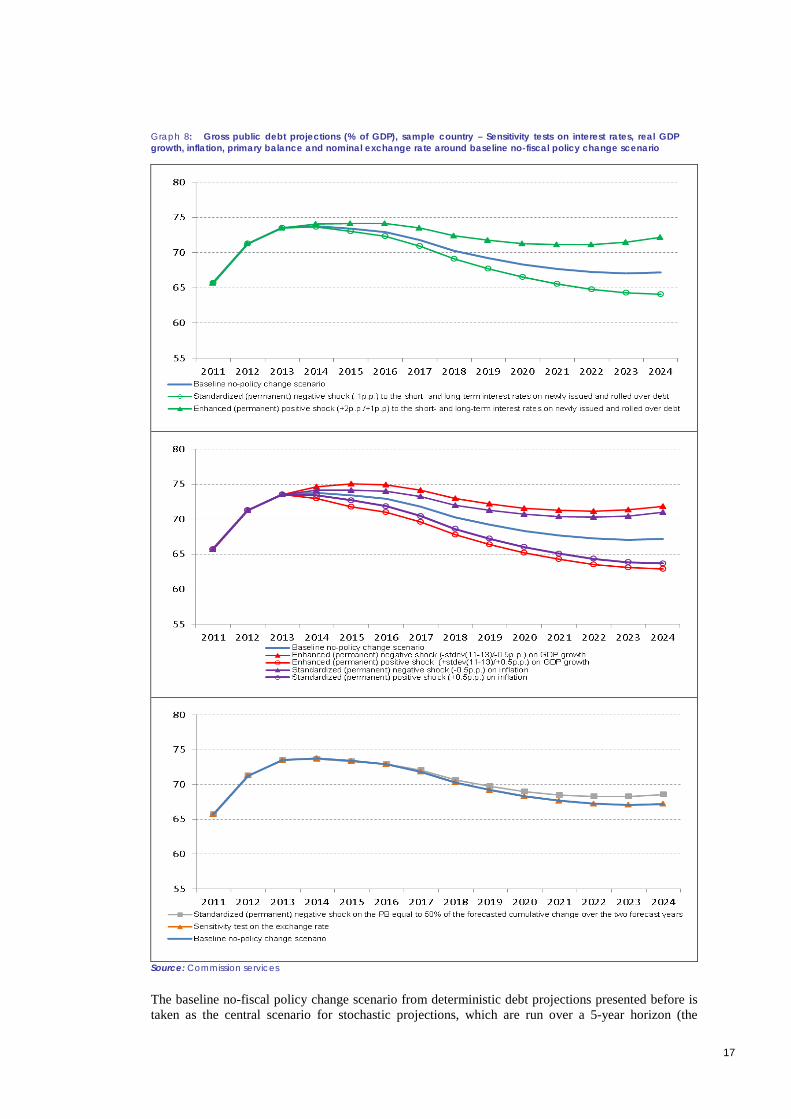
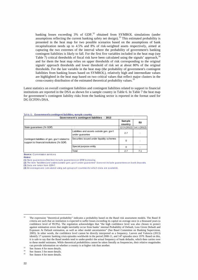
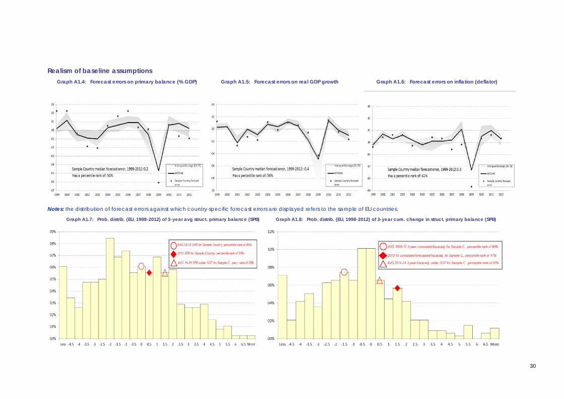
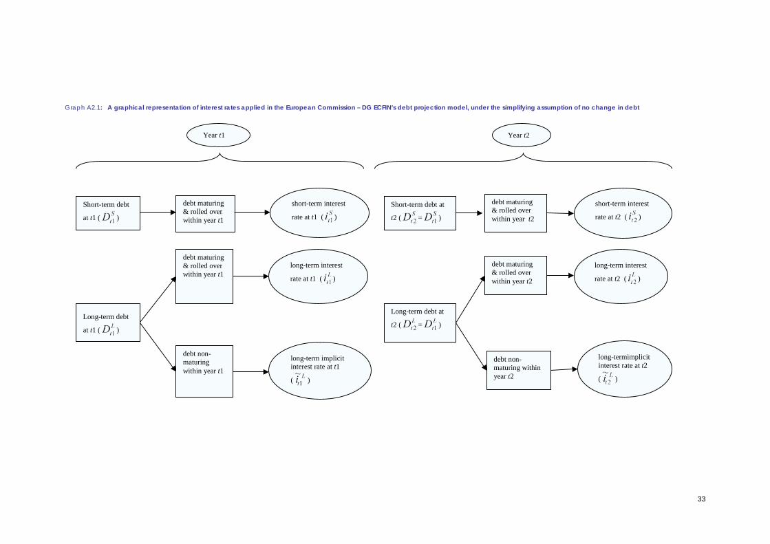

KC-AH-14-200-EN
-N