isostatic response of the australian lithosphere ... · pdf fileor zero thickness [turcotte...
TRANSCRIPT

JOURNAL OF GEOPHYSICAL RESEARCH, VOL. 105, NO. B8, PAGES 19,163-19,184, AUGUST 10, 2000
Isostatic response of the Australian lithosphere: Estimation of effective elastic thickness and anisotropy using multitaper spectral analysis
Frederik J. Simons, Maria T. Zuber, and Jun Korenaga Department of Earth, Atmospheric and Planetary Sciences, Massachusetts Institute of Technology, Cambridge
Abstract. Gravity and topography provide important insights regarding the degree and mechanisms of isostatic compensation. The azimuthally isotropic coherence function be- tween the Bouguer gravity anomaly and topography evolves from high to low for increasing wavenumber, a diagnostic that can be predicted for a variety of lithospheric loading models and used in inversions for flexural rigidity thereof. In this study we investigate the isostatic response of continental Australia. We consider the effects of directionally anisotropic plate strength on the coherel•ce. The anisotropic coherence function is calculated for regions of Australia that have distinctive geological and geophysical properties. The coherence estimation is performed by the Thomson multiple-Slepian-taper spectral analysis method extended to two-dimensional fields. Our analysis reveals the existence of flexural anisotropy in central Australia, indicative of a weaker N-S direction of lower Te. This observation is consistent with the suggestion that the parallel faults in that area act to make the lithosphere weaker in the direction perpendicular to them. It can. also be related to the N-S direction of maximum stress and possibly the presence of E-W running zones weakened due to differential sediment burial rates. We also demonstrate that the multitaper method has distinct advantages for computing the isotropic coherence function. The ability to make many independent estimates of the isostatic response that are minimally affected by spectral leakage results in a coherence that is more robust than with modified periodogram methods, particularly at low wavenumbers. Our analysis elucidates the reasons for discrepancies in previous estimates of effective elastic thickness Te of the Australian lithosphere. In isotropic inversions for Te, we obtain values that are as much as a factor of 2 less than those obtained in standard inversions of the periodogram coherence using Bouguer gravity and topography but greater than those obtained by inversions that utilize free-air rather than Bouguer gravity and ignore the presence of subsurface loads. However, owing to the low spectral power of the Australian topography, the uncertainty on any estimate of Te is substantial.
1. Introduction
1.1. Admittance and Coherence Calculations
Mountain belts are generally underlain by "roots" that are less dense than the surrounding mantle. In the most extreme, fully compensated case, they are in a state of near-Airy isostasy that corresponds to a lithosphere with no strength or zero thickness [Turcotte and Schubert, 1982]. In this case the free-air gravity anomaly is small and approaches zero for the longest wavelengths, and the Bouguer gravity anomaly is nonzero, reflecting the crustal root. Generally, the Bouguer anomaly is strongly correlated with the topog- raphy at long wavelengths. In other scenarios the litho- sphere has more rigidity or strength and can support topo- graphic loads without much of a compensating crustal root.
Copyright 2000 by the American Geophysical Union.
Paper number 2000JB900157. 0148-0227/00/2000JB900157509.00
For wholly uncompensated topography the free-air anomaly, not the Bouguer anomaly, will be correlated with topogra- phy [Lambeck, 1988; Fowler, 1990; Blakely, 1995]. In gen- eral, the correlation of the Bouguer anomaly to topography is wavelength-dependent. The wavelength range at which the transition from compensated to uncompensated topogra- phy occurs is diagnostic of the lithospheric rigidity. Thicker or more rigid lithospheres tend to undergo the transition from highly compensated to uncompensated topography at longer wavelengths than thinner or weaker lithospheres [e.g., Karner, 1982; Forsyth, 1985].
Admittance and coherence functions, spectral measures of the isostatic response of gravity to topography, can be used to invert for an effective elastic thickness Te or flex- ural rigidity D [Timoshenko and Woinowsky-Krieger, 1959], assuming surface and/or subsurface loading of an elastic plate overlying a fluid substrate. This has been done for both oceanic and continental plates in a variety of settings [e.g., McKenzie and Bowin, 1976; McNutt and Parker, 1978;
19,163

19,164 SIMONS ET AL.: ISOSTATIC RESPONSE OF AUSTRALIA
Forsyth, 1985; Zuber et al., 1989; McKenzie and Fairhead, 1997].
1.2. Surface and Subsurface Loading
Loading of the lithosphere may occur at the surface z = 0 or at some subsurface depth z = zm. For an elastic plate which is loaded at the top by the emplacement of topog- raphy, a density contrast at an interface located at z = Zc provides compensation for the applied load. It is generally assumed that subsurface loads are to be applied in the form of relief at the Moho discontinuity (a seismic discontinuity indicative of large density contrasts) and that surface loads are compensated by deflecting the Moho. In other words: Zrn -- Zc ---- Zmoho. An alternative approach is to find zc independently from the slope of the shortest-wavelength piecewise linear segment of the log gravity power spectrum [Karner and Watts, 1983; Bechtel et al., 1987; Zuber et al., 1989]. However, although the inferred loads are sensitive to the assumed densities and thicknesses of the layers, the flex- ural rigidity from coherence analysis is fairly insensitive to those assumptions [Forsyth, 1985; Lowry and Smith, 1994]. A simple two-interface model is therefore preferred by most authors [e.g., Ebinger and Hayward, 1996; Gwavava et al., 1996]. The amplitude of Moho relief is found from down- ward continuation of the Bouguer anomaly. If no subsur- face loading is allowed, however, the effective depth of com- pensation zc reenters the equation [McKenzie and Fairhead, 1997]. McKenzie and Fairhead [1997] determine zc as a free parameter by minimizing a penalty function of the ad- mittance of free-air gravity and topography which includes zc and the effective elastic thickness Te.
1.3. Statistical Independence of Top and Bottom Loading
One of the basic assumptions of the coherence method is that surface and subsurface loading are statistically indepen- dent. In many cases, however, surface and subsurface load- ing are likely to be tectonically related and therefore spa- tially correlated processes [Forsyth, 1985]. In general, as the degree of correlation increases, a downward bias in the esti- mated Te is observed [Macario et al., 1995]. The breakdown of the assumption of statistical independence was clearly ob- served by Zuber et al. [ 1989] in the case of central Australia. Correlated loads may reflect either a real (tectonic) relation- ship between surface and subsurface loading, or it may indi- cate that the uniform plate model was applied in an area of markedly nonuniform flexural rigidity [Zuber et al., 1989]. In addition, the presence of anisotropy in the loading re- sponse may explain the breakdown of the uniform isotropic coherence method and the associated poor fits of observed to modeled values [Stephenson and Lambeck, 1985]. Finally, erosion processes that reduce the amplitude of the topogra- phy at all wavelengths without changing the shape may be responsible for the coherence of subsurface with surface to- pography [McKenzie and Fairhead, 1997].
1.4. Erosion
Erosion may play an important role in modifying the gravity to topography relationships, predominantly at short wavelengths [Stephenson, 1984; Forsyth, 1985]. The re- moval of the topographic expression of subsurface loads leaves only the Bouguer gravity anomaly and reduces the co- herence with topography. The associated shift to longer tran- sitional wavelengths of the coherence biases the Te upward. To address this problem, McKenzie and Fairhead [ 1997] ad- vocate using the free-air rather than the Bouguer anomaly in admittance calculations, arguing that, whether or not subsur- face loads are present, surface topography must always be a load, and part of the free-air gravity anomaly must therefore always be coherent with topography. McKenzie and Fair- head [ 1997] find much lower values of elastic thickness than those obtained from inversions performed using the Bouguer anomaly in coherence calculations. In their analysis, they prefer values of f = 0 for the ratio of bottom to surface loading. As a result, their depth of compensation z• shifts to midcrustal values and the T• estimates are reduced until none exceed 25 km. The assumption of top loading alone biases toward lower values of T•.
1.5. Influence of the Spectral Estimation Technique
McKenzie and Fairhead [1997] advocate, with little ex- planation, the use of the multitaper spectral analysis method of Thomson [1982] rather than the traditional mirrored or windowed (in other words: modified) periodogram method of Bechtel et al. [1987] or the higher-resolution maximum entropy method developed by Lowry and Smith [1994]. In this paper, we provide formal justification of the merits of the multitaper method and focus on two particular issues: the nature of bias at long wavelengths and the role of an- isotropy in the loading response. To illustrate the technique, we analyze topography and Bouguer gravity data from conti- nental Australia, where we identify evidence for anisotropy and interpret it in terms of geologic setting. Allowing for both surface and subsurface loading, we obtain estimates of the effective elastic thickness that are intermediate between
the previous values of Zuber et al. [ 1989] and McKenzie and Fairhead [ 1997].
2. Coherence Studies of the Mechanical
Lithosphere
2.1. Transfer Function Approach: Linear Filter Theory
The correlation between the Bouguer gravity field and sur- face topography requires a rigorous definition. Dorman and Lewis [ 1970] related topography to gravity anomalies as
Ag(ro) - / h(r)q(r - to) dr 2 + n(ro). (1) Here Ag(ro) represents the (Bouguer) gravity anomaly at position ro due to topographic height h(r), E is the surface

SIMONS ET AL.: ISOSTATIC RESPONSE OF AUSTRALIA 19,165
of interest, and q(r) is the unknown kernel function that re- lates the gravity anomaly to the load that causes it [Phillips and Lainbeck, 1980; Karner, 1982; Lainbeck, 1988]. All through the paper, boldface letters will denote vectors of ar- bitrary dimension. In particular, k = (kx, ky) and [k[ = k. The system is characterized by "geologic" noise n(ro) that is not of isostatic origin and for which no further assump- tions are made other than that it is uncorrelated with topog- raphy. The latter assumption, stated in the wavenumber do- main as Snh (k) = 0, allows us to calculate the Fourier trans- form of the kernel as
ShAg(k) (2) ' where 5' represents the cross-spectral density of the two ran- dom variables identified by the subscripts (for an elabora- tion, see the Appendix). The function •(k) is the isostatic response or admittance function [Bendat and Piersol, 1986, 1993]. If the gravitational anomaly is in phase with the to- pography, •(k) is real.
We may renormalize the admittance by the power spectral density of the gravity anomaly and use the quantity
[$nzx9(k)l 2 .),2 (k) - Sa9zx9 (k)Shh (k) ; 0 _< 72 (k) _< 1, (3)
instead of (2). This function is referred to as the coherence [Bendat and Piersol, 1986, 1993].
2.2. Spectral Estimation of Stochastic Signals: Importance of Averaging
The quantitative study of isostasy requires an estimation of the (cross-)spectral properties of two random variables. For any of ]V proposed spectral estimators • to be an ideal estimator of the true spectrum S, we would have, in function of the wave vector k:
¾k' E{•(k)} - S(k), (4a) lim var{o6(k)} - 0, (4b)
¾k' •= k' cov{•(k'),•(k)} - 0. (4c)
Here E denotes an expectation or averaging operator, and var and cov stand for variance and covariance, respectively. Thus we require that the estimate be unbiased (equation (4a)), have well-behaved estimation variance (equation (4b)), and map all power at the appropriate frequencies without leakage (equation (4c)).
The periodogram, the squared magnitude of the Fourier coefficients of the signal, is a first-order spectral estimator [Tukey, 1967; Kay and Marple, 1981; Percival and Walden, 1993]. With the periodogram the coherence function is ap- proximated by [Bendat and Piersol, 1986, 1993; Touzi et al., 1996, 1999]
IE{F(k)G*(k)}[ 2 72(k)- E{G(k)G*(k)}E{F(k)F*(k)}' (5)
where F and G denote the Fourier transforms of the random
variables f and g (e.g., gravity and topography), and the as- terisk is used to denote complex conjugation.
Modifying the periodogram by mirroring or windowing the data set with a single window are both attempts to im- prove the estimation properties of the periodogram [Tukey, 1967; Welch, 1967; Percival and Walden, 1993]. The choice of the data window(s) primarily controls bias, while the smoothing or averaging operation reduces the estimation variance [see Chave et al., 1987, and the Appendix].
It is important to reflect upon the physical nature of the co- herence, and the role of averaging in its estimation. Indeed, without any averaging the numerator and denominator of (5) would be equal and the coherence exactly unity. By averag- ing over N different spectral estimates we are attempting to satisfy (4a), hoping that the estimate • (in the case of (5), this is the periodogram) is asymptotically unbiased in the sense
lim E{•(k)} - S(k). (6) N--•oo
The coherence function measures the consistency of the phase relationship between two fields, regardless of their amplitude. It is a measure of the variance of the phases associated with the individual terms whose expected values are obtained. For two fields that are uncorrelated at wave
vector kl, the phases of the various cross-spectral estimates over which one averages are randomly distributed. For the component o6(kl), averaging will then result in a cancella- tion, yielding 72(kl) -• 0. For signals that are correlated at k2, on the other hand, the interference of the phases will be constructive, and 72(k2) -• 1 upon averaging. Differ- ent representations or spectral estimates of the same process can be obtained by analyzing overlapping segments of the data, repeated measurements or, as we shall see, from data windowed with different orthogonal tapers.
Figure 1 illustrates the importance of averaging. In Fig- ure l a, two time series are given. Both have peaks in the power spectrum representing two distinct frequencies (Fig- ure lb). At one frequency the signals are exactly in phase, while at the other they are off by 7r/4. A value of 15 % white noise was added to both signals. If no averaging is done and the periodogram estimate of the cross-spectral density is di- vided by the individual spectral densities (as prescribed by (3) and (5)), the coherence equals unity over the entire range of frequencies (Figure l c, dashed line). Providing multiple representations of the same stochastic process by splitting the signals in overlapping, windowed segments, and averag- ing the numerator and denominator of (5) before the divi- sion (a modified periodogram procedure called Welch Over- lapping Segment Algorithm (WOSA) [Welch, 1967]), cor- rectly yields coherence peaks at both input frequencies (Fig- ure lc, shaded area). With the multitaper method averages are made over different windowed versions (described in de- tail in the Appendix) of the entire data set, and the coher- ence also peaks at both frequencies (Figure l c, open area).

19,166 SIMONS ET AL.' ISOSTATIC RESPONSE OF AUSTRALIA
•-"'• O. 8
ø0.6
.=0.4
0.2
0
0.03
1 20 40 60 80 1000.03 0.6 1
o
-20
;4o -:20 nø
-40
Time (is) Fr,
•/2 •
0 -•/2 •
0.6 1 0.03 0.6 1
Frequency f (Hz) Frequency f (Hz)
Figure 1. The importance of averaging in coherence estima- tion. (a) Top signal: 3 sin(3/50•rt) + 1 cos(6/5•rt). Bottom signal: 2sin(3/100trt) + 2cos(3/5•rt + •r/4); 15% white noise has been added to each. The phase relationship be- tween the two time series is consistent over the length of the sequence. (b) Power spectral density. (c) Coherence esti- mates. Disregarding the noise level, the coherence should peak at 1 for both 0.03 and 0.6 Hz input frequencies. Thick dashed line, periodogram estimate without averaging; thin solid line, shaded area, with Welch overlapping segment algorithm, windowing with cosine tapers; thick solid line, open area, multitaper estimate. The resolution bandwidth is 80 mHz. (d) Phase of the cross-spectral density for multi- taper (solid) and WOSA (dashed). Where the coherence is one, the correct phase difference between the components is retrieved (solid circles).
The broadness of the multitaper coherence peaks is due to the fixed bandwidth of the Slepian tapers (see Riedel and Sidorenko [1995] and the Appendix), which we set at 80 mHz for this example. Omitting further detail until later sec- tions, we note that the multitaper coherence estimate is much less noisy than WOSA [see also Bronez, 1992]. The phase angle of the cross-spectrum correctly gives the phase differ- ence between the two signals where the coherence equals unity. Both the Welch method (Figure ld, dashed line) and the multitaper method (Figure ld, solid line) pick out the in- put 0 and -7r/4 phase shift at 30 and 600 mHz, respectively (Figure 1 d, solid circles).
2.3. Different Ways to Average Spectral Estimates
In coherence analyses applied to determining effective elastic lithosphere thickness, three main approaches of av- eraging to get the necessary reduction in estimation variance of the coherence have been followed.
2.3.1. Bin averaging. Assuming second-order station- arity in the data [Welch, 1967; Kay and Marple, 1981; Ben- dat and Piersol, 1986], the time series may be subdivided into overlapping segments, each of which is detrended and windowed and then Fourier transformed (such as the calcu- lation that produced the thin solid gray filled line in Fig- ure lc). The overlap of the data sequences assures that the down-weighted portions of sequence N - 1 receive more weight in sequence N, so that a minimum of statistical in- formation is discarded. However, section averaging is in- appropriate for short signals. Also, the overlap between the sections needs to be sufficient to yield high efficiency, yet ensure approximate independence of the raw spectra [Chave et al., 1987]. Finally, because the highest resolvable wavelength is the inverse of the fundamental (Rayleigh) fre- quency 1/(NAt) [Kay and Marple, 1981] with N the data length and At the sampling interval, reducing N compro- mises long-wavelength resolution. For applications of bin averaging to lithospheric studies, see, for example, McKen- zie and Bowin [ 1976].
2.3.2. Ensemble averaging. If different sample func- tions are available (e.g., gravity and topography data ac- quired as multiple passes over the same geologic feature), each of them can provide an independent spectral estimate. The assumption of ergodicity guarantees that all the en- sembles are realizations of the same random process [Kay and Marple, 1981; Bendat and Piersol, 1986]. Lithospheric studies utilizing this principle are, for example, those by Watts [1978] and Detrick and Watts [1979].
2.3.3. Smoothing in wave vector space. Averaging be- comes more problematic in the two-dimensional case, as there can be only one data set for a given region, and the region itself is hard to subdivide. Usually, a single spectral estimate is calculated on a mirrored or windowed data set, but in the latter case the information contained in the down-
weighted edges of the data window is partially lost, while in the former spurious power is introduced at (long) wave- lengths not present in the data. The spectrum can then be estimated as a moving average of the unsmoothed estimator [Stephenson and Beaumont, 1980], or the original estimate can be binned into annuli of wavenumber bands [Bechtel et al., 1987]. Moving averaging can badly bias the spectrum if the phase changes over the averaging band [Park et al., 1987b; Kuo et al., 1990; Mellors et al., 1998]. Moreover, with wavenumber binning the long-wavelength part of the spectrum will be based on fewer data points than are the higher frequencies. This leads to a positive long wavelength bias for the coherence [Munk and Cartwright, 1966]. And finally, if the variation of the coherence with direction is of interest to us we cannot average azimuthally.
3. Multitaper Method for Two-Dimensional Spectral Analysis
The multitaper technique, as originally proposed by Thom- son [1982], reduces the estimation variance of the spec- trum by calculating o o as a weighted average over a number

SIMONS ET AL.' ISOSTATIC RESPONSE OF AUSTRALIA 19,167
,, ,, ,. ,...
0 0.5 1 0 5 10
Normalized data le,ngth i
.•, i
0.9
I c I I I i
2 4 6 8
Taper number Normalized data length
Duration x frequency
t:'"' : ': , ;..•...,.• ½:% ,+,',•,•,.,.•o, ,•..•. _• 4' '•,..•' •"'"% •'"•,,•" '. • •' '•.
-o
- -20
--40 m
- -60 .• o
-80
-lOO
1
0.6 >•
0.4? 0.2 •
Figure 2. Properties of the dpss. (a) Data tapers ht,k for NW - 4 and k - 1, ..., 5 with normalized height and as a fraction of the data length N. (b) Spectral windows •k (f) belonging to the tapers to the left. The sidelobe level, and hence the bias in the spectral estimation, of the higher order windows increases with order k. (c) Eigenvalues A• associated with the eigentapers. (d) Buildup of dpss taper
K h2 for K - 1 8. Using only one taper, much information is lost. With an energy defined as •=• t,• ,..., increasingly complete set of eigentapers, the information is extracted evenly from all samples.
k of independent direct spectral estimates •t with weights At. The eigenspectra o6t that satisfy (4a) are based on the data windowed by a function hi(r) to be determined. If all •t, l - 1, ..., k are pairwise uncorrelated with a com- mon variance, then the variance associated with the average estimate will be smaller by 1/k [Bronez, 1992; Riedel and Sidorenko, 1995], meeting the objective of (4b). To mini- mize spectral leakage in the sense of (4c), we need to find data windows hi(r) whose spectral responses •t(k) (see (A4)) have the narrowest central lobe and the smallest pos- sible sidelobe level (this is expressed as an energy concen- tration criterion). Slepian [1978] found that the ideal data windows hi(r) are given by discrete prolate spheroidal se- quences (dpss). The width of the central lobe of •t(k) is a measure of the resolution of the estimates (see (A3) and (A6)) and is defined at the discretion of the analyst. The half width W is usually an integer multiple j of the fundamental frequency: W = j/(NAt); commonly, j is quoted as NW (assuming At = 1). For every such choice of resolution bandwidth, there are k = 2NW useful tapers; this number is known as the Shannon number in information theory. The dpss are the solutions to an eigenvalue problem (see the Ap- pendix), and therefore the windows ht (r) are orthogonal and the resulting eigenspectra •t (approximately) uncorrelated. The associated eigenvalues At can be used as weights. The Slepian tapers minimize a particular concentration criterion (see (A8) and (A9)). Other criteria can be used and different
sets of orthogonal tapers may be found that have similar per- formance as the Slepian tapers [Riedel and Sidorenko, 1995; Walden et al., 1998; Komm et al., 1999]. Throughout this pa- per, however, we will call the multiple-taper method which uses Slepian windows "the" multitaper method.
The properties of a set of one-dimensional Slepian tapers are summarized in Figure 2. In Figure 2a the first five ta- pers of a sequence with NW - 4 are given. We assume At -- 1 and nondimensionalize the frequency axis by plot- ting N f, i.e. duration times frequency, so the central lobe is confined within [-NW, +NW] (Figure 2b, dashed vertical line at Nf = 4). The first spectral window assures over 100 dB of bias protection outside the inner domain of NW = 4 [see also Chave et al., 1987]. As the order of the tapers in- creases they become more and more oscillatory. Their cen- tral resolution peak broadens and splits and the level of side- lobes increases. For NW = 4, the Shannon number 2NW indicates the order beyond which the eigenvalues A• drop steeply to zero (Figure 2c). Conventionally, only the first 2NW - 1 eigentapers are used. Most popular data win- dows in nonmultitaper applications are fairly similar to the zeroth-order multitaper window. The disadvantage of having only one data window is that valuable statistical informa- tion is discarded, by virtue only of being on the edge of the data. Any information that is lost in this way is retrieved by the higher-order multitaper windows [Walden, 1990; Komm et al., 1999]. An increasingly complete set of eigentapers

19,168 SIMONS ET AL.' ISOSTATIC RESPONSE OF AUSTRALIA
1 x 1 1 x2 1 x3
2xl 2x2 2x3
3xl 3x2 3x3
Figure 3. A subset of the two-dimensional tapers used in the analysis, formed by taking the outer product of any two combinations k x k' (indicated in the legend) of the 1-D tapers ht,k of Figure 2.
extracts information more and more evenly from the entire signal, without this arbitrary down-weighting, as shown in Figure 2d.
Originally formulated for one-dimensional (l-D) time se- ries, the extension to two-dimensional fields is readily made [Liu and van Veen, 1992; Hanssen, 1997]. The additivity of the Fourier transform allows us to calculate the 2-D trans-
form by applying the algorithm to the rows of the data matrix first, tapered with one taper, and then performing the trans- form on the columns of the result, tapered with a different taper. This is equivalent to tapering the data with 2-D tapers given by the outer (dyadic) product of combinations of 1-D tapers. A subset of the 2-D tapers that we used is given in Figure 3. The weights of the combination of two such tapers have to be given by the product of their individual eigenval- ues [Hanssen, 1997]. In this way, using k different tapers in r• dimensions, K = k '• independent sets of windowed data are obtained. The spectral estimation variance can be calculated explicitly using (A 15).
The spectral windows 7-((k) associated with the tapers of Figure 3 are plotted as contour lines in Figure 4. As in Fig- ure 2b, the axis plots duration times frequency, which illus- trates the effect of the resolution parameter NW. For the chosen set of tapers, NW = 4 and hence the central lobe is concentrated within the bounds of -4 to +4 (Figure 4, dash- dotted lines). We are looking from above onto the (kx, plane; hence a horizontal or vertical section through these plots would be identical to the spectral windows plotted in Figure 2b. As in the 1-D case, with increasing order of the tapers the sidelobe level increases and hence the resolution decays. However, incorporating many independent tapers into the spectral estimation reduces the estimation variance. Resolution and variance trade off.
4. Tests With Synthetic Data 4.1. Motivation
The use of the multitaper method for determining admit- tance and coherence functions in Te studies is not a nov-
elty. Scheirer et al. [1995] reported its usefulness for the estimation of the elastic thickness of the Basin and Range province, and McKenzie and Fairhead [1997] present it as their method of choice. We believe that an application of this method should be accompanied by a rigorous theoretical dis- cussion of its merits, as well as a thorough testing on realistic synthetic data sets. The remaining part of the discussion of Te can then be devoted to the different assumptions involved in calculating the forward models, most notably the role of subsurface loading (see also section 1.2). New to the topic of elastic thickness estimation, however, is the realization
that only the multitaper method is able to produce reliable 2-D 3, 2 (k) estimates, such that anisotropy in the loading re- sponse can be investigated without resorting to smoothing or binning procedures in wave vector space, procedures which, as we have argued in section 2.3.3, are inherently flawed.
4.2. Data Generation
As this is, to our knowledge, the first time the two-dimen- sional extension of the multitaper method is used in order to detect anisotropic power in the coherence, our approach needs to be tested with synthetic data sets. Besides, even in
4 -• ø • ....
-4 I ••• l -10 •
10
4
o
-4
-10
lxl
I I . .
I ' ' I
2xl ' I ' I '
4 ' '
0 O'
-4 I ' '1
-10
-10-4 0 4 10
3xl
lx2 lx3
2x2
o'oo_ o0_•5• •
-10-4 0 4 10
3x2
' I . '
2x3
.....
-10-4 0 4 10
3x3
Figure 4. Spectral windows 7-(k(k) (see (A4)) associated with the tapers of Figure 3, plotted as functions of the dura- tion x half bandwidth product. NW - 4. Contouring is at -105,-75,-45, and-15 dB.

SIMONS ET AL.' ISOSTATIC RESPONSE OF AUSTRALIA 19,169
1
•,o.8
.•OA co 0.2
0
0
-30 + ß
o • I i" •'¾'k•. •..,...•.• ..... N W= 2.5
-01 0 • -120
• I rW,,•,. ' + .... ] • ++,
+• '++ •/4 •/2 • 0 •/4 •/2 3•/4
Wave,umber k Wave,umber k
Figure 5. Influence of resolution bandwidth NW upon synthetic data with isotropic coherence. Fre- quency space is nonphysical, hence contained within angular frequency between 0 and +7r. (a) Isotropic input coherence (pluses). In shaded symbols, multitaper estimates for NW values of 2, 2.5, 3, 3.5, and 4. NW = 4 is the value we adopt in the subsequent analyses. The a: scale is logarithmic. (b) Spectral windows 7•(f) (see (A7)), offset for clarity. With increasing NW, the resolution degrades (the central peak broadens) but is still acceptable compared to the input coherence (pluses, scaled to fit the figure). The a: scale is linear.
the isotropic or 1-D case some thought must be given to the selection of the resolution parameter NW.
As indicated in section 2.2, the coherence function is a
measure of the consistency of the phase relationship between individual measurements of a particular Fourier component, independent of its magnitude. This suggests a way of syn- thesizing two fields with a known coherence [Lowry and Smith, 1994]. Suppose we are able to get one direct cross- spectral density estimate •fg between two fields f and g at a particular wave vector k l. As f and g are not neces- sarily in phase at k•, this is in general a complex number, represented as r exp i•. In order to obtain a stable estimate of the cross-spectral density of both stochastic random vari- ables we need to perform such a measurement a number k times and average the results. If both fields are highly cor- related, the 1 = 1, ..., k individual terms will have the form r expi(• + A•t), where for every 1, A•t << •. Hence the average for this component adds up to a nonzero complex number, and, normalized, 72 -• 1. If, on the other hand, every measurement yields a widely varying phase vector so that A•t = O(•), the average will have a magnitude that is near zero, and 72 -• 0. Taking the Fourier representation of some field H(k) and creating a second field H(k) + N(k) using some function 72 (k), as described by
IN(k)l 2 - iS(k)l 2 _ r2(k) , (7)
the coherence between H(k) and H(k) + N(k) is given by 72(k). Thus to make 72 -• 0 at a certain wave vector, we add "noise" with a magnitude comparable to the Fourier component at the same wave vector but a random distribu- tion of phases. To make 72 -• 1 we simply add random- phase noise with much less amplitude. Any field H(k) can
be taken as the start of this procedure, although it is desir- able that its power spectrum have some resemblance to the actual data in the gravity-topography analysis (e.g., having a red spectrum).
4.3. Tests With Synthetic (An)isotropic Coherence
Synthetic tests are presented in Figure 5 and Plate 1. In the tests the wavenumber ranges from -7r to +7r, the Nyquist wavenumbers +kN for sampling intervals of unit step, At -- 1' kN -- 27rf•v; f•v -- 1/(2At). Where indicated, the scale is in decibels (dB). Because of symmetry we will plot the results for k - 0 -• 7r.
Figure 5 depicts the results of a first test. The input co- herence function (pluses), given in Figure 5a, is isotropic, so ,2 (k) - ,2 (Ikl). The multitaper estimates are compared to the input for values of the resolution parameter NW vary- ing from 2 to 4 in 0.5 increments. As NW approaches 4, the final value, the estimate follows the synthetic curve more closely. The positive bias at high wavenumbers decreases monotonically with higher NW. This test enables us to identify an acceptable resolution parameter NW. Our final choice is NW - 4. All the following analyses presented in this paper have used NW - 4 and k - 7 so at all times the resolution half bandwidth is given by W - 4/(NAt) with N the total data length and At the sampling interval. We have repeated our measurements with different values of NW. We will report this in section 6.2.3.
For the set of tapers used, Figure 5b gives the average - k
spectral windows, 7/ - •t=l 7/t(k) (see (A6)) for the dif- ferent values of NW and k - 2NW - 1. The half width of
_
the central lobe 7/gives the resolution of the coherence es- timate. So, for N - 100 and At -- 1, the wavenumber res- olution 2kw - 27r2W - 27rj/N, where j - 2,2.5,...,4,

19,170 SIMONS ET AL.: ISOSTATIC RESPONSE OF AUSTRALIA
of the different curves is 2/507r, 2.5/507r,3/507r, 3.5/507r, and
4/507r. For clarity, we have offset the different spectral win- dows in the •j direction and plotted the synthetic coherence function used in Figure 5a on top of them on the same linear x scale but scaled to fit the plot box in the •j direction.
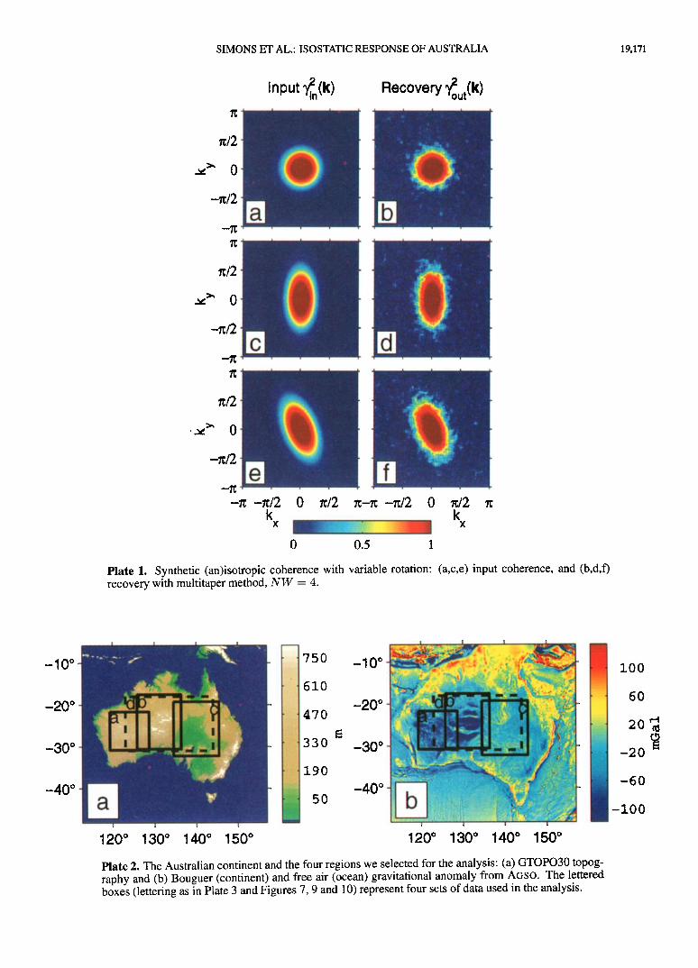
In Plate 1 we test the ability of the 2-D multitaper method to correctly resolve isotropic and anisotropic input coher- ences, the latter with varying orientation. Based on Plates l a and lb, we conclude that we will not unnecessarily re- ject the hypothesis of isotropy should we measure the co- herence function between actual data. If the input is isotro- pic, then the measurements reveal nothing to the contrary. In Plates lc-lf, anisotropic input fields are analyzed. The input is found in Plates l c and l e, whereas the multitaper measurements are found in Plates ld and l f. From this test
we deduce the ability of our implementation of the multita- per method to infer anisotropy in the coherence function and detect its major axis.
4.4. Other Methods to Compute 2-D Coherence
Stephenson and Beaumont [1980] were the first to con- sider the possibility of directional anisotropy in the loading response of continental lithosphere (the Canadian Shield). Later, Stephenson and Lambeck [1985] investigated the an- isotropy of central Australia. More recently, Lowry and Smith [1995] give examples of anisotropic Te for North America. The methods used in the above studies are sim-
ilar in that one representation of the data is used, only mir- rored, windowed or extended with a maximum-entropy cri- terion. The result is a 2-D coherence map that is nowhere near the true coherence spectrum: only after an averaging procedure is applied does this estimate approach the true coherence. We have verified that it is possible to obtain a certain form of stability by smoothing in wave vector space [as in Stephenson and Beaumont, 1980], averaging over an azimuthal wedge around a certain direction of interest [as in Stephenson and Lambeck, 1985], or performing binning over overlapping azimuthal wedges [the procedure used by Lowry and Smith, 1995] (A. R. Lowry, personal communi- cation, 1999). All of these methods are ad hoc and the bias and instabilities present in the modified periodogram method are amplified by virtue of taking even fewer samples in the azimuthal averaging. It is in this light that we present the 2-D multitaper estimate as the only unbiased 2-D coherence estimate. At every wave vector, the coherence estimate is based upon the average of multiple orthogonal representa- tions of the data, and its error is therefore not dependent on the position in wave vector space.
4.5. Comparison With Maximum Entropy Spectral Analysis
An alternative method of coherence estimation is Max-
imum Entropy Spectral Estimation (MESA) [Burg, 1975]. Lowry and Smith [1994] show the superior performance of MESA with respect to the periodogram method especially when the box size is small. Our tests compare favorably to the maximum entropy results shown by Lowry and Smith
[ 1994]. Other authors have confirmed the multitaper perfor- mance with respect to MESA [e.g., Lees and Park, 1995]. The original maximum entropy approach of estimating spec- tra is a parametric method which assumes autoregressive sig- nals [Percival and WaMen, 1993]. Following Burg [1975], maximum entropy spectral analysis is based on choosing the spectrum which corresponds to the most random or the most unpredictable time series whose autocorrelation func- tion agrees with the known values. However, many differ- ent spectral density functions can have the same autoco- variance sequence up to a certain lag. Hence, in general, maximum entropy spectra tend to represent noise processes poorly [Kay and Marple, 1981; Malik and Lim, 1982; Perci- val and Walden, 1993].
The multitaper method is nonparametric. Tapering re- places the spectral windows of traditional (windowed) peri- odogram estimates with a unique and optimal set of windows that have better sidelobe properties. The amount of bias and leakage is exactly assessable [Bronez, 1992; Riedel and Sidorenko, 1995] in a nonsubjective way (from the shape of the spectral windows in Figures 2b, 4, and 5b), and given the multiplicity of the windows, the confidence intervals around the spectrum can be reduced dramatically compared to any other method.
5. Application to the Study of Australia 5.1. Makeup of the Australian Continent
Using various geophysical and geological criteria, Aus- tralia can be divided into three major structural units [Veev- ers, 1984; Drummond, 1991; Braun et al., 1998; Wellman, 1998; Simons et al., 1999b]. At this scale the three domains represent the dominant age provinces as well. For a tectonic map, see Figure 6.
5.1.1. Archean. The westernmost part, composed of Archean cratons (the Pilbara and Yilgarn cratons formed about 3500 and 3100 Ma ago), is geologically stable. It is characterized by high Moho depths (in places exceeding 50 km) [Wellman, 1979; Shibutani et al., 1996; Clitheroe et al., 2000] and low heat flow values (,-•40-50 mW m -2) [Cull and Denham, 1979; Cull, 1991 ]. The highest effective elas- tic thicknesses on the continent have previously been mea- sured there (Te - 130 km) [Zuber et al., 1989].
5.1.2. Proterozoic. Central Australia is made up of a structurally complex, heavily faulted Proterozoic block-and- basin structure. The extensive faulting has resulted in ex- treme Moho offsets with amplitude variations of more than 20 km [Lambeck, 1983; Lambeck and Penney, 1984; Lam- beck et al., 1988; Goleby et al., 1989; McQueen and Lam- beck, 1996]. Elastic thickness measurements have yielded values around T• - 90 km [Zuber et al., 1989]. Anisotropy in the isostatic response has been suggested [Stephenson and Lambeck, 1985].
5.1.3. Phanerozoic. Terranes to the east of the Tasman
Line [Murray et al., 1989] (roughly the easternmost third of the continent) are Phanerozoic in age. The easternmost rim of the continent is marked by a mountainous range which is
SIMONS ET AL.' ISOSTATIC RESPONSE OF AUSTRALIA 19,171
Input •in(k) Recovery •ut(k)
nt2
-n/2
-n/2
re/2
-n/2
-•: -•z!2 0 nt2 •z-n -•c12 0 nt2 k k
x x
o 0.5 1
Plate 1. Synthetic (an)isotropic coherence with variable rotation' (a,c,e) input coherence, and (b,d,f) recovery with multitaper method, NW - 4.
_10 ø
_20 ø
i i i ...... - ..
_30 ø I _ I
-40 ø
610
470
330
190
I
I •
120 ø 130 ø 140 ø 150 ø 120 ø 130 ø 140 ø 150 ø
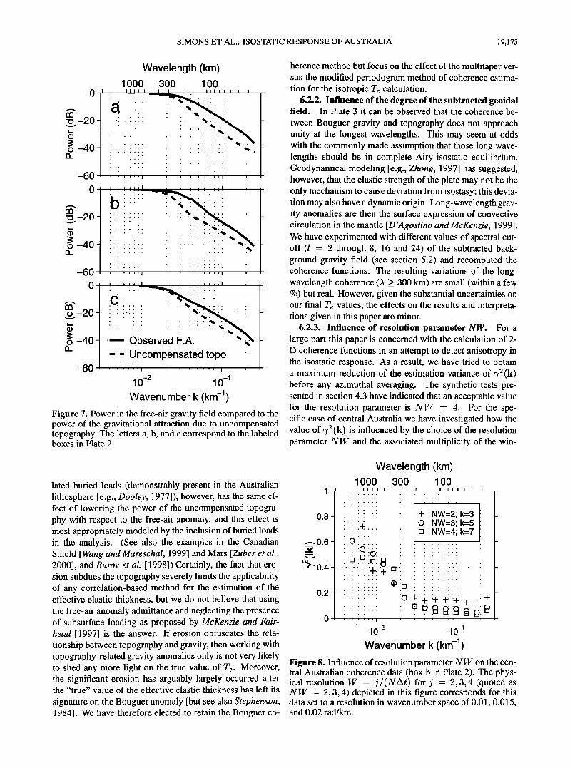
Plate 2. The Australian continent and the four regions we selected for the analysis: (a) GTOPO30 topog- raphy and (b) Bouguer (continent) and free air (ocean) gravitational anomaly from AGSO. The lettered boxes (lettering as in Plate 3 and Figures 7, 9 and 10) represent four sets of data used in the analysis.
lOO
6o
20.•
-20
-60
-lOO

19,172 SIMONS ET AL.: ISOSTATIC RESPONSE OF AUSTRALIA
Kimberley
King Leopold
Pine
Halls Creek
McArthur
Victoria River
Coen
Georgetown
Pilbara
Capricorn
Gawler
Albany-Fraser Kimban
ß :':' ::-: '- -"• Proterozoic Basin
[•- •'"• Archaean Craton I I 000 km 1
Figure 6. Tectonic map of Australia [from Myers et al., 1996].
in close to local isostatic equilibrium [Murray et al., 1989], volcanism as recent as 10 Ma, high heat flow (,-•70-100 mW m -2) [Cull and Denham, 1979; Cull, 1991] and low man- tle conductivity values [Lilley et al., 1981; Finlayson, 1982]. Shear wave speeds from seismic tomography measurements are anomalously low [Zielhuis and van der Hilst, 1996; Si- mons et al., 1999b]: there is a pronounced low-velocity anomaly starting at about 80 km. The available Te mea-
broad average of the continent (box d in Plate 2). To provide continuity with the earlie]" work by Zuber et al. [1989], we apply their mirrored periodogram method of spectral analy- sis alongside with the multitaper method to calculate an iso- tropic Te. Any discrepancy of our results with those from Zuber et al. [ 1989] is due to the coherence measurement it- self. In the discussion we will focus on the assumptions of the modeling, which account for the discrepancies between
surements were among the lowest of the continent: 30-80 the present work and the study by McKenzie and Fairhead km for the Phanerozoic Interior Lowlands and 15-35 km for [ 1997]. the Eastern Highlands [Zuber et al., 1989]. They have been interpreted in relation to the short time period since the last
5.2. Gravity and Topography Data major thermal event and the deep extent of low mantle con- ductivity values [see also Gough, 1974; Karner et al., 1983; Gravity data were obtained from the Australian Geolog- Bechtel, 1989; Mareschal et al., 1995]: the low rigidity and ical Survey Organisation (AGSO; see Plate 2b), which cal- subsurface loading in southeastern Australia are consistent culated Bouguer anomalies with a density of 2670 kg m -a. with crustal underplating, igneous intrusion and thermal per- No terrain correction was applied. According to AGSO the turbation of the upper mantle as mechanisms for the uplift data precision is of the order of 0.1 mGal (1 mGal = 10 -s and compensation of the highlands [Zuber et al., 1989]. m s-2), but no detailed statistics are available. It is to be
It is the aim of this paper to include another complicating expected that this uncertainty increases with the wavelength factor into the study of T•: its anisotropy. We choose three of the anomaly. At longer wavelengths the gravity field er- regions of Australia (see the boxes labeled a through c in ror from geoidal coefficients obtained from satellite track- Plate 2) that approximately correspond to the threefold char- ing is +0.5 mGal on the best-determined parts of the globe acterization described above, and investigate the presence of [Lemoine et al., 1998]. Anisotropy in the data distribution isostatic anisotropy. A fourth region attempts to capture a was not a concern at the wavelengths that we consider.

SIMONS ET AL.: ISOSTATIC RESPONSE OF AUSTRALIA 19,173
0 0.1 0.2 0.3 0.4 0.5 0.15 '
0.1
O.O5
•>' 0
-0.05
0.15
0.1
0.05
•>' 0
-0.05
0.15
0.1
0.05
,,' 0
-0.05
0.15
0.1
0.O5
',- 0
-0.O5
-o. 1 o o. 1 k
x
Wavelength (kin) 1000 300 100
1
0.2 "i"i' . ,i•';;:•,'!'.• !'!'!'!!! ..... !"' o '!,,i:. ' ! ::.:i ' ':
0.2
0
• ; • ;;;! ! , ; : : : ::• ,
•'0.6- %.-O.4
ß , , : ß ; : ; ::::
0.2 ' '.. ,? .........................
0 '
i , , , , • ,.,i , ..............
I ,.. ß ....... ... ....... . .........
0.8- "!'i' ":": ..... '-"":":":'•':'::': .......... '"'0.6 ''" ' :' ' : : :::::: ,.• ,• ,:'t ........
%0.4-'-:-. !'?!!i' '-' ,, '!"i"i'!'i'i'i'? .......... ...............
0.2- : :::::: : •. :.::..:: 0-.: ;:::::-."'- .' : - - - ß
, , t , t • ,, ,, t . ß i • ,•j .....
10 -2 10 -1 Wavenumber k (km -•)
Plate 3. Coherence measurement of four regions of Australia. The letters a through d correspond to the labeled boxes in Plate 2. (left) Multitaper 2-D coherence used as an indication of anisotropy in the isostatic response. We interpret the shape of the 2-D coherence of central Australia (Plate 3b) as a direction of N-S weakness of the plate. (right) Azimuthally averaged multitaper (blue squares) and periodogram coherence (red circles). Confidence intervals are plotted at 2or. See sections 6.2.2 and 6.2.3 for a discussion on the low coherence values at low wave numbers.

19,174 SIMONS ET AL.: ISOSTATIC RESPONSE OF AUSTRALIA
Topography data (see Plate 2a) were taken from a 30 arc sec (,-• 1 km) digital elevation model, GTOPO30 [Gesch et al., 1999]. The uncertainty for the Australian region is about 4-60 m.
Both data sets were resampled at the same rate and pro- jected onto a Cartesian grid. Prior to analyzing the data, a background gravity field obtained from a spherical harmonic expansion of satellite-derived geoidal coefficients [Lemoine et al., 1998] was removed. We tapered the spherical har- monic spectrum of this background field with a cosine func- tion which took a value of 1 at degree 1 = 7 (,X ,,• 5300 km) to 0 at 1 = 11 (A ,,• 3500 km) (the degree-to-wavelength conversion is described by Jeans [1923] [see also Brune, 1964]). In this way, we attempted to filter out the gravita-
The error bars plotted correspond to 4-2A3,2' (k). The variance of the coherence estimate 3,2(k) obtained
with the multitaper method is calculated using (A15). The waveband-averaged,./2 (Ikl) has this variance, normalized by the number of points in the annulus, n(k). The error bars plotted are twice the standard deviation.
West and east Australia (Plates 3a and 3c) show little or no indication of anisotropic isostatic response. In contrast, the central Australian domain (Plate 3b) is characterized by a north-south direction where the coherence is higher than the azimuthal average. This feature extends over most of the wavenumber band. It is certainly more prominent than the slightly higher coherences in the E-W direction which become visible in the high-frequency range only. In section
tional contribution from large-scale mantle processes [Dickey 7.2 we will interpret this feature in terms of anisotropy in et al., 1998] (such as subducted slabs, whose gravity sig- nature correlates well with the geoid up to about 1 = 9 [Hager, 1984]), while avoiding Gibbs phenomena [Sandwell and Renkin, 1988]. In the past, various authors have sub- tracted background gravity fields with different degree cut- offs:/ = 16 [McNutt and Parker, 1978], 1 = 22 [Stephen- son and Beaumont, 1980], or not at all [Zuber et al., 1989; McKenzie and Fairhead, 1997]. We defer the discussion of the influence different choices of cutoff 1 have on the coher-
ence to section 6.2.2. Finally, before Fourier transformation, a best fitting plane trend was removed from the data.
6. Results
6.1. Anisotropy in the Isostatic Response
lithospheric strength. For region d, the N-S anisotropy is the most prominent feature, suggesting that it is an important factor in the isostatic response of the continent as a whole.
Consistency tests with randomly rotated data sets have shown no indication that any of the interpreted features is an artifact.
The following points can be made. (1) With the peri- odogram method and the bias correction of (8), the coher- ence values at long wavelengths can become negative. This occurs for low coherence values in the center of the spectral calculation, when the annuli-averaging method has at most tens of samples. A negative coherence is physically impos- sible and biases the solution as an inversion is performed. (2) Even after the bias correction of (8), the coherence is still biased toward higher values at the longer wavelengths.
In Plates 3a-3c, the results for each of the three geophys- Again, a lack of terms in the averaging procedure is respon- ically distinct regions (labeled a through c in Plate 2) are sible for biasing the coherence toward 1. (3)The uncertain- summarized. Plate 3d analyzes the data box d marked by ties of the estimate increase dramatically with wavelength as a dashed line in Plate 2; it represents a broad average of the number n(k) decreases (see (9)). (4) We notice that the the response of the entire continent. In the left column the wavelengths at which the transition between high and low two-dimensional, wave vector-dependent coherence func- coherence occurs are longer for the periodogram method. tion 3`2(k) calculated with the two-dimensional multitaper As a result, the elastic thicknesses of the Australian conti- method is given. On the right-hand side a comparison is nent given by Zuber et al. [1989] are likely to have been made between the azimuthal average of the multitaper co- overestimated (see section 6.2.7). herence, -r2(Ikl) (blue squares) and the isotropic mirrored
6.2. Isotropic Elastic Thickness Inversions periodogram method of Zuber et al. [ 1989] (red circles). The periodogram method is standard and was applied to 6.2.1. Power of uncompensated topography. McKen-
the data after mirroring. No window was applied. The zie and Fairhead [1997] discuss the importance of com- quoted coherence values of the periodogram method have paring the spectral power present in the free-air gravita- had a bias correction applied to them as follows [Munk and tional anomaly with the power of the gravity anomaly due Cartwright, 1966]: to the attraction of surface topography obtained by multi-
,./2' (k) - n(k)3`2(k) - I (8) n(k) - I
The unprimed coherences refer to the those calculated be- fore the bias correction, and n(k) is the number of points in
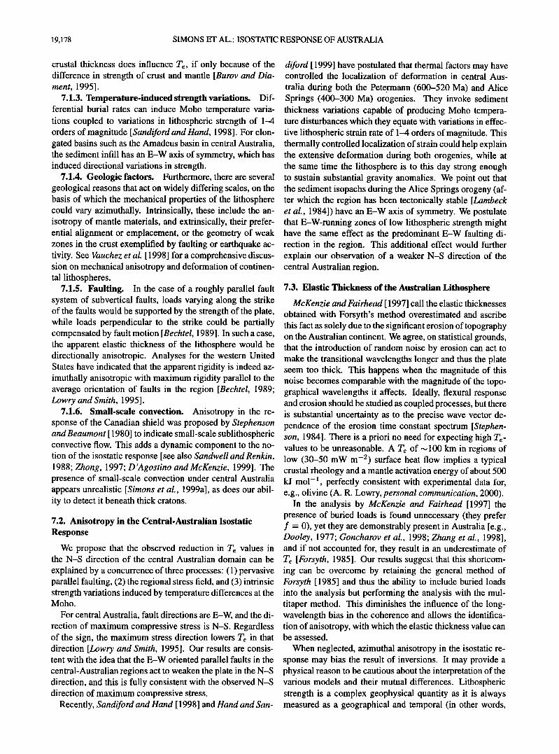
plying the elevation in meters by 2•rpG=0.11194 to give gravity anomalies in milligals (mGal). Figure 7 shows that the power due to uncompensated topography is everywhere lower than that of the free-air anomaly. Erosional processes diminish the power of topography [Stephenson, 1984] and this limits the use of the Bouguer coherence method of the wavenumber band. The standard error of the unbiased
coherence ,./2' is calculated from [Bendat and Piersol, 1986, Forsyth [ 1985]. In general, erosion can be treated as a noise 1993] process which randomizes the phase relationship between
topography and gravity, and as such it annihilates the coher-
23`2(k) ence. If this happens at the shorter wavelengths, the transi- A3`2'(k) - (1 - 3`2(k)) v •i• ' (9) tional wavelength is shifted to longer wavelengths, and the Te estimates are biased upward. The presence of uncorre-
SIMONS ET AL.' ISOSTATIC RESPONSE OF AUSTRALIA 19,175
Wavelength (km) 1000 300 100
I II I I I I I I II I I I I I I .............. ß
•,•-20- i i i iii' -
o-40- :":':':::' ' ß ::::':: ß '•" -
ß
"• -20 - -':'-:--:-:-:;; .... :---:-•-,,;--: '. ';: ......... • : :::::: : : : :::•.:• : g _ o -40- - -!- -!- -!-i'
ß
......
-60 ...... , ........ , . I 0
"•-20--':--:-:-:-:;:- ..... i'"i"i'i":"':': ...... •" - • ' '"øb e FA. ' .... '....- o-4O-.- serv d . -.•.-
- - Uncompensated topo ' ß
-60 ...... i ...... ,
10 -2 10 -1 Wavenumber k (krn -1)
Figure 7. Power in the free-air gravity field compared to the power of the gravitational attraction due to uncompensated topography. The letters a, b, and c correspond to the labeled boxes in Plate 2.
herenee method but focus on the effect of the multitaper ver- sus the modified periodogram method of coherence estima- tion for the isotropic Te calculation.
6.2.2. Influence of the degree of the subtracted geoidal field. In Plate 3 it can be observed that the coherence be-
tween Bouguer gravity and topography does not approach unity at the longest wavelengths. This may seem at odds with the commonly made assumption that those long wave- lengths should be in complete Airy-isostatic equilibrium. Geodynamical modeling [e.g., Zhong, 1997] has suggested, however, that the elastic strength of the plate may not be the only mechanism to cause deviation from isostasy; this devia- tion may also have a dynamic origin. Long-wavelength grav- ity anomalies are then the surface expression of convective circulation in the mantle [D 'A gostino and McKenzie, 1999]. We have experimented with different values of spectral cut- off (! - 2 through 8, 16 and 24) of the subtracted back- ground gravity field (see section 5.2) and recomputed the coherence functions. The resulting variations of the long- wavelength coherence (A _> 300 km) are small (within a few %) but real. However, given the substantial uncertainties on our final Te values, the effects on the results and interpreta- tions given in this paper are minor.
6.2.3. Influence of resolution parameter NW. For a large part this paper is concerned with the calculation of 2- D coherence functions in an attempt to detect anisotropy in the isostatic response. As a result, we have tried to obtain a maximum reduction of the estimation variance of 72(k) before any azimuthal averaging. The synthetic tests pre- sented in section 4.3 have indicated that an acceptable value for the resolution parameter is NW - 4. For the spe- cific case of central Australia we have investigated how the value of 3, 2 (k) is influenced by the choice of the resolution parameter NW and the associated multiplicity of the win-
lated buried loads (demonstrably present in the Australian lithosphere [e.g., Dooley, 1977]), however, has the same ef- fect of lowering the power of the uncompensated topogra- phy with respect to the free-air anomaly, and this effect is most appropriately modeled by the inclusion of buried loads in the analysis. (See also the examples in the Canadian Shield [Wang and Mareschal, 1999] and Mars [Zuber et al., 2000], and Burov et al. [1998]) Certainly, the fact that ero- sion subdues the topography severely limits the applicability of any correlation-based method for the estimation of the effective elastic thickness, but we do not believe that using the free-air anomaly admittance and neglecting the presence of subsurface loading as proposed by McKenzie and Fair- head [1997] is the answer. If erosion obfuscates the rela- tionship between topography and gravity, then working with topography-related gravity anomalies only is not very likely to shed any more light on the true value of Te. Moreover, the significant erosion has arguably largely occurred after the "true" value of the effective elastic thickness has left its
signature on the Bouguer anomaly [but see also Stephenson, 1984]. We have therefore elected to retain the Bouguer co-
Wavelength (km) 1000 3OO 100
1 IIII I I I IIII I I I I
0.8- -.--:-:-:-:;; .......
•0.6- - O..:.:.:::. .......
ea'e' 0.4 - ": ....... :' :4-: •'r• .... .......
.......
....i 'i'i'i!i' .... :":': :": :'' • .'+: .+: :+ + .......
' ' ' ' ' '1 ' ' ' ' ' ' ' '1
10 -2 10 -1
Wavenumber k (krn -•) Figure 8. Influence of resolution parameter NW on the cen- tral Australian coherence data (box b in Plate 2). The phys- ical resolution W - j/(NAt) for j - 2, 3, 4 (quoted as NW - 2, 3, 4) depicted in this figure corresponds for this data set to a resolution in wavenumber space of 0.01, 0.015, and 0.02 rad/km.
+ NW=2; k=3 _ 0 NW=3; k=5 [] NW=4; k=7
_
......
......
......
......
......
......
.......
.......
......

19,176 SIMONS ET AL.' ISOSTATIC RESPONSE OF AUSTRALIA
dows k - 2NW - 1. In Figure 8 it can be seen that us- ing smaller values of NW increases the coherence values at low wavenumbers. However, it can be verified that all
these values fall within each other's uncertainties. In Fig- ure 5 we have inferred from the width of the central lobe of
the spectral windows associated with the tapering that the wavenumber resolution does not suffer too greatly from in- creasing NW. In 2-D, the estimation variance is reduced as the square of the number of tapers, which is why we have adopted a value of NW - 4. As a consequence, we have to pay particular attention to the transitional wavelength, and downweight the influence of the low-wavenumber coher- ences when evaluating the model fits with predicted coher- ences.
6.2.4. Influence of box size. From the foregoing, it is apparent that the box sizes used in this study are adequate to capture the flexural wavelengths and the transition from high to low coherence. Increasing or decreasing the size of the data selection modestly, as we have verified, does not alter the coherence measurements in any appreciable way. Lowry and Smith [1994] have in fact pointed out that it is possible to make reliable measurements with box sizes much smaller than ours. Moreover, our selection of three dominant
geophysical provinces has an appealing physical relevance. 6.2.5. Subsurface to surface loading ratios. The ne-
cessity of including buried loads can be substantiated by cal- culating the observed ratio of bottom to top loading f, as de- fined by Forsyth [ 1985]. This ratio is wavelength dependent. We have calculated this f ratio and found that it increases with wavelength but stays well within the range of 0.2 to 5.0 postulated by Forsyth [1985] for the transitional wave- lengths. Similar behavior was found for the elastic thickness estimates of the Canadian Shield by Wang and Mareschal [1999]. The choice f - 0 made by McKenzie and Fairhead [1997] appears to be a philosophical one.
6.2.6. Calculation of errors. In the inversion for iso-
tropic elastic thickness we follow a procedure identical to that used by Zuber et al. [ 1989]. Any discrepancy in our cal- culations is due to the intrinsic uncertainty of the coherence measurement. The influence of the gravity data itself and the revised Moho depth estimates (interpolated from Wellman [1979], Shibutani et al. [1996], and Clitheroe et al. [2000]) are expected to be minor. In the inversion we use an L2 norm of the model misfit divided by the standard error; this is identical to the work by McKenzie and Fairhead[1997]. The results for the three regions of Plate 2 are given in Fig- ures 9a-9c. We have excluded the first three wavenumbers
from the error calculation. This is based on the fact that we
are trying to capture the transitional wavelength, and the ob- servation made from Figure 8 that the first few wavenumbers are relatively sensitive to the choice of NW. Only the cen- tral Australian domain presents a clear minimum in the root- mean-square error (RMSE) (Figure 9b). We have kept the value of that minimum error in choosing the optimal Te for both western (Figure 9a) and eastern Australia (Figure 9c). From the plots, however, it should be clear that the range of allowable Te values is fairly broad, and curves like this may be used to infer an absolute uncertainty of our T• estimate of
30 i
LLI 20-
rr10-
0
30
LLI 20-
rr10-
0
30
. . .
' lal
i i
UJ 20- '- I .............
• I . rr10 ......................... . -.-
0 , ! • 20 40 60
T (km) e
Figure 9. Model misfit in the inversion of coherence for ef- fective elastic thickness for the three analysis regions corre- sponding to the lettered boxes in Plate 2. RMSE, root-mean- square error.
at least + 10 km. This uncertainty is purely based on the data and the quality of the fits; even more is to be expected when variations in Young's modulus or Poisson's ratio of the crust are to be incorporated [Lowry and Smith, 1995].
6.2.7. Elastic thickness values. Figure 10, finally, rep- resents the comparison of multitaper T• estimates with the estimates derived from the mirrored periodogram method, which are essentially identical to the values given by Zuber et al. [1989], only we reprogrammed their codes and used more recent data sets. Figures 10a-10c give the multitaper results (solid), for the three regions labeled a through c in Plate 2. Figures 10d-f show the corresponding periodogram estimates (shaded). In all analyses a Poisson ratio of 0.25, a Young's modulus of 10 TM N m -2, a crustal density of 2650 kg m -3, and a mantle density of 3300 kg m -3 were main- tained. Moho depths, taken from Wellman [ 1979], Shibutani et al. [ 1996] and Clitheroe et al. [2000], were fixed at 50 km (Figures 10a and 10d), 40 km (Figures 10b and 10e) and 35 km (Figures 10c and 1 Of).
As we have seen in Plate 3, the transitional wavelengths obtained with our method are shorter than those from the
periodogram method. Also, the new coherence estimates are better behaved. The only difference lies in the coherence estimation, but as can be seen, its effects on the effective

SIMONS ET AL.: ISOSTATIC RESPONSE OF AUSTRALIA 19,177
0.8
•0.6
0.2
Wavelength (km) 1000 300 100
ii i i i i i i i
, , ,,..[ • • ......
Wavelength (km) 1000 300 100
i i ] i i i i I I Illl
ß Te= 35 km
Wavelength (km) 1000 300 100
ii i i i i i i i IIII
= 45 km
i
•0.6
T = 96
•?ii•ii•i '" :e: 1::
0.2 i•: i i:':!• ..... ß ß .•: i::' 10 -2 10 -1
Wavenumber k (km -1)
i ii i i i i i i i ii i i
i, li,• i Te= 86 km
........
10 -2 10 -1
Wavenumber k (km -1)
i ] I i i i ] i i ! i J ] l
ß
?•!•:: ' ' Te= 77 km
""'•x: ß :.::• •;.i'•.•:. ,•;. •, ß ......
10 -2 10 -1
Wavenumber k (km -1)
Figure 10. Isotropic T•. inversions of the three boxes lettered a through c in Plate 2. (a-c) Inversion with multitaper coherence estimates. Circles, measurements with 2a error bar; crosses, prediction. (d-f) Same for periodogram measurements. The inversion for both coherence measurement methods is identical: topographic loading and one interface of subsurface loading are considered [Forsyth, 1985; Zuber et al., 1989], the interface being the local average Moho depth of 50 km for Figures 10a and 10d, 45 km for Figures 10b and 10e and 35 km for Figures 10c and 10f.
elastic thickness are relatively profound. The values for T• that we obtain here are as much as a factor of 2 lower than
those found by Zuber et al. [1989].
7. Discussion
7.1. Anisotropic Mechanical Properties
A zeroth-order model for an elastically anisotropic litho- sphere is one in which the average plate strength is made up of one direction which is "stronger" than the isotropic aver- age, and another, "weaker" direction.
7.1.1. Stress state. The stress state of the continent
is an important factor in the creation of anisotropic coher- ence functions [Lowry and Smith, 1995]. Flexural isostasy proposes that it is the stress distribution within the plate that supports the weight of the loads. In-plane tectonic (deviatoric) stresses (which are adequate representations of the lithospheric stress state [Turcotte and Schubert, 1982]) are predominantly associated with plate tectonics, through mechanisms of ridge push, slab pull, continental conver- gence, viscous drag at the base of the lithosphere or cur- vature changes with latitude [Lambeck et al., 1984; Coblentz et al., 1995, 1998]. Other processes are also at play, and moreover, the stress state may be inherent to the mechanical and thermal properties of the lithosphere [Lambeck et al., 1984]. In viscoelastic models, stress relaxation rates may
vary with direction. Stephenson and Lambeck [1985] pro- posed that regional compressive stresses help support near- surface loads in preferred directions. However, Lowry and Smith [1995] have shown that directions of both maximum compressive and extensional tectonic stress lower the Te val- ues in the same direction due to the shifting of the yield envelope which reduces the depth-integrated fiber stresses and hence the Te. Unfortunately, very few extensive in situ stress measurements are available for Australia. Borehole
break-out measurements, where available, are notorious for their scatter [Hillis et al., 1998, 1999]. However, on the ba- sis of focal mechanisms of the infrequent earthquakes in the area the direction of maximum compressive stress for cen- tral Australia scatters around N-S [Lambeck, 1983;Lambeck et al., 1984; Stephenson and Lambeck, 1985; Zoback, 1992; Spassov, 1998]. For a N-S maximum compressive stress orientation we expect a Te reduction in the same direction.
7.1.2. Moho depth. In an inversion for Te, both sur- face and subsurface loading can and should be considered. However, subsurface interface depths need to be maintained throughout the region under study. Although the effect of uncertainties in the locations of the internal density strati- fication on the coherence is reported to be minor [Forsyth, 1985, Figure 9], azimuthal crustal thickness variations (such as those that characterize central Australia) will introduce a variation of mechanical properties with direction. The
19,178 SIMONS ET AL.: ISOSTATIC RESPONSE OF AUSTRALIA
crustal thickness does influence Te, if only because of the difference in strength of crust and mantle [Burov and Dia- ment, 1995].
7.1.3. Temperature-induced strength variations. Dif- ferential burial rates can induce Moho temperature varia- tions coupled to variations in lithospheric strength of 1-4 orders of magnitude [Sandiford and Hand, 1998]. For elon- gated basins such as the Amadeus basin in central Australia, the sediment infill has an E-W axis of symmetry, which has induced directional variations in strength.
7.1.4. Geologic factors. Furthermore, there are several geological reasons that act on widely differing scales, on the basis of which the mechanical properties of the lithosphere could vary azimuthally. Intrinsically, these include the an- isotropy of mantle materials, and extrinsically, their prefer-
diford [1999] have postulated that thermal factors may have controlled the localization of deformation in central Aus-
tralia during both the Petemann (600-520 Ma) and Alice Springs (400-300 Ma) orogenies. They invoke sediment thickness variations capable of producing Moho tempera- ture disturbances which they equate with variations in effec- tive lithospheric strain rate of 1-4 orders of magnitude. This thermally controlled localization of strain could help explain the extensive deformation during both orogenies, while at the same time the lithosphere is to this day strong enough to sustain substantial gravity anomalies. We point out that the sediment isopachs during the Alice Springs orogeny (af- ter which the region has been tectonically stable [Lambeck et al., 1984]) have an E-W axis of symmetry. We postulate that E-W-running zones of low lithospheric strength might
ential alignment or emplacement, or the geometry of weak have the same effect as the predominant E-W faulting di- zones in the crust exemplified by faulting or earthquake ac- rection in the region. This additional effect would further tivity. See Vauchez et al. [1998] for a comprehensive discus- explain our observation of a weaker N-S direction of the sion on mechanical anisotropy and deformation of continen- central Australian region. tal lithospheres.
7.1.5. Faulting. In the case of a roughly parallel fault 7.3. Elastic Thickness of the Australian Lithosphere system of subvertical faults, loads varying along the strike of the faults would be supported by the strength of the plate, while loads perpendicular to the strike could be partially compensated by fault motion [Bechtel, 1989]. In such a case, the apparent elastic thickness of the lithosphere would be directionally anisotropic. Analyses for the western United States have indicated that the apparent rigidity is indeed az- imuthally anisotropic with maximum rigidity parallel to the average orientation of faults in the region [Bechtel, 1989; Lowry and Smith, 1995].
McKenzie and Fairhead [ 1997] call the elastic thicknesses obtained with Forsyth's method overestimated and ascribe this fact as solely due to the significant erosion of topography on the Australian continent. We agree, on statistical grounds, that the introduction of random noise by erosion can act to make the transitional wavelengths longer and thus the plate seem too thick. This happens when the magnitude of this noise becomes comparable with the magnitude of the topo- graphical wavelengths it affects. Ideally, flexural response and erosion should be studied as coupled processes, but there
7.1.6. Small-scale convection. Anisotropy in the re- is substantial uncertainty as to the precise wave vector de- sponse of the Canadian shield was proposed by Stephenson pendence of the erosion time constant spectrum [Stephen- and Beaumont [ 1980] to indicate small-scale sublithospheric son, 1984]. There is a priori no need for expecting high Te- convective flow. This adds a dynamic component to the no- values to be unreasonable. A T• of • 100 km in regions of tion of the isostatic response [see also Sandwell and Renkin, low (30-50 mW m -2) surface heat flow implies a typical 1988; Zhong, 1997; D'Agostino and McKenzie, 1999]. The crustal rheology and a mantle activation energy of about 500 presence of small-scale convection under central Australia kJ mo1-1, perfectly consistent with experimental data for, appears unrealistic [Simons et al., 1999a], as does our abil- ity to detect it beneath thick cratons.
7.2. Anisotropy in the Central-Australian Isostatic Response
We propose that the observed reduction in T• values in the N-S direction of the central Australian domain can be
explained by a concurrence of three processes: (1) pervasive parallel faulting, (2) the regional stress field, and (3) intrinsic
e.g., olivine (A. R. Lowry, personal communication, 2000). In the analysis by McKenzie and Fairhead [1997] the
presence of buried loads is found unnecessary (they prefer f = 0), yet they are demonstrably present in Australia [e.g., Dooley, 1977; Goncharov et al., 1998; Zhang et al., 1998], and if not accounted for, they result in an underestimate of Te [Forsyth, 1985]. Our results suggest that this shortcom- ing can be overcome by retaining the general method of Forsyth [1985] and thus the ability to include buried loads
strength variations induced by temperature differences at the into the analysis but performing the analysis with the mul- Moho.
For central Australia, fault directions are E-W, and the di- rection of maximum compressive stress is N-S. Regardless of the sign, the maximum stress direction lowers T• in that direction [Lowry and Smith, 1995]. Our results are consis- tent with the idea that the E-W oriented parallel faults in the central-Australian regions act to weaken the plate in the N-S direction, and this is fully consistent with the observed N-S direction of maximum compressive stress.
Recently, Sandiford and Hand [ 1998] and Hand and San-
titaper method. This diminishes the influence of the long- wavelength bias in the coherence and allows the identifica- tion of anisotropy, with which the elastic thickness value can be assessed.
When neglected, azimuthal anisotropy in the isostatic re- sponse may bias the result of inversions. It may provide a physical reason to be cautious about the interpretation of the various models and their mutual differences. Lithospheric strength is a complex geophysical quantity as it is always measured as a geographical and temporal (in other words,

SIMONS ET AL.: ISOSTATIC RESPONSE OF AUSTRALIA 19,179
geological) average [Burov and Diament, 1995]. With the anisotropy we have determined in the response functions of the Australian continent, the concept of "strength" will need to be expanded to include the notion that it is a directional average as well. To quantify the precise effect of the azi- muthal variability on the isostatic response will require the use of forward models.
Zuber et al. [1989, p. 9353] wrote that "Regions within the continent with different ages and tectonic histories ex- hibit different elastic thicknesses that increase with the time
since lithospheric stabilization." [See also Karner et al., 1983; Bechtel et al., 1990; Djomani et al., 1999]. This pic- ture is definitely a first-order one. In the past decade, much research has been done on the control on the effective elas-
tic thickness of the thermal budget of the continent, sedi- ment covering, the ambient stress field, strain rate, continen- tal rheology, crust-mantle coupling, faulting, composition, plate curvature, crustal thickness and numerous other fac- tors [see, e.g., Burov and Diament, 1995; Lowry and Smith, 1995; Ebinger and Hayward, 1996; Lavier and Steckler, 1997, 1998; Burov et al., 1998, and references therein]. Te values are integrations of all these processes through time and space and the correlation with surface observables such as crustal ages is not unambiguous.
On the whole, our isotropic Te values are fairly similar for all three regions. Given the large number of competing fac- tors influencing T• and their intrinsic variability within those regions, this is not unexpected. Recent observations have indicated that even the direct surface observables are not as
homogeneous throughout regions of equal crustal age as was once thought. To cite three examples, there are (1) large vari- ations in heat flow values, even within similar tectonic and
age domains due to significant crustal contributions [Jaupart and Mareschal, 1999]; (2) significant differences in upper mantle seismic structure within domains of seemingly simi- lar geologic signature [Simons et al., 1999b] (in contrast to earlier inferences that the depth of high-velocity keels un- der stable continents was well correlated with formation age [Polet and Anderson, 1995]); and (3) large uncertainties in the state of stress of the continent [Hillis et al., 1998] and analytical models thereof [Coblentz et al., 1995].
We envisage that further analysis will include detailed comparisons with forward models and the extension of this method to models with higher spatial resolution (optimiz- ing the method to account for smaller box sizes, as given by Zuber et al. [1989] and Lowry and Smith [1994]). Crust- mantle decoupling is expected to have a profound effect on the mechanisms of isostatic compensation [ter Voorde et al., 1998], and subsequent work will investigate the potential in- terplay between the instantaneous elastic response from seis- mic shallow upper mantle studies [Simons et al., 1999b] and its azimuthal anisotropy [Simons et al., 1999a] and the long- term mechanical isostatic response.
8. Conclusions
The focus of this paper has been to reassess the nature of the isostatic response to loading in Australia. We extended the multitaper method of Thomson [ 1982] to two dimensions
to derive an estimate of coherence that is less affected by bias than other methods of spectral analysis due to the ability to make more independent estimates of the response func- tion. This method also allows us to detect anisotropy when it is present. Our results show the presence of anisotropy in the response of Bouguer gravity to topography in cen- tral Australia. We interpret the anisotropic coherence as in- dicative of a weaker elastic lithosphere in the N-S direction, perpendicular to the E-W direction of faulting, consistent with the T•-lowering effect of the N-S direction of maxi- mum compressive stress [Lowry and Smith, 1995] and pos- sibly also correlated with proposed E-W trending variations in Moho temperature associated with differential sediment loading [Sandiford and Hand, 1998].
Isotropic coherence estimates made by averaging out the anisotropy of our anisotropic models are more robust than those obtained by traditional isotropic methods. Using Bou- guer gravity and topography, our multitaper coherences yield elastic thicknesses that are up to a factor of 2 lower than pre- vious inversions that used periodogram coherences [Zuber et al., 1989]. But our elastic thickness values are greater than suggested by admittance inversions based on free-air gravity that ignored the presence of subsurface loads [McKenzie and Fairhead, 1997]. The significant erosion of Australia is one likely cause for our T• estimates to be on the high side; on the other hand, the bottom-to-top loading ratio of f = 0 preferred by McKenzie and Fairhead [1997] biases the T• values toward lower values.
Appendix: A. Multitaper Estimation of Coherence
Coherence is the wavenumber domain analogue of cor- relation. The squared coherence function 3'•g(k) between two stochastic processes {f(r)} and {•7(r)} is the magni- tude squared of the cross-spectral density function $fg of both fields, normalized by the power spectral density func- tions of the individual fields $ff and Sgg:
ISfa(k)l 2 7•g(k)- Sff(k)Sgg(k)' (A1)
Here r = (z, y) and k = (kx, k u) denote spatial coordinates and wave vectors, respectively.
The estimation of the power spectral density function (and by extension, of the cross-spectral density function) forms the subject of this section. For more detailed treatments of the multitaper method, see Thomson [ 1982], Slepian [ 1983], and Percival and Walden [1993]. A comprehensive discus- sion about quadratic spectrum estimators in general is given by Mullis and Scharf [1991]. Performance comparisons with other methods are given by Bronez [1992], Lees and Park [1995], Riedel and Sidorenko [1995], and Komm et al. [1999].
In the following, we will consider 1-D processes (time se- ries). We drop the subscripts identifying the fields and give the dependence in terms of the temporal (or spatial) variable t and the frequency f, denoting the sampling interval with At. The Nyquist frequency f•v = 1/(2At). The asterisk is

19,180 SIMONS ET AL.' ISOSTATIC RESPONSE OF AUSTRALIA
used to denote complex conjugation. Let xt be a portion of length N of a stationary process whose power spectral den- sity function is given by S(f). Suppose we were to window those data with a taper ht, by fo •rming the (point-by-point) product Yt = htxt. The quantity S(f), given by
N 2
•(f) - At E htXtC-i27rftAt -- Atr(f)r*(f), t=l
(A2) is a direct spectral estimator for the stochastic process. This can be seen as follows. Applying the Cram6r spectral repre- sentation theorem [Priestley, 1981 ], it follows that the first- moment properties of this spectral estimator are given by
1/(2At)
E{•(f)} - / 't-l(f - f')S(f') df'. (A3) --1/(2At)
So •(f) is indeed a spectral estimator; it represents the con- volution of the true power spectral density function with the function ød(f). ød(f) is called the spectral window, obtained from the windowing coefficients by Fourier transforming
1 N
Z ht½-i2rrftAt t=l
(A4)
It is the sidelobe level of ød(f) that determines the extent to which •(f) is free of leakage. Ideally, ød(f)is a delta function.
Next, suppose we define the multitaper method (MTM) estimate of the spectrum to be the (possibly weighted) aver- age of k direct spectral estimators St, 1 - 1...k(f)
k-1
•MTM(f) _ • Z •'(f)' (A5) /:0
where each •t is given by an equation of the kind of (A2). From (A3) it then follows that the first moment of this mul- titaper spectral estimate is given by
with
fN
E{•OMTM(f)} -- / 7•(f -- f')X(f') --fN
(A6)
k-1
•(f) - • Z ødr(f)' (A7) /=0
Note that 1/(2At) - fN corresponds to the Nyquist fre- quency. The degree to which the estimated spectrum is free of leakage is determined by the leakage characteristics of the preponderant data tapers. But more importantly, the esti- mation variance of the estimator •MTM (f) is much smaller
than that of the individual spectra •t(f). If the 2•t(f) are mutually uncorrelated with common variance, then the vari- ance of the resulting estimate •MTM (f) will be smaller than that of •t (f) by a factor of 1/k.
The sidelobe level of the ?-{t(f) (in other words, its devi- ation from a delta function) is crucial to the unbiasedness of the spectral estimate. We desire a set of tapers that, while limited in the time/spatial domain by the finite data size N, are optimally band limited in the sense that they have the majority of their energy concentrated in some frequency in- terval [-W,W], where--fN < -W < f < W < fN. Clearly, 2W represents the resolution bandwidth of the spec- tral estimation using such a window. With the definition of ød(f) as in (A4), the frequency concentration •2 (W) of the data tapers is measured as the fraction of energy in this fre- quency interval, by
w fN
•2(W) -- / ?'•l(f) df / / w /
(AS)
and, desirably, •2 (W) > 1/2. For concentration in the time domain we define
Ih,zl (A9) t=0 / t=-oo • and again, if c• 2 (N) > 1/2, then the majority of the energy is concentrated in the index range 0 to N - 1.
A nontrivial band limited signal cannot be time limited as well. We may ask how large c•2(N) can be for ht,! band lim- ited to Ill <_ w < fN. The concentration problem amounts to an optimization. It is straightforward to rewrite the con- centration measure of (A9) in the frequency domain as
-1
f f Hl(f)NT)(f, f'; N)½i•(N-•)(I-I')Ht*(f' ) df dr', (AlO)
where/)(f, f';N) denotes Dirichlet's kernel given by
7)(f, f'; N) - 1 sin[N7r(f' - f)] (A11) N sin[7r(f'- f)] '
We can recognize (A10) as a formulation of Rayleigh's principle of variational analysis [Dahlen and Tromp, 1998], from which we deduce that the value of a2(N, W) in (A10) will be extremized if the following equation is satisfied:
w
NZ)(f , f'; N)ei=(N-i)(/-t')Ht(f) df -- oz•Ht (f'), -W
(A12) for If'l _< w. It is convenient to reformat (A12) to the time domain. After some manipulation (as given by Park et al. [1987a] and Lindberg and Park [1987]), we can rewrite it as
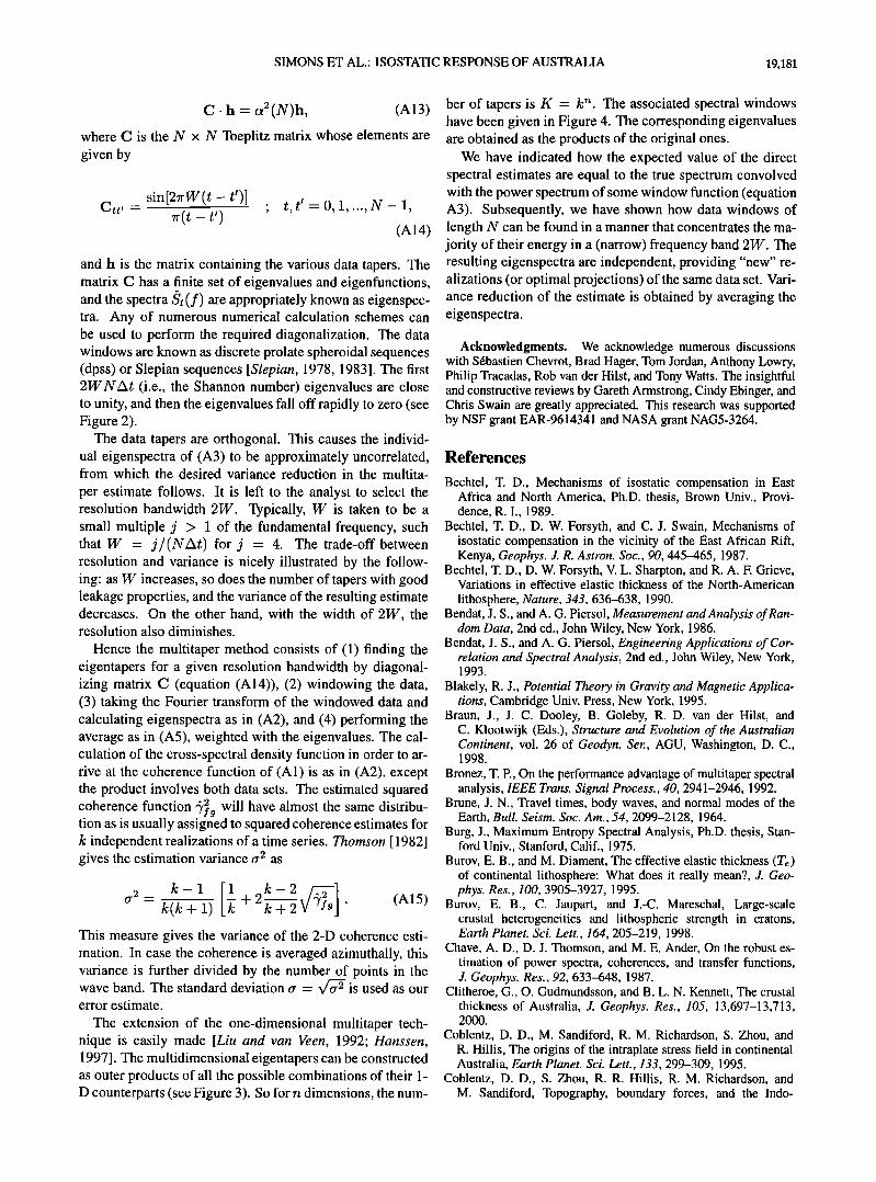
SIMONS ET AL.' ISOSTATIC RESPONSE OF AUSTRALIA 19,181
C. h - c•2 (N)h, (A13)
where C is the N x N Toeplitz matrix whose elements are given by
sin[2•rW(t- t')] Ctt' : ;
t') t, t t -- 0, 1, ..., N - 1,
(A14)
and h is the matrix containing the various data tapers. The matrix C has a finite set of eigenvalues and eigenfunctions, and the spectra •l(f) are appropriately known as eigenspec- tra. Any of numerous numerical calculation schemes can be used to perform the required diagonalization. The data windows are known as discrete prolate spheroidal sequences (dpss) or Slepian sequences [Slepian, 1978, 1983]. The first 2WNAt (i.e., the Shannon number) eigenvalues are close to unity, and then the eigenvalues fall off rapidly to zero (see Figure 2).
The data tapers are orthogonal. This causes the individ- ual eigenspectra of (A3) to be approximately uncorrelated, from which the desired variance reduction in the multita-
per estimate follows. It is left to the analyst to select the resolution bandwidth 2W. Typically, W is taken to be a small multiple j > 1 of the fundamental frequency, such that W = j/(NAt) for j = 4. The trade-off between resolution and variance is nicely illustrated by the follow- ing: as W increases, so does the number of tapers with good leakage properties, and the variance of the resulting estimate decreases. On the other hand, with the width of 2W, the resolution also diminishes.
Hence the multitaper method consists of (1) finding the eigentapers for a given resolution bandwidth by diagonal- izing matrix C (equation (AI4)), (2) windowing the data, (3) taking the Fourier transform of the windowed data and calculating eigenspectra as in (A2), and (4) performing the average as in (A5), weighted with the eigenvalues. The cal- culation of the cross-spectral density function in order to ar- rive at the coherence function of (A1) is as in (A2), except the product involves both data sets. The estimated squared coherence function •/•a will have almost the same distribu- tion as is usually assigned to squared coherence estimates for k independent realizations of a time series. Thomson [ 1982] gives the estimation variance o -2 as
0 -2 _-- k-1
k(k + 1) 1 (A15) +2k+ 2 This measure gives the variance of the 2-D coherence esti- mation. In case the coherence is averaged azimuthally, this variance is further divided by the number of points in the wave band. The standard deviation 0- = v/•a 2 is used as our error estimate.
The extension of the one-dimensional multitaper tech- nique is easily made [Liu and van Veen, 1992; Hanssen, 1997]. The multidimensional eigentapers can be constructed as outer products of all the possible combinations of their 1- D counterparts (see Figure 3). So for n dimensions, the num-
bet of tapers is K = k ". The associated spectral windows have been given in Figure 4. The corresponding eigenvalues are obtained as the products of the original ones.
We have indicated how the expected value of the direct spectral estimates are equal to the true spectrum convolved with the power spectrum of some window function (equation A3). Subsequently, we have shown how data windows of length N can be found in a manner that concentrates the ma- jority of their energy in a (narrow) frequency band 2W. The resulting eigenspectra are independent, providing "new" re- alizations (or optimal projections) of the same data set. Vari- ance reduction of the estimate is obtained by averaging the eigenspectra.
Acknowledgments. We acknowledge numerous discussions with S6bastien Chevrot, Brad Hager, Tom Jordan, Anthony Lowry, Philip Tracadas, Rob van der Hilst, and Tony Watts. The insightful and constructive reviews by Gareth Armstrong, Cindy Ebinger, and Chris Swain are greatly appreciated. This research was supported by NSF grant EAR-9614341 and NASA grant NAG5-3264.
References
Bechtel, T. D., Mechanisms of isostatic compensation in East Africa and North America, Ph.D. thesis, Brown Univ., Provi- dence, R. I., 1989.
Bechtel, T. D., D. W. Forsyth, and C. J. Swain, Mechanisms of isostatic compensation in the vicinity of the East African Rift, Kenya, Geophys. J. R. Astron. Soc., 90, 445-465, 1987.
Bechtel, T D., D. W. Forsyth, V. L. Sharpton, and R. A. F. Grieve, Variations in effective elastic thickness of the North-American
lithosphere, Nature, 343, 636-638, 1990. Bendat, J. S., and A. G. Piersol, Measurement and Analysis of Ran-
dom Data, 2nd ed., John Wiley, New York, 1986. Bendat, J. S., and A. G. Piersol, Engineering Applications of Cor-
relation and Spectral Analysis, 2nd ed., John Wiley, New York, 1993.
Blakely, R. J., Potential Theory in Gravity and Magnetic Applica- tions, Cambridge Univ. Press, New York, 1995.
Braun, J., J. C. Dooley, B. Goleby, R. D. van der Hilst, and C. Klootwijk (Eds.), Structure and Evolution of the Australian Continent, vol. 26 of Geodyn. Ser., AGU, Washington, D.C., 1998.
Bronez, T P., On the per/brmance advantage of multitaper spectral analysis, IEEE Trans. Signal Process., 40, 2941-2946, 1992.
Brune, J. N., Travel times, body waves, and normal modes of the Earth, Bull. Seism. Soc. Am., 54, 2099-2128, 1964.
Burg, J., Maximum Entropy Spectral Analysis, Ph.D. thesis, Stan- ford Univ., Stanford, Calif., 1975.
Burov, E. B., and M. Diament, The effective elastic thickness (T,) of continental lithosphere: What does it really mean?, J. Geo- phys. Res., I00, 3905-3927, 1995.
Burov, E. B., C. Jaupart, and J.-C. Mareschal, Large-scale crustal heterogeneities and lithospheric strength in cratons, Earth Planet. Sci. Lett., 164, 205-219, 1998.
Chave, A.D., D. J. Thomson, and M. E. Ander, On the robust es- timation of power spectra, coherences, and transfer functions, J. Geophys. Res., 92, 633-648, 1987.
Clitheroe, G., O. Gudmundsson, and B. L. N. Kennett, The crustal thickness of Australia, J. Geophys. Res., 105, 13,697-13,713, 2000.
Coblentz, D. D., M. Sandiford, R. M. Richardson, S. Zhou, and R. Hillis, The origins of the intraplate stress field in continental Australia, Earth Planet. Sci. Lett., 133, 299-309, 1995.
Coblentz, D. D., S. Zhou, R. R. Hillis, R. M. Richardson, and M. Sandiford, Topography, boundary forces, and the Indo-

19,182 SIMONS ET AL.: ISOSTATIC RESPONSE OF AUSTRALIA
Australian intraplate stress field, J. Geophys. Res., 103, 919-931, 1998.
Cull, J., Heat flow and regional geophysics in Australia, in Terres- trial Heat Flow and the Lithosphere Structure, edited by V. Cer- mak and L. Rybach, pp. 486-500, Springer-Verlag, New York, 1991.
Cull, J.P., and D. Denham, Regional variations in Australian heat flow, BMR J. Aust. Geol. Geophys., 4, 1-13, 1979.
D'Agostino, N., and D. McKenzie, Convective support of long- wavelength topography in the Apennines (Italy), Terra Nova, 11, 234-238, 1999.
Dahlen, F. A., and J. Tromp, Theoretical Global Seisinology, Princeton Univ. Press, Princeton, N.J., 1998.
Detrick, R. S., and A. B. Watts, An analysis of isostasy in the world's oceans, 3, Aseismic ridges, J. Geophys. Res., 84, 3637- 3653, 1979.
Dickey, J. O., et al., Satellite gravity: Insights into the solid Earth and its fluid envelope, Eos Trans. AGU, 79, 237, 242-243, 1998.
Djomani, Y. H. P., J. D. Fairhead, and W. L. Griffin, The flexural rigidity of Fennoscandia: Reflection of the tectonothermal age of the lithospheric mantle, Earth Planet. Sci. Lett., 174, 139-154, 1999.
Dooley, J. C., Implications of Australian seismic and gravity mea- surements for the structure and composition of the upper mantle, BMR J. Aust. Geol. Geophys., pp. 1-5, 1977.
Dorman, L. M., and B. T Lewis, Experimental isostasy, 1, Theory of the determination of the Earth's isostatic response to a con- centrated load, J. Geophys. Res., 75, 3357-3365, 1970.
Drummond, B. (Ed.), The Australian Lithosphere, Geol. Soc. Aust., Sydney, 1991.
Ebinger, C., and N. Hayward, Soft plates and hot spots: Views from Afar, J. Geophys. Res., 101, 21,859-21,876, 1996.
Finlayson, D. M., Geophysical differences in the lithosphere be- tween Phanerozoic and Precambrian Australia, Tectonophysics, 84, 287-312, 1982.
Forsyth, D. W., Subsurface loading and estimates of the flexural rigidity of continental lithosphere, J. Geophys. Res., 90, 12,623- 12,632, 1985.
Fowler, C., The Solid Earth, Cambridge Univ. Press, New York, 1990.
Gesch, D., K. L. Verdin, and S. K. Greenlee, New land surface digital elevation model covers the Earth, Eos Trans. AGU, 80, 69-70, 1999.
Goleby, B. R., R. D. Shaw, C. Wright, and B. L. N. Kennett, Geophysical evidence for "thick-skinned" crustal deformation in central Australia, Nature, 337, 325-330, 1989.
Goncharov, A. G., M.D. Lizinsky, C. D. N. Collins, K. A. Kalnin, T. N. Fomin, B. J. Drummond, B. R. Goleby, and L. N. Pla- tonenkova, Intra-crustal "seismic isostasy" in the Baltic Shield and Australian Precambrian cratons from deep seismic profiles and the Kola Superdeep Bore Hole data, in Structure and Evolu- tion of the Australian Continent, edited by J. Braun, J. C. Dooley, B. Goleby, R. D. van der Hilst, and C. Klootwijk, vol. 26 of Geo- dyn. Ser., pp. 119-138, AGU, Washington, D.C., 1998.
Gough, D. I., Electrical conductivity under western North Amer- ica in relation to heat flow, seismology and structure, J. Geo- magn. Geoelectr., 26, 105-123, 1974.
Gwavava, O., C. J. Swain, and F. Podmore, Mechanisms of iso- static compensation of the Zimbabwe and Kaapvaal cratons, the Limpopo belt and the Mozambique basin, Geophys. J. Int., 127, 635-650, 1996.
Hager, B. H., Subducted slabs and the geoid: Constraints on mantle rheology and flow, J. Geophys. Res., 89, 6003-6015, 1984.
Hand, M., and M. Sandiford, Intraplate deformation in central Australia, the link between subsidence and fault reactivation, Tectonophysics, 305, 121-140, 1999.
Hanssen, A., Multidimensional multitaper spectral estimation, Sig- nal Process., 58, 327-332, 1997.
Hillis, R. R., J. J. Meyer, and S. D. Reynolds, The Australian stress map, Explor. Geophys., 29, 420-427, 1998.
Hillis, R. R., J. R. Enever, and S. D. Reynolds, In situ stress field of eastern Australia, Aust. J. Earth Sci., 46, 813-825, 1999.
Jaupart, C., and J.-C. Mareschal, Thermal structure and thickness of continental roots, Lithos, 48, 93-114, 1999.
Jeans, J., The propagation of earthquake waves, Phi- los. Trans. R. Soc. London, Ser. A, 102, 554-574, 1923.
Kamer, G. D., Spectral representation of isostatic models, BMR J. Aust. Geol. Geophys., 7, 55-62, 1982.
Kamer, G. D., and A. B. Watts, Gravity-anomalies and flexure of the lithosphere at mountain ranges, J. Geophys. Res., 88, 449- 477, 1983.
Kamer, G. D., M. S. Steckler, and J. A. Thorne, Long-term thermo- mechanical properties of the continental lithosphere, Nature, 304, 250-253, 1983.
Kay, S. M., and S. L. Marple, Spectrum analysis: A modem per- spective, Proc. IEEE, 69, 1380-1419, 1981.
Komm, R. W., Y. Gu, F. Hill, P. B. Stark, and I. K. Fodor, Multitaper spectral analysis and wavelet denoising applied to helioseismic data, Astroph. J., 519, 401-421, 1999.
Kuo, C., C. Lindberg, and D. J. Thomson, Coherence established between atmospheric carbon dioxide and global temperature, Nature, 343, 709-714, 1990.
Lambeck, K., Structure and evolution of the intracratonic basins of central Australia, Geophys. J. R. Astron. Soc., 74, 843-886, 1983.
Lambeck, K., Geophysical Geodesy, Oxford Univ. Press, New York, 1988.
Lambeck, K., and C. Penney, Teleseismic travel time anomalies and crustal structure in central Australia, Phys. Earth Planet. Inter., 34, 46-56, 1984.
Lambeck, K., H. W. S. McQueen, R. A. Stephenson, and D. Denham, The state of stress within the Australian continent, Ann. Geophys., 2, 723-742, 1984.
Lambeck, K., G. Burgess, and R. D. Shaw, Teleseismic travel-time anomalies and deep crustal structure in central Australia, Geo- phys. J. Int., 94, 105-124, 1988.
Lavier, L. L., and M. S. Steckler, The effect of sedimentary cover on the flexural strength of continental lithosphere, Nature, 389, 476-479, 1997.
Lavier, L. L., and M. S. Steckler, The effect of sedimentary cover on the flexural strength of continental lithosphere, Correction, Nature, 392, 843, 1998.
Lees, J. M., and J. Park, Multiple-taper spectral analysis: A stand- alone C-subroutine, Comput. Geosci., 21, 199-236, 1995.
Lemoine, F., et al., The Development of the Joint NASA GSFC and the National Imagery and Mapping Agency (NIMA) Geopoten- tial Model EGM96, NASA Goddard Space Flight Cent., Green- belt, Md., 1998.
Lilley, F. E. M., D. V. Woods, and M. N. Sloane, Electrical conduc- tivity from Australian magnetometer arrays using spatial gradi- ent data, Phys. Earth Planet. Inter., 25, 202-209, 1981.
Lindberg, C. R., and J. Park, Multiple-taper spectral analysis of terrestrial free oscillations, II, Geophys. J. R. Astron. Soc., 91, 795-836, 1987.
Liu, T-C., and B. D. van Veen, Multiple window based mini- mum variance spectrum estimation for multidimensional random fields, IEEE Trans. Signal Process., 40, 578-589, 1992.
Lowry, A. R., and R. B. Smith, Flexural rigidity of the Basin and Range-Colorado Plateau-Rocky Mountain transition from coher- ence analysis of gravity and topography, J. Geophys. Res., 99, 20,123-20,140, 1994.
Lowry, A. R., and R. B. Smith, Strength and rheology of the western U.S. Cordillera, J. Geophys. Res., 100, 17,947-17,963, 1995.
Macario, A., A. Malinvemo, and W. F. Haxby, On the robustness of elastic thickness estimates obtained using the coherence method, J. Geophys. Res., 100, 15,163-15,172, 1995.
Malik, N., and J. S. Lim, Properties of two-dimensional maximum entropy power spectrum estimates, IEEE Trans. Acoust. Speech Signal Process., 30, 788-798, 1982.
SIMONS ET AL.: ISOSTATIC RESPONSE OF AUSTRALIA 19,183
Mareschal, M., R. L. Kellett, R. D. Kurtz, J. N. Ludden, S. Ji, and R. C. Bailey, Archaean cratonic roots, mantle shear zones and deep electrical anisotropy, Nature, 375, 134-137, 1995.
McKenzie, D., and C. Bowin, The relationship between bathymetry and gravity in the Atlantic Ocean, J. Geophys. Res., 81, 1903- 1915, 1976.
McKenzie, D., and J. D. Fairhead, Estimates of the effective elas- tic thickness of the continental lithosphere from Bouguer and free air gravity anomalies, J. Geophys. Res., 102, 27,523-27,552, 1997.
McNutt, M. K., and R. L. Parker, Isostasy in Australia and the evo- lution of the compensation mechanism, Science, 199, 773-775, 1978.
McQueen, H. W. S., and K. Lambeck, Determination of crustal structure in central Australia by inversion of traveltime residuals, Geophys. J. lnt., 126, 645-662, 1996.
Mellors, R., F. Vernon, and D. J. Thomson, Detection of disper- sive signals using multitaper dual-frequency coherence, Geo- phys. J. lnt., 135, 146-154, 1998.
Mullis, C. T., and L. L. Scharf, Quadratic estimators of the power spectrum, in Advances in Spectrum Analysis and Array Process- ing, edited by S. Haykin, vol. 1, chap. 1, pp. 1-57, Prentice Hall, Englewood Cliffs, N.J., 1991.
Munk, W. H., and D. E. Cartwright, Tidal spectroscopy and predic- tion, Philos. Trans. R. Soc. London, Ser. A, 259, 533-581, 1966.
Murray, C. G., E. Scheibner, and R. N. Walker, Regional geologi- cal interpretation of a digital coloured residual Bouguer gravity image of eastern Australia with a wavelength cut-off of 250 km, Aust. J. Earth Sci., 36, 423-449, 1989.
Myers, J. S., R. D. Shaw, and I. M. Tyler, Tectonic evolution of Proterozoic Australia, Tectonics, 15, 1431-1446, 1996.
Park, J., C. R. Lindberg, and D. J. Thomson, Multiple-taper spec- tral analysis of terrestrial free oscillations, I, Geophys. J. R. As- tron. Soc., 91,755-794, 1987a.
Park, J., C. R. Lindberg, and F. L. Vernon, Multitaper spectral analysis of high-frequency seismograms, J. Geophys. Res., 92, 12,675-12,684, 1987b.
Percival, D. B., and A. T Walden, Spectral Analysis for Physi- cal Applications, Multitaper and Conventional Univariate Tech- niques, Cambridge Univ. Press, New York, 1993.
Phillips, R. J., and K. Lambeck, Gravity fields of the terrestrial planets: Long-wavelength anomalies and tectonics, Rev. Geo- phys., 18, 27-76, 1980.
Polet, J., and D. L. Anderson, Depth extent of cratons as inferred from tomographic studies, Geology, 23, 205-208, 1995.
Priestley, M., Spectral Analysis and Time Series, Academic Press, San Diego, Calif., 1981.
Riedel, K. S., and A. Sidorenko, Minimum bias multiple taper spec- tral estimation, IEEE Trans. Signal Process., 43, 188-195, 1995.
Sandiford, M., and M. Hand, Controls on the locus of intraplate deformation in central Australia, Earth Planet. Sci. Lett., 162, 97-110, 1998.
Sandwell, D. T., and M. L. Renkin, Compensation of swells and plateaus in the North Pacific: No direct evidence for mantle con- vection, J. Geophys. Res., 93, 2775-2783, 1988.
Scheirer, D., D. W. Forsyth, and A. Hosford, Multitaper estimates of the lithospheric strength of the Basin and Range province (abstract), Eos Trans. AGU, 76(17), Spring Meet. Suppl., S282, 1995.
Shibutani, T., M. Sambridge, and B. L. N. Kennett, Genetic algo- rithm inversion for receiver functions with application to crust and uppermost mantle structure beneath eastern Australia, Geo- phys. Res. Lett., 23, 1829-1832, 1996.
Simons, F. J., R. D. van der Hilst, and J.-P. Montagner, Az- imuthal anisotropy of the Australian upper mantle (abstract), Eos Trans. AGU, 80(46), Fall Meet. Suppl., F729, 1999a.
Simons, F. J., A. Zielhuis, and R. D. van der Hilst, The deep struc- ture of the Australian continent from surface-wave tomography, Lithos, 48, 17-43, 1999b.
Slepian, D., Prolate spheroidal wave functions, Fourier analysis and uncertainty, V, The discrete case, Bell Syst. Tech. J., 57, 1371-1429, 1978.
Slepian, D., Some comments on Fourier-analysis, uncertainty and modeling, SIAM Rev., 25, 379-393, 1983.
Spassoy, E., The stress field in Australia from composite fault plane solutions of the strongest earthquakes in the continent, J. Seis- mol.,2, 173-178, 1998.
Stephenson, R., Flexural models of continental lithosphere based on the long-term erosional decay of topography, Geo- phys. J. R. Astron. Soc., 77, 385-4 13, 1984.
Stephenson, R., and C. Beaumont, Small-scale convection in the upper mantle and the isostatic response of the Canadian shield, in Mechanisms of Continental Drift and Plate Tectonics, edited by P. A. Davies and S. K. Runcorn, pp. 111-122, Academic Press, San Diego, Calif., 1980.
Stephenson, R., and K. Lambeck, Isostatic response of the litho- sphere with in-plane stress: Application to central Australia, J. Geophys. Res., 90, 8581-8588, 1985.
ter Voorde, M., R. T. van Balen, G. Bertotti, and S. A. P. L. Cloet- ingh, The influence of a stratified rheology on the flexural re- sponse of the lithosphere to (un)loading by extensional faulting, Geophys. J. lnt., 134, 721-735, 1998.
Thomson, D. J., Spectrum estimation and harmonic analysis, Proc. IEEE, 70, 1055-1096, 1982.
Timoshenko, S., and S. Woinowsky-Krieger, Theory of Plates and Shells, 2nd ed., McGraw-Hill, New York, 1959.
Touzi, R., A. Lopes, and P. Vachon, Estimation of the coherence function for interferometric SAR applications, in European Con- ference on Synthetic Aperture Radar 1996, pp. 241-244, EU- SAR, K6nigswinter, Germany, 1996.
Touzi, R., A. Lopes, J. Bruniquel, and P. Vachon, Coherence esti- mation for SAR imagery, IEEE Trans. Geosci. Remote Sens., 37, 135-149, 1999.
Tukey, J. W., An introduction to the calculations of numerical spec- trum analysis, in Advanced Seminar on Spectral Analysis of Time Series, edited by B. Harris, pp. 25-46, John Wiley, New York, 1967.
Turcotte, D. L., and G. Schubert, Geodynamics, Application of Continuum Physics to Geological Problems, John Wiley, New York, 1982.
Vauchez, A., A. Tommasi, and G. Barruol, Rheological heterogene- ity, mechanical anisotropy and deformation of the continental lithosphere, Tectonophysics, 296, 61-86, 1998.
Veevers, J. J. (Ed.), Phanerozoic Earth History of Australia, Oxford Univ. Press, New York, 1984.
Walden, A., Improved low-frequency decay estimation using the multitaper spectral-analysis method, Geophys. Prospect., 38, 61-86, 1990.
Walden, A. T., D. B. Percival, and E. J. McCoy, Spectrum esti- mation by wavelet thresholding of multitaper estimators, IEEE Trans. Signal Process., 46, 3153-3165, 1998.
Wang, Y., and J.-C. Mareschal, Elastic thickness of the lithosphere in the central Canadian shield, Geophys. Res. Lett., 26, 3033- 3036, 1999.
Watts, A. B., An analysis of isostasy in the world's oceans, 1, Hawaiian-Emperor seamount chain, J. Geophys. Res., 83, 5989- 6004, 1978.
Welch, P. D., The use of Fast Fourier Transform for the estimation of power spectra: A method based on time averaging over short, modified periodograms, IEEE Trans. Audio Electroacoust., 15, 70-73, 1967.
Wellman, P., On the isostatic compensation of Australian topogra- phy, BMR J. Aust. Geol. Geophys., 4, 373-382, 1979.
Wellman, P., Mapping of geophysical domains in the Australian continental crust using gravity and magnetic anomalies, in Structure and Evolution of the Australian Continent, edited by J. Braun, J. C. Dooley, B. Goleby, R. D. van der Hilst, and

19,184 SIMONS ET AL.: ISOSTATIC RESPONSE OF AUSTRALIA
C. Klootwijk, vol. 26 of Geodyn. Ser., pp. 59-71, AGU, Wash- ington, D.C., 1998.
Zhang, Y., E. Scheibner, B. E. Hobbs, A. Ord, B. J. Drummond, and S. J. D. Cox, Lithospheric structure in Southeast Australia: A model based on gravity, geoid and mechanical analyses, in Structure and Evolution of the Australian Continent, edited by J. Braun, J. C. Dooley, B. Goleby, R. D. van der Hilst, and C. Klootwijk, vol. 26 of Geodyn. Ser., pp. 89-108, AGU, Wash- ington, D.C., 1998.
Zhong, S., Dynamics of crustal compensation and its influences on crustal isostasy, J. Geophys. Res., 102, 15,287-15,299, 1997.
Zielhuis, A., and R. D. van der Hilst, Upper-mantle shear veloc- ity beneath eastern Australia from inversion of waveforms from SKIPPY portable arrays, Geophys. J. Int., 127, 1-16, 1996.
Zoback, M. L., First- and second-order patterns of stress in the lithosphere: The World Stress Map project, J. Geophys. Res., 97, 11,703-11,728, 1992.
Zuber, M. T., T. D. Bechtel, and D. W. Forsyth, Effective elastic thicknesses of the lithosphere and mechanisms of isostatic com- pensation in Australia, J. Geophys. Res., 94, 9353-9367, 1989.
Zuber, M. T., et al., Internal structure and early thermal evolution of Mars from Mars Global Surveyor topography and gravity, Sci- ence, 287, 1788-1793, 2000.
J. Korenaga, F. J. Simons, and M. T Zuber, Department of Earth, Atmospheric and Planetary Sciences, Massachusetts Institute of Technology, Rm 54-517A, Cambridge, MA 02139. (fjsimons @mit.edu)
(Received November 17, 1999; revised March 16, 2000; accepted April 26, 2000.)