Isospectralization, or how to hear shape, style, and correspondence

Luca Cosmo

University of Venice

luca.cosmo@unive.it

Mikhail Panine

Ecole Polytechnique

mpanine@lix.polytechnique.fr

Arianna Rampini

Sapienza University of Rome

rampini@di.uniroma1.it

Maks Ovsjanikov

Ecole Polytechnique

maks@lix.polytechnique.fr

Michael M. Bronstein

Imperial College London / USI

m.bronstein@imperial.ac.uk

Emanuele Rodola

Sapienza University of Rome

emanuele.rodola@uniroma1.it

Abstract

The question whether one can recover the shape of a

geometric object from its Laplacian spectrum (‘hear the

shape of the drum’) is a classical problem in spectral ge-

ometry with a broad range of implications and applica-

tions. While theoretically the answer to this question is neg-

ative (there exist examples of iso-spectral but non-isometric

manifolds), little is known about the practical possibility

of using the spectrum for shape reconstruction and opti-

mization. In this paper, we introduce a numerical proce-

dure called isospectralization, consisting of deforming one

shape to make its Laplacian spectrum match that of an-

other. We implement the isospectralization procedure using

modern differentiable programming techniques and exem-

plify its applications in some of the classical and notori-

ously hard problems in geometry processing, computer vi-

sion, and graphics such as shape reconstruction, pose and

style transfer, and dense deformable correspondence.

1. Introduction

Can one hear the shape of the drum? This classical

question in spectral geometry, made famous by Mark Kac’s

eponymous paper [21], inquires about the possibility of re-

covering the structure of a geometric object from its Lapla-

cian spectrum. Empirically, the relation between shape and

its acoustic properties has long been known and can be

traced back at least to medieval bellfounders. However,

while it is known that the spectrum carries many geomet-

ric and topological properties of the shape such as the area,

total curvature, number of connected components, etc., it

is now known that one cannot ‘hear’ the metric. Exam-

ples of high-dimensional manifolds that are isospectral but

not isometric have been constructed in 1964 [27] (predating

Kac’s paper), but it took until 1992 to produce a counter-

example of 2D polygons giving a negative answer to Kac’s

opt.

target

init.

Initialization Reconstruction

Without isospectralization With isospectralization

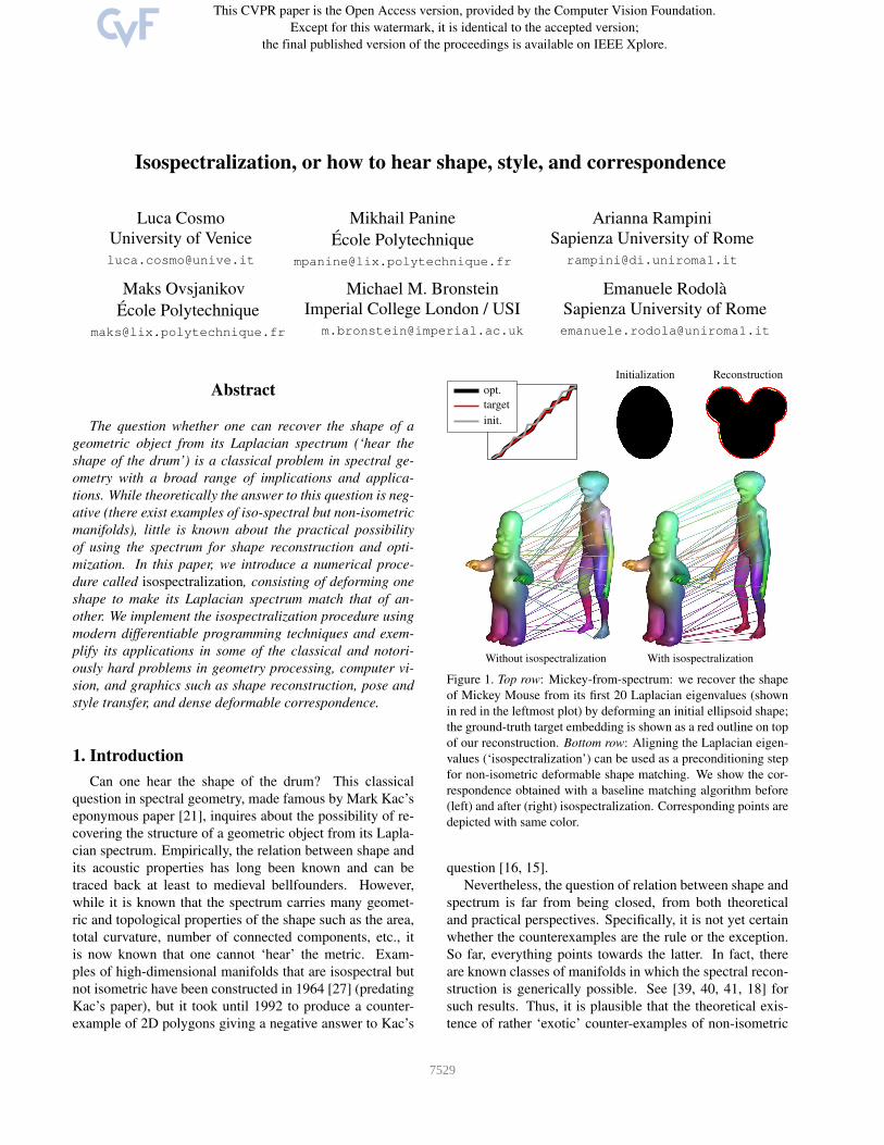
Figure 1. Top row: Mickey-from-spectrum: we recover the shape

of Mickey Mouse from its first 20 Laplacian eigenvalues (shown

in red in the leftmost plot) by deforming an initial ellipsoid shape;

the ground-truth target embedding is shown as a red outline on top

of our reconstruction. Bottom row: Aligning the Laplacian eigen-

values (‘isospectralization’) can be used as a preconditioning step

for non-isometric deformable shape matching. We show the cor-

respondence obtained with a baseline matching algorithm before

(left) and after (right) isospectralization. Corresponding points are

depicted with same color.

question [16, 15].

Nevertheless, the question of relation between shape and

spectrum is far from being closed, from both theoretical

and practical perspectives. Specifically, it is not yet certain

whether the counterexamples are the rule or the exception.

So far, everything points towards the latter. In fact, there

are known classes of manifolds in which the spectral recon-

struction is generically possible. See [39, 40, 41, 18] for

such results. Thus, it is plausible that the theoretical exis-

tence of rather ‘exotic’ counter-examples of non-isometric

43217529

isospectral manifolds does not preclude the possibility of

reconstructing the shape from its spectrum in practice.

This is exactly the direction explored in our paper. We

introduce a numerical procedure we call isospectralization,

which consists in deforming a mesh in order to align its

(finite) Laplacian spectrum with a given one. We imple-

ment this procedure using modern differentiable program-

ming tools used in deep learning applications and show its

usefulness in some of the fundamental problems in geome-

try processing, computer vision, and graphics.

For example, we argue that isospectralization (with some

additional priors such as smoothness and enclosed volume)

can in some cases be used to recover the structure of an

object from its spectrum, thus practically hearing the shape

of the drum (see Figure 1, top row).

Outside of the rare counterexamples, the reconstruction

is ambiguous up to intrinsic isometry. This ambiguity man-

ifests itself as a choice of an embedding of the mesh into

R3. This enables us to use the isospectralization procedure

to transfer style and pose across objects similarly to [11]:

we initialize with a source shape and apply isospectraliza-

tion to obtain the eigenvalues of the target shape; the result

is a shape in the pose of the source shape but with geometric

details of the target.

Even more remarkably, we show that pre-warping non-

isometric shapes by means of isospectralization can signifi-

cantly help in solving the problem of finding intrinsic corre-

spondences between them (Figure 1, bottom row), suggest-

ing that our procedure could be a universal pre-processing

technique for general correspondence pipelines.

Contribution. We consider the shape-from-eigenvalues

problem and investigate its relevance in a selection of prob-

lems from computer vision and graphics. Our key contribu-

tions can be summarized as follows:

• Despite being highly non-linear and hard to compute,

we show for the first time that the inverse mapping be-

tween a geometric domain and its Laplacian spectrum

is addressable with modern numerical tools;

• We propose the adoption of simple regularizers to

drive the spectrum alignment toward numerically op-

timal solutions;

• We showcase our method in the 2D and 3D settings,

and show applications of style transfer and dense map-

ping of non-isometric deformable shapes.

2. Related work

The possibility of reconstructing shape from spectrum is

of interest in theoretical physics [22], and has been explored

by theoreticians since the ’60s starting from Leon Green’s

question if a Riemannian manifold is fully determined by

its (complete) spectrum [6]. The isospectrality vs isometry

question received a negative answer in the seminal work of

Milnor [27], and additional counterexamples were provided

by Kac [21] and Gordon et al. [16] to name some classical

examples. A complete survey of the theoretical literature

on the topic is out of the scope of this paper; below, we

only consider the far less well-explored practical question

of how to realize metric embeddings from the sole knowl-

edge of the (finite) Laplacian eigenvalues.

A related but more general class of problems takes the

somewhat misleading name of inverse eigenvalue prob-

lems [13], dealing with the reconstruction of a generic phys-

ical system from prescribed spectral data. Different formu-

lations of the problem exist depending on the matrix repre-

sentation of the system; in the majority of cases, however, at

least partial knowledge of the eigenvectors is also assumed.

In the fields of computer vision and geometry process-

ing, Reuter et al. [32, 33] investigated the informativeness

of the Laplacian eigenvalues for the task of 3D shape re-

trieval. The authors proposed to employ the Laplacian

spectrum as a global shape signature (dubbed the ‘shape

DNA’), demonstrating good accuracy in distinguishing dif-

ferent shape classes. However, measuring the extent to

which eigenvalues carry geometric and topological infor-

mation about the shape was left as an open question.

More recently, there have been attempts at reconstructing

3D shapes from a full Laplacian matrix or other intrinsic op-

erators [11, 14]. Such methods differ from our approach in

that they leverage the complete information encoded in the

input operator matrix, while we only assume to be given the

operator’s eigenvalues as input. Further, these approaches

follow a two-step optimization process, in which the Rie-

mannian metric (edge lengths in the discrete case) is first

reconstructed from the input matrix, and an embedding is

obtained in a second step. As we will show, we operate

“end-to-end” by solving directly for the final embedding. It

is worthwhile to mention that the problem of reconstructing

a shape from its metric is considered a challenging problem

in itself [10, 12]. In computer graphics, several shape mod-

eling pipelines involve solving for an embedding under a

known mesh connectivity and additional extrinsic informa-

tion in the form of user-provided positional landmarks [35].

More closely related to our problem is the shape regis-

tration method of [17, 19]. The authors propose to solve

for a conformal rescaling of the metric of two given sur-

faces, so that the resulting eigenvalues align well. While

this approach shares with ours the overall objective of align-

ing spectra, the underlying assumption is for the Laplacian

matrices and geometric embeddings to be given. A simi-

lar approach was recently proposed in the conformal pre-

warping technique of [34] for shape correspondence using

functional maps.

A related, but different, inverse spectral problem has

7530

been tackled in [7]. There, the task is to optimize the shape

of metallophone keys to produce a desired sound when

struck in a specific place. Prescribing the sound consists

of prescribing a sparse selection of frequencies (eigenval-

ues) and the amplitudes to which the frequencies are excited

when the key is struck. It is also desirable that the other

frequencies be suppressed. This is different from the recon-

struction pursued in our work, since we prescribe a precise

sequence of eigenvalues. Further, amplitude suppression in

[7] is implemented by designing the nodal sets of specific

eigenfunctions, thus bringing this type of approach closer to

a partially described inverse eigenvalue problem [13, Chap-

ter 5].

Perhaps most closely related to our approach are meth-

ods that have explored the possibility of reconstructing

shapes from their spectrum in the case of coarsely trian-

gulated surfaces [1] and planar domains [31]. These works

also indicate that non-isometric isospectral shapes are ex-

ceedingly rare. Compared to the present paper, [1] and [31]

study shapes with a low number of degrees of freedom.

There, the shapes are prescribed by fewer than 30 param-

eters, while we allow every vertex in the mesh to move.

3. Background

Manifolds. We model a shape as a compact connected 2-

dimensional Riemannian manifold X (possibly with bound-

ary ∂X ) embedded either in R2 (flat shape) or R

3 (sur-

face). The intrinsic gradient ∇ and the positive semi-

definite Laplace-Beltrami operator ∆ on X generalize the

corresponding notions of gradient and Laplacian from Eu-

clidean spaces to manifolds. In particular, ∆ admits a spec-

tral decomposition

∆ϕi(x) = λiϕi(x) x ∈ int(X ) (1)

〈∇ϕi(x), n(x)〉 = 0 x ∈ ∂X , (2)

with homogeneous Neumann boundary conditions (2); here

n denotes the normal vector to the boundary.

Spectrum. The spectrum of X is the sequence of eigenval-

ues of its Laplacian. These form a discrete set, which is a

canonically ordered non-decreasing sequence:

0 = λ1 < λ2 ≤ · · · , (3)

where λ1 has multiplicity 1 due to the connectedness of X ;

for i > 1, the multiplicity of λi is related to the intrin-

sic symmetries of X . The growth rate of the ordered se-

quence (λi) is further related to the total surface area of Xvia Weyl’s asymptotic law [38]:

λi ∼4π

∫

Xdx

i , i → ∞ . (4)

This result makes it clear that size can be directly de-

duced from the spectrum (i.e., one can “hear the size” of the

vi

vj

vk v

h

vi

vj

vh

ℓij

ℓjk

ℓki ℓhi

ℓjhℓij

ℓhi

ℓjh

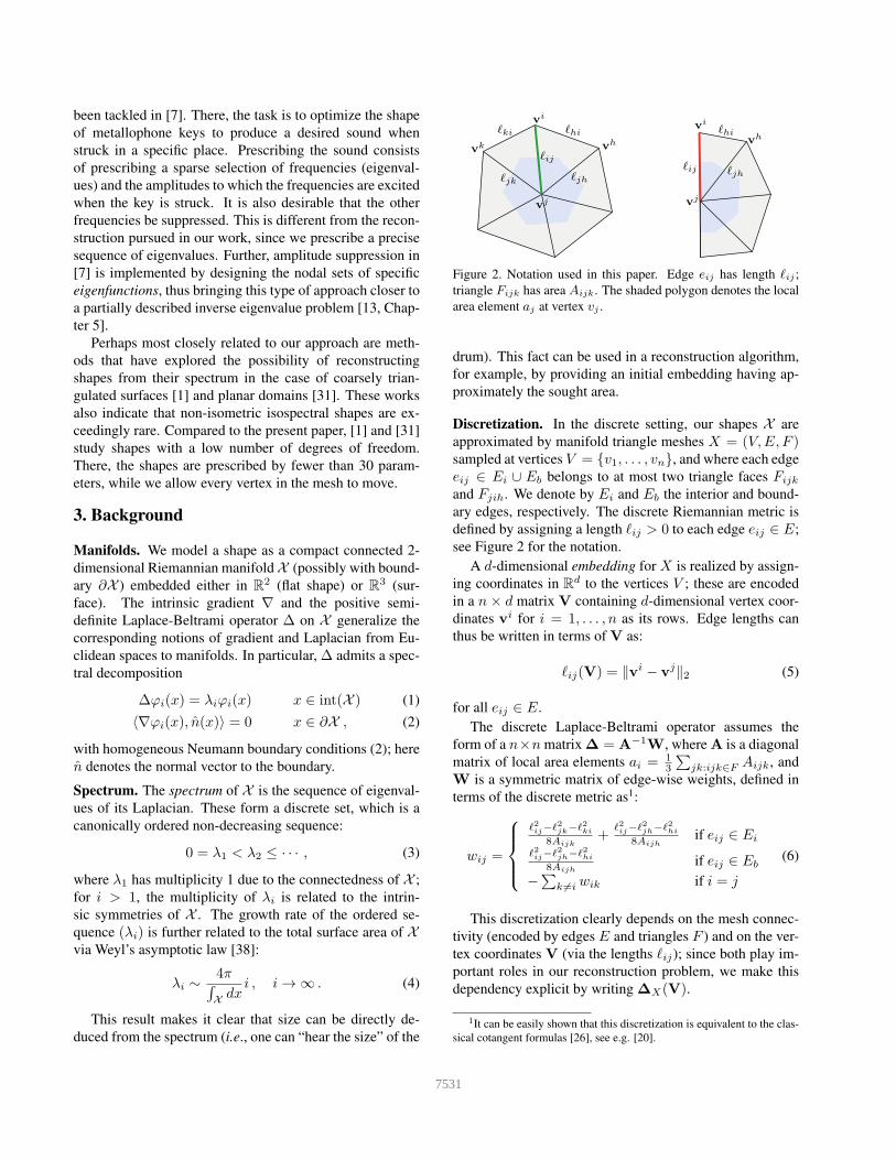
Figure 2. Notation used in this paper. Edge eij has length ℓij ;

triangle Fijk has area Aijk. The shaded polygon denotes the local

area element aj at vertex vj .

drum). This fact can be used in a reconstruction algorithm,

for example, by providing an initial embedding having ap-

proximately the sought area.

Discretization. In the discrete setting, our shapes X are

approximated by manifold triangle meshes X = (V,E, F )sampled at vertices V = {v1, . . . , vn}, and where each edge

eij ∈ Ei ∪ Eb belongs to at most two triangle faces Fijk

and Fjih. We denote by Ei and Eb the interior and bound-

ary edges, respectively. The discrete Riemannian metric is

defined by assigning a length ℓij > 0 to each edge eij ∈ E;

see Figure 2 for the notation.

A d-dimensional embedding for X is realized by assign-

ing coordinates in Rd to the vertices V ; these are encoded

in a n× d matrix V containing d-dimensional vertex coor-

dinates vi for i = 1, . . . , n as its rows. Edge lengths can

thus be written in terms of V as:

ℓij(V) = ‖vi − vj‖2 (5)

for all eij ∈ E.

The discrete Laplace-Beltrami operator assumes the

form of a n×n matrix ∆ = A−1

W, where A is a diagonal

matrix of local area elements ai =1

3

∑

jk:ijk∈F Aijk, and

W is a symmetric matrix of edge-wise weights, defined in

terms of the discrete metric as1:

wij =

ℓ2ij−ℓ2jk−ℓ2ki

8Aijk+

ℓ2ij−ℓ2jh−ℓ2hi

8Aijhif eij ∈ Ei

ℓ2ij−ℓ2jh−ℓ2hi

8Aijhif eij ∈ Eb

−∑

k 6=i wik if i = j

(6)

This discretization clearly depends on the mesh connec-

tivity (encoded by edges E and triangles F ) and on the ver-

tex coordinates V (via the lengths ℓij); since both play im-

portant roles in our reconstruction problem, we make this

dependency explicit by writing ∆X(V).

1It can be easily shown that this discretization is equivalent to the clas-

sical cotangent formulas [26], see e.g. [20].

7531

Init. k = 10 k = 20 k = 30 Target

0.90 0.90 0.90

0.92 0.92 0.91

0.93 0.94 0.94

Figure 3. Shape recovery at increasing mesh resolution (n = 100,

200, and 300 vertices increasing top to bottom) and bandwidth

(k = 10, 20, and 30 eigenvalues increasing left to right). In each

test, the mesh graph connectivity of the target is known and input to

the optimization process. We report the IOU score below each re-

construction. A finer sampling significantly improves reconstruc-

tion quality, whereas extending the bandwidth above k = 30 does

not lead to further improvement.

4. Isospectralization

Our approach builds upon the assumption that knowl-

edge of a limited portion of the spectrum is enough to fix

the shape of the domain, given some minimal amount of

additional information which we phrase as simple regular-

izers. We consider inverse problems of this form:

minV∈Rn×d

‖λ(∆X(V))− µ‖ω + ρX(V) , (7)

where V is the (unknown) embedding of the mesh vertices

in Rd, ∆X(V) is the associated discrete Laplacian, ‖ · ‖ω

is a weighted norm defined below, and µ,λ ∈ Rk+ respec-

tively denote the input sequence and the first k eigenvalues

of ∆X(V). Function ρX is a regularizer for the embed-

ding, implementing the natural expectation that the sought

solution should satisfy certain desirable properties.

Using a standard ℓ2 norm for the data term in (7) would

not lead to accurate shape recovery: Since the high end of

the spectrum accounts for small geometric variations of the

embedding, a local optimum can be reached by perfectly

aligning the high frequencies and concentrating most of the

alignment error on the lower end (which accounts for the

more global shape appearance). To make error diffusion

more balanced, we thus adopt the weighted norm

‖λ− µ‖ω =

k∑

i=1

1

i(λi − µi)

2 . (8)

Problem (7) seeks a Euclidean embedding whose Lapla-

cian eigenvalues align to the ones given as input. This prob-

lem is highly non-linear and thus particularly difficult, mak-

ing it susceptible to local minima. Nevertheless, in all our

Init.

0.92 0.95 0.93

0.93 0.95 0.93

Figure 4. Shape recovery with unknown mesh connectivity, under

two different initializations. We report the IOU score below each

recovered embedding. Differently from Figure 3, in these tests the

mesh tessellation was chosen arbitrarily and is in no way related

to the input sequence of eigenvalues.

tests we observed almost perfect alignment; we refer to the

implementation Section 4.3 for further details.

4.1. Flat shapes

When the embedding space is R2, a shape X is entirely

determined by its boundary ∂X . For this reason, we con-

sider a variant of Problem (7) where we optimize only for

the boundary vertices.

Regularizers. We adopt the composite penalty

ρX(V) = ρX,1(V) + ρX,2(V) , (9)

where ρX,1(V) is a Tikhonov regularizer promoting short

edge lengths and thus a uniformly sized mesh:

ρX,1(V) =∑

eij∈Eb

ℓ2ij(V) , (10)

and ρX,2(V) is defined as:

ρX,2(V) = (∑

ijk∈F

(Rπ2

(vj − vi))⊤(vk − v

i))− , (11)

where Rπ2

=(

0 −1

1 0

)

rotates 2D vectors by π2

and (x)− =

(min{0, x})2. This term penalizes triangle flips that may

occur throughout the optimization, and works under the as-

sumption of clockwise oriented triangles.

Error measure. We quantify the reconstruction quality as

the area ratio of the intersection of the recovered and target

embeddings over their union (IOU, the higher the better) af-

ter an optimal alignment has been carried out. In our plots,

we visualize the recovered embedding with a blue outline,

and the ground-truth (unknown) target with a red outline.

Mesh resolution and bandwidth. By operating with a dis-

crete Laplace operator, our optimization problem is directly

affected by the quality of the discretization. We investi-

gate this dependency by running an evaluation at varying

7532

Init Reconstruction

Init.

Opt.

Targ.

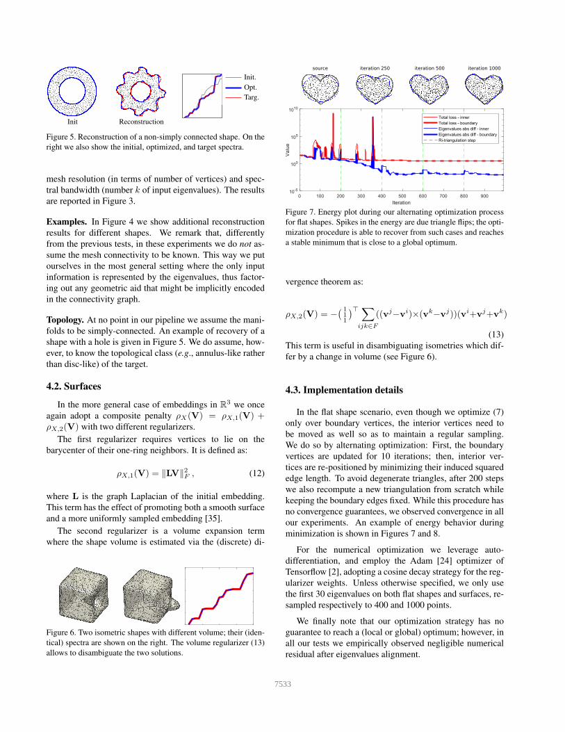
Figure 5. Reconstruction of a non-simply connected shape. On the

right we also show the initial, optimized, and target spectra.

mesh resolution (in terms of number of vertices) and spec-

tral bandwidth (number k of input eigenvalues). The results

are reported in Figure 3.

Examples. In Figure 4 we show additional reconstruction

results for different shapes. We remark that, differently

from the previous tests, in these experiments we do not as-

sume the mesh connectivity to be known. This way we put

ourselves in the most general setting where the only input

information is represented by the eigenvalues, thus factor-

ing out any geometric aid that might be implicitly encoded

in the connectivity graph.

Topology. At no point in our pipeline we assume the mani-

folds to be simply-connected. An example of recovery of a

shape with a hole is given in Figure 5. We do assume, how-

ever, to know the topological class (e.g., annulus-like rather

than disc-like) of the target.

4.2. Surfaces

In the more general case of embeddings in R3 we once

again adopt a composite penalty ρX(V) = ρX,1(V) +ρX,2(V) with two different regularizers.

The first regularizer requires vertices to lie on the

barycenter of their one-ring neighbors. It is defined as:

ρX,1(V) = ‖LV‖2F , (12)

where L is the graph Laplacian of the initial embedding.

This term has the effect of promoting both a smooth surface

and a more uniformly sampled embedding [35].

The second regularizer is a volume expansion term

where the shape volume is estimated via the (discrete) di-

Figure 6. Two isometric shapes with different volume; their (iden-

tical) spectra are shown on the right. The volume regularizer (13)

allows to disambiguate the two solutions.

0 100 200 300 400 500 600 700 800 900

Iteration

10-5

100

105

1010

Va

lue

Total loss - inner

Total loss - boundary

Eigenvalues abs diff - inner

Eigenvalues abs diff - boundary

Ri-triangulation step

source iteration 250 iteration 500 iteration 1000

Figure 7. Energy plot during our alternating optimization process

for flat shapes. Spikes in the energy are due triangle flips; the opti-

mization procedure is able to recover from such cases and reaches

a stable minimum that is close to a global optimum.

vergence theorem as:

ρX,2(V) = −( 111

)⊤∑

ijk∈F

((vj−vi)×(vk−v

j))(vi+vj+v

k)

(13)

This term is useful in disambiguating isometries which dif-

fer by a change in volume (see Figure 6).

4.3. Implementation details

In the flat shape scenario, even though we optimize (7)

only over boundary vertices, the interior vertices need to

be moved as well so as to maintain a regular sampling.

We do so by alternating optimization: First, the boundary

vertices are updated for 10 iterations; then, interior ver-

tices are re-positioned by minimizing their induced squared

edge length. To avoid degenerate triangles, after 200 steps

we also recompute a new triangulation from scratch while

keeping the boundary edges fixed. While this procedure has

no convergence guarantees, we observed convergence in all

our experiments. An example of energy behavior during

minimization is shown in Figures 7 and 8.

For the numerical optimization we leverage auto-

differentiation, and employ the Adam [24] optimizer of

Tensorflow [2], adopting a cosine decay strategy for the reg-

ularizer weights. Unless otherwise specified, we only use

the first 30 eigenvalues on both flat shapes and surfaces, re-

sampled respectively to 400 and 1000 points.

We finally note that our optimization strategy has no

guarantee to reach a (local or global) optimum; however, in

all our tests we empirically observed negligible numerical

residual after eigenvalues alignment.

7533

source iteration 100 iteration 400 iteration 1200

0 200 400 600 800 1000 1200

Iteration

10-3

10-2

10-1

100

101

102

Va

lue

Total loss

Eigenvalues absolute difference

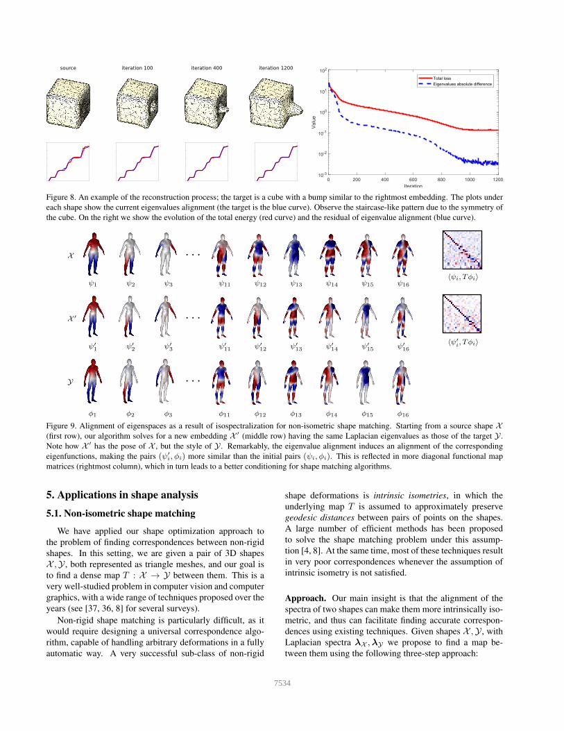
Figure 8. An example of the reconstruction process; the target is a cube with a bump similar to the rightmost embedding. The plots under

each shape show the current eigenvalues alignment (the target is the blue curve). Observe the staircase-like pattern due to the symmetry of

the cube. On the right we show the evolution of the total energy (red curve) and the residual of eigenvalue alignment (blue curve).

· · ·

· · ·

· · ·

X

X ′

Y

φ1 φ2 φ3 φ11 φ12 φ13 φ14 φ15 φ16

ψ′1

ψ′2

ψ′3

ψ′11

ψ′12

ψ′13

ψ′14

ψ′15

ψ′16

ψ1 ψ2 ψ3 ψ11 ψ12 ψ13 ψ14 ψ15 ψ16

〈ψi, Tφi〉

〈ψ′i, Tφi〉

Figure 9. Alignment of eigenspaces as a result of isospectralization for non-isometric shape matching. Starting from a source shape X(first row), our algorithm solves for a new embedding X ′ (middle row) having the same Laplacian eigenvalues as those of the target Y .

Note how X ′ has the pose of X , but the style of Y . Remarkably, the eigenvalue alignment induces an alignment of the corresponding

eigenfunctions, making the pairs (ψ′i, φi) more similar than the initial pairs (ψi, φi). This is reflected in more diagonal functional map

matrices (rightmost column), which in turn leads to a better conditioning for shape matching algorithms.

5. Applications in shape analysis

5.1. Non­isometric shape matching

We have applied our shape optimization approach to

the problem of finding correspondences between non-rigid

shapes. In this setting, we are given a pair of 3D shapes

X ,Y , both represented as triangle meshes, and our goal is

to find a dense map T : X → Y between them. This is a

very well-studied problem in computer vision and computer

graphics, with a wide range of techniques proposed over the

years (see [37, 36, 8] for several surveys).

Non-rigid shape matching is particularly difficult, as it

would require designing a universal correspondence algo-

rithm, capable of handling arbitrary deformations in a fully

automatic way. A very successful sub-class of non-rigid

shape deformations is intrinsic isometries, in which the

underlying map T is assumed to approximately preserve

geodesic distances between pairs of points on the shapes.

A large number of efficient methods has been proposed

to solve the shape matching problem under this assump-

tion [4, 8]. At the same time, most of these techniques result

in very poor correspondences whenever the assumption of

intrinsic isometry is not satisfied.

Approach. Our main insight is that the alignment of the

spectra of two shapes can make them more intrinsically iso-

metric, and thus can facilitate finding accurate correspon-

dences using existing techniques. Given shapes X ,Y , with

Laplacian spectra λX ,λY we propose to find a map be-

tween them using the following three-step approach:

7534

0 0.1 0.2 0.3 0.4 0.50

20

40

60

80

100

Geodesic error

%C

orr

esp

on

den

ces

Before

After

Reference ReferenceBefore

isospec.

After

isospec.

Before

isospec.

After

isospec.

Figure 10. Results on non-isometric shape matching. The plots on the left are averaged over 60 non-isometric shape pairs from the FAUST

inter-subject dataset [9]. In order to visualize correspondence, we use it to transfer a texture from reference shape to target.

1. Deform X to obtain X ′ whose spectrum λX ′ is better

aligned with λY .

2. Compute the correspondence T ′ : X ′ → Y using an

existing isometric shape matching algorithm.

3. Convert T ′ to T : X → Y using the identity map

between X and X ′.

Our main intuition is that as mentioned above, despite the

existence of exceptional counter-examples, in most practi-

cal cases this procedure is very likely to make shapes X ′

and Y close to being isometric. Therefore, we would ex-

pect an isometric shape matching algorithm to match Y to

X ′ better than to the original shape X . Finally, after com-

puting a map T : X ′ → Y , we can trivially convert it to a

map, since X ,X ′ are in 1-1 correspondence.

The approach described above builds upon the remark-

able observation that aligning the Laplacian eigenvalues

also induces an alignment of the eigenspaces of the two

shapes. This is illustrated on a real example in Figure 9,

where we show a subset of eigenfunctions for two non-

isometric surfaces (a man and a woman) before and after

isospectralization. In a sense, isospectralization implements

a notion of correspondence-free alignment of the functional

spaces spanned by the first k Laplacian eigenfunctions.

Implementation. For this and the following application,

we replaced the optimization variables by optimizing over a

displacement field rather than the absolute vertex positions

in Problem (7). Doing so, we observed a better quality of

the recovered embeddings.

We have implemented the approach described above

by using an existing shape correspondence algorithm [28]

based on the functional maps framework [29, 30]. One

of the advantages of this approach is that it is purely in-

trinsic and only depends on the quantities derived from the

Laplace-Beltrami operators of the two shapes.

Remark. The exact embedding of the optimized shape X ′

Figure 11. Non-isometric shape matching before (left) and after

(right) isospectralization. The correspondence is computed ac-

cording to the algorithm of Section 5.1.

does not play a role, and can be different from that of Y .

In other words, we do not aim to reproduce the shape Y ,

but rather only use our shape optimization strategy as an

auxiliary step to facilitate shape correspondence.

We use the functional maps-based algorithm of [28] with

the open source implementation provided by the authors.

This algorithm is based on first solving for a functional map

represented in the Laplacian eigenbasis [3] by using sev-

eral descriptor-preservation and regularization constraints,

and then converting the functional map to a pointwise one.

As done in [28], we used the wave kernel signature [5] as

descriptors and commutativity with the Laplace-Beltrami

operators for map regularization. This leads to a convex

optimization problem which can be efficiently solved with

an iterative quasi-Newton method. Finally, we convert the

functional map to a pointwise one using nearest neighbor

search in the spectral domain as in [29]. We evaluate the

quality of the final correspondence by measuring the aver-

age geodesic error with respect to some externally-provided

ground truth map [23]. We refer to Figures 1 (bottom row),

10, 11, and 12 for quantitative and qualitative results.

5.2. Style transfer

As a second possible application we explore the task of

style transfer between deformable shapes. Given a pair of

7535

0 0.1 0.2 0.3 0.4 0.50

0.2

0.4

0.6

0.8

1

Geodesic error

%C

orr

esp

on

den

ces

homer to alien

before

after

0 0.1 0.2 0.3 0.4 0.5

Geodesic error

horse to camel

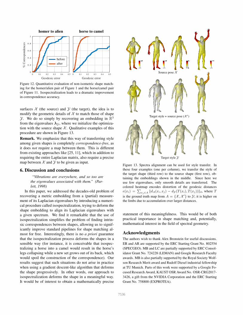
Figure 12. Quantitative evaluation of non-isometric shape match-

ing for the homer/alien pair of Figure 1 and the horse/camel pair

of Figure 11. Isospectralization leads to a dramatic improvement

in correspondence accuracy.

surfaces X (the source) and Y (the target), the idea is to

modify the geometric details of X to match those of shape

Y . We do so simply by recovering an embedding in R3

from the eigenvalues λY , where we initialize the optimiza-

tion with the source shape X . Qualitative examples of this

procedure are shown in Figure 13.

Remark. We emphasize that this way of transferring style

among given shapes is completely correspondence-free, as

it does not require a map between them. This is different

from existing approaches like [25, 11], which in addition to

requiring the entire Laplacian matrix, also require a precise

map between X and Y to be given as input.

6. Discussion and conclusions

“Vibrations are everywhere, and so too are

the eigenvalues associated with them.” (Par-

lett, 1998)

In this paper, we addressed the decades-old problem of

recovering a metric embedding from a (partial) measure-

ment of its Laplacian eigenvalues by introducing a numeri-

cal procedure called isospectralization, trying to deform the

shape embedding to align its Laplacian eigenvalues with

a given spectrum. We find it remarkable that the use of

isospectralization simplifies the problem of finding intrin-

sic correspondences between shapes, allowing us to signif-

icantly improve standard pipelines for shape matching al-

most for free. Interestingly, there is no a priori guarantee

that the isospectralization process deforms the shapes in a

sensible way (for instance, it is conceivable that isospec-

tralizing a horse into a camel would result in the horse’s

legs collapsing while a new set grows out of its back, which

would spoil the construction of the correspondence). Our

results suggest that such situations do not arise in practice

when using a gradient descent-like algorithm that deforms

the shape progressively. In other words, our approach to

isospectralization deforms the shape in a meaningful way.

It would be of interest to obtain a mathematically precise

Source pose X

Target style + source pose (X ′)

Target style Y

Figure 13. Spectra alignment can be used for style transfer. In

these four examples (one per column), we transfer the style of

the target shape (third row) to the source shape (first row), ob-

taining the embeddings shown in the middle. Since here we

use few eigenvalues, only smooth details are transferred. The

colored heatmap encodes distortion of the geodesic distances

e(xi) =∑

xj∈A ‖dA(xi, xj) − dY(T (xi), T (xj))‖2, where T

is the ground truth map from A = {X ,X ′} to Y; it is higher on

the limbs due to accumulation over larger distances.

statement of this meaningfulness. This would be of both

practical importance in shape matching and, potentially,

mathematical interest in the field of spectral geometry.

Acknowledgments

The authors wish to thank Alex Bronstein for useful discussions.

ER and AR are supported by the ERC Starting Grant No. 802554

(SPECGEO). MB and LC are partially supported by ERC Consol-

idator Grant No. 724228 (LEMAN) and Google Research Faculty

awards. MB is also partially supported by the Royal Society Wolf-

son Research Merit award and Rudolf Diesel industrial fellowship

at TU Munich. Parts of this work were supported by a Google Fo-

cused Research Award, KAUST OSR Award No. OSR-CRG2017-

3426, a gift from the NVIDIA Corporation and the ERC Starting

Grant No. 758800 (EXPROTEA).

7536

References

[1] David Aasen, Tejal Bhamre, and Achim Kempf. Shape from

sound: toward new tools for quantum gravity. Physical Re-

view Letters, 110(12):121301, 2013.

[2] Martın Abadi, Ashish Agarwal, Paul Barham, et al. Tensor-

Flow: Large-scale machine learning on heterogeneous sys-

tems, 2015. Software available from tensorflow.org.

[3] Yonathan Aflalo, Haim Brezis, and Ron Kimmel. On the op-

timality of shape and data representation in the spectral do-

main. SIAM Journal on Imaging Sciences, 8(2):1141–1160,

2015.

[4] Yonathan Aflalo, Anastasia Dubrovina, and Ron Kimmel.

Spectral generalized multi-dimensional scaling. Interna-

tional Journal of Computer Vision, 118(3):380–392, 2016.

[5] Mathieu Aubry, Ulrich Schlickewei, and Daniel Cremers.

The Wave Kernel Signature: A Quantum Mechanical Ap-

proach to Shape Analysis. In Proc. ICCV Workshops, 2011.

[6] Marcel Berger. A panoramic view of Riemannian geometry.

Springer Science & Business Media, 2012.

[7] Gaurav Bharaj, David IW Levin, James Tompkin, Yun

Fei, Hanspeter Pfister, Wojciech Matusik, and Changxi

Zheng. Computational design of metallophone contact

sounds. TOG, 34(6), 2015.

[8] Silvia Biasotti, Andrea Cerri, Alex Bronstein, and Michael

Bronstein. Recent trends, applications, and perspectives in

3d shape similarity assessment. Computer Graphics Forum,

35(6):87–119, 2016.

[9] Federica Bogo, Javier Romero, Matthew Loper, and

Michael J Black. FAUST: Dataset and Evaluation for 3d

Mesh Registration. In Proc. CVPR, 2014.

[10] Vincent Borrelli, Saıd Jabrane, Francis Lazarus, and Boris

Thibert. Flat tori in three-dimensional space and convex in-

tegration. PNAS, 2012.

[11] Davide Boscaini, Davide Eynard, Drosos Kourounis, and

Michael M Bronstein. Shape-from-operator: Recovering

shapes from intrinsic operators. Computer Graphics Forum,

34(2):265–274, 2015.

[12] Albert Chern, Felix Knoppel, Ulrich Pinkall, and Peter

Schroder. Shape from metric. TOG, 37(4):63:1–63:17, 2018.

[13] Moody Chu and Gene Golub. Inverse eigenvalue problems:

theory, algorithms, and applications. Oxford University

Press, 2005.

[14] Etienne Corman, Justin Solomon, Mirela Ben-Chen,

Leonidas Guibas, and Maks Ovsjanikov. Functional charac-

terization of intrinsic and extrinsic geometry. TOG, 36(2):14,

2017.

[15] Carolyn Gordon, David Webb, and Scott Wolpert. Isospec-

tral plane domains and surfaces via Riemannian orbifolds.

Inventiones Mathematicae, 110(1):1–22, 1992.

[16] Carolyn Gordon, David L. Webb, and Scott Wolpert. One

cannot hear the shape of a drum. Bulletin of the American

Mathematical Society, 27:134–138, 1992.

[17] Hajar Hamidian, Jiaxi Hu, Zichun Zhong, and Jing Hua.

Quantifying shape deformations by variation of geometric

spectrum. In Proc. MICCAI, 2016.

[18] Hamid Hezari and Steve Zelditch. Inverse Spectral Problem

for Analytic (Z/2Z)-Symmetric Domains in RN . Geometric

and Functional Analysis, 20(1):160–191, 2010.

[19] Jiaxi Hu, Hajar Hamidian, Zichun Zhong, and Jing Hua.

Visualizing shape deformations with variation of geometric

spectrum. IEEE TVCG, 23(1):721–730, 2017.

[20] Alec Jacobson and Olga Sorkine-Hornung. A cotan-

gent laplacian for images as surfaces. Technical re-

port/Department of Computer Science, ETH, Zurich, 757,

2012.

[21] Mark Kac. Can one hear the shape of a drum? The American

Mathematical Monthly, 73(4):1–23, 1966.

[22] Achim Kempf. Spacetime could be simultaneously contin-

uous and discrete, in the same way that information can be.

New Journal of Physics, 12(11):115001, 2010.

[23] Vladimir G Kim, Yaron Lipman, and Thomas Funkhouser.

Blended Intrinsic Maps. TOG, 30(4):79, 2011.

[24] Diederik P. Kingma and Jimmy Ba. Adam: A method for

stochastic optimization. CoRR, abs/1412.6980, 2014.

[25] Bruno Levy. Laplace-beltrami eigenfunctions towards an al-

gorithm that ”understands” geometry. In Proc. SMI, June

2006.

[26] Mark Meyer, Mathieu Desbrun, Peter Schroder, and Alan H

Barr. Discrete differential-geometry operators for triangu-

lated 2-manifolds. In Visualization and Mathematics III,

pages 35–57. Springer, 2003.

[27] John Milnor. Eigenvalues of the Laplace operator on certain

manifolds. PNAS, 51(4):542, 1964.

[28] Dorian Nogneng and Maks Ovsjanikov. Informative descrip-

tor preservation via commutativity for shape matching. Com-

puter Graphics Forum, 36(2):259–267, 2017.

[29] Maks Ovsjanikov, Mirela Ben-Chen, Justin Solomon, Adrian

Butscher, and Leonidas Guibas. Functional Maps: A

Flexible Representation of Maps Between Shapes. TOG,

31(4):30, 2012.

[30] Maks Ovsjanikov, Etienne Corman, Michael Bronstein,

Emanuele Rodola, Mirela Ben-Chen, Leonidas Guibas,

Frederic Chazal, and Alex Bronstein. Computing and pro-

cessing correspondences with functional maps. In SIG-

GRAPH Courses, pages 5:1–5:62, 2017.

[31] Mikhail Panine and Achim Kempf. Towards spectral geo-

metric methods for euclidean quantum gravity. Physical Re-

view D, 93(8):084033, 2016.

[32] Martin Reuter, Franz-Erich Wolter, and Niklas Peinecke.

Laplace-spectra as fingerprints for shape matching. In Proc.

SPM, SPM ’05, pages 101–106, New York, NY, USA, 2005.

ACM.

[33] Martin Reuter, Franz-Erich Wolter, and Niklas Peinecke.

Laplace-beltrami spectra as ’shape-dna’ of surfaces and

solids. Computer Aided Design, 38(4):342–366, Apr. 2006.

[34] Stefan C Schonsheck, Michael M Bronstein, and Rongjie

Lai. Nonisometric surface registration via conformal laplace-

beltrami basis pursuit. arXiv:1809.07399, 2018.

[35] Olga Sorkine and Daniel Cohen-Or. Least-squares meshes.

In Proc. Shape Modeling Applications, 2004. Proceedings,

pages 191–199, 2004.

7537

[36] Gary KL Tam, Zhi-Quan Cheng, Yu-Kun Lai, Frank C Lang-

bein, Yonghuai Liu, David Marshall, Ralph R Martin, Xian-

Fang Sun, and Paul L Rosin. Registration of 3d point

clouds and meshes: a survey from rigid to nonrigid. IEEE

Trans. Visualization and Computer Graphics, 19(7):1199–

1217, 2013.

[37] Oliver Van Kaick, Hao Zhang, Ghassan Hamarneh, and

Daniel Cohen-Or. A survey on shape correspondence. In

Computer Graphics Forum, volume 30, pages 1681–1707,

2011.

[38] Hermann Weyl. Uber die asymptotische Verteilung

der Eigenwerte. Nachrichten von der Gesellschaft der

Wissenschaften zu Gottingen, Mathematisch-Physikalische

Klasse, pages 110–117, 1911.

[39] Steve Zelditch. The inverse spectral problem for surfaces of

revolution. J. Diff. Geom., 49(2):207–264, 1998.

[40] Steve Zelditch. Spectral determination of analytic bi-

axisymmetric plane domains. Geometric & Functional Anal-

ysis GAFA, 10(3):628–677, 2000.

[41] Steve Zelditch. Inverse Spectral Problem for Analytic Do-

mains, II: Z2-symmetric domains. Annals of Mathematics,

170(1):205–269, 2009.

7538