isolated and ephemeral wetlands of southern appalachia
TRANSCRIPT

Clemson UniversityTigerPrints
All Dissertations Dissertations
5-2014
Isolated and Ephemeral Wetlands of SouthernAppalachia: Biotic Communities andEnvironmental Drivers Across Multiple Temporaland Spatial ScalesJoanna HawleyClemson University, [email protected]
Follow this and additional works at: https://tigerprints.clemson.edu/all_dissertations
Part of the Civil and Environmental Engineering Commons, and the Environmental SciencesCommons
This Dissertation is brought to you for free and open access by the Dissertations at TigerPrints. It has been accepted for inclusion in All Dissertations byan authorized administrator of TigerPrints. For more information, please contact [email protected].
Recommended CitationHawley, Joanna, "Isolated and Ephemeral Wetlands of Southern Appalachia: Biotic Communities and Environmental Drivers AcrossMultiple Temporal and Spatial Scales" (2014). All Dissertations. 1330.https://tigerprints.clemson.edu/all_dissertations/1330

ISOLATED AND EPHEMERAL WETLANDS OF SOUTHERN APPALACHIA: BIOTIC COMMUNITIES AND ENVIRONMENTAL DRIVERS ACROSS MULTIPLE
TEMPORAL AND SPATIAL SCALES
A DissertationPresented to
the Graduate School of Clemson University
In Partial Fulfillment of the Requirements for the Degree
Doctor of Philosophy Wildlife and Fisheries Biology
by Joanna Hawley Howard
May 2014
Accepted by: Robert F. Baldwin, Committee Chair
Michael Childress Hugh Hanlin
Elizabeth Baldwin

ii
ABSTRACT
Throughout the world, wetlands are known to support a wide variety of taxa as
well as high levels of biodiversity and species richness. Although the ecological
significance of wetlands is well documented in the scientific literature, efforts to map and
assess wetlands on regional or national scales (e.g., National Wetlands Inventory (NWI))
often overlook wetlands which are either very small (< 1 ha) or have ephemeral
hydroperiods. While the vast majority of wetland research in the southeastern United
States has focused on wetlands distributed across the coastal plain ecoregion, very little
information exists on small and/or ephemeral wetlands in areas of southern Appalachia,
although there are several notable exceptions. Despite the paucity of small wetland data
in this region, the southeastern US is known as a hotspot for both aquatic biodiversity and
species endemism. My goal with this project was to examine the biotic communities
inhabiting small, ephemeral and geographically-isolated wetlands to identify the major
environmental drivers that contribute to observed community patterns and species’
distributions. I studied a set of small, mostly-ephemeral, mostly-isolated wetlands (N =
41) in the upper Piedmont and lower Blue Ridge ecoregions of South Carolina from
January-June of 2010 and 2011 and focused my efforts on describing the structure, biotic
communities and surrounding habitat characteristics of my study wetlands. I observed
high levels of species richness and biodiversity in this previously-undocumented wetland
system, despite the small size and ephemeral nature of study wetlands. My results
indicated that the amphibian and benthic invertebrate communities of small, ephemeral
wetlands responded to different environmental drivers (e.g., wetland depth, area,

iii
hydroperiod, canopy cover, surrounding land use types) occurring across multiple spatial
and temporal scales. Additionally, the amphibian community was significantly influenced
by a number of environmental variables occurring at both the within-pond scale and
larger spatial scales (250 m, 500 m and 1 km surrounding land cover variables). By
contrast, the benthic invertebrate community was significantly influenced primarily by
variables occurring at the within-pond scale. This wetland system also served as both
breeding and overwintering habitat for a variety of species such as wood frogs
(Lithobates sylvatica), spotted salamanders (Ambystoma maculatum), bullfrogs
(Lithobates catesbeiana), cricket frogs (Acris crepitans). This study highlights the
ecological importance of small, ephemeral aquatic habitats in a region where little
research exists regarding such systems; these often-unnoticed ecosystems are likely the
result of a combination of historical anthropogenic and natural environmental process.
These legacy wetlands (i.e., wetlands that are the unintended result of some human-
induced environmental change in either the recent or long-term past) are found
ubiquitously across the landscape and are often missed by coarse-filter mapping
approaches (e.g., National Wetlands Inventory). I observed many study wetlands to be
extremely small in size (< 0.05 ha) and that many wetlands were habitats of circumstance
and opportunity rather than of permanence and predictability. The ephemerality of the
majority of study wetlands demonstrates the biological significance of small, temporary
habitats for many species requiring these habitats for breeding activity. Despite the small
size and ephemeral nature of my study wetlands, I found that these wetlands represented
a large proportion of amphibian biodiversity in the regional species pool and thus, are an

iv
important conservation feature at the local, landscape and regional scales. My study
demonstrates that small, semi-isolated, mostly-ephemeral wetlands in southern
Appalachia support high levels of biodiversity and are an important asset deserving of
further study and conservation recognition.

v
DEDICATION
This manuscript is dedicated to my parents, M.H. Hawley and P.H. Easler, for
always supporting me and for always letting me ‘dance and prance and clap my hands’ as
loudly and as proudly my heart desires. I also dedicate this manuscript to my husband,
J.A. Howard for putting up with me during this long process and for supporting and
encouraging me, even when I did not believe in myself and my own abilities. Lastly, I
dedicate this manuscript to my grandparents and my anchors, A.E. and R. L. Hall, who
were the foundation for much of my life, particularly my education, my academic
pursuits, my love for nature and for bluegrass music.

vi
ACKNOWLEDGMENTS
I would like to thank Clemson University and the School of Agricultural, Forest
and Environmental Sciences for my teaching assistantships and consistent support during
my time at Clemson. Additionally, I would like to thank the EPA for the ‘Wetlands
Program Development Grant – Region Four,’ which supported my dissertation research
and field work. I am deeply indebted to Dr. Bryan Brown for his detailed knowledge of
aquatic systems, multivariate statistics, and editorial skills as well as to Mr. Don
Lipscomb for his GIS and mapping assistance as well as his biblical patience in teaching
me to work with historical aerial imagery. I would like to thank Dr. Dan Richter, Dr.
Amber Pitt, Dr. Heather Brooker, Jenna Stanek, Cora Allard-Keese, Paul Leonard, and
Dr. Cady Etheredge for their gracious feedback, input and support throughout my time at
Clemson. I am also deeply grateful to Dr. Robert Baldwin, Dr. Michael Childress, Dr.
Elizabeth Baldwin, and Dr. Hugh Hanlin for serving on my doctoral committee and for
guiding me through this process.

vii
TABLE OF CONTENTS
Page
TITLE PAGE .................................................................................................................... i
ABSTRACT ..................................................................................................................... ii
DEDICATION ................................................................................................................ iv
ACKNOWLEDGMENTS ............................................................................................... v
LIST OF TABLES ......................................................................................................... vii
LIST OF FIGURES ...................................................................................................... viii
CHAPTER
1. RELATIONSHIPS BETWEEN WETLAND CHARACTERISTICS AND AMPHIBIAN AND INVERTEBRATE COMMUNITIES IN EPHEMERAL AND ISOLATED WETLANDS IN SOUTHERN APPALACHIA ...................................................................................................... 1
Introduction .............................................................................................. 1 Methods.................................................................................................... 7 Results .................................................................................................... 12 Discussion and Conclusions .................................................................. 20
2. THE IMPACT OF CURRENT AND HISTORICAL LANDLAND USES ON AMPHIBIAN AND INVERTEBRATE DISTRIBUTIONS IN ISOLATED WETLANDS IN THE UPPER PIEDMONT AND LOWER BLUE
RIDGE ECOGREIONS OF THE SOUTHEASTERN US ................................... 27 Introduction ............................................................................................ 27 Methods.................................................................................................. 30 Results .................................................................................................... 39 Discussion and Conclusions .................................................................. 43
3. THE UTILITY OF STATE PARKS AS A CONSERVATIONAS A CONSERVATION TOOL FOR ISOLATED AND
EPHEMERAL WETLANDS: A CASE STUDY FROM THE SOUTHERN BLUE RIDGE................................................................................. 52
Introduction ............................................................................................ 52

viii
TABLE OF CONTENTS (continued) Page
Contribution of the SC State Parks System: A Case Study ................... 54 Methods.................................................................................................. 58 Results .................................................................................................... 61 Discussion and Conclusions .................................................................. 66
APPENDICES ............................................................................................................... 74
A: All Environmental Variables Collected .................................................. 75-76
B: Multi-Model Averaging of Wood Frog Models .......................................... 77
C: Multi-Model Averaging of Spotted Salamander Models............................. 79
REFERENCES ......................................................................................................... 79-95

ix
LIST OF TABLES
Table Page
1.1 Amphibian Species’ Detection Probabilities ............................................... 16
1.2 Significant Environmental Drivers of the Amphibian Community ................................................................................................. 18
1.3 Significant Environmental Drivers of the Invertebrate Community .................................................................................................. 20
2.1 Literature Used for Model Formulation ....................................................... 37
2.2 Model Variables for Wood Frogs ................................................................ 38
2.3 Model Variables for Spotted Salamanders .................................................. 38
2.4 Variance Partitioning Results for Amphibian And Invertebrate Communities .................................................................... 43
2.5 Top-Supported Models for Wood Frogs ...................................................... 43
2.6 Top-Supported Models for Spotted Salamanders ........................................ 44
3.1 All Variables Used in Park vs. Non-Park Analyses ..................................... 63

x
LIST OF FIGURES
Figure Page
1.1 Study Area and Study Wetlands ...................................................................... 2
1.2.1 Relationship between Amphibian Species Richness and Log-transformed Wetland Area ............................................................ 14
1.2.2 Relationship between Breeding Amphibian Species Richness and Log-transformed Wetland Area ............................................................ 14
1.2.3 Relationship between Total Taxonomic Richness and Log-transformed Wetland Area ............................................................ 15
1.3 Relationship between Invertebrate Genera Richness and Wetland Hydroperiod ............................................................................ 17
1.4 NMDS Ordination of Amphibian Community With Significant Environmental Variables .................................................. 19
1.5 NMDS Ordination of Invertebrate Community With Significant Environmental Variables .................................................. 20
2.1 Relationship between Invertebrate Genera Richness and Wetland Hydroperiod ....................................................................... 41-42
3.1 Depth Relationships in Park versus Non-park Wetlands ............................. 64
3.2 Invertebrate Richness in Park versus Non-park Wetlands ........................... 65
3.3 Total Taxonomic Richness in Park versus Non-park Wetlands .................. 66
3.4 Mean Tolerance Values in Park versus Non-park Wetlands ....................... 66
1
CHAPTER ONE
RELATIONSHIPS BETWEEN WETLAND CHARACTERISTICS AND AMPHIBIAN AND INVERTEBRATE COMMUNITIES IN EPHEMERAL AND ISOLATED
WETLANDS IN SOUTHERN APPALACHIA
INTRODUCTION
Wetlands are a globally-threatened resource that provide essential habitat for
numerous taxa (Goodale and Aber 2001). Wetlands also provide important ecosystem
services that are vital to human health and well-being, for example wildlife food
production and flood control (Paige 1985, Black et al. 1998, Brooks and Hayashi 2002).
Estimates of historical wetland losses vary but it is generally accepted that approximately
50% of wetlands have been lost, primarily as a result of agricultural activities and
development (Palang et al. 2011). Particularly vulnerable are small wetlands that because
of their geographic isolation from navigable water bodies, fall through regulatory cracks
of most legislation (Calhoun et al. 2003, Meyer et al. 2003). Small and/or isolated
wetlands are ecologically-important systems that host high levels of biodiversity and are
important to multiple taxonomic groups including birds (Cox 1988, Fairbairn and
Dinsmore 2001, Horn et al. 2005, Dewi et al. 2013), invertebrates (Brooks 2000, Baber et
al. 2004, Schilling et al. 2008), amphibians (Gibbs 1993, Holomuzki et al. 1994), reptiles
(Bergstrom et al. 1990, Joyal et al. 2001), mammals (Glitzenstein et al. 1990, Metts et al.
2001, Falkengren-Grerup et al. 2006, Stevens et al. 2007) and plants (Clewell and Lea
1989, Houlahan and Findlay 2003). These wetlands are particularly at risk as they are not
covered by most laws and policies and are also inadequately mapped (Pitt et al. 2012).

2
Figure 1.1 Map of study area showing the relevant ecoregions of South Carolina and study wetlands (N = 41)

3
Varying degrees of wetland inundation and isolation across the landscape may help to
support different and diverse communities of amphibians and benthic macroinvertebrates
(Stein et al. 1999, Ficetola and De Bernardi 2004, Gibbons et al. 2006). Along with
variable hydroperiods, small and/or isolated wetlands may exhibit variation in their
degree of connectivity to other bodies of water, with some wetlands totally surrounded by
upland terrestrial habitat with no discernible hydrological connections to other
waterbodies (Leibowitz 2003). The majority of studies focusing on wetlands of the
southeastern US have focused on coastal plain wetlands (Pechmann et al. 1991, Semlitsch
et al. 1996b, Stein et al. 1999, Bridges and Dorcas 2000, Snodgrass et al. 2000b,
Snodgrass et al. 2000c, Engeman et al. 2007, Morris and Maret 2007, Svancara et al.
2009, Puerta-Piñero et al. 2012) and few studies have examined wetlands in the upper
Piedmont and lower Blue Ridge ecoregions (but see Hook et al. 1994, Petranka et al.
2004). One reason for this common omission could be the cryptic signature of small,
isolated wetlands (Burne and Lathrop 2007, Pitt et al. 2012). Because these wetlands are
often extremely small in size (< 0.05 ha) and highly-dynamic across time and space, they
are difficult to identify using traditional mapping techniques based on data that is
available to the general public. Furthermore, dense canopy cover and steep changes in
topography can make these features difficult to locate across the landscape. The natural
variability of small and/or isolated wetland systems contributes to their high biodiversity
but also means that they are difficult to identify and conserve unless they are connected
to a ‘navigable waterway’ via a hydrologically, biologically or chemically ‘significant

4
nexus’ (Semlitsch and Bodie 1998, Mank 2003, Wolking 2006, Murphy 2007, Leibowitz
et al. 2008).
Conservation of small, potentially-isolated wetlands is a contentious subject in the US
with multiple agencies being charged with the task of identifying and managing wetlands
connected to navigable waterways (Downing et al. 2003, Murphy 2007). Furthermore,
the ambiguous nature of recent United States Supreme Court rulings has led to confusion
surrounding which wetlands are under federal jurisdiction and which wetlands are not
(Leibowitz et al. 2008). While much research has demonstrated the importance of small,
ephemeral wetlands at local and landscape scales, they are afforded very little protection
under federal laws and relatively few states have taken measures to protect these
ecosystems (see Preisser et al. 2000, Lathrop et al. 2005, Laurance et al. 2012).
Furthermore, despite research indicating the importance of amphibian movement among
different habitat types areas (Gibbs 1998, Baldwin et al. 2006a) and the importance of
areas adjacent to navigable waterways (e.g., floodplains which often contain ephemeral
wetlands), conservation efforts are not trending towards protection of small, ephemeral or
isolated aquatic systems (Correa-Araneda et al. 2012). The temporally- and spatially-
dynamic nature of these wetlands typically means that identification, assessment and
conservation efforts are often difficult at large extents. Small wetlands, particularly in the
southeastern US, continue to be lost to development and other anthropogenic activities,
with over 630,000 acres (254,952 ha) of wetlands lost between 2004 and 2009 (Fetcher
and Fellows 2011). By identifying how these cryptic ecosystems function biologically

5
and structurally, I hope to identify conservation priorities which are beyond the scope of
the majority of current legal jurisdiction.
The importance of ephemeral and isolated wetlands to both breeding and non-
breeding amphibians cannot be overstated and is well-established in the literature
throughout the world. Several species in the southeastern US (e.g., wood frogs, spotted
salamanders, spade-foot toads) are known to rely heavily on these habitats to complete
necessary steps in their life cycles. Amphibians are influenced by conditions at multiple
scales as many species, particularly those using small wetlands, migrate to and from
uplands, and multiple sites at landscape scales are important in metapopulation dynamics
(Hecnar and McLoskey 1996, Semlitsch and Bodie 1998). Additionally, the southeastern
US is a hotspot for aquatic diversity and endemism and thus, conservation of multiple
habitat types is critical in order to ensure the ability of amphibian populations to persist.
Small, isolated and/or ephemeral wetlands also serve as breeding habitat for a wide array
of benthic invertebrates, which can serve as both predators of and prey for amphibian
larvae in wetlands.
My goal in this study was to examine the effect of wetland structural and chemical
characteristics on community responses of amphibians and benthic macroinvertebrates in
a series of small, semi-isolated, mostly-ephemeral wetlands in the southeastern US. I was
also interested in identifying biotic and abiotic drivers across multiple spatial scales that
were significantly related to the biological communities inhabiting these wetlands.
Previous work in both laboratory and field settings have examined how amphibian and
benthic macroinvertebrate communities interact with and influence one another in aquatic

6
habitats (e.g., competition, predation, food web alteration); these studies have produced
mixed results with some research identifying pronounced effects of invertebrates on
amphibian larvae and other studies finding little to no significant impacts, or ‘zero sum
game’ dynamics between the two communities (Werner and Gilliam 1984, Werner and
Peacor 2003, Batzer et al. 2004, Ranvestel et al. 2004, Dutra and Callisto 2005, Werner et
al. 2007c, Colon-Gaud et al. 2009). I hypothesized that certain wetland characteristics
such as area, depth, hydroperiod and surrounding landscape characteristics would differ
in relative importance to the amphibian and benthic macroinvertebrate communities. I
believe that these two communities are influenced differently by environmental drivers
within my study system, with the amphibian community likely influenced by a greater
number of drivers compared to the benthic invertebrate community. Therefore, these two
groups should potentially be considered separately in bioassessment and management
actions. I studied a total of 41 wetlands across the upper Piedmont and lower Blue Ridge
ecoregions of South Carolina (termed ‘southern Appalachia’ for this manuscript) in order
to examine the responses of the biotic communities that occur in these systems to
environmental drivers at within-pond, local and landscape scales.
METHODS
Data collection
I collected environmental and community data at a total of 41 ephemeral, semi-
isolated wetlands in the upper Piedmont and lower Blue Ridge ecoregions of South
Carolina (Figure 1.1) over a two-year period in order to understand their structure and

7
biological function across the landscape. Wetlands were identified using a combination of
remote sensing methods and local ecological knowledge (Pitt et al. 2012). For each
wetland, I collected a total of sixty environmental variables relating to water chemistry,
water quality, habitat parameters, and land cover variables across three spatial scales (see
Appendix A for full list of variables collected) three times between January and June of
2010 and 2011. These three rounds of data collection were timed to coincide with
seasonal waves of amphibian breeding effort documented for this area (Conant and
Collins 1991, Weir and Mossman 2005). Wetlands were visited between two and four
additional times throughout the year and we established amphibian presence through the
use of call surveys, visual encounter surveys, egg mass counts and dip-net surveys. I
approached each wetland quietly and listened for approximately five minutes to identify
calling anurans. I then carefully searched each wetland’s shoreline out to 5 m from the
wetland’s edge, carefully overturning rocks, logs and other debris searching for adult
amphibians in adjacent terrestrial habitats. All amphibians were identified to the species
and returned to the wetland with the exception of larvae, of which a small sample of
those we were unable to field-ID were taken to the laboratory, and euthanized with
Tricaine Methanesulfate (i.e., ‘Finquel,’ ARGENT Chemical Laboratories, Inc.,
Redmond, WA), and preserved for later identification using a buffered 10% buffered
formalin solution. I calculated detection probabilities for amphibians incorporating our
multiple site visits and multiple lines of evidence using PRESENCE software, which
generates both occupancy and detection probabilities (United State Geological Survey,
2014) (Table 2.2) Because of the strong seasonality of breeding of many study species –

8
e.g., wood frogs (early January), spotted salamanders (January-February), marbled
salamanders (October-December), bullfrogs (April-July), green frogs (April-August), I
adjusted the sampling visits which were included in calculation of detection probabilities
(AmphibiaWeb 2014, Wilson 2014). The level of detectability can depend on any number
of things in these naturalized wetlands – whether or not water is present, how long the
water lasts, precipitation and weather events, natural breeding cycles of amphibians,
which is why I used multiple lines of evidence and multiple site visits during multiple
years to detect amphibian presence. I had a minimum of two researchers present for each
site visit and because wetlands were so small (avg = 0.00706 ha, min = 0.00029 ha, max
= 0.354214 ha), my impression from the field was that my sampling effort and site visits
were extensive enough to detect the majority of species present in habitats of interest
(i.e., wetlands and not streams). For certain species (e.g., Plethodontid and other stream-
associated salamanders), I did not expect to detect them in our study pools and their
presence was observed only in wetlands with a surficial stream connection. Such
occurrences were generally restricted to higher-elevation, mountainous portions of our
study area in the lower Blue Ridge of SC.
At each wetland, I selected a 1 m2 sampling area to collect benthic
macroinvertebrates; within this sampling area, we disturbed the substrate manually and
collected the sample using a D-frame dip net with mesh (Wildco Inc., Yulee, FL). For
each wetland, I sampled for benthic invertebrates in each microhabitat that I observed so
the samples would be representative of the entire wetland. Upon returning to the lab,
benthic macroinvertebrate samples were filtered using a mesh filter and preserved in 80%

9
ethanol for later identification. Each time a wetland was visited over the two year study
period I documented the presence or absence of standing water and used this data to
estimate the number of fill/dry cycles; we used this as a proxy for wetland hydroperiod.
Pools with at least one observed fill/dry cycle were classified as ‘ephemeral’ and pools
that were not observed to ever fully dry during the course of our study were classified as
‘permanent.’
Remotely-Sensed Data
I acquired landscape composition data from the USGS Seamless server data
warehouse and used the 2006 National Land Cover Database data to extract land use/land
cover data for the upper Piedmont and lower Blue Ridge ecoregions of SC (ESRI 2011). I
reclassified the land cover data into the following seven categories: open water,
disturbed/successional, cultivated, pasture, forested (both deciduous and evergreen), low-
density development and high-density development. I then calculated the area of each
land cover type at three spatial scales: local (150 m), patch (500 m) and landscape (1km)
scales. Because much research has demonstrated the importance of landscape-scale
variables in influencing wetland communities (Knutson et al. 1999, Ford et al. 2000,
Porej et al. 2004, Buskirk 2005), I used these landscape variables as predictors in
conjunction with within-pond variables to explain variation in amphibian and benthic
macroinvertebrate distributions.
Statistical Analyses
I examined the effect of wetland depth, area and hydroperiod on both amphibian and
benthic invertebrate richness and diversity (of adult amphibians only) using Shannon-

10
Weiner’s H and Hurlbert’s PIE (Probability of an Interspecific Encounter), which
calculates the proportion of encounters that will be from another species for one
individual. I also examined the effect of wetland area on species richness of amphibians,
breeding amphibians, benthic macroinvertebrate richness and diversity, and species
richness of other vertebrates observed to utilize wetland habitats during the two year
study period. I used Pearson product-moment correlations to examine relationships
among dependent and independent variables and to investigate collinearity among
variables.
I performed a Non-Metric Multidimensional Scaling (NMDS) analysis to ordinate
both amphibian and benthic macroinvertebrate communities using presence-nonpresence
data collected over both years of the study period. NMDS is a distance-based ordination
method that maximizes rank-order correlations between samples and species in
ordination space (McCune and Grace 2002). Unlike many other techniques, NMDS is an
iterative method that stops only when a satisfactory solution is found. NMDS analysis
makes no assumptions about the structure of the data and can be used with any distance
metric and are flexible in terms of the type of data used for analysis (e.g., binary,
continuous). I performed each ordination using k = 3 dimensions in order to maintain
realistic biological and graphical interpretability. I then used an environmental fit
function from the ‘Vegan’ package in R Statistical Software (Desmond et al. 2002), to
relate these community ordinations to collected environmental variables. The ‘envfit’
function seeks to find the direction (in multidimensional space) that has a maximum
correlation with an external set of variables (i.e., collected environmental variables)

11
(Desmond et al. 2002). Using this function, I performed permutation tests (permutations
= 10,000) to assess the significance of environmental vectors at α = 0.05. To account for
collinearity among the increasingly-large spatial scales of data collection, I applied a
correction factor in which I removed the area of the concentric buffers (250 and 500 m)
from the next largest spatial scale; this allows the technique to analyze land cover data at
500 m and 1 km spatial scales separately and without including the spatially
autocorrelated information from smaller spatial scales (Zuur et al. 2009, Ibbe et al. 2011).
All statistical analysis were performed using R statistical software (R Core Development
Team, 2012).
RESULTS
I found a total of twenty-four amphibian species in our study wetlands, all with
detection probabilities < 1.0 (Table 1.1). I found that total amphibian species richness,
breeding amphibian species richness and total taxonomic richness were significantly
related to log-transformed wetland area (Figures 1.2.1, 1.2.2 and 1.2.3).

12
Figure 1.2.1 Relationship between amphibian species richness and log-transformed pool area (R2 = 0.20999, F-ratio = 11.6323, p = 0.0015) of N = 41 ephemeral and/or isolated wetlands in SC
Amphiboan
Breeding R
ichness
Figure 1.2.2 Relationship between breeding amphibian species richness and log-transformed pool area (R2 = 0.104879, F-ratio = 4.5695, p = 0.0389) of N = 41 ephemeral and/or isolated wetlands in SC

13
Figure 1.2.3 Relationship between total taxonomic richness and log-transformed wetland area (R2 = 0.097895, F-ratio = 4.2322, p = 0.0464) of N = 41 ephemeral and/or isolated wetlands in SC
I found sufficient evidence to suggest that amphibian species richness was
significantly and positively related to average wetland area (log-transformed) (Figure
1.2.1; R2 = 0.22974, df = 40, F-ratio = 11.6323, p = 0.0015) with the largest wetlands
having the highest levels of amphibian species richness. Conversely, benthic
macroinvertebrate taxonomic richness was not significantly related to wetland area or
depth. We found no significant relationship between amphibian species richness and
permanent versus ephemeral wetlands (collapsed into binary categories, 0 = permanent, 1
= at least one drying event).

14
Table 1.1 Species detection probabilities calculated for (N = 40) study wetlands, adjusted for relevant breeding period for species with strong seasonality of breeding.
Species Adjusted P(j)
Lithobates sylvatica 0.5500
Ambystoma maculatum 0.4844
Acris crepitans 0.4146
Lithobates clamitans 0.3902
Pseudacris ferarium 0.3171
Lithobates sphenocephalus 0.2927
Lithobates catesbeiana 0.2927
Notopthalmus viridescens 0.2683
Desmognathus fuscus 0.2195
Bufo americanus 0.1951
Pseudacris crucifer 0.1885
Desmognathus ocoee 0.0732
Desmognathus monticola 0.0732
Eurycea cirrigera 0.0488
Bufo fowleri 0.0488
Gastrophryne carolinensis 0.0488
Lithobates palustris 0.0488
Bufo terrestris 0.0488
Ambystoma opacum 0.0061
Hyla chrysoscelis 0.0061
Plethodon glutinosis complex 0.0061
Eurycea guttolineata 0.003
Plethodon metcalfi 0.003
Pseudotriton ruber 0.003
I investigated the relationships between hydroperiod versus wetland area and
depth and found no significant relationship among these factors. I found significant
differences in amphibian species richness between wetlands with and without fish
(Wilcoxon Rank-Sums test, X2 = 7.6935, df = 1, p = 0.0055), with higher median levels
of diversity observed in wetlands with fish. Benthic macroinvertebrate richness and
diversity did not differ significantly between wetlands with and without fish. I found

15
significant differences in benthic macroinvertebrate genus richness (two-sample t-test, df
= 40, F-ratio = 4.2985, p = 0.0448) between permanent and ephemeral ponds with more
permanent wetlands having significantly higher invertebrate richness as compared
wetlands with shorter hydroperiods (Figure 1.3). Presence of amphibian reproductive
activity was significantly and negatively related to total abundance of three benthic
macroinvertebrate orders Ephemoptera, Plecoptera and Tricoptera (Wilcoxon Rank-Sums
test, X2 = 9.7327, df = 1, p = 0.0018). These three orders are commonly referred to as
‘EPT’ and are considered to be ‘sensitive’ organisms (i.e., higher abundances of these
organisms are indicative of high water quality) that are used with other aquatic indices to
indicate water quality in rapid bioassessment protocols by the US Environmental
Protection Agency.
Figure 1.3 We observed significant differences in invertebrate richness in permanent (0 observed fill/dry cycles) versus ephemeral wetlands (1 or more observed fill/dry cycles) (Two-sample t-test, df = 39, p = 0.0448) in N = 41 study wetlands

16
The NMDS ordination performed on amphibian community data converged on a
solution after 45 tries and with a final stress of 11.45963 using k = 3 dimensions. The
NMDS ordination performed on benthic macroinvertebrate community data converged
on a solution after 3 tries with a final stress level of 0.112399 using k = 3 dimensions.
NMDS ordination of the amphibian and benthic macroinvertebrate communities followed
by fitting of environmental vectors revealed that the amphibian community as a whole
was significantly related to biotic and abiotic variables at the within-pond, pond-adjacent
(5 m buffer), local (250 m), patch (500 m), and landscape scales (1 km) ( Table 1.2). The
benthic macroinvertebrate community was primarily driven by variables occurring at the
within-pond scale, with the analysis retaining only two significant landscape scale
variables (Table 1.3).
Table 1.2 Environmental variables, across all spatial scales, which were significantly related to the NMDS ordination of the amphibian community.
Variable R2 P-value pH 0.1621 0.030 Pool canopy cover 0.2354 0.003 Wetland depth 0.2013 0.016 Conductivity 0.2252 0.012 % Current Forested (250 m) 0.2771 0.002 % Current Disturbed (250 m) 0.1901 0.019 % Current Forested (500 m) 0.2841 0.003 % Current Disturbed (500 m) 0.2498 0.006 % Current Forested (1 km) 0.1887 0.026 % Current Disturbed (1 km) 0.1959 0.024 % Historical Forest (250 m) 0.2883 0.006 % Historical Cultivated (250 km) 0.2360 0.046 % Historical Forested (500 m) 0.2658 0.020 % Historical Forested (1 km) 0.3049 0.006 % Historical Cultivated (1 km) 0.2835 0.009 % Historical Pastureland (1 km) 0.2758 0.011

17
Figure 1.4 NMDS ordination biplot amphibian community data from (N = 40) study wetlands in the upper Piedmont and lower Blue Ridge ecoregions plotted against significant variables retained at alpha = 0.05 by the ‘envfit’ function in R.(ACCR = Acris crepitans, AMMA = Ambystoma maculatum, AMOP = Ambystoma opacum, BUAM = Bufo americanus, BUFO = Bufo fowleri, BUTE = Bufo terrestris, DEFU = Desmognathus fuscus, DEOC = Desmognathus ocoee, DEMO = Desmognathus monticola, EUCI = Eurycea cirrigera, EUGU = Eurycea guttolineata, GACA = Gastrophryne carolinensis, NOVI = Notopthalmus viridescens, PLGL = Plethodon glutinosis complex, PLME = Plethodon metcalfi, PSCR = Pseudacris crucifer, PSMO = Psuedotriton montanus, PSRU = Pseudotriton ruber, PSFE = Pseudacris ferarium, RACA = Rana (Lithobates) catesbeiana, RAPA = Rana (Lithobates) palustris, RASP = Rana (Lithobates) sphenocephalus, RASY = Rana (Lithobates) sylvatica, UnidentRanid = Unidentified Ranid)

18
Table 1.3 Environmental variables, across all spatial scales, which were significantly related to the NMDS ordination of the benthic invertebrate community
Variable R2 p-value pH 0.1921 0.022 Coliform Concentration 0.1792 0.023 Pool canopy cover 0.5511 0.001 % Current Forested (250 m) 0.1553 0.035 % Historical Cultivated (250 m) 0.1671 0.071 % Historical Disturbed (1 km) 0.1774 0.065
Figure 1.5 NMDS ordination biplot of benthic invertebrate community data, sorted by Functional Feeding Groups, from (N = 41) study wetlands in the upper Piedmont and

19
lower Blue Ridge ecoregions plotted against significant variables retained at alpha = 0.05 by the ‘envfit’ function in R.
DISCUSSION AND CONCLUSIONS
I found that wetland hydroperiod (permanent versus ephemeral) had a
fundamentally different effect on the amphibian and benthic macroinvertebrate
communities in our study system. Specifically, mostly permanent wetlands (i.e., wetlands
that were not observed to dry during the duration of our study period) showed trends of
higher levels of amphibian species richness and significantly higher levels of invertebrate
taxonomic richness. Hydroperiod is a well-established driver of aquatic assemblages in
many wetland systems (Snodgrass et al. 2000a, Weyrauch and Grubb 2004, Babbitt 2005,
Baldwin et al. 2006b, Hermy and Verheyen 2007, Werner et al. 2007a) and while I
observed higher levels of amphibian species richness in more permanent wetlands, these
results were not statistically significant and other work has found the highest levels of
species richness in ponds with intermediate hydroperiod (Kolozsvary and Swihart 1999,
Babbitt et al. 2003, Babbitt 2005). While permanent ponds contained the highest levels of
species richness, I did observe that ephemeral wetlands still supported distinct aquatic
communities not necessarily found in larger wetlands. Previous work has found that
wetlands which hold water for only a portion of the year provide critical breeding habitat
for species which require an ephemeral hydroperiod to successfully reproduce
(Bergstrom et al. 1990, Li et al. 2010). Hydroperiod can be considered as an indicator of
the degree of wetland permanence and is also indicative of some aspects of the predation

20
regime in our study wetlands as wetlands with longer, more permanent hydroperiods are
more likely to contain fish and other predators.
Much work has demonstrated the strong role of fish in determining amphibian
assemblages (Wellborn et al. 1996, Rubbo and Kiesecker 2005, Werner et al. 2007a) and
it is generally accepted that fish act as predators on amphibian larvae and have overall
negative impacts on amphibians (Wellborn et al. 1996, Werner and Peacor 2003). I found
that amphibian species richness was higher in wetlands with fish present whereas benthic
macroinvertebrate richness was higher in wetlands lacking fish, indicating different
responses to potential predation by the two communities. My results may be due to the
fact that fish establishment typically occurs only in more permanent ponds which, in my
study, tended to be larger in area, deeper, and likely provided more resources for a wider
array of amphibians. Conversely, small, isolated wetlands with ephemeral hydroperiods
allow for a fish-free environment which attracts more sensitive species that are equipped
to better deal with rapid drying conditions; however, unlike vernal pools of the
northeastern US, there were few fishless, long-hydroperiod wetlands in my study system
meaning less optimal breeding habitat that is available to specialists such as wood frogs
and spotted salamanders.
I found that wetland area and depth appeared to impact the amphibian community
more strongly in relative comparison to the macroinvertebrate community. These results
further suggest that amphibian and invertebrate communities, both of which are thought
to be sensitive taxa and potential indicator species, should be considered separately when

21
performing bioassessments in aquatic habitats (i.e., one ‘sensitive’ taxonomic group
should not necessarily be used as a proxy for or an indication of the other).
Assessment efforts often utilize the benthic macroinvertebrate EPT taxa (used by
the Environmental Protection Agency) as part of their freshwater rapid bioassessment
protocols (Barbour et al. 1999) and the presence and/or abundances of individuals from
one or all of these orders is considered an indication of good water quality (Eaton and
Lenat 1991, Lenat and Barbour 1994, Zube 1995). In general, these protocols were
developed entirely for use in stream ecosystems as opposed to wetlands (but see Brooks
2000, Sharma and Rawat 2009, Bischof et al. 2013). Other work has suggested that
amphibian and benthic macroinvertebrate communities respond similarly to specific
environmental variables at both the local and landscape scale (Ford et al. 2000, Rubbo
and Kiesecker 2005, Hermy and Verheyen 2007, Werner et al. 2007b); however, my
results indicate that in this study system, these two communities may not respond in
tandem as a single aquatic community. Although studying the two taxa separately will
likely involve more intense sampling effort over longer periods of time in order to fully
capture wetland functioning across space and time (particularly in the context of
relatively longer amphibian life cycles), my results emphasize that these two
communities should be considered separately in the context of assessment, conservation
and management actions.
Both overall and breeding amphibian species richness were significantly and
positively related to wetland area, suggesting that area is an important predictor of both
wetland-breeding and non-breeding amphibian species. This finding has been

22
demonstrated in numerous other amphibian studies (Findlay and Houlahan 1997, Baber et
al. 2004, Porej and Hetherington 2005, Werner et al. 2007a) and represents a way in
which this study system potentially reflects general patterns of wetland structure and
function in other regions of the US. Additionally, log-transformed wetland area was also
significantly and positively related to the total species richness of other vertebrates (e.g.,
beavers, raccoons, waterfowl, etc) observed to utilize these wetlands. While wetland area
may be an important driver for the overall amphibian community, I found no significant
relationship between wetland area and adult amphibian abundance. This finding appears
somewhat counterintuitive, as greater wetland area potentially implies more shoreline,
greater habitat complexity, and better opportunities to partition resources spatially and
temporally among calling or mating amphibians. Moreover, I did not find a significant
relationship between amphibian breeding richness and wetland hydroperiod. It is possible
that my measure of hydroperiod (estimated number of fill/dry cycles and general
inundation observations during site visits) was not precise enough to accurately depict the
differences in hydroperiod regime among our study wetlands, as I did not collect data on
wetland morphometry or estimate volumes (Brooks and Hayashi 2002). Also, it is likely
that the use of multiple data loggers at each wetland site would more precisely reflect
environmental changes (e.g., temperature) that correspond to the exact time of wetland
drying.
While benthic macroinvertebrate diversity was not significantly related to wetland
hydroperiod, I found that benthic macroinvertebrate genus richness was significantly
related to hydroperiod with permanent wetlands having higher levels of species richness.

23
Numerous studies have demonstrated the significance of hydroperiod as a driving factor
for benthic macroinvertebrate richness and other community dynamics in temporary
wetlands (Brooks 2000, Bischof et al. 2013). While large wetlands are clearly important
in supporting many aquatic species, this is not to say that small wetlands are somehow
less valuable or significant in providing habitat and resources for amphibians and other
wildlife.
The NMDS ordination revealed that amphibian composition was significantly
related to biotic and abiotic variables across multiple spatial scales whereas the
invertebrate community was related primarily to within-pool variables with few
associations with landscape scale variables. Specifically, the benthic macroinvertebrate
composition was significantly influenced by canopy cover, wetland pH and total coliform
levels. My results agree with other work demonstrating that benthic macroinvertebrates
from seasonal wetlands were strongly influenced by canopy cover and other within-pond
attributes as well (Bischof et al. 2013). Previous work in the southeastern US has
revealed similar patterns in which benthic macroinvertebrates are primarily driven by or
sensitive to within-pond or the most local spatial scale of data collection as opposed to
larger-scale, landscape variables (Tangen et al. 2003, 2014). Other research has
demonstrated the significance of environmental drivers occurring across multiple spatial
scales for amphibian communities (Kolozsvary and Swihart 1999, Lehtinen et al. 1999,
Ficetola and De Bernardi 2004, Herrmann et al. 2005a). This further suggests that the two
communities are influenced by different environmental drivers and thus, these

24
communities should not be considered as proxies for one another in assessment or
management efforts for wetlands in our study area.
Isolated and ephemeral wetlands of southern Appalachia not previously been
studied in this level of detail and this study is the first, to my knowledge, to characterize
both amphibian and benthic macroinvertebrate communities in small and/or isolated
wetlands in the upper Piedmont and lower Blue Ridge ecoregions. My work revealed that
this wetland system is of particular importance and serves as both breeding and stopover
habitat for various taxonomic groups. Specifically, many of my study pools served as
breeding habitat for spotted salamanders, wood frogs, and several toad species. My
results reinforce the notion that even extremely small (< 0.05 ha) wetlands can function
to support diverse communities in our study area. Moreover, this study has highlighted
some significant differences between the responses of the amphibian and benthic
macroinvertebrate community and this suggests that these two taxonomic groups should
be assessed and conserved as separate entities. Presence or high abundances of ‘sensitive’
benthic macroinvertebrate taxa do not necessarily imply that the water is of high quality
for other taxonomic groups such as amphibians.
Small and/or isolated wetlands exist all over the US in many different forms and
originating from many different natural and human-driven forces. My work suggests that
such wetlands are an important local and landscape feature supporting numerous
taxonomic groups in the upper Piedmont and lower Blue Ridge ecoregions of the
southeastern US. Furthermore, the communities inhabiting these wetlands respond to
environmental drivers in different ways and across different spatial scales and not

25
considered as proxies for one another. The future status of small and/or isolated wetlands
in the US still remains largely ambiguous as legislation has yet to reflect the science
conducted on these ecosystems and the communities they support. Despite the cryptic
nature of these small ecosystems, I believe that they are of paramount importance for
aquatic conservation and the maintenance of aquatic biodiversity at the local and regional
scale.

26
CHAPTER TWO
THE IMPACT OF CURRENT AND HISTORICAL LAND USES ON AMPHIBIAN AND INVERTEBRATE DISTRIBUTIONS IN ISOLATED WETLANDS IN THE
UPPER PIEDMONT AND LOWER BLUE RIDGE ECOGREIONS OF THE SOUTHEASTERN US
INTRODUCTION
Species’ interactions with surrounding environments determine distributions and
patterns of diversity and understanding the processes that underlie such patterns is a
major goal of ecology (Odum and Barrett 1971). Understanding the ways in which
species’ responses and distributions are modified by anthropogenically-driven forces is a
major challenge for conservationists and ecologists alike (Groom et al. 2006). Because
very few, if any, habitats remain untouched by human influence, it is important to
consider not only current anthropogenic influences and land use changes but historical
dynamics and the role that these historical factors play in influencing present-day
distributions (Hall et al. 2002, Foster and Aber 2004). Even prehistoric humans exerted
significant impacts on landscapes across the globe through traditional practices involving
burning, agriculture, deforestation, hunting and domestication of flora and fauna
(Delcourt and Delcourt 1997, Figueroa and Aronson 2006). The southeastern US has a
long and intensive history of human-induced, landscape-scale changes spanning the
Paleo-Indian era through European colonization and to the present day (Trimble 1974,
Trimble and Weirich 1987, Delcourt and Delcourt 1997, Cowell 1998, Richter et al.
2000), specifically in terms of large-scale agriculture and resulting exhaustion of
nutrients and losses of soil (Huntington et al. 2000, Trimble 2008). By recognizing the
ecological patterns of this region as a product of both natural and anthropogenic forces

27
through space and time, I hope to better understand the ecology and functional roles of
extremely small (< 0.05 ha) wetlands in this area.
Studying the effects of historical land use on habitats and natural resources may
be essential for understanding present-day distribution patterns of plants, animals and
habitats and may add explanatory power to studies seeking to explain these patterns
(Foster 1992, Cowell 1998, De Wet et al. 1998, Hamin 2001, Foster et al. 2003, Piha et
al. 2007). Many studies and previous research support the relevance of incorporating
historical data in order to better predict and mediate future environmental changes
resulting from climate change and other abiotic stressors (Foster et al. 2003, Thieme et al.
2012, Samojlik et al. 2013) and to better facilitate recovery and restoration efforts (De
Wet et al. 1998, Shafer 1999, Hamin 2001). Much research has indicated the importance
of considering historical land use as a predictor variable driving present-day distributions
of amphibians (Piha et al. 2007, Semlitsch et al. 2007), waterfowl (Taft and Haig 2003),
invertebrates (Kalisz and Dotson 1989, Callaham et al. 2006), fish (Evans et al. 1996,
Harding et al. 1998) and vegetation (Foster 1992, Koerner et al. 1997, Donohue et al.
2000, Bellemare et al. 2002, Verheyen et al. 2003, Flinn and Vellend 2005, Hermy and
Verheyen 2007, Standish et al. 2008). Furthermore, the persistent effects land-use
practices such as logging, agriculture, and the textile industry have negatively affected
other resources such as soil, water, nutrient cycling dynamics (Richter et al. 2000,
Dupouey et al. 2002). Other work has suggested that time lags between the onset of
disturbance and actual responses of organisms may explain the significance of historical

28
landscape patterns in explaining present-day patterns of flora and fauna (Vellend et al.
2006, Hermy and Verheyen 2007).
My goal was to understand the role of historical landscape condition on the
amphibian and invertebrate communities inhabiting small, mostly-ephemeral wetlands in
the upper Piedmont and lower Blue Ridge ecoregions of the central southeastern US.
Furthermore, I wanted to look beyond the community level and focus specifically on the
impacts of historical landscape condition on two wetland-dependent species, wood frogs
and spotted salamanders. These two species are widely distributed across the eastern
portion of the North American continent, are known to depend primarily on isolated
and/or ephemeral wetlands for breeding habitat, and have been studied intensely in other
regions of the US (Paton and Crouch 2002, Faccio 2003, Baber et al. 2004, Egan and
Paton 2004, Homan et al. 2004, Regosin et al. 2005, Skidds et al. 2007, Berven 2009,
Howard et al. 2012).
My goal in this study was to understand the individual contribution of historical
and current landscape condition to examine the role that land use legacies play in
determining present-day aquatic communities in mostly-ephemeral habitats. I predict that
historical land use will be equally, if not more, important as current land use data in
explaining variation in amphibian and macroinvertebrate communities. Additionally, I
wanted to understand the specific role of historical landscape condition on two wetland-
dependent species, wood frogs and spotted salamanders. I predict that spotted
salamanders will be more sensitive to historical land use data because they are relatively
longer-lived, less-vagile and have lower reproductive rates compared to wood frogs.

29
METHODS
Study Area
My study area is part of the southern Appalachian region known as the southern
Blue Ridge escarpment where the upper Piedmont ecoregion meets the lower Blue Ridge
(Fig 1.1). The area has high levels of habitat heterogeneity, endemism, and species
biodiversity (Murdock 1994, Stevens et al. 2006). Study wetlands were located within
four northwestern counties of South Carolina: Oconee, Pickens, Anderson, and
Greenville counties. This area contains portions of both the upper Piedmont and lower
Blue Ridge ecoregions and has undergone intensive land use changes before and after the
period of European colonization (Denevan 1992, Delcourt and Delcourt 1997,
Dotterweich 2013). Study wetlands were chosen through a combination of remote-
sensing efforts and the utilization of local ecological knowledge to identify extremely
small wetlands in the area (Pitt et al. 2012). The average area of study wetlands was
0.0071 ha (min = 0.0003, max = 0.3542 ha); due to the extremely small size of these
features, local ecological knowledge played an important role in the initial locating of
study wetlands (Pitt et al. 2012).
Data Collection & Manipulation
I examined a set of N = 41 isolated wetlands in the upper Piedmont and lower
Blue Ridge ecoregions of South Carolina in January – June 2010 and 2011. While I had a
total of 41 wetlands included in the study, one wetland was dry during each site visit,
with the exception of the first visit, and I did not find any amphibians in or around said
wetland; therefore, I removed this wetland for analyses of the amphibian community (N =

30
40 in such cases). For each wetland, I performed multiple site visits (6 visits per wetland
per year) and used multiple lines of evidence (call surveys, dip net sweeps, egg mass
counts, and visual encounter surveys) to establish amphibian presence in wetlands. I
approached each wetland quietly and listened for approximately five minutes to identify
calling anurans. I then carefully searched each wetland’s shoreline out to 5 m from the
wetland’s edge, carefully overturning rocks, logs and other debris searching for adult
amphibians in adjacent terrestrial habitats. The majority of amphibians were identified in
the field to the species level. For amphibian larvae, I removed one individual of each
apparent species and returned them to the lab for later identification. All larvae were
anesthetized using TriMethelSulfate (Finquel – Carolina Biological Supply, Burlington,
NC) and were identified to the species level in the lab. I also sampled for benthic
macroinvertebrates three times per year in each wetland using a mesh, D-net frame
(Wildco Inc., Yulee, FL); each sample was returned to the lab, rinsed over a fine mesh
filter and preserved in a 90% ethanol solution for later identification. All benthic
macroinvertebrates were identified to the genus level. I collected additional variables
related to water quality and chemistry using a YSI sonde (Xylem Co., Yellow Springs,
Ohio) at each wetland during our study period (Appendix A). I also collected information
regarding wetland inundation and hydroperiod length. Because of inconsistencies in the
information provided by dataloggers, I was unable to create detailed hydrographs for
each wetland and as a result, I was likely unable to recognize every fill/dry cycle that
occurred for every single wetland. As a result, I used the number of times a wetland was
inundated (versus the number of times a wetland was dry) during all site visits as a

31
surrogate for hydroperiod. This method gave a good indication of which wetlands were
permanent or semi-permanent (i.e., did not totally dry during our study period) and which
wetlands were ephemeral (i.e., those wetlands that dried up completely one or more times
during our study period).
Using the USGS Earth Explorer website (http://earthexplorer.usgs.gov/), I
downloaded black and white infrared aerial photographs, taken by the US Department of
Agriculture (USDA) that corresponded to each wetland’s GPS location measured at each
wetland’s edge (USGS 2010). I also obtained georeferenced photographs taken by the
Soil Conservation Service in 1935 from Clemson University. The earliest aerial images
were taken in 1935 and the most recent photos were taken in 1955. Despite the twenty
year gap between the oldest and most recent photographs, this time range still allows for
interpretation of major land uses during and immediately following the major period of
farm abandonment in the southeastern US (Trimble 1974, Hayes Jr. 2001, Lobao and
Meyer 2001). Because there are often time lags between the onset of a disturbance (e.g.,
agriculture) and species’ responses to this disturbance (e.g., changes in population
dynamics over time), it is essential to consider historical elements such as large-scale
agriculture and reforestation dynamics and how these factors continue to influence
present-day distributions of plants and animals (Vellend et al. 2006, Gustavsson et al.
2007, Kuussaari et al. 2009, Sang et al. 2010, Ibbe et al. 2011).
In ArcGIS (Tangen et al. 2003), I georeferenced each photograph using at least 8
control points and an RMS2 error of no more than 16. After georeferencing each
photograph and delineating approximate wetland locations on historical aerial

32
photographs, using GPS location points, I drew polygons around all distinguishable
features (houses, barns, fields, lakes, etc) and classified each polygon as either 1) open
water, 2) disturbed/successional, 3) pasture land, 4) agricultural land, 5) forested land, 6)
low density development and 7) high density development. I then created new shapefile
layers for each wetland with historical land use/land cover classified at the 250 m, 500 m
and 1 km spatial scale using concentric buffers around each wetland.
Data Analysis
For amphibians, I examined relationships between species richness, diversity and
individual species distributions and 1) current land use/land cover and 2) historical land
use/land cover to explore the general relationships and to see if there were any
pronounced effects of current or historical landscape condition. All statistical analyses
were performed using R Statistical Software (R Core Development Team, 2012). In order
to examine the variance explained by current versus historical land uses, I performed two
methods of variance partitioning in order to compare their results and better understand
the effects of past and present land uses on amphibian and benthic macrovinvertebrate
communities: the variance partitioning function in the Vegan package and distance-based
Redundancy analysis based on the ‘capscale’ function.
I used the ‘varpart’ function in the Vegan package to partition variance attributed
to current and historical land uses into individual fractions. This method can be used to
determine the likelihood of separate sets of predictors in explaining patterns in
community structure (Peres-Neto et al. 2006). The function allows the user to partition
variation in response variables explained by at least two different data matrices

33
individually and together (Desmond et al. 2002, Peres-Neto et al. 2006). In order to
examine the variance explained by each explanatory table (current and historical land
uses, in this case), the function uses adjusted R2 values (Peres-Neto et al. 2006). This
method is advantageous because the issue of collinearity in explanatory matrices is
circumvented (Desmond et al. 2002, Howard et al. 2012). I used a distance-based
Redundancy Analysis (db-RDA) to partition variance in species occurrence and
distribution data for amphibians and benthic invertebrates respectively. This method of
variance partitioning allows the researcher to examine communities and their relationship
to environmental factors (Legendre et al. 2005, Peres-Neto et al. 2006, Sinkko et al.
2011). Distance-based RDA is a constrained ordination of data using non-Euclidean
distance measures (Sinkko et al. 2011). We performed this analysis using the ‘capscale’
function in R to assess the relative contribution of current versus historical landscape
condition on amphibian and benthic macroinvertebrates communities. To test for
significant relationships with environmental variables, I performed ANOVAs on analysis
results in relation to collected environmental variables (water chemistry and quality
parameters, land use across multiple spatial scales) followed by permutation tests to
assess the overall significance of the resulting ordination as compared randomly-
generated patterns (permutations = 10,000). I repeated the same set of steps for the
benthic macroinvertebrate abundance data.
Because I wanted more information, on a species level, regarding the most
influential environmental drivers (as opposed to more broad, community-level
interpretations), I performed binomial logistic regression followed by information

34
theoretic model selection for two selected species. I chose wood frogs and spotted
salamanders because they were the most ubiquitously-found species across all of my
sampling sites and events, both are thought to be in decline due to human activities and
both species are considered regionally significant to some degree. Both species breed in
ephemeral wetlands and lay large, conspicuous egg masses that are readily censused to
indicate presence and can also be used to make inferences regarding the dynamics of the
breeding population. Candidate models for each species were formulated on the basis of
1) initial exploratory data analyses, 2) multivariate ordination and classification
techniques and 3) previously-identified significant variables based on the literature for
both species (Table 2.1). Using these methods, I organized a set of candidate models for
both wood frogs (Model Variables, see Table 2.2) and spotted salamanders (Model
Variables, see Table 2.3). Models were evaluated using Akaike’s Information Criterion
for small sample sizes (AICc) (Burnham and Anderson 2004) and model weights were
then used to identify models that best predicted wood frog and spotted salamander
occurrence in small, seasonal wetlands. We considered only models with ∆AICc < 2 as
the overall top-supported models. We purposely omitted hydroperiod from our candidate
models for reasons discussed below (see Discussion).

35
Table 2.1 Literature used for formulation of candidate models for analysis of environmental drivers of spotted salamander and wood frog communities in N = 40 wetlands in the upper Piedmont and lower Blue Ridge ecoregions, SC
Species Structuring Variables Author Year
Wood Frogs Wetland Depth, Dissolved Oxygen Brindle et al. 2009
Dissolved Oxygen Sacerdote et al. 2009
Wetland Depth Skidds et al. 2007
Canopy cover Egan & Paton 2004
Water temp Dougherty et al. 2011
Landscape condition Baldwin et al. 2006
Canopy Cover Earl et al. 2011
Spotted Salamanders Wetland Area Egan & Paton 2004
Wetland Depth Skidds et al. 2007
Wetland Depth Dougherty et al. 2011
Canopy cover Egan & Paton 2004
Canopy cover Baldwin et al. 2006
Distance to nearest wetland Baldwin et al. 2006
Canopy Cover Earl et al. 2011

36
Table 2.2 Model variables used for binomial regression and model selection for wood frogs (Lithobates sylvaticus) in (N = 40) study wetlands in the upper Piedmont and lower Blue Ridge of South Carolina
Model Variables – Lithobathes sylvaticus Dissolved oxygen* Nitrate concentration Wetland Depth (cm)* Water Temperature Total Abundance of Shredder Invertebrates Total Abundance of Parasite Invertebrates* % Pool Canopy Cover Historical Forested Area (500 m)* Historical Forested Area (1 km) Current Forested Area (250 m) Current Forested Area (500 m) Current Disturbed Area (1 km)
*Denotes variables that were included in models with ∆AICc < 2 Table 2.3 Model variables used for binomial regression and model selection for spotted salamanders (Ambystoma maculatum) in (N = 40) study wetlands in the upper Piedmont and lower Blue Ridge of South Carolina
Model Variables – Ambystoma maculatum Wetland Depth (cm)* Wetland Area (m2)* % Canopy Cover (5 m buffer) Invertebrate Taxonomic Richness* Average Invertebrate Tolerance Value Total Abundance of Filterer Invertebrates* Distance to nearest road (m)* Distance to nearest known wetland (m)* Historical Amount of Open Water (250 m)* Historical Cultivated Area (500 m)* Historical Low-Density Development (1 km) Historical Pasture Area (1 km) Current Pasture Area (250 m)
*Denotes variables that were included in models with ∆AICc < 2

37
RESULTS
The db-RDA performed on the amphibian community explained a total of 12.27% of
constrained variation in amphibian distribution data. Permutation tests indicated that the
analysis was significant (F = 1.6724, p = 0.005) using 10,000 permutations. The db-RDA
performed on the benthic macroinvertebrate community was not significant as indicated
by permutation tests.
The ‘varpart’ function indicated that current and historical land cover had relatively
little influence on the invertebrate community (Table 2.4). Conversely, the same function
performed on the amphibian community demonstrated that historical landscape condition
was more influential and explained more variance than current landscape condition.
Although these results indicated a pattern, they were not conducive to clear interpretation
at the community level for the amphibians specifically; therefore I also utilized species-
specific models including historical and current land cover variables.
Classification of wetlands by percent historical (Fig. 2.2.1) and current (Fig 2.2.2)
forested area revealed that most sites were situated in historically forested environments
with most wetlands located in areas with > 95% forest cover at the 250 m, 500 m and 1
km scales. While the majority of wetlands remain in primarily forested environments,
only nineteen out of forty-one wetlands currently have more than 60% forest cover across
all three spatial scales.
Wood Frog Model Results
The best-fitting candidate model for wood frogs (Table 2.5) included wetland
turbidity (negative relationship – neg), dissolved oxygen (positive relationship - pos), and

38
amount of historical forested area at the 500 m spatial scale (neg). These three variables
were all present in four of the top-supported models, along with total benthic
macroinvertebrate parasite abundance (pos), representative depth (neg), total benthic
macroinvertebrate shredder abundance (neg), and nitrate concentrations (pos). I used
multi-model averaging to select the top-supported model for wood frogs (Appendix B).

39

40

41
Table 2.4 Results of variance partitioning analysis for the amphibian and benthic invertebrate communities of (N = 40) wetlands in the lower Blue Ridge and upper Piedmont ecoregions. With two explanatory variables (current land use, historical land use), the fraction [a] represents the variation described, uniquely, by the set of current landscape variables and [b] represents the variation described, uniquely, by the set of historical landscape variables.
Taxa Fraction Model Fit (Adj. R2)
Amphibian Current Land Cover [ a ] 0.045
Historic Land Cover [ b ] 0.229
Invertebrate Current Land Cover [ a ] 0.022
Historic Land Cover [ b ] 0.059
Table 2.5 The top-supported models describing wood frog distributions in N = 40 study wetlands throughout the upper Piedmont and lower Blue Ridge ecoregions of South Carolina
Selected Models - Lithobates sylvaticus AICc ΔAICc R2 Weight
turbidity (-)
+ DO (+)
+ HistForested500 (-)
43.36 0 0.378 0.231
DO (+)
+ HistForested500 (-)
43.48 0.11 0.331 0.218
DO (+)
+ HistForested500 (-)
+ HistForested1000 (-)
43.88 0.51 0.331 0.179
turbidity (-)
+ DO (+)
+ Parasites (+)
+ HistForested500 (-)
44.05 0.68 0.414 0.164
DO (+)
+ Total Parasites (+)
+ HistForested500 (-)
44.86 1.49 0.351 0.111
turbidity (-)
+ DO (+)
+ temp (-)
+ Parasites (+)
+
HistForested500 (-)
45.08 1.71 0.445 0.098

42
Spotted Salamander Model Results
The models identified by AICc and model weights for spotted salamanders were
considerably more complex compared to wood frogs despite the facts that similar
numbers of variables were used in each global model (spotted salamander model = 13
variables, wood frog model = 12 variables). The best-fitting candidate model for spotted
salamanders (Table 2.6) included wetland invertebrate richness (pos), area (neg), depth
(neg), total benthic macroinvertebrate filterer abundance (neg), distance to nearest
wetland (neg), distance to nearest road (pos), historical amount of open water at the 250
m spatial scale (neg) and historical amount of cultivation at the 250 m scale (pos). I used
multi-model averaging to select the top-supported model for spotted salamanders
(Appendix C).
Table 2.6 The top-supported models describing spotted salamander distributions in N = 40 study wetlands throughout the upper Piedmont and lower Blue Ridge ecoregions of South Carolina
Selected Models - Ambystoma maculatum AICc ΔAICc R2 Weight
Invert Richness (+)
+ Area (-)
+ Depth (-)
+ Filterers (-)
+ Dist to Wetland (-)
+ Dist to Road (+)
+
Hist Open Water250 (-)
+ Hist Cultivated500 (+)
44.06 0 0.64 0.681
Invert Richness (+)
+ Area (-)
+ Filterers (-)
+
Hist Open Water250 (-)
+ Hist Cultivated500 (+)
44.83 0.76 0.45 0.463
DISCUSSION AND CONCLUSIONS
My overall results indicated differential responses between the invertebrate and
amphibian communities throughout our study wetlands in response to historical
landscape condition. Amphibians exhibited significant relationships with historical
43
landscape condition at both the community and species level while the invertebrate
community was not significantly related to any variables describing historical landscape
condition. Furthermore, I did not find any evidence to suggest that either community was
significantly influenced by current landscape condition. These results indicate potentially
different sets of environmental drivers which structure these communities and this
finding underscores the importance of considering these communities separately in both
conservation and management action of small, seasonal wetlands throughout the
southeast.
The best predictive models for wood frog occurrence included wetland turbidity
(neg), dissolved oxygen (pos) and amount of historical forest area at the 500 m scale
(neg). As expected, wetland turbidity negatively was negatively related to wood frog
presence; this finding agrees with much previous work demonstrating negative impacts of
high levels of turbidity and fine sediments larval development and survivorship (Wood
and Richardson 2009). Previous research has indicated the importance of wetland
turbidity and it’s negative impact on amphibian larvae (Schmutzer et al. 2008) and
overall amphibian abundance (Brodman et al. 2003). Furthermore, high levels of turbidity
may inhibit the ability of amphibian larvae to detect predators in aquatic environments,
which strongly influences survivorship rates (Relyea 2003). Previous research has
indicated that dissolved oxygen is a major environmental driver of the distributions of
many aquatic taxa, including wood frogs and spotted salamanders (Stevens et al. 2006).
Although current land cover variables were included in both models, it is surprising
that they were not in best-fit for either wood frogs or spotted salamanders. This finding
44
may suggest that certain amphibian species (e.g., habitat specialists, sensitive species) in
this region are still responding to environmental disturbances occurring decades ago.
Given the region’s history of intensive agricultural activity and the level of soil
exhaustion, deforestation and other issues that accompanied this agriculture, it is not
surprising that certain species distributions are better explain by historical rather than
current land cover conditions. The observed negative influence of historical forested area
on current wood frog occurrence may reflect the significance and legacy effect of
historical agriculture in our study area. A number of my study wetlands originated as
manmade farm ponds, likely constructed from the late-nineteenth to early-twentieth
century, which were found ubiquitously throughout agricultural areas. Agriculture served
to both drain natural wetlands and to create artificial ponds and those ponds may persist
as functional, naturalized wetlands today (Baldwin et al. 2006b). Previous work has
demonstrated the importance of both local and landscape-scale processes on wood frog
populations and the importance of forested areas at multiple spatial scales (Porej et al.
2004, Baldwin et al. 2006a, Petranka et al. 2007). Wood frogs are known to have strong
associations with upland habitats and fairly extensive movement capabilities (> 1 km) in
relative comparison to spotted (and other fossorial) salamanders (Berven and Grudzien
1990, Baldwin et al. 2006a). Wood frogs’ greater vagilities mean they can make more
use of available space and can likely move more freely from wetland to wetland or from
adverse environmental conditions. Previous work in this region has identified wood
frogs’ abilities to shift away from breeding sites and find new ones in the face of adverse
environmental conditions (e.g., fish introductions) (Petranka et al. 2007). We observed

45
similar flexibility in breeding pond selection of wood frogs during our study; a wetland
created by a beaver dam was restored to its original stream condition via dam removal in
the summer between breeding seasons. At the onset of the following breeding season, the
local wood frog population simply moved across the gravel road to a previously-
unoccupied, small, streamside pool that was isolated completely by an oxbow-type
formation. This observed flexibility in breeding activity may be part of what allows wood
frogs to continually persist in spatially- and temporally-unpredictable, southernmost point
of their range.
The relative complexity of spotted salamander models may suggest that fossorial,
slow-moving (Rittenhouse and Semlitsch 2006) and highly-philopatric (Gamble 2004,
Gamble et al. 2007), ambystomatids are influenced by a greater number of environmental
variables as they are less vagile in general, with some notable exceptions (see Gamble et
al. 2007), and less able to move great distances to escape unfavorable environmental
conditions. For example, previous work has found that spotted salamanders continue
actively breeding in seasonal wetlands despite to near-total removal of adjacent terrestrial
habitat (Scheffers et al. 2013); this work also suggests a time lag between the onset of an
environmental disturbance and the response of a given species (Hossack et al. 2013).
Additionally, spotted salamanders may be influenced by more environmental drivers due
to their long larval developmental periods, potentially more complex interactions with
other wetland biota (e.g., carnivorous larvae), and their longer life spans in comparison to
wood frogs, which are explosive breeders with high reproductive rates and variable
annual survival.

46
Total invertebrate richness was significantly related to spotted salamander
occurrence; this finding reflects the significance of the invertebrate community for
carnivorous salamander larvae (Davic and Welsh 2004, Benoy 2008, Hentges and
Stewart 2010). It is well established that spotted salamander larvae regularly feed on
wetland invertebrates and I found invertebrate taxonomic richness was positively
associated with spotted salamander occurrences in this system of small, seasonal
wetlands. My results indicated that spotted salamander occurrence was negatively related
to wetland area, which was highly significant in both of the top-fitting models. Much
work has demonstrated the importance small (< 1 ha) wetlands for wetland-breeding
amphibians such as spotted salamanders and wetland area may be related to other
parameters such as predation regime.
Other studies corroborate my findings that wetland depth is a significant driver for
breeding dynamics of terrestrial salamanders (Hecnar and McLoskey 1998, Howard et al.
2012). Furthermore, my results indicated higher occurrences of spotted salamanders in
more isolated wetlands (i.e., those wetlands with greater distances to nearest known
wetland) which has also been confirmed in other portions of the species’ range (Veysey
et al. 2011) and emphasizes the overall significance of surrounding vernal pools in
influencing spotted salamander breeding (Baldwin et al. 2006b). The significance of
distance to nearest known wetland suggests the importance of adjacent upland habitat;
this finding may indicate sensitivity of spotted salamanders to anthropogenic processes
occurring in upland habitats, including historical anthropogenic processes such as
agriculture and large-scale deforestation (Denoel and Lehmann 2006). Other work has

47
identified wetland area and distance to proximate wetlands as a significant driver for
ambystomatid salamanders (Porej et al. 2004, Denoel and Lehmann 2006), particularly in
terms of metapopulation dynamics (Gamble et al. 2007) and surrounding landscape
context. As noted in other studies, it is possible that the coarseness of the species
distribution data (i.e., presence/non-presence rather than abundance), may mask
potentially significant relationships that would be identified if more fine-scale, detailed
data were available on amphibian abundance and population dynamics throughout my
study system (Guerry and Hunter 2002). The top-suppored models (∆AICc < 2) for
spotted salamanders included historical amount of open water at the 250 m scale (neg)
and amount of cultivated area at the 500 m scale (pos). I found that spotted salamanders
occurred more in wetlands with greater levels of historical cultivated areas. Historically
cultivated areas may be indicative of long-term reforestation following widespread farm
abandonment and this reforestation and partial ecosystem recovery may potentially
explain the relationship between spotted salamander presence and historical cultivation at
the 500 m scale. Furthermore, historically cultivated areas may indicate the presence of
aquatic features such as farm ponds which not only persist in the current landscape but
also were observed to contain breeding populations of spotted salamanders in my study
system.
Other studies have demonstrated the sensitivity of various species of salamanders to
substrate changes and to historical substrate compaction (e.g., abandoned logging roads)
and other major land cover changes such as widespread deforestation (Faccio 2003,
Semlitsch et al. 2007, Connette and Semlitsch 2013). Connette and Semlitsch (2013)

48
found that terrestrial salamander abundances still had not fully recovered to ‘peak
abundance’ levels more than one hundred years after large-scale deforestation for timber
harvesting. Previous work has shown that agriculture and other large-scale deforestation
processes are associated with increasingly isolated wetland populations and the intense
agricultural history of the study area may continue to influence salamander distributions
throughout the study region (Petranka et al. 1993, Semlitsch et al. 2007).
I omitted hydroperiod from candidate models for several reasons: 1) wetland
hydroperiod is likely the most commonly-studied and cited variable of importance for
pond-breeding amphibians (Pechmann et al. 1989, Semlitsch et al. 1996a, Wissinger et al.
1999, Semlitsch 2000, Snodgrass et al. 2000a, Snodgrass et al. 2000b, Herrmann et al.
2005b, Rubbo and Kiesecker 2005, Baldwin et al. 2006b, Otto et al. 2007, Petranka et al.
2007, Skidds et al. 2007, Werner et al. 2007a, Karraker and Gibbs 2009,
Vanschoenwinkel et al. 2009, Werner et al. 2009, Korfel et al. 2010, Howard et al. 2012,
McCaffery et al. 2014) which makes the importance of standing water an obvious, 2) the
majority of our wetlands were observed to dry at least once during the two year study
period and 3) our hydrographs were extremely variable from wetlands in this region and
our datalogger records were difficult to interpret with any degree of accuracy. Although
hydroperiod is clearly one of the strongest structuring forces of aquatic systems, my lack
of high quality hydroperiod data allowed me to examine potential secondary drivers
influencing amphibian and invertebrate communities in my study wetlands.
In this study, it is important to remember that almost all study ponds were in
relatively forested areas, with the exception of a few, so these results may not be

49
extrapolated to highly-fragmented, urbanized areas. Although land use history has proven
useful in explaining variation in wetland communities, there are certainly limitations
associated with historical data sources (Egan and Howell 2001, Hamin 2001). In my case,
the photo resolution of historical aerial photograph was not consistent across the various
images we used and this may have impacted my ability to delineate different land use
categories. While the period of 1935-1955 was a time of significant change for this
region, the majority of the study sites were historically located in mostly-forested areas
and many of them remain in forested regions. Previous work has pointed out the
importance of documents which, although scattered across space and time, all aim to
provide large-scale overviews of our selected areas at approximately the same scale and
resolutions (Borgström et al. 2012). The photographs corresponding to the wetlands that
were, and still are, located in or adjacent to highly-developed areas (N = 10 wetlands,
24%) came from a 1935 set of aerial photographs taken by the Soil Conservation Service
of Clemson University and the surrounding areas; this was the earliest set of aerial
images used for my study and I am confident that it accurately depicts the small amount
of high-density development occurring in the 1930’s in and around the city of Clemson,
SC. In contrast, the remaining study wetlands were historically and currently situated in
mostly-forested, mountainous, more rural areas of the study region, I am confident that
the later time period (1940-1950s) in which the aerial images were taken for sites located
farther away from Clemson (gradient running southwest to northeast) were still accurate
representations of these areas (i.e., if an area was forested in 1940 or 1950, it is highly

50
unlikely that they were under low or high-density development earlier in the twentieth
century).
This study has demonstrated the importance of both current and historical land cover
condition on amphibians inhabiting small and/or isolated wetlands across our southern
Appalachia. In the face of rapidly-changing landscapes, human-induced climate change
and other direct and indirect environmental stressors, conservationists and managers
should attempt to incorporate historical data into analyses of current species distributions;
this should be done in order to 1) gain a better understanding of the processes that acted
and interacted to form present-day landscapes and 2) to improve our ability to respond to
future environmental changes based on our knowledge of the past.

51
CHAPTER THREE
THE UTILITY OF STATE PARKS AS A CONSERVATION TOOL FOR ISOLATED AND EPHMERAL WETLANDS: A CASE STUDY FROM THE SOUTHERN BLUE
RIDGE
INTRODUCTION
Much research has demonstrated the importance of parks and other such protected
areas for the ecological, conservation, social, and cultural benefits they provide (Lewis et
al. 1990, Kellert et al. 2000, Gibbons 2003). Publicly-owned lands that are designated as
parks, either at the local, state, or federal levels, are important tools for conservation of
biodiversity (Locke and Dearden 2005, Maiorano et al. 2006, Leroux et al. 2010). Despite
the importance of such areas, much work has demonstrated that the effective size of parks
and protected areas is much smaller in reality as a result of human encroachment and
increasingly-fragmented landscapes (Hayes 2006, Fetcher and Fellows 2011). Protected
areas constitute approximately 12% of the earth’s total surface and have been described
as ‘the most important core unit for in situ conservation,’ (Lewis et al. 1990). State parks
and other publicly-protected areas across North America have served as useful tools for
wildlife conservation and for successful interaction among scientists, managers, and the
general public. From an international perspective, state parks of the US fall under either
Category IV IUCN protected areas, representing habitat/species management areas and
protected landscapes (Kellert et al. 2000), and these areas may help fill the local gaps in
current protected area networks occurring at larger scales.

52
In the US, there are 6,624 state parks that receive approximately 725 million visits
per year and contribute more than US $20 billion to local economies and communities
(Bergstrom et al. 1990, Cordell et al. 1992). In some areas, state park holdings may
encompass greater swaths of area compared to federal lands in the same region (e.g.,
Adirondack State Park, ~ 6,000,000 acres, (Bolgiano 1998); Baxter State Park, ~ 140,000
acres (Johnston et al. 2008), and thus are excellent targets for mapping and managing
specific species, communities and habitat types on both local and landscape scales
(Bolgiano 1998). Within their boundaries, state parks are typically protected from most
types of development and extreme changes in land use and as such, they provide
significant conservation targets across multiple spatial scales. Such small, protected areas
may help contribute to important conservation coverage for under-protected habitats.
State parks may aid in the identification and conservation of areas hosting high levels of
species richness and/or endemism through filling certain geographical gaps in existing
conservation networks (Bedford and Godwin 2003). Furthermore, state parks and
protected lands offer a conservation advantage for cryptic, undocumented ecosystems or
habitats occurring on a smaller spatial scales (< 1 ha) which may not be afforded
protection by any other means. Because state parks serve as a type of a priori
conservation framework, areas which are identified as ecologically important within state
park boundaries can be more rapidly prioritized for targeted management. Furthermore,
the small-scale nature of state park protection matches the scale of cryptic ecosystems
such as small, ephemeral wetlands. Although state parks were not typically established

53
for the explicit purposes of biodiversity conservation, they may still serve important
ecological functions that are currently understudied.
Biodiversity management has historically been confined to parks and protected
areas and these types of formally-protected areas may potentially help to mitigate the
effects of climate change and habitat losses by preventing further habitat fragmentation,
degradation and the spread of non-native species (Estes et al. 2011). Throughout the US,
state parks are afforded direct protection (both currently and historically) from localized
development pressures and this may help to protect small (< 1 ha) ecosystems such as
ephemeral wetlands, streams and other temporally-dynamic ecosystems. Ephemeral
wetlands and streams often serve as critical breeding habitat for certain amphibian and
invertebrate species and these aquatic habitats are all but essentially overlooked by most
regulatory legislation in the US and globally (Murphy 2007, Leibowitz et al. 2008). State
parks are often at higher elevations and include areas adjacent to or encompassing
headwater streams which are an essential resource, particularly in the southeastern US.
Furthermore, human interaction with the environment is maintained and managed by park
personnel who, on an individual basis, may be more likely to be conservation-minded and
in some cases, possess local ecological knowledge regarding the locations and dynamics
of small or under-studied ecosystems (Sacerdote and King 2009).
Contributions of the SC State Park System: A Case Study
South Carolina is composed of five ecological regions that extend from the
coastal plain into the montane forest habitats in the lower Blue Ridge. In addition to its
diversity of habitats, South Carolina has experienced a long history of land use for

54
millennia by both indigenous peoples (Delcourt and Delcourt 1997) and European and
African settlers (Dotterweich 2013). South Carolina was formally established in 1710 by
King Charles I and, like many other colonies, SC’s revenue was based primarily on its
agricultural economy of rice, indigo, cotton and tobacco as well as other forms of
resource extraction (e.g., timber and naval stores) (Ruffin 1992, Cowdrey 1995, Cox
2005, Dotterweich 2013). Because much of the south’s exports and economy were
largely dependent upon intensive agriculture rooted in a culture of slavery, the state
eventually experienced a total economic collapse following the end of the Civil War
(Temin 1976, Woodman 1979, Ruffin 1992). This social and economic turmoil
continued into the twentieth century and through the Great Depression, with high rates of
unemployment, poverty and widespread farm abandonment (Trimble 1974, Yarnell 1998,
Hayes Jr. 2001, Gaston et al. 2006). Although South Carolina was already entrenched in
economic depression long before the 1929 crash of the US stock market, this national
crisis served to further damage the South’s unstable socio-economic climate (Bishop et al.
1995). In 1933, New Deal legislation was enacted in South Carolina and by the fall of the
same year, approximately 25% of the state’s population was either employed or assisted
by ‘alphabet’ agencies including the Civilian Conservation Corps (CCC), the Works
Progress Administration (WPA), and the Soil Conservation Service (SCS) (Gaston et al.
2006). These agencies funded a multitude of projects including improvements to
infrastructure, literacy training, the construction of more than 2,000 primary and
secondary schools, environmental reforestation efforts and soil conservation education
(Gaston et al. 2006).

55
Prior to the introduction of the CCC in the 1930’a, South Carolina, along with
most other states, had no designated state parks within its boundaries (Bishop et al. 1995,
Imai et al. 2008). By the end of the Great Depression the CCC had constructed sixteen
state parks in South Carolina and by doing so, had provided employment, recreation, and
skill training for thousands of citizens, including women and African Americans (Gaston
et al. 2006). The CCC’s activity through the state in the 1930’s led to the formal creation
of the state park system in South Carolina, which continues to heavily contribute to SC’s
tourist economy (Bishop et al. 1995). In 2011, the SC state park system, comprised of 47
total parks spanning approximately 32,000 hectares, generated a record revenue amount
of US $21 million (Bergstrom et al. 1990). With tourism directly or indirectly supporting
one in ten jobs in the state, the fiscal impact of SC tourism, including SC state parks, is
US $1.2 billion in local and state-wide revenue (SC Department of Parks, Recreation and
Tourism 2008)
The CCC constructed many state parks and protected areas to protect historic sites
(Bishop et al. 1995) and this type of mandated preservation may help ameliorate the
effects of immediate development pressures that are documented and prevalent in the
region (see Brown et al. 2005). Visible signs of the CCC’s efforts are still evident today
throughout various SC state parks and include structures such as stone dams, hiking
trails, rock walls, bridges, roadways, amphitheaters, campsites and lakes (Gaston et al.
2006).
Within their geographical boundaries, state parks are typically protected from
direct development and dramatic changes in land use (e.g., widespread deforestation,

56
large increases in impervious surface cover) which can drastically alter hydrology and
natural regimes of nearby aquatic systems (Mitsch and Gosselink 1993, Richardson and
McCarthy 1994, Walsh et al. 2005, Julian and Gardner 2014). State parks in the upper
Piedmont and lower Blue Ridge ecoregions of SC represent a potentially untapped
resource for small-scale ecosystem conservation and may offer a built-in network of
protected areas to aid in the identification and protection of isolated, small, or otherwise
cryptic habitats (e.g., ephemeral and/or isolated wetlands). A general lack of federal or
state protection for extremely small (< 0.05 ha) isolated wetlands may necessitate the use
of state parks as a feasible way to protect these important landscape features (Abell et al.
2007). Because of the limited legal protection awarded to small, geographically-isolated
and/or ephemeral wetlands (Murphy 2007, Leibowitz et al. 2008), state parks and
protected areas may constitute a major component of the conservation of these small yet
ecologically-significant habitats. Numerous studies have documented the importance of
ephemeral and or/geographically isolated wetlands for supporting wildlife and
biodiversity across multiple spatial scales (Gibbs 1993, Snodgrass et al. 2000c, Roe et al.
2003). A previous project aimed at producing a map inventory and assessment system for
these wetlands relied heavily on SC state park personnel for access to and information
regarding wetlands as well as directions or guided tours to wetlands (Pitt et al. 2012).
Here I demonstrate the conservation role played by SC state parks in locating, studying
and conserving extremely small, mostly-isolated wetlands in the southeastern US.
The upper Piedmont and lower Blue Ridge ecoregions (i.e., “the upstate”) of
South Carolina is an area rich with biodiversity, natural history and a number of state

57
parks across the region. Additionally, this area is plagued by a multitude of
anthropogenic issues (e.g., suburban sprawl, increased impervious surface cover,
increased human population density) that are only predicted to increase in the future
(Boitani et al. 2008). My objectives for this study were to use the SC state park system as
a case study to 1) examine the structural and functional differences between wetlands
located inside versus outside the state park system, and 2) suggest a conservation
framework for small wetlands in these areas that incorporates both state parks and
specific adjacent areas with variable ownership status. I posit that wetlands within state
parks are likely to have lower adjacent road densities, more variable hydroperiods and
higher total taxonomic richness compare to wetlands outside of state parks. I wanted to
examine what role, if any, the state park system could play in conserving a system of
small, temporally-dynamic wetlands.
METHODS
Under an EPA-funded study to identify and characterize small, isolated and/or
ephemeral wetlands in the upstate of SC, I sought out SC state park personnel to assist us
in locating such wetlands, which may be too small to be identified using freely available
remote sensing data (Pitt et al. 2012). This project was able to eventually map
approximately 4500 wetlands remotely. I also relied heavily on local ecological
knowledge of these wetlands in order to supplement our knowledge of this system. I
called and emailed park rangers and described what types of water features in which I
was interested (small, ephemeral, partially or totally isolated) and then arranged visits to

58
see potential wetlands. Through numerous site visits (1-2 initial visits per state park) and
hikes in five different state parks across 3 counties in the upper Piedmont and lower Blue
Ridge ecoregions (Oconee, Pickens and Greenville counties), I was able to identify 19
wetland sites to include in this study, giving me a sample size of 41 study sites (Figure
1.2). During site visits, additional information was gained from Park rangers who showed
me potential water features of interest; certain personnel were even able to provide
historical insight into these areas, provide natural history detail and assist in monitoring
efforts. This was useful because it gave me a frame of reference, both current and
historical, for the areas I was studying which likely could not be found in any text book
or previously published material.
For each wetland, I collected a total of sixty environmental variables relating to water
chemistry (pH, Conductivity), water quality (temperature, total coliform), wetland
structure (depth, area), habitat parameters (elevation, canopy cover), and land cover
variables across three spatial scales (see Appendix A for full list of variables collected)
three times between January and June of 2010 and 2011. These three rounds of data
collection were timed to coincide with seasonal waves of amphibian breeding effort
documented for this area (Conant and Collins 1991, Weir and Mossman 2005). Wetlands
were visited between two and four additional times throughout the year for amphibian
call surveys, visual encounter surveys, egg mass counts and dip-net surveys. I approached
each wetland quietly and listened for approximately five minutes to identify calling
anurans. I then carefully searched each wetland’s shoreline out to 5 m from the wetland’s
edge, carefully overturning rocks, logs and other debris searching for adult amphibians in
59
adjacent terrestrial habitats. All amphibians were identified to the species and returned to
the wetland with the exception of larvae, of which a small sample of those we were
unable to field-ID were taken to the laboratory, and euthanized with Tricaine
Methanesulfate (i.e., ‘Finquel,’ ARGENT Chemical Laboratories, Inc., Redmond, WA),
and preserved for later identification using a buffered 10% buffered formalin solution. I
calculated detection probabilities for amphibians incorporating our multiple site visits and
multiple lines of evidence using PRESENCE software, which generates both occupancy
and detection probabilities (United State Geological Survey, 2014) (Table 2.2)
At each wetland, we selected a 1 m2 sampling area to collect benthic
macroinvertebrates; within this sampling area, we disturbed the substrate manually and
collected the sample using a D-frame dip net with 2 mm mesh (Wildco Inc., Yulee, FL).
For each wetland, I sampled for benthic invertebrates in each microhabitat that I observed
so the samples would be representative of the entire wetland. Upon returning to the lab,
benthic macroinvertebrate samples were filtered a mesh filter and preserved in 80%
ethanol for later identification. Invertebrates were later identified to the genus level and
abundances of each genera were used to calculated Shannon-Weiner’s diversity index. I
also assigned tolerance values to benthic macroinvertebrate generas, where they were
available, based on North Carolina’s Freshwater Biotic Integrity index (Zedler and
Kercher 2005). I then averaged all tolerance values for each wetland and created a mean
assemblage tolerance value for each wetland based on its assemblage of benthic
macroinvertebrates (B.L. Brown, pers. comm.). This measure was used as an additional
proxy for water quality in my wetland system. I calculated the abundance of three

60
invertebrates orders (Ephemeroptera, Plecoptera, Trichoptera - EPT) which are
commonly used in freshwater bioassesments as a surrogate for water quality in aquatic
systems (Lenat and Barbour 1994). Each time a wetland was visited over the two year
study period I documented the presence or absence of standing water and used this data
to estimate the number of fill/dry cycles; I used this as a proxy for wetland hydroperiod.
Pools with at least one observed fill/dry cycle were classified as ‘ephemeral’ and pools
that were not observed to ever fully dry during the course of the study were classified as
‘permanent.’ I calculated the total taxonomic richness of each wetland, using the total
number of invertebrate, amphibian, reptilian, mammalian and avian species observed
utilizing study sites during our study period.
I examined each variable for normality and attempted to normalize variables using
standard transformation techniques (e.g., logarithmic, square-root). I conducted two-
sample Student T-tests, one-way ANOVAs and non-parametric Wilcoxon Rank-Sums
tests to examine the responses and identify differences between the two study sets of
wetlands. To adjust for multiple comparisons, I calculated adjusted alpha levels (0.05/15
= 0.003). All statistics were performed using JMP 10.2 Statistical software (Version 10.0,
Cary, NC, Rodriguez-Rodriguez and Martinez-Vega 2012) and R (R Core Development
Team, Vienna, 2012).
RESULTS
My study sites consisted of nineteen wetlands that were located inside state park
boundaries and twenty-one wetlands that were located outside of state park boundaries.
By ecoregion, there were more state parks located in the lower Blue Ridge (16 park

61
wetlands, 12 non-park wetlands) compared to the upper Piedmont (3 park wetlands, 10
non-park wetlands). State park wetlands constituted nearly half (46.34%) of my total
study sites (N = 41). I found a total of 21 amphibian species throughout the 19 wetlands
within SC state parks, with an average of 4.05 (± 2.55) species per wetland. This was
compared to a total of 16 amphibian species that were found at non-park sites with these
wetlands averaging 3.86 (±1.98) species per wetland, although not statistically
significant.
Table 3.1 All variables tested (n = 15) under the hypothesis that wetlands located within state parks differed significantly compared to wetlands not located within state parks.
Tested Variables
Total Taxonomic Richness* Amphibian Species Richness Invertebrate Genera Richness^ Invertebrate Diversity (Shannon's H) EPT Abundance* Average Tolerance Value^ log(Pool Depth)* Pool Area Elevation* pH Dissolved Oxygen Conductivity/Salinity Temperature Turbidity Pool Canopy Cover * - significant at α = 0.0033 ^ - marginally significant (0.0033 < p < 0.005)
I observed significant differences in log-transformed average representative depth
of park wetlands versus non-park wetlands (Figure 3.3), with park wetlands having, on

62
average, shallower and more variable depths (two-sample t(39) = 2.2490, p = 0.00302).
Wetlands outside of the SC State Park system showed less variability in representative
depth and tended to be deeper on average than park pools. Although not tested, I
observed that wetlands within the SC state park system tended to have more surface
hydrological connections to other bodies of water whereas wetlands outside of the SC
state park system tended to be more discrete ponds.
Log (Representative
Depth)
Figure 3.1 Student’s two-sample T-test examining the differences in representative depths of wetlands within parks (n = 19) versus wetlands outside (n = 22) SC State Parks (two-sample t(39) = -2.2490, p = 0.0302).
Using a non-parametric Wilcoxon-Ranks sum test, I found significant differences
in median abundances of sensitive EPT benthic macroinvertebrates, with state park
wetlands having significantly higher abundances of EPT invertebrates than non-park
wetlands based on a chi-square approximation (X2 = 11.8882, p = 0.0006), suggesting
higher water quality in these areas. Using Students’ t-tests, I found marginally significant
differences in benthic macroinvertebrate genera richness between park and non-park
wetlands (two-sample t(39) = 3.006, p = 0.0046), with park wetlands having significantly

63
higher median levels of benthic macroinvertebrate richness compared to non-park
wetlands (Figure 3.2).
InvertRichness
Figure 3.2 Results of Student’s two-sample T-test examining the differences in averate benthic macroinvertebrate genera richness in wetlands within parks (n = 19) versus wetlands outside (n = 22) of SC State Parks (two-sample t(39) = 3.006, p = 0.0046).
Using a Student’s t-test to test for differences in cumulative taxonomic richness
(amphibians + other vertebrates (mammals, reptiles and birds) + benthic
macroinvertebrates), I found that wetlands located within SC state parks have
significantly higher mean levels of total taxonomic richness (two-sample t(39) = 4.0426, p
= 0.0002) than pools that were not located in state parks (Figure 3.3). Using a Student’s
two-sample t-test, I compared average wetland assemblage tolerance values between
wetlands within state parks and wetlands outside of state parks; I found marginally
significant differences in average tolerance values (two-sample t(39) = 2.7608, p =
0.0044), with park wetlands having significantly lower mean tolerance values than non-
park wetlands (Figure 3.4).

64
Figure 3.3 Results of a Student’s two-sample t-test examining differences in total taxonomic richness in wetlands within parks (n = 19) versus wetlands outside (n = 22) of SC state parks (two-sample t(39) = 2.7608, p = 0.0044)
2
4
6
8
10
12
nonpark park
Park vs. Non-park
Figure 3.4 Results of Student’s two-sample T-test examining the differences between average tolerance values of benthic macroinvertebrate assemblages in wetlands within parks (n = 19) versus outside (n = 22) of SC State Parks (two-sample t(39) = 4.0426, p = 0.0002).

65
Using a non-parametric Wilcoxon Rank-Sums test, I found that wetlands within
SC state parks had higher median elevation than wetlands that were not located in parks
(Wilcoxon test, X2=9.0396, df=1, p=0.0026).
DISCUSSION AND CONCLUSIONS
My goal in this study was to understand the role that smaller, localized protected
areas play in conserving smaller, localized ecosystems across the landscape. Moreover, I
examined what, if any, specific role the SC state park system could play in conserving a
cryptic wetland system that is currently afforded little protection or regulation at the
federal or state level. I found significant differences between wetlands inside and outside
of the state park system with regard to their habitat characteristics and biotic
communities. I did not observe any significant differences in wetland area between park
and non-park sites; this is not surprising as I designed our study to focus specifically on
smaller, more cryptic wetlands. I did observe that park wetlands were more variable and
shallower on average than non-park wetlands. Previous work has shown that shallower
and more variable wetland depths may lead to decreased hydroperiod (McNeely 1994) so
it is reasonable to assume that park pools may be maintaining some degree of
ephemerality, or a wider array of wetland hydroperiods more efficiently than non-park
wetlands. It is possible that a lack of regular monitoring and little to no prevention of
manmade interferences (e.g., nearby development, road-building, etc) in non-park
wetlands allows for processes to occur which may increase water depth hydroperiod;
such processes often result in alteration of the natural hydroperiod to one with a greater
degree of permanence and less natural ephemerality (Goodale and Aber 2001, Zedler
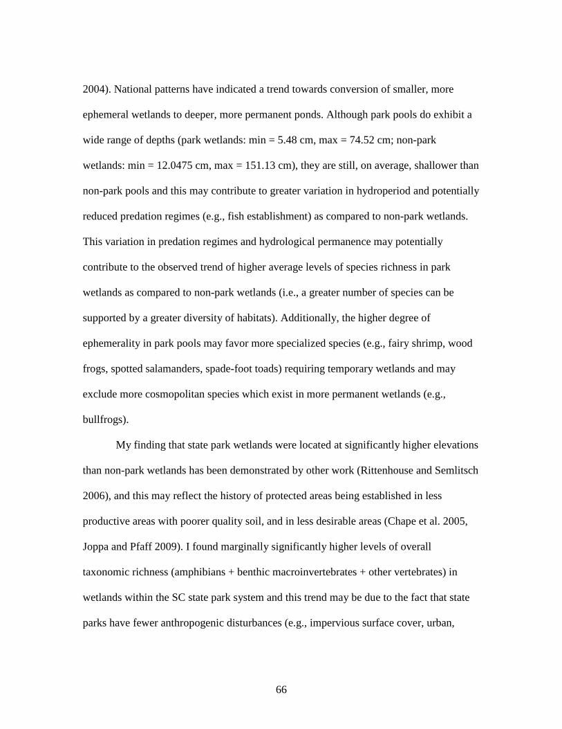
66
2004). National patterns have indicated a trend towards conversion of smaller, more
ephemeral wetlands to deeper, more permanent ponds. Although park pools do exhibit a
wide range of depths (park wetlands: min = 5.48 cm, max = 74.52 cm; non-park
wetlands: min = 12.0475 cm, max = 151.13 cm), they are still, on average, shallower than
non-park pools and this may contribute to greater variation in hydroperiod and potentially
reduced predation regimes (e.g., fish establishment) as compared to non-park wetlands.
This variation in predation regimes and hydrological permanence may potentially
contribute to the observed trend of higher average levels of species richness in park
wetlands as compared to non-park wetlands (i.e., a greater number of species can be
supported by a greater diversity of habitats). Additionally, the higher degree of
ephemerality in park pools may favor more specialized species (e.g., fairy shrimp, wood
frogs, spotted salamanders, spade-foot toads) requiring temporary wetlands and may
exclude more cosmopolitan species which exist in more permanent wetlands (e.g.,
bullfrogs).
My finding that state park wetlands were located at significantly higher elevations
than non-park wetlands has been demonstrated by other work (Rittenhouse and Semlitsch
2006), and this may reflect the history of protected areas being established in less
productive areas with poorer quality soil, and in less desirable areas (Chape et al. 2005,
Joppa and Pfaff 2009). I found marginally significantly higher levels of overall
taxonomic richness (amphibians + benthic macroinvertebrates + other vertebrates) in
wetlands within the SC state park system and this trend may be due to the fact that state
parks have fewer anthropogenic disturbances (e.g., impervious surface cover, urban,

67
suburban and exurban areas) and less movement barriers for many different taxonomic
groups inhabiting these parks. Although these results were only marginally significant at
an adjusted alpha = 0.0033, I believe this is close enough to my adjusted alpha level to
indicate importance. State parks may be actively managed for exotic or invasive species
and protected, to a certain degree, from such ecological challenges that could potentially
impact native populations inhabiting park wetlands (Houlahan and Findlay 2004, Barber
et al. 2012, Porter-Bolland et al. 2012). Small wetlands are difficult to locate using freely-
available remote sensing data and challenging to conserve because they are so dynamic
across space and time; therefore, a practical conservation approach may be to protect
large tracts of land (i.e., state parks and other protected areas) with the hopes that
multiple isolated and/or ephemeral wetlands and the connectivity between these wetlands
will be maintained within this protected area (Anderson and Ferree 2010). Although not
tested, I did observe a trend of higher levels of hydrological connectivity in wetlands
within state parks. These higher levels of connectivity within parks may contribute, in
part, to the maintenance of higher levels of overall taxonomic richness in these areas
(Meffe and Vrijenhoek 1988, Fagan 2002). Higher levels of hydrological connectivity
may allow more opportunities for movement and dispersal along both ephemeral and
permanent stream networks, providing a safer alternative to crossing roads (Fahrig et al.
1995, Carr and Fahrig 2001, Cote et al. 2009). Furthermore, vehicle traffic in state parks
is much tightly regulated, compared to non-park areas, and may pose less of a threat to
migrating and dispersing wildlife.

68
While not significant, I found that lower mean turbidity levels were associated
with park wetlands as compared to non-park wetlands (Wilcoxon Rank-Sums test, X2 =
6.4313, p = 0.012). In other words, state parks wetlands may have marginally better
water quality in terms of turbidity as compared to wetlands outside the state park system.
High levels of turbidity are known to negatively impact breeding amphibians (Brodman
et al. 2003, Boucher et al. 2013, Reyers 2013), benthic macroinvertebrates (Carls and
Ludeke 1984, Piquer-Rodríguez et al. 2012), fish (Petrosillo et al. 2010, Grebner et al.
2013) and other biota that reside in aquatic systems (Schmitz et al. 2012, Troupin and
Carmel 2014). Agricultural land use and development are strongly associated with
increased levels of turbidity and suspended solids in surrounding bodies of water (Shafer
2004, Riley et al. 2005) and it is possible that the overall lack of development within state
park boundaries may contribute to lower levels of turbidity and better water quality in
general. Furthermore, I observed marginally lower mean tolerance values for benthic
macroinvertebrate assemblages from wetlands within state parks; this may also support
the idea that aquatic systems within state parks have better water quality than those
waters that are outside of park boundaries, as lower tolerance values are generally
indicative of better water quality (Zube 1995). These findings suggest that state parks are
successful at maintaining higher levels of water quality and more sensitive assemblages
of aquatic organisms within park boundaries.
The local ecological knowledge and cooperation of state park personnel was
essential to the success of this study for both logistical and ecological reasons and I
believe that these parks may be essential to the future of small wetland conservation. SC

69
state parks and personnel made large contributions to the sample size (46.34%) of my
study. Because of their local ecological knowledge and careful attention to wetlands
across space and time I was able to find a number of wetlands that were well off the
beaten path. When planning or conducting ecological studies, negotiating with private
landowners can be challenging for a number of reasons including communication lapses,
road access problems, and privacy concerns. In contrast, state parks are conducive to
ecological studies because these parks are typically closed to the general public after dark
and are less exposed to local disturbance and intervention by outside sources (e.g.,
tampering with equipment, data loggers, etc) (Hurlbert 1984). Lower levels of outside
interference will almost certainly help researchers collect better, more consistent data and
reduce tampering and theft issues. In many SC state parks, rangers live full time on or
directly adjacent to park grounds and are often the first ones to note or be aware of major
changes in habitats (e.g., dam removals, flooding, drying, or major phenological events).
Occasionally, park personnel would update me on wetland conditions (e.g., frozen ponds,
amphibian calling) which allowed me to more wisely utilize resources in deciding which
sites to check first for amphibian breeding activity and to subsequently sample.
I also encountered the general public at various points during our sampling of
state park wetlands and this provided an opportunity for interaction, education and
meaningful dialogue between researchers and citizens regarding the importance of
isolated and/or ephemeral wetlands in the Blue Ridge and Piedmont ecoregions of SC.
These types of positive interactions help send a positive message to the public regarding
the state parks system’s important role in conserving specific habitats and the biotic

70
communities that rely on these habitats. These researcher-citizen interactions also
allowed for an opportunity for the general public to become educated about the value of
wetlands and we believe local interactions such as these can potentially help facilitate a
change in local public perception of wetland ecosystems and their importance (Wyatt and
Silman 2010). Although the role of state park personnel was critical to this project, I
recognize the practical limitations that are associated with the time and resource
constraints of state park employees. Park personnel are often busy with a multitude of
projects and may be unable to fulfill the additional role of locating cryptic ecosystems
that are, at times, well off the beaten path. This highlights the importance of collaborative
efforts among state parks, private landowners, NGOs and other stakeholders to take
advantage of parks as a priori conservation networks and to help ensure that important
habitats and ecosystems in parks do not go undocumented.
Other research has demonstrated the importance of the larger-scale, national park
system for conserving biodiversity in the southeastern US (Rodrigues et al. 2004b, Locke
and Dearden 2005, Stoll-Kleemann 2010). Furthermore, the national park system has
been termed ‘America’s longest standing conservation system,’ which emphasizes the
importance of utilizing public, protected lands for conservation efforts, particularly in the
species-rich, highly-endemic biotic communities of the southeastern US (Locke and
Dearden 2005). I suggest that by focusing on and incorporating smaller-scale, state parks
into large-scale conservation plans involving national parks (e.g., Great Smoky Mountain
National Park, Southeast Region Landscape Conservation Cooperative) and the
surrounding matrix of multi-use lands, biodiversity can be better conserved across a

71
range of spatial scales and reserve sizes (USGS 2014). This range of conservation, from
the local to the regional scale, will help conserve a variety of habitats that are important
to a number of ecological communities throughout the central southeast.
Although the importance of parks and protected areas is well established for their
role in landscape conservation, they are also vulnerable to activities occurring outside of
park boundaries (Kellert et al. 2000, Leverington et al. 2010, Stoll-Kleemann 2010,
Hansen et al. 2011). Other work has demonstrated that areas adjacent to parks and
protected areas actually attract human development as a result of the natural amenities
found in these areas (Zedler 2003, Rodrigues et al. 2004a, Maiorano et al. 2006, Hansen
et al. 2011). This development pressure, occurring at the urban-wildland interface and
other exurban land uses were the most rapidly-growing type of land use in the US from
1950-2000 (Rodrigues et al. 2004a, Brown et al. 2005). Consequently, the development
pressures in areas adjacent to parks may threaten the integrity of parks and other
protected areas and effective conservation of these areas and the habitats they contain is
paramount (Hayes 2006). Parks and other protected lands are influenced by and rely upon
processes occurring at landscape and regional scales; therefore, the main challenge for
parks is to maintain ecological integrity of protected areas in the face of ongoing
development and external pressures (Eken et al. 2004, Hayes 2006).
Relatively little research has evaluated the conservation value or biodiversity of
state parks in the US. What information exists is likely contained in internal documents
such as technical reports and other works that may not make it to peer-review or the
general public. To my knowledge, this project provides the first published comparison of
72
aquatic diversity of small and/or ephemeral wetlands in state parks compared to those
resources outside of state parks in the upper Piedmont and lower Blue Ridge ecoregions
of the southeastern US. Additionally I provide a model, using the SC state park system as
a case study, for identifying and conserving a cryptic ecosystem and under-protected
habitats as well as the myriad of species that utilizes them throughout the year. This study
demonstrates that local scale protected areas, such as state parks, may have considerable
conservation benefit for local scale ecosystems such as small, ephemeral wetlands.

73
APPENDICES

74
Appendix A
All Environmental Variables Collected
Variable Mean Standard Dev. Min Max Representative Depth (cm) 13.98 8.221 2.5 36.43 Deepest Depth (cm) 31.50 30.70 5.48 151.13 Pool Canopy Cover (%) 63.23 27.00 0 100.0 5m Canopy Cover (%) 73.29 14.94 19.43 90.67 Pool Area (m2) 371.6 714.3 2.905 3542.143 Chlorophyll (µg/L) 5.77 8.73 0.164 41.17 Total Coliform (MPN) 1518.28 765.23 1 2500 E. coli (MPN) 135.20 339.90 0 1683.2 Oxidative Reduction Potential (mV)
147.90 27.32 72.5 189.167
Dissolved Oxygen (%) 63.86 18.96 27.7 95.933 Turbidity (NTU) 23.59 19.36 4.733 89.3 Conductivity (ms/cm) 0.041 0.037 0.016 0.214 Temperature (°C) 10.96 1.70 5.55 14.31 pH 6.37 0.323 5.76 6.96 Hydroperiod (weeks) 28.41 9.604 4.5 52 Distance to nearest body of water (m)
128.27 153.07 1 562.9
Distance to nearest road (m) 211.96 283.55 1 1399.4 Distance to nearest known wetland (m)
1659.41 1561.11 32.3 6065.3
Open water area 250 m (%) 1.69 4.55 0 19.09 Disturbed/successional area 250 m
13.61 12.19 0 42.27
Pastureland area 250 m 2.25 5.06 0 17.74 Cultivated area 250 m 0 0 0 0 Forested area 250 m 81.48 18.25 25.45 100.0 Low-density development area 250 m
0.971 3.442 0 18.72
High-density development area 250 m
0 0 0 0
Open water area 500 m 1.83 4.34 0 17.69 Disturbed/successional area 500 m
9.31 8.12 0 32.87
Pasture area 500 m 2.77 6.27 0 33.45 Cultivated area 500 m 0 0 0 0 Forested area at 500 m 84.84 17.29 21.00 100.0 Low-density development area 1.197 4.117 0 21.95

75
500 m High-density development 500 m 0.064 0.411 0 2.635 Open water 1 km 2.040 3.656 0 17.317 Disturbed/successional area 1 km 7.550 6.287 0 22.315 Pasture area 1 km 2.454 5.282 0 31.57 Cultivated area 1 km 0.366 2.267 0 14.52 Forested area 1 km 86.63 13.89 37.72 100.0 Low-density development area 1 km
0.919 2.805 0 12.60
High-density development area 1 km
0.043 0.268 0 1.72
Hist open water 250 m 0.27 1.25 0 7.05 Hist disturbed/successional area 250 m
7.86 14.800 0 65.66
Hist pasture area 250 m 2.21 7.63 0 38.63 Hist cultivated area 250 m 2.91 9.11 0 54.81 Hist forested area 250 m 86.62 21.27 5.91 100.0 Hist low-density development area 250 m
0.12 0.55 0 3.51
Hist high-density development area 250 m
0 0 0 0
Hist open water 500 m 0.868 3.356 0 15.62 Hist disturbed/successional area 500 m
6.73 13.13 0 61.29
Hist pasture area 500 m 1.33 3.10 0 15.10 Hist cultivated area 500 m 4.63 8.91 0 41.27 Hist forested area 500 m 86.38 21.22 17.13 100.0 Hist low-density development area 500 m
0.057 0.010 0 0.478
Hist high-density development area 500 m
0 0 0 0
Hist open water 1 km 0.9157 2.34 0 10.78 Hist disturbed/successional area 1 km
5.41 9.98 0 39.83
Hist pasture area 1 km 1.57 2.53 0 9.80 Hist cultivated area 1 km 5.45 7.76 0 29.18 Hist forested area 1 km 86.30 18.63 0 100.0 Hist low-density development area 1 km
0.359 1.726 0 11.1
Hist high-density development area 1 km
0.0002 0.0015 0 0.0099

76
Appendix B
Model Averaging Table for Wood Frogs
Model # Variable Coefficient (±SE) Odds Ratio
1 DO 0.089415746 (± 0.003573) 0.916644096
1 Turbidity -1.029381875 (± 0.03917) 2.702469542
1 HistFor500 0.000005487 (± 6.0787E-06) 1.000015313
1 HistFor1000 -1.661567E-07 (± 6.8847E-07) 1.000000935
1 Parasites 0.124201105 (± 0.10289) 0.978907025
2 DO 0.089415746 (± 0.003573) 0.917938394
2 HistFor500 0.000005487 (± 6.0787E-06) 1.00000133
3 DO 0.07941 (± 0.003573) 0.923661146
3 HistFor500 0.000013769 (± 6.04863E-06) 0.999986231
3 HistFor1000 1.2075E-06 (± 6.88461E-07) 0.999998793
4 DO 0.09602 (± 0.003573) 0.908441823
4 Turbidity -0.96339 (± 0.039166) 2.620430193
4 Parasites 0.2271 (± 0.102882) 0.796854162
4 HistFor500 0.00001663 (± 6.07863E-06) 0.999983367
5 DO 0.0989833 (± 0.003573) 0.905757834
5 Turbidity -1.141978 (± 0.039166) 2.767781232
5 Temp -0.43876 1.550783055
5 Parasites 0.025467 (± 0.10288) 0.796854162
5 HistFor500 0.000013676 (± 6.88461E-06) 0.999998793

77
Appendix C
Model Averaging Table for Spotted Salamanders
Model # Variable Coefficient (± SE) Odds Ratio
1 Invert Richness 0.14396 (± 0.01941) 0.865922384
1 Depth 1.87944 (± 1.26281) 0.15267558
1 Area -0.0124 (± 0.003587) 1.012471124
1 Filterers -0.0091 (± 0.001903) 1.009141531
1 Dist to Wetland -0.0015707 NA
1 Dist to Road 0.005787 NA
1 Hist Open 250 -19.664873 (± 0.080514) 347013069
1 Hist Cult 500 0.0001452 (± 0.000105) 0.999854811
2 Invert RIchness 0.10514 (± 0.01941) 0.900198486
2 Depth -0.64618 (± 1.26281) 1.908237421
2 Area -0.00522 (± 0.003587) 1.005233648
2 Hist Open 250 -19.8259 (± 0.080514) 407642042.3
2 Hist Cult 500 0.00006413 (± 0.0001050) 0.999935872

78
REFERENCES
2012. R: A language and environment for statistical computing.in R. D. C. Team, editor. R Foundation for statistical computing, Vienna, Austria.
2014. SWANCC Decision.in L. Stetson, editor. Protection the Nation's Wetlands. Association of State Wetland Managers, Windham, ME, USA.
Abell, R., J. D. Allan, and B. Lehner. 2007. Unlocking the potential of protected areas for freshwaters. Biological Conservation 134:48-63.
AmphibiaWeb. 2014. Information on amphibian biology and conservation. AmphibiaWeb, Berkley, California.
Anderson, M. G. and C. E. Ferree. 2010. Conserving the Stage: Climate Change and the Geophysical Underpinnings of Species Diversity. Plos One 5.
Babbitt, K. J. 2005. The relative importance of wetland size and hydroperiod for amphibians in southern New Hampshire, USA. Wetlands Ecology and Management 13:269-279.
Babbitt, K. J., M. J. Baber, and T. L. Tarr. 2003. Patterns of larval amphibian distribution along a wetland hydroperiod gradient. Canadian Journal of Zoology 81:1539-1552.
Baber, M. J., E. Fleishman, K. J. Babbitt, and T. L. Tarr. 2004. The relationship between wetland hydroperiod and nestedness patterns in assemblages of larval amphibians and predatory macroinvertebrates. Oikos 107:16-27.
Baldwin, R. F., A. J. K. Calhoun, and P. G. DeMaynadier. 2006a. Conservation planning for amphibian species with complex habitat requirements: a case study using movements and habitat selection of the wood frog Rana sylvatica. Journal of Herpetology 40:442-453.
Baldwin, R. F., A. J. K. Calhoun, and P. G. deMaynadier. 2006b. The significance of hydroperiod and stand maturity for pool-breeding amphibians in forested landscapes. Canadian Journal of Zoology 84:1604-1615.
Barber, C. P., M. A. Cochrane, C. Souza, and A. Verissimo. 2012. Dynamic performance assessment of protected areas. Biological Conservation 149:6-14.
Barbour, M. T., J. Gerritsen, B. D. Snyder, and J. B. Stribling. 1999. Rapid bioassessment protocols for use in streams and wadeable rivers: periphyton, benthic macroinvertebrates and fish. United States Environmental Protection Agency, Washington D.C., USA.
Batzer, D. P., B. J. Palik, and R. Buech. 2004. Relationships between environmental characteristics and macroinvertebrate communities in seasonal woodland ponds of Minnesota. Journal of the North American Benthological Society 23:50-68.
Bedford, B. L. and K. S. Godwin. 2003. Fens of the United States: Distribution, characteristics, and scientific connection versus legal isolation. Wetlands 23:608-629.
Bellemare, J., G. Motzkin, and D. R. Foster. 2002. Legacies of the agricultural past in the forested present: an assessment of historical land‐use effects on rich mesic forests. Journal of Biogeography 29:1401-1420.

79
Benoy, G. A. 2008. Tiger salamanders in prairie potholes: A "fish in amphibian's garments?". Wetlands 28:464-472.
Bergstrom, J. C., H. K. Cordell, A. E. Watson, and G. A. Ashley. 1990. Economic impacts of state parks on state economies in the South. Southern Journal of Agricultural Economics 22.
Berven, K. A. 2009. Density dependence in the terrestrial stage of wood frogs: evidence from a 21-year population study. Copeia:328-338.
Berven, K. A. and T. A. Grudzien. 1990. Dispersal in the wood frog (Rana sylvativa) - implications for genetic population structure. Evolution 44:2047-2056.
Bischof, M. M., M. A. Hanson, M. R. Fulton, R. K. Kolka, S. D. Sebestyen, and M. G. Butler. 2013. Invertebrate community patterns in seasonal ponds in Minnesota, USA: response to hydrologic and environmental variability. Wetlands 33:245-256.
Bishop, K., A. Phillips, and L. Warren. 1995. Protected for ever?: Factors shaping the future of protected areas policy. Land use policy 12:291-305.
Black, A. E., E. Strand, R. G. Wright, J. M. Scott, P. Morgan, and C. Watson. 1998. Land use history at multiple scales: implications for conservation planning. Landscape and Urban Planning 43:49-63.
Boitani, L., R. M. Cowling, H. T. Dublin, G. M. Mace, J. Parrish, H. P. Possingham, R. L. Pressey, C. Rondinini, and K. A. Wilson. 2008. Change the IUCN protected area categories to reflect biodiversity outcomes. Plos Biology 6:436-438.
Bolgiano, C. 1998. The Appalachian forest: a search for roots and renewal. Stackpole Books.
Borgström, S., S. A. O. Cousins, and R. Lindborg. 2012. Outside the boundary – Land use changes in the surroundings of urban nature reserves. Applied Geography 32:350-359.
Boucher, T. M., M. Spalding, and C. Revenga. 2013. Role and Trends of Protected Areas in Conservation. Pages 485-503 in S. A. Levin, editor. Encyclopedia of Biodiversity (Second Edition). Academic Press, Waltham.
Bridges, A. S. and M. E. Dorcas. 2000. Temporal variation in anuran calling behavior: Implications for surveys and monitoring programs. Copeia:587-592.
Brodman, R., J. Ogger, T. Bogard, A. J. Long, R. A. Pulver, K. Mancuso, and D. Falk. 2003. Multivariate analyses of the influences of water chemistry and habitat parameters on the abundances of pond-breeding amphibians. Journal of Freshwater Ecology 18:425-436.
Brooks, R. T. 2000. Annual and seasonal variation and the effects of hydroperiod on benthic macroinvertebrates of seasonal forest ("vernal") ponds in central Massachusetts, USA. Wetlands 20:707-715.
Brooks, R. T. and M. Hayashi. 2002. Depth-area-volume and hydroperiod relationships of ephemeral (vernal) forest pools in southern New England. Wetlands 22:247-255.
Brown, D. G., K. M. Johnson, T. R. Loveland, and D. M. Theobald. 2005. Rural land-use trends in the conterminous United States, 1950-2000. Pages 1851-1863. Ecological Soc Amer.

80
Burne, M. R. and R. G. Lathrop, Jr. 2007. Remote and field identification of vernal pools. Crc Press-Taylor & Francis Group, 6000 Broken Sound Parkway Nw, Ste 300, Boca Raton, Fl 33487-2742 USA.
Burnham, K. and D. Anderson. 2004. Multimodal inference: understanding AIC and BIC in model selection. Sociological Methods & Research 33
261-304. Buskirk, J. V. 2005. Local and landscape influence on amphibian occurence and
abundance. Ecology 86:1936-1947. Calhoun, A. J. K., T. E. Walls, S. S. Stockwell, and M. McCollough. 2003. Evaluating
vernal pools as a basis for conservation strategies: A maine case study. Wetlands 23:70-81.
Callaham, M. A., D.D. Richter, D. C. Coleman, and M. Hofmockel. 2006. Long-term land-use effects on soil invertebrate communities in southern Piedmont soils, USA. European Journal of Soil Biology 42:S150-S156.
Carls, E. G. and A. K. Ludeke. 1984. State park contributions to natural area protection in Texas, USA. Biological Conservation 28:95-110.
Carr, L. W. and L. Fahrig. 2001. Effect of road traffic on two amphibian species of differing vagility. Conservation Biology 15:1071-1078.
Chape, S., J. Harrison, M. Spalding, and I. Lysenko. 2005. Measuring the extent and effectiveness of protected areas as an indicator for meeting global biodiversity targets. Philosophical Transactions of the Royal Society B-Biological Sciences 360:443-455.
Clewell, A. F. and R. Lea. 1989. Creation and restoration of forested wetland vegetation in the southeastern United States. Wetland creation and restoration: The status of the science 1:3-89.
Colon-Gaud, C., M. R. Whiles, S. S. Kilham, K. R. Lips, C. M. Pringle, S. Connelly, and S. D. Peterson. 2009. Assessing ecological responses to catastrophic amphibian declines: Patterns of macroinvertebrate production and food web structure in upland Panamanian streams. Limnology and Oceanography 54:331-343.
Conant, R. and J. T. Collins. 1991. The Peterson field guide series: A field guide to reptiles and amphibians of eastern and central North America - Third Edition.
Connette, G. M. and R. D. Semlitsch. 2013. Life history as a predictor of salamander recovery rate from timber harvest in southern appalachian forests, U.S.A. Conservation Biology 27:1399-1409.
Cordell, H. K., J. C. Bergstrom, and A. E. Watson. 1992. Economic-growth and interdependence effects of state park visitation in local and state economies. Journal of Leisure Research 24:253-268.
Correa-Araneda, F. J., J. Urrutia, Y. Soto-Mora, R. Figueroa, and E. Hauenstein. 2012. Effects of the hydroperiod on the vegetative and community structure of freshwater forested wetlands, Chile. Journal of Freshwater Ecology 27:459-470.
Cote, D., D. G. Kehler, C. Bourne, and Y. F. Wiersma. 2009. A new measure of longitudinal connectivity for stream networks. Landscape Ecology 24:101-113.
Cowdrey, A. E. 1995. This Land, This South: An Environmental History. Revised edition. The University of Kentucky Press.

81
Cowell, C. M. 1998. Historical change in vegetation and disturbance on the Georgia Piedmont. American Midland Naturalist 140:78-89.
Cox, J. L. 2005. The history of cotton. The Donning Company, Virginia Beach, Virginia. Cox, T. R. 1988. The park builders: a history of state parks in the Pacific northwest. Univ
of Washington Press. Davic, R. D. and H. H. Welsh. 2004. On the ecological roles of salamanders. Annual
Review of Ecology Evolution and Systematics 35:405-434. De Wet, A. P., J. Richardson, and C. Olympia. 1998. Interactions of land-use history and
current ecology in a recovering "urban wildland". Urban Ecosystems 2:237-262. Delcourt, H. R. and P. A. Delcourt. 1997. Pre-Columbian Native American use of fire on
southern Appalachian landscapes. Conservation Biology 11:1010-1014. Denevan, W. M. 1992. The pristine myth - the landscape of the America in 1492. Annals
of the Association of American Geographers 82:369-385. Denoel, M. and A. Lehmann. 2006. Multi-scale effect of landscape processes and habitat
quality on newt abundance: Implications for conservation. Biological Conservation 130:495-504.
Desmond, J. S., D. H. Deutschman, and J. B. Zedler. 2002. Spatial and temporal variation in estuarine fish and invertebrate assemblages: Analysis of an 11-year data set. Estuaries 25:552-569.
Dewi, S., M. van Noordwijk, A. Ekadinata, and J.-L. Pfund. 2013. Protected areas within multifunctional landscapes: Squeezing out intermediate land use intensities in the tropics? Land use policy 30:38-56.
Donohue, K., D. R. Foster, and G. Motzkin. 2000. Effects of the past and present on species distribution: land-use history and demography of wintergreen. Journal of Ecology 88:303-316.
Dotterweich, M. 2013. The history of human-induced soil erosion: Geomorphic legacies, early descriptions and research, and the development of soil conservation-A global synopsis. Geomorphology 201:1-34.
Downing, D. M., C. Winer, and L. D. Wood. 2003. Navigating through Clean Water Act jurisdiction: a legal review. Wetlands 23:475-493.
Dupouey, J.-L., E. Dambrine, J.-D. Laffite, and C. Moares. 2002. Irreversible impact of past land use on forest soils and biodiversity. Ecology 83:2978-2984.
Dutra, S. L. and M. Callisto. 2005. Macroinvertebrates as tadpole food: importance and body size relationships. Revista Brasileira De Zoologia 22:923-927.
Eaton, L. E. and D. R. Lenat. 1991. Comparison of a rapid bioassessment method with North Carolina's qualitative macroinvertebrate collection method. Journal of the North American Benthological Society 10:335-338.
Egan, D. and E. Howell. 2001. The historical ecology handbook: a restorationists guide to reference ecosystems. Island Press.
Egan, R. and P. Paton. 2004. Within-pond parameters affecting oviposition by wood frogs and spotted salamanders. Wetlands 24:1-13.
Eken, G., L. Bennun, T. M. Brooks, W. Darwall, L. D. C. Fishpool, M. Foster, D. Knox, P. Langhammer, P. Matiku, E. Radford, P. Salaman, W. Sechrest, M. L. Smith, S.

82
Spector, and A. Tordoff. 2004. Key biodiversity areas as site conservation targets. BioScience 54:1110-1118.
Engeman, R. M., A. Stevens, J. Allen, J. Dunlap, M. Daniel, D. Teague, and B. Constantin. 2007. Feral swine management for conservation of an imperiled wetland habitat: Florida’s vanishing seepage slopes. Biological Conservation 134:440-446.
ESRI. 2011. ArcGIS Desktop: Release 10. Environmental Systems Research Institute, Redlands, CA, USA.
Estes, J. A., J. Terborgh, J. S. Brashares, M. E. Power, J. Berger, W. J. Bond, S. R. Carpenter, T. E. Essington, R. D. Holt, J. B. C. Jackson, R. J. Marquis, L. Oksanen, T. Oksanen, R. T. Paine, E. K. Pikitch, W. J. Ripple, S. A. Sandin, M. Scheffer, T. W. Schoener, J. B. Shurin, A. R. E. Sinclair, M. E. Soule, R. Virtanen, and D. A. Wardle. 2011. Trophic Downgrading of Planet Earth. Science 333:301-306.
Evans, D. O., K. H. Nicholls, Y. C. Allen, and M. J. McMurtry. 1996. Historical land use, phosphorus loading, and loss of fish habitat in Lake Simcoe, Canada. Canadian Journal of Fisheries and Aquatic Sciences 53:194-218.
Faccio, S. D. 2003. Postbreeding emigration and habitat use by Jefferson and Spotted salamanders in Vermont. Journal of Herpetology 37:479-489.
Fagan, W. F. 2002. Connectivity, fragmentation, and extinction risk in dendritic metapopulations. Ecology 83:3243-3249.
Fahrig, L., J. H. Pedlar, S. E. Pope, P. D. Taylor, and J. F. Wegner. 1995. Effect of road density on amphibian density. Biological Conservation 73:177-182.
Fairbairn, S. E. and J. J. Dinsmore. 2001. Local and landscape-level influences on wetland bird communities of the prairie pothole region of Iowa, USA. Wetlands 21:41-47.
Falkengren-Grerup, U., D.-J. t. Brink, and J. Brunet. 2006. Land use effects on soil N, P, C and pH persist over 40–80 years of forest growth on agricultural soils. Forest Ecology and Management 225:74-81.
Fetcher, A. and V. Fellows. 2011. Five-year survey shows wetland losses are slowing, marking conservation gains and need for continued investing in habitat U.S. Department of the Interior, Washington, D.C., USA.
Ficetola, G. F. and F. De Bernardi. 2004. Amphibians in a human-dominated landscape: the community structure is related to habitat features and isolation. Biological Conservation 119:219-230.
Figueroa, E. and J. Aronson. 2006. New linkages for protected areas: Making them worth conserving and restoring. Journal for Nature Conservation 14:225-232.
Findlay, C. and J. Houlahan. 1997. Anthropogenic correlates of species richness in southeasrn Ontario wetlands. Conservation Biology 11:1000-1009.
Flinn, K. M. and M. Vellend. 2005. Recovery of forest plant communities in post-agricultural landscapes. Frontiers in Ecology and the Environment 3:243-250.
Ford, W. M., R. H. Odom, P. E. Hale, and B. R. Chapman. 2000. Stand-age, stand characteristics, and landform effects on understory herbaceous communities in southern Appalachian cove-hardwoods. Biological Conservation 93:237-246.

83
Foster, D., F. Swanson, J. Aber, I. Burke, N. Brokaw, D. Tilman, and A. Knapp. 2003. The importance of land-use legacies in ecology and conservation. BioScience 53:77-88.
Foster, D. F. 1992. Land-use history (1730-1990) and vegetation dynamics in central New England, USA. The Journal of Ecology 80:753-771.
Foster, D. R. and J. D. Aber. 2004. Forests in Time: The Environmental Consequences of 1,000 Years of Change in New England. Yale University Press, New Haven.
Gamble, L., K. McGarigal, and B. Compton. 2007. Fidelity and dispersal in the pond-breeding amphibian, Ambystoma opacum: implications for spatio-temporal population dynamics and conservation. Biological Conservation 139:247-257.
Gamble, L. R. 2004. Landscape-level population structure and local variability in marbled salamanders (Ambystoma opacum) of western Massachusetts: applied lessons from metapopulation theory. University of Massachusetts at Amherst.
Gaston, K. J., K. Charman, S. F. Jackson, P. R. Armsworth, A. Bonn, R. A. Briers, C. S. Q. Callaghan, R. Catchpole, J. Hopkins, W. E. Kunin, J. Latham, P. Opdam, R. Stoneman, D. A. Stroud, and R. Tratt. 2006. The ecological effectiveness of protected areas: The United Kingdom. Biological Conservation 132:76-87.
Gibbons, J. W. 2003. Terrestrial habitat: A vital component for herpetofauna of isolated wetlands. Wetlands 23:630-635.
Gibbons, J. W., C. T. Winne, D. E. Scott, J. D. Willson, X. Glaudas, K. M. Andrews, B. D. Todd, L. A. Fedewa, L. Wilkinson, R. N. Tsaliagos, S. J. Harper, J. L. Greene, T. D. Tuberville, B. S. Metts, M. E. Dorcast, J. P. Nestor, C. A. Young, T. Akre, R. N. Reed, K. A. Buhlmann, J. Norman, D. A. Croshaw, C. Hagen, and B. B. Rothermel. 2006. Remarkable amphibian biomass and abundance in an isolated wetland: Implications for wetland conservation. Conservation Biology 20:1457-1465.
Gibbs, J. P. 1993. Importance of small wetlands for the persistence of local populations of wetland-associated animals Wetlands 13:25-31.
Gibbs, J. P. 1998. Amphibian movements in response to forest edges, roads and streambeds in southern New England. Journal of Wildlife Management 62:584-589.
Glitzenstein, J. S., C. D. Canham, M. J. McDonnell, and D. R. Streng. 1990. Effects of environment and land-use history on upland forests of the Cary-Arboretum, Hudson Valley, New York. Bulletin of the Torrey Botanical Club 117:106-122.
Goodale, C. L. and J. D. Aber. 2001. The long-term effects of land-use history on nitrogen cycling in northern hardwood forests. Ecological Applications 11:253-267.
Grebner, D. L., P. Bettinger, and J. P. Siry. 2013. Chapter 7 - Forest Recreation. Pages 167-189 in D. L. Grebner, P. Bettinger, and J. P. Siry, editors. Introduction to Forestry and Natural Resources. Academic Press, San Diego.
Groom, M. J., G. K. Meffe, and C. R. Carroll. 2006. Principles of conservation biology. Sinauer Associates Sunderland.

84
Guerry, A. D. and M. L. Hunter. 2002. Amphibian distributions in a landscape of forests and agriculture: an examination of landscape composition and configuration. Conservation Biology 16:745-754.
Gustavsson, E., T. Lennartsson, and M. Emanuelsson. 2007. Land use more than 200 years ago explains current grassland plant diversity in a Swedish agricultural landscape. Biological Conservation 138:47-59.
Hall, B., G. Motzkin, D. R. Foster, M. Syfert, and J. Burk. 2002. Three hundred years of forest and land-use change in Massachusetts, USA. Journal of Biogeography 29:1319-1335.
Hamin, E. M. 2001. The US National Park Service's partnership parks: collaborative responses to middle landscapes. Land use policy 18:123-135.
Hansen, A. J., C. R. Davis, N. Piekielek, J. Gross, D. M. Theobald, S. Goetz, F. Melton, and R. DeFries. 2011. Delineating the ecosystems containing protected areas for monitoring and management. BioScience 61:363-373.
Harding, J. S., E. F. Benfield, P. V. Bolstad, G. S. Helfman, and E. B. D. Jones. 1998. Stream biodiversity: the ghost of land use past. Proceedings of the National Academy of Sciences 95:14843-14847.
Hayes Jr., J. 2001. South Carolina and the New Deal. The University of South Carolina Press, Columbia, South Carolina.
Hayes, T. M. 2006. Parks, people, and forest protection: An institutional assessment of the effectiveness of protected areas. World Development 34:2064-2075.
Hecnar, S. J. and R. T. McLoskey. 1996. Regional dynamics and the status of amphibians. Ecology 77:2091-2097.
Hecnar, S. J. and R. T. McLoskey. 1998. Species richness patterns of amphibians in southwestern Ontario ponds. Journal of Biogeography 25:763-772.
Hentges, V. A. and T. W. Stewart. 2010. Macroinvertebrate Assemblages in Iowa Prairie Pothole Wetlands and Relation to Environmental Features. Wetlands 30:501-511.
Hermy, M. and K. Verheyen. 2007. Legacies of the past in the present-day forest biodiversity: a review of past land-use effects on forest plant species composition and diversity. Pages 361-371 Sustainability and Diversity of Forest Ecosystems. Springer.
Herrmann, H., K. Babbitt, M. Baber, and R. Congalton. 2005a. Effects of landscape characteristics on amphibian distribution in a forest-dominated landscape. Biological Conservation 123:139-149.
Herrmann, H. L., K. J. Babbitt, M. J. Baber, and R. G. Congalton. 2005b. Effects of landscape characteristics on amphibian distribution in a forest-dominated landscape. Biological Conservation 123:139-149.
Holomuzki, J. R., J. P. Collins, and P. E. Brunkow. 1994. Trophic control of fishless ponds by tiger salamander larvae. Oikos 71:55-64.
Homan, R. N., B. S. Windmiller, and J. M. Reed. 2004. Critical thresholds associated with habitat loss for two vernal pool-breeding amphibians. Ecological Applications 14:1547-1553.

85
Hook, D. D., W. H. McKee, T. M. Williams, S. Jones, D. V. Blaricom, and J. Parsons. 1994. Hydrologic and wetland characteristics of a piedmont bottom in South Carolina. Water, Air and Soil Pollution 77:293-320.
Horn, D. J., M. L. Phillips, R. R. Koford, W. R. Clark, M. A. Sovada, and R. J. Greenwood. 2005. Landscape composition, patch size, and distance to edges: Interactions affecting duck reproductive success. Ecological Applications 15:1367-1376.
Hossack, B. R., W. H. Lowe, and P. S. Corn. 2013. Rapid Increases and Time-Lagged Declines in Amphibian Occupancy after Wildfire. Conservation Biology 27:219-228.
Houlahan, J. and C. Findlay. 2004. Effect of invasive plant species on temperate wetland plant diversity. Conservation Biology 18:1132-1138.
Houlahan, J. E. and C. S. Findlay. 2003. The effects of adjacent land use on wetland amphibian species richness and community composition. Canadian Journal of Fisheries and Aquatic Sciences 60:1078-1094.
Howard, J. H., R. F. Baldwin, and B. L. Brown. 2012. Exploratory analysis for complex-life-cycle amphibians: Revealing complex forest-reproductive effort relationships using redundancy analysis. Forest Ecology and Management 270:175-182.
Huntington, T., R. Hooper, C. Johnson, B. Aulenbach, R. Cappellao, and A. Blum. 2000. Calcium depletion in a southeastern United States forest ecosystem. Soil Science of America Journal 64:1845-1858.
Hurlbert, S. H. 1984. Pseudoreplication and the design of ecological field experiments. Ecological Monographs 54:187-211.
Ibbe, M., P. Milberg, A. Tunér, and K.-O. Bergman. 2011. History matters: Impact of historical land use on butterfly diversity in clear-cuts in a boreal landscape. Forest Ecology and Management 261:1885-1891.
Imai, K., G. King, and O. Lau. 2008. Toward a common framework for statistical analysis and development. Journal of Computational and Graphical Statistics 17:892-913.
Johnston, C. A., D. M. Ghioca, M. Tulbure, B. L. Bedford, M. Bourdaghs, C. B. Frieswyk, L. Vaccaro, and J. B. Zedler. 2008. Partitioning vegetation response to anthropogenic stress to develop multi-taxa wetland indicators. Ecological Applications 18:983-1001.
Joppa, L. N. and A. Pfaff. 2009. High and Far: Biases in the Location of Protected Areas. Plos One 4.
Joyal, L. A., M. McCollough, and M. L. Hunter. 2001. Landscape ecology approaches to wetland species conservation: a case study of two turtle species in southern Maine. Conservation Biology 15:1755-1762.
Julian, J. P. and R. H. Gardner. 2014. Land cover effects on runoff patterns in eastern Piedmont (USA) watersheds. Hydrological Processes 28:1525-1538.
Kalisz, P. and D. Dotson. 1989. Land-use history and the occurrence of exotic earthworms in the mountains of eastern Kentucky. American Midland Naturalist:288-297.

86
Karraker, N. E. and J. P. Gibbs. 2009. Amphibian production in forested landscapes in relation to wetland hydroperiod: A case study of vernal pools and beaver ponds. Biological Conservation 142:2293-2302.
Kellert, S. R., J. N. Mehta, S. A. Ebbin, and L. L. Lichtenfeld. 2000. Community natural resource management: Promise, rhetoric, and reality. Society & Natural Resources 13:705-715.
Knutson, M. G., J. R. Sauer, D. A. Olsen, M. J. Mossman, L. M. Hemesath, and M. J. Lannoo. 1999. Effects of landscape composition and wetland fragmentation on frog and toad abundance and species richness in Iowa and Wisconsin, USA. Conservation Biology 13:1437-1446.
Koerner, W., J. Dupouey, E. Dambrine, and M. Benoit. 1997. Influence of past land use on the vegetation and soils of present day forest in the Vosges mountains, France. Journal of Ecology:351-358.
Kolozsvary, M. B. and R. K. Swihart. 1999. Habitat fragmentation and the distribution of amphibians: patch and landscape correlates in farmland. Canadian Journal of Zoology 77:1288-1299.
Korfel, C. A., W. J. Mitsch, T. E. Hetherington, and J. J. Mack. 2010. Hydrology, Physiochemistry, and Amphibians in Natural and Created Vernal Pool Wetlands. Restoration Ecology 18:843-854.
Kuussaari, M., R. Bommarco, R. K. Heikkinen, A. Helm, J. Krauss, R. Lindborg, E. Ockinger, M. Partel, J. Pino, F. Roda, C. Stefanescu, T. Teder, M. Zobel, and I. Steffan-Dewenter. 2009. Extinction debt: a challenge for biodiversity conservation. Trends in Ecology & Evolution 24:564-571.
Lathrop, R. G., P. Montesano, J. Tesauro, and B. Zarate. 2005. Statewide mapping and assessment of vernal pools: a New Jersey case study. Journal of Environmental Management 76:230-238.
Laurance, W. F., H. Koster, M. Grooten, A. B. Anderson, P. A. Zuidema, S. Zwick, R. J. Zagt, A. J. Lynam, M. Linkie, and N. P. R. Anten. 2012. Making conservation research more relevant for conservation practitioners. Biological Conservation 153:164-168.
Legendre, P., D. Borcard, and P. R. Peres-Neto. 2005. Analyzing beta diversity: partitioning the spatial variation of community composition data. Ecological Monographs 75:435-450.
Lehtinen, R. M., S. M. Galatowitsch, and J. R. Tester. 1999. Consequences of habitat loss and fragmentation for wetland amphibian assemblages. Wetlands 19:1-12.
Leibowitz, S. G. 2003. Isolated wetlands and their functions: an ecological perspective. Wetlands 23:517-531.
Leibowitz, S. G., P. J. Wigington, M. C. Rains, and D. M. Downing. 2008. Non-navigable streams and adjacent wetlands: addressing science needs following the Supreme Court's Rapanos decision. Frontiers in Ecology and the Environment 6:366-373.
Lenat, D. R. and M. T. Barbour. 1994. Using benthic macroinvertebrate community structure for rapid, cost-effective, water quality monitoring: rapid bioassessment.

87
Pages 187-216 in S. L. Loeb and A. Spacie, editors. Biological Monitoring of Aquatic Systems. CRC Press, Boca Raton, FL, USA.
Leroux, S. J., M. A. Krawchuk, F. Schmiegelow, S. G. Cumming, K. Lisgo, L. G. Anderson, and M. Petkova. 2010. Global protected areas and IUCN designations: Do the categories match the conditions? Biological Conservation 143:609-616.
Leverington, F., K. L. Costa, H. Pavese, A. Lisle, and M. Hockings. 2010. A Global Analysis of Protected Area Management Effectiveness. Environmental Management 46:685-698.
Lewis, D., G. B. Kaweche, and A. Mwenya. 1990. Wildlife conservation outside protected areas - lessons from an experiment in Zambia. Conservation Biology 4:171-180.
Li, J., D. d. Richter, A. Mendoza, and P. Heine. 2010. Effects of land-use history on soil spatial heterogeneity of macro- and trace elements in the Southern Piedmont USA. Geoderma 156:60-73.
Lobao, L. and K. Meyer. 2001. The great agricultural transition: Crisis, change and social consequences of twentieth century US farming. Annual Review of Sociology 27:103-124.
Locke, H. and P. Dearden. 2005. Rethinking protected area categories and the new paradigm. Environmental Conservation 32:1-10.
Maiorano, L., A. Falcucci, and L. Boitani. 2006. Gap analysis of terrestrial vertebrates in Italy: Priorities for conservation planning in a human dominated landscape. Biological Conservation 133:455-473.
Mank, B. C. 2003. The murky future of the Clean Water Act after SWANCC: Using a hydrological connection approach to saving the Clean Water Act. Ecology Law Quarterly 30:811-891.
McCaffery, R. M., L. A. Eby, B. A. Maxell, and P. S. Corn. 2014. Breeding site heterogeneity reduces variability in frog recruitment and population dynamics. Biological Conservation 170:169-176.
McCune, B. and J. B. Grace. 2002. Analysis of Ecological Communities. 2nd edition. MjM Software Design, Glenedon Beach.
McNeely, J. A. 1994. Protected areas for the 21st century - working to provide benefits to society. Biodiversity and Conservation 3:390-405.
Meffe, G. K. and R. C. Vrijenhoek. 1988. Conservation genetics in the management of desert fishes. Conservation Biology 2:157-169.
Metts, B. S., J. D. Lanham, and K. R. Russell. 2001. Evaluation of herpetofaunal communities on upland streams and beaver-impounded streams in the upper Piedmont of South Carolina. American Midland Naturalist 145:54-65.
Meyer, J. L., L. A. Kaplan, J. D. Newbold, D. L. Strayer, J. B. Woltemade, J. B. Zedler, R. Beilfuss, Q. Carpenter, R. D. Semlitsch, M. C. Watzin, and P. H. Zedler. 2003. Where rivers are born: The scientific imperative for defending small streams and wetlands. Sierra Club and American Rivers.
Mitsch, W. J. and J. G. Gosselink. 1993. Wetlands. Second edition. Van Nostrand Reinhold Co. Inc., 115 Fifth Avenue, New York, New York 10003, USA Molly Millars Lane, Wokingham, England.

88
Morris, K. M. and T. J. Maret. 2007. Effects of timber management on pond-breeding salamanders. Journal of Wildlife Management 71:1034-1041.
Murdock, N. A. 1994. Rare and endangered plants and animals of southern Appalachian wetlands. Water, Air and Soil Pollution 77:385-405.
Murphy, J. 2007. Hard to Navigate:" Rapanos" and the Future of Protecting Our Waters. Natural Resources & Environment 22:3-8.
Odum, E. P. and G. W. Barrett. 1971. Fundamentals of ecology. Otto, C., D. Forester, and J. W. Snodgrass. 2007. Influences of wetland and landscape
characteristics on the distribution of carpenter frogs. Wetlands 27:261-269. Paige, J. C. 1985. The Civilian Conservation Corps and the National Park Service, 1933-
1942: An Administrative History. Palang, H., T. Spek, and M. Stenseke. 2011. Digging in the past: New conceptual models
in landscape history and their relevance in peri-urban landscapes. Landscape and Urban Planning 100:344-346.
Paton, P. W. C. and W. B. Crouch. 2002. Using the phenology of pond-breeding amphibians to develop conservation strategies. Conservation Biology 16:194-204.
Pechmann, J., D. Scott, R. Semlitsch, J. Caldwell, L. Vitt, and J. Gibbons. 1991. Declining amphibian populations: the problem of separating human impacts from natural fluctuations. Science 253:892-895.
Pechmann, J. H. K., D. E. Scott, J. W. Gibbons, and R. D. Semlitsch. 1989. Influence of wetland hydroperiod on diversity and abundance of metamorphosing juvenile amphibians. Wetlands Ecology and Management 1:3-11.
Peres-Neto, P. R., P. Legendre, S. Dray, and D. Borcard. 2006. Variation partitioning of species data matrices: estimation and comparison of fractions. Ecology 87:2614-2625.
Petranka, J. W., M. D. B. Eldridge, and K. E. Haley. 1993. Effects of timber harvesting on southern Appalachian salamanders. Conservation Biology 7:363-370.
Petranka, J. W., E. M. Harp, C. T. Holbrook, and J. A. Hamel. 2007. Long-term persistence of amphibian populations in a restored wetland complex. Biological Conservation 138:371-380.
Petranka, J. W., C. K. Smith, and A. Floyd Scott. 2004. Identifying the minimal demographic unit for monitoring pond-breeding amphibians. Ecological Applications 14:1065-1078.
Petrosillo, I., T. Semeraro, and G. Zurlini. 2010. Detecting the ‘conservation effect’ on the maintenance of natural capital flow in different natural parks. Ecological Economics 69:1115-1123.
Piha, H., M. Luoto, and J. Merila. 2007. Amphibian occurrence is influenced by current and historic landscape characteristics. Ecological Applications 17:2298-2309.
Piquer-Rodríguez, M., T. Kuemmerle, D. Alcaraz-Segura, R. Zurita-Milla, and J. Cabello. 2012. Future land use effects on the connectivity of protected area networks in southeastern Spain. Journal for Nature Conservation 20:326-336.
Pitt, A. L., R. F. Baldwin, D. J. Lipscomb, B. L. Brown, J. E. Hawley, C. M. Allard-Keese, and P. B. Leonard. 2012. The missing wetlands: using local ecological knowledge to find cryptic ecosystems. Biodiversity and Conservation 21:51-63.

89
Porej, D. and T. E. Hetherington. 2005. Designing wetlands for amphibians: the importance of predatory fish and shallow littoral zones in structuring of amphibian communities. Wetlands Ecology and Management 13:445-455.
Porej, D., M. Micacchion, and T. E. Hetherington. 2004. Core terrestrial habitat for conservation of local populations of salamanders and wood frogs in agricultural landscapes. Biological Conservation 120:399-409.
Porter-Bolland, L., E. A. Ellis, M. R. Guariguata, I. Ruiz-Mallen, S. Negrete-Yankelevich, and V. Reyes-Garcia. 2012. Community managed forests and forest protected areas: An assessment of their conservation effectiveness across the tropics. Forest Ecology and Management 268:6-17.
Preisser, E. L., J. Y. Kefer, and J. D. Lawrence. 2000. Vernal pool conservation in Connecticut: an assessment and recommendations. Environmental Management 26:503-513.
Puerta-Piñero, C., J. M. Espelta, B. Sánchez-Humanes, A. Rodrigo, L. Coll, and L. Brotons. 2012. History matters: Previous land use changes determine post-fire vegetation recovery in forested Mediterranean landscapes. Forest Ecology and Management 279:121-127.
Ranvestel, A. W., K. R. Lips, C. M. Pringle, M. R. Whiles, and R. J. Bixby. 2004. Neotropical tadpoles influence stream benthos: evidence for the ecological consequences of decline in amphibian populations. Freshwater Biology 49:274-285.
Regosin, J. V., B. S. Windmiller, R. N. Homan, and J. M. Reed. 2005. Variation in terrestrial habitat use by four pool-breeding amphibians. Journal of Wildlife Management 69:1481-1493.
Relyea, R. A. 2003. Predator cues and pesticides: A double dose of danger for amphibians. Ecological Applications 13:1515-1521.
Reyers, B. 2013. Conserving Biodiversity Outside Protected Areas. Pages 289-305 in S. A. Levin, editor. Encyclopedia of Biodiversity (Second Edition). Academic Press, Waltham.
Richardson, C. J. and E. J. McCarthy. 1994. Effect of land development and forest management on hydrologic response in southeastern coastal wetlands - a review. Wetlands 14:56-71.
Richter, D. D., D. Markewitz, P. R. Heine, V. Jin, J. Raikas, K. Tian, and C. G. Wells. 2000. Legacies of agriculture and forest regrowth in the nitrogen of old-field soils. Forest Ecology and Management 138:233-248.
Riley, S. P. D., G. T. Busteed, L. B. Kats, T. L. Vandergon, L. F. S. Lee, R. G. Dagit, J. L. Kerby, R. N. Fisher, and R. M. Sauvajot. 2005. Effects of urbanization on the distribution and abundance of amphibians and invasive species in southern California streams. Conservation Biology 19:1894-1907.
Rittenhouse, T. A. G. and R. D. Semlitsch. 2006. Grasslands as movement barriers for a forest-associated salamander: Migration behavior of adult and juvenile salamanders at a distinct habitat edge. Biological Conservation 131:14-22.
Rodrigues, A. S. L., H. R. Akcakaya, S. J. Andelman, M. I. Bakarr, L. Boitani, T. M. Brooks, J. S. Chanson, L. D. C. Fishpool, G. A. B. Da Fonseca, K. J. Gaston, M.

90
Hoffmann, P. A. Marquet, J. D. Pilgrim, R. L. Pressey, J. Schipper, W. Sechrest, S. N. Stuart, L. G. Underhill, R. W. Waller, M. E. J. Watts, and X. Yan. 2004a. Global gap analysis: Priority regions for expanding the global protected-area network. BioScience 54:1092-1100.
Rodrigues, A. S. L., S. J. Andelman, M. I. Bakarr, L. Boitani, T. M. Brooks, R. M. Cowling, L. D. C. Fishpool, G. A. B. da Fonseca, K. J. Gaston, M. Hoffmann, J. S. Long, P. A. Marquet, J. D. Pilgrim, R. L. Pressey, J. Schipper, W. Sechrest, S. N. Stuart, L. G. Underhill, R. W. Waller, M. E. J. Watts, and X. Yan. 2004b. Effectiveness of the global protected area network in representing species diversity. Nature 428:640-643.
Rodriguez-Rodriguez, D. and J. Martinez-Vega. 2012. Proposal of a system for the integrated and comparative assessment of protected areas. Ecological Indicators 23:566-572.
Roe, J. H., B. A. Kingsbury, and N. R. Herbert. 2003. Wetland and upland use patterns in semi-aquatic snakes: Implications for wetland conservation. Wetlands 23:1003-1014.
Rubbo, M. J. and J. M. Kiesecker. 2005. Amphibian breeding distribution in an urbanized landscape. Conservation Biology 19:504-511.
Ruffin, E. 1992. Agriculture, geology, and society in antebellum South Carolina. The University of Georgia Press, Athens, Georgia.
Sacerdote, A. B. and R. B. King. 2009. Dissolved oxygen requirements for hatching success of two Ambystomatid salamanders in restored ephemeral ponds. Wetlands 29:1202-1213.
Samojlik, T., I. D. Rotherham, and B. Jedrzejewska. 2013. Quantifying Historic Human Impacts on Forest Environments: A Case Study in Bialowieza Forest, Poland. Environmental History 18:576-602.
Sang, A., T. Teder, A. Helm, and M. Pärtel. 2010. Indirect evidence for an extinction debt of grassland butterflies half century after habitat loss. Biological Conservation 143:1405-1413.
Scheffers, B. R., B. L. S. Furman, and J. P. Evans. 2013. Salamanders continue to breed in ephemeral ponds following the removal of surrounding terrestrial habitat. Herpetological Conservation and Biology 8:715-723.
Schilling, K. E., M. K. Jha, Y. K. Zhang, P. W. Gassman, and C. F. Wolter. 2008. Impact of land use and land cover change on the water balance of a large agricultural watershed: Historical effects and future directions. Water Resources Research 44.
Schmitz, M. F., D. G. G. Matos, I. De Aranzabal, D. Ruiz-Labourdette, and F. D. Pineda. 2012. Effects of a protected area on land-use dynamics and socioeconomic development of local populations. Biological Conservation 149:122-135.
Schmutzer, A. C., M. J. Gray, E. C. Burton, and D. L. Miller. 2008. Impacts of cattle on amphibian larvae and the aquatic environment. Freshwater Biology 53:2613-2625.
Semlitsch, R., T. Ryan, K. Hamed, M. Chatfield, B. Drehman, N. Pekarek, M. Spath, and A. Watland. 2007. Salamander abundance along road edges and within abandoned logging roads in Appalachian forests. Conservation Biology 21:159-167.

91
Semlitsch, R. D. 2000. Principles for management of aquatic-breeding amphibians. Journal of Wildlife Management 64:615-631.
Semlitsch, R. D. and J. R. Bodie. 1998. Are small, isolated wetlands expendable? Conservation Biology 12:1129-1133.
Semlitsch, R. D., D. E. Scott, J. H. K. Pechmann, and J. W. Gibbons. 1996a. Structure and dynamics of an amphibian community. Evidence from a 16-year study of a natural pond. Pages 217-248 in M. L. Cody and J. A. Smallwood, editors. Long-term studies of vertebrate communities. Academic Press.
Semlitsch, R. D., D. E. Scott, J. H. K. Pechmann, and J. W. Gibbons. 1996b. Structure and dynamics of an amphibian community: evidence from a 16-year study of a natural pond. Pages 217-248 in M. L. Cody and J. A. Smallwood, editors. Long-term studies of vertebrate communities. Academic Press.
Shafer, C. L. 1999. National park and reserve planning to protect biological diversity: some basic elements. Landscape and Urban Planning 44:123-153.
Shafer, C. L. 2004. A geography of hope: pursuing the voluntary preservation of America’s natural heritage. Landscape and Urban Planning 66:127-171.
Sharma, R. C. and J. S. Rawat. 2009. Monitoring of aquatic macroinvertebrates as biodindicator for assessing the health of wetlands: a case study in the central Himalayas, India. Ecological Indicators 9:118-128.
Sinkko, H., K. Lukkari, A. S. Jama, L. M. Sihvonen, K. Sivonen, M. Leivuori, M. Rantanen, L. Paulin, and C. Lyra. 2011. Phosphorus Chemistry and Bacterial Community Composition Interact in Brackish Sediments Receiving Agricultural Discharges. Plos One 6.
Skidds, D., F. Golet, P. Paton, and J. Michell. 2007. Habitat correlates of reproductive effort in wood frogs and spotted salamanders in an urbanizing watershed. Journal of Herpetology 41:439-450.
Snodgrass, J., M. Komoroski, L. Bryan, and J. Burger. 2000a. Relationships among isolated wetland size, hydroperiod, and amphibian species richness: implications for wetland regulations. Conservation Biology 14:414-419.
Snodgrass, J. W., A. L. Bryan, and J. Burger. 2000b. Development of expectations of larval amphibian assemblage structure in southeastern depression wetlands. Ecological Applications 10:1219-1229.
Snodgrass, J. W., M. J. Komoroski, A. L. Bryan, and J. Burger. 2000c. Relationships among isolated wetland size, hydroperiod, and amphibian species richness: Implications for wetland regulations. Conservation Biology 14:414-419.
South Carolina Department of Parks, R. a. T. 2008. The economic contribution of tourism in South Carolina. Pages 1-12. Travel Industry Association, Columbia, SC, USA.
Standish, R. J., V. A. Cramer, and R. J. Hobbs. 2008. Land‐use legacy and the persistence of invasive Avena barbata on abandoned farmland. Journal of Applied Ecology 45:1576-1583.
Stein, T. V., D. H. Anderson, and D. Thompson. 1999. Identifying and managing for community benefits in Minnesota state parks. Journal of Park and Recreation Administration 17:1-19.

92
Stevens, C. E., C. A. Paszkowski, and A. L. Foote. 2007. Beaver (Castor canadensis) as a surrogate species for conserving anuran amphibians on boreal streams in Alberta, Canada. Biological Conservation 134:1-13.
Stevens, C. E., C. A. Paszkowski, and G. J. Scrimgeour. 2006. Older is better: Beaver ponds on boreal streams as breeding habitat for the wood frog. Journal of Wildlife Management 70:1360-1371.
Stoll-Kleemann, S. 2010. Evaluation of management effectiveness in protected areas: Methodologies and results. Basic and Applied Ecology 11:377-382.
Svancara, L. K., J. M. Scott, T. R. Loveland, and A. B. Pidgorna. 2009. Assessing the landscape context and conversion risk of protected areas using satellite data products. Remote Sensing of Environment 113:1357-1369.
Taft, O. W. and S. M. Haig. 2003. Historical wetlands in Oregon’s Willamette Valley: Implications for restoration of winter waterbird habitat. Wetlands 23:51-64.
Tangen, B. A., M. G. Butler, and J. E. Michael. 2003. Weak correspondence between macroinvertebrate assemblages and land use in Prairie Pothole Region wetlands, USA. Wetlands 23:104-115.
Temin, P. 1976. The post-bellum recovery of the South and the cost of the Civil War. The Journal of Economic History 36:898-907.
Thieme, M. L., J. Rudulph, J. Higgins, and J. A. Takats. 2012. Protected areas and freshwater conservation: A survey of protected area managers in the Tennessee and Cumberland River Basins, USA. Journal of Environmental Management 109:189-199.
Trimble, S. W. 1974. Man-induced soil erosion on the southern piedmont 1700-1970. Soil and Conservation Society Ankeny, Iowa.
Trimble, S. W. 2008. Americans should be proud of their accomplishments in soil conservation: A tale of two regions. Journal of Soil and Water Conservation 63:99A-99A.
Trimble, S. W. and F. H. Weirich. 1987. Reforestation reduces streamflow in the southeastern United States. Journal of Soil and Water Conservation 42:274-276.
Troupin, D. and Y. Carmel. 2014. Can agro-ecosystems efficiently complement protected area networks? Biological Conservation 169:158-166.
USGS. 2010. Earth Explorer Website. USGS. 2014. Presence 6.2.in D. Mackenzie, editor. United States Geological Survey. Vanschoenwinkel, B., A. Hulsmans, E. De Roeck, C. De Vries, M. Seaman, and L.
Brendonck. 2009. Community structure in temporary freshwater pools: disentangling the effects of habitat size and hydroregime. Freshwater Biology 54:1487-1500.
Vellend, M., K. Verheyen, H. Jacquemyn, A. Kolb, H. Van Calster, G. Peterken, and M. Hermy. 2006. Extinction debt of forest plants persists for more than a century following habitat fragmentation. Ecology 87:542-548.
Verheyen, K., G. R. Guntenspergen, B. Biesbrouck, and M. Hermy. 2003. An integrated analysis of the effects of past land use on forest herb colonization at the landscape scale. Journal of Ecology 91:731-742.
93
Veysey, J. S., S. D. Mattfeldt, and K. J. Babbitt. 2011. Comparative influence of isolation, landscape, and wetland characteristics on egg-mass abundance of two pool-breeding amphibian species. Landscape Ecology 26:661-672.
Walsh, C. J., A. H. Roy, J. W. Feminella, P. D. Cottingham, P. M. Groffman, and R. P. Morgan. 2005. The urban stream syndrome: current knowledge and the search for a cure. Journal of the North American Benthological Society 24:706-723.
Weir, L. A. and M. J. Mossman. 2005. North American Amphibian Monitoring Program (NAAMP). Univ California Press, Berkeley.
Wellborn, G. A., D. K. Skelly, and E. E. Werner. 1996. Mechanisms creating community structure across a freshwater habitat gradient. Annual Review of Ecological Systems 27:337-363.
Werner, E. E. and J. F. Gilliam. 1984. The ontogenetic niche and species interactions in size structured populations. Annual Review of Ecology and Systematics 15:393-425.
Werner, E. E. and S. D. Peacor. 2003. A review of trait-mediated indirect interactions in ecological communities. Ecology 84:1083-1100.
Werner, E. E., R. A. Relyea, K. L. Yurewicz, D. K. Skelly, and C. J. Davis. 2009. Comparative landscape dynamics of two anuran species: climate-driven interaction of local and regional processes. Ecological Monographs 79:503-521.
Werner, E. E., D. K. Skelly, R. A. Relyea, and K. L. Yurewicz. 2007a. Amphibian species richness across environmental gradients. Oikos 116:1697-1712.
Werner, E. E., K. L. Yurewicz, D. K. Skelly, and R. A. Relyea. 2007b. Turnover in an amphibian metacommunity: the role of local and regional factors. Oikos 116:1713-1725.
Werner, E. E., K. L. Yurewicz, D. K. Skelly, and R. A. Relyea. 2007c. Turnover in an amphibian metacommunity: the role of local and regional factors. Oikos 116:1713-1725.
Weyrauch, S. L. and T. C. Grubb. 2004. Patch and landscape characteristics associated with the distribution of woodland amphibians in an agricultural fragmented landscape: an information-theoretic approach. Biological Conservation 115:443-450.
Wilson, J. D. 2014. Reptiles and amphibians of South Carolina and Georgia. Savannah River Ecology Laboratory, Athens, GA.
Wissinger, S. A., H. H. Whiteman, G. B. Sparks, G. L. Rouse, and W. S. Brown. 1999. Foraging trade-offs along a predator-permanence gradient in subalpine wetlands. Ecology 80:2102-2116.
Wolking, T. 2006. Four years after SWANCC; Regaining ground in federal wetlands protection. Ecology Law Quarterly 33:933-943.
Wood, S. L. R. and J. S. Richardson. 2009. Impact of sediment and nutrient inputs on growth and survival of tadpoles of the Western Toad. Freshwater Biology 54:1120-1134.
Woodman, H. D. 1979. Post-Civil War Southern Agriculture and the Law. Agricultural History 53:319-337.

94
Wyatt, J. L. and M. R. Silman. 2010. Centuries-old logging legacy on spatial and temporal patterns in understory herb communities. Forest Ecology and Management 260:116-124.
Yarnell, S. L. 1998. The southern Appalachians: a history of the landscape. DIANE Publishing.
Zedler, J. B. 2004. Compensating for wetland losses in the United States. Ibis 146:92-100.
Zedler, J. B. and S. Kercher. 2005. Wetland resources: Status, trends, ecosystem services, and restorability. Pages 39-74 Annual Review of Environment and Resources. Annual Reviews, Palo Alto.
Zedler, P. H. 2003. Vernal pools and the concept of "isolated wetlands". Wetlands 23:597-607.
Zube, E. H. 1995. Greenways and the US National Park system. Landscape and Urban Planning 33:17-25.
Zuur, A. F., E. N. Ieno, N. J. Walker, A. A. Saveliev, and G. M. Smith. 2009. Mixed Effects Models and Extensions in Ecology with R. Mixed Effects Models and Extensions in Ecology with R. Springer, 233 Spring Street, New York, Ny 10013, United States.