ISMI 2015

International Symposium on Semiconductor Manufacturing Intelligence

16th – 18th October 2015, Daejeon, South Korea

www.xs3d.kaist.ac.kr/ismi2015/

Simulation Based Experimental Investigation for

Performance Assessment of Scheduling Policies in

Wafer Fabrication

Rashmi Singh1, M. Mathirajan2

Indian Institute of Science, Bangalore, India

Email Id: - rashmi@mgmt.iisc.ernet.in

Outline of the presentation

Introduction

Literature Review

Research Objective

Simulation Model for Mini Fab

Experimental Design

Experimentation and Analysis

Conclusions and Future Research

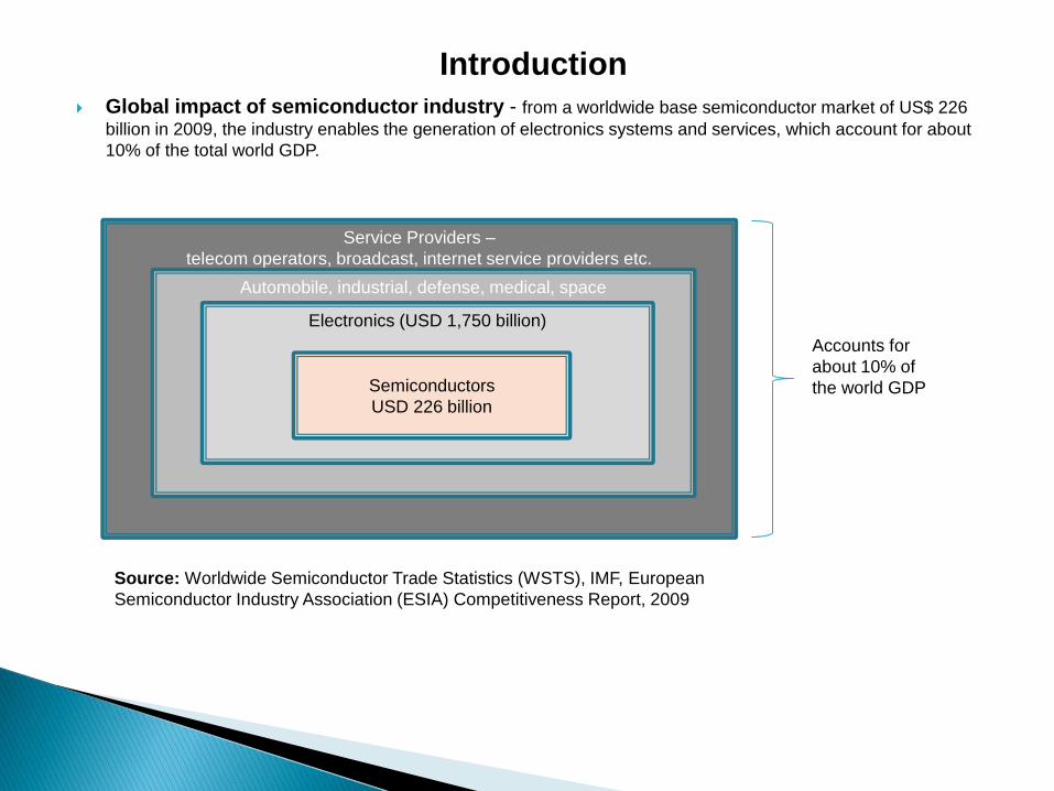
Global impact of semiconductor industry - from a worldwide base semiconductor market of US$ 226

billion in 2009, the industry enables the generation of electronics systems and services, which account for about

10% of the total world GDP.

Introduction

Service Providers –

telecom operators, broadcast, internet service providers etc.

Automobile, industrial, defense, medical, space

Electronics (USD 1,750 billion)

Semiconductors

USD 226 billion

Accounts for

about 10% of

the world GDP

Source: Worldwide Semiconductor Trade Statistics (WSTS), IMF, European

Semiconductor Industry Association (ESIA) Competitiveness Report, 2009

Cyclical nature of global semiconductor industry - industry is research- and development-intensive at

the design stage and capital-intensive during the manufacturing phase. This is accompanied by continuous growth

in a cyclical pattern with high volatility.

Generally, cycles include an expansion and peak period, followed by a slowdown phase, and eventually a

downturn stage.

This industry has witnessed six major cycles since 1970, and there is good reason to believe that 2009 marked

the end of the downturn phase of another cycle.

Contd…

Source: EY research 2010

Expansion and peak phase 2-3 years of strong (20%) growth

Slowdown phase

Downturn phase 1-2 years of flat or declining phase

Split of semiconductor revenues by segment, 2015 –

Discrete Semiconductors – transistors, diodes, etc

purpose of which is switching, amplifying and transmitting electrical signals (quite stable due to lower presence in

computer applications).

Optoelectronics – electrical or optical transducers

Sensors – sense physical quantity and convert it to electrical signals

Integrated circuits – miniaturize electronic circuits (integrating a large number of tiny transistors into a small chip).

It includes analog (14%), memory (20%), micro (21%) and logic (29%) components.

Contd…

Source: Worldwide Semiconductor Trade Statistics (WSTS)

84%

2%8%

6%

Revenues

IntegratedCircuits (84%)

Sensors (2%)

Optoelectronics(8%)

Discrete (6%)

Indian semiconductor industry overview - India is playing a major and increasing role in the global

electronics industry, which motivates the development of a local semiconductor manufacturing base.

The global electronics industry is very large and growing. India’s electronics industry is already important and

growing at 7x the global rate

India market currently represents ~2% of the global production of electronics and is expected to grow at 22% per

year

Global production of electronics, 2004-2020E$ Trillions

India has around $7 billion in annual semiconductor consumption and the import burden driven by this disparity

will grow significant by 2020 to $45-50 billion.

India has a significant human capital presence already in semiconductors, but is currently focused on design. With

a large talent pool of 200K+ design engineers, India semiconductor design market has grown at 28% over the last

7 years

Contd…

Source: ESDM DOIT report, NSF, Study on semiconductor design embedded software and services industry and IC economics report

0

0.5

1

1.5

2

2.5

3

2004 2009 2014E 2020E

Motivation

Very expensive equipment ($200K - $14M) and very expensive clean rooms (<$3K per sq.ft.)

28% price increases of equipment per year

Equipment purchases account for 70%-80% of capital expenditure in new fabs

Cost of new fabs is doubling every 3 years

Revenue opportunity/wafer is ($5000 - $12,500)

World Semiconductor Trade Statistics (WSTS) anticipates the semiconductor revenue to rise steadily from

2013 ($306 billion) total to $325 billion this year, $336 billion in 2015 to reach $350 billion by 2016.

National Democratic Alliance (NDA) government’s flagship ‘Make in India’ programme, the centre plans to

spend 10 billions of dollars to put in place an ecosystem for electronics manufacturing in the country.

Implementation of an improved control strategies could result in a considerable amount of increased profits

because the capital investment and sales revenue of wafer fab are extremely large.

http://www.informatik.uni-rostock.de/~lin/GC/Slides/Fowler.pdf

http://www.forbes.com/sites/jimhandy/2014/06/26/wsts-updates-semiconductor-forecast-325-billion-in-2014/

http://www.livemint.com/Industry/ZRBFOTaucH1NO9el7JLZXJ/Govt-to-invest-10-billion-in-two-computer-chipmanufacturin.html

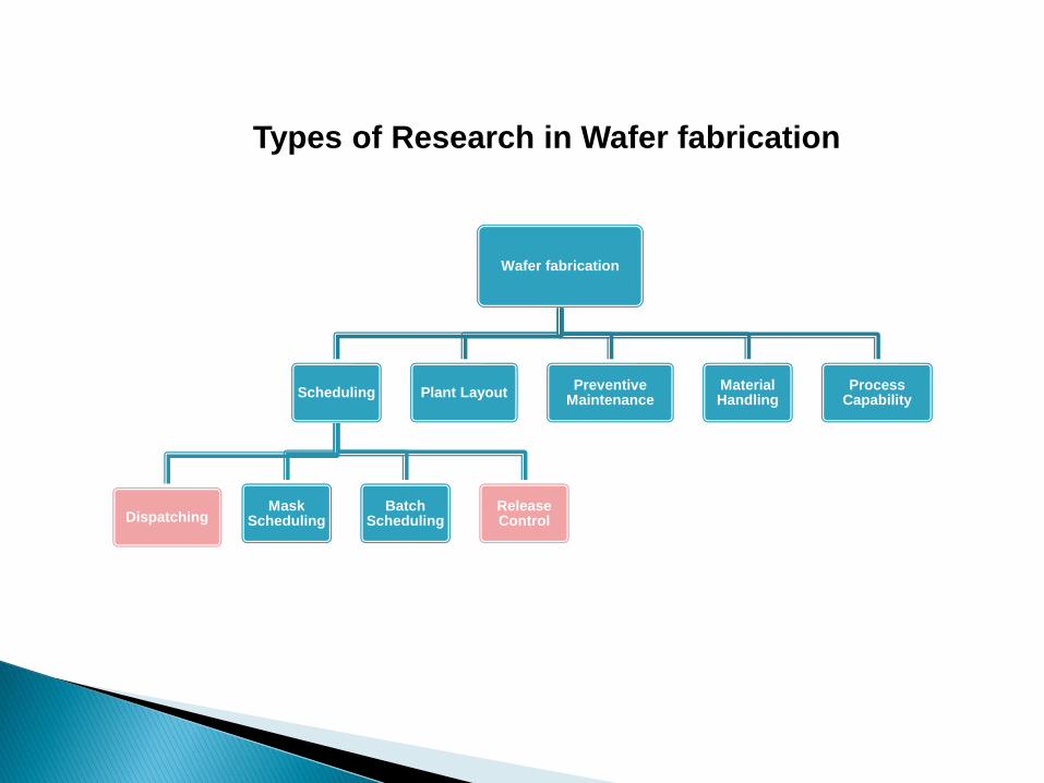
Wafer fabrication

Scheduling

DispatchingMask

SchedulingBatch

SchedulingRelease Control

Plant LayoutPreventive

MaintenanceMaterial Handling

Process Capability

Types of Research in Wafer fabrication

Release

Policies

Model Characteristics References

Immediate

Release (IMR)

No breakdown or manpower limitation,

Poisson (mean rate is 1.0728 per hr),

exponential processing time (1-4hr).

Ragatz and Mabert [1988], Bobrowski and

Park [1989], Ahmed and Fisher [1992], Kim

et al [1996], Rose ([1999] & [2001])

Random Release

(RAND)

No rework, no set-ups time, no batch

process, neither operators nor

transporters are modeled.

Ragatz and Mabert [1988], Bobrowski and

Park [1989]

Constant Release

(CONST)

Single product, hypothetical fab, batch

process is not considered. No rework,

no set-ups time, no batch process,

neither operators nor transporters are

modeled.

Wein [1988], Glassey and Resende [1988],

Gilland [2002] and Lin et al [2007], Glassey

et al. [1996], Chern and Huang [2004], Lou

and Kager [1989], Kim et al [1996]

Workload

Regulating (WR)

Single product, machine breakdown

considered are not standard, throughput

time and compared (RAND, CONST,

CONWIP and WR), processing times

include set-ups, operator unavailability

and rework and no batch process.

Wein [1988], Glassey and Resende [1988],

Glassey et al. [1996], Chern and Huang

[2004], Rose [1999] & Kim et al [1996]

Literature Review in Wafer Fabrication

Release Policies Model Characteristics References

Starvation Avoidance (SA) Single product, hypothetical fab, batch process is

not considered, trade-off curve and compared

(CONST, WR, CONWIP & SA) using SRPT &

FIFO.

Glassey and Resende [1988]

Descending Control (DEC) No yield loss, all machines are available all the

time, set-ups are negligible and used exponential

processing time. Compared (CONST, CONWIP,

WR & DEC). Adaptive in MTO situations.

Glassey et al. [1996]

Constant Work-in-process

(CONWIP)

No rework, no set-ups time, no batch process,

neither operators nor transporters are modeled.

Spearman et al [1990], Glassey and

Resende [1988], Wein [1988], Glassey et al.

[1996], Chern and Huang [2004], Rose

([1999] & [2001])

Workload Regulated Batch-

sizing rule or (k, w) rule

No yield loss, single product, neither operators

nor transporters are modeled, no travel time is

considered. Compared with (CONST, CONWIP,

WR & (k, w)).

Chern and Huang [2004]

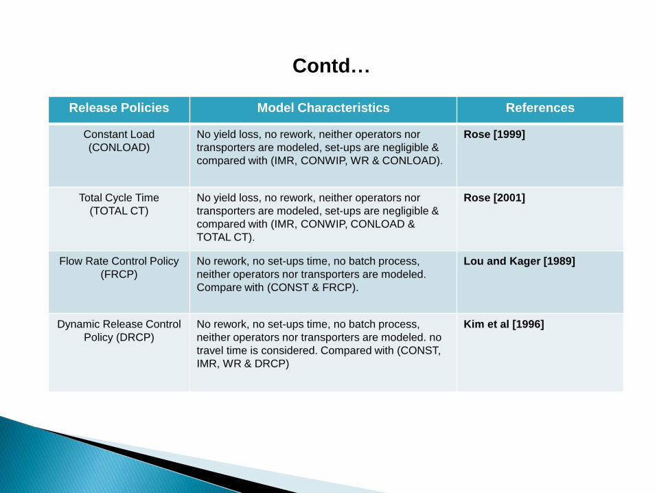
Contd…

Release Policies Model Characteristics References

Constant Load

(CONLOAD)

No yield loss, no rework, neither operators nor

transporters are modeled, set-ups are negligible &

compared with (IMR, CONWIP, WR & CONLOAD).

Rose [1999]

Total Cycle Time

(TOTAL CT)

No yield loss, no rework, neither operators nor

transporters are modeled, set-ups are negligible &

compared with (IMR, CONWIP, CONLOAD &

TOTAL CT).

Rose [2001]

Flow Rate Control Policy

(FRCP)

No rework, no set-ups time, no batch process,

neither operators nor transporters are modeled.

Compare with (CONST & FRCP).

Lou and Kager [1989]

Dynamic Release Control

Policy (DRCP)

No rework, no set-ups time, no batch process,

neither operators nor transporters are modeled. no

travel time is considered. Compared with (CONST,

IMR, WR & DRCP)

Kim et al [1996]

Contd…

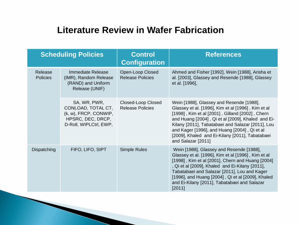
Scheduling Policies Control

Configuration

References

Release

Policies

Immediate Release

(IMR), Random Release

(RAND) and Uniform

Release (UNIF)

Open-Loop Closed

Release Policies

Ahmed and Fisher [1992], Wein [1988], Arisha et

al. [2003], Glassey and Resende [1988], Glassey

et al. [1996],

SA, WR, PWR,

CONLOAD, TOTAL CT,

(k, w), FRCP, CONWIP,

HPSRC, DEC, DRCP,

D-Roll, WIPLCtrl, EWP,

Closed-Loop Closed

Release Policies

Wein [1988], Glassey and Resende [1988],

Glassey et al. [1996], Kim et al [1996] , Kim et al

[1998] , Kim et al [2001] , Gilland [2002] , Chern

and Huang [2004] , Qi et al [2009], Khaled and Ei-

Kilany [2011], Tabatabaei and Salazar [2011], Lou

and Kager [1996], and Huang [2004] , Qi et al

[2009], Khaled and Ei-Kilany [2011], Tabatabaei

and Salazar [2011]

Dispatching FIFO, LIFO, SIPT Simple Rules Wein [1988], Glassey and Resende [1988],

Glassey et al. [1996], Kim et al [1996] , Kim et al

[1998] , Kim et al [2001], Chern and Huang [2004]

, Qi et al [2009], Khaled and Ei-Kilany [2011],

Tabatabaei and Salazar [2011], Lou and Kager

[1996], and Huang [2004] , Qi et al [2009], Khaled

and Ei-Kilany [2011], Tabatabaei and Salazar

[2011]

Literature Review in Wafer Fabrication

Trade-off Curve for Scheduling Policies

Cycle Time

C(t)

Throughput

(t)

Policy A

Policy B

CA (t)

CB (t)

The objective is to find the scheduling policy that is efficient on the

frontier of delay and throughput.

Problem Definition and Objective

The problem can be characterized by a set of jobs, where each job requires six operations to complete the

fabrication process. The operations must be performed in a specific sequence at specific stations.

The scheduling policies are compared based on the delay/throughput trade-off curve.

This curve describes the waiting time or cycle time as a function of fab throughput. Waiting time is defined to be

the time a job spends in the fab that is processing time plus waiting time, while throughput is the average

number of jobs that leave the fab.

Policy A is superior to policy B for a given throughput t

Machine E

Machine C, DMachine A, B

A

B

C

D

E

Step 1

Step 5

Step 2

Step 4

Step 3

Step 6

Wafer

In

Wafer

Out

Diffusion WorkstationIon Implantation

Workstation

Lithography

Workstation

Simulation Model for Mini-Fab

Station 1 Station 2 Station 3

http://aar.faculty.asu.edu/research/intel/papers/fabspec.html

Process Flow – Start > S1 > S2 > S3 > S4 > S6 > Out

All wafers follow this sequence subject to all machine restrictions such as batching and setups

Equipment Set – Machines, Batch Size and Setup Time

Three Workstation : Diffusion, Ion Implantation and Lithography

Diffusion is a batch process which can batch 3 lots/jobs together

Setup time is given at lithography station

(5min for product change, 10 mins for step change and 12 mins for both step and product change)

Process - Processing Time (S1: 225 mins, S2: 30 mins, S3: 55 mins, S4: 50 mins, S5: 255 mins, S6: 10 mins),

This is purely the run time of the process

Personnel – Two production operators are required for load/unload process and to provide setups

Load – S1 & S5: 20 mins, S2 & S4: 15 mins, S3 & S6: 10 mins

Unload – S1 & S5: 40 mins, S2 & S4: 15 mins S3 & S6: 10 mins

The mini-fab operates the 24 hours of the day, 7 days of week.

Each day of operations is composed of two shifts of 12 hours.

http://aar.faculty.asu.edu/research/intel/papers/fabspec.html

Mini Fab Description

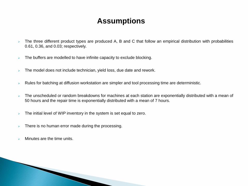
The three different product types are produced A, B and C that follow an empirical distribution with probabilities

0.61, 0.36, and 0.03; respectively.

The buffers are modelled to have infinite capacity to exclude blocking.

The model does not include technician, yield loss, due date and rework.

Rules for batching at diffusion workstation are simpler and tool processing time are deterministic.

The unscheduled or random breakdowns for machines at each station are exponentially distributed with a mean of

50 hours and the repair time is exponentially distributed with a mean of 7 hours.

The initial level of WIP inventory in the system is set equal to zero.

There is no human error made during the processing.

Minutes are the time units.

Assumptions

To compute the performance measure for scheduling policies, full factorial design is considered in this

study and thus total 45 (15 × 3) configurations are studied.

Arena simulation software is used to build the model and conduct these experiments.

In the course of the simulation, each scenario is tested for 200 replications of 9600 hours length each.

This number and length of replications provided uniformly good statistical precision across the outputs (95%

confidence interval half widths within 3% of the respective sample means).

The data obtained after the 4800 hours are used for the performance analysis.

The performance indices considered in this experiment are cycle time, WIP and throughput.

Delay: - It is the time elapsed between a job entering the facility and leaving the facility as a finished product,

consisting of processing time, transportation time between workstations, set-ups time, loading and unloading time

and waiting time in queues divided by the total processing time.

WIP: - It is a number of jobs present in the Mini Fab during the non-transient run time period

Throughput: - It is the number of jobs that came out after the last step in the process.

Experimental Design

Although the delay and throughput is the main performance measure, the WIP at the bottleneck is also important.

It is important to minimize the variability in these performance measures.

The standard deviation for each performance measure and coefficient of variation is also computed. The

coefficient of variation (CV) is a relative measure and it is computed by dividing the standard deviation value with

average value of the measures.

In Mini Fab, the work station (LT) for the process of lithography is found to be the bottleneck for all the tested

cases. The different dispatching rules are applied only at the bottleneck work station.

The different system loads are controlled by start rate for UNIF, critical values for WR and DRCP and WIP levels

for CONWIP, DEC, HPSRC and EWIP, safety stock for SA, reference WIPLOAD for WIPLCtrl, average processing

time between wafer start and first bottleneck stage for Droll, threshold value for CONLOAD, average remaining

cycle time for TOTAL CT, (k, w) value for (k, w), reference inventory and reference surplus value in FRCP and

parameter value in PWR.

Contd…

Effect of Dispatching Rules

TABLE I. UNIF/ FIFO POLICIY PERFORMANCE IN MINI FAB

Experimentation and Analysis

Delay (cycle time/total

processing time)

Throughput Departure Interval WIP at

Bottleneck

Mean Standard

Deviation

95%

Confidence

Interval

Mean Mean Standard

Deviation

(STD)

Coefficient of

Variation

(STD/Mean)

Mean Standard

Deviation

2306 818 113 1116 258 414 1.6 2.32 2.97

2371 880 122 1161 248 398 1.6 2.67 3.33

2442 909 126 1210 237 382 1.61 3.0 3.59

2539 1003 139 1264 228 367 1.61 3.56 4.14

2680 1062 147 1321 217 351 1.62 4.28 4.67

2970 1226 169 1384 208 334 1.61 5.78 5.77

3530 1468 203 1456 197 312 1.58 8.73 7.50

5216 2007 278 1532 188 283 1.51 17.78 11.15

20156 3565 494 1565 184 260 1.41 102.42 20.85

TABLE II. UNIF/ LIFO POLICIY PERFORMANCE IN MINI FAB

Contd…

Delay (cycle time/total

processing time)

Throughput Departure Interval WIP at

Bottleneck

Mean Standard

Deviation

95%

Confidence

Interval

Mean Mean Standard

Deviation

(STD)

Coefficient of

Variation

(STD/Mean)

Mean Standard

Deviation

2346 1223 169 1117 258 409 1.6 2.34 3.00

2389 1371 190 1161 248 397 1.6 2.61 3.29

2483 1595 221 1210 238 387 1.62 3.06 3.76

2576 1837 254 1263 228 373 1.64 3.58 4.19

2743 2261 313 1322 218 357 1.63 4.43 4.81

3031 3065 424 1384 208 340 1.62 5.93 5.88

3550 4602 637 1453 198 321 1.58 8.80 7.58

5625 12939 1793 1532 188 296 1.53 20.76 11.63

5863 13806 1913 1542 187 285 1.52 128.11 26.47

TABLE III. UNIF/ SIPT POLICIY PERFORMANCE IN MINI FAB

Contd…

Delay (cycle time/total

processing time)

Throughput Departure Interval WIP at

Bottleneck

Mean Standard

Deviation

95%

Confidence

Interval

Mean Mean Standard

Deviation

(STD)

Coefficient of

Variation

(STD/Mean)

Mean Standard

Deviation

2233 712 99 1116 258 398 1.54 1.92 2.52

2292 758 105 1162 248 386 1.56 2.18 2.80

2330 769 107 1211 238 372 1.56 2.40 2.96

2401 808 112 1264 228 360 1.58 2.79 3.27

2520 853 118 1321 218 347 1.59 3.31 3.64

2734 953 132 1385 208 336 1.62 4.32 4.32

3038 1065 148 1454 198 321 1.62 5.88 5.20

4028 1396 193 1532 188 308 1.64 11.01 7.58

10629 2047 284 1600 180 298 1.66 48.16 12.26

Effect of Dispatching Rules

Delay/Throughput Trade-off Curves for Uniform Release

UNIF Release Performance in Mini Fab with three dispatching rules

Contd…

It is observed from both the Tables I – III and the trade-off curve, that Uniform release policy with SIPT dispatching rule outperformed both FIFO and LIFO dispatching rule.

It is also noticed from the last row of Table II and Table III that for all values of throughput rate SIPT produced schedules with less mean delay than FIFO, achieving reduction of approximately 47% in mean delay at the throughput rate of about 1 job per 178 minutes.

Likewise, it is noted from Table II and Table III that for all values of throughput rate FIFO produced schedules with slightly less mean delay than LIFO except for the throughput rate of about 1 job per 178 minutes.

With respect to the coefficient of variation of inter departure times (CVID) SIPT produced schedules with less CVID than both FIFO and LIFO for throughput rate values greater than of about 1 job per 218 minutes.

Moreover, SIPT dispatching rule produced schedules with shorter queue of work at the bottleneck work station.

However, the detailed simulation results for (14 × 3 × 200) simulation runs generated similarly but are not given in detail due to the time restriction and only important observations are discussed.

It is observed that SIPT dispatching rule outperformed both FIFO and LIFO dispatching rules in all release policies except for EWIP in which FIFO outperformed other two dispatching rules. The reason for this change could be the variability of WIP at the bottleneck workstation which triggers the release of jobs into the system under this release policy.

Contd…

Contd…

Effect of Release Policies

Delay/Throughput Trade-off Curves for Release Policies with SIPT Dispatching Rule

Release Policies Performance in Mini Fab with SIPT dispatching Rule

It is evident from the trade-off curve, that the starvation avoidance (SA) produced schedules with less mean delay than other fourteen release policies at all the throughput rate values.

The improvement was most remarkable against Uniform release policy, where the mean delay reduction is approximately 81%.

SA outperformed Uniform release policy with respect to CVID times at higher throughput rate values. When compared to WR, SA produced schedules with approximately 50% less mean delay at the higher end of throughput range.

The performance of all closed loop release policies was better than open loop release policy except for FRCP, PWR and EWIP.

The objective of FRCP release policy was to minimize the work in process inventory cost, so under this release policy jobs get on hold at each step and therefore it increases the delay.

The estimation for bottleneck workload is not proper under PWR release policy due to the normalization of processing time and thus it increases the delay.

The control criteria in EWIP release policy is the arrival rate which is varied according to the WIP of bottleneck workstation. Thus there is an increase in delay due to high variability in arrival rate.

Contd…

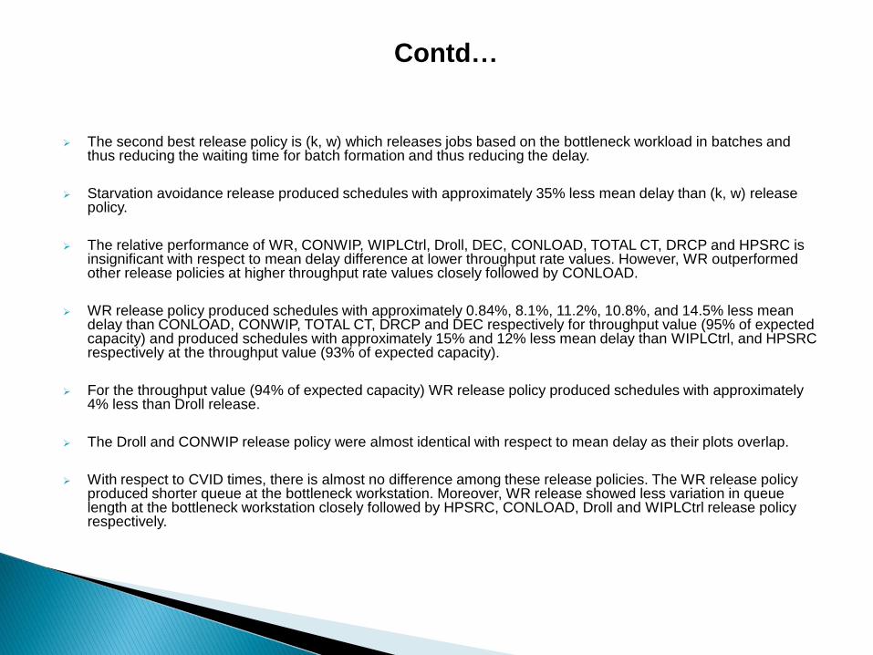
The second best release policy is (k, w) which releases jobs based on the bottleneck workload in batches and thus reducing the waiting time for batch formation and thus reducing the delay.

Starvation avoidance release produced schedules with approximately 35% less mean delay than (k, w) release policy.

The relative performance of WR, CONWIP, WIPLCtrl, Droll, DEC, CONLOAD, TOTAL CT, DRCP and HPSRC is insignificant with respect to mean delay difference at lower throughput rate values. However, WR outperformed other release policies at higher throughput rate values closely followed by CONLOAD.

WR release policy produced schedules with approximately 0.84%, 8.1%, 11.2%, 10.8%, and 14.5% less mean delay than CONLOAD, CONWIP, TOTAL CT, DRCP and DEC respectively for throughput value (95% of expected capacity) and produced schedules with approximately 15% and 12% less mean delay than WIPLCtrl, and HPSRC respectively at the throughput value (93% of expected capacity).

For the throughput value (94% of expected capacity) WR release policy produced schedules with approximately 4% less than Droll release.

The Droll and CONWIP release policy were almost identical with respect to mean delay as their plots overlap.

With respect to CVID times, there is almost no difference among these release policies. The WR release policy produced shorter queue at the bottleneck workstation. Moreover, WR release showed less variation in queue length at the bottleneck workstation closely followed by HPSRC, CONLOAD, Droll and WIPLCtrl release policy respectively.

Contd…

Conclusions and Future Research

In conclusion, with respect to Mini-Fab, varying the dispatching rule for a fixed release policy did not show as

much mean delay sensitivity as fixing the dispatching rule and varying the release policy.

It is observed that release policies plays more significant role than dispatching rules in improving the

performance of wafer fabs with respect to delay and throughput.

It is observed that with most of the release policies, SIPT dispatching rule produced less mean delay at all

throughput rate values and SA provides higher throughput rate with less mean delay among all the release

policies. Generally, it is concluded that SIPT was the best dispatching rule and SA the superior release policy.

The future research will focus on developing an efficient and robust closed loop release policy for wafer

fabrication environment by considering the real time status and uncertainties in the system.

Thank you

References[1] Ahmed, I. and Fisher, W. W, “Due date assignment, job order release and sequencing interaction in job shop

scheduling,” Decision sciences, 23, 633-647, 1992.

[2] Arisha, Amr, Young Paul, Baradie, M.El and Hashmi, M.S.J, “Intelligent shop scheduling for semiconductor

manufacturing,” PhD Thesis, School of Mechanical and Manufacturing Engineering, Dublin City University, 2003.

[3] Bobrowski, P. M. and Park, P. S, “Work release strategies in a dual resource constrained job shop,” OMEGA

International Journal of Management Science, vol. 17, no. 2, pp, 177-188, 1989.

[4] Fowler, J. W., Hogg, G. L., and Mason, S. J., “Workload Control in the semiconductor industry," Production

Planning and Control, vol. 13, no. 7, pp. 568-578, 2002.

[5] Gilland G. Wendell, “A simulation study comparing performance of conwip and bottleneck based release rules,”

Production planning and control: the management of operations, 13:2, pp 211-219, 2002.

[6] Glassey, C. R. and Resende, M. G, “Closed-loop job release control for VLSI circuit manufacturing,” IEEE

Transactions on Semiconductor Manufacturing, 1, 36 46, 1988.

[7] Kempf, K, “Intel five-machine six-step Mini-Fab description,”

http://aar.faculty.asu.edu/research/intel/papers/fabspec.html, 2015.

[8] Kim Jongsoo, Leachman Robert.C, and Suhn Byungkyoo, “Dynamic Release Control Policy for the Semiconductor

Wafer Fabrication Lines,” Journal of the Operational Research Society 47, 1516-1525, 1996.