isas / gsfc · 04/03/2016 · 5.4. time assignment for mxs ... table 11. operation mode of the smu...

ASTRO-H

ASTRO-H Time assignment system

Version 0.9.7

4 Mar 2016

ISAS / GSFC

Prepared by: Yukikatsu Terada (Saitama Univ, Japan), Lorella Angelini (NASA/GSFC),

Michael Witthoeft (NASA/GSFC)

2

Table of Contents 1. Introduction ............................................................................................................................. 9 1.1. Purpose .................................................................................................................................... 9 1.2. Applicable Documents ............................................................................................................ 9 2. Overview ............................................................................................................................... 10 2.1. Science Requirement on Time assignment system ............................................................... 10 2.2. Definition of Words .............................................................................................................. 10 2.3. Definition of Time ................................................................................................................ 12 2.4. Basic concept of the time assignment in ASCA, Suzaku, and ASTRO-H .............................. 13 2.4.1. ASCA case .................................................................................................................... 14 2.4.2. Suzaku case ................................................................................................................... 15 2.4.3. ASTRO-H case ............................................................................................................. 16 2.5. Overview of the time assignment process in ASTRO-H ....................................................... 17 2.5.1. Schematic view of ASTRO-H Time Assignment ......................................................... 17 2.5.2. Task flow of ASTRO-H Time Assignment .................................................................. 17 2.6. Definition of TI for ASTRO-H and its Distribution .............................................................. 20 3. Data Acquisition system onboard Spacecraft ....................................................................... 21 3.1. Structure of the SpaceWire network of ASTRO-H .............................................................. 21 3.2. Distribution of TIME_CODE under ASTRO-H SpaceWire network .................................. 22 3.3. GPS receiver (GPSR) and SMU for the ASTRO-H mission ................................................. 23 3.3.1. Overview of GPSR for ASTRO-H ............................................................................... 23 3.3.2. Synchronization of clocks between GPSR and SMU ................................................... 24 3.3.3. Synchronization Algorithm of TI in transition mode ................................................... 28 3.3.4. Duplication or Skip of TIs at the transition mode of TI time system ........................... 29 3.3.5. Telemetry of GPSR via SMU ....................................................................................... 30 3.4. TIME packet from ASTRO-H satellite .................................................................................. 32 3.5. Ground system ...................................................................................................................... 33 3.5.1. Receive time at the ground station ................................................................................ 33 3.5.2. Time assignment at SIRIUS .......................................................................................... 33 3.5.3. Time table from SIRIUS for the TIM file ..................................................................... 35 3.6. Summary of Time System of inputs and outputs for the time assignment ........................... 36 4. Generation of a look-up table between L32TI and TIME (Tim file) .................................... 38 4.1. Origin and format of TIM file ............................................................................................... 38 4.2. Extract frequency and temperature trends ............................................................................ 39 4.3. Generation of TIM file TIM_LOOKUP extension with GPS information ........................... 41 4.3.1. GPS Mode (GPS and SMU clocks are synchronized) .................................................. 43 4.3.2. Suzaku Mode (GPS and SMU clocks are not synchronized) ....................................... 44 4.3.3. Transition mode: From SMU time to GPS time ........................................................... 49 5. Time Assignment of HK data ............................................................................................... 51 5.1. Flow chart of time assignment of HK ................................................................................... 51 5.2. Conversion from L32TI to TT (TIME) ................................................................................. 51 5.3. Conversion from TT to UTC ................................................................................................ 53 5.4. Time assignment for MXS .................................................................................................... 54 6. Time Assignment of Science Data ........................................................................................ 57

3

6.1. Overview of time assignment of Science data ...................................................................... 57 6.2. Summary of LOCAL_TIME ................................................................................................. 58 6.2.1. SXI ................................................................................................................................ 59 6.2.2. HXI Camera and SGD Compton Camera (CC) ............................................................ 60 6.2.3. HXI/SGD Shield ........................................................................................................... 61 6.2.4. SXS ............................................................................................................................... 62 6.3. Adjustment of Delay/Offset time .......................................................................................... 65 6.3.1. Summary of delay (Delay CALDB file) ....................................................................... 65 6.3.2. CAMS offset by acquisition ......................................................................................... 65 6.3.3. SXI offset by Data Modes ............................................................................................. 66 7. List of calibration items and CALDB for time assignment .................................................. 70 7.1. Error budget in timing accuracy of ASTRO-H ..................................................................... 70 7.2. Calibration items for scientific analyses ................................ Error! Bookmark not defined. 7.3. Summary of CALDB files .................................................................................................... 71 8. Appendix ............................................................................................................................... 77 8.1. Overview of the SpaceWire protocol .................................................................................... 77 8.1.1. Standard Communication Protocol, SpaceWire .......................................................... 77 8.1.2. Characters and codes in the lowest layer of the protocol .............................................. 77 8.1.3. TIME_CODE distribution across a SpaceWire network .............................................. 79 8.1.4. RMAP protocol ............................................................................................................. 82 8.1.5. SpaceWire-D protocol and Time Slot for Quality of Service. ...................................... 82

4

Figures

Figure 1. Summary of time assignment system of ASCA, Suzaku, and ASTRO-H. .............. 13 Figure 2. Schematic view of ASTRO-H Time assignment. .................................................. 17 Figure 3. Flow chart of the time assignment process of ASTRO-H. .................................... 18 Figure 4. Network Structure of ASTRO-H. .......................................................................... 21 Figure 5. Simplified view of the ASTRO-H network configuration. ................................... 22 Figure 6. Block diagram of GPSR = GPSA + GPSL + GPSP. ............................................. 23 Figure 7. State machine of SMU operation modes listed in Table 11. ................................. 24 Figure 8. Example of mode transition of the SMU and GPS. ............................................... 24 Figure 9. Overview of timing system onboard ASTRO-H. .................................................. 25 Figure 10. Example of relation between TAI and SA-TI. .................................................... 26 Figure 11. Algorithm of time assignment with TIM file ...................................................... 34 Figure 12. An example of contents of TIM file, 1st and 2nd extensions. ............................... 39 Figure 13. Extraction of trend data by ahtrendtemp and generation of caldb information. . 40 Figure 14. Flow chart of ahmktim. ........................................................................................ 42 Figure 15. Schematic view of counters in calculation from L32TI, S_TIME, into TIME. .. 43 Figure 16. Same as Figure 15, but another case. .................................................................. 43 Figure 17. Schematic view of the calculation of L32TI-TIME relation during GPS-

unsynchronized. ............................................................................................................ 45 Figure 18. Timing accuracy vs days of absent ground connection (Fig 4 in Terada et al

2008) ............................................................................................................................. 47 Figure 19. Same as Figure 17, but for case (2) GPS – Suzaku Mode, using original TIM file.

....................................................................................................................................... 48 Figure 20. Flow chart of time assignment of HK by ahtime. ............................................... 51 Figure 21. Algorithm of time assignment of HK FITS with TIM file .................................. 52 Figure 22. Schematic timing chart for MXS irradiation. ...................................................... 55 Figure 23. Timing chart for MXS pulses and coarse / fine GTIs. ........................................ 56 Figure 24. Flow chart of time assignment of Science data by ahtime. ................................. 57 Figure 25. Schematic view of calculation of fine L32TI of SXI. ......................................... 59 Figure 26. Algorithm to get fine L32TI from LOCAL_TIME with look-up table between

them. .............................................................................................................................. 60 Figure 27. Timing chart for the SXI exposure by data modes. ............................................. 66 Figure 28. Timing chart for distribution of timing information. Error budgets (Table 35) and

calibration items are shown in star marks and left right arrow, respectively. .............. 70 Figure 29. Examples of the network topology for the SpaceWire. ....................................... 77 Figure 30. Data and control characters in SpaceWire [4] ..................................................... 78 Figure 31. Control codes in SpaceWire [4]. ......................................................................... 78 Figure 32. Distribution of TIME_CODE in nominal case (I) ............................................... 79 Figure 33. Distribution of TIME_CODE in nominal case (II) ............................................. 80 Figure 34. Distribution of TIME_CODE in transmission error case .................................... 81 Figure 35. SpaceWire and RMAP layer. .............................................................................. 82 Figure 36. Definition of Time Slot for ASTRO-H. .............................................................. 83

5

Tables Table 1. Science requirement on timing ............................................................................... 10 Table 2. Definition of terms .................................................................................................. 11 Table 3. Definition of Epoch of TIME. ................................................................................ 12 Table 4. Definition of timing of TIME column. ................................................................... 12 Table 5. Overview of time assignment of ASCA data .......................................................... 14 Table 6. Overview of time assignment of Suzaku data ........................................................ 15 Table 7. Overview of time assignment of ASTRO-H data ................................................... 16 Table 8. Definition of Time Indicator (TI) of ASTRO-H. .................................................... 20 Table 9. Definition of epoch and tick of TI. ......................................................................... 20 Table 10. Timing and orbital accuracy of GPSR. ................................................................ 23 Table 11. Operation mode of the SMU for time assignment. ............................................... 24 Table 12. Spec of the quartz onboard SMU. ......................................................................... 26 Table 13. GPS telemetry to identify the TIME system for TI .............................................. 27 Table 14. TIME systems tree by GPS telemetry ................................................................... 27 Table 15. Telemetry for SMU status on GPS ....................................................................... 31 Table 16. Format of TIME packet. ...................................................................................... 32 Table 17. Definition of epoch of R_TIME. .......................................................................... 33 Table 18. Definition of epoch of S_TIME. ........................................................................... 33 Table 19. Time systems of L32TI, S_TIME, and TIME. ..................................................... 36 Table 20. Table of leap second between 1980 and 2012. ..................................................... 37 Table 21. Definition of TIM file. .......................................................................................... 38 Table 22. Column and extension names for SMU quartz frequency and temperature. ........ 40 Table 23. Summary of inputs and outputs in time assignment process of HK FITS. ........... 51 Table 24. definition of TIME in section 5. .......................................................................... 51 Table 25. Format of TI_LED[1,2,3,4]_START_STOP for MXS ......................................... 55 Table 26. Definition of TIME for Science data in section 5.4. ............................................. 57 Table 27. List of LOCAL_TIME counters. ......................................................................... 58 Table 28. Column name of LOCAL_TIME for SXI. ........................................................... 59 Table 29. Column name of LOCAL_TIME for HXI CAMERA and SGD CC. .................. 60 Table 30. Column names of LOCAL_TIME 1 and 2 for SGD WAM. ................................ 61 Table 31. Column names of LOCAL_TIME of the SXS. .................................................... 62 Table 32. Definition of offset and telemetry period of CAMS data ..................................... 66 Table 33. Formula to calculate the timing offset for the SXI by data modes. ...................... 67 Table 34. List of time (sec) for SXI timing chart. (ver 2013-12-17) .................................... 69 Table 35. Error budget of ASTRO-H Time assignment. ...................................................... 70 Table 36. Definition of TIME_CODE for ASTRO-H .......................................................... 83 Table 37. Definition of slots in the communication of nodes in ASTRO-H. Bus slot,

System slot, and free slot are shown in yellow, magenta, and white, respectively. ..... 84

6

NOTE to editors: Document version must be updated every time the document is edited and always add a record in the change record table. The document number is between 0-1 when in draft form, and set to 1 when first version is completed and approved. Use the tracking tool to record changes when in draft version. The document at any draft version must always be in the wiki page either under the draft section or final section.

7

CHANGE RECORD PAGE (1 of 1)

DOCUMENT TITLE :ASTRO-H Time Assignment system ISSUE DATE PAGES

AFFECTED DESCRIPTION

Version 0.1 Mar 2012 All First draft Version 0.2 May 2012 all Add overview of tasks Version 0.3 June 2012 all Review with GSFC Version 0.4 July 2012 all Send Engineer GSFC/NASA Version 0.5 Sept 2012 all Updates with inputs from f2f

meetings with NEC. Change the definition of TI, U32TI, and L32TI etc.

Version 0.6 Dec 2012 All Reorganize the document, Update Chaper 4 and 5 to reflect what the software is actually doing. Add a section of the MXS.

Version 0.7 Jan 2013 all For Build-2 (2013 Feb) Version 0.7.2 Dec 2013 all Fix Editorial errors in MS Doc Version 0.8 Jan 2014 SXI For build-4 (2014 Feb).

Add description for time assignment of the SXI by data modes.

Version 0.9 Sep 2014 all For TIME review on Sep 2014. Session rearrangement. Check consistency with TIME TRF.

Version 0.9.1 Oct 2014 all Feedback from TIME review. * Update of overview of TIME * Description ahtrendtemp updated * Define TIM file extensions name and Updates cases of GPS/Suzaku modes for mktim. * fix GPS information * Updates for MXS, mxstime

Version 0.9.2 Feb 2015 Section 1.1 Section 3.5.3 Section 4.3.2 Section 6.1 Section 6.2.4

* Requirement on each instrument * Add description for Time table * Update calc. of TIME from L32TI. * Update LOCAL_TIME table. * Updates for SXS, SAMPLE_CNTs for arrival time and trigger time.

8

Version 0.9.3 Apr 2015 Section 3.6 Section 4.2 Section 4.3

Fix MJDREFF value Change the values of SMUUNIT (A for SMU-A and B for SMU-B) Fix keyword name GPSOFFET

Version 0.9.4 June 2015 Section 3.3 Section 4.1 Section 4.2 Section 6.1

Describe GPS flags in starting SMU. L32TI format in fine TIM file is 1D. Value added for PERIODCL. Monotonic check of LOCAL_TIME in PROC_STATUS.

Version 0.9.5 July 2015 Section 3.6 Section 4.2 Section 6.2

Add leapsec entry on 1 Jul 2015. Update the column/extension list for ahmktrendtemp. Add policy in orbit. Review LOCAL_TIME list.

Version 0.9.6 Sep 2015 Section 2.1 Section 3.6 Section 6.3.3

Timing goal for SXI updated. Definition of TIMEDEL, TIMEPIXR Delete +0.5*Exposure term from SXI

Version 0.9.7 Mar 2016 Section 7.2 all

Add description for on-ground measurements. Delete DRAFT

9

1. Introduction 1.1. Purpose This document describes the time assignment system of the ASTRO-H and the algorithms of conversion from the telemetry to time. 1.2. Applicable Documents The requirements and information in this document, ASTH-SCT-021, are described in the following documents: [1] ASTRO-H System Design, ASTH-100 [2] Y.Terada et al., Publications of the Astronomical Society of Japan, 60, S25-S34 (2008) [3] ASTRO-H Satellite Time Design, ASTH-NT-D10137, draft 3. [4] SpaceWire standard, ECSS-E-ST-50-12C [5] The operation and uses of the SpaceWire Time-Code, International SpaceWire Seminar 2003. [6] SpaceWire Remote Access Memory Protocol, Steve Parkes and Chris McClements, 2005 [7] ASTRO-H/Sprint Telemetry/Command Design Criteria, ASTH-111, rev5 [8] ASTRO-H Telemetry/Command/Network Design, ASTH-113, rev3 [9] ASTRO-H pre-pipe-line process, ASTH-SCT-002 [10] ASTRO-H Timing Design, ASTH-200-07, rev1 (Sep 2014)

10

2. Overview 2.1. Science Requirement on Time assignment system One of final goals of ASTRO-H mission is to study the nature of high energy astrophysical objects. Time variability is one of the important features of objects. As a summary of requirements from science observations of active galactic nuclei, galactic black holes, and neutron pulsars, etc, the requirement and calibration goal of the absolute timing accuracy is 300 and 30 micro second, respectively. [1] The time assignment system of ASTRO-H, including onboard system, ground system, and off-line analyses tools, should achieve this requirement shown in Table 1 .

Requirement 200 µs absolute accuracy Goal 30 µs absolute accuracy

Table 1. Science requirement on timing For reference, the requirements for the hardware design of each instrument are summarized in Table 2. All the requirements for the designs (Table 2) cover the system requirement above (Table 1).

Instrument Requirement for the design Reference SXS 10 ms absolute accuracy

80 µs absolute accuracy Goal ASTH-200-63

SXI 61.0 µs relative accuracy from TI ASTH-SXI-E-008 HXI 60 µs relative accuracy from TI HXI-MEMO-2012-002 SGD Same as HXI system To be identified

Table 2. Hardware requirement on timing 2.2. Definition of Words The definitions of technical terms described in this document are summarized in the following Table 3.

Name description TI Time Indicator, which is a counter value of the clock onboard for time

assignment. In ASTRO-H case, TI is a 38-bit counter (see Table 9. ). A part of TI (i.e., L32TI) is always in the telemetry for all the packets.

L32TI Lower 32-bit of the TI. (see Table 9. ) Note that L32TI when the space packet is generated is stored in the secondary header of the Space Packet (= CCSDS packet for ASTRO-H).

U32TI Upper 32-bit of the TI. (see Table 9. ). Normally, this information is not appeared in the telemetry.

TIME Time second since the epoch. The epoch is defined in Table 4. TIME

11

should be filled in the pipe-line process. S_TIME Time second when the space packet is sent to the telemetry = data

recorder (DR) or ground station. The epoch is the same as that of TIME (Table 4). S_TIME is calculated and filled by SIRIUS and stored in the pre-pipe-line process.

R_TIME Time second when the space packet is received by the ground station. The epoch is the same as that of TIME (Table 4). If the space packet is recorded on DR in orbit and reprocessed when the spacecraft is in communication with a ground station, R_TIME is not the same as S_TIME. S_TIME is recorded on ground and filled by SIRIUS, but not stored in the pre-pipe-line process (except for TIM file).

TIM file Time information, containing TI vs TIME values calibrated. The TIME_PACKETS extension is prepared on ground by Time packet (section 3.4) and R_TIME for it, and SIRIUS uses this relation in TIME_PACKETS extension to calculate S_TIME. In pipe line process, we generate the finer relation between TI and TIME, reflecting GPSR status into TIM_LOOKUP extension. (see Table 23)

TAI time system Atomic Time , with the unit of duration the System International (SI) second defined as the duration of 9,192,631,770 cycles of radiation corresponding to the transition between two hyperfine levels of the ground state of cesium 133. The TAI is the International Atomic Time scale, a statistical timescale based on a large number of atomic clocks.

UTC time system

Coordinated Universal Time (UTC) differs from TAI by an integral number of seconds. UTC is kept within 0.9 seconds of UT1 by the introduction of one-second steps to UTC, the "leap second" (see Table 20). To date these steps have always been positive.

TT time system Dynamical Time replaced ephemeris time as the independent argument in dynamical theories and ephemerides. Its unit of duration is based on the orbital motions of the Earth, Moon, and planets. Terrestrial Time (TT), (or Terrestrial Dynamical Time, TDT), with unit of duration 86400 SI seconds on the geoids, is the independent argument of apparent geocentric ephemerides. TDT = TAI + 32.184 seconds. In summary,TT = TAI + 32.184 sec = UTC + LeapSecond + 32.184 sec.

GPS time Please note that GPS time = TAI – 19 sec Table 3. Definition of terms

12

2.3. Definition of Time The “time assignment” means the calculation from values in the telemetry into the time information, which should be stored in the TIME column for each row in the FITS file. The definition of TIME in the ASTRO-H mission is the second from the epoch, 1st January 2014, 00:00:00 UT, as defined in Table 4.

Epoch of TIME 2014-01-01 00:00:00 UTC MJD 56658.0007775925926 (TT) Table 4. Definition of Epoch of TIME.

The timing indicated by the TIME column depends on the types of the telemetry, i.e., the house keeping (HK) data or science data. The definitions are shown in the following Table 5. Type Timing of TIME Telemetry type 1 Time when the space packet is generated at the sub-system

onboard spacecraft. For payload instruments, the space packet is generated on the PSP for the SXS or DE for other instruments.

HK

2 Time when the event (SXS, SXI) or occurrence (HXI, SGD) triggers on the electronics onboard the spacecraft. The arrival time of events.

Science HK (*)

(*) Some HK, which is used for dead time correction, for example, should have TIME definition of type 2. Table 5. Definition of timing of TIME column.

13

2.4. Basic concept of the time assignment in ASCA, Suzaku, and ASTRO-H Time assignment system of ASTRO-H was developed by following lessons learned from ASCA, ASTRO-E, and Suzaku satellite. A schematic view of time assignment system of these satellites is summarized in Figure 1. X-rays are detected and processed at the sensor, shown in “S” in the figure, and the telemetry data is generated at the digital electronics, shown in “DE”. The central computer, shown in “DP” or “SMU”, gathers telemetry data from each instruments onboard the spacecraft, and send them to the ground station, shown in “UTC”. Assignment of time should be performed by several steps following the hardware configuration such as the specs of communication lines, number of clocks onboard and on ground, and their synchronization.

Figure 1. Summary of time assignment system of ASCA, Suzaku, and ASTRO-H.

14

2.4.1. ASCA case The frame format was used for communication of instruments in ASCA spacecraft. The frame was always sent from DE to DP even when no data is generated, and thus, the time of the frame is well defined by the pointer position of the record in DR. In other words, this time information is synchronized to the counter value in DP, which is defined as the “Spacecraft Time Counter” or “TI (time indicator)”. The arrival time of X-rays detected by the Gas Imaging Spectrometer (GIS) onboard ASCA was measured by 1/1024 (in best) of the clock tick for sending of the frame. Thus, the time assignment of ASCA data was performed by the following 3 steps.

Step From To Description 0. Recording Point

of the frame Spacecraft Time Counter = TI

TI is exactly recorded at the starting point of the frame, so this is simple conversion.

1. TI Drift corrected TI Correction of drifts of the quartz (which is the origin of the Spacecraft Time Counter) by the temperature.

2. Drift corrected TI

UTC Cross calibration between TI and UTC is carried out on ground station, after the correction of time delay from the satellite to the receiver on ground. This step is performed only when the spacecraft communicate with the ground station (CONTACT PASS). Note that leap second information is needed in the conversion.

Table 6. Overview of time assignment of ASCA data

15

2.4.2. Suzaku case The CCSDS packet was applied to the communication in the Suzaku spacecraft, and so the data is not recorded to DR when there is no telemetry. The spacecraft has only one unique clock (the Spacecraft Time counter) for time assignment in DP, and it was distributed to components on the payload. Each instrument uses the Spacecraft Time counter for the time assignment, which will be appeared in the secondary header of the CCSDS packet as TI (time indicator). Finer timing resolution than the TI (1/4096 sec) was needed for science data. Since the original time clock (i.e., the Spacecraft Time counter) has 1.9 usec timing resolution, finer time value can be attached on the instruments sides by their hardware using the time clock from DP. These sub-counters are well synchronized to the original time clock, and are appeared in the HK telemetry periodically. Therefore, the time assignment of Suzaku science telemetry was performed by the following steps. Step 1 is skipped for HK.

Step From To Description 1. EvTime &

TI Fine TI EvTime is the time counter in event, which has

finer timing resolution than TI and is synchronized to TI clock. In this step, EvTime and TI are combined into fine TI, which is the TI equivalent value and having finer time resolution.

2. Fine TI Drift-corrected TI Same as step 1 in ASCA case, Table 6 3. Drift-corrected

TI UTC Same as step 2 in ASCA case, Table 6

Table 7. Overview of time assignment of Suzaku data

16

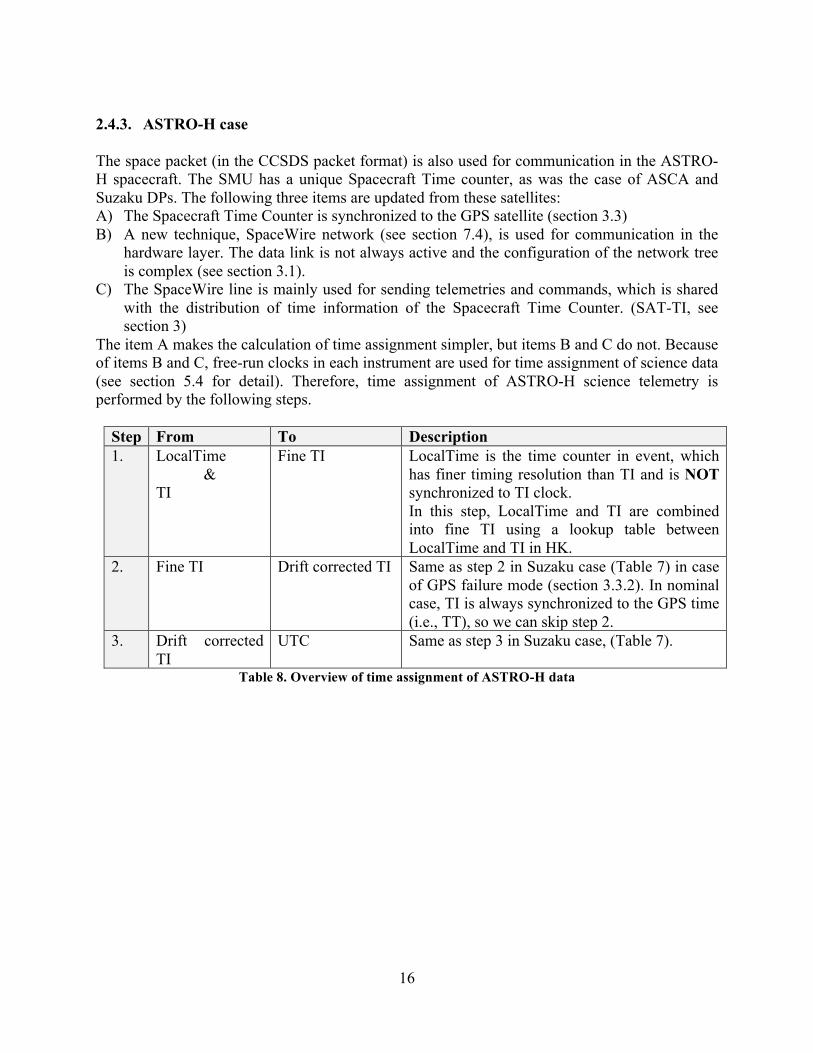
2.4.3. ASTRO-H case The space packet (in the CCSDS packet format) is also used for communication in the ASTRO-H spacecraft. The SMU has a unique Spacecraft Time counter, as was the case of ASCA and Suzaku DPs. The following three items are updated from these satellites: A) The Spacecraft Time Counter is synchronized to the GPS satellite (section 3.3) B) A new technique, SpaceWire network (see section 7.4), is used for communication in the

hardware layer. The data link is not always active and the configuration of the network tree is complex (see section 3.1).

C) The SpaceWire line is mainly used for sending telemetries and commands, which is shared with the distribution of time information of the Spacecraft Time Counter. (SAT-TI, see section 3)

The item A makes the calculation of time assignment simpler, but items B and C do not. Because of items B and C, free-run clocks in each instrument are used for time assignment of science data (see section 5.4 for detail). Therefore, time assignment of ASTRO-H science telemetry is performed by the following steps.

Step From To Description 1. LocalTime

& TI

Fine TI LocalTime is the time counter in event, which has finer timing resolution than TI and is NOT synchronized to TI clock. In this step, LocalTime and TI are combined into fine TI using a lookup table between LocalTime and TI in HK.

2. Fine TI Drift corrected TI Same as step 2 in Suzaku case (Table 7) in case of GPS failure mode (section 3.3.2). In nominal case, TI is always synchronized to the GPS time (i.e., TT), so we can skip step 2.

3. Drift corrected TI

UTC Same as step 3 in Suzaku case, (Table 7).

Table 8. Overview of time assignment of ASTRO-H data

17

2.5. Overview of the time assignment process in ASTRO-H 2.5.1. Schematic view of ASTRO-H Time Assignment As reviewed in ASCA, Suzaku, ASTRO-H cases (section 0), ASTRO-H cannot use the same software approach of ASCA or Suzaku in the sense that

l ASTRO-H carries GPSR (and timing software should support GPSR failure mode), l on-board delay happens in distribution of time, and l Instruments use their own clock for finer time resolution.

A schematic view of flow chart of time information is summarized in Figure 2.

Figure 2. Schematic view of ASTRO-H Time assignment.

The GPS receiver (section 3.3) on board ASTRO-H recognizes the atomic time in TAI (Table

3) and reports it to SMU. When the GPS satellites are locked off, then the synchronization between TAI and TI (Time indicator; Table 3. Definition for ASTRO-H is described in section 2.6) on SMU is missing. This status is reported in the GPS telemetry (section 3.3). The SMU distributes the timing information in the TI format to the instruments via two ways

(RMAP of U32TI and TIME_CODE; for detail see section 2.6). Instruments recognize the TI from U32TI and TIME_CODE and put L32TI value to all their telemetries. In order to assign finer time resolution than TI for science telemetries, instruments has their own LOCAL_TIMEs, which are the instrument clocks and are not synchronized to TI but have finer time resolution (section 6.1). The science telemetry always contains L32TI and LOCAL_TIME, and their HK reports the relation between U32TI and LOCAL_TIME (but for the SXI). A rough time, in the same definition of TIME (i.e., second from the ASTRO-H Epoch; Table 4), S_TIME (Table 3) is assigned for all the space packets on ground. 2.5.2. Task flow of ASTRO-H Time Assignment

18

Basic concept of timing software design is “to have common framework between instruments onboard ASTRO-H.” Since GPS status affects all the time assignments for instruments, the timing tasks are divided into (a) pre-process part and (b) main part. As shown in Figure 3, the time assignment processes of the ASTRO-H data consist of three steps, which correspond to three tasks named (1) ahtrendtemp, (2) ahmktim, and (3&4) ahtime. The steps (1) and (2) correspond to the pre-process part (a) common for all the instruments, and steps (3) and (4) in one task correspond to (b) main task for time assignment.

Figure 3. Flow chart of the time assignment process of ASTRO-H.

The first step (1) is prepared for the Suzaku mode, i.e., the mode when the GPS does not work. In Suzaku mode, the relation between quartz frequency and the temperature is used for correction of short-time frustration of Spacecraft Time Counter (= TI values) as the step 1 or 2 for ASCA or Suzaku, respectively (sections 2.4.1 and 2.4.2). At launch time, the temperature dependency of SMU quartz frequency is measured on ground for flight model SMU-A and SMU-B and stored in CALDB area. The main purpose for this step (1) is to be able to check the validity of the ground measurement. In every observation (OBSID), the temperature of the quartz on SMU and its frequency

information with TIME is extracted from the common HK (section 4.2) and stored into the trend archive area. Independently, another pipeline which is executed periodically (e.g., once a month) calls the ahtrendtemp task to make a “SMU quartz frequency vs temperature table”. The quartz frequency information is valid only when the TI is synchronized to GPS time. This information

19

is sent to the telemetry by command. Since the operation plan is well defined yet at 2014 Sep, the frequency to run ahtrendtemp is not defined yet (say once a month). The second step (2) is a kind of pre-processing part of the time assignment. As described in section 2.4.3, the time assignment process requires switching two kinds of algorithms between (a) nominal mode with GPS synchronization and (b) Suzaku mode without GPS. Since the main task of time assignment (ahtime) is designed to assign time event by event on the fly, the ahmktime pre-searches the status of GPS receiver (GPSR) and identify epochs to apply these algorithms. This information is stored in the GPS gti file. The results are summarized as the relation between TI and TT time, which will be used in the step 3 in Table 8 at section 2.4.2. This relation will be stored on the TIM_LOOKUP extension of TIM file (Table 3). The final processes (3) and (4) are done by single task named ahtime. The TIME column of HK is filled by the task with TIM_LOOKUP extension in TIME file (Table 3) from S_TIME and L32TI (details are described in section 3.5.3) in the process (3). Since the higher time resolution is required for the science data (as described in section 2.4.3), look-up table information in HK file is used for time assignment of science events in the process (4). Details are described in section 5.4.

20

2.6. Definition of TI for ASTRO-H and its Distribution As described in section 0, the Time Indicator (TI) of ASTRO-H is generated and controlled on SMU, and distributed to user nodes on the SpaceWire network. The format and definitions of TI are summarized in Table 9. Please use the following definition to avoid confusion.

Bit assign (6-bit) 32 (26-bit) 7 (6-bit) 0 Definition TI on SMU (38-bit)

L32TI in the secondary header of Space packet (32-bit) Distribution U32TI

RMAPwrite from SMU at time slot (3) TIME_CODE

(0..63) Coverage 226--232 s 1 s – 226 sec 2-6 s – 1 s

Table 9. Definition of Time Indicator (TI) of ASTRO-H. The original clock for time assignment is the TI (TI) on SMU, which has 38-bit length. The lowest bit has time resolution of 2-6 sec = 15.625 m sec, covering 232 sec = 4,294,967,296 sec ~ 136 year. The upper 32-bit of the TI value (U32TI), whose lowest bit indicates 1 second ticks, is distributed to user nodes via RMAPwrite (section 7.4.4) at the time slot (No.3) (see section 7.4.5, Table 41). The lower 6-bit of the TI is distributed via TIME_CODE (section 7.4.2) at the edge of time slots (section 7.4.2). Note that the timing of receiving TIME_CODE at user node has latency in micro second order during the distribution, which will be described in section 7.4.3. In the spacepacket of the telemetry, lower 32-bit of TI is stored in the secondary header of the CCSDS packet. This value is called as L32TI, which covers from 2-6 sec to 226 sec = 67,108,864 sec. Therefore, the L32TI carries every about 2.1 years. (Normally, the secondary header of a space packet is called as TI, but for ASTRO-H, it is called as L32TI. ) Normally, TI (or L32TI) is synchronized to the GPS time provided by the GPS receiver (GPSR) onboard the spacecraft. They have the origin of 0:0:0 UTC of 6 Jan, 1980. The behaviors when the TI is not synchronized to GPS time are described in the next section 3.

Epock of TI 1980-01-06 00:00:00 UTC (= TAI-19s) Definition of tick (1 sec) TAI (international atomic time) Resolution 15.625 m sec

Table 10. Definition of epoch and tick of TI.

21

3. Data Acquisition system onboard Spacecraft As described in section 2, detail designs of the communication system on board the spacecraft (section 7.4) and the rule of distribution of the time information L32TI to instruments (section 0) and that of synchronization between L32TI and GPS-time system (section 0) are important for the calculation of TIME. In addition, communication between the spacecraft and the ground stations (section 3.5), including the rule of recording and restoring space packets on the data recorder (DR; section 3.3.3) should be considered in the time assignment process. These items are summarized in this section. 3.1. Structure of the SpaceWire network of ASTRO-H The data acquisition system onboard ASTRO-H uses a standard network, called SpaceWire. The details for SpaceWire protocol are described in section 7.4. As described in section 7.4.1, any topology of the network tree can be acceptable for the SpaceWire network. The key features of ASTRO-H SpaceWire network can be listed as follows.

ü The network has a TREE type structure, in which the SMU is the Master node, ü The network has many redundant links to avoid single failure of a link, ü the attitude control unit has an independent network from the main data-acquisition

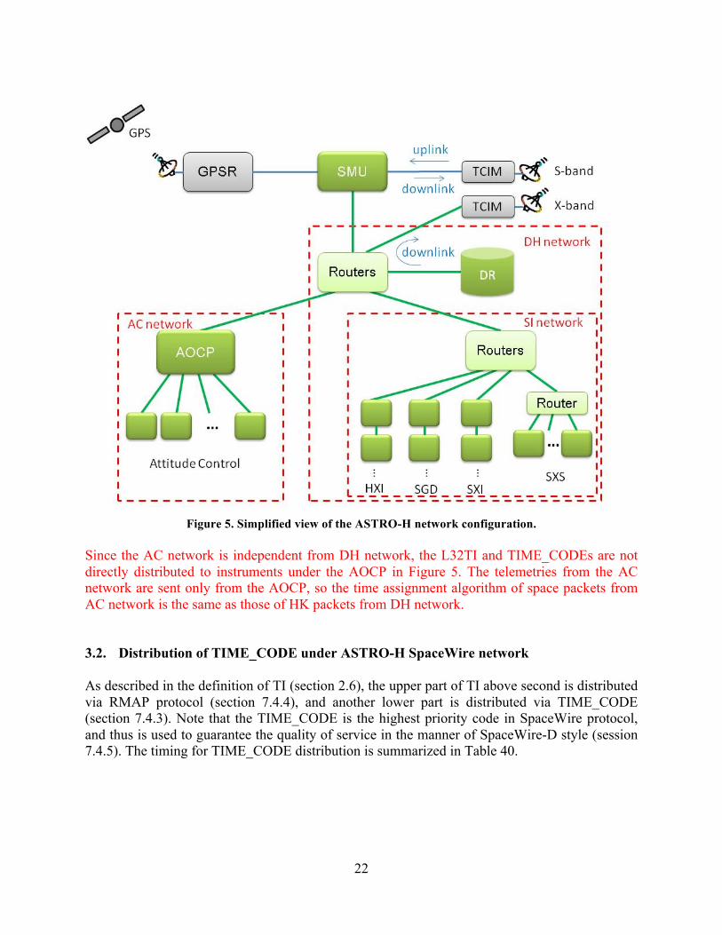
network for safety of the spacecraft (DH network and AC network) The detail design of the configuration for ASTRO-H SpaceWire network is shown in Figure 4 taken from the document ASTH-113 [8]. Since it may be hard to understand, so a simplified version of the configuration is shown in Figure 5.

Figure 4. Network Structure of ASTRO-H.

22

Figure 5. Simplified view of the ASTRO-H network configuration.

Since the AC network is independent from DH network, the L32TI and TIME_CODEs are not directly distributed to instruments under the AOCP in Figure 5. The telemetries from the AC network are sent only from the AOCP, so the time assignment algorithm of space packets from AC network is the same as those of HK packets from DH network. 3.2. Distribution of TIME_CODE under ASTRO-H SpaceWire network As described in the definition of TI (section 2.6), the upper part of TI above second is distributed via RMAP protocol (section 7.4.4), and another lower part is distributed via TIME_CODE (section 7.4.3). Note that the TIME_CODE is the highest priority code in SpaceWire protocol, and thus is used to guarantee the quality of service in the manner of SpaceWire-D style (session 7.4.5). The timing for TIME_CODE distribution is summarized in Table 40.

23

3.3. GPS receiver (GPSR) and SMU for the ASTRO-H mission 3.3.1. Overview of GPSR for ASTRO-H The ASTRO-H satellite carries GPS receiver (GPSR), as already described in section 0. The hardware is the new generation GPS receiver (NGPSR) developed by JAXA, which consists of GPS antenna (GPSA), GPS Low noise amplifier (GPSL), and GPS processor (GPSP). The GPSP can process three inputs from GPSA+GPSL in maximum. The block diagram of GPSR system is shown in Figure 6. For detail, please check ASTH-100.

Figure 6. Block diagram of GPSR = GPSA + GPSL + GPSP.

The outputs from the NGPSR are as follows; l 1PPS: 1 Hz pulse signal, which indicate the start of the second, l 1MPPS: 1 M Hz pulse signal, l Time data: the TAI value of the time at 1PPS signal, l Telemetry raw data: GPSR generate the 8192 byte data every second, which contains time

and orbital information. A part of the raw data is edited as space packet at SMU, which will be appeared on the telemetry (section 3.3.3).

The accuracy of this GPSR is listed in Table 11. The accuracy for orbital parameters depends on the status of receiving GPS signals and the algorithm on board GPSP of calculation of orbit. The timing accuracy of pulses from GPSR is less than 200 n sec in nominal cases.

Accuracy of parameters Normal MNV Orbit control Orbit Position 3 – 10 m 3 – 10 m 6 – 20 m

Velocity 0.03 – 0.05 m/s 0.06 – 0.07 m/s 1.0 m/s Time < ± 100 n sec < ± 100 n sec < ± 100 n sec

Time 1PPS accuracy < ± 200 n sec < ± 200 n sec < ± 250 n sec 1MPPS accuracy < ± 200 n sec < ± 200 n sec < ± 250 n sec

Table 11. Timing and orbital accuracy of GPSR.

GPSA

GPSL

Number of antenna is 2. Each antenna has 2 ch, L1 and L2.

1PPS

1MPPS

1PPS base time data GPSP

Telemetry/command

24

3.3.2. Synchronization of clocks between GPSR and SMU The time indicator (TI) is a subset of SA-TI on SMU (section 3.1), which has to be synchronized to the GPS (i.e., 1PPS, 1MPPS, and GPS data; section 3.3.1) from GPSR, but it may happen that the GPSR cannot receive any or part of GSP signals and the synchronization breaks. We have to avoid a big jump in the TI value even after the recovery of GPS signal, so the SMU has the following five modes in Table 12 and Figure 7. Thus, the GPS status (lock-on or lock-off) does NOT completely correspond to the SMU synchronization mode (synchronized or unsynchronized); i.e., we have transition mode in the SMU mode, as illustrated in Figure 8. Note that the SMU ON and the Time Initial modes are only used for initial operation of the satellite.

SMU Mode

GPS Mode

Time System

Epoch Length of one second

GPS synchronized

GPS lock-on

TAI 1980-01-06 0:0:0 UT Same as TAI

Transition SMU original

N/A Longer than TAI GPS unsynchronized

GPS lock-off 1980-01-06 0:0:0 UT or Set by command

Defined by the quartz on SMU

Time Initial N/A Set by command SMU ON N/A N/A N/A N/A

Table 12. Operation mode of the SMU for time assignment.

Figure 7. State machine of SMU operation modes listed in Table 12.

Figure 8. Example of mode transition of the SMU and GPS.

Time

GPS mode

Lock-on

Lock-off

Lock-on

sync

unsync

sync trans

SMU mode

25

A schematic structure of the timing system onboard ASTRO-H is shown in

Figure 9. SMU receives the 1PPS, 1MPPS, and the time data from GPSR (section 3.3.1), and generate TI from GPS data or its own quartz, depending on the mode of SMU as described above. Then, the L32TI (a part of TI) is distributed to user nodes via SpaceWire network (section 3.1) using RMAP (section 7.4.4) and TIME_CODE (section 7.4.2). The SMU also generate SA-1PPS and SA-1MPPS from SA-TI, which are distributed to two components, TCIM for generation of TIM packet (section 3.3.3) and AOCP for attitude control of the satellite. The TCIM also receives TI via SpaceWire link and generate TIM value, which is synchronized to TI and is used for generating TIME packets (section 3.3.3).

Figure 9. Overview of timing system onboard ASTRO-H. In summary, TI, L32TI, and TIM are synchronized with each other, but are not always synchronized to the GPS. When the GPS satellites are locked-off from GPSR, they run freely following quartz on SMU (GPS unsynchronized mode). Then, if the GPS locks, the SMU status moves into the transition mode, as illustrated in Figure 8. In this mode, SMU knows both GPS time (TAI) and his own time (TI), and try to synchronize TI to TAI by the following four steps. (1) The SMU monitors the phase difference between 1PPS from GPS and SA-1PPS. (2) The SMU elongates and contacts the length of SA-1PPS by ±1 -- 256 µsec par

TIME_CODE. (3) When the difference between 1PPS and SA-1PPS is less than 64 µsec, then the SMU

elongates and contacts the length of SA-1PPS by ± 1 – 32 µsec par TIME_CODE only at the time slot (0).

(4) If the difference between 1PPS and SA-1PPS is less than 1 µsec, the transition mode finishes. Note that the SA-1MPPS is already synchronized to 1MPPS at the end of stage (4), i.e., difference is less than 100 nsec.

1PPS 1MPPS Time data SA-1PPS

SA-1MPPS

RMAP(upper TI)

TIME_CODE

SA-TI & TIME_CODE

unsync/trns sync

GPSR

SMU

SpW router

AOCP

TCIM

node

node node

L32TI

TI TIM

SA-1PPS SA-1MPPS

SpaceWire Other link

To GROUND

26

Figure 10. Example of relation between TAI and SA-TI. A schematic plot between the TAI and L32TI are shown in Figure 10. In the GPS unsynchronized mode, the SA-TI is generated by quartz on SMU. The features of the quartz onboard SMU are summarized below, Table 13. The frequency of the quartz has a dependence on its temperature, whose relation can be measured on ground (and hopefully in orbit). The stability would be improved if we correct the drift of the frequency by its temperature at the off-line analyses.

Item Spec reference Frequency 50MHz Stability of frequency Temperature ±50 ppm -55 °C -- +125°C

Changes (30days) ±1.5ppm 70°C±3°C Changes (1 year) ±10 ppm 70°C±3°C

Accuracy of tick ≦240µs (TBD) Table 13. Spec of the quartz onboard SMU.

In order to distinguish these modes, following 4 items in the GPS telemetry (section 3.3.5) are used. The name, a, b, c, and d, are defined in the Timing design document ASTH-200-07. (Note that the definition of a, b, c, d, were c, a, b, d in Build 5.)

Name Column name in COM HK Description a SMU_A_DHFS_TI_MNG_TIM_CRNT_TIM Current time system of SMU.

[1: in GPS time, 0: in SMU quartz time] b SMU_A_DHFS_TI_MNG_TIM_GPS_SYC_STAT The timing synchronization status

between the SMU and GPSR. [1:synchronize, 0:un-synchronize]

c SMU_A_DHFS_TI_MNG_TIM_AUT_SYC Enable/Disable of time system switch.

TAI

GPS lock-on GPS lock-on

synchronized mode

Unsynchronized mode

transition mode

synchronized mode

coarse

fine

L32TI

27

This is the hardware setting for SMU, whether the function to automatically change the time system of SMU is enable or disable. [ 1: Enable tim-system switch (i.e., TI can be synchronized to GPSR)

0: Disable (i.e., TI is always generated from SMU quartz)]

d SMU_A_DHFS_TI_MNG_TIM_GPS_STAT The hardware status of GPSR. [1: timing clock and time data are OK.

0: timing clock and time data are NG] Extension name is HK_SMU_A_DHFS_TI_MNG_HK_TI_MNG_8n7_Block ( I&T test)

HK_SMU_A_DHFS_SIB2GEN_dhfs_tlm_attseq (After 2014) Table 14. GPS telemetry to identify the TIME system for TI

We can identify the SMU time system by these flags. The Table 15 represents the status of SMU-GPSR. The telemetry name, a, b, c, and d are defined in Table 14.

a b c d Mode/Status Ground Software

0

0

0 0 Unsynchronized Mode

TI = SMU time system Calc Suzaku Mode 1

1

0 Transition Mode, and the TI is generated from SMU quartz. Calc Suzaku Mode

1 Transition Mode, but the TI is difference both from SMU quartz and GPS time.

ERROR, but proceed timing calculation in Suzaku Mode (*)

1

0 0

Illegal Condition (out of plan) Error 1

1

0 Not Defined (**) Error

1 End of Transition Mode (TI ~ GPS time, verifying the GPS time system for 32 second)

ERROR, but proceed timing calculation in GPS Mode. Stable.

1

0 0

0

Illegal Condition Error

1

1 0 1

1

0 0 1

1 0

1 Synchronized mode TI = GPS Time

Normal conversion Calc in TI=TAI mode.

Table 15. TIME systems tree by GPS telemetry (*)This is approximate method, because we do not the relation between TI and TAI at the beginning of transition mode = end of unsynchronized mode (section 3.3.3).

28

In starting up SMU, these flags change as follows. The value changes from 0 to 1 in the order of flags d, b, and a.

Flags Time0 Time1 Time2 Time3 a 0 0 0 1 b 0 0 1 1 c always set to 1 d 0 1 1 1

3.3.3. Synchronization Algorithm of TI in transition mode The difference between TI and TAI in transition mode will be sent in the telemetry only at the beginning of the transition mode. In correction of TI to TAI, we need an algorithm on board SMU to synchronize TI to TAI. (NEC people will provide the algorithm of synchronization in transition mode; see the memo in 28 Aug 2012) [NOT YET DONE 2014 Sep] Notice: When the difference between L32TI and GPS time is larger than 1.0 second at the beginning of the transition mode, SMU will shift the U32TI and drift lower bit of TI under second order. Therefore, the TI could be jumped by +N or –N second. l In other words, the same TI value can be appeared more than twice. l We have to check the jump of TI by monitoring the secondary header and sequence number

of CCSDS packet of SMU HK.

29

3.3.4. Duplication or Skip of TIs at the transition mode of TI time system When the difference between TI and GPS time is larger than 1.0 second at the beginning of the transition mode, SMU will shift the U32TI and drift lower bit of TI under second order. Therefore, the TI could be jumped by +N or –N second. l In other words, the same TI value can be appeared more than twice. Example, 1 2 3 4 4 4 4 5

6 7 ,…. in FITS file (time sorted). [duplication] l In other cases, several TIs may be skipped. Example, 1 2 5 6 7 … in FITS file. [skip] Please note that the TI equivalent values in TIME packet (section 3.4) also skip or duplicate and so TI in TIM file is also affected. In order to detect these duplication or skip, we have to monitor the R_TIME, and TI in the ESSENSIAL HK extension of the SYSTEM HK (TBR), which is periodically appeared in the telemetry in normal condition. Note that S_TIME is not useful for this detection, because it is calculated by SIRIUS via some method (which we do not know). In the following example, the TI appears twice when R_TIME = 2.0, 3.0, 4.0, and 5.0. R_TIME(s) TI from time packet 1.0 100 2.0 200 3.0 300 4.0 200 5.0 300 6.0 400 7.0 500 For detection,

ü delta TI / delta R_TIME < 0.0 … duplication occurs ü delta TI / delta R_TIME > 64 (s-1) … skip occurs

Note that R_TIME is not available in FFF stage, because of limitation of L1TSD tool. The order of spacepacket should be guaranteed when we access the SIRIUS database, which is defined in ASTH-SCT-002.

30

3.3.5. Telemetry of GPSR via SMU The attributes of GPS and SUM in the telemetry, which are related to time assignment, are summarized in Table 16.

HK Extension name Column name Size Description COM HK_SMU_A_D

HFS_TI_MNG_HK_TI_MNG_8N7_BLOCK

SMU_A_DHFS_TI_MNG_TIM_GPS_SYC_STAT

1-bit The synchronization status between the SMU and GPSR. (1:synchronize, 0: un-synchronize) (flag-a)

COM SMU_A_DHFS_TI_MNG_TIM_GPS_SYC_STAT

1-bit Hardware setting for SMU, whether we turn on the function to automatically change the time system of SMU. (1: Enable time-system switch, i.e., the TI can be synchronized to GPSR) (0: Disable time-system switch, i.e., the TI is always generated by SMU quartz. ) (flag-b)

COM SMU_A_DHFS_TI_MNG_TIM_AUT_SYC

1-bit Time system of SMU (1: TI is in GPS time) (0: TI is generated by SMU quartz) (flag-c)

COM SMU_A_DHFS_TI_MNG_TIM_GPS_STAT

1-bit The hardware status of GPSR (1; clock and data from GPSR is valid) (0: clock and data from GPSR is not valid) (flag-d)

COM SMU_A_DHFS_TI_MNG_TIM_TCAL_INF

32bit Quartz counts, accumulated in 16 seconds. The LSB is 20 nsec. (frequency information)

COM SMU_A_DHFS_TI_MNG_TIM_TCAL_TIME

32bit U32TI when the acquisition of quartz counts started.

COM HK_SMU_A_DHFS_TI_MNG_BLOCK_GET_TI_MNG

SMU_A_DHFS_TI_MNG_TIM_GPS_WEK

16bit GPS week number from GPSR

COM SMU_A_DHFS_TI_MNG_TIM_GPS_SEC

32bit GPS week second from GPSR

COM 1-bit GPS base clock status. Validity of 1MPPS and 1PPS, judged by SMU. 1: ok, 0:ng.

COM SMU_A_DHFS_TI_MNG_TIM_GPS_SKP_STAT

1-bit Time jump flag. SMU detected the jump in time from GPSR. 1: Jumped, 0:not jumped.

COM SMU_A_DHFS_TI_MNG_TIM_GPS_CHNG_CNT

8-bit Time system change count. Number of changes into the GPSR time system

COM SMU_A_DHFS_TI_MNG_TIM_SPC_CNT

32bit SpaceCube clock count. Time since the SpaceCube2 is booted. LSB=1s.

COM SMU_A_DHFS_TI_MNG_TIM_TI_OFFSET

32bit TI to GPS time offset . Difference between GPS time and SpaceCube2 time in second. LSB=1s.

COM SMU_A_DHFS_TI_MNG_STY_TI

32bit Satellite time U32TI.

COM SMU_A_DHFS_TI_ 8bit Time since start monitoring synchronization

31

MNG_TIM_RESYNC_MON_CNT

(LSB=1s)

COM SMU_A_DHFS_TI_MNG_TIM_RESYNC_FAIL_CNT

8 bit Failure counts of time synchronization

COM HK_SMU_A_HCE_HCE_A_SENS_STS

HCE_A.SensStsList.SensSts114Temp HCE_B.SensStsList.SensSts111Temp

10 bit

The temperature of the board in SMU. The sensor is near the quartz of SMU. LSB=0.16 degrees (to be calibrated).

Table 16. Telemetry for SMU status on GPS

32

3.4. TIME packet from ASTRO-H satellite The TIME packet contains the TIM information at TCIM described in section 3.3.2. The format is defined in Table 17. The latch timing of TIM counter is well defined in the telemetry and command design rule, ASTH-111 [7]; i.e., at the edge of the time in sending the transfer frame data, which contains space packets. The basic information to retrieve TIME packet is as follows;

l Frequency = 30 sec l APID = 0x001 (SMU-A), 0x004 (SMU-B) l Lower FOID = 0x20 l Attribute ID = 0x0027

Feild Length Description

VCID 6-bits (1) VCID of the transfer frame VC Frame Count 24-bits (2) VC frame count Sending Time of the Transfer Frame (TIM)

LSB = 1 s 30-bits (3) Upper TI latched at 1PPS LSB = 1 µs 20-bits (4) Lower TI, measured by 1MPPS

Valid in the range of 1 – 999,999. Table 17. Format of TIME packet.

The TIME packet is used for generating a look-up table between TI and TIME in

TIME_PACKETS extension of TIM file (Table 23). The TI is converted from TIM values in the packet and the R_TIME assigned on ground is used for TIME (section 3.5). Note: TIM in Table 17 contains finer time resolution than L32TI, but the L32TI in TIME_PACKETS extension drops finer time resolution. Items (3) and (4) in Table 17 can be used for generation of TI-equivalent value. When the SMU is not in the synchronized mode, 1 second in 1MPPS is not exactly the same as 1,000,000 but values in a range of 983,616 to 1,016384. In case the item (4) exceeds 1,000,000, the item (3) has 1.0 small value consistently. Therefore, in generation of TI, the first operation is to add (3) and (4).

33

3.5. Ground system 3.5.1. Receive time at the ground station The time when the space packet is received on the ground station is stamped for each space packet. The time is described in UTC, not in TAI, and so the leap second is already considered. This information is recorded in the SDTP header (see the SCT document, ASTH-SCT-002 [9]) when we get a space packet, but is deleted in the RPT and FFF stages, because it is not used in the time assignment process in the pipe line. The UTC values stamped on ground when the ground station receives TIM packets (section 3.4) are converted into TAI values, named R_TIME, and recorded in the TIM File, which is one of the products of the pre-pipe line process [9]. In calculation of R_TIME, the following time delays are subtracted from the original value. l Internal time delay from TCIM to S-band transponder in orbit l Propagation delay from the satellite to the antenna of the ground station, calculated by the

orbital parameter of the satellite l Propagation and processing delays from when the transfer frame is received to when the

UTC is stamped by the time assignment component on ground. The epoch of S_TIME is the same as that of TIME in Table 4.

Epoch of R_TIME 2014-01-01 00:00:00 UTC MJD 56658.0007775925926 (TT) Table 18. Definition of epoch of R_TIME.

In summary, the TIM file describes a look-up table between L32TI vs. TAI, which correspond to the TIM value in the TIME packet and R_TIME on ground. The detail of the format of TIM file is described in ASTH-SCT-002 [9]. (to be updated. We need calculation from TIM to L32TI.) 3.5.2. Time assignment at SIRIUS The SIRIUS database at ISAS is the first storage of the telemetry of the ISAS missions. The space packets are retrieved from SIRIUS database and are converted into RPT and FFF [9]. The raw information of TIM file is also retrieved from the SIRIUS database, and thus the calculations described in section 3.5.1 are performed on the SIRIUS side. The SIRIUS also provides a function to assign “rough” time when the space packet was generated in orbit. This rough time is stored in the S_TIME column of FFF files. The S_TIME is described in TAI, whose epoch is the same as TIME. This time assignment function is a mission independent one, and so the SIRIUS does NOT care whether the GPSR is used for the mission or not. That’s why the S_TIME is a “rough” time, which is calculated without GPS information.

Epoch of R_TIME 2014-01-01 00:00:00 UTC MJD 56658.0007775925926 (TT) Table 19. Definition of epoch of S_TIME.

The inputs of the time assignment function at SIRIUS are as follows. l L32TI in the secondary header of the CCSDS format of the space packet

34

l R_TIME in the SDTP header of the space packet l TIM file, which describes the relation between L32TI vs R_TIME when the satellite

communicate with the ground station. In the calculation of S_TIME, the function uses the interpolation function between two or more data points in TIM file. Since the L32TI carries by 2 years (section 3.1), we need R_TIME to identify the round of the L32TI in the calculation. In summary, the time assignment proceeds by the following steps. The flow is also demonstrated in Figure 11.

(1) Read R_TIME from the space packet (2) Search row in TIM file around R_TIME (3) Calculate the interpolation function between S_TIME and L32TI (4) Read L32TI from the space packet (5) Get S_TIME from L32TI and interpolation function

Figure 11. Algorithm of time assignment with TIM file

When the data is out of range, the tools do calculation of extrapolation and should show warning messages.

S_TIME

L32TI

Data in TIME file Interpolation func.

(1) R_TIME in space packet

(4) L32TI in space packet

(2) Pick up data from TIM file

(3) calc interpolation function (5) Get S_TIME at TI.

35

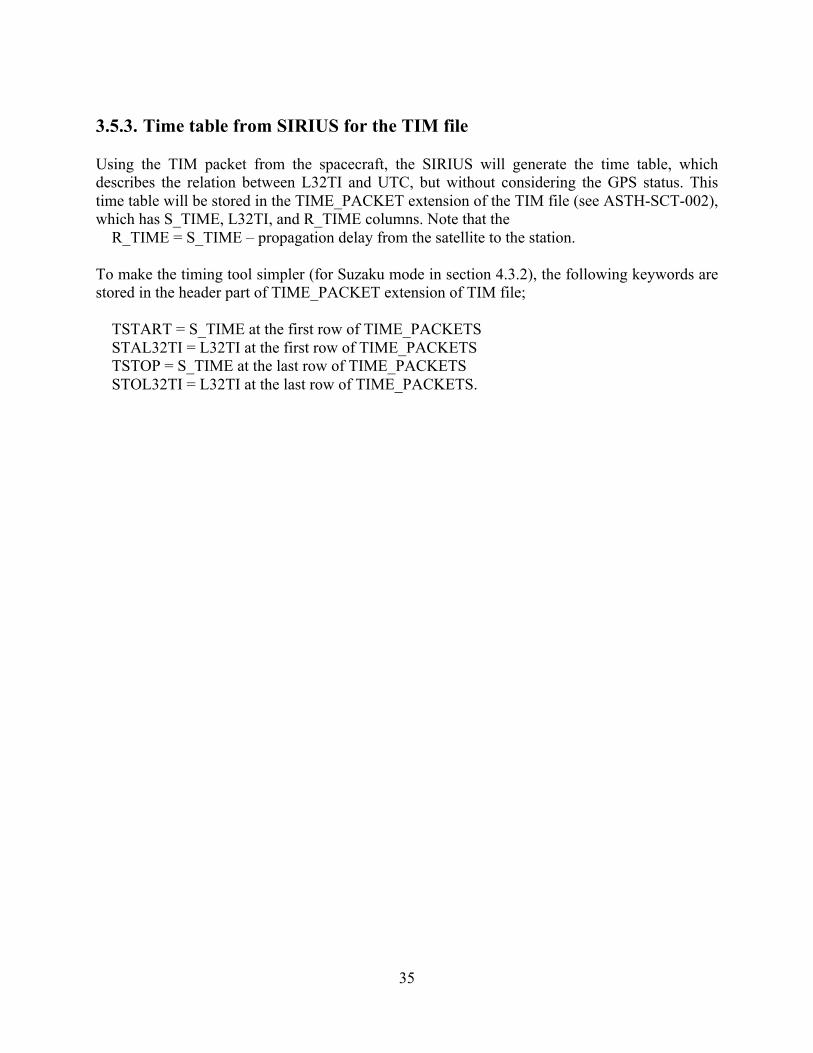
3.5.3. Time table from SIRIUS for the TIM file Using the TIM packet from the spacecraft, the SIRIUS will generate the time table, which describes the relation between L32TI and UTC, but without considering the GPS status. This time table will be stored in the TIME_PACKET extension of the TIM file (see ASTH-SCT-002), which has S_TIME, L32TI, and R_TIME columns. Note that the

R_TIME = S_TIME – propagation delay from the satellite to the station. To make the timing tool simpler (for Suzaku mode in section 4.3.2), the following keywords are stored in the header part of TIME_PACKET extension of TIM file;

TSTART = S_TIME at the first row of TIME_PACKETS STAL32TI = L32TI at the first row of TIME_PACKETS TSTOP = S_TIME at the last row of TIME_PACKETS STOL32TI = L32TI at the last row of TIME_PACKETS.

36

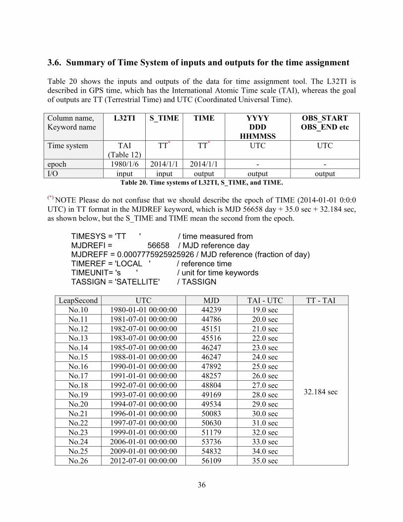
3.6. Summary of Time System of inputs and outputs for the time assignment Table 20 shows the inputs and outputs of the data for time assignment tool. The L32TI is described in GPS time, which has the International Atomic Time scale (TAI), whereas the goal of outputs are TT (Terrestrial Time) and UTC (Coordinated Universal Time). Column name, Keyword name

L32TI S_TIME TIME YYYY DDD

HHMMSS

OBS_START OBS_END etc

Time system TAI (Table 12)

TT* TT* UTC UTC

epoch 1980/1/6 2014/1/1 2014/1/1 - - I/O input input output output output

Table 20. Time systems of L32TI, S_TIME, and TIME.

(*) NOTE Please do not confuse that we should describe the epoch of TIME (2014-01-01 0:0:0 UTC) in TT format in the MJDREF keyword, which is MJD 56658 day + 35.0 sec + 32.184 sec, as shown below, but the S_TIME and TIME mean the second from the epoch.

TIMESYS = 'TT ' / time measured from MJDREFI = 56658 / MJD reference day MJDREFF = 0.0007775925925926 / MJD reference (fraction of day) TIMEREF = 'LOCAL ' / reference time TIMEUNIT= 's ' / unit for time keywords TASSIGN = 'SATELLITE' / TASSIGN

LeapSecond UTC MJD TAI - UTC TT - TAI

No.10 1980-01-01 00:00:00 44239 19.0 sec

32.184 sec

No.11 1981-07-01 00:00:00 44786 20.0 sec No.12 1982-07-01 00:00:00 45151 21.0 sec No.13 1983-07-01 00:00:00 45516 22.0 sec No.14 1985-07-01 00:00:00 46247 23.0 sec No.15 1988-01-01 00:00:00 46247 24.0 sec No.16 1990-01-01 00:00:00 47892 25.0 sec No.17 1991-01-01 00:00:00 48257 26.0 sec No.18 1992-07-01 00:00:00 48804 27.0 sec No.19 1993-07-01 00:00:00 49169 28.0 sec No.20 1994-07-01 00:00:00 49534 29.0 sec No.21 1996-01-01 00:00:00 50083 30.0 sec No.22 1997-07-01 00:00:00 50630 31.0 sec No.23 1999-01-01 00:00:00 51179 32.0 sec No.24 2006-01-01 00:00:00 53736 33.0 sec No.25 2009-01-01 00:00:00 54832 34.0 sec No.26 2012-07-01 00:00:00 56109 35.0 sec

37

No.27 2015-07-01 00:00:00 57204 36.0 sec No.28 TBD (*) TBD (*) 37.0 sec

Table 21. Table of leap second between 1980 and 2012. (*) At the time of drafting this document (2012 June), we do NOT know whether we have another leap second from now to 2014-01-01. The timing keywords for TIMEDEL and TIMEPIXR are defined in ASTH-SCT-006. For reference the following table is used for pre-launch FFF. (Note that originally the TIME for SXI was defined as TIMEPIXR=0.5, having +0.5*Exposure in the formula, but was deleted. Currently TIMEPIXR for all the instruments are set to 0.)

Instrument TIMEDEL TIMEPIXR SXS 0.001 sec 0 SXI FW 4 sec 0 SXI FW Burst 2 sec 0 SXI 1/8 W 0.5 sec 0 SXI 1/8 W Burst 0.1 sec 0 HXI 0.000256 sec 0 SGD 0.000256 sec 0 SHIELD GRB 0.016 sec 0 SHIELD SCALAR 2 sec 0 SHIELD HISTO 4 sec 0

Table 22. definition of TIMEDEL and TIMEPIXR

38

4. Generation of a look-up table between L32TI and TIME (Tim file) The time assignment of HK and science data (Section 2.4.3 ) depend on a look-up table between the time indicator (L32TI) and time. The file containing this look-up table is called the TIME file (or TIM_LOOKUP extension in TIME file Table 3). The TIM file contains two extensions, but only the look-up table in the second extension is used for time assignment. The look-up table in the first extension is generated by SIRIUS with data for when the Astro-H satellite is in contact with the ground station (~90 min intervals). The look-up table in the second extension, however, is generated from HK files thereby having a finer time resolution. This chapter will outline the two-step procedure to generate this second extension:

1. extract temperature and frequency data from HK files (extension name is TBD) using the ahtrendtemp tool

2. relate L32TI with time based on the GPS mode (synchronized, unsynchronized, transition); this step is performed by ahmktim

4.1. Origin and format of TIM file The TIM file is originally provided on the FFF stage from SIRIUS system at ISAS (as described in section 3.5). The original TIM file (TIME_PACKETS extension) contains the relation between L32TI and TT measured on the ground station when the satellite is contact with the station. Therefore, the typical time interval between measurements is about 90 minutes, which is the period of the orbit. The original TIM file (TIME_PACKETS extension) contains a single extension (TBD, at least 1st extension contains the followings). The tool, ahmktim, will add a TIM_LOOKUP extension containing the look-up table to use for time assignment. Table 21 gives details about the two extensions and an example of the contents of the 2nd extension of the TIM file is shown in Figure 11. In order to have finer accuracy in L32TI in TIM_LOOKUP extension, it is written in ‘1D’ format not in ‘1J’ as is in other extensions.

Ext name Origin Task Source Interval of data TIME_PACKETS SIRIUS,

Pre pipe-line mktim Time packet,

Ground station Intervals between contact paths (~90 min)

TIM_LOOKUP Pipeline in Jp ahmktim GPSR Periods of the telemetry ( ~ 1 - 4sec)

Table 23. Definition of TIM file.

39

Figure 12. An example of contents of TIM file, 1st and 2nd extensions.

4.2. Extract frequency and temperature trends As described in section 3.3.3, the raw counter values of the quartz on SMU and the temperature of SMU are recorded in the telemetry from SMU, which is stored in the COM HK file. These telemetries are valid when the TI is synchronized to GPS time, and valid only for the active SMU. The SMU unit (‘A’ for SMU-A, ‘B’ for SMU-B) can be identified by the SMUUNIT keyword. On the daily pipeline process, these information will be stored in the trend area. The task, ahtrendtemp, extracts these data from trend archive and calculate the frequency vs. temperature table into a CALDB type FITS file, labeled TFMMYY_MMYY extension where MMYY give the start and end dates of the processed data. This process is performed every month (TBD after launch). The ahtrendtemp tool combines the trend data from all the HK-type FITS files from the last TBD months. Frequency data must be computed from the quartz counter which is stored in a separate extension from the temperatures. The column name and extension name of the quartz counter and temperature are summarized in Column name Extension name S_TIME S_TIME HK_SMU_A_AUX_HCE_HK2 for SMU-A

HK_SMU_A_AUX_HCE_HK3 for SMU-B Temperature HCE_A_SENS_SMU_A_TEMP_CAL for A

HCE_A_SENS_SMU_B_TEMP_CAL for B HK_SMU_A_AUX_HCE_HK2 for SMU-A HK_SMU_A_AUX_HCE_HK3 for SMU-B

S_TIME S_TIME HK_SMU_A_DHFS_TI_MNG_block_get_ti_mng for A HK_SMU_B_DHFS_TI_MNG_block_get_ti_mng for B

L32TI L32TI HK_SMU_A_DHFS_TI_MNG_block_get_ti_mng for A HK_SMU_B_DHFS_TI_MNG_block_get_ti_mng for B

QUARTZ_U32TI SMU_A_DHFS_TI_MNG_TIM_TCAL_TIME for A SMU_A_DHFS_TI_MNG_TIM_TCAL_TIME for B

HK_SMU_A_DHFS_TI_MNG_block_get_ti_mng for A HK_SMU_B_DHFS_TI_MNG_block_get_ti_mng for B

RAW_QUARTZ_CLOCK SMU_A_DHFS_TI_MNG_TIM_TCAL_INF for A SMU_B_DHFS_TI_MNG_TIM_TCAL_INF for B


Table 24. The quartz counter is converted to the L32TI equivalent count. Normally the LSB of the quartz counter is 20 ns and the acquisition time is 16 second. Since the time resolution of L32TI is 1/64 sec, the conversion factor between them is 16 sec / 20 nsec * (1/64 sec) = 12,500,000, which is stored as the keyword ‘PERIODCL’ = 12,500,000. The temperature assigned to each frequency is determined by interpolating the data points from the temperature extension by converted U32TI to S_TIME.

TT (s)

L32TI

1st extension, from FFF 2nd extension, added in SFF

40

Column name Extension name S_TIME S_TIME HK_SMU_A_AUX_HCE_HK2 for SMU-A

HK_SMU_A_AUX_HCE_HK3 for SMU-B Temperature HCE_A_SENS_SMU_A_TEMP_CAL for A

HCE_A_SENS_SMU_B_TEMP_CAL for B HK_SMU_A_AUX_HCE_HK2 for SMU-A HK_SMU_A_AUX_HCE_HK3 for SMU-B

S_TIME S_TIME HK_SMU_A_DHFS_TI_MNG_block_get_ti_mng for A HK_SMU_B_DHFS_TI_MNG_block_get_ti_mng for B

L32TI L32TI HK_SMU_A_DHFS_TI_MNG_block_get_ti_mng for A HK_SMU_B_DHFS_TI_MNG_block_get_ti_mng for B

QUARTZ_U32TI SMU_A_DHFS_TI_MNG_TIM_TCAL_TIME for A SMU_A_DHFS_TI_MNG_TIM_TCAL_TIME for B


RAW_QUARTZ_CLOCK SMU_A_DHFS_TI_MNG_TIM_TCAL_INF for A SMU_B_DHFS_TI_MNG_TIM_TCAL_INF for B


Table 24. Column and extension names for SMU quartz frequency and temperature. Once gathered, ahtrendtemp bins the frequency data by temperature and averages all data within each bin. The default averaging scheme is to compute the mean of both frequency and temperature; ; i.e.,

Freq.(average) = sum of freq. / number of measurements , but other schemes will be supported (To be described). The number of measurements in the averaging operation is also stored into the output CALDB file. Figure 11 shows example trend data and the resulting frequency vs. temperature curve.

Figure 13. Extraction of trend data by ahtrendtemp and generation of caldb information. The policy to update CALDB (FvT) in orbit: (Discussed on 1 July 2015)

Trend data TI

clk_cnt

temp

Freq (tick/sec)

temp Plot

41

We will update CALDB (FvT) in orbit when we find some inconsistency between the ground calibration and outputs from ahmktrendtemp. The ahtime cannot access CALDB (FvT) because TIME is blank at this moment. First pre-launch version of CALDB has FvT table from I&T test on the 2nd extension of CALDB, FvT, with the validity date at 2014-01-01 00:00:00 UTC.

4.3. Generation of TIM file TIM_LOOKUP extension with GPS information In the calculation of the TIM_LOOKUP xtension of TIM file, the synchronization status between the GPSR and SMU (section 0) affects the quality of time assignment. Therefore, we have to switch between three algorithms of time assignment:

i. SMU clock is synchronized to GPS (GPS mode) ii. SMU clock is not synchronized to GPS. (Suzaku mode)

iii. transition period to allow the unsynchronized time to be smoothly adjusted to the synchronized mode (transition mode)

The order of these modes must match the order given above, where transition mode is then following by GPS mode. The remainder of this section will describe the algorithms for each mode, in turn. The task, ahmktim, will determine the GPS mode and apply the appropriate algorithm, see schematic in Figure 14. The task will also generate a GPS gti file recording the intervals corresponding to the GPS mode only. Upon output, ahmktim, will record one of the following status to the PROC_STATUS column of each row:

• GPS mode • Suzaku mode • Transition mode: okay • Transition mode: duplicate region • Transition mode: skip region

Note: details of the PROC_STATUS flags currently implemented are the followings: 1) ahmktim writes the GPS status in the GPS_STATUS column defined as 3bits with the folloing value 1st X GPS mode on =1 off =0 2st X Suzaku mode on=1 off=0 3rd X quality of transition mode ok=0 bad=1 (note 1st & 2nd must be 0) 2) ahtime instead records the time goodness into the PROC_STATUS column so we need a definition of N the lenght Nx PROC_STATUS column. Lets assume that the lenght is 34 bits where the 1st 17 are assigned to Japan and the following 17bits are for US

42

The ahmktim will use 3 bits mark as Upper case X with the folloing value 1st X GPS mode on =1 off =0 2st X Suzaku mode on=1 off=0 3rd X quality of transition mode ok=0 bad=1 (note 1st & 2nd must be 0) The definition of the ‘STATUS’ column is as follows;

Bit-1: ok/notok Bit 2-3: GPS/Suzaku/transition Bit-4-5: monotonic/skip/duplicate Bit-6-10: different errors cases.

Figure 14. Flow chart of ahmktim.

43

4.3.1. GPS Mode (GPS and SMU clocks are synchronized) In case when the SMU clock is synchronized to GPS, the TIs always have the epoch of 1980-01-06 0:0:0 UTC, as shown in Table 10. The conversion process from L32TI to TIME at ahmktim is a simple calculation of changing epochs from 1980-01-06 0:0:0 UTC to 2014-01-01 0:0:0 UTC. In the calculation, we have to consider the following three items. l Since these epochs are defined in UTC values, the offset between them has leap seconds. l The L32TI counters caries by 226 sec = 67,108,864 sec ~ 2.1 years (see section 3.3.2).

Figure 15. Schematic view of counters in calculation from L32TI, S_TIME, into TIME.

Figure 15 shows the schematic view of relations between L32TI, S_TIME, and TIME in calculation of time. The offset between epochs of L32TI and TIME is

X = 12414 days + leapsec(between 1980-2014, 16 sec) = 1,072,569,616 sec, Note that this value will be recorded as ‘GPSOFFET’ keyword in the FITS header of each file.

The number of caries of L32TI counter at 2014-01-01 is 15)2( 26 ==XINTN . In the same way,

when the data is generated, the number of reset of L32TI counter is

)2

_( 26

XTIMESINTn += ,

and thus the origin of current L32TI value is ( Xn −× 262 ) sec from 2014-01-01. Since the L32TI has time resolution of 26 sec, the second from the origin of L32TI counter to the data point is L32TI/26 sec. Finally, the time second of the data since 2014/1/1 0:0:0 is

TIME 2626

26626

232}2)

2_({

232)2( TILXXTIMESINTTILXn +−×

+=+−×= .

Since S_TIME is a rough time, the n may be n-1 or n+1 when the S_TIME, the timing of reset of L32TI, and TI are near with each other (case shown in Figure 16). Calculate L32TI at S_TIME and check the difference between L32TI at S_TIME and that at the data, | L32TIS_TIME – L32TIdata | is less than 225 second. In this case, use (n-1) or (n+1) instead of n.

Figure 16. Same as Figure 15, but another case.

Time (sec)

… 1 2 3 15 16 n

1980/1/1 2014/1/1 data X S_TIME

TI

L32TI

44

4.3.2. Suzaku Mode (GPS and SMU clocks are not synchronized) When the GPS and SMU clocks are not synchronized (section 3.3.2), the TI is generated from a free-run clock on board SMU. The calculation of the relation between L32TI and TIME are done by the following two steps.

Step 1) Correction of the drift of the frequency by the temperature of the quartz. Step 2) Calculation of time tick and get final relation between L32TI and TIME.

As shown in Figure 17, L32TI values may fluctuate by time during the SMU is in the GPS unsynchronized mode (shown in red). We can use the data points during the SMU is in GPS synchronized mode (shown in green). The first step of calculation of the TIM file is the drift correction by temperature, whose relation was calibrated in a way in section ???. The modified L32TI (TIdrift) is described as

∫ TIdtδL+TIL=TIL drift 323232 , where δL32TI is a drift value at the temperature, and is equal to the inverse of the frequency (Hz = tick/sec) and time duration from the beginning of the GPS unsynchronized mode (sec). As indicated in Figure 17, the last value of L32TIdrift at the end of the GPS unsynchronized mode (shown in red on the second panel) is not the same value of transition-mode L32TI at that time (green); label this difference ΔT. To correct this discrepancy, an averaged time tick during the GPS unsynchronized mode, each L32TIdrift value is adjusted by an amount proportional to ΔT. If the adjusted value is labeled L32TIcor, then the formula is

L32TIcor= L32TIdrift + slope * (S_TIME – S_TIME1) where S_TIME corresponds to L32TIdrift and S_TIME1 is for the last L32TI value of GPS-synch mode (immediately before first Suzaku mode point). The L32TIcor value is written in the TIM file with TIME=S_TIME.

45

Figure 17. Schematic view of the calculation of L32TI-TIME relation during GPS-unsynchronized.

GPS synchronized mode GPS unsynchronized mode

TIME

TI Raw Data

TIME is unknown


TIME

TI Drift corrected

TIME is unknown


TIME

TI tick corrected

TIME is calculated

46

Here shows an example for Figure 17. L32TI and δTI are inputs at the first step of the raw data. Let’s assume the GPSR is not synchronized to SMU between TIME=0.000 and 10.000 and synchronized at TIME=10.000. Please note that we do not know exact TIME during the SMU is not synchronized mode (TIME=2,4,6,8 in this case). In the second step, we can calculate the TIdrift by equation in page Error! Bookmark not defined., as demonstrated in the following table. TIME L32TI δTI TIdrift - (tick) (tick/sec) (tick) 0.000 0.0 0.00 0.00 2.000(*) 2.01 0.01 2.01 + 0.01 x 2 4.000(*) 4.02 0.02 4.02 + 0.01 x 2 + 0.02 x 2 6.000(*) 6.03 0.01 6.03 + 0.01 x 2 + 0.02 x 2 + 0.01 x 2 8.000(*) 8.05 -0.01 8.05 + 0.01 x 2 + 0.02 x 2 + 0.01 x 2 – 0.01 x 2 10.000 10.0 -0.01 10.0 + 0.01 x 2 + 0.02 x 2 + 0.01 x 2 – 0.01 x 2 -0.01 x 2 (*) we do not know the value. When the GPSR and SMU are synchronized again at TIME=10.000, the TIdrift is calculated to be 10.0 + 0.01 x 2 + 0.02 x 2 + 0.01 x 2 – 0.01 x 2 = 10.06 at the end of the 2nd step, but this value should be 10.000 in this example. In the third step, we have to change the slope between TIME and L32TI by (10.06 – 10.00) / 10.000 = 0.0060 (tick/sec). Using this slope, TIME can be calculated by

TIslopeTITIME driftcal ×+= , as shown in the following table. TIME L32TI TIMEcalc - (tick) (tick) 0.000 0.0 0.00 2.000(*) 2.01 2.01 + 0.01 x 2 – 0.0060 x 2.01 4.000(*) 4.02 4.02 + 0.01 x 2 + 0.02 x 2 – 0.0060 x 4.02 6.000(*) 6.03 6.03 + 0.01 x 2 + 0.02 x 2 + 0.01 x 2 – 0.0060 x 6.03 8.000(*) 8.05 8.05 + 0.01 x 2 + 0.02 x 2 + 0.01 x 2 – 0.01 x 2 – 0.0060 x 8.05 10.000 10.0 10.0 + 0.01 x 2 + 0.02 x 2 + 0.01 x 2 – 0.01 x 2 -0.01 x 2 – 0.0060 x 10.00 Finally, we get the table between TIMEcalc vs L32TI.

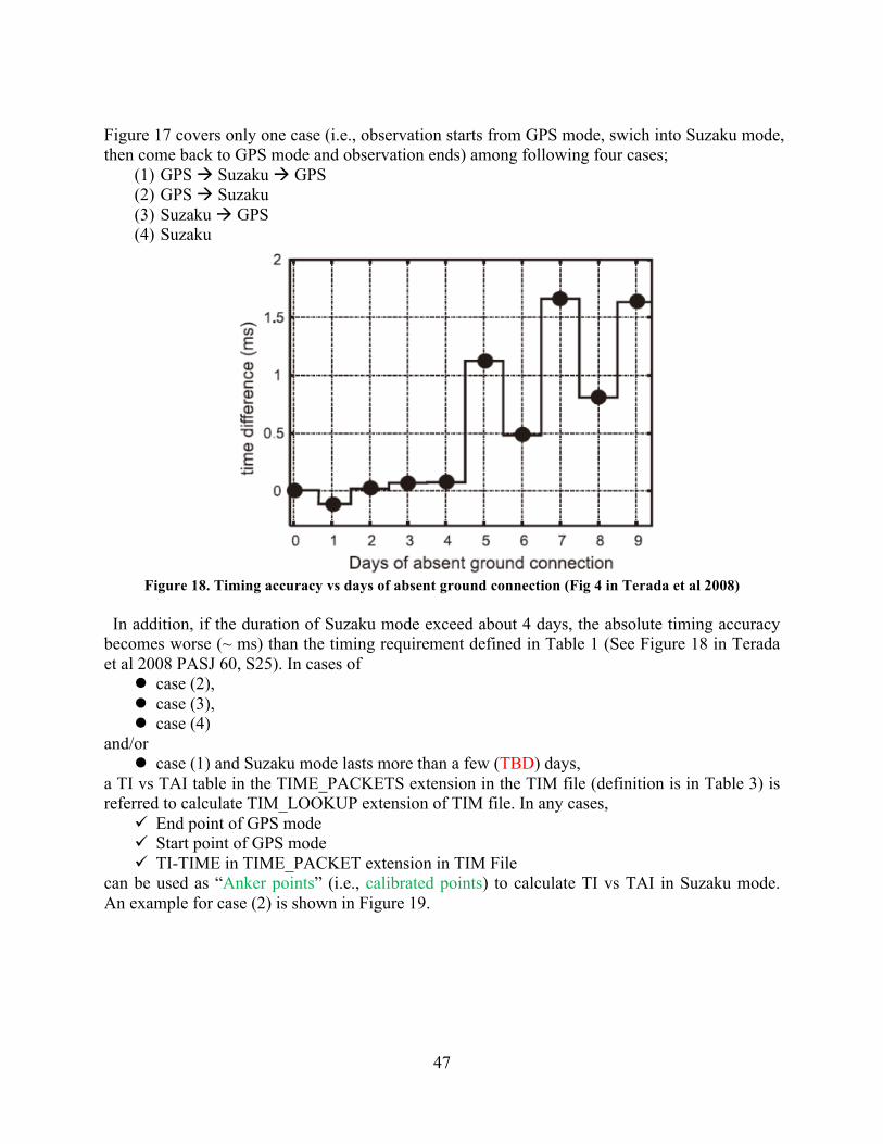
47

Figure 17 covers only one case (i.e., observation starts from GPS mode, swich into Suzaku mode, then come back to GPS mode and observation ends) among following four cases;

(1) GPS à Suzaku à GPS (2) GPS à Suzaku (3) Suzaku à GPS (4) Suzaku

Figure 18. Timing accuracy vs days of absent ground connection (Fig 4 in Terada et al 2008)

In addition, if the duration of Suzaku mode exceed about 4 days, the absolute timing accuracy

becomes worse (~ ms) than the timing requirement defined in Table 1 (See Figure 18 in Terada et al 2008 PASJ 60, S25). In cases of

l case (2), l case (3), l case (4)

and/or l case (1) and Suzaku mode lasts more than a few (TBD) days,

a TI vs TAI table in the TIME_PACKETS extension in the TIM file (definition is in Table 3) is referred to calculate TIM_LOOKUP extension of TIM file. In any cases,

ü End point of GPS mode ü Start point of GPS mode ü TI-TIME in TIME_PACKET extension in TIM File

can be used as “Anker points” (i.e., calibrated points) to calculate TI vs TAI in Suzaku mode. An example for case (2) is shown in Figure 19.

48

Figure 19. Same as Figure 17, but for case (2) GPS – Suzaku Mode, using original TIM file.

GPS synchronized mode GPS unsynchronized mode TIM file, TIME_PACKETS

TIME

TI Raw Data

TIME is unknown


TIME

TI Drift corrected

TIME is unknown


TIME

TI tick corrected

TIME is calculated

49

4.3.3. Transition mode: From SMU time to GPS time In transition mode of SMU (section 3.3.2), the L32TI is artificially drifted by SMU to match GPS time. Currently (Aug 2012), we have two options in SMU telemetry;

(1) We get the difference between L32TI and GPS time (TAI-19s) during the transition mode. (2) We get the difference between L32TI and GPS time (TAI-19s) only when the transition

mode starts. In this case, NEC people provide the algorithm of synchronization in orbit (section 3.3.3)

In either case, we can calculate the relation between L32TI and TAI during the transition mode in the same manner as with GPS synchronized mode, but only after two conditions are checked:

• is the point in a skip region • is the point in a duplicate region

Both of these conditions do not allow for time assignment to occur since the relevant TIM data are untrustworthy. The skip region is defined when adjacent points are separated by a certain distance (called?). Both points are marked as being in the skip region. Besides adjacent transition-mode points, a skip region can be defined between one transition-mode point and a GPS- or Suzaku-mode point. The duplicate region occurs when the L32TI vs. TIME curve is not monotonic. All points where multiple L32TI values are possible are marked as members of the duplicate region. For each duplicate region, a single GPS-mode point is possible (last point of the duplicate region), then remaining points must be transition-mode points. Below are examples of monotonic (normal), skip, and duplicate regions and which points are marked as members of each region. Monotonic:

• each point is larger than the previous • ahtime operation same as GPS mode

Skip:

• points are monotonic • large gap (size TBD) between two points • yellow points flagged as skipped • ahtime operation TBD (maybe interpolation)

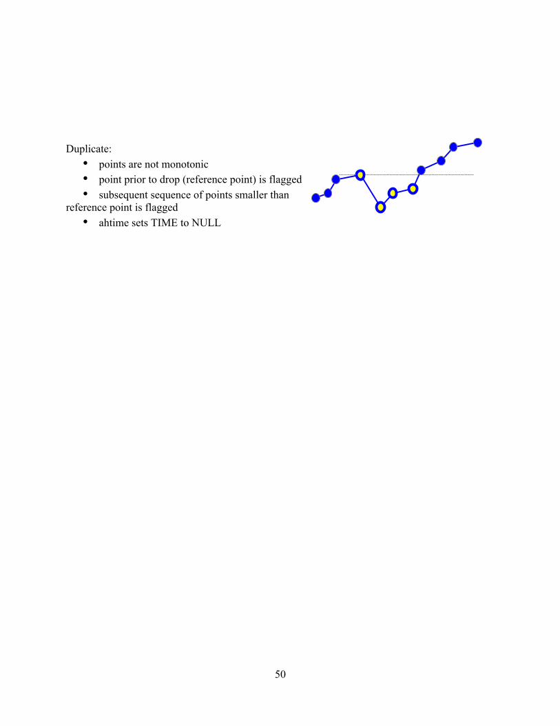
50

Duplicate:

• points are not monotonic • point prior to drop (reference point) is flagged • subsequent sequence of points smaller than

reference point is flagged • ahtime sets TIME to NULL

51

5. Time Assignment of HK data 5.1. Flow chart of time assignment of HK As described in section 2.4.3, the time-assignment process of the space packet (HK) by ahtime contains following two steps after we get a TIM_LOOKUP extension of TIM file by ahmktim. The second step is applied only for HK files, not event files.

1. L32TI to TT (TIME column) with S_TIME and TIM file (section 5.2) 2. TT to UTC (columns YYYY, DDD, HH, MM, SS, US) (section 5.3)

Note that all extensions in HK files start with “HK_”. Each extension must contain columns: L32TI, U32TI, S_TIME, TIME. The inputs and outputs of ahtime are summarized in Table 25.

Input Reference Output L32TI Row, HK TIM file

(TIM_LOOKUP ext.) TIME TT Row, HK

S_TIME Row, HK YYYY UTC Row, HK DDD UTC Row, HK HH UTC Row, HK MM UTC Row, HK SS UTC Row, HK US UTC Row, HK TSTART TT Header, HK TSTOP TT Header, HK DATE_OBS UTC Header, HK DATE_END UTC Header, HK

Table 25. Summary of inputs and outputs in time assignment process of HK FITS. The definition of TIME here is type 1 in Table 5 and gives the number of seconds elapsed

since the Astro-H epoch. The flow chart in Figure 20, gives a schematic of the time assignment algorithm for HK files as implemented by the tool, ahtime.

Definition of TIME in section 5 Type 1 in Table 5

Table 26. definition of TIME in section 5.

Figure 20. Flow chart of time assignment of HK by ahtime.

5.2. Conversion from L32TI to TT (TIME)

52

We can apply the same procedure in SIRIUS (section 3.5.2) in conversion from L32TI and S_TIME to TIME.

(1) Read S_TIME from the space packet (2) Search row in the TIM_LOOKUP extension of TIM file around S_TIME (3) Calculate the interpolation function between S_TIME and L32TI (4) Read L32TI from the space packet (5) Get TIME from L32TI and interpolation function

Figure 21. Algorithm of time assignment of HK FITS with TIM file

The interpolation function can be described in the following ** methods. Method 1) Linear function from 2 or 4 points. Method 2) To be added (Study) Comment: Since the stability of TI (after correction of temperature drift in case of GPS failure) is better than 10-8 s/s, the linear function is enough for our purpose, when the time steps in TIM file is less than 10 -- 100 sec.

TIME

TI

Data in TIME file Interpolation func.

(1) S_TIME in space packet

(4) TI in space packet

(2) Pick up data from TIM file

(3) calc interpolation function (5) Get TIME at TI.

53

5.3. Conversion from TT to UTC As described in section 3.5.3, the relation between TT to UTC is

TT = TAI + 32.184 sec = UTC + LeapSecond + 32.184 sec. This conversion is general, so we can use the atFunction library and leap second table in CALDB. (see atMissionToAtTime(); etc.)

54

5.4. Time assignment for MXS The MXS HK files will contain on/off intervals for the MXS. These intervals are written in the HK FITS file. The current MXS telemetry values:

The current timing tasks calculates only the TIME column present in the FFF but do not calculate times starting from the TI_LED[1-4]_START/STOP present in the telemetry. Therefore we need a separate tasks to calculate the times in second from the Astro-H epoch

55

starting from the value in the telemetry TI_LED[1-4]_START/STOP. However the FFF HK for the MXS should contain empty columns output of the calculations. The assumption here are the following:

the TI_LED[1-4]_START/STOP do not represent the duration of a single pulse, instead the represent the interval of time in which the MXS is actively being pulsed. Other columns denote the length and separation of these pulses within the START/STOP interval. With these additional columns, it can be determined exactly when the MXS source is active.

Figure 22. Schematic timing chart for MXS irradiation.

The S_TIME or L32TI are written in the HK extension as usual. The TI_LED[1-4]_START/STOP are written as 40 bits, where the upper 2-bits are reserved bits and lower 38-bits are written in the format of TI, as shown in the following Table 27.

Bits 0-1 (MSB) Reserved. Bits 2-33 U32TI (see Table 9). Bits 34-39 SpaceWire TIME_CODE (see section 7.4)

Table 27. Format of TI_LED[1,2,3,4]_START_STOP for MXS A row in the MXS extension does not define a single pulse (see Figure 22) . Instead, rows are written every second. If the MXS has been turned on or off since the last update, then TI_LED[1-4]_ON/OFF will be updated to the new value. The MXS timing tool must detect which TI_LED[1-4]_ON or _OFF have changed and flag each row with the current on/off state. There are 4 LED it should be clarified what TI_LED[1-4]_ON/OFF will eventually be included in the MXS GTI. An Issue: TI_LEDx_ON/OFF information could be overwritten when the ON/OFF commands are sequencially sent in short time. Possible issue: if a complete MXS interval occurs in the second between the output of HK rows, then ambiguity exists with how many complete or partial intervals occurred. Is there another column present in the extension that will resolve this ambiguity? Or, do intervals always span more than one second? Another issue: it has been observed that the MXS pulse has a trailing tail, but it has not been determined if this is important.

56

The timing tool, mxstime, calculate the following TIME and GTI;

l Time for each of the LED, TIME_LED[1-4]_ON and TIME_LED[1-4]_OFF, which are populated from TI_LED[1-4]_ON and TI_KED[1-4]_OFF.

l Coarse GTI between the TIME LED ON and OFF. l Fine GTI, giving the start and stop for each individual pulse. (see Figure 23)

The pulse period (PLS_SPC) and the pulse length (PLS_LEN) are used to calculate the fine GTI. The delay between SMU and MXS (see section 6.3.1) is also applied.

Figure 23. Timing chart for MXS pulses and coarse / fine GTIs.

57

6. Time Assignment of Science Data 6.1. Overview of time assignment of Science data The science requirement for the accuracy of TIME of Science data is 30 µsec as described in section 2.1, whereas the resolution of L32TI is only 2-6 sec = 64 msec as described in section 3.1. Thus, the nominal algorithm for time assignment of space packet (section 5) is not sufficient for Science data. In addition, the type of TIME (see Table 5) is different from that of HK. Science data is in the EVENTS extension which contains columns: L32TI, U32TI, S_TIME, TIME.

Definition of TIME in section 5.4 Type 2 in Table 5

Table 28. Definition of TIME for Science data in section 5.4. To have finer resolution in TIME of Science data, each instrument has their own clock, which is not synchronized to the SA-TI (see section 2.6) but has finer resolution, and latches a value when they detect an event. We call this clock LOCAL_TIME. Since they are not synchronized to TI, we have to calibrate them first and then we can use them for time assignment. Thus, the time assignment of Science data contains following additional one step 0 from section 5, as already summarized in section 2.4.3.

0. LOCAL_TIME to L32TI with look-up table between them (section ) 1. L32TI to TT with S_TIME and TIM file (section 5.2) 2. TT to UTC (DATE_OBS and DATE_END keywords) (section 5.3)

Here, we call the L32TI equivalent value calculated in step 0, fine TI. The input in step 1 should be the fine L32TI instead of L32TI for HK case. The flow chart is shown in Figure 24. Note that the later parts are the same as Figure 20. Note that the calculation of fine_TI from LOCAL_TIME assumes that LOCAL_TIME is monotonic to L32TI. This relation is checked before the calculation and flags as bad in PROC_STATUS (see ASTH-SCT-002).

Figure 24. Flow chart of time assignment of Science data by ahtime.

58

6.2. Summary of LOCAL_TIME The instruments have their own configuration on free-run clocks for LOCAL_TIME values, depending

on the limitations in hardware (logic size of FPGA, definition of components onboard the spacecraft) etc. In summary, they carry the following LOCAL_TIMEs shown in

Table 29.

Table 29. List of LOCAL_TIME counters.

Note 1: SAMPLECNT for SXS is calculated by sxssamcnt from TRIG_LP (24-bit, 80us) and TIME_VERNIER (4-bits, 5 us) Note 2: LATCH_U32TI in SXS HK is originally stored as four values in one space packet, which is expanded at FFF stage. Note 3: HK_TI_INTER1 in HXI HK or SGD HK is one of the four acquisitions in one space packet.

SYSTEM LTIME1EVT LTIME2EVT

HKEXTNAME LTIME1HK LTIME2

TI1HK

SXS-Pixel SampleCnt (28-bits 5 us)

PSP_ID HK_ALLUSR SampleCnt PSP_ID Latch_U32TI (32-bits, 1s)

SXS-Baseline SampleCnt PSP_ID HK_ALLUSR SampleCnt PSP_ID Latch_U32TI SXS-Noiserec SampleCnt PSP_ID HK_ALLUSR SampleCnt PSP_ID Latch_U32TI SXS-Pulserec SampleCnt PSP_ID HK_ALLUSR SampleCnt PSP_ID Latch_U32TI SXS_Template SXS_Noisespec SXS_Avepulse SXS-Antico SampleCnt PSP_ID HK_ALLUSR SampleCnt PSP_ID Latch_U32TI1 SXI Seq_Start_Time

(32-bit, 61.0 us)

HXI_Camera Local_time (32-bits, 25.6 us)

HK_SCL_HK SCL_LOCAL_TIME1 SCL_TI_INTER1

HXI_ShieldGRB Grb_freeze_time (32-bit, 16 ms)

HK_APMU_HK HK_LOCAL_TIME1_2 HK_TI_INTER1

HXI_Shield1RATE SGD_CC Local_time

(32-bits, 25.6 us) HK_CPMU_HK HK_LOCAL_TIME1_1 HK_TI_INTER1

SGD_Shield1GRB Grb_freeze_time (32-bit, 16 ms)

HK_APMU1_HK HK_LOCAL_TIME1_2 HK_TI_INTER1

SGD_Shield2GRB Grb_freeze_time HK_APMU2_HK HK_LOCAL_TIME1_2 HK_TI_INTER1 SGD_Shield1RATE SGD_Shield1RATE CAMS Time_code HK

59

6.2.1. SXI The time assignment system of the SXI is the simplest case, because their LOCAL_TIME counter, SEQ_START_TIME (32bit, 61.0 µs) is synchronized to TIME_CODE in every 15.6 msec, and thus the lowest bit of SEQ_START_TIME represents the exact 2-14 sec. Since it is synchronized to L32TI, the SXI does not have a look-up table in HK.

LOCAL_TIME 1 in Event LOCAL_TIME 1 in HK SEQ_START_TIME

(32bit, 61.0 µs) NONE

Table 30. Column name of LOCAL_TIME for SXI. The schematic view of calculation of fine L32TI is shown in Figure 25; attach upper 4-bits of L32TI to SEQ_START_TIME, then we get fine L32TI value with time resolution of 2-14 sec. Note that the upper 4-bit of TI should be subtracted by 1 when the SEQ_START_TIME carries.

Figure 25. Schematic view of calculation of fine L32TI of SXI.

The acquisition time depends on the data mode of the SXI, which can be described as the offset from the SEQ_START_TIME (see section 6.3.3).

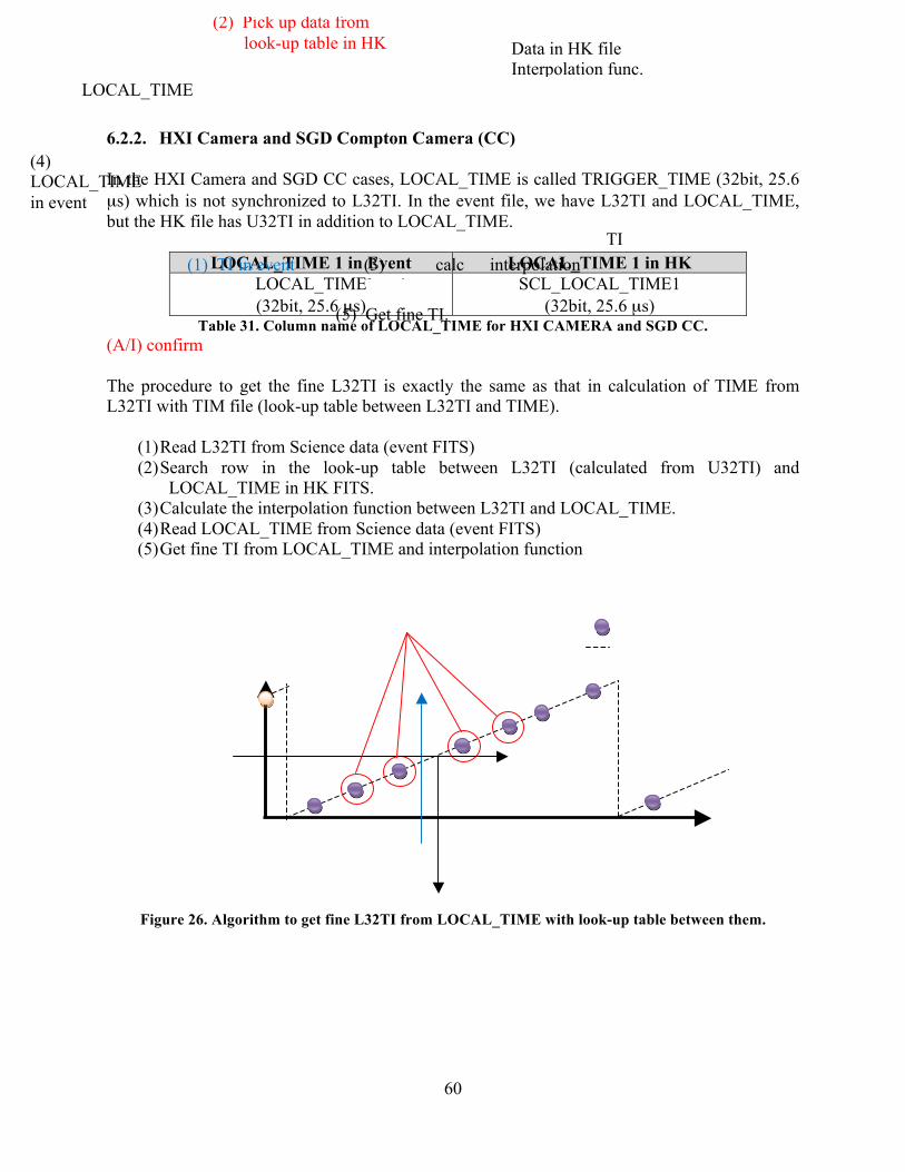
60

6.2.2. HXI Camera and SGD Compton Camera (CC) In the HXI Camera and SGD CC cases, LOCAL_TIME is called TRIGGER_TIME (32bit, 25.6 µs) which is not synchronized to L32TI. In the event file, we have L32TI and LOCAL_TIME, but the HK file has U32TI in addition to LOCAL_TIME.

LOCAL_TIME 1 in Event LOCAL_TIME 1 in HK LOCAL_TIME (32bit, 25.6 µs)

SCL_LOCAL_TIME1 (32bit, 25.6 µs)

Table 31. Column name of LOCAL_TIME for HXI CAMERA and SGD CC. (A/I) confirm The procedure to get the fine L32TI is exactly the same as that in calculation of TIME from L32TI with TIM file (look-up table between L32TI and TIME).

(1) Read L32TI from Science data (event FITS) (2) Search row in the look-up table between L32TI (calculated from U32TI) and

LOCAL_TIME in HK FITS. (3) Calculate the interpolation function between L32TI and LOCAL_TIME. (4) Read LOCAL_TIME from Science data (event FITS) (5) Get fine TI from LOCAL_TIME and interpolation function

Figure 26. Algorithm to get fine L32TI from LOCAL_TIME with look-up table between them.

TI

LOCAL_TIME

Data in HK file Interpolation func.

(1) TI in event

(4) LOCAL_TIME in event

(2) Pick up data from look-up table in HK

(3) calc interpolation function (5) Get fine TI.

61

6.2.3. HXI/SGD Shield In case of SGD-WAM, the instrument has two LOCAL_TIMEs. In HK file, we can extract the table between L32TI, LOCAL_TIME1, and LOCAL_TIME2.

LOCAL_TIME 1 in Event LOCAL_TIME 1 in HK GRB_FREEZE_TIME

(32bit, 102.4 µs) HK_LOCAL_TIME1_2

(32bit, 102.4 µs) Table 32. Column names of LOCAL_TIME 1 and 2 for SGD WAM.

In the time assignment, we have to calculate the LOCAL_TIME1 equivalent value from LOCAL_TIME2 by a look-up table between them, then we can calculate fine L32TI from LOCAL_TIME1 equivalent value by a look-up table between LOCAL_TIME1 and L32TI. The algorithm using look-up table is the same as section 6.2.2. In the current design, LOCAL_TIME2 and L32TI appears in the same HK data, so we do not need to use the LOCAL_TIME1. (i.e., only LOCAL_TIME1 is enough for time assignment.). However, the hardware design may change in near future, it is better to support double look-up tables for WAMs. Needless to say, the TIME for SHIELD also has the meening (b) in Table 5.

62

6.2.4. SXS The SXS has only one LOCAL_TIME counter, SAMPLECNT, but the information of this counter appears in several way as listed in Table 33. Three issues complicate the SXS time assignment. First, the SXS HK data is split across several extensions based on the PSP. Second, four acquisitions are included in one space packet. Third, the local time from SXS (both HK and event data) is split among several columns as shown in Table 33. The first issue is resolved by running the tool, ahmodhkext, which combines the HK look-up tables into a single extension, ALLUSR_HK, where the column, PSP_ID, identifies the PSP. On the second issue, four acquisitions are divided into four rows. As for the third issue, the multiple local times from HK and event data are then combined with the tool, sxssamcnt, using the procedure described below. Upon completion, the local time for both HK and science is stored in the SAMPLECNT column. Only after handling both of these issues can the time assignment be performed with ahtime.

LOCAL_TIME in Event LOCAL_TIME in HK TRIG_LP (24-bit, 80 µsec)

TIME_VERNIER(4-bit, 5 µsec) WFRB_WRITE_LP

WFRB_SAMPLE_CNT

LATCH_SAMPLE_CNT1 (32-bit, 80 µsec) LATCH_BASE_CNT1 (0—399, 0.2 µsec)




The above 4 acquisitions are stored as each LATCH_SAMPLE_CNT and LATCH_BASE_CNT in FFF.

SAMPLECNT (5 µsec) SAMPLECNT (in 5 usec) Table 33. Column names of LOCAL_TIME of the SXS.

In HK file, the resolution of LATCH_SAMPLE_CNTn (n = none, 1, 2, 3, 4) is 80 µsec and LATCH_BASE_CNTn (n= none, 1, 2, 3, 4) is represents the finer part of the time with a resolution of 0.2 µsec. Then, we can calculate the SAMPLECNT with finer timing resolution by the same algorithm as the calculation of fine TI in the SXI case shown in Figure 25. Since the resolution of SAMPLECNT in Event file is 5 µsec, we can drop the finer information than this value for HK. Then, we get the look-up table between TI and SampleCnt in the 5 µsec resolution. The formula is

SAMPLECNT = (LATCH_SAMPLE_CNT + LATCH_BASE_CNT/400) Note that the LATCH_BASE_CNT carries every BASE_CNT_ROUNT_UP = 400 clocks when the sample rate of the Xbox and PSP are set to 12.5 kHz. In case of the sample rate = 16 kHz, the BASE_CNT_ROUNT_UP is 320. The calculation of SAMPLECNT in event file from TRIG_LP and TIME_VERNIER is more complicated. The FFF contains the origin of SAMPLECNT (N) in the header part of Event FITS

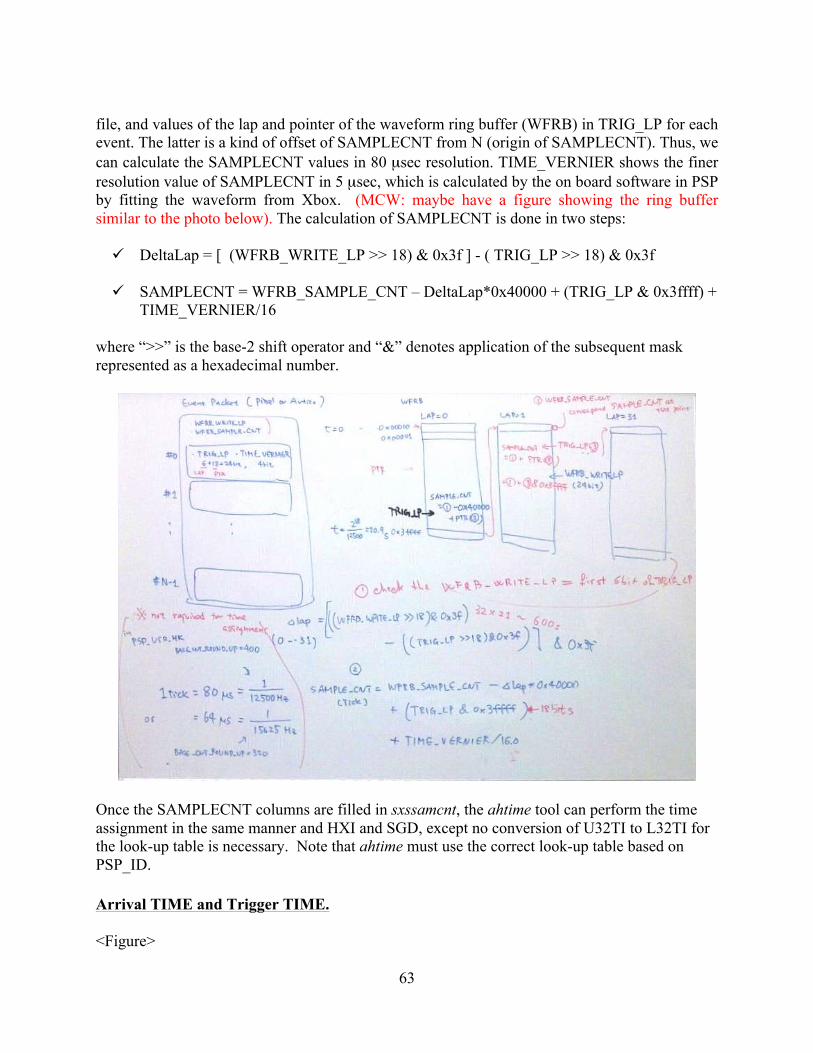
63

file, and values of the lap and pointer of the waveform ring buffer (WFRB) in TRIG_LP for each event. The latter is a kind of offset of SAMPLECNT from N (origin of SAMPLECNT). Thus, we can calculate the SAMPLECNT values in 80 µsec resolution. TIME_VERNIER shows the finer resolution value of SAMPLECNT in 5 µsec, which is calculated by the on board software in PSP by fitting the waveform from Xbox. (MCW: maybe have a figure showing the ring buffer similar to the photo below). The calculation of SAMPLECNT is done in two steps: ü DeltaLap = [ (WFRB_WRITE_LP >> 18) & 0x3f ] - ( TRIG_LP >> 18) & 0x3f ü SAMPLECNT = WFRB_SAMPLE_CNT – DeltaLap*0x40000 + (TRIG_LP & 0x3ffff) +

TIME_VERNIER/16 where “>>” is the base-2 shift operator and “&” denotes application of the subsequent mask represented as a hexadecimal number.

Once the SAMPLECNT columns are filled in sxssamcnt, the ahtime tool can perform the time assignment in the same manner and HXI and SGD, except no conversion of U32TI to L32TI for the look-up table is necessary. Note that ahtime must use the correct look-up table based on PSP_ID. Arrival TIME and Trigger TIME. <Figure>

64

For the Pixel event data, photon arrival time is ahead of the time when the electronics (PSP)

triggers the signal processing, as defined in the figure. The arrival time can be adjusted by the rise time of the waveform. This effect can be calculated at the sxsssamcnt phase and the actual formula is describes as,

SAMPLECNT = SAMPLECNTTRIG - a * (0.25 * RISE_TIME) - b * DERIV_MAX – c, where SAMPLECNT and SAMPLECNTTRIG are in real number and coefficients a, b, and c are listed in the CALDB file. Since the coefficients should be prepared by the grades, High_Res, Mid_res, and Low_res, and could have time dependency, the CALDB contains TIME valid date, AH, BH, CH (a, b, c values for Hi_res), AM, BM, CM (a, b, c for Mid_res), and AL, BL, CL (a, b, c, for Low_Res). Before launch, they are a = 1.0, b = 0.0, and c=0.0. In the SXS FITS file, the following columns will be prepared and filled by the timing tasks.

Pixel PULSEREC NOISEREC

SAMPLECNT Sample cnt at arrival time, calculated by the equation

SAMPLECNTTRIG Sample cnt at trigger time TRIGTIME TIME at trigger time calculated by

SAMPLECNTTRIG TIME TIME at arrival time, calculated by

SAMPLECNT Antico SAMPLECNT Sample cnt at trigger time

TIME TIME at trigger time calculated by SAMPLECNT

LOST GTI SAMPLECNT1 Sample cnt for start lp SAMPLECNT2 Sample cnt for stop lp START TIME at the start of lost STOP TIME at the end of los TIME = START

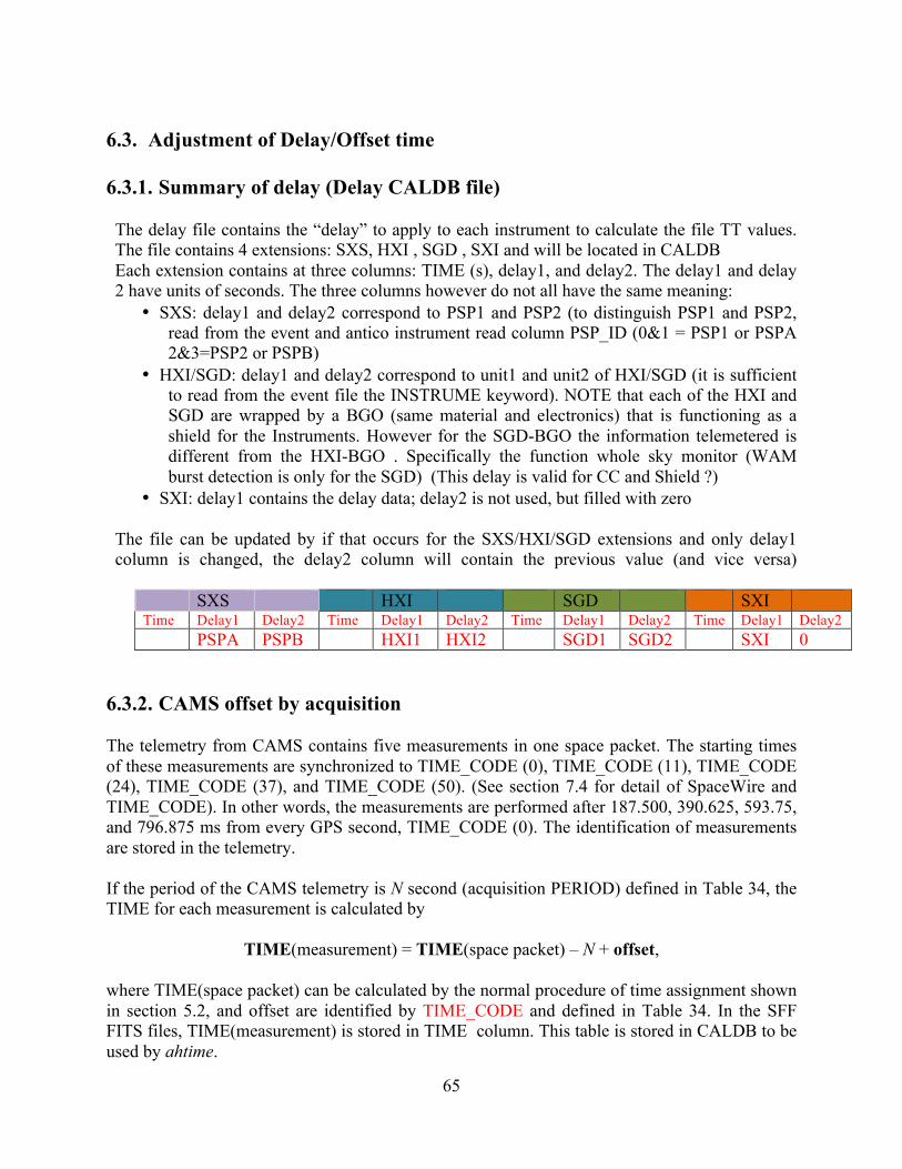
65

6.3. Adjustment of Delay/Offset time 6.3.1. Summary of delay (Delay CALDB file) The delay file contains the “delay” to apply to each instrument to calculate the file TT values. The file contains 4 extensions: SXS, HXI , SGD , SXI and will be located in CALDB Each extension contains at three columns: TIME (s), delay1, and delay2. The delay1 and delay 2 have units of seconds. The three columns however do not all have the same meaning:

• SXS: delay1 and delay2 correspond to PSP1 and PSP2 (to distinguish PSP1 and PSP2, read from the event and antico instrument read column PSP_ID (0&1 = PSP1 or PSPA 2&3=PSP2 or PSPB)

• HXI/SGD: delay1 and delay2 correspond to unit1 and unit2 of HXI/SGD (it is sufficient to read from the event file the INSTRUME keyword). NOTE that each of the HXI and SGD are wrapped by a BGO (same material and electronics) that is functioning as a shield for the Instruments. However for the SGD-BGO the information telemetered is different from the HXI-BGO . Specifically the function whole sky monitor (WAM burst detection is only for the SGD) (This delay is valid for CC and Shield ?)

• SXI: delay1 contains the delay data; delay2 is not used, but filled with zero The file can be updated by if that occurs for the SXS/HXI/SGD extensions and only delay1 column is changed, the delay2 column will contain the previous value (and vice versa)

SXS HXI SGD SXI Time Delay1 Delay2 Time Delay1 Delay2 Time Delay1 Delay2 Time Delay1 Delay2 PSPA PSPB HXI1 HXI2 SGD1 SGD2 SXI 0

6.3.2. CAMS offset by acquisition The telemetry from CAMS contains five measurements in one space packet. The starting times of these measurements are synchronized to TIME_CODE (0), TIME_CODE (11), TIME_CODE (24), TIME_CODE (37), and TIME_CODE (50). (See section 7.4 for detail of SpaceWire and TIME_CODE). In other words, the measurements are performed after 187.500, 390.625, 593.75, and 796.875 ms from every GPS second, TIME_CODE (0). The identification of measurements are stored in the telemetry. If the period of the CAMS telemetry is N second (acquisition PERIOD) defined in Table 34, the TIME for each measurement is calculated by

TIME(measurement) = TIME(space packet) – N + offset,

where TIME(space packet) can be calculated by the normal procedure of time assignment shown in section 5.2, and offset are identified by TIME_CODE and defined in Table 34. In the SFF FITS files, TIME(measurement) is stored in TIME column. This table is stored in CALDB to be used by ahtime.

66

offset (sec) TIME_CODE 0.000000 0 0.015625 1 0.031250 2

…. … 0.984375 63

PERIOD

N=1.0000 (sec) Table 34. Definition of offset and telemetry period of CAMS data

6.3.3. SXI offset by Data Modes The time at the beginning of the exposure for the SXI depends on data modes. Schematic view of the timing chart for burst mode and/or window option of SXI is shown in Figure 27.

Figure 27. Timing chart for the SXI exposure by data modes.

67

The offset from SEQ_START_TIME is defined by “dead time + transfer time” in Figure 27, whose values can be identified by 14 keywords defined in ASTH-SCT-003 (TIMEDEL , TIMTRANB , TIMTRANA, EXPDEADA, EXPDEADB, FLUSHIMB, LASTDEAD, LASTDEL, NOMEXPO, TIMEPIXR, CCDSIZE) in the SXI event FITS. Note that the transfer time is NOT included in the exposure time, although an event can be detected during the transfer time (but the position cannot be assigned). The detail information for timing chart of the SXI are summarized in Table 35 and Table 36. Note that these parameters will be tuned in the check-out phase after launch (e.g, transfer time depends on the window position).

Full Window No

Burst Full Window

Burst 2s 1/8 Window No

Burst 1/8 Window Burst 0.1s

How to assign time for each event

For all the event in the i-th frame, the same time value should be assigned. However, events exposed in one frame are readout in the next frame in CCD. Define seqstart[i] to be the time of the SEQ_START in the i-th frame, and the eventtime[i] to be the time of each event in the i-th frame. eventtime[i] = seqstart[i-1]

+ Delaytime + DeadTimeB0 + TransferImagetoStoreTimeB0 + FlushImageTime0 + 0.5*Exposure1,

where DeadTimeB0, TransferImagetoStoreTimeB0, FlushImageTime0, and Exposure1 denote the duration of each time span.

Each event in the i-th frame should be classified into 1st to 8th exposure according to the value of RAWY. Assuming RAWY has values from 0 to 639, an event RAWY=0-79 belongs to the 1st exposure in the previous frame, which the one in RAWY=80-159 belongs to the 2nd exposure. Therefore, j=1+int (mod(RAWY/80,8)). All the event in exch of the i-th frame j-th (j=1,2,3,...,8) exposure should have the same time value. Define seqstart[i] to be the time of the SEQ_START in the i-th frame, and the eventtime[i][j] to be the time of each event in the j-th (j=1,...,8) exposure in the i-th frame. eventtime[i][j] = seqstart[i-1]

+ Delaytime + DeadTimeB0 + TransferImagetoStoreTimeB0 + FlushImageTime0 + Exposure1 + TransferImagetoStoreTimeA1 + DeadTimeA1 + DeadTimeB1 + TransferImagetoStoreTimeB1 + FlushImageTime1 + Exposure2 + .... + FlushImageTime(j-1) + 0.5*Exposure(j) ,

where DeadTimeB0, TransferImagetoStoreTimeB0, FlushImageTime0, and Exposure1 etc. denote the duration of each time span.

Table 35. Formula to calculate the timing offset for the SXI by data modes.

68

DelayTime Delay in analog readout chain plus that in digital processing. To be defined, but common for all the modes.

RepetetionInFrame 1 1 8 8

duration from SEQ_START duration from

SEQ_START duration from SEQ_START duration from

SEQ_START

(unit) s s s s s s s s

DeadTimeB0 0.0000000 0.0000000 1.9865664 1.9865664 0.0000000 0.0000000 0.3633408 0.3633408

TransferImagetoStoreTimeB0 0.0368640 0.0368640 0.0000000 1.9865664 0.0368640 0.0368640 0.0000000 0.3633408

FlushImageTime0 0.0000000 0.0368640 0.0368640 2.0234304 0.0000000 0.0368640 0.0368640 0.4002048

Exposure1 3.9631360 4.0000000 1.9395648 3.9629952 0.4631184 0.4999824 0.0605952 0.4608000

TransferImagetoStoreTimeA1 0.0000000 4.0000000 0.0368640 3.9998592 0.0000000 0.4999824 0.0368640 0.4976640

DeadTimeA1 0.0000000 4.0000000 0.0001408 4.0000000 0.0000000 0.4999824 0.0023184 0.4999824

DeadTimeB1 0.0000000 0.4999824 0.3633408 0.8633232

TransferImagetoStoreTimeB1 0.0368640 0.5368464 0.0000000 0.8633232

FlushImageTime1 0.0000000 0.5368464 0.0368640 0.9001872

Exposure2 0.4631184 0.9999648 0.0605952 0.9607824

TransferImagetoStoreTimeA2 0.0000000 0.9999648 0.0368640 0.9976464

DeadTimeA2 0.0000000 0.9999648 0.0023184 0.9999648

DeadTimeB2 0.0000000 0.9999648 0.3633408 1.3633056


FlushImageTime2 0.0000000 1.0368288 0.0368640 1.4001696

Exposure3 0.4631184 1.4999472 0.0605952 1.4607648


DeadTimeA3 0.0000000 1.4999472 0.0023184 1.4999472

DeadTimeB3 0.0000000 1.4999472 0.3633408 1.8632880


FlushImageTime3 0.0000000 1.5368112 0.0368640 1.9001520

Exposure4 0.4631184 1.9999296 0.0605952 1.9607472


DeadTimeA4 0.0000000 1.9999296 0.0023184 1.9999296

DeadTimeB4 0.0000000 1.9999296 0.3633408 2.3632704


FlushoImageTime4 0.0000000 2.0367936 0.0368640 2.4001344

Exposure5 0.4631184 2.4999120 0.0605952 2.4607296


DeadTimeA5 0.0000000 2.4999120 0.0023184 2.4999120

DeadTimeB5 0.0000000 2.4999120 0.3633408 2.8632528


FlushoImageTime5 0.0000000 2.5367760 0.0368640 2.9001168

Exposure6 0.4631184 2.9998944 0.0605952 2.9607120


DeadTimeA6 0.0000000 2.9998944 0.0023184 2.9998944

69

DeadTimeB6 0.0000000 2.9998944 0.3633408 3.3632352


FlushImageTime6 0.0000000 3.0367584 0.0368640 3.4000992

Exposure7 0.4631184 3.4998768 0.0605952 3.4606944


DeadTimeA7 0.0000000 3.4998768 0.0023184 3.4998768

DeadTimeB7 0.0000000 3.4998768 0.3633408 3.8632176


FlushImageTime7 0.0000000 3.5367408 0.0368640 3.9000816

Exposure8 0.4632592 4.0000000 0.0605952 3.9606768


DeadTimeA8 0.0000000 4.0000000 0.0024592 4.0000000

*) Exposure8 is longer than others by 0.1408ms

*) DeadTimeA8 is longer than others by 0.1408ms

Table 36. List of time (sec) for SXI timing chart. (ver 2013-12-17)

70

7. List of calibration items and CALDB for time assignment 7.1. Error budget in timing accuracy of ASTRO-H In order to achieve the final timing goal (Table 1), the error items which affects the timing accuracy are listed in the timing chart shown in Figure 28. These items are listed in Table 37 and errors are assigned by item to control the overall uncertainties. Therefore the Table 37 represents the error budget for the timing accuracy.

Figure 28. Timing chart for distribution of timing information. Error budgets (Table 37) and calibration

items are shown in star marks and left right arrow, respectively. ID Component Error Items Error Allowed

A GPSR Jitter between leading edge of second for atomic time (TAI) and 1 PPS signal output.

0.2 usec

B SMU Jitter from 1 PPS signal from GPSR and TIME_CODE emitted from SMU.

0.5 usec

C SpaceWire network Jitter of TIME_CODE at user node after propagation in SpaceWire network.

2.0 usec

D SpaceWire network Systematic error in the correction of TIME_CODE jitter at user node. (i.e., uncertainties for delay CALDB)

1.0 usec

E SpaceWire user node Timing uncertainties in receiving TIME_CODE and TI generation.

1.0 usec

F SpaceWire user node Timing uncertainties for periodic signal inputs (like X-ray pulsars) due to finite timing resolution of LOCAL_TIME.

20.0 usec

G Ground System Accuracy of orbital determination of the spacecraft.

3.0 usec (= 1 km)

Table 37. Error budget of ASTRO-H Time assignment.

71

7.2. Ground measurements for Time Assignments In Table 37, the item A, D are ensured as the hardware design of GPSR and Digital Electronics

(DE), respectively. The item G is a requirement for orbital determination. Therefore, we measured the items B, C, D on ground. Item F is estimated using the simulator, heasim. 7.2.1. Measurement of Item B: timing delay and jitter between GPSR and TIME_CODE The measurement was performed in the I&T test at TKSC in 29 October 2013. The

configuration is shown in Figure 29. The timing delay and jitter between the GPS signal and TIME_CODE are measured twice. The number of measurement was 1910 and 1619. The distribution is shown in Figure 30. Note that the figure includes the timing delay of TIME_CODE E/R at 375 nsec. As a result, the delay for item B was 539 ±50 nsec and 541 ±45 nsec with 1 sigma error. In summary, the delay of GPSR should be listed as 540 nsec and the jitter (in 3 sigma; item B)

is 143 nsec, which is within the error budget Table 37 (500 nsec).

Figure 29. Configuration of the ground test for measurement of item (B)

72

Figure 30. Distribution of delay time of Item (B)

73

7.2.2. Estimation of Items E and F: Propagation delay and jitter of TIME_CODE The propagation delay of TIME_CODE from SMU to user node can be described as the sum of delays of each component. The delay and jitter in each component are summarized in Table 38.

Component Link rate Delay Jitter Notes SMU 50 MHz 540 ns 143 ns Budget B; section 7.2.1 SpW Router 10 MHz 1814 ns 800 ns SpW Router 20 MHz 1114 ns 400 ns SpW Router 25 MHz 974 ns 320 ns SpW Router 50 MHz 694 ns 160 ns Report from NEC (2013/6/18) MIO 20 MHz 1600 ns 400 ns Iwase et al SpaceCard 20 MHz 1590 ns 390 ns Iwase et al HXI cable (6 m len.) 30 ns * 5 ns / 1 m SXIDE-DPU 1000 ns 680 ns Report from MHI (2015/5/27)

Table 38. Delay and Jitter of payload components After summing up the delay and jitter of components, the final values are listed in Table 39. In the calculation of jitter values, a simulation of the propagation of TIME_CODE was used as demonstrated in Figure 31. Note that the delay values are stored in the delay CALDB file (ah_gen_delay.fits). INSTRUM

E

Delay

(ns)

Jitter

(ns)

Routing

(GPSR – user node)

HXI-1 5418 755 GPSR

SMU

(50 MHz)

SRW1-DH

(50 MHz)

SWR1-SI

(25 MHz)

HXI1_DE_FPGA

(20 MHz)

SpW cable 6m

(10 MHz)

HXI1_DPU_MIO

1

(20 MHz)

HXI1_DPU

_MIO2

HXI-2 6112 766 GPSR

SMU

(50 MHz)

SRW1-DH

(50 MHz)

SRW3-

DH

(50 MHz)

SWR1-SI

(25 MHz)

HXI2_DE_FPGA

(20 MHz)

SpW cable 6m

(10 MHz)

HXI2_DPU

_MIO1

(20 MHz)

HXI2_DPU

_MIO2

SGD-1 3798 476 GPSR

SMU

(50 MHz)

SRW1-DH

(50 MHz)

SWR1-SI

(25 MHz)

SGD1_DE_FPG

A

(20 MHz)

SGD1_DPU_MI

O1

SGD-2 4492 493 GPSR

SMU

(50 MHz)

SRW1-DH

(50 MHz)

SRW3-

DH

(50 MHz)

SWR3-SI

(25 MHz)

SGD2_DE_FPG

A

(20 MHz)

SGD2_DPU_MI

O1

SXI 3902 1041 GPSR

SMU

(50 MHz)

SRW1-DH

(50 MHz)

SRW3-

DH

(50 MHz)

SWR3-SI

(25 MHz)

SXI_DE_FPGA

(20 MHz)

DE-to-MIO

sync

SXI_PE_MI

O1

SXS 6082 767 GPSR

SMU

(50 MHz)

SRW1-DH

(50 MHz)

SWR1-SI

(50 MHz)

SXS-SWR

(25 MHz)

PSP-

SpC_FPGA

(20 MHz)

PSP-SpC_CPU

(20 MHz)

PSP-

MIO_FPG

A

CAMS 3048 717 GPSR

SMU

(50 MHz)

SRW1-DH

(50 MHz)

SWR1-SI

(10 MHz) AMS-LD

FW 2902 270 GPSR SMU

(50 MHz)

SRW1-DH

(50 MHz)

SWR1-SI

(50 MHz)

SXS-SWR

(25 MHz) SXS-FEW

Table 39. Delay and Jitter of instruments, estimated.

74

Figure 31. An example of the output of a simulation to calculate the propagation of SpaceWire

TIME_CODE. 7.2.3. Measurement of Items E and F: Propagation delay and jitter of TIME_CODE The measurement was performed in the I&T test at TKSC in 29 October 2013. Since the time assigned for this measurement is quite limited using the flight-model spacecraft, one of eight configurations in Table 39 , SMU to SGD1, was measured. Two sets of propagation delays of TIME_CODE were measured; between 1) SMU-A and SGD1-DE and 2) SMU-A and SGD1-DPU. The measurements were performed twice to check the effect of the traffics; when the SpaceWire communication is vacant and busy. The setup of the measurement is shown in Figure 32.

Figure 32. Configuration to measure Items D and E (SpaceWire TIME_CODE delay).

75

As shown in Figure 33 and Figure 34, the delay and jitter (3 sigma) show no difference between two cases (SpaceWire was busy or not). The results between SMU-A and SGD1-DE were 1668 ± 310 nsec and thoese between SMU-A and SGD1-DPT were 3258 ± 496 nsec. The expected values in section 7.2.2 were 1529 ± 315 nsec and 3252 ± 444 nsec, respectively. Therefore, the difference on the delay between the expected and measured values (error item D) are within 140 nsec, which is within the error budget for item D in Table 37. In addition the jitter (315 or 444 nsec) are also within the error budget for item E in Table 37.

Figure 33. Results of measurement items D and E; delay between SMU and SGD1-DE (left) and SMU

and SGD1-DPU (right) when the SpaceWire network is not busy.

Figure 34. Same figure as Figure 33, but measured when the SpaceWire network is busy.

76

7.2.4. Measurement of temperature dependency of the frequency of SMU The first measurement was performed only on SMU-A at NEC, before shipping to the spacecraft on 28 October 2014. The SMU was set on the thermal vacuum chamber and the temperature and the frequency of the quarts on board SMU were monitored by the digital multi-meter and frequency counter, respectively. Note that the monitoring point of the temperature is not the same as the point where the HCE reports in the telemetry. The temperature was changed from -10 degC to 73 degC by three cycles. A hysteresis was found in the frequency between rising-up and falling down the temperature. The averaged curve can be found in blue data points in Figure 35. The second measurement was performed on the spacecraft at TKSC during the thermal vacuum test on 25 June – 5 July 2015. Two columns in COM HK1 for ahtrendtemp are checked

SMU_A_DHFS_TI_MNG_TIM_TCAL_INF SMU_A_DHFS_TI_MNG_TIM_TCAL_TIME

After we sent the command to acquire the frequency measurement. The values are plotted in red points in Figure 35.

Figure 35. Temperature dependency of the quartz frequency of SMU-A (left) and –B (right)

7.2.5. Measurement of SXS TIME coefficiencies To be filled by the SXS team? (PoC is Tashiro-san). 7.3. Summary of CALDB files See ASTH-SCT-004.

77

Appendix 7.4. Overview of the SpaceWire protocol 7.4.1. Standard Communication Protocol, SpaceWire As is shown in section 0, in old days, communication links between components in spacecraft are designed only for single purpose of this satellite. It could be easier for developer of the onboard instruments, but it cost much both in design and verification tests. A mission-independent standard-protocol would reduce such costs and time. The SpaceWire is one of the standard communication protocol onboard satellites, which was and will be widely used for science missions in ESA, JAXA, and NASA. The SpaceWire links, nodes, and networks are specified in the ECSS-E-ST-50-12C standard [4], and additionally a number of higher layer protocols are defined in the ECSS-E-ST-50-51C, 52C, and 53C, all published by the European Cooperation for Space Standardization (ECSS). Specification of SpaceWire in the hardware layer can be listed as follows.

ü High speed serial link (… reduces number of lines) ü Data and Strobe encoding method (… sends data and clock simultaneously) ü LVDS (Low Voltage Differential Signaling) method (… represents high noise tolerance

and reduce the electric power in communication ) One of the important features of SpaceWire is the high capability of having a free-type network topology. Examples are shown in Figure 36. The ASTRO-H has a TREE type topology, shown in (d) case in this figure, and has redundant links. The square or circle in Figure 36 is called as Node.

Figure 36. Examples of the network topology for the SpaceWire.

7.4.2. Characters and codes in the lowest layer of the protocol The communication data on the SpaceWire link is divided into “characters”. The characters have the following two types. Note that the character level protocol in SpaceWire follows the IEEE standard 1355-1995.

A) Data character Data character has 10-bit values, consisting of parity-bit, data-control flag, and 8-bit data.

78

B) Control character Control character has 4-bit values, consisting of parity-bit, data-control flag, and 2-bit control bits, representing 4 types of control token, FCT (flow control token), EOP (end of packet), EEP (error end of packet), and ESC (escape).

Figure 37. Data and control characters in SpaceWire [4]

With the combination of characters, the following Control Codes are defined for special use.

(1) NULL NULL is formed from ESC followed by FCT. NULL is transmitted whenever a link is not sending data or control tokens.

(2) TIME_CODE TIME_CODE is used to support the distribution of system time across the network. TIME_CODE is formed by ESC (4-bit) followed by a single data-character (10-bits, including 6-bits time information in T0 .. T5, and 2-bit control flags in T6 and T7.).

Figure 38. Control codes in SpaceWire [4].

79

7.4.3. TIME_CODE distribution across a SpaceWire network The TIME_CODE is important to understand the time assignment system of ASTRO-H, because it is used for distributions of TIs in orbit. The details are described in section 3.2. In the distribution of TIME_CODE, we have to be careful about a possible failure in the distribution. The detail description of distribution of TIME_CODE can be found in the document [5]. As described in section 7.4.2, TIME_CODE carries 6-bit data (i.e., T0, T1, T2, T3, T4, T5, T6 in Figure 38), which represents a time-count value (i.e, 0 to 63). Only one node (see definition in section 7.4.1) in a system has a responsibility for generating TIME_CODE. This node is called as Time Master. Only the Time Master can assert an active TICK_IN signal, which is a hardware interface to receive TIME_CODE. Normally, the TICK_IN signal is generated periodically, and the time-count in TIME_CODE is incremented by one in generation of TICK_IN by Time Master. In ASTRO-H case, TICK_IN signal is produced every 2-6 seconds, and so the time-count value carries every 1.0 second. An example of the distribution of TIME_CODE is shown in Figure 39. All the nodes have time-count value 40 in the initial state (1) for example. A TICK_IN signal is assorted in step (2), and transmitted in step (3), and then routers forward the TIME_CODE to other links, as shown in step (4).

Node 1 40

Node 2 40

Router 1 40

Router 3 40

Router 2 40 (1) Initial State

Node 1 41

Node 2 40

Router 1 40

Router 3 40

Router 2 40 (2) TICK_IN assorted

Node 1 41

Node 2 40

Router 1 41

Router 3 40

Router 2 40 (3) Transmitted

Node 1 41

Node 2 40

Router 1 41

Router 3 41

Router 2 41 (4) Routers forward TIME_CODE

Figure 39. Distribution of TIME_CODE in nominal case (I)

80

In the distribution, all the nodes keep the time-count value and check the consistency between the value in TIME_CODE and that in their own. For example, at the step (4) in Figure 39, the node 2 receives TIME_CODE (41) more than once, as described in (4-a) and (4-c) in Figure 40. At this stage, node 2 already records the time counter value 41, so these multiple TIME_CODEs are ignored ( i.e., do not update the time-counter value and do not forward TICK_IN signal). The router 3 also receive the TIME_CODE (41) again as shown in (4-b), and also ignore the second arrival.

Figure 40. Distribution of TIME_CODE in nominal case (II) The time-count in TIME_CODE may not be one more than the current time-count when a TIME_CODE is lost or when a link is reset and/or restarted after a disconnected. They are other cases than the above (Figure 40). In such cases, it takes several ticks to recover from the initial error. Figure 41 shows a SpaceWire network in which a TIME_CODE with a time-count of 20 is lost between routers 1 and 2 at step (1). Then, the next tick node 1 sends out the TIME_CODE 21, and router 1 forwards this TIME_CODE (21) to router 2, as shown in step (2). This is not the same as, nor one more than current time-count of router 2, so the router 2 updates its time-count but do not emit the TIME_CODE at all. On the next tick at step (3) in the figure, TIME_CODE (22) is sent from node 1 to router 1, which forwards it on to router 2. Now, time-count 22 is one more than the current value of 21, so the router 2 emits TIME_CODE properly. The same procedure as steps (2) and (3) are performed for node 2 at this stage, so the network is recovered when the next TIME_CODE (23) is propagated to node 2 at step (4). Therefore, it takes several ticks to recover from the initial error.

Node 1 41

Node 2 41

Router 1 41

Router 3 41

Router 2 41 (4-a) N2 receives code

Node 1 41

Node 2 41

Router 1 41

Router 3 41

Router 2 41 (4-b) R3 receives code again

Node 1 41

Node 2 41

Router 1 41

Router 3 41

Router 2 41 (4-c) N2 also receives

code

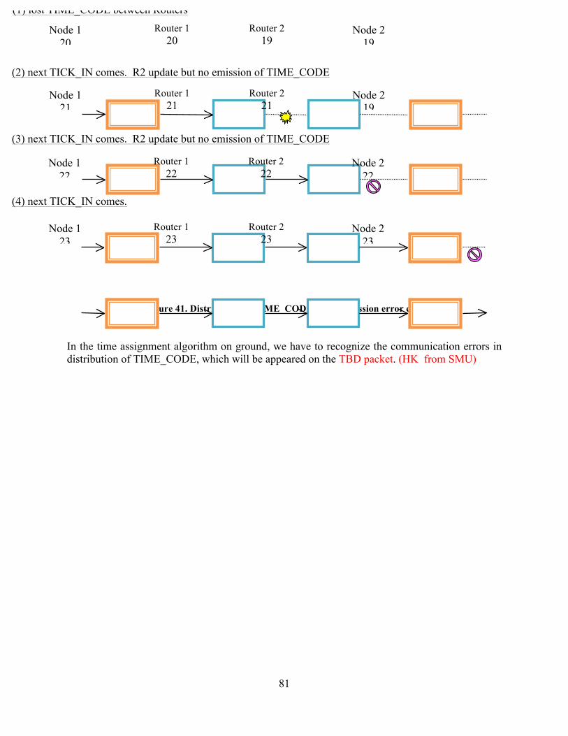
81

Figure 41. Distribution of TIME_CODE in transmission error case

In the time assignment algorithm on ground, we have to recognize the communication errors in distribution of TIME_CODE, which will be appeared on the TBD packet. (HK from SMU)

Node 1 20

Node 2 19

Router 1 20

Router 2 19

(1) lost TIME_CODE between Routers

Node 1 21

Node 2 19

Router 1 21

Router 2 21

(2) next TICK_IN comes. R2 update but no emission of TIME_CODE

Node 1 22

Node 2 22

Router 1 22

Router 2 22

(3) next TICK_IN comes. R2 update but no emission of TIME_CODE

Node 1 23

Node 2 23

Router 1 23

Router 2 23

(4) next TICK_IN comes.

82

7.4.4. RMAP protocol The SpaceWire provides a standardization of a high-speed communications network for a spacecraft at the physical and data link levels. The remote memory access protocol (RMAP) is a higher-level protocol, which provides the standard method to transfer of data between two SpaceWire nodes, as shown in Figure 42. Since the RMAP protocol is implemented on the SpaceWire I/O hardware, users can easily access a memory space on a SpaceWire node without any CPU accesses. Thus, the onboard hardware can be more simplified.

Figure 42. SpaceWire and RMAP layer.

A SpaceWire node can push or pull a data to or from another node by sending a message defined in RMAP protocol, which are RMAPwrite or RMAPread, respectively. The formats of these messages carried on the SpaceWire links are well defined on the document [6]. The message has header part in the SpaceWire communication, but these header parts do not appear in the SMCP message in the spacepacket. In this document, we skip descriptions on the format and timing of RMAP command. Please check the document [6] for detail. 7.4.5. SpaceWire-D protocol and Time Slot for Quality of Service. The most important feature in the design of the onboard network of the spacecraft is the safety of the satellite. Even when the SpaceWire links are fully busy for communications between nodes on board, an emergency message should not be disturbed by other non-emergency data and should be delivered quickly to the proper component in orbit. The SpaceWire network and RMAP protocol does not guarantee such a quality of service (QoS). Therefore, ASTRO-H satellite adopts new method to have enough band-pass for bus nodes, as described below. Such a new protocol is now described as one of standard high-level protocols on SpaceWire, named SpaceWire-D. The period of the generation of TIME_CODE at the Master node, SMU, for ASTRO-H is 2-6 sec = 15.625 m sec, and the time-counter 0 of TIME_CODE corresponds to the edge of the boundary of second; i.e., the value under second is .0000000000. Thus, the time-counter N in TIME_CODE corresponds to the value under second, N x 2-6.

Period of TIME_CODE Every 2-6 second

Hardware layer SpaceWire

User Application

RMAP Protocol

83

TIME_CODE(0) Edge of Second (t.000000 s) Table 40. Definition of TIME_CODE for ASTRO-H

Since the TIME_CODE is distributed to all the nodes on the ASTRO-H SpaceWire network, we can use the TIME_CODE as a tick of the network and define Time Slots by the ticks. For example, “time slot (N)” , where N is 0 to 63, corresponds to the epoch between the arrival of TIME_CODE(N) and TIME_CODE(N+1). Then, we have 64 time slots in one second, as illustrated in Figure 43.

Figure 43. Definition of Time Slot for ASTRO-H.

Then, for the ASTRO-H data acquisition system, the time in time slot (4n+0), where n = 0, 1, 2, … 15, are assigned for the bus components, and time epochs of time slot (1, 2, 3, 61, 62, 63) are used for transfer of basic information between SMU and user nodes, as shown in Table 41. Therefore, payload instruments, like SXS, SXI, HXI, and SGD, cannot communicate their telemetry and/or commands during these time slots. Such a restriction is defined in the telemetry-and-command design rule [7].

Time slot (4n+0)

Time slot (4n+1)

Time slot (4n+2)

Time slot (4n+3)

0 1 2 3 4 5 6 7 8 9 10 11 16 17 18 19 20 21 22 23 24 25 26 27 28 29 30 31 32 33 34 35 36 37 38 39 40 41 42 43

15.625ms

0 1 2 3 61 62 63

TC (0)

TC (1)

TC (2)

TC (0)

Time Slot

1 s time

0

84

44 45 46 47 48 49 50 51 52 53 54 55 56 57 58 59 60 61 62 63

Table 41. Definition of slots in the communication of nodes in ASTRO-H. Bus slot, System slot, and free slot are shown in yellow, magenta, and white, respectively.