is working capital management value-enhancing? evidence ... annual meetings/2014-… · is working...

Is working capital management value-enhancing? Evidence from firm performance and

investments

Nihat Aktasa,*, Ettore Crocib, and Dimitris Petmezasc

a WHU Otto Beisheim School of Management, Vallendar, Germany

b Universita' Cattolica del Sacro Cuore, Milan, Italy

c Surrey Business School, University of Surrey, Guildford, UK

This draft: January 2, 2014

ABSTRACT This paper examines the value effect of working capital management (WCM) for a large sample of US firms over the period 1982-2011. Taking into account omitted variables and reverse causality, we show that the decrease in working capital across time leads to increasing performance. This relationship is driven by firms that have substantial cash unnecessarily tied up in working capital. Importantly, we also show that corporate investment is the channel through which improvement in WCM translates into superior performance. Finally, the value effect of WCM is attenuated during the financial crisis, due to the contraction of the investment opportunity set.

JEL classification: G31, G32 Keywords: Working capital management, Performance, Investment, Reverse causality, Risk *Corresponding author. Tel.: +49 261 6509 224. E-mail addresses: [email protected] (N. Aktas), [email protected] (E. Croci), [email protected] (D. Petmezas).

Acknowledgement We thank Yakov Amihud, Hubert de la Bruslerie, Lorenzo Caprio, Riccardo Calcagno, Andrey Golubov, Ulrich Hofbaur, Alexander Kempf, François Larmande, Oguzhan Ozbas, Alain Schatt, Oktay Tas, Nickolaos Travlos, and seminar participants at the University of Cologne, University of Lausanne, and Istanbul Technical University for their comments and suggestions. We are grateful to Rongbing Huang and Inessa Love for sharing with us their codes for estimating the long-differencing technique and the PVAR model, respectively. All remaining errors are our own.

1

1. Introduction

Working capital management is a notion that traditionally appears in all standard corporate finance

textbooks highlighting its importance for corporations. At the end of 2011, US firms’ total investment in

working capital (i.e., inventories plus receivables) amounted to $4.2 trillion, which is 24% of their total

sales and above 18% of the book value of their assets.1 Almost 40% of this aggregate working capital has

been financed by accounts payable (i.e., supplier credit), leading to an aggregate investment in net

operating working capital (NWC) of $2.5 trillion.2

During the same period of time, the aggregate investment in NWC is comparable to the aggregate

amount held in cash by US firms. While the literature on cash holding is well developed,3 to the best of

our knowledge, scholars in finance paid relatively little direct attention to cash tied up in working

capital.4 Without being exhaustive, the few exceptions are the following. Sartoris and Hill (1983),

advocate the use of an integrated cash flow approach to working capital management. Fazzari and

Petersen (1993) emphasize the role of working capital as a source of funds to smooth investment. Shin

and Soenen (1998) document a negative contemporaneous relation between NWC and firm

performance. Hill, Kelly, and Highfield (2010) analyze the determinants of investment in NWC, and show

that, on top of industry effects, both firm operating and financing conditions explain the heterogeneity in

terms of NWC management. Kieschnick, Laplante, and Moussawi (2013), relying on a valuation

1 Source: Compustat database.

2 In its simplest expression net operating working capital (NWC) corresponds to inventories plus receivables minus

accounts payable. Unless otherwise specified, this is the definition that we adopt throughout the rest of this paper. 3 See, e.g., the following studies on cash holdings: Harford (1999), Opler, Pinkowitz, Stulz, and Williamson (1999),

Almeida, Campello, and Weisbach (2004), Faulkender and Wang (2006), Dittmar, Mahrt-Smith, and Servaes (2003), Dittmar and Mahrt-Smith (2007), Harford, Mansi, and Maxwell (2008), Bates, Kahle, and Stulz (2009), Denis and Sibilkov (2010), Lins, Servaes, and Tufano (2010), Gao, Harford, and Li (2013), and Harford, Klasa, and Maxwell (forthcoming). 4 The working capital literature focusing on non-US samples and the literature on the components of NWC (i.e.,

inventories, receivables, and accounts payable) are however much more developed [see, e.g., Hill, Kelly, and Highfield (2010), or Banos-Caballero, Garcia-Teruel, and Martinez-Solano (2012), for a comprehensive review].

2

framework similar to Faulkender and Wang (2006), report that on average the incremental dollar

invested in NWC is worth less than the incremental dollar held in cash.

Nevertheless, practitioners and consulting firms advising companies put relatively more emphasis

on the importance of working capital management for firm performance. Ek and Guerin (2011) argue

that there is tremendous latitude for improving the efficiency of working capital management in most

companies. Ernst & Young (2012), in its working capital management report devoted to the leading 1,000

US companies in year 2011, emphasizes that the unnecessary portion of NWC represents between $330

billion and $590 billion. This range of cash opportunity corresponds to between 3% and 6% of their

aggregate sales. Another leading consulting firm, Boston Consulting Group, stresses that the power of

working capital as a potential source of cash to fund growth is often neglected by companies. For

example, the following anecdotal evidence from Buchmann, Roos, Jung, and Wörtler (2008) is

particularly interesting: “Once the root causes of excess working capital are addressed, cash flows more

freely and can be put to far better use. For example, one company cut working capital by 30 percent and

used the cash to fund a major acquisition in Asia without having to take on debt and the associated

interest costs.”

The aforementioned discussion naturally raises the following questions. Do firms indeed over-invest

in NWC as claimed by practitioners? To what extent does improvement in working capital management

across time (i.e., decrease in unnecessary cash tied up in working capital across time) translate into

higher firm performance? And, is there a potential channel through which the decrease in NWC affects

firm performance?

The literature proposes several theoretical arguments to understand the relation between

overinvestment in working capital and firm performance. Overinvestment in working capital may

generate adverse effects and lead to value destruction for shareholders. Lev and Thiagarajan (1993)

argue that disproportionate (relative to sales) inventory increases are often considered as a negative

3

signal implying difficulties in generating sales. Furthermore, such inventory increases suggest that

earnings are expected to decline as management attempts to lower inventory levels. Further,

disproportionate accounts receivable (relative to sales) increases may suggest difficulties in selling the

firm's products, as well as an increasing likelihood of future earnings decreases from increases in

receivables' provisions. Additionally, like any investment, increases in working capital require additional

financing, which in turn involves financing and opportunity costs (see, e.g., Kieschnick, Laplante, and

Moussawi, 2013). Therefore, ceteris paribus, firms that hold high working capital on their balance sheet

potentially face also high interest expenses and bankruptcy risk.5 Moreover, too much cash tied up in

NWC might also impede firms from implementing value-enhancing investment projects in the short run

(see, e.g., Ek and Guerin, 2011). The existence of these potential costs implies a negative relationship

between investment in working capital and firm performance, in particular at high level of working

capital investment.

In an important departure from prior studies, this article also focuses on corporate investment as a

possible channel through which improvement in working capital management translates into higher firm

performance. In a frictionless environment, investment does not depend on internal funds available,

because firms can always raise external financing to fund all positive net present value projects

(Modigliani and Miller, 1958). However, in reality, the existence of capital market frictions increases the

cost of outside financing relative to the cost of internal funds (Myers and Majluf, 1984). This is the

reason why some firms with value-enhancing projects often underinvest, leading to low firm

performance. According to Denis and Sibilkov (2010), a solution to alleviate this underinvestment effect

5 Concerning the financial risk associated with holding high working capital, the illustration in Shin and Soenen

(1998) is particularly relevant. In 1994, Wal-Mart and Kmart were two similar companies in terms of capital structures, but Kmart had a substantially higher NWC relative to its sales in comparison to Wal-Mart. Kmart went into financial troubles essentially due to the financial costs of its poor working capital management. The company closed 110 stores in 1994, and ultimately filed for Chapter 11 bankruptcy protection in 2002.

4

is to rely on internal funds, such as cash flows and cash holdings. Eckbo and Kisser (2013) emphasize that

the reduction in working capital is also an important source of internal funds.

Therefore, motivated by prior literature which suggests that working capital could be considered as

a source of internal fund (Fazzari and Petersen, 1993; Eckbo and Kisser, 2013), or substitute to cash

(Bates, Kahle, and Stulz, 2009), we argue in this paper that corporate investment is a potential channel

through which working capital improvement (i.e., decrease in unnecessary working capital from one

period to the next) should affect firm performance. Indeed, the improvement in working capital

management increases firm’s financial flexibility in the short run thanks to the release of unnecessary

cash invested in working capital, and also in the long run thanks to relatively less financing needs to fund

day-to-day operating activities. Additionally, financially flexible firms have a greater ability to take

investment opportunities (see, e.g., Denis and Sibilkov, 2010; Duchin, Ozbas, and Sensoy, 2010).

Therefore, if too much cash is tied up in working capital, we expect that improvement in working capital

management across time should lead to increasing corporate investment over the next period. We

therefore expect a positive relationship between the decrease in unnecessary NWC across time and

corporate investment.

To assess the effect of working capital management on firm performance and investment, we use a

sample of 15,541 unique Compustat firms with available observations between 1982 and 2011. We first

document that the cross-sectional average and median NWC-to-sales ratio has decreased significantly

through time between 1982 and 2011.6 In our sample, the yearly average NWC-to-sales declined from

24% in 1982 to 17% in 2011, with the sample average being 20%.

Then, we measure the effect of working capital improvement on stock performance. Since working

capital needs are different from one industry to the other and, from one firm to the other in a given

industry (see, e.g., Hill, Kelly, and Highfield, 2010), it is essential to control for known determinants of

6 It is common in the literature to relate the firm’s NWC to its sales. We have also used the ratio NWC/total assets

and our results are qualitatively similar.

5

working capital needs. To do so, we adopt a two-step procedure. We first estimate the firm’s working

capital needs using variables known to affect the NWC-to-sales ratio (step 1). Then, we use in the

performance and investment regressions the residual from the first stage as a measure of the firm’s

excess NWC (step 2).

We document, using fixed effects regressions, that the decrease in excess NWC across time is

associated on average with superior stock performance over the next period. Using long-run

performance measures over a 3-year horizon, we also show that the effect of a decrease in excess NWC

on firm performance is persistent through time. Moreover, the corresponding economic effects are

substantial: a one standard deviation decrease in excess NWC across time is associated with an increase

of 0.72% in excess stock return over the next period, and an increase of 3.78% in excess stock return

over the next 3-year period.

Given that the decrease in NWC across time is associated with higher firm performance, the natural

question which emerges is why all firms do not reduce systematically the level of their working capital?

Investment in working capital has also positive effects, because it allows firms to growth by increasing

sales and earnings. In particular, larger inventories are known, among other issues, to reduce supply

cost, provide hedge against input price fluctuations, and minimize loss of sales due to potential stock-

outs (see, e.g., Blinder and Maccini, 1991; Fazzari and Petersen, 1993; Corsten and Gruen, 2004).

Supplying credit to customers may also affect positively firm sales because it allows for price

discrimination, serves as a warranty for product quality, and fosters long-term relationship with

customers (see, e.g., Brennan, Maksimovic, and Zechner, 1988; Long, Malitz, and Ravid, 1993; Summers

and Wilson, 2002). Therefore, only the reduction of the unnecessary portion of NWC should lead to

superior firm performance. To test this conjecture, we rely on an asymmetric model and show that the

decrease in excess NWC is positively associated with stock performance over the subsequent period only

for firms that have abnormally high investment in working capital (i.e., firms with positive excess NWC).

6

The corresponding economic effects are substantial: for firms with abnormally high working capital, a

one standard deviation decrease in excess NWC across time leads to a 1.56% (4.46%) increase in excess

stock return over the next 1-year (3-year) period. On the other hand, there is no effect of investment in

working capital on stock performance for firms with negative excess NWC.

To better establish that the causality between working capital and stock performance runs from

working capital to stock performance (forward causality) and not from stock performance to working

capital (reverse causality), we undertake three additional tests. We first adopt a dynamic model with

firm fixed effects, and estimate the model parameters using the long difference technique, which is

known to better account for reverse causality when the explanatory variable of interest is highly

persistent (see, e.g., Hahn, Hausman, and Kuersteiner, 2007; Huang and Ritter; 2009, Chang and Zhang,

forthcoming). Then, to evaluate the relative importance of forward causality and reverse causality, we

use panel-data vector autoregression specification, which is known to control for autocorrelation, time

trends, and time-invariant firm-specific unobserved heterogeneity (see, e.g., Holtz-Eakin, Newey, and

Rosen, 1988; Grinstein and Michaely, 2005; Love and Zicchino, 2006). Finally, we also assess the

robustness of the performance result by using a calendar time portfolio regression approach in the spirit

of Eberhart, Maxwell, and Siddique (2004). This test focuses on the effect of large decreases in NWC on

future stock returns for firms with positive excess NWC, with the control group being modeled using a

propensity score matching. These additional checks confirm the significantly negative and causal effect

of working capital level on firm performance.

After having documented the positive effect of improvement in working capital management on

firm performance, particularly for firms that have unnecessary cash tied up in working capital, we

investigate the channel through which improvement in working capital management translates into

superior firm performance. Following the literature, we argue that the decrease in excess NWC increases

the financial flexibility of the firm and releases cash in the short run which can be channeled towards

7

more efficient usage, such as allowing the firm to undertake additional value-enhancing investments. We

therefore investigate the effect of excess NWC on corporate investment. Following Bates, Kahle, and

Stulz (2009), we consider both capital expenditures and cash outflows associated with acquisitions as

measures of corporate investment. To control for the maintenance investment and given that only the

unanticipated component of the investment is expected to be associated with superior stock

performance (see, e.g., McConnell and Muscarella, 1985), we consider the change in investment over

the next period as dependent variable.

Our results strongly support our conjectures as we find, using a linear model, that a decrease in

excess NWC across time is positively associated with an increase in investment over the next period. The

economic effect of a decrease in excess NWC across time on future investment is economically

meaningful. A one standard deviation decrease in excess NWC across time is associated with an average

increase of 0.48% in the unanticipated component of corporate investment (relative to total assets) over

the next period. For the average firm in our sample, this corresponds to an increase in investment of

$9.5 million. We also check which of the two components of investment drives the results. The effect of

excess NWC on total investment is essentially driven by the impact of excess NWC on cash acquisitions.

We also use an asymmetric specification to disentangle the investment responses of firms with

abnormally high working capital (i.e., positive excess NWC) from the ones with abnormally low working

capital (i.e., negative excess NWC). Consistent with our stock performance analysis, the decrease in

excess NWC across time is associated with an increase in investment over the next period only for firms

that have abnormally high cash tied up in working capital.

We also perform three complementary tests in order to provide additional evidence that the

investment channel is the main channel through which working capital management translates into

superior firm performance. We first study the effect of working capital management on operating

performance. The investment channel posits that future stock performance is negatively related to

8

excess NWC because the release of cash allows the firm to undertake additional efficient investment. If

this is the main explanation, then the additional efficient investments should also lead to increasing

operating performance in the future. We therefore expect that future operating performance is also

negatively related to excess NWC, in particular for firms that have positive excess NWC. This is exactly

what we find using the return on assets as a measure of operating performance.

Our second complementary test looks at the effect of working capital management on firm risk,

because an excessively aggressive working capital policy might increase firm risk. Therefore, the negative

relation between excess NWC and stock performance might be due to increasing firm risk following a

decrease in NWC. To assess whether the risk channel drives our performance results, we regress firm risk

on excess NWC and a set of standard risk determinants from the literature. We uncover a negative

relation between firm risk and excess NWC only for firms with negative excess NWC. Our results rule out

the risk channel as a potential driver of the negative relation between firm performance and positive

excess NWC.

Our third complementary test uses the recent financial crisis as a negative shock on the investment

opportunity set and revisits the effect of working capital management on firm performance around the

crisis.7 Indeed, if the investment channel is the key driver of the performance effect of NWC

management, then in the context of a shrinking investment opportunity set, the value effect of working

capital management should be attenuated, if not totally offset. Our results confirm this intuition.

Relative to the pre-crisis period, our results indicate that the crisis offsets completely the value effect of

working capital management. A possible explanation is that during crises the expected return on

investment falls, giving less incentive for firms to take on new investments [see, e.g., the evidence

around the Asian financial crisis in Johnson, Boone, Breach, and Friedman (2000); Mitton (2002); Baek,

7 Duchin, Ozbas, and Sensoy (2010) show that the crisis deepened by evolving from a supply-shock on financing to a

demand-side effect on corporate investment, particularly following the stock market meltdown of September-October 2008.

9

Kang, and Park (2004)]. Therefore, our results suggest that the release of cash through efficient working

capital management is valuable in times of expanding investment opportunity set, reinforcing the role

played by the investment channel to understand the value effect of working capital management.

Our study is related to prior works analyzing the performance effect of working capital

management. Relying on a linear model without fixed effects, Shin and Soenen (1998) uncover a

negative contemporaneous relation between NWC and corporate profitability for a sample of US firms

over the period 1975-1994. Deloof (2003) analyze a sample of Belgian firms for the period 1991-1996

and report a negative contemporaneous relation between NWC and operating performance, with the

result being only significant in a specification without firm fixed effects. Banos-Caballero, Garcia-Teruel,

and Martinez-Solano (2012) focus on a sample of small and medium-sized Spanish firms for the period

2002-2007, and show that there is a concave relationship between NWC and operating performance.

Banos-Caballero, Garcia-Teruel, and Martinez-Solano (2014) consider a sample of UK firms for the period

2001-2007 and document an inverted U-shape relation between NWC and stock performance.

Our study contributes to the existing literature in several ways. We provide the first comprehensive

analysis which enriches our knowledge regarding the traditional notion of working capital management

across time. In particular, using an asymmetric model, we uncover that the documented negative

relationship between excess NWC and firm stock performance is confined to firms with abnormally high

NWC. Additionally, unlike prior literature, we shed light on the role played by the investment channel,

which serves as a plausible candidate to understand the value effect of working capital management.

Our empirical framework simultaneously controls for industry-, firm- and year-effects, and, unlike most

previous studies which use contemporaneous variables, our main variables of interest, as well as all

independent variables, are lagged by one period in order to alleviate the concern that working capital,

firm performance, and investment may be simultaneously determined in equilibrium. We also directly

tackle reverse causality between working capital and performance, and control errors-in-variable bias

10

potentially affecting the estimation of the excess NWC. Finally, we broaden the scope of the literature by

analyzing the effect of working capital management around the crisis and on firm risk.

We organize the remainder of this article as follows: in Section 2, we describe the sample used in

the empirical analysis and the considered empirical methods. Section 3 is devoted to the empirical

analysis of the relationship between improvement in working capital management and firm performance

and investment. Section 4 provides additional tests to address reverse causality between investment in

NWC and firm performance. Section 5 presents the robustness checks on the investment channel. In

particular, we analyze the effect of NWC on operating performance and firm risk, and use the recent

financial crisis as a shock on investment opportunities. Section 6 concludes the study.

2. Sample construction and empirical methods

2.1. Sample construction

We construct a sample of US listed firms from the WRDS merged CRSP/Compustat files for the

period 1982 to 2011. We exclude financial institutions, defined as firms with SIC codes inside the interval

6000-6999. In total, we have 15,541 unique firms in our main sample, with 140,508 firm-year

observations.

The second column of Table 1 reports the number of sample firms in each year. The number of firms

per year ranges from 3,431 in 2011 to 6,295 in 1997. The number of firms increases through time during

the first half of the sample period, with the wave of dot.com IPOs being clearly apparent in the second

half of the 1990s. The decrease in the number of listed firms after year 2001 is consistent with the

increasing frequency of going private transactions after the passage of Sarbanes-Oxley Act of 2002 (see

Engel, Hayes, and Wang, 2007).

We also provide in Table 1 the aggregate values for total assets, sales, cash holdings, net operating

working capital (NWC) and the components of NWC for each sample year. All dollar values are in billions

and converted to real values in 2005 dollars using the consumer price index (CPI). It is important to note

11

that while the aggregate cash tied up in NWC is more than three times of the aggregate cash holdings at

the beginning of the sample period, cash holdings become as important as the aggregate investment in

NWC towards the end of the sample period. The last row in Table 1 reports the average yearly growth

rate of the corresponding variables. Between 1982 and 2011, all the considered variables display a

clearly increasing trend. Over the sample period, total assets and sales grew on average at a yearly rate

of 4.5% and 3.2%, respectively. Over the same period of time, the aggregate amount held in cash has

grown at a higher rate relatively to total assets (and sales), a pattern which is consistent with Bates,

Kahle, and Stulz (2009). The aggregate amount invested in NWC increased less relatively to total assets,

sales and cash holdings, with an annual growth rate of 2.6%. Among the three components of NWC,

inventories have grown less (annual growth rate of 1.9%) in comparison to receivables and payables

(annual growth rate of 4%). These patterns indicate that firms hold on average relatively less working

capital through time, and in particular inventories.

[Please Insert Table 1 About Here]

Figure 1 reports the cross-sectional average and median NWC-to-sales ratio from 1982 to 2011. The

average (median) NWC-to-sales ratio over this period is approximately 20% (19%). The decreasing time

trends in average and median NWC-to-sales ratio are clearly apparent in Figure 1. The yearly average

(median) NWC-to-sales declined from 24% (22%) in 1982 to 17% (15%) in 2011. The cross-sectional

standard deviation of the NWC-to-sales ratio per year, reported also in Figure 1, also (slightly) decreases

over the sample period, indicating that firm heterogeneity in terms of NWC-to-sales ratio did not

increase through time.

[Please Insert Figure 1 About Here]

To assess whether the time trend in the NWC-to-sales ratio between 1982 and 2011 is statistically

significant, we regress the NWC-to-sales ratio on a constant and time measured in years (not reported in

a table). The coefficient on the time trend for the average NWC-to-sales ratio corresponds to a yearly

12

decrease of –0.32% and has a p-value below 0.01. The R-square of the regression is 92%. For the median,

the slope coefficient represents a 0.28% yearly decrease. It also has a p-value below 0.01. The R-square is

95%. This indicates the existence of a significant decreasing time trend in NWC-to-sales ratio over the

sample period.

To assess which one of the three components of the NWC contributed the most in the decrease of

the NWC-to-sales ratio, we report in Figure 2 the evolution through time of the average inventories,

receivables and payables, scaled by sales. The three components of the NWC-to-sales ratio decreased

significantly through time, but the decrease is relatively more pronounced for the average inventories-

to-sales ratio. Unreported results indicate that the slope coefficients of the linear time trend for

inventories, receivables and payables are respectively –0.25%, –0.14%, and –0.07%. The three slope

coefficients are statistically significant with p-values below 0.01. The corresponding R-squares are 95%

for inventories, 74% for receivables, and 29% for payables.


The sample composition changes through time, due to some firms entering and others leaving the

sample. To check whether the time series pattern of the average and median NWC-to-sales ratio is

affected by the changing sample composition, we present two additional figures. In Figure 3, we report

the time series of the average and median NWC-to-sales ratio for 643 surviving firms (i.e., firms that are

in the sample since 1982, which corresponds to the start of the sampling period). For this subsample of

firms, both the average and median NWC-to-sales ratio display also a clearly decreasing trend. The

average NWC-to-sales ratio moves from 23% at the beginning of the sample period to 19% at the end of

the sampling period, while the median goes from 21% to 17%.


What about firms entering and leaving the sample? Are leaving (entering) firms the least (most)

efficient ones in terms of working capital management? Figure 4 provides some answers to these

13

questions by comparing the pattern of the average NWC-to-sales ratio through time for three non-

overlapping subsamples of firms. The first group, denoted enter in Figure 4, includes firms entering the

sample in the corresponding year and remaining in the sample at least one year. The exit group

corresponds to the subsample of firms exiting the sample over the next year, and the stay group is made

of firms that do not enter or exit the sample in the corresponding year. In comparison to firms that are

entering and exiting the sample in a given year, firms that remain in the sample are clearly not the most

efficient ones in terms of working capital management. Moreover, the pattern of the average NWC-to-

sales ratios for firms entering and exiting the sample suggests that entering firms do not have

systematically lower working capital ratio than firms exiting the sample. So the decreasing patterns

highlighted in Figure 1 cannot be attributed solely to changing sample composition.


2.2. Variable definitions

This paper examines the effect of working capital management on firm performance and

investment. Working capital needs are different from one industry to the other and from one firm to the

other. In particular, Hill, Kelly, and Highfield (2010) show that, on top of industry effects, both firm

operating and financing conditions explain the heterogeneity in terms of NWC management. To assess

the effect of working capital management on firm performance, it is therefore important to control for

known determinants of working capital needs. This is the reason why we adopt a two-step procedure in

this paper. The first step estimates the firm’s working capital needs using variables known to affect the

NWC-to-sales ratio. In the second step, we use the residual from the first stage as a measure of the

firm’s excess NWC-to-sales ratio in both the performance and investment regressions.

The next subsections describe the variable of interest and the dependent variables used in the

multivariate analyses.

14

2.2.1. Excess NWC

Our main variable of interest is the excess NWC-to-sales ratio, denoted excess NWC throughout the

paper. We first estimate the firm’s normal NWC-to-sales ratio in year t using the following determinants

taken from Hill, Kelly, and Highfield (2010): sales volatility, 1-year sales growth rate, operating cash flow,

and a dummy variable for financial distress (variable definitions are in Appendix A). All the explanatory

variables are lagged by one period. Damodaran (2012) argues that mature firms require less working

capital per unit of sales. We therefore also consider firm age as an additional determinant of the normal

NWC-to-sales ratio. We regress the NWC-to-sales ratio on these determinants separately for each

industry/year, such that our procedure controls implicitly for industry and year effects. To group firms

into industries, we use the Fama-French 49-industry classification. We remove the four industries related

to financial activities (i.e., banking, insurance, real estate, and trading). In total, we have 45 industries

and 30 years, leading by construction to 1,350 industry/year regressions. However, for some

industry/years in our sample, we do not have sufficient observations to run the corresponding

regressions. The first-stage regression estimation is therefore only possible for 1,296 industry/years.

The fit of the first-stage model is summarized in Panel A of Table 2, in which we report the summary

statistics for the Fisher-statistic, adjusted R-square, and number of observations used in the regressions.

More detailed statistics are provided in Appendix B. The first-stage regressions use on average 113

observations. The average adjusted R-square is 12.42%, which is in the same range as in Hill, Kelly, and

Highfield (2012), who report an R-square between 11% and 15% according to the specification used. The

average Fisher-statistic is 4.15, indicating that on average the considered regression model fits the data

sufficiently well.

For every firm in a given year, the excess NWC is the residual of the corresponding first-stage

regression (i.e., NWC-to-sales ratio minus its predicted value from the regression), and measures the

15

unnecessary cash tied up in working capital.8 A positive excess NWC indicates that the firm is over-

investing in working capital. This implies that there is room for the firm to increase the efficiency of its

working capital management across time by adopting a relatively more aggressive working capital policy

(such as by reducing inventories and payment delays granted to customers). A negative excess NWC

indicates that the firm is currently adopting an extremely aggressive working capital policy, which

potentially increases the risk of sales loss essentially due to potential stock-outs and customer

dissatisfactions driven by aggressive receivable collections (see, e.g., Fazzari and Petersen, 1993; Corsten

and Gruen, 2004; Kieschnick, Laplante, and Moussawi, 2013). In this case, additional investment in

working capital is expected to be more valuable because, among others, larger inventories can prevent

input shortages and interruptions in the production process (see, e.g., Blinder and Maccini, 1991);

further, increasing trade credit supply can stimulate sales because it allows for price discrimination,

serves as a warranty for product quality, and fosters long-term relationship with customers (see, e.g.,

Brennan, Maksimovic, and Zechner, 1988; Long, Malitz, and Ravid, 1993; Summers and Wilson, 2002).

We implicitly assume that the efficient NWC of the firm (i.e., the NWC level adopted by a shareholder

value maximizing manager who trade-offs benefits and costs of investment in working capital) is the one

which leads to insignificant excess NWC.

The summary statistics presented in Panel B of Table 2 show that the average NWC-to-sales ratio is

19.99%, a figure which is very close to the 19.79% reported by Hill, Kelly, and Highfield (2010).

Concerning the abnormal component of the NWC-to-sales ratio, the mean is 0.10% and the median

–1.09%, indicating that the distribution of the excess NWC is positively skewed. We report also summary

statistics on the distribution of the excess NWC conditional on its sign. For positive values of the excess

NWC (i.e., subsample of firms with conservative NWC policy), the average and median are 11.55% and

8 In addition to the use of the regression-based excess NWC measure, we also assess the robustness of our results

by relying on a more simple industry adjustment procedure, which consists in subtracting from the NWC-to-sales ratio of a given firm the ratio of the median firm in the corresponding industry/year. Our main findings are not sensitive to this choice. The results are available upon request from the authors.

16

7.25%, respectively. For negative values (i.e., subsample of firms with aggressive NWC policy), the

corresponding average and median are –9.40% and –6.92%, respectively.

2.2.2. Dependent variables

We use excess stock return adjusted for firm size and market-to-book as a measure of stock

performance. Following Barber and Lyon (1997), we define excess return for time t as the difference

between the return of the buy-and-hold investment in the sample firm i less the return of the buy-and-

hold investment in a benchmark portfolio:

∏ ( ) ∏ ( )

, (1)

where Ri,m is the return for firm i, Rp,m is the return of the benchmark portfolio for month m, and T is the

investment horizon in number of months. We compute excess returns over 1-year horizon (T = 12). To

assess whether the effect of working capital management on firm performance persists through time,

we consider also the excess returns over a 3-year horizon (T = 36 months). Following Daniel and Titman

(1997), the benchmark portfolios are the twenty-five Fama-French value-weighted portfolios

constructed by independently sorting stocks on size (ME) and book-to-market (BE/ME) characteristics.9

Each sample firm is assigned to a size and book-to-market portfolios using Fama-French ME and BE/ME

breakpoints.10

Following Bates, Kahle, and Stulz (2009), we consider both capital expenditures (CAPEX) and cash

outflows associated with acquisitions as a measure of corporate investment. The investment variables

are scaled by total assets at the beginning of the period. We use the change in investment as our

dependent variable in the investment regressions, because in an efficient capital market only the

unanticipated component of the investment is expected to be associated with superior stock

performance (see, e.g., McConnell and Muscarella, 1985). Moreover, the use of the change in

9 For other applications of the 25-portfolio approach to compute excess stock returns see also Faulkender and

Wang (2006) and Denis and Sibilkov (2010). 10

ME and BE/ME breakpoints are available on Kenneth French’s website.

17

investment as dependent variable controls to some extent for the maintenance investment (i.e., the

investment which is necessary for the firm to keep functioning at current levels of growth in a

competitive environment), and allows focusing only on the part of the investment devoted to firm

growth.

Some of our tests use also measures of operating performance and firm risk as dependent variables.

We use the return on assets (ROA) as a measure of operating performance. Similar to stock

performance, we consider operating performance over 1-year and 3-year periods. The 3-year average

ROA at time t is the average ROA between year t and t + 2. As a measure of firm risk, we use total risk

following Coles, Daniel, and Naveen (2006), which corresponds to the annualized standard deviation of

daily stock returns (see also, e.g., Armstrong and Vashishtha, 2012).

Panel B of Table 2 reports summary statistics for the dependent variables. The median firm has a

1-year (3-year) excess stock return of –11.86% (–34.00%), while the mean excess return is –2.82%

(–9.72%), consistent with the distribution of excess stock returns being positively skewed (see, e.g.,

Barber and Lyon, 1997).11 The 1-year (3-year average) ROA has a mean value of 5.01% (6.60%) in our

sample, while the median is 10.62% (10.83%), indicating that the distribution of ROA is negatively

skewed in our sample. The mean CAPEX and cash acquisition represent 7.64% and 3.10% of total assets,

respectively. These two variables are positively skewed.


2.3. Econometric specifications and methods

We study the impact of excess NWC on firm performance and investment using the following linear

regression specification:

, (2)

11

The non-zero mean excess return is mainly due to the winsorization of the variable at the 1st and 99th percentiles. The mean of the 1-year excess return before winsorization is much lower with a value of –0.003 in our sample.

18

where, V is the dependent variable measuring either firm performance or investment, and αt and ηi

represent year and firm fixed effects, respectively. Given the panel structure of our dataset and the use

of fixed effects, a negative (positive) coefficient measures the increase (decrease) in firm performance

or investment associated with a one unit decrease in excess NWC across time. Control refers to a set of

control variables known to affect firm performance or investment.

In Equation (2), all right-hand side variables are lagged by one period in order to alleviate the

concern that net operating working capital, firm performance, and corporate investment may be

simultaneously determined in equilibrium. To control for time-invariant firm characteristics, all

regressions include firm fixed effects, which allows mitigating missing variable issues. The inclusion of

year fixed effects controls for changing economic and financing conditions through time. It is also

important to note that industry fixed effects are indirectly controlled for through the use of

industry/year regressions to estimate the excess NWC. We also cluster standard errors at the firm level

for the statistical tests to account for heteroskedasticity and auto-correlation at the firm level (see

Petersen, 2009; Thompson, 2011). Throughout the article, we winsorize all variables at the 1st and 99th

percentiles to mitigate the influence of extreme values.

To examine whether the relation between excess NWC and firm performance (or investment) is

nonlinear, we rely on an asymmetric model, in which we allow the slope coefficient of the considered

regression model to be different for positive and negative excess NWC. Intuitively, if the excess NWC

measures the deviation from the optimal NWC, we expect that only the decrease in positive excess NWC

across time is associated with increasing firm performance. To test this intuition, the considered

nonlinear specification is the following one:

[ ] [ ( )]

, (3)

19

where, is a dummy variable taking value one if the corresponding excess NWC is positive (i.e.,

abnormally high cash tied up in net working capital), and 0 otherwise.

In the performance regressions, following the literature, we consider as control variables the market

value of equity (as a proxy for firm size), firm age, leverage, risk, and intangible assets (see, e.g., Coles,

Daniel, and Naveen, 2008; Duchin, Matsusaka, and Ozbas, 2010). Future stock performance is also

related to R&D expenses (see, e.g., Chan, Lakonishok and Sougiannis, 2001) and asset growth (see, e.g.,

Cooper, Gulen, and Schill, 2008; Lipson, Mortal, and Schill, 2011). To control for the asset growth effect,

we use fixed asset growth instead of total asset growth, because the latter includes also components of

the working capital. In the investment regressions, in addition to firm size, leverage, and risk, we also

include variables known to be correlated with growth opportunities, such as cash flow, Tobin’s Q, and

sales growth (see, e.g., Lang, Ofek, and Stulz, 1996). Variable definitions are in Appendix A. Summary

statistics for the considered control variables can be found in Panel B of Table 2.

2.4. Preliminary analysis

Table 3 reports the average and median of our dependent and control variables for subsamples

based on the sign of the excess NWC. For each variable, the last two columns display the p-values from a

test of mean differences and a test of median differences between negative and positive excess NWC

subsamples, respectively.

In comparison to firms with negative excess NWC, firms with positive excess NWC have on average

significantly lower stock and operating performance over both 1-year and 3-year horizons. They also

invest on average slightly less in capital expenditures, but undertake relatively more cash acquisitions.

Firms with positive excess NWC are also slightly more risky than firms with negative excess NWC.

It is also interesting to note that the mean and median for the considered control variables are

statistically different between firms with positive and negative excess NWC. Regardless the proxy used

for firm size (i.e., total assets, sales or market value of equity), firms with positive excess NWC are

20

smaller in comparison to firms with negative excess NWC. The mean and median Tobin’s Q for the two

subsamples suggest that firms with negative excess NWC have on average slightly more growth

opportunities, but both fixed asset growth and sales growth are lower on average for these firms in

comparison to firms with positive excess NWC. Firms with negative excess NWC are relatively less

leveraged and riskier, and they are slightly older than firms with positive excess NWC.


The evidence reported in Table 3 indicates that firm characteristics are significantly different

between the two subsamples (positive versus negative excess NWC subsamples). It is therefore

important to control for these characteristics in the multivariate analyses. To further investigate the

relation between excess NWC, firm performance, and investment, in the next sub-section, we rely on a

multivariate framework and control for the panel structure of our data set.

3. Empirical evidence

This section first explores the relationship between excess NWC and stock performance. Then, we

assess whether corporate investment is a potential channel through which working capital management

translates into higher firm performance.

3.1. Working capital management and stock performance

Table 4 presents the stock performance regressions. Panel A reports the results on the linear model.

The dependent variable is the 1-year excess return in the first two columns, and the 3-year excess return

in the last two columns. All the independent variables are lagged by one period with respect to the

dependent variables, and all specifications include firm and year fixed effects. The first and third columns

present the specifications without control variables. In Panel A, both the 1-year and 3-year excess

returns are negatively associated with the excess NWC of the previous period. This indicates that the

decrease in excess NWC across time leads on average to increasing stock performance in subsequent

21

years. The inclusion of control variables in columns 2 and 4 does not alter the conclusion pertaining to

the positive effect on stock performance of a decreasing excess NWC across time. The coefficient

estimates of excess NWC are negative and statistically significant both in columns 2 and 4 with a value of

–0.0473 (p-value = 0.08) and –0.2475 (p-value = 0.00), respectively. The corresponding economic effects

are substantial: a one standard deviation decrease in excess NWC across time is associated with an

increase of 0.72% in excess stock return over the next period, and an increase of 3.78% in excess stock

return over the next 3-year period.

After having established that the decrease in (excess) NWC across time is associated with higher

stock performance, the natural question that arises is why all firms do not reduce systematically the level

of their working capital? All firms do not have the means to reduce their NWC. For firms with already low

level of NWC, further reduction might increase substantially the risk of stock-outs and sales, thus

affecting negatively their performance. Therefore, only the reduction of the unnecessary cash tied up in

working capital (i.e., positive excess NWC) is expected to lead to superior firm performance.

To test this conjecture, we rely on an asymmetric model in Panel B of Table 4. The regression

specifications include two interaction variables: the first variable, excess NWC × D, interacts the excess

NWC with a dummy variable identifying firms with positive excess NWC, and the second variable, excess

NWC x (1 – D), interacts the excess NWC with a dummy variable identifying firms with negative excess

NWC. The results in Panel B of Table 4 indicate that the decrease in excess NWC across time is positively

associated with stock performance over the subsequent period only for firms that have abnormally high

investment in working capital. The coefficient estimates of the first interaction term (excess NWC × D)

are statistically highly significant with values of –0.1354 (p-value = 0.00) and –0.3425 (p-value = 0.00) for

the 1-year and 3-year excess return regressions, respectively. The economic effects of a decrease in

excess NWC for firms with positive excess NWC are quite substantial: a one standard deviation decrease

in positive excess NWC is associated with an increase of 1.56% in excess stock return over the next

22

period, and an increase of 4.46% in excess stock return over the next 3-year period. The effect of excess

NWC on firm performance is not significant at conventional levels for firms that have negative excess

NWC (see the specifications with control variables in Panel B of Table 4).


Concerning the control variables, in all specifications in Table 4, the coefficients of firm size,

leverage, and R&D are statistically significant at conventional levels. Consistent with the literature, stock

performance decreases with leverage and firm size (see, e.g., Faulkender and Wang, 2006; Duchin,

Matsusaka, and Ozbas, 2010), and increases with R&D expenses (Chan, Lakonishok and Sougiannis,

2001). In Table 4, we also use the variable fixed asset growth to control for the asset growth effect,

because the asset pricing literature provides cross-sectional evidence that growing firms are associated

with low future stock returns (see, e.g., Cooper, Gulen, and Schill, 2008). The variable fixed asset growth

appears to be statistically insignificant at conventional levels in Table 4.

3.2. Working capital management and investment

So far, the performance regressions suggest that firms that are able to reduce the level of their

unnecessary NWC across time are increasing their stock performance. Moreover, the 3-year excess

return results indicate that the performance effect of a decrease in excess NWC is persistent through

time. In this section, our aim is to assess whether corporate investment is a potential channel through

which the decrease in excess NWC across time translates into superior firm performance.

The improvement in working capital management increases firm’s financial flexibility in the short

run thanks to the release of unnecessary cash tied up in working capital, and also in the long run due to

relatively less financing needs to fund day-to-day operating activities. Financially flexible firms have a

greater ability to take investment opportunities (see, e.g., Denis and Sibilkov, 2010; Duchin, Ozbas, and

Sensoy, 2010). Therefore, the decline in excess NWC across time is expected to lead to increasing

corporate investment. Table 5 tests this idea using the change in investment ratio as dependent variable.

23

Column 1 considers the change in total investment, while columns 2 and 3 show the change in CAPEX

and the change in cash acquisitions, respectively. All the independent variables are lagged by one period

with respect to the dependent variables, and all specifications include firm and year fixed effects.

Panel A of Table 5 presents the results of the linear model. The coefficient estimate of excess NWC is

significantly negative in column 1 with a value of –0.0317 (p-value = 0.00), indicating that a decrease in

excess NWC across time is associated on average with an increase in investment over the next period.

The effect of excess NWC on total investment is essentially driven by the impact of excess NWC on cash

acquisitions. In fact, the coefficient of excess NWC is not significant in the specification which uses the

change in CAPEX as dependent variable (see column 2), while the coefficient of excess NWC is negative

and statistically significant with a value of –0.0327 (p-value = 0.00) in the specification which uses the

change in cash acquisition (see column 3). With regards to the economic effect, a one standard deviation

decrease in excess NWC across time is associated with an increase of 0.48% of the unanticipated

component of total investment over the next period.

Panel B of Table 5 reports the results of the asymmetric model, which controls in the investment

regressions for the sign of the excess NWC by using two interaction variables [i.e. excess NWC × D and

excess NWC × (1 – D)]. The dummy variable D identifies positive excess NWC. In column 1, the coefficient

estimate of excess NWC × D is negative and statistically significant with a value of –0.0688 (p-value =

0.00), while the coefficient of excess NWC × (1 – D) is positive with a value of 0.0211 and statistically

insignificant at conventional levels (the corresponding p-value is 0.10). It is important to note that the

asymmetric effect of excess NWC on corporate investment parallels to a large extent the asymmetric

effect of excess NWC on firm performance. The decrease in excess NWC across time leads to increasing

corporate investment over the subsequent period only for firms that have abnormally high investment in

working capital.

24

Concerning the component of investment, the asymmetric model provides also interesting results

for CAPEX. Both positive and negative excess NWC affect significantly the change in capital expenditures

over the next period, but the sign of the corresponding coefficient estimate is negative for positive

excess NWC (value = –0.0076, p-value = 0.07) and positive for negative excess NWC (value = 0.0215, p-

value = 0.00). For cash acquisitions, only the coefficient estimate of excess NWC × D is statistically

significant with a value of –0.0532 (p-value = 0.00), indicating that the change in cash acquisitions

increases following a decrease in excess NWC across time.

Taken collectively, the results in Tables 4 and 5 indicate that the decrease in NWC across time for

firms with abnormally high investment in working capital is associated with increasing firm performance,

because firms channel towards efficient investments the cash release from unnecessary investment in

working capital.


4. Causal effect of working capital management on firm performance

To alleviate omitted variable bias and endogeneity issues, we used in the previous section fixed

effect regressions with lagged right-hand side variables. While robust to omitted variable bias, this

approach might not address adequately the potential reverse causality problem between working capital

management (WCM) and firm performance, particularly in the presence of persistent endogenous

variables and autocorrelated dependent variable (see, e.g., Chang and Zhang, forthcoming).

4.1. Long difference approach to assess the causal impact of WCM on firm performance

To better account for reverse causality, as a first test, we model the relation between excess NWC

and firm performance using a dynamic panel model with fixed effects. We employ Hahn, Hausman, and

Kuersteiner’s (2007) long difference technique, which consists in taking multi-year rather than one-year

difference, to estimate the model parameters. The long difference technique relies on a small set of

25

moment conditions and is less biased than the mean-differencing and system generalized method of

moment (GMM) estimators (see, e.g., Hahn, Hausman, and Kuersteiner, 2007; Huang and Ritter, 2009;

Chang and Zhang, forthcoming). Another important advantage of the long difference technique over

other methods is that it can better identify causal relation when the explanatory variable of interest is

highly persistent (Chang and Zhang, forthcoming). Two recent applications of the long difference

estimator in finance are Huang and Ritter (2009), in which the authors study the speed of adjustment to

target leverage ratio, and Chang and Zhang (forthcoming), who use the approach to assess the causal

effect of managerial entrenchment on firm value.

We are interested in the estimation of the following equation:

( ) )

( ) ( ), (4)

or

[ ] [ ] [ ]

[ ] [ ], (5)

where V denotes the 1-year excess stock return. Like Chang and Zhang (forthcoming), we are interested

in the coefficient of the endogenous variable, .

To estimate Equation (5), we follow Hahn, Hausman, and Kuersteiner (2007), Huang and Ritter

(2009), and Chang and Zhang (forthcoming) by taking an iterated two-stage least squares (2SLS)

approach. To obtain the initial coefficient estimates ( , and ), we use and

as valid instruments for [ ] and [ ], respectively,

and estimate Equation (5) with 2SLS. Hahn, Hausman, and Kuersteiner (2007) suggest that the residuals

are also valid instruments. Therefore, each iteration ends with updating coefficient estimates ( , and

) using the residuals as well as and as instruments to estimate Equation

(5) with 2SLS. Following Hahn, Hausman, and Kuersteiner (2007), we iterate this process three times and

26

report the results of the third iteration in Panel A of Table 6. We adopt a differencing length of 4 years (k

= 4), which allows us to have sufficiently long differences without losing too many observations.

The results in Panel A of Table 6 indicate that the changes in excess NWC have a significantly

negative impact on firm performance after controlling for the influence of past changes in firm

performance on the changes in the excess NWC. The coefficient of the variable of interest is –0.3075 and

highly significant with a p-value of 0.02. The magnitude of the effect appears to be economically

significant: a one standard deviation (15.29%) decrease in excess NWC is associated with an increase in

1-year excess return by 4.70% (=–15.29% x –0.3075) over a period of four years, or 1.18% annually. The

coefficients of the control variables are consistent with those reported in Panel A of Table 4, except for

fixed asset growth.

Based on the long difference approach that is able to uncover the dynamic relation between

working capital and firm performance while controlling for possible omitted variables, reverse causality,

and autocorrelation in the dependent variable, our results indicate a clear and negative causal effect of

excess NWC on stock performance.


4.2. PVAR specification to gauge the relative importance of forward and backward causality

The causal relation between investment in working capital and stock performance can be

bidirectional, and the two directions of causality are not necessarily mutually exclusive. To evaluate the

relative importance of forward causality (working capital level affecting stock performance) and reverse

causality (stock performance affecting working capital level), we use a panel-data vector autoregression

(PVAR) approach proposed by Holtz-Eakin, Newey, and Rosen (1988). The PVAR method is widely used as

a tool for disentangling the causality effect and investigating intertemporal interactions between

variables (see, e.g., Grinstein and Michaely, 2005; Love and Zicchino, 2006; Goto, Watanabe, and Xu,

2009; Chang and Zhang, forthcoming). This approach combines the conventional vector autoregression

27

technique, which allows a vector of variables to be endogenously determined in the system, with the

panel-data approach, which controls for unobserved firm-specific heterogeneity. Following Love and

Zucchino (2006), our two-equation reduced-form PVAR model can be written as follows.

∑ ∑

(6)

∑ ∑

(7)

where m is the number of time lags that is sufficiently large to ensure that εi,t and ωi,t are white noise

error terms, xt and yt are year fixed effects, and fi and gi are unobserved firm fixed effects.

Following Love and Zicchino (2006), we take the forward mean-differencing approach to tackle the

concern that firm fixed effects are correlated with the regressors due to lags of the dependent variables.

This procedure removes the fixed effects by transforming all variables in the model to deviations from

forward means (i.e., the mean values of all future observations for each firm in a given year). This

transformation preserves homoscedasticity and the orthogonality between transformed variables and

lagged regressors (Arellano and Bover, 1995). Moreover, it enables us to use the lagged values of

regressors as instruments to estimate the coefficients with the GMM approach. We remove also year

fixed effects by subtracting the mean value of each variable computed for each year.

We estimate the coefficients of the system given in Equations (6) and (7) and report the results for

m = 1 in Panel B of Table 6.12 In column 1 we report the results of the model with 2 variables {1-year

excess return, excess NWC}, while in column 2 we report the results of the model with 3 variables {1-

year excess return, positive excess NWC, negative excess NWC}. Column 1 suggests a strong negative

causal effect of excess NWC on excess stock return (p-value = 0.00), while the effect of excess stock

return on excess NWC is statistically insignificant at conventional levels (p-value = 0.16). In column 2, we

assess whether the response of stock performance is symmetric for positive and negative excess NWC.

The results indicate that the negative association between excess NWC and firm performance is driven

12

The results are qualitatively the same for m=2 and m=3. These unreported results are available upon request from the authors.

28

by firms with positive excess NWC. This provides additional support for the robustness of the results

presented in Panel B of Table 4. Consistent with column 1, the excess stock return does not seem to

affect significantly both positive and negative excess NWC. Taken together, these results indicate that

reverse causality appears not to be significant in our sample.

Based on the coefficient estimates of the PVAR model, it is possible to construct impulse-response

functions, which trace the impact of a one standard deviation shock (or innovation) to one endogenous

variable on the current and future values of other endogenous variables in the system, assuming that the

shock reverts to zero in subsequent periods. Since the effect of stock performance on excess NWC is not

statistically significant in Panel B of Table 6, we present in Figure 5 the response of stock performance to

a shock in excess NWC. The considered impulse-response function is in bold line and the 5% error bands

generated by Monte Carlo simulation are in dotted lines. A one standard deviation decrease in excess

NWC in the current period (year 0) results in an increase in firm performance by approximately 0.80%

over the next period, and the magnitude of the response decreases through time, vanishing almost

completely after 4 years. The results in Panel B of Table 6 and Figure 5 provide additional support for our

main findings in Table 4.


4.3. Abnormal performance using long-short portfolios approaches

As a final test, we replicate Eberhart, Maxwell, and Siddique’s (2004) calendar time portfolio

regression approach. Eberhart, Maxwell, and Siddique (2004) analyze the effect of a significant increase

in R&D expenses on future stock performance. We follow their long-short portfolio approach in order to

better assess whether superior future firm performance for firms with excess NWC is a response to

improvement in working capital management. We focus on firms with large decreases in NWC in a given

year (i.e., the long portfolio). The corresponding control group (i.e., the short portfolio) is either the risk

free rate or a sample of firms with similar characteristics that do not decrease their NWC.

29

A decrease in working capital in year t is considered to be large if the following four conditions are

met simultaneously: (i) NWC-to-sale ratio of at least 15% in year t–1, (ii) positive excess NWC in year t–1,

(iii) decrease in the dollar value of NWC of at least 10% in year t, and (iv) decrease in NWC-to-sale ratio

of at least 10% in year t. Conditions (i) and (ii) are imposed to make sure that the firm included in the

long portfolio has substantial amount of investment in NWC. Conditions (iii) and (iv) are similar to those

used by Eberhart, Maxwell, and Siddique (2004). That is to ensure that the decrease in NWC is

meaningful both in dollar values and in percentage terms.

The firm enters at the end of time t into the long portfolio if a large decrease in NWC is observed in

that period, and the firm is kept into the portfolio over the next 36 months. The benchmark return is

either the risk-free rate or the return of a portfolio of matched firms. In the latter case, we use a

propensity score matching approach. We use as explanatory variable the same set of variables as in the

model used to compute the normal NWC (see legend of Table 2) and industry dummies. We then match

each firm in the long portfolio with an industry firm with the closest propensity score. To estimate the

abnormal performance (i.e., alpha), we use the Fama and French (1993) three-factor model and the

Carhart (1997) four-factor model.

Panel A of Table 7 reports the results. The alpha is highly significant in 3 specifications out of 4. The

results indicate that stock performance increases abnormally over the next 3-year period following a

large decrease in NWC. In Panel B of Table 7, we use an alternative approach to build the zero-

investment equally weighted portfolio. The portfolio is long on firms with negative excess NWC and short

on firms with positive NWC. The portfolio is rebalanced each year based on the sign of the excess NWC

of the previous year. The estimated alpha is highly significant in Panel B, both with the three- and four-

factor models.


30

5. Additional results and robustness checks

5.1. Further tests to assess the robustness of the investment channel

In this sub-section, to check the robustness of the investment channel as the main channel through

which working capital management translates into superior firm performance, we perform three

additional tests. We first study the effect of working capital management on operating performance. We

then assess the impact of working capital management on firm risk. We finally use the recent financial

crisis as a negative shock on investment opportunity set to revisit the effect of NWC management on

firm performance and investment.

5.1.1. Working capital management and operating performance

The investment channel suggests that future stock performance is negatively related to excess NWC

because the release of cash allows a firm to undertake additional efficient investment. If this is the main

explanation, then these additional efficient investments should also lead to increasing operating

performance in the future. We therefore expect that operating performance is also negatively related to

excess NWC.

Panel A of Table 8 reports the regression results on operating performance. We use the same

econometric approach and the same set of control variable as in Table 4. In columns 1 and 2, the

dependent variable is the next period return on assets (ROA). In columns 3 and 4, the dependent

variable is the average ROA over the next 3-year period. Columns 1 and 3 report the estimation results of

the linear model. The coefficient estimates of excess NWC are negative and statistically significant at

conventional levels in all specifications. Consistent with the effect on stock performance and corporate

investment, a decrease in excess NWC across time leads to superior operating performance over the

next 1-year and 3-year periods. The corresponding economic effects are also meaningful: a one standard

deviation decrease in excess NWC across time is associated with an increase of 0.50% in ROA over the

next period, and an increase of 0.48% in average ROA over the next 3-year period.

31

In Panel A of Table 8, columns 2 and 4 report the results of the asymmetric model for both the 1-

year ROA and 3-year average ROA regressions. For positive excess NWC, the coefficient estimates of

excess NWC are –0.1360 (p-value = 0.00) and –0.1025 (p-value = 0.00) in columns 2 and 4, respectively.

For negative excess NWC, the coefficient estimates of excess NWC are 0.1131 (p-value = 0.00) and

0.0686 (p-value = 0.00) in columns 2 and 4, respectively. These results indicate that positive and negative

excess NWC do not have a symmetric impact on operating performance. The effect of positive excess

NWC on operating performance is significantly negative, while the effect of negative excess NWC is

significantly positive. These results indicate that a decrease in excess NWC across time leads to

increasing operating performance over the subsequent period only for firms that have abnormally high

investment in working capital. For firms that have abnormally low investment in working capital, it is the

increase in excess NWC across time which is associated with superior operating performance. The

economic effects are stronger with the asymmetric model: for firms that have abnormally high (low)

cash tied up in NWC, a one standard deviation decrease (increase) in excess NWC across time is

associated with an increase of 1.77% (1.06%) in ROA over the next period.

Overall, the operating performance results suggest that there is an optimum level of working capital,

and corporate managers that are able to get closer to this optimum, either by reducing or taking

additional investment in working capital, increase the operating performance of their firms. With regards

to the control variables, intangible assets, age, R&D and risk (risk only for 1-year ROA) carry a negative

and significant coefficient at the 1% level, while firm size and leverage are positively associated with ROA

again at the 1% significance level.


5.1.2. Working capital management and firm risk

Firm risk is a plausible alternative explanation for the increase in stock performance following a

decrease in working capital. A firm adopting an excessively aggressive working capital policy might

32

increase firm risk, among others, because of fluctuations in supply cost and loss of sales due to potential

stock-outs (see, e.g., Blinder and Maccini, 1991; Fazzari and Petersen, 1993; Corsten and Gruen, 2004).

Therefore, the negative relation between NWC and firm performance might be due to increasing firm

risk following a decrease in NWC. To assess whether the risk channel drives our performance results, we

regress firm risk on excess NWC and a set of determinants. Panel B of Table 8 reports the results.

Following, Coles, Daniel, and Naveen (2006), the proxy used for firm risk is the annualized standard

deviation of firm daily returns (see also, e.g., Armstrong and Vashishtha, 2012). On top of time invariant

firm characteristics, the considered determinants taken from the literature are firm size, leverage, book-

to-market and sales growth (see, e.g., Coles, Daniel, and Naveen, 2006; Armstrong and Vashishtha,

2012). We also control for changing economic and financing conditions through time using year

dummies.

In Panel B of Table 8, column 1 displays the result of the linear model, and column 2 gives the

estimation results of the asymmetric model. In the linear model, excess NWC is negatively related to firm

risk, indicating that an aggressive NWC policy through time increases firm risk over the next period.

However, the asymmetric model in Panel B of Table 8 show that the negative relation between excess

NWC and firm risk is driven by firms that have negative excess NWC. For firms with positive excess NWC,

the relation between NWC and firm risk is positive, without being statistically significant at conventional

level. This indicates that the release of unnecessary cash tied up in working capital does not lead to

increasing firm risk, a result which rules out the risk channel as a potential driver of the negative relation

between firm performance and positive excess NWC.

Concerning the control variables, the sign of the coefficient estimates are broadly consistent with

the literature. Firm risk decreases with size and sales growth, and it increases with leverage and book-to-

market (see, e.g., Coles, Daniel, and Naveen, 2006; Armstrong and Vashishtha, 2012).

33

5.1.3. The financial crisis as a shock on investment opportunities

The recent financial crisis affected negatively corporate investment [see, e.g., Campello, Graham,

and Harvey (2010) for survey evidence]. In our sample, the average investment over total assets declined

by 9% over the crisis period, 2007-2009, relative to the 3-year pre-crisis period, 2004-2006. Duchin,

Ozbas, and Sensoy (2010) show that over the crisis period, the crisis deepened by evolving from a supply-

shock on financing to a demand-side effect on corporate investment, in particular following the stock

market meltdown of September-October 2008. In this section, we use the financial crisis as a negative

shock to the investment opportunity set and revisit the effect of working capital management on firm

performance and investment around the crisis. Indeed, if the investment channel is the key driver of the

performance effect of working capital management, then in the context of a shrinking investment

opportunity set, the effect of working capital management on firm performance and investment should

be attenuated, if not totally offset. We test this intuition in this section.

The considered empirical framework builds on Duchin, Ozbas, and Sensoy (2010) and uses firm-level

observations for years between 2004 and 2009. Using fixed-effect panel regressions, we compare the

relationship between working capital and performance before and during the financial crisis.

Table 9 presents the results of the fixed effect regressions. Crisis is an indicator variable which

identifies the crisis period. It takes value one for years 2007-2009, zero otherwise. Panel A of Table 9

focuses on stock performance, and Panel B on corporate investment. We use the asymmetric model with

the same set of control variables as in Tables 4 and 5. We additionally include into the specification the

crisis indicator variable, and its interactions with positive excess NWC and negative excess NWC. We use

the letter in Table 9 to denote the coefficient estimate of the corresponding variable: ( )

corresponds to the marginal effect of positive (negative) excess NWC on firm performance for the pre-

crisis period; ( ) measures the incremental impact of the crisis on the relationship between positive

34

(negative) excess NWC and firm performance; and the sum of and ( and ) gives the marginal

effect of positive (negative) excess NWC on firm performance for the crisis period.

In Panel A, the dependent variable is the 1-year excess return. Consistent with the results in Table 4,

stock performance is negatively (positively) related to excess NWC over the pre-crisis period for firms

with positive (negative) excess NWC. During the crisis, however, the relationship between firm

performance and excess NWC appears to break down; the sum of and as well as the sum of and

are not statistically different from zero. This indicates that the crisis offsets completely the

performance effect of working capital management. A possible explanation is that during crises the

expected return on investment falls, giving less incentive for firms to take on new investments [see, e.g.,

the evidence around the Asian financial crisis in Johnson, Boone, Breach, and Friedman (2000); Mitton

(2002); Baek, Kang, and Park (2004)]. Therefore, the contraction of the investment opportunity set

during the crisis probably does not allow firms to take on additional efficient investment. The results in

Panel B of Table 9 are also consistent with this conjecture. While the decrease in positive excess NWC

leads to increasing investment during the pre-crisis period, the financial crisis attenuates this effect. This

result suggests that the release of cash through efficient working capital management is only valuable in

times of expanding investment opportunity set, reinforcing the role played by the investment channel to

understand the value effect of working capital management.


5.2. Robustness checks

We check the robustness of our main findings by carrying out two additional analyses. We first

assess the robustness of our main results to errors-in-variable bias in the estimation of the excess NWC.

We then check whether our findings are a by-product of the substitution effect between NWC and cash

reserves documented by Bates, Kahle, and Stulz (2009).

35

5.2.1. Errors-in-variable bias

The first robustness check is related to the existence of potential errors-in-variable bias in the

estimation of the excess NWC, which is our variable of interest. Observed excess NWC is derived from a

first-stage statistical procedure. Estimation errors at the first stage might have an impact on the validity

of inferences drawn in the second stage. To alleviate this concern, we standardize the excess NWC by its

standard error, and use the standardized excess NWC as independent variable in Panel A of Table 10.

The standardization procedure allows to put more weight on statistically significant excess NWC and to

reduce the observed heteroskedasticity.

Columns 1 and 2 present the results of the stock performance regressions, and columns 3 and 4 the

investment regressions. We use the same econometric approach and the same set of control variables as

in Tables 4 and 5, respectively. For brevity, the coefficients of the control variable are not reported in

Table 10. The results in Panel A of Table 10 are qualitatively similar to Tables 4 and 5. NWC is negatively

related to both performance and investment, and these relations are due to firms with positive excess

NWC. This indicates that our main findings are robust to potential errors-in-variable bias.


5.2.2. Controlling for cash reserves

Bates, Kahle, and Stulz (2009) show that there is a substitution effect between cash reserves and

investment in working capital. So far, we have not included cash reserves as a control variable in the

performance and investment regressions, exposing our results to a potential omitted variable bias. To

assess whether NWC plays a role on top of the effect of cash on performance and investment, Panel B of

Table 10 includes also cash reserves as an additional control variable. The results are qualitatively similar

to Panel A of Table 10, suggesting that the negative effect of excess NWC on firm performance and

investment for firms with unnecessary cash tied up in working capital (i.e., firms with positive excess

NWC) is robust to the inclusion of cash reserves into the specification.

36

6. Conclusion

This paper provides comprehensive evidence of a relationship between working capital

management and firm performance using an exhaustive sample of US firms over a 30-year period

between 1982 and 2011. In particular, we find that a decrease in NWC across time is positively

associated with both stock and operating performance. Even more importantly, we show that this stock

performance effect is driven by the decrease in unnecessary cash tied up in NWC across time. We also

rule out the possibility that the results are driven by reverse causality and increasing firm risk.

Taken together, our results support the view that improvement in working capital management is

associated with higher firm performance, essentially because the increased financial flexibility and the

cash release from the improvement allow firms to undertake, among others, additional efficient

investments. Our study implies that efficient working capital management is highly valuable, particularly

in periods of expanding investment opportunity set.

Our results have also important corporate policy implications. Given the magnitude of working

capital as a proportion of firm assets, corporate managers should put particular emphasis in maximizing

its utility at the benefit of their shareholders. In particular, our findings imply that corporate managers

should avoid having too much cash unnecessarily tied up in working capital and target an optimum level

of working capital. Such efficient management would provide a new source of internally-generated

funds, which could be ultimately employed in more profitable investment opportunities at the benefit of

the firms’ shareholders.

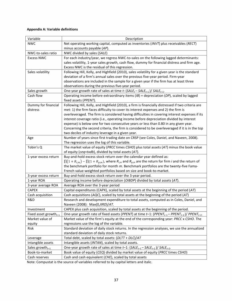
37

Appendix A: Variable definitions

Variable Description

NWC Net operating working capital, computed as inventories (INVT) plus receivables (RECT) minus accounts payable (AP).

NWC-to-sales ratio NWC divided by sales (SALE)

Excess NWC For each industry/year, we regress NWC-to-sales on the following lagged determinants: sales volatility, 1-year sales growth, cash flow, dummy for financial distress and firm age. Excess NWC is the residual of this regression.

Sales volatility Following Hill, Kelly, and Highfield (2010), sales volatility for a given year is the standard deviation of a firm’s annual sales over the previous five-year period. Firm-year observations are included in the sample for a given year if the firm has at least three observations during the previous five-year period.

Sales growth One-year growth rate of sales at time t: (SALEt – SALEt–1 )/ SALEt–1.

Cash flow Operating income before extraordinary items (IB) + depreciation (DP), scaled by lagged fixed assets (PPENT).

Dummy for financial distress

Following Hill, Kelly, and Highfield (2010), a firm is financially distressed if two criteria are met: 1) the firm faces difficulty to cover its interest expenses and 2) the firm is overleveraged. The firm is considered having difficulties in covering interest expenses if its interest coverage ratio (i.e., operating income before depreciation divided by interest expense) is below one for two consecutive years or less than 0.80 in any given year. Concerning the second criteria, the firm is considered to be overleveraged if it is in the top two deciles of industry leverage in a given year.

Age Number of years since first trading date on CRSP (see Coles, Daniel, and Naveen, 2008). The regression uses the log of this variable.

Tobin’s Q The market value of equity (PRCC times CSHO) plus total assets (AT) minus the book value of equity (ceq+txdb), divided by total assets (AT).

1-year excess return Buy-and-hold excess stock return over the calendar year defined as: ∏( ) ∏( ), where Ri,m and Rp,m are the return for firm i and the return of

the benchmark portfolio for month m. Benchmark portfolios are the twenty-five Fama-French value-weighted portfolios based on size and book-to-market.

3-year excess return Buy-and-hold excess stock return over the 3-year period.

1-year ROA Operating income before depreciation (OIBDP) divided by total assets (AT).

3-year average ROA Average ROA over the 3-year period

CAPEX Capital expenditures (CAPX), scaled by total assets at the beginning of the period (AT)

Cash acquisition Cash acquisitions (AQC), scaled by total assets at the beginning of the period (AT)

R&D Research and development expenditure to total assets, computed as in Coles, Daniel, and Naveen (2008): Max(0,XRD)/AT.

Investment CAPEX plus cash acquisition, scaled by total assets at the beginning of the period.

Fixed asset growtht–1 One-year growth rate of fixed assets (PPENT) at time t–1: (PPENTt–1 – PPENTt–2 )/ PPENTt–2.

Market value of equity

Market value of the firm’s equity at the end of the corresponding year: PRCC x CSHO. The regressions use the log of the variable.

Risk Standard deviation of daily stock returns. In the regression analyses, we use the annualized standard deviation of daily stock returns.

Leverage Total debt, scaled by total assets: (DLTT + DLC)/AT

Intangible assets Intangible assets (INTAN), scaled by total assets.

Sales growtht–1 One-year growth rate of sales at time t–1: (SALEt–1 – SALEt–2 )/ SALEt–2.

Book-to-market Book value of equity (CEQ) divided by market value of equity (PRCC times CSHO)

Cash reserves Cash and cash equivalent (CHE), scaled by total assets

Note: Compustat is the source of variables referred to by capital letters and italic.

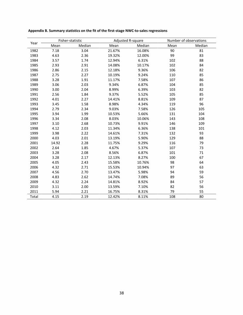
38

Appendix B. Summary statistics on the fit of the first-stage NWC-to-sales regressions

Year Fisher-statistic Adjusted R-square Number of observations

Mean Median Mean Median Mean Median

1982 7.18 3.04 21.67% 16.08% 90 81 1983 4.63 2.36 19.32% 12.00% 99 83 1984 3.57 1.74 12.94% 6.31% 102 88 1985 2.93 2.91 14.08% 10.17% 102 84 1986 2.86 2.15 12.18% 9.36% 106 82 1987 2.75 2.27 10.19% 9.24% 110 85 1988 3.28 1.91 11.17% 7.58% 107 86 1989 3.06 2.03 9.34% 6.87% 104 85 1990 3.00 2.04 8.99% 6.39% 103 82 1991 2.56 1.84 9.37% 5.52% 105 85 1992 4.01 2.27 14.41% 8.81% 109 87 1993 3.45 1.58 8.98% 4.34% 119 96 1994 2.79 2.34 9.03% 7.58% 126 105 1995 3.94 1.99 10.53% 5.66% 131 104 1996 3.34 2.08 8.03% 10.06% 143 108 1997 3.10 2.68 10.73% 9.91% 146 109 1998 4.12 2.03 11.34% 6.36% 138 101 1999 3.98 2.22 14.61% 7.31% 132 93 2000 4.03 2.01 13.19% 5.90% 129 88 2001 14.92 2.28 11.75% 9.29% 116 79 2002 2.64 1.85 4.67% 5.37% 107 73 2003 3.28 2.08 8.56% 6.87% 101 71 2004 3.28 2.17 12.13% 8.27% 100 67 2005 4.05 2.43 15.58% 10.76% 98 64 2006 4.32 2.71 15.53% 10.94% 97 63 2007 4.56 2.70 13.47% 5.98% 94 59 2008 4.83 2.62 14.74% 7.08% 89 56 2009 4.32 2.24 14.81% 8.92% 84 57 2010 3.11 2.00 13.59% 7.10% 82 56 2011 5.94 2.21 16.75% 8.31% 79 55

Total 4.15 2.19 12.42% 8.11% 108 80

39

References

Almeida, H., Campello, M., Weisbach, M. S., 2004. The cash flow sensitivity of cash. Journal of Finance 58, 1777–1804.

Arellano, M., Bover, O., 1995. Another look at the instrumental variable estimation of error-components models. Journal of Econometrics 68, 29–51.

Armstrong, Ch. S., Vashishtha, R., 2012. Executive stock options, differential risk-taking incentives, and firm value. Journal of Financial Economics 104, 70–88.

Baek, J. S., Kang, J. K., Park, K. S., 2004. Corporate governance and firm value: evidence from the Korean financial crisis. Journal of Financial Economics 71, 265–313.

Banos-Caballero, S., Garcia-Teruel, P.J., Martinez-Solano, P., 2012. How does working capital management affect the profitability of Spanish SMEs? Small Business Economics 39, 517–529.

Banos-Caballero, S., Garcia-Teruel, P.J., Martinez-Solano, P., 2014. Working capital management, corporate performance, and financial constraints. Journal of Business Research 67, 332–338.

Barber, B. M., Lyon, J. D., 1997. Detecting long-run abnormal stock returns: The empirical power and specification of test statistics. Journal of Financial Economics 43, 341–372.

Bates, T. W., Kahle, K. M., Stulz, R. M., 2009. Why do U.S. firms hold so much more cash than they used to? Journal of Finance 64, 1985–2022.

Blinder, A. S., Maccini, L. J., 1991. The resurgence of inventory research: What have we learned? Journal of Economic Survey 5, 291–328.

Brennan, M., Maksimovic, V., Zechner, J., 1988. Vendor financing. Journal of Finance 43, 1127–1141. Buchmann, P., Roos, A., Jung, U., Wörtler, M., 2008. Cash for growth: The neglected power of working-

capital management. The Boston Consulting Group. Available at https://www.bcgperspectives.com/. Campello, M., Graham, J. R., Harvey, C. R., 2010. The real effects of financial constraints: evidence from a

financial crisis. Journal of Financial Economics 97, 470–487. Carhart, M., 1997. On persistence in mutual fund performance. Journal of Finance 52, 57–82. Chan, L. K., Lakonishok, J., Sougiannis, T., 2001. The stock market valuation of research and development

expenditures. Journal of Finance 56, 2431–2456. Chang, X., Zhang, H. F., forthcoming. Managerial entrenchment and firm value: A dynamic perspective.

Journal of Financial and Quantitative Analysis. Coles, J. L., Daniel, N. D., Naveen, L., 2006. Managerial incentives and risk-taking. Journal of Financial

Economics 79, 431-468. Coles, J. L., Daniel, N. D., Naveen, L., 2008. Boards: Does one size fit all? Journal of Financial Economics

87, 329–356. Cooper, M. J., Gulen, H., Schill, M. J., 2008. Asset growth and the cross-section of stock returns. Journal

of Finance 63, 1609–1651. Corsten, D., Gruen, T., 2004. Stock-outs cause walkouts. Harvard Business Review 82, 26–28. Damodaran, A., 2012. Investment Valuation: Tools and Techniques for Determining the Value of any

Asset. Wiley Finance, 3rd Edition. Daniel, K., Titman, E., 1997. Evidence on the characteristics of cross sectional variation in stock returns.

Journal of Finance 52, 1–33. Deloof, M., 2003. Does working capital management affect profitability of Belgian firms? Journal of

Business Finance & Accounting 30, 573–587. Denis, D. J., Sibilkov, V., 2010. Financial constraints, investment, and the value of cash holdings. Review

of Financial Studies 23, 247–269. Dittmar, A., Mahrt-Smith, J., 2007. Corporate governance and the value of cash holdings. Journal of

Financial Economics 83, 599–634.

https://www.bcgperspectives.com/

40

Dittmar, A., Mahrt-Smith, J., Servaes, H., 2003. International corporate governance and corporate cash holding. Journal of Financial and Quantitative Analysis 38, 111-133.

Duchin, R., Matsusaka, J. G., Ozbas, O., 2010. When are outside directors effective? Journal of Financial Economics 96, 195–214.

Duchin, R., Ozbas, O., Sensoy, B. A., 2010. Costly external finance, corporate finance, and the subprime mortgage credit crisis. Journal of Financial Economics 97, 418–435.

Eckbo, B. E., Kisser, M., 2013. Corporate funding: Who finances externally? Unpublished working paper. Tuck School of Business at Darmouth.

Eberhart, A. C., Maxwell, W. F., Siddique, A. R., 2004. An examination of long-term abnormal stock returns and operating performance following R&D increases. Journal of Finance 59, 623–649.

Engel, E., Hayes, R. M., and Wang, X., 2007. The Sarbanes-Oxley Act and firms’ going-private decisions. Journal of Accounting and Economics 44, 116–146.

Ek, R., Guerin, S., 2011. Is there a right level of working capital? Journal of Corporate Treasury Management 4, 137–149.

Ernst & Young, 2012, All tied up: Working capital management report. Available at: www.ey.com. Fama, E. F., French, K. R., 1993. Common risk factors in the returns on stocks and bonds. Journal of

Financial Economics 33, 3–56. Fazzari, S. M., Petersen, B. C., 1993. Working capital and fixed investment: New evidence on financing

constraints. RAND Journal of Economics 24, 328–342. Faulkender, M., Wang, R., 2006. Corporate financial policy and the value of cash. Journal of Finance 61,

1957–1990. Gao, H., Harford, J., Li, K., 2013. Determinants of corporate cash policy: Insights from private firms.

Journal of Financial Economics 109, 623–639. Goto, S., Watanabe, M., Xu, Y., 2009. Strategic disclosure and stock returns: Theory and evidence from

US cross-listing. Review of Financial Studies 22, 1585–1620. Grinstein, Y., Michaely, R., 2005. Institutional holdings and payout policy. Journal of Finance 60, 1389–

1425. Hahn, J., Hausman, J., Kuersteiner, G., 2007. Long difference instrumental variables estimation for

dynamic panel models with fixed effects. Journal of Econometrics 140, 574–617. Harford, J., 1999. Corporate cash reserves and acquisitions. Journal of Finance 54, 1969–1997. Harford, J., Klasa, S., Maxwell, W., forthcoming. Refinancing risk and cash holdings. Journal of Finance. Harford, J., Mansi, S., Maxwell, W., 2008. Corporate governance and firm cash holdings. Journal of

Financial Economics 87, 535–555. Hill, M. D., Kelly, G. W., Highfield, M. J., 2010. Net operating working capital behavior: A first look.

Financial Management 39, 783–805. Holtz-Eakin, D., Newey, W., Rosen, H. S., 1988. Estimating vector autoregressions with panel data.

Econometrica 56, 1371–1395. Huang, R., Ritter, J. R., 2009. Testing theories of capital structure and estimating the speed of

adjustment. Journal of Financial and Quantitative Analysis 44, 237–271. Johnson, S., Boone, P., Breach, A., Friedman, E., 2000. Corporate governance in the Asian financial crisis,

1997-1998. Journal of Financial Economics 58, 141–186. Kieschnick, R., Laplante, M., Moussawi, R., 2013. Working capital management and shareholders’ wealth.

Review of Finance 17, 1827–1852. Lang, L., Ofek, E., Stulz, R. M., 1996. Leverage, investment, and firm growth. Journal of Financial

Economics 40, 3–29. Lev, B., Thiagarajan, S. R., 1993. Fundamental information analysis. Journal of Accounting Research 31,

190–215.

http://www.ey.com/

41

Lins, K. V., Servaes, H., Tufano, P., 2010. What drives corporate liquidity? An international survey of cash holdings and lines of credit. Journal of Financial Economics 2010, 160–176.

Lipson, M. L., Mortal, S., Schill, M. J., 2011. On the scope and drivers of the asset growth effect. Journal of Financial and Quantitative Analysis 46, 1651–1682.

Long, M. S., Malitz, I. B., Ravid, S. A., 1993. Trade credit, quality guarantees and product marketability. Financial Management 22, 117–127.

Love, I., Zicchino, L., 2006. Financial development and dynamic investment behavior: Evidence from Panel VAR. Quarterly Review of Economics and Finance 46, 190–210.

McConnell, J. J., Muscarella, C. J., 1985. Corporate capital expenditures decisions and the market value of the firm. Journal of Financial Economics 14, 399–422.

Mitton, T., 2002. A cross-firm analysis of the impact of corporate governance on the East Asian financial crisis. Journal of Financial Economics 64, 215–241.

Modigliani, F., Miller, M., 1958. The cost of capital, corporation finance and the theory of investment. American Economic Review 53, 261–297.

Myers, S, Majluf, N., 1984. Corporate financing and investment decisions when firms have information that investors do not have. Journal of Financial Economics 13, 187–221.

Opler, T., Pinkowitz, L., Stulz, R., Williamson, R. 1999. The determinants and implications of corporate cash holdings. Journal of Financial Economics 52, 3–46.

Petersen, M. A., 2009. Estimating standard errors in finance panel data sets: comparing approaches. Review of Financial Studies 22, 435–480.

Sartoris, W. L., Hill, N. C., 1983. A generalized cash flow approach to short-term financial decisions. Journal of Finance 38, 349–360.

Shin, H., Soenen, L., 1998. Efficiency of working capital management and corporate profitability. Financial Practice and Education 8, 37–45.

Summers, B., Wilson, N., 2002. Trade credit terms offered by small firms: Survey evidence and empirical analysis. Journal of Business and Finance Accounting 29, 317–335.

Thompson, S. B., 2011. Simple formulas for standard errors that cluster by both firm and time. Journal of Financial Economics 99, 1–10.

42

Figure 1. Time series of summary statistics for NWC-to-sales ratio. This figure plots cross-sectional summary statistics for NWC-to-sales ratio for US non-financial firms by year from 1982 to 2011. NWC corresponds to inventories plus receivables minus accounts payable.

Figure 2. Yearly average inventories, receivables and accounts payable. This figure plots the cross-sectional average for inventories, receivables, and payables scaled by sales for US non-financial firms by year from 1982 to 2011.

10%

15%

20%

25%

30%

19

82

19

84

19

86

19

88

19

90

19

92

19

94

19

96

19

98

20

00

20

02

20

04

20

06

20

08

20

10

Mean Median Standard deviation

5%

10%

15%

20%

25%

19

82

19

84

19

86

19

88

19

90

19

92

19

94

19

96

19

98

20

00

20

02

20

04

20

06

20

08

20

10

Inventories Receivables Accounts payable

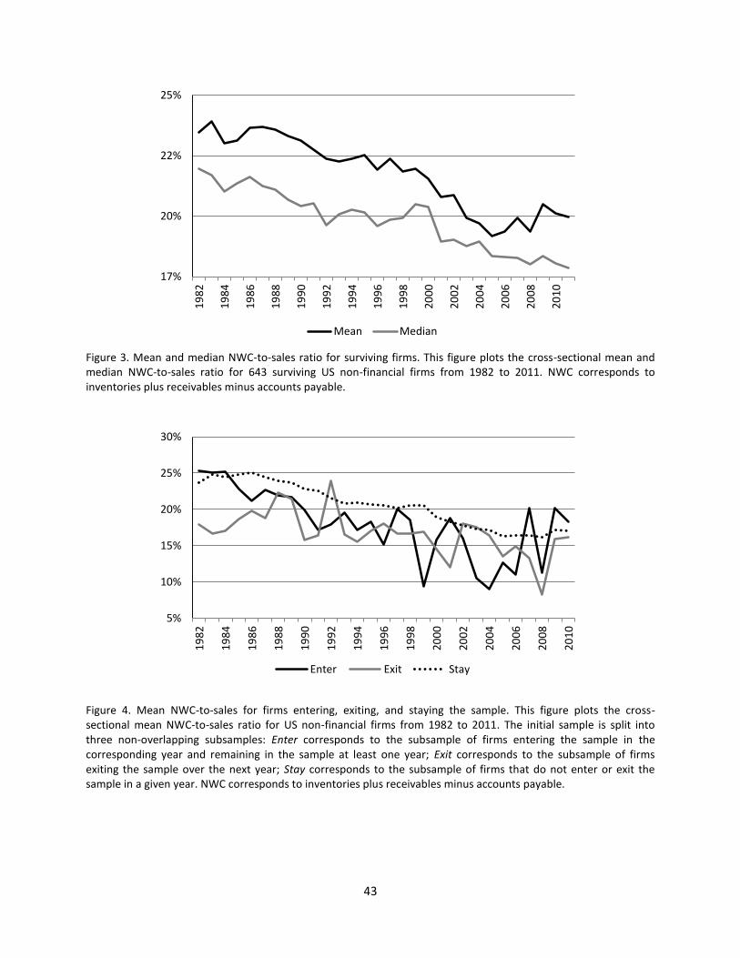
43

Figure 3. Mean and median NWC-to-sales ratio for surviving firms. This figure plots the cross-sectional mean and median NWC-to-sales ratio for 643 surviving US non-financial firms from 1982 to 2011. NWC corresponds to inventories plus receivables minus accounts payable.

Figure 4. Mean NWC-to-sales for firms entering, exiting, and staying the sample. This figure plots the cross-sectional mean NWC-to-sales ratio for US non-financial firms from 1982 to 2011. The initial sample is split into three non-overlapping subsamples: Enter corresponds to the subsample of firms entering the sample in the corresponding year and remaining in the sample at least one year; Exit corresponds to the subsample of firms exiting the sample over the next year; Stay corresponds to the subsample of firms that do not enter or exit the sample in a given year. NWC corresponds to inventories plus receivables minus accounts payable.

17%

20%

22%

25%

19

82

19

84

19

86

19

88

19

90

19

92

19

94

19

96

19

98

20

00

20

02

20

04

20

06

20

08

20

10

Mean Median

5%

10%

15%

20%

25%

30%

19

82

19

84

19

86

19

88

19

90

19

92

19

94

19

96

19

98

20

00

20

02

20

04

20

06

20

08

20

10

Enter Exit Stay

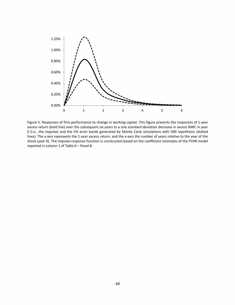
44

Figure 5. Responses of firm performance to change in working capital. This figure presents the responses of 1-year excess return (bold line) over the subsequent six years to a one standard deviation decrease in excess NWC in year 0 (i.e., the impulse) and the 5% error bands generated by Monte Carlo simulations with 500 repetitions (dotted lines). The y-axis represents the 1-year excess return, and the x-axis the number of years relative to the year of the shock (year 0). The impulse-response function is constructed based on the coefficient estimates of the PVAR model reported in column 1 of Table 6 – Panel B.

0.00%

0.20%

0.40%

0.60%

0.80%

1.00%

1.20%

0 1 2 3 4 5 6

45

Table 1 Aggregate values by year The table reports yearly aggregate values for total assets, sales, cash holdings, net operating working capital (NWC) and its component. NWC corresponds to inventories (INV) plus receivables (REC) minus accounts payable (AP). The sample contains listed non-financial US firms from the WRDS merged CRSP/Compustat files for the period 1982 to 2011. The sample includes 140,508 observations for 15,541 unique firms. All dollar values are in billions and adjusted to 2005 dollars by the consumer price index. N is the number of firms. The last row displays the annual growth rate of the corresponding variables.

Year N Assets Sales Cash NWC INV REC AP

1982 3, 918 5, 243 5, 928 304 981 725 714 458 1983 4, 306 5, 380 5, 915 393 951 685 751 485 1984 4, 386 5, 497 6, 090 382 992 707 766 481 1985 4, 346 5, 687 6, 064 399 1, 004 702 800 498 1986 4, 481 5, 945 5, 845 476 1, 026 696 810 479 1987 4, 670 6, 381 6, 295 538 1, 112 747 902 537 1988 4, 585 7, 346 6, 680 548 1, 582 770 1, 464 653 1989 4, 463 7, 708 6, 892 561 1, 677 790 1, 564 677 1990 4, 439 8, 103 7, 231 563 1, 685 822 1, 589 725 1991 4, 520 8, 313 7, 220 591 1, 651 818 1, 537 703 1992 4, 701 8, 453 7, 371 623 1, 593 813 1, 468 688 1993 5, 161 8, 933 7, 673 659 1, 663 835 1, 545 717 1994 5, 459 9, 586 8, 397 718 1, 805 902 1, 667 763 1995 5, 687 10, 146 8, 985 734 1, 977 979 1, 829 832 1996 6, 191 10, 893 9, 506 808 1, 983 985 1, 895 897 1997 6, 295 11, 454 10, 037 834 2, 052 997 1, 978 923 1998 5, 961 12, 541 10, 330 944 2, 088 1, 032 2, 028 973 1999 5, 772 14, 350 10, 995 1, 091 2, 133 1, 063 2, 238 1, 168 2000 5, 648 16, 112 12, 137 1, 207 2, 162 1, 121 2, 378 1, 337 2001 5, 096 16, 074 11, 973 1, 245 2, 161 1, 054 2, 347 1, 240 2002 4, 696 16, 097 11, 809 1, 361 2, 147 1, 067 2, 369 1, 289 2003 4, 417 17, 223 12, 723 1, 661 2, 227 1, 132 2, 455 1, 359 2004 4, 377 17, 922 13, 965 1, 813 2, 442 1, 243 2, 678 1, 479 2005 4, 275 17, 627 14, 017 1, 730 2, 463 1, 234 2, 649 1, 421 2006 4, 184 18, 364 14, 827 1, 705 2, 392 1, 301 2, 577 1, 487 2007 4, 028 18, 382 14, 655 1, 655 2, 393 1, 287 2, 547 1, 441 2008 3, 810 17, 488 14, 994 1, 567 2, 255 1, 220 2, 280 1, 245 2009 3, 644 18, 114 12, 919 1, 907 2, 074 1, 145 2, 176 1, 247 2010 3, 561 19, 072 14, 168 2, 100 2, 120 1, 226 2, 284 1, 389 2011 3, 431 19, 401 15, 184 2, 025 2, 136 1, 290 2, 297 1, 452

Growth rate N/A 4.5% 3.2% 6.5% 2.6% 1.9% 4.0% 3.9%

46

Table 2 Summary statistics The sample includes listed non-financial U.S. firms from the WRDS merged CRSP/Compustat files for the period 1982 to 2011. Panel A reports summary statistics about the fit of the ordinary least square models used to estimate the normal NWC-to-sales ratio. To estimate the normal NWC-to-sales ratio, we regress for each industry/year the NWC-to-sales ratio on the following lagged determinants: sales volatility, 1-year sales growth, free cash flow, dummy for financial distress and firm age. We estimate in total 1,296 regressions (45 Fama-French industries times 30 years, some industry/years are removed from the sample because of no sufficient observations to estimate the model). Summary statistics for Fisher-statistic, R-square, and number of observations used in the industry/year regressions are displayed in Panel A. Panel B provides summary statistics on our sample firms. Q1 and Q3 denote the first and third quartiles, respectively. Variable definitions are provided in Appendix A. All dollar values are in millions and adjusted to 2005 dollars by the consumer price index. N denotes the sample size. Panel A. Fit of the first stage OLS regression

Mean Median Q1 Q3 St. dev. N

Fisher-statistic 4.15 2.19 1.18 4.13 15.46 1,296 Adjusted R-square 12.42% 8.11% 1.61% 19.00% 23.71% 1,296 Number of observations 113 84 36 153 102 1,296

Panel B. Sample characteristics

Mean Median Q1 Q3 St. dev. N

NWC variables NWC-to-sales ratio 19.99% 18.59% 9.06% 29.72% 26.49% 140,508 Excess NWC 0.10% –1.09% –7.66% 6.26% 15.29% 99,879 Positive excess NWC 11.55% 7.27% 3.06% 14.87% 13.03% 45,298 Negative excess NWC –9.40% –6.92% –12.33% –3.30% 9.36% 54,581

Dependent variables 1-year excess return –2.82% –11.86% –42.89% 22.22% 66.31% 126,825 3-year excess return –9.72% –34.00% –85.91% 33.24% 142.24% 98,499 1-year ROA 5.01% 10.62% 2.31% 16.57% 23.49% 140,115 3-year average ROA 6.60% 10.83% 3.88% 16.21% 19.25% 109,918 CAPEX 7.64% 4.76% 2.24% 9.23% 9.24% 123,596 Cash acquisition 3.10% 0.00% 0.00% 0.63% 9.82% 118,957 Risk 3.89% 3.25% 2.16% 4.87% 2.42% 137,349

Control variables Total assets 1,971.92 164.88 38.73 834.89 6,096.63 140,508 Sales 1,673.88 164.46 34.19 807.91 5,030.62 140,508

Market value of equity 1,804.77 153.73 33.35 804.86 5,687.63 139,462 Tobin’s Q 1.99 1.38 1.03 2.17 1.80 135,075 R&D 4.75% 0.00% 0.00% 5.14% 9.95% 140,506 Cash flow –29.12% 24.52% 0.68% 60.84% 397.12% 128,037 Fixed asset growth 19.27% 4.51% –6.27% 22.61% 65.45% 128,306 Sales growth 20.89% 9.05% –2.27% 25.03% 62.27% 116,636 Intangible assets 10.00% 2.24% 0.00% 13.83% 15.46% 124,695 Leverage 23.66% 20.38% 4.10% 36.70% 21.44% 140,129 Age 12.94 8.00 3.00 18.00 14.24 140,504 Book-to-market 0.65 0.51 0.27 0.86 0.70 139,396 Cash reserves 17.72% 8.71% 2.42% 25.31% 21.25% 140,490

47

Table 3 Sample characteristics: Negative versus positive excess NWC This table compares the sample characteristics of firms with negative and positive excess NWC. The excess NWC corresponds to the excess NWC-to-sales ratio. For each industry/year, we regress the NWC-to-sales ratio on the following lagged determinants: sales volatility, 1-year sales growth, cash flow, dummy for financial distress and firm age. Excess NWC is the residual of this regression. Variable definitions are provided in Appendix A. All dollar values are in million and adjusted to 2005 dollars by the consumer price index. For each variable, the last two columns display the p-values from a test of mean differences and a test of median differences between negative and positive excess NWC subsamples, respectively.

Variable Negative

excess NWC Positive

excess NWC p-value for

positive – negative

Mean Median Mean Median Mean Median

1-year excess return –1.47% –8.82% –2.69% –11.41% 0.00 0.00 3-year excess return –5.82% –26.28% –12.41% –35.01% 0.00 0.00 1-year ROA 8.44% 12.22% 6.83% 10.35% 0.00 0.00 3-year average ROA 9.78% 12.41% 7.73% 10.47% 0.00 0.00 CAPEX 7.52% 5.04% 6.23% 4.07% 0.00 0.00 Cash acquisition 2.50% 0.00% 3.15% 0.00% 0.00 0.20 Risk 3,50% 2,81% 3,67% 3.03% 0.00 0.00 Total assets 2,690.90 287.35 2,196.35 211.52 0.00 0.00 Sales 2,486.20 329.94 1,680.41 201.82 0.00 0.00 Market value of equity 2,482.54 244.94 1,927.32 166.91 0.00 0.00 Tobin’s Q 1.82 1.34 1.72 1.26 0.00 0.00 R&D 4.19% 0.00% 4.29% 0.09% 0.07 0.00 Cash flow –4.05% 25.58% –8.18% 26.72% 0.06 0.00 Fixed asset growth 10.82% 3.02% 14.44% 3.37% 0.00 0.00 Sales growth 13.05% 7.15% 14.01% 7.24% 0.00 0.34 Intangible assets 10.63% 3.02% 9.90% 2.76% 0.00 0.00 Leverage 23.91% 21.09% 24.36% 22.22% 0.00 0.00 Age 17.67 13.00 16.81 12.00 0.00 0.00 Book-to-market 0.64 0.52 0.74 0.59 0.00 0.00 Cash reserves 16.33% 8.22% 14.00% 6.84% 0.00 0.00

48

Table 4 Excess net working capital and stock performance This table reports the fixed effects stock performance regressions. The dependent variable is the 1-year excess return in columns 1 and 2, and the 3-year excess return in columns 3 and 4. Variable definitions are provided in Appendix A. The independent variables are lagged by one period with respect to the dependent variables. Panel A reports the estimation of the linear model [see Equation (2)], and Panel B the estimation of the asymmetric model [Equation (3)]. In Panel B, D is a dummy variable taking value one if the corresponding excess NWC is positive (i.e., firms with abnormally high level of cash tied up in NWC) and 0 otherwise. The used proxy for firm size is the market value of equity. Standard errors are robust and clustered at firm level. Panel A. Linear model

Variable

(1) (2) (3) (4)

1-year excess return 3-year excess return

Coef. p-value Coef. p-value Coef. p-value Coef. p-value

Excess NWCt – 1 –0.0958 0.00 –0.0473 0.08 –0.3048 0.00 –0.2475 0.00 Firm sizet – 1 –0.2806 0.00 –0.8112 0.00 Intangible assetst – 1 –0.0432 0.23 –0.2046 0.06 Leveraget – 1 –0.1698 0.00 –0.1510 0.03 Aget – 1 –0.0157 0.11 0.0165 0.60 R&Dt – 1 0.4343 0.00 0.5205 0.02 Riskt – 1 0.0386 0.02 –0.0072 0.87 Fixed assets growtht – 1 –0.0068 0.21 –0.0010 0.93 Firm- and year-fixed effects Yes Yes Yes Yes Adjusted R-square 0.0439 0.145 0.102 0.283 Fisher statistic 130.16 0.00 190.70 0.00 133.05 0.00 190.29 0.00 Number of observations 88,089 77,256 68,978 60,072

Panel B. Asymmetric model

Variable

(1) (2) (3) (4)

1-year excess return 3-year excess return


Excess NWCt – 1 × D –0.1354 0.00 –0.1197 0.00 –0.2818 0.01 –0.3425 0.00 Excess NWCt – 1 × (1 – D) –0.0392 0.41 0.0553 0.30 –0.3374 0.01 –0.1137 0.39 Firm sizet – 1 –0.2807 0.00 –0.8112 0.00 Intangible assetst – 1 –0.0446 0.21 –0.2068 0.06 Leveraget – 1 –0.1695 0.00 –0.1506 0.03 Aget – 1 –0.0163 0.09 0.0156 0.62 R&Dt – 1 0.4396 0.00 0.5265 0.02 Riskt – 1 0.0391 0.02 –0.0068 0.88 Fixed assets growtht – 1 –0.0065 0.23 –0.0007 0.95 Firm- and year-fixed effects Yes Yes Yes Yes Adjusted R-square 0.044 0.145 0.102 0.283 Fisher statistic 126.14 0.00 186.18 0.00 128.57 0.00 184.95 0.00 Number of observations 88,089 77,256 68,978 60,072

49

Table 5 Excess net working capital and corporate investment The table presents the fixed effects investment regressions. We define investment as the sum of capital expenditures (CAPEX) and cash acquisition, scaled by total assets at the beginning of the period. In column 1, the dependent variable is the change in investment at time t. In column 2, the dependent variable is the change in CAPEX at time t. In column 3, the dependent variable is the change in cash acquisition at time t. In Panel B, D is a dummy variable taking value one if the corresponding excess NWC is positive (i.e., firms with abnormally high level of cash tied up in NWC) and 0 otherwise. The used proxy for firm size is the market value of equity. Variable definitions are provided in Appendix A. Standard errors are robust and clustered at firm level. Panel A. Linear model

Variable

(1) (2) (3)

Change in investment Change in CAPEX Change in acquisition

Coef. p-value Coef. p-value Coef. p-value

Excess NWCt – 1 –0.0317 0.00 0.0044 0.15 –0.0327 0.00 Firm sizet – 1 –0.0354 0.00 –0.0133 0.00 –0.0203 0.00 Leveraget – 1 –0.2565 0.00 –0.0647 0.00 –0.1715 0.00 Riskt – 1 –0.0074 0.01 –0.0010 0.41 –0.0069 0.00 Log of Tobin’s Q t – 1 0.0776 0.00 0.0285 0.00 0.0440 0.00 Cash flowt – 1 0.0006 0.04 0.0001 0.42 0.0005 0.04 Sales growtht – 1 –0.0497 0.00 –0.0158 0.00 –0.0321 0.00 Firm- and year-fixed effects Yes Yes Yes Adjusted R-square 0.085 0.052 0.056 Fisher statistic 70.64 0.00 59.66 0.00 38.93 0.00 Number of observations 76,456 82,464 77,333

Panel B. Asymmetric model

Variable

(1) (2) (3)

Change in investment Change in CAPEX Change in acquisition

Coef. p-value Coef. p-value Coef. p-value

Excess NWCt – 1 × D –0.0688 0.00 –0.0076 0.07 –0.0532 0.00 Excess NWCt – 1 × (1 – D) 0.0211 0.10 0.0215 0.00 –0.0033 0.70 Firm sizet – 1 –0.0353 0.00 –0.0133 0.00 –0.0203 0.00 Leveraget – 1 –0.2563 0.00 –0.0646 0.00 –0.1713 0.00 Riskt – 1 –0.0072 0.01 –0.0010 0.44 –0.0068 0.00 Log of Tobin’s Q t – 1 0.0778 0.00 0.0286 0.00 0.0441 0.00 Cash flowt – 1 0.0005 0.09 0.0001 0.62 0.0005 0.06 Sales growtht – 1 –0.0502 0.00 –0.0159 0.00 –0.0324 0.00 Firm- and year-fixed effects Yes Yes Yes Adjusted R-square 0.085 0.053 0.056 Fisher statistic 68.97 0.00 58.37 0.00 38.06 0.00 Number of observations 76,456 82,464 77,333

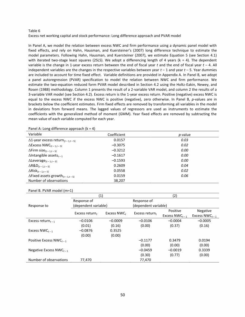
50

Table 6 Excess net working capital and stock performance: Long difference approach and PVAR model In Panel A, we model the relation between excess NWC and firm performance using a dynamic panel model with fixed effects, and rely on Hahn, Hausman, and Kuersteiner’s (2007) long difference technique to estimate the model parameters. Following Hahn, Hausman, and Kuersteiner (2007), we estimate Equation 5 (see Section 4.1) with iterated two-stage least squares (2SLS). We adopt a differencing length of 4 years (k = 4). The dependent variable is the change in 1-year excess return between the end of fiscal year t and the end of fiscal year t – 4. All independent variables are the changes in the respective variables between year t – 1 and year t – 5. Year dummies are included to account for time fixed effect. Variable definitions are provided in Appendix A. In Panel B, we adopt a panel autoregression (PVAR) specification to model the relation between NWC and firm performance. We estimate the two-equation reduced form PVAR model described in Section 4.2 using the Holtz-Eakin, Newey, and Rosen (1988) methodology. Column 1 presents the result of a 2-variable VAR model, and column 2 the results of a 3-variable VAR model (see Section 4.2). Excess return is the 1-year excess return. Positive (negative) excess NWC is equal to the excess NWC if the excess NWC is positive (negative), zero otherwise. In Panel B, p-values are in brackets below the coefficient estimates. Firm fixed effects are removed by transforming all variables in the model in deviations from forward means. The lagged values of regressors are used as instruments to estimate the coefficients with the generalized method of moment (GMM). Year fixed effects are removed by subtracting the mean value of each variable computed for each year. Panel A: Long difference approach (k = 4)

Variable Coefficient p-value

1-year excess return[t – 1,t – 5] 0.0157 0.03

Excess NWC[t – 1,t – 5] –0.3075 0.02

Firm size[t – 1,t – 5] –0.3212 0.00

Intangible assetst – 1 –0.1617 0.00

Leverage[t – 1,t – 5] –0.1593 0.00

R&D[t – 1,t – 5] 0.2609 0.04

Risk[t – 1,t – 5] 0.0558 0.02

Fixed assets growth[t – 1,t – 5] 0.0159 0.06 Number of observations 38,207

Panel B. PVAR model (m=1)

Response to

(1) (2)

Response of (dependent variable)

Response of (dependent variable)

Excess returnt Excess NWCt Excess returnt Positive

Excess NWCt – 1 Negative

Excess NWCt – 1

Excess returnt – 1 –0.0106 (0.01)

–0.0009 (0.16)

–0.0106 (0.00)

–0.0004 (0.37)

–0.0005 (0.16)

Excess NWCt – 1 –0.0876 (0.00)

0.3525 (0.00)

Positive Excess NWCt – 1 –0.1177 (0.00)

0.3479 (0.00)

0.0194 (0.00)

Negative Excess NWCt – 1 –0.0459 (0.30)

–0.0019 (0.77)

0.3339 (0.00)

Number of observations 77,470 77,470

51

Table 7 Long-term abnormal stock returns using long-short portfolios Panel A reports long-term abnormal stock returns for the sample of firms with large NWC decreases over the period 1982-2011. The dependent variable is the monthly equally weighted return for a portfolio of stocks with large decreases in NWC in the past three years (i.e., the long portfolio, whose return is denoted Rp) minus the return on a benchmark portfolio (short portfolio). A firm enters at the end of time t into the long portfolio if it satisfies the following four conditions: (i) NWC/sale of at least 15% in year t–1; (ii) decrease in the dollar value of NWC of at least 10% in year t; (iii) decrease in NWC/Sale of at least 10% in year t; and (iv) positive excess NWC in year t–1. The firm is kept into the long portfolio over 36 months. In columns 1 and 2, the benchmark portfolio is the 1-month Treasury bill (i.e., the risk-free asset). In columns 3 and 4, the benchmark portfolio is constructed using a propensity score matching approach. We model using a probit for the probability of having a large decrease in NWC in a given year. We use as explanatory variable the same set of variables as in the model used to compute the normal level NWC (see legend of Table 2) and industry dummies. We then match the event firms with industry firms with the closest propensity score. Panel B reports long-term abnormal stock returns for a zero-investment equally weighted portfolio, which is long on firms with negative excess NWC and short on firms with positive NWC. The portfolio is rebalanced each year based on the sign of the excess NWC of the previous year. Both in Panel A and Panel B, to estimate the abnormal performance (i.e., alpha), we use the Fama and French (1993) three-factor model and the Cahart (1997) four-factor model. Rf is the 1-month T-bill return, Rm is the CRSP value-weighted market index return, SMB is the return on a portfolio of small stocks minus the return on a portfolio of large stocks, HML is the return on a portfolio of stocks with high book-to-market ratios minus the return on a portfolio of stocks with low book-to-market ratios, and UMD is the return on high momentum stocks minus the return on low momentum stocks. We use standard errors robust to heteroskedasticity. N denotes the number of observations. Panel A. Large decrease in NWC and portfolio return

Rp – Rf Rp – Benchmark return

(1) (2) (3) (4)


Alpha 0.004 0.03 0.006 0.00 0.002 0.10 0.002 0.04 Rm – Rf 1.070 0.00 1.014 0.00 0.002 0.91 –0.009 0.58 SMB 1.069 0.00 1.081 0.00 0.178 0.00 0.181 0.00 HML 0.004 0.96 –0.066 0.45 0.006 0.86 –0.008 0.82 UMD –0.228 0.00 –0.046 0.04 Adj. R-square 0.818 0.834 0.110 0.124 Fisher statistic 417.75 0.00 422.71 0.00 9.06 0.00 8.03 0.00 N 324 324 324 324

Panel B. Zero-investment portfolio: long in negative excess NWC firms and short in positive excess NWC firms

(1) (2)

Coef. p-value Coef. p-value

Alpha 0.001 0.00 0.001 0.00 Rm – Rf 0.013 0.25 0.014 0.22 SMB –0.081 0.00 –0.081 0.00 HML 0.021 0.24 0.021 0.22 UMD 0.001 0.92 Adj. R-square 0.101 0.098 Fisher statistic 10.39 0.00 7.76 0.00 N 348 348

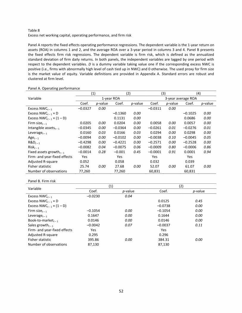
52

Table 8 Excess net working capital, operating performance, and firm risk Panel A reports the fixed effects operating performance regressions. The dependent variable is the 1-year return on assets (ROA) in columns 1 and 2, and the average ROA over a 3-year period in columns 3 and 4. Panel B presents the fixed effects firm risk regressions. The dependent variable is firm risk, which is defined as the annualized standard deviation of firm daily returns. In both panels, the independent variables are lagged by one period with respect to the dependent variables. D is a dummy variable taking value one if the corresponding excess NWC is positive (i.e., firms with abnormally high level of cash tied up in NWC) and 0 otherwise. The used proxy for firm size is the market value of equity. Variable definitions are provided in Appendix A. Standard errors are robust and clustered at firm level. Panel A. Operating performance

Variable

(1) (2) (3) (4)

1-year ROA 3-year average ROA


Excess NWCt – 1 –0.0327 0.00 –0.0311 0.00 Excess NWCt – 1 × D –0.1360 0.00 –0.1025 0.00 Excess NWCt – 1 × (1 – D) 0.1131 0.00 0.0686 0.00 Firm sizet – 1 0.0205 0.00 0.0204 0.00 0.0058 0.00 0.0057 0.00 Intangible assetst – 1 –0.0345 0.00 –0.0364 0.00 –0.0261 0.01 –0.0276 0.01 Leveraget – 1 0.0160 0.03 0.0166 0.03 0.0294 0.00 0.0298 0.00 Aget – 1 –0.0094 0.00 –0.0102 0.00 –0.0038 0.10 –0.0045 0.05 R&Dt – 1 –0.4298 0.00 –0.4221 0.00 –0.2571 0.00 –0.2528 0.00 Riskt – 1 –0.0082 0.04 –0.0075 0.06 –0.0009 0.80 –0.0006 0.86 Fixed assets growtht – 1 –0.0014 0.28 –0.001 0.45 –0.0001 0.91 0.0001 0.94 Firm- and year-fixed effects Yes Yes Yes Yes Adjusted R-square 0.052 0.058 0.032 0.039 Fisher statistic 25.74 0.00 27.68 0.00 52.07 0.00 61.07 0.00 Number of observations 77,260 77,260 60,831 60,831

Panel B. Firm risk

Variable (1) (2)


Excess NWCt – 1 –0.0230 0.04 Excess NWCt – 1 × D 0.0125 0.45 Excess NWCt – 1 × (1 – D) –0.0738 0.00 Firm sizet – 1 –0.1054 0.00 –0.1054 0.00 Leveraget – 1 0.1647 0.00 0.1644 0.00 Book-to-markett – 1 0.0146 0.00 0.0146 0.00 Sales growtht – 1 –0.0042 0.07 –0.0037 0.11 Firm- and year-fixed effects Yes Yes Adjusted R-square 0.295 0.296 Fisher statistic 395.86 0.00 384.31 0.00 Number of observations 87,130 87,130

53

Table 9 The effect of working capital management around the financial crisis This table presents estimates from fixed effects regressions explaining firm performance and investment for years between 2004 and 2009. In Panel A, the dependent variable is the 1-year excess return, and in Panel B, the change in investment. We define investment as the sum of capital expenditures (CAPEX) and cash acquisition, scaled by total assets at the beginning of the period. Crisis is an indicator variable which identifies the financial crisis. It is equal to one for fiscal years 2007, 2008 and 2009. D is a dummy variable taking value one if the corresponding excess NWC is positive (i.e., firms with abnormally high level of cash tied up in NWC) and 0 otherwise. Variable definitions are provided in Appendix A. Control variables in Panel A (Panel B) are the same as in Table 4 (Table 5). Standard errors are robust and clustered at firm level. refers to the coefficient estimate of the corresponding variable. Panel A. Stock performance

Variable (1) (2)


Excess NWCt – 1 × D, –0.2738 0.02 –0.2277 0.04

Excess NWCt – 1 × (1 – D), 0.4367 0.00 0.3801 0.00

Excess NWCt – 1 × D × Crisis, 0.4918 0.00 0.3539 0.00

Excess NWCt – 1 × (1 – D) × Crisis, –0.3295 0.03 –0.2598 0.06 Crisis –0.2702 0.00 –0.2400 0.00 Control variables No Yes Firm-fixed effects Yes Yes Adjusted R-square 0.040 0.286 Fisher statistic 120.33 0.00 245.68 0.00 Number of observations 19,383 18,697

0.2180 0.13 0.1262 0.30

0.1072 0.53 0.1203 0.43

Panel B. Corporate investment

Variable (1) (2)


Excess NWCt – 1 × D, –0.1588 0.00 –0.1442 0.00

Excess NWCt – 1 × (1 – D), –0.0806 0.02 0.0022 0.95

Excess NWCt – 1 × D × Crisis, 0.0691 0.01 0.0895 0.00

Excess NWCt – 1 × (1 – D) × Crisis, –0.0481 0.16 –0.0279 0.46 Crisis –0.0303 0.00 –0.0078 0.02 Control variables No Yes Firm-fixed effects Yes Yes Adjusted R-square 0.010 0.138 Fisher statistic 40.97 0.00 70.41 0.00 Number of observations 18,643 17,467

–0.0897 0.01 –0.0547 0.13

–0.1287 0.00 –0.0257 0.54

54

Table 10 Excess net working capital, firm performance, and investment: Additional checks This table replicates column 2 of Table 4 and column 1 of Table 5 using standardized excess NWC as variable of interest instead of excess NWC. Stand. Excess NWC corresponds to excess NWC divided by its standard error. D is a dummy variable taking value one if the corresponding excess NWC is positive (i.e., firms with abnormally high level of cash tied up in NWC), and 0 otherwise. Control variables are the same as in Tables 4 and 5. In Panel B, we include cash reserves as an additional control variable. Variable definitions are provided in Appendix A. Standard errors are robust and clustered at firm level. Panel A. Approach robust to errors-in-variable

Variable

(1) (2) (3) (4)

1-year excess return Change in investment


Stand. Excess NWCt – 1 –0.008 0.06 –0.007 0.00 Stand. Excess NWCt – 1 × D –0.016 0.02 –0.012 0.00 Stand. Excess NWCt – 1 × (1 – D) 0.003 0.74 –0.001 0.68 Control variables Yes Yes Yes Yes Firm- and year-fixed effects Yes Yes Yes Yes Adjusted R-square 0.145 0.145 0.085 0.085 Fisher statistic 190.02 0.00 185.02 0.00 70.17 0.00 68.38 0.00 Number of observations 77,007 77,007 76,205 76,205

Panel B. Controlling for cash reserves

Variable

(1) (2) (3) (4)

1-year excess return Change in investment


Stand. Excess NWCt – 1 –0.008 0.06 –0.005 0.00 Stand. Excess NWCt – 1 × D –0.016 0.02 –0.011 0.00 Stand. Excess NWCt – 1 × (1 – D) 0.003 0.75 0.004 0.10 Cash reserves –0.006 0.86 –0.003 0.92 0.149 0.0 0.151 0.00 Control variables Yes Yes Yes Yes Firm- and year-fixed effects Yes Yes Yes Yes Adjusted R-square 0.145 0.145 0.094 0.094 Fisher statistic 184.99 0.00 180.19 0.00 74.95 0.00 73.16 0.00 Number of observations 77,001 77,001 76,199 76,199

is working capital management value-enhancing? evidence ... annual meetings/2014-… · is working...

Documents