Is the Potential for International Diversi�cation

Disappearing?�

Peter Christo¤ersen Vihang Errunza Kris Jacobs Hugues Langlois

University of Toronto McGill University University of Houston McGill University

November 18, 2011

Abstract

Quantifying the evolution of security co-movements is critical for asset pricing and portfolio

allocation, hence we investigate patterns and trends in correlations and tail dependence for

developed markets (DMs) and emerging markets (EMs). We use the standard DCC and DECO

correlation models, and we also develop a nonstationary DECO model as well as a novel

dynamic skewed t-copula to allow for dynamic and asymmetric tail dependence. We show

that it is possible to characterize co-movements for many countries simultaneously. We �nd

that correlations have signi�cantly trended upward for both DMs and EMs, but correlations

between EMs are much lower than between DMs. Tail dependence has also increased but its

level is still very low for EMs as compared to DMs. Thus, while the correlation patterns suggest

that the diversi�cation potential of DMs has reduced drastically over time, our �ndings suggest

that EMs o¤er signi�cant diversi�cation bene�ts, especially during large market moves.

JEL Classi�cation: G12

Keywords: Asset allocation, dynamic correlation, dynamic copula, asymmetric dependence.

�Christo¤ersen, Errunza, and Jacobs gratefully acknowledge �nancial support from IFM2 and SSHRC. Errunzais also supported by the Bank of Montreal Chair at McGill University. Hugues Langlois is funded by NSERC andCIREQ. We are grateful to the Editor, Geert Bekaert as well as two anonymous referees for comments on an earlierversion of the paper. We also thank Lieven Baele, Greg Bauer, Phelim Boyle, Ines Chaieb, Rob Engle, Frank deJong, Rene Garcia, Sergei Sarkissian, Ernst Schaumburg, and seminar participants at the Bank of Canada, EDHEC,HEC Montreal, NYU Stern, SUNY Bu¤alo, Tilburg University, and WLU for helpful comments.

1

1 Introduction

Understanding and quantifying the evolution of security co-movements is critical for asset pricing

and portfolio allocation. The traditional case for international diversi�cation bene�ts has relied

largely on the existence of low cross-country correlations. Initially, the literature studied developed

markets, but over the last two decades much of the focus has shifted to the diversi�cation ben-

e�ts o¤ered by emerging markets.1 Two critical questions, with important implications for asset

allocation and international diversi�cation, are of special interest for academics and practitioners

alike.

First, how have cross-country correlations changed through time? It is far from straightforward

to address this ostensibly simple question without making additional assumptions. Computing

rolling correlations is subject to well-known drawbacks. Multivariate GARCH models, as for exam-

ple in Longin and Solnik (1995), seem to provide a solution, but the implementation of these models

using large numbers of countries is subject to well known dimensionality problems, as discussed by

Solnik and Roulet (2000). As a result, most of the available evidence on the time-variation in cross-

country correlations is based on factor models.2 In a recent paper, Bekaert, Hodrick, and Zhang

(2009) convincingly argue that the evidence from this literature is mixed at best and state that (see

p. 2591): �It is fair to say that there is no de�nitive evidence that cross-country correlations are

signi�cantly and permanently higher now than they were, say, 10 years ago.�Bekaert, Hodrick, and

Zhang (2009) proceed to investigate international stock return co-movements for 23 DMs during

1980-2005, and �nd an upward trend in return correlations only among the subsample of European

stock markets, but not for North American and East Asian markets.

The second question is whether correlation is a satisfactory measure of dependence in interna-

tional markets, or if we need to consider di¤erent measures, notably those that focus on the de-

pendence between tail events? This question is related to the analysis of correlation asymmetries,

and changes in correlation as a function of business cycle conditions or stock market performance.

Following the seminal paper by Longin and Solnik (2001) and the corroborating evidence of Ang

1For early studies documenting the bene�ts of international diversi�cation, see Solnik (1974) for developed marketsand Errunza (1977) for emerging markets. For more recent evidence, see for example Erb, Harvey and Viskanta(1994), DeSantis and Gerard (1997), Errunza, Hogan and Hung (1999), and Bekaert and Harvey (2000).

2King, Sentana, and Wadhwani (1994) do not �nd evidence of increasing cross-country correlations for 16 devel-oped markets during the period 1970-1988, except around the market crash of 1987. Carrieri, Errunza, and Hogan(2007) do not �nd a common pattern in the correlation trend for eight emerging markets (EMs) during 1977-2000. Eil-ing and Gerard (2007) �nd an upward time trend in co-movements between 24 developed markets but not between26 emerging markets over the period 1973-2005. Goetzmann, Li, and Rouwenhorst (2005) document substantialchanges in the correlation structure of world equity markets over the past 150 years. Baele and Inghelbrecht (2009)report increasing correlations over the period 1973-2007 for their sample of 21 DMs. See also Karolyi and Stulz(1996), Forbes and Rigobon (2002), Brooks and Del Negro (2003), Lewis (2006), and Rangel (2011).

2

and Bekaert (2002) and Ang and Chen (2002), the hypothesis that cross-market correlations rise

in periods of high volatility has been supplanted by the notion that correlations increase in down

markets, but not in up markets.3 Longin and Solnik (2001) use extreme value theory in bivariate

monthly models for the U.S. with either the U.K., France, Germany, or Japan during 1959-1996.

Ang and Bekaert (2002) develop a regime switching dynamic asset allocation model, and estimate

it for the U.S., U.K., and German system over the period 1970-1997. Both papers estimate return

extremes at predetermined threshold values, i.e. they de�ne the tail observations ex ante, and then

compute unconditional correlations for the tail for a small sample of developed markets.4

This paper substantially contributes to our understanding of both these important questions.

Regarding the patterns and trends in correlations over time, we argue that recent advances make

it feasible to overcome dimensionality and optimization problems in international �nance applica-

tions. We characterize time-varying correlations using weekly returns during the 1973-2009 period

for a large number of countries (either thirteen or seventeen EMs, sixteen DMs, as well as combi-

nations of the EM and DM samples), without relying on a factor model. We implement models

that overcome the dimensionality problems, and that are easy to estimate. To do so, we rely on

the variance targeting idea in Engle and Mezrich (1996) and the numerically e¢ cient composite

likelihood procedure proposed by Engle, Shephard and Sheppard (2008). The composite likelihood

estimation procedure is essential for estimating dynamic correlation models on large sets of weekly

international equity data such as ours. We use the �exible dynamic conditional correlation (DCC)

model of Engle (2002) and Tse and Tsui (2002), as well as the dynamic equicorrelation (DECO)

model of Engle and Kelly (2009) that can be estimated on large sets of assets using conventional

maximum likelihood estimation. We thus demonstrate that it is possible to estimate correlation

patterns in international markets using large numbers of countries and extensive time series, without

relying on a factor model that may bias inference. Our implementation is relatively straightforward

and computationally fast, which allows us to report results using several estimation approaches,

while assessing the robustness of our �ndings.

Regarding the second question, the DECO and DCC correlation models with normal innovations

do not generate the levels of tail dependence required by the data, nor do they generate asymmetries

in correlations. Hence, we introduce copula approaches to capture nonlinear dependence across

markets. We �t the tails of the marginal distributions using the Generalized Pareto distribution

(GP), and the joint distribution is modeled using time-varying copulas. We develop a novel skewed

3On tail dependence, see also Poon, Rockinger, and Tawn (2004). On the related topic of contagion, see forexample Forbes and Rigobon (2002), Bekaert, Harvey, and Ng (2005), and Bae, Karolyi, and Stulz (2003).

4A related literature explores the relationship between industrial structure and the dynamics of equity marketreturns and cross-country correlations. See for instance Roll (1992), Heston and Rouwenhorst (1994), Gri¢ n andKarolyi (1998), Dumas, Harvey and Ruiz (2003), and Carrieri, Errunza and Sarkissian (2007).

3

dynamic t copula which allows for asymmetric and dynamic tail dependence in large portfolios.

Our results based on DCC and DECO models are extremely robust and suggest that correlations

have been signi�cantly trending upward for both DMs and EMs. However, the correlation between

DMs has been higher than the correlation between EMs at all times in our sample. For developed

markets, the average correlation with other developed markets is higher than the average correlation

with emerging markets. For emerging markets, the correlation with developed markets is generally

somewhat higher than the correlation with the other emerging markets, but the di¤erences are

small. When dividing our sample into four regions: EU and developed non-EU, Latin America, and

Emerging Eurasia, we �nd that the correlation between all four regions have gone up, and so has

the average correlation within each region. While the range of correlations for DMs has narrowed

around the increasing trend in correlation levels, this is not the case for EMs. Emerging markets

thus still o¤er substantial correlation-based diversi�cation bene�ts to investors.

Our robust �nding of an upward trend in correlations is all the more remarkable because the

parametric models we use enforce mean-reversion in volatilities and correlation, and we estimate the

models using long samples of weekly returns. The data clearly pull the models away from the average

correlation in the samples we investigate. In order to explicitly address the issue of nonstationarity

in correlations, we develop a new two-component correlation model which includes a nonstationary

long-run correlation component. We refer to this model as Spline DECO. Its estimates con�rm the

upward trends in correlation across DMs and EMs.

We �nd overwhelming evidence that the assumption of multivariate normality is inappropriate.

Results from the dynamic t copula indicate substantial tail dependence. Moreover, tail dependence

as measured by the skewed t copula is asymmetric and increasing through time for both EMs

and DMs. We demonstrate that the skewed t copula can capture the empirical asymmetries in

threshold correlations. However, the most striking �nding is that the level of the tail dependence

is still very low at the end of the sample period for EMs as compared to DMs. Our �ndings on tail

dependence thus suggest that EMs have o¤ered diversi�cation bene�ts during large market moves.

The underlying intuition for this �nding is that while �nancial crises in EMs are frequent, many of

them are country-speci�c. Thus, although the bene�ts of international diversi�cation might have

lessened both for DMs and EMs, a strong case can still be made for EMs, and the diversi�cation

bene�ts from adding emerging markets to a portfolio appear to be signi�cant.

We contribute to the literature in several ways. At the methodological level, we demonstrate

that it is possible to model correlation dynamics and tail dependence in international equity markets

using large samples, without relying on factor models. We build a new correlation model with a

nonstationary low-frequency component, as well as a new fully-speci�ed dynamic model that can

capture nonlinear and asymmetric dependence in a large number of equity markets.

4

From an empirical perspective, we document several important stylized facts. First, we demon-

strate that measures of international dependence have increased signi�cantly over the course of our

sample. This is of course a purely descriptive statement, and does not imply that correlations will

remain high. Second, we document the inadequacy of the multivariate normality assumption for

modeling international equity returns, and we provide a genuinely multivariate characterization of

asymmetries in international equity markets. We also document asymmetric threshold correlation

patterns for EMs, and �nd that they di¤er from those for DMs. Longin and Solnik (2001) document

asymmetric threshold correlation patterns for the United States vis-a-vis other DMs, but to the best

of our knowledge the literature does not contain evidence on EMs. We demonstrate that our multi-

variate asymmetric model can capture the threshold correlation patterns observed in DMs and EMs.

Third, we extend existing results on dependence to a more recent period characterized by signi�cant

liberalizations for the EM sample, as well as substantial market turmoil during 2007-2009, which

helps identify tail dependence. These results also allow us to elaborate on existing �ndings and

further investigate if correlations for EMs are impacted by measures of market openness. Fourth,

we use our estimates to compute a measure of conditional diversi�cation bene�ts, and we �nd that

diversi�cation bene�ts decreased over our sample period. Fifth, we investigate the relationships

between correlations and volatilities. Our model does not assume a factor structure but we do �nd

a signi�cant positive association between correlations and volatilities.

The paper proceeds as follows. Section 2 provides a brief outline of DCC and DECO correlation

models, with special emphasis on the estimation of large systems. Section 3 presents the data,

as well as empirical results on time variation in linear correlations. Sections 4 and 5 build and

estimate a new set of copula models with dynamic tail dependence, asymmetry and dynamic copula

correlations. Section 6 investigates the linear correlations further, computes threshold correlations

and develops the new two-component correlation model that includes a nonstationary long-run

component. Section 7 concludes.

2 Dynamic Linear Dependence Models for Many Equity

Markets

This section outlines the various models we use to capture dynamic dependence across equity

markets. We describe how the dynamic conditional correlation model of Engle (2002) and Tse and

Tsui (2002) can be implemented simultaneously on many assets.

5

2.1 The Dynamic Conditional Correlation Approach

In the existing literature, the scalar BEKK model has been the standard econometric approach for

capturing dynamic dependence.5 Implementations of multivariate GARCH models have tradition-

ally used a limited number of countries because of dimensionality problems.6 Further, the de�ning

characteristic of the scalar BEKK model is that the parameters are identical across all conditional

variance and covariance dynamics. This common persistence across all variances and covariances

is clearly restrictive. Cappiello, Engle and Sheppard (2006) have found that the persistence in

correlation di¤ers from that in variance when looking at international stock and bond markets.7

Equally important is the restriction that the functional form of the variance dynamic is required

to be identical to the form of the covariance dynamic. This rules out for example asset-speci�c

leverage e¤ects in volatility, which has been found to be an important stylized fact in equity index

returns (see for example Black, 1976, and Engle and Ng, 1993). The leverage e¤ect is an asymmetric

volatility response that captures the fact that a large negative shock to an equity market increases

the equity market volatility by much more than a positive shock of the same magnitude.

Hence, we implement the �exible dynamic conditional correlation (DCC) model of Engle (2002)

and Tse and Tsui (2002).8 Allowing for a leverage e¤ect in conditional variance, we assume that

the return on asset i at time t follows an Engle-Ng (1993) dynamic

Ri;t = �i;t + "i;t = �i;t + �i;tzi;t (2.1)

�2i;t = !i + �i ("i;t�1 � �i�i;t�1)2 + �i�2i;t�1: (2.2)

Because the covariance is just the product of correlations and standard deviations, we can write

�t = Dt�tDt (2.3)

where Dt has the standard deviations �i;t on the diagonal and zeros elsewhere, and where �t has

ones on the diagonal and conditional correlations o¤ the diagonal.

We implement the modi�ed DCC model discussed in Aielli (2009), in which the correlation

5The BEKK model is most often used to estimate factor models with a GARCH structure. See for instanceDeSantis and Gerard (1997, 1998), and Carrieri, Errunza, and Hogan (2007) for examples. See Ramchand andSusmel (1998), Baele (2005), and Baele and Inghlebrecht (2009) for more general multivariate GARCH models withregime switching.

6See for instance Solnik and Roulet (2000), Longin and Solnik (1995) and Karolyi (1995) for early examples ofbivariate models.

7See Kroner and Ng (1998) and Solnik and Roulet (2000) for a more elaborate discussion of the restrictionsimposed in the �rst generation of multivariate GARCH models.

8Our main �nding of an upward trend in correlation in our samples is con�rmed when using the BEKK approach.Results for the BEKK model are available upon request.

6

dynamics are driven by the cross-products of the return shocks

~�t = � + ��~�t�1 + ��~zt�1~z>t�1 (2.4)

where ~zi;t = zi;tq~�ii;t. These cross-products are used to de�ne the conditional correlations via the

normalization

�DCCij;t = ~�ij;t=

q~�ii;t~�jj;t: (2.5)

This normalization ensures that all correlations remain in the �1 to 1 interval.If N denotes the number of equity markets under study then the DCC model has N(N�1)=2+2

parameters to be estimated. Below we will study up to 17 emerging markets and 16 mature

markets, thus N = 33 and so the DCC model will have 530 parameters. It is well recognized

in the literature that it is impossible to estimate these parameters reliably due to the need to use

numerical optimization techniques, see for instance Solnik and Roulet (2000) for a discussion. In

order to operationalize estimation, we follow DeSantis and Gerard (1997) who rely on the targeting

idea in Engle and Mezrich (1996).

Taking expectations on both sides of (2.4) and solving for the unconditional correlation matrix~� of the vector ~zt, yields

~� = �= (1� �� �) : (2.6)

Note that this relationship enables us to rewrite the DCC model in a more intuitive form

~�t = (1� �� � ��) ~� + ��~�t�1 + ��~zt�1~z>t�1 (2.7)

which shows that the conditional correlation in DCC is a weighted average of the long-run correla-

tion, yesterday�s conditional correlation, and yesterday�s innovation cross-product.

Now, if we use the sample correlation matrix, �̂ = 1T

PTt=1 ~zt~z

>t as an estimate of the uncon-

ditional correlation matrix, ~�, then the numerical optimizer only has to search in two dimensions,

namely over �� and ��, rather than in the original 530 dimensions. Note that this implementation

also ensures that the estimated DCC model yields a positive semi-de�nite correlation matrix, be-

cause ~zt~z>t and thus �̂ is positive semi-de�nite by construction. Appendix A contains more details

on the implementation of correlation targeting in the DCC model.

The standard DCC model is symmetric in the sense that a negative pair of asset return shocks

impact correlation in the same way as do a positive pair of return shocks of the same magnitude. One

may reasonably wonder if such symmetry is empirically valid. We therefore consider the asymmetric

7

DCC model in Cappiello, Engle and Sheppard (2006) in which

~�t = (1� �� � ��)~� + ��~�t�1 + ��~zt�1~z>t�1 + ���~�t�1~�

>t�1 � E

h~�t�1~�

>t�1

i�where ~�t�1 = ~zt�1I(~zt�1 < 0). In our application the empirical support for the correlation asym-

metry parameter, ��, turned out to be weak and so we only report results for the symmetric DCC

model below.

Even when using correlation targeting, estimation is cumbersome in large-dimensional problems

due to the need to invert the N by N correlation matrix, �t, on every day in the sample for every

likelihood evaluation. The likelihood in turn must be evaluated many times in the numerical opti-

mization routine. More importantly, Engle, Shephard, and Sheppard (2008) �nd that in large-scale

estimation problems, the parameters � and � which drive the correlation dynamics are estimated

with bias when using conventional estimation techniques. They propose an ingenious solution based

on the composite likelihood de�ned as

CL(�; �) =TXt=1

NXi=1

Xj>i

ln f(��; ��; zit; zjt) (2.8)

where f(��; ��; zit; zjt) denotes the bivariate normal distribution of asset pair i and j, and where

correlation targeting is imposed.

The composite log-likelihood is thus based on summing the log-likelihoods of pairs of assets. Each

pair yields a valid (but ine¢ cient) likelihood for � and �, but summing over all pairs produces an

estimator which is relatively e¢ cient, numerically fast, and free of bias even in large-scale problems.

We use the composite log-likelihood in all our estimations below. We have found it to be very

reliable and robust, e¤ectively turning a numerically impossible task into a manageable one. The

composite likelihood procedure allows us to estimate dynamic correlations in larger systems of

international equity data using longer time series of returns than previously done in the literature.

This is important because long time series on large sets of countries are needed for the identi�cation

of variance and covariance dynamics.

2.2 The Dynamic EquiCorrelation Approach

The dynamic equicorrelation (DECO) model in Engle and Kelly (2009) can be viewed as a special

case of the DCC model in which the correlations are equal across all pairs of countries but where

this common so-called equicorrelation is changing over time. The resulting dynamic correlation can

be thought of as an average dynamic correlation between the countries included in the analysis.

8

Following Engle and Kelly (2009), we parameterize the dynamic equicorrelation matrix as

�DECOt = (1� �t)IN + �tJN�N

where �t is a scalar, IN denotes the n-dimensional identity matrix and JN�N is an N � N matrix

of ones.

The scalar dynamic equicorrelation, �t, is obtained by taking the cross-sectional average each

period of the DCC conditional correlation matrix in (2.5)

�t =1

N(N � 1)�J1�N�

DCCt JN�1 �N

�: (2.9)

Note that subtracting N eliminates the trivial term arising from the ones on the diagonal of �DCCt .

The determinant of the DECO correlation matrix is simply

���DECOt

�� = (1� �t)N�1 (1 + (N � 1) �t)and from this we can derive the inverse correlation matrix as

��DECOt

��1=

1

(1� �t)

�IN �

�t1 + (N � 1)�t

JN�N

�:

The simple structure of the inverse correlation matrix ensures that the model can be estimated on

large sets of assets using conventional maximum likelihood estimation. The dynamic correlation

parameters �� and �� embedded in �t will not be estimated with bias even when N is large.

2.3 Measuring Conditional Diversi�cation Bene�ts

If correlations are changing over time, then the bene�ts of portfolio diversi�cation will be changing

as well. We therefore need to develop a dynamic measure of diversi�cation bene�ts.9 First, let us

de�ne portfolio volatility �PF;t generically as

�PF;t �qw>t �twt =

qw>t Dt�tDtwt

where wt is the vector of portfolio weights at time t and Dt is the diagonal matrix of volatilities as

in (2.3).

Consider then the extreme case of a portfolio without any diversi�cation bene�ts, that is, the

9Our dynamic measure is related to the static measure in Choueifaty and Coignard (2008).

9

correlation matrix �t is a matrix of ones. The portfolio volatility at time t can be expressed in this

case as

��PF;t =qw>t DtJN�NDtwt = w

>t �t

where �t denotes the vector of individual asset volatilities at time t.

The opposite extreme would correspond to each pair of assets having a correlation of �1 inwhich case it is possible to �nd a long-only portfolio such that the portfolio volatility �PF;t is zero.

Using these upper and lower bounds on portfolio volatility, we de�ne the conditional diversi�-

cation bene�t as

CDBt =��PF;t � �PF;t

��PF;t= 1�

pw>t �twtw>t �t

: (2.10)

This measure describes the level of diversi�cation bene�ts in a concise manner. It is increasing as

the correlations decrease, and it is normalized to lie between zero and one: The portfolio volatility

in the numerator has a lower bound of zero and the denominator is always positive in a long-only

portfolio.

When computing CDBt one must �rst decide on the portfolio weights, w. One approach is to

construct the minimum variance portfolio each week and compute the CDBt value corresponding

to this portfolio. Alternatively, we could choose the weights that maximize CDBt.10 We follow the

second approach. We further impose that the weights sum to one and we rule out short-selling.

In order to assess how much of the conditional diversi�cation bene�t stems from active asset

allocation, we also construct a CDBEWt measure for an equal-weighted portfolio. In this case

CDBEWt = 1�pw>t �twtw>t �t

= 1�pJ1�N�tJN�1J1�N�t

. (2.11)

By de�nition CDBEWt will be less than or equal to the optimal CDBt at any point in time. The

di¤erence between the CDBt and CDBEWt measures will tell us about the extent to which changing

volatilities and correlations can potentially be exploited via dynamic asset allocation and about the

optimality (or lack thereof) of an equal-weighted portfolio over time.11

3 Empirical Correlation Analysis

This section contains our empirical �ndings on correlation patterns. We �rst describe the di¤erent

data sets that we use and brie�y discuss the univariate results. We then analyze the time-variation

10The two approaches will coincide only when the volatilities are identical across assets.11DeMiguel, Garlappi and Uppal (2009) and Tu and Zhou (2011) analyze the relative performance of equal-weighted

versus optimally-weighted portfolios in an unconditional setting.

10

in linear correlations. Subsequently we measure the dispersion in correlations across pairs of assets

at each point in time and check if this dispersion has changed over time.

3.1 Data and Univariate Models

We employ the following three data sets:

First, from DataStream we collect weekly closing U.S. dollar returns for the following 16 de-

veloped markets: Australia, Austria, Belgium, Canada, Denmark, France, Germany, Hong Kong,

Ireland, Italy, Japan, Netherlands, Singapore, Switzerland, U.K., and U.S. This data set contains

1,901 weekly observations from January 12, 1973 through June 12, 2009.

Second, from Standard and Poor�s we collect the IFCG weekly closing U.S. dollar returns for

the following 13 emerging markets: Argentina, Brazil, Chile, Colombia, India, Jordan, Korea,

Malaysia, Mexico, Philippines, Taiwan, Thailand, and Turkey. This data set contains 1,021 weekly

observations from January 6, 1989 through July 25, 2008.

Third, from Standard and Poor�s we collect the weekly closing investable IFCI U.S. dollar returns

for the following 17 emerging markets: Argentina, Brazil, Chile, China, Hungary, India, Indonesia,

Korea, Malaysia, Mexico, Peru, Philippines, Poland, South Africa, Taiwan, Thailand, and Turkey.

This data set contains 728 weekly returns from July 7, 1995 through June 12, 2009.

We use two emerging markets data sets because they have their distinct advantages. The

IFCG data set spans a longer time period, and represents a broad measure of emerging market

returns, but is not available after July 25, 2008. The IFCI data set tracks returns on a portfolio of

emerging market securities that are legally and practically available to foreign investors. The index

construction takes into account portfolio �ow restrictions, liquidity, size and �oat. It continues to

be updated but the sample period is shorter, which is a disadvantage in model estimation and of

course in assessing long-term trends in correlation.

Table 1 contains descriptive statistics on the 1989-2008 data set. While the cross-country vari-

ations are large, Table 1 shows that the average annualized return in the developed markets was

12.06%, versus 17.68% in the emerging markets. This emerging market premium is re�ective of

an annual standard deviation of 33.63% versus only 18.41% in developed markets. Kurtosis is on

average higher in emerging markets, indicating more tail risk. But skewness is slightly positive in

emerging markets and slightly negative in mature markets, suggesting that emerging markets are

not more risky from this perspective. The �rst-order autocorrelations are small for most countries.

The Ljung-Box (LB) test that the �rst 20 weekly autocorrelations are zero is not rejected in most

developed markets but it is rejected in most emerging markets. We will use an autoregressive model

of order two, AR(2), for each market to pick up this return dependence. The Ljung-Box test that

11

the �rst 20 autocorrelations in absolute returns are zero is strongly rejected for all 29 markets. In

the DECO and DCC models, we will employ a GARCH(1,1) model for each market to pick up

this second-moment dependence. We use the NGARCH model of Engle and Ng (1993) found in

equation (2.2) to account for asymmetries.

Table 2 reports the results from the estimation of the AR(2)-NGARCH(1,1) models on each

market for the 1989-2008 data set. The results are fairly standard. The volatility updating parame-

ter, �, is around 0.1, and the autoregressive variance parameter, �, is around 0.8. The parameter

� governs the volatility asymmetry and is also known as the leverage e¤ect. It is commonly found

to be large and positive in developed markets and we �nd that here as well. Austria is the only

outlier in this regard. Interestingly, the average leverage e¤ect is much closer to zero in the emerg-

ing markets. The slightly negative average is driven largely by the unusual estimate of -3.38 for

Jordan. The model-implied variance persistence is high for all countries, as is commonly found in

the literature.

The Ljung-Box (LB) test on the model residuals show that the AR(2) models are able to pick up

the weak evidence of return predictability found in Table 1. Impressively, the GARCH models are

also able to pick up the strong persistence in absolute returns found in Table 1. Note also that the

GARCH model picks up much of the excess kurtosis found in Table 1. The remaining nonnormality

will be addressed using copula modeling below.

We conclude from Tables 1 and 2 that the AR(2)-NGARCH(1,1) models are successful in de-

livering the white-noise residuals that are required to obtain unbiased estimates of the dynamic

correlations. We will therefore use the AR(2)-NGARCH(1,1) model in the DECO and DCC appli-

cations.

3.2 Correlation Patterns Over Time

Table 3 reports the parameter estimates and log likelihood values for the DECO and DCC correla-

tion models. We report results for the three data sets introduced above. For each set of countries

we estimate two versions of each model: one version allowing for correlation dynamics and another

where the correlation dynamics are shut down, and thus �� = �� = 0. A conventional likelihood ra-

tio test would suggest that the restricted model is rejected for all sets of countries, but unfortunately

the standard chi-squared asymptotics are not available for composite likelihoods.

The correlation persistence (�� + ��) is close to one in all models, implying very slow mean-

reversion in correlations. In the DECO model, persistence is estimated to be essentially one, re-

�ecting the upward trend in correlations which we now discuss.

We present time series of dynamic equicorrelations (DECOs) for several samples. The left panels

12

in Figure 1 present results for twenty-nine developed and emerging markets for the sample period

January 20, 1989 to July 25, 2008. As explained in Section 3.1, sixteen of these markets are

developed and thirteen are emerging markets. We also present DECOs for each group of countries

separately. We refer to this sample as the 1989-2008 sample.

The right panels in Figure 1 present results for thirty-three developed and emerging markets

for the sample period July 21, 1995 to June 12, 2009. This sample contains the same sixteen

developed markets, and seventeen emerging markets. There is considerable overlap between this

sample of emerging markets and the one used in the left panels of Figure 1. Section 3.1 discusses

the di¤erences. We refer to this sample as the 1995-2009 sample.

The top left-hand panel in Figure 2 contains the time series of DECOs for the group of sixteen

developed markets between January 26, 1973 and June 12, 2009. We refer to this sample as

the 1973-2009 sample. Figure 2 also shows results for the 1989-2008 and the 1995-2009 data for

comparison.

These �gures contain some of the main messages of our paper. The DECOs in Figures 1 and

2, which can usefully be thought of as the average of the pairwise correlations between all pairs of

countries in the sample, �uctuate considerably from year to year, but have been on an upward trend

since the early 1970s. Figure 2 shows that for the sixteen developed markets, the DECO increased

from approximately 0.3 in the mid-1970s to between 0.7 and 0.8 in 2009. Figure 1 indicates that

over the 1989-2009 period, the DECO correlations between emerging markets are lower than those

between developed markets, but that they have also been trending upward, from approximately

0.1-0.2 in the early nineties to over 0.5 in 2009.

Because the DECO model assumes correlation is time-varying with a model-implied long-run

mean, one may wonder whether the choice of sample period strongly a¤ects inference on correlation

estimates at a particular point in time. Figure 2 addresses this issue by reporting DECO estimates

for the sixteen developed markets for three di¤erent sample periods. Whereas there are some

di¤erences, the correlation estimate at a particular point in time is remarkably robust to the sample

period used, and the conclusion that correlations have been trending upward clearly does not depend

on the sample period used. Comparing the left and right panels of Figure 1, it can be seen that a

similar conclusion obtains for the emerging markets, even though this comparison is more tenuous,

as the sample composition and the return data used for the emerging markets are somewhat di¤erent

across panels.

13

3.3 Cross-Sectional Di¤erences in Dependence

The DECO correlations give us a good idea of the evolution of correlation over time in a given

sample of markets. They can usefully be thought of as an average of all possible permutations of

pairwise correlations in the sample. The next question is how much cross-sectional heterogeneity

there is in the correlations. The DCC framework discussed in Section 2.1 is designed to address

this question. It yields a time-varying correlation series for each possible permutation of markets

in the sample.

Reporting on all these time-varying pairwise correlation paths is not feasible, and we have to

aggregate the correlation information in some way. Figures 2-5 provide an overview of the results.

The right-side panels in Figure 2 provide the average across all markets of the DCC paths, and

compare them with the DECO paths. The top-right panel provides the average DCC for the sixteen

developed markets from 1973 through 2009. The middle-right panel provides the average DCC for

the same sixteen markets for the 1989-2008 sample period, and the bottom-right panel for the 1995-

2009 period. The left-side panels provide the DECO correlations. Figure 2 demonstrates that the

DECO can indeed be thought of as an average of the DCCs. Moreover, Figure 2 demonstrates that

the average DCC correlation at each point in time is robust to the sample period used in estimation,

as is the case for the DECO.12

Figure 3 uses the 1989-2008 sample to report, for each of the twenty-nine countries in the

sample, the average of its DCC correlations with all other countries using light grey lines. Figure

3.A contains the 16 developed markets and Figure 3.B contains the 13 emerging markets. While

these paths are averages, they give a good indication of the di¤erences between individual countries,

and they are also informative of the di¤erences between developed and emerging markets. In order

to further study these di¤erences, each �gure also gives the average of the market�s DCC correlations

with all (other) developed markets using black lines and all (other) emerging markets using dark

grey lines. Figure 3.A and 3.B yields some very interesting conclusions. First, the DCC correlation

paths display an upward trend for all 29 countries, except Jordan. Second, for developed markets

the average correlation with other developed markets is higher than the average correlation with

emerging markets at virtually each point in time for virtually all markets. Third, for emerging

markets the correlation with developed markets is generally higher than the correlation with other

emerging markets. However, the di¤erence between the two correlation paths is much smaller than

in the case of developed markets. In several cases the average correlation paths are very similar.

12In Figure 3, and throughout the paper, we report equal-weighted averages of the pairwise correlations from theDCC models. Value-weighted correlations (not reported here) also display an increasing pattern during the last10-15 years. Note that in the benchmark DECO model all pairwise correlations are identical and so the weighting isirrelevant.

14

Note that in Figure 3.A the trend patterns for European countries are also not very di¤erent from

those for other DMs. Notice that, even if their level is still somewhat lower, the correlations

for Japan and the US have increased just as for the European countries during the last decade.

Inspection of the pairwise DCC paths, which are not reported because of space constraints, reveals

that the trend patterns are remarkably consistent for almost all pairs of countries, and there is no

meaningful di¤erence between European countries and other DMs.

Figure 3 reports the average correlation between the DCC of each market and that of other

markets. It could be argued that instead the correlation between each market and the average

return of the other markets ought to be considered. We have computed these correlations as well.

While the correlation with the average return is nearly always higher than the average correlation

from Figure 3, the conclusion that the correlations are trending upwards is not a¤ected. In order

to save space we do not show the plots of the correlation with average returns on other markets.

We can use the correlation paths from the DCC model to assess regional patterns in correlation

dynamics. Figure 4 does exactly this. We divide the 16 DMs into two regions (EU and non-EU)

and we divide the 13 EMs into another two EM regions: Latin American and Emerging Eurasia.13

We report in Figure 4 the average correlation within and across the four regions, based on the

DCC model�s country-speci�c correlation paths. Strikingly, Figure 4 shows that the increasing

correlation patterns are evident within each of the four regions and also across all the six possible

pairs of regions. The highest levels of correlation are found in the upper-left panel which shows

the intra-EU correlations. The lowest level of correlations are found in the bottom-right panel

which shows the intra Emerging Eurasia correlations. Emerging Eurasia in the right-most column

generally has the lowest interregional correlations.

Figures 3 and 4 do not tell the entire story, because we have to resort to reporting correlation

averages due to space constraints. Figure 5 provides additional perspective by providing correlation

dispersions for the developed markets, emerging markets, and all markets respectively. In particular,

at each point in time, the shaded areas in Figure 5 shows the range between the 10th and 90th

percentile based on all pairwise correlations between groups of countries. The top panel considers

the sixteen developed countries. The middle panel in Figure 5 reports the same statistics for the

emerging markets for the 1989-2008 sample and the bottom panel shows all 29 markets together.

While the increasing level of correlations is evident, the range of correlations seems to have narrowed

for developed markets, widened a bit for emerging markets, and the range width seems to have

stayed roughly constant for all markets taken together. The wide range of correlations found within

13The European Union (EU) includes Austria, Belgium, Denmark, France, Germany, Ireland, Italy, Netherlands,and the UK. Developed Non-EU includes Australia, Canada, Hong Kong, Japan, Singapore, Switzerland, and the US.Latin America includes Argentina, Brazil, Chile, Colombia, and Mexico. Emerging Eurasia includes India, Jordan,Korea, Malaysia, Philippines, Taiwan, Thailand, and Turkey.

15

emerging markets again suggests that the potential for diversi�cation bene�ts are greater here.

Figure 6 plots the conditional diversi�cation bene�t measures developed in equations (2.10)

and (2.11) for developed, emerging, and all markets using the dynamic correlations from the DCC

model. The CDB-optimal portfolio is depicted with a black line in Figure 6 and it shows a clearly

decreasing trend in diversi�cation bene�ts in DMs (top panel): Correlations have been rising rapidly

and the bene�ts of diversi�cation have been decreasing during the last ten years. Figure 6 shows

that it is not possible to avoid the declining bene�ts from international diversi�cation via active

asset allocation. Diversi�cation bene�ts have also somewhat decreased in emerging markets (middle

panel) but the level of bene�t is still much higher than in developed markets. When combining

the developed and emerging markets (bottom panel), the diversi�cation bene�ts are declining as

well but the level is again much higher than when considering developed markets alone. Emerging

markets thus still o¤er substantial correlation-based diversi�cation bene�ts to investors.

The grey lines in Figure 6 show the bene�ts from diversi�cation in an equal-weighted portfolio.

In the case of DMs in the top panel it is striking how close the equal-weighted portfolio is to the

CDB-optimal portfolio in terms of diversi�cation bene�ts. In the case of EMs in the middle panel

the di¤erences between the two lines are a bit larger and in the bottom panel of Figure 6 the

di¤erences are the largest. This shows that when EMs are included in a DM portfolio, not only are

the bene�ts of diversi�cation much larger, the scope for active asset allocation is much greater as

well.

4 Dynamic Nonlinear Dependence

We have relied on the multivariate normal distribution to implement the dynamic correlation mod-

els. The multivariate normal distribution is the standard choice in the literature because it is

convenient, and because quasi maximum likelihood results ensure that the dynamic correlation pa-

rameters will be estimated consistently even when the normal distribution assumption is incorrect,

as long as the dynamic models are correctly speci�ed.

While the multivariate distribution is a convenient statistical choice, the economic motivation

for using it is more dubious. It is well-known (see for example Longin and Solnik, 2001, and Ang and

Bekaert, 2002) that international equity returns display threshold correlations not captured by the

normal distribution: Large down moves in international equity markets are highly correlated, which

is of course crucial for assessing the bene�ts of diversi�cation. The dynamic correlation models

considered above can generate more realistic threshold correlations, but likely not to the degree

required by the data. Moreover, they are symmetric by design, and cannot accommodate Longin

and Solnik�s (2001) �nding that returns are more correlated in down markets. In this section, we

16

therefore go beyond the dynamic multivariate normal distributions implied by the DCC and DECO

models discussed above and introduce dynamic copula models which have the potential to generate

empirically relevant levels of threshold correlations as well as asymmetric threshold correlations.

We will continue to allow for the asymmetry arising from the leverage e¤ect in variance as well as

for an asymmetric marginal distribution in each country.

Copulas constitute an extremely convenient tool for building a multivariate distribution for a set

of assets from any choice of marginal distributions for each individual asset.14 From Patton (2006),

who relies on Sklar (1959), we can decompose the conditional multivariate density function into a

conditional copula density function and the product of the conditional marginal distributions

ft (zt) = ct (F1;t (z1;t) ; F2;t (z2;t) ; :::; FN;t (zN;t))NQi=1

fi;t (zi;t) :

From this the multivariate log-likelihood function can be constructed as

L =TXt=1

NXi=1

log (fi;t (zi;t)) +TXt=1

log (ct (F1;t (z1;t) ; F2;t (z2;t) ; :::; FN;t (zN;t)))

The upshot of this decomposition is that we can make assumptions about the marginal densities

that are independent of the assumptions made about the copula function. Below we will assume

that the marginal densities di¤er across assets but are constant over time, fi;t (zi;t) = fi (zi;t) and so

of course Fi;t (zi;t) = Fi (zi;t), and we will allow for the copula function to potentially be dynamic.

We will also again rely on the composite likelihood approach when estimating the models.

It is of course crucial to �rst specify appropriate and potentially non-normal marginal distribu-

tions in order to ensure that the copula-based multivariate distribution will be well speci�ed. This

is the topic to which we now turn.

4.1 Building the Marginal Distributions

In order to allow for �exible marginal distributions (see Ghysels, Plazzi and Valkanov, 2011) we

use a kernel approach to nonparametrically estimate the empirical cumulative distribution function

(EDF) of each standardized return time series, zi;t. Recall from (2.1) that

zi;t =Ri;t � �i;t�i;t

where �i;t is obtained from an AR model.

14McNeil, Frey and Embrechts (2005) provide an authoritative review of the use of copulas in risk management.

17

Nonparametric kernel EDF estimates are well suited for the interior of the distribution where

most of the data is found, but tend to perform poorly when applied to the tails of the distribution.

Fortunately, a key result in extreme value theory shows that the Generalized Pareto distribution

(GP) �ts the tails of a wide variety of distributions. Thus we �t the tails of the marginal distributions

using the GP.

The marginal densities are constructed by combining the kernel EDF for the central 80% of

the distribution mass with the GP distribution for the two tails. We write the cumulative density

function as

�i = Fi(zi) (4.1)

We refer to McNeil (1999) and McNeil and Frey (2000) for more details on our approach.

4.2 Modeling Multivariate Nonnormality

The most widely applied copula function is built from the multivariate normal distribution and

referred to as the Gaussian copula. Though convenient to use, it is not �exible enough to capture

the tail dependence in asset returns. We therefore investigate the t copula which is constructed from

the multivariate standardized student�s t distribution. The t copula cumulative density function is

de�ned as

C(�1; �2; :::; �N ; ; �) = t;�(t�1� (�1); t

�1� (�2); :::; t

�1� (�N)) (4.2)

where t;� (�) is the multivariate standardized student�s t density with correlation matrix and �degrees of freedom. t�1� (�i) is the inverse cumulative density function of the univariate Student�s t

distribution, and the marginal probabilities �i = Fi(zi) are from (4.1). More details on the t- copula

are provided in Appendix B.

Note that the matrix captures the correlation of the fractiles z�i � t�1� (�i) and not of the

return shock zi. We refer to as the copula correlation matrix in order to distinguish it from the

conventional matrix of linear correlations studied above. Notice also that

z�i � t�1� (�i) = t�1� (Fi(zi))

so that if the marginal distributions Fi are close to the tv distribution, then z�i will be close to ziand the copula correlations will be close to the conventional linear correlations.

18

4.3 Allowing for Dynamic Copula Correlations

We now combine copula functions with the dynamic correlation models considered above. We again

rely on the parsimonious DCC and DECO approaches. Using the fractiles z�i � t�1� (�i) instead ofthe return shock zt in the DCC model yields dynamics for the conditional copula correlations, as

follows~t = + � ~t�1 + �~z

�t�1~z

�>t�1 (4.3)

where ~z�i;t = z�i;t

qv�22~ii;t using the Aielli (2009) modi�cation. These cross-products are used to

de�ne the conditional copula correlations via the normalization

DCCij;t = ~ij;t=

q~ii;t ~jj;t: (4.4)

In the empirics below we will refer to the model combining the copula density in (4.2) and the copula

correlation dynamics in (4.3) as the t DCC copula model. We also estimate the t DECO copula

in which the dynamic copula correlations are identical across all pairs of assets. The parameters

in these dynamic t copula models are easily estimated using the composite likelihood approach

discussed above.

4.4 Allowing for Multivariate Asymmetries

The presence of asymmetry in the threshold correlations of international equity returns has long been

established, see for example Longin and Solnik (2001) and Ang and Bekaert (2002). Unfortunately,

the standard t copula model considered so far implies symmetric threshold correlations. To address

this problem, we consider the skewed t distribution discussed in Demarta and McNeil (2005), which

we use to develop an asymmetric t copula. In parallel with the symmetric t copula we can write

the skewed t copula cumulative density function

C(�1; �2; :::; �N ; ; �; v) = t;�;�(t�1�;�(�1); t

�1�;�(�2); :::; t

�1�;�(�N))

where � is an asymmetry parameter, t;�;� (�) is the multivariate asymmetric standardized student�st density with correlation matrix , and t�1�;�(�i) is the inverse cumulative density function of the

univariate asymmetric Student�s t distribution. The univariate probabilities �i = Fi(zi) are from

(4.1) as before. The skewed t copula is built from the asymmetric multivariate t distribution

and the symmetric t copula is nested when � tends to zero. Appendix C provides the details

needed to implement the skewed t copula. Note that the semiparametric approach to the marginal

distributions captures any univariate skewness present in the equity returns. The � parameter

19

captures multivariate asymmetry.

For the sake of parsimony in our high-dimensional applications, we report on a version of the

skewed t copula where the asymmetry parameter � is a scalar. It is straightforward to develop a

more general version of the skewed t copula allowing for an N -dimensional vector of asymmetry

parameters. But such a model is not easily estimated on a large number of countries.

Asymmetry in the bivariate distribution of asset returns has generally been modeled using

copulas from the Archimedean family which include the Clayton, the Gumbel, and the Joe-Clayton

speci�cations.15 These models are rarely used in high-dimensional applications. The skewed t copula

is parsimonious, tractable in high dimension, and �exible, allowing us to model non-linear and

asymmetric dependence with the degree of freedom parameter, v, and the asymmetry parameter,

�, while retaining a dynamic conditional copula correlation matrix, . Figure A.1 plots probability

contours for the bivariate case for two parameterizations of the skewed t copula, as well as the

special cases of the t copula and the normal copula. The probability levels for each contour are kept

the same for all four �gures. The ability of the skewed t copula to generate substantial asymmetries

with realistic parameter values is evident.

4.5 Allowing for Dynamic Degrees of Freedom

So far we have assumed that the degree of freedom parameter, v is constant over time. Allowing

for dynamics in v and thus in the degree of nonnormality can be done in several ways. Inspired by

Engle and Rangel (2008, 2010), we assume that the degree of freedom evolves as a quadratic trend

�t = c� exp

�w�0 t+ w

�1(t� t0)2

�;

where we impose a lower bound on the dynamic so that the degree of freedom �t is above the

number required for �nite second moments, which is two in the symmetric case and four in the

asymmetric case.16

5 Empirical Nonlinear Dependence Analysis

The empirical results in Section 3 demonstrate that it is feasible to characterize dynamic correlations

between a large number of markets. While these results are of great interest, it is worthwhile keeping

in mind that correlation is an inadequate dependence measure for analyzing �nancial markets,

15See for example Patton (2004, 2006).16Engle and Rangel (2008, 2010) model multiple quadratic splines, thus allowing for structural breaks in the

quadratic part of the trend. Our results are qualitatively similar when allowing for multiple splines functions.

20

because it relies on normality, and the deviations of normality for (international) stock returns are

well documented. The methods developed in Section 4 show that it is feasible to analyze dependence

more generally in international stock returns using a fully-speci�ed conditional distribution model

for a large number of markets.

When characterizing multivariate dependence using the DCC and DECO models, the normality

assumption enters in two critical ways: First, the marginal distribution of returns for each country

is assumed to be normal; Second, the joint distribution is also assumed to be normal. The t copula

introduced in Section 4.2 and the skewed t copula introduced in Section 4.4 allow us to address the

appropriateness of these assumptions.17

5.1 Model Estimates

Table 4 reports the parameter estimates and composite likelihood values of the di¤erent t copula

models we consider. The top row shows the DCC copulas, the second row the DECO copulas,

and the third row the DECO copulas with dynamic degree of freedom. The left column shows

the symmetric t copulas and the right column shows the skewed t copulas. Note that the copula

correlation persistence is�as was the case in Table 3�very close to one in all models.

Comparing the symmetric to the asymmetric version of the t copula, we observe that the intro-

duction of the asymmetry parameter does not seem to impact the correlation parameters much, nor

the estimated degrees of freedom. This suggests that the asymmetry parameter captures a di¤erent

dimension of dependence.

5.2 Tail Dependence

The various t copula models developed above generalize the normal copula by allowing for non-zero

dependence in the tails. One way to measure the lower tail dependence is via the probability limit

�Li;j;t = lim�!0

Pr[�i;t � �j�j;t � �] = lim�!0

Ct(�; �)

�(5.1)

where � is the tail probability. The upper tail dependence at time t can similarly be de�ned by

�Ui;j;t = lim�!1

Pr[�i;t � �j�j;t � �] = lim�!1

1� 2� + Ct(�; �)1� � (5.2)

17We also estimated a Gaussian copula with dynamic correlation. We omit these results to save space, but they areavailable on request. Comparison with the DCC results and the t copula results indicates that marginal distributionsare fairly close to normal, but normality is a poor assumption for the joint distribution.

21

The normal copula has the empirically questionable property that this tail dependence is zero,

whereas it is positive in the various t copula models we develop.18

In the conventional symmetric t copula the lower and upper tail dependences are identical, that is

�Li;j;t = �Ui;j;t. Based on the work by Longin and Solnik (2001) and Ang and Bekaert (2002), we suspect

that this symmetry is not valid in international equity index returns and we therefore investigate

the upper and lower tail dependence separately using the skewed t copula model developed above.

Figure 7 plots the dynamic measure of tail-dependence in equations (5.1) and (5.2) for the skewed

t copula for the DCC (left panels) and the DECO (right panels) models. We report the average of

the bivariate tail dependence across all pairs of countries.19 In each graph, the dark line depicts

the evolution of the upper tail dependence, while the gray line is for the lower tail dependence.20

The tail dependence measure depends on the degree of freedom, v, the copula correlation, i;j, and

the asymmetry parameter, �. Figure 7 shows quite dramatic di¤erences across markets. The tail

dependence in developed markets has risen markedly during the last twenty years. Remarkably,

while the emerging market tail dependence measures in the middle panel of Figure 7 have also

increased, they remain very low compared to developed markets. When considering all markets

in the bottom panel of Figure 7, we �nd that while the tail dependence is rising, it is still much

lower than for the developed markets alone. From this perspective, the diversi�cation bene�ts

from adding emerging markets to a portfolio appear to be large compared to those o¤ered by

developed markets alone, even if these bene�ts have become smaller over time. In all cases, lower

tail dependence is higher than upper tail dependence suggesting an important asymmetry in the

multivariate distribution of international equity returns.

5.3 Threshold Correlations

Figure 7 suggests that the skewed t DCC copula model may be able to capture Longin and Solnik�s

(2001) �nding that downside threshold correlations are much larger than their upside counterparts.

Figure 8 explores this in more detail. We follow the empirical setup in Ang and Bekaert (2002),

and compare the pattern in empirical threshold correlations with threshold correlations from data

generated using the estimated model parameters. Speci�cally, for each pair of countries we compute

18See Patton (2006) for an application of the extreme dependence measure to exchange rates.19The tail dependence concept introduced above is inherently bivariate and not easily generalized to the high-

dimensional case. In higher dimensions, tail dependence is de�ned as the probability limit of all variables beingbelow a threshold conditional on a subset of them being below the same threshold. However, in a portfolio context,it is not obvious how that conditioning subset should be de�ned. In order to convey the empirical evolution of taildependence for many countries, we report the average of the bivariate tail dependence across all pairs of countries.20To the best of our knowledge a closed form solution is not available for the tail dependence measure in the skewed

t copula. We therefore approximate by simulation using � = 0:001.

22

threshold correlations from the return shocks as follows

e��(zi;t; zj;t) =(Corr (zi;t; zj;tjzi;t � �; zj;t � �) if � � 0;Corr (zi;t; zj;tjzi;t > �; zj;t > �) if � > 0:

where zi;t is the shock for country i corresponding to the return standardized by an AR-NGARCH

model as before. The correlations are computed for a grid of thresholds � (denoted in standard

deviations) so long as at least 20 observations are available. We plot in Figure 8 the pairwise

threshold correlations averaged across countries.

When considering monthly returns in the US versus other DMs Longin and Solnik (2001) found

that the downside threshold correlations were much larger than their upside counterparts. The solid

black line in the top panel of Figure 8 con�rms and extends the �ndings of Longin and Solnik (2001):

When computing the average of all possible pairwise threshold correlations for weekly returns in

sixteen DMs we �nd that the downside threshold correlations indeed are much larger.

The bottom panel of Figure 8 shows the average threshold correlations for EMs. In this case

we have a shorter sample period available and fewer countries and so we estimate the threshold

correlations less precisely. When comparing the top and bottom panels of Figure 8 we see that the

downside threshold correlations are higher for developed markets than for emerging markets which

con�rms our earlier �ndings.

As is well-known, asymmetric threshold correlations cannot be captured using a multivariate

normal distribution: threshold correlations in the normal distribution are symmetric, and also

decrease rather quickly in the tails. The dashed lines in Figure 8 show this. Figure 8 also indicates

that the symmetric t DCC copula is successful in producing higher threshold correlations, but by

design these correlations are of course also symmetric. The skewed t DCC copula clearly achieves

its aim: it produces an asymmetric pattern in threshold correlations, with substantially higher

downside threshold correlations. Indeed, the skewed tDCC copula �ts the EM threshold correlations

remarkably well. While the model is also very successful in capturing the level of the downside

correlations for DMs, it generates upside correlations that are too high in this case. We hasten

to add that the DCC copula models have been estimated to maximize the composite likelihood

and not to minimize the distance between model based threshold correlations and their empirical

counterpart. It is therefore not surprising that the models are not capturing the threshold correlation

patterns perfectly.

When considering the results in Figure 8, it may seem surprising that we did not �nd evidence for

the asymmetric DCCmodel mentioned in Section 2.1. Note, however, that the threshold correlations

in Figure 8 capture asymmetric nonlinear dependence whereas the asymmetric DCC model captures

the response of linear dependence to joint positive versus joint negative shocks. When we simulate

23

the asymmetric DCC model, we �nd that it produces a threshold correlation pattern which is very

similar to that in the multivariate Gaussian distribution shown in Figure 8. We conclude that the

asymmetric DCC model mentioned in Section 2.1 cannot capture the asymmetric threshold patterns

found in the data, and that our asymmetric copula approach is preferable from this perspective.

6 Extensions and Robustness

We now further explore some of the implications of our empirical estimates.

First, most correlation estimates in the existing literature are obtained using factor models, and

therefore a positive association between volatilities and correlations is built into the models. We do

not use a factor model, and therefore our estimates are useful to further investigate the relationship

between volatilities and correlations.

Second, our key �nding above is that the bene�ts from diversi�cation across developed markets

have largely disappeared, but that the bene�ts from diversifying across emerging markets are still

intact. To anticipate how these diversi�cation bene�ts might change in the future, it is of interest

to investigate the e¤ects of the easing of cross-border capital �ow controls and increasing levels of

market integration on correlations.21

Third, we employ mean-reverting models in the analysis above. These models should bias the

results against �nding long-term trends in correlation. Nevertheless the sample-paths we extract

from the models display increasing long-term trends in correlation. It is natural to wonder if these

patterns are con�rmed in a model that explicitly allows for non-stationarity in the correlation

dynamics. We develop such a model below and �nd that it con�rms the increase in correlations

over the sample. Fourth, we investigate if a fully model-free (but ad-hoc) approach con�rms the

long-term upward trend in the correlation paths. It does.

6.1 Correlation and Volatility

Factor models typically imply a positive relationship between correlation and volatility. Because

we obtain our results without the aid of a factor model, it is worth investigating if this positive

relationship is con�rmed by our results.

We consider three sets of regressions for EM countries and three for DM countries. For EM

countries, we consider the average correlation with other EMs, the average correlation with DMs,

and the average correlation with all other markets as regressands, and we do the same for DMs. For

each of these six cases, we run two regressions. Consider for instance the case of EM countries, and

21See Bekaert et al (2011), and Carrieri et al (2010) for the evolution of market integration for EMs.

24

consider the average correlation with other EMs. We then estimate panel regressions of the form

ln(�EM;EMi;t ) = bi;0 + b1� + b2 ln (�EM;t) + �i;t; i = 1; :::; NEM (6.1)

ln(�EM;EMi;t ) = bi;0 + b1� + b2 ln (�i;t) + �i;t; i = 1; :::; NEM (6.2)

where ln( ) is the natural logarithm and �EM;EMi;t is the average correlation between EM country

i and all other EM countries in month t. On the right-hand-side bi;0 is a country speci�c �xed

e¤ect, � is a time trend, �EM;t denotes the average volatility across EMs in month t, and �i;t is

EM country i�s own volatility. We use weekly data, and use the longest time period available in

each case. Following Petersen (2009), we compute White standard errors adjusted for within cluster

(country) correlation. The other regressions for EMs and regressions for DM countries are similar.

Table 5 shows that the correlation time-trend is signi�cantly positive at the 1% level for all

speci�cations, con�rming the visual impression of upward trending correlations in Figures 1-4. The

average volatilities are always signi�cantly positive, which is often found in the risk management

literature: correlations tend to rise when volatility rises, which clearly lowers the bene�ts of diver-

si�cation. The countries�own volatility is also always estimated with a positive coe¢ cient, but the

estimates are not always statistically signi�cant.

In summary, we �nd that the EM correlations have clearly trended upwards in this period. We

�nd robust evidence of a positive relationship between volatility and correlation. Because volatilities

and correlations are highly autocorrelated, we also estimated these regressions in di¤erences, and

obtained similar results.

6.2 Correlation and Market Development

We now investigate the relationship between �nancial development and correlation in emerging

markets.

In order to measure �nancial development, we �rst rely on Bekaert (1995) and Edison and

Warnock (2003), who use a direct measure of de jure market openness. Their measure is de�ned

as the ratio of the market capitalizations of the investable and global indexes from S&P/IFC,

and we denote it by �MCR�below. The IFC Global (IFCG) index is designed to represent the

market portfolio for each country, whereas the IFC Investable (IFCI) index is designed to represent

a portfolio of domestic equities that are available to foreign investors. When the MCR measure

is one, the market capitalization of the investable index is equal to that of the market-wide index

indicating that all of that countries�stocks are available to foreign investors. We also consider a

measure of emerging market integration based on Errunza and Losq (1985). This measure was most

25

recently used in Carrieri, Chaieb, and Errunza (2010) and we refer to it as �EMI�below. The

correlation between the MCR and EMI measures is �0:10 on average, and therefore they clearlymeasure di¤erent aspects of emerging market development.

Due to MCR and EMI data availability, our sample is restricted to the period August 1995 to

December 2006 for the 17 emerging markets in the IFCI index. AsMCR and EMI are available on

a monthly basis, we average the weekly GARCH volatilities and the DCC correlations each month.

Table 6 reports regression results. As in Table 5, we use as regressands three sets of correlations for

each EM country: The average correlation with other EMs, the average correlation with DMs, and

the average correlation with all other markets. Using the case of correlations with other emerging

markets as an example, we estimate the following panel regressions, using the same notation and

panel setup as in Section 6.1

�EM;EMi;t = bi;0 + b1� + b2MCRi;t + �i;t; i = 1; :::; NEM (6.3)

�EM;EMi;t = bi;0 + b1� + b2EMIi;t + �i;t; i = 1; :::; NEM (6.4)

�EM;EMi;t = bi;0 + b1� + b2MCRi;t + b3EMIi;t + b4 log (�EM;t) + �i;t; i = 1; :::; NEM (6.5)

�EM;EMi;t = bi;0 + b1� + b2MCRi;t + b3EMIi;t + b4 log (�i;t) + �i;t; i = 1; :::; NEM (6.6)

Overall, Table 6 indicates that the impact of the market cap ratio MCR is positive and signi�cant

at the 5% level, whereas the impact of the market integration indicator EMI is positive but not

signi�cantly estimated. This insigni�cance is not surprising as the theory underlying the EMI

measure does not predict a relationship between correlation and market integration. The results

also con�rm the positive relationship between volatilities and correlations, but just as in Table 5,

it is only when using cross-sectionally averaged volatilities as regressors that we obtain statistically

signi�cant results.

6.3 Nonstationary Correlation Dynamics

The correlation regressions in Tables 5 and 6 show a very clear pattern: The simple linear time-

trend in correlation is positive and strongly signi�cant in all cases. This �nding suggests that the

mean-reverting DCC and DECO models considered so far may be inadequate at fully describing

the evolution of international equity index correlations over time. The mean-reverting models will

try to pull the correlation path back down towards the unconditional mean even if the observed

returns keep pushing the correlation paths higher. Even if the correlations were not trending up

one could reasonably argue that a constant long-run correlation is unrealistic for the relatively long

time-series that we are analyzing here.

26

In this section we therefore propose a new way to model a slowly varying long-run component in

correlation. Engle and Rangel (2008) model low-frequency dynamics in volatility using an extended

GARCHmodel that features a dynamic long-run component given by a quadratic exponential spline.

Engle and Rangel (2010) develop a Factor Spline GARCH for covariance by using a quadratic

spline for the market stationary variance and each asset�s idiosyncratic long run risk. We try to

avoid imposing a factor structure and instead use the Spline GARCH idea in a DECO correlation

framework. We assume that the long-run component of correlation evolves as a quadratic trend

�LRt = �

c+ w0t+

kXi=1

wimax(t� ti�1; 0)2!

(6.7)

where the double logistic function �(x) = 1�e�x1+e�x is used to restrict �

LRt to be between �1 and 1.

The number of quadratic splines is denoted by k and the spline connection dates, ti, are assumed

to be equally spaced in time.

Our DECO correlation dynamics are built from the DCC model as before, but the constant

matrix of unconditional correlations, ~�, is replaced by

~�LRt = (1� �LRt )IN + �LRt JN�N

so that we now have the dynamic

~�t = (1� �� � ��) ~�LRt + ��~�t�1 + ��~zt�1~z>t�1: (6.8)

We also need the normalization in (2.5) and the DECO restriction in (2.9).

Following Engle and Rangel (2008), we use the BIC model selection criteria to chose the optimal

number of splines, k. The BIC typically indicated a low number and so for transparency we simply

set k = 1 everywhere, implying a quadratic trend with no breaks. The estimation results are

reported in Table 7. Comparing log likelihoods with the left side of Panel B in Table 3, we see

that the improvements in likelihood compared with the standard DECO model are quite modest.

The simple DECO model with very high persistence seems to be able to adequately capture the

correlation pattern over time. Comparing the Spline DECO likelihoods with the special case of

no stochastics (�� = �� = 0) shows that the spline function alone is capable of capturing the

correlation dynamics quite well.

The right panels of Figure 9 shows the evolution of total correlation as well as the dynamic

long-run correlation in the new Spline DECO model. For comparison, the basic DECO correlations

from Figure 1 are repeated in the left panels of Figure 9. The dramatic upward trend in correlation

27

is clear in both models. It is quite striking that the �exible exponential-quadratic Spline DECO

model we develop implies an almost linearly rising trend in correlation through the recent decade.

6.4 Model-Free Correlations

The Spline DECO model developed above is of course just one approach to capturing potential

non-stationarity in the correlation dynamic. However, any parametric approach requires modeling

decisions that may e¤ect results. We therefore end our analysis with a completely model-free (but

not assumption-free) alternative to correlation estimation.

Figure 10 plots the average (across all pairs of countries) model-free rolling correlations using

a relatively short 6-month estimation window (denoted by grey lines) and using a relatively long

2-year estimation window (denoted by black lines). Both estimates use weekly returns to compute

the rolling correlations.

Figure 10 shows that it is not the DECO model structure nor the Spline DECO model structure

that are driving the upward-sloping trend result. The model-free estimates of dynamic correlation in

Figure 10 show the same upward trend in correlation evident in Figures 1 and 9. The disadvantage

of the model-free rolling estimates of dynamic correlation is that they depend greatly on the width

of the data window chosen: A long window will result in stable but potentially biased estimates of

the true dynamic correlation, whereas a very short window will result in very noisy estimates. The

dynamic models we apply have the important advantage of letting the data choose�via maximum

likelihood estimation�the optimal weights on past data points.

7 Summary and Conclusion

We characterize time-varying correlations using long samples of weekly returns for a large number

of countries. We implement models that overcome econometric complications arising from the

dimensionality problem, and that are easier to estimate, using variance targeting and the composite

likelihood procedure.

Results based on the DCC and the DECO as well as on our new Spline DECO model are

extremely robust and suggest that correlations have been signi�cantly trending upward for both

DMs and EMs. Correlations between DMs have exceeded correlations between EMs throughout the

1989-2009 period. Moreover, for developed markets, the average correlation with other developed

markets is higher than the average correlation with emerging markets. For emerging markets, the

correlation with developed markets is generally somewhat higher than the correlation with the

other emerging markets, but the di¤erences are small. While the range of correlation for DMs

28

has narrowed around the increasing trend in correlation levels, this is not the case for EMs, where

the range instead appears to have widened. Overall the correlation analysis suggests that the

diversi�cation bene�ts have largely disappeared for DMs but that EMs still o¤er some correlation-

based diversi�cation bene�ts.

We develop a novel skewed dynamic t copula which allows for asymmetric and dynamic tail de-

pendence in large portfolios. Results from the dynamic t copula indicate substantial and asymmetric

tail dependence with lower tail dependence being larger than upper tail dependence. Moreover, tail

dependence as measured by the t copula is large and increasing through time for DMs, but remains

low for EMs. Our �ndings on tail dependence indicate signi�cant diversi�cation opportunities

in EMs, due to the fact that while equity market crises in EMs are frequent, many of them are

country-speci�c. From this perspective, our results suggest that although diversi�cation bene�ts

have lessened in the case of DMs, the case for EMs remains strong.

These results have very important implications for portfolio management, and it may prove

interesting to explore them in future work. It may also prove useful to investigate the robustness of

our �ndings to allowing for multiple regimes, or to the inclusion of multiple stochastic components,

as for example in the model of Colacito, Engle, and Ghysels (2009). Our new Spline DECO model

represents an initial step in this direction.

29

References

[1] Aielli, G.P., 2009, Dynamic Conditional Correlations: On Properties and Estimation, Working

paper: Department of Statistics, University of Florence.

[2] Ang, A., and G. Bekaert, 2002, International Asset Allocation with Regime Shifts, Review of

Financial Studies 15, 1137-1187.

[3] Ang, A. and J. Chen, 2002, Asymmetric Correlations of Equity Portfolios, Journal of Financial

Economics 63, 443-494.

[4] Bae, K.-H., Karolyi, G.A., and R. Stulz, 2003, A New Approach to Measuring Financial

Contagion, Review of Financial Studies 16, 717-763.

[5] Baele, L., 2005, Volatility Spillover E¤ects in European Equity Markets, Journal of Financial

and Quantitative Analysis 40, 373�402.

[6] Baele, L., and K. Inghelbrecht, 2009, Time-Varying Integration and International Diversi�ca-

tion Strategies, Journal of Empirical Finance 16, 368-387.

[7] Bekaert, G., 1995, Market integration and investment barriers in emerging equity markets, The

World Bank Economic Review 1, 75-107.

[8] Bekaert, G., and C. Harvey, 2000, Foreign Speculators and Emerging Equity Markets, Journal

of Finance 55, 565-613.

[9] Bekaert, G., Harvey, C., Lundblad, C. and S. Siegel, 2011, What Segments Markets? Working

Paper, Columbia University.

[10] Bekaert, G., Harvey, C., and A. Ng, 2005, Market Integration and Contagion, Journal of

Business 78, 39-69.

[11] Bekaert, G., Hodrick, R., and X. Zhang, 2009, International Stock Return Comovements,

Journal of Finance 64, 2591-2626.

[12] Black, F., 1976, Studies of Stock Price Volatility Changes, In: Proceedings of the 1976 Meetings

of the Business and Economic Statistics Section, American Statistical Association, 177-181.

[13] Brooks, R., and M. Del Negro, 2003, The Rise in Comovement Across National Stock Markets:

Market Integration or IT Bubble? Journal of Empirical Finance 11, 659-680.

30

[14] Cappiello, L., Engle, R., and K. Sheppard, 2006, Asymmetric Dynamics in the Correlations of

Global Equity and Bond Returns, Journal of Financial Econometrics 4, 537-572.

[15] Carrieri, F., Chaieb, I., and V. Errunza, 2010, Do Implicit Barriers Matter for Globalization?,

Working Paper, McGill University.

[16] Carrieri, F., Errunza, V., and K. Hogan, 2007, Characterizing World Market Integration

Through Time, Journal of Financial and Quantitative Analysis 42, 915-940.

[17] Carrieri F., Errunza, V., and S. Sarkissian, 2007, Industrial Structure, Market Integration, and

International Portfolio Diversi�cation, Working Paper, McGill University.

[18] Choueifaty, Y., and Y. Coignard, 2008, Toward Maximum Diversi�cation, The Journal of

Portfolio Management, 35, 1, 40-51.

[19] Colacito, R., Engle, R., and E. Ghysels, 2009, A Component Model for Dynamic Correlations,

Working Paper, New York University.

[20] Demarta, S., and A.J. McNeil, 2004, The t Copula and Related Copulas, International Statis-

tical Review 73, 1, 111-129.

[21] DeMiguel, V., L. Garlappi and R. Uppal, 2009, Optimal versus Naive Diversi�cation: How

Ine¢ cient Is the 1/N Portfolio Strategy?, Review of Financial Studies 22, 1915�1953.

[22] DeSantis, G., and B. Gerard, 1997, International Asset Pricing and Portfolio Diversi�cation

with Time-Varying Risk, Journal of Finance 52, 1881-1912.

[23] De Santis, G., and B. Gerard, 1998, How Big is the Premium for Currency Risk, Journal of

Financial Economics 49, 375�412.

[24] Dumas, B., Harvey, C., and P. Ruiz, 2003, Are Correlations of Stock Returns Justi�ed by

Subsequent Changes in National Outputs? Journal of International Money and Finance 22,

777-811.

[25] Edison, H.J. and F.E. Warnock, 2003. A simple measure of the intensity of capital controls,

Journal of Empirical Finance, 10, 81-103.

[26] Eiling, E., and B. Gerard, 2007, Dispersion, Equity Return Correlations and Market Integra-

tion, Working Paper, University of Toronto.

31

[27] Engle, R., 2002, Dynamic Conditional Correlation: A Simple Class of Multivariate GARCH

Models, Journal of Business and Economic Statistics 20, 339-350.

[28] Engle, R., and B. Kelly, 2009, Dynamic Equicorrelation, Working Paper, New York University.

[29] Engle R., and J. Mezrich, 1996, GARCH for Groups, Risk 9, 36�40.

[30] Engle, R., and V. Ng, 1993, Measuring and Testing the Impact of News on Volatility, Journal

of Finance 48, 1749-1778.

[31] Engle, R., and J. Rangel, 2008, The Spline GARCH Model for Low Frequency Volatility and

its Global Macroeconomic Causes, Review of Financial Studies 21, 1187-1222.

[32] Engle, R., and J. Rangel, 2010, The Factor-Spline-GARCH Model for High and Low Frequency

Correlations, Working Paper, New York University.

[33] Engle, R., Shephard, N., and K. Sheppard, 2008, Fitting Vast Dimensional Time-Varying

Covariance Models, Working Paper, New York University.

[34] Erb, C., Harvey, C., and T. Viskanta, 1994, Forecasting International Equity Correlations,

Financial Analysts Journal 4, 32-45.

[35] Errunza, V., 1977, Gains from Portfolio Diversi�cation into Less Developed Countries�Securi-

ties, Journal of International Business Studies 55, 83-99.

[36] Errunza, V., and E. Losq, 1985, International Asset Pricing Under Mild Segmentation: Theory

and Test, Journal of Finance, 40, 105-124.

[37] Errunza, V., Hogan, K., and M-W. Hung, 1999, Can the Gains from International Diversi�ca-

tion be Achieved without Trading Abroad? Journal of Finance 54, 2075-2107.

[38] Forbes, K., and R. Rigobon, 2002, No Contagion, Only Interdependence: Measuring Stock

Market Co-Movements, Journal of Finance 57, 2223-2261.

[39] Ghysels, E., A. Plazzi, and R. Valkanov, 2011, Conditional Skewness of StockMarket Returns in

Developed and Emerging Markets and its Economic Fundamentals, Working Paper, University

of North Carolina.

[40] Goetzmann, W., Li, L., and K. G. Rouwenhorst, 2005, Long-Term Global Market Correlations,

Journal of Business 78, 1-38.

32

[41] Gri¢ n, J., and A. G. Karolyi, 1998, Another Look at the Role of the Industrial Structure of

Markets for International Diversi�cation Strategies, Journal of Financial Economics 50, 351-

373.

[42] Heston, S., and G. K. Rouwenhorst, 1994, Does Industrial Structure Explain the Bene�ts of

International Diversi�cation? Journal of Financial Economics 36, 3-27.

[43] Karolyi, G.A., 1995, A Multivariate GARCH Model of International Transmissions of Stock

Returns and Volatility: The Case of the United States and Canada, Journal of Business and

Economic Statistics 13, 11-25.

[44] Karolyi, G.A., and R. Stulz, 1996, Why do Markets Move Together? An Investigation of

U.S.-Japan Stock Return Comovements, Journal of Finance 51, 951-986.

[45] King, M., Sentana, E., and S. Wadhwani, 1994, Volatility and Links Between National Stock

Markets, Econometrica 62, 901-933.

[46] Kroner, K., and V. Ng, 1998, Modeling Asymmetric Comovement of Asset Returns, Review of

Financial Studies 11, 817-844.

[47] Lewis, K.K., 2006, Is the International Diversi�cation Potential Diminishing? Foreign Equity

Inside and Outside the US, Working Paper, the Wharton School at the University of Pennsyl-

vania.

[48] Longin, F., and B. Solnik, 1995, Is the Correlation in International Equity Returns Constant:

1960-1990?, Journal of International Money and Finance 14, 3-26.

[49] Longin, F., and B. Solnik, 2001, Extreme Correlation of International Equity Markets, Journal

of Finance 56, 649-676.

[50] McNeil, A., 1999, Extreme Value Theory for Risk Managers, Internal Modeling CAD II, Risk

Books, 93-113.

[51] McNeil, A., and R. Frey, 2000, Estimation of Tail-Related Risk Measures for Heteroscedastic

Financial Time Series: an Extreme Value Approach, Journal of Empirical Finance 7, 271-300.

[52] McNeil, A., Frey, R., and P. Embrechts, 2005, Quantitative Risk Management, Princeton:

Princeton University Press.

[53] Patton, A., 2004, On the out-of-sample importance of skewness and asymmetric dependence

for asset allocation, Journal of Financial Econometrics, 2, 130-168.

33

[54] Patton, A., 2006, Modelling Asymmetric Exchange Rate Dependence, International Economic

Review 47, 527-556.

[55] Petersen, M.A., 2009, Estimating Standard Errors in Finance Panel Data Sets: Comparing

Approaches, Review of Financial Studies, 22, 435-480.

[56] Poon, S.-H., Rockinger, M., and J. Tawn, 2004, Extreme Value Dependence in Financial Mar-

kets: Diagnostics, Models, and Financial Implications, Review of Financial Studies 17, 581-610.

[57] Ramchand, L., and R. Susmel, 1998, Volatility and Cross Correlation Across Major Stock

Markets, Journal of Empirical Finance 5, 397-416.

[58] Rangel, J., 2011, FX Comovements: Disentangling the Role of Market Factors, Carry-trades

and Idiosyncratic Components, Working Paper, Banco de Mexico.

[59] Roll, R., 1992, Industrial Structure and the Comparative Behavior of International Stock

Market Indices, Journal of Finance 47, 3-42.

[60] Sklar, A., 1959, Fonctions de répartition à n dimensions et leurs marges, Publications de

l�Institut de Statistique de L�Université de Paris 8, 229-231.

[61] Solnik, B., 1974, The International Pricing of Risk: An Empirical Investigation of the World

Capital Market Structure, Journal of Finance 29, 365-378.

[62] Solnik, B., and J. Roulet, 2000, Dispersion as Cross-Sectional Correlation, Financial Analysts

Journal 56, 54-61.

[63] Tse, Y., and A. Tsui, 2002, A Multivariate GARCH Model with Time-Varying Correlations,

Journal of Business and Economic Statistics 20, 351-362.

[64] Tu, J. and G. Zhou, 2011, Markowitz meets Talmud: A Combination of Sophisticated and

Naive Diversi�cation Strategies, Journal of Financial Economics, 99, 204-215.

34

Appendix

Appendix A. Correlation Targeting in DCC

Correlation targeting in the DCC model allows us to signi�cantly reduce the number of parameters

estimated via numerical optimization of the likelihood function. We need to estimate ��, ��, and~� in the DCC recursion

~�t = (1� �� � ��) ~� + ��~�t�1 + ��~zt�1~z>t�1: (7.1)

But if we can target the long run correlation ~� to its sample analogue �̂ = 1T

PTt=1 ~zt~z

>t then we

need only to estimate the scalars �� and �� in the numerical MLE procedure.

Recall that ~zi;t = zi;tq~�ii;t. A circularity problem is apparent because we need ~�ii;t to estimate

~�, which in turn is required to compute the time series of ~�ii;t. Note however that ~� is a correlation

matrix, so that ~�ii = 1, for all i, and note also that only the diagonal elements of ~�t are needed

to compute ~zi;t. Aielli (2009) therefore proposes to �rst compute equation (7.1) for the diagonal

elements only, that is~�ii;t = (1� �� � ��) + ��~�ii;t�1 + ��~z2i;t�1

for all i and t. Having computed the ~�ii;t, the sample correlation matrix of the ~zi;t can be obtained

which in turn yields �̂ = 1T

PTt=1 ~zt~z

>t , and the recursion in (7.1) can now be run replacing ~� by �̂.

Appendix B. The t Copula

The conventional symmetric N -dimensional t distribution has the stochastic representation

X =pWZ (7.2)

where W is an inverse gamma variable W � IG��2; �2

�, Z is a normal variable Z � N (0N ;), and

where Z and W are independent.

The probability density function of the t copula de�ned from the t distribution is given by

c(u; v;) =���+N2

�jj 12�

��2

� ���2

����+12

�!N �1 + 1vz�>�1z�

�� �+N2QN

j=1

�1 +

z�2j�

�� �+12

35

where z� = t�1v (u) and tv(u) is the univariate Student�s t density function given by

tv(u) =

uZ�1

���+12

�p���

��2

� �1 + x2�

�� �+12

dx:

Appendix C. The Skewed t Copula

The skewed t distribution discussed in Demarta and McNeil (2005) has the more general stochastic

representation

X =pWZ + �W (7.3)

where � is the asymmetry parameter, W is again an inverse gamma variable W � IG��2; �2

�, Z is

a normal variable Z � N (0N ;), and Z and W are again independent. The skewed t distribution

generalizes the t distribution by adding a second term related to the same inverse gamma random

variable which is scaled by an asymmetry parameter �. Note that the conventional symmetric t

distribution is nested when � tends to zero.

The probability density function of the skewed t copula de�ned from the asymmetric t distrib-

ution is given by

c(u;�; v;) =

2(��2)(N�1)

2 K �+N2

�q(� + z�>�1z�)�2�1

�ez

�>�1�

���2

�1�N jj 12 �q(� + z�>�1z�)�2�1�� �+N2 �

1 + 1vz�>�1z�

� �+N2

�NYj=1

�q�� + (z�j )

2��2�� �+1

2�1 + 1

v

�z�j�2� �+1

2

K �+12

�q�� + (z�j )

2��2�ez

�j �

(7.4)

where K(�) is the modi�ed Bessel function of third kind, and where the fractiles z� = t�1�;v(u) are

de�ned from the asymmetric univariate student t density de�ned by

t�;v(u) =

uZ�1

21��+N2 K �+1

2

�q(� + x2)�2

�ex�

���2

�p��

�q(� + x2)�2

�� �+12 �1 + x2

�

� �+12

dx: (7.5)

The asymmetric Student t quantile function, t�1�;v(u), is not known in closed form but can be

well approximated by simulating 100,000 replications of equation 7.3. Note that we constrain the

copula to have the same asymmetry parameter, �, across all assets.

36

The moments of theW variable are given bymi = �i=�Qi

j=1(� � 2j)�, and from the the normal

mixture structure of the distribution, we can derive the expected value

E [X] = E (E [XjW ]) = E(W )� = �

� � 2�

and the variance-covariance matrix

Cov (X) = E (V ar(XjW )) + V ar (E [XjW ])

=�

� � 2 +2�2�2

(� � 2)2(� � 4) : (7.6)

Notice that the covariances are �nite if � > 4. These moments provide the required link between

the multivariate asymmetric t distribution and the copula correlation matrix .

37

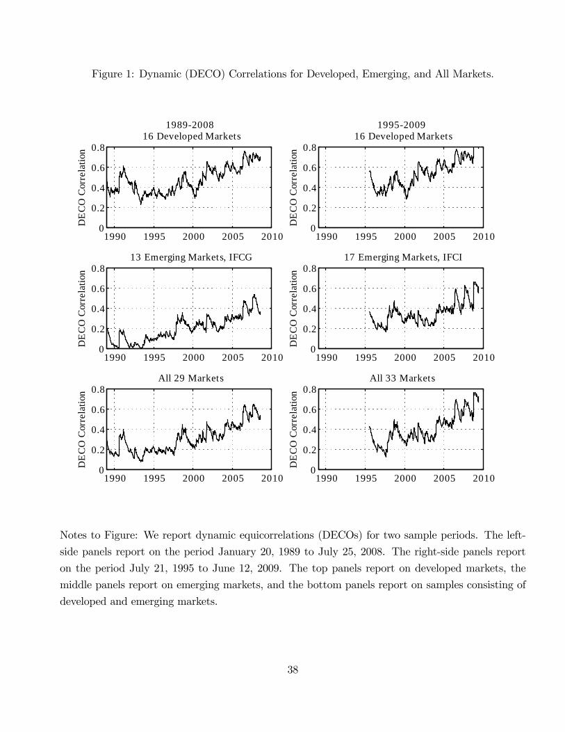
Figure 1: Dynamic (DECO) Correlations for Developed, Emerging, and All Markets.

1990 1995 2000 2005 20100

0.2

0.4

0.6

0.8

1989­200816 Developed Markets

DE

CO

 Cor

rela

tion

1990 1995 2000 2005 20100

0.2

0.4

0.6

0.813 Emerging Markets, IFCG

DE

CO

 Cor

rela

tion

1990 1995 2000 2005 20100

0.2

0.4

0.6

0.8All 29 Markets

DE

CO

 Cor

rela

tion

1990 1995 2000 2005 20100

0.2

0.4

0.6

0.8

1995­200916 Developed Markets

DE

CO

 Cor

rela

tion

1990 1995 2000 2005 20100

0.2

0.4

0.6

0.817 Emerging Markets, IFCI

DE

CO

 Cor

rela

tion

1990 1995 2000 2005 20100

0.2

0.4

0.6

0.8All 33 Markets

DE

CO

 Cor

rela

tion

Notes to Figure: We report dynamic equicorrelations (DECOs) for two sample periods. The left-

side panels report on the period January 20, 1989 to July 25, 2008. The right-side panels report

on the period July 21, 1995 to June 12, 2009. The top panels report on developed markets, the

middle panels report on emerging markets, and the bottom panels report on samples consisting of

developed and emerging markets.

38

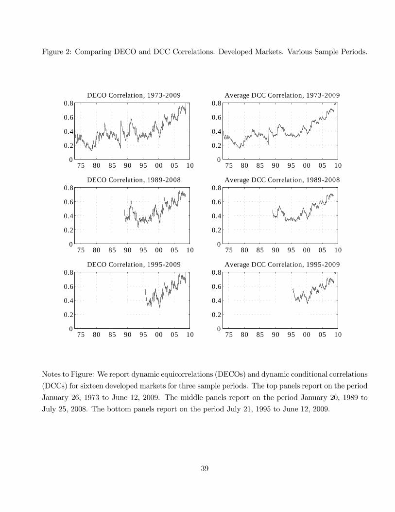
Figure 2: Comparing DECO and DCC Correlations. Developed Markets. Various Sample Periods.

75 80 85 90 95 00 05 100

0.2

0.4

0.6

0.8DECO Correlat ion, 1973­2009

75 80 85 90 95 00 05 100

0.2

0.4

0.6

0.8DECO Correlat ion, 1989­2008

75 80 85 90 95 00 05 100

0.2

0.4

0.6

0.8DECO Correlat ion, 1995­2009

75 80 85 90 95 00 05 100

0.2

0.4

0.6

0.8Average DCC Correlat ion, 1973­2009

75 80 85 90 95 00 05 100

0.2

0.4

0.6

0.8Average DCC Correlat ion, 1989­2008

75 80 85 90 95 00 05 100

0.2

0.4

0.6

0.8Average DCC Correlat ion, 1995­2009

Notes to Figure: We report dynamic equicorrelations (DECOs) and dynamic conditional correlations

(DCCs) for sixteen developed markets for three sample periods. The top panels report on the period

January 26, 1973 to June 12, 2009. The middle panels report on the period January 20, 1989 to

July 25, 2008. The bottom panels report on the period July 21, 1995 to June 12, 2009.

39

Figure 3.A: Correlations for Each Developed Market.

90 95 00 05 10

0

0.2

0.4

0.6

Australia

90 95 00 05 10

0

0.2

0.4

0.6

Austria

90 95 00 05 10

0

0.2

0.4

0.6

Belgium

90 95 00 05 10

0

0.2

0.4

0.6

Canada

90 95 00 05 10

0

0.2

0.4

0.6

Denmark

90 95 00 05 10

0

0.2

0.4

0.6

France

90 95 00 05 10

0

0.2

0.4

0.6

Germany

90 95 00 05 10

0

0.2

0.4

0.6

Hong kong

90 95 00 05 10

0

0.2

0.4

0.6

Ireland

90 95 00 05 10

0

0.2

0.4

0.6

Italy

90 95 00 05 10

0

0.2

0.4

0.6

Japan

90 95 00 05 10

0

0.2

0.4

0.6

Netherlands

90 95 00 05 10

0

0.2

0.4

0.6

Singapore

90 95 00 05 10

0

0.2

0.4

0.6

Switzerland

90 95 00 05 10

0

0.2

0.4

0.6

UK

90 95 00 05 10

0

0.2

0.4

0.6

US

Notes to Figure: We report dynamic conditional correlations for sixteen developed markets for the

period January 20, 1989 to July 21, 2008. For each country, at each point in time we report three

averages of conditional correlations with other countries: the average of correlations with the �fteen

other developed markets (black line), with the thirteen emerging markets (dark grey line), and with

the �fteen developed and thirteen emerging markets (light grey line).

40

Figure 3.B: Correlations for each Emerging Market.

90 95 00 05 10

0

0.2

0.4

0.6

Argentina

90 95 00 05 10

0

0.2

0.4

0.6

Brazil

90 95 00 05 10

0

0.2

0.4

0.6

Chile

90 95 00 05 10

0

0.2

0.4

0.6

Colombia

90 95 00 05 10

0

0.2

0.4

0.6

India

90 95 00 05 10

0

0.2

0.4

0.6

Jordan

90 95 00 05 10

0

0.2

0.4

0.6

Korea

90 95 00 05 10

0

0.2

0.4

0.6

Malaysia

90 95 00 05 10

0

0.2

0.4

0.6

Mexico

90 95 00 05 10

0

0.2

0.4

0.6

P hilippines

90 95 00 05 10

0

0.2

0.4

0.6

Taiwan

90 95 00 05 10

0

0.2

0.4

0.6

Thailand

90 95 00 05 10

0

0.2

0.4

0.6

Turkey

Notes to Figure: We report dynamic conditional correlations for thirteen emerging markets for the

period January 20, 1989 to July 25, 2008. For each country, at each point in time we report three

averages of conditional correlations with other countries: the average of correlations with sixteen

developed markets (black line), with the twelve other emerging markets (dark grey line), and with

the sixteen developed and twelve emerging markets (light grey line).

41

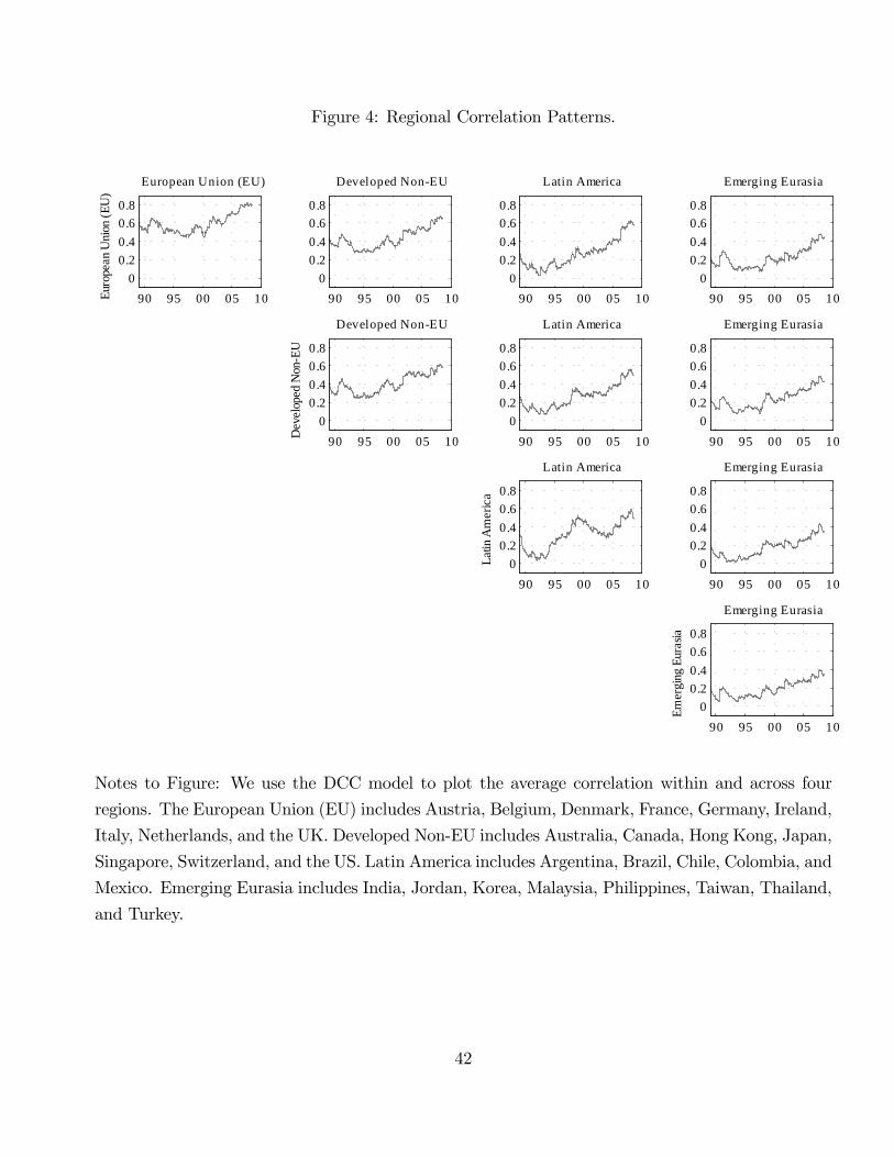
Figure 4: Regional Correlation Patterns.

90 95 00 05 100

0.20.40.60.8

European Union (EU)

Euro

pean

 Uni

on (E

U)

90 95 00 05 100

0.20.40.60.8

Developed Non­EU

90 95 00 05 100

0.20.40.60.8

Latin America

90 95 00 05 100

0.20.40.60.8

Emerging Eurasia

90 95 00 05 100

0.20.40.60.8

Developed Non­EU

Dev

elop

ed N

on­E

U

90 95 00 05 100

0.20.40.60.8

Latin America

90 95 00 05 100

0.20.40.60.8

Emerging Eurasia

90 95 00 05 100

0.20.40.60.8

Latin AmericaLa

tin A

mer

ica

90 95 00 05 100

0.20.40.60.8

Emerging Eurasia

90 95 00 05 100

0.20.40.60.8

Emerging Eurasia

Emer

ging

 Eur

asia

Notes to Figure: We use the DCC model to plot the average correlation within and across four

regions. The European Union (EU) includes Austria, Belgium, Denmark, France, Germany, Ireland,

Italy, Netherlands, and the UK. Developed Non-EU includes Australia, Canada, Hong Kong, Japan,

Singapore, Switzerland, and the US. Latin America includes Argentina, Brazil, Chile, Colombia, and

Mexico. Emerging Eurasia includes India, Jordan, Korea, Malaysia, Philippines, Taiwan, Thailand,

and Turkey.

42

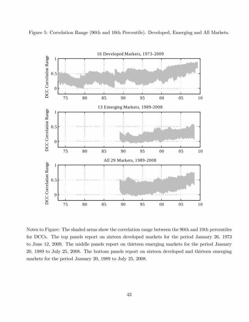
Figure 5: Correlation Range (90th and 10th Percentile). Developed, Emerging and All Markets.

75 80 85 90 95 00 05 10

0

0.5

116 Developed Markets, 1973­2009

DC

C C

orre

latio

n R

ange

75 80 85 90 95 00 05 10

0

0.5

113 Emerging Markets, 1989­2008

DC

C C

orre

latio

n R

ange

75 80 85 90 95 00 05 10

0

0.5

1All 29 Markets, 1989­2008

DC

C C

orre

latio

n R

ange

Notes to Figure: The shaded areas show the correlation range between the 90th and 10th percentiles

for DCCs. The top panels report on sixteen developed markets for the period January 26, 1973

to June 12, 2009. The middle panels report on thirteen emerging markets for the period January

20, 1989 to July 25, 2008. The bottom panels report on sixteen developed and thirteen emerging

markets for the period January 20, 1989 to July 25, 2008.

43

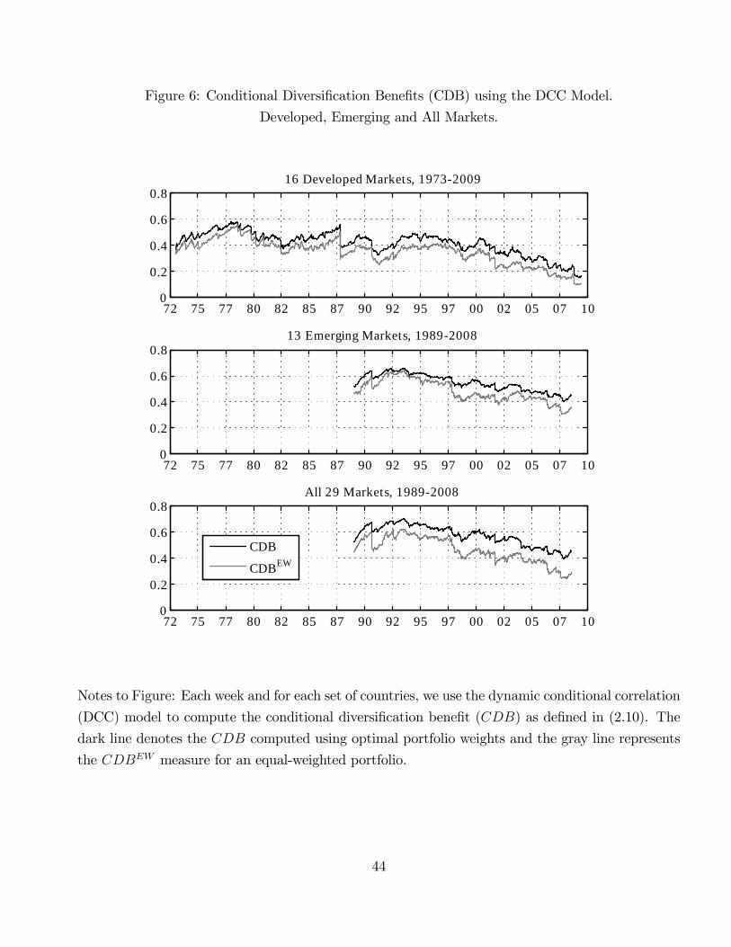
Figure 6: Conditional Diversi�cation Bene�ts (CDB) using the DCC Model.

Developed, Emerging and All Markets.

72 75 77 80 82 85 87 90 92 95 97 00 02 05 07 100

0.2

0.4

0.6

0.816 Developed Markets, 1973­2009

72 75 77 80 82 85 87 90 92 95 97 00 02 05 07 100

0.2

0.4

0.6

0.813 Emerging Markets, 1989­2008

72 75 77 80 82 85 87 90 92 95 97 00 02 05 07 100

0.2

0.4

0.6

0.8All 29 Markets, 1989­2008

CDB

CDBEW

Notes to Figure: Each week and for each set of countries, we use the dynamic conditional correlation

(DCC) model to compute the conditional diversi�cation bene�t (CDB) as de�ned in (2.10). The

dark line denotes the CDB computed using optimal portfolio weights and the gray line represents

the CDBEW measure for an equal-weighted portfolio.

44

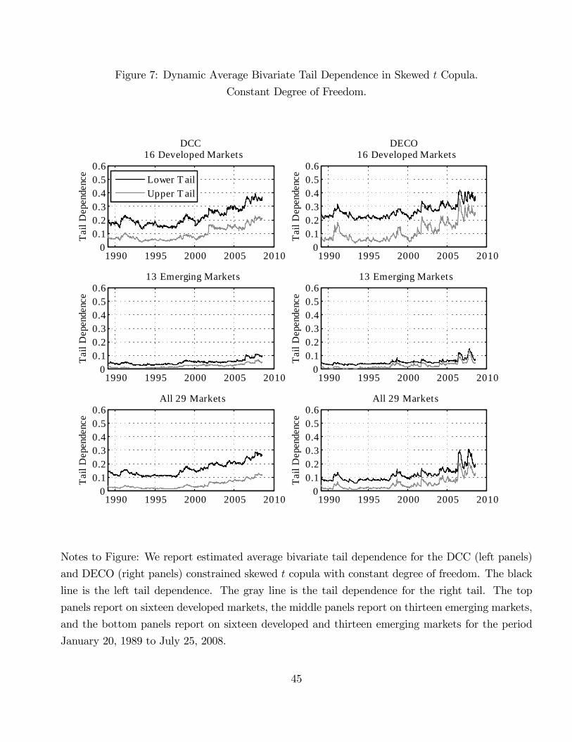
Figure 7: Dynamic Average Bivariate Tail Dependence in Skewed t Copula.

Constant Degree of Freedom.

1990 1995 2000 2005 20100

0.10.20.30.40.50.6

DCC16 Developed Markets

Tai

l Dep

ende

nce

Lower T ailUpper T ail

1990 1995 2000 2005 20100

0.10.20.30.40.50.6

DECO16 Developed Markets

Tai

l Dep

ende

nce

1990 1995 2000 2005 20100

0.10.20.30.40.50.6

13 Emerging Markets

Tai

l Dep

ende

nce

1990 1995 2000 2005 20100

0.10.20.30.40.50.6

13 Emerging Markets

Tai

l Dep

ende

nce

1990 1995 2000 2005 20100

0.10.20.30.40.50.6

All 29 Markets

Tai

l Dep

ende

nce

1990 1995 2000 2005 20100

0.10.20.30.40.50.6

All 29 Markets

Tai

l Dep

ende

nce

Notes to Figure: We report estimated average bivariate tail dependence for the DCC (left panels)

and DECO (right panels) constrained skewed t copula with constant degree of freedom. The black

line is the left tail dependence. The gray line is the tail dependence for the right tail. The top

panels report on sixteen developed markets, the middle panels report on thirteen emerging markets,

and the bottom panels report on sixteen developed and thirteen emerging markets for the period

January 20, 1989 to July 25, 2008.

45

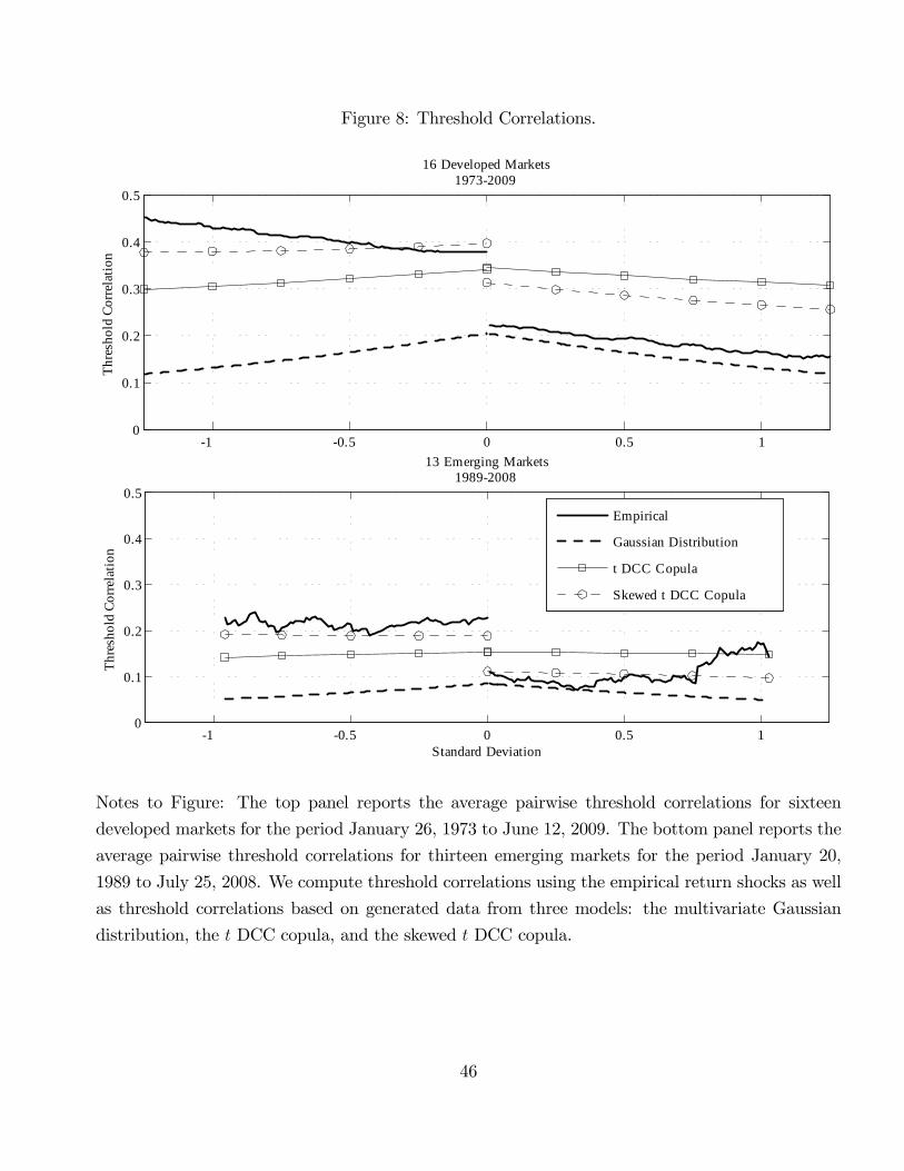
Figure 8: Threshold Correlations.

­1 ­0.5 0 0.5 10

0.1

0.2

0.3

0.4

0.5

16 Developed Markets1973­2009

Thre

shol

d Co

rrela

tion

­1 ­0.5 0 0.5 10

0.1

0.2

0.3

0.4

0.5

13 Emerging Markets1989­2008

Thre

shol

d Co

rrela

tion

Standard Deviation

Empirical

Gaussian Distribution

t DCC Copula

Skewed t DCC Copula

Notes to Figure: The top panel reports the average pairwise threshold correlations for sixteen

developed markets for the period January 26, 1973 to June 12, 2009. The bottom panel reports the

average pairwise threshold correlations for thirteen emerging markets for the period January 20,

1989 to July 25, 2008. We compute threshold correlations using the empirical return shocks as well

as threshold correlations based on generated data from three models: the multivariate Gaussian

distribution, the t DCC copula, and the skewed t DCC copula.

46

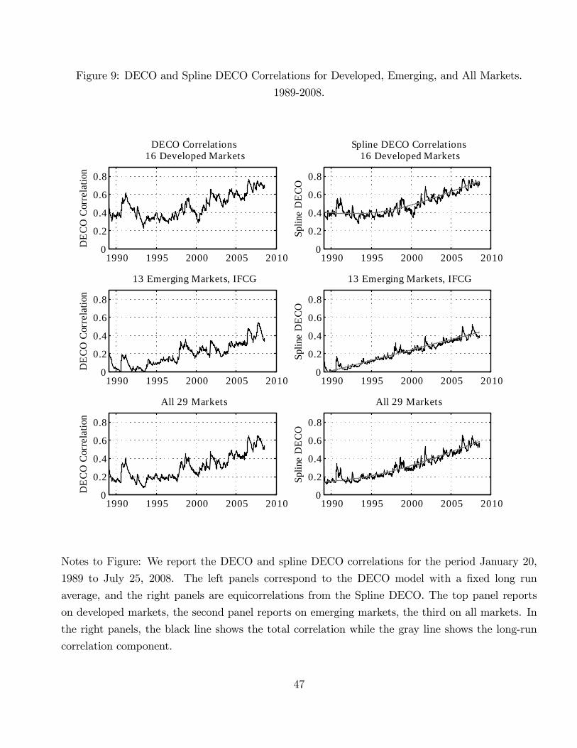
Figure 9: DECO and Spline DECO Correlations for Developed, Emerging, and All Markets.

1989-2008.

1990 1995 2000 2005 20100

0.2

0.4

0.6

0.8

DECO Correlat ions16 Developed Markets

DE

CO

 Cor

rela

tion

1990 1995 2000 2005 20100

0.2

0.4

0.6

0.8

Spline DECO Correlat ions16 Developed Markets

Splin

e D

EC

O

1990 1995 2000 2005 20100

0.2

0.4

0.6

0.8

13 Emerging Markets, IFCG

DE

CO

 Cor

rela

tion

1990 1995 2000 2005 20100

0.2

0.4

0.6

0.8

All 29 Markets

DE

CO

 Cor

rela

tion

1990 1995 2000 2005 20100

0.2

0.4

0.6

0.8

13 Emerging Markets, IFCG

Splin

e D

EC

O

1990 1995 2000 2005 20100

0.2

0.4

0.6

0.8

All 29 Markets

Splin

e D

EC

O

Notes to Figure: We report the DECO and spline DECO correlations for the period January 20,

1989 to July 25, 2008. The left panels correspond to the DECO model with a �xed long run

average, and the right panels are equicorrelations from the Spline DECO. The top panel reports

on developed markets, the second panel reports on emerging markets, the third on all markets. In

the right panels, the black line shows the total correlation while the gray line shows the long-run

correlation component.

47

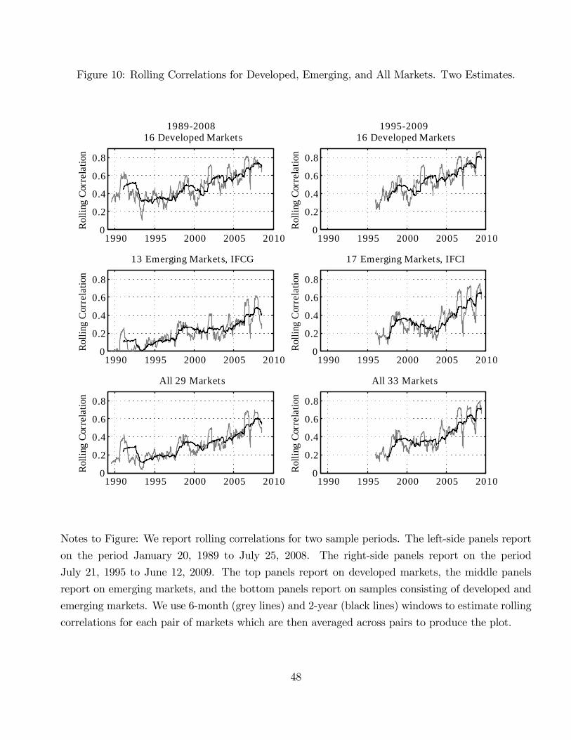
Figure 10: Rolling Correlations for Developed, Emerging, and All Markets. Two Estimates.

1990 1995 2000 2005 20100

0.2

0.4

0.6

0.8

1989­200816 Developed Markets

Rol

ling 

Cor

rela

tion

1990 1995 2000 2005 20100

0.2

0.4

0.6

0.8

13 Emerging Markets, IFCG

Rol

ling 

Cor

rela

tion

1990 1995 2000 2005 20100

0.2

0.4

0.6

0.8

All 29 Markets

Rol

ling 

Cor

rela

tion

1990 1995 2000 2005 20100

0.2

0.4

0.6

0.8

1995­200916 Developed Markets

Rol

ling 

Cor

rela

tion

1990 1995 2000 2005 20100

0.2

0.4

0.6

0.8

17 Emerging Markets, IFCI

Rol

ling 

Cor

rela

tion

1990 1995 2000 2005 20100

0.2

0.4

0.6

0.8

All 33 Markets

Rol

ling 

Cor

rela

tion

Notes to Figure: We report rolling correlations for two sample periods. The left-side panels report

on the period January 20, 1989 to July 25, 2008. The right-side panels report on the period

July 21, 1995 to June 12, 2009. The top panels report on developed markets, the middle panels

report on emerging markets, and the bottom panels report on samples consisting of developed and

emerging markets. We use 6-month (grey lines) and 2-year (black lines) windows to estimate rolling

correlations for each pair of markets which are then averaged across pairs to produce the plot.

48

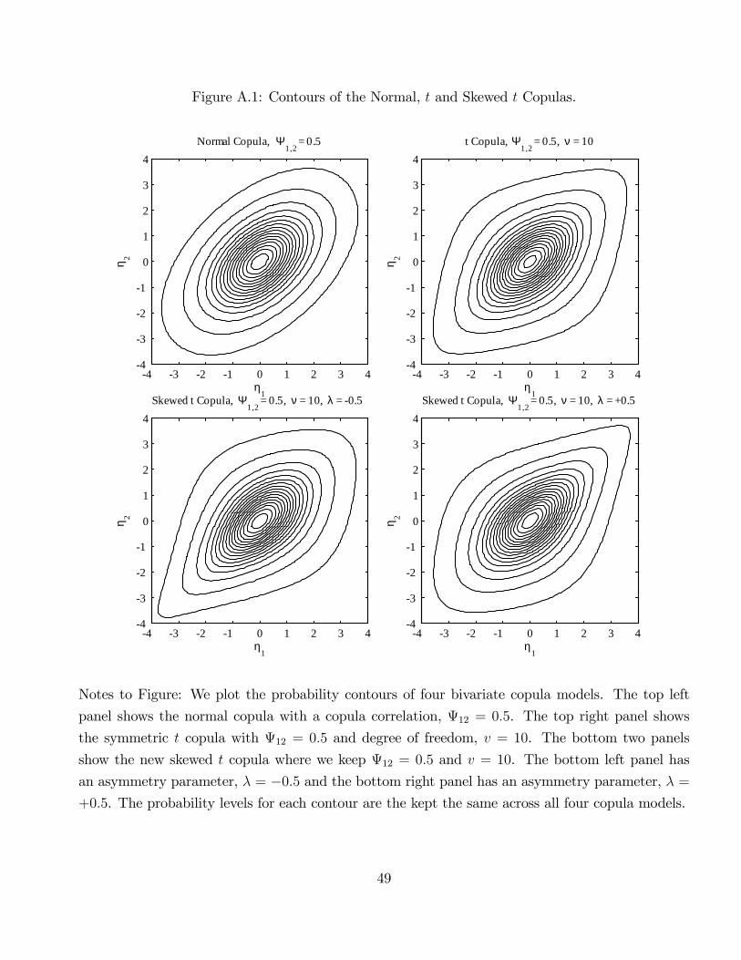
Figure A.1: Contours of the Normal, t and Skewed t Copulas.

η1

η 2

Normal Copula, Ψ1,2

 = 0.5

­4 ­3 ­2 ­1 0 1 2 3 4­4

­3

­2

­1

0

1

2

3

4

η1

η 2

t Copula, Ψ1,2

 = 0.5, ν = 10

­4 ­3 ­2 ­1 0 1 2 3 4­4

­3

­2

­1

0

1

2

3

4

η1

η 2

Skewed t Copula, Ψ1,2

 = 0.5, ν = 10, λ = ­0.5

­4 ­3 ­2 ­1 0 1 2 3 4­4

­3

­2

­1

0

1

2

3

4

η1

η 2Skewed t Copula, Ψ

1,2 = 0.5, ν = 10, λ = +0.5

­4 ­3 ­2 ­1 0 1 2 3 4­4

­3

­2

­1

0

1

2

3

4

Notes to Figure: We plot the probability contours of four bivariate copula models. The top left

panel shows the normal copula with a copula correlation, 12 = 0:5. The top right panel shows

the symmetric t copula with 12 = 0:5 and degree of freedom, v = 10. The bottom two panels

show the new skewed t copula where we keep 12 = 0:5 and v = 10. The bottom left panel has

an asymmetry parameter, � = �0:5 and the bottom right panel has an asymmetry parameter, � =+0:5. The probability levels for each contour are the kept the same across all four copula models.

49

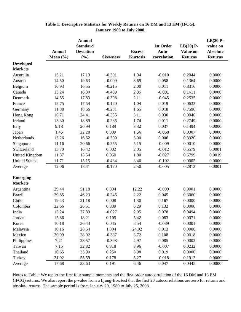
Annual Mean (%)

Annual Standard Deviation

(%) SkewnessExcess

Kurtosis

1st Order Auto-

correlation

LB(20) P-Value on Returns

LB(20 P-value on Absolute Returns

Developed MarketsAustralia 13.21 17.13 -0.301 1.94 -0.010 0.2044 0.0000Austria 14.50 19.63 -0.009 3.69 0.058 0.1364 0.0000Belgium 10.93 16.55 -0.215 2.00 0.011 0.8316 0.0000Canada 13.24 16.30 -0.489 2.35 -0.001 0.1611 0.0000Denmark 14.55 17.83 -0.308 2.11 -0.045 0.2535 0.0000France 12.75 17.54 -0.120 1.04 0.019 0.0632 0.0000Germany 11.88 18.66 -0.231 1.65 0.018 0.7596 0.0000Hong Kong 16.71 24.41 -0.355 3.11 0.030 0.0046 0.0000Ireland 13.30 18.89 -0.286 1.74 0.011 0.2749 0.0000Italy 9.18 20.99 0.189 3.32 0.037 0.1494 0.0000Japan 1.45 22.28 0.339 1.56 -0.068 0.0307 0.0000Netherlands 13.26 16.62 -0.300 3.00 0.006 0.3920 0.0000Singapore 11.16 20.66 -0.255 5.15 -0.009 0.0010 0.0000Switzerland 13.70 16.42 0.002 2.05 -0.012 0.5579 0.0001United Kingdom 11.37 15.54 0.060 1.80 -0.027 0.6799 0.0019United States 11.71 15.15 -0.434 3.46 -0.102 0.0005 0.0000Average 12.06 18.41 -0.170 2.50 -0.005 0.2813 0.0001

Emerging MarketsArgentina 29.44 51.18 0.804 12.22 -0.009 0.0001 0.0000Brazil 29.85 46.23 -0.246 2.22 0.045 0.3060 0.0000Chile 19.43 21.18 0.008 1.30 0.167 0.0000 0.0000Colombia 22.66 26.51 0.339 6.29 0.132 0.0000 0.0000India 15.24 27.89 -0.027 2.05 0.078 0.0494 0.0000Jordan 15.86 18.21 0.195 5.42 0.083 0.0071 0.0000Korea 10.18 36.43 0.045 8.54 -0.089 0.0001 0.0000Malaysia 10.16 28.64 1.394 24.02 0.013 0.0000 0.0000Mexico 20.99 28.02 -0.387 3.72 0.108 0.0018 0.0000Philippines 7.21 28.57 -0.393 4.97 0.085 0.0002 0.0000Taiwan 7.15 32.82 0.318 3.96 -0.007 0.0232 0.0000Thailand 10.65 35.90 0.250 3.98 0.019 0.0000 0.0000Turkey 31.02 55.59 0.178 5.27 -0.018 0.1912 0.0000Average 17.68 33.63 0.191 6.46 0.047 0.0445 0.0000

Table 1: Descriptive Statistics for Weekly Returns on 16 DM and 13 EM (IFCG).January 1989 to July 2008.

Notes to Table: We report the first four sample moments and the first order autocorrelation of the 16 DM and 13 EM (IFCG) returns. We also report the p-value from a Ljung-Box test that the first 20 autocorrelations are zero for returns and absolute returns. The sample period is from January 20, 1989 to July 25, 2008.

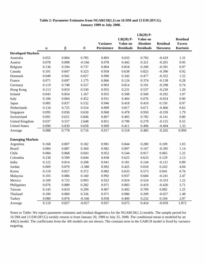
Variance

Persistence

LB(20) P-Value on Residuals

LB(20) P-Value on Absolute Residuals

Residual Skewness

Residual Excess

Kurtosis

Developed MarketsAustralia 0.055 0.804 0.785 0.893 0.633 0.702 -0.419 1.31Austria 0.078 0.898 -0.166 0.978 0.442 0.321 -0.201 0.95Belgium 0.136 0.594 0.737 0.804 0.818 0.200 -0.391 0.97Canada 0.101 0.847 0.323 0.958 0.638 0.825 -0.396 0.92Denmark 0.049 0.941 0.027 0.990 0.342 0.477 -0.352 1.52France 0.071 0.697 1.175 0.866 0.124 0.374 -0.138 0.28Germany 0.119 0.748 0.557 0.903 0.814 0.101 -0.298 0.74Hong Kong 0.113 0.810 0.530 0.955 0.231 0.537 -0.230 1.20Ireland 0.043 0.854 1.167 0.955 0.508 0.560 -0.292 1.07Italy 0.106 0.804 0.452 0.931 0.404 0.076 -0.054 0.90Japan 0.085 0.837 0.532 0.946 0.418 0.410 0.150 0.97Netherlands 0.134 0.725 0.554 0.899 0.817 0.671 -0.466 0.62Singapore 0.095 0.836 0.630 0.968 0.478 0.950 -0.359 1.79Switzerland 0.091 0.651 0.846 0.807 0.405 0.782 -0.141 0.80United Kingdom 0.037 0.557 2.648 0.851 0.799 0.278 -0.155 0.55United States 0.090 0.839 0.658 0.969 0.411 0.496 -0.494 1.33Average 0.088 0.778 0.716 0.917 0.518 0.485 -0.265 0.994

Emerging MarketsArgentina 0.168 0.807 0.182 0.981 0.844 0.280 0.109 1.03Brazil 0.084 0.887 0.360 0.982 0.907 0.167 -0.395 1.14Chile 0.084 0.868 0.043 0.952 0.544 0.917 0.065 1.25Colombia 0.238 0.599 0.044 0.838 0.625 0.633 0.129 2.13India 0.122 0.814 0.208 0.941 0.181 0.144 -0.121 0.89Jordan 0.009 0.879 -3.380 0.992 0.425 0.018 0.243 4.04Korea 0.110 0.857 0.372 0.982 0.633 0.573 0.041 0.76Malaysia 0.103 0.886 0.160 0.992 0.937 0.684 -0.241 2.47Mexico 0.109 0.723 0.903 0.922 0.924 0.524 -0.333 1.22Philippines 0.076 0.889 0.282 0.971 0.883 0.419 -0.420 3.71Taiwan 0.143 0.810 0.299 0.967 0.492 0.709 0.082 1.25Thailand 0.100 0.860 0.336 0.971 0.986 0.209 -0.027 1.48Turkey 0.080 0.876 -0.166 0.958 0.400 0.232 0.104 2.97Average 0.110 0.827 -0.027 0.957 0.675 0.424 -0.059 1.872

January 1989 to July 2008.Table 2: Parameter Estimates from NGARCH(1,1) on 16 DM and 13 EM (IFCG).

Notes to Table: We report parameter estimates and residual diagnostics for the NGARCH(1,1) models. The sample period for 16 DM and 13 EM (IFCG) weekly returns is from January 20, 1989 to July 25, 2008. The conditional mean is modeled by an AR(2) model. The coefficients from the AR models are not shown. The constant term in the GARCH model is fixed by variance targeting.

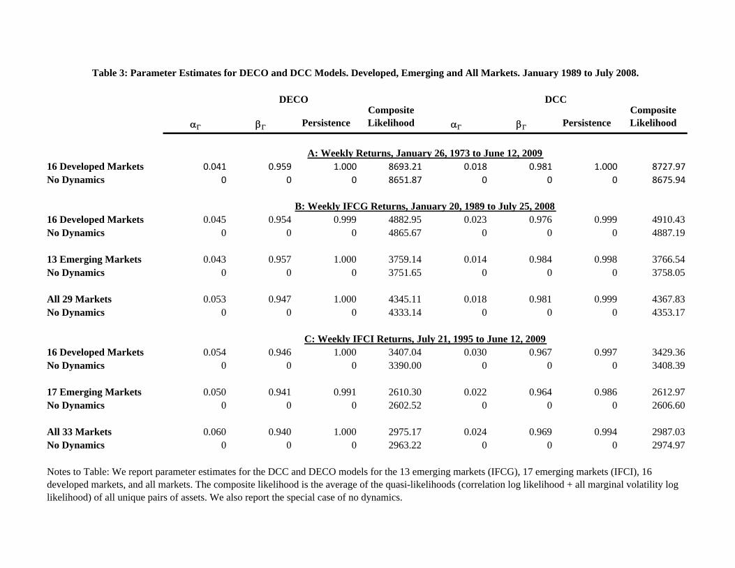
PersistenceComposite Likelihood Persistence

Composite Likelihood

16 Developed Markets 0.041 0.959 1.000 8693.21 0.018 0.981 1.000 8727.97No Dynamics 0 0 0 8651.87 0 0 0 8675.94

16 Developed Markets 0.045 0.954 0.999 4882.95 0.023 0.976 0.999 4910.43No Dynamics 0 0 0 4865.67 0 0 0 4887.19

13 Emerging Markets 0.043 0.957 1.000 3759.14 0.014 0.984 0.998 3766.54No Dynamics 0 0 0 3751.65 0 0 0 3758.05

All 29 Markets 0.053 0.947 1.000 4345.11 0.018 0.981 0.999 4367.83No Dynamics 0 0 0 4333.14 0 0 0 4353.17

16 Developed Markets 0.054 0.946 1.000 3407.04 0.030 0.967 0.997 3429.36No Dynamics 0 0 0 3390.00 0 0 0 3408.39

17 Emerging Markets 0.050 0.941 0.991 2610.30 0.022 0.964 0.986 2612.97No Dynamics 0 0 0 2602.52 0 0 0 2606.60

All 33 Markets 0.060 0.940 1.000 2975.17 0.024 0.969 0.994 2987.03No Dynamics 0 0 0 2963.22 0 0 0 2974.97

Notes to Table: We report parameter estimates for the DCC and DECO models for the 13 emerging markets (IFCG), 17 emerging markets (IFCI), 16 developed markets, and all markets. The composite likelihood is the average of the quasi-likelihoods (correlation log likelihood + all marginal volatility log likelihood) of all unique pairs of assets. We also report the special case of no dynamics.

B: Weekly IFCG Returns, January 20, 1989 to July 25, 2008

C: Weekly IFCI Returns, July 21, 1995 to June 12, 2009

Table 3: Parameter Estimates for DECO and DCC Models. Developed, Emerging and All Markets. January 1989 to July 2008.

DECO DCC

A: Weekly Returns, January 26, 1973 to June 12, 2009

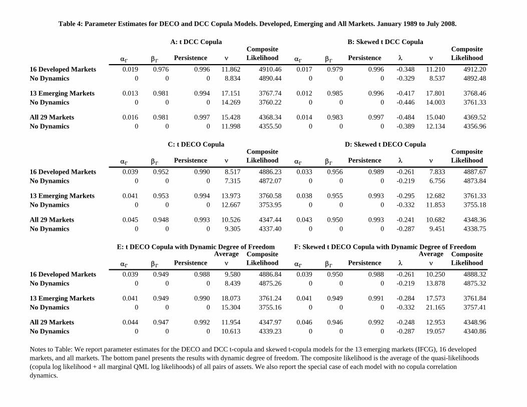
Persistence Composite Likelihood Persistence

Composite Likelihood

16 Developed Markets 0.019 0.976 0.996 11.862 4910.46 0.017 0.979 0.996 -0.348 11.210 4912.20No Dynamics 0 0 0 8.834 4890.44 0 0 0 -0.329 8.537 4892.48

13 Emerging Markets 0.013 0.981 0.994 17.151 3767.74 0.012 0.985 0.996 -0.417 17.801 3768.46No Dynamics 0 0 0 14.269 3760.22 0 0 0 -0.446 14.003 3761.33

All 29 Markets 0.016 0.981 0.997 15.428 4368.34 0.014 0.983 0.997 -0.484 15.040 4369.52No Dynamics 0 0 0 11.998 4355.50 0 0 0 -0.389 12.134 4356.96

Persistence Composite Likelihood Persistence

Composite Likelihood

16 Developed Markets 0.039 0.952 0.990 8.517 4886.23 0.033 0.956 0.989 -0.261 7.833 4887.67No Dynamics 0 0 0 7.315 4872.07 0 0 0 -0.219 6.756 4873.84

13 Emerging Markets 0.041 0.953 0.994 13.973 3760.58 0.038 0.955 0.993 -0.295 12.682 3761.33No Dynamics 0 0 0 12.667 3753.95 0 0 0 -0.332 11.853 3755.18

All 29 Markets 0.045 0.948 0.993 10.526 4347.44 0.043 0.950 0.993 -0.241 10.682 4348.36No Dynamics 0 0 0 9.305 4337.40 0 0 0 -0.287 9.451 4338.75

PersistenceAverage

Composite Likelihood Persistence

Average

Composite Likelihood

16 Developed Markets 0.039 0.949 0.988 9.580 4886.84 0.039 0.950 0.988 -0.261 10.250 4888.32No Dynamics 0 0 0 8.439 4875.26 0 0 0 -0.219 13.878 4875.32

13 Emerging Markets 0.041 0.949 0.990 18.073 3761.24 0.041 0.949 0.991 -0.284 17.573 3761.84No Dynamics 0 0 0 15.304 3755.16 0 0 0 -0.332 21.165 3757.41

All 29 Markets 0.044 0.947 0.992 11.954 4347.97 0.046 0.946 0.992 -0.248 12.953 4348.96No Dynamics 0 0 0 10.613 4339.23 0 0 0 -0.287 19.057 4340.86

Notes to Table: We report parameter estimates for the DECO and DCC t-copula and skewed t-copula models for the 13 emerging markets (IFCG), 16 developed markets, and all markets. The bottom panel presents the results with dynamic degree of freedom. The composite likelihood is the average of the quasi-likelihoods (copula log likelihood + all marginal QML log likelihoods) of all pairs of assets. We also report the special case of each model with no copula correlation dynamics.

Table 4: Parameter Estimates for DECO and DCC Copula Models. Developed, Emerging and All Markets. January 1989 to July 2008.

C: t DECO Copula

E: t DECO Copula with Dynamic Degree of Freedom F: Skewed t DECO Copula with Dynamic Degree of Freedom

D: Skewed t DECO Copula

B: Skewed t DCC CopulaA: t DCC Copula

Time Trend Vol DMs Vol EMs Vol All Vol(i) R2

0.1055 ** 0.9719 ** 0.3726(0.0013) (0.0724)

0.0965 ** 0.1143 0.3532(0.0012) (0.0742)

0.0755 ** 0.4543 ** 0.2395(0.0016) (0.1384)

0.0763 ** 0.0388 0.2366(0.0016) (0.1203)

0.0858 ** 0.7021 ** 0.2982(0.0015) (0.1017)

0.0833 ** 0.0459 0.2898(0.0014) (0.0958)

0.0793 ** 0.6609 ** 0.5540(0.0005) (0.0487)

0.0720 ** 0.3446 ** 0.5297(0.0005) (0.0889)

0.0269 ** 0.4641 ** 0.4573(0.0003) (0.0345)

0.0269 ** 0.2197 ** 0.3976(0.0003) (0.0328)

0.0426 ** 0.3392 ** 0.4505(0.0004) (0.0552)

0.0410 ** 0.1948 ** 0.4180(0.0004) (0.0608)

Table 5: Correlation and Volatility.

Notes to Table: We estimate panel regressions for the 17 emerging markets in the IFCI index and 16 developed markets, using weekly data. All samples are 1989-2008, except for Panel E, where we have 1973-2009 data available. Country fixed effects are included in each specification, and White standard errors adjusted for country cluster correlations are provided in parentheses. Vol DMs, Vol EMs, and Vol All are the equally-weighted averages of the logs of monthly volatilities across all DMs, all EMs, and all markets respectively. Vol(i) is the market specific log of in monthly volatility. The estimate of the time trend is annualized. * indicates significance at the 5% level, and ** indicates significance at the 1% level.

Panel A: Regressand: Average Weekly Emerging Market DCC Correlation With All Other Emerging Markets

Panel B: Regressand: Average Weekly Emerging Market DCC Correlation With All Developed Markets

Panel C: Regressand: Average Weekly Emerging Market DCC Correlation With All Other Markets

Panel D: Regressand: Average Weekly Developed Market DCC Correlation With All Emerging Markets

Panel E: Regressand: Average Weekly Developed Market DCC Correlation With All Other Developed Markets

Panel F: Regressand: Average Weekly Developed Market DCC Correlation With All Other Markets

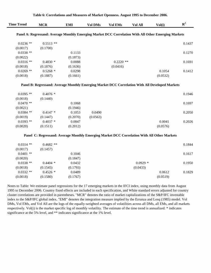
Time Trend MCR EMI Vol DMs Vol EMs Vol All Vol(i) R2

0.0236 ** 0.5513 ** 0.1437(0.0017) (0.1700)

0.0338 ** 0.1133 0.1270(0.0022) (0.1873)

0.0316 ** 0.4830 * 0.0088 0.2220 ** 0.1691(0.0018) (0.1876) (0.1636) (0.0416)

0.0269 ** 0.5268 * 0.0298 0.1054 0.1412(0.0018) (0.1887) (0.1661) (0.0532)

0.0395 ** 0.4076 * 0.1946(0.0018) (0.1440)

0.0470 ** 0.1068 0.1697(0.0021) (0.1946)

0.0384 ** 0.4147 * 0.1053 0.0490 0.2050(0.0019) (0.1447) (0.2070) (0.0563)

0.0393 ** 0.4037 * 0.0847 0.0041 0.2026(0.0020) (0.1511) (0.2012) (0.0576)

0.0314 ** 0.4682 ** 0.1844(0.0017) (0.1457)

0.0401 ** 0.1046 0.1617(0.0020) (0.1847)

0.0338 ** 0.4404 * 0.0432 0.0929 * 0.1950(0.0018) (0.1545) (0.1793) (0.0433)

0.0332 ** 0.4526 * 0.0489 0.0612 0.1829(0.0018) (0.1580) (0.1767) (0.0519)

Table 6: Correlations and Measures of Market Openness. August 1995 to December 2006.

Notes to Table: We estimate panel regressions for the 17 emerging markets in the IFCI index, using monthly data from August 1995 to December 2006. Country fixed effects are included in each specification, and White standard errors adjusted for country cluster correlations are provided in parentheses. "MCR" denotes the ratio of market capitalizations of the S&P/IFC investable index to the S&P/IFC global index. "EMI" denotes the integration measure implied by the Errunza and Losq (1985) model. Vol DMs, Vol EMs, and Vol All are the logs of the equally-weighted averages of volatilities across all DMs, all EMs, and all markets respectively. Vol(i) is the market specific log of monthly volatility. The estimate of the time trend is annualized. * indicates significance at the 5% level, and ** indicates significance at the 1% level.

Panel A: Regressand: Average Monthly Emerging Market DCC Correlation With All Other Emerging Markets

Panel B: Regressand: Average Monthly Emerging Market DCC Correlation With All Developed Markets

Panel C: Regressand: Average Monthly Emerging Market DCC Correlation With All Other Markets

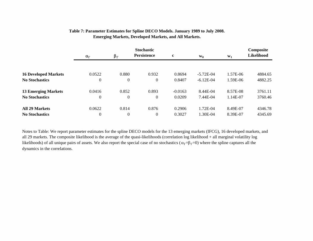
Stochastic Persistence c w0 w1

Composite Likelihood

16 Developed Markets 0.0522 0.880 0.932 0.8694 -5.72E-04 1.57E-06 4884.65No Stochastics 0 0 0 0.8407 -6.12E-04 1.59E-06 4882.25

13 Emerging Markets 0.0416 0.852 0.893 -0.0163 8.44E-04 8.57E-08 3761.11No Stochastics 0 0 0 0.0209 7.44E-04 1.14E-07 3760.46

All 29 Markets 0.0622 0.814 0.876 0.2906 1.72E-04 8.49E-07 4346.78No Stochastics 0 0 0 0.3027 1.30E-04 8.39E-07 4345.69

Table 7: Parameter Estimates for Spline DECO Models. January 1989 to July 2008.Emerging Markets, Developed Markets, and All Markets.

Notes to Table: We report parameter estimates for the spline DECO models for the 13 emerging markets (IFCG), 16 developed markets, and all 29 markets. The composite likelihood is the average of the quasi-likelihoods (correlation log likelihood + all marginal volatility log likelihoods) of all unique pairs of assets. We also report the special case of no stochastics (==0) where the spline captures all the dynamics in the correlations.